Volatility Modeling: Taming the Beast: Strategies for Volatility Modeling in Finance

1. Understanding the Markets Mood Swings

volatility in the financial markets is akin to the weather patterns of the natural world: unpredictable, dynamic, and immensely influential. It represents the degree of variation of a trading price series over time, commonly measured by the standard deviation of logarithmic returns. Understanding volatility is crucial for investors and traders alike, as it is a fundamental aspect that affects investment decisions, risk management strategies, and market sentiment analysis. It's the heartbeat of the market, pulsating with every news release, economic report, and global event.

From the perspective of a portfolio manager, volatility is a double-edged sword. On one hand, it can provide opportunities for significant gains when markets move favorably. On the other, it can lead to substantial losses during market downturns. For option traders, volatility is the core upon which their strategies are built, as it directly influences option pricing and the potential for profit. Economists view market volatility as an indicator of economic health, where high volatility often signals uncertainty and potential economic distress.

Here's an in-depth look at the facets of market volatility:

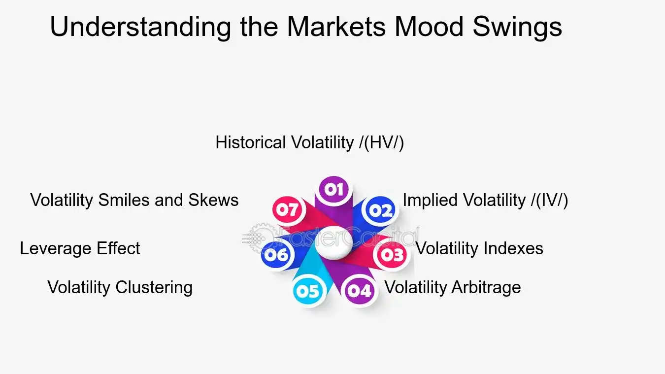
1. Historical Volatility (HV): This reflects the past market behavior and is calculated by determining the standard deviation of past market prices. For example, if a stock has exhibited significant price swings in the past, its HV would be high, indicating a riskier investment.

2. Implied Volatility (IV): Unlike HV, IV looks forward, gauging market sentiment and expectations of future price movements. It's derived from option prices and can be seen as the market's forecast of a likely movement in a security's price.

3. Volatility Indexes: These are measures of market expectations of near-term volatility conveyed by stock index option prices. The most famous example is the cboe Volatility index (VIX), often referred to as the "fear index," which measures the market's expectation of 30-day volatility.

4. Volatility Arbitrage: This strategy involves taking advantage of the difference between the forecasted future price volatility (IV) and the actual price movement (HV). Traders might use a model like the Black-Scholes to identify mispriced assets.

5. Volatility Clustering: It's observed that large changes in prices tend to be followed by more large changes, and small changes tend to be followed by small changes. This phenomenon is a key concept in econometric models like GARCH (Generalized Autoregressive Conditional Heteroskedasticity) used for forecasting volatility.

6. Leverage Effect: Typically, there is a negative correlation between stock returns and volatility changes; as a stock's price decreases, volatility tends to increase. This is partly due to the leverage effect, where a drop in an asset's price leads to higher leverage if the asset is financed with debt.

7. Volatility Smiles and Skews: In options trading, a volatility smile is a pattern in which at-the-money options have lower IVs than in- or out-of-the-money options. A skew indicates that out-of-the-money put options have higher IVs than call options, suggesting a higher probability of a market drop.

Understanding these concepts is vital for anyone involved in the financial markets, as they provide a framework for assessing risk and potential reward. By mastering the art of volatility modeling, one can better navigate the capricious seas of finance, turning what seems like a beast into a powerful ally in the quest for investment success.

2. A Comparative Analysis

Volatility is the heartbeat of the financial markets, a quantifiable measure of market risk and an indicator of investor sentiment. In the realm of volatility modeling, two distinct types of volatility are often analyzed: historical volatility (HV) and implied volatility (IV). While HV looks back at the past, calculating the rate of price changes for a security over a set period, IV peers into the market's crystal ball, derived from the prices of options and reflecting the market's expectations of future volatility. This comparative analysis delves into the nuances of HV and IV, exploring their methodologies, applications, and the insights they offer to traders, risk managers, and financial analysts.

1. Methodology:

- Historical Volatility: Calculated by determining the standard deviation of daily price changes over a specific time frame, typically annualized. For example, if a stock has a daily volatility of 1% and there are 252 trading days in a year, the annualized HV would be $$ HV = 1\% \times \sqrt{252} $$.

- Implied Volatility: Extracted from the black-Scholes model or other option pricing models, IV represents the market's forecast of a likely movement in a security's price. It is the volatility value that, when input into an option pricing model, gives a market price for the option.

2. Applications:

- Historical Volatility is used for:

- Risk Management: Assessing the risk profile of portfolios.

- Asset Allocation: Determining the weight of risky assets.

- Implied Volatility is used for:

- Option Pricing: Setting premiums for options contracts.

- Market Sentiment Analysis: Gauging the mood of the market.

3. Insights:

- Historical Volatility offers a retrospective view and is useful for analyzing the past behavior of market prices, aiding in the development of trading strategies that assume past patterns will repeat.

- Implied Volatility, on the other hand, is forward-looking and can be indicative of upcoming events or market expectations. For instance, a sudden spike in IV could imply that traders anticipate significant news about a company.

Example: Consider a pharmaceutical company awaiting FDA approval for a new drug. Leading up to the announcement, the IV of its options might increase significantly, reflecting the uncertainty and the wide range of possible outcomes. Post-announcement, depending on the outcome, the HV will capture the actual market reaction, which could be a sharp increase or decrease in the stock price.

While HV and IV serve different purposes and are derived from different perspectives, they are both crucial for a comprehensive understanding of market dynamics. Their comparative analysis allows investors to harness the full spectrum of volatility to make informed decisions and manage risk effectively. The interplay between HV and IV is a dance of numbers that narrates the story of market sentiment, past, present, and anticipated future.

3. Key Formulas and Models

Volatility is the heartbeat of the financial markets, a quantifiable measure of market risk and an indicator of the investor's appetite for risk. It represents the degree of variation of a trading price series over time, usually measured by the standard deviation of logarithmic returns. Understanding and modeling volatility is crucial for traders and investors alike, as it affects portfolio risk, asset pricing, and market stability. The mathematical modeling of volatility involves a blend of statistical tools, probability theory, and financial insights, allowing us to peek into the seemingly chaotic market movements and extract patterns and predictions.

From the perspective of a quantitative analyst, volatility is not just a measure but a whole landscape to navigate. Here are some key elements and models that form the bedrock of volatility mathematics:

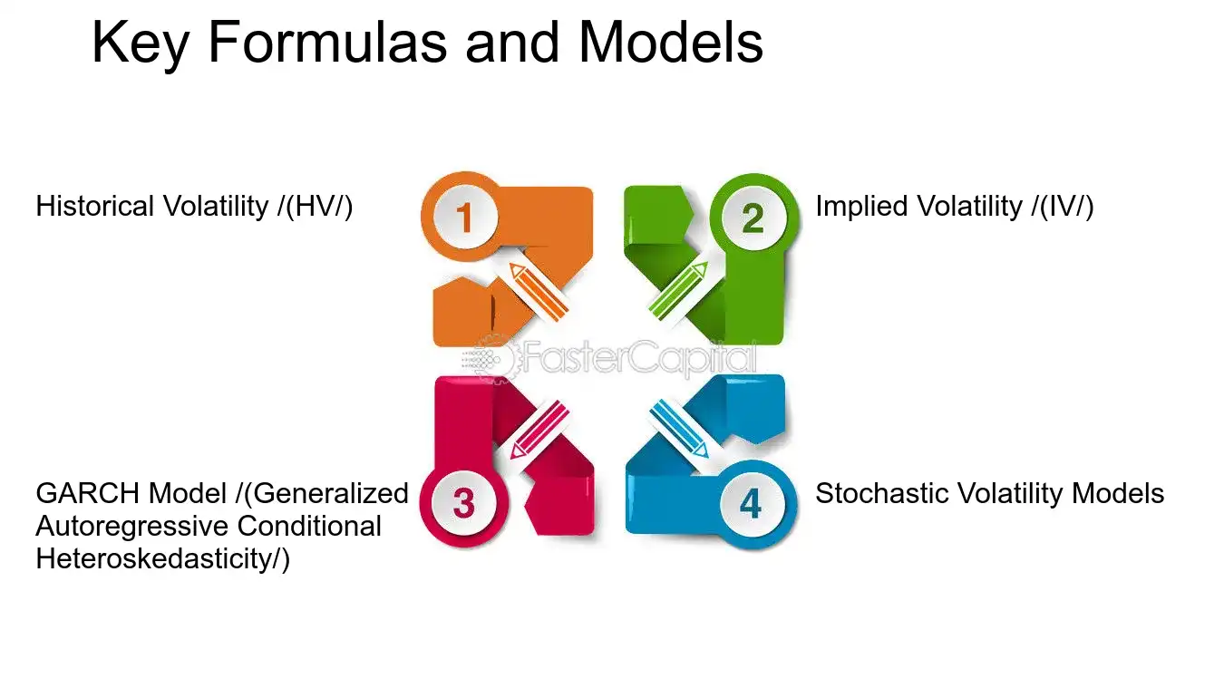
1. Historical Volatility (HV): This is the simplest form of volatility, calculated using the standard deviation of past market prices. For example, the annualized HV of a stock might be computed as:

$$ HV = \sqrt{252} \times \sqrt{\frac{1}{n-1} \sum_{i=1}^{n} (ln(\frac{P_i}{P_{i-1}}) - \overline{ln(\frac{P}{P_{-1}})})^2} $$

Where \( P_i \) is the price at time \( i \), \( n \) is the number of observations, and \( \overline{ln(\frac{P}{P_{-1}})} \) is the average of the logarithmic returns.

2. Implied Volatility (IV): Unlike HV, which looks at the past, IV is forward-looking and is derived from the market price of an option. It reflects the market's view of the likelihood of changes in a given security's price. If we consider the Black-Scholes model, IV can be extracted by solving the following equation for \( \sigma \):

$$ C = S_0 N(d_1) - X e^{-rT} N(d_2) $$

Where \( C \) is the call option price, \( S_0 \) is the current price of the stock, \( X \) is the strike price, \( r \) is the risk-free interest rate, \( T \) is the time to expiration, \( N() \) is the cumulative distribution function of the standard normal distribution, and \( d_1 \) and \( d_2 \) are calculated using \( \sigma \), the IV.

3. GARCH Model (Generalized Autoregressive Conditional Heteroskedasticity): This model allows volatility to change over time as a function of past errors or shocks. It's expressed as:

$$ \sigma_t^2 = \alpha_0 + \alpha_1 \epsilon_{t-1}^2 + \beta_1 \sigma_{t-1}^2 $$

Where \( \sigma_t^2 \) is the forecasted variance, \( \alpha_0 \) is a constant, \( \alpha_1 \) is the coefficient for the lagged squared error term \( \epsilon_{t-1}^2 \), and \( \beta_1 \) is the coefficient for the lagged variance \( \sigma_{t-1}^2 \).

4. stochastic Volatility models: These models assume that volatility is a random process itself, often driven by factors such as market sentiment or macroeconomic events. The Heston model is a popular example, where the variance \( v_t \) follows a mean-reverting square root process:

$$ dv_t = \kappa (\theta - v_t) dt + \xi \sqrt{v_t} dW_t $$

Where \( \kappa \) is the rate of mean reversion, \( \theta \) is the long-term variance, \( \xi \) is the volatility of the volatility, and \( dW_t \) is a Wiener process.

By incorporating these models into our analysis, we can gain a deeper understanding of market dynamics and better manage the risks associated with trading and investing. For instance, a fund manager might use the GARCH model to estimate future volatility and adjust their portfolio accordingly to maintain a desired level of risk exposure. Similarly, an option trader might rely on the IV to price options more accurately or to identify potential trading opportunities when the market's implied volatility diverges significantly from their own volatility forecasts based on historical data.

The mathematics of volatility is a complex but fascinating subject that draws from various disciplines to provide insights into market behavior. By mastering these key formulas and models, one can hope to tame the beast that is market volatility and navigate the financial markets with greater confidence and skill.

4. Behavioral Patterns in Finance

Volatility clustering and mean reversion are two fundamental concepts that have profound implications for financial modeling and risk management. Volatility clustering refers to the phenomenon where large changes in asset prices are followed by large changes — of either sign — and small changes tend to be followed by small changes. This pattern suggests a persistence in the level of volatility, contradicting the random walk hypothesis which assumes price movements are independent and identically distributed. On the other hand, mean reversion is the tendency of a variable, such as an asset price, to converge over time towards its long-term average value. This behavior is often observed in financial markets where asset prices and returns can deviate from their historical average, but eventually tend to return to that average, reflecting a natural equilibrium.

From a trader's perspective, these patterns can be both a challenge and an opportunity. For quantitative analysts, they are crucial patterns to capture in volatility models. Let's delve deeper into these concepts:

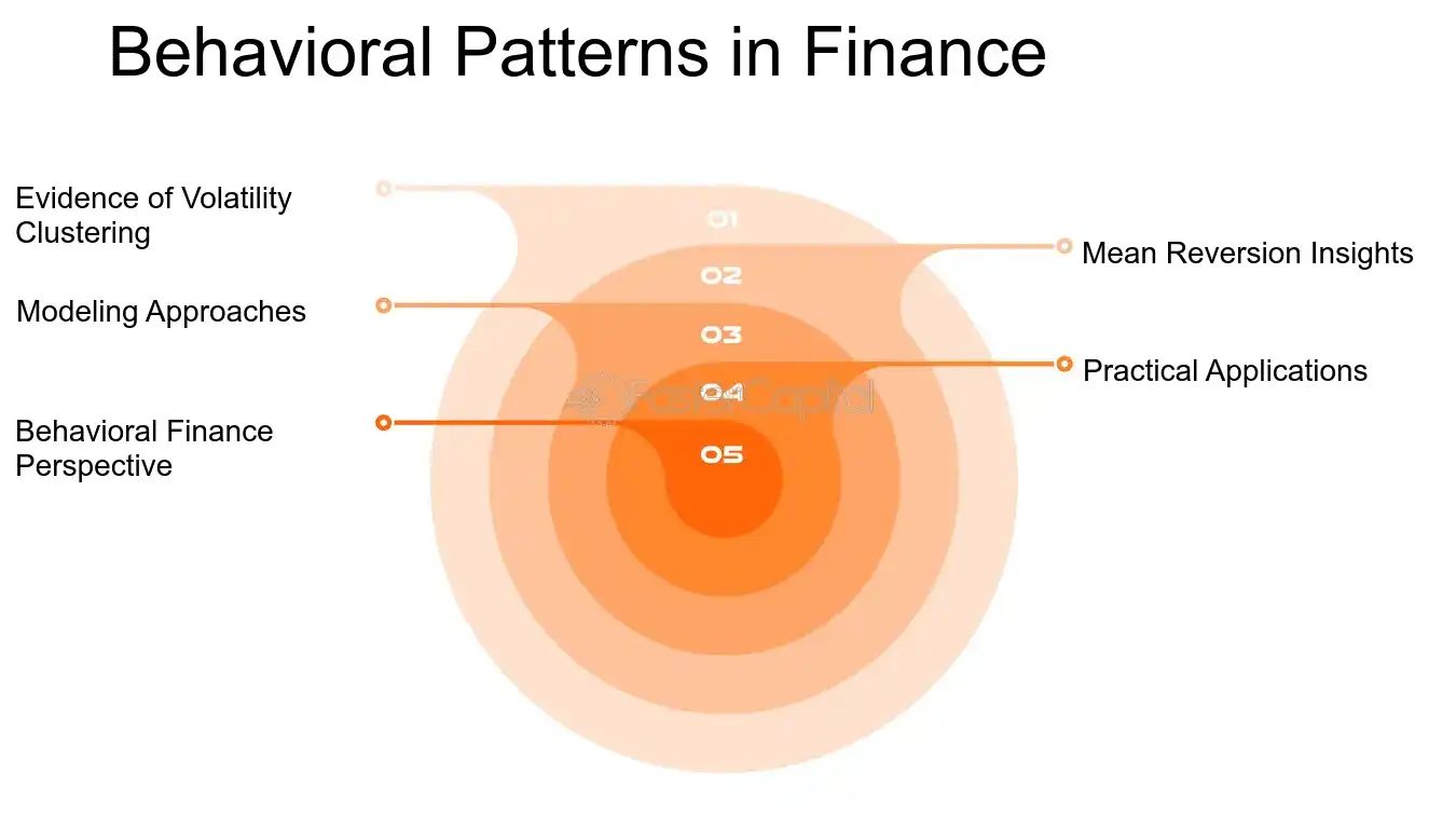
1. Evidence of Volatility Clustering:

- historical Data analysis: Empirical studies of financial time series have consistently shown that periods of high volatility tend to cluster. For example, the stock market crash of 1987 and the financial crisis of 2008 were both characterized by high volatility that persisted for several days or months.

- GARCH Models: Generalized autoregressive Conditional heteroskedasticity (GARCH) models are commonly used to model volatility clustering. They allow for past variances to affect current variance, capturing the persistence in volatility levels.

2. Mean Reversion Insights:

- Statistical Tests: Tests such as the augmented Dickey-fuller (ADF) test are used to detect mean reversion in time series data. A significant result suggests that the price series does not follow a random walk and is likely to exhibit mean-reverting behavior.

- Pairs Trading: This strategy involves taking offsetting positions in two co-integrated assets. When their price ratio deviates from the historical average, a trader would go long on the underperformer and short on the overperformer, betting on the reversion of their price ratio to the mean.

3. Modeling Approaches:

- Stochastic Volatility Models: These models, such as the Heston model, assume that volatility is a random process itself, which can help in capturing the mean-reverting nature of volatility.

- jump-Diffusion models: These models incorporate sudden jumps in asset prices, which can be a response to news or events, alongside the usual continuous price movements.

4. Practical Applications:

- Risk Management: Understanding volatility clustering helps in estimating the likelihood of extreme events, which is crucial for setting appropriate risk limits.

- Option Pricing: Mean reversion can impact the pricing of options, particularly for long-dated options where the mean-reverting characteristic of volatility can affect the option's time value.

5. behavioral Finance perspective:

- Investor Sentiment: Behavioral finance suggests that volatility clustering may be partly driven by the collective behavior of investors, where periods of fear or greed lead to bursts of market activity.

- Overreaction and Correction: Mean reversion can also be seen as a consequence of the market overreacting to information and subsequently correcting itself.

Examples to Highlight Ideas:

- Volatility Clustering Example: During the COVID-19 pandemic, the VIX index, which measures market volatility, exhibited significant clustering as investors reacted to the unfolding crisis.

- Mean Reversion Example: The Japanese yen has historically shown mean-reverting tendencies against the US dollar, often pulling back after significant deviations from its long-term average exchange rate.

Volatility clustering and mean reversion are not just statistical artifacts; they reflect underlying market dynamics and investor behavior. Understanding these patterns is essential for anyone involved in financial markets, from traders to risk managers, and they play a critical role in the development of robust volatility models.

5. Predictive Models for Volatility

In the realm of finance, volatility is akin to a double-edged sword. On one hand, it represents opportunity for traders and investors to capitalize on price movements; on the other, it embodies the risk that can erode profits just as quickly as they were made. The ability to forecast future volatility is a coveted skill in financial markets, as it allows for better risk management and strategic planning. Predictive models for volatility are therefore essential tools for anyone looking to tame the unpredictable nature of financial markets.

From the perspective of a quantitative analyst, predictive models are grounded in statistical and mathematical theories. They often employ historical data to identify patterns and correlations that can signal impending volatility. The GARCH (Generalized Autoregressive Conditional Heteroskedasticity) model, for example, is a popular approach that captures the 'clustering' effect of volatility, where high-volatility events tend to follow each other.

Portfolio managers, on the other hand, might favor a more pragmatic approach, combining quantitative models with market intuition. They may use the VIX index, often referred to as the 'fear gauge', which reflects market expectations of volatility over the coming 30 days, derived from S&P 500 index options.

Here are some in-depth insights into predictive models for volatility:

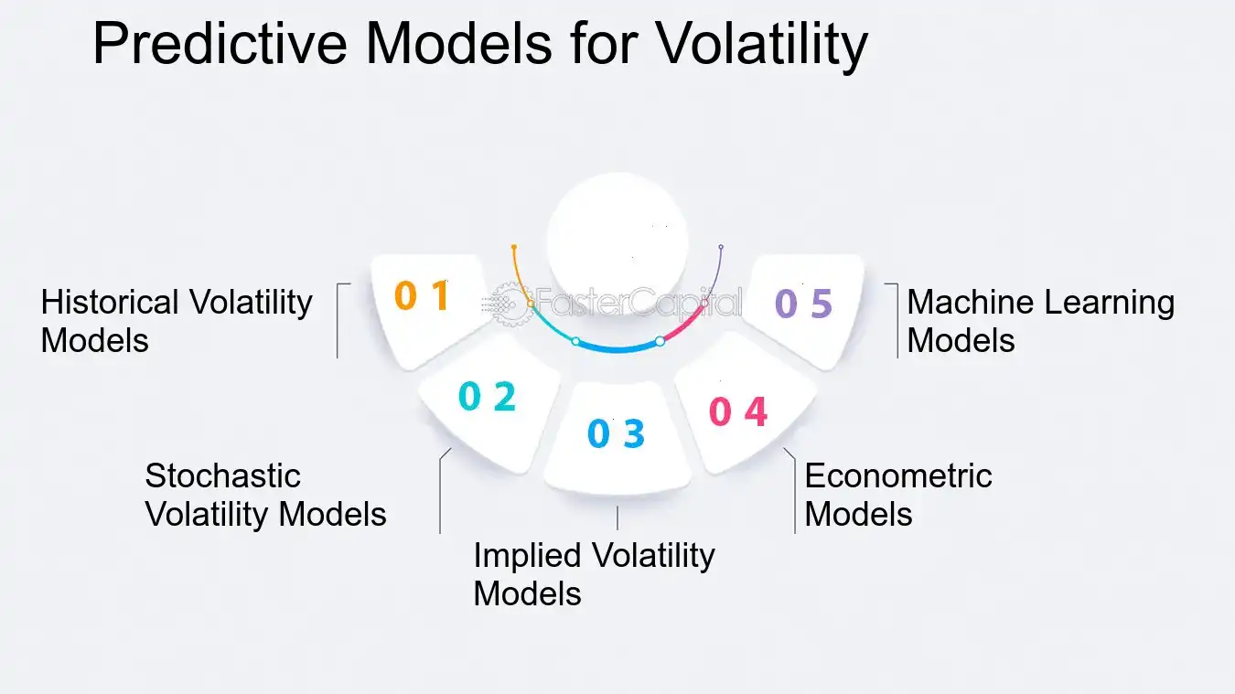
1. Historical Volatility Models: These models analyze past market data to predict future volatility. For example, a simple moving average of past volatility can serve as a baseline forecast.

2. Stochastic Volatility Models: These models assume that volatility is a random process influenced by market factors. The Heston model is a well-known stochastic volatility model that allows for a more realistic representation of market dynamics.

3. Implied Volatility Models: Derived from the pricing of options, implied volatility reflects the market's forecast of future volatility. The Black-Scholes model is a foundational model that uses implied volatility to price options.

4. econometric models: Econometric models like ARCH and GARCH incorporate time-series data to predict volatility. They are particularly useful for capturing the autocorrelation in financial time series.

5. machine Learning models: Recent advancements in machine learning have led to the development of models that can learn from vast datasets and detect complex patterns. Neural networks and support vector machines are examples of such models.

To illustrate, let's consider the Flash Crash of 2010, where the dow Jones Industrial average plunged about 1000 points in just a few minutes. A predictive model that could have foreseen such an event might have saved traders and investors from significant losses. While no model is foolproof, the integration of various models can provide a more robust forecast, enabling market participants to brace for, or even benefit from, the inevitable turbulence that lies ahead.

While forecasting future volatility is inherently challenging due to the chaotic nature of financial markets, the development and refinement of predictive models continue to offer valuable insights. By understanding and applying these models, one can better navigate the tumultuous waters of finance, turning volatility from a fearsome beast into a manageable entity.

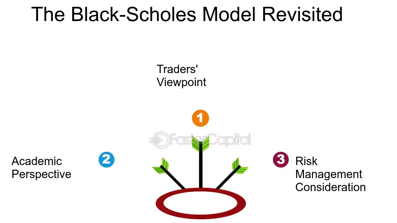
6. The Black-Scholes Model Revisited

The Black-Scholes model, a cornerstone in the world of financial derivatives, has been the subject of intense scrutiny and adaptation since its inception. Originally designed to price european-style options, it has become a foundational tool for traders and financial analysts seeking to understand and harness the complexities of market volatility. The model's beauty lies in its ability to distill the chaotic movements of the market into a structured framework, allowing for the calculation of theoretical option prices. However, the model's assumptions—such as constant volatility and the ability to trade continuously—have often been criticized, leading to the development of various extensions and modifications that aim to capture the dynamic nature of financial markets more accurately.

Insights from Different Perspectives:

1. Traders' Viewpoint:

- Traders often adjust the Black-Scholes model to account for market realities, such as the smile effect where implied volatility differs for in-the-money and out-of-the-money options.

- They may use historical volatility as a benchmark while also considering implied volatility to gauge market sentiment.

2. Academic Perspective:

- Academics have proposed numerous variations of the model, incorporating stochastic volatility, jump diffusion, and other factors to better model real-world scenarios.

- The Heston model, for instance, allows for a stochastic volatility term, providing a more flexible approach to pricing options.

3. Risk Management Consideration:

- From a risk management standpoint, the Black-Scholes model serves as a starting point for the Greeks—sensitivities of the option's price to various parameters—which are crucial for hedging strategies.

- Modifications to the model can lead to more accurate delta, gamma, and vega calculations, which are vital for managing portfolio risk.

In-Depth Information:

1. Volatility Smile and Surface:

- The volatility smile is a pattern observed where implied volatility is higher for deep in-the-money and out-of-the-money options. This phenomenon led to the creation of the volatility surface, a three-dimensional graph plotting implied volatility against strike price and time to expiration.

2. Local Volatility Models:

- Local volatility models, such as the one developed by Dupire, allow the volatility to vary with both the price of the underlying asset and time, providing a more granular approach to option pricing.

3. monte Carlo simulations:

- monte Carlo methods can be used to price options under the Black-scholes framework, especially when dealing with path-dependent options like Asian or lookback options.

Examples to Highlight Ideas:

- Example of a Volatility Smile Adjustment:

Suppose a trader observes a pronounced volatility smile in the market for a particular stock. To price an out-of-the-money call option accurately, the trader might use an implied volatility that is higher than the historical volatility of the stock, reflecting the market's anticipation of potential upward movement.

- Example of a Stochastic Volatility Model:

Consider an option on a commodity like oil, where price swings can be sudden and severe. A stochastic volatility model like the Heston model would allow the volatility to change over time, capturing the erratic behavior of the commodity's price movements.

Revisiting the Black-Scholes model is not just an academic exercise; it is a practical necessity for those engaged in the financial markets. By understanding and adapting the model to fit the ever-evolving landscape of market volatility, finance professionals can better price options, manage risk, and ultimately, make more informed trading decisions.

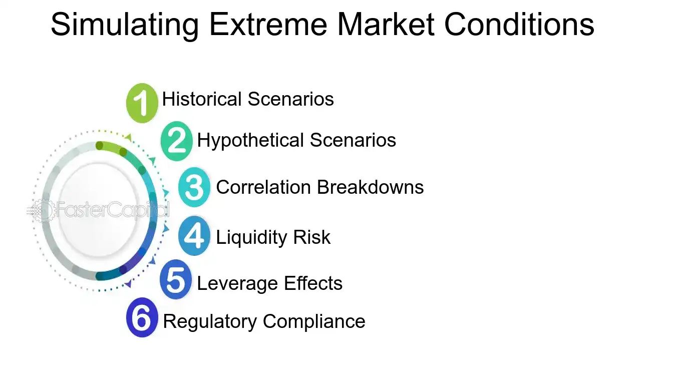
7. Simulating Extreme Market Conditions

In the realm of finance, stress testing portfolios is akin to a fire drill for asset managers. It's a proactive approach to evaluate how investment portfolios would withstand sudden and severe market shifts. This simulation of extreme market conditions is not just about predicting downturns; it's about understanding the resilience of a portfolio under duress. By incorporating various economic scenarios, including market crashes, geopolitical crises, or rapid interest rate changes, stress tests can reveal vulnerabilities that aren't apparent during normal market conditions.

From the perspective of a risk manager, stress testing is a cornerstone of risk management. It allows for the identification of asset classes and individual investments that might be overexposed to market volatility. On the other hand, portfolio managers view stress testing as a means to test investment strategies against historical and hypothetical events, ensuring that the portfolio's strategy aligns with the investor's risk tolerance and investment horizon.

Here's an in-depth look at the components of stress testing portfolios:

1. Historical Scenarios: This involves revisiting past market crises, such as the 2008 financial crisis or the dot-com bubble burst, to see how the current portfolio would have fared. For example, a portfolio heavily invested in technology stocks might simulate the impact of the dot-com crash to gauge potential losses.

2. Hypothetical Scenarios: These are based on "what-if" situations, like a sudden 10% drop in the stock market or a rapid spike in oil prices. For instance, if a portfolio has significant exposure to the energy sector, simulating a scenario where oil prices double can help assess the impact on the portfolio's value.

3. Correlation Breakdowns: Stress tests often assume that correlations between asset classes remain constant, but extreme conditions can disrupt these relationships. For example, during the 2008 crisis, assets that were traditionally negatively correlated moved in the same direction, exacerbating losses.

4. Liquidity Risk: In extreme market conditions, even the most liquid assets can become difficult to sell without significant price concessions. A stress test might simulate a scenario where key assets in the portfolio cannot be liquidated without a 20% haircut to their values.

5. Leverage Effects: For portfolios utilizing leverage, stress tests must account for the magnified impact of market movements. A 5% market drop could mean a 15% loss for a portfolio leveraged 3:1, pushing the need for additional collateral or forced liquidations.

6. Regulatory Compliance: Stress testing also helps ensure that portfolios comply with regulatory requirements, such as those imposed by the basel III framework, which mandates certain capital cushions for banks against stressed market conditions.

By employing these methods, stress testing serves as a critical tool for portfolio management, providing insights that go beyond standard risk metrics like volatility or Value at Risk (VaR). It's a rigorous exercise that prepares investors for the worst, hoping it never comes to pass, but ready if it does. The ultimate goal is not just to survive the storm but to navigate through it with confidence.

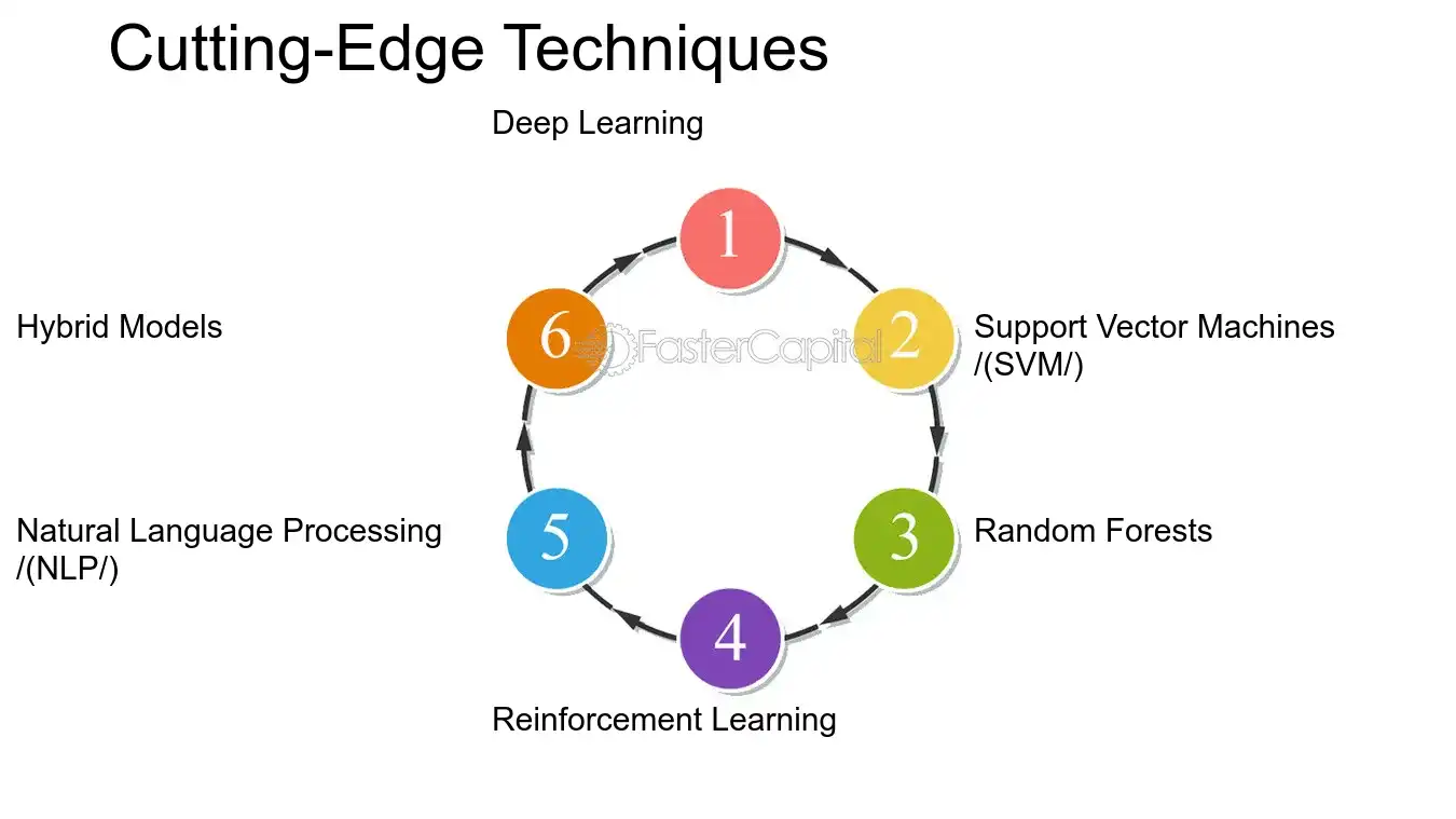
8. Cutting-Edge Techniques

The application of machine learning in volatility prediction represents a significant leap forward in financial modeling. Traditional models, such as the GARCH (Generalized Autoregressive Conditional Heteroskedasticity) and its variants, have long been the standard for volatility forecasting. However, they often fall short in capturing the complex, non-linear dynamics present in financial markets. machine learning techniques, by contrast, are adept at uncovering intricate patterns in large datasets, leading to more accurate and robust predictions. These methods range from supervised learning approaches, like regression trees and neural networks, to unsupervised techniques, such as clustering algorithms, all of which contribute to a more nuanced understanding of market volatility.

From the perspective of a quantitative analyst, machine learning offers tools that can adapt to new data without the need for manual recalibration, a common necessity with traditional econometric models. Portfolio managers, on the other hand, value machine learning for its ability to enhance risk management by providing more reliable measures of market uncertainty. Meanwhile, algorithmic traders utilize these predictions to adjust their strategies in real-time, capitalizing on volatile market conditions.

Here are some cutting-edge techniques in machine learning that are reshaping volatility prediction:

1. Deep Learning: Neural networks, particularly deep learning models like long Short-Term memory (LSTM) networks, have shown great promise in predicting financial time series data. For example, an LSTM model can be trained on historical price data to forecast future volatility, capturing dependencies over long sequences that simpler models might miss.

2. Support Vector Machines (SVM): SVMs are powerful for classification and regression problems. In volatility prediction, they can be used to classify periods of high and low volatility or to predict the magnitude of future volatility based on historical price changes and other market indicators.

3. Random Forests: This ensemble learning method combines multiple decision trees to improve predictive accuracy and control over-fitting. By aggregating the predictions of numerous trees, random forests can provide a more stable and reliable forecast of volatility.

4. Reinforcement Learning: This area of machine learning is concerned with how agents ought to take actions in an environment to maximize cumulative reward. Applied to volatility prediction, reinforcement learning algorithms can dynamically adjust to changing market conditions to optimize trading strategies.

5. natural Language processing (NLP): Sentiment analysis using NLP can extract insights from news articles, social media, and financial reports, which can then be used to predict market sentiment and, consequently, volatility. For instance, a spike in negative sentiment might precede increased market volatility.

6. Hybrid Models: Combining machine learning techniques with traditional econometric models can yield superior results. A hybrid model might use a neural network to capture non-linear patterns and a GARCH model to ensure that the volatility dynamics adhere to financial theory.

To illustrate, consider a scenario where a deep learning model is used to predict the volatility of a stock index. The model is trained on historical data, including price changes, trading volume, and economic indicators. Once trained, the model can forecast future volatility, which can then inform trading decisions, such as whether to increase or decrease position sizes based on expected market turbulence.

machine learning is revolutionizing the field of volatility prediction, offering a suite of sophisticated tools that can handle the complexity and unpredictability of financial markets. As these techniques continue to evolve, they will undoubtedly become even more integral to the strategies of traders, analysts, and portfolio managers alike.

9. Mitigating the Impact of Volatility

In the realm of finance, volatility is often viewed as a double-edged sword. On one hand, it can provide opportunities for significant profit, but on the other, it can lead to substantial losses. effective risk management strategies are crucial for mitigating the impact of volatility and ensuring that it does not derail the financial objectives of individuals or institutions. These strategies involve a combination of analytical techniques, market insight, and proactive oversight to navigate through the turbulent waters of financial markets.

1. Diversification: A fundamental strategy to mitigate risk is diversification. By spreading investments across various asset classes, sectors, and geographies, one can reduce the impact of a downturn in any single area. For example, an investor might combine stocks, bonds, real estate, and commodities in their portfolio to balance out the risks.

2. Hedging: Hedging involves taking an offsetting position in a related asset to reduce the risk of adverse price movements. Common hedging instruments include options, futures, and swaps. For instance, an oil company might use futures contracts to lock in the price of oil, protecting against the volatility of oil prices.

3. Asset Allocation: Adjusting the mix of assets can also manage volatility. This strategy requires regularly reviewing and rebalancing the portfolio to align with one's risk tolerance and investment horizon. For example, as an individual approaches retirement, they might shift from stocks to bonds to reduce exposure to market fluctuations.

4. stop-Loss orders: These orders can limit losses by automatically selling an asset when its price falls to a certain level. For instance, a trader might set a stop-loss order 10% below the purchase price of a stock to prevent larger losses in a declining market.

5. Volatility Indexes: Monitoring volatility indexes like the vix, which measures the market's expectation of volatility, can provide insights into market sentiment and potential risk. Investors can use this information to adjust their investment strategies accordingly.

6. Risk Parity: This approach allocates capital based on the risk contributed by each asset, rather than the expected return. For example, if bonds are less volatile than stocks, a risk parity strategy might involve investing more in bonds to achieve a balanced risk profile.

7. Stress Testing: Simulating various market scenarios can help investors understand potential risks and prepare for extreme events. For example, stress testing a portfolio against historical events like the 2008 financial crisis can reveal vulnerabilities.

8. Value at Risk (VaR): VaR is a statistical technique used to measure and quantify the level of financial risk within a firm or portfolio over a specific time frame. This metric can help in determining the potential for loss and in making informed decisions to mitigate risk.

While volatility can never be completely eliminated, employing a combination of these strategies can help investors manage their exposure and protect their investments. It's about finding the right balance between risk and return, and being prepared for the inevitable ups and downs of the market. The key is to remain vigilant, adaptable, and informed, making adjustments as market conditions evolve.

Read Other Blogs