Lagrange's Mean Value Theorem

Lagrange's Mean Value Theorem (LMVT) is a fundamental result in differential calculus, providing a formalized way to understand the behavior of differentiable functions. This theorem generalizes Rolle's Theorem and has significant applications in various fields of engineering, physics, and applied mathematics. This article explores Lagrange's Mean Value Theorem, its mathematical formulation, proof, and applications in engineering.

Lagrange's Mean Value Theorem

What is Lagrange's Mean Value Theorem?

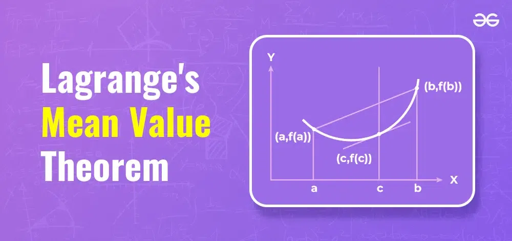
Lagrange's Mean Value Theorem states that if a function f satisfies the following conditions on the interval [a,b]:

1. f is continuous on [a,b]
2. f is differentiable on (a,b)

then there exists at least one point c in (a,b) such that:

f'(c) = \frac{f(b) - f(a)}{b - a}

This means that there is at least one point where the instantaneous rate of change (the derivative) of the function is equal to the average rate of change over the interval.

Proof of Lagrange's Mean Value Theorem

To prove LMVT, consider the function f(x) and the auxiliary function g(x) defined by:

g(x) = f(x) - (\frac{f(b) - f(a)}{b - a}) (x -a)

1. The function g(x) is continuous on [a,b][a, b][a,b] and differentiable on (a,b)
2. At x = a, g(a) = f(a).
3. At x = b, g(b) = f(b) - (\frac{f(b) - f(a)}{b - a}) (b − a) = f(b)−(f(b)−f(a)) = f(a).

Thus, g(a) = g(b), and by Rolle's Theorem, there exists a point c ∈ (a,b) such that g′(c) = 0.

Differentiating g(x):

g′(x) = f′(x) - \frac{f(b) - f(a)}{b - a}

Setting g′(c) = 0:

f′(c) = \frac{f(b) - f(a)}{b - a}

Hence, the theorem is proven.

Applications of Lagrange's Mean Value Theorem in Engineering

1. Motion Analysis

In mechanical and aerospace engineering, LMVT is used to analyze the motion of objects. By considering the displacement of an object over time, LMVT helps in understanding the object's velocity at specific points, crucial for designing and controlling the movement of machinery and vehicles.

2. Structural Engineering

In structural engineering, LMVT assists in analyzing stress and strain distributions in materials. By applying LMVT to the deformation functions, engineers can predict points where the material experiences maximum or minimum stress, essential for ensuring structural integrity and safety.

3. Electrical Engineering

In electrical engineering, LMVT is used in the analysis of electrical circuits. For instance, when analyzing the change in voltage or current over a period, LMVT helps in identifying points where the rate of change is equivalent to the average rate, aiding in the design and optimization of circuits.

4. Fluid Dynamics

In fluid dynamics, LMVT helps in understanding the flow rate of fluids through pipes and channels. By applying LMVT to the velocity profiles of fluids, engineers can determine points where the instantaneous flow rate equals the average flow rate, which is crucial for designing efficient fluid transport systems.

5. Control Systems

In control systems engineering, LMVT is used to analyze the response of systems to various inputs. By applying LMVT to the output response of a system, engineers can identify points where the system's response rate matches the average rate, aiding in the design and tuning of controllers.

Related Articles:

• Rolle’s Theorem and Lagrange’s Mean Value Theorem
• Lagrange’s Mean Value Theorem

Lagrange's Mean Value Theorem - Sample Problems

Example 1: Consider f(x) = x^2 on the interval [1, 3].

Step 1: Verify the conditions:

f(x) = x^2 is continuous on [1, 3] and differentiable on (1, 3).

Step 2: Calculate [f(b) - f(a)] / (b - a):

[f(3) - f(1)] / (3 - 1) = (9 - 1) / 2 = 4

Step 3: Find f'(x):

f'(x) = 2x

Step 4: Solve f'(c) = 4:

2c = 4

c = 2

Therefore, c = 2 satisfies the Mean Value Theorem.

Example 2: Consider f(x) = sin(x) on the interval [0, π/2].

Step 1: Verify the conditions:

sin(x) is continuous on [0, π/2] and differentiable on (0, π/2).

Step 2: Calculate [f(b) - f(a)] / (b - a):

[sin(π/2) - sin(0)] / (π/2 - 0) = (1 - 0) / (π/2) = 2/π

Step 3: Find f'(x):

f'(x) = cos(x)

Step 4: Solve cos(c) = 2/π:

c = arccos(2/π) ≈ 0.6435 radians

Therefore, c ≈ 0.6435 satisfies the Mean Value Theorem.

Example 3: Consider f(x) = ln(x) on the interval [1, e].

Step 1: Verify the conditions:

ln(x) is continuous on [1, e] and differentiable on (1, e).

Step 2: Calculate [f(b) - f(a)] / (b - a):

[ln(e) - ln(1)] / (e - 1) = (1 - 0) / (e - 1) = 1/(e - 1)

Step 3: Find f'(x):

f'(x) = 1/x

Step 4: Solve 1/c = 1/(e - 1):

c = e - 1

Therefore, c = e - 1 satisfies the Mean Value Theorem

Example 4:f(x) = x^3 on the interval [0, 2]

f(x) = x^3 on the interval [0, 2]

Step 1: f(x) = x^3 is continuous on [0, 2] and differentiable on (0, 2).

Step 2: [f(2) - f(0)] / (2 - 0) = (8 - 0) / 2 = 4

Step 3: f'(x) = 3x^2

Step 4: Solve 3c^2 = 4

c = √(4/3) ≈ 1.15

Example 5: f(x) = e^x on the interval [0, 1]

Step 1: e^x is continuous on [0, 1] and differentiable on (0, 1).

Step 2: [f(1) - f(0)] / (1 - 0) = (e - 1) / 1 = e - 1

Step 3: f'(x) = e^x

Step 4: Solve e^c = e - 1

c = ln(e - 1) ≈ 0.54

Example 6: f(x) = cos(x) on the interval [0, π]

Step 1: cos(x) is continuous on [0, π] and differentiable on (0, π).

Step 2: [f(π) - f(0)] / (π - 0) = (-1 - 1) / π = -2/π

Step 3: f'(x) = -sin(x)

Step 4: Solve -sin(c) = -2/π

c = arcsin(2/π) ≈ 0.69

Example 7: f(x) = x^2 - 3x + 2 on the interval [1, 4]

Step 1: x^2 - 3x + 2 is continuous on [1, 4] and differentiable on (1, 4).

Step 2: [f(4) - f(1)] / (4 - 1) = [(16 - 12 + 2) - (1 - 3 + 2)] / 3 = 6/3 = 2

Step 3: f'(x) = 2x - 3

Step 4: Solve 2c - 3 = 2

c = 2.5

Example 8: f(x) = √x on the interval [1, 9]

Step 1: √x is continuous on [1, 9] and differentiable on (1, 9).

Step 2: [f(9) - f(1)] / (9 - 1) = (3 - 1) / 8 = 1/4

Step 3: f'(x) = 1 / (2√x)

Step 4: Solve 1 / (2√c) = 1/4

c = 4

Example 9: f(x) = x^3 - x on the interval [-1, 2]

Step 1: x^3 - x is continuous on [-1, 2] and differentiable on (-1, 2).

Step 2: [f(2) - f(-1)] / (2 - (-1)) = [(8 - 2) - (-1 + 1)] / 3 = 6/3 = 2

Step 3: f'(x) = 3x^2 - 1

Step 4: Solve 3c^2 - 1 = 2

3c^2 = 3

c = ±1

Both c = 1 and c = -1 satisfy the theorem.

Example 10: f(x) = ln(x+1) on the interval [0, e-1]

Step 1: ln(x+1) is continuous on [0, e-1] and differentiable on (0, e-1).

Step 2: [f(e-1) - f(0)] / ((e-1) - 0) = [ln(e) - ln(1)] / (e-1) = 1 / (e-1)

Step 3: f'(x) = 1 / (x+1)

Step 4: Solve 1 / (c+1) = 1 / (e-1)

c+1 = e-1

c = e-2 ≈ 0.72

Practice Problems on Lagrange's Mean Value Theorem

1. Find the value of c guaranteed by the Mean Value Theorem for f(x) = x² + 2x on the interval [0, 3].

2. Verify that f(x) = x³ satisfies the conditions of the Mean Value Theorem on [-1, 2], and find all values of c that satisfy the conclusion of the theorem.

3. Determine whether there is a value of c that satisfies the Mean Value Theorem for f(x) = |x| on the interval [-2, 2].

4. Find the value of c guaranteed by the Mean Value Theorem for f(x) = sin(x) on the interval [0, π/3].

5. For f(x) = e^x, find the value of c guaranteed by the Mean Value Theorem on the interval [ln 2, ln 5]

6. Verify that f(x) = 1/x satisfies the conditions of the Mean Value Theorem on [1, 4], and find the value of c that satisfies the conclusion of the theorem.

7. Find all values of c that satisfy the Mean Value Theorem for f(x) = x⁴ - 2x² on the interval [-1, 1].

8. Determine whether there is a value of c that satisfies the Mean Value Theorem for f(x) = tan(x) on the interval [0, π/4].

9. For f(x) = ln(x² + 1), find the value of c guaranteed by the Mean Value Theorem on the interval [0, 1].

10. Verify that f(x) = cos(x) satisfies the conditions of the Mean Value Theorem on [0, 2π], and find all values of c in this interval that satisfy the conclusion of the theorem.

Conclusion

Lagrange's Mean Value Theorem is a powerful tool in calculus, providing essential insights into the behavior of differentiable functions. Its applications in engineering are vast, aiding in the analysis and design of systems in motion analysis, structural engineering, electrical circuits, fluid dynamics, and control systems. Understanding and applying LMVT is crucial for solving complex engineering problems involving rates of change and function behaviors.