


![xxii Introduction
book demonstrate how Python can work side by side with Arduino code and
JavaScript. Real software projects often use a mix of software technologies,
and Python fits very well into such layered architectures.
The following example demonstrates the ease of working with Python.
While developing code for the Raspberry Pi weather monitor in Chapter
14, I wrote this string looking at the oscilloscope output from the tempera-
ture/humidity sensor:
0011011100000000000110100000000001010001
Since I don’t speak binary (especially at 7 am on a Sunday morning),
I fired up the Python interpreter and entered:
>>> str = '0011011100000000000110100000000001010001'
>>> len(str)
40
>>> [int(str[i:i+8], 2) for i in range(0, 40, 8)]
[55, 0, 26, 0, 81]
This code splits up the 40-bit string into five 8-bit integers, which I can
actually interpret. The data above is decoded as a 55.0 percent humidity
reading at a temperature of 26.0 degrees centigrade, and the checksum
is 55 + 26 = 81.
This example demonstrates the practical use of the Python interpreter
as a very power calculator. You don’t need to write a complete program to do
quick computations; just open up the interpreter and get going. This is just
one of the many reasons why I love Python, and why I think you will too.
Python Versions
This book was built with Python 3.3.3, but all code is compatible with
Python 2.7.x and 3.x.
The Code in This Book
I’ve done my best throughout this book to walk you through the code for
each project in detail, piece by piece. You can either enter the code yourself
or download the complete source code (using the Download Zip option) for
all programs in the book at https://github.com/electronut/pp/.
You’ll find several exciting projects in the following pages. I hope you
have as much fun playing with them as I had creating them. And don’t forget
to explore further with the exercises presented at the end of each project.
I wish you many happy hours of programming with Python Playground!
www.it-ebooks.info](https://image.slidesharecdn.com/pythonplaygroundgeekyprojectsforthecuriousprogrammerpdfdrive-220717171538-9c44c48d/85/Python-Playground_-Geeky-Projects-for-the-Curious-Programmer-PDFDrive-pdf-23-320.jpg)


![4 Chapter 1
• Making simple plots with the matplotlib library
• Creating and saving data files
Anatomy of the iTunes Playlist File
The information in an iTunes library can be exported into playlist files.
(Choose File4Library4Export Playlist in iTunes.) The playlist files are
written in Extensible Markup Language (XML), a text-based language
designed to represent text-based information hierarchically. It consists of
a tree-like collection of user-defined tags in the form <myTag>, each of which
can have attribute and child tags with additional information.
When you open a playlist file in a text editor, you’ll see something like
this abbreviated version:
<?xml version="1.0" encoding="UTF-8"?>
u <!DOCTYPE plist PUBLIC "-//Apple Computer//DTD PLIST 1.0//EN" "http://www
.apple.com/DTDs/PropertyList-1.0.dtd">
v <plist version="1.0">
w <dict>
x <key>Major Version</key><integer>1</integer>
<key>Minor Version</key><integer>1</integer>
--snip--
y <key>Tracks</key>
<dict>
<key>2438</key>
<dict>
<key>Track ID</key><integer>2438</integer>
<key>Name</key><string>Yesterday</string>
<key>Artist</key><string>The Beatles</string>
<key>Composer</key><string>Lennon [John], McCartney [Paul]</string>
<key>Album</key><string>Help!</string>
</dict>
--snip--
</dict>
z <key>Playlists</key>
<array>
<dict>
<key>Name</key><string>Now</string>
<key>Playlist ID</key><integer>21348</integer>
--snip--
<array>
<dict>
<key>Track ID</key><integer>6382</integer>
</dict>
--snip--
</array>
</dict>
</array>
</dict>
</plist>
www.it-ebooks.info](https://image.slidesharecdn.com/pythonplaygroundgeekyprojectsforthecuriousprogrammerpdfdrive-220717171538-9c44c48d/85/Python-Playground_-Geeky-Projects-for-the-Curious-Programmer-PDFDrive-pdf-27-320.jpg)

![6 Chapter 1
Finding Duplicates
You’ll start by finding duplicate tracks with the findDuplicates() method, as
shown here:
def findDuplicates(fileName):
print('Finding duplicate tracks in %s...' % fileName)
# read in a playlist
u plist = plistlib.readPlist(fileName)
# get the tracks from the Tracks dictionary
v tracks = plist['Tracks']
# create a track name dictionary
w trackNames = {}
# iterate through the tracks
x for trackId, track in tracks.items():
try:
y name = track['Name']
duration = track['Total Time']
# look for existing entries
z if name in trackNames:
# if a name and duration match, increment the count
# round the track length to the nearest second
{ if duration//1000 == trackNames[name][0]//1000:
count = trackNames[name][1]
| trackNames[name] = (duration, count+1)
else:
# add dictionary entry as tuple (duration, count)
} trackNames[name] = (duration, 1)
except:
# ignore
pass
At u, the readPlist() method takes a p-list file as input and returns the
top-level dictionary. You access the Tracks dictionary at v, and at w, you
create an empty dictionary to keep track of duplicates. At x, you begin
iterating through the Tracks dictionary using the items() method, which is
commonly used in Python to retrieve both the key and the value of a dic-
tionary as you iterate through it.
At y, you retrieve the name and duration of each track in the diction-
ary. You check to see whether the current track name already exists in the
dictionary being built by using the in keyword z. If so, the program checks
whether the track lengths of the existing and newly found tracks are identi-
cal { by dividing the track length of each by 1,000 with the // operator to
convert milliseconds to seconds and then rounding to the nearest second.
(Of course, this means that two tracks that differ in length only by milli
seconds are considered to be the same length.) If you determine that the
two track lengths are equal, you get the value associated with name, which
is the tuple (duration, count), and increment count at |. If this is the first
time the program has come across the track name, it creates a new entry
for it, with a count of 1 }.
www.it-ebooks.info](https://image.slidesharecdn.com/pythonplaygroundgeekyprojectsforthecuriousprogrammerpdfdrive-220717171538-9c44c48d/85/Python-Playground_-Geeky-Projects-for-the-Curious-Programmer-PDFDrive-pdf-29-320.jpg)
![Parsing iTunes Playlists 7
You enclose the body of the code’s main for loop in a try block because
some music tracks may not have the track name defined. In that case, you
skip the track and include only pass (which does nothing) in the except
section.
Extracting Duplicates
To extract duplicates, you use this code:
# store duplicates as (name, count) tuples
u dups = []
for k, v in trackNames.items():
v if v[1] > 1:
dups.append((v[1], k))
# save duplicates to a file
w if len(dups) > 0:
print("Found %d duplicates. Track names saved to dup.txt" % len(dups))
else:
print("No duplicate tracks found!")
x f = open("dups.txt", "w")
for val in dups:
y f.write("[%d] %sn" % (val[0], val[1]))
f.close()
At u, you create an empty list to hold the duplicates. Next, you iterate
through the trackNames dictionary, and if count (accessed with v[1] because
it’s the second element in the tuple) is greater than 1, you append a tuple
with (name, count) to the list. At w, the program prints information about
what it has found and then saves that information to a file using the open()
method x. At y, you iterate through the dups list, writing out the dupli-
cate entries.
Finding Tracks Common Across Multiple Playlists
Now let’s look at how you find music tracks that are common across mul-
tiple playlists:
def findCommonTracks(fileNames):
# a list of sets of track names
u trackNameSets = []
for fileName in fileNames:
# create a new set
v trackNames = set()
# read in playlist
w plist = plistlib.readPlist(fileName)
# get the tracks
tracks = plist['Tracks']
# iterate through the tracks
for trackId, track in tracks.items():
try:
# add the track name to a set
x trackNames.add(track['Name'])
www.it-ebooks.info](https://image.slidesharecdn.com/pythonplaygroundgeekyprojectsforthecuriousprogrammerpdfdrive-220717171538-9c44c48d/85/Python-Playground_-Geeky-Projects-for-the-Curious-Programmer-PDFDrive-pdf-30-320.jpg)
![8 Chapter 1
except:
# ignore
pass
# add to list
y trackNameSets.append(trackNames)
# get the set of common tracks
z commonTracks = set.intersection(*trackNameSets)
# write to file
if len(commonTracks) > 0:
{ f = open("common.txt", "w")
for val in commonTracks:
s = "%sn" % val
| f.write(s.encode("UTF-8"))
f.close()
print("%d common tracks found. "
"Track names written to common.txt." % len(commonTracks))
else:
print("No common tracks!")
First, you pass a list of playlist filenames to findCommonTracks(), which
creates an empty list u to store a set of objects created from each play
list. The
program then iterates through each file in the list. For each file, you
create
a Python set object called trackNames v; then as in findDuplicates(), you use
plistlib to read in the file w and get the Tracks dictionary. Next, you iter-
ate through each track in this dictionary and add the trackNames object x.
Once the program has finished with all tracks in a file, it adds this set to
trackNameSets y.
At z, you use the set.intersection() method to get the set of tracks that
are common among the sets. (You use the Python * operator to unpack the
argument lists.) If the program finds any tracks that are common among
sets, it writes the track names to a file. At {, you open the file, and the two
lines that follow do the actual writing. Use encode() to format the output
and to ensure that any Unicode characters are handled correctly |.
Collecting Statistics
Next, use the plotStats() method to collect statistics for the track names:
def plotStats(fileName):
# read in a playlist
u plist = plistlib.readPlist(fileName)
# get the tracks from the playlist
tracks = plist['Tracks']
# create lists of song ratings and track durations
v ratings = []
durations = []
# iterate through the tracks
for trackId, track in tracks.items():
try:
w ratings.append(track['Album Rating'])
durations.append(track['Total Time'])
www.it-ebooks.info](https://image.slidesharecdn.com/pythonplaygroundgeekyprojectsforthecuriousprogrammerpdfdrive-220717171538-9c44c48d/85/Python-Playground_-Geeky-Projects-for-the-Curious-Programmer-PDFDrive-pdf-31-320.jpg)
![Parsing iTunes Playlists 9
except:
# ignore
pass
# ensure that valid data was collected
x if ratings == [] or durations == []:
print("No valid Album Rating/Total Time data in %s." % fileName)
return
The goal here is to gather ratings and track durations and then do
some plotting. At u and in the lines that follow, you read the playlist file
and get access to the Tracks dictionary. Next, you create two empty lists to
store ratings and durations v. (Ratings in iTunes playlists are stored as
integers in the range [0, 100]). Iterating through the tracks, you get and
append the ratings and durations to the appropriate lists at w. Finally, the
sanity check at x makes sure you collected valid data from the playlist file.
Plotting Your Data
You’re now ready to plot some data.
# scatter plot
u x = np.array(durations, np.int32)
# convert to minutes
v x = x/60000.0
w y = np.array(ratings, np.int32)
x pyplot.subplot(2, 1, 1)
y pyplot.plot(x, y, 'o')
z pyplot.axis([0, 1.05*np.max(x), -1, 110])
{ pyplot.xlabel('Track duration')
| pyplot.ylabel('Track rating')
# plot histogram
pyplot.subplot(2, 1, 2)
} pyplot.hist(x, bins=20)
pyplot.xlabel('Track duration')
pyplot.ylabel('Count')
# show plot
~ pyplot.show()
At u, you put the data for the track durations into a 32-bit integer
array using numpy.array() (imported as np in the code); then at v, you use
numpy to apply an operation to every element in the array. In this case,
you’re converting the duration in milliseconds to seconds by dividing
each value by 60 × 1000. You store the track ratings in another numpy array,
y, at w.
Use matplotlib to draw two plots in the same figure. At x, the argu-
ments to subplot()—namely, (2, 1, 1)—tell matplotlib that the figure
should have two rows (2) and one column (1) and that the next plot should
go in the first row (1). You create the plot at y by calling plot(), and the
o tells
matplotlib to use circles to represent the data.
www.it-ebooks.info](https://image.slidesharecdn.com/pythonplaygroundgeekyprojectsforthecuriousprogrammerpdfdrive-220717171538-9c44c48d/85/Python-Playground_-Geeky-Projects-for-the-Curious-Programmer-PDFDrive-pdf-32-320.jpg)

![Parsing iTunes Playlists 11
options at the same time. The argparse module provides a solution to this
challenge in the form of mutually exclusive argument groups. At v, you use
the parser.add_mutually_exclusive_group() method to create such a group.
At w, x, and y, you specify the command line options mentioned
earlier and enter the variable names (args.plFiles, args.plFile, and
args.plFileD) the parsed values should be stored in. The actual parsing
is done at z. Once the arguments are parsed, you pass them to the appro-
priate functions,
findCommonTracks(), plotStats(), and findDuplicates(), as
discussed earlier in this chapter.
To see whether an argument was parsed, test the appropriate variable
name in args. For example, if the user did not use the --common option
(which finds common tracks among playlists), args.plFiles should be set
to None after parsing.
You handle the case in which the user didn’t enter any arguments at {.
The Complete Code
Here is the complete program. You can also find the code and some test
data for this project at https://github.com/electronut/pp/tree/master/playlist/.
import re, argparse
import sys
from matplotlib import pyplot
import plistlib
import numpy as np
def findCommonTracks(fileNames):
"""
Find common tracks in given playlist files,
and save them to common.txt.
"""
# a list of sets of track names
trackNameSets = []
for fileName in fileNames:
# create a new set
trackNames = set()
# read in playlist
plist = plistlib.readPlist(fileName)
# get the tracks
tracks = plist['Tracks']
# iterate through the tracks
for trackId, track in tracks.items():
try:
# add the track name to a set
trackNames.add(track['Name'])
except:
# ignore
pass
# add to list
trackNameSets.append(trackNames)
www.it-ebooks.info](https://image.slidesharecdn.com/pythonplaygroundgeekyprojectsforthecuriousprogrammerpdfdrive-220717171538-9c44c48d/85/Python-Playground_-Geeky-Projects-for-the-Curious-Programmer-PDFDrive-pdf-34-320.jpg)
![12 Chapter 1
# get the set of common tracks
commonTracks = set.intersection(*trackNameSets)
# write to file
if len(commonTracks) > 0:
f = open("common.txt", 'w')
for val in commonTracks:
s = "%sn" % val
f.write(s.encode("UTF-8"))
f.close()
print("%d common tracks found. "
"Track names written to common.txt." % len(commonTracks))
else:
print("No common tracks!")
def plotStats(fileName):
"""
Plot some statistics by reading track information from playlist.
"""
# read in a playlist
plist = plistlib.readPlist(fileName)
# get the tracks from the playlist
tracks = plist['Tracks']
# create lists of song ratings and track durations
ratings = []
durations = []
# iterate through the tracks
for trackId, track in tracks.items():
try:
ratings.append(track['Album Rating'])
durations.append(track['Total Time'])
except:
# ignore
pass
# ensure that valid data was collected
if ratings == [] or durations == []:
print("No valid Album Rating/Total Time data in %s." % fileName)
return
# scatter plot
x = np.array(durations, np.int32)
# convert to minutes
x = x/60000.0
y = np.array(ratings, np.int32)
pyplot.subplot(2, 1, 1)
pyplot.plot(x, y, 'o')
pyplot.axis([0, 1.05*np.max(x), -1, 110])
pyplot.xlabel('Track duration')
pyplot.ylabel('Track rating')
# plot histogram
pyplot.subplot(2, 1, 2)
pyplot.hist(x, bins=20)
pyplot.xlabel('Track duration')
pyplot.ylabel('Count')
www.it-ebooks.info](https://image.slidesharecdn.com/pythonplaygroundgeekyprojectsforthecuriousprogrammerpdfdrive-220717171538-9c44c48d/85/Python-Playground_-Geeky-Projects-for-the-Curious-Programmer-PDFDrive-pdf-35-320.jpg)
![Parsing iTunes Playlists 13
# show plot
pyplot.show()
def findDuplicates(fileName):
"""
Find duplicate tracks in given playlist.
"""
print('Finding duplicate tracks in %s...' % fileName)
# read in playlist
plist = plistlib.readPlist(fileName)
# get the tracks from the Tracks dictionary
tracks = plist['Tracks']
# create a track name dictionary
trackNames = {}
# iterate through tracks
for trackId, track in tracks.items():
try:
name = track['Name']
duration = track['Total Time']
# look for existing entries
if name in trackNames:
# if a name and duration match, increment the count
# round the track length to the nearest second
if duration//1000 == trackNames[name][0]//1000:
count = trackNames[name][1]
trackNames[name] = (duration, count+1)
else:
# add dictionary entry as tuple (duration, count)
trackNames[name] = (duration, 1)
except:
# ignore
pass
# store duplicates as (name, count) tuples
dups = []
for k, v in trackNames.items():
if v[1] > 1:
dups.append((v[1], k))
# save duplicates to a file
if len(dups) > 0:
print("Found %d duplicates. Track names saved to dup.txt" % len(dups))
else:
print("No duplicate tracks found!")
f = open("dups.txt", 'w')
for val in dups:
f.write("[%d] %sn" % (val[0], val[1]))
f.close()
# gather our code in a main() function
def main():
# create parser
descStr = """
This program analyzes playlist files (.xml) exported from iTunes.
"""
parser = argparse.ArgumentParser(description=descStr)
www.it-ebooks.info](https://image.slidesharecdn.com/pythonplaygroundgeekyprojectsforthecuriousprogrammerpdfdrive-220717171538-9c44c48d/85/Python-Playground_-Geeky-Projects-for-the-Curious-Programmer-PDFDrive-pdf-36-320.jpg)


![22 Chapter 2
about its center, which gives you a hint to the shape of the curve. If you
count them in Figure 2-4, you’ll see that the number of petals or lobes in
the drawing is exactly 44!
Once you express the radii ratio in the reduced form r/R, the range
for the parameter q to draw the spiro is [0, 2pr]. This tells you when to stop
drawing a particular spiro. Without know the ending range of the angle,
you would be looping around, repeating the curve unnecessarily.
Turtle Graphics
You’ll use Python’s turtle module to create your drawings; it’s a simple draw-
ing program modeled after the idea of a turtle dragging its tail through the
sand, creating patterns. The turtle module includes methods you can use
to set the position and color of the pen (the turtle’s tail) and many other
useful functions for drawing. As you will see, all you need is a handful of
graphics functions to create cool-looking spiros.
For example, this program uses turtle to draw a circle. Enter the follow-
ing code, save it as drawcircle.py, and run it in Python:
import math
u import turtle
# draw the circle using turtle
def drawCircleTurtle(x, y, r):
# move to the start of circle
v turtle.up()
w turtle.setpos(x + r, y)
x turtle.down()
# draw the circle
y for i in range(0, 365, 5):
z a = math.radians(i)
{ turtle.setpos(x + r*math.cos(a), y + r*math.sin(a))
| drawCircleTurtle(100, 100, 50)
} turtle.mainloop()
You start by importing the turtle module at u. Next, you define the
drawCircleTurtle() method, which calls up() at v. This tells Python to move
the pen up; in other words, take the pen off the virtual paper so that it
won’t draw as you move the turtle. You want to position the turtle before
you start drawing.
At w, you set the turtle’s position to the first point on the horizontal
axis: (x + r, y), where (x, y) is the center of the circle. Now you’re ready to
draw, so you call down() at x. At y, you start a loop using range(0, 365, 5),
which increments the variable i in steps of 5 from 0 to 360. The i variable
is the angle parameter you’ll pass into the parametric circle equation, but
first you convert it from degrees to radians at z. (Most computer programs
require radians for angle-based calculations.)
www.it-ebooks.info](https://image.slidesharecdn.com/pythonplaygroundgeekyprojectsforthecuriousprogrammerpdfdrive-220717171538-9c44c48d/85/Python-Playground_-Geeky-Projects-for-the-Curious-Programmer-PDFDrive-pdf-45-320.jpg)


![26 Chapter 2
# increment the angle
v self.a += self.step
# draw a step
R, k, l = self.R, self.k, self.l
# set the angle
w a = math.radians(self.a)
x = self.R*((1-k)*math.cos(a) + l*k*math.cos((1-k)*a/k))
y = self.R*((1-k)*math.sin(a) - l*k*math.sin((1-k)*a/k))
self.t.setpos(self.xc + x, self.yc + y)
# if drawing is complete, set the flag
x if self.a >= 360*self.nRot:
self.drawingComplete = True
# drawing is now done so hide the turtle cursor
self.t.hideturtle()
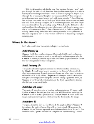
At u, the update() method checks to see whether the drawingComplete flag
is set; if not, it continues through the rest of the code. At v, update() incre-
ments the current angle. Beginning at w, it calculates the (x, y) position
corresponding to the current angle and moves the turtle there, drawing the
line segment in the process.
When I discussed the Spirograph equations, I talked about the period-
icity of the curve. A Spirograph starts repeating itself after a certain angle.
At x, you see whether the angle has reached the full range computed for
this particular curve. If so, you set the drawingComplete flag because the draw-
ing is complete. Finally, you hide the turtle cursor so you can see your beau-
tiful creation.
The SpiroAnimator Class
The SpiroAnimator class will let you draw random spiros simultaneously. This
class uses a timer to draw the curves one segment at a time; this technique
updates the graphics periodically and lets the program process events
such as button presses, mouse clicks, and so on. But this timer technique
requires some restructuring in the drawing code.
# a class for animating Spirographs
class SpiroAnimator:
# constructor
def __init__(self, N):
# set the timer value in milliseconds
u self.deltaT = 10
# get the window dimensions
v self.width = turtle.window_width()
self.height = turtle.window_height()
# create the Spiro objects
w self.spiros = []
for i in range(N):
# generate random parameters
x rparams = self.genRandomParams()
# set the spiro parameters
y spiro = Spiro(*rparams)
self.spiros.append(spiro)
www.it-ebooks.info](https://image.slidesharecdn.com/pythonplaygroundgeekyprojectsforthecuriousprogrammerpdfdrive-220717171538-9c44c48d/85/Python-Playground_-Geeky-Projects-for-the-Curious-Programmer-PDFDrive-pdf-49-320.jpg)


![30 Chapter 2
Parsing Command Line Arguments and Initialization
Like in Chapter 1, you use argparse in the main() method to parse command
line options sent to the program.
u parser = argparse.ArgumentParser(description=descStr)
# add expected arguments
v parser.add_argument('--sparams', nargs=3, dest='sparams', required=False,
help="The three arguments in sparams: R, r, l.")
# parse args
w args = parser.parse_args()
At u, you create the argument parser object, and at v, you add the
--sparams optional argument to the parser. You make the call that does the
actual parsing at w.
Next, the code sets up some turtle parameters.
# set the width of the drawing window to 80 percent of the screen width
u turtle.setup(width=0.8)
# set the cursor shape to turtle
v turtle.shape('turtle')
# set the title to Spirographs!
w turtle.title("Spirographs!")
# add the key handler to save our drawings
x turtle.onkey(saveDrawing, "s")
# start listening
y turtle.listen()
# hide the main turtle cursor
z turtle.hideturtle()
At u, you use setup() to set the width of the drawing window to 80 per-
cent of the screen width. (You could also give setup() specific height and
origin parameters.) You set the cursor shape to turtle at v, and you set
the title of the program window to Spirographs! at w. At x, you use onkey()
with saveDrawing to save the drawing when you press S. Then, at y, you call
listen() to make the window listen for user events. Finally, at z, you hide
the turtle cursor.
Once the command line arguments are parsed, the rest of the code
proceeds as follows:
# check for any arguments sent to --sparams and draw the Spirograph
u if args.sparams:
v params = [float(x) for x in args.sparams]
# draw the Spirograph with the given parameters
col = (0.0, 0.0, 0.0)
w spiro = Spiro(0, 0, col, *params)
x spiro.draw()
www.it-ebooks.info](https://image.slidesharecdn.com/pythonplaygroundgeekyprojectsforthecuriousprogrammerpdfdrive-220717171538-9c44c48d/85/Python-Playground_-Geeky-Projects-for-the-Curious-Programmer-PDFDrive-pdf-53-320.jpg)
![Spirographs 31
else:
# create the animator object
y spiroAnim = SpiroAnimator(4)
# add a key handler to toggle the turtle cursor
z turtle.onkey(spiroAnim.toggleTurtles, "t")
# add a key handler to restart the animation
{ turtle.onkey(spiroAnim.restart, "space")
# start the turtle main loop
| turtle.mainloop()
At u, you first check whether any arguments were given to --sparams; if
so, you extract them from the string and use a list comprehension to convert
them into floats at v. (A list comprehension is a Python construct that lets
you create a list in a compact and powerful way. For example, a = [2*x for x
in range(1, 5)] creates a list of the first four even numbers.)
At w, you use any extracted parameters to construct the Spiro object
(with the help of the Python * operator, which converts the list into argu-
ments). Then, at x, you call draw(), which draws the spiro.
Now, if no arguments were specified on the command line, you enter
random mode. At y, you create a SpiroAnimator object, passing it the argu-
ment 4, which tells it to create four drawings. At z, use onkey to capture
any presses of the T key so that you can use it to toggle the turtle cursors
(toggleTurtles), and at {, handle presses of the spacebar (space) so that
you can use it to restart the animation at any point. Finally, at |, you call
mainloop() to tell the tkinter window to stay open, listening for events.
The Complete Code
Here is the complete Spirograph program. You can also download the code
for this project from https://github.com/electronut/pp/blob/master/spirograph/
spiro.py.
import sys, random, argparse
import numpy as np
import math
import turtle
import random
from PIL import Image
from datetime import datetime
from fractions import gcd
# a class that draws a Spirograph
class Spiro:
# constructor
def __init__(self, xc, yc, col, R, r, l):
# create the turtle object
self.t = turtle.Turtle()
# set the cursor shape
self.t.shape('turtle')
www.it-ebooks.info](https://image.slidesharecdn.com/pythonplaygroundgeekyprojectsforthecuriousprogrammerpdfdrive-220717171538-9c44c48d/85/Python-Playground_-Geeky-Projects-for-the-Curious-Programmer-PDFDrive-pdf-54-320.jpg)

![Spirographs 33
# drawing is now done so hide the turtle cursor
self.t.hideturtle()
# update by one step
def update(self):
# skip the rest of the steps if done
if self.drawingComplete:
return
# increment the angle
self.a += self.step
# draw a step
R, k, l = self.R, self.k, self.l
# set the angle
a = math.radians(self.a)
x = self.R*((1-k)*math.cos(a) + l*k*math.cos((1-k)*a/k))
y = self.R*((1-k)*math.sin(a) - l*k*math.sin((1-k)*a/k))
self.t.setpos(self.xc + x, self.yc + y)
# if drawing is complete, set the flag
if self.a >= 360*self.nRot:
self.drawingComplete = True
# drawing is now done so hide the turtle cursor
self.t.hideturtle()
# clear everything
def clear(self):
self.t.clear()
# a class for animating Spirographs
class SpiroAnimator:
# constructor
def __init__(self, N):
# set the timer value in milliseconds
self.deltaT = 10
# get the window dimensions
self.width = turtle.window_width()
self.height = turtle.window_height()
# create the Spiro objects
self.spiros = []
for i in range(N):
# generate random parameters
rparams = self.genRandomParams()
# set the spiro parameters
spiro = Spiro(*rparams)
self.spiros.append(spiro)
# call timer
turtle.ontimer(self.update, self.deltaT)
# restart spiro drawing
def restart(self):
for spiro in self.spiros:
# clear
spiro.clear()
# generate random parameters
rparams = self.genRandomParams()
www.it-ebooks.info](https://image.slidesharecdn.com/pythonplaygroundgeekyprojectsforthecuriousprogrammerpdfdrive-220717171538-9c44c48d/85/Python-Playground_-Geeky-Projects-for-the-Curious-Programmer-PDFDrive-pdf-56-320.jpg)

![Spirographs 35
img.save(fileName + '.png', 'png')
# show the turtle cursor
turtle.showturtle()
# main() function
def main():
# use sys.argv if needed
print('generating spirograph...')
# create parser
descStr = """This program draws Spirographs using the Turtle module.
When run with no arguments, this program draws random Spirographs.
Terminology:
R: radius of outer circle
r: radius of inner circle
l: ratio of hole distance to r
"""
parser = argparse.ArgumentParser(description=descStr)
# add expected arguments
parser.add_argument('--sparams', nargs=3, dest='sparams', required=False,
help="The three arguments in sparams: R, r, l.")
# parse args
args = parser.parse_args()
# set the width of the drawing window to 80 percent of the screen width
turtle.setup(width=0.8)
# set the cursor shape to turtle
turtle.shape('turtle')
# set the title to Spirographs!
turtle.title("Spirographs!")
# add the key handler to save our drawings
turtle.onkey(saveDrawing, "s")
# start listening
turtle.listen()
# hide the main turtle cursor
turtle.hideturtle()
# check for any arguments sent to --sparams and draw the Spirograph
if args.sparams:
params = [float(x) for x in args.sparams]
# draw the Spirograph with the given parameters
col = (0.0, 0.0, 0.0)
spiro = Spiro(0, 0, col, *params)
spiro.draw()
else:
# create the animator object
spiroAnim = SpiroAnimator(4)
# add a key handler to toggle the turtle cursor
turtle.onkey(spiroAnim.toggleTurtles, "t")
www.it-ebooks.info](https://image.slidesharecdn.com/pythonplaygroundgeekyprojectsforthecuriousprogrammerpdfdrive-220717171538-9c44c48d/85/Python-Playground_-Geeky-Projects-for-the-Curious-Programmer-PDFDrive-pdf-58-320.jpg)


![38 Chapter 2
3. Try drawing a Koch snowflake, a fractal curve constructed using recur-
sion (a function that calls itself), with the turtle. You can structure your
recursive function call like this:
# recursive Koch snowflake
def kochSF(x1, y1, x2, y2, t):
# compute intermediate points p2, p3
if segment_length > 10:
# recursively generate child segments
# flake #1
kochSF(x1, y1, p1[0], p1[1], t)
# flake #2
kochSF(p1[0], p1[1], p2[0], p2[1], t)
# flake #3
kochSF(p2[0], p2[1], p3[0], p3[1], t)
# flake #4
kochSF(p3[0], p3[1], x2, y2, t)
else:
# draw
# ...
If you get really stuck, you can find my solution at http://electronut
.in/koch-snowflake-and-the-thue-morse-sequence/.
www.it-ebooks.info](https://image.slidesharecdn.com/pythonplaygroundgeekyprojectsforthecuriousprogrammerpdfdrive-220717171538-9c44c48d/85/Python-Playground_-Geeky-Projects-for-the-Curious-Programmer-PDFDrive-pdf-61-320.jpg)


![42 Chapter 3
This simulation consists of the following components:
• A property defined in one- or two-dimensional space
• A mathematical rule to change this property for each step in the
simulation
• A way to display or capture the state of the system as it evolves
The cells in Conway’s Game of Life can be either ON or OFF. The game
starts with an initial condition, in which each cell is assigned one state and
mathematical rules determine how its state will change over time. The
amazing thing about Conway’s Game of Life is that with just four
simple
rules the system evolves to produce patterns that behave in incredibly
complex ways, almost as if they were alive. Patterns include “gliders” that
slide across the grid, “blinkers” that flash on and off, and even replicating
patterns.
Of course, the philosophical implications of this game are also signifi-
cant, because they suggest that complex structures can evolve from simple
rules without following any sort of preset pattern.
Here are some of the main concepts covered in this project:
• Using matplotlib imshow to represent a 2D grid of data
• Using matplotlib for animation
• Using the numpy array
• Using the % operator for boundary conditions
• Setting up a random distribution of values
How It Works
Because the Game of Life is built on a grid of nine squares, every cell has
eight neighboring cells, as shown in Figure 3-1. A given cell (i, j) in the
simulation is accessed on a grid [i][j], where i and j are the row and col-
umn indices, respectively. The value of a given cell at a given instant of time
depends on the state of its neighbors at the previous time step.
Conway’s Game of Life has four rules.
1. If a cell is ON and has fewer than two neighbors that are ON, it
turns OFF.
2. If a cell is ON and has either two or three neighbors that are ON,
it remains ON.
3. If a cell is ON and has more than three neighbors that are ON, it
turns OFF.
4. If a cell is OFF and has exactly three neighbors that are ON, it
turns ON.
www.it-ebooks.info](https://image.slidesharecdn.com/pythonplaygroundgeekyprojectsforthecuriousprogrammerpdfdrive-220717171538-9c44c48d/85/Python-Playground_-Geeky-Projects-for-the-Curious-Programmer-PDFDrive-pdf-65-320.jpg)

![44 Chapter 3
NOTE This is similar to how boundaries work in Pac-Man. If you go off the top of the
screen, you appear on the bottom. If you go off the left side of the screen, you appear
on the right side. This kind of boundary condition is common in 2D simulations.
Here’s a description of the algorithm you’ll use to apply the four rules
and run the simulation:
1. Initialize the cells in the grid.
2. At each time step in the simulation, for each cell (i, j) in the grid, do
the following:
a. Update the value of cell (i, j) based on its neighbors, taking into
account the boundary conditions.
b. Update the display of grid values.
Requirements
You’ll use numpy arrays and the matplotlib library to display the simulation
output, and you’ll use the matplotlib animation module to update the simula-
tion. (See Chapter 1 for a review of matplotlib.)
The Code
You’ll develop the code for the simulation bit by bit inside the Python inter-
preter by examining the pieces needed for different parts. To see the full
project code, skip ahead to “The Complete Code” on page 49.
First, import the modules you’ll be using for this project:
>>> import numpy as np
>>> import matplotlib.pyplot as plt
>>> import matplotlib.animation as animation
Now let’s create the grid.
Representing the Grid
To represent whether a cell is alive (ON) or dead (OFF) on the grid, you’ll
use the values 255 and 0 for ON and OFF, respectively. You’ll display the cur-
rent state of the grid using the imshow() method in matplotlib, which repre-
sents a matrix of numbers as an image. Enter the following:
u >>> x = np.array([[0, 0, 255], [255, 255, 0], [0, 255, 0]])
v >>> plt.imshow(x, interpolation='nearest')
plt.show()
At u, you define a 2D numpy array of shape (3, 3), where each element
of the array is an integer value. You then use the plt.show() method to dis-
play this matrix of values as an image, and you pass in the interpolation
option as 'nearest' at v to get sharp edges for the cells (or they’d be fuzzy).
www.it-ebooks.info](https://image.slidesharecdn.com/pythonplaygroundgeekyprojectsforthecuriousprogrammerpdfdrive-220717171538-9c44c48d/85/Python-Playground_-Geeky-Projects-for-the-Curious-Programmer-PDFDrive-pdf-67-320.jpg)
![Conway’s Game of Life 45
Figure 3-3 shows the output of this code.
Figure 3-3: Displaying a grid of values
Notice that the value of 0 (OFF) is shown in dark gray and 255 (ON) is
shown in light gray, which is the default colormap used in imshow().
Initial Conditions
To begin the simulation, set an initial state for each cell in the 2D grid.
You can use a random distribution of ON and OFF cells and see what kind
of patterns emerge, or you can add some specific patterns and see how they
evolve. You’ll look at both approaches.
To use a random initial state, use the choice() method from the random
module in numpy. Enter the following:
np.random.choice([0, 255], 4*4, p=[0.1, 0.9]).reshape(4, 4)
Here is the output:
array([[255, 255, 255, 255],
[255, 255, 255, 255],
[255, 255, 255, 255],
[255, 255, 255, 0]])
np.random.choice chooses a value from the given list [0, 255], with the
probability of the appearance of each value given in the parameter p=[0.1,
0.9]. Here, you ask for 0 to appear with a probability of 0.1 (or 10 percent)
and for 255 to appear with a probability of 90 percent. (The two values in p
must add up to 1.) Because this choice() method creates a one-dimensional
array of 16 values, you use .reshape to make it a two-dimensional array.
www.it-ebooks.info](https://image.slidesharecdn.com/pythonplaygroundgeekyprojectsforthecuriousprogrammerpdfdrive-220717171538-9c44c48d/85/Python-Playground_-Geeky-Projects-for-the-Curious-Programmer-PDFDrive-pdf-68-320.jpg)
![46 Chapter 3
To set up the initial condition to match a particular pattern instead
of just filling in a random set of values, initialize the two-
dimensional grid
to zeros and then use a method to add a pattern at a particular row and col-
umn in the grid, as shown here:
def addGlider(i, j, grid):
"""adds a glider with top left cell at (i, j)"""
u glider = np.array([[0, 0, 255],
[255, 0, 255],
[0, 255, 255]])
v grid[i:i+3, j:j+3] = glider
w grid = np.zeros(N*N).reshape(N, N)
x addGlider(1, 1, grid)
At u, you define the glider pattern (an observed pattern that moves
steadily across the grid) using a numpy array of shape (3, 3). At v, you can
see how you use the numpy slice operation to copy this pattern array into the
simulation’s two-dimensional grid, with its top-left corner placed at the
coordinates you specify as i and j. You create an N×N array of zeros at w,
and at x, you call the addGlider() method to initialize the grid with the
glider pattern.
Boundary Conditions
Now we can think about how to implement the toroidal boundary condi-
tions. First, let’s see what happens at the right edge of a grid of size N×N.
The cell at the end of row i is accessed as grid[i][N-1]. Its neighbor to the
right is grid[i][N], but according to the toroidal boundary conditions, the
value accessed as grid[i][N] should be replaced by grid[i][0]. Here’s one
way to do that:
if j == N-1:
right = grid[i][0]
else:
right = grid[i][j+1]
Of course, you’d need to apply similar boundary conditions to the
left, top, and bottom sides of the grid, but doing so would require adding
a lot more code because each of the four edges of the grid would need to
be tested. A much more compact way to accomplish this is with Python’s
modulus (%) operator, as shown here:
>>> N = 16
>>> i1 = 14
>>> i2 = 15
>>> (i1+1)%N
15
>>> (i2+1)%N
0
www.it-ebooks.info](https://image.slidesharecdn.com/pythonplaygroundgeekyprojectsforthecuriousprogrammerpdfdrive-220717171538-9c44c48d/85/Python-Playground_-Geeky-Projects-for-the-Curious-Programmer-PDFDrive-pdf-69-320.jpg)
![Conway’s Game of Life 47
As you can see, the % operator gives the remainder for the integer divi-
sion by N. You can use this operator to make the values wrap around at the
edge by rewriting the grid access code like this:
right = grid[i][(j+1)%N]
Now when a cell is on the edge of the grid (in other words, when j = N-1),
asking for the cell to the right with this method will give you (j+1)%N, which
sets j back to 0, making the right side of the grid wrap to the left side. When
you do the same for the bottom of the grid, it wraps around to the top.
Implementing the Rules
The rules of the Game of Life are based on the number of neighboring cells
that are ON or OFF. To simplify the application of these rules, you can cal-
culate the total number of neighboring cells in the ON state. Because the
ON states have a value of 255, you can just sum the values of all the neighbors
and divide by 255 to get the number of ON cells. Here is the relevant code:
# apply Conway's rules
if grid[i, j] == ON:
u if (total < 2) or (total > 3):
newGrid[i, j] = OFF
else:
if total == 3:
v newGrid[i, j] = ON
At u, any cell that is ON is turned OFF if it has fewer than two neigh-
bors that are ON or if it has more than three neighbors that are ON. The
code at v applies only to OFF cells: a cell is turned ON if exactly three
neighbors are ON.
Now it’s time to write the complete code for the simulation.
Sending Command Line Arguments to the Program
The following code sends command line arguments to your program:
# main() function
def main():
# command line argumentss are in sys.argv[1], sys.argv[2], ...
# sys.argv[0] is the script name and can be ignored
# parse arguments
u parser = argparse.ArgumentParser(description="Runs Conway's Game of Life
simulation.")
# add arguments
v parser.add_argument('--grid-size', dest='N', required=False)
w parser.add_argument('--mov-file', dest='movfile', required=False)
x parser.add_argument('--interval', dest='interval', required=False)
y parser.add_argument('--glider', action='store_true', required=False)
args = parser.parse_args()
www.it-ebooks.info](https://image.slidesharecdn.com/pythonplaygroundgeekyprojectsforthecuriousprogrammerpdfdrive-220717171538-9c44c48d/85/Python-Playground_-Geeky-Projects-for-the-Curious-Programmer-PDFDrive-pdf-70-320.jpg)
![48 Chapter 3
The main() function begins by defining command line parameters for
the program. You use the argparse class at u to add command line options
to the code, and then you add various options to it in the following lines.
At v, you specify the simulation grid size N, and at w, you specify the file-
name for the saved .mov file. At x, you set the animation update interval in
milliseconds, and at y, you start the simulation with a glider pattern.
Initializing the Simulation
Continuing through the code, you come to the following section, which ini-
tializes the simulation:
# set grid size
N = 100
if args.N and int(args.N) > 8:
N = int(args.N)
# set animation update interval
updateInterval = 50
if args.interval:
updateInterval = int(args.interval)
# declare grid
u grid = np.array([])
# check if "glider" demo flag is specified
if args.glider:
grid = np.zeros(N*N).reshape(N, N)
addGlider(1, 1, grid)
else:
# populate grid with random on/off - more off than on
grid = randomGrid(N)
Still within the main() function, this portion of the code applies any
parameters called at the command line, once the command line options
have been parsed. For example, the lines that follow u set up the initial
conditions, either a random pattern by default or a glider pattern.
Finally, you set up the animation.
# set up the animation
u fig, ax = plt.subplots()
img = ax.imshow(grid, interpolation='nearest')
v ani = animation.FuncAnimation(fig, update, fargs=(img, grid, N, ),
frames=10,
interval=updateInterval,
save_count=50)
# number of frames?
# set the output file
if args.movfile:
ani.save(args.movfile, fps=30, extra_args=['-vcodec', 'libx264'])
plt.show()
www.it-ebooks.info](https://image.slidesharecdn.com/pythonplaygroundgeekyprojectsforthecuriousprogrammerpdfdrive-220717171538-9c44c48d/85/Python-Playground_-Geeky-Projects-for-the-Curious-Programmer-PDFDrive-pdf-71-320.jpg)
![Conway’s Game of Life 49
At u, you configure the matplotlib plot and animation parameters.
At v, animation.FuncAnimation() calls the function update(), defined earlier
in the program, which updates the grid according to the rules of Conway’s
Game of Life using toroidal boundary conditions.
The Complete Code
Here is the complete program for your Game of Life simulation. You can
also download the code for this project from https://github.com/electronut/pp/
blob/master/conway/conway.py.
import sys, argparse
import numpy as np
import matplotlib.pyplot as plt
import matplotlib.animation as animation
ON = 255
OFF = 0
vals = [ON, OFF]
def randomGrid(N):
"""returns a grid of NxN random values"""
return np.random.choice(vals, N*N, p=[0.2, 0.8]).reshape(N, N)
def addGlider(i, j, grid):
"""adds a glider with top-left cell at (i, j)"""
glider = np.array([[0, 0, 255],
[255, 0, 255],
[0, 255, 255]])
grid[i:i+3, j:j+3] = glider
def update(frameNum, img, grid, N):
# copy grid since we require 8 neighbors for calculation
# and we go line by line
newGrid = grid.copy()
for i in range(N):
for j in range(N):
# compute 8-neghbor sum using toroidal boundary conditions
# x and y wrap around so that the simulation
# takes place on a toroidal surface
total = int((grid[i, (j-1)%N] + grid[i, (j+1)%N] +
grid[(i-1)%N, j] + grid[(i+1)%N, j] +
grid[(i-1)%N, (j-1)%N] + grid[(i-1)%N, (j+1)%N] +
grid[(i+1)%N, (j-1)%N] + grid[(i+1)%N, (j+1)%N])/255)
# apply Conway's rules
if grid[i, j] == ON:
if (total < 2) or (total > 3):
newGrid[i, j] = OFF
else:
if total == 3:
newGrid[i, j] = ON
www.it-ebooks.info](https://image.slidesharecdn.com/pythonplaygroundgeekyprojectsforthecuriousprogrammerpdfdrive-220717171538-9c44c48d/85/Python-Playground_-Geeky-Projects-for-the-Curious-Programmer-PDFDrive-pdf-72-320.jpg)
![50 Chapter 3
# update data
img.set_data(newGrid)
grid[:] = newGrid[:]
return img,
# main() function
def main():
# command line arguments are in sys.argv[1], sys.argv[2], ...
# sys.argv[0] is the script name and can be ignored
# parse arguments
parser = argparse.ArgumentParser(description="Runs Conway's Game of Life
simulation.")
# add arguments
parser.add_argument('--grid-size', dest='N', required=False)
parser.add_argument('--mov-file', dest='movfile', required=False)
parser.add_argument('--interval', dest='interval', required=False)
parser.add_argument('--glider', action='store_true', required=False)
parser.add_argument('--gosper', action='store_true', required=False)
args = parser.parse_args()
# set grid size
N = 100
if args.N and int(args.N) > 8:
N = int(args.N)
# set animation update interval
updateInterval = 50
if args.interval:
updateInterval = int(args.interval)
# declare grid
grid = np.array([])
# check if "glider" demo flag is specified
if args.glider:
grid = np.zeros(N*N).reshape(N, N)
addGlider(1, 1, grid)
else:
# populate grid with random on/off - more off than on
grid = randomGrid(N)
# set up the animation
fig, ax = plt.subplots()
img = ax.imshow(grid, interpolation='nearest')
ani = animation.FuncAnimation(fig, update, fargs=(img, grid, N, ),
frames=10,
interval=updateInterval,
save_count=50)
# number of frames?
# set the output file
if args.movfile:
ani.save(args.movfile, fps=30, extra_args=['-vcodec', 'libx264'])
plt.show()
www.it-ebooks.info](https://image.slidesharecdn.com/pythonplaygroundgeekyprojectsforthecuriousprogrammerpdfdrive-220717171538-9c44c48d/85/Python-Playground_-Geeky-Projects-for-the-Curious-Programmer-PDFDrive-pdf-73-320.jpg)


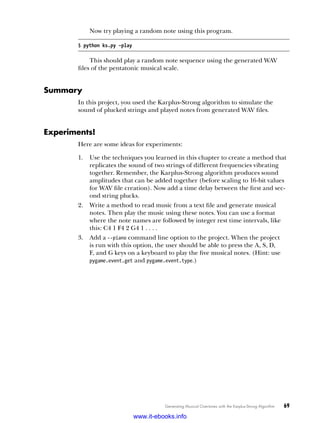
![Generating Musical Overtones with the Karplus-Strong Algorithm 57
the algorithm used to generate these notes and save the sounds as WAV
files. You’ll also create a way to play them at random and learn how to do
the following:
• Implement a ring buffer using the Python deque class.
• Use numpy arrays and ufuncs.
• Play WAV files using pygame.
• Plot a graph using matplotlib.
• Play the pentatonic musical scale.
In addition to implementing the Karplus-Strong algorithm in Python,
you’ll also explore the WAV file format and see how to generate notes
within a pentatonic musical scale.
How It Works
The Karplus-Strong algorithm can simulate the sound of a plucked string
by using a ring buffer of displacement values to simulate a string tied down at
both ends, similar to a guitar string.
A ring buffer (also known as a circular buffer) is a fixed-length buffer
( just an array of values) that wraps around itself. In other words, when you
reach the end of the buffer, the next element you access will be the first
element in the buffer. (See “Implementing the Ring Buffer with deque” on
page 61 for more about ring buffers.)
The length (N) of the ring buffer is related to the fundamental fre-
quency of vibration according to the equation N = S/f, where S is the sam-
pling rate and f is the frequency.
At the start of the simulation, the buffer is filled with random values in
the range [−0.5, 0.5], which you might think of as representing the random
displacement of a plucked string as it vibrates.
In addition to the ring buffer, you use a samples buffer to store the inten-
sity of the sound at any particular time. The length of this buffer and the
sampling rate determine the length of the sound clip.
The Simulation
The simulation proceeds until the sample buffer is filled in a kind of feed-
back scheme, as shown in Figure 4-3. For each step of the simulation, you
do the following:
1. Store the first value from the ring buffer in the samples buffer.
2. Calculate the average of the first two elements in the ring buffer.
3. Multiply this average value by an attenuation factor (in this case, 0.995).
4. Append this value to the end of the ring buffer.
5. Remove the first element of the ring buffer.
www.it-ebooks.info](https://image.slidesharecdn.com/pythonplaygroundgeekyprojectsforthecuriousprogrammerpdfdrive-220717171538-9c44c48d/85/Python-Playground_-Geeky-Projects-for-the-Curious-Programmer-PDFDrive-pdf-80-320.jpg)

![Generating Musical Overtones with the Karplus-Strong Algorithm 59
row, which represents time step 2. The last value in time step 2 is the attenu-
ated average of the first and last values of time step 1, which is calculated as
0.995 × ((0.1 + –0.5) ÷ 2) = –0.199.
Creating WAV Files
The Waveform Audio File Format (WAV) is used to store audio data. This for-
mat is convenient for small audio projects because it is simple and doesn’t
require you to deal with complicated compression techniques.
In its simplest form, WAV files consist of a series of bits representing the
amplitude of the recorded sound at a given point in time, called the resolu-
tion. You’ll use 16-bit resolution in this project. WAV files also have a set sam-
pling rate, which is the number of times the audio is sampled, or read, every
second. In this project, you use a sampling rate of 44,100 Hz, the rate used
in audio CDs. Let’s generate a five-second audio clip of a 220 Hz sine wave
using Python. First, you represent a sine wave using this formula:
A = sin(2pft)
Here, A is the amplitude of the wave, f is the frequency, and t is the cur-
rent time index. Now you rewrite this equation as follows:
A = sin(2pfi/R)
In this equation, i is the index of the sample, and R is the sampling rate.
Using these two equations, you can create a WAV file for a 200 Hz sine wave
as follows:
import numpy as np
import wave, math
sRate = 44100
nSamples = sRate * 5
u x = np.arange(nSamples)/float(sRate)
v vals = np.sin(2.0*math.pi*220.0*x)
w data = np.array(vals*32767, 'int16').tostring()
file = wave.open('sine220.wav', 'wb')
x file.setparams((1, 2, sRate, nSamples, 'NONE', 'uncompressed'))
file.writeframes(data)
file.close()
At u and v, you create a numpy array (see Chapter 1) of amplitude
values,
according to the second sine wave equation. The numpy array is a fast and
convenient way to apply functions to arrays such as the sin() function.
At w, the computed sine wave values in the range [–1, 1] are scaled to
16-bit values and converted to a string so they can be written to a file. At x,
you set the parameters for the WAV file; in this case, it’s a single-channel
(mono), two-byte (16-bit), uncompressed format. Figure 4-4 shows the
generated sine220.wav file in Audacity, a free audio editor. As expected,
you see a sine wave of frequency 220 Hz, and when you play the file, you
hear a 220 Hz tone for five seconds.
www.it-ebooks.info](https://image.slidesharecdn.com/pythonplaygroundgeekyprojectsforthecuriousprogrammerpdfdrive-220717171538-9c44c48d/85/Python-Playground_-Geeky-Projects-for-the-Curious-Programmer-PDFDrive-pdf-82-320.jpg)

![Generating Musical Overtones with the Karplus-Strong Algorithm 61
Requirements
In this project, you’ll use the Python wave module to create audio files in
WAV format. You’ll use numpy arrays for the Karplus-Strong algorithm and
the deque class from Python collections to implement the ring buffer. You’ll
also play back the WAV files with the pygame module.
The Code
Now let’s develop the various pieces of code required to implement the
Karplus-Strong algorithm and then put them together for the complete
program. To see the full project code, skip ahead to “The Complete Code”
on page 65.
Implementing the Ring Buffer with deque
Recall from earlier that the Karplus-Strong algorithm uses a ring buf-
fer to generate a musical note. You’ll implement the ring buffer using
Python’s deque container (pronounced “deck”)—part of Python’s collections
module—which provides specialized container data types in an array. You
can insert and remove elements from the beginning (head) or end (tail)
of a deque (see Figure 4-5). This insertion and removal process is a O(1), or
a “constant time” operation, which means it takes the same amount of time
regardless of how big the deque container gets.
deque
popleft() append()
O(1) O(1)
head tail
Figure 4-5: Ring buffer using deque
The following code shows how you would use deque in Python:
>>> from collections import deque
u >>> d = deque(range(10))
>>> print(d)
deque([0, 1, 2, 3, 4, 5, 6, 7, 8, 9])
v >>> d.append(-1)
>>> print(d)
deque([0, 1, 2, 3, 4, 5, 6, 7, 8, 9, -1])
w >>> d.popleft()
0
>>> print d
deque([1, 2, 3, 4, 5, 6, 7, 8, 9, -1])
At u, you create the deque container by passing in a list created by the
range() method. At v, you append an element to the end of the deque con-
tainer, and at w, you pop (remove) the first element from the head of the
deque. Both these operations happen quickly.
www.it-ebooks.info](https://image.slidesharecdn.com/pythonplaygroundgeekyprojectsforthecuriousprogrammerpdfdrive-220717171538-9c44c48d/85/Python-Playground_-Geeky-Projects-for-the-Curious-Programmer-PDFDrive-pdf-84-320.jpg)
![62 Chapter 4
Implementing the Karplus-Strong Algorithm
You also use a deque container to implement the Karplus-Strong algorithm
for the ring buffer, as shown here:
# generate note of given frequency
def generateNote(freq):
nSamples = 44100
sampleRate = 44100
N = int(sampleRate/freq)
# initialize ring buffer
u buf = deque([random.random() - 0.5 for i in range(N)])
# initialize samples buffer
v samples = np.array([0]*nSamples, 'float32')
for i in range(nSamples):
w samples[i] = buf[0]
x avg = 0.996*0.5*(buf[0] + buf[1])
buf.append(avg)
buf.popleft()
# convert samples to 16-bit values and then to a string
# the maximum value is 32767 for 16-bit
y samples = np.array(samples*32767, 'int16')
z return samples.tostring()
At u, you initialize deque with random numbers in the range [–0.5, 0.5].
At v, you set up a float array to store the sound samples. The length of this
array matches the sampling rate, which means the sound clip will be gener-
ated for one second.
The first element in deque is copied to the samples buffer at w. At x,
and in the lines that follow, you can see the low-pass filter and attenuation
in action. At y, the samples array is converted into a 16-bit format by mul-
tiplying each value by 32,767 (a 16-bit signed integer can take only values
from −32,768 to 32,767), and at z, it is converted to a string representation
for the wave module, which you’ll use to save this data to a file.
Writing a WAV File
Once you have the audio data, you can write it to a WAV file using the
Python wave module.
def writeWAVE(fname, data):
# open file
u file = wave.open(fname, 'wb')
# WAV file parameters
nChannels = 1
sampleWidth = 2
frameRate = 44100
nFrames = 44100
# set parameters
v file.setparams((nChannels, sampleWidth, frameRate, nFrames,
'NONE', 'noncompressed'))
www.it-ebooks.info](https://image.slidesharecdn.com/pythonplaygroundgeekyprojectsforthecuriousprogrammerpdfdrive-220717171538-9c44c48d/85/Python-Playground_-Geeky-Projects-for-the-Curious-Programmer-PDFDrive-pdf-85-320.jpg)
![Generating Musical Overtones with the Karplus-Strong Algorithm 63
w file.writeframes(data)
file.close()
At u, you create a WAV file, and at v, you set its parameters using a
single-channel, 16-bit, uncompressed format. Finally, at w, you write the
data to the file.
Playing WAV Files with pygame
Now you’ll use the Python pygame module to play the WAV files generated by
the algorithm. pygame is a popular Python module used to write games. It’s
built on top of the Simple DirectMedia Layer (SDL) library, a high-perfor-
mance, low-level library that gives you access to sound, graphics, and input
devices on a computer.
For convenience, you encapsulate the code in a NotePlayer class, as
shown here:
# play a WAV file
class NotePlayer:
# constructor
def __init__(self):
u pygame.mixer.pre_init(44100, -16, 1, 2048)
pygame.init()
# dictionary of notes
v self.notes = {}
# add a note
def add(self, fileName):
w self.notes[fileName] = pygame.mixer.Sound(fileName)
# play a note
def play(self, fileName):
try:
x self.notes[fileName].play()
except:
print(fileName + ' not found!')
def playRandom(self):
"""play a random note"""
y index = random.randint(0, len(self.notes)-1)
z note = list(self.notes.values())[index]
note.play()
At u , you preinitialize the pygame mixer class with a sampling rate of
44,100, 16-bit signed values, a single channel, and a buffer size of 2,048. At
v, you create a dictionary of notes, which stores the pygame sound objects
against the filenames. Next, in NotePlayer’s add() method w, you create the
sound object and store it in the notes dictionary.
Notice in play() how the dictionary is used at x to select and play the
sound object associated with a filename. The playRandom() method picks a
random note from the five notes you’ve generated and plays it. Finally, at y,
randint() selects a random integer from the range [0, 4] and at z picks a
note to play from the dictionary.
www.it-ebooks.info](https://image.slidesharecdn.com/pythonplaygroundgeekyprojectsforthecuriousprogrammerpdfdrive-220717171538-9c44c48d/85/Python-Playground_-Geeky-Projects-for-the-Curious-Programmer-PDFDrive-pdf-86-320.jpg)
![64 Chapter 4
The main() Method
Now let’s look at the main() method, which creates the notes and handles
various command line options to play the notes.
parser = argparse.ArgumentParser(description="Generating sounds with
Karplus String Algorithm")
# add arguments
u parser.add_argument('--display', action='store_true', required=False)
parser.add_argument('--play', action='store_true', required=False)
parser.add_argument('--piano', action='store_true', required=False)
args = parser.parse_args()
# show plot if flag set
if args.display:
gShowPlot = True
plt.ion()
# create note player
nplayer = NotePlayer()
print('creating notes...')
for name, freq in list(pmNotes.items()):
fileName = name + '.wav'
v if not os.path.exists(fileName) or args.display:
data = generateNote(freq)
print('creating ' + fileName + '...')
writeWAVE(fileName, data)
else:
print('fileName already created. skipping...')
# add note to player
w nplayer.add(name + '.wav')
# play note if display flag set
if args.display:
x nplayer.play(name + '.wav')
time.sleep(0.5)
# play a random tune
if args.play:
while True:
try:
y nplayer.playRandom()
# rest - 1 to 8 beats
z rest = np.random.choice([1, 2, 4, 8], 1,
p=[0.15, 0.7, 0.1, 0.05])
time.sleep(0.25*rest[0])
except KeyboardInterrupt:
exit()
First, you set up some command line options for the program using
argparse, as discussed in earlier projects. At u, if the --display command
line option was used, you set up a matplotlib plot to show how the waveform
www.it-ebooks.info](https://image.slidesharecdn.com/pythonplaygroundgeekyprojectsforthecuriousprogrammerpdfdrive-220717171538-9c44c48d/85/Python-Playground_-Geeky-Projects-for-the-Curious-Programmer-PDFDrive-pdf-87-320.jpg)

![66 Chapter 4
# set parameters
file.setparams((nChannels, sampleWidth, frameRate, nFrames,
'NONE', 'noncompressed'))
file.writeframes(data)
file.close()
# generate note of given frequency
def generateNote(freq):
nSamples = 44100
sampleRate = 44100
N = int(sampleRate/freq)
# initialize ring buffer
buf = deque([random.random() - 0.5 for i in range(N)])
# plot of flag set
if gShowPlot:
axline, = plt.plot(buf)
# initialize samples buffer
samples = np.array([0]*nSamples, 'float32')
for i in range(nSamples):
samples[i] = buf[0]
avg = 0.995*0.5*(buf[0] + buf[1])
buf.append(avg)
buf.popleft()
# plot of flag set
if gShowPlot:
if i % 1000 == 0:
axline.set_ydata(buf)
plt.draw()
# convert samples to 16-bit values and then to a string
# the maximum value is 32767 for 16-bit
samples = np.array(samples*32767, 'int16')
return samples.tostring()
# play a WAV file
class NotePlayer:
# constructor
def __init__(self):
pygame.mixer.pre_init(44100, -16, 1, 2048)
pygame.init()
# dictionary of notes
self.notes = {}
# add a note
def add(self, fileName):
self.notes[fileName] = pygame.mixer.Sound(fileName)
# play a note
def play(self, fileName):
try:
self.notes[fileName].play()
except:
print(fileName + ' not found!')
def playRandom(self):
"""play a random note"""
index = random.randint(0, len(self.notes)-1)
www.it-ebooks.info](https://image.slidesharecdn.com/pythonplaygroundgeekyprojectsforthecuriousprogrammerpdfdrive-220717171538-9c44c48d/85/Python-Playground_-Geeky-Projects-for-the-Curious-Programmer-PDFDrive-pdf-89-320.jpg)
![Generating Musical Overtones with the Karplus-Strong Algorithm 67
note = list(self.notes.values())[index]
note.play()
# main() function
def main():
# declare global var
global gShowPlot
parser = argparse.ArgumentParser(description="Generating sounds with
Karplus String Algorithm")
# add arguments
parser.add_argument('--display', action='store_true', required=False)
parser.add_argument('--play', action='store_true', required=False)
parser.add_argument('--piano', action='store_true', required=False)
args = parser.parse_args()
# show plot if flag set
if args.display:
gShowPlot = True
plt.ion()
# create note player
nplayer = NotePlayer()
print('creating notes...')
for name, freq in list(pmNotes.items()):
fileName = name + '.wav'
if not os.path.exists(fileName) or args.display:
data = generateNote(freq)
print('creating ' + fileName + '...')
writeWAVE(fileName, data)
else:
print('fileName already created. skipping...')
# add note to player
nplayer.add(name + '.wav')
# play note if display flag set
if args.display:
nplayer.play(name + '.wav')
time.sleep(0.5)
# play a random tune
if args.play:
while True:
try:
nplayer.playRandom()
# rest - 1 to 8 beats
rest = np.random.choice([1, 2, 4, 8], 1,
p=[0.15, 0.7, 0.1, 0.05])
time.sleep(0.25*rest[0])
except KeyboardInterrupt:
exit()
www.it-ebooks.info](https://image.slidesharecdn.com/pythonplaygroundgeekyprojectsforthecuriousprogrammerpdfdrive-220717171538-9c44c48d/85/Python-Playground_-Geeky-Projects-for-the-Curious-Programmer-PDFDrive-pdf-90-320.jpg)


![Boids: Simulating a Flock 73
The Code
First, you’ll compute the position and velocities of the boids. Next, you’ll
set up the boundary conditions for the simulation, look at how the boids
are drawn, and implement the Boids simulation rules discussed earlier.
Finally, you’ll add some interesting events to the simulation by adding boids
and scattering the flock. To see the full project code, skip ahead to “The
Complete Code” on page 82.
Computing the Position and Velocities of the Boids
The Boids simulation needs to compute the position and velocities of the
boids at each step by pulling information from numpy arrays. At the begin-
ning of the simulation, you place all boids in approximately the center of
the screen, with their velocities set in random directions.
u import math
v import numpy as np
w width, height = 640, 480
x pos = [width/2.0, height/2.0] + 10*np.random.rand(2*N).reshape(N, 2)
y angles = 2*math.pi*np.random.rand(N)
z vel = np.array(list(zip(np.sin(angles), np.cos(angles))))
You begin by importing the math module used in the calculations
that follow at u. At v, you import the numpy library as np (to save some typ-
ing). Then you set the width and height of the simulation window on the
screen w. At x, you create a numpy array pos by adding a random displace-
ment of 10 units to the center of the window. The code np.random.rand(2*N)
creates a one-dimensional array of 2N random numbers in the range [0, 1].
The reshape() call then converts this into a two-dimensional array of shape
(N, 2), which you’ll use to store the boids’ positions. Notice, too, the numpy
broadcasting rules in action here: the 1×2 array is added to each element in
the N×2 array.
Next, you create an array of
random unit velocity vectors (these
are vectors of magnitude 1.0, point-
ing in random directions) using the
following method: given an angle t,
the pair of numbers (cos(t), sin(t))
lie on a circle of radius 1.0, centered
at the origin (0, 0). If you draw a
line from the origin to a point on
this circle, it becomes a unit vector
that depends on the angle A. So if
you choose A at random, you end
up with a random velocity vector.
Figure 5-1 illustrates this scheme.
y
x
0
t1
t2
(cos(t1), sin(t1))
(cos(t2), sin(t2))
Figure 5-1: Generating random unit velocity
vectors
www.it-ebooks.info](https://image.slidesharecdn.com/pythonplaygroundgeekyprojectsforthecuriousprogrammerpdfdrive-220717171538-9c44c48d/85/Python-Playground_-Geeky-Projects-for-the-Curious-Programmer-PDFDrive-pdf-96-320.jpg)
![74 Chapter 5
At y, you generate an array of N random angles in the range [0, 2pi],
and at z, you create an array using the random vector method discussed
earlier and group the coordinates using the built-in zip() method. Here is
a simple example of zip(). This joins two lists into a list of tuples.
>>> zip([0, 1, 2], [3, 4, 5])
[(0, 3), (1, 4), (2, 5)]
Here you’ve generated two arrays, one with random positions clustered
within a 10-pixel radius around the center of the screen and the other with
unit velocities pointing in random directions. This means that at the start
of the simulation, the boids will all hover around the center of the screen,
pointed in random directions.
Setting Boundary Conditions
Birds fly in the boundless sky, but the boids must play in limited space.
To create that space, you’ll create boundary conditions as you did with the
toroidal boundary condition in the Conway simulation in Chapter 3. In this
case, you’ll apply a tiled boundary condition (actually the continuous space
version of the boundary condition you used in Chapter 3).
Think of the Boids simulation as taking place in a tiled space: when a
boid moves out of a tile, it moves in from the opposite direction to an iden-
tical tile. The main difference between the toroidal and tiled boundary
conditions is that this Boids simulation won’t take place on a discrete grid;
instead, the birds move over a continuous region. Figure 5-2 shows what
those tiled boundary conditions look like. Look at the tile in the middle.
The birds flying out to the right are entering the tile on the right, but the
boundary conditions ensure that they actually come right back into the
center tile through the tile at the left. You can see the same thing happen-
ing at the top and bottom tiles.
Here is how you implement the tiled boundary conditions for the Boids
simulation:
def applyBC(self):
"""apply boundary conditions"""
deltaR = 2.0
for coord in self.pos:
u if coord[0] > width + deltaR:
coord[0] = - deltaR
if coord[0] < - deltaR:
coord[0] = width + deltaR
if coord[1] > height + deltaR:
coord[1] = - deltaR
if coord[1] < - deltaR:
coord[1] = height + deltaR
www.it-ebooks.info](https://image.slidesharecdn.com/pythonplaygroundgeekyprojectsforthecuriousprogrammerpdfdrive-220717171538-9c44c48d/85/Python-Playground_-Geeky-Projects-for-the-Curious-Programmer-PDFDrive-pdf-97-320.jpg)

![76 Chapter 5
P
H
Figure 5-3: Representing a boid
In the following snippet, you draw the boid’s body and head as circular
markers using matplotlib.
fig = plt.figure()
ax = plt.axes(xlim=(0, width), ylim=(0, height))
u pts, = ax.plot([], [], markersize=10, c='k', marker='o', ls='None')
v beak, = ax.plot([], [], markersize=4, c='r', marker='o', ls='None')
w anim = animation.FuncAnimation(fig, tick, fargs=(pts, beak, boids),
interval=50)
You set the size and shape of the markers for the boid’s body (pts) and
head (beak) at u and v, respectively. You also add mouse button events to
the animation window at w. Now that you know how to draw the body and
beak, let’s see how to update their positions.
Updating the Boid’s Position
Once the ani
mation starts, you need to update both the boid’s position and
the location of the head, which tells you the direction in which the boid is
moving. You do so with this code:
u vec = self.pos + 10*self.vel/self.maxVel
v beak.set_data(vec.reshape(2*self.N)[::2], vec.reshape(2*self.N)[1::2])
At u, you calculate the position of the head by applying a displace-
ment of 10 units in the direction of the velocity (vel). This displacement
determines the distance between the beak and the body. At v, you update
(reshape) the matplotlib axis (set_data) with the new values of the head posi-
tion. The [::2] picks out the even-numbered elements (x-axis values) from
the velocity list, and the [1::2] picks out the odd-numbered elements (y-axis
values).
www.it-ebooks.info](https://image.slidesharecdn.com/pythonplaygroundgeekyprojectsforthecuriousprogrammerpdfdrive-220717171538-9c44c48d/85/Python-Playground_-Geeky-Projects-for-the-Curious-Programmer-PDFDrive-pdf-99-320.jpg)
![Boids: Simulating a Flock 77
Applying the Rules of the Boids
Now you’ll implement the three rules of boids in Python. Let’s do this the
“numpy way,” avoiding loops and using highly optimized numpy methods.
import numpy as np
from scipy.spatial.distance import squareform, pdist, cdist
def test2(pos, radius):
# get distance matrix
u distMatrix = squareform(pdist(pos))
# apply threshold
v D = distMatrix < radius
# compute velocity
w vel = pos*D.sum(axis=1).reshape(N, 1) - D.dot(pos)
return vel
You use the squareform() and pdist() methods at u (defined in the scipy
library) to calculate the pairwise distances between an array of points.
(You do this by picking any two points from the array and computing the
distance and then doing that for all such possible pairs.) For example, in
this code, you have three points, which means three possible pairs of points:
>>> import numpy as np
>>> from scipy.spatial.distance import squareform, pdist
>>> x = np.array([[0.0, 0.0], [1.0, 1.0], [2.0, 2.0]])
>>> squareform(pdist(x))
array([[ 0. , 1.41421356, 2.82842712],
[ 1.41421356, 0. , 1.41421356],
[ 2.82842712, 1.41421356, 0. ]])
The squareform() method gives you a 3×3 matrix, where an entry Mij gives
the distance between points Pi and Pj. Next, at v, you filter this matrix based
on distance. Using the same three-point example, you have the following:
>>> squareform(pdist(x)) < 1.4
array([[ True, False, False],
[False, True, False],
[False, False, True]], dtype=bool)
The < comparison sets the matrix entry for all distance pairs with a dis-
tance less than the given threshold, in this case, 1.4. This compact method
of expressing what you want is closer to how you actually think about it.
The method at w is a bit more complicated. The D.sum() method sums
the True values in the matrix in a column-wise fashion. The reshape is
required because the result of the sum is a one-dimensional array of N
values (shape (N, )), and you want it to be of shape (N, 1) so it’s compatible
for multiplication with the position array. D.dot() is just the dot product
(multiplication) of the matrix and the position vector.
www.it-ebooks.info](https://image.slidesharecdn.com/pythonplaygroundgeekyprojectsforthecuriousprogrammerpdfdrive-220717171538-9c44c48d/85/Python-Playground_-Geeky-Projects-for-the-Curious-Programmer-PDFDrive-pdf-100-320.jpg)

![Boids: Simulating a Flock 79
When you apply the separation rule at u, each boid is “pushed away”
from neighboring boids within a certain distance, as discussed at the begin-
ning of this section. At v, the calculated velocity is clamped or restricted to
a certain maximum value. (Without this check, the values would increase
with each time step, and the simulation would go haywire.)
When you apply the alignment rule at w, the velocities of all neigh-
boring boids within a radius of 50 units are added up and restricted to a
maximum. This is done so that the computed final velocity doesn’t increase
indefinitely. As a result, any given boid is influenced by and aligns itself
with the average velocity of the boids within the specified radius. (The use
of the compact numpy syntax for doing this computation makes things simple
and fast.)
Finally, when you apply the cohesion rule at x, you add a velocity vector
for each boid that points to the centroid or geometric center of the neighbor-
ing boids within a certain radius. You use the Boolean distance matrix and
numpy methods to arrive at a compact syntax.
Adding a Boid
The core rules in the Boids simulation will cause the boids to exhibit flock-
ing behavior. But let’s make things more interesting by adding a boid to the
flock in the
middle of a simulation to see how it behaves.
The following code creates a mouse event that will allow you to add
a boid by clicking the left mouse button. A boid will appear at the cursor
location with a random velocity assigned to it.
# add a "button press" event handler
u cid = fig.canvas.mpl_connect('button_press_event', buttonPress)
At u, you use the mpl_connect() method to add a button press event
to the matplotlib canvas. The buttonPress() method will be called every time
the mouse button is pressed in the simulation window.
Now, to handle the mouse event and actually create your boid, add
this code:
def buttonPress(self, event):
"""event handler for matplotlib button presses"""
# left-click to add a boid
u if event.button is 1:
v self.pos = np.concatenate((self.pos,
np.array([[event.xdata, event.ydata]])),
axis=0)
# generate a random velocity
w angles = 2*math.pi*np.random.rand(1)
v = np.array(list(zip(np.sin(angles), np.cos(angles))))
self.vel = np.concatenate((self.vel, v), axis=0)
self.N += 1
www.it-ebooks.info](https://image.slidesharecdn.com/pythonplaygroundgeekyprojectsforthecuriousprogrammerpdfdrive-220717171538-9c44c48d/85/Python-Playground_-Geeky-Projects-for-the-Curious-Programmer-PDFDrive-pdf-102-320.jpg)
![80 Chapter 5
At u, you ensure that the mouse event is a left-click. At v, you append
the mouse location given by (event.xdata, event.ydata) to your boid’s posi-
tion array. At w, and the lines that follow, you add a random velocity vector
to the boid’s velocity array and increment the count of boids by 1.
Scattering the Boids
The three simulation rules keep the boids in a flock as they move around.
But what happens when the flock is disturbed? To simulate this situation,
you can introduce a “scatter” effect: when you right-click in the user inter-
face (UI) window, the flock will scatter. You can think of this as how the
flock might respond to the sudden appearance of a predator or a loud noise
that spooks the birds. Here’s one way to implement this, as a continuation
of the buttonPress() method:
# right-click to scatter boids
u elif event.button is 3:
# add scattering velocity
v self.vel += 0.1*(self.pos - np.array([[event.xdata, event.ydata]]))
At u, you check whether the mouse button press is a right-click event.
At v, you change the velocity for every boid by adding a component in the
direction opposite the point where the disturbance arose (that is, where the
mouse was clicked). Initially, the boids will fly away from that point, but as
you will see, the three rules prevail, and the boids will coalesce again as a
flock.
Command Line Arguments
Here’s how command line arguments are handled for the boids program:
u parser = argparse.ArgumentParser(description="Implementing Craig
Reynolds's Boids...")
# add arguments
parser.add_argument('--num-boids', dest='N', required=False)
args = parser.parse_args()
# set the initial number of boids
N = 100
if args.N:
N = int(args.N)
# create boids
boids = Boids(N)
The main() method starts by setting up a command line option at u,
using the familiar argparse module.
www.it-ebooks.info](https://image.slidesharecdn.com/pythonplaygroundgeekyprojectsforthecuriousprogrammerpdfdrive-220717171538-9c44c48d/85/Python-Playground_-Geeky-Projects-for-the-Curious-Programmer-PDFDrive-pdf-103-320.jpg)
![Boids: Simulating a Flock 81
The Boids Class
Next, let’s look at the Boids class, which represents the simulation.
class Boids:
"""class that represents Boids simulation"""
def __init__(self, N):
"""initialize the Boid simulation"""
# initial position and velocities
u self.pos = [width/2.0, height/2.0] + 10*np.random.rand(2*N).reshape(N, 2)
# normalized random velocities
angles = 2*math.pi*np.random.rand(N)
self.vel = np.array(list(zip(np.sin(angles), np.cos(angles))))
self.N = N
# minimum distance of approach
self.minDist = 25.0
# maximum magnitude of velocities calculated by "rules"
self.maxRuleVel = 0.03
# maximum magnitude of the final velocity
self.maxVel = 2.0
The Boids class handles the initialization, updates the animation, and
applies the rules. The position and velocity arrays are initialized at u and
in the lines that follow.
boids.tick() is called at each time step to update the animation, as
shown here:
def tick(frameNum, pts, beak, boids):
#print frameNum
"""update function for animation"""
boids.tick(frameNum, pts, beak)
return pts, beak
You also need a way to limit the value of some vectors. Otherwise, the
velocities will keep increasing indefinitely with every time step, and the
simulation will come apart.
def limitVec(self, vec, maxVal):
"""limit the magnitude of the 2D vector"""
mag = norm(vec)
if mag > maxVal:
vec[0], vec[1] = vec[0]*maxVal/mag, vec[1]*maxVal/mag
u def limit(self, X, maxVal):
"""limit the magnitude of 2D vectors in array X to maxValue"""
for vec in X:
self.limitVec(vec, maxVal)
You define a limit() method at u that clamps the values in an array to a
value calculated by the simulation rules.
www.it-ebooks.info](https://image.slidesharecdn.com/pythonplaygroundgeekyprojectsforthecuriousprogrammerpdfdrive-220717171538-9c44c48d/85/Python-Playground_-Geeky-Projects-for-the-Curious-Programmer-PDFDrive-pdf-104-320.jpg)
![82 Chapter 5
The Complete Code
Here is the complete program for your Boids simulation. You can also
download the code for this project from https://github.com/electronut/pp/
blob/master/boids/boids.py.
import sys, argparse
import math
import numpy as np
import matplotlib.pyplot as plt
import matplotlib.animation as animation
from scipy.spatial.distance import squareform, pdist, cdist
from numpy.linalg import norm
width, height = 640, 480
class Boids:
"""class that represents Boids simulation"""
def __init__(self, N):
"""initialize the Boid simulation"""
# initial position and velocities
self.pos = [width/2.0, height/2.0] + 10*np.random.rand(2*N).reshape(N, 2)
# normalized random velocities
angles = 2*math.pi*np.random.rand(N)
self.vel = np.array(list(zip(np.sin(angles), np.cos(angles))))
self.N = N
# minimum distance of approach
self.minDist = 25.0
# maximum magnitude of velocities calculated by "rules"
self.maxRuleVel = 0.03
# maximum maginitude of the final velocity
self.maxVel = 2.0
def tick(self, frameNum, pts, beak):
"""Update the simulation by one time step."""
# get pairwise distances
self.distMatrix = squareform(pdist(self.pos))
# apply rules:
self.vel += self.applyRules()
self.limit(self.vel, self.maxVel)
self.pos += self.vel
self.applyBC()
# update data
pts.set_data(self.pos.reshape(2*self.N)[::2],
self.pos.reshape(2*self.N)[1::2])
vec = self.pos + 10*self.vel/self.maxVel
beak.set_data(vec.reshape(2*self.N)[::2],
vec.reshape(2*self.N)[1::2])
def limitVec(self, vec, maxVal):
"""limit the magnitide of the 2D vector"""
mag = norm(vec)
www.it-ebooks.info](https://image.slidesharecdn.com/pythonplaygroundgeekyprojectsforthecuriousprogrammerpdfdrive-220717171538-9c44c48d/85/Python-Playground_-Geeky-Projects-for-the-Curious-Programmer-PDFDrive-pdf-105-320.jpg)
![Boids: Simulating a Flock 83
if mag > maxVal:
vec[0], vec[1] = vec[0]*maxVal/mag, vec[1]*maxVal/mag
def limit(self, X, maxVal):
"""limit the magnitide of 2D vectors in array X to maxValue"""
for vec in X:
self.limitVec(vec, maxVal)
def applyBC(self):
"""apply boundary conditions"""
deltaR = 2.0
for coord in self.pos:
if coord[0] > width + deltaR:
coord[0] = - deltaR
if coord[0] < - deltaR:
coord[0] = width + deltaR
if coord[1] > height + deltaR:
coord[1] = - deltaR
if coord[1] < - deltaR:
coord[1] = height + deltaR
def applyRules(self):
# apply rule #1: Separation
D = self.distMatrix < 25.0
vel = self.pos*D.sum(axis=1).reshape(self.N, 1) - D.dot(self.pos)
self.limit(vel, self.maxRuleVel)
# distance threshold for alignment (different from separation)
D = self.distMatrix < 50.0
# apply rule #2: Alignment
vel2 = D.dot(self.vel)
self.limit(vel2, self.maxRuleVel)
vel += vel2;
# apply rule #3: Cohesion
vel3 = D.dot(self.pos) - self.pos
self.limit(vel3, self.maxRuleVel)
vel += vel3
return vel
def buttonPress(self, event):
"""event handler for matplotlib button presses"""
# left-click to add a boid
if event.button is 1:
self.pos = np.concatenate((self.pos,
np.array([[event.xdata, event.ydata]])),
axis=0)
# generate a random velocity
angles = 2*math.pi*np.random.rand(1)
v = np.array(list(zip(np.sin(angles), np.cos(angles))))
self.vel = np.concatenate((self.vel, v), axis=0)
self.N += 1
www.it-ebooks.info](https://image.slidesharecdn.com/pythonplaygroundgeekyprojectsforthecuriousprogrammerpdfdrive-220717171538-9c44c48d/85/Python-Playground_-Geeky-Projects-for-the-Curious-Programmer-PDFDrive-pdf-106-320.jpg)
![84 Chapter 5
# right-click to scatter boids
elif event.button is 3:
# add scattering velocity
self.vel += 0.1*(self.pos - np.array([[event.xdata, event.ydata]]))
def tick(frameNum, pts, beak, boids):
#print frameNum
"""update function for animation"""
boids.tick(frameNum, pts, beak)
return pts, beak
# main() function
def main():
# use sys.argv if needed
print('starting boids...')
parser = argparse.ArgumentParser(description="Implementing Craig
Reynold's Boids...")
# add arguments
parser.add_argument('--num-boids', dest='N', required=False)
args = parser.parse_args()
# set the initial number of boids
N = 100
if args.N:
N = int(args.N)
# create boids
boids = Boids(N)
# set up plot
fig = plt.figure()
ax = plt.axes(xlim=(0, width), ylim=(0, height))
pts, = ax.plot([], [], markersize=10, c='k', marker='o', ls='None')
beak, = ax.plot([], [], markersize=4, c='r', marker='o', ls='None')
anim = animation.FuncAnimation(fig, tick, fargs=(pts, beak, boids),
interval=50)
# add a "button press" event handler
cid = fig.canvas.mpl_connect('button_press_event', boids.buttonPress)
plt.show()
# call main
if __name__ == '__main__':
main()
www.it-ebooks.info](https://image.slidesharecdn.com/pythonplaygroundgeekyprojectsforthecuriousprogrammerpdfdrive-220717171538-9c44c48d/85/Python-Playground_-Geeky-Projects-for-the-Curious-Programmer-PDFDrive-pdf-107-320.jpg)


![ASCII Art 91
Figure 6-2: Average value of a grayscale image
This program will take a given image and first convert it to 8-bit gray-
scale so that each pixel has a grayscale value in the range [0, 255] (the range
of an 8-bit integer). Think of this 8-bit value as brightness, with 0 being black
and 255 being white and the values in between being shades of gray.
Next, it will split the image into a grid of M×N tiles (where M is the num-
ber of rows and N the number of columns in the ASCII image). The program
will then calculate the average brightness value for each tile in the grid and
match it with an appropriate ASCII character by predefining a ramp (an
increasing set of values) of ASCII characters to represent grayscale values in
the range [0, 255]. It will use these values as a lookup table for the bright-
ness values.
The finished ASCII art is just a bunch of lines of text. To display the
text, you’ll use a constant-width (also called monospace) font such as Courier
because unless each text character has the same width, the characters in the
image won’t line up properly along a grid and you’ll end up with unevenly
spaced and scrambled output.
The aspect ratio (the ratio of width to height) of the font used also
affects the final image. If the aspect ratio of the space taken up by a char-
acter is different from the aspect ratio of the image tile the character is
replacing, the final ASCII image will appear distorted. In effect, you’re try-
ing to replace an image tile with an ASCII character, so their shapes need
to match. For example, if you were to split your image into square tiles and
then replace each of the tiles with a font that is stretched in height, the final
output would appear stretched vertically.
To address this issue, you’ll scale the rows in your grid to match the
Courier aspect ratio. (You can send the program command line arguments
to modify the scaling to match other fonts.)
In sum, here are the steps the program takes to generate the ASCII
image:
1. Convert the input image to grayscale.
2. Split the image into M×N tiles.
3. Correct M (the number of rows) to match the image and font aspect
ratio.
www.it-ebooks.info](https://image.slidesharecdn.com/pythonplaygroundgeekyprojectsforthecuriousprogrammerpdfdrive-220717171538-9c44c48d/85/Python-Playground_-Geeky-Projects-for-the-Curious-Programmer-PDFDrive-pdf-114-320.jpg)
![92 Chapter 6
4. Compute the average brightness for each image tile and then look up a
suitable ASCII character for each.
5. Assemble rows of ASCII character strings and print them to a file to
form the final image.
Requirements
In this project, you’ll use Pillow, the friendly fork of the Python Imaging
Library, to read in the images, access their underlying data, and create and
modify them. You’ll also use the numpy library to compute averages.
The Code
You’ll begin by defining the grayscale levels used to generate the ASCII
art. Then you’ll look at how the image is split into tiles and how average
brightness is computed for those tiles. Next, you’ll work on replacing the
tiles with ASCII characters to generate the final output. Finally, you’ll set up
command line parsing for the program to allow a user to specify the output
size, output filename, and so on.
For the full project code, skip to “The Complete Code” on page 95.
Defining the Grayscale Levels and Grid
As the first step in creating your program, define the two grayscale levels
used to convert brightness values to ASCII characters as global values.
# 70 levels of gray
u gscale1 = "$@B%8&WM#*oahkbdpqwmZO0QLCJUYXzcvunxrjft/|()1{}[]?-_+~<>i!lI;:,"^
`". "
# 10 levels of gray
v gscale2 = "@%#*+=-:. "
The value gscale1 at u is the 70-level grayscale ramp, and gscale2 at v
is the simpler 10-level grayscale ramp. Both of these values are stored as
strings, with a range of characters that progress from darkest to lightest.
(To learn more about how characters are represented as grayscale values,
see Paul Bourke’s “Character Representation of Grey Scale Images” at
http://paulbourke.net/dataformats/asciiart/.)
Now that you have your grayscale ramps, you can set up the image. The
following code opens the image and splits it into a grid:
# open the image and convert to grayscale
u image = Image.open(fileName).convert("L")
# store the image dimensions
v W, H = image.size[0], image.size[1]
# compute the tile width
w w = W/cols
www.it-ebooks.info](https://image.slidesharecdn.com/pythonplaygroundgeekyprojectsforthecuriousprogrammerpdfdrive-220717171538-9c44c48d/85/Python-Playground_-Geeky-Projects-for-the-Curious-Programmer-PDFDrive-pdf-115-320.jpg)
![ASCII Art 93
# compute the tile height based on the aspect ratio and scale of the font
x h = w/scale
# compute the number of rows to use in the final grid
y rows = int(H/h)
At u, Image.open() opens the input image file and Image.convert() con-
verts the image to grayscale. The "L" stands for luminance, a measure of the
brightness of an image.
At v, you store the width and height of the input image. At w, you
compute the width of a tile for the number of columns (cols) specified by
the user. (The program uses a default of 80 columns if the user doesn’t set
another value in the command line.) For the division at w, use floating-
point, not integer division, in order to avoid truncation errors while calcu-
lating the dimensions of the tiles.
Once you know the width of a tile, you compute its height at x using
the vertical scale factor passed in as scale. At y, use this grid height to com-
pute the number of rows.
The scale factor sizes each tile to match the aspect ratio of the font you
are using to display the text so that the final image won’t be distorted. The
value for scale can be passed in as an argument, or it’s set to a default of
0.43, which works well for displaying the result in Courier.
Computing the Average Brightness
Next, you compute the average brightness for a tile in the grayscale image.
The function getAverageL() does the job.
u def getAverageL(image):
# get the image as a numpy array
v im = np.array(image)
# get the dimensions
w w,h = im.shape
# get the average
x return np.average(im.reshape(w*h))
At u, the image tile is passed in as a PIL Image object. Convert image into a
numpy array at v, at which point im becomes a two-dimensional array of bright-
ness for each pixel. At w, you store the dimensions (width and height) of the
image. At x, numpy.average() computes the average of the bright
ness values
in the image by using numpy.reshape() to first convert the two-dimensional
array of the dimensions width and height (w,h) into a flat one-dimensional
array whose length is a product of the width times the height (w*h). The
numpy.average() call then sums these array values and computes the average.
Generating the ASCII Content from the Image
The main part of the program generates the ASCII content from the image.
# an ASCII image is a list of character strings
u aimg = []
www.it-ebooks.info](https://image.slidesharecdn.com/pythonplaygroundgeekyprojectsforthecuriousprogrammerpdfdrive-220717171538-9c44c48d/85/Python-Playground_-Geeky-Projects-for-the-Curious-Programmer-PDFDrive-pdf-116-320.jpg)
![94 Chapter 6
# generate the list of tile dimensions
for j in range(rows):
v y1 = int(j*h)
y2 = int((j+1)*h)
# correct the last tile
if j == rows-1:
y2 = H
# append an empty string
w aimg.append("")
for i in range(cols):
# crop the image to fit the tile
x x1 = int(i*w)
x2 = int((i+1)*w)
# correct the last tile
y if i == cols-1:
x2 = W
# crop the image to extract the tile into another Image object
z img = image.crop((x1, y1, x2, y2))
# get the average luminance
{ avg = int(getAverageL(img))
# look up the ASCII character for grayscale value (avg)
if moreLevels:
| gsval = gscale1[int((avg*69)/255)]
else:
} gsval = gscale2[int((avg*9)/255)]
# append the ASCII character to the string
~ aimg[j] += gsval
In this section of the program, the ASCII image is first stored as a list
of strings, which is initialized at u. Next, you iterate through the calculated
number of row image tiles, and at v and the following line, you calculate
the starting and ending y-coordinates of each image tile. Although these
are floating-point calculations, truncate them to integers before passing
them to an image-cropping method.
Next, because dividing the image into tiles creates edge tiles of the same
size only when the image width is an integer multiple of the number of col-
umns, correct for the y-coordinate of the tiles in the last row by setting the
y-coordinate to the image’s actual height. By doing so, you ensure that the
top edge of the image isn’t truncated.
At w, you add an empty string into the ASCII as a compact way to rep-
resent the current image row. You’ll fill in this string next. (You treat the
string as a list of characters.)
At x and the next line, you compute the left and right x-coordinates of
each tile, and at y, you correct the x-coordinate for the last tile for the same
reasons you corrected the y-coordinate. Use image.crop() at z to extract the
image tile and then pass that tile to the getAverageL() function {, defined
in “Computing the Average Brightness” on page 93, to get the average
brightness of the tile. At }, you scale down the average brightness value
from [0, 255] to [0, 9] (the range of
values for the default 10-level grayscale
ramp). You then use gscale2 (the stored ramp string) as a lookup table for
www.it-ebooks.info](https://image.slidesharecdn.com/pythonplaygroundgeekyprojectsforthecuriousprogrammerpdfdrive-220717171538-9c44c48d/85/Python-Playground_-Geeky-Projects-for-the-Curious-Programmer-PDFDrive-pdf-117-320.jpg)

![96 Chapter 6
from PIL import Image
# grayscale level values from:
# http://paulbourke.net/dataformats/asciiart/
# 70 levels of gray
gscale1 = "$@B%8&WM#*oahkbdpqwmZO0QLCJUYXzcvunxrjft/|()1{}[]?-_+~<>i!lI;:,"^
`'. "
# 10 levels of gray
gscale2 = '@%#*+=-:. '
def getAverageL(image):
"""
Given PIL Image, return average value of grayscale value
"""
# get image as numpy array
im = np.array(image)
# get the dimensions
w,h = im.shape
# get the average
return np.average(im.reshape(w*h))
def covertImageToAscii(fileName, cols, scale, moreLevels):
"""
Given Image and dimensions (rows, cols), returns an m*n list of Images
"""
# declare globals
global gscale1, gscale2
# open image and convert to grayscale
image = Image.open(fileName).convert('L')
# store the image dimensions
W, H = image.size[0], image.size[1]
print("input image dims: %d x %d" % (W, H))
# compute tile width
w = W/cols
# compute tile height based on the aspect ratio and scale of the font
h = w/scale
# compute number of rows to use in the final grid
rows = int(H/h)
print("cols: %d, rows: %d" % (cols, rows))
print("tile dims: %d x %d" % (w, h))
# check if image size is too small
if cols > W or rows > H:
print("Image too small for specified cols!")
exit(0)
# an ASCII image is a list of character strings
aimg = []
# generate the list of tile dimensions
for j in range(rows):
y1 = int(j*h)
y2 = int((j+1)*h)
www.it-ebooks.info](https://image.slidesharecdn.com/pythonplaygroundgeekyprojectsforthecuriousprogrammerpdfdrive-220717171538-9c44c48d/85/Python-Playground_-Geeky-Projects-for-the-Curious-Programmer-PDFDrive-pdf-119-320.jpg)
![ASCII Art 97
# correct the last tile
if j == rows-1:
y2 = H
# append an empty string
aimg.append("")
for i in range(cols):
# crop the image to fit the tile
x1 = int(i*w)
x2 = int((i+1)*w)
# correct the last tile
if i == cols-1:
x2 = W
# crop the image to extract the tile into another Image object
img = image.crop((x1, y1, x2, y2))
# get the average luminance
avg = int(getAverageL(img))
# look up the ASCII character for grayscale value (avg)
if moreLevels:
gsval = gscale1[int((avg*69)/255)]
else:
gsval = gscale2[int((avg*9)/255)]
# append the ASCII character to the string
aimg[j] += gsval
# return text image
return aimg
# main() function
def main():
# create parser
descStr = "This program converts an image into ASCII art."
parser = argparse.ArgumentParser(description=descStr)
# add expected arguments
parser.add_argument('--file', dest='imgFile', required=True)
parser.add_argument('--scale', dest='scale', required=False)
parser.add_argument('--out', dest='outFile', required=False)
parser.add_argument('--cols', dest='cols', required=False)
parser.add_argument('--morelevels', dest='moreLevels', action='store_true')
# parse arguments
args = parser.parse_args()
imgFile = args.imgFile
# set output file
outFile = 'out.txt'
if args.outFile:
outFile = args.outFile
# set scale default as 0.43, which suits a Courier font
scale = 0.43
if args.scale:
scale = float(args.scale)
# set cols
cols = 80
if args.cols:
cols = int(args.cols)
www.it-ebooks.info](https://image.slidesharecdn.com/pythonplaygroundgeekyprojectsforthecuriousprogrammerpdfdrive-220717171538-9c44c48d/85/Python-Playground_-Geeky-Projects-for-the-Curious-Programmer-PDFDrive-pdf-120-320.jpg)


![Photomosaics 103
3. For each tile, find the best match from the input images.
4. Create the final mosaic by arranging the selected input images in an
M×N grid.
Splitting the Target Image
Begin by splitting the target image into an M×N grid according to the
scheme shown in Figure 7-2.
i (0 to w*nrows)
w
h
j
(0
to
h*ncols)
(i*w, i*j)
((i+1)*w, (j+1)*h)
Figure 7-2: Splitting the target image
The image in Figure 7-2 shows how you can split the original image into
a grid of tiles. The x-axis represents the grid columns, and the y-axis rep-
resents the grid rows.
Now let’s look at how to calculate the coordinates for a single tile from
this grid. The tile with index (i, j) has a top-left corner coordinate of (i*w,
i*j) and a bottom-right corner coordinate of ((i+1)*w, (j+1)*h), where w
and h stand for the width and height of a tile, respectively. These can be
used with the PIL to crop and create a tile from this image.
Averaging Color Values
Every pixel in an image has a color that can be represented by its red,
green, and blue values. In this case, you are using 8-bit images, so each
of these components has an 8-bit value in the range [0, 255]. Given an
image with a total of N pixels, the average RGB is calculated as follows:
r g b
r r r
N
g g g
N
b b b
N
avg
N N N
, , , ,
( ) =
+ + +
( ) + + +
( ) + + +
( )
1 2 1 2 1 2
Note that the average RGB is also a triplet, not a scalar or single num-
ber, because the averages are calculated separately for each color com-
ponent. You calculate the average RGB to match the tiles with the target
image.
www.it-ebooks.info](https://image.slidesharecdn.com/pythonplaygroundgeekyprojectsforthecuriousprogrammerpdfdrive-220717171538-9c44c48d/85/Python-Playground_-Geeky-Projects-for-the-Curious-Programmer-PDFDrive-pdf-126-320.jpg)
![104 Chapter 7
Matching Images
For each tile in the target image, you need to find a matching image from
the images in the input folder specified by the user. To determine whether
two images match, use the average RGB values. The closest match is the
image with the closest average RGB value.
The simplest way to do this is to calculate the distance between the RGB
values in a pixel to find the best match among the input images. You can
use the following distance calculation for 3D points from geometry:
D r r g g b b
1 2 1 2
2
1 2
2
1 2
2
,
= −
( ) + −
( ) + −
( )
Here you compute the distance between the points (r1, g1, b1) and
(r2, g2, b2). Given a target average RGB value and a list of average RGB
values from the input images, you can use a linear search and the distance
calculation for 3D points to find the closest matching image.
Requirements
For this project, you’ll use Pillow to read in the images, access their underly-
ing data, and create and modify the images. You’ll also use numpy to manipu-
late image data.
The Code
You’ll begin by reading in the tile images that you’ll use to create the photo
mosaic. Next, you’ll compute the average RGB value of the images, and
then split the target into a grid of images and find the best matches for
tiles. Finally, you’ll assemble the image tiles to create the final photomosaic.
To see the complete project code, skip ahead to “The Complete Code” on
page 110.
Reading in the Tile Images
First, read in the input images from the given folder. Here’s how to do that:
def getImages(imageDir):
"""
given a directory of images, return a list of Images
"""
u files = os.listdir(imageDir)
images = []
for file in files:
v filePath = os.path.abspath(os.path.join(imageDir, file))
try:
# explicit load so we don't run into resource crunch
w fp = open(filePath, "rb")
im = Image.open(fp)
images.append(im)
www.it-ebooks.info](https://image.slidesharecdn.com/pythonplaygroundgeekyprojectsforthecuriousprogrammerpdfdrive-220717171538-9c44c48d/85/Python-Playground_-Geeky-Projects-for-the-Curious-Programmer-PDFDrive-pdf-127-320.jpg)

![106 Chapter 7
and then compute the average RGB value by reshaping this array into a
more convenient form with shape (w*h, d) so that you can compute the
average using numpy.average() w.
Splitting the Target Image into a Grid
Now you need to split the target image into an M×N grid of smaller images.
Let’s create a method to do that.
def splitImage(image, size):
"""
given the image and dimensions (rows, cols), return an m*n list of images
"""
u W, H = image.size[0], image.size[1]
v m, n = size
w w, h = int(W/n), int(H/m)
# image list
imgs = []
# generate a list of dimensions
for j in range(m):
for i in range(n):
# append cropped image
x imgs.append(image.crop((i*w, j*h, (i+1)*w, (j+1)*h)))
return imgs
First, you gather the dimensions of the target image at u and the grid
size at v. At w, you calculate the dimensions of each tile in the target image
using basic division.
Now you need to iterate through the grid dimensions and cut out
and store each tile as a separate image. At x, image.crop() crops out a por-
tion of the image using the upper-left image coordinates and the dimen-
sions of the cropped image as arguments (as discussed in “Splitting the
Target Image” on page 103).
Finding the Best Match for a Tile
Now let’s find the best match for a tile from the folder of input images. You
create a utility method, getBestMatchIndex(), as follows:
def getBestMatchIndex(input_avg, avgs):
"""
return index of the best image match based on average RGB value distance
"""
# input image average
avg = input_avg
# get the closest RGB value to input, based on RGB distance
index = 0
u min_index = 0
v min_dist = float("inf")
w for val in avgs:
www.it-ebooks.info](https://image.slidesharecdn.com/pythonplaygroundgeekyprojectsforthecuriousprogrammerpdfdrive-220717171538-9c44c48d/85/Python-Playground_-Geeky-Projects-for-the-Curious-Programmer-PDFDrive-pdf-129-320.jpg)
![Photomosaics 107
x dist = ((val[0] - avg[0])*(val[0] - avg[0]) +
(val[1] - avg[1])*(val[1] - avg[1]) +
(val[2] - avg[2])*(val[2] - avg[2]))
y if dist < min_dist:
min_dist = dist
min_index = index
index += 1
return min_index
You are trying to find the closest match for the average RGB value,
input_avg, from the list avgs. The latter is a list of average RGB values from
the tile images.
To find the best match, you compare the average RGB values of the
input images. At u and v, you initialize the closest match index to 0 and
the minimum distance to infinity. This test will always pass the first time
since any distance will be less than infinity. At w, you loop through the
values in the list of averages and start computing distances at x using the
standard formula. (You compare squares of distance to reduce computation
time.) If the computed distance is less than the stored minimum distance
min_dist, it is replaced with the new minimum distance at y. At the end of
the iteration, you have the index of the average RGB value from the avgs list
that is closest to input_avg. Now you can use this index to select the match-
ing tile image from the list of tile images.
Creating an Image Grid
You need one more utility method before moving on to photomosaic
creation. The createImageGrid() method will create a grid of images of size
M×N. This image grid is the final photomosiac image, created from the
list of selected tile images.
def createImageGrid(images, dims):
"""
given a list of images and a grid size (m, n), create a grid of images
"""
u m, n = dims
# sanity check
assert m*n == len(images)
# get the maximum height and width of the images
# don't assume they're all equal
v width = max([img.size[0] for img in images])
height = max([img.size[1] for img in images])
# create the target image
w grid_img = Image.new('RGB', (n*width, m*height))
# paste the tile images into the image grid
for index in range(len(images)):
x row = int(index/n)
www.it-ebooks.info](https://image.slidesharecdn.com/pythonplaygroundgeekyprojectsforthecuriousprogrammerpdfdrive-220717171538-9c44c48d/85/Python-Playground_-Geeky-Projects-for-the-Curious-Programmer-PDFDrive-pdf-130-320.jpg)
![108 Chapter 7
y col = index - n*row
z grid_img.paste(images[index], (col*width, row*height))
return grid_img
At u, you gather the dimensions of the grid and then use assert to see
whether the number of images supplied to createImageGrid() matches the
grid size. (The assert method checks assumptions in your code, especially
during development and testing.) Now you have a list of tile images based
on the closest RGB match, which you’ll use to create an image grid rep-
resenting the photomosaic. Some of the selected images may not fill a tile
exactly because of differences in their sizes, but that won’t be a problem
because you’ll fill the tile with a black background first.
At v and in the following line, you compute the maximum width
and height of the tile images. (You haven’t made any assumptions regard-
ing the size of the selected input images; the code will work whether they’re
the same or different.) If the input images won’t completely fill a tile, the
spaces between the tiles will show as the background color, which is black
by default.
At w, you create an empty Image sized to fit all images in the grid; you’ll
paste the tile images into this. Then you fill the image grid. At z, you loop
through the selected images and paste them into the appropriate grid using
the Image.paste() method. The first argument to Image.paste() is the Image
object to be pasted, and the second is the top-left coordinate. Now you need
to figure out in which row and column to paste a tile image into the image
grid. To do so, you express the image index in terms of rows and columns.
The index of a tile in the image grid is given by N*row + col, where N is the
number of cells along the width and (row, col) is the coordinate in this grid;
at x, you give the row from the previous formula and at y the column.
Creating the Photomosaic
Now that you have all the required utilities, let’s write the main function
that creates the photomosaic.
def createPhotomosaic(target_image, input_images, grid_size, reuse_images=True):
"""
creates a photomosaic given target and input images
"""
print('splitting input image...')
# split the target image into tiles
u target_images = splitImage(target_image, grid_size)
print('finding image matches...')
# for each tile, pick one matching input image
output_images = []
# for user feedback
count = 0
v batch_size = int(len(target_images)/10)
www.it-ebooks.info](https://image.slidesharecdn.com/pythonplaygroundgeekyprojectsforthecuriousprogrammerpdfdrive-220717171538-9c44c48d/85/Python-Playground_-Geeky-Projects-for-the-Curious-Programmer-PDFDrive-pdf-131-320.jpg)
![Photomosaics 109
# calculate the average of the input image
avgs = []
for img in input_images:
w avgs.append(getAverageRGB(img))
for img in target_images:
# compute the average RGB value of the image
x avg = getAverageRGB(img)
# find the matching index of closest RGB value
# from a list of average RGB values
y match_index = getBestMatchIndex(avg, avgs)
z output_images.append(input_images[match_index])
# user feedback
{ if count > 0 and batch_size > 10 and count % batch_size is 0:
print('processed %d of %d...' %(count, len(target_images)))
count += 1
# remove the selected image from input if flag set
| if not reuse_images:
input_images.remove(match)
print('creating mosaic...')
# create photomosaic image from tiles
} mosaic_image = createImageGrid(output_images, grid_size)
# display the mosaic
return mosaic_image
The createPhotomosaic() method takes as input the target, the list of
input images, the size of the generated photomosaic, and a flag that indicates
whether an image can be reused. At u, it splits the target into a grid. Once
the image is split, you find matches for each tile from the images in the input
folder. (Because this process can be lengthy, you provide feedback to users
to let them know that the program is still working.)
At v, you set batch_size to one-tenth the total number of tile images.
This variable will be used to update the user in the code at {. (The choice
of one-tenth is arbitrary and simply a way for the program to say “I’m still
alive.” Each time the program processes a tenth of the images, it prints a
message indicating that it’s still running.)
At w, you compute the average RGB value for each image in the input
folder and store that value in the list avgs. Then you start iterating through
each tile in the target image grid. For each tile, you calculate the average
RGB value x; then, at y, you search for the closest match to this value in
the list of averages for the input images. The result is returned as an index,
which you use at z to retrieve the Image object and store it in a list.
At {, for every batch_size number of images processed, you print a
message to the user. At |, if the reuse_images flag is set to False, you remove
the selected input image from the list so that it won’t be reused in another
tile. (This works best when you have a wide range of input images to choose
from.) Finally, at }, you combine the images to create the final photomosaic.
www.it-ebooks.info](https://image.slidesharecdn.com/pythonplaygroundgeekyprojectsforthecuriousprogrammerpdfdrive-220717171538-9c44c48d/85/Python-Playground_-Geeky-Projects-for-the-Curious-Programmer-PDFDrive-pdf-132-320.jpg)
![110 Chapter 7
Adding the Command Line Options
The main() method of the program supports these command line options:
# parse arguments
parser = argparse.ArgumentParser(description='Creates a photomosaic from
input images')
# add arguments
parser.add_argument('--target-image', dest='target_image', required=True)
parser.add_argument('--input-folder', dest='input_folder', required=True)
parser.add_argument('--grid-size', nargs=2, dest='grid_size', required=True)
parser.add_argument('--output-file', dest='outfile', required=False)
This code contains three required command line parameters: the name
of the target, the name of the input folder of images, and the grid size. The
fourth parameter is for the optional filename. If the filename is omitted,
the photomosaic will be written to a file named mosaic.png.
Controlling the Size of the Photomosaic
One last issue to address is the size of the photomosaic. If you were to
blindly paste the input images together based on matching tiles in the tar-
get, you could end up with a huge photomosaic that is much bigger than
the target. To avoid this, resize the input images to match the size of each
tile in the grid. (This has the added benefit of speeding up the average
RGB computation since you’re using smaller images.) The main() method
also handles this:
print('resizing images...')
# for given grid size, compute the maximum width and height of tiles
u dims = (int(target_image.size[0]/grid_size[1]),
int(target_image.size[1]/grid_size[0]))
print("max tile dims: %s" % (dims,))
# resize
for img in input_images:
v img.thumbnail(dims)
You compute the target dimensions at u based on the specified grid
size; then, at v, you use the PIL Image.thumbnail() method to resize the
images to fit those dimensions.
The Complete Code
You can find the complete code for the project at https://github.com/electronut/
pp/tree/master/photomosaic/photomosaic.py.
import sys, os, random, argparse
from PIL import Image
import imghdr
import numpy as np
www.it-ebooks.info](https://image.slidesharecdn.com/pythonplaygroundgeekyprojectsforthecuriousprogrammerpdfdrive-220717171538-9c44c48d/85/Python-Playground_-Geeky-Projects-for-the-Curious-Programmer-PDFDrive-pdf-133-320.jpg)
![Photomosaics 111
def getAverageRGB(image):
"""
return the average color value as (r, g, b) for each input image
"""
# get each tile image as a numpy array
im = np.array(image)
# get the shape of each input image
w,h,d = im.shape
# get the average RGB value
return tuple(np.average(im.reshape(w*h, d), axis=0))
def splitImage(image, size):
"""
given the image and dimensions (rows, cols), returns an m*n list of images
"""
W, H = image.size[0], image.size[1]
m, n = size
w, h = int(W/n), int(H/m)
# image list
imgs = []
# generate a list of dimensions
for j in range(m):
for i in range(n):
# append cropped image
imgs.append(image.crop((i*w, j*h, (i+1)*w, (j+1)*h)))
return imgs
def getImages(imageDir):
"""
given a directory of images, return a list of Images
"""
files = os.listdir(imageDir)
images = []
for file in files:
filePath = os.path.abspath(os.path.join(imageDir, file))
try:
# explicit load so we don't run into a resource crunch
fp = open(filePath, "rb")
im = Image.open(fp)
images.append(im)
# force loading image data from file
im.load()
# close the file
fp.close()
except:
# skip
print("Invalid image: %s" % (filePath,))
return images
def getImageFilenames(imageDir):
"""
given a directory of images, return a list of image filenames
"""
files = os.listdir(imageDir)
filenames = []
www.it-ebooks.info](https://image.slidesharecdn.com/pythonplaygroundgeekyprojectsforthecuriousprogrammerpdfdrive-220717171538-9c44c48d/85/Python-Playground_-Geeky-Projects-for-the-Curious-Programmer-PDFDrive-pdf-134-320.jpg)
![112 Chapter 7
for file in files:
filePath = os.path.abspath(os.path.join(imageDir, file))
try:
imgType = imghdr.what(filePath)
if imgType:
filenames.append(filePath)
except:
# skip
print("Invalid image: %s" % (filePath,))
return filenames
def getBestMatchIndex(input_avg, avgs):
"""
return index of the best image match based on average RGB value distance
"""
# input image average
avg = input_avg
# get the closest RGB value to input, based on RGB distance
index = 0
min_index = 0
min_dist = float("inf")
for val in avgs:
dist = ((val[0] - avg[0])*(val[0] - avg[0]) +
(val[1] - avg[1])*(val[1] - avg[1]) +
(val[2] - avg[2])*(val[2] - avg[2]))
if dist < min_dist:
min_dist = dist
min_index = index
index += 1
return min_index
def createImageGrid(images, dims):
"""
given a list of images and a grid size (m, n), create a grid of images
"""
m, n = dims
# sanity check
assert m*n == len(images)
# get the maximum height and width of the images
# don't assume they're all equal
width = max([img.size[0] for img in images])
height = max([img.size[1] for img in images])
# create the target image
grid_img = Image.new('RGB', (n*width, m*height))
# paste the tile images into the image grid
for index in range(len(images)):
row = int(index/n)
www.it-ebooks.info](https://image.slidesharecdn.com/pythonplaygroundgeekyprojectsforthecuriousprogrammerpdfdrive-220717171538-9c44c48d/85/Python-Playground_-Geeky-Projects-for-the-Curious-Programmer-PDFDrive-pdf-135-320.jpg)
![Photomosaics 113
col = index - n*row
grid_img.paste(images[index], (col*width, row*height))
return grid_img
def createPhotomosaic(target_image, input_images, grid_size, reuse_images=True):
"""
creates photomosaic given target and input images
"""
print('splitting input image...')
# split the target image into tiles
target_images = splitImage(target_image, grid_size)
print('finding image matches...')
# for each tile, pick one matching input image
output_images = []
# for user feedback
count = 0
batch_size = int(len(target_images)/10)
# calculate the average of the input image
avgs = []
for img in input_images:
avgs.append(getAverageRGB(img))
for img in target_images:
# compute the average RGB value of the image
avg = getAverageRGB(img)
# find the matching index of closest RGB value
# from a list of average RGB values
match_index = getBestMatchIndex(avg, avgs)
output_images.append(input_images[match_index])
# user feedback
if count > 0 and batch_size > 10 and count % batch_size is 0:
print('processed %d of %d...' %(count, len(target_images)))
count += 1
# remove the selected image from input if flag set
if not reuse_images:
input_images.remove(match)
print('creating mosaic...')
# create photomosaic image from tiles
mosaic_image = createImageGrid(output_images, grid_size)
# display the mosaic
return mosaic_image
# gather our code in a main() function
def main():
# command line arguments are in sys.argv[1], sys.argv[2], ...
# sys.argv[0] is the script name itself and can be ignored
www.it-ebooks.info](https://image.slidesharecdn.com/pythonplaygroundgeekyprojectsforthecuriousprogrammerpdfdrive-220717171538-9c44c48d/85/Python-Playground_-Geeky-Projects-for-the-Curious-Programmer-PDFDrive-pdf-136-320.jpg)
![114 Chapter 7
# parse arguments
parser = argparse.ArgumentParser(description='Creates a photomosaic from
input images')
# add arguments
parser.add_argument('--target-image', dest='target_image', required=True)
parser.add_argument('--input-folder', dest='input_folder', required=True)
parser.add_argument('--grid-size', nargs=2, dest='grid_size', required=True)
parser.add_argument('--output-file', dest='outfile', required=False)
args = parser.parse_args()
###### INPUTS ######
# target image
target_image = Image.open(args.target_image)
# input images
print('reading input folder...')
input_images = getImages(args.input_folder)
# check if any valid input images found
if input_images == []:
print('No input images found in %s. Exiting.' % (args.input_folder, ))
exit()
# shuffle list to get a more varied output?
random.shuffle(input_images)
# size of the grid
grid_size = (int(args.grid_size[0]), int(args.grid_size[1]))
# output
output_filename = 'mosaic.png'
if args.outfile:
output_filename = args.outfile
# reuse any image in input
reuse_images = True
# resize the input to fit the original image size?
resize_input = True
##### END INPUTS #####
print('starting photomosaic creation...')
# if images can't be reused, ensure m*n <= num_of_images
if not reuse_images:
if grid_size[0]*grid_size[1] > len(input_images):
print('grid size less than number of images')
exit()
www.it-ebooks.info](https://image.slidesharecdn.com/pythonplaygroundgeekyprojectsforthecuriousprogrammerpdfdrive-220717171538-9c44c48d/85/Python-Playground_-Geeky-Projects-for-the-Curious-Programmer-PDFDrive-pdf-137-320.jpg)
![Photomosaics 115
# resizing input
if resize_input:
print('resizing images...')
# for given grid size, compute the maximum width and height of tiles
dims = (int(target_image.size[0]/grid_size[1]),
int(target_image.size[1]/grid_size[0]))
print("max tile dims: %s" % (dims,))
# resize
for img in input_images:
img.thumbnail(dims)
# create photomosaic
mosaic_image = createPhotomosaic(target_image, input_images, grid_size,
reuse_images)
# write out mosaic
mosaic_image.save(output_filename, 'PNG')
print("saved output to %s" % (output_filename,))
print('done.')
# standard boilerplate to call the main() function
# to begin the program
if __name__ == '__main__':
main()
Running the Photomosaic Generator
Here is a sample run of the program:
$ python photomosaic.py --target-image test-data/cherai.jpg --input-folder
test-data/set6/ --grid-size 128 128
reading input folder...
starting photomosaic creation...
resizing images...
max tile dims: (23, 15)
splitting input image...
finding image matches...
processed 1638 of 16384 ...
processed 3276 of 16384 ...
processed 4914 of 16384 ...
creating mosaic...
saved output to mosaic.png
done.
Figure 7-3(a) shows the target image, and Figure 7-3(b) shows the
photomosaic. You can see a close-up of the photomosaic in Figure 7-3(c).
www.it-ebooks.info](https://image.slidesharecdn.com/pythonplaygroundgeekyprojectsforthecuriousprogrammerpdfdrive-220717171538-9c44c48d/85/Python-Playground_-Geeky-Projects-for-the-Curious-Programmer-PDFDrive-pdf-138-320.jpg)


![120 Chapter 8
The perceived depth of the autostereogram depends on the horizontal
spacing of pixels. Because the first row in Figure 8-2 has the closest spacing,
it appears in front of the other rows. However, if the spacing of the points
were varied in the image, your brain would perceive each point at a differ-
ent depth, and you could see a virtual three-dimensional image appear.
Depth Maps
A depth map is an image where the value of each pixel represents a depth
value, which is the distance from the eye to the part of the object repre-
sented by that pixel. Depth maps are often shown as a grayscale image with
light areas for nearby points and darker areas for points farther away, as
shown in Figure 8-4.
Figure 8-4: A depth map
Notice that the nose of the shark, the lightest part of the image, seems
closest to you. The darker area toward the tail seems farthest away.
Because the depth map represents the depth or distance from the
center of each pixel to the eye, you can use it to get the depth value associ-
ated with a pixel location in the image. You know that horizontal shifts are
perceived as depth in images. So if you shift a pixel in a (patterned) image
proportionally to the corresponding pixel’s depth value, you would create
a depth perception for that pixel consistent with the depth map. If you do
this for all pixels, you will end up encoding the entire depth map into the
image, creating an autostereogram.
Depth maps store depth values for each pixel, and the resolution of the
value depends on the number of bits used to represent it. Because you will
be using common 8-bit images in this chapter, depth values will be in the
range [0, 255].
By the way, the image in Figure 8-4 is the same depth map used to
create the first autostereogram shown in Figure 8-1. You will soon learn
how to do this yourself.
www.it-ebooks.info](https://image.slidesharecdn.com/pythonplaygroundgeekyprojectsforthecuriousprogrammerpdfdrive-220717171538-9c44c48d/85/Python-Playground_-Geeky-Projects-for-the-Curious-Programmer-PDFDrive-pdf-143-320.jpg)

![122 Chapter 8
At u, you create a new Python Imaging Library (PIL) Image object using
the supplied dimensions (dims). The dimensions of the new image are given
as the tuple dims of the form (width, height). Next, store the width and height
of both the tile and the output files. At v, you determine the number of col-
umns, and at w, you determine the number of rows you need to have in the
intermediate image by dividing the final image dimension by those of the
tile. Add 1 to each measurement to make sure that the last tile on the right
is not missed when the output image dimension is not an exact integer
multiple of the tile dimension. Without this precaution, the right side of
the image might be cut off. Then, at x, loop through the rows and columns
and fill them with tiles. Determine the location of the top-left corner of the
tile by multiplying (j*w, i*h) so it aligns with the rows and columns. Once
complete, the method returns an Image object of the specified dimensions,
tiled with the input image tile.
Creating a Tile from Random Circles
If the user doesn’t provide a tile image, create a tile with random circles
using the createRandomTile() method.
# create an image tile filled with random circles
def createRandomTile(dims):
# create image
u img = Image.new('RGB', dims)
v draw = ImageDraw.Draw(img)
# set the radius of a random circle to 1% of
# width or height, whichever is smaller
w r = int(min(*dims)/100)
# number of circles
x n = 1000
# draw random circles
for i in range(n):
# -r makes sure that the circles stay inside and aren't cut off
# at the edges of the image so that they'll look better when tiled
y x, y = random.randint(0, dims[0]-r), random.randint(0, dims[1]-r)
z fill = (random.randint(0, 255), random.randint(0, 255),
random.randint(0, 255))
{ draw.ellipse((x-r, y-r, x+r, y+r), fill)
return img
At u, you create a new Image with the dimensions given by dim. Use
ImageDraw.Draw() v to draw circles inside the image with an arbitrarily cho-
sen radius of 1/100th of either the width or the height of the image, which-
ever is smaller w. (The Python * operator unpacks the width and height
values in the dims tuple so that it can be passed into the min() method.)
At x, set the number of circles to draw to 1000. Then calculate the
x- and y-coordinates of each circle by calling random.randint() to get ran-
dom integers in the range [0, width-r] and [0, height-r] y. The -r makes
sure the generated circles stay inside the image rectangle of dimensions
www.it-ebooks.info](https://image.slidesharecdn.com/pythonplaygroundgeekyprojectsforthecuriousprogrammerpdfdrive-220717171538-9c44c48d/85/Python-Playground_-Geeky-Projects-for-the-Curious-Programmer-PDFDrive-pdf-145-320.jpg)
![Autostereograms 123
width × height. Without the -r, you could end up drawing a circle right at
the edge of the image, which means it would be partly cut off. If you tiled
such an image to create the autostereogram, the result wouldn’t look good
because the circles at the edge between two tiles would have no spacing
between them.
To create a random circle, first draw the outline and then fill in a color.
At z, you select a color for the fill by randomly choosing RGB values from
the range [0, 255]. Finally, at {, you use the ellipse() method in draw to
draw each of your circles. The first argument to this method is the bound-
ing box of the circle, which is given by the top-left and bottom-right corners
as (x-r, y-r) and (x+r, y+r), respectively, where (x, y) is the center of the
circle and r is its radius.
Let’s test this method in the Python interpreter.
>>> import autos
>>> img = autos.createRandomTile((256, 256))
>>> img.save('out.png')
>>> exit()
Figure 8-5 shows the output from the test.
Figure 8-5: Sample run of createRandomTile()
As you can see in Figure 8-5, you have created a tile image with random
dots. You’ll use this to create the autostereogram.
Creating Autostereograms
Now let’s create some autostereograms. The createAutostereogram() method
does most of the work. Here it is:
def createAutostereogram(dmap, tile):
# convert the depth map to a single channel if needed
u if dmap.mode is not 'L':
dmap = dmap.convert('L')
www.it-ebooks.info](https://image.slidesharecdn.com/pythonplaygroundgeekyprojectsforthecuriousprogrammerpdfdrive-220717171538-9c44c48d/85/Python-Playground_-Geeky-Projects-for-the-Curious-Programmer-PDFDrive-pdf-146-320.jpg)
![124 Chapter 8
# if no image is specified for a tile, create a random circles tile
v if not tile:
tile = createRandomTile((100, 100))
# create an image by tiling
w img = createTiledImage(tile, dmap.size)
# create a shifted image using depth map values
x sImg = img.copy()
# get access to image pixels by loading the Image object first
y pixD = dmap.load()
pixS = sImg.load()
# shift pixels horizontally based on depth map
z cols, rows = sImg.size
for j in range(rows):
for i in range(cols):
{ xshift = pixD[i, j]/10
| xpos = i - tile.size[0] + xshift
} if xpos > 0 and xpos < cols:
~ pixS[i, j] = pixS[xpos, j]
# display the shifted image
return sImg
At u, you perform a sanity check to ensure that the depth map and
the image have the same dimensions. If the user doesn’t supply an image
for the tile, you create a random circle tile at v. At w, you create a tile that
matches the size of the supplied depth map image. You then make a copy of
this tiled image at x.
At y, you use the Image.Load() method, which loads image data into
memory. This method allows accessing image pixels as a two-dimensional
array in the form [i, j]. At z, you store the image dimensions as a number
of rows and columns, treating the image as a grid of individual pixels.
The core of the autostereogram creation algorithm lies in the way you
shift the pixels in the tiled image according to the information gathered
from the depth map. To do this, iterate through the tiled image and pro-
cess each pixel. At {, you look up the value of the shift associated with a pixel
from the depth map pixD. You then divide this depth value by 10 because you
are using 8-bit depth maps here, which means the depth varies from 0 to
255. If you divide these values by 10, you get depth values in the approxi-
mate range of 0 to 25. Since the depth map input image dimensions are
usually in the hundreds of pixels, these shift values work fine. (Play around
by changing the value you divide by to see how it affects the final image.)
At |, you calculate the new x position of the pixel by filling the auto
stereogram with the tiles. The value of a pixel keeps repeating every w pixels
and is expressed by the formula ai = ai + w, where ai is the color of a given
pixel at index i along the x-axis. (Because you’re considering rows, not col-
umns, of pixels, you ignore the y-direction.)
To create a perception of depth, make the spacing, or repeat interval,
proportional to the depth map value for that pixel. So in the final auto
stereogram image, every pixel is shifted by delta_i compared to the previous
(periodic) appearance of the same pixel. You can express this as b b
i i w t
= − +δ .
www.it-ebooks.info](https://image.slidesharecdn.com/pythonplaygroundgeekyprojectsforthecuriousprogrammerpdfdrive-220717171538-9c44c48d/85/Python-Playground_-Geeky-Projects-for-the-Curious-Programmer-PDFDrive-pdf-147-320.jpg)
![Autostereograms 125
Here, bi represents the color value of a given pixel at index i for the
final autostereogram image. This is exactly what you are doing at |. Pixels
with a depth map value of 0 (black) are not shifted and are perceived as the
background.
At ~, you replace each pixel with its shifted value. At }, check to make
sure you’re not trying to access a pixel that’s not in the image, which can
happen at the image’s edges because of the shift.
Command Line Options
Now let’s look at main() method of the program, where we provide some
command line options.
# create a parser
parser = argparse.ArgumentParser(description="Autosterograms...")
# add expected arguments
u parser.add_argument('--depth', dest='dmFile', required=True)
parser.add_argument('--tile', dest='tileFile', required=False)
parser.add_argument('--out', dest='outFile', required=False)
# parse args
args = parser.parse_args()
# set the output file
outFile = 'as.png'
if args.outFile:
outFile = args.outFile
# set tile
tileFile = False
if args.tileFile:
tileFile = Image.open(args.tileFile)
At u, as with previous projects, you define the command line options
for the program using argparse. The one required argument is the depth
map file, and the two optional arguments are the tile filename and the
name of the output file. If a tile image is not specified, the program will
generate a tile of random circles. If the output filename is not specified,
the output is written to an autostereogram file named as.png.
The Complete Code
Here is the complete autostereogram program. You can also download this
code from https://github.com/electronut/pp/blob/master/autos/autos.py.
import sys, random, argparse
from PIL import Image, ImageDraw
# create spacing/depth example
def createSpacingDepthExample():
tiles = [Image.open('test/a.png'), Image.open('test/b.png'),
Image.open('test/c.png')]
img = Image.new('RGB', (600, 400), (0, 0, 0))
spacing = [10, 20, 40]
www.it-ebooks.info](https://image.slidesharecdn.com/pythonplaygroundgeekyprojectsforthecuriousprogrammerpdfdrive-220717171538-9c44c48d/85/Python-Playground_-Geeky-Projects-for-the-Curious-Programmer-PDFDrive-pdf-148-320.jpg)
![126 Chapter 8
for j, tile in enumerate(tiles):
for i in range(8):
img.paste(tile, (10 + i*(100 + j*10), 10 + j*100))
img.save('sdepth.png')
# create an image filled with random circles
def createRandomTile(dims):
# create image
img = Image.new('RGB', dims)
draw = ImageDraw.Draw(img)
# set the radius of a random circle to 1% of
# width or height, whichever is smaller
r = int(min(*dims)/100)
# number of circles
n = 1000
# draw random circles
for i in range(n):
# -r makes sure that the circles stay inside and aren't cut off
# at the edges of the image so that they'll look better when tiled
x, y = random.randint(0, dims[0]-r), random.randint(0, dims[1]-r)
fill = (random.randint(0, 255), random.randint(0, 255),
random.randint(0, 255))
draw.ellipse((x-r, y-r, x+r, y+r), fill)
# return image
return img
# tile a graphics file to create an intermediate image of a set size
def createTiledImage(tile, dims):
# create the new image
img = Image.new('RGB', dims)
W, H = dims
w, h = tile.size
# calculate the number of tiles needed
cols = int(W/w) + 1
rows = int(H/h) + 1
# paste the tiles into the image
for i in range(rows):
for j in range(cols):
img.paste(tile, (j*w, i*h))
# output the image
return img
# create a depth map for testing
def createDepthMap(dims):
dmap = Image.new('L', dims)
dmap.paste(10, (200, 25, 300, 125))
dmap.paste(30, (200, 150, 300, 250))
dmap.paste(20, (200, 275, 300, 375))
return dmap
# given a depth map image and an input image,
# create a new image with pixels shifted according to depth
def createDepthShiftedImage(dmap, img):
# size check
assert dmap.size == img.size
www.it-ebooks.info](https://image.slidesharecdn.com/pythonplaygroundgeekyprojectsforthecuriousprogrammerpdfdrive-220717171538-9c44c48d/85/Python-Playground_-Geeky-Projects-for-the-Curious-Programmer-PDFDrive-pdf-149-320.jpg)
![Autostereograms 127
# create shifted image
sImg = img.copy()
# get pixel access
pixD = dmap.load()
pixS = sImg.load()
# shift pixels output based on depth map
cols, rows = sImg.size
for j in range(rows):
for i in range(cols):
xshift = pixD[i, j]/10
xpos = i - 140 + xshift
if xpos > 0 and xpos < cols:
pixS[i, j] = pixS[xpos, j]
# return shifted image
return sImg
# given a depth map (image) and an input image,
# create a new image with pixels shifted according to depth
def createAutostereogram(dmap, tile):
# convert the depth map to a single channel if needed
if dmap.mode is not 'L':
dmap = dmap.convert('L')
# if no image is specified for a tile, create a random circles tile
if not tile:
tile = createRandomTile((100, 100))
# create an image by tiling
img = createTiledImage(tile, dmap.size)
# create a shifted image using depth map values
sImg = img.copy()
# get access to image pixels by loading the Image object first
pixD = dmap.load()
pixS = sImg.load()
# shift pixels horizontally based on depth map
cols, rows = sImg.size
for j in range(rows):
for i in range(cols):
xshift = pixD[i, j]/10
xpos = i - tile.size[0] + xshift
if xpos > 0 and xpos < cols:
pixS[i, j] = pixS[xpos, j]
# return shifted image
return sImg
# main() function
def main():
# use sys.argv if needed
print('creating autostereogram...')
# create parser
parser = argparse.ArgumentParser(description="Autosterograms...")
# add expected arguments
parser.add_argument('--depth', dest='dmFile', required=True)
parser.add_argument('--tile', dest='tileFile', required=False)
parser.add_argument('--out', dest='outFile', required=False)
# parse args
args = parser.parse_args()
www.it-ebooks.info](https://image.slidesharecdn.com/pythonplaygroundgeekyprojectsforthecuriousprogrammerpdfdrive-220717171538-9c44c48d/85/Python-Playground_-Geeky-Projects-for-the-Curious-Programmer-PDFDrive-pdf-150-320.jpg)


![Understanding OpenGL 141
Vertex Buffers
Vertex buffers are an important mechanism used by OpenGL shaders.
Modern graphics hardware and OpenGL are designed to work with large
amounts of 3D geometry. Consequently, several mechanisms are built into
OpenGL to help transfer data from the program to the GPU. A typical setup
to draw 3D geometry in a program will do the following:
1. Define arrays of coordinates, colors, and other attributes for each vertex
of the 3D geometry.
2. Create a Vertex Array Object (VAO) and bind to it.
3. Create Vertex Buffer Objects (VBOs) for each attribute, defined on a
per-vertex basis.
4. Bind to the VBO and set the buffer data using the predefined arrays.
5. Specify the data and location of vertex attributes to be used in the
shader.
6. Enable the vertex attributes.
7. Render the data.
After you define the 3D geometry in terms of vertices, you create and
bind to a vertex array object. VAOs are a convenient way to group geometry
as multiple arrays of coordinates, colors, and so on. Then, for each attribute
of each vertex, you create a vertex buffer object and set your 3D data into it.
The VBO stores the vertex data in the GPU memory. Now, all that’s left is to
connect the buffer data so you can access it from your shaders. You do this
through calls that use the location of the variables employed in the shader.
Texture Mapping
Next let’s look at texture mapping, an important computer graphics tech-
nique that you’ll use in this chapter. Texture mapping is a way to give a scene
a realistic feel with the help of a 2D picture of a 3D object (like the backdrop
in a play). A texture is usually read from an image file and is stretched to
drape over a geometric region by mapping the 2D coordinates (in the range
[0, 1]) onto the 3D coordinates of the polygons. For example, Figure 9-6
shows an image draped onto one face of a cube. (I used GL_TRIANGLE_STRIP
primitives to draw the cube faces, and the ordering of the vertices is indi-
cated by the lines on the face.)
In Figure 9-6, the (0, 0) corner of the texture is mapped to the bottom-
left vertex of the cube face. Similarly, you can see how the other corners of
the texture are mapped, with the net effect that the texture is “pasted” onto
this cube face. The geometry of the cube face itself is defined as a triangle
strip, and the vertices zigzag from the bottom to the top left and from the
bottom to the top right. Textures are extremely powerful and versatile com-
puter graphics tools, as you’ll see in Chapter 11.
www.it-ebooks.info](https://image.slidesharecdn.com/pythonplaygroundgeekyprojectsforthecuriousprogrammerpdfdrive-220717171538-9c44c48d/85/Python-Playground_-Geeky-Projects-for-the-Curious-Programmer-PDFDrive-pdf-164-320.jpg)


![Understanding OpenGL 145
def run(self):
# initializer timer
u glfw.glfwSetTime(0)
t = 0.0
v while not glfw.glfwWindowShouldClose(self.win) and not self.exitNow:
# update every x seconds
w currT = glfw.glfwGetTime()
if currT - t > 0.1:
# update time
t = currT
# clear
x glClear(GL_COLOR_BUFFER_BIT | GL_DEPTH_BUFFER_BIT)
# build projection matrix
y pMatrix = glutils.perspective(45.0, self.aspect, 0.1, 100.0)
z mvMatrix = glutils.lookAt([0.0, 0.0, -2.0], [0.0, 0.0, 0.0],
[0.0, 1.0, 0.0])
# render
{ self.scene.render(pMatrix, mvMatrix)
# step
| self.scene.step()
} glfw.glfwSwapBuffers(self.win)
# poll for and process events
~ glfw.glfwPollEvents()
# end
glfw.glfwTerminate()
In the main loop, glfw.glfwSetTime ()resets the GLFW timer to 0 u. You’ll
use this timer to redraw the graphics at regular intervals. A while loop starts
at v and exits only if the window is closed or exitNow is set to True. When the
loop exits, glfw.glfwTerminate() is called to shut down GLFW cleanly.
Inside the loop, glfw.glfwGetTime() gets the current timer value w,
which you use to calculate the elapsed time since the last drawing. By set-
ting a desired interval here (in this case, to 0.1 seconds or 100 milliseconds),
you can adjust the rendering frame rate.
Next, at x, glClear() clears the depth and color buffers and replaces
them with the set background color to get ready for the next frame. At y,
you compute the projection matrix using the perspective() method defined
in
glutils.py (you’ll take a closer look at this in the next section). Here, you
ask for a 45-degree field of view and a near/far plane distance of 0.1/100.0.
Then, you set the modelview matrix at z using the lookAt() method defined
in glutils.py. Set the eye position at (0, 0, −2), looking at the origin (0, 0, 0)
with an “up” vector of (0, 1, 0). Then, call the render() method on the scene
object at {, passing in these matrices, and at |, call scene.step() so it can
update the variables necessary for the time step. At }, glfwSwapBuffers()
is called, which swaps the back and front buffers, thus displaying your
updated 3D graphic. The GLFW PollEvents() call at ~ checks for any UI
events and returns control to the while loop.
www.it-ebooks.info](https://image.slidesharecdn.com/pythonplaygroundgeekyprojectsforthecuriousprogrammerpdfdrive-220717171538-9c44c48d/85/Python-Playground_-Geeky-Projects-for-the-Curious-Programmer-PDFDrive-pdf-168-320.jpg)

![Understanding OpenGL 147
Defining the 3D Geometry
Let’s first define the 3D geometry for the square.
# define triangle strip vertices
u vertexData = numpy.array(
[-0.5, -0.5, 0.0,
0.5, -0.5, 0.0,
-0.5, 0.5, 0.0,
0.5, 0.5, 0.0], numpy.float32)
# set up vertex array object (VAO)
v self.vao = glGenVertexArrays(1)
glBindVertexArray(self.vao)
# vertices
w self.vertexBuffer = glGenBuffers(1)
glBindBuffer(GL_ARRAY_BUFFER, self.vertexBuffer)
# set buffer data
x glBufferData(GL_ARRAY_BUFFER, 4*len(vertexData), vertexData,
GL_STATIC_DRAW)
# enable vertex array
y glEnableVertexAttribArray(0)
# set buffer data pointer
z glVertexAttribPointer(0, 3, GL_FLOAT, GL_FALSE, 0, None)
# unbind VAO
{ glBindVertexArray(0)
At u, you define the array of vertices of the triangle strip used to
draw the square. Think of a square of side 1.0 centered at the origin. The
bottom-left vertex of this square has the coordinates (–0.5, –0.5, 0.0); the
next vertex (the bottom-right one) has the coordinates (0.5, –0.5, 0.0); and
so on. The order of the coordinates is that of a GL_TRIANGLE_STRIP. At v, you
create a VAO. Once you bind to this VAO, all upcoming calls will be bound
to it. At w, you create a VBO to manage the rendering of the vertex data.
Once the buffer is bound, the line at x sets the buffer data from the ver
tices you have defined.
Now you need to enable the shaders to access this data, and you do this
at y; glEnableVertexAttribArray() is called with an index of 0 because that is
the location you have set in the vertex shader for the vertex data variable.
At z, glVertexAttribPointer() sets the location and data format of the ver-
tex attribute array. The index of the attribute is 0, the number of compo-
nents is 3 (you use 3D vertices), and the data type of the vertex is GL_FLOAT.
You unbind the VAO at { so other related calls don’t interfere with it. In
OpenGL, it’s best practice to reset states when you are done. OpenGL is a
state machine, so if you leave things in a mess, they will remain that way.
The following code loads the image as an OpenGL texture:
# texture
self.texId = glutils.loadTexture('star.png')
The texture ID returned will be used later in rendering.
www.it-ebooks.info](https://image.slidesharecdn.com/pythonplaygroundgeekyprojectsforthecuriousprogrammerpdfdrive-220717171538-9c44c48d/85/Python-Playground_-Geeky-Projects-for-the-Curious-Programmer-PDFDrive-pdf-170-320.jpg)
![148 Chapter 9
Next we’ll update variables in the Scene object to make the square rotate
on the screen:
# step
def step(self):
# increment angle
u self.t = (self.t + 1) % 360
# set shader angle in radians
v glUniform1f(glGetUniformLocation(self.program, 'uTheta'),
math.radians(self.t))
At u, you increment the angle variable t and use the modulus opera‑
tor (%) to keep this value within [0, 360]. You then use the glUniform1f()
method at v to set this value in the shader program. As before, you use
glGetUniformLocation() to get the location of the uTheta angle variable from
the shader, and the Python math.radians() method to convert the angle from
degrees to radians.
Now let’s look at the main rendering code:
# render
def render(self, pMatrix, mvMatrix):
# use shader
u glUseProgram(self.program)
# set projection matrix
v glUniformMatrix4fv(self.pMatrixUniform, 1, GL_FALSE, pMatrix)
# set modelview matrix
glUniformMatrix4fv(self.mvMatrixUniform, 1, GL_FALSE, mvMatrix)
# show circle?
w glUniform1i(glGetUniformLocation(self.program, b'showCircle'),
self.showCircle)
# enable texture
x glActiveTexture(GL_TEXTURE0)
y glBindTexture(GL_TEXTURE_2D, self.texId)
z glUniform1i(self.tex2D, 0)
# bind VAO
{ glBindVertexArray(self.vao)
# draw
| glDrawArrays(GL_TRIANGLE_STRIP, 0, 4)
# unbind VAO
} glBindVertexArray(0)
At u, set up the rendering to use the shader program. Then, starting
at v, set the computed projection and modelview matrices in the shader
using the glUniformMatrix4fv() method. You use glUniform1i() at w to set
the current value of the showCircle variable in the fragment shader. OpenGL
has a concept of multiple texture units, and glActiveTexture() x activates
texture unit 0 (the default). At y, you bind the texture ID you generated
www.it-ebooks.info](https://image.slidesharecdn.com/pythonplaygroundgeekyprojectsforthecuriousprogrammerpdfdrive-220717171538-9c44c48d/85/Python-Playground_-Geeky-Projects-for-the-Curious-Programmer-PDFDrive-pdf-171-320.jpg)
![Understanding OpenGL 149
earlier to activate it for rendering. The sampler2D variable in the fragment
shader is set to texture unit 0 at z. At {, you bind to the VAO you created
previously. Now you see the benefit of using VAOs: you don’t need to repeat
a whole bunch of vertex buffer–related calls before the actual drawing.
At |, glDrawArrays() is called to render the bound vertex buffers. The primi-
tive type is a triangle strip, and there are four vertices to be rendered. You
unbind the VAO at }, which is always a good coding practice.
Defining the GLSL Shaders
Now let’s look at the most exciting part of the project—the GLSL shaders.
This is the vertex shader:
#version 330 core
u layout(location = 0) in vec3 aVert;
v uniform mat4 uMVMatrix;
uniform mat4 uPMatrix;
uniform float uTheta;
w out vec2 vTexCoord;
void main() {
// rotational transform
x mat4 rot = mat4(
vec4(cos(uTheta), sin(uTheta), 0.0, 0.0),
vec4(-sin(uTheta), cos(uTheta), 0.0, 0.0),
vec4(0.0, 0.0, 1.0, 0.0),
vec4(0.0, 0.0, 0.0, 1.0)
);
// transform vertex
y gl_Position = uPMatrix * uMVMatrix * rot * vec4(aVert, 1.0);
// set texture coordinate
z vTexCoord = aVert.xy + vec2(0.5, 0.5);
}
At u, you use the layout keyword to set explicitly the location of the
vertex attribute aVert—to 0, in this case. Starting at v, declare uniform vari-
ables: projection and modelview matrices and the rotation angle. These
will be set from the Python code. At w, you set a 2D vector vTexCoord as an
output from this shader. This will be available as an input to the fragment
shader. In the main() method in the shader, set up a rotation matrix at x,
which rotates around the z-axis by a given angle. You compute gl_Position
at y using a concatenation of projection, modelview, and rotation matrices.
At z, you set up a 2D vector as a texture coordinate. You may recall that you
defined the triangle strip for a square centered at the origin with side 1.0.
Because texture coordinates are in the range [0, 1], you can generate these
from the vertex coordinates by adding (0.5, 0.5) to the x- and y-values. This
also demonstrates the power and immense flexibility of shaders for your
computations. Texture coordinates and other variables are not sacrosanct;
you can set them to just about anything.
www.it-ebooks.info](https://image.slidesharecdn.com/pythonplaygroundgeekyprojectsforthecuriousprogrammerpdfdrive-220717171538-9c44c48d/85/Python-Playground_-Geeky-Projects-for-the-Curious-Programmer-PDFDrive-pdf-172-320.jpg)


![152 Chapter 9
// discard fragment outside circle
if (distance(vTexCoord, vec2(0.5, 0.5)) > 0.5) {
discard;
}
else {
fragColor = texture(tex2D, vTexCoord);
}
}
else {
fragColor = texture(tex2D, vTexCoord);
}
}
"""
class Scene:
""" OpenGL 3D scene class"""
# initialization
def __init__(self):
# create shader
self.program = glutils.loadShaders(strVS, strFS)
glUseProgram(self.program)
self.pMatrixUniform = glGetUniformLocation(self.program, b'uPMatrix')
self.mvMatrixUniform = glGetUniformLocation(self.program, b'uMVMatrix')
# texture
self.tex2D = glGetUniformLocation(self.program, b'tex2D')
# define triange strip vertices
vertexData = numpy.array(
[-0.5, -0.5, 0.0,
0.5, -0.5, 0.0,
-0.5, 0.5, 0.0,
0.5, 0.5, 0.0], numpy.float32)
# set up vertex array object (VAO)
self.vao = glGenVertexArrays(1)
glBindVertexArray(self.vao)
# vertices
self.vertexBuffer = glGenBuffers(1)
glBindBuffer(GL_ARRAY_BUFFER, self.vertexBuffer)
# set buffer data
glBufferData(GL_ARRAY_BUFFER, 4*len(vertexData), vertexData,
GL_STATIC_DRAW)
# enable vertex array
glEnableVertexAttribArray(0)
# set buffer data pointer
glVertexAttribPointer(0, 3, GL_FLOAT, GL_FALSE, 0, None)
# unbind VAO
glBindVertexArray(0)
# time
self.t = 0
www.it-ebooks.info](https://image.slidesharecdn.com/pythonplaygroundgeekyprojectsforthecuriousprogrammerpdfdrive-220717171538-9c44c48d/85/Python-Playground_-Geeky-Projects-for-the-Curious-Programmer-PDFDrive-pdf-175-320.jpg)


![Understanding OpenGL 155
def run(self):
# initializer timer
glfw.glfwSetTime(0)
t = 0.0
while not glfw.glfwWindowShouldClose(self.win) and not self.exitNow:
# update every x seconds
currT = glfw.glfwGetTime()
if currT - t > 0.1:
# update time
t = currT
# clear
glClear(GL_COLOR_BUFFER_BIT | GL_DEPTH_BUFFER_BIT)
# build projection matrix
pMatrix = glutils.perspective(45.0, self.aspect, 0.1, 100.0)
mvMatrix = glutils.lookAt([0.0, 0.0, -2.0], [0.0, 0.0, 0.0],
[0.0, 1.0, 0.0])
# render
self.scene.render(pMatrix, mvMatrix)
# step
self.scene.step()
glfw.glfwSwapBuffers(self.win)
# poll for and process events
glfw.glfwPollEvents()
# end
glfw.glfwTerminate()
def step(self):
# clear
glClear(GL_COLOR_BUFFER_BIT | GL_DEPTH_BUFFER_BIT)
# build projection matrix
pMatrix = glutils.perspective(45.0, self.aspect, 0.1, 100.0)
mvMatrix = glutils.lookAt([0.0, 0.0, -2.0], [0.0, 0.0, 0.0],
[0.0, 1.0, 0.0])
# render
self.scene.render(pMatrix, mvMatrix)
# step
self.scene.step()
glfw.SwapBuffers(self.win)
# poll for and process events
glfw.PollEvents()
# main() function
def main():
print("Starting simpleglfw. "
"Press any key to toggle cut. Press ESC to quit.")
rw = RenderWindow()
rw.run()
www.it-ebooks.info](https://image.slidesharecdn.com/pythonplaygroundgeekyprojectsforthecuriousprogrammerpdfdrive-220717171538-9c44c48d/85/Python-Playground_-Geeky-Projects-for-the-Curious-Programmer-PDFDrive-pdf-178-320.jpg)
![156 Chapter 9
# call main
if __name__ == '__main__':
main()
Running the OpenGL Application
Here is a sample run of the project:
$python simpleglfw.py
The output will be the same as shown in Figure 9-1.
Now let’s take a quick look at some of the utility methods defined in
glutils.py. This one loads an image into an OpenGL texture:
def loadTexture(filename):
"""load OpenGL 2D texture from given image file"""
u img = Image.open(filename)
v imgData = numpy.array(list(img.getdata()), np.int8)
w texture = glGenTextures(1)
x glBindTexture(GL_TEXTURE_2D, texture)
y glPixelStorei(GL_UNPACK_ALIGNMENT, 1)
z glTexParameterf(GL_TEXTURE_2D, GL_TEXTURE_WRAP_S, GL_CLAMP_TO_EDGE)
glTexParameterf(GL_TEXTURE_2D, GL_TEXTURE_WRAP_T, GL_CLAMP_TO_EDGE)
{ glTexParameterf(GL_TEXTURE_2D, GL_TEXTURE_MAG_FILTER, GL_LINEAR)
glTexParameterf(GL_TEXTURE_2D, GL_TEXTURE_MIN_FILTER, GL_LINEAR)
| glTexImage2D(GL_TEXTURE_2D, 0, GL_RGBA, img.size[0], img.size[1],
0, GL_RGBA, GL_UNSIGNED_BYTE, imgData)
return texture
The loadTexture() function uses the Python Imaging Library (PIL) Image
module at u to read the image file. Then it gets the data out of the Image
object onto an 8-bit numpy array at v. It creates an OpenGL texture object
at w, which is a prerequisite to doing anything with textures in OpenGL.
At x, you perform the now familiar binding to the texture object so all fur-
ther texture-related settings apply to this object. At y, you set the unpack-
ing alignment of data to 1, which means the image data will be considered
to be 1-byte or 8-bit data by the hardware. Starting at z, you tell OpenGL
what to do with the texture at the edges. In this case, it says to just clamp
the texture color to the edge of the geometry. (In specifying texture coor-
dinates, the convention is to use the letters S and T for the axes instead of
x and y.) At { and the following line, you specify the kind of interpolation
to be used when the texture is stretched or compressed to map onto a poly-
gon. In this case, linear filtering is specified. At |, you set the image data in
the bound texture. At this point, the image data is transferred to graphics
memory, and the texture is ready for use.
www.it-ebooks.info](https://image.slidesharecdn.com/pythonplaygroundgeekyprojectsforthecuriousprogrammerpdfdrive-220717171538-9c44c48d/85/Python-Playground_-Geeky-Projects-for-the-Curious-Programmer-PDFDrive-pdf-179-320.jpg)


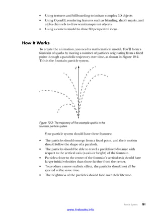

![Particle Systems 163
In Figure 10-3, the azimuth, φ, is the angle of the velocity vector to
the x-axis. The inclination, θ, is the angle made by the velocity vector to the
z-axis. The range of inclination chosen is such that the velocity vector lies
within the light gray shaded area in the figure.
The velocity directions should be chosen at random from the part of
the hemisphere enclosed within the large circle. These directions intersect
points on a sphere with a radius of one unit, so you can use the spherical
coordinate system to compute them. In addition, you want the magnitude
of the velocity to decrease as the angle from the axis increases. Keeping
this in mind, the initial velocity of a particle is as follows:
V V
i
0
2
1
= −
( )
α
Here, a is the ratio of the angle of inclination of the particle to the maxi-
mum angle (in this case, 20 degrees). As a result, the velocity decreases
(quad
ratically) as this ratio moves toward 1.0. The velocity, V, is a point on
the unit sphere and is as follows:
V = ( ) ( ) ( ) ( ) ( )
( )
si ,sin sin ,cos
θ φ θ φ φ
cos n
You choose a random inclination in the range of [0, 20] degrees and a
random azimuth in the range of [0, 360] degrees:
θ φ
= [ ]
( ) = [ ]
( )
random random
0 20 0 360
, , ,
This equation points the particle at a random spot in the region within
the circle in Figure 10-3. (Note that in this program, all angle calculations
need to be done in radians, not degrees.)
You also want to ensure the particles don’t all start at the same time.
(See “Experiments!” on page 189 to find out why.) To do this, you com-
pute a time lag for each particle, which you use later in the computation of
the particle’s position. The lag for the ith particle is computed as follows:
t i
lag
i
= 0 05
.
What about the arbitrary numerical constants in these equations?
Why use 0.05 for the lag time, for example, or 20 degrees for the maxi-
mum angle? The answer is experimentation. The important thing is to
make a basic model and then tweak these constants to get the best visual
effect. Change these parameters in your program to see how different
values influence the results.
Rendering the Particles
One simple way to render the particles is to draw them as points. OpenGL
has a GL_POINTS primitive that is essentially a dot on the screen; you can con-
trol the pixel size and color of the dot. But you want the particles to look like
little sparks and to spin around as they shoot up.
www.it-ebooks.info](https://image.slidesharecdn.com/pythonplaygroundgeekyprojectsforthecuriousprogrammerpdfdrive-220717171538-9c44c48d/85/Python-Playground_-Geeky-Projects-for-the-Curious-Programmer-PDFDrive-pdf-186-320.jpg)
![164 Chapter 10
Drawing sparks from scratch is too complicated, so you’ll take a picture
of a spark and paste it as a texture onto a rectangle (also called a quad). Each
particle in the fountain will be drawn as a textured triangular image of
a spark. But that leaves you with two problems. First, you don’t want square
sparks because that would look fake. Second, the quads will be aligned
incorrectly if you look at the fountain from other angles.
Using OpenGL Blending to Create More Realistic Sparks
To create more realistic-looking sparks, you’ll use OpenGL blending. You
combine the incoming fragment (after execution of the fragment shader)
with the content already in the frame buffer. The alpha channel is usually
involved in this operation.
For example, say you’re drawing two polygons onscreen and you want
to blend them together. You can use alpha blending to do the trick, which
works like placing two transparent sheets on top of each other. The alpha
channel represents the opacity of the pixel, which is a measure of how trans-
parent it is. In addition to the red, green, and blue components that represent
the color of a pixel, you can also store an alpha value, and the resulting color
scheme is called RGBA. For a 32-bit RGBA color scheme, the alpha value is
in the range [0, 255], with 0 being fully transparent and 255 fully opaque.
The alpha channel by itself doesn’t do anything. Only when you use the
alpha value to change the final RGB value of a pixel are various transpar-
ency effects created.
OpenGL gives you several ways to tailor your blending equations. For
your fountain particles, you’ll use the texture shown in Figure 10-4, but you
want the black regions of the texture to disappear so you see just the sparks.
RGB = (0, 0, 0)
RGB = (255, 255, 255)
Figure 10-4: The spark texture, labeled with RGB values:
(0, 0, 0) for black and (255, 255, 255) for white
You can make the black regions disappear by enabling OpenGL blend-
ing and multiplying the alpha value of a fragment by the texture color. For
the black regions, the RGB color value is (0, 0, 0), and if you multiply this
by an alpha value, you get 0. As a result, during blending, the opacity of
the black regions in the final image is set to 0 and you see only the back-
ground color, effectively cutting off the black regions in the spark texture.
(The alpha value is set in the fragment shader, as you’ll see in “Creating the
Fragment Shader” on page 171.)
www.it-ebooks.info](https://image.slidesharecdn.com/pythonplaygroundgeekyprojectsforthecuriousprogrammerpdfdrive-220717171538-9c44c48d/85/Python-Playground_-Geeky-Projects-for-the-Curious-Programmer-PDFDrive-pdf-187-320.jpg)


![Particle Systems 167
OpenGL vertex and fragment shaders are used in the program. Lastly,
you’ll look at how to put all of this together to render the particle system.
For the full project code, skip ahead to “The Complete Particle System Code”
on page 174.
The code for the fountain is encapsulated in a class called ParticleSystem,
which creates the particle system, sets up the OpenGL shaders, renders the
system using OpenGL, and restarts the animation every five seconds.
Defining the Particle Geometry
First, define the geometry of the particles by creating a Vertex Array Object
(VAO) to manage the subsequent vertex attribute arrays.
# create Vertex Array Object (VAO)
self.vao = glGenVertexArrays(1)
# bind VAO
glBindVertexArray(self.vao)
Each particle is a square, whose vertices and texture coordinates are
defined as follows:
# vertices
s = 0.2
u quadV = [
-s, s, 0.0,
-s, -s, 0.0,
s, s, 0.0,
s, -s, 0.0,
s, s, 0.0,
-s, -s, 0.0
]
v vertexData = numpy.array(numP*quadV, numpy.float32)
w self.vertexBuffer = glGenBuffers(1)
x glBindBuffer(GL_ARRAY_BUFFER, self.vertexBuffer)
y glBufferData(GL_ARRAY_BUFFER, 4*len(vertexData), vertexData,
GL_STATIC_DRAW)
# texture coordinates
z quadT = [
0.0, 1.0,
0.0, 0.0,
1.0, 1.0,
1.0, 0.0,
1.0, 1.0,
0.0, 0.0
]
tcData = numpy.array(numP*quadT, numpy.float32)
self.tcBuffer = glGenBuffers(1)
glBindBuffer(GL_ARRAY_BUFFER, self.tcBuffer)
glBufferData(GL_ARRAY_BUFFER, 4*len(tcData), tcData, GL_STATIC_DRAW)
www.it-ebooks.info](https://image.slidesharecdn.com/pythonplaygroundgeekyprojectsforthecuriousprogrammerpdfdrive-220717171538-9c44c48d/85/Python-Playground_-Geeky-Projects-for-the-Curious-Programmer-PDFDrive-pdf-190-320.jpg)
![168 Chapter 10
At u, you define the vertices of the square, with sides centered around
the origin and measuring 0.2 in length. The vertex ordering is the same as
for a couple of GL_TRIANGLES. You then create a numpy array at v by repeating
these vertices numP times—one quad for each particle in the system. (All the
geometry you are drawing is put into one big array.)
Next, you put these vertices into a vertex buffer object, as you did in
Chapter 9. The VBO is created at w and bound at x; then at y, the bound
buffer is filled with the vertex data. The 4*len(vertexData) code specifies that
4 bytes are needed for each element in the vertexData array.
Finally, you define the texture coordinates of the quad at z, and the
lines of code that follow set up the associated VBO.
Defining the Time-Lag Array for the Particles
Next, define the time-lag array for the particles. You want the time lag to be
the same for each set of four vertices, which represent a square-shaped par-
ticle, as you can see in the following code:
# time lags
u timeData = numpy.repeat(0.005*numpy.arange(numP, dtype=numpy.float32),
4)
self.timeBuffer = glGenBuffers(1)
glBindBuffer(GL_ARRAY_BUFFER, self.timeBuffer)
glBufferData(GL_ARRAY_BUFFER, 4*len(timeData), timeData,
GL_STATIC_DRAW)
At u, numpy.arange() creates an array of increasing values of the form
[0, 1, ... , numP–1]. Multiplying this array by 0.005 and using numpy.repeat()
with an argument of 4 produces an array of the form [0.0, 0.0, 0.0, 0.0, 0.005,
0.005, 0.005, 0.005, ...]. The code that follows sets up the VBO.
Setting the Initial Particle Velocities
You create the initial velocities of the particles next. The goal is to create
a spread of random velocities within a certain maximum angular displace-
ment from the vertical axis. Here’s the code:
# velocites
velocities = []
# cone angle
u coneAngle = math.radians(20.0)
# set up particle velocities
for i in range(numP):
# inclination
v angleRatio = random.random()
a = angleRatio*coneAngle
# azimuth
w t = random.random()*(2.0*math.pi)
# get velocity on sphere
x vx = math.sin(a)*math.cos(t)
vy = math.sin(a)*math.sin(t)
vz = math.cos(a)
www.it-ebooks.info](https://image.slidesharecdn.com/pythonplaygroundgeekyprojectsforthecuriousprogrammerpdfdrive-220717171538-9c44c48d/85/Python-Playground_-Geeky-Projects-for-the-Curious-Programmer-PDFDrive-pdf-191-320.jpg)
![Particle Systems 169
# speed decreases with angle
y speed = 15.0*(1.0 - angleRatio*angleRatio)
# add a set of calculated velocities
z velocities += 6*[speed*vx, speed*vy, speed*vz]
# set up velocity vertex buffer
self.velBuffer = glGenBuffers(1)
glBindBuffer(GL_ARRAY_BUFFER, self.velBuffer)
{ velData = numpy.array(velocities, numpy.float32)
glBufferData(GL_ARRAY_BUFFER, 4*len(velData), velData, GL_STATIC_DRAW)
At u, you define the cone angle used to restrict the trajectory of the
fountain particles. (Notice the conversion from degrees to radians using
the built-in math.radians() method.) Next, you calculate a velocity for
each particle using the formulas discussed in “Modeling the Motion of a
Particle” on page 162.
At v, you compute a random fraction of the maximum inclination
angle, which the lines that follow use to compute the current inclination.
Next, at w, you calculate the azimuth, and because random.random() returns
a value in [0, 1], you multiply the azimuth by 2.0*math.pi to get a random
angle from 0 to 2p radians.
Starting at x, you compute the velocity vector on the unit sphere using
the spherical coordinate formula. At y, use the angle ratio from v to
calculate a velocity inversely proportional to the vertical angle. Calculate the
particle’s final velocity at z and repeat this value for all six vertices of the
two triangles. At {, you create a numpy array from the Python list, and you’re
ready to create a VBO for velocities. Finally, you enable all vertex attri-
butes and set the data format for the vertex buffers. (Because this pro-
cess is similar to what you did in Chapter 9, I’ll skip the discussion here and
move on to the vertex shader.)
Creating the Vertex Shader
The vertex shader computes the trajectory of the particle system by process-
ing individual vertices. Here’s its code:
#version 330 core
in vec3 aVel;
in vec3 aVert;
in float aTime0;
in vec2 aTexCoord;
uniform mat4 uMVMatrix;
uniform mat4 uPMatrix;
uniform mat4 bMatrix;
uniform float uTime;
uniform float uLifeTime;
uniform vec4 uColor;
uniform vec3 uPos;
out vec4 vCol;
out vec2 vTexCoord;
www.it-ebooks.info](https://image.slidesharecdn.com/pythonplaygroundgeekyprojectsforthecuriousprogrammerpdfdrive-220717171538-9c44c48d/85/Python-Playground_-Geeky-Projects-for-the-Curious-Programmer-PDFDrive-pdf-192-320.jpg)
![170 Chapter 10
The vertex shader is executed for every vertex of the quad, for all
quads in the particle system. It first defines some variables in attribute
arrays, which represent the array you put into the VBOs; then uniform vari-
ables that remain constant while the shader is executed; and finally out
quantities, which are set in the vertex shader and passed to the fragment
shader for interpolation.
Now let’s look at the shader’s main() function:
void main() {
// set position
u float dt = uTime - aTime0;
v float alpha = clamp(1.0 - 2.0*dt/uLifeTime, 0.0, 1.0);
w if(dt < 0.0 || dt > uLifeTime || alpha < 0.01) {
// out of sight!
gl_Position = vec4(0.0, 0.0, -1000.0, 1.0);
}
else {
// calculate new position
x vec3 accel = vec3(0.0, 0.0, -9.8);
// apply a twist
float PI = 3.14159265358979323846264;
y float theta = mod(100.0*length(aVel)*dt, 360.0)*PI/180.0;
z mat4 rot = mat4(vec4(cos(theta), sin(theta), 0.0, 0.0),
vec4(-sin(theta), cos(theta), 0.0, 0.0),
vec4(0.0, 0.0, 1.0, 0.0),
vec4(0.0, 0.0, 0.0, 1.0));
// apply billboard matrix
{ vec4 pos2 = bMatrix*rot*vec4(aVert, 1.0);
// calculate position
| vec3 newPos = pos2.xyz + uPos + aVel*dt + 0.5*accel*dt*dt;
// apply transformations
} gl_Position = uPMatrix * uMVMatrix * vec4(newPos, 1.0);
}
// set color
~ vCol = vec4(uColor.rgb, alpha);
// set texture coordinates
vTexCoord = aTexCoord;
}
At u, you calculate the current elapsed time for a particular particle,
which is the difference between the current time step and the time lag for
that particle. Then you calculate an alpha value for the vertex at v, which
decreases as a function of elapsed time and has the particles fade over time.
You use the clamp() method in GLSL to restrict the values to the range [0, 1].
To make the particles disappear once their lifetime is over, you put
them outside your OpenGL view frustum, where they are clipped away.
At w, you see whether a particle’s lifetime is up (as set in the constructor
of the par
ticle system) or whether its alpha has dropped below a certain
value, in which case the final position is set to a value outside your view.
www.it-ebooks.info](https://image.slidesharecdn.com/pythonplaygroundgeekyprojectsforthecuriousprogrammerpdfdrive-220717171538-9c44c48d/85/Python-Playground_-Geeky-Projects-for-the-Curious-Programmer-PDFDrive-pdf-193-320.jpg)
![Particle Systems 171
You set particle acceleration to 9.8 m/s2
at x, the rate of acceleration
due to Earth’s gravity. To make the particles spin quickly as they fly out of
the fountain with their higher initial velocity, use the mod() method (similar
to the Python modulus operator, %), and at y, restrict the angle values to the
range [0, 360]. At z, apply this calculated angle as a rotation around the
z-axis of the quad according to the formula for the transformation matrix
for rotation by an angle q around the z-axis as follows:
R z
θ
θ θ
θ θ
,
cos sin . .
sin cos . .
. . . .
.
=
( ) ( )
− ( ) ( )
0 0 0 0
0 0 0 0
0 0 0 0 1 0 0 0
0 0 0.
. . .
0 0 0 1 0
At {, you apply two transformations to the particle’s vertices: the spin
rotation just computed and the rotation for the billboarding using bMatrix.
Calculate the current position of the vertex at | using the equation of
motion discussed earlier. (The uPos in this line simply lets you position the
origin of the fountain wherever you want.)
At }, you apply the modelview and projection matrices to the particle
position. Finally, at ~ and in the following line, set the colors and texture
coordinates to pass to the fragment shader for interpolation. (Note that you
set the alpha of the vertex based on the computation at v.)
Creating the Fragment Shader
Now let’s look at the fragment shader, which sets the color of the pixels.
#version 330 core
uniform sampler2D uSampler;
in vec4 vCol;
in vec2 vTexCoord;
out vec4 fragColor;
void main() {
// get the texture color
u vec4 texCol = texture2D(uSampler, vec2(vTexCoord.s, vTexCoord.t));
// multiply texture color by set vertex color; use the vertex color alpha
v fragColor = vec4(texCol.rgb*vCol.rgb, vCol.a);
}
At u, you use the GLSL texture2D() method to look up the base texture
color (the color you look up from the image used as texture) for the spark
image using the texture coordinates passed in from the vertex shader. Then,
you multiply this texture color value by the color of the spark fountain and
set the resulting color to the output variable fragColor v. The fountain color
is set randomly by the restart() method of ParticleSystem each time a par-
ticle system is restarted. The alpha is set based on the calculation done in
the vertex shader and is used for blending during rendering.
www.it-ebooks.info](https://image.slidesharecdn.com/pythonplaygroundgeekyprojectsforthecuriousprogrammerpdfdrive-220717171538-9c44c48d/85/Python-Playground_-Geeky-Projects-for-the-Curious-Programmer-PDFDrive-pdf-194-320.jpg)
![172 Chapter 10
Rendering
The code follows these steps to render the fountain particle system:
1. Enables the vertex/fragment program
2. Sets the modelview and projection matrices
3. Computes and sets the billboard matrix based on the current
camera view
4. Sets uniform variables for position, time, lifetime, and color
5. Enables vertex attribute arrays for vertices, texture coordinates, time
lags, and velocities
6. Enables texturing and binding to the particle spark texture
7. Disables depth buffer writing
8. Enables OpenGL blending
9. Draws the geometry
Let’s take a look at code snippets that implement some of these steps.
Computing the Rotation Matrix for Billboarding
This code computes the rotation matrix for billboarding:
N = camera.eye - camera.center
u N /= numpy.linalg.norm(N)
U = camera.up
U /= numpy.linalg.norm(U)
R = numpy.cross(U, N)
U2 = numpy.cross(N, R)
v bMatrix = numpy.array([R[0], U2[0], N[0], 0.0,
R[1], U2[1], N[1], 0.0,
R[2], U2[2], N[2], 0.0,
0.0, 0.0, 0.0, 1.0], numpy.float32)
w glUniformMatrix4fv(self.bMatrixU, 1, GL_TRUE, bMatrix)
You already looked at the theory behind formulating a rotation
matrix that will keep a quad “billboarded,” or aligned toward the view.
(This is required so that the fountain particles always face your viewing
direction.) At u, you use numpy.linalg.norm() to normalize the vectors.
(This makes the magnitude of the vector equal to 1.) At v, you assemble
the rotation matrix as a numpy array and then set it in the program at w.
The Main Rendering Code
The main rendering code uses alpha blending to give transparency to the
particle system. This technique is commonly used in OpenGL to render
semitransparent objects.
# enable texture
u glActiveTexture(GL_TEXTURE0)
www.it-ebooks.info](https://image.slidesharecdn.com/pythonplaygroundgeekyprojectsforthecuriousprogrammerpdfdrive-220717171538-9c44c48d/85/Python-Playground_-Geeky-Projects-for-the-Curious-Programmer-PDFDrive-pdf-195-320.jpg)

![174 Chapter 10
self.r = 10.0
self.theta = 0
self.eye = numpy.array(eye, numpy.float32)
self.center = numpy.array(center, numpy.float32)
self.up = numpy.array(up, numpy.float32)
def rotate(self):
"""rotate eye by one step"""
v self.theta = (self.theta + 1) % 360
# recalculate eye
w self.eye = self.center + numpy.array([
self.r*math.cos(math.radians(self.theta)),
self.r*math.sin(math.radians(self.theta)),
0.0], numpy.float32)
Three-dimensional perspective view is typically characterized by three
parameters: an eye position, an up vector, and a direction vector. The Camera
class groups these parameters and provides a convenient way to rotate the
view for every time step.
The constructor at u sets the initial values of the camera object. When
the rotate() method is called, you increment the rotation angle v and cal-
culate the new eye position and direction after the rotation w.
NOTE The point (r cos(θ), r sin(θ)) represents a point on a circle of radius r centered at the
origin, and θ is the angle that the line from the origin to the point makes with the
x-axis. The translation using center ensures this works even if your center of rotation
is not at the origin.
The Complete Particle System Code
This is the complete code for the particle system. You can also find it as
ps.py at https://github.com/electronut/pp/tree/master/particle-system/.
import sys, random, math
import OpenGL
from OpenGL.GL import *
import numpy
import glutils
strVS = """
#version 330 core
in vec3 aVel;
in vec3 aVert;
in float aTime0;
in vec2 aTexCoord;
uniform mat4 uMVMatrix;
uniform mat4 uPMatrix;
uniform mat4 bMatrix;
uniform float uTime;
www.it-ebooks.info](https://image.slidesharecdn.com/pythonplaygroundgeekyprojectsforthecuriousprogrammerpdfdrive-220717171538-9c44c48d/85/Python-Playground_-Geeky-Projects-for-the-Curious-Programmer-PDFDrive-pdf-197-320.jpg)

![176 Chapter 10
# a simple camera class
class Camera:
"""helper class for viewing"""
def __init__(self, eye, center, up):
self.r = 10.0
self.theta = 0
self.eye = numpy.array(eye, numpy.float32)
self.center = numpy.array(center, numpy.float32)
self.up = numpy.array(up, numpy.float32)
def rotate(self):
"""rotate eye by one step"""
self.theta = (self.theta + 1) % 360
# recalculate eye
self.eye = self.center + numpy.array([
self.r*math.cos(math.radians(self.theta)),
self.r*math.sin(math.radians(self.theta)),
0.0], numpy.float32)
# particle system class
class ParticleSystem:
# initialization
def __init__(self, numP):
# number of particles
self.numP = numP
# time variable
self.t = 0.0
self.lifeTime = 5.0
self.startPos = numpy.array([0.0, 0.0, 0.5])
# load texture
self.texid = glutils.loadTexture('star.png')
# create shader
self.program = glutils.loadShaders(strVS, strFS)
glUseProgram(self.program)
# set sampler
texLoc = glGetUniformLocation(self.program, b"uTex")
glUniform1i(texLoc, 0)
# uniforms
self.timeU = glGetUniformLocation(self.program, b"uTime")
self.lifeTimeU = glGetUniformLocation(self.program, b"uLifeTime")
self.pMatrixUniform = glGetUniformLocation(self.program, b'uPMatrix')
self.mvMatrixUniform = glGetUniformLocation(self.program, b"uMVMatrix")
self.bMatrixU = glGetUniformLocation(self.program, b"bMatrix")
self.colorU = glGetUniformLocation(self.program, b"uColor")
self.samplerU = glGetUniformLocation(self.program, b"uSampler")
self.posU = glGetUniformLocation(self.program, b"uPos")
# attributes
self.vertIndex = glGetAttribLocation(self.program, b"aVert")
self.texIndex = glGetAttribLocation(self.program, b"aTexCoord")
self.time0Index = glGetAttribLocation(self.program, b"aTime0")
self.velIndex = glGetAttribLocation(self.program, b"aVel")
www.it-ebooks.info](https://image.slidesharecdn.com/pythonplaygroundgeekyprojectsforthecuriousprogrammerpdfdrive-220717171538-9c44c48d/85/Python-Playground_-Geeky-Projects-for-the-Curious-Programmer-PDFDrive-pdf-199-320.jpg)
![Particle Systems 177
# render flags
self.enableBillboard = True
self.disableDepthMask = True
self.enableBlend = True
# which texture to use
self.useStarTexture = True
# restart - first time
self.restart(numP)
# step
def step(self):
# increment time
self.t += 0.01
# restart particle system
def restart(self, numP):
# set number of particles
self.numP = numP
# time variables
self.t = 0.0
self.lifeTime = 5.0
# color
self.col0 = numpy.array([random.random(), random.random(),
random.random(), 1.0])
# create Vertex Arrays Object (VAO)
self.vao = glGenVertexArrays(1)
# bind VAO
glBindVertexArray(self.vao)
# create attribute arrays and vertex buffers:
# vertices
s = 0.2
quadV = [
-s, s, 0.0,
-s, -s, 0.0,
s, s, 0.0,
s, -s, 0.0,
s, s, 0.0,
-s, -s, 0.0
]
vertexData = numpy.array(numP*quadV, numpy.float32)
self.vertexBuffer = glGenBuffers(1)
glBindBuffer(GL_ARRAY_BUFFER, self.vertexBuffer)
glBufferData(GL_ARRAY_BUFFER, 4*len(vertexData), vertexData,
GL_STATIC_DRAW)
# texture coordinates
quadT = [
0.0, 1.0,
0.0, 0.0,
www.it-ebooks.info](https://image.slidesharecdn.com/pythonplaygroundgeekyprojectsforthecuriousprogrammerpdfdrive-220717171538-9c44c48d/85/Python-Playground_-Geeky-Projects-for-the-Curious-Programmer-PDFDrive-pdf-200-320.jpg)
![178 Chapter 10
1.0, 1.0,
1.0, 0.0,
1.0, 1.0,
0.0, 0.0
]
tcData = numpy.array(numP*quadT, numpy.float32)
self.tcBuffer = glGenBuffers(1)
glBindBuffer(GL_ARRAY_BUFFER, self.tcBuffer)
glBufferData(GL_ARRAY_BUFFER, 4*len(tcData), tcData, GL_STATIC_DRAW)
# time lags
timeData = numpy.repeat(0.005*numpy.arange(numP, dtype=numpy.float32),
4)
self.timeBuffer = glGenBuffers(1)
glBindBuffer(GL_ARRAY_BUFFER, self.timeBuffer)
glBufferData(GL_ARRAY_BUFFER, 4*len(timeData), timeData,
GL_STATIC_DRAW)
# velocites
velocities = []
# cone angle
coneAngle = math.radians(20.0)
# set up particle velocities
for i in range(numP):
# inclination
angleRatio = random.random()
a = angleRatio*coneAngle
# azimuth
t = random.random()*(2.0*math.pi)
# get veocity on sphere
vx = math.sin(a)*math.cos(t)
vy = math.sin(a)*math.sin(t)
vz = math.cos(a)
# speed decreases with angle
speed = 15.0*(1.0 - angleRatio*angleRatio)
# add a set of calculated velocities
velocities += 6*[speed*vx, speed*vy, speed*vz]
# set up velocity vertex buffer
self.velBuffer = glGenBuffers(1)
glBindBuffer(GL_ARRAY_BUFFER, self.velBuffer)
velData = numpy.array(velocities, numpy.float32)
glBufferData(GL_ARRAY_BUFFER, 4*len(velData), velData, GL_STATIC_DRAW)
# enable arrays
glEnableVertexAttribArray(self.vertIndex)
glEnableVertexAttribArray(self.texIndex)
glEnableVertexAttribArray(self.time0Index)
glEnableVertexAttribArray(self.velIndex)
# set buffers
glBindBuffer(GL_ARRAY_BUFFER, self.vertexBuffer)
glVertexAttribPointer(self.vertIndex, 3, GL_FLOAT, GL_FALSE, 0, None)
glBindBuffer(GL_ARRAY_BUFFER, self.tcBuffer)
glVertexAttribPointer(self.texIndex, 2, GL_FLOAT, GL_FALSE, 0, None)
www.it-ebooks.info](https://image.slidesharecdn.com/pythonplaygroundgeekyprojectsforthecuriousprogrammerpdfdrive-220717171538-9c44c48d/85/Python-Playground_-Geeky-Projects-for-the-Curious-Programmer-PDFDrive-pdf-201-320.jpg)
![Particle Systems 179
glBindBuffer(GL_ARRAY_BUFFER, self.velBuffer)
glVertexAttribPointer(self.velIndex, 3, GL_FLOAT, GL_FALSE, 0, None)
glBindBuffer(GL_ARRAY_BUFFER, self.timeBuffer)
glVertexAttribPointer(self.time0Index, 1, GL_FLOAT, GL_FALSE, 0, None)
# unbind VAO
glBindVertexArray(0)
# render the particle system
def render(self, pMatrix, mvMatrix, camera):
# use shader
glUseProgram(self.program)
# set projection matrix
glUniformMatrix4fv(self.pMatrixUniform, 1, GL_FALSE, pMatrix)
# set modelview matrix
glUniformMatrix4fv(self.mvMatrixUniform, 1, GL_FALSE, mvMatrix)
# set up a billboard matrix to keep quad aligned to view direction
if self.enableBillboard:
N = camera.eye - camera.center
N /= numpy.linalg.norm(N)
U = camera.up
U /= numpy.linalg.norm(U)
R = numpy.cross(U, N)
U2 = numpy.cross(N, R)
bMatrix = numpy.array([R[0], U2[0], N[0], 0.0,
R[1], U2[1], N[1], 0.0,
R[2], U2[2], N[2], 0.0,
0.0, 0.0, 0.0, 1.0], numpy.float32)
glUniformMatrix4fv(self.bMatrixU, 1, GL_TRUE, bMatrix)
else:
# identity matrix
bMatrix = numpy.array([1.0, 0.0, 0.0, 0.0,
0.0, 1.0, 0.0, 0.0,
0.0, 0.0, 1.0, 0.0,
0.0, 0.0, 0.0, 1.0], numpy.float32)
glUniformMatrix4fv(self.bMatrixU, 1, GL_FALSE, bMatrix)
# set start position
glUniform3fv(self.posU, 1, self.startPos)
# set time
glUniform1f(self.timeU, self.t)
#set lifetime
glUniform1f(self.lifeTimeU, self.lifeTime)
# set color
glUniform4fv(self.colorU, 1, self.col0)
# enable texture
glActiveTexture(GL_TEXTURE0)
glBindTexture(GL_TEXTURE_2D, self.texid)
glUniform1i(self.samplerU, 0)
www.it-ebooks.info](https://image.slidesharecdn.com/pythonplaygroundgeekyprojectsforthecuriousprogrammerpdfdrive-220717171538-9c44c48d/85/Python-Playground_-Geeky-Projects-for-the-Curious-Programmer-PDFDrive-pdf-202-320.jpg)


![182 Chapter 10
-s, -s, s,
-s, -s, -s,
-s, s, s,
-s, s, -s,
-s, s, s,
-s, -s, -s,
s, -s, s,
s, -s,-s,
s, s, s,
s, s, -s,
s, s, s,
s, -s,-s
]
# set up vertex array object (VAO)
self.vao = glGenVertexArrays(1)
glBindVertexArray(self.vao)
# set up VBOs
vertexData = numpy.array(vertices, numpy.float32)
self.vertexBuffer = glGenBuffers(1)
glBindBuffer(GL_ARRAY_BUFFER, self.vertexBuffer)
glBufferData(GL_ARRAY_BUFFER, 4*len(vertexData), vertexData,
GL_STATIC_DRAW)
#enable arrays
self.vertIndex = glGetAttribLocation(self.program, "aVert")
glEnableVertexAttribArray(self.vertIndex)
# set buffers
glBindBuffer(GL_ARRAY_BUFFER, self.vertexBuffer)
glVertexAttribPointer(self.vertIndex, 3, GL_FLOAT, GL_FALSE, 0, None)
# unbind VAO
glBindVertexArray(0)
def render(self, pMatrix, mvMatrix):
# use shader
glUseProgram(self.program)
# set projection matrix
glUniformMatrix4fv(glGetUniformLocation(self.program, 'uPMatrix'),
1, GL_FALSE, pMatrix)
# set modelview matrix
glUniformMatrix4fv(glGetUniformLocation(self.program, 'uMVMatrix'),
1, GL_FALSE, mvMatrix)
# bind VAO
glBindVertexArray(self.vao)
# draw
glDrawArrays(GL_TRIANGLES, 0, 36)
# unbind VAO
glBindVertexArray(0)
www.it-ebooks.info](https://image.slidesharecdn.com/pythonplaygroundgeekyprojectsforthecuriousprogrammerpdfdrive-220717171538-9c44c48d/85/Python-Playground_-Geeky-Projects-for-the-Curious-Programmer-PDFDrive-pdf-205-320.jpg)
![Particle Systems 183
The code for the box uses simple vertex and fragment shaders to draw
a cube. The concepts used here are identical to what we discussed earlier in
this chapter and in Chapter 9.
The Code for the Main Program
The main source file for the project, psmain.py, sets up the GLFW window,
handles keyboard events, and creates the particle system. Skip ahead to
“The Complete Main Program Code” on page 186 if you’d like to see the
full program code.
class PSMaker:
"""GLFW Rendering window class for Particle System"""
def __init__(self):
u self.camera = Camera([15.0, 0.0, 2.5],
[0.0, 0.0, 2.5],
[0.0, 0.0, 1.0])
self.aspect = 1.0
self.numP = 300
self.t = 0
# flag to rotate camera view
self.rotate = True
# save current working directory
cwd = os.getcwd()
# initialize glfw; this changes cwd
v glfw.glfwInit()
# restore cwd
os.chdir(cwd)
# version hints
glfw.glfwWindowHint(glfw.GLFW_CONTEXT_VERSION_MAJOR, 3)
glfw.glfwWindowHint(glfw.GLFW_CONTEXT_VERSION_MINOR, 3)
glfw.glfwWindowHint(glfw.GLFW_OPENGL_FORWARD_COMPAT, GL_TRUE)
glfw.glfwWindowHint(glfw.GLFW_OPENGL_PROFILE,
glfw.GLFW_OPENGL_CORE_PROFILE)
# make a window
self.width, self.height = 640, 480
self.aspect = self.width/float(self.height)
self.win = glfw.glfwCreateWindow(self.width, self.height,
b"Particle System")
# make context current
glfw.glfwMakeContextCurrent(self.win)
# initialize GL
glViewport(0, 0, self.width, self.height)
glEnable(GL_DEPTH_TEST)
glClearColor(0.2, 0.2, 0.2,1.0)
www.it-ebooks.info](https://image.slidesharecdn.com/pythonplaygroundgeekyprojectsforthecuriousprogrammerpdfdrive-220717171538-9c44c48d/85/Python-Playground_-Geeky-Projects-for-the-Curious-Programmer-PDFDrive-pdf-206-320.jpg)


![186 Chapter 10
# draw nontransparent object first
w self.box.render(pMatrix, mvMatrix)
# render
x self.psys.render(pMatrix, mvMatrix, self.camera)
# step
y self.step()
glfw.glfwSwapBuffers(self.win)
# poll for and process events
glfw.glfwPollEvents()
# end
glfw.glfwTerminate()
This code is almost identical to the loop you used in Chapter 9. At u,
the while loop exits if either the exit flag is set or the GLFW window closes.
At v and in the following line, you use the GLFW timer to render only
when a certain amount of time (0.1 seconds) has elapsed, thus controlling
the frame rate of the rendering. You draw the box at w and the particle
system at x. (The order of rendering is important: transparent objects are
always drawn last so they can be blended and depth buffered correctly with
respect to the opaque objects in a scene.) At y, you update the particle sys-
tem for the current time step.
The Complete Main Program Code
Here is the complete code for psmain.py. You can also find this code at
https://github.com/electronut/pp/tree/master/particle-system/.
import sys, os, math, numpy
import OpenGL
from OpenGL.GL import *
import numpy
from ps import ParticleSystem, Camera
from box import Box
import glutils
import glfw
class PSMaker:
"""GLFW Rendering window class for Particle System"""
def __init__(self):
self.camera = Camera([15.0, 0.0, 2.5],
[0.0, 0.0, 2.5],
[0.0, 0.0, 1.0])
self.aspect = 1.0
self.numP = 300
self.t = 0
# flag to rotate camera view
self.rotate = True
www.it-ebooks.info](https://image.slidesharecdn.com/pythonplaygroundgeekyprojectsforthecuriousprogrammerpdfdrive-220717171538-9c44c48d/85/Python-Playground_-Geeky-Projects-for-the-Curious-Programmer-PDFDrive-pdf-209-320.jpg)


![Volume Rendering 195
NOTE In OpenGL, a color can be represented as a strip of 8-bit unsigned values (r, g, b),
where r, g, and b are in the range [0, 255]. It can also be represented as a 32-bit
floating-point value (r, g, b), where r, g, and b are in the range [0.0, 1.0]. These
representations are equivalent. For example, the red color (255, 0, 0) in the former
is the same as (1.0, 0.0, 0.0) in the latter.
To draw the cube, first draw its six faces using the OpenGL primitive
GL_TRIANGLES. Then color each vertex and use the interpolation provided by
OpenGL when it rasterizes polygons to take care of the colors between each
vertex. For example, Figure 11-4(a) shows the three front-faces of the cube.
The back-faces of the cube are drawn in Figure 11-4(b) by setting OpenGL
to cull front-faces.
A B C
Figure 11-4: Color cube used to compute rays
If you subtract the colors in Figure 11-4(a) from Figure 11-4(b) by sub-
tracting (r, g, b)front from (r, g, b)back, you actually compute a sect of vectors
that go from the front to the back of the cube because each color (r, g, b) on
this cube is the same as the 3D coordinate. Figure 11-4(c) shows the result.
(Negative values have been flipped to positive for the
purposes of this illus-
tration because negative numbers cannot be displayed as colors directly.)
Reading the color value (r, g, b) of a pixel, as shown in Figure 11-4(c), gives
the (rx, ry, rz) coordinates for the ray passing into the volume at that point.
Once you have the casting rays, you render them into an image or 2D
texture for later use with OpenGL’s frame buffer object (FBO) feature.
After this texture is generated, you can access it inside the shaders that
you’ll use to implement the ray casting algorithm.
Ray Casting in the GPU
To implement the ray casting algorithm, you first draw the back-faces of the
color cube into an FBO. Next, the front-faces are drawn on the screen. The
bulk of the ray casting algorithm happens in the fragment shader for this
second rendering, which runs for each pixel in the output. The ray is com-
puted by subtracting the front-face color of the incoming fragment from
www.it-ebooks.info](https://image.slidesharecdn.com/pythonplaygroundgeekyprojectsforthecuriousprogrammerpdfdrive-220717171538-9c44c48d/85/Python-Playground_-Geeky-Projects-for-the-Curious-Programmer-PDFDrive-pdf-218-320.jpg)

![Volume Rendering 197
implementing the volume ray casting algorithm. You’ll look at how to define
the cube geometry as well as how to draw the back- and front-faces of this
cube. You’ll then explore the volume ray casting algorithm and the associ-
ated vertex and fragment shaders. Finally, you’ll learn how to implement 2D
slicing of the volumetric data.
This project has seven Python files:
glutils.py Contains the utility methods for OpenGL shaders, transfor-
mations, and so on
makedata.py Contains utility methods for creating volumetric data
for testing
raycast.py Implements the RayCastRender class for ray casting
raycube.py Implements the RayCube class for use in RayCastRender
slicerender.py Implements the SliceRender class for 2D slicing of volu-
metric data
volreader.py Contains the utility method to read volumetric data into
the OpenGL 3D texture
volrender.py Contains the main methods that create the GLFW win-
dow and the renderers
We’ll cover all but two of these files in this chapter. The makedata.py
file lives with the other project files for this chapter at https://github.com/
electronut/pp/tree/master/volrender/. The glutils.py file can be downloaded
from https://github.com/electronut/pp/tree/master/common/.
Generating a 3D Texture
The first step is to read the volumetric data from a folder containing
images, as shown in the following code. To see the complete volreader.py
code, skip ahead to “The Complete 3D Texture Code” on page 199.
def loadVolume(dirName):
"""read volume from directory as a 3D texture"""
# list images in directory
u files = sorted(os.listdir(dirName))
print('loading images from: %s' % dirName)
imgDataList = []
count = 0
width, height = 0, 0
for file in files:
v file_path = os.path.abspath(os.path.join(dirName, file))
try:
# read image
w img = Image.open(file_path)
imgData = np.array(img.getdata(), np.uint8)
# check if all images are of the same size
x if count is 0:
width, height = img.size[0], img.size[1]
www.it-ebooks.info](https://image.slidesharecdn.com/pythonplaygroundgeekyprojectsforthecuriousprogrammerpdfdrive-220717171538-9c44c48d/85/Python-Playground_-Geeky-Projects-for-the-Curious-Programmer-PDFDrive-pdf-220-320.jpg)
![198 Chapter 11
imgDataList.append(imgData)
else:
y if (width, height) == (img.size[0], img.size[1]):
imgDataList.append(imgData)
else:
print('mismatch')
raise RunTimeError("image size mismatch")
count += 1
#print img.size
except:
# skip
print('Invalid image: %s' % file_path)
# load image data into single array
depth = count
z data = np.concatenate(imgDataList)
print('volume data dims: %d %d %d' % (width, height, depth))
# load data into 3D texture
{ texture = glGenTextures(1)
glPixelStorei(GL_UNPACK_ALIGNMENT, 1)
glBindTexture(GL_TEXTURE_3D, texture)
glTexParameterf(GL_TEXTURE_3D, GL_TEXTURE_WRAP_S, GL_CLAMP_TO_EDGE)
glTexParameterf(GL_TEXTURE_3D, GL_TEXTURE_WRAP_T, GL_CLAMP_TO_EDGE)
glTexParameterf(GL_TEXTURE_3D, GL_TEXTURE_WRAP_R, GL_CLAMP_TO_EDGE)
glTexParameterf(GL_TEXTURE_3D, GL_TEXTURE_MAG_FILTER, GL_LINEAR)
glTexParameterf(GL_TEXTURE_3D, GL_TEXTURE_MIN_FILTER, GL_LINEAR)
| glTexImage3D(GL_TEXTURE_3D, 0, GL_RED,
width, height, depth, 0,
GL_RED, GL_UNSIGNED_BYTE, data)
# return texture
} return (texture, width, height, depth)
The loadVolume() method first lists the files in the given directory using
the listdir() method from the os module u; then you load the image
files themselves. At v, the filename is appended to the directory using
os.path.abspath() and os.path.join(), eliminating the need to deal with
relative file paths and operating system (OS)–specific path conventions.
(You often see this useful idiom in Python code that traverses files and
directories.)
At w, you use the Image class from Python Imaging Library (PIL) to load
the image into an 8-bit numpy array. If the file specified is not an image or
if the image fails to load, an exception is thrown, and you catch it to print
an error.
Because you are loading these image slices into a 3D texture, you need
to ensure they all have the same dimensions (width × height), which you
confirm at x and y. You store the image dimensions for the first image
and compare them against new incoming images. Once all the images are
loaded into individual arrays, create the final array containing the 3D data
by joining these arrays using the concatenate() method from numpy z.
At { and in the lines that follow, you create an OpenGL texture and set
parameters for filtering and unpacking. Then, at |, load the 3D data array
www.it-ebooks.info](https://image.slidesharecdn.com/pythonplaygroundgeekyprojectsforthecuriousprogrammerpdfdrive-220717171538-9c44c48d/85/Python-Playground_-Geeky-Projects-for-the-Curious-Programmer-PDFDrive-pdf-221-320.jpg)
![Volume Rendering 199
into the OpenGL texture. The format used here is GL_RED, and the data for-
mat is GL_UNSIGNED_BYTE because you have only one 8-bit value associated with
each pixel in the data.
Finally, at }, you return the OpenGL texture ID and the dimensions of
the 3D texture.
The Complete 3D Texture Code
Here is the full code listing. You can also find the volreader.py file at https://
github.com/electronut/pp/tree/master/volrender/.
import os
import numpy as np
from PIL import Image
import OpenGL
from OpenGL.GL import *
from scipy import misc
def loadVolume(dirName):
"""read volume from directory as a 3D texture"""
# list images in directory
files = sorted(os.listdir(dirName))
print('loading images from: %s' % dirName)
imgDataList = []
count = 0
width, height = 0, 0
for file in files:
file_path = os.path.abspath(os.path.join(dirName, file))
try:
# read image
img = Image.open(file_path)
imgData = np.array(img.getdata(), np.uint8)
# check if all are of the same size
if count is 0:
width, height = img.size[0], img.size[1]
imgDataList.append(imgData)
else:
if (width, height) == (img.size[0], img.size[1]):
imgDataList.append(imgData)
else:
print('mismatch')
raise RunTimeError("image size mismatch")
count += 1
#print img.size
except:
# skip
print('Invalid image: %s' % file_path)
# load image data into single array
depth = count
www.it-ebooks.info](https://image.slidesharecdn.com/pythonplaygroundgeekyprojectsforthecuriousprogrammerpdfdrive-220717171538-9c44c48d/85/Python-Playground_-Geeky-Projects-for-the-Curious-Programmer-PDFDrive-pdf-222-320.jpg)
![200 Chapter 11
data = np.concatenate(imgDataList)
print('volume data dims: %d %d %d' % (width, height, depth))
# load data into 3D texture
texture = glGenTextures(1)
glPixelStorei(GL_UNPACK_ALIGNMENT, 1)
glBindTexture(GL_TEXTURE_3D, texture)
glTexParameterf(GL_TEXTURE_3D, GL_TEXTURE_WRAP_S, GL_CLAMP_TO_EDGE)
glTexParameterf(GL_TEXTURE_3D, GL_TEXTURE_WRAP_T, GL_CLAMP_TO_EDGE)
glTexParameterf(GL_TEXTURE_3D, GL_TEXTURE_WRAP_R, GL_CLAMP_TO_EDGE)
glTexParameterf(GL_TEXTURE_3D, GL_TEXTURE_MAG_FILTER, GL_LINEAR)
glTexParameterf(GL_TEXTURE_3D, GL_TEXTURE_MIN_FILTER, GL_LINEAR)
glTexImage3D(GL_TEXTURE_3D, 0, GL_RED,
width, height, depth, 0,
GL_RED, GL_UNSIGNED_BYTE, data)
#return texture
return (texture, width, height, depth)
# load texture
def loadTexture(filename):
img = Image.open(filename)
img_data = np.array(list(img.getdata()), 'B')
texture = glGenTextures(1)
glPixelStorei(GL_UNPACK_ALIGNMENT,1)
glBindTexture(GL_TEXTURE_2D, texture)
glTexParameterf(GL_TEXTURE_2D, GL_TEXTURE_WRAP_S, GL_CLAMP_TO_EDGE)
glTexParameterf(GL_TEXTURE_2D, GL_TEXTURE_WRAP_T, GL_CLAMP_TO_EDGE)
glTexParameterf(GL_TEXTURE_2D, GL_TEXTURE_MAG_FILTER, GL_LINEAR)
glTexParameterf(GL_TEXTURE_2D, GL_TEXTURE_MIN_FILTER, GL_LINEAR)
glTexImage2D(GL_TEXTURE_2D, 0, GL_RGBA, img.size[0], img.size[1],
0, GL_RGBA, GL_UNSIGNED_BYTE, img_data)
return texture
Generating Rays
The code for generating the rays is encapsulated in a class called RayCube.
This class is responsible for drawing the color cube and has methods to draw
the back-faces of the cube to an FBO or texture and to draw the front-faces
of the cube to the screen. To see the complete raycube.py code, skip ahead to
“The Complete Ray Generation Code” on page 206.
First, let’s define the shaders used by this class:
u strVS = """
#version 330 core
layout(location = 1) in vec3 cubePos;
layout(location = 2) in vec3 cubeCol;
uniform mat4 uMVMatrix;
uniform mat4 uPMatrix;
out vec4 vColor;
www.it-ebooks.info](https://image.slidesharecdn.com/pythonplaygroundgeekyprojectsforthecuriousprogrammerpdfdrive-220717171538-9c44c48d/85/Python-Playground_-Geeky-Projects-for-the-Curious-Programmer-PDFDrive-pdf-223-320.jpg)
![Volume Rendering 201
void main()
{
// set back-face color
vColor = vec4(cubeCol.rgb, 1.0);
// transformed position
vec4 newPos = vec4(cubePos.xyz, 1.0);
// set position
gl_Position = uPMatrix * uMVMatrix * newPos;
}
"""
v strFS = """
#version 330 core
in vec4 vColor;
out vec4 fragColor;
void main()
{
fragColor = vColor;
}
"""
At u, you define the vertex shader used by the RayCube class. This shader
has two input attributes, cubePos and cubeCol, which are used to access the
position and color values of the vertices, respectively. The modelview and
projection matrices are passed in with the uniform variables uMVMatrix and
pMatrix, respectively. The vColor variable is declared as output because it
needs to be passed on to the fragment shader, where it will be interpolated.
The fragment shader implemented at v sets the fragment color to the (inter-
polated) value of the incoming vColor set in the vertex shader.
Defining the Color Cube Geometry
Now let’s look at the geometry of the color cube, defined in the RayCube
class:
# cube vertices
u vertices = numpy.array([
0.0, 0.0, 0.0,
1.0, 0.0, 0.0,
1.0, 1.0, 0.0,
0.0, 1.0, 0.0,
0.0, 0.0, 1.0,
1.0, 0.0, 1.0,
1.0, 1.0, 1.0,
0.0, 1.0, 1.0
], numpy.float32)
www.it-ebooks.info](https://image.slidesharecdn.com/pythonplaygroundgeekyprojectsforthecuriousprogrammerpdfdrive-220717171538-9c44c48d/85/Python-Playground_-Geeky-Projects-for-the-Curious-Programmer-PDFDrive-pdf-224-320.jpg)
![202 Chapter 11
# cube colors
v colors = numpy.array([
0.0, 0.0, 0.0,
1.0, 0.0, 0.0,
1.0, 1.0, 0.0,
0.0, 1.0, 0.0,
0.0, 0.0, 1.0,
1.0, 0.0, 1.0,
1.0, 1.0, 1.0,
0.0, 1.0, 1.0
], numpy.float32)
# individual triangles
w indices = numpy.array([
4, 5, 7,
7, 5, 6,
5, 1, 6,
6, 1, 2,
1, 0, 2,
2, 0, 3,
0, 4, 3,
3, 4, 7,
6, 2, 7,
7, 2, 3,
4, 0, 5,
5, 0, 1
], numpy.int16)
The shaders are compiled, and the program object is created in the
RayCube constructor. The cube geometry is defined at u, and the colors are
defined at v.
The color cube has six faces, each of which can each be drawn as two
triangles for a total of 6×6, or 36, vertices. But rather than specify all 36 ver
tices, you specify the cube’s eight vertices and then define the triangles
using an indices array, as shown at w and illustrated in Figure 11-5.
X
Y
Z
0
1
2
3
4
5
6
7
Figure 11-5: Using indexing, a cube can
be represented as a collection of triangles,
with each face composed of two triangles.
www.it-ebooks.info](https://image.slidesharecdn.com/pythonplaygroundgeekyprojectsforthecuriousprogrammerpdfdrive-220717171538-9c44c48d/85/Python-Playground_-Geeky-Projects-for-the-Curious-Programmer-PDFDrive-pdf-225-320.jpg)


![208 Chapter 11
1.0, 0.0, 1.0,
1.0, 1.0, 1.0,
0.0, 1.0, 1.0
], numpy.float32)
# cube colors
colors = numpy.array([
0.0, 0.0, 0.0,
1.0, 0.0, 0.0,
1.0, 1.0, 0.0,
0.0, 1.0, 0.0,
0.0, 0.0, 1.0,
1.0, 0.0, 1.0,
1.0, 1.0, 1.0,
0.0, 1.0, 1.0
], numpy.float32)
# individual triangles
indices = numpy.array([
4, 5, 7,
7, 5, 6,
5, 1, 6,
6, 1, 2,
1, 0, 2,
2, 0, 3,
0, 4, 3,
3, 4, 7,
6, 2, 7,
7, 2, 3,
4, 0, 5,
5, 0, 1
], numpy.int16)
self.nIndices = indices.size
# set up vertex array object (VAO)
self.vao = glGenVertexArrays(1)
glBindVertexArray(self.vao)
#vertex buffer
self.vertexBuffer = glGenBuffers(1)
glBindBuffer(GL_ARRAY_BUFFER, self.vertexBuffer)
glBufferData(GL_ARRAY_BUFFER, 4*len(vertices), vertices, GL_STATIC_DRAW)
# vertex buffer - cube vertex colors
self.colorBuffer = glGenBuffers(1)
glBindBuffer(GL_ARRAY_BUFFER, self.colorBuffer)
glBufferData(GL_ARRAY_BUFFER, 4*len(colors), colors, GL_STATIC_DRAW);
# index buffer
self.indexBuffer = glGenBuffers(1)
glBindBuffer(GL_ELEMENT_ARRAY_BUFFER, self.indexBuffer);
glBufferData(GL_ELEMENT_ARRAY_BUFFER, 2*len(indices), indices,
GL_STATIC_DRAW)
www.it-ebooks.info](https://image.slidesharecdn.com/pythonplaygroundgeekyprojectsforthecuriousprogrammerpdfdrive-220717171538-9c44c48d/85/Python-Playground_-Geeky-Projects-for-the-Curious-Programmer-PDFDrive-pdf-231-320.jpg)


![216 Chapter 11
The input to the fragment shader is the cube vertex color. The frag-
ment shader also has access to the 2D texture generated by rendering the
color cube, the 3D texture containing the data, and the dimensions of the
OpenGL window.
While the fragment shader executes, you send in the front-faces of the
cube, so by looking up the incoming color value at u, you get the start-
ing point of the ray that goes into this cube. (Recall the discussion in
“Generating Rays” on page 193 about the connection between the colors
in the cube and ray directions.)
At v, you calculate the texture coordinate of the incoming fragment
on the screen. Divide the location of the fragment in window coordinates
by the window dimensions to map in the range [0, 1]. The ending point of
the ray is obtained at w by looking up the back-face color of the cube using
this texture coordinate.
At x, you calculate the ray direction and then calculate the normalized
direction and length of this ray, which will be useful in the ray casting com-
putation. Then, at y, you loop through the volume using the ray’s starting
point and direction until it hits the ray’s endpoint. Compute the ray’s cur-
rent position inside the data volume at z, and at {, look up the data value
at this point.
The blending equation, which gives you the x-ray effect, is performed
at | and }. You combine the dst value with the current value of the inten-
sity (which is attenuated using the alpha value), and the process continues
along the ray. (The alpha value keeps increasing.)
At ~, you check this alpha value until it equals the maximum thresh-
old of 0.95 and then exit this loop. The end result is a sort of average opacity
through the volume at each pixel, which produces a “see-through” or x-ray
effect. (Try varying the threshold and alpha attenuation to produce differ-
ent effects.)
The Complete Volume Ray Casting Code
Here is the full code listing. You can also find the raycast.py file at https://
github.com/electronut/pp/tree/master/volrender/.
import OpenGL
from OpenGL.GL import *
from OpenGL.GL.shaders import *
import numpy as np
import math, sys
import raycube, glutils, volreader
strVS = """
#version 330 core
layout(location = 1) in vec3 cubePos;
layout(location = 2) in vec3 cubeCol;
www.it-ebooks.info](https://image.slidesharecdn.com/pythonplaygroundgeekyprojectsforthecuriousprogrammerpdfdrive-220717171538-9c44c48d/85/Python-Playground_-Geeky-Projects-for-the-Curious-Programmer-PDFDrive-pdf-239-320.jpg)

![218 Chapter 11
// step through the ray
for(float t = 0.0; t < len; t += stepSize) {
// set position to end point of ray
vec3 samplePos = start + t*norm_dir;
// get texture value at position
float val = texture(texVolume, samplePos).r;
vec4 src = vec4(val);
// set opacity
src.a *= 0.1;
src.rgb *= src.a;
// blend with previous value
dst = (1.0 - dst.a)*src + dst;
// exit loop when alpha exceeds threshold
if(dst.a >= 0.95)
break;
}
// set fragment color
fragColor = dst;
}
"""
class Camera:
"""helper class for viewing"""
def __init__(self):
self.r = 1.5
self.theta = 0
self.center = [0.5, 0.5, 0.5]
self.eye = [0.5 + self.r, 0.5, 0.5]
self.up = [0.0, 0.0, 1.0]
def rotate(self, clockWise):
"""rotate eye by one step"""
if clockWise:
self.theta = (self.theta + 5) % 360
else:
self.theta = (self.theta - 5) % 360
# recalculate eye
self.eye = [0.5 + self.r*math.cos(math.radians(self.theta)),
0.5 + self.r*math.sin(math.radians(self.theta)),
0.5]
class RayCastRender:
"""class that does Ray Casting"""
def __init__(self, width, height, volume):
"""RayCastRender constr"""
# create RayCube object
self.raycube = raycube.RayCube(width, height)
www.it-ebooks.info](https://image.slidesharecdn.com/pythonplaygroundgeekyprojectsforthecuriousprogrammerpdfdrive-220717171538-9c44c48d/85/Python-Playground_-Geeky-Projects-for-the-Curious-Programmer-PDFDrive-pdf-241-320.jpg)

![220 Chapter 11
def reshape(self, width, height):
self.width = width
self.height = height
self.aspect = width/float(height)
self.raycube.reshape(width, height)
def close(self):
self.raycube.close()
2D Slicing
In addition to showing the 3D view of the volumetric data, you also want to
show 2D slices of the data in the x, y, and z directions onscreen. This code
is encapsulated in a class called SliceRender, which creates 2D volumetric
slices. To see the complete slicerender.py code, skip ahead to “The Complete
2D Slicing Code” on page 224.
Here is the initialization code that sets up the geometry for the slices:
# set up vertex array object (VAO)
self.vao = glGenVertexArrays(1)
glBindVertexArray(self.vao)
# define quad vertices
u vertexData = numpy.array([ 0.0, 1.0, 0.0,
0.0, 0.0, 0.0,
1.0, 1.0, 0.0,
1.0, 0.0, 0.0], numpy.float32)
# vertex buffer
self.vertexBuffer = glGenBuffers(1)
glBindBuffer(GL_ARRAY_BUFFER, self.vertexBuffer)
glBufferData(GL_ARRAY_BUFFER, 4*len(vertexData), vertexData,
GL_STATIC_DRAW)
# enable arrays
glEnableVertexAttribArray(self.vertIndex)
# set buffers
glBindBuffer(GL_ARRAY_BUFFER, self.vertexBuffer)
glVertexAttribPointer(self.vertIndex, 3, GL_FLOAT, GL_FALSE, 0, None)
# unbind VAO
glBindVertexArray(0)
This code sets up a VAO to manage the VBO, as in earlier examples.
The geometry defined at u is a square in the xy plane. (The vertex order
is that of the GL_TRIANGLE_STRIP, introduced in Chapter 9.) So whether or
not you are showing the slices perpendicular to x, y, or z, you use the same
geometry. What changes between these cases is the data plane that you
pick to display from within the 3D texture. I’ll return to this when I discuss
the vertex shader.
www.it-ebooks.info](https://image.slidesharecdn.com/pythonplaygroundgeekyprojectsforthecuriousprogrammerpdfdrive-220717171538-9c44c48d/85/Python-Playground_-Geeky-Projects-for-the-Curious-Programmer-PDFDrive-pdf-243-320.jpg)
![Volume Rendering 221
Next, render the 2D slices using SliceRender:
def draw(self):
# clear buffers
glClear(GL_COLOR_BUFFER_BIT | GL_DEPTH_BUFFER_BIT)
# build projection matrix
u pMatrix = glutils.ortho(-0.6, 0.6, -0.6, 0.6, 0.1, 100.0)
# modelview matrix
v mvMatrix = numpy.array([1.0, 0.0, 0.0, 0.0,
0.0, 1.0, 0.0, 0.0,
0.0, 0.0, 1.0, 0.0,
-0.5, -0.5, -1.0, 1.0], numpy.float32)
# use shader
glUseProgram(self.program)
# set projection matrix
glUniformMatrix4fv(self.pMatrixUniform, 1, GL_FALSE, pMatrix)
# set modelview matrix
glUniformMatrix4fv(self.mvMatrixUniform, 1, GL_FALSE, mvMatrix)
# set current slice fraction
w glUniform1f(glGetUniformLocation(self.program, b"uSliceFrac"),
float(self.currSliceIndex)/float(self.currSliceMax))
# set current slice mode
x glUniform1i(glGetUniformLocation(self.program, b"uSliceMode"),
self.mode)
# enable texture
glActiveTexture(GL_TEXTURE0)
glBindTexture(GL_TEXTURE_3D, self.texture)
glUniform1i(glGetUniformLocation(self.program, b"tex"), 0)
# bind VAO
glBindVertexArray(self.vao)
# draw
glDrawArrays(GL_TRIANGLE_STRIP, 0, 4)
# unbind VAO
glBindVertexArray(0)
Each 2D slice is a square, which you build up using an OpenGL triangle
strip primitive. This code goes through the render setup for the triangle
strip. Note that you implement the orthographic projection using the
glutils.ortho() method. At u, you set up a projection that adds 0.1 buffer
around the unit square representing the slice. When you draw something
with OpenGL, the default view (without any transformation applied) puts
the eye at (0, 0, 0) and looking down the z-axis with the y-axis pointing up.
At v, you apply the translation (–0.5, –0.5, –1.0) to your geometry to cen-
ter it around the z-axis. You set the current slice fraction at w (where, for
example, the 10th slice out of 100 would be 0.1), set the slice mode at x (to
view the slices in the x, y, or z direction, as represented by the integers 0,
1, and 2, respectively), and set both values to the shaders.
www.it-ebooks.info](https://image.slidesharecdn.com/pythonplaygroundgeekyprojectsforthecuriousprogrammerpdfdrive-220717171538-9c44c48d/85/Python-Playground_-Geeky-Projects-for-the-Curious-Programmer-PDFDrive-pdf-244-320.jpg)
![222 Chapter 11
The Vertex Shader
Now let’s look at the vertex shader for SliceRender:
# version 330 core
in vec3 aVert;
uniform mat4 uMVMatrix;
uniform mat4 uPMatrix;
uniform float uSliceFrac;
uniform int uSliceMode;
out vec3 texcoord;
void main() {
// x slice
if (uSliceMode == 0) {
u texcoord = vec3(uSliceFrac, aVert.x, 1.0-aVert.y);
}
// y slice
else if (uSliceMode == 1) {
v texcoord = vec3(aVert.x, uSliceFrac, 1.0-aVert.y);
}
// z slice
else {
w texcoord = vec3(aVert.x, 1.0-aVert.y, uSliceFrac);
}
// calculate transformed vertex
gl_Position = uPMatrix * uMVMatrix * vec4(aVert, 1.0);
}
The vertex shader takes the triangle strip vertex array as input and sets
a texture coordinate as output. The current slice fraction and slice mode
are passed in as uniform variables.
At u, you calculate the texture coordinates for the x slice. Because you
are slicing perpendicular to the x direction, you want a slice parallel to the
yz plane. The 3D vertices coming in to the vertex shader also double as
the 3D texture coordinates because they are in the range [0, 1], so the tex-
ture coordinates are given as (f, Vx, Vy), where f is the fraction of the slice
number in the direction of the x-axis and where Vx and Vy are the vertex
coordinates. Unfortunately, the resulting image will appear upside down
because the OpenGL coordinate system has its origin at the bottom left,
with the y direction pointing up; this is the reverse of what you want. To
resolve this problem, you change the texture coordinate t to (1 – t) and use
(f, Vx, 1 − Vy), as shown at u. At v and w, you use similar logic to compute
the texture coordinates for the y and z direction slices.
www.it-ebooks.info](https://image.slidesharecdn.com/pythonplaygroundgeekyprojectsforthecuriousprogrammerpdfdrive-220717171538-9c44c48d/85/Python-Playground_-Geeky-Projects-for-the-Curious-Programmer-PDFDrive-pdf-245-320.jpg)


![Volume Rendering 225
"""
strFS = """
# version 330 core
in vec3 texcoord;
uniform sampler3D tex;
out vec4 fragColor;
void main() {
// look up color in texture
vec4 col = texture(tex, texcoord);
fragColor = col.rrra;
}
"""
class SliceRender:
# slice modes
XSLICE, YSLICE, ZSLICE = 0, 1, 2
def __init__(self, width, height, volume):
"""SliceRender constructor"""
self.width = width
self.height = height
self.aspect = width/float(height)
# slice mode
self.mode = SliceRender.ZSLICE
# create shader
self.program = glutils.loadShaders(strVS, strFS)
glUseProgram(self.program)
self.pMatrixUniform = glGetUniformLocation(self.program, b'uPMatrix')
self.mvMatrixUniform = glGetUniformLocation(self.program,
b"uMVMatrix")
# attributes
self.vertIndex = glGetAttribLocation(self.program, b"aVert")
# set up vertex array object (VAO)
self.vao = glGenVertexArrays(1)
glBindVertexArray(self.vao)
# define quad vertices
vertexData = numpy.array([ 0.0, 1.0, 0.0,
0.0, 0.0, 0.0,
1.0, 1.0, 0.0,
1.0, 0.0, 0.0], numpy.float32)
# vertex buffer
self.vertexBuffer = glGenBuffers(1)
glBindBuffer(GL_ARRAY_BUFFER, self.vertexBuffer)
www.it-ebooks.info](https://image.slidesharecdn.com/pythonplaygroundgeekyprojectsforthecuriousprogrammerpdfdrive-220717171538-9c44c48d/85/Python-Playground_-Geeky-Projects-for-the-Curious-Programmer-PDFDrive-pdf-248-320.jpg)
![226 Chapter 11
glBufferData(GL_ARRAY_BUFFER, 4*len(vertexData), vertexData,
GL_STATIC_DRAW)
# enable arrays
glEnableVertexAttribArray(self.vertIndex)
# set buffers
glBindBuffer(GL_ARRAY_BUFFER, self.vertexBuffer)
glVertexAttribPointer(self.vertIndex, 3, GL_FLOAT, GL_FALSE, 0, None)
# unbind VAO
glBindVertexArray(0)
# load texture
self.texture, self.Nx, self.Ny, self.Nz = volume
# current slice index
self.currSliceIndex = int(self.Nz/2);
self.currSliceMax = self.Nz;
def reshape(self, width, height):
self.width = width
self.height = height
self.aspect = width/float(height)
def draw(self):
# clear buffers
glClear(GL_COLOR_BUFFER_BIT | GL_DEPTH_BUFFER_BIT)
# build projection matrix
pMatrix = glutils.ortho(-0.6, 0.6, -0.6, 0.6, 0.1, 100.0)
# modelview matrix
mvMatrix = numpy.array([1.0, 0.0, 0.0, 0.0,
0.0, 1.0, 0.0, 0.0,
0.0, 0.0, 1.0, 0.0,
-0.5, -0.5, -1.0, 1.0], numpy.float32)
# use shader
glUseProgram(self.program)
# set projection matrix
glUniformMatrix4fv(self.pMatrixUniform, 1, GL_FALSE, pMatrix)
# set modelview matrix
glUniformMatrix4fv(self.mvMatrixUniform, 1, GL_FALSE, mvMatrix)
# set current slice fraction
glUniform1f(glGetUniformLocation(self.program, b"uSliceFrac"),
float(self.currSliceIndex)/float(self.currSliceMax))
# set current slice mode
glUniform1i(glGetUniformLocation(self.program, b"uSliceMode"),
self.mode)
# enable texture
glActiveTexture(GL_TEXTURE0)
glBindTexture(GL_TEXTURE_3D, self.texture)
glUniform1i(glGetUniformLocation(self.program, b"tex"), 0)
www.it-ebooks.info](https://image.slidesharecdn.com/pythonplaygroundgeekyprojectsforthecuriousprogrammerpdfdrive-220717171538-9c44c48d/85/Python-Playground_-Geeky-Projects-for-the-Curious-Programmer-PDFDrive-pdf-249-320.jpg)
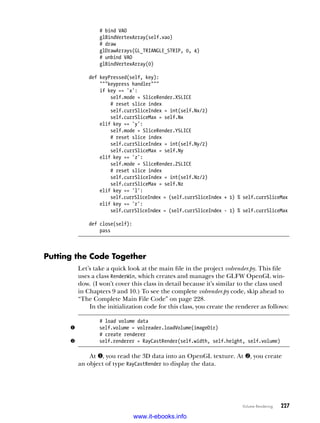
![228 Chapter 11
Pressing V on the keyboard toggles the code between volume and slice
rendering. Here is the keyboard handler for RenderWindow:
def onKeyboard(self, win, key, scancode, action, mods):
# print 'keyboard: ', win, key, scancode, action, mods
# ESC to quit
if key is glfw.GLFW_KEY_ESCAPE:
self.renderer.close()
self.exitNow = True
else:
u if action is glfw.GLFW_PRESS or action is glfw.GLFW_REPEAT:
if key == glfw.GLFW_KEY_V:
# toggle render mode
v if isinstance(self.renderer, RayCastRender):
self.renderer = SliceRender(self.width, self.height,
self.volume)
else:
self.renderer = RayCastRender(self.width, self.height,
self.volume)
# call reshape on renderer
self.renderer.reshape(self.width, self.height)
else:
# send keypress to renderer
w keyDict = {glfw.GLFW_KEY_X: 'x', glfw.GLFW_KEY_Y: 'y',
glfw.GLFW_KEY_Z: 'z', glfw.GLFW_KEY_LEFT: 'l',
glfw.GLFW_KEY_RIGHT: 'r'}
try:
self.renderer.keyPressed(keyDict[key])
except:
pass
Pressing esc quits the program. Other keypresses (V, X, Y, Z, and so on)
are handled at u (set so that it works whether you have just pressed the key
down or if you are keeping it pressed). At v, if V is pressed, you toggle the
renderer between volume and slice, using Python’s isinstance() method to
identify the current class type.
To handle keypress events other than esc, you use a dictionary w and
pass the key pressed to the renderer’s keyPressed() handler.
NOTE I’m choosing not to pass in the glfw.KEY values directly and using a dictionary to con-
vert these to character values instead, because it’s good practice to reduce dependen-
cies in source files. Currently, the only file in this project that depends on GLFW is
volrender.py. If you were to pass GLFW-specific types into other code, they would need
to import and depend on the GLFW library, but if you were to switch to yet another
OpenGL windowing toolkit, the code would become messy.
The Complete Main File Code
Here is the full code listing. You can also find the volrender.py file at https://
github.com/electronut/pp/tree/master/volrender/.
www.it-ebooks.info](https://image.slidesharecdn.com/pythonplaygroundgeekyprojectsforthecuriousprogrammerpdfdrive-220717171538-9c44c48d/85/Python-Playground_-Geeky-Projects-for-the-Curious-Programmer-PDFDrive-pdf-251-320.jpg)

![230 Chapter 11
def onKeyboard(self, win, key, scancode, action, mods):
# print 'keyboard: ', win, key, scancode, action, mods
# ESC to quit
if key is glfw.GLFW_KEY_ESCAPE:
self.renderer.close()
self.exitNow = True
else:
if action is glfw.GLFW_PRESS or action is glfw.GLFW_REPEAT:
if key == glfw.GLFW_KEY_V:
# toggle render mode
if isinstance(self.renderer, RayCastRender):
self.renderer = SliceRender(self.width, self.height,
self.volume)
else:
self.renderer = RayCastRender(self.width, self.height,
self.volume)
# call reshape on renderer
self.renderer.reshape(self.width, self.height)
else:
# send keypress to renderer
keyDict = {glfw.GLFW_KEY_X: 'x', glfw.GLFW_KEY_Y: 'y',
glfw.GLFW_KEY_Z: 'z', glfw.GLFW_KEY_LEFT: 'l',
glfw.GLFW_KEY_RIGHT: 'r'}
try:
self.renderer.keyPressed(keyDict[key])
except:
pass
def onSize(self, win, width, height):
#print 'onsize: ', win, width, height
self.width = width
self.height = height
self.aspect = width/float(height)
glViewport(0, 0, self.width, self.height)
self.renderer.reshape(width, height)
def run(self):
# start loop
while not glfw.glfwWindowShouldClose(self.win) and not self.exitNow:
# render
self.renderer.draw()
# swap buffers
glfw.glfwSwapBuffers(self.win)
# wait for events
glfw.glfwWaitEvents()
# end
glfw.glfwTerminate()
# main() function
def main():
print('starting volrender...')
# create parser
parser = argparse.ArgumentParser(description="Volume Rendering...")
# add expected arguments
parser.add_argument('--dir', dest='imageDir', required=True)
www.it-ebooks.info](https://image.slidesharecdn.com/pythonplaygroundgeekyprojectsforthecuriousprogrammerpdfdrive-220717171538-9c44c48d/85/Python-Playground_-Geeky-Projects-for-the-Curious-Programmer-PDFDrive-pdf-253-320.jpg)
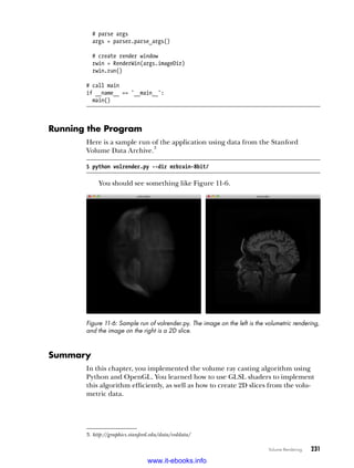


![236 Chapter 12
LDR1
LDR2
R1
R2
Figure 12-1: A simple light-dependent resistor (LDR) circuit
assembled on a breadboard and connected to an Arduino Uno
The Arduino
The Arduino is a platform built around a class of microcontroller chips
called the Atmel AVR. There are many Arduino boards on the market,
of varying size and capabilities. Figure 12-2 highlights some of the major
components in the Arduino Uno boards, one of the more common variet-
ies available. The headers on the Arduino board (as shown in Figure 12-2)
allow you to access the analog and digital pins of the microcontroller so
you can talk to other electronics by sending and receiving data. (I recom-
mend Arduino Workshop by John Boxall [No Starch Press, 2013] to get a
better understanding of the electronics and programming aspects of the
Arduino.)
www.it-ebooks.info](https://image.slidesharecdn.com/pythonplaygroundgeekyprojectsforthecuriousprogrammerpdfdrive-220717171538-9c44c48d/85/Python-Playground_-Geeky-Projects-for-the-Curious-Programmer-PDFDrive-pdf-259-320.jpg)


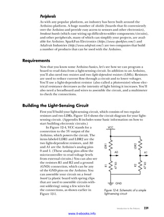
![240 Chapter 12
How the Circuit Works
In this circuit, each LDR, and the resistor beneath it, act as a resistor divider,
which is a simple circuit that uses two resistors to split an input voltage in two.
This setup means the voltage at A0, for instance, is calculated as follows:
V V
R
R R
LDR
0
1
1
=
+
R1 is the resistance of the resistor, and Rldr is the resistance of the LDR.
V is the supply voltage, and V0 is the voltage across R1. As the intensity of light
falling on the LDR changes, its resistance changes, and the voltage across it
changes accordingly. The voltage (somewhere between 0 and 5 volts) is read
at A0 and sent to your program as a 10-bit value, in the range [0, 1023]; that
is, the voltage range is mapped to an integer range of [0, 1023].
The value of the R1 and R2 resistors that you’ll use in the circuit
will depend on your choice of LDR. When you shine light on the LDR, its
electrical resistance decreases; as a result, Rldr decreases, which means V0
increases and a higher value is read in by the Arduino at the analog pin
connected to this LDR. To determine the value of resistance that you need
for R1 and R2, measure the resistance of the LDR using a multimeter under
different light conditions and plug that value in to the voltage equation.
You’re looking for a good variation in voltage (from 0V to 5V) across the
range of lighting conditions in which you will be using the LDR.
I ended up using 4.7k ohm resistors for R1 and R2 because my LDRs
varied in resistance from about 10k ohms (in the dark) to 1k ohm (in bright
light). Enter these values into the previous equation, and you’ll see that you
need a voltage range of 1.6V to 4V for the analog input. When you build the
circuit, you can start with 4.7k ohm resistors and change them as needed.
The Arduino Sketch
Now let’s write the Arduino sketch. Here’s the code that runs on the Arduino
to make it read signals from the circuit and send them to the computer over
a serial port:
#include "Arduino.h"
void setup()
{
// initialize serial communications
u Serial.begin(9600);
}
void loop()
{
// read A0
v int val1 = analogRead(0);
// read A1
w int val2 = analogRead(1);
www.it-ebooks.info](https://image.slidesharecdn.com/pythonplaygroundgeekyprojectsforthecuriousprogrammerpdfdrive-220717171538-9c44c48d/85/Python-Playground_-Geeky-Projects-for-the-Curious-Programmer-PDFDrive-pdf-263-320.jpg)
![Introduction to the Arduino 241
// print to serial
x Serial.print(val1);
Serial.print(" ");
Serial.print(val2);
Serial.print("n");
// wait
y delay(50);
}
At u, you enable serial communication inside the setup() method.
Because setup() is called only when your program starts, this is a good place
to put all of the initialization code. You initialize the baud rate (speed in
bits per second) for the serial communications to 9600 here, which is the
default for most devices and one that’s fast enough for your purposes.
The main code is in the loop() method. At v, you read the current signal
value from analog pin 0 (a 10-bit integer in the range [0, 1023]), and at w,
you read the current signal value from pin 1. At x and in the lines that fol-
low, use Serial.print() to send the values to the computer, formatted as two
integers separated by a space and followed by a newline character. At y, you
use delay() to suspend operations for a set time period, 50 milli
seconds in
this case, before the loop repeats. The value you use here determines the
rate at which the AVR microcontroller executes the loop() method.
To upload the sketch to your Arduino, connect the Arduino to your
computer, bring up its IDE, and start a new project. Then enter the code
into the sketch window and click Verify to compile the code. The IDE will
print any syntax-related errors and warnings. If all is well, click Upload to
send the sketch to the Arduino.
If you don’t see any errors at this stage, bring up the Serial Monitor
from the Tools menu of the Arduino software, and you should see some-
thing like this:
512 300
513 280
400 200
...
These are the analog values read from analog pins 0 and 1 and sent
serially through the Arduino’s USB port to your computer.
Creating the Real-Time Graph
To implement the scrolling real-time graph for your project, you’ll use a
deque, as discussed in Chapter 4. The deque consists of an array of N values;
adding and removing values at either end is quickly done. As new values
come in, they are appended to the deque, and the oldest value is popped
off. By plotting the values at regular intervals, you’ll produce a real-time
graph with the newest data always added on the left.
www.it-ebooks.info](https://image.slidesharecdn.com/pythonplaygroundgeekyprojectsforthecuriousprogrammerpdfdrive-220717171538-9c44c48d/85/Python-Playground_-Geeky-Projects-for-the-Curious-Programmer-PDFDrive-pdf-264-320.jpg)
![242 Chapter 12
The Python Code
Now let’s look at the Python program that reads from the serial port.
(For the complete project code, you can skip ahead to “The Complete
Python Code” on page 244.) To help better organize your code, define
a class AnalogPlot, which holds the data to be plotted. Here is the class
constructor:
class AnalogPlot:
# constructor
def __init__(self, strPort, maxLen):
# open serial port
u self.ser = serial.Serial(strPort, 9600)
v self.a0Vals = deque([0.0]*maxLen)
w self.a1Vals = deque([0.0]*maxLen)
x self.maxLen = maxLen
At u, the AnalogPlot constructor creates a Serial object from the
pySerial library. You’ll use this class for serial communications with the
Arduino. The first argument to the Serial constructor is the port name
string, which you can find in the IDE by selecting Tools4Serial Port (on
Windows, the string will be something like COM3; on Linux and OS X, it
will be something like /dev/tty.usbmodem411). The second argument to the
Serial constructor is the baud rate, which you set to 9600 to match the rate
you set in the Arduino sketch.
At v and w, you create deque objects to hold the analog values. You
initialize the deque objects with a list of zeros of size maxLen, the maximum
number of values you’ll plot at a given time. At x, this maxLen is stored in the
AnalogPlot object.
To plot the analog values in real time, use the deque objects to buffer the
most recent values, as shown in the AnalogPlot class.
# add data
def add(self, data):
assert(len(data) == 2)
u self.addToDeq(self.a0Vals, data[0])
v self.addToDeq(self.a1Vals, data[1])
# add to deque; pop oldest value
def addToDeq(self, buf, val):
w buf.pop()
x buf.appendleft(val)
As you saw earlier, the Arduino sends only two analog integer values per
line. In the add() method, the data values for each analog pin are added
into two deque objects at u and v, using the addToDeq() method. At w and x,
this method removes the oldest value from the tail of the deque using the
pop() method and then appends the latest value to the head of the deque
using the appendleft() method. When you plot values from this deque, the
most recent value will always appear at left on the graph.
www.it-ebooks.info](https://image.slidesharecdn.com/pythonplaygroundgeekyprojectsforthecuriousprogrammerpdfdrive-220717171538-9c44c48d/85/Python-Playground_-Geeky-Projects-for-the-Curious-Programmer-PDFDrive-pdf-265-320.jpg)
![Introduction to the Arduino 243
You use the matplotlib animation class to update the plot at set intervals.
(You may recall seeing this in action in the Boids project in Chapter 5.)
Here is the update() method in AnalogPlot, which will be called at each step
in the plot animation:
# update plot
def update(self, frameNum, a0, a1):
try:
u line = self.ser.readline()
v data = [float(val) for val in line.split()]
# print data
if(len(data) == 2):
w self.add(data)
x a0.set_data(range(self.maxLen), self.a0Vals)
y a1.set_data(range(self.maxLen), self.a1Vals)
except:
z pass
return a0, a1
The update() method reads in a line of serial data as a string at u, and
at v, you use a Python list comprehension to convert the values to floating-
point numbers and store them in a list. You use the split() method to split
a string based on whitespace so that a string read from the serial port as
512 600n will be converted to [512, 600].
After checking that the data has two values, you use AnalogPlot add()
at w to add the values to the deque. At x and y, you use the matplotlib
set_data() method to update the graph with the new values. The x values
for each plot are the numbers [0, ... maxLen], which you set using the range()
method. The y values are populated from the updated deque object.
All of this code is enclosed in a try block, and if an exception occurs,
the code jumps to pass at z, where you ignore the reading (pass doesn’t
do anything). (You use the try block because serial data can sometimes
be corrupted by a loose contact in your circuit, for example, and you don’t
want your program to crash just because some bad values are sent via the
serial port.)
When you’re ready to exit, you close the serial port to release any system
resources, as shown here:
# clean up
def close(self):
# close serial
self.ser.flush()
self.ser.close()
In your main() method, you need to set up the matplotlib animation:
# set up animation
u fig = plt.figure()
v ax = plt.axes(xlim=(0, maxLen), ylim=(0, 1023))
w a0, = ax.plot([], [])
www.it-ebooks.info](https://image.slidesharecdn.com/pythonplaygroundgeekyprojectsforthecuriousprogrammerpdfdrive-220717171538-9c44c48d/85/Python-Playground_-Geeky-Projects-for-the-Curious-Programmer-PDFDrive-pdf-266-320.jpg)
![244 Chapter 12
x a1, = ax.plot([], [])
y anim = animation.FuncAnimation(fig, analogPlot.update,
fargs=(a0, a1), interval=20)
# show plot
z plt.show()
At u, you get the matplotlib Figure module, which contains all the
plot elements. You access the Axes module and set the x and y limits for the
graph at v. The x limit is the number of samples, and the y limit is 1023
since that’s the top of the range of the analog values.
At w and x, you create two blank line objects (a0 and a1), which you
pass to the animation class to set up the callback that supplies the coordi-
nates for each line. Then, at y, set up the animation by passing in the
analogPlot update() method to be called with each animation step. You also
specify the arguments to call that method and the time interval in milli
seconds to 20. At z, you call plt.show() to start the animation.
The main() method of your program is also where you use the argparse
Python module to support command line options.
# create parser
parser = argparse.ArgumentParser(description="LDR serial")
# add expected arguments
parser.add_argument('--port', dest='port', required=True)
parser.add_argument('--N', dest='maxLen', required=False)
# parse args
args = parser.parse_args()
strPort = args.port
# plot parameters
maxLen = 100
if args.maxLen:
maxLen = int(args.maxLen)
The --port argument is required. It tells the program the name of the
serial port where the data is received (find this in the Arduino IDE under
Tools4Serial Port). The maxLen argument is optional and can be used to set
the number of points to plot at a time. (The default is 100 samples.)
The Complete Python Code
Here is the complete Python code for this project. You can also download
the complete code listing from https://github.com/electronut/pp/tree/master/
arduino-ldr/ldr.py.
import serial, argparse
from collections import deque
www.it-ebooks.info](https://image.slidesharecdn.com/pythonplaygroundgeekyprojectsforthecuriousprogrammerpdfdrive-220717171538-9c44c48d/85/Python-Playground_-Geeky-Projects-for-the-Curious-Programmer-PDFDrive-pdf-267-320.jpg)
![Introduction to the Arduino 245
import matplotlib.pyplot as plt
import matplotlib.animation as animation
# plot class
class AnalogPlot:
# constructor
def __init__(self, strPort, maxLen):
# open serial port
self.ser = serial.Serial(strPort, 9600)
self.a0Vals = deque([0.0]*maxLen)
self.a1Vals = deque([0.0]*maxLen)
self.maxLen = maxLen
# add data
def add(self, data):
assert(len(data) == 2)
self.addToDeq(self.a0Vals, data[0])
self.addToDeq(self.a1Vals, data[1])
# add to deque; pop oldest value
def addToDeq(self, buf, val):
buf.pop()
buf.appendleft(val)
# update plot
def update(self, frameNum, a0, a1):
try:
line = self.ser.readline()
data = [float(val) for val in line.split()]
# print data
if(len(data) == 2):
self.add(data)
a0.set_data(range(self.maxLen), self.a0Vals)
a1.set_data(range(self.maxLen), self.a1Vals)
except:
pass
return a0, a1
# clean up
def close(self):
# close serial
self.ser.flush()
self.ser.close()
# main() function
def main():
# create parser
parser = argparse.ArgumentParser(description="LDR serial")
# add expected arguments
parser.add_argument('--port', dest='port', required=True)
parser.add_argument('--N', dest='maxLen', required=False)
www.it-ebooks.info](https://image.slidesharecdn.com/pythonplaygroundgeekyprojectsforthecuriousprogrammerpdfdrive-220717171538-9c44c48d/85/Python-Playground_-Geeky-Projects-for-the-Curious-Programmer-PDFDrive-pdf-268-320.jpg)
![246 Chapter 12
# parse args
args = parser.parse_args()
#strPort = '/dev/tty.usbserial-A7006Yqh'
strPort = args.port
print('reading from serial port %s...' % strPort)
# plot parameters
maxLen = 100
if args.maxLen:
maxLen = int(args.maxLen)
# create plot object
analogPlot = AnalogPlot(strPort, maxLen)
print('plotting data...')
# set up animation
fig = plt.figure()
ax = plt.axes(xlim=(0, maxLen), ylim=(0, 1023))
a0, = ax.plot([], [])
a1, = ax.plot([], [])
anim = animation.FuncAnimation(fig, analogPlot.update,
fargs=(a0, a1), interval=20)
# show plot
plt.show()
# clean up
analogPlot.close()
print('exiting.')
# call main
if __name__ == '__main__':
main()
Running the Program
To test the program, assemble the LDR circuit, connect the Arduino to
your computer, upload the sketch, and then run the Python code.
$ python3 --port /dev/tty.usbmodem411 ldr.py
Figure 12-5 shows sample output of the program, specifically, a graph
generated when the LDRs are exposed to light and then covered. As you
can see in the graph, when the resistance of the LDRs changes, the ana-
log voltage read in by the Arduino also changes. The peak in the center
occurred when I quickly passed my hand over the LDRs, and the flat part
at the right occurred when I passed my hand over more slowly.
www.it-ebooks.info](https://image.slidesharecdn.com/pythonplaygroundgeekyprojectsforthecuriousprogrammerpdfdrive-220717171538-9c44c48d/85/Python-Playground_-Geeky-Projects-for-the-Curious-Programmer-PDFDrive-pdf-269-320.jpg)

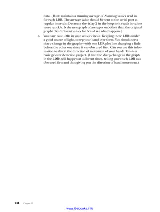


![254 Chapter 13
per second. On the other hand, a sample size that’s too large would average
out the changes in the signal, so you wouldn’t be getting a “real-time” fre-
quency response for the signal. For the sampling rate of 44100 Hz used for
this project, a sample size of 2048 represents data for about 0.046 seconds.
For this project, you need to split the audio data into its constituent fre-
quencies and use that information to control the motors. First, you’ll split
the range of frequencies (in Hz) into three bands: [0, 100], [100, 1000],
and [1000, 2500]. You’ll compute an average amplitude for each band, and
each value will affect the motors and resulting laser pattern differently,
as follows:
• Changes in the average amplitude of low frequencies will affect the
speed of the first motor.
• Changes in the average amplitude of middle frequencies will affect the
speed of the second motor.
• When high frequencies peak above a certain threshold, the first motor
will change direction.
Requirements
Here’s a list of the items you’ll need to build this project:
• A small laser pointer
• Two DC motors like the ones used in a small toy (rated for 9V)
• Two small mirrors approximately 1 inch or less in diameter
• A SparkFun Motor Driver 1A Dual TB6612FNG
• An Arduino Uno or similar board
• Wire to make connections (single-core hookup wires with male pins on
both sides work nicely)
• A four AA battery pack
• Some LEGO bricks to raise the motors and laser pointer off the mount-
ing board so the mirrors can spin freely
• A rectangular sheet of cardboard or acrylic about 8 inches × 6 inches to
mount the hardware
• A hot glue gun
• Soldering iron
Constructing the Laser Display
The first order of business is to attach the mirrors to the motors. The mir-
ror has to be at a slight angle to the motor shaft. To attach the mirror,
place it facedown on a flat surface and put a drop of hot glue in the center.
Carefully dip the motor shaft in the glue, keeping it perpendicular to the
www.it-ebooks.info](https://image.slidesharecdn.com/pythonplaygroundgeekyprojectsforthecuriousprogrammerpdfdrive-220717171538-9c44c48d/85/Python-Playground_-Geeky-Projects-for-the-Curious-Programmer-PDFDrive-pdf-277-320.jpg)


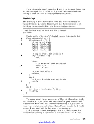

![Laser Audio Display 261
use the analogWrite() method to write a value in the range [0, 255] to an
Arduino output pin. (In contrast, the digitalWrite() method only lets you
write either a 1 or 0 to the output pin.)
At y, you set the pins for motor B.
Stopping the Motors
To stop the motors, you write a LOW to the standby pin of the motor driver.
void stop(){
//enable standby
digitalWrite(STBY, LOW);
}
The Python Code
Now let’s look at the Python code running on the computer. This code
does the heavy lifting: it reads in audio, computes the FFT, and sends
serial data to the Arduino. You can find the complete project code in “The
Complete Python Code” on page 267.
Selecting the Audio Device
First, you need to read in the audio data with the help of the pyaudio module.
Initialize the pyaudio module like this:
p = pyaudio.PyAudio()
Next, you access the computer’s audio input device using the helper
functions in pyaudio, as shown in the code for the getInputDevice() method:
# get pyaudio input device
def getInputDevice(p):
u index = None
v nDevices = p.get_device_count()
print('Found %d devices. Select input device:' % nDevices)
# print all devices found
for i in range(nDevices):
w deviceInfo = p.get_device_info_by_index(i)
x devName = deviceInfo['name']
y print("%d: %s" % (i, devName))
# get user selection
try:
# convert to integer
z index = int(input())
except:
pass
# print the name of the chosen device
if index is not None:
devName = p.get_device_info_by_index(index)["name"]
www.it-ebooks.info](https://image.slidesharecdn.com/pythonplaygroundgeekyprojectsforthecuriousprogrammerpdfdrive-220717171538-9c44c48d/85/Python-Playground_-Geeky-Projects-for-the-Curious-Programmer-PDFDrive-pdf-284-320.jpg)

![Laser Audio Display 263
• frames_per_buffer is set to the FFT buffer length.
• input_device_index is set to the device you chose in the getInputDevice()
method.
Computing the FFT of the Data Stream
Here is the code you use to read data from the stream:
# read a chunk of data
u data = stream.read(fftLen)
# convert the data to a numpy array
v dataArray = numpy.frombuffer(data, dtype=numpy.int16)
At u, you read the most recent fftLen samples from the audio input
stream. Then you convert this data into a 16-bit integer numpy array at v.
Now you compute the FFT of this data.
# get FFT of data
u fftVals = numpy.fft.rfft(dataArray)*2.0/fftLen
# get absolute values of complex numbers
v fftVals = numpy.abs(fftVals)
At u, you compute the FFT of the values in the numpy array, using the
rfft() method from the numpy fft module. This method takes a signal com-
posed of real numbers (like the audio data) and computes the FFT, which
generally results in a set of complex numbers. The 2.0/fftLen is a normaliza-
tion factor you use to map the FFT values to the expected range. Then,
because the rfft() method returns complex numbers, you use the numpy
abs() method v to get the magnitudes of these complex numbers, which
are real.
Extracting Frequency Information from the FFT Values
Next, you extract the relevant frequency information from the FFT values.
# average 3 frequency bands: 0-100 Hz, 100-1000 Hz, and 1000-2500 Hz
levels = [numpy.sum(fftVals[0:100])/100,
numpy.sum(fftVals[100:1000])/900,
numpy.sum(fftVals[1000:2500])/1500]
To analyze the audio signal, you split the frequency range into three
bands: 0 to 100 Hz, 100 to 1000 Hz, and 1000 to 2500 Hz. You are most
interested in the lower, bass band (0–100 Hz) and the midrange (100–
1000 Hz) frequencies, which roughly correspond to the beat and the vocals
in a song, respectively. For each range, you compute the average FFT value
using the numpy.sum() method in the code.
Converting Frequency to Motor Speed and Direction
Now convert this frequency information to motor speeds and directions.
www.it-ebooks.info](https://image.slidesharecdn.com/pythonplaygroundgeekyprojectsforthecuriousprogrammerpdfdrive-220717171538-9c44c48d/85/Python-Playground_-Geeky-Projects-for-the-Curious-Programmer-PDFDrive-pdf-286-320.jpg)
![264 Chapter 13
# 'H' (header), speed1, dir1, speed2, dir2
u vals = [ord('H'), 100, 1, 100, 1]
# speed1
v vals[1] = int(5*levels[0]) % 255
# speed2
w vals[3] = int(100 + levels[1]) % 255
# dir
d1 = 0
x if levels[2] > 0.1:
d1 = 1
vals[2] = d1
y vals[4] = 0
At u, you initialize a list of motor speeds and direction values to be sent
to the Arduino (the 5 bytes, starting with H discussed earlier). Use the built-
in ord() function to convert the string to an integer and then fill in this list
by converting the average values for the three frequency bands into motor
speeds and directions.
NOTE This part is a hack, really—there’s no particularly elegant rule governing these con-
versions. These values change constantly with the audio signal, and any method you
come up with will change the motor speeds and affect the laser pattern along with the
music. Just make sure your conversion puts the motor speeds in the [0, 255] range
and that the directions are always set to 1 or 0. The method I chose was simply based
on trial and error; I looked at FFT values while playing various types of music.
At v, you take the value from the lowest frequency range, scale it by a
factor of five, convert it to an integer, and use the modulus operator (%) to
ensure that the value lies within the [0, 255] range. This value controls the
speed of the first motor. At w, you add 100 to the middle frequency value
and place it in the [0, 255] range. This value controls the speed of the second
motor.
Then, at x, you switch the motor A direction whenever the value from
the highest frequency range crosses the threshold of 0.1. The motor B direc-
tion is kept at a constant 0 y. (I found through trial and error that these
methods produce a nice variation of patterns, but I encourage you to play
with these values and create your own conversions. There are no wrong
answers here.)
Testing the Motor Setup
Before testing the hardware with a live audio stream, let’s check the motor
setup. The function autoTest(), shown here, does just that:
# automatic test for sending motor speeds
def autoTest(ser):
print('starting automatic test...')
try:
while True:
www.it-ebooks.info](https://image.slidesharecdn.com/pythonplaygroundgeekyprojectsforthecuriousprogrammerpdfdrive-220717171538-9c44c48d/85/Python-Playground_-Geeky-Projects-for-the-Curious-Programmer-PDFDrive-pdf-287-320.jpg)
![Laser Audio Display 265
# for each direction combination
u for dr in [(0, 0), (1, 0), (0, 1), (1, 1)]:
# for a range of speeds
v for j in range(25, 180, 10):
w for i in range(25, 180, 10):
x vals = [ord('H'), i, dr[0], j, dr[1]]
y print(vals[1:])
z data = struct.pack('BBBBB', *vals)
{ ser.write(data)
sleep(0.1)
except KeyboardInterrupt:
print('exiting...')
# shut off motors
| vals = [ord('H'), 0, 1, 0, 1]
data = struct.pack('BBBBB', *vals)
ser.write(data)
ser.close()
This method takes the two motors through a range of motions by vary-
ing the speed and direction of each. Because the direction can be clockwise
or counterclockwise for each motor, four such combinations are represented
in the outer loop at u. For each combination, the loops at v and w run the
motors at various speeds.
NOTE I’m using range(25, 180, 10), which means the speed varies from 25 to 180 in steps
of 10. I am not using the full range of motion of the motor [0, 255] here because the
motors barely turn below a speed of 25 and they spin really fast above 200.
At x, you generate the 5-byte motor data values, and at y, you print
their direction and speed values. (The use of Python string splicing vals[1:]
will get all but the first element in the list.)
Pack the motor data into a byte array at z, and write it to the serial
port at {. Pressing ctrl-C interrupts this test, and at |, you handle this
exception by cleaning up, stopping the motors, and closing the serial port
like the responsible programmer you are.
Command Line Options
As with previous projects, you use the argparse module to parse command
line arguments for the program.
# main method
def main():
# parse arguments
parser = argparse.ArgumentParser(description='Analyzes audio input and
sends motor control information via serial port')
# add arguments
parser.add_argument('--port', dest='serial_port_name', required=True)
parser.add_argument('--mtest', action='store_true', default=False)
parser.add_argument('--atest', action='store_true', default=False)
args = parser.parse_args()
www.it-ebooks.info](https://image.slidesharecdn.com/pythonplaygroundgeekyprojectsforthecuriousprogrammerpdfdrive-220717171538-9c44c48d/85/Python-Playground_-Geeky-Projects-for-the-Curious-Programmer-PDFDrive-pdf-288-320.jpg)
![266 Chapter 13
In this code, the serial port is a required command line option. There
are also two optional command line options: one for an automatic test
(covered earlier) and another for a manual test (which I’ll discuss shortly).
Here is what happens once the command line options are parsed in the
main() method:
# open serial port
strPort = args.serial_port_name
print('opening ', strPort)
u ser = serial.Serial(strPort, 9600)
if args.mtest:
manualTest(ser)
elif args.atest:
autoTest(ser)
else:
v fftLive(ser)
At u, you use pySerial to open a serial port with the string passed in to
the program. The speed of serial communications, or the baud rate, is set at
9,600 bits per second. If no other command arguments (--atest or --mtest)
are used, you proceed at v to the audio processing and FFT computation,
encapsulated in the fftLive() method.
Manual Testing
This manual test lets you enter specific motor directions and speeds so that
you can see their effects on the laser pattern.
# manual test of motor direction and speeds
def manualTest(ser):
print('starting manual test...')
try:
while True:
print('enter motor control info such as < 100 1 120 0 >')
u strIn = raw_input()
v vals = [int(val) for val in strIn.split()[:4]]
w vals.insert(0, ord('H'))
x data = struct.pack('BBBBB', *vals)
y ser.write(data)
except:
print('exiting...')
# shut off the motors
z vals = [ord('H'), 0, 1, 0, 1]
data = struct.pack('BBBBB', *vals)
ser.write(data)
ser.close()
At u, you use the raw_input() method to wait until the user enters a
value at the command prompt. The expected entry is in the form 100 1
120 0, representing the speed and direction of motor A followed by that of
motor B. Parse the string into a list of integers at v. At w, you insert an 'H'
to complete the motor data, and at x and y, you pack this data and send it
www.it-ebooks.info](https://image.slidesharecdn.com/pythonplaygroundgeekyprojectsforthecuriousprogrammerpdfdrive-220717171538-9c44c48d/85/Python-Playground_-Geeky-Projects-for-the-Curious-Programmer-PDFDrive-pdf-289-320.jpg)
![Laser Audio Display 267
through the serial port in the expected format. When the user interrupts
the test using ctrl-C (or if any exception occurs), you clean up at z by
shutting down the motors and the serial port gracefully.
The Complete Python Code
Here is the complete Python code for this project. You’ll can also find this
at https://github.com/electronut/pp/tree/master/arduino-laser/laser.py.
import sys, serial, struct
import pyaudio
import numpy
import math
from time import sleep
import argparse
# manual test of motor direction speeds
def manualTest(ser):
print('staring manual test...')
try:
while True:
print('enter motor control info: eg. < 100 1 120 0 >')
strIn = raw_input()
vals = [int(val) for val in strIn.split()[:4]]
vals.insert(0, ord('H'))
data = struct.pack('BBBBB', *vals)
ser.write(data)
except:
print('exiting...')
# shut off motors
vals = [ord('H'), 0, 1, 0, 1]
data = struct.pack('BBBBB', *vals)
ser.write(data)
ser.close()
# automatic test for sending motor speeds
def autoTest(ser):
print('staring automatic test...')
try:
while True:
# for each direction combination
for dr in [(0, 0), (1, 0), (0, 1), (1, 1)]:
# for a range of speeds
for j in range(25, 180, 10):
for i in range(25, 180, 10):
vals = [ord('H'), i, dr[0], j, dr[1]]
print(vals[1:])
data = struct.pack('BBBBB', *vals)
ser.write(data)
sleep(0.1)
except KeyboardInterrupt:
print('exiting...')
www.it-ebooks.info](https://image.slidesharecdn.com/pythonplaygroundgeekyprojectsforthecuriousprogrammerpdfdrive-220717171538-9c44c48d/85/Python-Playground_-Geeky-Projects-for-the-Curious-Programmer-PDFDrive-pdf-290-320.jpg)
![268 Chapter 13
# shut off motors
vals = [ord('H'), 0, 1, 0, 1]
data = struct.pack('BBBBB', *vals)
ser.write(data)
ser.close()
# get pyaudio input device
def getInputDevice(p):
index = None
nDevices = p.get_device_count()
print('Found %d devices. Select input device:' % nDevices)
# print all devices found
for i in range(nDevices):
deviceInfo = p.get_device_info_by_index(i)
devName = deviceInfo['name']
print("%d: %s" % (i, devName))
# get user selection
try:
# convert to integer
index = int(input())
except:
pass
# print the name of the chosen device
if index is not None:
devName = p.get_device_info_by_index(index)["name"]
print("Input device chosen: %s" % devName)
return index
# FFT of live audio
def fftLive(ser):
# initialize pyaudio
p = pyaudio.PyAudio()
# get pyAudio input device index
inputIndex = getInputDevice(p)
# set FFT sample length
fftLen = 2**11
# set sample rate
sampleRate = 44100
print('opening stream...')
stream = p.open(format = pyaudio.paInt16,
channels = 1,
rate = sampleRate,
input = True,
frames_per_buffer = fftLen,
input_device_index = inputIndex)
try:
while True:
# read a chunk of data
data = stream.read(fftLen)
# convert to numpy array
dataArray = numpy.frombuffer(data, dtype=numpy.int16)
www.it-ebooks.info](https://image.slidesharecdn.com/pythonplaygroundgeekyprojectsforthecuriousprogrammerpdfdrive-220717171538-9c44c48d/85/Python-Playground_-Geeky-Projects-for-the-Curious-Programmer-PDFDrive-pdf-291-320.jpg)
![Laser Audio Display 269
# get FFT of data
fftVals = numpy.fft.rfft(dataArray)*2.0/fftLen
# get absolute values of complex numbers
fftVals = numpy.abs(fftVals)
# average 3 frequency bands: 0-100 Hz, 100-1000 Hz and 1000-2500 Hz
levels = [numpy.sum(fftVals[0:100])/100,
numpy.sum(fftVals[100:1000])/900,
numpy.sum(fftVals[1000:2500])/1500]
# the data sent is of the form:
# 'H' (header), speed1, dir1, speed2, dir2
vals = [ord('H'), 100, 1, 100, 1]
# speed1
vals[1] = int(5*levels[0]) % 255
# speed2
vals[3] = int(100 + levels[1]) % 255
# dir
d1 = 0
if levels[2] > 0.1:
d1 = 1
vals[2] = d1
vals[4] = 0
# pack data
data = struct.pack('BBBBB', *vals)
# write data to serial port
ser.write(data)
# a slight pause
sleep(0.001)
except KeyboardInterrupt:
print('stopping...')
finally:
print('cleaning up')
stream.close()
p.terminate()
# shut off motors
vals = [ord('H'), 0, 1, 0, 1]
data = struct.pack('BBBBB', *vals)
ser.write(data)
# close serial
ser.flush()
ser.close()
# main method
def main():
# parse arguments
parser = argparse.ArgumentParser(description='Analyzes audio input and
sends motor control information via serial port')
# add arguments
parser.add_argument('--port', dest='serial_port_name', required=True)
parser.add_argument('--mtest', action='store_true', default=False)
parser.add_argument('--atest', action='store_true', default=False)
www.it-ebooks.info](https://image.slidesharecdn.com/pythonplaygroundgeekyprojectsforthecuriousprogrammerpdfdrive-220717171538-9c44c48d/85/Python-Playground_-Geeky-Projects-for-the-Curious-Programmer-PDFDrive-pdf-292-320.jpg)
![270 Chapter 13
args = parser.parse_args()
# open serial port
strPort = args.serial_port_name
print('opening ', strPort)
ser = serial.Serial(strPort, 9600)
if args.mtest:
manualTest(ser)
elif args.atest:
autoTest(ser)
else:
fftLive(ser)
# call main function
if __name__ == '__main__':
main()
Running the Program
To test the project, assemble the hardware, connect the Arduino to the
computer, and upload the motor driver code into the Arduino. Make sure
the battery pack is connected and that your laser pointer is on and project-
ing on a flat surface like a wall. I recommend testing the laser display part
first by running the following program. (Don’t forget to change the serial
port string to match your computer!)
$ python3 laser.py --port /dev/tty.usbmodem411 --atest
('opening ', '/dev/tty.usbmodem1411')
staring automatic test...
[25, 0, 25, 0]
[35, 0, 25, 0]
[45, 0, 25, 0]
...
This test runs both motors through various combinations of speeds and
direction. You should see different laser patterns projected onto your wall.
To stop the program and the motors, press ctrl-C.
If the test succeeds, you’re ready to move on to the real show. Start play-
ing your favorite music on your computer and run the program as follows.
(Again, watch that serial port string!)
$ python3 laser.py --port /dev/tty.usbmodem411
('opening ', '/dev/tty.usbmodem1411')
Found 4 devices. Select input device:
0: Built-in Microph
1: Built-in Output
2: BoomDevice
3: AirParrot
0
Input device chosen: Built-in Microph
opening stream...
www.it-ebooks.info](https://image.slidesharecdn.com/pythonplaygroundgeekyprojectsforthecuriousprogrammerpdfdrive-220717171538-9c44c48d/85/Python-Playground_-Geeky-Projects-for-the-Curious-Programmer-PDFDrive-pdf-293-320.jpg)
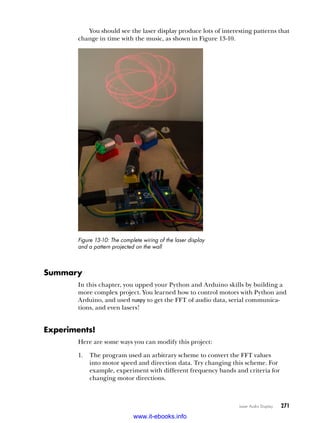


![A Raspberry Pi–Based Weather Monitor 281
Plotting with flot
Now let’s look at how you’ll plot your data. The flot library has an easy-to-
use and powerful API that lets you create nice-looking graphs with minimal
code. Basically, you set up some Hypertext Markup Language (HTML)
to hold a chart and provide an array of values to plot, and Flot handles the
rest, as shown in this example. (You’ll find this code in the file simple-flot.html
in the book’s code repository.)
<html>
<head>
<meta http-equiv="Content-Type" content="text/html; charset=utf-8">
<title>SimpleFlot</title>
u <style>
.demo-placeholder {
width: 80%;
height: 80%;
}
</style>
v <script language="javascript" type="text/javascript"
src="flot/jquery.js"></script>
<script language="javascript" type="text/javascript"
src="flot/jquery.flot.js"></script>
<script language="javascript" type="text/javascript">
w $(document).ready(function() {
// create plot
x var data = [];
for(var i = 0; i < 500; i ++) {
y data.push([i, Math.exp(-i/100)*Math.sin(Math.PI*i/10)]);
}
z var plot = $.plot("#placeholder", [data]);
});
</script>
</head>
<body>
<h3>A Simple Flot Plot</h3>
<div class="demo-container">
{ <div id="placeholder" class="demo-placeholder"></div>
</div>
</body>
</html>
At u, you define a CSS class (demo-placeholder) to set the width and
height of the placeholder element to hold your plot (which you’ll define in
the body of the document). At v, you declare the JavaScript files for the
libraries you’ll use in this HTML file: jquery.js and flot.js. (Note that jQuery
comes bundled with flot, so you don’t need to download it separately. Also,
ensure that you put the top-level flot directory into the same directory that
contains all the source code for this project.)
www.it-ebooks.info](https://image.slidesharecdn.com/pythonplaygroundgeekyprojectsforthecuriousprogrammerpdfdrive-220717171538-9c44c48d/85/Python-Playground_-Geeky-Projects-for-the-Curious-Programmer-PDFDrive-pdf-304-320.jpg)
![282 Chapter 14
Next, you use JavaScript to generate values to plot. At w, you use the
jQuery method $(document).ready() to define a function to be executed by
the browser as soon as the HTML file is loaded. Inside that function, at x,
you declare an empty JavaScript array and then loop 500 times, adding a
value of the form [i, y] to this array y. Each value represents the x- and
y-coordinates of this interesting function (chosen somewhat arbitrarily).
y x e x
x
( ) =
−
100
2
10
sin
π
, for x in the range [0, 500]
At z, you call plot() from the flot library to do the plotting. At {, the
plot() function takes as input the id of the HTML element that contains the
plot (the placeholder element). When you load the resulting HTML file in
a browser, you should see the plot shown in Figure 14-4.
Figure 14-4: A sample plot created with flot
I used flot’s default settings here, but you can customize your flot plots
extensively by adjusting colors, using data points instead of lines, adding
legends and titles, making the plot interactive, and more. (You’ll see how
when you design the chart for the weather data in “Plotting the Data” on
page 285.)
Shutting Down the Pi
Never abruptly disconnect the power supply to a running Raspberry Pi or
you’ll likely corrupt your filesystem, making the Pi unbootable. To shut
down the Pi’s user interface if you’re connected to it directly or from your
computer, enter the following via SSH:
$ sudo shutdown -h now
www.it-ebooks.info](https://image.slidesharecdn.com/pythonplaygroundgeekyprojectsforthecuriousprogrammerpdfdrive-220717171538-9c44c48d/85/Python-Playground_-Geeky-Projects-for-the-Curious-Programmer-PDFDrive-pdf-305-320.jpg)


![A Raspberry Pi–Based Weather Monitor 287
w grid: {clickable: true},
x yaxes: [{min: 0, max: 100}],
xaxes: [{min: 0, max: 100}],
};
// create empty plot
y var plot = $.plot("#placeholder", [[]], options);
The ready() function at u is called by the browser when the HTML
data has been fully loaded. At v, you declare an options object to customize
your plot. In this object, you tell the plot to display both lines and points,
and at w, you allow the plot grid to be clicked (for querying values). You
also set the axes limits at x. At y, create the actual plot by calling plot() with
three arguments: the ID of the element in which you want the plot to appear,
an array of values (which is empty to start), and the options object you just
set up.
Next let’s look at the JavaScript code that gets the sensor data:
// initialize data arrays
u var RH = [];
var T = [];
var timeStamp = [];
// get data from server
v function getData() {
// AJAX callback
w function onDataReceived(jsonData) {
x timeStamp.push(Date());
// add RH data
y RH.push(jsonData.RH);
// removed oldest
z if (RH.length > 100) {
RH.splice(0, 1);
}
// add T data
T.push(jsonData.T);
// removed oldest
if (T.length > 100) {
T.splice(0, 1);
}
{ s1 = [];
s2 = [];
for (var i = 0; i < RH.length; i++) {
s1.push([i, RH[i]]);
s2.push([i, T[i]]);
}
// set to plot
| plot.setData([s1, s2]);
plot.draw();
}
www.it-ebooks.info](https://image.slidesharecdn.com/pythonplaygroundgeekyprojectsforthecuriousprogrammerpdfdrive-220717171538-9c44c48d/85/Python-Playground_-Geeky-Projects-for-the-Curious-Programmer-PDFDrive-pdf-310-320.jpg)
![288 Chapter 14
// AJAX error handler
} function onError(){
$('#ajax-panel').html('<p><strong>Ajax error!</strong> </p>');
}
// make the AJAX call
~ $.ajax({
url: "getdata",
type: "GET",
dataType: "json",
success: onDataReceived,
error: onError
});
}
At u, you initialize empty arrays for the temperature and humidity
values, and a timeStamp array that stores the time when each value is col-
lected. You define a getData() method at v that you’ll call periodically
using a timer. At w, you define a onDataReceived() method that you’ll set as
a callback method for the AJAX call. Because in JavaScript you can define
functions within functions that can be used like regular variables, you can
define onDataReceived() within the getData() function and then pass it to the
AJAX call as a callback function.
The onDataReceived() function stores a timestamp for the data point
at x by creating a JavaScript Date object. Data from the server is passed into
OnDataReceived() using the jsonData object, and at y, you push the tempera-
ture data from this object into an array. At z, you remove the oldest element
in the array if the number of elements exceeds 100, which produces a scroll-
ing graph similar to the one you created for the Arduino light sensor project
in Chapter 12. You process the humidity data the same way.
At {, the collected data is formatted to make it suitable to be passed
to the plot() method. Since you’re plotting two variables simultaneously, you
need an array with three layers of the form:
[[[i0,RH0], [i1,RH1],...],[[i0,T0],[i1,T1]]
The data is set and plotted at |.
At }, you define an error callback, which AJAX will use in case of a
failure to display errors, using the HTML element with the ID ajax-panel
that you set up previously. At ~, you make the actual AJAX call, which speci-
fies the URL getdata, the Bottle route. The call uses the HTTP GET() method
to request data from the server in the json format. The AJAX setup call
sets the OnDataReceived() method as the success callback and onError() as
the error callback. This AJAX call returns immediately, and the callback
methods are activated asynchronously when data becomes available.
The update() Method
Now let’s look at the update() method that calls getData() every second.
www.it-ebooks.info](https://image.slidesharecdn.com/pythonplaygroundgeekyprojectsforthecuriousprogrammerpdfdrive-220717171538-9c44c48d/85/Python-Playground_-Geeky-Projects-for-the-Curious-Programmer-PDFDrive-pdf-311-320.jpg)

![290 Chapter 14
Adding Interactivity
You also want to provide some interactivity for the plot. The flot library pro-
vides a way for users to click data points to get values, which you enabled ear-
lier by passing clickable:true in options when you called the plot() function.
Here, you define the function to be called when a data point is clicked:
$("#placeholder").bind("plotclick", function (event, pos, item) {
if (item) {
u plot.highlight(item.series, item.datapoint);
v var strData = ' [Clicked Data: ' +
timeStamp[item.dataIndex] + ': T = ' +
T[item.dataIndex] + ', RH = ' + RH[item.dataIndex]
+ ']';
w $('#data-values').html(strData);
}
});
});
</script>
</head>
This function calls the flot highlight() method at u to draw a ring
around the point clicked. At v, it prepares a string to be displayed in
the HTML element with the ID data-values. When a data point is clicked,
flot passes in an item object to the function, which has a member called
dataIndex. You use this index to retrieve the relevant data from the time-
stamp, temperature, and humidity arrays defined in the ready() function.
Finally, the string is added to the HTML element w.
This concludes the embedded JavaScript in your Python code, but
you need one more Bottle route to find the JavaScript files that the web
page needs, as shown here:
@route('/<filename:re:.*.js>')
def javascripts(filename):
return static_file(filename, root='flot')
This code tells the Bottle server to find these files in the subdirectory
flot/ at the same level as your program.
The Complete Code
You can find the complete code listing for this project at https://github.com/
electronut/pp/tree/master/piweather/piweather.py.
from bottle import route, run, request, response
from bottle import static_file
import random, argparse
import RPi.GPIO as GPIO
from time import sleep
import Adafruit_DHT
www.it-ebooks.info](https://image.slidesharecdn.com/pythonplaygroundgeekyprojectsforthecuriousprogrammerpdfdrive-220717171538-9c44c48d/85/Python-Playground_-Geeky-Projects-for-the-Curious-Programmer-PDFDrive-pdf-313-320.jpg)
![A Raspberry Pi–Based Weather Monitor 291
@route('/hello')
def hello():
return "Hello Bottle World!"
@route('/<filename:re:.*.js>')
def javascripts(filename):
return static_file(filename, root='flot')
@route('/plot')
def plot():
return '''
<html>
<head>
<meta http-equiv="Content-Type" content="text/html; charset=utf-8">
<title>PiWeather</title>
<style>
.demo-placeholder {
width: 90%;
height: 50%;
}
</style>
<script language="javascript" type="text/javascript"
src="jquery.js"></script>
<script language="javascript" type="text/javascript"
src="jquery.flot.js"></script>
<script language="javascript" type="text/javascript"
src="jquery.flot.time.js"></script>
<script language="javascript" type="text/javascript">
$(document).ready(function() {
// plot options
var options = {
series: {
lines: {show: true},
points: {show: true}
},
grid: {clickable: true},
yaxes: [{min: 0, max: 100}],
xaxes: [{min: 0, max: 100}],
};
// create empty plot
var plot = $.plot("#placeholder", [[]], options);
// initialize data arrays
var RH = [];
var T = [];
var timeStamp = [];
// get data from server
function getData() {
// AJAX callback
function onDataReceived(jsonData) {
timeStamp.push(Date());
www.it-ebooks.info](https://image.slidesharecdn.com/pythonplaygroundgeekyprojectsforthecuriousprogrammerpdfdrive-220717171538-9c44c48d/85/Python-Playground_-Geeky-Projects-for-the-Curious-Programmer-PDFDrive-pdf-314-320.jpg)
![292 Chapter 14
// add RH data
RH.push(jsonData.RH);
// removed oldest
if (RH.length > 100) {
RH.splice(0, 1);
}
// add T data
T.push(jsonData.T);
// removed oldest
if (T.length > 100) {
T.splice(0, 1);
}
s1 = [];
s2 = [];
for (var i = 0; i < RH.length; i++) {
s1.push([i, RH[i]]);
s2.push([i, T[i]]);
}
// set to plot
plot.setData([s1, s2]);
plot.draw();
}
// AJAX error handler
function onError(){
$('#ajax-panel').html('<p><strong>Ajax error!</strong> </p>');
}
// make the AJAX call
$.ajax({
url: "getdata",
type: "GET",
dataType: "json",
success: onDataReceived,
error: onError
});
}
// define an update function
function update() {
// get data
getData();
// set timeout
setTimeout(update, 1000);
}
// call update
update();
// define click handler for LED control button
$('#ckLED').click(function() {
var isChecked = $("#ckLED").is(":checked") ? 1:0;
$.ajax({
url: '/ledctrl',
type: 'POST',
www.it-ebooks.info](https://image.slidesharecdn.com/pythonplaygroundgeekyprojectsforthecuriousprogrammerpdfdrive-220717171538-9c44c48d/85/Python-Playground_-Geeky-Projects-for-the-Curious-Programmer-PDFDrive-pdf-315-320.jpg)
![A Raspberry Pi–Based Weather Monitor 293
data: { strID:'ckLED', strState:isChecked }
});
});
$("#placeholder").bind("plotclick", function (event, pos, item) {
if (item) {
plot.highlight(item.series, item.datapoint);
var strData = ' [Clicked Data: ' +
timeStamp[item.dataIndex] + ': T = ' +
T[item.dataIndex] + ', RH = ' + RH[item.dataIndex]
+ ']';
$('#data-values').html(strData);
}
});
});
</script>
</head>
<body>
<div id="header">
<h2>Temperature/Humidity</h2>
</div>
<div id="content">
<div class="demo-container">
<div id="placeholder" class="demo-placeholder"></div>
</div>
<div id="ajax-panel"> </div>
</div>
<div>
<input type="checkbox" id="ckLED" value="on">Enable Lighting.
<span id="data-values"> </span>
</div>
</body>
</html>
'''
@route('/getdata', method='GET')
def getdata():
RH, T = Adafruit_DHT.read_retry(Adafruit_DHT.DHT11, 23)
# return dictionary
return {"RH": RH, "T": T}
@route('/ledctrl', method='POST')
def ledctrl():
val = request.forms.get('strState')
on = bool(int(val))
GPIO.output(18, on)
# main() function
def main():
print 'starting piweather...'
www.it-ebooks.info](https://image.slidesharecdn.com/pythonplaygroundgeekyprojectsforthecuriousprogrammerpdfdrive-220717171538-9c44c48d/85/Python-Playground_-Geeky-Projects-for-the-Curious-Programmer-PDFDrive-pdf-316-320.jpg)


![316 Appendix C
Making Your Pi Talk
Once the sound is working on your Pi, getting your Pi to talk isn’t that hard.
First, you need to install pyttsx, which is a Python text-to-speech library.
8
Install it as follows:
$ wget https://pypi.python.org/packages/source/p/pyttsx/pyttsx-1.1.tar.gz
$ gunzip pyttsx-1.1.tar.gz
$ tar -xf pyttsx-1.1.tar
$ cd pyttsx-1.1/
$ sudo python setup.py install
Then you need to install espeak, as shown here:
$ sudo apt-get install espeak
Now connect speakers to your Pi’s audio jack and run this code:
import sy:
import pyttsx
# main() function
def main():
# use sys.argv if needed
print 'running speech-test.py...'
engine = pyttsx.init()
str = "I speak. Therefore. I am. "
if len(sys.argv) > 1:
str = sys.argv[1]
engine.say(str)
engine.runAndWait()
# call main
if __name__ == '__main__':
main()
Making HDMI Work
You can plug your Raspberry Pi in to your monitor or TV using an HDMI
cable. To ensure it works the first time you boot the Pi, open the Pi’s SD card
in your computer and edit config.txt in the top-level directory, as shown here:
hdmi_force_hotplug=1
Now, when your Pi boots, you should be able to see the output via HDMI.
8. You’ll find the GitHub repository for pyttsx, a Python text-to-speech library, at https://
github.com/parente/pyttsx/.
www.it-ebooks.info](https://image.slidesharecdn.com/pythonplaygroundgeekyprojectsforthecuriousprogrammerpdfdrive-220717171538-9c44c48d/85/Python-Playground_-Geeky-Projects-for-the-Curious-Programmer-PDFDrive-pdf-339-320.jpg)


Python Playground_ Geeky Projects for the Curious Programmer ( PDFDrive ).pdf
- 1. G E E K Y P R O J E C T S F O R T H E C U R I O U S P R O G R A M M E R M A H E S H V E N K I T A C H A L A M PY THON PL AYGROUND PY THON PL AYGROUND SHELVE IN: PROGRAMMING LANGUAGES/ PYTHON $29.95 ($34.95 CDN) Python is a powerful programming language that’s easy to learn and fun to play with. But once you’ve gotten a handle on the basics, what do you do next? Python Playground is a collection of imaginative programming projects that will inspire you to use Python to make art and music, build simulations of real-world phenomena, and interact with hardware like the Arduino and Raspberry Pi. You’ll learn to use common Python tools and libraries like numpy, matplotlib, and pygame to do things like: • Generate Spirograph-like patterns using parametric equations and the turtle module • Create music on your computer by simulating frequency overtones • Translate graphical images into ASCII art • Write an autostereogram program that produces 3D images hidden beneath random patterns • Make realistic animations with OpenGL shaders by exploring particle systems, transparency, and billboarding techniques • Construct 3D visualizations using data from CT and MRI scans • Build a laser show that responds to music by hooking up your computer to an Arduino Programming shouldn’t be a chore. Have some solid, geeky fun with Python Playground. A B O U T T H E A U T H O R Mahesh Venkitachalam is a software engineer with two decades of programming experience. He has nurtured a passion for technology since the eighth grade, which he channels into his popular electronics and programming blog, electronut.in. P R O G R A M M I N G B A C K I N P U T T H E F U N P R O G R A M M I N G B A C K I N P U T T H E F U N The projects in this book are compatible with Python 2 and 3. P Y T H O N P L AY G R O U N D P Y T H O N P L AY G R O U N D V E N K I T A C H A L A M www.nostarch.com THE FINEST IN GEEK ENTERTAINMENT™ “I LIE FLAT.” This book uses a durable binding that won’t snap shut. www.it-ebooks.info
- 4. Python Playground Geeky Projects for the Curious Programmer by Mahesh Venkitachalam San Francisco www.it-ebooks.info
- 5. Python Playground. Copyright © 2016 by Mahesh Venkitachalam. All rights reserved. No part of this work may be reproduced or transmitted in any form or by any means, electronic or mechanical, including photocopying, recording, or by any information storage or retrieval system, without the prior written permission of the copyright owner and the publisher. First printing 19 18 17 16 15 1 2 3 4 5 6 7 8 9 ISBN-10: 1-59327-604-4 ISBN-13: 978-1-59327-604-1 Publisher: William Pollock Production Editor: Serena Yang Cover Illustration: Josh Ellingson Interior Design: Octopod Studios Developmental Editor: William Pollock Technical Reviewers: Nicholas Kramer and Raviprakash Jayaraman Copyeditor: Kim Wimpsett Compositor: Kathleen Miller Proofreader: Paula L. Fleming Figure 8-4 was created by Fred Hsu (March 2005) and has been reproduced under the Creative Commons Attribution-Share Alike 3.0 Unported license. For information on distribution, translations, or bulk sales, please contact No Starch Press, Inc. directly: No Starch Press, Inc. 245 8th Street, San Francisco, CA 94103 phone: 415.863.9900; info@nostarch.com www.nostarch.com Library of Congress Cataloging-in-Publication Data Venkitachalam, Mahesh. Python playground : geeky projects for the curious programmer / by Mahesh Venkitachalam. pages cm Includes index. ISBN 978-1-59327-604-1 -- ISBN 1-59327-604-4 1. Python (Computer program language) 2. Electronic apparatus and appliances--Automatic control. 3. Arduino (Programmable controller)--Programming. 4. Raspberry Pi (Computer)--Programming. I. Title. QA76.73.P98.V46 2015 005.13'3--dc23 2014046103 No Starch Press and the No Starch Press logo are registered trademarks of No Starch Press, Inc. Other product and company names mentioned herein may be the trademarks of their respective owners. Rather than use a trademark symbol with every occurrence of a trademarked name, we are using the names only in an editorial fashion and to the benefit of the trademark owner, with no intention of infringement of the trademark. The information in this book is distributed on an “As Is” basis, without warranty. While every precaution has been taken in the preparation of this work, neither the author nor No Starch Press, Inc. shall have any liability to any person or entity with respect to any loss or damage caused or alleged to be caused directly or indirectly by the information contained in it. www.it-ebooks.info
- 6. For my parents, A.V. Venkitachalam and N. Saraswathy, for giving me the greatest gift of all— an education & For Hema H = M 2 A www.it-ebooks.info
- 8. Br ie f Con t e n t s Acknowledgments . . . . . . . . . . . . . . . . . . . . . . . . . . . . . . . . . . . . . . . . . . . . . . . . . . . . xvii Introduction . . . . . . . . . . . . . . . . . . . . . . . . . . . . . . . . . . . . . . . . . . . . . . . . . . . . . . . . . xix Part I: Warming Up . . . . . . . . . . . . . . . . . . . . . . . . . . . . . . . . . . . . . . . . . . . . . . . 1 Chapter 1: Parsing iTunes Playlists . . . . . . . . . . . . . . . . . . . . . . . . . . . . . . . . . . . . . . . . . . 3 Chapter 2: Spirographs . . . . . . . . . . . . . . . . . . . . . . . . . . . . . . . . . . . . . . . . . . . . . . . . . 17 Part II: Simulating Life . . . . . . . . . . . . . . . . . . . . . . . . . . . . . . . . . . . . . . . . . . . 39 Chapter 3: Conway’s Game of Life . . . . . . . . . . . . . . . . . . . . . . . . . . . . . . . . . . . . . . . . . 41 Chapter 4: Generating Musical Overtones with the Karplus-Strong Algorithm . . . . . . . . . . . . 55 Chapter 5: Boids: Simulating a Flock . . . . . . . . . . . . . . . . . . . . . . . . . . . . . . . . . . . . . . . . 71 Part III: Fun with Images . . . . . . . . . . . . . . . . . . . . . . . . . . . . . . . . . . . . . . . . . 87 Chapter 6: ASCII Art . . . . . . . . . . . . . . . . . . . . . . . . . . . . . . . . . . . . . . . . . . . . . . . . . . . 89 Chapter 7: Photomosaics . . . . . . . . . . . . . . . . . . . . . . . . . . . . . . . . . . . . . . . . . . . . . . . 101 Chapter 8: Autostereograms . . . . . . . . . . . . . . . . . . . . . . . . . . . . . . . . . . . . . . . . . . . . . 117 Part IV: Enter 3D . . . . . . . . . . . . . . . . . . . . . . . . . . . . . . . . . . . . . . . . . . . . . . . 131 Chapter 9: Understanding OpenGL . . . . . . . . . . . . . . . . . . . . . . . . . . . . . . . . . . . . . . . . 133 Chapter 10: Particle Systems . . . . . . . . . . . . . . . . . . . . . . . . . . . . . . . . . . . . . . . . . . . . 159 Chapter 11: Volume Rendering . . . . . . . . . . . . . . . . . . . . . . . . . . . . . . . . . . . . . . . . . . 191 Part V: Hardware Hacking . . . . . . . . . . . . . . . . . . . . . . . . . . . . . . . . . . . . . . 233 Chapter 12: Introduction to the Arduino . . . . . . . . . . . . . . . . . . . . . . . . . . . . . . . . . . . . . 235 Chapter 13: Laser Audio Display . . . . . . . . . . . . . . . . . . . . . . . . . . . . . . . . . . . . . . . . . 249 Chapter 14: A Raspberry Pi–Based Weather Monitor . . . . . . . . . . . . . . . . . . . . . . . . . . . 273 Appendix A: Software Installation . . . . . . . . . . . . . . . . . . . . . . . . . . . . . . . . . . . . . . . . . 297 Appendix B: Basic Practical Electronics . . . . . . . . . . . . . . . . . . . . . . . . . . . . . . . . . . . . . 303 Appendix C: Raspberry Pi Tips and Tricks . . . . . . . . . . . . . . . . . . . . . . . . . . . . . . . . . . . 311 Index . . . . . . . . . . . . . . . . . . . . . . . . . . . . . . . . . . . . . . . . . . . . . . . . . . . . . . . . . . . . . 319 www.it-ebooks.info
- 10. Con t e n t s in De ta il Acknowledgments xvii Introduction xix Who Is This Book For? . . . . . . . . . . . . . . . . . . . . . . . . . . . . . . . . . . . . . . . . . . . . . . . xix What’s in This Book? . . . . . . . . . . . . . . . . . . . . . . . . . . . . . . . . . . . . . . . . . . . . . . . . xx Part I: Warming Up . . . . . . . . . . . . . . . . . . . . . . . . . . . . . . . . . . . . . . . . . . xx Part II: Simulating Life . . . . . . . . . . . . . . . . . . . . . . . . . . . . . . . . . . . . . . . . . xx Part III: Fun with Images . . . . . . . . . . . . . . . . . . . . . . . . . . . . . . . . . . . . . . . xx Part IV: Enter 3D . . . . . . . . . . . . . . . . . . . . . . . . . . . . . . . . . . . . . . . . . . . . xx Part V: Hardware Hacking . . . . . . . . . . . . . . . . . . . . . . . . . . . . . . . . . . . . . xxi Why Python? . . . . . . . . . . . . . . . . . . . . . . . . . . . . . . . . . . . . . . . . . . . . . . . . . . . . . xxi Python Versions . . . . . . . . . . . . . . . . . . . . . . . . . . . . . . . . . . . . . . . . . . . . xxii The Code in This Book . . . . . . . . . . . . . . . . . . . . . . . . . . . . . . . . . . . . . . . xxii part I: Warming Up 1 1 Parsing iTunes Playlists 3 Anatomy of the iTunes Playlist File . . . . . . . . . . . . . . . . . . . . . . . . . . . . . . . . . . . . . . . . 4 Requirements . . . . . . . . . . . . . . . . . . . . . . . . . . . . . . . . . . . . . . . . . . . . . . . . . . . . . . 5 The Code . . . . . . . . . . . . . . . . . . . . . . . . . . . . . . . . . . . . . . . . . . . . . . . . . . . . . . . . . 5 Finding Duplicates . . . . . . . . . . . . . . . . . . . . . . . . . . . . . . . . . . . . . . . . . . . . 6 Extracting Duplicates . . . . . . . . . . . . . . . . . . . . . . . . . . . . . . . . . . . . . . . . . . 7 Finding Tracks Common Across Multiple Playlists . . . . . . . . . . . . . . . . . . . . . . . 7 Collecting Statistics . . . . . . . . . . . . . . . . . . . . . . . . . . . . . . . . . . . . . . . . . . . . 8 Plotting Your Data . . . . . . . . . . . . . . . . . . . . . . . . . . . . . . . . . . . . . . . . . . . . 9 Command Line Options . . . . . . . . . . . . . . . . . . . . . . . . . . . . . . . . . . . . . . . 10 The Complete Code . . . . . . . . . . . . . . . . . . . . . . . . . . . . . . . . . . . . . . . . . . . . . . . . 11 Running the Program . . . . . . . . . . . . . . . . . . . . . . . . . . . . . . . . . . . . . . . . . . . . . . . . 14 Summary . . . . . . . . . . . . . . . . . . . . . . . . . . . . . . . . . . . . . . . . . . . . . . . . . . . . . . . . 15 Experiments! . . . . . . . . . . . . . . . . . . . . . . . . . . . . . . . . . . . . . . . . . . . . . . . . . . . . . . 15 2 Spirographs 17 Parametric Equations . . . . . . . . . . . . . . . . . . . . . . . . . . . . . . . . . . . . . . . . . . . . . . . . 18 Spirograph Equations . . . . . . . . . . . . . . . . . . . . . . . . . . . . . . . . . . . . . . . . . 19 Turtle Graphics . . . . . . . . . . . . . . . . . . . . . . . . . . . . . . . . . . . . . . . . . . . . . 22 Requirements . . . . . . . . . . . . . . . . . . . . . . . . . . . . . . . . . . . . . . . . . . . . . . . . . . . . . 23 The Code . . . . . . . . . . . . . . . . . . . . . . . . . . . . . . . . . . . . . . . . . . . . . . . . . . . . . . . . 23 The Spiro Constructor . . . . . . . . . . . . . . . . . . . . . . . . . . . . . . . . . . . . . . . . . 23 The Setup Functions . . . . . . . . . . . . . . . . . . . . . . . . . . . . . . . . . . . . . . . . . . 24 The restart() Method . . . . . . . . . . . . . . . . . . . . . . . . . . . . . . . . . . . . . . . . . . 24 www.it-ebooks.info
- 11. x Contents in Detail The draw() Method . . . . . . . . . . . . . . . . . . . . . . . . . . . . . . . . . . . . . . . . . . . 25 Creating the Animation . . . . . . . . . . . . . . . . . . . . . . . . . . . . . . . . . . . . . . . . 25 The SpiroAnimator Class . . . . . . . . . . . . . . . . . . . . . . . . . . . . . . . . . . . . . . . 26 The genRandomParams() Method . . . . . . . . . . . . . . . . . . . . . . . . . . . . . . . . . 27 Restarting the Program . . . . . . . . . . . . . . . . . . . . . . . . . . . . . . . . . . . . . . . . 28 The update() Method . . . . . . . . . . . . . . . . . . . . . . . . . . . . . . . . . . . . . . . . . 28 Showing or Hiding the Cursor . . . . . . . . . . . . . . . . . . . . . . . . . . . . . . . . . . . 29 Saving the Curves . . . . . . . . . . . . . . . . . . . . . . . . . . . . . . . . . . . . . . . . . . . 29 Parsing Command Line Arguments and Initialization . . . . . . . . . . . . . . . . . . . . 30 The Complete Code . . . . . . . . . . . . . . . . . . . . . . . . . . . . . . . . . . . . . . . . . . . . . . . . 31 Running the Spirograph Animation . . . . . . . . . . . . . . . . . . . . . . . . . . . . . . . . . . . . . . 36 Summary . . . . . . . . . . . . . . . . . . . . . . . . . . . . . . . . . . . . . . . . . . . . . . . . . . . . . . . . 37 Experiments! . . . . . . . . . . . . . . . . . . . . . . . . . . . . . . . . . . . . . . . . . . . . . . . . . . . . . . 37 part II: Simulating Life 39 3 Conway’s Game of Life 41 How It Works . . . . . . . . . . . . . . . . . . . . . . . . . . . . . . . . . . . . . . . . . . . . . . . . . . . . . 42 Requirements . . . . . . . . . . . . . . . . . . . . . . . . . . . . . . . . . . . . . . . . . . . . . . . . . . . . . 44 The Code . . . . . . . . . . . . . . . . . . . . . . . . . . . . . . . . . . . . . . . . . . . . . . . . . . . . . . . . 44 Representing the Grid . . . . . . . . . . . . . . . . . . . . . . . . . . . . . . . . . . . . . . . . . 44 Initial Conditions . . . . . . . . . . . . . . . . . . . . . . . . . . . . . . . . . . . . . . . . . . . . 45 Boundary Conditions . . . . . . . . . . . . . . . . . . . . . . . . . . . . . . . . . . . . . . . . . 46 Implementing the Rules . . . . . . . . . . . . . . . . . . . . . . . . . . . . . . . . . . . . . . . . 47 Sending Command Line Arguments to the Program . . . . . . . . . . . . . . . . . . . . 47 Initializing the Simulation . . . . . . . . . . . . . . . . . . . . . . . . . . . . . . . . . . . . . . 48 The Complete Code . . . . . . . . . . . . . . . . . . . . . . . . . . . . . . . . . . . . . . . . . . . . . . . . 49 Running the Game of Life Simulation . . . . . . . . . . . . . . . . . . . . . . . . . . . . . . . . . . . . . 51 Summary . . . . . . . . . . . . . . . . . . . . . . . . . . . . . . . . . . . . . . . . . . . . . . . . . . . . . . . . 52 Experiments! . . . . . . . . . . . . . . . . . . . . . . . . . . . . . . . . . . . . . . . . . . . . . . . . . . . . . . 52 4 Generating Musical Overtones with the Karplus-Strong Algorithm 55 How It Works . . . . . . . . . . . . . . . . . . . . . . . . . . . . . . . . . . . . . . . . . . . . . . . . . . . . . 57 The Simulation . . . . . . . . . . . . . . . . . . . . . . . . . . . . . . . . . . . . . . . . . . . . . . 57 Creating WAV Files . . . . . . . . . . . . . . . . . . . . . . . . . . . . . . . . . . . . . . . . . . 59 The Minor Pentatonic Scale . . . . . . . . . . . . . . . . . . . . . . . . . . . . . . . . . . . . . 60 Requirements . . . . . . . . . . . . . . . . . . . . . . . . . . . . . . . . . . . . . . . . . . . . . . . . . . . . . 61 The Code . . . . . . . . . . . . . . . . . . . . . . . . . . . . . . . . . . . . . . . . . . . . . . . . . . . . . . . . 61 Implementing the Ring Buffer with deque . . . . . . . . . . . . . . . . . . . . . . . . . . . . 61 Implementing the Karplus-Strong Algorithm . . . . . . . . . . . . . . . . . . . . . . . . . . 62 Writing a WAV File . . . . . . . . . . . . . . . . . . . . . . . . . . . . . . . . . . . . . . . . . . 62 Playing WAV Files with pygame . . . . . . . . . . . . . . . . . . . . . . . . . . . . . . . . . 63 The main() Method . . . . . . . . . . . . . . . . . . . . . . . . . . . . . . . . . . . . . . . . . . . 64 www.it-ebooks.info
- 12. Contents in Detail xi The Complete Code . . . . . . . . . . . . . . . . . . . . . . . . . . . . . . . . . . . . . . . . . . . . . . . . 65 Running the Plucked String Simulation . . . . . . . . . . . . . . . . . . . . . . . . . . . . . . . . . . . . 68 Summary . . . . . . . . . . . . . . . . . . . . . . . . . . . . . . . . . . . . . . . . . . . . . . . . . . . . . . . . 69 Experiments! . . . . . . . . . . . . . . . . . . . . . . . . . . . . . . . . . . . . . . . . . . . . . . . . . . . . . . 69 5 Boids: Simulating a Flock 71 How It Works . . . . . . . . . . . . . . . . . . . . . . . . . . . . . . . . . . . . . . . . . . . . . . . . . . . . . 72 Requirements . . . . . . . . . . . . . . . . . . . . . . . . . . . . . . . . . . . . . . . . . . . . . . . . . . . . . 72 The Code . . . . . . . . . . . . . . . . . . . . . . . . . . . . . . . . . . . . . . . . . . . . . . . . . . . . . . . . 73 Computing the Position and Velocities of the Boids . . . . . . . . . . . . . . . . . . . . . 73 Setting Boundary Conditions . . . . . . . . . . . . . . . . . . . . . . . . . . . . . . . . . . . . 74 Drawing a Boid . . . . . . . . . . . . . . . . . . . . . . . . . . . . . . . . . . . . . . . . . . . . . 75 Applying the Rules of the Boids . . . . . . . . . . . . . . . . . . . . . . . . . . . . . . . . . . 77 Adding a Boid . . . . . . . . . . . . . . . . . . . . . . . . . . . . . . . . . . . . . . . . . . . . . . 79 Scattering the Boids . . . . . . . . . . . . . . . . . . . . . . . . . . . . . . . . . . . . . . . . . . 80 Command Line Arguments . . . . . . . . . . . . . . . . . . . . . . . . . . . . . . . . . . . . . . 80 The Boids Class . . . . . . . . . . . . . . . . . . . . . . . . . . . . . . . . . . . . . . . . . . . . . 81 The Complete Code . . . . . . . . . . . . . . . . . . . . . . . . . . . . . . . . . . . . . . . . . . . . . . . . 82 Running the Boids Simulation . . . . . . . . . . . . . . . . . . . . . . . . . . . . . . . . . . . . . . . . . . 85 Summary . . . . . . . . . . . . . . . . . . . . . . . . . . . . . . . . . . . . . . . . . . . . . . . . . . . . . . . . 85 Experiments! . . . . . . . . . . . . . . . . . . . . . . . . . . . . . . . . . . . . . . . . . . . . . . . . . . . . . . 86 part iii: Fun with Images 87 6 ASCII Art 89 How It Works . . . . . . . . . . . . . . . . . . . . . . . . . . . . . . . . . . . . . . . . . . . . . . . . . . . . . 90 Requirements . . . . . . . . . . . . . . . . . . . . . . . . . . . . . . . . . . . . . . . . . . . . . . . . . . . . . 92 The Code . . . . . . . . . . . . . . . . . . . . . . . . . . . . . . . . . . . . . . . . . . . . . . . . . . . . . . . . 92 Defining the Grayscale Levels and Grid . . . . . . . . . . . . . . . . . . . . . . . . . . . . 92 Computing the Average Brightness . . . . . . . . . . . . . . . . . . . . . . . . . . . . . . . . 93 Generating the ASCII Content from the Image . . . . . . . . . . . . . . . . . . . . . . . . 93 Command Line Options . . . . . . . . . . . . . . . . . . . . . . . . . . . . . . . . . . . . . . . 95 Writing the ASCII Art Strings to a Text File . . . . . . . . . . . . . . . . . . . . . . . . . . 95 The Complete Code . . . . . . . . . . . . . . . . . . . . . . . . . . . . . . . . . . . . . . . . . . . . . . . . 95 Running the ASCII Art Generator . . . . . . . . . . . . . . . . . . . . . . . . . . . . . . . . . . . . . . . . 98 Summary . . . . . . . . . . . . . . . . . . . . . . . . . . . . . . . . . . . . . . . . . . . . . . . . . . . . . . . . 99 Experiments! . . . . . . . . . . . . . . . . . . . . . . . . . . . . . . . . . . . . . . . . . . . . . . . . . . . . . . 99 7 Photomosaics 101 How It Works . . . . . . . . . . . . . . . . . . . . . . . . . . . . . . . . . . . . . . . . . . . . . . . . . . . . 102 Splitting the Target Image . . . . . . . . . . . . . . . . . . . . . . . . . . . . . . . . . . . . . 103 Averaging Color Values . . . . . . . . . . . . . . . . . . . . . . . . . . . . . . . . . . . . . . 103 Matching Images . . . . . . . . . . . . . . . . . . . . . . . . . . . . . . . . . . . . . . . . . . . 104 www.it-ebooks.info
- 13. xii Contents in Detail Requirements . . . . . . . . . . . . . . . . . . . . . . . . . . . . . . . . . . . . . . . . . . . . . . . . . . . . 104 The Code . . . . . . . . . . . . . . . . . . . . . . . . . . . . . . . . . . . . . . . . . . . . . . . . . . . . . . . 104 Reading in the Tile Images . . . . . . . . . . . . . . . . . . . . . . . . . . . . . . . . . . . . 104 Calculating the Average Color Value of the Input Images . . . . . . . . . . . . . . . 105 Splitting the Target Image into a Grid . . . . . . . . . . . . . . . . . . . . . . . . . . . . . 106 Finding the Best Match for a Tile . . . . . . . . . . . . . . . . . . . . . . . . . . . . . . . . 106 Creating an Image Grid . . . . . . . . . . . . . . . . . . . . . . . . . . . . . . . . . . . . . . 107 Creating the Photomosaic . . . . . . . . . . . . . . . . . . . . . . . . . . . . . . . . . . . . . 108 Adding the Command Line Options . . . . . . . . . . . . . . . . . . . . . . . . . . . . . . 110 Controlling the Size of the Photomosaic . . . . . . . . . . . . . . . . . . . . . . . . . . . 110 The Complete Code . . . . . . . . . . . . . . . . . . . . . . . . . . . . . . . . . . . . . . . . . . . . . . . 110 Running the Photomosaic Generator . . . . . . . . . . . . . . . . . . . . . . . . . . . . . . . . . . . . 115 Summary . . . . . . . . . . . . . . . . . . . . . . . . . . . . . . . . . . . . . . . . . . . . . . . . . . . . . . . 116 Experiments! . . . . . . . . . . . . . . . . . . . . . . . . . . . . . . . . . . . . . . . . . . . . . . . . . . . . . 116 8 Autostereograms 117 How It Works . . . . . . . . . . . . . . . . . . . . . . . . . . . . . . . . . . . . . . . . . . . . . . . . . . . . 118 Perceiving Depth in an Autostereogram . . . . . . . . . . . . . . . . . . . . . . . . . . . 118 Depth Maps . . . . . . . . . . . . . . . . . . . . . . . . . . . . . . . . . . . . . . . . . . . . . . 120 Requirements . . . . . . . . . . . . . . . . . . . . . . . . . . . . . . . . . . . . . . . . . . . . . . . . . . . . 121 The Code . . . . . . . . . . . . . . . . . . . . . . . . . . . . . . . . . . . . . . . . . . . . . . . . . . . . . . . 121 Repeating a Given Tile . . . . . . . . . . . . . . . . . . . . . . . . . . . . . . . . . . . . . . . 121 Creating a Tile from Random Circles . . . . . . . . . . . . . . . . . . . . . . . . . . . . . 122 Creating Autostereograms . . . . . . . . . . . . . . . . . . . . . . . . . . . . . . . . . . . . . 123 Command Line Options . . . . . . . . . . . . . . . . . . . . . . . . . . . . . . . . . . . . . . 125 The Complete Code . . . . . . . . . . . . . . . . . . . . . . . . . . . . . . . . . . . . . . . . . . . . . . . 125 Running the Autostereogram Generator . . . . . . . . . . . . . . . . . . . . . . . . . . . . . . . . . . 128 Summary . . . . . . . . . . . . . . . . . . . . . . . . . . . . . . . . . . . . . . . . . . . . . . . . . . . . . . . 129 Experiments! . . . . . . . . . . . . . . . . . . . . . . . . . . . . . . . . . . . . . . . . . . . . . . . . . . . . . 129 part iv: Enter 3D 131 9 Understanding OpenGL 133 Old-School OpenGL . . . . . . . . . . . . . . . . . . . . . . . . . . . . . . . . . . . . . . . . . . . . . . . 134 Modern OpenGL: The 3D Graphics Pipeline . . . . . . . . . . . . . . . . . . . . . . . . . . . . . . 136 Geometric Primitives . . . . . . . . . . . . . . . . . . . . . . . . . . . . . . . . . . . . . . . . . 137 3D Transformations . . . . . . . . . . . . . . . . . . . . . . . . . . . . . . . . . . . . . . . . . 137 Shaders . . . . . . . . . . . . . . . . . . . . . . . . . . . . . . . . . . . . . . . . . . . . . . . . . 139 Vertex Buffers . . . . . . . . . . . . . . . . . . . . . . . . . . . . . . . . . . . . . . . . . . . . . 141 Texture Mapping . . . . . . . . . . . . . . . . . . . . . . . . . . . . . . . . . . . . . . . . . . . 141 Displaying OpenGL . . . . . . . . . . . . . . . . . . . . . . . . . . . . . . . . . . . . . . . . . 142 Requirements . . . . . . . . . . . . . . . . . . . . . . . . . . . . . . . . . . . . . . . . . . . . . . . . . . . . 142 www.it-ebooks.info
- 14. Contents in Detail xiii The Code . . . . . . . . . . . . . . . . . . . . . . . . . . . . . . . . . . . . . . . . . . . . . . . . . . . . . . . 142 Creating an OpenGL Window . . . . . . . . . . . . . . . . . . . . . . . . . . . . . . . . . . 142 Setting Callbacks . . . . . . . . . . . . . . . . . . . . . . . . . . . . . . . . . . . . . . . . . . . 143 The Scene Class . . . . . . . . . . . . . . . . . . . . . . . . . . . . . . . . . . . . . . . . . . . . 146 The Complete Code . . . . . . . . . . . . . . . . . . . . . . . . . . . . . . . . . . . . . . . . . . . . . . . 151 Running the OpenGL Application . . . . . . . . . . . . . . . . . . . . . . . . . . . . . . . . . . . . . . 156 Summary . . . . . . . . . . . . . . . . . . . . . . . . . . . . . . . . . . . . . . . . . . . . . . . . . . . . . . . 157 Experiments! . . . . . . . . . . . . . . . . . . . . . . . . . . . . . . . . . . . . . . . . . . . . . . . . . . . . . 157 10 Particle Systems 159 How It Works . . . . . . . . . . . . . . . . . . . . . . . . . . . . . . . . . . . . . . . . . . . . . . . . . . . . 161 Modeling the Motion of a Particle . . . . . . . . . . . . . . . . . . . . . . . . . . . . . . . 162 Setting a Maximum Spread . . . . . . . . . . . . . . . . . . . . . . . . . . . . . . . . . . . . 162 Rendering the Particles . . . . . . . . . . . . . . . . . . . . . . . . . . . . . . . . . . . . . . . 163 Using OpenGL Blending to Create More Realistic Sparks . . . . . . . . . . . . . . . 164 Using Billboarding . . . . . . . . . . . . . . . . . . . . . . . . . . . . . . . . . . . . . . . . . . 165 Animating the Sparks . . . . . . . . . . . . . . . . . . . . . . . . . . . . . . . . . . . . . . . . 166 Requirements . . . . . . . . . . . . . . . . . . . . . . . . . . . . . . . . . . . . . . . . . . . . . . . . . . . . 166 The Code for the Particle System . . . . . . . . . . . . . . . . . . . . . . . . . . . . . . . . . . . . . . . 166 Defining the Particle Geometry . . . . . . . . . . . . . . . . . . . . . . . . . . . . . . . . . . 167 Defining the Time-Lag Array for the Particles . . . . . . . . . . . . . . . . . . . . . . . . 168 Setting the Initial Particle Velocities . . . . . . . . . . . . . . . . . . . . . . . . . . . . . . . 168 Creating the Vertex Shader . . . . . . . . . . . . . . . . . . . . . . . . . . . . . . . . . . . . 169 Creating the Fragment Shader . . . . . . . . . . . . . . . . . . . . . . . . . . . . . . . . . . 171 Rendering . . . . . . . . . . . . . . . . . . . . . . . . . . . . . . . . . . . . . . . . . . . . . . . . 172 The Camera Class . . . . . . . . . . . . . . . . . . . . . . . . . . . . . . . . . . . . . . . . . . 173 The Complete Particle System Code . . . . . . . . . . . . . . . . . . . . . . . . . . . . . . . . . . . . . 174 The Box Code . . . . . . . . . . . . . . . . . . . . . . . . . . . . . . . . . . . . . . . . . . . . . . . . . . . . 180 The Code for the Main Program . . . . . . . . . . . . . . . . . . . . . . . . . . . . . . . . . . . . . . . 183 Updating the Particles at Each Step . . . . . . . . . . . . . . . . . . . . . . . . . . . . . . 184 The Keyboard Handler . . . . . . . . . . . . . . . . . . . . . . . . . . . . . . . . . . . . . . . 185 Managing the Main Program Loop . . . . . . . . . . . . . . . . . . . . . . . . . . . . . . . 185 The Complete Main Program Code . . . . . . . . . . . . . . . . . . . . . . . . . . . . . . . . . . . . . 186 Running the Program . . . . . . . . . . . . . . . . . . . . . . . . . . . . . . . . . . . . . . . . . . . . . . . 189 Summary . . . . . . . . . . . . . . . . . . . . . . . . . . . . . . . . . . . . . . . . . . . . . . . . . . . . . . . 189 Experiments! . . . . . . . . . . . . . . . . . . . . . . . . . . . . . . . . . . . . . . . . . . . . . . . . . . . . . 189 11 Volume Rendering 191 How It Works . . . . . . . . . . . . . . . . . . . . . . . . . . . . . . . . . . . . . . . . . . . . . . . . . . . . 192 Data Format . . . . . . . . . . . . . . . . . . . . . . . . . . . . . . . . . . . . . . . . . . . . . . 193 Generating Rays . . . . . . . . . . . . . . . . . . . . . . . . . . . . . . . . . . . . . . . . . . . 193 Displaying the OpenGL Window . . . . . . . . . . . . . . . . . . . . . . . . . . . . . . . . 196 Requirements . . . . . . . . . . . . . . . . . . . . . . . . . . . . . . . . . . . . . . . . . . . . . . . . . . . . 196 An Overview of the Project Code . . . . . . . . . . . . . . . . . . . . . . . . . . . . . . . . . . . . . . 196 Generating a 3D Texture . . . . . . . . . . . . . . . . . . . . . . . . . . . . . . . . . . . . . . . . . . . . 197 www.it-ebooks.info
- 15. xiv Contents in Detail The Complete 3D Texture Code . . . . . . . . . . . . . . . . . . . . . . . . . . . . . . . . . . . . . . . 199 Generating Rays . . . . . . . . . . . . . . . . . . . . . . . . . . . . . . . . . . . . . . . . . . . . . . . . . . 200 Defining the Color Cube Geometry . . . . . . . . . . . . . . . . . . . . . . . . . . . . . . 201 Creating the Frame Buffer Object . . . . . . . . . . . . . . . . . . . . . . . . . . . . . . . . 203 Rendering the Back-Faces of the Cube . . . . . . . . . . . . . . . . . . . . . . . . . . . . 204 Rendering the Front-Faces of the Cube . . . . . . . . . . . . . . . . . . . . . . . . . . . . 205 Rendering the Whole Cube . . . . . . . . . . . . . . . . . . . . . . . . . . . . . . . . . . . . 205 The Resize Handler . . . . . . . . . . . . . . . . . . . . . . . . . . . . . . . . . . . . . . . . . 206 The Complete Ray Generation Code . . . . . . . . . . . . . . . . . . . . . . . . . . . . . . . . . . . . 206 Volume Ray Casting . . . . . . . . . . . . . . . . . . . . . . . . . . . . . . . . . . . . . . . . . . . . . . . 212 The Vertex Shader . . . . . . . . . . . . . . . . . . . . . . . . . . . . . . . . . . . . . . . . . . 214 The Fragment Shader . . . . . . . . . . . . . . . . . . . . . . . . . . . . . . . . . . . . . . . . 214 The Complete Volume Ray Casting Code . . . . . . . . . . . . . . . . . . . . . . . . . . . . . . . . . 216 2D Slicing . . . . . . . . . . . . . . . . . . . . . . . . . . . . . . . . . . . . . . . . . . . . . . . . . . . . . . 220 The Vertex Shader . . . . . . . . . . . . . . . . . . . . . . . . . . . . . . . . . . . . . . . . . . 222 The Fragment Shader . . . . . . . . . . . . . . . . . . . . . . . . . . . . . . . . . . . . . . . . 223 A User Interface for 2D Slicing . . . . . . . . . . . . . . . . . . . . . . . . . . . . . . . . . . 223 The Complete 2D Slicing Code . . . . . . . . . . . . . . . . . . . . . . . . . . . . . . . . . . . . . . . . 224 Putting the Code Together . . . . . . . . . . . . . . . . . . . . . . . . . . . . . . . . . . . . . . . . . . . 227 The Complete Main File Code . . . . . . . . . . . . . . . . . . . . . . . . . . . . . . . . . . . . . . . . 228 Running the Program . . . . . . . . . . . . . . . . . . . . . . . . . . . . . . . . . . . . . . . . . . . . . . . 231 Summary . . . . . . . . . . . . . . . . . . . . . . . . . . . . . . . . . . . . . . . . . . . . . . . . . . . . . . . 231 Experiments! . . . . . . . . . . . . . . . . . . . . . . . . . . . . . . . . . . . . . . . . . . . . . . . . . . . . . 232 part v: Hardware Hacking 233 12 Introduction to the Arduino 235 The Arduino . . . . . . . . . . . . . . . . . . . . . . . . . . . . . . . . . . . . . . . . . . . . . . . . . . . . 236 The Arduino Ecosystem . . . . . . . . . . . . . . . . . . . . . . . . . . . . . . . . . . . . . . . . . . . . . 237 Language . . . . . . . . . . . . . . . . . . . . . . . . . . . . . . . . . . . . . . . . . . . . . . . . 238 IDE . . . . . . . . . . . . . . . . . . . . . . . . . . . . . . . . . . . . . . . . . . . . . . . . . . . . . 238 Community . . . . . . . . . . . . . . . . . . . . . . . . . . . . . . . . . . . . . . . . . . . . . . . 238 Peripherals . . . . . . . . . . . . . . . . . . . . . . . . . . . . . . . . . . . . . . . . . . . . . . . 239 Requirements . . . . . . . . . . . . . . . . . . . . . . . . . . . . . . . . . . . . . . . . . . . . . . . . . . . . 239 Building the Light-Sensing Circuit . . . . . . . . . . . . . . . . . . . . . . . . . . . . . . . . . . . . . . . 239 How the Circuit Works . . . . . . . . . . . . . . . . . . . . . . . . . . . . . . . . . . . . . . . 240 The Arduino Sketch . . . . . . . . . . . . . . . . . . . . . . . . . . . . . . . . . . . . . . . . . 240 Creating the Real-Time Graph . . . . . . . . . . . . . . . . . . . . . . . . . . . . . . . . . . 241 The Python Code . . . . . . . . . . . . . . . . . . . . . . . . . . . . . . . . . . . . . . . . . . . . . . . . . . 242 The Complete Python Code . . . . . . . . . . . . . . . . . . . . . . . . . . . . . . . . . . . . . . . . . . 244 Running the Program . . . . . . . . . . . . . . . . . . . . . . . . . . . . . . . . . . . . . . . . . . . . . . . 246 Summary . . . . . . . . . . . . . . . . . . . . . . . . . . . . . . . . . . . . . . . . . . . . . . . . . . . . . . . 247 Experiments! . . . . . . . . . . . . . . . . . . . . . . . . . . . . . . . . . . . . . . . . . . . . . . . . . . . . . 247 www.it-ebooks.info
- 16. Contents in Detail xv 13 Laser Audio Display 249 Generating Patterns with a Laser . . . . . . . . . . . . . . . . . . . . . . . . . . . . . . . . . . . . . . . 250 Motor Control . . . . . . . . . . . . . . . . . . . . . . . . . . . . . . . . . . . . . . . . . . . . . 251 The Fast Fourier Transform . . . . . . . . . . . . . . . . . . . . . . . . . . . . . . . . . . . . . 252 Requirements . . . . . . . . . . . . . . . . . . . . . . . . . . . . . . . . . . . . . . . . . . . . . . . . . . . . 254 Constructing the Laser Display . . . . . . . . . . . . . . . . . . . . . . . . . . . . . . . . . . 254 Wiring the Motor Driver . . . . . . . . . . . . . . . . . . . . . . . . . . . . . . . . . . . . . . 256 The Arduino Sketch . . . . . . . . . . . . . . . . . . . . . . . . . . . . . . . . . . . . . . . . . . . . . . . . 258 Configuring the Arduino’s Digital Output Pins . . . . . . . . . . . . . . . . . . . . . . . 258 The Main Loop . . . . . . . . . . . . . . . . . . . . . . . . . . . . . . . . . . . . . . . . . . . . 259 Stopping the Motors . . . . . . . . . . . . . . . . . . . . . . . . . . . . . . . . . . . . . . . . . 261 The Python Code . . . . . . . . . . . . . . . . . . . . . . . . . . . . . . . . . . . . . . . . . . . . . . . . . . 261 Selecting the Audio Device . . . . . . . . . . . . . . . . . . . . . . . . . . . . . . . . . . . . 261 Reading Data from the Input Device . . . . . . . . . . . . . . . . . . . . . . . . . . . . . . 262 Computing the FFT of the Data Stream . . . . . . . . . . . . . . . . . . . . . . . . . . . . 263 Extracting Frequency Information from the FFT Values . . . . . . . . . . . . . . . . . . 263 Converting Frequency to Motor Speed and Direction . . . . . . . . . . . . . . . . . . 263 Testing the Motor Setup . . . . . . . . . . . . . . . . . . . . . . . . . . . . . . . . . . . . . . 264 Command Line Options . . . . . . . . . . . . . . . . . . . . . . . . . . . . . . . . . . . . . . 265 Manual Testing . . . . . . . . . . . . . . . . . . . . . . . . . . . . . . . . . . . . . . . . . . . . 266 The Complete Python Code . . . . . . . . . . . . . . . . . . . . . . . . . . . . . . . . . . . . . . . . . . 267 Running the Program . . . . . . . . . . . . . . . . . . . . . . . . . . . . . . . . . . . . . . . . . . . . . . . 270 Summary . . . . . . . . . . . . . . . . . . . . . . . . . . . . . . . . . . . . . . . . . . . . . . . . . . . . . . . 271 Experiments! . . . . . . . . . . . . . . . . . . . . . . . . . . . . . . . . . . . . . . . . . . . . . . . . . . . . . 271 14 A Raspberry Pi–Based Weather Monitor 273 The Hardware . . . . . . . . . . . . . . . . . . . . . . . . . . . . . . . . . . . . . . . . . . . . . . . . . . . 274 The DHT11 Temperature and Humidity Sensor . . . . . . . . . . . . . . . . . . . . . . . 274 The Raspberry Pi . . . . . . . . . . . . . . . . . . . . . . . . . . . . . . . . . . . . . . . . . . . 275 Setting Up Your Pi . . . . . . . . . . . . . . . . . . . . . . . . . . . . . . . . . . . . . . . . . . 276 Installing and Configuring Software . . . . . . . . . . . . . . . . . . . . . . . . . . . . . . . . . . . . . 277 The Operating System . . . . . . . . . . . . . . . . . . . . . . . . . . . . . . . . . . . . . . . 277 Initial Configuration . . . . . . . . . . . . . . . . . . . . . . . . . . . . . . . . . . . . . . . . . 277 Wi-Fi Setup . . . . . . . . . . . . . . . . . . . . . . . . . . . . . . . . . . . . . . . . . . . . . . . 277 Setting Up the Programming Environment . . . . . . . . . . . . . . . . . . . . . . . . . . 278 Connecting via SSH . . . . . . . . . . . . . . . . . . . . . . . . . . . . . . . . . . . . . . . . . 279 The Bottle Web Framework . . . . . . . . . . . . . . . . . . . . . . . . . . . . . . . . . . . . 280 Plotting with flot . . . . . . . . . . . . . . . . . . . . . . . . . . . . . . . . . . . . . . . . . . . . 281 Shutting Down the Pi . . . . . . . . . . . . . . . . . . . . . . . . . . . . . . . . . . . . . . . . 282 Building the Hardware . . . . . . . . . . . . . . . . . . . . . . . . . . . . . . . . . . . . . . . . . . . . . . 283 The Code . . . . . . . . . . . . . . . . . . . . . . . . . . . . . . . . . . . . . . . . . . . . . . . . . . . . . . . 284 Handling Sensor Data Requests . . . . . . . . . . . . . . . . . . . . . . . . . . . . . . . . . 285 Plotting the Data . . . . . . . . . . . . . . . . . . . . . . . . . . . . . . . . . . . . . . . . . . . 285 The update() Method . . . . . . . . . . . . . . . . . . . . . . . . . . . . . . . . . . . . . . . . 288 www.it-ebooks.info
- 17. xvi Contents in Detail The JavaScript Handler for the LED . . . . . . . . . . . . . . . . . . . . . . . . . . . . . . . 289 Adding Interactivity . . . . . . . . . . . . . . . . . . . . . . . . . . . . . . . . . . . . . . . . . 290 The Complete Code . . . . . . . . . . . . . . . . . . . . . . . . . . . . . . . . . . . . . . . . . . . . . . . 290 Running the Program . . . . . . . . . . . . . . . . . . . . . . . . . . . . . . . . . . . . . . . . . . . . . . . 294 Summary . . . . . . . . . . . . . . . . . . . . . . . . . . . . . . . . . . . . . . . . . . . . . . . . . . . . . . . 295 Experiments! . . . . . . . . . . . . . . . . . . . . . . . . . . . . . . . . . . . . . . . . . . . . . . . . . . . . . 295 A Software Installation 297 Installing Source Code for the Book’s Projects . . . . . . . . . . . . . . . . . . . . . . . . . . . . . . 297 Installing on Windows . . . . . . . . . . . . . . . . . . . . . . . . . . . . . . . . . . . . . . . . . . . . . 298 Installing GLFW . . . . . . . . . . . . . . . . . . . . . . . . . . . . . . . . . . . . . . . . . . . . 298 Installing Prebuilt Binaries for Each Module . . . . . . . . . . . . . . . . . . . . . . . . . 298 Other Options . . . . . . . . . . . . . . . . . . . . . . . . . . . . . . . . . . . . . . . . . . . . . 299 Installing on OS X . . . . . . . . . . . . . . . . . . . . . . . . . . . . . . . . . . . . . . . . . . . . . . . . . 299 Installing Xcode and MacPorts . . . . . . . . . . . . . . . . . . . . . . . . . . . . . . . . . . 300 Installing Modules . . . . . . . . . . . . . . . . . . . . . . . . . . . . . . . . . . . . . . . . . . 300 Installing on Linux . . . . . . . . . . . . . . . . . . . . . . . . . . . . . . . . . . . . . . . . . . . . . . . . . 301 B Basic Practical Electronics 303 Common Components . . . . . . . . . . . . . . . . . . . . . . . . . . . . . . . . . . . . . . . . . . . . . . 304 Essential Tools . . . . . . . . . . . . . . . . . . . . . . . . . . . . . . . . . . . . . . . . . . . . . . . . . . . 306 Building Circuits . . . . . . . . . . . . . . . . . . . . . . . . . . . . . . . . . . . . . . . . . . . . . . . . . . 307 Going Further . . . . . . . . . . . . . . . . . . . . . . . . . . . . . . . . . . . . . . . . . . . . . . . . . . . . 310 C Raspberry Pi Tips and Tricks 311 Setting Up Wi-Fi . . . . . . . . . . . . . . . . . . . . . . . . . . . . . . . . . . . . . . . . . . . . . . . . . . 311 Checking Whether Your Pi Is Connected . . . . . . . . . . . . . . . . . . . . . . . . . . . . . . . . . 312 Preventing the Wi-Fi Adapter from Going to Sleep . . . . . . . . . . . . . . . . . . . . . . . . . . 312 Backing Up Your Code and Data from the Pi . . . . . . . . . . . . . . . . . . . . . . . . . . . . . . 313 Backing Up Your Entire Pi OS . . . . . . . . . . . . . . . . . . . . . . . . . . . . . . . . . . . . . . . . . 314 Logging In to Your Pi with SSH . . . . . . . . . . . . . . . . . . . . . . . . . . . . . . . . . . . . . . . . 314 Using the Raspberry Pi Camera . . . . . . . . . . . . . . . . . . . . . . . . . . . . . . . . . . . . . . . 315 Enabling Sound on Your Pi . . . . . . . . . . . . . . . . . . . . . . . . . . . . . . . . . . . . . . . . . . . 315 Making Your Pi Talk . . . . . . . . . . . . . . . . . . . . . . . . . . . . . . . . . . . . . . . . . . . . . . . 316 Making HDMI Work . . . . . . . . . . . . . . . . . . . . . . . . . . . . . . . . . . . . . . . . . . . . . . . 316 Making Your Pi Mobile . . . . . . . . . . . . . . . . . . . . . . . . . . . . . . . . . . . . . . . . . . . . . 317 Checking Your Raspberry Pi Hardware Version . . . . . . . . . . . . . . . . . . . . . . . . . . . . 317 Index 319 www.it-ebooks.info
- 18. Ack now l e dg m e n t s Writing a book is like running a marathon. Or so I’ve been told. But what I do know is that writing this book tested the limits of my endurance, and I couldn’t have done it without my personal cheerleading squad of close friends and family. First of all, I’d like to thank my wife Hema for her constant love, encouragement, and patience throughout the two years it took to com- plete this work. I thank my friend Raviprakash Jayaraman for being a co- conspirator in all my dubious projects, for being a technical reviewer for this book, and for interesting lunches, movies, and trips to the S.P. Road Zoo. I thank my friend Seby Kallarakkal for pushing me to pursue this book and for all the interesting discussions we had together. I am grateful to my pal Dr. Santosh Hemachandra for helpful discussions on fast Fourier transforms. I’d like to thank Karthikeyan Chellappa for help- ing me test out the installation of Python modules and for our running www.it-ebooks.info
- 19. xviii Acknowledgments sessions around Kaikondrahalli Lake. I would also like to thank Matthew Denham (with whom I conversed on reddit) for his help on the mathe matics of Spirographs. I’d like to thank Tyler Ortman and Bill Pollock of No Starch Press, for accepting my book proposal, and Serena Yang, for her professional work in editing the book. I’d like to thank Nicholas Kramer for his technical review of the book. I thank my parents A.V. Venkitachalam and N. Saraswathy for providing me with an education far beyond their financial means. Finally, I thank all my teachers who inspired me. I hope to remain a student all my life. www.it-ebooks.info
- 20. In t roduc t ion Welcome to Python Playground! Within these pages, you’ll find 14 exciting proj- ects designed to encourage you to explore the world of programming with Python. The projects cover a wide range of topics, such as draw- ing Spirograph-like patterns, creating ASCII art, 3D rendering, and projecting laser patterns in sync with music. In addition to being fun in and of themselves, these projects are designed to be jumping- off points for you to explore your own ideas by expanding on each of the projects. Who Is This Book For? Python Playground is written for anyone curious about how to use program- ming to understand and explore ideas. The projects in this book assume that you know basic Python syntax and basic programming concepts and that you’re familiar with high-school level mathematics. I’ve done my best to explain in detail the math you need for all projects. www.it-ebooks.info
- 21. xx Introduction This book is not intended to be your first book on Python. I won’t walk you through the basics. I will, however, show you how to use Python to solve a variety of real-world problems in a series of nontrivial projects. As you work through the projects, you’ll explore the nuances of the Python program- ming language and learn how to work with some popular Python libraries. But perhaps even more importantly, you’ll learn how to break down a prob- lem into parts, develop an algorithm to solve that problem, and then imple- ment a solution from the ground up using Python. It can be difficult to solve real-world problems because they are often open-ended and require exper- tise in various domains. But Python offers the tools to facilitate problem- solving. Overcoming difficulties and finding solutions to real problems is the most important part of your journey on the way to becoming an expert programmer. What’s in This Book? Let’s take a quick tour through the chapters in this book. Part I: Warming Up Chapter 1 will show you how to parse iTunes playlist files and gather use- ful information from them, such as track lengths and common tracks. In Chapter 2, we use parametric equations and Turtle graphics to draw curves like the ones generated by a Spirograph. Part II: Simulating Life This part is about using mathematical models to simulate phenomena. In Chapter 3, you’ll learn how to implement the Conway’s Game of Life algorithm to generate dynamic patterns that create other patterns as a sort of simulation of artificial life. Chapter 4 will show you how to create real- istic plucked string sounds using the Karplus-Strong algorithm. Then, in Chapter 5, you’ll learn how to implement the Boids algorithm to simulate the flocking behavior of birds. Part III: Fun with Images This part will introduce you to reading and manipulating 2D images with Python. Chapter 6 shows you how to create ASCII art from an image. In Chapter 7, you’ll make a photomosaic, and in Chapter 8, you’ll learn how to generate autostereograms, which create the illusion of a 3D image. Part IV: Enter 3D The projects in this part use the OpenGL 3D graphics library. Chapter 9 introduces the basics of using OpenGL to create simple 3D graphics. In Chapter 10, you’ll create a particle simulation—a fountain of fireworks that uses math and OpenGL shaders for computation and rendering. Then in www.it-ebooks.info
- 22. Introduction xxi Chapter 11, you’ll use OpenGL shaders to implement a volume ray casting algorithm to render volumetric data—a technique commonly used for medi- cal imaging such as MRI and CT scans. Part V: Hardware Hacking In the final part, you’ll use Python to explore the Arduino microcontroller and the Raspberry Pi. In Chapter 12, you’ll use the Arduino to read and plot sensor data from a simple circuit. In Chapter 13, you’ll combine Python with an Arduino to control two rotating mirrors and a laser to produce a laser show that responds to sound. In Chapter 14, you’ll use the Raspberry Pi to build a web-based weather monitoring system. Why Python? Python is an ideal language for exploring programming. As a multi paradigm language, it provides you with a lot of flexibility in how you structure your programs. You can use Python as a scripting language to simply execute code, as a procedural language to organize your program into a collection of functions which call each other, or as an object-oriented language that uses classes, inheritance, and modules to build up a hierarchy. This flexibility allows you to choose the programming style most suited to a particular project. When you develop using a more traditional language like C or C++, you have to compile and link your code before you can run it. With Python, you can run it directly after editing. (Under the hood, Python compiles your code into an intermediate bytecode that is then run by the Python inter- preter, but these processes are transparent to you, the user.) In practice, the process of modifying and running your code over and over is much less cumbersome with Python. Furthermore, the Python interpreter is a very handy tool for checking code syntax, getting help with modules, doing quick computations, and even testing code under development. For example, when I write Python code, I keep three windows open: a text editor, a shell, and a Python inter- preter. As I develop code in the editor, I import my functions or classes into the interpreter and test them as I go. Python has a very small set of simple and powerful data structures. If you already understand strings, lists, tuples, dictionaries, list comprehen- sions, and basic control structures such as for and while loops, you’re off to a great start. Python’s succinct and expressive syntax makes it easy to do complex operations with just a few lines of code. And once you’re familiar with Python’s built-in and third-party modules, you’ll have an arsenal of tools to tackle real problems like the ones covered on this book. There are standard ways to call C/C++ code from Python and vice versa, and because you can find libraries to do almost anything in Python, it’s easy to com- bine Python with other language modules in bigger projects. This is why Python is considered a great glue language—it makes it easy to combine diverse software components. The hardware projects at the end of this www.it-ebooks.info
- 23. xxii Introduction book demonstrate how Python can work side by side with Arduino code and JavaScript. Real software projects often use a mix of software technologies, and Python fits very well into such layered architectures. The following example demonstrates the ease of working with Python. While developing code for the Raspberry Pi weather monitor in Chapter 14, I wrote this string looking at the oscilloscope output from the tempera- ture/humidity sensor: 0011011100000000000110100000000001010001 Since I don’t speak binary (especially at 7 am on a Sunday morning), I fired up the Python interpreter and entered: >>> str = '0011011100000000000110100000000001010001' >>> len(str) 40 >>> [int(str[i:i+8], 2) for i in range(0, 40, 8)] [55, 0, 26, 0, 81] This code splits up the 40-bit string into five 8-bit integers, which I can actually interpret. The data above is decoded as a 55.0 percent humidity reading at a temperature of 26.0 degrees centigrade, and the checksum is 55 + 26 = 81. This example demonstrates the practical use of the Python interpreter as a very power calculator. You don’t need to write a complete program to do quick computations; just open up the interpreter and get going. This is just one of the many reasons why I love Python, and why I think you will too. Python Versions This book was built with Python 3.3.3, but all code is compatible with Python 2.7.x and 3.x. The Code in This Book I’ve done my best throughout this book to walk you through the code for each project in detail, piece by piece. You can either enter the code yourself or download the complete source code (using the Download Zip option) for all programs in the book at https://github.com/electronut/pp/. You’ll find several exciting projects in the following pages. I hope you have as much fun playing with them as I had creating them. And don’t forget to explore further with the exercises presented at the end of each project. I wish you many happy hours of programming with Python Playground! www.it-ebooks.info
- 24. Part I Wa r m ing Up “In the beginner’s mind there are many possibilities; in the expert’s mind there are few.” —Shunryu Suzuki www.it-ebooks.info
- 26. 1 Pa r sing i T u n e s Pl ay l i s t s Our Python expedition begins with a simple project that finds duplicate music tracks in iTunes playlist files and plots vari- ous statistics such as track lengths and ratings. You’ll start by taking a look at the iTunes playlist for- mat and then learn how to extract information from these files using Python. To plot this data, you’ll use the matplotlib library. In this project, you will learn the about the following topics: • XML and property list (p-list) files • Python lists and dictionaries • Using Python set objects • Using numpy arrays • Histograms and scatter plots www.it-ebooks.info
- 27. 4 Chapter 1 • Making simple plots with the matplotlib library • Creating and saving data files Anatomy of the iTunes Playlist File The information in an iTunes library can be exported into playlist files. (Choose File4Library4Export Playlist in iTunes.) The playlist files are written in Extensible Markup Language (XML), a text-based language designed to represent text-based information hierarchically. It consists of a tree-like collection of user-defined tags in the form <myTag>, each of which can have attribute and child tags with additional information. When you open a playlist file in a text editor, you’ll see something like this abbreviated version: <?xml version="1.0" encoding="UTF-8"?> u <!DOCTYPE plist PUBLIC "-//Apple Computer//DTD PLIST 1.0//EN" "http://www .apple.com/DTDs/PropertyList-1.0.dtd"> v <plist version="1.0"> w <dict> x <key>Major Version</key><integer>1</integer> <key>Minor Version</key><integer>1</integer> --snip-- y <key>Tracks</key> <dict> <key>2438</key> <dict> <key>Track ID</key><integer>2438</integer> <key>Name</key><string>Yesterday</string> <key>Artist</key><string>The Beatles</string> <key>Composer</key><string>Lennon [John], McCartney [Paul]</string> <key>Album</key><string>Help!</string> </dict> --snip-- </dict> z <key>Playlists</key> <array> <dict> <key>Name</key><string>Now</string> <key>Playlist ID</key><integer>21348</integer> --snip-- <array> <dict> <key>Track ID</key><integer>6382</integer> </dict> --snip-- </array> </dict> </array> </dict> </plist> www.it-ebooks.info
- 28. Parsing iTunes Playlists 5 The <dict> and <key> tags relate to the way a property list (p-list) file represents objects as dictionaries, which are data structures that link a key with a value to make it easy to find a corresponding value. P-list files use dictionaries of dictionaries, where values associated with a key in one dictionary are often themselves yet another dictionary (or even a list of dictionaries). The <xml> tag identifies the file as XML. Following this opening tag, a document type declaration (DTD) defines the structure of the XML docu- ment u. As you can see, Apple defines this structure at a uniform resource locator (URL) visible in the tag. At v, the file declares the top-level <plist> tag whose only child element is the dictionary <dict> w. This dictionary contains various keys including, at x, Major Version, Minor Version, and so on, but you’re interested in the Tracks key at y. Notice that the value corresponding to this key is also a dictionary, which maps an integer track ID to another dictionary containing elements such as Name, Artist, and so on. Each track in a music collection has a unique track ID key. The playlist order is defined at z by Playlists, a child of the top-level dictionary. Requirements In this project, we’ll use the built-in module plistlib to read the playlist files. We’ll also use the matplotlib library for plotting and numpy arrays to store data. The Code The goals in this project are to find duplicates in your music collection, identify tracks shared between playlists, plot the distribution of track dura- tions, and graph the relationship between song ratings and length. As your music collection grows, you’ll invariably end up with dupli- cate songs. To identify duplicates, search the names in the dictionary associ- ated with the Tracks key (discussed earlier) for duplicates and use track length as an additional criterion to detect duplicates, since a track with the same name but a different length is likely unique. To find tracks shared between two or more playlists, you’ll export the collections as playlist files, gather the track names for each playlist, and compare them as sets to discover common tracks by finding the intersection between sets. While gathering data from your music collection, you’ll create a couple of plots with the powerful matplotlib (http://matplotlib.org/) plotting pack- age developed by the late John Hunter. You’ll draw a histogram to show the distribution of track durations and a scatter plot to compare song rat- ings with song length. To see the full project code, skip ahead to “The Complete Code” on page 11. www.it-ebooks.info
- 29. 6 Chapter 1 Finding Duplicates You’ll start by finding duplicate tracks with the findDuplicates() method, as shown here: def findDuplicates(fileName): print('Finding duplicate tracks in %s...' % fileName) # read in a playlist u plist = plistlib.readPlist(fileName) # get the tracks from the Tracks dictionary v tracks = plist['Tracks'] # create a track name dictionary w trackNames = {} # iterate through the tracks x for trackId, track in tracks.items(): try: y name = track['Name'] duration = track['Total Time'] # look for existing entries z if name in trackNames: # if a name and duration match, increment the count # round the track length to the nearest second { if duration//1000 == trackNames[name][0]//1000: count = trackNames[name][1] | trackNames[name] = (duration, count+1) else: # add dictionary entry as tuple (duration, count) } trackNames[name] = (duration, 1) except: # ignore pass At u, the readPlist() method takes a p-list file as input and returns the top-level dictionary. You access the Tracks dictionary at v, and at w, you create an empty dictionary to keep track of duplicates. At x, you begin iterating through the Tracks dictionary using the items() method, which is commonly used in Python to retrieve both the key and the value of a dic- tionary as you iterate through it. At y, you retrieve the name and duration of each track in the diction- ary. You check to see whether the current track name already exists in the dictionary being built by using the in keyword z. If so, the program checks whether the track lengths of the existing and newly found tracks are identi- cal { by dividing the track length of each by 1,000 with the // operator to convert milliseconds to seconds and then rounding to the nearest second. (Of course, this means that two tracks that differ in length only by milli seconds are considered to be the same length.) If you determine that the two track lengths are equal, you get the value associated with name, which is the tuple (duration, count), and increment count at |. If this is the first time the program has come across the track name, it creates a new entry for it, with a count of 1 }. www.it-ebooks.info
- 30. Parsing iTunes Playlists 7 You enclose the body of the code’s main for loop in a try block because some music tracks may not have the track name defined. In that case, you skip the track and include only pass (which does nothing) in the except section. Extracting Duplicates To extract duplicates, you use this code: # store duplicates as (name, count) tuples u dups = [] for k, v in trackNames.items(): v if v[1] > 1: dups.append((v[1], k)) # save duplicates to a file w if len(dups) > 0: print("Found %d duplicates. Track names saved to dup.txt" % len(dups)) else: print("No duplicate tracks found!") x f = open("dups.txt", "w") for val in dups: y f.write("[%d] %sn" % (val[0], val[1])) f.close() At u, you create an empty list to hold the duplicates. Next, you iterate through the trackNames dictionary, and if count (accessed with v[1] because it’s the second element in the tuple) is greater than 1, you append a tuple with (name, count) to the list. At w, the program prints information about what it has found and then saves that information to a file using the open() method x. At y, you iterate through the dups list, writing out the dupli- cate entries. Finding Tracks Common Across Multiple Playlists Now let’s look at how you find music tracks that are common across mul- tiple playlists: def findCommonTracks(fileNames): # a list of sets of track names u trackNameSets = [] for fileName in fileNames: # create a new set v trackNames = set() # read in playlist w plist = plistlib.readPlist(fileName) # get the tracks tracks = plist['Tracks'] # iterate through the tracks for trackId, track in tracks.items(): try: # add the track name to a set x trackNames.add(track['Name']) www.it-ebooks.info
- 31. 8 Chapter 1 except: # ignore pass # add to list y trackNameSets.append(trackNames) # get the set of common tracks z commonTracks = set.intersection(*trackNameSets) # write to file if len(commonTracks) > 0: { f = open("common.txt", "w") for val in commonTracks: s = "%sn" % val | f.write(s.encode("UTF-8")) f.close() print("%d common tracks found. " "Track names written to common.txt." % len(commonTracks)) else: print("No common tracks!") First, you pass a list of playlist filenames to findCommonTracks(), which creates an empty list u to store a set of objects created from each play list. The program then iterates through each file in the list. For each file, you create a Python set object called trackNames v; then as in findDuplicates(), you use plistlib to read in the file w and get the Tracks dictionary. Next, you iter- ate through each track in this dictionary and add the trackNames object x. Once the program has finished with all tracks in a file, it adds this set to trackNameSets y. At z, you use the set.intersection() method to get the set of tracks that are common among the sets. (You use the Python * operator to unpack the argument lists.) If the program finds any tracks that are common among sets, it writes the track names to a file. At {, you open the file, and the two lines that follow do the actual writing. Use encode() to format the output and to ensure that any Unicode characters are handled correctly |. Collecting Statistics Next, use the plotStats() method to collect statistics for the track names: def plotStats(fileName): # read in a playlist u plist = plistlib.readPlist(fileName) # get the tracks from the playlist tracks = plist['Tracks'] # create lists of song ratings and track durations v ratings = [] durations = [] # iterate through the tracks for trackId, track in tracks.items(): try: w ratings.append(track['Album Rating']) durations.append(track['Total Time']) www.it-ebooks.info
- 32. Parsing iTunes Playlists 9 except: # ignore pass # ensure that valid data was collected x if ratings == [] or durations == []: print("No valid Album Rating/Total Time data in %s." % fileName) return The goal here is to gather ratings and track durations and then do some plotting. At u and in the lines that follow, you read the playlist file and get access to the Tracks dictionary. Next, you create two empty lists to store ratings and durations v. (Ratings in iTunes playlists are stored as integers in the range [0, 100]). Iterating through the tracks, you get and append the ratings and durations to the appropriate lists at w. Finally, the sanity check at x makes sure you collected valid data from the playlist file. Plotting Your Data You’re now ready to plot some data. # scatter plot u x = np.array(durations, np.int32) # convert to minutes v x = x/60000.0 w y = np.array(ratings, np.int32) x pyplot.subplot(2, 1, 1) y pyplot.plot(x, y, 'o') z pyplot.axis([0, 1.05*np.max(x), -1, 110]) { pyplot.xlabel('Track duration') | pyplot.ylabel('Track rating') # plot histogram pyplot.subplot(2, 1, 2) } pyplot.hist(x, bins=20) pyplot.xlabel('Track duration') pyplot.ylabel('Count') # show plot ~ pyplot.show() At u, you put the data for the track durations into a 32-bit integer array using numpy.array() (imported as np in the code); then at v, you use numpy to apply an operation to every element in the array. In this case, you’re converting the duration in milliseconds to seconds by dividing each value by 60 × 1000. You store the track ratings in another numpy array, y, at w. Use matplotlib to draw two plots in the same figure. At x, the argu- ments to subplot()—namely, (2, 1, 1)—tell matplotlib that the figure should have two rows (2) and one column (1) and that the next plot should go in the first row (1). You create the plot at y by calling plot(), and the o tells matplotlib to use circles to represent the data. www.it-ebooks.info
- 33. 10 Chapter 1 At z, you set slightly inflated ranges for both the x-axis and y-axis to produce some padding between the plot and the axes. At { and |, you set the text for the x-axis and y-axis labels. Now you plot the duration histogram in the second row of the same fig- ure using the matplotlib method hist() }. The bins argument sets the num- ber of data partitions, each of which is used for adding counts in that range. Finally, you call show() ~, and matplotlib displays your beautiful graph in a new window. Command Line Options Now let’s look at the main() method of the program to see how it handles command line arguments: def main(): # create parser descStr = """ This program analyzes playlist files (.xml) exported from iTunes. """ u parser = argparse.ArgumentParser(description=descStr) # add a mutually exclusive group of arguments v group = parser.add_mutually_exclusive_group() # add expected arguments w group.add_argument('--common', nargs='*', dest='plFiles', required=False) x group.add_argument('--stats', dest='plFile', required=False) y group.add_argument('--dup', dest='plFileD', required=False) # parse args z args = parser.parse_args() if args.plFiles: # find common tracks findCommonTracks(args.plFiles) elif args.plFile: # plot stats plotStats(args.plFile) elif args.plFileD: # find duplicate tracks findDuplicates(args.plFileD) else: { print("These are not the tracks you are looking for.") Most projects in this book have command line arguments. Rather than trying to parse them by hand and creating a mess, delegate this mundane task to Python’s argparse module. At u, you create an ArgumentParser object for this purpose. The program can be used to do three different things such as find common tracks among playlists, plot statistics, or find duplicate tracks in a playlist. However, it can do only one of them at a time, and you don’t want it to crash if the user decides to specify two or more of these www.it-ebooks.info
- 34. Parsing iTunes Playlists 11 options at the same time. The argparse module provides a solution to this challenge in the form of mutually exclusive argument groups. At v, you use the parser.add_mutually_exclusive_group() method to create such a group. At w, x, and y, you specify the command line options mentioned earlier and enter the variable names (args.plFiles, args.plFile, and args.plFileD) the parsed values should be stored in. The actual parsing is done at z. Once the arguments are parsed, you pass them to the appro- priate functions, findCommonTracks(), plotStats(), and findDuplicates(), as discussed earlier in this chapter. To see whether an argument was parsed, test the appropriate variable name in args. For example, if the user did not use the --common option (which finds common tracks among playlists), args.plFiles should be set to None after parsing. You handle the case in which the user didn’t enter any arguments at {. The Complete Code Here is the complete program. You can also find the code and some test data for this project at https://github.com/electronut/pp/tree/master/playlist/. import re, argparse import sys from matplotlib import pyplot import plistlib import numpy as np def findCommonTracks(fileNames): """ Find common tracks in given playlist files, and save them to common.txt. """ # a list of sets of track names trackNameSets = [] for fileName in fileNames: # create a new set trackNames = set() # read in playlist plist = plistlib.readPlist(fileName) # get the tracks tracks = plist['Tracks'] # iterate through the tracks for trackId, track in tracks.items(): try: # add the track name to a set trackNames.add(track['Name']) except: # ignore pass # add to list trackNameSets.append(trackNames) www.it-ebooks.info
- 35. 12 Chapter 1 # get the set of common tracks commonTracks = set.intersection(*trackNameSets) # write to file if len(commonTracks) > 0: f = open("common.txt", 'w') for val in commonTracks: s = "%sn" % val f.write(s.encode("UTF-8")) f.close() print("%d common tracks found. " "Track names written to common.txt." % len(commonTracks)) else: print("No common tracks!") def plotStats(fileName): """ Plot some statistics by reading track information from playlist. """ # read in a playlist plist = plistlib.readPlist(fileName) # get the tracks from the playlist tracks = plist['Tracks'] # create lists of song ratings and track durations ratings = [] durations = [] # iterate through the tracks for trackId, track in tracks.items(): try: ratings.append(track['Album Rating']) durations.append(track['Total Time']) except: # ignore pass # ensure that valid data was collected if ratings == [] or durations == []: print("No valid Album Rating/Total Time data in %s." % fileName) return # scatter plot x = np.array(durations, np.int32) # convert to minutes x = x/60000.0 y = np.array(ratings, np.int32) pyplot.subplot(2, 1, 1) pyplot.plot(x, y, 'o') pyplot.axis([0, 1.05*np.max(x), -1, 110]) pyplot.xlabel('Track duration') pyplot.ylabel('Track rating') # plot histogram pyplot.subplot(2, 1, 2) pyplot.hist(x, bins=20) pyplot.xlabel('Track duration') pyplot.ylabel('Count') www.it-ebooks.info
- 36. Parsing iTunes Playlists 13 # show plot pyplot.show() def findDuplicates(fileName): """ Find duplicate tracks in given playlist. """ print('Finding duplicate tracks in %s...' % fileName) # read in playlist plist = plistlib.readPlist(fileName) # get the tracks from the Tracks dictionary tracks = plist['Tracks'] # create a track name dictionary trackNames = {} # iterate through tracks for trackId, track in tracks.items(): try: name = track['Name'] duration = track['Total Time'] # look for existing entries if name in trackNames: # if a name and duration match, increment the count # round the track length to the nearest second if duration//1000 == trackNames[name][0]//1000: count = trackNames[name][1] trackNames[name] = (duration, count+1) else: # add dictionary entry as tuple (duration, count) trackNames[name] = (duration, 1) except: # ignore pass # store duplicates as (name, count) tuples dups = [] for k, v in trackNames.items(): if v[1] > 1: dups.append((v[1], k)) # save duplicates to a file if len(dups) > 0: print("Found %d duplicates. Track names saved to dup.txt" % len(dups)) else: print("No duplicate tracks found!") f = open("dups.txt", 'w') for val in dups: f.write("[%d] %sn" % (val[0], val[1])) f.close() # gather our code in a main() function def main(): # create parser descStr = """ This program analyzes playlist files (.xml) exported from iTunes. """ parser = argparse.ArgumentParser(description=descStr) www.it-ebooks.info
- 37. 14 Chapter 1 # add a mutually exclusive group of arguments group = parser.add_mutually_exclusive_group() # add expected arguments group.add_argument('--common', nargs='*', dest='plFiles', required=False) group.add_argument('--stats', dest='plFile', required=False) group.add_argument('--dup', dest='plFileD', required=False) # parse args args = parser.parse_args() if args.plFiles: # find common tracks findCommonTracks(args.plFiles) elif args.plFile: # plot stats plotStats(args.plFile) elif args.plFileD: # find duplicate tracks findDuplicates(args.plFileD) else: print("These are not the tracks you are looking for.") # main method if __name__ == '__main__': main() Running the Program Here is a sample run of the program: $ python playlist.py --common test-data/maya.xml test-data/rating.xml Here is the output: 5 common tracks found. Track names written to common.txt. $ cat common.txt God Shuffled His Feet Rubric Floe Stairway To Heaven Pi's Lullaby moksha:playlist mahesh$ Now let’s plot some statistics for the tracks. $ python playlist.py --stats test-data/rating.xml Figure 1-1 shows the output from this sample run. www.it-ebooks.info
- 38. Parsing iTunes Playlists 15 Figure 1-1: Sample run of playlist.py Summary In this project, we developed a program that analyzes iTunes playlists and, in the process, learned some useful Python constructs. In upcoming projects, you’ll build on some of the basics covered here to explore a wide range of interesting topics and delve deeper into Python. Experiments! Here are a few ways you could build on this program: 1. When finding duplicate tracks, you considered track duration as an additional criterion to determine whether two tracks were identical. But when finding common tracks, you used only track names to make comparisons. Incorporate track duration as an additional check in findCommonTracks(). 2. In the plotStats() method, you used the matplotlib hist() method to compute and display the histogram. Write code to compute the histogram manually and display it without using the hist() method. To display a plot as a bar chart, read up on bar charts in the matplotlib documentation. 3. Several mathe matical formulas exist for calculating a correlation coefficient, which measures the strength of a relationship between two variables. Read up on correlation and calculate a correlation value for a rating/duration scatter plot using your own music data. Consider other scatter plots you can make with data gleaned from your playlists. www.it-ebooks.info
- 40. 2 Spirog r a ph s You can use a Spirograph toy (shown in Figure 2-1) to draw mathematical curves. The toy consists of two different sized rings with plastic teeth, one large and one small. The small one has several holes. You put a pen or pencil through one of the holes and then rotate the smaller wheel inside the larger one (which has gears on its inside), keeping the pen in contact with the outer wheel, to draw an endless number of complex and wonderfully symmetric patterns. In this project, you’ll use Python to create an animation of Spirograph- like drawing curves. Our spiro.py program will use Python and parametric equations to describe the motion of the program’s Spirograph’s rings and draw the curves (which I call spiros). You’ll save the completed drawings as PNG image files and use command line options to specify parameters or to generate random spiros. www.it-ebooks.info
- 41. 18 Chapter 2 Figure 2-1: A Spirograph toy In this project, you’ll learn how to draw spiros on your computer. You’ll also learn how to do the following: • Create graphics with the turtle module. • Use parametric equations. • Use mathematical equations to generate curves. • Draw a curve using lines. • Use a timer to animate graphics. • Save graphics to image files. A word of caution about this project: I’ve chosen to use the turtle mod- ule for this project mainly for illustrative purposes and because it’s fun, but turtle is slow and not ideal for creating graphics when performance is criti- cal. (What do you expect from turtles?) If you want to draw something fast, there are better ways to do so, and you’ll explore some of these options in upcoming projects. Parametric Equations In this section, you will look at a simple example of using parametric equa- tions to draw a circle. Parametric equations express the coordinates of the points of a curve as functions of a variable, called a parameter. They make it easy to draw curves because you can just plug parameters into equations to produce a curve. NOTE If you’d rather not get into this math right now, you can skip ahead to the next sec- tion, which talks about the equations specific to the Spirograph project. www.it-ebooks.info
- 42. Spirographs 19 Let’s begin by considering that the equation used to describe a circle with radius r, centered at the origin of a two-dimensional plane, is. A circle consists of all the points at the x- and y-coordinates that satisfy this equation. Now, consider the following equations: x = r cos(q) y = r sin(q) These equations are a parametric representation of a circle, where the angle q is the parameter. Any value of (x, y) in these equations will satisfy the equation for a circle described earlier, x 2 + y 2 = r 2 . If you vary q from 0 to 2p, you can use these equations to compute a corresponding x-and-y coordinate along the circle. Figure 2-2 shows this scheme. (x, y) Y X θ 0 x = r cos(θ) y = r sin(θ) Figure 2-2: Describing a circle with a parametric equation Remember, these two equations apply to a circle centered at the origin of the coordinate system. You can put a circle at any point in the xy plane by translating the center of the circle to the point (a, b). So the more general parametric equations then become x = a + r cos(q) and y = b + r cos(q). Now let’s look at the equations that describe your spiros. Spirograph Equations Figure 2-3 shows a mathematical model of Spirograph-like motion. The model has no gears because they’re used in the toy only to prevent slippage, and here you don’t have to worry about anything slipping. www.it-ebooks.info
- 43. 20 Chapter 2 P = (x, y) Y X θ 0 R P r C Figure 2-3: Spirograph mathematical model In Figure 2-3, C is the center of the smaller circle, and P is the pen’s tip. The radius of the bigger circle is R, and that of the smaller circle is r. You express the ratio of the radii as follows: k r R = You express the ratio of segment PC to the smaller circle’s radius r as the variable l (l = PC / r), which determines how far the pen tip is from the center of the small circle. You then combine these variables to represent the motion of P to produce these parametric equations: x R k lk k k = − ( ) ( ) + − 1 1 cos cos θ θ y R k lk k k = − ( ) ( ) + − 1 1 sin sin θ θ NOTE These curves are called hypotrochoids and epitrochoids. Although the equations may look a bit scary, the derivation is pretty straightforward. See the Wikipedia page if you’d like to explore the math. 1 1. http://en.wikipedia.org/wiki/Spirograph/ www.it-ebooks.info
- 44. Spirographs 21 Figure 2-4 shows how you use these equations to produce a curve that varies based on the parameters used. By varying the parameters R, r, and l, you can produce an endless variety of fascinating curves. R = 220 r = 65 l = 0.8 Figure 2-4: A sample curve You draw the curve as a series of lines between points. If the points are close enough, the drawing looks like a smooth curve. If you’ve played with a real Spirograph, you know that depending on the parameters used, Spirographs can require many revolutions to com- plete. To determine when to stop drawing, you use the periodicity of the Spirograph (how long before the Spirograph starts repeating itself) by looking at the ratio of the radii of the inner and outer circles: r R You reduce this fraction by dividing the numerator and denominator by the greatest common divisor (GCD), and the numerator tells you how many periods the curve needs to complete itself. For example, in Figure 2-4, the GCD of (r, R) is 5. r R = 65 220 Here is the reduced form of this fraction: 65 5 220 5 13 44 / / ( ) ( ) = This tells you that in 13 revolutions, the curve will start repeating itself. The number 44 tells you the number of times the smaller circle revolves www.it-ebooks.info
- 45. 22 Chapter 2 about its center, which gives you a hint to the shape of the curve. If you count them in Figure 2-4, you’ll see that the number of petals or lobes in the drawing is exactly 44! Once you express the radii ratio in the reduced form r/R, the range for the parameter q to draw the spiro is [0, 2pr]. This tells you when to stop drawing a particular spiro. Without know the ending range of the angle, you would be looping around, repeating the curve unnecessarily. Turtle Graphics You’ll use Python’s turtle module to create your drawings; it’s a simple draw- ing program modeled after the idea of a turtle dragging its tail through the sand, creating patterns. The turtle module includes methods you can use to set the position and color of the pen (the turtle’s tail) and many other useful functions for drawing. As you will see, all you need is a handful of graphics functions to create cool-looking spiros. For example, this program uses turtle to draw a circle. Enter the follow- ing code, save it as drawcircle.py, and run it in Python: import math u import turtle # draw the circle using turtle def drawCircleTurtle(x, y, r): # move to the start of circle v turtle.up() w turtle.setpos(x + r, y) x turtle.down() # draw the circle y for i in range(0, 365, 5): z a = math.radians(i) { turtle.setpos(x + r*math.cos(a), y + r*math.sin(a)) | drawCircleTurtle(100, 100, 50) } turtle.mainloop() You start by importing the turtle module at u. Next, you define the drawCircleTurtle() method, which calls up() at v. This tells Python to move the pen up; in other words, take the pen off the virtual paper so that it won’t draw as you move the turtle. You want to position the turtle before you start drawing. At w, you set the turtle’s position to the first point on the horizontal axis: (x + r, y), where (x, y) is the center of the circle. Now you’re ready to draw, so you call down() at x. At y, you start a loop using range(0, 365, 5), which increments the variable i in steps of 5 from 0 to 360. The i variable is the angle parameter you’ll pass into the parametric circle equation, but first you convert it from degrees to radians at z. (Most computer programs require radians for angle-based calculations.) www.it-ebooks.info
- 46. Spirographs 23 At {, you compute the circle’s coordinates using the parametric equa- tions discussed previously, and set the turtle position accordingly, which draws a line from the last turtle position to the newly calculated one. (Technically, you’re producing an N-sided polygon, but because you’re using small angles, N will be very large, and the polygon will look like a circle.) At |, you call drawCircleTurtle() to draw the circle, and at }, you call mainloop(), which keeps the tkinter window open so that you can admire your circle. (tkinter is the default GUI library used by Python.) Now you’re ready to draw some spiros! Requirements You’ll use the following to create your spiros: • The turtle module for drawing • Pillow, a fork of the Python Imaging Library (PIL), to save the spiro images The Code First, define a class Spiro to draw the curves. You’ll use this class to draw a single curve in one go (using the draw() method) and to animate a set of random spiros using a timer and the update() method. To draw and animate the Spiro objects, you’ll use a class called SpiroAnimator. To see the full project code, skip ahead to “The Complete Code” on page 31. The Spiro Constructor Here is the Spiro constructor: # a class that draws a Spirograph class Spiro: # constructor def __init__(self, xc, yc, col, R, r, l): # create the turtle object u self.t = turtle.Turtle() # set the cursor shape v self.t.shape('turtle') # set the step in degrees w self.step = 5 # set the drawing complete flag x self.drawingComplete = False # set the parameters y self.setparams(xc, yc, col, R, r, l) # initialize the drawing z self.restart() www.it-ebooks.info
- 47. 24 Chapter 2 The Spiro constructor creates a new turtle object at u, which will help you draw multiple spiros simultaneously. At v, you set the shape of the turtle cursor to a turtle. (You’ll find other choices in the turtle docu- mentation at https://docs.python.org/3.3/library/turtle.html.) You set the angle increment for the parametric drawing to 5 degrees at w, and at x, you set a flag that you’ll use during the animation, which produces a bunch of spiros. At y and z, you call setup functions, as discussed next. The Setup Functions Let’s now take a look at the setparams() method, which helps initialize a Spiro object, as shown here: # set the parameters def setparams(self, xc, yc, col, R, r, l): # the Spirograph parameters u self.xc = xc self.yc = yc v self.R = int(R) self.r = int(r) self.l = l self.col = col # reduce r/R to its smallest form by dividing with the GCD w gcdVal = gcd(self.r, self.R) x self.nRot = self.r//gcdVal # get ratio of radii self.k = r/float(R) # set the color self.t.color(*col) # store the current angle y self.a = 0 At u, you store the coordinates of the center of the curve. Then you convert the radius of each circle (R and r) to an integer and store the values at v. At w, you use the gcd() method from the built-in Python mod- ule fractions to compute the GCD of the radii. You’ll use this information to determine the periodicity of the curve, which you save as self.nRot at x. Finally, at y, you store the current angle, a, which you’ll use to create the animation. The restart() Method Next, the restart() method resets the drawing parameters for the Spiro object and gets it ready for a redraw: # restart the drawing def restart(self): # set the flag u self.drawingComplete = False # show the turtle v self.t.showturtle() www.it-ebooks.info
- 48. Spirographs 25 # go to the first point w self.t.up() x R, k, l = self.R, self.k, self.l a = 0.0 y x = R*((1-k)*math.cos(a) + l*k*math.cos((1-k)*a/k)) y = R*((1-k)*math.sin(a) - l*k*math.sin((1-k)*a/k)) z self.t.setpos(self.xc + x, self.yc + y) { self.t.down() Here you use a Boolean flag drawingComplete to determine whether the drawing has been completed, and you initialize the flag at u. This flag is useful while multiple Spiro objects are being drawn because it allows you to keep track of whether a particular spiro is complete. At v, you show the turtle cursor, in case it was hidden. You lift up the pen at w so you can move to the first position at z without drawing a line. At x, you’re just using some local variables to keep the code compact. Then, at y, you compute the x- and y-coordinates with the angle a set to 0 to get the curve’s starting point. Finally, at {, you’ve finished, and you set the pen down. The setpos() call will draw the actual line. The draw() Method The draw() method draws the curve in one continuous line. # draw the whole thing def draw(self): # draw the rest of the points R, k, l = self.R, self.k, self.l u for i in range(0, 360*self.nRot + 1, self.step): a = math.radians(i) v x = R*((1-k)*math.cos(a) + l*k*math.cos((1-k)*a/k)) y = R*((1-k)*math.sin(a) - l*k*math.sin((1-k)*a/k)) self.t.setpos(self.xc + x, self.yc + y) # drawing is now done so hide the turtle cursor w self.t.hideturtle() At u, you iterate through the complete range of the parameter i, which is expressed in degrees as 360 times nRot. Compute the x- and y-coordinates for each value of the i parameter at v, and at w, hide the cursor because you’ve finished drawing. Creating the Animation The update() method shows the drawing method you use to draw the curve segment by segment to create an animation. # update by one step def update(self): # skip the rest of the steps if done u if self.drawingComplete: return www.it-ebooks.info
- 49. 26 Chapter 2 # increment the angle v self.a += self.step # draw a step R, k, l = self.R, self.k, self.l # set the angle w a = math.radians(self.a) x = self.R*((1-k)*math.cos(a) + l*k*math.cos((1-k)*a/k)) y = self.R*((1-k)*math.sin(a) - l*k*math.sin((1-k)*a/k)) self.t.setpos(self.xc + x, self.yc + y) # if drawing is complete, set the flag x if self.a >= 360*self.nRot: self.drawingComplete = True # drawing is now done so hide the turtle cursor self.t.hideturtle() At u, the update() method checks to see whether the drawingComplete flag is set; if not, it continues through the rest of the code. At v, update() incre- ments the current angle. Beginning at w, it calculates the (x, y) position corresponding to the current angle and moves the turtle there, drawing the line segment in the process. When I discussed the Spirograph equations, I talked about the period- icity of the curve. A Spirograph starts repeating itself after a certain angle. At x, you see whether the angle has reached the full range computed for this particular curve. If so, you set the drawingComplete flag because the draw- ing is complete. Finally, you hide the turtle cursor so you can see your beau- tiful creation. The SpiroAnimator Class The SpiroAnimator class will let you draw random spiros simultaneously. This class uses a timer to draw the curves one segment at a time; this technique updates the graphics periodically and lets the program process events such as button presses, mouse clicks, and so on. But this timer technique requires some restructuring in the drawing code. # a class for animating Spirographs class SpiroAnimator: # constructor def __init__(self, N): # set the timer value in milliseconds u self.deltaT = 10 # get the window dimensions v self.width = turtle.window_width() self.height = turtle.window_height() # create the Spiro objects w self.spiros = [] for i in range(N): # generate random parameters x rparams = self.genRandomParams() # set the spiro parameters y spiro = Spiro(*rparams) self.spiros.append(spiro) www.it-ebooks.info
- 50. Spirographs 27 # call timer z turtle.ontimer(self.update, self.deltaT) At u, the SpiroAnimator constructor sets deltaT to 10, which is the time interval in milliseconds you’ll use for the timer. At v, you store the dimen- sions of the turtle window. Then you create an empty array at w, which you’ll populate with Spiro objects. These encapsulate the Spirograph draw- ing and then loop N times (N is passed into SpiroAnimator in the construc- tor), create a new Spiro object at y, and add it to the list of Spiro objects. The rparams here is a tuple that you need to pass into the Spiro construc- tor. However, the constructor expects a list of arguments, so you use the Python * operator to convert a tuple to a list of arguments. Finally, at z, you set the turtle.ontimer() method to call update() every deltaT milliseconds. Notice at x that you call a helper method called genRandomParams(). You’ll look at that next. The genRandomParams() Method You’ll use the genRandomParams() method to generate random parameters to send to each Spiro object as it’s created in order to create a wide variety of curves. # generate random parameters def genRandomParams(self): width, height = self.width, self.height u R = random.randint(50, min(width, height)//2) v r = random.randint(10, 9*R//10) w l = random.uniform(0.1, 0.9) x xc = random.randint(-width//2, width//2) y yc = random.randint(-height//2, height//2) z col = (random.random(), random.random(), random.random()) { return (xc, yc, col, R, r, l) To generate random numbers, you use two methods from the random Python module: randint(), which returns random integers in the specified range, and uniform(), which does the same for floating-point numbers. At u, you set R to a random integer between 50 and the value of half the smallest dimension of your window, and at v, you set r to between 10 and 90 percent of R. Then at w, you set l to a random fraction between 0.1 and 0.9. At x and y, you select a random point on the screen to place the center of the spiro by selecting random x- and y-coordinates from within the screen boundaries. Assign a random color to the curve at z by setting random values to the red, green, and blue color components. Finally, at {, all of your calculated parameters are returned as a tuple. www.it-ebooks.info
- 51. 28 Chapter 2 Restarting the Program We’ll use another restart() method to restart the program. # restart spiro drawing def restart(self): for spiro in self.spiros: # clear spiro.clear() # generate random parameters rparams = self.genRandomParams() # set the spiro parameters spiro.setparams(*rparams) # restart drawing spiro.restart() This loops through all the Spiro objects, clears the previous drawing for each, assigns new spiro parameters, and then restarts the program. The update() Method The following code shows the update() method in SpiroAnimator, which is called by the timer to update all the Spiro objects used in the animation: def update(self): # update all spiros u nComplete = 0 for spiro in self.spiros: # update v spiro.update() # count completed spiros w if spiro.drawingComplete: nComplete += 1 # restart if all spiros are complete x if nComplete == len(self.spiros): self.restart() # call the timer y turtle.ontimer(self.update, self.deltaT) The update() method uses a counter nComplete to track the number of Spiro objects being drawn. After you initialize at u, it loops through the list of Spiro objects, updates them at v, and increments the counter at w if a Spiro is completed. Outside the loop at x, you check the counter to determine whether all the objects have finished drawing. If so, you restart the animation with fresh spiros by calling the restart() method. At the end of a restart() at y, you call the timer method, which calls update() again after deltaT milliseconds. www.it-ebooks.info
- 52. Spirographs 29 Showing or Hiding the Cursor Finally, you use the following method to toggle the turtle cursor on and off. This can be used to make the drawing go faster. # toggle turtle cursor on and off def toggleTurtles(self): for spiro in self.spiros: if spiro.t.isvisible(): spiro.t.hideturtle() else: spiro.t.showturtle() Saving the Curves Use the saveDrawing() method to save the drawings as PNG image files. # save drawings as PNG files def saveDrawing(): # hide the turtle cursor u turtle.hideturtle() # generate unique filenames v dateStr = (datetime.now()).strftime("%d%b%Y-%H%M%S") fileName = 'spiro-' + dateStr print('saving drawing to %s.eps/png' % fileName) # get the tkinter canvas w canvas = turtle.getcanvas() # save the drawing as a postscipt image x canvas.postscript(file = fileName + '.eps') # use the Pillow module to convert the postscript image file to PNG y img = Image.open(fileName + '.eps') z img.save(fileName + '.png', 'png') # show the turtle cursor { turtle.showturtle() At u, you hide the turtle cursor so that you won’t see it in the final drawing. Then, at v, you use datetime() to generate unique names for the image files by using the current time and date (in the day-month-year- hour-minute-second format). You append this string to spiro- to generate the filename. The turtle program uses user interface (UI) windows created by tkinter, and you use the canvas object of tkinter to save the window in the Embedded PostScript (EPS) file format at w and x. Because EPS is vector based, you can use it to print your images at high resolution, but PNG is more versatile, so you use Pillow to open the EPS file at y and save it as a PNG file at z. Finally, at {, you unhide the turtle cursor. www.it-ebooks.info
- 53. 30 Chapter 2 Parsing Command Line Arguments and Initialization Like in Chapter 1, you use argparse in the main() method to parse command line options sent to the program. u parser = argparse.ArgumentParser(description=descStr) # add expected arguments v parser.add_argument('--sparams', nargs=3, dest='sparams', required=False, help="The three arguments in sparams: R, r, l.") # parse args w args = parser.parse_args() At u, you create the argument parser object, and at v, you add the --sparams optional argument to the parser. You make the call that does the actual parsing at w. Next, the code sets up some turtle parameters. # set the width of the drawing window to 80 percent of the screen width u turtle.setup(width=0.8) # set the cursor shape to turtle v turtle.shape('turtle') # set the title to Spirographs! w turtle.title("Spirographs!") # add the key handler to save our drawings x turtle.onkey(saveDrawing, "s") # start listening y turtle.listen() # hide the main turtle cursor z turtle.hideturtle() At u, you use setup() to set the width of the drawing window to 80 per- cent of the screen width. (You could also give setup() specific height and origin parameters.) You set the cursor shape to turtle at v, and you set the title of the program window to Spirographs! at w. At x, you use onkey() with saveDrawing to save the drawing when you press S. Then, at y, you call listen() to make the window listen for user events. Finally, at z, you hide the turtle cursor. Once the command line arguments are parsed, the rest of the code proceeds as follows: # check for any arguments sent to --sparams and draw the Spirograph u if args.sparams: v params = [float(x) for x in args.sparams] # draw the Spirograph with the given parameters col = (0.0, 0.0, 0.0) w spiro = Spiro(0, 0, col, *params) x spiro.draw() www.it-ebooks.info
- 54. Spirographs 31 else: # create the animator object y spiroAnim = SpiroAnimator(4) # add a key handler to toggle the turtle cursor z turtle.onkey(spiroAnim.toggleTurtles, "t") # add a key handler to restart the animation { turtle.onkey(spiroAnim.restart, "space") # start the turtle main loop | turtle.mainloop() At u, you first check whether any arguments were given to --sparams; if so, you extract them from the string and use a list comprehension to convert them into floats at v. (A list comprehension is a Python construct that lets you create a list in a compact and powerful way. For example, a = [2*x for x in range(1, 5)] creates a list of the first four even numbers.) At w, you use any extracted parameters to construct the Spiro object (with the help of the Python * operator, which converts the list into argu- ments). Then, at x, you call draw(), which draws the spiro. Now, if no arguments were specified on the command line, you enter random mode. At y, you create a SpiroAnimator object, passing it the argu- ment 4, which tells it to create four drawings. At z, use onkey to capture any presses of the T key so that you can use it to toggle the turtle cursors (toggleTurtles), and at {, handle presses of the spacebar (space) so that you can use it to restart the animation at any point. Finally, at |, you call mainloop() to tell the tkinter window to stay open, listening for events. The Complete Code Here is the complete Spirograph program. You can also download the code for this project from https://github.com/electronut/pp/blob/master/spirograph/ spiro.py. import sys, random, argparse import numpy as np import math import turtle import random from PIL import Image from datetime import datetime from fractions import gcd # a class that draws a Spirograph class Spiro: # constructor def __init__(self, xc, yc, col, R, r, l): # create the turtle object self.t = turtle.Turtle() # set the cursor shape self.t.shape('turtle') www.it-ebooks.info
- 55. 32 Chapter 2 # set the step in degrees self.step = 5 # set the drawing complete flag self.drawingComplete = False # set the parameters self.setparams(xc, yc, col, R, r, l) # initialize the drawing self.restart() # set the parameters def setparams(self, xc, yc, col, R, r, l): # the Spirograph parameters self.xc = xc self.yc = yc self.R = int(R) self.r = int(r) self.l = l self.col = col # reduce r/R to its smallest form by dividing with the GCD gcdVal = gcd(self.r, self.R) self.nRot = self.r//gcdVal # get ratio of radii self.k = r/float(R) # set the color self.t.color(*col) # store the current angle self.a = 0 # restart the drawing def restart(self): # set the flag self.drawingComplete = False # show the turtle self.t.showturtle() # go to the first point self.t.up() R, k, l = self.R, self.k, self.l a = 0.0 x = R*((1-k)*math.cos(a) + l*k*math.cos((1-k)*a/k)) y = R*((1-k)*math.sin(a) - l*k*math.sin((1-k)*a/k)) self.t.setpos(self.xc + x, self.yc + y) self.t.down() # draw the whole thing def draw(self): # draw the rest of the points R, k, l = self.R, self.k, self.l for i in range(0, 360*self.nRot + 1, self.step): a = math.radians(i) x = R*((1-k)*math.cos(a) + l*k*math.cos((1-k)*a/k)) y = R*((1-k)*math.sin(a) - l*k*math.sin((1-k)*a/k)) self.t.setpos(self.xc + x, self.yc + y) www.it-ebooks.info
- 56. Spirographs 33 # drawing is now done so hide the turtle cursor self.t.hideturtle() # update by one step def update(self): # skip the rest of the steps if done if self.drawingComplete: return # increment the angle self.a += self.step # draw a step R, k, l = self.R, self.k, self.l # set the angle a = math.radians(self.a) x = self.R*((1-k)*math.cos(a) + l*k*math.cos((1-k)*a/k)) y = self.R*((1-k)*math.sin(a) - l*k*math.sin((1-k)*a/k)) self.t.setpos(self.xc + x, self.yc + y) # if drawing is complete, set the flag if self.a >= 360*self.nRot: self.drawingComplete = True # drawing is now done so hide the turtle cursor self.t.hideturtle() # clear everything def clear(self): self.t.clear() # a class for animating Spirographs class SpiroAnimator: # constructor def __init__(self, N): # set the timer value in milliseconds self.deltaT = 10 # get the window dimensions self.width = turtle.window_width() self.height = turtle.window_height() # create the Spiro objects self.spiros = [] for i in range(N): # generate random parameters rparams = self.genRandomParams() # set the spiro parameters spiro = Spiro(*rparams) self.spiros.append(spiro) # call timer turtle.ontimer(self.update, self.deltaT) # restart spiro drawing def restart(self): for spiro in self.spiros: # clear spiro.clear() # generate random parameters rparams = self.genRandomParams() www.it-ebooks.info
- 57. 34 Chapter 2 # set the spiro parameters spiro.setparams(*rparams) # restart drawing spiro.restart() # generate random parameters def genRandomParams(self): width, height = self.width, self.height R = random.randint(50, min(width, height)//2) r = random.randint(10, 9*R//10) l = random.uniform(0.1, 0.9) xc = random.randint(-width//2, width//2) yc = random.randint(-height//2, height//2) col = (random.random(), random.random(), random.random()) return (xc, yc, col, R, r, l) def update(self): # update all spiros nComplete = 0 for spiro in self.spiros: # update spiro.update() # count completed spiros if spiro.drawingComplete: nComplete += 1 # restart if all spiros are complete if nComplete == len(self.spiros): self.restart() # call the timer turtle.ontimer(self.update, self.deltaT) # toggle turtle cursor on and off def toggleTurtles(self): for spiro in self.spiros: if spiro.t.isvisible(): spiro.t.hideturtle() else: spiro.t.showturtle() # save drawings as PNG files def saveDrawing(): # hide the turtle cursor turtle.hideturtle() # generate unique filenames dateStr = (datetime.now()).strftime("%d%b%Y-%H%M%S") fileName = 'spiro-' + dateStr print('saving drawing to %s.eps/png' % fileName) # get the tkinter canvas canvas = turtle.getcanvas() # save the drawing as a postscipt image canvas.postscript(file = fileName + '.eps') # use the Pillow module to convert the poscript image file to PNG img = Image.open(fileName + '.eps') www.it-ebooks.info
- 58. Spirographs 35 img.save(fileName + '.png', 'png') # show the turtle cursor turtle.showturtle() # main() function def main(): # use sys.argv if needed print('generating spirograph...') # create parser descStr = """This program draws Spirographs using the Turtle module. When run with no arguments, this program draws random Spirographs. Terminology: R: radius of outer circle r: radius of inner circle l: ratio of hole distance to r """ parser = argparse.ArgumentParser(description=descStr) # add expected arguments parser.add_argument('--sparams', nargs=3, dest='sparams', required=False, help="The three arguments in sparams: R, r, l.") # parse args args = parser.parse_args() # set the width of the drawing window to 80 percent of the screen width turtle.setup(width=0.8) # set the cursor shape to turtle turtle.shape('turtle') # set the title to Spirographs! turtle.title("Spirographs!") # add the key handler to save our drawings turtle.onkey(saveDrawing, "s") # start listening turtle.listen() # hide the main turtle cursor turtle.hideturtle() # check for any arguments sent to --sparams and draw the Spirograph if args.sparams: params = [float(x) for x in args.sparams] # draw the Spirograph with the given parameters col = (0.0, 0.0, 0.0) spiro = Spiro(0, 0, col, *params) spiro.draw() else: # create the animator object spiroAnim = SpiroAnimator(4) # add a key handler to toggle the turtle cursor turtle.onkey(spiroAnim.toggleTurtles, "t") www.it-ebooks.info
- 59. 36 Chapter 2 # add a key handler to restart the animation turtle.onkey(spiroAnim.restart, "space") # start the turtle main loop turtle.mainloop() # call main if __name__ == '__main__': main() Running the Spirograph Animation Now it’s time to run your program. $ python spiro.py By default, the spiro.py program draws random spiros, as shown in Figure 2-5. Pressing S saves the drawing. Figure 2-5: A sample run of spiro.py www.it-ebooks.info
- 60. Spirographs 37 Now run the program again, this time passing in parameters on the command line to draw a particular spiro. $ python spiro.py --sparams 300 100 0.9 Figure 2-6 shows the output. As you can see, this code draws a single spiro with the parameters specified by the user, in contrast to Figure 2-5, which displays an animation of several random spiros. Figure 2-6: A sample run of spiro.py with specific parameters Summary In this project, you learned how to create Spirograph-like curves. You also learned how to adjust the input parameters to generate a variety of differ- ent curves and to animate them on screen. I hope you enjoy creating these spiros. (You’ll find a surprise in Chapter 13, where you’ll learn how to project spiros onto a wall!) Experiments! Here are some ways to experiment further with spiros. 1. Now that you know how to draw circles, write a program to draw ran- dom spirals. Find the equation for a logarithmic spiral in parametric form and then use it to draw the spirals. 2. You might have noticed that the turtle cursor is always oriented to the right as the curves are drawn, but that’s not how turtles move! Orient the turtle so that, as the curve is being drawn, it faces in the direction of drawing. (Hint: calculate the direction vector between successive points for every step and reorient the turtle using the turtle.setheading() method.) www.it-ebooks.info
- 61. 38 Chapter 2 3. Try drawing a Koch snowflake, a fractal curve constructed using recur- sion (a function that calls itself), with the turtle. You can structure your recursive function call like this: # recursive Koch snowflake def kochSF(x1, y1, x2, y2, t): # compute intermediate points p2, p3 if segment_length > 10: # recursively generate child segments # flake #1 kochSF(x1, y1, p1[0], p1[1], t) # flake #2 kochSF(p1[0], p1[1], p2[0], p2[1], t) # flake #3 kochSF(p2[0], p2[1], p3[0], p3[1], t) # flake #4 kochSF(p3[0], p3[1], x2, y2, t) else: # draw # ... If you get really stuck, you can find my solution at http://electronut .in/koch-snowflake-and-the-thue-morse-sequence/. www.it-ebooks.info
- 62. Part II Sim u l at ing L if e “First, let’s assume the cow is a sphere . . .” —Anonymous physics joke www.it-ebooks.info
- 64. 3 Con way ’s G a m e of L if e You can use a computer to study a system by creating a mathematical model for that system, writing a program to represent the model, and then letting the model evolve over time. There are many kinds of computer simulations, but I’ll focus on a famous one called Conway’s Game of Life, the work of the British mathematician John Conway. The Game of Life is an example of a cellular automaton, a collection of colored cells on a grid that evolve through a number of time steps according to a set of rules defining the states of neighboring cells. In this project, you’ll create an N×N grid of cells and simulate the evo- lution of the system over time by applying the rules of Conway’s Game of Life. You’ll display the state of the game at each time step and provide ways to save the output to a file. You’ll set the initial condition of the system to either a random distribution or a predesigned pattern. www.it-ebooks.info
- 65. 42 Chapter 3 This simulation consists of the following components: • A property defined in one- or two-dimensional space • A mathematical rule to change this property for each step in the simulation • A way to display or capture the state of the system as it evolves The cells in Conway’s Game of Life can be either ON or OFF. The game starts with an initial condition, in which each cell is assigned one state and mathematical rules determine how its state will change over time. The amazing thing about Conway’s Game of Life is that with just four simple rules the system evolves to produce patterns that behave in incredibly complex ways, almost as if they were alive. Patterns include “gliders” that slide across the grid, “blinkers” that flash on and off, and even replicating patterns. Of course, the philosophical implications of this game are also signifi- cant, because they suggest that complex structures can evolve from simple rules without following any sort of preset pattern. Here are some of the main concepts covered in this project: • Using matplotlib imshow to represent a 2D grid of data • Using matplotlib for animation • Using the numpy array • Using the % operator for boundary conditions • Setting up a random distribution of values How It Works Because the Game of Life is built on a grid of nine squares, every cell has eight neighboring cells, as shown in Figure 3-1. A given cell (i, j) in the simulation is accessed on a grid [i][j], where i and j are the row and col- umn indices, respectively. The value of a given cell at a given instant of time depends on the state of its neighbors at the previous time step. Conway’s Game of Life has four rules. 1. If a cell is ON and has fewer than two neighbors that are ON, it turns OFF. 2. If a cell is ON and has either two or three neighbors that are ON, it remains ON. 3. If a cell is ON and has more than three neighbors that are ON, it turns OFF. 4. If a cell is OFF and has exactly three neighbors that are ON, it turns ON. www.it-ebooks.info
- 66. Conway’s Game of Life 43 These rules are meant to mirror some basic ways that a group of organisms might fare over time: underpopulation and overpopulation kill cells by turning a cell OFF when it has fewer than two neighbors or more than three, and cells stay ON and reproduce by turn- ing another cell from OFF to ON when the population is balanced. But what about cells at the edge of the grid? Which cells are their neighbors? To answer this question, you need to think about boundary condi- tions, the rules that govern what happens to cells at the edges or boundaries of the grid. I’ll address this question by using toroidal boundary conditions, meaning that the square grid wraps around so that its shape is a torus. As shown in Figure 3-2, the grid is first warped so that its horizontal edges (A and B) join to form a cylinder, and then the cylinder’s vertical edges (C and D) are joined to form a torus. Once the torus has been formed, all cells have neighbors because the whole space has no edge. A B A B C D C D A B C D Figure 3-2: Conceptual visualization of toroidal boundary conditions (i-1, j-1) (i-1, j) (i-1, j+1) (i, j-1) (i, j) (i, j+1) (i+1, j-1) (i+1, j) (i+1, j+1) Figure 3-1: Eight neighboring cells www.it-ebooks.info
- 67. 44 Chapter 3 NOTE This is similar to how boundaries work in Pac-Man. If you go off the top of the screen, you appear on the bottom. If you go off the left side of the screen, you appear on the right side. This kind of boundary condition is common in 2D simulations. Here’s a description of the algorithm you’ll use to apply the four rules and run the simulation: 1. Initialize the cells in the grid. 2. At each time step in the simulation, for each cell (i, j) in the grid, do the following: a. Update the value of cell (i, j) based on its neighbors, taking into account the boundary conditions. b. Update the display of grid values. Requirements You’ll use numpy arrays and the matplotlib library to display the simulation output, and you’ll use the matplotlib animation module to update the simula- tion. (See Chapter 1 for a review of matplotlib.) The Code You’ll develop the code for the simulation bit by bit inside the Python inter- preter by examining the pieces needed for different parts. To see the full project code, skip ahead to “The Complete Code” on page 49. First, import the modules you’ll be using for this project: >>> import numpy as np >>> import matplotlib.pyplot as plt >>> import matplotlib.animation as animation Now let’s create the grid. Representing the Grid To represent whether a cell is alive (ON) or dead (OFF) on the grid, you’ll use the values 255 and 0 for ON and OFF, respectively. You’ll display the cur- rent state of the grid using the imshow() method in matplotlib, which repre- sents a matrix of numbers as an image. Enter the following: u >>> x = np.array([[0, 0, 255], [255, 255, 0], [0, 255, 0]]) v >>> plt.imshow(x, interpolation='nearest') plt.show() At u, you define a 2D numpy array of shape (3, 3), where each element of the array is an integer value. You then use the plt.show() method to dis- play this matrix of values as an image, and you pass in the interpolation option as 'nearest' at v to get sharp edges for the cells (or they’d be fuzzy). www.it-ebooks.info
- 68. Conway’s Game of Life 45 Figure 3-3 shows the output of this code. Figure 3-3: Displaying a grid of values Notice that the value of 0 (OFF) is shown in dark gray and 255 (ON) is shown in light gray, which is the default colormap used in imshow(). Initial Conditions To begin the simulation, set an initial state for each cell in the 2D grid. You can use a random distribution of ON and OFF cells and see what kind of patterns emerge, or you can add some specific patterns and see how they evolve. You’ll look at both approaches. To use a random initial state, use the choice() method from the random module in numpy. Enter the following: np.random.choice([0, 255], 4*4, p=[0.1, 0.9]).reshape(4, 4) Here is the output: array([[255, 255, 255, 255], [255, 255, 255, 255], [255, 255, 255, 255], [255, 255, 255, 0]]) np.random.choice chooses a value from the given list [0, 255], with the probability of the appearance of each value given in the parameter p=[0.1, 0.9]. Here, you ask for 0 to appear with a probability of 0.1 (or 10 percent) and for 255 to appear with a probability of 90 percent. (The two values in p must add up to 1.) Because this choice() method creates a one-dimensional array of 16 values, you use .reshape to make it a two-dimensional array. www.it-ebooks.info
- 69. 46 Chapter 3 To set up the initial condition to match a particular pattern instead of just filling in a random set of values, initialize the two- dimensional grid to zeros and then use a method to add a pattern at a particular row and col- umn in the grid, as shown here: def addGlider(i, j, grid): """adds a glider with top left cell at (i, j)""" u glider = np.array([[0, 0, 255], [255, 0, 255], [0, 255, 255]]) v grid[i:i+3, j:j+3] = glider w grid = np.zeros(N*N).reshape(N, N) x addGlider(1, 1, grid) At u, you define the glider pattern (an observed pattern that moves steadily across the grid) using a numpy array of shape (3, 3). At v, you can see how you use the numpy slice operation to copy this pattern array into the simulation’s two-dimensional grid, with its top-left corner placed at the coordinates you specify as i and j. You create an N×N array of zeros at w, and at x, you call the addGlider() method to initialize the grid with the glider pattern. Boundary Conditions Now we can think about how to implement the toroidal boundary condi- tions. First, let’s see what happens at the right edge of a grid of size N×N. The cell at the end of row i is accessed as grid[i][N-1]. Its neighbor to the right is grid[i][N], but according to the toroidal boundary conditions, the value accessed as grid[i][N] should be replaced by grid[i][0]. Here’s one way to do that: if j == N-1: right = grid[i][0] else: right = grid[i][j+1] Of course, you’d need to apply similar boundary conditions to the left, top, and bottom sides of the grid, but doing so would require adding a lot more code because each of the four edges of the grid would need to be tested. A much more compact way to accomplish this is with Python’s modulus (%) operator, as shown here: >>> N = 16 >>> i1 = 14 >>> i2 = 15 >>> (i1+1)%N 15 >>> (i2+1)%N 0 www.it-ebooks.info
- 70. Conway’s Game of Life 47 As you can see, the % operator gives the remainder for the integer divi- sion by N. You can use this operator to make the values wrap around at the edge by rewriting the grid access code like this: right = grid[i][(j+1)%N] Now when a cell is on the edge of the grid (in other words, when j = N-1), asking for the cell to the right with this method will give you (j+1)%N, which sets j back to 0, making the right side of the grid wrap to the left side. When you do the same for the bottom of the grid, it wraps around to the top. Implementing the Rules The rules of the Game of Life are based on the number of neighboring cells that are ON or OFF. To simplify the application of these rules, you can cal- culate the total number of neighboring cells in the ON state. Because the ON states have a value of 255, you can just sum the values of all the neighbors and divide by 255 to get the number of ON cells. Here is the relevant code: # apply Conway's rules if grid[i, j] == ON: u if (total < 2) or (total > 3): newGrid[i, j] = OFF else: if total == 3: v newGrid[i, j] = ON At u, any cell that is ON is turned OFF if it has fewer than two neigh- bors that are ON or if it has more than three neighbors that are ON. The code at v applies only to OFF cells: a cell is turned ON if exactly three neighbors are ON. Now it’s time to write the complete code for the simulation. Sending Command Line Arguments to the Program The following code sends command line arguments to your program: # main() function def main(): # command line argumentss are in sys.argv[1], sys.argv[2], ... # sys.argv[0] is the script name and can be ignored # parse arguments u parser = argparse.ArgumentParser(description="Runs Conway's Game of Life simulation.") # add arguments v parser.add_argument('--grid-size', dest='N', required=False) w parser.add_argument('--mov-file', dest='movfile', required=False) x parser.add_argument('--interval', dest='interval', required=False) y parser.add_argument('--glider', action='store_true', required=False) args = parser.parse_args() www.it-ebooks.info
- 71. 48 Chapter 3 The main() function begins by defining command line parameters for the program. You use the argparse class at u to add command line options to the code, and then you add various options to it in the following lines. At v, you specify the simulation grid size N, and at w, you specify the file- name for the saved .mov file. At x, you set the animation update interval in milliseconds, and at y, you start the simulation with a glider pattern. Initializing the Simulation Continuing through the code, you come to the following section, which ini- tializes the simulation: # set grid size N = 100 if args.N and int(args.N) > 8: N = int(args.N) # set animation update interval updateInterval = 50 if args.interval: updateInterval = int(args.interval) # declare grid u grid = np.array([]) # check if "glider" demo flag is specified if args.glider: grid = np.zeros(N*N).reshape(N, N) addGlider(1, 1, grid) else: # populate grid with random on/off - more off than on grid = randomGrid(N) Still within the main() function, this portion of the code applies any parameters called at the command line, once the command line options have been parsed. For example, the lines that follow u set up the initial conditions, either a random pattern by default or a glider pattern. Finally, you set up the animation. # set up the animation u fig, ax = plt.subplots() img = ax.imshow(grid, interpolation='nearest') v ani = animation.FuncAnimation(fig, update, fargs=(img, grid, N, ), frames=10, interval=updateInterval, save_count=50) # number of frames? # set the output file if args.movfile: ani.save(args.movfile, fps=30, extra_args=['-vcodec', 'libx264']) plt.show() www.it-ebooks.info
- 72. Conway’s Game of Life 49 At u, you configure the matplotlib plot and animation parameters. At v, animation.FuncAnimation() calls the function update(), defined earlier in the program, which updates the grid according to the rules of Conway’s Game of Life using toroidal boundary conditions. The Complete Code Here is the complete program for your Game of Life simulation. You can also download the code for this project from https://github.com/electronut/pp/ blob/master/conway/conway.py. import sys, argparse import numpy as np import matplotlib.pyplot as plt import matplotlib.animation as animation ON = 255 OFF = 0 vals = [ON, OFF] def randomGrid(N): """returns a grid of NxN random values""" return np.random.choice(vals, N*N, p=[0.2, 0.8]).reshape(N, N) def addGlider(i, j, grid): """adds a glider with top-left cell at (i, j)""" glider = np.array([[0, 0, 255], [255, 0, 255], [0, 255, 255]]) grid[i:i+3, j:j+3] = glider def update(frameNum, img, grid, N): # copy grid since we require 8 neighbors for calculation # and we go line by line newGrid = grid.copy() for i in range(N): for j in range(N): # compute 8-neghbor sum using toroidal boundary conditions # x and y wrap around so that the simulation # takes place on a toroidal surface total = int((grid[i, (j-1)%N] + grid[i, (j+1)%N] + grid[(i-1)%N, j] + grid[(i+1)%N, j] + grid[(i-1)%N, (j-1)%N] + grid[(i-1)%N, (j+1)%N] + grid[(i+1)%N, (j-1)%N] + grid[(i+1)%N, (j+1)%N])/255) # apply Conway's rules if grid[i, j] == ON: if (total < 2) or (total > 3): newGrid[i, j] = OFF else: if total == 3: newGrid[i, j] = ON www.it-ebooks.info
- 73. 50 Chapter 3 # update data img.set_data(newGrid) grid[:] = newGrid[:] return img, # main() function def main(): # command line arguments are in sys.argv[1], sys.argv[2], ... # sys.argv[0] is the script name and can be ignored # parse arguments parser = argparse.ArgumentParser(description="Runs Conway's Game of Life simulation.") # add arguments parser.add_argument('--grid-size', dest='N', required=False) parser.add_argument('--mov-file', dest='movfile', required=False) parser.add_argument('--interval', dest='interval', required=False) parser.add_argument('--glider', action='store_true', required=False) parser.add_argument('--gosper', action='store_true', required=False) args = parser.parse_args() # set grid size N = 100 if args.N and int(args.N) > 8: N = int(args.N) # set animation update interval updateInterval = 50 if args.interval: updateInterval = int(args.interval) # declare grid grid = np.array([]) # check if "glider" demo flag is specified if args.glider: grid = np.zeros(N*N).reshape(N, N) addGlider(1, 1, grid) else: # populate grid with random on/off - more off than on grid = randomGrid(N) # set up the animation fig, ax = plt.subplots() img = ax.imshow(grid, interpolation='nearest') ani = animation.FuncAnimation(fig, update, fargs=(img, grid, N, ), frames=10, interval=updateInterval, save_count=50) # number of frames? # set the output file if args.movfile: ani.save(args.movfile, fps=30, extra_args=['-vcodec', 'libx264']) plt.show() www.it-ebooks.info
- 74. Conway’s Game of Life 51 # call main if __name__ == '__main__': main() Running the Game of Life Simulation Now run the code: $ python3 conway.py This uses the default parameters for the simulation: a grid of 100×100 cells and an update interval of 50 milliseconds. As you watch the simula- tion, you’ll see how it progresses to create and sustain various patterns over time, as in Figure 3-4. (a) (b) Figure 3-4: Game of Life in progress Figure 3-5 shows some of the patterns to look for in the simulation. Besides the glider, look for a three-cell blinker and static patterns such as a block or loaf shape. Now change things up a bit by running the simulation with these parameters: $ python conway.py --grid-size 32 --interval 500 --glider This creates a simulation grid of 32×32, updates the ani mation every 500 milliseconds, and uses the initial glider pattern shown in the bottom right of Figure 3-5. www.it-ebooks.info
- 75. 52 Chapter 3 Block Loaf Glider Blinker (period 2) Figure 3-5: Patterns in Game of Life Summary In this project, you explored Conway’s Game of Life. You learned how to set up a basic computer simulation based on some rules and how to use matplotlib to visualize the state of the system as it evolves. My implementation of Conway’s Game of Life emphasizes simplicity over performance. You can speed up the computations in Game of Life in many different ways, and a tremendous amount of research has been done on how to do this. You’ll find a lot of this research with a quick Internet search. Experiments! Here are some ways to experiment further with Conway’s Game of Life. 1. Write an addGosperGun() method to add the pattern shown in Figure 3-6 to the grid. This pattern is called the Gosper Glider Gun. Run the simula- tion and observe what the gun does. Figure 3-6: Gosper Glider Gun www.it-ebooks.info
- 76. Conway’s Game of Life 53 2. Write a readPattern() method that reads in an initial pattern from a text file and uses it to set the initial conditions for the simulation. Here is a suggested format for this file: 8 0 0 0 255 ... The first line of the file defines N, and the rest of the file is just N×N integers (0 or 255) separated by whitespace. You can use Python methods such as open and file.read to do this. This exploration will help you study how any given pattern evolves with the rules of the Game of Life. Add a --pattern-file command line option to use this file while running the program. www.it-ebooks.info
- 78. 4 G e n e r at ing M u sic a l Ov e r t o n e s w i t h t h e K a r pl u s -S t rong A l gor i t h m One of the main characteristics of any musical sound is its pitch, or frequency. This is the number of vibrations per second in hertz (Hz). For example, the third string from the top of an acoustic guitar produces an D note with a frequency of 146.83 Hz. This is a sound you can approximate by creating a sine wave with a frequency of 146.83 Hz on a computer, as shown in Figure 4-1. Unfortunately, if you play this sine wave on your computer, it won’t sound anything like a guitar or a piano. What makes a computer sound so differ- ent from a musical instrument when playing the same note? www.it-ebooks.info
- 79. 56 Chapter 4 Figure 4-1: Sine wave at 146.83 Hz When you pluck a string on the guitar, the instrument produces a mix of frequencies with varying intensity, as shown in the spectral plot in Figure 4-2. The sound is most intense when the note is first struck, and the intensity dies off over time. The dominant frequency you hear when you pluck the D string on the guitar, called the fundamental frequency, is 146.83 Hz, but you also hear certain multiples of that frequency called over- tones. The sound of any instrument is comprised of this fundamental fre- quency and overtones, and it’s the combination of these that makes a guitar sound like a guitar. Figure 4-2: Spectral plot of note D4 played on guitar As you can see, to simulate the sound of a plucked string instrument on the computer, you need to be able to generate both the fundamental fre- quency and the overtones. The trick is to use the Karplus-Strong algorithm. In this project, you’ll generate five guitar-like notes of a musical scale (a series of related notes) using the Karplus-Strong algorithm. You’ll visualize www.it-ebooks.info
- 80. Generating Musical Overtones with the Karplus-Strong Algorithm 57 the algorithm used to generate these notes and save the sounds as WAV files. You’ll also create a way to play them at random and learn how to do the following: • Implement a ring buffer using the Python deque class. • Use numpy arrays and ufuncs. • Play WAV files using pygame. • Plot a graph using matplotlib. • Play the pentatonic musical scale. In addition to implementing the Karplus-Strong algorithm in Python, you’ll also explore the WAV file format and see how to generate notes within a pentatonic musical scale. How It Works The Karplus-Strong algorithm can simulate the sound of a plucked string by using a ring buffer of displacement values to simulate a string tied down at both ends, similar to a guitar string. A ring buffer (also known as a circular buffer) is a fixed-length buffer ( just an array of values) that wraps around itself. In other words, when you reach the end of the buffer, the next element you access will be the first element in the buffer. (See “Implementing the Ring Buffer with deque” on page 61 for more about ring buffers.) The length (N) of the ring buffer is related to the fundamental fre- quency of vibration according to the equation N = S/f, where S is the sam- pling rate and f is the frequency. At the start of the simulation, the buffer is filled with random values in the range [−0.5, 0.5], which you might think of as representing the random displacement of a plucked string as it vibrates. In addition to the ring buffer, you use a samples buffer to store the inten- sity of the sound at any particular time. The length of this buffer and the sampling rate determine the length of the sound clip. The Simulation The simulation proceeds until the sample buffer is filled in a kind of feed- back scheme, as shown in Figure 4-3. For each step of the simulation, you do the following: 1. Store the first value from the ring buffer in the samples buffer. 2. Calculate the average of the first two elements in the ring buffer. 3. Multiply this average value by an attenuation factor (in this case, 0.995). 4. Append this value to the end of the ring buffer. 5. Remove the first element of the ring buffer. www.it-ebooks.info
- 81. 58 Chapter 4 t1 t2... samples buffer ... ... + ring buffer popleft() average*0.995 Figure 4-3: Ring buffer and the Karplus-Strong algorithm To simulate a plucked string, fill a ring buffer with numbers that repre- sent the energy of the wave. The sample buffer, which represents the final sound data, is created by iterating through the values in the ring buffer. Use an averaging scheme (explained in a moment) to update values in the ring buffer. This feedback scheme is designed to simulate the energy traveling through a vibrating string. According to physics, for a vibrating string, the fundamental frequency is inversely proportional to its length. Since we are interested in generating sounds of a certain frequency, we choose a ring buffer length that is inversely proportional to that frequency. The averag- ing that happens in step 1 of the simulation acts as a low-pass filter that cuts off higher frequencies and allows lower frequencies through, thereby eliminating higher harmonics (that is, larger multiples of the fun damental frequency) because you’re mainly interested in the fundamental frequency. Finally, you use the attenuation factor to simulate the loss of energy as the wave travels back and forth along the string. The samples buffer that you use in step 1 of the simulation represents the amplitude of the generated sound over time. To calculate the amplitude at any given time, you update the ring buffer by calculating the average of its first two elements and multiplying the result by an attenuation factor. This calculated value is then appended to the end of the ring buffer, and the first element is removed. Now let’s look at a simple example of the algorithm in action. The fol- lowing table represents a ring buffer at two consecutive time steps. Each value in the ring buffer represents the amplitude of the sound. The buffer has five elements, and they are initially filled with some numbers. Time step 1 0.1 –0.2 0.3 0.6 –0.5 Time step 2 –0.2 0.3 0.6 –0.5 –0.199 As you go from time step 1 to step 2, apply the Karplus-Strong algo- rithm as follows. The first value in the first row, 0.1, is removed, and all sub- sequent values from time step 1 are added in the same order to the second www.it-ebooks.info
- 82. Generating Musical Overtones with the Karplus-Strong Algorithm 59 row, which represents time step 2. The last value in time step 2 is the attenu- ated average of the first and last values of time step 1, which is calculated as 0.995 × ((0.1 + –0.5) ÷ 2) = –0.199. Creating WAV Files The Waveform Audio File Format (WAV) is used to store audio data. This for- mat is convenient for small audio projects because it is simple and doesn’t require you to deal with complicated compression techniques. In its simplest form, WAV files consist of a series of bits representing the amplitude of the recorded sound at a given point in time, called the resolu- tion. You’ll use 16-bit resolution in this project. WAV files also have a set sam- pling rate, which is the number of times the audio is sampled, or read, every second. In this project, you use a sampling rate of 44,100 Hz, the rate used in audio CDs. Let’s generate a five-second audio clip of a 220 Hz sine wave using Python. First, you represent a sine wave using this formula: A = sin(2pft) Here, A is the amplitude of the wave, f is the frequency, and t is the cur- rent time index. Now you rewrite this equation as follows: A = sin(2pfi/R) In this equation, i is the index of the sample, and R is the sampling rate. Using these two equations, you can create a WAV file for a 200 Hz sine wave as follows: import numpy as np import wave, math sRate = 44100 nSamples = sRate * 5 u x = np.arange(nSamples)/float(sRate) v vals = np.sin(2.0*math.pi*220.0*x) w data = np.array(vals*32767, 'int16').tostring() file = wave.open('sine220.wav', 'wb') x file.setparams((1, 2, sRate, nSamples, 'NONE', 'uncompressed')) file.writeframes(data) file.close() At u and v, you create a numpy array (see Chapter 1) of amplitude values, according to the second sine wave equation. The numpy array is a fast and convenient way to apply functions to arrays such as the sin() function. At w, the computed sine wave values in the range [–1, 1] are scaled to 16-bit values and converted to a string so they can be written to a file. At x, you set the parameters for the WAV file; in this case, it’s a single-channel (mono), two-byte (16-bit), uncompressed format. Figure 4-4 shows the generated sine220.wav file in Audacity, a free audio editor. As expected, you see a sine wave of frequency 220 Hz, and when you play the file, you hear a 220 Hz tone for five seconds. www.it-ebooks.info
- 83. 60 Chapter 4 Figure 4-4: A sine wave at 220 Hz The Minor Pentatonic Scale A musical scale is a series of notes in increasing or decreasing pitch or fre- quency. A musical interval is the difference between two pitches. Usually, all notes in a piece of music are chosen from a particular scale. A semitone is a basic building block of a scale and is the smallest musical interval in Western music. A tone is twice the length of a semitone. The major scale, one of the most common musical scales, is defined by the interval pattern tone-tone-semitone-tone-tone-tone-semitone. We will briefly go into the pentatonic scale here, since we want to gen- erate musical notes in that scale. This section will tell you how we came up with the frequency numbers used by our program to generate these notes using the Karplus-Strong algorithm. The pentatonic scale is a five-note musi- cal scale. For example, the famous American song “Oh! Susanna” is based on a pentatonic scale. A variant of this scale is the minor pentatonic scale. This scale is given by the note sequence (tone+semitone)-tone-tone- (tone+semitone)-tone. Thus, the C minor pentatonic scale consists of the notes C, E-flat, F, G, and B-flat. Table 4-1 lists the frequencies of the five notes of a minor pentatonic scale that you will generate using the Karplus-Strong algorithm. (Here, C4 designates C in the fourth octave of a piano, or middle C, by convention.) Table 4-1: Notes in a Minor Pentatonic Scale Note Frequency (Hz) C4 261.6 E-flat 311.1 F 349.2 G 392.0 B-flat 466.2 www.it-ebooks.info
- 84. Generating Musical Overtones with the Karplus-Strong Algorithm 61 Requirements In this project, you’ll use the Python wave module to create audio files in WAV format. You’ll use numpy arrays for the Karplus-Strong algorithm and the deque class from Python collections to implement the ring buffer. You’ll also play back the WAV files with the pygame module. The Code Now let’s develop the various pieces of code required to implement the Karplus-Strong algorithm and then put them together for the complete program. To see the full project code, skip ahead to “The Complete Code” on page 65. Implementing the Ring Buffer with deque Recall from earlier that the Karplus-Strong algorithm uses a ring buf- fer to generate a musical note. You’ll implement the ring buffer using Python’s deque container (pronounced “deck”)—part of Python’s collections module—which provides specialized container data types in an array. You can insert and remove elements from the beginning (head) or end (tail) of a deque (see Figure 4-5). This insertion and removal process is a O(1), or a “constant time” operation, which means it takes the same amount of time regardless of how big the deque container gets. deque popleft() append() O(1) O(1) head tail Figure 4-5: Ring buffer using deque The following code shows how you would use deque in Python: >>> from collections import deque u >>> d = deque(range(10)) >>> print(d) deque([0, 1, 2, 3, 4, 5, 6, 7, 8, 9]) v >>> d.append(-1) >>> print(d) deque([0, 1, 2, 3, 4, 5, 6, 7, 8, 9, -1]) w >>> d.popleft() 0 >>> print d deque([1, 2, 3, 4, 5, 6, 7, 8, 9, -1]) At u, you create the deque container by passing in a list created by the range() method. At v, you append an element to the end of the deque con- tainer, and at w, you pop (remove) the first element from the head of the deque. Both these operations happen quickly. www.it-ebooks.info
- 85. 62 Chapter 4 Implementing the Karplus-Strong Algorithm You also use a deque container to implement the Karplus-Strong algorithm for the ring buffer, as shown here: # generate note of given frequency def generateNote(freq): nSamples = 44100 sampleRate = 44100 N = int(sampleRate/freq) # initialize ring buffer u buf = deque([random.random() - 0.5 for i in range(N)]) # initialize samples buffer v samples = np.array([0]*nSamples, 'float32') for i in range(nSamples): w samples[i] = buf[0] x avg = 0.996*0.5*(buf[0] + buf[1]) buf.append(avg) buf.popleft() # convert samples to 16-bit values and then to a string # the maximum value is 32767 for 16-bit y samples = np.array(samples*32767, 'int16') z return samples.tostring() At u, you initialize deque with random numbers in the range [–0.5, 0.5]. At v, you set up a float array to store the sound samples. The length of this array matches the sampling rate, which means the sound clip will be gener- ated for one second. The first element in deque is copied to the samples buffer at w. At x, and in the lines that follow, you can see the low-pass filter and attenuation in action. At y, the samples array is converted into a 16-bit format by mul- tiplying each value by 32,767 (a 16-bit signed integer can take only values from −32,768 to 32,767), and at z, it is converted to a string representation for the wave module, which you’ll use to save this data to a file. Writing a WAV File Once you have the audio data, you can write it to a WAV file using the Python wave module. def writeWAVE(fname, data): # open file u file = wave.open(fname, 'wb') # WAV file parameters nChannels = 1 sampleWidth = 2 frameRate = 44100 nFrames = 44100 # set parameters v file.setparams((nChannels, sampleWidth, frameRate, nFrames, 'NONE', 'noncompressed')) www.it-ebooks.info
- 86. Generating Musical Overtones with the Karplus-Strong Algorithm 63 w file.writeframes(data) file.close() At u, you create a WAV file, and at v, you set its parameters using a single-channel, 16-bit, uncompressed format. Finally, at w, you write the data to the file. Playing WAV Files with pygame Now you’ll use the Python pygame module to play the WAV files generated by the algorithm. pygame is a popular Python module used to write games. It’s built on top of the Simple DirectMedia Layer (SDL) library, a high-perfor- mance, low-level library that gives you access to sound, graphics, and input devices on a computer. For convenience, you encapsulate the code in a NotePlayer class, as shown here: # play a WAV file class NotePlayer: # constructor def __init__(self): u pygame.mixer.pre_init(44100, -16, 1, 2048) pygame.init() # dictionary of notes v self.notes = {} # add a note def add(self, fileName): w self.notes[fileName] = pygame.mixer.Sound(fileName) # play a note def play(self, fileName): try: x self.notes[fileName].play() except: print(fileName + ' not found!') def playRandom(self): """play a random note""" y index = random.randint(0, len(self.notes)-1) z note = list(self.notes.values())[index] note.play() At u , you preinitialize the pygame mixer class with a sampling rate of 44,100, 16-bit signed values, a single channel, and a buffer size of 2,048. At v, you create a dictionary of notes, which stores the pygame sound objects against the filenames. Next, in NotePlayer’s add() method w, you create the sound object and store it in the notes dictionary. Notice in play() how the dictionary is used at x to select and play the sound object associated with a filename. The playRandom() method picks a random note from the five notes you’ve generated and plays it. Finally, at y, randint() selects a random integer from the range [0, 4] and at z picks a note to play from the dictionary. www.it-ebooks.info
- 87. 64 Chapter 4 The main() Method Now let’s look at the main() method, which creates the notes and handles various command line options to play the notes. parser = argparse.ArgumentParser(description="Generating sounds with Karplus String Algorithm") # add arguments u parser.add_argument('--display', action='store_true', required=False) parser.add_argument('--play', action='store_true', required=False) parser.add_argument('--piano', action='store_true', required=False) args = parser.parse_args() # show plot if flag set if args.display: gShowPlot = True plt.ion() # create note player nplayer = NotePlayer() print('creating notes...') for name, freq in list(pmNotes.items()): fileName = name + '.wav' v if not os.path.exists(fileName) or args.display: data = generateNote(freq) print('creating ' + fileName + '...') writeWAVE(fileName, data) else: print('fileName already created. skipping...') # add note to player w nplayer.add(name + '.wav') # play note if display flag set if args.display: x nplayer.play(name + '.wav') time.sleep(0.5) # play a random tune if args.play: while True: try: y nplayer.playRandom() # rest - 1 to 8 beats z rest = np.random.choice([1, 2, 4, 8], 1, p=[0.15, 0.7, 0.1, 0.05]) time.sleep(0.25*rest[0]) except KeyboardInterrupt: exit() First, you set up some command line options for the program using argparse, as discussed in earlier projects. At u, if the --display command line option was used, you set up a matplotlib plot to show how the waveform www.it-ebooks.info
- 88. Generating Musical Overtones with the Karplus-Strong Algorithm 65 evolves during the Karplus-Strong algorithm. The ion() call enables inter active mode for matplotlib. You then create an instance of the NotePlayer class, generating the notes in a pentatonic scale using the generateNote() method. The frequencies for the five notes are defined in the global dic- tionary pmNotes. At v, you use the os.path.exists() method to see whether the WAV file has been created. If so, you skip the computation. (This is a handy optimi- zation if you’re running this program several times.) Once the note is computed and the WAV file created, you add the note to the NotePlayer dictionary at w and then play it at x if the display com- mand line option is used. At y, if the –play option is used, the playRandom() method in NotePlayer plays a note at random from the five notes. For a note sequence to sound even remotely musical, you need to add rests between the notes played, so you use the random.choice() method from numpy at z to choose a random rest interval. This method also lets you choose the probability of the rest inter- val, which you set so that a two-beat rest is the most probable and an eight- beat rest the least probable. Try changing these values to create your own style of random music! The Complete Code Now let’s put the program together. The complete code is shown here and can also be downloaded from https://github.com/electronut/pp/blob/master/ karplus/ks.py. import sys, os import time, random import wave, argparse, pygame import numpy as np from collections import deque from matplotlib import pyplot as plt # show plot of algorithm in action? gShowPlot = False # notes of a Pentatonic Minor scale # piano C4-E(b)-F-G-B(b)-C5 pmNotes = {'C4': 262, 'Eb': 311, 'F': 349, 'G':391, 'Bb':466} # write out WAV file def writeWAVE(fname, data): # open file file = wave.open(fname, 'wb') # WAV file parameters nChannels = 1 sampleWidth = 2 frameRate = 44100 nFrames = 44100 www.it-ebooks.info
- 89. 66 Chapter 4 # set parameters file.setparams((nChannels, sampleWidth, frameRate, nFrames, 'NONE', 'noncompressed')) file.writeframes(data) file.close() # generate note of given frequency def generateNote(freq): nSamples = 44100 sampleRate = 44100 N = int(sampleRate/freq) # initialize ring buffer buf = deque([random.random() - 0.5 for i in range(N)]) # plot of flag set if gShowPlot: axline, = plt.plot(buf) # initialize samples buffer samples = np.array([0]*nSamples, 'float32') for i in range(nSamples): samples[i] = buf[0] avg = 0.995*0.5*(buf[0] + buf[1]) buf.append(avg) buf.popleft() # plot of flag set if gShowPlot: if i % 1000 == 0: axline.set_ydata(buf) plt.draw() # convert samples to 16-bit values and then to a string # the maximum value is 32767 for 16-bit samples = np.array(samples*32767, 'int16') return samples.tostring() # play a WAV file class NotePlayer: # constructor def __init__(self): pygame.mixer.pre_init(44100, -16, 1, 2048) pygame.init() # dictionary of notes self.notes = {} # add a note def add(self, fileName): self.notes[fileName] = pygame.mixer.Sound(fileName) # play a note def play(self, fileName): try: self.notes[fileName].play() except: print(fileName + ' not found!') def playRandom(self): """play a random note""" index = random.randint(0, len(self.notes)-1) www.it-ebooks.info
- 90. Generating Musical Overtones with the Karplus-Strong Algorithm 67 note = list(self.notes.values())[index] note.play() # main() function def main(): # declare global var global gShowPlot parser = argparse.ArgumentParser(description="Generating sounds with Karplus String Algorithm") # add arguments parser.add_argument('--display', action='store_true', required=False) parser.add_argument('--play', action='store_true', required=False) parser.add_argument('--piano', action='store_true', required=False) args = parser.parse_args() # show plot if flag set if args.display: gShowPlot = True plt.ion() # create note player nplayer = NotePlayer() print('creating notes...') for name, freq in list(pmNotes.items()): fileName = name + '.wav' if not os.path.exists(fileName) or args.display: data = generateNote(freq) print('creating ' + fileName + '...') writeWAVE(fileName, data) else: print('fileName already created. skipping...') # add note to player nplayer.add(name + '.wav') # play note if display flag set if args.display: nplayer.play(name + '.wav') time.sleep(0.5) # play a random tune if args.play: while True: try: nplayer.playRandom() # rest - 1 to 8 beats rest = np.random.choice([1, 2, 4, 8], 1, p=[0.15, 0.7, 0.1, 0.05]) time.sleep(0.25*rest[0]) except KeyboardInterrupt: exit() www.it-ebooks.info
- 91. 68 Chapter 4 # random piano mode if args.piano: while True: for event in pygame.event.get(): if (event.type == pygame.KEYUP): print("key pressed") nplayer.playRandom() time.sleep(0.5) # call main if __name__ == '__main__': main() Running the Plucked String Simulation To run the code for this project, enter this in a command shell: $ python3 ks.py –display As you can see in Figure 4-6, the matplotlib plot shows how the Karplus- Strong algorithm converts the initial random displacements to create waves of the desired frequency. Figure 4-6: Sample run of Karplus-Strong algorithm www.it-ebooks.info
- 92. Generating Musical Overtones with the Karplus-Strong Algorithm 69 Now try playing a random note using this program. $ python ks.py –play This should play a random note sequence using the generated WAV files of the pentatonic musical scale. Summary In this project, you used the Karplus-Strong algorithm to simulate the sound of plucked strings and played notes from generated WAV files. Experiments! Here are some ideas for experiments: 1. Use the techniques you learned in this chapter to create a method that replicates the sound of two strings of different frequencies vibrating together. Remember, the Karplus-Strong algorithm produces sound amplitudes that can be added together (before scaling to 16-bit values for WAV file creation). Now add a time delay between the first and sec- ond string plucks. 2. Write a method to read music from a text file and generate musical notes. Then play the music using these notes. You can use a format where the note names are followed by integer rest time intervals, like this: C4 1 F4 2 G4 1 . . . . 3. Add a --piano command line option to the project. When the project is run with this option, the user should be able to press the A, S, D, F, and G keys on a keyboard to play the five musical notes. (Hint: use pygame.event.get and pygame.event.type.) www.it-ebooks.info
- 94. 5 Bo ids: Sim u l at ing a F l ock Look closely at a flock of birds or a school of fish, and you’ll notice that although the groups are composed of individual creatures, the group as a whole seems to have a life of its own. The birds in a flock align with each other as they move and flow over and around obstacles. They break formation when disturbed or startled but then regroup, as if controlled by some larger force. In 1986, Craig Reynolds created a realistic-looking simulation of the flocking behavior of birds called the Boids model. One remarkable thing about the Boids model (named after the stereotypical New Yorker’s pronun- ciation of the word birds) is that only three simple rules govern the inter- action between individuals in the flock, yet the model produces behavior similar to that of a real flock. The Boids model is widely studied and has even been used to animate computer-generated swarms like the marching penguins in the movie Batman Returns (1992). www.it-ebooks.info
- 95. 72 Chapter 5 In this project, you’ll use Reynolds’s three rules to create a Boids simu- lation of the flocking behavior of N birds and plot their positions and direc- tions of movement over time. You’ll also provide a method to add a bird to the flock as well as a scatter effect that you can use to study the effect of a local disturbance on the flock. Boids is called an N-body simulation because it models a dynamic system of N particles that exert forces on each other. How It Works The three core rules of the Boids simulation are as follows: Separation Keep a minimum distance between the boids. Alignment Point each boid in the average direction of movement of its local flockmates. Cohesion Move each boid toward the center of mass of its local flockmates. Boids simulations can add other rules, too, such as ones to avoid obstacles or scatter the flock when it’s disturbed, as you’ll learn in the fol- lowing sections. This version of Boids implements these core rules for every step in the simulation: • For all boids in the flock, do the following: • Apply the three core rules. • Apply any additional rules. • Apply all boundary conditions. • Update the positions and velocities of the boids. • Plot the new positions and velocities. As you will see, these simple rules create a flock with evolving, complex behavior. Requirements These are the Python tools you’ll be using in this simulation: • numpy arrays to store the positions and velocities of the boids • The matplotlib library to animate the boids • argparse to process command line options • The scipy.spatial.distance module, which has some really neat methods for calculating distances between points NOTE I chose to use matplotlib for boids as a matter of simplicity and convenience. To draw a huge number of boids as fast as possible, you might use something like the OpenGL library. You’ll explore graphics in more detail in Part 3 of this book. www.it-ebooks.info
- 96. Boids: Simulating a Flock 73 The Code First, you’ll compute the position and velocities of the boids. Next, you’ll set up the boundary conditions for the simulation, look at how the boids are drawn, and implement the Boids simulation rules discussed earlier. Finally, you’ll add some interesting events to the simulation by adding boids and scattering the flock. To see the full project code, skip ahead to “The Complete Code” on page 82. Computing the Position and Velocities of the Boids The Boids simulation needs to compute the position and velocities of the boids at each step by pulling information from numpy arrays. At the begin- ning of the simulation, you place all boids in approximately the center of the screen, with their velocities set in random directions. u import math v import numpy as np w width, height = 640, 480 x pos = [width/2.0, height/2.0] + 10*np.random.rand(2*N).reshape(N, 2) y angles = 2*math.pi*np.random.rand(N) z vel = np.array(list(zip(np.sin(angles), np.cos(angles)))) You begin by importing the math module used in the calculations that follow at u. At v, you import the numpy library as np (to save some typ- ing). Then you set the width and height of the simulation window on the screen w. At x, you create a numpy array pos by adding a random displace- ment of 10 units to the center of the window. The code np.random.rand(2*N) creates a one-dimensional array of 2N random numbers in the range [0, 1]. The reshape() call then converts this into a two-dimensional array of shape (N, 2), which you’ll use to store the boids’ positions. Notice, too, the numpy broadcasting rules in action here: the 1×2 array is added to each element in the N×2 array. Next, you create an array of random unit velocity vectors (these are vectors of magnitude 1.0, point- ing in random directions) using the following method: given an angle t, the pair of numbers (cos(t), sin(t)) lie on a circle of radius 1.0, centered at the origin (0, 0). If you draw a line from the origin to a point on this circle, it becomes a unit vector that depends on the angle A. So if you choose A at random, you end up with a random velocity vector. Figure 5-1 illustrates this scheme. y x 0 t1 t2 (cos(t1), sin(t1)) (cos(t2), sin(t2)) Figure 5-1: Generating random unit velocity vectors www.it-ebooks.info
- 97. 74 Chapter 5 At y, you generate an array of N random angles in the range [0, 2pi], and at z, you create an array using the random vector method discussed earlier and group the coordinates using the built-in zip() method. Here is a simple example of zip(). This joins two lists into a list of tuples. >>> zip([0, 1, 2], [3, 4, 5]) [(0, 3), (1, 4), (2, 5)] Here you’ve generated two arrays, one with random positions clustered within a 10-pixel radius around the center of the screen and the other with unit velocities pointing in random directions. This means that at the start of the simulation, the boids will all hover around the center of the screen, pointed in random directions. Setting Boundary Conditions Birds fly in the boundless sky, but the boids must play in limited space. To create that space, you’ll create boundary conditions as you did with the toroidal boundary condition in the Conway simulation in Chapter 3. In this case, you’ll apply a tiled boundary condition (actually the continuous space version of the boundary condition you used in Chapter 3). Think of the Boids simulation as taking place in a tiled space: when a boid moves out of a tile, it moves in from the opposite direction to an iden- tical tile. The main difference between the toroidal and tiled boundary conditions is that this Boids simulation won’t take place on a discrete grid; instead, the birds move over a continuous region. Figure 5-2 shows what those tiled boundary conditions look like. Look at the tile in the middle. The birds flying out to the right are entering the tile on the right, but the boundary conditions ensure that they actually come right back into the center tile through the tile at the left. You can see the same thing happen- ing at the top and bottom tiles. Here is how you implement the tiled boundary conditions for the Boids simulation: def applyBC(self): """apply boundary conditions""" deltaR = 2.0 for coord in self.pos: u if coord[0] > width + deltaR: coord[0] = - deltaR if coord[0] < - deltaR: coord[0] = width + deltaR if coord[1] > height + deltaR: coord[1] = - deltaR if coord[1] < - deltaR: coord[1] = height + deltaR www.it-ebooks.info
- 98. Boids: Simulating a Flock 75 Figure 5-2: Tiled boundary conditions At u, if the x-coordinate is greater than the width of the tile, you set it back to the left edge of the tile. The deltaR in this line provides a slight buf- fer, which allows the boid to move slightly outside the tile before it starts coming back in from the opposite direction, thus producing a better visual effect. You perform a similar check at the left, top, and bottom edges of the tile. Drawing a Boid To build the animation, you need to know the boid’s position and velocity, and have a way to indicate both position and direction of motion at each time step. Plotting the Boid’s Body and Head To animate the boids, you use matplotlib and a little trick to plot both posi- tion and velocity. Draw each boid as two circles, as shown in Figure 5-3. The larger circle represents the body, and the smaller one represents the head. Point P marks the center of the body, and H is the center of the head. You calculate the position of H according to the formula H = P + k × V, where V is the velocity of the boid and k is a constant. At any given time, the boid’s head is aligned in the direction of motion. This tells the boid’s direction of movement, which is better than just drawing the body alone. www.it-ebooks.info
- 99. 76 Chapter 5 P H Figure 5-3: Representing a boid In the following snippet, you draw the boid’s body and head as circular markers using matplotlib. fig = plt.figure() ax = plt.axes(xlim=(0, width), ylim=(0, height)) u pts, = ax.plot([], [], markersize=10, c='k', marker='o', ls='None') v beak, = ax.plot([], [], markersize=4, c='r', marker='o', ls='None') w anim = animation.FuncAnimation(fig, tick, fargs=(pts, beak, boids), interval=50) You set the size and shape of the markers for the boid’s body (pts) and head (beak) at u and v, respectively. You also add mouse button events to the animation window at w. Now that you know how to draw the body and beak, let’s see how to update their positions. Updating the Boid’s Position Once the ani mation starts, you need to update both the boid’s position and the location of the head, which tells you the direction in which the boid is moving. You do so with this code: u vec = self.pos + 10*self.vel/self.maxVel v beak.set_data(vec.reshape(2*self.N)[::2], vec.reshape(2*self.N)[1::2]) At u, you calculate the position of the head by applying a displace- ment of 10 units in the direction of the velocity (vel). This displacement determines the distance between the beak and the body. At v, you update (reshape) the matplotlib axis (set_data) with the new values of the head posi- tion. The [::2] picks out the even-numbered elements (x-axis values) from the velocity list, and the [1::2] picks out the odd-numbered elements (y-axis values). www.it-ebooks.info
- 100. Boids: Simulating a Flock 77 Applying the Rules of the Boids Now you’ll implement the three rules of boids in Python. Let’s do this the “numpy way,” avoiding loops and using highly optimized numpy methods. import numpy as np from scipy.spatial.distance import squareform, pdist, cdist def test2(pos, radius): # get distance matrix u distMatrix = squareform(pdist(pos)) # apply threshold v D = distMatrix < radius # compute velocity w vel = pos*D.sum(axis=1).reshape(N, 1) - D.dot(pos) return vel You use the squareform() and pdist() methods at u (defined in the scipy library) to calculate the pairwise distances between an array of points. (You do this by picking any two points from the array and computing the distance and then doing that for all such possible pairs.) For example, in this code, you have three points, which means three possible pairs of points: >>> import numpy as np >>> from scipy.spatial.distance import squareform, pdist >>> x = np.array([[0.0, 0.0], [1.0, 1.0], [2.0, 2.0]]) >>> squareform(pdist(x)) array([[ 0. , 1.41421356, 2.82842712], [ 1.41421356, 0. , 1.41421356], [ 2.82842712, 1.41421356, 0. ]]) The squareform() method gives you a 3×3 matrix, where an entry Mij gives the distance between points Pi and Pj. Next, at v, you filter this matrix based on distance. Using the same three-point example, you have the following: >>> squareform(pdist(x)) < 1.4 array([[ True, False, False], [False, True, False], [False, False, True]], dtype=bool) The < comparison sets the matrix entry for all distance pairs with a dis- tance less than the given threshold, in this case, 1.4. This compact method of expressing what you want is closer to how you actually think about it. The method at w is a bit more complicated. The D.sum() method sums the True values in the matrix in a column-wise fashion. The reshape is required because the result of the sum is a one-dimensional array of N values (shape (N, )), and you want it to be of shape (N, 1) so it’s compatible for multiplication with the position array. D.dot() is just the dot product (multiplication) of the matrix and the position vector. www.it-ebooks.info
- 101. 78 Chapter 5 test2 is much smaller than test1, but its real advantage is speed. Let’s use the Python timeit module to compare the performance of the previous two approaches. The following code, written inside the Python interpreter, assumes you have the code for the functions test1 and test2 typed in a file named test.py in the same directory: >>> from timeit import timeit >>> timeit('test1(pos, 100)', 'from test import test1, N, pos, width, height', number=100) 7.880876064300537 >>> timeit('test2(pos, 100)', 'from test import test2, N, pos, width, height', number=100) 0.036969900131225586 On my computer, the numpy code without loops runs about 200 times faster than the code that uses explicit loops! But why? Aren’t they both doing more or less the same thing? The reason is that as an interpreted language, Python is inherently slower than compiled languages like C. The numpy library brings the con venience of Python and performance nearly equal to that of C by providing highly optimized methods that operate on arrays of data. (You’ll find that numpy works best when you reorganize your algorithm as steps that operate on entire arrays at once, without looping through individual elements to perform computations.) Here is the method that applies the three rules for boids using the numpy techniques discussed earlier: def applyRules(self): # apply rule #1: Separation D = distMatrix < 25.0 u vel = self.pos*D.sum(axis=1).reshape(self.N, 1) - D.dot(self.pos) v self.limit(vel, self.maxRuleVel) # distance threshold for alignment (different from separation) D = distMatrix < 50.0 # apply rule #2: Alignment w vel2 = D.dot(self.vel) self.limit(vel2, self.maxRuleVel) vel += vel2; # apply rule #3: Cohesion x vel3 = D.dot(self.pos) - self.pos self.limit(vel3, self.maxRuleVel) vel += vel3 return vel www.it-ebooks.info
- 102. Boids: Simulating a Flock 79 When you apply the separation rule at u, each boid is “pushed away” from neighboring boids within a certain distance, as discussed at the begin- ning of this section. At v, the calculated velocity is clamped or restricted to a certain maximum value. (Without this check, the values would increase with each time step, and the simulation would go haywire.) When you apply the alignment rule at w, the velocities of all neigh- boring boids within a radius of 50 units are added up and restricted to a maximum. This is done so that the computed final velocity doesn’t increase indefinitely. As a result, any given boid is influenced by and aligns itself with the average velocity of the boids within the specified radius. (The use of the compact numpy syntax for doing this computation makes things simple and fast.) Finally, when you apply the cohesion rule at x, you add a velocity vector for each boid that points to the centroid or geometric center of the neighbor- ing boids within a certain radius. You use the Boolean distance matrix and numpy methods to arrive at a compact syntax. Adding a Boid The core rules in the Boids simulation will cause the boids to exhibit flock- ing behavior. But let’s make things more interesting by adding a boid to the flock in the middle of a simulation to see how it behaves. The following code creates a mouse event that will allow you to add a boid by clicking the left mouse button. A boid will appear at the cursor location with a random velocity assigned to it. # add a "button press" event handler u cid = fig.canvas.mpl_connect('button_press_event', buttonPress) At u, you use the mpl_connect() method to add a button press event to the matplotlib canvas. The buttonPress() method will be called every time the mouse button is pressed in the simulation window. Now, to handle the mouse event and actually create your boid, add this code: def buttonPress(self, event): """event handler for matplotlib button presses""" # left-click to add a boid u if event.button is 1: v self.pos = np.concatenate((self.pos, np.array([[event.xdata, event.ydata]])), axis=0) # generate a random velocity w angles = 2*math.pi*np.random.rand(1) v = np.array(list(zip(np.sin(angles), np.cos(angles)))) self.vel = np.concatenate((self.vel, v), axis=0) self.N += 1 www.it-ebooks.info
- 103. 80 Chapter 5 At u, you ensure that the mouse event is a left-click. At v, you append the mouse location given by (event.xdata, event.ydata) to your boid’s posi- tion array. At w, and the lines that follow, you add a random velocity vector to the boid’s velocity array and increment the count of boids by 1. Scattering the Boids The three simulation rules keep the boids in a flock as they move around. But what happens when the flock is disturbed? To simulate this situation, you can introduce a “scatter” effect: when you right-click in the user inter- face (UI) window, the flock will scatter. You can think of this as how the flock might respond to the sudden appearance of a predator or a loud noise that spooks the birds. Here’s one way to implement this, as a continuation of the buttonPress() method: # right-click to scatter boids u elif event.button is 3: # add scattering velocity v self.vel += 0.1*(self.pos - np.array([[event.xdata, event.ydata]])) At u, you check whether the mouse button press is a right-click event. At v, you change the velocity for every boid by adding a component in the direction opposite the point where the disturbance arose (that is, where the mouse was clicked). Initially, the boids will fly away from that point, but as you will see, the three rules prevail, and the boids will coalesce again as a flock. Command Line Arguments Here’s how command line arguments are handled for the boids program: u parser = argparse.ArgumentParser(description="Implementing Craig Reynolds's Boids...") # add arguments parser.add_argument('--num-boids', dest='N', required=False) args = parser.parse_args() # set the initial number of boids N = 100 if args.N: N = int(args.N) # create boids boids = Boids(N) The main() method starts by setting up a command line option at u, using the familiar argparse module. www.it-ebooks.info
- 104. Boids: Simulating a Flock 81 The Boids Class Next, let’s look at the Boids class, which represents the simulation. class Boids: """class that represents Boids simulation""" def __init__(self, N): """initialize the Boid simulation""" # initial position and velocities u self.pos = [width/2.0, height/2.0] + 10*np.random.rand(2*N).reshape(N, 2) # normalized random velocities angles = 2*math.pi*np.random.rand(N) self.vel = np.array(list(zip(np.sin(angles), np.cos(angles)))) self.N = N # minimum distance of approach self.minDist = 25.0 # maximum magnitude of velocities calculated by "rules" self.maxRuleVel = 0.03 # maximum magnitude of the final velocity self.maxVel = 2.0 The Boids class handles the initialization, updates the animation, and applies the rules. The position and velocity arrays are initialized at u and in the lines that follow. boids.tick() is called at each time step to update the animation, as shown here: def tick(frameNum, pts, beak, boids): #print frameNum """update function for animation""" boids.tick(frameNum, pts, beak) return pts, beak You also need a way to limit the value of some vectors. Otherwise, the velocities will keep increasing indefinitely with every time step, and the simulation will come apart. def limitVec(self, vec, maxVal): """limit the magnitude of the 2D vector""" mag = norm(vec) if mag > maxVal: vec[0], vec[1] = vec[0]*maxVal/mag, vec[1]*maxVal/mag u def limit(self, X, maxVal): """limit the magnitude of 2D vectors in array X to maxValue""" for vec in X: self.limitVec(vec, maxVal) You define a limit() method at u that clamps the values in an array to a value calculated by the simulation rules. www.it-ebooks.info
- 105. 82 Chapter 5 The Complete Code Here is the complete program for your Boids simulation. You can also download the code for this project from https://github.com/electronut/pp/ blob/master/boids/boids.py. import sys, argparse import math import numpy as np import matplotlib.pyplot as plt import matplotlib.animation as animation from scipy.spatial.distance import squareform, pdist, cdist from numpy.linalg import norm width, height = 640, 480 class Boids: """class that represents Boids simulation""" def __init__(self, N): """initialize the Boid simulation""" # initial position and velocities self.pos = [width/2.0, height/2.0] + 10*np.random.rand(2*N).reshape(N, 2) # normalized random velocities angles = 2*math.pi*np.random.rand(N) self.vel = np.array(list(zip(np.sin(angles), np.cos(angles)))) self.N = N # minimum distance of approach self.minDist = 25.0 # maximum magnitude of velocities calculated by "rules" self.maxRuleVel = 0.03 # maximum maginitude of the final velocity self.maxVel = 2.0 def tick(self, frameNum, pts, beak): """Update the simulation by one time step.""" # get pairwise distances self.distMatrix = squareform(pdist(self.pos)) # apply rules: self.vel += self.applyRules() self.limit(self.vel, self.maxVel) self.pos += self.vel self.applyBC() # update data pts.set_data(self.pos.reshape(2*self.N)[::2], self.pos.reshape(2*self.N)[1::2]) vec = self.pos + 10*self.vel/self.maxVel beak.set_data(vec.reshape(2*self.N)[::2], vec.reshape(2*self.N)[1::2]) def limitVec(self, vec, maxVal): """limit the magnitide of the 2D vector""" mag = norm(vec) www.it-ebooks.info
- 106. Boids: Simulating a Flock 83 if mag > maxVal: vec[0], vec[1] = vec[0]*maxVal/mag, vec[1]*maxVal/mag def limit(self, X, maxVal): """limit the magnitide of 2D vectors in array X to maxValue""" for vec in X: self.limitVec(vec, maxVal) def applyBC(self): """apply boundary conditions""" deltaR = 2.0 for coord in self.pos: if coord[0] > width + deltaR: coord[0] = - deltaR if coord[0] < - deltaR: coord[0] = width + deltaR if coord[1] > height + deltaR: coord[1] = - deltaR if coord[1] < - deltaR: coord[1] = height + deltaR def applyRules(self): # apply rule #1: Separation D = self.distMatrix < 25.0 vel = self.pos*D.sum(axis=1).reshape(self.N, 1) - D.dot(self.pos) self.limit(vel, self.maxRuleVel) # distance threshold for alignment (different from separation) D = self.distMatrix < 50.0 # apply rule #2: Alignment vel2 = D.dot(self.vel) self.limit(vel2, self.maxRuleVel) vel += vel2; # apply rule #3: Cohesion vel3 = D.dot(self.pos) - self.pos self.limit(vel3, self.maxRuleVel) vel += vel3 return vel def buttonPress(self, event): """event handler for matplotlib button presses""" # left-click to add a boid if event.button is 1: self.pos = np.concatenate((self.pos, np.array([[event.xdata, event.ydata]])), axis=0) # generate a random velocity angles = 2*math.pi*np.random.rand(1) v = np.array(list(zip(np.sin(angles), np.cos(angles)))) self.vel = np.concatenate((self.vel, v), axis=0) self.N += 1 www.it-ebooks.info
- 107. 84 Chapter 5 # right-click to scatter boids elif event.button is 3: # add scattering velocity self.vel += 0.1*(self.pos - np.array([[event.xdata, event.ydata]])) def tick(frameNum, pts, beak, boids): #print frameNum """update function for animation""" boids.tick(frameNum, pts, beak) return pts, beak # main() function def main(): # use sys.argv if needed print('starting boids...') parser = argparse.ArgumentParser(description="Implementing Craig Reynold's Boids...") # add arguments parser.add_argument('--num-boids', dest='N', required=False) args = parser.parse_args() # set the initial number of boids N = 100 if args.N: N = int(args.N) # create boids boids = Boids(N) # set up plot fig = plt.figure() ax = plt.axes(xlim=(0, width), ylim=(0, height)) pts, = ax.plot([], [], markersize=10, c='k', marker='o', ls='None') beak, = ax.plot([], [], markersize=4, c='r', marker='o', ls='None') anim = animation.FuncAnimation(fig, tick, fargs=(pts, beak, boids), interval=50) # add a "button press" event handler cid = fig.canvas.mpl_connect('button_press_event', boids.buttonPress) plt.show() # call main if __name__ == '__main__': main() www.it-ebooks.info
- 108. Boids: Simulating a Flock 85 Running the Boids Simulation Let’s see what happens when you run the simulation. Enter the following: $ python3 boids.py The Boids simulation should start, and all boids should cluster around the center of the window. Let the simulation run for a while, and the boids should start to flock as they form a pattern similar to the one shown in Figure 5-4. Figure 5-4: Sample run of boids Click the simulation window. A new boid should appear at that location, and its velocity should change as it encounters the flock. Now right-click. The flock should scatter initially but then recoalesce. Summary In this project, you simulated the flocking of birds (or boids) using the three rules proposed by Craig Reynolds. You looked at how to use numpy arrays and how to use explicit loops and numpy methods on entire arrays to improve the speed of computations. You used the scipy.spatial module to perform fast and convenient distance calculations, and you implemented a matplotlib trick that uses two markers to represent both the position and the direction of points. Finally, you added UI interaction in the form of a but- ton press to matplotlib plots. www.it-ebooks.info
- 109. 86 Chapter 5 Experiments! Here are some ways you might further explore flocking behavior: 1. Implement obstacle avoidance for your flock of boids by writing a new method called avoidObstacle() and applying it right after you apply the three rules, as follows: self.vel += self.applyRules() self.vel += self.avoidObstacle() The avoidObstacle() method should use a predefined tuple (x, y, R) to add a velocity component to a boid, pushing it away from the obstacle location (x, y), but only when the boid is within radius R of the obstacle. Think of this as the distance at which a boid sees the obstacle and steers away from it. You can specify the (x, y, R) tuple using a command line option. 2. What happens when the boids fly though a strong gust of wind? Simulate this by adding a global velocity component to all the boids at random time steps in the simulation. The boids should temporarily be affected by the wind but return to the flock once the wind stops. www.it-ebooks.info
- 110. Part III F u n w i t h Im ag e s “You can observe a lot by watching.” —Yogi Berra www.it-ebooks.info
- 111. www.it-ebooks.info
- 112. 6 ASCII A r t In the 1990s, when email ruled and graphics capabilities were limited, it was common to include a signature in your email that contained a graphic made of text, commonly called ASCII art. (ASCII is simply a character- encoding scheme.) Figure 6-1 shows a couple of examples. Although the Internet has made sharing images immeasurably easier, the humble text graphic isn’t quite dead yet. ASCII art has its origins in typewriter art created in the late 1800s. In the 1960s, when computers had minimal graphics-processing hardware, ASCII was used to represent images. These days, ASCII art continues as a form of expression on the Internet, and you can find a variety of creative examples online. www.it-ebooks.info
- 113. 90 Chapter 6 Figure 6-1: Examples of ASCII art In this project, you’ll use Python to create a program that generates ASCII art from graphical images. The program will let you specify the width of the output (the number of columns of text) and set a vertical scale factor. It also supports two mappings of grayscale values to ASCII characters: a sparse 10-level mapping and a more finely calibrated 70-level mapping. To generate your ASCII art from an image, you’ll learn how to do the following: • Convert images to grayscale using Pillow, a fork of the Python Imaging Library (PIL) • Compute the average brightness of a grayscale image using numpy • Use a string as a quick lookup table for grayscale values How It Works This project takes advantage of the fact that from a distance, we perceive grayscale images as the average value of their brightness. For example, in Figure 6-2, you can see a grayscale image of a building and, next to it, an image filled with the average brightness value of the building image. If you look at the images from across the room, they will look similar. The ASCII art is generated by splitting an image into tiles and replac- ing the average RGB value of a tile with an ASCII character. From a dis- tance, since our eyes have limited resolution, we sort of see the “average” values in ASCII art while losing the details that would otherwise make the art look less real. www.it-ebooks.info
- 114. ASCII Art 91 Figure 6-2: Average value of a grayscale image This program will take a given image and first convert it to 8-bit gray- scale so that each pixel has a grayscale value in the range [0, 255] (the range of an 8-bit integer). Think of this 8-bit value as brightness, with 0 being black and 255 being white and the values in between being shades of gray. Next, it will split the image into a grid of M×N tiles (where M is the num- ber of rows and N the number of columns in the ASCII image). The program will then calculate the average brightness value for each tile in the grid and match it with an appropriate ASCII character by predefining a ramp (an increasing set of values) of ASCII characters to represent grayscale values in the range [0, 255]. It will use these values as a lookup table for the bright- ness values. The finished ASCII art is just a bunch of lines of text. To display the text, you’ll use a constant-width (also called monospace) font such as Courier because unless each text character has the same width, the characters in the image won’t line up properly along a grid and you’ll end up with unevenly spaced and scrambled output. The aspect ratio (the ratio of width to height) of the font used also affects the final image. If the aspect ratio of the space taken up by a char- acter is different from the aspect ratio of the image tile the character is replacing, the final ASCII image will appear distorted. In effect, you’re try- ing to replace an image tile with an ASCII character, so their shapes need to match. For example, if you were to split your image into square tiles and then replace each of the tiles with a font that is stretched in height, the final output would appear stretched vertically. To address this issue, you’ll scale the rows in your grid to match the Courier aspect ratio. (You can send the program command line arguments to modify the scaling to match other fonts.) In sum, here are the steps the program takes to generate the ASCII image: 1. Convert the input image to grayscale. 2. Split the image into M×N tiles. 3. Correct M (the number of rows) to match the image and font aspect ratio. www.it-ebooks.info
- 115. 92 Chapter 6 4. Compute the average brightness for each image tile and then look up a suitable ASCII character for each. 5. Assemble rows of ASCII character strings and print them to a file to form the final image. Requirements In this project, you’ll use Pillow, the friendly fork of the Python Imaging Library, to read in the images, access their underlying data, and create and modify them. You’ll also use the numpy library to compute averages. The Code You’ll begin by defining the grayscale levels used to generate the ASCII art. Then you’ll look at how the image is split into tiles and how average brightness is computed for those tiles. Next, you’ll work on replacing the tiles with ASCII characters to generate the final output. Finally, you’ll set up command line parsing for the program to allow a user to specify the output size, output filename, and so on. For the full project code, skip to “The Complete Code” on page 95. Defining the Grayscale Levels and Grid As the first step in creating your program, define the two grayscale levels used to convert brightness values to ASCII characters as global values. # 70 levels of gray u gscale1 = "$@B%8&WM#*oahkbdpqwmZO0QLCJUYXzcvunxrjft/|()1{}[]?-_+~<>i!lI;:,"^ `". " # 10 levels of gray v gscale2 = "@%#*+=-:. " The value gscale1 at u is the 70-level grayscale ramp, and gscale2 at v is the simpler 10-level grayscale ramp. Both of these values are stored as strings, with a range of characters that progress from darkest to lightest. (To learn more about how characters are represented as grayscale values, see Paul Bourke’s “Character Representation of Grey Scale Images” at http://paulbourke.net/dataformats/asciiart/.) Now that you have your grayscale ramps, you can set up the image. The following code opens the image and splits it into a grid: # open the image and convert to grayscale u image = Image.open(fileName).convert("L") # store the image dimensions v W, H = image.size[0], image.size[1] # compute the tile width w w = W/cols www.it-ebooks.info
- 116. ASCII Art 93 # compute the tile height based on the aspect ratio and scale of the font x h = w/scale # compute the number of rows to use in the final grid y rows = int(H/h) At u, Image.open() opens the input image file and Image.convert() con- verts the image to grayscale. The "L" stands for luminance, a measure of the brightness of an image. At v, you store the width and height of the input image. At w, you compute the width of a tile for the number of columns (cols) specified by the user. (The program uses a default of 80 columns if the user doesn’t set another value in the command line.) For the division at w, use floating- point, not integer division, in order to avoid truncation errors while calcu- lating the dimensions of the tiles. Once you know the width of a tile, you compute its height at x using the vertical scale factor passed in as scale. At y, use this grid height to com- pute the number of rows. The scale factor sizes each tile to match the aspect ratio of the font you are using to display the text so that the final image won’t be distorted. The value for scale can be passed in as an argument, or it’s set to a default of 0.43, which works well for displaying the result in Courier. Computing the Average Brightness Next, you compute the average brightness for a tile in the grayscale image. The function getAverageL() does the job. u def getAverageL(image): # get the image as a numpy array v im = np.array(image) # get the dimensions w w,h = im.shape # get the average x return np.average(im.reshape(w*h)) At u, the image tile is passed in as a PIL Image object. Convert image into a numpy array at v, at which point im becomes a two-dimensional array of bright- ness for each pixel. At w, you store the dimensions (width and height) of the image. At x, numpy.average() computes the average of the bright ness values in the image by using numpy.reshape() to first convert the two-dimensional array of the dimensions width and height (w,h) into a flat one-dimensional array whose length is a product of the width times the height (w*h). The numpy.average() call then sums these array values and computes the average. Generating the ASCII Content from the Image The main part of the program generates the ASCII content from the image. # an ASCII image is a list of character strings u aimg = [] www.it-ebooks.info
- 117. 94 Chapter 6 # generate the list of tile dimensions for j in range(rows): v y1 = int(j*h) y2 = int((j+1)*h) # correct the last tile if j == rows-1: y2 = H # append an empty string w aimg.append("") for i in range(cols): # crop the image to fit the tile x x1 = int(i*w) x2 = int((i+1)*w) # correct the last tile y if i == cols-1: x2 = W # crop the image to extract the tile into another Image object z img = image.crop((x1, y1, x2, y2)) # get the average luminance { avg = int(getAverageL(img)) # look up the ASCII character for grayscale value (avg) if moreLevels: | gsval = gscale1[int((avg*69)/255)] else: } gsval = gscale2[int((avg*9)/255)] # append the ASCII character to the string ~ aimg[j] += gsval In this section of the program, the ASCII image is first stored as a list of strings, which is initialized at u. Next, you iterate through the calculated number of row image tiles, and at v and the following line, you calculate the starting and ending y-coordinates of each image tile. Although these are floating-point calculations, truncate them to integers before passing them to an image-cropping method. Next, because dividing the image into tiles creates edge tiles of the same size only when the image width is an integer multiple of the number of col- umns, correct for the y-coordinate of the tiles in the last row by setting the y-coordinate to the image’s actual height. By doing so, you ensure that the top edge of the image isn’t truncated. At w, you add an empty string into the ASCII as a compact way to rep- resent the current image row. You’ll fill in this string next. (You treat the string as a list of characters.) At x and the next line, you compute the left and right x-coordinates of each tile, and at y, you correct the x-coordinate for the last tile for the same reasons you corrected the y-coordinate. Use image.crop() at z to extract the image tile and then pass that tile to the getAverageL() function {, defined in “Computing the Average Brightness” on page 93, to get the average brightness of the tile. At }, you scale down the average brightness value from [0, 255] to [0, 9] (the range of values for the default 10-level grayscale ramp). You then use gscale2 (the stored ramp string) as a lookup table for www.it-ebooks.info
- 118. ASCII Art 95 the relevant ASCII value. The line at | is similar, except that it’s used only when the command line flag is set to use the ramp with 70 levels. Finally, you append the looked-up ASCII value, gsval, to the text row at ~, and the code loops until all rows are processed. Command Line Options Next, define some command line options for the program. This code uses the built-in argparse class: parser = argparse.ArgumentParser(description="descStr") # add expected arguments u parser.add_argument('--file', dest='imgFile', required=True) v parser.add_argument('--scale', dest='scale', required=False) w parser.add_argument('--out', dest='outFile', required=False) x parser.add_argument('--cols', dest='cols', required=False) y parser.add_argument('--morelevels', dest='moreLevels', action='store_true') At u, you include options to specify the image file to input (the only required argument) and to set the vertical scale factor v, the output file- name w, and the number of text columns in the ASCII output x. At y, you add a --morelevels option so the user can select the grayscale ramp with more levels. Writing the ASCII Art Strings to a Text File Finally, take the generated list of ASCII character strings and write those strings to a text file: # open a new text file u f = open(outFile, 'w') # write each string in the list to the new file v for row in aimg: f.write(row + 'n') # clean up w f.close() At u, you use the built-in open() method to open a new text file for writ- ing. Then you iterate through each string in the list and write it to the file at v. At w, you close the file object to release system resources. The Complete Code Here is the complete ASCII art program. You can also download the code for this project from https://github.com/electronut/pp/blob/master/ascii/ascii.py. import sys, random, argparse import numpy as np import math www.it-ebooks.info
- 119. 96 Chapter 6 from PIL import Image # grayscale level values from: # http://paulbourke.net/dataformats/asciiart/ # 70 levels of gray gscale1 = "$@B%8&WM#*oahkbdpqwmZO0QLCJUYXzcvunxrjft/|()1{}[]?-_+~<>i!lI;:,"^ `'. " # 10 levels of gray gscale2 = '@%#*+=-:. ' def getAverageL(image): """ Given PIL Image, return average value of grayscale value """ # get image as numpy array im = np.array(image) # get the dimensions w,h = im.shape # get the average return np.average(im.reshape(w*h)) def covertImageToAscii(fileName, cols, scale, moreLevels): """ Given Image and dimensions (rows, cols), returns an m*n list of Images """ # declare globals global gscale1, gscale2 # open image and convert to grayscale image = Image.open(fileName).convert('L') # store the image dimensions W, H = image.size[0], image.size[1] print("input image dims: %d x %d" % (W, H)) # compute tile width w = W/cols # compute tile height based on the aspect ratio and scale of the font h = w/scale # compute number of rows to use in the final grid rows = int(H/h) print("cols: %d, rows: %d" % (cols, rows)) print("tile dims: %d x %d" % (w, h)) # check if image size is too small if cols > W or rows > H: print("Image too small for specified cols!") exit(0) # an ASCII image is a list of character strings aimg = [] # generate the list of tile dimensions for j in range(rows): y1 = int(j*h) y2 = int((j+1)*h) www.it-ebooks.info
- 120. ASCII Art 97 # correct the last tile if j == rows-1: y2 = H # append an empty string aimg.append("") for i in range(cols): # crop the image to fit the tile x1 = int(i*w) x2 = int((i+1)*w) # correct the last tile if i == cols-1: x2 = W # crop the image to extract the tile into another Image object img = image.crop((x1, y1, x2, y2)) # get the average luminance avg = int(getAverageL(img)) # look up the ASCII character for grayscale value (avg) if moreLevels: gsval = gscale1[int((avg*69)/255)] else: gsval = gscale2[int((avg*9)/255)] # append the ASCII character to the string aimg[j] += gsval # return text image return aimg # main() function def main(): # create parser descStr = "This program converts an image into ASCII art." parser = argparse.ArgumentParser(description=descStr) # add expected arguments parser.add_argument('--file', dest='imgFile', required=True) parser.add_argument('--scale', dest='scale', required=False) parser.add_argument('--out', dest='outFile', required=False) parser.add_argument('--cols', dest='cols', required=False) parser.add_argument('--morelevels', dest='moreLevels', action='store_true') # parse arguments args = parser.parse_args() imgFile = args.imgFile # set output file outFile = 'out.txt' if args.outFile: outFile = args.outFile # set scale default as 0.43, which suits a Courier font scale = 0.43 if args.scale: scale = float(args.scale) # set cols cols = 80 if args.cols: cols = int(args.cols) www.it-ebooks.info
- 121. 98 Chapter 6 print('generating ASCII art...') # convert image to ASCII text aimg = covertImageToAscii(imgFile, cols, scale, args.moreLevels) # open a new text file f = open(outFile, 'w') # write each string in the list to the new file for row in aimg: f.write(row + 'n') # clean up f.close() print("ASCII art written to %s" % outFile) # call main if __name__ == '__main__': main() Running the ASCII Art Generator To run your finished program, enter a command like the following one, replacing data/robot.jpg with the relative path to the image file you want to use. $ python ascii.py --file data/robot.jpg --cols 100 Figure 6-3 shows the ASCII art that results from sending the image robot.jpg (at the left). Figure 6-3: Sample run of ascii.py Now you are all set to create your own ASCII art! www.it-ebooks.info
- 122. ASCII Art 99 Summary In this project, you learned how to generate ASCII art from any input image. You also learned how to convert an image to grayscale by computing aver- age brightness values and how to replace part of an image with a character based on the grayscale value. Have fun creating your own ASCII art! Experiments! Here are some ideas for exploring ASCII art further. 1. Run the program with the command line option --scale 1.0. How does the resulting image look? Experiment with different values for scale. Copy the output to a text editor and try setting the text to different (fixed-width) fonts to see how doing so affects the appearance of the final image. 2. Add the command line option --invert to the program to invert the ASCII art input values so that black appears white, and vice versa. (Hint: try subtracting the tile brightness value from 255 during lookup.) 3. In this project, you created lookup tables for grayscale values based on two-character hard-coded ramps. Implement a command line option to pass in a different character ramp to create the ASCII art, like so: python3 ascii.py --map "@$%^`." A ramp like the previous one should create the ASCII output using the given six-character ramp, where @ maps to a brightness value of 0 and . maps to a value of 255. www.it-ebooks.info
- 123. www.it-ebooks.info
- 124. 7 Ph o t om os a ic s When I was in the sixth grade, I saw a picture like the one shown in Figure 7-1 but couldn’t quite figure out what it was. After squinting at it for a while, I eventually fig- ured it out. (Turn the book upside down, and view it from across the room. I won’t tell anyone.) A photomosaic is an image split into a grid of rectangles, with each replaced by another image that matches the target (the image you ulti- mately want to appear in the photomosaic). In other words, if you look at a photomosaic from a distance, you see the target image; but if you come closer, you will see that the image actually consists of many smaller images. The puzzle works because of how the human eye functions. The low- resolution, blocky image shown in Figure 7-1 is hard to recognize up close, but when seen from a distance, you know what it represents because you perceive less detail, which makes the edges smooth. A photomosaic works according to a similar principle. From a distance, the image looks normal, but up close, the secret is revealed—each “block” is a unique image! www.it-ebooks.info
- 125. 102 Chapter 7 Figure 7-1: A puzzling image In this project, you’ll learn how to create photomosaics using Python. You’ll divide a target image into a grid of smaller images and replace each block in the grid with a suitable image to create a photomosaic of the origi- nal image. You’ll be able to specify the grid dimensions and choose whether input images can be reused in the mosaic. In this project, you’ll learn how to do the following: • Create images using the Python Imaging Library (PIL). • Compute the average RGB value of an image. • Crop images. • Replace part of an image by pasting in another image. • Compare RGB values using a measurement of average distance. How It Works To create a photomosaic, begin with a blocky, low-resolution version of the target image (because the number of tile images would be too great in a high-resolution image). The resolution of this image will determine the dimensions M×N (where M is the number of rows and N is the number of columns) of the mosaic. Next, replace each tile in the original image accord- ing to this methodology: 1. Read the tile images, which will replace the tiles in the original image. 2. Read the target image and split it into an M×N grid of tiles. www.it-ebooks.info
- 126. Photomosaics 103 3. For each tile, find the best match from the input images. 4. Create the final mosaic by arranging the selected input images in an M×N grid. Splitting the Target Image Begin by splitting the target image into an M×N grid according to the scheme shown in Figure 7-2. i (0 to w*nrows) w h j (0 to h*ncols) (i*w, i*j) ((i+1)*w, (j+1)*h) Figure 7-2: Splitting the target image The image in Figure 7-2 shows how you can split the original image into a grid of tiles. The x-axis represents the grid columns, and the y-axis rep- resents the grid rows. Now let’s look at how to calculate the coordinates for a single tile from this grid. The tile with index (i, j) has a top-left corner coordinate of (i*w, i*j) and a bottom-right corner coordinate of ((i+1)*w, (j+1)*h), where w and h stand for the width and height of a tile, respectively. These can be used with the PIL to crop and create a tile from this image. Averaging Color Values Every pixel in an image has a color that can be represented by its red, green, and blue values. In this case, you are using 8-bit images, so each of these components has an 8-bit value in the range [0, 255]. Given an image with a total of N pixels, the average RGB is calculated as follows: r g b r r r N g g g N b b b N avg N N N , , , , ( ) = + + + ( ) + + + ( ) + + + ( ) 1 2 1 2 1 2 Note that the average RGB is also a triplet, not a scalar or single num- ber, because the averages are calculated separately for each color com- ponent. You calculate the average RGB to match the tiles with the target image. www.it-ebooks.info
- 127. 104 Chapter 7 Matching Images For each tile in the target image, you need to find a matching image from the images in the input folder specified by the user. To determine whether two images match, use the average RGB values. The closest match is the image with the closest average RGB value. The simplest way to do this is to calculate the distance between the RGB values in a pixel to find the best match among the input images. You can use the following distance calculation for 3D points from geometry: D r r g g b b 1 2 1 2 2 1 2 2 1 2 2 , = − ( ) + − ( ) + − ( ) Here you compute the distance between the points (r1, g1, b1) and (r2, g2, b2). Given a target average RGB value and a list of average RGB values from the input images, you can use a linear search and the distance calculation for 3D points to find the closest matching image. Requirements For this project, you’ll use Pillow to read in the images, access their underly- ing data, and create and modify the images. You’ll also use numpy to manipu- late image data. The Code You’ll begin by reading in the tile images that you’ll use to create the photo mosaic. Next, you’ll compute the average RGB value of the images, and then split the target into a grid of images and find the best matches for tiles. Finally, you’ll assemble the image tiles to create the final photomosaic. To see the complete project code, skip ahead to “The Complete Code” on page 110. Reading in the Tile Images First, read in the input images from the given folder. Here’s how to do that: def getImages(imageDir): """ given a directory of images, return a list of Images """ u files = os.listdir(imageDir) images = [] for file in files: v filePath = os.path.abspath(os.path.join(imageDir, file)) try: # explicit load so we don't run into resource crunch w fp = open(filePath, "rb") im = Image.open(fp) images.append(im) www.it-ebooks.info
- 128. Photomosaics 105 # force loading the image data from file x im.load() # close the file y fp.close() except: # skip print("Invalid image: %s" % (filePath,)) return images At u, you use os.listdir() to gather the files in the imageDir directory in a list. Next, you iterate through each file in the list and load it into a PIL Image object. At v, you use os.path.abspath() and os.path.join() to get the complete filename of the image. This idiom is commonly used in Python to ensure that your code will work with both relative paths (for example, foobar) and absolute paths (c:foobar), as well as across operating systems with dif- ferent directory-naming conventions ( in Windows versus / in Linux). To load the files into PIL Image objects, you could pass each filename to the Image.open() method, but if your photo mosaic folder had hundreds or even thousands of images, doing so would be highly resource intensive. Instead, you can use Python to open each tile image and pass the file handle fp into PIL using Image.open(). Once the image has been loaded, close the file handle and release the system resources. At w, you open the image file using open(). In the lines that follow, you pass the handle to Image.open() and store the resulting image, im, in an array. You call Image.load() at x to force load the image data inside im because open() is a lazy operation. It identifies the image but doesn’t actually read all the image data until you try to use the image. At y, you close the file handle to release system resources. Calculating the Average Color Value of the Input Images Once you’ve read in the input images, you need to calculate their average color value, as well as the value for each tile in the target. Create a method getAverageRGB() to compute both values. def getAverageRGB(image): """ return the average color value as (r, g, b) for each input image """ # get each tile image as a numpy array u im = np.array(image) # get the shape of each input image v w,h,d = im.shape # get the average RGB value w return tuple(np.average(im.reshape(w*h, d), axis=0)) At u, you use numpy to convert each Image object into a data array. The numpy array returned has the shape (w, h, d), where w is the weight of the image, h is the height, and d is the depth, which, in this case, is three units (one each for R, G, and B) for RGB images. You store the shape tuple at v www.it-ebooks.info
- 129. 106 Chapter 7 and then compute the average RGB value by reshaping this array into a more convenient form with shape (w*h, d) so that you can compute the average using numpy.average() w. Splitting the Target Image into a Grid Now you need to split the target image into an M×N grid of smaller images. Let’s create a method to do that. def splitImage(image, size): """ given the image and dimensions (rows, cols), return an m*n list of images """ u W, H = image.size[0], image.size[1] v m, n = size w w, h = int(W/n), int(H/m) # image list imgs = [] # generate a list of dimensions for j in range(m): for i in range(n): # append cropped image x imgs.append(image.crop((i*w, j*h, (i+1)*w, (j+1)*h))) return imgs First, you gather the dimensions of the target image at u and the grid size at v. At w, you calculate the dimensions of each tile in the target image using basic division. Now you need to iterate through the grid dimensions and cut out and store each tile as a separate image. At x, image.crop() crops out a por- tion of the image using the upper-left image coordinates and the dimen- sions of the cropped image as arguments (as discussed in “Splitting the Target Image” on page 103). Finding the Best Match for a Tile Now let’s find the best match for a tile from the folder of input images. You create a utility method, getBestMatchIndex(), as follows: def getBestMatchIndex(input_avg, avgs): """ return index of the best image match based on average RGB value distance """ # input image average avg = input_avg # get the closest RGB value to input, based on RGB distance index = 0 u min_index = 0 v min_dist = float("inf") w for val in avgs: www.it-ebooks.info
- 130. Photomosaics 107 x dist = ((val[0] - avg[0])*(val[0] - avg[0]) + (val[1] - avg[1])*(val[1] - avg[1]) + (val[2] - avg[2])*(val[2] - avg[2])) y if dist < min_dist: min_dist = dist min_index = index index += 1 return min_index You are trying to find the closest match for the average RGB value, input_avg, from the list avgs. The latter is a list of average RGB values from the tile images. To find the best match, you compare the average RGB values of the input images. At u and v, you initialize the closest match index to 0 and the minimum distance to infinity. This test will always pass the first time since any distance will be less than infinity. At w, you loop through the values in the list of averages and start computing distances at x using the standard formula. (You compare squares of distance to reduce computation time.) If the computed distance is less than the stored minimum distance min_dist, it is replaced with the new minimum distance at y. At the end of the iteration, you have the index of the average RGB value from the avgs list that is closest to input_avg. Now you can use this index to select the match- ing tile image from the list of tile images. Creating an Image Grid You need one more utility method before moving on to photomosaic creation. The createImageGrid() method will create a grid of images of size M×N. This image grid is the final photomosiac image, created from the list of selected tile images. def createImageGrid(images, dims): """ given a list of images and a grid size (m, n), create a grid of images """ u m, n = dims # sanity check assert m*n == len(images) # get the maximum height and width of the images # don't assume they're all equal v width = max([img.size[0] for img in images]) height = max([img.size[1] for img in images]) # create the target image w grid_img = Image.new('RGB', (n*width, m*height)) # paste the tile images into the image grid for index in range(len(images)): x row = int(index/n) www.it-ebooks.info
- 131. 108 Chapter 7 y col = index - n*row z grid_img.paste(images[index], (col*width, row*height)) return grid_img At u, you gather the dimensions of the grid and then use assert to see whether the number of images supplied to createImageGrid() matches the grid size. (The assert method checks assumptions in your code, especially during development and testing.) Now you have a list of tile images based on the closest RGB match, which you’ll use to create an image grid rep- resenting the photomosaic. Some of the selected images may not fill a tile exactly because of differences in their sizes, but that won’t be a problem because you’ll fill the tile with a black background first. At v and in the following line, you compute the maximum width and height of the tile images. (You haven’t made any assumptions regard- ing the size of the selected input images; the code will work whether they’re the same or different.) If the input images won’t completely fill a tile, the spaces between the tiles will show as the background color, which is black by default. At w, you create an empty Image sized to fit all images in the grid; you’ll paste the tile images into this. Then you fill the image grid. At z, you loop through the selected images and paste them into the appropriate grid using the Image.paste() method. The first argument to Image.paste() is the Image object to be pasted, and the second is the top-left coordinate. Now you need to figure out in which row and column to paste a tile image into the image grid. To do so, you express the image index in terms of rows and columns. The index of a tile in the image grid is given by N*row + col, where N is the number of cells along the width and (row, col) is the coordinate in this grid; at x, you give the row from the previous formula and at y the column. Creating the Photomosaic Now that you have all the required utilities, let’s write the main function that creates the photomosaic. def createPhotomosaic(target_image, input_images, grid_size, reuse_images=True): """ creates a photomosaic given target and input images """ print('splitting input image...') # split the target image into tiles u target_images = splitImage(target_image, grid_size) print('finding image matches...') # for each tile, pick one matching input image output_images = [] # for user feedback count = 0 v batch_size = int(len(target_images)/10) www.it-ebooks.info
- 132. Photomosaics 109 # calculate the average of the input image avgs = [] for img in input_images: w avgs.append(getAverageRGB(img)) for img in target_images: # compute the average RGB value of the image x avg = getAverageRGB(img) # find the matching index of closest RGB value # from a list of average RGB values y match_index = getBestMatchIndex(avg, avgs) z output_images.append(input_images[match_index]) # user feedback { if count > 0 and batch_size > 10 and count % batch_size is 0: print('processed %d of %d...' %(count, len(target_images))) count += 1 # remove the selected image from input if flag set | if not reuse_images: input_images.remove(match) print('creating mosaic...') # create photomosaic image from tiles } mosaic_image = createImageGrid(output_images, grid_size) # display the mosaic return mosaic_image The createPhotomosaic() method takes as input the target, the list of input images, the size of the generated photomosaic, and a flag that indicates whether an image can be reused. At u, it splits the target into a grid. Once the image is split, you find matches for each tile from the images in the input folder. (Because this process can be lengthy, you provide feedback to users to let them know that the program is still working.) At v, you set batch_size to one-tenth the total number of tile images. This variable will be used to update the user in the code at {. (The choice of one-tenth is arbitrary and simply a way for the program to say “I’m still alive.” Each time the program processes a tenth of the images, it prints a message indicating that it’s still running.) At w, you compute the average RGB value for each image in the input folder and store that value in the list avgs. Then you start iterating through each tile in the target image grid. For each tile, you calculate the average RGB value x; then, at y, you search for the closest match to this value in the list of averages for the input images. The result is returned as an index, which you use at z to retrieve the Image object and store it in a list. At {, for every batch_size number of images processed, you print a message to the user. At |, if the reuse_images flag is set to False, you remove the selected input image from the list so that it won’t be reused in another tile. (This works best when you have a wide range of input images to choose from.) Finally, at }, you combine the images to create the final photomosaic. www.it-ebooks.info
- 133. 110 Chapter 7 Adding the Command Line Options The main() method of the program supports these command line options: # parse arguments parser = argparse.ArgumentParser(description='Creates a photomosaic from input images') # add arguments parser.add_argument('--target-image', dest='target_image', required=True) parser.add_argument('--input-folder', dest='input_folder', required=True) parser.add_argument('--grid-size', nargs=2, dest='grid_size', required=True) parser.add_argument('--output-file', dest='outfile', required=False) This code contains three required command line parameters: the name of the target, the name of the input folder of images, and the grid size. The fourth parameter is for the optional filename. If the filename is omitted, the photomosaic will be written to a file named mosaic.png. Controlling the Size of the Photomosaic One last issue to address is the size of the photomosaic. If you were to blindly paste the input images together based on matching tiles in the tar- get, you could end up with a huge photomosaic that is much bigger than the target. To avoid this, resize the input images to match the size of each tile in the grid. (This has the added benefit of speeding up the average RGB computation since you’re using smaller images.) The main() method also handles this: print('resizing images...') # for given grid size, compute the maximum width and height of tiles u dims = (int(target_image.size[0]/grid_size[1]), int(target_image.size[1]/grid_size[0])) print("max tile dims: %s" % (dims,)) # resize for img in input_images: v img.thumbnail(dims) You compute the target dimensions at u based on the specified grid size; then, at v, you use the PIL Image.thumbnail() method to resize the images to fit those dimensions. The Complete Code You can find the complete code for the project at https://github.com/electronut/ pp/tree/master/photomosaic/photomosaic.py. import sys, os, random, argparse from PIL import Image import imghdr import numpy as np www.it-ebooks.info
- 134. Photomosaics 111 def getAverageRGB(image): """ return the average color value as (r, g, b) for each input image """ # get each tile image as a numpy array im = np.array(image) # get the shape of each input image w,h,d = im.shape # get the average RGB value return tuple(np.average(im.reshape(w*h, d), axis=0)) def splitImage(image, size): """ given the image and dimensions (rows, cols), returns an m*n list of images """ W, H = image.size[0], image.size[1] m, n = size w, h = int(W/n), int(H/m) # image list imgs = [] # generate a list of dimensions for j in range(m): for i in range(n): # append cropped image imgs.append(image.crop((i*w, j*h, (i+1)*w, (j+1)*h))) return imgs def getImages(imageDir): """ given a directory of images, return a list of Images """ files = os.listdir(imageDir) images = [] for file in files: filePath = os.path.abspath(os.path.join(imageDir, file)) try: # explicit load so we don't run into a resource crunch fp = open(filePath, "rb") im = Image.open(fp) images.append(im) # force loading image data from file im.load() # close the file fp.close() except: # skip print("Invalid image: %s" % (filePath,)) return images def getImageFilenames(imageDir): """ given a directory of images, return a list of image filenames """ files = os.listdir(imageDir) filenames = [] www.it-ebooks.info
- 135. 112 Chapter 7 for file in files: filePath = os.path.abspath(os.path.join(imageDir, file)) try: imgType = imghdr.what(filePath) if imgType: filenames.append(filePath) except: # skip print("Invalid image: %s" % (filePath,)) return filenames def getBestMatchIndex(input_avg, avgs): """ return index of the best image match based on average RGB value distance """ # input image average avg = input_avg # get the closest RGB value to input, based on RGB distance index = 0 min_index = 0 min_dist = float("inf") for val in avgs: dist = ((val[0] - avg[0])*(val[0] - avg[0]) + (val[1] - avg[1])*(val[1] - avg[1]) + (val[2] - avg[2])*(val[2] - avg[2])) if dist < min_dist: min_dist = dist min_index = index index += 1 return min_index def createImageGrid(images, dims): """ given a list of images and a grid size (m, n), create a grid of images """ m, n = dims # sanity check assert m*n == len(images) # get the maximum height and width of the images # don't assume they're all equal width = max([img.size[0] for img in images]) height = max([img.size[1] for img in images]) # create the target image grid_img = Image.new('RGB', (n*width, m*height)) # paste the tile images into the image grid for index in range(len(images)): row = int(index/n) www.it-ebooks.info
- 136. Photomosaics 113 col = index - n*row grid_img.paste(images[index], (col*width, row*height)) return grid_img def createPhotomosaic(target_image, input_images, grid_size, reuse_images=True): """ creates photomosaic given target and input images """ print('splitting input image...') # split the target image into tiles target_images = splitImage(target_image, grid_size) print('finding image matches...') # for each tile, pick one matching input image output_images = [] # for user feedback count = 0 batch_size = int(len(target_images)/10) # calculate the average of the input image avgs = [] for img in input_images: avgs.append(getAverageRGB(img)) for img in target_images: # compute the average RGB value of the image avg = getAverageRGB(img) # find the matching index of closest RGB value # from a list of average RGB values match_index = getBestMatchIndex(avg, avgs) output_images.append(input_images[match_index]) # user feedback if count > 0 and batch_size > 10 and count % batch_size is 0: print('processed %d of %d...' %(count, len(target_images))) count += 1 # remove the selected image from input if flag set if not reuse_images: input_images.remove(match) print('creating mosaic...') # create photomosaic image from tiles mosaic_image = createImageGrid(output_images, grid_size) # display the mosaic return mosaic_image # gather our code in a main() function def main(): # command line arguments are in sys.argv[1], sys.argv[2], ... # sys.argv[0] is the script name itself and can be ignored www.it-ebooks.info
- 137. 114 Chapter 7 # parse arguments parser = argparse.ArgumentParser(description='Creates a photomosaic from input images') # add arguments parser.add_argument('--target-image', dest='target_image', required=True) parser.add_argument('--input-folder', dest='input_folder', required=True) parser.add_argument('--grid-size', nargs=2, dest='grid_size', required=True) parser.add_argument('--output-file', dest='outfile', required=False) args = parser.parse_args() ###### INPUTS ###### # target image target_image = Image.open(args.target_image) # input images print('reading input folder...') input_images = getImages(args.input_folder) # check if any valid input images found if input_images == []: print('No input images found in %s. Exiting.' % (args.input_folder, )) exit() # shuffle list to get a more varied output? random.shuffle(input_images) # size of the grid grid_size = (int(args.grid_size[0]), int(args.grid_size[1])) # output output_filename = 'mosaic.png' if args.outfile: output_filename = args.outfile # reuse any image in input reuse_images = True # resize the input to fit the original image size? resize_input = True ##### END INPUTS ##### print('starting photomosaic creation...') # if images can't be reused, ensure m*n <= num_of_images if not reuse_images: if grid_size[0]*grid_size[1] > len(input_images): print('grid size less than number of images') exit() www.it-ebooks.info
- 138. Photomosaics 115 # resizing input if resize_input: print('resizing images...') # for given grid size, compute the maximum width and height of tiles dims = (int(target_image.size[0]/grid_size[1]), int(target_image.size[1]/grid_size[0])) print("max tile dims: %s" % (dims,)) # resize for img in input_images: img.thumbnail(dims) # create photomosaic mosaic_image = createPhotomosaic(target_image, input_images, grid_size, reuse_images) # write out mosaic mosaic_image.save(output_filename, 'PNG') print("saved output to %s" % (output_filename,)) print('done.') # standard boilerplate to call the main() function # to begin the program if __name__ == '__main__': main() Running the Photomosaic Generator Here is a sample run of the program: $ python photomosaic.py --target-image test-data/cherai.jpg --input-folder test-data/set6/ --grid-size 128 128 reading input folder... starting photomosaic creation... resizing images... max tile dims: (23, 15) splitting input image... finding image matches... processed 1638 of 16384 ... processed 3276 of 16384 ... processed 4914 of 16384 ... creating mosaic... saved output to mosaic.png done. Figure 7-3(a) shows the target image, and Figure 7-3(b) shows the photomosaic. You can see a close-up of the photomosaic in Figure 7-3(c). www.it-ebooks.info
- 139. 116 Chapter 7 Figure 7-3: Photomosaic sample run Summary In this project, you learned how to create a photomosaic, given a target image and a collection of input images. When viewed from a distance, the photomosaic looks like the original image, but up close, you can see the individual images that make up the mosaic. Experiments! Here are some ways to further explore photomosaics. 1. Write a program that creates a blocky version of any image, similar to Figure 7-1. 2. With the code in this chapter, you created the photomosaic by pasting the matched images without any gaps in between. A more artistic pre- sentation might include a uniform gap of a few pixels around each tile image. How would you create the gap? (Hint: factor in the gaps when computing the final image dimensions and when doing the paste in createImageGrid().) 3. Most of the time in the program is spent finding the best match for a tile from the input folder. To speed up the pro gram, getBestMatchIndex() needs to run faster. Your implementation of this method was a simple linear search through the list of averages (treated as three-dimensional points). This task falls under the general problem of a nearest neighbor search. One particularly effective way to find the closest point is a k-d tree search. The scipy library has a convenient class called scipy.spatial .KDTree, which lets you create a k-d and query it for the nearest point matches. Try replacing the linear search with a k-d tree using SciPy. (See http://docs.scipy.org/doc/scipy/reference/generated/scipy.spatial.KDTree .html.) www.it-ebooks.info
- 140. 8 Au t os t e r eog r a m s Stare at Figure 8-1 for a minute. Do you see anything other than random dots? Figure 8-1 is an autostereogram, a two- dimensional image that creates the illusion of three dimensions. Auto stereo grams usually con- sist of repeating patterns that resolve into three dimensions on closer inspection. If you can’t see any sort of image, don’t worry; it took me a while and a bit of experimentation before I could. (If you aren’t having any luck with the version printed in this book, try the color version here: https://github.com/electronut/pp/images/. The footnote to the caption reveals what you should see.) In this project, you’ll use Python to create an autostereogram. Here are some of the concepts covered in this project: • Linear spacing and depth perception • Depth maps • Creating and editing images using Pillow • Drawing into images using Pillow www.it-ebooks.info
- 141. 118 Chapter 8 Figure 8-1: A puzzling image that might gnaw at you 1 The autostereograms you’ll generate in this project are designed for “wall-eyed” viewing. The best way to see them is to focus your eyes on a point behind the image (such as a wall). Almost magically, once you perceive some- thing in the patterns, your eyes should automatically bring it into focus, and when the three-dimensional image “locks in,” you will have a hard time shak- ing it off. (If you’re still having trouble viewing the image, see Gene Levin’s article “How to View Stereograms and Viewing Practice” 2 for help.) How It Works An autostereogram works by changing the linear spacing between pat- terns in an image, thereby creating the illusion of depth. When you look at repeating patterns in an autostereogram, your brain can interpret the spacing as depth information, especially if there are multiple patterns with different spacing. Perceiving Depth in an Autostereogram When your eyes converge at an imaginary point behind the image, your brain matches the points seen with your left eye with a different group seen by your right eye, and you see these points lying on a plane behind the image. The perceived distance to this plane depends on the amount of spacing in the pattern. For example, Figure 8-2 shows three rows of As. The As are equidistant within each row, but their horizontal spacing increases from top to bottom. 1. The hidden image is a shark. 2. http://colorstereo.com/texts_.txt/practice.htm www.it-ebooks.info
- 142. Autostereograms 119 Figure 8-2: Linear spacing and depth perception When this image is viewed “wall-eyed,” the top row in Figure 8-2 should appear to be behind the paper, the middle row should look like it’s a little behind the first row, and the bottom row should appear farthest from your eye. The text that says floating text should appear to “float” on top of these rows. Why does your brain interpret the spacing between these patterns as depth? Normally, when you look at a distant object, your eyes work together to focus and converge at the same point, with both eyes rotating inward to point directly at the object. But when viewing a “wall-eyed” autostereogram, focus and convergence happen at different locations. Your eyes focus on the autostereogram, but your brain sees the repeated patterns as coming from the same virtual (imaginary) object, and your eyes converge on a point behind the image, as shown in Figure 8-3. This combination of decoupled focus and convergence allows you to see depth in an autostereogram. L R L R Repeating pattern Eyes Eyes Convergence: Real distant object Convergence: Perceived stereogram object Focus Focus Figure 8-3: Seeing depth in autostereograms www.it-ebooks.info
- 143. 120 Chapter 8 The perceived depth of the autostereogram depends on the horizontal spacing of pixels. Because the first row in Figure 8-2 has the closest spacing, it appears in front of the other rows. However, if the spacing of the points were varied in the image, your brain would perceive each point at a differ- ent depth, and you could see a virtual three-dimensional image appear. Depth Maps A depth map is an image where the value of each pixel represents a depth value, which is the distance from the eye to the part of the object repre- sented by that pixel. Depth maps are often shown as a grayscale image with light areas for nearby points and darker areas for points farther away, as shown in Figure 8-4. Figure 8-4: A depth map Notice that the nose of the shark, the lightest part of the image, seems closest to you. The darker area toward the tail seems farthest away. Because the depth map represents the depth or distance from the center of each pixel to the eye, you can use it to get the depth value associ- ated with a pixel location in the image. You know that horizontal shifts are perceived as depth in images. So if you shift a pixel in a (patterned) image proportionally to the corresponding pixel’s depth value, you would create a depth perception for that pixel consistent with the depth map. If you do this for all pixels, you will end up encoding the entire depth map into the image, creating an autostereogram. Depth maps store depth values for each pixel, and the resolution of the value depends on the number of bits used to represent it. Because you will be using common 8-bit images in this chapter, depth values will be in the range [0, 255]. By the way, the image in Figure 8-4 is the same depth map used to create the first autostereogram shown in Figure 8-1. You will soon learn how to do this yourself. www.it-ebooks.info
- 144. Autostereograms 121 The code for this project will follow these steps: 1. Read in a depth map. 2. Read in a tile image or create a “random dot” tile. 3. Create a new image by repeating the tile. The dimensions of this image should match those of the depth map. 4. For each pixel in the new image, shift the pixel to the right by an amount proportional to the depth value associated with the pixel. 5. Write the autostereogram to a file. Requirements In this project, you’ll use Pillow to read in images, access their underlying data, and create and modify images. The Code To create an autostereogram from an input depth map image, you’ll first generate an intermediate image by repeating a given tile image. Next you’ll create a tile image filled with random dots. You’ll then go through the core code that creates an autostereogram by shifting an input image using infor- mation from a supplied depth map image. To see the complete project, skip ahead to “The Complete Code” on page 125. Repeating a Given Tile Let’s start by using the createTiledImage() method to tile a graphics file and create a new image with the dimensions specified by the tuple dims of the form (width, height). # tile a graphics file to create an intermediate image of a set size def createTiledImage(tile, dims): # create the new image u img = Image.new('RGB', dims) W, H = dims w, h = tile.size # calculate the number of tiles needed v cols = int(W/w) + 1 w rows = int(H/h) + 1 # paste the tiles into the image for i in range(rows): for j in range(cols): x img.paste(tile, (j*w, i*h)) # output the image return img www.it-ebooks.info
- 145. 122 Chapter 8 At u, you create a new Python Imaging Library (PIL) Image object using the supplied dimensions (dims). The dimensions of the new image are given as the tuple dims of the form (width, height). Next, store the width and height of both the tile and the output files. At v, you determine the number of col- umns, and at w, you determine the number of rows you need to have in the intermediate image by dividing the final image dimension by those of the tile. Add 1 to each measurement to make sure that the last tile on the right is not missed when the output image dimension is not an exact integer multiple of the tile dimension. Without this precaution, the right side of the image might be cut off. Then, at x, loop through the rows and columns and fill them with tiles. Determine the location of the top-left corner of the tile by multiplying (j*w, i*h) so it aligns with the rows and columns. Once complete, the method returns an Image object of the specified dimensions, tiled with the input image tile. Creating a Tile from Random Circles If the user doesn’t provide a tile image, create a tile with random circles using the createRandomTile() method. # create an image tile filled with random circles def createRandomTile(dims): # create image u img = Image.new('RGB', dims) v draw = ImageDraw.Draw(img) # set the radius of a random circle to 1% of # width or height, whichever is smaller w r = int(min(*dims)/100) # number of circles x n = 1000 # draw random circles for i in range(n): # -r makes sure that the circles stay inside and aren't cut off # at the edges of the image so that they'll look better when tiled y x, y = random.randint(0, dims[0]-r), random.randint(0, dims[1]-r) z fill = (random.randint(0, 255), random.randint(0, 255), random.randint(0, 255)) { draw.ellipse((x-r, y-r, x+r, y+r), fill) return img At u, you create a new Image with the dimensions given by dim. Use ImageDraw.Draw() v to draw circles inside the image with an arbitrarily cho- sen radius of 1/100th of either the width or the height of the image, which- ever is smaller w. (The Python * operator unpacks the width and height values in the dims tuple so that it can be passed into the min() method.) At x, set the number of circles to draw to 1000. Then calculate the x- and y-coordinates of each circle by calling random.randint() to get ran- dom integers in the range [0, width-r] and [0, height-r] y. The -r makes sure the generated circles stay inside the image rectangle of dimensions www.it-ebooks.info
- 146. Autostereograms 123 width × height. Without the -r, you could end up drawing a circle right at the edge of the image, which means it would be partly cut off. If you tiled such an image to create the autostereogram, the result wouldn’t look good because the circles at the edge between two tiles would have no spacing between them. To create a random circle, first draw the outline and then fill in a color. At z, you select a color for the fill by randomly choosing RGB values from the range [0, 255]. Finally, at {, you use the ellipse() method in draw to draw each of your circles. The first argument to this method is the bound- ing box of the circle, which is given by the top-left and bottom-right corners as (x-r, y-r) and (x+r, y+r), respectively, where (x, y) is the center of the circle and r is its radius. Let’s test this method in the Python interpreter. >>> import autos >>> img = autos.createRandomTile((256, 256)) >>> img.save('out.png') >>> exit() Figure 8-5 shows the output from the test. Figure 8-5: Sample run of createRandomTile() As you can see in Figure 8-5, you have created a tile image with random dots. You’ll use this to create the autostereogram. Creating Autostereograms Now let’s create some autostereograms. The createAutostereogram() method does most of the work. Here it is: def createAutostereogram(dmap, tile): # convert the depth map to a single channel if needed u if dmap.mode is not 'L': dmap = dmap.convert('L') www.it-ebooks.info
- 147. 124 Chapter 8 # if no image is specified for a tile, create a random circles tile v if not tile: tile = createRandomTile((100, 100)) # create an image by tiling w img = createTiledImage(tile, dmap.size) # create a shifted image using depth map values x sImg = img.copy() # get access to image pixels by loading the Image object first y pixD = dmap.load() pixS = sImg.load() # shift pixels horizontally based on depth map z cols, rows = sImg.size for j in range(rows): for i in range(cols): { xshift = pixD[i, j]/10 | xpos = i - tile.size[0] + xshift } if xpos > 0 and xpos < cols: ~ pixS[i, j] = pixS[xpos, j] # display the shifted image return sImg At u, you perform a sanity check to ensure that the depth map and the image have the same dimensions. If the user doesn’t supply an image for the tile, you create a random circle tile at v. At w, you create a tile that matches the size of the supplied depth map image. You then make a copy of this tiled image at x. At y, you use the Image.Load() method, which loads image data into memory. This method allows accessing image pixels as a two-dimensional array in the form [i, j]. At z, you store the image dimensions as a number of rows and columns, treating the image as a grid of individual pixels. The core of the autostereogram creation algorithm lies in the way you shift the pixels in the tiled image according to the information gathered from the depth map. To do this, iterate through the tiled image and pro- cess each pixel. At {, you look up the value of the shift associated with a pixel from the depth map pixD. You then divide this depth value by 10 because you are using 8-bit depth maps here, which means the depth varies from 0 to 255. If you divide these values by 10, you get depth values in the approxi- mate range of 0 to 25. Since the depth map input image dimensions are usually in the hundreds of pixels, these shift values work fine. (Play around by changing the value you divide by to see how it affects the final image.) At |, you calculate the new x position of the pixel by filling the auto stereogram with the tiles. The value of a pixel keeps repeating every w pixels and is expressed by the formula ai = ai + w, where ai is the color of a given pixel at index i along the x-axis. (Because you’re considering rows, not col- umns, of pixels, you ignore the y-direction.) To create a perception of depth, make the spacing, or repeat interval, proportional to the depth map value for that pixel. So in the final auto stereogram image, every pixel is shifted by delta_i compared to the previous (periodic) appearance of the same pixel. You can express this as b b i i w t = − +δ . www.it-ebooks.info
- 148. Autostereograms 125 Here, bi represents the color value of a given pixel at index i for the final autostereogram image. This is exactly what you are doing at |. Pixels with a depth map value of 0 (black) are not shifted and are perceived as the background. At ~, you replace each pixel with its shifted value. At }, check to make sure you’re not trying to access a pixel that’s not in the image, which can happen at the image’s edges because of the shift. Command Line Options Now let’s look at main() method of the program, where we provide some command line options. # create a parser parser = argparse.ArgumentParser(description="Autosterograms...") # add expected arguments u parser.add_argument('--depth', dest='dmFile', required=True) parser.add_argument('--tile', dest='tileFile', required=False) parser.add_argument('--out', dest='outFile', required=False) # parse args args = parser.parse_args() # set the output file outFile = 'as.png' if args.outFile: outFile = args.outFile # set tile tileFile = False if args.tileFile: tileFile = Image.open(args.tileFile) At u, as with previous projects, you define the command line options for the program using argparse. The one required argument is the depth map file, and the two optional arguments are the tile filename and the name of the output file. If a tile image is not specified, the program will generate a tile of random circles. If the output filename is not specified, the output is written to an autostereogram file named as.png. The Complete Code Here is the complete autostereogram program. You can also download this code from https://github.com/electronut/pp/blob/master/autos/autos.py. import sys, random, argparse from PIL import Image, ImageDraw # create spacing/depth example def createSpacingDepthExample(): tiles = [Image.open('test/a.png'), Image.open('test/b.png'), Image.open('test/c.png')] img = Image.new('RGB', (600, 400), (0, 0, 0)) spacing = [10, 20, 40] www.it-ebooks.info
- 149. 126 Chapter 8 for j, tile in enumerate(tiles): for i in range(8): img.paste(tile, (10 + i*(100 + j*10), 10 + j*100)) img.save('sdepth.png') # create an image filled with random circles def createRandomTile(dims): # create image img = Image.new('RGB', dims) draw = ImageDraw.Draw(img) # set the radius of a random circle to 1% of # width or height, whichever is smaller r = int(min(*dims)/100) # number of circles n = 1000 # draw random circles for i in range(n): # -r makes sure that the circles stay inside and aren't cut off # at the edges of the image so that they'll look better when tiled x, y = random.randint(0, dims[0]-r), random.randint(0, dims[1]-r) fill = (random.randint(0, 255), random.randint(0, 255), random.randint(0, 255)) draw.ellipse((x-r, y-r, x+r, y+r), fill) # return image return img # tile a graphics file to create an intermediate image of a set size def createTiledImage(tile, dims): # create the new image img = Image.new('RGB', dims) W, H = dims w, h = tile.size # calculate the number of tiles needed cols = int(W/w) + 1 rows = int(H/h) + 1 # paste the tiles into the image for i in range(rows): for j in range(cols): img.paste(tile, (j*w, i*h)) # output the image return img # create a depth map for testing def createDepthMap(dims): dmap = Image.new('L', dims) dmap.paste(10, (200, 25, 300, 125)) dmap.paste(30, (200, 150, 300, 250)) dmap.paste(20, (200, 275, 300, 375)) return dmap # given a depth map image and an input image, # create a new image with pixels shifted according to depth def createDepthShiftedImage(dmap, img): # size check assert dmap.size == img.size www.it-ebooks.info
- 150. Autostereograms 127 # create shifted image sImg = img.copy() # get pixel access pixD = dmap.load() pixS = sImg.load() # shift pixels output based on depth map cols, rows = sImg.size for j in range(rows): for i in range(cols): xshift = pixD[i, j]/10 xpos = i - 140 + xshift if xpos > 0 and xpos < cols: pixS[i, j] = pixS[xpos, j] # return shifted image return sImg # given a depth map (image) and an input image, # create a new image with pixels shifted according to depth def createAutostereogram(dmap, tile): # convert the depth map to a single channel if needed if dmap.mode is not 'L': dmap = dmap.convert('L') # if no image is specified for a tile, create a random circles tile if not tile: tile = createRandomTile((100, 100)) # create an image by tiling img = createTiledImage(tile, dmap.size) # create a shifted image using depth map values sImg = img.copy() # get access to image pixels by loading the Image object first pixD = dmap.load() pixS = sImg.load() # shift pixels horizontally based on depth map cols, rows = sImg.size for j in range(rows): for i in range(cols): xshift = pixD[i, j]/10 xpos = i - tile.size[0] + xshift if xpos > 0 and xpos < cols: pixS[i, j] = pixS[xpos, j] # return shifted image return sImg # main() function def main(): # use sys.argv if needed print('creating autostereogram...') # create parser parser = argparse.ArgumentParser(description="Autosterograms...") # add expected arguments parser.add_argument('--depth', dest='dmFile', required=True) parser.add_argument('--tile', dest='tileFile', required=False) parser.add_argument('--out', dest='outFile', required=False) # parse args args = parser.parse_args() www.it-ebooks.info
- 151. 128 Chapter 8 # set the output file outFile = 'as.png' if args.outFile: outFile = args.outFile # set tile tileFile = False if args.tileFile: tileFile = Image.open(args.tileFile) # open depth map dmImg = Image.open(args.dmFile) # create stereogram asImg = createAutostereogram(dmImg, tileFile) # write output asImg.save(outFile) # call main if __name__ == '__main__': main() Running the Autostereogram Generator Now let’s run the program using a depth map of a stool (stool-depth.png). $ python3 autos.py --depth data/stool-depth.png Figure 8-6 shows the depth map image on the left and the generated auto stereogram on the right. Because you haven’t supplied a graphic for the tile, this autostereogram is created using random tiles. Figure 8-6: Sample run of autos.py Now let’s give a tile image as input. Use the stool-depth.png depth map as you did earlier, but this time, supply the image escher-tile.jpg 3 for the tiles. $ python3 autos.py --depth data/stool-depth.png –tile data/escher-tile.jpg 3. http://calculus-geometry.hubpages.com/hub/Free-M-C-Escher-Tessellation-Background-Patterns -Tiling-Lizard-Background/ www.it-ebooks.info
- 152. Autostereograms 129 Figure 8-7 shows the output. Figure 8-7: Sample run of autos.py using tiles Summary In this project, you learned how to create autostereograms. Given a depth map image, you can now create either a random dot autostereogram or one tiled with an image you supply. Experiments! Here are some ways to further explore autostereograms. 1. Write code to create an image similar to Figure 8-2 that demonstrates how changes in the linear spacing in an image can create illusions of depth. (Hint: use image tiles and the Image.paste() method.) 2. Add a command line option to the program to specify the scale to be applied to the depth map values. (Remember that the code divides the depth map value by 10.) How does changing the value affect the autostereogram? 3. Learn to create your own depth maps from three-dimensional models using a tool like SketchUp (http://sketchup.com/) or access the many ready-made SketchUp models online. Use SketchUp’s Fog option to create your depth maps. If you need help, check out this YouTube video: https://www.youtube.com/watch?v=fDzNJYi6Bok/. www.it-ebooks.info
- 153. www.it-ebooks.info
- 154. Part IV E n t e r 3D “In One Dimensions, did not a moving Point produce a Line with two terminal points? In two Dimensions, did not a moving Line produce a Square with four terminal points? In Three Dimensions, did not a moving Square produce—did not the eyes of mine behold it— that blessed being, a Cube, with eight terminal points?” ―— Edwin A. Abbott, Flatland: A Romance of Many Dimensions www.it-ebooks.info
- 155. www.it-ebooks.info
- 156. 9 U n de r s ta n ding Ope nGL In this project, you’ll create a simple program that displays a texture-mapped square using OpenGL and GLFW. OpenGL adds a software interface to your graphics pro- cessing unit (GPU), and GLFW is a windowing tool- kit. You’ll also learn how to use the C-like OpenGL Shading Language (GLSL) to write shaders—code that executes in the GPU. Shaders bring immense flexibility to computa- tions in OpenGL. I’ll show you how to use GLSL shaders to transform and color geometry as you create a rotating, textured polygon (as shown in Figure 9-1). GPUs are optimized to perform the same operations on huge amounts of data repeatedly, in parallel, which makes them much faster than central processing units (CPUs) for this purpose. In addition to rendering com- puter graphics, they’re also being used for general-purpose computing, and specialized languages now let you use your GPU hardware for this purpose. You’ll leverage the GPU, OpenGL, and shaders in this project. www.it-ebooks.info
- 157. 134 Chapter 9 Figure 9-1: The final image for the project in this chapter: a rotating polygon with a star image. This square polygon boundary is clipped to a black circle using a shader. Python is an excellent “glue” language. There are a vast number of Python bindings available for libraries written in other languages, such as C, that allow you to use these libraries in Python. In this chapter and in Chapters 10 and 11, you’ll use PyOpenGL, the Python binding to OpenGL, to create computer graphics. OpenGL is a state machine, kind of like an electrical switch, with two states: ON and OFF. When you switch from one state to the other, the switch remains in that new state. However, OpenGL is more complex than a simple electrical switch; it’s more like a switchboard with numerous switches and dials. Once you change the state of a particular setting, it remains OFF unless you turn it ON. When you bind an OpenGL call to a particular object, sub sequent related OpenGL calls will be directed toward the bound object until it is unbound. Here are some of the concepts introduced in this project: • Using the GLFW windowing library for OpenGL • Using GLSL to write vertex and fragment shaders • Performing texture mapping • Using 3D transformations First, let’s take a look at how OpenGL works. Old-School OpenGL In most computer graphics systems, drawing is done by sending vertices through a series of interconnected functional blocks that form a pipeline. www.it-ebooks.info
- 158. Understanding OpenGL 135 Recently, the OpenGL application programming interface (API) transi- tioned from a fixed-function graphics pipeline to a programmable graphics pipeline. You’ll focus on modern OpenGL, but because you’ll find numer- ous “old-school” OpenGL examples on the Web, I’ll give you a taste of what the API used to look like so you’ll have a better sense of what has changed. For example, the following simple old-school OpenGL program draws a yellow rectangle on the screen: import sys from OpenGL.GLUT import * from OpenGL.GL import * def display(): glClear (GL_COLOR_BUFFER_BIT|GL_DEPTH_BUFFER_BIT) glColor3f (1.0, 1.0, 0.0) glBegin(GL_QUADS) glVertex3f (-0.5, -0.5, 0.0) glVertex3f (0.5, -0.5, 0.0) glVertex3f (0.5, 0.5, 0.0) glVertex3f (-0.5, 0.5, 0.0) glEnd() glFlush(); glutInit(sys.argv) glutInitDisplayMode(GLUT_SINGLE|GLUT_RGB) glutInitWindowSize(400, 400) glutCreateWindow("oldgl") glutDisplayFunc(display) glutMainLoop() Figure 9-2 shows the result. Figure 9-2: Output from a simple old-school OpenGL program www.it-ebooks.info
- 159. 136 Chapter 9 Using old-school OpenGL, you would specify individual vertices for the 3D primitive (a GL_QUAD, or rectangle, in this case), but then each ver- tex needs to be sent to the GPU separately, which is inefficient. This old- school model of programming doesn’t scale well and is really slow when your geometry becomes complex. It also offers only limited control over how the vertices and pixels on the screen are transformed. (As you will see in this project, you can use the new programmable pipeline paradigm to over- come these limitations.) Modern OpenGL: The 3D Graphics Pipeline To give you a sense of how modern OpenGL works at a high level, let’s make a triangle appear on the screen through a sequence of operations commonly known as the 3D graphics pipeline. Figure 9-3 shows a simplified representa- tion of the OpenGL 3D graphics pipeline. Vertex Shader Rasterization Fragment Shader Frame Buffer 3D Geometry Definition (VBOs, etc.) Frame Buffer Operations (depth test, blending, etc.) Figure 9-3: The (simplified) OpenGL graphics pipeline In the first step, you define the 3D geometry by defining the vertices of the triangle in 3D space and specifying the colors associated with each ver- tex. Next, you transform these vertices: the first transformation places the vertices in 3D space, and the second projects the 3D coordinates onto 2D space. The color values for the corresponding vertices are also calculated in this step based on factors such as lighting, typically in code called the vertex shader. Next, the geometry is rasterized (converted from geometric objects to pixels), and for each pixel, another block of code called the fragment shader is executed. Just as the vertex shader operates on 3D vertices, the fragment shader operates on the 2D pixels after rasterization. Finally, the pixel passes through a series of frame buffer operations, where it undergoes depth buffer testing (checking whether one fragment obscures another), blending (mixing two fragments with transparency), and other operations that combine its current color with what is already on the frame buffer at that location. These changes end up on the final frame buffer, which is typically displayed on the screen. www.it-ebooks.info
- 160. Understanding OpenGL 137 Geometric Primitives Because OpenGL is a low-level graphics library, you can’t ask it directly to draw a cube or a sphere, though libraries built on top of it can do such tasks for you. OpenGL understands only low-level geometric primitives such as points, lines, and triangles. Modern OpenGL supports only the primitive types GL_POINTS, GL_LINES, GL_LINE_STRIP, GL_LINE_LOOP, GL_TRIANGLES, GL_TRIANGLE_STRIP, and GL_TRIANGLE_FAN. Figure 9-4 shows how the vertices for the primitives are organized. Each vertex shown is a 3D coordinate such as (x, y, z). V0 V1 GL_POINTS GL_LINES GL_LINE_LOOP GL_LINE_STRIP GL_TRIANGLES GL_TRIANGLE_STRIP GL_TRIANGLE_FAN v0 v1 v2 v3 v0 v1 v2 v3 v4 v0 v1 v2 v3 v4 v0 v1 v2 v3 v4 v5 v0 v1 v2 v3 v4 v0 v1 v2 v3 v4 v5 Figure 9-4: OpenGL primitives To draw a sphere in OpenGL, first define the geometry of the sphere mathematically and compute its 3D vertices. Then, assemble the vertices into basic geometric primitives; for example, you could group each set of three vertices into a triangle. You can then render these vertices using OpenGL. 3D Transformations You can’t learn computer graphics without learning about 3D transfor- mations. Conceptually, these are quite simple to understand. You have an object—what can you do with it? You can move it, stretch (or squash) it, or rotate it. You can do other things to it too, but these three tasks are the operations or transformations most commonly performed on an object: translation, scale, and rotation. In addition to these commonly used www.it-ebooks.info
- 161. 138 Chapter 9 transformations, you’ll use a perspective projection to map the 3D objects onto the 2D plane of the screen. These transformations are all applied on the coordinates of the object you are trying to transform. While you’re probably familiar with 3D coordinates in the form (x, y, z), in 3D computer graphics you use coordinates in the form (x, y, z, w), called homogeneous coordinates. (These coordinates come from a branch of math- ematics called projective geometry, which is beyond the scope of this book.) Homogenous coordinates allow you to express these common 3D trans- formations as 4×4 matrices. But for purposes of these OpenGL projects, all you need to know is that the homogenous coordinate (x, y, z, w) is equiva- lent to the 3D coordinate (x/w, y/w, z/w, 1.0). A 3D point (1.0, 2.0, 3.0) can be expressed in homogeneous coordinates as (1.0, 2.0, 3.0, 1.0). Here is an example of a 3D transformation using a translation matrix. See how the matrix multiplication translates a point (x, y, z, 1.0) to (x + tx, y + ty, z +tz, 1.0). 1 0 0 0 1 0 0 0 1 0 0 0 1 1 t t t x y z x t y t z x y z x y × = + + + + tz 1 Two terms that you will encounter often in OpenGL are modelview and projection transformations. With the advent of customizable shaders in modern OpenGL, modelviews and projections are just generic transfor- mations. Historically, in old-school versions of OpenGL, the modelview transformations were applied to your 3D model to position it in space, and the projection transformations were used to map the 3D coordinates onto a 2D surface for display, as you’ll see in a moment. Modelview transfor- mations are user-defined transformations that let you position your 3D objects, and projection transformations are projective transformations that map 3D onto 2D. The two most commonly used 3D graphic projective transformations are orthographic and perspective, but here you’ll use only perspective projec- tions, which are defined by a field of view (the extent to which the eye can see), a near plane (the plane closest to the eye), a far plane (the plane farthest from the eye), and an aspect ratio (the ratio of the width to the height of the near plane). Together, these parameters constitute a camera model for a projection that determines how the 3D figure will be mapped onto a 2D screen, as shown in Figure 9-5. The truncated pyramid shown in the figure is the view frustum. The eye is the 3D location where you place the camera. (For orthographic projection, the eye will be at infinity, and the pyramid will become a rectangular cuboid.) Once the perspective projection is complete and before rasterization, the graphics primitives are clipped (or cut out) against the near and far planes, as shown in Figure 9-5. The near and far planes are chosen such that the 3D objects you want to appear onscreen lie inside the view frustum; otherwise, they will be clipped away. www.it-ebooks.info
- 162. Understanding OpenGL 139 Eye Near plane Far plane View frustum Field of view (vertical) h w Figure 9-5: Perspective projection camera model Shaders You’ve seen how shaders fit into the modern OpenGL programmable graphics pipeline. Now let’s look at a simple pair of vertex and fragment shaders to get a sense of how GLSL works. A Vertex Shader Here is a simple vertex shader: u #version 330 core v in vec3 aVert; w uniform mat4 uMVMatrix; x uniform mat4 uPMatrix; y out vec4 vCol; void main() { // apply transformations z gl_Position = uPMatrix * uMVMatrix * vec4(aVert, 1.0); // set color { vCol = vec4(1.0, 0.0, 0.0, 1.0); } At u, you set the version of GLSL used in the shader to version 3.3. Then, you define an input named aVert of type vec3 (a 3D vector) for the vertex shader using the keyword in v. At w and x, you define two variables of type mat4 (4×4 matrices), which correspond to the modelview and projec- tion matrices, respectively. The uniform prefix to these variables indicates that they do not change during execution of the vertex shader for a given www.it-ebooks.info
- 163. 140 Chapter 9 rendering call on a set of vertices. You use the out prefix at y to define the output of the vertex shader, which is a color variable of type vec4 (a 4D vec- tor to store red, green, blue, and alpha channels). Now you come to the main() function, where the vertex shader program starts. The value of gl_Position is computed at z by transforming the input aVert using the uniform matrices passed in. The GLSL variable gl_Position is used to store the transformed vertices. At {, you set the output color from the vertex shader to red with no transparency by using the value (1, 0, 0, 1). You’ll use this as input in the next shader in the pipeline. A Fragment Shader Now let’s look at a simple fragment shader: u #version 330 core v in vec4 vCol; w out vec4 fragColor; void main() { // use vertex color x fragColor = vCol; } After setting the version of GLSL used in the shader at u, you set vCol at v as the input to the fragment shader. This variable, vCol, was set as out- put from the vertex shader. (Remember, the vertex shader executes for every vertex in the 3D scene, whereas the fragment shader executes for every pixel on the screen.) During rasterization (which occurs between the vertex and fragment shaders), OpenGL converts the transformed vertices to pixels, and the color of the pixels lying between the vertices is calculated by interpolating the color values at the vertices. You set up an output color variable fragColor at w, and at x, the interpo- lated color is set as the output. By default, and in most cases, the intended output of the fragment shader is the screen, and the color you set ends up there (unless it’s affected by operations such as depth testing that occur in the final stage of the graphics pipeline). For the GPU to execute the shader code, it needs to be compiled and linked to instructions that the hardware understands. OpenGL provides ways to do this and reports detailed compiler and linker errors that will help you develop the shader code. The compilation process also generates a table of locations or indices for the variables declared in your shaders that you’ll use to connect variables in your Python code with those in the shader. www.it-ebooks.info
- 164. Understanding OpenGL 141 Vertex Buffers Vertex buffers are an important mechanism used by OpenGL shaders. Modern graphics hardware and OpenGL are designed to work with large amounts of 3D geometry. Consequently, several mechanisms are built into OpenGL to help transfer data from the program to the GPU. A typical setup to draw 3D geometry in a program will do the following: 1. Define arrays of coordinates, colors, and other attributes for each vertex of the 3D geometry. 2. Create a Vertex Array Object (VAO) and bind to it. 3. Create Vertex Buffer Objects (VBOs) for each attribute, defined on a per-vertex basis. 4. Bind to the VBO and set the buffer data using the predefined arrays. 5. Specify the data and location of vertex attributes to be used in the shader. 6. Enable the vertex attributes. 7. Render the data. After you define the 3D geometry in terms of vertices, you create and bind to a vertex array object. VAOs are a convenient way to group geometry as multiple arrays of coordinates, colors, and so on. Then, for each attribute of each vertex, you create a vertex buffer object and set your 3D data into it. The VBO stores the vertex data in the GPU memory. Now, all that’s left is to connect the buffer data so you can access it from your shaders. You do this through calls that use the location of the variables employed in the shader. Texture Mapping Next let’s look at texture mapping, an important computer graphics tech- nique that you’ll use in this chapter. Texture mapping is a way to give a scene a realistic feel with the help of a 2D picture of a 3D object (like the backdrop in a play). A texture is usually read from an image file and is stretched to drape over a geometric region by mapping the 2D coordinates (in the range [0, 1]) onto the 3D coordinates of the polygons. For example, Figure 9-6 shows an image draped onto one face of a cube. (I used GL_TRIANGLE_STRIP primitives to draw the cube faces, and the ordering of the vertices is indi- cated by the lines on the face.) In Figure 9-6, the (0, 0) corner of the texture is mapped to the bottom- left vertex of the cube face. Similarly, you can see how the other corners of the texture are mapped, with the net effect that the texture is “pasted” onto this cube face. The geometry of the cube face itself is defined as a triangle strip, and the vertices zigzag from the bottom to the top left and from the bottom to the top right. Textures are extremely powerful and versatile com- puter graphics tools, as you’ll see in Chapter 11. www.it-ebooks.info
- 165. 142 Chapter 9 X Y Triangle Strip Texture (0,0) (0,1) (1,1) (1,0) Figure 9-6: Texture mapping Displaying OpenGL Now let’s talk about how to get OpenGL to draw stuff on the screen. The entity that stores all the OpenGL state information is called the OpenGL con- text. Contexts have a viewable, window-like area where the OpenGL drawings go, and you can have multiple contexts per process or run of an application, but only one context per thread can be current at a time. (Fortunately, the window toolkit will take care of most of the context handling.) For your OpenGL output to appear in a window onscreen, you need the help of the operating system. For these projects, you’ll use GLFW, a light- weight cross-platform C library that lets you create and manage OpenGL contexts, display the 3D graphics in a window, and handle user input like mouse clicks and keyboard presses. (Appendix A covers the installation details for this library.) Because you’re writing code in Python and not C, you’ll also use a Python binding to GLFW (glfw.py, available in the common directory in the book’s code repository), which lets you access all the GLFW features using Python. Requirements We’ll use PyOpenGL, a popular Python binding for OpenGL, for rendering and numpy arrays to represent 3D coordinates and transformation matrices. The Code Let’s build a simple Python application using OpenGL. To see the complete project code, skip ahead to “The Complete Code” on page 151. Creating an OpenGL Window The first order of business is to set up GLFW so you have an OpenGL win- dow to render into. I’ve created a class called RenderWindow for this purpose. www.it-ebooks.info
- 166. Understanding OpenGL 143 Here is the initialization code for this class: class RenderWindow: """GLFW Rendering window class""" def __init__(self): # save current working directory cwd = os.getcwd() # initialize glfw u glfw.glfwInit() # restore cwd os.chdir(cwd) # version hints v glfw.glfwWindowHint(glfw.GLFW_CONTEXT_VERSION_MAJOR, 3) glfw.glfwWindowHint(glfw.GLFW_CONTEXT_VERSION_MINOR, 3) glfw.glfwWindowHint(glfw.GLFW_OPENGL_FORWARD_COMPAT, GL_TRUE) glfw.glfwWindowHint(glfw.GLFW_OPENGL_PROFILE, glfw.GLFW_OPENGL_CORE_PROFILE) # make a window self.width, self.height = 640, 480 self.aspect = self.width/float(self.height) w self.win = glfw.glfwCreateWindow(self.width, self.height, b'simpleglfw') # make the context current x glfw.glfwMakeContextCurrent(self.win) You initialize the GLFW library at u. Then, starting at v, you set the OpenGL version to the OpenGL 3.3 core profile. At w, you create an OpenGL-capable window with the dimensions 640×480. Finally, at x, you make the context current, and you’re ready to make OpenGL calls. Next, you make some initialization calls. # initialize GL u glViewport(0, 0, self.width, self.height) v glEnable(GL_DEPTH_TEST) w glClearColor(0.5, 0.5, 0.5, 1.0) At u, you set the viewport or screen dimensions (width and height) where OpenGL will render your 3D scene. At v, turn on depth testing with GL_DEPTH_TEST. At w, you set the color the background should become when glClear() is issued during rendering to 50 percent gray with an alpha setting of 1.0. (Alpha is a measure of the transparency of a pixel.) Setting Callbacks Next you register some event callbacks for user interface events within the GLFW window so you can respond to mouse clicks and keypresses. www.it-ebooks.info
- 167. 144 Chapter 9 # set window callbacks glfw.glfwSetMouseButtonCallback(self.win, self.onMouseButton) glfw.glfwSetKeyCallback(self.win, self.onKeyboard) glfw.glfwSetWindowSizeCallback(self.win, self.onSize) This code sets callbacks for mouse button presses, keyboard presses, and window resizing, respectively. Every time one of these events happens, the function registered as a callback is executed. The Keyboard Callback Let’s look at the keyboard callback: def onKeyboard(self, win, key, scancode, action, mods): #print 'keyboard: ', win, key, scancode, action, mods u if action == glfw.GLFW_PRESS: # ESC to quit if key == glfw.GLFW_KEY_ESCAPE: v self.exitNow = True else: # toggle cut w self.scene.showCircle = not self.scene.showCircle The onKeyboard() callback is called every time a keyboard event happens. The arguments to the function arrive filled with useful information such as what type of event occurred (key-up versus key-down, for example) and which key was pressed. The code glfw.GLFW_PRESS says to look only for key- down, or PRESS, events u. At v, you set an exit flag if the esc key is pressed. If any other key is pressed, you toggle a showCircle Boolean that will be passed into the fragment shader w. The Window-Resizing Event Here is the handler for the window-resizing event: def onSize(self, win, width, height): #print 'onsize: ', win, width, height self.width = width self.height = height self.aspect = width/float(height) u glViewport(0, 0, self.width, self.height) Every time the window size changes, you call glViewport() to reset the dimensions for the graphics to ensure that the 3D scene is drawn correctly on the screen u. You also store the dimensions in width and height and store the aspect ratio for the changed window in aspect. The Main Loop Now you come to the main loop of the program. (GLFW does not provide a default program loop.) www.it-ebooks.info
- 168. Understanding OpenGL 145 def run(self): # initializer timer u glfw.glfwSetTime(0) t = 0.0 v while not glfw.glfwWindowShouldClose(self.win) and not self.exitNow: # update every x seconds w currT = glfw.glfwGetTime() if currT - t > 0.1: # update time t = currT # clear x glClear(GL_COLOR_BUFFER_BIT | GL_DEPTH_BUFFER_BIT) # build projection matrix y pMatrix = glutils.perspective(45.0, self.aspect, 0.1, 100.0) z mvMatrix = glutils.lookAt([0.0, 0.0, -2.0], [0.0, 0.0, 0.0], [0.0, 1.0, 0.0]) # render { self.scene.render(pMatrix, mvMatrix) # step | self.scene.step() } glfw.glfwSwapBuffers(self.win) # poll for and process events ~ glfw.glfwPollEvents() # end glfw.glfwTerminate() In the main loop, glfw.glfwSetTime ()resets the GLFW timer to 0 u. You’ll use this timer to redraw the graphics at regular intervals. A while loop starts at v and exits only if the window is closed or exitNow is set to True. When the loop exits, glfw.glfwTerminate() is called to shut down GLFW cleanly. Inside the loop, glfw.glfwGetTime() gets the current timer value w, which you use to calculate the elapsed time since the last drawing. By set- ting a desired interval here (in this case, to 0.1 seconds or 100 milliseconds), you can adjust the rendering frame rate. Next, at x, glClear() clears the depth and color buffers and replaces them with the set background color to get ready for the next frame. At y, you compute the projection matrix using the perspective() method defined in glutils.py (you’ll take a closer look at this in the next section). Here, you ask for a 45-degree field of view and a near/far plane distance of 0.1/100.0. Then, you set the modelview matrix at z using the lookAt() method defined in glutils.py. Set the eye position at (0, 0, −2), looking at the origin (0, 0, 0) with an “up” vector of (0, 1, 0). Then, call the render() method on the scene object at {, passing in these matrices, and at |, call scene.step() so it can update the variables necessary for the time step. At }, glfwSwapBuffers() is called, which swaps the back and front buffers, thus displaying your updated 3D graphic. The GLFW PollEvents() call at ~ checks for any UI events and returns control to the while loop. www.it-ebooks.info
- 169. 146 Chapter 9 The Scene Class Now let’s look at the Scene class, which is responsible for initializing and drawing the 3D geometry. class Scene: """ OpenGL 3D scene class""" # initialization def __init__(self): # create shader u self.program = glutils.loadShaders(strVS, strFS) v glUseProgram(self.program) In the Scene class constructor, you first compile and load the shaders. For this, I’ve used the utility method loadShaders() u defined in glutils.py, which provides a convenient wrapper around the series of OpenGL calls required to load the shaders from the string, compile them, and link them into an OpenGL program object. Because OpenGL is a state machine, you need to set the code to use a particular “program object” (because a project could have multiple programs) using the glUseProgram() call at v. Now connect the variables in the Python code with those in the shaders. self.pMatrixUniform = glGetUniformLocation(self.program, b'uPMatrix') self.mvMatrixUniform = glGetUniformLocation(self.program, b'uMVMatrix') # texture self.tex2D = glGetUniformLocation(self.program, b'tex2D') This code uses the glGetUniformLocation() method to retrieve the locations of the variables uPMatrix, uMVMatrix, and tex2D defined inside the vertex and fragment shaders. These locations can then be used to set the values for the shader variables. Double Buffering Double buffering is a rendering technique for updating your onscreen graphics smoothly. The system maintains two buffers: a front buffer and a back buffer. The 3D rendering is first rendered into the back buffer, and when that’s done, the contents of the front buffer are swapped with those in the back. Since the buf- fer update happens quickly, this technique produces a smoother visual effect, especially during animation. The double buffering (like other features linked to the OS) is provided by the windowing toolkit (GLFW, in this case). www.it-ebooks.info
- 170. Understanding OpenGL 147 Defining the 3D Geometry Let’s first define the 3D geometry for the square. # define triangle strip vertices u vertexData = numpy.array( [-0.5, -0.5, 0.0, 0.5, -0.5, 0.0, -0.5, 0.5, 0.0, 0.5, 0.5, 0.0], numpy.float32) # set up vertex array object (VAO) v self.vao = glGenVertexArrays(1) glBindVertexArray(self.vao) # vertices w self.vertexBuffer = glGenBuffers(1) glBindBuffer(GL_ARRAY_BUFFER, self.vertexBuffer) # set buffer data x glBufferData(GL_ARRAY_BUFFER, 4*len(vertexData), vertexData, GL_STATIC_DRAW) # enable vertex array y glEnableVertexAttribArray(0) # set buffer data pointer z glVertexAttribPointer(0, 3, GL_FLOAT, GL_FALSE, 0, None) # unbind VAO { glBindVertexArray(0) At u, you define the array of vertices of the triangle strip used to draw the square. Think of a square of side 1.0 centered at the origin. The bottom-left vertex of this square has the coordinates (–0.5, –0.5, 0.0); the next vertex (the bottom-right one) has the coordinates (0.5, –0.5, 0.0); and so on. The order of the coordinates is that of a GL_TRIANGLE_STRIP. At v, you create a VAO. Once you bind to this VAO, all upcoming calls will be bound to it. At w, you create a VBO to manage the rendering of the vertex data. Once the buffer is bound, the line at x sets the buffer data from the ver tices you have defined. Now you need to enable the shaders to access this data, and you do this at y; glEnableVertexAttribArray() is called with an index of 0 because that is the location you have set in the vertex shader for the vertex data variable. At z, glVertexAttribPointer() sets the location and data format of the ver- tex attribute array. The index of the attribute is 0, the number of compo- nents is 3 (you use 3D vertices), and the data type of the vertex is GL_FLOAT. You unbind the VAO at { so other related calls don’t interfere with it. In OpenGL, it’s best practice to reset states when you are done. OpenGL is a state machine, so if you leave things in a mess, they will remain that way. The following code loads the image as an OpenGL texture: # texture self.texId = glutils.loadTexture('star.png') The texture ID returned will be used later in rendering. www.it-ebooks.info
- 171. 148 Chapter 9 Next we’ll update variables in the Scene object to make the square rotate on the screen: # step def step(self): # increment angle u self.t = (self.t + 1) % 360 # set shader angle in radians v glUniform1f(glGetUniformLocation(self.program, 'uTheta'), math.radians(self.t)) At u, you increment the angle variable t and use the modulus opera‑ tor (%) to keep this value within [0, 360]. You then use the glUniform1f() method at v to set this value in the shader program. As before, you use glGetUniformLocation() to get the location of the uTheta angle variable from the shader, and the Python math.radians() method to convert the angle from degrees to radians. Now let’s look at the main rendering code: # render def render(self, pMatrix, mvMatrix): # use shader u glUseProgram(self.program) # set projection matrix v glUniformMatrix4fv(self.pMatrixUniform, 1, GL_FALSE, pMatrix) # set modelview matrix glUniformMatrix4fv(self.mvMatrixUniform, 1, GL_FALSE, mvMatrix) # show circle? w glUniform1i(glGetUniformLocation(self.program, b'showCircle'), self.showCircle) # enable texture x glActiveTexture(GL_TEXTURE0) y glBindTexture(GL_TEXTURE_2D, self.texId) z glUniform1i(self.tex2D, 0) # bind VAO { glBindVertexArray(self.vao) # draw | glDrawArrays(GL_TRIANGLE_STRIP, 0, 4) # unbind VAO } glBindVertexArray(0) At u, set up the rendering to use the shader program. Then, starting at v, set the computed projection and modelview matrices in the shader using the glUniformMatrix4fv() method. You use glUniform1i() at w to set the current value of the showCircle variable in the fragment shader. OpenGL has a concept of multiple texture units, and glActiveTexture() x activates texture unit 0 (the default). At y, you bind the texture ID you generated www.it-ebooks.info
- 172. Understanding OpenGL 149 earlier to activate it for rendering. The sampler2D variable in the fragment shader is set to texture unit 0 at z. At {, you bind to the VAO you created previously. Now you see the benefit of using VAOs: you don’t need to repeat a whole bunch of vertex buffer–related calls before the actual drawing. At |, glDrawArrays() is called to render the bound vertex buffers. The primi- tive type is a triangle strip, and there are four vertices to be rendered. You unbind the VAO at }, which is always a good coding practice. Defining the GLSL Shaders Now let’s look at the most exciting part of the project—the GLSL shaders. This is the vertex shader: #version 330 core u layout(location = 0) in vec3 aVert; v uniform mat4 uMVMatrix; uniform mat4 uPMatrix; uniform float uTheta; w out vec2 vTexCoord; void main() { // rotational transform x mat4 rot = mat4( vec4(cos(uTheta), sin(uTheta), 0.0, 0.0), vec4(-sin(uTheta), cos(uTheta), 0.0, 0.0), vec4(0.0, 0.0, 1.0, 0.0), vec4(0.0, 0.0, 0.0, 1.0) ); // transform vertex y gl_Position = uPMatrix * uMVMatrix * rot * vec4(aVert, 1.0); // set texture coordinate z vTexCoord = aVert.xy + vec2(0.5, 0.5); } At u, you use the layout keyword to set explicitly the location of the vertex attribute aVert—to 0, in this case. Starting at v, declare uniform vari- ables: projection and modelview matrices and the rotation angle. These will be set from the Python code. At w, you set a 2D vector vTexCoord as an output from this shader. This will be available as an input to the fragment shader. In the main() method in the shader, set up a rotation matrix at x, which rotates around the z-axis by a given angle. You compute gl_Position at y using a concatenation of projection, modelview, and rotation matrices. At z, you set up a 2D vector as a texture coordinate. You may recall that you defined the triangle strip for a square centered at the origin with side 1.0. Because texture coordinates are in the range [0, 1], you can generate these from the vertex coordinates by adding (0.5, 0.5) to the x- and y-values. This also demonstrates the power and immense flexibility of shaders for your computations. Texture coordinates and other variables are not sacrosanct; you can set them to just about anything. www.it-ebooks.info
- 173. 150 Chapter 9 Now let’s look at the fragment shader: #version 330 core u in vec4 vCol; in vec2 vTexCoord; v uniform sampler2D tex2D; w uniform bool showCircle; x out vec4 fragColor; void main() { if (showCircle) { // discard fragment outside circle y if (distance(vTexCoord, vec2(0.5, 0.5)) > 0.5) { discard; } else { z fragColor = texture(tex2D, vTexCoord); } } else { { fragColor = texture(tex2D, vTexCoord); } } Starting at u, you define inputs to the fragment shader—the same color and texture coordinate variables you set as output in the vertex shader. Recall that the fragment shader operates on a per-pixel basis, so the values set for these variables are those for the current pixel, interpo- lated across the polygon. You declare a sampler2D variable at v, which is linked to a particular texture unit and is used to look up the texture value. At w, declare a Boolean uniform flag showCircle, which is set from the Python code, and at x, declare fragColor as the output from the fragment shader. By default, this goes to the screen (after final frame buffer opera- tions such as depth testing and blending). If the showCircle flag is not set, at {, you use the GLSL texture() method to look up the texture color value using the texture coordinate and the sampler. In effect, you are just texturing the triangle strip using the star image. But if the showCircle flag is true, at y, use the GLSL built-in method distance to check how far the current pixel is from the center of the polygon. It uses the (interpolated) texture coordinates for this pur- pose, which are passed in by the vertex shader. If the distance is greater than a certain threshold (0.5 in this case), it calls the GLSL discard method, which drops the current pixel. If the distance is less than the threshold, you set the appropriate color from the texture z. Basically, what this does is ignore pixels that are outside a circle with a radius of 0.5 centered at the midpoint of the square, thus cutting the polygon into a circle when showCircle is set. www.it-ebooks.info
- 174. Understanding OpenGL 151 The Complete Code The complete code for our simple OpenGL application resides in two files: simpleglfw.py, which has the code shown here and can be found at https:// github.com/electronut/pp/tree/master/simplegl/, and glutils.py, which includes some helper methods to make life easier and can be found in the common directory. import OpenGL from OpenGL.GL import * import numpy, math, sys, os import glutils import glfw strVS = """ #version 330 core layout(location = 0) in vec3 aVert; uniform mat4 uMVMatrix; uniform mat4 uPMatrix; uniform float uTheta; out vec2 vTexCoord; void main() { // rotational transform mat4 rot = mat4( vec4(cos(uTheta), sin(uTheta), 0.0, 0.0), vec4(-sin(uTheta), cos(uTheta), 0.0, 0.0), vec4(0.0, 0.0, 1.0, 0.0), vec4(0.0, 0.0, 0.0, 1.0) ); // transform vertex gl_Position = uPMatrix * uMVMatrix * rot * vec4(aVert, 1.0); // set texture coordinate vTexCoord = aVert.xy + vec2(0.5, 0.5); } """ strFS = """ #version 330 core in vec2 vTexCoord; uniform sampler2D tex2D; uniform bool showCircle; out vec4 fragColor; void main() { if (showCircle) { www.it-ebooks.info
- 175. 152 Chapter 9 // discard fragment outside circle if (distance(vTexCoord, vec2(0.5, 0.5)) > 0.5) { discard; } else { fragColor = texture(tex2D, vTexCoord); } } else { fragColor = texture(tex2D, vTexCoord); } } """ class Scene: """ OpenGL 3D scene class""" # initialization def __init__(self): # create shader self.program = glutils.loadShaders(strVS, strFS) glUseProgram(self.program) self.pMatrixUniform = glGetUniformLocation(self.program, b'uPMatrix') self.mvMatrixUniform = glGetUniformLocation(self.program, b'uMVMatrix') # texture self.tex2D = glGetUniformLocation(self.program, b'tex2D') # define triange strip vertices vertexData = numpy.array( [-0.5, -0.5, 0.0, 0.5, -0.5, 0.0, -0.5, 0.5, 0.0, 0.5, 0.5, 0.0], numpy.float32) # set up vertex array object (VAO) self.vao = glGenVertexArrays(1) glBindVertexArray(self.vao) # vertices self.vertexBuffer = glGenBuffers(1) glBindBuffer(GL_ARRAY_BUFFER, self.vertexBuffer) # set buffer data glBufferData(GL_ARRAY_BUFFER, 4*len(vertexData), vertexData, GL_STATIC_DRAW) # enable vertex array glEnableVertexAttribArray(0) # set buffer data pointer glVertexAttribPointer(0, 3, GL_FLOAT, GL_FALSE, 0, None) # unbind VAO glBindVertexArray(0) # time self.t = 0 www.it-ebooks.info
- 176. Understanding OpenGL 153 # texture self.texId = glutils.loadTexture('star.png') # show circle? self.showCircle = False # step def step(self): # increment angle self.t = (self.t + 1) % 360 # set shader angle in radians glUniform1f(glGetUniformLocation(self.program, 'uTheta'), math.radians(self.t)) # render def render(self, pMatrix, mvMatrix): # use shader glUseProgram(self.program) # set projection matrix glUniformMatrix4fv(self.pMatrixUniform, 1, GL_FALSE, pMatrix) # set modelview matrix glUniformMatrix4fv(self.mvMatrixUniform, 1, GL_FALSE, mvMatrix) # show circle? glUniform1i(glGetUniformLocation(self.program, b'showCircle'), self.showCircle) # enable texture glActiveTexture(GL_TEXTURE0) glBindTexture(GL_TEXTURE_2D, self.texId) glUniform1i(self.tex2D, 0) # bind VAO glBindVertexArray(self.vao) # draw glDrawArrays(GL_TRIANGLE_STRIP, 0, 4) # unbind VAO glBindVertexArray(0) class RenderWindow: """GLFW Rendering window class""" def __init__(self): # save current working directory cwd = os.getcwd() # initialize glfw - this changes cwd glfw.glfwInit() # restore cwd os.chdir(cwd) www.it-ebooks.info
- 177. 154 Chapter 9 # version hints glfw.glfwWindowHint(glfw.GLFW_CONTEXT_VERSION_MAJOR, 3) glfw.glfwWindowHint(glfw.GLFW_CONTEXT_VERSION_MINOR, 3) glfw.glfwWindowHint(glfw.GLFW_OPENGL_FORWARD_COMPAT, GL_TRUE) glfw.glfwWindowHint(glfw.GLFW_OPENGL_PROFILE, glfw.GLFW_OPENGL_CORE_PROFILE) # make a window self.width, self.height = 640, 480 self.aspect = self.width/float(self.height) self.win = glfw.glfwCreateWindow(self.width, self.height, b'simpleglfw') # make context current glfw.glfwMakeContextCurrent(self.win) # initialize GL glViewport(0, 0, self.width, self.height) glEnable(GL_DEPTH_TEST) glClearColor(0.5, 0.5, 0.5, 1.0) # set window callbacks glfw.glfwSetMouseButtonCallback(self.win, self.onMouseButton) glfw.glfwSetKeyCallback(self.win, self.onKeyboard) glfw.glfwSetWindowSizeCallback(self.win, self.onSize) # create 3D self.scene = Scene() # exit flag self.exitNow = False def onMouseButton(self, win, button, action, mods): #print 'mouse button: ', win, button, action, mods pass def onKeyboard(self, win, key, scancode, action, mods): #print 'keyboard: ', win, key, scancode, action, mods if action == glfw.GLFW_PRESS: # ESC to quit if key == glfw.GLFW_KEY_ESCAPE: self.exitNow = True else: # toggle cut self.scene.showCircle = not self.scene.showCircle def onSize(self, win, width, height): #print 'onsize: ', win, width, height self.width = width self.height = height self.aspect = width/float(height) glViewport(0, 0, self.width, self.height) www.it-ebooks.info
- 178. Understanding OpenGL 155 def run(self): # initializer timer glfw.glfwSetTime(0) t = 0.0 while not glfw.glfwWindowShouldClose(self.win) and not self.exitNow: # update every x seconds currT = glfw.glfwGetTime() if currT - t > 0.1: # update time t = currT # clear glClear(GL_COLOR_BUFFER_BIT | GL_DEPTH_BUFFER_BIT) # build projection matrix pMatrix = glutils.perspective(45.0, self.aspect, 0.1, 100.0) mvMatrix = glutils.lookAt([0.0, 0.0, -2.0], [0.0, 0.0, 0.0], [0.0, 1.0, 0.0]) # render self.scene.render(pMatrix, mvMatrix) # step self.scene.step() glfw.glfwSwapBuffers(self.win) # poll for and process events glfw.glfwPollEvents() # end glfw.glfwTerminate() def step(self): # clear glClear(GL_COLOR_BUFFER_BIT | GL_DEPTH_BUFFER_BIT) # build projection matrix pMatrix = glutils.perspective(45.0, self.aspect, 0.1, 100.0) mvMatrix = glutils.lookAt([0.0, 0.0, -2.0], [0.0, 0.0, 0.0], [0.0, 1.0, 0.0]) # render self.scene.render(pMatrix, mvMatrix) # step self.scene.step() glfw.SwapBuffers(self.win) # poll for and process events glfw.PollEvents() # main() function def main(): print("Starting simpleglfw. " "Press any key to toggle cut. Press ESC to quit.") rw = RenderWindow() rw.run() www.it-ebooks.info
- 179. 156 Chapter 9 # call main if __name__ == '__main__': main() Running the OpenGL Application Here is a sample run of the project: $python simpleglfw.py The output will be the same as shown in Figure 9-1. Now let’s take a quick look at some of the utility methods defined in glutils.py. This one loads an image into an OpenGL texture: def loadTexture(filename): """load OpenGL 2D texture from given image file""" u img = Image.open(filename) v imgData = numpy.array(list(img.getdata()), np.int8) w texture = glGenTextures(1) x glBindTexture(GL_TEXTURE_2D, texture) y glPixelStorei(GL_UNPACK_ALIGNMENT, 1) z glTexParameterf(GL_TEXTURE_2D, GL_TEXTURE_WRAP_S, GL_CLAMP_TO_EDGE) glTexParameterf(GL_TEXTURE_2D, GL_TEXTURE_WRAP_T, GL_CLAMP_TO_EDGE) { glTexParameterf(GL_TEXTURE_2D, GL_TEXTURE_MAG_FILTER, GL_LINEAR) glTexParameterf(GL_TEXTURE_2D, GL_TEXTURE_MIN_FILTER, GL_LINEAR) | glTexImage2D(GL_TEXTURE_2D, 0, GL_RGBA, img.size[0], img.size[1], 0, GL_RGBA, GL_UNSIGNED_BYTE, imgData) return texture The loadTexture() function uses the Python Imaging Library (PIL) Image module at u to read the image file. Then it gets the data out of the Image object onto an 8-bit numpy array at v. It creates an OpenGL texture object at w, which is a prerequisite to doing anything with textures in OpenGL. At x, you perform the now familiar binding to the texture object so all fur- ther texture-related settings apply to this object. At y, you set the unpack- ing alignment of data to 1, which means the image data will be considered to be 1-byte or 8-bit data by the hardware. Starting at z, you tell OpenGL what to do with the texture at the edges. In this case, it says to just clamp the texture color to the edge of the geometry. (In specifying texture coor- dinates, the convention is to use the letters S and T for the axes instead of x and y.) At { and the following line, you specify the kind of interpolation to be used when the texture is stretched or compressed to map onto a poly- gon. In this case, linear filtering is specified. At |, you set the image data in the bound texture. At this point, the image data is transferred to graphics memory, and the texture is ready for use. www.it-ebooks.info
- 180. Understanding OpenGL 157 Summary Congratulations on completing your first program using Python and OpenGL. You have begun your journey into the fascinating world of 3D graphics programming. Experiments! Here are some ideas for modifying this project. 1. The vertex shader in this project rotates the square around the z-axis (0, 0, 1). Can you make it rotate around the axis (1, 1, 0)? You can do this in two ways: first, by modifying the rotation matrix in the shader, and second, by computing this matrix in the Python code and passing it as a uniform into the shader. Try both! 2. In the project, the texture coordinates are generated inside the vertex shader and passed to the fragment shader. This is a trick, and it works only because of the convenient values chosen for the vertices of the tri angle strip. Pass the texture coordinates as a separate attribute into the vertex shader, similar to how the vertices are passed in. Now, can you make the star texture tile across the triangle strip? Instead of displaying a single star, you want to produce a 4×4 grid of stars on the square. (Hint: use texture coordinates greater than 1.0 and set GL_TEXTURE_WRAP_S/T parameters in glTexParameterf() to GL_REPEAT.) 3. By changing just your fragment shader, can you make your square look like Figure 9-7? (Hint: use the GLSL sin() function.) Figure 9-7: Using the fragment shader to block out concentric circles www.it-ebooks.info
- 181. www.it-ebooks.info
- 182. 10 Pa r t icl e S y s t e m s In the world of computer graphics, a particle system is a technique that uses many small graphical primitives (such as lines, points, triangles, and polygons) to represent objects such as smoke, fire, or even hair, which don’t have clear geometric shapes and hence are difficult to model using standard techniques. For example, how would you create an explosion on your computer (without using lighter fluid, that is)? Imagine the explosion originating from a point in space and growing outward as a rapidly expanding, com- plex, three-dimensional entity that changes shape and color over time. Trying to model this mathematically is daunting to say the least. But now think of the explosion as consisting of a bunch of tiny particles, each with an associated position and color. At the start of the explosion, the particles are bunched up at a single point in space. As time passes, they move outward and change color according to certain mathematical rules, allow- ing you to create an animation of the explosion by drawing all particles at www.it-ebooks.info
- 183. 160 Chapter 10 regular intervals. By using a good mathematical model, a large number of particles, and rendering techniques such as transparency and billboarding, you can create realistic-looking effects, as shown in Figure 10-1. Figure 10-1: Sample run of the completed project In this project, you’ll formulate a mathematical model for the motion of particles as a function of time and use shaders on the graphics processing unit (GPU) for computation. Then, you’ll devise a rendering scheme to draw these particles in a convincing way using a technique called billboarding, which makes a two-dimensional image look three-dimensional by keep- ing it constantly facing the viewer. You’ll also use OpenGL shaders to make the particles spin and to animate the scene. You’ll be able to turn the various effects on or off for comparison by using keypresses. The mathematical model will set the initial position and velocity of each particle and determine how the particles move over time. You’ll create sparks from square images by making the black region of each texture trans- parent, and you’ll keep each spark facing the viewer to make them look three-dimensional. You’ll animate the particles so that their positions are updated at regular intervals and their brightness fades over time. Here are some of the concepts you will explore: • Developing a mathematical model for a fountain particle system • Using GPU shaders for computation www.it-ebooks.info
- 184. Particle Systems 161 • Using textures and billboarding to imitate complex 3D objects • Using OpenGL rendering features such as blending, depth masks, and alpha channels to draw semitransparent objects • Using a camera model to draw 3D perspective views How It Works To create the animation, you need a mathematical model. You’ll form a fountain of sparks by moving a number of particles originating from a fixed point through a parabolic trajectory over time, as shown in Figure 10-2. This is the fountain particle system. Z Figure 10-2: The trajectory of five example sparks in the fountain particle system Your particle system should have these features: • The particles should emerge from a fixed point, and their motion should follow the shape of a parabola. • The particles should be able to travel a predefined distance with respect to the vertical axis (z-axis or height) of the fountain. • Particles closer to the center of the fountain’s vertical axis should have larger initial velocities than those farther from the center. • To produce a more realistic effect, the particles should not all be ejected at the same time. • The brightness of the particles should fade over their lifetime. www.it-ebooks.info
- 185. 162 Chapter 10 Modeling the Motion of a Particle Let’s assume that the particle system consists of N particles. The equation for motion of the ith particle is as follows: P P V t at t i i = + + 0 0 2 1 2 Here, Pt is the position at any given time, t. P0 is the initial position of the particle, V0 is the initial velocity of the particle, and a is the acceleration. Think of a as the force of gravity in your system, making the particles arc downward. These parameters are all three-dimensional vectors that can be expressed as three-dimensional coordinates. For instance, the value of acceleration you’ll use is (0, 0, –9.8), which is the acceleration of Earth’s gravity in the z direction (height) in meters per second squared. Setting a Maximum Spread To make the fountain look realistic, the particles should fly out at differ- ent angles with respect to the z-axis of the cone. But you also want to set a maximum spread so the initial velocity of each particle is within a certain range, funneling the particles into a fountain shape. To accomplish that, you’ll fix the maximum angle of velocity at 20 degrees with respect to the vertical axis, as shown in Figure 10-3. X Y Z Azimuth (φ) M a x i n c l i n a t i o n I n c l i n a t i o n θ M i n i n c li n a ti o n Figure 10-3: Limiting the range of each particle’s initial velocity. Each particle is assigned a velocity within the shaded circle. www.it-ebooks.info
- 186. Particle Systems 163 In Figure 10-3, the azimuth, φ, is the angle of the velocity vector to the x-axis. The inclination, θ, is the angle made by the velocity vector to the z-axis. The range of inclination chosen is such that the velocity vector lies within the light gray shaded area in the figure. The velocity directions should be chosen at random from the part of the hemisphere enclosed within the large circle. These directions intersect points on a sphere with a radius of one unit, so you can use the spherical coordinate system to compute them. In addition, you want the magnitude of the velocity to decrease as the angle from the axis increases. Keeping this in mind, the initial velocity of a particle is as follows: V V i 0 2 1 = − ( ) α Here, a is the ratio of the angle of inclination of the particle to the maxi- mum angle (in this case, 20 degrees). As a result, the velocity decreases (quad ratically) as this ratio moves toward 1.0. The velocity, V, is a point on the unit sphere and is as follows: V = ( ) ( ) ( ) ( ) ( ) ( ) si ,sin sin ,cos θ φ θ φ φ cos n You choose a random inclination in the range of [0, 20] degrees and a random azimuth in the range of [0, 360] degrees: θ φ = [ ] ( ) = [ ] ( ) random random 0 20 0 360 , , , This equation points the particle at a random spot in the region within the circle in Figure 10-3. (Note that in this program, all angle calculations need to be done in radians, not degrees.) You also want to ensure the particles don’t all start at the same time. (See “Experiments!” on page 189 to find out why.) To do this, you com- pute a time lag for each particle, which you use later in the computation of the particle’s position. The lag for the ith particle is computed as follows: t i lag i = 0 05 . What about the arbitrary numerical constants in these equations? Why use 0.05 for the lag time, for example, or 20 degrees for the maxi- mum angle? The answer is experimentation. The important thing is to make a basic model and then tweak these constants to get the best visual effect. Change these parameters in your program to see how different values influence the results. Rendering the Particles One simple way to render the particles is to draw them as points. OpenGL has a GL_POINTS primitive that is essentially a dot on the screen; you can con- trol the pixel size and color of the dot. But you want the particles to look like little sparks and to spin around as they shoot up. www.it-ebooks.info
- 187. 164 Chapter 10 Drawing sparks from scratch is too complicated, so you’ll take a picture of a spark and paste it as a texture onto a rectangle (also called a quad). Each particle in the fountain will be drawn as a textured triangular image of a spark. But that leaves you with two problems. First, you don’t want square sparks because that would look fake. Second, the quads will be aligned incorrectly if you look at the fountain from other angles. Using OpenGL Blending to Create More Realistic Sparks To create more realistic-looking sparks, you’ll use OpenGL blending. You combine the incoming fragment (after execution of the fragment shader) with the content already in the frame buffer. The alpha channel is usually involved in this operation. For example, say you’re drawing two polygons onscreen and you want to blend them together. You can use alpha blending to do the trick, which works like placing two transparent sheets on top of each other. The alpha channel represents the opacity of the pixel, which is a measure of how trans- parent it is. In addition to the red, green, and blue components that represent the color of a pixel, you can also store an alpha value, and the resulting color scheme is called RGBA. For a 32-bit RGBA color scheme, the alpha value is in the range [0, 255], with 0 being fully transparent and 255 fully opaque. The alpha channel by itself doesn’t do anything. Only when you use the alpha value to change the final RGB value of a pixel are various transpar- ency effects created. OpenGL gives you several ways to tailor your blending equations. For your fountain particles, you’ll use the texture shown in Figure 10-4, but you want the black regions of the texture to disappear so you see just the sparks. RGB = (0, 0, 0) RGB = (255, 255, 255) Figure 10-4: The spark texture, labeled with RGB values: (0, 0, 0) for black and (255, 255, 255) for white You can make the black regions disappear by enabling OpenGL blend- ing and multiplying the alpha value of a fragment by the texture color. For the black regions, the RGB color value is (0, 0, 0), and if you multiply this by an alpha value, you get 0. As a result, during blending, the opacity of the black regions in the final image is set to 0 and you see only the back- ground color, effectively cutting off the black regions in the spark texture. (The alpha value is set in the fragment shader, as you’ll see in “Creating the Fragment Shader” on page 171.) www.it-ebooks.info
- 188. Particle Systems 165 NOTE Instead of setting the alpha value in the shader, you could control the transparency by using the alpha channel in the texture image and setting different alpha values for the black-and-white regions. It’s much simpler to use the alpha value in the shader to create a texture with a black background and then make all black regions transpar- ent than it is to apply different transparency values to specific regions using the alpha channel in the texture. Using Billboarding For the second problem (quads being incorrectly aligned when you look at the fountain from other angles), you’ll use billboarding. Instead of draw- ing a complex three-dimensional object, you’ll position a two-dimensional picture such that you always view it head-on (perpendicular to the view direction) as a kind of billboard. For example, if you were developing a three-dimensional game with a landscape of trees in the background, you could replace the landscape with a textured polygon billboard. As long as the player doesn’t get too close, the fake “picture tree” looks realistic. Now let’s look at the math behind positioning a polygon so it always faces the view direction. Figure 10-5 shows how you can turn a textured quad into a billboard. u n(−v) u × n (Approximate up vector) Anchor point (Polygon normal/ inverse view direction) u' (Real up vector) Figure 10-5: Billboarding The alignment happens with respect to an anchor point on the quad. In this case, you’ve chosen the center of the quad. To align the quad, you need a set of three orthogonal vectors to create a minicoordinate system. The first vector of interest is n, which represents the normal vector of the quad. The normal vector extends perpendicular to the plane of the quad, which means the direction you set for the normal vector is the direction the www.it-ebooks.info
- 189. 166 Chapter 10 quad will be facing. You want the quad to face the view direction, v, so the n vector needs to align itself with this vector but in the opposite direction. Because the view direction faces into the screen, the normal vector of the quad should point in the opposite direction—out of the screen. This means you want direction n = –v. Now, choose a vector u, which is an approximate up vector for the final orientation of the quad. You choose u as (0, 0, 1) because the z-direction points “up.” (I say this vector is approx- imate because although you know the normal vector of the quad ahead of time, you don’t know the camera orientation yet.) Then you calculate the third vector, r, where r = u × n (the cross product of the two vectors). Now you have two orthogonal vectors, n and r, both in the plane of the quad. You get the third one by taking the cross product of these two. Thus, you have a new up vector of u′ = n × r = n × (u × n). You need a new up vector to ensure these three vectors are orthogonal, or perpendicular to each other. Finally, these vectors all need to be normalized to a length equal to one unit during calculation to create an orthonormal coordinate system (where all vectors are unit length and orthogonal). Once you have these three vectors, you can use a rotation matrix for an arbitrary orientation from 3D graphics theory. The rotation matrix R rotates the orthonormal coordinate system positioned at the origin onto the coordinate system formed by the vectors r, u′, and n: R r u n r u n r u n x x x y y y z z z = ′ ′ ′ 0 0 0 0 0 0 1 Applying this rotation matrix aligns your textured quad correctly toward the view direction, making it a billboard. Animating the Sparks To animate the fountain of sparks, draw the positions of the particle sys- tem at regular time intervals by updating both the rendering and the time, using the GLFW library. Requirements We’ll use PyOpenGL, a popular Python binding for OpenGL, for rendering and numpy arrays to represent 3D coordinates and transformation matrices. The Code for the Particle System Let’s begin by defining the 3D geometry of the particles used in the foun- tain. You’ll then look at how to create a time lag between particles in the animation, how to set initial velocities for the particles, and how the www.it-ebooks.info
- 190. Particle Systems 167 OpenGL vertex and fragment shaders are used in the program. Lastly, you’ll look at how to put all of this together to render the particle system. For the full project code, skip ahead to “The Complete Particle System Code” on page 174. The code for the fountain is encapsulated in a class called ParticleSystem, which creates the particle system, sets up the OpenGL shaders, renders the system using OpenGL, and restarts the animation every five seconds. Defining the Particle Geometry First, define the geometry of the particles by creating a Vertex Array Object (VAO) to manage the subsequent vertex attribute arrays. # create Vertex Array Object (VAO) self.vao = glGenVertexArrays(1) # bind VAO glBindVertexArray(self.vao) Each particle is a square, whose vertices and texture coordinates are defined as follows: # vertices s = 0.2 u quadV = [ -s, s, 0.0, -s, -s, 0.0, s, s, 0.0, s, -s, 0.0, s, s, 0.0, -s, -s, 0.0 ] v vertexData = numpy.array(numP*quadV, numpy.float32) w self.vertexBuffer = glGenBuffers(1) x glBindBuffer(GL_ARRAY_BUFFER, self.vertexBuffer) y glBufferData(GL_ARRAY_BUFFER, 4*len(vertexData), vertexData, GL_STATIC_DRAW) # texture coordinates z quadT = [ 0.0, 1.0, 0.0, 0.0, 1.0, 1.0, 1.0, 0.0, 1.0, 1.0, 0.0, 0.0 ] tcData = numpy.array(numP*quadT, numpy.float32) self.tcBuffer = glGenBuffers(1) glBindBuffer(GL_ARRAY_BUFFER, self.tcBuffer) glBufferData(GL_ARRAY_BUFFER, 4*len(tcData), tcData, GL_STATIC_DRAW) www.it-ebooks.info
- 191. 168 Chapter 10 At u, you define the vertices of the square, with sides centered around the origin and measuring 0.2 in length. The vertex ordering is the same as for a couple of GL_TRIANGLES. You then create a numpy array at v by repeating these vertices numP times—one quad for each particle in the system. (All the geometry you are drawing is put into one big array.) Next, you put these vertices into a vertex buffer object, as you did in Chapter 9. The VBO is created at w and bound at x; then at y, the bound buffer is filled with the vertex data. The 4*len(vertexData) code specifies that 4 bytes are needed for each element in the vertexData array. Finally, you define the texture coordinates of the quad at z, and the lines of code that follow set up the associated VBO. Defining the Time-Lag Array for the Particles Next, define the time-lag array for the particles. You want the time lag to be the same for each set of four vertices, which represent a square-shaped par- ticle, as you can see in the following code: # time lags u timeData = numpy.repeat(0.005*numpy.arange(numP, dtype=numpy.float32), 4) self.timeBuffer = glGenBuffers(1) glBindBuffer(GL_ARRAY_BUFFER, self.timeBuffer) glBufferData(GL_ARRAY_BUFFER, 4*len(timeData), timeData, GL_STATIC_DRAW) At u, numpy.arange() creates an array of increasing values of the form [0, 1, ... , numP–1]. Multiplying this array by 0.005 and using numpy.repeat() with an argument of 4 produces an array of the form [0.0, 0.0, 0.0, 0.0, 0.005, 0.005, 0.005, 0.005, ...]. The code that follows sets up the VBO. Setting the Initial Particle Velocities You create the initial velocities of the particles next. The goal is to create a spread of random velocities within a certain maximum angular displace- ment from the vertical axis. Here’s the code: # velocites velocities = [] # cone angle u coneAngle = math.radians(20.0) # set up particle velocities for i in range(numP): # inclination v angleRatio = random.random() a = angleRatio*coneAngle # azimuth w t = random.random()*(2.0*math.pi) # get velocity on sphere x vx = math.sin(a)*math.cos(t) vy = math.sin(a)*math.sin(t) vz = math.cos(a) www.it-ebooks.info
- 192. Particle Systems 169 # speed decreases with angle y speed = 15.0*(1.0 - angleRatio*angleRatio) # add a set of calculated velocities z velocities += 6*[speed*vx, speed*vy, speed*vz] # set up velocity vertex buffer self.velBuffer = glGenBuffers(1) glBindBuffer(GL_ARRAY_BUFFER, self.velBuffer) { velData = numpy.array(velocities, numpy.float32) glBufferData(GL_ARRAY_BUFFER, 4*len(velData), velData, GL_STATIC_DRAW) At u, you define the cone angle used to restrict the trajectory of the fountain particles. (Notice the conversion from degrees to radians using the built-in math.radians() method.) Next, you calculate a velocity for each particle using the formulas discussed in “Modeling the Motion of a Particle” on page 162. At v, you compute a random fraction of the maximum inclination angle, which the lines that follow use to compute the current inclination. Next, at w, you calculate the azimuth, and because random.random() returns a value in [0, 1], you multiply the azimuth by 2.0*math.pi to get a random angle from 0 to 2p radians. Starting at x, you compute the velocity vector on the unit sphere using the spherical coordinate formula. At y, use the angle ratio from v to calculate a velocity inversely proportional to the vertical angle. Calculate the particle’s final velocity at z and repeat this value for all six vertices of the two triangles. At {, you create a numpy array from the Python list, and you’re ready to create a VBO for velocities. Finally, you enable all vertex attri- butes and set the data format for the vertex buffers. (Because this pro- cess is similar to what you did in Chapter 9, I’ll skip the discussion here and move on to the vertex shader.) Creating the Vertex Shader The vertex shader computes the trajectory of the particle system by process- ing individual vertices. Here’s its code: #version 330 core in vec3 aVel; in vec3 aVert; in float aTime0; in vec2 aTexCoord; uniform mat4 uMVMatrix; uniform mat4 uPMatrix; uniform mat4 bMatrix; uniform float uTime; uniform float uLifeTime; uniform vec4 uColor; uniform vec3 uPos; out vec4 vCol; out vec2 vTexCoord; www.it-ebooks.info
- 193. 170 Chapter 10 The vertex shader is executed for every vertex of the quad, for all quads in the particle system. It first defines some variables in attribute arrays, which represent the array you put into the VBOs; then uniform vari- ables that remain constant while the shader is executed; and finally out quantities, which are set in the vertex shader and passed to the fragment shader for interpolation. Now let’s look at the shader’s main() function: void main() { // set position u float dt = uTime - aTime0; v float alpha = clamp(1.0 - 2.0*dt/uLifeTime, 0.0, 1.0); w if(dt < 0.0 || dt > uLifeTime || alpha < 0.01) { // out of sight! gl_Position = vec4(0.0, 0.0, -1000.0, 1.0); } else { // calculate new position x vec3 accel = vec3(0.0, 0.0, -9.8); // apply a twist float PI = 3.14159265358979323846264; y float theta = mod(100.0*length(aVel)*dt, 360.0)*PI/180.0; z mat4 rot = mat4(vec4(cos(theta), sin(theta), 0.0, 0.0), vec4(-sin(theta), cos(theta), 0.0, 0.0), vec4(0.0, 0.0, 1.0, 0.0), vec4(0.0, 0.0, 0.0, 1.0)); // apply billboard matrix { vec4 pos2 = bMatrix*rot*vec4(aVert, 1.0); // calculate position | vec3 newPos = pos2.xyz + uPos + aVel*dt + 0.5*accel*dt*dt; // apply transformations } gl_Position = uPMatrix * uMVMatrix * vec4(newPos, 1.0); } // set color ~ vCol = vec4(uColor.rgb, alpha); // set texture coordinates vTexCoord = aTexCoord; } At u, you calculate the current elapsed time for a particular particle, which is the difference between the current time step and the time lag for that particle. Then you calculate an alpha value for the vertex at v, which decreases as a function of elapsed time and has the particles fade over time. You use the clamp() method in GLSL to restrict the values to the range [0, 1]. To make the particles disappear once their lifetime is over, you put them outside your OpenGL view frustum, where they are clipped away. At w, you see whether a particle’s lifetime is up (as set in the constructor of the par ticle system) or whether its alpha has dropped below a certain value, in which case the final position is set to a value outside your view. www.it-ebooks.info
- 194. Particle Systems 171 You set particle acceleration to 9.8 m/s2 at x, the rate of acceleration due to Earth’s gravity. To make the particles spin quickly as they fly out of the fountain with their higher initial velocity, use the mod() method (similar to the Python modulus operator, %), and at y, restrict the angle values to the range [0, 360]. At z, apply this calculated angle as a rotation around the z-axis of the quad according to the formula for the transformation matrix for rotation by an angle q around the z-axis as follows: R z θ θ θ θ θ , cos sin . . sin cos . . . . . . . = ( ) ( ) − ( ) ( ) 0 0 0 0 0 0 0 0 0 0 0 0 1 0 0 0 0 0 0. . . . 0 0 0 1 0 At {, you apply two transformations to the particle’s vertices: the spin rotation just computed and the rotation for the billboarding using bMatrix. Calculate the current position of the vertex at | using the equation of motion discussed earlier. (The uPos in this line simply lets you position the origin of the fountain wherever you want.) At }, you apply the modelview and projection matrices to the particle position. Finally, at ~ and in the following line, set the colors and texture coordinates to pass to the fragment shader for interpolation. (Note that you set the alpha of the vertex based on the computation at v.) Creating the Fragment Shader Now let’s look at the fragment shader, which sets the color of the pixels. #version 330 core uniform sampler2D uSampler; in vec4 vCol; in vec2 vTexCoord; out vec4 fragColor; void main() { // get the texture color u vec4 texCol = texture2D(uSampler, vec2(vTexCoord.s, vTexCoord.t)); // multiply texture color by set vertex color; use the vertex color alpha v fragColor = vec4(texCol.rgb*vCol.rgb, vCol.a); } At u, you use the GLSL texture2D() method to look up the base texture color (the color you look up from the image used as texture) for the spark image using the texture coordinates passed in from the vertex shader. Then, you multiply this texture color value by the color of the spark fountain and set the resulting color to the output variable fragColor v. The fountain color is set randomly by the restart() method of ParticleSystem each time a par- ticle system is restarted. The alpha is set based on the calculation done in the vertex shader and is used for blending during rendering. www.it-ebooks.info
- 195. 172 Chapter 10 Rendering The code follows these steps to render the fountain particle system: 1. Enables the vertex/fragment program 2. Sets the modelview and projection matrices 3. Computes and sets the billboard matrix based on the current camera view 4. Sets uniform variables for position, time, lifetime, and color 5. Enables vertex attribute arrays for vertices, texture coordinates, time lags, and velocities 6. Enables texturing and binding to the particle spark texture 7. Disables depth buffer writing 8. Enables OpenGL blending 9. Draws the geometry Let’s take a look at code snippets that implement some of these steps. Computing the Rotation Matrix for Billboarding This code computes the rotation matrix for billboarding: N = camera.eye - camera.center u N /= numpy.linalg.norm(N) U = camera.up U /= numpy.linalg.norm(U) R = numpy.cross(U, N) U2 = numpy.cross(N, R) v bMatrix = numpy.array([R[0], U2[0], N[0], 0.0, R[1], U2[1], N[1], 0.0, R[2], U2[2], N[2], 0.0, 0.0, 0.0, 0.0, 1.0], numpy.float32) w glUniformMatrix4fv(self.bMatrixU, 1, GL_TRUE, bMatrix) You already looked at the theory behind formulating a rotation matrix that will keep a quad “billboarded,” or aligned toward the view. (This is required so that the fountain particles always face your viewing direction.) At u, you use numpy.linalg.norm() to normalize the vectors. (This makes the magnitude of the vector equal to 1.) At v, you assemble the rotation matrix as a numpy array and then set it in the program at w. The Main Rendering Code The main rendering code uses alpha blending to give transparency to the particle system. This technique is commonly used in OpenGL to render semitransparent objects. # enable texture u glActiveTexture(GL_TEXTURE0) www.it-ebooks.info
- 196. Particle Systems 173 v glBindTexture(GL_TEXTURE_2D, self.texid) w glUniform1i(self.samplerU, 0) # turn depth mask off if self.disableDepthMask: x glDepthMask(GL_FALSE) # enable blending if self.enableBlend: y glBlendFunc(GL_SRC_ALPHA, GL_ONE) z glEnable(GL_BLEND) # bind VAO { glBindVertexArray(self.vao) # draw | glDrawArrays(GL_TRIANGLES, 0, 6*self.numP) At u, you set the first OpenGL texture unit, (GL_TEXTURE0), active. You have only one texture unit, but because multiple texture units can be active at the same time in an OpenGL context, it’s good programming practice to call each explicitly. At v, you activate the texture object that you created using the spark image with glutils.loadTexture() in the constructor of ParticleSystem. Textures are accessed from within shaders using samplers, and at w, you set the sampler variable to use the first texture unit, GL_TEXTURE0. You then use OpenGL blending to cut out the black pixels in the texture, but these “invisible” pixels still have a depth value associated with them and can obscure parts of other particles that are behind them. To avoid this, dis- able writing to the depth buffer at x. NOTE Strictly speaking, this is the wrong way to draw because if you mix these semitranspar- ent objects with opaque objects, they will not be depth tested properly. The correct way to render such a scene is to first draw the opaque objects and then enable blending, sort the semitransparent objects in depth from back to front, and draw them last. But because you have so many moving particles, this simple approximation is acceptable, and in the end, it looks fine, which is what you care about. At y, you set up the OpenGL blending function to use the alpha in the source pixels coming from the fragment shader, and at z, you enable OpenGL blending. Then, bind to the created VAO at {, which enables all the vertex attributes you’ve set up, and draw the bound vertex buffer objects on the screen at |. The Camera Class Finally, the Camera class sets up the OpenGL viewing parameters: # a simple camera class class Camera: """helper class for viewing""" u def __init__(self, eye, center, up): www.it-ebooks.info
- 197. 174 Chapter 10 self.r = 10.0 self.theta = 0 self.eye = numpy.array(eye, numpy.float32) self.center = numpy.array(center, numpy.float32) self.up = numpy.array(up, numpy.float32) def rotate(self): """rotate eye by one step""" v self.theta = (self.theta + 1) % 360 # recalculate eye w self.eye = self.center + numpy.array([ self.r*math.cos(math.radians(self.theta)), self.r*math.sin(math.radians(self.theta)), 0.0], numpy.float32) Three-dimensional perspective view is typically characterized by three parameters: an eye position, an up vector, and a direction vector. The Camera class groups these parameters and provides a convenient way to rotate the view for every time step. The constructor at u sets the initial values of the camera object. When the rotate() method is called, you increment the rotation angle v and cal- culate the new eye position and direction after the rotation w. NOTE The point (r cos(θ), r sin(θ)) represents a point on a circle of radius r centered at the origin, and θ is the angle that the line from the origin to the point makes with the x-axis. The translation using center ensures this works even if your center of rotation is not at the origin. The Complete Particle System Code This is the complete code for the particle system. You can also find it as ps.py at https://github.com/electronut/pp/tree/master/particle-system/. import sys, random, math import OpenGL from OpenGL.GL import * import numpy import glutils strVS = """ #version 330 core in vec3 aVel; in vec3 aVert; in float aTime0; in vec2 aTexCoord; uniform mat4 uMVMatrix; uniform mat4 uPMatrix; uniform mat4 bMatrix; uniform float uTime; www.it-ebooks.info
- 198. Particle Systems 175 uniform float uLifeTime; uniform vec4 uColor; uniform vec3 uPos; out vec4 vCol; out vec2 vTexCoord; void main() { // set position float dt = uTime - aTime0; float alpha = clamp(1.0 - 2.0*dt/uLifeTime, 0.0, 1.0); if(dt < 0.0 || dt > uLifeTime || alpha < 0.01) { // out of sight! gl_Position = vec4(0.0, 0.0, -1000.0, 1.0); } else { // calculate new position vec3 accel = vec3(0.0, 0.0, -9.8); // apply a twist float PI = 3.14159265358979323846264; float theta = mod(100.0*length(aVel)*dt, 360.0)*PI/180.0; mat4 rot = mat4(vec4(cos(theta), sin(theta), 0.0, 0.0), vec4(-sin(theta), cos(theta), 0.0, 0.0), vec4(0.0, 0.0, 1.0, 0.0), vec4(0.0, 0.0, 0.0, 1.0)); // apply billboard matrix vec4 pos2 = bMatrix*rot*vec4(aVert, 1.0); // calculate position vec3 newPos = pos2.xyz + uPos + aVel*dt + 0.5*accel*dt*dt; // apply transformations gl_Position = uPMatrix * uMVMatrix * vec4(newPos, 1.0); } // set color vCol = vec4(uColor.rgb, alpha); // set tex coords vTexCoord = aTexCoord; } """ strFS = """ #version 330 core uniform sampler2D uSampler; in vec4 vCol; in vec2 vTexCoord; out vec4 fragColor; void main() { // get texture color vec4 texCol = texture(uSampler, vec2(vTexCoord.s, vTexCoord.t)); // multiply by set vertex color; use the vertex color alpha fragColor = vec4(texCol.rgb*vCol.rgb, vCol.a); } """ www.it-ebooks.info
- 199. 176 Chapter 10 # a simple camera class class Camera: """helper class for viewing""" def __init__(self, eye, center, up): self.r = 10.0 self.theta = 0 self.eye = numpy.array(eye, numpy.float32) self.center = numpy.array(center, numpy.float32) self.up = numpy.array(up, numpy.float32) def rotate(self): """rotate eye by one step""" self.theta = (self.theta + 1) % 360 # recalculate eye self.eye = self.center + numpy.array([ self.r*math.cos(math.radians(self.theta)), self.r*math.sin(math.radians(self.theta)), 0.0], numpy.float32) # particle system class class ParticleSystem: # initialization def __init__(self, numP): # number of particles self.numP = numP # time variable self.t = 0.0 self.lifeTime = 5.0 self.startPos = numpy.array([0.0, 0.0, 0.5]) # load texture self.texid = glutils.loadTexture('star.png') # create shader self.program = glutils.loadShaders(strVS, strFS) glUseProgram(self.program) # set sampler texLoc = glGetUniformLocation(self.program, b"uTex") glUniform1i(texLoc, 0) # uniforms self.timeU = glGetUniformLocation(self.program, b"uTime") self.lifeTimeU = glGetUniformLocation(self.program, b"uLifeTime") self.pMatrixUniform = glGetUniformLocation(self.program, b'uPMatrix') self.mvMatrixUniform = glGetUniformLocation(self.program, b"uMVMatrix") self.bMatrixU = glGetUniformLocation(self.program, b"bMatrix") self.colorU = glGetUniformLocation(self.program, b"uColor") self.samplerU = glGetUniformLocation(self.program, b"uSampler") self.posU = glGetUniformLocation(self.program, b"uPos") # attributes self.vertIndex = glGetAttribLocation(self.program, b"aVert") self.texIndex = glGetAttribLocation(self.program, b"aTexCoord") self.time0Index = glGetAttribLocation(self.program, b"aTime0") self.velIndex = glGetAttribLocation(self.program, b"aVel") www.it-ebooks.info
- 200. Particle Systems 177 # render flags self.enableBillboard = True self.disableDepthMask = True self.enableBlend = True # which texture to use self.useStarTexture = True # restart - first time self.restart(numP) # step def step(self): # increment time self.t += 0.01 # restart particle system def restart(self, numP): # set number of particles self.numP = numP # time variables self.t = 0.0 self.lifeTime = 5.0 # color self.col0 = numpy.array([random.random(), random.random(), random.random(), 1.0]) # create Vertex Arrays Object (VAO) self.vao = glGenVertexArrays(1) # bind VAO glBindVertexArray(self.vao) # create attribute arrays and vertex buffers: # vertices s = 0.2 quadV = [ -s, s, 0.0, -s, -s, 0.0, s, s, 0.0, s, -s, 0.0, s, s, 0.0, -s, -s, 0.0 ] vertexData = numpy.array(numP*quadV, numpy.float32) self.vertexBuffer = glGenBuffers(1) glBindBuffer(GL_ARRAY_BUFFER, self.vertexBuffer) glBufferData(GL_ARRAY_BUFFER, 4*len(vertexData), vertexData, GL_STATIC_DRAW) # texture coordinates quadT = [ 0.0, 1.0, 0.0, 0.0, www.it-ebooks.info
- 201. 178 Chapter 10 1.0, 1.0, 1.0, 0.0, 1.0, 1.0, 0.0, 0.0 ] tcData = numpy.array(numP*quadT, numpy.float32) self.tcBuffer = glGenBuffers(1) glBindBuffer(GL_ARRAY_BUFFER, self.tcBuffer) glBufferData(GL_ARRAY_BUFFER, 4*len(tcData), tcData, GL_STATIC_DRAW) # time lags timeData = numpy.repeat(0.005*numpy.arange(numP, dtype=numpy.float32), 4) self.timeBuffer = glGenBuffers(1) glBindBuffer(GL_ARRAY_BUFFER, self.timeBuffer) glBufferData(GL_ARRAY_BUFFER, 4*len(timeData), timeData, GL_STATIC_DRAW) # velocites velocities = [] # cone angle coneAngle = math.radians(20.0) # set up particle velocities for i in range(numP): # inclination angleRatio = random.random() a = angleRatio*coneAngle # azimuth t = random.random()*(2.0*math.pi) # get veocity on sphere vx = math.sin(a)*math.cos(t) vy = math.sin(a)*math.sin(t) vz = math.cos(a) # speed decreases with angle speed = 15.0*(1.0 - angleRatio*angleRatio) # add a set of calculated velocities velocities += 6*[speed*vx, speed*vy, speed*vz] # set up velocity vertex buffer self.velBuffer = glGenBuffers(1) glBindBuffer(GL_ARRAY_BUFFER, self.velBuffer) velData = numpy.array(velocities, numpy.float32) glBufferData(GL_ARRAY_BUFFER, 4*len(velData), velData, GL_STATIC_DRAW) # enable arrays glEnableVertexAttribArray(self.vertIndex) glEnableVertexAttribArray(self.texIndex) glEnableVertexAttribArray(self.time0Index) glEnableVertexAttribArray(self.velIndex) # set buffers glBindBuffer(GL_ARRAY_BUFFER, self.vertexBuffer) glVertexAttribPointer(self.vertIndex, 3, GL_FLOAT, GL_FALSE, 0, None) glBindBuffer(GL_ARRAY_BUFFER, self.tcBuffer) glVertexAttribPointer(self.texIndex, 2, GL_FLOAT, GL_FALSE, 0, None) www.it-ebooks.info
- 202. Particle Systems 179 glBindBuffer(GL_ARRAY_BUFFER, self.velBuffer) glVertexAttribPointer(self.velIndex, 3, GL_FLOAT, GL_FALSE, 0, None) glBindBuffer(GL_ARRAY_BUFFER, self.timeBuffer) glVertexAttribPointer(self.time0Index, 1, GL_FLOAT, GL_FALSE, 0, None) # unbind VAO glBindVertexArray(0) # render the particle system def render(self, pMatrix, mvMatrix, camera): # use shader glUseProgram(self.program) # set projection matrix glUniformMatrix4fv(self.pMatrixUniform, 1, GL_FALSE, pMatrix) # set modelview matrix glUniformMatrix4fv(self.mvMatrixUniform, 1, GL_FALSE, mvMatrix) # set up a billboard matrix to keep quad aligned to view direction if self.enableBillboard: N = camera.eye - camera.center N /= numpy.linalg.norm(N) U = camera.up U /= numpy.linalg.norm(U) R = numpy.cross(U, N) U2 = numpy.cross(N, R) bMatrix = numpy.array([R[0], U2[0], N[0], 0.0, R[1], U2[1], N[1], 0.0, R[2], U2[2], N[2], 0.0, 0.0, 0.0, 0.0, 1.0], numpy.float32) glUniformMatrix4fv(self.bMatrixU, 1, GL_TRUE, bMatrix) else: # identity matrix bMatrix = numpy.array([1.0, 0.0, 0.0, 0.0, 0.0, 1.0, 0.0, 0.0, 0.0, 0.0, 1.0, 0.0, 0.0, 0.0, 0.0, 1.0], numpy.float32) glUniformMatrix4fv(self.bMatrixU, 1, GL_FALSE, bMatrix) # set start position glUniform3fv(self.posU, 1, self.startPos) # set time glUniform1f(self.timeU, self.t) #set lifetime glUniform1f(self.lifeTimeU, self.lifeTime) # set color glUniform4fv(self.colorU, 1, self.col0) # enable texture glActiveTexture(GL_TEXTURE0) glBindTexture(GL_TEXTURE_2D, self.texid) glUniform1i(self.samplerU, 0) www.it-ebooks.info
- 203. 180 Chapter 10 # turn depth mask off if self.disableDepthMask: glDepthMask(GL_FALSE) # enable blending if self.enableBlend: glBlendFunc(GL_SRC_ALPHA, GL_ONE) glEnable(GL_BLEND) # bind VAO glBindVertexArray(self.vao) # draw glDrawArrays(GL_TRIANGLES, 0, 6*self.numP) # unbind VAO glBindVertexArray(0) # disable blend if self.enableBlend: glDisable(GL_BLEND) # turn depth mask on if self.disableDepthMask: glDepthMask(GL_TRUE) # disable texture glBindTexture(GL_TEXTURE_2D, 0) That’s all the code for the spark fountain, but let’s also draw a red box to represent the source of the fountain particle system. The Box Code To keep the viewer’s attention focused on the fountain, just draw a red cube without any lighting. import sys, random, math import OpenGL from OpenGL.GL import * import numpy import glutils strVS = """ #version 330 core in vec3 aVert; uniform mat4 uMVMatrix; uniform mat4 uPMatrix; out vec4 vCol; void main() { // apply transformations gl_Position = uPMatrix * uMVMatrix * vec4(aVert, 1.0); www.it-ebooks.info
- 204. Particle Systems 181 // set color vCol = vec4(0.8, 0.0, 0.0, 1.0); } """ strFS = """ #version 330 core in vec4 vCol; out vec4 fragColor; void main() { // use vertex color fragColor = vCol; } """ class Box: def __init__(self, side): self.side = side # load shaders self.program = glutils.loadShaders(strVS, strFS) glUseProgram(self.program) s = side/2.0 vertices = [ -s, s, -s, -s, -s, -s, s, s, -s, s, -s, -s, s, s, -s, -s, -s, -s, -s, s, s, -s, -s, s, s, s, s, s, -s, s, s, s, s, -s, -s, s, -s, -s, s, -s, -s, -s, s, -s, s, s, -s, -s, s, -s, s, -s, -s, -s, -s, s, s, -s, s, -s, s, s, s, s, s, -s, s, s, s, -s, s, -s, www.it-ebooks.info
- 205. 182 Chapter 10 -s, -s, s, -s, -s, -s, -s, s, s, -s, s, -s, -s, s, s, -s, -s, -s, s, -s, s, s, -s,-s, s, s, s, s, s, -s, s, s, s, s, -s,-s ] # set up vertex array object (VAO) self.vao = glGenVertexArrays(1) glBindVertexArray(self.vao) # set up VBOs vertexData = numpy.array(vertices, numpy.float32) self.vertexBuffer = glGenBuffers(1) glBindBuffer(GL_ARRAY_BUFFER, self.vertexBuffer) glBufferData(GL_ARRAY_BUFFER, 4*len(vertexData), vertexData, GL_STATIC_DRAW) #enable arrays self.vertIndex = glGetAttribLocation(self.program, "aVert") glEnableVertexAttribArray(self.vertIndex) # set buffers glBindBuffer(GL_ARRAY_BUFFER, self.vertexBuffer) glVertexAttribPointer(self.vertIndex, 3, GL_FLOAT, GL_FALSE, 0, None) # unbind VAO glBindVertexArray(0) def render(self, pMatrix, mvMatrix): # use shader glUseProgram(self.program) # set projection matrix glUniformMatrix4fv(glGetUniformLocation(self.program, 'uPMatrix'), 1, GL_FALSE, pMatrix) # set modelview matrix glUniformMatrix4fv(glGetUniformLocation(self.program, 'uMVMatrix'), 1, GL_FALSE, mvMatrix) # bind VAO glBindVertexArray(self.vao) # draw glDrawArrays(GL_TRIANGLES, 0, 36) # unbind VAO glBindVertexArray(0) www.it-ebooks.info
- 206. Particle Systems 183 The code for the box uses simple vertex and fragment shaders to draw a cube. The concepts used here are identical to what we discussed earlier in this chapter and in Chapter 9. The Code for the Main Program The main source file for the project, psmain.py, sets up the GLFW window, handles keyboard events, and creates the particle system. Skip ahead to “The Complete Main Program Code” on page 186 if you’d like to see the full program code. class PSMaker: """GLFW Rendering window class for Particle System""" def __init__(self): u self.camera = Camera([15.0, 0.0, 2.5], [0.0, 0.0, 2.5], [0.0, 0.0, 1.0]) self.aspect = 1.0 self.numP = 300 self.t = 0 # flag to rotate camera view self.rotate = True # save current working directory cwd = os.getcwd() # initialize glfw; this changes cwd v glfw.glfwInit() # restore cwd os.chdir(cwd) # version hints glfw.glfwWindowHint(glfw.GLFW_CONTEXT_VERSION_MAJOR, 3) glfw.glfwWindowHint(glfw.GLFW_CONTEXT_VERSION_MINOR, 3) glfw.glfwWindowHint(glfw.GLFW_OPENGL_FORWARD_COMPAT, GL_TRUE) glfw.glfwWindowHint(glfw.GLFW_OPENGL_PROFILE, glfw.GLFW_OPENGL_CORE_PROFILE) # make a window self.width, self.height = 640, 480 self.aspect = self.width/float(self.height) self.win = glfw.glfwCreateWindow(self.width, self.height, b"Particle System") # make context current glfw.glfwMakeContextCurrent(self.win) # initialize GL glViewport(0, 0, self.width, self.height) glEnable(GL_DEPTH_TEST) glClearColor(0.2, 0.2, 0.2,1.0) www.it-ebooks.info
- 207. 184 Chapter 10 # set window callbacks glfw.glfwSetMouseButtonCallback(self.win, self.onMouseButton) glfw.glfwSetKeyCallback(self.win, self.onKeyboard) glfw.glfwSetWindowSizeCallback(self.win, self.onSize) # create 3D w self.psys = ParticleSystem(self.numP) x self.box = Box(1.0) # exit flag y self.exitNow = False The class PSMaker creates the particle system, handles the GLFW window, and manages the rendering of the fountain and the box that represents its source. At u, you create a Camera object, which you use to set up the viewing parameters in OpenGL. The code block beginning at v sets up the GLFW window; at w, you create the ParticleSystem object, and at x, you create the Box object. At y, an exit flag is used in the main GLFW render loop, which you’ll look at next. Updating the Particles at Each Step You create the animation by updating a time variable in your main program loop, which in turn updates the time variable in the vertex shader. The next frame is computed and rendered using this new time value, thus updat- ing the position of the particles. The shader computes the new orientation of the particles, also making them spin. In addition, the shader computes the alpha values as a function of this time variable, which is used in the final rendering to make the sparks fade out. The step() method updates the particle system for each time step. def step(self): # increment time u self.t += 10 v self.psys.step() # rotate eye if self.rotate: w self.camera.rotate() # restart every 5 seconds if not int(self.t) % 5000: x self.psys.restart(self.numP) At u, you increment the time variable, which tracks elapsed time in milliseconds. The code at v calls the step() method in ParticleSystem so it can update itself. If the flag is set, the camera is rotated at w. Every five seconds (5,000 milli seconds), the particle system is restarted x. www.it-ebooks.info
- 208. Particle Systems 185 The Keyboard Handler Now let’s look at the keyboard handler for the GLFW window. u def onKeyboard(self, win, key, scancode, action, mods): #print 'keyboard: ', win, key, scancode, action, mods if action == glfw.GLFW_PRESS: # ESC to quit if key == glfw.GLFW_KEY_ESCAPE: self.exitNow = True elif key == glfw.GLFW_KEY_R: self.rotate = not self.rotate elif key == glfw.GLFW_KEY_B: # toggle billboarding self.psys.enableBillboard = not self.psys.enableBillboard elif key == glfw.GLFW_KEY_D: # toggle depth mask self.psys.disableDepthMask = not self.psys.disableDepthMask elif key == glfw.GLFW_KEY_T: # toggle transparency self.psys.enableBlend = not self.psys.enableBlend The keyboard handler at u is mainly there to make it easy for you to see what happens when you turn off the various rendering tricks that you employed to draw the particle system. This code lets you toggle rotation, billboarding, the depth mask, and transparency. Managing the Main Program Loop You have to manage your own main program loop when using GLFW. Here’s the loop you use in this program: def run(self): # initializer timer glfw.SetTime(0) t = 0.0 u while not glfw.glfwWindowShouldClose(self.win) and not self.exitNow: # update every x seconds v currT = glfw.glfwGetTime() if currT - t > 0.01: # update time t = currT # clear glClear(GL_COLOR_BUFFER_BIT | GL_DEPTH_BUFFER_BIT) # render pMatrix = glutils.perspective(100.0, self.aspect, 0.1, 100.0) # modelview matrix mvMatrix = glutils.lookAt(self.camera.eye, self.camera.center, self.camera.up) www.it-ebooks.info
- 209. 186 Chapter 10 # draw nontransparent object first w self.box.render(pMatrix, mvMatrix) # render x self.psys.render(pMatrix, mvMatrix, self.camera) # step y self.step() glfw.glfwSwapBuffers(self.win) # poll for and process events glfw.glfwPollEvents() # end glfw.glfwTerminate() This code is almost identical to the loop you used in Chapter 9. At u, the while loop exits if either the exit flag is set or the GLFW window closes. At v and in the following line, you use the GLFW timer to render only when a certain amount of time (0.1 seconds) has elapsed, thus controlling the frame rate of the rendering. You draw the box at w and the particle system at x. (The order of rendering is important: transparent objects are always drawn last so they can be blended and depth buffered correctly with respect to the opaque objects in a scene.) At y, you update the particle sys- tem for the current time step. The Complete Main Program Code Here is the complete code for psmain.py. You can also find this code at https://github.com/electronut/pp/tree/master/particle-system/. import sys, os, math, numpy import OpenGL from OpenGL.GL import * import numpy from ps import ParticleSystem, Camera from box import Box import glutils import glfw class PSMaker: """GLFW Rendering window class for Particle System""" def __init__(self): self.camera = Camera([15.0, 0.0, 2.5], [0.0, 0.0, 2.5], [0.0, 0.0, 1.0]) self.aspect = 1.0 self.numP = 300 self.t = 0 # flag to rotate camera view self.rotate = True www.it-ebooks.info
- 210. Particle Systems 187 # save current working directory cwd = os.getcwd() # initialize glfw; this changes cwd glfw.glfwInit() # restore cwd os.chdir(cwd) # version hints glfw.glfwWindowHint(glfw.GLFW_CONTEXT_VERSION_MAJOR, 3) glfw.glfwWindowHint(glfw.GLFW_CONTEXT_VERSION_MINOR, 3) glfw.glfwWindowHint(glfw.GLFW_OPENGL_FORWARD_COMPAT, GL_TRUE) glfw.glfwWindowHint(glfw.GLFW_OPENGL_PROFILE, glfw.GLFW_OPENGL_CORE_PROFILE) # make a window self.width, self.height = 640, 480 self.aspect = self.width/float(self.height) self.win = glfw.glfwCreateWindow(self.width, self.height, b"Particle System") # make context current glfw.glfwMakeContextCurrent(self.win) # initialize GL glViewport(0, 0, self.width, self.height) glEnable(GL_DEPTH_TEST) glClearColor(0.2, 0.2, 0.2,1.0) # set window callbacks glfw.glfwSetMouseButtonCallback(self.win, self.onMouseButton) glfw.glfwSetKeyCallback(self.win, self.onKeyboard) glfw.glfwSetWindowSizeCallback(self.win, self.onSize) # create 3D self.psys = ParticleSystem(self.numP) self.box = Box(1.0) # exit flag self.exitNow = False def onMouseButton(self, win, button, action, mods): #print 'mouse button: ', win, button, action, mods pass def onKeyboard(self, win, key, scancode, action, mods): #print 'keyboard: ', win, key, scancode, action, mods if action == glfw.GLFW_PRESS: # ESC to quit if key == glfw.GLFW_KEY_ESCAPE: self.exitNow = True elif key == glfw.GLFW_KEY_R: self.rotate = not self.rotate www.it-ebooks.info
- 211. 188 Chapter 10 elif key == glfw.GLFW_KEY_B: # toggle billboarding self.psys.enableBillboard = not self.psys.enableBillboard elif key == glfw.GLFW_KEY_D: # toggle depth mask self.psys.disableDepthMask = not self.psys.disableDepthMask elif key == glfw.GLFW_KEY_T: # toggle transparency self.psys.enableBlend = not self.psys.enableBlend def onSize(self, win, width, height): #print 'onsize: ', win, width, height self.width = width self.height = height self.aspect = width/float(height) glViewport(0, 0, self.width, self.height) def step(self): # increment time self.t += 10 self.psys.step() # rotate eye if self.rotate: self.camera.rotate() # restart every 5 seconds if not int(self.t) % 5000: self.psys.restart(self.numP) def run(self): # initializer timer glfw.glfwSetTime(0) t = 0.0 while not glfw.glfwWindowShouldClose(self.win) and not self.exitNow: # update every x seconds currT = glfw.glfwGetTime() if currT - t > 0.01: # update time t = currT # clear glClear(GL_COLOR_BUFFER_BIT | GL_DEPTH_BUFFER_BIT) # render pMatrix = glutils.perspective(100.0, self.aspect, 0.1, 100.0) # modelview matrix mvMatrix = glutils.lookAt(self.camera.eye, self.camera.center, self.camera.up) # draw nontransparent object first self.box.render(pMatrix, mvMatrix) # render self.psys.render(pMatrix, mvMatrix, self.camera) www.it-ebooks.info
- 212. Particle Systems 189 # step self.step() glfw.glfwSwapBuffers(self.win) # poll for and process events glfw.glfwPollEvents() # end glfw.glfwTerminate() # main() function def main(): # use sys.argv if needed print('starting particle system...') prog = PSMaker() prog.run() # call main if __name__ == '__main__': main() Running the Program To run the project, enter the following: $ python3 psmain.py Figure 10-1 at the beginning of this chapter shows the output. Summary In this chapter, you created a fountain particle system using Python and OpenGL. You learned to create a mathematical model for the particle sys- tem, set up shader programs, and use some OpenGL tricks to render the particles in a realistic-looking way. Experiments! Here are some ideas for more ways to experiment with particle system animation: 1. See what happens if you don’t have a time lag between the ejection of each particle. 2. Make the particles in the fountain grow in size as they shoot up. (Hint: scale the quad vertices in the vertex shader.) 3. As written, this code has each particle follow a perfect parabolic arc as it’s ejected from the fountain. Add some randomness to the path of the particles. (Hint: research the noise() method in GLSL, which you can use in the vertex shader.) www.it-ebooks.info
- 213. 190 Chapter 10 4. The particles in the fountain take a parabolic path, rising and then falling because of gravitational effects. Can you make them bounce off the floor when they fall? You may need to increase the lifetime of the particles to accomplish this. (Hint: the floor is at z = 0.0. In the vertex shader, reverse the z-component of the velocities as the points come close to the floor.) www.it-ebooks.info
- 214. 11 Vol u m e R e n de r ing MRI and CT scans are diagnostic processes that create volumetric data that consists of a set of 2D images showing cross sections through a 3D volume. Volume rendering is a com- puter graphics technique used to construct 3D images from this type of volumetric data. Although volume rendering is commonly used to analyze medical scans, it can also be used to create 3D scientific visualizations in academic disciplines such as geology, archeology, and molecular biology. The data captured by MRI and CT scans typically follows the form of a 3D grid of Nx×Ny×Nz, or Nz 2D “slices,” where each slice is an image of size Nx×Ny. Volume-rendering algorithms are used to display the collected slice data with some type of transparency, and various techniques are used to accentuate the parts of the rendered volume that are of interest. In this project, you’ll look at a volume-rendering algorithm called volume ray casting, which takes full advantage of the graphics-processing unit (GPU) to perform computations using OpenGL Shading Language www.it-ebooks.info
- 215. 192 Chapter 11 (GLSL) shaders. Your code executes for every pixel onscreen and leverages the GPU, which is designed to do parallel computations efficiently. You’ll use a folder of 2D images consisting of slices from a 3D data set to construct a volume- rendered image using the volume ray casting algorithm. You’ll also implement a method to show 2D slices of the data in the x, y, and z direc- tions so users can scroll through the slices using the arrow keys. Keyboard commands will let the user toggle between the 3D rendering and the 2D slices. Here are some of the topics covered in this project: • Using GLSL for GPU computations • Creating vertex and fragment shaders • Representing 3D volumetric data and using the volume ray casting algorithm • Using numpy arrays for 3D transformation matrices How It Works There are various ways to render a 3D data set. In this project, you’ll use the volume ray casting method, which is an image-based rendering technique used to generate the final image from the 2D slice, pixel by pixel. In contrast, typical 3D rendering methods are object based: they begin with a 3D object representation and then apply transformations to generate the pixels in the projected 2D image. In the volume ray casting method that you’ll use in this project, for each pixel in the output image, a ray is shot into the discrete 3D volumetric data set, which is typically represented as a cuboid. As the ray passes through the volume, the data is sampled at regular intervals, and the samples are combined, or composited, to compute the color value or intensity of the final image. (You might think of this process as similar to stacking a bunch of transparencies on top of each other and holding them up against a bright light to see a blend of all the sheets.) While volume ray casting rendering implementations typically use techniques such as applying gradients to improve the appearance of the final render, filtering to isolate 3D features, and using spatial optimization techniques to improve speed, you’ll just implement the basic ray casting algorithm and composite the final image by x-ray casting. (My implemen- tation is largely based on the seminal paper on this topic by Kruger and Westermann, published in 2003. 1 ) 1. J. Kruger and R. Westermann, “Acceleration Techniques for GPU-based Volume Rendering,” IEEE Visualization, 2003. www.it-ebooks.info
- 216. Volume Rendering 193 Data Format For this project, you’ll use medical data from 3D scans from the Stanford Volume Data Archive. 2 This archive offers a few excellent 3D medical data sets (both CT and MRI) of TIFF images, one for each 2D cross section of the volume. You’ll read a folder of these images into an OpenGL 3D texture; this is sort of like stacking a set of 2D images to form a cuboid, as shown in Figure 11-1. Figure 11-1: Building 3D volumetric data from 2D slices Recall from Chapter 9 that a 2D texture in OpenGL is addressed with a 2D coordinate (s, t). Similarly, a 3D texture is addressed using a 3D texture coordinate of the form (s, t, p). As you will see, storing the volumetric data as a 3D texture allows you to access the data quickly and provides you with interpolated values required by your ray casting scheme. Generating Rays Your goal in this project is to generate a perspective projection of the 3D volumetric data, as shown in Figure 11-2. Figure 11-2 shows the OpenGL view frustum as discussed in Chapter 9. Specifically, it shows how a ray from the eye enters this frustum at the near plane, passes through the cubic volume (which contains the volumetric data), and exits from the rear at the far plane. 2. http://graphics.stanford.edu/data/voldata/ www.it-ebooks.info
- 217. 194 Chapter 11 Eye Near plane (output window) Far plane View frustum Ray entry to 3D Ray entry to cube Ray exit from cube Figure 11-2: Perspective projection of 3D volumetric data To implement ray casting, you need to generate rays that go into the volume. For each pixel in the output window shown in Figure 11-2, you gen- erate a vector R that goes into the volume you consider a unit cube (which I’ll refer to as the color cube) defined between the coordinates (0, 0, 0) and (1, 1, 1). You color each point inside this cube with the RGB values equal to the 3D coordinates of the cube. The origin is colored (0, 0, 0), or black; the (1, 0, 0) corner is red; and the point on the cube diagonally opposite the origin is colored (1, 1, 1), or white. Figure 11-3 shows this cube. Yellow Green Blue Red White Figure 11-3: A color cube www.it-ebooks.info
- 218. Volume Rendering 195 NOTE In OpenGL, a color can be represented as a strip of 8-bit unsigned values (r, g, b), where r, g, and b are in the range [0, 255]. It can also be represented as a 32-bit floating-point value (r, g, b), where r, g, and b are in the range [0.0, 1.0]. These representations are equivalent. For example, the red color (255, 0, 0) in the former is the same as (1.0, 0.0, 0.0) in the latter. To draw the cube, first draw its six faces using the OpenGL primitive GL_TRIANGLES. Then color each vertex and use the interpolation provided by OpenGL when it rasterizes polygons to take care of the colors between each vertex. For example, Figure 11-4(a) shows the three front-faces of the cube. The back-faces of the cube are drawn in Figure 11-4(b) by setting OpenGL to cull front-faces. A B C Figure 11-4: Color cube used to compute rays If you subtract the colors in Figure 11-4(a) from Figure 11-4(b) by sub- tracting (r, g, b)front from (r, g, b)back, you actually compute a sect of vectors that go from the front to the back of the cube because each color (r, g, b) on this cube is the same as the 3D coordinate. Figure 11-4(c) shows the result. (Negative values have been flipped to positive for the purposes of this illus- tration because negative numbers cannot be displayed as colors directly.) Reading the color value (r, g, b) of a pixel, as shown in Figure 11-4(c), gives the (rx, ry, rz) coordinates for the ray passing into the volume at that point. Once you have the casting rays, you render them into an image or 2D texture for later use with OpenGL’s frame buffer object (FBO) feature. After this texture is generated, you can access it inside the shaders that you’ll use to implement the ray casting algorithm. Ray Casting in the GPU To implement the ray casting algorithm, you first draw the back-faces of the color cube into an FBO. Next, the front-faces are drawn on the screen. The bulk of the ray casting algorithm happens in the fragment shader for this second rendering, which runs for each pixel in the output. The ray is com- puted by subtracting the front-face color of the incoming fragment from www.it-ebooks.info
- 219. 196 Chapter 11 the back-face color of the color cube, which is read in from a texture. The computed ray is then used to accumulate and compute the final pixel value using the 3D volumetric texture data, available within the shader. Showing 2D Slices In addition to the 3D rendering, you show 2D slices of the data by extract- ing the 2D cross section from the 3D data perpendicular to the x-, y-, or z-axis and applying that as a texture on a quad. Because you store the vol- ume as a 3D texture, you can easily get the required data by specifying the texture coordinates (s, t, p). OpenGL’s built-in texture interpolation gives you the texture values anywhere inside the 3D texture. Displaying the OpenGL Window As in your other OpenGL projects, this project uses the GLFW library to display the OpenGL window. You’ll use handlers for drawing, for resizing the window, and for keyboard events. You’ll use keyboard events to toggle between volume and slice rendering, as well as for rotating and slicing through the 3D data. Requirements We’ll use PyOpenGL, a popular Python binding for OpenGL, for render- ing. We’ll also use numpy arrays to represent 3D coordinates and transfor mation matrices. An Overview of the Project Code You’ll begin by generating a 3D texture from the volumetric data read in from the file. Next you’ll look at a color cube technique for generat- ing rays from the eye that point into the volume, which is a key concept in Back-Face Culling In OpenGL, when you draw a primitive like a quad, the order in which you specify the vertices is important. By default, OpenGL assumes an ordering of GL_CCW, or counterclockwise. For a primitive with counterclockwise ordering, the normal vector will point “out” of the polygon. This becomes relevant when you try to draw geometry with closed areas, such as a cube. To optimize your rendering, you cannot draw invisible sides by turning on OpenGL back-face culling to compute the dot product of your view direction vector with the normal vector of the polygon. For back-facing polygons, the dot product will be nega- tive, and those faces can be dropped. OpenGL also provides an easy way to do the inverse—cull the front-faces, which is what you use in your algorithm. www.it-ebooks.info
- 220. Volume Rendering 197 implementing the volume ray casting algorithm. You’ll look at how to define the cube geometry as well as how to draw the back- and front-faces of this cube. You’ll then explore the volume ray casting algorithm and the associ- ated vertex and fragment shaders. Finally, you’ll learn how to implement 2D slicing of the volumetric data. This project has seven Python files: glutils.py Contains the utility methods for OpenGL shaders, transfor- mations, and so on makedata.py Contains utility methods for creating volumetric data for testing raycast.py Implements the RayCastRender class for ray casting raycube.py Implements the RayCube class for use in RayCastRender slicerender.py Implements the SliceRender class for 2D slicing of volu- metric data volreader.py Contains the utility method to read volumetric data into the OpenGL 3D texture volrender.py Contains the main methods that create the GLFW win- dow and the renderers We’ll cover all but two of these files in this chapter. The makedata.py file lives with the other project files for this chapter at https://github.com/ electronut/pp/tree/master/volrender/. The glutils.py file can be downloaded from https://github.com/electronut/pp/tree/master/common/. Generating a 3D Texture The first step is to read the volumetric data from a folder containing images, as shown in the following code. To see the complete volreader.py code, skip ahead to “The Complete 3D Texture Code” on page 199. def loadVolume(dirName): """read volume from directory as a 3D texture""" # list images in directory u files = sorted(os.listdir(dirName)) print('loading images from: %s' % dirName) imgDataList = [] count = 0 width, height = 0, 0 for file in files: v file_path = os.path.abspath(os.path.join(dirName, file)) try: # read image w img = Image.open(file_path) imgData = np.array(img.getdata(), np.uint8) # check if all images are of the same size x if count is 0: width, height = img.size[0], img.size[1] www.it-ebooks.info
- 221. 198 Chapter 11 imgDataList.append(imgData) else: y if (width, height) == (img.size[0], img.size[1]): imgDataList.append(imgData) else: print('mismatch') raise RunTimeError("image size mismatch") count += 1 #print img.size except: # skip print('Invalid image: %s' % file_path) # load image data into single array depth = count z data = np.concatenate(imgDataList) print('volume data dims: %d %d %d' % (width, height, depth)) # load data into 3D texture { texture = glGenTextures(1) glPixelStorei(GL_UNPACK_ALIGNMENT, 1) glBindTexture(GL_TEXTURE_3D, texture) glTexParameterf(GL_TEXTURE_3D, GL_TEXTURE_WRAP_S, GL_CLAMP_TO_EDGE) glTexParameterf(GL_TEXTURE_3D, GL_TEXTURE_WRAP_T, GL_CLAMP_TO_EDGE) glTexParameterf(GL_TEXTURE_3D, GL_TEXTURE_WRAP_R, GL_CLAMP_TO_EDGE) glTexParameterf(GL_TEXTURE_3D, GL_TEXTURE_MAG_FILTER, GL_LINEAR) glTexParameterf(GL_TEXTURE_3D, GL_TEXTURE_MIN_FILTER, GL_LINEAR) | glTexImage3D(GL_TEXTURE_3D, 0, GL_RED, width, height, depth, 0, GL_RED, GL_UNSIGNED_BYTE, data) # return texture } return (texture, width, height, depth) The loadVolume() method first lists the files in the given directory using the listdir() method from the os module u; then you load the image files themselves. At v, the filename is appended to the directory using os.path.abspath() and os.path.join(), eliminating the need to deal with relative file paths and operating system (OS)–specific path conventions. (You often see this useful idiom in Python code that traverses files and directories.) At w, you use the Image class from Python Imaging Library (PIL) to load the image into an 8-bit numpy array. If the file specified is not an image or if the image fails to load, an exception is thrown, and you catch it to print an error. Because you are loading these image slices into a 3D texture, you need to ensure they all have the same dimensions (width × height), which you confirm at x and y. You store the image dimensions for the first image and compare them against new incoming images. Once all the images are loaded into individual arrays, create the final array containing the 3D data by joining these arrays using the concatenate() method from numpy z. At { and in the lines that follow, you create an OpenGL texture and set parameters for filtering and unpacking. Then, at |, load the 3D data array www.it-ebooks.info
- 222. Volume Rendering 199 into the OpenGL texture. The format used here is GL_RED, and the data for- mat is GL_UNSIGNED_BYTE because you have only one 8-bit value associated with each pixel in the data. Finally, at }, you return the OpenGL texture ID and the dimensions of the 3D texture. The Complete 3D Texture Code Here is the full code listing. You can also find the volreader.py file at https:// github.com/electronut/pp/tree/master/volrender/. import os import numpy as np from PIL import Image import OpenGL from OpenGL.GL import * from scipy import misc def loadVolume(dirName): """read volume from directory as a 3D texture""" # list images in directory files = sorted(os.listdir(dirName)) print('loading images from: %s' % dirName) imgDataList = [] count = 0 width, height = 0, 0 for file in files: file_path = os.path.abspath(os.path.join(dirName, file)) try: # read image img = Image.open(file_path) imgData = np.array(img.getdata(), np.uint8) # check if all are of the same size if count is 0: width, height = img.size[0], img.size[1] imgDataList.append(imgData) else: if (width, height) == (img.size[0], img.size[1]): imgDataList.append(imgData) else: print('mismatch') raise RunTimeError("image size mismatch") count += 1 #print img.size except: # skip print('Invalid image: %s' % file_path) # load image data into single array depth = count www.it-ebooks.info
- 223. 200 Chapter 11 data = np.concatenate(imgDataList) print('volume data dims: %d %d %d' % (width, height, depth)) # load data into 3D texture texture = glGenTextures(1) glPixelStorei(GL_UNPACK_ALIGNMENT, 1) glBindTexture(GL_TEXTURE_3D, texture) glTexParameterf(GL_TEXTURE_3D, GL_TEXTURE_WRAP_S, GL_CLAMP_TO_EDGE) glTexParameterf(GL_TEXTURE_3D, GL_TEXTURE_WRAP_T, GL_CLAMP_TO_EDGE) glTexParameterf(GL_TEXTURE_3D, GL_TEXTURE_WRAP_R, GL_CLAMP_TO_EDGE) glTexParameterf(GL_TEXTURE_3D, GL_TEXTURE_MAG_FILTER, GL_LINEAR) glTexParameterf(GL_TEXTURE_3D, GL_TEXTURE_MIN_FILTER, GL_LINEAR) glTexImage3D(GL_TEXTURE_3D, 0, GL_RED, width, height, depth, 0, GL_RED, GL_UNSIGNED_BYTE, data) #return texture return (texture, width, height, depth) # load texture def loadTexture(filename): img = Image.open(filename) img_data = np.array(list(img.getdata()), 'B') texture = glGenTextures(1) glPixelStorei(GL_UNPACK_ALIGNMENT,1) glBindTexture(GL_TEXTURE_2D, texture) glTexParameterf(GL_TEXTURE_2D, GL_TEXTURE_WRAP_S, GL_CLAMP_TO_EDGE) glTexParameterf(GL_TEXTURE_2D, GL_TEXTURE_WRAP_T, GL_CLAMP_TO_EDGE) glTexParameterf(GL_TEXTURE_2D, GL_TEXTURE_MAG_FILTER, GL_LINEAR) glTexParameterf(GL_TEXTURE_2D, GL_TEXTURE_MIN_FILTER, GL_LINEAR) glTexImage2D(GL_TEXTURE_2D, 0, GL_RGBA, img.size[0], img.size[1], 0, GL_RGBA, GL_UNSIGNED_BYTE, img_data) return texture Generating Rays The code for generating the rays is encapsulated in a class called RayCube. This class is responsible for drawing the color cube and has methods to draw the back-faces of the cube to an FBO or texture and to draw the front-faces of the cube to the screen. To see the complete raycube.py code, skip ahead to “The Complete Ray Generation Code” on page 206. First, let’s define the shaders used by this class: u strVS = """ #version 330 core layout(location = 1) in vec3 cubePos; layout(location = 2) in vec3 cubeCol; uniform mat4 uMVMatrix; uniform mat4 uPMatrix; out vec4 vColor; www.it-ebooks.info
- 224. Volume Rendering 201 void main() { // set back-face color vColor = vec4(cubeCol.rgb, 1.0); // transformed position vec4 newPos = vec4(cubePos.xyz, 1.0); // set position gl_Position = uPMatrix * uMVMatrix * newPos; } """ v strFS = """ #version 330 core in vec4 vColor; out vec4 fragColor; void main() { fragColor = vColor; } """ At u, you define the vertex shader used by the RayCube class. This shader has two input attributes, cubePos and cubeCol, which are used to access the position and color values of the vertices, respectively. The modelview and projection matrices are passed in with the uniform variables uMVMatrix and pMatrix, respectively. The vColor variable is declared as output because it needs to be passed on to the fragment shader, where it will be interpolated. The fragment shader implemented at v sets the fragment color to the (inter- polated) value of the incoming vColor set in the vertex shader. Defining the Color Cube Geometry Now let’s look at the geometry of the color cube, defined in the RayCube class: # cube vertices u vertices = numpy.array([ 0.0, 0.0, 0.0, 1.0, 0.0, 0.0, 1.0, 1.0, 0.0, 0.0, 1.0, 0.0, 0.0, 0.0, 1.0, 1.0, 0.0, 1.0, 1.0, 1.0, 1.0, 0.0, 1.0, 1.0 ], numpy.float32) www.it-ebooks.info
- 225. 202 Chapter 11 # cube colors v colors = numpy.array([ 0.0, 0.0, 0.0, 1.0, 0.0, 0.0, 1.0, 1.0, 0.0, 0.0, 1.0, 0.0, 0.0, 0.0, 1.0, 1.0, 0.0, 1.0, 1.0, 1.0, 1.0, 0.0, 1.0, 1.0 ], numpy.float32) # individual triangles w indices = numpy.array([ 4, 5, 7, 7, 5, 6, 5, 1, 6, 6, 1, 2, 1, 0, 2, 2, 0, 3, 0, 4, 3, 3, 4, 7, 6, 2, 7, 7, 2, 3, 4, 0, 5, 5, 0, 1 ], numpy.int16) The shaders are compiled, and the program object is created in the RayCube constructor. The cube geometry is defined at u, and the colors are defined at v. The color cube has six faces, each of which can each be drawn as two triangles for a total of 6×6, or 36, vertices. But rather than specify all 36 ver tices, you specify the cube’s eight vertices and then define the triangles using an indices array, as shown at w and illustrated in Figure 11-5. X Y Z 0 1 2 3 4 5 6 7 Figure 11-5: Using indexing, a cube can be represented as a collection of triangles, with each face composed of two triangles. www.it-ebooks.info
- 226. Volume Rendering 203 Next, you need to put the vertex information into buffers. # set up vertex array object (VAO) self.vao = glGenVertexArrays(1) glBindVertexArray(self.vao) # vertex buffer self.vertexBuffer = glGenBuffers(1) glBindBuffer(GL_ARRAY_BUFFER, self.vertexBuffer) glBufferData(GL_ARRAY_BUFFER, 4*len(vertices), vertices, GL_STATIC_DRAW) # vertex buffer – cube vertex colors self.colorBuffer = glGenBuffers(1) glBindBuffer(GL_ARRAY_BUFFER, self.colorBuffer) glBufferData(GL_ARRAY_BUFFER, 4*len(colors), colors, GL_STATIC_DRAW) # index buffer self.indexBuffer = glGenBuffers(1) u glBindBuffer(GL_ELEMENT_ARRAY_BUFFER, self.indexBuffer); glBufferData(GL_ELEMENT_ARRAY_BUFFER, 2*len(indices), indices, GL_STATIC_DRAW) As with previous projects, you create and bind to a Vertex Array Object (VAO) and then define the buffers it manages. One difference here is that at u, the indices array is given the designation GL_ELEMENT_ARRAY_BUFFER, which means the elements in its buffer will be used to index and access the data in the color and vertex buffers. Creating the Frame Buffer Object Now let’s jump to the method that creates the frame buffer object, where you’ll direct your rendering. def initFBO(self): # create frame buffer object self.fboHandle = glGenFramebuffers(1) # create texture self.texHandle = glGenTextures(1) # create depth buffer self.depthHandle = glGenRenderbuffers(1) # bind glBindFramebuffer(GL_FRAMEBUFFER, self.fboHandle) glActiveTexture(GL_TEXTURE0) glBindTexture(GL_TEXTURE_2D, self.texHandle) # set parameters to draw the image at different sizes u glTexParameteri(GL_TEXTURE_2D, GL_TEXTURE_MIN_FILTER, GL_LINEAR) glTexParameteri(GL_TEXTURE_2D, GL_TEXTURE_MAG_FILTER, GL_LINEAR) glTexParameteri(GL_TEXTURE_2D, GL_TEXTURE_WRAP_S, GL_CLAMP_TO_EDGE) glTexParameteri(GL_TEXTURE_2D, GL_TEXTURE_WRAP_T, GL_CLAMP_TO_EDGE) www.it-ebooks.info
- 227. 204 Chapter 11 # set up texture glTexImage2D(GL_TEXTURE_2D, 0, GL_RGBA, self.width, self.height, 0, GL_RGBA, GL_UNSIGNED_BYTE, None) # bind texture to FBO v glFramebufferTexture2D(GL_FRAMEBUFFER, GL_COLOR_ATTACHMENT0, GL_TEXTURE_2D, self.texHandle, 0) # bind w glBindRenderbuffer(GL_RENDERBUFFER, self.depthHandle) glRenderbufferStorage(GL_RENDERBUFFER, GL_DEPTH_COMPONENT24, self.width, self.height) # bind depth buffer to FBO glFramebufferRenderbuffer(GL_FRAMEBUFFER, GL_DEPTH_ATTACHMENT, GL_RENDERBUFFER, self.depthHandle) # check status x status = glCheckFramebufferStatus(GL_FRAMEBUFFER) if status == GL_FRAMEBUFFER_COMPLETE: pass #print "fbo %d complete" % self.fboHandle elif status == GL_FRAMEBUFFER_UNSUPPORTED: print "fbo %d unsupported" % self.fboHandle else: print "fbo %d Error" % self.fboHandle Here you create a frame buffer object, a 2D texture, and a render buffer object; then, at u, you set up the texture parameters. The texture is bound to the frame buffer at v; at w and in the lines that follow, the render buffer sets up a 24-bit depth buffer and is attached to the frame buffer. At x, you check the status of the frame buffers and print a status message if something goes wrong. Now, as long as the frame buffer and render buffer are bound correctly, all of your rendering will go into the texture. Rendering the Back-Faces of the Cube Here is the code for rendering the back-faces of the color cube: def renderBackFace(self, pMatrix, mvMatrix): """renders back-face of ray-cube to a texture and returns it""" # render to FBO u glBindFramebuffer(GL_FRAMEBUFFER, self.fboHandle) # set active texture glActiveTexture(GL_TEXTURE0) # bind to FBO texture glBindTexture(GL_TEXTURE_2D, self.texHandle) # render cube with face culling enabled v self.renderCube(pMatrix, mvMatrix, self.program, True) # unbind texture w glBindTexture(GL_TEXTURE_2D, 0) www.it-ebooks.info
- 228. Volume Rendering 205 glBindFramebuffer(GL_FRAMEBUFFER, 0) glBindRenderbuffer(GL_RENDERBUFFER, 0) # return texture ID x return self.texHandle At u, bind the FBO, set the active texture unit, and bind to the texture handle so that you can render to the FBO. At v, you call the renderCube() method in RayCube, with a face-culling flag as an argument to allow you to draw either the front-face or the back-face of the cube using the same code. Set the flag to True to make the back-faces appear in the FBO texture. At w, you make the necessary calls to unbind from the FBO so that other rendering code is unaffected. The FBO texture ID is returned at x for use in the next stage of your algorithm. Rendering the Front-Faces of the Cube The following code is used to draw the front-faces of the color cube during the second rendering pass of the ray casting algorithm. It simply calls the renderCube() method discussed in the previous section, with the face-culling flag set to False. def renderFrontFace(self, pMatrix, mvMatrix, program): """render front-face of ray-cube""" # no face culling self.renderCube(pMatrix, mvMatrix, program, False) Rendering the Whole Cube Now let’s look at the renderCube() method, which draws the color cube dis- cussed previously: def renderCube(self, pMatrix, mvMatrix, program, cullFace): """renderCube uses face culling if flag set""" glClear(GL_COLOR_BUFFER_BIT | GL_DEPTH_BUFFER_BIT) # set shader program glUseProgram(program) # set projection matrix glUniformMatrix4fv(glGetUniformLocation(program, b'uPMatrix'), 1, GL_FALSE, pMatrix) # set modelview matrix glUniformMatrix4fv(glGetUniformLocation(program, b'uMVMatrix'), 1, GL_FALSE, mvMatrix) # enable face culling glDisable(GL_CULL_FACE) www.it-ebooks.info
- 229. 206 Chapter 11 u if cullFace: glFrontFace(GL_CCW) glCullFace(GL_FRONT) glEnable(GL_CULL_FACE) # bind VAO glBindVertexArray(self.vao) # animated slice v glDrawElements(GL_TRIANGLES, self.nIndices, GL_UNSIGNED_SHORT, None) # unbind VAO glBindVertexArray(0) # reset cull face if cullFace: # disable face culling glDisable(GL_CULL_FACE) As you can see in this listing, you clear the color and depth buffers and then select the shader program and set the transformation matrices. At u, you set a flag to control face culling, which determines whether the cube’s front-face or back-face is drawn. Also, you use glDrawElements() v because you’re using an index array to render the cube, rather than a vertex array. The Resize Handler Because the FBO is created for a particular window size, you need to re-create it when the window size changes. To do that, you create a resize handler for the RayCube class, as shown here: u def reshape(self, width, height): self.width = width self.height = height self.aspect = width/float(height) # re-create FBO self.clearFBO() self.initFBO() The reshape() function u is called when the OpenGL window is resized. The Complete Ray Generation Code Here is the full code listing. You can also find the raycube.py file at https:// github.com/electronut/pp/tree/master/volrender/. import OpenGL from OpenGL.GL import * from OpenGL.GL.shaders import * import numpy, math, sys import volreader, glutils www.it-ebooks.info
- 230. Volume Rendering 207 strVS = """ #version 330 core layout(location = 1) in vec3 cubePos; layout(location = 2) in vec3 cubeCol; uniform mat4 uMVMatrix; uniform mat4 uPMatrix; out vec4 vColor; void main() { // set back face color vColor = vec4(cubeCol.rgb, 1.0); // transformed position vec4 newPos = vec4(cubePos.xyz, 1.0); // set position gl_Position = uPMatrix * uMVMatrix * newPos; } """ strFS = """ #version 330 core in vec4 vColor; out vec4 fragColor; void main() { fragColor = vColor; } """ class RayCube: """class used to generate rays used in ray casting""" def __init__(self, width, height): """RayCube constructor""" # set dims self.width, self.height = width, height # create shader self.program = glutils.loadShaders(strVS, strFS) # cube vertices vertices = numpy.array([ 0.0, 0.0, 0.0, 1.0, 0.0, 0.0, 1.0, 1.0, 0.0, 0.0, 1.0, 0.0, 0.0, 0.0, 1.0, www.it-ebooks.info
- 231. 208 Chapter 11 1.0, 0.0, 1.0, 1.0, 1.0, 1.0, 0.0, 1.0, 1.0 ], numpy.float32) # cube colors colors = numpy.array([ 0.0, 0.0, 0.0, 1.0, 0.0, 0.0, 1.0, 1.0, 0.0, 0.0, 1.0, 0.0, 0.0, 0.0, 1.0, 1.0, 0.0, 1.0, 1.0, 1.0, 1.0, 0.0, 1.0, 1.0 ], numpy.float32) # individual triangles indices = numpy.array([ 4, 5, 7, 7, 5, 6, 5, 1, 6, 6, 1, 2, 1, 0, 2, 2, 0, 3, 0, 4, 3, 3, 4, 7, 6, 2, 7, 7, 2, 3, 4, 0, 5, 5, 0, 1 ], numpy.int16) self.nIndices = indices.size # set up vertex array object (VAO) self.vao = glGenVertexArrays(1) glBindVertexArray(self.vao) #vertex buffer self.vertexBuffer = glGenBuffers(1) glBindBuffer(GL_ARRAY_BUFFER, self.vertexBuffer) glBufferData(GL_ARRAY_BUFFER, 4*len(vertices), vertices, GL_STATIC_DRAW) # vertex buffer - cube vertex colors self.colorBuffer = glGenBuffers(1) glBindBuffer(GL_ARRAY_BUFFER, self.colorBuffer) glBufferData(GL_ARRAY_BUFFER, 4*len(colors), colors, GL_STATIC_DRAW); # index buffer self.indexBuffer = glGenBuffers(1) glBindBuffer(GL_ELEMENT_ARRAY_BUFFER, self.indexBuffer); glBufferData(GL_ELEMENT_ARRAY_BUFFER, 2*len(indices), indices, GL_STATIC_DRAW) www.it-ebooks.info
- 232. Volume Rendering 209 # enable attrs using the layout indices in shader aPosLoc = 1 aColorLoc = 2 # bind buffers: glEnableVertexAttribArray(1) glEnableVertexAttribArray(2) # vertex glBindBuffer(GL_ARRAY_BUFFER, self.vertexBuffer) glVertexAttribPointer(aPosLoc, 3, GL_FLOAT, GL_FALSE, 0, None) # color glBindBuffer(GL_ARRAY_BUFFER, self.colorBuffer) glVertexAttribPointer(aColorLoc, 3, GL_FLOAT, GL_FALSE, 0, None) # index glBindBuffer(GL_ELEMENT_ARRAY_BUFFER, self.indexBuffer) # unbind VAO glBindVertexArray(0) # FBO self.initFBO() def renderBackFace(self, pMatrix, mvMatrix): """renders back-face of ray-cube to a texture and returns it""" # render to FBO glBindFramebuffer(GL_FRAMEBUFFER, self.fboHandle) # set active texture glActiveTexture(GL_TEXTURE0) # bind to FBO texture glBindTexture(GL_TEXTURE_2D, self.texHandle) # render cube with face culling enabled self.renderCube(pMatrix, mvMatrix, self.program, True) # unbind texture glBindTexture(GL_TEXTURE_2D, 0) glBindFramebuffer(GL_FRAMEBUFFER, 0) glBindRenderbuffer(GL_RENDERBUFFER, 0) # return texture ID return self.texHandle def renderFrontFace(self, pMatrix, mvMatrix, program): """render front face of ray-cube""" # no face culling self.renderCube(pMatrix, mvMatrix, program, False) def renderCube(self, pMatrix, mvMatrix, program, cullFace): """render cube use face culling if flag set""" glClear(GL_COLOR_BUFFER_BIT | GL_DEPTH_BUFFER_BIT) www.it-ebooks.info
- 233. 210 Chapter 11 # set shader program glUseProgram(program) # set projection matrix glUniformMatrix4fv(glGetUniformLocation(program, b'uPMatrix'), 1, GL_FALSE, pMatrix) # set modelview matrix glUniformMatrix4fv(glGetUniformLocation(program, b'uMVMatrix'), 1, GL_FALSE, mvMatrix) # enable face culling glDisable(GL_CULL_FACE) if cullFace: glFrontFace(GL_CCW) glCullFace(GL_FRONT) glEnable(GL_CULL_FACE) # bind VAO glBindVertexArray(self.vao) # animated slice glDrawElements(GL_TRIANGLES, self.nIndices, GL_UNSIGNED_SHORT, None) # unbind VAO glBindVertexArray(0) # reset cull face if cullFace: # disable face culling glDisable(GL_CULL_FACE) def reshape(self, width, height): self.width = width self.height = height self.aspect = width/float(height) # re-create FBO self.clearFBO() self.initFBO() def initFBO(self): # create frame buffer object self.fboHandle = glGenFramebuffers(1) # create texture self.texHandle = glGenTextures(1) # create depth buffer self.depthHandle = glGenRenderbuffers(1) # bind glBindFramebuffer(GL_FRAMEBUFFER, self.fboHandle) glActiveTexture(GL_TEXTURE0) glBindTexture(GL_TEXTURE_2D, self.texHandle) www.it-ebooks.info
- 234. Volume Rendering 211 # set parameters to draw the image at different sizes glTexParameteri(GL_TEXTURE_2D, GL_TEXTURE_MIN_FILTER, GL_LINEAR) glTexParameteri(GL_TEXTURE_2D, GL_TEXTURE_MAG_FILTER, GL_LINEAR) glTexParameteri(GL_TEXTURE_2D, GL_TEXTURE_WRAP_S, GL_CLAMP_TO_EDGE) glTexParameteri(GL_TEXTURE_2D, GL_TEXTURE_WRAP_T, GL_CLAMP_TO_EDGE) # set up texture glTexImage2D(GL_TEXTURE_2D, 0, GL_RGBA, self.width, self.height, 0, GL_RGBA, GL_UNSIGNED_BYTE, None) # bind texture to FBO glFramebufferTexture2D(GL_FRAMEBUFFER, GL_COLOR_ATTACHMENT0, GL_TEXTURE_2D, self.texHandle, 0) # bind glBindRenderbuffer(GL_RENDERBUFFER, self.depthHandle) glRenderbufferStorage(GL_RENDERBUFFER, GL_DEPTH_COMPONENT24, self.width, self.height) # bind depth buffer to FBO glFramebufferRenderbuffer(GL_FRAMEBUFFER, GL_DEPTH_ATTACHMENT, GL_RENDERBUFFER, self.depthHandle) # check status status = glCheckFramebufferStatus(GL_FRAMEBUFFER) if status == GL_FRAMEBUFFER_COMPLETE: pass #print "fbo %d complete" % self.fboHandle elif status == GL_FRAMEBUFFER_UNSUPPORTED: print("fbo %d unsupported" % self.fboHandle) else: print("fbo %d Error" % self.fboHandle) glBindTexture(GL_TEXTURE_2D, 0) glBindFramebuffer(GL_FRAMEBUFFER, 0) glBindRenderbuffer(GL_RENDERBUFFER, 0) return def clearFBO(self): """clears old FBO""" # delete FBO if glIsFramebuffer(self.fboHandle): glDeleteFramebuffers(int(self.fboHandle)) # delete texture if glIsTexture(self.texHandle): glDeleteTextures(int(self.texHandle)) def close(self): """call this to free up OpenGL resources""" glBindTexture(GL_TEXTURE_2D, 0) glBindFramebuffer(GL_FRAMEBUFFER, 0) glBindRenderbuffer(GL_RENDERBUFFER, 0) www.it-ebooks.info
- 235. 212 Chapter 11 # delete FBO if glIsFramebuffer(self.fboHandle): glDeleteFramebuffers(int(self.fboHandle)) # delete texture if glIsTexture(self.texHandle): glDeleteTextures(int(self.texHandle)) # delete render buffer """ if glIsRenderbuffer(self.depthHandle): glDeleteRenderbuffers(1, int(self.depthHandle)) """ # delete buffers """ glDeleteBuffers(1, self._vertexBuffer) glDeleteBuffers(1, &_indexBuffer) glDeleteBuffers(1, &_colorBuffer) """ Volume Ray Casting Next, implement the ray casting algorithm in the RayCastRender class. The core of the algorithm happens inside the fragment shader used by this class, which also uses the RayCube class to help generate the rays. To see the complete raycast.py code, skip ahead to “The Complete Volume Ray Casting Code” on page 216. Begin by creating a RayCube object and loading the shaders in its constructor. def __init__(self, width, height, volume): """RayCastRender construction""" # create RayCube object u self.raycube = raycube.RayCube(width, height) # set dimensions self.width = width self.height = height self.aspect = width/float(height) # create shader v self.program = glutils.loadShaders(strVS, strFS) # texture w self.texVolume, self.Nx, self.Ny, self.Nz = volume # initialize camera x self.camera = Camera() The constructor creates an object of type RayCube at u, which is used to generate rays. At v, load the shaders used by the ray casting; then at w, www.it-ebooks.info
- 236. Volume Rendering 213 set the OpenGL 3D texture and dimensions, which are passed in as a tuple into the RayCastRender constructor. At x, you create a Camera class that you’ll use to set up the OpenGL perspective transformation for the 3D rendering. (This class is basically the same as the one used in Chapter 10.) Here is the rendering method for RayCastRender: def draw(self): # build projection matrix u pMatrix = glutils.perspective(45.0, self.aspect, 0.1, 100.0) # modelview matrix v mvMatrix = glutils.lookAt(self.camera.eye, self.camera.center, self.camera.up) # render # generate ray-cube back-face texture w texture = self.raycube.renderBackFace(pMatrix, mvMatrix) # set shader program x glUseProgram(self.program) # set window dimensions glUniform2f(glGetUniformLocation(self.program, b"uWinDims"), float(self.width), float(self.height)) # bind to texture unit 0, which represents back-faces of cube y glActiveTexture(GL_TEXTURE0) glBindTexture(GL_TEXTURE_2D, texture) glUniform1i(glGetUniformLocation(self.program, b"texBackFaces"), 0) # texture unit 1: 3D volume texture z glActiveTexture(GL_TEXTURE1) glBindTexture(GL_TEXTURE_3D, self.texVolume) glUniform1i(glGetUniformLocation(self.program, b"texVolume"), 1) # draw front-face of cubes { self.raycube.renderFrontFace(pMatrix, mvMatrix, self.program) At u, you set up a perspective projection matrix for the rendering, using the glutils.perspective() utility method. Then, you set the current camera parameters into the glutils.lookAt() method at v. At w, the first pass of the rendering is done, which uses the renderBackFace() method in RayCube to draw the back-faces of the color cube into a texture. (This method also returns the ID of the generated texture.) At x, enable the shaders for the ray casting algorithm; then at y, set up the texture returned at w to be used in the shader program as texture unit 0. At z, you set up the 3D texture created from the volumetric data you read in as texture unit 1 so that now both textures will be available www.it-ebooks.info
- 237. 214 Chapter 11 from your shaders. Finally, at {, you render the front-faces of the cube using the renderFrontFace() method in RayCube. When this code is executed, the shaders for RayCastRender will act on the vertices and fragments. The Vertex Shader Now you come to the shaders used by RayCastRender. Let’s look at the vertex shader first: #version 330 core u layout(location = 1) in vec3 cubePos; layout(location = 2) in vec3 cubeCol; v uniform mat4 uMVMatrix; uniform mat4 uPMatrix; w out vec4 vColor; void main() { // set position x gl_Position = uPMatrix * uMVMatrix * vec4(cubePos.xyz, 1.0); // set color y vColor = vec4(cubeCol.rgb, 1.0); } Starting at u, you set the input variables of position and color. The layout uses the same indices as defined in the RayCube vertex shader because RayCastRender uses the VBO defined in that class to draw the geometry, and the locations in the shaders have to match. At v and in the line that fol- lows, define the input transformation matrices. Then, set a color value as the shader output at w. The usual transformation that computes the built- in gl_Position output is included at x, and at y, you set the output as the current color of the cube vertex, which will be interpolated across vertices to give you the correct color in the fragment shader. The Fragment Shader The fragment shader is the star of the show. It implements the core of the ray casting algorithm. #version 330 core in vec4 vColor; uniform sampler2D texBackFaces; uniform sampler3D texVolume; uniform vec2 uWinDims; out vec4 fragColor; www.it-ebooks.info
- 238. Volume Rendering 215 void main() { // start of ray u vec3 start = vColor.rgb; // calculate texture coordinates at fragment, // which is a fraction of window coordinates v vec2 texc = gl_FragCoord.xy/uWinDims.xy; // get end of ray by looking up back-face color w vec3 end = texture(texBackFaces, texc).rgb; // calculate ray direction x vec3 dir = end – start; // normalized ray direction vec3 norm_dir = normalize(dir); // the length from front to back is calculated and // used to terminate the ray float len = length(dir.xyz); // ray step size float stepSize = 0.01; // x-ray projection vec4 dst = vec4(0.0); // step through the ray y for(float t = 0.0; t < len; t += stepSize) { // set position to end point of ray z vec3 samplePos = start + t*norm_dir; // get texture value at position { float val = texture(texVolume, samplePos).r; vec4 src = vec4(val); // set opacity | src.a *= 0.1; src.rgb *= src.a; // blend with previous value } dst = (1.0 - dst.a)*src + dst; // exit loop when alpha exceeds threshold ~ if(dst.a >= 0.95) break; } // set fragment color fragColor = dst; } www.it-ebooks.info
- 239. 216 Chapter 11 The input to the fragment shader is the cube vertex color. The frag- ment shader also has access to the 2D texture generated by rendering the color cube, the 3D texture containing the data, and the dimensions of the OpenGL window. While the fragment shader executes, you send in the front-faces of the cube, so by looking up the incoming color value at u, you get the start- ing point of the ray that goes into this cube. (Recall the discussion in “Generating Rays” on page 193 about the connection between the colors in the cube and ray directions.) At v, you calculate the texture coordinate of the incoming fragment on the screen. Divide the location of the fragment in window coordinates by the window dimensions to map in the range [0, 1]. The ending point of the ray is obtained at w by looking up the back-face color of the cube using this texture coordinate. At x, you calculate the ray direction and then calculate the normalized direction and length of this ray, which will be useful in the ray casting com- putation. Then, at y, you loop through the volume using the ray’s starting point and direction until it hits the ray’s endpoint. Compute the ray’s cur- rent position inside the data volume at z, and at {, look up the data value at this point. The blending equation, which gives you the x-ray effect, is performed at | and }. You combine the dst value with the current value of the inten- sity (which is attenuated using the alpha value), and the process continues along the ray. (The alpha value keeps increasing.) At ~, you check this alpha value until it equals the maximum thresh- old of 0.95 and then exit this loop. The end result is a sort of average opacity through the volume at each pixel, which produces a “see-through” or x-ray effect. (Try varying the threshold and alpha attenuation to produce differ- ent effects.) The Complete Volume Ray Casting Code Here is the full code listing. You can also find the raycast.py file at https:// github.com/electronut/pp/tree/master/volrender/. import OpenGL from OpenGL.GL import * from OpenGL.GL.shaders import * import numpy as np import math, sys import raycube, glutils, volreader strVS = """ #version 330 core layout(location = 1) in vec3 cubePos; layout(location = 2) in vec3 cubeCol; www.it-ebooks.info
- 240. Volume Rendering 217 uniform mat4 uMVMatrix; uniform mat4 uPMatrix; out vec4 vColor; void main() { // set position gl_Position = uPMatrix * uMVMatrix * vec4(cubePos.xyz, 1.0); // set color vColor = vec4(cubeCol.rgb, 1.0); } """ strFS = """ #version 330 core in vec4 vColor; uniform sampler2D texBackFaces; uniform sampler3D texVolume; uniform vec2 uWinDims; out vec4 fragColor; void main() { // start of ray vec3 start = vColor.rgb; // calculate texture coords at fragment, // which is a fraction of window coords vec2 texc = gl_FragCoord.xy/uWinDims.xy; // get end of ray by looking up back-face color vec3 end = texture(texBackFaces, texc).rgb; // calculate ray direction vec3 dir = end - start; // normalized ray direction vec3 norm_dir = normalize(dir); // the length from front to back is calculated and // used to terminate the ray float len = length(dir.xyz); // ray step size float stepSize = 0.01; // x-ray projection vec4 dst = vec4(0.0); www.it-ebooks.info
- 241. 218 Chapter 11 // step through the ray for(float t = 0.0; t < len; t += stepSize) { // set position to end point of ray vec3 samplePos = start + t*norm_dir; // get texture value at position float val = texture(texVolume, samplePos).r; vec4 src = vec4(val); // set opacity src.a *= 0.1; src.rgb *= src.a; // blend with previous value dst = (1.0 - dst.a)*src + dst; // exit loop when alpha exceeds threshold if(dst.a >= 0.95) break; } // set fragment color fragColor = dst; } """ class Camera: """helper class for viewing""" def __init__(self): self.r = 1.5 self.theta = 0 self.center = [0.5, 0.5, 0.5] self.eye = [0.5 + self.r, 0.5, 0.5] self.up = [0.0, 0.0, 1.0] def rotate(self, clockWise): """rotate eye by one step""" if clockWise: self.theta = (self.theta + 5) % 360 else: self.theta = (self.theta - 5) % 360 # recalculate eye self.eye = [0.5 + self.r*math.cos(math.radians(self.theta)), 0.5 + self.r*math.sin(math.radians(self.theta)), 0.5] class RayCastRender: """class that does Ray Casting""" def __init__(self, width, height, volume): """RayCastRender constr""" # create RayCube object self.raycube = raycube.RayCube(width, height) www.it-ebooks.info
- 242. Volume Rendering 219 # set dimensions self.width = width self.height = height self.aspect = width/float(height) # create shader self.program = glutils.loadShaders(strVS, strFS) # texture self.texVolume, self.Nx, self.Ny, self.Nz = volume # initialize camera self.camera = Camera() def draw(self): # build projection matrix pMatrix = glutils.perspective(45.0, self.aspect, 0.1, 100.0) # modelview matrix mvMatrix = glutils.lookAt(self.camera.eye, self.camera.center, self.camera.up) # render # generate ray-cube back-face texture texture = self.raycube.renderBackFace(pMatrix, mvMatrix) # set shader program glUseProgram(self.program) # set window dimensions glUniform2f(glGetUniformLocation(self.program, b"uWinDims"), float(self.width), float(self.height)) # texture unit 0, which represents back-faces of cube glActiveTexture(GL_TEXTURE0) glBindTexture(GL_TEXTURE_2D, texture) glUniform1i(glGetUniformLocation(self.program, b"texBackFaces"), 0) # texture unit 1: 3D volume texture glActiveTexture(GL_TEXTURE1) glBindTexture(GL_TEXTURE_3D, self.texVolume) glUniform1i(glGetUniformLocation(self.program, b"texVolume"), 1) # draw front face of cubes self.raycube.renderFrontFace(pMatrix, mvMatrix, self.program) #self.render(pMatrix, mvMatrix) def keyPressed(self, key): if key == 'l': self.camera.rotate(True) elif key == 'r': self.camera.rotate(False) www.it-ebooks.info
- 243. 220 Chapter 11 def reshape(self, width, height): self.width = width self.height = height self.aspect = width/float(height) self.raycube.reshape(width, height) def close(self): self.raycube.close() 2D Slicing In addition to showing the 3D view of the volumetric data, you also want to show 2D slices of the data in the x, y, and z directions onscreen. This code is encapsulated in a class called SliceRender, which creates 2D volumetric slices. To see the complete slicerender.py code, skip ahead to “The Complete 2D Slicing Code” on page 224. Here is the initialization code that sets up the geometry for the slices: # set up vertex array object (VAO) self.vao = glGenVertexArrays(1) glBindVertexArray(self.vao) # define quad vertices u vertexData = numpy.array([ 0.0, 1.0, 0.0, 0.0, 0.0, 0.0, 1.0, 1.0, 0.0, 1.0, 0.0, 0.0], numpy.float32) # vertex buffer self.vertexBuffer = glGenBuffers(1) glBindBuffer(GL_ARRAY_BUFFER, self.vertexBuffer) glBufferData(GL_ARRAY_BUFFER, 4*len(vertexData), vertexData, GL_STATIC_DRAW) # enable arrays glEnableVertexAttribArray(self.vertIndex) # set buffers glBindBuffer(GL_ARRAY_BUFFER, self.vertexBuffer) glVertexAttribPointer(self.vertIndex, 3, GL_FLOAT, GL_FALSE, 0, None) # unbind VAO glBindVertexArray(0) This code sets up a VAO to manage the VBO, as in earlier examples. The geometry defined at u is a square in the xy plane. (The vertex order is that of the GL_TRIANGLE_STRIP, introduced in Chapter 9.) So whether or not you are showing the slices perpendicular to x, y, or z, you use the same geometry. What changes between these cases is the data plane that you pick to display from within the 3D texture. I’ll return to this when I discuss the vertex shader. www.it-ebooks.info
- 244. Volume Rendering 221 Next, render the 2D slices using SliceRender: def draw(self): # clear buffers glClear(GL_COLOR_BUFFER_BIT | GL_DEPTH_BUFFER_BIT) # build projection matrix u pMatrix = glutils.ortho(-0.6, 0.6, -0.6, 0.6, 0.1, 100.0) # modelview matrix v mvMatrix = numpy.array([1.0, 0.0, 0.0, 0.0, 0.0, 1.0, 0.0, 0.0, 0.0, 0.0, 1.0, 0.0, -0.5, -0.5, -1.0, 1.0], numpy.float32) # use shader glUseProgram(self.program) # set projection matrix glUniformMatrix4fv(self.pMatrixUniform, 1, GL_FALSE, pMatrix) # set modelview matrix glUniformMatrix4fv(self.mvMatrixUniform, 1, GL_FALSE, mvMatrix) # set current slice fraction w glUniform1f(glGetUniformLocation(self.program, b"uSliceFrac"), float(self.currSliceIndex)/float(self.currSliceMax)) # set current slice mode x glUniform1i(glGetUniformLocation(self.program, b"uSliceMode"), self.mode) # enable texture glActiveTexture(GL_TEXTURE0) glBindTexture(GL_TEXTURE_3D, self.texture) glUniform1i(glGetUniformLocation(self.program, b"tex"), 0) # bind VAO glBindVertexArray(self.vao) # draw glDrawArrays(GL_TRIANGLE_STRIP, 0, 4) # unbind VAO glBindVertexArray(0) Each 2D slice is a square, which you build up using an OpenGL triangle strip primitive. This code goes through the render setup for the triangle strip. Note that you implement the orthographic projection using the glutils.ortho() method. At u, you set up a projection that adds 0.1 buffer around the unit square representing the slice. When you draw something with OpenGL, the default view (without any transformation applied) puts the eye at (0, 0, 0) and looking down the z-axis with the y-axis pointing up. At v, you apply the translation (–0.5, –0.5, –1.0) to your geometry to cen- ter it around the z-axis. You set the current slice fraction at w (where, for example, the 10th slice out of 100 would be 0.1), set the slice mode at x (to view the slices in the x, y, or z direction, as represented by the integers 0, 1, and 2, respectively), and set both values to the shaders. www.it-ebooks.info
- 245. 222 Chapter 11 The Vertex Shader Now let’s look at the vertex shader for SliceRender: # version 330 core in vec3 aVert; uniform mat4 uMVMatrix; uniform mat4 uPMatrix; uniform float uSliceFrac; uniform int uSliceMode; out vec3 texcoord; void main() { // x slice if (uSliceMode == 0) { u texcoord = vec3(uSliceFrac, aVert.x, 1.0-aVert.y); } // y slice else if (uSliceMode == 1) { v texcoord = vec3(aVert.x, uSliceFrac, 1.0-aVert.y); } // z slice else { w texcoord = vec3(aVert.x, 1.0-aVert.y, uSliceFrac); } // calculate transformed vertex gl_Position = uPMatrix * uMVMatrix * vec4(aVert, 1.0); } The vertex shader takes the triangle strip vertex array as input and sets a texture coordinate as output. The current slice fraction and slice mode are passed in as uniform variables. At u, you calculate the texture coordinates for the x slice. Because you are slicing perpendicular to the x direction, you want a slice parallel to the yz plane. The 3D vertices coming in to the vertex shader also double as the 3D texture coordinates because they are in the range [0, 1], so the tex- ture coordinates are given as (f, Vx, Vy), where f is the fraction of the slice number in the direction of the x-axis and where Vx and Vy are the vertex coordinates. Unfortunately, the resulting image will appear upside down because the OpenGL coordinate system has its origin at the bottom left, with the y direction pointing up; this is the reverse of what you want. To resolve this problem, you change the texture coordinate t to (1 – t) and use (f, Vx, 1 − Vy), as shown at u. At v and w, you use similar logic to compute the texture coordinates for the y and z direction slices. www.it-ebooks.info
- 246. Volume Rendering 223 The Fragment Shader Here is the fragment shader: # version 330 core u in vec3 texcoord; v uniform sampler3D texture; out vec4 fragColor; void main() { // look up color in texture w vec4 col = texture(tex, texcoord); x fragColor = col.rrra; } At u, the fragment shader declares texcoord as input, which was set as output in the vertex shader. The texture sampler is declared as a uniform at v. At w, you look up the texture color using texcoord, and at x, you set fragColor as the output. (Because you read in your texture only as the red channel, you use col.rrra.) A User Interface for 2D Slicing Now you need a way for the user to slice through the data. Do this using the keyboard handler for SliceRender. def keyPressed(self, key): """keypress handler""" if key == 'x': u self.mode = SliceRender.XSLICE # reset slice index self.currSliceIndex = int(self.Nx/2) self.currSliceMax = self.Nx elif key == 'y': self.mode = SliceRender.YSLICE # reset slice index self.currSliceIndex = int(self.Ny/2) self.currSliceMax = self.Ny elif key == 'z': self.mode = SliceRender.ZSLICE # reset slice index self.currSliceIndex = int(self.Nz/2) self.currSliceMax = self.Nz elif key == 'l': v self.currSliceIndex = (self.currSliceIndex + 1) % self.currSliceMax elif key == 'r': self.currSliceIndex = (self.currSliceIndex - 1) % self.currSliceMax www.it-ebooks.info
- 247. 224 Chapter 11 When the X, Y, or Z keys are pressed on the keyboard, SliceRender switches to the x, y, or z slice mode. You can see this in action at u for the x slice where you set the current slice index to the middle of the data and update the maximum slice number. When the left or right arrow keys on the keyboard are pressed, you page through the slices. At v, the slice index is incremented when the right arrow is pressed. The modulo opera- tor (%) ensures that the index “rolls over” to 0 when you exceed the maxi- mum value. The Complete 2D Slicing Code Here is the full code listing. You can also find the slicerender.py file at https:// github.com/electronut/pp/tree/master/volrender/. import OpenGL from OpenGL.GL import * from OpenGL.GL.shaders import * import numpy, math, sys import volreader, glutils strVS = """ # version 330 core in vec3 aVert; uniform mat4 uMVMatrix; uniform mat4 uPMatrix; uniform float uSliceFrac; uniform int uSliceMode; out vec3 texcoord; void main() { // x slice if (uSliceMode == 0) { texcoord = vec3(uSliceFrac, aVert.x, 1.0-aVert.y); } // y slice else if (uSliceMode == 1) { texcoord = vec3(aVert.x, uSliceFrac, 1.0-aVert.y); } // z slice else { texcoord = vec3(aVert.x, 1.0-aVert.y, uSliceFrac); } // calculate transformed vertex gl_Position = uPMatrix * uMVMatrix * vec4(aVert, 1.0); } www.it-ebooks.info
- 248. Volume Rendering 225 """ strFS = """ # version 330 core in vec3 texcoord; uniform sampler3D tex; out vec4 fragColor; void main() { // look up color in texture vec4 col = texture(tex, texcoord); fragColor = col.rrra; } """ class SliceRender: # slice modes XSLICE, YSLICE, ZSLICE = 0, 1, 2 def __init__(self, width, height, volume): """SliceRender constructor""" self.width = width self.height = height self.aspect = width/float(height) # slice mode self.mode = SliceRender.ZSLICE # create shader self.program = glutils.loadShaders(strVS, strFS) glUseProgram(self.program) self.pMatrixUniform = glGetUniformLocation(self.program, b'uPMatrix') self.mvMatrixUniform = glGetUniformLocation(self.program, b"uMVMatrix") # attributes self.vertIndex = glGetAttribLocation(self.program, b"aVert") # set up vertex array object (VAO) self.vao = glGenVertexArrays(1) glBindVertexArray(self.vao) # define quad vertices vertexData = numpy.array([ 0.0, 1.0, 0.0, 0.0, 0.0, 0.0, 1.0, 1.0, 0.0, 1.0, 0.0, 0.0], numpy.float32) # vertex buffer self.vertexBuffer = glGenBuffers(1) glBindBuffer(GL_ARRAY_BUFFER, self.vertexBuffer) www.it-ebooks.info
- 249. 226 Chapter 11 glBufferData(GL_ARRAY_BUFFER, 4*len(vertexData), vertexData, GL_STATIC_DRAW) # enable arrays glEnableVertexAttribArray(self.vertIndex) # set buffers glBindBuffer(GL_ARRAY_BUFFER, self.vertexBuffer) glVertexAttribPointer(self.vertIndex, 3, GL_FLOAT, GL_FALSE, 0, None) # unbind VAO glBindVertexArray(0) # load texture self.texture, self.Nx, self.Ny, self.Nz = volume # current slice index self.currSliceIndex = int(self.Nz/2); self.currSliceMax = self.Nz; def reshape(self, width, height): self.width = width self.height = height self.aspect = width/float(height) def draw(self): # clear buffers glClear(GL_COLOR_BUFFER_BIT | GL_DEPTH_BUFFER_BIT) # build projection matrix pMatrix = glutils.ortho(-0.6, 0.6, -0.6, 0.6, 0.1, 100.0) # modelview matrix mvMatrix = numpy.array([1.0, 0.0, 0.0, 0.0, 0.0, 1.0, 0.0, 0.0, 0.0, 0.0, 1.0, 0.0, -0.5, -0.5, -1.0, 1.0], numpy.float32) # use shader glUseProgram(self.program) # set projection matrix glUniformMatrix4fv(self.pMatrixUniform, 1, GL_FALSE, pMatrix) # set modelview matrix glUniformMatrix4fv(self.mvMatrixUniform, 1, GL_FALSE, mvMatrix) # set current slice fraction glUniform1f(glGetUniformLocation(self.program, b"uSliceFrac"), float(self.currSliceIndex)/float(self.currSliceMax)) # set current slice mode glUniform1i(glGetUniformLocation(self.program, b"uSliceMode"), self.mode) # enable texture glActiveTexture(GL_TEXTURE0) glBindTexture(GL_TEXTURE_3D, self.texture) glUniform1i(glGetUniformLocation(self.program, b"tex"), 0) www.it-ebooks.info
- 250. Volume Rendering 227 # bind VAO glBindVertexArray(self.vao) # draw glDrawArrays(GL_TRIANGLE_STRIP, 0, 4) # unbind VAO glBindVertexArray(0) def keyPressed(self, key): """keypress handler""" if key == 'x': self.mode = SliceRender.XSLICE # reset slice index self.currSliceIndex = int(self.Nx/2) self.currSliceMax = self.Nx elif key == 'y': self.mode = SliceRender.YSLICE # reset slice index self.currSliceIndex = int(self.Ny/2) self.currSliceMax = self.Ny elif key == 'z': self.mode = SliceRender.ZSLICE # reset slice index self.currSliceIndex = int(self.Nz/2) self.currSliceMax = self.Nz elif key == 'l': self.currSliceIndex = (self.currSliceIndex + 1) % self.currSliceMax elif key == 'r': self.currSliceIndex = (self.currSliceIndex - 1) % self.currSliceMax def close(self): pass Putting the Code Together Let’s take a quick look at the main file in the project volrender.py. This file uses a class RenderWin, which creates and manages the GLFW OpenGL win- dow. (I won’t cover this class in detail because it’s similar to the class used in Chapters 9 and 10.) To see the complete volrender.py code, skip ahead to “The Complete Main File Code” on page 228. In the initialization code for this class, you create the renderer as follows: # load volume data u self.volume = volreader.loadVolume(imageDir) # create renderer v self.renderer = RayCastRender(self.width, self.height, self.volume) At u, you read the 3D data into an OpenGL texture. At v, you create an object of type RayCastRender to display the data. www.it-ebooks.info
- 251. 228 Chapter 11 Pressing V on the keyboard toggles the code between volume and slice rendering. Here is the keyboard handler for RenderWindow: def onKeyboard(self, win, key, scancode, action, mods): # print 'keyboard: ', win, key, scancode, action, mods # ESC to quit if key is glfw.GLFW_KEY_ESCAPE: self.renderer.close() self.exitNow = True else: u if action is glfw.GLFW_PRESS or action is glfw.GLFW_REPEAT: if key == glfw.GLFW_KEY_V: # toggle render mode v if isinstance(self.renderer, RayCastRender): self.renderer = SliceRender(self.width, self.height, self.volume) else: self.renderer = RayCastRender(self.width, self.height, self.volume) # call reshape on renderer self.renderer.reshape(self.width, self.height) else: # send keypress to renderer w keyDict = {glfw.GLFW_KEY_X: 'x', glfw.GLFW_KEY_Y: 'y', glfw.GLFW_KEY_Z: 'z', glfw.GLFW_KEY_LEFT: 'l', glfw.GLFW_KEY_RIGHT: 'r'} try: self.renderer.keyPressed(keyDict[key]) except: pass Pressing esc quits the program. Other keypresses (V, X, Y, Z, and so on) are handled at u (set so that it works whether you have just pressed the key down or if you are keeping it pressed). At v, if V is pressed, you toggle the renderer between volume and slice, using Python’s isinstance() method to identify the current class type. To handle keypress events other than esc, you use a dictionary w and pass the key pressed to the renderer’s keyPressed() handler. NOTE I’m choosing not to pass in the glfw.KEY values directly and using a dictionary to con- vert these to character values instead, because it’s good practice to reduce dependen- cies in source files. Currently, the only file in this project that depends on GLFW is volrender.py. If you were to pass GLFW-specific types into other code, they would need to import and depend on the GLFW library, but if you were to switch to yet another OpenGL windowing toolkit, the code would become messy. The Complete Main File Code Here is the full code listing. You can also find the volrender.py file at https:// github.com/electronut/pp/tree/master/volrender/. www.it-ebooks.info
- 252. Volume Rendering 229 import sys, argparse, os from slicerender import * from raycast import * import glfw class RenderWin: """GLFW Rendering window class""" def __init__(self, imageDir): # save current working directory cwd = os.getcwd() # initialize glfw; this changes cwd glfw.glfwInit() # restore cwd os.chdir(cwd) # version hints glfw.glfwWindowHint(glfw.GLFW_CONTEXT_VERSION_MAJOR, 3) glfw.glfwWindowHint(glfw.GLFW_CONTEXT_VERSION_MINOR, 3) glfw.glfwWindowHint(glfw.GLFW_OPENGL_FORWARD_COMPAT, GL_TRUE) glfw.glfwWindowHint(glfw.GLFW_OPENGL_PROFILE, glfw.GLFW_OPENGL_CORE_PROFILE) # make a window self.width, self.height = 512, 512 self.aspect = self.width/float(self.height) self.win = glfw.glfwCreateWindow(self.width, self.height, b"volrender") # make context current glfw.glfwMakeContextCurrent(self.win) # initialize GL glViewport(0, 0, self.width, self.height) glEnable(GL_DEPTH_TEST) glClearColor(0.0, 0.0, 0.0, 0.0) # set window callbacks glfw.glfwSetMouseButtonCallback(self.win, self.onMouseButton) glfw.glfwSetKeyCallback(self.win, self.onKeyboard) glfw.glfwSetWindowSizeCallback(self.win, self.onSize) # load volume data self.volume = volreader.loadVolume(imageDir) # create renderer self.renderer = RayCastRender(self.width, self.height, self.volume) # exit flag self.exitNow = False def onMouseButton(self, win, button, action, mods): # print 'mouse button: ', win, button, action, mods pass www.it-ebooks.info
- 253. 230 Chapter 11 def onKeyboard(self, win, key, scancode, action, mods): # print 'keyboard: ', win, key, scancode, action, mods # ESC to quit if key is glfw.GLFW_KEY_ESCAPE: self.renderer.close() self.exitNow = True else: if action is glfw.GLFW_PRESS or action is glfw.GLFW_REPEAT: if key == glfw.GLFW_KEY_V: # toggle render mode if isinstance(self.renderer, RayCastRender): self.renderer = SliceRender(self.width, self.height, self.volume) else: self.renderer = RayCastRender(self.width, self.height, self.volume) # call reshape on renderer self.renderer.reshape(self.width, self.height) else: # send keypress to renderer keyDict = {glfw.GLFW_KEY_X: 'x', glfw.GLFW_KEY_Y: 'y', glfw.GLFW_KEY_Z: 'z', glfw.GLFW_KEY_LEFT: 'l', glfw.GLFW_KEY_RIGHT: 'r'} try: self.renderer.keyPressed(keyDict[key]) except: pass def onSize(self, win, width, height): #print 'onsize: ', win, width, height self.width = width self.height = height self.aspect = width/float(height) glViewport(0, 0, self.width, self.height) self.renderer.reshape(width, height) def run(self): # start loop while not glfw.glfwWindowShouldClose(self.win) and not self.exitNow: # render self.renderer.draw() # swap buffers glfw.glfwSwapBuffers(self.win) # wait for events glfw.glfwWaitEvents() # end glfw.glfwTerminate() # main() function def main(): print('starting volrender...') # create parser parser = argparse.ArgumentParser(description="Volume Rendering...") # add expected arguments parser.add_argument('--dir', dest='imageDir', required=True) www.it-ebooks.info
- 254. Volume Rendering 231 # parse args args = parser.parse_args() # create render window rwin = RenderWin(args.imageDir) rwin.run() # call main if __name__ == '__main__': main() Running the Program Here is a sample run of the application using data from the Stanford Volume Data Archive. 3 $ python volrender.py --dir mrbrain-8bit/ You should see something like Figure 11-6. Figure 11-6: Sample run of volrender.py. The image on the left is the volumetric rendering, and the image on the right is a 2D slice. Summary In this chapter, you implemented the volume ray casting algorithm using Python and OpenGL. You learned how to use GLSL shaders to implement this algorithm efficiently, as well as how to create 2D slices from the volu- metric data. 3. http://graphics.stanford.edu/data/voldata/ www.it-ebooks.info
- 255. 232 Chapter 11 Experiments! Here are a few ways you could keep tinkering with the volume ray casting program: 1. Currently, it’s hard to see the boundary of the volumetric data “cube” in the ray casting mode. Implement a class WireFrame that draws a box around this cube. Color the x-, y-, and z-axes red, green, and blue, respectively, and give each its own shaders. You will use WireFrame from within the RayCastRender class. 2. Implement data scaling. In the current implementation, you are draw- ing a cube for the volume and a square for 2D slices, which assumes you have a symmetric data set (that the number of slices are the same in each direction), but most real data has a varying number of slices. Medical data, in particular, often has fewer slices in the z direction, with dimensions such as 256×256×99, for example. To display this data correctly, you have to introduce a scale into your computations. One way to do so is to apply the scale to the cube vertices (3D volume) and square vertices (2D slice). The user can then input the scaling param- eters as command line arguments. 3. Our volume ray casting implementation uses x-ray casting to calculate the final color or intensity of a pixel. Another popular way to do this is to use maximum intensity projection (MIP) to set the maximum intensity at each pixel. Implement this in your code. (Hint: in the fragment shader of RayCastRender, modify the code that steps through the ray to check and set the maximum value along the ray, instead of blending values.) 4. Currently, the only UI you have implemented is rotation around the x-, y-, and z-axes. Implement a zoom feature so pressing I and O simultaneously will zoom in and out of the volume-rendered image. You could do this by setting the appropriate camera parameters in the glutils.lookAt() method, with one caveat: if you move your view inside the data cube, the ray casting will fail because OpenGL will clip the front-faces of the cube; the ray computation needed for ray casting requires both the front- and back-faces of the color cube to be rendered correctly. Instead, zoom by adjusting the field of view in the glutils.projecton() method. www.it-ebooks.info
- 256. Part V H a r dwa r e H ack ing “Those parts of the system that you can hit with a hammer (not advised) are called hardware; those program instruc- tions that you can only curse at are called software.” —Anonymous www.it-ebooks.info
- 257. www.it-ebooks.info
- 258. 12 In t rodu c t io n t o t h e A r du ino The Arduino is a simple microcontroller board and open source development envi- ronment on a programmable chip. All ver- sions of the Arduino contain the standard components of a computer, such as memory, a pro cessor, and an input/output system. In this chapter, you begin your journey into the world of microcon- trollers with the help of the Arduino. You’ll learn the basics of the Arduino platform and how to build Arduino programs in the Arduino program- ming language (a version of C++). You’ll learn how to program an Arduino to gather data from a simple light sensor circuit that you’ll build and then send this data to your computer via a serial port. Next you’ll use pySerial to interface with the Arduino over a serial port, gather data, and graph it in real time using matplotlib. The graph will scroll to the right as new values come in, much like an EKG monitor. Figure 12-1 shows the circuit setup. www.it-ebooks.info
- 259. 236 Chapter 12 LDR1 LDR2 R1 R2 Figure 12-1: A simple light-dependent resistor (LDR) circuit assembled on a breadboard and connected to an Arduino Uno The Arduino The Arduino is a platform built around a class of microcontroller chips called the Atmel AVR. There are many Arduino boards on the market, of varying size and capabilities. Figure 12-2 highlights some of the major components in the Arduino Uno boards, one of the more common variet- ies available. The headers on the Arduino board (as shown in Figure 12-2) allow you to access the analog and digital pins of the microcontroller so you can talk to other electronics by sending and receiving data. (I recom- mend Arduino Workshop by John Boxall [No Starch Press, 2013] to get a better understanding of the electronics and programming aspects of the Arduino.) www.it-ebooks.info
- 260. Introduction to the Arduino 237 Digital input/output pins Microcontroller External programming USB connector External power supply Power output Analog pins Figure 12-2: Components of the Arduino Uno board NOTE Although I use the Arduino Uno board for the projects in this book, you should be able to use unofficial boards. If you do, see the Arduino website (http://arduino.cc/) to learn the differences between boards. For instance, some boards use different pin- numbering conventions from the Uno. The Arduino Uno board has a microcontroller chip, a universal serial bus (USB) connection, a jack for an external power supply, digital input/ output pins, analog pins, a power output that can be used by external cir- cuits, and even pins for programming the chip directly. The Arduino boards include a bootloader, which is a program that allows you to upload and run code on the microcontroller. If the bootloader weren’t included, you would need to use an in-circuit serial programming (ICSP) pro- grammer to interact with the microcontroller. (The Arduino makes ICSP possible with pins for external programming called the ICSP headers.) The Arduino is easy to program because you can connect it to a computer via the USB port and use the Arduino software to upload code to the board. The most important component of an Arduino board is the AVR micro- controller, which is a computer on a chip. The AVR microcontroller on the Arduino Uno is an ATmega328 chip. It has a central processing unit (CPU), timers/counters, analog and digital pins, memory modules, and a clock module, among other things. The chip’s CPU executes the programs you upload. The timer/counter modules can be used to create periodic events within the program (such as checking a digital pin value every second). The analog pins use an analog-to-digital converter (ADC) module to convert the incoming analog signals to digital values, and the digital pins can act as either input or output depending on how you set them. The Arduino Ecosystem The Arduino sits at the center of an ecosystem that combines a programming language with an integrated development environment (IDE), a supportive and inventive community, and a host of peripherals. www.it-ebooks.info
- 261. 238 Chapter 12 Language The Arduino programming language is a simplified version of C++ with its origins in the Processing and Wiring prototyping languages. It is designed to be an easy language for people unfamiliar with programming. Programs written for the Arduino are called sketches. (For more on the Arduino pro- gramming language, visit http://arduino.cc/.) IDE The Arduino includes a simple IDE where you create sketches and upload them to the Arduino (see Figure 12-3). The IDE also includes a serial moni- tor that you can use to debug your applications by having the Arduino send information to the computer via the serial port. In addition, the IDE includes several example programs, as well as a bunch of standard libraries to per- form common tasks and interface with external peripheral boards. Figure 12-3: A sample program in the Arduino IDE Community The Arduino has a large user base, and if you have questions about a project, you can turn to the Arduino community for help. Too, the Arduino com- munity has developed many open source libraries that you can use in your project, and if you’re struggling with interfacing your Arduino to some sensor module, chances are someone has already solved the problem and a library is available to make your life easier. www.it-ebooks.info
- 262. Introduction to the Arduino 239 Peripherals As with any popular platform, an industry has been built around the Arduino platform. A huge number of shields (boards that fit conveniently over the Arduino and provide easy access to sensors and other electronics), breakout boards (which ease wiring up difficult-to-solder components/circuits), and other peripherals, many of which can simplify your projects, are avail- able for Arduino. SparkFun Electronics (https://www.sparkfun.com/) and Adafruit Industries (http://www.adafruit.com/) are two companies that build a number of products that can be used with the Arduino. Requirements Now that you know some Arduino basics, let’s see how we can program a board to read data from a light-sensing circuit. In addition to an Arduino, you’ll also need two resistors and two light-dependent resistors (LDRs). Resistors are used to reduce current flow through a circuit and to lower voltages. You’ll use a light-dependent resistor (also called a photoresistor) whose elec- trical resistance decreases as the intensity of light hitting it increases. You’ll also need a breadboard and wires to assemble the circuit, and a multimeter to check the connections. Building the Light-Sensing Circuit First you’ll build your light-sensing circuit, which consists of two regular resistors and two LDRs. Figure 12-4 shows the circuit diagram for your light- sensing circuit. (Appendix B includes some basic information on how to start building electronic circuits.) In Figure 12-4, VCC stands for a connection to the 5V output of the Arduino, which powers the circuit. The items labeled LDR1 and LDR2 are the two light- dependent resistors, and A0 and A1 are the Arduino’s analog pins 0 and 1. (These analog pins allow the microcontroller to read voltage levels from external circuits.) You can also see the resistors R1 and R2 and a ground (GND) connection, which can be any of the GND pins on the Arduino. You can assemble your circuit on a bread- board (a plastic board with spring clips that are used to assemble circuits with- out soldering) using a few wires for the connections, as shown earlier in Figure 12-1. VCC GND LDR1 LDR2 R1 R2 A0 A1 47 kΩ 47 kΩ Figure 12-4: Schematic of a simple light-sensing circuit www.it-ebooks.info
- 263. 240 Chapter 12 How the Circuit Works In this circuit, each LDR, and the resistor beneath it, act as a resistor divider, which is a simple circuit that uses two resistors to split an input voltage in two. This setup means the voltage at A0, for instance, is calculated as follows: V V R R R LDR 0 1 1 = + R1 is the resistance of the resistor, and Rldr is the resistance of the LDR. V is the supply voltage, and V0 is the voltage across R1. As the intensity of light falling on the LDR changes, its resistance changes, and the voltage across it changes accordingly. The voltage (somewhere between 0 and 5 volts) is read at A0 and sent to your program as a 10-bit value, in the range [0, 1023]; that is, the voltage range is mapped to an integer range of [0, 1023]. The value of the R1 and R2 resistors that you’ll use in the circuit will depend on your choice of LDR. When you shine light on the LDR, its electrical resistance decreases; as a result, Rldr decreases, which means V0 increases and a higher value is read in by the Arduino at the analog pin connected to this LDR. To determine the value of resistance that you need for R1 and R2, measure the resistance of the LDR using a multimeter under different light conditions and plug that value in to the voltage equation. You’re looking for a good variation in voltage (from 0V to 5V) across the range of lighting conditions in which you will be using the LDR. I ended up using 4.7k ohm resistors for R1 and R2 because my LDRs varied in resistance from about 10k ohms (in the dark) to 1k ohm (in bright light). Enter these values into the previous equation, and you’ll see that you need a voltage range of 1.6V to 4V for the analog input. When you build the circuit, you can start with 4.7k ohm resistors and change them as needed. The Arduino Sketch Now let’s write the Arduino sketch. Here’s the code that runs on the Arduino to make it read signals from the circuit and send them to the computer over a serial port: #include "Arduino.h" void setup() { // initialize serial communications u Serial.begin(9600); } void loop() { // read A0 v int val1 = analogRead(0); // read A1 w int val2 = analogRead(1); www.it-ebooks.info
- 264. Introduction to the Arduino 241 // print to serial x Serial.print(val1); Serial.print(" "); Serial.print(val2); Serial.print("n"); // wait y delay(50); } At u, you enable serial communication inside the setup() method. Because setup() is called only when your program starts, this is a good place to put all of the initialization code. You initialize the baud rate (speed in bits per second) for the serial communications to 9600 here, which is the default for most devices and one that’s fast enough for your purposes. The main code is in the loop() method. At v, you read the current signal value from analog pin 0 (a 10-bit integer in the range [0, 1023]), and at w, you read the current signal value from pin 1. At x and in the lines that fol- low, use Serial.print() to send the values to the computer, formatted as two integers separated by a space and followed by a newline character. At y, you use delay() to suspend operations for a set time period, 50 milli seconds in this case, before the loop repeats. The value you use here determines the rate at which the AVR microcontroller executes the loop() method. To upload the sketch to your Arduino, connect the Arduino to your computer, bring up its IDE, and start a new project. Then enter the code into the sketch window and click Verify to compile the code. The IDE will print any syntax-related errors and warnings. If all is well, click Upload to send the sketch to the Arduino. If you don’t see any errors at this stage, bring up the Serial Monitor from the Tools menu of the Arduino software, and you should see some- thing like this: 512 300 513 280 400 200 ... These are the analog values read from analog pins 0 and 1 and sent serially through the Arduino’s USB port to your computer. Creating the Real-Time Graph To implement the scrolling real-time graph for your project, you’ll use a deque, as discussed in Chapter 4. The deque consists of an array of N values; adding and removing values at either end is quickly done. As new values come in, they are appended to the deque, and the oldest value is popped off. By plotting the values at regular intervals, you’ll produce a real-time graph with the newest data always added on the left. www.it-ebooks.info
- 265. 242 Chapter 12 The Python Code Now let’s look at the Python program that reads from the serial port. (For the complete project code, you can skip ahead to “The Complete Python Code” on page 244.) To help better organize your code, define a class AnalogPlot, which holds the data to be plotted. Here is the class constructor: class AnalogPlot: # constructor def __init__(self, strPort, maxLen): # open serial port u self.ser = serial.Serial(strPort, 9600) v self.a0Vals = deque([0.0]*maxLen) w self.a1Vals = deque([0.0]*maxLen) x self.maxLen = maxLen At u, the AnalogPlot constructor creates a Serial object from the pySerial library. You’ll use this class for serial communications with the Arduino. The first argument to the Serial constructor is the port name string, which you can find in the IDE by selecting Tools4Serial Port (on Windows, the string will be something like COM3; on Linux and OS X, it will be something like /dev/tty.usbmodem411). The second argument to the Serial constructor is the baud rate, which you set to 9600 to match the rate you set in the Arduino sketch. At v and w, you create deque objects to hold the analog values. You initialize the deque objects with a list of zeros of size maxLen, the maximum number of values you’ll plot at a given time. At x, this maxLen is stored in the AnalogPlot object. To plot the analog values in real time, use the deque objects to buffer the most recent values, as shown in the AnalogPlot class. # add data def add(self, data): assert(len(data) == 2) u self.addToDeq(self.a0Vals, data[0]) v self.addToDeq(self.a1Vals, data[1]) # add to deque; pop oldest value def addToDeq(self, buf, val): w buf.pop() x buf.appendleft(val) As you saw earlier, the Arduino sends only two analog integer values per line. In the add() method, the data values for each analog pin are added into two deque objects at u and v, using the addToDeq() method. At w and x, this method removes the oldest value from the tail of the deque using the pop() method and then appends the latest value to the head of the deque using the appendleft() method. When you plot values from this deque, the most recent value will always appear at left on the graph. www.it-ebooks.info
- 266. Introduction to the Arduino 243 You use the matplotlib animation class to update the plot at set intervals. (You may recall seeing this in action in the Boids project in Chapter 5.) Here is the update() method in AnalogPlot, which will be called at each step in the plot animation: # update plot def update(self, frameNum, a0, a1): try: u line = self.ser.readline() v data = [float(val) for val in line.split()] # print data if(len(data) == 2): w self.add(data) x a0.set_data(range(self.maxLen), self.a0Vals) y a1.set_data(range(self.maxLen), self.a1Vals) except: z pass return a0, a1 The update() method reads in a line of serial data as a string at u, and at v, you use a Python list comprehension to convert the values to floating- point numbers and store them in a list. You use the split() method to split a string based on whitespace so that a string read from the serial port as 512 600n will be converted to [512, 600]. After checking that the data has two values, you use AnalogPlot add() at w to add the values to the deque. At x and y, you use the matplotlib set_data() method to update the graph with the new values. The x values for each plot are the numbers [0, ... maxLen], which you set using the range() method. The y values are populated from the updated deque object. All of this code is enclosed in a try block, and if an exception occurs, the code jumps to pass at z, where you ignore the reading (pass doesn’t do anything). (You use the try block because serial data can sometimes be corrupted by a loose contact in your circuit, for example, and you don’t want your program to crash just because some bad values are sent via the serial port.) When you’re ready to exit, you close the serial port to release any system resources, as shown here: # clean up def close(self): # close serial self.ser.flush() self.ser.close() In your main() method, you need to set up the matplotlib animation: # set up animation u fig = plt.figure() v ax = plt.axes(xlim=(0, maxLen), ylim=(0, 1023)) w a0, = ax.plot([], []) www.it-ebooks.info
- 267. 244 Chapter 12 x a1, = ax.plot([], []) y anim = animation.FuncAnimation(fig, analogPlot.update, fargs=(a0, a1), interval=20) # show plot z plt.show() At u, you get the matplotlib Figure module, which contains all the plot elements. You access the Axes module and set the x and y limits for the graph at v. The x limit is the number of samples, and the y limit is 1023 since that’s the top of the range of the analog values. At w and x, you create two blank line objects (a0 and a1), which you pass to the animation class to set up the callback that supplies the coordi- nates for each line. Then, at y, set up the animation by passing in the analogPlot update() method to be called with each animation step. You also specify the arguments to call that method and the time interval in milli seconds to 20. At z, you call plt.show() to start the animation. The main() method of your program is also where you use the argparse Python module to support command line options. # create parser parser = argparse.ArgumentParser(description="LDR serial") # add expected arguments parser.add_argument('--port', dest='port', required=True) parser.add_argument('--N', dest='maxLen', required=False) # parse args args = parser.parse_args() strPort = args.port # plot parameters maxLen = 100 if args.maxLen: maxLen = int(args.maxLen) The --port argument is required. It tells the program the name of the serial port where the data is received (find this in the Arduino IDE under Tools4Serial Port). The maxLen argument is optional and can be used to set the number of points to plot at a time. (The default is 100 samples.) The Complete Python Code Here is the complete Python code for this project. You can also download the complete code listing from https://github.com/electronut/pp/tree/master/ arduino-ldr/ldr.py. import serial, argparse from collections import deque www.it-ebooks.info
- 268. Introduction to the Arduino 245 import matplotlib.pyplot as plt import matplotlib.animation as animation # plot class class AnalogPlot: # constructor def __init__(self, strPort, maxLen): # open serial port self.ser = serial.Serial(strPort, 9600) self.a0Vals = deque([0.0]*maxLen) self.a1Vals = deque([0.0]*maxLen) self.maxLen = maxLen # add data def add(self, data): assert(len(data) == 2) self.addToDeq(self.a0Vals, data[0]) self.addToDeq(self.a1Vals, data[1]) # add to deque; pop oldest value def addToDeq(self, buf, val): buf.pop() buf.appendleft(val) # update plot def update(self, frameNum, a0, a1): try: line = self.ser.readline() data = [float(val) for val in line.split()] # print data if(len(data) == 2): self.add(data) a0.set_data(range(self.maxLen), self.a0Vals) a1.set_data(range(self.maxLen), self.a1Vals) except: pass return a0, a1 # clean up def close(self): # close serial self.ser.flush() self.ser.close() # main() function def main(): # create parser parser = argparse.ArgumentParser(description="LDR serial") # add expected arguments parser.add_argument('--port', dest='port', required=True) parser.add_argument('--N', dest='maxLen', required=False) www.it-ebooks.info
- 269. 246 Chapter 12 # parse args args = parser.parse_args() #strPort = '/dev/tty.usbserial-A7006Yqh' strPort = args.port print('reading from serial port %s...' % strPort) # plot parameters maxLen = 100 if args.maxLen: maxLen = int(args.maxLen) # create plot object analogPlot = AnalogPlot(strPort, maxLen) print('plotting data...') # set up animation fig = plt.figure() ax = plt.axes(xlim=(0, maxLen), ylim=(0, 1023)) a0, = ax.plot([], []) a1, = ax.plot([], []) anim = animation.FuncAnimation(fig, analogPlot.update, fargs=(a0, a1), interval=20) # show plot plt.show() # clean up analogPlot.close() print('exiting.') # call main if __name__ == '__main__': main() Running the Program To test the program, assemble the LDR circuit, connect the Arduino to your computer, upload the sketch, and then run the Python code. $ python3 --port /dev/tty.usbmodem411 ldr.py Figure 12-5 shows sample output of the program, specifically, a graph generated when the LDRs are exposed to light and then covered. As you can see in the graph, when the resistance of the LDRs changes, the ana- log voltage read in by the Arduino also changes. The peak in the center occurred when I quickly passed my hand over the LDRs, and the flat part at the right occurred when I passed my hand over more slowly. www.it-ebooks.info
- 270. Introduction to the Arduino 247 Figure 12-4: Sample run of the light-sensitive plotting program The two LDRs have different resistance characteristics, which is why the lines don’t coincide perfectly, but as you can see, they react to changes in light levels in the same way. Summary In this project, you were introduced to the world of microcontrollers and the Arduino platform. You learned Arduino programming syntax and how to upload a program to the Arduino. You also learned how to read analog values from an Arduino pin and create a simple LDR circuit. In addition, you learned how to send data from Arduino via the serial port and read it from the computer using Python. You also learned to visualize the data using a real-time scrolling graph and matplotlib. Experiments! Try these modifications to your Arduino project. 1. In your program, the graph scrolls from left to right; in other words, older values move to the right as new values come in from the left. Invert the scrolling direction so the graph moves from right to left. 2. The Arduino code reads analog values at regular intervals and sends them to the serial port. The incoming data could fluctuate in certain types of sensors, and applying some type of filtering to smooth out the data is common. Implement an averaging scheme for the LDR www.it-ebooks.info
- 271. 248 Chapter 12 data. (Hint: maintain a running average of N analog values read in for each LDR. The average value should be sent to the serial port at regular intervals. Decrease the delay() in the loop so it reads in values more quickly. Is the new graph of averages smoother than the original graph? Try different values for N and see what happens.) 3. You have two LDRs in your sensor circuit. Keeping these LDRs under a good source of light, sweep your hand over them. You should see a sharp change in the graphs—with one LDR plot line changing a little before the other one since it was obscured first. Can you use this infor- mation to detect the direction of movement of your hand? This is a basic gesture detection project. (Hint: the sharp change in the graph in the LDRs will happen at different times, telling you which LDR was obscured first and thus giving you the direction of hand movement.) www.it-ebooks.info
- 272. 13 L a se r Au dio Di spl ay In Chapter 12, you learned the basics of the Arduino, which is perfect for inter facing with low-level electronic devices. In this project, you’ll leverage the Arduino to build hardware to produce interesting laser pat- terns from audio signals. This time, Python will do more of the heavy lifting. In addition to handling serial communications, it will perform computations based on real-time audio data and use that data to adjust the motors in a laser display rig. For these purposes, think of a laser as an intense beam of light that remains focused in a tiny point, even when projected over a large distance. This focus is possible because the beam is organized so that its waves travel in one direction only and are in phase with each other. For this project, you’ll use an inexpensive, easily obtainable laser pointer to create a laser pattern that changes in sync to music (or any audio input). You’ll build www.it-ebooks.info
- 273. 250 Chapter 13 hardware that creates interesting patterns using the laser pointer and two rotating mirrors attached to motors. You’ll use the Arduino to set the direction and rotational speed of the motors, which you’ll control with Python via the serial port. The Python program will read audio input, analyze it, and convert it to motor speed and direction data to control the motors. You’ll also learn how to set the speed and direction of the motors to sync the patterns with music. In this project, you will push your Arduino and Python knowledge fur- ther. Here are some of the topics we’ll cover: • Generating interesting patterns with a laser and two rotating mirrors • Getting frequency information from a signal using fast Fourier transform • Computing fast Fourier transform using numpy • Reading audio data using pyaudio • Setting up serial communications between a computer and an Arduino • Driving motors with an Arduino Generating Patterns with a Laser To generate the laser patterns in this project, you’ll use a laser pointer and two mirrors attached to the shafts of two small DC motors as shown in Figure 13-1. If you shine a laser at the surface of the flat mirror (mirror A), the reflection projected will remain a point, even if the motor is spinning. Because the plane of reflection of the laser is perpendicular to the spinning axis of the motor, it’s as if the mirror is not rotating at all. Now, say the mirror is attached at an angle to the shaft, as shown on the right in Figure 13-1 (mirror B). As the shaft rotates, the projected point will trace an ellipse, and if the motor is spinning fast enough, the viewer will perceive the moving dot as a continuous shape. Motor A Mirror B Motor B Mirror A Figure 13-1: The flat mirror (mirror A) reflects a single dot. The reflection off the slanted mirror ( mirror B) creates a circle as the motor spins. www.it-ebooks.info
- 274. Laser Audio Display 251 What if you arrange the mirrors so that the point reflected off mirror A is projected onto mirror B? Now when motors A and B spin, the pattern created by the reflected point will be a combination of the two rotational movements of motors A and B, producing interesting patterns, as shown in Figure 13-2. Motor B Motor A Laser pointer Pattern Mirror B Mirror A Figure 13-2: Reflecting laser light off two rotating, slanted mirrors produces interesting, complex patterns. The exact patterns produced will depend on the speed and direction of rotation of the two motors, but they will be similar to the hypotrochoids produced by the Spirograph you explored in Chapter 2. Motor Control You’ll use the Arduino to control the speed and direction of your motors. This setup requires some care to make sure it can take the relatively high voltage of the motors, because the Arduino can handle only so much cur- rent before it is damaged. You can protect the Arduino, simplify the design, and reduce development time by using the SparkFun TB6612FNG periph- eral breakout board shown in Figure 13-3(a). Use the breakout board to con- trol two motors simultaneously from an Arduino. www.it-ebooks.info
- 275. 252 Chapter 13 A B Figure 13-3: SparkFun Motor Driver 1A Dual TB6612FNG Figure 13-3(b) shows the soldered backside of the breakout board. The A and B in the pin names denote the two motors. The IN pins control the direction of the motors, the 01 and 02 pins supply power to the motors, and the PWM pins control the motor speeds. By writing to these pins, you can control both the direction and speed of rotation for each motor, which is exactly what you need for this project. NOTE You could replace this breakout part with any motor control circuit you’re familiar with, as long as you modify the Arduino sketch appropriately. The Fast Fourier Transform Because the ultimate goal in this project is to control motor speeds based on audio input, you need to be able to analyze the frequency of the audio. Recall from Chapter 4 that tones from an acoustic instrument are a mix of several frequencies or overtones. In fact, any sound can be decom- posed into its constituent frequencies using Fourier transforms. When the Fourier transform is applied to digital signals, the result is called the discrete Fourier transform (DFT) because digital signals are comprised of many discrete samples. In this project, you’ll use Python to implement a fast Fourier trans- form (FFT) algorithm to compute the DFT. (Throughout this chapter I’ll use FFT to refer to both the algorithm and the result.) Here is a simple example of an FFT. Figure 13-4 shows a signal that combines just two sine waves, with the corresponding FFT below it. The wave at the top can be expressed by the following equation, which sums the two waves: y(t) = 4sin(2π10t) + 2.5sin(2π30t) Notice the 4 and 10 in the expression for the first wave—4 is the ampli- tude of the wave, and 10 is the frequency (in Hertz) of the wave. Meanwhile, the second wave has an amplitude of 2.5 and a frequency of 30. www.it-ebooks.info
- 276. Laser Audio Display 253 The FFT reveals the wave’s component frequencies and their relative amplitude, showing peaks at 10 Hz and 30 Hz. The intensity of the first peak is about twice that of the second peak. Figure 13-4: An audio signal captured from music (top) and its corresponding FFT (bottom) Now let’s look at a more complex example. Figure 13-5 shows an audio signal in the top frame and the corresponding FFT in the bottom frame. Figure 13-5: The FFT algorithm takes an amplitude signal (top) and computes its component frequencies (bottom). The audio input, or signal, is in the time domain because the amplitude data varies with time. The FFT is in the frequency domain. Notice in the fig- ure that the FFT displays a series of peaks showing the intensities of various frequencies in the signal. To compute an FFT, you need a set of samples. The choice of the num- ber of samples is a bit arbitrary, but a small sample size would not give you a good picture of the signal’s frequency content and might also mean a higher computational load because you would need to compute more FFTs www.it-ebooks.info
- 277. 254 Chapter 13 per second. On the other hand, a sample size that’s too large would average out the changes in the signal, so you wouldn’t be getting a “real-time” fre- quency response for the signal. For the sampling rate of 44100 Hz used for this project, a sample size of 2048 represents data for about 0.046 seconds. For this project, you need to split the audio data into its constituent fre- quencies and use that information to control the motors. First, you’ll split the range of frequencies (in Hz) into three bands: [0, 100], [100, 1000], and [1000, 2500]. You’ll compute an average amplitude for each band, and each value will affect the motors and resulting laser pattern differently, as follows: • Changes in the average amplitude of low frequencies will affect the speed of the first motor. • Changes in the average amplitude of middle frequencies will affect the speed of the second motor. • When high frequencies peak above a certain threshold, the first motor will change direction. Requirements Here’s a list of the items you’ll need to build this project: • A small laser pointer • Two DC motors like the ones used in a small toy (rated for 9V) • Two small mirrors approximately 1 inch or less in diameter • A SparkFun Motor Driver 1A Dual TB6612FNG • An Arduino Uno or similar board • Wire to make connections (single-core hookup wires with male pins on both sides work nicely) • A four AA battery pack • Some LEGO bricks to raise the motors and laser pointer off the mount- ing board so the mirrors can spin freely • A rectangular sheet of cardboard or acrylic about 8 inches × 6 inches to mount the hardware • A hot glue gun • Soldering iron Constructing the Laser Display The first order of business is to attach the mirrors to the motors. The mir- ror has to be at a slight angle to the motor shaft. To attach the mirror, place it facedown on a flat surface and put a drop of hot glue in the center. Carefully dip the motor shaft in the glue, keeping it perpendicular to the www.it-ebooks.info
- 278. Laser Audio Display 255 mirror until the glue hardens (see Figure 13-6). To test it, spin the mirror with your hand while shining the laser pointer at it. You should find the reflection of the laser dot moves in an ellipse when projected on a flat sur- face. Do the same for the second mirror. Figure 13-6: Attach the mirrors to each motor shaft at a slight angle. Aligning the Mirrors Next, align the laser pointer with the mirrors so that the laser reflects from mirror A to B, as shown in Figure 13-7. Be sure that the reflected laser light from mirror A stays within the circumference of mirror B for mirror A’s entire range of rotation. (This will take some trial and error.) To test the arrangement, manually rotate mirror A. Also, be sure to position mirror B so that the light reflected from its surface will fall on a flat surface (like a wall) for the full range of rotation of both the mirrors. Figure 13-7: The alignment of the laser and the mirrors NOTE As you tweak things, you will need to keep the laser pointer on. If your laser pointer has an on button, tape it down to keep the laser pointer on. (Or see “Experiments!” on page 271 for a more elegant way to control the power of the laser pointer.) www.it-ebooks.info
- 279. 256 Chapter 13 Once you’re happy with the placement of the mirrors, hot glue the laser pointer and the two motors with attached mirrors onto three identi- cal blocks to raise them up so that they’ll be able to rotate freely. Next, place the blocks on the mounting board, and when you’re happy with their arrangement, mark the location of each by tracing their edge with a pencil. Then glue the blocks onto the board. Powering the Motors If your motors did not come with wires attached to their terminals (most don’t), solder wires to both terminals, being sure to leave sufficient wire (say 6 inches) so that you can attach the motors to the motor driver board. The motors are powered by four AA batteries in a battery pack, which you can hot glue to the back of the mounting board, as shown in Figure 13-8. Figure 13-8: Glue the battery pack to the back of the mounting board. Now test the hardware by spinning both mirrors with your hands as the laser shines on them. If you spin them fast enough, you should see some interesting patterns emerging in a glimpse of what’s to come! Wiring the Motor Driver In this project, you’ll use the Sparkfun Motor Driver (TB6612FNG) to control the motors with the Arduino. I won’t go into the details of how this board works, but if you’re curious, you can start by reading up on an H bridge, a common circuit design that uses metal-oxide-semiconductor field- effect transistors (MOSFETs) to control motors. Now you’ll connect the motors to the SparkFun motor driver and the Arduino. There are quite a few wires to connect, as listed in Table 13-1. Label one motor A and the other B, and keep to this convention when wiring them. www.it-ebooks.info
- 280. Laser Audio Display 257 Table 13-1: SparkFun Motor Driver to Arduino Wiring From To Arduino Digital Pin 12 TB6612FNG Pin BIN2 Arduino Digital Pin 11 TB6612FNG Pin BIN1 Arduino Digital Pin 10 TB6612FNG Pin STBY Arduino Digital Pin 9 TB6612FNG Pin AIN1 Arduino Digital Pin 8 TB6612FNG Pin AIN2 Arduino Digital Pin 5 TB6612FNG Pin PWMB Arduino Digital Pin 3 TB6612FNG Pin PWMA Arduino 5V Pin TB6612FNG Pin VCC Arduino GND TB6612FNG Pin GND Arduino GND Battery Pack GND (–) Battery Pack VCC (+) TB6612FNG Pin VM Motor #1 Connector #1 (polarity doesn’t matter) TB6612FNG Pin A01 Motor #1 Connector #2 (polarity doesn’t matter) TB6612FNG Pin A02 Motor #2 Connector #1 (polarity doesn’t matter) TB6612FNG Pin B01 Motor #2 Connector #2 (polarity doesn’t matter) TB6612FNG Pin B02 Arduino USB connector Computer’s USB port Figure 13-9 shows everything wired up. Figure 13-9: The completely wired laser display Now let’s work on the Arduino sketch. www.it-ebooks.info
- 281. 258 Chapter 13 The Arduino Sketch You’ll start the sketch by setting up the digital output pins of the Arduino. Then, in the main loop, you will read data coming in via the serial port and convert the data into parameters that need to be sent to the motor driver board. You’ll also look at how to implement speed and direction control for the motors. Configuring the Arduino’s Digital Output Pins First, map the Arduino’s digital pins to the pins on the motor driver accord- ing to Table 13-1 and set the pins as outputs. // motor A connected to A01 and A02 // motor B connected to B01 and B02 u int STBY = 10; //standby // Motor A int PWMA = 3; //speed control int AIN1 = 9; //direction int AIN2 = 8; //direction // Motor B int PWMB = 5; //speed control int BIN1 = 11; //direction v int BIN2 = 12; //direction void setup(){ w pinMode(STBY, OUTPUT); pinMode(PWMA, OUTPUT); pinMode(AIN1, OUTPUT); pinMode(AIN2, OUTPUT); pinMode(PWMB, OUTPUT); pinMode(BIN1, OUTPUT); pinMode(BIN2, OUTPUT); // initialize serial communication x Serial.begin(9600); } From u to v, you map the names of the Arduino pins to the motor driver pins. For example, PWMA (Pulse With Modulation A) controls the speed of motor A and is assigned to Arduino pin 3. PWM is a way to power a device by sending digital pulses that switch on and off quickly such that the device “sees” a continuous voltage. The fraction of time that the digi- tal pulse is on is called the duty cycle and is expressed as a percentage. By changing this percentage, you can provide varying power levels to a device. PWM is often used to control dimmable LEDs and motor speeds. www.it-ebooks.info
- 282. Laser Audio Display 259 Then, you call the setup() method at w, and in the lines that follow, you set all seven digital pins as output. At x, you start serial communication, reading in serial data sent by the computer on the Arduino. The Main Loop The main loop in the sketch waits for serial data to arrive, parses it to extract the motor speed and direction, and uses that information to set the digital outputs for the driver board that controls the motors. // main loop that reads the motor data sent by laser.py void loop() { // data sent is of the form 'H' (header), speed1, dir1, speed2, dir2 u if (Serial.available() >= 5) { v if(Serial.read() == 'H') { // read the next 4 bytes w byte s1 = Serial.read(); byte d1 = Serial.read(); byte s2 = Serial.read(); byte d2 = Serial.read(); // stop the motor if both speeds are 0 x if(s1 == 0 && s2 == 0) { stop(); } else { // set the motors' speed and direction y move(0, s1, d1); move(1, s2, d2); } // slight pause for 20 ms z delay(20); } else { // if there is invalid data, stop the motors { stop(); } } else { // if there is no data, pause for 250 ms | delay(250); } } The motor control data is sent as a set of 5 bytes: H followed by 4 single- byte numbers, s1, d1, s2, and d2, which represent the speed and direction of the motors. Since serial data comes in continuously, at u, you check to ensure that you have received at least 5 bytes. If not, you delay for 250 milli seconds | and try to read the data again in the next cycle. At v, you check that the first byte you read in is an H to ensure that you’re at the beginning of a proper set of control data and that the next www.it-ebooks.info
- 283. 260 Chapter 13 4 bytes are what you expect them to be. If not, you stop the motors at { because the data may have been corrupted by transmission or connection errors. Beginning at w, the sketch reads the speed and direction data for the two motors. If both motor speeds are set to zero, stop the motors x. If not, the speed and direction values are assigned to the motors at y, using the move() method. At z, you add a small delay in data reading to allow the motors to keep up and to make sure you’re not reading in data too fast. Here is the move() method used to set the speed and direction of the motors: // set motor speed and direction // motor: A -> 1, B -> 0 // direction: 1/0 void move(int motor, int speed, int direction) { // disable standby u digitalWrite(STBY, HIGH); v boolean inPin1 = LOW; boolean inPin2 = HIGH; w if(direction == 1){ inPin1 = HIGH; inPin2 = LOW; } if(motor == 1){ x digitalWrite(AIN1, inPin1); digitalWrite(AIN2, inPin2); analogWrite(PWMA, speed); } else{ y digitalWrite(BIN1, inPin1); digitalWrite(BIN2, inPin2); analogWrite(PWMB, speed); } } The motor driver has a standby mode to save power when the motors are off. You leave standby by writing HIGH to the standby pin at u. At v, you define two Boolean variables, which determine the direction of rotation of the motors. At w, if the direction argument is set to 1, you flip the values of these variables, which allows you to switch the motor’s direction in the code that follows. You set the pins AIN1, AIN2, and PWMA for motor A at x. Pins AIN1 and AIN1 control the motor’s direction, and you use the Arduino digitalWrite() method to set one pin to HIGH (1) and one to LOW (0) as needed. In the case of pin PWMA, you send the PWM signal, which allows you to control the motor’s speed, as described earlier. To control the value of the PWM, you www.it-ebooks.info
- 284. Laser Audio Display 261 use the analogWrite() method to write a value in the range [0, 255] to an Arduino output pin. (In contrast, the digitalWrite() method only lets you write either a 1 or 0 to the output pin.) At y, you set the pins for motor B. Stopping the Motors To stop the motors, you write a LOW to the standby pin of the motor driver. void stop(){ //enable standby digitalWrite(STBY, LOW); } The Python Code Now let’s look at the Python code running on the computer. This code does the heavy lifting: it reads in audio, computes the FFT, and sends serial data to the Arduino. You can find the complete project code in “The Complete Python Code” on page 267. Selecting the Audio Device First, you need to read in the audio data with the help of the pyaudio module. Initialize the pyaudio module like this: p = pyaudio.PyAudio() Next, you access the computer’s audio input device using the helper functions in pyaudio, as shown in the code for the getInputDevice() method: # get pyaudio input device def getInputDevice(p): u index = None v nDevices = p.get_device_count() print('Found %d devices. Select input device:' % nDevices) # print all devices found for i in range(nDevices): w deviceInfo = p.get_device_info_by_index(i) x devName = deviceInfo['name'] y print("%d: %s" % (i, devName)) # get user selection try: # convert to integer z index = int(input()) except: pass # print the name of the chosen device if index is not None: devName = p.get_device_info_by_index(index)["name"] www.it-ebooks.info
- 285. 262 Chapter 13 print("Input device chosen: %s" % devName) { return index At u, you set an index variable to None. (This index is the return value for the function at {, and if it is returned as None, you know that no suit- able input device was found.) At v, you use the get_device_count() method to get the number of audio devices on the computer, including any audio hardware such as microphones, line inputs, or line outputs. You then iterate through all found devices, getting information about each. The get_device_info_by_index() function at w returns a dictionary containing information about various features of each audio device, but you’re interested only in the name of the device because you’re looking for an input device. You store the device name at x, and at y, you print out the index and name of the device. At z, you use the input() method to read the selection from the user, converting the string read in to an integer index. At {, this selected index is returned from the function. Reading Data from the Input Device Once you have selected the input device, you need to read data from it. To do so, you first open the audio stream, as shown here. (Note that all the code runs continuously in a while loop.) # set FFT sample length u fftLen = 2**11 # set sample rate v sampleRate = 44100 print('opening stream...') w stream = p.open(format = pyaudio.paInt16, channels = 1, rate = sampleRate, input = True, frames_per_buffer = fftLen, input_device_index = inputIndex) At u, you set the length of the FFT buffer—the number of audio samples you will use to compute the FFT—to 2048 (which is 2 11 ; FFT algorithms are optimized for powers of 2). Then, you set the sampling rate for pyaudio to 44100 or 44.1 kHz v, which is standard for CD-quality recordings. Next, you open the pyaudio stream w and specify several options: • pyaudio.paInt16 indicates that you’re reading in the data as 16-bit integers. • channels is set to 1 because you’re reading the audio as a single channel. • rate is set to the chosen sample rate of 44100 Hz. • input is set to True. www.it-ebooks.info
- 286. Laser Audio Display 263 • frames_per_buffer is set to the FFT buffer length. • input_device_index is set to the device you chose in the getInputDevice() method. Computing the FFT of the Data Stream Here is the code you use to read data from the stream: # read a chunk of data u data = stream.read(fftLen) # convert the data to a numpy array v dataArray = numpy.frombuffer(data, dtype=numpy.int16) At u, you read the most recent fftLen samples from the audio input stream. Then you convert this data into a 16-bit integer numpy array at v. Now you compute the FFT of this data. # get FFT of data u fftVals = numpy.fft.rfft(dataArray)*2.0/fftLen # get absolute values of complex numbers v fftVals = numpy.abs(fftVals) At u, you compute the FFT of the values in the numpy array, using the rfft() method from the numpy fft module. This method takes a signal com- posed of real numbers (like the audio data) and computes the FFT, which generally results in a set of complex numbers. The 2.0/fftLen is a normaliza- tion factor you use to map the FFT values to the expected range. Then, because the rfft() method returns complex numbers, you use the numpy abs() method v to get the magnitudes of these complex numbers, which are real. Extracting Frequency Information from the FFT Values Next, you extract the relevant frequency information from the FFT values. # average 3 frequency bands: 0-100 Hz, 100-1000 Hz, and 1000-2500 Hz levels = [numpy.sum(fftVals[0:100])/100, numpy.sum(fftVals[100:1000])/900, numpy.sum(fftVals[1000:2500])/1500] To analyze the audio signal, you split the frequency range into three bands: 0 to 100 Hz, 100 to 1000 Hz, and 1000 to 2500 Hz. You are most interested in the lower, bass band (0–100 Hz) and the midrange (100– 1000 Hz) frequencies, which roughly correspond to the beat and the vocals in a song, respectively. For each range, you compute the average FFT value using the numpy.sum() method in the code. Converting Frequency to Motor Speed and Direction Now convert this frequency information to motor speeds and directions. www.it-ebooks.info
- 287. 264 Chapter 13 # 'H' (header), speed1, dir1, speed2, dir2 u vals = [ord('H'), 100, 1, 100, 1] # speed1 v vals[1] = int(5*levels[0]) % 255 # speed2 w vals[3] = int(100 + levels[1]) % 255 # dir d1 = 0 x if levels[2] > 0.1: d1 = 1 vals[2] = d1 y vals[4] = 0 At u, you initialize a list of motor speeds and direction values to be sent to the Arduino (the 5 bytes, starting with H discussed earlier). Use the built- in ord() function to convert the string to an integer and then fill in this list by converting the average values for the three frequency bands into motor speeds and directions. NOTE This part is a hack, really—there’s no particularly elegant rule governing these con- versions. These values change constantly with the audio signal, and any method you come up with will change the motor speeds and affect the laser pattern along with the music. Just make sure your conversion puts the motor speeds in the [0, 255] range and that the directions are always set to 1 or 0. The method I chose was simply based on trial and error; I looked at FFT values while playing various types of music. At v, you take the value from the lowest frequency range, scale it by a factor of five, convert it to an integer, and use the modulus operator (%) to ensure that the value lies within the [0, 255] range. This value controls the speed of the first motor. At w, you add 100 to the middle frequency value and place it in the [0, 255] range. This value controls the speed of the second motor. Then, at x, you switch the motor A direction whenever the value from the highest frequency range crosses the threshold of 0.1. The motor B direc- tion is kept at a constant 0 y. (I found through trial and error that these methods produce a nice variation of patterns, but I encourage you to play with these values and create your own conversions. There are no wrong answers here.) Testing the Motor Setup Before testing the hardware with a live audio stream, let’s check the motor setup. The function autoTest(), shown here, does just that: # automatic test for sending motor speeds def autoTest(ser): print('starting automatic test...') try: while True: www.it-ebooks.info
- 288. Laser Audio Display 265 # for each direction combination u for dr in [(0, 0), (1, 0), (0, 1), (1, 1)]: # for a range of speeds v for j in range(25, 180, 10): w for i in range(25, 180, 10): x vals = [ord('H'), i, dr[0], j, dr[1]] y print(vals[1:]) z data = struct.pack('BBBBB', *vals) { ser.write(data) sleep(0.1) except KeyboardInterrupt: print('exiting...') # shut off motors | vals = [ord('H'), 0, 1, 0, 1] data = struct.pack('BBBBB', *vals) ser.write(data) ser.close() This method takes the two motors through a range of motions by vary- ing the speed and direction of each. Because the direction can be clockwise or counterclockwise for each motor, four such combinations are represented in the outer loop at u. For each combination, the loops at v and w run the motors at various speeds. NOTE I’m using range(25, 180, 10), which means the speed varies from 25 to 180 in steps of 10. I am not using the full range of motion of the motor [0, 255] here because the motors barely turn below a speed of 25 and they spin really fast above 200. At x, you generate the 5-byte motor data values, and at y, you print their direction and speed values. (The use of Python string splicing vals[1:] will get all but the first element in the list.) Pack the motor data into a byte array at z, and write it to the serial port at {. Pressing ctrl-C interrupts this test, and at |, you handle this exception by cleaning up, stopping the motors, and closing the serial port like the responsible programmer you are. Command Line Options As with previous projects, you use the argparse module to parse command line arguments for the program. # main method def main(): # parse arguments parser = argparse.ArgumentParser(description='Analyzes audio input and sends motor control information via serial port') # add arguments parser.add_argument('--port', dest='serial_port_name', required=True) parser.add_argument('--mtest', action='store_true', default=False) parser.add_argument('--atest', action='store_true', default=False) args = parser.parse_args() www.it-ebooks.info
- 289. 266 Chapter 13 In this code, the serial port is a required command line option. There are also two optional command line options: one for an automatic test (covered earlier) and another for a manual test (which I’ll discuss shortly). Here is what happens once the command line options are parsed in the main() method: # open serial port strPort = args.serial_port_name print('opening ', strPort) u ser = serial.Serial(strPort, 9600) if args.mtest: manualTest(ser) elif args.atest: autoTest(ser) else: v fftLive(ser) At u, you use pySerial to open a serial port with the string passed in to the program. The speed of serial communications, or the baud rate, is set at 9,600 bits per second. If no other command arguments (--atest or --mtest) are used, you proceed at v to the audio processing and FFT computation, encapsulated in the fftLive() method. Manual Testing This manual test lets you enter specific motor directions and speeds so that you can see their effects on the laser pattern. # manual test of motor direction and speeds def manualTest(ser): print('starting manual test...') try: while True: print('enter motor control info such as < 100 1 120 0 >') u strIn = raw_input() v vals = [int(val) for val in strIn.split()[:4]] w vals.insert(0, ord('H')) x data = struct.pack('BBBBB', *vals) y ser.write(data) except: print('exiting...') # shut off the motors z vals = [ord('H'), 0, 1, 0, 1] data = struct.pack('BBBBB', *vals) ser.write(data) ser.close() At u, you use the raw_input() method to wait until the user enters a value at the command prompt. The expected entry is in the form 100 1 120 0, representing the speed and direction of motor A followed by that of motor B. Parse the string into a list of integers at v. At w, you insert an 'H' to complete the motor data, and at x and y, you pack this data and send it www.it-ebooks.info
- 290. Laser Audio Display 267 through the serial port in the expected format. When the user interrupts the test using ctrl-C (or if any exception occurs), you clean up at z by shutting down the motors and the serial port gracefully. The Complete Python Code Here is the complete Python code for this project. You’ll can also find this at https://github.com/electronut/pp/tree/master/arduino-laser/laser.py. import sys, serial, struct import pyaudio import numpy import math from time import sleep import argparse # manual test of motor direction speeds def manualTest(ser): print('staring manual test...') try: while True: print('enter motor control info: eg. < 100 1 120 0 >') strIn = raw_input() vals = [int(val) for val in strIn.split()[:4]] vals.insert(0, ord('H')) data = struct.pack('BBBBB', *vals) ser.write(data) except: print('exiting...') # shut off motors vals = [ord('H'), 0, 1, 0, 1] data = struct.pack('BBBBB', *vals) ser.write(data) ser.close() # automatic test for sending motor speeds def autoTest(ser): print('staring automatic test...') try: while True: # for each direction combination for dr in [(0, 0), (1, 0), (0, 1), (1, 1)]: # for a range of speeds for j in range(25, 180, 10): for i in range(25, 180, 10): vals = [ord('H'), i, dr[0], j, dr[1]] print(vals[1:]) data = struct.pack('BBBBB', *vals) ser.write(data) sleep(0.1) except KeyboardInterrupt: print('exiting...') www.it-ebooks.info
- 291. 268 Chapter 13 # shut off motors vals = [ord('H'), 0, 1, 0, 1] data = struct.pack('BBBBB', *vals) ser.write(data) ser.close() # get pyaudio input device def getInputDevice(p): index = None nDevices = p.get_device_count() print('Found %d devices. Select input device:' % nDevices) # print all devices found for i in range(nDevices): deviceInfo = p.get_device_info_by_index(i) devName = deviceInfo['name'] print("%d: %s" % (i, devName)) # get user selection try: # convert to integer index = int(input()) except: pass # print the name of the chosen device if index is not None: devName = p.get_device_info_by_index(index)["name"] print("Input device chosen: %s" % devName) return index # FFT of live audio def fftLive(ser): # initialize pyaudio p = pyaudio.PyAudio() # get pyAudio input device index inputIndex = getInputDevice(p) # set FFT sample length fftLen = 2**11 # set sample rate sampleRate = 44100 print('opening stream...') stream = p.open(format = pyaudio.paInt16, channels = 1, rate = sampleRate, input = True, frames_per_buffer = fftLen, input_device_index = inputIndex) try: while True: # read a chunk of data data = stream.read(fftLen) # convert to numpy array dataArray = numpy.frombuffer(data, dtype=numpy.int16) www.it-ebooks.info
- 292. Laser Audio Display 269 # get FFT of data fftVals = numpy.fft.rfft(dataArray)*2.0/fftLen # get absolute values of complex numbers fftVals = numpy.abs(fftVals) # average 3 frequency bands: 0-100 Hz, 100-1000 Hz and 1000-2500 Hz levels = [numpy.sum(fftVals[0:100])/100, numpy.sum(fftVals[100:1000])/900, numpy.sum(fftVals[1000:2500])/1500] # the data sent is of the form: # 'H' (header), speed1, dir1, speed2, dir2 vals = [ord('H'), 100, 1, 100, 1] # speed1 vals[1] = int(5*levels[0]) % 255 # speed2 vals[3] = int(100 + levels[1]) % 255 # dir d1 = 0 if levels[2] > 0.1: d1 = 1 vals[2] = d1 vals[4] = 0 # pack data data = struct.pack('BBBBB', *vals) # write data to serial port ser.write(data) # a slight pause sleep(0.001) except KeyboardInterrupt: print('stopping...') finally: print('cleaning up') stream.close() p.terminate() # shut off motors vals = [ord('H'), 0, 1, 0, 1] data = struct.pack('BBBBB', *vals) ser.write(data) # close serial ser.flush() ser.close() # main method def main(): # parse arguments parser = argparse.ArgumentParser(description='Analyzes audio input and sends motor control information via serial port') # add arguments parser.add_argument('--port', dest='serial_port_name', required=True) parser.add_argument('--mtest', action='store_true', default=False) parser.add_argument('--atest', action='store_true', default=False) www.it-ebooks.info
- 293. 270 Chapter 13 args = parser.parse_args() # open serial port strPort = args.serial_port_name print('opening ', strPort) ser = serial.Serial(strPort, 9600) if args.mtest: manualTest(ser) elif args.atest: autoTest(ser) else: fftLive(ser) # call main function if __name__ == '__main__': main() Running the Program To test the project, assemble the hardware, connect the Arduino to the computer, and upload the motor driver code into the Arduino. Make sure the battery pack is connected and that your laser pointer is on and project- ing on a flat surface like a wall. I recommend testing the laser display part first by running the following program. (Don’t forget to change the serial port string to match your computer!) $ python3 laser.py --port /dev/tty.usbmodem411 --atest ('opening ', '/dev/tty.usbmodem1411') staring automatic test... [25, 0, 25, 0] [35, 0, 25, 0] [45, 0, 25, 0] ... This test runs both motors through various combinations of speeds and direction. You should see different laser patterns projected onto your wall. To stop the program and the motors, press ctrl-C. If the test succeeds, you’re ready to move on to the real show. Start play- ing your favorite music on your computer and run the program as follows. (Again, watch that serial port string!) $ python3 laser.py --port /dev/tty.usbmodem411 ('opening ', '/dev/tty.usbmodem1411') Found 4 devices. Select input device: 0: Built-in Microph 1: Built-in Output 2: BoomDevice 3: AirParrot 0 Input device chosen: Built-in Microph opening stream... www.it-ebooks.info
- 294. Laser Audio Display 271 You should see the laser display produce lots of interesting patterns that change in time with the music, as shown in Figure 13-10. Figure 13-10: The complete wiring of the laser display and a pattern projected on the wall Summary In this chapter, you upped your Python and Arduino skills by building a more complex project. You learned how to control motors with Python and Arduino, and used numpy to get the FFT of audio data, serial communica- tions, and even lasers! Experiments! Here are some ways you can modify this project: 1. The program used an arbitrary scheme to convert the FFT values into motor speed and direction data. Try changing this scheme. For example, experiment with different frequency bands and criteria for changing motor directions. www.it-ebooks.info
- 295. 272 Chapter 13 2. In this project, you converted frequency information gathered from the audio signal to motor speed and direction. Try making the motors move according to the overall “pulse” or volume of the music. For this, you can compute the root mean square (RMS) value of the amplitude of the signal. This computation is similar to the FFT calculation. Once you read in a chunk of audio data and put it into a numpy array x, you can compute the RMS value as follows: rms = numpy.sqrt(numpy.mean(x**2)) Also, remember that the amplitude in your project was expressed as a 16-bit signed integer, which can have a maximum value of 32,768 (a useful number to keep in mind for normalization). Use this RMS amplitude in conjunction with the FFT to generate a greater variation of laser patterns. 3. In the project, you rather crudely used some tape to keep the laser pointer on to test and run your hardware setup. Can you find a better way to control the laser? Read up about optoisolators and relays, 1 which are devices you can use to switch external circuits on and off. To use these, you first need to hack your laser pointer so it can be toggled by an external switch. One way to do so is to glue the button of the laser pointer to the ON position permanently, remove the batteries, and solder two leads onto the battery contacts. Now you can switch the laser pointer on and off manually using these wires and the laser pointer’s batteries. Next, replace this scheme with a digital switch by wiring the laser pointer through a relay or optoisolator and switching it on using a digital pin on your Arduino. If you use an optoisolator, you can toggle the laser on and off directly with the Arduino. If you’re using a relay, you will also need a driver, usually in the form of a simple transistor- based circuit. Once you have this set up, add some code so that when the Python program runs, a serial command is sent to the Arduino to switch on the laser pointer before the show starts. 1. “Relays and Optoisolators,” What-When-How, http://what-when-how.com/8051-microcontroller/ relays-and-optoisolators/. www.it-ebooks.info
- 296. 14 A R a spbe r ry Pi – B a se d W e at h e r Moni t or When you find that you need more com- putational power or support for peripherals such as USB or high-definition multimedia inter- face (HDMI) video, you leave the realm of micro- controllers like the Arduino and enter the computer realm. The Raspberry Pi is a tiny computer that can perform high-level tasks such as these quite well, espe- cially when compared to the Arduino. Like the Arduino, the Raspberry Pi is used in numerous interesting projects. Although it can fit in the palm of your hand, it’s a full computer (you can connect a monitor and keyboard to it), which has made it popular among educators and makers. In this chapter, you’ll use the Raspberry Pi together with a tempera- ture and humidity sensor (DHT11) to build a web-based temperature- and humidity-monitoring system. The code you run on the Pi will start the Bottle web server, which will listen for incoming connections. When you access the Pi’s Internet Protocol (IP) address on the local network, the www.it-ebooks.info
- 297. 274 Chapter 14 Bottle server should serve a web page containing a chart of the weather data. The handler on the Pi will communicate with the DHT11 sensor, retrieve data, and return it to the client, which will use the flot library to plot the sensor data in the browser. You’ll also provide web-based con- trol for a light-emitting diode (LED) attached to the Raspberry Pi. (This is just to demonstrate how you can control external devices via the Web using the Pi.) NOTE We’ll use Python 2.7 in this project. The Raspbian OS on the Raspberry Pi comes with Python 2.7 (run as python on shell) and Python 3 (run as python3 on shell) installed. The code, as written, is com patible with both. The Hardware Like any laptop or desktop computer sold today, a Pi has a central process- ing unit (CPU), random access memory (RAM), USB ports, video output, audio output, and network connectivity. But unlike most computers, the Pi is cheap: about $35. In addition, the Pi can easily interface with external hardware, thanks to its onboard general-purpose input/output (GPIO) pins, making it ideal for all kinds of embedded hardware projects. You’ll connect it up with a DHT11 temperature and humidity sensor to monitor your environment. The DHT11 Temperature and Humidity Sensor The DHT11 (see Figure 14-1) is a popular sensor that measures temperature and humidity. It has four pins—VDD (+), GND (−), DATA, and a fourth that is not used. The DATA pin connects to a microcontroller (in this case, a Raspberry Pi), and both input and output run through this pin. You’ll use the Adafruit Python library Adafruit_Python_DHT to communicate with a DHT11 to retrieve temperature and humidity data. Figure 14-1: The DHT11 temperature and humidity sensor www.it-ebooks.info
- 298. A Raspberry Pi–Based Weather Monitor 275 The Raspberry Pi As I write this, three models of Raspberry Pi are available: the Raspberry Pi 1 Model A+, the Raspberry Pi 1 Model B+, and the Raspberry Pi 2 Model B. For this project, I used an older Raspberry Pi Model B Rev 2, but the pin numbers used in this project are compatible across all models, and the code will work on any of the models without changes. Figure 14-2 shows a Raspberry Pi Model B computer that has two USB ports, an HDMI connector, a composite video output jack, an audio output jack, a micro USB port for power supply, an Ethernet port, and 26 GPIO pins arranged as two columns of 13 pins each. It also has an SD card slot on the bottom side of the board (not shown). The Raspberry Pi uses a Broadcom BCM2835 chip, which has an ARM CPU that runs at 700 MHz and consumes very little power. (This explains why the Pi doesn’t need any giant heat sinks to cool it down, like a desktop computer does). Model B also has 512MB of SDRAM. Most of these details are not important for this project, but they might come in handy if you want to impress folks with all the specs of your latest pocket computer. Figure 14-2: The Raspberry Pi Model B www.it-ebooks.info
- 299. 276 Chapter 14 Setting Up Your Pi Unlike the Arduino, you can’t just plug the Raspberry Pi in to your computer and start coding. As a full-fledged computer, the Pi needs an operating system and a few peripherals. At a minimum, I suggest the peripherals shown in Figure 14-3. • An 8GB or higher-capacity SD card with a suitable operating system • A Pi-compatible USB Wi-Fi adapter • A Pi-compatible power supply (The official recommendation is to use a 5V 1200 mA supply, or a 5V 2500 mA supply if you need to use all the USB ports.) • A case to protect your precious Pi • A keyboard and mouse (Consider a wireless combination that takes up only a single USB port for convenience.) • A composite video cable or an HDMI cable (See Appendix C for more on using an HDMI cable with the Pi.) Pi case Pi-compatible USB Wi-Fi adapter 8GB or higher-capacity SD card Pi-compatible power supply Keyboard and mouse Composite video cable Figure 14-3: Recommended set of Raspberry Pi peripherals NOTE Be sure to check the list of peripherals known to work with the Pi at http://elinux .org/RPI_VerifiedPeripherals before purchasing. www.it-ebooks.info
- 300. A Raspberry Pi–Based Weather Monitor 277 Installing and Configuring Software Now it’s time to set up your Raspberry Pi and get it ready for Python. I’ll cover the required steps briefly in the following section, but you should watch the setup videos available at the Raspberry Pi Foundation’s “Getting Started with NOOBS” page (http://www.raspberrypi.org/help/noobs-setup/) before installing. The Operating System Your Pi’s operating system and files will reside on an external SD card. Although you have your choice of several operating systems, I suggest installing Raspbian. The operating system needs to be installed in a particular way, and rather than bore you here with the details (which may well change), I’ll ask you to take a look at “RPi Easy SD Card Setup” on the Linux wiki at http://elinux.org/RPi_Easy_SD_Card_Setup or the “Using NOOBS” instructions at the same link, which is a bit more beginner-friendly. Initial Configuration Once you’ve installed your operating system, it’s time for the first boot. Plug in your formatted SD card, hook up a composite video cable to a TV or monitor, attach the keyboard and mouse, and connect the Pi to the power supply. When the Pi boots, a program called raspi-config should start, and you should see various configuration options. (You’ll find documen- tation for raspi-config at the Raspberry Pi Foundation’s website: https:// www.raspberrypi.org/documentation/configuration/raspi-config.md). Modify the configuration as follows: 1. Select Expand Filesystem to make use of the full SD card. 2. Select Enable Boot to Desktop/Scratch and then select Desktop. 3. Select Change Time Zone and set your time zone under Internationalization Options. 4. Go to Advanced Options and enable Overscan. 5. Go to SSH and enable remote command line access in the Advanced Options menu by choosing the Enable or Disable SSH Server option. Now select Finish; the Pi should reboot and display a desktop. Wi-Fi Setup You’ll connect your Pi wirelessly in this project. Assuming that you installed a compatible Wi-Fi adapter (after consulting the http://elinux.org/ site), Raspbian should automatically recognize the adapter when you plug it in. Assuming that all goes well, you’ll set up a static IP address by editing the network configuration file using the built-in Nano editor. (Nano has www.it-ebooks.info
- 301. 278 Chapter 14 a bare-bones UI, which can take some getting used to. The most impor- tant thing to remember is to press ctrl-X and enter Yes to save your file and exit.) You’ll run the commands in a terminal. Open LXTerminal (it should be installed with Raspbian) and enter the following: $ sudo nano /etc/network/interfaces This command opens the interfaces file, which you’ll use to configure the network settings, as shown here: auto lo iface lo inet loopback iface eth0 inet dhcp allow-hotplug wlan0 iface wlan0 inet manual wpa-roam /etc/wpa_supplicant/wpa_supplicant.conf iface default inet static address 192.x.x.x netmask 255.255.255.0 gateway 192.x.x.x Add or modify the address, netmask, and gateway lines at the end of the file to suit your local network. Enter the netmask for your network (likely 255.255.255.0), enter your network’s gateway (run ipconfig on Linux from a Linux terminal; press windows and R keys and then run ipconfig /all on Windows; or choose System Preferences4Network on OS X, and give your Pi a static network IP address that’s different from that of any other devices on your network. Now connect the Pi to your Wi-Fi network using the WiFi Config util- ity; you should see a shortcut for it on the desktop. (If you get stuck, try the Adafruit tutorials at https://learn.adafruit.com/. If all goes well, your Pi should connect to the Internet with the built-in browser Midori.) Setting Up the Programming Environment Next you’ll install your development environment, including the RPi.GPIO package needed to talk to external hardware, the Bottle web framework, and the tools needed to install other Python packages on your Raspberry Pi. Make sure you’re connected to the Internet and run these commands in a terminal, one at a time: $ sudo apt-get update $ sudo apt-get install python-setuptools $ sudo apt-get install python-dev $ sudo apt-get install python-rpi.gpio $ sudo easy_install bottle www.it-ebooks.info
- 302. A Raspberry Pi–Based Weather Monitor 279 Now, download the latest version of the flot JavaScript plotting library from http://www.flotcharts.org/, expand it to create the flot directory, and copy this directory into the same folder as your program. $ wget http://www.flotcharts.org/downloads/flot-x.zip $ unzip flot-x.zip $ mv flot myProjectDir/ Next, install the Adafruit_Python_DHT library (https://github.com/adafruit/ Adafruit_Python_DHT/), which you’ll use to retrieve data from the DHT11 sensor attached to your Pi, by running these commands in a terminal: $ git clone https://github.com/adafruit/Adafruit_Python_DHT.git $ cd Adafruit_Python_DHT $ sudo python setup.py install The Raspberry Pi should now be set up with all the software you need to build your weather monitor. Connecting via SSH Rather than connect your Pi to a monitor and control it using a connected mouse and keyboard, it’s much easier to work with the Pi by logging in to it from a desktop or laptop. Linux and OS X have built-in support for this sort of thing, in the form of Secure Shell (SSH). If you’re using Windows, install PuTTY to connect to the Pi. The following listing shows a typical SSH session: u moksha:~ mahesh$ ssh pi@192.168.4.32 v pi@192.168.4.32's password: w pi@raspberrypi ~ $ whoami pi pi@raspberrypi ~ $ In this session, at u, I’ve logged in to the Pi from my computer by entering the ssh command, the Pi’s default username (pi), and its IP address as ssh username@ip_address. When you enter ssh v, you should be prompted for a password. The default is raspberry. Once you think you’ve logged in to the Pi, make sure by entering the whoami command w. If the response is pi as shown earlier, you have logged in properly. NOTE It’s a good idea to change your Pi’s username and password to make it more secure. For more hints on working remotely with the Raspberry Pi, see Appendix C. www.it-ebooks.info
- 303. 280 Chapter 14 The Bottle Web Framework To monitor and control the Pi via a web interface, you’ll need to have it run a web server. You’ll use Bottle, a Python web framework with a simple inter- face. (In fact, the entire library consists of a single source file named bottle.py.) Here’s the code needed to serve a simple web page using Bottle: from bottle import route, run @route('/hello') def hello(): return "Hello Bottle World!" run(host='192.168.x.x', port=xxxx, debug=True) This code uses the Python decorator @route to define a route to a URL or path for the client to use to send a data request. The defined route calls the routing function, which returns a string. The run() method starts the Bottle server, which can now accept connections from clients. (Be sure to supply your own IP address and port number.) Note that I’ve set the debug flag to True to make it easier to diagnose problems.) Now open a browser on any computer connected to the local network and enter http://192.168.4.4:8080/hello. Connect to your Pi and Bottle should serve you a web page with the line “Hello Bottle World!”. With just a few lines of code, you’ve created a web server. The client will make requests to the server (Bottle, running on the Pi) using the Asynchronous JavaScript and XML (AJAX) framework. To make your AJAX calls easy to write, you’ll use the popular jQuery library. Py thon Decor ators A decorator in Python is @ syntax that takes a function as an argument and returns another function. A decorator provides a convenient way to “wrap” one function using another function. For example, this code @wrapper def myFunc(): return 'hi' is equivalent to doing the following: myFunc = wrapper(myFunc) Functions are first-class objects in Python that can be passed like variables. www.it-ebooks.info
- 304. A Raspberry Pi–Based Weather Monitor 281 Plotting with flot Now let’s look at how you’ll plot your data. The flot library has an easy-to- use and powerful API that lets you create nice-looking graphs with minimal code. Basically, you set up some Hypertext Markup Language (HTML) to hold a chart and provide an array of values to plot, and Flot handles the rest, as shown in this example. (You’ll find this code in the file simple-flot.html in the book’s code repository.) <html> <head> <meta http-equiv="Content-Type" content="text/html; charset=utf-8"> <title>SimpleFlot</title> u <style> .demo-placeholder { width: 80%; height: 80%; } </style> v <script language="javascript" type="text/javascript" src="flot/jquery.js"></script> <script language="javascript" type="text/javascript" src="flot/jquery.flot.js"></script> <script language="javascript" type="text/javascript"> w $(document).ready(function() { // create plot x var data = []; for(var i = 0; i < 500; i ++) { y data.push([i, Math.exp(-i/100)*Math.sin(Math.PI*i/10)]); } z var plot = $.plot("#placeholder", [data]); }); </script> </head> <body> <h3>A Simple Flot Plot</h3> <div class="demo-container"> { <div id="placeholder" class="demo-placeholder"></div> </div> </body> </html> At u, you define a CSS class (demo-placeholder) to set the width and height of the placeholder element to hold your plot (which you’ll define in the body of the document). At v, you declare the JavaScript files for the libraries you’ll use in this HTML file: jquery.js and flot.js. (Note that jQuery comes bundled with flot, so you don’t need to download it separately. Also, ensure that you put the top-level flot directory into the same directory that contains all the source code for this project.) www.it-ebooks.info
- 305. 282 Chapter 14 Next, you use JavaScript to generate values to plot. At w, you use the jQuery method $(document).ready() to define a function to be executed by the browser as soon as the HTML file is loaded. Inside that function, at x, you declare an empty JavaScript array and then loop 500 times, adding a value of the form [i, y] to this array y. Each value represents the x- and y-coordinates of this interesting function (chosen somewhat arbitrarily). y x e x x ( ) = − 100 2 10 sin π , for x in the range [0, 500] At z, you call plot() from the flot library to do the plotting. At {, the plot() function takes as input the id of the HTML element that contains the plot (the placeholder element). When you load the resulting HTML file in a browser, you should see the plot shown in Figure 14-4. Figure 14-4: A sample plot created with flot I used flot’s default settings here, but you can customize your flot plots extensively by adjusting colors, using data points instead of lines, adding legends and titles, making the plot interactive, and more. (You’ll see how when you design the chart for the weather data in “Plotting the Data” on page 285.) Shutting Down the Pi Never abruptly disconnect the power supply to a running Raspberry Pi or you’ll likely corrupt your filesystem, making the Pi unbootable. To shut down the Pi’s user interface if you’re connected to it directly or from your computer, enter the following via SSH: $ sudo shutdown -h now www.it-ebooks.info
- 306. A Raspberry Pi–Based Weather Monitor 283 N o t e Before you run the previous command, you need to be sure that you are logged in to your Pi. Otherwise, you may end up shutting down your host computer—if you’re running Linux, for instance. A few seconds after you enter the shutdown command, the Pi’s yellow indi- cator LED should blink exactly 10 times. Now you can pull the plug safely. Building the Hardware In addition to the Pi and the peripherals mentioned earlier, you’ll need one of each of the following, as well as hookup wires: • DHT11 sensor • 4.7k ohm resistor • 100 ohm resistor • Red LED • Breadboard Figure 14-5 shows how to wire everything up. The VDD pin of the DHT11 is connected to the +5V (pin #2 on the Pi), the DHT11 DATA pin is connected to pin #16 on the Pi, and the DHT11 GND pin is connected to GND on the Pi (pin #6). A 4.7k ohm resistor is connected between DATA and VDD. The cathode (negative) of the LED is connected to GND via a 100 ohm resistor, and the anode (positive) is connected to pin #18 of the Pi. 1 (VDD) 2 (DATA) 3 (unused) 4 (GND) DHT11 4.7 kΩ +5 V pin #6 (GND) pin #16 (board) pin #18 (board) 100 Ω LED pin #6 (GND) Figure 14-5: A schematic of the connections among the Raspberry Pi, the DHT11 circuit, and the LED www.it-ebooks.info
- 307. 284 Chapter 14 You can use a solderless breadboard to connect the DHT11 and LED circuits and test the setup, as shown in Figure 14-6. Then move the setup to a custom enclosure once you have it working to your satisfaction. Figure 14-6: The Raspberry Pi, DHT11, and LED connected with a breadboard The Code Now, you’ll develop the code to run on the Raspberry Pi. (If you want to see the full project code, skip ahead to “The Complete Code” on page 290.) Here’s the main() function: def main(): print 'starting piweather...' # create parser u parser = argparse.ArgumentParser(description="PiWeather...") # add expected arguments parser.add_argument('--ip', dest='ipAddr', required=True) parser.add_argument('--port', dest='portNum', required=True) # parse args args = parser.parse_args() # GPIO setup v GPIO.setmode(GPIO.BOARD) w GPIO.setup(18, GPIO.OUT) x GPIO.output(18, False) # start server y run(host=args.ipAddr, port=args.portNum, debug=True) At u, you set up a command line argument parser with two required arguments: --ip for the IP address where the server should be started and www.it-ebooks.info
- 308. A Raspberry Pi–Based Weather Monitor 285 --port for the server port number. At v, you start the GPIO pin setup. You use BOARD mode to indicate you’ll be using the pin-numbering convention based on the board’s physical layout. At w, you set up pin #18 as an output because you plan to write data out to it to control the LED, and at x, you set the pin value to False so the LED is turned off when you start. Then you start Bottle by supplying the IP address and port number, and set debug to True to monitor any warning messages y. Handling Sensor Data Requests Now let’s take a quick look at the function that handles sensor data requests: u @route('/getdata', method='GET') v def getdata(): w RH, T = Adafruit_DHT.read_retry(Adafruit_DHT.DHT11, 23) # return dictionary x return {"RH": RH, "T": T} This method defines a route called /getdata u. When the client accesses the URL /getdata defined by this route, the getdata() method is called v, which uses the Adafruit_DHT module to retrieve humidity and temperature data w. At x, the retrieved data is returned as a dictionary, which will be available on the client as a JavaScript Object Notation (JSON) object. JSON objects consist of lists of name-value pairs that can be read in as objects. In this case, getdata() returns a JSON object with two pairs: one for the humid- ity reading (RH) and one for temperature (T). Plotting the Data The plot() function handles the client’s plot requests. The first part of this function defines the HTML <head> section, which sets the Cascading Style Sheets (CSS) style and loads the necessary JavaScript code, as shown here: @route('/plot') def plot(): u return ''' <html> <head> <meta http-equiv="Content-Type" content="text/html; charset=utf-8"> <title>PiWeather</title> <style> .demo-placeholder { width: 90%; height: 50%; } </style> <script language="javascript" type="text/javascript" src="jquery.js"></script> <script language="javascript" type="text/javascript" src="jquery.flot.js"></script> <script language="javascript" type="text/javascript" src="jquery.flot.time.js"></script> www.it-ebooks.info
- 309. 286 Chapter 14 The plot() function is a Bottle route for the /plot URL, which means that the plot() method will be called when you connect to this URL. At u, plot() returns the entire HTML data as a single string, which will be dis- played by the client’s web browser. The initial lines in the listing are the HTML headers, CSS size declaration for the plot, and code to include the flot library—all similar to the setup that produces the flot chart example in Figure 14-4. The <body> element of the code shows the overall structure of the HTML. <body> <div id="header"> u <h2>Temperature/Humidity</h2> </div> <div id="content"> <div class="demo-container"> v <div id="placeholder" class="demo-placeholder"></div> </div> w <div id="ajax-panel"> </div> </div> <div> x <input type="checkbox" id="ckLED" value="on">Enable Lighting. y <span id="data-values"> </span> </div> </body> </html> At u, you simply add a title for the plot. Add a <placeholder> element at v, which will be filled later by the flot JavaScript code. At w, you define an HTML element with the ID ajax-panel, which will display any AJAX errors, and at x, you create a checkbox element with the ID ckLED, which controls the LED connected to the Raspberry Pi. Finally, you create another HTML element with the ID data-values y, where you display sensor data when the user clicks a data point in the plot. The JavaScript code will use all of these IDs to access and modify the corresponding elements. Now let’s dive in to the embedded JavaScript code that initiates sensor data requests as well as toggles the LED on and off. This code goes into the <script language="javascript"...> tag under the <head> of the HTML data. u $(document).ready(function() { // plot options v var options = { series: { lines: {show: true}, points: {show: true} }, www.it-ebooks.info
- 310. A Raspberry Pi–Based Weather Monitor 287 w grid: {clickable: true}, x yaxes: [{min: 0, max: 100}], xaxes: [{min: 0, max: 100}], }; // create empty plot y var plot = $.plot("#placeholder", [[]], options); The ready() function at u is called by the browser when the HTML data has been fully loaded. At v, you declare an options object to customize your plot. In this object, you tell the plot to display both lines and points, and at w, you allow the plot grid to be clicked (for querying values). You also set the axes limits at x. At y, create the actual plot by calling plot() with three arguments: the ID of the element in which you want the plot to appear, an array of values (which is empty to start), and the options object you just set up. Next let’s look at the JavaScript code that gets the sensor data: // initialize data arrays u var RH = []; var T = []; var timeStamp = []; // get data from server v function getData() { // AJAX callback w function onDataReceived(jsonData) { x timeStamp.push(Date()); // add RH data y RH.push(jsonData.RH); // removed oldest z if (RH.length > 100) { RH.splice(0, 1); } // add T data T.push(jsonData.T); // removed oldest if (T.length > 100) { T.splice(0, 1); } { s1 = []; s2 = []; for (var i = 0; i < RH.length; i++) { s1.push([i, RH[i]]); s2.push([i, T[i]]); } // set to plot | plot.setData([s1, s2]); plot.draw(); } www.it-ebooks.info
- 311. 288 Chapter 14 // AJAX error handler } function onError(){ $('#ajax-panel').html('<p><strong>Ajax error!</strong> </p>'); } // make the AJAX call ~ $.ajax({ url: "getdata", type: "GET", dataType: "json", success: onDataReceived, error: onError }); } At u, you initialize empty arrays for the temperature and humidity values, and a timeStamp array that stores the time when each value is col- lected. You define a getData() method at v that you’ll call periodically using a timer. At w, you define a onDataReceived() method that you’ll set as a callback method for the AJAX call. Because in JavaScript you can define functions within functions that can be used like regular variables, you can define onDataReceived() within the getData() function and then pass it to the AJAX call as a callback function. The onDataReceived() function stores a timestamp for the data point at x by creating a JavaScript Date object. Data from the server is passed into OnDataReceived() using the jsonData object, and at y, you push the tempera- ture data from this object into an array. At z, you remove the oldest element in the array if the number of elements exceeds 100, which produces a scroll- ing graph similar to the one you created for the Arduino light sensor project in Chapter 12. You process the humidity data the same way. At {, the collected data is formatted to make it suitable to be passed to the plot() method. Since you’re plotting two variables simultaneously, you need an array with three layers of the form: [[[i0,RH0], [i1,RH1],...],[[i0,T0],[i1,T1]] The data is set and plotted at |. At }, you define an error callback, which AJAX will use in case of a failure to display errors, using the HTML element with the ID ajax-panel that you set up previously. At ~, you make the actual AJAX call, which speci- fies the URL getdata, the Bottle route. The call uses the HTTP GET() method to request data from the server in the json format. The AJAX setup call sets the OnDataReceived() method as the success callback and onError() as the error callback. This AJAX call returns immediately, and the callback methods are activated asynchronously when data becomes available. The update() Method Now let’s look at the update() method that calls getData() every second. www.it-ebooks.info
- 312. A Raspberry Pi–Based Weather Monitor 289 // define an update function function update() { // get data u getData(); // set timeout v setTimeout(update, 1000); } // call update update(); The update() method first calls getData() at u and then uses the Java Script setTimeout() method at v to call itself after 1,000 milliseconds. As a result, getData() is called every second to request sensor data from the server. The JavaScript Handler for the LED Now let’s look at the JavaScript handler for the LED checkbox, which sends an AJAX request to the web server. // define the click handler for the LED control button u $('#ckLED').click(function() { v var isChecked = $("#ckLED").is(":checked") ? 1:0; w $.ajax({ url: '/ledctrl', type: 'POST', data: { strID:'ckLED', strState:isChecked } }); }); At u, you define a click handler for the checkbox with the ID ckLED that you created earlier in the HTML. This click handler function is called each time the user clicks the checkbox. The function stores the state of the checkbox v; then the code at w calls AJAX with the URL /ledctrl and the HTTP request type POST, which sends the checked state as data. The server-side handler for this AJAX request sets the GPIO pin of the Pi to on or off as per the request. u @route('/ledctrl', method='POST') def ledctrl(): v val = request.forms.get('strState') w on = bool(int(val)) x GPIO.output(18, on) At u, you define the Bottle route for the URL /ledctrl, which is a decora- tor for the ledctrl() method that handles this request. At v, you use the Bottle request object to access the string value of the strState param- eter sent by the client code, which is converted to a Boolean at w. Use the GPIO.output() method on pin #18 to toggle the LED connected to this pin on or off x. www.it-ebooks.info
- 313. 290 Chapter 14 Adding Interactivity You also want to provide some interactivity for the plot. The flot library pro- vides a way for users to click data points to get values, which you enabled ear- lier by passing clickable:true in options when you called the plot() function. Here, you define the function to be called when a data point is clicked: $("#placeholder").bind("plotclick", function (event, pos, item) { if (item) { u plot.highlight(item.series, item.datapoint); v var strData = ' [Clicked Data: ' + timeStamp[item.dataIndex] + ': T = ' + T[item.dataIndex] + ', RH = ' + RH[item.dataIndex] + ']'; w $('#data-values').html(strData); } }); }); </script> </head> This function calls the flot highlight() method at u to draw a ring around the point clicked. At v, it prepares a string to be displayed in the HTML element with the ID data-values. When a data point is clicked, flot passes in an item object to the function, which has a member called dataIndex. You use this index to retrieve the relevant data from the time- stamp, temperature, and humidity arrays defined in the ready() function. Finally, the string is added to the HTML element w. This concludes the embedded JavaScript in your Python code, but you need one more Bottle route to find the JavaScript files that the web page needs, as shown here: @route('/<filename:re:.*.js>') def javascripts(filename): return static_file(filename, root='flot') This code tells the Bottle server to find these files in the subdirectory flot/ at the same level as your program. The Complete Code You can find the complete code listing for this project at https://github.com/ electronut/pp/tree/master/piweather/piweather.py. from bottle import route, run, request, response from bottle import static_file import random, argparse import RPi.GPIO as GPIO from time import sleep import Adafruit_DHT www.it-ebooks.info
- 314. A Raspberry Pi–Based Weather Monitor 291 @route('/hello') def hello(): return "Hello Bottle World!" @route('/<filename:re:.*.js>') def javascripts(filename): return static_file(filename, root='flot') @route('/plot') def plot(): return ''' <html> <head> <meta http-equiv="Content-Type" content="text/html; charset=utf-8"> <title>PiWeather</title> <style> .demo-placeholder { width: 90%; height: 50%; } </style> <script language="javascript" type="text/javascript" src="jquery.js"></script> <script language="javascript" type="text/javascript" src="jquery.flot.js"></script> <script language="javascript" type="text/javascript" src="jquery.flot.time.js"></script> <script language="javascript" type="text/javascript"> $(document).ready(function() { // plot options var options = { series: { lines: {show: true}, points: {show: true} }, grid: {clickable: true}, yaxes: [{min: 0, max: 100}], xaxes: [{min: 0, max: 100}], }; // create empty plot var plot = $.plot("#placeholder", [[]], options); // initialize data arrays var RH = []; var T = []; var timeStamp = []; // get data from server function getData() { // AJAX callback function onDataReceived(jsonData) { timeStamp.push(Date()); www.it-ebooks.info
- 315. 292 Chapter 14 // add RH data RH.push(jsonData.RH); // removed oldest if (RH.length > 100) { RH.splice(0, 1); } // add T data T.push(jsonData.T); // removed oldest if (T.length > 100) { T.splice(0, 1); } s1 = []; s2 = []; for (var i = 0; i < RH.length; i++) { s1.push([i, RH[i]]); s2.push([i, T[i]]); } // set to plot plot.setData([s1, s2]); plot.draw(); } // AJAX error handler function onError(){ $('#ajax-panel').html('<p><strong>Ajax error!</strong> </p>'); } // make the AJAX call $.ajax({ url: "getdata", type: "GET", dataType: "json", success: onDataReceived, error: onError }); } // define an update function function update() { // get data getData(); // set timeout setTimeout(update, 1000); } // call update update(); // define click handler for LED control button $('#ckLED').click(function() { var isChecked = $("#ckLED").is(":checked") ? 1:0; $.ajax({ url: '/ledctrl', type: 'POST', www.it-ebooks.info
- 316. A Raspberry Pi–Based Weather Monitor 293 data: { strID:'ckLED', strState:isChecked } }); }); $("#placeholder").bind("plotclick", function (event, pos, item) { if (item) { plot.highlight(item.series, item.datapoint); var strData = ' [Clicked Data: ' + timeStamp[item.dataIndex] + ': T = ' + T[item.dataIndex] + ', RH = ' + RH[item.dataIndex] + ']'; $('#data-values').html(strData); } }); }); </script> </head> <body> <div id="header"> <h2>Temperature/Humidity</h2> </div> <div id="content"> <div class="demo-container"> <div id="placeholder" class="demo-placeholder"></div> </div> <div id="ajax-panel"> </div> </div> <div> <input type="checkbox" id="ckLED" value="on">Enable Lighting. <span id="data-values"> </span> </div> </body> </html> ''' @route('/getdata', method='GET') def getdata(): RH, T = Adafruit_DHT.read_retry(Adafruit_DHT.DHT11, 23) # return dictionary return {"RH": RH, "T": T} @route('/ledctrl', method='POST') def ledctrl(): val = request.forms.get('strState') on = bool(int(val)) GPIO.output(18, on) # main() function def main(): print 'starting piweather...' www.it-ebooks.info
- 317. 294 Chapter 14 # create parser parser = argparse.ArgumentParser(description="PiWeather...") # add expected arguments parser.add_argument('--ip', dest='ipAddr', required=True) parser.add_argument('--port', dest='portNum', required=True) # parse args args = parser.parse_args() # GPIO setup GPIO.setmode(GPIO.BOARD) GPIO.setup(18, GPIO.OUT) GPIO.output(18, False) # start server run(host=args.ipAddr, port=args.portNum, debug=True) # call main if __name__ == '__main__': main() Running the Program Once you’ve connected the Raspberry Pi to the DHT11 and LED circuit, SSH into the Pi from your computer and enter the following (substituting the IP address and port you have set up for your Pi): $ sudo python piweather.py --ip 192.168.x.x --port xxx Now open a browser and enter the IP address and port for your Pi into the browser’s address bar in this form: http://192.168.x.x:port/plot You should see a plot similar to the one in Figure 14-7. Figure 14-7: The resulting web page and chart from a sample run of piweather.py www.it-ebooks.info
- 318. A Raspberry Pi–Based Weather Monitor 295 If you click any data point in the graph, the Clicked Data section should update to show more information about that point. After 100 points are collected, the graph will start scrolling horizontally as new data comes in. (Click the Enable Lighting checkbox to toggle the LED on and off.) Summary In this project, you built a Raspberry Pi–based weather monitor that plots temperature and humidity data over a web interface. These were some of the concepts covered in this project: • Setting up a Raspberry Pi • Using Raspberry Pi GPIO pins to talk to hardware • Interfacing with the DHT11 temperature and humidity sensor • Creating a web server using the Bottle Python web framework • Making charts using the flot JavaScript library • Building a client-server application • Controlling hardware over a web interface Experiments! Try refining this project with these modifications: 1. Provide a way to export the sensor data. One simple way would be to maintain a list of (T, RH) tuples on the server, then write a Bottle route for /export, and, in this method, return the values in CSV format. Modify the /plot route so that it includes HTML code to place an Export button on the web page. When the button is clicked, have the corresponding AJAX code call the export() method on the server, which will send the CSV values to be displayed in the browser. These values can then be copied or saved by the user from the browser window. 2. The program plots the DHT11 data, but after 100 values, it starts scroll- ing. What if you want to see historic data over a longer period? One way would be to maintain a longer list of (T, RH) tuples on the server and then modify the server code to send HTML data with a button and the necessary JavaScript code to toggle between plotting the full range of data or just the most recent 100 values. How will you retrieve old data from before the Pi was switched off? (Hint: write the data to a text file when the server exits and load old data when it starts.) To really make this project scalable, use a database, such as SQLite. www.it-ebooks.info
- 319. www.it-ebooks.info
- 320. A Sof t wa r e In s ta l l at ion In this appendix, I will cover how to install Python, as well as the external modules and code used in the book. Since I’ve already covered the installation of several Raspberry Pi–specific projects in Chapter 14, I’ll skip those instructions here. The projects in this book have been tested with both Python 2.7.8 and Python 3.3.3. Installing Source Code for the Book’s Projects You can download source code for the book’s projects from https://github .com/electronut/pp/. Use the Download ZIP option at this site to retrieve the code. Once you download and extract the code, you need to add the path to the common folder in the downloaded code (generally pp-master/common) to your PYTHONPATH environment variable so that modules can find and use these Python files. www.it-ebooks.info
- 321. 298 Appendix A On Windows, you can do this by creating a PYTHONPATH environment vari- able or adding to one if it already exists. On OS X, you can add this line to your .profile file in your home directory (or create a file there if needed): export PYTHONPATH=$PYTHONPATH:path_to_common_folder Linux users can do something similar to OS X, in their .bashrc, .bash_ profile, or .cshrc/.login as appropriate. You can use the echo $SHELL command to see the default shell. Now, let’s look at how to install Python and the modules used in this book on Windows, OS X, and Linux. Installing on Windows First, download and install Python from https://www.python.org/download/. Installing GLFW For the OpenGL-based 3D graphics projects in this book, you need the GLFW library, which you can download at http://www.glfw.org/download.html. On Windows, after you install GLFW, set a GLFW_LIBRARY environment variable (type Edit Environment Variables in the search bar) to the full path of the installed glfw3.dll so that your Python binding for GLFW can find this library. The path will look something like C:glfw-3.0.4.bin.WIN32 lib-msvc120glfw3.dll. To use GLFW with Python, you use a module called pyglfw, which consists of a single Python file called glfw.py. You don’t need to install pyglfw because it comes with the source code for the book; you can find it in the common directory. But just in case you need to install a more recent version, here is the source: https://github.com/rougier/pyglfw/. You also need to ensure that your graphics card drivers are installed on your computer. This is a good thing in general since many software programs (especially games) make use of the graphics processing unit (GPU). Installing Prebuilt Binaries for Each Module The simplest way to install the necessary Python modules on Windows is to get prebuilt binaries. The links for each module are listed here. Download the appropriate installers (32 or 64 bit) for each. Depending on your Windows setup, you may need to run these installers with administrator privileges. pyaudio http://www.lfd.uci.edu/~gohlke/pythonlibs/#pyaudio pyserial http://www.lfd.uci.edu/~gohlke/pythonlibs/#pyserial www.it-ebooks.info
- 322. Software Installation 299 scipy http://www.lfd.uci.edu/~gohlke/pythonlibs/#scipy http://sourceforge.net/projects/scipy/files/scipy/ numpy http://www.lfd.uci.edu/~gohlke/pythonlibs/#numpy http://sourceforge.net/projects/numpy/files/NumPy/ pygame http://www.lfd.uci.edu/~gohlke/pythonlibs/#pygame Pillow http://www.lfd.uci.edu/~gohlke/pythonlibs/#pillow https://pypi.python.org/pypi/Pillow/2.5.0#downloads pyopengl http://www.lfd.uci.edu/~gohlke/pythonlibs/#pyopengl matplotlib http://www.lfd.uci.edu/~gohlke/pythonlibs/#matplotlib The matplotlib library depends on dateutil, pytz, pyparsing, and six, and you can get those from the following links: dateutil http://www.lfd.uci.edu/~gohlke/pythonlibs/#python-dateutil pytz http://www.lfd.uci.edu/~gohlke/pythonlibs/#pytz pyparsing http://www.lfd.uci.edu/~gohlke/pythonlibs/#pyparsing six http://www.lfd.uci.edu/~gohlke/pythonlibs/#six Other Options You can also build all the required packages yourself on Windows by install- ing the appropriate compilers. See https://docs.python.org/2/install/index.html #gnu-c-cygwin-mingw for a list of compatible compilers. Another option is to install the special Python distributions at http://www.scipy.org/install.html, which have most of these packages preinstalled. Installing on OS X Here are the recommended steps for installing Python and the necessary modules on OS X. www.it-ebooks.info
- 323. 300 Appendix A Installing Xcode and MacPorts The first step is to install Xcode. You can get it through the App Store, or if you are running an older version of the operating system, you can get a compatible version of Xcode from the Apple developer website at https:// developer.apple.com/. Once you install Xcode, make sure you also have the command line tools installed. The next step is to install MacPorts. You can refer to the MacPorts guide (http://guide.macports.org/#installing.xcode), which has detailed installation instructions to help you with this process. MacPorts installs its own version of Python, and it’s simplest to just use that version for your projects. (OS X also comes with Python built in, but installations on top of it are fraught with problems, so it’s best left alone.) Installing Modules Once you have MacPorts installed, you can install the required modules for the book using the port' command in the Terminal application. Use this command in a terminal window to check the versions of Python: $ port select --list python If you have multiple Python installations, you can make a particular version of Python active for MacPorts using this command (Python ver- sion 2.7 is selected here): $ port select --set python python27 Then you can install the required modules. Run these commands one by one in a terminal window. sudo port install py27-numpy sudo port install py27-Pillow sudo port install py27-matplotlib sudo port install py27-opengl sudo port install glfw sudo port install py27-scipy sudo port install py27-pyaudio sudo port install py27-serial sudo port install py27-game MacPorts usually installs its Python in /opt/local/. You can ensure you get the right version of Python in a terminal window by setting the PATH environment variable in your .profile. Here is how I have it set up: PATH=/opt/local/Library/Frameworks/Python.framework/Versions/2.7/bin:$PATH export PATH This code ensures that the right version of Python is available to run from any terminal. www.it-ebooks.info
- 324. Software Installation 301 Installing on Linux Linux usually comes with Python built in, as well as all the development tools needed to build the required packages. On most Linux distributions, you should be able to use pip to get the packages required for the book. See the following link for instructions on installing pip: http://pip.readthedocs .org/en/latest/installing.html. You can install a package using pip like this: sudo pip install matplotlib The other way to install a package is to download the module source distribution for it, which is usually in a .gz or .zip file. Once you unzip these files into a folder, you can then install them as follows: sudo python setup.py install You need to use one of these methods for each package needed for the book. www.it-ebooks.info
- 325. www.it-ebooks.info
- 326. B B a sic Pr ac t ic a l E l ec t ronic s In this appendix, I briefly cover some basic terminology, components, and tools related to building electronic circuits. Electronics is a branch of engineering that deals with the design and construction of electrical circuits that use active and passive electrical components. This topic is vast, so I am barely going to scratch the surface. 1 But from a hobbyist or DIY (do-it-yourself) perspective, you don’t need to know a whole lot to get started with electronics. You can learn as you build, and from my own experience, I can tell you that this is a fun and addictive hobby. I hope a quick tour through the following topics will inspire you to start reading up on the subject and put you on the path to designing and building your own circuits. 1. For a comprehensive reference on electronics, I recommend Paul Scherz and Simon Monk, Practical Electronics for Inventors, 3rd ed. (San Francisco: McGraw-Hill, 2013). www.it-ebooks.info
- 327. 304 Appendix B Common Components Most electronic components use materials that fall into the semiconductor category. Semiconductors have special electrical properties that make them an ideal choice for the construction of electronic devices. In this section, we look at some of the most common components used in circuits. Figure B-1 shows these components alongside the symbols used to represent them in circuit diagrams. Figure B-1: Common electronic components and their corresponding symbols Breadboard A breadboard is a perforated block used for prototyping electronic cir- cuits. The holes in a breadboard have spring-loaded clips in them and are interconnected in a simple way, allowing for easy experimentation. Instead of having to solder each connection, you plug in the compo- nents to the breadboard and use wires to connect them. Light-Dependent Resistor (LDR) An LDR is a type of resistor whose resistance decreases with the intensity of light falling on it. It is used as a light sensor in electronic circuits. Integrated Circuit (IC) An IC is a device that contains a complete electronic circuit. ICs are quite small and can contain billions of transistors in a square centimeter. www.it-ebooks.info
- 328. Basic Practical Electronics 305 Each IC usually has a specific application in mind, and the data sheet from the manufacturer provides the necessary schematics, electrical and physical characteristics, and sample applications to aid the user. A common IC that you may encounter is the 555, which is used mostly as a timer. Printed Circuit Board (PCB) To make an electronic circuit, you need a place to assemble the com- ponents. You typically do this on a PCB, a board consisting of an insula- tor with one or more layers of a conductive material (typically copper) on top of it. The conductive layer is shaped in such a way that it forms the wiring of the circuit. The components are mounted onto the PCB either as through-hole components or surface-mounted components and soldered to form an electrical connection with the conducting layer. Wires Not very high-tech, but you can’t make circuits without wires. You’ll use copper wires insulated by plastic. Resistor A resistor is one of the most common components found in a circuit. A resistor is used to decrease current or voltage in a circuit and is speci- fied in terms of its resistance, which is measured in ohms. For example, a 2.7k resistor has a resistance of 2.7 kilohms, or 2,700 ohms. A resistor has color-coded bands that indicate its resistance value, and two leads that are interchangeable because it has no polarity. Light-Emitting Diode (LED) LEDs are the little blinking lights you see in many circuits. An LED is a special type of diode, however, so it also has polarity and needs to be connected accordingly. It is often used in conjunction with a resistor, which limits the current flowing through it so it doesn’t get damaged. LEDs of different colors have different minimum “turn-on” voltages. Capacitor A capacitor is a device with two leads that is used to store an electrical charge. It is measured in terms of capacitance, which has units of farads. A typical capacitor has a capacitance measured in microfarads (μF). Capacitors come in polarized and unpolarized versions. Diode A diode is an electronic device that lets a current pass only in one direc- tion. Diodes are commonly used as rectifiers—devices that convert AC current to DC. A diode has two leads: an anode and a cathode. That means it has polarity, so the two leads need to be matched up correctly with the rest of the circuit. www.it-ebooks.info
- 329. 306 Appendix B Transistor A transistor can be thought of as an electronic switch. A transistor can also act as an amplifier of current or voltage. As a basic building block of integrated circuits, it is one of the most important electronic components. Transistors come in several types, but the most common ones are the bipolar junction transistor (BJT) and the metal-oxide- semiconductor field-effect transistor (MOSFET). A transistor usually has three leads. For the BJT, they are named base, collector, and emitter, whereas for a MOSFET, they are named gate, source, and drain. When the transistor is used as a switch, the current to the base for the BJT— or voltage to the gate in the case of MOSFET—is what enables the flow of current through the collector and emitter, thus acting as an on/off switch for an external load like an LED or a relay. Battery/Power Supply Most electronics work on small voltages ranging from 3 to 9 Volts, and this voltage can be supplied using batteries or power adapters that plug in to a wall AC outlet. Essential Tools In addition to the components just described, you also need some basic tools to get started with electronic circuits. Figure B-2 shows what you would typically find on the workbench of a hobbyist. Some of these essential tools are described next. Figure B-2: A typical electronics workbench, with a multimeter, a task lamp, clamps, a wire stripper, a screwdriver, needle-nose pliers, a loupe, solder, flux, an oscilloscope, and a soldering station. www.it-ebooks.info
- 330. Basic Practical Electronics 307 Multimeter A multimeter is an instrument used to measure the electrical character- istics of a circuit, such as voltage, current, capacitance, and resistance. It is also often used to measure continuity in a circuit, which indicates a continuous flow of current. A multimeter is quite useful when you’re trying to debug your circuit. Soldering Iron and Accessories Once you are satisfied that your circuit works on a breadboard, the next step is to transfer it to a PCB, and this requires soldering. Soldering is the processing of joining two metals using a heated filler metal. The filler, or solder, used to contain lead, but these days lead-free solder alloy is typically used, which is more environmentally sound. To solder a component, place it on the PCB, apply flux (a chemical that makes the soldering process easier), and apply the hot solder with the iron. When the solder cools, it forms a physical bond and an electrical connection between the component and the copper layer. Oscilloscope An oscilloscope is an instrument used to measure and display voltages from electronic circuits. It is a useful tool for analyzing electrical wave- forms. For example, you could use it to debug digital data coming out of a sensor or measure analog voltage coming out of an audio amplifier. It also has other specialized measurement functions like fast Fourier transform (FFT) and root mean square (RMS). Figure B-2 shows some other useful items for building circuits: a multi bit screwdriver, needle-nose pliers, wire stripper, clamps to hold your PCBs while soldering, a good table lamp for a well-lit work area, a magnifier that will help you inspect small components and solder joints, and a cleaner for your soldering iron tip. Building Circuits When building a circuit, start with a circuit diagram or schematic, which tells you how the components are connected to each other. Typically, you then construct this circuit on a breadboard, plugging in components and connecting them using wires. Once you have tested the circuit to your sat- isfaction, you might consider moving it to a PCB. Although the breadboard is convenient, it looks a bit like a rat’s nest, and all those loose wires can make it unreliable for deployment. You can either use a general-purpose PCB, which has fixed patterns of copper laid out in the bottom, or design your own PCB. The former works fine for small circuits. Typically, you solder in your components, use the copper connections that are already present, and then hack the rest by soldering additional wires as needed. Figure B-3 shows a schematic, the breadboard prototype, and the PCB construction for a simple circuit. www.it-ebooks.info
- 331. 308 Appendix B Figure B-3: Going from a schematic to a breadboard prototype to a PCB circuit If you want a really nice-looking PCB, you can design one yourself and have it manufactured inexpensively. Several software packages are available for designing your PCB, but the most common (free) ones include EAGLE 2 and KiCad. 3 EAGLE software has a Light edition that is free as long you use it only for nonprofit applications. It has certain restrictions (for instance, only two copper layers, a maximum PCB size of 4×3.2 inches, and one sche- matic per project), but these shouldn’t be too problematic for a hobbyist. EAGLE has a steep learning curve, however, and a somewhat confusing interface in my opinion. Before you get started, I recommend that you first watch some video tutorials. 4 A typical work flow in EAGLE is as follows. First, you create a circuit diagram in the schematic editor. For this, you need to add components 2. CadSoft EAGLE PCB design software, http://www.cadsoftusa.com/eagle-pcb-design-software/. 3. KiCad EDA software suite, http://www.kicad-pcb.org/display/KICAD/KiCad+EDA+Software+Suite/. 4. Jeremy Blum, “Tutorial 1 for Eagle: Schematic Design,” YouTube (June 14, 2012), https:// www.youtube.com/watch?v=1AXwjZoyNno. www.it-ebooks.info
- 332. Basic Practical Electronics 309 used in your circuit and then wire them. A huge number of component libraries are available for EAGLE, and chances are that your components are already listed in one of those libraries. (EAGLE also lets you create your own custom components.) Once you are done with your schematic, EAGLE can generate a PCB from it, which brings up a physical representation of your components. You then need to place and route your circuit to design the connection paths of the copper layer on the PCB. A typical EAGLE design is shown in Figure B-4. To the left is the schematic, and to the right is the corresponding board. Using EAGLE takes a bit of practice, but the YouTube tutorial will get you started. Figure B-4: A circuit schematic and the matching PCB design created with EAGLE Once you have designed the PCB, you need to manufacture it. Some techniques for making PCBs can be done at home, 5 which can be fun, but a more professional technique is to send your design to a PCB manufacturer. These companies typically accept a design format called Gerber, and you can generate these files right from EAGLE with a little setup. 6 Many companies make PCBs. One that I have used with good results is OSH Park. 7 Once you have your PCB built and components soldered, consider an enclosure for your project. Current manufacturing technologies allow you to design and build professional-looking enclosures using techniques like laser printing and 3D printing. You can use a com bination of 2D 8 and 3D 9 software to design your creations. A nice project by Rich Decibels illustrates the whole build process discussed here. 10 5. Some techniques for making PCBs at home can be found at https://embeddedinn.wordpress .com/tutorials/home-made-sigle-sided-pcbs/. 6. Akash Patel, “Generating Gerber files from EAGLE,” YouTube (April 7, 2010), https://www .youtube.com/watch?v=B_SbQeF83XU. 7. https://oshpark.com/. 8. For 2D software, see Inkscape, http://www.inkscape.org/en/. 9. For 3D software, see SketchUp, http://www.sketchup.com/. 10. Rich Decibels, “Laser-Cut Project Box Tutorial,” Ponoko (August 9, 2011), http://support .ponoko.com/entries/20344437-Laser-cut-project-box-tutorial/. www.it-ebooks.info
- 333. 310 Appendix B Going Further You can approach practical electronics from two angles. The first is from the ground up, where you learn to put together simple circuits, learn about analog and digital circuits, and eventually go on to learn about micro- controllers and interfacing circuits with computers. The other approach is from the programming angle, where you start with hardware-friendly boards like the Arduino and the Raspberry Pi and then learn about cir- cuits by building sensors and actuators for these boards. Both approaches are fine, and most of the time you will likely find yourself somewhere in between. I wish you grand success with your electronics projects, and once you build something, I hope you will take the time to document it and share it with the world. On websites like Instructables (http://www.instructables.com/), you can share your projects or find inspiration from projects by other DIYers around the globe. www.it-ebooks.info
- 334. C R a s pbe r ry Pi T ip s a n d T r icks As you learned in Chapter 14, the Raspberry Pi is a full computer with an operating system, which means it requires some setup procedures before you can start using it. I covered basic setup in that project, but here are some additional tips and tricks to prepare the Pi for your projects. Setting Up Wi-Fi In Chapter 14, I recommended using the built-in WiFi Config utility to set up Wi-Fi on your Raspberry Pi. However, there’s a quicker way to do the same thing using the command line. First, enter the following in the terminal to bring up the configuration file in the nano editor: $ sudo nano /etc/wpa_supplicant/wpa_supplicant.conf www.it-ebooks.info
- 335. 312 Appendix C This is what my file looks like: ctrl_interface=DIR=/var/run/wpa_supplicant GROUP=netdev update_config=1 network={ ssid=your-WiFi-network-name psk=your-password proto=RSN key_mgmt=WPA-PSK pairwise=TKIP auth_alg=OPEN } Edit the contents of your file and set ssid and psk to match your Wi-Fi set- tings. If the whole network section is missing, enter the settings (filling in the details that match your own Wi-Fi setup). Checking Whether Your Pi Is Connected You can use the ping command from another computer to check whether your Pi is connected to the local network. Here is what a ping session looks like: $ ping 192.168.4.32 PING 192.168.4.32 (192.168.4.32): 56 data bytes 64 bytes from 192.168.4.32: icmp_seq=0 ttl=64 time=13.677 ms 64 bytes from 192.168.4.32: icmp_seq=1 ttl=64 time=8.277 ms 64 bytes from 192.168.4.32: icmp_seq=2 ttl=64 time=9.313 ms --snip-- This ping output shows the number of bytes sent and the time it took to get a reply. If you see the message "Request timeout..." instead, then you know your Pi is not connected to the network. Preventing the Wi-Fi Adapter from Going to Sleep If you are unable to ping your Pi or SHH into it after a while, your USB Wi-Fi adapter may have gone to sleep. You can prevent this from happening by disabling power management. First, use this command to open the file that controls power management: $ sudo nano /etc/modprobe.d/8192cu.conf www.it-ebooks.info
- 336. Raspberry Pi Tips and Tricks 313 Then add the following to this file: # disable power management options 8192cu rtw_power_mgnt=0 Reboot your Pi and the Wi-Fi adapter should stay awake now. Backing Up Your Code and Data from the Pi As you put more and more code on your Raspberry Pi, you need a way to back up your files. rsync is a great utility that synchronizes files between two folders, even if they exist on different machines on a network. The rsync utility is extremely powerful, so do not meddle with it unless you are pay- ing attention—or else you might end up deleting your original files. If you are playing around with it for the first time, back up your test files first and use the -n, or “dry run,” flag. That way, rsync only tells you what it would do without actually doing it, and you have a chance to get comfortable with the program without accidentally deleting anything. Here is my script to back up my code directory (recursively) from the Raspberry Pi onto my computer running OS X: #!/bin/bash echo Backing up RPi #1... # set this to Raspberry Pi IP address PI_ADDR="192.168.4.31" # set this to the Raspberry Pi code directory # note that the trailing slash (/) is important with rsync PI_DIR="code/" # set this to the local code (backup) directory BKUP_DIR="/Users/mahesh/code/rpi1/" # run rsync # use this first to test: # rsync -uvrn pi@$PI_ADDR:$PI_DIR $BKUP_DIR rsync -uvr pi@$PI_ADDR:$PI_DIR $BKUP_DIR echo ... echo done. # play sound (for OS X only) afplay /System/Library/Sounds/Basso.aiff Modify this code to match your directories. For Linux and OS X users, rsync is already built in. Windows users can try grsync. 1 1. You can download grsync—an rsync port for Windows—from http://grsync-win.sourceforge.net/. www.it-ebooks.info
- 337. 314 Appendix C Backing Up Your Entire Pi OS Backing up the OS on your Pi is a good idea. That way, if the filesystem on your SD card gets corrupted as a result of improper shutdown, you can quickly rewrite the OS to the SD card without having to go through the whole setup. You can also use your backup for cloning your existing install on to another Pi. One solution, posted on StackExchange, 2 involves using the dd utility on Linux and OS X or the Win32 Disk Imager software on Windows. Logging In to Your Pi with SSH In Chapter 14, I discussed how you can conveniently use SSH to log in to your Pi and work. If you do this not only frequently but also from the same computer, you’ll probably find it annoying to enter the password every single time. With the ssh-keygen utility that comes with SSH, you can set up a public/private key scheme so you can securely log in to your Pi without entering the password. For OS X and Linux users, follow the next procedure. (For Windows users, PuTTY lets you do something similar. 3 ) From a termi- nal on your computer, enter the following, modifying your Pi’s IP address as needed: $ ssh-keygen Generating public/private rsa key pair. Enter file in which to save the key (/Users/xxx/.ssh/id_rsa): Enter passphrase (empty for no passphrase): Enter same passphrase again: Your identification has been saved in /Users/xxx/.ssh/id_rsa. Your public key has been saved in /Users/xxx/.ssh/id_rsa.pub. The key fingerprint is: --snip-- Now, copy this key file to the Pi: $ scp ~/.ssh/id_rsa.pub pi@192.168.4.32:.ssh/ The authenticity of host '192.168.4.32 (192.168.4.32)' can't be established. RSA key fingerprint is f1:ab:07:e7:dc:2e:f1:37:1b:6f:9b:66:85:2a:33:a7. Are you sure you want to continue connecting (yes/no)? yes Warning: Permanently added '192.168.4.32' (RSA) to the list of known hosts. pi@192.168.4.32's password: id_rsa.pub 100% 398 0.4KB/s 00:00 2. You’ll find instructions for backing up your Raspberry Pi’s SD card on Stack Exchange. “How do I backup my Raspberry Pi?” StackExchange, http://raspberrypi.stackexchange.com/ questions/311/how-do-i-backup-my-raspberry-pi/. 3. “How to Create SSH Keys with PuTTY to Connect to a VPS,” DigitalOcean (July 19, 2013), https://www.digitalocean.com/community/tutorials/how-to-create-ssh-keys-with-putty-to-connect-to-a-vps/. www.it-ebooks.info
- 338. Raspberry Pi Tips and Tricks 315 Then, log in to the Pi: $ ssh pi@192.168.4.32 pi@192.168.4.32's password: $ cd .ssh $ ls id_rsa.pub known_hosts $ cat id_rsa.pub >> authorized_keys $ ls authorized_keys id_rsa.pub known_hosts $ logout The next time you log in to the Pi, you won’t be asked for a password. Also, note that I am using an empty passphrase in ssh-keygen, which is not secure. This setup may be fine for Raspberry Pi hardware projects in which you aren’t very concerned about security, but for further discussion on working with SSH passphrases, see “Working with SSH Key Passphrases,” a helpful GitHub article. 4 Using the Raspberry Pi Camera If you want to take pictures with your Pi, a dedicated camera module is available. 5 The module has a camera with a fixed focal length and focus, and the camera supports both image capture (5 megapixels) and video capture (1080 pixels at 30 frames/second). It connects to your Pi via a rib- bon cable. Once you install the camera module, you can use the raspistill command to take photos or videos. Make sure camera support is enabled when you first boot up your Pi. Before you install the camera, take a look at the installation video. 6 This video also covers using the raspistill command. Enabling Sound on Your Pi The Raspberry Pi comes with an audio output jack. If you are unable to get any sound on your Pi, you may need to install ALSA utilities. The installa- tion is covered by an informative page by CAGE Web Design. 7 4. “Working with SSH Key Passphrases,” GitHub Help, https://help.github.com/articles/working -with-ssh-key-passphrases/. 5. Refer to the product page for the Raspberry Pi camera module, http://www.raspberrypi.org/ product/camera-module/. 6. TheRaspberryPiGuy, “Raspberry Pi—Camera Tutorial,” YouTube (May 26, 2013), https:// www.youtube.com/watch?v=T8T6S5eFpqE. 7. “Raspberry Pi—Getting Audio Working,” CAGE Web Design (February 9, 2013), http:// cagewebdev.com/index.php/raspberry-pi-getting-audio-working/. www.it-ebooks.info
- 339. 316 Appendix C Making Your Pi Talk Once the sound is working on your Pi, getting your Pi to talk isn’t that hard. First, you need to install pyttsx, which is a Python text-to-speech library. 8 Install it as follows: $ wget https://pypi.python.org/packages/source/p/pyttsx/pyttsx-1.1.tar.gz $ gunzip pyttsx-1.1.tar.gz $ tar -xf pyttsx-1.1.tar $ cd pyttsx-1.1/ $ sudo python setup.py install Then you need to install espeak, as shown here: $ sudo apt-get install espeak Now connect speakers to your Pi’s audio jack and run this code: import sy: import pyttsx # main() function def main(): # use sys.argv if needed print 'running speech-test.py...' engine = pyttsx.init() str = "I speak. Therefore. I am. " if len(sys.argv) > 1: str = sys.argv[1] engine.say(str) engine.runAndWait() # call main if __name__ == '__main__': main() Making HDMI Work You can plug your Raspberry Pi in to your monitor or TV using an HDMI cable. To ensure it works the first time you boot the Pi, open the Pi’s SD card in your computer and edit config.txt in the top-level directory, as shown here: hdmi_force_hotplug=1 Now, when your Pi boots, you should be able to see the output via HDMI. 8. You’ll find the GitHub repository for pyttsx, a Python text-to-speech library, at https:// github.com/parente/pyttsx/. www.it-ebooks.info
- 340. Raspberry Pi Tips and Tricks 317 Making Your Pi Mobile You can always use a power adapter for your Raspberry Pi. At some point, however, you might want to make your Pi mobile without the hassle of wires. For this, you need a battery pack. One option that works nicely is a rechargeable battery pack with a compatible micro USB output. I’ve had great results with the Anker Astro Mini 3000mAh External Battery, which can be found online for about $20. Checking Your Raspberry Pi Hardware Version Raspberry Pi comes in several flavors. You can check the hardware version of your Pi by logging in to your Pi and entering this in a terminal: $ cat /proc/cpuinfo Here is what the output looks like on my terminal: processor : 0 model name : ARMv6-compatible processor rev 7 (v6l) BogoMIPS : 2.00 Features : swp half thumb fastmult vfp edsp java tls CPU implementer : 0x41 CPU architecture: 7 CPU variant : 0x0 CPU part : 0xb76 CPU revision : 7 Hardware : BCM2708 Revision : 000f Serial : 00000000364a6f1c To understand the revision number, refer to the hardware revision history table at http://elinux.org/RPi_HardwareHistory. In my case, I have the Model B, with PCB Rev 2.0, made in Q4 2012. www.it-ebooks.info
- 341. www.it-ebooks.info
- 342. Symbols 2D slices, 192, 196 3D graphics pipeline, 136 3D printing, 309 3D textures, 193 3D transformations, 137–139 8-bit images, 91 16-bit resolution, of sound, 59, 62 555 IC, 305 @ syntax, 280 % (modulus operator), 46 // operator, 6 * operator, 8 A Abbot, Edwin, A., 131 Adafruit_Python_DHT library, 274, 279 ADC (analog-to-digital converter), 237 AJAX (Asynchronous JavaScript and XML) framework, 280 algorithmic complexity, 61 alpha channel, 164 amplitude, 58 analog-to-digital converter (ADC), 237 animation class, matplotlib module, 244 Arduino, 236, 249 analog data, 241 analogRead, 240 analogWrite, 261 ATmega328, 237 bootloader, 237 controlling motors, 260 delay, 241 digitalWrite, 260 ecosystem, 237–239 hardware, 237 loop, 240, 259 serial communications, 241 Serial Monitor, 238 setup, 240, 258 sketches, 238 Uno, 236–237, 254 argparse module, 10, 30, 48, 64, 244, 265 add_argument, 30, 265 group, 10 ArgumentParser, 10, 30, 80, 95, 110, 125, 244, 265 parse_args, 10, 30 artificial life. See Conway’s Game of Life ASCII art, 89–90 aspect ratio, 91 brightness, 91, 92 averaging, 93 command line options, 95 font, 91 generating, 90–92 ramp, 91, 92 tiles, 91 writing to text file, 95 aspect ratio, 91, 138 assert method, 108 Asynchronous JavaScript and XML (AJAX) framework, 280 Atmel AVR, 236 Audacity, 59 audio signal, 253 autostereograms, 117 command line options, 125 creating, 123–125 creating tiled image, 122–123 depth map, 120 depth perception, 119, 120 example of, 118, 128 linear spacing, 118, 119 random dots, 122 repeating patterns, 119 repeating a tile, 121–122 repeat interval, 124 wall-eyed viewing, 119 average color, 103 avoiding loops, 77 Index www.it-ebooks.info
- 343. 320 Index B backing up Raspberry Pi code, 313 OS, 314 base, 306 battery, 306 battery pack, 256 Berra, Yogi, 87 billboarding, 160, 165–166 blending, 164 of 3D volumetric data, 192 Open GL, 164 Boids simulations, 71 adding a boid, 79–80 animation, 81 boundary conditions, 74–75 drawing, 75–76 initial conditions, 73 limiting vector magnitude, 81 obstacle avoidance, 86 rules, 72, 77–79 scattering, 80 tiled boundary conditions, 74 time step, 81 bootloader, 237 Bottle web framework, 274, 278, 280 breadboard, 236, 239, 284, 304, 307 C camera, Raspberry Pi, 315 capacitance, 305 capacitor, 305 cellular automaton, 41 central processing unit (CPU), 133 centroid, 79 circuit diagram, 307 collections module, 61 collector, 306 color cube, 194 color representation, 195 command line arguments. See argparse module computer-generated swarms. See Boids simulations computer simulations. See Boids simulations; Conway’s Game of Life; Karplus- Strong algorithm config.txt, 316 constant time operation, 61 continuity, circuit, 307 Conway, John, 41 Conway’s Game of Life, 41 boundary conditions, 43–44 cells, 42 glider, defining, 46 Gosper Glider Gun, 52 initial conditions, 45–46 patterns blinker, 51, 52 block, 51, 52 glider, 51, 52 loaf, 51, 52 rules, 42, 44 toroidal boundary conditions, 43, 46–47 CPU (central processing unit), 133 cpuinfo, 317 CT scan, 191 D DC motor, 250 dd utility, 314 decorators, 280 depth encoding, 120 depth map, 120 depth perception, 119 deque class, 61, 241 appendleft, 242 pop, 242 deque container, 242 example, 61 ring buffer, 62 DHT11, 273, 274. See also weather monitor dictionaries, 5 items method, 6 diodes, 305 Document Type Declaration (DTD), 5 double buffering, 146 E EAGLE software, 308 electrical waveform, 307 Embedded PostScript (EPS), 29 emitter, 306 www.it-ebooks.info
- 344. Index 321 enclosure, 309 epitrochoids, 20 EPS (Embedded PostScript), 29 equation of motion, particle systems, 162 espeak, 316 Extensible Markup Language (XML), 4 extracting duplicate tracks, 7 F face culling, 195 farad, 305 far plane, 138 fast Fourier transform. See FFT FBO (frame buffer objects), 195 FFT (fast Fourier transform), 252, 307 amplitude, 252 example, 253 frequency, 253 sampling rate, 254 field of view, 138 file handles, 105 fixed-function graphics pipeline, 135 flocking behavior. See Boids simuations flot library, 274 adding interactivity with, 290 installing, 279 plotting with, 281–282 flux, 307 fountain particle systems, 160 animation, 166 Camera class, 173–174 clipping, 170 equation of motion, 162 fragment shader, 171 gravity, 162 initial velocity, 163 keyboard handler, 185 mathematical model, 161 parabola, 161 particle velocity, 162 random velocities, 168 spherical coordinates, 163 time lag, 163, 168 vertex shader, 169–171 fractions module, 24 fragment shader, 136 frame buffer objects (FBO), 195 frequency, 55 fundamental, 56, 57 G Game of Life. See Conway’s Game of Life GCD (greatest common divisor), 21 gcd method, 24 geometric primitive, 138 Gerber, 309 GL_CCW, 196 GLFW, 134, 196, 227 glfwCreateWindow, 143, 183 glfwGetTime, 145, 185 glfwInit, 143, 183 glfwMakeContextCurrent, 143, 183 glfwPollEvents, 145, 186 glfwSetKeyCallback, 144, 184 glfwSetMouseButtonCallback, 144, 184 glfwSetTime, 145 glfwSetWindowSizeCallback, 144, 184 glfwSwapBuffers, 145, 186 glfwTerminate, 145, 186 glfwWindowHint, 143, 183 glfwWindowShouldClose, 145, 185 keyboard events, 144 window resizing events, 144 GL_QUAD, 136 GLSL (OpenGL Shading Language), 191–192 clamp method, 170 compiling, 140 computing position, 149 discard method, 150 example, 139 float, 169 fragment shader, 136, 140, 171 gl_FragColor, 201 gl_FragCoord, 215 gl_Position, 139, 170, 201, 214 in, 139, 169 length, 215 linking, 140 mat4, 139, 200, 214 mod method, 170 normalize, 215 out, 140, 169 rasterization, 140 sampler2D, 214 sampler3D, 214 setting fragment color, 150 shader, 133 www.it-ebooks.info
- 345. 322 Index GLSL (OpenGL Shading Language), continued texture, 215 texture2D, 171 uniform, 139, 169, 200, 214 vec2, 169, 214 vec3, 139, 169 vec4, 139, 200, 214 vertex shader, 136, 149, 169–171 glTexImage3D, 198 GL_TRIANGLES, 195 GL_TRIANGLE_STRIP, 141 GND (ground) connection, 239 graphics processing unit (GPU), 133, 191 grayscale images, perceiving, 90 values, 90 greatest common divisor (GCD), 21 ground (GND) connection, 239 guitar, 56 H harmonics, 58 hdmi_force_hotplug, 316 high-definition multimedia interface (HDMI), 273, 316 histograms, 5, 10 homogeneous coordinates, 138 hot glue, 254 humidity sensor. See DHT11; weather monitor hypotrochoid, 20 I IC (integrated circuit), 304–305, 306 ICSP (in-circuit serial programming), 237 illusions. See autostereograms image based rendering, 192 in-circuit serial programming (ICSP), 237 integrated circuit (IC), 304–305, 306 iTunes playlists, parsing collecting track statistics, 8–9 command line options, 10–11 plotting track statistics, 9–10 J JavaScript Object Notation (JSON) object, 285 jQuery library, 280 and flot, 281 JSON (JavaScript Object Notation) object, 285 K Karplus-Strong algorithm, 57–59 low-pass filter, 58 KiCad software, 308 L laser, 249 patterns, generating, 250–253 pointer, 250 laser printing, 309 LDR (light-dependent resistor), 239, 304, 305 LED (light-emitting diode), 289, 305 light intensity, 240 light sensor, 304 linear spacing, 118, 119 list comprehension, 31 loops, avoiding, 77 low-pass filter, 58 luminance, 93 M magnitude, of vectors, 73 limiting, 81 major scale, 60 mapping, grayscale values to ASCII characters, 90 matplotlib library, 5, 44, 65 animation, 44, 48 FuncAnimation, 76 axes, 243 figure, 243 imshow, 44, 45 interpolation, 44 mouse button press, 79 mpl_connect, 79 pyplot, 9 set_data, 243 matrix multiplication, 138 www.it-ebooks.info
- 346. Index 323 medical data, 193 metal-oxide-semiconductor field-effect transistor (MOSFET), 256, 306 microcontroller, 310 microfarad, 305 min method, 122 minor pentatonic scale, 60 mirrors, 250, 254–255 modelview matrix, 201 modelview transformations, 138 modulus (%) operator, 46 MOSFET (metal-oxide-semiconductor field-effect transistor), 256, 306 motor control, 251–252 MRI, 191 multimeter, 307 musical scales, 60 N N-body simulation, 72 nearest neighbor search problem, 116 near plane, 138 normal vectors, 165–166 numpy library, 104, 142 abs, 263 arrange, 59, 168 arrays, 44, 48, 147 applying operations to elements, 9 concatenate method, 79, 198 repeat, 168 reshape, 46, 76, 93, 105 shape, 93, 105 slice, 46 sum, 77 zeros, 46, 48 average, 93, 105 broadcasting, 73 cross, 172 fft, 263 frombuffer, 263 image.crop, 94 linalg.norm, 172 optimization, 77 random module choice, 45, 64 rand, 73 sin, 59 sum, 263 O ohms, 305 OpenGL, 134 3D graphics pipeline, 136 3D transformations, 137–139 modelview, 138 projection, 138 alpha blending, 164 alpha channel, 164 billboarding, 165 binding, 134 blending, 164 clamp texture, 156 color representation, 195 context, 142 depth buffer, 173 displaying, 142 face culling, 195 geometric primitive, 137 glActiveTexture, 148, 172, 203 glBindBuffer, 147, 167, 203, 220 glBindFramebuffer, 203 glBindRenderbuffer, 204 glBindTexture, 148, 156, 173, 198, 203 glBindVertexArray, 147, 148, 167, 173, 203, 206, 220 glBlendFunc, 173 glBufferData, 147, 167, 203, 220 GL_CCW, 196, 206 glCheckFramebufferStatus, 204 glClear, 145, 185 glClearColor, 143, 183 GL_CULL_FACE, 205 glDepthMask, 173 glDrawArrays, 148, 173 glDrawElements, 206 GL_ELEMENT_ARRAY_BUFFER, 203 glEnable, 143, 173 glEnableVertexAttribArray, 147, 220 glFramebufferRenderbuffer, 204 glFramebufferTexture2D, 204 glfwSwapBuffers, 145 glGenBuffers, 147, 167, 203, 220 glGenFramebuffers, 203 glGenRenderbuffers, 203 glGenTextures, 156, 198, 203 glGenVertexArrays, 147, 167, 203, 220 glGetUniformLocation, 146 glPixelStorei, 156, 198 GL_POINTS, 163 www.it-ebooks.info
- 347. 324 Index OpenGL, continued GL_QUAD, 136 glRenderbufferStorage, 204 GLSL. See GLSL glTexImage2D, 156, 204 glTexImage3D, 198 glTexParameterf, 156, 198 glTexParameteri, 203 GL_TEXTURE0, 173 GL_TRIANGLES, 195 GL_TRIANGLE_STRIP, 137, 141 glUniform1f, 148 glUniform1i, 148, 173 glUniformMatrix4fv, 148, 172, 205 glUseProgram, 146, 148 glVertexAttribPointer, 147, 220 glViewport, 143, 183 linear filtering, 156 rasterization, 136 sparks, drawing, 163–164 state machine, 134 texture mapping, 141 texture unit, 148 vertex array object (VAO), 141 vertex buffer object (VBO), 141, 168 vertex shader, 169 OpenGL Shading Language. See GLSL orthographic projection, 138 oscilloscope, 307 os module listdir, 104, 197 path, 65 abspath, 104, 197 join, 104, 197 overtones, 56 P parabola, 161 parallel processing, 133 parametric equations, 18 for a circle, 19 for a Spirograph, 19–22 particle systems, 159. See also fountain particle systems pass keyword, 7 pattern, laser, 251 PCB (printed circuit board), 305 manufacturers, 309 pentatonic scale, 60 performance analysis, 78 peripherals, recommended for Raspberry Pi, 276 perspective projection, 138, 139 photomosaics, 101 averaging color values, 103, 105–106 command line options, 110 creating, 108–109 grid, 102, 106 matching images, 104, 106–107 measuring distance, 104 reading input images, 104 RGB values, 104, 107 splitting target image, 103, 106 photoresistor, 239, 304, 305 --piano option, 69 Pillow module, 23, 92, 104, 121 PIL. See Python Imaging Library (PIL) ping command, 312 playlists. See iTunes playlists, parsing p-list (property list) files, 5 plistlib module, 5 readPlist, 6 position vectors, 77 power adapter, 317 power management, Raspberry Pi, 312 power supply, 306 printed circuit board (PCB), 305 manufacturers, 309 Processing, 238 projection matrix, 201 projection transformations, 138 property list (p-list) files, 5 prototyping, 304 public/private key, 314 PuTTY, 314 PWM pins, 252 pyaudio module, 261 get_device_count, 261 get_device_info_by_index, 261 open, 262 paInt16, 262 stream, 263 pygame module, 61, 63 event, 69 mixer, 63 type, 69 PyOpenGL module, 142, 196 www.it-ebooks.info
- 348. Index 325 Python Imaging Library (PIL) convert method, 93 Image, 105, 156 convert, 123 copy, 124 crop, 94, 106 load, 105, 124 new, 107, 121, 122 open, 93, 104, 156, 197 paste, 108, 121 pixel access, 124 size, 106, 124 thumbnail, 110 ImageDraw, 122 luminance, 93 pyttsx library, 316 R radians, 163 random module choice, 65 hideturtle, 29 randint, 27, 63, 122 random, 169 uniform, 27 range method, 22 Raspberry Pi, 273, 311 ALSA utilities, 315 audio output jack, 315 backing up code, 313 OS, 314 camera, 315 config.txt, 316 configuring for Python, 277 connecting via SSH, 279 cpuinfo, 317 espeak, 316 hardware version, 317 HDMI, 316 hdmi_force_hotplug, 316 models, 275 power adapter, 317 power management, 312 pyttsx library, 316 raspistill command, 315 rechargeable battery pack, 317 recommended peripherals, 276 rsync utility, 313 setting up, 276 programming environment, 278–279 Wi-Fi, 277–278 shutting down, 282–283 speech API, 316 tips, 311 weather monitor. See weather monitor WiFi Config, 311 wpa_supplicant, 311 Raspbian, 277 raspistill command, 315 rasterization, 136 raw_input, 266 ray, 192 ray casting, 195–196 rechargeable battery pack, 317 rectifiers, 305 reflection, 250 relative paths, 105 resistance, 305 resistor, 239, 305 resistor divider, 240 resolution image, 102 sound, 59 Reynolds, Craig, 71 RGB values, 104 ring buffer, 57, 61 rotation matrix, 166 rsync utility, 313 S sampling rate, 59 scatter plots, 5 schematic, 307 scipy module arrays, squareform, 77 spatial.distance module, 77 semiconductor, 304 semitones, 60 serial module, 242 close, 243, 265, 266 flush, 243 generating laser patterns, 250 readline, 243 Serial, 242, 266 write, 265, 266 Serial Monitor, 241 serial port string, 266 www.it-ebooks.info
- 349. 326 Index set.intersection method, 8 set object, 8 shaders, 133, 139 fragment, 140 vertex, 139–140 signature, email, 89 sine wave, 55, 59 sketches, 238, 240. See also Arduino soldering, 307 sound amplitude, 58 frequency, 55 fundamental frequency, 56 overtones, 56 Sparkfun TB6612FNG, 251 connecting, 257 spectral plot, 56 speech API, 316 spherical coordinates, 163 split, 243 Spirographs. See also turtle module equations, 19–22 periodicity, 21 SSH, 314 ssh-keygen utility, 314 state machine, 134 struct.pack, 265, 266 surface-mounted component, 305 Suzuki, Shunryu, 1 system resources, 105 T TB6612FNG, SparkFun, 251 connecting, 257 temperature sensor. See DHT11 text-based graphics. See ASCII art texture mapping, 141–142 texture unit, 148 through-hole component, 305 timeit module, 78 time module, sleep, 64 timing, 78 tkinter module, 23 canvas.postscript, 29 tones, 60 transistor, 306 translation matrix, 138 turn-on voltage, for LEDs, 305 turtle module, 22 down, 22 drawing a circle, 22 drawing a Spirograph, 25 hiding the cursor, 29 listen, 30 mainloop, 22 onkey, 30 ontimer, 27 setpos, 22 setting the cursor, 23–24 setup, 30 showturtle, 29 title, 30 up, 22 window_height, 26 window_width, 26 V VAO (vertex array object), 141 VBO (vertex buffer object), 141 vectors magnitude of, 73 limiting, 81 normal, 165 position, 77 velocity, 73 velocity vectors, 73 vertex array object (VAO), 141 vertex buffer object (VBO), 141 vertex shader, 136 volume rendering, 191 2D slices, 196, 220 computing texture coodinates, 222 fragment shader, 223 keyboard handler, 223–224 rendering, 221 vertex shader, 222 3D texture coordinates, 193 color cube, 194 computing rays, 195 defining, 202 drawing, 205–206 drawing front-faces, 205 geometry definition, 201–202 rendering back-faces, 204–205 setting up FBO, 203–204 keyboard handler, 228 maximum intensity projection (MIP), 232 ray casting, 195–196 algorithm, 212 blending, 216 www.it-ebooks.info
- 350. Index 327 computation, 216 drawing, 213 fragment shader, 214–216 initialization, 212 vertex shader, 214 reading data, 197–199 resize handler, 206 scaling, 232 volumetric data, 191 W wave module, 59 WAV file format, 59–60 creating, 59 playing, 63 writing, 62–63 weather monitor exporting sensor data, 295 hardware, 283–284 HTML structure, 286 initating data sensor requests, 286–287 LED checkbox, 289 main function, 284–285 plotting data, 285–288, 295 retrieving sensor data, 287–288 sample data, 294 schematic for, 283 sensor data requests, 285 update method, 288–289 Wi-Fi adapter sleep mode, 312 Wi-Fi command line setup, 311 WiFi Config utility, 311 Win32 Disk Imager, 314 wire, 305 Wiring, 238 wpa_supplicant, 311 X XML (Extensible Markup Language), 4 Z zip method, 74 www.it-ebooks.info
- 351. www.it-ebooks.info
- 352. RESOURCES Visit http://nostarch.com/pythonplayground/ for resources, errata, and more. phone: 800.420.7240 or 415.863.9900 email: sales@nostarch.com web: www.nostarch.com Automate the Boring Stuff with Python PracticalProgrammingfor TotalBeginners by al sweigart april 2015, 504 pp., $29.95 isbn 978-1-59327-599-0 Black Hat Python PythonProgrammingfor HackersandPentesters by justin seitz december 2014, 192 pp., $34.95 isbn 978-1-59327-590-7 The SparkFun Guide to Processing CreateInteractiveArtwithCode by derek runberg august 2015, 312 pp., $29.95 isbn 978-1-59327-612-6 full color Arduino Workshop AHands-OnIntroduction with65Projects by john boxall may 2013, 392 pp., $29.95 isbn 978-1-59327-448-1 Doing Math with Python UseProgrammingtoExploreAlgebra, Statistics,Calculus,andMore! by amit saha august 2015, 264 pp., $29.95 isbn 978-1-59327-640-9 Python Crash Course AHands-On,Project-Based IntroductiontoProgramming by eric matthes fall 2015, 624 pp., $39.95 isbn 978-1-59327-603-4 More no-nonsense books from No Starch Press www.it-ebooks.info
- 353. G E E K Y P R O J E C T S F O R T H E C U R I O U S P R O G R A M M E R M A H E S H V E N K I T A C H A L A M PY THON PL AYGROUND PY THON PL AYGROUND SHELVE IN: PROGRAMMING LANGUAGES/ PYTHON $29.95 ($34.95 CDN) Python is a powerful programming language that’s easy to learn and fun to play with. But once you’ve gotten a handle on the basics, what do you do next? Python Playground is a collection of imaginative programming projects that will inspire you to use Python to make art and music, build simulations of real-world phenomena, and interact with hardware like the Arduino and Raspberry Pi. You’ll learn to use common Python tools and libraries like numpy, matplotlib, and pygame to do things like: • Generate Spirograph-like patterns using parametric equations and the turtle module • Create music on your computer by simulating frequency overtones • Translate graphical images into ASCII art • Write an autostereogram program that produces 3D images hidden beneath random patterns • Make realistic animations with OpenGL shaders by exploring particle systems, transparency, and billboarding techniques • Construct 3D visualizations using data from CT and MRI scans • Build a laser show that responds to music by hooking up your computer to an Arduino Programming shouldn’t be a chore. Have some solid, geeky fun with Python Playground. A B O U T T H E A U T H O R Mahesh Venkitachalam is a software engineer with two decades of programming experience. He has nurtured a passion for technology since the eighth grade, which he channels into his popular electronics and programming blog, electronut.in. P R O G R A M M I N G B A C K I N P U T T H E F U N P R O G R A M M I N G B A C K I N P U T T H E F U N The projects in this book are compatible with Python 2 and 3. P Y T H O N P L AY G R O U N D P Y T H O N P L AY G R O U N D V E N K I T A C H A L A M www.nostarch.com THE FINEST IN GEEK ENTERTAINMENT™ “I LIE FLAT.” This book uses a durable binding that won’t snap shut. www.it-ebooks.info