SlideShare a Scribd company logo
CE 59700: Digital Photogrammetric Systems Ayman F. Habib
1
Direct Linear Transformation &
Computer Vision Models
Chapter 7-A4
CE 59700: Digital Photogrammetric Systems Ayman F. Habib
2
Photogrammetry Vs. Computer Vision
• Conventional Photogrammetry is focusing on precise
geometric information extraction from imagery.
– Topographic mapping from space borne and airborne imagery
– Metrological information extraction through close-range
photogrammetry (terrestrial photogrammetry)
• Object-to-camera distance is less than 100meter
• Computer Vision (CV) is mainly concerned with
automated image understanding:
– Object recognition,
– Navigation and obstacle avoidance, and
– Object modeling
CE 59700: Digital Photogrammetric Systems Ayman F. Habib
3
Airborne Photogrammetric Mapping
CE 59700: Digital Photogrammetric Systems Ayman F. Habib
4
Airborne Photogrammetric Mapping
CE 59700: Digital Photogrammetric Systems Ayman F. Habib
5
Close-Range Photogrammetric Mapping
CE 59700: Digital Photogrammetric Systems Ayman F. Habib
6
CV: Object Recognition
CE 59700: Digital Photogrammetric Systems Ayman F. Habib
7
CV: Navigation & Obstacle Avoidance
CE 59700: Digital Photogrammetric Systems Ayman F. Habib
8
Photogrammetry Vs. Computer Vision
• Photogrammetry is always concerned with precise
geometric information extraction.
– Photogrammetric mapping considers potential deviations from
the assumed perspective projection.
• For Computer Vision (CV):
– Focus is always on automation.
– Object recognition and navigation applications do not require
precise derivation of geometric information.
– Depending on the application, object modeling might require
precise geometric information extraction.
– CV usually assumes that the collinearity of the object point,
perspective center, and corresponding image point is
maintained, even for un-calibrated cameras.
CE 59700: Digital Photogrammetric Systems Ayman F. Habib
9
Object-to-Image Coordinate
Transformation in Photogrammetry
Collinearity Equations
CE 59700: Digital Photogrammetric Systems Ayman F. Habib
10
o
a
A
oa = λ oA
These vectors should be defined w.r.t.
the same coordinate system.
Collinearity Equations
CE 59700: Digital Photogrammetric Systems Ayman F. Habib
11
Oi
xc
yc
zc
A
XA
YA
ZA
a
+
(xa, ya)
R( , , )
ω φ κ
XG
YG
ZG
OG
pp
+
c
(Perspective Center)
XO
ZO
YO
Collinearity Equations
CE 59700: Digital Photogrammetric Systems Ayman F. Habib
12
Collinearity Equations
The vector connecting the perspective center to the image point
w.r.t. the image coordinate system
o
a










−
−
−
−
−
=










−










−
−
=
=
c
dist
y
y
dist
x
x
c
y
x
dist
y
dist
x
r
v y
p
a
x
p
a
p
p
y
a
x
a
c
oa
i
0

CE 59700: Digital Photogrammetric Systems Ayman F. Habib
13
Collinearity Equations
The vector connecting the perspective center to the object point
w.r.t. the ground coordinate system
o
A










−
−
−
=










−










=
=
o
A
o
A
o
A
o
o
o
A
A
A
m
oA
o
Z
Z
Y
Y
X
X
Z
Y
X
Z
Y
X
r
V

CE 59700: Digital Photogrammetric Systems Ayman F. Habib
14
Where: λ is a scale factor (+ve).
Collinearity Equations
11 12 13
21 22 23
31 32 33
( , , )
c c m
i oa O m oA
a p x A o
a p y A o
A o
v r M V R r
x x dist m m m X X
y y dist m m m Y Y
c m m m Z Z
λ ω ϕ κ λ
λ
= = =
− − −
     
     
− − = −
     
     
− −
     


oA
oa λ
=
CE 59700: Digital Photogrammetric Systems Ayman F. Habib
15
Collinearity Equations
c
m
R
M =
y
o
A
o
A
o
A
o
A
o
A
o
A
p
a
x
o
A
o
A
o
A
o
A
o
A
o
A
p
a
dist
Z
Z
m
Y
Y
m
X
X
m
Z
Z
m
Y
Y
m
X
X
m
c
y
y
dist
Z
Z
m
Y
Y
m
X
X
m
Z
Z
m
Y
Y
m
X
X
m
c
x
x
+
−
+
−
+
−
−
+
−
+
−
−
=
+
−
+
−
+
−
−
+
−
+
−
−
=
)
(
)
(
)
(
)
(
)
(
)
(
)
(
)
(
)
(
)
(
)
(
)
(
33
32
31
23
22
21
33
32
31
13
12
11
m
c
R
R =
y
o
A
o
A
o
A
o
A
o
A
o
A
p
a
x
o
A
o
A
o
A
o
A
o
A
o
A
p
a
dist
Z
Z
r
Y
Y
r
X
X
r
Z
Z
r
Y
Y
r
X
X
r
c
y
y
dist
Z
Z
r
Y
Y
r
X
X
r
Z
Z
r
Y
Y
r
X
X
r
c
x
x
+
−
+
−
+
−
−
+
−
+
−
−
=
+
−
+
−
+
−
−
+
−
+
−
−
=
)
(
)
(
)
(
)
(
)
(
)
(
)
(
)
(
)
(
)
(
)
(
)
(
33
23
13
32
22
12
33
23
13
31
21
11
CE 59700: Digital Photogrammetric Systems Ayman F. Habib
16
Object-to-Image Coordinate
Transformation
Direct Linear Transformation
Computer Vision Model
CE 59700: Digital Photogrammetric Systems Ayman F. Habib
17
DLT & Computer Vision Models
• The DLT and computer vision models encompass:
– Collinearity Equations,
– Non-orthogonality (α) between the axes of the image/camera
coordinate system, and
– Two scale factors (Sx, Sy) along the axes of the image
coordinate system.
• DLT & CV models can directly deal with pixel
coordinates.
• We will start with modifying the rotation matrix to
consider the impact of the non-orthogonality (α).
– Primary rotation 𝜔 @ the 𝑋-axis of the ground coord. system
– Secondary rotation 𝜑 @ the 𝑌 -axis
– Tertiary rotation 𝜅 & (𝜅 + 𝛼) @ the𝑍 -axis
CE 59700: Digital Photogrammetric Systems Ayman F. Habib
18
Primary Rotation (ω)
X
Z
Y
& Xω
Yω
Zω
ω
CE 59700: Digital Photogrammetric Systems Ayman F. Habib
19
Primary Rotation (ω)










=






























−
=










ω
ω
ω
ω
ω
ω
ω
ω
ω
ω
ω
z
y
x
R
z
y
x
z
y
x
z
y
x
cos
sin
0
sin
cos
0
0
0
1
CE 59700: Digital Photogrammetric Systems Ayman F. Habib
20
Secondary Rotation (φ)
φ
Yω
Zω
Xω
Xωφ
Zωφ
& Yωφ
CE 59700: Digital Photogrammetric Systems Ayman F. Habib
21
Secondary Rotation (φ)










=






























−
=










φ
ω
φ
ω
φ
ω
φ
ω
ω
ω
φ
ω
φ
ω
φ
ω
ω
ω
ω
φ
φ
φ
φ
z
y
x
R
z
y
x
z
y
x
z
y
x
cos
0
sin
0
1
0
sin
0
cos
CE 59700: Digital Photogrammetric Systems Ayman F. Habib
22
Tertiary Rotation (κ)
Xωφ
Zωφ
Yωφ
Yωφκ
Xωφκ
& Zωφκ
κ
κ
κ
CE 59700: Digital Photogrammetric Systems Ayman F. Habib
23
Tertiary Rotation (κ)










=





























 −
=










κ
φ
ω
κ
φ
ω
κ
φ
ω
κ
φ
ω
φ
ω
φ
ω
κ
φ
ω
κ
φ
ω
κ
φ
ω
φ
ω
φ
ω
φ
ω
κ
κ
κ
κ
z
y
x
R
z
y
x
z
y
x
z
y
x
1
0
0
0
cos
sin
0
sin
cos
CE 59700: Digital Photogrammetric Systems Ayman F. Habib
24
Rotation in Space










=










κ
φ
ω
κ
φ
ω
κ
φ
ω
κ
φ
ω
z
y
x
R
R
R
z
y
x
// to the ground coordinate system // to the image coordinate system
CE 59700: Digital Photogrammetric Systems Ayman F. Habib
25
Rotation in Space
φ
ω
κ
φ
ω
κ
ω
κ
φ
ω
κ
ω
φ
ω
κ
φ
ω
κ
ω
κ
φ
ω
κ
ω
φ
κ
φ
κ
φ
κ
φ
ω
cos
cos
sin
sin
cos
cos
sin
cos
sin
cos
sin
sin
cos
sin
sin
sin
sin
cos
cos
cos
sin
sin
sin
cos
sin
sin
cos
cos
cos
:
33
32
31
23
22
21
13
12
11
33
32
31
23
22
21
13
12
11
=
+
=
−
=
−
=
−
=
+
=
=
−
=
=










=
=
r
r
r
r
r
r
r
r
r
where
r
r
r
r
r
r
r
r
r
R
R
R
R
CE 59700: Digital Photogrammetric Systems Ayman F. Habib
26
Xωφ
Zωφ
Yωφ
Yωφκ
Xωφκ
& Zωφκ
κ
κ
Consideration of the Non-Orthogonality (α)




















+
+
−
=










κ
φ
ω
κ
φ
ω
κ
φ
ω
φ
ω
φ
ω
φ
ω
α
κ
κ
α
κ
κ
Z
Y
X
Z
Y
X
1
0
0
0
)
cos(
sin
0
)
sin(
cos
CE 59700: Digital Photogrammetric Systems Ayman F. Habib
27




















+
+
−
=










κ
φ
ω
κ
φ
ω
κ
φ
ω
φ
ω
φ
ω
φ
ω
α
κ
κ
α
κ
κ
Z
Y
X
Z
Y
X
1
0
0
0
)
cos(
sin
0
)
sin(
cos




















−
−
−
=










κ
φ
ω
κ
φ
ω
κ
φ
ω
φ
ω
φ
ω
φ
ω
κ
α
κ
κ
κ
α
κ
κ
Z
Y
X
Z
Y
X
1
0
0
0
sin
cos
sin
0
cos
sin
cos
Consideration of the Non-Orthogonality (α)
κ
α
κ
α
κ
α
κ
α
κ
κ
α
κ
α
κ
α
κ
α
κ
sin
cos
sin
sin
cos
cos
)
cos(
cos
sin
sin
cos
cos
sin
)
sin(
−
=
−
=
+
+
=
+
=
+
Assuming small non-orthogonality angle (α)
CE 59700: Digital Photogrammetric Systems Ayman F. Habib
28
Consideration of the Non-Orthogonality (α)









 −









 −
=










−
−
−
1
0
0
0
1
0
0
1
1
0
0
0
cos
sin
0
sin
cos
1
0
0
0
sin
cos
sin
0
cos
sin
cos α
κ
κ
κ
κ
κ
α
κ
κ
κ
α
κ
κ



















 −
=



















 −
=










κ
φ
ω
κ
φ
ω
κ
φ
ω
κ
φ
ω
κ
φ
ω
κ
φ
ω
κ
φ
ω
α
α
Z
Y
X
R
Z
Y
X
R
R
R
Z
Y
X
1
0
0
0
1
0
0
1
1
0
0
0
1
0
0
1
CE 59700: Digital Photogrammetric Systems Ayman F. Habib
29
Consideration of the Non-Orthogonality (α)




















=










=










Z
Y
X
R
Z
Y
X
z
y
x
T
1
0
0
0
1
0
0
1 α
κ
φ
ω
κ
φ
ω
κ
φ
ω
// to the image coordinate system // to the ground coordinate system



















 −
=










κ
φ
ω
κ
φ
ω
κ
φ
ω
α
Z
Y
X
R
Z
Y
X
1
0
0
0
1
0
0
1
Note:
1 −𝛼 0
0 1 0
0 0 1
=
1 𝛼 0
0 1 0
0 0 1
CE 59700: Digital Photogrammetric Systems Ayman F. Habib
30
Consideration of the Non-Orthogonality (α)
• Collinearity Equations while considering the non-
orthogonality (α) between the axes of the image
coordinate system.










−
−
−










=










−
−
−
O
O
O
T
p
p
Z
Z
Y
Y
X
X
R
c
y
y
x
x
1
0
0
0
1
0
0
1 α
λ
CE 59700: Digital Photogrammetric Systems Ayman F. Habib
31










−
−
−










=










−
−
−
O
O
O
T
y
p
x
p
Z
Z
Y
Y
X
X
R
c
s
y
y
s
x
x
1
0
0
0
1
0
0
1
/
)
(
/
)
( α
λ










−
−
−










−
=










−
−
−
−
O
O
O
T
y
p
x
p
Z
Z
Y
Y
X
X
R
c
cs
y
y
cs
x
x
1
0
0
0
1
0
0
1
/
1
)
/(
)
(
)
/(
)
( α
λ
• Divide both sides by (-c).
Consideration of the Scale Factors
• Collinearity Equations while considering the non-
orthogonality (α) between the axes of the image
coordinate system & different scale factors.
CE 59700: Digital Photogrammetric Systems Ayman F. Habib
32
Consideration of the Scale Factors










−
−
−










′
=










−
−
−
−
O
O
O
T
y
p
x
p
Z
Z
Y
Y
X
X
R
c
y
y
c
x
x
1
0
0
0
1
0
0
1
1
)
/(
)
(
)
/(
)
( α
λ










−
−
−










′
=










−
−










−
−
O
O
O
T
p
p
y
x
Z
Z
Y
Y
X
X
R
y
y
x
x
c
c
1
0
0
0
1
0
0
1
1
)
(
)
(
1
0
0
0
/
1
0
0
0
/
1 α
λ










−
−
−




















−
−
′
=










−
−
O
O
O
T
y
x
p
p
Z
Z
Y
Y
X
X
R
c
c
y
y
x
x
1
0
0
0
1
0
0
1
1
0
0
0
0
0
0
1
)
(
)
( α
λ
• csx→ cx , csy→ cy & -λ/c → λ`.
CE 59700: Digital Photogrammetric Systems Ayman F. Habib
33
DLT & Computer Vision Models










−
−
−










−
−
−
′
=










−
−
O
O
O
T
y
x
x
p
p
Z
Z
Y
Y
X
X
R
c
c
c
y
y
x
x
1
0
0
0
0
0
1
)
(
)
( α
λ










−
−
−




















−
−
−
′
=










−
−
O
O
O
y
x
x
p
p
Z
Z
Y
Y
X
X
r
r
r
r
r
r
r
r
r
c
c
c
y
y
x
x
33
23
13
32
22
12
31
21
11
1
0
0
0
0
0
1
)
(
)
( α
λ
𝒙 − 𝒙𝒑
𝒚 − 𝒚𝒑
𝟏
=
𝟏 𝟎 −𝒙𝒑
𝟎 𝟏 −𝒚𝒑
𝟎 𝟎 𝟏
𝒙
𝒚
𝟏
𝟏 𝟎 −𝒙𝒑
𝟎 𝟏 −𝒚𝒑
𝟎 𝟎 𝟏
𝟏
=
𝟏 𝟎 𝒙𝒑
𝟎 𝟏 𝒚𝒑
𝟎 𝟎 𝟏
&
CE 59700: Digital Photogrammetric Systems Ayman F. Habib
34
DLT & Computer Vision Models
𝒙 − 𝒙𝒑
𝒚 − 𝒚𝒑
𝟏
= 𝛌′
−𝒄𝒙 −𝜶𝒄𝒙 𝟎
𝟎 −𝒄𝒚 𝟎
𝟎 𝟎 𝟏
𝑹𝑻
𝑿 − 𝑿𝑶
𝒀 − 𝒀𝑶
𝒁 − 𝒁𝑶
𝒙
𝒚
𝟏
= 𝛌′
𝟏 𝟎 𝒙𝒑
𝟎 𝟏 𝒚𝒑
𝟎 𝟎 𝟏
−𝒄𝒙 −𝜶𝒄𝒙 𝟎
𝟎 −𝒄𝒚 𝟎
𝟎 𝟎 𝟏
𝑹𝑻
𝑿 − 𝑿𝑶
𝒀 − 𝒀𝑶
𝒁 − 𝒁𝑶
𝒙
𝒚
𝟏
= 𝛌′
−𝒄𝒙 −𝜶𝒄𝒙 𝒙𝒑
𝟎 −𝒄𝒚 𝒚𝒑
𝟎 𝟎 𝟏
𝑹𝑻
𝑿 − 𝑿𝑶
𝒀 − 𝒀𝑶
𝒁 − 𝒁𝑶
𝒙
𝒚
𝟏
= 𝛌′
−𝒄𝒙 −𝜶𝒄𝒙 𝒙𝒑
𝟎 −𝒄𝒚 𝒚𝒑
𝟎 𝟎 𝟏
𝑹𝑻 −𝑹𝑻𝑿𝑶
𝑿
𝒀
𝒁
𝟏
𝑿𝑶 = 𝑿𝑶 𝒀𝑶 𝒁𝑶
𝑻
CE 59700: Digital Photogrammetric Systems Ayman F. Habib
35
DLT & Computer Vision Models
𝒙
𝒚
𝟏
= 𝛌′
−𝒄𝒙 −𝜶𝒄𝒙 𝒙𝒑
𝟎 −𝒄𝒚 𝒚𝒑
𝟎 𝟎 𝟏
𝑹𝑻 −𝑹𝑻𝑿𝒐
𝑿
𝒀
𝒁
𝟏
𝒙
𝒚
𝟏
= 𝛌 𝑲𝑹𝑻 𝑰𝟑 −𝑿𝒐
𝑿
𝒀
𝒁
𝟏
𝑲 =
−𝒄𝒙 −𝜶𝒄𝒙 𝒙𝒑
𝟎 −𝒄𝒚 𝒚𝒑
𝟎 𝟎 𝟏
Where:
CE 59700: Digital Photogrammetric Systems Ayman F. Habib
36
DLT & Computer Vision Models
[ ]
[ ]
3
3
'
1
1
0 { }
0 0 1
{ }
T
O
x x p
y p
T
O
X
x
Y
y K R I X
Z
c c x
K c y Calibration Matrix
R I X Exterior Orientation Matrix
λ
α
 
   
   
= −
   
   
 
 
− −
 
 
= − ≡
 
 
 
− ≡
𝑬𝒙𝒕𝒆𝒓𝒊𝒐𝒓 𝑶𝒓𝒊𝒆𝒏𝒕𝒂𝒕𝒊𝒐𝒏 𝑴𝒂𝒕𝒓𝒊𝒙 = 𝑹𝑻
𝟏 𝟎 𝟎 −𝑿𝑶
𝟎 𝟏 𝟎 −𝒀𝑶
𝟎 𝟎 𝟏 −𝒁𝑶
CE 59700: Digital Photogrammetric Systems Ayman F. Habib
37
DLT & Computer Vision Models
• The Direct Linear Transformation (DLT), which has
been developed by the photogrammetric community, is
an alternative to the collinearity equations that allows for
direct transformation between machine/pixel coordinates
and corresponding ground coordinates.
– 𝑥 = & 𝑦 =
• The DLT can be also represented by the following form:
–
𝑥
𝑦
1
=
𝐿 𝐿 𝐿 𝐿
𝐿 𝐿 𝐿 𝐿
𝐿 𝐿 𝐿 𝐿
𝑋
𝑌
𝑍
1
CE 59700: Digital Photogrammetric Systems Ayman F. Habib
38
DLT & Computer Vision Models
1 2 3
5 6 7
9 10 11
' 0
0 0 1
x x p
T
y p
L L L c c x
D L L L c y R
L L L
α
λ
− −
   
   
= = −
   
   
   
4
8
12
' 0
0 0 1
x x p O
T
y p O
O
L c c x X
L c y R Y
L Z
α
λ
− −
     
     
=− −
     
     
     
DLT: Direct Linear Transformation
𝐿 𝐿 𝐿 𝐿
𝐿 𝐿 𝐿 𝐿
𝐿 𝐿 𝐿 𝐿
= 𝛌 𝑲𝑹𝑻 𝑰𝟑 −𝑿𝒐
CE 59700: Digital Photogrammetric Systems Ayman F. Habib
39
DLT & CV Models: Pixel Coordinates
• The DLT & CV models can also consider the direct
transformation from pixel to ground coordinates.
𝒙
𝒚
𝟏
=
𝒖 − 𝒏𝒄 𝟐
⁄ × 𝒙_𝒑𝒊𝒙_𝒔𝒊𝒛𝒆
𝒏𝒓 𝟐
⁄ − 𝒗 × 𝒚_𝒑𝒊𝒙_𝒔𝒊𝒛𝒆
𝟏
u
v
CE 59700: Digital Photogrammetric Systems Ayman F. Habib
40
DLT & CV Models: Pixel Coordinates
𝒙
𝒚
𝟏
=
𝒖 − 𝒏𝒄 𝟐
⁄ × 𝒙_𝒑𝒊𝒙_𝒔𝒊𝒛𝒆
𝒏𝒓 𝟐
⁄ − 𝒗 × 𝒚_𝒑𝒊𝒙_𝒔𝒊𝒛𝒆
𝟏
𝒙
𝒚
𝟏
=
𝒙_𝒑𝒊𝒙_𝒔𝒊𝒛𝒆 𝟎 − 𝒏𝒄 𝟐
⁄ × 𝒙_𝒑𝒊𝒙_𝒔𝒊𝒛𝒆
𝟎 −𝒚_𝒑𝒊𝒙_𝒔𝒊𝒛𝒆 𝒏𝒓 𝟐
⁄ × 𝒚_𝒑𝒊𝒙_𝒔𝒊𝒛𝒆
𝟎 𝟎 𝟏
𝒖
𝒗
𝟏
𝒙
𝒚
𝟏
= 𝛌 𝑲𝑹𝑻 𝑰𝟑 −𝑿𝒐
𝑿
𝒀
𝒁
𝟏
𝒙_𝒑𝒊𝒙_𝒔𝒊𝒛𝒆 𝟎 − 𝒏𝒄 𝟐
⁄ × 𝒙_𝒑𝒊𝒙_𝒔𝒊𝒛𝒆
𝟎 −𝒚_𝒑𝒊𝒙_𝒔𝒊𝒛𝒆 𝒏𝒓 𝟐
⁄ × 𝒚_𝒑𝒊𝒙_𝒔𝒊𝒛𝒆
𝟎 𝟎 𝟏
𝒖
𝒗
𝟏
= 𝛌 𝑲𝑹𝑻 𝑰𝟑 −𝑿𝒐
𝑿
𝒀
𝒁
𝟏
CE 59700: Digital Photogrammetric Systems Ayman F. Habib
41
DLT & CV Models: Pixel Coordinates
𝒙_𝒑𝒊𝒙_𝒔𝒊𝒛𝒆 𝟎 − 𝒏𝒄 𝟐
⁄ × 𝒙_𝒑𝒊𝒙_𝒔𝒊𝒛𝒆
𝟎 −𝒚_𝒑𝒊𝒙_𝒔𝒊𝒛𝒆 𝒏𝒓 𝟐
⁄ × 𝒚_𝒑𝒊𝒙_𝒔𝒊𝒛𝒆
𝟎 𝟎 𝟏
𝒖
𝒗
𝟏
= 𝛌 𝑲𝑹𝑻 𝑰𝟑 −𝑿𝒐
𝑿
𝒀
𝒁
𝟏
𝒖
𝒗
𝟏
= 𝛌
𝒙_𝒑𝒊𝒙_𝒔𝒊𝒛𝒆 𝟎 − 𝒏𝒄 𝟐
⁄ × 𝒙_𝒑𝒊𝒙_𝒔𝒊𝒛𝒆
𝟎 −𝒚_𝒑𝒊𝒙_𝒔𝒊𝒛𝒆 𝒏𝒓 𝟐
⁄ × 𝒚_𝒑𝒊𝒙_𝒔𝒊𝒛𝒆
𝟎 𝟎 𝟏
𝟏
𝑲𝑹𝑻 𝑰𝟑 −𝑿𝒐
𝑿
𝒀
𝒁
𝟏
𝒙_𝒑𝒊𝒙_𝒔𝒊𝒛𝒆 𝟎 − 𝒏𝒄 𝟐
⁄ × 𝒙_𝒑𝒊𝒙_𝒔𝒊𝒛𝒆
𝟎 −𝒚_𝒑𝒊𝒙_𝒔𝒊𝒛𝒆 𝒏𝒓 𝟐
⁄ × 𝒚_𝒑𝒊𝒙_𝒔𝒊𝒛𝒆
𝟎 𝟎 𝟏
𝟏
=
𝟏 𝒙_𝒑𝒊𝒙_𝒔𝒊𝒛𝒆
⁄ 𝟎 𝒏𝒄 𝟐
⁄
𝟎 − 𝟏 𝒚_𝒑𝒊𝒙_𝒔𝒊𝒛𝒆
⁄ 𝒏𝒓 𝟐
⁄
𝟎 𝟎 𝟏
𝒖
𝒗
𝟏
= 𝛌
𝟏 𝒙_𝒑𝒊𝒙_𝒔𝒊𝒛𝒆
⁄ 𝟎 𝒏𝒄 𝟐
⁄
𝟎 − 𝟏 𝒚_𝒑𝒊𝒙_𝒔𝒊𝒛𝒆
⁄ 𝒏𝒓 𝟐
⁄
𝟎 𝟎 𝟏
𝑲𝑹𝑻 𝑰𝟑 −𝑿𝒐
𝑿
𝒀
𝒁
𝟏
CE 59700: Digital Photogrammetric Systems Ayman F. Habib
42
DLT & CV Models: Pixel Coordinates
• Modified Calibration Matrix:
𝐾 =
𝟏 𝒙_𝒑𝒊𝒙_𝒔𝒊𝒛𝒆
⁄ 𝟎 𝒏𝒄 𝟐
⁄
𝟎 − 𝟏 𝒚_𝒑𝒊𝒙_𝒔𝒊𝒛𝒆
⁄ 𝒏𝒓 𝟐
⁄
𝟎 𝟎 𝟏
−𝒄𝒙 −𝜶𝒄𝒙 𝒙𝒑
𝟎 −𝒄𝒚 𝒚𝒑
𝟎 𝟎 𝟏
𝐾 =
−𝒄𝒙 𝒙_𝒑𝒊𝒙_𝒔𝒊𝒛𝒆
⁄ −𝜶𝒄𝒙 𝒙_𝒑𝒊𝒙_𝒔𝒊𝒛𝒆
⁄ 𝒙𝒑 𝒙_𝒑𝒊𝒙_𝒔𝒊𝒛𝒆
⁄ + 𝒏𝒄 𝟐
⁄
0 𝒄 𝒚_𝒑𝒊𝒙_𝒔𝒊𝒛𝒆
⁄ −𝑦𝒑 𝑦_𝒑𝒊𝒙_𝒔𝒊𝒛𝒆
⁄ + 𝒏 𝟐
⁄
0 0 1
𝒖
𝒗
𝟏
= 𝛌 𝑲 𝑹𝑻 𝑰𝟑 −𝑿𝒐
𝑿
𝒀
𝒁
𝟏
CE 59700: Digital Photogrammetric Systems Ayman F. Habib
43
DLT & CV Models: Pixel Coordinates
• For DLT when working with pixel coordinates, we have
the following model.
–
𝐿 𝐿 𝐿 𝐿
𝐿 𝐿 𝐿 𝐿
𝐿 𝐿 𝐿 𝐿
= 𝛌 𝑲 𝑹𝑻 𝑰𝟑 −𝑿𝒐
•
𝐿 𝐿 𝐿
𝐿 𝐿 𝐿
𝐿 𝐿 𝐿
= 𝛌 𝑲 𝑹𝑻
•
𝐿
𝐿
𝐿
= −𝛌 𝑲 𝑹𝑻
𝑿𝒐
𝑌𝒐
𝑍𝒐
CE 59700: Digital Photogrammetric Systems Ayman F. Habib
44
Modern Photogrammetry & Computer Vision
• Modern Photogrammetry and Computer Vision are
converging fields.
Art and science of tool development for automatic
generation of spatial and descriptive information from
multi-sensory data and/or systems
CE 59700: Digital Photogrammetric Systems Ayman F. Habib
45
DLT → IOPs & EOPs
Approach # 1
CE 59700: Digital Photogrammetric Systems Ayman F. Habib
46
DLT → IOP & EOP
1 2 3
5 6 7
9 10 11
0
0 0 1
x x p
T
y p
L L L c c x
D L L L c y R
L L L
α
λ
− −
   
   
= = −
   
   
   
4
8
12
0
0 0 1
x x p O
T
y p O
O
L c c x X
L c y R Y
L Z
α
λ
− −
     
     
=− −
     
     
     
𝐿
𝐿
𝐿
= −
𝐿 𝐿 𝐿
𝐿 𝐿 𝐿
𝐿 𝐿 𝐿
𝑋
𝑌𝒐
𝑍𝒐
CE 59700: Digital Photogrammetric Systems Ayman F. Habib
47
DLT → IOP & EOP
No Sign Ambiguity




















−
=










O
O
O
Z
Y
X
L
L
L
L
L
L
L
L
L
L
L
L
11
10
9
7
6
5
3
2
1
12
8
4
• Given:
• Then:




















−
=










−
12
8
4
1
11
10
9
7
6
5
3
2
1
L
L
L
L
L
L
L
L
L
L
L
L
Z
Y
X
O
O
O
CE 59700: Digital Photogrammetric Systems Ayman F. Habib
48
DLT → IOP & EOP










−
−
−










−
−
−
=
1
0
0
0
1
0
0
0
2
p
p
y
x
x
p
y
p
x
x
T
y
x
c
c
c
y
c
x
c
c
D
D α
α
λ




















=
=
=
11
7
3
10
6
2
9
5
1
11
10
9
7
6
5
3
2
1
2
)
(
)
(
L
L
L
L
L
L
L
L
L
L
L
L
L
L
L
L
L
L
KK
R
K
R
K
D
D T
T
T
T
T
λ
λ
λ
2
2
11
2
10
2
9
3
3
)
( λ
=
+
+
=
× L
L
L
D
D T
}
{
2
11
2
10
2
9 Ambiguity
Sign
L
L
L +
+
±
=
λ
Then:
CE 59700: Digital Photogrammetric Systems Ayman F. Habib
49
DLT → IOP & EOP
p
T
x
L
L
L
L
L
L
D
D 2
3
11
2
10
1
9
1
3
)
( λ
=
+
+
=
×
)
(
)
(
2
11
2
10
2
9
3
11
2
10
1
9
L
L
L
L
L
L
L
L
L
xp
+
+
+
+
=
No Sign Ambiguity
Then:




















=
=
=
11
7
3
10
6
2
9
5
1
11
10
9
7
6
5
3
2
1
2
)
(
)
(
L
L
L
L
L
L
L
L
L
L
L
L
L
L
L
L
L
L
KK
R
K
R
K
D
D T
T
T
T
T
λ
λ
λ
CE 59700: Digital Photogrammetric Systems Ayman F. Habib
50
p
T
y
L
L
L
L
L
L
D
D 2
7
11
6
10
5
9
2
3
)
( λ
=
+
+
=
×
DLT → IOP & EOP
)
(
)
(
2
11
2
10
2
9
7
11
6
10
5
9
L
L
L
L
L
L
L
L
L
yp
+
+
+
+
=
No Sign Ambiguity
Then:




















=
=
=
11
7
3
10
6
2
9
5
1
11
10
9
7
6
5
3
2
1
2
)
(
)
(
L
L
L
L
L
L
L
L
L
L
L
L
L
L
L
L
L
L
KK
R
K
R
K
D
D T
T
T
T
T
λ
λ
λ
CE 59700: Digital Photogrammetric Systems Ayman F. Habib
51
)
(
)
( 2
2
2
2
7
2
6
2
5
2
2 y
p
T
c
y
L
L
L
D
D +
=
+
+
=
× λ
DLT → IOP & EOP




















=
=
=
11
7
3
10
6
2
9
5
1
11
10
9
7
6
5
3
2
1
2
)
(
)
(
L
L
L
L
L
L
L
L
L
L
L
L
L
L
L
L
L
L
KK
R
K
R
K
D
D T
T
T
T
T
λ
λ
λ
5
.
0
2
2
11
2
10
2
9
2
7
2
6
2
5
)
( 





−
+
+
+
+
= p
y y
L
L
L
L
L
L
c
No Sign Ambiguity
Then:
CE 59700: Digital Photogrammetric Systems Ayman F. Habib
52
DLT → IOP & EOP
)
(
)
( 2
7
3
6
2
5
1
2
1 p
p
y
x
T
y
x
c
c
L
L
L
L
L
L
D
D +
=
+
+
=
× α
λ




















=
=
=
11
7
3
10
6
2
9
5
1
11
10
9
7
6
5
3
2
1
2
)
(
)
(
L
L
L
L
L
L
L
L
L
L
L
L
L
L
L
L
L
L
KK
R
K
R
K
D
D T
T
T
T
T
λ
λ
λ






−
+
+
+
+
= p
p
y
x y
x
L
L
L
L
L
L
L
L
L
c
c
)
(
/
1 2
11
2
10
2
9
7
3
6
2
5
1
α
No Sign Ambiguity
Then:
CE 59700: Digital Photogrammetric Systems Ayman F. Habib
53
)
(
)
( 2
2
2
2
2
2
3
2
2
2
1
1
1 p
x
x
T
x
c
c
L
L
L
D
D +
+
=
+
+
=
× α
λ
DLT → IOP & EOP




















=
=
=
11
7
3
10
6
2
9
5
1
11
10
9
7
6
5
3
2
1
2
)
(
)
(
L
L
L
L
L
L
L
L
L
L
L
L
L
L
L
L
L
L
KK
R
K
R
K
D
D T
T
T
T
T
λ
λ
λ
5
.
0
2
2
2
2
11
2
10
2
9
2
3
2
2
2
1
)
( 





−
−
+
+
+
+
= p
x
x x
c
L
L
L
L
L
L
c α
No Sign Ambiguity
Then:
CE 59700: Digital Photogrammetric Systems Ayman F. Habib
54
DLT → IOP & EOP
• Given:
• Then:
φ
λ
λ sin
13
9 =
= r
L
Sign Ambiguity




















−
−
−
=










33
23
13
32
22
12
31
21
11
11
10
9
7
6
5
3
2
1
1
0
0
0
r
r
r
r
r
r
r
r
r
y
c
x
c
c
L
L
L
L
L
L
L
L
L
p
y
p
x
x α
λ
CE 59700: Digital Photogrammetric Systems Ayman F. Habib
55
Collinearity Equations
• Objective: Resolve the sign ambiguity in λ
• Since the scale factor is always +ve
• Assuming that the origin (0, 0, 0) is visible in the
imagery
ve
Z
Z
r
Y
Y
r
X
X
r O
O
O −

−
+
−
+
− )
(
)
(
)
( 33
23
13
ve
Z
r
Y
r
X
r O
O
O −

−
−
− 33
23
13










−
+
−
+
−
−
+
−
+
−
−
+
−
+
−
=










−
−
−
)
(
)
(
)
(
)
(
)
(
)
(
)
(
)
(
)
(
33
23
13
32
22
12
31
21
11
O
O
O
O
O
O
O
O
O
p
p
Z
Z
r
Y
Y
r
X
X
r
Z
Z
r
Y
Y
r
X
X
r
Z
Z
r
Y
Y
r
X
X
r
S
c
y
y
x
x
CE 59700: Digital Photogrammetric Systems Ayman F. Habib
56
DLT → IOP & EOP
• By choosing L12 = 1.
12 13 23 33
13 23 33
13 23 33
( )
1 ( )
1
( )
O O O
O O O
O O O
L r X r Y r Z
r X r Y r Z
r X r Y r Z
λ
λ
λ
=− + +
= − − −
=
− − −
λ is Negative
2
11
2
10
2
9 L
L
L +
+
−
=
λ




















−
−
−
−
=










O
O
O
T
p
y
p
x
x
Z
Y
X
R
y
c
x
c
c
L
L
L
1
0
0
0
12
8
4 α
λ
CE 59700: Digital Photogrammetric Systems Ayman F. Habib
57
DLT → IOP & EOP
• No sign Ambiguity
2
11
2
10
2
9
9
13
9
sin
sin
L
L
L
L
r
L
+
+
−
=
=
=
φ
φ
λ
λ
CE 59700: Digital Photogrammetric Systems Ayman F. Habib
58
DLT → IOP & EOP
φ
ω
λ
λ
φ
ω
λ
λ
cos
cos
cos
sin
33
11
23
10
=
=
−
=
=
r
L
r
L
11
10
tan
L
L
−
=
ω
No Sign Ambiguity




















−
−
−
=










33
23
13
32
22
12
31
21
11
11
10
9
7
6
5
3
2
1
1
0
0
0
r
r
r
r
r
r
r
r
r
y
c
x
c
c
L
L
L
L
L
L
L
L
L
p
y
p
x
x α
λ
CE 59700: Digital Photogrammetric Systems Ayman F. Habib
59
DLT → IOP & EOP










−
−
−










=






























−
−
−
=










−
1
0
0
0
1
0
0
0
1
11
10
9
7
6
5
3
2
1
33
32
31
23
22
21
13
12
11
33
23
13
32
22
12
31
21
11
11
10
9
7
6
5
3
2
1
p
y
p
x
x
p
y
p
x
x
y
c
x
c
c
L
L
L
L
L
L
L
L
L
r
r
r
r
r
r
r
r
r
r
r
r
r
r
r
r
r
r
y
c
x
c
c
L
L
L
L
L
L
L
L
L
α
λ
α
λ
• Retrieve κ
• Note: There is an ambiguity in 𝜅 determination (±𝜅 cannot
be distinguished).
φ
κ cos
cos 11
r
=
CE 59700: Digital Photogrammetric Systems Ayman F. Habib
60
DLT → IOP & EOP
Approach # 2: Matrix Factorization
CE 59700: Digital Photogrammetric Systems Ayman F. Habib
61
DLT → IOP (Factorization # 1)
• Conceptual basis: Direct derivation of the calibration matrix
• Cholesky Decomposition of DDT→ λK (Calibration Matrix)?
Wrong










−
−
−










−
−
−
=




















=
=
=
1
0
0
0
1
0
0
0
)
(
)
(
2
11
7
3
10
6
2
9
5
1
11
10
9
7
6
5
3
2
1
2
p
p
y
x
x
p
y
p
x
x
T
T
T
T
T
T
y
x
c
c
c
y
c
x
c
c
D
D
L
L
L
L
L
L
L
L
L
L
L
L
L
L
L
L
L
L
KK
R
K
R
K
D
D
α
α
λ
λ
λ
λ
CE 59700: Digital Photogrammetric Systems Ayman F. Habib
62
1
1
)
(
−
−
=
=
N
M
M
M
N
CHO
T T
M
M
T
D
D
N = T
K
λ
K
λ
T
T
T
K
K
M
M
N
M
M
N
2
1
1
1
λ
=
=
=
−
−
−
1
1
)]
}
({
[ −
−
= T
DD
CHO
K
λ
T
K
λ
K
λ
DLT → IOP (Factorization # 2)
CE 59700: Digital Photogrammetric Systems Ayman F. Habib
63










−
−
−










=






























−
−
−
=










−
1
0
0
0
1
0
0
0
1
11
10
9
7
6
5
3
2
1
33
32
31
23
22
21
13
12
11
33
23
13
32
22
12
31
21
11
11
10
9
7
6
5
3
2
1
p
y
p
x
x
p
y
p
x
x
y
c
x
c
c
L
L
L
L
L
L
L
L
L
r
r
r
r
r
r
r
r
r
r
r
r
r
r
r
r
r
r
y
c
x
c
c
L
L
L
L
L
L
L
L
L
α
λ
α
λ
• Using the rotation matrix R, one can derive the individual
rotation angles ω, φ and κ.
DLT → Rotation Angles
CE 59700: Digital Photogrammetric Systems Ayman F. Habib
64
Analysis
CE 59700: Digital Photogrammetric Systems Ayman F. Habib
65
Perspective Center
• (XO, YO , ZO) is the intersection point of three different
planes whose surface normals are (L1, L2, L3), (L5, L6, L7)
and (L9, L10, L11), respectively.
𝐿
𝐿
𝐿
= −
𝐿 𝐿 𝐿
𝐿 𝐿 𝐿
𝐿 𝐿 𝐿
𝑋
𝑌
𝑍
𝐿 𝑋 + 𝐿 𝑌 +𝐿 𝑍 = −𝐿
𝐿 𝑋 + 𝐿 𝑌 +𝐿 𝑍 = −𝐿
𝐿 𝑋 + 𝐿 𝑌 +𝐿 𝑍 = −𝐿
CE 59700: Digital Photogrammetric Systems Ayman F. Habib
66
Perspective Center




















−
−
−
=










33
23
13
32
22
12
31
21
11
11
10
9
7
6
5
3
2
1
1
0
0
0
r
r
r
r
r
r
r
r
r
y
c
x
c
c
L
L
L
L
L
L
L
L
L
p
y
p
x
x α
λ
• Assuming:
– xp ≈ 0.0 and yp ≈ 0.0
– -αcx ≈ 0.0










−
−
−
−
−
−
=










33
23
13
32
22
12
31
21
11
11
10
9
7
6
5
3
2
1
r
r
r
r
c
r
c
r
c
r
c
r
c
r
c
L
L
L
L
L
L
L
L
L
y
y
y
x
x
x
λ
• The three surfaces are orthogonal to each other.
– This would lead to better intersection.
CE 59700: Digital Photogrammetric Systems Ayman F. Habib
67




















−
−
−
=










33
23
13
32
22
12
31
21
11
11
10
9
7
6
5
3
2
1
1
0
0
0
r
r
r
r
r
r
r
r
r
y
c
x
c
c
L
L
L
L
L
L
L
L
L
p
y
p
x
x α
λ
• Assuming:
– xp ≠ 0.0 and yp ≠ 0.0
– -αcx ≈ 0.0










+
−
+
−
+
−
+
−
+
−
+
−
=










33
23
13
33
32
23
22
13
12
33
31
23
21
13
11
11
10
9
7
6
5
3
2
1
r
r
r
r
y
r
c
r
y
r
c
r
y
r
c
r
x
r
c
r
x
r
c
r
x
r
c
L
L
L
L
L
L
L
L
L
p
y
p
y
p
y
p
x
p
x
p
x
λ
• As xp and yp increase, the surface normals become almost
parallel.
– This would lead to weak intersection.
Perspective Center
CE 59700: Digital Photogrammetric Systems Ayman F. Habib
68
• The rows of D are not correlated:
– They are orthogonal to each other.
• L-1 is well defined.










−
−
−










=










−
1
0
0
0
1
11
10
9
7
6
5
3
2
1
33
32
31
23
22
21
13
12
11
p
y
p
x
x
y
c
x
c
c
L
L
L
L
L
L
L
L
L
r
r
r
r
r
r
r
r
r α
λ
• Assuming:
– xp ≈ 0.0 and yp ≈ 0.0
– -αcx ≈ 0.0










−
−
−
−
−
−
=










33
23
13
32
22
12
31
21
11
11
10
9
7
6
5
3
2
1
r
r
r
r
c
r
c
r
c
r
c
r
c
r
c
L
L
L
L
L
L
L
L
L
y
y
y
x
x
x
λ
Rotation Angles
CE 59700: Digital Photogrammetric Systems Ayman F. Habib
69










−
−
−










=










−
1
0
0
0
1
11
10
9
7
6
5
3
2
1
33
32
31
23
22
21
13
12
11
p
y
p
x
x
y
c
x
c
c
L
L
L
L
L
L
L
L
L
r
r
r
r
r
r
r
r
r α
λ
• Assuming:
– xp ≠ 0.0 and yp ≠ 0.0
– -αcx ≈ 0.0










+
−
+
−
+
−
+
−
+
−
+
−
=










33
23
13
33
32
23
22
13
12
33
31
23
21
13
11
11
10
9
7
6
5
3
2
1
r
r
r
r
y
r
c
r
y
r
c
r
y
r
c
r
x
r
c
r
x
r
c
r
x
r
c
L
L
L
L
L
L
L
L
L
p
y
p
y
p
y
p
x
p
x
p
x
λ
• The rows of D tend to be highly correlated.
• L-1 is not well defined.
Rotation Angles

More Related Content

PDF
IMED 2018: An intro to Remote Sensing and Machine Learning
PPTX
Drone flight planning - Principles and Practices
PDF
landsat (9).pdf
PDF
Lecture 6 vertical photographs
PDF
Using deep learning in remote sensing
PPTX
Inverse distance weighting
PPT
DIFFERENTIAL GPS
PPT
GPS-errors-2
IMED 2018: An intro to Remote Sensing and Machine Learning
Drone flight planning - Principles and Practices
landsat (9).pdf
Lecture 6 vertical photographs
Using deep learning in remote sensing
Inverse distance weighting
DIFFERENTIAL GPS
GPS-errors-2

What's hot (20)

DOCX
Pengertian Fotogrametri dan Penginderaan Jauh
PPT
Surveying ii module iii class 1,2
PDF
How to download Sentinel 2 satellite data
PPTX
side-looking airborne radar
PDF
PPTX
Using Decision trees with GIS data for modeling and prediction
PPT
Photogrammetry - areaotriangulation
PPTX
Few Indicies(NDVI... etc) performed on ERDAS software using Model Maker
PDF
Principles of GIS unit 2
PPTX
DEM generation, Image Matching in Aerial Photogrammetry.pptx
PDF
DroneSurvey.pdf
PPT
Satellite image processing
PDF
Tutorial agisoft metashape pengolahan data drone - edi supriyanto, st
PPT
Remote Sensing fundamentals
PDF
Lecture01: Introduction to Photogrammetry
PPTX
GNSS application in Nepal
PPTX
Sources of errors in GNSS measurements and dilution of precision (DOP) parame...
PDF
2 sig konsep_dunia_nyata_sig
PPTX
PPT GPS dan GNSS.pptx
PDF
GIS and Remote Sensing
Pengertian Fotogrametri dan Penginderaan Jauh
Surveying ii module iii class 1,2
How to download Sentinel 2 satellite data
side-looking airborne radar
Using Decision trees with GIS data for modeling and prediction
Photogrammetry - areaotriangulation
Few Indicies(NDVI... etc) performed on ERDAS software using Model Maker
Principles of GIS unit 2
DEM generation, Image Matching in Aerial Photogrammetry.pptx
DroneSurvey.pdf
Satellite image processing
Tutorial agisoft metashape pengolahan data drone - edi supriyanto, st
Remote Sensing fundamentals
Lecture01: Introduction to Photogrammetry
GNSS application in Nepal
Sources of errors in GNSS measurements and dilution of precision (DOP) parame...
2 sig konsep_dunia_nyata_sig
PPT GPS dan GNSS.pptx
GIS and Remote Sensing
Ad

Similar to 16. DLT.pdf (20)

PPTX
Elements of Analytical Photogrammetry
PDF
Intro photo
PPT
PDF
Lecture 08 tilted photograph
PDF
Geometry of Aerial Photographs.pdf
PPT
Advanced Surveying photogrammetry methods.ppt
PPTX
Close range Photogrammeetry
PDF
Photogrammetry
PDF
01 introdcution to photogrammetry
PPTX
GST - First Class Intro, Unit 1 and Unit 2 Part.pptx
PDF
Saad alsheekh multi view
PPT
3DSensing.ppt
PDF
Using Generic Image Processing Operations to Detect a Calibration Grid
PDF
Lecture 7 (Digital Image Processing)
PPTX
Partha Presentation on Photogrammetry
PPTX
partha assignment ppt on photogrammetry
PPTX
BASIC CONCEPTS OF PHOTOGRAMMETRY
PDF
Visual Odometry using Stereo Vision
PDF
Aerial photogrammetry chapter pptx-1.pdf
PPTX
Computer Vision panoramas
Elements of Analytical Photogrammetry
Intro photo
Lecture 08 tilted photograph
Geometry of Aerial Photographs.pdf
Advanced Surveying photogrammetry methods.ppt
Close range Photogrammeetry
Photogrammetry
01 introdcution to photogrammetry
GST - First Class Intro, Unit 1 and Unit 2 Part.pptx
Saad alsheekh multi view
3DSensing.ppt
Using Generic Image Processing Operations to Detect a Calibration Grid
Lecture 7 (Digital Image Processing)
Partha Presentation on Photogrammetry
partha assignment ppt on photogrammetry
BASIC CONCEPTS OF PHOTOGRAMMETRY
Visual Odometry using Stereo Vision
Aerial photogrammetry chapter pptx-1.pdf
Computer Vision panoramas
Ad

More from Variable14 (8)

PPTX
12. Multi Resolution analysis, Scale invariant futures.pptx
PDF
3.SVM.pdf
PDF
6.Evaluationandmodelselection.pdf
PDF
2.Find_SandCandidateElimination.pdf
PPTX
2.ANN.pptx
PPTX
5.levelofAbstraction.pptx
PPTX
HR.pptx
PPTX
Emotional Intelligence.pptx
12. Multi Resolution analysis, Scale invariant futures.pptx
3.SVM.pdf
6.Evaluationandmodelselection.pdf
2.Find_SandCandidateElimination.pdf
2.ANN.pptx
5.levelofAbstraction.pptx
HR.pptx
Emotional Intelligence.pptx

Recently uploaded (20)

DOCX
ASol_English-Language-Literature-Set-1-27-02-2023-converted.docx
PDF
Well-logging-methods_new................
PPTX
Fundamentals of safety and accident prevention -final (1).pptx
PPTX
Construction Project Organization Group 2.pptx
PDF
Operating System & Kernel Study Guide-1 - converted.pdf
PDF
SM_6th-Sem__Cse_Internet-of-Things.pdf IOT
PDF
Evaluating the Democratization of the Turkish Armed Forces from a Normative P...
PDF
III.4.1.2_The_Space_Environment.p pdffdf
PPTX
Safety Seminar civil to be ensured for safe working.
PDF
Mitigating Risks through Effective Management for Enhancing Organizational Pe...
PDF
Enhancing Cyber Defense Against Zero-Day Attacks using Ensemble Neural Networks
PPTX
Geodesy 1.pptx...............................................
PDF
BIO-INSPIRED HORMONAL MODULATION AND ADAPTIVE ORCHESTRATION IN S-AI-GPT
PPTX
CH1 Production IntroductoryConcepts.pptx
PDF
Automation-in-Manufacturing-Chapter-Introduction.pdf
PPT
Project quality management in manufacturing
PPTX
CYBER-CRIMES AND SECURITY A guide to understanding
PDF
PPT on Performance Review to get promotions
PDF
PREDICTION OF DIABETES FROM ELECTRONIC HEALTH RECORDS
PPTX
CARTOGRAPHY AND GEOINFORMATION VISUALIZATION chapter1 NPTE (2).pptx
ASol_English-Language-Literature-Set-1-27-02-2023-converted.docx
Well-logging-methods_new................
Fundamentals of safety and accident prevention -final (1).pptx
Construction Project Organization Group 2.pptx
Operating System & Kernel Study Guide-1 - converted.pdf
SM_6th-Sem__Cse_Internet-of-Things.pdf IOT
Evaluating the Democratization of the Turkish Armed Forces from a Normative P...
III.4.1.2_The_Space_Environment.p pdffdf
Safety Seminar civil to be ensured for safe working.
Mitigating Risks through Effective Management for Enhancing Organizational Pe...
Enhancing Cyber Defense Against Zero-Day Attacks using Ensemble Neural Networks
Geodesy 1.pptx...............................................
BIO-INSPIRED HORMONAL MODULATION AND ADAPTIVE ORCHESTRATION IN S-AI-GPT
CH1 Production IntroductoryConcepts.pptx
Automation-in-Manufacturing-Chapter-Introduction.pdf
Project quality management in manufacturing
CYBER-CRIMES AND SECURITY A guide to understanding
PPT on Performance Review to get promotions
PREDICTION OF DIABETES FROM ELECTRONIC HEALTH RECORDS
CARTOGRAPHY AND GEOINFORMATION VISUALIZATION chapter1 NPTE (2).pptx

16. DLT.pdf

  • 1. CE 59700: Digital Photogrammetric Systems Ayman F. Habib 1 Direct Linear Transformation & Computer Vision Models Chapter 7-A4
  • 2. CE 59700: Digital Photogrammetric Systems Ayman F. Habib 2 Photogrammetry Vs. Computer Vision • Conventional Photogrammetry is focusing on precise geometric information extraction from imagery. – Topographic mapping from space borne and airborne imagery – Metrological information extraction through close-range photogrammetry (terrestrial photogrammetry) • Object-to-camera distance is less than 100meter • Computer Vision (CV) is mainly concerned with automated image understanding: – Object recognition, – Navigation and obstacle avoidance, and – Object modeling
  • 3. CE 59700: Digital Photogrammetric Systems Ayman F. Habib 3 Airborne Photogrammetric Mapping
  • 4. CE 59700: Digital Photogrammetric Systems Ayman F. Habib 4 Airborne Photogrammetric Mapping
  • 5. CE 59700: Digital Photogrammetric Systems Ayman F. Habib 5 Close-Range Photogrammetric Mapping
  • 6. CE 59700: Digital Photogrammetric Systems Ayman F. Habib 6 CV: Object Recognition
  • 7. CE 59700: Digital Photogrammetric Systems Ayman F. Habib 7 CV: Navigation & Obstacle Avoidance
  • 8. CE 59700: Digital Photogrammetric Systems Ayman F. Habib 8 Photogrammetry Vs. Computer Vision • Photogrammetry is always concerned with precise geometric information extraction. – Photogrammetric mapping considers potential deviations from the assumed perspective projection. • For Computer Vision (CV): – Focus is always on automation. – Object recognition and navigation applications do not require precise derivation of geometric information. – Depending on the application, object modeling might require precise geometric information extraction. – CV usually assumes that the collinearity of the object point, perspective center, and corresponding image point is maintained, even for un-calibrated cameras.
  • 9. CE 59700: Digital Photogrammetric Systems Ayman F. Habib 9 Object-to-Image Coordinate Transformation in Photogrammetry Collinearity Equations
  • 10. CE 59700: Digital Photogrammetric Systems Ayman F. Habib 10 o a A oa = λ oA These vectors should be defined w.r.t. the same coordinate system. Collinearity Equations
  • 11. CE 59700: Digital Photogrammetric Systems Ayman F. Habib 11 Oi xc yc zc A XA YA ZA a + (xa, ya) R( , , ) ω φ κ XG YG ZG OG pp + c (Perspective Center) XO ZO YO Collinearity Equations
  • 12. CE 59700: Digital Photogrammetric Systems Ayman F. Habib 12 Collinearity Equations The vector connecting the perspective center to the image point w.r.t. the image coordinate system o a           − − − − − =           −           − − = = c dist y y dist x x c y x dist y dist x r v y p a x p a p p y a x a c oa i 0 
  • 13. CE 59700: Digital Photogrammetric Systems Ayman F. Habib 13 Collinearity Equations The vector connecting the perspective center to the object point w.r.t. the ground coordinate system o A           − − − =           −           = = o A o A o A o o o A A A m oA o Z Z Y Y X X Z Y X Z Y X r V 
  • 14. CE 59700: Digital Photogrammetric Systems Ayman F. Habib 14 Where: λ is a scale factor (+ve). Collinearity Equations 11 12 13 21 22 23 31 32 33 ( , , ) c c m i oa O m oA a p x A o a p y A o A o v r M V R r x x dist m m m X X y y dist m m m Y Y c m m m Z Z λ ω ϕ κ λ λ = = = − − −             − − = −             − −         oA oa λ =
  • 15. CE 59700: Digital Photogrammetric Systems Ayman F. Habib 15 Collinearity Equations c m R M = y o A o A o A o A o A o A p a x o A o A o A o A o A o A p a dist Z Z m Y Y m X X m Z Z m Y Y m X X m c y y dist Z Z m Y Y m X X m Z Z m Y Y m X X m c x x + − + − + − − + − + − − = + − + − + − − + − + − − = ) ( ) ( ) ( ) ( ) ( ) ( ) ( ) ( ) ( ) ( ) ( ) ( 33 32 31 23 22 21 33 32 31 13 12 11 m c R R = y o A o A o A o A o A o A p a x o A o A o A o A o A o A p a dist Z Z r Y Y r X X r Z Z r Y Y r X X r c y y dist Z Z r Y Y r X X r Z Z r Y Y r X X r c x x + − + − + − − + − + − − = + − + − + − − + − + − − = ) ( ) ( ) ( ) ( ) ( ) ( ) ( ) ( ) ( ) ( ) ( ) ( 33 23 13 32 22 12 33 23 13 31 21 11
  • 16. CE 59700: Digital Photogrammetric Systems Ayman F. Habib 16 Object-to-Image Coordinate Transformation Direct Linear Transformation Computer Vision Model
  • 17. CE 59700: Digital Photogrammetric Systems Ayman F. Habib 17 DLT & Computer Vision Models • The DLT and computer vision models encompass: – Collinearity Equations, – Non-orthogonality (α) between the axes of the image/camera coordinate system, and – Two scale factors (Sx, Sy) along the axes of the image coordinate system. • DLT & CV models can directly deal with pixel coordinates. • We will start with modifying the rotation matrix to consider the impact of the non-orthogonality (α). – Primary rotation 𝜔 @ the 𝑋-axis of the ground coord. system – Secondary rotation 𝜑 @ the 𝑌 -axis – Tertiary rotation 𝜅 & (𝜅 + 𝛼) @ the𝑍 -axis
  • 18. CE 59700: Digital Photogrammetric Systems Ayman F. Habib 18 Primary Rotation (ω) X Z Y & Xω Yω Zω ω
  • 19. CE 59700: Digital Photogrammetric Systems Ayman F. Habib 19 Primary Rotation (ω)           =                               − =           ω ω ω ω ω ω ω ω ω ω ω z y x R z y x z y x z y x cos sin 0 sin cos 0 0 0 1
  • 20. CE 59700: Digital Photogrammetric Systems Ayman F. Habib 20 Secondary Rotation (φ) φ Yω Zω Xω Xωφ Zωφ & Yωφ
  • 21. CE 59700: Digital Photogrammetric Systems Ayman F. Habib 21 Secondary Rotation (φ)           =                               − =           φ ω φ ω φ ω φ ω ω ω φ ω φ ω φ ω ω ω ω φ φ φ φ z y x R z y x z y x z y x cos 0 sin 0 1 0 sin 0 cos
  • 22. CE 59700: Digital Photogrammetric Systems Ayman F. Habib 22 Tertiary Rotation (κ) Xωφ Zωφ Yωφ Yωφκ Xωφκ & Zωφκ κ κ κ
  • 23. CE 59700: Digital Photogrammetric Systems Ayman F. Habib 23 Tertiary Rotation (κ)           =                               − =           κ φ ω κ φ ω κ φ ω κ φ ω φ ω φ ω κ φ ω κ φ ω κ φ ω φ ω φ ω φ ω κ κ κ κ z y x R z y x z y x z y x 1 0 0 0 cos sin 0 sin cos
  • 24. CE 59700: Digital Photogrammetric Systems Ayman F. Habib 24 Rotation in Space           =           κ φ ω κ φ ω κ φ ω κ φ ω z y x R R R z y x // to the ground coordinate system // to the image coordinate system
  • 25. CE 59700: Digital Photogrammetric Systems Ayman F. Habib 25 Rotation in Space φ ω κ φ ω κ ω κ φ ω κ ω φ ω κ φ ω κ ω κ φ ω κ ω φ κ φ κ φ κ φ ω cos cos sin sin cos cos sin cos sin cos sin sin cos sin sin sin sin cos cos cos sin sin sin cos sin sin cos cos cos : 33 32 31 23 22 21 13 12 11 33 32 31 23 22 21 13 12 11 = + = − = − = − = + = = − = =           = = r r r r r r r r r where r r r r r r r r r R R R R
  • 26. CE 59700: Digital Photogrammetric Systems Ayman F. Habib 26 Xωφ Zωφ Yωφ Yωφκ Xωφκ & Zωφκ κ κ Consideration of the Non-Orthogonality (α)                     + + − =           κ φ ω κ φ ω κ φ ω φ ω φ ω φ ω α κ κ α κ κ Z Y X Z Y X 1 0 0 0 ) cos( sin 0 ) sin( cos
  • 27. CE 59700: Digital Photogrammetric Systems Ayman F. Habib 27                     + + − =           κ φ ω κ φ ω κ φ ω φ ω φ ω φ ω α κ κ α κ κ Z Y X Z Y X 1 0 0 0 ) cos( sin 0 ) sin( cos                     − − − =           κ φ ω κ φ ω κ φ ω φ ω φ ω φ ω κ α κ κ κ α κ κ Z Y X Z Y X 1 0 0 0 sin cos sin 0 cos sin cos Consideration of the Non-Orthogonality (α) κ α κ α κ α κ α κ κ α κ α κ α κ α κ sin cos sin sin cos cos ) cos( cos sin sin cos cos sin ) sin( − = − = + + = + = + Assuming small non-orthogonality angle (α)
  • 28. CE 59700: Digital Photogrammetric Systems Ayman F. Habib 28 Consideration of the Non-Orthogonality (α)           −           − =           − − − 1 0 0 0 1 0 0 1 1 0 0 0 cos sin 0 sin cos 1 0 0 0 sin cos sin 0 cos sin cos α κ κ κ κ κ α κ κ κ α κ κ                     − =                     − =           κ φ ω κ φ ω κ φ ω κ φ ω κ φ ω κ φ ω κ φ ω α α Z Y X R Z Y X R R R Z Y X 1 0 0 0 1 0 0 1 1 0 0 0 1 0 0 1
  • 29. CE 59700: Digital Photogrammetric Systems Ayman F. Habib 29 Consideration of the Non-Orthogonality (α)                     =           =           Z Y X R Z Y X z y x T 1 0 0 0 1 0 0 1 α κ φ ω κ φ ω κ φ ω // to the image coordinate system // to the ground coordinate system                     − =           κ φ ω κ φ ω κ φ ω α Z Y X R Z Y X 1 0 0 0 1 0 0 1 Note: 1 −𝛼 0 0 1 0 0 0 1 = 1 𝛼 0 0 1 0 0 0 1
  • 30. CE 59700: Digital Photogrammetric Systems Ayman F. Habib 30 Consideration of the Non-Orthogonality (α) • Collinearity Equations while considering the non- orthogonality (α) between the axes of the image coordinate system.           − − −           =           − − − O O O T p p Z Z Y Y X X R c y y x x 1 0 0 0 1 0 0 1 α λ
  • 31. CE 59700: Digital Photogrammetric Systems Ayman F. Habib 31           − − −           =           − − − O O O T y p x p Z Z Y Y X X R c s y y s x x 1 0 0 0 1 0 0 1 / ) ( / ) ( α λ           − − −           − =           − − − − O O O T y p x p Z Z Y Y X X R c cs y y cs x x 1 0 0 0 1 0 0 1 / 1 ) /( ) ( ) /( ) ( α λ • Divide both sides by (-c). Consideration of the Scale Factors • Collinearity Equations while considering the non- orthogonality (α) between the axes of the image coordinate system & different scale factors.
  • 32. CE 59700: Digital Photogrammetric Systems Ayman F. Habib 32 Consideration of the Scale Factors           − − −           ′ =           − − − − O O O T y p x p Z Z Y Y X X R c y y c x x 1 0 0 0 1 0 0 1 1 ) /( ) ( ) /( ) ( α λ           − − −           ′ =           − −           − − O O O T p p y x Z Z Y Y X X R y y x x c c 1 0 0 0 1 0 0 1 1 ) ( ) ( 1 0 0 0 / 1 0 0 0 / 1 α λ           − − −                     − − ′ =           − − O O O T y x p p Z Z Y Y X X R c c y y x x 1 0 0 0 1 0 0 1 1 0 0 0 0 0 0 1 ) ( ) ( α λ • csx→ cx , csy→ cy & -λ/c → λ`.
  • 33. CE 59700: Digital Photogrammetric Systems Ayman F. Habib 33 DLT & Computer Vision Models           − − −           − − − ′ =           − − O O O T y x x p p Z Z Y Y X X R c c c y y x x 1 0 0 0 0 0 1 ) ( ) ( α λ           − − −                     − − − ′ =           − − O O O y x x p p Z Z Y Y X X r r r r r r r r r c c c y y x x 33 23 13 32 22 12 31 21 11 1 0 0 0 0 0 1 ) ( ) ( α λ 𝒙 − 𝒙𝒑 𝒚 − 𝒚𝒑 𝟏 = 𝟏 𝟎 −𝒙𝒑 𝟎 𝟏 −𝒚𝒑 𝟎 𝟎 𝟏 𝒙 𝒚 𝟏 𝟏 𝟎 −𝒙𝒑 𝟎 𝟏 −𝒚𝒑 𝟎 𝟎 𝟏 𝟏 = 𝟏 𝟎 𝒙𝒑 𝟎 𝟏 𝒚𝒑 𝟎 𝟎 𝟏 &
  • 34. CE 59700: Digital Photogrammetric Systems Ayman F. Habib 34 DLT & Computer Vision Models 𝒙 − 𝒙𝒑 𝒚 − 𝒚𝒑 𝟏 = 𝛌′ −𝒄𝒙 −𝜶𝒄𝒙 𝟎 𝟎 −𝒄𝒚 𝟎 𝟎 𝟎 𝟏 𝑹𝑻 𝑿 − 𝑿𝑶 𝒀 − 𝒀𝑶 𝒁 − 𝒁𝑶 𝒙 𝒚 𝟏 = 𝛌′ 𝟏 𝟎 𝒙𝒑 𝟎 𝟏 𝒚𝒑 𝟎 𝟎 𝟏 −𝒄𝒙 −𝜶𝒄𝒙 𝟎 𝟎 −𝒄𝒚 𝟎 𝟎 𝟎 𝟏 𝑹𝑻 𝑿 − 𝑿𝑶 𝒀 − 𝒀𝑶 𝒁 − 𝒁𝑶 𝒙 𝒚 𝟏 = 𝛌′ −𝒄𝒙 −𝜶𝒄𝒙 𝒙𝒑 𝟎 −𝒄𝒚 𝒚𝒑 𝟎 𝟎 𝟏 𝑹𝑻 𝑿 − 𝑿𝑶 𝒀 − 𝒀𝑶 𝒁 − 𝒁𝑶 𝒙 𝒚 𝟏 = 𝛌′ −𝒄𝒙 −𝜶𝒄𝒙 𝒙𝒑 𝟎 −𝒄𝒚 𝒚𝒑 𝟎 𝟎 𝟏 𝑹𝑻 −𝑹𝑻𝑿𝑶 𝑿 𝒀 𝒁 𝟏 𝑿𝑶 = 𝑿𝑶 𝒀𝑶 𝒁𝑶 𝑻
  • 35. CE 59700: Digital Photogrammetric Systems Ayman F. Habib 35 DLT & Computer Vision Models 𝒙 𝒚 𝟏 = 𝛌′ −𝒄𝒙 −𝜶𝒄𝒙 𝒙𝒑 𝟎 −𝒄𝒚 𝒚𝒑 𝟎 𝟎 𝟏 𝑹𝑻 −𝑹𝑻𝑿𝒐 𝑿 𝒀 𝒁 𝟏 𝒙 𝒚 𝟏 = 𝛌 𝑲𝑹𝑻 𝑰𝟑 −𝑿𝒐 𝑿 𝒀 𝒁 𝟏 𝑲 = −𝒄𝒙 −𝜶𝒄𝒙 𝒙𝒑 𝟎 −𝒄𝒚 𝒚𝒑 𝟎 𝟎 𝟏 Where:
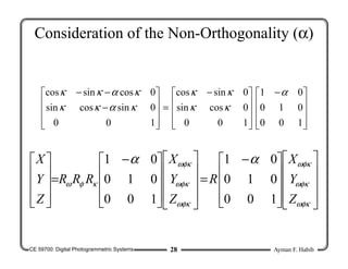
  • 36. CE 59700: Digital Photogrammetric Systems Ayman F. Habib 36 DLT & Computer Vision Models [ ] [ ] 3 3 ' 1 1 0 { } 0 0 1 { } T O x x p y p T O X x Y y K R I X Z c c x K c y Calibration Matrix R I X Exterior Orientation Matrix λ α           = −             − −     = − ≡       − ≡ 𝑬𝒙𝒕𝒆𝒓𝒊𝒐𝒓 𝑶𝒓𝒊𝒆𝒏𝒕𝒂𝒕𝒊𝒐𝒏 𝑴𝒂𝒕𝒓𝒊𝒙 = 𝑹𝑻 𝟏 𝟎 𝟎 −𝑿𝑶 𝟎 𝟏 𝟎 −𝒀𝑶 𝟎 𝟎 𝟏 −𝒁𝑶
  • 37. CE 59700: Digital Photogrammetric Systems Ayman F. Habib 37 DLT & Computer Vision Models • The Direct Linear Transformation (DLT), which has been developed by the photogrammetric community, is an alternative to the collinearity equations that allows for direct transformation between machine/pixel coordinates and corresponding ground coordinates. – 𝑥 = & 𝑦 = • The DLT can be also represented by the following form: – 𝑥 𝑦 1 = 𝐿 𝐿 𝐿 𝐿 𝐿 𝐿 𝐿 𝐿 𝐿 𝐿 𝐿 𝐿 𝑋 𝑌 𝑍 1
  • 38. CE 59700: Digital Photogrammetric Systems Ayman F. Habib 38 DLT & Computer Vision Models 1 2 3 5 6 7 9 10 11 ' 0 0 0 1 x x p T y p L L L c c x D L L L c y R L L L α λ − −         = = −             4 8 12 ' 0 0 0 1 x x p O T y p O O L c c x X L c y R Y L Z α λ − −             =− −                   DLT: Direct Linear Transformation 𝐿 𝐿 𝐿 𝐿 𝐿 𝐿 𝐿 𝐿 𝐿 𝐿 𝐿 𝐿 = 𝛌 𝑲𝑹𝑻 𝑰𝟑 −𝑿𝒐
  • 39. CE 59700: Digital Photogrammetric Systems Ayman F. Habib 39 DLT & CV Models: Pixel Coordinates • The DLT & CV models can also consider the direct transformation from pixel to ground coordinates. 𝒙 𝒚 𝟏 = 𝒖 − 𝒏𝒄 𝟐 ⁄ × 𝒙_𝒑𝒊𝒙_𝒔𝒊𝒛𝒆 𝒏𝒓 𝟐 ⁄ − 𝒗 × 𝒚_𝒑𝒊𝒙_𝒔𝒊𝒛𝒆 𝟏 u v
  • 40. CE 59700: Digital Photogrammetric Systems Ayman F. Habib 40 DLT & CV Models: Pixel Coordinates 𝒙 𝒚 𝟏 = 𝒖 − 𝒏𝒄 𝟐 ⁄ × 𝒙_𝒑𝒊𝒙_𝒔𝒊𝒛𝒆 𝒏𝒓 𝟐 ⁄ − 𝒗 × 𝒚_𝒑𝒊𝒙_𝒔𝒊𝒛𝒆 𝟏 𝒙 𝒚 𝟏 = 𝒙_𝒑𝒊𝒙_𝒔𝒊𝒛𝒆 𝟎 − 𝒏𝒄 𝟐 ⁄ × 𝒙_𝒑𝒊𝒙_𝒔𝒊𝒛𝒆 𝟎 −𝒚_𝒑𝒊𝒙_𝒔𝒊𝒛𝒆 𝒏𝒓 𝟐 ⁄ × 𝒚_𝒑𝒊𝒙_𝒔𝒊𝒛𝒆 𝟎 𝟎 𝟏 𝒖 𝒗 𝟏 𝒙 𝒚 𝟏 = 𝛌 𝑲𝑹𝑻 𝑰𝟑 −𝑿𝒐 𝑿 𝒀 𝒁 𝟏 𝒙_𝒑𝒊𝒙_𝒔𝒊𝒛𝒆 𝟎 − 𝒏𝒄 𝟐 ⁄ × 𝒙_𝒑𝒊𝒙_𝒔𝒊𝒛𝒆 𝟎 −𝒚_𝒑𝒊𝒙_𝒔𝒊𝒛𝒆 𝒏𝒓 𝟐 ⁄ × 𝒚_𝒑𝒊𝒙_𝒔𝒊𝒛𝒆 𝟎 𝟎 𝟏 𝒖 𝒗 𝟏 = 𝛌 𝑲𝑹𝑻 𝑰𝟑 −𝑿𝒐 𝑿 𝒀 𝒁 𝟏
  • 41. CE 59700: Digital Photogrammetric Systems Ayman F. Habib 41 DLT & CV Models: Pixel Coordinates 𝒙_𝒑𝒊𝒙_𝒔𝒊𝒛𝒆 𝟎 − 𝒏𝒄 𝟐 ⁄ × 𝒙_𝒑𝒊𝒙_𝒔𝒊𝒛𝒆 𝟎 −𝒚_𝒑𝒊𝒙_𝒔𝒊𝒛𝒆 𝒏𝒓 𝟐 ⁄ × 𝒚_𝒑𝒊𝒙_𝒔𝒊𝒛𝒆 𝟎 𝟎 𝟏 𝒖 𝒗 𝟏 = 𝛌 𝑲𝑹𝑻 𝑰𝟑 −𝑿𝒐 𝑿 𝒀 𝒁 𝟏 𝒖 𝒗 𝟏 = 𝛌 𝒙_𝒑𝒊𝒙_𝒔𝒊𝒛𝒆 𝟎 − 𝒏𝒄 𝟐 ⁄ × 𝒙_𝒑𝒊𝒙_𝒔𝒊𝒛𝒆 𝟎 −𝒚_𝒑𝒊𝒙_𝒔𝒊𝒛𝒆 𝒏𝒓 𝟐 ⁄ × 𝒚_𝒑𝒊𝒙_𝒔𝒊𝒛𝒆 𝟎 𝟎 𝟏 𝟏 𝑲𝑹𝑻 𝑰𝟑 −𝑿𝒐 𝑿 𝒀 𝒁 𝟏 𝒙_𝒑𝒊𝒙_𝒔𝒊𝒛𝒆 𝟎 − 𝒏𝒄 𝟐 ⁄ × 𝒙_𝒑𝒊𝒙_𝒔𝒊𝒛𝒆 𝟎 −𝒚_𝒑𝒊𝒙_𝒔𝒊𝒛𝒆 𝒏𝒓 𝟐 ⁄ × 𝒚_𝒑𝒊𝒙_𝒔𝒊𝒛𝒆 𝟎 𝟎 𝟏 𝟏 = 𝟏 𝒙_𝒑𝒊𝒙_𝒔𝒊𝒛𝒆 ⁄ 𝟎 𝒏𝒄 𝟐 ⁄ 𝟎 − 𝟏 𝒚_𝒑𝒊𝒙_𝒔𝒊𝒛𝒆 ⁄ 𝒏𝒓 𝟐 ⁄ 𝟎 𝟎 𝟏 𝒖 𝒗 𝟏 = 𝛌 𝟏 𝒙_𝒑𝒊𝒙_𝒔𝒊𝒛𝒆 ⁄ 𝟎 𝒏𝒄 𝟐 ⁄ 𝟎 − 𝟏 𝒚_𝒑𝒊𝒙_𝒔𝒊𝒛𝒆 ⁄ 𝒏𝒓 𝟐 ⁄ 𝟎 𝟎 𝟏 𝑲𝑹𝑻 𝑰𝟑 −𝑿𝒐 𝑿 𝒀 𝒁 𝟏
  • 42. CE 59700: Digital Photogrammetric Systems Ayman F. Habib 42 DLT & CV Models: Pixel Coordinates • Modified Calibration Matrix: 𝐾 = 𝟏 𝒙_𝒑𝒊𝒙_𝒔𝒊𝒛𝒆 ⁄ 𝟎 𝒏𝒄 𝟐 ⁄ 𝟎 − 𝟏 𝒚_𝒑𝒊𝒙_𝒔𝒊𝒛𝒆 ⁄ 𝒏𝒓 𝟐 ⁄ 𝟎 𝟎 𝟏 −𝒄𝒙 −𝜶𝒄𝒙 𝒙𝒑 𝟎 −𝒄𝒚 𝒚𝒑 𝟎 𝟎 𝟏 𝐾 = −𝒄𝒙 𝒙_𝒑𝒊𝒙_𝒔𝒊𝒛𝒆 ⁄ −𝜶𝒄𝒙 𝒙_𝒑𝒊𝒙_𝒔𝒊𝒛𝒆 ⁄ 𝒙𝒑 𝒙_𝒑𝒊𝒙_𝒔𝒊𝒛𝒆 ⁄ + 𝒏𝒄 𝟐 ⁄ 0 𝒄 𝒚_𝒑𝒊𝒙_𝒔𝒊𝒛𝒆 ⁄ −𝑦𝒑 𝑦_𝒑𝒊𝒙_𝒔𝒊𝒛𝒆 ⁄ + 𝒏 𝟐 ⁄ 0 0 1 𝒖 𝒗 𝟏 = 𝛌 𝑲 𝑹𝑻 𝑰𝟑 −𝑿𝒐 𝑿 𝒀 𝒁 𝟏
  • 43. CE 59700: Digital Photogrammetric Systems Ayman F. Habib 43 DLT & CV Models: Pixel Coordinates • For DLT when working with pixel coordinates, we have the following model. – 𝐿 𝐿 𝐿 𝐿 𝐿 𝐿 𝐿 𝐿 𝐿 𝐿 𝐿 𝐿 = 𝛌 𝑲 𝑹𝑻 𝑰𝟑 −𝑿𝒐 • 𝐿 𝐿 𝐿 𝐿 𝐿 𝐿 𝐿 𝐿 𝐿 = 𝛌 𝑲 𝑹𝑻 • 𝐿 𝐿 𝐿 = −𝛌 𝑲 𝑹𝑻 𝑿𝒐 𝑌𝒐 𝑍𝒐
  • 44. CE 59700: Digital Photogrammetric Systems Ayman F. Habib 44 Modern Photogrammetry & Computer Vision • Modern Photogrammetry and Computer Vision are converging fields. Art and science of tool development for automatic generation of spatial and descriptive information from multi-sensory data and/or systems
  • 45. CE 59700: Digital Photogrammetric Systems Ayman F. Habib 45 DLT → IOPs & EOPs Approach # 1
  • 46. CE 59700: Digital Photogrammetric Systems Ayman F. Habib 46 DLT → IOP & EOP 1 2 3 5 6 7 9 10 11 0 0 0 1 x x p T y p L L L c c x D L L L c y R L L L α λ − −         = = −             4 8 12 0 0 0 1 x x p O T y p O O L c c x X L c y R Y L Z α λ − −             =− −                   𝐿 𝐿 𝐿 = − 𝐿 𝐿 𝐿 𝐿 𝐿 𝐿 𝐿 𝐿 𝐿 𝑋 𝑌𝒐 𝑍𝒐
  • 47. CE 59700: Digital Photogrammetric Systems Ayman F. Habib 47 DLT → IOP & EOP No Sign Ambiguity                     − =           O O O Z Y X L L L L L L L L L L L L 11 10 9 7 6 5 3 2 1 12 8 4 • Given: • Then:                     − =           − 12 8 4 1 11 10 9 7 6 5 3 2 1 L L L L L L L L L L L L Z Y X O O O
  • 48. CE 59700: Digital Photogrammetric Systems Ayman F. Habib 48 DLT → IOP & EOP           − − −           − − − = 1 0 0 0 1 0 0 0 2 p p y x x p y p x x T y x c c c y c x c c D D α α λ                     = = = 11 7 3 10 6 2 9 5 1 11 10 9 7 6 5 3 2 1 2 ) ( ) ( L L L L L L L L L L L L L L L L L L KK R K R K D D T T T T T λ λ λ 2 2 11 2 10 2 9 3 3 ) ( λ = + + = × L L L D D T } { 2 11 2 10 2 9 Ambiguity Sign L L L + + ± = λ Then:
  • 49. CE 59700: Digital Photogrammetric Systems Ayman F. Habib 49 DLT → IOP & EOP p T x L L L L L L D D 2 3 11 2 10 1 9 1 3 ) ( λ = + + = × ) ( ) ( 2 11 2 10 2 9 3 11 2 10 1 9 L L L L L L L L L xp + + + + = No Sign Ambiguity Then:                     = = = 11 7 3 10 6 2 9 5 1 11 10 9 7 6 5 3 2 1 2 ) ( ) ( L L L L L L L L L L L L L L L L L L KK R K R K D D T T T T T λ λ λ
  • 50. CE 59700: Digital Photogrammetric Systems Ayman F. Habib 50 p T y L L L L L L D D 2 7 11 6 10 5 9 2 3 ) ( λ = + + = × DLT → IOP & EOP ) ( ) ( 2 11 2 10 2 9 7 11 6 10 5 9 L L L L L L L L L yp + + + + = No Sign Ambiguity Then:                     = = = 11 7 3 10 6 2 9 5 1 11 10 9 7 6 5 3 2 1 2 ) ( ) ( L L L L L L L L L L L L L L L L L L KK R K R K D D T T T T T λ λ λ
  • 51. CE 59700: Digital Photogrammetric Systems Ayman F. Habib 51 ) ( ) ( 2 2 2 2 7 2 6 2 5 2 2 y p T c y L L L D D + = + + = × λ DLT → IOP & EOP                     = = = 11 7 3 10 6 2 9 5 1 11 10 9 7 6 5 3 2 1 2 ) ( ) ( L L L L L L L L L L L L L L L L L L KK R K R K D D T T T T T λ λ λ 5 . 0 2 2 11 2 10 2 9 2 7 2 6 2 5 ) (       − + + + + = p y y L L L L L L c No Sign Ambiguity Then:
  • 52. CE 59700: Digital Photogrammetric Systems Ayman F. Habib 52 DLT → IOP & EOP ) ( ) ( 2 7 3 6 2 5 1 2 1 p p y x T y x c c L L L L L L D D + = + + = × α λ                     = = = 11 7 3 10 6 2 9 5 1 11 10 9 7 6 5 3 2 1 2 ) ( ) ( L L L L L L L L L L L L L L L L L L KK R K R K D D T T T T T λ λ λ       − + + + + = p p y x y x L L L L L L L L L c c ) ( / 1 2 11 2 10 2 9 7 3 6 2 5 1 α No Sign Ambiguity Then:
  • 53. CE 59700: Digital Photogrammetric Systems Ayman F. Habib 53 ) ( ) ( 2 2 2 2 2 2 3 2 2 2 1 1 1 p x x T x c c L L L D D + + = + + = × α λ DLT → IOP & EOP                     = = = 11 7 3 10 6 2 9 5 1 11 10 9 7 6 5 3 2 1 2 ) ( ) ( L L L L L L L L L L L L L L L L L L KK R K R K D D T T T T T λ λ λ 5 . 0 2 2 2 2 11 2 10 2 9 2 3 2 2 2 1 ) (       − − + + + + = p x x x c L L L L L L c α No Sign Ambiguity Then:
  • 54. CE 59700: Digital Photogrammetric Systems Ayman F. Habib 54 DLT → IOP & EOP • Given: • Then: φ λ λ sin 13 9 = = r L Sign Ambiguity                     − − − =           33 23 13 32 22 12 31 21 11 11 10 9 7 6 5 3 2 1 1 0 0 0 r r r r r r r r r y c x c c L L L L L L L L L p y p x x α λ
  • 55. CE 59700: Digital Photogrammetric Systems Ayman F. Habib 55 Collinearity Equations • Objective: Resolve the sign ambiguity in λ • Since the scale factor is always +ve • Assuming that the origin (0, 0, 0) is visible in the imagery ve Z Z r Y Y r X X r O O O −  − + − + − ) ( ) ( ) ( 33 23 13 ve Z r Y r X r O O O −  − − − 33 23 13           − + − + − − + − + − − + − + − =           − − − ) ( ) ( ) ( ) ( ) ( ) ( ) ( ) ( ) ( 33 23 13 32 22 12 31 21 11 O O O O O O O O O p p Z Z r Y Y r X X r Z Z r Y Y r X X r Z Z r Y Y r X X r S c y y x x
  • 56. CE 59700: Digital Photogrammetric Systems Ayman F. Habib 56 DLT → IOP & EOP • By choosing L12 = 1. 12 13 23 33 13 23 33 13 23 33 ( ) 1 ( ) 1 ( ) O O O O O O O O O L r X r Y r Z r X r Y r Z r X r Y r Z λ λ λ =− + + = − − − = − − − λ is Negative 2 11 2 10 2 9 L L L + + − = λ                     − − − − =           O O O T p y p x x Z Y X R y c x c c L L L 1 0 0 0 12 8 4 α λ
  • 57. CE 59700: Digital Photogrammetric Systems Ayman F. Habib 57 DLT → IOP & EOP • No sign Ambiguity 2 11 2 10 2 9 9 13 9 sin sin L L L L r L + + − = = = φ φ λ λ
  • 58. CE 59700: Digital Photogrammetric Systems Ayman F. Habib 58 DLT → IOP & EOP φ ω λ λ φ ω λ λ cos cos cos sin 33 11 23 10 = = − = = r L r L 11 10 tan L L − = ω No Sign Ambiguity                     − − − =           33 23 13 32 22 12 31 21 11 11 10 9 7 6 5 3 2 1 1 0 0 0 r r r r r r r r r y c x c c L L L L L L L L L p y p x x α λ
  • 59. CE 59700: Digital Photogrammetric Systems Ayman F. Habib 59 DLT → IOP & EOP           − − −           =                               − − − =           − 1 0 0 0 1 0 0 0 1 11 10 9 7 6 5 3 2 1 33 32 31 23 22 21 13 12 11 33 23 13 32 22 12 31 21 11 11 10 9 7 6 5 3 2 1 p y p x x p y p x x y c x c c L L L L L L L L L r r r r r r r r r r r r r r r r r r y c x c c L L L L L L L L L α λ α λ • Retrieve κ • Note: There is an ambiguity in 𝜅 determination (±𝜅 cannot be distinguished). φ κ cos cos 11 r =
  • 60. CE 59700: Digital Photogrammetric Systems Ayman F. Habib 60 DLT → IOP & EOP Approach # 2: Matrix Factorization
  • 61. CE 59700: Digital Photogrammetric Systems Ayman F. Habib 61 DLT → IOP (Factorization # 1) • Conceptual basis: Direct derivation of the calibration matrix • Cholesky Decomposition of DDT→ λK (Calibration Matrix)? Wrong           − − −           − − − =                     = = = 1 0 0 0 1 0 0 0 ) ( ) ( 2 11 7 3 10 6 2 9 5 1 11 10 9 7 6 5 3 2 1 2 p p y x x p y p x x T T T T T T y x c c c y c x c c D D L L L L L L L L L L L L L L L L L L KK R K R K D D α α λ λ λ λ
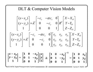
  • 62. CE 59700: Digital Photogrammetric Systems Ayman F. Habib 62 1 1 ) ( − − = = N M M M N CHO T T M M T D D N = T K λ K λ T T T K K M M N M M N 2 1 1 1 λ = = = − − − 1 1 )] } ({ [ − − = T DD CHO K λ T K λ K λ DLT → IOP (Factorization # 2)
  • 63. CE 59700: Digital Photogrammetric Systems Ayman F. Habib 63           − − −           =                               − − − =           − 1 0 0 0 1 0 0 0 1 11 10 9 7 6 5 3 2 1 33 32 31 23 22 21 13 12 11 33 23 13 32 22 12 31 21 11 11 10 9 7 6 5 3 2 1 p y p x x p y p x x y c x c c L L L L L L L L L r r r r r r r r r r r r r r r r r r y c x c c L L L L L L L L L α λ α λ • Using the rotation matrix R, one can derive the individual rotation angles ω, φ and κ. DLT → Rotation Angles
  • 64. CE 59700: Digital Photogrammetric Systems Ayman F. Habib 64 Analysis
  • 65. CE 59700: Digital Photogrammetric Systems Ayman F. Habib 65 Perspective Center • (XO, YO , ZO) is the intersection point of three different planes whose surface normals are (L1, L2, L3), (L5, L6, L7) and (L9, L10, L11), respectively. 𝐿 𝐿 𝐿 = − 𝐿 𝐿 𝐿 𝐿 𝐿 𝐿 𝐿 𝐿 𝐿 𝑋 𝑌 𝑍 𝐿 𝑋 + 𝐿 𝑌 +𝐿 𝑍 = −𝐿 𝐿 𝑋 + 𝐿 𝑌 +𝐿 𝑍 = −𝐿 𝐿 𝑋 + 𝐿 𝑌 +𝐿 𝑍 = −𝐿
  • 66. CE 59700: Digital Photogrammetric Systems Ayman F. Habib 66 Perspective Center                     − − − =           33 23 13 32 22 12 31 21 11 11 10 9 7 6 5 3 2 1 1 0 0 0 r r r r r r r r r y c x c c L L L L L L L L L p y p x x α λ • Assuming: – xp ≈ 0.0 and yp ≈ 0.0 – -αcx ≈ 0.0           − − − − − − =           33 23 13 32 22 12 31 21 11 11 10 9 7 6 5 3 2 1 r r r r c r c r c r c r c r c L L L L L L L L L y y y x x x λ • The three surfaces are orthogonal to each other. – This would lead to better intersection.
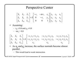
  • 67. CE 59700: Digital Photogrammetric Systems Ayman F. Habib 67                     − − − =           33 23 13 32 22 12 31 21 11 11 10 9 7 6 5 3 2 1 1 0 0 0 r r r r r r r r r y c x c c L L L L L L L L L p y p x x α λ • Assuming: – xp ≠ 0.0 and yp ≠ 0.0 – -αcx ≈ 0.0           + − + − + − + − + − + − =           33 23 13 33 32 23 22 13 12 33 31 23 21 13 11 11 10 9 7 6 5 3 2 1 r r r r y r c r y r c r y r c r x r c r x r c r x r c L L L L L L L L L p y p y p y p x p x p x λ • As xp and yp increase, the surface normals become almost parallel. – This would lead to weak intersection. Perspective Center
  • 68. CE 59700: Digital Photogrammetric Systems Ayman F. Habib 68 • The rows of D are not correlated: – They are orthogonal to each other. • L-1 is well defined.           − − −           =           − 1 0 0 0 1 11 10 9 7 6 5 3 2 1 33 32 31 23 22 21 13 12 11 p y p x x y c x c c L L L L L L L L L r r r r r r r r r α λ • Assuming: – xp ≈ 0.0 and yp ≈ 0.0 – -αcx ≈ 0.0           − − − − − − =           33 23 13 32 22 12 31 21 11 11 10 9 7 6 5 3 2 1 r r r r c r c r c r c r c r c L L L L L L L L L y y y x x x λ Rotation Angles
  • 69. CE 59700: Digital Photogrammetric Systems Ayman F. Habib 69           − − −           =           − 1 0 0 0 1 11 10 9 7 6 5 3 2 1 33 32 31 23 22 21 13 12 11 p y p x x y c x c c L L L L L L L L L r r r r r r r r r α λ • Assuming: – xp ≠ 0.0 and yp ≠ 0.0 – -αcx ≈ 0.0           + − + − + − + − + − + − =           33 23 13 33 32 23 22 13 12 33 31 23 21 13 11 11 10 9 7 6 5 3 2 1 r r r r y r c r y r c r y r c r x r c r x r c r x r c L L L L L L L L L p y p y p y p x p x p x λ • The rows of D tend to be highly correlated. • L-1 is not well defined. Rotation Angles