Lf 2020 rates_iii
3 likes922 views

This document introduces notations and conventions used in interest rate modeling. It defines key quantities like the zero coupon bond (ZC), discount factor, and continuously compounded spot rate. The continuously compounded spot rate r(t,T) represents the constant rate of return needed to accrue 1 unit from t to T. It also defines simply, annually, and q-times compounded rates. In the small time limit, all rates converge to the instantaneous short rate R(t). Lowercase denotes regular variables while uppercase denotes stochastic variables.


![Luc_Faucheux_2020
Notations and conventions in the rates world - V
¨ Simply compounded spot interest rate
¨ 𝑙 𝑡, 𝑇 =
-
,(#,%)
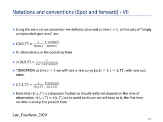
.
-.)*(#,%)
)*(#,%)
¨ Or alternatively, in the bootstrap form
¨ 𝜏 𝑡, 𝑇 . 𝑙 𝑡, 𝑇 . 𝑧𝑐 𝑡, 𝑇 = 1 − 𝑧𝑐(𝑡, 𝑇)
¨ 1 + 𝜏 𝑡, 𝑇 . 𝑙 𝑡, 𝑇 . 𝑧𝑐 𝑡, 𝑇 = 1
¨ 𝑧𝑐 𝑡, 𝑇 =
-
-/, #,% .1 #,%
¨ In the deterministic case:
¨ 𝑧𝑐 𝑡, 𝑇 =
-
-/, #,% .1 #,%
= 𝐷 𝑡, 𝑇 =
!(#)
!(%)
= exp(− ∫#
%
𝑅 𝑠 . 𝑑𝑠)
¨ 𝑙 𝑡, 𝑇 =
-
, #,%
. [1 − exp − ∫#
%
𝑅 𝑠 . 𝑑𝑠 ]
9](https://image.slidesharecdn.com/lf2020ratesiii-200825150705/85/Lf-2020-rates_iii-9-320.jpg)


![Luc_Faucheux_2020
Notations and conventions (lower case and UPPER CASE)
¨ I will try to stick to a convention where the the lower case denotes a regular variable, and an
upper case denotes a stochastic variable, as in before:
¨
78(9,#)
7#
= −
7
79
[𝑎 𝑡 . 𝑝 𝑥, 𝑡 −
7
79
[
-
5
𝑏 𝑡 5. 𝑝 𝑥, 𝑡 ]]
¨ 𝑋 𝑡: − 𝑋 𝑡; = ∫#<#;
#<#:
𝑑𝑋 𝑡 = ∫#<#;
#<#:
𝑎(𝑡). 𝑑𝑡) + ∫#<#;
#<#:
𝑏(𝑡). 𝑑𝑊(𝑡)
¨ 𝑑𝑋 𝑡 = 𝑎 𝑡 . 𝑑𝑡 + 𝑏(𝑡). 𝑑𝑊
¨ Where we should really write to be fully precise:
¨ 𝑝 𝑥, 𝑡 = 𝑝=(𝑥, 𝑡|𝑥 𝑡 = 𝑡& = 𝑋&, 𝑡 = 𝑡&)
¨ PDF Probability Density Function: 𝑝=(𝑥, 𝑡)
¨ Distribution function : 𝑃=(𝑥, 𝑡)
¨ 𝑃= 𝑥, 𝑡 = 𝑃𝑟𝑜𝑏𝑎𝑏𝑖𝑙𝑖𝑡𝑦 𝑋 ≤ 𝑥, 𝑡 = ∫3<.>
3<9
𝑝= 𝑦, 𝑡 . 𝑑𝑦 𝑝=(𝑥, 𝑡) =
7
79
𝑃= 𝑥, 𝑡
15](https://image.slidesharecdn.com/lf2020ratesiii-200825150705/85/Lf-2020-rates_iii-15-320.jpg)


![Luc_Faucheux_2020
Notations and conventions (Spot and forward) - XI
¨ We could also define any kind of buckets:
¨ 𝑧𝑐 𝑡 = 0, 𝑡 = 𝑡8, 𝑡 = 𝑡4 = ∏A<8
A<4
𝑧𝑐 𝑡 = 0, 𝑡 = 𝑡A, 𝑡 = 𝑡A + 1
¨ 𝑧𝑐 𝑡 = 0, 𝑡8, 𝑡4 =
-
-/, &,#-,#) .1 &,#-,#)
¨ And so for any joint sequence of buckets, we have the usual bootstrap equation
¨ 𝑧𝑐 𝑡 = 0, 𝑡 = 0, 𝑡 = 𝑡@ = ∏ 𝑧𝑐 𝑡 = 0, 𝑡 = 𝑡8, 𝑡 = 𝑡4
¨ 𝑧𝑐 𝑡 = 0, 𝑡 = 0, 𝑡 = 𝑡@ = ∏
-
-/, &,#-,#) .1 &,#-,#)
¨ Where the successive buckets [𝑡8, 𝑡4] covers the [0, 𝑡@] interval
¨ A picture usually being worth a thousand words:
23](https://image.slidesharecdn.com/lf2020ratesiii-200825150705/85/Lf-2020-rates_iii-23-320.jpg)


![Luc_Faucheux_2020
Forward contract - II
¨ We also define the quantities 𝑙 𝑡, 𝑡A, 𝑡Q that we call simply compounded forward rate for the
period [𝑡A, 𝑡Q] (observed at time 𝑡) as :
¨ 𝑧𝑐 𝑡, 𝑡A, 𝑡Q =
-
-/, #,#,,#/ .1 #,#,,#/
¨ A contract that pays $1 at time 𝑡Q is worth at time 𝑡:
¨ 𝑉_𝑝𝑟𝑖𝑛𝑐𝑖𝑝𝑎𝑙 𝑡 = 𝑧𝑐 𝑡, 𝑡, 𝑡Q
¨ A contract that pays 𝑋% paid on the 𝜏 𝑡, 𝑡A, 𝑡Q daycount convention, on $1 principal amount
at time 𝑡Q is worth at time 𝑡:
¨ 𝑉_𝑐𝑜𝑢𝑝𝑜𝑛 𝑡 = 𝑧𝑐 𝑡, 𝑡, 𝑡Q . 𝑋. 𝜏 𝑡, 𝑡A, 𝑡Q
39](https://image.slidesharecdn.com/lf2020ratesiii-200825150705/85/Lf-2020-rates_iii-39-320.jpg)


![Luc_Faucheux_2020
Forward contract - XXII
¨ To be even more precise:
¨ 𝔼#<#,
-
-/V #<#,,#,,#/ .,
|𝔉(𝑡) =
-
-/1 #,#,,#/ .,
¨ To illustrate that the period [𝑡A, 𝑡Q] is fixed and the random variable is 𝐿 𝑡, 𝑡A, 𝑡Q , that will fix
at time 𝑡A to 𝑙 𝑡A, 𝑡A, 𝑡Q , and will be set as an historical set to 𝑙 𝑡A, 𝑡A, 𝑡Q
¨ 𝐿 𝑡, 𝑡A, 𝑡Q = 𝑙 𝑡A, 𝑡A, 𝑡Q for all time 𝑡 > 𝑡A
60](https://image.slidesharecdn.com/lf2020ratesiii-200825150705/85/Lf-2020-rates_iii-60-320.jpg)


![Luc_Faucheux_2020
Early and discount measure - IV
78
𝑡"
𝑡!
𝑡𝑖𝑚𝑒
𝐿 𝑡, 𝑡0, 𝑡1 sets at time 𝑡0 and spans the period [𝑡0, 𝑡1]](https://image.slidesharecdn.com/lf2020ratesiii-200825150705/85/Lf-2020-rates_iii-78-320.jpg)


![Luc_Faucheux_2020
NOTATIONS - VII
¨ TERM investing
¨ At time 𝑡Q with time 𝑡 > 𝑡Q
¨ 𝑧𝑐 𝑡Q, 𝑡Q, 𝑡 is the the price at time 𝑡Q of a contract that will pay $1 at time 𝑡
¨ 𝔼#/
TU 𝑍𝐶 𝑡Q, 𝑡Q, 𝑡 |𝔉(𝑡Q) = 𝑧𝑐 𝑡Q, 𝑡Q, 𝑡
¨ DAILY re-investing
¨ 𝑧𝑐 𝑡Q, 𝑡Q, 𝑡 = 𝔼#/
TU 𝑍𝐶 𝑡Q, 𝑡Q, 𝑡 |𝔉(𝑡Q) = 𝔼#/
TU ∏#2#/
#2]#
𝑍𝐶 𝑡@, 𝑡@, 𝑡@/- |𝔉(𝑡Q)
¨ As time 𝑡@ goes from 𝑡Q to 𝑡, the daily overnight variable 𝑍𝐶 𝑡@, 𝑡@, 𝑡@/- become fixed to
𝑧𝑐 𝑡@, 𝑡@, 𝑡@/-
109](https://image.slidesharecdn.com/lf2020ratesiii-200825150705/85/Lf-2020-rates_iii-109-320.jpg)


![Luc_Faucheux_2020
NOTATIONS - X
¨ This might sound completely obvious, but it is worth at time using an illustrated example to
understand the difference between expected and realized value
¨ Of course of the rates had gone down drastically we would have received less than $1 in one
year
¨ If we build any dynamics of rates, where they can be expected to increase or decrease
following some kind of stochastic driver, we need to ensure that the expected values are
conserved (arbitrage free relationships)
¨ 𝑧𝑐 𝑡Q, 𝑡Q, 𝑡 = 𝔼#/
TU
𝑍𝐶 𝑡Q, 𝑡Q, 𝑡 |𝔉(𝑡Q) = 𝔼#/
TU ∏#2#/
#2]#
𝑍𝐶 𝑡@, 𝑡@, 𝑡@/- |𝔉(𝑡Q)
¨ 𝑧𝑐 𝑡Q, 𝑡Q, 𝑡 = 𝔼#/
TU
𝑍𝐶 𝑡Q, 𝑡Q, 𝑡Q/- . ∏#2#//-
#2]#
𝑍𝐶 𝑡@, 𝑡@, 𝑡@/- |𝔉(𝑡Q)
¨ 𝑧𝑐 𝑡Q, 𝑡Q, 𝑡 = 𝑧𝑐 𝑡Q, 𝑡Q, 𝑡Q + 1 . 𝔼#/
TU ∏#2#//-
#2]#
𝑍𝐶 𝑡@, 𝑡@, 𝑡@/- |𝔉(𝑡Q)
112](https://image.slidesharecdn.com/lf2020ratesiii-200825150705/85/Lf-2020-rates_iii-112-320.jpg)


![Luc_Faucheux_2020
A swap rate is a weighted basket of forward rates
¨ At-the-money swap rate equation: ∑A 𝐷𝐶𝐹 𝑖 . 𝐷 𝑖 . 𝑁 𝑖 . 𝑓 𝑖 = ∑Q 𝐷𝐶𝐹 𝑗 . 𝐷 𝑗 . 𝑁 𝑗 . 𝑅
¨ Above equation is valid at all times before the swap start, forwards and discount factors
being calculated on the then current discount curve the usual way, if the period I on the
float side starts at time ts(i) and ends at time te(i), and the forward is “aligned” with the
period (no swap in arrears or CMS like)
¨ 𝑅(𝑡) = ∑A 𝐷𝐶𝐹 𝑖 . 𝐷 𝑖 . 𝑁 𝑖 . 𝑓 𝑡, 𝑡𝑠 𝑖 , 𝑡𝑒(𝑖) /[∑Q 𝐷𝐶𝐹 𝑗 . 𝐷 𝑗 . 𝑁 𝑗 ]
¨ “frozen numeraire” approximation, expand above equation in first order in forward rates but
keeping the discount factors constant
¨ 𝑑𝑅(𝑡) = ∑A 𝐷𝐶𝐹 𝑖 . 𝐷 𝑖 . 𝑁 𝑖 . 𝑑𝑓 𝑡, 𝑡𝑠 𝑖 , 𝑡𝑒(𝑖) /[∑Q 𝐷𝐶𝐹 𝑗 . 𝐷 𝑗 . 𝑁 𝑗 ]
¨ Taking the square of the above yields the instantaneous volatility of the swap rate
¨ Λd
5 . 𝑑𝑡 =< 𝑑𝑅5 >=
∑A- ∑A5 𝐷𝐶𝐹 𝑖1 . 𝐷 𝑖1 . 𝑁 𝑖1 . 𝐷𝐶𝐹 𝑖2 . 𝐷 𝑖2 . 𝑁 𝑖2 . < 𝑑𝑓 𝑖1 . 𝑑𝑓 𝑖2 > /
[∑Q- ∑Q5 𝐷𝐶𝐹 𝑗1 . 𝐷 𝑗1 . 𝑁 𝑗1 𝐷𝐶𝐹 𝑗2 . 𝐷 𝑗2 . 𝑁 𝑗2 ]
119](https://image.slidesharecdn.com/lf2020ratesiii-200825150705/85/Lf-2020-rates_iii-119-320.jpg)
![Luc_Faucheux_2020
A swap rate is a weighted basket of forward rates
¨ instantaneous volatility of the swap rate
¨ Λd
5
. 𝑑𝑡 =< 𝑑𝑅5 >=
∑A- ∑A5 𝐷𝐶𝐹 𝑖1 . 𝐷 𝑖1 . 𝑁 𝑖1 . 𝐷𝐶𝐹 𝑖2 . 𝐷 𝑖2 . 𝑁 𝑖2 . < 𝑑𝑓 𝑖1 . 𝑑𝑓 𝑖2 > /
[∑Q- ∑Q5 𝐷𝐶𝐹 𝑗1 . 𝐷 𝑗1 . 𝑁 𝑗1 𝐷𝐶𝐹 𝑗2 . 𝐷 𝑗2 . 𝑁 𝑗2 ]
¨ Where 𝑑𝑓 𝑖1 = 𝑑𝑓 𝑡, 𝑡𝑠 𝑖1 , 𝑡𝑒(𝑖1) and 𝑑𝑓 𝑖2 = 𝑑𝑓 𝑡, 𝑡𝑠 𝑖2 , 𝑡𝑒(𝑖2)
¨ In abbreviated notation
¨ < 𝑑𝑓 𝑖1 . 𝑑𝑓 𝑖2 >= 𝜎 𝑖1 . 𝜎 𝑖2 . 𝜌 𝑖1, 𝑖2 . 𝑑𝑡
¨ So to calculate the instantaneous volatility of the swap rate you need the instantaneous
volatility of each forward BUT ALSO the instantaneous correlation matrix between the
forward constituting the weighted basket.
120](https://image.slidesharecdn.com/lf2020ratesiii-200825150705/85/Lf-2020-rates_iii-120-320.jpg)


![Luc_Faucheux_2020
Looking at the timing convexity - XIII
¨ ? = 𝔼#,
TU 𝑉 𝑡A, $𝐿 𝑡, 𝑡A, 𝑡Q . 𝜏, 𝑡A, 𝑡A |𝔉(𝑡)
¨ ? = 𝔼#,
TU
𝑉 𝑡A, $𝐿 𝑡, 𝑡A, 𝑡Q . 𝜏. (1 + 𝐿 𝑡, 𝑡A, 𝑡Q . 𝜏 ), 𝑡A, 𝑡Q |𝔉(𝑡)
¨ ? = 𝔼#,
TU 𝑉 𝑡A, $[𝐿 𝑡, 𝑡A, 𝑡Q . 𝜏 + 𝐿 𝑡, 𝑡A, 𝑡Q . 𝜏
5
], 𝑡A, 𝑡Q |𝔉(𝑡)
¨ Expressed in this fashion we see a rate square term than appears, for which we will have to
compute an expectation
¨ So there will be most likely some convexity to compute, hence a convexity adjustment
¨ Chances are that this convexity adjustment will depend on the specifics of the dynamics
(volatility, distribution) that we will assume for the rate
¨ Derivatives with the square of rates were somewhat popular in the early 90s until something
blew up, lawsuit, then people stopped trading it
137](https://image.slidesharecdn.com/lf2020ratesiii-200825150705/85/Lf-2020-rates_iii-137-320.jpg)
![Luc_Faucheux_2020
Looking at the timing convexity - XIV
¨ Now, we are looking at the payoff:
¨ 𝐻 𝑡 = $[𝐿 𝑡, 𝑡A, 𝑡Q . 𝜏 + 𝐿 𝑡, 𝑡A, 𝑡Q . 𝜏
5
]
¨ Which is fixed and known for all time 𝑡 > 𝑡A and is paid at time 𝑡Q
¨ ? = 𝔼#,
TU
𝑉 𝑡A, $[𝐻(𝑡)], 𝑡A, 𝑡Q |𝔉(𝑡)
¨ And so we almost there, but from the tower property we then have:
¨ ? = 𝔼#/
TU
𝑉 𝑡A, $[𝐻(𝑡)], 𝑡A, 𝑡Q |𝔉(𝑡)
¨ Under the terminal measure associated with the 𝑍𝐶 𝑡, 𝑡, 𝑡Q discount factor
¨ So
¨ 𝔼#/
TU 𝑉 𝑡A, $[𝐻(𝑡)], 𝑡A, 𝑡Q |𝔉(𝑡) = 𝔼#/
TU 𝑉 𝑡A, $
[(#)
TU #/,#/,#/
, 𝑡A, 𝑡Q |𝔉(𝑡) =
? #,$[[(#)],#,,#/
)* #,#,#/
138](https://image.slidesharecdn.com/lf2020ratesiii-200825150705/85/Lf-2020-rates_iii-138-320.jpg)
![Luc_Faucheux_2020
Looking at the timing convexity - XV
¨ ? = 𝔼#,
TU 𝑉 𝑡A, $𝐿 𝑡, 𝑡A, 𝑡Q . 𝜏, 𝑡A, 𝑡A |𝔉(𝑡)
¨ ? = 𝔼#/
TU
𝑉 𝑡A, $[𝐻(𝑡)], 𝑡A, 𝑡Q |𝔉(𝑡)
¨ With:
¨ 𝐻 𝑡 = $[𝐿 𝑡, 𝑡A, 𝑡Q . 𝜏 + 𝐿 𝑡, 𝑡A, 𝑡Q . 𝜏
5
]
¨ 𝑉 𝑡, $[𝐻(𝑡)], 𝑡A, 𝑡Q = 𝑧𝑐 𝑡, 𝑡, 𝑡Q . 𝔼#/
TU
𝑉 𝑡A, $[𝐻(𝑡)], 𝑡A, 𝑡Q |𝔉(𝑡)
¨ NOW we know that under the Forward measure (terminal- 𝑡Q measure):
¨ 𝔼#/
TU 𝑉 𝑡Q, $𝐿 𝑡, 𝑡A, 𝑡Q , 𝑡A, 𝑡Q |𝔉(𝑡) = 𝑙 𝑡, 𝑡A, 𝑡Q
¨ 𝔼#/
TU 𝑉 𝑡Q, $𝐿 𝑡, 𝑡A, 𝑡Q . 𝜏, 𝑡A, 𝑡Q |𝔉(𝑡) = 𝑙 𝑡, 𝑡A, 𝑡Q . 𝜏
¨ Remember we can only drop the daycount fraction 𝜏 = 𝜏 𝑡, 𝑡A, 𝑡Q in some very specific
cases
139](https://image.slidesharecdn.com/lf2020ratesiii-200825150705/85/Lf-2020-rates_iii-139-320.jpg)
![Luc_Faucheux_2020
Looking at the timing convexity - XVI
¨ In general because the forward rate is only defined as:
¨ 𝑍𝐶 𝑡, 𝑡A, 𝑡Q =
-
-/V #,#,,#/ .,
¨ And because only 𝑍𝐶 𝑡, 𝑡A, 𝑡Q is meaningful (unique, does not depend on conventions, and is
the numeraire, hence the arbitrage conditions are quite nice), always better to just carry this
daycount fraction around, just to remind us that 𝐿 𝑡, 𝑡A, 𝑡Q in itself does not have as strong a
meaning as 𝑍𝐶 𝑡, 𝑡A, 𝑡Q
¨ 𝔼#/
TU
𝑉 𝑡Q, $𝐿 𝑡, 𝑡A, 𝑡Q . 𝜏, 𝑡A, 𝑡Q |𝔉(𝑡) = 𝑙 𝑡, 𝑡A, 𝑡Q . 𝜏
¨ 𝑉 𝑡, $[𝐻(𝑡)], 𝑡A, 𝑡Q = 𝑧𝑐 𝑡, 𝑡, 𝑡Q . 𝔼#/
TU 𝑉 𝑡A, $[𝐻(𝑡)], 𝑡A, 𝑡Q |𝔉(𝑡)
¨ 𝐻 𝑡 = [𝐿 𝑡, 𝑡A, 𝑡Q . 𝜏 + 𝐿 𝑡, 𝑡A, 𝑡Q . 𝜏
5
]
¨ 𝔼#/
TU 𝑉 𝑡A, $[𝐻(𝑡)], 𝑡A, 𝑡Q |𝔉(𝑡) = 𝔼#/
TU 𝑉 𝑡A, $[𝐿 𝑡, 𝑡A, 𝑡Q . 𝜏 + 𝐿 𝑡, 𝑡A, 𝑡Q . 𝜏
5
], 𝑡A, 𝑡Q |𝔉(𝑡)
140](https://image.slidesharecdn.com/lf2020ratesiii-200825150705/85/Lf-2020-rates_iii-140-320.jpg)
![Luc_Faucheux_2020
Looking at the timing convexity - XVII
¨ 𝔼#/
TU 𝑉 𝑡A, $[𝐻(𝑡)], 𝑡A, 𝑡Q |𝔉(𝑡) = 𝔼#/
TU 𝑉 𝑡A, $[𝐿 𝑡, 𝑡A, 𝑡Q . 𝜏 + 𝐿 𝑡, 𝑡A, 𝑡Q . 𝜏
5
], 𝑡A, 𝑡Q |𝔉(𝑡)
¨ 𝔼#/
TU 𝑉 𝑡A, $[𝐻(𝑡)], 𝑡A, 𝑡Q |𝔉(𝑡) = 𝔼#/
TU 𝑉 𝑡A, $[𝐿 𝑡, 𝑡A, 𝑡Q . 𝜏], 𝑡A, 𝑡Q |𝔉(𝑡) +
𝔼#/
TU 𝑉 𝑡A, $[ 𝐿 𝑡, 𝑡A, 𝑡Q . 𝜏
5
], 𝑡A, 𝑡Q |𝔉(𝑡)
¨ 𝔼#/
TU
𝑉 𝑡Q, $𝐿 𝑡, 𝑡A, 𝑡Q . 𝜏, 𝑡A, 𝑡Q |𝔉(𝑡) = 𝑙 𝑡, 𝑡A, 𝑡Q . 𝜏
¨ 𝔼#/
TU
𝑉 𝑡A, $[𝐻(𝑡)], 𝑡A, 𝑡Q |𝔉(𝑡) = 𝑙 𝑡, 𝑡A, 𝑡Q . 𝜏 + 𝔼#/
TU
𝑉 𝑡A, $[ 𝐿 𝑡, 𝑡A, 𝑡Q . 𝜏
5
], 𝑡A, 𝑡Q |𝔉(𝑡)
¨ 𝑉 𝑡, $[𝐻(𝑡)], 𝑡A, 𝑡Q = 𝑧𝑐 𝑡, 𝑡, 𝑡Q . 𝔼#/
TU
𝑉 𝑡A, $[𝐻(𝑡)], 𝑡A, 𝑡Q |𝔉(𝑡)
¨ 𝑉 𝑡, $[𝐿 𝑡, 𝑡A, 𝑡Q . 𝜏], 𝑡A, 𝑡A = 𝑧𝑐 𝑡, 𝑡, 𝑡A . 𝔼#,
TU 𝑉 𝑡A, $𝐿 𝑡, 𝑡A, 𝑡Q . 𝜏, 𝑡A, 𝑡A |𝔉(𝑡)
¨ 𝑉 𝑡, $[𝐿 𝑡, 𝑡A, 𝑡Q . 𝜏], 𝑡A, 𝑡A = 𝑉 𝑡, $[𝐻(𝑡)], 𝑡A, 𝑡Q
¨ 𝑉 𝑡, $[𝐿 𝑡, 𝑡A, 𝑡Q . 𝜏], 𝑡A, 𝑡A = 𝑧𝑐 𝑡, 𝑡, 𝑡Q . 𝔼#/
TU
𝑉 𝑡A, $[𝐻(𝑡)], 𝑡A, 𝑡Q |𝔉(𝑡)
141](https://image.slidesharecdn.com/lf2020ratesiii-200825150705/85/Lf-2020-rates_iii-141-320.jpg)
![Luc_Faucheux_2020
Looking at the timing convexity - XVIII
¨ 𝑉 𝑡, $[𝐿 𝑡, 𝑡A, 𝑡Q . 𝜏], 𝑡A, 𝑡A = 𝑧𝑐 𝑡, 𝑡, 𝑡Q . 𝔼#/
TU 𝑉 𝑡A, $[𝐻(𝑡)], 𝑡A, 𝑡Q |𝔉(𝑡)
¨ 𝔼#/
TU 𝑉 𝑡A, $[𝐻(𝑡)], 𝑡A, 𝑡Q |𝔉(𝑡) = 𝑙 𝑡, 𝑡A, 𝑡Q . 𝜏 + 𝔼#/
TU 𝑉 𝑡A, $[ 𝐿 𝑡, 𝑡A, 𝑡Q . 𝜏
5
], 𝑡A, 𝑡Q |𝔉(𝑡)
¨
? #,$[V #,#,,#/ .,],#,,#,
)* #,#,#/
= 𝑙 𝑡, 𝑡A, 𝑡Q . 𝜏 + 𝔼#/
TU 𝑉 𝑡A, $[ 𝐿 𝑡, 𝑡A, 𝑡Q . 𝜏
5
], 𝑡A, 𝑡Q |𝔉(𝑡)
¨
? #,$[V #,#,,#/ .,],#,,#,
)* #,#,#/
= 𝑙 𝑡, 𝑡A, 𝑡Q + 𝐶𝑜𝑛𝑣𝑒𝑥𝑖𝑡𝑦(𝑡)
¨ 𝐶𝑜𝑛𝑣𝑒𝑥𝑖𝑡𝑦 𝑡 =
-
,
. 𝔼#/
TU
𝑉 𝑡A, $[ 𝐿 𝑡, 𝑡A, 𝑡Q . 𝜏
5
], 𝑡A, 𝑡Q |𝔉(𝑡)
¨ The value at time 𝑡 of receiving at time (𝑡 = 𝑡A )the rate 𝐿 𝑡, 𝑡A, 𝑡Q that covers the period
[𝑡A, 𝑡Q] and will fix to 𝐿 𝑡 = 𝑡A, 𝑡A, 𝑡Q = 𝑙 𝑡A, 𝑡A, 𝑡Q at time (𝑡 = 𝑡A), equal to something that is
the value of that forward rate 𝑙 𝑡, 𝑡A, 𝑡Q (AS COMPUTED from the yield curve at time 𝑡)
discounted by the usual discount factor 𝑧𝑐 𝑡, 𝑡, 𝑡Q UP TO TIME 𝑡Q, PLUS SOMETHING ELSE
142](https://image.slidesharecdn.com/lf2020ratesiii-200825150705/85/Lf-2020-rates_iii-142-320.jpg)
![Luc_Faucheux_2020
Looking at the timing convexity - XIX
¨ That SOMETHING ELSE is quite complicated.
¨ That SOMETHING ELSE is called the arrears convexity adjustment
¨ That SOMETHING ELSE we will call 𝐶𝑜𝑛𝑣𝑒𝑥𝑖𝑡𝑦(𝑡)
¨ 𝐶𝑜𝑛𝑣𝑒𝑥𝑖𝑡𝑦 𝑡 =
-
,
. 𝔼#/
TU
𝑉 𝑡A, $[ 𝐿 𝑡, 𝑡A, 𝑡Q . 𝜏
5
], 𝑡A, 𝑡Q |𝔉(𝑡)
¨ 𝐶𝑜𝑛𝑣𝑒𝑥𝑖𝑡𝑦 𝑡 is what you need to add to the value 𝑙 𝑡, 𝑡A, 𝑡Q computed from the yield
curve at time 𝑡 to properly value a contract that will pay 𝐿 𝑡, 𝑡A, 𝑡Q at time 𝑡A
¨
? #,$[V #,#,,#/ .,],#,,#,
)* #,#,#/
= 𝑙 𝑡, 𝑡A, 𝑡Q + 𝐶𝑜𝑛𝑣𝑒𝑥𝑖𝑡𝑦(𝑡)
¨
? #,$[V #,#,,#/ .,],#,,#/
)* #,#,#/
= 𝑙 𝑡, 𝑡A, 𝑡Q
143](https://image.slidesharecdn.com/lf2020ratesiii-200825150705/85/Lf-2020-rates_iii-143-320.jpg)
![Luc_Faucheux_2020
Looking at the timing convexity - XX
¨ OK, so again not trying to be pedantic with notations
¨ Hopefully this section has illustrated some of the pitfalls that occurs when we do not
enunciate all the details of the payoff (when it is being set, when it is being paid, how is this
payoff defined as a function of the ZCB, Zero Coupon Bonds, which are the present values of
FIXED $1 cash flows in the future, which are know for all time with certainty, and can be
traded and hedged in the market)
¨ Lots of assumptions that can easily break down.
¨
? #,$[V #,#,,#/ .,],#,,#,
)* #,#,#/
= 𝑙 𝑡, 𝑡A, 𝑡Q + 𝐶𝑜𝑛𝑣𝑒𝑥𝑖𝑡𝑦(𝑡)
¨
? #,$[V #,#,,#/ .,],#,,#/
)* #,#,#/
= 𝑙 𝑡, 𝑡A, 𝑡Q
¨ Just a small difference in the timing of the payment makes a HUGE difference. That is why
Goldman Sachs are still one of the most profitable firm on the planet, they know their
convexity…(they also doing God’s work so that helps).
144](https://image.slidesharecdn.com/lf2020ratesiii-200825150705/85/Lf-2020-rates_iii-144-320.jpg)
![Luc_Faucheux_2020
Looking at the timing convexity - XXI
¨
? #,$[V #,#,,#/ .,],#,,#,
)* #,#,#/
=
? #,$[V #,#,,#/ .,],#,,#/
)* #,#,#/
+ 𝐶𝑜𝑛𝑣𝑒𝑥𝑖𝑡𝑦(𝑡)
¨ 𝑉 𝑡, $[𝐿 𝑡, 𝑡A, 𝑡Q . 𝜏], 𝑡A, 𝑡A = 𝑉 𝑡, $[𝐿 𝑡, 𝑡A, 𝑡Q . 𝜏], 𝑡A, 𝑡Q + 𝑧𝑐 𝑡, 𝑡, 𝑡Q . 𝐶𝑜𝑛𝑣𝑒𝑥𝑖𝑡𝑦(𝑡)
¨ 𝑉 𝑡, $[𝐿 𝑡, 𝑡A, 𝑡Q . 𝜏], 𝑡A, 𝑡A is the value at time 𝑡 of a contract that will pay at time 𝑡A the
forward rate 𝐿 𝑡, 𝑡A, 𝑡Q covering the [𝑡A 𝑡Q] period, and fixing at 𝐿 𝑡, 𝑡A, 𝑡Q = 𝑙 𝑡A, 𝑡A, 𝑡Q at
time (𝑡 = 𝑡A)
¨ 𝑉 𝑡, $[𝐿 𝑡, 𝑡A, 𝑡Q . 𝜏], 𝑡A, 𝑡Q is the value at time 𝑡 of a contract that will pay at time 𝑡Q the
forward rate 𝐿 𝑡, 𝑡A, 𝑡Q covering the [𝑡A 𝑡Q] period, and fixing at 𝐿 𝑡, 𝑡A, 𝑡Q = 𝑙 𝑡A, 𝑡A, 𝑡Q at
time (𝑡 = 𝑡A)
¨
? #,$[V #,#,,#/ .,],#,,#/
)* #,#,#/
= 𝑙 𝑡, 𝑡A, 𝑡Q
¨ 𝑉 𝑡, $[𝐿 𝑡, 𝑡A, 𝑡Q . 𝜏], 𝑡A, 𝑡Q = 𝑧𝑐 𝑡, 𝑡, 𝑡Q . 𝑙 𝑡, 𝑡A, 𝑡Q
145](https://image.slidesharecdn.com/lf2020ratesiii-200825150705/85/Lf-2020-rates_iii-145-320.jpg)
![Luc_Faucheux_2020
Looking at the timing convexity - XXII
¨ 𝑉 𝑡, $[𝐿 𝑡, 𝑡A, 𝑡Q . 𝜏], 𝑡A, 𝑡Q = 𝑧𝑐 𝑡, 𝑡, 𝑡Q . 𝑙 𝑡, 𝑡A, 𝑡Q
¨ That is nice, we compute the forward rate from the yield curve at time 𝑡
¨ That is what we do for regular swap all the time
¨ We also know the discount factors 𝑧𝑐 𝑡, 𝑡, 𝑡Q from the discount/yield curve
¨ So no biggie there, we just need a yield curve (discount curve) to value this contract and we
happily get a price from the Swap desk. We do not care about the volatility or any other
dynamics of rates.
¨ Then…boom..we get a call from a broker telling us that he has a client who has an “interest”
in a contract that is exactly as above except that it pays 𝐿 𝑡, 𝑡A, 𝑡Q at time 𝑡A rather than time
𝑡Q. No big deal right ? You can easily price that up right ? Oh also it is for big size and rather
urgent, but that is ok because the client will pay though “mid” (i.e. your valuation using only
the yield curve) because the client is really axed and is really keen on doing that now, and
with you because you are awesome, and where are you going to dinner tonight? Maybe
with the brokerage fee that I will make we can go to a nice restaurant of your choice….
146](https://image.slidesharecdn.com/lf2020ratesiii-200825150705/85/Lf-2020-rates_iii-146-320.jpg)
![Luc_Faucheux_2020
Looking at the timing convexity - XXIII
¨ So then what most dealers did (and many might still do, worth giving it a try from time to
time) is to say:
¨ 𝑉 𝑡, $[𝐿 𝑡, 𝑡A, 𝑡Q . 𝜏], 𝑡A, 𝑡Q is the value at time 𝑡 of a contract that will pay at time 𝑡Q the
forward rate 𝐿 𝑡, 𝑡A, 𝑡Q covering the [𝑡A 𝑡Q] period, and fixing at 𝐿 𝑡, 𝑡A, 𝑡Q = 𝑙 𝑡A, 𝑡A, 𝑡Q at
time (𝑡 = 𝑡A)
¨
? #,$[V #,#,,#/ .,],#,,#/
)* #,#,#/
= 𝑙 𝑡, 𝑡A, 𝑡Q
¨ 𝑉 𝑡, $[𝐿 𝑡, 𝑡A, 𝑡Q . 𝜏], 𝑡A, 𝑡Q = 𝑧𝑐 𝑡, 𝑡, 𝑡Q . 𝑙 𝑡, 𝑡A, 𝑡Q
¨ Ok, want to change the payment date from 𝑡Q to 𝑡A?
¨ No biggie, answer is:
¨ 𝑉 𝑡, $[𝐿 𝑡, 𝑡A, 𝑡Q . 𝜏], 𝑡A, 𝑡A = 𝑧𝑐 𝑡, 𝑡, 𝑡A . 𝑙 𝑡, 𝑡A, 𝑡Q
¨ Et voila !
147](https://image.slidesharecdn.com/lf2020ratesiii-200825150705/85/Lf-2020-rates_iii-147-320.jpg)

![Luc_Faucheux_2020
Looking at the timing convexity - XXV
¨ A trader that puts on a trade not within his or her limits or mandates usually gets
reprimanded, and is potentially a fireable offense, and nowadays is something that gets
reported to the regulators for sure
¨ So you can imagine what kind of mess this kind of things creates.
¨ I heard that at the time at Salomon management pulled everyone in a room to teach them
the convexity of an arrears contract. I would have liked to be in the room when swap and
bond traders had to go through the derivation of:
¨
? #,$[V #,#,,#/ .,],#,,#,
)* #,#,#/
= 𝑙 𝑡, 𝑡A, 𝑡Q . 𝜏 + 𝔼#/
TU
𝑉 𝑡A, $[ 𝐿 𝑡, 𝑡A, 𝑡Q . 𝜏
5
], 𝑡A, 𝑡Q |𝔉(𝑡)
¨ I heard that the person doing the teaching at the time as Ravit Mandell, who ended up being
my boss at Salomon when I joined there in 2002.
¨ I could not find the paper if there was one at the time (I put the paper I wrote at the time
when I was at DKPFP working for Richard Robb at the end of Part II).
149](https://image.slidesharecdn.com/lf2020ratesiii-200825150705/85/Lf-2020-rates_iii-149-320.jpg)


![Luc_Faucheux_2020
Looking at it from the FRA point of view - VII
¨ If we choose for 𝐾 what Blyth refers to as the “naïve” choice: 𝐾 = 𝑙 𝑡, 𝑡A, 𝑡Q
¨
?:8; #
)* #,#,#/
= $𝜏 𝑙 𝑡, 𝑡A, 𝑡Q − 𝐾 = 0
¨ 𝑉jck 𝑡 = 0
¨
? #
)* #,#,#/
= $ 𝑙 𝑡, 𝑡A, 𝑡Q . 𝜏 − 𝐾. 𝜏 + 𝜏5. 𝔼#/
TU 𝐿 𝑡, 𝑡A, 𝑡Q
5
𝔉 𝑡 − 𝜏5. 𝐾. 𝑙 𝑡, 𝑡A, 𝑡Q
¨
? #
)* #,#,#/
= 0 + 𝜏5. 𝔼#/
TU 𝐿 𝑡, 𝑡A, 𝑡Q
5
𝔉 𝑡 − 𝜏5. 𝐾. 𝑙 𝑡, 𝑡A, 𝑡Q
¨
? #
)* #,#,#/
= 𝜏5. [𝔼#/
TU 𝐿 𝑡, 𝑡A, 𝑡Q
5
𝔉 𝑡 − 𝑙 𝑡, 𝑡A, 𝑡Q
5
]
¨ And in the terminal measure:
¨ 𝔼#/
TU
𝑉 𝑡Q, $𝐿 𝑡, 𝑡A, 𝑡Q . 𝜏, 𝑡A, 𝑡Q |𝔉(𝑡) = 𝑙 𝑡, 𝑡A, 𝑡Q . 𝜏
159](https://image.slidesharecdn.com/lf2020ratesiii-200825150705/85/Lf-2020-rates_iii-159-320.jpg)
![Luc_Faucheux_2020
Looking at it from the FRA point of view - VII
¨ So we end up getting for the FRA choosing: 𝐾 = 𝑙 𝑡, 𝑡A, 𝑡Q
¨
? #
)* #,#,#/
= 𝜏5. [𝔼#/
TU
𝐿 𝑡, 𝑡A, 𝑡Q
5
𝔉 𝑡 − 𝑙 𝑡, 𝑡A, 𝑡Q
5
]
¨
? #
)* #,#,#/
= 𝜏5. [𝔼#/
TU
𝐿 𝑡, 𝑡A, 𝑡Q
5
𝔉 𝑡 − 𝔼#/
TU
𝐿 𝑡, 𝑡A, 𝑡Q 𝔉 𝑡
5
]
¨
? #
)* #,#,#/
= 𝜏5. [𝔼 𝐿5 − 𝔼 𝐿 5]
¨
-
,+ .
? #
)* #,#,#/
= 𝔼 𝐿5 − 𝔼 𝐿 5 = 𝔼 𝐿5 − 𝔼 𝐿 . 𝔼 𝐿
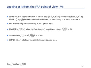
¨ Now here is the cool thing about the Jensen inequality, no matter what is the distribution
for 𝐿:
¨ 𝔼 𝐿5 − 𝔼 𝐿 . 𝔼 𝐿 > 0
160](https://image.slidesharecdn.com/lf2020ratesiii-200825150705/85/Lf-2020-rates_iii-160-320.jpg)


![Luc_Faucheux_2020
Summary - IV
¨ Lower case means that the value is known, or fixed or observed
¨ Upper case means the random variable
¨ At each point in time 𝑡, we observe the discount curve 𝑧𝑐 𝑡, 𝑡, 𝑡Q
¨ At each point in time 𝑡, we observe the bootstrapped discount curve 𝑧𝑐 𝑡, 𝑡A, 𝑡Q
¨ The discount factors 𝑍𝐶 𝑡, 𝑡A, 𝑡Q evolve randomly in time 𝑡 for a given period [𝑡A, 𝑡Q]
¨ The corresponding rates we defined as:
¨ 𝐿 𝑡, 𝑡A, 𝑡Q =
-
, #,#,,#/
. [
-
TU #,#,,#/
− 1]
¨ Also evolves randomly in time 𝑡 for a given period [𝑡A, 𝑡Q]
¨ Note that we have not yet defined any dynamics (normal, lognormal,..) of those variables
yet
193](https://image.slidesharecdn.com/lf2020ratesiii-200825150705/85/Lf-2020-rates_iii-193-320.jpg)
![Luc_Faucheux_2020
Summary - V
¨ 𝐿 𝑡, 𝑡A, 𝑡Q =
-
, #,#,,#/
. [
-
TU #,#,,#/
− 1]
¨ 𝐿 𝑡, 𝑡A, 𝑡Q . 𝜏 𝑡, 𝑡A, 𝑡Q =
-
TU #,#,,#/
. [1 − 𝑍𝐶 𝑡, 𝑡A, 𝑡Q ]
¨ When 𝑡 reaches 𝑡A, the random rate 𝐿 𝑡, 𝑡A, 𝑡Q gets fixed to 𝑙 𝑡 = 𝑡A, 𝑡A, 𝑡Q
¨ (The forward rate becomes fixed to the spot rate)
¨ When 𝑡 reaches 𝑡A, the random discount 𝑍𝐶 𝑡, 𝑡A, 𝑡Q gets fixed to 𝑧𝑐 𝑡 = 𝑡A, 𝑡A, 𝑡Q
¨ Random variables are observed at a given point in time
¨ HOWEVER what matters in Finance is not only the observation (“fixing”) time, but WHEN a
particular payoff function of those random variables is paid.
¨ The fixing time and the payment time do not have to be the same
¨ In fact most of the time they are not
194](https://image.slidesharecdn.com/lf2020ratesiii-200825150705/85/Lf-2020-rates_iii-194-320.jpg)


![Luc_Faucheux_2020
Summary - IX
¨ 𝔼#,
TU
𝑉 𝑡A, $1 𝑡 , 𝑡A, 𝑡Q |𝔉(𝑡) = 𝔼#,
TU
𝑉 𝑡A, $𝑍𝐶(𝑡, 𝑡A, 𝑡Q), 𝑡A, 𝑡A |𝔉(𝑡) = 𝑧𝑐(𝑡, 𝑡A, 𝑡Q)
¨ 𝔼#,
TU 𝑉 𝑡A, $𝐻 𝑡 , 𝑡A, 𝑡Q |𝔉(𝑡) = 𝔼#,
TU 𝑉 𝑡A, $𝐻 𝑡 . 𝑍𝐶(𝑡, 𝑡A, 𝑡Q), 𝑡A, 𝑡A |𝔉(𝑡)
¨ Note that in the case of a general claim that could be a function of the 𝑍𝐶(𝑡, 𝑡A, 𝑡Q), we cannot
split the expectation of the products into a product of expectation
¨ But we can use the covariance formula, which is a useful trick used in Tuckmann book, especially
when computing the forward-future convexity adjustment
¨ 𝐶𝑜𝑣𝑎𝑟 𝑋, 𝑌 = 𝔼{𝑋 − 𝔼 𝑋 }. 𝔼{𝑌 − 𝔼[𝑌]}
¨ 𝐶𝑜𝑣𝑎𝑟 𝑋, 𝑌 = 𝔼[𝑋. 𝑌] − 𝔼 𝑋 . 𝔼 𝑌
¨ So in the above, something we should start getting used to:
¨ 𝔼#,
TU 𝑉 𝑡A, $𝐻 𝑡 . 𝑍𝐶(𝑡, 𝑡A, 𝑡Q), 𝑡A, 𝑡A |𝔉(𝑡) =
𝔼#,
TU 𝑉 𝑡A, $𝐻 𝑡 , 𝑡A, 𝑡A |𝔉(𝑡) . 𝔼#,
TU 𝑉 𝑡A, $𝑍𝐶(𝑡, 𝑡A, 𝑡Q), 𝑡A, 𝑡A |𝔉(𝑡) +
𝐶𝑂𝑉𝐴𝑅{𝑉 𝑡A, $𝐻 𝑡 , 𝑍𝐶(𝑡, 𝑡A, 𝑡Q), 𝑡A, 𝑡A |𝔉(𝑡)}
198](https://image.slidesharecdn.com/lf2020ratesiii-200825150705/85/Lf-2020-rates_iii-198-320.jpg)


Lf 2020 rates_iii
- 1. Luc_Faucheux_2020 THE RATES WORLD – Part III Some more math: Why can we price a swap without knowing the volatility? 1
- 2. Luc_Faucheux_2020 Couple of notes on those slides ¨ Those are part III of the the slides on Rates ¨ Follows part I and II where he introduced concepts of yield curve and swap pricing ¨ Applied to Interest rate model, so uses a lot of materials from other decks (in particular trees, also curve) ¨ This one ties it all together (at least tries to) ¨ In this section we introduce more specifically the concept of measures ¨ The goal again of this deck is NOT to be a formal course in rates modeling (there are tons of good textbooks out there), but to develop the intuition, the notation and the confidence that comes with having a firm grasp to be able to read those textbooks ¨ In particular, by the end of this section, you should have a firm grasp of the notations so that you do not get picked off by convexity and payment timing ¨ Notation a tad of an overkill but found it to be useful, might need some work to read textbooks (but then again not two of them have the same notation anyways) 2
- 3. Luc_Faucheux_2020 Couple of notes on those slides - II ¨ The notation in most textbooks is quite horrendous ¨ It is also not consistent ¨ I have come up over the years with a notation that works for me ¨ Hopefully you can also find it useful ¨ In the end, the closest it is with is the Piterbarg convention ¨ Goal of this section is to introduce this notation, and show how it can be useful, in particular when dealing with confusing things like CMS versus Forward swaps, Libor in arrears versus Libor in advance, terminal measure and so on and so forth (there was someone I knew who kept saying all the time “and so on and so forth”, used to drive me nuts) 3
- 4. Luc_Faucheux_2020 Rates notation and Swaps (summary of part II) 4
- 5. Luc_Faucheux_2020 Notations and conventions in the rates world ¨ The Langevin equation is quite commonly used when modeling interest rates. ¨ Since interest rates are the “speed” or “velocity” of the Money Market Numeraire, it is quite natural to have thought about using the Langevin equation which represents the “speed” of a Brownian particle. ¨ As a result, a number of quantities in Finance are related to the exponential of the integral over time of the short-term rate (instantaneous spot rate) ¨ For example (Fabio Mercurio p. 3), the stochastic discount factor 𝐷(𝑡, 𝑇) between two time instants 𝑡 and 𝑇 is the amount at time 𝑡 that is “equivalent” to one unit of currency payable at time 𝑇, and is equal to ¨ 𝐷 𝑡, 𝑇 = !(#) !(%) = exp(− ∫# % 𝑅 𝑠 . 𝑑𝑠) ¨ The Bank account (Money-market account) is such that: ¨ 𝑑𝐵 𝑡 = 𝑅 𝑡 . 𝐵 𝑡 . 𝑑𝑡 with 𝐵 𝑡 = 0 = 1 ¨ 𝐵 𝑡 = exp(∫& # 𝑅 𝑠 . 𝑑𝑠) 5
- 6. Luc_Faucheux_2020 Notations and conventions in the rates world - II ¨ Mostly following Mercurio’s conventions in the this section. ¨ We can define a very useful quantity: ZCB: Zero Coupon Bond also called pure discount bond. It is a contract that guarantees the holder the payment on one unit of currency at maturity, with no intermediate payment. ¨ 𝑧𝑐 𝑡, 𝑇 is the value of the contract at time 𝑡 ¨ 𝑧𝑐 𝑇, 𝑇 = 1 ¨ Note that 𝑧𝑐 𝑡, 𝑇 is a known quantity at time 𝑡. It is the value of a contract (like a Call option is known, it is no longer a stochastic variable) ¨ On the other hand, ¨ 𝐷 𝑡, 𝑇 = !(#) !(%) = exp(− ∫# % 𝑅 𝑠 . 𝑑𝑠) and 𝐵 𝑡 = exp(∫& # 𝑅 𝑠 . 𝑑𝑠) ¨ Are just functions of 𝑅 𝑠 . If we place ourselves in a situation where the short-term rate 𝑅 𝑠 is a stochastic process then both the MMN (BAN) noted 𝐵 𝑡 (Money market numeraire, or Bank Account Numeraire), as well as the discount factor 𝐷 𝑡, 𝑇 , should not be expected to not be stochastic (unless a very peculiar situation) 6
- 7. Luc_Faucheux_2020 Notations and conventions in the rates world - III ¨ In the case of deterministic short-term rate, there is no stochastic component. ¨ In that case: ¨ 𝐷 𝑡, 𝑇 = 𝑧𝑐 𝑡, 𝑇 ¨ When stochastic, 𝑧𝑐 𝑡, 𝑇 is the expectation of 𝐷 𝑡, 𝑇 , like the Call option price was the expectation of the call payoff. ¨ From the Zero Coupon bond we can define a number of quantities: 7
- 8. Luc_Faucheux_2020 Notations and conventions in the rates world -IV ¨ Continuously compounded spot interest rate: ¨ 𝑟 𝑡, 𝑇 = − '(()*(#,%)) ,(#,%) ¨ Where 𝜏(𝑡, 𝑇) is the year fraction, using whatever convention (ACT/360, ACT/365, 30/360, 30/250,..) and possible holidays calendar we want. In the simplest case: ¨ 𝜏 𝑡, 𝑇 = 𝑇 − 𝑡 ¨ 𝑧𝑐 𝑡, 𝑇 . exp 𝑟 𝑡, 𝑇 . 𝜏 𝑡, 𝑇 = 1 ¨ 𝑧𝑐 𝑡, 𝑇 = exp −𝑟 𝑡, 𝑇 . 𝜏 𝑡, 𝑇 ¨ In the deterministic case: ¨ 𝑧𝑐 𝑡, 𝑇 = exp −𝑟 𝑡, 𝑇 . 𝜏 𝑡, 𝑇 = 𝐷 𝑡, 𝑇 = !(#) !(%) = exp(− ∫# % 𝑅 𝑠 . 𝑑𝑠) ¨ 𝑟 𝑡, 𝑇 = - , #,% . ∫# % 𝑅 𝑠 . 𝑑𝑠 8
- 9. Luc_Faucheux_2020 Notations and conventions in the rates world - V ¨ Simply compounded spot interest rate ¨ 𝑙 𝑡, 𝑇 = - ,(#,%) . -.)*(#,%) )*(#,%) ¨ Or alternatively, in the bootstrap form ¨ 𝜏 𝑡, 𝑇 . 𝑙 𝑡, 𝑇 . 𝑧𝑐 𝑡, 𝑇 = 1 − 𝑧𝑐(𝑡, 𝑇) ¨ 1 + 𝜏 𝑡, 𝑇 . 𝑙 𝑡, 𝑇 . 𝑧𝑐 𝑡, 𝑇 = 1 ¨ 𝑧𝑐 𝑡, 𝑇 = - -/, #,% .1 #,% ¨ In the deterministic case: ¨ 𝑧𝑐 𝑡, 𝑇 = - -/, #,% .1 #,% = 𝐷 𝑡, 𝑇 = !(#) !(%) = exp(− ∫# % 𝑅 𝑠 . 𝑑𝑠) ¨ 𝑙 𝑡, 𝑇 = - , #,% . [1 − exp − ∫# % 𝑅 𝑠 . 𝑑𝑠 ] 9
- 10. Luc_Faucheux_2020 Notations and conventions in the rates world - VI ¨ Annually compounded spot interest rate ¨ 𝑦 𝑡, 𝑇 = - )*(#,%)!/#(%,') − 1 ¨ Or alternatively, in the bootstrap form ¨ (1 + 𝑦 𝑡, 𝑇 ). 𝑧𝑐 𝑡, 𝑇 -/, #,% = 1 ¨ (1 + 𝑦 𝑡, 𝑇 ), #,% . 𝑧𝑐 𝑡, 𝑇 = 1 ¨ 𝑧𝑐 𝑡, 𝑇 = - (-/3 #,% )# %,' ¨ In the deterministic case: ¨ 𝑧𝑐 𝑡, 𝑇 = - (-/3 #,% )# %,' = 𝐷 𝑡, 𝑇 = !(#) !(%) = exp(− ∫# % 𝑅 𝑠 . 𝑑𝑠) 10
- 11. Luc_Faucheux_2020 Notations and conventions in the rates world - VII ¨ 𝑞-times per year compounded spot interest rate ¨ 𝑦4 𝑡, 𝑇 = 4 )*(#,%)!/)#(%,') − 𝑞 ¨ Or alternatively, in the bootstrap form ¨ (1 + - 4 𝑦4 𝑡, 𝑇 ). 𝑧𝑐 𝑡, 𝑇 -/4, #,% = 1 ¨ (1 + - 4 𝑦4 𝑡, 𝑇 )4., #,% . 𝑧𝑐 𝑡, 𝑇 = 1 ¨ 𝑧𝑐 𝑡, 𝑇 = - (-/ ! ) .3) #,% )).# %,' ¨ In the deterministic case: ¨ 𝑧𝑐 𝑡, 𝑇 = - (-/ ! ) .3) #,% )).# %,' = 𝐷 𝑡, 𝑇 = !(#) !(%) = exp(− ∫# % 𝑅 𝑠 . 𝑑𝑠) 11
- 12. Luc_Faucheux_2020 Notations and conventions in the rates world - VIII ¨ In bootstrap form which is the intuitive way: ¨ Continuously compounded spot: 𝑧𝑐 𝑡, 𝑇 = exp −𝑟 𝑡, 𝑇 . 𝜏 𝑡, 𝑇 ¨ Simply compounded spot: 𝑧𝑐 𝑡, 𝑇 = - -/, #,% .1 #,% ¨ Annually compounded spot: 𝑧𝑐 𝑡, 𝑇 = - (-/3 #,% )# %,' ¨ 𝑞-times per year compounded spot 𝑧𝑐 𝑡, 𝑇 = - (-/ ! ) .3) #,% )).# %,' 12
- 13. Luc_Faucheux_2020 Notations and conventions in the rates world - IX ¨ In the small 𝜏 𝑡, 𝑇 → 0 limit (also if the rates themselves are such that they are <<1) ¨ In bootstrap form which is the intuitive way: ¨ Continuously compounded spot: 𝑧𝑐 𝑡, 𝑇 = 1 − 𝑟 𝑡, 𝑇 . 𝜏 𝑡, 𝑇 + 𝒪(𝜏5. 𝑟5) ¨ Simply compounded spot: 𝑧𝑐 𝑡, 𝑇 = 1 − 𝑙 𝑡, 𝑇 . 𝜏 𝑡, 𝑇 + 𝒪(𝜏5. 𝑙5) ¨ Annually compounded spot: 𝑧𝑐 𝑡, 𝑇 = 1 − 𝑦 𝑡, 𝑇 . 𝜏 𝑡, 𝑇 + 𝒪(𝜏5. 𝑦5) ¨ 𝑞-times per year compounded spot 𝑧𝑐 𝑡, 𝑇 = 1 − 𝑦4 𝑡, 𝑇 . 𝜏 𝑡, 𝑇 + 𝒪(𝜏5. 𝑦4 5) ¨ So in the limit of small 𝜏 𝑡, 𝑇 (and also small rates), in particular when 𝑇 → 𝑡, all rates converge to the same limit we call ¨ 𝐿𝑖𝑚 𝑇 → 𝑡 = lim %→# ( -.)* #,% , #,% ) 13
- 14. Luc_Faucheux_2020 Notations and conventions in the rates world - X ¨ In the deterministic case using the continuously compounded spot rate for example: ¨ 𝑧𝑐 𝑡, 𝑇 = exp −𝑟 𝑡, 𝑇 . 𝜏 𝑡, 𝑇 = 𝐷 𝑡, 𝑇 = !(#) !(%) = exp(− ∫# % 𝑅 𝑠 . 𝑑𝑠) ¨ 𝑟 𝑡, 𝑇 = - , #,% . ∫# % 𝑅 𝑠 . 𝑑𝑠 ¨ When 𝑇 → 𝑡, 𝑟 𝑡, 𝑇 → 𝑅(𝑡) ¨ So: 𝐿𝑖𝑚 𝑇 → 𝑡 = lim %→# ( -.)* #,% , #,% ) = 𝑅(𝑡) ¨ So 𝑅(𝑡) can be seen as the limit of all the different rates defined above. ¨ You can also do this using any of the rates defined previously 14
- 15. Luc_Faucheux_2020 Notations and conventions (lower case and UPPER CASE) ¨ I will try to stick to a convention where the the lower case denotes a regular variable, and an upper case denotes a stochastic variable, as in before: ¨ 78(9,#) 7# = − 7 79 [𝑎 𝑡 . 𝑝 𝑥, 𝑡 − 7 79 [ - 5 𝑏 𝑡 5. 𝑝 𝑥, 𝑡 ]] ¨ 𝑋 𝑡: − 𝑋 𝑡; = ∫#<#; #<#: 𝑑𝑋 𝑡 = ∫#<#; #<#: 𝑎(𝑡). 𝑑𝑡) + ∫#<#; #<#: 𝑏(𝑡). 𝑑𝑊(𝑡) ¨ 𝑑𝑋 𝑡 = 𝑎 𝑡 . 𝑑𝑡 + 𝑏(𝑡). 𝑑𝑊 ¨ Where we should really write to be fully precise: ¨ 𝑝 𝑥, 𝑡 = 𝑝=(𝑥, 𝑡|𝑥 𝑡 = 𝑡& = 𝑋&, 𝑡 = 𝑡&) ¨ PDF Probability Density Function: 𝑝=(𝑥, 𝑡) ¨ Distribution function : 𝑃=(𝑥, 𝑡) ¨ 𝑃= 𝑥, 𝑡 = 𝑃𝑟𝑜𝑏𝑎𝑏𝑖𝑙𝑖𝑡𝑦 𝑋 ≤ 𝑥, 𝑡 = ∫3<.> 3<9 𝑝= 𝑦, 𝑡 . 𝑑𝑦 𝑝=(𝑥, 𝑡) = 7 79 𝑃= 𝑥, 𝑡 15
- 16. Luc_Faucheux_2020 Notations and conventions (Spot and forward) ¨ So far we have defined quantities depending on 2 variables in time: ¨ For example, in the case of the continuously compounded spot interest rate: ¨ 𝑟 𝑡, 𝑇 = − '(()*(#,%)) ,(#,%) ¨ It is the constant rate at which an investment of 𝑧𝑐(𝑡, 𝑇) at time 𝑡 accrues continuously to yield 1 unit of currency at maturity 𝑇. ¨ 𝑧𝑐 𝑡, 𝑇 = exp −𝑟 𝑡, 𝑇 . 𝜏 𝑡, 𝑇 ¨ It is observed at time 𝑡 until maturity, hence the naming convention SPOT ¨ CAREFUL: Spot sometimes depending on the markets (US treasury) could mean the settlement of payment (so T+2). A SPOT-starting swap does NOT start today but T+2, subject to London and NY holidays ¨ So different currencies will have different definitions of what SPOT means ¨ ALWAYS CHECK WHAT PEOPLE MEAN BY “SPOT” 16
- 17. Luc_Faucheux_2020 Notations and conventions (Spot and forward) - II ¨ So really we should have expressed: ¨ 𝑧𝑐 𝑡, 𝑇 = exp −𝑟 𝑡, 𝑇 . 𝜏 𝑡, 𝑇 as: ¨ 𝑧𝑐 𝑡, 𝑡, 𝑇 = exp −𝑟 𝑡, 𝑡, 𝑇 . 𝜏 𝑡, 𝑇 ¨ This is a SPOT contract that when entered at time 𝑡 guarantees the payment of one unit of currency at time 𝑇 ¨ To give a quick glance at the numeraire framework, we will say that we choose the Zero Coupon bond as a numeraire to value claims. ¨ In that case the ratio of a claim to that numeraire is a martingale, and in particular at maturity of the contract ¨ 𝔼 - )* %,%,% = ? )*(#,#,%) = 𝔼 - )* %,%,% = 𝔼 - - = 1 since 𝑧𝑐 𝑇, 𝑇, 𝑇 = 1 ¨ So the value of a contract at time 𝑡 that pays 1 at time 𝑇 is: ¨ 𝑝𝑣(𝑡) = 𝑧𝑐(𝑡, 𝑡, 𝑇) 17
- 18. Luc_Faucheux_2020 Notations and conventions (Spot and forward) - III ¨ This can be viewed at obviously simple or very complicated depending how you look at it ¨ In the “deterministic” world of curve building it is quite simple, until you realize that rates do have volatility. ¨ In essence, the question is the following: When pricing swaps and bonds, you only need a yield curve and you do not need to know anything about the dynamics of rates (volatility structure), even though you know that they do move. ¨ Why is that ? ¨ The answer in short, is that you can only do that for products (coincidentally bonds and swaps that are 99% of the gamut of products out there) that are LINEAR as a function of the numeraire which we chose to be the Zero Coupon Bonds, or discount factors. ¨ There is a neat trick that shows that swaps are LINEAR functions of the discount factors ¨ magic trick, 9 -/9 = 9/-.- -/9 = -/9.- -/9 = 1 − - -/9 or more simply: 𝑥 = 𝑥 + 1 − 1 18
- 19. Luc_Faucheux_2020 Notations and conventions (Spot and forward) - VII ¨ Using the extra set on convention we defined, observed at time 𝑡 = 0, all the sets of “simply compounded spot rates” are: ¨ 𝑙 0,0, 𝑇 = - ,(&,&,%) . -.)*(&,&,%) )*(&,&,%) ¨ Or alternatively, in the bootstrap form ¨ 𝑧𝑐 0,0, 𝑇 = - -/, &,&,% .1 &,&,% ¨ TOMORROW at time 𝑡 = 1 we will have a new curve {𝑧𝑐 𝑡 = 1, 𝑡 = 1, 𝑇 } with new spot rates: ¨ 𝑙 1,1, 𝑇 = - ,(-,-,%) . -.)*(-,-,%) )*(-,-,%) ¨ Note that 𝜏(𝑡, 𝑡, 𝑇) is a daycount fraction so should really not depend on the time of observation, 𝜏 𝑡, 𝑡, 𝑇 = 𝜏(𝑡, 𝑇) but to avoid confusion we will keep as is, the first time variable is always the present time 19
- 20. Luc_Faucheux_2020 Notations and conventions (Spot and forward) - VIII ¨ NOW we are absolutely free to compute the following quantities: ¨ Bear in mind that for now those are “just” definitions, we have not said anything linking those quantities to any kind of expectations from a distribution or dynamics ¨ From today’s curve: {𝑧𝑐 𝑡 = 0, 𝑡 = 0, 𝑇 } ¨ We can compute: ¨ 𝑧𝑐 𝑡 = 0, 𝑡 = 𝑡-, 𝑡 = 𝑡5 = 𝑧𝑐 𝑡 = 0, 𝑡 = 0, 𝑡 = 𝑡5 /𝑧𝑐 𝑡 = 0, 𝑡 = 0, 𝑡 = 𝑡- ¨ Of course we have trivially: 𝑧𝑐 𝑡 = 0, 𝑡 = 𝑡-, 𝑡 = 𝑡- ¨ In particular it is useful to define the daily increments: ¨ 𝑧𝑐 𝑡 = 0, 𝑡 = 𝑡-, 𝑡 = 𝑡- + 1 = 𝑧𝑐 𝑡 = 0, 𝑡 = 0, 𝑡 = 𝑡- + 1 /𝑧𝑐 𝑡 = 0, 𝑡 = 0, 𝑡 = 𝑡- ¨ And from those what we will define as the “simply compounded forward rate observed as of today 𝑡 = 0) ¨ 𝑙 0, 𝑡-, 𝑡5 = - ,(&,#!,#+) . -.)*(&,#!,#+) )*(&,#!,#+) 20
- 21. Luc_Faucheux_2020 Notations and conventions (Spot and forward) - IX ¨ 𝑙 0, 𝑡-, 𝑡5 = - ,(&,#!,#+) . -.)*(&,#!,#+) )*(&,#!,#+) ¨ In the bootstrap form: ¨ 𝑧𝑐 0, 𝑡-, 𝑡5 = - -/, &,#!,#+ .1 &,#!,#+ ¨ Using the daily: ¨ 𝑧𝑐 0, 𝑡-, 𝑡- + 1 = - -/, &,#!,#!/- .1 &,#!,#!/- ¨ And since: ¨ 𝑧𝑐 𝑡 = 0, 𝑡 = 𝑡-, 𝑡 = 𝑡- + 1 = 𝑧𝑐 𝑡 = 0, 𝑡 = 0, 𝑡 = 𝑡- + 1 /𝑧𝑐 𝑡 = 0, 𝑡 = 0, 𝑡 = 𝑡- ¨ 𝑧𝑐 𝑡 = 0, 𝑡 = 0, 𝑡 = 𝑡- + 1 = 𝑧𝑐 𝑡 = 0, 𝑡 = 𝑡-, 𝑡 = 𝑡- + 1 ∗ 𝑧𝑐 𝑡 = 0, 𝑡 = 0, 𝑡 = 𝑡- 21
- 22. Luc_Faucheux_2020 Notations and conventions (Spot and forward) - X ¨ 𝑧𝑐 𝑡 = 0, 𝑡 = 0, 𝑡 = 𝑡- + 1 = 𝑧𝑐 𝑡 = 0, 𝑡 = 𝑡-, 𝑡 = 𝑡- + 1 ∗ 𝑧𝑐 𝑡 = 0, 𝑡 = 0, 𝑡 = 𝑡- ¨ So we also have: ¨ 𝑧𝑐 𝑡 = 0, 𝑡 = 0, 𝑡 = 𝑡@ = 𝑧𝑐 𝑡 = 0, 𝑡 = 0, 𝑡 = 0 ∗ ∏A<& A<@ 𝑧𝑐 𝑡 = 0, 𝑡 = 𝑡A, 𝑡 = 𝑡A + 1 ¨ Since: 𝑧𝑐 𝑡 = 0, 𝑡 = 0, 𝑡 = 0 = 1 ¨ Note that we also have: 𝑧𝑐 𝑡 = 0, 𝑡 = 𝑇, 𝑡 = 𝑇 = 1 ¨ 𝑧𝑐 𝑡 = 0, 𝑡 = 0, 𝑡 = 𝑡@ = ∏A<& A<@ 𝑧𝑐 𝑡 = 0, 𝑡 = 𝑡A, 𝑡 = 𝑡A + 1 ¨ 𝑧𝑐 0, 𝑡-, 𝑡- + 1 = - -/, &,#!,#!/- .1 &,#!,#!/- ¨ 𝑧𝑐 𝑡 = 0, 𝑡 = 0, 𝑡 = 𝑡@ = ∏A<& A<@ - -/, &,#,,#,/- .1 &,#,,#,/- 22
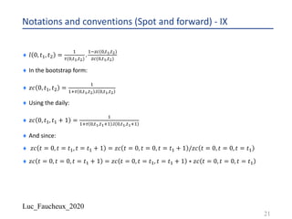
- 23. Luc_Faucheux_2020 Notations and conventions (Spot and forward) - XI ¨ We could also define any kind of buckets: ¨ 𝑧𝑐 𝑡 = 0, 𝑡 = 𝑡8, 𝑡 = 𝑡4 = ∏A<8 A<4 𝑧𝑐 𝑡 = 0, 𝑡 = 𝑡A, 𝑡 = 𝑡A + 1 ¨ 𝑧𝑐 𝑡 = 0, 𝑡8, 𝑡4 = - -/, &,#-,#) .1 &,#-,#) ¨ And so for any joint sequence of buckets, we have the usual bootstrap equation ¨ 𝑧𝑐 𝑡 = 0, 𝑡 = 0, 𝑡 = 𝑡@ = ∏ 𝑧𝑐 𝑡 = 0, 𝑡 = 𝑡8, 𝑡 = 𝑡4 ¨ 𝑧𝑐 𝑡 = 0, 𝑡 = 0, 𝑡 = 𝑡@ = ∏ - -/, &,#-,#) .1 &,#-,#) ¨ Where the successive buckets [𝑡8, 𝑡4] covers the [0, 𝑡@] interval ¨ A picture usually being worth a thousand words: 23
- 24. Luc_Faucheux_2020 Notations and conventions (Spot and forward) - XII 24 𝑧𝑐 0,0,0 = 1 𝑧𝑐 0,0, 𝑡!" = 𝑧𝑐 0,0,0 ∗ 1 1 + 𝜏 0, 𝑡!#, 𝑡!" . 𝑙 0, 𝑡!#, 𝑡!" 𝑡𝑖𝑚𝑒 𝑡 = 0 = 𝑡A& 𝑡A- 𝑡A5 𝑡AL 𝑡AM 𝑧𝑐 0,0, 𝑡!$ = 𝑧𝑐 0,0, 𝑡!" ∗ 1 1 + 𝜏 0, 𝑡!", 𝑡!$ . 𝑙 0, 𝑡!", 𝑡!$ 𝑧𝑐 0,0, 𝑡!% = 𝑧𝑐 0,0, 𝑡!$ ∗ 1 1 + 𝜏 0, 𝑡!$, 𝑡!% . 𝑙 0, 𝑡!$, 𝑡!% 𝑧𝑐 0,0, 𝑡!& = 𝑧𝑐 0,0, 𝑡!% ∗ 1 1 + 𝜏 0, 𝑡!%, 𝑡!& . 𝑙 0, 𝑡!%, 𝑡!&
- 25. Luc_Faucheux_2020 Notations and conventions (Spot and forward) - XIII ¨ 𝑧𝑐 𝑡 = 0, 𝑡 = 0, 𝑡 = 𝑡@ = ∏ - -/, &,#-,#) .1 &,#-,#) ¨ Usually if 𝑡8 < 𝑡4 the daycount fraction is positive (not time traveling yet) ¨ Usually the rates tend to be positive, 𝑙 0, 𝑡8, 𝑡4 > 0 ¨ Note that this is proven to be absolutely wrong recently, but most textbooks still have the usual graph, showing the decrease over time 𝑇 of the quantity 𝑧𝑐 0,0, 𝑇 ¨ This is the famous time value of money principle 25
- 26. Luc_Faucheux_2020 Notations and conventions (Spot and forward) - XIV 26 𝑧𝑐 0,0,0 = 1 𝑧𝑐 0,0, 𝑡!" = 𝑧𝑐 0,0,0 ∗ 1 1 + 𝜏 0, 𝑡!#, 𝑡!" . 𝑙 0, 𝑡!#, 𝑡!" 𝑡𝑖𝑚𝑒 𝑇𝑡 = 0 𝑡A- 𝑡A5 𝑡AL 𝑡AM 𝑧𝑐 0,0, 𝑡!$ = 𝑧𝑐 0,0, 𝑡!" ∗ 1 1 + 𝜏 0, 𝑡!", 𝑡!$ . 𝑙 0, 𝑡!", 𝑡!$ 𝑧𝑐 0,0, 𝑡!% = 𝑧𝑐 0,0, 𝑡!$ ∗ 1 1 + 𝜏 0, 𝑡!$, 𝑡!% . 𝑙 0, 𝑡!$, 𝑡!% 𝑧𝑐 0,0, 𝑡!& = 𝑧𝑐 0,0, 𝑡!% ∗ 1 1 + 𝜏 0, 𝑡!%, 𝑡!& . 𝑙 0, 𝑡!%, 𝑡!& 𝑧𝑐 0,0,0 = 1 𝑧𝑐 0,0, 𝑇 𝑧𝑐 0,0, 𝑇 → ∞ = 0
- 27. Luc_Faucheux_2020 Pricing a swap (slides from part II) 27
- 28. Luc_Faucheux_2020 Pricing a swap on today’s yield curve - VII ¨ LIBOR and SOFR are not the same, and it is going to be interesting to see how one can replace the other, which is something that regulators are keen on ¨ We assume that 𝑙𝑖𝑏𝑜𝑟 𝑡A, 𝑡A, 𝑡A/- = 𝑙 𝑡A, 𝑡A, 𝑡A/- ¨ NOTE that this could be far from being true (in fact the whole reason why regulators want to get rid of LIBOR is because it was subject to manipulations and we deemed not representative of the true borrowing cost) ¨ BUT assuming that 𝑙𝑖𝑏𝑜𝑟 𝑡A, 𝑡A, 𝑡A/- = 𝑙 𝑡A, 𝑡A, 𝑡A/- , the payoff of a single period of the float side of a swap (float-let, or float side of a swap-let), we assume that the payment will be: ¨ 𝜏 𝑡A, 𝑡A, 𝑡A/- . 𝑙 𝑡A, 𝑡A, 𝑡A/- = 𝜏 𝑡A, 𝑡A, 𝑡A/- . - ,(#,,#,,#,.!) . -.)*(#,,#,,#,.!) )*(#,,#,,#,.!) ¨ 𝜏 𝑡A, 𝑡A, 𝑡A/- . 𝑙 𝑡A, 𝑡A, 𝑡A/- = -.)*(#,,#,,#,.!) )*(#,,#,,#,.!) 28
- 29. Luc_Faucheux_2020 Pricing a swap on today’s yield curve - VIII ¨ One more time: ¨ 𝜏 𝑡A, 𝑡A, 𝑡A/- . 𝑙 𝑡A, 𝑡A, 𝑡A/- = -.)*(#,,#,,#,.!) )*(#,,#,,#,.!) ¨ At time 𝑡A, the discounted value of that payment occurring at time 𝑡A/-back to 𝑡A (then present value), will be: ¨ 𝑧𝑐 𝑡A, 𝑡A, 𝑡A/- . 𝜏 𝑡A, 𝑡A, 𝑡A/- . 𝑙 𝑡A, 𝑡A, 𝑡A/- = 1 − 𝑧𝑐(𝑡A, 𝑡A, 𝑡A/-) ¨ This is exactly equal to receiving $1 at time 𝑡A and paying $1 at time 𝑡A/- ¨ It is a linear sum of fixed cash flows ¨ So it can be hedged (replicated) by a portfolio equal to paying $1 at time 𝑡A and receiving $1 at time 𝑡A/- ¨ The price at any point in time of this contract should then ALSO be equal to the price of the replicating portfolio (otherwise there would be arbitrage) 29
- 30. Luc_Faucheux_2020 Pricing a swap on today’s yield curve - IX ¨ And SO we would like to write something like this: at any point in time the value of the replicating portfolio is: ¨ 𝑝𝑣 𝑡A = 1 − 𝑧𝑐(𝑡A, 𝑡A, 𝑡A/-) ¨ 𝑝𝑣 𝑡 < 𝑡A = 𝑧𝑐 𝑡, 𝑡, 𝑡A . (1 − 𝑧𝑐 𝑡A, 𝑡A, 𝑡A/- ) ¨ 𝑝𝑣 𝑡 < 𝑡A = 𝑧𝑐 𝑡, 𝑡, 𝑡A − 𝑧𝑐 𝑡, 𝑡, 𝑡A . 𝑧𝑐 𝑡A, 𝑡A, 𝑡A/- ¨ At time 𝑡, the value of 𝑧𝑐 𝑡, 𝑡, 𝑡A is receiving $1 at time 𝑡A ¨ NOW comes the question: What is 𝑧𝑐 𝑡, 𝑡, 𝑡A . 𝑧𝑐 𝑡A, 𝑡A, 𝑡A/- ? ¨ More crucially, at time 𝑡 we DO NOT KNOW what will be 𝑧𝑐 𝑡A, 𝑡A, 𝑡A/- ¨ SO we cannot really write something like we did above ¨ BUT We also know that this portfolio is also just receiving $1 at time 𝑡A and paying $1 at time 𝑡A/-, and so the present value at time 𝑡 of this portfolio is: ¨ 𝑝𝑣 𝑡 < 𝑡A = 𝑧𝑐 𝑡, 𝑡, 𝑡A − 𝑧𝑐 𝑡, 𝑡, 𝑡A/- 30
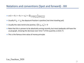
- 31. Luc_Faucheux_2020 Pricing a swap on today’s yield curve - X ¨ IN PARTICULAR the above holds for today’s yield curve ¨ To summarize: ¨ The fixed leg of a swap is easy to price using today’s yield curve, it is a series of fixed and known cash flows ¨ The float leg of a swap is also easy to price as it turns out that for a REGULAR swap (libor rate set at the beginning of the period, paid at the end) the floating cash flow is exactly equal to a replicating portfolio of receiving $1 at the beginning of the period and receiving $1 back at the end of the period ¨ So in most textbooks you might find any of the following graphs (apologies for the poor drawing skills). 31
- 32. Luc_Faucheux_2020 Pricing a swap on today’s yield curve - XI ¨ SWAP FIXED RECEIVE VERSUS REGULAR FLOAT PAY (pay Float, receive Fixed) 32 𝑡𝑖𝑚𝑒 Above the line: We receive Below the line: We pay 𝑡 = 0 𝑡! 𝑋. 𝜏(0, 𝑡A, 𝑡A/-) 𝜏(0, 𝑡A, 𝑡A/-). 𝑙(0, 𝑡A, 𝑡A/-)
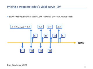
- 33. Luc_Faucheux_2020 Pricing a swap on today’s yield curve - XV ¨ SWAP FIXED RECEIVE VERSUS REGULAR FLOAT PAY (pay Float, receive Fixed) 33 𝑡𝑖𝑚𝑒 $1 $1 𝑋. 𝜏 0, 𝑡A, 𝑡A/- = 𝑋. 𝜏 𝑋. 𝜏 𝑋. 𝜏 𝑋. 𝜏 $1 $1 $1 $1 $1 $1
- 34. Luc_Faucheux_2020 Pricing a swap on today’s yield curve - XXII ¨ 𝑝𝑣_𝑓𝑙𝑜𝑎𝑡 0 = ∑A 𝑙(0, 𝑡A, 𝑡A/-). 𝜏(0, 𝑡A, 𝑡A/-). 𝑧𝑐(0,0, 𝑡A/-) ¨ 𝑝𝑣_𝑓𝑙𝑜𝑎𝑡 0 = ∑A{−𝑧𝑐 0,0, 𝑡A/- + 𝑧𝑐(0,0, 𝑡A)} ¨ 𝑝𝑣_𝑓𝑖𝑥𝑒𝑑 0 = ∑A 𝑋. 𝜏(0, 𝑡A, 𝑡A/-). 𝑧𝑐(0,0, 𝑡A/-) ¨ Note that we assumed that both fixed and float side has same frequency and daycount convention for sake of simplicity. Having different frequency and daycount convention, which is the usual case, does not change anything, only add some more notation (see the deck on the curve) ¨ Note that this is also BEFORE the swap “starts”. Once time passes by, the Floating leg gets set to a fixed amount (BBA LIBOR fixing), and that float swaplet just becomes a simple fixed period 34
- 35. Luc_Faucheux_2020 Pricing a swap on today’s yield curve - XXIII ¨ The Swap Rate is the value of the coupon on the Fixed side such that the present value of the swap is 0 (swap is on market) ¨ 𝑝𝑣_𝑓𝑙𝑜𝑎𝑡 0 = ∑A 𝑙(0, 𝑡A, 𝑡A/-). 𝜏(0, 𝑡A, 𝑡A/-). 𝑧𝑐(0,0, 𝑡A/-) ¨ 𝑝𝑣_𝑓𝑙𝑜𝑎𝑡 0 = ∑A{−𝑧𝑐 0,0, 𝑡A/- + 𝑧𝑐(0,0, 𝑡A)} ¨ 𝑝𝑣_𝑓𝑖𝑥𝑒𝑑 0 = ∑A 𝑋. 𝜏(0, 𝑡A, 𝑡A/-). 𝑧𝑐(0,0, 𝑡A/-) ¨ 𝑝𝑣_𝑓𝑙𝑜𝑎𝑡 0 = 𝑝𝑣_𝑓𝑖𝑥𝑒𝑑 0 = ∑A 𝑆𝑅. 𝜏(0, 𝑡A, 𝑡A/-). 𝑧𝑐(0,0, 𝑡A/-) ¨ 𝑆𝑅(0, 𝑇N, 𝑇O) = ∑, 1(&,#,,#,.!).,(&,#,,#,.!).)*(&,&,#,.!) ∑, ,(&,#,,#,.!).)*(&,&,#,.!) ¨ The Swap Rate is a weighted average of the forward rates 𝑙(0, 𝑡A, 𝑡A/-) for a given start of the swap 𝑇N and maturity 𝑇O 35
- 37. Luc_Faucheux_2020 Summary ¨ The concept of a forward contract is quite central to derivatives valuation. ¨ We have somewhat done it without realizing it in the previous two sections (like Mr Jourdain). ¨ Worth going over it again in a formal manner ¨ Especially important to have the concept of a forward contract down, when we introduce in part IV the concept of a future contract 37
- 38. Luc_Faucheux_2020 Forward contract ¨ On any given day 𝑡 we have a zero-coupon curve 𝑧𝑐(𝑡, 𝑡A, 𝑡Q) ¨ The Zero coupon curve is such that: 𝑧𝑐 𝑡, 𝑡A, 𝑡A = 1 and in particular 𝑧𝑐 𝑡, 𝑡, 𝑡 = 1 ¨ The quantities 𝑧𝑐(𝑡, 𝑡, 𝑡Q) are the price at time 𝑡 of a Zero-Coupon Bond paying $1 at time 𝑡Q ¨ 𝔼 - )* %,%,% |𝑡 = ? )*(#,#,%) = 𝔼 - )* %,%,% |𝑡 = 𝔼 - - |𝑡 = 1 since 𝑧𝑐 𝑇, 𝑇, 𝑇 = 1 ¨ So the value of a contract at time 𝑡 that pays 1 at time 𝑇 is: ¨ 𝑝𝑣(𝑡) = 𝑧𝑐(𝑡, 𝑡, 𝑇) ¨ We can construct by bootstrapping all intermediate quantities 𝑧𝑐(𝑡, 𝑡A, 𝑡Q) ¨ And so for any joint sequence of buckets, we have the usual bootstrap equation ¨ 𝑧𝑐 𝑡 = 0, 𝑡 = 0, 𝑡 = 𝑇 = ∏ 𝑧𝑐 𝑡 = 0, 𝑡 = 𝑡A, 𝑡 = 𝑡Q 38
- 39. Luc_Faucheux_2020 Forward contract - II ¨ We also define the quantities 𝑙 𝑡, 𝑡A, 𝑡Q that we call simply compounded forward rate for the period [𝑡A, 𝑡Q] (observed at time 𝑡) as : ¨ 𝑧𝑐 𝑡, 𝑡A, 𝑡Q = - -/, #,#,,#/ .1 #,#,,#/ ¨ A contract that pays $1 at time 𝑡Q is worth at time 𝑡: ¨ 𝑉_𝑝𝑟𝑖𝑛𝑐𝑖𝑝𝑎𝑙 𝑡 = 𝑧𝑐 𝑡, 𝑡, 𝑡Q ¨ A contract that pays 𝑋% paid on the 𝜏 𝑡, 𝑡A, 𝑡Q daycount convention, on $1 principal amount at time 𝑡Q is worth at time 𝑡: ¨ 𝑉_𝑐𝑜𝑢𝑝𝑜𝑛 𝑡 = 𝑧𝑐 𝑡, 𝑡, 𝑡Q . 𝑋. 𝜏 𝑡, 𝑡A, 𝑡Q 39
- 40. Luc_Faucheux_2020 Forward contract - III ¨ A contract that pays 𝑙 𝑡A, 𝑡A, 𝑡Q paid on the 𝜏 𝑡, 𝑡A, 𝑡Q daycount convention, on $1 principal amount at time 𝑡Q is worth at time 𝑡: ¨ 𝑉_𝑓𝑙𝑜𝑎𝑡 𝑡 = 𝑧𝑐 𝑡, 𝑡, 𝑡Q . 𝑙(𝑡, 𝑡A, 𝑡Q). 𝜏(𝑡, 𝑡A, 𝑡Q) ¨ NOTE: this one is not trivial ¨ It is because as we defined 𝑙(𝑡, 𝑡A, 𝑡Q) as: ¨ 𝑧𝑐 𝑡, 𝑡A, 𝑡Q = - -/, #,#,,#/ .1 #,#,,#/ we have also ¨ 𝑧𝑐 𝑡, 𝑡A, 𝑡Q . 𝑙 𝑡, 𝑡A, 𝑡Q . 𝜏 𝑡, 𝑡A, 𝑡Q = 1 − 𝑧𝑐 𝑡, 𝑡A, 𝑡Q ¨ And ¨ 𝑧𝑐 𝑡, 𝑡, 𝑡Q = 𝑧𝑐 𝑡, 𝑡, 𝑡A . 𝑧𝑐 𝑡, 𝑡A, 𝑡Q ¨ So: 𝑧𝑐 𝑡, 𝑡A, 𝑡Q = )* #,#,#/ )* #,#,#, 40
- 41. Luc_Faucheux_2020 Forward contract - IV ¨ We also defined: ¨ It is because as we defined 𝑙(𝑡A, 𝑡A, 𝑡Q) as: ¨ 𝑧𝑐 𝑡A, 𝑡A, 𝑡Q = - -/, #,,#,,#/ .1 #,,#,,#/ we have also ¨ 𝑧𝑐 𝑡A, 𝑡A, 𝑡Q . 𝑙 𝑡A, 𝑡A, 𝑡Q . 𝜏 𝑡A, 𝑡A, 𝑡Q = 1 − 𝑧𝑐 𝑡A, 𝑡A, 𝑡Q ¨ 𝑧𝑐 𝑡, 𝑡A, 𝑡Q . 𝑙 𝑡, 𝑡A, 𝑡Q . 𝜏 𝑡, 𝑡A, 𝑡Q = 1 − 𝑧𝑐 𝑡, 𝑡A, 𝑡Q ¨ At time 𝑡A, the quantity 𝑙 𝑡A, 𝑡A, 𝑡Q is known and will be “fixed” ¨ At time 𝑡Q, the quantity 𝑙(𝑡A, 𝑡A, 𝑡Q). 𝜏(𝑡A, 𝑡A, 𝑡Q) will be paid out. ¨ It is usually convenient to express this in terms of a FRA agreement (Forward Rate Agreement) with a “floating” leg and a fixed leg. 41
- 42. Luc_Faucheux_2020 Forward contract - V ¨ The forward contract then exchanges two cashflows at time 𝑡Q: ¨ A floating amount that had been fixed at time 𝑡A to 𝑙 𝑡A, 𝑡A, 𝑡Q . 𝜏 𝑡A, 𝑡A, 𝑡Q ¨ A fixed amount that we will call: 𝐾. 𝜏 𝑡A, 𝑡A, 𝑡Q ¨ The payout of the FRA contract at time 𝑡Q is : {𝑙 𝑡A, 𝑡A, 𝑡Q − 𝐾}. 𝜏 𝑡A, 𝑡A, 𝑡Q ¨ We want to compute for time 𝑡 < 𝑡A the value of 𝐾(𝑡) such that the FRA contract has zero value (zero PV) ¨ For 𝑡 = 𝑡A we have 𝐾(𝑡A) = 𝑙 𝑡A, 𝑡A, 𝑡Q ¨ We also have by definition: ¨ 𝑧𝑐 𝑡A, 𝑡A, 𝑡Q . 𝑙 𝑡A, 𝑡A, 𝑡Q . 𝜏 𝑡A, 𝑡A, 𝑡Q = 1 − 𝑧𝑐 𝑡A, 𝑡A, 𝑡Q 42
- 43. Luc_Faucheux_2020 Forward contract - VI ¨ Looks again at the usual graph of a portfolio consisting of a long position ZCB (Zero Coupon Bond) maturing at time 𝑡A, and a short position {1 + 𝐾(𝑡). 𝜏 𝑡A, 𝑡A, 𝑡Q } maturing (paid) at time 𝑡Q 43 𝑡𝑖𝑚𝑒 𝑡! 𝑡" 𝑧𝑐 𝑡, 𝑡Q, 𝑡Q = $1 𝑧𝑐 𝑡, 𝑡A, 𝑡A = $1 𝐾(𝑡). 𝜏 𝑡, 𝑡A, 𝑡Q
- 44. Luc_Faucheux_2020 Forward contract - VII ¨ At time 𝑡A, the payoff 𝑧𝑐 𝑡A, 𝑡A, 𝑡A = $1 is put in a deposit with the then- current interest rate 𝑙 𝑡A, 𝑡A, 𝑡Q for maturity 𝑡Q ¨ At time 𝑡Q, this will have value: ( - )* #,,#,,#/ ) ¨ Remember that: ¨ 𝑧𝑐 𝑡A, 𝑡A, 𝑡Q = - -/, #,,#,,#/ .1 #,,#,,#/ ¨ 𝑧𝑐 𝑡A, 𝑡A, 𝑡Q . 𝑙 𝑡A, 𝑡A, 𝑡Q . 𝜏 𝑡A, 𝑡A, 𝑡Q = 1 − 𝑧𝑐 𝑡A, 𝑡A, 𝑡Q 44
- 45. Luc_Faucheux_2020 Forward contract - VIII ¨ So at time 𝑡Q, the portfolio will have value: ¨ 𝑉 𝑡Q = - )* #,,#,,#/ − 1 − 𝐾(𝑡). 𝜏 𝑡, 𝑡A, 𝑡Q ¨ 𝑉 𝑡Q = 1 + 𝜏 𝑡A, 𝑡A, 𝑡Q . 𝑙 𝑡A, 𝑡A, 𝑡Q − 1 − 𝐾(𝑡). 𝜏 𝑡, 𝑡A, 𝑡Q ¨ 𝑉 𝑡Q = 𝜏 𝑡A, 𝑡A, 𝑡Q . {𝑙 𝑡A, 𝑡A, 𝑡Q − 𝐾 𝑡 } ¨ This portfolio at time 𝑡Q has the same exact payout than the FRA contract we just defined. ¨ This portfolio at time 𝑡 < 𝑡Q has a value: ¨ 𝑉 𝑡 = 𝑧𝑐 𝑡, 𝑡, 𝑡A − 𝑧𝑐 𝑡, 𝑡, 𝑡Q − 𝐾 𝑡 . 𝜏 𝑡, 𝑡A, 𝑡Q . 𝑧𝑐 𝑡, 𝑡, 𝑡Q ¨ This portfolio (which is identical to the FRA contract, and so should have same value at all time from the law of one price), has at time 𝑡 < 𝑡Q a value of 0 when: 45
- 46. Luc_Faucheux_2020 Forward contract - IX ¨ 𝑉 𝑡 = 𝑧𝑐 𝑡, 𝑡, 𝑡A − 𝑧𝑐 𝑡, 𝑡, 𝑡Q − 𝐾 𝑡 . 𝜏 𝑡, 𝑡A, 𝑡Q . 𝑧𝑐 𝑡, 𝑡, 𝑡Q = 0 ¨ 𝐾 𝑡 . 𝜏 𝑡, 𝑡A, 𝑡Q = )* #,#,#, .)* #,#,#/ )* #,#,#/ ¨ 𝐾 𝑡 . 𝜏 𝑡, 𝑡A, 𝑡Q = )* #,#,#, )* #,#,#/ − 1 ¨ )* #,#,#, )* #,#,#/ = 1 + 𝐾 𝑡 . 𝜏 𝑡, 𝑡A, 𝑡Q ¨ 𝑧𝑐 𝑡, 𝑡, 𝑡Q = 𝑧𝑐 𝑡, 𝑡, 𝑡A . - -/R # ., #,#,,#/ ¨ We defined 𝑙(𝑡, 𝑡A, 𝑡Q) as: ¨ 𝑧𝑐 𝑡, 𝑡A, 𝑡Q = 𝑧𝑐 𝑡, 𝑡, 𝑡A . - -/, #,#,,#/ .1 #,#,,#/ 46
- 47. Luc_Faucheux_2020 Forward contract - X ¨ So we have 𝐾 𝑡 = 𝑙 𝑡, 𝑡A, 𝑡Q ¨ It was worth going through that derivation because it can be confusing at times. ¨ Note that really all we said is that the value of the fixed rate 𝐾 𝑡 that is such that the value of receiving 𝐾 𝑡 . 𝜏 𝑡, 𝑡A, 𝑡Q at time 𝑡Q is equal to the value of receiving 𝜏 𝑡A, 𝑡A, 𝑡Q . 𝑙 𝑡A, 𝑡A, 𝑡Q at time 𝑡Q is such that: ¨ 𝐾 𝑡A = 𝑙 𝑡A, 𝑡A, 𝑡Q ¨ 𝐾 𝑡 = 𝑙 𝑡, 𝑡A, 𝑡Q ¨ With the definition from the ZCB curve at time 𝑡 and 𝑡A: ¨ 𝑧𝑐 𝑡, 𝑡A, 𝑡Q = 𝑧𝑐 𝑡, 𝑡, 𝑡A . - -/, #,#,,#/ .1 #,#,,#/ ¨ 𝑧𝑐 𝑡A, 𝑡A, 𝑡Q = 𝑧𝑐 𝑡A, 𝑡A, 𝑡A . - -/, #,,#,,#/ .1 #,,#,,#/ = - -/, #,,#,,#/ .1 #,,#,,#/ 47
- 48. Luc_Faucheux_2020 Forward contract - XI ¨ Note that really all we said is that the value of the fixed rate 𝐾 𝑡 that is such that the value of receiving 𝐾 𝑡 . 𝜏 𝑡, 𝑡A, 𝑡Q at time 𝑡Q is equal to the value of receiving 𝜏 𝑡A, 𝑡A, 𝑡Q . 𝑙 𝑡A, 𝑡A, 𝑡Q at time 𝑡Q is such that: 𝐾 𝑡 = 𝑙 𝑡, 𝑡A, 𝑡Q ¨ We are NOT saying for example that the value of the fixed rate 𝐾 𝑡 that is such that the value of receiving 𝐾 𝑡 . 𝜏 𝑡, 𝑡A, 𝑡Q at time 𝑡A is equal to the value of receiving 𝜏 𝑡A, 𝑡A, 𝑡Q . 𝑙 𝑡A, 𝑡A, 𝑡Q at time 𝑡A is such that: 𝐾 𝑡 = 𝑙 𝑡, 𝑡A, 𝑡Q ¨ This would be wrong as we will see when looking at the arrears/advance issue. ¨ We are also not saying for example that: ¨ 𝔼# 𝑙 𝑡A, 𝑡A, 𝑡Q 𝑡A = 𝑙 𝑡, 𝑡A, 𝑡Q ¨ In a sense the only thing we are saying and using is the following: ¨ 𝔼# $1 𝑡A = 𝑧𝑐 𝑡, 𝑡, 𝑡A ¨ And the nested tower properties that follows 48
- 49. Luc_Faucheux_2020 Forward contract - XII ¨ 𝑧𝑐 𝑡, 𝑡A, 𝑡Q . 𝑙 𝑡, 𝑡A, 𝑡Q . 𝜏 𝑡, 𝑡A, 𝑡Q = 1 − 𝑧𝑐 𝑡, 𝑡A, 𝑡Q ¨ )* #,#,#/ )* #,#,#, . 𝑙 𝑡, 𝑡A, 𝑡Q . 𝜏 𝑡, 𝑡A, 𝑡Q = 1 − )* #,#,#/ )* #,#,#, ¨ 𝑧𝑐 𝑡, 𝑡, 𝑡Q . 𝑙 𝑡, 𝑡A, 𝑡Q . 𝜏 𝑡, 𝑡A, 𝑡Q = 𝑧𝑐 𝑡, 𝑡, 𝑡A − 𝑧𝑐 𝑡, 𝑡, 𝑡Q ¨ Because the contract payoff on the LHS can be expressed as a linear sum of 𝑧𝑐 𝑡, 𝑡, 𝑡A on the RHS, WITHOUT any consideration on the dynamics of the curve, the value of that contract at time 𝑡 is equal to the RHS ¨ NOTE that if the RHS was a non-linear (convex) function of the 𝑧𝑐 𝑡, 𝑡, 𝑡A , this would NOT be true, and there would be a convexity adjustment ¨ NOTE if the timing (the time values) are such that you CANNOT express the contract as a linear functions of the 𝑧𝑐 𝑡, 𝑡, 𝑡A , this would NOT be true and there would be a convexity adjustment ¨ For a “regular” contract we get the famous graph we have been describing at length before : 49
- 50. Luc_Faucheux_2020 Forward contract - XIII ¨ Going back once again to the replicating portfolio of $1 cash flows ¨ At time 𝑡A, the quantity 𝑙 𝑡A, 𝑡A, 𝑡Q is known and fixed ¨ 𝑧𝑐 𝑡A, 𝑡A, 𝑡Q . 𝑙 𝑡A, 𝑡A, 𝑡Q . 𝜏 𝑡, 𝑡A, 𝑡Q = 𝑧𝑐 𝑡A, 𝑡A, 𝑡A − 𝑧𝑐 𝑡A, 𝑡A, 𝑡Q ¨ 𝑧𝑐 𝑡A, 𝑡A, 𝑡Q . 𝑙 𝑡A, 𝑡A, 𝑡Q . 𝜏 𝑡, 𝑡A, 𝑡Q = 1 − 𝑧𝑐 𝑡A, 𝑡A, 𝑡Q ¨ So the portfolio paying 𝑙 𝑡A, 𝑡A, 𝑡Q . 𝜏 𝑡, 𝑡A, 𝑡Q at time 𝑡Q has a present discounted value at time 𝑡A equal to ¨ 𝑉 𝑡A = 𝑧𝑐 𝑡A, 𝑡A, 𝑡Q . 𝑙 𝑡A, 𝑡A, 𝑡Q . 𝜏 𝑡, 𝑡A, 𝑡Q = 1 − 𝑧𝑐 𝑡A, 𝑡A, 𝑡Q ¨ This is also equal to a portfolio receiving $1 at time 𝑡A and paying $1 at time 𝑡Q ¨ The value of that portfolio at time 𝑡 < 𝑡A is thus: ¨ 𝑉 𝑡 = 𝑧𝑐 𝑡, 𝑡, 𝑡A − 𝑧𝑐 𝑡, 𝑡, 𝑡Q 50
- 51. Luc_Faucheux_2020 Forward contract - XIV ¨ 𝑉 𝑡 = 𝑧𝑐 𝑡, 𝑡, 𝑡A − 𝑧𝑐 𝑡, 𝑡, 𝑡Q ¨ Is the value of the portfolio at time 𝑡 that is receiving $1 at time 𝑡A and paying $1 at time 𝑡Q ¨ Because of the “law of one price”, or replication or no arbitrage, this is ALSO the value at time 𝑡 of a portfolio that will pay 𝑙 𝑡A, 𝑡A, 𝑡Q . 𝜏 𝑡, 𝑡A, 𝑡Q at time 𝑡Q, where the quantity 𝑙 𝑡A, 𝑡A, 𝑡Q is STILL unknown at time 𝑡 < 𝑡A ¨ HOWEVER at time 𝑡 < 𝑡A, we have defined the quantity 𝑙 𝑡, 𝑡A, 𝑡Q as the following: ¨ 𝑧𝑐 𝑡, 𝑡, 𝑡Q . 𝑙 𝑡, 𝑡A, 𝑡Q . 𝜏 𝑡, 𝑡A, 𝑡Q = 𝑧𝑐 𝑡, 𝑡, 𝑡A − 𝑧𝑐 𝑡, 𝑡, 𝑡Q ¨ Or using the familiar bootstrap form: ¨ 𝑧𝑐 𝑡, 𝑡, 𝑡Q = 𝑧𝑐 𝑡, 𝑡, 𝑡A . - -/1 #,#,,#/ ., #,#,,#/ ¨ And so the value of the portfolio is also equal to: ¨ 𝑉 𝑡 = 𝑧𝑐 𝑡, 𝑡, 𝑡A − 𝑧𝑐 𝑡, 𝑡, 𝑡Q = 𝑧𝑐 𝑡, 𝑡, 𝑡Q . 𝑙 𝑡, 𝑡A, 𝑡Q . 𝜏 𝑡, 𝑡A, 𝑡Q 51
- 52. Luc_Faucheux_2020 Forward contract - XV ¨ Again, it is quite remarkable that we can compute the present value of a quantity that is not know yet without any consideration to the dynamics or volatility. ¨ This is because not matter what dynamics we choose, the rule of no-arbitrage (law of one price) leaves us no choice for payoffs that can be expressed as a linear function or combination of ($1) cashflows ¨ At time 𝑡 < 𝑡A, we defined somewhat arbitrarily the quantity 𝑙 𝑡, 𝑡A, 𝑡Q as: ¨ 𝑧𝑐 𝑡, 𝑡, 𝑡Q = 𝑧𝑐 𝑡, 𝑡, 𝑡A . - -/1 #,#,,#/ ., #,#,,#/ using the discount curve 𝑧𝑐 𝑡, 𝑡, 𝑡A ¨ At time 𝑡 < 𝑡A, we do now know yet the quantity 𝑙 𝑡A, 𝑡A, 𝑡Q but it will be fixed as: ¨ 𝑧𝑐 𝑡A, 𝑡A, 𝑡Q = 𝑧𝑐 𝑡A, 𝑡A, 𝑡A . - -/, #,,#,,#/ .1 #,,#,,#/ = - -/, #,,#,,#/ .1 #,,#,,#/ using the discount curve 𝑧𝑐 𝑡A, 𝑡A, 𝑡Q 52
- 53. Luc_Faucheux_2020 Forward contract - VXI ¨ We have written essentially: ¨ 𝑉 𝑡 = 𝑧𝑐 𝑡, 𝑡, 𝑡A − 𝑧𝑐 𝑡, 𝑡, 𝑡Q = 𝑧𝑐 𝑡, 𝑡, 𝑡Q . 𝑙 𝑡, 𝑡A, 𝑡Q . 𝜏 𝑡, 𝑡A, 𝑡Q ¨ 𝑉 𝑡A = 𝑧𝑐 𝑡A, 𝑡A, 𝑡Q . 𝑙 𝑡A, 𝑡A, 𝑡Q . 𝜏 𝑡, 𝑡A, 𝑡Q = 1 − 𝑧𝑐 𝑡A, 𝑡A, 𝑡Q ¨ 𝑉 𝑡Q = 𝑙 𝑡A, 𝑡A, 𝑡Q . 𝜏 𝑡, 𝑡A, 𝑡Q = - )* #,,#,,#/ − )* #,,#,,#/ )* #,,#,,#/ = - )* #,,#,,#/ − 1 ¨ The value at time 𝑡 < 𝑡A of a contract paying $1 at time 𝑡A is martingale under the zero coupon numeraire 𝑧𝑐 𝑡, 𝑡, 𝑡A : ¨ ?(#,$-,#,) )* #,#,#, = 𝔼#, ?(#,,$-,#,) )* #,,#,,#, = 𝔼#, ?(#,,$-,#,) - = 1 ¨ The value at time 𝑡 < 𝑡Q of a contract paying $1 at time 𝑡Q is martingale under the zero coupon numeraire 𝑧𝑐 𝑡, 𝑡, 𝑡Q : ¨ ?(#,$-,#/) )* #,#,#/ = 𝔼#/ ?(#,,$-,#/) )* #/,#/,#/ = 𝔼#/ ?(#,,$-,#/) - = 1 53
- 54. Luc_Faucheux_2020 Forward contract - XVII ¨ The value at time 𝑡 < 𝑡A of a contract paying $1 at time 𝑡A is martingale under the zero coupon numeraire 𝑧𝑐 𝑡, 𝑡, 𝑡A : ¨ ?(#,$-,#,) )* #,#,#, = 𝔼#, ?(#,,$-,#,) TU #,,#,,#, = 𝔼#, ?(#,,$-,#,) - = 𝔼#, - - = 𝔼#, 1 = 1 ¨ 𝑉 𝑡, $1, 𝑡A = 𝑧𝑐 𝑡, 𝑡, 𝑡A ¨ The value at time 𝑡 < 𝑡Q of a contract paying $1 at time 𝑡Q is martingale under the zero coupon numeraire 𝑧𝑐 𝑡, 𝑡, 𝑡Q : ¨ ?(#,$-,#/) )* #,#,#/ = 𝔼#/ ?(#/,$-,#/) TU #/,#/,#/ = 𝔼#/ ?(#/,$-,#/) - = 𝔼#, - - = 𝔼#, 1 = 1 ¨ 𝑉 𝑡, $1, 𝑡Q = 𝑧𝑐 𝑡, 𝑡, 𝑡Q ¨ Note that we are starting to refine the notation 𝑉 𝑡, $1, 𝑡Q 54
- 55. Luc_Faucheux_2020 Forward contract - XVIII ¨ The value at time 𝑡A < 𝑡Q of a contract paying $1 at time 𝑡Q is martingale under the zero coupon numeraire 𝑧𝑐 𝑡A, 𝑡A, 𝑡Q : ¨ ?(#,,$-,#/) )* #,,#,,#/ = 𝔼#/ ?(#/,$-,#/) TU #/,#/,#/ = 𝔼#/ ?(#/,$-,#/) - = 1 ¨ 𝑉(𝑡A, $1, 𝑡Q) = 𝑧𝑐 𝑡A, 𝑡A, 𝑡Q ¨ And then we can estimate the value of a portfolio resulting in any linear combinations of those quantities ¨ Again, apologies if that seems obvious, but time and time again people get confused, usually because the timing of the payoff is different (arrears/advance), or the payoff itself is not a linear function (options, future contract,..) 55
- 56. Luc_Faucheux_2020 Forward contract – XVIII - a ¨ Note that we are starting to refine the notation 𝑉 𝑡, $1, 𝑡Q ¨ 𝑉 𝑡 = 𝑉 𝑡, $1, 𝑡Q 56 𝑃𝑎𝑖𝑑 𝑎𝑡 𝑡𝑖𝑚𝑒 𝑡Q 𝑃𝑎𝑦𝑜𝑓𝑓 𝑓𝑢𝑛𝑐𝑡𝑖𝑜𝑛 (𝑖𝑛 𝑡ℎ𝑖𝑠 𝑐𝑎𝑠𝑒 $1) 𝑉𝑎𝑙𝑢𝑒 𝑜𝑓 𝑡ℎ𝑒 𝑝𝑎𝑦𝑜𝑓𝑓 𝑜𝑏𝑠𝑒𝑟𝑣𝑒𝑑 𝑎𝑡 𝑡𝑖𝑚𝑒 𝑡
- 57. Luc_Faucheux_2020 Forward contract - XIX ¨ 𝑉 𝑡 = 𝑧𝑐 𝑡, 𝑡, 𝑡Q . 𝑙 𝑡, 𝑡A, 𝑡Q . 𝜏 𝑡, 𝑡A, 𝑡Q ¨ 𝑉 𝑡A = 𝑧𝑐 𝑡A, 𝑡A, 𝑡Q . 𝑙 𝑡A, 𝑡A, 𝑡Q . 𝜏 𝑡, 𝑡A, 𝑡Q ¨ 𝑉 𝑡Q = 𝑙 𝑡A, 𝑡A, 𝑡Q . 𝜏 𝑡, 𝑡A, 𝑡Q since 𝑧𝑐 𝑡Q, 𝑡Q, 𝑡Q = 1 ¨ Assuming that the forward rates do obey some dynamics and are random, we can start to familiarize ourselves with the following notation, and start following the rule that we should always use the numeraire that sets to 1 at payoff (terminal measure), NOT at fixing, and for simplicity, starting to just use 𝜏 𝑡, 𝑡A, 𝑡Q = 𝜏 ¨ ?(#) )* #,#,#/ = 𝔼#/ V #,,#,,#/ ., TU #/,#/,#/ = 𝔼#/ 𝐿 𝑡A, 𝑡A, 𝑡Q . 𝜏 = 𝑙 𝑡, 𝑡A, 𝑡Q . 𝜏 ¨ 𝑉 𝑡 = 𝑉(𝑡, $𝐿 𝑡, 𝑡A, 𝑡Q . 𝜏, 𝑡Q) ¨ ?(#,$V #,#,,#/ .,,#/) )* #,#,#/ = 𝔼#/ ?(#/,$V #,,#,,#/ .,,#/) TU #/,#/,#/ = 𝔼#/ ?(#/,$1 #,,#,,#/ .,,#/) - = 𝑙 𝑡, 𝑡A, 𝑡Q . 𝜏 57
- 58. Luc_Faucheux_2020 Forward contract - XX ¨ HOWEVER ¨ ?(#) )* #,#,#, = 𝔼#, V #,,#,,#/ ., TU #,,#,,#/ = 𝔼#, V #,,#,,#/ ., -/V #,,#,,#/ ., = ?(#,) )* #,,#,,#, = 𝑉 𝑡A ¨ 𝔼#, V #,,#,,#/ ., -/V #,,#,,#/ ., = 𝑧𝑐 𝑡, 𝑡A, 𝑡Q . 𝑙 𝑡, 𝑡A, 𝑡Q . 𝜏 = 1 #,#,,#/ ., -/1 #,#,,#/ ., ¨ SO THE ONLY THING THAT I CAN SAY IS: ¨ 𝔼#, V #,,#,,#/ ., -/V #,,#,,#/ ., = 1 #,#,,#/ ., -/1 #,#,,#/ ., ¨ AND ABSOLUTELY NOT: ¨ 𝔼#, 𝐿 𝑡A, 𝑡A, 𝑡Q = 𝑙 𝑡, 𝑡A, 𝑡Q ¨ It is always useful when confused to always goes back to this 58
- 59. Luc_Faucheux_2020 Forward contract - XXI ¨ 𝔼#, V #,,#,,#/ ., -/V #,,#,,#/ ., = 1 #,#,,#/ ., -/1 #,#,,#/ ., ¨ 𝔼#, V #,,#,,#/ ., -/V #,,#,,#/ ., = 𝔼#, V #,,#,,#/ .,/-.- -/V #,,#,,#/ ., = 𝔼#, 1 − - -/V #,,#,,#/ ., = 1 − 𝔼#, - -/V #,,#,,#/ ., ¨ 1 #,#,,#/ ., -/1 #,#,,#/ ., = 1 #,#,,#/ .,/-.- -/1 #,#,,#/ ., = 1 − - -/1 #,#,,#/ ., ¨ 𝔼#, - -/V #,,#,,#/ ., |𝔉(𝑡) = - -/1 #,#,,#/ ., where 𝔉(𝑡) indicates the filtration at time 𝑡, knowledge of the world at time 𝑡, so essentially the discount curve 𝑧𝑐 𝑡, 𝑡A, 𝑡A ¨ Which illustrates even more poignantly the fact that the expectation of the discount factors are conserved, not the expectation of the forward rates. ¨ No matter what dynamics we use for 𝐿 𝑡, 𝑡A, 𝑡Q , it will have to respect the arbitrage conditions above. 59
- 60. Luc_Faucheux_2020 Forward contract - XXII ¨ To be even more precise: ¨ 𝔼#<#, - -/V #<#,,#,,#/ ., |𝔉(𝑡) = - -/1 #,#,,#/ ., ¨ To illustrate that the period [𝑡A, 𝑡Q] is fixed and the random variable is 𝐿 𝑡, 𝑡A, 𝑡Q , that will fix at time 𝑡A to 𝑙 𝑡A, 𝑡A, 𝑡Q , and will be set as an historical set to 𝑙 𝑡A, 𝑡A, 𝑡Q ¨ 𝐿 𝑡, 𝑡A, 𝑡Q = 𝑙 𝑡A, 𝑡A, 𝑡Q for all time 𝑡 > 𝑡A 60
- 61. Luc_Faucheux_2020 Terminal and Forward measures 61
- 62. Luc_Faucheux_2020 Terminal and Forward measures ¨ Terminal measure and Forward measure. ¨ You sometimes encounter those terms in textbooks. ¨ They both mean 𝔼#/ to crudely simplify ¨ ” 𝑡Q -terminal” because that is when the payoff is paid out, and where 𝑍𝐶 𝑡Q, 𝑡Q, 𝑡Q = 1, making the integration over the distribution simpler ¨ “𝑡Q -forward” because under that measure (and only this one), the simply compounded forward rate 𝐿 𝑡A, 𝑡A, 𝑡Q is a martingale ¨ 𝔼#/ 𝐿 𝑡A, 𝑡A, 𝑡Q |𝔉(𝑡) = 𝑙 𝑡, 𝑡A, 𝑡Q ¨ Note that: ¨ 𝔼#, - -/V #,,#,,#/ ., |𝔉(𝑡) = - -/1 #,#,,#/ ., 62
- 63. Luc_Faucheux_2020 Terminal and Forward measures - II ¨ Let’s convince ourselves once again that the forward measure is aptly named: ¨ (Cent fois sur le metier remettez votre ouvrage…) ¨ 𝔼#/ 𝐿 𝑡A, 𝑡A, 𝑡Q |𝔉(𝑡) = 𝑙 𝑡, 𝑡A, 𝑡Q ¨ More specifically this is the expectation under the measure associated with the zero-coupon bond numeraire 𝑍𝐶 𝑡Q, 𝑡Q, 𝑡Q = 1, so sometimes noted for sake of precision and completeness: ¨ 𝔼#/ TU 𝐿 𝑡A, 𝑡A, 𝑡Q |𝔉(𝑡) = 𝑙 𝑡, 𝑡A, 𝑡Q ¨ We are now almost to the point where what we are writing looks serious and what we could find in a textbook, but we slowly built it to make sure that we have a firm ground to stand on ¨ Took us a couple hundred slides, but we almost finally now have a notation that is almost complete ¨ Because we built it gradually, hopefully by now you have a good intuition of what it is, and will not be scared when you encounter something like that in the first few pages of a textbook on quantitative finances 63
- 64. Luc_Faucheux_2020 Terminal and Forward measures - III ¨ 𝔼#/ TU 𝐿 𝑡A, 𝑡A, 𝑡Q |𝔉(𝑡) = 𝑙 𝑡, 𝑡A, 𝑡Q ¨ Let’s look at claim payoff paid at time 𝑡Q: ¨ 𝑉 𝑡Q = 𝑙 𝑡A, 𝑡A, 𝑡Q . 𝜏 𝑡, 𝑡A, 𝑡Q = 𝑙 𝑡A, 𝑡A, 𝑡Q . 𝜏 ¨ At time 𝑡Q, the quantity 𝑙 𝑡A, 𝑡A, 𝑡Q is known ¨ Actually it is known at time: 𝑡A < 𝑡Q ¨ Up until time 𝑡A, so for time 𝑡 < 𝑡A, it is a random variable 𝐿 𝑡, 𝑡A, 𝑡Q ¨ Up until time 𝑡A, so for time 𝑡 < 𝑡A, we can always define from the discount curve at time t a quantity 𝑙(𝑡, 𝑡A, 𝑡Q) defined by: ¨ 𝑧𝑐 𝑡, 𝑡, 𝑡Q = 𝑧𝑐 𝑡, 𝑡, 𝑡A . - -/1 #,#,,#/ ., #,#,,#/ = 𝑧𝑐 𝑡, 𝑡, 𝑡A . - -/1 #,#,,#/ ., 64
- 65. Luc_Faucheux_2020 Terminal and Forward measures - IV ¨ The claim payoff paid at time 𝑡Q: ¨ 𝑉 𝑡Q = 𝑙 𝑡A, 𝑡A, 𝑡Q . 𝜏 𝑡, 𝑡A, 𝑡Q = 𝑙 𝑡A, 𝑡A, 𝑡Q . 𝜏 ¨ Which again is equal to: ¨ 𝑉 𝑡Q = 𝑙 𝑡A, 𝑡A, 𝑡Q . 𝜏 𝑡, 𝑡A, 𝑡Q = - )* #,,#,,#/ − )* #,,#,,#/ )* #,,#,,#/ = - )* #,,#,,#/ − 1 ¨ It is at time 𝑡Q > 𝑡A the value of receiving a fixed and known quantity at time 𝑡A ¨ 𝔼#/ TU 1|𝔉(𝑡) = 𝑧𝑐 𝑡, 𝑡, 𝑡Q because $1 is a tradeable asset (you need to be able to trade assets in order to create a portfolio and in particular a replicating portfolio in order to create the law of one price, or no arbitrage. If you cannot trade the asset, the whole discussion is rather pointless). ¨ The claim that pays $1 at time 𝑡Q is a martingale under the zero-coupon associated measure, and its value at time 𝑡 is 65
- 66. Luc_Faucheux_2020 Terminal and Forward measures - V ¨ ?(#,$-,#/) )* #,#,#/ = 𝔼#/ ?(#/,$-,#/) TU #/,#/,#/ = 𝔼#/ ?(#/,$-,#/) - = 𝔼#/ - - = 𝔼#/ 1 = 1 ¨ 𝑉 𝑡, $1, 𝑡Q = 𝑧𝑐 𝑡, 𝑡, 𝑡Q ¨ Similarly the payoff that returns - )* #,,#,,#/ at time 𝑡Q is equivalent to returning $1 at time 𝑡A and investing it until 𝑡Q ¨ ?(#,$-,#,) )* #,#,#/ = ?(#,$-,#,) )* #,#,#, .)* #,#,,#/ = - )* #,#,,#/ . 𝔼#, ?(#,,$-,#,) TU #,,#,,#, = - )* #,#,,#/ ¨ 𝑉 𝑡, $1, 𝑡A = )* #,#,#/ )* #,#,,#/ = 𝑧𝑐 𝑡, 𝑡, 𝑡A 66
- 67. Luc_Faucheux_2020 Terminal and Forward measures - VI ¨ Note that the reason why seem to be harping over the same thing ad nauseam, is because with the current LIBOR/SOFR transition for example, there will not be any longer a “regular” swap, and in essence even a swap becomes a path dependent Asian option. ¨ SO it is crucial that we get a firm understanding that we can build on ¨ Note that the theory of how to price SOFR swaps for example is still very much so being worked out right now, with papers from Pieterbag for example in Risk Magazine ¨ The confusing thing in Finance as opposed to say usual stochastic processes, is that what matters is not only when 𝑋(𝑡) is being observed and is fixed at 𝑥(𝑡), BUT ALSO and more importantly when it is getting paid (when it can be replicated or offset with a portfolio of simple cash flows, if that is possible) ¨ In many ways, regular stochastic processes in Physics for example do not have this added layer of complexity, the stochastic variable 𝑋(𝑡) is being observed at time 𝑡, period. There is no concept of “observed at time 𝑡 and paid at another time 𝑇 in the future” 67
- 68. Luc_Faucheux_2020 Terminal and Forward measures - VII ¨ 𝑉 𝑡Q = 𝑙 𝑡A, 𝑡A, 𝑡Q . 𝜏 𝑡, 𝑡A, 𝑡Q = 𝑙 𝑡A, 𝑡A, 𝑡Q . 𝜏 ¨ 𝑉 𝑡Q, $𝑙 𝑡A, 𝑡A, 𝑡Q . 𝜏, 𝑡Q = 𝑙 𝑡A, 𝑡A, 𝑡Q . 𝜏 𝑡, 𝑡A, 𝑡Q = 𝑙 𝑡A, 𝑡A, 𝑡Q . 𝜏 ¨ 𝑙 𝑡A, 𝑡A, 𝑡Q . 𝜏 = - )* #,,#,,#/ − 1 ¨ 𝑉 𝑡Q, $𝑙 𝑡A, 𝑡A, 𝑡Q . 𝜏, 𝑡Q = 𝑉 𝑡Q, $1, 𝑡A − 𝑉 𝑡Q, $1, 𝑡Q 68 𝑡! 𝑡" = 0
- 69. Luc_Faucheux_2020 Terminal and Forward measures - VIII ¨ 𝑉 𝑡Q, $𝑙 𝑡A, 𝑡A, 𝑡Q . 𝜏, 𝑡Q = 𝑉 𝑡Q, $1, 𝑡A − 𝑉 𝑡Q, $1, 𝑡Q ¨ 𝑉 𝑡Q, $1, 𝑡Q = 1 ¨ 𝑉 𝑡Q, $1, 𝑡A = - )* #,,#,,#/ ¨ 𝑉 𝑡Q, $𝑙 𝑡A, 𝑡A, 𝑡Q . 𝜏, 𝑡Q = - )* #,,#,,#/ − 1 69
- 70. Luc_Faucheux_2020 Terminal and Forward measures - IX ¨ 𝑉 𝑡A, $𝑙 𝑡A, 𝑡A, 𝑡Q . 𝜏, 𝑡Q = 𝑉 𝑡A, $1, 𝑡A − 𝑉 𝑡A, $1, 𝑡Q ¨ 𝑉 𝑡A, $1, 𝑡A = 1 ¨ ?(#,,$-,#/) )* #,,#,,#/ = 𝔼#/ ?(#/,$-,#/) TU #/,#/,#/ = 𝔼#/ ?(#/,$-,#/) - = 𝔼#/ - - = 𝔼#/ 1 = 1 ¨ 𝑉 𝑡A, $1, 𝑡Q = 𝑧𝑐 𝑡A, 𝑡A, 𝑡Q ¨ 𝑉 𝑡A, $𝑙 𝑡A, 𝑡A, 𝑡Q . 𝜏, 𝑡Q = 1 − 𝑧𝑐 𝑡A, 𝑡A, 𝑡Q 70
- 71. Luc_Faucheux_2020 Terminal and Forward measures - X ¨ 𝑉 𝑡, $𝑙 𝑡A, 𝑡A, 𝑡Q . 𝜏, 𝑡Q = 𝑉 𝑡, $1, 𝑡A − 𝑉 𝑡, $1, 𝑡Q ¨ ?(#,$-,#/) )* #,#,#/ = 𝔼#/ ?(#/,$-,#/) TU #/,#/,#/ = 𝔼#/ ?(#/,$-,#/) - = 𝔼#/ - - = 𝔼#/ 1 = 1 ¨ 𝑉 𝑡, $1, 𝑡Q = 𝑧𝑐 𝑡, 𝑡, 𝑡Q ¨ ?(#,$-,#,) )* #,#,#, = 𝔼#, ?(#,,$-,#,) TU #,,#,,#, = 𝔼#, ?(#,,$-,#,) - = 𝔼#, - - = 𝔼#, 1 = 1 ¨ 𝑉 𝑡, $1, 𝑡A = 𝑧𝑐 𝑡, 𝑡, 𝑡A ¨ 𝑉 𝑡, $𝑙 𝑡A, 𝑡A, 𝑡Q . 𝜏, 𝑡Q = 𝑧𝑐 𝑡, 𝑡, 𝑡A − 𝑧𝑐 𝑡, 𝑡, 𝑡Q 71
- 72. Luc_Faucheux_2020 Terminal and Forward measures - XI ¨ 𝑉 𝑡, $𝑙 𝑡A, 𝑡A, 𝑡Q . 𝜏, 𝑡Q = 𝑧𝑐 𝑡, 𝑡, 𝑡A − 𝑧𝑐 𝑡, 𝑡, 𝑡Q ¨ ? #,$1 #,,#,,#/ .,,#/ )* #,#,#/ = )* #,#,#, )* #,#,#/ − 1 ¨ 𝑧𝑐 𝑡, 𝑡, 𝑡Q = 𝑧𝑐 𝑡, 𝑡, 𝑡A . - -/1 #,#,,#/ ., ¨ ? #,$1 #,,#,,#/ .,,#/ )* #,#,#/ = 1 + 𝑙 𝑡, 𝑡A, 𝑡Q . 𝜏 − 1 = 𝑙 𝑡, 𝑡A, 𝑡Q . 𝜏 ¨ ? #,$1 #,,#,,#/ .,,#/ )* #,#,#/ = 𝔼#/ TU ? #/,$1 #,,#,,#/ .,,#/ TU #/,#/,#/ |𝔉(𝑡) = 𝔼#/ TU ? #/,$1 #,,#,,#/ .,,#/ - |𝔉(𝑡) ¨ ? #,$V #,,#,,#/ .,,#/ )* #,#,#/ = 𝔼#/ TU 𝑉 𝑡Q, $𝐿 𝑡A, 𝑡A, 𝑡Q . 𝜏, 𝑡Q |𝔉(𝑡) = 𝑙 𝑡, 𝑡A, 𝑡Q . 𝜏 72
- 73. Luc_Faucheux_2020 Terminal and Forward measures - XII ¨ 𝔼#/ TU 𝑉 𝑡Q, $𝐿 𝑡A, 𝑡A, 𝑡Q . 𝜏, 𝑡Q |𝔉(𝑡) = 𝑙 𝑡, 𝑡A, 𝑡Q . 𝜏 ¨ 𝔼#/ TU 𝑉 𝑡Q, $𝐿 𝑡A, 𝑡A, 𝑡Q , 𝑡Q |𝔉(𝑡) = 𝑙 𝑡, 𝑡A, 𝑡Q ¨ This is why people refer to it as the “Forward measure” ¨ But you have to be careful ¨ 1) that measure is the one associated to the zero coupon numeraire so there is a discounting ¨ 2) that is true only at the end of the period (terminal) ¨ So it ALWAYS pays out to over-notify for a while (with whether or not the variable had been fixed, the observation time, the payment time, the $ to indicate that this is a claim payoff, maybe even specify using the claim value 𝑉 𝑡Q, $𝐿 𝑡A, 𝑡A, 𝑡Q , 𝑡Q 73
- 74. Luc_Faucheux_2020 Early and Discount measure 74
- 75. Luc_Faucheux_2020 Early and discount measure ¨ The Terminal measure and Forward measure was essentially 𝔼#/ to crudely simplify ¨ I do not know what is the name for the 𝔼#, , where you estimate at the beginning of the period and not at the end, haven’t found a textbook that actually defines it. ¨ So if 𝔼#/ is called “Terminal” or “𝑡Q-terminal” or “forward” measure (because any simply compounded forward rate spanning a time interval ending in 𝑡Q is martingale under the 𝑡Q- terminal or 𝑡Q-forward measure, associated with the 𝑍𝐶 𝑡, 𝑡, 𝑡Q numeraire) ¨ Maybe we can call the 𝔼#, the “early” or “discount” measure ¨ Or we can keep on calling it the “𝑡A-terminal” measure, associated with the 𝑍𝐶 𝑡, 𝑡, 𝑡A numeraire ¨ Always better to over-specify to make sure that we are working in the right measure 75
- 76. Luc_Faucheux_2020 Early and discount measure - II ¨ I like it better than the usual terminal measure because the estimation point coincides with the fixing of the forward rates. ¨ It is also the one you have to use when pricing claims in a tree method going backward in the tree (Mercurio p.38) ¨ Suppose that you have a payoff based on the rate 𝐿 𝑡, 𝑡A, 𝑡Q that sets at time 𝑡A and pays at time 𝑡Q ¨ You value this payoff 𝑉 𝑡, $𝐹𝑈𝑁𝐶𝑇𝐼𝑂𝑁{𝐿 𝑡, 𝑡A, 𝑡Q }, 𝑡Q using a tree that you have calibrated and doing backward method: you calculate the claim payoff on the final nodes in the tree and then proceed to discount backward in the tree until the unique node at the origin of the tree ¨ This is where the issue arises because the rate 𝐿 𝑡, 𝑡A, 𝑡Q was fixed to 𝑙 𝑡A, 𝑡A, 𝑡Q at time 𝑡A ¨ And so going backward would require the knowledge at time 𝑡Q of quantities that are only known at time 𝑡A 76
- 77. Luc_Faucheux_2020 Early and discount measure - III 77 𝑡" 𝑡! 𝑡𝑖𝑚𝑒
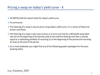
- 78. Luc_Faucheux_2020 Early and discount measure - IV 78 𝑡" 𝑡! 𝑡𝑖𝑚𝑒 𝐿 𝑡, 𝑡0, 𝑡1 sets at time 𝑡0 and spans the period [𝑡0, 𝑡1]
- 79. Luc_Faucheux_2020 Early and discount measure - V ¨ At time 𝑡A at each node in the tree we know the value 𝑙 𝑡A, 𝑡A, 𝑡Q ¨ However proceeding forward to 𝑡Q which is where the payoff occurs (in a regular swap, caplet,..so that we can value this payoff without consideration to the dynamics of the rates), on any given node we do not know what value of 𝑙 𝑡A, 𝑡A, 𝑡Q to use. ¨ This is the problem using the 𝑡Q-terminal or forward measure in practice. 79
- 80. Luc_Faucheux_2020 Early and discount measure - VI ¨ The tower property (to summarize what it is when applied in time, until you know, you don’t know, after you know you know) ¨ General Tower property: ¨ 𝔼 𝑋 = 𝔼(𝔼 𝑋 𝑌 ) ¨ If we are in the case where 𝑌 = 𝑌A is “countable” ¨ 𝔼 𝑋 = ∑A 𝔼 𝑋 𝑌A . 𝑃(𝑌A) 80
- 81. Luc_Faucheux_2020 Early and discount measure - VII ¨ For the uniquely defined payoffs we have the following: ¨ 𝔼#/ TU 𝑉 𝑡Q, $𝐿 𝑡A, 𝑡A, 𝑡Q , 𝑡Q |𝔉(𝑡) = 𝑙 𝑡, 𝑡A, 𝑡Q ¨ 𝔼#, TU 𝑉 𝑡A, $ V #,,#,,#/ ., -/V #,,#,,#/ ., , 𝑡A |𝔉(𝑡) = 1 #,#,,#/ ., -/1 #,#,,#/ ., ¨ 𝔼#, TU 𝑉 𝑡A, $ - -/V #,,#,,#/ ., , 𝑡A |𝔉(𝑡) = - -/1 #,#,,#/ ., ¨ For a more general payoff function $𝐻(𝑡) assumed that we can measure (compute it) at time 𝑡A ¨ 𝔼#, TU 𝑉 𝑡A, $𝐻(𝑡A), 𝑡Q |𝔉(𝑡) = 𝔼#, TU 𝑉 𝑡A, $𝐻 𝑡A . 𝑍𝐶(𝑡 = 𝑡A, 𝑡 = 𝑡A, 𝑡Q , 𝑡A|𝔉(𝑡) 81
- 82. Luc_Faucheux_2020 Early and discount measure - VIII ¨ In particular, since: ¨ 𝑍𝐶 𝑡, 𝑡, 𝑡Q = - -/V #,#,#/ ., ¨ 𝔼#, TU 𝑉 𝑡A, $1, 𝑡Q |𝔉(𝑡) = 𝔼#, TU 𝑉 𝑡A, $1. 𝑍𝐶(𝑡 = 𝑡A, 𝑡 = 𝑡A, 𝑡Q , 𝑡A|𝔉(𝑡) ¨ 𝔼#, TU 𝑉 𝑡A, $1, 𝑡Q |𝔉(𝑡) = 𝔼#, TU 𝑉 𝑡A, $ - -/V #<#,,#<#,,#/ ., , 𝑡A|𝔉(𝑡) ¨ And since: ¨ 𝔼#, TU 𝑉 𝑡A, $ - -/V #,,#,,#/ ., , 𝑡A |𝔉(𝑡) = - -/1 #,#,,#/ ., ¨ 𝔼#, TU 𝑉 𝑡A, $1, 𝑡Q |𝔉(𝑡) = - -/1 #,#,,#/ ., 82
- 83. Luc_Faucheux_2020 Early and discount measure - IX ¨ Similarly ¨ 𝔼#, TU 𝑉 𝑡A, $𝐿 𝑡 = 𝑡A, 𝑡 = 𝑡A, 𝑡Q . 𝜏, 𝑡Q |𝔉(𝑡) = 𝔼#, TUo p 𝑉q r 𝑡A, $𝐿 𝑡 = 𝑡A, 𝑡 = 𝑡A, 𝑡Q . 𝜏. 𝑍𝐶(𝑡 = 𝑡A, 𝑡 = 𝑡A, 𝑡Q , 𝑡A|𝔉(𝑡) ¨ 𝔼#, TU 𝑉 𝑡A, $𝐿 𝑡A, 𝑡A, 𝑡Q . 𝜏, 𝑡Q |𝔉(𝑡) = 𝔼#, TU 𝑉(𝑡A, $ V #,,#,,#/ ., -/V #,,#,,#/ ., , 𝑡A)|𝔉(𝑡) ¨ And since ¨ 𝔼#, TU 𝑉 𝑡A, $ V #,,#,,#/ ., -/V #,,#,,#/ ., , 𝑡A |𝔉(𝑡) = 1 #,#,,#/ ., -/1 #,#,,#/ ., ¨ 𝔼#, TU 𝑉 𝑡A, $𝐿 𝑡A, 𝑡A, 𝑡Q . 𝜏, 𝑡Q |𝔉(𝑡) = 𝔼#, TU 𝑉(𝑡A, $ V #,,#,,#/ ., -/V #,,#,,#/ ., , 𝑡A)|𝔉(𝑡) = 1 #,#,,#/ ., -/1 #,#,,#/ ., 83
- 85. Luc_Faucheux_2020 Summary - I ¨ Again, to be really precise, we should really write for example: ¨ 𝑉 𝑡, $𝐿 𝑡A, 𝑡A, 𝑡Q , 𝑡Q = 𝑉 𝑡, $𝐿 𝑡 = 𝑡A, 𝑡A, 𝑡Q , 𝑡Q = 𝑉 𝑡, $𝐿 𝑡, 𝑡A, 𝑡Q , 𝑡A, 𝑡Q ¨ 𝑉(𝑡) = 𝑉 𝑡, $𝐻(𝑡), 𝑡A, 𝑡Q 85 𝑃𝑎𝑖𝑑 𝑎𝑡 𝑡𝑖𝑚𝑒 𝑡Q 𝐹𝑖𝑥𝑒𝑑 𝑜𝑟 𝑠𝑒𝑡 𝑎𝑡 𝑡𝑖𝑚𝑒 𝑡A 𝐺𝑒𝑛𝑒𝑟𝑎𝑙 𝑃𝑎𝑦𝑜𝑓𝑓 𝐻 𝑡 𝑖𝑛 𝑐𝑢𝑟𝑟𝑒𝑛𝑐𝑦 $ 𝑉𝑎𝑙𝑢𝑒 𝑜𝑓 𝑡ℎ𝑒 𝑝𝑎𝑦𝑜𝑓𝑓 𝑜𝑏𝑠𝑒𝑟𝑣𝑒𝑑 𝑎𝑡 𝑡𝑖𝑚𝑒 𝑡
- 86. Luc_Faucheux_2020 Summary - II ¨ ? #,$-(#),#/,#/ )*(#,#,#/) = 𝔼#/ TU ? #/,$-(#),#/,#/ TU(#/,#/,#/ |𝔉(𝑡) = 𝔼#/ TU 𝑉 𝑡Q, $1(𝑡), 𝑡Q, 𝑡Q |𝔉(𝑡) = 1 ¨ 𝑉 𝑡, $1(𝑡), 𝑡Q, 𝑡Q = 𝑧𝑐(𝑡, 𝑡, 𝑡Q) ¨ 𝔼#, TU 𝑉 𝑡A, $1 𝑡 , 𝑡A, 𝑡Q |𝔉(𝑡) = 𝔼#, TU 𝑉 𝑡A, $𝑍𝐶(𝑡, 𝑡A, 𝑡Q), 𝑡A, 𝑡A |𝔉(𝑡) ¨ Note that for a constant payoff of $1 ¨ 𝔼#/ TU 𝑉 𝑡Q, $1(𝑡), 𝑡Q, 𝑡Q |𝔉(𝑡) = 𝔼#/ TU 𝑉 𝑡Q, $1(𝑡), 𝑡A, 𝑡Q |𝔉(𝑡) = 1 ¨ What matters is that the timing of the measure is the same as the timing of the payment. ¨ 𝔼#, TU 𝑉 𝑡A, $𝐻 𝑡 , 𝑡A, 𝑡Q |𝔉(𝑡) = 𝔼#, TU 𝑉 𝑡A, $𝐻 𝑡 . 𝑍𝐶(𝑡, 𝑡A, 𝑡Q), 𝑡A, 𝑡A |𝔉(𝑡) ¨ Note that 𝐻 𝑡 could be quite complicated in itself, could be for example for a caplet with no offset in timing, one discrete set ¨ 𝐻 𝑡 = 𝑀𝐴𝑋(𝐿 𝑡, 𝑡A, 𝑡Q − 𝐾, 0) 86
- 87. Luc_Faucheux_2020 Summary - III ¨ 𝑉 𝑡, $1(𝑡), 𝑡Q, 𝑡Q = 𝑧𝑐(𝑡, 𝑡, 𝑡Q) ¨ 𝑉 𝑡, $1(𝑡), 𝑡A, 𝑡A = 𝑧𝑐(𝑡, 𝑡, 𝑡A) ¨ 𝑉 𝑡, $1(𝑡), 𝑡A, 𝑡Q = 𝑧𝑐(𝑡, 𝑡, 𝑡Q) ¨ 𝔼#, TU 𝑉 𝑡A, $𝐻 𝑡 , 𝑡A, 𝑡Q |𝔉(𝑡) = 𝔼#, TU 𝑉 𝑡A, $𝐻 𝑡 . 𝑍𝐶(𝑡, 𝑡A, 𝑡Q), 𝑡A, 𝑡A |𝔉(𝑡) ¨ 𝔼#, TU 𝑉 𝑡A, $1, 𝑡A, 𝑡Q |𝔉(𝑡) = 𝔼#, TU 𝑉 𝑡A, $1. 𝑍𝐶(𝑡, 𝑡A, 𝑡Q), 𝑡A, 𝑡A |𝔉(𝑡) 87
- 88. Luc_Faucheux_2020 ¨ In the VERY SPECIFIC case (a chance in a million, doctor!) where we define the quantities: ¨ 𝑍𝐶 𝑡, 𝑡A, 𝑡Q = - -/V #,#,,#/ ., and 𝑧𝑐 𝑡, 𝑡A, 𝑡Q = - -/1 #,#,,#/ ., ¨ $𝐻 𝑡 = $𝐿 𝑡, 𝑡A, 𝑡Q = $ - , ( - TU #,#,,#/ − 1) ¨ 𝔼#/ TU 𝑉 𝑡Q, $𝐿 𝑡, 𝑡A, 𝑡Q , 𝑡A, 𝑡Q |𝔉(𝑡) = 𝑙 𝑡, 𝑡A, 𝑡Q = - , ( - )* #,#,,#/ − 1) ¨ 𝔼#, TU 𝑉 𝑡A, $ V #,#,,#/ ., -/V #,#,,#/ ., , 𝑡A, 𝑡A |𝔉(𝑡) = 1 #,#,,#/ ., -/1 #,#,,#/ ., ¨ 𝔼#, TU 𝑉 𝑡A, $ - -/V #,#,,#/ ., , 𝑡A, 𝑡A |𝔉(𝑡) = - -/1 #,#,,#/ ., ¨ 𝔼#, TU 𝑉 𝑡A, $𝑍𝐶 𝑡, 𝑡A, 𝑡Q , 𝑡A, 𝑡A |𝔉(𝑡) = 𝑧𝑐 𝑡, 𝑡A, 𝑡Q = 𝔼#, TU 𝑉 𝑡A, $1 𝑡 , 𝑡A, 𝑡Q |𝔉(𝑡) Summary - IV 88
- 89. Luc_Faucheux_2020 89 Another way to look at deferred premium
- 90. Luc_Faucheux_2020 Deferred premium - I ¨ 𝔼#, TU 𝑉 𝑡A, $1 𝑡 , 𝑡A, 𝑡Q |𝔉(𝑡) = 𝔼#, TU 𝑉 𝑡A, $𝑍𝐶(𝑡, 𝑡A, 𝑡Q), 𝑡A, 𝑡A |𝔉(𝑡) ¨ 𝑉 𝑡A, $1 𝑡 , 𝑡A, 𝑡Q is the value at time 𝑡A of the payoff equal to , $1 𝑡 = $1 that sets at time 𝑡A and is paid at time 𝑡Q ¨ Let’s figure out what is the general payoff , $𝐽(𝑡) so that: ¨ 𝔼#, TU 𝑉 𝑡A, $1 𝑡 , 𝑡A, 𝑡Q |𝔉(𝑡) = 𝔼#, TU 𝑉 𝑡A, $𝐽(𝑡)), 𝑡A, 𝑡A |𝔉(𝑡) ¨ We know that: ¨ 𝑉 𝑡, $1(𝑡), 𝑡Q, 𝑡Q = 𝑧𝑐(𝑡, 𝑡, 𝑡Q) ¨ 𝑉 𝑡, $1(𝑡), 𝑡A, 𝑡A = 𝑧𝑐(𝑡, 𝑡, 𝑡A) ¨ 𝑉 𝑡, $1(𝑡), 𝑡A, 𝑡Q = 𝑧𝑐(𝑡, 𝑡, 𝑡Q) 90
- 91. Luc_Faucheux_2020 Deferred premium - II ¨ 𝑉 𝑡, $𝐽(𝑡), 𝑡A, 𝑡A is a martingale under the terminal measure associated with 𝑍𝐶_𝑡A ¨ ? #,$W(#),#,,#, )*(#,#,#,) = 𝔼#, TU ? #,,$W(#),#,,#, TU(#,#,,#,) |𝔉(𝑡) = 𝔼#, TU 𝑉 𝑡A, $𝐽(𝑡), 𝑡A, 𝑡A |𝔉(𝑡) ¨ $𝐽(𝑡) is a payoff that is such that when evaluated at time 𝑡A and paid at time 𝑡A, it is always equal to a payoff of $1 paid at time 𝑡Q ¨ From the ”law of one price” or “no-arbitrage”, the value of this payoff $𝐽(𝑡) evaluated at ANY time prior to the setting will also be equal to a payoff of $1 paid at time 𝑡Q ¨ So 𝑉 𝑡, $𝐽(𝑡), 𝑡A, 𝑡A = 𝑉 𝑡, $1, 𝑡A, 𝑡Q = 𝑧𝑐(𝑡, 𝑡, 𝑡Q) ¨ )*(#,#,#/) )*(#,#,#,) = 𝔼#, TU ? #,,$W(#),#,,#, TU(#,#,,#,) |𝔉(𝑡) = 𝔼#, TU 𝑉 𝑡A, $𝐽(𝑡), 𝑡A, 𝑡A |𝔉(𝑡) = 𝑧𝑐(𝑡, 𝑡A, 𝑡Q) 91
- 92. Luc_Faucheux_2020 Deferred premium - III ¨ ? #,$W(#),#,,#, )*(#,#,#,) = 𝔼#, TU ? #,,$W(#),#,,#, TU(#,#,,#,) |𝔉(𝑡) = 𝔼#, TU 𝑉 𝑡A, $𝐽(𝑡), 𝑡A, 𝑡A |𝔉(𝑡) ¨ ? #,$W(#),#,,#, )*(#,#,#/) = 𝔼#, TU ? #,,$W(#),#,,#, TU(#,#,,#/) |𝔉(𝑡) = 1 always since: ¨ 𝑉 𝑡, $𝐽(𝑡), 𝑡A, 𝑡A = 𝑉 𝑡, $1, 𝑡A, 𝑡Q = 𝑧𝑐(𝑡, 𝑡, 𝑡Q) ¨ So 𝑉 𝑡A, $𝐽(𝑡), 𝑡A, 𝑡A = 𝑍𝐶(𝑡, 𝑡A, 𝑡Q) when evaluated at time 𝑡A under the filtration 𝔉(𝑡) ¨ Plugging this back into: ¨ 𝔼#, TU 𝑉 𝑡A, $1 𝑡 , 𝑡A, 𝑡Q |𝔉(𝑡) = 𝔼#, TU 𝑉 𝑡A, $𝐽(𝑡)), 𝑡A, 𝑡A |𝔉(𝑡) ¨ We get: ¨ 𝔼#, TU 𝑉 𝑡A, $1 𝑡 , 𝑡A, 𝑡Q |𝔉(𝑡) = 𝔼#, TU 𝑉 𝑡A, $𝑍𝐶(𝑡, 𝑡A, 𝑡Q), 𝑡A, 𝑡A |𝔉(𝑡) 92
- 93. Luc_Faucheux_2020 Deferred premium - IV ¨ We also get from: ¨ )*(#,#,#/) )*(#,#,#,) = 𝔼#, TU ? #,,$W(#),#,,#, TU(#,#,,#,) |𝔉(𝑡) = 𝔼#, TU 𝑉 𝑡A, $𝐽(𝑡), 𝑡A, 𝑡A |𝔉(𝑡) = 𝑧𝑐(𝑡, 𝑡A, 𝑡Q) ¨ 𝔼#, TU 𝑉 𝑡A, $𝑍𝐶(𝑡, 𝑡A, 𝑡Q), 𝑡A, 𝑡A |𝔉(𝑡) = 𝑧𝑐(𝑡, 𝑡A, 𝑡Q) ¨ So similarly to the forward rate spanning a period ending in 𝑡Q was a martingale under the terminal measure associated with the ZC ending in 𝑡Q ¨ 𝔼#/ TU 𝑉 𝑡Q, $𝐿 𝑡, 𝑡A, 𝑡Q , 𝑡A, 𝑡Q |𝔉(𝑡) = 𝑙 𝑡, 𝑡A, 𝑡Q ¨ The Zeros are also martingale under the “early” measure ¨ 𝔼#, TU 𝑉 𝑡A, $𝑍𝐶(𝑡, 𝑡A, 𝑡Q), 𝑡A, 𝑡A |𝔉(𝑡) = 𝑧𝑐(𝑡, 𝑡A, 𝑡Q) 93
- 94. Luc_Faucheux_2020 Deferred premium - V ¨ This is somewhat of an over-formalization of the rule: “if you invest $1 today until time 𝑡Q, your expectation now should be equal to investing that $1 until time 𝑡A, then re-investing it until time 𝑡Q” ¨ Note that this is an expectation now based on your knowledge or filtration 𝔉(𝑡) ¨ It is only on average 94 𝑡"𝑡!𝑡 𝑡𝑖𝑚𝑒 $1 { 1 𝑧𝑐(𝑡, 𝑡, 𝑡Q) } { 1 𝑧𝑐(𝑡, 𝑡, 𝑡A) } {? }
- 95. Luc_Faucheux_2020 Deferred premium - VI ¨ What is {? } ¨ {? } is the expected return on { - )*(#,#,#,) } invested at time 𝑡A until time 𝑡Q ¨ { - )*(#,#,#,) } is the known return at time 𝑡 of investing $1 until time 𝑡A ¨ { - )*(#,#,#/) } is the known return at time 𝑡 of investing $1 until time 𝑡Q 95 𝑡𝑖𝑚𝑒 $1 { 1 𝑧𝑐(𝑡, 𝑡, 𝑡Q) } { 1 𝑧𝑐(𝑡, 𝑡, 𝑡A) } {? } 𝑡"𝑡!𝑡
- 96. Luc_Faucheux_2020 Deferred premium - VII ¨ So by the ”law of one price” ¨ - )* #,#,#, . ? = { - )*(#,#,#/) } ¨ ? = )* #,#,#, )*(#,#,#/) = - )*(#,#,,#/) 96 𝑡𝑖𝑚𝑒 $1 { 1 𝑧𝑐(𝑡, 𝑡, 𝑡Q) } { 1 𝑧𝑐(𝑡, 𝑡, 𝑡A) } { 1 𝑧𝑐(𝑡, 𝑡A, 𝑡Q) } 𝑡"𝑡!𝑡
- 97. Luc_Faucheux_2020 Deferred premium - VIII ¨ In the formalism of Lyashenko and Mercurio (2019) of the “extended zero-coupon”, they define: ¨ 𝑧𝑐 𝑡, 𝑡, 𝑡A = - )*(#,#,#,) when 𝑡 > 𝑡A ¨ 𝑧𝑐 𝑡, 𝑡A, 𝑡Q . 𝑧𝑐 𝑡, 𝑡Q, 𝑡A = 1 with 𝑡Q > 𝑡A ¨ 𝑧𝑐 𝑡, 𝑡Q, 𝑡A = - )*(#,#,,#/) with 𝑡Q > 𝑡A ¨ It is somewhat convenient to respect the general formalism but can be confusing at time, but thought to mention it because you might find it in textbooks. ¨ In any case, make sure to identify always the quantities that are KNOWN and the ones that are still UNKNOWN. 97
- 98. Luc_Faucheux_2020 Deferred premium - IX ¨ What is {? } ¨ {? } is the expected return on { - )*(#,#,#,) } invested at time 𝑡A until time 𝑡Q ¨ {? } is the expected return on {𝑎𝑛𝑦𝑡ℎ𝑖𝑛𝑔} invested at time 𝑡A until time 𝑡Q ¨ In particular, ¨ {? } is the expected return on {$1} invested at time 𝑡A until time 𝑡Q ¨ {? } is the inverse of the expected value at time 𝑡A of a contract that pays $1 at time 𝑡Q ¨ At time 𝑡A this contract will be known in value and equal to 𝑧𝑐(𝑡A, 𝑡A, 𝑡Q) ¨ At time 𝑡 < 𝑡A this contract is not known yet in value and equal to 𝑍𝐶(𝑡, 𝑡A, 𝑡Q) ¨ Remember the way to avoid being confused it to ALWAYS go back the “value of a contract”, not implied yield, nor return or anything like that, the only thing you can trade is cash flows, and so you only want to really think in terms of value of contract paying a given cashflow 98
- 99. Luc_Faucheux_2020 Deferred premium - X ¨ - {?} = 𝔼#, TU 𝑉 𝑡A, $1 𝑡 , 𝑡A, 𝑡Q |𝔉(𝑡) = 𝔼#, TU 𝑉 𝑡A, $𝑍𝐶(𝑡, 𝑡A, 𝑡Q), 𝑡A, 𝑡A |𝔉(𝑡) = 𝑧𝑐(𝑡, 𝑡A, 𝑡Q) ¨ So this looks circular, but this is all consistent, we do not seem to be missing any intuition or anything like this. 99
- 100. Luc_Faucheux_2020 Deferred premium - XI 100 𝑡𝑖𝑚𝑒 $1 { 1 𝑧𝑐(𝑡, 𝑡, 𝑡Q) } { 1 𝑧𝑐(𝑡, 𝑡, 𝑡A) } {? } 1 {? } = 𝔼#, TU 𝑉 𝑡A, $1 𝑡 , 𝑡A, 𝑡Q |𝔉(𝑡) = 𝔼#, TU 𝑉 𝑡A, $𝑍𝐶(𝑡, 𝑡A, 𝑡Q), 𝑡A, 𝑡A |𝔉(𝑡) = 𝑧𝑐(𝑡, 𝑡A, 𝑡Q) 𝑡"𝑡!𝑡
- 101. Luc_Faucheux_2020 101 The life of a forward rate (from the trees deck)
- 102. Luc_Faucheux_2020 NOTATIONS ¨ Because this is from a previous deck, notations are slightly different ¨ f(t,t1,t2) is the forward rate between the time t1 and t2 on the curve observed at time t ¨ f(t,t1,t2) is what we have in this deck as: 𝑙 𝑡, 𝑡-, 𝑡5 ¨ The rows are the yield curve for any point in time ¨ This is to illustrate the evolution of forward rates, something that is useful when dealing with BGM implementations of rates modeling ¨ At time 𝑡, we can calculate the quantities: 𝑙 𝑡, 𝑡-, 𝑡5 ¨ 𝐿 𝑡, 𝑡-, 𝑡5 is a RANDOM variable that will fix to 𝑙 𝑡, 𝑡-, 𝑡5 at time 𝑡- ¨ 𝐿 𝑡-, 𝑡-, 𝑡5 = 𝑙 𝑡-, 𝑡-, 𝑡5 ¨ The value of a contract that will pay 𝑙 𝑡-, 𝑡-, 𝑡5 at time 𝑡5 can be expressed (because this is how we defined 𝑙 𝑡-, 𝑡-, 𝑡5 ) as a linear sum of fixed $1 cash flows, which are martingales under their terminal measure (associated to the zero coupon discount numeraire) 102
- 103. Luc_Faucheux_2020 NOTATIONS - II ¨ 𝔼#/ TU 𝑉 𝑡Q, $𝐿 𝑡, 𝑡A, 𝑡Q , 𝑡A, 𝑡Q |𝔉(𝑡) = 𝑙 𝑡, 𝑡A, 𝑡Q ¨ 𝔼#, TU 𝑉 𝑡A, $ V #,#,,#/ ., -/V #,#,,#/ ., , 𝑡A, 𝑡A |𝔉(𝑡) = 1 #,#,,#/ ., -/1 #,#,,#/ ., ¨ 𝔼#, TU 𝑉 𝑡A, $ - -/V #,#,,#/ ., , 𝑡A, 𝑡A |𝔉(𝑡) = - -/1 #,#,,#/ ., ¨ When the observation and the payment are in sync, the correct random variable to choose is the discount factor 𝑍𝐶 𝑡, 𝑡A, 𝑡Q that will fix to 𝑧𝑐 𝑡A, 𝑡A, 𝑡Q at time 𝑡A ¨ It is also the correct variable to choose because we can define many different rates and yield, but ONLY ONE DISCOUNT CURVE ¨ HOWEVER, historically models have been written on the yield or rates, not on the ZC, another reason why people sometimes get confused (I know I do, if the previous slides were not ample evidence of that fact) and sometimes think that the yield is the correct martingale. This will change the yield. 103
- 104. Luc_Faucheux_2020 NOTATIONS – II - a ¨ However we should not be too harsh. ¨ First of all it would have been a little counterintuitive to truly base all valuations on a model where the zero coupons are the true martingales ¨ Also in the terminal measure some forwards are also martingales (only the ones that span a time interval ENDING at the time 𝑡Q of the 𝑡Q-terminal measure associated with the 𝑍𝐶 𝑡, 𝑡, 𝑡Q zero coupon ¨ ALSO there is a market (Eurodollar options, caps and floors,..) that do give very directly some parameters of the distribution for the rates. ¨ So it is not completely misguided to have worked on “rates modeling” and not “discount modeling” ¨ It took some time with the HJM or BGM framework to essentially put the arbitrage-free relationship at the core of the model ¨ REMEMBER, you can arbitrage discount factors, you cannot arbitrage rates, to crudely simplify 104
- 105. Luc_Faucheux_2020 NOTATIONS - III ¨ 𝔼#/ TU 𝑉 𝑡Q, $𝐿 𝑡A, 𝑡A, 𝑡Q , 𝑡Q |𝔉(𝑡) = 𝑙 𝑡, 𝑡A, 𝑡Q ¨ In order to avoid mistakes, always remember that the ratio with the ZC in the denominator ¨ 𝔼#/ TU 𝑉 𝑡Q, $𝐻(𝑡Q), 𝑡Q |𝔉(𝑡) = ? #,$[ #/ ,#/ )* #,#,#/ ¨ So when evaluating a claim with payoff $𝐻(𝑡Q) observed at time 𝑡Q and paid at time 𝑡Q, you are really and ALWAYS really evaluating the claim equal to : ¨ $ [(#/) TU #/,#/,#/ = 𝑉 𝑡Q, $ [ #/ TU #/,#/,#/ , 𝑡Q = 𝑉 𝑡Q, $𝐻 𝑡Q , 𝑡Q because 𝑍𝐶 𝑡Q, 𝑡Q, 𝑡Q = 1 105
- 106. Luc_Faucheux_2020 NOTATIONS - IV ¨ Another point on the Tower property ¨ A time 𝑡, we know the discount curve: 𝑧𝑐 𝑡, 𝑡, 𝑡A ¨ That curve will move in time in a random manner 𝑍𝐶 𝑢, 𝑢, 𝑡A with 𝑡 < 𝑢 < 𝑡A ¨ It will “die” or expire at time 𝑡A with 𝑍𝐶 𝑡A, 𝑡A, 𝑡A = 1 ALWAYS ¨ Note that this assumption is questionable once you start taking credit consideration into the mix, or even more interestingly on a longer time scale the very existence of a currency 106
- 107. Luc_Faucheux_2020 NOTATIONS - V ¨ Extended Zero-Coupon (Mercurio – 2019) ¨ Sometimes it is convenient to cover the whole surface {𝑡A, 𝑡Q} instead of restricting ourselves to: 𝑡 < 𝑡A< 𝑡Q ¨ 𝑍𝐶 𝑡, 𝑡A, 𝑡Q is a random variable with 𝑡 < 𝑡A< 𝑡Q ¨ It is such that 𝑍𝐶 𝑡, 𝑡, 𝑡Q is the price at time 𝑡 of a contract that will pay $1 at time 𝑡Q ¨ 𝑍𝐶 𝑡, 𝑡, 𝑡 = 1 always ¨ All the other quantities 𝑍𝐶 𝑡, 𝑡A, 𝑡Q are computed from the bootstrap method ¨ 𝑍𝐶 𝑡, 𝑡, 𝑡Q = 𝑍𝐶 𝑡, 𝑡, 𝑡A ∗ 𝑍𝐶 𝑡, 𝑡A, 𝑡Q ¨ At time 𝑡 the random variable 𝑍𝐶 𝑡, 𝑡A, 𝑡Q fixes to 𝑧𝑐 𝑡, 𝑡A, 𝑡Q 107
- 108. Luc_Faucheux_2020 NOTATIONS - VI ¨ No one prevents us from defining the variables: ¨ 𝑍𝐶 𝑡, 𝑡, 𝑡Q = 𝑍𝐶 𝑡, 𝑡, 𝑡A . - -/V #,#,,#/ ., Those are random variables ¨ 𝑧𝑐 𝑡, 𝑡, 𝑡Q = 𝑧𝑐 𝑡, 𝑡, 𝑡A . - -/1 #,#,,#/ ., Those are known and fixed at time 𝑡 ¨ Similarly we can extend those definitions to the following for matter of convenience: ¨ When 𝑡 > 𝑡Q , 𝑍𝐶 𝑡, 𝑡, 𝑡Q is the price at time 𝑡 of a contract that DID pay $1 at time 𝑡Q ¨ So it is essentially $1 paid at time 𝑡Q in the past and reinvested up until time 𝑡 ¨ It could have been daily re-investing at the overnight rate, it could have been term re- investing locking a then term rate. At that time 𝑡Q, BOTH strategies had the same value (same expected value for daily re-investing versus known value for term-re-investing) ¨ As time goes by, those values WILL diverge (crucial for LIBOR/SOFR !!!) 108
- 109. Luc_Faucheux_2020 NOTATIONS - VII ¨ TERM investing ¨ At time 𝑡Q with time 𝑡 > 𝑡Q ¨ 𝑧𝑐 𝑡Q, 𝑡Q, 𝑡 is the the price at time 𝑡Q of a contract that will pay $1 at time 𝑡 ¨ 𝔼#/ TU 𝑍𝐶 𝑡Q, 𝑡Q, 𝑡 |𝔉(𝑡Q) = 𝑧𝑐 𝑡Q, 𝑡Q, 𝑡 ¨ DAILY re-investing ¨ 𝑧𝑐 𝑡Q, 𝑡Q, 𝑡 = 𝔼#/ TU 𝑍𝐶 𝑡Q, 𝑡Q, 𝑡 |𝔉(𝑡Q) = 𝔼#/ TU ∏#2#/ #2]# 𝑍𝐶 𝑡@, 𝑡@, 𝑡@/- |𝔉(𝑡Q) ¨ As time 𝑡@ goes from 𝑡Q to 𝑡, the daily overnight variable 𝑍𝐶 𝑡@, 𝑡@, 𝑡@/- become fixed to 𝑧𝑐 𝑡@, 𝑡@, 𝑡@/- 109
- 110. Luc_Faucheux_2020 NOTATIONS - VIII ¨ At time 𝑡Q with time 𝑡 > 𝑡Q we are indifferent (same on average) to lock in $1 until time 𝑡 or re-invest on any partition (daily being only one of them) ¨ HOWEVER once we are past the fixing, things start to diverge. ¨ For example just to illustrate. ¨ At time 𝑡Q with time 𝑡 = 𝑡Q + 365 > 𝑡Q, rates were 5% flat (assuming ACT/365 and no holidays and no roll convention for sake of simplicity) ¨ So 𝑧𝑐 𝑡Q, 𝑡Q, 𝑡 = - -/ 3 !44 . 563 563 = 0.95238 ¨ At time 𝑡Q the price of receiving $1 in one year can be purchased / sold / traded / locked-in for a price of 𝑧𝑐 𝑡Q, 𝑡Q, 𝑡 = - -/ 3 !44 . 563 563 = 0.95238 ¨ At time 𝑡Q the price of receiving $1 in one DAY can be purchased / sold / traded / locked-in for a price of 𝑧𝑐 𝑡Q, 𝑡Q, 𝑡Q + 1 = - -/ 3 !44 . ! 563 = 0.99986 110
- 111. Luc_Faucheux_2020 NOTATIONS - IX ¨ At time 𝑡Q the price of receiving $1 in one year can be purchased / sold / traded / locked-in for a price of 𝑧𝑐 𝑡Q, 𝑡Q, 𝑡 = - -/ 3 !44 . 563 563 = 0.95238 ¨ At time 𝑡Q the price of receiving $1 in one DAY can be purchased / sold / traded / locked-in for a price of 𝑧𝑐 𝑡Q, 𝑡Q, 𝑡Q + 1 = - -/ 3 !44 . ! 563 = 0.99986 ¨ At time 𝑡Q if we invest $0.99986 for one DAY we will receive in one day $1 ¨ At time 𝑡Q if we invest $0.95238 for one DAY we will receive in one day $ &.^_5L` &.^^^`a = $0.95251 ¨ Now let’s suppose we get a massive inflationary shock and rates jump to 30% flat at time (𝑡Q+1). We can now invest that $0.95251 for 364 days left and receive in 364 days: ¨ $ &.^_5_- ! !. 54 !44. 567 563 = $ &.^_5_- &.ba^b- = $1.23748, much greater than the $1 we locked in using term investing 111
- 112. Luc_Faucheux_2020 NOTATIONS - X ¨ This might sound completely obvious, but it is worth at time using an illustrated example to understand the difference between expected and realized value ¨ Of course of the rates had gone down drastically we would have received less than $1 in one year ¨ If we build any dynamics of rates, where they can be expected to increase or decrease following some kind of stochastic driver, we need to ensure that the expected values are conserved (arbitrage free relationships) ¨ 𝑧𝑐 𝑡Q, 𝑡Q, 𝑡 = 𝔼#/ TU 𝑍𝐶 𝑡Q, 𝑡Q, 𝑡 |𝔉(𝑡Q) = 𝔼#/ TU ∏#2#/ #2]# 𝑍𝐶 𝑡@, 𝑡@, 𝑡@/- |𝔉(𝑡Q) ¨ 𝑧𝑐 𝑡Q, 𝑡Q, 𝑡 = 𝔼#/ TU 𝑍𝐶 𝑡Q, 𝑡Q, 𝑡Q/- . ∏#2#//- #2]# 𝑍𝐶 𝑡@, 𝑡@, 𝑡@/- |𝔉(𝑡Q) ¨ 𝑧𝑐 𝑡Q, 𝑡Q, 𝑡 = 𝑧𝑐 𝑡Q, 𝑡Q, 𝑡Q + 1 . 𝔼#/ TU ∏#2#//- #2]# 𝑍𝐶 𝑡@, 𝑡@, 𝑡@/- |𝔉(𝑡Q) 112
- 113. Luc_Faucheux_2020 The glorious life of a valiant forward ¨ f(t,t1,t2) is the forward rate between the time t1 and t2 on the curve observed at time t ¨ t, t1 and t2 are by convention in absolute ¨ f(t,t1,t2) evolves from (t) to (t+1) into f(t+1,t1,t2) with instantaneous volatility 𝜎(𝑡, 𝑡-, 𝑡5) ¨ f(t,t1,t2) “dies” as the anchor overnight rate on the curve observed at time t2 ¨ “Rolling forward” convention as opposed to “constant forward” 113 f(0,0,1) f(0,1,2) f(0,2,3) f(0,3,4) f(0,4,5) f(0,5,6) f(0,6,7) f(0,7,8) f(0,8,9) f(0,9,10) f(0,10,11) f(0,11,12) f(1,1,2) f(1,6,7) f(2,2,3) f(2,6,7) f(3,3,4) f(3,6,7) f(4,4,5) f(4,6,7) f(5,5,6) f(5,6,7) f(6,6,7) f(7,7,8) f(8,8,9) f(9,9,10) f(10,10,11) f(11,11,12) f(12,12,13)
- 114. Luc_Faucheux_2020 The glorious life of a valiant forward ¨ Each line can be viewed as the new curve at time t, that curve is then known at time t ¨ One can think of this table as one stochastic path of the yield curve over time ¨ This is a “slice” of a cube that would be the possible paths for that yield curve ¨ Today (t=0) curve is defined by the successive forwards f(0,0,1), f(0,1,2)….. ¨ At time t the curve will then be defined by the successive forwards f(t,t,t+1), f(t,t+1,t+2),… ¨ Similar to our HJM spreadsheet but sliding down the curve back one every time 114 f(0,0,1) f(0,1,2) f(0,2,3) f(0,3,4) f(0,4,5) f(0,5,6) f(0,6,7) f(0,7,8) f(0,8,9) f(0,9,10) f(0,10,11) f(0,11,12) f(1,1,2) f(1,6,7) f(2,2,3) f(2,6,7) f(3,3,4) f(3,6,7) f(4,4,5) f(4,6,7) f(5,5,6) f(5,6,7) f(6,6,7) f(7,7,8) f(8,8,9) f(9,9,10) f(10,10,11) f(11,11,12) f(12,12,13)
- 115. Luc_Faucheux_2020 The glorious life of a valiant forward ¨ In practice, 𝜎 𝑡, 𝑡-, 𝑡5 tends to 0 when (t=t1), and has a maximum in the “belly” of the curve ¨ In reality, 𝜎 𝑡, 𝑡-, 𝑡5 is also dependent on the actual forward f(t,t1,t2) as well as previous instantaneous volatilities (GARCH for example) and previous forwards ¨ A common assumption is for the volatility 𝜎 𝑡, 𝑡-, 𝑡5 to be stationary for the same class of forwards. A class of forward is defined as all forwards of equal maturity T: (t2-t1=T) ¨ 𝜎 𝑡, 𝑡-, 𝑡5 = †𝜎 𝑡- − 𝑡 115 f(0,0,1) f(0,1,2) f(0,2,3) f(0,3,4) f(0,4,5) f(0,5,6) f(0,6,7) f(0,7,8) f(0,8,9) f(0,9,10) f(0,10,11) f(0,11,12) f(1,1,2) f(1,6,7) f(1,11,12) f(2,2,3) f(2,6,7) f(2,11,12) f(3,3,4) f(3,6,7) f(3,11,12) f(4,4,5) f(4,6,7) f(4,11,12) f(5,5,6) f(5,6,7) f(5,11,12) f(6,6,7) f(6,11,12) f(7,7,8) f(7,11,12) f(8,8,9) f(8,11,12) f(9,9,10) f(9,11,12) f(10,10,11) f(10,11,12) f(11,11,12) f(12,12,13)
- 116. Luc_Faucheux_2020 Regular Eurodollar options or caplet ¨ Average variance for the forward over the life, option expires at the same time that the forward ¨ 𝜎5. 𝑡- = ∫#<& #<#! 𝜎5 𝑡, 𝑡-, 𝑡5 . 𝑑𝑡 = ∫#<& #<#! †𝜎5 𝑡- − 𝑡 . 𝑑𝑡 ¨ Pricing different option for different strikes K, and expressing those option prices in a common model (say Lognormal or Normal) will return the skew and smile expressed within that model 116 f(0,0,1) f(0,1,2) f(0,2,3) f(0,3,4) f(0,4,5) f(0,5,6) f(0,6,7) f(0,7,8) f(0,8,9) f(0,9,10) f(0,10,11) f(0,11,12) f(1,1,2) f(1,11,12) f(2,2,3) f(2,11,12) f(3,3,4) f(3,11,12) f(4,4,5) f(4,11,12) f(5,5,6) f(5,11,12) f(6,6,7) f(6,11,12) f(7,7,8) f(7,11,12) f(8,8,9) f(8,11,12) f(9,9,10) f(9,11,12) f(10,10,11) f(10,11,12) f(11,11,12) f(12,12,13)
- 117. Luc_Faucheux_2020 Mid-curve Eurodollar options or forward caplets ¨ Average variance for the forward over the option, option expires BEFORE the forward at a time Texp ¨ 𝜎5. 𝑡c98 = ∫#<& #<#89- 𝜎5 𝑡, 𝑡-, 𝑡5 . 𝑑𝑡 = ∫#<& #<#89- †𝜎5 𝑡- − 𝑡 . 𝑑𝑡 ¨ Pricing different option for different strikes K, and expressing those option prices in a common model (say Lognormal or Normal) will return the skew and smile expressed within that model 117 f(0,0,1) f(0,1,2) f(0,2,3) f(0,3,4) f(0,4,5) f(0,5,6) f(0,6,7) f(0,7,8) f(0,8,9) f(0,9,10) f(0,10,11) f(0,11,12) f(1,1,2) f(1,11,12) f(2,2,3) f(2,11,12) f(3,3,4) f(3,11,12) f(4,4,5) f(4,11,12) f(5,5,6) f(5,11,12) f(6,6,7) f(6,11,12) f(7,7,8) Texpiry f(7,11,12) f(8,8,9) f(9,9,10) f(10,10,11) f(11,11,12) f(12,12,13)
- 118. Luc_Faucheux_2020 A swap is a weighted basket of forwards ¨ Consider a swap with swap rate R (at-the-money swap rate) – Nfloat periods on the Float side with forecasted forward f(i) – indexed by i, with – daycount fraction DCF(i), – discount D(i) – Notional N(i) – Nfixed periods on the Fixed side, – indexed by j, with – daycount fraction DCF(j), – discount D(j) – Notional N(j) ! ! 𝐷𝐶𝐹 𝑖 . 𝐷 𝑖 . 𝑁 𝑖 . 𝑓 𝑖 = ! " 𝐷𝐶𝐹 𝑗 . 𝐷 𝑗 . 𝑁 𝑗 . 𝑅 118
- 119. Luc_Faucheux_2020 A swap rate is a weighted basket of forward rates ¨ At-the-money swap rate equation: ∑A 𝐷𝐶𝐹 𝑖 . 𝐷 𝑖 . 𝑁 𝑖 . 𝑓 𝑖 = ∑Q 𝐷𝐶𝐹 𝑗 . 𝐷 𝑗 . 𝑁 𝑗 . 𝑅 ¨ Above equation is valid at all times before the swap start, forwards and discount factors being calculated on the then current discount curve the usual way, if the period I on the float side starts at time ts(i) and ends at time te(i), and the forward is “aligned” with the period (no swap in arrears or CMS like) ¨ 𝑅(𝑡) = ∑A 𝐷𝐶𝐹 𝑖 . 𝐷 𝑖 . 𝑁 𝑖 . 𝑓 𝑡, 𝑡𝑠 𝑖 , 𝑡𝑒(𝑖) /[∑Q 𝐷𝐶𝐹 𝑗 . 𝐷 𝑗 . 𝑁 𝑗 ] ¨ “frozen numeraire” approximation, expand above equation in first order in forward rates but keeping the discount factors constant ¨ 𝑑𝑅(𝑡) = ∑A 𝐷𝐶𝐹 𝑖 . 𝐷 𝑖 . 𝑁 𝑖 . 𝑑𝑓 𝑡, 𝑡𝑠 𝑖 , 𝑡𝑒(𝑖) /[∑Q 𝐷𝐶𝐹 𝑗 . 𝐷 𝑗 . 𝑁 𝑗 ] ¨ Taking the square of the above yields the instantaneous volatility of the swap rate ¨ Λd 5 . 𝑑𝑡 =< 𝑑𝑅5 >= ∑A- ∑A5 𝐷𝐶𝐹 𝑖1 . 𝐷 𝑖1 . 𝑁 𝑖1 . 𝐷𝐶𝐹 𝑖2 . 𝐷 𝑖2 . 𝑁 𝑖2 . < 𝑑𝑓 𝑖1 . 𝑑𝑓 𝑖2 > / [∑Q- ∑Q5 𝐷𝐶𝐹 𝑗1 . 𝐷 𝑗1 . 𝑁 𝑗1 𝐷𝐶𝐹 𝑗2 . 𝐷 𝑗2 . 𝑁 𝑗2 ] 119
- 120. Luc_Faucheux_2020 A swap rate is a weighted basket of forward rates ¨ instantaneous volatility of the swap rate ¨ Λd 5 . 𝑑𝑡 =< 𝑑𝑅5 >= ∑A- ∑A5 𝐷𝐶𝐹 𝑖1 . 𝐷 𝑖1 . 𝑁 𝑖1 . 𝐷𝐶𝐹 𝑖2 . 𝐷 𝑖2 . 𝑁 𝑖2 . < 𝑑𝑓 𝑖1 . 𝑑𝑓 𝑖2 > / [∑Q- ∑Q5 𝐷𝐶𝐹 𝑗1 . 𝐷 𝑗1 . 𝑁 𝑗1 𝐷𝐶𝐹 𝑗2 . 𝐷 𝑗2 . 𝑁 𝑗2 ] ¨ Where 𝑑𝑓 𝑖1 = 𝑑𝑓 𝑡, 𝑡𝑠 𝑖1 , 𝑡𝑒(𝑖1) and 𝑑𝑓 𝑖2 = 𝑑𝑓 𝑡, 𝑡𝑠 𝑖2 , 𝑡𝑒(𝑖2) ¨ In abbreviated notation ¨ < 𝑑𝑓 𝑖1 . 𝑑𝑓 𝑖2 >= 𝜎 𝑖1 . 𝜎 𝑖2 . 𝜌 𝑖1, 𝑖2 . 𝑑𝑡 ¨ So to calculate the instantaneous volatility of the swap rate you need the instantaneous volatility of each forward BUT ALSO the instantaneous correlation matrix between the forward constituting the weighted basket. 120
- 121. Luc_Faucheux_2020 A swap evolving to the first set ¨ Example above : a 5x12 swap evolving on the volatility surface up until the first set 121 f(0,0,1) f(0,1,2) f(0,2,3) f(0,3,4) f(0,4,5) f(0,5,6) f(0,6,7) f(0,7,8) f(0,8,9) f(0,9,10) f(0,10,11) f(0,11,12) f(1,1,2) f(1,5,6) f(1,6,7) f(1,7,8) f(1,8,9) f(1,9,10) f(1,10,11) f(1,11,12) f(2,2,3) f(2,5,6) f(2,6,7) f(2,7,8) f(2,8,9) f(2,9,10) f(2,10,11) f(2,11,12) f(3,3,4) f(3,5,6) f(3,6,7) f(3,7,8) f(3,8,9) f(3,9,10) f(3,10,11) f(3,11,12) f(4,4,5) f(4,5,6) f(4,6,7) f(4,7,8) f(4,8,9) f(4,9,10) f(4,10,11) f(4,11,12) f(5,5,6) f(5,6,7) f(5,7,8) f(5,8,9) f(5,9,10) f(5,10,11) f(5,11,12) f(6,6,7) f(7,7,8) f(8,8,9) f(9,9,10) f(10,10,11) f(11,11,12) f(12,12,13)
- 122. Luc_Faucheux_2020 A swap evolving to maturity ¨ Example above : a 5x12 swap evolving on the volatility surface up until maturity 122 f(0,0,1) f(0,1,2) f(0,2,3) f(0,3,4) f(0,4,5) f(0,5,6) f(0,6,7) f(0,7,8) f(0,8,9) f(0,9,10) f(0,10,11) f(0,11,12) f(1,1,2) f(1,5,6) f(1,6,7) f(1,7,8) f(1,8,9) f(1,9,10) f(1,10,11) f(1,11,12) f(2,2,3) f(2,5,6) f(2,6,7) f(2,7,8) f(2,8,9) f(2,9,10) f(2,10,11) f(2,11,12) f(3,3,4) f(3,5,6) f(3,6,7) f(3,7,8) f(3,8,9) f(3,9,10) f(3,10,11) f(3,11,12) f(4,4,5) f(4,5,6) f(4,6,7) f(4,7,8) f(4,8,9) f(4,9,10) f(4,10,11) f(4,11,12) f(5,5,6) f(5,6,7) f(5,7,8) f(5,8,9) f(5,9,10) f(5,10,11) f(5,11,12) f(6,6,7) f(6,7,8) f(6,8,9) f(6,9,10) f(6,10,11) f(6,11,12) f(7,7,8) f(7,8,9) f(7,9,10) f(7,10,11) f(7,11,12) f(8,8,9) f(8,9,10) f(8,10,11) f(8,11,12) f(9,9,10) f(9,10,11) f(9,11,12) f(10,10,11) f(10,11,12) f(11,11,12) f(12,12,13)
- 123. Luc_Faucheux_2020 A swaption is a mid-curve on the basket of forwards ¨ Example above : a “5y7y” swaption, or a 5y option on a 7y swap, equating the year to the time units ¨ Option expires at time t5, underlying is a swap starting at time t5 and ending at time t12 ¨ Note that only the first forward gets to experience the “whole life” volatility, all the other forwards essentially will experience the “mid-curve” or truncated volatility up to the swaption expiry 123 f(0,0,1) f(0,1,2) f(0,2,3) f(0,3,4) f(0,4,5) f(0,5,6) f(0,6,7) f(0,7,8) f(0,8,9) f(0,9,10) f(0,10,11) f(0,11,12) f(1,1,2) f(1,5,6) f(1,6,7) f(1,7,8) f(1,8,9) f(1,9,10) f(1,10,11) f(1,11,12) f(2,2,3) f(2,5,6) f(2,6,7) f(2,7,8) f(2,8,9) f(2,9,10) f(2,10,11) f(2,11,12) f(3,3,4) f(3,5,6) f(3,6,7) f(3,7,8) f(3,8,9) f(3,9,10) f(3,10,11) f(3,11,12) f(4,4,5) f(4,5,6) f(4,6,7) f(4,7,8) f(4,8,9) f(4,9,10) f(4,10,11) f(4,11,12) f(5,5,6) f(5,6,7) f(5,7,8) f(5,8,9) f(5,9,10) f(5,10,11) f(5,11,12) f(6,6,7) f(7,7,8) f(8,8,9) f(9,9,10) f(10,10,11) f(11,11,12) f(12,12,13)
- 124. Luc_Faucheux_2020 Another look at the timing convexity 124
- 125. Luc_Faucheux_2020 Looking at the timing convexity ¨ We can note 2 things. ¨ 1) when dealing with complicated models (like HJM, BGM,..) the arbitrage condition will impose what the drift should be (in HJM the drift will be constrained by a specific formula) ¨ 2) Because the functional of the rates as a function of the discount factors, and the other way around is non-linear, when looking at payoffs of the rate that do not match the regular case, we will get a convexity adjustment on the forward rate, and that convexity adjustment will depend on the specific model we use for the dynamics of rates, and will have to be calibrated somehow to the market. ¨ Because the function 𝑓 𝑥 = - -/9 is convex ¨ 𝔼 𝑓 𝑥 <> - -/𝔼{9} ¨ In fact: 𝔼 𝑓 𝑥 > - -/𝔼{9} ¨ So right now we can see that we will need to adjust down the value of forward rates from the implied dynamics in order to respect the arbitrage relation 125
- 126. Luc_Faucheux_2020 Looking at the timing convexity - II 126 𝑡 𝑡 𝑡𝑖𝑚𝑒 𝑡! 𝑡" 𝑧𝑐 𝑡, 𝑡Q, 𝑡Q = $1 𝑧𝑐 𝑡, 𝑡A, 𝑡A = $1 𝑡𝑖𝑚𝑒 𝑙 𝑡, 𝑡A, 𝑡Q . 𝜏 𝑡, 𝑡A, 𝑡Q = 𝑡" 𝑡!
- 127. Luc_Faucheux_2020 Looking at the timing convexity - III ¨ In the market the floating leg of regular swaps are such that it pays an index called LIBOR 𝑙𝑖𝑏𝑜𝑟 𝑡A, 𝑡A, 𝑡Q that is fixed by the BBA (British Banker Association) at 11am LN (London) time on 𝑡A (actually spot from 𝑡A as all transactions are spot based, spot is 2 NY&LN business days from 𝑡A ) and is supposed to be representative of the unsecured borrowing cost in the interbank markets, from 𝑡A to 𝑡Q ¨ IF YOU ASSUME that 𝑙𝑖𝑏𝑜𝑟 𝑡A, 𝑡A, 𝑡Q = 𝑙 𝑡A, 𝑡A, 𝑡Q , THEN you can value a swap using only the yield curve at time 𝑡 with the quantities 𝑙 𝑡, 𝑡A, 𝑡Q , and the swap will be such that the Fixed leg and the floating leg will be given by the formula ¨ 𝑝𝑣_𝑓𝑙𝑜𝑎𝑡 𝑡 = ∑A 𝑙(𝑡, 𝑡A, 𝑡A/-). 𝜏(𝑡, 𝑡A, 𝑡A/-). 𝑧𝑐(𝑡, 𝑡, 𝑡A/-) ¨ 𝑝𝑣_𝑓𝑙𝑜𝑎𝑡 𝑡 = ∑A{−𝑧𝑐 𝑡, 𝑡, 𝑡A/- + 𝑧𝑐(𝑡, 𝑡, 𝑡A)} ¨ 𝑝𝑣_𝑓𝑖𝑥𝑒𝑑 𝑡 = ∑A 𝑋. 𝜏(𝑡, 𝑡A, 𝑡A/-). 𝑧𝑐(𝑡, 𝑡, 𝑡A/-) ¨ Where the summation goes over the successive swap periods 127
- 128. Luc_Faucheux_2020 Looking at the timing convexity - IV ¨ The Swap Rate is the value of the coupon on the Fixed side such that the present value at time 𝑡 of the swap is 0 (swap is on market) ¨ 𝑝𝑣_𝑓𝑙𝑜𝑎𝑡 𝑡 = 𝑝𝑣_𝑓𝑖𝑥𝑒𝑑 𝑡 = ∑A 𝑆𝑅. 𝜏(𝑡, 𝑡A, 𝑡A/-). 𝑧𝑐(𝑡, 𝑡, 𝑡A/-) ¨ 𝑆𝑅(𝑡, 𝑇N, 𝑇O) = ∑, 1(#,#,,#,.!).,(#,#,,#,.!).)*(#,#,#,.!) ∑, ,(#,#,,#,.!).)*(#,#,#,.!) ¨ The Swap Rate at time 𝑡 is a weighted average of the forward rates 𝑙(𝑡, 𝑡A, 𝑡A/-) for a given start of the swap 𝑇N and maturity 𝑇O 128
- 129. Luc_Faucheux_2020 Looking at the timing convexity - V ¨ LIBOR IN ARREARS-IN ADVANCE ¨ A contract that pays 𝑙 𝑡, 𝑡A, 𝑡Q paid on the 𝜏 𝑡, 𝑡A, 𝑡Q daycount convention, on $1 principal amount at time 𝑡Q is worth at time 𝑡: ¨ 𝑉f1g;# # = 𝑧𝑐 𝑡, 𝑡, 𝑡Q . 𝑙 𝑡, 𝑡A, 𝑡Q . 𝜏 𝑡, 𝑡A, 𝑡Q = 𝑉_𝑓𝑙𝑜𝑎𝑡_𝑎𝑑𝑣𝑎𝑛𝑐𝑒 𝑡 ¨ Regular case (Libor set in advance paid in arrears) ¨ A contract that pays 𝑙 𝑡, 𝑡A, 𝑡Q paid on the 𝜏 𝑡, 𝑡A, 𝑡Q daycount convention, on $1 principal amount at time 𝑡A is worth at time 𝑡: ¨ 𝑉f1g;# # = 𝑧𝑐 𝑡, 𝑡, 𝑡A . 𝑙 𝑡, 𝑡A, 𝑡Q . 𝜏 𝑡, 𝑡A, 𝑡Q = 𝑉_𝑓𝑙𝑜𝑎𝑡_𝑎𝑟𝑟𝑒𝑎𝑟𝑠 𝑡 ¨ ? ¨ That would be what most people assumed and did in 1995 when Goldman Sachs called them up, and what most people would still do I would surmise, and would be wrong ! 129
- 130. Luc_Faucheux_2020 Looking at the timing convexity - VI ¨ Note that there is another added twist because the “arrears” case is usually set in arrears/paid in arrears (at the end of the period). ¨ So you can offset by one period. ¨ But in any case, remember that the regular case (the good one where we can express the contract as a linear function of zero discount factors) is such that the libor rate is set at the beginning of the period and paid at the end ¨ In the weird “arrears” case, the libor rate is set and paid at the same time ¨ Let’s try to value this contract: ¨ We had by definition: ¨ 𝑧𝑐 𝑡, 𝑡, 𝑡Q . 𝑙 𝑡, 𝑡A, 𝑡Q . 𝜏 𝑡, 𝑡A, 𝑡Q = 𝑧𝑐 𝑡, 𝑡, 𝑡A − 𝑧𝑐 𝑡, 𝑡, 𝑡Q ¨ What we are after is: ¨ 𝑧𝑐 𝑡, 𝑡, 𝑡A . 𝑙 𝑡, 𝑡A, 𝑡Q . 𝜏 𝑡, 𝑡A, 𝑡Q 130
- 131. Luc_Faucheux_2020 Looking at the timing convexity - VII ¨ Going through the previous derivation: ¨ 𝑧𝑐 𝑡, 𝑡A, 𝑡Q = - -/, #,#,,#/ .1 #,#,,#/ we have also ¨ 𝑧𝑐 𝑡, 𝑡A, 𝑡Q . 𝑙 𝑡, 𝑡A, 𝑡Q . 𝜏 𝑡, 𝑡A, 𝑡Q = 1 − 𝑧𝑐 𝑡, 𝑡A, 𝑡Q ¨ And ¨ 𝑧𝑐 𝑡, 𝑡, 𝑡Q = 𝑧𝑐 𝑡, 𝑡, 𝑡A . 𝑧𝑐 𝑡, 𝑡A, 𝑡Q ¨ So: 𝑧𝑐 𝑡, 𝑡A, 𝑡Q = )* #,#,#/ )* #,#,#, ¨ 𝑧𝑐 𝑡, 𝑡A, 𝑡A = 1 so: ¨ 𝑙 𝑡, 𝑡A, 𝑡Q . 𝜏 𝑡, 𝑡A, 𝑡Q = 𝑧𝑐 𝑡, 𝑡A, 𝑡A . 𝑙 𝑡, 𝑡A, 𝑡Q . 𝜏 𝑡, 𝑡A, 𝑡Q = 1 − 𝑧𝑐 𝑡, 𝑡A, 𝑡Q . )* #,#,,#, )* #,#,,#/ ¨ This is NOT a linear function of the zero coupon discount factors. 131
- 132. Luc_Faucheux_2020 Looking at the timing convexity - VIII ¨ 𝑙 𝑡, 𝑡A, 𝑡Q . 𝜏 𝑡, 𝑡A, 𝑡Q = 𝑧𝑐 𝑡, 𝑡A, 𝑡A . 𝑙 𝑡, 𝑡A, 𝑡Q . 𝜏 𝑡, 𝑡A, 𝑡Q = 1 − 𝑧𝑐 𝑡, 𝑡A, 𝑡Q . )* #,#,,#, )* #,#,,#/ ¨ 𝑧𝑐 𝑡, 𝑡A, 𝑡Q = )* #,#,#/ )* #,#,#, ¨ 𝑙 𝑡, 𝑡A, 𝑡Q . 𝜏 𝑡, 𝑡A, 𝑡Q = 1 − )* #,#,#/ )* #,#,#, . )* #,#,,#, )* #,#,,#/ ¨ 𝑙 𝑡, 𝑡A, 𝑡Q . 𝜏 𝑡, 𝑡A, 𝑡Q = 1 − )* #,#,#/ )* #,#,#, . - )* #,#,,#/ = 1 − )* #,#,#/ )* #,#,#, . )* #,#,#, )* #,#,#/ ¨ 𝑙 𝑡, 𝑡A, 𝑡Q . 𝜏 𝑡, 𝑡A, 𝑡Q = )* #,#,#, )* #,#,#/ − 1 ¨ 𝑙 𝑡, 𝑡A, 𝑡Q . 𝜏 𝑡, 𝑡A, 𝑡Q = 𝑧𝑐 𝑡, 𝑡, 𝑡A − 𝑧𝑐 𝑡, 𝑡, 𝑡Q . - )* #,#,#/ ¨ Again, NOT a linear function of the quantities 𝑧𝑐 𝑡, 𝑡, 𝑡A 132
- 133. Luc_Faucheux_2020 Looking at the timing convexity - IX ¨ Blyth p.142 (using our notations) ¨ A contract that pays 𝑙 𝑡, 𝑡A, 𝑡Q paid on the 𝜏 𝑡, 𝑡A, 𝑡Q daycount convention, on $1 principal amount at time 𝑡Q is worth at time 𝑡: ¨ 𝑉f1g;# # = 𝑧𝑐 𝑡, 𝑡, 𝑡Q . 𝑙 𝑡, 𝑡A, 𝑡Q . 𝜏 𝑡, 𝑡A, 𝑡Q = 𝑉_𝑓𝑙𝑜𝑎𝑡_𝑎𝑑𝑣𝑎𝑛𝑐𝑒 𝑡 ¨ Regular case (Libor set in advance paid in arrears) ¨ 𝔼#, TU 𝑉 𝑡A, $ V #,#,,#/ ., -/V #,#,,#/ ., , 𝑡A, 𝑡A |𝔉(𝑡) = 1 #,#,,#/ ., -/1 #,#,,#/ ., ¨ Note that the random variable 𝐿 𝑡, 𝑡A, 𝑡Q gets fixed to 𝑙 𝑡A, 𝑡A, 𝑡Q at time 𝑡 = 𝑡A and is then constant thereafter ¨ The ARREARS case correspond to : ¨ 𝔼#, TU 𝑉 𝑡A, $𝐿 𝑡, 𝑡A, 𝑡Q . 𝜏, 𝑡A, 𝑡A |𝔉(𝑡) =? 133
- 134. Luc_Faucheux_2020 Looking at the timing convexity - X ¨ We trying to evaluate: ¨ 𝔼#, TU 𝑉 𝑡A, $𝐿 𝑡, 𝑡A, 𝑡Q . 𝜏, 𝑡A, 𝑡A |𝔉(𝑡) =? ¨ We know that under the terminal measure (”paid at time 𝑡Q”) we have: ¨ 𝔼#/ TU 𝑉 𝑡Q, $𝐿 𝑡, 𝑡A, 𝑡Q , 𝑡A, 𝑡Q |𝔉(𝑡) = 𝑙 𝑡, 𝑡A, 𝑡Q ¨ So that looks promising, we just need to change the payment of the claim $𝐿 𝑡, 𝑡A, 𝑡Q . 𝜏 from being paid at time 𝑡A to being paid at time 𝑡Q ¨ Turns out that we know how to do that because we went through the trouble of looking at deferred claim (told you there was some logic to all that madness) ¨ 𝔼#, TU 𝑉 𝑡A, $𝐻 𝑡 , 𝑡A, 𝑡Q |𝔉(𝑡) = 𝔼#, TU 𝑉 𝑡A, $𝐻 𝑡 . 𝑍𝐶(𝑡, 𝑡A, 𝑡Q), 𝑡A, 𝑡A |𝔉(𝑡) ¨ Almost looks like what we want with $𝐻 𝑡 = $𝐿 𝑡, 𝑡A, 𝑡Q . 𝜏, but instead of bringing the expectation ”backward in time ” from time 𝑡Q to time 𝑡A, we want to push it “forward in time” from time 𝑡A to time 𝑡Q 134
- 135. Luc_Faucheux_2020 Looking at the timing convexity - XI ¨ So far on all those slides we have applied the magic trick : 1 = 1 ¨ Or more exactly: 1 − 1 = 0 ¨ As in : = -/= = =/-.- -/= = 1 − - -/= ¨ We will now use a different variant of that magic trick 1 = 1 ¨ As in for any reasonable variable 𝑋, we have 𝑋 = 𝑋 ¨ Or say it otherwise: = = = 1 ¨ We plug this into: ¨ 𝔼#, TU 𝑉 𝑡A, $𝐿 𝑡, 𝑡A, 𝑡Q . 𝜏, 𝑡A, 𝑡A |𝔉(𝑡) ¨ With 𝑋 = 𝑍𝐶(𝑡, 𝑡A, 𝑡Q) 135
- 136. Luc_Faucheux_2020 Looking at the timing convexity - XII ¨ ? = 𝔼#, TU 𝑉 𝑡A, $𝐿 𝑡, 𝑡A, 𝑡Q . 𝜏, 𝑡A, 𝑡A |𝔉(𝑡) = 𝔼#, TU 𝑉 𝑡A, $𝐿 𝑡, 𝑡A, 𝑡Q . 𝜏. TU(#,#,,#/) TU(#,#,,#/) , 𝑡A, 𝑡A |𝔉(𝑡) ¨ ? = 𝔼#, TU 𝑉 𝑡A, $V #,#,,#/ ., TU(#,#,,#/) . 𝑍𝐶(𝑡, 𝑡A, 𝑡Q), 𝑡A, 𝑡A |𝔉(𝑡) ¨ ? = 𝔼#, TU 𝑉 𝑡A, $V #,#,,#/ ., TU(#,#,,#/) , 𝑡A, 𝑡Q |𝔉(𝑡) ¨ And we have by definition: ¨ 𝑍𝐶 𝑡, 𝑡A, 𝑡Q = - -/V #,#,,#/ ., ¨ - TU #,#,,#/ = 1 + 𝐿 𝑡, 𝑡A, 𝑡Q . 𝜏 ¨ ? = 𝔼#, TU 𝑉 𝑡A, $𝐿 𝑡, 𝑡A, 𝑡Q . 𝜏. (1 + 𝐿 𝑡, 𝑡A, 𝑡Q . 𝜏 ), 𝑡A, 𝑡Q |𝔉(𝑡) 136
- 137. Luc_Faucheux_2020 Looking at the timing convexity - XIII ¨ ? = 𝔼#, TU 𝑉 𝑡A, $𝐿 𝑡, 𝑡A, 𝑡Q . 𝜏, 𝑡A, 𝑡A |𝔉(𝑡) ¨ ? = 𝔼#, TU 𝑉 𝑡A, $𝐿 𝑡, 𝑡A, 𝑡Q . 𝜏. (1 + 𝐿 𝑡, 𝑡A, 𝑡Q . 𝜏 ), 𝑡A, 𝑡Q |𝔉(𝑡) ¨ ? = 𝔼#, TU 𝑉 𝑡A, $[𝐿 𝑡, 𝑡A, 𝑡Q . 𝜏 + 𝐿 𝑡, 𝑡A, 𝑡Q . 𝜏 5 ], 𝑡A, 𝑡Q |𝔉(𝑡) ¨ Expressed in this fashion we see a rate square term than appears, for which we will have to compute an expectation ¨ So there will be most likely some convexity to compute, hence a convexity adjustment ¨ Chances are that this convexity adjustment will depend on the specifics of the dynamics (volatility, distribution) that we will assume for the rate ¨ Derivatives with the square of rates were somewhat popular in the early 90s until something blew up, lawsuit, then people stopped trading it 137
- 138. Luc_Faucheux_2020 Looking at the timing convexity - XIV ¨ Now, we are looking at the payoff: ¨ 𝐻 𝑡 = $[𝐿 𝑡, 𝑡A, 𝑡Q . 𝜏 + 𝐿 𝑡, 𝑡A, 𝑡Q . 𝜏 5 ] ¨ Which is fixed and known for all time 𝑡 > 𝑡A and is paid at time 𝑡Q ¨ ? = 𝔼#, TU 𝑉 𝑡A, $[𝐻(𝑡)], 𝑡A, 𝑡Q |𝔉(𝑡) ¨ And so we almost there, but from the tower property we then have: ¨ ? = 𝔼#/ TU 𝑉 𝑡A, $[𝐻(𝑡)], 𝑡A, 𝑡Q |𝔉(𝑡) ¨ Under the terminal measure associated with the 𝑍𝐶 𝑡, 𝑡, 𝑡Q discount factor ¨ So ¨ 𝔼#/ TU 𝑉 𝑡A, $[𝐻(𝑡)], 𝑡A, 𝑡Q |𝔉(𝑡) = 𝔼#/ TU 𝑉 𝑡A, $ [(#) TU #/,#/,#/ , 𝑡A, 𝑡Q |𝔉(𝑡) = ? #,$[[(#)],#,,#/ )* #,#,#/ 138
- 139. Luc_Faucheux_2020 Looking at the timing convexity - XV ¨ ? = 𝔼#, TU 𝑉 𝑡A, $𝐿 𝑡, 𝑡A, 𝑡Q . 𝜏, 𝑡A, 𝑡A |𝔉(𝑡) ¨ ? = 𝔼#/ TU 𝑉 𝑡A, $[𝐻(𝑡)], 𝑡A, 𝑡Q |𝔉(𝑡) ¨ With: ¨ 𝐻 𝑡 = $[𝐿 𝑡, 𝑡A, 𝑡Q . 𝜏 + 𝐿 𝑡, 𝑡A, 𝑡Q . 𝜏 5 ] ¨ 𝑉 𝑡, $[𝐻(𝑡)], 𝑡A, 𝑡Q = 𝑧𝑐 𝑡, 𝑡, 𝑡Q . 𝔼#/ TU 𝑉 𝑡A, $[𝐻(𝑡)], 𝑡A, 𝑡Q |𝔉(𝑡) ¨ NOW we know that under the Forward measure (terminal- 𝑡Q measure): ¨ 𝔼#/ TU 𝑉 𝑡Q, $𝐿 𝑡, 𝑡A, 𝑡Q , 𝑡A, 𝑡Q |𝔉(𝑡) = 𝑙 𝑡, 𝑡A, 𝑡Q ¨ 𝔼#/ TU 𝑉 𝑡Q, $𝐿 𝑡, 𝑡A, 𝑡Q . 𝜏, 𝑡A, 𝑡Q |𝔉(𝑡) = 𝑙 𝑡, 𝑡A, 𝑡Q . 𝜏 ¨ Remember we can only drop the daycount fraction 𝜏 = 𝜏 𝑡, 𝑡A, 𝑡Q in some very specific cases 139
- 140. Luc_Faucheux_2020 Looking at the timing convexity - XVI ¨ In general because the forward rate is only defined as: ¨ 𝑍𝐶 𝑡, 𝑡A, 𝑡Q = - -/V #,#,,#/ ., ¨ And because only 𝑍𝐶 𝑡, 𝑡A, 𝑡Q is meaningful (unique, does not depend on conventions, and is the numeraire, hence the arbitrage conditions are quite nice), always better to just carry this daycount fraction around, just to remind us that 𝐿 𝑡, 𝑡A, 𝑡Q in itself does not have as strong a meaning as 𝑍𝐶 𝑡, 𝑡A, 𝑡Q ¨ 𝔼#/ TU 𝑉 𝑡Q, $𝐿 𝑡, 𝑡A, 𝑡Q . 𝜏, 𝑡A, 𝑡Q |𝔉(𝑡) = 𝑙 𝑡, 𝑡A, 𝑡Q . 𝜏 ¨ 𝑉 𝑡, $[𝐻(𝑡)], 𝑡A, 𝑡Q = 𝑧𝑐 𝑡, 𝑡, 𝑡Q . 𝔼#/ TU 𝑉 𝑡A, $[𝐻(𝑡)], 𝑡A, 𝑡Q |𝔉(𝑡) ¨ 𝐻 𝑡 = [𝐿 𝑡, 𝑡A, 𝑡Q . 𝜏 + 𝐿 𝑡, 𝑡A, 𝑡Q . 𝜏 5 ] ¨ 𝔼#/ TU 𝑉 𝑡A, $[𝐻(𝑡)], 𝑡A, 𝑡Q |𝔉(𝑡) = 𝔼#/ TU 𝑉 𝑡A, $[𝐿 𝑡, 𝑡A, 𝑡Q . 𝜏 + 𝐿 𝑡, 𝑡A, 𝑡Q . 𝜏 5 ], 𝑡A, 𝑡Q |𝔉(𝑡) 140
- 141. Luc_Faucheux_2020 Looking at the timing convexity - XVII ¨ 𝔼#/ TU 𝑉 𝑡A, $[𝐻(𝑡)], 𝑡A, 𝑡Q |𝔉(𝑡) = 𝔼#/ TU 𝑉 𝑡A, $[𝐿 𝑡, 𝑡A, 𝑡Q . 𝜏 + 𝐿 𝑡, 𝑡A, 𝑡Q . 𝜏 5 ], 𝑡A, 𝑡Q |𝔉(𝑡) ¨ 𝔼#/ TU 𝑉 𝑡A, $[𝐻(𝑡)], 𝑡A, 𝑡Q |𝔉(𝑡) = 𝔼#/ TU 𝑉 𝑡A, $[𝐿 𝑡, 𝑡A, 𝑡Q . 𝜏], 𝑡A, 𝑡Q |𝔉(𝑡) + 𝔼#/ TU 𝑉 𝑡A, $[ 𝐿 𝑡, 𝑡A, 𝑡Q . 𝜏 5 ], 𝑡A, 𝑡Q |𝔉(𝑡) ¨ 𝔼#/ TU 𝑉 𝑡Q, $𝐿 𝑡, 𝑡A, 𝑡Q . 𝜏, 𝑡A, 𝑡Q |𝔉(𝑡) = 𝑙 𝑡, 𝑡A, 𝑡Q . 𝜏 ¨ 𝔼#/ TU 𝑉 𝑡A, $[𝐻(𝑡)], 𝑡A, 𝑡Q |𝔉(𝑡) = 𝑙 𝑡, 𝑡A, 𝑡Q . 𝜏 + 𝔼#/ TU 𝑉 𝑡A, $[ 𝐿 𝑡, 𝑡A, 𝑡Q . 𝜏 5 ], 𝑡A, 𝑡Q |𝔉(𝑡) ¨ 𝑉 𝑡, $[𝐻(𝑡)], 𝑡A, 𝑡Q = 𝑧𝑐 𝑡, 𝑡, 𝑡Q . 𝔼#/ TU 𝑉 𝑡A, $[𝐻(𝑡)], 𝑡A, 𝑡Q |𝔉(𝑡) ¨ 𝑉 𝑡, $[𝐿 𝑡, 𝑡A, 𝑡Q . 𝜏], 𝑡A, 𝑡A = 𝑧𝑐 𝑡, 𝑡, 𝑡A . 𝔼#, TU 𝑉 𝑡A, $𝐿 𝑡, 𝑡A, 𝑡Q . 𝜏, 𝑡A, 𝑡A |𝔉(𝑡) ¨ 𝑉 𝑡, $[𝐿 𝑡, 𝑡A, 𝑡Q . 𝜏], 𝑡A, 𝑡A = 𝑉 𝑡, $[𝐻(𝑡)], 𝑡A, 𝑡Q ¨ 𝑉 𝑡, $[𝐿 𝑡, 𝑡A, 𝑡Q . 𝜏], 𝑡A, 𝑡A = 𝑧𝑐 𝑡, 𝑡, 𝑡Q . 𝔼#/ TU 𝑉 𝑡A, $[𝐻(𝑡)], 𝑡A, 𝑡Q |𝔉(𝑡) 141
- 142. Luc_Faucheux_2020 Looking at the timing convexity - XVIII ¨ 𝑉 𝑡, $[𝐿 𝑡, 𝑡A, 𝑡Q . 𝜏], 𝑡A, 𝑡A = 𝑧𝑐 𝑡, 𝑡, 𝑡Q . 𝔼#/ TU 𝑉 𝑡A, $[𝐻(𝑡)], 𝑡A, 𝑡Q |𝔉(𝑡) ¨ 𝔼#/ TU 𝑉 𝑡A, $[𝐻(𝑡)], 𝑡A, 𝑡Q |𝔉(𝑡) = 𝑙 𝑡, 𝑡A, 𝑡Q . 𝜏 + 𝔼#/ TU 𝑉 𝑡A, $[ 𝐿 𝑡, 𝑡A, 𝑡Q . 𝜏 5 ], 𝑡A, 𝑡Q |𝔉(𝑡) ¨ ? #,$[V #,#,,#/ .,],#,,#, )* #,#,#/ = 𝑙 𝑡, 𝑡A, 𝑡Q . 𝜏 + 𝔼#/ TU 𝑉 𝑡A, $[ 𝐿 𝑡, 𝑡A, 𝑡Q . 𝜏 5 ], 𝑡A, 𝑡Q |𝔉(𝑡) ¨ ? #,$[V #,#,,#/ .,],#,,#, )* #,#,#/ = 𝑙 𝑡, 𝑡A, 𝑡Q + 𝐶𝑜𝑛𝑣𝑒𝑥𝑖𝑡𝑦(𝑡) ¨ 𝐶𝑜𝑛𝑣𝑒𝑥𝑖𝑡𝑦 𝑡 = - , . 𝔼#/ TU 𝑉 𝑡A, $[ 𝐿 𝑡, 𝑡A, 𝑡Q . 𝜏 5 ], 𝑡A, 𝑡Q |𝔉(𝑡) ¨ The value at time 𝑡 of receiving at time (𝑡 = 𝑡A )the rate 𝐿 𝑡, 𝑡A, 𝑡Q that covers the period [𝑡A, 𝑡Q] and will fix to 𝐿 𝑡 = 𝑡A, 𝑡A, 𝑡Q = 𝑙 𝑡A, 𝑡A, 𝑡Q at time (𝑡 = 𝑡A), equal to something that is the value of that forward rate 𝑙 𝑡, 𝑡A, 𝑡Q (AS COMPUTED from the yield curve at time 𝑡) discounted by the usual discount factor 𝑧𝑐 𝑡, 𝑡, 𝑡Q UP TO TIME 𝑡Q, PLUS SOMETHING ELSE 142
- 143. Luc_Faucheux_2020 Looking at the timing convexity - XIX ¨ That SOMETHING ELSE is quite complicated. ¨ That SOMETHING ELSE is called the arrears convexity adjustment ¨ That SOMETHING ELSE we will call 𝐶𝑜𝑛𝑣𝑒𝑥𝑖𝑡𝑦(𝑡) ¨ 𝐶𝑜𝑛𝑣𝑒𝑥𝑖𝑡𝑦 𝑡 = - , . 𝔼#/ TU 𝑉 𝑡A, $[ 𝐿 𝑡, 𝑡A, 𝑡Q . 𝜏 5 ], 𝑡A, 𝑡Q |𝔉(𝑡) ¨ 𝐶𝑜𝑛𝑣𝑒𝑥𝑖𝑡𝑦 𝑡 is what you need to add to the value 𝑙 𝑡, 𝑡A, 𝑡Q computed from the yield curve at time 𝑡 to properly value a contract that will pay 𝐿 𝑡, 𝑡A, 𝑡Q at time 𝑡A ¨ ? #,$[V #,#,,#/ .,],#,,#, )* #,#,#/ = 𝑙 𝑡, 𝑡A, 𝑡Q + 𝐶𝑜𝑛𝑣𝑒𝑥𝑖𝑡𝑦(𝑡) ¨ ? #,$[V #,#,,#/ .,],#,,#/ )* #,#,#/ = 𝑙 𝑡, 𝑡A, 𝑡Q 143
- 144. Luc_Faucheux_2020 Looking at the timing convexity - XX ¨ OK, so again not trying to be pedantic with notations ¨ Hopefully this section has illustrated some of the pitfalls that occurs when we do not enunciate all the details of the payoff (when it is being set, when it is being paid, how is this payoff defined as a function of the ZCB, Zero Coupon Bonds, which are the present values of FIXED $1 cash flows in the future, which are know for all time with certainty, and can be traded and hedged in the market) ¨ Lots of assumptions that can easily break down. ¨ ? #,$[V #,#,,#/ .,],#,,#, )* #,#,#/ = 𝑙 𝑡, 𝑡A, 𝑡Q + 𝐶𝑜𝑛𝑣𝑒𝑥𝑖𝑡𝑦(𝑡) ¨ ? #,$[V #,#,,#/ .,],#,,#/ )* #,#,#/ = 𝑙 𝑡, 𝑡A, 𝑡Q ¨ Just a small difference in the timing of the payment makes a HUGE difference. That is why Goldman Sachs are still one of the most profitable firm on the planet, they know their convexity…(they also doing God’s work so that helps). 144
- 145. Luc_Faucheux_2020 Looking at the timing convexity - XXI ¨ ? #,$[V #,#,,#/ .,],#,,#, )* #,#,#/ = ? #,$[V #,#,,#/ .,],#,,#/ )* #,#,#/ + 𝐶𝑜𝑛𝑣𝑒𝑥𝑖𝑡𝑦(𝑡) ¨ 𝑉 𝑡, $[𝐿 𝑡, 𝑡A, 𝑡Q . 𝜏], 𝑡A, 𝑡A = 𝑉 𝑡, $[𝐿 𝑡, 𝑡A, 𝑡Q . 𝜏], 𝑡A, 𝑡Q + 𝑧𝑐 𝑡, 𝑡, 𝑡Q . 𝐶𝑜𝑛𝑣𝑒𝑥𝑖𝑡𝑦(𝑡) ¨ 𝑉 𝑡, $[𝐿 𝑡, 𝑡A, 𝑡Q . 𝜏], 𝑡A, 𝑡A is the value at time 𝑡 of a contract that will pay at time 𝑡A the forward rate 𝐿 𝑡, 𝑡A, 𝑡Q covering the [𝑡A 𝑡Q] period, and fixing at 𝐿 𝑡, 𝑡A, 𝑡Q = 𝑙 𝑡A, 𝑡A, 𝑡Q at time (𝑡 = 𝑡A) ¨ 𝑉 𝑡, $[𝐿 𝑡, 𝑡A, 𝑡Q . 𝜏], 𝑡A, 𝑡Q is the value at time 𝑡 of a contract that will pay at time 𝑡Q the forward rate 𝐿 𝑡, 𝑡A, 𝑡Q covering the [𝑡A 𝑡Q] period, and fixing at 𝐿 𝑡, 𝑡A, 𝑡Q = 𝑙 𝑡A, 𝑡A, 𝑡Q at time (𝑡 = 𝑡A) ¨ ? #,$[V #,#,,#/ .,],#,,#/ )* #,#,#/ = 𝑙 𝑡, 𝑡A, 𝑡Q ¨ 𝑉 𝑡, $[𝐿 𝑡, 𝑡A, 𝑡Q . 𝜏], 𝑡A, 𝑡Q = 𝑧𝑐 𝑡, 𝑡, 𝑡Q . 𝑙 𝑡, 𝑡A, 𝑡Q 145
- 146. Luc_Faucheux_2020 Looking at the timing convexity - XXII ¨ 𝑉 𝑡, $[𝐿 𝑡, 𝑡A, 𝑡Q . 𝜏], 𝑡A, 𝑡Q = 𝑧𝑐 𝑡, 𝑡, 𝑡Q . 𝑙 𝑡, 𝑡A, 𝑡Q ¨ That is nice, we compute the forward rate from the yield curve at time 𝑡 ¨ That is what we do for regular swap all the time ¨ We also know the discount factors 𝑧𝑐 𝑡, 𝑡, 𝑡Q from the discount/yield curve ¨ So no biggie there, we just need a yield curve (discount curve) to value this contract and we happily get a price from the Swap desk. We do not care about the volatility or any other dynamics of rates. ¨ Then…boom..we get a call from a broker telling us that he has a client who has an “interest” in a contract that is exactly as above except that it pays 𝐿 𝑡, 𝑡A, 𝑡Q at time 𝑡A rather than time 𝑡Q. No big deal right ? You can easily price that up right ? Oh also it is for big size and rather urgent, but that is ok because the client will pay though “mid” (i.e. your valuation using only the yield curve) because the client is really axed and is really keen on doing that now, and with you because you are awesome, and where are you going to dinner tonight? Maybe with the brokerage fee that I will make we can go to a nice restaurant of your choice…. 146
- 147. Luc_Faucheux_2020 Looking at the timing convexity - XXIII ¨ So then what most dealers did (and many might still do, worth giving it a try from time to time) is to say: ¨ 𝑉 𝑡, $[𝐿 𝑡, 𝑡A, 𝑡Q . 𝜏], 𝑡A, 𝑡Q is the value at time 𝑡 of a contract that will pay at time 𝑡Q the forward rate 𝐿 𝑡, 𝑡A, 𝑡Q covering the [𝑡A 𝑡Q] period, and fixing at 𝐿 𝑡, 𝑡A, 𝑡Q = 𝑙 𝑡A, 𝑡A, 𝑡Q at time (𝑡 = 𝑡A) ¨ ? #,$[V #,#,,#/ .,],#,,#/ )* #,#,#/ = 𝑙 𝑡, 𝑡A, 𝑡Q ¨ 𝑉 𝑡, $[𝐿 𝑡, 𝑡A, 𝑡Q . 𝜏], 𝑡A, 𝑡Q = 𝑧𝑐 𝑡, 𝑡, 𝑡Q . 𝑙 𝑡, 𝑡A, 𝑡Q ¨ Ok, want to change the payment date from 𝑡Q to 𝑡A? ¨ No biggie, answer is: ¨ 𝑉 𝑡, $[𝐿 𝑡, 𝑡A, 𝑡Q . 𝜏], 𝑡A, 𝑡A = 𝑧𝑐 𝑡, 𝑡, 𝑡A . 𝑙 𝑡, 𝑡A, 𝑡Q ¨ Et voila ! 147
- 148. Luc_Faucheux_2020 Looking at the timing convexity - XXIV ¨ So..Boom…you traded at the wrong price (you got picked off). ¨ Turns out that you were not the only one as the “client” did not only come to you but to everyone on the street (that is referred to as a “drive-by” in the business). ¨ So now good chance to turn around and try to get rid of the position because everyone has the same on. And oh by the way this kind of trade really works wonders if after doing the trade it is nicely being socialized in the market that there is convexity in the trade, so now everyone knows. ¨ Also, a funny twist. Usually swap desk have only limits having to do with duration (because they are swap desk, or linear desk, or Delta One desks). Swap desks usually do not have Vega limits or Vega mandates (they are not option desks). However by trading this contract on a swap desk, you know have a Vega position (you have an option position on a desk that is not supposed to have one). ¨ That creates a ”mandate breach” or “limit breach”. ¨ That is usually a big No-No in most firms. 148
- 149. Luc_Faucheux_2020 Looking at the timing convexity - XXV ¨ A trader that puts on a trade not within his or her limits or mandates usually gets reprimanded, and is potentially a fireable offense, and nowadays is something that gets reported to the regulators for sure ¨ So you can imagine what kind of mess this kind of things creates. ¨ I heard that at the time at Salomon management pulled everyone in a room to teach them the convexity of an arrears contract. I would have liked to be in the room when swap and bond traders had to go through the derivation of: ¨ ? #,$[V #,#,,#/ .,],#,,#, )* #,#,#/ = 𝑙 𝑡, 𝑡A, 𝑡Q . 𝜏 + 𝔼#/ TU 𝑉 𝑡A, $[ 𝐿 𝑡, 𝑡A, 𝑡Q . 𝜏 5 ], 𝑡A, 𝑡Q |𝔉(𝑡) ¨ I heard that the person doing the teaching at the time as Ravit Mandell, who ended up being my boss at Salomon when I joined there in 2002. ¨ I could not find the paper if there was one at the time (I put the paper I wrote at the time when I was at DKPFP working for Richard Robb at the end of Part II). 149
- 150. Luc_Faucheux_2020 Looking at the timing convexity - XXVI ¨ Only paper I could find from that time was the following from March 1995: 150
- 151. Luc_Faucheux_2020 Looking at the timing convexity - XXVII ¨ Then again the swap desk at Salomon had since 1972 or so a 3 factor model for rates, that was known as 2+IRMA, but you can find some references in textbooks as G2++ (Mercurio) or Gauss+ (Tuckman) ¨ So am sure that Libor in arrears convexity was not an issue for them ¨ Because the curve was already built from the 2+ model and hence already had Vega and sensitivities to the model parameters ¨ So swaps and options were already combined in a way ¨ Same at GS ¨ Some other firms who built the swap desk from the deterministic point with a swap desk separate from an option desk (if there was an option desk at all), were not so lucky on that famous arrears/advance trade 151
- 152. Luc_Faucheux_2020 Looking at it from the FRA point of view (Blyth p. 142) 152
- 153. Luc_Faucheux_2020 Looking at it from the FRA point of view ¨ Blyth (p.142 / 143) does it a little differently by looking at the forward FRA contract. ¨ Worth redoing the derivation to make sure we understand 153
- 154. Luc_Faucheux_2020 Looking at it from the FRA point of view - II ¨ Again just like in the Forward section we will look to solve for a value 𝐾 𝑡 = 𝐾, so that a forward contract that at time 𝑡A pays {$𝐾 𝑡 . 𝜏} and receive {$𝐿 𝑡, 𝑡A, 𝑡Q . 𝜏}, where 𝐿 𝑡, 𝑡A, 𝑡Q gets fixed (becomes a constant) at time 𝑡 = 𝑡A ¨ At time 𝑡 = 𝑡A, the value of this forward contract is {$ − 𝐾. 𝜏 + 𝐿 𝑡 = 𝑡A, 𝑡A, 𝑡Q . 𝜏} ¨ 𝑉 𝑡 = 𝑡A = {$ − 𝐾. 𝜏 + 𝐿 𝑡 = 𝑡A, 𝑡A, 𝑡Q . 𝜏} ¨ At time 𝑡 = 𝑡Q, the value of this forward contract is: ¨ 𝑉 𝑡 = 𝑡Q = $ − 𝐾. 𝜏 + 𝐿 𝑡 = 𝑡A, 𝑡A, 𝑡Q . 𝜏 . - TU(#,#,,#/) ¨ 𝑉 𝑡 = 𝑡Q = $ − 𝐾. 𝜏 + 𝐿 𝑡 = 𝑡A, 𝑡A, 𝑡Q . 𝜏 . (1 + 𝐿 𝑡 = 𝑡A, 𝑡A, 𝑡Q . 𝜏) ¨ 𝑉 𝑡 = 𝑡Q = $ 𝐿 𝑡 = 𝑡A, 𝑡A, 𝑡Q . 𝜏 − 𝐾. 𝜏 + 𝜏5{𝐿 𝑡 = 𝑡A, 𝑡A, 𝑡Q 5 − 𝐾. 𝐿 𝑡 = 𝑡A, 𝑡A, 𝑡Q } 154
- 155. Luc_Faucheux_2020 Looking at it from the FRA point of view - III ¨ 𝑉 𝑡 = 𝑡Q = $ 𝐿 𝑡 = 𝑡A, 𝑡A, 𝑡Q . 𝜏 − 𝐾. 𝜏 + 𝜏5{𝐿 𝑡 = 𝑡A, 𝑡A, 𝑡Q 5 − 𝐾. 𝐿 𝑡 = 𝑡A, 𝑡A, 𝑡Q } ¨ ? # )* #,#,#/ = 𝔼#/ TU ? #<#/ TU #/,#/,#/ |𝔉(𝑡) = 𝔼#/ TU 𝑉 𝑡 = 𝑡Q |𝔉(𝑡) ¨ ? # )* #,#,#/ = 𝔼#/ TU $ 𝐿 𝑡, 𝑡A, 𝑡Q . 𝜏 − 𝐾. 𝜏 + 𝜏5{𝐿 𝑡, 𝑡A, 𝑡Q 5 − 𝐾. 𝐿 𝑡, 𝑡A, 𝑡Q }|𝔉(𝑡) ¨ Since in the terminal- 𝑡Q forward measure: ¨ 𝔼#/ TU 𝑉 𝑡Q, $𝐿 𝑡, 𝑡A, 𝑡Q . 𝜏, 𝑡A, 𝑡Q |𝔉(𝑡) = 𝑙 𝑡, 𝑡A, 𝑡Q . 𝜏 ¨ ? # )* #,#,#/ = $ 𝑙 𝑡, 𝑡A, 𝑡Q . 𝜏 − 𝐾. 𝜏 + 𝔼#/ TU +𝜏5{𝐿 𝑡, 𝑡A, 𝑡Q 5 − 𝐾. 𝐿 𝑡, 𝑡A, 𝑡Q }|𝔉(𝑡) ¨ ? # )* #,#,#/ = $ 𝑙 𝑡, 𝑡A, 𝑡Q . 𝜏 − 𝐾. 𝜏 + 𝜏5. 𝔼#/ TU {𝐿 𝑡, 𝑡A, 𝑡Q 5 − 𝐾. 𝐿 𝑡, 𝑡A, 𝑡Q }|𝔉(𝑡) 155
- 156. Luc_Faucheux_2020 Looking at it from the FRA point of view - IV ¨ ? # )* #,#,#/ = $ 𝑙 𝑡, 𝑡A, 𝑡Q . 𝜏 − 𝐾. 𝜏 + 𝜏5. 𝔼#/ TU {𝐿 𝑡, 𝑡A, 𝑡Q 5 − 𝐾. 𝐿 𝑡, 𝑡A, 𝑡Q }|𝔉(𝑡) ¨ ? # )* #,#,#/ = $ 𝑙 𝑡, 𝑡A, 𝑡Q . 𝜏 − 𝐾. 𝜏 + 𝜏5. 𝔼#/ TU 𝐿 𝑡, 𝑡A, 𝑡Q 5 𝔉 𝑡 − 𝜏5. 𝐾. 𝑙 𝑡, 𝑡A, 𝑡Q ¨ Note that a regular FRA contract is a contract that at time 𝑡Q pays {$𝐾 𝑡 . 𝜏} and receive {$𝐿 𝑡, 𝑡A, 𝑡Q . 𝜏}, where 𝐿 𝑡, 𝑡A, 𝑡Q gets fixed (becomes a constant) at time 𝑡 = 𝑡A ¨ At time 𝑡 = 𝑡Q, the value of this forward contract is: ¨ 𝑉jck 𝑡 = 𝑡Q = $ − 𝐾. 𝜏 + 𝐿 𝑡, 𝑡A, 𝑡Q . 𝜏 ¨ ?:8; # )* #,#,#/ = 𝔼#/ TU ?:8; #<#/ TU #/,#/,#/ |𝔉(𝑡) = 𝔼#/ TU 𝑉jck 𝑡 = 𝑡Q |𝔉(𝑡) ¨ ?:8; # )* #,#,#/ = 𝔼#/ TU $ − 𝐾. 𝜏 + 𝐿 𝑡, 𝑡A, 𝑡Q . 𝜏|𝔉(𝑡) 156
- 157. Luc_Faucheux_2020 Looking at it from the FRA point of view - V ¨ ?:8; # )* #,#,#/ = 𝔼#/ TU $ − 𝐾. 𝜏 + 𝐿 𝑡, 𝑡A, 𝑡Q . 𝜏|𝔉(𝑡) ¨ Since in the terminal- 𝑡Q forward measure: ¨ 𝔼#/ TU 𝑉 𝑡Q, $𝐿 𝑡, 𝑡A, 𝑡Q . 𝜏, 𝑡A, 𝑡Q |𝔉(𝑡) = 𝑙 𝑡, 𝑡A, 𝑡Q . 𝜏 ¨ ?:8; # )* #,#,#/ = $𝜏(𝑙 𝑡, 𝑡A, 𝑡Q − 𝐾) ¨ Which has zero value when 𝐾 = 𝑙 𝑡, 𝑡A, 𝑡Q ¨ Compared to: ¨ ? # )* #,#,#/ = $ 𝑙 𝑡, 𝑡A, 𝑡Q . 𝜏 − 𝐾. 𝜏 + 𝜏5. 𝔼#/ TU 𝐿 𝑡, 𝑡A, 𝑡Q 5 𝔉 𝑡 − 𝜏5. 𝐾. 𝑙 𝑡, 𝑡A, 𝑡Q 157
- 158. Luc_Faucheux_2020 Looking at it from the FRA point of view - VI ¨ So what Blyth refers to as the “naïve” choice for 𝐾 is 𝐾 = 𝑙 𝑡, 𝑡A, 𝑡Q ¨ It is not so naïve and sort of makes sense ¨ 𝐾 = 𝑙 𝑡, 𝑡A, 𝑡Q is the value we have to plug in a FRA contract that at time 𝑡Q pays {$𝐾 𝑡 . 𝜏} and receive {$𝐿 𝑡, 𝑡A, 𝑡Q . 𝜏}, where 𝐿 𝑡, 𝑡A, 𝑡Q gets fixed (becomes a constant) at time 𝑡 = 𝑡A so that this contract is worth 0 ¨ If it is worth zero, then who cares when we pay it right ? Zero is zero no matter what. ¨ So this should also be the same value 𝐾 = 𝑙 𝑡, 𝑡A, 𝑡Q that we have to plug in a FRA contract that at time 𝑡A pays {$𝐾 𝑡 . 𝜏} and receive {$𝐿 𝑡, 𝑡A, 𝑡Q . 𝜏}, where 𝐿 𝑡, 𝑡A, 𝑡Q gets fixed (becomes a constant) at time 𝑡 = 𝑡A so that this contract is worth 0 ¨ You can easily see where it would be very easy to get confused. ¨ The way out of the confusion is to always goes back to what is tradeable: you cannot trade a forward rate, you can only trade and hedge a fixed cash flows, or a combination of fixed cashflows. Anything else is an option and you need to go talk to your option trader, not your swap trader 158
- 159. Luc_Faucheux_2020 Looking at it from the FRA point of view - VII ¨ If we choose for 𝐾 what Blyth refers to as the “naïve” choice: 𝐾 = 𝑙 𝑡, 𝑡A, 𝑡Q ¨ ?:8; # )* #,#,#/ = $𝜏 𝑙 𝑡, 𝑡A, 𝑡Q − 𝐾 = 0 ¨ 𝑉jck 𝑡 = 0 ¨ ? # )* #,#,#/ = $ 𝑙 𝑡, 𝑡A, 𝑡Q . 𝜏 − 𝐾. 𝜏 + 𝜏5. 𝔼#/ TU 𝐿 𝑡, 𝑡A, 𝑡Q 5 𝔉 𝑡 − 𝜏5. 𝐾. 𝑙 𝑡, 𝑡A, 𝑡Q ¨ ? # )* #,#,#/ = 0 + 𝜏5. 𝔼#/ TU 𝐿 𝑡, 𝑡A, 𝑡Q 5 𝔉 𝑡 − 𝜏5. 𝐾. 𝑙 𝑡, 𝑡A, 𝑡Q ¨ ? # )* #,#,#/ = 𝜏5. [𝔼#/ TU 𝐿 𝑡, 𝑡A, 𝑡Q 5 𝔉 𝑡 − 𝑙 𝑡, 𝑡A, 𝑡Q 5 ] ¨ And in the terminal measure: ¨ 𝔼#/ TU 𝑉 𝑡Q, $𝐿 𝑡, 𝑡A, 𝑡Q . 𝜏, 𝑡A, 𝑡Q |𝔉(𝑡) = 𝑙 𝑡, 𝑡A, 𝑡Q . 𝜏 159
- 160. Luc_Faucheux_2020 Looking at it from the FRA point of view - VII ¨ So we end up getting for the FRA choosing: 𝐾 = 𝑙 𝑡, 𝑡A, 𝑡Q ¨ ? # )* #,#,#/ = 𝜏5. [𝔼#/ TU 𝐿 𝑡, 𝑡A, 𝑡Q 5 𝔉 𝑡 − 𝑙 𝑡, 𝑡A, 𝑡Q 5 ] ¨ ? # )* #,#,#/ = 𝜏5. [𝔼#/ TU 𝐿 𝑡, 𝑡A, 𝑡Q 5 𝔉 𝑡 − 𝔼#/ TU 𝐿 𝑡, 𝑡A, 𝑡Q 𝔉 𝑡 5 ] ¨ ? # )* #,#,#/ = 𝜏5. [𝔼 𝐿5 − 𝔼 𝐿 5] ¨ - ,+ . ? # )* #,#,#/ = 𝔼 𝐿5 − 𝔼 𝐿 5 = 𝔼 𝐿5 − 𝔼 𝐿 . 𝔼 𝐿 ¨ Now here is the cool thing about the Jensen inequality, no matter what is the distribution for 𝐿: ¨ 𝔼 𝐿5 − 𝔼 𝐿 . 𝔼 𝐿 > 0 160
- 161. Luc_Faucheux_2020 Looking at it from the FRA point of view - VII ¨ So the value of a contract which at time 𝑡A pays {$𝑙 𝑡, 𝑡A, 𝑡Q . 𝜏} and receive {$𝐿 𝑡, 𝑡A, 𝑡Q . 𝜏}, where 𝐿 𝑡, 𝑡A, 𝑡Q gets fixed (becomes a constant) at time 𝑡 = 𝑡A, IS ALWAYS POSITIVE !! ¨ This is something we saw already in the Options deck ¨ 𝔼 𝑓(𝐿) > 𝑓(𝔼 𝐿 ) when the function 𝑓(𝑥) is positively convex ( l+f(9) l9+ > 0) ¨ In the case of 𝑓 𝑥 = 𝑥5, l+f(9) l9+ = 2 > 0 ¨ 𝔼 𝐿5 > 𝔼 𝐿 5 whatever the distribution we assume for 𝐿 161
- 162. Luc_Faucheux_2020 A blast from the past The Jensen inequality from the Options deck 162
- 163. Luc_Faucheux_2020 163 What is Convexity? ¨ Change in Duration. ¨ Curvature. ¨ Second derivative. ¨ Deviation from straight line. ¨ Departure from linearity.
- 164. Luc_Faucheux_2020 164 What is convex? ¨ Bond price as a function of yield? ¨ Eurodollar future price as a function of forward rate? ¨ Ln(x) as a function of x? ¨ (1-2x) as a function of x? ¨ Bond price as a function of coupon? ¨ Bond price as a function of face amount? ¨ (1/x) as a function of x?
- 165. Luc_Faucheux_2020 165 Answers. ¨ Bond price as a function of yield? YES (+) ¨ Eurodollar future price as a function of forward rate? NO ¨ Ln(x) as a function of x? YES (-) ¨ (1-2x) as a function of x? NO ¨ Bond price as a function of coupon? NO ¨ Bond price as a function of face amount? NO ¨ (1/x) as a function of x? YES (+)
- 166. Luc_Faucheux_2020 166 If it’s linear, forget about Volatility. x f(x)
- 167. Luc_Faucheux_2020 167 If it’s linear, forget about Volatility. x f(x) <x> f(<x>)
- 168. Luc_Faucheux_2020 168 If it’s linear, forget about Volatility. x f(x) x f(x) xMAXxMin <x> f(<x>)
- 169. Luc_Faucheux_2020 169 If it’s linear, forget about Volatility. x f(x) x f(x) x f(x) x f(x) xMAXxMin f(<x>) <x>
- 170. Luc_Faucheux_2020 170 If it’s linear, forget about Volatility. ¨ Average of f(x) = f(Average of x). ¨ <f(x)> = f(<x>). ¨ A linear transformation is a simple scaling (inches to centimeters, Celsius to Farenheit,…).
- 171. Luc_Faucheux_2020 171 If it’s convex, mind the Volatility. x f(x)
- 172. Luc_Faucheux_2020 172 If it’s convex, mind the Volatility. xMAXxMin x f(x) x f(x) <x>
- 173. Luc_Faucheux_2020 173 If it’s convex, mind the Volatility. xMAXxMin x f(x) x f(x) <x>
- 174. Luc_Faucheux_2020 174 If it’s convex, mind the Volatility. xMAXxMin x f(x) x f(x) <x>
- 175. Luc_Faucheux_2020 175 If it’s convex, mind the Volatility. xMAXxMin x f(x) x f(x) f(<x>) <f(x)> <x>
- 176. Luc_Faucheux_2020 176 Positively and negatively convex. ¨ If the function f is positively convex… the average of f(x) is greater than f(<x>). ¨ If the function f is negatively convex… the average of f(x) is smaller than f(<x>).
- 177. Luc_Faucheux_2020 177 If it’s convex, mind the Volatility. xMAXxMin x f(x) x f(x) Average x f (average of x) average of f (x)
- 178. Luc_Faucheux_2020 178 Positively and negatively convex, an option payoff. ¨ If the payout of an option is positively convex… – the average of all possible option payouts is greater than the value of the payout at the average of the underlying ¨ If the payout of an option is negatively convex… – the average of all possible option payouts is smaller than the value of the payout at the average of the underlying ¨ Extreme case… – Consider an option expiring in 2 minutes that is at-the-money. The position is convex, so the average of all possible payouts is positive, although the payout at the average of the underlying = 0 (since the option is at-the-money)
- 179. Luc_Faucheux_2020 179 For the mathematically inclined. ¨ Taylor expansion (Brooke Taylor, 1715). )().( 2 1 ).()()( 32 2 2 dxdx dx fd dx dx df xfdxxf O+++=+
- 180. Luc_Faucheux_2020 180 Math 101, part deux. )().( 2 1 ).()()( )().( 2 1 ).()()( 32 2 2 32 2 2 dxdx dx fd dx dx df xfdxxf dxdx dx fd dx dx df xfdxxf O++-+=- O+++=+
- 181. Luc_Faucheux_2020 181 Math 101, part trois. )().( 2 1 )( 2 )()( 32 2 2 dxdx dx fd xf dxxfdxxf O++= þ ý ü î í ì ++-
- 182. Luc_Faucheux_2020 182 Math 101, part quatre (sometimes called Jensen inequality) )().( 2 1 2 )()( 2 )()( 32 2 2 dxdx dx fddxxdxx f dxxfdxxf O++ þ ý ü î í ì ++- = þ ý ü î í ì ++- ConvexityxofAveragefxfofAverage dx dx fd xofAveragefxfofAverage += += )()( ).( 2 1 )()( 2 2 2 Convexity adjustments and such only work if the function is “well behaved”. Convexity adjustments would not work on a portfolio of Digital bets for example
- 183. Luc_Faucheux_2020 183 Math 101, the fin. ¨ If the function f is positively convex… the average of f(x) is greater than f(<x>). ¨ If the function f is negatively convex… the average of f(x) is smaller than f(<x>). ¨ Convexity = ¨ Volatility = ¨ Actually to more precise, (𝑑𝑥)5 is the variance, or square of volatility multiplied by times to expiry (observation) 2 2 dx fd 2 )(dx
- 184. Luc_Faucheux_2020 Looking at it from the FRA point of view - VIII ¨ So going back to the contract at hand, ¨ - ,+ . ? # )* #,#,#/ = 𝔼 𝐿5 − 𝔼 𝐿 5 = 𝔼 𝐿5 − 𝔼 𝐿 . 𝔼 𝐿 ¨ - ,+ . ? # )* #,#,#/ = 𝔼 𝑓(𝐿) − 𝑓(𝔼 𝐿 ) ¨ Where 𝑓 𝐿 = 𝐿5 ¨ 𝔼 𝑓(𝐿) − 𝑓 𝔼 𝐿 ~ - 5 . l+f V l9+ . < 𝛿𝐿5 > ~ < 𝛿𝐿5 > ~ 2. 𝑙5. 𝜎Vgk 5 . 𝑇 in a lognormal framework ¨ We can do the exact calculation for a given distribution but this is more for a scaling argument 184
- 185. Luc_Faucheux_2020 Looking at it from the FRA point of view - IX ¨ Note that unlike an option this convexity is “strikeless” ¨ There is no strike for that option ¨ The Gamma is more or less constant for all value of the forward rates ¨ So you will not be able to hedge that convexity with only a simple call option ¨ Blyth p 143 has a beautiful argument that shows that to hedge that convexity you will need essentially an infinite number of call options for all strikes spanning the real set ¨ The Vega is interesting also ¨ It is proportional to the volatility, so has positive Volga ¨ In essence when looking at the Volga, this convexity is ALWAYS out-of-the money ¨ So if you ended up trading this arrears contract on a swap desk, you are in big trouble…. 185
- 186. Luc_Faucheux_2020 Looking at it from the FRA point of view - X ¨ - ,+ . ? # )* #,#,#/ = 𝔼 𝑓(𝐿) − 𝑓(𝔼 𝐿 )~ 2. 𝑙5. 𝜎Vgk 5 . 𝑇 ¨ The higher the rates the higher the convexity adjustment ¨ The higher the volatility the higher the convexity adjustment ¨ The longer the time to fixing the higher the convexity adjustment ¨ In May 1995, when Goldman Sachs did their trade, volatility was high, rates were high and they did a 10 year swap ¨ (They also did it on Libor12m, the longer the tenor of the forward rate the higher the convexity adjustment, we do not see that from the scaling argument, but we can derive it, which we will do in Part IV) 186
- 188. Luc_Faucheux_2020 Summary - I ¨ When looking at payoffs, we should ALWAYS specify the following: What is the payoff function, when is it fixed, when is it paid, at what time are we trying to compute its value ¨ 𝑉(𝑡) = 𝑉 𝑡, $𝐻(𝑡), 𝑡A, 𝑡Q 188 𝑃𝑎𝑖𝑑 𝑎𝑡 𝑡𝑖𝑚𝑒 𝑡Q 𝐹𝑖𝑥𝑒𝑑 𝑜𝑟 𝑠𝑒𝑡 𝑎𝑡 𝑡𝑖𝑚𝑒 𝑡A 𝐺𝑒𝑛𝑒𝑟𝑎𝑙 𝑃𝑎𝑦𝑜𝑓𝑓 𝐻 𝑡 𝑖𝑛 𝑐𝑢𝑟𝑟𝑒𝑛𝑐𝑦 $ 𝑉𝑎𝑙𝑢𝑒 𝑜𝑓 𝑡ℎ𝑒 𝑝𝑎𝑦𝑜𝑓𝑓 𝑜𝑏𝑠𝑒𝑟𝑣𝑒𝑑 𝑎𝑡 𝑡𝑖𝑚𝑒 𝑡
- 189. Luc_Faucheux_2020 Summary – I -a ¨ 𝑉(𝑡) = 𝑉 𝑡, $𝐻(𝑡), 𝑡A, 𝑡Q ¨ Most simple payoffs $𝐻(𝑡) are a function of random variables that gets fixed at the same time 𝑡A, hence why I isolated 𝑡A ¨ However (say SOFR or OIS), the function $𝐻(𝑡) could be as complicated as it can be, and in the case of averaging indices, could be an integral or a discrete sum over a number of observations point. ¨ It could also be the MAX or MIN over a given period, or a range accrual ¨ So the possibilities are endless in order to customize this function, making the observation time 𝑡A meaningless in the very general case ¨ Again, a lot of the simple payoffs have a single discrete time 𝑡A for “fixing”, which is generally different from the payment time 𝑡Q, hence the reason why I explicitly kept it as a variable on its own 189
- 190. Luc_Faucheux_2020 Summary – I -b ¨ In some ways, this is why quantitative finance can be so tricky for people used to simple stochastic processes. ¨ Usually we deal with random variables 𝑋(𝑡), which are observed at time 𝑡 ¨ HOWEVER in finance, we are looking at random payoff that are observed at time 𝑡A and PAID at time 𝑡A, where those two points in time usually do not align ¨ This is what usually creates most of the confusion because the deferred payment is actually a big deal as soon as we introduce volatility (non-deterministic) and correlation between the payoffs and the Zero discount factors ¨ So ALWAYS explicitly describe the actual payoff and especially WHEN it is paid out ¨ A perfect example of the consequence of this timing difference is the Libor in arrears / in advance trade or the CMS versus swap rate ¨ BTW, those trades are not that common, but you see in most textbooks, because they were famous at the time, but also they are a great way to check our understanding and knowledge, to make sure that we do not get tricked. 190
- 191. Luc_Faucheux_2020 Summary - II ¨ At each point in time 𝑡, we observe the discount curve 𝑧𝑐 𝑡, 𝑡, 𝑡Q 191 𝑂𝑏𝑠𝑒𝑟𝑣𝑒𝑑 𝑎𝑡 𝑡𝑖𝑚𝑒 𝑡 𝑆𝑡𝑎𝑟𝑡 𝑜𝑓 𝑡ℎ𝑒 𝑝𝑒𝑟𝑖𝑜𝑑 𝐸𝑛𝑑 𝑜𝑓 𝑡ℎ𝑒 𝑝𝑒𝑟𝑖𝑜𝑑
- 192. Luc_Faucheux_2020 Summary - III ¨ At each point in time 𝑡, we observe the discount curve 𝑧𝑐 𝑡, 𝑡, 𝑡Q ¨ 𝑧𝑐 𝑡, 𝑡, 𝑡Q is the price at time 𝑡 of a contract that will pay $1 at time 𝑡Q ¨ At that point in time 𝑡 one can define the “then-spot simply compounded rate” as: ¨ 𝑧𝑐 𝑡, 𝑡, 𝑡Q = - -/1 #,#,#/ ., #,#,#/ ¨ For any point 𝑡A such that 𝑡 < 𝑡A < 𝑡Q we can bootstrap the following discount factors: ¨ 𝑧𝑐 𝑡, 𝑡, 𝑡Q = 𝑧𝑐 𝑡, 𝑡, 𝑡A ∗ 𝑧𝑐 𝑡, 𝑡A, 𝑡Q ¨ We can then also define the “then-forward simply compounded rate” as: ¨ 𝑧𝑐 𝑡, 𝑡A, 𝑡Q = - -/1 #,#,,#/ ., #,#,,#/ 192
- 193. Luc_Faucheux_2020 Summary - IV ¨ Lower case means that the value is known, or fixed or observed ¨ Upper case means the random variable ¨ At each point in time 𝑡, we observe the discount curve 𝑧𝑐 𝑡, 𝑡, 𝑡Q ¨ At each point in time 𝑡, we observe the bootstrapped discount curve 𝑧𝑐 𝑡, 𝑡A, 𝑡Q ¨ The discount factors 𝑍𝐶 𝑡, 𝑡A, 𝑡Q evolve randomly in time 𝑡 for a given period [𝑡A, 𝑡Q] ¨ The corresponding rates we defined as: ¨ 𝐿 𝑡, 𝑡A, 𝑡Q = - , #,#,,#/ . [ - TU #,#,,#/ − 1] ¨ Also evolves randomly in time 𝑡 for a given period [𝑡A, 𝑡Q] ¨ Note that we have not yet defined any dynamics (normal, lognormal,..) of those variables yet 193
- 194. Luc_Faucheux_2020 Summary - V ¨ 𝐿 𝑡, 𝑡A, 𝑡Q = - , #,#,,#/ . [ - TU #,#,,#/ − 1] ¨ 𝐿 𝑡, 𝑡A, 𝑡Q . 𝜏 𝑡, 𝑡A, 𝑡Q = - TU #,#,,#/ . [1 − 𝑍𝐶 𝑡, 𝑡A, 𝑡Q ] ¨ When 𝑡 reaches 𝑡A, the random rate 𝐿 𝑡, 𝑡A, 𝑡Q gets fixed to 𝑙 𝑡 = 𝑡A, 𝑡A, 𝑡Q ¨ (The forward rate becomes fixed to the spot rate) ¨ When 𝑡 reaches 𝑡A, the random discount 𝑍𝐶 𝑡, 𝑡A, 𝑡Q gets fixed to 𝑧𝑐 𝑡 = 𝑡A, 𝑡A, 𝑡Q ¨ Random variables are observed at a given point in time ¨ HOWEVER what matters in Finance is not only the observation (“fixing”) time, but WHEN a particular payoff function of those random variables is paid. ¨ The fixing time and the payment time do not have to be the same ¨ In fact most of the time they are not 194
- 195. Luc_Faucheux_2020 Summary - VI ¨ A very common and useful numeraire is the Zero Discount factor whose period end is the payment date for the payoff. ¨ The value of a claim that pays on the payment date, normalized by the Zeros, is a martingale. ¨ The measure under which we compute expectations, that is associated to the Zeros whose period end is the payment date is often referred to as the Terminal measure of Forward measure ¨ You are free to choose another numeraire or another measure of course (see the deck on Numeraire), it is a matter of what makes the computation convenient without obscuring the intuition. ¨ In particular if the claim always pays $1 at time 𝑡Q ¨ ? #,$-,#,,#/ )* #,#,#/ = 𝔼#/ TU ? #/,$-,#,,#/ TU #/,#/,#/ |𝔉(𝑡) = 𝔼#/ TU ? #/,$-,#,,#/ - |𝔉(𝑡) = 𝔼#/ TU - - |𝔉(𝑡) = 1 ¨ 𝑉 𝑡, $1, 𝑡A, 𝑡Q = 𝑧𝑐 𝑡, 𝑡, 𝑡Q 195
- 196. Luc_Faucheux_2020 Summary - VII ¨ We have derived a couple of useful formulas ¨ Zero coupons: ¨ 𝔼#, TU 𝑉 𝑡A, $1 𝑡 , 𝑡A, 𝑡A |𝔉(𝑡) = 1 ¨ ? #,$-,#,,#, )* #,#,#, = 𝔼#, TU ? #,,$- # ,#,,#, TU #,,#,,#, |𝔉(𝑡) = 1 ¨ 𝑉 𝑡, $1, 𝑡A, 𝑡A = 𝑧𝑐 𝑡, 𝑡, 𝑡A ¨ ? #,$-,#,,#/ )* #,#,#/ = 𝔼#/ TU ? #,,$- # ,#,,#/ TU #/,#/,#/ |𝔉(𝑡) = 1 ¨ 𝑉 𝑡, $1, 𝑡A, 𝑡Q = 𝑧𝑐 𝑡, 𝑡, 𝑡Q 196
- 197. Luc_Faucheux_2020 Summary - VIII ¨ Deferred premium ¨ 𝔼#, TU 𝑉 𝑡A, $1 𝑡 , 𝑡A, 𝑡Q |𝔉(𝑡) = 𝔼#, TU 𝑉 𝑡A, $𝑍𝐶(𝑡, 𝑡A, 𝑡Q), 𝑡A, 𝑡A |𝔉(𝑡) = 𝑧𝑐(𝑡, 𝑡A, 𝑡Q) ¨ ? #,$-,#,,#, )* #,#,#, = 𝔼#, TU ? #,,$- # ,#,,#, TU #,,#,,#, |𝔉(𝑡) = 1 ¨ ? #,$-,#,,#/ )* #,#,#/ = 𝔼#/ TU ? #,,$- # ,#,,#/ TU #/,#/,#/ |𝔉(𝑡) = 1 ¨ ? #,$-,#,,#/ )* #,#,#, = 𝔼#, TU ? #,,$- # ,#,,#/ TU #,,#,,#, |𝔉(𝑡) = 𝔼#, TU 𝑉 𝑡A, $𝑍𝐶(𝑡, 𝑡A, 𝑡Q), 𝑡A, 𝑡A |𝔉(𝑡) = 𝑧𝑐(𝑡, 𝑡A, 𝑡Q) ¨ 𝑉 𝑡, $1, 𝑡A, 𝑡Q = 𝑧𝑐 𝑡, 𝑡, 𝑡A . 𝑧𝑐 𝑡, 𝑡A, 𝑡Q = 𝑧𝑐 𝑡, 𝑡, 𝑡Q ¨ If the general claim $𝐻 𝑡 is fixed at time 𝑡A ¨ 𝔼#, TU 𝑉 𝑡A, $𝐻 𝑡 , 𝑡A, 𝑡Q |𝔉(𝑡) = 𝔼#, TU 𝑉 𝑡A, $𝐻 𝑡 . 𝑍𝐶(𝑡, 𝑡A, 𝑡Q), 𝑡A, 𝑡A |𝔉(𝑡) 197
- 198. Luc_Faucheux_2020 Summary - IX ¨ 𝔼#, TU 𝑉 𝑡A, $1 𝑡 , 𝑡A, 𝑡Q |𝔉(𝑡) = 𝔼#, TU 𝑉 𝑡A, $𝑍𝐶(𝑡, 𝑡A, 𝑡Q), 𝑡A, 𝑡A |𝔉(𝑡) = 𝑧𝑐(𝑡, 𝑡A, 𝑡Q) ¨ 𝔼#, TU 𝑉 𝑡A, $𝐻 𝑡 , 𝑡A, 𝑡Q |𝔉(𝑡) = 𝔼#, TU 𝑉 𝑡A, $𝐻 𝑡 . 𝑍𝐶(𝑡, 𝑡A, 𝑡Q), 𝑡A, 𝑡A |𝔉(𝑡) ¨ Note that in the case of a general claim that could be a function of the 𝑍𝐶(𝑡, 𝑡A, 𝑡Q), we cannot split the expectation of the products into a product of expectation ¨ But we can use the covariance formula, which is a useful trick used in Tuckmann book, especially when computing the forward-future convexity adjustment ¨ 𝐶𝑜𝑣𝑎𝑟 𝑋, 𝑌 = 𝔼{𝑋 − 𝔼 𝑋 }. 𝔼{𝑌 − 𝔼[𝑌]} ¨ 𝐶𝑜𝑣𝑎𝑟 𝑋, 𝑌 = 𝔼[𝑋. 𝑌] − 𝔼 𝑋 . 𝔼 𝑌 ¨ So in the above, something we should start getting used to: ¨ 𝔼#, TU 𝑉 𝑡A, $𝐻 𝑡 . 𝑍𝐶(𝑡, 𝑡A, 𝑡Q), 𝑡A, 𝑡A |𝔉(𝑡) = 𝔼#, TU 𝑉 𝑡A, $𝐻 𝑡 , 𝑡A, 𝑡A |𝔉(𝑡) . 𝔼#, TU 𝑉 𝑡A, $𝑍𝐶(𝑡, 𝑡A, 𝑡Q), 𝑡A, 𝑡A |𝔉(𝑡) + 𝐶𝑂𝑉𝐴𝑅{𝑉 𝑡A, $𝐻 𝑡 , 𝑍𝐶(𝑡, 𝑡A, 𝑡Q), 𝑡A, 𝑡A |𝔉(𝑡)} 198
- 199. Luc_Faucheux_2020 Summary - X ¨ 𝔼#, TU 𝑉 𝑡A, $𝐻 𝑡 . 𝑍𝐶(𝑡, 𝑡A, 𝑡Q), 𝑡A, 𝑡A |𝔉(𝑡) = 𝔼#, TU 𝑉 𝑡A, $𝐻 𝑡 , 𝑡A, 𝑡A |𝔉(𝑡) . 𝔼#, TU 𝑉 𝑡A, $𝑍𝐶(𝑡, 𝑡A, 𝑡Q), 𝑡A, 𝑡A |𝔉(𝑡) + 𝐶𝑂𝑉𝐴𝑅{𝑉 𝑡A, $𝐻 𝑡 , 𝑍𝐶(𝑡, 𝑡A, 𝑡Q), 𝑡A, 𝑡A |𝔉(𝑡)} ¨ 𝔼#, TU 𝑉 𝑡A, $𝐻 𝑡 . 𝑍𝐶(𝑡, 𝑡A, 𝑡Q), 𝑡A, 𝑡A |𝔉(𝑡) = 𝔼#, TU 𝑉 𝑡A, $𝐻 𝑡 , 𝑡A, 𝑡A |𝔉(𝑡) . 𝑧𝑐 𝑡, 𝑡A, 𝑡Q + 𝐶𝑂𝑉𝐴𝑅{𝑉 𝑡A, $𝐻 𝑡 , 𝑍𝐶(𝑡, 𝑡A, 𝑡Q), 𝑡A, 𝑡A |𝔉(𝑡)} ¨ This looks like we just replaced something by something more complicated, but it highlights the fact that if the claim is NOT correlated with the discount 𝑍𝐶(𝑡, 𝑡A, 𝑡Q) ¨ Then: ¨ 𝐶𝑂𝑉𝐴𝑅 𝑉 𝑡A, $𝐻 𝑡 , 𝑍𝐶 𝑡, 𝑡A, 𝑡Q , 𝑡A, 𝑡A 𝔉 𝑡 = 0 ¨ And: ¨ 𝔼#, TU 𝑉 𝑡A, $𝐻 𝑡 . 𝑍𝐶(𝑡, 𝑡A, 𝑡Q), 𝑡A, 𝑡A |𝔉(𝑡) = 𝑧𝑐 𝑡, 𝑡A, 𝑡Q . 𝔼#, TU 𝑉 𝑡A, $𝐻 𝑡 , 𝑡A, 𝑡A |𝔉(𝑡) 199
- 200. Luc_Faucheux_2020 Summary - XI ¨ When there is NO correlation between the claim and the Zeros ¨ 𝔼#, TU 𝑉 𝑡A, $𝐻 𝑡 . 𝑍𝐶(𝑡, 𝑡A, 𝑡Q), 𝑡A, 𝑡A |𝔉(𝑡) = 𝑧𝑐 𝑡, 𝑡A, 𝑡Q . 𝔼#, TU 𝑉 𝑡A, $𝐻 𝑡 , 𝑡A, 𝑡A |𝔉(𝑡) ¨ If the general claim $𝐻 𝑡 is fixed at time 𝑡A ¨ 𝔼#, TU 𝑉 𝑡A, $𝐻 𝑡 , 𝑡A, 𝑡Q |𝔉(𝑡) = 𝔼#, TU 𝑉 𝑡A, $𝐻 𝑡 . 𝑍𝐶(𝑡, 𝑡A, 𝑡Q), 𝑡A, 𝑡A |𝔉(𝑡) ¨ 𝔼#, TU 𝑉 𝑡A, $𝐻 𝑡 , 𝑡A, 𝑡Q |𝔉(𝑡) = 𝑧𝑐 𝑡, 𝑡A, 𝑡Q . 𝔼#, TU 𝑉 𝑡A, $𝐻 𝑡 , 𝑡A, 𝑡A |𝔉(𝑡) ¨ ? #,$[(#),#,,#/ )* #,#,#, = 𝔼#, TU ? #,,$[ # ,#,,#/ TU #,,#,,#, |𝔉(𝑡) = 𝔼#, TU 𝑉 𝑡A, $𝐻 𝑡 , 𝑡A, 𝑡Q |𝔉(𝑡) ¨ ? #,$[(#),#,,#/ )* #,#,#, = 𝑧𝑐 𝑡, 𝑡A, 𝑡Q . 𝔼#, TU 𝑉 𝑡A, $𝐻 𝑡 , 𝑡A, 𝑡A |𝔉(𝑡) ¨ 𝑉 𝑡, $𝐻(𝑡), 𝑡A, 𝑡Q = 𝑧𝑐 𝑡, 𝑡, 𝑡A . 𝑧𝑐 𝑡, 𝑡A, 𝑡Q . 𝔼#, TU 𝑉 𝑡A, $𝐻 𝑡 , 𝑡A, 𝑡A |𝔉(𝑡) ¨ 𝑉 𝑡, $𝐻(𝑡), 𝑡A, 𝑡Q = 𝑧𝑐 𝑡, 𝑡, 𝑡Q . 𝔼#, TU 𝑉 𝑡A, $𝐻 𝑡 , 𝑡A, 𝑡A |𝔉(𝑡) 200
- 201. Luc_Faucheux_2020 Summary - XI ¨ 𝑉 𝑡, $𝐻(𝑡), 𝑡A, 𝑡Q = 𝑧𝑐 𝑡, 𝑡, 𝑡Q . 𝔼#, TU 𝑉 𝑡A, $𝐻 𝑡 , 𝑡A, 𝑡A |𝔉(𝑡) ¨ Note again that the above is ONLY true if there is no correlation between the claim and the discount ¨ If there is, the Covariance term will appear, (this will be the famed convexity adjustment) ¨ Expressing the convexity adjustment as a covariance term sometimes makes it easier to compute (Tuckmann book) but also put front and center the fact that if you value a claim that is a function of the Zeros, and the timing is not the regular timing for the payment (value a LIBOR in ARREARS trade for example), or that function is not a linear combination of the Zeros (value a LIBOR square trade for example) YOU WILL HAVE a convexity adjustment to take into account ¨ IF CORRELATION ¨ 𝑉 𝑡, $𝐻(𝑡), 𝑡A, 𝑡Q = 𝑧𝑐 𝑡, 𝑡, 𝑡Q . 𝔼#, TU 𝑉 𝑡A, $𝐻 𝑡 , 𝑡A, 𝑡A |𝔉(𝑡) + 𝑧𝑐 𝑡, 𝑡, 𝑡A . 𝐶𝑂𝑉𝐴𝑅#, TU 𝑉 𝑡A, $𝐻 𝑡 , 𝑍𝐶 𝑡, 𝑡A, 𝑡Q , 𝑡A, 𝑡A 𝔉 𝑡 201
- 202. Luc_Faucheux_2020 Summary - XII ¨ If the payoff has no correlation, you can “move” the payment up and down the curve as per the deterministic zeros (lower case), like you would on a swap desk ¨ If the payoff has ANY correlation with the zeros, go talk to the option desk because there is some convexity ¨ There are however some special payoffs that ARE function of the zeros but for which the convexity magically disappear, and you can price them in the deterministic world of lower case, and go talk to the swap trader (hint: those payoffs are the regular swaps). ¨ Those are in the next slide ¨ The magic trick is usually (1 = 1), or (𝑋 = 𝑋), or (𝑋 − 𝑋 = 0) or ( = = = 1) or (1 − 1 = 0) 202
- 203. Luc_Faucheux_2020 ¨ 𝑍𝐶 𝑡, 𝑡A, 𝑡Q = - -/V #,#,,#/ ., and 𝑧𝑐 𝑡, 𝑡A, 𝑡Q = - -/1 #,#,,#/ ., ¨ $𝐻 𝑡 = $𝐿 𝑡, 𝑡A, 𝑡Q = $ - , ( - TU #,#,,#/ − 1) ¨ 𝔼#/ TU 𝑉 𝑡Q, $𝐿 𝑡, 𝑡A, 𝑡Q , 𝑡A, 𝑡Q |𝔉(𝑡) = 𝑙 𝑡, 𝑡A, 𝑡Q = - , ( - )* #,#,,#/ − 1) ¨ 𝔼#, TU 𝑉 𝑡A, $ V #,#,,#/ ., -/V #,#,,#/ ., , 𝑡A, 𝑡A |𝔉(𝑡) = 1 #,#,,#/ ., -/1 #,#,,#/ ., ¨ 𝔼#, TU 𝑉 𝑡A, $ - -/V #,#,,#/ ., , 𝑡A, 𝑡A |𝔉(𝑡) = - -/1 #,#,,#/ ., = 𝑧𝑐 𝑡, 𝑡A, 𝑡Q = )* #,#,#/ )* #,#,#, ¨ 𝔼#, TU 𝑉 𝑡A, $𝑍𝐶 𝑡, 𝑡A, 𝑡Q , 𝑡A, 𝑡A |𝔉(𝑡) = 𝑧𝑐 𝑡, 𝑡A, 𝑡Q = 𝔼#, TU 𝑉 𝑡A, $1 𝑡 , 𝑡A, 𝑡Q |𝔉(𝑡) ¨ THIS is why you can value a swap in the deterministic world (lower case, no volatility, no convexity, no dynamics, no option trader involved, just a swap trader and one discount curve) ¨ I think that we are good for the day Summary - XIII 203
- 204. Luc_Faucheux_2020 So at least for now….. 204