SlideShare a Scribd company logo
Asian Develpment Bank


Handbook for the Economic
Analysis of Water Supply Projects


ISBN: 971-561-220-2
361 pages
Pub. Date: 1999
http://www.adb.org/Documents/Handbooks/Water_Supply_Projects


Contents
I.     Introduction
II.    The Project Framework
III.   Demand Analysis and Forecasting
IV.    Least-Cost Analysis
V.     Financial Benefit-Cost Analysis
VI.    Economic Benefit-Cost Analysis
VII.   Sensistivity and Risk Analysis
VIII. Financial Sustainability and Pricing
IX.    Distribution Analysis and Impact on Poverty Reduction
Appendix
A.     Data Collection
B.     Case Study: Urban Water Supply Project
       1.    Annex
B.     Case Study: Rural Water Supply Project]
       1.    Annex


Glossary
References
CHAPTER 1

INTRODUCTION
2     HANDBOOK FOR THE ECONOMIC ANALYSIS OF WATER SUPPLY PROJECTS


CONTENTS
1.1       All about the Handbook .............................................................................................................. 3
          1.1.1       Introduction..................................................................................................................... 3
          1.1.2       Uses of the Handbook .................................................................................................. 4
1.2       Characteristics of Water Supply Projects .................................................................................. 4
          1.2.1       Water as an Economic Good ....................................................................................... 4
1.3       The Water Supply Project ............................................................................................................ 6
          1.3.1       Economic Rationale and Role of Economic Analysis ............................................. 6
          1.3.2       Macroeconomic and Sectoral Context ........................................................................ 6
          1.3.3       Procedures for Economic Analysis ............................................................................. 7
          1.3.4       Economic Analysis and ADB’s Project Cycle ........................................................... 9
          1.3.5       Project Preparation and Economic Analysis ............................................................. 9
          1.3.6       Identifying the Gap between Forecast Need and
                          Output from the Existing Facility.....................................................................11
1.4       Least-Cost Analysis for Choosing an Alternative.................................................................12
          1.4.1       Introduction...................................................................................................................12
          1.4.2       Choosing the Least-Cost Alternative ........................................................................12
1.5       Financial and Economic Analyses...........................................................................................13
          1.5.1       With- and Without-Project Cases..............................................................................13
          1.5.2       Financial vs. Economic Analysis ...............................................................................14
          1.5.3       Financial vs. Economic Viability ...............................................................................15
1.6       Identification, Quantification, Valuation of Economic Benefits and Costs......................16
          1.6.1       Nonincremental and Incremental Outputs and Inputs..........................................16
          1.6.2       Demand and Supply Prices.........................................................................................16
          1.6.3       Identification and Quantification of Costs ..............................................................16
          1.6.4       Identification and Quantification of Benefits..........................................................18
          1.6.5       Valuation of Economic Costs and Benefits.............................................................19
          1.6.6       Economic Viability.......................................................................................................19
1.7       Sensitivity and Risk Analysis .....................................................................................................20
1.8       Sustainability and Pricing ...........................................................................................................20
1.9       Distribution Analysis and Impact on Poverty ..............................................................................21


Figures
Figure1.1 Flow Chart for Economic Analysis of Water Supply and Sanitation Projects………..8
CHAPTER 1: INTRODUCTION   3


        1.1 All about the Handbook

        1.1.1    Introduction

1.            Water is rapidly becoming a scarce resource in almost all countries and
cities with growing population on the one hand, and fast growing economies,
commercial and developmental activities on the other.

2.              This scarcity makes water both a social and an economic good. Its users
range from poor households with basic needs to agriculturists, farmers, industries and
from commercial undertakings with their needs for economic activity to rich households
for their higher standard of living.

3.             For all these uses, the water supply projects (WSPs) and water resources
development programs are being proposed for extension and augmentation; likewise
with the rehabilitation of water supply for which measures for subsequent sustainability
are being adopted.

4.             It is, therefore, essential to carry out an economic analysis of projects so
that planners, policy makers, water enterprises and consumers are aware of the actual
economic cost of scarce water resources, and the appropriate levels of tariff and cost
recovery needed to financially sustain it.

5.               In February 1997, the Bank issued the Guidelines for the Economic Analysis of
Projects for projects in all sectors, and subsequently issued the Guidelines for the Economic
Analysis of Water Supply Projects” (March 1998) which focuses on the water supply sector.
The treatment of subsidies and a framework for subsidy policies is contained in the
Bank Criteria for Subsidies (September 1996).

6.             This Handbook is an attempt to translate the provisions of the water
supply guidelines into a practical and self-explanatory work with numerous illustrations
and numerical calculations for the use of all involved in planning, designing, appraising
and evaluating WSPs.

7.            In this document, short illustrations have been used to explain various
concepts of economic analyses. Subsequently, they are applied in real project situations
which have been taken from earlier Bank-financed and other WSPs, or from case
4     HANDBOOK FOR THE ECONOMIC ANALYSIS OF WATER SUPPLY PROJECTS


studies conducted in different countries in Asia as part of a Bank-financed Regional
Technical Assistance Project (RETA).


          1.1.2 Uses of the Handbook

8.              This Handbook is written for non-economists (planners, engineers,
financial analysts, sociologists) involved in the planning, preparation, implementation,
and management of WSPs, including: staff of government agencies and water utilities;
consultants and staff of non-governmental organizations (NGOs); and staff of
national and international financing institutions.

9.             Since the Handbook focuses on the application of principles and
methods of economic analysis to WSPs, it is also a practical guide that can be used by
economists in the economic analysis of WSPs.

10.               The Handbook can also be used for the following purposes:

          (i)     as a reference guide for government officials, project analysts and
                  economists of developing member counries (DMC) in the design,
                  economic analysis and evaluation of WSPs;

          (ii)    as a guide for consultants and other professional staff engaged in the
                  feasibility study of WSPs, applying the provisions of the Bank’s Guidelines
                  for the Economic Analysis of Water Supply Projects; and

          (iii)   as a training guide for the use of trainors of “Economic Analysis of
                  Water Supply Projects”


          1.2 Characteristics of Water Supply Projects

          1.2.1    Water as an Economic Good

11.               The characteristic features of water supply include the following:

          (i)     Water is usually a location-specific resource and mostly a nontradable
                  output.
CHAPTER 1: INTRODUCTION   5


      (ii)    Markets for water may be subject to imperfection.
              Features related to the imperfect nature of water markets include
              physical constraints, the high costs of investment for certain
              applications, legal constraints, complex institutional structures, the vital
              interests of different user groups, limitations in the development of
              transferable rights to water, cultural values and concerns of resource
              sustainability.

      (iii)   Investments are occurring in medium term (typically 10 years) phases
              and have a long investment life (20 to 30 years).

      (iv)    Pricing of water has rarely been efficient. Tariffs are often set below the
              average economic cost, which jeopardizes a sustainable delivery of water
              services. If water availability is limited, and competition for water among
              potential water users (households, industries, agriculture) is high, the
              opportunity cost of water (OCW) is also high. Scarcity rent occurs in
              situations where the water resource is depleting. OCW and depletion
              premium have rarely been considered in the design of tariff structures. If
              the water entity is not fully recovering the average cost of water,
              government subsidies or finance from other sources is necessary to
              ensure sustainable water service delivery.

      (v)     Water is vital for human life and, therefore, a precious commodity.
              WSPs generate significant benefits, yet water is still wasted on a large
              scale. In DMC cities and towns, there is a very high incidence of
              unaccounted-for-water (UFW). An ADB survey among 50 water
              enterprises in Asian countries over the year 1995 revealed an average
              UFW rate of 35 percent.

      (vi)    Economies of scale in WSPs are moderate in production and
              transmission but rather low in the distribution of water.

The above characteristics have implications on the design of WSPs and should be
considered as early as the planning and appraisal stages of project preparation.
6   HANDBOOK FOR THE ECONOMIC ANALYSIS OF WATER SUPPLY PROJECTS


        1.3 The Water Supply Project

        1.3.1 Economic Rationale and Role of Economic Analysis

12.             The main rationale for Bank operations is the failure of markets to
adequately provide what society wants. This is particularly true in the water supply
sector. The provision of basic water supply services to poorer population groups
generates positive external benefits, such as improved health conditions of the targeted
project beneficiaries; but these are not internalized in the financial cost calculation.

13.            The Bank provides the finance for water supply services to assist DMCs
in providing safe water to households, promoting enhanced cost recovery over time,
creating an enabling environment including capacity building and decentralized
management of water supply operations, and setting up of autonomous water
enterprises and private companies which are run on a commercial basis.

14.            While economic analysis is useful in justifying the Bank’s intervention in
terms of economic viability, it should also be considered as a major tool in designing
water supply operations. There is a scope for better integrating social and economic
considerations in the overall project design. Demand for water depends on the price
charged, a function of the cost of water supply which, in turn, depends on demand.
This interdependence requires careful analysis in all water supply operations. Safe water
should be generally provided at an affordable price and using an appropriate level of
service matching the beneficiaries’ preferences and their willingness to pay.


        1.3.2 Macroeconomic and Sectoral Context

15.             The purpose of the economic analysis of projects is to bring about a
better allocation of scarce resources. Projects must relate to the Bank’s sectoral strategy
and also to the overall development strategy of the country.

16.            In a WSP, the goal may be “improved health and living conditions,
reduction of poverty, increased productivity and economic growth, etc.”. Based on
careful problem analysis, the Project (Logical) Framework establishes such a format
showing the linkages between “Inputs and Outputs”, “Outputs and Purpose”, “Purpose
and Sectoral Goal” and “Sectoral Goal and Macro Objective”. The key assumptions
regarding project-related activities, management capacity, and sector policies beyond the
control and management of the Project Authority are made explicit.
CHAPTER 1: INTRODUCTION   7


          1.3.3       Procedures for Economic Analysis

17.            The economic analysis of a WSP (urban or rural) has to follow a
sequence of interrelated steps:

          (i)       Defining the project objectives and economic rationale as mentioned
                    above.

          (ii)      Demand analysis and forecasting effective demand for project outputs.
                    This is to be based on either secondary information sources or socio-
                    economic and other surveys in the project area.

          (iii)     Establishing the gap between future demand and supply from existing
                    facilities after ensuring their optimum use.

          (iv)      Identifying project alternatives to meet the above gap in terms of
                    technology, process, scale and location through a least-cost and/or cost-
                    effectiveness analysis using economic prices for all inputs.

          (v)       Identifying benefits, both quantifiable and nonquantifiable, and
                    determining whether economic benefits exceed economic costs.

          (vi)      Assessing whether the project’s net benefits will be sustainable
                    throughout the life of the project through cost-recovery, tariff and
                    subsidy (if any) based on financial (liquidity) analysis and financial
                    benefit-cost analysis.

          (vii)     Testing for risks associated with the project through sensitivity and risk
                    analyses.

          (viii)    Identifying and assessing distributional effects of the project and poverty
                    reduction impact.

Figure 1.1 shows a flowchart for the economic analysis of a water supply project.
8      HANDBOOK FOR THE ECONOMIC ANALYSIS OF WATER SUPPLY PROJECTS


                    Figure 1.1 Flow Chart for Economic Analysis of Water
                                           Supply and Sanitation Projects
                                                                Project
                                                               Rationale
                                                              & Objectives


                                                                                                        Socioeconomic Survey
     Survey of Existing Facilities,Uses
                                                                                                        Including Contingent
          & Constraints (if any)                                                                              Valuation


         Identify Measures                                 Demand Analysis
         for Optimum Use                                                                           Institutional
                                                        & Demand Forecasting
        of Existing Facilities                       (including effective demand)                  Assessment


                                                           Establish the Gap
                                                      Between Future Demand &
                                                     Existing Facilities After Their
                                                            Optimum Use

                                                                                                     Environmental
                                                     Identify Technical Alternatives                  Assessment
                                                        to meet the above Gap                         (IEE ,EIA)


                                               Least-cost Analysis (with Economic Price)
                                                       & Choice of the Alternative
                                             (Design, Process, Technology, & Scale, etc.)
                                                           (AIFC & AIEC)


                                                    Identifying Benefits (Quantifiable)                          Tariff Design,
                                                                                                                Cost Recovery,
                                                    Identifying Nonquantifiable items                          & Subsidy (if any)
                                                                 (if any)                                        Enumeration


           Economic                                                                                     Financial
          Benefit-cost                                                                                Benefit-cost
          Analysis with                                                                              Analysis with
         Economic Price                                                                              Financial Price
            (EIRR)                                                                                       (FIRR)

                                                          Uncertainty Analysis
                                                          (Sensitivity & Risk)

     Distribution of Project
             Effects
                                                                                                                      Financial
                                                                                           Sustainability            Analysis &
        Poverty Reduction                                                                                             Plan for
                                                                                            (Physical &
             Impact                                                                       Environmental)            Sustainability


             -   parts of the economic analysis


    AIFC - average incremental financial cost; AIEC - average incremental economic cost; EIRR - economic internal rate of
    EIA - environmental impact
    return;                                ; FIRR - financial internal rate of return; IEE - initial environmental
    assessment                             examination
CHAPTER 1: INTRODUCTION   9


        1.3.4 Economic Analysis and ADB’s Project Cycle

18.              Economic analysis comes into play at the different stages of the project
cycle: project identification, project preparation and project appraisal.

19.             Project identification largely results from the formulation of the Bank’s
country sectoral strategy and country program. This means that the basic decision to
allocate resources to the water supply sector for a certain (sector) loan project has been
taken at an early stage and that the project has, in principle, been identified for
implementation with assistance from the ADB.

20.            In the project preparation stage, the planner has to make an optimal choice
of the design, process, technology, scale and location etc. based on the most efficient
use of the countries’ resources. Here, the economic analysis of projects again comes
into play.

21.            In the project appraisal stage, the economic analysis plays a substantial part
to ensure optimal allocation of a nation’s resources and to meet the sustainability criteria
set by both the recipient country and the ADB from the social, institutional,
environmental, economic and financial viewpoints.


        1.3.5 Project Preparation and Economic Analysis

22.              Before any detailed preparation is done, it is necessary for the design
team to get acquainted with the area where the project is identified. This is to acquire
knowledge about the physical features, present situation regarding existing facilities and
their use constraints (if any) against their optimal use, the communities and users
specially their socio-economic conditions, etc.

23.             To get these information, the following surveys must be undertaken in
the area:

        (i)     Reconnaissance survey – to collect basic information of the area and to
                have discussions with the beneficiaries and key persons involved in the
                design, implementation and management of the project. Relevant data
                collection also pertains to information available in earlier studies and
                reports.
10   HANDBOOK FOR THE ECONOMIC ANALYSIS OF WATER SUPPLY PROJECTS


         (ii)    Socio-economic survey – to get detailed information about the
                 household size, earnings, activities, present expenditure for water supply
                 facilities, along with health statistics related to water-related diseases, etc.

                 It is important to analyze the potential project beneficiaries, their
                 preferences for a specific level of service and their willingness to pay for
                 the level of service to be provided under the project. The analysis of
                 beneficiaries should show the number of poor beneficiaries, i.e., those
                 below the country’s poverty line, and their ability to pay. Such
                 information is required to ensure that poor households will have access
                 to the project’s services and to know whether, and to what extent, “cost-
                 recovery” can be done.

         (iii)   Contingent Valuation Method − An important contribution in arriving
                 at the effective demand for water supply facilities, even where there are
                 no formal water charges, is the contingent valuation survey. This is
                 based on questions put to households on how much they are willing to
                 pay (WTP) for the use of different levels of water quantities. These data
                 may help build up some surrogate demand curve and estimate benefits
                 from a WSP.

         (iv)    Survey of existing water supply facilities − Knowledge of the present
                 water supply sources, treatment (if any) and distribution is also needed.
                 It is also necessary to know the quantity and quality of water and
                 unaccounted-for-water (UFW) and any constraints and bottlenecks
                 which are coming in the way of the optimum use of the existing facility.

24.            Using the information taken from the survey results and other secondary
data sources, effective demand for water can then be estimated. Two important
considerations are:

         (i)     Effective demand is a function of the price charged. This is ideally based
                 on the economic cost of water supply provision to ensure optimal use of
                 the facility, and neither over-consumption nor under-consumption
                 especially by the poor should occur. The former leads to wastage
                 contributing to operational deficits and the latter results in loss of
                 welfare to the community.

         (ii)    Reliable water demand projections, though difficult, are key in the
                 analysis of alternatives for determining the best size and timing of
                 investments.
CHAPTER 1: INTRODUCTION   11


25.            Approaches to demand estimation for urban and rural areas are usually
different. In the urban areas, the existing users are normally charged for the water
supply; in the rural areas, there may not be any formal water supply and the rural
households often do not have to pay for water use. An attempt can be made in urban
areas to arrive at some figure of price elasticity and probably income elasticity of
demand. This is more difficult in the case of water supply in rural areas with a
preponderance of poor households.


        1.3.6 Identifying the gap between Forecast Need and
              Output from the Existing Facility

26.             Once demand forecasting has been done, it is necessary to arrive at
the output (physical, institutional and organizational) which the project should provide.
The existing facilities may not be optimally used due to several reasons, among them:

        (i)     UFW due to high technical and nontechnical losses in the system;

        (ii)    inadequate management system, organizational deficiency and poor
                operation and maintenance leading to deterioration of the physical
                assets; and

        (iii)   any bottleneck in the supply network at any point starting from the raw
                water extraction to the households and other users’ end.

27.               Before embarking on a detailed preparation of the project, it is necessary
to take measures to ensure optimal use of the facilities. These measures should be both
physical and policy related. The physical measures are like leakage control, replacing faulty
valves and adequate maintenance and operation, etc.; policy measures can be charging
an economically efficient tariff and implementing institutional reforms, etc.

28.              The output required from the proposed WSP should only be determined
after establishing the gap between the future needs based on the effective demand and
the restored output of the existing facilities ensuring their optimal use. Attention needs
to be focused on the identification and possible application of instruments to manage
and conserve demand, such as (progressive) water tariffs, fiscal incentives, pricing of raw
water, educational campaigns, introducing water saving devices, taxing of waste water
discharges, etc.
12   HANDBOOK FOR THE ECONOMIC ANALYSIS OF WATER SUPPLY PROJECTS


     1.4 Least-Cost Analysis
                 for Choosing an Alternative
          1.4.1 Introduction

29.            After arriving at the scope of the WSP based on the gap mentioned
above, the next task is to identify the least-cost alternative of achieving the required
output. Economic costs should be used for examining the technology, scale, location
and timing of alternative project designs. All the life-cycle costs (market and non-
market) associated with each alternative are to be taken into account.

30.              The alternatives are not to be confined to technical or physical elements
only, e.g., ground water or surface water, gravity or pumping, large or small scale, etc.
They can also include activities due to policy measures, e.g., leakage detection and
control, institutional reforms and managerial reorganization.


          1.4.2 Choosing the Least-Cost Alternative

31.                 There can be two main cases for the choice from mutually exclusive
options:

          (i)       the alternatives deliver the same output or benefit, quantity wise and
                    quality wise;

          (ii)      the alternatives produce different outputs or benefits.


Case 1.

32.      In the first case, the least-cost analysis compares the life cycle cost
Streams of all the options and selects the one with the lowest present value of the
economic costs. The discount rate to be used is the economic opportunity cost of
capital (EOCC) taken as 12 percent in real terms.

33.           Alternatively, it is possible to estimate the equalizing discount rate (EDR)
between each pair of mutually exclusive options for comparison. The EDR is also equal
to the economic internal rate of return (EIRR) of the incremental cash flows of the
CHAPTER 1: INTRODUCTION   13


mutually exclusive options. The EDR/EIRR of the incremental cash flows can then be
compared with the EOCC for choice among alternatives.

34.             The least-cost choice can also be done by calculating the average
incremental economic cost (AIEC) of each alternative. The AEIC is the present value
of incremental investment and operating costs in with-project and without-project
situations divided by the present value of incremental output (say, in m3) also in both
with-project and without-project alternative. The discount rate to be used is the EOCC
= 12 percent. This will establish the project alternative with the lower per unit
economic cost.

Case 2.

35.             In this second case, it is possible to select the least economic cost option
by calculating per unit economic costs of all the project options. Because water
demand, supply cost and price charged for water tend to be closely interrelated, least-
cost analysis should account for the effect of uncertain demand. Lower-than-forecast
demand results in higher average costs, which can push up water prices and depress
demand further.

36.             Sensitivity analysis can be used to show whether the project option
remains the least-cost alternative under adverse changes in key variables. The scale of
the project may vary in relation to prices charged to consumers and the size may
influence the least-cost alternative.


          1.5 Financial and Economic Analyses
          1.5.1 With- and Without-Project Cases

37.             After choosing the best among alternatives, the next step is to test the
financial and economic viability of the project, which is the chosen, least-cost
alternative. The initial step in testing the financial and economic viability of a project is
to identify and quantify the costs and benefits.

38.            To identify project costs and benefits and to compare the net benefit
flows, the without-project situation should be compared with the with-project situation.
The without-project situation is different from the before-project situation. The
without-project situation is that one which would prevail without the project vis-à-vis
14    HANDBOOK FOR THE ECONOMIC ANALYSIS OF WATER SUPPLY PROJECTS


factors like population increase. As water is getting more scarce, the water use pattern
and the cost are also likely to change.


          1.5.2 Financial vs. Economic Analysis

39.             Financial and economic analyses have similar features. Both estimate the
net benefits of an investment project based on the difference between the with-project
and the without-project situations.

40.              However, the concept of financial net benefit is not the same as
economic net benefit. While financial net benefit provides a measure of the commercial
(financial) viability of the project on the project-operating entity, economic net benefit
indicates the real worth of a project to the country.

41.             Financial and economic analyses are also complementary. For a project
to be economically viable, it must be financially sustainable. If a project is not financially
sustainable, there will be no adequate funds to properly operate, maintain and replace
assets; thus the quality of the water service will deteriorate, eventually affecting demand
and the realization of financial revenues and economic benefits.

42.            It has sometimes been suggested that financial viability not be made a
concern because as long as a project is economically sound, it can be supported through
government subsidies. However, in most cases, governments face severe budgetary
constraints and consequently, the affected project entity may run into severe liquidity
problems, thereby jeopardizing even its economic viability.

43.              The basic difference between the financial and economic benefit-cost
analyses of the project is that the former compares benefits and costs to the enterprise
in constant financial prices, while the latter compares the benefits and costs to the
whole economy measured in constant economic prices. Financial prices are market
prices of goods and services that include the effects of government intervention and
distortions in the market structure. Economic prices reflect the true cost and value to
the economy of goods and services after adjustment for the effects of government
intervention and distortions in the market structure through shadow pricing of the
financial prices. In such analyses, depreciation charges, sunk costs and expected changes
in the general price should not be included.

44.            In financial analysis, the taxes and subsidies included in the price of
goods and services are integral parts of financial prices, but they are treated differently in
economic analysis. Financial and economic analyses also differ in their treatment of
CHAPTER 1: INTRODUCTION   15


external effects (benefits and costs), favorable effects on health and the UFW of a WSP.
Economic analysis attempts to value such externalities, health effects and nontechnical
losses.


       1.5.3 Financial vs. Economic Viability

45.    The steps in determining the financial viability of the proposed project include:

       (i)     identifying and quantifying the costs and revenues;

       (ii)    calculating the project net benefits;

       (iii)   estimating the average incremental financial cost, financial net present
               value and financial internal rate of return (FIRR).

               The FIRR is the rate of return at which the present value of the stream
               of incremental net flows in financial prices is zero. If the FIRR is equal
               to or greater than the financial opportunity cost of capital, the project is
               considered financially viable. Thus, financial benefit-cost analysis covers
               the profitability aspect of the project.

46.            The steps in determining the economic viability of a project include the
               following:

       (i)     identifying and quantifying (in physical terms) the costs and benefits;

       (ii)    valuing the costs and benefits, to the extent feasible, in monetary terms;
               and

       (iii)   estimating the EIRR or economic net present value (NPV) discounted at
               EOCC = 12 percent by comparing benefits with the costs.

               The EIRR is the rate of return for which the present value of the net
               benefit stream becomes zero, or at which the present value of the
               benefit stream is equal to the present value of the cost stream. For a
               project to be acceptable, the EIRR should be greater than the economic
               opportunity cost of capital. The Bank uses 12 percent as the minimum
               rate of return for projects; but for projects with considerable
               nonquantifiable benefits, 10 percent may be acceptable.
16    HANDBOOK FOR THE ECONOMIC ANALYSIS OF WATER SUPPLY PROJECTS


          1.6 Identification, Quantification, Valuation
                  of Economic Benefits and Costs

          1.6.1 Nonincremental and Incremental Outputs and Inputs

47.           Nonincremental outputs are project outputs that replace existing water
production or supply. For example, a water supply project may replace existing supply
by water vendors or household/community wells.

48.              Incremental outputs are project outputs that add to existing supply to
meet new demands. For example, the demand for water is expected to increase in the
case of a real decline in water supply costs or tariffs.

49.            Incremental inputs are for project demands that are met by an overall
expansion of the water supply system.

50.              Nonincremental inputs are inputs that are not met by an expansion of
overall supply but from existing supplies, i.e., taking supply away from existing users.
For example, water supply to a new industrial plant is done by using water away from
existing agricultural water.


          1.6.2 Demand and Supply Prices

51.            In economic analysis, the market prices of inputs and outputs are
adjusted to account for the effects of government intervention and market structure.
The adjusted prices are termed as shadow prices and are based either on the supply
price, the demand price, or a weighted average of the two. Different shadow prices are
used for incremental output, nonincremental output, incremental input and
nonincremental input.


          1.6.3 Identification and Quantification of Costs

52.           In estimating the economic costs, some items of the financial costs are
to be excluded while other items, which are not part of financial costs are to be
CHAPTER 1: INTRODUCTION   17


included. The underlying principle is that project costs represent the difference in costs
between the without-project and the with-project situations. Cost items and the way
they are to be treated in project economic analysis, are as follows:

       (i)     Sunk Costs. They exist in both with-project and without-project
               situations and thus are not additional costs for achieving benefits. They
               are, therefore, not to be included.

       (ii)    Contingencies. As the economic benefit-cost analysis is to be done in
               constant (or real) prices, the general price contingencies should not be
               included.

       (iii)   Working Capital. Only inventories that constitute real claims on the
               nation’s resources should be included in the project economic costs.
               Others items of working capital reflect loan receipts and repayment
               flows are not to be included.

       (iv)    Transfer payments. Taxes, duties and subsidies are transfer payments
               as they transfer command over resources from one party (taxpayers and
               subsidy receivers) to another (the government, the tax receivers and
               subsidy givers) without reducing or increasing the amount of resources
               available in the economy as a whole. Hence, these transfer payments are
               not economic costs. However, in certain circumstances when valuing the
               economic cost of an input or an output, taxes are to be included:

               (a)     If the government is correcting for external environmental costs
                       by a correcting tax to reduce the production of water, such a
                       transfer payment is part of the economic costs.

               (b)     The economic value of incremental outputs will include any tax
                       element imposed on the output, which is included in the market
                       price at which it sells.

       (v)     External Costs. Environmental costs arising out of a project activity,
               such as river water pollution due to discharge of untreated sewage
               effluent, is an instance of such costs. It may be necessary to internalize
               this external cost by including all relevant effects and investments like
               pollution control equipment costs and effects in the project statement.

       (vi)    Opportunity Cost of Water. If, for example, a drinking water project
               uses raw water diverted from agriculture, the use of this water for
18    HANDBOOK FOR THE ECONOMIC ANALYSIS OF WATER SUPPLY PROJECTS


                   drinking will result in a loss for farmers. These costs are measured as the
                   opportunity cost of water which, in this example, equals the “benefits
                   foregone” of the use of that water in agriculture.

          (vii)    Depletion Premium. In water supply projects where the source of
                   water is ground water and the natural rate of recharge or replenishment
                   of the aquifer is less than its consumptive use, the phenomenon of
                   depletion occurs. In such cases, significant cost increase may take place
                   as the aquifer stock depletes; the appropriate valuation of water has to
                   include a depletion premium in the economic analysis.

          (viii)   Depreciation. The stream of investment assets includes initial
                   investments and replacements during the project’s life. This stream of
                   expenditure, which is included in the benefit-cost analysis, will generally
                   not coincide with the time profile of depreciation and amortization in
                   the financial accounts and as such, the latter should not be included once
                   the former is included.


          1.6.4 Identification and Quantification of Benefits

53.                The gross benefit from a new water supply is made up of two parts:

          (i)      resource cost savings on the nonincremental water consumed in
                   switching from alternative supplies to the new water supply system
                   resulting from the project; and

          (ii)     the WTP for incremental water consumed.

54.             Resource cost savings are estimated by multiplying the quantity of water
consumed without the project (i.e., nonincremental quantity) by the average economic
supply price in the without-project situation.

55.             The WTP for incremental supplies can be estimated through a demand
curve indicating the different quantities of water demand that could be consumed at
different price levels between the without-project level of demand and the with-project
level of demand. The economic value of incremental consumption is the average value
derived from the curve times the quantity of incremental water. Where there is
inadequate data to estimate a demand curve, a contingent valuation methodology can be
applied to obtain an estimate of WTP for incremental output.
CHAPTER 1: INTRODUCTION   19


56.            The gross benefit stream should be adjusted for the economic value of
water that is consumed but not paid for, i.e., sold but not paid for (bad debts) and
consumed but not sold (non-technical losses). It can be assumed that this group of
consumers derives, on the average, the same benefit from the water as those who pay.

57.            Other benefits of a WSP include health benefits. These benefits are due
to the provision of safe water and are also likely to occur provided that the adverse
health impacts of an increased volume of wastewaters can be minimized.


       1.6.5 Valuation of Economic Costs and Benefits

58.             The economic costs and benefits must be valued at their economic
prices. For this purpose, the market prices should be converted into their economic
prices to take into account the effects of government interventions and market
structures. The economic pricing can be conducted in two different currencies (national
vs. foreign currency) and at the two different price levels (domestic vs. world prices).

59.             To remove the market distortions in financial prices of goods and
services and to arrive at the economic prices, a set of ratios between the economic price
value and the financial price value for project inputs and outputs are used to convert the
constant price financial values of project benefits and costs into economic values.
These are called conversion factors, which can be used for groups of typical items, like
energy and water resources.


       1.6.6 Economic Viability

60.             Once the economic benefit and cost streams are derived, a project
resource statement can be developed and the EIRR for the project can be calculated.
Bank practice is to use 12 percent as the minimum rate of return for projects for which
an EIRR can be calculated, although for projects with considerable nonquantifiable
benefits, 10 percent may be acceptable. For rural WSPS, there may be limitations to
value the economic benefits, thus making it difficult to calculate a reliable EIRR.
However, the economic analysis may be undertaken on the basis of the least-cost or
cost effectiveness analysis using the economic price of water.
20    HANDBOOK FOR THE ECONOMIC ANALYSIS OF WATER SUPPLY PROJECTS


          1.7 Sensitivity and Risk Analysis
61.              In calculating the EIRR or ENPV for WSPs, the most
likely values of the variables are incorporated in the cost and benefit streams. Future
values are difficult to predict and there will always be some uncertainty about the project
results. Sensitivity analysis is therefore undertaken to identify those benefit and cost
parameters that are both uncertain and to which EIRR and FIRR are sensitive.

62.     The results of the sensitivity analysis should be summarized, where
possible, in a sensitivity indicator and in a switching value. A sensitivity indicator shows
the percentage change in NPV (or EIRR) to the percentage change in a selected
variable. A high value for the indicator indicates project sensitivity to the variable.
Switching values show the change in a variable required for the project decision to
switch from acceptance to rejection. For large projects and those close to the cut-off
rate, a quantitative risk analysis incorporating different ranges for key variables is
recommended. Measures mitigating against major sources of uncertainty are
incorporated into the project design, thus improving it.


          1.8 Sustainability and Pricing
63.            For a project to be sustainable, it must be both financially and
economically viable. A financially viable project will continue to produce economic
benefits, which are sustained throughout the project life.

64.               Assessing sustainability includes:

          (i)     undertaking financial analysis at both the water enterprise level and the
                  project level (i.e., covering the financial liquidity aspect of the project at
                  both levels);

          (ii)    examining the role of cost recovery through water pricing; and

          (iii)   evaluating the project’s fiscal impact, i.e., whether the government can
                  afford to pay the level of financial subsidies that may be necessary for
                  the project to survive.

65.             Subsidies aimed at helping the poor may not always benefit them in a
sustained manner. Underpricing can lead to waste of water (by the non-poor in
particular), deterioration of the water system and services, and ultimately to higher
CHAPTER 1: INTRODUCTION   21


prices for all. Cross subsidies could also distort prices and should generally be
discouraged. To minimize economic costs and maximize socioeconomic development
impact, any level of subsidies should be carefully targeted to lower the price charged for
water to poor and low-income households.

66.             To minimize financial subsidies, projects should be designed to supply
services that people want and are willing to pay for.


       1.9 Distribution Analysis
               and Impact on Poverty
67.             Water supply provision, especially in the rural areas and shantytowns in
urban areas, is considered to be important for poverty reduction. The poverty-reducing
impact of a project is determined by evaluating the expected distribution of net
economic benefits to different groups such as consumers and suppliers, including labor
and the government.
CHAPTER 2

PROJECT FRAMEWORK
24 HANDBOOK FOR THE ECONOMIC ANALYSIS OF WATER SUPPLY


CONTENTS
2.1         The Project Framework..............................................................................................................25
            2.1.1         Introduction...................................................................................................................25
2.2         Purpose .........................................................................................................................................25
2.3.        Concept of a Project Framework: Cause and Effect.............................................................26
2.4         Design of a Project Framework................................................................................................27
2.5         Project Targets: The Verifiable Indicators of Project Achievement...............................................29
2.6         Project Monitoring Mechanisms: The Means of Verification or
            “How Do We Obtain the Evidence?” .............................................................................................30
2.7         Risks and Assumptions ..............................................................................................................30
2.8         The Project Framework Matrix: An Example .........................................................................31


Figures
Figure 2.1 The Project Cycle .................................................................................................................... 26
Figure 2.2 Basic Relations Between PFW Elements............................................................................ 27

Boxes
Box 2.1      Logical Order of Cause and Effect………………………………………………..                                                                                        26
Box 2.2      Example of Project Goal…………………………………………………………..                                                                                              28
Box 2.3      Example of the Purpose of the Project…………………………………………….                                                                                      28
Box 2.4      Example of Project Outputs……………………………………………………….                                                                                             28
Box 2.5      Example of Activities……………………………………………………….……...                                                                                             28
Box 2.6      Example of Project Targets………………………………………………………...                                                                                           29
Box 2.7      Example of Risks and Assumptions………………………………………………..                                                                                         30

Tables
Table 2.1 Project Design Summary………………………………………………………… 27
Table 2.2 Example of Inputs in Water Supply Projects…………………………………….. 29
Table 2.3 Water Supply and Sanitation Project Framework………………………………... 32
CHAPTER 2 : PROJECT FRAMEWORK   25


       2.1      The Project Framework

       2.1.1 Introduction

1.              The Project Framework (PFW) is a conceptual tool for preparing the
design of a project. It is a disciplined approach to sector and project analysis. This part
of the Handbook is based on the ADB publication Using the Logical Framework for Sector
Analysis and Project Design: A User’s Guide (June 1998).

2.              In February 1998, the ADB Post Evaluation Office has issued the first
draft of a new Project Performance Management System (PPMS). With regard to
project design, the PPMS incorporates the PFW but adds other techniques, like problem
analyses, formulation of solutions, identification of baseline and target values and
definition of accountabilities. Because the draft PPMS is yet to be finalized and
approved, this Handbook will only refer to the PFW as the basic tool for project design.
It is expected, however, that the PPMS will gradually be adopted as the methodology to
be utilized.


       2.2 Purpose
3.              The first step in carrying out a feasibility study for a water supply
project (WSP), and as such also the first step in the economic analysis of such projects,
is to prepare a PFW. Its purposes are:

       (i)     to establish clearly the objectives and outputs which the project will be
               accountable to deliver (these objectives and outputs must be quantifiable
               and measurable);

       (ii)    to promote dialogue and participation by all stakeholders;

       (iii)   to facilitate project implementation planning and monitoring;

       (iv)    to establish a clear basis for project evaluation during the operational
               phase; this requires a systematic comparison of project objectives,
               outputs and with actual achievements.
26 HANDBOOK FOR THE ECONOMIC ANALYSIS OF WATER SUPPLY


4.            The PFW establishes the linkages between project design, project
implementation and project evaluation. This is illustrated in Figure 2.1.

         Figure 2.1 The Project Cycle                  5.               The PFW is a tool for
                                                       preparing the project design. It describes the
                    Design                             goals, objectives, expected outputs, inputs
                                                       and activities, key risks and assumptions and
                                                       project costs. Preparing the PFW ensures
                                                       that the project design is responsive to
                   Logical
                                                       specific needs, constraints and opportunities,
                 Framework                             since it requires an analysis of problems and
                                                       objectives to be achieved as a preparatory
                                                       step leading to the design of a project.
  Evaluation                    Implementation

                                          6.             The preparation of the PFW
                                          is a team effort in which, ideally, all
                                          stakeholders involved in project preparation,
should participate. The PFW facilitates project design and preparation by focusing
attention on key project issues and laying out a process for establishing the main
features of a project. As such, the preparation of a PFW should be an integrated and
mandatory part of the Terms of Reference of any feasibility study.


        2.3 The Concept of the Project Framework:
                  Cause and Effect
7.      The core concept underlying the PFW lies in creating a logical order of cause
and effect. This is stated in Box 2.1.

                                Box 2.1 Logical Order of Cause and Effect

        if certain inputs are provided and activities carried out,
        then a set of project outputs will be realized and

                  if these outputs materialize,
                  then the project will achieve certain project objectives, and

                             if these objectives are achieved
                             then the project will contribute to achieve the overall goal of the sector.
CHAPTER 2 : PROJECT FRAMEWORK   27


8.              The above statement indicates a certain hierarchy between the different
components of the PFW. The basic relations between inputs, activities, outputs and
impacts, objectives and goal can be seen in Figure 2.2.

                      Figure 2.2 Basic Relations Between PFW Elements
                                  if                      then


   ACTIVITIES                                      PURPOSE                     GOAL
                           OUTPUTS                 (objective)
                               I

            if                   then                      if                       then


        2.4 The Design of a Project Framework

9.             The basic building blocks of a PFW are five key project elements, each
one linked to another in a cause-effect relationship. These five elements are described as
the design summary. They are presented in Table 2.1 and can be described as follows:

                             Table 2.1 Project Design Summary
    DESIGN SUMMARY             PROJECT                PROJECT                   RISKS/
                              TARGETS              MONITORING                ASSUMPTIONS
                                                    MECHANISMS
  1. Goal

  2. Purpose


  3. Project Components
     Project Outputs

  4. Activities             5. Inputs
28 HANDBOOK FOR THE ECONOMIC ANALYSIS OF WATER SUPPLY


10.             The Goal: the PFW begins with identifying the overall sector or area
goal to be targeted by the project. It is the higher order or general objective to which
the project contributes. Together with other projects, the proposed WSP will
contribute to achieving such sector and area goals. An example is presented in Box 2.2.

                             Box 2.2 Example of Project Goal
         In the case of water supply projects, a common goal is 'improved health and living
  conditions, reduced poverty and increased economic growth and productivity (goal)’. This
  goal has multiple dimensions as both human development and economic growth are
  targeted.

11.             The Purpose, Immediate or Project-Specific Objective (why the
project is being done): describes the immediate output or direct impact that we hope to
achieve by carrying out the project. By achieving the immediate objective, the project
will contribute to achieving the broader sector goal. An example is provided in Box 2.3.

                      Box 2.3 Example of the Purpose of the Project
        If access to and use of clean water by the community is assured (purpose), then the
  project will contribute to improving community health and productivity (which is the
  broader sector goal).

12.            Project Outputs (what the project will deliver): the tangible and
measurable deliverables that the project is directly accountable for and for which it is
given budgeted amounts of time and resources. Outputs are specific results, produced
by managing well the project components. They should be presented as
accomplishments rather than as activities. This is illustrated in Box 2.4.

                            Box 2.4 Example of Project Outputs
        A typical project output could be phrased as: 'water supply systems rehabilitated
  and/or constructed' and 'O&M systems upgraded and operational'. Typical project
  components would include the procurement of materials and equipment, construction
  works, institutional strengthening and capacity building, community development and
  consultancy services.

13.            Activities (how the project is carried out): each project output will be
achieved through a series or cluster of activities. An example is shown in Box 2.5.

                              Box 2.5 Example of Activities
          Typical examples of activities taking place in water supply projects include the
  acquisition of land, the procurement of materials and equipment, implementation of
  construction works, the preparation of an Operation & Maintenance Manual, training of
  staff, implementation of community education programs.
CHAPTER 2 : PROJECT FRAMEWORK   29


14.            Inputs: the time and physical resources needed to produce outputs.
These are usually comprised of the budgeted costs needed for the purchase and supply
of materials, the costs of construction, the costs for consultancy services, etc. An
example is shown in Table 2.2.

                   Table 2.2 Example of Inputs in Water Supply Projects
                        EXPENDITURE CATEGORIES                           COSTS
                                                                         (US$mn)

                1. Land                                                     2
                2. Material Supplies                                        32
                3. Physical Works                                           16
                4. Consultancy Services                                     6

                 Total Cost of Inputs                                       55


       2.5 Project Targets: The Verifiable Indicators
               of Project Achievement
15.             Practical and cost-effective project measures need to be established to
verify accomplishment of goal, objective and outputs. These performance indicators are
referred to as the project’s operational targets. The project targets essentially quantify
the results, benefits or impacts expected from the project and thus make them
measurable or at least tangible. Performance measures at the ‘objective level’ measure
End of Project Impact.

16.           Project targets are measurable indicators which should be presented in
terms of quantity, quality and time. This is illustrated in Box 2.6.

                          Box 2.6 Example of Project Targets
 A quantitative target could be ‘to provide adequate water supply to 15,000 households in
 district Adebe’. The quality characteristic can be added to this target: ‘provide drinking
 water in accordance with WHO standards for 24 hours per day at a pressure of 10 mwc’.
 The time dimension can also be added: ‘before 31 December 1999’.
30 HANDBOOK FOR THE ECONOMIC ANALYSIS OF WATER SUPPLY


        2.6 Project Monitoring Mechanisms: The Means of
                 Verification or “How Do We Obtain the Evidence?”1
17.             The project manager, the government and the Bank need a management
information system (MIS) that provides feedback on project progress at all levels of
the Design Summary. This includes progress in disbursements, completion of activities,
achievement of outputs, purpose and goals. Both measurable or verifiable indicators
and means/mechanisms of verification provide the basis for project monitoring and
evaluation systems.

18.             To establish an effective monitoring and evaluation system or project
performance management system, it is necessary to establish as part of the project
design, flexible, inexpensive and effective means of verifying the status of project
progress, at goal, objective and output level. In WSPs, sources of information could be
progress reports, reports of review missions, water utility reports, statistical data, survey
data, etc.

        2.7 Risks and Assumptions
19.              Risks and assumptions are statements about external and uncertain
factors which may affect each of the levels in the Design Summary, and which have to
be taken into account in the project design through mitigating measures. They may
include the assumption that other projects will achieve their objectives. If worded
positively, these statements are assumptions; if worded negatively, they are indicative of
risk areas. This is illustrated in Box 2.7.

                            Box 2.7 Example of Risks and Assumptions
        In water supply projects, assumptions could include:
                 • the timely availability of land for construction of water intake;
                 • the timely disbursement of funds;
                 • a stable political situation;
                 • the timely completion of the dam; and
                 • regular adjustment of water tariffs.
        In terms of risks, these assumptions would be formulated as follows:
                 • land not timely available for construction;
                 • funds not timely disbursed;
                 • political instability;
                 • dam not ready in time;
                 • water tariffs not regularly adjusted.

1 The newly-developed ADB-Project Performance Management System (PPMS) provides additional
information and techniques on how to establish means and measures of verification.
CHAPTER 2 : PROJECT FRAMEWORK   31


20.             Assumptions are conditions that must be fulfilled if the project is to
succeed, but which are not under the direct control of the project. It is important to
identify the so-called “killer assumptions” which, if not fulfilled, could stop the project
from achieving its objectives. The following actions can be taken to manage killer
assumptions:

       (i)     assess the consequences of doing nothing;
       (ii)    change project design;
       (iii)   add a new project;
       (iv)    closely monitor the project; and
       (v)     ensure sufficient flexibility in the project design.

21.              Certain risks can be eliminated by putting them as a condition to be
fulfilled before project implementation. For example, water tariffs must be increased to
achieve a targeted level of cost recovery; or the water enterprise should receive autono-
mous status before the loan can become effective. In rural WSPs, another example
would be to set certain criteria which must be met by sub-projects before they are
approved.

22.            Risks and assumptions made should be carefully taken into account in
the risk and sensitivity analysis to be conducted as part of the economic and financial
analysis.


       2.8 The Project Framework Matrix: An example

23.           Project Framework Matrices have been prepared for many projects. An
example of such a matrix for a typical WSP is presented in Table 2.3.
Table 2.3 Water Supply Project Framework
 Design Summary                       Project Targets                    Proj. Monitoring Mechanisms        Risks/Assumptions

1.Sector/Area
Goals                  -Prevalence of water-related diseases among       - Yearly epidemiological reports   - no political
1.1 Improved              target population reduced by 15% by 1999.          of the Ministry of Health            instability
    Health Situation   -50% of people below poverty line have access     - Water Enterprisereports          - no natural disasters
1.2 Improved              to water supply facilities by 1999.            - Country report                   - sound macro-
    Living             -Increased industrial development.                - End of project reports           economic policies
        Conditions     -10% reduction of absenteeism by 1999 due to      - Health Surveys
1.3 Sustained Socio-       improved socio-economic/ living conditions.
    Economic Dev.      -70% of women of target population have
                            improved living conditions (more time,
                              convenience, etc.) by 1999.
2. Project                                                                                                  -no unexpected
                                                                                                            population growth in
Objective/Purpose                                                                                           target areas.
2.1 Provide            -Increase access to safe water supply to 70% of   - Water Enterprise reports         -current ground water
   improved and               the target population by December 1999.    - Progress reports                 tables will decrease
   sustained water                                                                                          dramatically because
                                                                                                            of drought (risk).
   supply to the
                                                                                                            -loan effectiveness by
   population of a
                                                                                                            first of January 1996.
   specified area.
3.   Components/
                                                                                                            - no delays in
Outputs                - four intakes, two treatment plants, 20,000      - Progress reports
3.1. - Existing                house connections by 1997;                - Water Enterprise reports         contracting (building)
infrastructure         - 33.5 km transmission and distribution pipes                                        contractors and
rehabilitated;                                                                                              delivery of materials
                               completed/replaced by 1997;
-Physical              - 24 hours service level operational;
infrastructure         - reduction of unaccounted for water from 40%
constructed;                   to 30% by 1999.
34 HANDBOOK FOR THE ECONOMIC ANALYSIS OF WATER SUPPLY


                                         Table 2.3 Water Supply Project Framework
 Design Summary                        Project Targets                      Proj. Monitoring Mechanisms           Risks/Assumptions

3.2 Mitigating         -Water resources study completed by 1995;            - Environmental profile (and          - no environmental
                       -water quality protection measures in place by         three yearly updates);                 disasters
measures for                                                                - Progress reports                    - government ability
                                1996;
negative               -facilities to transport and treat wastewater in     - Reports of Ministry of                  to enforce
environmental                   place by 1997;                                Water & Provincial Water
                                                                                                                      environmental
                       -target population educated about water related        Authorities
effects in place.                                                           - Reports of Environmental                protection
                                environmental hazards;
                                                                              Protection Agency/Water Basin           measures.
                       -water reduction program operational by end of
                                1996.                                         Authority
3.3 Sustainable Org.   - 100% of required postings fulfilled with           - Progress reports                    - sufficient qualified
                       trained and motivated staff by 1999;                 - Water Enterprise reports            local staff available
and Management                                                                                                    and willing to work in
established.           - effective O&M systems in place;                    - Management training reports         remote areas;
                       - management systems and procedures                  and training needs assessments of
                       operational by 1997;                                 staff;                                - no halt on
                                                                                                                  governmental
                       - autonomous status water enterprise approved        - Data from management info           vacancies;
                       by 1997.                                             systems;
                                                                            - Organogram of water                 - autonomy to water
                                                                            enterprise/staffing list indicating   enterprise granted.
                                                                            qualifications of staff.
3.4 Financial          -water enterprise ability to recover full costs by   - monthly and yearly financial        - proposed tariff
                               1998;                                        reports of water enterprise;
sustainability of      -billing and collection system operational by                                              increases approved by
                                                                            - progress reports.                   government.
water enterprise               January 1997;
                       -financial management system effective;
achieved               -achieve reduction in “unaccounted for water”
                               from 40% to 30% by 1999.
3.5 User-oriented      -achieve 90% coverage of target population          - Special reports (Hygiene       - no health disasters
Activities                    (m/f) with hygiene education program by         education/ environmental
-Customers aware               1999;                                           education at schools)
about new services     -70% of target population (m/f) know at least       - Progress reports
                               two out of three communicated hygiene       - Water enterprise reports
and about the safe
                               messages;
use of water;          -collection rates increased from 60% to 85% by          (consumer complaints list)
-Customers use                 1998;                                       -Reports of the Ministry of
                       - 50% of target population (m/f) apply at least        Health and the Ministry of
water supply
                              two out of three communicated hygiene
facilities safely                                                              Education
                               behavior messages;
4. Activities          5.     Inputs
4.1Develop Physical    5.1    - consultancy services for detailed eng’g.
Infrastructure                      design / supervision (US$3 mn)
-Detailed Eng’g.              - $2 mn government funding for land          - Progress reports and Review    - loan awarded;
     Design                         acquisition;                                  missions                  - government funds
-Land acquisition             - $50.5 mn funding for procurement of        - Special reports                   awarded;
-Procurement                        equipment and materials
-Construction                 - provision for operational expenses
-Supervision
-Environmental
     Management
4.2.Environmental      5.2. - local consultancy services planned studies   - Progress reports and Review    - materials available
component                             (10 person months)                         missions                          on time;
-water rescues study        - international consultancy services (6        - Special reports                - no delay in
-water quality                        person months)                                                        consultancy services;
protection measures         - local staff + government funding
-facilities                 - US$1.5 mn funding for procurement of
                                      equipment and materials
                            - US$3 mn for construction works
36 HANDBOOK FOR THE ECONOMIC ANALYSIS OF WATER SUPPLY


4.3Establish            5.3. - US$ 0.8 mn p.a. government funding for      - Progress reports and Review   - resettlement
Organization and                    local staff (operational costs)               missions                 program effective
                              - US$ 0.6 mn for consultancy                 - Special reports               - contractors available
Management                    - US$1.4 mn for training
-Institutional Dev.                                                                                        on time;
-Organization Dev.
-Human Resource
     Dev.
4.4   Establish         5.4. - US$0.3 mn for computer and                  - Progress reports and Review
sustainable financial                 management information system               missions
                             - international consultancy services (4 mm)   - Special reports
framework                    - local consultancy services (12 mm)
-establish tariff            - computer hardware US$0.7 mn
   structure
-financial
management
system operational
4.5 Community-          5.6. - US$0.5 mn for training and extension        - Progress reports and Review
Oriented Activities                   materials;                                  missions
-community info              - 36 person months local consultancy staff,   - Special reports
programs                              12 person months international
-Health education                     consultants;
-community org               - US$0.2 mn for vehicles/other transport
-PublicRelations                      means;
                             - US$0.5 mn for public relations and mass
programs                              media activities;
                             - local staff
                           Source: RETA 5608 Case Studies on Selected Water Supply Projects
CHAPTER 3

DEMAND ANALYSIS AND FORECASTING
38 HANDBOOK FOR THE ECONOMIC ANALYSIS OF WATER SUPPLY


CONTENTS
3.1    Effective Water Demand ..........................................................................................................40
       3.1.1        Defining Effective Demand for Water.....................................................................40
       3.1.2        Increasing Cost of Water Supply ...............................................................................41
3.2    The Demand for Water: Some Concepts ................................................................................42
       3.2.1        Incremental vs. Nonincremental Demand for Water.............................................42
       3.2.2        The Relation between Price and Quantity................................................................42
       3.2.3        The Concept of Price Elasticity of Demand............................................................44
       3.2.4        Different Demand Curves for Different Products .................................................45
       3.2.5        The Relation between Household Income and the Demand for Water .............46
       3.2.6        Other Determinants of the Demand for Water ......................................................48
3.3    The Use of Water Pricing to “Manage” Demand ..................................................................51
       3.3.1        Instruments of Demand Management......................................................................51
       3.3.2        Cumulative Effects of Water Demand Management
                    and Conservation Programs .......................................................................................54
3.4    Data Collection ............................................................................................................................55
       3.4.1        Cost Effectiveness of Data Collection......................................................................55
       3.4.2        Sources for Data Collection ......................................................................................55
       3.4.3        Contingency Valuation Method (CVM)....................................................................56
3.5    Demand Forecasting...................................................................................................................56
       3.5.1         Forecasting Urban Water Supply: the Case of Thai Nguyen ...............................56
CHAPTER 3: DEMAND ANALYSIS & FORECASTING   39


Figures
Figure 3.1 An Individual’s Water Demand Curve:
           Linear and Non-Linear Relationships…………………………………………..…43
Figure 3.2 Demand Curves for Water from Public Taps vs. House Connections…………… 45
Figure 3.3 Relation between Demand and Income: Shift of Demand Curve……………….. 47
Figure 3.4 Demand Management………………………………………………………….. 51

Boxes
Box 3.1  Example of Constrained Water Demand……………………………………………40
Box 3.2  The Future Costs of Water……………………………………………………….. 41
Box 3.3  Relationship between WTP and Income…………………………………………….46
Box 3.4  Increased Water Tariff in Bogor, Indonesia…………………………………………52
Box 3.5  Demand Management and Investment Planning in Australia……………………… 54
Box 3.6  Thai Nguyen Case Study: Description of Service Area…………………………… 57
Box 3.7  Thai Nguyen Case Study:
         Assumptions Used, Ability to Pay and Willingness to Pay………………………...…58
Box 3.8 Thai Nguyen Case Study: Number of Persons per Connection…………………… 60
Box 3.9 Thai Nguyen Case Study: Existing Consumption………………………………… 61
Box 3.10 Thai Nguyen Case Study: Indication of the Price Elasticity……………………….. 64
Box 3.11 Thai Nguyen Case Study: Estimating Future Demand…………………………… 65
Box 3.12 Thai Nguyen Total Domestic Demand…………………………………………… 66
Box 3.13 Example of Estimating Industrial Consumption…………………………………… 67
Box 3.14 Example of Estimating Nondomestic Consumption……………………… ……… 68
Box 3.15 Application of Technical Parameters……………………………………………….. 70
Box 3.16 Determination of Nonincremental Water………………………………………… 75

Tables
Table 3.1   Major Determinants of Water Demand…………………………………………… 50
Table 3.2   Demand Forecast and Required……………………………………………………71
Table 3.3   Nonincremental Water from connected users (in lcd)…………………………… 73
Table 3.4   Average Nonincremental Water of nonconnected users (in lcd)……………………74
Table 3.5   Calculation of Nonincremental Demand…………………………………………. 77
40 HANDBOOK FOR THE ECONOMIC ANALYSIS OF WATER SUPPLY


        3.1 Effective Water Demand

        3.1.1 Defining Effective Demand for Water

1.               The “effective demand” for water is the quantity of water demanded of
a given quality at a specified price. The analysis of demand for water, including
realistically forecasting future levels of demand, is an important and critical step in the
economic analysis of water supply projects. The results of demand analysis will enable
the project team to:

      (i)        determine the service level(s) to be provided;
      (ii)       determine the size and timing of investments;
      (iii)      estimate the financial and economic benefits of the project; and
      (iv)       assess the ability and willingness to pay of the project beneficiaries.
                 Furthermore, the surveys carried out during the demand assessment will
                 provide data on cost savings, willingness to pay, income and other data
                 needed for economic analysis.

2.              It is useful to note the difference between “effective demand” for water
and “actual consumption” of water. Water consumption is the actual quantity of water
consumed whereas effective demand relates that quantity to the price of water. For
example, a low level of water consumption may not represent effective demand but may
instead indicate a constraint in the existing supply of water. This is illustrated in Box 3.1.

                        Box 3.1 Example of Constrained Water Demand
  In Rawalpindi, Pakistan, the existing water supply system provided water for only an average
  of 3.8 hours per day and, on average, six days per week. Families connected to the public
  water supply system used an average 76 lcd. An additional 16 lcd was collected from secondary
  sources. From the household survey it appeared that during the (dry) summer, 86 percent of
  the population found the supply of water insufficient compared to 50 percent during the
  winter. Effective demand for water was higher than the quantity the utility was able to supply.
  This suggests that effective demand was constrained by existing supply levels.

  Source: RETA 5608 - Case Study on the Water Supply and Sanitation Project, Rawalpindi, Pakistan
CHAPTER 3: DEMAND ANALYSIS & FORECASTING   41


         3.1.2 Increasing Cost of Water Supply
3.                The demand for water is rising rapidly, resulting in water becoming
increasingly scarce. At the same time, the unit cost of water is increasing, as water
utilities shift to water sources farther away from the demand centers. Water from more
distant sources may also be of lower quality. The costs of transporting water from the
source to the consumer and that of water treatment necessary to meet potable water
standards are becoming significant components of the unit cost of water.

4.             The increase in the cost of water can be seen when the cost per cubic
meter of water used by current water utilities is compared with the cost per cubic meter
of water in new water supply projects (WSPs). This relation is shown in Box 3.2.

                                  Box 3.2 The Future Cost of Water
For example, the current cost of water in Hyderabad is below $0.2 per m3 whereas in the figure below,
the calculated cost of future water to be supplied through new schemes is more than $0.6 per m3. This
means that future water is more than three times as expensive as water from the existing resources. Note
that the points on line 1 indicate that future costs of water equal the current cost; the points on line 2
indicate that the future costs per unit are twice the current costs.

                                        Line 3                      Line 2
         Future Cost                                                              Line 1
                1.4
                                 Amman
                1.2

                1.0
                                                                         Line 1: Current costs
                0.8                     Mexico City                          equal future costs

                            Hyderabad                                    Line 2: Future costs
                0.6            Lima                                          are twice as high
                             Algiers                                         as current costs
                0.4
                          Dhaka                                          Line 3: Future costs
                0.2        Banglaore                                         are three times as
                         Shenyang                                            high as current
                                                                             costs
                0.0
                   0.0     0.2   0.4     0.6     0.8   1.0   1.2   1.4                3
                                                                              US$/m
                                        Current Cost

          Source: Serageldin, Ismail. 1994. The Financing Challenge.
42 HANDBOOK FOR THE ECONOMIC ANALYSIS OF WATER SUPPLY


5.              Box 3.2 reinforces the importance of making optimum use of scarce
water resources by avoiding inefficiencies and wastage in existing supplies and designing
efficient future investment projects. In designing new projects, it is becoming
increasingly important to make optimum use of existing resources to be able to avoid or
postpone costly investments in the future.


       3.2 The Demand for Water: Some Concepts

       3.2.1 Incremental vs. Nonincremental Demand for Water
6.              A WSP usually increases the supply of water either by making more
effective use of existing supply capacity or by adding additional supply capacity. To the
consumer, the additional capacity supplied will either displace and/or add to already
existing water sources. Every person uses water for drinking, cooking, bathing, washing
of clothes, for sanitation purposes, etc. Sources of water include piped water supply
systems, dugwells, hand pumps, canals, ponds, rivers, bottled water, water from vendors,
rainwater, etc.

7.               If the additional supply of water is used to displace already existing
sources, it is called nonincremental demand. For example, a household which obtains a
new connection to the piped water supply system may no longer make use of the
existing dugwell.

8.              If the additional supply of water generates an increase in existing
consumption, it is called incremental demand. For example, a household obtaining its
water from a well at a distance of 300 meters may increase its water consumption from
450 liters to 650 liters per day after a public tap is installed in closer proximity to the
house.


       3.2.2 The Relation between Price and Quantity

9.               From an economic perspective, the price of water is an important
determinant of per capita water consumption. The relation between the quantity of water
used and the price is illustrated by a demand or willingness-to-pay curve for water, an
example of which is given in Figure 3.1.
CHAPTER 3: DEMAND ANALYSIS & FORECASTING      43


10.                The downward sloping demand curve indicates the “decreasing
marginal value” of water. The first five liters of water per capita per day will be extremely
valuable as they are necessary to sustain life. This is illustrated by curve D1D1 in Figure
3.1. The second five liters will also be valuable, (e.g. in their use for hygienic purposes).
The next five liters are valuable for food preparation, cooking and washing of clothes.
All other factors being equal, for each additional increment of water, the marginal value
of water tends to decline as the individual is putting the water to less and less valuable
uses. Consequently, the individual’s willingness to pay for each increment of water will
gradually decrease.

11.             D1 D1 in Figure 3.1. represents a non-linear curve for an average
household and shows an example of an individual’s water demand or willingness-to-pay
curve. If the water tariff is increased from $0.25 to $0.50, this individual would (all
other factors remaining equal) reduce daily consumption from 140 liters to 115 liters.


                    Figure 3.1 An Individual’s Water Demand Curve:
                              Linear and Non-linear Relationships
  Price
  (US$/m 3
                                      D 1D 1

       1.00

         . 75

         .50
                    D 2D 2
         . 25


                0                                              140
                                         115                               Quantity (lcd )


12.              In this Handbook, a linear demand curve will often be used for
illustrative purposes, as indicated by line D2 D2. However, the nonlinear relationship
between quantity and price is probably a better approximation of the actual behavior of
water users.
44 HANDBOOK FOR THE ECONOMIC ANALYSIS OF WATER SUPPLY


       3.2.3 The Concept of Price Elasticity of Demand
13.           One question which often arises when considering the demand curve is
how much the quantity demanded by an individual will change when the price per unit
of water changes. The price elasticity of demand is a measure that describes the degree
of responsiveness of the quantity of water to a given price change and is defined as
follows:

                percentage change in the quantity of water demanded
      ep = -    ---------------------------------------------------------------------------
                 percentage change in the price per unit of water
               dQ/Q       dQ       P      dQ       P              P
      ep =   - ------ = - ---- x ---- = - ----- x ---- = slope x ----
               dP/P        Q      dP      dP       Q              Q


14.            The price elasticity of demand for water is normally negative because the
demand curve is downward sloping, which means that an increase (decrease) in price is
expected to lead to a reduction (increase) in demand.

15.              If ep < |1 |, demand is ‘inelastic’. For example, if an increase of 25
percent in water fees leads to a 10 percent reduction in the demand for water, this would
result in a price elasticity of -0.40. The relative change in quantity demanded (dQ/Q) is,
in this case, smaller than the relative change in price (dP/P).

16.             If ep > |1 |, demand is elastic. For example, if a 25 percent increase in
water fees leads to a 50 percent reduction in demand, this would result in a price
elasticity of -2. The percentage change in quantity demanded is larger than the
percentage change in price.

17.              For a linear demand curve as can be verified through the formula for ep,
the higher the price, the higher the absolute value of price elasticity. Using a nonlinear
demand curve (Figure 3.1), it can be seen that for the first few liters of water, demand
will be very inelastic, meaning that the consumer is willing to pay a high price for the
given volume of water. As the marginal value of the water gradually declines, the
consumer’s demand will become increasingly elastic, meaning that price fluctuations will
result in larger changes in quantity demanded.

18.            In studies carried out by the World Bank (Lovei, 1992), it has been
found that the price elasticity for water typically ranges between -0.2 and -0.8, indicating
CHAPTER 3: DEMAND ANALYSIS & FORECASTING                    45


inelastic demand. For example, e = -0.2 means that a 10 percent increase in price would
lead to a reduction in the quantity demanded by only 2 percent.


         3.2.4 Different Demand Curves for Different Products
19.               The definition of effective demand mentions “ the demand for water of
a certain quality”. The quality of the product “water” is not easily explained and a
number of characteristics are normally included in defining it, including chemical
composition (e.g., WHO standards), taste and smell, water pressure, reliability of supply,
accessibility and convenience. The first two characteristics determine the quality of water
in the stricter sense. The other characteristics define water quality in its broader sense.

20.            The combination of these characteristics will determine the “product”
water or service level. Up to a certain point, an individual is prepared to pay a higher
price for a product with a higher quality. For the same “quantity” of water, an individual
will be willing to pay a higher price for a higher quality product. For example,
consumers are normally willing to pay a higher price for water from a house connection
than for water from a public tap. In this case, there are two different demand curves:
one for house connections (HC) as shown in Figure 3.2, and one for public taps (PT) as
shown in Figure 3.3.

    F i g u r e 3 . 2 D e m a n d C u r v e s f o r W a t e r f r o m P u b lic T a p s v s . H o u s e C o n n e c t i o n s


     WTP
     (price per m 3 )               P2


                                                                                        HC
                                    P1
                                                                        PT


                                      O
                                                              Q1                                     Quantity (m3)
46 HANDBOOK FOR THE ECONOMIC ANALYSIS OF WATER SUPPLY


       3.2.5       The Relation between Household Income and the
                   Demand for Water
21.            Households with high income are normally able and willing to pay more
for a given quantity of water than households with lower incomes. In relative terms (as a
percent of income) however, people with higher incomes are prepared to pay smaller
percentages of their income for water than people with lower incomes. These statements
were confirmed in the case studies and are illustrated in Box 3.3.


                      Box 3.3 Relationship Between WTP and Income

 The relationship between willingness to pay and month income has been confirmed in the
 case studies. For example, in Jamalpur, Bangladesh, the relationship as illustrated below was
 found.


  WTP (TK/month)                                            WTP % Income

     140                                                    3.5%

     120                                                    3.0%
                                                                            Average of WTP
                                                                            % of Income
                                             1
     100                                                    2.5%            Log.(Avg. of WTP)
                                                                            Log. (% of Income)
      80                                                    2.0%


      60                                                    1.5%    Curve 1: Y = 20.891Ln(X) – 113.22
                                                                                 R 2 = 0.3848
                                                                    Curve 2: Y = -0.008Ln(X) + 0.0821
      40                                                    1.0%                 R 2 = 0.8298

      20                                 2                  0.5%    Y refers to dependent variable on
                                                                    vertical axis.

       0                                                     0.0%   X refers to the independent
           0   5000    10000   15000   20000     25000   30000      variable (horizontal axis)
                       HH Income (TK/month)

 Curve 1 explains the relationship between income and WTP in absolute terms. Households
 with higher income are willing to pay more for the total quantity of water consumed. Curve 2
 illustrates the relation between income and WTP as a percentage of income. When income
 increases, a smaller proportion of household income is set aside to pay for water.

   Source: RETA 5608 Case Study on the Jamalpur Water Supply and Sanitation Project,
   Bangladesh
CHAPTER 3: DEMAND ANALYSIS & FORECASTING       47


22.             An increase in income will cause the demand curve for water to shift to
the right (from D1 to D2), as illustrated in Figure 3.4. At price P1 the quantity of water
consumed increases from OQ1 to OQ2. The shift in the demand curve to the right also
indicates a higher willingness to pay (from P1 to P2) for the same quantity of water OQ1.

         Figure 3.3 Relation between Demand and Income: Shift of Demand Curve
       WTP/m3

                         P2


                         P1
                                                                      D2

                                                                 D1

                           O              Q1               Q2      Quantity of water (m3)


23.           The relation between water consumption and income can be expressed in
terms of “income elasticity”. The formula for income elasticity is as follows:

                              Percentage change in quantity of water consumed
                 ei =         ---------------------------------------------------------------------
                                         Percentage change in Income

                         dQ/Q         dQ                          I
                 ei = + -------- = -------- x                   ------
                          dI/I         dI                         Q

24.              The literature on the relation between income and water consumption is
rather limited, but a value between 0.4 and 0.5 appears to be reasonable (see e.g.
Katzman 1977, Hubbell 1977 and Meroz 1986). A positive income elasticity of 0.4
means that if an individual’s household income increases by 10 percent, consumption is
expected to increase by 4 percent. A value which is less than one shows that the demand
for water is rather inelastic to changes in income.

25.            For example: consider the case that income increases from Rp200,000
(I1) to Rp300,000 (I2 ), and water consumption increases from 15 m3/month (Q1) to 18
m3/month (Q2). In this case, income elasticity is calculated as follows:
48 HANDBOOK FOR THE ECONOMIC ANALYSIS OF WATER SUPPLY


               ei =     (dQ/DI x I/Q)
                  =      ((Q2-Q1)/(I2-I1)) x I1/Q1
                  =      ((18-15)/(300,000-200,000)) x 200,000/15
                  =      0.4


       3.2.6 Other Determinants of the Demand for Water
26.            In addition to price and income, other factors or determinants can also
influence the demand for water. A checklist of possible water demand determinants is
presented in Table 3.1. Each project may have its own set of water demand determinants
and the importance of a given factor may differ from one project to another. The major
determinants of water demand are briefly discussed below:

       (i)     Domestic Demand

               (a)     Population. Population (especially population growth) is a very
                       important factor in determining future demand. Population
                       growth may consist of natural growth or, in certain cases,
                       migration (e.g. from rural to urban areas). Small differences in
                       demographic trends have large effects on water consumption.
                       For example, all other factors remaining constant, an annual
                       population growth of 2 percent over a period of 20 years results
                       in an increase in consumption of approximately 50 percent;
                       whereas an annual growth of only 1.5 percent generates an
                       additional consumption of about 35 percent over the same
                       period.

               (b)     Access to and Costs of Alternative Sources. If water from other
                       sources of good quality is readily available, people will generally
                       be less interested to displace their current sources. For example,
                       in areas where shallow ground water of good quality is available
                       throughout the year and when households have their own
                       dugwells, people may be less inclined to apply for a connection
                       to a new piped system especially if the price of piped water is
                       higher than the unit cost of water from the alternative source.

               (c)     Availability and Quality of Service. If existing water supply companies
                       provide a fully satisfactory service to their customers, households
CHAPTER 3: DEMAND ANALYSIS & FORECASTING     49


                       not yet connected will usually be more interested in connecting to
                       an expanded water supply system.

      (ii)   Nondomestic Demand

             (a)       Size and Type of Industry. Logically, size and the type of industry
                       will, to a large extent, determine the quantity of future
                       consumption of water.

             (b)       Industrial growth. Economic development and regional or urban
                       development may strongly influence future demand for water.

             (c)       Legal obligations. In certain countries or industrial areas, industries
                       must apply for a permit to make use of alternative sources (for
                       example, ground water) or are obligated to connect to piped
                       systems, if available.

27.            The demand for water is often analyzed for relatively homogeneous
groups of users. In many cases, a distinction is made between domestic and
nondomestic users. Furthermore, demand from domestic users is often separately
analyzed for :

      (i)          users currently connected to the system (existing connections) and

      (ii)         those to be connected to the system under the proposed project (new
                   connections).
50 HANDBOOK FOR THE ECONOMIC ANALYSIS OF WATER SUPPLY


                        Table 3.1 Major Determinants of Water Demand
       A. Domestic Demand
               1.    Number and size of households
               2.    Family income and income distribution
               3.    Costs of water presently used
               4.    Cost of future water used
               5.    Connection charges
               6.    Availability and quality of service
               7.    Cost and availability of water using devices
               8.    Availability of alternative water sources
               9.    Present water consumption
               10.   Legal requirements
               11.   Population density
               12.   Cultural influences
       B. Commercial Demand
               1.    Sales or value added of non-subsistence commercial sector
               2.    Costs and volume of water presently used
               3.    Price of future water used
               4.    Connection charges
               5.    Costs of water using appliances
               6.    Quality and reliability of service
               7.    Working hours of various types of commercial establishments
               8.    Legal requirements
       C. Industrial Demand
               1.    Present and future costs of water
               2.    Type of industry and water use intensity
               3.    Relative price of alternative sources
               4.    Quality and reliability of supply
               5.    Costs of treatment and disposal of waste water
               6.    Legal requirements
       D. Agricultural Demand (for [non] piped water supply)
               1.    Present and future costs of water
               2.    Availability of other sources
               3.    Quality and reliability of supply
               4.    Supply cost of alternative water systems
               5.    Number of cattle
               6.    Legal requirements
       E. Public Services Demand
               1.    Present and future costs of water
               2.    Per capita revenue of local governments
               3.    Number and size of public schools, hospitals etc.
               4.    Legal requirements
CHAPTER 3: DEMAND ANALYSIS & FORECASTING   51


28.             The factors which determine domestic demand may differ between the
urban and the rural sector. In the rural sector, special attention needs to be given to
such things as the availability of alternative water sources, the income and ability to pay
for or contribute to the project facilities and their management, the choice of technology
and the use of water for other purposes like agriculture (e.g. livestock or vegetable
growing) and, the ability to operate and maintain facilities. In the rural context, the
assessment of effective demand will have to be carried out in close consultation with the
local population, and attention needs to be given to issues such as community
participation and hygiene education.

29.            The factors which determine demand will, to a large extent, define the
need for information. The project analyst will have to determine the key factors which
need to be considered into the analysis and design of the project.


       3.3 The Use of Water Pricing to “Manage” Demand
30.            In Section 3.2 the relation between the price of water and the quantity of
water was explained. This section deals with some applications of this concept.


       3.3.1       Instruments of Demand Management
31.             To understand how the quantity of water demanded can be influenced,
let us look again at the demand curve for water, as illustrated in Figure 3.4.


                             Figure 3.4 Demand Management
               3
         Price/m
                                       D1
                        D2
                                                 B
                   P2

                   P1                       C               A


                   O                    Q3 Q2           Q1 Quantity (m3)
52 HANDBOOK FOR THE ECONOMIC ANALYSIS OF WATER SUPPLY


32.          Assume that present demand is Q1 at price P1. This refers to point A on
demand curve D1. To reduce demand, one can try to:

       (i)       reduce the quantity demanded by increasing the price of (excessive)
                 water use. This will result in a reduction of demand from, for example,
                 point A to B (movement along the same demand curve). At a higher
                 price (OP2), a smaller quantity of water (OQ2) is demanded. By
                 introducing financial incentives, consumers (domestic and nondomestic)
                 can be expected to reduce their water consumption. Often, the objectives
                 and reasons for such a policy will have to be thoroughly explained to the
                 users through public education programs. Examples of introducing
                 financial measures include:

                 (a)      increasing the average water tariff;

                 (b)      introducing progressive water tariff structures, aiming at
                          reduction of excessive water use;

                 (c)      increasing tariffs for wastewater discharge: (industries will be
                          particularly sensitive to this measure);

                 (d)      introducing ground water abstraction fees;

                 (e)      fiscal incentives (e.g. for investments in water saving devices or
                          treatment plants);

                 (f)   utilization of water markets: experience from water markets in the
                       United States and Gujarat, India indicates that water markets
                       create a framework which contributes to the efficient use of
                       water.
                 An example of application of pricing effects is given in Box 3.4.

                     Box 3.4 Increased Water Tariff in Bogor, Indonesia
 In 1988, after increases in average water tariffs for domestic users (about 115 percent) and
 nondomestic users (170 percent), the consumption of water per household dropped from an
 average of about 38 m3 per household per month to an average of about 27 m3 per month.
 This price increase was accompanied by an intensive public education program. This has
 resulted in consumption being maintained below previous levels, notwithstanding the fact that
 real water prices have since declined and incomes have continued to increase until mid-1997.

 Source: IWACO-WASECO. 1989(October). Bogor Water Supply Project: The Impact of the Price Increase in June
 1988 on the Demand for Water in Bogor.
CHAPTER 3: DEMAND ANALYSIS & FORECASTING   53


        Price increases may also have undesirable effects. In the case of a
        significant increase in the price of water by a utility, consumers may,
        whenever feasible, divert to other water sources. For example, in Jakarta,
        excessive use of ground water causes land levels to go down. If, in this
        situation water tariffs are significantly increased, many consumers would
        again divert to ground water as a main source of water. A tariff increase
        introduced by the utility would, therefore, have to be accompanied by
        other measures to control the use of ground water, such as: (higher) fees
        for the use of ground water to industries; taxes to domestic users of
        ground water; and educational programs.

(ii)    move the demand curve to the left, resulting in a reduction in the
        quantity demanded from point A to point C. This means that at the same
        price level (P1), the quantity of water demanded will be reduced from
        OQ1 to OQ3. This can be achieved through:

        (a)    introduction of water saving devices;

        (b)    changing consumer behavior through educational programs;

        (c)    legal measures (e.g. regulating the use of ground water);

        (d)    industrial “water-audit” programs. This entails a review of the use
               of water and waste water in industrial plants, with the purpose of
               reducing the use of water.

(iii)   save the use of water or avoid waste of water resources on the supply
        side. Such measures could include:

        (a)    increase in efficiency at the utility level (reduction of production
               losses, UFW); and

        (b)    institutional changes (merger of utilities may create economies of
               scale).

In most cases, water demand management and conservation policies will consist
of a comprehensive set of measures to be carried out over a longer period of
time to achieve the desired results.
54 HANDBOOK FOR THE ECONOMIC ANALYSIS OF WATER SUPPLY


          3.3.2 Cumulative Effects of Water Demand Management and
                Conservation Programs
33.            There is empirical evidence that domestic and nondomestic water
consumption can be reduced by at least 20 to 30 percent by adopting appropriate
demand management and conservation policies. Reduced water consumption will also
result in reduced volumes of polluted water and will, in general, have positive
environmental effects. Reductions in demand, in turn, will lead to substantial savings in
needed investments as shown in Box 3.5. Finally, the water saved can be used for higher
valued uses by other sectors in the economy.


               Box 3.5 Demand Management and Investment Planning in Australia
In Melbourne, Australia, a combination of water demand management measures was used, such
as: water pricing reforms, water saving devices, public education, etc. As a result, Melbourne’s
1993 water demand projection (line 2) differs substantially from the 1981 trend (line 1). The shift
to the right of the water trend curve has delayed the need to invest in additional supplies by
about six years. The deferral in investment was valued at $25 million. This is illustrated in the
figure below.

   million cubic meter per year
  800


  700

                                                                             2
  600
                        1
  500


  400


  300


  200
                                                                                                         1981 Trend
  100
                                                                                                         Current Trend

   0
   1977   1980   1983       1986   1989   1992   1995   1998   2001   2004   2007   2010   2013   2016   2019     2022   2025


Source: Bhatia, Ramesh; Rita Cestti and James Winpenny. Water Conservation and Reallocation: Best Practice
Cases in Improving Economic Efficiency and Environmental Quality. A World Bank-ODI Joint Study.
CHAPTER 3: DEMAND ANALYSIS & FORECASTING   55


       3.4       Data Collection

       3.4.1 Cost Effectiveness of Data Collection
34.             Data collection should be cost efficient and cost effective. The purpose
of data collection is to improve the accuracy of the estimates and predictions made in
designing and analyzing a WSP. It is therefore important to carefully consider which data
are needed and where and how to obtain them.

35.            The collection of data will require resources in terms of time and money.
The benefit or value of additional data will gradually decrease. The project analyst will
have to decide at which point the benefits of the additional data will no longer justify the
cost made. At minimum, conducting a limited but representative household survey
should provide essential information which could save large sums of money in terms of
reduced investment.


       3.4.2 Sources for Data Collection
36. Some methods of data collection, as they were used in the preparation of
the case studies on which this Handbook is partly based, are presented in Appendix A.
Section 1 of this appendix deals with:

       (i)     collection of secondary data from existing studies, water enterprises,
               government agencies, etc.;

       (ii)    conducting reconnaissance surveys in the area to observe the actual field
               situation; and

       (iii)   collection of primary data through field observations and household
               surveys.

37.            Household surveys normally provide:

       (i)     data about family size, occupation, income etc.;

       (ii)    data about the quantity, quality and costs related to the current water
               supply (and sanitation) situation; and
56 HANDBOOK FOR THE ECONOMIC ANALYSIS OF WATER SUPPLY


       (iii)   data about the future use of water supply and sanitation: the preferences
               of respondents with regard to the future level of service, type of facility
               and what they are willing to pay for the preferred level of service.


       3.4.3 Contingency Valuation Method
38.            Using Contingency Valuation Method (CVM), the consumer is asked
how much he or she is willing to pay for the preferred level of service. The data can be
analyzed to provide the project analyst with an indication of the actual shape of the
demand curve for water, thus helping to estimate the price elasticity of demand which is
an important parameter in demand management. An example is given in Appendix A.


       3.5      Demand Forecasting
39.               Some of the initial steps in demand forecasting is defining the different
service levels and preparing a rough estimate of the price of supplying these service levels
in a specific village or town. Subsequently, water quantity demanded is estimated for the
different combinations of service level and price.

40.             Estimating a demand curve for a new WSP is difficult in practice and will,
in most cases, require adequate resources and extensive field research. The Handbook
emphasizes the need to undertake a comprehensive analysis of water demand for without-
project and with-project situations for reasons explained earlier. Data on the factors which
determine the demand for water will provide the project analyst with a better
understanding of what is required and will enable him/her to formulate a better project.


       3.5.1 Forecasting Urban Water Supply: the Case of Thai Nguyen

41.              The techniques and methods used in water demand forecasting will be
explained in this section by making use of a case study. The case study describes the
steps in demand forecasting as it was carried out for Thai Nguyen, Viet Nam, one of the
case studies developed in preparing this Handbook. Some of the data have been slightly
adapted for illustration purposes.

42.          The general process and specific considerations in forecasting water
demand are explained in the text. The application of these principles to demand
CHAPTER 3: DEMAND ANALYSIS & FORECASTING     57


forecasting in Thai Nguyen is described in the boxes. The data needed to carry out the
demand analysis are presented in Table 3.2. A short description of Thai Nguyen is
presented in Box 3.6.

               Box 3.6 Thai Nguyen Case Study: Description of the Project Area

 Thai Nguyen is located 80 km to the north of Hanoi on the Cau River. At the end of 1995, the
 population was 191,600 persons. The existing water supply system had 5,114 metered
 connections, which provided approximately 24 percent of the population with water.

 The economy of Thai Nguyen is based on state enterprises, mainly heavy industry. There are also
 universities in the town. The main source of non-piped water supply is shallow groundwater,
 obtained through open wells or with electric pumps. A very small part of the population uses
 water from the river.

 Source: RETA 5608 Case Study on the Provincial Towns Water Supply and Sanitation Project, Thai
 Nguyen, Viet Nam


Step 1: Estimating present and future population

43.              A starting point in demand forecasting is determining the size and future
growth of the population in the project area. This step is explained below, whereas the
application of this step in Thai Nguyen is given in Box 3.7.

       (i)      The first step is to estimate the size of the existing population. In most
                cases, different estimates are available from different secondary sources.
                Often, the survey team will have to make its own estimate based on the
                different figures obtained.

       (ii)     The second step is to determine the service or project area (the area which
                will be covered by the project) and the number of people living there. The
                most important consideration in this respect is the expressed interest from
                potential customers. Furthermore, the service area will have to be
                determined in consultation with the project engineer, the municipal
                authorities and/or the water enterprise. Technical, economic and political
                considerations will play a role.

       (iii)    The third step is to estimate future population growth in the project area.
                This estimate will be based on available data about national, provincial or
                local population growth. It should also take into account the effects of
                urban and/or regional development plans and the effects of migration
                from rural to urban areas.
58 HANDBOOK FOR THE ECONOMIC ANALYSIS OF WATER SUPPLY


     Box 3.7 Thai Nguyen Case Study: Assumptions Used, Ability to Pay and Willingness to Pay
 Assumptions:
 In the case of Thai Nguyen, these figures and assumptions have been applied (Table 3.2, lines 1-10):
 (i) The annual population growth for Thai Nguyen has been estimated at 3% up to the year
 1999 and 2.5% after that (line 1). These figures are lower compared to other Vietnamese
 towns because of its location in the mountainous northern part of Viet Nam; this percentage
 is applied to the population figures (line 2).
 (ii) At present, the service area in Thai Nguyen covers only part of the town area with a 1995
 population of 140,442 (line 4). The service area will remain the same in the new project. The
 population in the service area is assumed to grow faster compared to the general population
 growth because of better infrastructure facilities (line 3). The major expansion in the number
 of connections is assumed to take place between 1996 and 2000, then gradually after that,until
 75% coverage is achieved (line 5).
 (iii) One of the targets of the project was to achieve 75% coverage in the year 2020 (line 10).
 This figure was checked with the findings of a household survey, as follows:
 First, 93% of the population expressed an interest in connecting to the system by means of a house
 connection. Interest for other service levels ( public tap) was very low.
 Second, willingness to pay for water in Thai Nguyen amounted to an average of VND3,005 per m3
 (VND2,317 per m3 for connected households and VND3,119 per m3 for non-connected households).
 WTP for connected households is lower than WTP for non-connected households. This might be
 explained by the fact that connected households are most likely influenced by the current average water
 tariff of VND900 per month. It can be assumed that willingness to pay will increase when income and
 service levels increase. For these reasons, it was concluded that the set target of 75% coverage was
 realistic.
 Third, with regard to ability to pay for water, a so-called “affordability tariff” was calculated. The
 affordability tariff indicates the average tariff at which a certain percentage of the population can afford to
 use a minimum amount of water and not spend more than a given percentage of his/her income. An
 example of this calculation is given below:
       Items                                                 Unit              1996              2000
       Average Monthly Income                              VND‘000             1,052          1,184
       Lowest Income at 75% Coverage                       VND‘000              600            675
       Min. expenditure on water (5% of income)            VND‘000               30           33.8
       Minimum consumption                                    Lcd                60            60
       Average HH size                                      persons             4.26          4.26
       Average monthly consumption                            m3                7.78          7.78
       Affordability tariff                                VND/m3              3,856          4,344
       Estimated costs of water                            VND/m3              4,000          4,000

 In Thai Nguyen, average monthly income in 1996 was VND1,052,000. 75%of the population had an
 income higher than VND600.000. Taking 5% as an indicator of the maximum ability to pay, this means a
 maximum amount of VND30,000 per month. Assuming a minimum consumption of 60 lcd and an
 average household size of 4.26 results in a minimum required monthly consumption of 7.78 m3 per
 month. The affordability tariff is calculated as VND30,000/ 7.78 m3 = VND3,856/m3.
     This indicates that in the year 1996, 75% of the population can afford to pay an average tariff of
 VND3,856 per m3 (based on a minimum consumption of 60 lcd) and not spend more than 5% of
 his/her income. Comparing the affordability tariff with the estimated average costs of water to be
 provided by the project, indicated that the target of 75% was realistic.
 Source: RETA 5608 Case Study on the Provincial Towns Water Supply and Sanitation Project, Thai
 Nguyen, Viet Nam
CHAPTER 3: DEMAND ANALYSIS & FORECASTING      59


          (iv)       Finally the project has to determine which level of coverage it intends to
                     achieve. Often, project objectives contain statements such as:

                       “provide safe water supply to 75 percent of the population of town x”.

                     In this statement, it is assumed that the town area and service or project
                     area are the same.

44.            It is strongly recommended that such statements are verified in the field
by asking potential customers:

          (i)        whether or not they are willing to connect to a new or expanded
                     water supply system;

          (ii)       which service level they prefer;

          (iii)      whether or not they are willing and able to pay for the related costs; and

          (iv)       how much they are willing to pay.

Step 2:           Estimating the number of persons to be connected

45.                  The number of persons making use of one connection needs to be
determined.

          (i)        One figure which is often available is the average size of the household.
                     This figure may, however, differ from the number of persons making use
                     of one connection. Other persons may live in or near the house, making
                     use of the same connection. Sometimes this information is available from
                     the water enterprise; otherwise, it should be checked in the survey. An
                     assumption will have to be made whether or not this number will remain
                     the same over the project period. With increasing coverage in the service
                     area and decreasing family size over the years, it may be assumed that the
                     number of persons making use of one connection will gradually decrease.

          (ii)       Depending on the coverage figures assumed in step 1(iv) and the data
                     found under step 2(i), the annual increase in the population served and
                     the annual increase in the number of connection can be calculated.
60 HANDBOOK FOR THE ECONOMIC ANALYSIS OF WATER SUPPLY


                  Box 3.8 Thai Nguyen Case Study: Number of Persons per Connection

    In Thai Nguyen, the number of connections in 1995 was 5,114 ( Table 3.2, line 6). The
    average household size was 4.26. In the household survey it was found that the average
    number of persons making use of one connection is 6.5. In many cases, private connections
    were in fact used as a kind of yard connection. It was assumed that with the increasing
    number of connections in town, the number of persons making use of one connection would
    gradually decrease from 6.5 in 1995 to the level of 4.26 in year 2010 (line 8). By multiplying
    the end of year number of connections by the number of persons per connection and
    comparing this to the total population in the service area, the end of year coverage in the
    service area is calculated (line 9 and 10).

    Source: RETA 5608 Case Study on the Provincial Towns Water Supply & Sanitation,Thai Nguyen, Viet
    Nam


Step 3:           Estimating water consumption from the piped system1 before-project

46.              The starting point for estimating demand for water in the with-project
situation is to estimate demand or consumption before-project. In piped water supply
systems with working watermeters, estimating existing consumption is straightforward.
In some cases, consumption before the project will provide a reasonable indicator of
demand for water at a certain price level. In cases where the current system capacity is
insufficient, consumption may be lower than actual demand. In those cases, data from
other utilities may provide indications of normal consumption patterns.

47.              In the case of piped water supply systems without installed watermeters,
it is often difficult to estimate water consumption before-project. In general,
households do not have a clear idea of how much water they consume per day;
therefore, directly asking these households does not provide reliable answers. In the case
studies, the following methods were suggested to address this problem:

          (i)        measuring the volume of water storage facilities available in the house
                     and estimating how much of the storage capacity is used on a day-to-day
                     basis;

          (ii)       carrying out a small in-depth survey among a selected number of users;

          (iii)      installation of temporary water meters at a selected number of
                     connections, including consideration of seasonal variations;
1         Existing consumption from nonconnected households will be estimated later as part of step nine
(estimating incremental and nonincremental demand). Refer to Box 3.16.
CHAPTER 3: DEMAND ANALYSIS & FORECASTING   61


          (iv)      estimating the number of buckets of water which are carried/hauled by a
                    household on a day-to-day basis from each supply source, and

          (v)       if data on total production and/or distribution of water are available, an
                    estimate can be made about consumption per household, after deducting
                    the estimated UFW.

Step 4:          Estimating Demand for Water Without-Project

48.              The without-project situation is not necessarily the same as the before-
project situation

          (i)       The water company may be under pressure to connect additional
                    customers to the system even though the system capacity is not
                    sufficient. This, in turn, may reduce average consumption per capita and
                    service levels and people would have to start looking for alternative
                    sources. In case the project includes a rehabilitation component, it is
                    reasonable to assume that the current level of water service will gradually
                    deteriorate in the without-project scenario.

                    The application of steps 3 and 4 in Thai Nguyen is given in Box 3.9.

                 Box 3.9 Thai Nguyen : Demand before-project and without-project

 In the case of Thai Nguyen, existing consumption was found to be 103 lcd. Because the water
 pressure was considered sufficient by the large majority of customers and an average supply of
 about 23 hours per day could be maintained throughout the year, it was therefore assumed that
 the consumption before-project of 103 lcd equals demand at the current price level.

 Furthermore, because the project basically aims at an expansion of supply to achieve a higher
 coverage, it has been assumed that demand without-project will remain equal to demand “just
 before the project”.

 Source: RETA 5608 Case Study on the Provincial Towns Water Supply and Sanitation Project, Thai
 Nguyen, Viet Nam


Step 5:          Estimating Demand for Water With-Project

49.            Future demand for water at the household level will depend on a number
of factors. The most important factors are changes in service level, water tariffs and
income. When extrapolating demand to cover new supply areas, other factors such as
62 HANDBOOK FOR THE ECONOMIC ANALYSIS OF WATER SUPPLY


differences in income, housing, alternative sources, etc. will have to be taken into
account.

       (i)     Service Level. Improvements in service level include for example:

               (a)     increased number of supply hours;

               (b)     improved water quality;

               (c)     higher water pressure;

               (d)     a shift from public tap to piped house connection; and

               (e)     a shift from own facilities to a connection to a piped system.

               In general, it is difficult to assess the effect of these physical improvements
               on individual water consumption. Households will, in most cases, not be
               able to provide accurate estimates. In case the project will result in
               considerable improvements in existing supply conditions, the best source
               of information is data from other water enterprises that supply water in
               comparable conditions.

               In case the present water supply system functions satisfactorily and
               demand is not constrained, existing consumption data may be taken as the
               basis for future water demand estimates.

       (ii)    Water Tariffs. An increase in water charges will generally result in a
               decrease in the demand for water. In case the household remains on the
               same demand curve, the extent of the decrease will be determined, among
               others, by the numerical value of the price elasticity of the demand for
               water . Difficulties in estimating the price elasticity include:

               (a)     new WSPs often generate a better level of service and may,
                       therefore, cause a shift from one demand curve to a new demand
                       curve as another product is offered. In this case, price elasticities
                       pertaining to the old demand curve could only be used as a proxy
                       for the true price elasticity which is very difficult to determine.

               (b)     a situation of constrained supply exists and therefore, existing
                       demand is not known;
CHAPTER 3: DEMAND ANALYSIS & FORECASTING    63


(c)    it is very difficult to estimate how much individual households will
       reduce water consumption when prices are increased because
       individual households will have great difficulty in providing reliable
       estimates.

If available, data on earlier price increases and subsequent reduction in
water consumption can be examined. If such data are not available, it is
recommended to use conservative estimates based on experiences
described in the literature.

An indication of changes in demand as a result of price increases can also
be obtained from willingness-to-pay surveys. An example is provided in
Box 3.10. However, it should be noticed that the percentage of households
is only a rough proxy for the true dependent variable which is the quantity
of water consumed expressed in m3.
64 HANDBOOK FOR THE ECONOMIC ANALYSIS OF WATER SUPPLY


       Box 3.10 Thai Nguyen: Relation between WTP and Number of Households

 In Thai Nguyen, the willingness-to-pay survey for already connected households provided the results as
 given in the Table below. The 1996 tariff is VND900/m3 and therefore, all households are apparently
 willing to pay that amount. Subsequently, 83 percent of households is willing to pay a tariff of
 VND1,500/m3, 61 percent is willing to pay VND2,000/m3, etc. These figures can be depicted in a graph
 shown in the Box. The line connecting the dots could be considered as a “surrogate demand curve”.

                         Percentage
                             of
                         Households         WTP/m3
      WTP (VND/m3)      (Cumulative)             6000
         5,500                0
                                                 5000
         5,000                2
         4,500                2                  4000
         4,000                4                  3000                                                3
         3,500               11                                                            WTP/m
         3,000               26                  2000
         2,500               37                  1000
         2,000               61
         1,500               83                      0
         1,000               96                          0       20        40        60       80         100
           900              100                              Percentage of Households (Cumulative)


 Assume that in this case, the new tariff has been fixed at VND1,500/m3. An indication of the relative
 change in the number of HH (q) to relative changes in tariff (p) for these values is as follows:

                       (q2-q1)/q1 = (83-100)/100 = - 0.26
                        (p2-p1)/p1 (1,500-900/900)

 Assuming a constant average consumption per HH, this figure provides an indication of the value of the
 point price elasticity for connected households.


       (iii)     Income Levels. In most cases, it is expected that the real income level of
                 households will increase over the lifetime of a WSP, which is normally 20
                 to 30 years. When real income increases, the demand for water is also
                 expected to increase, depending on the value of income elasticity. A
                 generally accepted level of income elasticity is between 0.4 and 0.5. An
                 application of the issues raised above for Thai Nguyen is presented in Box
                 3.11.
CHAPTER 3: DEMAND ANALYSIS & FORECASTING       65


               Box 3.11 Thai Nguyen Case Study: Estimating Future Demand

 In Thai Nguyen, the following assumptions were made to estimate future demand:

 • Existing per capita consumption equals existing demand: Q = 103 lcd (Table 3.2, line 12);
 • The proposed tariff for the year 2010 is VND2,000/m3 and for the year 2020, it is
 VND2,500/m3. This results in required annual real price increases (dP/P) of 5.87 percent
 during the period 1997-2010 and 2.26 percent in the period 2011-2020 (line 38).
 • A price elasticity was estimated at – 0.3 (line 37);
 • increases in real income of 4 percent per annum (based on national forecasts) (line 42);
 • an income elasticity of + 0.50 was assumed based on literature (line 41).

 A sample calculation of the above estimate for the first year (1997) is given below:

 Price Elasticity = [dQ/Q] / [dP/P];
 dP/P = + 5.87%.
 Therefore, - 0.3 = dQ/Q/ 0.0587; or:
 dQ /Q = - 0.01761 = - 1.76% (when prices increase with 5.87 percent, demand for water will
 decrease with 1.76 percent: line 40). The decreased demand for water indicates the price effects.

 Income Elasticity = dQ/Q / dI/I;
 dI/I = + 4%.
 Therefore, 0.5 = dQ/Q/0.04, or:
 dQ/Q = 0.02 = 2 % (an increase in income of 4 percent will result in an increase in water
 demand with 2 percent, line 43). This increased water demand represents the income effects.

 The combined effect of changes in price and income on quantity demanded shows a net result
 of: 2% - 1.76 % = 0.24% (see line 44 and line 11).
 The positive effect of the income increase is slightly larger than the negative effect of the price
 increase. Per capita consumption in this case will increase from 1996 to 1997 by 103 x 0.0024 =
 0.24 liter.

 Source: RETA 5608 Case Study on the Provincial Towns Water Supply and Sanitation Project, Thai
 Nguyen, Viet Nam.


Step 6:    Calculating Total Domestic Demand With-Project

50.           Based on the projections for population and per capita water
consumption, the domestic demand for water can be calculated by multiplying the
number of persons served with the daily consumption as shown in Box 3.12.
66 HANDBOOK FOR THE ECONOMIC ANALYSIS OF WATER SUPPLY


                          Box 3.12       Thai Nguyen Total Domestic Demand

 The total domestic demand for Thai Nguyen for the year 1995 is calculated as follows:

     Basic calculations for estimating Total Domestic Demanda
      Table3.2                 Item                  Unit             Value          Explanation
      Line no.
          9      Persons served                No.                        33,241
         12      Per capita consumption        Lcd                           103
         13      Total Consumption per day m3/day                          3,424      (33,241 x 103)/1000
         14      Total Consumption per year ‘000 m3/year                   1,250       (3,424 x 365)/1000
         15       Household consumption        m3/month                     20.4   1,250,000/ (12 x 5,114)

a/   - Calculations may slightly differ due to rounding off of original figures.


Step 7:             Nondomestic consumers

51.              In general, future demand for water from the nondomestic sector is
difficult to estimate. Future demand will depend, among others, on the price of water,
reliability of supply, type and size of industries, regional and urban development plans,
legal requirements, etc.

52.            In the short run, the nondomestic sector is less likely to quickly
increase/decrease the use of water as a result of changes in prices, meaning that
nondomestic demand for water is more inelastic than domestic water demand. Reasons for
this include:

            (i)       the users of water are often not the persons who have to pay for it (for
                      example, in offices, hotels);

            (ii)      for industries, the costs of water are, in general, very small as compared to
                      other production costs; and,

            (iii)     any increase in the price of water is likely to be incorporated in the cost-
                      price of the product produced and be charged to the consumer.

53.             In the medium to long run, however, large nondomestic consumers will
often compare the costs of water from other sources with the costs of water from the
piped system. If they can obtain cheaper water from other sources, they may not be willing
to connect to the piped system, unless there is a legal obligation.
CHAPTER 3: DEMAND ANALYSIS & FORECASTING     67


54.             In some cases, the government may wish to encourage industries to apply
water saving technologies and the application of such technologies will be encouraged by
higher water tariffs such as discussed in Box 3.13.

                   Box 3.13 Example of Estimating Industrial Consumption

 When projecting industrial demand for three cities in China, industrial water consumption
 was expected to grow at a rate of 8.7 percent per annum, based on expected industrial
 growth rates for the next ten years. At the same time, a survey conducted by the municipal
 authorities revealed that water consumption of industries in the cities was two to five times
 higher than water use in comparable industries in many other countries. In an effort to
 conserve water, the cities now require industries to improve water consumption efficiency
 by imposing penalties for excessive use. At the same time, water allocations to new
 industries are now based on prudent water use for the concerned industrial sector. Based on
 these new policies and their strict enforcement, it is expected that water consumption levels
 will be reduced to about 70 percent of existing levels. This would result in an industrial water
 consumption growth of 4.7 percent per annum, compared with the initially much higher
 growth rate of 8.7 percent.

 Source: WB-SAR. 1991. Liaoning Urban Infrastructure Project. China.


55.            Depending on available information about existing nondomestic
consumption, estimates of economic and industrial growth, regional and urban
development plans, employment figures, (expected) legislation, the application of water
saving technologies, etc., approaches in estimating nondomestic water demand include:

        (i)       the application of past growth rates for nondomestic water consumption;

        (ii)      the application of population growth rates to existing water consumption
                  of, for instance, government institutions;

        (iii)     the application of industrial- or economic growth rates to existing
                  nondomestic consumption;

        (iv)      estimate nondomestic consumption as a (changing) percentage of
                  estimated domestic consumption; and

         (v)      estimate the effects of water conservation technologies on nondomestic
                  consumption;

        The estimates for nondomestic consumption in Thai Nguyen are given in Table
        3.2 and illustrated in Box 3.14.
68 HANDBOOK FOR THE ECONOMIC ANALYSIS OF WATER SUPPLY


                 Box 3.14 Example of Estimating Nondomestic Consumption

  In Thai Nguyen, a small survey was conducted among nondomestic users. It appeared that
  enterprises were willing to pay up to VND3,500/m3. At higher tariffs, however, they would start
  developing alternative water sources.

  Based on secondary data analysis, the following assumptions were developed:

  • government/social sector at 2.5 percent per year based on forecasts for population growth
  (Table 3.2, line 16)
  • commercial sector growth at 3.0 percent per year (line 21);
  • industrial sector growth at 4 percent per year, based on forecasted industrial growth (line 26);

  The calculations are presented in Table 3.2 lines 16 - 29. Calculations for the different sectors are
  basically the same. The number of connections is first multiplied with the annual growth figure
  for the sector. This figure is then multiplied by the average consumption per connection per day
  and subsequently with 365 to find the annual figures.

  Example: Commercial consumption in 1996 amounts to 20 x 1.03 x 5,147 x 365/1000 = 38,700
  m3/year (figures in Table 3.2 may slightly differ due to rounding).

  Source: RETA 5608 Case Study on the Provincial Towns Water Supply and Sanitation Project, Thai
  Nguyen, Viet Nam


Step 8:      Application of Technical Parameters

56.              After having added domestic and nondomestic demand (see lines 31/32 in
Table 3.2), certain technical parameters need to be incorporated in order to determine the
total demand for water.

Unaccounted for Water

57.               Normally a certain percentage of the water supplied to consumers is lost
due to technical losses (physical leakages) and/or nontechnical losses (unmetered
consumption, illegal connections). This so-called Unaccounted For Water (UFW) is
normally expressed as a percentage of the volume of distributed water. In 1995, the
average percentage of UFW in 50 Asian cities was 35 percent of water distributed (Water
Utilities Data Book for the Asian and Pacific Region, 1997). This high level of UFW illustrates
the inefficient use of existing water resources and is of great concern to the management
of water utilities. A reduction of the UFW rate is therefore normally a specific objective in
the formulation of new WSPs.
CHAPTER 3: DEMAND ANALYSIS & FORECASTING   69


58.            It will be necessary to include a realistic estimate of UFW in a demand
estimate for a WSP. This percentage will naturally relate to the existing UFW rate and
should be based on realistic targets for UFW reduction.

59.              It is also necessary to estimate the proportion of technical and
nontechnical losses in UFW because, in economic analysis, nontechnical losses (which add
to the welfare of the population served) are included in the assessment of economic
benefits. This assessment is often difficult and the project analyst will have to make a
reasonable estimate in consultation with water enterprise staff. The percentage reduction
in UFW should be set realistically in consultation with the project engineers (for technical
losses) and utility managers (for nontechnical losses). A reduction in UFW will normally
require a sizable portion of the project investment cost.

Peak Factor

60.             The demand for water will very seldom be a constant flow. Demand for
water may vary from one season to another and throughout the day. Daily demand will
show variations and there will be peak hours during the day, depending on local
conditions. These seasonal and daily peak factors will influence the size of the total
installed capacity. These are technical parameters and will be determined by project
engineers.

61.              The demand for water is seldom constant. Rather it varies, albeit
seasonally, daily and/or based on other predictable demand characteristics. At different
times of the year the demand for water may be higher than others due to factors such as
heat which may increase the demand for water for hygiene, drinking and other purposes.
At different times of the day the demand for water may be higher than others, based on
people’s and industries needs and patterns of consumption. At other periods, the stock
and flow requirements of the system may be impacted by other predictable events, such
as an industrial activity. These seasonal, daily and other predictable demand factors are
known as peak factors.

62.              In determining the total installed capacity of a planned project, the
technical staff needs to consider both these peak demand factors and the projected
growth in demand. Failure to do so could result in the project becoming supply
constrained and unable to fully meet the demand requirements of its targeted
beneficiaries from its outset.

63.              Data about daily and seasonal water consumption patterns will normally be
available from secondary data or may be collected in the household survey. The
application of technical parameters in Thai Nguyen is given in Box 3.15.
70 HANDBOOK FOR THE ECONOMIC ANALYSIS OF WATER SUPPLY


                               Box 3.15 Application of Technical Parameters

     In the case of Thai Nguyen, the objective was to reduce UFW from its existing level of 39
     percent in year 1995 to 25 percent in year 2015 (Table 3.2, line 33). The Peak Factor has
     been estimated at 1.1.

     The calculation, for example, in the year 1996 is as follows:
                                                                                        ‘000 m3/year
     Water Demand (domestic + nondomestic; line 32)                           =         2,665
     UFW = (2,665,000/(1-0.38)) x 0.38 (line 34)                              =         1,633
     Peak factor 10% x (2,665,000+1,633,000)                                  =           430
     Total Production Capacity required (line 36)                             =         4,728

     (Please note that the figures resulting from the above calculations slightly differ from the figures in Table 3.2,
     due to rounding off.)
HANDBOOK FOR THE ECONOMIC ANALYSIS OF WATER SUPPLY


                                        Table 3.2 Demand Forecast and Required Production Capacity
     Financial Analysis Stages 1& 2             Unit    1995   1996    1997   1998   1999   2000   2005                 2010     2015     2020
     1. POPULATION
 1   Population Growth                      %             3.0%    3.0%    3.0%    3.0%    3.0%    2.5%    2.5%    2.5%    2.5%    2.5%
 2   Total Population Thai Nguyen           Number      191,615 197,363 203,284 209,383 215,664 221,056 250,105 282,970 320,155 362,226
 3   Growth (in service area)               %             3.0%    3.0%    4.5%    4.5%    4.5%    3.0%    3.0%    3.0%    3.0%    3.0%
 4   Total Population in Service Area       Number      140,442 144,655 151,165 157,967 165,076 170,028 197,109 228,503 264,898 307,089
 5   Increase in No of Connections          %          100.00      10%     37%     37%     37%     37%      7%      7%      3%      3%
 6   No of Connections (end of year)        Number            %
                                                          5,114 5,625 7,683 10,494 14,332 19,574 27,495 38,620 45,695 54,065
 7   Increase Person/Connection             %             0.0% -2.8% -2.8% -2.8% -2.8% -2.8% -2.8%                0.0%    0.0%    0.0%
 8   Person per Water Connection            Number           6.5     6.3     6.1     6.0     5.8     5.6     4.9   4.26    4.26    4.26
 9   Population Served                      Number       33,241 35,549 47,204 62,681 83,231 110,518 134,843 164,522 194,659 230,317
10   Coverage                               %              24%     25%     31%     40%     50%     65%     68%     72%     73%     75%
     2. DEMAND
     A. HOUSEHOLDS
11   Increase per capita consumption        %            -46%    0.22%    0.24%    0.24%    0.24%    0.24%    0.24%    0.24%    1.32%    1.32%
12   Per capita consumption                 l/con/d        103      103      103      104      104      104      105      107      114      122
13   Total consumption/day                  m³/d         3,424    3,670    4,884    6,501    8,653   11,518   14,222   17,561   22,189   28,036
14   Total consumption                      000m³/yr     1,250    1,339    1,783    2,373    3,158    4,204    5,191    6,410    8,099   10,233
15   Total Consumption                      m³/mo/        20.4     19.8     19.3     18.8     18.4     17.9     15.7     13.8     14.8     15.8
                                            conn
     B. GOVERNMENT
16   Increase in No of Connections          %              2%    2.5%     2.5%     2.5%     2.5%      2.5%     2.5%     2.5%     2.5%     2.5%
17   No of Connections (end of year)        Number         221     227      232      238      244       250      283      320      362      410
18   Consumption                            l/con/d      8,895   8,984    8,826    8,670    8,518     8,368    7,656    7,006    6,772    6,546
20   Total Consumption                      000m³/yr       718     745      748      753      758       766      791      818      895      982
     C. COMMERCIAL
21   Increase in No of Connections          %            -83%     3.0%     3.0%     3.0%     3.0%     3.0%     3.0%     3.0%     3.0%     3.0%
22   No of Connections (end of year)        Number          20       21       21       22       23       23       27       31       36       42
24   Total consumption                      m³/d           102     107      108      109      110      112      119      126      141      158
25   Total                                  000m³/yr        37       39       39       40       40       41       43       46       51       58
     D. INDUSTRIAL
26   Increase in No of Connections          %              4%     4.0%     4.0%     4.0%     4.0%     4.0%     4.0%     4.0%     4.0%     4.0%
27   No of Connections (end of year)        Number          17       18       18       19       20       21       25       31       37       45
72 HANDBOOK FOR THE ECONOMIC ANALYSIS OF WATER SUPPLY


28 Consumption                            l/con/d        82,848 83,676 82,203 80,756 79,334 77,937 71,313 65,251 63,072 60,966
29 Total consumption                      m³/d            1,408 1,479 1,511 1,544 1,578 1,612 1,795 1,998 2,349 2,763
30 Total                                  000m³/yr          514      541     552        564     576      590      655      729      858 1,011
   TOTAL DEMAND
31 No of Connections (end of year)        Number          5,372 5,890 7,955 10,772 14,618 19,868 27,830 39,002 46,130 54,562
32 Total Water Demand                     000m³/yr        2,519 2,665 3,122 3,730 4,533 5,601 6,680 8,003 9,903 12,284
   3. PRODUCTION
33 UFW (%)                                %                39%      38%     38%        37%     36%      33%      30%      27%      25%    25%
34 UFW                                    000m³/yr        1,626 1,666 1,890 2,185 2,569                2,759 2,863 2,960 3,301           4,095
35 Peak factor (10%)                      000m³/yr          414      433     501        591     710      836      954 1,096 1,320 1,638
36 Required Production('000m³/Year)       000m³/yr        4,559 4,764 5,513 6,506 7,813 9,195 10,497 12,059 14,524 18,016
   PER CAPITA DEMAND                                               1996     1997      1998    1999      2000    2005      2010     2015   2020
   (HOUSEHOLDS)
37 Price Elasticity                                               -0.300 -0.300 -0.300 -0.300 -0.300 -0.300 -0.300 -0.300 -0.300
38 Price Increase                                                         5.87% 5.87% 5.87% 5.87% 5.87% 5.87% 2.26% 2.26%
39 Tariff                                                            900     953 1,009 1,068 1,131 1,504 2,000 2,236 2,500
40 Price Effect                                               0        0 -1.76% -1.76% -1.76% -1.76% -1.76% -1.76% -0.68% -0.68%
41 Income Elasticity                                               0.500 0.500 0.500 0.500 0.500 0.500 0.500 0.500 0.500
42 Income Increase                                                4.00% 4.00% 4.00% 4.00% 4.00% 4.00% 4.00% 4.00% 4.00%
43 Income Effect                                                          2.00% 2.00% 2.00% 2.00% 2.00% 2.00% 2.00% 2.00%
44 Combined Effect (Increase lcd)                                         0.24% 0.24% 0.24% 0.24% 0.24% 0.24% 1.32% 1.32%
45 Liters/Capita/Day                                                 103     103        104     104      104      105      107      114    122
   No - number; l/con/d - liters per connection per day; m³/d - cubic meter per day; '000m³/yr - thousand cubic meter per year; m³/mo/conn -
   cubic meter per month per connection
CHAPTER 3: DEMAND ANALYSIS & FORECASTING   73


Step 9:         Calculating Incremental and Nonincremental Demand

64.               In demand forecasting, it is necessary to prepare separate estimates for
incremental and nonincremental demand with-project. When estimating the project’s
economic benefits, both categories of demand are valued in different ways as will be
further explained in Chapter 6. Because the average volume of nonincremental water
generally differs between connected and nonconnected users, and because other variables
such as income and price may also differ, it is useful to do a separate analysis for these
two groups of users.

          (i)      Users already connected to a piped system. The calculation of
                   nonincremental demand is best explained by a simple example as shown
                   in Table 3.3.


              Table 3.3 Nonincremental Water from connected users ( in lcd)
                          Without With     Incremental       Non            Incremental
                          Project Project Piped Water    Incremental        demand for
                                             Supplied   demand piped piped water
                                                            water
Average water use from      75     100          25
piped system
Average water used from     15      0                         15
other sources
Average total Water Used    90     100                                           10


                   Before-project and without-project, already connected households use,
                   on average, 90 lcd (75 lcd from the piped system and 15 lcd from other
                   sources such as vendors or wells). With-project, production capacity will
                   be increased, and the already connected users are expected to increase
                   their consumption to 100 lcd. The additional supply of piped water in
                   this case is an average of 25 lcd, consisting of 15 lcd which displaces
                   water from other sources (nonincremental demand) and 10 lcd of
                   incremental consumption.

                   There is also a need to consider the question whether or not the current
                   demand figures with-project and without-project will change over time.
                   Estimates of future water consumption with-project have been made in
                   Box 3.11. In the without-project situation, current consumption figures
                   may change over time as a result in changes in income, prices or changes
74 HANDBOOK FOR THE ECONOMIC ANALYSIS OF WATER SUPPLY


               in service levels. The project analyst will have to develop reasonable
               assumptions about taking these factors into account.

       (ii)    Users not yet connected to a piped system. Again, two questions need
               to be answered. The first question is: what will be the nonincremental use
               of water in the with-project situation? An example is given in Table 3.4.


          Table 3.4 Average Nonincremental Water of nonconnected users (in lcd)
                            Without With     Additional Nonincremental Incremental
                            Project Project Piped Water piped water       piped water
                                              Supplied      demand           demand
Average water use from         0     100         100
piped system
Average water used from       65      0                       65
other sources
Average total Water Used      65     100                                        35


               In this example, the average user will:

       (i)     displace all the water currently used from other sources (non incremental
               demand = 65 lcd); and

       (ii)    increase consumption from 65 lcd to 100 lcd (incremental demand = 35
               lcd). The additional supply of piped water will be 100 lcd on average.

               The second question is: whether or not these figures will change over
               time. Box 3.16 provides an example which explains how the quantity of
               nonincremental water can be determined. A summary of step 9 is
               presented in Table 3.5 showing incremental demand for both connected
               and nonconnected households as well as nonincremental demand for
               water.

               The above is applied to the case of Thai Nguyen in Box 3.16.
CHAPTER 3: DEMAND ANALYSIS & FORECASTING            75


             Box 3.16 Determination of Incremental and Nonincremental Water
          In Thai Nguyen the existing supply capacity of about 10,000 m3 per day is fully used. Increases
in demand can only be met if the UFW is reduced, but this will require considerable investments.
Domestic demand:
          Demand from presently connected households before-project is, on average, 103 lcd; and
because the system is operating at full capacity, it is assumed that this figure will remain the same
without-project. The household survey showed that the use of other sources by households, which are
currently connected to the system, is negligible. It is assumed that this figure also will not change in the
future. Furthermore, with-project, the average water use from the piped system will gradually increase
(see Table 3.2, line 12). Therefore, the increased consumption of presently connected households can be
considered as incremental water demand. The calculation for 1998 is as follows:
With the Project: (lines refer to table 3.5)
          1998 Demand without the project                  103 lcd                     (line 8)
          1998 Demand with the project                     104 lcd                     (line 9)
          1995-98 Increase in per capita consumption:
                  (1.0022 x 1.0024 x 1.0024 = 1.007 =)     0.70 %                      (line 2)
          1998 Demand without the project:                 1,250,000 m3/year           (line 1)
          1998 Demand with the project:                    1,258,750 m3/year           (line 3)
          1998 Incremental Demand                          8,750 m3/year               (line 4)
          The average water use of non-connected households in Thai Nguyen before the project was
estimated at 564 liters per day. With an average number of 5.5 persons per house, this means an average
use of about 102 lcd (which is very close to the average consumption of users of the piped system). It
is assumed that in without-project situation, this figure will not change in future. Furthermore, it is
assumed that the average use of these households with-project and when they will be connected will
increase in a similar way as the presently connected households.1/ The increase in average consumption
is considered as Incremental demand. Nonconnected households which will obtain a new connection
are assumed to displace all their present sources with water from the piped system. Therefore, this is
considered as nonincremental demand.
The calculation is as follows:
Line      6           1998 number of connections           10494
          5           1995 number of connections           5114
                      Incremental number of connections 5380
          7           1998 persons per connection          5.97
          9           1998 average water use               103.7 lcd
          8           1995 average water use               103 lcd
          10          1998 Incremental demand               8,206 m3/ year
                                                           (= 5380 x 5.97 x (103.7-103) x 365/1000)
          -           1998 additional supply               1,215,705 m3/year
                      nonconnected HH                      (= 5380 x 5.97 x 103.7 x 365/1000)
          -           1998 nonincremental demand           1,207,499 m3/year
                      nonconnected HH                      (= 1,215,705 - 8,206)
(Please note that the figures resulting from the above calculations slightly differ from the figures in Table
3.5, due to rounding off).

1/ It should be noticed, however, that this simplifying assumption may not hold in practice. As a result
of the lower water price (with the project), the average water consumption of previously nonconnected
households may actually increase more than the average water use of connected households. If empirical
evidence is available, this should then be taken into account in the demand forecast.
76 HANDBOOK FOR THE ECONOMIC ANALYSIS OF WATER SUPPLY


Non Domestic Demand:
          Without any further data available, it has been assumed that existing nondomestic consumers
will continue to consume the same average volume of water with-project and without-project. Therefore,
all additional nondomestic demand will come from industries not presently connected to the system
which will fully displace existing sources. Therefore, all nondomestic water can be considered as
nonincremental.
          From the above it can be seen that except for the incremental demands from existing and
future connections, all other demand can be considered nonincremental. It has been assumed that
without-project demand from existing users will remain constant at 2,519,000 m3 per year (Table
3.5,line 11) . The calculations for (non) incremental demand for the year 1998 are as follows:

         1998 Total Demand without the project        2,519,000 m3/year          (line 11)
         1998 Total Demand with the project           3,730,000 m3/year          (line 12)
             (refer to Table 3.2, line 32)
         1998 Supply by the Project:                  1,211,000 m3/year          (line   13)
         1998 Incr. demand connected HH               8,750 m3/year              (line   14)
         1998 Incr. demand non-conn. HH               8,447 m3/year              (line   15)
         1998 Nonincremental demand                   1,193,803 m3/year          (line   16)

          As can be seen in the case of Thai Nguyen, the incremental water demand with-project is
rather small, which is caused by the fact that the current use of water from other sources by non-
connected households is relatively high and therefore, these households will only marginally increase
their water consumption.
Table 3.5 Calculation of Nonincremental Demand
                                  Unit         1995    1996     1997        1998     1999     2000     2005     2010     2015     2020
  Connected Households
1 Current conn HH consumption ‘000m³/yr        1,250   1,250   1,250        1,250    1,250    1,250    1,250    1,250    1,250
                                                                                                                                  1,250
 2 Increase per capita consumption   %                   0.22%    0.24%    0.24%    0.24%    0.24%    0.24%    0.24%    1.32%    1.32%
 3 Future conn HH consumption        ‘000m³/yr   1,250    1,252    1,255    1,258    1,261    1,264    1,280    1,295    1,383    1,477
 4 Incremental Demand ConnHH         ‘000m³/yr       0        2        5        8       11       14       30       45      133      227
   Nonconnected Households
 5 Current no. of connections                    5,114   5,114    5,114     5,114    5,114    5,114    5,114    5,114    5,114    5,114
 6 Future no. of connections                     5,114   5,625    7,683    10,494   14,332   19,574   27,495   38,620   45,695   54,065
 7 No. of persons per connection                  6.50    6.32     6.14      5.97     5.81     5.65     4.90     4.26     4.26     4.26
 8 Current Avg. water use            lcd           103     103      103       103      103      103      103      103      103      103
 9 Future Avg. Water use             lcd           103     103      103       104      104      104      105      107      114      122
10 Incr demand                                       0       0        3         8       19       36       99      195      693    1,426
     Connected+Nonconn HH
11   Total Existing Demand           ‘000m³/yr   2,519   2,519    2,519     2,519    2,519    2,519    2,519    2,519    2,519    2,519
12   Total Future Demand             ‘000m³/yr   2,519   2,665    3,122     3,730    4,533    5,601    6,680    8,003    9,903   12,284
13   Additional Supply by Project    ‘000m³/yr       0     146      603     1,211    2,014    3,082    4,161    5,484    7,384    9,765
14   Incr Demand Conn HH             ‘000m³/yr       0       2        5         8       11       14       30       45      133      227
15   Incr Demand Nonconn HH          ‘000m³/yr       0       0        3         8       19       36       99      195      693    1,426
16   Nonincr Demand                                  0     143      595     1,194    1,984    3,031    4,033    5,245    6,558
                                                                                                                                  8,113
CHAPTER 4

LEAST-COST ANALYSIS
80    HANDBOOK FOR THE ECONOMIC ANALYSIS OF WATER SUPPLY PROJECTS


CONTENTS

4.1     Introduction..................................................................................................................................82
4.2     Identifying Feasible Options .....................................................................................................83
        4.2.1        Technological Measures and Options ……………………………………….83
        4.2.2        Policy Measures and Options.....................................................................................84
4.3     Identification and Valuation of Costs for Feasible Options................................................87
        4.3.1        Identification of Cost Elements.................................................................................87
                     4.3.1.1 Capital Costs ...................................................................................................87
                     4.3.1.2 Annual Operation and Maintenance Costs................................................89
        4.3.2        Non-Market Cost Items ..............................................................................................90
                     4.3.2.1 Opportunity Cost of Water ..........................................................................90
                     4.3.2.2 Depletion Premium for the Withdrawal
                             of Ground water............................................................................................91
                     4.3.2.3 Household Cost Associated with a Technological Option
                             (Tubewell with Hand Pump).......................................................................93
4.4     Conversion Factors for Costing of Options in Economic Prices.......................................95
4.5     Methodologies for Carrying Out Least-Cost Analyses .........................................................97
        4.5.1        Alternatives Delivering the Same Output: Overview of Methods.......................98
        4.5.2        Lowest AIEC Approach..............................................................................................98
        4.5.3        Lowest PVEC Approach.............................................................................................99
        4.5.4        Equalizing Discount Rate (EDR) Approach ...........................................................99
        4.5.5        Comparative Advantages and Disadvantages of the Three Approaches..........100
4.6     Outputs from the alternatives are not the same...................................................................101
        4.6.1        Normalization Procedure..........................................................................................101
Annex
4.A     Opportunity Cost of Water Calculation: Case Study………………………………...102
4.B     Data for the Illustrated Case of a Viet Nam Town WSP............................................. .…107
CHAPTER 4: LEAST-COST ANALYSIS   81


Boxes
Box 4.1 Technological Options in Rural Areas…………………………………………….. 83
Box 4.2 Technological Options in Urban Areas……………………………………………. 84
Box 4.3 Identifying Feasible Project Options in a Rural Setting……………………………. 84
Box 4.4 Identifying Project Options in an Urban Setting:
        Case 1 (Unaccounted-for-Water)…………………………………………………... 85
Box 4.5 Identifying Project Options in an Urban Setting:
        Case 2 (Metering and Leakage control)……………………………………………. 86
Box 4.6 Demand Management through Pricing……………………………………………. 86
Box 4.7 Normalizing Procedure…………………………………………………………… 101

Tables
Table 4.1      Capital Cost Items for a Ground Water Pumping Scheme………………….. 88
Table 4.2      Capital Cost Items for a Surface Water Scheme…………………………….. 89
Table 4.3      Operation and Maintenance Costs for Two Alternatives……………………. 90
Table 4.4      Calculating the Opportunity Cost of Water for Alternative 2
              (Surface Water)………………………………………………………………... 91
Table 4.5      Depletion Premium for Replacing Ground Water with Surface Water
              (Alternative 1)………………………………………………………………. 93
Table 4.6      Calculation of Composite Conversion Factor for Alternative 1……………... 96
Table 4.7      Calculation of Composite Conversion Factor for Alternative 2……………... 97
Table 4.A     Opportunity Cost of Water based on
              Irrigation Benefits Foregone………………………………………………….. 106
Table 4.B.1   Discounted Value of Quantity of Water Supplied…………………………….. 108
Table 4.B.2   Quantity of Water to be Produced
               for the Ground Water and Surface Water Alternative…...……………………. 109
Table 4.B.3   Life Cycle Cost Stream for Alternative 1…………………………………….… 114
Table 4.B.4   Life Cycle Cost Stream for Alternative 2…………………………………….… 115
Table 4.B.5   Equalizing Discount Rate……………………………………………………... 116
Table 4.B.6   IRR of the Incremental Cash Flow……………………………………………. .118
82   HANDBOOK FOR THE ECONOMIC ANALYSIS OF WATER SUPPLY PROJECTS


        4.1 Introduction
1.              Given the project’s objectives and after having arrived at the demand
forecast, the next task is to identify the options or alternative ways of producing the
required project output. The selection of the least-cost alternative in economic terms
from the technically feasible options promotes production efficiency and ensures the
most economically optimum choice. The alternatives need not be limited to technical or
physical ones only but could also include options related to policy measures. The
options related to the technical measures may include:

        (i)     different designs and technologies;

        (ii)    different scale (large-scale or small-scale) and time phasing of the same
                project;

        (iii)   the same project in different locations.

2.             The options related to policy measures may include demand and supply
management. Both can achieve optimum use of the existing facilities: the former by
introducing proper tariff or pricing and metering of supply; the latter by, for instance,
leakage detection and control of an existing water distribution system to reduce the
unaccounted-for-water (UFW) to the maximum extent possible. The options
considered must be realistic, not merely hypothetical, and can be implemented.

3.               Once the alternatives are identified, the next step is to estimate the entire
life-cycle costs (initial capital costs and future operating and maintenance costs) for each
option, first in financial prices and then in economic prices by applying appropriate
shadow price conversion factors. Estimating the entire life-cycle costs involves close
cooperation between the economist and the engineer.

4.              Finally, the discounted value of the economic costs for each option is to
be worked out using the economic discount rate of 12 percent. On this basis, the
alternative with the least economic cost can be selected. The different methodological
approaches are explained in this chapter.

5.              It must be noted that least-cost analysis, while ensuring production
efficiency, does not provide any indication of the economic feasibility of the project
since even a least-cost alternative may have costs that exceed the benefits (in both
financial and economic terms).
CHAPTER 4: LEAST-COST ANALYSIS   83


        4.2 Identifying Feasible Options

        4.2.1 Technological Measures and Options

6.               Depending on the source of water supply and the configuration and
characteristics of the area where the water is needed, the following technological options
can be considered:

        i)         surface or ground water supply scheme; and

        ii)        gravity or pumping scheme.

These options are not necessarily mutually exclusive: a ground water supply scheme
requires pumping while a surface water scheme may make use of gravity flow of water,
at least, partially.

7.               Again, for the choice of components in a water supply scheme, there
may be several technological options for both urban and rural areas. Some of these
options are listed in Box 4.1 and Box 4.2.

                                Box 4.1 Technological Options in Rural Areas

   1.         Increasing the quantity of available water
              • new source of water - ground water with use of hand pumps
                   or community wells;
              • new source of water – surface water with house connections,
                   yard connection or public standposts;
              • rainwater collection, treatment, and distribution;
              • water conservation through rehabilitation of existing distribution
                   system, or through better uses of existing source.
   2.         Storage systems
              • building new community storage systems like ground level
                   reservoir or overhead tanks;
              • extending existing storage systems (if possible).
   3.         Distribution systems
              • new systems incorporating either house connections and/or
                   community standposts; and
              • extending existing water delivery systems.
84        HANDBOOK FOR THE ECONOMIC ANALYSIS OF WATER SUPPLY PROJECTS


                         Box 4.2 Technological Options in Urban Areas

     1.         Increasing the quantity of available water
                • water conservation through rehabilitation of existing distribution
                     system;
                • new source of surface water - nearby river or canal, etc.;
                • ground water from deep or shallow wells.
     2.         Treatment plants
                • Different types and processes in treatment plants and installations.
     3.         Storage systems
                • building new storage tanks - overhead or ground level;
                • extending the existing storage systems.
     4.         Distribution systems
                • Standpipes (community use)
                • Yard connections
                • House connections
                • Tanker
                • Bottled water

8.              Box 4.3 below illustrates the identification of feasible options for three
Indonesian villages.

                  Box 4.3 Identifying Feasible Project Options in a Rural Setting

 Three Indonesian villages identified for inclusion in a rural water supply project are
 exposed to the effects of degrading ground water quality and dry dugwells in the dry
 season. Rainfall, on the other hand, occurs with reasonable frequency. Options identified
 for the least cost analysis appropriately included the following:
      • rainwater collection (with storage);
      • hand pumps, small bore well;
      • hand pumps, small bore well with upflow filter units; and
      • piped water supply system.
 By including all these options in the consideration of alternatives, the analysis explored not
 only the conventional water supply systems but also the use of relevant and potentially
 viable traditional options.

 Source: RETA 5608 Case Study Report, RWS&S Sector Project, Indonesia.
CHAPTER 4: LEAST-COST ANALYSIS      85


        4.2.2 Policy Measures and Options

9.                Management measures and options may include any of the following:

        (i)       reducing the percentage of UFW (especially technical losses and
                  particularly in urban areas) through leakage detection and control, thus
                  increasing water availability from existing facilities;

        (ii)      reducing water consumption from consumers by introducing metering
                  for the first time;

        (iii)     reducing water consumption through appropriate cost recovery
                  measures where there was no or very little cost recovery before, or
                  through the introduction of progressive tariff structures;

        (iv)      carrying out public health education programs to promote efficient use
                  of water; and

        (v)       implementing a commercial management system.

10.           In Box 4.4, an illustration shows how supply of water was augmented by
reducing UFW.

                    Box 4.4 Identifying Project Options in an Urban Setting
                             Case 1 : Unaccounted-for-Water

 The city of Murcia in Spain (pop. 350,000) was faced with a high unaccounted-for-water
 (UFW) level of 44 percent. By implementing a new commercial management system that
 better accounted for all water uses and users, the municipal company reduced UFW to 23
 percent over five years. The resulting water savings proved adequate to increase the number
 of water connections by 19,000 and achieve 100 percent coverage.

 Source: Yepes, Guillermo. 1995. Adopted from Reduction of unaccounted-for-water, the job can be done. The
 World Bank.


11.            Box 4.5 shows an illustration of “metering” in combination with leakage
reduction programs in Singapore.
86   HANDBOOK FOR THE ECONOMIC ANALYSIS OF WATER SUPPLY PROJECTS


                  Box 4.5 Identifying Project Options in an Urban Setting
                                         Case 2: Metering and Leakage Control

 The city-state of Singapore (pop. 2.8 million) has scarce water resources. By sustaining a
 consistent metering and leak reduction program, the Public Utilities Board has succeeded
 in reducing unaccounted-for-water (UFW) from the already low level of 10.6 percent in
 1989 to 6 percent in 1994. “The goal of the utility is not to have zero UFW, but rather to
 reduce it to a point where benefits equal costs.”

 Source: Yepes, Guillermo. 1995. Adopted from Reduction of unaccounted-for-water, the job can be done.
 The World Bank.


12.               Based on cross-sectional data for 26 industrial firms in Jamshedpur,
India, a price elasticity of demand of –0.49 was estimated, meaning that a 100 percent
price increase would cause industrial demand to fall by 49 percent. (Source: World
Bank-ODI Joint Study. 1992 draft. Policies for Water Conservation and Reallocation, “Good
Practice” Cases in Improving Efficiency and Equity.) The calculation is shown in Box 4.6.


                        Box 4.6 Demand Management Through Pricing

          Price elasticity of demand                       = -0.49
          Percentage increase of tariff                    = 100%

                                                                Percentage change in demand
          Percentage change of water use                   =    -------------------------------------
                                                                 Percentage change in price

                                                           = -0.49      x 100% = -49%

          Meaning a 49 percent decrease in water consumption.


13.              In situations where tariffs are substantially below cost, an increase in
tariffs is likely to lead to a reduced demand; in this way, more water will become
available for additional supply. This measure stimulates a more efficient use of water
(avoiding wasteful overuse) and will result in postponing physical expansion of the water
supply system.
CHAPTER 4: LEAST-COST ANALYSIS   87


       4.3 Identification and Valuation of Costs
           for Feasible Options

       4.3.1 Identification of Cost Elements


14.            The economic costs associated with each of the identified options
should be the life-cycle costs: i.e., initial capital costs, replacement costs, and future
operating and maintenance costs. Such costs should include both adjusted financial and
non-market costs.

15.              The non-market costs reflect costs due to external effects which are not
reflected in the project’s own financial cost stream. These costs may include:

       (i)     environmental costs, such as depletion premium (scarcity rent) for the
               use of ground water if the normal replenishment of the aquifer falls
               short of the extraction from it, and

       (ii)    opportunity cost of water, e.g. if water is diverted from existing uses
               such as agricultural uses, etc.

The costs may also include household costs (if any) to bring the quality of the water
service to the same standard for all the comparable options. This would also be the case
in rural schemes where, for instance, yard connections installed at different distances
from the house would involve different values of collecting time for the household
(Refer to Section 4.3.2.3).

       4.3.1.1 Capital Costs

16.           Typical items to be included in the capital cost streams of a ground water
pumping scheme with output of say 60,000m3/day supply in a town in Viet Nam is
shown in Table 4.1.
88   HANDBOOK FOR THE ECONOMIC ANALYSIS OF WATER SUPPLY PROJECTS


              Table 4.1 Capital Cost Items for a Ground Water Pumping Scheme
  Capital Costs Items                        Unit    Quantity     Unit Cost        Total
                                                                 (VND‘000)     (VNDmillion)
  1. Rehabilitation of existing boreholes
     for supply of 10,000 m3/day          m3/day       10,000             L.S.          1,665
  2. Constructing new boreholes for
     supply of 50,000 m3/day              no.              28           1,111         28,305
  3. Installing pumps                     m³/day       50,000             266         13,220
  4. Treatment installation               m³/day       50,000             444         22,200
  5. Constructing elevated storage        m³            6,000           1,221           7,326
  6. Constructing ground storage          m³            7,500             777           5,828
  7. Water transmission pipelines
     i) 375 mm dia.                       m            10,000           1,365         13,653
     ii) 525 mm dia.                      m             2,300           2,309           5,310
     iii) 600 mm dia.                     m            10,000           3,108         31,080
  8. Distribution system
     i) Clear water pumping station       m            60,000          172.05         10,323
     ii) Secondary and other connections  no.          70,000          621.60         43,512
  Subtotal Costs                                                                     182,422
  Physical contingency                                    8%                          14,594
  Total Costs excluding tax                                                          197,015
  Tax (weighted average)                                  7%                          13,791
  TOTAL COSTS                                                                        210,806
  Source: Adopted from RETA 5608 Case Study of Thai Nguyen (Viet Nam) Provincial Towns Water
  Supply and Sanitation Project


17.           Alternatively, the cost of a surface water scheme with the same output of
60,000m3/day in the same town in Viet Nam will be as follows:
CHAPTER 4: LEAST-COST ANALYSIS   89


                    Table 4.2 Capital Cost Items for a Surface Water Scheme
               Capital Costs Item             Unit    Quantity   Unit Cost         Total
                                                                (VND‘000)     (VND million)
  1. Raw Water Pumping Station
     of 60,000 m3/day                        m³/day     60,000         188.7           11,322
  2. Storage Pond at intake
     of 60,000 m3/day                        m³/day     60,000          5.55             3,330
  3. Water Treatment plant
     of 60,000m3/day                         m³/day     60,000       1,165.5           69,930
  4. Elevated Storage tank                   m³          6,000         1,221             7,326
  5. Ground Level Storage tank               m³          7,500           777             5,827
  6. Water Transmission Mains:
     i)    Canal to treatment plant
           525 mm dia.                       m           6,000         2,308           13,853
     ii) Clean water to distribution
           system
           - 600 mm dia.                     m           1,200         3,108           3,4230
           - 525 mm dia.                     m           2,300       2,308.8             5,310
  7. Distribution system
     i)    Clear water pumping stations      m³/day     60,000        172.05           10,323
     ii) Secondary and other connections no.            70,000        621.60           43,512
  SUBTOTAL COSTS                                                                     174,163
  Physical Contingency                                     8%                          13,933
  Total Costs excluding Tax                                                          188,096
  Tax (weighted average)                                   7%                          13,166
  TOTAL COSTS including tax                                                          201,263
  Source: Adopted from RETA 5608 Case Study of Thai Nguyen (Viet Nam) Provincial Towns Water
  Supply and Sanitation Project


18.            According to the Tables 4.1 and 4.2, the capital cost in financial terms of
the ground water-pumping scheme of VND210,807 million exceeds the capital cost in
financial terms of the surface water scheme of VND201,263 million by some five
percent.

        4.3.1.2 Annual Operation and Maintenance Costs

19.             The next step is to estimate the operation and maintenance costs for
both options. In Table 4.3, the O&M costs are shown for the two options (ground
water and surface water) in the town in Viet Nam. The capital cost used in the base
capital cost excludes physical contingency and taxes.
90   HANDBOOK FOR THE ECONOMIC ANALYSIS OF WATER SUPPLY PROJECTS


              Table 4.3 Operation and Maintenance Costs for Two Alternatives

  ALTERNATIVE 1 (Ground Water) O&M Costs
    Costs of annual O&M (weighted average                    =     1.135%
      percentage of the Capital Costs
    Hence, annual O&M cost yearly in financial price         =     (182,422) x (0.01135)
                                                             =     VND2,070 million
     Add, physical contingency of 8 percent                  =     (2,070) x (1.08)
                                                             =     VND2,236 million
     Add, taxes and duties of 7 percent                      =     (2,236) x (1.07)
     TOTAL O&M COSTS PER YEAR                                =     VND2,393 million

  ALTERNATIVE 2 (Surface Water Scheme) O&M Costs
    Costs of annual O&M (weighted average                 =        1.432%
    percentage of the Capital costs)
    Hence, annual O&M cost per year in financial price    =        (174,163) x (0.01432)
                                                          =        VND2,494 million
    Add, physical contingency of 8 percent                =        (2,494) x (1.08)
                                                          =        VND2,694 million
    Add, taxes and duties of 7 percent                    =        (2,694) x (1.07)
    TOTAL O&M COSTS PER YEAR                              =        VND2,882 million
  Source: Adopted from RETA 5608 Case Study of Thai Nguyen (Viet   Nam) Provincial Towns Water
  Supply and Sanitation Project


        4.3.2 Non-Market Cost Items

                 4.3.2.1 Opportunity Cost of Water

20.             Some situations may arise where water availability is limited so that the
town’s demand for water cannot be fully met by the new, previously unused sources. In
such cases, it may be necessary to divert water from its existing uses, e.g., from
agriculture, to meet the town’s demand for drinking water. In this example, the
opportunity cost of water diverted from its use in agriculture will be the agricultural
benefits foregone as a result of reduced agricultural production.

21.             A sample calculation is shown in Table 4.4 for the town in Viet Nam for
its water supply alternative 2 (surface water). A maximum of 25,000 m3/day can be
drawn from the existing canal source. This leaves a gap of 5,000 m3/day, assuming that
the water demand to be supplied is 30,000 m3/day. This gap is to be met by diverting
water from its existing agricultural use.
CHAPTER 4: LEAST-COST ANALYSIS    91


22.            The value of water in agricultural use is estimated through the marginal
loss of net agricultural output, at economic prices, per unit of water diverted to the
town users (refer also to Chapter 6).

23.              The net benefit in financial prices derived from the loss of agricultural
output is estimated at VND2,800 per m3 of water used in agriculture. Since agricultural
prices for the staple crops grown are regulated and some of the inputs are subsidized,
the conversion factor for the output from the agricultural water is estimated at 1.98.
In economic prices therefore, it amounts to VND5,544 (=2,800 x 1.98) per m³ of
water. The opportunity cost of diverted water is therefore expected to be VND10,118
million per day ( =(5,544 x 5,000) x 365) when 5,000 m³/day is diverted from
agricultural use.

           Table 4.4 Calculating the Opportunity Cost of Water for Alternative 2
                                          (Surface Water)
         Year             Quantity of water diverted from   Economic value of diverted water
                              agriculture water use                 (106 VND)
                                   (m3 per day)
         0–8                          NIL                                  -
          9                           1,088                 1.088 x 5.544 x 365 = 2,202
        10 - 25                       5000                    5.00 x 5.544 x 365 = 10,118


24.             Annex 4.1 presents a more detailed example of how the opportunity
cost of water can be calculated, based on foregone irrigation benefits.


       4.3.2.2 Depletion Premium for the Withdrawal of Ground water

25.             The depletion premium is a premium imposed on the economic cost of
depletable resources, such as ground water, representing the loss to the national
economy in the future of using up the resource today. The premium can be estimated as
the additional cost of an alternative supply of the resource or a substitute, such as
surface water, when the least-cost source of supply has been depleted.

26.             In this example, the time until exhaustion is assumed to be 25 years and
the alternative source to replace the ground water is surface water to be brought from a
long distance. The marginal economic cost of water supply (ground water) without
depletion premium is assumed to be about VND2,535 per m3. It is expected that the
marginal cost of replacing water (surface water) will be around VND2,578 per m3, which
is VND43 per m3 higher.
92    HANDBOOK FOR THE ECONOMIC ANALYSIS OF WATER SUPPLY PROJECTS


27.            The formula to calculate the scarcity rent (refer to Appendix 6 of the
ADB Guidelines for the Economic Analysis of Projects) is as follows:

                 Depletion premium        =        (C2 - C1)e-r(T-t)

        where C2         = cost of water per m3 of alternative source;
              C1         = cost of water per m3 of exhausting source;
              T          = time period of exhaustion;
              t          = time period considered;
              r          = rate of discount (r = 0.12);
              e          = exponential constant = 2.7183

28.              For example, the depletion premium in year 2 is calculated as:

                 (2,578 - 2,535) x 2.7183 -0.12(25-2) = VND2.72 per m³;

                 and for year 3 as,

                 (2,578 - 2,535) x 2.7183 -0.12(25-3) = VND3.07 per m³.

As can be seen, the premium or scarcity rent increases each year as the stock of water
diminishes. Table 4.5 shows the depletion premium for the ground water supply.
CHAPTER 4: LEAST-COST ANALYSIS   93


            Table 4.5 Depletion Premium for Replacing Ground Water
                        with Surface Water (Alternative 1)
     Year         Depletion        Annual                    Discounted Value
                  Premium         Premium                       (106 VND)
                 (VND/m3)       (VND million)     at 12%         At 15%           at 10%
       0              -              -                -              -                -
       1              2                2             1.79           1.74             1.82
       2              3                5             3.99           3.78             4.13
       3              3                8             5.69           5.26             6.01
       4              3              11              6.99           6.29             7.51
       5              4              18             10.21           8.95            11.18
       6              4              23             11.65           9.94            12.98
       7              5              34             15.38          12.78            17.45
       8              6              49             19.79          16.02            22.86
       9              6              57             20.55          16.21            24.17
      10              7              77             24.79          19.03            29.68
      11              8              88             25.30          18.91            30.84
      12              9              99             25.41          18.50            31.54
      13             10             110             25.21          17.88            31.87
      14             11             120             24.55          16.96            31.60
      15             13             142             25.94          17.45            33.99
      16             15             164             26.75          17.53            35.69
      17             16             175             25.48          16.26            34.62
      18             19             208             27.04          16.81            34.42
      19             21             230             26.70          16.17            37.61
      20             24             263             27.27          16.07            39.08
      21             27             296             27.40          15.72            39.99
      22             30             329             27.17          15.20            40.40
      23             34             372             27.45          14.95            41.55
      24             38             416             27.41          14.52            42.22
      25             43             471             27.69          14.32            43.47
                                                  517.54          347.25          686.68


               4.3.2.3 Household Cost Associated with a Technological Option
                       (Tubewell with Hand Pump).

29.              This section considers the household cost associated with a
technological option when such an option is analyzed vis-a-vis other options with no
such associated costs, assuming that the benefits are the same. This could, e.g., be the
case in a rural setting where rainwater collectors are compared with tubewells.
94   HANDBOOK FOR THE ECONOMIC ANALYSIS OF WATER SUPPLY PROJECTS


30.           The following illustration shows how such a cost can be arrived at. In
Jamalpur. a semi-urban town in Bangladesh, the following costs were identified in
connection with the operation of tubewells with hand pumps:

       (i)      Economic life of tubewells        =    ten years

       (ii)     Capital Cost (Annualized) with Economic Price

                Initial Installation Cost = Tk2,500

                Capital Recovery Factor for 10 years @ 12 percent discount rate =
                0.177.

                Annualized capital cost = (2,500) x (0.177) =      Tk442.5

                The annual cost including operation and maintenance cost (10 percent
                of annualized capital costs) = (442.5) x (1.1) = Tk486.75

       (iii)    Time Cost in Collecting Water:

                The total use of water per household per year with an average of six
                members per household is 153 m3. Household members spend on
                average a total of 1.0 minute per 20 liters of water in travelling and
                collecting water. Hence, the number of hours spent on collection 153 m3
                of water per year is equal to:

                    153 x 1,000
                =               = 128 hours
                      20 x 60

                Unskilled labor wage rate = Tk4.00 per hour

                Value of travelling and collecting time in a year = 128 x 4
                = Tk512 in financial price

                Shadow Wage Rate Factor = 0.85 (refer to Chapter 6)

                Value of travelling and collecting time in economic prices = 512 x 0.85
                = Tk435.2
CHAPTER 4: LEAST-COST ANALYSIS   95


       (iv)    Storage Costs

               The investment cost in economic terms of the household storage in
               connection with tubewell and hand pump is about Tk150 per household.
               With an economic life of five years and an economic discount rate of
               12 percent, the annual value is estimated to be Tk41.61 (= 150 x capital
               recovery factor for five years and 12 percent interest).

               With annual operation and maintenance cost of 10 percent of the
               annualized capital cost, the annual cost of storage facility works out to be
               41.61 x 1.1 = Tk45.77.

       (v)     Total Cost per m3 of Water

              The total annual household cost in economic prices with the tubewell
              and hand pump in Jamalpur in Bangladesh is equal to: [Installation plus
              O&M Cost] + [Time Costs in Collecting Water] + [Storage Costs] or
              486.75 + 435.2 + 45.77 = Tk967.72
                                                      967.72
       Therefore, the economic cost per m3 of water =        = Tk6.32 per m3
                                                       153


       4.4 Conversion Factors for Costing of Options
               in Economic Prices
31.            The cost in market prices must be converted to its economic price
before applying least-cost analysis. The procedures for such conversion are detailed in
Chapter 6.

32.              The calculation of composite Conversion Factors (CF) for the capital
and operating and maintenance costs of the two options for the Viet Nam town is
illustrated in Tables 4.6 and 4.7.
96    HANDBOOK FOR THE ECONOMIC ANALYSIS OF WATER SUPPLY PROJECTS


            Table 4.6 Calculation of Composite Conversion Factor for Alternative 1
                                        (Ground Water Supply)
                      Items                      Break-up of           Basic C.F.        C.F.
                                                financial costs     (using domestic   (Composite)
                                                                    price numeraire
                                                     (A)                   (B)          (A x B)
     A. Capital Costs
        (i) Traded Elements:
              (Direct and Indirect)                  0.67                1.25            0.838
        (ii) Non-Traded Elements:
              Domestic material and Equipment        0.18                1.00            0.180
              Labor (skilled)                        0.02                1.20            0.024
              Labor (unskilled)                      0.06                0.80            0.048
        (iii) Taxes and Duties                       0.07                0.00                -
                                                     1.00                                 1.09
     B. Operation and Maintenance Costs
        (i) Traded Elements:
             (Direct and Indirect)
        (ii) Non-Traded Elements:                    0.05                1.25            0.063
             Domestic material (including
               Chemicals and Equipment)              0.20                1.00            0.200
             Labor (skilled)                         0.12                1.20            0.144
             Labor (unskilled)                       0.10                0.80            0.080
             Power supply                            0.46                1.30            0.598
       (iii) Taxes and Duties                        0.07                0.00                -
                                                     1.00                                1.085
CHAPTER 4: LEAST-COST ANALYSIS   97

          Table 4.7 Calculation of Composite Conversion Factor for Alternative 2
                                      (Surface Water Supply)
                  Items                      Break-up of       Basic C.F. (using        C.F.
                                            financial costs     domestic price       (Composite)
                                                                  numeraire
                                                 (A)                  (B)               (A x B)
 A. Capital Costs
    (i) Traded Elements:
          (Direct and Indirect)                  0.50                1.25               0.625
    (ii) Non-Traded Elements:
          Domestic material and Equipment        0.30                1.00               0.300
          Labor (skilled)                        0.02                1.20               0.024
          Labor (unskilled)                      0.11                0.80               0.088
    (iii) Taxes and Duties                       0.07                0.00                   -
                                                 1.00                                   1.037

 B. Operation and Maintenance Costs              0.10                1.25               0.125
    (i) Traded Elements:
         (Direct and Indirect)
    (ii) Non-Traded Elements:                    0.20                1.00               0.200
         Domestic material and Equipment         0.10                1.20               0.120
         Labor (skilled)                         0.12                0.80               0.096
         Labor (unskilled)                       0.41                1.30               0.533
   (iii) Taxes and Duties                        0.07                0.00                   -
                                                 1.00                                   1.074


        4.5 Methodologies for Carrying Out
                 Least-Cost Analyses
33.     Least-cost analyses generally deal with the ranking of mutually exclusive
options or alternative ways of producing the same output of the same quality. In some
cases, there may be differences in the outputs (quantity wise or quality wise) of the
alternatives. Two types of cases may arise in choosing between alternatives through the
least-cost analysis:

        (i)      alternatives deliver the same output;

        (ii)     outputs of the alternatives are not the same.
98    HANDBOOK FOR THE ECONOMIC ANALYSIS OF WATER SUPPLY PROJECTS


        4.5.1 Alternatives Delivering the Same Output: Overview of
              Methods

34.                There exist different methods to choose between alternatives:

        (i)        the lowest Average Incremental Economic Cost or AIEC;

        (ii)       the lowest Present Value of Economic Costs or PVEC;

        (iii)      the Equalizing Discount Rate or EDR.

All methods are illustrated here. The Guidelines for the Economic Analysis of Water Supply
Projects recommend the use of the AIEC method.


        4.5.2 Lowest AIEC Approach

35.            The average incremental economic cost is the present value of
incremental investment and operation costs of the project alternative in economic
prices, divided by the present value of incremental output of the project alternative.
Costs and outputs are derived from a with-project and without-project comparison, and
discounting is done at the economic discount rate of 12 percent. The equation is as
follows:

                        n                        n
         AIC = (∑ (Ct / (1 + d) t )) / (∑ (O t / (1 + d) t ))
                       t =0                     t =0


where Ct           =    incremental investment and operating cost in year t;
      Ot           =    incremental output in year t;
      n            =    project life in years;
      d            =    discount rate.

36.             Tables 4.B.3 and 4.B.4 in the Annex show the calculation of AIEC using
a discount rate of 12 percent for both alternatives 1 and 2 (ground water supply scheme
and the surface water supply scheme respectively). The results are as follows:


                Alternative 1 (ground water scheme)          Alternative 2 (surface water scheme)

 AIEC                  VND2,545 per m3                 <            VND2,616 per m3
CHAPTER 4: LEAST-COST ANALYSIS   99


37.             Since the AIEC for the ground water scheme of VND2,545 per m3 is
lower than the AIEC for surface water scheme of VND2,584 per m3, the least-cost
solution for the supply of water to the town is alternative 1 (ground water scheme).


       4.5.3 Lowest PVEC Approach

38.             This straightforward method can be applied to the cost streams (in
economic prices) for all options. The choice of the least-cost option will be based on
the lowest present value of incremental economic costs, discounted at the economic
discount rate of 12 percent.

39.            Tables 4.B.3 and 4.B.4 in the Annex show the application of this
approach for the two options in the Viet Nam town mentioned above, i.e., ground
water supply scheme and surface water supply scheme. The results are as follows:

       Alternative 1 (ground water supply)

               PVEC1 = VND123.8 billion (see Table 4.B.3)

       Alternative 2 (surface water supply)

               PVEC2 = VND127.8 billion (see Table 4.B.4)

               As PVEC1 < PVEC2

       The alternative 1 (ground water scheme) is the least-cost option.


       4.5.4 Equalizing Discount Rate Approach

40.             A third approach on which the choice between mutually exclusive
options can be based, is to calculate the equalizing discount rate (EDR) for each pair of
options. The EDR is the discount rate at which the present values of two life-cycle cost
streams are equal, thus indicating the discount rate at which preference changes. The
EDR can be interpolated if the present values of the cost streams have been determined
at two different discount rates, or may be arrived at by calculating the IRR (internal rate
of return) of the incremental cost stream, that is the difference between the cost
streams for each pair of alternatives.
100   HANDBOOK FOR THE ECONOMIC ANALYSIS OF WATER SUPPLY PROJECTS


41.            Table 4.B.5 in the Annex shows the calculation of EDR. Both
diagrammatic and algebraic approaches are illustrated. They are shown for the two
options considered (the ground water and the surface water schemes). Table 4.B.6 in the
Annex shows the IRR of the incremental cost stream.


        4.5.5 Comparative Advantages and Disadvantages
              of the Three Approaches

42.             AIEC Approach. This method not only arrives at the least-cost option
but also clearly indicates the long-run marginal cost (LRMC) in economic prices, an
essential core information for tariff design. The methodology, however, needs
explaining why discounting the water quantity is to be done to arrive at the unit price of
water.

43.             PVEC Approach. This method is easiest to apply as straightforward
discounting is needed at one fixed rate of discount. However, information available is
limited. It does not indicate the per unit cost of water, nor does it indicate which
option will be the least-cost if the discount rate is different from what has been used for
calculation.

44.             EDR Approach. Unlike the other two methods, this approach gives a
clear indication as to which option is the least-cost at different discount rates rather than
at a fixed discount rate. However, the calculations needed are more than in the other
two methods and it requires understanding that EDR is also the IRR of the incremental
cash flow of one option over the other.

Results

45.             The results show that the EDR is 13.66 percent. In other words, the
additional capital costs involved in choosing option 1 (ground water scheme) as against
option 2 (surface water scheme) has a return of 13.66 percent, which is above the
acceptable rate of return of 12 percent. Therefore, the lowest life-cycle cost option is
option 1 (ground water scheme).
CHAPTER 4: LEAST-COST ANALYSIS 101


        4.6 Outputs from the Alternatives are not the same
46.             In principle, the LCA is applied to mutually exclusive options, which
generate identical benefits. If those benefits are not the same, a normalization procedure
can be applied to allow for comparison


        4.6.1 Normalization Procedure

47.              Where one alternative has a larger but identical output than another, the
costs of the smaller project should be increased to allow for its smaller output. This can
be done by adding the value of the foregone benefits to the cost of the smaller
alternative. Box 4.7 shows an example of the normalizing method, applied to the data of
two alternatives considered (ground water and surface water supply schemes) for the
Viet Nam town. It is assumed that while the ground water supply scheme is able to
meet the full demand of the town (30,000 m3/day), the surface water scheme is only
able to supply 25,000 m3/day. The surface water source is limited due to shortage of
availability of water resources.

                                Box 4.7 Normalizing Procedure
  Present Value of Outputs
    Ground water scheme         =                  48.858 m3 (in millions)
    Surface water scheme        =                  44.127 m3 (in millions)
  Present Value of Costs
    Ground water scheme         =                  VND123,858.00 (in millions)
     Surface water scheme       =                  VND101,578.00 (in millions)

  Output of the surface water scheme is lower than that of ground water scheme by
        48.858 = 44.127
  =         48.858              =    9.68%

  The marginal cost of supply or AIEC of surface water scheme

  =     101,578.26              = VND2,301.95 per m3
          44.127
  The normalized cost of surface water should be increased by 9.68 percent to ensure equivalence.

  Normalized cost of surface water =    2,301.95 x 1.0968 = VND2,524.78 per m3

  This normalized cost (not the un-normalized AIEC of the surface water VND2,301.95 per m3)
  should be compared with the AIEC of the ground water scheme.
102     HANDBOOK FOR THE ECONOMIC ANALYSIS OF WATER SUPPLY PROJECTS


                                            ANNEX 4.A.
                    Opportunity Cost of Water Calculation : Case Study

1.         Introduction

The opportunity cost of water (OCW) can be calculated in numerous ways which are
indicative of the foregone benefit of utilizing the water for a water supply project
(WSP)1 as compared to its next best alternative. In particular, the foregone benefit in
irrigation and in hydropower generation are common methods of estimating the
opportunity cost of water. In the former case, the value is based on the highest value
irrigation crop being displaced when water is diverted from irrigation purposes for water
supply schemes. In the latter, it is based on the reduced value of electricity production
caused by water being diverted for water supply purposes upstream of the hydropower
station. (i.e., less water is available for electricity generation). In either case, the OCW
value in economic terms gets charged as a cost in the economic analysis of the WSP.

This annex proceeds with an example of how the opportunity cost of water based on
foregone irrigation benefits may be calculated. The basis for the example is a case study
in the Philippines undertaken during preparation of the Handbook for the Economic
Analysis of Water Supply Projects.

2.         Economic Assumptions

Through comparison of cropping patterns, intensities and yields, rice was demonstrated
to be the highest value irrigation crop in the project affected area. The case study
country is a net importer of rice. Consequently, the basis for the estimation of the
opportunity cost of water is the import parity price of rice.

Economic costs and benefits were denominated in terms of the domestic price
numeraire and are expressed in constant 1996 dollar prices. For purposes of illustration
all prices and costs are presented in foreign currency costs, the $ being the foreign
currency unit selected. Traded components were adjusted to economic prices using a
shadow exchange rate factor (SERF) of 1.11 and non-traded components were valued at
domestic market prices. Labor was adjusted using the Shadow Wage Rate Factor
(SWRF) for unskilled labor in the country of .9.

The without-project scenario has one rainfed crop wheras the with-project scenario has
one dry season irrigated crop and one wet season irrigated crop.


1   A water supply project is defined as non-irrigation water supply for purposes of this example.
CHAPTER 4: LEAST-COST ANALYSIS 103


The estimate of OCW is calculated for an indicative production year when full yields
have been achieved from the irrigation scheme.

3.      Import Parity Price of Rice

The calculation of the opportunity cost of water is presented in Table 4.A. For ease of
presentation the reference to line numbers are all with respect to Table 4.A.

The calculation begins with the calculation of the import parity price of rice for the
rainfed, dry season irrigated and wet season irrigated crop scenarios. The benchmark
world price of rice used for analysis purposes is Thai (5 percent broken). This
benchmark price may be obtained from the World Bank’s quarterly publication
Commodity Markets and the Developing Countries.2 This benchmark price is equivalent for the
without-project and with-project scenarios. It is shown in line 2.

The quality of the rainfed and the wet season irrigated crop are equivalent and are 10
percent lower quality than Thai (5 percent broken). The wet season crop is of the same
quality as Thai (5 percent broken). The quality adjustment factors for the without-
project and the with-project scenarios are presented in line 3.

To calculate the quality adjusted price FOB Bangkok shown in line 4, the
benchmark price presented in line 2 is multiplied by the quality adjustment factor given
in line 3 for each scenario.

It is now necessary to estimate the economic price at the port of importer (i.e., border
price). This is done by adding the costs of shipping and handling from the port in
Bangkok to the port of destination (say, Manila). These costs are based on weight or
volume and are assumed identical for the with-project and the without-project
scenarios. They are estimated at $33 as shown in line 5. By adding the quality adjusted
price FOB Bangkok (line 4) and the shipping and handling costs (line 5) the CIF Port of
Destination, or in this case CIF Manila, price is calculated. This is given in line 6.

As the domestic price numeraire has been selected for purposes of economic analysis it
is now necessary to convert the CIF Manila price from a financial price to an economic
price by applying the shadow wage rate factor (SERF). The CIF Manila price (line 6) is
muliplied by the SERF (line 7) to derive the quality adjusted economic price at the
border, as shown in line 8. All costs are traded to this point and must be adjusted by the
SERF.

2The prices used in the example may not be identical to those presented in the World Bank Commodity
Markets and the Developing Country Reports.
104   HANDBOOK FOR THE ECONOMIC ANALYSIS OF WATER SUPPLY PROJECTS


It is also necessary to determine the economic farmgate price by calculating the costs
incurred in transporting and handling the rice from the port to the farmgate. In practice,
this typically includes consideration of dealer’s margins, milling costs and other costs
associated with the transportation and handling from the port to the farmgate. It is
necessary to apportion these costs on the basis of being traded and nontraded and
further separate labor costs. The SERF is to be applied to the traded components and
the shadow wage rate factor (SWRF) to the labor component. For ease of illustration, all
costs are considered under the category local shipping and handling in line 9 and are
considered to be nontraded. The farmgate price can be calculated by adding the CIF
Manila price (line 8) and the local shipping and handling costs (line 9). The farmgate
prices for the rainfed, dry season irrigated and wet season irrigated crops are presented
in line 10. This represents the import parity price of rice at the farmgate. It is not
necessary to calculate an average farmgate price for the incremental analysis. It will be
accomodated in the comparison of the with-project and the without-project analysis of
crop production and farm inputs.

4.      Crop Production Analysis

The next step is to perform a simplified crop production analysis. In practice, this
requires knowledge of the cropping patterns, cropping intensities, yields, dry paddy to
milled rice conversion factors and other factors impacting on the quality and quantity of
rice yields without-project and with-project. In this illustration, the analysis of alternative
crop production models indicated that paddy production had the highest value both
without the project and for both the wet and dry season cropping pattern with the
project. The paddy yields in tons per hectare for the rainfed, wet season irrigation and
dry season irrigation are shown in line 12. The paddy yields represent dry paddy. The
production of rice from dried paddy is calculated by applying the processing factor
(0.59) shown in line 13 to the paddy yields in line 12. Rice production in tons per
hectare are given in line 14. The gross returns in dollars per hectare given in line 16 are
then calculated by multiplying the rice production estimates shown in line 14 by the
farmgate price shown in line 15 (i.e., identical to the farmgate price calculated in line 10).
The incremental gross margin is the difference in the with-project and the without-
project scenarios calculated by taking the sum of the gross margins for irrigated crops
and deducting the gross margin from rainfed crops.

5.      Farm Inputs

Farm inputs represent the input costs required for crop production including labor,
draught animals or machinery, seed, fertilizer, irrigation and other input factors. In
practice, the market price of each input are shadow priced to derive economic values on
a dollar-per-hectare basis. For purposes of this illustration farm inputs are shown as
CHAPTER 4: LEAST-COST ANALYSIS 105


non-labor and labor inputs only. Non-labor inputs are assumed to be non-traded,
requiring no further shadow pricing and are shown in line 18. Labor requires adjustment
by the shadow wage rate factor (SWRF). The economic price of labor shown in line 21
is calculated by multiplying the price of labor shown in line 19 by the SWRF given in
line 20. Total farm inputs shown in line 22 are the sum of non-labor inputs (line 18) and
economic labor costs (line 21). Incremental farm inputs from the project are calculated
by taking the sum of the wet season and dry season farm inputs (i.e., with-project
production ) and deducting the rainfed farm inputs (i.e., without-project production) as
given in line 22.

6.     Net Return

The net return for each scenario given in line 26 is the difference between the gross
returns (line 24) and farm inputs (line 25), where the values of gross returns and farm
inputs are equivalent to the values calculated in lines 16 and 22 respectively. Incremental
net returns from the project are calculated by taking the sum of the wet season and dry
season net returns (i.e., with-project production ) and deducting the rainfed net returns
(i.e., without-project production) as shown in line 26.

7.     Water Requirements

Water requirements for irrigation purposes are now introduced into the calculation. As
shown in line 28 in the rainfed scenario, there is no additional water requirement, and
dry season irrigation requirements are less than wet season irrigation requirements. This
is because during the wet season, rainfall provides much of the water requirement and
irrigation provides the additional requirement to increase productivity. During the dry
season, irrigation water accounts for the entire crop requirement. As shown in line 29,
there are also losses from evaporation, transpiration and non-technical reasons incurred
in the supply of irrigation water. The total irrigation water requirements for the wet and
dry season are shown in line 30 and is equivalent to the sum of lines 28 and 29 . The
incremental water requirement is equal to the sum of the wet and dry season irrigation
water requirement.

8.     Opportunity Cost of Water

It is now possible to calculate the opportunity cost of water (OCW). It is calculated by
taking the incremental net return shown in line 32 which is derived from line 26 and
dividing by the incremental gross water requirement shown in line 33, which is derived
from line 30. In this example, as shown in line 34, the opportunity cost of water is
approximately $0.02 per m3. This OCW can now be used as an input cost in the
economic cost estimate for the WSP.
106   HANDBOOK FOR THE ECONOMIC ANALYSIS OF WATER SUPPLY PROJECTS


             Opportunity Cost of Water based on Irrigation Benefits Foregone
                              (Based on Import Parity Price of Rice
 Line               Item                    Units     Rainfed        Dry       Wet       Incre-
 No.                                                    Crop        Season    Season     mental
  1 a) Import Parity Price of Rice Calculation                    Irrigated Irrigated
  2    Rice FOB Bangkok                     $/ton           323          323      323
  3    Quality Adjustment                                    0.9          0.9      1.0
  4    Quality Adjusted Price               $/ton         290.7        290.7      323
       FOB Bangkok
  5    Shipping and Handling                $/ton            33           33        33
  6    Landed Price(CIF Port of Entry)      $/ton         323.7        323.7      356
  7    Shadow Exchange Rate Factor (SERF)                  1.11         1.11      1.11
  8    Quality Adjusted Economic            $/ton         359.3        359.3     395.2
       Border Price
  9    Local Shipping and Handling          $/ton              5            5        5
  10   Farmgate Price                       $/ton         364.3        364.3     400.2
 11    b) Crop Production Analysis
 12       Paddy Yields                       tons/ha        1.5         3.7       2.6
 13       Processing Factor                                0.59        0.59      0.59
 14       Processed Rice Production          tons/ha        0.9         2.2       1.5
 15       Farmgate Price                      $/ton       364.3       364.3     400.2
 16       Gross Returns                        $/ha       322.4       795.3     613.8     1,086.7
 17    c) Farm Inputs
 18       Non-labor Farm Inputs               $/ha          66         226       150
 19       Labor Inputs                        $/ha          66         155       119
 20       Shadow Wage Rate Factor (SWRF)                    0.9         0.9       0.9
 21       Economic Price of Labor             $/ha         59.4       139.5     107.1
 22       Farm Inputs in Econ. Prices         $/ha        125.4       365.5     257.1      497.2
 23    d) Net Return                          $/ha
 24       Gross Returns                       $/ha        322.4       795.3     613.8     1,086.7
 25       Farm Inputs in Econ. Prices         $/ha        125.4       365.5     257.1       497.2
 26       Net Return                          $/ha        197.0       429.8     356.7       589.5
 27    e) Water Requirements
 28       Water Required at Farm              m3/ha           0     13,500      9,500     23,000
 29       Water Losses Reservoir to           m3/ha           0      3,500      2,500      6,000
          Farm
 30       Gross Water Requirement             m3/ha           0     17,000     12,000     29,000
 31    f) Opportunity Cost of Water
 32       Net Return                          $/ha                                          589.5
 33       Gross Water Requirement             m3/ha                                      29,000.0
 34       Opportunity Cost of Water           $/m3                                        0.0203
CHAPTER 4: LEAST-COST ANALYSIS 107


                                      ANNEX 4.B
                            Data for the Illustrated Case
                         of a Viet Nam Town Water Supply

1.     Water Demand Forecast

The quantity of water demanded per day in the town is estimated at 23,077 m3 in year 0
and it is expected to grow at the rate of 7.2 percent per year. Thus it is projected that
the demand will amount to 46,145 m3 per day in year 10.

Even though the demand will continue to grow beyond year 10, the proposed water
supply project (WSP) will have a maximum output so as to meet the growing demand
for only ten years from year 0.

It is expected that the new project will supply the incremental quantity of water
demanded from year 1 up to the end of the life of the project, which is assumed to be
25 years.

As the non-revenue water in the system is approximately 30 percent, the quantity to be
produced to meet the required revenue demand will vary from 30,000 m3 per day (=
23,077 x 1.3) in year 0 to 60,000 m3 per day (= 46,165 x 1.3) in year 10. Columns 1 to 5
of Table 4.B.1 show the quantity to be produced by the WSP.
108    HANDBOOK FOR THE ECONOMIC ANALYSIS OF WATER SUPPLY PROJECTS


                      Table 4.B.1 Discounted Value of Quantity of Water Supplied
     Column 6 of this table shows the discounted value when the water quantities are discounted at the rate of 12%.
     Col 1       Col 2                 Col 3                      Col 4                    Col 5                 Col 6
     Year         Sale           Quantity to be               Incremental             Quantity to be         Discounted
              Quantity          produced per day             quantity to be            produced by          value @ 12%
               per day        (sale quantity x 1.3*)       produced/day by           the project in a discount rate
                                                               the project                  year
                  (m3)                  (m3)                      (m3)                     (Mm3)                (Mm3)
        0       23,077                30,000                         -                        -                    -
        1       24,738                32,160                      2,160                      0.79                0.705
        2       26,520                34,476                      4,476                      1.63                1.299
        3       28,428                36,957                      6,957                      2.54                1.808
        4       30,475                39,618                      9,618                      3.51                2.231
        5       32,670                42,471                     12,471                      4.55                2.582
        6       35,022                45,528                     15,528                     5.67                 2.872
        7       37,544                48,807                     18,807                      6.86                3.103
        8       40,246                52,320                     22,320                      8.14                3.288
        9       43,145                56,088                     26,088                      9.52                3.329
      10        46,154                60,000                     30,000                    10.95
      11        46,154                60,000                     30,000                    10.95
      12        46,154                60,000                     30,000                    10.95
      13        46,154                60,000                     30,000                    10.95
      14        46,154                60,000                     30,000                    10.95
      15        46,154                60,000                     30,000                    10.95
      16        46,154                60,000                     30,000                    10.95
      17        46,154                60,000                     30,000                    10.95
      18        46,154                60,000                     30,000                    10.95                =27.537
      19        46,154                60,000                     30,000                    10.95
      20        46,154                60,000                     30,000                    10.95
      21        46,154                60,000                     30,000                    10.95
      22        46,154                60,000                     30,000                    10.95
      23        46,154                60,000                     30,000                    10.95
      24        46,154                60,000                     30,000                    10.95
      25        46,154                60,000                     30,000                    10.95
                                                                                                               48.858
     *UFW is assumed to be 30 percent.

2.         Supply of Water from the Two Alternatives of the Project

Whereas alternative 1 (ground water scheme) will be supplying the annual water
requirements of the town from year 1 to year 25 (see Column 5 of Table 4.B.1),
alternative 2 (surface water scheme) will be supplying the project from year 1 to year 8;
but from year 9 to year 25, the project water supply will be confined to 25,000 m3 per
day. The remaining quantity of 1,088 m3/day (= 26,088 m3 – 25,000 m3) in year 9 and
CHAPTER 4: LEAST-COST ANALYSIS 109


5,000 m3/day (= 30,000 m3 – 25,000 m3) from year 10 to year 25 will be met by water
diverted from agricultural use. This is shown in Table 4.B.2.

                     Table 4.B.2 Quantity of Water to be Produced
                 for the Ground water and Surface Water Alternative
   Year          Alternative 1                           Alternative 2
                (ground water)                          (surface water)
               from the project        from the project           diverted from agricultural
                    (Mm3)                  (Mm3)                              use
     0                 -                       -                            (Mm3)
                                                                               -
     1                0.79                   0.79                              -
     2                1.63                   1.63                              -
     3                2.54                   2.54                              -
     4                3.51                   3.51                              -
     5                4.55                   4.55                              -
     6                5.67                   5.67                              -
     7                6.86                   6.86                              -
     8                8.14                   8.14                              -
     9                9.52                   9.125                           0.395
    10               10.95                   9.125                           1.825
    11               10.95                   9.125                           1.825
    12               10.95                   9.125                           1.825
    13               10.95                   9.125                           1.825
    14               10.95                   9.125                           1.825
    15               10.95                   9.125                           1.825
    16               10.95                   9.125                           1.825
    17               10.95                   9.125                           1.825
    18               10.95                   9.125                           1.825
    19               10.95                   9.125                           1.825
    20               10.95                   9.125                           1.825
    21               10.95                   9.125                           1.825
    22               10.95                   9.125                           1.825
    23               10.95                   9.125                           1.825
    24               10.95                   9.125                           1.825
    25               10.95                   9.125                           1.825
110   HANDBOOK FOR THE ECONOMIC ANALYSIS OF WATER SUPPLY PROJECTS


3.      Construction Period

                 The project construction period is expected to be four years. The
physical progress determining the financial expenditure during the construction period
will be as follows:


                                   Year                Physical Progress
                                     0                          5%
                                     1                         30%
                                     2                         45%
                                     3                         20%
                                                             100%


4.      Depletion Premium for Alternative 1 (Ground Water Supply)

The depletion premium worked out in section 4.3.2.2 is to be added as “other costs” in
the case of alternative 1 (see data in Table 4.5).

5.      Opportunity Cost of Water for Alternative 2 (Surface Water Supply)

The opportunity cost of water diverted from agricultural use (0.395 million m3 in year 9
and 1.825 million m3 in years 10 to 25) are to be added as “other costs” (see data in
Table 4.4).

6.      Capital Costs (Ground Water Supply) and (Surface Water Supply)

They are given in Tables 4.1 and 4.2.

7.      Operation and Maintenance Costs

They are given in Table 4.3.
CHAPTER 4: LEAST-COST ANALYSIS   111


LEAST-COST SOLUTION OF THE CASE

1.     Capital Costs:

A.     Alternative 1 (ground water scheme)

The total economic cost of the scheme for a daily supply of 60,000 m3 is estimated at
VND229,779 million (from section 3.A below). The maximum water supply of the
project will be only half of 60,000 m3 per day i.e. 30,000 m3 per day. The cost function
of capital and O&M cost of the water supply scheme shows that the economics of scale
factor is 0.7 as ascertained in the Viet Nam Town by the RETA 5608 Study.

The cost function of water supply with the use of scale factor is as follows:
       C       = k (Q)α

Where C        = Cost
      k        = constant
      Q        = Quantity
      α        = Scale factor

Applying this for 60,000 m3 water per day, the cost function is:
       C60000 = k (60,000)0.7

To arrive at the cost for 30,000m3/day, the following relationship can be used:

       C30000   k (30,000)0.7
       ------- = -----------
       C60000   k (60,000)0.7

or
       C30000 = C60000 (1/2)0.7
               = (229,779) x (1/2)0.7
               = 229,779 x 0.61557
               = VND141,445 million.

This cost is expected to be distributed as follows during the construction period.
112   HANDBOOK FOR THE ECONOMIC ANALYSIS OF WATER SUPPLY PROJECTS


                           (Year)                (%)                VND Million

                             0                    5%                    7,072
                             1                   30%                   42,434
                             2                   45%                   63,651
                             3                   20%                   28,289
                                                100%                  141,446


B.      Alternative 2 (surface water scheme)

The maximum amount of water which can be drawn from the canal is 25,000 m3 per
day. The remaining 5,000 m3 per day will be met by diverting water from existing
agricultural use. The capital economic cost for supply of 60,000m3/day has been worked
out to be VND208,710 million (from Section 3A below). Hence, the capital cost for a
supply of 25,000m3/day from the surface water scheme

= (208,710) x           25,000 0.7    = (208,710) x (0.54182)          = VND113,083 million
                        60,000

The distribution of this cost over the construction period is as follows:

                           (Year)                (%)                VND million

                             0                    5%                    5,654
                             1                   30%                   33,925
                             2                   45%                   50,887
                             3                   20%                   22,617
                                                100%                  113,083


2.      Operating and Maintenance Costs

A.      For Alternative 1 (ground water scheme)

The economic O&M costs per year for supply of 60,000 m3/day was worked out to be
VND2,596 million (from Section 3.B below). The supply in year 1 is 2,160 m3/day and
it is expected to rise up to 30,000 m3/day in year 10. The scale factor is expected to be
the same 0.7 as O&M is proportional to the size of the plant. Hence, the O&M costs
will be:
CHAPTER 4: LEAST-COST ANALYSIS 113


                               2,160 0.7
       In year 1: (2,596) x    60,000       = VND253.35 million


       In year 10: (2,596) x   30,000 0.7   = VND1,598.03 million
                               60,000

B.     Alternative 2 (surface water scheme)

The economic O&M costs per year for supply of 60,000 m3/day was worked out to be
VND3,095 million (from section 3.A below). Hence the O&M costs will be:
                               2,160 0.7
       In year 1: (3,095) x                 = VND 302.05 million
                                60,000

                               25,000 0.7
       In year 10: (3,095) x   60,000       = VND 1,676.92 million

3.     Economic Costs of the Two Options

They can now be arrived at:

(A)    Capital Costs for 60,000 m3/day Supply

       Alternative 1 (ground water supply)
       Economic Costs = [Market Costs] x CFI
       Economic costs = [VND210,806.5 mn] x [1.09] = VND229,779 mn
       (Note: CFI = 1.09 from Table 4.6; Market costs are taken from Table 4.1.)

       Alternative 2 (surface water supply)
       Economic Costs = [Market Costs] x CF2
       Economic Costs = [VND201,262.92 mn] x [1.037] = VND208,709 mn.
       (Note: CF2 = 1.037 from Table 4.7; Market costs are taken from Table 4.2.)

(B)    O&M Costs for 60,000m3/day Supply

       Alternative 1 (ground water supply)
       Economic Costs = [Market Costs] x CFI
       Economic Costs = [VND2,392.67mn] x [1.085] = VND2,596.05 mn
       (Note: CFI = 1.085 from Table 4.6; Market costs are taken from Table 4.3.)
114   HANDBOOK FOR THE ECONOMIC ANALYSIS OF WATER SUPPLY PROJECTS


        Alternative 2 (Surface Water Supply)
        Economic Costs = [Market Costs] x CF2
        Economic Costs = [VND2,882.09mn] x [1.074] = VND3,095.36 mn
        (Note: CF2 = 1.074 from Table 4.7; Market costs are taken from Table 4.3.)


                        Table 4.B.3 Life Cycle Costs Stream of Alternative 1
                                          (Ground Water Supply)
  (A) Without Depletion Premium
    Year      Capital costs    O&M Costs        Total Costs     Discount Factor Discounted value
                                                                    for 12%
               (VND106)         (VND106)         (VND106)        discount rate       (VND106)
       0           7,072             -             7,072.00          1.0000            7,072.00
       1         42,434            253.35        42,687.25           0.8929           38,115.54
       2         63,651            421.91        64,072.91           0.7972           51,078.04
       3         28,289            574.50        28,863.50           0.7118           20,545.04
       4                           720.71            720.71          0.6355              458.01
       5                           864.43            864.43          0.5674              490.48
       6                         1,007.81          1,007.81          0.5066              510.56
       7                         1,152.45         1,152.45           0.4523              521.25
       8                         1,299.23         1,299.23           0.4039              524.76
       9                         1,499.13         1,499.13           0.3606              522.55
     10                          1,598.03         1,598.03           0.3220              514.57
   11-25                         1,598.03         1,598.03          2.1929a/           3,504.31
                                                                                     123,858.00
  a/ Discount factor 2.1929 = 7.8431 – 5.6502 where 5.6502 is the sum of discount factors for the

  first ten years.
  PVEC = VND123,858.00 million.
  The discounted value of water = 48,858 million m3 (from Table 4.B.1).
             123,858
  AIEC =      48.858      = VND2,535 per m3

  (B)       With Depletion Premium
  Total PVEC = Total Discounted Costs
             = [Discounted cost without D.P.]
                 + [Discounted value of depletion premium (from Table 4.4)]
             = (123,858) + (517.54) = VND124,375.54million.


  Therefore, the    AIEC =        124,375.54    = VND2,545 per m3
                                   48.858
CHAPTER 4: LEAST-COST ANALYSIS 115


                       Table 4.B.4 Life Cycle Cost Stream for Alternative 2
                                          (Surface Water)
 Year         Capital     O&M costs      Other costs          Total         D.F. for      Discounted
              Costs       (VNDmn)       from Table4.5                        12%             Cost
            (VNDmn)                       (VNDmn)           (VND mn)         D.R.         (VNDmn)
   0           5,654           -                             5,654.00        1.0000         5,654.00
   1          33,925         302.05                         34,227.00        0.8929        30,561.29
   2          50,887         503.01                         51,390.00        0.7972        40,968.11
   3          22,617         684.94                         23,302.00        0.7118        16,586.36
   4                         859.24                            859.24        0.6355           546.00
   5                       1,030.59                          1,030.59        0.5674           584.80
   6                       1,201.53                          1,201.53        0.5066           608.70
   7                       1,373.97                          1,373.96        0.4523           621.40
   8                       1,548.96                          1,548.96        0.4039           625.60
   9                       1,676.92         2,202            3,878.92        0.3606         1,398.70
 10                        1,676.92        10,118           11,794.92        0.3220         3,798.00
11-25                      1,696.72        10,118           11,794.92       2.1929a/       25,865.10
                                                                                          127,818.06
a/   2.1929 = 7.8431 − 5.6502
                                                        127,818.06
PVEC = VND 127818.06 million, and AIEC =                                    = VND2,616.11 per m3
                                                          48.858
PVEC (without other costs) = VND101,578.26 million (in column 4)
Table 4.B.5 Equalizing Discount Rate
               ALTERNATIVE I (Ground Water Supply)                   ALTERNATIVE II (Surface Water Supply)
               Cost Stream      Discounted Costs (VND10  6)     Cost Stream         Discounted Costs (VND106)
  Year         (excluding      at 12% rate at 15% rate of       (excluding     at 12% rate of       at 15% rate of
           depletion premium)  of discount        discount  depletion premium) discount                discount
               VND(106)                                         (VND106)
    0            7,072.00         7,072.00         7,072.00       5,654.00          5,654.00             5,654.00
    1           42,687.25        38,115.54        37,120.80      34,227.00         30,561.29           29,763.80
    2           64,072.91        51,078.04        48,445.50      51,390.00         40,968.11           38,856.00
    3           28,863.50        20,545.04        18,977.80      23,302.00         16,586.36           15,321.07
    4              720.71           458.01           412.10         859.24            546.00               491.30
    5              864.43           490.48           429.80       1,030.59            584.80               512.40
    6            1,007.81           510.56           435.70       1,201.53            608.70               519.40
    7            1,152.45           521.25           433.20       1,373.96            621.40               516.50
    8            1,299.23           524.76           424.70       1,548.96            625.60               506.40
    9            1,499.13           522.55           426.20       3,878.92          1,398.70             1,102.80
   10            1,598.03           514.57           395.00      11,794.92          3,798.00             2,915.70
 11-25           1,598.03         3,504.31         2,309.60      11,794.92         25,865.10           17,047.20
                               123,858.00        116,882.40                    127,818.06               113,206.57
Add discounted value of
depletion premium (from            517.54            347.25
Table 4.5)
                              124,375.54         117,229.65
DISCOUNTED
COSTS
              Equalizing Discount Rate
       6
 (VND10 )
                           Alternative 1 (ground water)
127,818
                                       Alternative 2 (surface water)
124,376
120,00

                                                          117,229.65

                                                          113,206.57
110,000

                       Equalizing
                      discount rate
100,000             13.39%
       12%   13%                 14%                 15%

             DISCOUNT RATES
Table 4.B.6 IRR of the Incremental Cash Flow (Alternative 1 - Alternative 2)
Year           Alternative 1         Alternative 2    Difference in    Discount    Discounted value          Discount   Discounted value
              (Ground water)        (Surface Water)    cost streams    factor for    of cost stream           factors    of cost-stream
                Cost stream           Cost stream     (Alt 2 - Alt 1)  15% DR          differences           for 12%       differences
                (VND106)               (VND106)         (VND106)                       (VND106)                 DR         (VND106)
 0                      7,072.00            5,654.00         -1,418.00   10000                -1,418.00       1.0000             -1,418.00
 1                     42,687.25           34,227.00         -8,460.25   0.8696               -7,357.74       0.8929             -7,553.79
 2                     64,072.91           51,390.00       -12,682.90    0.7561               -9,590.09       0.7972           -10,110.70
 3                     28,863.50           23,302.00          -5,561.5   0.6575               -3,656.78       0.7118             -3,958.57
 4                        720.71              859.24          +138.53    0.5718                 +79.20        0.6355               +88.04
 5                        864.43            1,030.59          +166.16    0.4972                 +82.61        0.5674               +94.28
 6                      1,007.81            1,201.53          +193.72    0.4323                 +83.75        0.5066               +98.14
 7                      1,152.45            1,373.96          +221.51    0.3759                 +83.27        0.4523              +100.20
 8                      1,299.23            1,548.96          +249.73    0.3269                 +81.64        0.4039              +100.86
 9                      1,449.13            3,878.92       +2,429.79     0.2843                +690.79        0.3606              +876.21
10                      1,598.03           11,794.92      +10,196.89     0.2472              +2,520.52        0.3220            +3,283.13
11-25                   1,598.03           11,794.92      +10,196.89    1.4453a/           +14,738.39 2.1929b/                +22,360.92
                                                                                              -3,661.53                         +3,960.69
a/   1.4453 = 6.4641 − 5.0188
b/   2.1929 = 7.8431 − 5.6502
007 t econanalysis projects
CHAPTER 4: LEAST-COST ANALYSIS   119


Notes for Table 4.B.6:

(1)    Without depletion premium in Alternative 1:                   3,960.69
       IRR of the incremental cash flow    = 12 + (15 - 12) x 3,960.69 + 3,661.53

                                              = 12 + 1.56 = 13.56%

(2)    With depletion premium in Alternative 1:

       Discounted value of depletion premium (refer to Table 4.5 in para. 4.3.2.2)
             (i)     at 12% Rate of Discount       =       VDN517.54 million
             (ii)    at 15% Rate of Discount       =       VND347.25 million

       Discounted cost stream differential:
             (i)     at 12% Rate of Discount         =       3,960.69 − 517.54
                                                     =       3,443.15
               (ii)      at 15% Rate of Discount     =       −3,661.53 − 347.25
                                                     =       −4,008.78
                                                                          3,443.15
       IRR of the incremental cash flow = 12 + (15 - 12) x
                                                                   3,443.15 + 4,008.78
                                          = 12 + 1.39 = 13.39%
CHAPTER 5

FINANCIAL BENEFIT-COST ANALYSIS
122   HANDBOOK FOR THE ECONOMIC ANALYSIS OF WATER SUPPLY PROJECTS


CONTENTS
5.1      Introduction................................................................................................................................123
5.2      Financial Revenues....................................................................................................................124
5.3      Project Costs ..............................................................................................................................126
         5.3.1       Investments...................................................................................................................127
         5.3.2       Operations and Maintenance .....................................................................................129
         5.3.3       Reinvestments………………………………………………………………129
         5.3.4       Residual Values ............................................................................................................129
5.4      Net Financial Benefits ..............................................................................................................130
5.5      Financial Opportunity Cost of Capital and
         Weighted Average Cost of Capital………………………………………………….131
5.6      Calculating the Weighted Average Cost of Capital .............................................................131
5.7      Financial IRR and NPV ...........................................................................................................133


Tables
Table 5.1   Estimation of Project Revenues (1996 Prices)……………………………………125
Table 5.2   Project Cost Estimates………………………………………………………… 128
Table 5.3   Net Financial Benefits………………………………………………………… 130
Table 5.4   Sample Calculation of Weighted Average Cost of Capital……………………… 132
Table 5.5   Estimation of FIRR and FNPV (in Million VND, 1996 Prices)………………… 134
CHAPTER 5: FINANCIAL BENEFIT-COST ANALYSIS   123


        5.1 Introduction
1.               The purpose of the financial benefit-cost analysis is to assess the
financial viability of the proposed project, i.e., if the proposed project is financially
attractive or not from the entity’s viewpoint. This analysis is done for the chosen least-
cost alternative which is identified following methodology described in Chapter 4.

2.              In the financial benefit-cost analysis, the unit of analysis is the project and
not the entire economy nor the entire water utility. Therefore, a focus on the additional
financial benefits and costs to the water utility, attributable to the project, is maintained.
In contrast, the economic benefit-cost analysis evaluates the project from the viewpoint
of the entire economy whereas the financial analysis evaluates the entire water utility by
providing projected balance, income, and sources and applications of fund statements.
Financial analysis is the subject of the ADB Guidelines on the Financial Analysis of Projects.

3.               The financial benefit-cost analysis includes the following eight steps:

        (i)      determine annual project revenues;
        (ii)     determine project costs;
        (iii)    calculate annual project net benefits;
        (iv)     determine the appropriate discount rate (i.e., weighted average cost of
                 capital serving as proxy for the financial opportunity cost of capital);
        (v)      calculate the average incremental financial cost;
        (vi)     calculate the financial net present value;
        (vii)    calculate the financial internal rate of return; and
        (viii)   risk and sensitivity analysis.

4.             Project revenues, costs and net benefits are determined on a with-project
and without-project basis. They are estimated in constant prices for a selected year (e.g.,
constant 1998 prices), typically using the official exchange rate at appraisal. The revenues
of the project comprise of entirely user charges, that is, no government subsidies are
included.
124   HANDBOOK FOR THE ECONOMIC ANALYSIS OF WATER SUPPLY PROJECTS


        5.2 Financial Revenues
5.             The focus of the financial benefit-cost analysis is on the financial
benefits and costs of the project intervention. Hence, the project’s water sales revenues
are determined on a with-project and without-project basis. In this way, the
contribution of the project to the total revenues of the utility is estimated.

6.              The project revenues are usually determined for different groups of
users, such as households, government institutions and private commercial/industrial
establishments. Each may have a different consumption pattern, may be charged a
different tariff and may respond differently to tariff increases. These price-quantity
relationships are part of the demand forecast presented in Chapter 3.

7.              Table 5.1 illustrates the calculation of project revenues. In the example,
the existing water supply system has reached its maximum supply capacity. It has been
assumed that, without the project, the system will be properly maintained and operated
so that the present volume and quality of water supply can be maintained in the future.
With the project, the water supply system will be extended to supply (increased
quantities of) water to existing as well as new consumers. The project water supply and
revenues are determined as the difference between the with-project and the without-
project situations.
CHAPTER 5: FINANCIAL BENEFIT-COST ANALYSIS       125


                   Table 5.1 Estimation of Project Revenues (1996 prices)
                                    unit             1996 1997  1998  1999      2000      2005
1 Domestic consumers
2 Water supplied with-project ‘000 m³              1,239 1,518 1,864 2,289     2,819      3,954
3 Water supplied without-           ‘000 m³        1,239 1,239 1,239 1,239     1,239      1,239
   project
4 Project water supply              ‘000 m³             0   279   625 1,050    1,580     2,715
5 Average tariff                    VND/m³ 2,220 2,394 2,581 2,782             3,000     4,500
6 Project revenues                  VND mn              0   668 1,613 2,922    4,740    12,217
7 Government establishments
8 Water supplied with-project ‘000 m³                 293   300   308   315      324       454
9 Water supplied without-           ‘000 m³           293   293   293   293      293       293
   project
10 Project water supply             ‘000 m³             0     7    15    22       31        161
11 Average tariff                   VND/m³ 2,800 3,061 3,347 3,659             4,000      4,500
12 Project revenues                 VND mn              0    21    50    80      124        726
13 Private establishments
14 Water supplied with-project ‘000 m³                332   339   348   356      366       513
15 Water supplied without-          ‘000 m³           332   332   332   332      332       332
   project
16 Project water supply             ‘000 m³             0     7    16    24       34        181
17 Average tariff                   VND/m³ 4,500 4,620 4,743 4,870             5,000      5,500
18 Project revenues                 VND mn              0    32    76   117      170        997
19 Subtotal water revenues
20 Total project water revenues VND mn                  0   722 1,739 3,119    5,034    13,940
21 Total project water supply       ‘000 m³             0   293   656 1,096    1,645     3,058
22 Connection fees
23 Average connection fee           ‘000 VND 1,500 1,500 1,500 1,500           1,500      1,500
24 New connections with-            number              0 1,701 2,045 2,459    2,957          0
   project
25 New connections without-         number              0     0     0     0        0             0
   project
26 Additional connections           number              0 1,701 2,045 2,459    2,957         0
27 Project connection fees          VND mn              0 2,552 3,068 3,689    4,436         0
28 Total project revenues           VND mn              0 3,273 4,807 6,807    9,470    13,940
Note: Years 2001-2004 are not shown in this example.
126   HANDBOOK FOR THE ECONOMIC ANALYSIS OF WATER SUPPLY PROJECTS


8.             The average tariff presented in constant 1996 prices as shown in Table
5.1, was projected to increase significantly with the implementation of the project, to
achieve a higher level of cost recovery, as follows (VND/m³):

                                                                Year
                                          ------------------------------------------------
                 consumers                 1996                 2000                  2005
                 domestic                 2,220                3,000                 4,500
                 government               2,800                4,000                 4,500
                 private                  4,500                5,000                 5,500

9.            This tariff proposal took into account the ability to pay of domestic
consumers and involves some degree of cross-subsidization between domestic and non-
domestic consumers.

10.              The water demand forecast used for illustrative purposes includes the
effect of price as well as real per capita income increases on demand. Overall increase in
water demand will mainly result from new domestic consumers connected to the new
water system project, as shown in Table 5.1.


        5.3 Project Costs
11.            Once the least-cost alternative has been selected, the preliminary project
cost estimates are typically worked out in greater detail by the engineer. The following
main categories are distinguished:

        (i)      investments;
        (ii)     operation and maintenance; and
        (iii)    re-investments during the life cycle.

12.            Again, the costs should be attributed to the project on a with-project
and without- project basis. Only the additional costs due to the project should be taken
into account. The basis to attribute costs to the project should be the formulated with-
project and without-project scenarios. In Section 5.2 for example, it was assumed that
without the project, the existing water supply would be properly maintained and
operated, and that the present level of services would continue if the project were not
implemented. The project costs should be calculated on an annual basis and should be
equal to the with-project costs less the without-project costs. It should also be noted
that in many cases the system would deteriorate further in the without-project scenario.
CHAPTER 5: FINANCIAL BENEFIT-COST ANALYSIS   127


       5.3.1 Investments

13.             The breakdown of an investment cost estimate of total US$83.00 million
(including IDC) is shown in Table 5.2 where foreign and local currency components
were distinguished to establish the foreign exchange implications of the project and
counterpart financing requirements. Following the general principles of discounting
according to which costs and benefits are entered in the analysis in the year in which
they occur, interest during construction (IDC) is excluded from the costs used in the
financial benefit-cost analysis.
128    HANDBOOK FOR THE ECONOMIC ANALYSIS OF WATER SUPPLY PROJECTS


                        Table 5.2 Project Cost Estimates a / ($ million)
                                                  Foreign        Local b/                   Total
                     Component                   Currency
  A.     WATER SUPPLY
        1.  Land                                                -             1.17             1.17
        2.  Civil Works
            -Drilling of Wells by Contractors                0.92             1.85            2.77
            -Civil Works by Contractors                     12.75            19.94           32.69
            -Civil Works by WDs                              1.85            10.15           12.00
        3. Procurement of Equipment
            -Pipes and Fittings                              4.16             0.46             4.62
            -Pumps and Motors                                1.39             0.15             1.54
            -Water Meters                                    2.78             0.30             3.08
            -Office Equipment                                0.28             0.03             0.31
            -Stored Materials                                1.60             0.47             2.07
        4. Studies and Construction Management                 -              1.54             1.54
            by Administration
        Subtotal (A)                                        25.73            36.06           61.79
  B. HEALTH EDUC & WATER TESTING
        1. Health and Hygiene Education Program                 -             0.08             0.08
        2. Water Quality Testing Program
           a. Training for Staff and Conduct of Testing         -             0.02             0.02
           b. Civil Works                                       -             0.18             0.18
           c. Procurement of Equipment
              - Equipment for Water Analysis                 0.56             0.06             0.62
              Laboratories
              - Chemicals and Reagents                       0.07             0.01             0.08
              - Portable Water Analysis Kits                 0.41             0.05             0.46
           d. Land                                              -             0.16             0.16
        Subtotal (B)                                         1.04             0.56             1.60
  C. INSTITUTIONAL DEVELOPMENT
        1. Capacity-Building Program
           - Training of Water Districts’ Staff                 -             0.96            0.96
           - LWUA’s Project Management Staff                 0.06             0.03            0.09
        2. Benefit Monitoring and Evaluation                    -             0.07            0.07
        3. Consulting Services                               1.60             3.25            4.85
        Subtotal (C)                                         1.66             4.31            5.97
      D. INTEREST DURING CONSTRUCTION                        6.68             6.96           13.64
         TOTAL                                              35.11            47.89           83.00
         PERCENT                                             42.3             57.7          100.00
      a/ August 1996 price level
      b/ Local cost includes duties and taxes estimated at $6.4 million equivalent or 10% of civil
      works, equipment, materials and consulting services.
CHAPTER 5: FINANCIAL BENEFIT-COST ANALYSIS   129


      5.3.2    Operation and maintenance

14.              Estimates of operation and maintenance (O&M) costs are usually
provided to the economist by the engineer or financial analyst. In practice, different
ways of estimating O&M costs are used. One approach is to estimate the O&M costs as
a percentage of (accumulated) investment costs. Another approach might be to analyze
the utility’s past performance and to relate the total O&M costs to the volume of water
produced and/or distributed. And a third approach relates specific costs items to
specific outputs and totals them in a second step. For example, costs of electricity and
chemicals could be calculated on the basis of a specific requirement per m³ produced
and the labor requirements could be calculated on the basis of the number of employees
per connection.

15.            The elements of O&M costs may include:

         •     labor;
         •     electricity;
         •     chemicals;
         •     materials;
         •     overhead;
         •     raw water charges;
         •     insurance;
         •     other.


         5.3.3 Reinvestments

16.             Different project investment assets have different lifetimes and need
replacement within the project lifetime. The cost of those reinvestments needs to be
included in the project’s benefit-cost calculation.

         5.3.4 Residual values

17.             The residual value of project assets at the end of the project life should
be included in the benefit-cost analysis as a negative cost (or benefit).
130   HANDBOOK FOR THE ECONOMIC ANALYSIS OF WATER SUPPLY PROJECTS


         5.4 Net Financial Benefits
18.            The project net benefit is the difference between the project revenues
and project costs. Sometimes, the net benefit stream is called the (net) cash flow.

19.            An example of a net benefit calculation is shown in Table 5.3. Here,
the project revenues are drawn from Table 5.1. The project costs comprise of (i)
phased investment costs during 1996-1999; (ii) operation and maintenance costs
(VND1,400 per m³ water sold); (iii) sales taxes (1 percent on water sales, 3 percent on
connection fees); (iv) business and land taxes (lump sum of VND100 mn per year);
and (iv) connection costs (VND1.425 mn per connection).

                          Table 5.3 Net Financial Benefits (1996 VND mn)
                                      1996       1997      1998      1999         2000     2005
                                                                                           2026
1   Project revenues
2   Water sales revenues
3   Domestic consumers                       0          668    1,613     2,922    4,740   12,217
4   Government                               0           21       50        80      124      726
    establishments
5 Private establishments                     0           32       76       117      170      997
6 Subtotal                                   0          722    1,739     3,119    5,034   13,940
7 Connection fees                            0        2,552    3,068     3,689    4,436        0
8 Total project revenues                     0        3,273    4,807     6,807    9,470   13,940
9 Project costs
10 Investments                           7,184       43,107   64,660    28,738        0        0
11 Operation and                             0          410      918     1,534    2,303    4,281
    maintenance
12 Sales taxes                               0           84       109       142     183      139
13 Business/land tax                         0          100       100       100     100      100
14 Connection costs                          0        2,424     2,914     3,504   4,214        0
15 Total project costs                   7,184       46,125    68,702    34,018   6,800    4,520
16 Net financial benefit                -7,184      -42,852   -63,895   -27,211   2,669    9,420
Note: Years 2001-2004 are no shown in this example.

20.             Discounted at FOCC, the net benefit stream during the lifetime of the
project (30 years) shows the project’s worth. An internal rate of return calculated on
the net benefit stream shows the project’s profitability. Both profitability measures will
be further discussed in section 5.6. after the discount rate to be used is determined.
CHAPTER 5: FINANCIAL BENEFIT-COST ANALYSIS   131


        5.5 Financial Opportunity Cost of Capital
                and Weighted Average Cost of Capital
21.            For water supply projects (WSPs), the weighted average cost of
capital (WACC) is typically used as the benchmark to assess the financial viability of the
project. Although it is an accepted benchmark, it is important to understand that the
WACC may not fully reflect the financial opportunity cost of capital (FOCC) in the
market. Although a project may generate sufficient returns to allow full recovery of all
investment and O&M costs while still yielding a small return on investment, this return
may not be sufficient incentive for the owner to make the original investment or to
maintain the investment.

22.              Private foreign investors will be looking for returns on equity that
also includes an allowance for risks, such as political and economic. Private domestic
investors will also have alternative investments, whether they be in financial assets, other
productive activities or areas such as real estate. Government investment may be guided
by whether the funds are fungible, by the real cost of investment funds and the
economic benefits of the project. If funds are fungible, they may be more interested in
investing in projects with higher returns, economic and/or financial.

23.             Finally, projects with low returns are riskier to implement and
strain the financial sustainability of the corporate entity (public or private) charged with
its operation and maintenance. Consequently, it is important to keep these issues in
mind when comparing the FIRR of a project against a benchmark such as the WACC.
These issues become particularly important as the role of government in the supply and
operation and maintenance of infrastructure services changes and private sector
participation becomes more prevalent.


        5.6 Calculating the Weighted Average Cost of Capital
24.               The discount rate to be used in financial benefit-cost analysis is the
weighted average cost of capital (WACC). This WACC represents the cost incurred by
the entity in raising the capital necessary to implement the project. Since most projects
use several sources to raise capital and each of these sources may seek a different
return, the WACC represents a weighted average of the different returns paid to these
sources. The WACC is calculated first by estimating the nominal cost of the different
132   HANDBOOK FOR THE ECONOMIC ANALYSIS OF WATER SUPPLY PROJECTS


sources of capital. In Table 5.4, the nominal cost after corporate tax is shown. In a
second step, the WACC in nominal terms is corrected for inflation to form the WACC
in real terms, as shown in Table 5.4.


             Table 5.4 Sample Calculation of Weighted Average Cost of Capital

                                      Weight               Nominal            After Tax
                                                              Cost            (Tax 40%)
 ADB loan                             40%                   6.70%               4.02%
 Commercial loan                      20%                  12.00%               7.20%
 Grant                                 5%                   0.00%               0.00%
 Equity participation                 35%                  10.00%              10.00%
 Total                                100%
 WACC,nominal                                                                   6.55%
 Inflation rate                                                                 4.00%
 WACC,real[(1+0.0655)/(1+0.0400)]-1                                             2.45%

25.               In this example, the project provides its own equity capital (35 percent)
and raises additional capital from local banks (20 percent), from the ADB (40 percent),
and obtains a grant from the government (5 percent). The project entity pays a different
nominal return to each source of capital, including the expected return of 10 percent on
its equity to its shareholders.

26.             Interest payments to the ADB and to the commercial bank are
deductible from pretax income, with corporate taxes of 40 percent (60 percent of
interest payments to the ADB and to the commercial bank remains as the actual cost of
capital to the project). Dividend paid to shareholders (if any) is not subject to corporate
tax; it might be subject to personal income tax, which does not impose a cost to the
utility.

27.            The weighted average cost of capital in nominal terms is obtained by
multiplying the nominal cost of each source of capital after tax with its respective
weight. In Table 5.4, it is calculated as 6.55 percent. To obtain the WACC in real terms,
the nominal WACC is corrected for inflation of 4 percent as follows:

                 WACC real = {(1+ WACC nominal)/(1+inflation)} –1

28.             In the example, the WACC in real terms amounts to 2.45 percent.
This is the discount rate to be used in the financial benefit-cost analysis of this particular
project as a proxy for the financial opportunity cost of capital (FOCC).
CHAPTER 5: FINANCIAL BENEFIT-COST ANALYSIS   133


29.             The sample calculation in Table 5.3 has been done “after tax”. For
the purpose of distribution analysis, however, the NPV is calculated “before tax”, using
a discount rate of 12 percent in both financial and economic analysis.


       5.7 Financial IRR and NPV
30.             The profitability of a project to the entity is indicated by the
project’s financial internal rate of return (FIRR). The FIRR is also the discount rate at
which the present value of the net benefit stream in financial terms becomes zero.

31.              In Table 5.5, project revenues, project costs and project net benefits
have been presented for the full project period (i.e., 30 years) where, for the purpose of
the illustration, it has been assumed that revenues and costs will remain constant from
year 2006 onwards.
134    HANDBOOK FOR THE ECONOMIC ANALYSIS OF WATER SUPPLY PROJECTS


                           Table 5.5 Estimation of FIRR and FNP
                                          (1996 prices )
      Year          Project              Project           Project             Project
                     Water                Cost            Revenues           Net Benefit
                   (‘000 m³)           (VND mn.)         (VND mn.)           (VND mn.)
      1996             0                  7,184               0                 -7,184
      1997            293                46,125             3,273              -42,852
      1998            656                68,702             4,807              -63,895
      1999           1,096               34,018             6,807              -27,211
      2000           1,645                6,800             9,470                2,669
      2001           1,891                2,810             6,306                3,496
      2002           2,153                3,193             7,795                4,602
      2003           2,435                3,604             9,535                5,931
      2004           2,736                4,045            11,568                7,522
      2005           3,058                4,520            13,940                9,420
      2006           3,058                4,520            13,940                9,420
      2007           3,058                4,520            13,940                9,420
      2008           3,058                4,520            13,940                9,420
      2009           3,058                4,520            13,940                9,420
      2010           3,058                4,520            13,940                9,420
      2011           3,058                4,520            13,940                9,420
      2012           3,058                4,520            13,940                9,420
      2013           3,058                4,520            13,940                9,420
      2014           3,058                4,520            13,940                9,420
      2015           3,058                4,520            13,940                9,420
      2016           3,058                4,520            13,940                9,420
      2017           3,058                4,520            13,940                9,420
      2018           3,058                4,520            13,940                9,420
      2019           3,058                4,520            13,940                9,420
      2020           3,058                4,520            13,940                9,420
      2021           3,058                4,520            13,940                9,420
      2022           3,058                4,520            13,940                9,420
      2023           3,058                4,520            13,940                9,420
      2024           3,058                4,520            13,940                9,420
      2025           3,058                4,520            13,940                9,420
      2026           3,058                4,520            13,940                9,420
 PV@2.45%      52,440                   224,359              240,285          15,925
 Per m 3                                  4,278                4,582             304
 FIRR                                                                          3.24%
 FNPV @ 2.45%                                                          VNDmn 15,925
 FNPV @ 3.24%                                                          VNDmn        0
 FNPV @ 12.00%                                                         VNDmn –66,903
CHAPTER 5: FINANCIAL BENEFIT-COST ANALYSIS   135


32.             The discount rate at which the present value of the net benefits
becomes zero works out to be 3.24 percent. This is the FIRR, which should be
compared to the WACC. If the FIRR exceeds the WACC, the project is considered to
be financially viable. If the FIRR is below the WACC, the project would only be
financially viable if subsidized by the government. In the example, the FIRR of 3.24
percent is above the WACC of 2.45 percent, and hence the project is financially viable.

33.             The financial net present value (FNPV) shows the present value of the
net benefit stream, or the projects’ worth today. The discount rate to be used here is the
WACC. A positive FNPV indicates a profitable project, i.e. the project generates
sufficient funds to cover its cost, including loan repayments and interest payments. If
the FNPV, discounted at the WACC of 2.45 percent, turns out to be positive, the
project is earning an interest of at least the required 2.45 percent. In the example, as the
FIRR is 3.24 percent, the project earns an interest of 3.24 percent. The project, thus,
earns more than the required 2.45 percent interest, recovers all investment and recurrent
costs, and yields a very small profit.

34.             A negative FNPV points to a project that does not generate sufficient
returns to recover its costs, to repay its loan and to pay interest. Note that, as a general
principle of discounting cash flows for the purpose of IRR calculations, loan repayments
and interest payments are not considered part of the economic cost.

35.             Discounted at the WACC of 2.45 percent, the FNPV of the project is
positive VND1.59 billion. The project is thus financially profitable. If a discount rate of
3.24 percent is used (equal to the FIRR), the FNPV equals (by definition) zero.

36.             The example shows that if the discount rate used (2.45 percent) is below
the FIRR (3.24 percent), the FNPV is positive; vice versa, if the discount rate used (5,
10, 12 percent) is above the FIRR (3.24 percent), the FNPV is negative.

37.             The last line of Table 5.4 has included the discounted volume of project
water and the discounted values of project costs, revenues and net benefits. The AIFC
is VND4,278 per m3 calculated as the present value of project costs divided by the
present value of the quantity of project water. Similarly the present value of project
revenues divided by the present value of project water represents the average financial
revenue per m³, in the example VND4,582 per m³; and the present value of project net
benefits divided by the present value of project water indicates the profit (loss) per m³,
in the example VND304 per m³.
CHAPTER 6

ECONOMIC BENEFIT-COST ANALYSIS
138   HANDBOOK FOR THE ECONOMIC ANALYSIS OF WATER SUPPLY


CONTENTS

6.1    Identification of Economic Benefits and Costs ..............................................................140
       6.1.1 Basic Principles ......................................................................................................140
       6.1.2 With and Without-cases: Comparison ...............................................................140
       6.1.3 Nonincremental and Incremental Inputs and Outputs...................................141
                6.1.3.1 Introduction..............................................................................................141
                6.1.3.2 Nonincremental Inputs ..........................................................................142
                6.1.3.3 Incremental Inputs ..................................................................................142
                6.1.3.4 Nonincremental Output.........................................................................142
                6.1.3.5 Incremental Output.................................................................................142
       6.1.4 Demand and Supply Prices..................................................................................142
6.2    Quantification of Economic Costs....................................................................................143
       6.2.1 Taxes, Duties, and Subsidies ...............................................................................143
       6.2.2 External Effects.....................................................................................................144
       6.2.3 Working Capital.....................................................................................................144
6.3    Quantification of Economic Benefits ...............................................................................144
       6.3.1 Benefits from a Water Supply Project................................................................144
       6.3.2 Measuring Other Benefits of a Water Supply Project .....................................148
                6.3.2.1 Health Benefits ........................................................................................148
                6.3.2.2 Time Cost Saving Benefit.......................................................................149
                6.3.2.3 Demand Curve Analysis and other Benefits .......................................149
6.4    Valuation of Economic Benefits and Costs.....................................................................150
       6.4.1 General....................................................................................................................150
       6.4.2 Principle of Shadow Pricing (Economic Pricing).............................................151
                6.4.2.1 Opportunity Cost ....................................................................................151
       6.4.3 Conversion Factors and Numeraire ...................................................................152
                6.4.3.1 Numeraire .................................................................................................152
                6.4.3.2 Border Price..............................................................................................153
                6.4.3.3 Traded and Nontraded Goods and Services......................................153
                6.4.3.4 Conversion Factors .................................................................................155
6.5    Valuation of Economic Benefits and Costs of Water Supply Projects .......................158
       6.5.1 Economic Benefits of Water Supply Projects ..................................................158
       6.5.2 Economic Value of Water Supply Input ...........................................................162
       6.5.3 Summary of Basic Criteria Used In Economic Valuation
                of the Project Outputs and Inputs .....................................................................164
6.6    Economic Benefit-Cost Analysis: An Illustration...........................................................164
       6.6.1 Financial and Economic Statement of a Water Supply Project .....................164
       6.6.2 Economic Benefits................................................................................................167
                6.6.2.1 Water Sold ................................................................................................167
                6.6.2.2 Unaccounted for Water ..........................................................................167
CHAPTER 6: ECONOMIC BENEFIT-COST ANALYSIS                               139


          6.6.3   Economic Costs.....................................................................................................168
          6.6.4   Results .....................................................................................................................169
          6.6.5   Basic Differences between Financial
                  and Economic Benefit-cost Analyses.................................................................169


Figures
Figure 6.1 With- and Without-Project vs. Before- and After-Project………………….…141
Figure 6.2 Concept of Gross Benefits…………………………………………………….146
Figure 6.3 Nonincremental and Incremental Benefits…………………………………….147

Boxes
Box 6.1  Value of Time Spent on Water Collection………………………………………..149
Box 6.2  Calculating Opportunity Cost of Water…………………………………………..152
Box 6.3  SCF and SERF…………………………………………………………………...155
Box 6.4  Calculation of Economic Valuation of Benefit
         (Using Domestic Price Numeraire)……………………………………………….160
Box 6.5 Calculation of Economic Valuation of Benefit
        (Using World Price Numeraire)……………………………………………………161
Box 6.6 Calculation of Economic Valuation of Input
        (Using Domestic Price Numeraire)………………………………………………...163

Tables
Table 6.1   Shadow Prices of Project Outputs and Inputs …………………………………143
Table 6.2   Unit of Account       ……………………………………………………………152
Table 6.3   Economic Price of Electricity (per kWh)………………………………………….157
Table 6.4   Basis for Economic Valuation of Project Outputs and Inputs…………………….164
Table 6.5   Financial Statement………………………………………………………………..165
Table 6.6    Economic Statement……………………………………………………………...166
Table 6.7   Conversion of Financial into Economic Costs…………………………………….168
Table 6.8   Conversion of Financial Operation and Maintenance Cost………………………...169
140    HANDBOOK FOR THE ECONOMIC ANALYSIS OF WATER SUPPLY


      6.1          Identification of Economic Benefits and Costs

            6.1.1 Basic Principles

1.                After choosing the best among project alternatives and verifying the
financial viability of the selected option, the next step is to test the economic viability of
that option. The initial step in testing the economic viability of a project is to identify,
quantify and value the economic costs and benefits. Two important principles to be
followed are:

            (i)    Comparison between with- and without-project situations; and

            (ii)   Distinction between nonincremental and incremental inputs (costs) and
                   outputs (benefits).


            6.1.2 With- and Without-cases: Comparison

2.               The comparison between “with” and “without” the project is often
different from the comparison between “before” and “after” the project. The without-
project situation is that which would prevail if the project is not undertaken. For
example, population in the project area will grow leading to an increase in the use of
water; and water sources will become increasingly scarce and remote, contributing to a
higher cost of water to the consumers. The situation, therefore, will not remain static at
the level just “before” the project.

3.              The project inputs and outputs should be identified, quantified and
valued by comparing the without-project situation with that of the with-project to cover
the relevant project benefits and costs. Figure 6.1 shows the differences of the real
economic cost of water in the with- and without-project and the before- and after-
project situations. A similar diagram could also be used to show the differences in the
benefits between the various project situations.
CHAPTER 6: ECONOMIC BENEFIT-COST ANALYSIS   141


   Figure 6.1 “With” and “Without” Project vs. “Before” and “After” Project

   Real economic
   cost of Water
                                              Without the Project


       Just “Before” the Project

                   Just “After” the Project

                                                                With the Project

   0                         Life of the Project                        30 years (say)
                            TIME (YEAR OF THE PROJECT)
       “With” and “Without”-                        “Before” and “After” -


       6.1.3 Nonincremental and Incremental Inputs and Outputs

               6.1.3.1 Introduction

4.             In identifying project benefits and costs, a distinction is to be made
between nonincremental and incremental inputs (costs), and between nonincremental
and incremental outputs (benefits). This distinction is important because nonincremental
and incremental effects are valued in different ways. Nonincremental inputs are project
demands that are met by existing supplies while incremental inputs are project demands
that are met by an increase in the total supply of the input. Nonincremental outputs are
project outputs that replace existing outputs while incremental outputs expand supply to
meet new or additional demands.

5.             Inputs (either nonincremental or incremental) to a water supply project
(WSP) may include expenditure categories such as water, electricity, labor, equipment
and materials, etc., while outputs (either nonincremental or incremental) may include
water supply and/or sanitation services.
142   HANDBOOK FOR THE ECONOMIC ANALYSIS OF WATER SUPPLY


                6.1.3.2 Nonincremental Inputs

6.                In some cases, water supply to a user of water, say an industrial plant, is
to be met (partly or fully) by an existing stock of available water without expansion of
overall supply. For example, such supply is met by withdrawing water from existing users
in, say, agriculture. Such water is defined as nonincremental water input.


                6.1.3.3 Incremental Inputs

7.             If a water demand is to be met by an expansion of the water supply
system, the water supply input should be considered as incremental supply of water.


                6.1.3.4 Nonincremental Output

8.               If the output of a WSP replaces the existing supply to the users, that
output is defined as nonincremental output. For example, if the present source of water
to the consumers is from vendors or from wells, a canal and or a river (with time and
effort spent on such use of water), the supply of water from the project which replaces
this is to be considered nonincremental.


                6.1.3.5 Incremental Output

9.             The supply of water from a project that meets additional or induced
demand (possibly as a result of availability of higher quality of water at lower cost) is to
be considered as incremental output.


                6.1.4 Demand and Supply Prices
10.             In economic analysis, the market prices of inputs and outputs are
adjusted to consider the effects of government intervention and market failures. Shadow
prices based either on the supply price or the demand price, or a weighted average of the
two, are used. Different shadow prices are used for incremental output, nonincremental
output, incremental input and nonincremental input. Incremental outputs and
nonincremental inputs are valued in the same manner, i.e., in terms of their adjusted
demand price or willingness to pay. Nonincremental outputs and incremental inputs are
valued in terms of their adjusted supply price or opportunity costs. This is shown in
Table 6.1.
CHAPTER 6: ECONOMIC BENEFIT-COST ANALYSIS   143


                   Table 6.1   Shadow Prices of Project Outputs and Inputs
                            Incremental                          Nonincremental
  Outputs               Adjusted demand price                 Adjusted supply price
                         or willingness to pay                  or opportunity cost

  Inputs                 Adjusted supply price                Adjusted demand price
                          or opportunity cost                  or willingness to pay


       6.2 Quantification of Economic Costs
11.              In estimating the economic costs, some items of the financial costs are to
be excluded while some items not considered in the financial costs are to be included.
This is to reflect costs from the viewpoint of the economy as a whole rather than from
the viewpoint of the individual entity. They are summarized below:


       6.2.1 Taxes, Duties, and Subsidies
12.             Taxes, duties, and subsidies are called transfer payments because they
transfer command over resources from one party (taxpayers and subsidy receivers) to
another (government, the tax receivers and subsidy givers) without reducing or
increasing the amount of real resources available to the economy as a whole. Hence,
such transfer payments are not economic costs.

13.              However, these transfer payments are to be included in the economic
costs in certain circumstances, including:

       (i)     if the government is correcting environmental costs through a tax or a
               pollution charge;

       (ii)    if the water supply input is nonincremental (refer to para. 6.1.3 above).
               For example, the volume of water withdrawn from existing agricultural
               use which is supplied to a newly established industrial plant is to be
               considered as water. Its economic cost is based on the demand price of
               agricultural water and as such, the transfer element (tax or subsidy) is a
               part of the demand price.
144   HANDBOOK FOR THE ECONOMIC ANALYSIS OF WATER SUPPLY


       6.2.2 External Effects
14.             These refer to such effects of a WSP on the activities of
individuals/entities outside the project that affect their costs and benefits but which are
not directly reflected in the financial cash flow of the project. For example,
environmental effects of a WSP, such as river water pollution due to discharge of
untreated wastewater effluent, affect activities like fishing and washing downstream.

15.           Other examples include the following:

       (i)     a WSP uses ground water from an aquifer and the natural rate of
               recharge of that aquifer is less than the withdrawal rate of water. This
               results in a “depletion” of the resource for which a premium is to be
               imposed as an economic cost to the project.

       (ii)    a WSP uses scarce or limited water resources and there is competition
               among the users of raw water. This may lead to withdrawing water from
               existing users (e.g., irrigation) to provide water to a new industrial estate,
               thus imposing a disbenefit to the existing agriculture users. This case is
               referred to as (nonincremental) water inputs in paragraph 6.1.3 above.


       6.2.3 Working Capital
16.            A certain amount of working capital is normally required to run a WSP.
This working capital includes inventories and spare parts which must be available to
facilitate smooth day-to-day operations. Items of working capital reflect not only
inventories but also loan receipts, repayment flows, etc. However, for the purpose of
economic analysis, only inventories that constitute real claims on a nation’s resources
should be included.


       6.3 Quantification of Economic Benefits

       6.3.1 Benefits from a Water Supply Project
17.            Gross benefits from a WSP can be estimated conveniently by
apportioning the supply of water into nonincremental output and incremental output.
CHAPTER 6: ECONOMIC BENEFIT-COST ANALYSIS   145


These were explained in para. 6.1.3.

18.            The following example, with calculation and diagram, explains the
concepts of valuing incremental and nonincremental demand.

Data:

A piped WSP is proposed to meet a growing demand for an area from its existing level
of 150 m3 per year to 250 m3 per year. The present supply of 150 m3 per year is met as
follows: 25 percent from vendors and 75 percent from household wells, at the following
financial prices which include the cost of home processing of water to a quality closer to
that of piped supply.


         Sources               Proportion      Annual Quantity            Cost/m3
Private vendors                  25%             37.5 m3                       5L
Household wells                  75%            112.5 m3                       3L
Average of supply price                                                        4L/m3

This is a public water supply scheme and the price of piped water supply is only 1.5 liters
per m3, which is lower than the present cost of supply. Due to the higher quality and
lower price of piped supplies, the existing supply of water by vendors and household
wells will be fully replaced. The concept of gross benefits is illustrated in Figure 6.2.
146   HANDBOOK FOR THE ECONOMIC ANALYSIS OF WATER SUPPLY


                               Figure 6.2 Concept of Gross Benefits
  Price of water per m³
        8.00                        Demand curve/
                                    WTP
        7.00
                                                                      3
        6.00                               Demand price “W o” = 4/m

        5.00
                                                           Demand price “W” = 1.5/m3
        4.00                                               (Tariff charged)
                   Supply Line “W o”
        3.00

        2.00               A                     B

        1.00        Supply Line “W”

        0.00
               0        50        100     150     200      250     300
                                                 Water Consumption (m³/year)
                             Quantity of Water


Quantity consumed:
              Qwo          =150 m3/yr      =         water from vendors and wells
              Qw           =250 m3/yr      =         water from the project
Prices:
              Pwo          =4L/m3          =         cost of water (existing)without-project
              Pw           =1.5L/m3        =         tariff with-project

 Non-incremental benefit due to full replacement of existing supply
 (based on average supply price)      =      AREA A
                                      =      (Qwo) x (Pwo)
                                      =      150 x 4
                                      =      600 L
CHAPTER 6: ECONOMIC BENEFIT-COST ANALYSIS   147


Incremental benefit due to future increase of water use
(based on average demand price)        =       AREA B
                                       =       1/2 (Pwo + Pw) x (Qw - Qwo)
                                       =       1/2 (4 + 1.5 ) x (250 - 150)
                                       =       275 L

Total gross benefit                        =        Area A + Area B
                                           =        600 + 275
                                           =        875 L

The prices used in this example are in financial terms. They are to be expressed in
economic terms by applying economic valuation methodology described in Section 6.4.

19.             From the example, it can be seen that the nonincremental part of the
gross benefit is based on the average supply price of water in the without-project
situation whereas the incremental part is based on the average demand price of water. In
the example, the demand curve is taken to be a straight line. But if the demand curve is
arrived at by some other method including the contingency valuation method, the actual
demand curve (which may not be a straight line) can be used to arrive at the gross
benefit of incremental water by calculating the area below the demand curve, as shown
in Figure 6.3.


                   Figure 6.3 Nonincremental and incremental Benefits


        Price or
        cost of
        water
        /m3


                                                                        m3

                       Nonincremental     Incremental     Water Consumption
                                        Qwo             Qw
148   HANDBOOK FOR THE ECONOMIC ANALYSIS OF WATER SUPPLY


       6.3.2 Measuring Other Benefits of a Water Supply Project

               6.3.2.1 Health Benefits

20.             WSPs have been justified on the basis of expected public and private
health benefits, which are likely to occur with the project due to the overall improvement
in the quality of drinking water. Such benefits are likely to occur provided the adverse
health impacts of an increased volume of wastewater can be eliminated or minimized.

21.            Drinking unsafe water may cause water-related diseases, such as
Diarrhoea, Roundworm, Guinea Worm and Schistosomiasis. People affected by these
diseases may have to purchase medicines, consult a doctor or lose a day’s wage.
Accordingly, health benefits due to the provision of safe water have two dimensions:
avoided private/public health expenditures; and economic value of days of sickness
saved.

22.           Whether for the existing use of water (nonincremental) or its future
extended use (incremental), it is often difficult to estimate the health benefits in
monetary terms. The reasons include:

       (i)     improved health due to safe water and sanitation alone is difficult to
               arrive at. For example, public health programs may promote boiling or
               chemical treatment of water and improve the overall health conditions.
               Such improvement could not be attributed to the provision of safe water.

       (ii)    the supply of safe water alone may not improve health unless
               complementary actions are taken, such as hygienic use of water through
               hygiene education, nutritional measures, etc.

       (iii)   The ultimate effect of health benefit is the increased labor productivity
               due to the “healthy life days” (HLDs) saved, which may possibly be
               estimated in quantitative terms; but to arrive at the value of increased
               productivity in monetary terms is difficult and complicated as appropriate
               data is rarely available.

23.              Because of these reasons, it is customary to confine the health benefit-
related analysis to cost effectiveness analysis and arrive at HLDs saved per unit of money
spent. In the case of projects with a low EIRR or where the EIRR cannot be calculated,
the alternative with the highest HLDs per unit of money spent should be selected.
CHAPTER 6: ECONOMIC BENEFIT-COST ANALYSIS         149


24.            In practice, health benefits are often not valued but treated as non-
quantifiable benefits. If health benefits are expected to be significant, the EIRR analysis
should then be supplemented with a qualitative, if possible quantitative, assessment of
the importance of such benefits. There may be cases where a valuation of health benefits
can be done.


                 6.3.2.2 Time Cost Saving Benefit

25.              In the without-project situation, time spent in collecting water from the
nearest source of water supply (e.g., wells, tank, river, standposts on the road) may be
considerable, especially during the dry season. An important benefit from a piped water
supply and provision of public taps is that it brings the source of water very near to the
households. Time saved in with- and without-project situations can be estimated. What
is difficult, however, is how to value time in monetary terms. Different approaches have
been used by different agencies and authorities. Box 6.1 shows three such examples.


                       Box 6.1 Value of Time Spent on Water Collection
 There are different approaches to value time savings:
 • The Inter-American Development Bank assumes that time savings should be valued at 50
     percent of the market wage rate for unskilled labor;
 • Whittington, et al (1990) conclude that the value of time might be near- or even above-the-
     market wage rate for unskilled labor;
 • A 1996 WB SAR on the Rural Water Supply and Sanitation Project in Nepal, has taken (i) 30
     percent of time saved, devoted to economic activities, at the full rural market wage; (ii) 16
     percent of time saved, devoted to household activities, at 50 percent of the rural market wage;
     and the remainder 54 percent at 25 percent of the rural market wage. This comes to a
     weighted average of 51.5 percent of the rural market wage.


26.              It is, however, difficult to find out the precise value of time without a
considerable amount of research and data. As an approximation, it is suggested that the
value of time saved is calculated on the basis of the local minimum wage rate for casual
unskilled labor.


                 6.3.2.3 Demand Curve Analysis and Other Benefits

27.             It is suggested in para. 6.3.1 that a demand curve be estimated by
establishing the user’s behavior in the without-project situation (such as vendor’s charges
paid or costs of well’s operation) as one point on the demand curve and the water
charges levied by the government or water authorities as a second point on the demand
curve. Water charges for piped water are the basis for the future water use with-project.
150   HANDBOOK FOR THE ECONOMIC ANALYSIS OF WATER SUPPLY


Alternatively, a surrogate demand curve may be derived using the contingency valuation
method to derive gross economic benefits. If such demand curves are well established
and reflect the user’s marginal willingness to pay, then again bringing in health benefits
and time saving benefits separately will lead to double counting.

28.              Costs due to ill-health (arising out of unsafe water) and costs of time
spent in collecting water in the existing without-project situation (if at all it can be valued
in monetary terms) may, however, be used to arrive at the point in the demand curve in
the without-project situation.


        6.4 Valuation of Economic Benefits and Costs

        6.4.1 General
29.             Once the costs and benefits, including external effects, have been
identified and quantified, they should be valued. Decisions by the producers and users
of project output are based on financial prices. To appraise the consequences of their
decisions on the national economy, benefits and costs are to be valued at economic
prices. Therefore, the (financial) market prices are to be adjusted to account for the
effects of government interventions and market structures.

        (i)     transfer payments - taxes, duties and subsidies incorporated in market
                prices of goods and services;

        (ii)    official price of foreign exchange where government controls foreign
                exchange markets;

        (iii)   wage rates of labor where minimum wage legislation affects wage rates;
                and,

        (iv)    commercial cost of capital where government controls the capital market.

30.           Hence, as market rates in those cases are poor indicators of the economic
worth of resources concerned, they need to be converted into their shadow prices for
economic analysis.
CHAPTER 6: ECONOMIC BENEFIT-COST ANALYSIS   151


       6.4.2 Principle of Shadow Pricing (Economic Pricing)

               6.4.2.1 Opportunity Cost

31.             Opportunity cost is the benefit foregone from not using a good or a
resource in its next best alternative use. To value the benefits (outputs) and costs, the
opportunity cost measured in economic prices is the appropriate value to be used in
project economic analyses.

32.             Opportunity Cost of Labor. Assuming that surplus labor is available in
the project area, the economic cost of labor employed in a new project will approximate
the economic value of net output lost elsewhere, which is reflected in the rural labor
wage of casual labor (say 40 taka per day). The labor rate used in the financial analysis of
the project is the government controlled minimum wage rate of 60 taka per day. The
ratio of the economic opportunity cost of labor to the project wage rate will be 40/60 =
0.67. This means that the true economic cost of labor is two-thirds of the wages paid in
financial prices.

33.            Opportunity Cost of Land. The economic value of land in a project is
best determined through its opportunity cost. For example, for new projects in a rural
area, the opportunity cost of land will typically be the net agricultural output foregone,
measured at economic prices.

34.             Opportunity Cost of Water. Depending on the source of water, the
opportunity cost of water may vary from zero to a very high figure. If the water in the
area is abundant, the opportunity cost of using such water is zero; but if, on the contrary,
the water is scarce and an urban water supply scheme has to use some water by taking it
away from existing agriculture or industrial use, the opportunity cost of water will be
equal to the value of net agricultural or industrial production lost by diverting water from
these alternative uses. Box 6.2 shows a typical calculation.
152     HANDBOOK FOR THE ECONOMIC ANALYSIS OF WATER SUPPLY


                                 Box 6.2       Calculating Opportunity Cost of Water

      Water for drinking purposes is required to be diverted from present agricultural use.

      (1) Annual net income from 1 ha. of paddy is
                  from (existing) irrigated land                   =                Tk11,600
                  annual net income from rainfed land              =                Tk7,100
                  (in future when irrigation water is not available)                -----------------
                  Benefit from irrigation                          =                Tk4,500

      (2) Farmers’ need of water                                            =       8,000m3 per ha.
                   for irrigation at present

      (3) Incremental net benefit from irrigation                           =       Tk4,500/8,000m3
                                                                            =       Tk0.56 / m3

      (4) Opportunity cost of diverted water                                =       Tk0.56 / m3

      Note: Net income = total production output (sales) - total production costs


           6.4.3 Conversion Factors and Numeraire

                      6.4.3.1 Numeraire

35.              Economic pricing can be done in two different currencies and at two
different price levels. The choice of currency and the price level specifies the numeraire
or unit in which the project effects are measured, such as:

           (i)        Domestic price level numeraire, when all economic prices are expressed
                      in their equivalent domestic price level values; and

           (ii)       World Price level numeraire, when all economic prices are expressed in
                      their equivalent world price levels.

                                                  Table 6.2     Unit of Account
                                                                               Currency
                      Price Level                                 National                        Foreign
            Domestic Prices                                     Domestic, taka                 Domestic, dollars
            World Prices                                         World, taka                    World, dollars
CHAPTER 6: ECONOMIC BENEFIT-COST ANALYSIS   153


36.             As the Guidelines for the Economic Analysis of Projects makes clear, provided
equivalent assumptions are made in the analyses, the choice of the numeraire (whether
the world price or the domestic price level numeraire) will not alter the decision on a
project. However, in some special cases, especially in WSPs, it is convenient to conduct
the economic analysis of a project in units of domestic prices. These cases relate to
projects where distributional effects and the question of a subsidy to users below the
poverty line are important policy issues.

37.             The example in section 6.5 shows the relevant calculation using both
numeraires.


                6.4.3.2 Border Price

38.            The world price mentioned in Table 6.2 is represented by the country’s
price of imported or exported goods at the border.

        (i)     for imported items, the border price is the c.i.f. value (cost, insurance and
                freight) expressed in domestic currency by using the official exchange
                rate (OER).

                Example: The c.i.f. value of an imported water supply pump is
                $20,000.00 and the OER is P40 = $1. The economic border price of the
                pump expressed in domestic currency is 20,000 X 40 = P800,000.

        (ii)    for exported items the border price is the f.o.b. value (free on board)
                expressed in domestic currency using the OER.


                6.4.3.3 Traded and Nontraded Goods and Services

39.             Goods and services which are imported or exported are known as traded
items and their production and consumption affect a country’s level of exports or
imports. Using the world price numeraire in economic valuation (c.i.f. for imports and
f.o.b. for exports expressed in domestic currency by using OER), there is no need for
any further conversion. If, however, the domestic price level numeraire is used in
economic valuation, the c.i.f. and f.o.b. values are to be converted to their domestic price
equivalent by using the relevant conversion factor (e.g., shadow exchange rate factor,
SERF) which is the reciprocal value of the standard conversion factor (SCF).

40.            The link between the domestic and world price numeraire is provided by
a parameter reflecting the average ratio of world to domestic prices for an economy. If
154   HANDBOOK FOR THE ECONOMIC ANALYSIS OF WATER SUPPLY


the analysis is done in world price or border price equivalent, this parameter is the
standard conversion factor (SCF) which compares world prices with domestic prices. In
a domestic price system, its reciprocal − the ratio of the shadow to the official exchange
rate (SER/OER), sometimes termed the foreign exchange conversion factor − is used.
In either system, the relative valuation of traded to nontraded goods is provided by the
average ratio of world to domestic prices.

41.           Box 6.3 shows the commonly used equation for calculating the SCF.
CHAPTER 6: ECONOMIC BENEFIT-COST ANALYSIS    155


                                         Box 6.3 SCF and SERF

                            Border price                    Official exchange rate (OER)
         SCF      =        -----------------        ≈       ---------------------------------------
                           Domestic price                   Shadow exchange rate (SER)

                                               M+X
                  =        ---------------------------------------------
                           { M (1 + tm - sm)} + {X (1 - tx + sx)}

     Where:
     M&X -        are total imports and exports, respectively, in a particular year at world prices and
                  converted into local currency at the OER.
     tm & tx -    are the average rate of taxes on imports and exports, respectively, calculated as the
                  ratio of tax collected to M and X.
     sm & sx -    are the average rate of subsidy on imports and exports, respectively, calculated as the
                  ratio of subsidy paid to M and X.

     Illustration: Philippines 1994
     M =           495,134 million pesos
     X =           202,698 million pesos
     Tax on imports       = 88,278 m pesos                  tm = 88,278 / 495,134 = 0.178
     Subsidy on imports = 0                                 sm = 0
     Tax on exports      = 17 million peso                  tx = 17 / 202,698 = 0.00008
     Subsidy on exports = 0                                 sx = 0

                                                  (495,134) + (202,698)
     Hence, SCF =          --------------------------------------------------------------------
                                       {495,134 x (1 + 0.178)} + {202,698 x (1 - .00008)}
                   =       0.888

     Also, SERF = SER/OER = 1/SCF = 1 / 0.888 = 1.126 – 1.13 (Rounded).
     In other words a SCF = .888 results in a 13 percent premium on foreign exchange.


                 6.4.3.4 Conversion Factors

42.             To remove the market distortions in financial prices of goods and
services and to arrive at the economic prices, a set of ratios between the economic price
value and the financial price value for project inputs and outputs is used to convert the
constant price financial values of project benefits and costs into their corresponding
economic values. The general equation is as follows:
156   HANDBOOK FOR THE ECONOMIC ANALYSIS OF WATER SUPPLY


               CFi      =        EPi / FPi

       where CFi        =        conversion factor for i
             EPi        =        economic value of i
             FPi        =        financial value of i

43.              Conversion factors can be used for groups of similar items like
engineering, construction, transport, energy and water resources used in a particular
project, or for the economy as a whole as in the SCF or SERF. The former are referred
to as project specific conversion factors for inputs while the latter refer to national
parameters. These are briefly discussed hereafter.


National parameters:

44.             Several nontraded inputs occur in nearly all projects. These include
construction, transport, water, power and distribution. It is useful to calculate specific
conversion factors for these commonly occurring inputs on a country basis so that
consistent values are used across different projects in a country. These are known as
national parameters. Their determination is normally the work of national institutions,
such as the Ministry of Finance and/or an Economic Development Unit or Central
Planning Organization, if any. In countries where national parameters are not available,
international financial institutions (World Bank, regional development banks like ADB)
attempt to use conversion factors (e.g., SWR, SER and SCF) derived from recent
consultant reports or research studies available in the country concerned and try to
update them periodically.


Project specific conversion factors for inputs:

45.             Where the supply of nontraded inputs is being expanded, specific
conversion factors can be calculated through a cost breakdown at financial prices. The
following calculations show an illustration of electricity charges in a WSP.

               National conversion factors:
               SCF                              =          0.885
               SERF                             =          1.13
               Labor (unskilled)                =          0.7 in domestic price(=SWR)
               Labor (skilled)                  =          1.0 in domestic price
CHAPTER 6: ECONOMIC BENEFIT-COST ANALYSIS   157


                Cost breakdown of electricity supply per kWh:
                Fuel (traded)                               =      P 0.900
                Skilled labor                               =      P 0.015
                Unskilled labor                             =      P 0.025
                Capital charges
                         Traded element                     =      P 0.300
                         Nontraded element                  =      P 0.340
                Domestic materials (nontraded)              =      P 0.120
                                                                 -----------
                Subtotal                                     =     P1.700
                Government tax                               =     P0.170
                                                                   -----------
                Total                                        =     P1.870


                      Table 6.3 Economic Price of Electricity (per kWh)
                                            World Price               Domestic Price
                                             Numeraire                   Numeraire
                        Financial   Conversion     Economic     Conversion      Economic
                          Cost        Factor        Value (P)     Factor         Value (P)
 Fuel (traded)            0.900         1.0           0.900        1.13            1.017
 Skilled labor            0.015     1.0 x 0.885       0.013        1.00            0.015
 Unskilled labor          0.025     0.7 x 0.885       0.015        0.70            0.018
 Capital charge
   Traded                 0.300         1.0          0.300           1.13          0.339
   Nontraded              0.340        0.885         0.301           1.00          0.340
 Domestic Materials       0.120        0.885         0.106           1.00          0.120
 (nontraded)
 Government tax           0.170          0           0.000           0.00          0.000
                          1.870                      1.635                         1.849

C.F. in world price numeraire = 1.635 / 1.87 = 0.874

C.F. in domestic price numeraire = 1.849 / 1.87 = 0.989

The financial price of electricity has to be adjusted to its economic price by multiplying
with this project specific conversion factor.
158   HANDBOOK FOR THE ECONOMIC ANALYSIS OF WATER SUPPLY


      6.5 Valuation of Economic Benefits and Costs
                        of Water Supply Projects

       6.5.1 Economic Benefits of Water Supply Projects
46.             This can be best explained by an illustration. The benefit evaluation in
financial terms of the nonincremental and incremental components of demand discussed
in Section 6.3.1 will be used for this purpose.

47.            The data are again shown below:

               Qwo      =        quantity without-project             =      150 m3/yr
               Qw       =        quantity with-project                =      250 m3/yr
               Pwo      =        financial cost/price of existing
                                         water supply                 =      4 P/m3
               Pw       =        (financial) tariff with project      =      1.5 P/m3

               Nonincremental benefit based on average supply price=         600 P
               Incremental benefit based on average demand price =           275 P
                                                                            ---------
               Total gross benefit per year in financial terms        =      875 P

               Letter P may refer to any other local currency unit.


For economic valuation purposes, the breakdown of the items into traded, nontraded,
labor and transfer payments (if any) is needed. The numerical values of the national
parameters, i.e.: SCF/SERF, SWRF, etc. should also be known.


Demand and supply:

48.              The existing annual demand is met partly (25 percent) by the supply from
private vendors and partly (75 percent) by the operation of household wells at the
following financial prices, which include the costs of home processing of water to a
quality close to that of piped supplies:
CHAPTER 6: ECONOMIC BENEFIT-COST ANALYSIS   159


       Sources                Proportion            Yearly Quantity             Cost(P)/m3
       Private vendors          25%                     37.5 m3                    8.61
       Household wells          75%                   112.5 m3                     2.46
       Total                   100%                    150.0 m3                    4.00
                                                                            (weighted average)


Breakdown of costs

       1.      Private vendors’ supply price   (8.61 P/m3)
               Unskilled labor                  =      4.31 P/m3        =         50%
               Nontraded materials              =      3.44 P/m3        =         40%
               Traded element                   =      0.86 P/m3        =         10%
               Total                            =      8.61 P/m3        =        100%

       2.      Household wells’ price (2.46L/m3)
               Traded element                =         1.72 P/m3        =         70%
               Unskilled Labor               =         0.37 P/m3        =         15%
               Nontraded materials           =         0.37 P/m3        =         15%
               Total                         =         2.46 P/m3        =        100%

The steps followed in calculating the economic benefit are shown in Box 6.4 (using
domestic price numeraire) and in Box 6.5 (using world price numeraire).
160   HANDBOOK FOR THE ECONOMIC ANALYSIS OF WATER SUPPLY


                      Box 6.4   Calculation of Economic Benefits
                            (Using Domestic Price Numeraire)

                                SWRF            =       0.7
                                SERF            =       1.2
                                Premium         =        .2

A.      Economic Valuation of Nonincremental Benefits
          Source of            Cost                      Conversion Economic
            Water         Components         Amount        Factor   Price (P)
      Private Vendors Traded                  0.86          1.20      1.03
                      Unskilled labor         4.31          0.70      3.02
                      Nontraded materials     3.44          1.00      3.44
                      Total                   8.61                    7.49
      Household wells Traded                  1.72          1.20      2.06
                      Unskilled labor         0.37          0.70      0.26
                      Nontraded materials     0.37          1.00      0.37
                      Total                   2.46                    2.69

        Weighted average economic value of nonincremental water
        =      (0.25 x 7.49) + (0.75 x 2.69)
        =      1.87 + 2.02 = 3.89 P/m3

B.      Economic Valuation of Incremental Benefits

        Average cost/price of water without-project     =         4 P/m3
        Tariff of water with-project                    =         1.5 P/m3

        Average demand price with- and without-
        project (using domestic price numeraire)        =         (4 + 1.5) / 2
                                                        =         2.75 P/m3

C.      Economic Value of Water Supply Project (using domestic price numeraire)

        Gross economic benefits of water supply project
        =       (Economic value of      +       (Economic value of
                nonincremental water)             incremental water)
        =       (150 x 3.89)            +       (250 – 150) x 2.75
        =       858.5 P
CHAPTER 6: ECONOMIC BENEFIT-COST ANALYSIS   161


                       Box 6.5 Calculation of Economic Benefits
                             (Using World Price Numeraire)

                               SCF = 1/SERF             = 1/1.2 = 0.83
                               SWRF = 0.7 x SCF          = 0.58


A.       Economic Value of Nonincremental Benefits
         Source of                Cost                       Conversion     Economic
           Water              Components           Amount      Factor        Price (P)
     Private Vendors     Traded                     0.86        1.00          0.86
                         Unskilled labor            4.31        0.58          2.50
                         Nontraded materials        3.44        0.83          2.86
                         Total                      8.61                      6.22
     Household wells     Traded                     1.72        1.00          1.72
                         Unskilled labor            0.37        0.58          0.21
                         Nontraded materials        0.37        0.83          0.31
                         Total                      2.46                      2.24

         Weighted average economic value of nonincremental water
     =        (0.25 x 6.22) + (0.75 x 2.24)
     =        3.235 P/m3 = 3.24 P/m3 (rounded)

B.   Economic Valuation of Incremental Benefits
     Average cost/price of water without-project         =       4 P/m3
     Tariff of water with-project                        =       1.5 P/m3

     Average demand price with and without the
     Project (in financial prices)                       =       (4 + 1.5)/2
                                                         =       2.75 P/m3

     World price equivalent of average demand price      =       2.75 x SCF
                                                         =       2.75 x 0.83
                                                         =       2.28 P/m3

C.   Economic Value of Water Supply Project (in world price numeraire)
     Gross economic benefits of water supply project
     =       (Economic value of      +       (Economic value of
             nonincremental water)           incremental water)
     =       (150 x 3.24)            +       (250 – 150) x 2.28
     =       714.00 P
162   HANDBOOK FOR THE ECONOMIC ANALYSIS OF WATER SUPPLY


        6.5.2 Economic Value of Water Supply Input
49.              This can best be illustrated by an example. A newly established industrial
plant needs a large quantity of water from the public water supply. Two thirds of the
total requirement of the industrial plant (180,000 m3 per year) will be met from an
expansion of the existing water supply. To meet the remaining one third of the supply
to the industrial plant, it will be necessary for the public water supply organization to
withdraw this water from existing agricultural use as there is a strict limitation to the
water resource. Hence, the water supply to the industrial plant will be as follows:

                Nonincremental water input                      =       1/3 of 180,000
                (diverted from agricultural use)                =       60,000 m3

                Incremental water input                         =       2/3 of 180,000
                (to be met from expansion)                      =       120,000 m3

Data:

        The financial cost breakdown of the incremental water input is as follows:

                                                                               Taka/10m3
                        Tradable inputs                         =       37.5
                        Power                                   =       90.0
                        Capital charges
                                Construction (nontraded)        =       31.3
                                Equipment (traded)              =        8.7
                        Unskilled labor                         =       92.5
                        Nontraded domestic materials            =       16.3
                        Subtotal                                =      276.3
                        Taxes and duties                        =       27.6
                        Total                                   =      303.9 per 10 m3

        Therefore, the financial cost per cubic meter is 30.39 taka.

        The economic valuation of water supply input is illustrated in Box 6.6.
CHAPTER 6: ECONOMIC BENEFIT-COST ANALYSIS        163


         Box 6.6 Economic Valuation of Inputs (Using Domestic Price Numeraire)

                               Conversion factors (national parameters):
                                        SERF =           1.25
                                        SWRF =           0.68

A. Economic Price of Incremental Water input (120,000 m3) in domestic price numeraire
                                       Financial Cost                    Breakdown of
                                        Breakdown        Conversion Economic Price
                  Items                (Taka/10 m3)        Factor        (Taka/10m3)
     Tradable inputs                        37.5             1.25            46.88
     Power                                  90.0            0.989 */         89.01
     Capital Charges
         Construction (nontraded)           31.3             1.00            31.30
          Equipment (traded)                8.70             1.25            10.88
     Labor                                  92.5             0.68            62.90
     Nontraded domestic
          materials                         16.3             1.00            16.30
     Taxes and duties                       27.6               0               -
     Total                                 303.9                            257.27
    */ - worked out separately. This shows there is a heavy subsidy in power supply.
     The economic price per cubic meter is 25.73 taka.

B. Economic Price of nonincremental water input (60,000m3)
       Water diverted from agricultural use to meet the industrial demand is estimated through the
   marginal loss of net agricultural output, at shadow prices per unit of water diverted to the new
   users.
       Opportunity cost of water in financial price diverted from agricultural use is 0.56 taka per m3
   of water. The data used here is taken from paragraph 6.4.2.1 in Box 6.2.

C. Conversion factor for the agricultural product lost by withdrawing water from agriculture
        Agricultural prices for the crops grown in the area are regulated and some of the inputs like
   ‘energy’ and ‘water’ are subsidized. The net effect is expressed in a conversion factor relative to
   the financial cost of a unit of water. The conversion factor is calculated as 2.55 in domestic price
   numeraire.
        Economic price of nonincremental water input for industrial use (diverting from agricultural
   use) can now be worked out: 0.56 x 2.55 = 1.428 Taka per m3.

    Total value of the water input for industrial use
    = (Economic price of incremental water) + (Economic price of nonincremental water)
    = (120,000 x 3.03) + (60,000 x 1.428)
    = 363,600 + 65,520
    = 429,120.00 Taka
164   HANDBOOK FOR THE ECONOMIC ANALYSIS OF WATER SUPPLY


          6.5.3     Summary of Basic Criteria Used In Economic
                    Valuation of the Project Outputs and Inputs
50.           The basic criteria used in the economic valuation of incremental and
nonincremental outputs and inputs are summarized in Table 6.4.

                  Table 6.4 Economic Valuation of Project Outputs and Inputs
                             Incremental                             Nonincremental
                       Basic             Illustration           Basic            Illustration
                      Criteria           (refer to..)          Criteria          (refer to..)

 Outputs          Adjusted demand        Example in      Adjusted supply price     Example in
                   price or WTP          para. 6.5.1.1    or opportunity cost      para 6.5.1.1
                                             (B)                                       (A)

 Inputs       Adjusted supply price      Example in       Adjusted demand        Example in para.
                       or                para. 6.5.2       price or WTP               6.5
                opportunity cost             (A)                                      (B)


      6.6         Economic Benefit-Cost Analysis: An
                  Illustration
51.             This section shows a simple illustration of an economic benefit cost
analysis. The example starts with the financial benefit-cost analysis, so that the links and
differences between both analyses can be brought out.

          6.6.1 Financial and Economic Statement of a WSP
52.             Table 6.5 shows the financial statement of a WSP providing 1.00 Mm³ of
water per year. The quantity of water sold is assumed to build up annually by batches of
200,000 m³, from year 1998 to reach full project supply by 2002. At an average tariff of
Rs2.00 per m³, the financial revenues of this project will eventually reach Rs2 mn per
year.
CHAPTER 6: ECONOMIC BENEFIT-COST ANALYSIS    165


                                Table 6.5 Financial statement
    Year       Water      Financial                 Financial costs                    Net
                Sold      revenues Investment          O&M             Total     Financial Benefit
              '000 m³      Rs '000       Rs '000       Rs '000        Rs '000        Rs '000
    A            B           D             E              F           G=E+F          H=D-G
   1997               0             0        11,000              0        11,000            -11,000
   1998             200           400                         440            440                -40
   1999             400           800                         440            440                360
   2000             600         1,200                         440            440                760
   2001             800         1,600                         440            440              1,160
   2002           1,000         2,000                         440            440              1,560
   2003           1,000         2,000                         440            440              1,560
   2004           1,000         2,000                         440            440              1,560
   2005           1,000         2,000                         440            440              1,560
   2006           1,000         2,000                         440            440              1,560
   2007           1,000         2,000                         440            440              1,560
   2008           1,000         2,000                         440            440              1,560
   2009           1,000         2,000                         440            440              1,560
   2010           1,000         2,000                         440            440              1,560
   2011           1,000         2,000                         440            440              1,560
   2012           1,000         2,000                         440            440              1,560
NPV @7%           6,876        13,752        10,280         3,745         14,026               -274
Per m³ sold                     2.00          1.50           0.54           2.04              -0.04
                                                                           AIFC
                                                                                   FIRR =     6.5%


53.             The investment cost of the project amounts to Rs11.00 million and the
annual operation and maintenance cost is estimated to be 4 percent of the investment.
The weighted average cost of capital (WACC) is 7 percent. The calculation of the WACC
is not shown in this example. The financial net present value of the project, discounted
at 7 percent, is negative (Rs274,000). The FIRR is 6.5 percent, which is below the
WACC of 7 percent. The AIFC at 7 percent is Rs2.04 per m³.

54.           The economic benefit-cost analysis of the project involves the
conversion of financial into economic values and introduces a new cost element: the
opportunity cost of water. In this example, the domestic price numeraire is used. The
economic statement is given in Table 6.6.
Table 6.6 Economic Project Resource Statement
Year             Water sold             UFWa/           Total Total         Gross benefits                Resource costs                     Net
          Non- Incr.        Total NTLb/ TLc/   Total    water water Non- Incr. NTL         Total Invest O&M OCW          Total            economic
           incr.                                        prod. cons. incr.                Benefit ment                     cost             benefit
         '000m3 '000m3 '000m3 '000m3 '000m3 '000m3 '000m3 '000m3 Rs'000 Rs'000Rs'000 Rs'000 Rs'000Rs'000 Rs'000          Rs'000            Rs'000
     A       B     C     D=B+C     E     F    G=E+F H=D+G I=D+E J           K     L M=J+K+L N            O      P    Q=N+O+P               R=M-Q
1997       0          0        0     0       0       0       0       0       0       0     0         0 12,100    0         0     12,100     -12,100
1998      80        120      200    29      57      86     286     229     400     360 109         869         447        57        504         365
1999     160        240      400    57     114     171     571     457     800     720 217       1,737         447       114        561       1,176
2000     240        360      600    86     171     257     857     686   1,200   1,080 326       2,606         447       171        618       1,988
2001     320        480      800   114     229     343   1,143     914   1,600   1,440 434       3,474         447       229        675       2,799
2002     400        600    1,000   143     286     429   1,429   1,143   2,000   1,800 543       4,343         447       286        732       3,611
2003     400        600    1,000   143     286     429   1,429   1,143   2,000   1,800 543       4,343         447       286        732       3,611
2004     400        600    1,000   143     286     429   1,429   1,143   2,000   1,800 543       4,343         447       286        732       3,611
2005     400        600    1,000   143     286     429   1,429   1,143   2,000   1,800 543       4,343         447       286        732       3,611
2006     400        600    1,000   143     286     429   1,429   1,143   2,000   1,800 543       4,343         447       286        732       3,611
2007     400        600    1,000   143     286     429   1,429   1,143   2,000   1,800 543       4,343         447       286        732       3,611
2008     400        600    1,000   143     286     429   1,429   1,143   2,000   1,800 543       4,343         447       286        732       3,611
2009     400        600    1,000   143     286     429   1,429   1,143   2,000   1,800 543       4,343         447       286        732       3,611
2010     400        600    1,000   143     286     429   1,429   1,143   2,000   1,800 543       4,343         447       286        732       3,611
2011     400        600    1,000   143     286     429   1,429   1,143   2,000   1,800 543       4,343         447       286        732       3,611
2012     400        600    1,000   143     286     429   1,429   1,143   2,000   1,800 543       4,343         447       286        732       3,611
NPV    1,859      2,789    4,649   664   1,328   1,992   6,641   5,313   9,297   8,368 2,524    20,18810,804 2,716     1,328     14,848       5,341
@
12%
Per m³                                                                    1.75    1.58   0.48     3.80   2.03   0.51    0.25 AIEC= 2.79        1.01
consumed
a/ Unaccounted for water                                                                                                                       EIRR
b/ Non-technical losses                                                                                                                        19.0%
c/ Technical losses
6.6.2             Economic Benefits
                6.6.2.1 Water Sold

55.             The economic benefit-cost analysis distinguishes between
nonincremental and incremental water. Forty percent of the total annual volume of
water sold (column D) displaces water previously obtained from other sources (i.e.
nonincremental water, column B). The remaining 60 percent is an addition to total water
demand (i.e. incremental water, column C).

56.             The methodology for valuing nonincremental and incremental water is
different. Nonincremental water is valued on the basis of resource cost savings. This
proxy for the economic supply price of water without the project is estimated to be
Rs5.00 per m³. Incremental water is valued on the basis of willingness to pay as proxy for
the average demand price with (Rs2.00/m³) and without (assumed at Rs4.00/m³) the
project. It is estimated to be Rs3.00 per m³. All these prices are in economic terms.
Columns J and K give the total economic values of nonincremental and incremental
water sold, derived by multiplying the quantity of non-incremental and incremental water
by their respective values.


                6.6.2.2         Unaccounted-for-Water

57.             Thirty percent of the volume of water produced will not generate any
financial revenue; this unaccounted-for-water (column G) is lost during the distribution
process. The concept of unaccounted-for-water (UFW) is used by the engineer to
estimate the required volume of water production (column H) and production capacity.

58.             A portion of UFW may, in practice, be consumed. The reason why it is
administratively lost is that it is either consumed illegally or that its consumption has not
been metered. This portion of UFW is called nontechnical losses. In the example, it has
been estimated to be 10 percent (column E) of the total water production. The
remaining 20 percent of UFW is leakage, known as technical losses (column F).

59.            The economic benefit-cost analysis is concerned with all participants in
the economy and the benefits are the benefits to the entire society. As such, the focus is
on water consumed instead of water sold; this is why the value of nontechnical losses
should be taken into account. In the example, it is assumed that nontechnical losses
occur for both nonincremental and incremental water. Therefore, the value of
nontechnical losses per m³ is determined as the weighted average of the economic value
of incremental and nonincremental water per m³; in the example this would be Rs3.80
per m³ (40% x Rs5.00 + 60% x Rs3.00). Such weighing is not necessary if nontechnical
168   HANDBOOK FOR THE ECONOMIC ANALYSIS OF WATER SUPPLY PROJECTS


losses would only occur for nonincremental water. The economic value of NTL would
then be Rs5/m3.


        6.6.3 Economic Costs
60.            In this example, the domestic price numeraire is used. The SERF is 1.25
and the SWRF 0.80. Nontraded inputs have been valued at the domestic price, using a
conversion factor equivalent to 1.0. The breakdown of the investment cost into different
components and the conversion to economic cost are shown in Table 6.7.


                    Table 6.7 Conversion of Financial into Economic Costs
                                  Financial              CF                 Economic
                                   Rs'000                                    Rs'000
 Traded                             6,000               1.25                  7,500
 Non-traded
  Unskilled labor                    2,000              0.80                  1,600
  Local Materials                    3,000              1.00                  3,000
 Total                              11,000                                   12,100


61.              The economic cost of the investment is Rs12.1 million. The financial
annual operation and maintenance cost of the project (i.e., 4 percent of the investment)
has been shadow-priced in Table 6.8. The conversion factor for electricity is 1.10 which
indicates that electricity is a subsidized input.


            Table 6.8   Conversion of financial operation and maintenance cost
                                  Financial               CF              Economic
                                      %                                      %
Traded                              30.0%                1.25              37.5%
Non-traded
 Unskilled labor                    40.0%               0.80                 32.0%
 Electricity                        20.0%               1.10                 22.0%
 Local Materials                    10.0%               1.00                 10.0%
Total                               100%                                     101.5%
CF = (101.5/100) =                                      1.015
CHAPTER 6: ECONOMIC BENEFIT-COST    ANALYSIS   169


62.             The average weighing of conversion factors for the O&M costs results in
a CF of 1.015. The annual O&M cost is calculated as 11,000 x 4% x 1.015 = 447. The
third cost component considered in this example is the opportunity cost of
water,estimated as Rs0.20 per m³ of water produced. This estimate is arrived at as a
separate exercise not shown in this example. In year 2001, the OCW is equal to 1,143 x
.2 = 229.


       6.6.4 Results
63.          Table 6.6 shows that project is viable from the economic viewpoint: the
ENPV at 12 percent discount rate is positive Rs5.3 million and the EIRR 19.0 percent.
The AIEC at 12 percent is Rs2.79 per m³ while the economic benefit per m³ is Rs3.80.
The net economic benefit per m³ is Rs1.01.


       6.6.5 Basic Differences between Financial and Economic
             Benefit-cost Analyses
64.             The examples show the basic differences between financial benefit cost
analysis and economic benefit-cost analysis:

       (i)     the financial benefit-cost analysis is concerned with the project entity
               whereas the economic benefit-cost analysis is concerned with the entire
               economy;

       (ii)    in financial benefit-cost analysis, discounting is done at the FOCC
               (approximated by the WACC) whereas in economic benefit-cost
               analysis, discounting is done at the EOCC of 12 percent. The Bank’s
               Guidelines for the Economic Analysis of Projects provide an explanation of the
               chosen discount rate.

       (iii)   in financial benefit-cost analysis, benefits are valued on the basis of water
               sold whereas the economic benefit-cost analysis values its benefits on the
               basis of water consumed. The difference is the nontechnical loss;

       (iv)    the average incremental financial cost (AIFC) is based on the present
               value (at the FOCC) of water sold (6.876 Mm³ in Table 6.5) and the
               average incremental economic cost of water (AIEC) on the present value
               (at the EOCC) of water consumed (5.313 Mm³);
170   HANDBOOK FOR THE ECONOMIC ANALYSIS OF WATER SUPPLY PROJECTS


       (v)     the valuation of economic benefits differentiates between incremental
               and nonincremental demand for water in the calculation of financial
               revenues. This distinction is not necessary;

       (vi)    in economic analysis, project inputs are shadow-priced to show their true
               value to the society. Some inputs may not have a financial cost and are
               not shown in the financial benefit-cost analysis (e.g., if raw water at the
               intake is available to the water supply utility for free). However, they
               should be shown in the economic benefit-cost analysis if the input has a
               scarcity value (e.g., if raw water is diverted from another alternative use
               such as irrigation or hydropower);

       (vii)   in financial benefit-cost analysis, the FIRR should be compared with the
               FOCC, and in economic benefit-cost analysis, the EIRR should be
               compared with the EOCC, to assess the project’s viability in financial or
               economic terms, respectively.
CHAPTER 7

SENSITIVITY AND RISK ANALYSES
172   HANDBOOK FOR THE ECONOMIC ANALYSIS OF WATER SUPPLY PROJECTS


CONTENTS

7.1      Introduction................................................................................................................................173
7.2      The Purpose of Sensitivity Analysis.......................................................................................174
7.3      How to Carry Out Sensitivity Analysis..................................................................................174
7.4      Risk Analysis ..............................................................................................................................181
         7.4.1        Qualitative Risk Analysis ..........................................................................................181
         7.4.2        Quantitative Risk Analysis........................................................................................183


Tables
Table 7.1 Base Case of a Water Supply Project………………………….………………………179
Table 7.2 Sensitivity Analysis: A Numerical Example……………….…………………………...180

Boxes
Box 7.1 Definitions……………………………………………...……………………………..173
Box 7.2 Variables in Water Supply Projects to be considered in
        Sensitivity Analysis………………………………………………...……………….…..176
Box 7.3 Use of Sensitivity Indicators and Switching Values……………………..……………...177
CHAPTER 7: SENSITIVITY & RISK ANALYSES   173


       7.1 Introduction
1.               The financial and economic benefit-cost analysis of water supply projects
(WSPs) is based on forecasts of quantifiable variables such as demand, costs, water
availability and benefits. The values of these variables are estimated based on the most
probable forecasts, which cover a long period of time. The values of these variables for
the most probable outcome scenario are influenced by a great number of factors, and
the actual values may differ considerably from the forecasted values, depending on
future developments. It is therefore useful to consider the effects of likely changes in
the key variables on the viability (EIRR and FIRR) of a project. Performing sensitivity
and risk analysis does this.

                                    Box 7.1 Definitions
   Sensitivity Analysis shows to what extent the viability of a project is influenced by
      variations in major quantifiable variables.
   Risk Analysis considers the probability that changes in major quantifiable variables will
      actually occur.


2.              The viability of projects is evaluated based on a comparison of its
internal rate of return (FIRR and EIRR) to the financial or economic opportunity cost
of capital. Alternatively, the project is considered to be viable when the Net Present
Value (NPV) is positive, using the selected EOCC or FOCC as discount rate. Sensitivity
and risk analyses, therefore, focus on analyzing the effects of changes in key variables on
the project’s IRR or NPV, the two most widely used measures of project worth.

3.               In the economic analysis of WSPSs, there are also other aspects of
project feasibility which may require sensitivity and risk analysis. These include:

       (i)     Demand Analysis: to assess the sensitivity of the demand forecast to
               changes in population growth, per capita consumption, water tariffs, etc.

       (ii)    Least Cost Analysis: to verify whether the selected least-cost
               alternative remains the preferred option under adverse conditions;

       (iii)   Sustainability Analysis: to assess possible threats to the sustainability of
               the project.

       (iv)    Distributional Analysis: to analyze whether the project will actually
               benefit the poor.
174   HANDBOOK FOR THE ECONOMIC ANALYSIS OF WATER SUPPLY PROJECTS


This chapter aims at explaining the general concept of sensitivity and risk analysis.

4.              Sensitivity and risk analyses are particularly concerned with factors, and
combinations of factors, that may lead to unfavorable consequences. These factors
would normally have been identified in the project (logical) framework as “project risks”
or “project assumptions”. Sensitivity analysis tries to estimate the effect on achieving
project objectives if certain assumptions do not, or only partly, materialize. Risk analysis
assesses the actual risk that certain assumptions do not, or only partly, occur.


        7.2 The Purpose of Sensitivity Analysis
5.              Sensitivity analysis is a technique for investigating the impact of changes
in project variables on the base-case (most probable outcome scenario). Typically, only
adverse changes are considered in sensitivity analysis. The purpose of sensitivity analysis
is:

        (i)      to help identify the key variables which influence the project cost and benefit
                 streams. In WSPs, key variables to be normally included in sensitivity analysis
                 include water demand, investment cost, O&M cost, financial revenues,
                 economic benefits, financial benefits, water tariffs, availability of raw water
                 and discount rates.

        (ii)     to investigate the consequences of likely adverse changes in these key
                 variables;

        (iii)    to assess whether project decisions are likely to be affected by such changes;
                 and,

        (iv)     to identify actions that could mitigate possible adverse effects on the project.


        7.3 Performance of Sensitivity Analysis
6.            Sensitivity analysis needs to be carried out in a systematic manner. To
meet the above purposes, the following steps are suggested:

        (i)      identify key variables to which the project decision may be sensitive;
CHAPTER 7: SENSITIVITY & RISK ANALYSES   175


        (ii)     calculate the effect of likely changes in these variables on the base-case IRR
                 or NPV, and calculate a sensitivity indicator and/or switching value;
        (iii)    consider possible combinations of variables that may change simultaneously
                 in an adverse direction;
        (iv)     analyze the direction and scale of likely changes for the key variables
                 identified, involving identification of the sources of change.

The information generated can be presented in a tabular form with an accompanying
commentary and set of recommendations, such as the example shown in 7.2. The different
steps are described in the following paragraphs:


Step 1: Identifying the Key Variables

7.               The base case project economic analysis incorporates many variables:
quantities and their inter-relationships, prices or economic values and the timing of
project effects. Some of these variables will be predictable or relatively small in value in
the project context. It is not necessary to investigate the sensitivity of the measures of project
worth to such variables. Other variables may be less predictable or larger in value. Variables
related to sectoral policy and capacity building may also be important. As they are more
difficult to quantify, they are not further considered hereafter but should be assessed in a
qualitative manner.

8.               As a result of previous experience (from post-evaluation studies) and
analysis of the project context, a preliminary set of likely key variables can be chosen on the
following basis:
         (i)     Variables which are numerically large. For example: investment cost,
                 projected water demand;
         (ii)    Essential variables, which may be small, but the value of which is very
                 important for the design of the project. For example: assumed population
                 growth and water tariffs;
         (iii)   Variables occurring early in the project life. For example: investment costs
                 and initial fixed operating costs, which will be relatively unaffected by
                 discounting;
         (iv)    Variables affected by economic changes, such as, changes in real income.

        Important variables to be considered in WSPs include :
176   HANDBOOK FOR THE ECONOMIC ANALYSIS OF WATER SUPPLY PROJECTS


                  Box 7.2   Variables in Water Supply Projects to be considered
                                       in Sensitivity Analysis
  Possible Key Variables          Quantifiable Variables             Underlying Variables
 Water Demand               • Population growth                • Price Elasticity
                              Achieved coverage                • Income Elasticity
                            Household Consumption
                            • Non Domestic Consumption
                            • Unaccounted for Water
 Investment Costs           • Water Demand
 (Economic & Financial)     • Construction Period
                            • Real Prices
                            • Conversion Factors
 O&M Costs                  • Personnel Costs (wages/No. of
                            staff, etc.)
                            • Cost of Energy
                            • Cost of Maintenance
                            • Efficiency of Utility
 Financial Revenues         • Quantity of water consumed       • Water Tariffs
                            • Service level                    • UFW (bad debts)
                            • Income from connection fees
 Economic Benefits          • Water Demand                     • Willingness to Pay
                            • Resource Costs Savings
 Cost Recovery              • Water Tariffs
                            • Subsidies


Step 2 and 3: Calculation of Effects of Changing Variables

9.       The values of the basic indicators of project viability (EIRR and ENPV
should be recalculated for different values of key variables. This is preferably done by
calculating “sensitivity indicators” and “switching values”. The meaning of these concepts is
presented in Box 7.3 and a sample calculation immediately follows.
Sensitivity indicators and switching values can be calculated for the IRR and NPV, see Box
7.3.
CHAPTER 7: SENSITIVITY & RISK ANALYSES   177


             Box 7.3     Use of Sensitivity Indicators and Switching Values
                          Sensitivity Indicator                              Switching Value
Definition   1. Towards the Net Present Value                  1. Towards the Net Present Value The
             Compares percentage change in NPV                 percentage change in a variable or
             with percentage change in a variable or           combination of variables to reduce the
             combination of variables.                         NPV to zero (0).
             2. Towards the Internal Rate of                   2. Towards the Internal Rate of Return
             Return Compares percentage change in              The percentage change in a variable or
             IRR above the cut-off rate with                   combination of variables to reduce the
             percentage change in a variable or                IRR to the cut-off rate (=discount rate).
             combination of variables.


Expression     1. Towards the Net Present Value                 1. Towards the Net Present Value
                       (NPVb - NPV1) / NPVb                          (100 x NPVb)         (Xb – X1)
             SI = ------------------------------               SV = ----------------- x -----------
                         (Xb - X1 ) / Xb                              (NPVb - NPV1)           Xb
             where:                                            where:
             Xb - value of variable in the base case           Xb - value of variable in the base case
             X1 - value of the variable in the                 X1 - value of the variable in the sensitivity
             sensitivity test                                   test
             NPVb - value of NPV in the base case              NPVb – value of NPV in the base case
             NPV1 - value of the variable in the               NPV1 – value of the variable in the
             sensitivity test                                  sensitivity test
             2. Towards the Internal Rate of                   2. Towards the Internal Rate of Return
             Return
                                                                      (100 x (IRRb – d)      (Xb – X1)
                       (IRRb - IRR1) / (IRRb – d)              SV = ---------------------- x -----------
             SI = ------------------------------------------             (IRRb - IRR1)          Xb
                         (Xb - X1 ) / Xb                        where:
             where:
                                                               Xb - value of variable in the base case
             Xb - value of variable in the base case
                                                               X1 - value of the variable in the sensitivity
             X1 - value of the variable in the                  test
             sensitivity test
                                                               IRRb - value of IRR in the base case
             IRRb - value of IRR in the base case
                                                               IRR1 – value of the variable in the
             IRR1Value of the variable in the
                                                               sensitivity test
             sensitivity test
                                                               d     - discount rate
             d     - discount rate
178    HANDBOOK FOR THE ECONOMIC ANALYSIS OF WATER SUPPLY PROJECTS


                 Box 7.3    Use of Sensitivity Indicators and Switching Values
                              Sensitivity Indicator                                   Switching Value
Calculation      1. Towards the Net Present Value                    1. Towards the Net Present Value
example             Base Case:                                           Base Case:
                       Price = Pb = 300                                     Price = Pb = 300
                      NPVb = 20,912                                        NPVb = 20,912
                    Scenario 1:                                          Scenario 1
                      P1     = 270 (10% change)                            P1     = 270 (10% change)
                      NPV1 = 6,895                                         NPV1 = 6,895

                      (20,912 – 6,895) / 20,912                           (100 x 20,912) (300-270)
                 SI = --------------------------- = 6.70             SV = ------------------ x ----------- = 14.9%
                        (300 – 270) / 300                                (20,912 – 6,895)         300

                 2. Towards the Internal Rate of 2. Towards the Internal Rate of Return
                 Return
                                                    Base Case:
                    Base Case:
                                                      Price = Pb = 300
                      Price = Pb = 300
                                                      IRRb = 15.87%
                      IRRb = 15.87%
                                                    Scenario 1:
                    Scenario 1:
                                                      P1     = 270 (10% change)
                      P1     = 270 (10% change)
                                                      IRR1 = 13.31%
                      IRR1 = 13.31%
                                                      d      = 12%
                      d      = 12%
                                                                            (100 x (0.1587-0.12))         (300-270)
                         (0.1587 – 0.1331) / (0.1587- 0.12)
                                                                     SV = ------------------------- x ----------
                 SI = -----------------------------------------
                                                                               (0.1587 - 0.1331)             300
                               (300 – 270) / 300
                                                                          = 15.1%
                       = 6.61
Interpretation    (i) percentage change in NPV                        A change of approximately 15 % in the price variable
                  respectively                                        is necessary before the NPV becomes zero or before
                  (ii) percentage change in IRR above the cut-off the IRR equals the cut-off rate.
                  rate (12%)is larger than percentage change in
                  variable: price is a key variable for the project.
Characteristic    Indicates to which variables the project result is Measures extent of change for a variable which will
                  or is not sensitive. Suggests further examination leave the project decision unchanged.
                  of change in variable.


10.               The switching value is, by definition, the reciprocal of the sensitivity
indicator. Sensitivity indicators and switching values calculated towards the IRR yield slightly
different results if compared to SIs and SVs calculated towards the NPV. This is because the
CHAPTER 7: SENSITIVITY & RISK ANALYSES   179


IRR approach discounts all future net benefits at the IRR value and the NPV approach at
the discount rate d.


                    Table 7.1 Base Case of a Water Supply Project
Economic           PV      1996 1997 1998 1999 2000 2001 2002                2003 2004      2005
statement         @12%
Benefits:
- Non-incremental  1,674      0  225 270 315 360         405    450           450    450        450
water
- Incremental        167      0    23   27    32    36    41     45            45     45         45
water
- Non-technical      263      0    35   42    50    57    64     71            71     71         71
losses
Total               2,104      0    283   339   396   453    509      566     566    566        566
Costs:
- Investment        1,687 1,889       0     0     0     0      0        0       0      0          0
- O&M                 291      0     61    61    61    61     61       61      61     61         61
Total               1,978 1,889      61    61    61    61     61       61      61     61         61
Net cash flow         126 -1,889    222   278   335   391    448      505     505    505        505


11.               In the base case, the ENPV is 126 and the EIRR is 13.7 percent. The
sensitivity of the base case ENPV has been analyzed for (adverse) changes in several key
variables, as follows:

        (i)     An increase in investment cost by 20 percent;

        (ii)    A decrease in economic benefits by 20 percent;

        (iii)   An increase in costs of operation and maintenance by 20 percent.

        (iv)    A delay in the period of construction, causing a delay in revenue generation
                by one year.

Proposed changes in key variables should be well explained. The sensitivity analysis should
be based on the most likely changes. The effects of the above changes are summarized in
Table 7.2 below.
180   HANDBOOK FOR THE ECONOMIC ANALYSIS OF WATER SUPPLY PROJECTS


                          Table 7.2 Sensitivity Analysis: A Numerical Example
            Item                    Change      NPV          IRR             SI            SV
                                                              %            (NPV)         (NPV)
  Base Case                                      126         13.7
  Investment                    + 20%           - 211         9.6           13.3          7.5%
  Benefits                      - 20%            -294         7.8           16.6           6%
  O&M Costs                     + 20%             68         12.9            2.3         43.4%
  Construction delays           one year          -99        10.8      NPV 178% lower
  SI = Sensitivity Indicator, SV = Switching Value
  Source: Based on the data in Table 7.1.


12.              Combinations of variables can also be considered. For example, the effect
on the ENPV or EIRR of a simultaneous decline in economic benefits and an increase in
investment cost can be computed. In specifying the combinations to be included, the project
analyst should state the rationale for any particular combination to ensure it is plausible.


Step 4: Analysis of Effects of Changes in Key Variables

13.              In the case of an increase in investment costs of 20 percent, the sensitivity
indicator is 13.34. This means that the change of 20 percent in the variable (investment cost)
 results in a change of (13.3 x 20 percent) = 266 percent in the ENPV. It follows that the
higher the SI, the more sensitive the NPV is to the change in the concerned variable.

14.              In the same example, the switching value is 7.5 percent which is the
reciprocal value of the SI x 100. This means that a change (increase) of 7.5 percent in the key
variable (investment cost) will cause the ENPV to become zero. The lower the SV, the
more sensitive the NPV is to the change in the variable concerned and the higher the risk
with the project.

15.                  At this point the results of the sensitivity analysis should be reviewed. It
should be asked: (I) which are the variables with high sensitivity indicators; and (ii) how likely
are the (adverse) changes (as indicated by the switching value) in the values of the variables
that would alter the project decision?
CHAPTER 7: SENSITIVITY & RISK ANALYSES   181


        7.4 Risk Analysis
        7.4.1 Qualitative Risk Analysis

16.             In cases where project results are expected to be particularly sensitive to
certain variables, it has to be assessed how likely it is that such changes would occur.
This likelihood can be assessed by studying experiences in earlier, comparable projects
and by investigating the situation in the sector as a whole.

17.             Steps should be taken to reduce the extent of uncertainty surrounding those
variables where possible. This may require remedial actions at the project, sector or national
level. Examples of actions are:

        (i)     At the project level,

                (a)     make specific agreements to ensure contractor performance and
                        project quality during construction works to reduce the likelihood of
                        delays;

                (b)     enter into an agreement of long term supply contracts at specified
                        quality and prices to reduce uncertainty of operating costs;

                (c)     formulate capacity building activities to ensure appropriate technical
                        and financial management of water supply systems;

                (d)     conduct information or awareness building/educational programs to
                        ensure the involvement of customers and to improve the hygienic
                        use of water;

                (e)     incorporate the cost of sanitation or wastewater collection and
                        treatment into project economic costs        to ensure      that
                        environmental effects can be mitigated;

                (f)     implement a pilot phase to test technical assumptions and observe
                        user’s reactions, in case there is considerable uncertainty in a large
                        project or program;

                (g)     set certain criteria which have to be met by subprojects before
                        approval; for example, in rural WSPs, villages would have to fulfill
182   HANDBOOK FOR THE ECONOMIC ANALYSIS OF WATER SUPPLY PROJECTS


                         certain criteria (e.g., community involvement) to be included in the
                         program. This is especially important in sector loans where most
                         (small) subprojects will be prepared after loan approval.

        (ii)     At the sector level,

                 (a)     make price and tariff adjustments to ensure sufficient revenues for
                         utilities and to ensure their financial liquidity and sustainability;

                 (b)     conduct technical assistance programs to develop appropriate
                         project and operational management skills for staff in water
                         enterprises;

                 (c)     implement loan covenants to prompt necessary (policy) institutional
                         and legal reforms.

        (iii)    At the national or macro level,

                 (a)     implement changes in tax and credit policy to influence incentives
                         and simplify procedures for the import of goods;

                 (b)     reformulate incentives (e.g. corporate taxes for utilities) to encourage
                         higher levels of investment;

                 (c)     implement legislative reform and regulation to provide an enabling
                         environment for productive activities.

18.             The results of the sensitivity analysis should be stated along with the
associated mitigating actions being recommended, and the remaining areas of
uncertainty that they do not address. Sensitivity analysis is useful at all stages of project
processing: at the design stage to incorporate appropriate changes; at the appraisal stage
to establish a basis for monitoring; and, during project implementation to take
corrective measures. The uncertainty surrounding the results of the economic and
financial analysis is expected to decrease as the project moves into the operational
phase.

19.                   For the key variables and combinations of such variables, a statement
can be presented including: the source of variation for the key variables; the likelihood that
variation will occur; the measures that could be taken to mitigate or reduce the likelihood of
an adverse change; and the switching values and/or sensitivity indicators.
CHAPTER 7: SENSITIVITY & RISK ANALYSES   183


       7.4.2 Quantitative Risk Analysis

20.             The purpose of quantitative risk analysis is to estimate the probability
that the project EIRR will fall below the opportunity cost of capital; or that the NPV,
using the EIRR as the discount rate, will fall below zero. A statement of such an
estimate means that decisions can be based not just on the single base-case EIRR but
also on the probability that the project will prove unacceptable. Projects with smaller
base-case EIRRs may involve less uncertainty and have a higher probability of being
acceptable in implementation. Projects with higher base-case EIRRs may be less certain
and involve greater risk. Risk analysis can be applied also to projects without
measurable benefits, for example to assess the probability that unit costs will be greater
than a standard figure.

21.             Undertaking a risk analysis requires more information than for sensitivity
analysis. It should be applied to selected projects that are large or marginal, or where a
key variable is subject to a considerable range of uncertainty. A large project is one
which takes a high proportion of government or the country's investment resources, for
example a project using more than 5 percent of the government’s investment budget in
the peak project investment years. A marginal project is one where the base-case EIRR
is only marginally higher than the opportunity cost of capital. A decision should be
taken at an early stage of analysis whether to include a risk analysis in the appraisal
or not.
CHAPTER 8

FINANCIAL SUSTAINABILITY ANALYSIS
186   HANDBOOK FOR THE ECONOMIC ANALYSIS OF WATER SUPPLY PROJECTS


CONTENTS
8.1      Introduction................................................................................................................................187

8.2      Financial Sustainability .............................................................................................................187
         8.2.1        Project Funding and Fiscal Impact .........................................................................189
         8.2.2        Cost Recovery from Beneficiaries ...........................................................................189
         8.2.3        User Charges................................................................................................................190
                      8.2.3.1 Economic Effect of Charges.....................................................................190
                      8.2.3.2 Case of Expansion of Supply Network ...................................................190
8.3      Issue of Subsidy.........................................................................................................................190

         8.3.1        Subsidy and its Justification......................................................................................191

8.4      Affordability and Income Transfers.......................................................................................192
         8.4.1        Affordability of Charges Paid by Users at Different Levels of Income ...........192
         8.4.2        Cost Recovery and Tariff Design
                      (based on Affordability Considerations and Cross-subsidization)....................196
8.5      Demand Management...............................................................................................................196

8.6      Financial Returns to the Project Participants .......................................................................200
         8.6.1        Return to Equity.........................................................................................................200
         8.6.2        Assessment of “Return to Equity” of 4.3 percent................................................202
8.7      Financial Analysis at the Enterprise Level ............................................................................205

Boxes
Box 8.1 The “Five Percent Rule” for Improved Water Services:
        Can Households Afford More……………………………………………………...195
Box 8.2 Real Rate of Interest Calculation…….……………………………………………...201

Tables
Table 8.1 Mysore Water Supply and Sanitation Component Affordability Analysis…………194
Table 8.2 Supply Expansion with Financial Price Below AIFC……………………….……..198
Table 8.3 Supply Expansion and Demand Management
          with Financial Price Equal to AIEC……………………………………………....199
Table 8.4 Cash Flow Statement….………………………………………………………….204

ANNEX……………………………………………………………………………...206
CHAPTER 8 : FINANCIAL SUSTAINABILITY ANALYSIS 187


       8.1 Introduction
1.               Sustainable development is development that lasts. Economic viability of
a water supply project (WSP) depends on its financial viability, i.e., sustainability of the
project’s financial returns. The economic analysis of projects should include an analysis
of the financial viability of project agencies and environmental sustainability of project
inputs and outputs. Unless such factors are taken into account, economic benefits may
not be sustained at the level necessary to generate an acceptable EIRR over the useful
life of the project.

2.             This chapter focuses on the relationship between financial sustainability
and economic viability of WSPs. Environmental sustainability is not explicitly defined or
discussed in this handbook; to the extent possible, environmental costs and benefits
should be internalized into the economic cost and benefit estimation of the WSP per se.

3.              There are other dimensions of sustainabilityinstitutional sustainability
and technical sustainability. With regard to institutional sustainability, the financial
impact of the project on the concerned institutions needs to be evaluated and the
question to be asked is whether or not these institutions are able to pay the financial
subsidies that may be needed for the WSP to survive. Economic analysis may also
suggest institutional changes or policy measures needed to sustain the financial and
economic benefits generated by the project. Technical sustainability is looked after as
part of the analysis of alternatives and determination of the least-cost option, which is
done in the early project preparation or feasibility stage.


       8.2 Financial Sustainability
4.            There are mainly three aspects of financial sustainability in connection
with a given WSP:

       (i)     First, project funding and fiscal impact on government budget. WSPs are
               frequently funded by the government and full cost recovery especially
               from poor water users may not be possible even for their basic
               minimum needs.

       (ii)    Second, full or partial cost recovery of project costs from project
               beneficiaries. WSPs, like projects in other sectors, can hardly be
               sustained on government subsidy alone, without the revenue generation
188   HANDBOOK FOR THE ECONOMIC ANALYSIS OF WATER SUPPLY PROJECTS


                  from the sector itself. Cost recovery and proper design of water tariff
                  based on the costs of supply are required.

         (iii)    Third, financial incentives are necessary to ensure participation in the
                  project of all stakeholders. In the context of a WSP, the participants
                  include:

                  •   lenders who lend money for capital investment;

                  •   guarantors who guarantee the loan (In public projects like WSPs, the
                      government is often the guarantor.);

                  •   suppliers of inputs to the project;

                  •   users of project output (households/industries); and

                  •   the organization which sponsors and runs the project (water
                      enterprise).

5.              Each of these participants must have sufficient incentives to participate,
i.e., must have sufficient returns from the project.

                  •   lenders must have their original loan amount and interests paid back
                      in time as per the debt-repayment schedule agreed between the
                      project entity and the lenders;

                  •   the guarantor should have profit-tax paid by the project especially
                      when the project is run by a corporate entity so that there is an
                      incentive to guarantee;

                  •   suppliers of project inputs should have their payments in time by the
                      project entity;

                  •   users must be willing to pay and pay on time the charges levied for
                      their use of water outputs.

6.             The above items are dealt with in two financial statementsincome
statement and cash flow statement which are an essential part of the financial analysis of
the project. The incentive for the project entity to participate is reflected by the “return
to equity”, which has to be worked out from the cash flow statement of the financial
CHAPTER 8 : FINANCIAL SUSTAINABILITY ANALYSIS 189


analysis of the project. Equity funding also includes the shareholders who contribute to
the project. An example is shown in section 8.6.


       8.2.1 Project Funding and Fiscal Impact

7.              A financial plan at constant prices is necessary to assess the need for
funds to finance project expenditures, both during the construction or implementation
phase and the period of operation. If the project does not generate sufficient funds to
cover all operating expenditures, then steps should be taken to ensure that the utility or
government commits adequate funds for operational purposes (fiscal impact).

8.              Similarly, through tax revenues and concession fees, projects can impact
positively on the utility or government budget. Consequently, a fiscal impact assessment
is an important consideration when structuring user charges, operator fees and taxes.

9.              Where the funds required to operate the project are not covered through
budgetary reallocation or efficiency improvements, they will have to be met through
extra taxation or from borrowing. The economic effects of extra taxes and borrowing
by government can be assessed at the national level. In either case, it is important to
consider the effects of extra taxation or borrowing on the groups who are the principal
project beneficiaries, especially the poor.

10.             Assessing the fiscal impact is particularly important for projects where
subsidies are involved and for undertakings (e.g., rural WSPs) where the government is
the main project sponsor.


       8.2.2 Cost Recovery from Beneficiaries

11.             User charges from the beneficiaries to finance operational expenditures
involve several issues, such as:

       (i)     economic effect of water charges;

       (ii)    charges for existing and new users in the case of expansion of the supply
               network;

       (iii)   affordability of tariff by different users; and
190   HANDBOOK FOR THE ECONOMIC ANALYSIS OF WATER SUPPLY PROJECTS


         (iv)     cost recovery.


         8.2.3 User Charges
                  8.2.3.1 Economic Effect of Charges

12.           The basic principle behind user charges is that users should pay             the
economic cost of the water services as the economic price of water should ensure           the
optimum “economic efficiency” of water charges. Theoretically, this ensures                the
optimum use of waterneither over-use (i.e., waste) nor under-use (below                   the
minimum quantity to sustain adequate health and other criteria).

13.             The appropriate cost for users to pay is the “Long-Run Marginal
Economic Cost” (LRMEC) which includes both the investment and O&M costs. This is
approximated by the Average Incremental Economic Cost (AIEC) derived from the
least-cost method of supplying the water. This cost should be taken as the appropriate
target for charging water users where a project stands alone.


                  8.2.3.2 Case of Expansion of Supply Network

14.           Where a project extends an existing network, the tariff should be related
to the AIEC of the water supply but spread over existing as well as new users.


         8.3 Issue of Subsidy
15.              Financial “adequacy” will be achieved only if the average financial
cost can be recovered from users. As mentioned in paragraph 13, AIEC should be the
appropriate target for charging water users. AIEC can, however, be more than or less
than AIFC. First, if the AIEC is less than the AIFC, charges based on AIEC will create
financial deficiency and financial sustainability will not be achieved based on user’s
charges alone. Second case, if AIEC is more than the AIFC, which may happen
especially in the later years of the project, there is no difficulty in achieving the financial
sustainability if water charges are based on AIEC. The first case requires governmental
intervention in the form of “subsidy”.

16.            The difference between the average financial price of water charged and
the AIFC is referred to as the AFS (average financial subsidy). Similarly, the difference
CHAPTER 8 : FINANCIAL SUSTAINABILITY ANALYSIS 191


between the AIEC and the economic price of water charged is referred to as the AES
(average economic subsidy). AFS and AES may not coincide due to market distortions,
magnitude of nontechnical losses in the water supply system and externalities like
environmental costs and benefits. Bank’s policy is to eliminate “subsidy” over time
where they are not justified. However, in projects like WSPs particularly in the rural
areas, the subsidy arises in most cases.


       8.3.1 Subsidy and its Justification

17.             Generally, subsidies should be progressively reduced or phased out to
the extent feasible because they may lead to macro-economic pressures via the budget
and inefficient resource allocation. However, in certain conditions, subsidies may be
justified. The ADB’s document “Criteria for Subsidies” identifies conditions under
which subsidies could be justified.

       (i)     Situations exist in which positive externalities occur where social returns
               from a project exceed private returns, like when health benefits to
               beneficiaries or environmental improvements due to the water supply
               projects are not reflected in the flow of financial benefits.

       (ii)    In industries with decreasing costs (due to e.g. economies of scale), say
               water industries, the cost of producing the marginal unit of output does
               not cover the full average costs. This would entail a loss for producers.
               Producers need to be subsidized to attain the economically (and socially)
               optimal levels of output.

       (iii)   There may be a need to compensate for the effects of market distortions
               which may have to be offset through subsidies. For example, a
               government may have a very high tax on imported machinery but may
               consider it appropriate to provide a general subsidy for the purchase of
               equipment for water supply.

       (iv)    A fourth situation is the case of redistribution, where subsidies are
               targeted at the poor; it is often considered desirable to provide subsidies
               for basic minimum water consumption to these groups.

       (v)     In case of positive environmental effects generated by the project which
               would not directly benefit the users, it may be justifiable to subsidize at
               least part of the costs made to generate these benefits.
192   HANDBOOK FOR THE ECONOMIC ANALYSIS OF WATER SUPPLY PROJECTS


         (vi)     There are special considerations that may require subsidies, such as in
                  the context of transitional economies where the market institutions are
                  yet to develop fully.


         8.4 Affordability and Income Transfers
18.             Although subsidies may be justifiable on the basis of the above
considerations, it will be preferable as a first step to take recourse to “income transfer”.
For example, a cross-subsidy from the rich household users to poor household users is
built into the water tariff structure. This may eliminate the need for subsidizing the
water supply operations as a whole.

19.            Tariff structures can be designed to ensure that those who use more
water per capita (high income group) pay more than the single average tariff for all the
groups and compensate for the lower than average tariff paid by the low income and
poor households.

20.              Subsidy from the central exchequer should be avoided as much as
possible in an effort to avoid transfers from other sectors to water supply sector as this
hampers the self-sufficiency of the water supply sector, which is needed to ensure
financial sustainability of WSPs.


         8.4.1 Affordability of Charges Paid by Users at Different Levels
               of Income

21.              For any project to be financially sustainable, consumers must be able to
afford to pay the price charged and the total monthly or annual bill. Affordability
analysis typically compares the household cost of water consumption with a measure of
household income.

22.     Household consumption varies with several factors as discussed in
Chapter 3. These factors may include household size, income, quantities used for basic
uses such as drinking, cooking, and cleaning associated with the low-income group and
non-basic uses such as watering lawn or washing cars etc. associated with the middle or
high-income groups.
CHAPTER 8 : FINANCIAL SUSTAINABILITY ANALYSIS 193


23.            Affordability analyses are mainly meant for the low-income group in the
project area and the poor households, i.e., those below the poverty line. A monthly bill
based on the designed water tariff and projected average water consumption is worked
out for an average household of the low-income group and compared with the average
monthly income of the household in that group. A typical analysis of affordability for
the town of Mysore in India is shown in Table 8.1 on the next page.
Table 8.1 Mysore Water Supply and Sanitation Component Affordability Analysis
Item                                              Estimated                                            Projected
                               FY 1993 FY 1994 FY 1995 FY 1996 FY 1997 FY 1998 FY 1999 FY 2000 FY 2001 FY 2002 FY 2003 FY 2004 FY 2005
Tariffs and Monthly Bill
 Domestic Water and               0.76     1.23    1.47     1.99     3.36    4.20    4.62    5.08    7.62    8.38    9.22   10.14   11.16
      Sewerage Tariff(Rs/m3)
 Monthly Water Consumption        18.0     18.0    18.0     18.0     18.0    18.0    18.0    18.0    18.0    18.0    18.0    18.0    18.0
      - LIG Household (m3)
 Monthly Bill                       14      22       26       36      60      76      83      91     137     151     166     183     201
      - LIG Household (Rs)
 Monthly Water Consumption        15.0     15.0    15.0     15.0     15.0    15.0    15.0    15.0    15.0    15.0    15.0    15.0    15.0
      - EWS Household (m3)
 Monthly Bill                       11      18       22       30      50      63      69      76     114     126     138     152     167
      - EWS Household (Rs)
Household Incomes
 Upper Limit of LIG              2,650    2,891   3,153    3,439    3,752   4,092   4,464   4,869   5,311   5,794   6,320   6,894   7,519
      (Rs/month)
 Upper Limit of EWS              1,250    1,364   1,487    1,622    1,770   1,930   2,106   2,297   2,505   2,733   2,981   3,252   3,547
       (Rs/month)
Percent of
Household Income
Devoted to
Water and Sewerage
 Upper Limit of LIG                0.5      0.8      0.8        1     1.6     1.8     1.9     1.9     2.6     2.6     2.6     2.6     2.7
 Upper Limit of EWS                0.9      1.4      1.5      1.8     2.8     3.3     3.3     3.3     4.6     4.6     4.6     4.7     4.7
LIG - Low-income Group
EWS – Economically
      weaker section
CHAPTER 8 : FINANCIAL SUSTAINABILITY ANALYSIS 195


24.             It can be seen from the Box that a household at the upper limit of
the low-income group with only Rs2,650/month in 1993 would pay approximately 2.7
percent of income (i.e., a monthly bill of Rs201 as a percentage of a household income
of Rs7,519) for water and sanitation upon the full implementation of tariff (increased
from Rs0.76/m3 to Rs11.16/m3) in ten years’ time in 2005. Even the household earning
as low as only Rs1,250/month in 1993 would pay only 4.7 percent of income for water
and sanitation in the year 2005. Cost recovery was thus justified for the project loan as
the household expenditure on water supply and sanitation facilities did not exceed 5
percent of the household income, which is generally accepted as norm by international
development banks and financial institutions.

25.             However, affordability indicators of this nature are somewhat
arbitrary and crude and, therefore, must be used with great care allowing for variation of
circumstances in different locations and different countries. The Box 8.1 below shows
an example where households from some Moroccan towns were willing to pay more
than 5 percent of their income if house connections were given.


             Box 8.1 The “Five Percent Rule” for Improved Water Services:
                                 Can Households Afford More?
 Results of a household-willingness-to-pay survey in five small Moroccan cities revealed that
 respondents would pay 7 to 10 percent of total household income for individual water
 connections, and subsequent commodity charges despite already having a reliable and free
 standpost service.

 Source: McPhail, Alexander A. 1993. Quoted from: The “Five Percent Rule” For Improved Water Service:
 Can Households Afford More? The World Bank, World Development, Vol. 21, No 6, pp. 963-973.


26.             If the result of the affordability analysis is that the low-income
households would have to spend a relatively high proportion of their income to cover
their basic needs for water, the following actions may be appropriate:

       •        comparison is to be made between the predicted expenditures on water
                with-project and expenditures without-project. If users are actually
                paying the same or higher costs without-project, they may be expected
                to spend at least a similar portion of their income for future water
                consumption provided by the project.
196   HANDBOOK FOR THE ECONOMIC ANALYSIS OF WATER SUPPLY PROJECTS


         •        consideration should be given as to whether or not users will still be
                  interested to obtain lower service levels in which case cost to households
                  can be reduced and brought within the affordable level; and

         •        consideration is to be given as to whether cross-subsidization from
                  higher income groups to the low-income group can be incorporated in
                  the tariff design so that the average cost recovery is almost equal to
                  AIFC.


         8.4.2 Cost Recovery and Tariff Design (based on Affordability
         Considerations and Cross-subsidization)

27.             The annex to this chapter has an illustration of a tariff design for a town
in India showing an increasing water consumption from low (with 40 liters per capita
per day, lcd) to middle (80 lcd) to high income groups (150 lcd), incorporating cross
subsidization from the higher income groups to lower income groups. The AIFC is
Rs6.96/m3 and the AIEC is Rs6.71/m3,using domestic price numeraire for arriving at
economic costs. The AIEC is lower because of the high value of non-technical losses
(water consumed but not paid for) which represent a benefit in the economic analysis.
The charges are, therefore, based on AIFC for ensuring financial sustainability.


         8.5 Demand Management
28.              The economic cost of subsidies to the water industry may be quite large.
The sustainability of WSPs may be adversely affected if the subsidy required is very
large. In such a situation, successful demand management can yield economic savings
which may be greater than economic benefits from supply expansions. Depending on
the price elasticity of demand, the result of an increase in the price of water may be:

         •        a decrease in the quantity of water demanded;
         •        an increase in sales revenue; and
         •        a reduction in capital costs.

29.            This is best explained through the following illustration relating to a
WSP in India, the Channapatna/Ramanagaran WSP. Tables 8.2 and 8.3 −Water Supply
Expansion with Financial Price below AIFC and Water Supply Expansion with Demand
CHAPTER 8 : FINANCIAL SUSTAINABILITY ANALYSIS 197


Management Option with Financial Price equal to AIFC − contain the data and
calculations for two cases. The results are summarized as follows:

       A.     Supply expansion with Financial Price below AIFC: (See Table 8.2)

              AIFC = Rs6.96 per m3
              Financial Price = Rs5.00 per m3
              Present Value at 12% Discount Rate
                     -        Financial Benefit = Rs151.25 x 106
                     -        Quantity Demanded = 30250 m3
                     -        Financial Costs = Rs210.4 x 106
                     -        Net Financial Cost = Rs.59.15 x 106
                              = Rs (210.4-151.25) x 106

       B.     Supply expansion and Demand Management with Financial Price equal
              to AIFC: (See Table 8.3)

              AIFC = Rs6.96/m3
              Financial Price = Rs.6.96/m3
              Present Values @ 12% Discount Rate:
                     - Financial Benefit = Rs184.4 x 106
                     - Quantity Demanded with application of price
                          = 26529.25 m3
                     - Price Elasticity of demand = -0.4
                     - Value of Financial Costs = Rs184.5 x 106
                     - Net Financial Costs = 0

30.             Without demand management, the financial subsidy (the difference
between the average price and the AIFC) is equal to Rs1.96/m3 (= Rs6.96 – Rs5.0).
This subsidy represents 28.16 percent of the costs. With demand management, higher
charge for water and lower demand (but also lower investment costs), the final subsidy
is reduced to zero as the full financial cost is being met.
198    HANDBOOK FOR THE ECONOMIC ANALYSIS OF WATER SUPPLY PROJECTS


                    Table 8.2 Supply Expansion with Financial Price Below AIFC
  Year Financial         Quantity     Financial      Financial    Financial      Total Financial Net Financial
             Price      Demanded       Benefit         Costs        Costs             Costs        Benefits
            (Rs/m3)       (000m3)      (Rs 106)       (Rs 106)     (Rs 106)          (Rs 106)       (Rs 106)
              (A)           (B)       (AxB = C)        (D1)         (D2)          (D= D1+D2)       (E=C-D)
   0                                0              0         39.4              0              39.4         -39.4
   1                5              82           0.41         90.0              0              90.0      (89.59)
   2                5             130           0.65         73.1              0              73.1      (72.45)
   3                5             179        0.895           22.5              0              22.5      (21.61)
   4                5           3,500        17.50                           3.7               3.7        13.80
   5                5           4,885        24.43                           2.7               2.7        21.73
   6                5           5,204        28.02                           2.9               2.9        25.12
   7                5           5,807        26.54                           2.9               2.9        23.64
   8                5           5,412        27.06                           3.5               3.5        23.56
   9                5           5,896        29.48                           7.8               7.8        21.68
   10               5           6,059        30.30                           8.1               8.1        22.20
   11               5           6,226        31.13                           8.3               8.3        22.83
   12               5           6,397        31.98                           8.5               8.5        23.48
   13               5           6,812        34.06                           9.0               9.0        25.06
   14               5           6,948        34.76                           9.3               9.3        25.46
   15               5           7,086        35.43                           9.5               9.5        25.93
   16               5           7,112        35.56                          10.0              10.0        25.56
   17               5           7,112        35.56                          10.0              10.0        25.56
   18               5           7,112        35.56                          10.0              10.0        25.56
   19               5           7,112        35.56           33.7           10.0              10.0        (8.14)
 20-34              5           7,112        35.56                          10.0              10.0        25.56
Present value                 30,250       151.25                                          210.4        (59.15)
@12%
Average cost in Rs. Per m3                      5                                AIFC=6.955              (1.96)
CHAPTER 8 : FINANCIAL SUSTAINABILITY ANALYSIS 199


                   Table 8.3 Supply Expansion and Demand Management
                                   with Financial Price Equal to AIEC
Year    Financial Quantity Financial             Financial     O&M           Financial Net Financial
          Price Demanded Benefit                   Costs       Costs           Costs        Costs
         (Rs/m3)  (‘000m3)  ( Rs 106)             (Rs 106)    (Rs 106)        (Rs 106)    ( Rs 106)
           (A)       (B)   (C = AxB)               (D1)        (D2)        (D= D1+D2)    (E=C-D)
     0       -                 0            0        34.55             0          34.55         (34.55)
     1         6.96        71.91        0.500         78.9             0          78.93         (78.93)
     2         6.96       114.01        0.794        64.11             0          64.11         (64.11)
     3         6.96       156.98        1.092        19.73             0          19.73         (19.73)
     4         6.96     3,069.50        21.36                       3.25           3.25           18.11
     5         6.96     4,284.15        29.82                       2.37           2.37           27.45
     6         6.96     4,563.91        31.76                       2.54           2.54           29.22
     7         6.96     4,654.24        32.39                       2.54           2.54           29.85
     8         6.96     4,746.32        33.03                       3.07           3.07           29.96
     9         6.96     5,170.79        35.99                       6.84           6.84           29.15
    10         6.96     5,313.74        36.98                       7.10           7.10           29.88
    11         6.96     5,460.20        38.00                       7.28           7.28           30.72
    12         6.96     5,610.17        39.05                       7.45           7.45           31.60
    13         6.96     5,974.12        41.58                       7.89           7.89           33.69
    14         6.96     6,093.40        42.41                       8.16           8.16           34.25
    15         6.96     6,214.42        43.25                       8.33           8.33           34.92
    16         6.96     6,237.22        43.41                       8.77           8.77           34.64
    17         6.96     6,237.22        43.41                       8.77           8.77           34.64
    18         6.96     6,237.22        43.41                       8.77           8.77           34.64
    19         6.96     6,237.22        43.41        29.55          8.77           8.77           34.64
    20         6.96     6,237.22        43.41                       8.77           8.77           34.64
    21         6.96     6,237.22        43.41                       8.77           8.77           34.64
    22         6.96     6,237.22        43.41                       8.77           8.77           34.64
    23         6.96     6,237.22        43.41                       8.77           8.77           34.64
    24         6.96     6,237.22        43.41                       8.86           8.86           34.55
 25-33         6.96     6,237.22        43.41                       9.91           9.91           33.50
    34         6.96     6,237.22        43.41                      10.00          10.00           33.41
Present value          26,529.25       184.40                                     184.5            -0.1
@12%
Average cost in Rs. per m3                6.96                             AIFC = 6.96
200   HANDBOOK FOR THE ECONOMIC ANALYSIS OF WATER SUPPLY PROJECTS


Notes:
         Q2 = Q1 x { (1 + e x A/2) / (1 – e x A/2) }
         Where: Q2 = Quantity demanded as a result of price increase to Rs 6.95/m3 = P2
                  Q1 = Quantity demanded at the original price of Rs 5.00/m3 = P1
                   e = Price elasticity of demand = -0.4 assumed
                     (P2 – P1)/ (P2 + P1)         (6.95 – 5.0)/ (6.96 + 5.0)
         and       A=                       =                                   = 0.3278
                               2                              2

         Hence,    Q2 = Q1 x      {1 + (-.4) x 0.3278/2}         = Q1 x 0.877
                                  {1 – (-.4) x 0.3278/2}


         8.6 Financial Returns to the Project Participants
31.             In cases where the main project participant is a corporation, either
public or private, the income statement and cash flow statement built up in the project’s
financial analysis show the net income generated by the project investment after
allowing for loan flows, loan payments and taxation of profit. After meeting all these
financial obligations and financing the need for working capital where applicable, the
residual money is the return to the project sponsor’s own contribution and contribution
to shareholders who have also a stake in the project investment. This return to equity is
to be worked out and it should be high enough to attract their participation in the
project.


         8.6.1 Return to Equity

32.             The following illustration relates to the Channapatna/Ramanagaran WSP
in Karnataka State of India which is to be implemented through a corporate entity. The
income and cash flow statements of the project have been worked out based on the
following basic features:

         1)       Initial investment is spread over four years.

         2)       The loan from the Bank which covers 80 percent of the total investment
                  has a grace period of 5 years and is then repayable over a 20-year period
                  at an interest rate of 6.9 percent. However, consistent with government
                  policy, this is re-lent to the water entity by the government at a nominal
                  interest of 12 percent. The anticipated inflation is 3.2 percent per
                  annum. Thus, the real rate of interest amounts to 8.5 percent. The
                  calculation is shown in Box 8.2 below.
CHAPTER 8 : FINANCIAL SUSTAINABILITY ANALYSIS 201


                         Box 8.2 Real Rate of Interest Calculation

The relationship between inflation, nominal interest rate and real interest rate is stated in the
following equation:
                         (1 + i) (1 + rr) = (1 + rn)

                 or       rr = {(1 + rn)/(1 + i)} - 1

                 where     i = annual rate of inflation
                           rr = real rate of interest
                           rn = nominal rate of interest
                 In this case,
                           i = 0.032
                           rn = 0.12
                 hence,
                           (1 + .032) (1 +rr) = (1 + 0.12)

                 or       rr = 8.5 percent


      3)       The remaining 20 percent of the investment comes from a government
               grant to the water entity for which no payment of interest or principal is
               to be made.

      4)       Project assets are operated for 31 years, after which there is no
               residual value.

      5)       O&M costs increase gradually with increasing supply of water.

      6)       The average price of water rises over the 35-year project period from
               Rs1.72 per m3 to Rs6.18 per m3 in real terms.

      7)       Water sales on the basis of project supplies increase over the first 12
                years of
               the project, then remain at a constant level.

      8)       Twenty percent of UFW are nontechnical losses and do not
               generate any revenue.

      9)       The water entity would become liable for profit tax (remuneration
202   HANDBOOK FOR THE ECONOMIC ANALYSIS OF WATER SUPPLY PROJECTS


                  to the guarantorthe government) at the rate of 46 percent of gross
                  profit from the year onward when accumulated profit is no more
                  negative.

33.            The cash flow statement is shown in Annex 3 (Table 8.3) of this chapter.
The “return to equity” works out to be 4.3 percent.


         8.6.2 Assessment of “Return to Equity” of 4.3 percent

34.            The return to equity of 4.3 percent is generally considered to be low.
The following key questions are:

         (i)      will this low return induce foreign investment funds, or private domestic
                  investment, or even government investment?

         (ii)     does a 4.3 percent return to equity provide sufficient incentive to the
                  project owner to undertake and maintain the investment?

         (iii)    is the return to equity as low as 4.3 percent sufficient to justify an
                  operation of the water supply project on a corporate basis?

Case of Foreign Investment

35.            Most private foreign investors in many countries would be looking for
returns of 16 to 20 percent in real financial prices. Hence, a return of only 4.3 percent
per annum would not appear to be acceptable to foreign investors.

Case of Private Domestic Investment

36.            Private domestic investors are likely to have alternative investment
opportunities that yield much higher than 4.3 percent in real terms. They will, therefore,
also be excluded in such an investment with low return to equity.

Case of Government Investment

37.              Government investment, again, depends on the cost of investment
funds. What is the opportunity cost of investment funds for most of the member
countries? Combining estimates of returns to savers and investors and allowing for the
elasticity of demand and supply of investment funds suggest that the cost of investment
in real financial prices is between 10 percent and 12 percent. Government may wish to
CHAPTER 8 : FINANCIAL SUSTAINABILITY ANALYSIS 203


achieve these rates of interest in project investments in financial terms. Hence, it is
unlikely that government funds will be available for a WSP generating a low return of 4.3
percent. However, governments may still support this WSP, considering the economic
and environmental benefits not captured in the financial benefit calculation.

Project Implementation Risk

38.              A return of 4.3 percent to equity is too low to justify the project. The
risk is high as the small return may quickly become zero, or negative in case there is a
high cost-overrun in implementing the project and/or if the projected level of demand
for water does not materialize. This will then require an undesirable level of subsidy to
be sustained over the life of the project.

39.             However, if instead of relending the loan (with Bank’s rate of 6.9
percent) to the domestic water entity at a high rate of 12 percent (resulting in a real rate
of 8.6 percent, see Box 8.3) , the government sets the relending equal to the Bank’s
terms (such as, five years of grace period at 6.9 percent interest rate), the return to
equity improves considerably and becomes 11.9 percent. This rate of return would then
be sufficient for a water authority to be set up on a corporate basis.

40.              A change in onlending rate (refer to para. 39 above ) raises the issue of
who carries the foreign exchange risk. The issues of foreign exchange movements and
risk sharing are important in cases where the water enterprise uses external finance but
gets its main revenue from the domestic household and industrial/commercial sector. In
the example presented in section 8.6.2, the lowering of the relending rate from 12
percent to 6.9 percent means that the government has to shoulder the foreign exchange
risk. Any adverse foreign exchange movements may then have an impact on fiscal
sustainability .
Table 8.4 Cash Flow Statement
Items                    1       2        3      4    5       6      7        8         9      10  11    12      13     14     15      16     17      18
Cash Inflows
Water Sales               0.0      0.1      0.2 0.6 11.8 25.1 27.2            28.3 29.4 32.2 33.3 34.3 35.5 37.9 38.9                  39.8    40.2   40.4
Loan                     31.5    72.1 58.5 18.0
Total Cash Inflows       31.5    72.2 58.7 18.6 11.8 25.1 27.2                28.3 29.4 32.2 33.3 34.3 35.5 37.9 38.9                  39.8    40.2   40.4
Cash Outflows
Capital Costs            39.4    89.9 72.9 21.9
O&M Costs                                              2.2     4.6    5.1       5.3       5.9 6.2   6.4    6.6    6.8    7.2    7.4     8.0     8.0    8.0
Loan Repayments                                                5.0    5.4       5.9       6.4 6.9   7.5    8.2    8.9    9.6 10.5      11.4    12.4   13.4
Interest Payments                                             21.0 20.5       20.1 19.6 19.0 18.4 17.8 17.1 16.3 15.5                  14.6    13.6   12.5
Tax Payments                                                                                                                            5.4     6.1    6.8
Total Cash Outflows      39.4    89.9 72.9 21.9        2.2 30.6 31.1          31.3 31.9 32.2 32.4 32.6 32.8 33.2 33.4                  39.4    40.1   40.8
Net Cash Flows           -7.9 - 17 .7    -14.2 -3.3    9.6 -5.5 -3.9          -3.0      -2.5 0.0    0.9    1.7    2.7    4.7    5.5     0.4     0.1   -0.4
Note: Loan inflow is calculated as 80 percent of capital investment cost over the four years of project implementation.
                                                   Table 8.4 Cash Flow Statement (continuation)
         Items          19     20     21     22 23       24     25      26        27        28    29      30        31       32       33      34      35
Cash Inflows
Water Sales            40.6 40.8 41.0 41.2 41.5 41.6 41.9                42.1 42.2 42.5            42.7     42.9      43.1 43.3       43.6    43.8    44.0
Loan
Total Cash Inflows     40.6 40.8 41.0 41.2 41.5 41.6 41.9                42.1 42.2 42.5            42.7     42.9      43.1 43.3       43.6    43.8    44.0
Cash Outflows
Capital Costs                  33.6
O&M Costs                8.0    8.0 8.1       8.1 8.1     8.1    8.1      9.0       9.0       9.0    9.0     9.0       9.0    9.0      9.0     9.0     9.0
Loan Repayments        14.6 15.9 17.2 18.7 20.3 22.1 24.0
Interest Payments      11.4 10.1 8.8          7.3 5.7     3.9    2.1
Tax Payments             7.5    8.2 9.0       9.8 10.7 11.7 12.7         13.4 13.6 13.7            13.8     14.0      14.1 14.3       14.4    14.6    14.7
Total Cash Outflows 41.5 75.8 43.0 43.9 44.8 45.8 46.9                   22.4 22.6 22.7            22.8     23.0      23.1 23.3       23.4    23.6    23.7
Net Cash Flows          -0.9 -35.0 -2.0 -2.7 -3.3 -4.2 -5.0              19.7 19.6 19.8            19.9     19.9      20.0 20.0       20.2    20.2    20.3
                                                             IRR = 4.3% ≈ return to equity
CHAPTER 8 : FINANCIAL SUSTAINABILITY ANALYSIS 205


        8.7 Financial Analysis at the Enterprise Level
41.             Project sustainability is also contingent upon the overall financial
performance of the enterprise, either public or private, undertaking the project and the
enterprise’s incentive to invest in the project. That is, in addition to the project
generating sufficient incentive (i.e., profitability and/or return to investment) to the
project sponsor undertaking and maintaining the investment, the financial performance
of the enterprise must also be sufficient to attract capital to the project and the
forecasted cash flow of the enterprise must be sufficient to finance the project.

42.             The financial performance of the enterprise prior to the project
investment must be sound in order to attract capital to the project. This analysis is
undertaken as part of the financial analysis for each project in accordance with the
Bank’s Guidelines for the Financial Analysis of Projects, in three financial statementsincome
statement, cash flow statement and balance sheet.

43.              Assuming that requisite financial analysis has been performed and the
project has been found to be financially viable, an analysis of the projected financial
statements of the enterprise will identify any cash flow implications on the financial
sustainability at both the project and the enterprise level.
206    HANDBOOK FOR THE ECONOMIC ANALYSIS OF WATER SUPPLY PROJECTS


                                              Annex
                         Tariff Design for Financial Sustainability
                                         (an Illustration)
               Based on data from Karnataka Urban Infrastructure Development Project


(1)       Population in year 5 of the project = 80,000

(2)       Household size = 4

(3)       No. of households = 20,000

(4)       High income group = 0.15 x 20,000 = 3,000 nos. households
          (Rs5,000 to Rs7,000 per month)

(5)       Middle income group = 0.65 x 20,000 = 13,000 nos. households
          (Rs2,400 to Rs5,000 per month)

(6)       Low income group households = 0.20 x 20,000 = 4,000 nos.
          (Rs1,250.00 per month to Rs2,400 per month)

(7)       Consumption per capita per day: (liters per capita per day = lcd)
          • one connection outside house = 40.00 lcd (for low income group)
          • one connection inside house = 80.0 lcd (for middle income group)
          • two connections inside house = 150.0 lcd (for high income group)

(8)       Total consumption per day: (in m3)
             1
                     (3,000 x 4 x 150) + (13,000 x 4 x 80) + (4,000 x 4 x 40) = 6,600m3
            1000
(9)       Consumption per day by commercial and small industrial plants
          = ten percent of total consumption = 660m3

(10)      Quantity of water sold per day = (6,600 + 660) m3 = 7,260 m3

(11)      AIFC = Rs6.96/m3
          AIEC = Rs.6.71/m3 (using domestic price numeraire)

(12)      Total financial cost to be met per day
          = 7260 x 6.96 = Rs50,529.60
CHAPTER 8 : FINANCIAL SUSTAINABILITY ANALYSIS 207


(13)   Provision for uncollected water charges = six percent of total water sales.

(14)   Charges for commercial businesses and industrial plants = Rs10.00/m3
       As AIFC < Rs10/m3, the commercial/industrial sector cross-subsidizes the
       household sector.

(15)   Payments (per day) by commercial houses and industrial plants
       = (660) x (10) = Rs6,600.00

(16)   Remaining financial costs (per day) are to be met by the households
       = Rs50,529.6 – Rs660.00
       = Rs43,929.60

(17)   Charges for different income groups

       •   low income group = Rs5.00/m3 < AIFC (40 for lcd)
       •   middle income group
               first 40 Lcd = Rs5.00/m3 < AIFC
               next 40 Lcd = Rs8.00/m3 > AIFC
       •   high income group
               first 40 Lcd = Rs5.00/m3 < AIFC
               next 40 Lcd = Rs8.00/m3 > AIFC
               next 70 Lcd = Rs13.00/m3 > AIFC

(18)   Total charges from households per day:

       from low income group

              = 4,000 x  (4 x 40 x 5)      = Rs3,200.00
                            1,000
       from middle income group
                             (4 x 40 x 5) + (4 x 40 x 8)
              = 13,000 x                                    = Rs27,040
                                        1,000
       for high income group
                           (4 x 40 x 5) + (4 x 40 x 8.0) + (70 x 4 x 13.00)
               = 3,000 x                        1,000
              = Rs17,160.00
208    HANDBOOK FOR THE ECONOMIC ANALYSIS OF WATER SUPPLY PROJECTS


          TOTAL CHARGES FROM ALL HOUSEHOLDS (PER DAY)
          = Rs3,200.00 + Rs27,040 + Rs17,160 = Rs47,400.00

          Total water sales (per day) from commercial/industrial sector and households
          = Rs47,400.00 + Rs6,600.00 = Rs54,000.00

(19)      Provision for uncollected water sales value (per day) as a percentage of total sales
                     (54,000.00 – 50,529.60)
          = 100 x          (54,000.00)            = 6.4%

(20)      Test for “affordability”:

          Lowest income group
                  Monthly payment from               = (3,200.00/4,000) x 30 = Rs24.00
                  each household

                   Lowest monthly income             = Rs1,250.00
                   of low income group
                                                           24.00
                   Water charges as a           =            =
                                                          1,250.00   x 100 = 1.92%
                   percentage of monthly income

          Middle income group
                  Monthly payment from               = (27,040/13,000) x 30 = Rs62.4
                  each household

                   Lowest monthly income             = Rs2,400.00
                   of middle income group
                                                            62.4
                   Water charges as a           =                    x 100 = 2.6%
                                                           2,400
                   percentage of monthly income

          High income group
                  Monthly payments from              = (17,160/3,000) x 30 = Rs171.60
                  each household

                   Lowest monthly income             = Rs5,000.00
                   of high income group
                                                           171.60
                   Water charges as a           =          5,000     x 100 = 3.43%
                   percentage of monthly income
CHAPTER 8 : FINANCIAL SUSTAINABILITY ANALYSIS 209


Remarks:

Key questions to be asked for the tariff design are:

       •       Have we got adequate finance to ensure financial sustainability?
       •       Are the water charges “affordable” to the consumers, especially to the
               poorer section of the community?
       •       Is the economic price covered by the water charges?

The answers to these questions are “yes”.

       •       Is there any “subsidy” involved?
               There is no general subsidy, either financial or economic. However,
               there is cross-subsidy from the high-income group to the low-income
               group, as can be seen below:

               Low-income group: -
                       (100% @ Rs5.00/m3)
                       This is less than AIFC = Rs6.96/m3
               Middle income group : -
                       (50% @ Rs5.00/m3 and 50% @ 8.00/m3)
                       Weighted average rate = 0.5 x 5 + 0.5 x 8 = Rs6.5/m3
                       This is slightly less than AIFC = Rs6.96/m3
               High-income group: -
                       (0.267 @ Rs5.00/m3, 0.267 @ Rs8.0/m3 and 0.466 @ Rs
                       3
               13.0/m )
                       Weighted average rate = 0.267 x 5.0 + 0.267 x 8 + 0.466 x 13
                                                 = Rs9.53
                       This is higher than AIFC = Rs6.96/m3

       •       Weighted average price of water

                     660              640          4,160                  1,800
               =    ------- x 10   + ------- x 5 + ------- x 6.5       + ------- x 9.53
                    7,260            7,260         7,260                 7,260

               = Rs7.44/m3
CHAPTER 9
DISTRIBUTION ANALYSIS
AND IMPACT ON POVERTY
212   HANDBOOK FOR THE ECONOMIC ANALYSIS OF WATER SUPPLY


CONTENTS

9.1      Concept and Rationale..............................................................................................................213
9.2      Distribution of Project Benefits and Costs...........................................................................213
9.3      Analysis of Beneficiaries ..........................................................................................................218
9.4      Distribution Analysis ................................................................................................................219
9.5       Poverty Impact Analysis .........................................................................................................221
9.6      Limitations of the PIR..............................................................................................................222


Tables
Table 9.1   BasicData…………………………………………………………………………214
Table 9.2   Piped Water Demand and Production………………………………………..…...215
Table 9.3   Project Financial Benefits and Costs………………………………………….…...216
Table 9.4   Volumes of Water from which Economic Benefits are Derived…………….…….217
Table 9.5   Project Economic Benefits and Costs………………………………………..…...218
Table 9.6   Distribution of Net Economic Benefits………………………………………….220
Table 9.7   Poverty Impact Ratio…………………………………………………………….222
Table 9.8   Sensitivity of the PIR…………………………………………………………….223
CHAPTER9 : DISTRIBUTION ANALYSIS/IMPACT ON POVERTY    213


      9.1 Concept and Rationale
1.              The cost and benefits of a water supply project (WSP) are shared among
different groups. Based on the results from the financial and economic benefit-cost
analysis, an assessment of the distribution of project benefits and costs can be given to
show which participant will gain from the project or incur a loss.

2.             For example, consumers might gain due to the project if they can obtain
water with the project at a lower price than without the project. Meanwhile, farmers
might loose with the project when less irrigation water is available, and the government
might loose when it subsidises the utility if it does not generate sufficient financial funds.

3.              In general, distribution analysis is useful:

        i)      to assess whether the expected distribution of project effects
                corresponds with the objectives of the project (e.g., increased well-
                being) ;

        ii)     to assess the likely impact of policy changes on the distribution of
                project benefits (e.g., pricing and exchange rate policy); and

        iii)    to provide the basis for the poverty impact assessment (Section 9.5).
                This assessment evaluates which portion of the net gains of the project
                will ultimately benefit the poor.

4.             The distribution analysis depends on data from both the financial and
economic benefit-cost analyses. As financial benefit-cost analysis is done using the
domestic price level numeraire, the latter will be used in the examples throughout this
chapter.


      9.2 Distribution of Project Benefits and Costs
5.              The following is an example of a statement on the distribution of project
benefits and costs in a WSP. The assumptions used to derive the economic benefits and
costs are presented in Table 9.1.
214   HANDBOOK FOR THE ECONOMIC ANALYSIS OF WATER SUPPLY


                                        Table 9.1 Basic data
Demand without-project                                                           200 ‘000m³/year
Price of water without-project                                                    2.50 Rs/m³
Price of water with-project (tariff)                                              1.50 Rs/m³
Price elasticity of demand                                                        -0.5
                                  Demand with-project                             240 ‘000m³/year
                                  Incremental water                                 40 ‘000m³/year
                                  Nonincremental water                            200 ‘000m3/year
                                  Average demand price with-& without- project    2.00 Rs/m³
Economic supply price of water without-project                                    2.25 Rs/m³

Unaccounted for water                                                            30%
                               non-technical losses                              10%
                               and technical losses                              20%

Investment costs (financial)
Equipment                                                                        1,37 Rs‘000
                                                                                     1
Installation (labor)                                                               171 Rs‘000

Operation and Maintenance
Operating labor (% investment)                                                   1.0%
Electricity (% investment)                                                       1.5%
Other operating costs (% investment)                                             0.5%

Conversion factors (domestic price numeraire)
Equipment (traded component)                                                      1.11    SERF
Installation (labor)                                                              0.90    SWR
Operating (labor)                                                                 0.90    SWR
Electricity (subsidized)                                                          1.20     CF
Other operating costs                                                             1.00     CF

Opportunity cost of water
Opportunity cost of water                                                         0.10 Rs/m³ prod.

6.               The with-project demand forecast for year 2002, the time horizon for
this project, has been assessed on the basis of the following assumptions:

         (i)       the project is expected to replace a demand from alternative sources of
                   200,000 m³/year (nonincremental demand);

         (ii)      the average financial price of water without the project is Rs2.50 per m³;

         (iii)     the average financial price or tariff with the project will be Rs1.50 per
                   m³;
CHAPTER9 : DISTRIBUTION ANALYSIS/IMPACT ON POVERTY   215


       (iv)    the price elasticity of demand is -0.50.

7.            As a result of a 40 percent price decrease [(2.50-1.50)/2.50] x 100, the
demand with the project is expected to increase by 20 percent [(-0.50 x -0.40) x 100],
from 200,000 m³ to 240,000 m³ per year.

8.             This demand would build up during five years, from 50 percent of the
ultimate demand forecast in 1997, 60 percent in 1998 until full supply capacity is
reached in 2002. On the basis of an unaccounted-for-water (UFW) of 30 percent, the
project water production would be [240,000/(1 - 0.30)] or 343,000 m³ (rounded). The
demand and production of piped water with the project is shown in the table below.

                       Table 9.2      Piped Water Demand and Production
 Piped Water Demand               Unit 1996 1997 1998 1999 2000 2001 2002 2003 2004 2005
 and Production
  - Demand/Capacity                          50% 60% 70% 80% 90% 100% 100% 100% 100%
  build- up with-project
 - Piped water demand          ‘000 m3        120 144 168 192 216 240 240 240 240
 -UFW (30% of production) ‘000 m3              51 62    72 82     93 103 103 103 103
 Piped water production        ‘000 m 3       171 206 240 274 309 343 343 343 343

9.            The financial cash flow statement of the project during the project life is
presented in Table 9.3. The project lifetime is for presentational purposes, assumed to
be ten years.

10.              The revenues are calculated on the basis of the forecasted demand and
tariffs. For example, in 1997, revenues are equal to (50% x 240,000 x 1.5) or Rs180,000.
The investment cost of the project is Rs1,371,000 for equipment and Rs171,000 for
installation labor. Operating labor is estimated at 1 percent of the total investment of
Rs1.543 mn, electricity at 1.5 percent and other O&M at 0.5 percent. At the projected
tariff level, the water utility will not recover the full incremental cost of the project at
financial prices, discounted at 12 percent which is the assumed WACC. At this rate, the
utility will have a loss of Rs259,000 in present value. So, the project is only viable if
subsidized.
216   HANDBOOK FOR THE ECONOMIC ANALYSIS OF WATER SUPPLY


                            Table 9.3      Project Financial Benefits and Costs
                                           (Rs’000, 1996 prices)
  Financial statement       PV  1996 1997 1998 1999 2000 2001 2002 2003 2004 2005
                           @12%
 Benefits:
 - Revenue                  1,339            180   216   252   288   324   360    360   360   360
 Total                      1,339            180   216   252   288   324   360    360   360   360
 Costs:
 - Equipment                1,224 1,371
 - Installation (labor)       153 171
 - Operating labor             73             15    15    15    15    15    15     15    15    15
 - Electricity                110             23    23    23    23    23    23     23    23    23
 - Other operating costs       37              8     8     8     8     8     8      8     8     8
 Total                      1,598 1,543       46    46    46    46    46    46     46    46    46
 Net cash flow               -259 -1,543     134   170   206   242   278   314    314   314   314


11.             The economic analysis of the project introduces the following
considerations:

        (i)      with the project, increased quantities of water will be available at a lower
                 cost, representing an economic benefit to the user. Nonincremental
                 water (200,000 m³/year) has been valued by its economic supply price
                 without the project of Rs2.25 per m³ and incremental water (40,000
                 m³/year) by its average demand price of Rs2.00 per m³ [(1.50 +
                 2.50)/2].

        (ii)     water consumed but not sold (non-technical losses) does not generate
                 revenues for the utility. It, however, does benefit the consumer. At full
                 capacity, the volume of the non-technical losses is 10 percent of water
                 produced, or 34,300 m³ per year (10% of 343,000). Valued at the
                 weighted average economic value of incremental and nonincremental
                 water of Rs2.21 per m³ (5/6 x 2.25 + 1/6 x 2), the worth of NTL is
                 Rs76,000 (rounded) per annum, as of year 2002. From Table 9.4, it can
                 be seen that the weights 5/6 and 1/6 are constant during 1997-2005.

                 Volumes of incremental and nonincremental water demand, and of
                 nontechnical losses are shown in the table below. The economic
                 benefits derived from this water consumed are comprised in Table 9.5.
CHAPTER9 : DISTRIBUTION ANALYSIS/IMPACT ON POVERTY          217


            Table 9.4 Volumes of Water from which Economic Benefits are Derived
                              Unit 1996 1997 1998 1999 2000 2001 2002 2003 2004 2005
 Demand/Capacity                            50% 60% 70% 80% 90% 100% 100% 100% 100%
     build- up with-project
 Water demand               ‘000 m3          120 144 168 192 216                  240 240 240       240
     with-project 1/
 Water demand               ‘000 m3          100 120 140 160 180                  200 200 200       200
     without-project 2/

 Nonincremental water ‘000 m3                100 120 140 160 180                  200 200 200       200
 Incremental water          ‘000 m3           20    24      28     32     36       40    40     40   40
 Nontechnical losses        ‘000 m3           17    21      24     27     31       34    34     34   34
    (10% of production)
 1/ Piped water demand, ultimately reaching 240,000 m3 per year, building up according to percentages

 given.
 2/ Water from alternative sources, to be replaced by the project, ultimately reaching 200,000 m3,

 building up according to percentages given.

        (iii)    there is a difference between the economic price of foreign exchange
                 and the official exchange rate. A SERF of 1.11 has been estimated for
                 the country, implying that foreign exchange components have a higher
                 economic than financial cost to the country. All equipment has to be
                 imported;

        (iv)     the economic cost of labor is below the financial cost. The SWRF has
                 been estimated at 0.90 and is applied to the installation labor and to
                 operating labor;

        (v)      electricity is subsidized by the government. The economic cost of
                 electricity is 20 percent higher than the financial cost;

        (vi)     the benefit foregone in agricultural production (opportunity cost of
                 water) has been estimated at Rs0.10 per m³ of water produced (343,000
                 m³ at full capacity).

12.             The financial project statement has been adjusted taking into account the
above considerations to arrive at the project economic statement, as given in Table 9.5.
This Table also shows the annual flow of benefits, other than revenue. The discounted
economic benefits are now larger than the discounted economic costs. The economy
will benefit as the project has a positive present value of Rs392,000. The project is
economically justified.
218   HANDBOOK FOR THE ECONOMIC ANALYSIS OF WATER SUPPLY


                            Table 9.5 Project Economic Benefits and Costs
                                         (Rs’000, 1995 prices)
 Economic statement        PV@     1996 1997 1998 1999 2000 2001            2002   2003 2004 2005
                            12%
 Benefits:
 - Nonincremental water    1,674         225    270    315   360      405    450   450   450   450
 - Incremental water         298          40     48     56    64       72     80    80    80    80
 - Non-technical losses      282          38     45     53    61       68     76    76    76    76
 Total                     2,253         303    363    424   485      545    606   606   606   606
 Costs:
 - Equipment               1,361 1,524
 - Installation              138 154
 - Operating labor            66          14     14     14       14    14     14    14    14    14
 - Electricity               132          28     28     28       28    28     28    28    28    28
 - Other operating costs      37           8      8      8        8     8      8     8     8     8
 -Opportunity cost           128          17     21     24       27    31     34    34    34    34
    of water
 Total                     1,861 1,678 67        70     73    77       80     84    84    84    84
 Net cash flow               392 -1,678 236     293    351   408      465    522   522   522   522


      9.3 Analysis of Beneficiaries
13.              In the example, the following beneficiaries of the project have been
identified:

        (i)      Consumers. These will benefit from the project because of the lower
                 cost of water and the accompanied induced increase in consumption.
                 They also reap economic benefits because of the economic value of
                 non-technical losses;

        (ii)     Government/economy. Because of the overvaluation of the domestic
                 currency at the official exchange rate, the economic cost of the
                 equipment exceeds its financial cost by the extent of the SERF. The loss
                 is borne by the government and economy; the government is providing
                 a subsidy on electricity, this represents a cost (loss) to the government.

14.           The diverted water is assumed to result in a lower agricultural production
value, as expressed by the opportunity cost of water. This loss is borne by the
government or by the farmers who are treated as a part of the economy.
CHAPTER9 : DISTRIBUTION ANALYSIS/IMPACT ON POVERTY    219


        (i)     Labor. The financial cost of labor exceeds its opportunity cost; the
                difference accrues as a gain to the laborers;

        (ii)    Utility. There is a loss to the utility because not all of the full financial
                costs including capital costs, are recovered.


      9.4 Distribution Analysis
15.             The financial and economic statements are shown in Table 9.6. The
gains and losses to different participants in the project (distribution of project effects)
are also indicated. The gains and losses to the different participants are determined by
the difference between financial and economic benefits and costs.

16.          The overall results are a negative financial net present value (FNPV) of
Rs 259,000 and a positive economic net present value (ENPV) of Rs392,000. The
ENPV exceeds the FNPV by Rs651,000.

17.           Two participants lose from the project. The utility will suffer a loss
of Rs259,000. The rest of the economy will suffer a loss of:

                (i)      Rs136,000, because foreign exchange is available at a price lower
                         than its economic price;

                (ii)     Rs22,000, because the financial price of electricity is below the
                         economic cost; and

                (iii)    Rs128,000, because water previously used in irrigated agriculture
                         will be diverted to household use.

The result is a total loss of Rs286,000.

18.            On the other hand, two participants are expected to gain. Labor will gain
by Rs23,000 at the projected wages, and consumers will gain by Rs914,000. These gains
and losses in part compensate for each other; the net gain is positive and equal to the
ENPV of Rs392,000.
220    HANDBOOK FOR THE ECONOMIC ANALYSIS OF WATER SUPPLY


                                        Table 9.6      Distribution of Net Economic Benefits
                                                        (Rs’000, present values at 12% discount rate)
                                                                Difference               Distribution of Project Effects
                         Financial                  Economic    Economic
                          Present    Conversion      Present      minus                        Gov't/
                          Values       Factor        Values      Financial     Utility      Economy           Labor    Consumers    Total
Benefits:
Total benefits               1,339                      2,253           914                                                   914       914
Costs:
- Equipment                  1,224          1.11        1,361           136                          -136                              -136
- Installation (labor)         153          0.90          138           -15                                       15                     15
- Operating labor               73          0.90           66            -7                                        7                      7
- Electricity                  110          1.20          132            22                             -22                             -22
- Other operating               37          1.00           37             0                                                               0
  costs
- Opportunity                                            128            128                          -128                              -128
  cost of water
Total costs                  1,598                      1,861           263
Net benefits                  -259                        392           651          -259                                              -259
Gains and Losses                                                                     -259            -286         23          914       392
CHAPTER 9: DISTRIBUTION ANALYSIS/IMPACT ON POVERTY   221


                9.5 Poverty Impact Analysis
19.             The initial step required to trace the poverty reduction impact of a
project is to evaluate the expected distribution of net economic benefits to different
groups as summarized in Table 9.6. The next step is to assign the economic benefits
to the poor and to the non-poor. The poor are defined as those living below the
country specific poverty line. An example of a calculation of a poverty impact ratio
is given in Table 9.7 and discussed below.

20.              The first line in Table 9.7 repeats the gains and losses for the
government/economy, consumers and laborers from the last line in Table 9.6. In
the second line, it has been assumed that the negative financial return to the utility of
Rs259,000 is subsidized by the government, resulting in an additional loss to the
government. This represents a loss of potential fiscal resources which could be used,
for instance, in poverty alleviation programs.

21.             The proportion of benefits accruing to the poor are estimated as
follows for losses and gains to:

        (i)       Government/economy. An assessment of the targeting of
                  government expenditures shows that on average, 50 percent of all
                  government expenditures reach the poor. Losses/gains to the
                  government/economy are decreasing/increasing the available
                  government funds, therewith decreasing/increasing government
                  expenditures directly targeted to the needs of the poor;

        (ii)      Labor. Thirty-three percent of the operating and installation
                  labor needed for the project is carried out by poor people;

        (iii)     Consumers. A socioeconomic survey has been conducted in
                  the project service area and it was found that 40 percent of the new
                  consumers are below the poverty line.

22.             A poverty impact ratio (PIR), expressing the proportion of net
economic benefits accruing to the poor, can be calculated by comparing net
economic benefits to the poor with the net economic benefits to the economy as a
whole. In this case, as shown in Table 9.7, the PIR is 0.26 (= 101/392), which
indicates that 26 percent of the economic benefits (present value) of the project will
reach the poor.
222   HANDBOOK FOR THE ECONOMIC ANALYSIS OF WATER SUPPLY


                       Definition of Poverty Impact Ratio (PIR)

                                   Benefits to the poor
                       PIR =       -----------------------------
                                   Total economic benefits


23.            The PIR should be assessed in relation to the population, which is
poor in the project area. For example, if 20 percent of the population in the area is
poor, and the PIR amounts to 0.26, the project would have a positive poverty
reducing impact.


                           Table 9.7      Poverty Impact Ratio
                            (Rs’000, present values at 12% discount rate)
                                      Gov't/
                                     Economy            Labor     Consumers   Total
Gains and Losses (NEB-NFB)              -286              23         914       651
Financial return utility                -259                                  -259
Benefits                                -544              23         914       392
Proportion of poor                      0.50             0.33        0.40
Benefits to poor                        -272              7          366      101
                           Poverty impact ratio: 101 / 392 = 0.26


      9.6 Limitations of the PIR
24.             The distribution analysis and PIR calculation consider the economic
benefits of the project. A part of this benefit is the economic cost of water replaced
by the project, such as the cost of water sold by vendors, households’ wells and
kerosene. The PIR does not take into account the question whether this
replacement affects poor or non-poor people. For example, if vendors will loose
their jobs as a result of the project, the expressed PIR does not take this into
account.

25.            The proportion of benefits going to the poor is difficult to estimate.
For the consumer benefits, the estimate is usually based on survey data. The portion
of the economic benefits to the economy affecting the poor, or cost that the project
imposes on the government or economy, can be estimated on the basis of the
existing budgetary policy of the government. The portion of project labor that is
CHAPTER 9: DISTRIBUTION ANALYSIS/IMPACT ON POVERTY   223


carried out by poor people has to be based on some broad assumptions but may be
easier to estimate.

26.             Note that the distribution analysis and the PIR calculation can only
be done if the same discount rate is used in both financial and economic benefit-
costs analysis. In the example a discount rate of 12 percent has been used in both
the economic and financial analysis. Sensitivity analysis using other discount rates
might be appropriate. Such an analysis is presented in Table 9.8.


                                Table 9.8 Sensitivity of the PIR
                                     (at different discount rates)
                Discount rate                                        PIR
                 12%                                                 0.26
                 10%                                                 0.32
                 7%                                                  0.37


27.             Different discount rates result in different PIRs. In this example, it
appears that the higher the discount rate, the lower the PIR and vice versa. A relative
high discount rate (e.g., 12 percent) gives relatively high weight to costs and benefits
in the early project years, and relatively low weight to costs and benefits that accrue
in later years. On the other hand, a relatively low discount rate (e.g., 7 percent) gives
relatively low weight to costs and benefits in the early project years, and relatively
high weight to costs and benefits that accrue in later years.
APPENDIX A

DATA COLLECTION
226   HANDBOOK FOR THE ECONOMIC ANALYSIS OF WATER SUPPLY PROJECTS


A.1    Methods of Data Collection..................................................................................... 227
        A.1.1 Collection of Secondary Data....................................................................... 227
        A.1.2 Reconnaissance Survey ................................................................................ 227
        A.1.3 Collection of Primary Data .......................................................................... 228
A.2    Contingent Valuation Method (CVM)....................................................................... 230
        A.2.1 Introduction................................................................................................ 230
        A.2.2 Concept of CVM and Advantages ................................................................ 230
        A.2.3 Use of WTP Data ....................................................................................... 231
        A.2.4 Design of WTP Questions........................................................................... 232
        A.2.5 Reliability of WTP Data .............................................................................. 233

A.3     Sample Socioeconomic Survey Questionnaire (Household)…………………………237
APPENDIX A: DATA
                                                                         COLLECTION      227

A.1     METHODS OF DATA COLLECTION

        A.1.1     Collection of Secondary Data

1.               When preparing new projects, examination of seconday data will always have
to take place, whereas gathering of primary data is only needed when secondary data are
considered insufficient or unreliable. The sources of secondary data are given in the box below.

                                Box 1 Sources of Secondary Data

  1.   Water enterprises: Financial and Technical Reports, Customer Information,
       reports of utilities in similar areas;
  2.   Local government agencies: Urban and Regional Development Plans, Demographic Data,
       Socioeconomic Reports, Statistical Reports, etc.
  3.   Non-governmental organizations: Survey Reports, Publications, etc.
  4.   Universities: Research Publications, scientific work;
  5.   Public health authorities: Data on Public Health, Waterborne Diseases.


2.               Data on population projections are often available from secondary sources.
Information on current water consumption, income and current water sources can also be
collected from secondary data in many cases. Estimating consumption through analysis of time
series data can be applied when data are available on water consumption level and on
explanatory variables such as income, service levels, alternative sources, water tariffs and
weather conditions. A prerequisite for this type of analysis is that the data are applicable to the
new project situation. Econometric analysis can be carried out for projects in larger urban areas
where piped water has been available for a longer period of time, where alternative resources are
limited and where existing water tariffs are close enough to the expected future tariffs in the
with project scenario.

        A.1.2     Reconnaissance Survey

3.              During a reconnaissance survey, secondary and primary data are collected. Such
surveys are useful to obtain a more detailed picture of the project area. During the survey,
technical and non-technical data may be collected from local organizations, or data may be
based on own observations.

4.               To stimulate integrated formulation of the project scope, the composition of
the survey team should include technical experts (water supply engineers) as well as economists.
The viability of different service levels or technical options should be investigated at this early
stage.

5.               During the reconnaissance survey, it is also useful to consult with certain key
actors in the project area such as government officials and community leaders, and to carry out a
228   HANDBOOK FOR THE ECONOMIC ANALYSIS OF WATER SUPPLY PROJECTS


small number of representative interviews with community members to obtain a good picture of
the local situation and conditions (situational analysis).

        A.1.3      Collection of Primary Data

6.                 Primary data can be collected through field observations or, more importantly,
by conducting surveys among selected households and/or industries and institutions. These
surveys should be undertaken if insufficient secondary data are available on one or more of the
following items: existing water use patterns; present expenditures for water (financial and non-
financial); preferred service levels; willingness to pay for water and connection fees; and income.

7.                It would be carrying it too far to include in this Handbook an extensive guide
on how to conduct these surveys. A sample questionnaire is given in Appendix A.3. Lessons
learned in carrying out the four case studies under RETA 5608 are as follows:

        (i)      Local Research Organizations. During the field studies it was found that in
                 all countries, there exists sufficient capability and capacity to carry out surveys
                 for primary data collection and processing. These sources may include
                 universities, research institutes, consultancy firms, community organizations,
                 etc. It was also found that it is of the utmost importance that the surveyor be
                 closely involved in the preparation and implementation of customer surveys.

        (ii)     In-depth surveys versus larger surveys. The researcher should consider the
                 usefulness of obtaining data by means of either a larger household survey or a
                 smaller in-depth survey. In the case of Rawalpindi, e.g., where the persons
                 interviewed were mostly the (male) heads of the household and where no
                 water meters were installed, it appeared impossible to obtain reliable data about
                 existing water consumption from the larger household survey. Instead, it was
                 necessary to carry out a smaller in-depth survey involving the women in the
                 households to obtain more reliable estimates.

        (iii)    Timeframe and preparation. It is often thought that the implementation of
                 household surveys requires extensive resources and a long period of time. In
                 the case studies carried out under RETA 5608, the experience has been that
                 when working with an experienced domestic team, surveys can be carried out
                 rather swiftly. The cost of carrying out the household survey in the four case
                 studies in Bangladesh, Indonesia, Pakistan and Viet Nam was between $5,000
                 to $8,500 per survey among, on average, 300 households. The survey included
                 preparation of questionnaire and field survey, implementation of the survey,
                 processing, and analysis of data and report writing. A typical timeframe for
                 carrying out a household survey is shown in Box 3.7.
APPENDIX A: DATA
                                                                                 COLLECTION   229


                        Box 2. Timeframe for Conducting Household Survey

Before start of the survey
             Preparation of questionnaire
             Preparation of survey team
             Analysis of secondary data
             Inform relevant authorities
             Preliminary stratification

day 1:          Discussions with survey team
                Field testing of questionnaire
                Visit relevant authorities and obtain introductory letter

day 2:          Adapt and finalize questionnaire
                Training of surveyors including further field tests

day 3:          Finalize training of surveyors
                Start of the survey

day 4-5:        Monitoring of first results
                Adapt/change questions where needed

The actual survey may need between five to ten days, depending on the number of surveyors and the
number of interviews to be conducted. Normally, one surveyor is able to conduct between five and ten
interviews per day and therefore, a survey team consisting of five persons would be able to conduct
between 125 and 250 interviews per week.

Source: RETA 5608: Economic Evaluation of WSPs


         (iv)       Length of the questionnaire. In this context, it is useful to note that most
                    questionnaires contain questions which are later not used in the analysis. An
                    important reason is that different actors are involved in the design of the
                    questionnaires and that each of these actors has his/her own wishes. It is
                    recommended to carefully assess the usefulness of each question and to keep
                    the questionnaire (which should be in local language) as short as possible. An
                    example of a household questionnaire is attached as Appendix A.3.

         (v)        Defining the new water service level. In many cases, it may be difficult to
                    clearly and realistically define the new product (improved water supply) to be
                    used as a basis for the willingness-to-pay questions. In the case of the
                    Rawalpindi water supply project (WSP) for example, it was not considered
                    feasible to achieve 24 hours water supply at good pressure within a foreseeable
                    period of time. Instead, project engineers expected that they would be able to
                    achieve ten hours per day of clean water supply at good pressures.
230   HANDBOOK FOR THE ECONOMIC ANALYSIS OF WATER SUPPLY PROJECTS


8.               It is also important to present alternative options, where these exist. In urban
areas, these may include public taps. In the case of rural water supply, potential customers may
not always have a clear idea of different technical options, and it may be necessary to bring
pictures or drawings of the new faciltities required for each option.

A.2     CONTINGENT VALUATION METHOD (CVM)

        A.2.1    Introduction

9.                This section draws on the 1988 WASH Guidelines for Conducting Willingness-to-Pay
Studies for Improved Water Services in Developing Countries. This very useful Guidelines contains
detailed examples on how to design and conduct a willingness-to-pay (WSP) survey.

        A.2.2    Concept of CVM and Advantages

10.              The CVM is a direct means of estimating the economic benefits of an improved
water supply. One simply asks how much the consumer is willing to pay for a given level of
service. The method is called “contingent valuation” because the respondent is asked about what
he or she would do in a hypothetical (or contingent) situation in which the level of service is
expected to be improved.

11.              This approach has the following advantages:

        (i)      one can observe the current water situation of the households, inquire about
                 the level of service people want and how much they are willing to pay for it;

        (ii)     the consumer can value services for which indirect approaches would be
                 imperfect (e.g., what are the benefits of increased reliability, higher water
                 quality, etc.);


        (iii)    the analyst can estimate the reactions of households to prices or technologies
                 beyond the range of past experience;

        (iv)     the answers of respondents to WTP questions are easily understood by non-
                 economists and decision-makers;

        (v)      CVM can be used to easily derive estimates of economic benefits without the
                 use of econometric techniques;

        (vi)     the CVM could also be used to assess the benefits of improved water services
                 to industries and commercial establishments.
APPENDIX A: DATA
                                                                         COLLECTION      231

12.              One possible drawback of the CVM approach is that the full economic benefits
(e.g. health improvements) of an improved level of water service may not be well perceived by
the beneficiaries and that answers may be unreliable and give biased estimates of WTPs for a
number of reasons discussed further below.

        A.2.3   Use of WTP data

13.              Both policy makers and water resource planners in developing countries are
becoming increasingly interested in conducting WTP studies to learn more about households’
preferences for improved water supplies and their willingness and ability to contribute to the
costs of operation, maintenance and construction. Water sector professionals now consider it
necessary to incorporate communities’ preferences regarding proposed water supply systems in
the design of the project. WTP studies can provide useful information to assist policy makers,
planners and project analysts in making four types of decisions:

        •       Setting Priorities. If a water agency or donor has a limited budget and must
                choose between villages or towns to receive a piped water supply, WTP surveys
                can assist in prioritizing investments or site selection. For example, villages
                which show high WTP for improved water supplies are likely to benefit
                considerably from a new piped water system, and the potential for cost recovery
                of the operation and maintenance costs is likely to be high. Similarly, if a village
                has many high-quality traditional water sources nearby, WTP for a piped water
                supply system is likely to be low.

        •       Choice of service level. Planners in developing countries have often assumed
                that a community should be provided with the highest level of service possible,
                as long as the cost for households to obtain the water does not exceed 5
                percent of the household income. It has also been assumed that as long as this
                5 percent is not exceeded, households would abandon their existing water
                supply in favor of the improved system. These assumptions have proven to be
                incorrect in many cases. WTP surveys can assist in defining the appropriate
                technology and service level;

        •       Tariff design. Water utilities are under increasing pressure to be financially
                viable and to raise the prices they charge for water to reflect better the cost of
                the service. However, few water utilities in developing countries have adequate
                information on which to base decisions regarding tariff design. If prices are set
                too low, revenues will not be sufficient to cover the costs of supplying water. If
                prices are set too high, households may not be able to afford connecting to a
                piped water supply, and again revenues will be low. With WTP information, the
                relationship between the price of water, the number of households connected
                and revenues can be estimated;
232   HANDBOOK FOR THE ECONOMIC ANALYSIS OF WATER SUPPLY PROJECTS


        •         Project design and benefit-cost analysis. Provided that households
                  understand all the changes and perceive all the benefits which will result from
                  an improved water supply, the WTP bids can serve as a measure of the
                  economic benefits of the project.

        A.2.4     Design of WTP Questions

14.               In general, WTP surveys are based on either of two types of questions:

        (i)       respondents may be asked a direct, open-ended question such as: “What is the
                  maximum amount of money you would be willing to pay (for a specified good or service)?” or,

        (ii)      respondents are presented with a specific choice which requires a yes/no
                  answer, like “Suppose a water distribution line were installed in front of your house, and
                  assuming the connection fee was x (in local currency), and that the monthly tariff was y (flat
                  charge or per m³) would you choose to connect to the new water distribution system?”

  Different questions can be combined and bidding games can be developed.


                                          Box 1 Bidding Game
                                             (Tariff per month)

  When the new project starts, and assuming (i) if piped water quantity is increased to 12 hours supply
  per day at adequate pressure so that you can get the additional supply of water of good quality and (ii)
  the tariffs are re-fixed at Tk …. per month, would you want a connection and pay for the bill? [go to
  the bidding game]

        1.        (a) No, I do not want a connection.
                  (b) Yes, I want a connection; if 1(b), then go to 2.
        2.        Tk400 If “Yes”, then stop; if “No”, go to 3
        3.        Tk350 If “Yes”, then stop; if “No”, go to 4
        4.        Tk300 If “Yes”, then stop; if “No”, go to 5
        5.        Tk250 If “Yes”, then stop; if “No”, go to 6
        6.        Tk200 If “Yes”, then stop; if “No”, go to 7
        7.        Tk150 If “Yes”, then stop; if “No”, go to 8
        8.        Tk100 If “Yes”, then stop; if “No”, go to 9
        9.        Tk75      If “Yes”, then stop; if “No”, go to 10
       10.        Tk50      If “Yes”, then stop; if “No”, go to 11
       11         Tk25      If “Yes”, then stop; if “No”, explain.


15.              In Box 6.7, the bidding game starts at the higher amount of Tk400. The
selection of the initial amount is important and should reflect realism; e.g., the initial amount
should generally not be higher than two times the unit cost of the enhanced level of service.
APPENDIX A: DATA
                                                                            COLLECTION       233


A.2.5   Reliability of WTP Data

16.               Professionals are often concerned about the validity and reliability of
respondents’ answers to hypothetical WTP questions. Two main concerns are at issue here. The
first is whether respondents will answer WTP questions honestly and accurately. The second is
whether WTP responses are reliable measures of economic benefits.

17.             Systematic (non-random) differences between respondents’ answers to WTP
questions and their true WTP can arise for many reasons:

Strategic bias

18.               Strategic biases may occur when the respondent believes he or she can
influence a decision or plan by not answering the enumerator’s question honestly.


                                        Box 2 Strategic Bias

  A research team from the University of Karachi was conducting a WTP study for the World Bank and
  went into a poor peri-urban area of Karachi to pre-test an early version of their WTP questionnaire. A
  neighborhood was selected and a community leader was informed about the purpose of the research
  team’s visit.

  The team went to the first house on the block to conduct the first interview and within five minutes
  after starting the interview, a truck rolled by. The driver leaned out his window and shouted that the
  water situation in the neighborhood was terrible and that the research team should arrange for the
  government to provide a water distribution line immediately.

  In such an environment, there is clearly a risk that misinformation and rumors about a WTP study will
  affect the answers respondents give and possibly encourage them to attempt to influence the results of
  the study by giving biased responses to the WTP questions. In this example, WTP would probably be
  an underestimate of the economic benefits because the respondent might believe that not he but the
  government should pay for the water service.

  Source: Wash, 1988


19.               Strategic biases occur when respondents understate their true willingness to
pay for an improved level of water service while others pay for the provision of the good or
service. On the other hand, if the price to be charged for the improved water service is not tied
to an individual’s WTP and the respondent is aware of this, he may overstate his true WTP to
ensure its provision.
234   HANDBOOK FOR THE ECONOMIC ANALYSIS OF WATER SUPPLY PROJECTS


20.             The problem of strategic biases can be reduced by carefully stressing the
importance of a truthful answer. The questionnaire used in Phan Thiet (Viet Nam) started with
the following opening statement, which the enumerator was asked to read exactly as it was given
and not paraphrase it.


                                      Box 3 Opening Statement

         As you are aware, the present water supply system in Phan Thiet town has been unreliable and
  it has not been possible to improve the service level due to lack of financial funds. Now, the Water
  Supply and Drainage Company of Binh Thuan Province intends to improve and extend the water
  supply system in the town. The intended improvements of the system will be better water quality and
  higher pressure 24 hours a day. To do this, the company has planned to borrow the money from the
  Asian Development Bank. Repayments of the loan and operation and maintenance expenditures will
  have to be covered by the revenues from all water users.
         Now, I’m going to ask you some questions to learn whether your household is interested in
  having a connection and would be willing to pay to make use of the water supply system (non-
  connected households) or improve the reliability of the water supply scheme serving this town (already
  connected households). It is important that you answer the questions as truthfully as you can so that
  we can really know whether you wish to have a better quality of service or not, and which amount you
  can afford and are willing to pay for it. If you and the other people we interview say that you cannot
  pay anything or anything more than you are currently paying, even if these statements are not true,
  then perhaps it is not possible to improve and extend the water supply system. If what you say is that
  what you can pay is actually too much, then you might not be able to pay your monthly water bill. It is
  therefore important to answer the questions honestly.

  Source: RETA 5608 Case Study on the Provincial Towns Water Supply and Sanitation Project, Phan Thiet, Viet
  Nam


21.               According to Hanley and Spash (1993), the available empirical evidence
suggests that contingent valuation studies are less prone to strategic bias than was once believed.
If strategic biases do occur, the use of WTP bids to measure the economic benefits of a water
supply, becomes a doubtful operation.

Design Bias

22.               The design of a WTP study includes the way information is presented to
individuals, the order in which it is presented, the question format and the amount and type of
information presented. The following items can affect the response:

        •         Choice of the bid question. Open-ended questions or bidding games may influence
                  the average WTP;
APPENDIX A: DATA
                                                                           COLLECTION      235


        •          Starting point bias. In bidding games, the starting point given to respondents can
                   influence the final bid offered. This can be caused by impatience of the
                   respondent or can happen because a starting point may suggest what size of a
                   bid is appropriate;

        •          Nature of information provided. The amount of effort enumerators spent on
                   describing the positive features (pressure, availability, quality) of a (improved)
                   piped water supply might influence the WTP of respondents.

23.              Empirical research indicates that a bidding game with a higher starting point is
less prone to biases than that with a low starting point; it is recommended to start the bidding
game with the highest bid and come down until the respondent indicates that he/she is willing
to pay the indicated amount. An appropriate starting point might be two to three times the
estimated cost of the service. If field testing of the questionnaire indicates that large proportions
of the sample have chosen the highest bid, then the top bid should be increased.

Hypothetical Bias

24.              A respondent who does not know his willingness to pay and does not wish to
exert the mental energy to think about his preferences may simply guess at an answer to a WTP
question. The enumerator should pay particular attention if this situation occurs and endeavor to
reduce the bias through careful explanation about the benefits of the project.

Compliance Bias

25.             Respondents in a particular cultural context may feel it appropriate to answer
some kinds of questions in specific ways or may attempt to give answers that they think will
please the enumerator. This compliance bias can result in substantial differences between
reported and true WTP values.

26.               WASH (1988) experience indicates the importance of using enumerators with
close ties to the community in which the surveys are to be conducted. The enumerators may be
local school teachers, secondary school graduates or government employees; but, whatever their
occupation, they should be respected within the community and have a good understanding of
the local economy, social traditions, the design and benefits of the proposed project.

Existing tariffs

27.              In situations where a piped water supply exists, individuals with and without a
piped water supply may feel that the existing (subsidized) tariff constitutes a fair WTP bid. An
improved level of water service should normally result in an expressed WTP which is higher
than the existing tariff, assuming there are no biases in the answer and the respondent is fully
aware about the full economic benefits.
236   HANDBOOK FOR THE ECONOMIC ANALYSIS OF WATER SUPPLY PROJECTS


Gender bias

28.               The point of concern here is that in many cultures, fetching water is a job for
women and often children. Thus, the provision of improved water supplies may have important
implications for traditional social roles of men and women. If a woman whose time would be
saved is married, her husband might consider the change in his wife’s traditional role improper.
He might disapprove not merely because of the potential change of power relations in the
family, but also because the new “modern” roles and lifestyles may seem to him to depart from a
right and customary way of life. The husband’s valuation of the consequences of the improved
water supply might thus be negative, or diminished. Consequently, WTP by male respondents
might be less than WTP by female respondents.

29.               Therefore, the survey should attempt to cover an equal number of men and
women. This might implicate that a part of the survey is conducted during the day, and another
part during the evening. In some cultures, especially Islamic, female surveyors might have a
better access to the women in the household.

Health

30.               Willingness to pay measures the economic benefits correctly only to the extent
that all health and non-health related benefits are fully perceived by the beneficiaries. This may
not always be the case at the time of the survey, especially when respondents have low
educational status. Health education campaigns may enhance the people’s WTP over time.
APPENDIX A: DATA
                                                                    COLLECTION     237


A.3    SAMPLE SOCIOECONOMIC SURVEY QUESTIONNAIRE

                                           Part 1
                                     General Information
                                    ALL HOUSEHOLDS 1

Identification:
          Location : ________________________________
          Serial No.: ________________________________

Household Head

A.1    Interviewee is head of the household                                      _______
       (1) Yes           (2) No

A.2    Head of the household                                                     _______
       (1) Male        (2) Female

A.3    Education of the head of the household                                    _______
       (1) No Schooling
       (2) Primary Education (1-5 years)
       (3) Secondary Education (6-12 years)
       (4) Higher Education (> 12 years)

A.4    Occupation of the head of the household                                   _______
       (1) Agriculture or fishing
       (2) Own business
       (3) (Semi-)Government employee/Retired
       (4) Private employee
       (5) Housewife
       (6) Others

A.5    Number of persons living in the household
       No. of adults (> 16 years)                                                _______
       No. of minors (< 16 years)                                                _______

A.6    Mode of Transport:                                                        _______
       (1) Bicycle
       (2) Motorbike
       (3) Own Car
       (4) Public Transport
       (5) By foot
       (6) Others
238    HANDBOOK FOR THE ECONOMIC ANALYSIS OF WATER SUPPLY PROJECTS


Housing Characteristics

A.7      Tenurial status of the house                                _______
         (1) Owned          (2) Rented      (3) Others

A.8      Type of Dwelling                                            _______
         (1) Concrete
         (2) Wood
         (3) Tin-shed
         (4) Others

A.9      Rental value of the dwelling per month                      _______

Source of Water

A.10     Primary Source of Water                                     _______
         (1) House connection
         (2) Public street hydrant
         (3) Neighbor
         (4) Private tubewell
         (5) Dugwell
         (6) Pond
         (7) River
         (8) Others

Note: If source is 1, go to Schedule B
      If source is 2, go to Schedule C
      If source is 3 through 8, go to Schedule D
APPENDIX A: DATA
                                                                            COLLECTION     239


                                 Part 2
               FOR HOUSEHOLDS WITH IN-HOUSE CONNECTIONS


B.1    Two most important reasons
       for having a connection                                            _______ & _______ (1)
Convenience
       (2) Health
       (3) Reliability
       (4) Modernization
       (5) Alternative source is not sufficient
       (6) Cheaper
       (7) Others

B.2     Last monthly bill                                                                _______
        Consumption per month (m³)                                                       _______

B.3     Do you sell piped water to others, e.g. neighbors?                               _______
        (1) Yes (2) No
        If yes, how many cubic meters per month?                                         _______

B.4     How many persons outside your household use
        water delivered through your connection?                                         _______

B.5     Water availability                                                               _______
        (1) Sufficient all year
        (2) Insufficient during dry season
        (3) Sometimes insufficient
        (4) Insufficient mostly

B.6     How many hours per day do you receive water
        from the piped system?                                                           _______

        How many days per week do you receive water
        from piped system?                                                               _______

        In summer/dry season, how many days do you
        receive water from piped system?                                                 _______

        In winter/rainy season, how many days do you
        receive water from piped system?                                                 _______

B.7     What do you think of the quality of the water
        delivered?
        a. Taste                                                                         _______
           (1) Good     (2) Average        (3) Bad
        b. Smell
           (1) Good     (2) Average        (3) Bad                                       _______
240    HANDBOOK FOR THE ECONOMIC ANALYSIS OF WATER SUPPLY PROJECTS


         c. Color
            (1) Good           (2) Average     (3) Bad                               _______

B.8      Is there any relation between the quality
         of water and the illnesses in your household?
         (1) Yes             (2) No                                                  _______

B.9      How many persons in your household were ill
         during the last year due to the consumption
         of unsafe water?                                                            _______

         How many days of sickness per person?                                       _______

         If the sick person got treatment, how much was
         the medical cost?                                                           _______

B.10     Which of the following diseases occurred in
         your household during the last year in your area?                           _______
         (insert a list of waterborne diseases)

B.11     Water pressure:                                                             _______
         (1) Strong                    (3) Generally strong
         (2) Weak                      (4) Sometimes weak

B.12     How do you treat water?                                                     _______
         (1) Boil and filter
         (2) Boil
         (3) Filter
         (4) Others
         (5) None

B.13     What type of storage do you have; what is
         the total volume of your storage and how much
         was the installation cost?

                               Type                      Liters or Gallons   Installation Cost
           (1) Overhead tank
           (2) Underground tank
           (3) Drum
           (4) Bucket/vessel
           (5) Others
           (6) None
APPENDIX A: DATA
                                                                                             COLLECTION                 241


B.14     Water from secondary source, if any:

Secondary           Distance                     If source is used                     Use of source          Monthly Inst
Sources           from Source                                                                                 Exps.a Costb
                     (meter)        Consumption(l           Collecting Time           Days/ Mos./y              LC/           LC
                                      itre/day)               (min./day)               Mo.    r                month
Neighbor
Public Street
Hydrant
Private
Tubewell
Dugwell
Pond
River
Water
Vendors
Others

a/       Include Operations and Maintenance costs, payments made to the delivery person or the tanker, cost of electricity, etc.
b/       Include construction cost of well, cost of pump and its installation etc.

B.15     How many additional hours per day of water supply
         will be required to meet all your needs?                                                                   _______

B.16     Do you prefer a:                                                                                           _______
         (1) Fixed Charge (2) Metered Bill


                                                            Bidding Game
                                                           (Tariff per month)

B.17     When the new project will start, and if piped water quantity is sufficiently increased to 24
hours supply per day at adequate pressure so that you can get the additional supply of water needed
with a good quality, and if the tariff rates are re-fixed at ______(local currency) per month, would you
pay for the bill? (Go to the Bidding Game.)
         (1)       > 400 LC/month               (6)       150 LC/month
         (2)       350 LC/month                 (7)       100 LC/month
         (3)       300 LC/month                 (8)       75 LC/month
         (4)       250 LC/month                 (9)       50 LC/month
         (5)       200 LC/month                 (10)      25 LC/month (existing tariff)
242   HANDBOOK FOR THE ECONOMIC ANALYSIS OF WATER SUPPLY PROJECTS


                                   Part 3
                  FOR HOUSEHOLDS WITH PRIMARY SOURCE OF
                          PUBLIC STREET HYDRANT


C.1     Distance from the public street hydrant:                    _______

C.2     Consumption (liter/day)                                     _______

C.3     Collecting time (min/day)                                   _______

C.4     Monthly charges, if any.                                    _______

C.5     Water availability                                          _______
        (1) Sufficient all year
        (2) Insufficient during dry season
        (3) Sometimes insufficient
        (4) Insufficient mostly

C.6     How many hours per day do you receive water
        from the public street hydrant?                             _______

        How many days per week do you receive water
        from the public street hydrant?                             _______

        In summer/dry season, how many days do you
        receive water from the public street hydrant?               _______

        In winter/rainy season, how many days do you
        receive water from the public street hydrant?               _______

C.7     What do you think of the quality of the water
        delivered?
        a. Taste                                                    _______
           (1) Good     (2) Average        (3) Bad
        b. Smell
           (1) Good     (2) Average        (3) Bad                  _______
        c. Color
           (1) Good     (2) Average        (3) Bad                  _______

C.8     Is there any relation between the quality
        of water and illnesses in your household?                   _______
        (1) Yes             (2) No


C.9     How many persons in your household were ill
        during the last year due to the consumption
        of unsafe water?                                            _______
APPENDIX A: DATA
                                                                           COLLECTION      243

       How many days of sickness per person?                                            _______

       If the sick person got treatment, how much was
       the medical cost?                                                                _______

C.10   Which of the following diseases occurred in
       your household during the last year?                                             _______
       (insert a list of waterborne diseases)

C.11   Water flow:                                                                      _______
       (1) Strong                  (3) Generally strong
       (2) Weak                    (4) Sometimes weak

C.12   How do you treat water?                                                          _______
       (1)    Boil and filter
       (2)    Boil
       (3)    Filter
       (4)    Others
       (5)    None

C.13   What type of storage do you have, what is
       the total volume of your storage and how much
       was the installation cost?

                            Type                     Liters or Gallons        Installation Cost
        (1) Overhead tank
        (2) Underground tank
        (3) Drum
        (4) Bucket/vessel
        (5) Others
        (6) None
244    HANDBOOK FOR THE ECONOMIC ANALYSIS OF WATER SUPPLY PROJECTS


C.14       Water from secondary source, if any:

Secondary          Distance                    If source is used                     Use of source           Monthly         Inst
Sources              from                                                                                    Exps.a          Costb
                    Source
                   (meter)          Consumption           Collecting Time           Days/ Mos./                LC/            LC
                                     (litre/day)            (min./day)               Mo.   yr                 month
House
Connection
Neighbor
Private
Tubewell
Dugwell
Pond
River
Water
Vendors
Others


a/ Include Operations and Maintenance costs, payments made to the delivery person or the tanker, cost of electricity, etc.
b/ Include construction cost of well, cost of pump and its installation etc.

C.15       Reasons for not having in-house connection:                                                                __________
           (1) Connection fee too high
           (2) Monthly charges too high
           (3) Connection is not available
           (4) Present arrangement satisfactory
           (5) Rented house
           (6) Waiting list
           (7) Others, specify:                                                                                       __________
APPENDIX A: DATA
                                                                         COLLECTION      245


                                        Bidding Game
                                       (Tariff per month)

C.16   If piped water quantity is sufficiently supplied 24 hours per day at adequate pressure so
       that you can get sufficient piped water with a good quality, and the tariff rates are re-
       fixed at LC .. per month, would you want a connection and pay for the bill? [Go to the
       Bidding Game.]
       (1) Yes           (2) No                                                    _______

C.17   If yes, how much you are willing to spend for the connection fee and material and labor?
       (1) > 400 LC/month
       (2) 350 LC/month
       (3) 300 LC/month
       (4) 250 LC/month
       (5) 200 LC/month
       (6) 150 LC/month
       (7) 100 LC/month
       (8) 75 LC/month
       (9) 50 LC/month
       (10) 25 LC/month
       (11) < 25 LC/month; Explain

C.18   Do you prefer a:                                                               _______
       (1) Fixed Charge (2) Metered Bill
246    HANDBOOK FOR THE ECONOMIC ANALYSIS OF WATER SUPPLY PROJECTS


                                     Part 4
                   FOR HOUSEHOLDS WHOSE PRIMARY WATER SOURCE
                              IS NON-PIPED WATER


D.1        Sources of Water

Secondary            Distance                     If source is used                      Use of source          Monthly Inst
Sources            from Source                                                                                  Exps.a Costb
                      (meter)          Consumption           Collecting Time           Days/ Mos./yr              LC/        LC
                                        (litre/day)            (min./day)               Mo.                      month
House
Connection
Neighbor
Private
Tubewell
Dugwell
Pond
River
Water
Vendors
Others

a/ Include Operations and Maintenance costs, payments made to the delivery person or the tanker, cost of electricity, etc.
b/ Include construction cost of well, cost of pump and its installation etc.

D.2        Water availability                                                                                         _______
           (1) Sufficient all year
           (2) Insufficient during dry season
           (3) Sometimes insufficient
           (4) Insufficient mostly

D.3        What do you think of the quality of the water
           delivered?
           a. Taste                                                                                                   _______
              (1) Good     (2) Average        (3) Bad
           b. Smell
              (1) Good     (2) Average        (3) Bad                                                                 _______
           c. Color
              (1) Good     (2) Average        (3) Bad                                                                 _______


D.4        Is there any relation between the quality
           of water and illnesses in your household?                                                                  _______
           (1) Yes             (2) No
APPENDIX A: DATA
                                                                          COLLECTION      247


D.5   How many persons in your household were ill
      during the last year due to the consumption
      of unsafe water?                                                                 _______

      How many days of sickness per person?                                            _______

      If the sick person got treatment, how much was
      the medical cost?                                                                _______

D.6   Which of the following diseases occurred in
      your household during the last year?                                             _______
      (insert a list of waterborne diseases)

D.7   How do you treat water?                                                          _______
      (1)    Boil and filter
      (2)    Boil
      (3)    Filter
      (4)    Others
      (5)    None

D.8   What type of storage do you have, what is
      the total volume of your storage and how much
      was the installation cost?

                           Type                     Liters or Gallons        Installation Cost
       (1) Overhead tank
       (2) Underground tank
       (3) Drum
       (4) Bucket/vessel
       (5) Others
       (6) None

D.9   Reasons for not having in-house connection:                                      __________

      (1) Connection fee too high
      (2) Monthly charges too high
      (3) Connection is not available
      (4) Present arrangement satisfactory
      (5) Rented house
      (6) Waiting list
      (7) Others, specify:                                                             __________
248    HANDBOOK FOR THE ECONOMIC ANALYSIS OF WATER SUPPLY PROJECTS


D.10     Reasons for not having a public street hydrant                                    __________
         as main source:
         (1) Charges too high
         (2) Not available
         (3) Too far away
         (4) Present arrangement satisfactory
         (5) Others, specify ………………………………


                                                Bidding Game
                                               (Tariff per month)

D.11     When the new project starts, and if piped water quantity is supplied 24 hours per day at
         adequate pressure so that you can get sufficient water with a good quality, and the tariff rates
         are re-fixed at LC .. per month, would you want a connection and pay for the bill?
         (1) Yes           (2) No

         If yes, go to the Bidding Game.
         (1) > 400 LC/month
         (2) 350 LC/month
         (3) 3400 LC/month
         (4) 250 LC/month
         (5) 200 LC/month
         (6) 150 LC/month
         (7) 100 LC/month
         (8) 75 LC/month
         (9) 50 LC/month
         (10) 25 LC/month; Explain

D.12     Do you prefer a:                                                                  _______
         (1) Fixed Charge (2) Metered Bill

D.13     If you want an in-house connection, how much you are willing to spend to have it (for the
         connection fee and material and labor)?                                    _______

D.14     If you do not want to have a house connection, would you like to use a public street hydrant?
         (1) Yes          (2) No

         If Yes, what is the maximum distance the hydrant should be located from your house?
         ________ (meters)

         If Yes, how much LC per bucket of 20 liters are you prepared to pay? [Go to a bidding game]
         1. 5 LC/bucket                   5. 1 LC/bucket
         2. 4 LC/bucket                   6. 0.75 LC/bucket
         3. 3 LC/bucket                   7. 0.50 LC/bucket
         4. 2 LC/bucket                   8. 0.25LC/bucket
APPENDIX A: DATA
                                                                      COLLECTION     249

                                         Part 5
                                   Sanitation Services
                                  ALL HOUSEHOLDS

      How do you dispose off your wastewater?

E.1   Human waste water (Excreta/Urina)                                            _______
      (1) Sewerage system           (2) Septic tank
      (3) Open drainage canals      (4) Into the street/road
      (5) Into the open field/river (6) In the garden/compound
      (7) Other, specify.......

E.2   Grey waste water (washing/bathing/kitchen)                                   _______
      (1) Sewerage system            (2) Septic tank
      (3) Open drainage canals       (4) Into the street/road
      (5) Into the open field/river  (6) In the garden/compound
      (7) Others, specify.......

E.3   Are you satisfied with the current disposal                                  _______
      of your wastewater?
      (1) Yes
      (2) Moderately
      (3) Not at all

E.4   Would you prefer to have an improved wastewater
      disposal system?                                                             _______
       (1) Yes      (2) No

ONLY CONTINUE IF ANSWER TO E.4 IS YES

E.5   Which improved wastewater disposal system
      do you prefer?                                                               _______
      (1) Septic tank/soak pit in compound
      (2) Open drains
      (3) Others, specify ....

E.6   The project plans to provide a credit scheme to provide funds for low cost sanitation by
      means of a revolving fund. Are you interested to obtain a loan from this fund to
      improve your sanitation facilities and if yes, how much are you willing to pay back per
      month?.
      (1) > 200 LC per month             (5) 50 LC per month
      (2) 150 LC per month               (6) 25 LC per month
      (3) 100 LC per month               (7) 0 LC per month
      (4) 75 LC per month
250   HANDBOOK FOR THE ECONOMIC ANALYSIS OF WATER SUPPLY PROJECTS


                                        Part 6
                                 EXPENSES AND INCOME
                                   ALL HOUSEHOLDS


Monthly Expenses on:

        F.1 Food                                                    _______

        F.2 Clothing                                                _______

        F.2 Housing(rent, repair etc.                               _______

        F.3 Transport                                               _______

        F.4 Utilities                                               _______

        F.5 Education                                               _______

        F.6 Health                                                  _______

        F.7 Others                                                  _______

F.8     How many persons contribute to
        household income?                                           _______

F.9     How much income savings per year, if any, can
        you make?                                                   _______

F.9     Total household income per month                            _______
        (Direct estimate, do not calculate from above)


        Interviewer’s Name:       _______________________
        Signature:                _______________________
        Date:                     _______________________
APPENDIX B

      CASE STUDY FOR
URBAN WATER SUPPLY PROJECT
252      HANDBOOK FOR THE ECONOMIC ANALYSIS OF WATER SUPPLY PROJECTS


CONTENTS
B.1. Introduction............................................................................................................................ 254
     B.1.1 General .................................................................................................................... 254
     B.1.2 Description of the Project………………………………………………...254
     B.1.3 With and Without Project Cases.......................................................................... 255
     B.1.4 Prices and Currency ............................................................................................... 255
     B.1.5 Project Lifetime ...................................................................................................... 255
B.2. Analysis of Volume and Cost of Present Demand.......................................................... 255
     B.2.1 Present Water Consumption ................................................................................ 255
     B.2.2 Present Supply Cost of Water .............................................................................. 256
B.3. Water Demand Forecast ...................................................................................................... 257
     B.3.1 Population and Coverage...................................................................................... 258
     B.3.2 Demand Without the Project ............................................................................... 258
             B.3.2.1 Existing Consumers ................................................................................ 258
             B.3.2.2 Consumers of Water from other Sources........................................ 259
     B.3.3 Demand with the Project ...................................................................................... 260
             B.3.3.1 Per Capita Consumption........................................................................ 260
             B.3.3.2 Existing consumers ............................................................................. 260
             B.3.3.3 New Consumers ...................................................................................... 260
             B.3.3.4 Total Demand and Required Capacity............................................. 261
             B.3.3.5 Project Water Supply .......................................................................... 261
             B.3.3.6 Project Water Consumption .............................................................. 263
B.4. Financial Benefit-Cost Analysis .......................................................................................... 263
     B.4.1 Project Revenues .................................................................................................... 263
     B.4.2 Project Costs ........................................................................................................... 264
             B.4.2.1 Investments........................................................................................... 264
             B.4.2.2 Operation and Maintenance............................................................... 265
             B.4.2.3 Raw Water Tax .................................................................................... 265
     B.4.3 FNPV and FIRR .................................................................................................... 266
B.5. Economic Benefit-Cost Analysis ........................................................................................ 267
     B.5.1 Economic Benefits ................................................................................................. 267
             B.5.1.1 Existing Consumers ............................................................................ 267
             B.5.1.2 New consumers ................................................................................... 268
             B.5.1.3 Total Value of Project Water............................................................. 268
     B.5.2 Calculation of Economic Project Costs.............................................................. 270
             B.5.2.1 Investment ............................................................................................ 270
             B.5.2.2 Operation and Maintenance............................................................... 271
             B.5.2.3 Opportunity Cost of Water................................................................ 271
     B.5.3 ENPV and EIRR.................................................................................................... 272
     B.5.4 Sensitivity Analysis................................................................................................. 273
B.6  Sustainability........................................................................................................................... 276
     B.6.1 Average Incremental Financial Cost and Financial Subsidy ........................... 276
     B.6.2 Average Incremental Economic Cost and Economic Subsidy....................... 277
APPENDIX : CASE STUDY FOR URBAN WSP
                                                                                            B                                                   253


    B.7. Distribution Analysis and Poverty Impact........................................................................ 277
    B.8 Recommendations................................................................................................................. 280

Tables
Table B1: Financial and economic cost of water from different sources ................................... 257
Table B2: Population and coverage................................................................................................... 258
Table B3: Demand for water, without the project.......................................................................... 259
Table B4: Demand for water, with project ...................................................................................... 262
Table B5: Project water consumption............................................................................................... 263
Table B6: Project financial revenues................................................................................................. 264
Table B7: Project investment and disbursement profile................................................................ 265
Table B8: Project costs........................................................................................................................ 266
Table B9: FNPV and FIRR................................................................................................................ 267
Table B10: Gross economic benefits ................................................................................................ 269
Table B11: Conversion of investment cost (1996 VND m.) ........................................................ 270
Table B12: Project cost in economic prices..................................................................................... 272
Table B13: EIRR and ENPV............................................................................................................. 273
Table B14: Sensitivity analysis to the EIRR .................................................................................... 274
Table B15: AIFC and financial subsidy............................................................................................ 276
Table B16: AIEC and economic subsidy ......................................................................................... 277
Table B17: Distribution of project effects
     (VND m., present values @ 12 percent discount rate)........................................................ 278
Table B18: Poverty impact ratio
     (VND m., present values @ 12 percent discount rate)........................................................ 280

Annexes
B.1 Cost and Volume of Water
     collected from alternative sources, nonconnected households………………………281
B.2 Complete Flows of Project Water, Costs, Revenues and Benefits…………….................282
B.3 Distribution Analysis and Poverty Impact Reduction…………………………...............283
B.4 Economic Benefit-Cost Analysis………………………………………………..............285
254   HANDBOOK FOR THE ECONOMIC ANALYSIS OF WATER SUPPLY PROJECTS


B.1     INTRODUCTION

        B.1.1    General

1.               This Appendix provides the reader with an example of several steps which are
conducted in the process of economic benefit-cost analysis. The concepts which are used have
been discussed in (previous) chapters of the Handbook. The example is simplified. It is based on
case studies conducted in Viet Nam. The focus is on one consumer-group: households using
house connections. In this example, the following will be discussed:

      (i)       analysis of present water consumption;
      (ii)      forecast of water demand, with- and without-project;
      (iii)     financial benefit-cost analysis;
      (iv)      economic benefit-cost analysis;
      (v)       sensitivity analysis of the ENPV;
      (vi)      sustainability;
      (vii)     distribution analysis and poverty impact reduction.

2.              Preceding the case study, a least-cost analysis, including and based on water
demand forecasting, has identified the preferable option. The least-cost analysis itself is not
presented. The text and tables will refer to the case studies as “the Project”. These tables will
show the benefits and costs for selected years. Tables presenting each year of the project life are
given in Annexes to Appendix B.

        B.1.2    Description of the Project

3.             The population of the town, living within the service area in 1996, is estimated
at 100,000. The population is increasing at 3 percent per year due to natural growth and
immigration from rural areas.

4.               The project’s objective is to increase piped water supply to households within
the service area from its present coverage of 45 percent to 70 percent by year 2000, and 80
percent by 2005. Household surveys have indicated that this is a realistic goal (85 percent of the
population stated a clear preference for piped water services).

5.                The data above form the basis of the demand forecast as shown in the annexes.
The forecast is used to further formulate and design the project. For phase 1 investments, the
supply capacity is designed to meet the year 2005 project demand forecast of 2.6 Mm³ per year.
To meet increased demand beyond 2006, a phase 2 project is required. Phase 2 is not included
in the analysis. The utility will supply water of good quality at adequate pressure 24 hours per
day. It is expected that the first new households will benefit from the project in year 1997. The
lifetime of phase 1 investments is 30 years.
APPENDIX : CASE STUDY FOR URBAN WSP
                                                                 B                              255

        B.1.3    With- and Without-Project Cases

6.               At present, 45,000 persons are supplied with piped water services through
7,500 connections. The quality of water obtained from the existing supply system is adequate,
but the quantity of water is mostly insufficient (i.e., water is supplied less than 24 hours a day).
The proposed project includes a reinforcement and extension of the existing supply system.
However, no major rehabilitation of the system is foreseen in the project. It has therefore been
considered that rehabilitation, if required, will take place outside of the project. The water supply
company can maintain its existing level of service in the without-project situation. Consequently,
the without-project piped water supply is assumed to remain constant in the without-project
situation.

        B.1.4    Prices and Currency

7.               Throughout the analysis, the domestic price numeraire will be used. All prices
are expressed in constant values of the base year, 1996. The currency is Viet Nam Dong, VND.
The exchange rate used is $1 = VND11,000.

        B.1.5    Project Lifetime

8.              The project lifetime is 30 years (1996-2026), including an implementation
period of four years. Year 2026 is the last year when benefits and costs due to the project are
expected to occur. The project is designed to meet demand through 2005. In the tables in this
Appendix, the main project variables remain constant in the period 2006-2026.

B.2     ANALYSIS OF VOLUME and COST OF PRESENT DEMAND

9.             As part of the study, a household survey of 200 nonconnected households and
100 connected households has been conducted.

        B.2.1    Present Water Consumption

10.               Nonconnected households. Detailed data on the present consumption of
nonconnected households are presented in Annex B.1. The consumption per nonconnected
household per month was estimated on the basis of daily quantities of water collected from a
specific source. In a second step, this estimate was corrected for the number of days and months
that the source is not used. The estimated demand is 13.5 m³ per household per month. The
average household size is 5.7 persons. The present per capita consumption is approximately 78
liters per day.

11.             Connected households. The average piped water consumption for a
connected household is currently 85 lcd, which is not sufficient to satisfy demand. The collected
data show that an additional 15 lcd is collected from secondary sources, mainly from open wells.
256   HANDBOOK FOR THE ECONOMIC ANALYSIS OF WATER SUPPLY PROJECTS


        B.2.2   Present Supply Cost of Water

12.               Nonconnected households. Nonconnected households obtain water from
alternative sources. According to the survey, water is obtained mainly from neighbors, wells with
electric pumps, open wells and vendors, as shown in column H of Annex B.1. The costs
involved relate to collecting time, cash expenditures for water and investments.

13.              The average collecting time per household is 36 minutes per day and the
average consumption per household is 445 liters per day (5.7 x 7.8). It thus takes a household
about one hour and 20 minutes to collect 1 m³ of water (36/0.445 = 81 minutes). The value of
time is estimated on the basis of the observed wage rate for unskilled labor in construction work
of VND3,000 per hour in the project area.

14.              The cash expenditures for water obtained from neighbors and vendors
constitute a major part of the supply cost. In the project area, some households sell (from piped
and non-piped sources) water to their neighbors at prices close to the prices of vendors
(VND10,000 - 13,000 per m³).

15.              The investment costs in alternative sources range from VND250,000 for
tankers to VND1.3 million for wells with electric pumps. These have been converted to a per m³
equivalent by using a capital recovery factor, with a 12 percent interest and an assumed lifetime
of 15 years.

16.            This approach has also been applied to the cost of storage facilities (on average
VND450,000 per household). The average cost of storage facilities comes therewith on
approximately VND500 per m³.

17.              Table B.1 depicts the supply cost of water from the four most important
alternative sources as they are used by nonconnected households. Also shown is the proportion
of water obtained from that source as a percentage of total of water consumed. The data are
rounded off, and are based on the detailed data in Annex B.1.
APPENDIX : CASE STUDY FOR URBAN WSP
                                                                     B                                   257


           Table B.1 Financial and Economic Cost of Water from Various Sources
                    %         financial demand price          cost break down (%)            economic
                                    (VND/m³)                                                   supply
                 of water    source    storage   total    traded        Non-traded             cost a/
                consumed                                            Labor     Equipment     (VND/m³)
CF    b/                                                     1.11      0.65          1.00
Neighbor              10%    18,100        500 18,600       20%        40%           40%           16,409
Electric well         10%     3,300        500 3,800        30%        60%           10%            3,129
Open well             70%     3,200        500 3,700        10%        80%           10%            2,705
Vendor                10%    18,500        500 19,000       20%        50%           30%           16,097
Total/Ave            100%      6,230       500    6,730     20%        49%           31%            5,457
a/              using domestic price numeraire
b/              Conversion factor for traded items is the SERF of 1.11, for (unskilled) labor 0.65 and for
                other non-traded 1.00


18.            The financial demand price of water obtained from neighbors and vendors is
approximately VND19,000 per m³; and of water obtained from open wells or from electric
wells, VND3,700 - 3,800 per m³. The (weighted) average financial demand price is VND6,730
per m³.

19.              This financial price has been apportioned into a traded component, a (unskilled)
labor component and a nontraded equipment component. To estimate the economic supply cost
of water, the traded component has been shadow-priced with the SERF of 1.11, the unskilled
labor component with the SWRF of 0.65 and the nontraded component with a conversion factor
of 1.00. The average economic supply cost of water obtained from alternative sources is
VND5,457 per m³.

20.             Connected households. Connected households use approximately 15 lcd of
water from alternative sources, mainly from open wells. The survey indicated that the costs
involved are comparable to the cost for nonconnected households. The financial demand price
of water from alternative sources has therefore been taken at VND3,700 per m³, and the
economic supply cost at VND2,705 per m³.


B.3        WATER DEMAND FORECAST

21.              The population and demand forecast for the project in years 1996-2005 are
given in Tables B.2 to B.5. The project supply capacity of 3.6 Mm³ is designed to meet the year
258   HANDBOOK FOR THE ECONOMIC ANALYSIS OF WATER SUPPLY PROJECTS


2005 demand, the time horizon of the project. The lifetime of the project is 30 years. Constant
benefits and costs will occur from 2006 until year 2026. It is necessary to look at the demand for
water with the project and without the project because economic benefits of the project occur as
a result of a change in cost of water and the induced change in demand. The focus is
consequently on incremental and nonincremental water, used by existing and new consumers.

        B.3.1    Population and Coverage

22.                 A summary of the data is presented in Table B.2 (lines 1-5). As shown in
this Table, the population in the service area (100,000 in 1996) is expected to grow at an annual
rate of 3 percent, slightly above the national average, due to natural growth and immigration
from rural areas. The population increases to 130,000 by the year 2005. The project aims at a
gradual increase in coverage, from the present 45 percent of the population to 70 percent in
2000 and 80 percent in 2005. The population served with the project increases by almost 60,000
consumers, from 45,000 consumers in 1996 to 104,000 persons by the year 2005.


                              Table B.2 Population and Coverage
                                         Unit    1996     1997      2000      2005       2006
                                                                                         2026
1     Population and coverage
2     Population growth                %          3.0%      3.0%    3.0%        3.0%
3     Population in service area       person   100,000   103,000 112,551     130,478    130,478
4     Coverage (present/target)        %           45%       51%     70%         80%        80%
5     Population served with project   person    45,000    52,530 78,786      104,382    104,382

        B.3.2    Demand Without-Project

                 B.3.2.1 Existing Consumers

23.               Relevant data are presented in Table B.3, lines 6-17. The water supply system is
maintained and operated at a level that is required to continue providing the existing level of
services to 45,000 consumers through 7,500 existing connections. Without the project, no
further service extension (in terms of volume, connections, quality) will occur.

24.              The total per capita demand of water of 100 lcd in 1996 grows by 0.5 percent
annually to 105 lcd in 2005. Since the existing water supply system operates at its maximum
capacity, this demand will meet only 85 lcd of piped water (i.e., the present level of piped water
supplied). The remaining 15 to 20 lcd would have to be obtained from other sources. The total
piped water consumption is 1.4 Mm³ per year. Water obtained from other sources would
increase from 246,000 m³ in 1996 to 322,000 m³ by 2005.
APPENDIX : CASE STUDY FOR URBAN WSP
                                                               B                              259


                 B.3.2.2 Consumers of Water from other Sources

25.               Relevant data are presented in Table B.3, lines 19-23. In the without-project
water demand projection, the focus is on the without-project demand for water obtained from
other (than piped water) sources for the portion of the population which will be connected with
and as a result of the project. It is the consumption of water from other sources that will be
displaced as a result of the project. The number of new consumers is obtained by deducting the
existing population served (line 10) from the target population to be served (line 5). Ultimately,
59,000 additional consumers will benefit from the project. Their existing 1996 water demand
from other sources of 78 lcd is assumed to grow at 0.5 percent annually to reach 82 lcd by 2005
and to total 1.8 Mm³ by 2005.
260    HANDBOOK FOR THE ECONOMIC ANALYSIS OF WATER SUPPLY PROJECTS


                          Table B.3 Demand for water, without-project
                                             unit     1996       1997      2000     2005      2006
                                                                                              2026
6     WITHOUT-PROJECT
7     Existing consumers
8     Number of connections                no           7,500     7,500     7,500     7,500     7,500
9     Person per connection                person        6.00      6.00      6.00      6.00      6.00
10    Persons served                       person      45,000    45,000    45,000    45,000    45,000
11    Increase in per capita demand        %                      0.5%      0.5%      0.5%
12    Total per capita demand              lcd            100       101       102       105       105
13    Per capita piped water consumption   lcd             85        85        85        85        85


14 Per capita water consumption other lcd                  15         16       17        20        20
   source
15 Total piped water consumption        '000 m³         1,396     1,396     1,396     1,396     1,396
16 Total water consumption other source '000 m³           246       255       279       322       322
17 Total water demand                   '000 m³         1,643     1,651     1,676     1,718     1,718
18
19 Consumers of water from other sources
20 Number of persons                    person               0    7,530    33,786    59,382    59,382
21 Increase in per capita demand        %                         0.5%      0.5%      0.5%
22 Per capita demand other sources         lcd             78         78       80        82        82
23 Total water demand other sources        '000 m³          0        215      981     1,768     1,768


         B.3.3 Demand with the Project

         Data on demand are presented in Table B.4.

                 B.3.3.1 Per Capita Consumption

26.              The per capita demand forecast, which is assumed equal for existing and new
consumers, is built around the assumptions of a price elasticity of -0.35 (i.e., based on survey
data) and an income elasticity of 0.50 (literature) [lines 25-34]. The forecast considers that:

         (i)      financial analysis at the enterprise level shows that the tariff should be increased
                  to meet the financial targets set in the loan covenant of the project. An annual
APPENDIX : CASE STUDY FOR URBAN WSP
                                                               B                               261

                increase of 2 percent (in real terms) is proposed. As a result, the existing tariff
                of VND2,800 per m³ will increase to VND3,346 per m³ by the year 2005. This
                price increase is, ceteris paribus, expected to cause a 0.7 percent annual demand
                reduction (0.02 x -0.35); and

        (ii)    macro-economic forecasts for the country estimate a 2.5 percent real per capita
                income increase. This income increase is, ceteris paribus, expected to cause a 1.25
                percent annual demand increase (0.025 x 0.50).

27.             The net effect is a 0.55 percent annual increase in per capita demand. The per
capita piped water demand increases moderately from 100 lcd in 1996 to 105 lcd by the year
2005. After 2005, no further increase in the per capita demand has been assumed.

                B.3.3.2 Existing consumers

28.              Since the financial demand price of water from other sources including open
wells is above the price of piped water, and since supplies of piped water are no longer
constrained, the project is expected to replace all water previously obtained from other sources
[lines 36-41]. The per capita piped water demand increases from 85 lcd in 1996 to 101 lcd in
1997, as a result of replacement and as a result of price and income effects. The total piped
water demand will reach 1.7 Mm³ per year by 2005.

                B.3.3.3 New Consumers

29.             The number of persons to be served is a result of the set targets. The number
of new connections is determined by the average household size of 5.70 persons [lines 43-48].
The project water is expected to fully displace water obtained from alternative sources. The new
consumers will develop a similar consumption pattern as that of old consumers. The total piped
water demand will reach 2.3 Mm³ per year by 2005.

                B.3.3.4 Total Demand and Required Capacity

30.               The total piped water demand with the project will reach 4.0 Mm³ annually by
the year 2005 [lines 50-55]. Unaccounted for water with the project is expected to decrease from
its present 35 percent to 25 percent by the year 2000 due to the purchase of leakage detection
equipment and monitoring systems. As a result, a part of the additional demand can be met by
the existing supply capacity. The total piped water production will reach 5.3 Mm³ by the year
2005 (4.0/(1-0.25). The total required supply capacity is calculated on basis of a peak factor of
1.15 and increases from the present 2.5 Mm³ per year to 6.1 Mm³ (5.3 x 1.15) per year by the
year 2005.
262   HANDBOOK FOR THE ECONOMIC ANALYSIS OF WATER SUPPLY PROJECTS


                 B.3.3.5 Project Water Supply

31.               This section indicates the additional volumes of water sold and produced as a
result of the project [lines 56-60]. The volume of project water sold is determined on a with- and
without-project basis. For example, without the project, 1.4 Mm³ is sold in the year 2005 (line
15) while with the project, 4.0 Mm³ (line 51). Hence, the Project has increased the volume of
water sold by 2.6 Mm³.

32.               The volume of project water produced is determined by the increase in water
production as compared to the base year 1996 (line 53). In 2005, it reaches 3.2 Mm³ per year
(i.e., 5.3 Mm³ - 2.1 Mm³). The project should add an additional supply capacity of 3.6 Mm³ per
year for the 2005 horizon (i.e., 6.1 Mm³ - 2.5 Mm³, lines 55 and 59).
APPENDIX : CASE STUDY FOR URBAN WSP
                                                                    B                                263


                          Table B.4 Demand for Water, with the Project
                                            unit   1996       1997       2000       2005          2006
                                                                                                  2026
24   WITH-PROJECT
25   Per capita consumption
26   Tariff increase                  %                        2.00%      2.00%      2.00%
27   Tariff                           VND/m³        2,800       2,856      3,031      3,346         3,346
28   Price elasticity                                           -0.35      -0.35      -0.35         -0.35
29   Price effect on demand           %                       -0.70%     -0.70%     -0.70%         0.00%
30   Income elasticity                                           0.50       0.50       0.50          0.50
31   Per capita income increase       %                        2.50%      2.50%      2.50%
32   Income effect on demand          %                        1.25%      1.25%      1.25%         0.00%
33   Total effect                     %                        0.55%      0.55%      0.55%         0.00%
34   Per capita piped water demand    lcd            100          101        102        105           105
35
36   Existing consumers
37   Number of connections            no            7,500       7,500      7,500      7,500         7,500
38   Person per connection            person         6.00        6.00       6.00       6.00          6.00
39   Persons served                   person       45,000      45,000     45,000     45,000        45,000
40   Per capita piped water demand    lcd              85         101        102        105           105
41   Total piped water demand         '000 m³       1,396       1,652      1,679      1,726         1,726
42
43   New consumers
44   Persons to be served             person           0        7,530     33,786     59,382        59,382
45   Person per connection            person          na         5.70       5.70       5.70          5.70
46   Number of connections            no              na        1,321      5,927     10,418        10,418
47 Per capita piped water demand      lcd             na          101        102        105           105
48 Total piped water demand           '000 m³         na          276      1,261      2,277         2,277
49
50   Total
51   Total piped water demand         '000 m³       1,396       1,928      2,939      4,003         4,003
52   Unaccounted for water            %            35.0%       32.5%      25.0%      25.0%         25.0%
53   Total piped water production     '000 m³       2,148       2,856      3,919      5,337         5,337
54   Peak factor                                     1.15        1.15       1.15       1.15          1.15
55   Required capacity                '000 m³       2,470       3,285      4,507      6,138         6,138
56   PROJECT WATER SUPPLY
57   Project water sold               '000 m³           0         532      1,543      2,607         2,607
58   Project water produced           '000 m³           0         708      1,771      3,189         3,189
59   Existing supply capacity         '000 m³       2,500       2,500      2,500      2,500         2,500
60   Required proj. supply capacity   '000 m³           0         785      2,007      3,638         3,638
264   HANDBOOK FOR THE ECONOMIC ANALYSIS OF WATER SUPPLY PROJECTS


                  B.3.3.6 Project Water Consumption

33.             The data are presented in Table B.5, lines 61-70. This section separates the total
project water demand into incremental and nonincremental demand. The distinction is important
when valuing water in economic terms.

34.             The demand forecast has assumed that all water from other than piped sources
will be replaced; this is the non-incremental water and is shown in lines 16 and 23. The
remainder of the project water delivered is incremental water. which is the difference between
the with- and without-project consumption (i.e., line 41-line 17, line 48-line 23). The Table
shows that the most of the project water sold (i.e., 2005: 0.3+2.3=2.6 Mm³) displaces water
from other sources (2005: 0.3+1.8=2.1 Mm³). The remainder adds to the total water
consumption (2005: 0.5 Mm³).

                             Table B.5 Project Water Consumption
                                unit       1996       1997          2000      2005      2006
                                                                                        2006
61    PROJECT WATER
      CONSUMPTION
62    Existing consumers
63    Nonincremental water    '000 m³                    255           279       322         322
64    Incremental water       '000 m³                      1             3         8           8
65    Project water sold      '000 m³                    255           283       329         329
66
67    New consumers
68    Nonincremental water    '000 m³                    215            981     1,768      1,768
69    Incremental water       '000 m³                     61            279       509        509
70    Project water sold      '000 m³                    276          1,261     2,277      2,277


B.4      FINANCIAL BENEFIT-COST ANALYSIS

         B.4.1    Project Revenues

35.              The data are presented in Table B.6, lines 71-79. The financial revenues of the
project are made up of revenues on project water sold and connection fees. The connection fee
is VND0.5 m per connection. All other data needed to calculate the financial revenues (i.e. the
project water sold, tariffs and connections) stem from previous sections (lines 57; 27 and 46).
From year 2006 and onwards, no new connections due to the project have been projected and
APPENDIX : CASE STUDY FOR URBAN WSP
                                                              B                              265

hence, no additional connection fees are received. The financial revenues will remain constant at
VND8.7 billion per annum in years 2006 to 2026.

                             Table B.6 Project Financial Revenues
                                         unit        1996     1997       2000      2005     2006
                                                                                            2026
71   Project water sold
72   Project water sold                  '000 m³        0       532     1,543     2,607     2,607
73   Tariff                              VND/m³     2,800     2,856     3,031     3,346     3,346
74   Project revenues from sales         VND m.         0     1,519     4,678     8,722     8,722
75   Connection fees
76   New connections per year            no.            0     1,321     1,745       978         0
77   Connection fee                      VND m.      0.50      0.50      0.50      0.50      0.50
78   Project revenues from connections   VND m.         0       661       872       489         0
79   Total Project Revenues              VND m.         0     2,179     5,550     9,211     8,722


        B.4.2   Project Costs

      The data on project costs are presented in Table B.8.

                B.4.2.1 Investments

36.              For selecting the project, a least-cost analysis on the basis of preliminary
economic cost estimates was carried out among the different project alternatives [lines 80-92].
The economic analysis given in this Appendix is for the project selected through the least-cost
analysis. The cost of the chosen least-cost alternative includes the development of a new source,
water treatment plant, ground and elevated storage, pump station, distribution system, sanitation
and drainage, consulting services, investigations and institutional support. Including physical
contingencies calculated at 8 percent of the project cost subtotal, the total project cost is
estimated to be VND64.5 billion. The investment costs are scheduled for disbursement during
1996-1999. Details are given in Table B.7.
266   HANDBOOK FOR THE ECONOMIC ANALYSIS OF WATER SUPPLY PROJECTS


                    Table B.7 Project Investment and Disbursement Profile
                                      Total             Disbursement in project years (%)
                                     VND m.            1996         1997         1998       1999
 Source development                      18,000        40%          40%          20%         0%
 Water treatment                          2,475        40%          30%          30%         0%
 Ground storage                             360        20%          50%          30%         0%
 Elevated storage                         1,620        20%          50%          30%         0%
 Pump station                               675        40%          50%          10%         0%
 Distribution system                     18,000        20%          60%          10%        10%
 Sanitation and drainage                  3,150        30%          30%          20%        20%
 Consulting services                      9,900        50%          40%          10%         0%
 Investigations                             180        50%          40%          10%         0%
 Institutional support                    5,400        20%          30%          30%        20%
 Subtotal                                59,760
 Physical contingencies @ 8%              4,781
 Total investment                        64,541


                  B.4.2.2 Operation and Maintenance

37.              The operation and maintenance costs, expressed as a percentage of the total
project investment, comprise of: labor (0.5percent); electricity (1.0percent); chemicals
(0.7percent); and other O&M (0.9percent) [lines 93-98]. An adjustment for a real increase of the
price of labor has been made. The wages have been assumed to increase by the percentage real
growth in per capita income of 2.5 percent per annum. The cost of operating and maintenance
are expected to reach some VND2.1 billion per annum in project year 2005.

                  B.4.2.3 Raw Water Tax

38.              The proposed project diverts water from a water reservoir which is located just
outside the town [lines 89-93]. The reservoir is also used for a medium sized irrigation scheme
of 3,000 hectares. The local irrigation authority, which is responsible for the management and
operation of the reservoir, has imposed a raw water tax. The water supply utility pays VND200
per m³ of water diverted from the reservoir. The additional raw water taxes due to the project
are applied to all water produced by the project (line 100 = line 58). The utility will pay an
additional VND638 million per year to the authority once the Project reaches its full capacity.
APPENDIX : CASE STUDY FOR URBAN WSP
                                                               B                                267


                                     Table B.8 Project Costs
                                            Unit      1996     1997      1998     1999       2006
                                                                                             2026
80     Investments
81     Source development                VND m.       7,200     7,200     3,600        0            0
82     Water treatment                   VND m.         990       743       743        0            0
83     Ground storage                    VND m.          72       180       108        0            0
84     Elevated storage                  VND m.         324       810       486        0            0
85     Pump station                      VND m.         270       338        68        0            0
86     Distribution system               VND m.       3,600    10,800     1,800    1,800            0
87     Sanitation and drainage           VND m.         945       945       630      630            0
88     Consulting services               VND m.       4,950     3,960       990        0            0
89     Investigations                    VND m.          90        72        18        0            0
90     Institutional support             VND m.       1,080     1,620     1,620    1,080            0
91     Physical contingencies @ 8%       VND m.       1,562     2,133       805      281            0
92     Total investment                  VND m.      21,083    28,800    10,867    3,791            0
93     Operation and maintenance
94     Labor                             VND m.           0       256       319      348        403
95     Electricity                       VND m.           0       499       608      645        645
96     Chemicals                         VND m.           0       349       425      452        452
97     Other O&M                         VND m.           0       449       547      581        581
98     Total O&M                         VND m.           0     1,553     1,899    2,026      2,081
99     Raw water tax
100    Project water produced            '000 m³          0       708     1,040    1,375      3,189
101    Raw water tax/m³                  VND/m³         200       200       200      200        200
102    Project raw water tax             VND m.           0       142       208      275        638
103    Total project costs               VND m.      21,083    30,495    12,974    6,091      2,719


        B.4.3   FNPV and FIRR

39.                  The data for calculating FNPV and FIRR are presented in Table B.9 lines
104-108. The project costs are deducted from the project revenues on an annual basis to
estimate the net cash flow of the project (line 108). The FIRR of 6.26 percent is just below the
(assumed) WACC of 7 percent. The FNPV at 7 percent is negative VND4.8 billion. (The cash
flow for all project years 1996-2026 is appended as Annex B.2.)
268    HANDBOOK FOR THE ECONOMIC ANALYSIS OF WATER SUPPLY PROJECTS


                                     Table B.9 FNPV and FIRR
                                      Unit     PV     1996     1997      2000      2005     2006
                                              @ 7%                                          2026
 104   Revenues project water sold   VND m.   77,387       0     1,519     4,678    8,722    8,722
 105   Revenues connection fees      VND m.    3,633       0       661       872      489        0
 106   Total project revenues        VND m.   81,020       0     2,179     5,550    9,211    8,722
 107   Total project costs           VND m.   85,773 21,083     30,495     2,389    2,719    2,719
 108   Net cash flow                 VND m.   -4,753 -21,083   -28,315     3,161    6,492    6,004
 109
 110 FIRR                                  6.26%
 111 FNPV @ 7%                       VNDm. -4,753


B.5      ECONOMIC BENEFIT-COST ANALYSIS

         B.5.1   Economic Benefits

40.                The demand and supply prices of water obtained from alternative sources differ
significantly for existing and for new consumers as shown in Table B.10. Therefore, incremental
and nonincremental project water has been valued separately for new and existing consumers.

                 B.5.1.1 Existing Consumers

41.               The value of nonincremental water is based on the economic supply cost of
water (i.e., resource savings) displaced by the project [lines 112-115]. In the case of existing
consumers, this is the cost of water obtained from open wells, estimated at VND2,705 per m³
(1996). The cost involves a high labor component (80 percent), which is mainly for collecting
water. On the basis of a 2.5 percent annually per capita real income growth, the economic supply
cost has been increased by 2 percent (80% x 2.5%) each year, from VND2,705 per m³ in 1996 to
VND3,233 in 2005. The value of nonincremental water increases to VND10 billion by the year
2005 and remains constant in years 2006-2026.

42.              The value of incremental water is based on the average willingness to pay as a
proxy for the demand price of water for the project [lines 117-121]. The demand price of water
without the project is the financial demand price of water from open wells, VND3,700 per m³ in
1996 (refer Table 1). The average demand price of water with the project is equal to the tariff,
VND2,800 per m³ in 1996. Both prices are increasing at 2 percent annually. The total value of
incremental water reaches VND30 million by the year 2005 and remains constant in the years
2006-2026.
APPENDIX : CASE STUDY FOR URBAN WSP
                                                               B                              269

                 B.5.1.2 New consumers

43.              In the case of new consumers, the weighted average of the economic supply
cost of water from alternative sources of VND5,457 per m³ in 1996 (Table 1) is used to value
nonincremental water [lines 122-125]. This supply cost is based on the cost of water obtained
from wells, vendors and neighbors. It comprises approximately 50 percent labor. On the basis of
a 2.5 percent annual per capita income growth, this cost has been increased by 1.25 percent
annually (50% x 2.5%). By the year 2005, the total value of nonincremental water amounts to
VND10.9 billion.

44.             The average demand price with and without the project determines the value of
incremental project water [lines 127-131]. The financial demand price of water without the
project is VND6,730 per m³ (Table 1) and with the project, it is equal to the tariff of VND2,800
per m³ in 1996. Again, the tariff increases by 2 percent annually, and the demand price of water
without the project by 1.25 percent. The value of incremental water reaches VND2.8 billion by
the year 2005.

                 B.5.1.3 Total Value of Project Water

45.               The total value of incremental and nonincremental water to old and new
consumers make up the total gross economic benefit of the project as summarized in Table B.10
[lines 132-135]. The largest portion of project water will displace water previously obtained from
other sources. The value of nonincremental water reaches VND11.8 billion by 2005; the value
of incremental water, VND2.8 billion; and the total value of project water, VND 14.6 billion.
270    HANDBOOK FOR THE ECONOMIC ANALYSIS OF WATER SUPPLY PROJECTS


                               Table B.10 Gross Economic Benefits
                                                unit     1996       1997     2000     2005     2006
                                                                                               2026
 112    Existing consumers
 113    Nonincremental water                 '000 m³          0        255      279      322      322
 114    Economic supply price n.i. water     VND/m³       2,705      2,759    2,928    3,233    3,233
 115    Value of nonincremental water        VND m.           0        702      818    1,040    1,040
 116
 117    Incremental water                    '000 m³          0          1        3        8        8
 118    Demand price w/o project             VND/m³       3,700      3,774    4,005    4,422    4,422
 119    Demand price with project (tariff)   VND/m³       2,800      2,856    3,031    3,346    3,346
 120    Average demand price                 '000 m³      3,250      3,315    3,518    3,884    3,884
 121    Value of incremental water           VND m.           0          3       12       30       30
 122    New consumers
 123    Nonincremental water                 '000 m³          0        215      981    1,768    1,768
 124    Economic supply price n.i. water     VND/m³       5,457      5,522    5,724    6,075    6,075
 125    Value of nonincremental water        VND m.             0    1,190    5,616   10,743 10,743
 126
 127    Incremental water                    '000 m³          0         61      279      509      509
 128    Demand price w/o project             VND/m³       6,730      6,811    7,059    7,493    7,493
 129    Demand price with project (tariff)   VND/m³       2,800      2,856    3,031    3,346    3,346
 130    Average demand price                 VND/m³       4,765      4,833    5,045    5,419    5,419
 131    Value of incremental water           VND m.           0        294    1,409    2,758    2,758
 132    Total value project water
 133    Value nonincremental water       VND m.                 0    1,892    6,435   11,783 11,783
 134    Value incremental water          VND m.                 0      297    1,421    2,788 2,788
 135    Total value project water (gross VND m.                 0    2,189    7,855   14,571 14,571
        benefit)
APPENDIX : CASE STUDY FOR URBAN WSP
                                                                   B                                271

        B.5.2     Calculation of Economic Project Costs

                  B.5.2.1 Investment

46.               The investment cost of the project has been apportioned into: (i) traded; (ii)
unskilled labor (non-traded); and (iii) other non-traded components as summarized in Table B.11
[lines 136-148].


            Table B.11 Conversion of (Financial) Investment Cost (1996 VND m.)
                                Financial                   breakdown                    Economic
                                   cost        % Trad       Unsk. Lab       Other            a/
 Conversion factor                                  1.11           0.65           1.00
 Source development                  18,000         70%            15%           15%              18,455
 Water treatment                      2,475         60%            20%           20%               2,467
 Ground storage                         360         40%            20%           40%                 351
 Elevated storage                     1,620         40%            20%           40%               1,579
 Pump station                           675         70%            20%           10%                 680
 Distribution system                 18,000         40%            20%           40%              17,540
 Sanitation and drainage              3,150         50%            20%           30%               3,105
 Consulting services                  9,900         70%             0%           30%              10,670
 Investigations                         180         25%             0%           75%                 185
 Institutional support                5,400         50%             0%           50%               5,700
 Subtotal                            59,760                                                       60,731
 Physical contingencies @             4,781                                                        4,858
 8%
 Grand total                          64,541                                                      65,589
 Note:          a/ using domestic price level numeraire
                Conversion factor tradable component is SERF of 1.11
                Conversion factor unskilled labor is SWRF of 0.65


47.              The SERF of 1.11 is used to shadow price the tradable component while the
SWRF of 0.65, to shadow price the unskilled labor component. Since the domestic price
numeraire is being used, non-tradables do not need further adjustment. The disbursement profile
shown in Table B.7 has been used to calculate the investment in economic prices per year in
Table B.12.
272   HANDBOOK FOR THE ECONOMIC ANALYSIS OF WATER SUPPLY PROJECTS


                B.5.2.2 Operation and Maintenance

48.             The operation and maintenance costs in financial terms (lines 93-98) have been
converted to economic values as follows [lines 149-154]:

        (i)     Labor. Approximately 10 percent of the operating labor cost is unskilled labor
                (conversion factor 0.65) and the other 50 percent, skilled labor (conversion
                factor 1.00). The financial labor cost has been converted to economic by 0.965
                (10% x 0.65 + 90% x 1.00);

        (ii)    Electricity. The national conversion factor for electricity based on the
                domestic price numeraire is 1.1;

        (iii)   Chemicals. Chemicals, such as chlorine and lime, used by the utility to treat
                water are traded internationally. It is assumed that 90 percent of the cost to the
                utility would represent the traded component, which is converted to economic
                by the SERF. The other 10 percent would represent the non-traded component,
                such as local transport and storage, which requires no adjustment. The financial
                cost of chemicals has been converted to economic by 1.1 (90% x 1.11 + 10% x
                1);.

        (iv)    Other. Other operation costs, such as overhead, office utensils, small materials,
                has been assumed as half traded (CF 1.11) and half non-traded (CF 1.0). The
                financial cost has been converted to economic by 1.056 (50% x 1.11 +50% x
                1.00).

                B.5.2.3 Opportunity Cost of Water

49.              The raw water tax of VND200 per m³ paid to the irrigation authority
underestimates the economic value of additional raw water used as an input for drinking water
supply [lines 155-159]. It has been concluded that the expansion of the drinking water supply for
the town prohibits the planned expansion of the irrigation scheme by 200 hectares. An
assessment of the opportunity cost of water indicates that the economic value of raw water used
for irrigation is approximately VND400 per m³. The total economic benefit foregone in
irrigation would be VND1.3 billion in 2005, when the water supply project demands an
additional volume of 3.2 Mm³ raw water.
APPENDIX : CASE STUDY FOR URBAN WSP
                                                                 B                                 273


                         Table B.12 Project Cost in Economic Prices
                                       unit       1996       1997       1998        1999       2006
                                                                                               2026
 136   Investments
 137   Source development            VND mn 7,382          7,382     3,691      0          0
 138   Water treatment               VND mn   987          740       740        0          0
 139   Ground storage                VND mn   70           175       105        0          0
 140   Elevated storage              VND mn   316          789       474        0          0
 141   Pump station                  VND mn   272          340       68         0          0
 142   Distribution system           VND mn   3,508        10,524    1,754      1,754      0
 143   Sanitation and drainage       VND mn   931          931       621        621        0
 144   Consulting services           VND mn   5,335        4,268     1,067      0          0
 145   Investigations                VND mn   93           74        19         0          0
 146   Institutional support         VND mn   1,140        1,710     1,710      1,140      0
 147   Physical contingencies @ 8%   VND mn   1,603        2,155     820        281        0
 148   Total investment              VND mn   21,636       29,089    11,068     3,796      0
 149   Operation & maintenance
 150   Labor                         VND mn   0            247       308        335        389
 151   Electricity                   VND mn   0            549       668        710        710
 152   Chemicals                     VND mn   0            384       468        497        497
 153   Other O&M                     VND mn   0            474       577        613        613
 154   Total O&M                     VND mn 0              1,653     2,021      2,155      2,209
 155   Opportunity cost of water
 156   Project water produced        '000 m³ 0             708       1,040      1,375      3,189
 157   Opportunity cost of water     VND/m³ 400            400       400        400        400
 158   Opportunity cost of water     VND mn 0              283       416        550        1,276
 159   Project economic cost         VND mn 21,636         31,026    13,505     6,502      3,485


       B.5.3    ENPV and EIRR

50.              Table B.13 presents a summary of the economic benefits and costs for the
Project, used to estimate the ENPV and EIRR. [lines 160-164]. The non-technical losses (10
percent of water produced) are added to the volume of project water sold to form the total
project water consumed. The total volume of project water consumed is 2.9 Mm³ in 2005.
274   HANDBOOK FOR THE ECONOMIC ANALYSIS OF WATER SUPPLY PROJECTS


51.              The first two lines (lines 166 and 167) recapture the value of incremental and
nonincremental water [lines 166-169]. The value of non-technical losses per m³ is the weighted
average of the value of incremental and non-incremental water per m³. In 2005, the total value
of non-technical losses amounts to VND1.8 billion (319,000 m³ x [(VND11.78 mn + VND2.79
mn)/2.697 Mm3]).

52.             The net cash flow of the project is the difference between the economic
benefits and costs [lines 170-175]. Discounted at 12 percent, the ENPV is positive VND5.5
billion. The EIRR is 13.1 percent, which exceeds the EOCC of 12 percent by 1.1 percent. The
project is economically viable albeit marginally. A table which shows the cash flow for the entire
1996-2026 period is appended as Annex B.2.

                                 Table B.13 EIRR and ENPV
                                    Unit     PV       1996       1997      2000    2005     2006
                                            @ 12%                                           2026
160 Project water sold           '000 m³     13,295          0      532    1,543    2,607    2,607
161 Project water produced       '000 m³     16,120          0      708    1,771    3,189    3,189
162 Non-technical losses         %                       10%        10%     10%      10%      10%
163 Non-technical losses         '000 m³      1,612        0          71     177      319      319
164 Project water consumed       '000 m³     14,907          0      603    1,720    2,926    2,926
165 Gross benefits
166 Value nonincremental water   VND mn      58,037          0    1,892    6,435   11,783   11,783
167 Value incremental water      VND mn      13,268          0      297    1,421    2,788    2,788
168 Value of non-technical       VND mn       8,643          0      292      902    1,783    1,783
    losses
169 Project economic benefits    VND mn      79,948          0    2,481    8,757   16,354   16,354
170 Project economic benefits    VND mn      79,948          0    2,481    8,757   16,354   16,354
171 Project economic cost        VND mn      74,455    21,636 31,026       2,872    3,485    3,485
172 Project net cash flow        VND mn       5,493   -21,636 -28,545      5,885   12,869   12,869
173
174 EIRR                                     13.1%
175 ENPV @ 12%                    VNDmn       5,493


        B.5.4    Sensitivity Analysis

53.              The EIRR of 13.1 percent is marginally sufficient to justify the project.
Sensitivity analysis is important to test the robustness of the project under unforeseen
circumstances. Table 14 assesses the impact of a change in selected parameters on the EIRR.
For each parameter, the value in the base-case and two sensitivity tests are given.
APPENDIX : CASE STUDY FOR URBAN WSP
                                                               B                                     275


54.            Switching values are also calculated. A switching values is the percentage
change in the parameter required to reduce the EIRR to the cut-off rate of 12 percent (i.e.,
EOCC).

                          Table B.14 Results of Sensitivity Analysis
Parameter                               Unit    Base                Scenario               Switching
                                                Value                Values                 Values
                                                                1              2             (SVs)
SERF                                                1.11            1.25           1.00          23%
EIRR                                              13.1%          12.5%         13.6%
SWRF                                                0.65           0.50          0.80            20%
EIRR                                              13.1%          11.8%         14.2%
Operating life                    years               30             25            20
EIRR                                              13.1%          12.6%         11.7%
Economic benefits minus                                0%           10%            20%               7%
EIRR                                              13.1%          11.5%             9.8%
Investment cost plus                                   0%           10%            20%           36%
EIRR                                              13.1%          12.8%         12.5%
Water demand (1996)               lcd               100              90            85                6%
EIRR                                              13.1%          11.2%         10.2%
Coverage 2000 (2005 + 10%)        % pop            70%            65%              60%               5%
EIRR                                              13.1%          11.5%             9.8%
Real income growth per caput      % per year       2.5%           1.5%          0.5%             36%
EIRR                                              13.1%          11.9%         10.7%
Income elasticity                                   0.50           0.40          0.30            62%
EIRR                                              13.1%          12.7%         12.4%
Price elasticity                                   -0.35            -0.50          -0.60        111%
EIRR                                              13.1%          12.7%         12.4%
Population growth                 % per year       3.0%           2.0%             0.0%          21%
EIRR                                              13.1%          11.3%             7.6%
Delay in benefits                 years                 0              1              2
EIRR                                              13.1%          12.7%         12.1%


55.             As summarized in Table B.14, the switching values demonstrate that the
project’s EIRR would fall from 13.1 percent to 12 percent if:
276   HANDBOOK FOR THE ECONOMIC ANALYSIS OF WATER SUPPLY PROJECTS


        (i)      the SERF was 23 percent higher (i.e., 1.37 compared to 1.11). A higher SERF
                 increases the economic price of traded materials used in the project;

        (ii)     the SWRF was 20 percent lower (i.e., .52 compared to .65). A lower SWRF
                 reduces the economic supply cost of water replaced by the project (a benefit to
                 the project), and reduces the economic opportunity cost of unskilled labor
                 inputs (a cost to the project). The first effect is stronger than the second;

        (iii)    economic benefits fell by 7 percent;

        (iv)     the economic value of project assets increased by 36 percent;

        (v)      the existing per capita demand for piped water of 100 lcd was overestimated by
                 6 percent and resources to connect additional consumers were not available;

        (vi)     the achieved coverage in the year 2000 was 5 percent below target, so that the
                 population coverage in 2000 would be 67 percent (95% x 70%) and in 2005, 77
                 percent (67% + 10%);

        (vii)    the real income growth per capita was reduced by 36 percent, from 2.5 percent
                 to 1.6 percent (64% x 2.5%). A lower per capital income growth leads to a
                 lower than expected demand, causes the economic supply cost of water
                 displaced by the project to be lower in later years of the analysis, and reduces
                 the value of operating labor. The first two effects affect the EIRR negatively,
                 the third positively. The net effect is negative;

        (viii)   the income elasticity of demand fell by 62 percent, from .50 to 0.19 (38% x
                 0.50). A lower income elasticity implies that the expected increase in incomes
                 will translate into lower additional demand than projected, and hence an
                 oversized project;

        (ix)     the price elasticity of demand increased by 111 percent, from -0.35 to -0.74
                 (111% x -0.35). The higher (absolute) value of the price elasticity, in
                 combination with an annual 2 percent tariff increase, would lead to a lower
                 demand than initially foreseen;

        (x)      population growth was 21 percent lower than projected at 2.4 percent per
                 annum (79% x 3%). This would cause the total demand to be less than
                 anticipated;

        (xi)     and all other parameters do not change. If the lifetime of the project assets is
                 reduced to 25 or to 20 years, the EIRR would decrease to 12.6 percent and 11.7
APPENDIX : CASE STUDY FOR URBAN WSP
                                                                 B                              277

                 percent, respectively. If the project benefits were deferred by one or two years,
                 the EIRR would decrease to 12.7 percent and 12.1 percent respectively.


B.6     SUSTAINABILITY

56.              Sustainability has different dimensions, including financial, economic,
environmental and institutional. A simplified test of financial sustainability of the project is
assessed by comparing the average tariff with the AIFC, which is a test of the ability of the
project to cover all costs, including financing charges, and make an adequate return on
investment. The difference is the financial subsidy. The ADB expects that if financial subsidies
are required, a justification is provided and an assessment of the ability of the government to
subsidize the project is made. Sustainability analysis also involves financial analysis at the entity
level. However, for purposes of this example, it is not included.

57.              Most of these steps are not discussed in this section. It is limited to the
calculation of the AIC and subsidies of the urban case study discussed throughout this Annex.
The calculation is shown in Table 15 and Table 16. (The flows of water, costs and benefits are
shown for all project years in Annex B.2.)

        B.6.1    Average Incremental Financial Cost and Financial Subsidy

58.              [lines 176-182] The average incremental financial cost of water is calculated by
dividing the present value of the project cost at financial values by the present value of project
water sold. The average tariff is calculated by dividing the present value of financial revenues by
the present value of project water sold. Discounting is done at the WACC of 7 percent, which is
used as a proxy of the FOCC. The flows of project water, costs and revenue have been
calculated in the previous tables and are repeated here (line 176 = line 103, line 177 = line 79
and line 178 = line 57).

59.              The AIFC in the example is VND3,617 per m³ (VND85.7 billion/23.7 Mm³ x
1,000). The average tariff is VND3,416 per m³ (VND81.0 billion/23.7 Mm³ x 1,000). The
financial subsidy amounts to VND200 per m³ (3,617 - 3,416). With the proposed tariffs, 94
percent (3,416/3,617) of all costs will be recovered through user charges.
278   HANDBOOK FOR THE ECONOMIC ANALYSIS OF WATER SUPPLY PROJECTS


                            Table B.15 AIFC and Financial Subsidy
                                   unit    PV     1996     1997   2000           2005      2006
                                          @ 7%                                             2026
176 Total project costs        VND m.      85,773 21,083 30,495    2,389           2,719    2,719
177 Total project revenues     VND m.      81,020      0 2,179     5,550           9,211    8,722
178 Project water sold         '000 m³     23,717      0     532   1,543           2,607    2,607
179 AIFC @ 7%                  VND/m³       3,617
180 Average tariff @ 7%        VND/m³       3,416
    (incl. connection fees)
181 Financial subsidy          VND/m³         200
182 Financial cost recovery % VND/m³         94%


        B.6.2    Average Incremental Economic Cost and Economic Subsidy

60.              The average incremental economic cost of water is calculated by dividing the
present value of the project cost at economic values by the present value of project water
consumed [lines 183-188]. The average tariff is calculated by dividing the present value of
financial revenues by the present value of project water consumed. The quantity of water
consumed includes non-technical losses. Discounting is done at the EOCC of 12 percent. The
flows of project water, costs and revenues have been calculated in the previous tables and are
repeated here (line 183 = line 159; line 184 = line 117 and line 185 = line 164).

61.              The AIEC in the example is VND4,995 per m³ and the average tariff is
VND3,073 per m³. The economic subsidy amounts to VND1,922 per m³. The most important
reason for the AIEC to exceed the AIFC is the discount rate of 12 percent used.

                               Table B.16 AIEC and Economic Subsidy
                                   unit    PV        1996       1997    2000     2005      2006
                                          @ 12%                                            2026
 183 Project economic cost      VND m.      74,455   21,636 31,026       2,872    3,485     3,485
 184 Total project revenues     VND m.      45,802        0 2,179        5,550    9,211     8,722
 185 Project water consumed '000 m³         14,907          0     603    1,720    2,926     2,926
 186 AIEC @ 12%                 VND/m³       4,995
 187 Average tariff @ 12%       VND/m³       3,073
     (incl. connection fees)
 188 Economic subsidy           VND/m³       1,922
APPENDIX : CASE STUDY FOR URBAN WSP
                                                               B                              279

B.7     DISTRIBUTION ANALYSIS and POVERTY IMPACT

62.              In Annex B.3, a summary of the financial and economic statement of the
Project is shown. For purposes of distribution analysis, the discount rate used in both statements
is 12 percent. Table B.17 summarizes the present values and shows the distribution of project
effects among the different participants.

63.              As a result of the project, some participants loose and others gain. At a
discount rate of 12 percent, the utility will suffer a loss of VND23.6 billion. The economy will
suffer a loss because the overvaluation of the currency causes the financial values of traded
goods to be below the economic costs by VND4.3 billion. The farming community will loose by
VND3.2 billion because it is unable to extend irrigated agricultural land due to the diversion of
water to the water supply project.

64.               Laborers gain by VND2.5 billion because the project pays wages in excess of
the economic opportunity cost of labor. The consumers will gain by VND34.1 billion because
they can avail of increased quantities of water at a lower cost than without the project.

65.              The distribution analysis indicates that the largest share of the gains to
consumers and labor (total VND36.6 billion) are in fact paid for by the government/economy
and by farmers (total VND31.1 billion). The net gain to the economy is much less than the net
gain to the consumers, which is VND5.5 billion.

Poverty Impact Indicator.

66.               Nationwide, 50 percent of the population is living in poverty. Poverty is more
evident in rural than in urban areas; approximately 60 percent of the rural and 30 percent of the
urban population are classified as poor. The socio-economic survey showed that the project
town and its surrounding area show similar poverty characteristics.
Table B.17 Distribution of project effects (VND m., PVs @ 12 percent discount rate)
                                               Difference                Distribution of Project Effects
                           Financial Economic Economic
                            Present   Present    minus                  Gov't/
                            Values    Values    Financial     Utility  Economy Farmers           Labor          Consumers
Benefits:
Total project benefits         45,802      79,948   34,146                                                          34,146
Costs:
Project investment
  Traded element               29,523      32,803     3,280                  -3,280
  Unskilled labor               6,884       4,475    -2,409                                          2,409
  Non-traded equipment         15,520      15,520         0                       0
Operation and maintenance
  Labor                         2,616       2,524       -92                                                92
  Electricity                   4,498       4,948       450                    -450
  Chemicals                     3,149       3,463       315                    -315
  Other O&M                     4,048       4,273       225                    -225
Opportunity cost of water       3,224       6,448     3,224                             -3,224
Total project costs            69,462      74,455
Net benefits                  -23,660       5,493   29,153      -23,660
Gains and losses                                                -23,660      -4,270     -3,224       2,501          34,146
 Source: Present values @ 12 percent in Annex 3.
APPENDIX : CASE STUDY FOR URBAN WSP
                                                                B                              279

67.              For each class of beneficiary, the Project’s benefits have been distributed to the
poor as follows:

        (i)      government/economy: the loss of VND27.9 billion will reduce the available
                 government funds. A budgetary assessment estimates that 40 percent of the
                 government expenditures are targeted to the poor;
        (ii)     farmers: the loss in total of VND3.2 billion due to the downsized planned
                 extension of the medium sized irrigation scheme by 200 hectares may be
                 counterproductive in terms of alleviating rural poverty. Sixty percent of the
                 beneficiaries from the existing and proposed irrigation are poor farmers.
        (iii)    labor: the gain of VND2.5 billion is a result of the project wages for unskilled
                 labor, which are above the opportunity cost of unskilled labor. Sixty percent of
                 unskilled labor are considered as poor;
        (iv)     consumers: the gain to the consumers is VND34.1 billion. Approximately 40
                 percent of the new consumers are estimated to be poor.

The poverty impact ratio for the project is calculated in Table B.18.


            Table B.18 Poverty impact ratio (VND m., PVs @ 12 percent discount rate)
                                  Gov't/
                                 Economy Farmers            Labor      Consumers     Total
Gains and losses (NEB-NFB)           -4,270       -3,224        2,501       34,146      29,153
Financial return utility            -23,660                                            -23,660
Benefits                            -27,930       -3,224        2,501       34,146       5,493
Proportion of poor                     0.40          0.60        0.60         0.40
Benefits to poor                    -11,172       -1,934        1,501       13,658       2,053
                            Poverty impact ratio: 2,053 / 5,493 = 0.37


68.              The poverty impact ratio, which is calculated as the benefits to the poor
divided by the total benefits, is 0.37 (VND2,053 m / VND5,493 m.). Compared to an urban
population living in poverty of 30 percent, it is concluded that the project has a moderate
poverty reducing impact for the town.

B.8     RECOMMENDATIONS

69.             The project is a beneficial project, although marginally, as the EIRR is 13.1
percent. This EIRR is particularly prone to variations in assumptions underlying the total
demand forecast. These assumptions include forecasts on population coverage, per capita piped
water demand, income changes, income elasticity and price elasticity. The lowest switching
values occur for changes in per capita water demand and population coverage. Six percent
overestimated per capita demand (94 instead of 100 lcd) and a 5 percent lower than planned
coverage by year 2000 (from 70 to 67 percent) reduces the EIRR to 12 percent.
280   HANDBOOK FOR THE ECONOMIC ANALYSIS OF WATER SUPPLY PROJECTS


70.               Considering that: (i) the substantial and constrained piped water demand of 85
lcd by existing consumers, supplemented with 15 lcd of water from alternative sources against a
cost which is above the cost of water form the project; and (ii) a consumption of non-piped
water of 78 lcd by nonconnected households at a cost which is more than twice the cost of
water with the project, a piped water demand estimate of 100 lcd is considered a reasonable and
conservative estimate.

71.              The population coverage target of 70 percent by 2000 (and 80 percent by
2005) is below the 85 percent of the population which stated a clear preference for piped water
supply. The stated coverage targets are supply constrained and actions at the entity level could
be taken to increase efficiency.

72.               The project is marginally financially sustainable. The estimated costs are
covered by user charges (94 percent). Operating losses, if any, might be covered by the local
community. The entity could pay 6.26 percent interest on its loans, while it is estimated that 7
percent is required.
Annex B.4 Economic Benefit-Cost Analysis                                                                                                 Annex B.4        page 1/8
                                                 unit        1996      1997      1998      1999      2000      2001      2002      2003      2004      2005        2006
                                                                                                                                                                   2026
1    Population and coverage
2    Population growth                           %           3.0%      3.0%      3.0%      3.0%      3.0%      3.0%      3.0%      3.0%      3.0%      3.0%
3    Population in service area                  person    100,000   103,000   106,090   109,273   112,551   115,928   119,406   122,988   126,678   130,478     130,478
4    Coverage (present/target)                   %            45%       51%       57%       63%       70%       72%       74%       76%       78%       80%         80%
5    Population served with project              person     45,000    52,530    60,471    68,842    78,786    83,468    88,360    93,471    98,809   104,382     104,382


                                                 unit        1996      1997      1998      1999      2000      2001      2002      2003      2004      2005        2006
                                                                                                                                                                   2026
6    WITHOUT-PROJECT
7    Existing consumers
8    Number of connections                       no          7,500     7,500     7,500     7,500     7,500     7,500     7,500     7,500     7,500     7,500       7,500
9    Person per connection                       person       6.00      6.00      6.00      6.00      6.00      6.00      6.00      6.00      6.00      6.00        6.00
10   Persons served                              person     45,000    45,000    45,000    45,000    45,000    45,000    45,000    45,000    45,000    45,000      45,000
11   Increase in per capita demand               %                     0.5%      0.5%      0.5%      0.5%      0.5%      0.5%      0.5%      0.5%      0.5%
12   Total per capita demand                     lcd           100       101       101       102       102       103       103       104       104       105         105
13   Per capita piped water consumption          lcd            85        85        85        85        85        85        85        85        85        85          85
14   Per capita water consumption other source   lcd            15        16        16        17        17        18        18        19        19        20          20
15   Total piped water consumption               '000 m³     1,396     1,396     1,396     1,396     1,396     1,396     1,396     1,396     1,396     1,396       1,396
16   Total water consumption other source        '000 m³       246       255       263       271       279       288       296       305       313       322         322
17   Total water demand                          '000 m³     1,643     1,651     1,659     1,667     1,676     1,684     1,692     1,701     1,709     1,718       1,718
18
19   Consumers of water from other sources
20   Number of persons                           person         0      7,530    15,471    23,842    33,786    38,468    43,360    48,471    53,809    59,382      59,382
21   Increase in per capita demand               %                     0.5%      0.5%      0.5%      0.5%      0.5%      0.5%      0.5%      0.5%      0.5%
22   Per capita demand other sources             lcd           78         78        79        79        80        80        80        81        81        82          82
23   Total water demand other sources            '000 m³        0        215       445       689       981     1,123     1,272     1,429     1,594     1,768       1,768
Annex B.4 Economic Benefit-Cost Analysis                                                                                      Annex B.4         page 2/8
                                        unit       1996      1997      1998      1999      2000      2001      2002      2003      2004      2005        2006
                                                                                                                                                         2026
24   WITH-PROJECT
25   Per capita consumption
26   Tariff increase                    %                   2.00%     2.00%     2.00%     2.00%     2.00%     2.00%     2.00%     2.00%     2.00%
27   Tariff                             VND/m³     2,800     2,856     2,913     2,971     3,031     3,091     3,153     3,216     3,281     3,346       3,346
28   Price elasticity                                        -0.35     -0.35     -0.35     -0.35     -0.35     -0.35     -0.35     -0.35     -0.35       -0.35
29   Price effect on demand             %                  -0.70%    -0.70%    -0.70%    -0.70%    -0.70%    -0.70%    -0.70%    -0.70%    -0.70%       0.00%
30   Income elasticity                                        0.50      0.50      0.50      0.50      0.50      0.50      0.50      0.50      0.50        0.50
31   Per capita income increase         %                   2.50%     2.50%     2.50%     2.50%     2.50%     2.50%     2.50%     2.50%     2.50%
32   Income effect on demand            %                   1.25%     1.25%     1.25%     1.25%     1.25%     1.25%     1.25%     1.25%     1.25%       0.00%
33   Total effect                       %                   0.55%     0.55%     0.55%     0.55%     0.55%     0.55%     0.55%     0.55%     0.55%       0.00%
34   Per capita piped water demand      lcd         100        101       101       102       102       103       103       104       104       105         105
35
36   Existing consumers
37   Number of connections              no         7,500    7,500     7,500     7,500     7,500     7,500     7,500     7,500     7,500     7,500        7,500
38   Person per connection              person      6.00     6.00      6.00      6.00      6.00      6.00      6.00      6.00      6.00      6.00         6.00
39   Persons served                     peson     45,000   45,000    45,000    45,000    45,000    45,000    45,000    45,000    45,000    45,000       45,000
40   Per capita piped water demand      lcd           85      101       101       102       102       103       103       104       104       105          105
41   Total piped water demand           '000 m³    1,396    1,652     1,661     1,670     1,679     1,688     1,697     1,707     1,716     1,726        1,726
42
43   New consumers
44   Persons to be served               person        0     7,530    15,471    23,842    33,786    38,468    43,360    48,471    53,809    59,382       59,382
45   Person per connection              person       na      5.70      5.70      5.70      5.70      5.70      5.70      5.70      5.70      5.70         5.70
46   Number of connections              no           na     1,321     2,714     4,183     5,927     6,749     7,607     8,504     9,440    10,418       10,418
47   Per capita piped water demand      lcd          na       101       101       102       102       103       103       104       104       105          105
48   Total piped water demand           '000 m³      na       276       571       885     1,261     1,443     1,636     1,838     2,052     2,277        2,277
49
50   Total
51   Total piped water demand           '000 m³    1,396    1,928     2,232     2,554     2,939     3,131     3,333     3,545     3,768     4,003        4,003
52   Unaccounted for water              %         35.0%    32.5%     30.0%     27.5%     25.0%     25.0%     25.0%     25.0%     25.0%     25.0%        25.0%
53   Total piped water production       '000 m³    2,148    2,856     3,188     3,523     3,919     4,175     4,444     4,727     5,024     5,337        5,337
54   Peak factor                                    1.15     1.15      1.15      1.15      1.15      1.15      1.15      1.15      1.15      1.15         1.15
55   Required capacity                  '000 m³    2,470    3,285     3,666     4,052     4,507     4,801     5,111     5,436     5,778     6,138        6,138
56   PROJECT WATER SUPPLY
57   Project water sold                 '000 m³        0      532       835     1,158     1,543     1,735     1,937     2,149     2,372     2,607        2,607
58   Project water produced             '000 m³        0      708     1,040     1,375     1,771     2,027     2,296     2,579     2,877     3,189        3,189
59   Existing supply capacity           '000 m³    2,500    2,500     2,500     2,500     2,500     2,500     2,500     2,500     2,500     2,500        2,500
60   Required project supply capacity   '000 m³        0      785     1,166     1,552     2,007     2,301     2,611     2,936     3,278     3,638        3,638
Annex B.4 Economic Benefit-Cost Analysis                                                                     Annex B.4      page 3/8
                                       unit      1996    1997    1998    1999    2000    2001    2002    2003    2004    2005        2006
                                                                                                                                     2026
61   PROJECT WATER CONSUMPTION
62   Existing consumers
63   Nonincremental water              '000 m³            255     263     271     279     288     296     305     313     322         322
64   Incremental water                 '000 m³              1       2       2       3       4       5       6       7       8           8
65   Project water sold                '000 m³            255     264     274     283     292     301     311     320     329         329
66
67   New consumers
68   Nonincremental water              '000 m³            215     445     689      981   1,123   1,272   1,429   1,594   1,768       1,768
69   Incremental water                 '000 m³             61     126     196      279     320     364     409     458     509         509
70   Project water sold                '000 m³            276     571     885    1,261   1,443   1,636   1,838   2,052   2,277       2,277


                                       unit      1996    1997    1998    1999    2000    2001    2002    2003    2004    2005        2006
                                                                                                                                     2026
71   Project water sold
72   Project water sold                '000 m³       0     532     835   1,158   1,543   1,735   1,937   2,149   2,372   2,607       2,607
73   Tariff                            VND/m³    2,800   2,856   2,913   2,971   3,031   3,091   3,153   3,216   3,281   3,346       3,346
74   Project revenues                  VND mn        0   1,519   2,434   3,442   4,678   5,364   6,108   6,912   7,782   8,722       8,722
75   Connection fees
76   Incremental connections in year   no.           0   1,321   1,393   1,469   1,745     821     858     897     936     978           0
77   Connection fee                    VND mn     0.50    0.50    0.50    0.50    0.50    0.50    0.50    0.50    0.50    0.50        0.50
78   Project revenues                  VND mn        0     661     697     734     872     411     429     448     468     489           0
79   Total project revenues            VND mn        0   2,179   3,130   4,176   5,550   5,775   6,537   7,360   8,251   9,211       8,722
Annex B.4 Economic Benefit-Cost Analysis                                                                       Annex B.4       page 4/8
                                    unit          1996     1997     1998    1999    2000    2001    2002    2003    2004    2005         2006
                                                                                                                                         2026
80    Investments
81    Source development            VND mn        7,200    7,200    3,600       0      0       0       0       0       0         0          0
82    Water treatment               VND mn          990      743      743       0      0       0       0       0       0         0          0
83    Ground storage                VND mn           72      180      108       0      0       0       0       0       0         0          0
84    Elevated storage              VND mn          324      810      486       0      0       0       0       0       0         0          0
85    Pump station                  VND mn          270      338       68       0      0       0       0       0       0         0          0
86    Distribution system           VND mn        3,600   10,800    1,800   1,800      0       0       0       0       0         0          0
87    Sanitation and drainage       VND mn          945      945      630     630      0       0       0       0       0         0          0
88    Consulting services           VND mn        4,950    3,960      990       0      0       0       0       0       0         0          0
89    Investigations                VND mn           90       72       18       0      0       0       0       0       0         0          0
90    Institutional support         VND mn        1,080    1,620    1,620   1,080      0       0       0       0       0         0          0
91    Physical contingencies @ 8%   VND mn        1,562    2,133      805     281      0       0       0       0       0         0          0
92    Total investment              VND mn       21,083   28,800   10,867   3,791      0       0       0       0       0         0          0
93    Operation and maintenance
94    Labour                        VND mn           0       256      319     348     356     365     374     384     393     403          403
95    Electricity                   VND mn           0       499      608     645     645     645     645     645     645     645          645
96    Chemicals                     VND mn           0       349      425     452     452     452     452     452     452     452          452
97    Other O&M                     VND mn           0       449      547     581     581     581     581     581     581     581          581
98    Total O&M                     VND mn           0     1,553    1,899   2,026   2,034   2,043   2,052   2,062   2,071   2,081        2,081
99    Raw water tax
100   Project water produced        '000 m³           0      708    1,040   1,375   1,771   2,027   2,296   2,579   2,877   3,189        3,189
101   Raw water tax/m³              VND/m³          200      200      200     200     200     200     200     200     200     200          200
102   Project raw water tax         VND mn            0      142      208     275     354     405     459     516     575     638          638
103   Total project costs           VND mn       21,083   30,495   12,974   6,091   2,389   2,449   2,512   2,577   2,647   2,719        2,719
Annex B.4 Economic Benefit-Cost Analysis                                                                                                   Annex B.4       page 5/8
                                                  unit       PV          1996      1997     1998     1999    2000    2001     2002     2003     2004     2005         2006
                                                            @ 7%                                                                                                      2026
104   Revenues project water sold                 VND mn     77,387          0     1,519    2,434    3,442   4,678   5,364    6,108    6,912    7,782    8,722       8,722
105   Revenues connection fees                    VND mn       3,633         0       661      697      734     872     411      429      448      468      489           0
106   Total project revenues                      VND mn     81,020          0     2,179    3,130    4,176   5,550   5,775    6,537    7,360    8,251    9,211       8,722
107   Total project costs                         VND mn     85,773     21,083    30,495   12,974    6,091   2,389   2,449    2,512    2,577    2,647    2,719       2,719
108   Net cash flow                               VND mn      -4,753   -21,083   -28,315   -9,843   -1,915   3,161   3,326    4,025    4,783    5,604    6,492       6,004
109
110   FIRR                                                    6.26%
111   FNPV @ 7%                                   VND mn      -4,753
                                                              -4,753   -21,083   -28,315   -9,843   -1,915   3,161   3,326    4,025    4,783    5,604    6,492       6,004


                                                  unit                   1996      1997     1998     1999    2000    2001     2002     2003     2004     2005        2006
                                                                                                                                                                     2026
112   Existing consumers
113   Nonincremental water                        '000 m³                   0       255       263     271      279     288      296      305      313      322         322
114   Economic supply price n.i. water            VND/m³                2,705     2,759     2,814   2,871    2,928   2,987    3,046    3,107    3,169    3,233       3,233
115   Value of nonincremental water               VND mn                    0       702       740     778      818     860      903      947      993    1,040       1,040
116
117   Incremental water                           '000 m³                   0         1         2       2        3       4        5        6        7        8           8
118   Demand price w/o project                    VND/m³                3,700     3,774     3,849   3,926    4,005   4,085    4,167    4,250    4,335    4,422       4,422
119   Demand price with project (tariff)          VND/m³                2,800     2,856     2,913   2,971    3,031   3,091    3,153    3,216    3,281    3,346       3,346
120   Average demand price                        '000 m³               3,250     3,315     3,381   3,449    3,518   3,588    3,660    3,733    3,808    3,884       3,884
121   Value of incremental water                  VND mn                    0         3         6       9       12      15       19       22       26       30          30
122   New consumers
123   Nonincremental water                        '000 m³                   0       215       445     689      981   1,123    1,272    1,429    1,594    1,768       1,768
124   Economic supply price n.i. water            VND/m³                5,457     5,522     5,589   5,656    5,724   5,792    5,862    5,932    6,003    6,075       6,075
125   Value of nonincremental water               VND mn                    0     1,190     2,486   3,897    5,616   6,504    7,456    8,477    9,571   10,743      10,743
126
127   Incremental water                           '000 m³                   0        61       126     196      279     320      364      409      458      509         509
128   Demand price w/o project                    VND/m³                6,730     6,811     6,892   6,975    7,059   7,144    7,229    7,316    7,404    7,493       7,493
129   Demand price with project (tariff)          VND/m³                2,800     2,856     2,913   2,971    3,031   3,091    3,153    3,216    3,281    3,346       3,346
130   Average demand price                        VND/m³                4,765     4,833     4,903   4,973    5,045   5,118    5,191    5,266    5,342    5,419       5,419
131   Value of incremental water                  VND mn                    0       294       618     973    1,409   1,639    1,888    2,156    2,446    2,758       2,758
132   Total value project water
133   Value nonincremental water                  VND mn                    0     1,892     3,226   4,675    6,435   7,364    8,359    9,424   10,564   11,783      11,783
134   Value incremental water                     VND mn                    0       297       624     982    1,421   1,654    1,906    2,178    2,472    2,788       2,788
135   Total value project water (gross benefit)   VND mn                    0     2,189     3,850   5,657    7,855   9,018   10,265   11,602   13,036   14,571      14,571
Annex B.4 Economic Benefit-Cost Analysis                                                                       Annex B.4       page 6/8
                                    unit          1996     1997     1998    1999    2000    2001    2002    2003    2004    2005         2006
                                                                                                                                         2026
136   Investments
137   Source development            VND mn        7,382    7,382    3,691       0      0       0       0       0       0         0          0
138   Water treatment               VND mn          987      740      740       0      0       0       0       0       0         0          0
139   Ground storage                VND mn           70      175      105       0      0       0       0       0       0         0          0
140   Elevated storage              VND mn          316      789      474       0      0       0       0       0       0         0          0
141   Pump station                  VND mn          272      340       68       0      0       0       0       0       0         0          0
142   Distribution system           VND mn        3,508   10,524    1,754   1,754      0       0       0       0       0         0          0
143   Sanitation and drainage       VND mn          931      931      621     621      0       0       0       0       0         0          0
144   Consulting services           VND mn        5,335    4,268    1,067       0      0       0       0       0       0         0          0
145   Investigations                VND mn           93       74       19       0      0       0       0       0       0         0          0
146   Institutional support         VND mn        1,140    1,710    1,710   1,140      0       0       0       0       0         0          0
147   Physical contingencies @ 8%   VND mn        1,603    2,155     820     281       0       0       0       0       0         0          0
148   Total investment              VND mn       21,636   29,089   11,068   3,796      0       0       0       0       0         0          0
149   Operation and maintenance
150   Labour                        VND mn           0       247      308     335     344     352     361     370     379     389          389
151   Electricity                   VND mn           0       549      668     710     710     710     710     710     710     710          710
152   Chemicals                     VND mn           0       384      468     497     497     497     497     497     497     497          497
153   Other O&M                     VND mn           0       474      577     613     613     613     613     613     613     613          613
154   Total O&M                     VND mn           0     1,653    2,021   2,155   2,164   2,172   2,181   2,190   2,199   2,209        2,209
155   Opportunity cost of water
156   Project water produced        '000 m³           0      708    1,040   1,375   1,771   2,027   2,296   2,579   2,877   3,189        3,189
157   Opportunity cost of water     VND/m³          400      400      400     400     400     400     400     400     400     400          400
158   Opportunity cost of water     VND mn            0      283      416     550     709     811     918   1,032   1,151   1,276        1,276
159   Project economic cost         VND mn       21,636   31,026   13,505   6,502   2,872   2,983   3,100   3,222   3,350   3,485        3,485
Annex B.4 Economic Benefit-Cost Analysis                                                                                       Annex B.4       page 7/8
                                      unit       PV          1996      1997     1998    1999    2000     2001     2002     2003     2004     2005         2006
                                                @ 12%                                                                                                     2026
160   Project water sold              '000 m³    13,295        0        532       835   1,158   1,543    1,735    1,937    2,149    2,372    2,607       2,607
161   Project water produced          '000 m³    16,120        0        708     1,040   1,375   1,771    2,027    2,296    2,579    2,877    3,189       3,189
162   Non-technical losses            %                      10%       10%       10%     10%     10%      10%      10%      10%      10%      10%         10%
163   Non-technical losses            '000 m³     1,612        0         71       104     138     177      203      230      258      288      319         319
164   Project water consumed          '000 m³    14,907        0        603       939   1,296   1,720    1,938    2,167    2,407    2,660    2,926       2,926
165   Gross benefits
166   Value nonincremental water      VND mn     58,037          0     1,892    3,226   4,675   6,435    7,364    8,359    9,424   10,564   11,783      11,783
167   Value incremental water         VND mn     13,268          0       297      624     982   1,421    1,654    1,906    2,178    2,472    2,788       2,788
168   Value of non-technical losses   VND mn      8,643          0       292      479     672     902    1,054    1,217    1,392    1,581    1,783       1,783
169   Project economic benefits       VND mn     79,948          0     2,481    4,329   6,329   8,757   10,071   11,482   12,995   14,616   16,354      16,354
170   Project economic benefits       VND mn     79,948          0     2,481    4,329   6,329   8,757   10,071   11,482   12,995   14,616   16,354      16,354
171   Project economic cost           VND mn     74,455     21,636    31,026   13,505   6,502   2,872    2,983    3,100    3,222    3,350    3,485       3,485
172   Project net cash flow           VND mn      5,493    -21,636   -28,545   -9,176    -173   5,885    7,088    8,382    9,773   11,266   12,869      12,869
173
174   EIRR                                        13.1%
175   ENPV @ 12%                      VND mn       5,493
Annex B.4 Economic Benefit-Cost Analysis                                                                                               Annex B.4      page 8/8
      Financial sustainability
                                                     unit       PV        1996     1997     1998    1999    2000    2001    2002    2003    2004    2005        2006
                                                               @ 7%                                                                                             2026
176   Total project costs                            VND mn     85,773   21,083   30,495   12,974   6,091   2,389   2,449   2,512   2,577   2,647   2,719       2,719
177   Total project revenues                         VND mn     81,020       0     2,179    3,130   4,176   5,550   5,775   6,537   7,360   8,251   9,211       8,722
178   Project water sold                             '000 m³    23,717       0      532      835    1,158   1,543   1,735   1,937   2,149   2,372   2,607       2,607
179   AIFC @ 7%                                      VND/m³      3,617
180   Average tariff @ 7% (incl. connection fees)    VND/m³      3,416
181   Financial subsidy                              VND/m³        200
182   Financial cost recovery %                      VND/m³       94%


      Economic sustainability
                                                     unit       PV        1996     1997     1998    1999    2000    2001    2002    2003    2004    2005        2006
                                                               @ 12%                                                                                            2026
183   Project economic cost                          VND mn     74,455   21,636   31,026   13,505   6,502   2,872   2,983   3,100   3,222   3,350   3,485       3,485
184   Total project revenues                         VND mn     45,802       0     2,179    3,130   4,176   5,550   5,775   6,537   7,360   8,251   9,211       8,722
185   Project water consumed                         '000 m³    14,907       0      603      939    1,296   1,720   1,938   2,167   2,407   2,660   2,926       2,926
186   AIEC @ 12%                                     VND/m³      4,995
187   Average tariff @ 12% (incl. connection fees)   VND/m³      3,073
188   Economic subsidy                               VND/m³      1,922
APPENDIX C

          CASE STUDY
FOR RURAL WATER SUPPLY PROJECT
294    HANDBOOK FOR THE ECONOMIC ANALYSIS OF WATER SUPPLY PROJECTS


CONTENTS

C.1      Introduction................................................................................................................................296
C.2      The Village LOA LEPU ..........................................................................................................296
C.3      Project Framework....................................................................................................................298
         C.3.1 Government Policies .................................................................................................298
         C.3.2 Sector Objective .........................................................................................................299
         C.3.3 Case Study Objective.................................................................................................299
         C.3.4 Project Components ..................................................................................................299
         C.3.5 Project Resources .......................................................................................................300
C.4      Demand Forecast ......................................................................................................................300
         C.4.1 Current Water Consumption....................................................................................300
         C.4.2 Future Water Demand...............................................................................................300
         C.4.3 Incremental vs. Nonincremental Water Demand .................................................302
C.5      Least-Cost Analysis ...................................................................................................................302
         C.5.1 Technical Options at Project Level.........................................................................302
         C.5.2 Technical Options for LOA LEPU ........................................................................304
         C.5.3 Capital and O&M Costs............................................................................................305
         C.5.4 Economic vs. Financial Prices ................................................................................306
         C.5.5 Costs for the Household ...........................................................................................307
         C.5.6 Least-Cost Analysis for LOA LEPU ......................................................................309
C.6      Economic Benefit-Cost Analysis ............................................................................................310
         C.6.1 Introduction.................................................................................................................310
         C.6.2 Methodology to Estimate Economic Benefits.......................................................310
         C.6.3 Cost Savings Method for Estimating Nonincremental Water Benefits ............310
         C.6.4 Valuation of Incremental Demand for Water .......................................................313
         C.6.5 Valuation of Sanitation Benefits ..............................................................................313
         C.6.6 Economic Gross Benefits .........................................................................................313
         C.6.7 Economic Benefit-Cost Analysis .............................................................................314
         C.6.8 Sensitivity Analysis.....................................................................................................314
C.7      Financial Benefit-Cost Analysis ..............................................................................................315
         C.7.1 Financial Costs............................................................................................................315
         C.7.2 Financial Benefits .......................................................................................................316
C.8.     Sustainability Analysis...............................................................................................................316
         C.8.1 Introduction.................................................................................................................316
         C.8.2 Comparison between AIC and Average Tariff......................................................317
         C.8.3 Sustainability Analysis................................................................................................317
C.9      Distribution Analysis ................................................................................................................318
         C.9.1 Introduction.................................................................................................................318
         C.9.2 Participating Groups..................................................................................................318
C.10     Nonquantifiable Effects...........................................................................................................319
         C.10.1 Social and Gender Effects ........................................................................................319
         C.10.2 Health Effects .............................................................................................................320
APPENDIX C : CASE STUDY FOR RURAL WSP                         295


C.11        Treatment of Uncertainty.........................................................................................................320
            C.11.1 Introduction.................................................................................................................320
            C.11.2 Key Assumptions to Achieve Project Targets
                  and Possible Mitigative Actions .................................................................................320

Tables
Table C.1 Basic Data for Loa Lepu…………………………………………………………...297
Table C.2 Demand for Water Supply and Sanitation Facilities……………………………..
301
Table C.3 Average nonincremental demand for water……………………………………. 302
Table C.4 Determination of Size of Investment for Different Alternatives………………... 305
Table C.5 Investment Costs and annual O&M Costs, including 10% sales tax……………. 306
Table C.6 Calculation of Economic Price of the Communal Hand pumps Option……… 307
Table C.7 Average Costs per Household for Different Options ………………………….. 308
Table C.8 Calculation of Present Values and AIEC for Alternative Technical Options……..309
Table C.9 Water supply for Different Technical Options………………………………… 310
Table C.10 Economic Costs of Nonincremental Water (results from HH survey)………… 312
Table C.11 Annual Gross Project Benefits (in Rp*1000 per year)……………………………314
Table C.12 Economic Benefit Cost Analysis…………………………………………………314
Table C.13 Switching Values (SV) and Sensitivity Indicators (SI)……………………………315
Table C.14 Calculation of Present Values in Financial Prices and AIFC………………… 316
Table C.15 Benefits of the Participating Groups……………………………………………..319

ANNEX
C.1   Urban Water Supply and Sanitaton Project Framework...........................................................322
C.2   Financial Prices vs. Economic Prices...........................................................................................324
C.3   Least-CostAnalysis........................................................................................................................................ 328
C.4   Economic Benefit-Cost Analysis................................................................................................................ 342
C.5   Financial Benefit-Cost Analysis................................................................................................................. 343
296   HANDBOOK FOR THE ECONOMIC ANALYSIS OF WATER SUPPLY PROJECTS


C.1     INTRODUCTION

1.               To obtain an insight into the applicability of the economic evaluation of water
supply projects (WSPs) in a true rural setting, one small village named Loa Lepu in a remote area
in Kalimantan, Indonesia was selected for purposes of this case study. For this village, the
following steps in the economic analysis were carried out:

        (i)      Determination of Scope and Objectives
        (ii)     Assessment of Demand
        (iii)    Least-Cost Analysis
        (iv)     Economic Benefit-Cost Analysis
        (v)      Financial Benefit-Cost Analysis
        (vi)     Sustainability Analysis
        (vii)    Distributional Analysis
        (viii)   Analysis of Untangible Effects
        (ix)     Analysis of Uncertainty

2.            In this case study, each of the different steps in economic evaluation is dealt
with in a separate section. The last paragraph summarizes the conclusions and
recommendations.

3.               The activities planned for Loa Lepu are part of the Rural Water Supply and
Sanitation Sector Project in Indonesia, which supports the governments’ policy to promote water
supply and sanitation services in less developed villages and rural growth centers and focuses on
the low-income population. The project aims at:

        (i)      providing safe, adequate and reliable water supply and sanitation services to
                 selected low-income rural communities through community-based
                 arrangements; and,

        (ii)     to support hygiene and sanitation education, water quality surveillance and
                 community management activities in the project area. The project area covers
                 12 provinces and consists of 3,000 rural communities.

C.2     The Village LOA LEPU

4.               In order to obtain a first impression of the area to be studied, a reconnaissance
visit was carried out in February 1996. Subsequently, a household survey was carried out in the
village in March 1996. The results of both surveys form the basis for the economic analysis.

5.             During the reconnaissance survey, basic data on the village was collected. These
concerned population, rainfall, water resources, present water supply and sanitation facilities and
the socio-economic situation. Based on these data, preliminary design options were formulated
APPENDIX C : CASE STUDY FOR RURAL WSP   297

and the questionnaire to be used in the household survey was adapted to fit the local situation.
An overview of basic data for Loa Lepu is provided in Table C.1.

6.                The selected village, Loa Lepu, is located in the Kabupaten Kutai in the
province East Kalimantan. Suitable water sources in the area are limited. Ground water is
available at a depth of about four meters, but the quality is often bad and dugwells run dry in the
dry season. River water is becoming increasingly polluted. Rainfall is abundant in the rainy
season but less regular in the dry season, which lasts from June to November. Periods without
rain, however, are seldom very long.


                                 Table C.1 Basic Data for Loa Lepu
             Indicator                                        Unit          Loa Lepu
             Population                                      Number           594
             Average HH Size in sample                       Number            5.1
             Existing Water Supply
             Unprotected Wells                                  %                20
             Untreated River Water                              %                80
             Existing Sanitation                                              latrines
             Profession
             Farmers                                            %               80
             Entrepreneur                                       %               4
             Fixed employment                                   %               12
             Informal sector                                    %               4
             Average Quantity of water carried home per HH
             rainy season                                      l/day            137
             dry season                                        l/day            149
             Average distance from source
             rainy season                                     meter             58
             dry season                                       meter             62
             Preferred alternative source
             Rainwater collector                                %                4
             Hand pump                                          %               52
             Public Tap                                         %               40
             No reply                                           %                4
             Average Income                                  Rp/month         221,280
             Average Rainfall                                mm/year           1962
298   HANDBOOK FOR THE ECONOMIC ANALYSIS OF WATER SUPPLY PROJECTS


7.               The total population in the village is 594, with an average household size of 5.1
persons. A large part of the population is occupied in agricultural activities from which they
derive an average income of Rp221,280 per month.

8.               The local public health unit (Puskesmas) in the area reported that a total of
3,718 persons or 4 percent of a total service population of 91,197 visited the unit with com-
plaints about water-related diseases in 1994.

9.                Approximately 70 percent of the population of Loa Lepu is concentrated near
the Makaram river while the remaining 30 percent is living scattered at distances up to 10 km
from the river. Potential water sources for water supply are: shallow ground water, the Makaram
river and rainwater. The population is making use of unprotected water sources such as open
dug wells and the river. The water in the dug wells is two to four meters below ground level but
the quality is poor. In the dry season, the dug wells run dry. The average distance from the water
source is approximately 60 meters. The average annual rainfall in the area is 1,962 mm.

10.              People were asked how many buckets of water they carried on average to their
homes per day. From this, an average water use of 143 liters per HH, or 28 liters per capita per
day (lcd), could be derived. People also use water from wells and the river, which they do not
carry home. This water is used for washing, bathing and sanitation purposes. For defecation
purposes, simple latrines, mostly without septic tanks, are used. Domestic wastewater flows
through small drainage canals into the fields or rivers. There is a clear interest in alternative
water supply and sanitation facilities. There also exists a remarkable interest and willingness to
pay for the upgrading of sanitary facilities.

C.3     PROJECT FRAMEWORK

11.              A detailed description of the project framework is provided in Annex C.1 of
this chapter. A short explanation follows.

        C.3.1    Government Policies

12.              The provision of water supply and sanitation has been a central issue in
government policy over the past 30 years, with priority on low-income communities and
underdeveloped areas with poor water resources and a high incidence of waterborne diseases.
The government has provided safe water supply to 14,000 villages during the fifth Five-Year
Plan and aims to provide access to clean water to another 20,600 villages or 16.5 million people
during the sixth Five-Year Plan (Repelita VI).

13.              Based on experience from earlier RWSS programs, government activities in this
field are now guided by the following policies:
APPENDIX C : CASE STUDY FOR RURAL WSP   299

        (i)     increased community participation in planning, implementation, operation and
                rehabilitation of RWSS facilities;

        (ii)    special attention on drinking water quality surveillance and sanitation;

        (iii)   target communities in water scarce areas, coastal or transmigration areas or
                communities facing endemic diarrhoea and other waterborne diseases;

        (iv)    flexible planning and channelling of funds;

        (v)     decentralized project implementation and local accountability for delivery;

        (vi)    an important role for women in program design and implementation;

        (vii)   recovery of O&M costs and in addition, contribution in kind (labor) to capital
                costs.

        C.3.2   Sector Objective

14.               The Rural Water Supply and Sanitation Project as a whole, of which the
activities in Loa Lepu form a part, has set the following objectives:

        (i)     providing safe, adequate and reliable water supply and sanitation services to
                selected low-income rural communities through community-based
                arrangements; and,

        ii)     supporting hygiene and sanitation education, water quality surveillance and
                community management activities in the project area.

        C.3.3   Case Study Objective

15.             Based on the results of both the reconnaissance and the household surveys, it
was decided to formulate these objectives for improved water supply and sanitation facilities in
Loa Lepu:

        (i)     to provide safe and low-cost water supply alternatives to the population, which
                presently has no access to protected water sources;

        (ii)    to provide latrines to that part of the population which is not satisfied with
                existing facilities and which expresses a willingness to pay for those facilities.
300   HANDBOOK FOR THE ECONOMIC ANALYSIS OF WATER SUPPLY PROJECTS


           C.3.4   Project Components

16.           In order to achieve the project objectives mentioned above, the project includes
three components:

           (i)     the construction of simple low-cost piped and non-piped water supply systems
                   and/or the rehabilitation of existing water supply systems;

           (ii)    provision of sanitation sub-projects in the project area through the construction
                   of sanitary public and private latrines;

           (iii)   the provision of a) implementation support to the local offices of the Ministry
                   of Public Works; b) a hygiene and sanitation education and water quality
                   surveillance program to be implemented by the Ministry of Health; and c)
                   community management and WSS institutional development programs to be
                   implemented by the Ministry of Home Affairs.

           C.3.5   Project Resources

17.              The resources to be allocated to the project will be utilized for land acquisition,
civil works, equipment and materials, incremental Operation and Maintenance (O&M) costs and
for consultancy services for feasibility studies, detailed design, supervision and for institutional
support.

C.4        DEMAND FORECAST

           C.4.1   Current Water Consumption

18.                Current water consumption must be separated into two parts:

           (i)     water carried to and consumed in the house;

           (ii)    water used at the sites of the river and wells respectively.

19.             The first component, water carried and used in the house, has been estimated at
143 liters per HH per day, or an average use of 28 lcd. In addition, it has been estimated that
households use an additional 50 percent of that volume of water (14 lcd) outside the house for
washing in the river or near the well, bathing in the river, etc. The total current water
consumption is, therefore, estimated at 42 lcd.

20.                Current annual water consumption in Loa Lepu is, therefore, estimated as
follows:

                   In-house consumption: (594 x 28 x 365)/1,000 = 6,071 m3/year.
APPENDIX C : CASE STUDY FOR RURAL WSP   301


                 Outside the house:        (594 x 14 x 365)/1,000 = 3,036 m3/year

        C.4.2    Future Water Demand

21.              During the household survey, people were offered three technical alternatives
for water supply to chose from, being:

        Alternative 1:    Communal hand pumps (one hand pump for ten families);

        Alternative 2:    A small piped system in the center of town with public taps (ten
                          families per PT) and the remaining part of the village with communal
                          hand pumps;

        Alternative 3:    Rainwater collectors (one rainwater collector per four families)

In the remaining text of this case study, alternative 1 will be indicated as HP, alternative 2 as
HP/PT and alternative 3 as RWC.

22.                The data collected during the reconnaissance survey and the household survey
provide the expressed preference of the communities for the different types of water supply
facilities offered to them. This preference is based on the consumers’ perception of water,
quality, reliability and convenience, which they relate to the different types of supply. The
outcome of the survey is presented in columns 2 and 3 of Table C.2. It is assumed that water
from the above facilities will be used for ‘in house water consumption’.

23.               Based on national standards and in line with figures observed in similar
situations, the average consumption per person per day for the use of hand pumps and public
taps is estimated at 50 lcd whereas the average use for rainwater collectors is estimated at 33 lcd
(this figure is based on an average use of 50 lcd in the rainy season but only 16 lcd in the dry
season).

24.               If the different types of water supply facilities would be installed in accordance
with the expressed preference of the community, and if the average water consumption per type
of facility (based on national standards) is multiplied with the number of users, the quantity of
water demanded by the community can be calculated at 10,715 m3/year.
302   HANDBOOK FOR THE ECONOMIC ANALYSIS OF WATER SUPPLY PROJECTS


             Table C.2          Demand for Water Supply and Sanitation Facilities
 Type of facility               Number of         in %           Avg. Water             Calculated demand
                                   HH                         Consumption (lcd)1            (m3/year)
                                interested
 Rainwater Collector                 5             4                   33                      286
 Communal Hand pumps                61             52                  50                     5,637
 Public Tap                         47             40                  50                     4,336
 No Reply                            5             4                   492                     456
 Sanitation                        107             92                   -                       -
 Total Demand                                                                                10,715
 1 Based on national standards and field observations.
 2A weighed average of the other users.


25.             It is likely that some households will also continue to use water from other
sources than the above. In particular, households which choose rainwater collectors would have
to rely on secondary sources in the dry season.

        C.4.3     Incremental vs. Nonincremental Water Demand

26.              A distinction is made between nonincremental water and incremental water
provided by the project. Nonincremental water will be water provided by the project which
displaces water already used from existing sources and would be used in the without-project
situation. Incremental water is water provided by the project, which will add to the existing and
future water consumption without the project. For purposes of analysis, the future without-
project scenario is assumed to remain at existing levels.

27.              The volume of incremental water will depend on the technical option which
will be selected. Table C.3 below shows the average incremental and nonincremental water
demand, which is supplied for by the project.

                   Table C.3 Average Nonincremental Demand for Water
                Total Water Demand   Total Water Demand With Water Supplied by the Project
                Without the Project         the Project
Alternative    In     Outside    Total     In      Outside       Total           Non     Incremental Total
              house    house              house     house                    Incremental
HP              28       14        42        50          5        55             42          8        50
HP/PT           28       14        42        50          5        55             42          8        50
RWC             28       14        42        33          12       45             33          0        33
APPENDIX C : CASE STUDY FOR RURAL WSP   303


28.             Total water demand without the project is estimated at an average 42 lcd.
Depending on the alternative chosen, in-house water consumption will increase to 33 lcd (RWC)
or 50 lcd (HP and PT).

29.               In the case of alternatives 1 and 2, the 50 lcd of water supplied by the project
will fully replace the old sources (42 lcd = non incremental) and add an additional 8 lcd (which
refers to incremental water). In addition, households are assumed to still use some water (5 lcd)
outside the house. In the case of alternative 3 (RWC), the average of 33 lcd supplied by the
project will be fully used to replace old sources and therefore the total volume of water supplied
by the project is non-incremental (even though total demand of these customers increases).

C.5     LEAST-COST ANALYSIS

        C.5.1    Technical Options at Project Level

30.               The purpose of the Least-Cost Analysis is to identify the least-cost alternative
option for water supply and sanitation, which will adequately achieve the project objective. For
the project, standard low-cost water supply and sanitation options were developed by the
Department of Public Works, including communal hand pumps (HP), rainwater collectors
(RWC), small piped systems with public taps (PT), public and school latrines and private
latrines, as follows:

        (i)      Water Supply Options

                 (a)     Rainwater Collector:
                         Volume                    -       10 m³
                         Number of users           -       20 persons/RWC
                         Unit Price                 -      Rp1,725,000
                         Annual O&M costs          -       approximately 0.5% of investment
                         Avg. consumption          -       33 lcd

                 (b)     Hand pump small bore wells:
                         Number of users        -          50 persons/HP
                         Unit Price              -         Rp2,025,000
                         Annual O&M Costs       -          approximately 2.5% of investment
                         Avg. consumption       -          50 lcd

                 (c )    Hand pump small bore wells with upflow filter units:
                         Number of users         -      50 persons/HP
                         Unit Price               -     Rp2,625,000
                         Annual O&M Costs       -       approximately 4% of investment
                         Avg. consumption        -      50 lcd
304   HANDBOOK FOR THE ECONOMIC ANALYSIS OF WATER SUPPLY PROJECTS


                 (d)     Piped system + PT:
                         Number of users per PT      -      50 persons
                         Investment Cost              -     Rp40,000,000
                         Annual O&M Costs            -      approximately 7% of investment
                         Avg. consumption             -     50 lcd

        (ii)             Sanitation Options

                 (a)     Private latrine:
                         Number of users              -     10 persons
                         Unit Price                    -    Rp91,700
                         Annual O&M costs             -     approximately 2.5% of investment

                 (b)     Public latrine:
                         Number of users              -     600 persons
                         Unit Price                    -    Rp2,500,000
                         Annual O&M costs             -     approximately 2.5% of investment

31.               The project approached the sanitation component by providing one public
latrine to the village, to be located at a central location (school, market, etc). Furthermore,
private latrines would be installed in accordance with demand from the population. The project
support should be seen as promotion of improved hygiene behavior of the community.

        C.5.2    Technical Options for LOA LEPU

32.            During the reconnaissance survey, the technical options for the village were
determined. During the household survey, the interest of the population in each of the options
was measured. Based on this, the following technical alternatives were formulated for Loa Lepu:

Alternative 1:   100 percent coverage through hand pump wells provided with small upflow
                 filtration units per well. Ground water is sufficiently available in the area, but
                 the water quality is, in some cases, effected by high contents of iron. Therefore,
                 these wells will be equipped with simple filtration units.

Alternative 2:   70 percent covered by a small piped scheme with pumped/treated water from
                 the Makaram river. The remaining 30 percent of the population will be covered
                 with hand pump wells since this part of the population is living at a great
                 distance from the river.

Alternative 3:   100 percent coverage through rainwater collectors by using 10 m³ ferro-cement
                 reservoirs serving approximately 20 persons per collector.
APPENDIX C : CASE STUDY FOR RURAL WSP   305

Sanitation:         Based on the Household Survey, it is assumed that the 92 percent of
                    households who expressed interest will obtain a new latrine. Furthermore, one
                    school latrine will be installed.

33.              Table C.4 summarizes the size of the investment for each of the alternatives.
For example, 20 people make use of one rainwater collector, which means that in order to cover
the total population with RWC’s, a total of 30 RWC’s would have to be installed.

           Table C.4 Determination of Size of Investment for Different Alternatives
                  Item                  Unit        Alternative1       Alternative2       Alternative3
                                                        HP               PT/HP               RWC
  COVERAGE
  Hand pump Wells                    % of pop           100                 33                 0
  Rainwater Collectors               % of pop            0                   0                100
  Piped Water Public Taps            % of pop            0                  67                 0
  Total Coverage                     % of pop           100                 100               100
  NO. OF FACILITIES
  New. RWC’s needed1                  Number             0                   0                30
  New HP Wells needed2                Number            12                   4                 0
  PT’s needed                         Number             0                   8                 0
  Number of private latrines          Number            107                 107               107
  Number of School Latrines           Number             1                   1                 1
  1   Average number of users per RWC is 4 families or 20 persons
  2   Average number of users per PT/HP is 10 families or 50 persons


          C.5.3     Capital and O&M Costs

34.              The capital costs of the different alternatives, as well as the number of users per
unit, are based on the standard designs as developed by the MPW. With proper maintenance, it
is expected that these facilities will have a lifetime of 20 years. The O&M costs of the facilities
differ per type of facility. Because the project will provide water supply and sanitation facilities
to 3,000 small villages scattered over different provinces in Indonesia, it has been assumed that
project funds will not be used for future investments, which will be necessary as a result of
population growth. Therefore, only the initial investment and the related O&M costs have been
taken into account.
306   HANDBOOK FOR THE ECONOMIC ANALYSIS OF WATER SUPPLY PROJECTS


35.             Based on the cost estimates of the project loan, it has been assumed that
overhead costs for project management, community development and water quality monitoring
activities amount to 10 percent of the physical investment costs. The financial cost estimates for
investment costs and O&M costs for the different alternatives are presented in Table C.5.

                         Table C.5 Investment Costs and annual O&M Costs,
                                          including 10% sales tax
                                             (in Rp’000)
                                     HP              HP/PT            RWC            Sanitation
 Investment Cost
 Equipment                                23,148          36,155           36,750            7,387
 Labor                                     8,352          14,345           15,000            4,925
 Sub Total                                31,500          50,500           51,750           12,312
 Overhead Cost (10%)                       3,150           5,050            5,175            1,231
 Grand Total                              34,650          55,550           56,925           13,543


 Annual O&M Cost
 Equipment                                 1,095           2,161              184                 160
 Labor                                       209             209               75                 148
 Total                                     1,304           2,370              259                 308


        C.5.4    Economic vs. Financial Prices

36.             Least-Cost Analysis is carried out in economic prices and, in this case, using
domestic price numeraire. First, the 10 percent sales tax included in the investment and O&M
costs is deducted from the financial costs. The cost estimates are then apportioned into traded
and nontraded components and (unskilled) labor. Finally, financial prices are multiplied with the
respective conversion factors to arrive at economic prices.

37.             The shadow exchange rate factor for foreign exchange has been estimated at
1.06. The figure was obtained from an ADB regional study on Shadow Pricing in 1993. The
conversion factor for unskilled labor has been estimated at 0.65, reflecting the fact that the real
market price of labor is lower than the official wage rates which are used in the financial cost
estimates.

38.              An example of the calculation of the economic prices for alternative 1
(communal hand pumps) is given in Table C.5 below, whereas the calculation for the other
options is attached as Annex C.2 to this Appendix.
APPENDIX C : CASE STUDY FOR RURAL WSP    307


                           Table C.6 Calculation of Economic Price
                           of the Communal Hand pumps Option
                                              (Rp’000)
                              Financial Costs Financial costs       Conversion       Economic Value
                              including taxes excluding sales tax     Factor
Investment Cost
Traded (60%)                           13,889             12,500              1.06             13,250
Non Traded (40%)                        9,259              8,333              1.00              8,333
Labor                                   8,352              7,517              0.65              4,886
Overhead Cost (10%)                     3,150              3,150              1.00              3,150
Grand Total                            34,650             31,500                               29,619


Annual O&M Cost
Traded (60%)                              657                591              1.06                   627
Non Traded (40%)                          438                394              1.00                   394
Labor                                     209                188              0.65                   122
Total                                   1,304              1,174                                   1,143

39.              In the area, no shortage of water is expected in the foreseeable future; therefore,
the opportunity costs of water are considered to be zero. The environmental impact of the
project is considered negligible; therefore, the environmental costs have not been valued. The
costs of draining the additional volume of water supplied are assumed to be covered by the costs
for additional sanitation facilities.

        C.5.5     Costs for the Household

40.             Besides the investment and direct O&M costs, the future users of the facilities
will also make costs. These costs differ per selected alternative and will have to be taken into
account in the Least-Cost Analysis. The costs per household are presented in Table C.7.
308   HANDBOOK FOR THE ECONOMIC ANALYSIS OF WATER SUPPLY PROJECTS


                 Table C.7 Average Costs per Household for Different Options
Option         Quantity Average Avg. Time      Collection Other Costs Average Total Costs
               of Water distance to needed for   Costs      per HH      Costs   per HH
                 Used      source   Collection  per HH                 per HH   rp/year
               l/day per meters hrs/month                  rp/month
                  HH                           rp/month               rp/ month
No. Column        1        2            3            4              5         6            7
RWC              168       15           3           436             50       486         5,832
HP               255       30           6           871             50       921        11,052
PT               255       30           6           871             50       921        11,052

Explanation:

Column 1:        The average household size is 5.1, which is multiplied by the average
                 consumption per capita per day for each of the alternatives (e.g. for RWC: 5.1 x
                 33 = 168.3 liters per day);

Column 2:        With regard to distance, it has been assumed that the average distance for RWC
                 is less than for PT and HP because only four houses make use of one RWC
                 and ten households use one PT or HP.

Column 3:        At present, the average time needed for water collection is 12 hours per HH per
                 month. It has been estimated that households with RWC’s will save 75 percent
                 collection time as compared to the situation before the project; and households
                 with HP/PT will save 50 percent collection time.

Column 4:        The costs of time used for collecting water has been estimated at 65 percent of
                 the minimum wage rate of Rp343.75 per hour. This is subsequently multiplied
                 with the shadow wage rate of 0.65, resulting in a cost of Rp145 per hour, which
                 is multiplied by the number of hours needed per month.

Column 5:        The column of other costs include the costs for storage which has been
                 assumed at 50 percent of the current storage costs of Rp50 per month. These
                 costs are considered to be nontraded costs and therefore, no conversion factor
                 has been applied. No costs for chemicals will be needed after the introduction
                 of the new facilities. Boiling of water for drinking and cooking will still be
                 needed; but as no data were available, these costs have not been included in the
                 calculations.

Columns 6 & 7: The costs per HH per month and per year are calculated by adding columns 4
               and 5 and multiplying by 12.
APPENDIX C : CASE STUDY FOR RURAL WSP    309

          C.5.6    LEAST-COST ANALYSIS for LOA LEPU

41.               For each of the alternatives, the investment costs and the annual O&M costs
have been calculated, as well as the annual costs made by the households (see Annex C.3 to this
Appendix). The figures are now used to calculate the present values of the costs for each of the
alternatives. Subsequently, the present values of the costs are related to the volume of water
supplied for each of the options in order to calculate the AIEC. The calculations are presented
in Table C.8. The economic costs have been discounted at the EOCC of 12 percent. The
calculations lead to the following results:


 Table C.8        Calculation of Present Values and AIEC for Alternative Technical Options
 Number                 Investments                  Unit         Alt.1        Alt. 2         Alt.3
                                                                  HP          HP/PT            RWC
    1      Investment Cost Water Supply Yr 1        Rp’000          29,619        47,153         48,216
    2      Investment Costs for Sanitation Yr 1     Rp’000          10,920        10,920         10,920
    3      PV Investment Costs Water Supply         Rp’000          36,196        51,851         52,800
           and Sanitation
    4      PV of O&M and HH Costs for WS&S          Rp’000          17,571        23,948             7,446
           Year 1-20
    5      Total Present Value                      Rp’000          53,767        75,799         60,246
    6      PV of Water Supplied Year 1-20          ‘000 m3          71,290        71,290         47,054
    7      AIEC of Water Supply                     Rp/m3              754         1,063          1,280

Lines 1 & 2:       present the estimated costs of investment of water supply and sanitation works
                   in year 1.

Line 3:            gives the Present Value of the total investment costs in year 0 using a discount
                   rate of 12 percent.

Line 4:            gives the Present Value of the annual O&M costs plus the annual costs made
                   by households over the project life using a discount rate of 12 percent.

Line 5:            gives the Total Present Value for each of the alternatives.

Line 6:            gives the discounted value of the annual volumes of water supplied by each of
                   the project alternatives over the project life.

Line 7:            divides the present value of total costs by the present value of the volume of
                   water supplied to calculate an AIEC for each of the options.
310   HANDBOOK FOR THE ECONOMIC ANALYSIS OF WATER SUPPLY PROJECTS


42.           Based on the Least-Cost Analysis, it is concluded that the quantity of water
demanded is most efficiently supplied by means of communal hand pumps with an AIEC of
water of Rp774 per m3. Therefore, this alternative is selected as the preferred option.

43.             It could be argued that the three alternatives provide different benefits to the
consumers. However, besides the costs of investment and O&M, also the costs to the household
in terms of time needed for water collection has been taken into account; and these costs have
been related to the quantity of water provided. Therefore, it is considered that the choice
between the alternatives in this case can be made based on the Least-Cost Analysis.

C.6     ECONOMIC BENEFIT-COST ANALYSIS

        C.6.1    Introduction

44.            The economic benefit-cost analysis will show whether economic benefits exceed
economic costs and whether the project is economically viable.

        C.6.2    Methodology to Estimate Economic Benefits

45.             The economic benefits of the project consist of two components:

        (i)      Cost savings on nonincremental supply

        (ii)     The Willingness-to-Pay based on average demand price for incremental water
                 supplies

46.              Table C.9 shows how incremental demand is calculated. The existing supply
without the project can be divided into two components being in-house consumption and
consumption outside the house. In-house consumption is estimated at 28 lcd which would
amount to 6,071 m3 per year; whereas water used outside the house (14 lcd) is estimated at 3,035
m3/year. As the future without-project supply is maintained at the existing supply level, the
incremental demand is equal to the difference in the water supplied by the project and existing
supplies evaluated annually.

        C.6.3    Cost Savings Method for Estimating Nonincremental Water Benefits

                  Table C.9 Water supply for Different Technical Options
 Technical Option Supplied by the Project Total Supply with- Existing Supply      Incremental
                           (lcd)          project (m3/year) without-project         Demand
                                                                (m3/year)          (m3/year)
 100% HP                    50                  10,840              9,106            1,734
APPENDIX C : CASE STUDY FOR RURAL WSP   311

47.              When the new supply facilities will be introduced, it is predicted that
households will shift from the old sources of water to the new sources of water. The old sources
of water will be displaced with the new water source and the costs related to the ‘old’ sources
will therefore be saved.

48.              Nonincremental water consists of water carried to the house for in-house
consumption and water used outside the house. The estimated cost components related to these
different uses are explained below:

        (i)     Water for in-house consumption:

                (a)      Time needed to collect water. Time has been valued at Rp145/hour
                          which is 65% of the official minimum wage rate of Rp2750 per day
                         divided by 8 hours per day and subsequently multiplied by the shadow
                         wage rate factor (SWRF) of 0.65. Based on past economic growth
                         figures, it has been assumed that the minimum wage rate will show a
                         real increase of 3 percent per annum;

                (b)      Chemicals to clean the water will no longer be needed. Villagers
                         used calcium hypochlorite to disinfect water used from unprotected
                         sources. One family uses about 100 grams per month, which cost
                         Rp250. These costs will be saved when new water supply facilities are
                         introduced. Chemicals and filters in this case are considered nontraded
                         goods. Boiling will still be needed, but these costs have not been
                         included in the calculations.

                (c)      Costs of storage. All households store water in drums with an average
                         value of Rp13,200. The related construction works are considered
                         nontraded. Assuming a 10-year lifetime for these drums, the average
                         costs amount to Rp100 per month.

        The costs related to the in-house water consumption differ between the dry season and
        the rainy season. The results of the HH survey are presented in Table C.10. From the
        table it can be seen that the weighted average costs per household for the existing in
        house water supply is Rp1,738 per HH per month. With an average consumption of
        143 liters per HH per day, this amounts to a weighted average of Rp472 per m3(see
        Table C.2.2, Annex C below). The total costs per year for the in-house water supply in
        Loa Lepu will then be 6,071 m3 x Rp472 = Rp2,865,512 (rounded off to Rp2,866,000)
        per year. These costs will be saved by switching to an alternative source of water.
312   HANDBOOK FOR THE ECONOMIC ANALYSIS OF WATER SUPPLY PROJECTS


       Table C.10     Economic Costs of Nonincremental Water (results from HH survey)
 Source          No Average Average Average        Collect. Other Average Month/ Total Cost
                 of Quantity distance Collect.     Costs in Costs in Costs per Year  per HH
                 HH liters per    to     Time      Rp per Rp per      HH/           per season
                       HH       source hours per   month month Month                   in Rp
                               (meters) month      per HH
 Rainy
 Season
 Dugwell          3     138         89    16.59     2,410     350     2,760       6      16,560
 River/          19     147         58    11.52     1,673     350     2,023       6      12,138
 Waterpond
 Neighbors        3      69         23    2.14      311       350      661        6       3,968
 Average                137         58     11       1,598     350     1,948       6      11,689
 Rainy Season
 Dry Season
 Dugwell          1      92         92    11.44     1,661     350     2,011       6      12,065
 River/          21     163         66    14.54     2,111     350     2,461       6      14,766
 Waterpond
 Neighbors        3      69         23    2.14      311       350      661        6       3,968
 Average dry            149         62     13       1,877     350     2,227       6      13,362
 season
 Average/               143         60     12       1,738     350     2,088      12      25,056
 Total
   Source: Table C.2.2 in Annex C


          (ii)    Water used outside the house:

          Water outside the house is used for washing, bathing and sanitation purposes. Users will
          have to walk to the source and maybe carry clothes to the river/well. The water used
          outside the house is not treated or cleaned in any way. The value of nonincremental
          water used outside the house is estimated at half the value of the water used in the
          house. The total costs per year for the water used outside the house is 3,035 m3 x
          Rp236 = Rp716,260 per year.
APPENDIX C : CASE STUDY FOR RURAL WSP   313

        C.6.4   Valuation of Incremental Demand for Water

49.             Incremental water is valued at the average demand price, which is approximated
by the average between the current and future costs of water supply in financial prices. The
future supply costs of water with the project to the consumers are as follows:

        (i)     In accordance with government policies, users will have to pay for the costs of
                O&M. Construction works will be carried out by local contractors and
                therefore, users will not contribute to the costs of investment. The financial
                costs of O&M of water supply are estimated at Rp1,304,000 per year.

        (ii)    Furthermore, households themselves still make costs which are calculated in
                financial prices. These costs are calculated in the same manner as was
                demonstrated in Table C.10 above; but in this case, the costs of time of
                collecting the water is calculated at its financial value of 0.65 x 2750/8 =
                Rp223/hour. This adds up to Rp1,294,000 per year.

50.             The future supply costs to the household per m3 of water supplied with the
project are (Rp1,304,000 + Rp1,294,000)/ 10840 = Rp239/m3.

51.             The supply costs of water without the project in economic prices have been
calculated in Table C.10, applying the SWRF of 0.65 to the value of time needed for water
collection. The resulting weighed average supply costs of water without the project are then
calculated as Rp679 per m3.

52.             The average demand price is approximated by the average between future and
current costs of water supply to the consumer which is (Rp697 + Rp239.7)/2 = Rp468/m3.
The value of incremental water is thus estimated at 1734 m3 x Rp468/m3 = Rp811,512.

        C.6.5   Valuation of Sanitation Benefits

53.               For sanitation, no data are available with regard to current resource cost
savings in the without-project situation. Using the contingency valuation methodology, an
average WTP was expressed by the users of Rp1,641 per month. This WTP is taken as an
approximation of the benefits which can be attributed from the sanitation component provided
by the project. The total annual value of benefits derived from the sanitation component is thus
calculated is follows:

        No. of HH x monthly WTP x 12 = 107 x 1641 x 12 = Rp2,107,044 per year.
314   HANDBOOK FOR THE ECONOMIC ANALYSIS OF WATER SUPPLY PROJECTS


        C.6.6    Economic Gross Benefits

54.              Gross benefits are defined as the cost savings on nonincremental water and the
average demand price for incremental water as calculated in the previous sections. As
investments for sanitation are also included in the project, the WTP for sanitation facilities is
also added to this, which results in the following:

                Table C.11 Annual Gross Project Benefits (in Rp’1000 per year)
  Component                                                        Gross Annual Benefits
  Nonincremental Water used in the house                                    2,866
  Nonincremental Water used outside the house                                716
  Incremental Water                                                          812
  Sanitation                                                                2,107
  Total Gross Benefits per annum                                            6,501

        C.6.7    Economic Benefit-Cost Analysis

55.             Based on the estimates of costs and benefits, the EIRR can now be calculated
as is shown in Table C.12. Detailed calculations are presented in Annex C.4.

                             Table C.12   Economic Benefit Cost Analysis
  Present Value of         Present Value of  Present Value of        Net Present Value     EIRR
  Investment Cost        O&M Costs Year 1-20 Benefits Year 1-20           Rp’000
      Rp’000                   Rp’000             Rp’000
       36,196                   17,571               53,767                -568            12 %

56.            Based on the EIRR rates as shown above, the project would be viable with an
EIRR of 12 percent and a NPV of Rp-568,000.

                 C.6.8       Sensitivity Analysis

57.             The sensitivity analysis appraises the impact of changes in key parameters on
the EIRR as calculated in the previous section. The following changes have been investigated:

                 (i)         An increase in the investment cost;

                 (ii)        A reduction in the economic benefits;

                 (iii)       A reduction in the lifetime of the investments.
APPENDIX C : CASE STUDY FOR RURAL WSP   315

58.              For variations in each of the above parameters, the sensitivity indicators and the
switching values have been determined. The sensitivity indicator is the ratio of percentage
change in the ENPV divided by the percentage change in the parameter. A switching value
indicates the percentage change in a certain parameter required to reduce the EIRR equal to the
opportunity cost of capital, or the ENPV equal to zero. The calculations show the following
results:

                Table C.13 Switching Values (SV) and Sensitivity Indicators (SI)
Parameter                        %    NPV before       NPV after        SV               SI
                               change    change         change
                                       ( Rp’000)       (Rp’000)
Increase in Investment Cost    + 10%       -568          -5,947        1.05%             95
Reduction in Benefits              - 10%        - 568           -5,890  1.06%       94
Reduction in assets lifetime       - 10%        - 568           -2,868 2.46 %       41
E.g. the Switching Value in the first row is calculated as follows:
SV = 100 x (NPVb/NPVb−NPV1) x (Xb−X/Xb) = 100 x [-568/(-568 + 5,947)] x (.10) = 1.06%
and the Sensitivity Indicator as follows:
SI = [(NPVb − NPV1)/NPVb] / [(Xb − X1)/Xb ]= [(-568 + 5,947)/-568] / 0.10 = 95


59.              From Table C.13, it can be seen that an increase in the investment costs of 1.05
percent will result in an ENPV of zero. The same result will be reached if benefits differ 1.06
percent from the estimated values, or if the lifetime of assets will vary with 2.46 percent. The
percentages are very low, which is not surprising, because the value of the calculated EIRR is 12
percent, which is equivalent to the cut-off rate.

60.             The Sensitivity Indicator shows that the project results are most sensitive to
both changes in the estimated benefits and costs. The factor is larger than one, indicating that
the relative change in ENPV is larger than the relative change in the parameter, which means
that these parameters are important for the project result.

C.7     FINANCIAL BENEFIT-COST ANALYSIS

        C.7.1     Financial Costs

61.               The cost estimates for the project, as presented in Table C.14, are expressed in
financial prices, including taxes.
316    HANDBOOK FOR THE ECONOMIC ANALYSIS OF WATER SUPPLY PROJECTS


           Table C.14 Calculation of Present Values in Financial Prices and AIFC
   No.                     INVESTMENTS                               Unit             PV in
                                                                                      Rp’000
  1        Investment Cost Water Supply and Sanitation Yr 1            Rp’000               48,330
  2        PV Investment Costs Water Supply and Sanitation             Rp’000               43,152
  3        PV of O&M Costs for WS&S Year 1-20                          Rp’000               10,601
  4        Total Present Value                                         Rp’000               53,753
  5        PV of Water Supplied Year 1-20                             ‘000 m3               71,290
  6        AIFC of Water Supply                                        Rp/m3                   754

The AIFC for the project is estimated at Rp754/m3 (which happens to be equal to AIEC).

         C.7.2    Financial Benefits

62.              In the project under consideration, there are no fixed financial revenues. The
recovery of O&M costs is the responsibility of the households and, where applicable, local
village organizations. For this reason, no attempt was made to carry out a financial benefit-cost
analysis.

C.8.     SUSTAINABILITY ANALYSIS

         C.8.1    Introduction

63.               Economic analysis encompasses testing for project sustainability. For a project
to be sustainable, it must be both financially and economically viable and have sufficient annual
cash flow to meet O&M and financing costs at a minimum. Unless the project is financially
viable, economic benefits will not materialize. If the project’s EIRR is above the cut-off rate, the
project is economically viable to society. However, if its FIRR is below the cut-off rate, the
project does not provide sufficient incentives for the project sponsors to invest and will only be
sustainable if subsidized by the government.

64.              In urban piped water supply projects, calculations for financial and economic
sustainability make use of the average incremental cost formula, which equals the present value
of the stream of future capital and O&M costs (at either financial or economic costs), divided by
the present value of future quantities of water. The value of the AIC is subsequently compared
with the average tariff.

65.            The AIC calculations mentioned above can also be used in the case of rural
water supply and sanitation projects, but because the future quantity of water is unknown (or
APPENDIX C : CASE STUDY FOR RURAL WSP   317

 uncertain) and because there is no formal tariff structure to compare with, the figures will only
 be indicative.

         C.8.2    Comparison between AIC and Average Tariff

66.               The AIFC as well as the AIEC have been both calculated at Rp754 per m3. The
average tariff or revenues could be calculated as the estimated O&M costs per m3 which is
covered by the users themselves. The annual O&M costs for WS&S have been estimated at
Rp1,612,000 per year. The average ‘tariff’ in this case would be Rp1,612,000/10,840 m3 =
Rp149 per m3. The financial subsidy amounts to Rp754 - Rp149 = Rp605 per m3 or (10,840 m3
x Rp605) = Rp6.6 million per year.

         C.8.3    Sustainability Analysis

 67.               The policy of the Government of Indonesia for water supply and sanitation in
 rural areas is that the O&M costs for the project will be covered by the community and that the
 investment costs will be financed by the Government. Where possible, the community may also
 contribute to the investment cost of the project by providing labor.

 68.               The large amounts needed for financial subsidies are due to the fact that the
 consumers do not contribute to the investment related costs of the project. As the investment
 costs will be financed up front by the Government, the sustainability of the project will depend
 on whether or not the users will cover the expenditures for Operation and Maintenance.

 69.              The O&M costs for the type of facilities installed in the villages under
 consideration (hand pumps), will partly consist of (own) labor, and partly of buying replacements
 for parts of the equipment. The responsibility for this is put upon the village authorities or the
 user groups.

 70.              For water supply, a system to collect monthly fees apparently does not exist. For
 sanitation, there is the possibility to create a revolving fund from which the population can
 obtain a credit and pay back on a monthly basis.

 71.             For the above reasons, it can be assumed that O&M will take place on an ad
 hoc basis, where labor will be provided in kind by the communities and where money will be
 collected from the users to pay for replacement of items of equipment at the time when this is
 needed.

 72.                As the average expressed willingness to pay for water and sanitation exceeds by
 far the required O&M costs, it can be concluded that the schemes in principle are sustainable. It
 is strongly recommended that the village authorities or user groups establish some kind of
 collection system on a regular basis to ensure that sufficient funds are available when
 breakdowns occur. It is also recommended that simple organizational arrangements be made at
 village level to take care of regular O&M facilities.
318   HANDBOOK FOR THE ECONOMIC ANALYSIS OF WATER SUPPLY PROJECTS


C.9     DISTRIBUTIONAL ANALYSIS

        C.9.1    Introduction

73.               The poverty reducing impact of a project is traced by evaluating the expected
distribution of net economic benefits to different groups. As the financial prices determine
which participating group controls the net economic benefits, the first step would be to estimate
the present value of net financial benefits per participating group. Next, the difference between
net benefits by group at economic and financial prices is added to net financial benefits by
group, to give the distribution of net economic benefits per group. Finally, the net economic
benefits are allocated in proportion to each group. A Poverty Impact Ratio (PIR) expressing the
proportion of net economic benefits accruing to the poor can be calculated by comparing which
part of net economic benefits accrues to the poor as compared to the economic benefits of the
project as a whole.

74.              In this case, no attempt has been made to calculate the net financial benefits and
therefore, the above procedure will not be fully applied. However, a qualitative assessment will
be attempted below.

        C.9.2    Participating Groups

75.               For the purpose of poverty impact analysis, project beneficiaries are divided
into three groups: the poor, the non-poor and the government. Net economic benefits by group
are distributed between these three groups in accordance with the extent that they benefit from
the project. In the case that net economic benefits are allocated to the government, it is assumed
that 50 percent of these amounts will benefit the poor. For Loa Lepu, it is has been assumed
that 80 percent of the population consists of poor households with an income of less than
Rp300,000 ($128) per month. With regard to the group ‘labor’, it has been assumed that 80
percent of this group is poor.

76.             The benefits for each of the groups are briefly explained in the following table:
APPENDIX C : CASE STUDY FOR RURAL WSP   319


                       Table C.15 Benefits of the Participating Groups
       Group                                 Financial vs. Economic Benefits
 Consumers             Consumers will benefit from the fact that they derive gross benefits estimated
 (80percent poor)      at Rp53.8 million. For this they will ‘pay’ only Rp17.6 million, which is the
                       present value of the annual O&M costs and other costs made by the
                       households. Consumers will therefore have a net benefit of about Rp36.2
                       million, which is mainly caused by the fact that the government will cover the
                       costs of investments.
 Government            The government will cover the costs of investments made in the project. Ten
                       percent of these costs will be refunded to the government as sales tax.
                       Furthermore, the economic costs of investments differ from the financial
                       costs. The economic costs of traded goods are higher than the financial costs
                       and these extra costs are paid by the economy as a whole. The economic costs
                       of labor are lower as compared to the financial costs. These costs can be
                       considered as a kind of subsidy to the labor force.
 Labor                 Labor benefits from the project, in the assumption that they are willing to work
 (80percent poor)      at lower wages than they actually receive. The difference between the official
                       wage rates and the actual market rates are considered as a benefit to labor.


As 80 percent of both consumers and the labor force are considered poor, and because most of
the benefits of the project can be allocated to these groups, it can be concluded that the project
will benefit the poor groups in society.

C.10     NONQUANTIFIABLE EFFECTS

77.               Below, some nonquantifiable effects of the project are presented. These effects,
which are beneficial to the communities concerned, can be considered as benefits derived from the
project. The calculated EIRR is therefore most likely underestimated. The positive health impact must
especially be considered as a major positive effect of the project.

         C.10.1 Social and Gender Effects

78.               The provision of water supply facilities which are closer to the families’ homes
and are of better quality will save resources of (in general) poor families which have previously
been devoted to collecting and treating water. These family resources can now be spent on other
activities such as education, income generating activities and leisure time.

79.             Improved water supply will most likely be particularly beneficial for women
because of their role in managing the households. The improved water supply situation will
allow them more time for other activities.
320    HANDBOOK FOR THE ECONOMIC ANALYSIS OF WATER SUPPLY PROJECTS


80.                Women, in general, also have the primary responsibility for the health and
hygiene education of their children. Improved water supply and sanitation facilities may facilitate
their role in this respect.

         C.10.2 Health Effects

81.              The provision of water supply and sanitation facilities may be considered as a
major health intervention which is expected to decrease health care expenditures and the total
number of healthy days lost. This may especially apply to those people who are presently making
use of river water.

82.             From the data of the district health office in the project area, it appears that in
1994, 4 percent of the population visited the office with a water-related disease. Considering that
only those persons who have a more serious form of disease are likely to visit the health office,
the actual occurrence of water-related diseases is probably much higher. It is expected that the
occurrence of water-related diseases will decrease as a result of the project. These cost-savings,
however, could not be quantified and have therefore not been included in the calculated cost
savings.

C.11     TREATMENT of UNCERTAINTY

         C.11.1 Introduction

83.              The purpose of Risk Analysis is to estimate the probability that the project
EIRR will fall below the opportunity cost of capital or that the NPV will fall below zero. In this
particular case study, no quantitative Risk Analysis has been attempted because the case study
only dealt with one small village out of a total of 3,000 villages to be covered by the project.
Instead, the focus has been on a qualitative analysis of the main risks involved and on proposing
mitigative measures which can be taken to reduce the risks involved in project implementation.

         C.11.2 Key Assumptions to Achieve Project Targets and Possible Mitigative
                Actions

84.              Some general risks and/or assumptions made for the project have been
described in Chapter 2 and include political and economic stability as well as the non-occurrence
of natural disasters. These risks are difficult to assess but, certainly in the long run, they cannot
be neglected. (For example, in 1996 the above risks were not considered as large whereas in
1998, both economic and political situations have undergone considerable changes and
enormous forest fires have destroyed large parts of the project area).

85.               Aside from the more general risks described above, the effects of changes in
certain specific variables have been calculated in paragraph 6.6 of this Handbook. These changes
involve:
(i) an increase in investment costs; (ii) a decrease in project benefits; and, (iii) a reduced lifetime
APPENDIX C : CASE STUDY FOR RURAL WSP   321

of the installations. The chances that these variables may actually occur and possible mitigative
actions are discussed below:

        (i)      Increases in Investment Costs. The risk that investment costs will actually
                 increase is not considered very likely because the project is dealing with a large
                 number of relatively small investments which are produced on a large scale. It
                 is, however, recommended that the costs of the project are closely monitored
                 during the lifetime of the project.

        (ii)     Decreases in Project Benefits. From section 6.6, it can be seen that the EIRR
                 is most sensitive to variations in project benefits. The risk that project benefits
                 are substantially below the results in the three villages can, however, be
                 substantially reduced by a careful selection of the villages to be included in the
                 project. In general, it can be said that in villages where water resources are of
                 poor quality or far from the demand point, WTP and cost savings will be
                 higher as compared to villages with adequate water resources. If the distance
                 from the households to the water sources in the village in this case study is
                 increased to an average of 150 meters, the EIRR would double.

        (iii)    Reduced Lifetime of Installations. The effect of a reduced lifetime of project
                 installations is considered a major threat to the success of the Project. In many
                 villages in Indonesia, the remnants of on site water supply and sanitation
                 facilities, which were installed in previous water supply and sanitation projects,
                 can be found. Reduced lifetime of facilities is mainly due to a lack of O&M
                 which, in turn, is caused by a lack of commitment and involvement of the
                 communities. This issue may be addressed by: a) ensuring that the facilities
                 meet a real need in the villages where they are installed; and b) that the
                 communities are closely involved and made responsible in the planning and
                 operation. The project design, to some extent, includes provisions to enable
                 sufficient community involvement; but it is recommended that this issue is
                 closely monitored during project implementation.

86.              From the above it can be concluded that the most important mitigative
measures to reduce the risk for the project lie in a careful selection of the villages to be included
in the project and a close involvement of the communities in the planning, implementation and
O&M of water supply and sanitation facilities.
322   HANDBOOK FOR THE ECONOMIC ANALYSIS OF WATER SUPPLY PROJECTS


  Annex C.1 Urban Water Supply and Sanitation Project Framework                                                                 Page 1/2

         Design Summary                       Project Targets                    Project Monitoring Mecha-         Risks/Assumptions
  1. Sector/Area Goals
  1.1 Improved Health            - Prevalence of water-related diseases         - Yearly epidemiological reports - no political instability
      Situation                        among target population reduced              of the district Health Office - no natural disaster in
  1.2 Improved Living Conditions       by 15% by 1999;                          - Progress reports                    project area
      and                        - 75% of people below poverty line             - End of project report           - macro-economic
      reduced poverty                 have access to safe W&S facilities        - Special reports                   development continues
  1.3 Improved Productivity           by 1999;
                                 - time spent on collection of water in
                                      target area reduced by 50%;
                                 - number of sick days in the project
                                   area has been reduced by 20%
  2. Project Objective/Purpose
  2.1 Provide safe and reliable       - Access to safe water supply and sa-     - Water Enterprise Reports       - current water tables will
      water supply and sanitation          nitation facilities for 75% of the   - Progress reports                   not decrease drama-
      facilities to the population in      target population by December        - Epidemiological/ Health            tically because of dro-
      the project area.                    1999.                                    Surveys                          ught.
  2.2 Carry out a hygiene and                                                   - Reports of the Ministries of
      sanitation campaign and         - Improved capacity to carry out hygie-         Home Affairs and Health    - loan effectiveness by
      water quality monitoring          ne and sanitation campaigns and water   - Project Progress Reports           first of January 1996.
      program.                          quality monitoring programs
APPENDIX C : CASE STUDY FOR RURAL WSP   323


 Annex C.1    Urban Water Supply and Sanitation Project Framework                                                        Page 2/2
3. Project
    Components/Outputs
3.1 Carry out construction /       - Water supply facilities for 75% of      - Progress Reports         - no delays in contracting
    rehabilitation of water          target population installed &           - Water Enterprise Reports   (building) contractors
    supply facilities.               operational.                            - Reports of MOPW, MOHA,     and delivery of
3.2 Carry out construction &       - Sanitation facilities for 75% of target   MOH                        materials;
    rehabilitation of sanitation     population installed & operational.                                - WS&S facilities
    facilities.                    - water surveillance program carried out                               properly installed;
3.3 Implement project, carry         on regular basis.                                                  - adequate O&M systems
    out water quality              - hygiene and sanitation programs                                      established.
    surveillance program and         carried out on regular basis
    hygiene and sanitation
    campaign.
4. Activities                      5. Inputs
4.1 Develop Physical               5.1 Water Supply: Land, Civil Works, - Progress Reports and Review -loan approval
    Infrastructure for Water           Equipment and Materials, Studies        missions               -government funds
    Supply and Sanitation              and DED, Construction,                - Special Reports                 approved
    Facilities                         Supervision and O&M: $104,6
    - Surveys                          million;
    - acquire Land                 5.2 Sanitation: Civil Works, equipment
    - Procurement                      and materials, incremental O&M:
    - Construction                     $12,0 million
    - Supervision                  5.3 Institutional Support:
    - Comm. Mgt.                       implementation assistance, hyg. ed.
4.2 Set up and carry out               program, water surv. program, inst.
    Water Surveillance, Sanita-        devt. progr, comm. mgt. program,
    tion and Hygiene campaigns         project administration: $15,6 million
Page 1/4
                                         Annex C.2
                           Financial Prices vs. Economic Prices

Table C.2.1 Conversion of Financial Prices into Economic Prices
                             Financial Prices Rp’000 Conversion Factor   Economic
Communal Hand Pumps
 Investment Cost (excl. tax)
   Traded goods                                12,500      1.06                     13,250
   Non-traded goods                             8,333      1.00                      8,333
   Labor                                        7,517      0.65                      4,886
   Project Overhead                             3,150      1.00                      3,150
   Total Investment Cost                       31,500                               29,619
 Annual O&M Costs (excl.tax)
   Traded goods                                   591      1.06                       627
   Non-traded goods                               394      1.00                       394
   Labor                                          188      0.65                       122
                                                1,174                                1143
Hand pumps and Public Taps
 Investment Cost (excl. tax)
   Traded goods                                19,524      1.06                     20,695
   Non-traded goods                            13,016      1.00                     13,016
   Labor                                       12,911      0.65                      8,392
   Project Overhead                             5,050      1.00                      5,050
   Total Investment Cost                       50,500                               47,153
 Annual O&M Costs (excl.tax)
   Traded goods                                 1,129      1.06                      1,197
   Non-traded goods                               753      1.00                        753
   Labor                                          251      0.65                        163
                                                2,133                                2,113
Table C.2.1 Conversion of Financial prices into Economic Prices   Page2/4

 Rainwater Collectors
 Investment Cost (excl. tax)
   Traded goods                             19,845      1.06         21,036
   Non-traded goods                         13,230      1.00         13,230
   Labor                                    13,500      0.65          8,775
   Project Overhead                          5,175      1.00          5,175
   Total Investment Cost                    51,750                   48,216
 Annual O&M Costs (excl.tax)
   Traded goods                                99       1.06           105
   Non-traded goods                            66       1.00            66
   Labor                                       68       0.65            44
                                              233                      215
Sanitation
 Investment Cost (excl. tax)
   Traded goods                              2,659      1.06          2,819
   Non-traded goods                          3,989      1.00          3,989
   Labor                                     4,433      0.65          2,881
   Project Overhead                          1,231      1.00          1,231
   Total Investment Cost                    12,312                   10,920
 Annual O&M Costs (excl.tax)
   Traded goods                                72       1.06            76
   Non-traded goods                            72       1.00            72
   Labor                                      133       0.65            87
                                              277                      235
Table C.2.2 Economic Costs of Households                                                                               Page 3/4
          Source         No. Average Average Average Coll. Costs         Other    Average Costs Month/Year Total Costs Average
                         of   Quantity distance Collect.     /month      Costs      per HH                 per HH per Costs
                         HH     per       to source  Time    per HH                per month                season or   Rp/m3
                             day (liters) (meters) hours/m                                                     yr.
EXISTING
FACILITIES
RAINY SEASON
Cost of Collecting Water                                145
(Rp/hr)
Dugwell                   3           138        89    16.59     2,410      350           2,760          6      16,560      658
Hand pump                 0             0          0    0.00         0        0               0          6           0        0
Electric Pump             0             0          0    0.00         0        0               0          6           0        0
Rainwater Collector       0             0          0    0.00         0        0               0          6           0        0
River/Waterpond          19           147        58    11.52     1,673      350           2,023          6      12,138      452
Watervendor               0             0          0    0.00         0        0               0          6           0        0
Neighbor                  3            69        23     2.14       311      350             661          6       3,968      315
Public tap                0             0          0    0.00         0        0               0          6           0        0
Average Rainy Season                  137        58       11     1,598      350           1,948          6      11,689      461
Table C.2.2 Economic Costs of Households                                                    Page 4/4

DRY SEASON
Dugwell               1        92          92   11.44   1,661   350   2,011    6   12,065       719
Hand pump             0         0           0    0.00       0     0       0    6        0         0
Electric Pump         0         0           0    0.00       0     0       0    6        0         0
Rainwater Collector   0         0           0    0.00       0     0       0    6        0         0
River/Waterpond       21      163          66   14.54   2,111   350   2,461    6   14,766       496
Water vendor          0         0           0    0.00       0     0       0    6        0         0
Neighbor              3        69          23    2.14     311   350     661    6    3,968       315
Public tap            0         0           0    0.00       0     0       0    6        0         0
Average dry season            149          62      13   1,877   350   2,227    6   13,362       484
Average                       143          60      12   1,738   350   2,088   12   25,051       472
NEW FACILITIES
(Costs for HH)
RWC                   117     168          15    3.00    436     50    486    12    5,828        95
HP                    117     255          30    6.00    871     50    921    12   11,057       119
PT                    117     255          30    6.00    871     50    921    12   11,057       119
Page 1/4

                       Annex C.3 LEAST-COST ANALYSIS
Table C.3.1 Basic Data
            Item                 Unit     Quantity   Existing    Alt 1    Alt 2       Alt 3
WATER SUPPLY
COVERAGE
 Total Population                no.                      594      594       594        594
 Household size                  no.                       5.1      5.1       5.1        5.1
 covered by
   Unprotected Wells           % of pop                    20        0         0          0
   Untreated River Water       % of pop                    80        0         0          0
   Hand pump Wells             % of pop                     0      100        33          0
   Rainwater Collectors        % of pop                     0        0         0        100
   Piped Water Public Taps     % of pop                     0        0        67          0
 Total Coverage                % of pop                   100      100       100        100
ALTERNATIVE
FACILITIES
 Source development              no.
 No. of benef. per RWC           no.        20
 No. of benef. per HP/PT         no.        50
 Number of incr. RWC             no.                                 0         0         30
 Number of incr. HP Wells        no.                                12         4          0
 Number of PT                    no.                                 0         8          0
 Number of private latrines      no.                               107       107        107
 No. of School Latrines          no.                                 1         1          1
INVESTMENTS WS&S
 Sanitation Financial Prices   Rp’000                            13,680   13,680      13,680
 Sanitation Ec.Prices          Rp’000                            10,920   10,920      10,920
 Water Supply Fin Pr           Rp’000                            34,650   55,550      56,925
 Water Supply Ec.Pr.           Rp’000                            29,619   47,153      48,216
 WS&S Financial Prices         Rp’000                            48,330   69,230      70,605
 WS&S Economic Prices          Rp’000                            40,539   58,073      59,136
NUMBER OF
BENEFICIARIES
 WS through RWC                  no.                                 0         0        594
 WS through HP Well              no.                               594       196          0
 WS through piped scheme         no.                                 0       398          0
 Total beneficiaries WS          no.                               594       594        594
Table C.3.1 Basic Data                                  Page 2/4
ANNUAL COSTS WS
  Water Supply Fin Prices     Rp’000    1,304   2,370      259
  Sanitation Fin Prices       Rp’000      308     308      308
  Water Supply Econ Prices    Rp’000    1,143   2,113      215
  Sanitation Econ Prices      Rp’000      235     235      235
  HH Financial Prices         Rp’000    1,952   1,952    1,952
  HH Economic Prices          Rp’000    1,294   1,294      682
  Total Financial Prices      Rp’000    3,564   4,630    2,519
  Total Economic Prices       Rp’000    2,672   3,641    1,132
PROJECT BENEFITS
  NI In-House Water           m3/year   6,071   6,071    6,071
  NI Out-house water          m3/year   3,035   3,035    1,084
  Incremental Water           m3/year   1,734   1,734        0
  Supply Costs NIW (inside)   Rp/m3       472     472      472
  Supply Costs NIW (outside) Rp/m3        236     236      236
  Future Supply Cost WS      Rp/mo./    2,319   3,078    1,575
  Water Demand               m3/mo./        8       8        5
  Future WS&S Cost            Rp/m3       299     397      308
  Current Supply Cost WS      Rp/m3       679     679      679
  Annual Benefits NIW-in      Rp’000    2,866   2,866    2,866
  Annual Benefits NIW-out     Rp’000      716     716      256
  Annual Benefits IW          Rp’000      848     933        0
  Annual Benefits Sanitation  Rp’000    2,107   2,107    2,107
Total Annual Benefits         Rp’000    6,537   6,622    5,229
Page 3/4
Table C.3.2 Comparison of Costs Among Alternatives
                   Alternative 1              Alternative 2                 Alternative 3
   Year      Capital Oper. Total Capital Oper.              Total   Capital    Oper.      Total
              Cost     Cost      Cost    Cost     Cost      Cost     Cost       Cost      Cost
            (Rp’000) (Rp’000) (Rp’000) (Rp’000) (Rp’000) (Rp’000) (Rp’000) (Rp’000) (Rp’000)
   1996       40,539         0 40,539 58,073            0 58,073 59,136               0    59,136
   1997                 2,672 2,672                3,641      3,641              1,132      1,132
   1998                 2,672 2,672                3,641      3,641              1,132      1,132
   1999                 2,672 2,672                3,641      3,641              1,132      1,132
   2000                 2,672 2,672                3,641      3,641              1,132      1,132
   2001                 2,672 2,672                3,641      3,641              1,132      1,132
   2002                 2,672 2,672                3,641      3,641              1,132      1,132
   2003                 2,672 2,672                3,641      3,641              1,132      1,132
   2004                 2,672 2,672                3,641      3,641              1,132      1,132
   2005                 2,672 2,672                3,641      3,641              1,132      1,132
   2006                 2,672 2,672                3,641      3,641              1,132      1,132
   2007                 2,672 2,672                3,641      3,641              1,132      1,132
   2008                 2,672 2,672                3,641      3,641              1,132      1,132
   2009                 2,672 2,672                3,641      3,641              1,132      1,132
   2010                 2,672 2,672                3,641      3,641              1,132      1,132
   2011                 2,672 2,672                3,641      3,641              1,132      1,132
   2012                 2,672 2,672                3,641      3,641              1,132      1,132
   2013                 2,672 2,672                3,641      3,641              1,132      1,132
   2014                 2,672 2,672                3,641      3,641              1,132      1,132
   2015                 2,672 2,672                3,641      3,641              1,132      1,132
Discounted
Value         36,196 17,571 53,767 51,851 23,948 75,799 52,800                   7,446     60,246
Table C.3.2 Comparison of Costs Among Alternatives          Page 4/4
   Supply                 Supply                 Supply     Supply
                           in m3                  in m3      in m3
   1996                           0                     0          0
   1997                      10,840                10,840      7,155
   1998                      10,840                10,840      7,155
   1999                      10,840                10,840      7,155
   2000                      10,840                10,840      7,155
   2001                      10,840                10,840      7,155
   2002                      10,840                10,840      7,155
   2003                      10,840                10,840      7,155
   2004                      10,840                10,840      7,155
   2005                      10,840                10,840      7,155
   2006                      10,840                10,840      7,155
   2007                      10,840                10,840      7,155
  2008                       10,840                10,840      7,155
   2009                      10,840                10,840      7,155
   2010                      10,840                10,840      7,155
   2011                      10,840                10,840      7,155
   2012                      10,840                10,840      7,155
   2013                      10,840                10,840      7,155
   2014                      10,840                10,840      7,155
   2015                      10,840                10,840      7,155
Discounted
Value                        71,290                71,290    47,054
AIEC(incl.    Sanitation)       754                 1,063     1,280
Annex C.4 Economic Benefit-Cost Analysis
   Page 1/1       Alternative 1                        Alternative 2                                          Alternative 3
Year Capital Oper. Total Gross        Net Capital Oper. Total      Gross  Net                Capital    Oper.     Total     Gross Net
      Cost   Cost     Cost Benefits Benefits Cost Cost    Cost Benefits Benefits              Cost       Cost     Cost Benefits Benefits
     Rp’000 Rp’000 Rp’000 Rp’000 Rp’000 Rp’000 Rp’000 Rp’000 Rp’000 Rp’000                   Rp’000     Rp’000 Rp’000 Rp’000 Rp’000
1996 40,539 0       40,539   0        -40,539 69,230 0         69,230   0         -69,230   70,605     0        70,605   0        -70,605
1997        2,672   2,672    6,733    4,062           4,630    4,630    6,821     2,191                2,519    2,519    5,386    2,867
1998        2,672   2,672    6,935    4,264           4,630    4,630    7,025     2,395                2,519    2,519    5,547    3,028
1999        2,672   2,672    7,143    4,472           4,630    4,630    7,236     2,606                2,519    2,519    5,714    3,195
2000        2,672   2,672    7,358    4,686           4,630    4,630    7,453     2,823                2,519    2,519    5,885    3,366
2001        2,672   2,672    7,578    4,907           4,630    4,630    7,677     3,047                2,519    2,519    6,062    3,543
2002        2,672   2,672    7,806    5,134           4,630    4,630    7,907     3,277                2,519    2,519    6,243    3,724
2003        2,672   2,672    8,040    5,368           4,630    4,630    8,144     3,514                2,519    2,519    6,431    3,912
2004        2,672   2,672    8,281    5,609           4,630    4,630    8,389     3,759                2,519    2,519    6,624    4,105
2005        2,672   2,672    8,530    5,858           4,630    4,630    8,640     4,010                2,519    2,519    6,822    4,303
2006        2,672   2,672    8,785    6,114           4,630    4,630    8,900     4,270                2,519    2,519    7,027    4,508
2007        2,672   2,672    9,049    6,377           4,630    4,630    9,167     4,537                2,519    2,519    7,238    4,719
2008        2,672   2,672    9,321    6,649           4,630    4,630    9,442     4,812                2,519    2,519    7,455    4,936
2009        2,672   2,672    9,600    6,928           4,630    4,630    9,725     5,095                2,519    2,519    7,679    5,160
2010        2,672   2,672    9,888    7,216           4,630    4,630    10,017    5,387                2,519    2,519    7,909    5,390
2011        2,672   2,672    10,185   7,513           4,630    4,630    10,317    5,687                2,519    2,519    8,146    5,627
2012        2,672   2,672    10,490   7,819           4,630    4,630    10,627    5,997                2,519    2,519    8,391    5,872
2013        2,672   2,672    10,805   8,133           4,630    4,630    10,945    6,315                2,519    2,519    8,642    6,123
2014        2,672   2,672    11,129   8,457           4,630    4,630    11,274    6,644                2,519    2,519    8,902    6,383
2015        2,672   2,672    11,463   8,791           4,630    4,630    1,1,612   6,982                2,519    2,519    9,169    6,650
NPV 36,196 17,571   53,767   53,199   -568     61,812                   53,890    -38,372   63,040     16,566   79,607   42,552   -37056
EIRR                                  0.12            30,450   92,262             0.02                                            0.02
Annex 5 Financial Benefit-Cost Analysis
                                  Alternative 1
Year    Capital   Operating       Total            Gross       Net
         Cost       Cost          Cost            Benefits   Benefits
       (Rp’000)   (Rp’000)      (Rp’000)          (Rp’000)   (Rp’000)
1996    48,330        0          48,330              0       -48,330
1997                1,612         1,612            1,612        0
1998                1,612         1,612            1,612        0
1999                1,612         1,612            1,612        0
2000                1,612         1,612            1,612        0
2001                1,612         1,612            1,612        0
2002                1,612         1,612            1,612        0
2003                1,612         1,612            1,612        0
2004                1,612         1,612            1,612        0
2005                1,612         1,612            1,612        0
2006                1,612         1,612            1,612        0
2007                1,612         1,612            1,612        0
2008                1,612         1,612            1,612        0
2009                1,612         1,612            1,612        0
2010                1,612         1,612            1,612        0
2011                1,612         1,612            1,612        0
2012                1,612         1,612            1,612        0
2013                1,612         1,612            1,612        0
2014                1,612         1,612            1,612        0
2015                1,612         1,612            1,612        0
FNPV    43,152     10,601        53,753           10,601     -43,152
GLOSSARY

Ability-to-pay (ATP). The affordability or the ability of the users to pay for the water services,
    as expressed by the ratio of the monthly household water consumption expenditure to the
    monthly household income.

Average incremental cost (AIC). The present value of investment and operation costs, divided
   by the present value of the quantity of output. Costs and output are calculated from the
   difference between the with- and without-project situations, and are discounted. It is
   expressed in the following formula:
      n                     n

    ∑ (C t / (1 + d) t ) / ∑ (O t / (1 + d) t )
     t =o                  t=o
    where     Ct   is project investment and operation cost in year t;
              Ot     is project output in year t;
              n      is the project life in years;
    and       d      is the discount rate.

Average incremental economic cost (AIEC). The present value of investment and operation
   costs at economic prices, divided by the present value of the quantity of output consumed.
   Costs and output are calculated from the difference between the with- and without-project
   situations, and are discounted at the economic opportunity cost of capital.

Average incremental financial cost (AIFC). The present value of investment and operation
   costs at financial prices divided by the present value of the quantity of output sold. Costs and
   output are calculated from the difference between the with- and without-project situations,
   and are discounted at the financial opportunity cost of capital.

Benefit stream. A series of benefit values extending over a period of time.

Border price. The unit price of a traded good at a country’s border; that is, f.o.b. price for
   exports and c.i.f. price for imports. The border price is measured at the point of entry to a
   country or, for landlocked countries, at the railhead or trucking point.

Capital recovery factor. The factor expressed as: [i(1 + i )n ] / [(1 + I )n - 1] where i = the rate
   of interest and n = the number of years, is used to calculate the annual payment that will
   repay a loan of one currency unit in n years with compound interest on the unpaid balance.
   The factor permits calculating equal annual value (amortized value) of a loan (or initial cost)
   of a project.

Ceteris paribus assumption. Literally means “other things being equal”; usually used in
   economics to indicate that all other relevant variables, except the ones specified, are
   assumed not to change.
GLOSSARY 363


Constant prices. Price values from which any change (observed or expected) in the general
   price level is omitted. When applied to all project costs and benefits over the life of the
   project, the resulting project statement is in constant prices with value of money at the year
   when the project statement is made.

Consumer surplus. Savings to consumers arising from the difference between what they are
   willing to pay for an output and what they actually have to pay.

Contingency allowance in an estimate. An amount included in a project account to allow for
   adverse conditions that will add to base costs. Physical contingencies allow for physical
   events, such as adverse weather during construction, and are included in both the financial
   and economic benefit-cost analysis. Price contingencies allow for general inflation during the
   implementation period and are omitted from the financial and economic benefit-cost
   analyses since the analyses are done in constant prices.

Contingent Valuation Method (CVM). A direct method of nonmarket valuation in which
   consumers are asked directly their willingness to pay for a specific quantity or quality of
   goods or services such as water supply.

Conversion factor. Ratio between the economic price and the financial price for a project
   output or input, which can be used to convert the financial values of project benefits and
   costs to economic values. Conversion factors can also be applied for groups of typical items,
   such as water supply, transport, etc., and for the economy as a whole, as in the standard
   conversion factor.

Cost-effectiveness analysis (CEA). An analysis that seeks to find the best alternative activity,
   process, or intervention that minimizes resource use to achieve a desired result.
   Alternatively, where resources are constrained, analysis that seeks to identify the best
   alternative that maximizes results for a given application of resources. CEA is applied when
   project effects can be identified and quantified but not adequately valued, such as health
   benefit due to safe water and sanitation.

Cost recovery. The extent to which user charges for goods and services recover the full costs of
   providing such services, including a return on capital employed. Can be defined in terms of
   financial cost recovery using financial costs or economic cost recovery using economic
   costs.

Cost stream. A series of cost values extending over a period of time.

Cross-subsidization. Any subsidy that is received by a given group, usually poor people, is
   paid by higher-income group through higher prices.

Current prices. Price values that include the effects of general price inflation; that is, a past
   price value as actually observed and a future value or price as expected to occur. Current
364    HANDBOOK FOR THE ECONOMIC ANALYSIS OF WATER SUPPLY PROJECTS


      prices are only used in financial analysis. In financial and economic benefit-cost analyses,
      constant prices are used.

Cut-off rate. The rate of return below which a project is considered unacceptable, often taken to
   be the opportunity cost of capital. The cut-off rate would be the minimum acceptable
   internal rate of return for a project. The cut-off rate is the FOCC in financial analysis and
   the EOCC in economic analysis.

Demand curve.      A graphic representation of the inverse relationship between the price of
  water and the quantity of the water that consumers wish to purchase per period of time,
  ceteris paribus.

Demand for water. The various quantities of water which buyers are willing to purchase per
  period of time depending on the price of water charged, their income, time spent on
  collecting water, seasonal variation, etc.

Demand Management.          Demand management refers to the controlling of water demand;
  hence, production. This may be effected in a number of ways: (i) leakage detection; (ii)
  reduction of illegal or unmetered consumption; and (iii) pricing policies. The demand
  management is sometimes effected through intermittent water supplies and restriction of the
  use of garden hoses, etc.

Demand price. The price at which purchasers are willing to buy a given amount of project
  output, or the price at which a project is willing to buy a given amount of a project input.
  For any good or service, the demand price is the market price received by the supplier plus
  consumption taxes and less consumption subsidies.

Depletion premium. A premium imposed on the economic cost of depletable resources,
   representing the loss to the national economy in the future because of using up the resource
   today. The premium is frequently estimated as the additional cost of an alternative supply of
   the resource, or a substitute, when the least cost source of supply has been depleted.

Depreciation. The anticipated reduction over time in the value of an asset that is brought
   about by physical use or obsolescence.

Discounting. The process of finding the present value of a future amount by multiplying the
   future amount by a discount factor.

Discount factor. How much 1 at a future date is worth today, as in the expression 1 / (1 + i )n
   where i = the discount rate (interest rate) and n= the number of years. Generally, this
   expression is obtained in the form of a discount factor from a set of compounding and
   discounting tables, or can be calculated using a computer.
GLOSSARY 365


Discount rate. A percentage representing the rate at which the value of benefits and costs
   decrease in the future compared to the present. The rate can be based on the alternative
   return in other uses given up by committing resources to a particular project, or on the
   preference for benefits today rather than later. The discount rate is used to determine the
   present value of future benefit and cost streams.

Distribution analysis. An analysis of the distribution of gains and losses as a result of the
    project between different project participants, users, government, etc. It also forms the basis
    for calculating the Poverty Impact Ratio.

Economic analysis. An analysis done in economic values. In general, economic analysis omits
   transfer payments and values all items at their value in use or their opportunity cost to the
   society. External costs and benefits are included in the economic analysis.

Economic benefit. A monetary measure of preference satisfaction or welfare improvement
   from a change in quantity or quality of a good or service. A person’s welfare change is the
   maximum amount that a person would be willing to pay to obtain that improvement.

Economic benefit-cost analysis. The analysis for estimating the internal rate of return and
   NPV of the project costs and benefits measured in economic prices over a specified period
   of time.

Economic efficiency. An investment or intervention is economically efficient when it
   maximizes the value of output from the resources available or minimizes the value of inputs
   to meet an output.

Economic life. The period during which a fixed asset is capable of yielding services. It is that
   life of an asset beyond which it is uneconomic to use the asset and below which it is
   uneconomic to give up the asset. As distinguished from physical life, it is a period which is
   often longer, during which a fixed asset can continue to function notwithstanding its
   acquired obsolescence, inefficient operation, and high cost of maintenance or obsolete
   product.

Economic price. Price of goods and services which reflect their values or opportunity costs to
   the economy as a whole. This is also called the shadow price.

Economic resource. An economic resource is a scarce resource in the sense that it is limited in
   quantity related to the desire for the resource. Water as a scare resource is an economic
   good.

Economic subsidy.     The difference between the average tariff and the average incremental
   economic cost (AIEC) of water sold when the price per m3 of water charged to the users is
   below the economic costs.
366     HANDBOOK FOR THE ECONOMIC ANALYSIS OF WATER SUPPLY PROJECTS


Economies of scale. This occurs when the increasing size of production in the long run
   permits the per unit cost of production to fall, or each unit of output to be produced more
   cheaply.

Efficient water pricing. From an economic viewpoint, the efficiency-pricing rule in the long
    run is one that equalizes price to (long run) marginal costs (LRMC). As the LRMC is
    difficult to estimate, AIEC is used as an approximation.

Economic internal rate of return (EIRR). The rate of return that would be achieved on all
   project resource costs, where all benefits and costs are measured in economic prices. The
   EIRR is calculated as the rate of discount for which the present value of the net benefit
   stream becomes zero, or at which the present value of the benefit stream is equal to the
   present value of the cost stream. For a project to be acceptable, the EIRR should be greater
   than the economic opportunity cost of capital.

Economic opportunity cost of capital (EOCC). The real rate of return in economic prices on
   the marginal unit of investment in its best alternative use. The value of the EOCC is
   difficult to calculate and the Bank uses 12 percent in most projects.

Economic viability. A project is economically viable if the economic internal rate of return
   (EIRR) is above the EOCC.

Effective demand for water. The quantity of water demanded of a given quality at a specified
    price based on the economic cost of water supply provision to ensure optimal use of the
    facility.

Elasticity (point) of demand for water. A measure of the responsiveness of quantity of
   water demanded (e.g., m3) to a small change in market price, defined by the formula:

           percentage change in quantity demanded
      η = -----------------------------------------------------------
                  percentage change in price

   Also called demand elasticity, price elasticity.

Environmental sustainability. The assessment that a project’s outputs can be produced
   without permanent and unacceptable change in the natural environment on which it and
   other economic activities depend, over the life of the project.

Environmental sanitation. The concept generally refers to facilities and services regarding (i)
   human waste disposal; (ii) solid waste management; and (iii) stormwater drainage, sewerage,
   and wastewater treatment. Human waste disposal covers both on-site low-cost sanitation
   facilities (latrines, septic tanks, soakpits) and use of tankers for sludge removal and off-site
   disposal and treatment. Solid waste management and disposal is generally not a component
GLOSSARY 367


    in Bank-assisted water supply and sanitation projects; but it is usually included in integrated
    urban development projects. Solid waste disposal facilities may comprise dumpsites, access
    roads, collection facilities, composing equipment, etc.

Environmental valuation. The estimation of the use and nonuse values of the environmental
   effects of a project. These valuations can be based on underlying damage functions for
   environmental stressors, identifying the extra physical costs of projects or the physical
   benefits of mitigatory actions. They can also be based on market behavior, which may reveal
   the value placed by different groups on avoiding environmental costs or enjoying
   environmental benefits.

Equalizing discount rate (EDR). The discount rate at which the present values of the costs of
   two project alternatives are equal. It is the same as the internal rate of return on the
   incremental effects of undertaking an alternative with larger net costs earlier in the net
   benefit stream rather than an alternative with also early but lower net costs. The EDR is
   compared with the opportunity cost of capital to determine whether the alternative with
   larger net costs is worthwhile. Also referred to as the crossover discount rate, it is also the
   discount rate above or below which the preferred alternative changes from one to another.

Export and import parity prices. Estimated prices at the farmgate or project boundary, which
   are derived by adjusting the c.i.f. or f.o.b. prices by all the relevant charges between the
   farmgate and the project boundary and the point where the c.i.f. or f.o.b. is quoted.

External effects. Effects of an economic activity not included in the project statement from the
   point of view of the main project participants, and therefore not included in the financial
   costs and revenues that accrue to them. Externalities represent part of the difference
   between private costs and benefits, and social costs and benefits. As much as possible,
   externalities should be quantified and valued and included in the project statement for
   economic analysis.

Financial analysis. An analysis done using constant market prices of goods and services to
   arrive at the financial internal rate of return (FIRR). Financial analysis is also done for the
   entire project entity and includes the preparation of Income Statements, Fund or Cash Flow
   Statements and Balance Sheet Statements with current prices over a certain period.

Financial benefits. Refer to the financial revenues that would accrue to the main project
   participant.

Financial benefit-cost analysis. The analysis for estimating the FIRR that would be achieved
   on all project costs and benefits measured in financial prices over a specified period of time.

Financial internal rate of return (FIRR). The rate of return that would be achieved on all
   project costs, where all costs are measured in financial prices and when benefits represent
   the financial revenues that would accrue to the main project participant. The FIRR is the
368     HANDBOOK FOR THE ECONOMIC ANALYSIS OF WATER SUPPLY PROJECTS


      rate of discount for which the present value of the net revenue stream becomes zero, or at
      which the present value of the revenue stream is equal to the present value of the cost
      stream. It should be compared with the financial opportunity cost of capital to assess the
      financial sustainability of a project.

Financial price. Market price of any good or service.

Financial subsidy. The difference between the average tariff and the average incremental
   financial cost (AIFC) of water sold when the price per m3 of water charged to the users is
   below the financial costs.

Financial sustainability. The assessment that a project will: (i) have sufficient funds to meet all
   its resource and financing obligations, whether these funds come from user charges or
   budget sources; (ii) provide sufficient incentive to maintain the participation of all project
   participants; and (iii) be able to respond to adverse changes in financial conditions.

Financial opportunity cost of capital (FOCC). The opportunity cost of using investment
   resources at market prices in a project. This is often taken as the weighted average
   borrowing rate of capital used in the project.

Foreign exchange premium. The proportion by which the official exchange rate overstates
   the real exchange rate to the economy or, in other words, the true opportunity cost of using
   a dollar.

Gross economic benefit. The total economic value of project output, measured as the sum of
   the economic value of nonincremental output that displaces other supplies and the
   economic value of incremental output that increases supplies.

Household. All the people who live under one roof and who make joint financial decisions.

Household size. The number of people who live under one roof and who make joint financial
  decisions.

Income elasticity of demand. A measure of the responsiveness of quantity demanded to a
   small change in income, defined by the formula:

      ηΥ = percentage change in quantity demanded
           ---------------------------------------------------------
                   percentage change in income

Incremental. Increase in quantity with the project.

Incremental benefit. An additional benefit received from a project over and above what
    would be received without project situation.
GLOSSARY 369


Incremental demand for water.           An increase in existing consumption generated by the
    additional supply of water.

Incremental input. Input that is supplied from an increase in production of the input over and
    above what would be produced and supplied in the without-project situation.

Incremental output. Additional output produced by a project over and above what would be
    available and demanded in the without-project situation.

Inflation rate. The rate of increase per year in the general price level of an economy.

Intangible. In project analysis, refers to a cost or benefit that, although having value, cannot
    realistically be assessed in actual or approximate money terms. Intangible benefits include
    health, education, employment generation, etc. Intangible costs, on the other hand, are often
    the absence of the related benefits such as, disease, illiteracy, environmental degradation, etc.

Least-cost analysis. Analysis used to identify the least-cost option for meeting project demand
   for water by comparing the costs of technically feasible but mutually exclusive alternatives
   for supplying comparable quantity and quality of water. The analysis should be carried out
   using discounted values over the life of a project using the opportunity cost of capital,
   where possible, as the discount rate.

Least-cost alternative in economic analysis. An alternative that represents the least-cost
   addition to the optimal expansion plan for water supply in the project area. Costing is in
   economic, not in financial terms, and the discount rate to be used is the EOCC.

Net present value (NPV). The difference between the present value of the benefit stream and
   the present value of the cost stream for a project. The net present value calculated at the
   discount rate should be greater than zero or positive in order for a project to be acceptable.
   When analyzing (mutually exclusive) alternatives, the alternative with the greatest net present
   value is preferred.

Nominal prices. See Current prices.

Nonincremental. Non-increase in quantity with the project.

Nonincremental benefit. Benefit arising out of giving up an existing supply of goods and
  services as a result of a project.

Nonincremental demand for water. Existing consumption of water wherein the additional
  (or new) supply of water displaces the existing water sources.
370   HANDBOOK FOR THE ECONOMIC ANALYSIS OF WATER SUPPLY PROJECTS


Nonincremental output. Output, produced by a project, that substitutes for supplies that
  would be available in the without-project situation.

Nonincremental input. Input that is supplied to a project that, in the without-project
  situation, would be produced and supplied to another project.

Non-revenue water. The water produced but not paid for.

Non-technical loss. The water produced but lost through water theft as in using unmetered
  taps or tampered meters, for instance. This increases the cost of supply and reduces sales
  revenue, but benefits consumers who do not pay.

Nontraded outputs and inputs. Goods and services, related with a project, that are not
   imported or exported by the country because: (i) by their nature they must be produced and
   sold within the domestic economy − for example, domestic transport and construction; (ii)
   of government policy that prohibits international trade; or (iii) there is no international
   market for the product given its quality or cost.

Numeraire. A unit of measure that makes it possible to find out the real change in net national
  income (i.e. ENPV). It can be measured at two different price levels. These are: the
  domestic price level, where all economic prices are expressed in their equivalent domestic
  price level (the domestic price numeraire); and the world price level, where all economic
  prices are expressed at their equivalent world price level (the world price numeraire).

Official exchange rate (OER). The rate, established by the monetary authorities of a country,
    at which domestic currency may be exchanged for foreign currency. Where there are no
    currency controls, the official exchange rate is taken to be the market rate.

Opportunity cost. The value of something foregone. The benefit foregone from not using a
   good or resource in its best alternative use. Measured at economic prices, it represents the
   appropriate value to use in project economic analysis.

Opportunity cost for labor. The opportunity cost of using labor input in a project rather than
   in its next best alternative use.

Opportunity cost for land. The opportunity cost of using land as input in a project rather than
   in its next best alternative use.

Opportunity cost for water. The opportunity cost of water as input in a project rather than in
   its next best alternative use.

Peak factor. The rate at which the demand for water reaches a maximum level during the day.
GLOSSARY 371


Present value. The value at present of an amount to be received or paid at some time in the
   future. Determined by multiplying the future amount by a discount factor.

Profit (or loss). The excess of revenue over cost or of cost over revenue.

Poor. Refers to household whose income falls below the country-specific poverty line.

Poverty impact ratio. The ratio of the net economic benefits accruing to the poor to the total
   net economic benefits of a project.

Productive efficiency. Achievement of a specific level of output or objective using the most
   cost-effective means. In economic analysis of a given water supply project, the analyst uses
   least-cost analysis of feasible project alternatives to test for productive efficiency.

Project alternatives. Technically feasible ways of achieving a project’s objective. Project
    alternatives can be defined in terms of different possible locations, technologies, scales and
    timings. It can also refer to alternatives between physical investments, policy changes and
    capacity building activities. Mutually exclusive project alternatives are such that the selection
    of one option leads to the rejection of others.

Project cycle. A sequence of analytical phases through which a project passes. This includes
    identification, preparation, appraisal, implementation and evaluation of projects.

Project framework. A logical framework for a proposed project, which serves as a tool for
    preparing the project design, project monitoring and evaluation. It describes the goals,
    objectives, outputs, inputs and activities, verifiable indicators, means of verification and key
    risks and assumptions and project costs.

Real exchange rate. The price of foreign currency in terms of domestic currency where the rate
   of exchange is adjusted for the relative value of actual or expected domestic and
   international inflation.

Risk analysis. The analysis of project risks associated with the value of key project variables,
   and therefore the risk associated with the overall project result. Quantitative risk analysis
   considers the range of possible values for key variables, and the probability with which they
   may occur. Simultaneous and random variation within these ranges leads to a combined
   probability that the project will be unacceptable. When deciding on a particular project or a
   portfolio of projects, decision-makers may take into account not only the expected scale of
   project net benefits but also the risk that they will not be achieved.

Sensitivity analysis. The analysis of the possible effects of adverse changes on a project. Values
   of key variables are changed one at a time, or in combinations, to assess the extent to which
   the overall project result (NPV, IRR) would be affected. Where the project is shown to be
   sensitive to the value of a variable that is uncertain, that is, where relatively small and likely
372    HANDBOOK FOR THE ECONOMIC ANALYSIS OF WATER SUPPLY PROJECTS


      changes in a variable affect the overall project result, mitigating actions at the project, sector,
      or national level should be considered.

Sensitivity indicator. The ratio of the percentage change in NPV to the percentage change in a
   selected variable. A high value for the indicator indicates project sensitivity to the variable.

Shadow exchange rate. The economic price of foreign currency used in the economic
   valuation of goods and services. The shadow exchange rate can be calculated as the
   weighted average of the demand price and the supply price for foreign exchange.
   Alternatively, it can be estimated as the ratio of the value of all goods in an economy at
   domestic market prices to the value of all goods in an economy at their border price
   equivalent values. Generally, the shadow exchange rate is greater than the official exchange
   rate, indicating that domestic purchasers place a higher value on foreign currency resources
   than is given by the official exchange rate.

Shadow exchange rate factor (SERF). The ratio of the economic price of foreign currency to
   its market price. Alternatively, the ratio of the shadow to the official exchange rate. In
   general, greater than 1. The inverse of the SCF.

Shadow price. The price of goods and services from the point of view of a nation. The value
   used in economic analysis for a cost or benefit in a project when the market price is a poor
   estimate of their national opportunity costs.

Shadow wage rate (SWR). The economic price of labor measured in the appropriate numeraire
   (domestic or world price) as the weighted average of its demand and supply price. For labor
   that is scarce, the SWR is likely to be equal to or greater than the project wage. For labor
   that is not scarce, the SWR is likely to be less than the project wage. Where labor markets
   for labor that is not scarce are competitive, the SWR can be approximated by a market wage
   rate for casual unskilled labor in the relevant location, and adjusted to the appropriate
   numeraire.

Shadow wage rate factor (SWRF). The ratio of the shadow wage rate of a unit of a certain
   type of labor, measured in the appropriate numeraire, and the project wage for the same
   category of labor. Alternatively, the ratio of the economic and financial cost of labor. The
   SWRF can be used to convert the financial cost of labor into its economic cost.

Standard conversion factor (SCF). The ratio of the economic price value of all goods in an
    economy at their border price equivalent values to their domestic market price value. It
    represents the extent to which border price equivalent values, in general, are lower than
    domestic market price values. The SCF will generally be less than one. For economic
    analysis using the world price numeraire, it is applied to all project items valued at their
    domestic market price values to convert them to a border price equivalent value, while items
    valued at their border price equivalent value are left unadjusted. The SCF and SERF are the
    inverse of each other.
GLOSSARY 373


Subsidy. In the provision of utility services, the difference between average user charges and the
   average incremental cost of supply. A subsidy can be estimated in economic terms using
   economic costs of supply, or in financial terms using financial costs of supply. The
   economic effects of a subsidy include the consequences of meeting them through generating
   funds elsewhere in the economy. Subsidies need explicit justification on efficiency grounds,
   or should be justified to ensure access to a selected number of basic goods.

Supply price. The price at which project inputs are available, or the price at which an alternative
   to the project is available. In the economic evaluation of projects, the supply price should be
   converted to economic values and transfer payments should be excluded.

Switching value. In sensitivity analysis, the percentage change in a variable for the project
   decision to change, that is, for the NPV to become zero or the IRR to fall to the cut-off rate.

Technical loss. The water produced which is lost through pipe leakages in the transmission
   and distribution networks, or in the storage. This increases the cost of supply and reduces
   sales revenue.

Traded inputs and outputs. Inputs and outputs of a project which go across the border of the
   country. These are the goods and services whose production or consumption affects a
   country’s level of imports or exports. Project effects estimated in terms of traded goods and
   services can be measured directly through their border price equivalent value — the world
   price for the traded product for the country concerned, adjusted to the project location.
   Border prices for exported outputs can be adjusted to the project location by subtracting the
   cost of transport, distribution, handling and processing for export measured at economic
   prices. Border prices for imported inputs can be adjusted by adding such costs to the project
   site. Outputs that substitute for imports can be adjusted by the difference in transport,
   distribution and handling costs between the existing point of sale and the project site.
   Project inputs that reduce exports can be adjusted by the difference in domestic costs
   between the point of production and the project location. The border prices can be adjusted
   to the project location in either financial or economic terms. See also import parity price and
   export parity price.

Transactions costs. The costs, other than price, incurred in the process of exchanging goods
   and services. These include the costs of negotiating and enforcing contracts, and the costs
   of collecting charges for goods and services provided. The scale of economic and financial
   transactions costs can affect the market structure for a good.

Transfer payment. A payment made without receiving any good or service in return. Transfer
   payments transfer command over resources from one party to another without reducing or
   increasing the amount of resources available as a whole. Taxes, duties and subsidies are
   examples of items that, in most circumstances, may be considered to be transfer payments.
374   HANDBOOK FOR THE ECONOMIC ANALYSIS OF WATER SUPPLY PROJECTS


Unaccounted for Water (UFW). The difference between the water produced (and distributed)
   and the water sold, or the water produced but not sold. UFW may consist of technical
   losses and non-technical losses. The distinction between technical and non-technical losses
   is important for the economic analysis of water supply projects. Whereas both technical and
   non-technical losses increase the cost of supply and reduce sales revenue, non-technical
   losses benefit consumers who do not pay. Usually, UFW is expressed as a percentage of
   production, i.e.,
                                    Water Produced - Water Sold
                        UFW = -------------------------------------------- X 100%
                                         Water Produced

Unit of account. The currency used to express the economic value of project inputs and
   outputs. Generally, the currency of the country in which the project is located will be used
   as the unit of account. Occasionally, however, an international currency may also be used as
   the unit of account. Economic values using the domestic price numeraire can be expressed
   in either a domestic or international currency. Similarly, economic values using the world
   price numeraire can be expressed in either a domestic or international currency.

User fee. A charge levied upon users for the services rendered or goods supplied by a project.

Water management. Concerned with finding an appropriate balance between the costs of
   water supply and the benefits of water use. Water supply management includes the activities
   required to locate, develop and exploit new sources of water in a cost-effective way. Water
   demand management addresses the ways in which water is used and the various tools
   available to promote more desirable levels (decreases or increase in water use) and patterns
   of use.

Water Sector. All water uses, including water supply. Potable water supply is treated as a
   subsector. Water supply to irrigation, industry, hydropower, etc. is also treated as a
   subsector.

Weighted average cost of capital (WACC). Measured on after-tax income tax basis, WACC
   is determined by ascertaining the actual lending (or onlending) rates, together with the cost
   of equity contributed as a result of the project. To obtain the WACC in real terms, the
   inflation factor is to be deducted from the estimated cost of borrowing and equity capital.

Willingness to pay (WTP). The maximum amount consumers are prepared to pay for a good
    or service. The total area under the demand curve represents total WTP.

WTP curve. A curve that represents the relationship between the quantity of water and the price
  of water that consumers are prepared to pay per period of time, ceteris paribus.

WTP studies. Household surveys in which members of a household are asked a series of
  structured questions designed to determine the maximum amount of money the household
GLOSSARY 375


    is willing to pay for a good or service. Also termed “contingent valuation” studies because
    the respondent is asked about what he or she would do in a hypothetical (or contingent)
    situation.

With- and without-project. The future situations with and without a proposed water supply
   project. In project analysis, the relevant comparison is the net benefit with the project
   compared with the net benefit without the project. This is distinguished from a “before- and
   after-” project comparison because even without the project, the net benefit in the project
   area may change.


World price. The price at which goods and services are available on the international market.
   The world price for the country is the border price, the price in foreign exchange paid for
   imports. It is the c.i.f. value (inclusive of cost, insurance and freight) at the port, railhead or
   trucking point or the f.o.b. value (price in foreign exchange received for exports at the port,
   railhead, or trucking point).
376   HANDBOOK FOR THE ECONOMIC ANALYSIS OF WATER SUPPLY PROJECTS


REFERENCES


ADB. 1997 (February). Guidelines for the Economic Analysis of Projects.

ADB. 1995. Interim Guidelines for the Economic Analysis of Water Supply Projects.

ADB. 1998. Guidelines for the Economic Analysis of Water Supply Projects.

ADB – Report and Recommendation to the President. 1997. Loan No 1544 - PRC: Zhejiang-
  Shanxi Water Supply Project.

ADB. Melamchi Water Supply Project. Fact Finding Mission, Preliminary Economic and Financial
      Analysis.

ADB. Guidelines for Preparation and Presentation of Financial Analysis.

ADB. 1997. The Project Framework: A Handbook for Staff Guidance.

ADB. 1997. Board Information Paper: Bank Criteria For Subsidies.

ADB. 1993 (November). Water Utilities Data Book: Asia and Pacific Region.

Belli, P., J. Anderson, H. Barnum, J. Dixon and J. Tan. 1998. Handbook on Economic Analysis of
          Investment Operations. Operational Core Services Network and Learning & Leadership
          Center.

Bhatia, Ramesh; Rita Cestti and James Winpenny. Water Conservation and Reallocation: Best Practice
        Cases in Improving Economic Efficiency and Environmental Quality. A World Bank-ODI Joint
        Study.

Bhatia, R. 1993. Water Conservation and Pollution Control in Industires: How to Use Water Tariffs,
        Pollution Taxes and Fiscal Incentives (Draft).

FAO. 1995. Reforming Water Resources Policy: A Guide to Methods, Processes and Practices. FAO
      Irrigation and Drainage Paper No. 52.

Garn, Harvey A. 1993 (August). Pricing and Demand Management: A Theme Paper on Managing Water
       Resources to Meet Megacity Needs. The World Bank.

Garn, Harvey A. 1992. “Financing of Water Supply and Sanitation Services” in Water Supply and
   Sanitation: Beyond the Decade. World Bank.
GLOSSARY 377


Hanley, Nick and Clive L. Spash. 1993. Cost-benefit analysis and the environment. Aldershot, Hants,
        England : Brookfield, Vt. : E. Elgar.

Hubbell, L.K. 1977. “The Residential Demand for Water and Sewerage Service in Developing
   Countries: A Cse Study of Nairobi.” A paper prepared for the Urban and Regional
   Economics Division of the World Bank. 26 pages.

IWACO-WASECO. 1989 (October). Bogor Water Supply Project: The Impact of the Price Increase in
     June 1988 on the Demand for Water in Bogor.

Katzman, M. T. 1977 (February). “Income and Price Elasticities of Demand for Water in
      Developing Countries.” Water Resources Bulletin. Vol. 13, No. 1, pp. 47-55.

Lovei, Laszlo. 1992 (October). “An Approach to the Economic Analysis of Water Supply
   Projects”. Policy Research Working Paper, Infrastructure and Urban Development, The
   World Bank (WPS 1005).

McPhail, Alexander A. (1993). The “Five Percent Rule” For Improved Water Service: Can Households
       Afford More? The World Bank, World Development, Vol. 21, No 6, pp. 963-973.

Meroz, A. 1968. “A Quantitative Analysis of Urban Water Demand in Developing Countries.”
   Working Paper, The World Bank, Development Economics Department.

                  Powers, T. and C. A. Valencia. 1980. “SIMOP Urban Water Model: Users
                  Manual. A Model for Economic Appraisal of Potable Water Projects in Urban
                  Areas”. Inter-American Development Bank. Papers on Project Analysis No. 5.
                  Economic and Social Development Department, Country Studies Division,
                  Project Methodology Unit. Washington D.C. 37 pages plus appendices.

RETA 5608 Case Studies on ADB Water Supply and Sanitation Projects
      Bangladesh Second Water And Sanitation Project
      Rawalpindi (Pakistan) Urban Water Supply and Sanitation Project
      Thai Nguyen City (Viet Nam) Provincial Towns Water Supply and Sanitation Project
      Phan Thiet Town (Viet Nam) Provincial Towns Water Supply and Sanitation Project
      Indonesia Rural Water Supply and Sanitation Sector Project

RETA 5608 Case Studies on the Opportunity Cost of Water in the Philippines and the People’s
   Republic of China.

Serageldin, Ismail. 1994. Water supply, sanitation and environmental sustainability: the financing challenge.
        Washington : World Bank.

UNDP-World Bank Water and Sanitation Program, Willingness to Pay for Water in Rural Punjab,
     Pakistan.
378   HANDBOOK FOR THE ECONOMIC ANALYSIS OF WATER SUPPLY PROJECTS


The World Bank Water Demand Research Team. 1993. The Demand for Water in Rural Areas:
      Determinants and Policy Implications. Research Observer, Vol. 8, No. 1. World Bank.

Water and Sanitation for Health (WASH) Project. 1988 (October). “Guidelines for Conducting
   Willingness to Pay Studies for Improved Water Services in Developing Countries”. WASH
   Field Report No. 306 prepared for the Office of Health, Bureau for Science and
   Technology, U.S. Agency for International Development.

Whitlam, G. and L. Lucero. 1994 (June). An Economic Analysis of Piped Water Projects. ADB -
       EDRC/EDEV.

Whittington, Dale; X. Mu and R. Roche. 1990. “Calculating the Value of Time Spent Collecting
   Water: Some estimates for Uganda, Kenya”. World Development. Vol. 18, No. 2. Pp. 269-
   280.

Whittington, Dale and V. Swarna. 1994 (January). The Economic Benefits of Potable Water Supply
        Projects to Households in Developing Countries. Economic Staff Paper No. 53, EDRC, Asian
        Development Bank.

World Bank. 1996 (June). Impact Evaluation Report on the Water Supply and Wastewater Services in
       Bombay, India. Report No. 15849, page 23. Washington DC.

World Bank - Staff Appraisal Report. 1991. Liaoning Urban Infrastructure Project, China.

World Bank – Staff Appraisal Report. 1996. Rural Water Supply and Sanitation Project, Nepal.

Young, Robert A. 1996. Measuring Economic Benefits for Water Investments and Policies. World Bank
   Technical Paper No. 338.

Yepes, Guillermo. 1995. Reduction of unaccounted-for-water, the job can be done. The World Bank.

Young, Robert A. 1996. “Water Economics” in Handbook of Water Resources. L. Mays, ed.
   McGraw-Hill.
GLOSSARY 379


ABBREVIATIONS


ADB      -      Asian Development Bank
AES      -      Average economic subsidy
AFS      -      Average financial subsidy
AIC      -      Average incremental cost
AIEB     -      Average incremental economic benefit
AIEC     -      Average incremental economic cost
AIFB     -      Average incremental financial benefit
AIFC     -      Average incremental financial cost
ATP      -      Ability to pay
avg      -      Average
BME      -      Benefit monitoring and evaluation system
CEA      -      Cost effectiveness analysis
CF       -      Conversion factor
c.i.f.   -      Cost, insurance and freight
con      -      Connection
CVM      -      Contingent valuation method
d        -      Day
DMC      -      Developing member county
EBCA     -      Economic benefit-cost analysis
EIA      -      Environmental impact assessment
EIRR     -      Economic internal rate of return
ENPV     -      Economic net present value
EOCC     -      Economic opportunity cost of capital
FBCA     -      Financial benefit-cost analysis
FIRR     -      Financial internal rate of return
FNPV     -      Financial net present value
f.o.b.   -      Free on board
FOCC     -      Financial opportunity cost of capital
ha.      -      hectare
HH       -      Household
HC       -      Household connection
HLD      -      Health life days
HP       -      Hand pump
hr       -      hour
IRR      -      Internal rate of return
kwh      -      kilowatt hour
lcd      -      liters per capita per day
380   HANDBOOK FOR THE ECONOMIC ANALYSIS OF WATER SUPPLY PROJECTS


l/con/d         -        liters per connection per day
l/min           -        liters per minute
log             -        logarithm
LRMEC           -        Long-run marginal economic cost
m               -        meter
mm              -        millimeter
mn              -        million
m3              -        cubic meter
Mm3             -        million cubic meter
mo.             -        month
Ln              -        Natural logarithm
LCA             -        Least-cost analysis
MPW             -        Ministry of Public Works
NA              -        Not available/not applicable
NEB             -        Net economic benefits
NFB             -        Net financial benefits
ND              -        Not determined
NGO             -        Non-governmental organization
No.             -        Number
NPV             -        Net present value
NRW             -        Non-revenue water
NTL             -        Non-technical losses
O&M             -        Operation & maintenance
OCW             -        Opportunity cost of water
OER             -        Official exchange rate
Para.           -        Paragraph
PFW             -        Project Framework
PIR             -        Poverty impact ratio
PPTA            -        Project preparatory technical assistance
PT              -        Public tap
PV              -        Present value
RCS             -        Resource cost savings
Rp              -        Rupiah (Indian currency)
Re/Rs           -        Rupee/Rupees (Pakistan currency)
RWC             -        Rainwater collector
RETA            -        Regional Technical Assistance
RRP             -        Report and Recommendation to the President
RWSP            -        Rural Water Supply Project
RWSS            -        Rural Water Supply and Sanitation Project
SCF             -        Standard conversion factor
SER             -        Shadow exchange rate
GLOSSARY 381


SERF     -   Shadow exchange rate factor
SI       -   Sensitivity indicator
SV       -   Switching value
SWR      -   Shadow wage rate
SWRF     -   Shadow wage rate factor
TK       -   Taka (Bangladesh currency)
TL       -   Technical losses
TOR      -   Terms of reference
UFW      -   Unaccounted for water
UWSP     -   Urban Water Supply Project
VND      -   Viet Nam Dong
WACC     -   Weighted average cost of capital
WB-SAR   -   World Bank – Staff Appraisal Report
WHO      -   World Health Organization
WSP      -   Water supply project
WS&SP    -   Water supply and sanitation project
WTP      -   Willingness to pay
yr.      -   year
382   HANDBOOK FOR THE ECONOMIC ANALYSIS OF WATER SUPPLY PROJECTS


Notes
In this Handbook, “$” refers to US dollars

More Related Content

PDF
Global financial development report 2013
PDF
Radici Plastics: a Leader on Innovation with a Range of High Performance Poly...
PPTX
Decision making matters
PDF
RadiciGroup White Paper 2013
PDF
BinGenius
PPTX
Why it’s hard to believe in failure
PDF
Prof. Dr. Sárdi Katalin - Az agronómia elmélete és gyakorlata a precíziós gaz...
PPT
Design and Implement an Effective Volunteer Management Program
Global financial development report 2013
Radici Plastics: a Leader on Innovation with a Range of High Performance Poly...
Decision making matters
RadiciGroup White Paper 2013
BinGenius
Why it’s hard to believe in failure
Prof. Dr. Sárdi Katalin - Az agronómia elmélete és gyakorlata a precíziós gaz...
Design and Implement an Effective Volunteer Management Program

Viewers also liked (19)

PPTX
Google alerts
PPTX
ELynch_finalpresentation_ist676
PPTX
Zlatko radovanović pokrivanje biber crepom
PDF
The Qur'an & Modern Science - compatible or incompatible
PDF
Poliammidi speciali per la sostituzione dei metalli
PPT
Certificazioni di eccellenza
PPTX
Presentation2 manipulation
PPTX
Mezőgazdaság percrol percre
PPTX
PDF
Radyarn® uv stabilized
PPTX
Vibe case study
PDF
RadiciGroup for Sustainability report - Key elements 2014 - Czech
PPTX
819 info simplification final
PPTX
Maus András - Pr Cikk Tuning
PDF
RadiciGroup for Sustainability Report - Key Elements 06 - Product Sustainabil...
PPTX
Radici Novacips - Storia delle certificazioni dei sistemi di gestione
PPTX
De challenge
PDF
Untitled Presentation
PDF
La Sperimentazione della Metodologia Product Environmental Footprint per Valo...
Google alerts
ELynch_finalpresentation_ist676
Zlatko radovanović pokrivanje biber crepom
The Qur'an & Modern Science - compatible or incompatible
Poliammidi speciali per la sostituzione dei metalli
Certificazioni di eccellenza
Presentation2 manipulation
Mezőgazdaság percrol percre
Radyarn® uv stabilized
Vibe case study
RadiciGroup for Sustainability report - Key elements 2014 - Czech
819 info simplification final
Maus András - Pr Cikk Tuning
RadiciGroup for Sustainability Report - Key Elements 06 - Product Sustainabil...
Radici Novacips - Storia delle certificazioni dei sistemi di gestione
De challenge
Untitled Presentation
La Sperimentazione della Metodologia Product Environmental Footprint per Valo...
Ad

Similar to 007 t econanalysis projects (20)

PDF
Watershed Impact - for Public Lands
PDF
Watershed Impact - for Public Lands
PDF
Pricing water resources to finance their sustainable management. EUWI Finance...
PDF
Professional Work / Report Writing Sample: AMishra UNHabitat India Smart Citi...
PDF
guidelines-wind-resourceds-assessment.pdf
PDF
Presentation- Fourth Roundtable on Financing Water- Wiebke Bartz-Zuccala
PDF
Handbook for IWRM in basins
PDF
Roof Top Gardens - LOW IMPACT DEVELOPMENT for BIG BOX RETAILERS
PPT
Needs and gaps Climate Change Study for SITWA_niras
PDF
Aquaculture Economics And Financing - Management And Analysis
PDF
Benefits Of Investing In Water And Sanitation An Oecd Perspective Oecd
PDF
No low regrets investments WP3_francois brikké_28 aug
PDF
Agribusiness Roadmap February 2009
PDF
Bmp for municipal water users
PDF
USAID Water Strategy
PDF
DesignManual.pdf
PDF
Guidelines for economic analysis ADB
PDF
Manual on artificial recharge of ground water
PDF
Evaluation and Monitoring of Transboundary Aspects of Maritime Spatial Planni...
Watershed Impact - for Public Lands
Pricing water resources to finance their sustainable management. EUWI Finance...
Professional Work / Report Writing Sample: AMishra UNHabitat India Smart Citi...
guidelines-wind-resourceds-assessment.pdf
Presentation- Fourth Roundtable on Financing Water- Wiebke Bartz-Zuccala
Handbook for IWRM in basins
Roof Top Gardens - LOW IMPACT DEVELOPMENT for BIG BOX RETAILERS
Needs and gaps Climate Change Study for SITWA_niras
Aquaculture Economics And Financing - Management And Analysis
Benefits Of Investing In Water And Sanitation An Oecd Perspective Oecd
No low regrets investments WP3_francois brikké_28 aug
Agribusiness Roadmap February 2009
Bmp for municipal water users
USAID Water Strategy
DesignManual.pdf
Guidelines for economic analysis ADB
Manual on artificial recharge of ground water
Evaluation and Monitoring of Transboundary Aspects of Maritime Spatial Planni...
Ad

007 t econanalysis projects

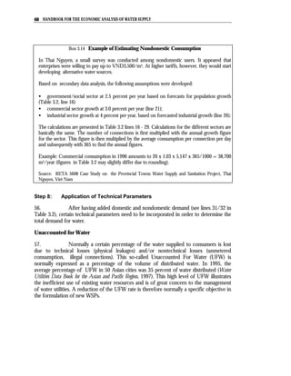
  • 1. Asian Develpment Bank Handbook for the Economic Analysis of Water Supply Projects ISBN: 971-561-220-2 361 pages Pub. Date: 1999 http://www.adb.org/Documents/Handbooks/Water_Supply_Projects Contents I. Introduction II. The Project Framework III. Demand Analysis and Forecasting IV. Least-Cost Analysis V. Financial Benefit-Cost Analysis VI. Economic Benefit-Cost Analysis VII. Sensistivity and Risk Analysis VIII. Financial Sustainability and Pricing IX. Distribution Analysis and Impact on Poverty Reduction Appendix A. Data Collection B. Case Study: Urban Water Supply Project 1. Annex B. Case Study: Rural Water Supply Project] 1. Annex Glossary References
  • 3. 2 HANDBOOK FOR THE ECONOMIC ANALYSIS OF WATER SUPPLY PROJECTS CONTENTS 1.1 All about the Handbook .............................................................................................................. 3 1.1.1 Introduction..................................................................................................................... 3 1.1.2 Uses of the Handbook .................................................................................................. 4 1.2 Characteristics of Water Supply Projects .................................................................................. 4 1.2.1 Water as an Economic Good ....................................................................................... 4 1.3 The Water Supply Project ............................................................................................................ 6 1.3.1 Economic Rationale and Role of Economic Analysis ............................................. 6 1.3.2 Macroeconomic and Sectoral Context ........................................................................ 6 1.3.3 Procedures for Economic Analysis ............................................................................. 7 1.3.4 Economic Analysis and ADB’s Project Cycle ........................................................... 9 1.3.5 Project Preparation and Economic Analysis ............................................................. 9 1.3.6 Identifying the Gap between Forecast Need and Output from the Existing Facility.....................................................................11 1.4 Least-Cost Analysis for Choosing an Alternative.................................................................12 1.4.1 Introduction...................................................................................................................12 1.4.2 Choosing the Least-Cost Alternative ........................................................................12 1.5 Financial and Economic Analyses...........................................................................................13 1.5.1 With- and Without-Project Cases..............................................................................13 1.5.2 Financial vs. Economic Analysis ...............................................................................14 1.5.3 Financial vs. Economic Viability ...............................................................................15 1.6 Identification, Quantification, Valuation of Economic Benefits and Costs......................16 1.6.1 Nonincremental and Incremental Outputs and Inputs..........................................16 1.6.2 Demand and Supply Prices.........................................................................................16 1.6.3 Identification and Quantification of Costs ..............................................................16 1.6.4 Identification and Quantification of Benefits..........................................................18 1.6.5 Valuation of Economic Costs and Benefits.............................................................19 1.6.6 Economic Viability.......................................................................................................19 1.7 Sensitivity and Risk Analysis .....................................................................................................20 1.8 Sustainability and Pricing ...........................................................................................................20 1.9 Distribution Analysis and Impact on Poverty ..............................................................................21 Figures Figure1.1 Flow Chart for Economic Analysis of Water Supply and Sanitation Projects………..8
  • 4. CHAPTER 1: INTRODUCTION 3 1.1 All about the Handbook 1.1.1 Introduction 1. Water is rapidly becoming a scarce resource in almost all countries and cities with growing population on the one hand, and fast growing economies, commercial and developmental activities on the other. 2. This scarcity makes water both a social and an economic good. Its users range from poor households with basic needs to agriculturists, farmers, industries and from commercial undertakings with their needs for economic activity to rich households for their higher standard of living. 3. For all these uses, the water supply projects (WSPs) and water resources development programs are being proposed for extension and augmentation; likewise with the rehabilitation of water supply for which measures for subsequent sustainability are being adopted. 4. It is, therefore, essential to carry out an economic analysis of projects so that planners, policy makers, water enterprises and consumers are aware of the actual economic cost of scarce water resources, and the appropriate levels of tariff and cost recovery needed to financially sustain it. 5. In February 1997, the Bank issued the Guidelines for the Economic Analysis of Projects for projects in all sectors, and subsequently issued the Guidelines for the Economic Analysis of Water Supply Projects” (March 1998) which focuses on the water supply sector. The treatment of subsidies and a framework for subsidy policies is contained in the Bank Criteria for Subsidies (September 1996). 6. This Handbook is an attempt to translate the provisions of the water supply guidelines into a practical and self-explanatory work with numerous illustrations and numerical calculations for the use of all involved in planning, designing, appraising and evaluating WSPs. 7. In this document, short illustrations have been used to explain various concepts of economic analyses. Subsequently, they are applied in real project situations which have been taken from earlier Bank-financed and other WSPs, or from case
  • 5. 4 HANDBOOK FOR THE ECONOMIC ANALYSIS OF WATER SUPPLY PROJECTS studies conducted in different countries in Asia as part of a Bank-financed Regional Technical Assistance Project (RETA). 1.1.2 Uses of the Handbook 8. This Handbook is written for non-economists (planners, engineers, financial analysts, sociologists) involved in the planning, preparation, implementation, and management of WSPs, including: staff of government agencies and water utilities; consultants and staff of non-governmental organizations (NGOs); and staff of national and international financing institutions. 9. Since the Handbook focuses on the application of principles and methods of economic analysis to WSPs, it is also a practical guide that can be used by economists in the economic analysis of WSPs. 10. The Handbook can also be used for the following purposes: (i) as a reference guide for government officials, project analysts and economists of developing member counries (DMC) in the design, economic analysis and evaluation of WSPs; (ii) as a guide for consultants and other professional staff engaged in the feasibility study of WSPs, applying the provisions of the Bank’s Guidelines for the Economic Analysis of Water Supply Projects; and (iii) as a training guide for the use of trainors of “Economic Analysis of Water Supply Projects” 1.2 Characteristics of Water Supply Projects 1.2.1 Water as an Economic Good 11. The characteristic features of water supply include the following: (i) Water is usually a location-specific resource and mostly a nontradable output.
  • 6. CHAPTER 1: INTRODUCTION 5 (ii) Markets for water may be subject to imperfection. Features related to the imperfect nature of water markets include physical constraints, the high costs of investment for certain applications, legal constraints, complex institutional structures, the vital interests of different user groups, limitations in the development of transferable rights to water, cultural values and concerns of resource sustainability. (iii) Investments are occurring in medium term (typically 10 years) phases and have a long investment life (20 to 30 years). (iv) Pricing of water has rarely been efficient. Tariffs are often set below the average economic cost, which jeopardizes a sustainable delivery of water services. If water availability is limited, and competition for water among potential water users (households, industries, agriculture) is high, the opportunity cost of water (OCW) is also high. Scarcity rent occurs in situations where the water resource is depleting. OCW and depletion premium have rarely been considered in the design of tariff structures. If the water entity is not fully recovering the average cost of water, government subsidies or finance from other sources is necessary to ensure sustainable water service delivery. (v) Water is vital for human life and, therefore, a precious commodity. WSPs generate significant benefits, yet water is still wasted on a large scale. In DMC cities and towns, there is a very high incidence of unaccounted-for-water (UFW). An ADB survey among 50 water enterprises in Asian countries over the year 1995 revealed an average UFW rate of 35 percent. (vi) Economies of scale in WSPs are moderate in production and transmission but rather low in the distribution of water. The above characteristics have implications on the design of WSPs and should be considered as early as the planning and appraisal stages of project preparation.
  • 7. 6 HANDBOOK FOR THE ECONOMIC ANALYSIS OF WATER SUPPLY PROJECTS 1.3 The Water Supply Project 1.3.1 Economic Rationale and Role of Economic Analysis 12. The main rationale for Bank operations is the failure of markets to adequately provide what society wants. This is particularly true in the water supply sector. The provision of basic water supply services to poorer population groups generates positive external benefits, such as improved health conditions of the targeted project beneficiaries; but these are not internalized in the financial cost calculation. 13. The Bank provides the finance for water supply services to assist DMCs in providing safe water to households, promoting enhanced cost recovery over time, creating an enabling environment including capacity building and decentralized management of water supply operations, and setting up of autonomous water enterprises and private companies which are run on a commercial basis. 14. While economic analysis is useful in justifying the Bank’s intervention in terms of economic viability, it should also be considered as a major tool in designing water supply operations. There is a scope for better integrating social and economic considerations in the overall project design. Demand for water depends on the price charged, a function of the cost of water supply which, in turn, depends on demand. This interdependence requires careful analysis in all water supply operations. Safe water should be generally provided at an affordable price and using an appropriate level of service matching the beneficiaries’ preferences and their willingness to pay. 1.3.2 Macroeconomic and Sectoral Context 15. The purpose of the economic analysis of projects is to bring about a better allocation of scarce resources. Projects must relate to the Bank’s sectoral strategy and also to the overall development strategy of the country. 16. In a WSP, the goal may be “improved health and living conditions, reduction of poverty, increased productivity and economic growth, etc.”. Based on careful problem analysis, the Project (Logical) Framework establishes such a format showing the linkages between “Inputs and Outputs”, “Outputs and Purpose”, “Purpose and Sectoral Goal” and “Sectoral Goal and Macro Objective”. The key assumptions regarding project-related activities, management capacity, and sector policies beyond the control and management of the Project Authority are made explicit.
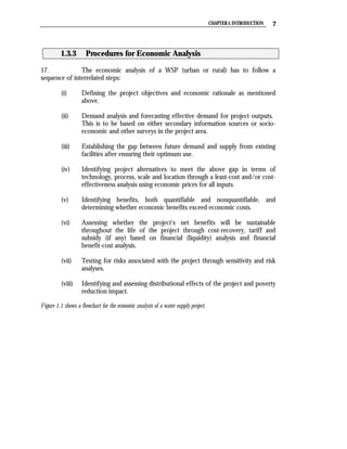
  • 8. CHAPTER 1: INTRODUCTION 7 1.3.3 Procedures for Economic Analysis 17. The economic analysis of a WSP (urban or rural) has to follow a sequence of interrelated steps: (i) Defining the project objectives and economic rationale as mentioned above. (ii) Demand analysis and forecasting effective demand for project outputs. This is to be based on either secondary information sources or socio- economic and other surveys in the project area. (iii) Establishing the gap between future demand and supply from existing facilities after ensuring their optimum use. (iv) Identifying project alternatives to meet the above gap in terms of technology, process, scale and location through a least-cost and/or cost- effectiveness analysis using economic prices for all inputs. (v) Identifying benefits, both quantifiable and nonquantifiable, and determining whether economic benefits exceed economic costs. (vi) Assessing whether the project’s net benefits will be sustainable throughout the life of the project through cost-recovery, tariff and subsidy (if any) based on financial (liquidity) analysis and financial benefit-cost analysis. (vii) Testing for risks associated with the project through sensitivity and risk analyses. (viii) Identifying and assessing distributional effects of the project and poverty reduction impact. Figure 1.1 shows a flowchart for the economic analysis of a water supply project.
  • 9. 8 HANDBOOK FOR THE ECONOMIC ANALYSIS OF WATER SUPPLY PROJECTS Figure 1.1 Flow Chart for Economic Analysis of Water Supply and Sanitation Projects Project Rationale & Objectives Socioeconomic Survey Survey of Existing Facilities,Uses Including Contingent & Constraints (if any) Valuation Identify Measures Demand Analysis for Optimum Use Institutional & Demand Forecasting of Existing Facilities (including effective demand) Assessment Establish the Gap Between Future Demand & Existing Facilities After Their Optimum Use Environmental Identify Technical Alternatives Assessment to meet the above Gap (IEE ,EIA) Least-cost Analysis (with Economic Price) & Choice of the Alternative (Design, Process, Technology, & Scale, etc.) (AIFC & AIEC) Identifying Benefits (Quantifiable) Tariff Design, Cost Recovery, Identifying Nonquantifiable items & Subsidy (if any) (if any) Enumeration Economic Financial Benefit-cost Benefit-cost Analysis with Analysis with Economic Price Financial Price (EIRR) (FIRR) Uncertainty Analysis (Sensitivity & Risk) Distribution of Project Effects Financial Sustainability Analysis & Poverty Reduction Plan for (Physical & Impact Environmental) Sustainability - parts of the economic analysis AIFC - average incremental financial cost; AIEC - average incremental economic cost; EIRR - economic internal rate of EIA - environmental impact return; ; FIRR - financial internal rate of return; IEE - initial environmental assessment examination
  • 10. CHAPTER 1: INTRODUCTION 9 1.3.4 Economic Analysis and ADB’s Project Cycle 18. Economic analysis comes into play at the different stages of the project cycle: project identification, project preparation and project appraisal. 19. Project identification largely results from the formulation of the Bank’s country sectoral strategy and country program. This means that the basic decision to allocate resources to the water supply sector for a certain (sector) loan project has been taken at an early stage and that the project has, in principle, been identified for implementation with assistance from the ADB. 20. In the project preparation stage, the planner has to make an optimal choice of the design, process, technology, scale and location etc. based on the most efficient use of the countries’ resources. Here, the economic analysis of projects again comes into play. 21. In the project appraisal stage, the economic analysis plays a substantial part to ensure optimal allocation of a nation’s resources and to meet the sustainability criteria set by both the recipient country and the ADB from the social, institutional, environmental, economic and financial viewpoints. 1.3.5 Project Preparation and Economic Analysis 22. Before any detailed preparation is done, it is necessary for the design team to get acquainted with the area where the project is identified. This is to acquire knowledge about the physical features, present situation regarding existing facilities and their use constraints (if any) against their optimal use, the communities and users specially their socio-economic conditions, etc. 23. To get these information, the following surveys must be undertaken in the area: (i) Reconnaissance survey – to collect basic information of the area and to have discussions with the beneficiaries and key persons involved in the design, implementation and management of the project. Relevant data collection also pertains to information available in earlier studies and reports.
  • 11. 10 HANDBOOK FOR THE ECONOMIC ANALYSIS OF WATER SUPPLY PROJECTS (ii) Socio-economic survey – to get detailed information about the household size, earnings, activities, present expenditure for water supply facilities, along with health statistics related to water-related diseases, etc. It is important to analyze the potential project beneficiaries, their preferences for a specific level of service and their willingness to pay for the level of service to be provided under the project. The analysis of beneficiaries should show the number of poor beneficiaries, i.e., those below the country’s poverty line, and their ability to pay. Such information is required to ensure that poor households will have access to the project’s services and to know whether, and to what extent, “cost- recovery” can be done. (iii) Contingent Valuation Method − An important contribution in arriving at the effective demand for water supply facilities, even where there are no formal water charges, is the contingent valuation survey. This is based on questions put to households on how much they are willing to pay (WTP) for the use of different levels of water quantities. These data may help build up some surrogate demand curve and estimate benefits from a WSP. (iv) Survey of existing water supply facilities − Knowledge of the present water supply sources, treatment (if any) and distribution is also needed. It is also necessary to know the quantity and quality of water and unaccounted-for-water (UFW) and any constraints and bottlenecks which are coming in the way of the optimum use of the existing facility. 24. Using the information taken from the survey results and other secondary data sources, effective demand for water can then be estimated. Two important considerations are: (i) Effective demand is a function of the price charged. This is ideally based on the economic cost of water supply provision to ensure optimal use of the facility, and neither over-consumption nor under-consumption especially by the poor should occur. The former leads to wastage contributing to operational deficits and the latter results in loss of welfare to the community. (ii) Reliable water demand projections, though difficult, are key in the analysis of alternatives for determining the best size and timing of investments.
  • 12. CHAPTER 1: INTRODUCTION 11 25. Approaches to demand estimation for urban and rural areas are usually different. In the urban areas, the existing users are normally charged for the water supply; in the rural areas, there may not be any formal water supply and the rural households often do not have to pay for water use. An attempt can be made in urban areas to arrive at some figure of price elasticity and probably income elasticity of demand. This is more difficult in the case of water supply in rural areas with a preponderance of poor households. 1.3.6 Identifying the gap between Forecast Need and Output from the Existing Facility 26. Once demand forecasting has been done, it is necessary to arrive at the output (physical, institutional and organizational) which the project should provide. The existing facilities may not be optimally used due to several reasons, among them: (i) UFW due to high technical and nontechnical losses in the system; (ii) inadequate management system, organizational deficiency and poor operation and maintenance leading to deterioration of the physical assets; and (iii) any bottleneck in the supply network at any point starting from the raw water extraction to the households and other users’ end. 27. Before embarking on a detailed preparation of the project, it is necessary to take measures to ensure optimal use of the facilities. These measures should be both physical and policy related. The physical measures are like leakage control, replacing faulty valves and adequate maintenance and operation, etc.; policy measures can be charging an economically efficient tariff and implementing institutional reforms, etc. 28. The output required from the proposed WSP should only be determined after establishing the gap between the future needs based on the effective demand and the restored output of the existing facilities ensuring their optimal use. Attention needs to be focused on the identification and possible application of instruments to manage and conserve demand, such as (progressive) water tariffs, fiscal incentives, pricing of raw water, educational campaigns, introducing water saving devices, taxing of waste water discharges, etc.
  • 13. 12 HANDBOOK FOR THE ECONOMIC ANALYSIS OF WATER SUPPLY PROJECTS 1.4 Least-Cost Analysis for Choosing an Alternative 1.4.1 Introduction 29. After arriving at the scope of the WSP based on the gap mentioned above, the next task is to identify the least-cost alternative of achieving the required output. Economic costs should be used for examining the technology, scale, location and timing of alternative project designs. All the life-cycle costs (market and non- market) associated with each alternative are to be taken into account. 30. The alternatives are not to be confined to technical or physical elements only, e.g., ground water or surface water, gravity or pumping, large or small scale, etc. They can also include activities due to policy measures, e.g., leakage detection and control, institutional reforms and managerial reorganization. 1.4.2 Choosing the Least-Cost Alternative 31. There can be two main cases for the choice from mutually exclusive options: (i) the alternatives deliver the same output or benefit, quantity wise and quality wise; (ii) the alternatives produce different outputs or benefits. Case 1. 32. In the first case, the least-cost analysis compares the life cycle cost Streams of all the options and selects the one with the lowest present value of the economic costs. The discount rate to be used is the economic opportunity cost of capital (EOCC) taken as 12 percent in real terms. 33. Alternatively, it is possible to estimate the equalizing discount rate (EDR) between each pair of mutually exclusive options for comparison. The EDR is also equal to the economic internal rate of return (EIRR) of the incremental cash flows of the
  • 14. CHAPTER 1: INTRODUCTION 13 mutually exclusive options. The EDR/EIRR of the incremental cash flows can then be compared with the EOCC for choice among alternatives. 34. The least-cost choice can also be done by calculating the average incremental economic cost (AIEC) of each alternative. The AEIC is the present value of incremental investment and operating costs in with-project and without-project situations divided by the present value of incremental output (say, in m3) also in both with-project and without-project alternative. The discount rate to be used is the EOCC = 12 percent. This will establish the project alternative with the lower per unit economic cost. Case 2. 35. In this second case, it is possible to select the least economic cost option by calculating per unit economic costs of all the project options. Because water demand, supply cost and price charged for water tend to be closely interrelated, least- cost analysis should account for the effect of uncertain demand. Lower-than-forecast demand results in higher average costs, which can push up water prices and depress demand further. 36. Sensitivity analysis can be used to show whether the project option remains the least-cost alternative under adverse changes in key variables. The scale of the project may vary in relation to prices charged to consumers and the size may influence the least-cost alternative. 1.5 Financial and Economic Analyses 1.5.1 With- and Without-Project Cases 37. After choosing the best among alternatives, the next step is to test the financial and economic viability of the project, which is the chosen, least-cost alternative. The initial step in testing the financial and economic viability of a project is to identify and quantify the costs and benefits. 38. To identify project costs and benefits and to compare the net benefit flows, the without-project situation should be compared with the with-project situation. The without-project situation is different from the before-project situation. The without-project situation is that one which would prevail without the project vis-à-vis
  • 15. 14 HANDBOOK FOR THE ECONOMIC ANALYSIS OF WATER SUPPLY PROJECTS factors like population increase. As water is getting more scarce, the water use pattern and the cost are also likely to change. 1.5.2 Financial vs. Economic Analysis 39. Financial and economic analyses have similar features. Both estimate the net benefits of an investment project based on the difference between the with-project and the without-project situations. 40. However, the concept of financial net benefit is not the same as economic net benefit. While financial net benefit provides a measure of the commercial (financial) viability of the project on the project-operating entity, economic net benefit indicates the real worth of a project to the country. 41. Financial and economic analyses are also complementary. For a project to be economically viable, it must be financially sustainable. If a project is not financially sustainable, there will be no adequate funds to properly operate, maintain and replace assets; thus the quality of the water service will deteriorate, eventually affecting demand and the realization of financial revenues and economic benefits. 42. It has sometimes been suggested that financial viability not be made a concern because as long as a project is economically sound, it can be supported through government subsidies. However, in most cases, governments face severe budgetary constraints and consequently, the affected project entity may run into severe liquidity problems, thereby jeopardizing even its economic viability. 43. The basic difference between the financial and economic benefit-cost analyses of the project is that the former compares benefits and costs to the enterprise in constant financial prices, while the latter compares the benefits and costs to the whole economy measured in constant economic prices. Financial prices are market prices of goods and services that include the effects of government intervention and distortions in the market structure. Economic prices reflect the true cost and value to the economy of goods and services after adjustment for the effects of government intervention and distortions in the market structure through shadow pricing of the financial prices. In such analyses, depreciation charges, sunk costs and expected changes in the general price should not be included. 44. In financial analysis, the taxes and subsidies included in the price of goods and services are integral parts of financial prices, but they are treated differently in economic analysis. Financial and economic analyses also differ in their treatment of
  • 16. CHAPTER 1: INTRODUCTION 15 external effects (benefits and costs), favorable effects on health and the UFW of a WSP. Economic analysis attempts to value such externalities, health effects and nontechnical losses. 1.5.3 Financial vs. Economic Viability 45. The steps in determining the financial viability of the proposed project include: (i) identifying and quantifying the costs and revenues; (ii) calculating the project net benefits; (iii) estimating the average incremental financial cost, financial net present value and financial internal rate of return (FIRR). The FIRR is the rate of return at which the present value of the stream of incremental net flows in financial prices is zero. If the FIRR is equal to or greater than the financial opportunity cost of capital, the project is considered financially viable. Thus, financial benefit-cost analysis covers the profitability aspect of the project. 46. The steps in determining the economic viability of a project include the following: (i) identifying and quantifying (in physical terms) the costs and benefits; (ii) valuing the costs and benefits, to the extent feasible, in monetary terms; and (iii) estimating the EIRR or economic net present value (NPV) discounted at EOCC = 12 percent by comparing benefits with the costs. The EIRR is the rate of return for which the present value of the net benefit stream becomes zero, or at which the present value of the benefit stream is equal to the present value of the cost stream. For a project to be acceptable, the EIRR should be greater than the economic opportunity cost of capital. The Bank uses 12 percent as the minimum rate of return for projects; but for projects with considerable nonquantifiable benefits, 10 percent may be acceptable.
  • 17. 16 HANDBOOK FOR THE ECONOMIC ANALYSIS OF WATER SUPPLY PROJECTS 1.6 Identification, Quantification, Valuation of Economic Benefits and Costs 1.6.1 Nonincremental and Incremental Outputs and Inputs 47. Nonincremental outputs are project outputs that replace existing water production or supply. For example, a water supply project may replace existing supply by water vendors or household/community wells. 48. Incremental outputs are project outputs that add to existing supply to meet new demands. For example, the demand for water is expected to increase in the case of a real decline in water supply costs or tariffs. 49. Incremental inputs are for project demands that are met by an overall expansion of the water supply system. 50. Nonincremental inputs are inputs that are not met by an expansion of overall supply but from existing supplies, i.e., taking supply away from existing users. For example, water supply to a new industrial plant is done by using water away from existing agricultural water. 1.6.2 Demand and Supply Prices 51. In economic analysis, the market prices of inputs and outputs are adjusted to account for the effects of government intervention and market structure. The adjusted prices are termed as shadow prices and are based either on the supply price, the demand price, or a weighted average of the two. Different shadow prices are used for incremental output, nonincremental output, incremental input and nonincremental input. 1.6.3 Identification and Quantification of Costs 52. In estimating the economic costs, some items of the financial costs are to be excluded while other items, which are not part of financial costs are to be
  • 18. CHAPTER 1: INTRODUCTION 17 included. The underlying principle is that project costs represent the difference in costs between the without-project and the with-project situations. Cost items and the way they are to be treated in project economic analysis, are as follows: (i) Sunk Costs. They exist in both with-project and without-project situations and thus are not additional costs for achieving benefits. They are, therefore, not to be included. (ii) Contingencies. As the economic benefit-cost analysis is to be done in constant (or real) prices, the general price contingencies should not be included. (iii) Working Capital. Only inventories that constitute real claims on the nation’s resources should be included in the project economic costs. Others items of working capital reflect loan receipts and repayment flows are not to be included. (iv) Transfer payments. Taxes, duties and subsidies are transfer payments as they transfer command over resources from one party (taxpayers and subsidy receivers) to another (the government, the tax receivers and subsidy givers) without reducing or increasing the amount of resources available in the economy as a whole. Hence, these transfer payments are not economic costs. However, in certain circumstances when valuing the economic cost of an input or an output, taxes are to be included: (a) If the government is correcting for external environmental costs by a correcting tax to reduce the production of water, such a transfer payment is part of the economic costs. (b) The economic value of incremental outputs will include any tax element imposed on the output, which is included in the market price at which it sells. (v) External Costs. Environmental costs arising out of a project activity, such as river water pollution due to discharge of untreated sewage effluent, is an instance of such costs. It may be necessary to internalize this external cost by including all relevant effects and investments like pollution control equipment costs and effects in the project statement. (vi) Opportunity Cost of Water. If, for example, a drinking water project uses raw water diverted from agriculture, the use of this water for
  • 19. 18 HANDBOOK FOR THE ECONOMIC ANALYSIS OF WATER SUPPLY PROJECTS drinking will result in a loss for farmers. These costs are measured as the opportunity cost of water which, in this example, equals the “benefits foregone” of the use of that water in agriculture. (vii) Depletion Premium. In water supply projects where the source of water is ground water and the natural rate of recharge or replenishment of the aquifer is less than its consumptive use, the phenomenon of depletion occurs. In such cases, significant cost increase may take place as the aquifer stock depletes; the appropriate valuation of water has to include a depletion premium in the economic analysis. (viii) Depreciation. The stream of investment assets includes initial investments and replacements during the project’s life. This stream of expenditure, which is included in the benefit-cost analysis, will generally not coincide with the time profile of depreciation and amortization in the financial accounts and as such, the latter should not be included once the former is included. 1.6.4 Identification and Quantification of Benefits 53. The gross benefit from a new water supply is made up of two parts: (i) resource cost savings on the nonincremental water consumed in switching from alternative supplies to the new water supply system resulting from the project; and (ii) the WTP for incremental water consumed. 54. Resource cost savings are estimated by multiplying the quantity of water consumed without the project (i.e., nonincremental quantity) by the average economic supply price in the without-project situation. 55. The WTP for incremental supplies can be estimated through a demand curve indicating the different quantities of water demand that could be consumed at different price levels between the without-project level of demand and the with-project level of demand. The economic value of incremental consumption is the average value derived from the curve times the quantity of incremental water. Where there is inadequate data to estimate a demand curve, a contingent valuation methodology can be applied to obtain an estimate of WTP for incremental output.
  • 20. CHAPTER 1: INTRODUCTION 19 56. The gross benefit stream should be adjusted for the economic value of water that is consumed but not paid for, i.e., sold but not paid for (bad debts) and consumed but not sold (non-technical losses). It can be assumed that this group of consumers derives, on the average, the same benefit from the water as those who pay. 57. Other benefits of a WSP include health benefits. These benefits are due to the provision of safe water and are also likely to occur provided that the adverse health impacts of an increased volume of wastewaters can be minimized. 1.6.5 Valuation of Economic Costs and Benefits 58. The economic costs and benefits must be valued at their economic prices. For this purpose, the market prices should be converted into their economic prices to take into account the effects of government interventions and market structures. The economic pricing can be conducted in two different currencies (national vs. foreign currency) and at the two different price levels (domestic vs. world prices). 59. To remove the market distortions in financial prices of goods and services and to arrive at the economic prices, a set of ratios between the economic price value and the financial price value for project inputs and outputs are used to convert the constant price financial values of project benefits and costs into economic values. These are called conversion factors, which can be used for groups of typical items, like energy and water resources. 1.6.6 Economic Viability 60. Once the economic benefit and cost streams are derived, a project resource statement can be developed and the EIRR for the project can be calculated. Bank practice is to use 12 percent as the minimum rate of return for projects for which an EIRR can be calculated, although for projects with considerable nonquantifiable benefits, 10 percent may be acceptable. For rural WSPS, there may be limitations to value the economic benefits, thus making it difficult to calculate a reliable EIRR. However, the economic analysis may be undertaken on the basis of the least-cost or cost effectiveness analysis using the economic price of water.
  • 21. 20 HANDBOOK FOR THE ECONOMIC ANALYSIS OF WATER SUPPLY PROJECTS 1.7 Sensitivity and Risk Analysis 61. In calculating the EIRR or ENPV for WSPs, the most likely values of the variables are incorporated in the cost and benefit streams. Future values are difficult to predict and there will always be some uncertainty about the project results. Sensitivity analysis is therefore undertaken to identify those benefit and cost parameters that are both uncertain and to which EIRR and FIRR are sensitive. 62. The results of the sensitivity analysis should be summarized, where possible, in a sensitivity indicator and in a switching value. A sensitivity indicator shows the percentage change in NPV (or EIRR) to the percentage change in a selected variable. A high value for the indicator indicates project sensitivity to the variable. Switching values show the change in a variable required for the project decision to switch from acceptance to rejection. For large projects and those close to the cut-off rate, a quantitative risk analysis incorporating different ranges for key variables is recommended. Measures mitigating against major sources of uncertainty are incorporated into the project design, thus improving it. 1.8 Sustainability and Pricing 63. For a project to be sustainable, it must be both financially and economically viable. A financially viable project will continue to produce economic benefits, which are sustained throughout the project life. 64. Assessing sustainability includes: (i) undertaking financial analysis at both the water enterprise level and the project level (i.e., covering the financial liquidity aspect of the project at both levels); (ii) examining the role of cost recovery through water pricing; and (iii) evaluating the project’s fiscal impact, i.e., whether the government can afford to pay the level of financial subsidies that may be necessary for the project to survive. 65. Subsidies aimed at helping the poor may not always benefit them in a sustained manner. Underpricing can lead to waste of water (by the non-poor in particular), deterioration of the water system and services, and ultimately to higher
  • 22. CHAPTER 1: INTRODUCTION 21 prices for all. Cross subsidies could also distort prices and should generally be discouraged. To minimize economic costs and maximize socioeconomic development impact, any level of subsidies should be carefully targeted to lower the price charged for water to poor and low-income households. 66. To minimize financial subsidies, projects should be designed to supply services that people want and are willing to pay for. 1.9 Distribution Analysis and Impact on Poverty 67. Water supply provision, especially in the rural areas and shantytowns in urban areas, is considered to be important for poverty reduction. The poverty-reducing impact of a project is determined by evaluating the expected distribution of net economic benefits to different groups such as consumers and suppliers, including labor and the government.
  • 24. 24 HANDBOOK FOR THE ECONOMIC ANALYSIS OF WATER SUPPLY CONTENTS 2.1 The Project Framework..............................................................................................................25 2.1.1 Introduction...................................................................................................................25 2.2 Purpose .........................................................................................................................................25 2.3. Concept of a Project Framework: Cause and Effect.............................................................26 2.4 Design of a Project Framework................................................................................................27 2.5 Project Targets: The Verifiable Indicators of Project Achievement...............................................29 2.6 Project Monitoring Mechanisms: The Means of Verification or “How Do We Obtain the Evidence?” .............................................................................................30 2.7 Risks and Assumptions ..............................................................................................................30 2.8 The Project Framework Matrix: An Example .........................................................................31 Figures Figure 2.1 The Project Cycle .................................................................................................................... 26 Figure 2.2 Basic Relations Between PFW Elements............................................................................ 27 Boxes Box 2.1 Logical Order of Cause and Effect……………………………………………….. 26 Box 2.2 Example of Project Goal………………………………………………………….. 28 Box 2.3 Example of the Purpose of the Project……………………………………………. 28 Box 2.4 Example of Project Outputs………………………………………………………. 28 Box 2.5 Example of Activities……………………………………………………….……... 28 Box 2.6 Example of Project Targets………………………………………………………... 29 Box 2.7 Example of Risks and Assumptions……………………………………………….. 30 Tables Table 2.1 Project Design Summary………………………………………………………… 27 Table 2.2 Example of Inputs in Water Supply Projects…………………………………….. 29 Table 2.3 Water Supply and Sanitation Project Framework………………………………... 32
  • 25. CHAPTER 2 : PROJECT FRAMEWORK 25 2.1 The Project Framework 2.1.1 Introduction 1. The Project Framework (PFW) is a conceptual tool for preparing the design of a project. It is a disciplined approach to sector and project analysis. This part of the Handbook is based on the ADB publication Using the Logical Framework for Sector Analysis and Project Design: A User’s Guide (June 1998). 2. In February 1998, the ADB Post Evaluation Office has issued the first draft of a new Project Performance Management System (PPMS). With regard to project design, the PPMS incorporates the PFW but adds other techniques, like problem analyses, formulation of solutions, identification of baseline and target values and definition of accountabilities. Because the draft PPMS is yet to be finalized and approved, this Handbook will only refer to the PFW as the basic tool for project design. It is expected, however, that the PPMS will gradually be adopted as the methodology to be utilized. 2.2 Purpose 3. The first step in carrying out a feasibility study for a water supply project (WSP), and as such also the first step in the economic analysis of such projects, is to prepare a PFW. Its purposes are: (i) to establish clearly the objectives and outputs which the project will be accountable to deliver (these objectives and outputs must be quantifiable and measurable); (ii) to promote dialogue and participation by all stakeholders; (iii) to facilitate project implementation planning and monitoring; (iv) to establish a clear basis for project evaluation during the operational phase; this requires a systematic comparison of project objectives, outputs and with actual achievements.
  • 26. 26 HANDBOOK FOR THE ECONOMIC ANALYSIS OF WATER SUPPLY 4. The PFW establishes the linkages between project design, project implementation and project evaluation. This is illustrated in Figure 2.1. Figure 2.1 The Project Cycle 5. The PFW is a tool for preparing the project design. It describes the Design goals, objectives, expected outputs, inputs and activities, key risks and assumptions and project costs. Preparing the PFW ensures that the project design is responsive to Logical specific needs, constraints and opportunities, Framework since it requires an analysis of problems and objectives to be achieved as a preparatory step leading to the design of a project. Evaluation Implementation 6. The preparation of the PFW is a team effort in which, ideally, all stakeholders involved in project preparation, should participate. The PFW facilitates project design and preparation by focusing attention on key project issues and laying out a process for establishing the main features of a project. As such, the preparation of a PFW should be an integrated and mandatory part of the Terms of Reference of any feasibility study. 2.3 The Concept of the Project Framework: Cause and Effect 7. The core concept underlying the PFW lies in creating a logical order of cause and effect. This is stated in Box 2.1. Box 2.1 Logical Order of Cause and Effect if certain inputs are provided and activities carried out, then a set of project outputs will be realized and if these outputs materialize, then the project will achieve certain project objectives, and if these objectives are achieved then the project will contribute to achieve the overall goal of the sector.
  • 27. CHAPTER 2 : PROJECT FRAMEWORK 27 8. The above statement indicates a certain hierarchy between the different components of the PFW. The basic relations between inputs, activities, outputs and impacts, objectives and goal can be seen in Figure 2.2. Figure 2.2 Basic Relations Between PFW Elements if then ACTIVITIES PURPOSE GOAL OUTPUTS (objective) I if then if then 2.4 The Design of a Project Framework 9. The basic building blocks of a PFW are five key project elements, each one linked to another in a cause-effect relationship. These five elements are described as the design summary. They are presented in Table 2.1 and can be described as follows: Table 2.1 Project Design Summary DESIGN SUMMARY PROJECT PROJECT RISKS/ TARGETS MONITORING ASSUMPTIONS MECHANISMS 1. Goal 2. Purpose 3. Project Components Project Outputs 4. Activities 5. Inputs
  • 28. 28 HANDBOOK FOR THE ECONOMIC ANALYSIS OF WATER SUPPLY 10. The Goal: the PFW begins with identifying the overall sector or area goal to be targeted by the project. It is the higher order or general objective to which the project contributes. Together with other projects, the proposed WSP will contribute to achieving such sector and area goals. An example is presented in Box 2.2. Box 2.2 Example of Project Goal In the case of water supply projects, a common goal is 'improved health and living conditions, reduced poverty and increased economic growth and productivity (goal)’. This goal has multiple dimensions as both human development and economic growth are targeted. 11. The Purpose, Immediate or Project-Specific Objective (why the project is being done): describes the immediate output or direct impact that we hope to achieve by carrying out the project. By achieving the immediate objective, the project will contribute to achieving the broader sector goal. An example is provided in Box 2.3. Box 2.3 Example of the Purpose of the Project If access to and use of clean water by the community is assured (purpose), then the project will contribute to improving community health and productivity (which is the broader sector goal). 12. Project Outputs (what the project will deliver): the tangible and measurable deliverables that the project is directly accountable for and for which it is given budgeted amounts of time and resources. Outputs are specific results, produced by managing well the project components. They should be presented as accomplishments rather than as activities. This is illustrated in Box 2.4. Box 2.4 Example of Project Outputs A typical project output could be phrased as: 'water supply systems rehabilitated and/or constructed' and 'O&M systems upgraded and operational'. Typical project components would include the procurement of materials and equipment, construction works, institutional strengthening and capacity building, community development and consultancy services. 13. Activities (how the project is carried out): each project output will be achieved through a series or cluster of activities. An example is shown in Box 2.5. Box 2.5 Example of Activities Typical examples of activities taking place in water supply projects include the acquisition of land, the procurement of materials and equipment, implementation of construction works, the preparation of an Operation & Maintenance Manual, training of staff, implementation of community education programs.
  • 29. CHAPTER 2 : PROJECT FRAMEWORK 29 14. Inputs: the time and physical resources needed to produce outputs. These are usually comprised of the budgeted costs needed for the purchase and supply of materials, the costs of construction, the costs for consultancy services, etc. An example is shown in Table 2.2. Table 2.2 Example of Inputs in Water Supply Projects EXPENDITURE CATEGORIES COSTS (US$mn) 1. Land 2 2. Material Supplies 32 3. Physical Works 16 4. Consultancy Services 6 Total Cost of Inputs 55 2.5 Project Targets: The Verifiable Indicators of Project Achievement 15. Practical and cost-effective project measures need to be established to verify accomplishment of goal, objective and outputs. These performance indicators are referred to as the project’s operational targets. The project targets essentially quantify the results, benefits or impacts expected from the project and thus make them measurable or at least tangible. Performance measures at the ‘objective level’ measure End of Project Impact. 16. Project targets are measurable indicators which should be presented in terms of quantity, quality and time. This is illustrated in Box 2.6. Box 2.6 Example of Project Targets A quantitative target could be ‘to provide adequate water supply to 15,000 households in district Adebe’. The quality characteristic can be added to this target: ‘provide drinking water in accordance with WHO standards for 24 hours per day at a pressure of 10 mwc’. The time dimension can also be added: ‘before 31 December 1999’.
  • 30. 30 HANDBOOK FOR THE ECONOMIC ANALYSIS OF WATER SUPPLY 2.6 Project Monitoring Mechanisms: The Means of Verification or “How Do We Obtain the Evidence?”1 17. The project manager, the government and the Bank need a management information system (MIS) that provides feedback on project progress at all levels of the Design Summary. This includes progress in disbursements, completion of activities, achievement of outputs, purpose and goals. Both measurable or verifiable indicators and means/mechanisms of verification provide the basis for project monitoring and evaluation systems. 18. To establish an effective monitoring and evaluation system or project performance management system, it is necessary to establish as part of the project design, flexible, inexpensive and effective means of verifying the status of project progress, at goal, objective and output level. In WSPs, sources of information could be progress reports, reports of review missions, water utility reports, statistical data, survey data, etc. 2.7 Risks and Assumptions 19. Risks and assumptions are statements about external and uncertain factors which may affect each of the levels in the Design Summary, and which have to be taken into account in the project design through mitigating measures. They may include the assumption that other projects will achieve their objectives. If worded positively, these statements are assumptions; if worded negatively, they are indicative of risk areas. This is illustrated in Box 2.7. Box 2.7 Example of Risks and Assumptions In water supply projects, assumptions could include: • the timely availability of land for construction of water intake; • the timely disbursement of funds; • a stable political situation; • the timely completion of the dam; and • regular adjustment of water tariffs. In terms of risks, these assumptions would be formulated as follows: • land not timely available for construction; • funds not timely disbursed; • political instability; • dam not ready in time; • water tariffs not regularly adjusted. 1 The newly-developed ADB-Project Performance Management System (PPMS) provides additional information and techniques on how to establish means and measures of verification.
  • 31. CHAPTER 2 : PROJECT FRAMEWORK 31 20. Assumptions are conditions that must be fulfilled if the project is to succeed, but which are not under the direct control of the project. It is important to identify the so-called “killer assumptions” which, if not fulfilled, could stop the project from achieving its objectives. The following actions can be taken to manage killer assumptions: (i) assess the consequences of doing nothing; (ii) change project design; (iii) add a new project; (iv) closely monitor the project; and (v) ensure sufficient flexibility in the project design. 21. Certain risks can be eliminated by putting them as a condition to be fulfilled before project implementation. For example, water tariffs must be increased to achieve a targeted level of cost recovery; or the water enterprise should receive autono- mous status before the loan can become effective. In rural WSPs, another example would be to set certain criteria which must be met by sub-projects before they are approved. 22. Risks and assumptions made should be carefully taken into account in the risk and sensitivity analysis to be conducted as part of the economic and financial analysis. 2.8 The Project Framework Matrix: An example 23. Project Framework Matrices have been prepared for many projects. An example of such a matrix for a typical WSP is presented in Table 2.3.
  • 32. Table 2.3 Water Supply Project Framework Design Summary Project Targets Proj. Monitoring Mechanisms Risks/Assumptions 1.Sector/Area Goals -Prevalence of water-related diseases among - Yearly epidemiological reports - no political 1.1 Improved target population reduced by 15% by 1999. of the Ministry of Health instability Health Situation -50% of people below poverty line have access - Water Enterprisereports - no natural disasters 1.2 Improved to water supply facilities by 1999. - Country report - sound macro- Living -Increased industrial development. - End of project reports economic policies Conditions -10% reduction of absenteeism by 1999 due to - Health Surveys 1.3 Sustained Socio- improved socio-economic/ living conditions. Economic Dev. -70% of women of target population have improved living conditions (more time, convenience, etc.) by 1999. 2. Project -no unexpected population growth in Objective/Purpose target areas. 2.1 Provide -Increase access to safe water supply to 70% of - Water Enterprise reports -current ground water improved and the target population by December 1999. - Progress reports tables will decrease sustained water dramatically because of drought (risk). supply to the -loan effectiveness by population of a first of January 1996. specified area. 3. Components/ - no delays in Outputs - four intakes, two treatment plants, 20,000 - Progress reports 3.1. - Existing house connections by 1997; - Water Enterprise reports contracting (building) infrastructure - 33.5 km transmission and distribution pipes contractors and rehabilitated; delivery of materials completed/replaced by 1997; -Physical - 24 hours service level operational; infrastructure - reduction of unaccounted for water from 40% constructed; to 30% by 1999.
  • 33. 34 HANDBOOK FOR THE ECONOMIC ANALYSIS OF WATER SUPPLY Table 2.3 Water Supply Project Framework Design Summary Project Targets Proj. Monitoring Mechanisms Risks/Assumptions 3.2 Mitigating -Water resources study completed by 1995; - Environmental profile (and - no environmental -water quality protection measures in place by three yearly updates); disasters measures for - Progress reports - government ability 1996; negative -facilities to transport and treat wastewater in - Reports of Ministry of to enforce environmental place by 1997; Water & Provincial Water environmental -target population educated about water related Authorities effects in place. - Reports of Environmental protection environmental hazards; Protection Agency/Water Basin measures. -water reduction program operational by end of 1996. Authority 3.3 Sustainable Org. - 100% of required postings fulfilled with - Progress reports - sufficient qualified trained and motivated staff by 1999; - Water Enterprise reports local staff available and Management and willing to work in established. - effective O&M systems in place; - Management training reports remote areas; - management systems and procedures and training needs assessments of operational by 1997; staff; - no halt on governmental - autonomous status water enterprise approved - Data from management info vacancies; by 1997. systems; - Organogram of water - autonomy to water enterprise/staffing list indicating enterprise granted. qualifications of staff. 3.4 Financial -water enterprise ability to recover full costs by - monthly and yearly financial - proposed tariff 1998; reports of water enterprise; sustainability of -billing and collection system operational by increases approved by - progress reports. government. water enterprise January 1997; -financial management system effective; achieved -achieve reduction in “unaccounted for water” from 40% to 30% by 1999.
  • 34. 3.5 User-oriented -achieve 90% coverage of target population - Special reports (Hygiene - no health disasters Activities (m/f) with hygiene education program by education/ environmental -Customers aware 1999; education at schools) about new services -70% of target population (m/f) know at least - Progress reports two out of three communicated hygiene - Water enterprise reports and about the safe messages; use of water; -collection rates increased from 60% to 85% by (consumer complaints list) -Customers use 1998; -Reports of the Ministry of - 50% of target population (m/f) apply at least Health and the Ministry of water supply two out of three communicated hygiene facilities safely Education behavior messages; 4. Activities 5. Inputs 4.1Develop Physical 5.1 - consultancy services for detailed eng’g. Infrastructure design / supervision (US$3 mn) -Detailed Eng’g. - $2 mn government funding for land - Progress reports and Review - loan awarded; Design acquisition; missions - government funds -Land acquisition - $50.5 mn funding for procurement of - Special reports awarded; -Procurement equipment and materials -Construction - provision for operational expenses -Supervision -Environmental Management 4.2.Environmental 5.2. - local consultancy services planned studies - Progress reports and Review - materials available component (10 person months) missions on time; -water rescues study - international consultancy services (6 - Special reports - no delay in -water quality person months) consultancy services; protection measures - local staff + government funding -facilities - US$1.5 mn funding for procurement of equipment and materials - US$3 mn for construction works
  • 35. 36 HANDBOOK FOR THE ECONOMIC ANALYSIS OF WATER SUPPLY 4.3Establish 5.3. - US$ 0.8 mn p.a. government funding for - Progress reports and Review - resettlement Organization and local staff (operational costs) missions program effective - US$ 0.6 mn for consultancy - Special reports - contractors available Management - US$1.4 mn for training -Institutional Dev. on time; -Organization Dev. -Human Resource Dev. 4.4 Establish 5.4. - US$0.3 mn for computer and - Progress reports and Review sustainable financial management information system missions - international consultancy services (4 mm) - Special reports framework - local consultancy services (12 mm) -establish tariff - computer hardware US$0.7 mn structure -financial management system operational 4.5 Community- 5.6. - US$0.5 mn for training and extension - Progress reports and Review Oriented Activities materials; missions -community info - 36 person months local consultancy staff, - Special reports programs 12 person months international -Health education consultants; -community org - US$0.2 mn for vehicles/other transport -PublicRelations means; - US$0.5 mn for public relations and mass programs media activities; - local staff Source: RETA 5608 Case Studies on Selected Water Supply Projects
  • 36. CHAPTER 3 DEMAND ANALYSIS AND FORECASTING
  • 37. 38 HANDBOOK FOR THE ECONOMIC ANALYSIS OF WATER SUPPLY CONTENTS 3.1 Effective Water Demand ..........................................................................................................40 3.1.1 Defining Effective Demand for Water.....................................................................40 3.1.2 Increasing Cost of Water Supply ...............................................................................41 3.2 The Demand for Water: Some Concepts ................................................................................42 3.2.1 Incremental vs. Nonincremental Demand for Water.............................................42 3.2.2 The Relation between Price and Quantity................................................................42 3.2.3 The Concept of Price Elasticity of Demand............................................................44 3.2.4 Different Demand Curves for Different Products .................................................45 3.2.5 The Relation between Household Income and the Demand for Water .............46 3.2.6 Other Determinants of the Demand for Water ......................................................48 3.3 The Use of Water Pricing to “Manage” Demand ..................................................................51 3.3.1 Instruments of Demand Management......................................................................51 3.3.2 Cumulative Effects of Water Demand Management and Conservation Programs .......................................................................................54 3.4 Data Collection ............................................................................................................................55 3.4.1 Cost Effectiveness of Data Collection......................................................................55 3.4.2 Sources for Data Collection ......................................................................................55 3.4.3 Contingency Valuation Method (CVM)....................................................................56 3.5 Demand Forecasting...................................................................................................................56 3.5.1 Forecasting Urban Water Supply: the Case of Thai Nguyen ...............................56
  • 38. CHAPTER 3: DEMAND ANALYSIS & FORECASTING 39 Figures Figure 3.1 An Individual’s Water Demand Curve: Linear and Non-Linear Relationships…………………………………………..…43 Figure 3.2 Demand Curves for Water from Public Taps vs. House Connections…………… 45 Figure 3.3 Relation between Demand and Income: Shift of Demand Curve……………….. 47 Figure 3.4 Demand Management………………………………………………………….. 51 Boxes Box 3.1 Example of Constrained Water Demand……………………………………………40 Box 3.2 The Future Costs of Water……………………………………………………….. 41 Box 3.3 Relationship between WTP and Income…………………………………………….46 Box 3.4 Increased Water Tariff in Bogor, Indonesia…………………………………………52 Box 3.5 Demand Management and Investment Planning in Australia……………………… 54 Box 3.6 Thai Nguyen Case Study: Description of Service Area…………………………… 57 Box 3.7 Thai Nguyen Case Study: Assumptions Used, Ability to Pay and Willingness to Pay………………………...…58 Box 3.8 Thai Nguyen Case Study: Number of Persons per Connection…………………… 60 Box 3.9 Thai Nguyen Case Study: Existing Consumption………………………………… 61 Box 3.10 Thai Nguyen Case Study: Indication of the Price Elasticity……………………….. 64 Box 3.11 Thai Nguyen Case Study: Estimating Future Demand…………………………… 65 Box 3.12 Thai Nguyen Total Domestic Demand…………………………………………… 66 Box 3.13 Example of Estimating Industrial Consumption…………………………………… 67 Box 3.14 Example of Estimating Nondomestic Consumption……………………… ……… 68 Box 3.15 Application of Technical Parameters……………………………………………….. 70 Box 3.16 Determination of Nonincremental Water………………………………………… 75 Tables Table 3.1 Major Determinants of Water Demand…………………………………………… 50 Table 3.2 Demand Forecast and Required……………………………………………………71 Table 3.3 Nonincremental Water from connected users (in lcd)…………………………… 73 Table 3.4 Average Nonincremental Water of nonconnected users (in lcd)……………………74 Table 3.5 Calculation of Nonincremental Demand…………………………………………. 77
  • 39. 40 HANDBOOK FOR THE ECONOMIC ANALYSIS OF WATER SUPPLY 3.1 Effective Water Demand 3.1.1 Defining Effective Demand for Water 1. The “effective demand” for water is the quantity of water demanded of a given quality at a specified price. The analysis of demand for water, including realistically forecasting future levels of demand, is an important and critical step in the economic analysis of water supply projects. The results of demand analysis will enable the project team to: (i) determine the service level(s) to be provided; (ii) determine the size and timing of investments; (iii) estimate the financial and economic benefits of the project; and (iv) assess the ability and willingness to pay of the project beneficiaries. Furthermore, the surveys carried out during the demand assessment will provide data on cost savings, willingness to pay, income and other data needed for economic analysis. 2. It is useful to note the difference between “effective demand” for water and “actual consumption” of water. Water consumption is the actual quantity of water consumed whereas effective demand relates that quantity to the price of water. For example, a low level of water consumption may not represent effective demand but may instead indicate a constraint in the existing supply of water. This is illustrated in Box 3.1. Box 3.1 Example of Constrained Water Demand In Rawalpindi, Pakistan, the existing water supply system provided water for only an average of 3.8 hours per day and, on average, six days per week. Families connected to the public water supply system used an average 76 lcd. An additional 16 lcd was collected from secondary sources. From the household survey it appeared that during the (dry) summer, 86 percent of the population found the supply of water insufficient compared to 50 percent during the winter. Effective demand for water was higher than the quantity the utility was able to supply. This suggests that effective demand was constrained by existing supply levels. Source: RETA 5608 - Case Study on the Water Supply and Sanitation Project, Rawalpindi, Pakistan
  • 40. CHAPTER 3: DEMAND ANALYSIS & FORECASTING 41 3.1.2 Increasing Cost of Water Supply 3. The demand for water is rising rapidly, resulting in water becoming increasingly scarce. At the same time, the unit cost of water is increasing, as water utilities shift to water sources farther away from the demand centers. Water from more distant sources may also be of lower quality. The costs of transporting water from the source to the consumer and that of water treatment necessary to meet potable water standards are becoming significant components of the unit cost of water. 4. The increase in the cost of water can be seen when the cost per cubic meter of water used by current water utilities is compared with the cost per cubic meter of water in new water supply projects (WSPs). This relation is shown in Box 3.2. Box 3.2 The Future Cost of Water For example, the current cost of water in Hyderabad is below $0.2 per m3 whereas in the figure below, the calculated cost of future water to be supplied through new schemes is more than $0.6 per m3. This means that future water is more than three times as expensive as water from the existing resources. Note that the points on line 1 indicate that future costs of water equal the current cost; the points on line 2 indicate that the future costs per unit are twice the current costs. Line 3 Line 2 Future Cost Line 1 1.4 Amman 1.2 1.0 Line 1: Current costs 0.8 Mexico City equal future costs Hyderabad Line 2: Future costs 0.6 Lima are twice as high Algiers as current costs 0.4 Dhaka Line 3: Future costs 0.2 Banglaore are three times as Shenyang high as current costs 0.0 0.0 0.2 0.4 0.6 0.8 1.0 1.2 1.4 3 US$/m Current Cost Source: Serageldin, Ismail. 1994. The Financing Challenge.
  • 41. 42 HANDBOOK FOR THE ECONOMIC ANALYSIS OF WATER SUPPLY 5. Box 3.2 reinforces the importance of making optimum use of scarce water resources by avoiding inefficiencies and wastage in existing supplies and designing efficient future investment projects. In designing new projects, it is becoming increasingly important to make optimum use of existing resources to be able to avoid or postpone costly investments in the future. 3.2 The Demand for Water: Some Concepts 3.2.1 Incremental vs. Nonincremental Demand for Water 6. A WSP usually increases the supply of water either by making more effective use of existing supply capacity or by adding additional supply capacity. To the consumer, the additional capacity supplied will either displace and/or add to already existing water sources. Every person uses water for drinking, cooking, bathing, washing of clothes, for sanitation purposes, etc. Sources of water include piped water supply systems, dugwells, hand pumps, canals, ponds, rivers, bottled water, water from vendors, rainwater, etc. 7. If the additional supply of water is used to displace already existing sources, it is called nonincremental demand. For example, a household which obtains a new connection to the piped water supply system may no longer make use of the existing dugwell. 8. If the additional supply of water generates an increase in existing consumption, it is called incremental demand. For example, a household obtaining its water from a well at a distance of 300 meters may increase its water consumption from 450 liters to 650 liters per day after a public tap is installed in closer proximity to the house. 3.2.2 The Relation between Price and Quantity 9. From an economic perspective, the price of water is an important determinant of per capita water consumption. The relation between the quantity of water used and the price is illustrated by a demand or willingness-to-pay curve for water, an example of which is given in Figure 3.1.
  • 42. CHAPTER 3: DEMAND ANALYSIS & FORECASTING 43 10. The downward sloping demand curve indicates the “decreasing marginal value” of water. The first five liters of water per capita per day will be extremely valuable as they are necessary to sustain life. This is illustrated by curve D1D1 in Figure 3.1. The second five liters will also be valuable, (e.g. in their use for hygienic purposes). The next five liters are valuable for food preparation, cooking and washing of clothes. All other factors being equal, for each additional increment of water, the marginal value of water tends to decline as the individual is putting the water to less and less valuable uses. Consequently, the individual’s willingness to pay for each increment of water will gradually decrease. 11. D1 D1 in Figure 3.1. represents a non-linear curve for an average household and shows an example of an individual’s water demand or willingness-to-pay curve. If the water tariff is increased from $0.25 to $0.50, this individual would (all other factors remaining equal) reduce daily consumption from 140 liters to 115 liters. Figure 3.1 An Individual’s Water Demand Curve: Linear and Non-linear Relationships Price (US$/m 3 D 1D 1 1.00 . 75 .50 D 2D 2 . 25 0 140 115 Quantity (lcd ) 12. In this Handbook, a linear demand curve will often be used for illustrative purposes, as indicated by line D2 D2. However, the nonlinear relationship between quantity and price is probably a better approximation of the actual behavior of water users.
  • 43. 44 HANDBOOK FOR THE ECONOMIC ANALYSIS OF WATER SUPPLY 3.2.3 The Concept of Price Elasticity of Demand 13. One question which often arises when considering the demand curve is how much the quantity demanded by an individual will change when the price per unit of water changes. The price elasticity of demand is a measure that describes the degree of responsiveness of the quantity of water to a given price change and is defined as follows: percentage change in the quantity of water demanded ep = - --------------------------------------------------------------------------- percentage change in the price per unit of water dQ/Q dQ P dQ P P ep = - ------ = - ---- x ---- = - ----- x ---- = slope x ---- dP/P Q dP dP Q Q 14. The price elasticity of demand for water is normally negative because the demand curve is downward sloping, which means that an increase (decrease) in price is expected to lead to a reduction (increase) in demand. 15. If ep < |1 |, demand is ‘inelastic’. For example, if an increase of 25 percent in water fees leads to a 10 percent reduction in the demand for water, this would result in a price elasticity of -0.40. The relative change in quantity demanded (dQ/Q) is, in this case, smaller than the relative change in price (dP/P). 16. If ep > |1 |, demand is elastic. For example, if a 25 percent increase in water fees leads to a 50 percent reduction in demand, this would result in a price elasticity of -2. The percentage change in quantity demanded is larger than the percentage change in price. 17. For a linear demand curve as can be verified through the formula for ep, the higher the price, the higher the absolute value of price elasticity. Using a nonlinear demand curve (Figure 3.1), it can be seen that for the first few liters of water, demand will be very inelastic, meaning that the consumer is willing to pay a high price for the given volume of water. As the marginal value of the water gradually declines, the consumer’s demand will become increasingly elastic, meaning that price fluctuations will result in larger changes in quantity demanded. 18. In studies carried out by the World Bank (Lovei, 1992), it has been found that the price elasticity for water typically ranges between -0.2 and -0.8, indicating
  • 44. CHAPTER 3: DEMAND ANALYSIS & FORECASTING 45 inelastic demand. For example, e = -0.2 means that a 10 percent increase in price would lead to a reduction in the quantity demanded by only 2 percent. 3.2.4 Different Demand Curves for Different Products 19. The definition of effective demand mentions “ the demand for water of a certain quality”. The quality of the product “water” is not easily explained and a number of characteristics are normally included in defining it, including chemical composition (e.g., WHO standards), taste and smell, water pressure, reliability of supply, accessibility and convenience. The first two characteristics determine the quality of water in the stricter sense. The other characteristics define water quality in its broader sense. 20. The combination of these characteristics will determine the “product” water or service level. Up to a certain point, an individual is prepared to pay a higher price for a product with a higher quality. For the same “quantity” of water, an individual will be willing to pay a higher price for a higher quality product. For example, consumers are normally willing to pay a higher price for water from a house connection than for water from a public tap. In this case, there are two different demand curves: one for house connections (HC) as shown in Figure 3.2, and one for public taps (PT) as shown in Figure 3.3. F i g u r e 3 . 2 D e m a n d C u r v e s f o r W a t e r f r o m P u b lic T a p s v s . H o u s e C o n n e c t i o n s WTP (price per m 3 ) P2 HC P1 PT O Q1 Quantity (m3)
  • 45. 46 HANDBOOK FOR THE ECONOMIC ANALYSIS OF WATER SUPPLY 3.2.5 The Relation between Household Income and the Demand for Water 21. Households with high income are normally able and willing to pay more for a given quantity of water than households with lower incomes. In relative terms (as a percent of income) however, people with higher incomes are prepared to pay smaller percentages of their income for water than people with lower incomes. These statements were confirmed in the case studies and are illustrated in Box 3.3. Box 3.3 Relationship Between WTP and Income The relationship between willingness to pay and month income has been confirmed in the case studies. For example, in Jamalpur, Bangladesh, the relationship as illustrated below was found. WTP (TK/month) WTP % Income 140 3.5% 120 3.0% Average of WTP % of Income 1 100 2.5% Log.(Avg. of WTP) Log. (% of Income) 80 2.0% 60 1.5% Curve 1: Y = 20.891Ln(X) – 113.22 R 2 = 0.3848 Curve 2: Y = -0.008Ln(X) + 0.0821 40 1.0% R 2 = 0.8298 20 2 0.5% Y refers to dependent variable on vertical axis. 0 0.0% X refers to the independent 0 5000 10000 15000 20000 25000 30000 variable (horizontal axis) HH Income (TK/month) Curve 1 explains the relationship between income and WTP in absolute terms. Households with higher income are willing to pay more for the total quantity of water consumed. Curve 2 illustrates the relation between income and WTP as a percentage of income. When income increases, a smaller proportion of household income is set aside to pay for water. Source: RETA 5608 Case Study on the Jamalpur Water Supply and Sanitation Project, Bangladesh
  • 46. CHAPTER 3: DEMAND ANALYSIS & FORECASTING 47 22. An increase in income will cause the demand curve for water to shift to the right (from D1 to D2), as illustrated in Figure 3.4. At price P1 the quantity of water consumed increases from OQ1 to OQ2. The shift in the demand curve to the right also indicates a higher willingness to pay (from P1 to P2) for the same quantity of water OQ1. Figure 3.3 Relation between Demand and Income: Shift of Demand Curve WTP/m3 P2 P1 D2 D1 O Q1 Q2 Quantity of water (m3) 23. The relation between water consumption and income can be expressed in terms of “income elasticity”. The formula for income elasticity is as follows: Percentage change in quantity of water consumed ei = --------------------------------------------------------------------- Percentage change in Income dQ/Q dQ I ei = + -------- = -------- x ------ dI/I dI Q 24. The literature on the relation between income and water consumption is rather limited, but a value between 0.4 and 0.5 appears to be reasonable (see e.g. Katzman 1977, Hubbell 1977 and Meroz 1986). A positive income elasticity of 0.4 means that if an individual’s household income increases by 10 percent, consumption is expected to increase by 4 percent. A value which is less than one shows that the demand for water is rather inelastic to changes in income. 25. For example: consider the case that income increases from Rp200,000 (I1) to Rp300,000 (I2 ), and water consumption increases from 15 m3/month (Q1) to 18 m3/month (Q2). In this case, income elasticity is calculated as follows:
  • 47. 48 HANDBOOK FOR THE ECONOMIC ANALYSIS OF WATER SUPPLY ei = (dQ/DI x I/Q) = ((Q2-Q1)/(I2-I1)) x I1/Q1 = ((18-15)/(300,000-200,000)) x 200,000/15 = 0.4 3.2.6 Other Determinants of the Demand for Water 26. In addition to price and income, other factors or determinants can also influence the demand for water. A checklist of possible water demand determinants is presented in Table 3.1. Each project may have its own set of water demand determinants and the importance of a given factor may differ from one project to another. The major determinants of water demand are briefly discussed below: (i) Domestic Demand (a) Population. Population (especially population growth) is a very important factor in determining future demand. Population growth may consist of natural growth or, in certain cases, migration (e.g. from rural to urban areas). Small differences in demographic trends have large effects on water consumption. For example, all other factors remaining constant, an annual population growth of 2 percent over a period of 20 years results in an increase in consumption of approximately 50 percent; whereas an annual growth of only 1.5 percent generates an additional consumption of about 35 percent over the same period. (b) Access to and Costs of Alternative Sources. If water from other sources of good quality is readily available, people will generally be less interested to displace their current sources. For example, in areas where shallow ground water of good quality is available throughout the year and when households have their own dugwells, people may be less inclined to apply for a connection to a new piped system especially if the price of piped water is higher than the unit cost of water from the alternative source. (c) Availability and Quality of Service. If existing water supply companies provide a fully satisfactory service to their customers, households
  • 48. CHAPTER 3: DEMAND ANALYSIS & FORECASTING 49 not yet connected will usually be more interested in connecting to an expanded water supply system. (ii) Nondomestic Demand (a) Size and Type of Industry. Logically, size and the type of industry will, to a large extent, determine the quantity of future consumption of water. (b) Industrial growth. Economic development and regional or urban development may strongly influence future demand for water. (c) Legal obligations. In certain countries or industrial areas, industries must apply for a permit to make use of alternative sources (for example, ground water) or are obligated to connect to piped systems, if available. 27. The demand for water is often analyzed for relatively homogeneous groups of users. In many cases, a distinction is made between domestic and nondomestic users. Furthermore, demand from domestic users is often separately analyzed for : (i) users currently connected to the system (existing connections) and (ii) those to be connected to the system under the proposed project (new connections).
  • 49. 50 HANDBOOK FOR THE ECONOMIC ANALYSIS OF WATER SUPPLY Table 3.1 Major Determinants of Water Demand A. Domestic Demand 1. Number and size of households 2. Family income and income distribution 3. Costs of water presently used 4. Cost of future water used 5. Connection charges 6. Availability and quality of service 7. Cost and availability of water using devices 8. Availability of alternative water sources 9. Present water consumption 10. Legal requirements 11. Population density 12. Cultural influences B. Commercial Demand 1. Sales or value added of non-subsistence commercial sector 2. Costs and volume of water presently used 3. Price of future water used 4. Connection charges 5. Costs of water using appliances 6. Quality and reliability of service 7. Working hours of various types of commercial establishments 8. Legal requirements C. Industrial Demand 1. Present and future costs of water 2. Type of industry and water use intensity 3. Relative price of alternative sources 4. Quality and reliability of supply 5. Costs of treatment and disposal of waste water 6. Legal requirements D. Agricultural Demand (for [non] piped water supply) 1. Present and future costs of water 2. Availability of other sources 3. Quality and reliability of supply 4. Supply cost of alternative water systems 5. Number of cattle 6. Legal requirements E. Public Services Demand 1. Present and future costs of water 2. Per capita revenue of local governments 3. Number and size of public schools, hospitals etc. 4. Legal requirements
  • 50. CHAPTER 3: DEMAND ANALYSIS & FORECASTING 51 28. The factors which determine domestic demand may differ between the urban and the rural sector. In the rural sector, special attention needs to be given to such things as the availability of alternative water sources, the income and ability to pay for or contribute to the project facilities and their management, the choice of technology and the use of water for other purposes like agriculture (e.g. livestock or vegetable growing) and, the ability to operate and maintain facilities. In the rural context, the assessment of effective demand will have to be carried out in close consultation with the local population, and attention needs to be given to issues such as community participation and hygiene education. 29. The factors which determine demand will, to a large extent, define the need for information. The project analyst will have to determine the key factors which need to be considered into the analysis and design of the project. 3.3 The Use of Water Pricing to “Manage” Demand 30. In Section 3.2 the relation between the price of water and the quantity of water was explained. This section deals with some applications of this concept. 3.3.1 Instruments of Demand Management 31. To understand how the quantity of water demanded can be influenced, let us look again at the demand curve for water, as illustrated in Figure 3.4. Figure 3.4 Demand Management 3 Price/m D1 D2 B P2 P1 C A O Q3 Q2 Q1 Quantity (m3)
  • 51. 52 HANDBOOK FOR THE ECONOMIC ANALYSIS OF WATER SUPPLY 32. Assume that present demand is Q1 at price P1. This refers to point A on demand curve D1. To reduce demand, one can try to: (i) reduce the quantity demanded by increasing the price of (excessive) water use. This will result in a reduction of demand from, for example, point A to B (movement along the same demand curve). At a higher price (OP2), a smaller quantity of water (OQ2) is demanded. By introducing financial incentives, consumers (domestic and nondomestic) can be expected to reduce their water consumption. Often, the objectives and reasons for such a policy will have to be thoroughly explained to the users through public education programs. Examples of introducing financial measures include: (a) increasing the average water tariff; (b) introducing progressive water tariff structures, aiming at reduction of excessive water use; (c) increasing tariffs for wastewater discharge: (industries will be particularly sensitive to this measure); (d) introducing ground water abstraction fees; (e) fiscal incentives (e.g. for investments in water saving devices or treatment plants); (f) utilization of water markets: experience from water markets in the United States and Gujarat, India indicates that water markets create a framework which contributes to the efficient use of water. An example of application of pricing effects is given in Box 3.4. Box 3.4 Increased Water Tariff in Bogor, Indonesia In 1988, after increases in average water tariffs for domestic users (about 115 percent) and nondomestic users (170 percent), the consumption of water per household dropped from an average of about 38 m3 per household per month to an average of about 27 m3 per month. This price increase was accompanied by an intensive public education program. This has resulted in consumption being maintained below previous levels, notwithstanding the fact that real water prices have since declined and incomes have continued to increase until mid-1997. Source: IWACO-WASECO. 1989(October). Bogor Water Supply Project: The Impact of the Price Increase in June 1988 on the Demand for Water in Bogor.
  • 52. CHAPTER 3: DEMAND ANALYSIS & FORECASTING 53 Price increases may also have undesirable effects. In the case of a significant increase in the price of water by a utility, consumers may, whenever feasible, divert to other water sources. For example, in Jakarta, excessive use of ground water causes land levels to go down. If, in this situation water tariffs are significantly increased, many consumers would again divert to ground water as a main source of water. A tariff increase introduced by the utility would, therefore, have to be accompanied by other measures to control the use of ground water, such as: (higher) fees for the use of ground water to industries; taxes to domestic users of ground water; and educational programs. (ii) move the demand curve to the left, resulting in a reduction in the quantity demanded from point A to point C. This means that at the same price level (P1), the quantity of water demanded will be reduced from OQ1 to OQ3. This can be achieved through: (a) introduction of water saving devices; (b) changing consumer behavior through educational programs; (c) legal measures (e.g. regulating the use of ground water); (d) industrial “water-audit” programs. This entails a review of the use of water and waste water in industrial plants, with the purpose of reducing the use of water. (iii) save the use of water or avoid waste of water resources on the supply side. Such measures could include: (a) increase in efficiency at the utility level (reduction of production losses, UFW); and (b) institutional changes (merger of utilities may create economies of scale). In most cases, water demand management and conservation policies will consist of a comprehensive set of measures to be carried out over a longer period of time to achieve the desired results.
  • 53. 54 HANDBOOK FOR THE ECONOMIC ANALYSIS OF WATER SUPPLY 3.3.2 Cumulative Effects of Water Demand Management and Conservation Programs 33. There is empirical evidence that domestic and nondomestic water consumption can be reduced by at least 20 to 30 percent by adopting appropriate demand management and conservation policies. Reduced water consumption will also result in reduced volumes of polluted water and will, in general, have positive environmental effects. Reductions in demand, in turn, will lead to substantial savings in needed investments as shown in Box 3.5. Finally, the water saved can be used for higher valued uses by other sectors in the economy. Box 3.5 Demand Management and Investment Planning in Australia In Melbourne, Australia, a combination of water demand management measures was used, such as: water pricing reforms, water saving devices, public education, etc. As a result, Melbourne’s 1993 water demand projection (line 2) differs substantially from the 1981 trend (line 1). The shift to the right of the water trend curve has delayed the need to invest in additional supplies by about six years. The deferral in investment was valued at $25 million. This is illustrated in the figure below. million cubic meter per year 800 700 2 600 1 500 400 300 200 1981 Trend 100 Current Trend 0 1977 1980 1983 1986 1989 1992 1995 1998 2001 2004 2007 2010 2013 2016 2019 2022 2025 Source: Bhatia, Ramesh; Rita Cestti and James Winpenny. Water Conservation and Reallocation: Best Practice Cases in Improving Economic Efficiency and Environmental Quality. A World Bank-ODI Joint Study.
  • 54. CHAPTER 3: DEMAND ANALYSIS & FORECASTING 55 3.4 Data Collection 3.4.1 Cost Effectiveness of Data Collection 34. Data collection should be cost efficient and cost effective. The purpose of data collection is to improve the accuracy of the estimates and predictions made in designing and analyzing a WSP. It is therefore important to carefully consider which data are needed and where and how to obtain them. 35. The collection of data will require resources in terms of time and money. The benefit or value of additional data will gradually decrease. The project analyst will have to decide at which point the benefits of the additional data will no longer justify the cost made. At minimum, conducting a limited but representative household survey should provide essential information which could save large sums of money in terms of reduced investment. 3.4.2 Sources for Data Collection 36. Some methods of data collection, as they were used in the preparation of the case studies on which this Handbook is partly based, are presented in Appendix A. Section 1 of this appendix deals with: (i) collection of secondary data from existing studies, water enterprises, government agencies, etc.; (ii) conducting reconnaissance surveys in the area to observe the actual field situation; and (iii) collection of primary data through field observations and household surveys. 37. Household surveys normally provide: (i) data about family size, occupation, income etc.; (ii) data about the quantity, quality and costs related to the current water supply (and sanitation) situation; and
  • 55. 56 HANDBOOK FOR THE ECONOMIC ANALYSIS OF WATER SUPPLY (iii) data about the future use of water supply and sanitation: the preferences of respondents with regard to the future level of service, type of facility and what they are willing to pay for the preferred level of service. 3.4.3 Contingency Valuation Method 38. Using Contingency Valuation Method (CVM), the consumer is asked how much he or she is willing to pay for the preferred level of service. The data can be analyzed to provide the project analyst with an indication of the actual shape of the demand curve for water, thus helping to estimate the price elasticity of demand which is an important parameter in demand management. An example is given in Appendix A. 3.5 Demand Forecasting 39. Some of the initial steps in demand forecasting is defining the different service levels and preparing a rough estimate of the price of supplying these service levels in a specific village or town. Subsequently, water quantity demanded is estimated for the different combinations of service level and price. 40. Estimating a demand curve for a new WSP is difficult in practice and will, in most cases, require adequate resources and extensive field research. The Handbook emphasizes the need to undertake a comprehensive analysis of water demand for without- project and with-project situations for reasons explained earlier. Data on the factors which determine the demand for water will provide the project analyst with a better understanding of what is required and will enable him/her to formulate a better project. 3.5.1 Forecasting Urban Water Supply: the Case of Thai Nguyen 41. The techniques and methods used in water demand forecasting will be explained in this section by making use of a case study. The case study describes the steps in demand forecasting as it was carried out for Thai Nguyen, Viet Nam, one of the case studies developed in preparing this Handbook. Some of the data have been slightly adapted for illustration purposes. 42. The general process and specific considerations in forecasting water demand are explained in the text. The application of these principles to demand
  • 56. CHAPTER 3: DEMAND ANALYSIS & FORECASTING 57 forecasting in Thai Nguyen is described in the boxes. The data needed to carry out the demand analysis are presented in Table 3.2. A short description of Thai Nguyen is presented in Box 3.6. Box 3.6 Thai Nguyen Case Study: Description of the Project Area Thai Nguyen is located 80 km to the north of Hanoi on the Cau River. At the end of 1995, the population was 191,600 persons. The existing water supply system had 5,114 metered connections, which provided approximately 24 percent of the population with water. The economy of Thai Nguyen is based on state enterprises, mainly heavy industry. There are also universities in the town. The main source of non-piped water supply is shallow groundwater, obtained through open wells or with electric pumps. A very small part of the population uses water from the river. Source: RETA 5608 Case Study on the Provincial Towns Water Supply and Sanitation Project, Thai Nguyen, Viet Nam Step 1: Estimating present and future population 43. A starting point in demand forecasting is determining the size and future growth of the population in the project area. This step is explained below, whereas the application of this step in Thai Nguyen is given in Box 3.7. (i) The first step is to estimate the size of the existing population. In most cases, different estimates are available from different secondary sources. Often, the survey team will have to make its own estimate based on the different figures obtained. (ii) The second step is to determine the service or project area (the area which will be covered by the project) and the number of people living there. The most important consideration in this respect is the expressed interest from potential customers. Furthermore, the service area will have to be determined in consultation with the project engineer, the municipal authorities and/or the water enterprise. Technical, economic and political considerations will play a role. (iii) The third step is to estimate future population growth in the project area. This estimate will be based on available data about national, provincial or local population growth. It should also take into account the effects of urban and/or regional development plans and the effects of migration from rural to urban areas.
  • 57. 58 HANDBOOK FOR THE ECONOMIC ANALYSIS OF WATER SUPPLY Box 3.7 Thai Nguyen Case Study: Assumptions Used, Ability to Pay and Willingness to Pay Assumptions: In the case of Thai Nguyen, these figures and assumptions have been applied (Table 3.2, lines 1-10): (i) The annual population growth for Thai Nguyen has been estimated at 3% up to the year 1999 and 2.5% after that (line 1). These figures are lower compared to other Vietnamese towns because of its location in the mountainous northern part of Viet Nam; this percentage is applied to the population figures (line 2). (ii) At present, the service area in Thai Nguyen covers only part of the town area with a 1995 population of 140,442 (line 4). The service area will remain the same in the new project. The population in the service area is assumed to grow faster compared to the general population growth because of better infrastructure facilities (line 3). The major expansion in the number of connections is assumed to take place between 1996 and 2000, then gradually after that,until 75% coverage is achieved (line 5). (iii) One of the targets of the project was to achieve 75% coverage in the year 2020 (line 10). This figure was checked with the findings of a household survey, as follows: First, 93% of the population expressed an interest in connecting to the system by means of a house connection. Interest for other service levels ( public tap) was very low. Second, willingness to pay for water in Thai Nguyen amounted to an average of VND3,005 per m3 (VND2,317 per m3 for connected households and VND3,119 per m3 for non-connected households). WTP for connected households is lower than WTP for non-connected households. This might be explained by the fact that connected households are most likely influenced by the current average water tariff of VND900 per month. It can be assumed that willingness to pay will increase when income and service levels increase. For these reasons, it was concluded that the set target of 75% coverage was realistic. Third, with regard to ability to pay for water, a so-called “affordability tariff” was calculated. The affordability tariff indicates the average tariff at which a certain percentage of the population can afford to use a minimum amount of water and not spend more than a given percentage of his/her income. An example of this calculation is given below: Items Unit 1996 2000 Average Monthly Income VND‘000 1,052 1,184 Lowest Income at 75% Coverage VND‘000 600 675 Min. expenditure on water (5% of income) VND‘000 30 33.8 Minimum consumption Lcd 60 60 Average HH size persons 4.26 4.26 Average monthly consumption m3 7.78 7.78 Affordability tariff VND/m3 3,856 4,344 Estimated costs of water VND/m3 4,000 4,000 In Thai Nguyen, average monthly income in 1996 was VND1,052,000. 75%of the population had an income higher than VND600.000. Taking 5% as an indicator of the maximum ability to pay, this means a maximum amount of VND30,000 per month. Assuming a minimum consumption of 60 lcd and an average household size of 4.26 results in a minimum required monthly consumption of 7.78 m3 per month. The affordability tariff is calculated as VND30,000/ 7.78 m3 = VND3,856/m3. This indicates that in the year 1996, 75% of the population can afford to pay an average tariff of VND3,856 per m3 (based on a minimum consumption of 60 lcd) and not spend more than 5% of his/her income. Comparing the affordability tariff with the estimated average costs of water to be provided by the project, indicated that the target of 75% was realistic. Source: RETA 5608 Case Study on the Provincial Towns Water Supply and Sanitation Project, Thai Nguyen, Viet Nam
  • 58. CHAPTER 3: DEMAND ANALYSIS & FORECASTING 59 (iv) Finally the project has to determine which level of coverage it intends to achieve. Often, project objectives contain statements such as: “provide safe water supply to 75 percent of the population of town x”. In this statement, it is assumed that the town area and service or project area are the same. 44. It is strongly recommended that such statements are verified in the field by asking potential customers: (i) whether or not they are willing to connect to a new or expanded water supply system; (ii) which service level they prefer; (iii) whether or not they are willing and able to pay for the related costs; and (iv) how much they are willing to pay. Step 2: Estimating the number of persons to be connected 45. The number of persons making use of one connection needs to be determined. (i) One figure which is often available is the average size of the household. This figure may, however, differ from the number of persons making use of one connection. Other persons may live in or near the house, making use of the same connection. Sometimes this information is available from the water enterprise; otherwise, it should be checked in the survey. An assumption will have to be made whether or not this number will remain the same over the project period. With increasing coverage in the service area and decreasing family size over the years, it may be assumed that the number of persons making use of one connection will gradually decrease. (ii) Depending on the coverage figures assumed in step 1(iv) and the data found under step 2(i), the annual increase in the population served and the annual increase in the number of connection can be calculated.
  • 59. 60 HANDBOOK FOR THE ECONOMIC ANALYSIS OF WATER SUPPLY Box 3.8 Thai Nguyen Case Study: Number of Persons per Connection In Thai Nguyen, the number of connections in 1995 was 5,114 ( Table 3.2, line 6). The average household size was 4.26. In the household survey it was found that the average number of persons making use of one connection is 6.5. In many cases, private connections were in fact used as a kind of yard connection. It was assumed that with the increasing number of connections in town, the number of persons making use of one connection would gradually decrease from 6.5 in 1995 to the level of 4.26 in year 2010 (line 8). By multiplying the end of year number of connections by the number of persons per connection and comparing this to the total population in the service area, the end of year coverage in the service area is calculated (line 9 and 10). Source: RETA 5608 Case Study on the Provincial Towns Water Supply & Sanitation,Thai Nguyen, Viet Nam Step 3: Estimating water consumption from the piped system1 before-project 46. The starting point for estimating demand for water in the with-project situation is to estimate demand or consumption before-project. In piped water supply systems with working watermeters, estimating existing consumption is straightforward. In some cases, consumption before the project will provide a reasonable indicator of demand for water at a certain price level. In cases where the current system capacity is insufficient, consumption may be lower than actual demand. In those cases, data from other utilities may provide indications of normal consumption patterns. 47. In the case of piped water supply systems without installed watermeters, it is often difficult to estimate water consumption before-project. In general, households do not have a clear idea of how much water they consume per day; therefore, directly asking these households does not provide reliable answers. In the case studies, the following methods were suggested to address this problem: (i) measuring the volume of water storage facilities available in the house and estimating how much of the storage capacity is used on a day-to-day basis; (ii) carrying out a small in-depth survey among a selected number of users; (iii) installation of temporary water meters at a selected number of connections, including consideration of seasonal variations; 1 Existing consumption from nonconnected households will be estimated later as part of step nine (estimating incremental and nonincremental demand). Refer to Box 3.16.
  • 60. CHAPTER 3: DEMAND ANALYSIS & FORECASTING 61 (iv) estimating the number of buckets of water which are carried/hauled by a household on a day-to-day basis from each supply source, and (v) if data on total production and/or distribution of water are available, an estimate can be made about consumption per household, after deducting the estimated UFW. Step 4: Estimating Demand for Water Without-Project 48. The without-project situation is not necessarily the same as the before- project situation (i) The water company may be under pressure to connect additional customers to the system even though the system capacity is not sufficient. This, in turn, may reduce average consumption per capita and service levels and people would have to start looking for alternative sources. In case the project includes a rehabilitation component, it is reasonable to assume that the current level of water service will gradually deteriorate in the without-project scenario. The application of steps 3 and 4 in Thai Nguyen is given in Box 3.9. Box 3.9 Thai Nguyen : Demand before-project and without-project In the case of Thai Nguyen, existing consumption was found to be 103 lcd. Because the water pressure was considered sufficient by the large majority of customers and an average supply of about 23 hours per day could be maintained throughout the year, it was therefore assumed that the consumption before-project of 103 lcd equals demand at the current price level. Furthermore, because the project basically aims at an expansion of supply to achieve a higher coverage, it has been assumed that demand without-project will remain equal to demand “just before the project”. Source: RETA 5608 Case Study on the Provincial Towns Water Supply and Sanitation Project, Thai Nguyen, Viet Nam Step 5: Estimating Demand for Water With-Project 49. Future demand for water at the household level will depend on a number of factors. The most important factors are changes in service level, water tariffs and income. When extrapolating demand to cover new supply areas, other factors such as
  • 61. 62 HANDBOOK FOR THE ECONOMIC ANALYSIS OF WATER SUPPLY differences in income, housing, alternative sources, etc. will have to be taken into account. (i) Service Level. Improvements in service level include for example: (a) increased number of supply hours; (b) improved water quality; (c) higher water pressure; (d) a shift from public tap to piped house connection; and (e) a shift from own facilities to a connection to a piped system. In general, it is difficult to assess the effect of these physical improvements on individual water consumption. Households will, in most cases, not be able to provide accurate estimates. In case the project will result in considerable improvements in existing supply conditions, the best source of information is data from other water enterprises that supply water in comparable conditions. In case the present water supply system functions satisfactorily and demand is not constrained, existing consumption data may be taken as the basis for future water demand estimates. (ii) Water Tariffs. An increase in water charges will generally result in a decrease in the demand for water. In case the household remains on the same demand curve, the extent of the decrease will be determined, among others, by the numerical value of the price elasticity of the demand for water . Difficulties in estimating the price elasticity include: (a) new WSPs often generate a better level of service and may, therefore, cause a shift from one demand curve to a new demand curve as another product is offered. In this case, price elasticities pertaining to the old demand curve could only be used as a proxy for the true price elasticity which is very difficult to determine. (b) a situation of constrained supply exists and therefore, existing demand is not known;
  • 62. CHAPTER 3: DEMAND ANALYSIS & FORECASTING 63 (c) it is very difficult to estimate how much individual households will reduce water consumption when prices are increased because individual households will have great difficulty in providing reliable estimates. If available, data on earlier price increases and subsequent reduction in water consumption can be examined. If such data are not available, it is recommended to use conservative estimates based on experiences described in the literature. An indication of changes in demand as a result of price increases can also be obtained from willingness-to-pay surveys. An example is provided in Box 3.10. However, it should be noticed that the percentage of households is only a rough proxy for the true dependent variable which is the quantity of water consumed expressed in m3.
  • 63. 64 HANDBOOK FOR THE ECONOMIC ANALYSIS OF WATER SUPPLY Box 3.10 Thai Nguyen: Relation between WTP and Number of Households In Thai Nguyen, the willingness-to-pay survey for already connected households provided the results as given in the Table below. The 1996 tariff is VND900/m3 and therefore, all households are apparently willing to pay that amount. Subsequently, 83 percent of households is willing to pay a tariff of VND1,500/m3, 61 percent is willing to pay VND2,000/m3, etc. These figures can be depicted in a graph shown in the Box. The line connecting the dots could be considered as a “surrogate demand curve”. Percentage of Households WTP/m3 WTP (VND/m3) (Cumulative) 6000 5,500 0 5000 5,000 2 4,500 2 4000 4,000 4 3000 3 3,500 11 WTP/m 3,000 26 2000 2,500 37 1000 2,000 61 1,500 83 0 1,000 96 0 20 40 60 80 100 900 100 Percentage of Households (Cumulative) Assume that in this case, the new tariff has been fixed at VND1,500/m3. An indication of the relative change in the number of HH (q) to relative changes in tariff (p) for these values is as follows: (q2-q1)/q1 = (83-100)/100 = - 0.26 (p2-p1)/p1 (1,500-900/900) Assuming a constant average consumption per HH, this figure provides an indication of the value of the point price elasticity for connected households. (iii) Income Levels. In most cases, it is expected that the real income level of households will increase over the lifetime of a WSP, which is normally 20 to 30 years. When real income increases, the demand for water is also expected to increase, depending on the value of income elasticity. A generally accepted level of income elasticity is between 0.4 and 0.5. An application of the issues raised above for Thai Nguyen is presented in Box 3.11.
  • 64. CHAPTER 3: DEMAND ANALYSIS & FORECASTING 65 Box 3.11 Thai Nguyen Case Study: Estimating Future Demand In Thai Nguyen, the following assumptions were made to estimate future demand: • Existing per capita consumption equals existing demand: Q = 103 lcd (Table 3.2, line 12); • The proposed tariff for the year 2010 is VND2,000/m3 and for the year 2020, it is VND2,500/m3. This results in required annual real price increases (dP/P) of 5.87 percent during the period 1997-2010 and 2.26 percent in the period 2011-2020 (line 38). • A price elasticity was estimated at – 0.3 (line 37); • increases in real income of 4 percent per annum (based on national forecasts) (line 42); • an income elasticity of + 0.50 was assumed based on literature (line 41). A sample calculation of the above estimate for the first year (1997) is given below: Price Elasticity = [dQ/Q] / [dP/P]; dP/P = + 5.87%. Therefore, - 0.3 = dQ/Q/ 0.0587; or: dQ /Q = - 0.01761 = - 1.76% (when prices increase with 5.87 percent, demand for water will decrease with 1.76 percent: line 40). The decreased demand for water indicates the price effects. Income Elasticity = dQ/Q / dI/I; dI/I = + 4%. Therefore, 0.5 = dQ/Q/0.04, or: dQ/Q = 0.02 = 2 % (an increase in income of 4 percent will result in an increase in water demand with 2 percent, line 43). This increased water demand represents the income effects. The combined effect of changes in price and income on quantity demanded shows a net result of: 2% - 1.76 % = 0.24% (see line 44 and line 11). The positive effect of the income increase is slightly larger than the negative effect of the price increase. Per capita consumption in this case will increase from 1996 to 1997 by 103 x 0.0024 = 0.24 liter. Source: RETA 5608 Case Study on the Provincial Towns Water Supply and Sanitation Project, Thai Nguyen, Viet Nam. Step 6: Calculating Total Domestic Demand With-Project 50. Based on the projections for population and per capita water consumption, the domestic demand for water can be calculated by multiplying the number of persons served with the daily consumption as shown in Box 3.12.
  • 65. 66 HANDBOOK FOR THE ECONOMIC ANALYSIS OF WATER SUPPLY Box 3.12 Thai Nguyen Total Domestic Demand The total domestic demand for Thai Nguyen for the year 1995 is calculated as follows: Basic calculations for estimating Total Domestic Demanda Table3.2 Item Unit Value Explanation Line no. 9 Persons served No. 33,241 12 Per capita consumption Lcd 103 13 Total Consumption per day m3/day 3,424 (33,241 x 103)/1000 14 Total Consumption per year ‘000 m3/year 1,250 (3,424 x 365)/1000 15 Household consumption m3/month 20.4 1,250,000/ (12 x 5,114) a/ - Calculations may slightly differ due to rounding off of original figures. Step 7: Nondomestic consumers 51. In general, future demand for water from the nondomestic sector is difficult to estimate. Future demand will depend, among others, on the price of water, reliability of supply, type and size of industries, regional and urban development plans, legal requirements, etc. 52. In the short run, the nondomestic sector is less likely to quickly increase/decrease the use of water as a result of changes in prices, meaning that nondomestic demand for water is more inelastic than domestic water demand. Reasons for this include: (i) the users of water are often not the persons who have to pay for it (for example, in offices, hotels); (ii) for industries, the costs of water are, in general, very small as compared to other production costs; and, (iii) any increase in the price of water is likely to be incorporated in the cost- price of the product produced and be charged to the consumer. 53. In the medium to long run, however, large nondomestic consumers will often compare the costs of water from other sources with the costs of water from the piped system. If they can obtain cheaper water from other sources, they may not be willing to connect to the piped system, unless there is a legal obligation.
  • 66. CHAPTER 3: DEMAND ANALYSIS & FORECASTING 67 54. In some cases, the government may wish to encourage industries to apply water saving technologies and the application of such technologies will be encouraged by higher water tariffs such as discussed in Box 3.13. Box 3.13 Example of Estimating Industrial Consumption When projecting industrial demand for three cities in China, industrial water consumption was expected to grow at a rate of 8.7 percent per annum, based on expected industrial growth rates for the next ten years. At the same time, a survey conducted by the municipal authorities revealed that water consumption of industries in the cities was two to five times higher than water use in comparable industries in many other countries. In an effort to conserve water, the cities now require industries to improve water consumption efficiency by imposing penalties for excessive use. At the same time, water allocations to new industries are now based on prudent water use for the concerned industrial sector. Based on these new policies and their strict enforcement, it is expected that water consumption levels will be reduced to about 70 percent of existing levels. This would result in an industrial water consumption growth of 4.7 percent per annum, compared with the initially much higher growth rate of 8.7 percent. Source: WB-SAR. 1991. Liaoning Urban Infrastructure Project. China. 55. Depending on available information about existing nondomestic consumption, estimates of economic and industrial growth, regional and urban development plans, employment figures, (expected) legislation, the application of water saving technologies, etc., approaches in estimating nondomestic water demand include: (i) the application of past growth rates for nondomestic water consumption; (ii) the application of population growth rates to existing water consumption of, for instance, government institutions; (iii) the application of industrial- or economic growth rates to existing nondomestic consumption; (iv) estimate nondomestic consumption as a (changing) percentage of estimated domestic consumption; and (v) estimate the effects of water conservation technologies on nondomestic consumption; The estimates for nondomestic consumption in Thai Nguyen are given in Table 3.2 and illustrated in Box 3.14.
  • 67. 68 HANDBOOK FOR THE ECONOMIC ANALYSIS OF WATER SUPPLY Box 3.14 Example of Estimating Nondomestic Consumption In Thai Nguyen, a small survey was conducted among nondomestic users. It appeared that enterprises were willing to pay up to VND3,500/m3. At higher tariffs, however, they would start developing alternative water sources. Based on secondary data analysis, the following assumptions were developed: • government/social sector at 2.5 percent per year based on forecasts for population growth (Table 3.2, line 16) • commercial sector growth at 3.0 percent per year (line 21); • industrial sector growth at 4 percent per year, based on forecasted industrial growth (line 26); The calculations are presented in Table 3.2 lines 16 - 29. Calculations for the different sectors are basically the same. The number of connections is first multiplied with the annual growth figure for the sector. This figure is then multiplied by the average consumption per connection per day and subsequently with 365 to find the annual figures. Example: Commercial consumption in 1996 amounts to 20 x 1.03 x 5,147 x 365/1000 = 38,700 m3/year (figures in Table 3.2 may slightly differ due to rounding). Source: RETA 5608 Case Study on the Provincial Towns Water Supply and Sanitation Project, Thai Nguyen, Viet Nam Step 8: Application of Technical Parameters 56. After having added domestic and nondomestic demand (see lines 31/32 in Table 3.2), certain technical parameters need to be incorporated in order to determine the total demand for water. Unaccounted for Water 57. Normally a certain percentage of the water supplied to consumers is lost due to technical losses (physical leakages) and/or nontechnical losses (unmetered consumption, illegal connections). This so-called Unaccounted For Water (UFW) is normally expressed as a percentage of the volume of distributed water. In 1995, the average percentage of UFW in 50 Asian cities was 35 percent of water distributed (Water Utilities Data Book for the Asian and Pacific Region, 1997). This high level of UFW illustrates the inefficient use of existing water resources and is of great concern to the management of water utilities. A reduction of the UFW rate is therefore normally a specific objective in the formulation of new WSPs.
  • 68. CHAPTER 3: DEMAND ANALYSIS & FORECASTING 69 58. It will be necessary to include a realistic estimate of UFW in a demand estimate for a WSP. This percentage will naturally relate to the existing UFW rate and should be based on realistic targets for UFW reduction. 59. It is also necessary to estimate the proportion of technical and nontechnical losses in UFW because, in economic analysis, nontechnical losses (which add to the welfare of the population served) are included in the assessment of economic benefits. This assessment is often difficult and the project analyst will have to make a reasonable estimate in consultation with water enterprise staff. The percentage reduction in UFW should be set realistically in consultation with the project engineers (for technical losses) and utility managers (for nontechnical losses). A reduction in UFW will normally require a sizable portion of the project investment cost. Peak Factor 60. The demand for water will very seldom be a constant flow. Demand for water may vary from one season to another and throughout the day. Daily demand will show variations and there will be peak hours during the day, depending on local conditions. These seasonal and daily peak factors will influence the size of the total installed capacity. These are technical parameters and will be determined by project engineers. 61. The demand for water is seldom constant. Rather it varies, albeit seasonally, daily and/or based on other predictable demand characteristics. At different times of the year the demand for water may be higher than others due to factors such as heat which may increase the demand for water for hygiene, drinking and other purposes. At different times of the day the demand for water may be higher than others, based on people’s and industries needs and patterns of consumption. At other periods, the stock and flow requirements of the system may be impacted by other predictable events, such as an industrial activity. These seasonal, daily and other predictable demand factors are known as peak factors. 62. In determining the total installed capacity of a planned project, the technical staff needs to consider both these peak demand factors and the projected growth in demand. Failure to do so could result in the project becoming supply constrained and unable to fully meet the demand requirements of its targeted beneficiaries from its outset. 63. Data about daily and seasonal water consumption patterns will normally be available from secondary data or may be collected in the household survey. The application of technical parameters in Thai Nguyen is given in Box 3.15.
  • 69. 70 HANDBOOK FOR THE ECONOMIC ANALYSIS OF WATER SUPPLY Box 3.15 Application of Technical Parameters In the case of Thai Nguyen, the objective was to reduce UFW from its existing level of 39 percent in year 1995 to 25 percent in year 2015 (Table 3.2, line 33). The Peak Factor has been estimated at 1.1. The calculation, for example, in the year 1996 is as follows: ‘000 m3/year Water Demand (domestic + nondomestic; line 32) = 2,665 UFW = (2,665,000/(1-0.38)) x 0.38 (line 34) = 1,633 Peak factor 10% x (2,665,000+1,633,000) = 430 Total Production Capacity required (line 36) = 4,728 (Please note that the figures resulting from the above calculations slightly differ from the figures in Table 3.2, due to rounding off.)
  • 70. HANDBOOK FOR THE ECONOMIC ANALYSIS OF WATER SUPPLY Table 3.2 Demand Forecast and Required Production Capacity Financial Analysis Stages 1& 2 Unit 1995 1996 1997 1998 1999 2000 2005 2010 2015 2020 1. POPULATION 1 Population Growth % 3.0% 3.0% 3.0% 3.0% 3.0% 2.5% 2.5% 2.5% 2.5% 2.5% 2 Total Population Thai Nguyen Number 191,615 197,363 203,284 209,383 215,664 221,056 250,105 282,970 320,155 362,226 3 Growth (in service area) % 3.0% 3.0% 4.5% 4.5% 4.5% 3.0% 3.0% 3.0% 3.0% 3.0% 4 Total Population in Service Area Number 140,442 144,655 151,165 157,967 165,076 170,028 197,109 228,503 264,898 307,089 5 Increase in No of Connections % 100.00 10% 37% 37% 37% 37% 7% 7% 3% 3% 6 No of Connections (end of year) Number % 5,114 5,625 7,683 10,494 14,332 19,574 27,495 38,620 45,695 54,065 7 Increase Person/Connection % 0.0% -2.8% -2.8% -2.8% -2.8% -2.8% -2.8% 0.0% 0.0% 0.0% 8 Person per Water Connection Number 6.5 6.3 6.1 6.0 5.8 5.6 4.9 4.26 4.26 4.26 9 Population Served Number 33,241 35,549 47,204 62,681 83,231 110,518 134,843 164,522 194,659 230,317 10 Coverage % 24% 25% 31% 40% 50% 65% 68% 72% 73% 75% 2. DEMAND A. HOUSEHOLDS 11 Increase per capita consumption % -46% 0.22% 0.24% 0.24% 0.24% 0.24% 0.24% 0.24% 1.32% 1.32% 12 Per capita consumption l/con/d 103 103 103 104 104 104 105 107 114 122 13 Total consumption/day m³/d 3,424 3,670 4,884 6,501 8,653 11,518 14,222 17,561 22,189 28,036 14 Total consumption 000m³/yr 1,250 1,339 1,783 2,373 3,158 4,204 5,191 6,410 8,099 10,233 15 Total Consumption m³/mo/ 20.4 19.8 19.3 18.8 18.4 17.9 15.7 13.8 14.8 15.8 conn B. GOVERNMENT 16 Increase in No of Connections % 2% 2.5% 2.5% 2.5% 2.5% 2.5% 2.5% 2.5% 2.5% 2.5% 17 No of Connections (end of year) Number 221 227 232 238 244 250 283 320 362 410 18 Consumption l/con/d 8,895 8,984 8,826 8,670 8,518 8,368 7,656 7,006 6,772 6,546 20 Total Consumption 000m³/yr 718 745 748 753 758 766 791 818 895 982 C. COMMERCIAL 21 Increase in No of Connections % -83% 3.0% 3.0% 3.0% 3.0% 3.0% 3.0% 3.0% 3.0% 3.0% 22 No of Connections (end of year) Number 20 21 21 22 23 23 27 31 36 42 24 Total consumption m³/d 102 107 108 109 110 112 119 126 141 158 25 Total 000m³/yr 37 39 39 40 40 41 43 46 51 58 D. INDUSTRIAL 26 Increase in No of Connections % 4% 4.0% 4.0% 4.0% 4.0% 4.0% 4.0% 4.0% 4.0% 4.0% 27 No of Connections (end of year) Number 17 18 18 19 20 21 25 31 37 45
  • 71. 72 HANDBOOK FOR THE ECONOMIC ANALYSIS OF WATER SUPPLY 28 Consumption l/con/d 82,848 83,676 82,203 80,756 79,334 77,937 71,313 65,251 63,072 60,966 29 Total consumption m³/d 1,408 1,479 1,511 1,544 1,578 1,612 1,795 1,998 2,349 2,763 30 Total 000m³/yr 514 541 552 564 576 590 655 729 858 1,011 TOTAL DEMAND 31 No of Connections (end of year) Number 5,372 5,890 7,955 10,772 14,618 19,868 27,830 39,002 46,130 54,562 32 Total Water Demand 000m³/yr 2,519 2,665 3,122 3,730 4,533 5,601 6,680 8,003 9,903 12,284 3. PRODUCTION 33 UFW (%) % 39% 38% 38% 37% 36% 33% 30% 27% 25% 25% 34 UFW 000m³/yr 1,626 1,666 1,890 2,185 2,569 2,759 2,863 2,960 3,301 4,095 35 Peak factor (10%) 000m³/yr 414 433 501 591 710 836 954 1,096 1,320 1,638 36 Required Production('000m³/Year) 000m³/yr 4,559 4,764 5,513 6,506 7,813 9,195 10,497 12,059 14,524 18,016 PER CAPITA DEMAND 1996 1997 1998 1999 2000 2005 2010 2015 2020 (HOUSEHOLDS) 37 Price Elasticity -0.300 -0.300 -0.300 -0.300 -0.300 -0.300 -0.300 -0.300 -0.300 38 Price Increase 5.87% 5.87% 5.87% 5.87% 5.87% 5.87% 2.26% 2.26% 39 Tariff 900 953 1,009 1,068 1,131 1,504 2,000 2,236 2,500 40 Price Effect 0 0 -1.76% -1.76% -1.76% -1.76% -1.76% -1.76% -0.68% -0.68% 41 Income Elasticity 0.500 0.500 0.500 0.500 0.500 0.500 0.500 0.500 0.500 42 Income Increase 4.00% 4.00% 4.00% 4.00% 4.00% 4.00% 4.00% 4.00% 4.00% 43 Income Effect 2.00% 2.00% 2.00% 2.00% 2.00% 2.00% 2.00% 2.00% 44 Combined Effect (Increase lcd) 0.24% 0.24% 0.24% 0.24% 0.24% 0.24% 1.32% 1.32% 45 Liters/Capita/Day 103 103 104 104 104 105 107 114 122 No - number; l/con/d - liters per connection per day; m³/d - cubic meter per day; '000m³/yr - thousand cubic meter per year; m³/mo/conn - cubic meter per month per connection
  • 72. CHAPTER 3: DEMAND ANALYSIS & FORECASTING 73 Step 9: Calculating Incremental and Nonincremental Demand 64. In demand forecasting, it is necessary to prepare separate estimates for incremental and nonincremental demand with-project. When estimating the project’s economic benefits, both categories of demand are valued in different ways as will be further explained in Chapter 6. Because the average volume of nonincremental water generally differs between connected and nonconnected users, and because other variables such as income and price may also differ, it is useful to do a separate analysis for these two groups of users. (i) Users already connected to a piped system. The calculation of nonincremental demand is best explained by a simple example as shown in Table 3.3. Table 3.3 Nonincremental Water from connected users ( in lcd) Without With Incremental Non Incremental Project Project Piped Water Incremental demand for Supplied demand piped piped water water Average water use from 75 100 25 piped system Average water used from 15 0 15 other sources Average total Water Used 90 100 10 Before-project and without-project, already connected households use, on average, 90 lcd (75 lcd from the piped system and 15 lcd from other sources such as vendors or wells). With-project, production capacity will be increased, and the already connected users are expected to increase their consumption to 100 lcd. The additional supply of piped water in this case is an average of 25 lcd, consisting of 15 lcd which displaces water from other sources (nonincremental demand) and 10 lcd of incremental consumption. There is also a need to consider the question whether or not the current demand figures with-project and without-project will change over time. Estimates of future water consumption with-project have been made in Box 3.11. In the without-project situation, current consumption figures may change over time as a result in changes in income, prices or changes
  • 73. 74 HANDBOOK FOR THE ECONOMIC ANALYSIS OF WATER SUPPLY in service levels. The project analyst will have to develop reasonable assumptions about taking these factors into account. (ii) Users not yet connected to a piped system. Again, two questions need to be answered. The first question is: what will be the nonincremental use of water in the with-project situation? An example is given in Table 3.4. Table 3.4 Average Nonincremental Water of nonconnected users (in lcd) Without With Additional Nonincremental Incremental Project Project Piped Water piped water piped water Supplied demand demand Average water use from 0 100 100 piped system Average water used from 65 0 65 other sources Average total Water Used 65 100 35 In this example, the average user will: (i) displace all the water currently used from other sources (non incremental demand = 65 lcd); and (ii) increase consumption from 65 lcd to 100 lcd (incremental demand = 35 lcd). The additional supply of piped water will be 100 lcd on average. The second question is: whether or not these figures will change over time. Box 3.16 provides an example which explains how the quantity of nonincremental water can be determined. A summary of step 9 is presented in Table 3.5 showing incremental demand for both connected and nonconnected households as well as nonincremental demand for water. The above is applied to the case of Thai Nguyen in Box 3.16.
  • 74. CHAPTER 3: DEMAND ANALYSIS & FORECASTING 75 Box 3.16 Determination of Incremental and Nonincremental Water In Thai Nguyen the existing supply capacity of about 10,000 m3 per day is fully used. Increases in demand can only be met if the UFW is reduced, but this will require considerable investments. Domestic demand: Demand from presently connected households before-project is, on average, 103 lcd; and because the system is operating at full capacity, it is assumed that this figure will remain the same without-project. The household survey showed that the use of other sources by households, which are currently connected to the system, is negligible. It is assumed that this figure also will not change in the future. Furthermore, with-project, the average water use from the piped system will gradually increase (see Table 3.2, line 12). Therefore, the increased consumption of presently connected households can be considered as incremental water demand. The calculation for 1998 is as follows: With the Project: (lines refer to table 3.5) 1998 Demand without the project 103 lcd (line 8) 1998 Demand with the project 104 lcd (line 9) 1995-98 Increase in per capita consumption: (1.0022 x 1.0024 x 1.0024 = 1.007 =) 0.70 % (line 2) 1998 Demand without the project: 1,250,000 m3/year (line 1) 1998 Demand with the project: 1,258,750 m3/year (line 3) 1998 Incremental Demand 8,750 m3/year (line 4) The average water use of non-connected households in Thai Nguyen before the project was estimated at 564 liters per day. With an average number of 5.5 persons per house, this means an average use of about 102 lcd (which is very close to the average consumption of users of the piped system). It is assumed that in without-project situation, this figure will not change in future. Furthermore, it is assumed that the average use of these households with-project and when they will be connected will increase in a similar way as the presently connected households.1/ The increase in average consumption is considered as Incremental demand. Nonconnected households which will obtain a new connection are assumed to displace all their present sources with water from the piped system. Therefore, this is considered as nonincremental demand. The calculation is as follows: Line 6 1998 number of connections 10494 5 1995 number of connections 5114 Incremental number of connections 5380 7 1998 persons per connection 5.97 9 1998 average water use 103.7 lcd 8 1995 average water use 103 lcd 10 1998 Incremental demand 8,206 m3/ year (= 5380 x 5.97 x (103.7-103) x 365/1000) - 1998 additional supply 1,215,705 m3/year nonconnected HH (= 5380 x 5.97 x 103.7 x 365/1000) - 1998 nonincremental demand 1,207,499 m3/year nonconnected HH (= 1,215,705 - 8,206) (Please note that the figures resulting from the above calculations slightly differ from the figures in Table 3.5, due to rounding off). 1/ It should be noticed, however, that this simplifying assumption may not hold in practice. As a result of the lower water price (with the project), the average water consumption of previously nonconnected households may actually increase more than the average water use of connected households. If empirical evidence is available, this should then be taken into account in the demand forecast.
  • 75. 76 HANDBOOK FOR THE ECONOMIC ANALYSIS OF WATER SUPPLY Non Domestic Demand: Without any further data available, it has been assumed that existing nondomestic consumers will continue to consume the same average volume of water with-project and without-project. Therefore, all additional nondomestic demand will come from industries not presently connected to the system which will fully displace existing sources. Therefore, all nondomestic water can be considered as nonincremental. From the above it can be seen that except for the incremental demands from existing and future connections, all other demand can be considered nonincremental. It has been assumed that without-project demand from existing users will remain constant at 2,519,000 m3 per year (Table 3.5,line 11) . The calculations for (non) incremental demand for the year 1998 are as follows: 1998 Total Demand without the project 2,519,000 m3/year (line 11) 1998 Total Demand with the project 3,730,000 m3/year (line 12) (refer to Table 3.2, line 32) 1998 Supply by the Project: 1,211,000 m3/year (line 13) 1998 Incr. demand connected HH 8,750 m3/year (line 14) 1998 Incr. demand non-conn. HH 8,447 m3/year (line 15) 1998 Nonincremental demand 1,193,803 m3/year (line 16) As can be seen in the case of Thai Nguyen, the incremental water demand with-project is rather small, which is caused by the fact that the current use of water from other sources by non- connected households is relatively high and therefore, these households will only marginally increase their water consumption.
  • 76. Table 3.5 Calculation of Nonincremental Demand Unit 1995 1996 1997 1998 1999 2000 2005 2010 2015 2020 Connected Households 1 Current conn HH consumption ‘000m³/yr 1,250 1,250 1,250 1,250 1,250 1,250 1,250 1,250 1,250 1,250 2 Increase per capita consumption % 0.22% 0.24% 0.24% 0.24% 0.24% 0.24% 0.24% 1.32% 1.32% 3 Future conn HH consumption ‘000m³/yr 1,250 1,252 1,255 1,258 1,261 1,264 1,280 1,295 1,383 1,477 4 Incremental Demand ConnHH ‘000m³/yr 0 2 5 8 11 14 30 45 133 227 Nonconnected Households 5 Current no. of connections 5,114 5,114 5,114 5,114 5,114 5,114 5,114 5,114 5,114 5,114 6 Future no. of connections 5,114 5,625 7,683 10,494 14,332 19,574 27,495 38,620 45,695 54,065 7 No. of persons per connection 6.50 6.32 6.14 5.97 5.81 5.65 4.90 4.26 4.26 4.26 8 Current Avg. water use lcd 103 103 103 103 103 103 103 103 103 103 9 Future Avg. Water use lcd 103 103 103 104 104 104 105 107 114 122 10 Incr demand 0 0 3 8 19 36 99 195 693 1,426 Connected+Nonconn HH 11 Total Existing Demand ‘000m³/yr 2,519 2,519 2,519 2,519 2,519 2,519 2,519 2,519 2,519 2,519 12 Total Future Demand ‘000m³/yr 2,519 2,665 3,122 3,730 4,533 5,601 6,680 8,003 9,903 12,284 13 Additional Supply by Project ‘000m³/yr 0 146 603 1,211 2,014 3,082 4,161 5,484 7,384 9,765 14 Incr Demand Conn HH ‘000m³/yr 0 2 5 8 11 14 30 45 133 227 15 Incr Demand Nonconn HH ‘000m³/yr 0 0 3 8 19 36 99 195 693 1,426 16 Nonincr Demand 0 143 595 1,194 1,984 3,031 4,033 5,245 6,558 8,113
  • 78. 80 HANDBOOK FOR THE ECONOMIC ANALYSIS OF WATER SUPPLY PROJECTS CONTENTS 4.1 Introduction..................................................................................................................................82 4.2 Identifying Feasible Options .....................................................................................................83 4.2.1 Technological Measures and Options ……………………………………….83 4.2.2 Policy Measures and Options.....................................................................................84 4.3 Identification and Valuation of Costs for Feasible Options................................................87 4.3.1 Identification of Cost Elements.................................................................................87 4.3.1.1 Capital Costs ...................................................................................................87 4.3.1.2 Annual Operation and Maintenance Costs................................................89 4.3.2 Non-Market Cost Items ..............................................................................................90 4.3.2.1 Opportunity Cost of Water ..........................................................................90 4.3.2.2 Depletion Premium for the Withdrawal of Ground water............................................................................................91 4.3.2.3 Household Cost Associated with a Technological Option (Tubewell with Hand Pump).......................................................................93 4.4 Conversion Factors for Costing of Options in Economic Prices.......................................95 4.5 Methodologies for Carrying Out Least-Cost Analyses .........................................................97 4.5.1 Alternatives Delivering the Same Output: Overview of Methods.......................98 4.5.2 Lowest AIEC Approach..............................................................................................98 4.5.3 Lowest PVEC Approach.............................................................................................99 4.5.4 Equalizing Discount Rate (EDR) Approach ...........................................................99 4.5.5 Comparative Advantages and Disadvantages of the Three Approaches..........100 4.6 Outputs from the alternatives are not the same...................................................................101 4.6.1 Normalization Procedure..........................................................................................101 Annex 4.A Opportunity Cost of Water Calculation: Case Study………………………………...102 4.B Data for the Illustrated Case of a Viet Nam Town WSP............................................. .…107
  • 79. CHAPTER 4: LEAST-COST ANALYSIS 81 Boxes Box 4.1 Technological Options in Rural Areas…………………………………………….. 83 Box 4.2 Technological Options in Urban Areas……………………………………………. 84 Box 4.3 Identifying Feasible Project Options in a Rural Setting……………………………. 84 Box 4.4 Identifying Project Options in an Urban Setting: Case 1 (Unaccounted-for-Water)…………………………………………………... 85 Box 4.5 Identifying Project Options in an Urban Setting: Case 2 (Metering and Leakage control)……………………………………………. 86 Box 4.6 Demand Management through Pricing……………………………………………. 86 Box 4.7 Normalizing Procedure…………………………………………………………… 101 Tables Table 4.1 Capital Cost Items for a Ground Water Pumping Scheme………………….. 88 Table 4.2 Capital Cost Items for a Surface Water Scheme…………………………….. 89 Table 4.3 Operation and Maintenance Costs for Two Alternatives……………………. 90 Table 4.4 Calculating the Opportunity Cost of Water for Alternative 2 (Surface Water)………………………………………………………………... 91 Table 4.5 Depletion Premium for Replacing Ground Water with Surface Water (Alternative 1)………………………………………………………………. 93 Table 4.6 Calculation of Composite Conversion Factor for Alternative 1……………... 96 Table 4.7 Calculation of Composite Conversion Factor for Alternative 2……………... 97 Table 4.A Opportunity Cost of Water based on Irrigation Benefits Foregone………………………………………………….. 106 Table 4.B.1 Discounted Value of Quantity of Water Supplied…………………………….. 108 Table 4.B.2 Quantity of Water to be Produced for the Ground Water and Surface Water Alternative…...……………………. 109 Table 4.B.3 Life Cycle Cost Stream for Alternative 1…………………………………….… 114 Table 4.B.4 Life Cycle Cost Stream for Alternative 2…………………………………….… 115 Table 4.B.5 Equalizing Discount Rate……………………………………………………... 116 Table 4.B.6 IRR of the Incremental Cash Flow……………………………………………. .118
  • 80. 82 HANDBOOK FOR THE ECONOMIC ANALYSIS OF WATER SUPPLY PROJECTS 4.1 Introduction 1. Given the project’s objectives and after having arrived at the demand forecast, the next task is to identify the options or alternative ways of producing the required project output. The selection of the least-cost alternative in economic terms from the technically feasible options promotes production efficiency and ensures the most economically optimum choice. The alternatives need not be limited to technical or physical ones only but could also include options related to policy measures. The options related to the technical measures may include: (i) different designs and technologies; (ii) different scale (large-scale or small-scale) and time phasing of the same project; (iii) the same project in different locations. 2. The options related to policy measures may include demand and supply management. Both can achieve optimum use of the existing facilities: the former by introducing proper tariff or pricing and metering of supply; the latter by, for instance, leakage detection and control of an existing water distribution system to reduce the unaccounted-for-water (UFW) to the maximum extent possible. The options considered must be realistic, not merely hypothetical, and can be implemented. 3. Once the alternatives are identified, the next step is to estimate the entire life-cycle costs (initial capital costs and future operating and maintenance costs) for each option, first in financial prices and then in economic prices by applying appropriate shadow price conversion factors. Estimating the entire life-cycle costs involves close cooperation between the economist and the engineer. 4. Finally, the discounted value of the economic costs for each option is to be worked out using the economic discount rate of 12 percent. On this basis, the alternative with the least economic cost can be selected. The different methodological approaches are explained in this chapter. 5. It must be noted that least-cost analysis, while ensuring production efficiency, does not provide any indication of the economic feasibility of the project since even a least-cost alternative may have costs that exceed the benefits (in both financial and economic terms).
  • 81. CHAPTER 4: LEAST-COST ANALYSIS 83 4.2 Identifying Feasible Options 4.2.1 Technological Measures and Options 6. Depending on the source of water supply and the configuration and characteristics of the area where the water is needed, the following technological options can be considered: i) surface or ground water supply scheme; and ii) gravity or pumping scheme. These options are not necessarily mutually exclusive: a ground water supply scheme requires pumping while a surface water scheme may make use of gravity flow of water, at least, partially. 7. Again, for the choice of components in a water supply scheme, there may be several technological options for both urban and rural areas. Some of these options are listed in Box 4.1 and Box 4.2. Box 4.1 Technological Options in Rural Areas 1. Increasing the quantity of available water • new source of water - ground water with use of hand pumps or community wells; • new source of water – surface water with house connections, yard connection or public standposts; • rainwater collection, treatment, and distribution; • water conservation through rehabilitation of existing distribution system, or through better uses of existing source. 2. Storage systems • building new community storage systems like ground level reservoir or overhead tanks; • extending existing storage systems (if possible). 3. Distribution systems • new systems incorporating either house connections and/or community standposts; and • extending existing water delivery systems.
  • 82. 84 HANDBOOK FOR THE ECONOMIC ANALYSIS OF WATER SUPPLY PROJECTS Box 4.2 Technological Options in Urban Areas 1. Increasing the quantity of available water • water conservation through rehabilitation of existing distribution system; • new source of surface water - nearby river or canal, etc.; • ground water from deep or shallow wells. 2. Treatment plants • Different types and processes in treatment plants and installations. 3. Storage systems • building new storage tanks - overhead or ground level; • extending the existing storage systems. 4. Distribution systems • Standpipes (community use) • Yard connections • House connections • Tanker • Bottled water 8. Box 4.3 below illustrates the identification of feasible options for three Indonesian villages. Box 4.3 Identifying Feasible Project Options in a Rural Setting Three Indonesian villages identified for inclusion in a rural water supply project are exposed to the effects of degrading ground water quality and dry dugwells in the dry season. Rainfall, on the other hand, occurs with reasonable frequency. Options identified for the least cost analysis appropriately included the following: • rainwater collection (with storage); • hand pumps, small bore well; • hand pumps, small bore well with upflow filter units; and • piped water supply system. By including all these options in the consideration of alternatives, the analysis explored not only the conventional water supply systems but also the use of relevant and potentially viable traditional options. Source: RETA 5608 Case Study Report, RWS&S Sector Project, Indonesia.
  • 83. CHAPTER 4: LEAST-COST ANALYSIS 85 4.2.2 Policy Measures and Options 9. Management measures and options may include any of the following: (i) reducing the percentage of UFW (especially technical losses and particularly in urban areas) through leakage detection and control, thus increasing water availability from existing facilities; (ii) reducing water consumption from consumers by introducing metering for the first time; (iii) reducing water consumption through appropriate cost recovery measures where there was no or very little cost recovery before, or through the introduction of progressive tariff structures; (iv) carrying out public health education programs to promote efficient use of water; and (v) implementing a commercial management system. 10. In Box 4.4, an illustration shows how supply of water was augmented by reducing UFW. Box 4.4 Identifying Project Options in an Urban Setting Case 1 : Unaccounted-for-Water The city of Murcia in Spain (pop. 350,000) was faced with a high unaccounted-for-water (UFW) level of 44 percent. By implementing a new commercial management system that better accounted for all water uses and users, the municipal company reduced UFW to 23 percent over five years. The resulting water savings proved adequate to increase the number of water connections by 19,000 and achieve 100 percent coverage. Source: Yepes, Guillermo. 1995. Adopted from Reduction of unaccounted-for-water, the job can be done. The World Bank. 11. Box 4.5 shows an illustration of “metering” in combination with leakage reduction programs in Singapore.
  • 84. 86 HANDBOOK FOR THE ECONOMIC ANALYSIS OF WATER SUPPLY PROJECTS Box 4.5 Identifying Project Options in an Urban Setting Case 2: Metering and Leakage Control The city-state of Singapore (pop. 2.8 million) has scarce water resources. By sustaining a consistent metering and leak reduction program, the Public Utilities Board has succeeded in reducing unaccounted-for-water (UFW) from the already low level of 10.6 percent in 1989 to 6 percent in 1994. “The goal of the utility is not to have zero UFW, but rather to reduce it to a point where benefits equal costs.” Source: Yepes, Guillermo. 1995. Adopted from Reduction of unaccounted-for-water, the job can be done. The World Bank. 12. Based on cross-sectional data for 26 industrial firms in Jamshedpur, India, a price elasticity of demand of –0.49 was estimated, meaning that a 100 percent price increase would cause industrial demand to fall by 49 percent. (Source: World Bank-ODI Joint Study. 1992 draft. Policies for Water Conservation and Reallocation, “Good Practice” Cases in Improving Efficiency and Equity.) The calculation is shown in Box 4.6. Box 4.6 Demand Management Through Pricing Price elasticity of demand = -0.49 Percentage increase of tariff = 100% Percentage change in demand Percentage change of water use = ------------------------------------- Percentage change in price = -0.49 x 100% = -49% Meaning a 49 percent decrease in water consumption. 13. In situations where tariffs are substantially below cost, an increase in tariffs is likely to lead to a reduced demand; in this way, more water will become available for additional supply. This measure stimulates a more efficient use of water (avoiding wasteful overuse) and will result in postponing physical expansion of the water supply system.
  • 85. CHAPTER 4: LEAST-COST ANALYSIS 87 4.3 Identification and Valuation of Costs for Feasible Options 4.3.1 Identification of Cost Elements 14. The economic costs associated with each of the identified options should be the life-cycle costs: i.e., initial capital costs, replacement costs, and future operating and maintenance costs. Such costs should include both adjusted financial and non-market costs. 15. The non-market costs reflect costs due to external effects which are not reflected in the project’s own financial cost stream. These costs may include: (i) environmental costs, such as depletion premium (scarcity rent) for the use of ground water if the normal replenishment of the aquifer falls short of the extraction from it, and (ii) opportunity cost of water, e.g. if water is diverted from existing uses such as agricultural uses, etc. The costs may also include household costs (if any) to bring the quality of the water service to the same standard for all the comparable options. This would also be the case in rural schemes where, for instance, yard connections installed at different distances from the house would involve different values of collecting time for the household (Refer to Section 4.3.2.3). 4.3.1.1 Capital Costs 16. Typical items to be included in the capital cost streams of a ground water pumping scheme with output of say 60,000m3/day supply in a town in Viet Nam is shown in Table 4.1.
  • 86. 88 HANDBOOK FOR THE ECONOMIC ANALYSIS OF WATER SUPPLY PROJECTS Table 4.1 Capital Cost Items for a Ground Water Pumping Scheme Capital Costs Items Unit Quantity Unit Cost Total (VND‘000) (VNDmillion) 1. Rehabilitation of existing boreholes for supply of 10,000 m3/day m3/day 10,000 L.S. 1,665 2. Constructing new boreholes for supply of 50,000 m3/day no. 28 1,111 28,305 3. Installing pumps m³/day 50,000 266 13,220 4. Treatment installation m³/day 50,000 444 22,200 5. Constructing elevated storage m³ 6,000 1,221 7,326 6. Constructing ground storage m³ 7,500 777 5,828 7. Water transmission pipelines i) 375 mm dia. m 10,000 1,365 13,653 ii) 525 mm dia. m 2,300 2,309 5,310 iii) 600 mm dia. m 10,000 3,108 31,080 8. Distribution system i) Clear water pumping station m 60,000 172.05 10,323 ii) Secondary and other connections no. 70,000 621.60 43,512 Subtotal Costs 182,422 Physical contingency 8% 14,594 Total Costs excluding tax 197,015 Tax (weighted average) 7% 13,791 TOTAL COSTS 210,806 Source: Adopted from RETA 5608 Case Study of Thai Nguyen (Viet Nam) Provincial Towns Water Supply and Sanitation Project 17. Alternatively, the cost of a surface water scheme with the same output of 60,000m3/day in the same town in Viet Nam will be as follows:
  • 87. CHAPTER 4: LEAST-COST ANALYSIS 89 Table 4.2 Capital Cost Items for a Surface Water Scheme Capital Costs Item Unit Quantity Unit Cost Total (VND‘000) (VND million) 1. Raw Water Pumping Station of 60,000 m3/day m³/day 60,000 188.7 11,322 2. Storage Pond at intake of 60,000 m3/day m³/day 60,000 5.55 3,330 3. Water Treatment plant of 60,000m3/day m³/day 60,000 1,165.5 69,930 4. Elevated Storage tank m³ 6,000 1,221 7,326 5. Ground Level Storage tank m³ 7,500 777 5,827 6. Water Transmission Mains: i) Canal to treatment plant 525 mm dia. m 6,000 2,308 13,853 ii) Clean water to distribution system - 600 mm dia. m 1,200 3,108 3,4230 - 525 mm dia. m 2,300 2,308.8 5,310 7. Distribution system i) Clear water pumping stations m³/day 60,000 172.05 10,323 ii) Secondary and other connections no. 70,000 621.60 43,512 SUBTOTAL COSTS 174,163 Physical Contingency 8% 13,933 Total Costs excluding Tax 188,096 Tax (weighted average) 7% 13,166 TOTAL COSTS including tax 201,263 Source: Adopted from RETA 5608 Case Study of Thai Nguyen (Viet Nam) Provincial Towns Water Supply and Sanitation Project 18. According to the Tables 4.1 and 4.2, the capital cost in financial terms of the ground water-pumping scheme of VND210,807 million exceeds the capital cost in financial terms of the surface water scheme of VND201,263 million by some five percent. 4.3.1.2 Annual Operation and Maintenance Costs 19. The next step is to estimate the operation and maintenance costs for both options. In Table 4.3, the O&M costs are shown for the two options (ground water and surface water) in the town in Viet Nam. The capital cost used in the base capital cost excludes physical contingency and taxes.
  • 88. 90 HANDBOOK FOR THE ECONOMIC ANALYSIS OF WATER SUPPLY PROJECTS Table 4.3 Operation and Maintenance Costs for Two Alternatives ALTERNATIVE 1 (Ground Water) O&M Costs Costs of annual O&M (weighted average = 1.135% percentage of the Capital Costs Hence, annual O&M cost yearly in financial price = (182,422) x (0.01135) = VND2,070 million Add, physical contingency of 8 percent = (2,070) x (1.08) = VND2,236 million Add, taxes and duties of 7 percent = (2,236) x (1.07) TOTAL O&M COSTS PER YEAR = VND2,393 million ALTERNATIVE 2 (Surface Water Scheme) O&M Costs Costs of annual O&M (weighted average = 1.432% percentage of the Capital costs) Hence, annual O&M cost per year in financial price = (174,163) x (0.01432) = VND2,494 million Add, physical contingency of 8 percent = (2,494) x (1.08) = VND2,694 million Add, taxes and duties of 7 percent = (2,694) x (1.07) TOTAL O&M COSTS PER YEAR = VND2,882 million Source: Adopted from RETA 5608 Case Study of Thai Nguyen (Viet Nam) Provincial Towns Water Supply and Sanitation Project 4.3.2 Non-Market Cost Items 4.3.2.1 Opportunity Cost of Water 20. Some situations may arise where water availability is limited so that the town’s demand for water cannot be fully met by the new, previously unused sources. In such cases, it may be necessary to divert water from its existing uses, e.g., from agriculture, to meet the town’s demand for drinking water. In this example, the opportunity cost of water diverted from its use in agriculture will be the agricultural benefits foregone as a result of reduced agricultural production. 21. A sample calculation is shown in Table 4.4 for the town in Viet Nam for its water supply alternative 2 (surface water). A maximum of 25,000 m3/day can be drawn from the existing canal source. This leaves a gap of 5,000 m3/day, assuming that the water demand to be supplied is 30,000 m3/day. This gap is to be met by diverting water from its existing agricultural use.
  • 89. CHAPTER 4: LEAST-COST ANALYSIS 91 22. The value of water in agricultural use is estimated through the marginal loss of net agricultural output, at economic prices, per unit of water diverted to the town users (refer also to Chapter 6). 23. The net benefit in financial prices derived from the loss of agricultural output is estimated at VND2,800 per m3 of water used in agriculture. Since agricultural prices for the staple crops grown are regulated and some of the inputs are subsidized, the conversion factor for the output from the agricultural water is estimated at 1.98. In economic prices therefore, it amounts to VND5,544 (=2,800 x 1.98) per m³ of water. The opportunity cost of diverted water is therefore expected to be VND10,118 million per day ( =(5,544 x 5,000) x 365) when 5,000 m³/day is diverted from agricultural use. Table 4.4 Calculating the Opportunity Cost of Water for Alternative 2 (Surface Water) Year Quantity of water diverted from Economic value of diverted water agriculture water use (106 VND) (m3 per day) 0–8 NIL - 9 1,088 1.088 x 5.544 x 365 = 2,202 10 - 25 5000 5.00 x 5.544 x 365 = 10,118 24. Annex 4.1 presents a more detailed example of how the opportunity cost of water can be calculated, based on foregone irrigation benefits. 4.3.2.2 Depletion Premium for the Withdrawal of Ground water 25. The depletion premium is a premium imposed on the economic cost of depletable resources, such as ground water, representing the loss to the national economy in the future of using up the resource today. The premium can be estimated as the additional cost of an alternative supply of the resource or a substitute, such as surface water, when the least-cost source of supply has been depleted. 26. In this example, the time until exhaustion is assumed to be 25 years and the alternative source to replace the ground water is surface water to be brought from a long distance. The marginal economic cost of water supply (ground water) without depletion premium is assumed to be about VND2,535 per m3. It is expected that the marginal cost of replacing water (surface water) will be around VND2,578 per m3, which is VND43 per m3 higher.
  • 90. 92 HANDBOOK FOR THE ECONOMIC ANALYSIS OF WATER SUPPLY PROJECTS 27. The formula to calculate the scarcity rent (refer to Appendix 6 of the ADB Guidelines for the Economic Analysis of Projects) is as follows: Depletion premium = (C2 - C1)e-r(T-t) where C2 = cost of water per m3 of alternative source; C1 = cost of water per m3 of exhausting source; T = time period of exhaustion; t = time period considered; r = rate of discount (r = 0.12); e = exponential constant = 2.7183 28. For example, the depletion premium in year 2 is calculated as: (2,578 - 2,535) x 2.7183 -0.12(25-2) = VND2.72 per m³; and for year 3 as, (2,578 - 2,535) x 2.7183 -0.12(25-3) = VND3.07 per m³. As can be seen, the premium or scarcity rent increases each year as the stock of water diminishes. Table 4.5 shows the depletion premium for the ground water supply.
  • 91. CHAPTER 4: LEAST-COST ANALYSIS 93 Table 4.5 Depletion Premium for Replacing Ground Water with Surface Water (Alternative 1) Year Depletion Annual Discounted Value Premium Premium (106 VND) (VND/m3) (VND million) at 12% At 15% at 10% 0 - - - - - 1 2 2 1.79 1.74 1.82 2 3 5 3.99 3.78 4.13 3 3 8 5.69 5.26 6.01 4 3 11 6.99 6.29 7.51 5 4 18 10.21 8.95 11.18 6 4 23 11.65 9.94 12.98 7 5 34 15.38 12.78 17.45 8 6 49 19.79 16.02 22.86 9 6 57 20.55 16.21 24.17 10 7 77 24.79 19.03 29.68 11 8 88 25.30 18.91 30.84 12 9 99 25.41 18.50 31.54 13 10 110 25.21 17.88 31.87 14 11 120 24.55 16.96 31.60 15 13 142 25.94 17.45 33.99 16 15 164 26.75 17.53 35.69 17 16 175 25.48 16.26 34.62 18 19 208 27.04 16.81 34.42 19 21 230 26.70 16.17 37.61 20 24 263 27.27 16.07 39.08 21 27 296 27.40 15.72 39.99 22 30 329 27.17 15.20 40.40 23 34 372 27.45 14.95 41.55 24 38 416 27.41 14.52 42.22 25 43 471 27.69 14.32 43.47 517.54 347.25 686.68 4.3.2.3 Household Cost Associated with a Technological Option (Tubewell with Hand Pump). 29. This section considers the household cost associated with a technological option when such an option is analyzed vis-a-vis other options with no such associated costs, assuming that the benefits are the same. This could, e.g., be the case in a rural setting where rainwater collectors are compared with tubewells.
  • 92. 94 HANDBOOK FOR THE ECONOMIC ANALYSIS OF WATER SUPPLY PROJECTS 30. The following illustration shows how such a cost can be arrived at. In Jamalpur. a semi-urban town in Bangladesh, the following costs were identified in connection with the operation of tubewells with hand pumps: (i) Economic life of tubewells = ten years (ii) Capital Cost (Annualized) with Economic Price Initial Installation Cost = Tk2,500 Capital Recovery Factor for 10 years @ 12 percent discount rate = 0.177. Annualized capital cost = (2,500) x (0.177) = Tk442.5 The annual cost including operation and maintenance cost (10 percent of annualized capital costs) = (442.5) x (1.1) = Tk486.75 (iii) Time Cost in Collecting Water: The total use of water per household per year with an average of six members per household is 153 m3. Household members spend on average a total of 1.0 minute per 20 liters of water in travelling and collecting water. Hence, the number of hours spent on collection 153 m3 of water per year is equal to: 153 x 1,000 = = 128 hours 20 x 60 Unskilled labor wage rate = Tk4.00 per hour Value of travelling and collecting time in a year = 128 x 4 = Tk512 in financial price Shadow Wage Rate Factor = 0.85 (refer to Chapter 6) Value of travelling and collecting time in economic prices = 512 x 0.85 = Tk435.2
  • 93. CHAPTER 4: LEAST-COST ANALYSIS 95 (iv) Storage Costs The investment cost in economic terms of the household storage in connection with tubewell and hand pump is about Tk150 per household. With an economic life of five years and an economic discount rate of 12 percent, the annual value is estimated to be Tk41.61 (= 150 x capital recovery factor for five years and 12 percent interest). With annual operation and maintenance cost of 10 percent of the annualized capital cost, the annual cost of storage facility works out to be 41.61 x 1.1 = Tk45.77. (v) Total Cost per m3 of Water The total annual household cost in economic prices with the tubewell and hand pump in Jamalpur in Bangladesh is equal to: [Installation plus O&M Cost] + [Time Costs in Collecting Water] + [Storage Costs] or 486.75 + 435.2 + 45.77 = Tk967.72 967.72 Therefore, the economic cost per m3 of water = = Tk6.32 per m3 153 4.4 Conversion Factors for Costing of Options in Economic Prices 31. The cost in market prices must be converted to its economic price before applying least-cost analysis. The procedures for such conversion are detailed in Chapter 6. 32. The calculation of composite Conversion Factors (CF) for the capital and operating and maintenance costs of the two options for the Viet Nam town is illustrated in Tables 4.6 and 4.7.
  • 94. 96 HANDBOOK FOR THE ECONOMIC ANALYSIS OF WATER SUPPLY PROJECTS Table 4.6 Calculation of Composite Conversion Factor for Alternative 1 (Ground Water Supply) Items Break-up of Basic C.F. C.F. financial costs (using domestic (Composite) price numeraire (A) (B) (A x B) A. Capital Costs (i) Traded Elements: (Direct and Indirect) 0.67 1.25 0.838 (ii) Non-Traded Elements: Domestic material and Equipment 0.18 1.00 0.180 Labor (skilled) 0.02 1.20 0.024 Labor (unskilled) 0.06 0.80 0.048 (iii) Taxes and Duties 0.07 0.00 - 1.00 1.09 B. Operation and Maintenance Costs (i) Traded Elements: (Direct and Indirect) (ii) Non-Traded Elements: 0.05 1.25 0.063 Domestic material (including Chemicals and Equipment) 0.20 1.00 0.200 Labor (skilled) 0.12 1.20 0.144 Labor (unskilled) 0.10 0.80 0.080 Power supply 0.46 1.30 0.598 (iii) Taxes and Duties 0.07 0.00 - 1.00 1.085
  • 95. CHAPTER 4: LEAST-COST ANALYSIS 97 Table 4.7 Calculation of Composite Conversion Factor for Alternative 2 (Surface Water Supply) Items Break-up of Basic C.F. (using C.F. financial costs domestic price (Composite) numeraire (A) (B) (A x B) A. Capital Costs (i) Traded Elements: (Direct and Indirect) 0.50 1.25 0.625 (ii) Non-Traded Elements: Domestic material and Equipment 0.30 1.00 0.300 Labor (skilled) 0.02 1.20 0.024 Labor (unskilled) 0.11 0.80 0.088 (iii) Taxes and Duties 0.07 0.00 - 1.00 1.037 B. Operation and Maintenance Costs 0.10 1.25 0.125 (i) Traded Elements: (Direct and Indirect) (ii) Non-Traded Elements: 0.20 1.00 0.200 Domestic material and Equipment 0.10 1.20 0.120 Labor (skilled) 0.12 0.80 0.096 Labor (unskilled) 0.41 1.30 0.533 (iii) Taxes and Duties 0.07 0.00 - 1.00 1.074 4.5 Methodologies for Carrying Out Least-Cost Analyses 33. Least-cost analyses generally deal with the ranking of mutually exclusive options or alternative ways of producing the same output of the same quality. In some cases, there may be differences in the outputs (quantity wise or quality wise) of the alternatives. Two types of cases may arise in choosing between alternatives through the least-cost analysis: (i) alternatives deliver the same output; (ii) outputs of the alternatives are not the same.
  • 96. 98 HANDBOOK FOR THE ECONOMIC ANALYSIS OF WATER SUPPLY PROJECTS 4.5.1 Alternatives Delivering the Same Output: Overview of Methods 34. There exist different methods to choose between alternatives: (i) the lowest Average Incremental Economic Cost or AIEC; (ii) the lowest Present Value of Economic Costs or PVEC; (iii) the Equalizing Discount Rate or EDR. All methods are illustrated here. The Guidelines for the Economic Analysis of Water Supply Projects recommend the use of the AIEC method. 4.5.2 Lowest AIEC Approach 35. The average incremental economic cost is the present value of incremental investment and operation costs of the project alternative in economic prices, divided by the present value of incremental output of the project alternative. Costs and outputs are derived from a with-project and without-project comparison, and discounting is done at the economic discount rate of 12 percent. The equation is as follows: n n AIC = (∑ (Ct / (1 + d) t )) / (∑ (O t / (1 + d) t )) t =0 t =0 where Ct = incremental investment and operating cost in year t; Ot = incremental output in year t; n = project life in years; d = discount rate. 36. Tables 4.B.3 and 4.B.4 in the Annex show the calculation of AIEC using a discount rate of 12 percent for both alternatives 1 and 2 (ground water supply scheme and the surface water supply scheme respectively). The results are as follows: Alternative 1 (ground water scheme) Alternative 2 (surface water scheme) AIEC VND2,545 per m3 < VND2,616 per m3
  • 97. CHAPTER 4: LEAST-COST ANALYSIS 99 37. Since the AIEC for the ground water scheme of VND2,545 per m3 is lower than the AIEC for surface water scheme of VND2,584 per m3, the least-cost solution for the supply of water to the town is alternative 1 (ground water scheme). 4.5.3 Lowest PVEC Approach 38. This straightforward method can be applied to the cost streams (in economic prices) for all options. The choice of the least-cost option will be based on the lowest present value of incremental economic costs, discounted at the economic discount rate of 12 percent. 39. Tables 4.B.3 and 4.B.4 in the Annex show the application of this approach for the two options in the Viet Nam town mentioned above, i.e., ground water supply scheme and surface water supply scheme. The results are as follows: Alternative 1 (ground water supply) PVEC1 = VND123.8 billion (see Table 4.B.3) Alternative 2 (surface water supply) PVEC2 = VND127.8 billion (see Table 4.B.4) As PVEC1 < PVEC2 The alternative 1 (ground water scheme) is the least-cost option. 4.5.4 Equalizing Discount Rate Approach 40. A third approach on which the choice between mutually exclusive options can be based, is to calculate the equalizing discount rate (EDR) for each pair of options. The EDR is the discount rate at which the present values of two life-cycle cost streams are equal, thus indicating the discount rate at which preference changes. The EDR can be interpolated if the present values of the cost streams have been determined at two different discount rates, or may be arrived at by calculating the IRR (internal rate of return) of the incremental cost stream, that is the difference between the cost streams for each pair of alternatives.
  • 98. 100 HANDBOOK FOR THE ECONOMIC ANALYSIS OF WATER SUPPLY PROJECTS 41. Table 4.B.5 in the Annex shows the calculation of EDR. Both diagrammatic and algebraic approaches are illustrated. They are shown for the two options considered (the ground water and the surface water schemes). Table 4.B.6 in the Annex shows the IRR of the incremental cost stream. 4.5.5 Comparative Advantages and Disadvantages of the Three Approaches 42. AIEC Approach. This method not only arrives at the least-cost option but also clearly indicates the long-run marginal cost (LRMC) in economic prices, an essential core information for tariff design. The methodology, however, needs explaining why discounting the water quantity is to be done to arrive at the unit price of water. 43. PVEC Approach. This method is easiest to apply as straightforward discounting is needed at one fixed rate of discount. However, information available is limited. It does not indicate the per unit cost of water, nor does it indicate which option will be the least-cost if the discount rate is different from what has been used for calculation. 44. EDR Approach. Unlike the other two methods, this approach gives a clear indication as to which option is the least-cost at different discount rates rather than at a fixed discount rate. However, the calculations needed are more than in the other two methods and it requires understanding that EDR is also the IRR of the incremental cash flow of one option over the other. Results 45. The results show that the EDR is 13.66 percent. In other words, the additional capital costs involved in choosing option 1 (ground water scheme) as against option 2 (surface water scheme) has a return of 13.66 percent, which is above the acceptable rate of return of 12 percent. Therefore, the lowest life-cycle cost option is option 1 (ground water scheme).
  • 99. CHAPTER 4: LEAST-COST ANALYSIS 101 4.6 Outputs from the Alternatives are not the same 46. In principle, the LCA is applied to mutually exclusive options, which generate identical benefits. If those benefits are not the same, a normalization procedure can be applied to allow for comparison 4.6.1 Normalization Procedure 47. Where one alternative has a larger but identical output than another, the costs of the smaller project should be increased to allow for its smaller output. This can be done by adding the value of the foregone benefits to the cost of the smaller alternative. Box 4.7 shows an example of the normalizing method, applied to the data of two alternatives considered (ground water and surface water supply schemes) for the Viet Nam town. It is assumed that while the ground water supply scheme is able to meet the full demand of the town (30,000 m3/day), the surface water scheme is only able to supply 25,000 m3/day. The surface water source is limited due to shortage of availability of water resources. Box 4.7 Normalizing Procedure Present Value of Outputs Ground water scheme = 48.858 m3 (in millions) Surface water scheme = 44.127 m3 (in millions) Present Value of Costs Ground water scheme = VND123,858.00 (in millions) Surface water scheme = VND101,578.00 (in millions) Output of the surface water scheme is lower than that of ground water scheme by 48.858 = 44.127 = 48.858 = 9.68% The marginal cost of supply or AIEC of surface water scheme = 101,578.26 = VND2,301.95 per m3 44.127 The normalized cost of surface water should be increased by 9.68 percent to ensure equivalence. Normalized cost of surface water = 2,301.95 x 1.0968 = VND2,524.78 per m3 This normalized cost (not the un-normalized AIEC of the surface water VND2,301.95 per m3) should be compared with the AIEC of the ground water scheme.
  • 100. 102 HANDBOOK FOR THE ECONOMIC ANALYSIS OF WATER SUPPLY PROJECTS ANNEX 4.A. Opportunity Cost of Water Calculation : Case Study 1. Introduction The opportunity cost of water (OCW) can be calculated in numerous ways which are indicative of the foregone benefit of utilizing the water for a water supply project (WSP)1 as compared to its next best alternative. In particular, the foregone benefit in irrigation and in hydropower generation are common methods of estimating the opportunity cost of water. In the former case, the value is based on the highest value irrigation crop being displaced when water is diverted from irrigation purposes for water supply schemes. In the latter, it is based on the reduced value of electricity production caused by water being diverted for water supply purposes upstream of the hydropower station. (i.e., less water is available for electricity generation). In either case, the OCW value in economic terms gets charged as a cost in the economic analysis of the WSP. This annex proceeds with an example of how the opportunity cost of water based on foregone irrigation benefits may be calculated. The basis for the example is a case study in the Philippines undertaken during preparation of the Handbook for the Economic Analysis of Water Supply Projects. 2. Economic Assumptions Through comparison of cropping patterns, intensities and yields, rice was demonstrated to be the highest value irrigation crop in the project affected area. The case study country is a net importer of rice. Consequently, the basis for the estimation of the opportunity cost of water is the import parity price of rice. Economic costs and benefits were denominated in terms of the domestic price numeraire and are expressed in constant 1996 dollar prices. For purposes of illustration all prices and costs are presented in foreign currency costs, the $ being the foreign currency unit selected. Traded components were adjusted to economic prices using a shadow exchange rate factor (SERF) of 1.11 and non-traded components were valued at domestic market prices. Labor was adjusted using the Shadow Wage Rate Factor (SWRF) for unskilled labor in the country of .9. The without-project scenario has one rainfed crop wheras the with-project scenario has one dry season irrigated crop and one wet season irrigated crop. 1 A water supply project is defined as non-irrigation water supply for purposes of this example.
  • 101. CHAPTER 4: LEAST-COST ANALYSIS 103 The estimate of OCW is calculated for an indicative production year when full yields have been achieved from the irrigation scheme. 3. Import Parity Price of Rice The calculation of the opportunity cost of water is presented in Table 4.A. For ease of presentation the reference to line numbers are all with respect to Table 4.A. The calculation begins with the calculation of the import parity price of rice for the rainfed, dry season irrigated and wet season irrigated crop scenarios. The benchmark world price of rice used for analysis purposes is Thai (5 percent broken). This benchmark price may be obtained from the World Bank’s quarterly publication Commodity Markets and the Developing Countries.2 This benchmark price is equivalent for the without-project and with-project scenarios. It is shown in line 2. The quality of the rainfed and the wet season irrigated crop are equivalent and are 10 percent lower quality than Thai (5 percent broken). The wet season crop is of the same quality as Thai (5 percent broken). The quality adjustment factors for the without- project and the with-project scenarios are presented in line 3. To calculate the quality adjusted price FOB Bangkok shown in line 4, the benchmark price presented in line 2 is multiplied by the quality adjustment factor given in line 3 for each scenario. It is now necessary to estimate the economic price at the port of importer (i.e., border price). This is done by adding the costs of shipping and handling from the port in Bangkok to the port of destination (say, Manila). These costs are based on weight or volume and are assumed identical for the with-project and the without-project scenarios. They are estimated at $33 as shown in line 5. By adding the quality adjusted price FOB Bangkok (line 4) and the shipping and handling costs (line 5) the CIF Port of Destination, or in this case CIF Manila, price is calculated. This is given in line 6. As the domestic price numeraire has been selected for purposes of economic analysis it is now necessary to convert the CIF Manila price from a financial price to an economic price by applying the shadow wage rate factor (SERF). The CIF Manila price (line 6) is muliplied by the SERF (line 7) to derive the quality adjusted economic price at the border, as shown in line 8. All costs are traded to this point and must be adjusted by the SERF. 2The prices used in the example may not be identical to those presented in the World Bank Commodity Markets and the Developing Country Reports.
  • 102. 104 HANDBOOK FOR THE ECONOMIC ANALYSIS OF WATER SUPPLY PROJECTS It is also necessary to determine the economic farmgate price by calculating the costs incurred in transporting and handling the rice from the port to the farmgate. In practice, this typically includes consideration of dealer’s margins, milling costs and other costs associated with the transportation and handling from the port to the farmgate. It is necessary to apportion these costs on the basis of being traded and nontraded and further separate labor costs. The SERF is to be applied to the traded components and the shadow wage rate factor (SWRF) to the labor component. For ease of illustration, all costs are considered under the category local shipping and handling in line 9 and are considered to be nontraded. The farmgate price can be calculated by adding the CIF Manila price (line 8) and the local shipping and handling costs (line 9). The farmgate prices for the rainfed, dry season irrigated and wet season irrigated crops are presented in line 10. This represents the import parity price of rice at the farmgate. It is not necessary to calculate an average farmgate price for the incremental analysis. It will be accomodated in the comparison of the with-project and the without-project analysis of crop production and farm inputs. 4. Crop Production Analysis The next step is to perform a simplified crop production analysis. In practice, this requires knowledge of the cropping patterns, cropping intensities, yields, dry paddy to milled rice conversion factors and other factors impacting on the quality and quantity of rice yields without-project and with-project. In this illustration, the analysis of alternative crop production models indicated that paddy production had the highest value both without the project and for both the wet and dry season cropping pattern with the project. The paddy yields in tons per hectare for the rainfed, wet season irrigation and dry season irrigation are shown in line 12. The paddy yields represent dry paddy. The production of rice from dried paddy is calculated by applying the processing factor (0.59) shown in line 13 to the paddy yields in line 12. Rice production in tons per hectare are given in line 14. The gross returns in dollars per hectare given in line 16 are then calculated by multiplying the rice production estimates shown in line 14 by the farmgate price shown in line 15 (i.e., identical to the farmgate price calculated in line 10). The incremental gross margin is the difference in the with-project and the without- project scenarios calculated by taking the sum of the gross margins for irrigated crops and deducting the gross margin from rainfed crops. 5. Farm Inputs Farm inputs represent the input costs required for crop production including labor, draught animals or machinery, seed, fertilizer, irrigation and other input factors. In practice, the market price of each input are shadow priced to derive economic values on a dollar-per-hectare basis. For purposes of this illustration farm inputs are shown as
  • 103. CHAPTER 4: LEAST-COST ANALYSIS 105 non-labor and labor inputs only. Non-labor inputs are assumed to be non-traded, requiring no further shadow pricing and are shown in line 18. Labor requires adjustment by the shadow wage rate factor (SWRF). The economic price of labor shown in line 21 is calculated by multiplying the price of labor shown in line 19 by the SWRF given in line 20. Total farm inputs shown in line 22 are the sum of non-labor inputs (line 18) and economic labor costs (line 21). Incremental farm inputs from the project are calculated by taking the sum of the wet season and dry season farm inputs (i.e., with-project production ) and deducting the rainfed farm inputs (i.e., without-project production) as given in line 22. 6. Net Return The net return for each scenario given in line 26 is the difference between the gross returns (line 24) and farm inputs (line 25), where the values of gross returns and farm inputs are equivalent to the values calculated in lines 16 and 22 respectively. Incremental net returns from the project are calculated by taking the sum of the wet season and dry season net returns (i.e., with-project production ) and deducting the rainfed net returns (i.e., without-project production) as shown in line 26. 7. Water Requirements Water requirements for irrigation purposes are now introduced into the calculation. As shown in line 28 in the rainfed scenario, there is no additional water requirement, and dry season irrigation requirements are less than wet season irrigation requirements. This is because during the wet season, rainfall provides much of the water requirement and irrigation provides the additional requirement to increase productivity. During the dry season, irrigation water accounts for the entire crop requirement. As shown in line 29, there are also losses from evaporation, transpiration and non-technical reasons incurred in the supply of irrigation water. The total irrigation water requirements for the wet and dry season are shown in line 30 and is equivalent to the sum of lines 28 and 29 . The incremental water requirement is equal to the sum of the wet and dry season irrigation water requirement. 8. Opportunity Cost of Water It is now possible to calculate the opportunity cost of water (OCW). It is calculated by taking the incremental net return shown in line 32 which is derived from line 26 and dividing by the incremental gross water requirement shown in line 33, which is derived from line 30. In this example, as shown in line 34, the opportunity cost of water is approximately $0.02 per m3. This OCW can now be used as an input cost in the economic cost estimate for the WSP.
  • 104. 106 HANDBOOK FOR THE ECONOMIC ANALYSIS OF WATER SUPPLY PROJECTS Opportunity Cost of Water based on Irrigation Benefits Foregone (Based on Import Parity Price of Rice Line Item Units Rainfed Dry Wet Incre- No. Crop Season Season mental 1 a) Import Parity Price of Rice Calculation Irrigated Irrigated 2 Rice FOB Bangkok $/ton 323 323 323 3 Quality Adjustment 0.9 0.9 1.0 4 Quality Adjusted Price $/ton 290.7 290.7 323 FOB Bangkok 5 Shipping and Handling $/ton 33 33 33 6 Landed Price(CIF Port of Entry) $/ton 323.7 323.7 356 7 Shadow Exchange Rate Factor (SERF) 1.11 1.11 1.11 8 Quality Adjusted Economic $/ton 359.3 359.3 395.2 Border Price 9 Local Shipping and Handling $/ton 5 5 5 10 Farmgate Price $/ton 364.3 364.3 400.2 11 b) Crop Production Analysis 12 Paddy Yields tons/ha 1.5 3.7 2.6 13 Processing Factor 0.59 0.59 0.59 14 Processed Rice Production tons/ha 0.9 2.2 1.5 15 Farmgate Price $/ton 364.3 364.3 400.2 16 Gross Returns $/ha 322.4 795.3 613.8 1,086.7 17 c) Farm Inputs 18 Non-labor Farm Inputs $/ha 66 226 150 19 Labor Inputs $/ha 66 155 119 20 Shadow Wage Rate Factor (SWRF) 0.9 0.9 0.9 21 Economic Price of Labor $/ha 59.4 139.5 107.1 22 Farm Inputs in Econ. Prices $/ha 125.4 365.5 257.1 497.2 23 d) Net Return $/ha 24 Gross Returns $/ha 322.4 795.3 613.8 1,086.7 25 Farm Inputs in Econ. Prices $/ha 125.4 365.5 257.1 497.2 26 Net Return $/ha 197.0 429.8 356.7 589.5 27 e) Water Requirements 28 Water Required at Farm m3/ha 0 13,500 9,500 23,000 29 Water Losses Reservoir to m3/ha 0 3,500 2,500 6,000 Farm 30 Gross Water Requirement m3/ha 0 17,000 12,000 29,000 31 f) Opportunity Cost of Water 32 Net Return $/ha 589.5 33 Gross Water Requirement m3/ha 29,000.0 34 Opportunity Cost of Water $/m3 0.0203
  • 105. CHAPTER 4: LEAST-COST ANALYSIS 107 ANNEX 4.B Data for the Illustrated Case of a Viet Nam Town Water Supply 1. Water Demand Forecast The quantity of water demanded per day in the town is estimated at 23,077 m3 in year 0 and it is expected to grow at the rate of 7.2 percent per year. Thus it is projected that the demand will amount to 46,145 m3 per day in year 10. Even though the demand will continue to grow beyond year 10, the proposed water supply project (WSP) will have a maximum output so as to meet the growing demand for only ten years from year 0. It is expected that the new project will supply the incremental quantity of water demanded from year 1 up to the end of the life of the project, which is assumed to be 25 years. As the non-revenue water in the system is approximately 30 percent, the quantity to be produced to meet the required revenue demand will vary from 30,000 m3 per day (= 23,077 x 1.3) in year 0 to 60,000 m3 per day (= 46,165 x 1.3) in year 10. Columns 1 to 5 of Table 4.B.1 show the quantity to be produced by the WSP.
  • 106. 108 HANDBOOK FOR THE ECONOMIC ANALYSIS OF WATER SUPPLY PROJECTS Table 4.B.1 Discounted Value of Quantity of Water Supplied Column 6 of this table shows the discounted value when the water quantities are discounted at the rate of 12%. Col 1 Col 2 Col 3 Col 4 Col 5 Col 6 Year Sale Quantity to be Incremental Quantity to be Discounted Quantity produced per day quantity to be produced by value @ 12% per day (sale quantity x 1.3*) produced/day by the project in a discount rate the project year (m3) (m3) (m3) (Mm3) (Mm3) 0 23,077 30,000 - - - 1 24,738 32,160 2,160 0.79 0.705 2 26,520 34,476 4,476 1.63 1.299 3 28,428 36,957 6,957 2.54 1.808 4 30,475 39,618 9,618 3.51 2.231 5 32,670 42,471 12,471 4.55 2.582 6 35,022 45,528 15,528 5.67 2.872 7 37,544 48,807 18,807 6.86 3.103 8 40,246 52,320 22,320 8.14 3.288 9 43,145 56,088 26,088 9.52 3.329 10 46,154 60,000 30,000 10.95 11 46,154 60,000 30,000 10.95 12 46,154 60,000 30,000 10.95 13 46,154 60,000 30,000 10.95 14 46,154 60,000 30,000 10.95 15 46,154 60,000 30,000 10.95 16 46,154 60,000 30,000 10.95 17 46,154 60,000 30,000 10.95 18 46,154 60,000 30,000 10.95 =27.537 19 46,154 60,000 30,000 10.95 20 46,154 60,000 30,000 10.95 21 46,154 60,000 30,000 10.95 22 46,154 60,000 30,000 10.95 23 46,154 60,000 30,000 10.95 24 46,154 60,000 30,000 10.95 25 46,154 60,000 30,000 10.95 48.858 *UFW is assumed to be 30 percent. 2. Supply of Water from the Two Alternatives of the Project Whereas alternative 1 (ground water scheme) will be supplying the annual water requirements of the town from year 1 to year 25 (see Column 5 of Table 4.B.1), alternative 2 (surface water scheme) will be supplying the project from year 1 to year 8; but from year 9 to year 25, the project water supply will be confined to 25,000 m3 per day. The remaining quantity of 1,088 m3/day (= 26,088 m3 – 25,000 m3) in year 9 and
  • 107. CHAPTER 4: LEAST-COST ANALYSIS 109 5,000 m3/day (= 30,000 m3 – 25,000 m3) from year 10 to year 25 will be met by water diverted from agricultural use. This is shown in Table 4.B.2. Table 4.B.2 Quantity of Water to be Produced for the Ground water and Surface Water Alternative Year Alternative 1 Alternative 2 (ground water) (surface water) from the project from the project diverted from agricultural (Mm3) (Mm3) use 0 - - (Mm3) - 1 0.79 0.79 - 2 1.63 1.63 - 3 2.54 2.54 - 4 3.51 3.51 - 5 4.55 4.55 - 6 5.67 5.67 - 7 6.86 6.86 - 8 8.14 8.14 - 9 9.52 9.125 0.395 10 10.95 9.125 1.825 11 10.95 9.125 1.825 12 10.95 9.125 1.825 13 10.95 9.125 1.825 14 10.95 9.125 1.825 15 10.95 9.125 1.825 16 10.95 9.125 1.825 17 10.95 9.125 1.825 18 10.95 9.125 1.825 19 10.95 9.125 1.825 20 10.95 9.125 1.825 21 10.95 9.125 1.825 22 10.95 9.125 1.825 23 10.95 9.125 1.825 24 10.95 9.125 1.825 25 10.95 9.125 1.825
  • 108. 110 HANDBOOK FOR THE ECONOMIC ANALYSIS OF WATER SUPPLY PROJECTS 3. Construction Period The project construction period is expected to be four years. The physical progress determining the financial expenditure during the construction period will be as follows: Year Physical Progress 0 5% 1 30% 2 45% 3 20% 100% 4. Depletion Premium for Alternative 1 (Ground Water Supply) The depletion premium worked out in section 4.3.2.2 is to be added as “other costs” in the case of alternative 1 (see data in Table 4.5). 5. Opportunity Cost of Water for Alternative 2 (Surface Water Supply) The opportunity cost of water diverted from agricultural use (0.395 million m3 in year 9 and 1.825 million m3 in years 10 to 25) are to be added as “other costs” (see data in Table 4.4). 6. Capital Costs (Ground Water Supply) and (Surface Water Supply) They are given in Tables 4.1 and 4.2. 7. Operation and Maintenance Costs They are given in Table 4.3.
  • 109. CHAPTER 4: LEAST-COST ANALYSIS 111 LEAST-COST SOLUTION OF THE CASE 1. Capital Costs: A. Alternative 1 (ground water scheme) The total economic cost of the scheme for a daily supply of 60,000 m3 is estimated at VND229,779 million (from section 3.A below). The maximum water supply of the project will be only half of 60,000 m3 per day i.e. 30,000 m3 per day. The cost function of capital and O&M cost of the water supply scheme shows that the economics of scale factor is 0.7 as ascertained in the Viet Nam Town by the RETA 5608 Study. The cost function of water supply with the use of scale factor is as follows: C = k (Q)α Where C = Cost k = constant Q = Quantity α = Scale factor Applying this for 60,000 m3 water per day, the cost function is: C60000 = k (60,000)0.7 To arrive at the cost for 30,000m3/day, the following relationship can be used: C30000 k (30,000)0.7 ------- = ----------- C60000 k (60,000)0.7 or C30000 = C60000 (1/2)0.7 = (229,779) x (1/2)0.7 = 229,779 x 0.61557 = VND141,445 million. This cost is expected to be distributed as follows during the construction period.
  • 110. 112 HANDBOOK FOR THE ECONOMIC ANALYSIS OF WATER SUPPLY PROJECTS (Year) (%) VND Million 0 5% 7,072 1 30% 42,434 2 45% 63,651 3 20% 28,289 100% 141,446 B. Alternative 2 (surface water scheme) The maximum amount of water which can be drawn from the canal is 25,000 m3 per day. The remaining 5,000 m3 per day will be met by diverting water from existing agricultural use. The capital economic cost for supply of 60,000m3/day has been worked out to be VND208,710 million (from Section 3A below). Hence, the capital cost for a supply of 25,000m3/day from the surface water scheme = (208,710) x 25,000 0.7 = (208,710) x (0.54182) = VND113,083 million 60,000 The distribution of this cost over the construction period is as follows: (Year) (%) VND million 0 5% 5,654 1 30% 33,925 2 45% 50,887 3 20% 22,617 100% 113,083 2. Operating and Maintenance Costs A. For Alternative 1 (ground water scheme) The economic O&M costs per year for supply of 60,000 m3/day was worked out to be VND2,596 million (from Section 3.B below). The supply in year 1 is 2,160 m3/day and it is expected to rise up to 30,000 m3/day in year 10. The scale factor is expected to be the same 0.7 as O&M is proportional to the size of the plant. Hence, the O&M costs will be:
  • 111. CHAPTER 4: LEAST-COST ANALYSIS 113 2,160 0.7 In year 1: (2,596) x 60,000 = VND253.35 million In year 10: (2,596) x 30,000 0.7 = VND1,598.03 million 60,000 B. Alternative 2 (surface water scheme) The economic O&M costs per year for supply of 60,000 m3/day was worked out to be VND3,095 million (from section 3.A below). Hence the O&M costs will be: 2,160 0.7 In year 1: (3,095) x = VND 302.05 million 60,000 25,000 0.7 In year 10: (3,095) x 60,000 = VND 1,676.92 million 3. Economic Costs of the Two Options They can now be arrived at: (A) Capital Costs for 60,000 m3/day Supply Alternative 1 (ground water supply) Economic Costs = [Market Costs] x CFI Economic costs = [VND210,806.5 mn] x [1.09] = VND229,779 mn (Note: CFI = 1.09 from Table 4.6; Market costs are taken from Table 4.1.) Alternative 2 (surface water supply) Economic Costs = [Market Costs] x CF2 Economic Costs = [VND201,262.92 mn] x [1.037] = VND208,709 mn. (Note: CF2 = 1.037 from Table 4.7; Market costs are taken from Table 4.2.) (B) O&M Costs for 60,000m3/day Supply Alternative 1 (ground water supply) Economic Costs = [Market Costs] x CFI Economic Costs = [VND2,392.67mn] x [1.085] = VND2,596.05 mn (Note: CFI = 1.085 from Table 4.6; Market costs are taken from Table 4.3.)
  • 112. 114 HANDBOOK FOR THE ECONOMIC ANALYSIS OF WATER SUPPLY PROJECTS Alternative 2 (Surface Water Supply) Economic Costs = [Market Costs] x CF2 Economic Costs = [VND2,882.09mn] x [1.074] = VND3,095.36 mn (Note: CF2 = 1.074 from Table 4.7; Market costs are taken from Table 4.3.) Table 4.B.3 Life Cycle Costs Stream of Alternative 1 (Ground Water Supply) (A) Without Depletion Premium Year Capital costs O&M Costs Total Costs Discount Factor Discounted value for 12% (VND106) (VND106) (VND106) discount rate (VND106) 0 7,072 - 7,072.00 1.0000 7,072.00 1 42,434 253.35 42,687.25 0.8929 38,115.54 2 63,651 421.91 64,072.91 0.7972 51,078.04 3 28,289 574.50 28,863.50 0.7118 20,545.04 4 720.71 720.71 0.6355 458.01 5 864.43 864.43 0.5674 490.48 6 1,007.81 1,007.81 0.5066 510.56 7 1,152.45 1,152.45 0.4523 521.25 8 1,299.23 1,299.23 0.4039 524.76 9 1,499.13 1,499.13 0.3606 522.55 10 1,598.03 1,598.03 0.3220 514.57 11-25 1,598.03 1,598.03 2.1929a/ 3,504.31 123,858.00 a/ Discount factor 2.1929 = 7.8431 – 5.6502 where 5.6502 is the sum of discount factors for the first ten years. PVEC = VND123,858.00 million. The discounted value of water = 48,858 million m3 (from Table 4.B.1). 123,858 AIEC = 48.858 = VND2,535 per m3 (B) With Depletion Premium Total PVEC = Total Discounted Costs = [Discounted cost without D.P.] + [Discounted value of depletion premium (from Table 4.4)] = (123,858) + (517.54) = VND124,375.54million. Therefore, the AIEC = 124,375.54 = VND2,545 per m3 48.858
  • 113. CHAPTER 4: LEAST-COST ANALYSIS 115 Table 4.B.4 Life Cycle Cost Stream for Alternative 2 (Surface Water) Year Capital O&M costs Other costs Total D.F. for Discounted Costs (VNDmn) from Table4.5 12% Cost (VNDmn) (VNDmn) (VND mn) D.R. (VNDmn) 0 5,654 - 5,654.00 1.0000 5,654.00 1 33,925 302.05 34,227.00 0.8929 30,561.29 2 50,887 503.01 51,390.00 0.7972 40,968.11 3 22,617 684.94 23,302.00 0.7118 16,586.36 4 859.24 859.24 0.6355 546.00 5 1,030.59 1,030.59 0.5674 584.80 6 1,201.53 1,201.53 0.5066 608.70 7 1,373.97 1,373.96 0.4523 621.40 8 1,548.96 1,548.96 0.4039 625.60 9 1,676.92 2,202 3,878.92 0.3606 1,398.70 10 1,676.92 10,118 11,794.92 0.3220 3,798.00 11-25 1,696.72 10,118 11,794.92 2.1929a/ 25,865.10 127,818.06 a/ 2.1929 = 7.8431 − 5.6502 127,818.06 PVEC = VND 127818.06 million, and AIEC = = VND2,616.11 per m3 48.858 PVEC (without other costs) = VND101,578.26 million (in column 4)
  • 114. Table 4.B.5 Equalizing Discount Rate ALTERNATIVE I (Ground Water Supply) ALTERNATIVE II (Surface Water Supply) Cost Stream Discounted Costs (VND10 6) Cost Stream Discounted Costs (VND106) Year (excluding at 12% rate at 15% rate of (excluding at 12% rate of at 15% rate of depletion premium) of discount discount depletion premium) discount discount VND(106) (VND106) 0 7,072.00 7,072.00 7,072.00 5,654.00 5,654.00 5,654.00 1 42,687.25 38,115.54 37,120.80 34,227.00 30,561.29 29,763.80 2 64,072.91 51,078.04 48,445.50 51,390.00 40,968.11 38,856.00 3 28,863.50 20,545.04 18,977.80 23,302.00 16,586.36 15,321.07 4 720.71 458.01 412.10 859.24 546.00 491.30 5 864.43 490.48 429.80 1,030.59 584.80 512.40 6 1,007.81 510.56 435.70 1,201.53 608.70 519.40 7 1,152.45 521.25 433.20 1,373.96 621.40 516.50 8 1,299.23 524.76 424.70 1,548.96 625.60 506.40 9 1,499.13 522.55 426.20 3,878.92 1,398.70 1,102.80 10 1,598.03 514.57 395.00 11,794.92 3,798.00 2,915.70 11-25 1,598.03 3,504.31 2,309.60 11,794.92 25,865.10 17,047.20 123,858.00 116,882.40 127,818.06 113,206.57 Add discounted value of depletion premium (from 517.54 347.25 Table 4.5) 124,375.54 117,229.65
  • 115. DISCOUNTED COSTS Equalizing Discount Rate 6 (VND10 ) Alternative 1 (ground water) 127,818 Alternative 2 (surface water) 124,376 120,00 117,229.65 113,206.57 110,000 Equalizing discount rate 100,000 13.39% 12% 13% 14% 15% DISCOUNT RATES
  • 116. Table 4.B.6 IRR of the Incremental Cash Flow (Alternative 1 - Alternative 2) Year Alternative 1 Alternative 2 Difference in Discount Discounted value Discount Discounted value (Ground water) (Surface Water) cost streams factor for of cost stream factors of cost-stream Cost stream Cost stream (Alt 2 - Alt 1) 15% DR differences for 12% differences (VND106) (VND106) (VND106) (VND106) DR (VND106) 0 7,072.00 5,654.00 -1,418.00 10000 -1,418.00 1.0000 -1,418.00 1 42,687.25 34,227.00 -8,460.25 0.8696 -7,357.74 0.8929 -7,553.79 2 64,072.91 51,390.00 -12,682.90 0.7561 -9,590.09 0.7972 -10,110.70 3 28,863.50 23,302.00 -5,561.5 0.6575 -3,656.78 0.7118 -3,958.57 4 720.71 859.24 +138.53 0.5718 +79.20 0.6355 +88.04 5 864.43 1,030.59 +166.16 0.4972 +82.61 0.5674 +94.28 6 1,007.81 1,201.53 +193.72 0.4323 +83.75 0.5066 +98.14 7 1,152.45 1,373.96 +221.51 0.3759 +83.27 0.4523 +100.20 8 1,299.23 1,548.96 +249.73 0.3269 +81.64 0.4039 +100.86 9 1,449.13 3,878.92 +2,429.79 0.2843 +690.79 0.3606 +876.21 10 1,598.03 11,794.92 +10,196.89 0.2472 +2,520.52 0.3220 +3,283.13 11-25 1,598.03 11,794.92 +10,196.89 1.4453a/ +14,738.39 2.1929b/ +22,360.92 -3,661.53 +3,960.69 a/ 1.4453 = 6.4641 − 5.0188 b/ 2.1929 = 7.8431 − 5.6502
  • 118. CHAPTER 4: LEAST-COST ANALYSIS 119 Notes for Table 4.B.6: (1) Without depletion premium in Alternative 1: 3,960.69 IRR of the incremental cash flow = 12 + (15 - 12) x 3,960.69 + 3,661.53 = 12 + 1.56 = 13.56% (2) With depletion premium in Alternative 1: Discounted value of depletion premium (refer to Table 4.5 in para. 4.3.2.2) (i) at 12% Rate of Discount = VDN517.54 million (ii) at 15% Rate of Discount = VND347.25 million Discounted cost stream differential: (i) at 12% Rate of Discount = 3,960.69 − 517.54 = 3,443.15 (ii) at 15% Rate of Discount = −3,661.53 − 347.25 = −4,008.78 3,443.15 IRR of the incremental cash flow = 12 + (15 - 12) x 3,443.15 + 4,008.78 = 12 + 1.39 = 13.39%
  • 120. 122 HANDBOOK FOR THE ECONOMIC ANALYSIS OF WATER SUPPLY PROJECTS CONTENTS 5.1 Introduction................................................................................................................................123 5.2 Financial Revenues....................................................................................................................124 5.3 Project Costs ..............................................................................................................................126 5.3.1 Investments...................................................................................................................127 5.3.2 Operations and Maintenance .....................................................................................129 5.3.3 Reinvestments………………………………………………………………129 5.3.4 Residual Values ............................................................................................................129 5.4 Net Financial Benefits ..............................................................................................................130 5.5 Financial Opportunity Cost of Capital and Weighted Average Cost of Capital………………………………………………….131 5.6 Calculating the Weighted Average Cost of Capital .............................................................131 5.7 Financial IRR and NPV ...........................................................................................................133 Tables Table 5.1 Estimation of Project Revenues (1996 Prices)……………………………………125 Table 5.2 Project Cost Estimates………………………………………………………… 128 Table 5.3 Net Financial Benefits………………………………………………………… 130 Table 5.4 Sample Calculation of Weighted Average Cost of Capital……………………… 132 Table 5.5 Estimation of FIRR and FNPV (in Million VND, 1996 Prices)………………… 134
  • 121. CHAPTER 5: FINANCIAL BENEFIT-COST ANALYSIS 123 5.1 Introduction 1. The purpose of the financial benefit-cost analysis is to assess the financial viability of the proposed project, i.e., if the proposed project is financially attractive or not from the entity’s viewpoint. This analysis is done for the chosen least- cost alternative which is identified following methodology described in Chapter 4. 2. In the financial benefit-cost analysis, the unit of analysis is the project and not the entire economy nor the entire water utility. Therefore, a focus on the additional financial benefits and costs to the water utility, attributable to the project, is maintained. In contrast, the economic benefit-cost analysis evaluates the project from the viewpoint of the entire economy whereas the financial analysis evaluates the entire water utility by providing projected balance, income, and sources and applications of fund statements. Financial analysis is the subject of the ADB Guidelines on the Financial Analysis of Projects. 3. The financial benefit-cost analysis includes the following eight steps: (i) determine annual project revenues; (ii) determine project costs; (iii) calculate annual project net benefits; (iv) determine the appropriate discount rate (i.e., weighted average cost of capital serving as proxy for the financial opportunity cost of capital); (v) calculate the average incremental financial cost; (vi) calculate the financial net present value; (vii) calculate the financial internal rate of return; and (viii) risk and sensitivity analysis. 4. Project revenues, costs and net benefits are determined on a with-project and without-project basis. They are estimated in constant prices for a selected year (e.g., constant 1998 prices), typically using the official exchange rate at appraisal. The revenues of the project comprise of entirely user charges, that is, no government subsidies are included.
  • 122. 124 HANDBOOK FOR THE ECONOMIC ANALYSIS OF WATER SUPPLY PROJECTS 5.2 Financial Revenues 5. The focus of the financial benefit-cost analysis is on the financial benefits and costs of the project intervention. Hence, the project’s water sales revenues are determined on a with-project and without-project basis. In this way, the contribution of the project to the total revenues of the utility is estimated. 6. The project revenues are usually determined for different groups of users, such as households, government institutions and private commercial/industrial establishments. Each may have a different consumption pattern, may be charged a different tariff and may respond differently to tariff increases. These price-quantity relationships are part of the demand forecast presented in Chapter 3. 7. Table 5.1 illustrates the calculation of project revenues. In the example, the existing water supply system has reached its maximum supply capacity. It has been assumed that, without the project, the system will be properly maintained and operated so that the present volume and quality of water supply can be maintained in the future. With the project, the water supply system will be extended to supply (increased quantities of) water to existing as well as new consumers. The project water supply and revenues are determined as the difference between the with-project and the without- project situations.
  • 123. CHAPTER 5: FINANCIAL BENEFIT-COST ANALYSIS 125 Table 5.1 Estimation of Project Revenues (1996 prices) unit 1996 1997 1998 1999 2000 2005 1 Domestic consumers 2 Water supplied with-project ‘000 m³ 1,239 1,518 1,864 2,289 2,819 3,954 3 Water supplied without- ‘000 m³ 1,239 1,239 1,239 1,239 1,239 1,239 project 4 Project water supply ‘000 m³ 0 279 625 1,050 1,580 2,715 5 Average tariff VND/m³ 2,220 2,394 2,581 2,782 3,000 4,500 6 Project revenues VND mn 0 668 1,613 2,922 4,740 12,217 7 Government establishments 8 Water supplied with-project ‘000 m³ 293 300 308 315 324 454 9 Water supplied without- ‘000 m³ 293 293 293 293 293 293 project 10 Project water supply ‘000 m³ 0 7 15 22 31 161 11 Average tariff VND/m³ 2,800 3,061 3,347 3,659 4,000 4,500 12 Project revenues VND mn 0 21 50 80 124 726 13 Private establishments 14 Water supplied with-project ‘000 m³ 332 339 348 356 366 513 15 Water supplied without- ‘000 m³ 332 332 332 332 332 332 project 16 Project water supply ‘000 m³ 0 7 16 24 34 181 17 Average tariff VND/m³ 4,500 4,620 4,743 4,870 5,000 5,500 18 Project revenues VND mn 0 32 76 117 170 997 19 Subtotal water revenues 20 Total project water revenues VND mn 0 722 1,739 3,119 5,034 13,940 21 Total project water supply ‘000 m³ 0 293 656 1,096 1,645 3,058 22 Connection fees 23 Average connection fee ‘000 VND 1,500 1,500 1,500 1,500 1,500 1,500 24 New connections with- number 0 1,701 2,045 2,459 2,957 0 project 25 New connections without- number 0 0 0 0 0 0 project 26 Additional connections number 0 1,701 2,045 2,459 2,957 0 27 Project connection fees VND mn 0 2,552 3,068 3,689 4,436 0 28 Total project revenues VND mn 0 3,273 4,807 6,807 9,470 13,940 Note: Years 2001-2004 are not shown in this example.
  • 124. 126 HANDBOOK FOR THE ECONOMIC ANALYSIS OF WATER SUPPLY PROJECTS 8. The average tariff presented in constant 1996 prices as shown in Table 5.1, was projected to increase significantly with the implementation of the project, to achieve a higher level of cost recovery, as follows (VND/m³): Year ------------------------------------------------ consumers 1996 2000 2005 domestic 2,220 3,000 4,500 government 2,800 4,000 4,500 private 4,500 5,000 5,500 9. This tariff proposal took into account the ability to pay of domestic consumers and involves some degree of cross-subsidization between domestic and non- domestic consumers. 10. The water demand forecast used for illustrative purposes includes the effect of price as well as real per capita income increases on demand. Overall increase in water demand will mainly result from new domestic consumers connected to the new water system project, as shown in Table 5.1. 5.3 Project Costs 11. Once the least-cost alternative has been selected, the preliminary project cost estimates are typically worked out in greater detail by the engineer. The following main categories are distinguished: (i) investments; (ii) operation and maintenance; and (iii) re-investments during the life cycle. 12. Again, the costs should be attributed to the project on a with-project and without- project basis. Only the additional costs due to the project should be taken into account. The basis to attribute costs to the project should be the formulated with- project and without-project scenarios. In Section 5.2 for example, it was assumed that without the project, the existing water supply would be properly maintained and operated, and that the present level of services would continue if the project were not implemented. The project costs should be calculated on an annual basis and should be equal to the with-project costs less the without-project costs. It should also be noted that in many cases the system would deteriorate further in the without-project scenario.
  • 125. CHAPTER 5: FINANCIAL BENEFIT-COST ANALYSIS 127 5.3.1 Investments 13. The breakdown of an investment cost estimate of total US$83.00 million (including IDC) is shown in Table 5.2 where foreign and local currency components were distinguished to establish the foreign exchange implications of the project and counterpart financing requirements. Following the general principles of discounting according to which costs and benefits are entered in the analysis in the year in which they occur, interest during construction (IDC) is excluded from the costs used in the financial benefit-cost analysis.
  • 126. 128 HANDBOOK FOR THE ECONOMIC ANALYSIS OF WATER SUPPLY PROJECTS Table 5.2 Project Cost Estimates a / ($ million) Foreign Local b/ Total Component Currency A. WATER SUPPLY 1. Land - 1.17 1.17 2. Civil Works -Drilling of Wells by Contractors 0.92 1.85 2.77 -Civil Works by Contractors 12.75 19.94 32.69 -Civil Works by WDs 1.85 10.15 12.00 3. Procurement of Equipment -Pipes and Fittings 4.16 0.46 4.62 -Pumps and Motors 1.39 0.15 1.54 -Water Meters 2.78 0.30 3.08 -Office Equipment 0.28 0.03 0.31 -Stored Materials 1.60 0.47 2.07 4. Studies and Construction Management - 1.54 1.54 by Administration Subtotal (A) 25.73 36.06 61.79 B. HEALTH EDUC & WATER TESTING 1. Health and Hygiene Education Program - 0.08 0.08 2. Water Quality Testing Program a. Training for Staff and Conduct of Testing - 0.02 0.02 b. Civil Works - 0.18 0.18 c. Procurement of Equipment - Equipment for Water Analysis 0.56 0.06 0.62 Laboratories - Chemicals and Reagents 0.07 0.01 0.08 - Portable Water Analysis Kits 0.41 0.05 0.46 d. Land - 0.16 0.16 Subtotal (B) 1.04 0.56 1.60 C. INSTITUTIONAL DEVELOPMENT 1. Capacity-Building Program - Training of Water Districts’ Staff - 0.96 0.96 - LWUA’s Project Management Staff 0.06 0.03 0.09 2. Benefit Monitoring and Evaluation - 0.07 0.07 3. Consulting Services 1.60 3.25 4.85 Subtotal (C) 1.66 4.31 5.97 D. INTEREST DURING CONSTRUCTION 6.68 6.96 13.64 TOTAL 35.11 47.89 83.00 PERCENT 42.3 57.7 100.00 a/ August 1996 price level b/ Local cost includes duties and taxes estimated at $6.4 million equivalent or 10% of civil works, equipment, materials and consulting services.
  • 127. CHAPTER 5: FINANCIAL BENEFIT-COST ANALYSIS 129 5.3.2 Operation and maintenance 14. Estimates of operation and maintenance (O&M) costs are usually provided to the economist by the engineer or financial analyst. In practice, different ways of estimating O&M costs are used. One approach is to estimate the O&M costs as a percentage of (accumulated) investment costs. Another approach might be to analyze the utility’s past performance and to relate the total O&M costs to the volume of water produced and/or distributed. And a third approach relates specific costs items to specific outputs and totals them in a second step. For example, costs of electricity and chemicals could be calculated on the basis of a specific requirement per m³ produced and the labor requirements could be calculated on the basis of the number of employees per connection. 15. The elements of O&M costs may include: • labor; • electricity; • chemicals; • materials; • overhead; • raw water charges; • insurance; • other. 5.3.3 Reinvestments 16. Different project investment assets have different lifetimes and need replacement within the project lifetime. The cost of those reinvestments needs to be included in the project’s benefit-cost calculation. 5.3.4 Residual values 17. The residual value of project assets at the end of the project life should be included in the benefit-cost analysis as a negative cost (or benefit).
  • 128. 130 HANDBOOK FOR THE ECONOMIC ANALYSIS OF WATER SUPPLY PROJECTS 5.4 Net Financial Benefits 18. The project net benefit is the difference between the project revenues and project costs. Sometimes, the net benefit stream is called the (net) cash flow. 19. An example of a net benefit calculation is shown in Table 5.3. Here, the project revenues are drawn from Table 5.1. The project costs comprise of (i) phased investment costs during 1996-1999; (ii) operation and maintenance costs (VND1,400 per m³ water sold); (iii) sales taxes (1 percent on water sales, 3 percent on connection fees); (iv) business and land taxes (lump sum of VND100 mn per year); and (iv) connection costs (VND1.425 mn per connection). Table 5.3 Net Financial Benefits (1996 VND mn) 1996 1997 1998 1999 2000 2005 2026 1 Project revenues 2 Water sales revenues 3 Domestic consumers 0 668 1,613 2,922 4,740 12,217 4 Government 0 21 50 80 124 726 establishments 5 Private establishments 0 32 76 117 170 997 6 Subtotal 0 722 1,739 3,119 5,034 13,940 7 Connection fees 0 2,552 3,068 3,689 4,436 0 8 Total project revenues 0 3,273 4,807 6,807 9,470 13,940 9 Project costs 10 Investments 7,184 43,107 64,660 28,738 0 0 11 Operation and 0 410 918 1,534 2,303 4,281 maintenance 12 Sales taxes 0 84 109 142 183 139 13 Business/land tax 0 100 100 100 100 100 14 Connection costs 0 2,424 2,914 3,504 4,214 0 15 Total project costs 7,184 46,125 68,702 34,018 6,800 4,520 16 Net financial benefit -7,184 -42,852 -63,895 -27,211 2,669 9,420 Note: Years 2001-2004 are no shown in this example. 20. Discounted at FOCC, the net benefit stream during the lifetime of the project (30 years) shows the project’s worth. An internal rate of return calculated on the net benefit stream shows the project’s profitability. Both profitability measures will be further discussed in section 5.6. after the discount rate to be used is determined.
  • 129. CHAPTER 5: FINANCIAL BENEFIT-COST ANALYSIS 131 5.5 Financial Opportunity Cost of Capital and Weighted Average Cost of Capital 21. For water supply projects (WSPs), the weighted average cost of capital (WACC) is typically used as the benchmark to assess the financial viability of the project. Although it is an accepted benchmark, it is important to understand that the WACC may not fully reflect the financial opportunity cost of capital (FOCC) in the market. Although a project may generate sufficient returns to allow full recovery of all investment and O&M costs while still yielding a small return on investment, this return may not be sufficient incentive for the owner to make the original investment or to maintain the investment. 22. Private foreign investors will be looking for returns on equity that also includes an allowance for risks, such as political and economic. Private domestic investors will also have alternative investments, whether they be in financial assets, other productive activities or areas such as real estate. Government investment may be guided by whether the funds are fungible, by the real cost of investment funds and the economic benefits of the project. If funds are fungible, they may be more interested in investing in projects with higher returns, economic and/or financial. 23. Finally, projects with low returns are riskier to implement and strain the financial sustainability of the corporate entity (public or private) charged with its operation and maintenance. Consequently, it is important to keep these issues in mind when comparing the FIRR of a project against a benchmark such as the WACC. These issues become particularly important as the role of government in the supply and operation and maintenance of infrastructure services changes and private sector participation becomes more prevalent. 5.6 Calculating the Weighted Average Cost of Capital 24. The discount rate to be used in financial benefit-cost analysis is the weighted average cost of capital (WACC). This WACC represents the cost incurred by the entity in raising the capital necessary to implement the project. Since most projects use several sources to raise capital and each of these sources may seek a different return, the WACC represents a weighted average of the different returns paid to these sources. The WACC is calculated first by estimating the nominal cost of the different
  • 130. 132 HANDBOOK FOR THE ECONOMIC ANALYSIS OF WATER SUPPLY PROJECTS sources of capital. In Table 5.4, the nominal cost after corporate tax is shown. In a second step, the WACC in nominal terms is corrected for inflation to form the WACC in real terms, as shown in Table 5.4. Table 5.4 Sample Calculation of Weighted Average Cost of Capital Weight Nominal After Tax Cost (Tax 40%) ADB loan 40% 6.70% 4.02% Commercial loan 20% 12.00% 7.20% Grant 5% 0.00% 0.00% Equity participation 35% 10.00% 10.00% Total 100% WACC,nominal 6.55% Inflation rate 4.00% WACC,real[(1+0.0655)/(1+0.0400)]-1 2.45% 25. In this example, the project provides its own equity capital (35 percent) and raises additional capital from local banks (20 percent), from the ADB (40 percent), and obtains a grant from the government (5 percent). The project entity pays a different nominal return to each source of capital, including the expected return of 10 percent on its equity to its shareholders. 26. Interest payments to the ADB and to the commercial bank are deductible from pretax income, with corporate taxes of 40 percent (60 percent of interest payments to the ADB and to the commercial bank remains as the actual cost of capital to the project). Dividend paid to shareholders (if any) is not subject to corporate tax; it might be subject to personal income tax, which does not impose a cost to the utility. 27. The weighted average cost of capital in nominal terms is obtained by multiplying the nominal cost of each source of capital after tax with its respective weight. In Table 5.4, it is calculated as 6.55 percent. To obtain the WACC in real terms, the nominal WACC is corrected for inflation of 4 percent as follows: WACC real = {(1+ WACC nominal)/(1+inflation)} –1 28. In the example, the WACC in real terms amounts to 2.45 percent. This is the discount rate to be used in the financial benefit-cost analysis of this particular project as a proxy for the financial opportunity cost of capital (FOCC).
  • 131. CHAPTER 5: FINANCIAL BENEFIT-COST ANALYSIS 133 29. The sample calculation in Table 5.3 has been done “after tax”. For the purpose of distribution analysis, however, the NPV is calculated “before tax”, using a discount rate of 12 percent in both financial and economic analysis. 5.7 Financial IRR and NPV 30. The profitability of a project to the entity is indicated by the project’s financial internal rate of return (FIRR). The FIRR is also the discount rate at which the present value of the net benefit stream in financial terms becomes zero. 31. In Table 5.5, project revenues, project costs and project net benefits have been presented for the full project period (i.e., 30 years) where, for the purpose of the illustration, it has been assumed that revenues and costs will remain constant from year 2006 onwards.
  • 132. 134 HANDBOOK FOR THE ECONOMIC ANALYSIS OF WATER SUPPLY PROJECTS Table 5.5 Estimation of FIRR and FNP (1996 prices ) Year Project Project Project Project Water Cost Revenues Net Benefit (‘000 m³) (VND mn.) (VND mn.) (VND mn.) 1996 0 7,184 0 -7,184 1997 293 46,125 3,273 -42,852 1998 656 68,702 4,807 -63,895 1999 1,096 34,018 6,807 -27,211 2000 1,645 6,800 9,470 2,669 2001 1,891 2,810 6,306 3,496 2002 2,153 3,193 7,795 4,602 2003 2,435 3,604 9,535 5,931 2004 2,736 4,045 11,568 7,522 2005 3,058 4,520 13,940 9,420 2006 3,058 4,520 13,940 9,420 2007 3,058 4,520 13,940 9,420 2008 3,058 4,520 13,940 9,420 2009 3,058 4,520 13,940 9,420 2010 3,058 4,520 13,940 9,420 2011 3,058 4,520 13,940 9,420 2012 3,058 4,520 13,940 9,420 2013 3,058 4,520 13,940 9,420 2014 3,058 4,520 13,940 9,420 2015 3,058 4,520 13,940 9,420 2016 3,058 4,520 13,940 9,420 2017 3,058 4,520 13,940 9,420 2018 3,058 4,520 13,940 9,420 2019 3,058 4,520 13,940 9,420 2020 3,058 4,520 13,940 9,420 2021 3,058 4,520 13,940 9,420 2022 3,058 4,520 13,940 9,420 2023 3,058 4,520 13,940 9,420 2024 3,058 4,520 13,940 9,420 2025 3,058 4,520 13,940 9,420 2026 3,058 4,520 13,940 9,420 PV@2.45% 52,440 224,359 240,285 15,925 Per m 3 4,278 4,582 304 FIRR 3.24% FNPV @ 2.45% VNDmn 15,925 FNPV @ 3.24% VNDmn 0 FNPV @ 12.00% VNDmn –66,903
  • 133. CHAPTER 5: FINANCIAL BENEFIT-COST ANALYSIS 135 32. The discount rate at which the present value of the net benefits becomes zero works out to be 3.24 percent. This is the FIRR, which should be compared to the WACC. If the FIRR exceeds the WACC, the project is considered to be financially viable. If the FIRR is below the WACC, the project would only be financially viable if subsidized by the government. In the example, the FIRR of 3.24 percent is above the WACC of 2.45 percent, and hence the project is financially viable. 33. The financial net present value (FNPV) shows the present value of the net benefit stream, or the projects’ worth today. The discount rate to be used here is the WACC. A positive FNPV indicates a profitable project, i.e. the project generates sufficient funds to cover its cost, including loan repayments and interest payments. If the FNPV, discounted at the WACC of 2.45 percent, turns out to be positive, the project is earning an interest of at least the required 2.45 percent. In the example, as the FIRR is 3.24 percent, the project earns an interest of 3.24 percent. The project, thus, earns more than the required 2.45 percent interest, recovers all investment and recurrent costs, and yields a very small profit. 34. A negative FNPV points to a project that does not generate sufficient returns to recover its costs, to repay its loan and to pay interest. Note that, as a general principle of discounting cash flows for the purpose of IRR calculations, loan repayments and interest payments are not considered part of the economic cost. 35. Discounted at the WACC of 2.45 percent, the FNPV of the project is positive VND1.59 billion. The project is thus financially profitable. If a discount rate of 3.24 percent is used (equal to the FIRR), the FNPV equals (by definition) zero. 36. The example shows that if the discount rate used (2.45 percent) is below the FIRR (3.24 percent), the FNPV is positive; vice versa, if the discount rate used (5, 10, 12 percent) is above the FIRR (3.24 percent), the FNPV is negative. 37. The last line of Table 5.4 has included the discounted volume of project water and the discounted values of project costs, revenues and net benefits. The AIFC is VND4,278 per m3 calculated as the present value of project costs divided by the present value of the quantity of project water. Similarly the present value of project revenues divided by the present value of project water represents the average financial revenue per m³, in the example VND4,582 per m³; and the present value of project net benefits divided by the present value of project water indicates the profit (loss) per m³, in the example VND304 per m³.
  • 135. 138 HANDBOOK FOR THE ECONOMIC ANALYSIS OF WATER SUPPLY CONTENTS 6.1 Identification of Economic Benefits and Costs ..............................................................140 6.1.1 Basic Principles ......................................................................................................140 6.1.2 With and Without-cases: Comparison ...............................................................140 6.1.3 Nonincremental and Incremental Inputs and Outputs...................................141 6.1.3.1 Introduction..............................................................................................141 6.1.3.2 Nonincremental Inputs ..........................................................................142 6.1.3.3 Incremental Inputs ..................................................................................142 6.1.3.4 Nonincremental Output.........................................................................142 6.1.3.5 Incremental Output.................................................................................142 6.1.4 Demand and Supply Prices..................................................................................142 6.2 Quantification of Economic Costs....................................................................................143 6.2.1 Taxes, Duties, and Subsidies ...............................................................................143 6.2.2 External Effects.....................................................................................................144 6.2.3 Working Capital.....................................................................................................144 6.3 Quantification of Economic Benefits ...............................................................................144 6.3.1 Benefits from a Water Supply Project................................................................144 6.3.2 Measuring Other Benefits of a Water Supply Project .....................................148 6.3.2.1 Health Benefits ........................................................................................148 6.3.2.2 Time Cost Saving Benefit.......................................................................149 6.3.2.3 Demand Curve Analysis and other Benefits .......................................149 6.4 Valuation of Economic Benefits and Costs.....................................................................150 6.4.1 General....................................................................................................................150 6.4.2 Principle of Shadow Pricing (Economic Pricing).............................................151 6.4.2.1 Opportunity Cost ....................................................................................151 6.4.3 Conversion Factors and Numeraire ...................................................................152 6.4.3.1 Numeraire .................................................................................................152 6.4.3.2 Border Price..............................................................................................153 6.4.3.3 Traded and Nontraded Goods and Services......................................153 6.4.3.4 Conversion Factors .................................................................................155 6.5 Valuation of Economic Benefits and Costs of Water Supply Projects .......................158 6.5.1 Economic Benefits of Water Supply Projects ..................................................158 6.5.2 Economic Value of Water Supply Input ...........................................................162 6.5.3 Summary of Basic Criteria Used In Economic Valuation of the Project Outputs and Inputs .....................................................................164 6.6 Economic Benefit-Cost Analysis: An Illustration...........................................................164 6.6.1 Financial and Economic Statement of a Water Supply Project .....................164 6.6.2 Economic Benefits................................................................................................167 6.6.2.1 Water Sold ................................................................................................167 6.6.2.2 Unaccounted for Water ..........................................................................167
  • 136. CHAPTER 6: ECONOMIC BENEFIT-COST ANALYSIS 139 6.6.3 Economic Costs.....................................................................................................168 6.6.4 Results .....................................................................................................................169 6.6.5 Basic Differences between Financial and Economic Benefit-cost Analyses.................................................................169 Figures Figure 6.1 With- and Without-Project vs. Before- and After-Project………………….…141 Figure 6.2 Concept of Gross Benefits…………………………………………………….146 Figure 6.3 Nonincremental and Incremental Benefits…………………………………….147 Boxes Box 6.1 Value of Time Spent on Water Collection………………………………………..149 Box 6.2 Calculating Opportunity Cost of Water…………………………………………..152 Box 6.3 SCF and SERF…………………………………………………………………...155 Box 6.4 Calculation of Economic Valuation of Benefit (Using Domestic Price Numeraire)……………………………………………….160 Box 6.5 Calculation of Economic Valuation of Benefit (Using World Price Numeraire)……………………………………………………161 Box 6.6 Calculation of Economic Valuation of Input (Using Domestic Price Numeraire)………………………………………………...163 Tables Table 6.1 Shadow Prices of Project Outputs and Inputs …………………………………143 Table 6.2 Unit of Account ……………………………………………………………152 Table 6.3 Economic Price of Electricity (per kWh)………………………………………….157 Table 6.4 Basis for Economic Valuation of Project Outputs and Inputs…………………….164 Table 6.5 Financial Statement………………………………………………………………..165 Table 6.6 Economic Statement……………………………………………………………...166 Table 6.7 Conversion of Financial into Economic Costs…………………………………….168 Table 6.8 Conversion of Financial Operation and Maintenance Cost………………………...169
  • 137. 140 HANDBOOK FOR THE ECONOMIC ANALYSIS OF WATER SUPPLY 6.1 Identification of Economic Benefits and Costs 6.1.1 Basic Principles 1. After choosing the best among project alternatives and verifying the financial viability of the selected option, the next step is to test the economic viability of that option. The initial step in testing the economic viability of a project is to identify, quantify and value the economic costs and benefits. Two important principles to be followed are: (i) Comparison between with- and without-project situations; and (ii) Distinction between nonincremental and incremental inputs (costs) and outputs (benefits). 6.1.2 With- and Without-cases: Comparison 2. The comparison between “with” and “without” the project is often different from the comparison between “before” and “after” the project. The without- project situation is that which would prevail if the project is not undertaken. For example, population in the project area will grow leading to an increase in the use of water; and water sources will become increasingly scarce and remote, contributing to a higher cost of water to the consumers. The situation, therefore, will not remain static at the level just “before” the project. 3. The project inputs and outputs should be identified, quantified and valued by comparing the without-project situation with that of the with-project to cover the relevant project benefits and costs. Figure 6.1 shows the differences of the real economic cost of water in the with- and without-project and the before- and after- project situations. A similar diagram could also be used to show the differences in the benefits between the various project situations.
  • 138. CHAPTER 6: ECONOMIC BENEFIT-COST ANALYSIS 141 Figure 6.1 “With” and “Without” Project vs. “Before” and “After” Project Real economic cost of Water Without the Project Just “Before” the Project Just “After” the Project With the Project 0 Life of the Project 30 years (say) TIME (YEAR OF THE PROJECT) “With” and “Without”- “Before” and “After” - 6.1.3 Nonincremental and Incremental Inputs and Outputs 6.1.3.1 Introduction 4. In identifying project benefits and costs, a distinction is to be made between nonincremental and incremental inputs (costs), and between nonincremental and incremental outputs (benefits). This distinction is important because nonincremental and incremental effects are valued in different ways. Nonincremental inputs are project demands that are met by existing supplies while incremental inputs are project demands that are met by an increase in the total supply of the input. Nonincremental outputs are project outputs that replace existing outputs while incremental outputs expand supply to meet new or additional demands. 5. Inputs (either nonincremental or incremental) to a water supply project (WSP) may include expenditure categories such as water, electricity, labor, equipment and materials, etc., while outputs (either nonincremental or incremental) may include water supply and/or sanitation services.
  • 139. 142 HANDBOOK FOR THE ECONOMIC ANALYSIS OF WATER SUPPLY 6.1.3.2 Nonincremental Inputs 6. In some cases, water supply to a user of water, say an industrial plant, is to be met (partly or fully) by an existing stock of available water without expansion of overall supply. For example, such supply is met by withdrawing water from existing users in, say, agriculture. Such water is defined as nonincremental water input. 6.1.3.3 Incremental Inputs 7. If a water demand is to be met by an expansion of the water supply system, the water supply input should be considered as incremental supply of water. 6.1.3.4 Nonincremental Output 8. If the output of a WSP replaces the existing supply to the users, that output is defined as nonincremental output. For example, if the present source of water to the consumers is from vendors or from wells, a canal and or a river (with time and effort spent on such use of water), the supply of water from the project which replaces this is to be considered nonincremental. 6.1.3.5 Incremental Output 9. The supply of water from a project that meets additional or induced demand (possibly as a result of availability of higher quality of water at lower cost) is to be considered as incremental output. 6.1.4 Demand and Supply Prices 10. In economic analysis, the market prices of inputs and outputs are adjusted to consider the effects of government intervention and market failures. Shadow prices based either on the supply price or the demand price, or a weighted average of the two, are used. Different shadow prices are used for incremental output, nonincremental output, incremental input and nonincremental input. Incremental outputs and nonincremental inputs are valued in the same manner, i.e., in terms of their adjusted demand price or willingness to pay. Nonincremental outputs and incremental inputs are valued in terms of their adjusted supply price or opportunity costs. This is shown in Table 6.1.
  • 140. CHAPTER 6: ECONOMIC BENEFIT-COST ANALYSIS 143 Table 6.1 Shadow Prices of Project Outputs and Inputs Incremental Nonincremental Outputs Adjusted demand price Adjusted supply price or willingness to pay or opportunity cost Inputs Adjusted supply price Adjusted demand price or opportunity cost or willingness to pay 6.2 Quantification of Economic Costs 11. In estimating the economic costs, some items of the financial costs are to be excluded while some items not considered in the financial costs are to be included. This is to reflect costs from the viewpoint of the economy as a whole rather than from the viewpoint of the individual entity. They are summarized below: 6.2.1 Taxes, Duties, and Subsidies 12. Taxes, duties, and subsidies are called transfer payments because they transfer command over resources from one party (taxpayers and subsidy receivers) to another (government, the tax receivers and subsidy givers) without reducing or increasing the amount of real resources available to the economy as a whole. Hence, such transfer payments are not economic costs. 13. However, these transfer payments are to be included in the economic costs in certain circumstances, including: (i) if the government is correcting environmental costs through a tax or a pollution charge; (ii) if the water supply input is nonincremental (refer to para. 6.1.3 above). For example, the volume of water withdrawn from existing agricultural use which is supplied to a newly established industrial plant is to be considered as water. Its economic cost is based on the demand price of agricultural water and as such, the transfer element (tax or subsidy) is a part of the demand price.
  • 141. 144 HANDBOOK FOR THE ECONOMIC ANALYSIS OF WATER SUPPLY 6.2.2 External Effects 14. These refer to such effects of a WSP on the activities of individuals/entities outside the project that affect their costs and benefits but which are not directly reflected in the financial cash flow of the project. For example, environmental effects of a WSP, such as river water pollution due to discharge of untreated wastewater effluent, affect activities like fishing and washing downstream. 15. Other examples include the following: (i) a WSP uses ground water from an aquifer and the natural rate of recharge of that aquifer is less than the withdrawal rate of water. This results in a “depletion” of the resource for which a premium is to be imposed as an economic cost to the project. (ii) a WSP uses scarce or limited water resources and there is competition among the users of raw water. This may lead to withdrawing water from existing users (e.g., irrigation) to provide water to a new industrial estate, thus imposing a disbenefit to the existing agriculture users. This case is referred to as (nonincremental) water inputs in paragraph 6.1.3 above. 6.2.3 Working Capital 16. A certain amount of working capital is normally required to run a WSP. This working capital includes inventories and spare parts which must be available to facilitate smooth day-to-day operations. Items of working capital reflect not only inventories but also loan receipts, repayment flows, etc. However, for the purpose of economic analysis, only inventories that constitute real claims on a nation’s resources should be included. 6.3 Quantification of Economic Benefits 6.3.1 Benefits from a Water Supply Project 17. Gross benefits from a WSP can be estimated conveniently by apportioning the supply of water into nonincremental output and incremental output.
  • 142. CHAPTER 6: ECONOMIC BENEFIT-COST ANALYSIS 145 These were explained in para. 6.1.3. 18. The following example, with calculation and diagram, explains the concepts of valuing incremental and nonincremental demand. Data: A piped WSP is proposed to meet a growing demand for an area from its existing level of 150 m3 per year to 250 m3 per year. The present supply of 150 m3 per year is met as follows: 25 percent from vendors and 75 percent from household wells, at the following financial prices which include the cost of home processing of water to a quality closer to that of piped supply. Sources Proportion Annual Quantity Cost/m3 Private vendors 25% 37.5 m3 5L Household wells 75% 112.5 m3 3L Average of supply price 4L/m3 This is a public water supply scheme and the price of piped water supply is only 1.5 liters per m3, which is lower than the present cost of supply. Due to the higher quality and lower price of piped supplies, the existing supply of water by vendors and household wells will be fully replaced. The concept of gross benefits is illustrated in Figure 6.2.
  • 143. 146 HANDBOOK FOR THE ECONOMIC ANALYSIS OF WATER SUPPLY Figure 6.2 Concept of Gross Benefits Price of water per m³ 8.00 Demand curve/ WTP 7.00 3 6.00 Demand price “W o” = 4/m 5.00 Demand price “W” = 1.5/m3 4.00 (Tariff charged) Supply Line “W o” 3.00 2.00 A B 1.00 Supply Line “W” 0.00 0 50 100 150 200 250 300 Water Consumption (m³/year) Quantity of Water Quantity consumed: Qwo =150 m3/yr = water from vendors and wells Qw =250 m3/yr = water from the project Prices: Pwo =4L/m3 = cost of water (existing)without-project Pw =1.5L/m3 = tariff with-project Non-incremental benefit due to full replacement of existing supply (based on average supply price) = AREA A = (Qwo) x (Pwo) = 150 x 4 = 600 L
  • 144. CHAPTER 6: ECONOMIC BENEFIT-COST ANALYSIS 147 Incremental benefit due to future increase of water use (based on average demand price) = AREA B = 1/2 (Pwo + Pw) x (Qw - Qwo) = 1/2 (4 + 1.5 ) x (250 - 150) = 275 L Total gross benefit = Area A + Area B = 600 + 275 = 875 L The prices used in this example are in financial terms. They are to be expressed in economic terms by applying economic valuation methodology described in Section 6.4. 19. From the example, it can be seen that the nonincremental part of the gross benefit is based on the average supply price of water in the without-project situation whereas the incremental part is based on the average demand price of water. In the example, the demand curve is taken to be a straight line. But if the demand curve is arrived at by some other method including the contingency valuation method, the actual demand curve (which may not be a straight line) can be used to arrive at the gross benefit of incremental water by calculating the area below the demand curve, as shown in Figure 6.3. Figure 6.3 Nonincremental and incremental Benefits Price or cost of water /m3 m3 Nonincremental Incremental Water Consumption Qwo Qw
  • 145. 148 HANDBOOK FOR THE ECONOMIC ANALYSIS OF WATER SUPPLY 6.3.2 Measuring Other Benefits of a Water Supply Project 6.3.2.1 Health Benefits 20. WSPs have been justified on the basis of expected public and private health benefits, which are likely to occur with the project due to the overall improvement in the quality of drinking water. Such benefits are likely to occur provided the adverse health impacts of an increased volume of wastewater can be eliminated or minimized. 21. Drinking unsafe water may cause water-related diseases, such as Diarrhoea, Roundworm, Guinea Worm and Schistosomiasis. People affected by these diseases may have to purchase medicines, consult a doctor or lose a day’s wage. Accordingly, health benefits due to the provision of safe water have two dimensions: avoided private/public health expenditures; and economic value of days of sickness saved. 22. Whether for the existing use of water (nonincremental) or its future extended use (incremental), it is often difficult to estimate the health benefits in monetary terms. The reasons include: (i) improved health due to safe water and sanitation alone is difficult to arrive at. For example, public health programs may promote boiling or chemical treatment of water and improve the overall health conditions. Such improvement could not be attributed to the provision of safe water. (ii) the supply of safe water alone may not improve health unless complementary actions are taken, such as hygienic use of water through hygiene education, nutritional measures, etc. (iii) The ultimate effect of health benefit is the increased labor productivity due to the “healthy life days” (HLDs) saved, which may possibly be estimated in quantitative terms; but to arrive at the value of increased productivity in monetary terms is difficult and complicated as appropriate data is rarely available. 23. Because of these reasons, it is customary to confine the health benefit- related analysis to cost effectiveness analysis and arrive at HLDs saved per unit of money spent. In the case of projects with a low EIRR or where the EIRR cannot be calculated, the alternative with the highest HLDs per unit of money spent should be selected.
  • 146. CHAPTER 6: ECONOMIC BENEFIT-COST ANALYSIS 149 24. In practice, health benefits are often not valued but treated as non- quantifiable benefits. If health benefits are expected to be significant, the EIRR analysis should then be supplemented with a qualitative, if possible quantitative, assessment of the importance of such benefits. There may be cases where a valuation of health benefits can be done. 6.3.2.2 Time Cost Saving Benefit 25. In the without-project situation, time spent in collecting water from the nearest source of water supply (e.g., wells, tank, river, standposts on the road) may be considerable, especially during the dry season. An important benefit from a piped water supply and provision of public taps is that it brings the source of water very near to the households. Time saved in with- and without-project situations can be estimated. What is difficult, however, is how to value time in monetary terms. Different approaches have been used by different agencies and authorities. Box 6.1 shows three such examples. Box 6.1 Value of Time Spent on Water Collection There are different approaches to value time savings: • The Inter-American Development Bank assumes that time savings should be valued at 50 percent of the market wage rate for unskilled labor; • Whittington, et al (1990) conclude that the value of time might be near- or even above-the- market wage rate for unskilled labor; • A 1996 WB SAR on the Rural Water Supply and Sanitation Project in Nepal, has taken (i) 30 percent of time saved, devoted to economic activities, at the full rural market wage; (ii) 16 percent of time saved, devoted to household activities, at 50 percent of the rural market wage; and the remainder 54 percent at 25 percent of the rural market wage. This comes to a weighted average of 51.5 percent of the rural market wage. 26. It is, however, difficult to find out the precise value of time without a considerable amount of research and data. As an approximation, it is suggested that the value of time saved is calculated on the basis of the local minimum wage rate for casual unskilled labor. 6.3.2.3 Demand Curve Analysis and Other Benefits 27. It is suggested in para. 6.3.1 that a demand curve be estimated by establishing the user’s behavior in the without-project situation (such as vendor’s charges paid or costs of well’s operation) as one point on the demand curve and the water charges levied by the government or water authorities as a second point on the demand curve. Water charges for piped water are the basis for the future water use with-project.
  • 147. 150 HANDBOOK FOR THE ECONOMIC ANALYSIS OF WATER SUPPLY Alternatively, a surrogate demand curve may be derived using the contingency valuation method to derive gross economic benefits. If such demand curves are well established and reflect the user’s marginal willingness to pay, then again bringing in health benefits and time saving benefits separately will lead to double counting. 28. Costs due to ill-health (arising out of unsafe water) and costs of time spent in collecting water in the existing without-project situation (if at all it can be valued in monetary terms) may, however, be used to arrive at the point in the demand curve in the without-project situation. 6.4 Valuation of Economic Benefits and Costs 6.4.1 General 29. Once the costs and benefits, including external effects, have been identified and quantified, they should be valued. Decisions by the producers and users of project output are based on financial prices. To appraise the consequences of their decisions on the national economy, benefits and costs are to be valued at economic prices. Therefore, the (financial) market prices are to be adjusted to account for the effects of government interventions and market structures. (i) transfer payments - taxes, duties and subsidies incorporated in market prices of goods and services; (ii) official price of foreign exchange where government controls foreign exchange markets; (iii) wage rates of labor where minimum wage legislation affects wage rates; and, (iv) commercial cost of capital where government controls the capital market. 30. Hence, as market rates in those cases are poor indicators of the economic worth of resources concerned, they need to be converted into their shadow prices for economic analysis.
  • 148. CHAPTER 6: ECONOMIC BENEFIT-COST ANALYSIS 151 6.4.2 Principle of Shadow Pricing (Economic Pricing) 6.4.2.1 Opportunity Cost 31. Opportunity cost is the benefit foregone from not using a good or a resource in its next best alternative use. To value the benefits (outputs) and costs, the opportunity cost measured in economic prices is the appropriate value to be used in project economic analyses. 32. Opportunity Cost of Labor. Assuming that surplus labor is available in the project area, the economic cost of labor employed in a new project will approximate the economic value of net output lost elsewhere, which is reflected in the rural labor wage of casual labor (say 40 taka per day). The labor rate used in the financial analysis of the project is the government controlled minimum wage rate of 60 taka per day. The ratio of the economic opportunity cost of labor to the project wage rate will be 40/60 = 0.67. This means that the true economic cost of labor is two-thirds of the wages paid in financial prices. 33. Opportunity Cost of Land. The economic value of land in a project is best determined through its opportunity cost. For example, for new projects in a rural area, the opportunity cost of land will typically be the net agricultural output foregone, measured at economic prices. 34. Opportunity Cost of Water. Depending on the source of water, the opportunity cost of water may vary from zero to a very high figure. If the water in the area is abundant, the opportunity cost of using such water is zero; but if, on the contrary, the water is scarce and an urban water supply scheme has to use some water by taking it away from existing agriculture or industrial use, the opportunity cost of water will be equal to the value of net agricultural or industrial production lost by diverting water from these alternative uses. Box 6.2 shows a typical calculation.
  • 149. 152 HANDBOOK FOR THE ECONOMIC ANALYSIS OF WATER SUPPLY Box 6.2 Calculating Opportunity Cost of Water Water for drinking purposes is required to be diverted from present agricultural use. (1) Annual net income from 1 ha. of paddy is from (existing) irrigated land = Tk11,600 annual net income from rainfed land = Tk7,100 (in future when irrigation water is not available) ----------------- Benefit from irrigation = Tk4,500 (2) Farmers’ need of water = 8,000m3 per ha. for irrigation at present (3) Incremental net benefit from irrigation = Tk4,500/8,000m3 = Tk0.56 / m3 (4) Opportunity cost of diverted water = Tk0.56 / m3 Note: Net income = total production output (sales) - total production costs 6.4.3 Conversion Factors and Numeraire 6.4.3.1 Numeraire 35. Economic pricing can be done in two different currencies and at two different price levels. The choice of currency and the price level specifies the numeraire or unit in which the project effects are measured, such as: (i) Domestic price level numeraire, when all economic prices are expressed in their equivalent domestic price level values; and (ii) World Price level numeraire, when all economic prices are expressed in their equivalent world price levels. Table 6.2 Unit of Account Currency Price Level National Foreign Domestic Prices Domestic, taka Domestic, dollars World Prices World, taka World, dollars
  • 150. CHAPTER 6: ECONOMIC BENEFIT-COST ANALYSIS 153 36. As the Guidelines for the Economic Analysis of Projects makes clear, provided equivalent assumptions are made in the analyses, the choice of the numeraire (whether the world price or the domestic price level numeraire) will not alter the decision on a project. However, in some special cases, especially in WSPs, it is convenient to conduct the economic analysis of a project in units of domestic prices. These cases relate to projects where distributional effects and the question of a subsidy to users below the poverty line are important policy issues. 37. The example in section 6.5 shows the relevant calculation using both numeraires. 6.4.3.2 Border Price 38. The world price mentioned in Table 6.2 is represented by the country’s price of imported or exported goods at the border. (i) for imported items, the border price is the c.i.f. value (cost, insurance and freight) expressed in domestic currency by using the official exchange rate (OER). Example: The c.i.f. value of an imported water supply pump is $20,000.00 and the OER is P40 = $1. The economic border price of the pump expressed in domestic currency is 20,000 X 40 = P800,000. (ii) for exported items the border price is the f.o.b. value (free on board) expressed in domestic currency using the OER. 6.4.3.3 Traded and Nontraded Goods and Services 39. Goods and services which are imported or exported are known as traded items and their production and consumption affect a country’s level of exports or imports. Using the world price numeraire in economic valuation (c.i.f. for imports and f.o.b. for exports expressed in domestic currency by using OER), there is no need for any further conversion. If, however, the domestic price level numeraire is used in economic valuation, the c.i.f. and f.o.b. values are to be converted to their domestic price equivalent by using the relevant conversion factor (e.g., shadow exchange rate factor, SERF) which is the reciprocal value of the standard conversion factor (SCF). 40. The link between the domestic and world price numeraire is provided by a parameter reflecting the average ratio of world to domestic prices for an economy. If
  • 151. 154 HANDBOOK FOR THE ECONOMIC ANALYSIS OF WATER SUPPLY the analysis is done in world price or border price equivalent, this parameter is the standard conversion factor (SCF) which compares world prices with domestic prices. In a domestic price system, its reciprocal − the ratio of the shadow to the official exchange rate (SER/OER), sometimes termed the foreign exchange conversion factor − is used. In either system, the relative valuation of traded to nontraded goods is provided by the average ratio of world to domestic prices. 41. Box 6.3 shows the commonly used equation for calculating the SCF.
  • 152. CHAPTER 6: ECONOMIC BENEFIT-COST ANALYSIS 155 Box 6.3 SCF and SERF Border price Official exchange rate (OER) SCF = ----------------- ≈ --------------------------------------- Domestic price Shadow exchange rate (SER) M+X = --------------------------------------------- { M (1 + tm - sm)} + {X (1 - tx + sx)} Where: M&X - are total imports and exports, respectively, in a particular year at world prices and converted into local currency at the OER. tm & tx - are the average rate of taxes on imports and exports, respectively, calculated as the ratio of tax collected to M and X. sm & sx - are the average rate of subsidy on imports and exports, respectively, calculated as the ratio of subsidy paid to M and X. Illustration: Philippines 1994 M = 495,134 million pesos X = 202,698 million pesos Tax on imports = 88,278 m pesos tm = 88,278 / 495,134 = 0.178 Subsidy on imports = 0 sm = 0 Tax on exports = 17 million peso tx = 17 / 202,698 = 0.00008 Subsidy on exports = 0 sx = 0 (495,134) + (202,698) Hence, SCF = -------------------------------------------------------------------- {495,134 x (1 + 0.178)} + {202,698 x (1 - .00008)} = 0.888 Also, SERF = SER/OER = 1/SCF = 1 / 0.888 = 1.126 – 1.13 (Rounded). In other words a SCF = .888 results in a 13 percent premium on foreign exchange. 6.4.3.4 Conversion Factors 42. To remove the market distortions in financial prices of goods and services and to arrive at the economic prices, a set of ratios between the economic price value and the financial price value for project inputs and outputs is used to convert the constant price financial values of project benefits and costs into their corresponding economic values. The general equation is as follows:
  • 153. 156 HANDBOOK FOR THE ECONOMIC ANALYSIS OF WATER SUPPLY CFi = EPi / FPi where CFi = conversion factor for i EPi = economic value of i FPi = financial value of i 43. Conversion factors can be used for groups of similar items like engineering, construction, transport, energy and water resources used in a particular project, or for the economy as a whole as in the SCF or SERF. The former are referred to as project specific conversion factors for inputs while the latter refer to national parameters. These are briefly discussed hereafter. National parameters: 44. Several nontraded inputs occur in nearly all projects. These include construction, transport, water, power and distribution. It is useful to calculate specific conversion factors for these commonly occurring inputs on a country basis so that consistent values are used across different projects in a country. These are known as national parameters. Their determination is normally the work of national institutions, such as the Ministry of Finance and/or an Economic Development Unit or Central Planning Organization, if any. In countries where national parameters are not available, international financial institutions (World Bank, regional development banks like ADB) attempt to use conversion factors (e.g., SWR, SER and SCF) derived from recent consultant reports or research studies available in the country concerned and try to update them periodically. Project specific conversion factors for inputs: 45. Where the supply of nontraded inputs is being expanded, specific conversion factors can be calculated through a cost breakdown at financial prices. The following calculations show an illustration of electricity charges in a WSP. National conversion factors: SCF = 0.885 SERF = 1.13 Labor (unskilled) = 0.7 in domestic price(=SWR) Labor (skilled) = 1.0 in domestic price
  • 154. CHAPTER 6: ECONOMIC BENEFIT-COST ANALYSIS 157 Cost breakdown of electricity supply per kWh: Fuel (traded) = P 0.900 Skilled labor = P 0.015 Unskilled labor = P 0.025 Capital charges Traded element = P 0.300 Nontraded element = P 0.340 Domestic materials (nontraded) = P 0.120 ----------- Subtotal = P1.700 Government tax = P0.170 ----------- Total = P1.870 Table 6.3 Economic Price of Electricity (per kWh) World Price Domestic Price Numeraire Numeraire Financial Conversion Economic Conversion Economic Cost Factor Value (P) Factor Value (P) Fuel (traded) 0.900 1.0 0.900 1.13 1.017 Skilled labor 0.015 1.0 x 0.885 0.013 1.00 0.015 Unskilled labor 0.025 0.7 x 0.885 0.015 0.70 0.018 Capital charge Traded 0.300 1.0 0.300 1.13 0.339 Nontraded 0.340 0.885 0.301 1.00 0.340 Domestic Materials 0.120 0.885 0.106 1.00 0.120 (nontraded) Government tax 0.170 0 0.000 0.00 0.000 1.870 1.635 1.849 C.F. in world price numeraire = 1.635 / 1.87 = 0.874 C.F. in domestic price numeraire = 1.849 / 1.87 = 0.989 The financial price of electricity has to be adjusted to its economic price by multiplying with this project specific conversion factor.
  • 155. 158 HANDBOOK FOR THE ECONOMIC ANALYSIS OF WATER SUPPLY 6.5 Valuation of Economic Benefits and Costs of Water Supply Projects 6.5.1 Economic Benefits of Water Supply Projects 46. This can be best explained by an illustration. The benefit evaluation in financial terms of the nonincremental and incremental components of demand discussed in Section 6.3.1 will be used for this purpose. 47. The data are again shown below: Qwo = quantity without-project = 150 m3/yr Qw = quantity with-project = 250 m3/yr Pwo = financial cost/price of existing water supply = 4 P/m3 Pw = (financial) tariff with project = 1.5 P/m3 Nonincremental benefit based on average supply price= 600 P Incremental benefit based on average demand price = 275 P --------- Total gross benefit per year in financial terms = 875 P Letter P may refer to any other local currency unit. For economic valuation purposes, the breakdown of the items into traded, nontraded, labor and transfer payments (if any) is needed. The numerical values of the national parameters, i.e.: SCF/SERF, SWRF, etc. should also be known. Demand and supply: 48. The existing annual demand is met partly (25 percent) by the supply from private vendors and partly (75 percent) by the operation of household wells at the following financial prices, which include the costs of home processing of water to a quality close to that of piped supplies:
  • 156. CHAPTER 6: ECONOMIC BENEFIT-COST ANALYSIS 159 Sources Proportion Yearly Quantity Cost(P)/m3 Private vendors 25% 37.5 m3 8.61 Household wells 75% 112.5 m3 2.46 Total 100% 150.0 m3 4.00 (weighted average) Breakdown of costs 1. Private vendors’ supply price (8.61 P/m3) Unskilled labor = 4.31 P/m3 = 50% Nontraded materials = 3.44 P/m3 = 40% Traded element = 0.86 P/m3 = 10% Total = 8.61 P/m3 = 100% 2. Household wells’ price (2.46L/m3) Traded element = 1.72 P/m3 = 70% Unskilled Labor = 0.37 P/m3 = 15% Nontraded materials = 0.37 P/m3 = 15% Total = 2.46 P/m3 = 100% The steps followed in calculating the economic benefit are shown in Box 6.4 (using domestic price numeraire) and in Box 6.5 (using world price numeraire).
  • 157. 160 HANDBOOK FOR THE ECONOMIC ANALYSIS OF WATER SUPPLY Box 6.4 Calculation of Economic Benefits (Using Domestic Price Numeraire) SWRF = 0.7 SERF = 1.2 Premium = .2 A. Economic Valuation of Nonincremental Benefits Source of Cost Conversion Economic Water Components Amount Factor Price (P) Private Vendors Traded 0.86 1.20 1.03 Unskilled labor 4.31 0.70 3.02 Nontraded materials 3.44 1.00 3.44 Total 8.61 7.49 Household wells Traded 1.72 1.20 2.06 Unskilled labor 0.37 0.70 0.26 Nontraded materials 0.37 1.00 0.37 Total 2.46 2.69 Weighted average economic value of nonincremental water = (0.25 x 7.49) + (0.75 x 2.69) = 1.87 + 2.02 = 3.89 P/m3 B. Economic Valuation of Incremental Benefits Average cost/price of water without-project = 4 P/m3 Tariff of water with-project = 1.5 P/m3 Average demand price with- and without- project (using domestic price numeraire) = (4 + 1.5) / 2 = 2.75 P/m3 C. Economic Value of Water Supply Project (using domestic price numeraire) Gross economic benefits of water supply project = (Economic value of + (Economic value of nonincremental water) incremental water) = (150 x 3.89) + (250 – 150) x 2.75 = 858.5 P
  • 158. CHAPTER 6: ECONOMIC BENEFIT-COST ANALYSIS 161 Box 6.5 Calculation of Economic Benefits (Using World Price Numeraire) SCF = 1/SERF = 1/1.2 = 0.83 SWRF = 0.7 x SCF = 0.58 A. Economic Value of Nonincremental Benefits Source of Cost Conversion Economic Water Components Amount Factor Price (P) Private Vendors Traded 0.86 1.00 0.86 Unskilled labor 4.31 0.58 2.50 Nontraded materials 3.44 0.83 2.86 Total 8.61 6.22 Household wells Traded 1.72 1.00 1.72 Unskilled labor 0.37 0.58 0.21 Nontraded materials 0.37 0.83 0.31 Total 2.46 2.24 Weighted average economic value of nonincremental water = (0.25 x 6.22) + (0.75 x 2.24) = 3.235 P/m3 = 3.24 P/m3 (rounded) B. Economic Valuation of Incremental Benefits Average cost/price of water without-project = 4 P/m3 Tariff of water with-project = 1.5 P/m3 Average demand price with and without the Project (in financial prices) = (4 + 1.5)/2 = 2.75 P/m3 World price equivalent of average demand price = 2.75 x SCF = 2.75 x 0.83 = 2.28 P/m3 C. Economic Value of Water Supply Project (in world price numeraire) Gross economic benefits of water supply project = (Economic value of + (Economic value of nonincremental water) incremental water) = (150 x 3.24) + (250 – 150) x 2.28 = 714.00 P
  • 159. 162 HANDBOOK FOR THE ECONOMIC ANALYSIS OF WATER SUPPLY 6.5.2 Economic Value of Water Supply Input 49. This can best be illustrated by an example. A newly established industrial plant needs a large quantity of water from the public water supply. Two thirds of the total requirement of the industrial plant (180,000 m3 per year) will be met from an expansion of the existing water supply. To meet the remaining one third of the supply to the industrial plant, it will be necessary for the public water supply organization to withdraw this water from existing agricultural use as there is a strict limitation to the water resource. Hence, the water supply to the industrial plant will be as follows: Nonincremental water input = 1/3 of 180,000 (diverted from agricultural use) = 60,000 m3 Incremental water input = 2/3 of 180,000 (to be met from expansion) = 120,000 m3 Data: The financial cost breakdown of the incremental water input is as follows: Taka/10m3 Tradable inputs = 37.5 Power = 90.0 Capital charges Construction (nontraded) = 31.3 Equipment (traded) = 8.7 Unskilled labor = 92.5 Nontraded domestic materials = 16.3 Subtotal = 276.3 Taxes and duties = 27.6 Total = 303.9 per 10 m3 Therefore, the financial cost per cubic meter is 30.39 taka. The economic valuation of water supply input is illustrated in Box 6.6.
  • 160. CHAPTER 6: ECONOMIC BENEFIT-COST ANALYSIS 163 Box 6.6 Economic Valuation of Inputs (Using Domestic Price Numeraire) Conversion factors (national parameters): SERF = 1.25 SWRF = 0.68 A. Economic Price of Incremental Water input (120,000 m3) in domestic price numeraire Financial Cost Breakdown of Breakdown Conversion Economic Price Items (Taka/10 m3) Factor (Taka/10m3) Tradable inputs 37.5 1.25 46.88 Power 90.0 0.989 */ 89.01 Capital Charges Construction (nontraded) 31.3 1.00 31.30 Equipment (traded) 8.70 1.25 10.88 Labor 92.5 0.68 62.90 Nontraded domestic materials 16.3 1.00 16.30 Taxes and duties 27.6 0 - Total 303.9 257.27 */ - worked out separately. This shows there is a heavy subsidy in power supply. The economic price per cubic meter is 25.73 taka. B. Economic Price of nonincremental water input (60,000m3) Water diverted from agricultural use to meet the industrial demand is estimated through the marginal loss of net agricultural output, at shadow prices per unit of water diverted to the new users. Opportunity cost of water in financial price diverted from agricultural use is 0.56 taka per m3 of water. The data used here is taken from paragraph 6.4.2.1 in Box 6.2. C. Conversion factor for the agricultural product lost by withdrawing water from agriculture Agricultural prices for the crops grown in the area are regulated and some of the inputs like ‘energy’ and ‘water’ are subsidized. The net effect is expressed in a conversion factor relative to the financial cost of a unit of water. The conversion factor is calculated as 2.55 in domestic price numeraire. Economic price of nonincremental water input for industrial use (diverting from agricultural use) can now be worked out: 0.56 x 2.55 = 1.428 Taka per m3. Total value of the water input for industrial use = (Economic price of incremental water) + (Economic price of nonincremental water) = (120,000 x 3.03) + (60,000 x 1.428) = 363,600 + 65,520 = 429,120.00 Taka
  • 161. 164 HANDBOOK FOR THE ECONOMIC ANALYSIS OF WATER SUPPLY 6.5.3 Summary of Basic Criteria Used In Economic Valuation of the Project Outputs and Inputs 50. The basic criteria used in the economic valuation of incremental and nonincremental outputs and inputs are summarized in Table 6.4. Table 6.4 Economic Valuation of Project Outputs and Inputs Incremental Nonincremental Basic Illustration Basic Illustration Criteria (refer to..) Criteria (refer to..) Outputs Adjusted demand Example in Adjusted supply price Example in price or WTP para. 6.5.1.1 or opportunity cost para 6.5.1.1 (B) (A) Inputs Adjusted supply price Example in Adjusted demand Example in para. or para. 6.5.2 price or WTP 6.5 opportunity cost (A) (B) 6.6 Economic Benefit-Cost Analysis: An Illustration 51. This section shows a simple illustration of an economic benefit cost analysis. The example starts with the financial benefit-cost analysis, so that the links and differences between both analyses can be brought out. 6.6.1 Financial and Economic Statement of a WSP 52. Table 6.5 shows the financial statement of a WSP providing 1.00 Mm³ of water per year. The quantity of water sold is assumed to build up annually by batches of 200,000 m³, from year 1998 to reach full project supply by 2002. At an average tariff of Rs2.00 per m³, the financial revenues of this project will eventually reach Rs2 mn per year.
  • 162. CHAPTER 6: ECONOMIC BENEFIT-COST ANALYSIS 165 Table 6.5 Financial statement Year Water Financial Financial costs Net Sold revenues Investment O&M Total Financial Benefit '000 m³ Rs '000 Rs '000 Rs '000 Rs '000 Rs '000 A B D E F G=E+F H=D-G 1997 0 0 11,000 0 11,000 -11,000 1998 200 400 440 440 -40 1999 400 800 440 440 360 2000 600 1,200 440 440 760 2001 800 1,600 440 440 1,160 2002 1,000 2,000 440 440 1,560 2003 1,000 2,000 440 440 1,560 2004 1,000 2,000 440 440 1,560 2005 1,000 2,000 440 440 1,560 2006 1,000 2,000 440 440 1,560 2007 1,000 2,000 440 440 1,560 2008 1,000 2,000 440 440 1,560 2009 1,000 2,000 440 440 1,560 2010 1,000 2,000 440 440 1,560 2011 1,000 2,000 440 440 1,560 2012 1,000 2,000 440 440 1,560 NPV @7% 6,876 13,752 10,280 3,745 14,026 -274 Per m³ sold 2.00 1.50 0.54 2.04 -0.04 AIFC FIRR = 6.5% 53. The investment cost of the project amounts to Rs11.00 million and the annual operation and maintenance cost is estimated to be 4 percent of the investment. The weighted average cost of capital (WACC) is 7 percent. The calculation of the WACC is not shown in this example. The financial net present value of the project, discounted at 7 percent, is negative (Rs274,000). The FIRR is 6.5 percent, which is below the WACC of 7 percent. The AIFC at 7 percent is Rs2.04 per m³. 54. The economic benefit-cost analysis of the project involves the conversion of financial into economic values and introduces a new cost element: the opportunity cost of water. In this example, the domestic price numeraire is used. The economic statement is given in Table 6.6.
  • 163. Table 6.6 Economic Project Resource Statement Year Water sold UFWa/ Total Total Gross benefits Resource costs Net Non- Incr. Total NTLb/ TLc/ Total water water Non- Incr. NTL Total Invest O&M OCW Total economic incr. prod. cons. incr. Benefit ment cost benefit '000m3 '000m3 '000m3 '000m3 '000m3 '000m3 '000m3 '000m3 Rs'000 Rs'000Rs'000 Rs'000 Rs'000Rs'000 Rs'000 Rs'000 Rs'000 A B C D=B+C E F G=E+F H=D+G I=D+E J K L M=J+K+L N O P Q=N+O+P R=M-Q 1997 0 0 0 0 0 0 0 0 0 0 0 0 12,100 0 0 12,100 -12,100 1998 80 120 200 29 57 86 286 229 400 360 109 869 447 57 504 365 1999 160 240 400 57 114 171 571 457 800 720 217 1,737 447 114 561 1,176 2000 240 360 600 86 171 257 857 686 1,200 1,080 326 2,606 447 171 618 1,988 2001 320 480 800 114 229 343 1,143 914 1,600 1,440 434 3,474 447 229 675 2,799 2002 400 600 1,000 143 286 429 1,429 1,143 2,000 1,800 543 4,343 447 286 732 3,611 2003 400 600 1,000 143 286 429 1,429 1,143 2,000 1,800 543 4,343 447 286 732 3,611 2004 400 600 1,000 143 286 429 1,429 1,143 2,000 1,800 543 4,343 447 286 732 3,611 2005 400 600 1,000 143 286 429 1,429 1,143 2,000 1,800 543 4,343 447 286 732 3,611 2006 400 600 1,000 143 286 429 1,429 1,143 2,000 1,800 543 4,343 447 286 732 3,611 2007 400 600 1,000 143 286 429 1,429 1,143 2,000 1,800 543 4,343 447 286 732 3,611 2008 400 600 1,000 143 286 429 1,429 1,143 2,000 1,800 543 4,343 447 286 732 3,611 2009 400 600 1,000 143 286 429 1,429 1,143 2,000 1,800 543 4,343 447 286 732 3,611 2010 400 600 1,000 143 286 429 1,429 1,143 2,000 1,800 543 4,343 447 286 732 3,611 2011 400 600 1,000 143 286 429 1,429 1,143 2,000 1,800 543 4,343 447 286 732 3,611 2012 400 600 1,000 143 286 429 1,429 1,143 2,000 1,800 543 4,343 447 286 732 3,611 NPV 1,859 2,789 4,649 664 1,328 1,992 6,641 5,313 9,297 8,368 2,524 20,18810,804 2,716 1,328 14,848 5,341 @ 12% Per m³ 1.75 1.58 0.48 3.80 2.03 0.51 0.25 AIEC= 2.79 1.01 consumed a/ Unaccounted for water EIRR b/ Non-technical losses 19.0% c/ Technical losses
  • 164. 6.6.2 Economic Benefits 6.6.2.1 Water Sold 55. The economic benefit-cost analysis distinguishes between nonincremental and incremental water. Forty percent of the total annual volume of water sold (column D) displaces water previously obtained from other sources (i.e. nonincremental water, column B). The remaining 60 percent is an addition to total water demand (i.e. incremental water, column C). 56. The methodology for valuing nonincremental and incremental water is different. Nonincremental water is valued on the basis of resource cost savings. This proxy for the economic supply price of water without the project is estimated to be Rs5.00 per m³. Incremental water is valued on the basis of willingness to pay as proxy for the average demand price with (Rs2.00/m³) and without (assumed at Rs4.00/m³) the project. It is estimated to be Rs3.00 per m³. All these prices are in economic terms. Columns J and K give the total economic values of nonincremental and incremental water sold, derived by multiplying the quantity of non-incremental and incremental water by their respective values. 6.6.2.2 Unaccounted-for-Water 57. Thirty percent of the volume of water produced will not generate any financial revenue; this unaccounted-for-water (column G) is lost during the distribution process. The concept of unaccounted-for-water (UFW) is used by the engineer to estimate the required volume of water production (column H) and production capacity. 58. A portion of UFW may, in practice, be consumed. The reason why it is administratively lost is that it is either consumed illegally or that its consumption has not been metered. This portion of UFW is called nontechnical losses. In the example, it has been estimated to be 10 percent (column E) of the total water production. The remaining 20 percent of UFW is leakage, known as technical losses (column F). 59. The economic benefit-cost analysis is concerned with all participants in the economy and the benefits are the benefits to the entire society. As such, the focus is on water consumed instead of water sold; this is why the value of nontechnical losses should be taken into account. In the example, it is assumed that nontechnical losses occur for both nonincremental and incremental water. Therefore, the value of nontechnical losses per m³ is determined as the weighted average of the economic value of incremental and nonincremental water per m³; in the example this would be Rs3.80 per m³ (40% x Rs5.00 + 60% x Rs3.00). Such weighing is not necessary if nontechnical
  • 165. 168 HANDBOOK FOR THE ECONOMIC ANALYSIS OF WATER SUPPLY PROJECTS losses would only occur for nonincremental water. The economic value of NTL would then be Rs5/m3. 6.6.3 Economic Costs 60. In this example, the domestic price numeraire is used. The SERF is 1.25 and the SWRF 0.80. Nontraded inputs have been valued at the domestic price, using a conversion factor equivalent to 1.0. The breakdown of the investment cost into different components and the conversion to economic cost are shown in Table 6.7. Table 6.7 Conversion of Financial into Economic Costs Financial CF Economic Rs'000 Rs'000 Traded 6,000 1.25 7,500 Non-traded Unskilled labor 2,000 0.80 1,600 Local Materials 3,000 1.00 3,000 Total 11,000 12,100 61. The economic cost of the investment is Rs12.1 million. The financial annual operation and maintenance cost of the project (i.e., 4 percent of the investment) has been shadow-priced in Table 6.8. The conversion factor for electricity is 1.10 which indicates that electricity is a subsidized input. Table 6.8 Conversion of financial operation and maintenance cost Financial CF Economic % % Traded 30.0% 1.25 37.5% Non-traded Unskilled labor 40.0% 0.80 32.0% Electricity 20.0% 1.10 22.0% Local Materials 10.0% 1.00 10.0% Total 100% 101.5% CF = (101.5/100) = 1.015
  • 166. CHAPTER 6: ECONOMIC BENEFIT-COST ANALYSIS 169 62. The average weighing of conversion factors for the O&M costs results in a CF of 1.015. The annual O&M cost is calculated as 11,000 x 4% x 1.015 = 447. The third cost component considered in this example is the opportunity cost of water,estimated as Rs0.20 per m³ of water produced. This estimate is arrived at as a separate exercise not shown in this example. In year 2001, the OCW is equal to 1,143 x .2 = 229. 6.6.4 Results 63. Table 6.6 shows that project is viable from the economic viewpoint: the ENPV at 12 percent discount rate is positive Rs5.3 million and the EIRR 19.0 percent. The AIEC at 12 percent is Rs2.79 per m³ while the economic benefit per m³ is Rs3.80. The net economic benefit per m³ is Rs1.01. 6.6.5 Basic Differences between Financial and Economic Benefit-cost Analyses 64. The examples show the basic differences between financial benefit cost analysis and economic benefit-cost analysis: (i) the financial benefit-cost analysis is concerned with the project entity whereas the economic benefit-cost analysis is concerned with the entire economy; (ii) in financial benefit-cost analysis, discounting is done at the FOCC (approximated by the WACC) whereas in economic benefit-cost analysis, discounting is done at the EOCC of 12 percent. The Bank’s Guidelines for the Economic Analysis of Projects provide an explanation of the chosen discount rate. (iii) in financial benefit-cost analysis, benefits are valued on the basis of water sold whereas the economic benefit-cost analysis values its benefits on the basis of water consumed. The difference is the nontechnical loss; (iv) the average incremental financial cost (AIFC) is based on the present value (at the FOCC) of water sold (6.876 Mm³ in Table 6.5) and the average incremental economic cost of water (AIEC) on the present value (at the EOCC) of water consumed (5.313 Mm³);
  • 167. 170 HANDBOOK FOR THE ECONOMIC ANALYSIS OF WATER SUPPLY PROJECTS (v) the valuation of economic benefits differentiates between incremental and nonincremental demand for water in the calculation of financial revenues. This distinction is not necessary; (vi) in economic analysis, project inputs are shadow-priced to show their true value to the society. Some inputs may not have a financial cost and are not shown in the financial benefit-cost analysis (e.g., if raw water at the intake is available to the water supply utility for free). However, they should be shown in the economic benefit-cost analysis if the input has a scarcity value (e.g., if raw water is diverted from another alternative use such as irrigation or hydropower); (vii) in financial benefit-cost analysis, the FIRR should be compared with the FOCC, and in economic benefit-cost analysis, the EIRR should be compared with the EOCC, to assess the project’s viability in financial or economic terms, respectively.
  • 168. CHAPTER 7 SENSITIVITY AND RISK ANALYSES
  • 169. 172 HANDBOOK FOR THE ECONOMIC ANALYSIS OF WATER SUPPLY PROJECTS CONTENTS 7.1 Introduction................................................................................................................................173 7.2 The Purpose of Sensitivity Analysis.......................................................................................174 7.3 How to Carry Out Sensitivity Analysis..................................................................................174 7.4 Risk Analysis ..............................................................................................................................181 7.4.1 Qualitative Risk Analysis ..........................................................................................181 7.4.2 Quantitative Risk Analysis........................................................................................183 Tables Table 7.1 Base Case of a Water Supply Project………………………….………………………179 Table 7.2 Sensitivity Analysis: A Numerical Example……………….…………………………...180 Boxes Box 7.1 Definitions……………………………………………...……………………………..173 Box 7.2 Variables in Water Supply Projects to be considered in Sensitivity Analysis………………………………………………...……………….…..176 Box 7.3 Use of Sensitivity Indicators and Switching Values……………………..……………...177
  • 170. CHAPTER 7: SENSITIVITY & RISK ANALYSES 173 7.1 Introduction 1. The financial and economic benefit-cost analysis of water supply projects (WSPs) is based on forecasts of quantifiable variables such as demand, costs, water availability and benefits. The values of these variables are estimated based on the most probable forecasts, which cover a long period of time. The values of these variables for the most probable outcome scenario are influenced by a great number of factors, and the actual values may differ considerably from the forecasted values, depending on future developments. It is therefore useful to consider the effects of likely changes in the key variables on the viability (EIRR and FIRR) of a project. Performing sensitivity and risk analysis does this. Box 7.1 Definitions Sensitivity Analysis shows to what extent the viability of a project is influenced by variations in major quantifiable variables. Risk Analysis considers the probability that changes in major quantifiable variables will actually occur. 2. The viability of projects is evaluated based on a comparison of its internal rate of return (FIRR and EIRR) to the financial or economic opportunity cost of capital. Alternatively, the project is considered to be viable when the Net Present Value (NPV) is positive, using the selected EOCC or FOCC as discount rate. Sensitivity and risk analyses, therefore, focus on analyzing the effects of changes in key variables on the project’s IRR or NPV, the two most widely used measures of project worth. 3. In the economic analysis of WSPSs, there are also other aspects of project feasibility which may require sensitivity and risk analysis. These include: (i) Demand Analysis: to assess the sensitivity of the demand forecast to changes in population growth, per capita consumption, water tariffs, etc. (ii) Least Cost Analysis: to verify whether the selected least-cost alternative remains the preferred option under adverse conditions; (iii) Sustainability Analysis: to assess possible threats to the sustainability of the project. (iv) Distributional Analysis: to analyze whether the project will actually benefit the poor.
  • 171. 174 HANDBOOK FOR THE ECONOMIC ANALYSIS OF WATER SUPPLY PROJECTS This chapter aims at explaining the general concept of sensitivity and risk analysis. 4. Sensitivity and risk analyses are particularly concerned with factors, and combinations of factors, that may lead to unfavorable consequences. These factors would normally have been identified in the project (logical) framework as “project risks” or “project assumptions”. Sensitivity analysis tries to estimate the effect on achieving project objectives if certain assumptions do not, or only partly, materialize. Risk analysis assesses the actual risk that certain assumptions do not, or only partly, occur. 7.2 The Purpose of Sensitivity Analysis 5. Sensitivity analysis is a technique for investigating the impact of changes in project variables on the base-case (most probable outcome scenario). Typically, only adverse changes are considered in sensitivity analysis. The purpose of sensitivity analysis is: (i) to help identify the key variables which influence the project cost and benefit streams. In WSPs, key variables to be normally included in sensitivity analysis include water demand, investment cost, O&M cost, financial revenues, economic benefits, financial benefits, water tariffs, availability of raw water and discount rates. (ii) to investigate the consequences of likely adverse changes in these key variables; (iii) to assess whether project decisions are likely to be affected by such changes; and, (iv) to identify actions that could mitigate possible adverse effects on the project. 7.3 Performance of Sensitivity Analysis 6. Sensitivity analysis needs to be carried out in a systematic manner. To meet the above purposes, the following steps are suggested: (i) identify key variables to which the project decision may be sensitive;
  • 172. CHAPTER 7: SENSITIVITY & RISK ANALYSES 175 (ii) calculate the effect of likely changes in these variables on the base-case IRR or NPV, and calculate a sensitivity indicator and/or switching value; (iii) consider possible combinations of variables that may change simultaneously in an adverse direction; (iv) analyze the direction and scale of likely changes for the key variables identified, involving identification of the sources of change. The information generated can be presented in a tabular form with an accompanying commentary and set of recommendations, such as the example shown in 7.2. The different steps are described in the following paragraphs: Step 1: Identifying the Key Variables 7. The base case project economic analysis incorporates many variables: quantities and their inter-relationships, prices or economic values and the timing of project effects. Some of these variables will be predictable or relatively small in value in the project context. It is not necessary to investigate the sensitivity of the measures of project worth to such variables. Other variables may be less predictable or larger in value. Variables related to sectoral policy and capacity building may also be important. As they are more difficult to quantify, they are not further considered hereafter but should be assessed in a qualitative manner. 8. As a result of previous experience (from post-evaluation studies) and analysis of the project context, a preliminary set of likely key variables can be chosen on the following basis: (i) Variables which are numerically large. For example: investment cost, projected water demand; (ii) Essential variables, which may be small, but the value of which is very important for the design of the project. For example: assumed population growth and water tariffs; (iii) Variables occurring early in the project life. For example: investment costs and initial fixed operating costs, which will be relatively unaffected by discounting; (iv) Variables affected by economic changes, such as, changes in real income. Important variables to be considered in WSPs include :
  • 173. 176 HANDBOOK FOR THE ECONOMIC ANALYSIS OF WATER SUPPLY PROJECTS Box 7.2 Variables in Water Supply Projects to be considered in Sensitivity Analysis Possible Key Variables Quantifiable Variables Underlying Variables Water Demand • Population growth • Price Elasticity Achieved coverage • Income Elasticity Household Consumption • Non Domestic Consumption • Unaccounted for Water Investment Costs • Water Demand (Economic & Financial) • Construction Period • Real Prices • Conversion Factors O&M Costs • Personnel Costs (wages/No. of staff, etc.) • Cost of Energy • Cost of Maintenance • Efficiency of Utility Financial Revenues • Quantity of water consumed • Water Tariffs • Service level • UFW (bad debts) • Income from connection fees Economic Benefits • Water Demand • Willingness to Pay • Resource Costs Savings Cost Recovery • Water Tariffs • Subsidies Step 2 and 3: Calculation of Effects of Changing Variables 9. The values of the basic indicators of project viability (EIRR and ENPV should be recalculated for different values of key variables. This is preferably done by calculating “sensitivity indicators” and “switching values”. The meaning of these concepts is presented in Box 7.3 and a sample calculation immediately follows. Sensitivity indicators and switching values can be calculated for the IRR and NPV, see Box 7.3.
  • 174. CHAPTER 7: SENSITIVITY & RISK ANALYSES 177 Box 7.3 Use of Sensitivity Indicators and Switching Values Sensitivity Indicator Switching Value Definition 1. Towards the Net Present Value 1. Towards the Net Present Value The Compares percentage change in NPV percentage change in a variable or with percentage change in a variable or combination of variables to reduce the combination of variables. NPV to zero (0). 2. Towards the Internal Rate of 2. Towards the Internal Rate of Return Return Compares percentage change in The percentage change in a variable or IRR above the cut-off rate with combination of variables to reduce the percentage change in a variable or IRR to the cut-off rate (=discount rate). combination of variables. Expression 1. Towards the Net Present Value 1. Towards the Net Present Value (NPVb - NPV1) / NPVb (100 x NPVb) (Xb – X1) SI = ------------------------------ SV = ----------------- x ----------- (Xb - X1 ) / Xb (NPVb - NPV1) Xb where: where: Xb - value of variable in the base case Xb - value of variable in the base case X1 - value of the variable in the X1 - value of the variable in the sensitivity sensitivity test test NPVb - value of NPV in the base case NPVb – value of NPV in the base case NPV1 - value of the variable in the NPV1 – value of the variable in the sensitivity test sensitivity test 2. Towards the Internal Rate of 2. Towards the Internal Rate of Return Return (100 x (IRRb – d) (Xb – X1) (IRRb - IRR1) / (IRRb – d) SV = ---------------------- x ----------- SI = ------------------------------------------ (IRRb - IRR1) Xb (Xb - X1 ) / Xb where: where: Xb - value of variable in the base case Xb - value of variable in the base case X1 - value of the variable in the sensitivity X1 - value of the variable in the test sensitivity test IRRb - value of IRR in the base case IRRb - value of IRR in the base case IRR1 – value of the variable in the IRR1Value of the variable in the sensitivity test sensitivity test d - discount rate d - discount rate
  • 175. 178 HANDBOOK FOR THE ECONOMIC ANALYSIS OF WATER SUPPLY PROJECTS Box 7.3 Use of Sensitivity Indicators and Switching Values Sensitivity Indicator Switching Value Calculation 1. Towards the Net Present Value 1. Towards the Net Present Value example Base Case: Base Case: Price = Pb = 300 Price = Pb = 300 NPVb = 20,912 NPVb = 20,912 Scenario 1: Scenario 1 P1 = 270 (10% change) P1 = 270 (10% change) NPV1 = 6,895 NPV1 = 6,895 (20,912 – 6,895) / 20,912 (100 x 20,912) (300-270) SI = --------------------------- = 6.70 SV = ------------------ x ----------- = 14.9% (300 – 270) / 300 (20,912 – 6,895) 300 2. Towards the Internal Rate of 2. Towards the Internal Rate of Return Return Base Case: Base Case: Price = Pb = 300 Price = Pb = 300 IRRb = 15.87% IRRb = 15.87% Scenario 1: Scenario 1: P1 = 270 (10% change) P1 = 270 (10% change) IRR1 = 13.31% IRR1 = 13.31% d = 12% d = 12% (100 x (0.1587-0.12)) (300-270) (0.1587 – 0.1331) / (0.1587- 0.12) SV = ------------------------- x ---------- SI = ----------------------------------------- (0.1587 - 0.1331) 300 (300 – 270) / 300 = 15.1% = 6.61 Interpretation (i) percentage change in NPV A change of approximately 15 % in the price variable respectively is necessary before the NPV becomes zero or before (ii) percentage change in IRR above the cut-off the IRR equals the cut-off rate. rate (12%)is larger than percentage change in variable: price is a key variable for the project. Characteristic Indicates to which variables the project result is Measures extent of change for a variable which will or is not sensitive. Suggests further examination leave the project decision unchanged. of change in variable. 10. The switching value is, by definition, the reciprocal of the sensitivity indicator. Sensitivity indicators and switching values calculated towards the IRR yield slightly different results if compared to SIs and SVs calculated towards the NPV. This is because the
  • 176. CHAPTER 7: SENSITIVITY & RISK ANALYSES 179 IRR approach discounts all future net benefits at the IRR value and the NPV approach at the discount rate d. Table 7.1 Base Case of a Water Supply Project Economic PV 1996 1997 1998 1999 2000 2001 2002 2003 2004 2005 statement @12% Benefits: - Non-incremental 1,674 0 225 270 315 360 405 450 450 450 450 water - Incremental 167 0 23 27 32 36 41 45 45 45 45 water - Non-technical 263 0 35 42 50 57 64 71 71 71 71 losses Total 2,104 0 283 339 396 453 509 566 566 566 566 Costs: - Investment 1,687 1,889 0 0 0 0 0 0 0 0 0 - O&M 291 0 61 61 61 61 61 61 61 61 61 Total 1,978 1,889 61 61 61 61 61 61 61 61 61 Net cash flow 126 -1,889 222 278 335 391 448 505 505 505 505 11. In the base case, the ENPV is 126 and the EIRR is 13.7 percent. The sensitivity of the base case ENPV has been analyzed for (adverse) changes in several key variables, as follows: (i) An increase in investment cost by 20 percent; (ii) A decrease in economic benefits by 20 percent; (iii) An increase in costs of operation and maintenance by 20 percent. (iv) A delay in the period of construction, causing a delay in revenue generation by one year. Proposed changes in key variables should be well explained. The sensitivity analysis should be based on the most likely changes. The effects of the above changes are summarized in Table 7.2 below.
  • 177. 180 HANDBOOK FOR THE ECONOMIC ANALYSIS OF WATER SUPPLY PROJECTS Table 7.2 Sensitivity Analysis: A Numerical Example Item Change NPV IRR SI SV % (NPV) (NPV) Base Case 126 13.7 Investment + 20% - 211 9.6 13.3 7.5% Benefits - 20% -294 7.8 16.6 6% O&M Costs + 20% 68 12.9 2.3 43.4% Construction delays one year -99 10.8 NPV 178% lower SI = Sensitivity Indicator, SV = Switching Value Source: Based on the data in Table 7.1. 12. Combinations of variables can also be considered. For example, the effect on the ENPV or EIRR of a simultaneous decline in economic benefits and an increase in investment cost can be computed. In specifying the combinations to be included, the project analyst should state the rationale for any particular combination to ensure it is plausible. Step 4: Analysis of Effects of Changes in Key Variables 13. In the case of an increase in investment costs of 20 percent, the sensitivity indicator is 13.34. This means that the change of 20 percent in the variable (investment cost) results in a change of (13.3 x 20 percent) = 266 percent in the ENPV. It follows that the higher the SI, the more sensitive the NPV is to the change in the concerned variable. 14. In the same example, the switching value is 7.5 percent which is the reciprocal value of the SI x 100. This means that a change (increase) of 7.5 percent in the key variable (investment cost) will cause the ENPV to become zero. The lower the SV, the more sensitive the NPV is to the change in the variable concerned and the higher the risk with the project. 15. At this point the results of the sensitivity analysis should be reviewed. It should be asked: (I) which are the variables with high sensitivity indicators; and (ii) how likely are the (adverse) changes (as indicated by the switching value) in the values of the variables that would alter the project decision?
  • 178. CHAPTER 7: SENSITIVITY & RISK ANALYSES 181 7.4 Risk Analysis 7.4.1 Qualitative Risk Analysis 16. In cases where project results are expected to be particularly sensitive to certain variables, it has to be assessed how likely it is that such changes would occur. This likelihood can be assessed by studying experiences in earlier, comparable projects and by investigating the situation in the sector as a whole. 17. Steps should be taken to reduce the extent of uncertainty surrounding those variables where possible. This may require remedial actions at the project, sector or national level. Examples of actions are: (i) At the project level, (a) make specific agreements to ensure contractor performance and project quality during construction works to reduce the likelihood of delays; (b) enter into an agreement of long term supply contracts at specified quality and prices to reduce uncertainty of operating costs; (c) formulate capacity building activities to ensure appropriate technical and financial management of water supply systems; (d) conduct information or awareness building/educational programs to ensure the involvement of customers and to improve the hygienic use of water; (e) incorporate the cost of sanitation or wastewater collection and treatment into project economic costs to ensure that environmental effects can be mitigated; (f) implement a pilot phase to test technical assumptions and observe user’s reactions, in case there is considerable uncertainty in a large project or program; (g) set certain criteria which have to be met by subprojects before approval; for example, in rural WSPs, villages would have to fulfill
  • 179. 182 HANDBOOK FOR THE ECONOMIC ANALYSIS OF WATER SUPPLY PROJECTS certain criteria (e.g., community involvement) to be included in the program. This is especially important in sector loans where most (small) subprojects will be prepared after loan approval. (ii) At the sector level, (a) make price and tariff adjustments to ensure sufficient revenues for utilities and to ensure their financial liquidity and sustainability; (b) conduct technical assistance programs to develop appropriate project and operational management skills for staff in water enterprises; (c) implement loan covenants to prompt necessary (policy) institutional and legal reforms. (iii) At the national or macro level, (a) implement changes in tax and credit policy to influence incentives and simplify procedures for the import of goods; (b) reformulate incentives (e.g. corporate taxes for utilities) to encourage higher levels of investment; (c) implement legislative reform and regulation to provide an enabling environment for productive activities. 18. The results of the sensitivity analysis should be stated along with the associated mitigating actions being recommended, and the remaining areas of uncertainty that they do not address. Sensitivity analysis is useful at all stages of project processing: at the design stage to incorporate appropriate changes; at the appraisal stage to establish a basis for monitoring; and, during project implementation to take corrective measures. The uncertainty surrounding the results of the economic and financial analysis is expected to decrease as the project moves into the operational phase. 19. For the key variables and combinations of such variables, a statement can be presented including: the source of variation for the key variables; the likelihood that variation will occur; the measures that could be taken to mitigate or reduce the likelihood of an adverse change; and the switching values and/or sensitivity indicators.
  • 180. CHAPTER 7: SENSITIVITY & RISK ANALYSES 183 7.4.2 Quantitative Risk Analysis 20. The purpose of quantitative risk analysis is to estimate the probability that the project EIRR will fall below the opportunity cost of capital; or that the NPV, using the EIRR as the discount rate, will fall below zero. A statement of such an estimate means that decisions can be based not just on the single base-case EIRR but also on the probability that the project will prove unacceptable. Projects with smaller base-case EIRRs may involve less uncertainty and have a higher probability of being acceptable in implementation. Projects with higher base-case EIRRs may be less certain and involve greater risk. Risk analysis can be applied also to projects without measurable benefits, for example to assess the probability that unit costs will be greater than a standard figure. 21. Undertaking a risk analysis requires more information than for sensitivity analysis. It should be applied to selected projects that are large or marginal, or where a key variable is subject to a considerable range of uncertainty. A large project is one which takes a high proportion of government or the country's investment resources, for example a project using more than 5 percent of the government’s investment budget in the peak project investment years. A marginal project is one where the base-case EIRR is only marginally higher than the opportunity cost of capital. A decision should be taken at an early stage of analysis whether to include a risk analysis in the appraisal or not.
  • 182. 186 HANDBOOK FOR THE ECONOMIC ANALYSIS OF WATER SUPPLY PROJECTS CONTENTS 8.1 Introduction................................................................................................................................187 8.2 Financial Sustainability .............................................................................................................187 8.2.1 Project Funding and Fiscal Impact .........................................................................189 8.2.2 Cost Recovery from Beneficiaries ...........................................................................189 8.2.3 User Charges................................................................................................................190 8.2.3.1 Economic Effect of Charges.....................................................................190 8.2.3.2 Case of Expansion of Supply Network ...................................................190 8.3 Issue of Subsidy.........................................................................................................................190 8.3.1 Subsidy and its Justification......................................................................................191 8.4 Affordability and Income Transfers.......................................................................................192 8.4.1 Affordability of Charges Paid by Users at Different Levels of Income ...........192 8.4.2 Cost Recovery and Tariff Design (based on Affordability Considerations and Cross-subsidization)....................196 8.5 Demand Management...............................................................................................................196 8.6 Financial Returns to the Project Participants .......................................................................200 8.6.1 Return to Equity.........................................................................................................200 8.6.2 Assessment of “Return to Equity” of 4.3 percent................................................202 8.7 Financial Analysis at the Enterprise Level ............................................................................205 Boxes Box 8.1 The “Five Percent Rule” for Improved Water Services: Can Households Afford More……………………………………………………...195 Box 8.2 Real Rate of Interest Calculation…….……………………………………………...201 Tables Table 8.1 Mysore Water Supply and Sanitation Component Affordability Analysis…………194 Table 8.2 Supply Expansion with Financial Price Below AIFC……………………….……..198 Table 8.3 Supply Expansion and Demand Management with Financial Price Equal to AIEC……………………………………………....199 Table 8.4 Cash Flow Statement….………………………………………………………….204 ANNEX……………………………………………………………………………...206
  • 183. CHAPTER 8 : FINANCIAL SUSTAINABILITY ANALYSIS 187 8.1 Introduction 1. Sustainable development is development that lasts. Economic viability of a water supply project (WSP) depends on its financial viability, i.e., sustainability of the project’s financial returns. The economic analysis of projects should include an analysis of the financial viability of project agencies and environmental sustainability of project inputs and outputs. Unless such factors are taken into account, economic benefits may not be sustained at the level necessary to generate an acceptable EIRR over the useful life of the project. 2. This chapter focuses on the relationship between financial sustainability and economic viability of WSPs. Environmental sustainability is not explicitly defined or discussed in this handbook; to the extent possible, environmental costs and benefits should be internalized into the economic cost and benefit estimation of the WSP per se. 3. There are other dimensions of sustainabilityinstitutional sustainability and technical sustainability. With regard to institutional sustainability, the financial impact of the project on the concerned institutions needs to be evaluated and the question to be asked is whether or not these institutions are able to pay the financial subsidies that may be needed for the WSP to survive. Economic analysis may also suggest institutional changes or policy measures needed to sustain the financial and economic benefits generated by the project. Technical sustainability is looked after as part of the analysis of alternatives and determination of the least-cost option, which is done in the early project preparation or feasibility stage. 8.2 Financial Sustainability 4. There are mainly three aspects of financial sustainability in connection with a given WSP: (i) First, project funding and fiscal impact on government budget. WSPs are frequently funded by the government and full cost recovery especially from poor water users may not be possible even for their basic minimum needs. (ii) Second, full or partial cost recovery of project costs from project beneficiaries. WSPs, like projects in other sectors, can hardly be sustained on government subsidy alone, without the revenue generation
  • 184. 188 HANDBOOK FOR THE ECONOMIC ANALYSIS OF WATER SUPPLY PROJECTS from the sector itself. Cost recovery and proper design of water tariff based on the costs of supply are required. (iii) Third, financial incentives are necessary to ensure participation in the project of all stakeholders. In the context of a WSP, the participants include: • lenders who lend money for capital investment; • guarantors who guarantee the loan (In public projects like WSPs, the government is often the guarantor.); • suppliers of inputs to the project; • users of project output (households/industries); and • the organization which sponsors and runs the project (water enterprise). 5. Each of these participants must have sufficient incentives to participate, i.e., must have sufficient returns from the project. • lenders must have their original loan amount and interests paid back in time as per the debt-repayment schedule agreed between the project entity and the lenders; • the guarantor should have profit-tax paid by the project especially when the project is run by a corporate entity so that there is an incentive to guarantee; • suppliers of project inputs should have their payments in time by the project entity; • users must be willing to pay and pay on time the charges levied for their use of water outputs. 6. The above items are dealt with in two financial statementsincome statement and cash flow statement which are an essential part of the financial analysis of the project. The incentive for the project entity to participate is reflected by the “return to equity”, which has to be worked out from the cash flow statement of the financial
  • 185. CHAPTER 8 : FINANCIAL SUSTAINABILITY ANALYSIS 189 analysis of the project. Equity funding also includes the shareholders who contribute to the project. An example is shown in section 8.6. 8.2.1 Project Funding and Fiscal Impact 7. A financial plan at constant prices is necessary to assess the need for funds to finance project expenditures, both during the construction or implementation phase and the period of operation. If the project does not generate sufficient funds to cover all operating expenditures, then steps should be taken to ensure that the utility or government commits adequate funds for operational purposes (fiscal impact). 8. Similarly, through tax revenues and concession fees, projects can impact positively on the utility or government budget. Consequently, a fiscal impact assessment is an important consideration when structuring user charges, operator fees and taxes. 9. Where the funds required to operate the project are not covered through budgetary reallocation or efficiency improvements, they will have to be met through extra taxation or from borrowing. The economic effects of extra taxes and borrowing by government can be assessed at the national level. In either case, it is important to consider the effects of extra taxation or borrowing on the groups who are the principal project beneficiaries, especially the poor. 10. Assessing the fiscal impact is particularly important for projects where subsidies are involved and for undertakings (e.g., rural WSPs) where the government is the main project sponsor. 8.2.2 Cost Recovery from Beneficiaries 11. User charges from the beneficiaries to finance operational expenditures involve several issues, such as: (i) economic effect of water charges; (ii) charges for existing and new users in the case of expansion of the supply network; (iii) affordability of tariff by different users; and
  • 186. 190 HANDBOOK FOR THE ECONOMIC ANALYSIS OF WATER SUPPLY PROJECTS (iv) cost recovery. 8.2.3 User Charges 8.2.3.1 Economic Effect of Charges 12. The basic principle behind user charges is that users should pay the economic cost of the water services as the economic price of water should ensure the optimum “economic efficiency” of water charges. Theoretically, this ensures the optimum use of waterneither over-use (i.e., waste) nor under-use (below the minimum quantity to sustain adequate health and other criteria). 13. The appropriate cost for users to pay is the “Long-Run Marginal Economic Cost” (LRMEC) which includes both the investment and O&M costs. This is approximated by the Average Incremental Economic Cost (AIEC) derived from the least-cost method of supplying the water. This cost should be taken as the appropriate target for charging water users where a project stands alone. 8.2.3.2 Case of Expansion of Supply Network 14. Where a project extends an existing network, the tariff should be related to the AIEC of the water supply but spread over existing as well as new users. 8.3 Issue of Subsidy 15. Financial “adequacy” will be achieved only if the average financial cost can be recovered from users. As mentioned in paragraph 13, AIEC should be the appropriate target for charging water users. AIEC can, however, be more than or less than AIFC. First, if the AIEC is less than the AIFC, charges based on AIEC will create financial deficiency and financial sustainability will not be achieved based on user’s charges alone. Second case, if AIEC is more than the AIFC, which may happen especially in the later years of the project, there is no difficulty in achieving the financial sustainability if water charges are based on AIEC. The first case requires governmental intervention in the form of “subsidy”. 16. The difference between the average financial price of water charged and the AIFC is referred to as the AFS (average financial subsidy). Similarly, the difference
  • 187. CHAPTER 8 : FINANCIAL SUSTAINABILITY ANALYSIS 191 between the AIEC and the economic price of water charged is referred to as the AES (average economic subsidy). AFS and AES may not coincide due to market distortions, magnitude of nontechnical losses in the water supply system and externalities like environmental costs and benefits. Bank’s policy is to eliminate “subsidy” over time where they are not justified. However, in projects like WSPs particularly in the rural areas, the subsidy arises in most cases. 8.3.1 Subsidy and its Justification 17. Generally, subsidies should be progressively reduced or phased out to the extent feasible because they may lead to macro-economic pressures via the budget and inefficient resource allocation. However, in certain conditions, subsidies may be justified. The ADB’s document “Criteria for Subsidies” identifies conditions under which subsidies could be justified. (i) Situations exist in which positive externalities occur where social returns from a project exceed private returns, like when health benefits to beneficiaries or environmental improvements due to the water supply projects are not reflected in the flow of financial benefits. (ii) In industries with decreasing costs (due to e.g. economies of scale), say water industries, the cost of producing the marginal unit of output does not cover the full average costs. This would entail a loss for producers. Producers need to be subsidized to attain the economically (and socially) optimal levels of output. (iii) There may be a need to compensate for the effects of market distortions which may have to be offset through subsidies. For example, a government may have a very high tax on imported machinery but may consider it appropriate to provide a general subsidy for the purchase of equipment for water supply. (iv) A fourth situation is the case of redistribution, where subsidies are targeted at the poor; it is often considered desirable to provide subsidies for basic minimum water consumption to these groups. (v) In case of positive environmental effects generated by the project which would not directly benefit the users, it may be justifiable to subsidize at least part of the costs made to generate these benefits.
  • 188. 192 HANDBOOK FOR THE ECONOMIC ANALYSIS OF WATER SUPPLY PROJECTS (vi) There are special considerations that may require subsidies, such as in the context of transitional economies where the market institutions are yet to develop fully. 8.4 Affordability and Income Transfers 18. Although subsidies may be justifiable on the basis of the above considerations, it will be preferable as a first step to take recourse to “income transfer”. For example, a cross-subsidy from the rich household users to poor household users is built into the water tariff structure. This may eliminate the need for subsidizing the water supply operations as a whole. 19. Tariff structures can be designed to ensure that those who use more water per capita (high income group) pay more than the single average tariff for all the groups and compensate for the lower than average tariff paid by the low income and poor households. 20. Subsidy from the central exchequer should be avoided as much as possible in an effort to avoid transfers from other sectors to water supply sector as this hampers the self-sufficiency of the water supply sector, which is needed to ensure financial sustainability of WSPs. 8.4.1 Affordability of Charges Paid by Users at Different Levels of Income 21. For any project to be financially sustainable, consumers must be able to afford to pay the price charged and the total monthly or annual bill. Affordability analysis typically compares the household cost of water consumption with a measure of household income. 22. Household consumption varies with several factors as discussed in Chapter 3. These factors may include household size, income, quantities used for basic uses such as drinking, cooking, and cleaning associated with the low-income group and non-basic uses such as watering lawn or washing cars etc. associated with the middle or high-income groups.
  • 189. CHAPTER 8 : FINANCIAL SUSTAINABILITY ANALYSIS 193 23. Affordability analyses are mainly meant for the low-income group in the project area and the poor households, i.e., those below the poverty line. A monthly bill based on the designed water tariff and projected average water consumption is worked out for an average household of the low-income group and compared with the average monthly income of the household in that group. A typical analysis of affordability for the town of Mysore in India is shown in Table 8.1 on the next page.
  • 190. Table 8.1 Mysore Water Supply and Sanitation Component Affordability Analysis Item Estimated Projected FY 1993 FY 1994 FY 1995 FY 1996 FY 1997 FY 1998 FY 1999 FY 2000 FY 2001 FY 2002 FY 2003 FY 2004 FY 2005 Tariffs and Monthly Bill Domestic Water and 0.76 1.23 1.47 1.99 3.36 4.20 4.62 5.08 7.62 8.38 9.22 10.14 11.16 Sewerage Tariff(Rs/m3) Monthly Water Consumption 18.0 18.0 18.0 18.0 18.0 18.0 18.0 18.0 18.0 18.0 18.0 18.0 18.0 - LIG Household (m3) Monthly Bill 14 22 26 36 60 76 83 91 137 151 166 183 201 - LIG Household (Rs) Monthly Water Consumption 15.0 15.0 15.0 15.0 15.0 15.0 15.0 15.0 15.0 15.0 15.0 15.0 15.0 - EWS Household (m3) Monthly Bill 11 18 22 30 50 63 69 76 114 126 138 152 167 - EWS Household (Rs) Household Incomes Upper Limit of LIG 2,650 2,891 3,153 3,439 3,752 4,092 4,464 4,869 5,311 5,794 6,320 6,894 7,519 (Rs/month) Upper Limit of EWS 1,250 1,364 1,487 1,622 1,770 1,930 2,106 2,297 2,505 2,733 2,981 3,252 3,547 (Rs/month) Percent of Household Income Devoted to Water and Sewerage Upper Limit of LIG 0.5 0.8 0.8 1 1.6 1.8 1.9 1.9 2.6 2.6 2.6 2.6 2.7 Upper Limit of EWS 0.9 1.4 1.5 1.8 2.8 3.3 3.3 3.3 4.6 4.6 4.6 4.7 4.7 LIG - Low-income Group EWS – Economically weaker section
  • 191. CHAPTER 8 : FINANCIAL SUSTAINABILITY ANALYSIS 195 24. It can be seen from the Box that a household at the upper limit of the low-income group with only Rs2,650/month in 1993 would pay approximately 2.7 percent of income (i.e., a monthly bill of Rs201 as a percentage of a household income of Rs7,519) for water and sanitation upon the full implementation of tariff (increased from Rs0.76/m3 to Rs11.16/m3) in ten years’ time in 2005. Even the household earning as low as only Rs1,250/month in 1993 would pay only 4.7 percent of income for water and sanitation in the year 2005. Cost recovery was thus justified for the project loan as the household expenditure on water supply and sanitation facilities did not exceed 5 percent of the household income, which is generally accepted as norm by international development banks and financial institutions. 25. However, affordability indicators of this nature are somewhat arbitrary and crude and, therefore, must be used with great care allowing for variation of circumstances in different locations and different countries. The Box 8.1 below shows an example where households from some Moroccan towns were willing to pay more than 5 percent of their income if house connections were given. Box 8.1 The “Five Percent Rule” for Improved Water Services: Can Households Afford More? Results of a household-willingness-to-pay survey in five small Moroccan cities revealed that respondents would pay 7 to 10 percent of total household income for individual water connections, and subsequent commodity charges despite already having a reliable and free standpost service. Source: McPhail, Alexander A. 1993. Quoted from: The “Five Percent Rule” For Improved Water Service: Can Households Afford More? The World Bank, World Development, Vol. 21, No 6, pp. 963-973. 26. If the result of the affordability analysis is that the low-income households would have to spend a relatively high proportion of their income to cover their basic needs for water, the following actions may be appropriate: • comparison is to be made between the predicted expenditures on water with-project and expenditures without-project. If users are actually paying the same or higher costs without-project, they may be expected to spend at least a similar portion of their income for future water consumption provided by the project.
  • 192. 196 HANDBOOK FOR THE ECONOMIC ANALYSIS OF WATER SUPPLY PROJECTS • consideration should be given as to whether or not users will still be interested to obtain lower service levels in which case cost to households can be reduced and brought within the affordable level; and • consideration is to be given as to whether cross-subsidization from higher income groups to the low-income group can be incorporated in the tariff design so that the average cost recovery is almost equal to AIFC. 8.4.2 Cost Recovery and Tariff Design (based on Affordability Considerations and Cross-subsidization) 27. The annex to this chapter has an illustration of a tariff design for a town in India showing an increasing water consumption from low (with 40 liters per capita per day, lcd) to middle (80 lcd) to high income groups (150 lcd), incorporating cross subsidization from the higher income groups to lower income groups. The AIFC is Rs6.96/m3 and the AIEC is Rs6.71/m3,using domestic price numeraire for arriving at economic costs. The AIEC is lower because of the high value of non-technical losses (water consumed but not paid for) which represent a benefit in the economic analysis. The charges are, therefore, based on AIFC for ensuring financial sustainability. 8.5 Demand Management 28. The economic cost of subsidies to the water industry may be quite large. The sustainability of WSPs may be adversely affected if the subsidy required is very large. In such a situation, successful demand management can yield economic savings which may be greater than economic benefits from supply expansions. Depending on the price elasticity of demand, the result of an increase in the price of water may be: • a decrease in the quantity of water demanded; • an increase in sales revenue; and • a reduction in capital costs. 29. This is best explained through the following illustration relating to a WSP in India, the Channapatna/Ramanagaran WSP. Tables 8.2 and 8.3 −Water Supply Expansion with Financial Price below AIFC and Water Supply Expansion with Demand
  • 193. CHAPTER 8 : FINANCIAL SUSTAINABILITY ANALYSIS 197 Management Option with Financial Price equal to AIFC − contain the data and calculations for two cases. The results are summarized as follows: A. Supply expansion with Financial Price below AIFC: (See Table 8.2) AIFC = Rs6.96 per m3 Financial Price = Rs5.00 per m3 Present Value at 12% Discount Rate - Financial Benefit = Rs151.25 x 106 - Quantity Demanded = 30250 m3 - Financial Costs = Rs210.4 x 106 - Net Financial Cost = Rs.59.15 x 106 = Rs (210.4-151.25) x 106 B. Supply expansion and Demand Management with Financial Price equal to AIFC: (See Table 8.3) AIFC = Rs6.96/m3 Financial Price = Rs.6.96/m3 Present Values @ 12% Discount Rate: - Financial Benefit = Rs184.4 x 106 - Quantity Demanded with application of price = 26529.25 m3 - Price Elasticity of demand = -0.4 - Value of Financial Costs = Rs184.5 x 106 - Net Financial Costs = 0 30. Without demand management, the financial subsidy (the difference between the average price and the AIFC) is equal to Rs1.96/m3 (= Rs6.96 – Rs5.0). This subsidy represents 28.16 percent of the costs. With demand management, higher charge for water and lower demand (but also lower investment costs), the final subsidy is reduced to zero as the full financial cost is being met.
  • 194. 198 HANDBOOK FOR THE ECONOMIC ANALYSIS OF WATER SUPPLY PROJECTS Table 8.2 Supply Expansion with Financial Price Below AIFC Year Financial Quantity Financial Financial Financial Total Financial Net Financial Price Demanded Benefit Costs Costs Costs Benefits (Rs/m3) (000m3) (Rs 106) (Rs 106) (Rs 106) (Rs 106) (Rs 106) (A) (B) (AxB = C) (D1) (D2) (D= D1+D2) (E=C-D) 0 0 0 39.4 0 39.4 -39.4 1 5 82 0.41 90.0 0 90.0 (89.59) 2 5 130 0.65 73.1 0 73.1 (72.45) 3 5 179 0.895 22.5 0 22.5 (21.61) 4 5 3,500 17.50 3.7 3.7 13.80 5 5 4,885 24.43 2.7 2.7 21.73 6 5 5,204 28.02 2.9 2.9 25.12 7 5 5,807 26.54 2.9 2.9 23.64 8 5 5,412 27.06 3.5 3.5 23.56 9 5 5,896 29.48 7.8 7.8 21.68 10 5 6,059 30.30 8.1 8.1 22.20 11 5 6,226 31.13 8.3 8.3 22.83 12 5 6,397 31.98 8.5 8.5 23.48 13 5 6,812 34.06 9.0 9.0 25.06 14 5 6,948 34.76 9.3 9.3 25.46 15 5 7,086 35.43 9.5 9.5 25.93 16 5 7,112 35.56 10.0 10.0 25.56 17 5 7,112 35.56 10.0 10.0 25.56 18 5 7,112 35.56 10.0 10.0 25.56 19 5 7,112 35.56 33.7 10.0 10.0 (8.14) 20-34 5 7,112 35.56 10.0 10.0 25.56 Present value 30,250 151.25 210.4 (59.15) @12% Average cost in Rs. Per m3 5 AIFC=6.955 (1.96)
  • 195. CHAPTER 8 : FINANCIAL SUSTAINABILITY ANALYSIS 199 Table 8.3 Supply Expansion and Demand Management with Financial Price Equal to AIEC Year Financial Quantity Financial Financial O&M Financial Net Financial Price Demanded Benefit Costs Costs Costs Costs (Rs/m3) (‘000m3) ( Rs 106) (Rs 106) (Rs 106) (Rs 106) ( Rs 106) (A) (B) (C = AxB) (D1) (D2) (D= D1+D2) (E=C-D) 0 - 0 0 34.55 0 34.55 (34.55) 1 6.96 71.91 0.500 78.9 0 78.93 (78.93) 2 6.96 114.01 0.794 64.11 0 64.11 (64.11) 3 6.96 156.98 1.092 19.73 0 19.73 (19.73) 4 6.96 3,069.50 21.36 3.25 3.25 18.11 5 6.96 4,284.15 29.82 2.37 2.37 27.45 6 6.96 4,563.91 31.76 2.54 2.54 29.22 7 6.96 4,654.24 32.39 2.54 2.54 29.85 8 6.96 4,746.32 33.03 3.07 3.07 29.96 9 6.96 5,170.79 35.99 6.84 6.84 29.15 10 6.96 5,313.74 36.98 7.10 7.10 29.88 11 6.96 5,460.20 38.00 7.28 7.28 30.72 12 6.96 5,610.17 39.05 7.45 7.45 31.60 13 6.96 5,974.12 41.58 7.89 7.89 33.69 14 6.96 6,093.40 42.41 8.16 8.16 34.25 15 6.96 6,214.42 43.25 8.33 8.33 34.92 16 6.96 6,237.22 43.41 8.77 8.77 34.64 17 6.96 6,237.22 43.41 8.77 8.77 34.64 18 6.96 6,237.22 43.41 8.77 8.77 34.64 19 6.96 6,237.22 43.41 29.55 8.77 8.77 34.64 20 6.96 6,237.22 43.41 8.77 8.77 34.64 21 6.96 6,237.22 43.41 8.77 8.77 34.64 22 6.96 6,237.22 43.41 8.77 8.77 34.64 23 6.96 6,237.22 43.41 8.77 8.77 34.64 24 6.96 6,237.22 43.41 8.86 8.86 34.55 25-33 6.96 6,237.22 43.41 9.91 9.91 33.50 34 6.96 6,237.22 43.41 10.00 10.00 33.41 Present value 26,529.25 184.40 184.5 -0.1 @12% Average cost in Rs. per m3 6.96 AIFC = 6.96
  • 196. 200 HANDBOOK FOR THE ECONOMIC ANALYSIS OF WATER SUPPLY PROJECTS Notes: Q2 = Q1 x { (1 + e x A/2) / (1 – e x A/2) } Where: Q2 = Quantity demanded as a result of price increase to Rs 6.95/m3 = P2 Q1 = Quantity demanded at the original price of Rs 5.00/m3 = P1 e = Price elasticity of demand = -0.4 assumed (P2 – P1)/ (P2 + P1) (6.95 – 5.0)/ (6.96 + 5.0) and A= = = 0.3278 2 2 Hence, Q2 = Q1 x {1 + (-.4) x 0.3278/2} = Q1 x 0.877 {1 – (-.4) x 0.3278/2} 8.6 Financial Returns to the Project Participants 31. In cases where the main project participant is a corporation, either public or private, the income statement and cash flow statement built up in the project’s financial analysis show the net income generated by the project investment after allowing for loan flows, loan payments and taxation of profit. After meeting all these financial obligations and financing the need for working capital where applicable, the residual money is the return to the project sponsor’s own contribution and contribution to shareholders who have also a stake in the project investment. This return to equity is to be worked out and it should be high enough to attract their participation in the project. 8.6.1 Return to Equity 32. The following illustration relates to the Channapatna/Ramanagaran WSP in Karnataka State of India which is to be implemented through a corporate entity. The income and cash flow statements of the project have been worked out based on the following basic features: 1) Initial investment is spread over four years. 2) The loan from the Bank which covers 80 percent of the total investment has a grace period of 5 years and is then repayable over a 20-year period at an interest rate of 6.9 percent. However, consistent with government policy, this is re-lent to the water entity by the government at a nominal interest of 12 percent. The anticipated inflation is 3.2 percent per annum. Thus, the real rate of interest amounts to 8.5 percent. The calculation is shown in Box 8.2 below.
  • 197. CHAPTER 8 : FINANCIAL SUSTAINABILITY ANALYSIS 201 Box 8.2 Real Rate of Interest Calculation The relationship between inflation, nominal interest rate and real interest rate is stated in the following equation: (1 + i) (1 + rr) = (1 + rn) or rr = {(1 + rn)/(1 + i)} - 1 where i = annual rate of inflation rr = real rate of interest rn = nominal rate of interest In this case, i = 0.032 rn = 0.12 hence, (1 + .032) (1 +rr) = (1 + 0.12) or rr = 8.5 percent 3) The remaining 20 percent of the investment comes from a government grant to the water entity for which no payment of interest or principal is to be made. 4) Project assets are operated for 31 years, after which there is no residual value. 5) O&M costs increase gradually with increasing supply of water. 6) The average price of water rises over the 35-year project period from Rs1.72 per m3 to Rs6.18 per m3 in real terms. 7) Water sales on the basis of project supplies increase over the first 12 years of the project, then remain at a constant level. 8) Twenty percent of UFW are nontechnical losses and do not generate any revenue. 9) The water entity would become liable for profit tax (remuneration
  • 198. 202 HANDBOOK FOR THE ECONOMIC ANALYSIS OF WATER SUPPLY PROJECTS to the guarantorthe government) at the rate of 46 percent of gross profit from the year onward when accumulated profit is no more negative. 33. The cash flow statement is shown in Annex 3 (Table 8.3) of this chapter. The “return to equity” works out to be 4.3 percent. 8.6.2 Assessment of “Return to Equity” of 4.3 percent 34. The return to equity of 4.3 percent is generally considered to be low. The following key questions are: (i) will this low return induce foreign investment funds, or private domestic investment, or even government investment? (ii) does a 4.3 percent return to equity provide sufficient incentive to the project owner to undertake and maintain the investment? (iii) is the return to equity as low as 4.3 percent sufficient to justify an operation of the water supply project on a corporate basis? Case of Foreign Investment 35. Most private foreign investors in many countries would be looking for returns of 16 to 20 percent in real financial prices. Hence, a return of only 4.3 percent per annum would not appear to be acceptable to foreign investors. Case of Private Domestic Investment 36. Private domestic investors are likely to have alternative investment opportunities that yield much higher than 4.3 percent in real terms. They will, therefore, also be excluded in such an investment with low return to equity. Case of Government Investment 37. Government investment, again, depends on the cost of investment funds. What is the opportunity cost of investment funds for most of the member countries? Combining estimates of returns to savers and investors and allowing for the elasticity of demand and supply of investment funds suggest that the cost of investment in real financial prices is between 10 percent and 12 percent. Government may wish to
  • 199. CHAPTER 8 : FINANCIAL SUSTAINABILITY ANALYSIS 203 achieve these rates of interest in project investments in financial terms. Hence, it is unlikely that government funds will be available for a WSP generating a low return of 4.3 percent. However, governments may still support this WSP, considering the economic and environmental benefits not captured in the financial benefit calculation. Project Implementation Risk 38. A return of 4.3 percent to equity is too low to justify the project. The risk is high as the small return may quickly become zero, or negative in case there is a high cost-overrun in implementing the project and/or if the projected level of demand for water does not materialize. This will then require an undesirable level of subsidy to be sustained over the life of the project. 39. However, if instead of relending the loan (with Bank’s rate of 6.9 percent) to the domestic water entity at a high rate of 12 percent (resulting in a real rate of 8.6 percent, see Box 8.3) , the government sets the relending equal to the Bank’s terms (such as, five years of grace period at 6.9 percent interest rate), the return to equity improves considerably and becomes 11.9 percent. This rate of return would then be sufficient for a water authority to be set up on a corporate basis. 40. A change in onlending rate (refer to para. 39 above ) raises the issue of who carries the foreign exchange risk. The issues of foreign exchange movements and risk sharing are important in cases where the water enterprise uses external finance but gets its main revenue from the domestic household and industrial/commercial sector. In the example presented in section 8.6.2, the lowering of the relending rate from 12 percent to 6.9 percent means that the government has to shoulder the foreign exchange risk. Any adverse foreign exchange movements may then have an impact on fiscal sustainability .
  • 200. Table 8.4 Cash Flow Statement Items 1 2 3 4 5 6 7 8 9 10 11 12 13 14 15 16 17 18 Cash Inflows Water Sales 0.0 0.1 0.2 0.6 11.8 25.1 27.2 28.3 29.4 32.2 33.3 34.3 35.5 37.9 38.9 39.8 40.2 40.4 Loan 31.5 72.1 58.5 18.0 Total Cash Inflows 31.5 72.2 58.7 18.6 11.8 25.1 27.2 28.3 29.4 32.2 33.3 34.3 35.5 37.9 38.9 39.8 40.2 40.4 Cash Outflows Capital Costs 39.4 89.9 72.9 21.9 O&M Costs 2.2 4.6 5.1 5.3 5.9 6.2 6.4 6.6 6.8 7.2 7.4 8.0 8.0 8.0 Loan Repayments 5.0 5.4 5.9 6.4 6.9 7.5 8.2 8.9 9.6 10.5 11.4 12.4 13.4 Interest Payments 21.0 20.5 20.1 19.6 19.0 18.4 17.8 17.1 16.3 15.5 14.6 13.6 12.5 Tax Payments 5.4 6.1 6.8 Total Cash Outflows 39.4 89.9 72.9 21.9 2.2 30.6 31.1 31.3 31.9 32.2 32.4 32.6 32.8 33.2 33.4 39.4 40.1 40.8 Net Cash Flows -7.9 - 17 .7 -14.2 -3.3 9.6 -5.5 -3.9 -3.0 -2.5 0.0 0.9 1.7 2.7 4.7 5.5 0.4 0.1 -0.4 Note: Loan inflow is calculated as 80 percent of capital investment cost over the four years of project implementation. Table 8.4 Cash Flow Statement (continuation) Items 19 20 21 22 23 24 25 26 27 28 29 30 31 32 33 34 35 Cash Inflows Water Sales 40.6 40.8 41.0 41.2 41.5 41.6 41.9 42.1 42.2 42.5 42.7 42.9 43.1 43.3 43.6 43.8 44.0 Loan Total Cash Inflows 40.6 40.8 41.0 41.2 41.5 41.6 41.9 42.1 42.2 42.5 42.7 42.9 43.1 43.3 43.6 43.8 44.0 Cash Outflows Capital Costs 33.6 O&M Costs 8.0 8.0 8.1 8.1 8.1 8.1 8.1 9.0 9.0 9.0 9.0 9.0 9.0 9.0 9.0 9.0 9.0 Loan Repayments 14.6 15.9 17.2 18.7 20.3 22.1 24.0 Interest Payments 11.4 10.1 8.8 7.3 5.7 3.9 2.1 Tax Payments 7.5 8.2 9.0 9.8 10.7 11.7 12.7 13.4 13.6 13.7 13.8 14.0 14.1 14.3 14.4 14.6 14.7 Total Cash Outflows 41.5 75.8 43.0 43.9 44.8 45.8 46.9 22.4 22.6 22.7 22.8 23.0 23.1 23.3 23.4 23.6 23.7 Net Cash Flows -0.9 -35.0 -2.0 -2.7 -3.3 -4.2 -5.0 19.7 19.6 19.8 19.9 19.9 20.0 20.0 20.2 20.2 20.3 IRR = 4.3% ≈ return to equity
  • 201. CHAPTER 8 : FINANCIAL SUSTAINABILITY ANALYSIS 205 8.7 Financial Analysis at the Enterprise Level 41. Project sustainability is also contingent upon the overall financial performance of the enterprise, either public or private, undertaking the project and the enterprise’s incentive to invest in the project. That is, in addition to the project generating sufficient incentive (i.e., profitability and/or return to investment) to the project sponsor undertaking and maintaining the investment, the financial performance of the enterprise must also be sufficient to attract capital to the project and the forecasted cash flow of the enterprise must be sufficient to finance the project. 42. The financial performance of the enterprise prior to the project investment must be sound in order to attract capital to the project. This analysis is undertaken as part of the financial analysis for each project in accordance with the Bank’s Guidelines for the Financial Analysis of Projects, in three financial statementsincome statement, cash flow statement and balance sheet. 43. Assuming that requisite financial analysis has been performed and the project has been found to be financially viable, an analysis of the projected financial statements of the enterprise will identify any cash flow implications on the financial sustainability at both the project and the enterprise level.
  • 202. 206 HANDBOOK FOR THE ECONOMIC ANALYSIS OF WATER SUPPLY PROJECTS Annex Tariff Design for Financial Sustainability (an Illustration) Based on data from Karnataka Urban Infrastructure Development Project (1) Population in year 5 of the project = 80,000 (2) Household size = 4 (3) No. of households = 20,000 (4) High income group = 0.15 x 20,000 = 3,000 nos. households (Rs5,000 to Rs7,000 per month) (5) Middle income group = 0.65 x 20,000 = 13,000 nos. households (Rs2,400 to Rs5,000 per month) (6) Low income group households = 0.20 x 20,000 = 4,000 nos. (Rs1,250.00 per month to Rs2,400 per month) (7) Consumption per capita per day: (liters per capita per day = lcd) • one connection outside house = 40.00 lcd (for low income group) • one connection inside house = 80.0 lcd (for middle income group) • two connections inside house = 150.0 lcd (for high income group) (8) Total consumption per day: (in m3) 1 (3,000 x 4 x 150) + (13,000 x 4 x 80) + (4,000 x 4 x 40) = 6,600m3 1000 (9) Consumption per day by commercial and small industrial plants = ten percent of total consumption = 660m3 (10) Quantity of water sold per day = (6,600 + 660) m3 = 7,260 m3 (11) AIFC = Rs6.96/m3 AIEC = Rs.6.71/m3 (using domestic price numeraire) (12) Total financial cost to be met per day = 7260 x 6.96 = Rs50,529.60
  • 203. CHAPTER 8 : FINANCIAL SUSTAINABILITY ANALYSIS 207 (13) Provision for uncollected water charges = six percent of total water sales. (14) Charges for commercial businesses and industrial plants = Rs10.00/m3 As AIFC < Rs10/m3, the commercial/industrial sector cross-subsidizes the household sector. (15) Payments (per day) by commercial houses and industrial plants = (660) x (10) = Rs6,600.00 (16) Remaining financial costs (per day) are to be met by the households = Rs50,529.6 – Rs660.00 = Rs43,929.60 (17) Charges for different income groups • low income group = Rs5.00/m3 < AIFC (40 for lcd) • middle income group first 40 Lcd = Rs5.00/m3 < AIFC next 40 Lcd = Rs8.00/m3 > AIFC • high income group first 40 Lcd = Rs5.00/m3 < AIFC next 40 Lcd = Rs8.00/m3 > AIFC next 70 Lcd = Rs13.00/m3 > AIFC (18) Total charges from households per day: from low income group = 4,000 x (4 x 40 x 5) = Rs3,200.00 1,000 from middle income group (4 x 40 x 5) + (4 x 40 x 8) = 13,000 x = Rs27,040 1,000 for high income group (4 x 40 x 5) + (4 x 40 x 8.0) + (70 x 4 x 13.00) = 3,000 x 1,000 = Rs17,160.00
  • 204. 208 HANDBOOK FOR THE ECONOMIC ANALYSIS OF WATER SUPPLY PROJECTS TOTAL CHARGES FROM ALL HOUSEHOLDS (PER DAY) = Rs3,200.00 + Rs27,040 + Rs17,160 = Rs47,400.00 Total water sales (per day) from commercial/industrial sector and households = Rs47,400.00 + Rs6,600.00 = Rs54,000.00 (19) Provision for uncollected water sales value (per day) as a percentage of total sales (54,000.00 – 50,529.60) = 100 x (54,000.00) = 6.4% (20) Test for “affordability”: Lowest income group Monthly payment from = (3,200.00/4,000) x 30 = Rs24.00 each household Lowest monthly income = Rs1,250.00 of low income group 24.00 Water charges as a = = 1,250.00 x 100 = 1.92% percentage of monthly income Middle income group Monthly payment from = (27,040/13,000) x 30 = Rs62.4 each household Lowest monthly income = Rs2,400.00 of middle income group 62.4 Water charges as a = x 100 = 2.6% 2,400 percentage of monthly income High income group Monthly payments from = (17,160/3,000) x 30 = Rs171.60 each household Lowest monthly income = Rs5,000.00 of high income group 171.60 Water charges as a = 5,000 x 100 = 3.43% percentage of monthly income
  • 205. CHAPTER 8 : FINANCIAL SUSTAINABILITY ANALYSIS 209 Remarks: Key questions to be asked for the tariff design are: • Have we got adequate finance to ensure financial sustainability? • Are the water charges “affordable” to the consumers, especially to the poorer section of the community? • Is the economic price covered by the water charges? The answers to these questions are “yes”. • Is there any “subsidy” involved? There is no general subsidy, either financial or economic. However, there is cross-subsidy from the high-income group to the low-income group, as can be seen below: Low-income group: - (100% @ Rs5.00/m3) This is less than AIFC = Rs6.96/m3 Middle income group : - (50% @ Rs5.00/m3 and 50% @ 8.00/m3) Weighted average rate = 0.5 x 5 + 0.5 x 8 = Rs6.5/m3 This is slightly less than AIFC = Rs6.96/m3 High-income group: - (0.267 @ Rs5.00/m3, 0.267 @ Rs8.0/m3 and 0.466 @ Rs 3 13.0/m ) Weighted average rate = 0.267 x 5.0 + 0.267 x 8 + 0.466 x 13 = Rs9.53 This is higher than AIFC = Rs6.96/m3 • Weighted average price of water 660 640 4,160 1,800 = ------- x 10 + ------- x 5 + ------- x 6.5 + ------- x 9.53 7,260 7,260 7,260 7,260 = Rs7.44/m3
  • 207. 212 HANDBOOK FOR THE ECONOMIC ANALYSIS OF WATER SUPPLY CONTENTS 9.1 Concept and Rationale..............................................................................................................213 9.2 Distribution of Project Benefits and Costs...........................................................................213 9.3 Analysis of Beneficiaries ..........................................................................................................218 9.4 Distribution Analysis ................................................................................................................219 9.5 Poverty Impact Analysis .........................................................................................................221 9.6 Limitations of the PIR..............................................................................................................222 Tables Table 9.1 BasicData…………………………………………………………………………214 Table 9.2 Piped Water Demand and Production………………………………………..…...215 Table 9.3 Project Financial Benefits and Costs………………………………………….…...216 Table 9.4 Volumes of Water from which Economic Benefits are Derived…………….…….217 Table 9.5 Project Economic Benefits and Costs………………………………………..…...218 Table 9.6 Distribution of Net Economic Benefits………………………………………….220 Table 9.7 Poverty Impact Ratio…………………………………………………………….222 Table 9.8 Sensitivity of the PIR…………………………………………………………….223
  • 208. CHAPTER9 : DISTRIBUTION ANALYSIS/IMPACT ON POVERTY 213 9.1 Concept and Rationale 1. The cost and benefits of a water supply project (WSP) are shared among different groups. Based on the results from the financial and economic benefit-cost analysis, an assessment of the distribution of project benefits and costs can be given to show which participant will gain from the project or incur a loss. 2. For example, consumers might gain due to the project if they can obtain water with the project at a lower price than without the project. Meanwhile, farmers might loose with the project when less irrigation water is available, and the government might loose when it subsidises the utility if it does not generate sufficient financial funds. 3. In general, distribution analysis is useful: i) to assess whether the expected distribution of project effects corresponds with the objectives of the project (e.g., increased well- being) ; ii) to assess the likely impact of policy changes on the distribution of project benefits (e.g., pricing and exchange rate policy); and iii) to provide the basis for the poverty impact assessment (Section 9.5). This assessment evaluates which portion of the net gains of the project will ultimately benefit the poor. 4. The distribution analysis depends on data from both the financial and economic benefit-cost analyses. As financial benefit-cost analysis is done using the domestic price level numeraire, the latter will be used in the examples throughout this chapter. 9.2 Distribution of Project Benefits and Costs 5. The following is an example of a statement on the distribution of project benefits and costs in a WSP. The assumptions used to derive the economic benefits and costs are presented in Table 9.1.
  • 209. 214 HANDBOOK FOR THE ECONOMIC ANALYSIS OF WATER SUPPLY Table 9.1 Basic data Demand without-project 200 ‘000m³/year Price of water without-project 2.50 Rs/m³ Price of water with-project (tariff) 1.50 Rs/m³ Price elasticity of demand -0.5 Demand with-project 240 ‘000m³/year Incremental water 40 ‘000m³/year Nonincremental water 200 ‘000m3/year Average demand price with-& without- project 2.00 Rs/m³ Economic supply price of water without-project 2.25 Rs/m³ Unaccounted for water 30% non-technical losses 10% and technical losses 20% Investment costs (financial) Equipment 1,37 Rs‘000 1 Installation (labor) 171 Rs‘000 Operation and Maintenance Operating labor (% investment) 1.0% Electricity (% investment) 1.5% Other operating costs (% investment) 0.5% Conversion factors (domestic price numeraire) Equipment (traded component) 1.11 SERF Installation (labor) 0.90 SWR Operating (labor) 0.90 SWR Electricity (subsidized) 1.20 CF Other operating costs 1.00 CF Opportunity cost of water Opportunity cost of water 0.10 Rs/m³ prod. 6. The with-project demand forecast for year 2002, the time horizon for this project, has been assessed on the basis of the following assumptions: (i) the project is expected to replace a demand from alternative sources of 200,000 m³/year (nonincremental demand); (ii) the average financial price of water without the project is Rs2.50 per m³; (iii) the average financial price or tariff with the project will be Rs1.50 per m³;
  • 210. CHAPTER9 : DISTRIBUTION ANALYSIS/IMPACT ON POVERTY 215 (iv) the price elasticity of demand is -0.50. 7. As a result of a 40 percent price decrease [(2.50-1.50)/2.50] x 100, the demand with the project is expected to increase by 20 percent [(-0.50 x -0.40) x 100], from 200,000 m³ to 240,000 m³ per year. 8. This demand would build up during five years, from 50 percent of the ultimate demand forecast in 1997, 60 percent in 1998 until full supply capacity is reached in 2002. On the basis of an unaccounted-for-water (UFW) of 30 percent, the project water production would be [240,000/(1 - 0.30)] or 343,000 m³ (rounded). The demand and production of piped water with the project is shown in the table below. Table 9.2 Piped Water Demand and Production Piped Water Demand Unit 1996 1997 1998 1999 2000 2001 2002 2003 2004 2005 and Production - Demand/Capacity 50% 60% 70% 80% 90% 100% 100% 100% 100% build- up with-project - Piped water demand ‘000 m3 120 144 168 192 216 240 240 240 240 -UFW (30% of production) ‘000 m3 51 62 72 82 93 103 103 103 103 Piped water production ‘000 m 3 171 206 240 274 309 343 343 343 343 9. The financial cash flow statement of the project during the project life is presented in Table 9.3. The project lifetime is for presentational purposes, assumed to be ten years. 10. The revenues are calculated on the basis of the forecasted demand and tariffs. For example, in 1997, revenues are equal to (50% x 240,000 x 1.5) or Rs180,000. The investment cost of the project is Rs1,371,000 for equipment and Rs171,000 for installation labor. Operating labor is estimated at 1 percent of the total investment of Rs1.543 mn, electricity at 1.5 percent and other O&M at 0.5 percent. At the projected tariff level, the water utility will not recover the full incremental cost of the project at financial prices, discounted at 12 percent which is the assumed WACC. At this rate, the utility will have a loss of Rs259,000 in present value. So, the project is only viable if subsidized.
  • 211. 216 HANDBOOK FOR THE ECONOMIC ANALYSIS OF WATER SUPPLY Table 9.3 Project Financial Benefits and Costs (Rs’000, 1996 prices) Financial statement PV 1996 1997 1998 1999 2000 2001 2002 2003 2004 2005 @12% Benefits: - Revenue 1,339 180 216 252 288 324 360 360 360 360 Total 1,339 180 216 252 288 324 360 360 360 360 Costs: - Equipment 1,224 1,371 - Installation (labor) 153 171 - Operating labor 73 15 15 15 15 15 15 15 15 15 - Electricity 110 23 23 23 23 23 23 23 23 23 - Other operating costs 37 8 8 8 8 8 8 8 8 8 Total 1,598 1,543 46 46 46 46 46 46 46 46 46 Net cash flow -259 -1,543 134 170 206 242 278 314 314 314 314 11. The economic analysis of the project introduces the following considerations: (i) with the project, increased quantities of water will be available at a lower cost, representing an economic benefit to the user. Nonincremental water (200,000 m³/year) has been valued by its economic supply price without the project of Rs2.25 per m³ and incremental water (40,000 m³/year) by its average demand price of Rs2.00 per m³ [(1.50 + 2.50)/2]. (ii) water consumed but not sold (non-technical losses) does not generate revenues for the utility. It, however, does benefit the consumer. At full capacity, the volume of the non-technical losses is 10 percent of water produced, or 34,300 m³ per year (10% of 343,000). Valued at the weighted average economic value of incremental and nonincremental water of Rs2.21 per m³ (5/6 x 2.25 + 1/6 x 2), the worth of NTL is Rs76,000 (rounded) per annum, as of year 2002. From Table 9.4, it can be seen that the weights 5/6 and 1/6 are constant during 1997-2005. Volumes of incremental and nonincremental water demand, and of nontechnical losses are shown in the table below. The economic benefits derived from this water consumed are comprised in Table 9.5.
  • 212. CHAPTER9 : DISTRIBUTION ANALYSIS/IMPACT ON POVERTY 217 Table 9.4 Volumes of Water from which Economic Benefits are Derived Unit 1996 1997 1998 1999 2000 2001 2002 2003 2004 2005 Demand/Capacity 50% 60% 70% 80% 90% 100% 100% 100% 100% build- up with-project Water demand ‘000 m3 120 144 168 192 216 240 240 240 240 with-project 1/ Water demand ‘000 m3 100 120 140 160 180 200 200 200 200 without-project 2/ Nonincremental water ‘000 m3 100 120 140 160 180 200 200 200 200 Incremental water ‘000 m3 20 24 28 32 36 40 40 40 40 Nontechnical losses ‘000 m3 17 21 24 27 31 34 34 34 34 (10% of production) 1/ Piped water demand, ultimately reaching 240,000 m3 per year, building up according to percentages given. 2/ Water from alternative sources, to be replaced by the project, ultimately reaching 200,000 m3, building up according to percentages given. (iii) there is a difference between the economic price of foreign exchange and the official exchange rate. A SERF of 1.11 has been estimated for the country, implying that foreign exchange components have a higher economic than financial cost to the country. All equipment has to be imported; (iv) the economic cost of labor is below the financial cost. The SWRF has been estimated at 0.90 and is applied to the installation labor and to operating labor; (v) electricity is subsidized by the government. The economic cost of electricity is 20 percent higher than the financial cost; (vi) the benefit foregone in agricultural production (opportunity cost of water) has been estimated at Rs0.10 per m³ of water produced (343,000 m³ at full capacity). 12. The financial project statement has been adjusted taking into account the above considerations to arrive at the project economic statement, as given in Table 9.5. This Table also shows the annual flow of benefits, other than revenue. The discounted economic benefits are now larger than the discounted economic costs. The economy will benefit as the project has a positive present value of Rs392,000. The project is economically justified.
  • 213. 218 HANDBOOK FOR THE ECONOMIC ANALYSIS OF WATER SUPPLY Table 9.5 Project Economic Benefits and Costs (Rs’000, 1995 prices) Economic statement PV@ 1996 1997 1998 1999 2000 2001 2002 2003 2004 2005 12% Benefits: - Nonincremental water 1,674 225 270 315 360 405 450 450 450 450 - Incremental water 298 40 48 56 64 72 80 80 80 80 - Non-technical losses 282 38 45 53 61 68 76 76 76 76 Total 2,253 303 363 424 485 545 606 606 606 606 Costs: - Equipment 1,361 1,524 - Installation 138 154 - Operating labor 66 14 14 14 14 14 14 14 14 14 - Electricity 132 28 28 28 28 28 28 28 28 28 - Other operating costs 37 8 8 8 8 8 8 8 8 8 -Opportunity cost 128 17 21 24 27 31 34 34 34 34 of water Total 1,861 1,678 67 70 73 77 80 84 84 84 84 Net cash flow 392 -1,678 236 293 351 408 465 522 522 522 522 9.3 Analysis of Beneficiaries 13. In the example, the following beneficiaries of the project have been identified: (i) Consumers. These will benefit from the project because of the lower cost of water and the accompanied induced increase in consumption. They also reap economic benefits because of the economic value of non-technical losses; (ii) Government/economy. Because of the overvaluation of the domestic currency at the official exchange rate, the economic cost of the equipment exceeds its financial cost by the extent of the SERF. The loss is borne by the government and economy; the government is providing a subsidy on electricity, this represents a cost (loss) to the government. 14. The diverted water is assumed to result in a lower agricultural production value, as expressed by the opportunity cost of water. This loss is borne by the government or by the farmers who are treated as a part of the economy.
  • 214. CHAPTER9 : DISTRIBUTION ANALYSIS/IMPACT ON POVERTY 219 (i) Labor. The financial cost of labor exceeds its opportunity cost; the difference accrues as a gain to the laborers; (ii) Utility. There is a loss to the utility because not all of the full financial costs including capital costs, are recovered. 9.4 Distribution Analysis 15. The financial and economic statements are shown in Table 9.6. The gains and losses to different participants in the project (distribution of project effects) are also indicated. The gains and losses to the different participants are determined by the difference between financial and economic benefits and costs. 16. The overall results are a negative financial net present value (FNPV) of Rs 259,000 and a positive economic net present value (ENPV) of Rs392,000. The ENPV exceeds the FNPV by Rs651,000. 17. Two participants lose from the project. The utility will suffer a loss of Rs259,000. The rest of the economy will suffer a loss of: (i) Rs136,000, because foreign exchange is available at a price lower than its economic price; (ii) Rs22,000, because the financial price of electricity is below the economic cost; and (iii) Rs128,000, because water previously used in irrigated agriculture will be diverted to household use. The result is a total loss of Rs286,000. 18. On the other hand, two participants are expected to gain. Labor will gain by Rs23,000 at the projected wages, and consumers will gain by Rs914,000. These gains and losses in part compensate for each other; the net gain is positive and equal to the ENPV of Rs392,000.
  • 215. 220 HANDBOOK FOR THE ECONOMIC ANALYSIS OF WATER SUPPLY Table 9.6 Distribution of Net Economic Benefits (Rs’000, present values at 12% discount rate) Difference Distribution of Project Effects Financial Economic Economic Present Conversion Present minus Gov't/ Values Factor Values Financial Utility Economy Labor Consumers Total Benefits: Total benefits 1,339 2,253 914 914 914 Costs: - Equipment 1,224 1.11 1,361 136 -136 -136 - Installation (labor) 153 0.90 138 -15 15 15 - Operating labor 73 0.90 66 -7 7 7 - Electricity 110 1.20 132 22 -22 -22 - Other operating 37 1.00 37 0 0 costs - Opportunity 128 128 -128 -128 cost of water Total costs 1,598 1,861 263 Net benefits -259 392 651 -259 -259 Gains and Losses -259 -286 23 914 392
  • 216. CHAPTER 9: DISTRIBUTION ANALYSIS/IMPACT ON POVERTY 221 9.5 Poverty Impact Analysis 19. The initial step required to trace the poverty reduction impact of a project is to evaluate the expected distribution of net economic benefits to different groups as summarized in Table 9.6. The next step is to assign the economic benefits to the poor and to the non-poor. The poor are defined as those living below the country specific poverty line. An example of a calculation of a poverty impact ratio is given in Table 9.7 and discussed below. 20. The first line in Table 9.7 repeats the gains and losses for the government/economy, consumers and laborers from the last line in Table 9.6. In the second line, it has been assumed that the negative financial return to the utility of Rs259,000 is subsidized by the government, resulting in an additional loss to the government. This represents a loss of potential fiscal resources which could be used, for instance, in poverty alleviation programs. 21. The proportion of benefits accruing to the poor are estimated as follows for losses and gains to: (i) Government/economy. An assessment of the targeting of government expenditures shows that on average, 50 percent of all government expenditures reach the poor. Losses/gains to the government/economy are decreasing/increasing the available government funds, therewith decreasing/increasing government expenditures directly targeted to the needs of the poor; (ii) Labor. Thirty-three percent of the operating and installation labor needed for the project is carried out by poor people; (iii) Consumers. A socioeconomic survey has been conducted in the project service area and it was found that 40 percent of the new consumers are below the poverty line. 22. A poverty impact ratio (PIR), expressing the proportion of net economic benefits accruing to the poor, can be calculated by comparing net economic benefits to the poor with the net economic benefits to the economy as a whole. In this case, as shown in Table 9.7, the PIR is 0.26 (= 101/392), which indicates that 26 percent of the economic benefits (present value) of the project will reach the poor.
  • 217. 222 HANDBOOK FOR THE ECONOMIC ANALYSIS OF WATER SUPPLY Definition of Poverty Impact Ratio (PIR) Benefits to the poor PIR = ----------------------------- Total economic benefits 23. The PIR should be assessed in relation to the population, which is poor in the project area. For example, if 20 percent of the population in the area is poor, and the PIR amounts to 0.26, the project would have a positive poverty reducing impact. Table 9.7 Poverty Impact Ratio (Rs’000, present values at 12% discount rate) Gov't/ Economy Labor Consumers Total Gains and Losses (NEB-NFB) -286 23 914 651 Financial return utility -259 -259 Benefits -544 23 914 392 Proportion of poor 0.50 0.33 0.40 Benefits to poor -272 7 366 101 Poverty impact ratio: 101 / 392 = 0.26 9.6 Limitations of the PIR 24. The distribution analysis and PIR calculation consider the economic benefits of the project. A part of this benefit is the economic cost of water replaced by the project, such as the cost of water sold by vendors, households’ wells and kerosene. The PIR does not take into account the question whether this replacement affects poor or non-poor people. For example, if vendors will loose their jobs as a result of the project, the expressed PIR does not take this into account. 25. The proportion of benefits going to the poor is difficult to estimate. For the consumer benefits, the estimate is usually based on survey data. The portion of the economic benefits to the economy affecting the poor, or cost that the project imposes on the government or economy, can be estimated on the basis of the existing budgetary policy of the government. The portion of project labor that is
  • 218. CHAPTER 9: DISTRIBUTION ANALYSIS/IMPACT ON POVERTY 223 carried out by poor people has to be based on some broad assumptions but may be easier to estimate. 26. Note that the distribution analysis and the PIR calculation can only be done if the same discount rate is used in both financial and economic benefit- costs analysis. In the example a discount rate of 12 percent has been used in both the economic and financial analysis. Sensitivity analysis using other discount rates might be appropriate. Such an analysis is presented in Table 9.8. Table 9.8 Sensitivity of the PIR (at different discount rates) Discount rate PIR 12% 0.26 10% 0.32 7% 0.37 27. Different discount rates result in different PIRs. In this example, it appears that the higher the discount rate, the lower the PIR and vice versa. A relative high discount rate (e.g., 12 percent) gives relatively high weight to costs and benefits in the early project years, and relatively low weight to costs and benefits that accrue in later years. On the other hand, a relatively low discount rate (e.g., 7 percent) gives relatively low weight to costs and benefits in the early project years, and relatively high weight to costs and benefits that accrue in later years.
  • 220. 226 HANDBOOK FOR THE ECONOMIC ANALYSIS OF WATER SUPPLY PROJECTS A.1 Methods of Data Collection..................................................................................... 227 A.1.1 Collection of Secondary Data....................................................................... 227 A.1.2 Reconnaissance Survey ................................................................................ 227 A.1.3 Collection of Primary Data .......................................................................... 228 A.2 Contingent Valuation Method (CVM)....................................................................... 230 A.2.1 Introduction................................................................................................ 230 A.2.2 Concept of CVM and Advantages ................................................................ 230 A.2.3 Use of WTP Data ....................................................................................... 231 A.2.4 Design of WTP Questions........................................................................... 232 A.2.5 Reliability of WTP Data .............................................................................. 233 A.3 Sample Socioeconomic Survey Questionnaire (Household)…………………………237
  • 221. APPENDIX A: DATA COLLECTION 227 A.1 METHODS OF DATA COLLECTION A.1.1 Collection of Secondary Data 1. When preparing new projects, examination of seconday data will always have to take place, whereas gathering of primary data is only needed when secondary data are considered insufficient or unreliable. The sources of secondary data are given in the box below. Box 1 Sources of Secondary Data 1. Water enterprises: Financial and Technical Reports, Customer Information, reports of utilities in similar areas; 2. Local government agencies: Urban and Regional Development Plans, Demographic Data, Socioeconomic Reports, Statistical Reports, etc. 3. Non-governmental organizations: Survey Reports, Publications, etc. 4. Universities: Research Publications, scientific work; 5. Public health authorities: Data on Public Health, Waterborne Diseases. 2. Data on population projections are often available from secondary sources. Information on current water consumption, income and current water sources can also be collected from secondary data in many cases. Estimating consumption through analysis of time series data can be applied when data are available on water consumption level and on explanatory variables such as income, service levels, alternative sources, water tariffs and weather conditions. A prerequisite for this type of analysis is that the data are applicable to the new project situation. Econometric analysis can be carried out for projects in larger urban areas where piped water has been available for a longer period of time, where alternative resources are limited and where existing water tariffs are close enough to the expected future tariffs in the with project scenario. A.1.2 Reconnaissance Survey 3. During a reconnaissance survey, secondary and primary data are collected. Such surveys are useful to obtain a more detailed picture of the project area. During the survey, technical and non-technical data may be collected from local organizations, or data may be based on own observations. 4. To stimulate integrated formulation of the project scope, the composition of the survey team should include technical experts (water supply engineers) as well as economists. The viability of different service levels or technical options should be investigated at this early stage. 5. During the reconnaissance survey, it is also useful to consult with certain key actors in the project area such as government officials and community leaders, and to carry out a
  • 222. 228 HANDBOOK FOR THE ECONOMIC ANALYSIS OF WATER SUPPLY PROJECTS small number of representative interviews with community members to obtain a good picture of the local situation and conditions (situational analysis). A.1.3 Collection of Primary Data 6. Primary data can be collected through field observations or, more importantly, by conducting surveys among selected households and/or industries and institutions. These surveys should be undertaken if insufficient secondary data are available on one or more of the following items: existing water use patterns; present expenditures for water (financial and non- financial); preferred service levels; willingness to pay for water and connection fees; and income. 7. It would be carrying it too far to include in this Handbook an extensive guide on how to conduct these surveys. A sample questionnaire is given in Appendix A.3. Lessons learned in carrying out the four case studies under RETA 5608 are as follows: (i) Local Research Organizations. During the field studies it was found that in all countries, there exists sufficient capability and capacity to carry out surveys for primary data collection and processing. These sources may include universities, research institutes, consultancy firms, community organizations, etc. It was also found that it is of the utmost importance that the surveyor be closely involved in the preparation and implementation of customer surveys. (ii) In-depth surveys versus larger surveys. The researcher should consider the usefulness of obtaining data by means of either a larger household survey or a smaller in-depth survey. In the case of Rawalpindi, e.g., where the persons interviewed were mostly the (male) heads of the household and where no water meters were installed, it appeared impossible to obtain reliable data about existing water consumption from the larger household survey. Instead, it was necessary to carry out a smaller in-depth survey involving the women in the households to obtain more reliable estimates. (iii) Timeframe and preparation. It is often thought that the implementation of household surveys requires extensive resources and a long period of time. In the case studies carried out under RETA 5608, the experience has been that when working with an experienced domestic team, surveys can be carried out rather swiftly. The cost of carrying out the household survey in the four case studies in Bangladesh, Indonesia, Pakistan and Viet Nam was between $5,000 to $8,500 per survey among, on average, 300 households. The survey included preparation of questionnaire and field survey, implementation of the survey, processing, and analysis of data and report writing. A typical timeframe for carrying out a household survey is shown in Box 3.7.
  • 223. APPENDIX A: DATA COLLECTION 229 Box 2. Timeframe for Conducting Household Survey Before start of the survey Preparation of questionnaire Preparation of survey team Analysis of secondary data Inform relevant authorities Preliminary stratification day 1: Discussions with survey team Field testing of questionnaire Visit relevant authorities and obtain introductory letter day 2: Adapt and finalize questionnaire Training of surveyors including further field tests day 3: Finalize training of surveyors Start of the survey day 4-5: Monitoring of first results Adapt/change questions where needed The actual survey may need between five to ten days, depending on the number of surveyors and the number of interviews to be conducted. Normally, one surveyor is able to conduct between five and ten interviews per day and therefore, a survey team consisting of five persons would be able to conduct between 125 and 250 interviews per week. Source: RETA 5608: Economic Evaluation of WSPs (iv) Length of the questionnaire. In this context, it is useful to note that most questionnaires contain questions which are later not used in the analysis. An important reason is that different actors are involved in the design of the questionnaires and that each of these actors has his/her own wishes. It is recommended to carefully assess the usefulness of each question and to keep the questionnaire (which should be in local language) as short as possible. An example of a household questionnaire is attached as Appendix A.3. (v) Defining the new water service level. In many cases, it may be difficult to clearly and realistically define the new product (improved water supply) to be used as a basis for the willingness-to-pay questions. In the case of the Rawalpindi water supply project (WSP) for example, it was not considered feasible to achieve 24 hours water supply at good pressure within a foreseeable period of time. Instead, project engineers expected that they would be able to achieve ten hours per day of clean water supply at good pressures.
  • 224. 230 HANDBOOK FOR THE ECONOMIC ANALYSIS OF WATER SUPPLY PROJECTS 8. It is also important to present alternative options, where these exist. In urban areas, these may include public taps. In the case of rural water supply, potential customers may not always have a clear idea of different technical options, and it may be necessary to bring pictures or drawings of the new faciltities required for each option. A.2 CONTINGENT VALUATION METHOD (CVM) A.2.1 Introduction 9. This section draws on the 1988 WASH Guidelines for Conducting Willingness-to-Pay Studies for Improved Water Services in Developing Countries. This very useful Guidelines contains detailed examples on how to design and conduct a willingness-to-pay (WSP) survey. A.2.2 Concept of CVM and Advantages 10. The CVM is a direct means of estimating the economic benefits of an improved water supply. One simply asks how much the consumer is willing to pay for a given level of service. The method is called “contingent valuation” because the respondent is asked about what he or she would do in a hypothetical (or contingent) situation in which the level of service is expected to be improved. 11. This approach has the following advantages: (i) one can observe the current water situation of the households, inquire about the level of service people want and how much they are willing to pay for it; (ii) the consumer can value services for which indirect approaches would be imperfect (e.g., what are the benefits of increased reliability, higher water quality, etc.); (iii) the analyst can estimate the reactions of households to prices or technologies beyond the range of past experience; (iv) the answers of respondents to WTP questions are easily understood by non- economists and decision-makers; (v) CVM can be used to easily derive estimates of economic benefits without the use of econometric techniques; (vi) the CVM could also be used to assess the benefits of improved water services to industries and commercial establishments.
  • 225. APPENDIX A: DATA COLLECTION 231 12. One possible drawback of the CVM approach is that the full economic benefits (e.g. health improvements) of an improved level of water service may not be well perceived by the beneficiaries and that answers may be unreliable and give biased estimates of WTPs for a number of reasons discussed further below. A.2.3 Use of WTP data 13. Both policy makers and water resource planners in developing countries are becoming increasingly interested in conducting WTP studies to learn more about households’ preferences for improved water supplies and their willingness and ability to contribute to the costs of operation, maintenance and construction. Water sector professionals now consider it necessary to incorporate communities’ preferences regarding proposed water supply systems in the design of the project. WTP studies can provide useful information to assist policy makers, planners and project analysts in making four types of decisions: • Setting Priorities. If a water agency or donor has a limited budget and must choose between villages or towns to receive a piped water supply, WTP surveys can assist in prioritizing investments or site selection. For example, villages which show high WTP for improved water supplies are likely to benefit considerably from a new piped water system, and the potential for cost recovery of the operation and maintenance costs is likely to be high. Similarly, if a village has many high-quality traditional water sources nearby, WTP for a piped water supply system is likely to be low. • Choice of service level. Planners in developing countries have often assumed that a community should be provided with the highest level of service possible, as long as the cost for households to obtain the water does not exceed 5 percent of the household income. It has also been assumed that as long as this 5 percent is not exceeded, households would abandon their existing water supply in favor of the improved system. These assumptions have proven to be incorrect in many cases. WTP surveys can assist in defining the appropriate technology and service level; • Tariff design. Water utilities are under increasing pressure to be financially viable and to raise the prices they charge for water to reflect better the cost of the service. However, few water utilities in developing countries have adequate information on which to base decisions regarding tariff design. If prices are set too low, revenues will not be sufficient to cover the costs of supplying water. If prices are set too high, households may not be able to afford connecting to a piped water supply, and again revenues will be low. With WTP information, the relationship between the price of water, the number of households connected and revenues can be estimated;
  • 226. 232 HANDBOOK FOR THE ECONOMIC ANALYSIS OF WATER SUPPLY PROJECTS • Project design and benefit-cost analysis. Provided that households understand all the changes and perceive all the benefits which will result from an improved water supply, the WTP bids can serve as a measure of the economic benefits of the project. A.2.4 Design of WTP Questions 14. In general, WTP surveys are based on either of two types of questions: (i) respondents may be asked a direct, open-ended question such as: “What is the maximum amount of money you would be willing to pay (for a specified good or service)?” or, (ii) respondents are presented with a specific choice which requires a yes/no answer, like “Suppose a water distribution line were installed in front of your house, and assuming the connection fee was x (in local currency), and that the monthly tariff was y (flat charge or per m³) would you choose to connect to the new water distribution system?” Different questions can be combined and bidding games can be developed. Box 1 Bidding Game (Tariff per month) When the new project starts, and assuming (i) if piped water quantity is increased to 12 hours supply per day at adequate pressure so that you can get the additional supply of water of good quality and (ii) the tariffs are re-fixed at Tk …. per month, would you want a connection and pay for the bill? [go to the bidding game] 1. (a) No, I do not want a connection. (b) Yes, I want a connection; if 1(b), then go to 2. 2. Tk400 If “Yes”, then stop; if “No”, go to 3 3. Tk350 If “Yes”, then stop; if “No”, go to 4 4. Tk300 If “Yes”, then stop; if “No”, go to 5 5. Tk250 If “Yes”, then stop; if “No”, go to 6 6. Tk200 If “Yes”, then stop; if “No”, go to 7 7. Tk150 If “Yes”, then stop; if “No”, go to 8 8. Tk100 If “Yes”, then stop; if “No”, go to 9 9. Tk75 If “Yes”, then stop; if “No”, go to 10 10. Tk50 If “Yes”, then stop; if “No”, go to 11 11 Tk25 If “Yes”, then stop; if “No”, explain. 15. In Box 6.7, the bidding game starts at the higher amount of Tk400. The selection of the initial amount is important and should reflect realism; e.g., the initial amount should generally not be higher than two times the unit cost of the enhanced level of service.
  • 227. APPENDIX A: DATA COLLECTION 233 A.2.5 Reliability of WTP Data 16. Professionals are often concerned about the validity and reliability of respondents’ answers to hypothetical WTP questions. Two main concerns are at issue here. The first is whether respondents will answer WTP questions honestly and accurately. The second is whether WTP responses are reliable measures of economic benefits. 17. Systematic (non-random) differences between respondents’ answers to WTP questions and their true WTP can arise for many reasons: Strategic bias 18. Strategic biases may occur when the respondent believes he or she can influence a decision or plan by not answering the enumerator’s question honestly. Box 2 Strategic Bias A research team from the University of Karachi was conducting a WTP study for the World Bank and went into a poor peri-urban area of Karachi to pre-test an early version of their WTP questionnaire. A neighborhood was selected and a community leader was informed about the purpose of the research team’s visit. The team went to the first house on the block to conduct the first interview and within five minutes after starting the interview, a truck rolled by. The driver leaned out his window and shouted that the water situation in the neighborhood was terrible and that the research team should arrange for the government to provide a water distribution line immediately. In such an environment, there is clearly a risk that misinformation and rumors about a WTP study will affect the answers respondents give and possibly encourage them to attempt to influence the results of the study by giving biased responses to the WTP questions. In this example, WTP would probably be an underestimate of the economic benefits because the respondent might believe that not he but the government should pay for the water service. Source: Wash, 1988 19. Strategic biases occur when respondents understate their true willingness to pay for an improved level of water service while others pay for the provision of the good or service. On the other hand, if the price to be charged for the improved water service is not tied to an individual’s WTP and the respondent is aware of this, he may overstate his true WTP to ensure its provision.
  • 228. 234 HANDBOOK FOR THE ECONOMIC ANALYSIS OF WATER SUPPLY PROJECTS 20. The problem of strategic biases can be reduced by carefully stressing the importance of a truthful answer. The questionnaire used in Phan Thiet (Viet Nam) started with the following opening statement, which the enumerator was asked to read exactly as it was given and not paraphrase it. Box 3 Opening Statement As you are aware, the present water supply system in Phan Thiet town has been unreliable and it has not been possible to improve the service level due to lack of financial funds. Now, the Water Supply and Drainage Company of Binh Thuan Province intends to improve and extend the water supply system in the town. The intended improvements of the system will be better water quality and higher pressure 24 hours a day. To do this, the company has planned to borrow the money from the Asian Development Bank. Repayments of the loan and operation and maintenance expenditures will have to be covered by the revenues from all water users. Now, I’m going to ask you some questions to learn whether your household is interested in having a connection and would be willing to pay to make use of the water supply system (non- connected households) or improve the reliability of the water supply scheme serving this town (already connected households). It is important that you answer the questions as truthfully as you can so that we can really know whether you wish to have a better quality of service or not, and which amount you can afford and are willing to pay for it. If you and the other people we interview say that you cannot pay anything or anything more than you are currently paying, even if these statements are not true, then perhaps it is not possible to improve and extend the water supply system. If what you say is that what you can pay is actually too much, then you might not be able to pay your monthly water bill. It is therefore important to answer the questions honestly. Source: RETA 5608 Case Study on the Provincial Towns Water Supply and Sanitation Project, Phan Thiet, Viet Nam 21. According to Hanley and Spash (1993), the available empirical evidence suggests that contingent valuation studies are less prone to strategic bias than was once believed. If strategic biases do occur, the use of WTP bids to measure the economic benefits of a water supply, becomes a doubtful operation. Design Bias 22. The design of a WTP study includes the way information is presented to individuals, the order in which it is presented, the question format and the amount and type of information presented. The following items can affect the response: • Choice of the bid question. Open-ended questions or bidding games may influence the average WTP;
  • 229. APPENDIX A: DATA COLLECTION 235 • Starting point bias. In bidding games, the starting point given to respondents can influence the final bid offered. This can be caused by impatience of the respondent or can happen because a starting point may suggest what size of a bid is appropriate; • Nature of information provided. The amount of effort enumerators spent on describing the positive features (pressure, availability, quality) of a (improved) piped water supply might influence the WTP of respondents. 23. Empirical research indicates that a bidding game with a higher starting point is less prone to biases than that with a low starting point; it is recommended to start the bidding game with the highest bid and come down until the respondent indicates that he/she is willing to pay the indicated amount. An appropriate starting point might be two to three times the estimated cost of the service. If field testing of the questionnaire indicates that large proportions of the sample have chosen the highest bid, then the top bid should be increased. Hypothetical Bias 24. A respondent who does not know his willingness to pay and does not wish to exert the mental energy to think about his preferences may simply guess at an answer to a WTP question. The enumerator should pay particular attention if this situation occurs and endeavor to reduce the bias through careful explanation about the benefits of the project. Compliance Bias 25. Respondents in a particular cultural context may feel it appropriate to answer some kinds of questions in specific ways or may attempt to give answers that they think will please the enumerator. This compliance bias can result in substantial differences between reported and true WTP values. 26. WASH (1988) experience indicates the importance of using enumerators with close ties to the community in which the surveys are to be conducted. The enumerators may be local school teachers, secondary school graduates or government employees; but, whatever their occupation, they should be respected within the community and have a good understanding of the local economy, social traditions, the design and benefits of the proposed project. Existing tariffs 27. In situations where a piped water supply exists, individuals with and without a piped water supply may feel that the existing (subsidized) tariff constitutes a fair WTP bid. An improved level of water service should normally result in an expressed WTP which is higher than the existing tariff, assuming there are no biases in the answer and the respondent is fully aware about the full economic benefits.
  • 230. 236 HANDBOOK FOR THE ECONOMIC ANALYSIS OF WATER SUPPLY PROJECTS Gender bias 28. The point of concern here is that in many cultures, fetching water is a job for women and often children. Thus, the provision of improved water supplies may have important implications for traditional social roles of men and women. If a woman whose time would be saved is married, her husband might consider the change in his wife’s traditional role improper. He might disapprove not merely because of the potential change of power relations in the family, but also because the new “modern” roles and lifestyles may seem to him to depart from a right and customary way of life. The husband’s valuation of the consequences of the improved water supply might thus be negative, or diminished. Consequently, WTP by male respondents might be less than WTP by female respondents. 29. Therefore, the survey should attempt to cover an equal number of men and women. This might implicate that a part of the survey is conducted during the day, and another part during the evening. In some cultures, especially Islamic, female surveyors might have a better access to the women in the household. Health 30. Willingness to pay measures the economic benefits correctly only to the extent that all health and non-health related benefits are fully perceived by the beneficiaries. This may not always be the case at the time of the survey, especially when respondents have low educational status. Health education campaigns may enhance the people’s WTP over time.
  • 231. APPENDIX A: DATA COLLECTION 237 A.3 SAMPLE SOCIOECONOMIC SURVEY QUESTIONNAIRE Part 1 General Information ALL HOUSEHOLDS 1 Identification: Location : ________________________________ Serial No.: ________________________________ Household Head A.1 Interviewee is head of the household _______ (1) Yes (2) No A.2 Head of the household _______ (1) Male (2) Female A.3 Education of the head of the household _______ (1) No Schooling (2) Primary Education (1-5 years) (3) Secondary Education (6-12 years) (4) Higher Education (> 12 years) A.4 Occupation of the head of the household _______ (1) Agriculture or fishing (2) Own business (3) (Semi-)Government employee/Retired (4) Private employee (5) Housewife (6) Others A.5 Number of persons living in the household No. of adults (> 16 years) _______ No. of minors (< 16 years) _______ A.6 Mode of Transport: _______ (1) Bicycle (2) Motorbike (3) Own Car (4) Public Transport (5) By foot (6) Others
  • 232. 238 HANDBOOK FOR THE ECONOMIC ANALYSIS OF WATER SUPPLY PROJECTS Housing Characteristics A.7 Tenurial status of the house _______ (1) Owned (2) Rented (3) Others A.8 Type of Dwelling _______ (1) Concrete (2) Wood (3) Tin-shed (4) Others A.9 Rental value of the dwelling per month _______ Source of Water A.10 Primary Source of Water _______ (1) House connection (2) Public street hydrant (3) Neighbor (4) Private tubewell (5) Dugwell (6) Pond (7) River (8) Others Note: If source is 1, go to Schedule B If source is 2, go to Schedule C If source is 3 through 8, go to Schedule D
  • 233. APPENDIX A: DATA COLLECTION 239 Part 2 FOR HOUSEHOLDS WITH IN-HOUSE CONNECTIONS B.1 Two most important reasons for having a connection _______ & _______ (1) Convenience (2) Health (3) Reliability (4) Modernization (5) Alternative source is not sufficient (6) Cheaper (7) Others B.2 Last monthly bill _______ Consumption per month (m³) _______ B.3 Do you sell piped water to others, e.g. neighbors? _______ (1) Yes (2) No If yes, how many cubic meters per month? _______ B.4 How many persons outside your household use water delivered through your connection? _______ B.5 Water availability _______ (1) Sufficient all year (2) Insufficient during dry season (3) Sometimes insufficient (4) Insufficient mostly B.6 How many hours per day do you receive water from the piped system? _______ How many days per week do you receive water from piped system? _______ In summer/dry season, how many days do you receive water from piped system? _______ In winter/rainy season, how many days do you receive water from piped system? _______ B.7 What do you think of the quality of the water delivered? a. Taste _______ (1) Good (2) Average (3) Bad b. Smell (1) Good (2) Average (3) Bad _______
  • 234. 240 HANDBOOK FOR THE ECONOMIC ANALYSIS OF WATER SUPPLY PROJECTS c. Color (1) Good (2) Average (3) Bad _______ B.8 Is there any relation between the quality of water and the illnesses in your household? (1) Yes (2) No _______ B.9 How many persons in your household were ill during the last year due to the consumption of unsafe water? _______ How many days of sickness per person? _______ If the sick person got treatment, how much was the medical cost? _______ B.10 Which of the following diseases occurred in your household during the last year in your area? _______ (insert a list of waterborne diseases) B.11 Water pressure: _______ (1) Strong (3) Generally strong (2) Weak (4) Sometimes weak B.12 How do you treat water? _______ (1) Boil and filter (2) Boil (3) Filter (4) Others (5) None B.13 What type of storage do you have; what is the total volume of your storage and how much was the installation cost? Type Liters or Gallons Installation Cost (1) Overhead tank (2) Underground tank (3) Drum (4) Bucket/vessel (5) Others (6) None
  • 235. APPENDIX A: DATA COLLECTION 241 B.14 Water from secondary source, if any: Secondary Distance If source is used Use of source Monthly Inst Sources from Source Exps.a Costb (meter) Consumption(l Collecting Time Days/ Mos./y LC/ LC itre/day) (min./day) Mo. r month Neighbor Public Street Hydrant Private Tubewell Dugwell Pond River Water Vendors Others a/ Include Operations and Maintenance costs, payments made to the delivery person or the tanker, cost of electricity, etc. b/ Include construction cost of well, cost of pump and its installation etc. B.15 How many additional hours per day of water supply will be required to meet all your needs? _______ B.16 Do you prefer a: _______ (1) Fixed Charge (2) Metered Bill Bidding Game (Tariff per month) B.17 When the new project will start, and if piped water quantity is sufficiently increased to 24 hours supply per day at adequate pressure so that you can get the additional supply of water needed with a good quality, and if the tariff rates are re-fixed at ______(local currency) per month, would you pay for the bill? (Go to the Bidding Game.) (1) > 400 LC/month (6) 150 LC/month (2) 350 LC/month (7) 100 LC/month (3) 300 LC/month (8) 75 LC/month (4) 250 LC/month (9) 50 LC/month (5) 200 LC/month (10) 25 LC/month (existing tariff)
  • 236. 242 HANDBOOK FOR THE ECONOMIC ANALYSIS OF WATER SUPPLY PROJECTS Part 3 FOR HOUSEHOLDS WITH PRIMARY SOURCE OF PUBLIC STREET HYDRANT C.1 Distance from the public street hydrant: _______ C.2 Consumption (liter/day) _______ C.3 Collecting time (min/day) _______ C.4 Monthly charges, if any. _______ C.5 Water availability _______ (1) Sufficient all year (2) Insufficient during dry season (3) Sometimes insufficient (4) Insufficient mostly C.6 How many hours per day do you receive water from the public street hydrant? _______ How many days per week do you receive water from the public street hydrant? _______ In summer/dry season, how many days do you receive water from the public street hydrant? _______ In winter/rainy season, how many days do you receive water from the public street hydrant? _______ C.7 What do you think of the quality of the water delivered? a. Taste _______ (1) Good (2) Average (3) Bad b. Smell (1) Good (2) Average (3) Bad _______ c. Color (1) Good (2) Average (3) Bad _______ C.8 Is there any relation between the quality of water and illnesses in your household? _______ (1) Yes (2) No C.9 How many persons in your household were ill during the last year due to the consumption of unsafe water? _______
  • 237. APPENDIX A: DATA COLLECTION 243 How many days of sickness per person? _______ If the sick person got treatment, how much was the medical cost? _______ C.10 Which of the following diseases occurred in your household during the last year? _______ (insert a list of waterborne diseases) C.11 Water flow: _______ (1) Strong (3) Generally strong (2) Weak (4) Sometimes weak C.12 How do you treat water? _______ (1) Boil and filter (2) Boil (3) Filter (4) Others (5) None C.13 What type of storage do you have, what is the total volume of your storage and how much was the installation cost? Type Liters or Gallons Installation Cost (1) Overhead tank (2) Underground tank (3) Drum (4) Bucket/vessel (5) Others (6) None
  • 238. 244 HANDBOOK FOR THE ECONOMIC ANALYSIS OF WATER SUPPLY PROJECTS C.14 Water from secondary source, if any: Secondary Distance If source is used Use of source Monthly Inst Sources from Exps.a Costb Source (meter) Consumption Collecting Time Days/ Mos./ LC/ LC (litre/day) (min./day) Mo. yr month House Connection Neighbor Private Tubewell Dugwell Pond River Water Vendors Others a/ Include Operations and Maintenance costs, payments made to the delivery person or the tanker, cost of electricity, etc. b/ Include construction cost of well, cost of pump and its installation etc. C.15 Reasons for not having in-house connection: __________ (1) Connection fee too high (2) Monthly charges too high (3) Connection is not available (4) Present arrangement satisfactory (5) Rented house (6) Waiting list (7) Others, specify: __________
  • 239. APPENDIX A: DATA COLLECTION 245 Bidding Game (Tariff per month) C.16 If piped water quantity is sufficiently supplied 24 hours per day at adequate pressure so that you can get sufficient piped water with a good quality, and the tariff rates are re- fixed at LC .. per month, would you want a connection and pay for the bill? [Go to the Bidding Game.] (1) Yes (2) No _______ C.17 If yes, how much you are willing to spend for the connection fee and material and labor? (1) > 400 LC/month (2) 350 LC/month (3) 300 LC/month (4) 250 LC/month (5) 200 LC/month (6) 150 LC/month (7) 100 LC/month (8) 75 LC/month (9) 50 LC/month (10) 25 LC/month (11) < 25 LC/month; Explain C.18 Do you prefer a: _______ (1) Fixed Charge (2) Metered Bill
  • 240. 246 HANDBOOK FOR THE ECONOMIC ANALYSIS OF WATER SUPPLY PROJECTS Part 4 FOR HOUSEHOLDS WHOSE PRIMARY WATER SOURCE IS NON-PIPED WATER D.1 Sources of Water Secondary Distance If source is used Use of source Monthly Inst Sources from Source Exps.a Costb (meter) Consumption Collecting Time Days/ Mos./yr LC/ LC (litre/day) (min./day) Mo. month House Connection Neighbor Private Tubewell Dugwell Pond River Water Vendors Others a/ Include Operations and Maintenance costs, payments made to the delivery person or the tanker, cost of electricity, etc. b/ Include construction cost of well, cost of pump and its installation etc. D.2 Water availability _______ (1) Sufficient all year (2) Insufficient during dry season (3) Sometimes insufficient (4) Insufficient mostly D.3 What do you think of the quality of the water delivered? a. Taste _______ (1) Good (2) Average (3) Bad b. Smell (1) Good (2) Average (3) Bad _______ c. Color (1) Good (2) Average (3) Bad _______ D.4 Is there any relation between the quality of water and illnesses in your household? _______ (1) Yes (2) No
  • 241. APPENDIX A: DATA COLLECTION 247 D.5 How many persons in your household were ill during the last year due to the consumption of unsafe water? _______ How many days of sickness per person? _______ If the sick person got treatment, how much was the medical cost? _______ D.6 Which of the following diseases occurred in your household during the last year? _______ (insert a list of waterborne diseases) D.7 How do you treat water? _______ (1) Boil and filter (2) Boil (3) Filter (4) Others (5) None D.8 What type of storage do you have, what is the total volume of your storage and how much was the installation cost? Type Liters or Gallons Installation Cost (1) Overhead tank (2) Underground tank (3) Drum (4) Bucket/vessel (5) Others (6) None D.9 Reasons for not having in-house connection: __________ (1) Connection fee too high (2) Monthly charges too high (3) Connection is not available (4) Present arrangement satisfactory (5) Rented house (6) Waiting list (7) Others, specify: __________
  • 242. 248 HANDBOOK FOR THE ECONOMIC ANALYSIS OF WATER SUPPLY PROJECTS D.10 Reasons for not having a public street hydrant __________ as main source: (1) Charges too high (2) Not available (3) Too far away (4) Present arrangement satisfactory (5) Others, specify ……………………………… Bidding Game (Tariff per month) D.11 When the new project starts, and if piped water quantity is supplied 24 hours per day at adequate pressure so that you can get sufficient water with a good quality, and the tariff rates are re-fixed at LC .. per month, would you want a connection and pay for the bill? (1) Yes (2) No If yes, go to the Bidding Game. (1) > 400 LC/month (2) 350 LC/month (3) 3400 LC/month (4) 250 LC/month (5) 200 LC/month (6) 150 LC/month (7) 100 LC/month (8) 75 LC/month (9) 50 LC/month (10) 25 LC/month; Explain D.12 Do you prefer a: _______ (1) Fixed Charge (2) Metered Bill D.13 If you want an in-house connection, how much you are willing to spend to have it (for the connection fee and material and labor)? _______ D.14 If you do not want to have a house connection, would you like to use a public street hydrant? (1) Yes (2) No If Yes, what is the maximum distance the hydrant should be located from your house? ________ (meters) If Yes, how much LC per bucket of 20 liters are you prepared to pay? [Go to a bidding game] 1. 5 LC/bucket 5. 1 LC/bucket 2. 4 LC/bucket 6. 0.75 LC/bucket 3. 3 LC/bucket 7. 0.50 LC/bucket 4. 2 LC/bucket 8. 0.25LC/bucket
  • 243. APPENDIX A: DATA COLLECTION 249 Part 5 Sanitation Services ALL HOUSEHOLDS How do you dispose off your wastewater? E.1 Human waste water (Excreta/Urina) _______ (1) Sewerage system (2) Septic tank (3) Open drainage canals (4) Into the street/road (5) Into the open field/river (6) In the garden/compound (7) Other, specify....... E.2 Grey waste water (washing/bathing/kitchen) _______ (1) Sewerage system (2) Septic tank (3) Open drainage canals (4) Into the street/road (5) Into the open field/river (6) In the garden/compound (7) Others, specify....... E.3 Are you satisfied with the current disposal _______ of your wastewater? (1) Yes (2) Moderately (3) Not at all E.4 Would you prefer to have an improved wastewater disposal system? _______ (1) Yes (2) No ONLY CONTINUE IF ANSWER TO E.4 IS YES E.5 Which improved wastewater disposal system do you prefer? _______ (1) Septic tank/soak pit in compound (2) Open drains (3) Others, specify .... E.6 The project plans to provide a credit scheme to provide funds for low cost sanitation by means of a revolving fund. Are you interested to obtain a loan from this fund to improve your sanitation facilities and if yes, how much are you willing to pay back per month?. (1) > 200 LC per month (5) 50 LC per month (2) 150 LC per month (6) 25 LC per month (3) 100 LC per month (7) 0 LC per month (4) 75 LC per month
  • 244. 250 HANDBOOK FOR THE ECONOMIC ANALYSIS OF WATER SUPPLY PROJECTS Part 6 EXPENSES AND INCOME ALL HOUSEHOLDS Monthly Expenses on: F.1 Food _______ F.2 Clothing _______ F.2 Housing(rent, repair etc. _______ F.3 Transport _______ F.4 Utilities _______ F.5 Education _______ F.6 Health _______ F.7 Others _______ F.8 How many persons contribute to household income? _______ F.9 How much income savings per year, if any, can you make? _______ F.9 Total household income per month _______ (Direct estimate, do not calculate from above) Interviewer’s Name: _______________________ Signature: _______________________ Date: _______________________
  • 245. APPENDIX B CASE STUDY FOR URBAN WATER SUPPLY PROJECT
  • 246. 252 HANDBOOK FOR THE ECONOMIC ANALYSIS OF WATER SUPPLY PROJECTS CONTENTS B.1. Introduction............................................................................................................................ 254 B.1.1 General .................................................................................................................... 254 B.1.2 Description of the Project………………………………………………...254 B.1.3 With and Without Project Cases.......................................................................... 255 B.1.4 Prices and Currency ............................................................................................... 255 B.1.5 Project Lifetime ...................................................................................................... 255 B.2. Analysis of Volume and Cost of Present Demand.......................................................... 255 B.2.1 Present Water Consumption ................................................................................ 255 B.2.2 Present Supply Cost of Water .............................................................................. 256 B.3. Water Demand Forecast ...................................................................................................... 257 B.3.1 Population and Coverage...................................................................................... 258 B.3.2 Demand Without the Project ............................................................................... 258 B.3.2.1 Existing Consumers ................................................................................ 258 B.3.2.2 Consumers of Water from other Sources........................................ 259 B.3.3 Demand with the Project ...................................................................................... 260 B.3.3.1 Per Capita Consumption........................................................................ 260 B.3.3.2 Existing consumers ............................................................................. 260 B.3.3.3 New Consumers ...................................................................................... 260 B.3.3.4 Total Demand and Required Capacity............................................. 261 B.3.3.5 Project Water Supply .......................................................................... 261 B.3.3.6 Project Water Consumption .............................................................. 263 B.4. Financial Benefit-Cost Analysis .......................................................................................... 263 B.4.1 Project Revenues .................................................................................................... 263 B.4.2 Project Costs ........................................................................................................... 264 B.4.2.1 Investments........................................................................................... 264 B.4.2.2 Operation and Maintenance............................................................... 265 B.4.2.3 Raw Water Tax .................................................................................... 265 B.4.3 FNPV and FIRR .................................................................................................... 266 B.5. Economic Benefit-Cost Analysis ........................................................................................ 267 B.5.1 Economic Benefits ................................................................................................. 267 B.5.1.1 Existing Consumers ............................................................................ 267 B.5.1.2 New consumers ................................................................................... 268 B.5.1.3 Total Value of Project Water............................................................. 268 B.5.2 Calculation of Economic Project Costs.............................................................. 270 B.5.2.1 Investment ............................................................................................ 270 B.5.2.2 Operation and Maintenance............................................................... 271 B.5.2.3 Opportunity Cost of Water................................................................ 271 B.5.3 ENPV and EIRR.................................................................................................... 272 B.5.4 Sensitivity Analysis................................................................................................. 273 B.6 Sustainability........................................................................................................................... 276 B.6.1 Average Incremental Financial Cost and Financial Subsidy ........................... 276 B.6.2 Average Incremental Economic Cost and Economic Subsidy....................... 277
  • 247. APPENDIX : CASE STUDY FOR URBAN WSP B 253 B.7. Distribution Analysis and Poverty Impact........................................................................ 277 B.8 Recommendations................................................................................................................. 280 Tables Table B1: Financial and economic cost of water from different sources ................................... 257 Table B2: Population and coverage................................................................................................... 258 Table B3: Demand for water, without the project.......................................................................... 259 Table B4: Demand for water, with project ...................................................................................... 262 Table B5: Project water consumption............................................................................................... 263 Table B6: Project financial revenues................................................................................................. 264 Table B7: Project investment and disbursement profile................................................................ 265 Table B8: Project costs........................................................................................................................ 266 Table B9: FNPV and FIRR................................................................................................................ 267 Table B10: Gross economic benefits ................................................................................................ 269 Table B11: Conversion of investment cost (1996 VND m.) ........................................................ 270 Table B12: Project cost in economic prices..................................................................................... 272 Table B13: EIRR and ENPV............................................................................................................. 273 Table B14: Sensitivity analysis to the EIRR .................................................................................... 274 Table B15: AIFC and financial subsidy............................................................................................ 276 Table B16: AIEC and economic subsidy ......................................................................................... 277 Table B17: Distribution of project effects (VND m., present values @ 12 percent discount rate)........................................................ 278 Table B18: Poverty impact ratio (VND m., present values @ 12 percent discount rate)........................................................ 280 Annexes B.1 Cost and Volume of Water collected from alternative sources, nonconnected households………………………281 B.2 Complete Flows of Project Water, Costs, Revenues and Benefits…………….................282 B.3 Distribution Analysis and Poverty Impact Reduction…………………………...............283 B.4 Economic Benefit-Cost Analysis………………………………………………..............285
  • 248. 254 HANDBOOK FOR THE ECONOMIC ANALYSIS OF WATER SUPPLY PROJECTS B.1 INTRODUCTION B.1.1 General 1. This Appendix provides the reader with an example of several steps which are conducted in the process of economic benefit-cost analysis. The concepts which are used have been discussed in (previous) chapters of the Handbook. The example is simplified. It is based on case studies conducted in Viet Nam. The focus is on one consumer-group: households using house connections. In this example, the following will be discussed: (i) analysis of present water consumption; (ii) forecast of water demand, with- and without-project; (iii) financial benefit-cost analysis; (iv) economic benefit-cost analysis; (v) sensitivity analysis of the ENPV; (vi) sustainability; (vii) distribution analysis and poverty impact reduction. 2. Preceding the case study, a least-cost analysis, including and based on water demand forecasting, has identified the preferable option. The least-cost analysis itself is not presented. The text and tables will refer to the case studies as “the Project”. These tables will show the benefits and costs for selected years. Tables presenting each year of the project life are given in Annexes to Appendix B. B.1.2 Description of the Project 3. The population of the town, living within the service area in 1996, is estimated at 100,000. The population is increasing at 3 percent per year due to natural growth and immigration from rural areas. 4. The project’s objective is to increase piped water supply to households within the service area from its present coverage of 45 percent to 70 percent by year 2000, and 80 percent by 2005. Household surveys have indicated that this is a realistic goal (85 percent of the population stated a clear preference for piped water services). 5. The data above form the basis of the demand forecast as shown in the annexes. The forecast is used to further formulate and design the project. For phase 1 investments, the supply capacity is designed to meet the year 2005 project demand forecast of 2.6 Mm³ per year. To meet increased demand beyond 2006, a phase 2 project is required. Phase 2 is not included in the analysis. The utility will supply water of good quality at adequate pressure 24 hours per day. It is expected that the first new households will benefit from the project in year 1997. The lifetime of phase 1 investments is 30 years.
  • 249. APPENDIX : CASE STUDY FOR URBAN WSP B 255 B.1.3 With- and Without-Project Cases 6. At present, 45,000 persons are supplied with piped water services through 7,500 connections. The quality of water obtained from the existing supply system is adequate, but the quantity of water is mostly insufficient (i.e., water is supplied less than 24 hours a day). The proposed project includes a reinforcement and extension of the existing supply system. However, no major rehabilitation of the system is foreseen in the project. It has therefore been considered that rehabilitation, if required, will take place outside of the project. The water supply company can maintain its existing level of service in the without-project situation. Consequently, the without-project piped water supply is assumed to remain constant in the without-project situation. B.1.4 Prices and Currency 7. Throughout the analysis, the domestic price numeraire will be used. All prices are expressed in constant values of the base year, 1996. The currency is Viet Nam Dong, VND. The exchange rate used is $1 = VND11,000. B.1.5 Project Lifetime 8. The project lifetime is 30 years (1996-2026), including an implementation period of four years. Year 2026 is the last year when benefits and costs due to the project are expected to occur. The project is designed to meet demand through 2005. In the tables in this Appendix, the main project variables remain constant in the period 2006-2026. B.2 ANALYSIS OF VOLUME and COST OF PRESENT DEMAND 9. As part of the study, a household survey of 200 nonconnected households and 100 connected households has been conducted. B.2.1 Present Water Consumption 10. Nonconnected households. Detailed data on the present consumption of nonconnected households are presented in Annex B.1. The consumption per nonconnected household per month was estimated on the basis of daily quantities of water collected from a specific source. In a second step, this estimate was corrected for the number of days and months that the source is not used. The estimated demand is 13.5 m³ per household per month. The average household size is 5.7 persons. The present per capita consumption is approximately 78 liters per day. 11. Connected households. The average piped water consumption for a connected household is currently 85 lcd, which is not sufficient to satisfy demand. The collected data show that an additional 15 lcd is collected from secondary sources, mainly from open wells.
  • 250. 256 HANDBOOK FOR THE ECONOMIC ANALYSIS OF WATER SUPPLY PROJECTS B.2.2 Present Supply Cost of Water 12. Nonconnected households. Nonconnected households obtain water from alternative sources. According to the survey, water is obtained mainly from neighbors, wells with electric pumps, open wells and vendors, as shown in column H of Annex B.1. The costs involved relate to collecting time, cash expenditures for water and investments. 13. The average collecting time per household is 36 minutes per day and the average consumption per household is 445 liters per day (5.7 x 7.8). It thus takes a household about one hour and 20 minutes to collect 1 m³ of water (36/0.445 = 81 minutes). The value of time is estimated on the basis of the observed wage rate for unskilled labor in construction work of VND3,000 per hour in the project area. 14. The cash expenditures for water obtained from neighbors and vendors constitute a major part of the supply cost. In the project area, some households sell (from piped and non-piped sources) water to their neighbors at prices close to the prices of vendors (VND10,000 - 13,000 per m³). 15. The investment costs in alternative sources range from VND250,000 for tankers to VND1.3 million for wells with electric pumps. These have been converted to a per m³ equivalent by using a capital recovery factor, with a 12 percent interest and an assumed lifetime of 15 years. 16. This approach has also been applied to the cost of storage facilities (on average VND450,000 per household). The average cost of storage facilities comes therewith on approximately VND500 per m³. 17. Table B.1 depicts the supply cost of water from the four most important alternative sources as they are used by nonconnected households. Also shown is the proportion of water obtained from that source as a percentage of total of water consumed. The data are rounded off, and are based on the detailed data in Annex B.1.
  • 251. APPENDIX : CASE STUDY FOR URBAN WSP B 257 Table B.1 Financial and Economic Cost of Water from Various Sources % financial demand price cost break down (%) economic (VND/m³) supply of water source storage total traded Non-traded cost a/ consumed Labor Equipment (VND/m³) CF b/ 1.11 0.65 1.00 Neighbor 10% 18,100 500 18,600 20% 40% 40% 16,409 Electric well 10% 3,300 500 3,800 30% 60% 10% 3,129 Open well 70% 3,200 500 3,700 10% 80% 10% 2,705 Vendor 10% 18,500 500 19,000 20% 50% 30% 16,097 Total/Ave 100% 6,230 500 6,730 20% 49% 31% 5,457 a/ using domestic price numeraire b/ Conversion factor for traded items is the SERF of 1.11, for (unskilled) labor 0.65 and for other non-traded 1.00 18. The financial demand price of water obtained from neighbors and vendors is approximately VND19,000 per m³; and of water obtained from open wells or from electric wells, VND3,700 - 3,800 per m³. The (weighted) average financial demand price is VND6,730 per m³. 19. This financial price has been apportioned into a traded component, a (unskilled) labor component and a nontraded equipment component. To estimate the economic supply cost of water, the traded component has been shadow-priced with the SERF of 1.11, the unskilled labor component with the SWRF of 0.65 and the nontraded component with a conversion factor of 1.00. The average economic supply cost of water obtained from alternative sources is VND5,457 per m³. 20. Connected households. Connected households use approximately 15 lcd of water from alternative sources, mainly from open wells. The survey indicated that the costs involved are comparable to the cost for nonconnected households. The financial demand price of water from alternative sources has therefore been taken at VND3,700 per m³, and the economic supply cost at VND2,705 per m³. B.3 WATER DEMAND FORECAST 21. The population and demand forecast for the project in years 1996-2005 are given in Tables B.2 to B.5. The project supply capacity of 3.6 Mm³ is designed to meet the year
  • 252. 258 HANDBOOK FOR THE ECONOMIC ANALYSIS OF WATER SUPPLY PROJECTS 2005 demand, the time horizon of the project. The lifetime of the project is 30 years. Constant benefits and costs will occur from 2006 until year 2026. It is necessary to look at the demand for water with the project and without the project because economic benefits of the project occur as a result of a change in cost of water and the induced change in demand. The focus is consequently on incremental and nonincremental water, used by existing and new consumers. B.3.1 Population and Coverage 22. A summary of the data is presented in Table B.2 (lines 1-5). As shown in this Table, the population in the service area (100,000 in 1996) is expected to grow at an annual rate of 3 percent, slightly above the national average, due to natural growth and immigration from rural areas. The population increases to 130,000 by the year 2005. The project aims at a gradual increase in coverage, from the present 45 percent of the population to 70 percent in 2000 and 80 percent in 2005. The population served with the project increases by almost 60,000 consumers, from 45,000 consumers in 1996 to 104,000 persons by the year 2005. Table B.2 Population and Coverage Unit 1996 1997 2000 2005 2006 2026 1 Population and coverage 2 Population growth % 3.0% 3.0% 3.0% 3.0% 3 Population in service area person 100,000 103,000 112,551 130,478 130,478 4 Coverage (present/target) % 45% 51% 70% 80% 80% 5 Population served with project person 45,000 52,530 78,786 104,382 104,382 B.3.2 Demand Without-Project B.3.2.1 Existing Consumers 23. Relevant data are presented in Table B.3, lines 6-17. The water supply system is maintained and operated at a level that is required to continue providing the existing level of services to 45,000 consumers through 7,500 existing connections. Without the project, no further service extension (in terms of volume, connections, quality) will occur. 24. The total per capita demand of water of 100 lcd in 1996 grows by 0.5 percent annually to 105 lcd in 2005. Since the existing water supply system operates at its maximum capacity, this demand will meet only 85 lcd of piped water (i.e., the present level of piped water supplied). The remaining 15 to 20 lcd would have to be obtained from other sources. The total piped water consumption is 1.4 Mm³ per year. Water obtained from other sources would increase from 246,000 m³ in 1996 to 322,000 m³ by 2005.
  • 253. APPENDIX : CASE STUDY FOR URBAN WSP B 259 B.3.2.2 Consumers of Water from other Sources 25. Relevant data are presented in Table B.3, lines 19-23. In the without-project water demand projection, the focus is on the without-project demand for water obtained from other (than piped water) sources for the portion of the population which will be connected with and as a result of the project. It is the consumption of water from other sources that will be displaced as a result of the project. The number of new consumers is obtained by deducting the existing population served (line 10) from the target population to be served (line 5). Ultimately, 59,000 additional consumers will benefit from the project. Their existing 1996 water demand from other sources of 78 lcd is assumed to grow at 0.5 percent annually to reach 82 lcd by 2005 and to total 1.8 Mm³ by 2005.
  • 254. 260 HANDBOOK FOR THE ECONOMIC ANALYSIS OF WATER SUPPLY PROJECTS Table B.3 Demand for water, without-project unit 1996 1997 2000 2005 2006 2026 6 WITHOUT-PROJECT 7 Existing consumers 8 Number of connections no 7,500 7,500 7,500 7,500 7,500 9 Person per connection person 6.00 6.00 6.00 6.00 6.00 10 Persons served person 45,000 45,000 45,000 45,000 45,000 11 Increase in per capita demand % 0.5% 0.5% 0.5% 12 Total per capita demand lcd 100 101 102 105 105 13 Per capita piped water consumption lcd 85 85 85 85 85 14 Per capita water consumption other lcd 15 16 17 20 20 source 15 Total piped water consumption '000 m³ 1,396 1,396 1,396 1,396 1,396 16 Total water consumption other source '000 m³ 246 255 279 322 322 17 Total water demand '000 m³ 1,643 1,651 1,676 1,718 1,718 18 19 Consumers of water from other sources 20 Number of persons person 0 7,530 33,786 59,382 59,382 21 Increase in per capita demand % 0.5% 0.5% 0.5% 22 Per capita demand other sources lcd 78 78 80 82 82 23 Total water demand other sources '000 m³ 0 215 981 1,768 1,768 B.3.3 Demand with the Project Data on demand are presented in Table B.4. B.3.3.1 Per Capita Consumption 26. The per capita demand forecast, which is assumed equal for existing and new consumers, is built around the assumptions of a price elasticity of -0.35 (i.e., based on survey data) and an income elasticity of 0.50 (literature) [lines 25-34]. The forecast considers that: (i) financial analysis at the enterprise level shows that the tariff should be increased to meet the financial targets set in the loan covenant of the project. An annual
  • 255. APPENDIX : CASE STUDY FOR URBAN WSP B 261 increase of 2 percent (in real terms) is proposed. As a result, the existing tariff of VND2,800 per m³ will increase to VND3,346 per m³ by the year 2005. This price increase is, ceteris paribus, expected to cause a 0.7 percent annual demand reduction (0.02 x -0.35); and (ii) macro-economic forecasts for the country estimate a 2.5 percent real per capita income increase. This income increase is, ceteris paribus, expected to cause a 1.25 percent annual demand increase (0.025 x 0.50). 27. The net effect is a 0.55 percent annual increase in per capita demand. The per capita piped water demand increases moderately from 100 lcd in 1996 to 105 lcd by the year 2005. After 2005, no further increase in the per capita demand has been assumed. B.3.3.2 Existing consumers 28. Since the financial demand price of water from other sources including open wells is above the price of piped water, and since supplies of piped water are no longer constrained, the project is expected to replace all water previously obtained from other sources [lines 36-41]. The per capita piped water demand increases from 85 lcd in 1996 to 101 lcd in 1997, as a result of replacement and as a result of price and income effects. The total piped water demand will reach 1.7 Mm³ per year by 2005. B.3.3.3 New Consumers 29. The number of persons to be served is a result of the set targets. The number of new connections is determined by the average household size of 5.70 persons [lines 43-48]. The project water is expected to fully displace water obtained from alternative sources. The new consumers will develop a similar consumption pattern as that of old consumers. The total piped water demand will reach 2.3 Mm³ per year by 2005. B.3.3.4 Total Demand and Required Capacity 30. The total piped water demand with the project will reach 4.0 Mm³ annually by the year 2005 [lines 50-55]. Unaccounted for water with the project is expected to decrease from its present 35 percent to 25 percent by the year 2000 due to the purchase of leakage detection equipment and monitoring systems. As a result, a part of the additional demand can be met by the existing supply capacity. The total piped water production will reach 5.3 Mm³ by the year 2005 (4.0/(1-0.25). The total required supply capacity is calculated on basis of a peak factor of 1.15 and increases from the present 2.5 Mm³ per year to 6.1 Mm³ (5.3 x 1.15) per year by the year 2005.
  • 256. 262 HANDBOOK FOR THE ECONOMIC ANALYSIS OF WATER SUPPLY PROJECTS B.3.3.5 Project Water Supply 31. This section indicates the additional volumes of water sold and produced as a result of the project [lines 56-60]. The volume of project water sold is determined on a with- and without-project basis. For example, without the project, 1.4 Mm³ is sold in the year 2005 (line 15) while with the project, 4.0 Mm³ (line 51). Hence, the Project has increased the volume of water sold by 2.6 Mm³. 32. The volume of project water produced is determined by the increase in water production as compared to the base year 1996 (line 53). In 2005, it reaches 3.2 Mm³ per year (i.e., 5.3 Mm³ - 2.1 Mm³). The project should add an additional supply capacity of 3.6 Mm³ per year for the 2005 horizon (i.e., 6.1 Mm³ - 2.5 Mm³, lines 55 and 59).
  • 257. APPENDIX : CASE STUDY FOR URBAN WSP B 263 Table B.4 Demand for Water, with the Project unit 1996 1997 2000 2005 2006 2026 24 WITH-PROJECT 25 Per capita consumption 26 Tariff increase % 2.00% 2.00% 2.00% 27 Tariff VND/m³ 2,800 2,856 3,031 3,346 3,346 28 Price elasticity -0.35 -0.35 -0.35 -0.35 29 Price effect on demand % -0.70% -0.70% -0.70% 0.00% 30 Income elasticity 0.50 0.50 0.50 0.50 31 Per capita income increase % 2.50% 2.50% 2.50% 32 Income effect on demand % 1.25% 1.25% 1.25% 0.00% 33 Total effect % 0.55% 0.55% 0.55% 0.00% 34 Per capita piped water demand lcd 100 101 102 105 105 35 36 Existing consumers 37 Number of connections no 7,500 7,500 7,500 7,500 7,500 38 Person per connection person 6.00 6.00 6.00 6.00 6.00 39 Persons served person 45,000 45,000 45,000 45,000 45,000 40 Per capita piped water demand lcd 85 101 102 105 105 41 Total piped water demand '000 m³ 1,396 1,652 1,679 1,726 1,726 42 43 New consumers 44 Persons to be served person 0 7,530 33,786 59,382 59,382 45 Person per connection person na 5.70 5.70 5.70 5.70 46 Number of connections no na 1,321 5,927 10,418 10,418 47 Per capita piped water demand lcd na 101 102 105 105 48 Total piped water demand '000 m³ na 276 1,261 2,277 2,277 49 50 Total 51 Total piped water demand '000 m³ 1,396 1,928 2,939 4,003 4,003 52 Unaccounted for water % 35.0% 32.5% 25.0% 25.0% 25.0% 53 Total piped water production '000 m³ 2,148 2,856 3,919 5,337 5,337 54 Peak factor 1.15 1.15 1.15 1.15 1.15 55 Required capacity '000 m³ 2,470 3,285 4,507 6,138 6,138 56 PROJECT WATER SUPPLY 57 Project water sold '000 m³ 0 532 1,543 2,607 2,607 58 Project water produced '000 m³ 0 708 1,771 3,189 3,189 59 Existing supply capacity '000 m³ 2,500 2,500 2,500 2,500 2,500 60 Required proj. supply capacity '000 m³ 0 785 2,007 3,638 3,638
  • 258. 264 HANDBOOK FOR THE ECONOMIC ANALYSIS OF WATER SUPPLY PROJECTS B.3.3.6 Project Water Consumption 33. The data are presented in Table B.5, lines 61-70. This section separates the total project water demand into incremental and nonincremental demand. The distinction is important when valuing water in economic terms. 34. The demand forecast has assumed that all water from other than piped sources will be replaced; this is the non-incremental water and is shown in lines 16 and 23. The remainder of the project water delivered is incremental water. which is the difference between the with- and without-project consumption (i.e., line 41-line 17, line 48-line 23). The Table shows that the most of the project water sold (i.e., 2005: 0.3+2.3=2.6 Mm³) displaces water from other sources (2005: 0.3+1.8=2.1 Mm³). The remainder adds to the total water consumption (2005: 0.5 Mm³). Table B.5 Project Water Consumption unit 1996 1997 2000 2005 2006 2006 61 PROJECT WATER CONSUMPTION 62 Existing consumers 63 Nonincremental water '000 m³ 255 279 322 322 64 Incremental water '000 m³ 1 3 8 8 65 Project water sold '000 m³ 255 283 329 329 66 67 New consumers 68 Nonincremental water '000 m³ 215 981 1,768 1,768 69 Incremental water '000 m³ 61 279 509 509 70 Project water sold '000 m³ 276 1,261 2,277 2,277 B.4 FINANCIAL BENEFIT-COST ANALYSIS B.4.1 Project Revenues 35. The data are presented in Table B.6, lines 71-79. The financial revenues of the project are made up of revenues on project water sold and connection fees. The connection fee is VND0.5 m per connection. All other data needed to calculate the financial revenues (i.e. the project water sold, tariffs and connections) stem from previous sections (lines 57; 27 and 46). From year 2006 and onwards, no new connections due to the project have been projected and
  • 259. APPENDIX : CASE STUDY FOR URBAN WSP B 265 hence, no additional connection fees are received. The financial revenues will remain constant at VND8.7 billion per annum in years 2006 to 2026. Table B.6 Project Financial Revenues unit 1996 1997 2000 2005 2006 2026 71 Project water sold 72 Project water sold '000 m³ 0 532 1,543 2,607 2,607 73 Tariff VND/m³ 2,800 2,856 3,031 3,346 3,346 74 Project revenues from sales VND m. 0 1,519 4,678 8,722 8,722 75 Connection fees 76 New connections per year no. 0 1,321 1,745 978 0 77 Connection fee VND m. 0.50 0.50 0.50 0.50 0.50 78 Project revenues from connections VND m. 0 661 872 489 0 79 Total Project Revenues VND m. 0 2,179 5,550 9,211 8,722 B.4.2 Project Costs The data on project costs are presented in Table B.8. B.4.2.1 Investments 36. For selecting the project, a least-cost analysis on the basis of preliminary economic cost estimates was carried out among the different project alternatives [lines 80-92]. The economic analysis given in this Appendix is for the project selected through the least-cost analysis. The cost of the chosen least-cost alternative includes the development of a new source, water treatment plant, ground and elevated storage, pump station, distribution system, sanitation and drainage, consulting services, investigations and institutional support. Including physical contingencies calculated at 8 percent of the project cost subtotal, the total project cost is estimated to be VND64.5 billion. The investment costs are scheduled for disbursement during 1996-1999. Details are given in Table B.7.
  • 260. 266 HANDBOOK FOR THE ECONOMIC ANALYSIS OF WATER SUPPLY PROJECTS Table B.7 Project Investment and Disbursement Profile Total Disbursement in project years (%) VND m. 1996 1997 1998 1999 Source development 18,000 40% 40% 20% 0% Water treatment 2,475 40% 30% 30% 0% Ground storage 360 20% 50% 30% 0% Elevated storage 1,620 20% 50% 30% 0% Pump station 675 40% 50% 10% 0% Distribution system 18,000 20% 60% 10% 10% Sanitation and drainage 3,150 30% 30% 20% 20% Consulting services 9,900 50% 40% 10% 0% Investigations 180 50% 40% 10% 0% Institutional support 5,400 20% 30% 30% 20% Subtotal 59,760 Physical contingencies @ 8% 4,781 Total investment 64,541 B.4.2.2 Operation and Maintenance 37. The operation and maintenance costs, expressed as a percentage of the total project investment, comprise of: labor (0.5percent); electricity (1.0percent); chemicals (0.7percent); and other O&M (0.9percent) [lines 93-98]. An adjustment for a real increase of the price of labor has been made. The wages have been assumed to increase by the percentage real growth in per capita income of 2.5 percent per annum. The cost of operating and maintenance are expected to reach some VND2.1 billion per annum in project year 2005. B.4.2.3 Raw Water Tax 38. The proposed project diverts water from a water reservoir which is located just outside the town [lines 89-93]. The reservoir is also used for a medium sized irrigation scheme of 3,000 hectares. The local irrigation authority, which is responsible for the management and operation of the reservoir, has imposed a raw water tax. The water supply utility pays VND200 per m³ of water diverted from the reservoir. The additional raw water taxes due to the project are applied to all water produced by the project (line 100 = line 58). The utility will pay an additional VND638 million per year to the authority once the Project reaches its full capacity.
  • 261. APPENDIX : CASE STUDY FOR URBAN WSP B 267 Table B.8 Project Costs Unit 1996 1997 1998 1999 2006 2026 80 Investments 81 Source development VND m. 7,200 7,200 3,600 0 0 82 Water treatment VND m. 990 743 743 0 0 83 Ground storage VND m. 72 180 108 0 0 84 Elevated storage VND m. 324 810 486 0 0 85 Pump station VND m. 270 338 68 0 0 86 Distribution system VND m. 3,600 10,800 1,800 1,800 0 87 Sanitation and drainage VND m. 945 945 630 630 0 88 Consulting services VND m. 4,950 3,960 990 0 0 89 Investigations VND m. 90 72 18 0 0 90 Institutional support VND m. 1,080 1,620 1,620 1,080 0 91 Physical contingencies @ 8% VND m. 1,562 2,133 805 281 0 92 Total investment VND m. 21,083 28,800 10,867 3,791 0 93 Operation and maintenance 94 Labor VND m. 0 256 319 348 403 95 Electricity VND m. 0 499 608 645 645 96 Chemicals VND m. 0 349 425 452 452 97 Other O&M VND m. 0 449 547 581 581 98 Total O&M VND m. 0 1,553 1,899 2,026 2,081 99 Raw water tax 100 Project water produced '000 m³ 0 708 1,040 1,375 3,189 101 Raw water tax/m³ VND/m³ 200 200 200 200 200 102 Project raw water tax VND m. 0 142 208 275 638 103 Total project costs VND m. 21,083 30,495 12,974 6,091 2,719 B.4.3 FNPV and FIRR 39. The data for calculating FNPV and FIRR are presented in Table B.9 lines 104-108. The project costs are deducted from the project revenues on an annual basis to estimate the net cash flow of the project (line 108). The FIRR of 6.26 percent is just below the (assumed) WACC of 7 percent. The FNPV at 7 percent is negative VND4.8 billion. (The cash flow for all project years 1996-2026 is appended as Annex B.2.)
  • 262. 268 HANDBOOK FOR THE ECONOMIC ANALYSIS OF WATER SUPPLY PROJECTS Table B.9 FNPV and FIRR Unit PV 1996 1997 2000 2005 2006 @ 7% 2026 104 Revenues project water sold VND m. 77,387 0 1,519 4,678 8,722 8,722 105 Revenues connection fees VND m. 3,633 0 661 872 489 0 106 Total project revenues VND m. 81,020 0 2,179 5,550 9,211 8,722 107 Total project costs VND m. 85,773 21,083 30,495 2,389 2,719 2,719 108 Net cash flow VND m. -4,753 -21,083 -28,315 3,161 6,492 6,004 109 110 FIRR 6.26% 111 FNPV @ 7% VNDm. -4,753 B.5 ECONOMIC BENEFIT-COST ANALYSIS B.5.1 Economic Benefits 40. The demand and supply prices of water obtained from alternative sources differ significantly for existing and for new consumers as shown in Table B.10. Therefore, incremental and nonincremental project water has been valued separately for new and existing consumers. B.5.1.1 Existing Consumers 41. The value of nonincremental water is based on the economic supply cost of water (i.e., resource savings) displaced by the project [lines 112-115]. In the case of existing consumers, this is the cost of water obtained from open wells, estimated at VND2,705 per m³ (1996). The cost involves a high labor component (80 percent), which is mainly for collecting water. On the basis of a 2.5 percent annually per capita real income growth, the economic supply cost has been increased by 2 percent (80% x 2.5%) each year, from VND2,705 per m³ in 1996 to VND3,233 in 2005. The value of nonincremental water increases to VND10 billion by the year 2005 and remains constant in years 2006-2026. 42. The value of incremental water is based on the average willingness to pay as a proxy for the demand price of water for the project [lines 117-121]. The demand price of water without the project is the financial demand price of water from open wells, VND3,700 per m³ in 1996 (refer Table 1). The average demand price of water with the project is equal to the tariff, VND2,800 per m³ in 1996. Both prices are increasing at 2 percent annually. The total value of incremental water reaches VND30 million by the year 2005 and remains constant in the years 2006-2026.
  • 263. APPENDIX : CASE STUDY FOR URBAN WSP B 269 B.5.1.2 New consumers 43. In the case of new consumers, the weighted average of the economic supply cost of water from alternative sources of VND5,457 per m³ in 1996 (Table 1) is used to value nonincremental water [lines 122-125]. This supply cost is based on the cost of water obtained from wells, vendors and neighbors. It comprises approximately 50 percent labor. On the basis of a 2.5 percent annual per capita income growth, this cost has been increased by 1.25 percent annually (50% x 2.5%). By the year 2005, the total value of nonincremental water amounts to VND10.9 billion. 44. The average demand price with and without the project determines the value of incremental project water [lines 127-131]. The financial demand price of water without the project is VND6,730 per m³ (Table 1) and with the project, it is equal to the tariff of VND2,800 per m³ in 1996. Again, the tariff increases by 2 percent annually, and the demand price of water without the project by 1.25 percent. The value of incremental water reaches VND2.8 billion by the year 2005. B.5.1.3 Total Value of Project Water 45. The total value of incremental and nonincremental water to old and new consumers make up the total gross economic benefit of the project as summarized in Table B.10 [lines 132-135]. The largest portion of project water will displace water previously obtained from other sources. The value of nonincremental water reaches VND11.8 billion by 2005; the value of incremental water, VND2.8 billion; and the total value of project water, VND 14.6 billion.
  • 264. 270 HANDBOOK FOR THE ECONOMIC ANALYSIS OF WATER SUPPLY PROJECTS Table B.10 Gross Economic Benefits unit 1996 1997 2000 2005 2006 2026 112 Existing consumers 113 Nonincremental water '000 m³ 0 255 279 322 322 114 Economic supply price n.i. water VND/m³ 2,705 2,759 2,928 3,233 3,233 115 Value of nonincremental water VND m. 0 702 818 1,040 1,040 116 117 Incremental water '000 m³ 0 1 3 8 8 118 Demand price w/o project VND/m³ 3,700 3,774 4,005 4,422 4,422 119 Demand price with project (tariff) VND/m³ 2,800 2,856 3,031 3,346 3,346 120 Average demand price '000 m³ 3,250 3,315 3,518 3,884 3,884 121 Value of incremental water VND m. 0 3 12 30 30 122 New consumers 123 Nonincremental water '000 m³ 0 215 981 1,768 1,768 124 Economic supply price n.i. water VND/m³ 5,457 5,522 5,724 6,075 6,075 125 Value of nonincremental water VND m. 0 1,190 5,616 10,743 10,743 126 127 Incremental water '000 m³ 0 61 279 509 509 128 Demand price w/o project VND/m³ 6,730 6,811 7,059 7,493 7,493 129 Demand price with project (tariff) VND/m³ 2,800 2,856 3,031 3,346 3,346 130 Average demand price VND/m³ 4,765 4,833 5,045 5,419 5,419 131 Value of incremental water VND m. 0 294 1,409 2,758 2,758 132 Total value project water 133 Value nonincremental water VND m. 0 1,892 6,435 11,783 11,783 134 Value incremental water VND m. 0 297 1,421 2,788 2,788 135 Total value project water (gross VND m. 0 2,189 7,855 14,571 14,571 benefit)
  • 265. APPENDIX : CASE STUDY FOR URBAN WSP B 271 B.5.2 Calculation of Economic Project Costs B.5.2.1 Investment 46. The investment cost of the project has been apportioned into: (i) traded; (ii) unskilled labor (non-traded); and (iii) other non-traded components as summarized in Table B.11 [lines 136-148]. Table B.11 Conversion of (Financial) Investment Cost (1996 VND m.) Financial breakdown Economic cost % Trad Unsk. Lab Other a/ Conversion factor 1.11 0.65 1.00 Source development 18,000 70% 15% 15% 18,455 Water treatment 2,475 60% 20% 20% 2,467 Ground storage 360 40% 20% 40% 351 Elevated storage 1,620 40% 20% 40% 1,579 Pump station 675 70% 20% 10% 680 Distribution system 18,000 40% 20% 40% 17,540 Sanitation and drainage 3,150 50% 20% 30% 3,105 Consulting services 9,900 70% 0% 30% 10,670 Investigations 180 25% 0% 75% 185 Institutional support 5,400 50% 0% 50% 5,700 Subtotal 59,760 60,731 Physical contingencies @ 4,781 4,858 8% Grand total 64,541 65,589 Note: a/ using domestic price level numeraire Conversion factor tradable component is SERF of 1.11 Conversion factor unskilled labor is SWRF of 0.65 47. The SERF of 1.11 is used to shadow price the tradable component while the SWRF of 0.65, to shadow price the unskilled labor component. Since the domestic price numeraire is being used, non-tradables do not need further adjustment. The disbursement profile shown in Table B.7 has been used to calculate the investment in economic prices per year in Table B.12.
  • 266. 272 HANDBOOK FOR THE ECONOMIC ANALYSIS OF WATER SUPPLY PROJECTS B.5.2.2 Operation and Maintenance 48. The operation and maintenance costs in financial terms (lines 93-98) have been converted to economic values as follows [lines 149-154]: (i) Labor. Approximately 10 percent of the operating labor cost is unskilled labor (conversion factor 0.65) and the other 50 percent, skilled labor (conversion factor 1.00). The financial labor cost has been converted to economic by 0.965 (10% x 0.65 + 90% x 1.00); (ii) Electricity. The national conversion factor for electricity based on the domestic price numeraire is 1.1; (iii) Chemicals. Chemicals, such as chlorine and lime, used by the utility to treat water are traded internationally. It is assumed that 90 percent of the cost to the utility would represent the traded component, which is converted to economic by the SERF. The other 10 percent would represent the non-traded component, such as local transport and storage, which requires no adjustment. The financial cost of chemicals has been converted to economic by 1.1 (90% x 1.11 + 10% x 1);. (iv) Other. Other operation costs, such as overhead, office utensils, small materials, has been assumed as half traded (CF 1.11) and half non-traded (CF 1.0). The financial cost has been converted to economic by 1.056 (50% x 1.11 +50% x 1.00). B.5.2.3 Opportunity Cost of Water 49. The raw water tax of VND200 per m³ paid to the irrigation authority underestimates the economic value of additional raw water used as an input for drinking water supply [lines 155-159]. It has been concluded that the expansion of the drinking water supply for the town prohibits the planned expansion of the irrigation scheme by 200 hectares. An assessment of the opportunity cost of water indicates that the economic value of raw water used for irrigation is approximately VND400 per m³. The total economic benefit foregone in irrigation would be VND1.3 billion in 2005, when the water supply project demands an additional volume of 3.2 Mm³ raw water.
  • 267. APPENDIX : CASE STUDY FOR URBAN WSP B 273 Table B.12 Project Cost in Economic Prices unit 1996 1997 1998 1999 2006 2026 136 Investments 137 Source development VND mn 7,382 7,382 3,691 0 0 138 Water treatment VND mn 987 740 740 0 0 139 Ground storage VND mn 70 175 105 0 0 140 Elevated storage VND mn 316 789 474 0 0 141 Pump station VND mn 272 340 68 0 0 142 Distribution system VND mn 3,508 10,524 1,754 1,754 0 143 Sanitation and drainage VND mn 931 931 621 621 0 144 Consulting services VND mn 5,335 4,268 1,067 0 0 145 Investigations VND mn 93 74 19 0 0 146 Institutional support VND mn 1,140 1,710 1,710 1,140 0 147 Physical contingencies @ 8% VND mn 1,603 2,155 820 281 0 148 Total investment VND mn 21,636 29,089 11,068 3,796 0 149 Operation & maintenance 150 Labor VND mn 0 247 308 335 389 151 Electricity VND mn 0 549 668 710 710 152 Chemicals VND mn 0 384 468 497 497 153 Other O&M VND mn 0 474 577 613 613 154 Total O&M VND mn 0 1,653 2,021 2,155 2,209 155 Opportunity cost of water 156 Project water produced '000 m³ 0 708 1,040 1,375 3,189 157 Opportunity cost of water VND/m³ 400 400 400 400 400 158 Opportunity cost of water VND mn 0 283 416 550 1,276 159 Project economic cost VND mn 21,636 31,026 13,505 6,502 3,485 B.5.3 ENPV and EIRR 50. Table B.13 presents a summary of the economic benefits and costs for the Project, used to estimate the ENPV and EIRR. [lines 160-164]. The non-technical losses (10 percent of water produced) are added to the volume of project water sold to form the total project water consumed. The total volume of project water consumed is 2.9 Mm³ in 2005.
  • 268. 274 HANDBOOK FOR THE ECONOMIC ANALYSIS OF WATER SUPPLY PROJECTS 51. The first two lines (lines 166 and 167) recapture the value of incremental and nonincremental water [lines 166-169]. The value of non-technical losses per m³ is the weighted average of the value of incremental and non-incremental water per m³. In 2005, the total value of non-technical losses amounts to VND1.8 billion (319,000 m³ x [(VND11.78 mn + VND2.79 mn)/2.697 Mm3]). 52. The net cash flow of the project is the difference between the economic benefits and costs [lines 170-175]. Discounted at 12 percent, the ENPV is positive VND5.5 billion. The EIRR is 13.1 percent, which exceeds the EOCC of 12 percent by 1.1 percent. The project is economically viable albeit marginally. A table which shows the cash flow for the entire 1996-2026 period is appended as Annex B.2. Table B.13 EIRR and ENPV Unit PV 1996 1997 2000 2005 2006 @ 12% 2026 160 Project water sold '000 m³ 13,295 0 532 1,543 2,607 2,607 161 Project water produced '000 m³ 16,120 0 708 1,771 3,189 3,189 162 Non-technical losses % 10% 10% 10% 10% 10% 163 Non-technical losses '000 m³ 1,612 0 71 177 319 319 164 Project water consumed '000 m³ 14,907 0 603 1,720 2,926 2,926 165 Gross benefits 166 Value nonincremental water VND mn 58,037 0 1,892 6,435 11,783 11,783 167 Value incremental water VND mn 13,268 0 297 1,421 2,788 2,788 168 Value of non-technical VND mn 8,643 0 292 902 1,783 1,783 losses 169 Project economic benefits VND mn 79,948 0 2,481 8,757 16,354 16,354 170 Project economic benefits VND mn 79,948 0 2,481 8,757 16,354 16,354 171 Project economic cost VND mn 74,455 21,636 31,026 2,872 3,485 3,485 172 Project net cash flow VND mn 5,493 -21,636 -28,545 5,885 12,869 12,869 173 174 EIRR 13.1% 175 ENPV @ 12% VNDmn 5,493 B.5.4 Sensitivity Analysis 53. The EIRR of 13.1 percent is marginally sufficient to justify the project. Sensitivity analysis is important to test the robustness of the project under unforeseen circumstances. Table 14 assesses the impact of a change in selected parameters on the EIRR. For each parameter, the value in the base-case and two sensitivity tests are given.
  • 269. APPENDIX : CASE STUDY FOR URBAN WSP B 275 54. Switching values are also calculated. A switching values is the percentage change in the parameter required to reduce the EIRR to the cut-off rate of 12 percent (i.e., EOCC). Table B.14 Results of Sensitivity Analysis Parameter Unit Base Scenario Switching Value Values Values 1 2 (SVs) SERF 1.11 1.25 1.00 23% EIRR 13.1% 12.5% 13.6% SWRF 0.65 0.50 0.80 20% EIRR 13.1% 11.8% 14.2% Operating life years 30 25 20 EIRR 13.1% 12.6% 11.7% Economic benefits minus 0% 10% 20% 7% EIRR 13.1% 11.5% 9.8% Investment cost plus 0% 10% 20% 36% EIRR 13.1% 12.8% 12.5% Water demand (1996) lcd 100 90 85 6% EIRR 13.1% 11.2% 10.2% Coverage 2000 (2005 + 10%) % pop 70% 65% 60% 5% EIRR 13.1% 11.5% 9.8% Real income growth per caput % per year 2.5% 1.5% 0.5% 36% EIRR 13.1% 11.9% 10.7% Income elasticity 0.50 0.40 0.30 62% EIRR 13.1% 12.7% 12.4% Price elasticity -0.35 -0.50 -0.60 111% EIRR 13.1% 12.7% 12.4% Population growth % per year 3.0% 2.0% 0.0% 21% EIRR 13.1% 11.3% 7.6% Delay in benefits years 0 1 2 EIRR 13.1% 12.7% 12.1% 55. As summarized in Table B.14, the switching values demonstrate that the project’s EIRR would fall from 13.1 percent to 12 percent if:
  • 270. 276 HANDBOOK FOR THE ECONOMIC ANALYSIS OF WATER SUPPLY PROJECTS (i) the SERF was 23 percent higher (i.e., 1.37 compared to 1.11). A higher SERF increases the economic price of traded materials used in the project; (ii) the SWRF was 20 percent lower (i.e., .52 compared to .65). A lower SWRF reduces the economic supply cost of water replaced by the project (a benefit to the project), and reduces the economic opportunity cost of unskilled labor inputs (a cost to the project). The first effect is stronger than the second; (iii) economic benefits fell by 7 percent; (iv) the economic value of project assets increased by 36 percent; (v) the existing per capita demand for piped water of 100 lcd was overestimated by 6 percent and resources to connect additional consumers were not available; (vi) the achieved coverage in the year 2000 was 5 percent below target, so that the population coverage in 2000 would be 67 percent (95% x 70%) and in 2005, 77 percent (67% + 10%); (vii) the real income growth per capita was reduced by 36 percent, from 2.5 percent to 1.6 percent (64% x 2.5%). A lower per capital income growth leads to a lower than expected demand, causes the economic supply cost of water displaced by the project to be lower in later years of the analysis, and reduces the value of operating labor. The first two effects affect the EIRR negatively, the third positively. The net effect is negative; (viii) the income elasticity of demand fell by 62 percent, from .50 to 0.19 (38% x 0.50). A lower income elasticity implies that the expected increase in incomes will translate into lower additional demand than projected, and hence an oversized project; (ix) the price elasticity of demand increased by 111 percent, from -0.35 to -0.74 (111% x -0.35). The higher (absolute) value of the price elasticity, in combination with an annual 2 percent tariff increase, would lead to a lower demand than initially foreseen; (x) population growth was 21 percent lower than projected at 2.4 percent per annum (79% x 3%). This would cause the total demand to be less than anticipated; (xi) and all other parameters do not change. If the lifetime of the project assets is reduced to 25 or to 20 years, the EIRR would decrease to 12.6 percent and 11.7
  • 271. APPENDIX : CASE STUDY FOR URBAN WSP B 277 percent, respectively. If the project benefits were deferred by one or two years, the EIRR would decrease to 12.7 percent and 12.1 percent respectively. B.6 SUSTAINABILITY 56. Sustainability has different dimensions, including financial, economic, environmental and institutional. A simplified test of financial sustainability of the project is assessed by comparing the average tariff with the AIFC, which is a test of the ability of the project to cover all costs, including financing charges, and make an adequate return on investment. The difference is the financial subsidy. The ADB expects that if financial subsidies are required, a justification is provided and an assessment of the ability of the government to subsidize the project is made. Sustainability analysis also involves financial analysis at the entity level. However, for purposes of this example, it is not included. 57. Most of these steps are not discussed in this section. It is limited to the calculation of the AIC and subsidies of the urban case study discussed throughout this Annex. The calculation is shown in Table 15 and Table 16. (The flows of water, costs and benefits are shown for all project years in Annex B.2.) B.6.1 Average Incremental Financial Cost and Financial Subsidy 58. [lines 176-182] The average incremental financial cost of water is calculated by dividing the present value of the project cost at financial values by the present value of project water sold. The average tariff is calculated by dividing the present value of financial revenues by the present value of project water sold. Discounting is done at the WACC of 7 percent, which is used as a proxy of the FOCC. The flows of project water, costs and revenue have been calculated in the previous tables and are repeated here (line 176 = line 103, line 177 = line 79 and line 178 = line 57). 59. The AIFC in the example is VND3,617 per m³ (VND85.7 billion/23.7 Mm³ x 1,000). The average tariff is VND3,416 per m³ (VND81.0 billion/23.7 Mm³ x 1,000). The financial subsidy amounts to VND200 per m³ (3,617 - 3,416). With the proposed tariffs, 94 percent (3,416/3,617) of all costs will be recovered through user charges.
  • 272. 278 HANDBOOK FOR THE ECONOMIC ANALYSIS OF WATER SUPPLY PROJECTS Table B.15 AIFC and Financial Subsidy unit PV 1996 1997 2000 2005 2006 @ 7% 2026 176 Total project costs VND m. 85,773 21,083 30,495 2,389 2,719 2,719 177 Total project revenues VND m. 81,020 0 2,179 5,550 9,211 8,722 178 Project water sold '000 m³ 23,717 0 532 1,543 2,607 2,607 179 AIFC @ 7% VND/m³ 3,617 180 Average tariff @ 7% VND/m³ 3,416 (incl. connection fees) 181 Financial subsidy VND/m³ 200 182 Financial cost recovery % VND/m³ 94% B.6.2 Average Incremental Economic Cost and Economic Subsidy 60. The average incremental economic cost of water is calculated by dividing the present value of the project cost at economic values by the present value of project water consumed [lines 183-188]. The average tariff is calculated by dividing the present value of financial revenues by the present value of project water consumed. The quantity of water consumed includes non-technical losses. Discounting is done at the EOCC of 12 percent. The flows of project water, costs and revenues have been calculated in the previous tables and are repeated here (line 183 = line 159; line 184 = line 117 and line 185 = line 164). 61. The AIEC in the example is VND4,995 per m³ and the average tariff is VND3,073 per m³. The economic subsidy amounts to VND1,922 per m³. The most important reason for the AIEC to exceed the AIFC is the discount rate of 12 percent used. Table B.16 AIEC and Economic Subsidy unit PV 1996 1997 2000 2005 2006 @ 12% 2026 183 Project economic cost VND m. 74,455 21,636 31,026 2,872 3,485 3,485 184 Total project revenues VND m. 45,802 0 2,179 5,550 9,211 8,722 185 Project water consumed '000 m³ 14,907 0 603 1,720 2,926 2,926 186 AIEC @ 12% VND/m³ 4,995 187 Average tariff @ 12% VND/m³ 3,073 (incl. connection fees) 188 Economic subsidy VND/m³ 1,922
  • 273. APPENDIX : CASE STUDY FOR URBAN WSP B 279 B.7 DISTRIBUTION ANALYSIS and POVERTY IMPACT 62. In Annex B.3, a summary of the financial and economic statement of the Project is shown. For purposes of distribution analysis, the discount rate used in both statements is 12 percent. Table B.17 summarizes the present values and shows the distribution of project effects among the different participants. 63. As a result of the project, some participants loose and others gain. At a discount rate of 12 percent, the utility will suffer a loss of VND23.6 billion. The economy will suffer a loss because the overvaluation of the currency causes the financial values of traded goods to be below the economic costs by VND4.3 billion. The farming community will loose by VND3.2 billion because it is unable to extend irrigated agricultural land due to the diversion of water to the water supply project. 64. Laborers gain by VND2.5 billion because the project pays wages in excess of the economic opportunity cost of labor. The consumers will gain by VND34.1 billion because they can avail of increased quantities of water at a lower cost than without the project. 65. The distribution analysis indicates that the largest share of the gains to consumers and labor (total VND36.6 billion) are in fact paid for by the government/economy and by farmers (total VND31.1 billion). The net gain to the economy is much less than the net gain to the consumers, which is VND5.5 billion. Poverty Impact Indicator. 66. Nationwide, 50 percent of the population is living in poverty. Poverty is more evident in rural than in urban areas; approximately 60 percent of the rural and 30 percent of the urban population are classified as poor. The socio-economic survey showed that the project town and its surrounding area show similar poverty characteristics.
  • 274. Table B.17 Distribution of project effects (VND m., PVs @ 12 percent discount rate) Difference Distribution of Project Effects Financial Economic Economic Present Present minus Gov't/ Values Values Financial Utility Economy Farmers Labor Consumers Benefits: Total project benefits 45,802 79,948 34,146 34,146 Costs: Project investment Traded element 29,523 32,803 3,280 -3,280 Unskilled labor 6,884 4,475 -2,409 2,409 Non-traded equipment 15,520 15,520 0 0 Operation and maintenance Labor 2,616 2,524 -92 92 Electricity 4,498 4,948 450 -450 Chemicals 3,149 3,463 315 -315 Other O&M 4,048 4,273 225 -225 Opportunity cost of water 3,224 6,448 3,224 -3,224 Total project costs 69,462 74,455 Net benefits -23,660 5,493 29,153 -23,660 Gains and losses -23,660 -4,270 -3,224 2,501 34,146 Source: Present values @ 12 percent in Annex 3.
  • 275. APPENDIX : CASE STUDY FOR URBAN WSP B 279 67. For each class of beneficiary, the Project’s benefits have been distributed to the poor as follows: (i) government/economy: the loss of VND27.9 billion will reduce the available government funds. A budgetary assessment estimates that 40 percent of the government expenditures are targeted to the poor; (ii) farmers: the loss in total of VND3.2 billion due to the downsized planned extension of the medium sized irrigation scheme by 200 hectares may be counterproductive in terms of alleviating rural poverty. Sixty percent of the beneficiaries from the existing and proposed irrigation are poor farmers. (iii) labor: the gain of VND2.5 billion is a result of the project wages for unskilled labor, which are above the opportunity cost of unskilled labor. Sixty percent of unskilled labor are considered as poor; (iv) consumers: the gain to the consumers is VND34.1 billion. Approximately 40 percent of the new consumers are estimated to be poor. The poverty impact ratio for the project is calculated in Table B.18. Table B.18 Poverty impact ratio (VND m., PVs @ 12 percent discount rate) Gov't/ Economy Farmers Labor Consumers Total Gains and losses (NEB-NFB) -4,270 -3,224 2,501 34,146 29,153 Financial return utility -23,660 -23,660 Benefits -27,930 -3,224 2,501 34,146 5,493 Proportion of poor 0.40 0.60 0.60 0.40 Benefits to poor -11,172 -1,934 1,501 13,658 2,053 Poverty impact ratio: 2,053 / 5,493 = 0.37 68. The poverty impact ratio, which is calculated as the benefits to the poor divided by the total benefits, is 0.37 (VND2,053 m / VND5,493 m.). Compared to an urban population living in poverty of 30 percent, it is concluded that the project has a moderate poverty reducing impact for the town. B.8 RECOMMENDATIONS 69. The project is a beneficial project, although marginally, as the EIRR is 13.1 percent. This EIRR is particularly prone to variations in assumptions underlying the total demand forecast. These assumptions include forecasts on population coverage, per capita piped water demand, income changes, income elasticity and price elasticity. The lowest switching values occur for changes in per capita water demand and population coverage. Six percent overestimated per capita demand (94 instead of 100 lcd) and a 5 percent lower than planned coverage by year 2000 (from 70 to 67 percent) reduces the EIRR to 12 percent.
  • 276. 280 HANDBOOK FOR THE ECONOMIC ANALYSIS OF WATER SUPPLY PROJECTS 70. Considering that: (i) the substantial and constrained piped water demand of 85 lcd by existing consumers, supplemented with 15 lcd of water from alternative sources against a cost which is above the cost of water form the project; and (ii) a consumption of non-piped water of 78 lcd by nonconnected households at a cost which is more than twice the cost of water with the project, a piped water demand estimate of 100 lcd is considered a reasonable and conservative estimate. 71. The population coverage target of 70 percent by 2000 (and 80 percent by 2005) is below the 85 percent of the population which stated a clear preference for piped water supply. The stated coverage targets are supply constrained and actions at the entity level could be taken to increase efficiency. 72. The project is marginally financially sustainable. The estimated costs are covered by user charges (94 percent). Operating losses, if any, might be covered by the local community. The entity could pay 6.26 percent interest on its loans, while it is estimated that 7 percent is required.
  • 277. Annex B.4 Economic Benefit-Cost Analysis Annex B.4 page 1/8 unit 1996 1997 1998 1999 2000 2001 2002 2003 2004 2005 2006 2026 1 Population and coverage 2 Population growth % 3.0% 3.0% 3.0% 3.0% 3.0% 3.0% 3.0% 3.0% 3.0% 3.0% 3 Population in service area person 100,000 103,000 106,090 109,273 112,551 115,928 119,406 122,988 126,678 130,478 130,478 4 Coverage (present/target) % 45% 51% 57% 63% 70% 72% 74% 76% 78% 80% 80% 5 Population served with project person 45,000 52,530 60,471 68,842 78,786 83,468 88,360 93,471 98,809 104,382 104,382 unit 1996 1997 1998 1999 2000 2001 2002 2003 2004 2005 2006 2026 6 WITHOUT-PROJECT 7 Existing consumers 8 Number of connections no 7,500 7,500 7,500 7,500 7,500 7,500 7,500 7,500 7,500 7,500 7,500 9 Person per connection person 6.00 6.00 6.00 6.00 6.00 6.00 6.00 6.00 6.00 6.00 6.00 10 Persons served person 45,000 45,000 45,000 45,000 45,000 45,000 45,000 45,000 45,000 45,000 45,000 11 Increase in per capita demand % 0.5% 0.5% 0.5% 0.5% 0.5% 0.5% 0.5% 0.5% 0.5% 12 Total per capita demand lcd 100 101 101 102 102 103 103 104 104 105 105 13 Per capita piped water consumption lcd 85 85 85 85 85 85 85 85 85 85 85 14 Per capita water consumption other source lcd 15 16 16 17 17 18 18 19 19 20 20 15 Total piped water consumption '000 m³ 1,396 1,396 1,396 1,396 1,396 1,396 1,396 1,396 1,396 1,396 1,396 16 Total water consumption other source '000 m³ 246 255 263 271 279 288 296 305 313 322 322 17 Total water demand '000 m³ 1,643 1,651 1,659 1,667 1,676 1,684 1,692 1,701 1,709 1,718 1,718 18 19 Consumers of water from other sources 20 Number of persons person 0 7,530 15,471 23,842 33,786 38,468 43,360 48,471 53,809 59,382 59,382 21 Increase in per capita demand % 0.5% 0.5% 0.5% 0.5% 0.5% 0.5% 0.5% 0.5% 0.5% 22 Per capita demand other sources lcd 78 78 79 79 80 80 80 81 81 82 82 23 Total water demand other sources '000 m³ 0 215 445 689 981 1,123 1,272 1,429 1,594 1,768 1,768
  • 278. Annex B.4 Economic Benefit-Cost Analysis Annex B.4 page 2/8 unit 1996 1997 1998 1999 2000 2001 2002 2003 2004 2005 2006 2026 24 WITH-PROJECT 25 Per capita consumption 26 Tariff increase % 2.00% 2.00% 2.00% 2.00% 2.00% 2.00% 2.00% 2.00% 2.00% 27 Tariff VND/m³ 2,800 2,856 2,913 2,971 3,031 3,091 3,153 3,216 3,281 3,346 3,346 28 Price elasticity -0.35 -0.35 -0.35 -0.35 -0.35 -0.35 -0.35 -0.35 -0.35 -0.35 29 Price effect on demand % -0.70% -0.70% -0.70% -0.70% -0.70% -0.70% -0.70% -0.70% -0.70% 0.00% 30 Income elasticity 0.50 0.50 0.50 0.50 0.50 0.50 0.50 0.50 0.50 0.50 31 Per capita income increase % 2.50% 2.50% 2.50% 2.50% 2.50% 2.50% 2.50% 2.50% 2.50% 32 Income effect on demand % 1.25% 1.25% 1.25% 1.25% 1.25% 1.25% 1.25% 1.25% 1.25% 0.00% 33 Total effect % 0.55% 0.55% 0.55% 0.55% 0.55% 0.55% 0.55% 0.55% 0.55% 0.00% 34 Per capita piped water demand lcd 100 101 101 102 102 103 103 104 104 105 105 35 36 Existing consumers 37 Number of connections no 7,500 7,500 7,500 7,500 7,500 7,500 7,500 7,500 7,500 7,500 7,500 38 Person per connection person 6.00 6.00 6.00 6.00 6.00 6.00 6.00 6.00 6.00 6.00 6.00 39 Persons served peson 45,000 45,000 45,000 45,000 45,000 45,000 45,000 45,000 45,000 45,000 45,000 40 Per capita piped water demand lcd 85 101 101 102 102 103 103 104 104 105 105 41 Total piped water demand '000 m³ 1,396 1,652 1,661 1,670 1,679 1,688 1,697 1,707 1,716 1,726 1,726 42 43 New consumers 44 Persons to be served person 0 7,530 15,471 23,842 33,786 38,468 43,360 48,471 53,809 59,382 59,382 45 Person per connection person na 5.70 5.70 5.70 5.70 5.70 5.70 5.70 5.70 5.70 5.70 46 Number of connections no na 1,321 2,714 4,183 5,927 6,749 7,607 8,504 9,440 10,418 10,418 47 Per capita piped water demand lcd na 101 101 102 102 103 103 104 104 105 105 48 Total piped water demand '000 m³ na 276 571 885 1,261 1,443 1,636 1,838 2,052 2,277 2,277 49 50 Total 51 Total piped water demand '000 m³ 1,396 1,928 2,232 2,554 2,939 3,131 3,333 3,545 3,768 4,003 4,003 52 Unaccounted for water % 35.0% 32.5% 30.0% 27.5% 25.0% 25.0% 25.0% 25.0% 25.0% 25.0% 25.0% 53 Total piped water production '000 m³ 2,148 2,856 3,188 3,523 3,919 4,175 4,444 4,727 5,024 5,337 5,337 54 Peak factor 1.15 1.15 1.15 1.15 1.15 1.15 1.15 1.15 1.15 1.15 1.15 55 Required capacity '000 m³ 2,470 3,285 3,666 4,052 4,507 4,801 5,111 5,436 5,778 6,138 6,138 56 PROJECT WATER SUPPLY 57 Project water sold '000 m³ 0 532 835 1,158 1,543 1,735 1,937 2,149 2,372 2,607 2,607 58 Project water produced '000 m³ 0 708 1,040 1,375 1,771 2,027 2,296 2,579 2,877 3,189 3,189 59 Existing supply capacity '000 m³ 2,500 2,500 2,500 2,500 2,500 2,500 2,500 2,500 2,500 2,500 2,500 60 Required project supply capacity '000 m³ 0 785 1,166 1,552 2,007 2,301 2,611 2,936 3,278 3,638 3,638
  • 279. Annex B.4 Economic Benefit-Cost Analysis Annex B.4 page 3/8 unit 1996 1997 1998 1999 2000 2001 2002 2003 2004 2005 2006 2026 61 PROJECT WATER CONSUMPTION 62 Existing consumers 63 Nonincremental water '000 m³ 255 263 271 279 288 296 305 313 322 322 64 Incremental water '000 m³ 1 2 2 3 4 5 6 7 8 8 65 Project water sold '000 m³ 255 264 274 283 292 301 311 320 329 329 66 67 New consumers 68 Nonincremental water '000 m³ 215 445 689 981 1,123 1,272 1,429 1,594 1,768 1,768 69 Incremental water '000 m³ 61 126 196 279 320 364 409 458 509 509 70 Project water sold '000 m³ 276 571 885 1,261 1,443 1,636 1,838 2,052 2,277 2,277 unit 1996 1997 1998 1999 2000 2001 2002 2003 2004 2005 2006 2026 71 Project water sold 72 Project water sold '000 m³ 0 532 835 1,158 1,543 1,735 1,937 2,149 2,372 2,607 2,607 73 Tariff VND/m³ 2,800 2,856 2,913 2,971 3,031 3,091 3,153 3,216 3,281 3,346 3,346 74 Project revenues VND mn 0 1,519 2,434 3,442 4,678 5,364 6,108 6,912 7,782 8,722 8,722 75 Connection fees 76 Incremental connections in year no. 0 1,321 1,393 1,469 1,745 821 858 897 936 978 0 77 Connection fee VND mn 0.50 0.50 0.50 0.50 0.50 0.50 0.50 0.50 0.50 0.50 0.50 78 Project revenues VND mn 0 661 697 734 872 411 429 448 468 489 0 79 Total project revenues VND mn 0 2,179 3,130 4,176 5,550 5,775 6,537 7,360 8,251 9,211 8,722
  • 280. Annex B.4 Economic Benefit-Cost Analysis Annex B.4 page 4/8 unit 1996 1997 1998 1999 2000 2001 2002 2003 2004 2005 2006 2026 80 Investments 81 Source development VND mn 7,200 7,200 3,600 0 0 0 0 0 0 0 0 82 Water treatment VND mn 990 743 743 0 0 0 0 0 0 0 0 83 Ground storage VND mn 72 180 108 0 0 0 0 0 0 0 0 84 Elevated storage VND mn 324 810 486 0 0 0 0 0 0 0 0 85 Pump station VND mn 270 338 68 0 0 0 0 0 0 0 0 86 Distribution system VND mn 3,600 10,800 1,800 1,800 0 0 0 0 0 0 0 87 Sanitation and drainage VND mn 945 945 630 630 0 0 0 0 0 0 0 88 Consulting services VND mn 4,950 3,960 990 0 0 0 0 0 0 0 0 89 Investigations VND mn 90 72 18 0 0 0 0 0 0 0 0 90 Institutional support VND mn 1,080 1,620 1,620 1,080 0 0 0 0 0 0 0 91 Physical contingencies @ 8% VND mn 1,562 2,133 805 281 0 0 0 0 0 0 0 92 Total investment VND mn 21,083 28,800 10,867 3,791 0 0 0 0 0 0 0 93 Operation and maintenance 94 Labour VND mn 0 256 319 348 356 365 374 384 393 403 403 95 Electricity VND mn 0 499 608 645 645 645 645 645 645 645 645 96 Chemicals VND mn 0 349 425 452 452 452 452 452 452 452 452 97 Other O&M VND mn 0 449 547 581 581 581 581 581 581 581 581 98 Total O&M VND mn 0 1,553 1,899 2,026 2,034 2,043 2,052 2,062 2,071 2,081 2,081 99 Raw water tax 100 Project water produced '000 m³ 0 708 1,040 1,375 1,771 2,027 2,296 2,579 2,877 3,189 3,189 101 Raw water tax/m³ VND/m³ 200 200 200 200 200 200 200 200 200 200 200 102 Project raw water tax VND mn 0 142 208 275 354 405 459 516 575 638 638 103 Total project costs VND mn 21,083 30,495 12,974 6,091 2,389 2,449 2,512 2,577 2,647 2,719 2,719
  • 281. Annex B.4 Economic Benefit-Cost Analysis Annex B.4 page 5/8 unit PV 1996 1997 1998 1999 2000 2001 2002 2003 2004 2005 2006 @ 7% 2026 104 Revenues project water sold VND mn 77,387 0 1,519 2,434 3,442 4,678 5,364 6,108 6,912 7,782 8,722 8,722 105 Revenues connection fees VND mn 3,633 0 661 697 734 872 411 429 448 468 489 0 106 Total project revenues VND mn 81,020 0 2,179 3,130 4,176 5,550 5,775 6,537 7,360 8,251 9,211 8,722 107 Total project costs VND mn 85,773 21,083 30,495 12,974 6,091 2,389 2,449 2,512 2,577 2,647 2,719 2,719 108 Net cash flow VND mn -4,753 -21,083 -28,315 -9,843 -1,915 3,161 3,326 4,025 4,783 5,604 6,492 6,004 109 110 FIRR 6.26% 111 FNPV @ 7% VND mn -4,753 -4,753 -21,083 -28,315 -9,843 -1,915 3,161 3,326 4,025 4,783 5,604 6,492 6,004 unit 1996 1997 1998 1999 2000 2001 2002 2003 2004 2005 2006 2026 112 Existing consumers 113 Nonincremental water '000 m³ 0 255 263 271 279 288 296 305 313 322 322 114 Economic supply price n.i. water VND/m³ 2,705 2,759 2,814 2,871 2,928 2,987 3,046 3,107 3,169 3,233 3,233 115 Value of nonincremental water VND mn 0 702 740 778 818 860 903 947 993 1,040 1,040 116 117 Incremental water '000 m³ 0 1 2 2 3 4 5 6 7 8 8 118 Demand price w/o project VND/m³ 3,700 3,774 3,849 3,926 4,005 4,085 4,167 4,250 4,335 4,422 4,422 119 Demand price with project (tariff) VND/m³ 2,800 2,856 2,913 2,971 3,031 3,091 3,153 3,216 3,281 3,346 3,346 120 Average demand price '000 m³ 3,250 3,315 3,381 3,449 3,518 3,588 3,660 3,733 3,808 3,884 3,884 121 Value of incremental water VND mn 0 3 6 9 12 15 19 22 26 30 30 122 New consumers 123 Nonincremental water '000 m³ 0 215 445 689 981 1,123 1,272 1,429 1,594 1,768 1,768 124 Economic supply price n.i. water VND/m³ 5,457 5,522 5,589 5,656 5,724 5,792 5,862 5,932 6,003 6,075 6,075 125 Value of nonincremental water VND mn 0 1,190 2,486 3,897 5,616 6,504 7,456 8,477 9,571 10,743 10,743 126 127 Incremental water '000 m³ 0 61 126 196 279 320 364 409 458 509 509 128 Demand price w/o project VND/m³ 6,730 6,811 6,892 6,975 7,059 7,144 7,229 7,316 7,404 7,493 7,493 129 Demand price with project (tariff) VND/m³ 2,800 2,856 2,913 2,971 3,031 3,091 3,153 3,216 3,281 3,346 3,346 130 Average demand price VND/m³ 4,765 4,833 4,903 4,973 5,045 5,118 5,191 5,266 5,342 5,419 5,419 131 Value of incremental water VND mn 0 294 618 973 1,409 1,639 1,888 2,156 2,446 2,758 2,758 132 Total value project water 133 Value nonincremental water VND mn 0 1,892 3,226 4,675 6,435 7,364 8,359 9,424 10,564 11,783 11,783 134 Value incremental water VND mn 0 297 624 982 1,421 1,654 1,906 2,178 2,472 2,788 2,788 135 Total value project water (gross benefit) VND mn 0 2,189 3,850 5,657 7,855 9,018 10,265 11,602 13,036 14,571 14,571
  • 282. Annex B.4 Economic Benefit-Cost Analysis Annex B.4 page 6/8 unit 1996 1997 1998 1999 2000 2001 2002 2003 2004 2005 2006 2026 136 Investments 137 Source development VND mn 7,382 7,382 3,691 0 0 0 0 0 0 0 0 138 Water treatment VND mn 987 740 740 0 0 0 0 0 0 0 0 139 Ground storage VND mn 70 175 105 0 0 0 0 0 0 0 0 140 Elevated storage VND mn 316 789 474 0 0 0 0 0 0 0 0 141 Pump station VND mn 272 340 68 0 0 0 0 0 0 0 0 142 Distribution system VND mn 3,508 10,524 1,754 1,754 0 0 0 0 0 0 0 143 Sanitation and drainage VND mn 931 931 621 621 0 0 0 0 0 0 0 144 Consulting services VND mn 5,335 4,268 1,067 0 0 0 0 0 0 0 0 145 Investigations VND mn 93 74 19 0 0 0 0 0 0 0 0 146 Institutional support VND mn 1,140 1,710 1,710 1,140 0 0 0 0 0 0 0 147 Physical contingencies @ 8% VND mn 1,603 2,155 820 281 0 0 0 0 0 0 0 148 Total investment VND mn 21,636 29,089 11,068 3,796 0 0 0 0 0 0 0 149 Operation and maintenance 150 Labour VND mn 0 247 308 335 344 352 361 370 379 389 389 151 Electricity VND mn 0 549 668 710 710 710 710 710 710 710 710 152 Chemicals VND mn 0 384 468 497 497 497 497 497 497 497 497 153 Other O&M VND mn 0 474 577 613 613 613 613 613 613 613 613 154 Total O&M VND mn 0 1,653 2,021 2,155 2,164 2,172 2,181 2,190 2,199 2,209 2,209 155 Opportunity cost of water 156 Project water produced '000 m³ 0 708 1,040 1,375 1,771 2,027 2,296 2,579 2,877 3,189 3,189 157 Opportunity cost of water VND/m³ 400 400 400 400 400 400 400 400 400 400 400 158 Opportunity cost of water VND mn 0 283 416 550 709 811 918 1,032 1,151 1,276 1,276 159 Project economic cost VND mn 21,636 31,026 13,505 6,502 2,872 2,983 3,100 3,222 3,350 3,485 3,485
  • 283. Annex B.4 Economic Benefit-Cost Analysis Annex B.4 page 7/8 unit PV 1996 1997 1998 1999 2000 2001 2002 2003 2004 2005 2006 @ 12% 2026 160 Project water sold '000 m³ 13,295 0 532 835 1,158 1,543 1,735 1,937 2,149 2,372 2,607 2,607 161 Project water produced '000 m³ 16,120 0 708 1,040 1,375 1,771 2,027 2,296 2,579 2,877 3,189 3,189 162 Non-technical losses % 10% 10% 10% 10% 10% 10% 10% 10% 10% 10% 10% 163 Non-technical losses '000 m³ 1,612 0 71 104 138 177 203 230 258 288 319 319 164 Project water consumed '000 m³ 14,907 0 603 939 1,296 1,720 1,938 2,167 2,407 2,660 2,926 2,926 165 Gross benefits 166 Value nonincremental water VND mn 58,037 0 1,892 3,226 4,675 6,435 7,364 8,359 9,424 10,564 11,783 11,783 167 Value incremental water VND mn 13,268 0 297 624 982 1,421 1,654 1,906 2,178 2,472 2,788 2,788 168 Value of non-technical losses VND mn 8,643 0 292 479 672 902 1,054 1,217 1,392 1,581 1,783 1,783 169 Project economic benefits VND mn 79,948 0 2,481 4,329 6,329 8,757 10,071 11,482 12,995 14,616 16,354 16,354 170 Project economic benefits VND mn 79,948 0 2,481 4,329 6,329 8,757 10,071 11,482 12,995 14,616 16,354 16,354 171 Project economic cost VND mn 74,455 21,636 31,026 13,505 6,502 2,872 2,983 3,100 3,222 3,350 3,485 3,485 172 Project net cash flow VND mn 5,493 -21,636 -28,545 -9,176 -173 5,885 7,088 8,382 9,773 11,266 12,869 12,869 173 174 EIRR 13.1% 175 ENPV @ 12% VND mn 5,493
  • 284. Annex B.4 Economic Benefit-Cost Analysis Annex B.4 page 8/8 Financial sustainability unit PV 1996 1997 1998 1999 2000 2001 2002 2003 2004 2005 2006 @ 7% 2026 176 Total project costs VND mn 85,773 21,083 30,495 12,974 6,091 2,389 2,449 2,512 2,577 2,647 2,719 2,719 177 Total project revenues VND mn 81,020 0 2,179 3,130 4,176 5,550 5,775 6,537 7,360 8,251 9,211 8,722 178 Project water sold '000 m³ 23,717 0 532 835 1,158 1,543 1,735 1,937 2,149 2,372 2,607 2,607 179 AIFC @ 7% VND/m³ 3,617 180 Average tariff @ 7% (incl. connection fees) VND/m³ 3,416 181 Financial subsidy VND/m³ 200 182 Financial cost recovery % VND/m³ 94% Economic sustainability unit PV 1996 1997 1998 1999 2000 2001 2002 2003 2004 2005 2006 @ 12% 2026 183 Project economic cost VND mn 74,455 21,636 31,026 13,505 6,502 2,872 2,983 3,100 3,222 3,350 3,485 3,485 184 Total project revenues VND mn 45,802 0 2,179 3,130 4,176 5,550 5,775 6,537 7,360 8,251 9,211 8,722 185 Project water consumed '000 m³ 14,907 0 603 939 1,296 1,720 1,938 2,167 2,407 2,660 2,926 2,926 186 AIEC @ 12% VND/m³ 4,995 187 Average tariff @ 12% (incl. connection fees) VND/m³ 3,073 188 Economic subsidy VND/m³ 1,922
  • 285. APPENDIX C CASE STUDY FOR RURAL WATER SUPPLY PROJECT
  • 286. 294 HANDBOOK FOR THE ECONOMIC ANALYSIS OF WATER SUPPLY PROJECTS CONTENTS C.1 Introduction................................................................................................................................296 C.2 The Village LOA LEPU ..........................................................................................................296 C.3 Project Framework....................................................................................................................298 C.3.1 Government Policies .................................................................................................298 C.3.2 Sector Objective .........................................................................................................299 C.3.3 Case Study Objective.................................................................................................299 C.3.4 Project Components ..................................................................................................299 C.3.5 Project Resources .......................................................................................................300 C.4 Demand Forecast ......................................................................................................................300 C.4.1 Current Water Consumption....................................................................................300 C.4.2 Future Water Demand...............................................................................................300 C.4.3 Incremental vs. Nonincremental Water Demand .................................................302 C.5 Least-Cost Analysis ...................................................................................................................302 C.5.1 Technical Options at Project Level.........................................................................302 C.5.2 Technical Options for LOA LEPU ........................................................................304 C.5.3 Capital and O&M Costs............................................................................................305 C.5.4 Economic vs. Financial Prices ................................................................................306 C.5.5 Costs for the Household ...........................................................................................307 C.5.6 Least-Cost Analysis for LOA LEPU ......................................................................309 C.6 Economic Benefit-Cost Analysis ............................................................................................310 C.6.1 Introduction.................................................................................................................310 C.6.2 Methodology to Estimate Economic Benefits.......................................................310 C.6.3 Cost Savings Method for Estimating Nonincremental Water Benefits ............310 C.6.4 Valuation of Incremental Demand for Water .......................................................313 C.6.5 Valuation of Sanitation Benefits ..............................................................................313 C.6.6 Economic Gross Benefits .........................................................................................313 C.6.7 Economic Benefit-Cost Analysis .............................................................................314 C.6.8 Sensitivity Analysis.....................................................................................................314 C.7 Financial Benefit-Cost Analysis ..............................................................................................315 C.7.1 Financial Costs............................................................................................................315 C.7.2 Financial Benefits .......................................................................................................316 C.8. Sustainability Analysis...............................................................................................................316 C.8.1 Introduction.................................................................................................................316 C.8.2 Comparison between AIC and Average Tariff......................................................317 C.8.3 Sustainability Analysis................................................................................................317 C.9 Distribution Analysis ................................................................................................................318 C.9.1 Introduction.................................................................................................................318 C.9.2 Participating Groups..................................................................................................318 C.10 Nonquantifiable Effects...........................................................................................................319 C.10.1 Social and Gender Effects ........................................................................................319 C.10.2 Health Effects .............................................................................................................320
  • 287. APPENDIX C : CASE STUDY FOR RURAL WSP 295 C.11 Treatment of Uncertainty.........................................................................................................320 C.11.1 Introduction.................................................................................................................320 C.11.2 Key Assumptions to Achieve Project Targets and Possible Mitigative Actions .................................................................................320 Tables Table C.1 Basic Data for Loa Lepu…………………………………………………………...297 Table C.2 Demand for Water Supply and Sanitation Facilities…………………………….. 301 Table C.3 Average nonincremental demand for water……………………………………. 302 Table C.4 Determination of Size of Investment for Different Alternatives………………... 305 Table C.5 Investment Costs and annual O&M Costs, including 10% sales tax……………. 306 Table C.6 Calculation of Economic Price of the Communal Hand pumps Option……… 307 Table C.7 Average Costs per Household for Different Options ………………………….. 308 Table C.8 Calculation of Present Values and AIEC for Alternative Technical Options……..309 Table C.9 Water supply for Different Technical Options………………………………… 310 Table C.10 Economic Costs of Nonincremental Water (results from HH survey)………… 312 Table C.11 Annual Gross Project Benefits (in Rp*1000 per year)……………………………314 Table C.12 Economic Benefit Cost Analysis…………………………………………………314 Table C.13 Switching Values (SV) and Sensitivity Indicators (SI)……………………………315 Table C.14 Calculation of Present Values in Financial Prices and AIFC………………… 316 Table C.15 Benefits of the Participating Groups……………………………………………..319 ANNEX C.1 Urban Water Supply and Sanitaton Project Framework...........................................................322 C.2 Financial Prices vs. Economic Prices...........................................................................................324 C.3 Least-CostAnalysis........................................................................................................................................ 328 C.4 Economic Benefit-Cost Analysis................................................................................................................ 342 C.5 Financial Benefit-Cost Analysis................................................................................................................. 343
  • 288. 296 HANDBOOK FOR THE ECONOMIC ANALYSIS OF WATER SUPPLY PROJECTS C.1 INTRODUCTION 1. To obtain an insight into the applicability of the economic evaluation of water supply projects (WSPs) in a true rural setting, one small village named Loa Lepu in a remote area in Kalimantan, Indonesia was selected for purposes of this case study. For this village, the following steps in the economic analysis were carried out: (i) Determination of Scope and Objectives (ii) Assessment of Demand (iii) Least-Cost Analysis (iv) Economic Benefit-Cost Analysis (v) Financial Benefit-Cost Analysis (vi) Sustainability Analysis (vii) Distributional Analysis (viii) Analysis of Untangible Effects (ix) Analysis of Uncertainty 2. In this case study, each of the different steps in economic evaluation is dealt with in a separate section. The last paragraph summarizes the conclusions and recommendations. 3. The activities planned for Loa Lepu are part of the Rural Water Supply and Sanitation Sector Project in Indonesia, which supports the governments’ policy to promote water supply and sanitation services in less developed villages and rural growth centers and focuses on the low-income population. The project aims at: (i) providing safe, adequate and reliable water supply and sanitation services to selected low-income rural communities through community-based arrangements; and, (ii) to support hygiene and sanitation education, water quality surveillance and community management activities in the project area. The project area covers 12 provinces and consists of 3,000 rural communities. C.2 The Village LOA LEPU 4. In order to obtain a first impression of the area to be studied, a reconnaissance visit was carried out in February 1996. Subsequently, a household survey was carried out in the village in March 1996. The results of both surveys form the basis for the economic analysis. 5. During the reconnaissance survey, basic data on the village was collected. These concerned population, rainfall, water resources, present water supply and sanitation facilities and the socio-economic situation. Based on these data, preliminary design options were formulated
  • 289. APPENDIX C : CASE STUDY FOR RURAL WSP 297 and the questionnaire to be used in the household survey was adapted to fit the local situation. An overview of basic data for Loa Lepu is provided in Table C.1. 6. The selected village, Loa Lepu, is located in the Kabupaten Kutai in the province East Kalimantan. Suitable water sources in the area are limited. Ground water is available at a depth of about four meters, but the quality is often bad and dugwells run dry in the dry season. River water is becoming increasingly polluted. Rainfall is abundant in the rainy season but less regular in the dry season, which lasts from June to November. Periods without rain, however, are seldom very long. Table C.1 Basic Data for Loa Lepu Indicator Unit Loa Lepu Population Number 594 Average HH Size in sample Number 5.1 Existing Water Supply Unprotected Wells % 20 Untreated River Water % 80 Existing Sanitation latrines Profession Farmers % 80 Entrepreneur % 4 Fixed employment % 12 Informal sector % 4 Average Quantity of water carried home per HH rainy season l/day 137 dry season l/day 149 Average distance from source rainy season meter 58 dry season meter 62 Preferred alternative source Rainwater collector % 4 Hand pump % 52 Public Tap % 40 No reply % 4 Average Income Rp/month 221,280 Average Rainfall mm/year 1962
  • 290. 298 HANDBOOK FOR THE ECONOMIC ANALYSIS OF WATER SUPPLY PROJECTS 7. The total population in the village is 594, with an average household size of 5.1 persons. A large part of the population is occupied in agricultural activities from which they derive an average income of Rp221,280 per month. 8. The local public health unit (Puskesmas) in the area reported that a total of 3,718 persons or 4 percent of a total service population of 91,197 visited the unit with com- plaints about water-related diseases in 1994. 9. Approximately 70 percent of the population of Loa Lepu is concentrated near the Makaram river while the remaining 30 percent is living scattered at distances up to 10 km from the river. Potential water sources for water supply are: shallow ground water, the Makaram river and rainwater. The population is making use of unprotected water sources such as open dug wells and the river. The water in the dug wells is two to four meters below ground level but the quality is poor. In the dry season, the dug wells run dry. The average distance from the water source is approximately 60 meters. The average annual rainfall in the area is 1,962 mm. 10. People were asked how many buckets of water they carried on average to their homes per day. From this, an average water use of 143 liters per HH, or 28 liters per capita per day (lcd), could be derived. People also use water from wells and the river, which they do not carry home. This water is used for washing, bathing and sanitation purposes. For defecation purposes, simple latrines, mostly without septic tanks, are used. Domestic wastewater flows through small drainage canals into the fields or rivers. There is a clear interest in alternative water supply and sanitation facilities. There also exists a remarkable interest and willingness to pay for the upgrading of sanitary facilities. C.3 PROJECT FRAMEWORK 11. A detailed description of the project framework is provided in Annex C.1 of this chapter. A short explanation follows. C.3.1 Government Policies 12. The provision of water supply and sanitation has been a central issue in government policy over the past 30 years, with priority on low-income communities and underdeveloped areas with poor water resources and a high incidence of waterborne diseases. The government has provided safe water supply to 14,000 villages during the fifth Five-Year Plan and aims to provide access to clean water to another 20,600 villages or 16.5 million people during the sixth Five-Year Plan (Repelita VI). 13. Based on experience from earlier RWSS programs, government activities in this field are now guided by the following policies:
  • 291. APPENDIX C : CASE STUDY FOR RURAL WSP 299 (i) increased community participation in planning, implementation, operation and rehabilitation of RWSS facilities; (ii) special attention on drinking water quality surveillance and sanitation; (iii) target communities in water scarce areas, coastal or transmigration areas or communities facing endemic diarrhoea and other waterborne diseases; (iv) flexible planning and channelling of funds; (v) decentralized project implementation and local accountability for delivery; (vi) an important role for women in program design and implementation; (vii) recovery of O&M costs and in addition, contribution in kind (labor) to capital costs. C.3.2 Sector Objective 14. The Rural Water Supply and Sanitation Project as a whole, of which the activities in Loa Lepu form a part, has set the following objectives: (i) providing safe, adequate and reliable water supply and sanitation services to selected low-income rural communities through community-based arrangements; and, ii) supporting hygiene and sanitation education, water quality surveillance and community management activities in the project area. C.3.3 Case Study Objective 15. Based on the results of both the reconnaissance and the household surveys, it was decided to formulate these objectives for improved water supply and sanitation facilities in Loa Lepu: (i) to provide safe and low-cost water supply alternatives to the population, which presently has no access to protected water sources; (ii) to provide latrines to that part of the population which is not satisfied with existing facilities and which expresses a willingness to pay for those facilities.
  • 292. 300 HANDBOOK FOR THE ECONOMIC ANALYSIS OF WATER SUPPLY PROJECTS C.3.4 Project Components 16. In order to achieve the project objectives mentioned above, the project includes three components: (i) the construction of simple low-cost piped and non-piped water supply systems and/or the rehabilitation of existing water supply systems; (ii) provision of sanitation sub-projects in the project area through the construction of sanitary public and private latrines; (iii) the provision of a) implementation support to the local offices of the Ministry of Public Works; b) a hygiene and sanitation education and water quality surveillance program to be implemented by the Ministry of Health; and c) community management and WSS institutional development programs to be implemented by the Ministry of Home Affairs. C.3.5 Project Resources 17. The resources to be allocated to the project will be utilized for land acquisition, civil works, equipment and materials, incremental Operation and Maintenance (O&M) costs and for consultancy services for feasibility studies, detailed design, supervision and for institutional support. C.4 DEMAND FORECAST C.4.1 Current Water Consumption 18. Current water consumption must be separated into two parts: (i) water carried to and consumed in the house; (ii) water used at the sites of the river and wells respectively. 19. The first component, water carried and used in the house, has been estimated at 143 liters per HH per day, or an average use of 28 lcd. In addition, it has been estimated that households use an additional 50 percent of that volume of water (14 lcd) outside the house for washing in the river or near the well, bathing in the river, etc. The total current water consumption is, therefore, estimated at 42 lcd. 20. Current annual water consumption in Loa Lepu is, therefore, estimated as follows: In-house consumption: (594 x 28 x 365)/1,000 = 6,071 m3/year.
  • 293. APPENDIX C : CASE STUDY FOR RURAL WSP 301 Outside the house: (594 x 14 x 365)/1,000 = 3,036 m3/year C.4.2 Future Water Demand 21. During the household survey, people were offered three technical alternatives for water supply to chose from, being: Alternative 1: Communal hand pumps (one hand pump for ten families); Alternative 2: A small piped system in the center of town with public taps (ten families per PT) and the remaining part of the village with communal hand pumps; Alternative 3: Rainwater collectors (one rainwater collector per four families) In the remaining text of this case study, alternative 1 will be indicated as HP, alternative 2 as HP/PT and alternative 3 as RWC. 22. The data collected during the reconnaissance survey and the household survey provide the expressed preference of the communities for the different types of water supply facilities offered to them. This preference is based on the consumers’ perception of water, quality, reliability and convenience, which they relate to the different types of supply. The outcome of the survey is presented in columns 2 and 3 of Table C.2. It is assumed that water from the above facilities will be used for ‘in house water consumption’. 23. Based on national standards and in line with figures observed in similar situations, the average consumption per person per day for the use of hand pumps and public taps is estimated at 50 lcd whereas the average use for rainwater collectors is estimated at 33 lcd (this figure is based on an average use of 50 lcd in the rainy season but only 16 lcd in the dry season). 24. If the different types of water supply facilities would be installed in accordance with the expressed preference of the community, and if the average water consumption per type of facility (based on national standards) is multiplied with the number of users, the quantity of water demanded by the community can be calculated at 10,715 m3/year.
  • 294. 302 HANDBOOK FOR THE ECONOMIC ANALYSIS OF WATER SUPPLY PROJECTS Table C.2 Demand for Water Supply and Sanitation Facilities Type of facility Number of in % Avg. Water Calculated demand HH Consumption (lcd)1 (m3/year) interested Rainwater Collector 5 4 33 286 Communal Hand pumps 61 52 50 5,637 Public Tap 47 40 50 4,336 No Reply 5 4 492 456 Sanitation 107 92 - - Total Demand 10,715 1 Based on national standards and field observations. 2A weighed average of the other users. 25. It is likely that some households will also continue to use water from other sources than the above. In particular, households which choose rainwater collectors would have to rely on secondary sources in the dry season. C.4.3 Incremental vs. Nonincremental Water Demand 26. A distinction is made between nonincremental water and incremental water provided by the project. Nonincremental water will be water provided by the project which displaces water already used from existing sources and would be used in the without-project situation. Incremental water is water provided by the project, which will add to the existing and future water consumption without the project. For purposes of analysis, the future without- project scenario is assumed to remain at existing levels. 27. The volume of incremental water will depend on the technical option which will be selected. Table C.3 below shows the average incremental and nonincremental water demand, which is supplied for by the project. Table C.3 Average Nonincremental Demand for Water Total Water Demand Total Water Demand With Water Supplied by the Project Without the Project the Project Alternative In Outside Total In Outside Total Non Incremental Total house house house house Incremental HP 28 14 42 50 5 55 42 8 50 HP/PT 28 14 42 50 5 55 42 8 50 RWC 28 14 42 33 12 45 33 0 33
  • 295. APPENDIX C : CASE STUDY FOR RURAL WSP 303 28. Total water demand without the project is estimated at an average 42 lcd. Depending on the alternative chosen, in-house water consumption will increase to 33 lcd (RWC) or 50 lcd (HP and PT). 29. In the case of alternatives 1 and 2, the 50 lcd of water supplied by the project will fully replace the old sources (42 lcd = non incremental) and add an additional 8 lcd (which refers to incremental water). In addition, households are assumed to still use some water (5 lcd) outside the house. In the case of alternative 3 (RWC), the average of 33 lcd supplied by the project will be fully used to replace old sources and therefore the total volume of water supplied by the project is non-incremental (even though total demand of these customers increases). C.5 LEAST-COST ANALYSIS C.5.1 Technical Options at Project Level 30. The purpose of the Least-Cost Analysis is to identify the least-cost alternative option for water supply and sanitation, which will adequately achieve the project objective. For the project, standard low-cost water supply and sanitation options were developed by the Department of Public Works, including communal hand pumps (HP), rainwater collectors (RWC), small piped systems with public taps (PT), public and school latrines and private latrines, as follows: (i) Water Supply Options (a) Rainwater Collector: Volume - 10 m³ Number of users - 20 persons/RWC Unit Price - Rp1,725,000 Annual O&M costs - approximately 0.5% of investment Avg. consumption - 33 lcd (b) Hand pump small bore wells: Number of users - 50 persons/HP Unit Price - Rp2,025,000 Annual O&M Costs - approximately 2.5% of investment Avg. consumption - 50 lcd (c ) Hand pump small bore wells with upflow filter units: Number of users - 50 persons/HP Unit Price - Rp2,625,000 Annual O&M Costs - approximately 4% of investment Avg. consumption - 50 lcd
  • 296. 304 HANDBOOK FOR THE ECONOMIC ANALYSIS OF WATER SUPPLY PROJECTS (d) Piped system + PT: Number of users per PT - 50 persons Investment Cost - Rp40,000,000 Annual O&M Costs - approximately 7% of investment Avg. consumption - 50 lcd (ii) Sanitation Options (a) Private latrine: Number of users - 10 persons Unit Price - Rp91,700 Annual O&M costs - approximately 2.5% of investment (b) Public latrine: Number of users - 600 persons Unit Price - Rp2,500,000 Annual O&M costs - approximately 2.5% of investment 31. The project approached the sanitation component by providing one public latrine to the village, to be located at a central location (school, market, etc). Furthermore, private latrines would be installed in accordance with demand from the population. The project support should be seen as promotion of improved hygiene behavior of the community. C.5.2 Technical Options for LOA LEPU 32. During the reconnaissance survey, the technical options for the village were determined. During the household survey, the interest of the population in each of the options was measured. Based on this, the following technical alternatives were formulated for Loa Lepu: Alternative 1: 100 percent coverage through hand pump wells provided with small upflow filtration units per well. Ground water is sufficiently available in the area, but the water quality is, in some cases, effected by high contents of iron. Therefore, these wells will be equipped with simple filtration units. Alternative 2: 70 percent covered by a small piped scheme with pumped/treated water from the Makaram river. The remaining 30 percent of the population will be covered with hand pump wells since this part of the population is living at a great distance from the river. Alternative 3: 100 percent coverage through rainwater collectors by using 10 m³ ferro-cement reservoirs serving approximately 20 persons per collector.
  • 297. APPENDIX C : CASE STUDY FOR RURAL WSP 305 Sanitation: Based on the Household Survey, it is assumed that the 92 percent of households who expressed interest will obtain a new latrine. Furthermore, one school latrine will be installed. 33. Table C.4 summarizes the size of the investment for each of the alternatives. For example, 20 people make use of one rainwater collector, which means that in order to cover the total population with RWC’s, a total of 30 RWC’s would have to be installed. Table C.4 Determination of Size of Investment for Different Alternatives Item Unit Alternative1 Alternative2 Alternative3 HP PT/HP RWC COVERAGE Hand pump Wells % of pop 100 33 0 Rainwater Collectors % of pop 0 0 100 Piped Water Public Taps % of pop 0 67 0 Total Coverage % of pop 100 100 100 NO. OF FACILITIES New. RWC’s needed1 Number 0 0 30 New HP Wells needed2 Number 12 4 0 PT’s needed Number 0 8 0 Number of private latrines Number 107 107 107 Number of School Latrines Number 1 1 1 1 Average number of users per RWC is 4 families or 20 persons 2 Average number of users per PT/HP is 10 families or 50 persons C.5.3 Capital and O&M Costs 34. The capital costs of the different alternatives, as well as the number of users per unit, are based on the standard designs as developed by the MPW. With proper maintenance, it is expected that these facilities will have a lifetime of 20 years. The O&M costs of the facilities differ per type of facility. Because the project will provide water supply and sanitation facilities to 3,000 small villages scattered over different provinces in Indonesia, it has been assumed that project funds will not be used for future investments, which will be necessary as a result of population growth. Therefore, only the initial investment and the related O&M costs have been taken into account.
  • 298. 306 HANDBOOK FOR THE ECONOMIC ANALYSIS OF WATER SUPPLY PROJECTS 35. Based on the cost estimates of the project loan, it has been assumed that overhead costs for project management, community development and water quality monitoring activities amount to 10 percent of the physical investment costs. The financial cost estimates for investment costs and O&M costs for the different alternatives are presented in Table C.5. Table C.5 Investment Costs and annual O&M Costs, including 10% sales tax (in Rp’000) HP HP/PT RWC Sanitation Investment Cost Equipment 23,148 36,155 36,750 7,387 Labor 8,352 14,345 15,000 4,925 Sub Total 31,500 50,500 51,750 12,312 Overhead Cost (10%) 3,150 5,050 5,175 1,231 Grand Total 34,650 55,550 56,925 13,543 Annual O&M Cost Equipment 1,095 2,161 184 160 Labor 209 209 75 148 Total 1,304 2,370 259 308 C.5.4 Economic vs. Financial Prices 36. Least-Cost Analysis is carried out in economic prices and, in this case, using domestic price numeraire. First, the 10 percent sales tax included in the investment and O&M costs is deducted from the financial costs. The cost estimates are then apportioned into traded and nontraded components and (unskilled) labor. Finally, financial prices are multiplied with the respective conversion factors to arrive at economic prices. 37. The shadow exchange rate factor for foreign exchange has been estimated at 1.06. The figure was obtained from an ADB regional study on Shadow Pricing in 1993. The conversion factor for unskilled labor has been estimated at 0.65, reflecting the fact that the real market price of labor is lower than the official wage rates which are used in the financial cost estimates. 38. An example of the calculation of the economic prices for alternative 1 (communal hand pumps) is given in Table C.5 below, whereas the calculation for the other options is attached as Annex C.2 to this Appendix.
  • 299. APPENDIX C : CASE STUDY FOR RURAL WSP 307 Table C.6 Calculation of Economic Price of the Communal Hand pumps Option (Rp’000) Financial Costs Financial costs Conversion Economic Value including taxes excluding sales tax Factor Investment Cost Traded (60%) 13,889 12,500 1.06 13,250 Non Traded (40%) 9,259 8,333 1.00 8,333 Labor 8,352 7,517 0.65 4,886 Overhead Cost (10%) 3,150 3,150 1.00 3,150 Grand Total 34,650 31,500 29,619 Annual O&M Cost Traded (60%) 657 591 1.06 627 Non Traded (40%) 438 394 1.00 394 Labor 209 188 0.65 122 Total 1,304 1,174 1,143 39. In the area, no shortage of water is expected in the foreseeable future; therefore, the opportunity costs of water are considered to be zero. The environmental impact of the project is considered negligible; therefore, the environmental costs have not been valued. The costs of draining the additional volume of water supplied are assumed to be covered by the costs for additional sanitation facilities. C.5.5 Costs for the Household 40. Besides the investment and direct O&M costs, the future users of the facilities will also make costs. These costs differ per selected alternative and will have to be taken into account in the Least-Cost Analysis. The costs per household are presented in Table C.7.
  • 300. 308 HANDBOOK FOR THE ECONOMIC ANALYSIS OF WATER SUPPLY PROJECTS Table C.7 Average Costs per Household for Different Options Option Quantity Average Avg. Time Collection Other Costs Average Total Costs of Water distance to needed for Costs per HH Costs per HH Used source Collection per HH per HH rp/year l/day per meters hrs/month rp/month HH rp/month rp/ month No. Column 1 2 3 4 5 6 7 RWC 168 15 3 436 50 486 5,832 HP 255 30 6 871 50 921 11,052 PT 255 30 6 871 50 921 11,052 Explanation: Column 1: The average household size is 5.1, which is multiplied by the average consumption per capita per day for each of the alternatives (e.g. for RWC: 5.1 x 33 = 168.3 liters per day); Column 2: With regard to distance, it has been assumed that the average distance for RWC is less than for PT and HP because only four houses make use of one RWC and ten households use one PT or HP. Column 3: At present, the average time needed for water collection is 12 hours per HH per month. It has been estimated that households with RWC’s will save 75 percent collection time as compared to the situation before the project; and households with HP/PT will save 50 percent collection time. Column 4: The costs of time used for collecting water has been estimated at 65 percent of the minimum wage rate of Rp343.75 per hour. This is subsequently multiplied with the shadow wage rate of 0.65, resulting in a cost of Rp145 per hour, which is multiplied by the number of hours needed per month. Column 5: The column of other costs include the costs for storage which has been assumed at 50 percent of the current storage costs of Rp50 per month. These costs are considered to be nontraded costs and therefore, no conversion factor has been applied. No costs for chemicals will be needed after the introduction of the new facilities. Boiling of water for drinking and cooking will still be needed; but as no data were available, these costs have not been included in the calculations. Columns 6 & 7: The costs per HH per month and per year are calculated by adding columns 4 and 5 and multiplying by 12.
  • 301. APPENDIX C : CASE STUDY FOR RURAL WSP 309 C.5.6 LEAST-COST ANALYSIS for LOA LEPU 41. For each of the alternatives, the investment costs and the annual O&M costs have been calculated, as well as the annual costs made by the households (see Annex C.3 to this Appendix). The figures are now used to calculate the present values of the costs for each of the alternatives. Subsequently, the present values of the costs are related to the volume of water supplied for each of the options in order to calculate the AIEC. The calculations are presented in Table C.8. The economic costs have been discounted at the EOCC of 12 percent. The calculations lead to the following results: Table C.8 Calculation of Present Values and AIEC for Alternative Technical Options Number Investments Unit Alt.1 Alt. 2 Alt.3 HP HP/PT RWC 1 Investment Cost Water Supply Yr 1 Rp’000 29,619 47,153 48,216 2 Investment Costs for Sanitation Yr 1 Rp’000 10,920 10,920 10,920 3 PV Investment Costs Water Supply Rp’000 36,196 51,851 52,800 and Sanitation 4 PV of O&M and HH Costs for WS&S Rp’000 17,571 23,948 7,446 Year 1-20 5 Total Present Value Rp’000 53,767 75,799 60,246 6 PV of Water Supplied Year 1-20 ‘000 m3 71,290 71,290 47,054 7 AIEC of Water Supply Rp/m3 754 1,063 1,280 Lines 1 & 2: present the estimated costs of investment of water supply and sanitation works in year 1. Line 3: gives the Present Value of the total investment costs in year 0 using a discount rate of 12 percent. Line 4: gives the Present Value of the annual O&M costs plus the annual costs made by households over the project life using a discount rate of 12 percent. Line 5: gives the Total Present Value for each of the alternatives. Line 6: gives the discounted value of the annual volumes of water supplied by each of the project alternatives over the project life. Line 7: divides the present value of total costs by the present value of the volume of water supplied to calculate an AIEC for each of the options.
  • 302. 310 HANDBOOK FOR THE ECONOMIC ANALYSIS OF WATER SUPPLY PROJECTS 42. Based on the Least-Cost Analysis, it is concluded that the quantity of water demanded is most efficiently supplied by means of communal hand pumps with an AIEC of water of Rp774 per m3. Therefore, this alternative is selected as the preferred option. 43. It could be argued that the three alternatives provide different benefits to the consumers. However, besides the costs of investment and O&M, also the costs to the household in terms of time needed for water collection has been taken into account; and these costs have been related to the quantity of water provided. Therefore, it is considered that the choice between the alternatives in this case can be made based on the Least-Cost Analysis. C.6 ECONOMIC BENEFIT-COST ANALYSIS C.6.1 Introduction 44. The economic benefit-cost analysis will show whether economic benefits exceed economic costs and whether the project is economically viable. C.6.2 Methodology to Estimate Economic Benefits 45. The economic benefits of the project consist of two components: (i) Cost savings on nonincremental supply (ii) The Willingness-to-Pay based on average demand price for incremental water supplies 46. Table C.9 shows how incremental demand is calculated. The existing supply without the project can be divided into two components being in-house consumption and consumption outside the house. In-house consumption is estimated at 28 lcd which would amount to 6,071 m3 per year; whereas water used outside the house (14 lcd) is estimated at 3,035 m3/year. As the future without-project supply is maintained at the existing supply level, the incremental demand is equal to the difference in the water supplied by the project and existing supplies evaluated annually. C.6.3 Cost Savings Method for Estimating Nonincremental Water Benefits Table C.9 Water supply for Different Technical Options Technical Option Supplied by the Project Total Supply with- Existing Supply Incremental (lcd) project (m3/year) without-project Demand (m3/year) (m3/year) 100% HP 50 10,840 9,106 1,734
  • 303. APPENDIX C : CASE STUDY FOR RURAL WSP 311 47. When the new supply facilities will be introduced, it is predicted that households will shift from the old sources of water to the new sources of water. The old sources of water will be displaced with the new water source and the costs related to the ‘old’ sources will therefore be saved. 48. Nonincremental water consists of water carried to the house for in-house consumption and water used outside the house. The estimated cost components related to these different uses are explained below: (i) Water for in-house consumption: (a) Time needed to collect water. Time has been valued at Rp145/hour  which is 65% of the official minimum wage rate of Rp2750 per day divided by 8 hours per day and subsequently multiplied by the shadow wage rate factor (SWRF) of 0.65. Based on past economic growth figures, it has been assumed that the minimum wage rate will show a real increase of 3 percent per annum; (b) Chemicals to clean the water will no longer be needed. Villagers used calcium hypochlorite to disinfect water used from unprotected sources. One family uses about 100 grams per month, which cost Rp250. These costs will be saved when new water supply facilities are introduced. Chemicals and filters in this case are considered nontraded goods. Boiling will still be needed, but these costs have not been included in the calculations. (c) Costs of storage. All households store water in drums with an average value of Rp13,200. The related construction works are considered nontraded. Assuming a 10-year lifetime for these drums, the average costs amount to Rp100 per month. The costs related to the in-house water consumption differ between the dry season and the rainy season. The results of the HH survey are presented in Table C.10. From the table it can be seen that the weighted average costs per household for the existing in house water supply is Rp1,738 per HH per month. With an average consumption of 143 liters per HH per day, this amounts to a weighted average of Rp472 per m3(see Table C.2.2, Annex C below). The total costs per year for the in-house water supply in Loa Lepu will then be 6,071 m3 x Rp472 = Rp2,865,512 (rounded off to Rp2,866,000) per year. These costs will be saved by switching to an alternative source of water.
  • 304. 312 HANDBOOK FOR THE ECONOMIC ANALYSIS OF WATER SUPPLY PROJECTS Table C.10 Economic Costs of Nonincremental Water (results from HH survey) Source No Average Average Average Collect. Other Average Month/ Total Cost of Quantity distance Collect. Costs in Costs in Costs per Year per HH HH liters per to Time Rp per Rp per HH/ per season HH source hours per month month Month in Rp (meters) month per HH Rainy Season Dugwell 3 138 89 16.59 2,410 350 2,760 6 16,560 River/ 19 147 58 11.52 1,673 350 2,023 6 12,138 Waterpond Neighbors 3 69 23 2.14 311 350 661 6 3,968 Average 137 58 11 1,598 350 1,948 6 11,689 Rainy Season Dry Season Dugwell 1 92 92 11.44 1,661 350 2,011 6 12,065 River/ 21 163 66 14.54 2,111 350 2,461 6 14,766 Waterpond Neighbors 3 69 23 2.14 311 350 661 6 3,968 Average dry 149 62 13 1,877 350 2,227 6 13,362 season Average/ 143 60 12 1,738 350 2,088 12 25,056 Total Source: Table C.2.2 in Annex C (ii) Water used outside the house: Water outside the house is used for washing, bathing and sanitation purposes. Users will have to walk to the source and maybe carry clothes to the river/well. The water used outside the house is not treated or cleaned in any way. The value of nonincremental water used outside the house is estimated at half the value of the water used in the house. The total costs per year for the water used outside the house is 3,035 m3 x Rp236 = Rp716,260 per year.
  • 305. APPENDIX C : CASE STUDY FOR RURAL WSP 313 C.6.4 Valuation of Incremental Demand for Water 49. Incremental water is valued at the average demand price, which is approximated by the average between the current and future costs of water supply in financial prices. The future supply costs of water with the project to the consumers are as follows: (i) In accordance with government policies, users will have to pay for the costs of O&M. Construction works will be carried out by local contractors and therefore, users will not contribute to the costs of investment. The financial costs of O&M of water supply are estimated at Rp1,304,000 per year. (ii) Furthermore, households themselves still make costs which are calculated in financial prices. These costs are calculated in the same manner as was demonstrated in Table C.10 above; but in this case, the costs of time of collecting the water is calculated at its financial value of 0.65 x 2750/8 = Rp223/hour. This adds up to Rp1,294,000 per year. 50. The future supply costs to the household per m3 of water supplied with the project are (Rp1,304,000 + Rp1,294,000)/ 10840 = Rp239/m3. 51. The supply costs of water without the project in economic prices have been calculated in Table C.10, applying the SWRF of 0.65 to the value of time needed for water collection. The resulting weighed average supply costs of water without the project are then calculated as Rp679 per m3. 52. The average demand price is approximated by the average between future and current costs of water supply to the consumer which is (Rp697 + Rp239.7)/2 = Rp468/m3. The value of incremental water is thus estimated at 1734 m3 x Rp468/m3 = Rp811,512. C.6.5 Valuation of Sanitation Benefits 53. For sanitation, no data are available with regard to current resource cost savings in the without-project situation. Using the contingency valuation methodology, an average WTP was expressed by the users of Rp1,641 per month. This WTP is taken as an approximation of the benefits which can be attributed from the sanitation component provided by the project. The total annual value of benefits derived from the sanitation component is thus calculated is follows: No. of HH x monthly WTP x 12 = 107 x 1641 x 12 = Rp2,107,044 per year.
  • 306. 314 HANDBOOK FOR THE ECONOMIC ANALYSIS OF WATER SUPPLY PROJECTS C.6.6 Economic Gross Benefits 54. Gross benefits are defined as the cost savings on nonincremental water and the average demand price for incremental water as calculated in the previous sections. As investments for sanitation are also included in the project, the WTP for sanitation facilities is also added to this, which results in the following: Table C.11 Annual Gross Project Benefits (in Rp’1000 per year) Component Gross Annual Benefits Nonincremental Water used in the house 2,866 Nonincremental Water used outside the house 716 Incremental Water 812 Sanitation 2,107 Total Gross Benefits per annum 6,501 C.6.7 Economic Benefit-Cost Analysis 55. Based on the estimates of costs and benefits, the EIRR can now be calculated as is shown in Table C.12. Detailed calculations are presented in Annex C.4. Table C.12 Economic Benefit Cost Analysis Present Value of Present Value of Present Value of Net Present Value EIRR Investment Cost O&M Costs Year 1-20 Benefits Year 1-20 Rp’000 Rp’000 Rp’000 Rp’000 36,196 17,571 53,767 -568 12 % 56. Based on the EIRR rates as shown above, the project would be viable with an EIRR of 12 percent and a NPV of Rp-568,000. C.6.8 Sensitivity Analysis 57. The sensitivity analysis appraises the impact of changes in key parameters on the EIRR as calculated in the previous section. The following changes have been investigated: (i) An increase in the investment cost; (ii) A reduction in the economic benefits; (iii) A reduction in the lifetime of the investments.
  • 307. APPENDIX C : CASE STUDY FOR RURAL WSP 315 58. For variations in each of the above parameters, the sensitivity indicators and the switching values have been determined. The sensitivity indicator is the ratio of percentage change in the ENPV divided by the percentage change in the parameter. A switching value indicates the percentage change in a certain parameter required to reduce the EIRR equal to the opportunity cost of capital, or the ENPV equal to zero. The calculations show the following results: Table C.13 Switching Values (SV) and Sensitivity Indicators (SI) Parameter % NPV before NPV after SV SI change change change ( Rp’000) (Rp’000) Increase in Investment Cost + 10% -568 -5,947 1.05% 95 Reduction in Benefits - 10% - 568 -5,890 1.06% 94 Reduction in assets lifetime - 10% - 568 -2,868 2.46 % 41 E.g. the Switching Value in the first row is calculated as follows: SV = 100 x (NPVb/NPVb−NPV1) x (Xb−X/Xb) = 100 x [-568/(-568 + 5,947)] x (.10) = 1.06% and the Sensitivity Indicator as follows: SI = [(NPVb − NPV1)/NPVb] / [(Xb − X1)/Xb ]= [(-568 + 5,947)/-568] / 0.10 = 95 59. From Table C.13, it can be seen that an increase in the investment costs of 1.05 percent will result in an ENPV of zero. The same result will be reached if benefits differ 1.06 percent from the estimated values, or if the lifetime of assets will vary with 2.46 percent. The percentages are very low, which is not surprising, because the value of the calculated EIRR is 12 percent, which is equivalent to the cut-off rate. 60. The Sensitivity Indicator shows that the project results are most sensitive to both changes in the estimated benefits and costs. The factor is larger than one, indicating that the relative change in ENPV is larger than the relative change in the parameter, which means that these parameters are important for the project result. C.7 FINANCIAL BENEFIT-COST ANALYSIS C.7.1 Financial Costs 61. The cost estimates for the project, as presented in Table C.14, are expressed in financial prices, including taxes.
  • 308. 316 HANDBOOK FOR THE ECONOMIC ANALYSIS OF WATER SUPPLY PROJECTS Table C.14 Calculation of Present Values in Financial Prices and AIFC No. INVESTMENTS Unit PV in Rp’000 1 Investment Cost Water Supply and Sanitation Yr 1 Rp’000 48,330 2 PV Investment Costs Water Supply and Sanitation Rp’000 43,152 3 PV of O&M Costs for WS&S Year 1-20 Rp’000 10,601 4 Total Present Value Rp’000 53,753 5 PV of Water Supplied Year 1-20 ‘000 m3 71,290 6 AIFC of Water Supply Rp/m3 754 The AIFC for the project is estimated at Rp754/m3 (which happens to be equal to AIEC). C.7.2 Financial Benefits 62. In the project under consideration, there are no fixed financial revenues. The recovery of O&M costs is the responsibility of the households and, where applicable, local village organizations. For this reason, no attempt was made to carry out a financial benefit-cost analysis. C.8. SUSTAINABILITY ANALYSIS C.8.1 Introduction 63. Economic analysis encompasses testing for project sustainability. For a project to be sustainable, it must be both financially and economically viable and have sufficient annual cash flow to meet O&M and financing costs at a minimum. Unless the project is financially viable, economic benefits will not materialize. If the project’s EIRR is above the cut-off rate, the project is economically viable to society. However, if its FIRR is below the cut-off rate, the project does not provide sufficient incentives for the project sponsors to invest and will only be sustainable if subsidized by the government. 64. In urban piped water supply projects, calculations for financial and economic sustainability make use of the average incremental cost formula, which equals the present value of the stream of future capital and O&M costs (at either financial or economic costs), divided by the present value of future quantities of water. The value of the AIC is subsequently compared with the average tariff. 65. The AIC calculations mentioned above can also be used in the case of rural water supply and sanitation projects, but because the future quantity of water is unknown (or
  • 309. APPENDIX C : CASE STUDY FOR RURAL WSP 317 uncertain) and because there is no formal tariff structure to compare with, the figures will only be indicative. C.8.2 Comparison between AIC and Average Tariff 66. The AIFC as well as the AIEC have been both calculated at Rp754 per m3. The average tariff or revenues could be calculated as the estimated O&M costs per m3 which is covered by the users themselves. The annual O&M costs for WS&S have been estimated at Rp1,612,000 per year. The average ‘tariff’ in this case would be Rp1,612,000/10,840 m3 = Rp149 per m3. The financial subsidy amounts to Rp754 - Rp149 = Rp605 per m3 or (10,840 m3 x Rp605) = Rp6.6 million per year. C.8.3 Sustainability Analysis 67. The policy of the Government of Indonesia for water supply and sanitation in rural areas is that the O&M costs for the project will be covered by the community and that the investment costs will be financed by the Government. Where possible, the community may also contribute to the investment cost of the project by providing labor. 68. The large amounts needed for financial subsidies are due to the fact that the consumers do not contribute to the investment related costs of the project. As the investment costs will be financed up front by the Government, the sustainability of the project will depend on whether or not the users will cover the expenditures for Operation and Maintenance. 69. The O&M costs for the type of facilities installed in the villages under consideration (hand pumps), will partly consist of (own) labor, and partly of buying replacements for parts of the equipment. The responsibility for this is put upon the village authorities or the user groups. 70. For water supply, a system to collect monthly fees apparently does not exist. For sanitation, there is the possibility to create a revolving fund from which the population can obtain a credit and pay back on a monthly basis. 71. For the above reasons, it can be assumed that O&M will take place on an ad hoc basis, where labor will be provided in kind by the communities and where money will be collected from the users to pay for replacement of items of equipment at the time when this is needed. 72. As the average expressed willingness to pay for water and sanitation exceeds by far the required O&M costs, it can be concluded that the schemes in principle are sustainable. It is strongly recommended that the village authorities or user groups establish some kind of collection system on a regular basis to ensure that sufficient funds are available when breakdowns occur. It is also recommended that simple organizational arrangements be made at village level to take care of regular O&M facilities.
  • 310. 318 HANDBOOK FOR THE ECONOMIC ANALYSIS OF WATER SUPPLY PROJECTS C.9 DISTRIBUTIONAL ANALYSIS C.9.1 Introduction 73. The poverty reducing impact of a project is traced by evaluating the expected distribution of net economic benefits to different groups. As the financial prices determine which participating group controls the net economic benefits, the first step would be to estimate the present value of net financial benefits per participating group. Next, the difference between net benefits by group at economic and financial prices is added to net financial benefits by group, to give the distribution of net economic benefits per group. Finally, the net economic benefits are allocated in proportion to each group. A Poverty Impact Ratio (PIR) expressing the proportion of net economic benefits accruing to the poor can be calculated by comparing which part of net economic benefits accrues to the poor as compared to the economic benefits of the project as a whole. 74. In this case, no attempt has been made to calculate the net financial benefits and therefore, the above procedure will not be fully applied. However, a qualitative assessment will be attempted below. C.9.2 Participating Groups 75. For the purpose of poverty impact analysis, project beneficiaries are divided into three groups: the poor, the non-poor and the government. Net economic benefits by group are distributed between these three groups in accordance with the extent that they benefit from the project. In the case that net economic benefits are allocated to the government, it is assumed that 50 percent of these amounts will benefit the poor. For Loa Lepu, it is has been assumed that 80 percent of the population consists of poor households with an income of less than Rp300,000 ($128) per month. With regard to the group ‘labor’, it has been assumed that 80 percent of this group is poor. 76. The benefits for each of the groups are briefly explained in the following table:
  • 311. APPENDIX C : CASE STUDY FOR RURAL WSP 319 Table C.15 Benefits of the Participating Groups Group Financial vs. Economic Benefits Consumers Consumers will benefit from the fact that they derive gross benefits estimated (80percent poor) at Rp53.8 million. For this they will ‘pay’ only Rp17.6 million, which is the present value of the annual O&M costs and other costs made by the households. Consumers will therefore have a net benefit of about Rp36.2 million, which is mainly caused by the fact that the government will cover the costs of investments. Government The government will cover the costs of investments made in the project. Ten percent of these costs will be refunded to the government as sales tax. Furthermore, the economic costs of investments differ from the financial costs. The economic costs of traded goods are higher than the financial costs and these extra costs are paid by the economy as a whole. The economic costs of labor are lower as compared to the financial costs. These costs can be considered as a kind of subsidy to the labor force. Labor Labor benefits from the project, in the assumption that they are willing to work (80percent poor) at lower wages than they actually receive. The difference between the official wage rates and the actual market rates are considered as a benefit to labor. As 80 percent of both consumers and the labor force are considered poor, and because most of the benefits of the project can be allocated to these groups, it can be concluded that the project will benefit the poor groups in society. C.10 NONQUANTIFIABLE EFFECTS 77. Below, some nonquantifiable effects of the project are presented. These effects, which are beneficial to the communities concerned, can be considered as benefits derived from the project. The calculated EIRR is therefore most likely underestimated. The positive health impact must especially be considered as a major positive effect of the project. C.10.1 Social and Gender Effects 78. The provision of water supply facilities which are closer to the families’ homes and are of better quality will save resources of (in general) poor families which have previously been devoted to collecting and treating water. These family resources can now be spent on other activities such as education, income generating activities and leisure time. 79. Improved water supply will most likely be particularly beneficial for women because of their role in managing the households. The improved water supply situation will allow them more time for other activities.
  • 312. 320 HANDBOOK FOR THE ECONOMIC ANALYSIS OF WATER SUPPLY PROJECTS 80. Women, in general, also have the primary responsibility for the health and hygiene education of their children. Improved water supply and sanitation facilities may facilitate their role in this respect. C.10.2 Health Effects 81. The provision of water supply and sanitation facilities may be considered as a major health intervention which is expected to decrease health care expenditures and the total number of healthy days lost. This may especially apply to those people who are presently making use of river water. 82. From the data of the district health office in the project area, it appears that in 1994, 4 percent of the population visited the office with a water-related disease. Considering that only those persons who have a more serious form of disease are likely to visit the health office, the actual occurrence of water-related diseases is probably much higher. It is expected that the occurrence of water-related diseases will decrease as a result of the project. These cost-savings, however, could not be quantified and have therefore not been included in the calculated cost savings. C.11 TREATMENT of UNCERTAINTY C.11.1 Introduction 83. The purpose of Risk Analysis is to estimate the probability that the project EIRR will fall below the opportunity cost of capital or that the NPV will fall below zero. In this particular case study, no quantitative Risk Analysis has been attempted because the case study only dealt with one small village out of a total of 3,000 villages to be covered by the project. Instead, the focus has been on a qualitative analysis of the main risks involved and on proposing mitigative measures which can be taken to reduce the risks involved in project implementation. C.11.2 Key Assumptions to Achieve Project Targets and Possible Mitigative Actions 84. Some general risks and/or assumptions made for the project have been described in Chapter 2 and include political and economic stability as well as the non-occurrence of natural disasters. These risks are difficult to assess but, certainly in the long run, they cannot be neglected. (For example, in 1996 the above risks were not considered as large whereas in 1998, both economic and political situations have undergone considerable changes and enormous forest fires have destroyed large parts of the project area). 85. Aside from the more general risks described above, the effects of changes in certain specific variables have been calculated in paragraph 6.6 of this Handbook. These changes involve: (i) an increase in investment costs; (ii) a decrease in project benefits; and, (iii) a reduced lifetime
  • 313. APPENDIX C : CASE STUDY FOR RURAL WSP 321 of the installations. The chances that these variables may actually occur and possible mitigative actions are discussed below: (i) Increases in Investment Costs. The risk that investment costs will actually increase is not considered very likely because the project is dealing with a large number of relatively small investments which are produced on a large scale. It is, however, recommended that the costs of the project are closely monitored during the lifetime of the project. (ii) Decreases in Project Benefits. From section 6.6, it can be seen that the EIRR is most sensitive to variations in project benefits. The risk that project benefits are substantially below the results in the three villages can, however, be substantially reduced by a careful selection of the villages to be included in the project. In general, it can be said that in villages where water resources are of poor quality or far from the demand point, WTP and cost savings will be higher as compared to villages with adequate water resources. If the distance from the households to the water sources in the village in this case study is increased to an average of 150 meters, the EIRR would double. (iii) Reduced Lifetime of Installations. The effect of a reduced lifetime of project installations is considered a major threat to the success of the Project. In many villages in Indonesia, the remnants of on site water supply and sanitation facilities, which were installed in previous water supply and sanitation projects, can be found. Reduced lifetime of facilities is mainly due to a lack of O&M which, in turn, is caused by a lack of commitment and involvement of the communities. This issue may be addressed by: a) ensuring that the facilities meet a real need in the villages where they are installed; and b) that the communities are closely involved and made responsible in the planning and operation. The project design, to some extent, includes provisions to enable sufficient community involvement; but it is recommended that this issue is closely monitored during project implementation. 86. From the above it can be concluded that the most important mitigative measures to reduce the risk for the project lie in a careful selection of the villages to be included in the project and a close involvement of the communities in the planning, implementation and O&M of water supply and sanitation facilities.
  • 314. 322 HANDBOOK FOR THE ECONOMIC ANALYSIS OF WATER SUPPLY PROJECTS Annex C.1 Urban Water Supply and Sanitation Project Framework Page 1/2 Design Summary Project Targets Project Monitoring Mecha- Risks/Assumptions 1. Sector/Area Goals 1.1 Improved Health - Prevalence of water-related diseases - Yearly epidemiological reports - no political instability Situation among target population reduced of the district Health Office - no natural disaster in 1.2 Improved Living Conditions by 15% by 1999; - Progress reports project area and - 75% of people below poverty line - End of project report - macro-economic reduced poverty have access to safe W&S facilities - Special reports development continues 1.3 Improved Productivity by 1999; - time spent on collection of water in target area reduced by 50%; - number of sick days in the project area has been reduced by 20% 2. Project Objective/Purpose 2.1 Provide safe and reliable - Access to safe water supply and sa- - Water Enterprise Reports - current water tables will water supply and sanitation nitation facilities for 75% of the - Progress reports not decrease drama- facilities to the population in target population by December - Epidemiological/ Health tically because of dro- the project area. 1999. Surveys ught. 2.2 Carry out a hygiene and - Reports of the Ministries of sanitation campaign and - Improved capacity to carry out hygie- Home Affairs and Health - loan effectiveness by water quality monitoring ne and sanitation campaigns and water - Project Progress Reports first of January 1996. program. quality monitoring programs
  • 315. APPENDIX C : CASE STUDY FOR RURAL WSP 323 Annex C.1 Urban Water Supply and Sanitation Project Framework Page 2/2 3. Project Components/Outputs 3.1 Carry out construction / - Water supply facilities for 75% of - Progress Reports - no delays in contracting rehabilitation of water target population installed & - Water Enterprise Reports (building) contractors supply facilities. operational. - Reports of MOPW, MOHA, and delivery of 3.2 Carry out construction & - Sanitation facilities for 75% of target MOH materials; rehabilitation of sanitation population installed & operational. - WS&S facilities facilities. - water surveillance program carried out properly installed; 3.3 Implement project, carry on regular basis. - adequate O&M systems out water quality - hygiene and sanitation programs established. surveillance program and carried out on regular basis hygiene and sanitation campaign. 4. Activities 5. Inputs 4.1 Develop Physical 5.1 Water Supply: Land, Civil Works, - Progress Reports and Review -loan approval Infrastructure for Water Equipment and Materials, Studies missions -government funds Supply and Sanitation and DED, Construction, - Special Reports approved Facilities Supervision and O&M: $104,6 - Surveys million; - acquire Land 5.2 Sanitation: Civil Works, equipment - Procurement and materials, incremental O&M: - Construction $12,0 million - Supervision 5.3 Institutional Support: - Comm. Mgt. implementation assistance, hyg. ed. 4.2 Set up and carry out program, water surv. program, inst. Water Surveillance, Sanita- devt. progr, comm. mgt. program, tion and Hygiene campaigns project administration: $15,6 million
  • 316. Page 1/4 Annex C.2 Financial Prices vs. Economic Prices Table C.2.1 Conversion of Financial Prices into Economic Prices Financial Prices Rp’000 Conversion Factor Economic Communal Hand Pumps Investment Cost (excl. tax) Traded goods 12,500 1.06 13,250 Non-traded goods 8,333 1.00 8,333 Labor 7,517 0.65 4,886 Project Overhead 3,150 1.00 3,150 Total Investment Cost 31,500 29,619 Annual O&M Costs (excl.tax) Traded goods 591 1.06 627 Non-traded goods 394 1.00 394 Labor 188 0.65 122 1,174 1143 Hand pumps and Public Taps Investment Cost (excl. tax) Traded goods 19,524 1.06 20,695 Non-traded goods 13,016 1.00 13,016 Labor 12,911 0.65 8,392 Project Overhead 5,050 1.00 5,050 Total Investment Cost 50,500 47,153 Annual O&M Costs (excl.tax) Traded goods 1,129 1.06 1,197 Non-traded goods 753 1.00 753 Labor 251 0.65 163 2,133 2,113
  • 317. Table C.2.1 Conversion of Financial prices into Economic Prices Page2/4 Rainwater Collectors Investment Cost (excl. tax) Traded goods 19,845 1.06 21,036 Non-traded goods 13,230 1.00 13,230 Labor 13,500 0.65 8,775 Project Overhead 5,175 1.00 5,175 Total Investment Cost 51,750 48,216 Annual O&M Costs (excl.tax) Traded goods 99 1.06 105 Non-traded goods 66 1.00 66 Labor 68 0.65 44 233 215 Sanitation Investment Cost (excl. tax) Traded goods 2,659 1.06 2,819 Non-traded goods 3,989 1.00 3,989 Labor 4,433 0.65 2,881 Project Overhead 1,231 1.00 1,231 Total Investment Cost 12,312 10,920 Annual O&M Costs (excl.tax) Traded goods 72 1.06 76 Non-traded goods 72 1.00 72 Labor 133 0.65 87 277 235
  • 318. Table C.2.2 Economic Costs of Households Page 3/4 Source No. Average Average Average Coll. Costs Other Average Costs Month/Year Total Costs Average of Quantity distance Collect. /month Costs per HH per HH per Costs HH per to source Time per HH per month season or Rp/m3 day (liters) (meters) hours/m yr. EXISTING FACILITIES RAINY SEASON Cost of Collecting Water 145 (Rp/hr) Dugwell 3 138 89 16.59 2,410 350 2,760 6 16,560 658 Hand pump 0 0 0 0.00 0 0 0 6 0 0 Electric Pump 0 0 0 0.00 0 0 0 6 0 0 Rainwater Collector 0 0 0 0.00 0 0 0 6 0 0 River/Waterpond 19 147 58 11.52 1,673 350 2,023 6 12,138 452 Watervendor 0 0 0 0.00 0 0 0 6 0 0 Neighbor 3 69 23 2.14 311 350 661 6 3,968 315 Public tap 0 0 0 0.00 0 0 0 6 0 0 Average Rainy Season 137 58 11 1,598 350 1,948 6 11,689 461
  • 319. Table C.2.2 Economic Costs of Households Page 4/4 DRY SEASON Dugwell 1 92 92 11.44 1,661 350 2,011 6 12,065 719 Hand pump 0 0 0 0.00 0 0 0 6 0 0 Electric Pump 0 0 0 0.00 0 0 0 6 0 0 Rainwater Collector 0 0 0 0.00 0 0 0 6 0 0 River/Waterpond 21 163 66 14.54 2,111 350 2,461 6 14,766 496 Water vendor 0 0 0 0.00 0 0 0 6 0 0 Neighbor 3 69 23 2.14 311 350 661 6 3,968 315 Public tap 0 0 0 0.00 0 0 0 6 0 0 Average dry season 149 62 13 1,877 350 2,227 6 13,362 484 Average 143 60 12 1,738 350 2,088 12 25,051 472 NEW FACILITIES (Costs for HH) RWC 117 168 15 3.00 436 50 486 12 5,828 95 HP 117 255 30 6.00 871 50 921 12 11,057 119 PT 117 255 30 6.00 871 50 921 12 11,057 119
  • 320. Page 1/4 Annex C.3 LEAST-COST ANALYSIS Table C.3.1 Basic Data Item Unit Quantity Existing Alt 1 Alt 2 Alt 3 WATER SUPPLY COVERAGE Total Population no. 594 594 594 594 Household size no. 5.1 5.1 5.1 5.1 covered by Unprotected Wells % of pop 20 0 0 0 Untreated River Water % of pop 80 0 0 0 Hand pump Wells % of pop 0 100 33 0 Rainwater Collectors % of pop 0 0 0 100 Piped Water Public Taps % of pop 0 0 67 0 Total Coverage % of pop 100 100 100 100 ALTERNATIVE FACILITIES Source development no. No. of benef. per RWC no. 20 No. of benef. per HP/PT no. 50 Number of incr. RWC no. 0 0 30 Number of incr. HP Wells no. 12 4 0 Number of PT no. 0 8 0 Number of private latrines no. 107 107 107 No. of School Latrines no. 1 1 1 INVESTMENTS WS&S Sanitation Financial Prices Rp’000 13,680 13,680 13,680 Sanitation Ec.Prices Rp’000 10,920 10,920 10,920 Water Supply Fin Pr Rp’000 34,650 55,550 56,925 Water Supply Ec.Pr. Rp’000 29,619 47,153 48,216 WS&S Financial Prices Rp’000 48,330 69,230 70,605 WS&S Economic Prices Rp’000 40,539 58,073 59,136 NUMBER OF BENEFICIARIES WS through RWC no. 0 0 594 WS through HP Well no. 594 196 0 WS through piped scheme no. 0 398 0 Total beneficiaries WS no. 594 594 594
  • 321. Table C.3.1 Basic Data Page 2/4 ANNUAL COSTS WS Water Supply Fin Prices Rp’000 1,304 2,370 259 Sanitation Fin Prices Rp’000 308 308 308 Water Supply Econ Prices Rp’000 1,143 2,113 215 Sanitation Econ Prices Rp’000 235 235 235 HH Financial Prices Rp’000 1,952 1,952 1,952 HH Economic Prices Rp’000 1,294 1,294 682 Total Financial Prices Rp’000 3,564 4,630 2,519 Total Economic Prices Rp’000 2,672 3,641 1,132 PROJECT BENEFITS NI In-House Water m3/year 6,071 6,071 6,071 NI Out-house water m3/year 3,035 3,035 1,084 Incremental Water m3/year 1,734 1,734 0 Supply Costs NIW (inside) Rp/m3 472 472 472 Supply Costs NIW (outside) Rp/m3 236 236 236 Future Supply Cost WS Rp/mo./ 2,319 3,078 1,575 Water Demand m3/mo./ 8 8 5 Future WS&S Cost Rp/m3 299 397 308 Current Supply Cost WS Rp/m3 679 679 679 Annual Benefits NIW-in Rp’000 2,866 2,866 2,866 Annual Benefits NIW-out Rp’000 716 716 256 Annual Benefits IW Rp’000 848 933 0 Annual Benefits Sanitation Rp’000 2,107 2,107 2,107 Total Annual Benefits Rp’000 6,537 6,622 5,229
  • 322. Page 3/4 Table C.3.2 Comparison of Costs Among Alternatives Alternative 1 Alternative 2 Alternative 3 Year Capital Oper. Total Capital Oper. Total Capital Oper. Total Cost Cost Cost Cost Cost Cost Cost Cost Cost (Rp’000) (Rp’000) (Rp’000) (Rp’000) (Rp’000) (Rp’000) (Rp’000) (Rp’000) (Rp’000) 1996 40,539 0 40,539 58,073 0 58,073 59,136 0 59,136 1997 2,672 2,672 3,641 3,641 1,132 1,132 1998 2,672 2,672 3,641 3,641 1,132 1,132 1999 2,672 2,672 3,641 3,641 1,132 1,132 2000 2,672 2,672 3,641 3,641 1,132 1,132 2001 2,672 2,672 3,641 3,641 1,132 1,132 2002 2,672 2,672 3,641 3,641 1,132 1,132 2003 2,672 2,672 3,641 3,641 1,132 1,132 2004 2,672 2,672 3,641 3,641 1,132 1,132 2005 2,672 2,672 3,641 3,641 1,132 1,132 2006 2,672 2,672 3,641 3,641 1,132 1,132 2007 2,672 2,672 3,641 3,641 1,132 1,132 2008 2,672 2,672 3,641 3,641 1,132 1,132 2009 2,672 2,672 3,641 3,641 1,132 1,132 2010 2,672 2,672 3,641 3,641 1,132 1,132 2011 2,672 2,672 3,641 3,641 1,132 1,132 2012 2,672 2,672 3,641 3,641 1,132 1,132 2013 2,672 2,672 3,641 3,641 1,132 1,132 2014 2,672 2,672 3,641 3,641 1,132 1,132 2015 2,672 2,672 3,641 3,641 1,132 1,132 Discounted Value 36,196 17,571 53,767 51,851 23,948 75,799 52,800 7,446 60,246
  • 323. Table C.3.2 Comparison of Costs Among Alternatives Page 4/4 Supply Supply Supply Supply in m3 in m3 in m3 1996 0 0 0 1997 10,840 10,840 7,155 1998 10,840 10,840 7,155 1999 10,840 10,840 7,155 2000 10,840 10,840 7,155 2001 10,840 10,840 7,155 2002 10,840 10,840 7,155 2003 10,840 10,840 7,155 2004 10,840 10,840 7,155 2005 10,840 10,840 7,155 2006 10,840 10,840 7,155 2007 10,840 10,840 7,155 2008 10,840 10,840 7,155 2009 10,840 10,840 7,155 2010 10,840 10,840 7,155 2011 10,840 10,840 7,155 2012 10,840 10,840 7,155 2013 10,840 10,840 7,155 2014 10,840 10,840 7,155 2015 10,840 10,840 7,155 Discounted Value 71,290 71,290 47,054 AIEC(incl. Sanitation) 754 1,063 1,280
  • 324. Annex C.4 Economic Benefit-Cost Analysis Page 1/1 Alternative 1 Alternative 2 Alternative 3 Year Capital Oper. Total Gross Net Capital Oper. Total Gross Net Capital Oper. Total Gross Net Cost Cost Cost Benefits Benefits Cost Cost Cost Benefits Benefits Cost Cost Cost Benefits Benefits Rp’000 Rp’000 Rp’000 Rp’000 Rp’000 Rp’000 Rp’000 Rp’000 Rp’000 Rp’000 Rp’000 Rp’000 Rp’000 Rp’000 Rp’000 1996 40,539 0 40,539 0 -40,539 69,230 0 69,230 0 -69,230 70,605 0 70,605 0 -70,605 1997 2,672 2,672 6,733 4,062 4,630 4,630 6,821 2,191 2,519 2,519 5,386 2,867 1998 2,672 2,672 6,935 4,264 4,630 4,630 7,025 2,395 2,519 2,519 5,547 3,028 1999 2,672 2,672 7,143 4,472 4,630 4,630 7,236 2,606 2,519 2,519 5,714 3,195 2000 2,672 2,672 7,358 4,686 4,630 4,630 7,453 2,823 2,519 2,519 5,885 3,366 2001 2,672 2,672 7,578 4,907 4,630 4,630 7,677 3,047 2,519 2,519 6,062 3,543 2002 2,672 2,672 7,806 5,134 4,630 4,630 7,907 3,277 2,519 2,519 6,243 3,724 2003 2,672 2,672 8,040 5,368 4,630 4,630 8,144 3,514 2,519 2,519 6,431 3,912 2004 2,672 2,672 8,281 5,609 4,630 4,630 8,389 3,759 2,519 2,519 6,624 4,105 2005 2,672 2,672 8,530 5,858 4,630 4,630 8,640 4,010 2,519 2,519 6,822 4,303 2006 2,672 2,672 8,785 6,114 4,630 4,630 8,900 4,270 2,519 2,519 7,027 4,508 2007 2,672 2,672 9,049 6,377 4,630 4,630 9,167 4,537 2,519 2,519 7,238 4,719 2008 2,672 2,672 9,321 6,649 4,630 4,630 9,442 4,812 2,519 2,519 7,455 4,936 2009 2,672 2,672 9,600 6,928 4,630 4,630 9,725 5,095 2,519 2,519 7,679 5,160 2010 2,672 2,672 9,888 7,216 4,630 4,630 10,017 5,387 2,519 2,519 7,909 5,390 2011 2,672 2,672 10,185 7,513 4,630 4,630 10,317 5,687 2,519 2,519 8,146 5,627 2012 2,672 2,672 10,490 7,819 4,630 4,630 10,627 5,997 2,519 2,519 8,391 5,872 2013 2,672 2,672 10,805 8,133 4,630 4,630 10,945 6,315 2,519 2,519 8,642 6,123 2014 2,672 2,672 11,129 8,457 4,630 4,630 11,274 6,644 2,519 2,519 8,902 6,383 2015 2,672 2,672 11,463 8,791 4,630 4,630 1,1,612 6,982 2,519 2,519 9,169 6,650 NPV 36,196 17,571 53,767 53,199 -568 61,812 53,890 -38,372 63,040 16,566 79,607 42,552 -37056 EIRR 0.12 30,450 92,262 0.02 0.02
  • 325. Annex 5 Financial Benefit-Cost Analysis Alternative 1 Year Capital Operating Total Gross Net Cost Cost Cost Benefits Benefits (Rp’000) (Rp’000) (Rp’000) (Rp’000) (Rp’000) 1996 48,330 0 48,330 0 -48,330 1997 1,612 1,612 1,612 0 1998 1,612 1,612 1,612 0 1999 1,612 1,612 1,612 0 2000 1,612 1,612 1,612 0 2001 1,612 1,612 1,612 0 2002 1,612 1,612 1,612 0 2003 1,612 1,612 1,612 0 2004 1,612 1,612 1,612 0 2005 1,612 1,612 1,612 0 2006 1,612 1,612 1,612 0 2007 1,612 1,612 1,612 0 2008 1,612 1,612 1,612 0 2009 1,612 1,612 1,612 0 2010 1,612 1,612 1,612 0 2011 1,612 1,612 1,612 0 2012 1,612 1,612 1,612 0 2013 1,612 1,612 1,612 0 2014 1,612 1,612 1,612 0 2015 1,612 1,612 1,612 0 FNPV 43,152 10,601 53,753 10,601 -43,152
  • 326. GLOSSARY Ability-to-pay (ATP). The affordability or the ability of the users to pay for the water services, as expressed by the ratio of the monthly household water consumption expenditure to the monthly household income. Average incremental cost (AIC). The present value of investment and operation costs, divided by the present value of the quantity of output. Costs and output are calculated from the difference between the with- and without-project situations, and are discounted. It is expressed in the following formula: n n ∑ (C t / (1 + d) t ) / ∑ (O t / (1 + d) t ) t =o t=o where Ct is project investment and operation cost in year t; Ot is project output in year t; n is the project life in years; and d is the discount rate. Average incremental economic cost (AIEC). The present value of investment and operation costs at economic prices, divided by the present value of the quantity of output consumed. Costs and output are calculated from the difference between the with- and without-project situations, and are discounted at the economic opportunity cost of capital. Average incremental financial cost (AIFC). The present value of investment and operation costs at financial prices divided by the present value of the quantity of output sold. Costs and output are calculated from the difference between the with- and without-project situations, and are discounted at the financial opportunity cost of capital. Benefit stream. A series of benefit values extending over a period of time. Border price. The unit price of a traded good at a country’s border; that is, f.o.b. price for exports and c.i.f. price for imports. The border price is measured at the point of entry to a country or, for landlocked countries, at the railhead or trucking point. Capital recovery factor. The factor expressed as: [i(1 + i )n ] / [(1 + I )n - 1] where i = the rate of interest and n = the number of years, is used to calculate the annual payment that will repay a loan of one currency unit in n years with compound interest on the unpaid balance. The factor permits calculating equal annual value (amortized value) of a loan (or initial cost) of a project. Ceteris paribus assumption. Literally means “other things being equal”; usually used in economics to indicate that all other relevant variables, except the ones specified, are assumed not to change.
  • 327. GLOSSARY 363 Constant prices. Price values from which any change (observed or expected) in the general price level is omitted. When applied to all project costs and benefits over the life of the project, the resulting project statement is in constant prices with value of money at the year when the project statement is made. Consumer surplus. Savings to consumers arising from the difference between what they are willing to pay for an output and what they actually have to pay. Contingency allowance in an estimate. An amount included in a project account to allow for adverse conditions that will add to base costs. Physical contingencies allow for physical events, such as adverse weather during construction, and are included in both the financial and economic benefit-cost analysis. Price contingencies allow for general inflation during the implementation period and are omitted from the financial and economic benefit-cost analyses since the analyses are done in constant prices. Contingent Valuation Method (CVM). A direct method of nonmarket valuation in which consumers are asked directly their willingness to pay for a specific quantity or quality of goods or services such as water supply. Conversion factor. Ratio between the economic price and the financial price for a project output or input, which can be used to convert the financial values of project benefits and costs to economic values. Conversion factors can also be applied for groups of typical items, such as water supply, transport, etc., and for the economy as a whole, as in the standard conversion factor. Cost-effectiveness analysis (CEA). An analysis that seeks to find the best alternative activity, process, or intervention that minimizes resource use to achieve a desired result. Alternatively, where resources are constrained, analysis that seeks to identify the best alternative that maximizes results for a given application of resources. CEA is applied when project effects can be identified and quantified but not adequately valued, such as health benefit due to safe water and sanitation. Cost recovery. The extent to which user charges for goods and services recover the full costs of providing such services, including a return on capital employed. Can be defined in terms of financial cost recovery using financial costs or economic cost recovery using economic costs. Cost stream. A series of cost values extending over a period of time. Cross-subsidization. Any subsidy that is received by a given group, usually poor people, is paid by higher-income group through higher prices. Current prices. Price values that include the effects of general price inflation; that is, a past price value as actually observed and a future value or price as expected to occur. Current
  • 328. 364 HANDBOOK FOR THE ECONOMIC ANALYSIS OF WATER SUPPLY PROJECTS prices are only used in financial analysis. In financial and economic benefit-cost analyses, constant prices are used. Cut-off rate. The rate of return below which a project is considered unacceptable, often taken to be the opportunity cost of capital. The cut-off rate would be the minimum acceptable internal rate of return for a project. The cut-off rate is the FOCC in financial analysis and the EOCC in economic analysis. Demand curve. A graphic representation of the inverse relationship between the price of water and the quantity of the water that consumers wish to purchase per period of time, ceteris paribus. Demand for water. The various quantities of water which buyers are willing to purchase per period of time depending on the price of water charged, their income, time spent on collecting water, seasonal variation, etc. Demand Management. Demand management refers to the controlling of water demand; hence, production. This may be effected in a number of ways: (i) leakage detection; (ii) reduction of illegal or unmetered consumption; and (iii) pricing policies. The demand management is sometimes effected through intermittent water supplies and restriction of the use of garden hoses, etc. Demand price. The price at which purchasers are willing to buy a given amount of project output, or the price at which a project is willing to buy a given amount of a project input. For any good or service, the demand price is the market price received by the supplier plus consumption taxes and less consumption subsidies. Depletion premium. A premium imposed on the economic cost of depletable resources, representing the loss to the national economy in the future because of using up the resource today. The premium is frequently estimated as the additional cost of an alternative supply of the resource, or a substitute, when the least cost source of supply has been depleted. Depreciation. The anticipated reduction over time in the value of an asset that is brought about by physical use or obsolescence. Discounting. The process of finding the present value of a future amount by multiplying the future amount by a discount factor. Discount factor. How much 1 at a future date is worth today, as in the expression 1 / (1 + i )n where i = the discount rate (interest rate) and n= the number of years. Generally, this expression is obtained in the form of a discount factor from a set of compounding and discounting tables, or can be calculated using a computer.
  • 329. GLOSSARY 365 Discount rate. A percentage representing the rate at which the value of benefits and costs decrease in the future compared to the present. The rate can be based on the alternative return in other uses given up by committing resources to a particular project, or on the preference for benefits today rather than later. The discount rate is used to determine the present value of future benefit and cost streams. Distribution analysis. An analysis of the distribution of gains and losses as a result of the project between different project participants, users, government, etc. It also forms the basis for calculating the Poverty Impact Ratio. Economic analysis. An analysis done in economic values. In general, economic analysis omits transfer payments and values all items at their value in use or their opportunity cost to the society. External costs and benefits are included in the economic analysis. Economic benefit. A monetary measure of preference satisfaction or welfare improvement from a change in quantity or quality of a good or service. A person’s welfare change is the maximum amount that a person would be willing to pay to obtain that improvement. Economic benefit-cost analysis. The analysis for estimating the internal rate of return and NPV of the project costs and benefits measured in economic prices over a specified period of time. Economic efficiency. An investment or intervention is economically efficient when it maximizes the value of output from the resources available or minimizes the value of inputs to meet an output. Economic life. The period during which a fixed asset is capable of yielding services. It is that life of an asset beyond which it is uneconomic to use the asset and below which it is uneconomic to give up the asset. As distinguished from physical life, it is a period which is often longer, during which a fixed asset can continue to function notwithstanding its acquired obsolescence, inefficient operation, and high cost of maintenance or obsolete product. Economic price. Price of goods and services which reflect their values or opportunity costs to the economy as a whole. This is also called the shadow price. Economic resource. An economic resource is a scarce resource in the sense that it is limited in quantity related to the desire for the resource. Water as a scare resource is an economic good. Economic subsidy. The difference between the average tariff and the average incremental economic cost (AIEC) of water sold when the price per m3 of water charged to the users is below the economic costs.
  • 330. 366 HANDBOOK FOR THE ECONOMIC ANALYSIS OF WATER SUPPLY PROJECTS Economies of scale. This occurs when the increasing size of production in the long run permits the per unit cost of production to fall, or each unit of output to be produced more cheaply. Efficient water pricing. From an economic viewpoint, the efficiency-pricing rule in the long run is one that equalizes price to (long run) marginal costs (LRMC). As the LRMC is difficult to estimate, AIEC is used as an approximation. Economic internal rate of return (EIRR). The rate of return that would be achieved on all project resource costs, where all benefits and costs are measured in economic prices. The EIRR is calculated as the rate of discount for which the present value of the net benefit stream becomes zero, or at which the present value of the benefit stream is equal to the present value of the cost stream. For a project to be acceptable, the EIRR should be greater than the economic opportunity cost of capital. Economic opportunity cost of capital (EOCC). The real rate of return in economic prices on the marginal unit of investment in its best alternative use. The value of the EOCC is difficult to calculate and the Bank uses 12 percent in most projects. Economic viability. A project is economically viable if the economic internal rate of return (EIRR) is above the EOCC. Effective demand for water. The quantity of water demanded of a given quality at a specified price based on the economic cost of water supply provision to ensure optimal use of the facility. Elasticity (point) of demand for water. A measure of the responsiveness of quantity of water demanded (e.g., m3) to a small change in market price, defined by the formula: percentage change in quantity demanded η = ----------------------------------------------------------- percentage change in price Also called demand elasticity, price elasticity. Environmental sustainability. The assessment that a project’s outputs can be produced without permanent and unacceptable change in the natural environment on which it and other economic activities depend, over the life of the project. Environmental sanitation. The concept generally refers to facilities and services regarding (i) human waste disposal; (ii) solid waste management; and (iii) stormwater drainage, sewerage, and wastewater treatment. Human waste disposal covers both on-site low-cost sanitation facilities (latrines, septic tanks, soakpits) and use of tankers for sludge removal and off-site disposal and treatment. Solid waste management and disposal is generally not a component
  • 331. GLOSSARY 367 in Bank-assisted water supply and sanitation projects; but it is usually included in integrated urban development projects. Solid waste disposal facilities may comprise dumpsites, access roads, collection facilities, composing equipment, etc. Environmental valuation. The estimation of the use and nonuse values of the environmental effects of a project. These valuations can be based on underlying damage functions for environmental stressors, identifying the extra physical costs of projects or the physical benefits of mitigatory actions. They can also be based on market behavior, which may reveal the value placed by different groups on avoiding environmental costs or enjoying environmental benefits. Equalizing discount rate (EDR). The discount rate at which the present values of the costs of two project alternatives are equal. It is the same as the internal rate of return on the incremental effects of undertaking an alternative with larger net costs earlier in the net benefit stream rather than an alternative with also early but lower net costs. The EDR is compared with the opportunity cost of capital to determine whether the alternative with larger net costs is worthwhile. Also referred to as the crossover discount rate, it is also the discount rate above or below which the preferred alternative changes from one to another. Export and import parity prices. Estimated prices at the farmgate or project boundary, which are derived by adjusting the c.i.f. or f.o.b. prices by all the relevant charges between the farmgate and the project boundary and the point where the c.i.f. or f.o.b. is quoted. External effects. Effects of an economic activity not included in the project statement from the point of view of the main project participants, and therefore not included in the financial costs and revenues that accrue to them. Externalities represent part of the difference between private costs and benefits, and social costs and benefits. As much as possible, externalities should be quantified and valued and included in the project statement for economic analysis. Financial analysis. An analysis done using constant market prices of goods and services to arrive at the financial internal rate of return (FIRR). Financial analysis is also done for the entire project entity and includes the preparation of Income Statements, Fund or Cash Flow Statements and Balance Sheet Statements with current prices over a certain period. Financial benefits. Refer to the financial revenues that would accrue to the main project participant. Financial benefit-cost analysis. The analysis for estimating the FIRR that would be achieved on all project costs and benefits measured in financial prices over a specified period of time. Financial internal rate of return (FIRR). The rate of return that would be achieved on all project costs, where all costs are measured in financial prices and when benefits represent the financial revenues that would accrue to the main project participant. The FIRR is the
  • 332. 368 HANDBOOK FOR THE ECONOMIC ANALYSIS OF WATER SUPPLY PROJECTS rate of discount for which the present value of the net revenue stream becomes zero, or at which the present value of the revenue stream is equal to the present value of the cost stream. It should be compared with the financial opportunity cost of capital to assess the financial sustainability of a project. Financial price. Market price of any good or service. Financial subsidy. The difference between the average tariff and the average incremental financial cost (AIFC) of water sold when the price per m3 of water charged to the users is below the financial costs. Financial sustainability. The assessment that a project will: (i) have sufficient funds to meet all its resource and financing obligations, whether these funds come from user charges or budget sources; (ii) provide sufficient incentive to maintain the participation of all project participants; and (iii) be able to respond to adverse changes in financial conditions. Financial opportunity cost of capital (FOCC). The opportunity cost of using investment resources at market prices in a project. This is often taken as the weighted average borrowing rate of capital used in the project. Foreign exchange premium. The proportion by which the official exchange rate overstates the real exchange rate to the economy or, in other words, the true opportunity cost of using a dollar. Gross economic benefit. The total economic value of project output, measured as the sum of the economic value of nonincremental output that displaces other supplies and the economic value of incremental output that increases supplies. Household. All the people who live under one roof and who make joint financial decisions. Household size. The number of people who live under one roof and who make joint financial decisions. Income elasticity of demand. A measure of the responsiveness of quantity demanded to a small change in income, defined by the formula: ηΥ = percentage change in quantity demanded --------------------------------------------------------- percentage change in income Incremental. Increase in quantity with the project. Incremental benefit. An additional benefit received from a project over and above what would be received without project situation.
  • 333. GLOSSARY 369 Incremental demand for water. An increase in existing consumption generated by the additional supply of water. Incremental input. Input that is supplied from an increase in production of the input over and above what would be produced and supplied in the without-project situation. Incremental output. Additional output produced by a project over and above what would be available and demanded in the without-project situation. Inflation rate. The rate of increase per year in the general price level of an economy. Intangible. In project analysis, refers to a cost or benefit that, although having value, cannot realistically be assessed in actual or approximate money terms. Intangible benefits include health, education, employment generation, etc. Intangible costs, on the other hand, are often the absence of the related benefits such as, disease, illiteracy, environmental degradation, etc. Least-cost analysis. Analysis used to identify the least-cost option for meeting project demand for water by comparing the costs of technically feasible but mutually exclusive alternatives for supplying comparable quantity and quality of water. The analysis should be carried out using discounted values over the life of a project using the opportunity cost of capital, where possible, as the discount rate. Least-cost alternative in economic analysis. An alternative that represents the least-cost addition to the optimal expansion plan for water supply in the project area. Costing is in economic, not in financial terms, and the discount rate to be used is the EOCC. Net present value (NPV). The difference between the present value of the benefit stream and the present value of the cost stream for a project. The net present value calculated at the discount rate should be greater than zero or positive in order for a project to be acceptable. When analyzing (mutually exclusive) alternatives, the alternative with the greatest net present value is preferred. Nominal prices. See Current prices. Nonincremental. Non-increase in quantity with the project. Nonincremental benefit. Benefit arising out of giving up an existing supply of goods and services as a result of a project. Nonincremental demand for water. Existing consumption of water wherein the additional (or new) supply of water displaces the existing water sources.
  • 334. 370 HANDBOOK FOR THE ECONOMIC ANALYSIS OF WATER SUPPLY PROJECTS Nonincremental output. Output, produced by a project, that substitutes for supplies that would be available in the without-project situation. Nonincremental input. Input that is supplied to a project that, in the without-project situation, would be produced and supplied to another project. Non-revenue water. The water produced but not paid for. Non-technical loss. The water produced but lost through water theft as in using unmetered taps or tampered meters, for instance. This increases the cost of supply and reduces sales revenue, but benefits consumers who do not pay. Nontraded outputs and inputs. Goods and services, related with a project, that are not imported or exported by the country because: (i) by their nature they must be produced and sold within the domestic economy − for example, domestic transport and construction; (ii) of government policy that prohibits international trade; or (iii) there is no international market for the product given its quality or cost. Numeraire. A unit of measure that makes it possible to find out the real change in net national income (i.e. ENPV). It can be measured at two different price levels. These are: the domestic price level, where all economic prices are expressed in their equivalent domestic price level (the domestic price numeraire); and the world price level, where all economic prices are expressed at their equivalent world price level (the world price numeraire). Official exchange rate (OER). The rate, established by the monetary authorities of a country, at which domestic currency may be exchanged for foreign currency. Where there are no currency controls, the official exchange rate is taken to be the market rate. Opportunity cost. The value of something foregone. The benefit foregone from not using a good or resource in its best alternative use. Measured at economic prices, it represents the appropriate value to use in project economic analysis. Opportunity cost for labor. The opportunity cost of using labor input in a project rather than in its next best alternative use. Opportunity cost for land. The opportunity cost of using land as input in a project rather than in its next best alternative use. Opportunity cost for water. The opportunity cost of water as input in a project rather than in its next best alternative use. Peak factor. The rate at which the demand for water reaches a maximum level during the day.
  • 335. GLOSSARY 371 Present value. The value at present of an amount to be received or paid at some time in the future. Determined by multiplying the future amount by a discount factor. Profit (or loss). The excess of revenue over cost or of cost over revenue. Poor. Refers to household whose income falls below the country-specific poverty line. Poverty impact ratio. The ratio of the net economic benefits accruing to the poor to the total net economic benefits of a project. Productive efficiency. Achievement of a specific level of output or objective using the most cost-effective means. In economic analysis of a given water supply project, the analyst uses least-cost analysis of feasible project alternatives to test for productive efficiency. Project alternatives. Technically feasible ways of achieving a project’s objective. Project alternatives can be defined in terms of different possible locations, technologies, scales and timings. It can also refer to alternatives between physical investments, policy changes and capacity building activities. Mutually exclusive project alternatives are such that the selection of one option leads to the rejection of others. Project cycle. A sequence of analytical phases through which a project passes. This includes identification, preparation, appraisal, implementation and evaluation of projects. Project framework. A logical framework for a proposed project, which serves as a tool for preparing the project design, project monitoring and evaluation. It describes the goals, objectives, outputs, inputs and activities, verifiable indicators, means of verification and key risks and assumptions and project costs. Real exchange rate. The price of foreign currency in terms of domestic currency where the rate of exchange is adjusted for the relative value of actual or expected domestic and international inflation. Risk analysis. The analysis of project risks associated with the value of key project variables, and therefore the risk associated with the overall project result. Quantitative risk analysis considers the range of possible values for key variables, and the probability with which they may occur. Simultaneous and random variation within these ranges leads to a combined probability that the project will be unacceptable. When deciding on a particular project or a portfolio of projects, decision-makers may take into account not only the expected scale of project net benefits but also the risk that they will not be achieved. Sensitivity analysis. The analysis of the possible effects of adverse changes on a project. Values of key variables are changed one at a time, or in combinations, to assess the extent to which the overall project result (NPV, IRR) would be affected. Where the project is shown to be sensitive to the value of a variable that is uncertain, that is, where relatively small and likely
  • 336. 372 HANDBOOK FOR THE ECONOMIC ANALYSIS OF WATER SUPPLY PROJECTS changes in a variable affect the overall project result, mitigating actions at the project, sector, or national level should be considered. Sensitivity indicator. The ratio of the percentage change in NPV to the percentage change in a selected variable. A high value for the indicator indicates project sensitivity to the variable. Shadow exchange rate. The economic price of foreign currency used in the economic valuation of goods and services. The shadow exchange rate can be calculated as the weighted average of the demand price and the supply price for foreign exchange. Alternatively, it can be estimated as the ratio of the value of all goods in an economy at domestic market prices to the value of all goods in an economy at their border price equivalent values. Generally, the shadow exchange rate is greater than the official exchange rate, indicating that domestic purchasers place a higher value on foreign currency resources than is given by the official exchange rate. Shadow exchange rate factor (SERF). The ratio of the economic price of foreign currency to its market price. Alternatively, the ratio of the shadow to the official exchange rate. In general, greater than 1. The inverse of the SCF. Shadow price. The price of goods and services from the point of view of a nation. The value used in economic analysis for a cost or benefit in a project when the market price is a poor estimate of their national opportunity costs. Shadow wage rate (SWR). The economic price of labor measured in the appropriate numeraire (domestic or world price) as the weighted average of its demand and supply price. For labor that is scarce, the SWR is likely to be equal to or greater than the project wage. For labor that is not scarce, the SWR is likely to be less than the project wage. Where labor markets for labor that is not scarce are competitive, the SWR can be approximated by a market wage rate for casual unskilled labor in the relevant location, and adjusted to the appropriate numeraire. Shadow wage rate factor (SWRF). The ratio of the shadow wage rate of a unit of a certain type of labor, measured in the appropriate numeraire, and the project wage for the same category of labor. Alternatively, the ratio of the economic and financial cost of labor. The SWRF can be used to convert the financial cost of labor into its economic cost. Standard conversion factor (SCF). The ratio of the economic price value of all goods in an economy at their border price equivalent values to their domestic market price value. It represents the extent to which border price equivalent values, in general, are lower than domestic market price values. The SCF will generally be less than one. For economic analysis using the world price numeraire, it is applied to all project items valued at their domestic market price values to convert them to a border price equivalent value, while items valued at their border price equivalent value are left unadjusted. The SCF and SERF are the inverse of each other.
  • 337. GLOSSARY 373 Subsidy. In the provision of utility services, the difference between average user charges and the average incremental cost of supply. A subsidy can be estimated in economic terms using economic costs of supply, or in financial terms using financial costs of supply. The economic effects of a subsidy include the consequences of meeting them through generating funds elsewhere in the economy. Subsidies need explicit justification on efficiency grounds, or should be justified to ensure access to a selected number of basic goods. Supply price. The price at which project inputs are available, or the price at which an alternative to the project is available. In the economic evaluation of projects, the supply price should be converted to economic values and transfer payments should be excluded. Switching value. In sensitivity analysis, the percentage change in a variable for the project decision to change, that is, for the NPV to become zero or the IRR to fall to the cut-off rate. Technical loss. The water produced which is lost through pipe leakages in the transmission and distribution networks, or in the storage. This increases the cost of supply and reduces sales revenue. Traded inputs and outputs. Inputs and outputs of a project which go across the border of the country. These are the goods and services whose production or consumption affects a country’s level of imports or exports. Project effects estimated in terms of traded goods and services can be measured directly through their border price equivalent value — the world price for the traded product for the country concerned, adjusted to the project location. Border prices for exported outputs can be adjusted to the project location by subtracting the cost of transport, distribution, handling and processing for export measured at economic prices. Border prices for imported inputs can be adjusted by adding such costs to the project site. Outputs that substitute for imports can be adjusted by the difference in transport, distribution and handling costs between the existing point of sale and the project site. Project inputs that reduce exports can be adjusted by the difference in domestic costs between the point of production and the project location. The border prices can be adjusted to the project location in either financial or economic terms. See also import parity price and export parity price. Transactions costs. The costs, other than price, incurred in the process of exchanging goods and services. These include the costs of negotiating and enforcing contracts, and the costs of collecting charges for goods and services provided. The scale of economic and financial transactions costs can affect the market structure for a good. Transfer payment. A payment made without receiving any good or service in return. Transfer payments transfer command over resources from one party to another without reducing or increasing the amount of resources available as a whole. Taxes, duties and subsidies are examples of items that, in most circumstances, may be considered to be transfer payments.
  • 338. 374 HANDBOOK FOR THE ECONOMIC ANALYSIS OF WATER SUPPLY PROJECTS Unaccounted for Water (UFW). The difference between the water produced (and distributed) and the water sold, or the water produced but not sold. UFW may consist of technical losses and non-technical losses. The distinction between technical and non-technical losses is important for the economic analysis of water supply projects. Whereas both technical and non-technical losses increase the cost of supply and reduce sales revenue, non-technical losses benefit consumers who do not pay. Usually, UFW is expressed as a percentage of production, i.e., Water Produced - Water Sold UFW = -------------------------------------------- X 100% Water Produced Unit of account. The currency used to express the economic value of project inputs and outputs. Generally, the currency of the country in which the project is located will be used as the unit of account. Occasionally, however, an international currency may also be used as the unit of account. Economic values using the domestic price numeraire can be expressed in either a domestic or international currency. Similarly, economic values using the world price numeraire can be expressed in either a domestic or international currency. User fee. A charge levied upon users for the services rendered or goods supplied by a project. Water management. Concerned with finding an appropriate balance between the costs of water supply and the benefits of water use. Water supply management includes the activities required to locate, develop and exploit new sources of water in a cost-effective way. Water demand management addresses the ways in which water is used and the various tools available to promote more desirable levels (decreases or increase in water use) and patterns of use. Water Sector. All water uses, including water supply. Potable water supply is treated as a subsector. Water supply to irrigation, industry, hydropower, etc. is also treated as a subsector. Weighted average cost of capital (WACC). Measured on after-tax income tax basis, WACC is determined by ascertaining the actual lending (or onlending) rates, together with the cost of equity contributed as a result of the project. To obtain the WACC in real terms, the inflation factor is to be deducted from the estimated cost of borrowing and equity capital. Willingness to pay (WTP). The maximum amount consumers are prepared to pay for a good or service. The total area under the demand curve represents total WTP. WTP curve. A curve that represents the relationship between the quantity of water and the price of water that consumers are prepared to pay per period of time, ceteris paribus. WTP studies. Household surveys in which members of a household are asked a series of structured questions designed to determine the maximum amount of money the household
  • 339. GLOSSARY 375 is willing to pay for a good or service. Also termed “contingent valuation” studies because the respondent is asked about what he or she would do in a hypothetical (or contingent) situation. With- and without-project. The future situations with and without a proposed water supply project. In project analysis, the relevant comparison is the net benefit with the project compared with the net benefit without the project. This is distinguished from a “before- and after-” project comparison because even without the project, the net benefit in the project area may change. World price. The price at which goods and services are available on the international market. The world price for the country is the border price, the price in foreign exchange paid for imports. It is the c.i.f. value (inclusive of cost, insurance and freight) at the port, railhead or trucking point or the f.o.b. value (price in foreign exchange received for exports at the port, railhead, or trucking point).
  • 340. 376 HANDBOOK FOR THE ECONOMIC ANALYSIS OF WATER SUPPLY PROJECTS REFERENCES ADB. 1997 (February). Guidelines for the Economic Analysis of Projects. ADB. 1995. Interim Guidelines for the Economic Analysis of Water Supply Projects. ADB. 1998. Guidelines for the Economic Analysis of Water Supply Projects. ADB – Report and Recommendation to the President. 1997. Loan No 1544 - PRC: Zhejiang- Shanxi Water Supply Project. ADB. Melamchi Water Supply Project. Fact Finding Mission, Preliminary Economic and Financial Analysis. ADB. Guidelines for Preparation and Presentation of Financial Analysis. ADB. 1997. The Project Framework: A Handbook for Staff Guidance. ADB. 1997. Board Information Paper: Bank Criteria For Subsidies. ADB. 1993 (November). Water Utilities Data Book: Asia and Pacific Region. Belli, P., J. Anderson, H. Barnum, J. Dixon and J. Tan. 1998. Handbook on Economic Analysis of Investment Operations. Operational Core Services Network and Learning & Leadership Center. Bhatia, Ramesh; Rita Cestti and James Winpenny. Water Conservation and Reallocation: Best Practice Cases in Improving Economic Efficiency and Environmental Quality. A World Bank-ODI Joint Study. Bhatia, R. 1993. Water Conservation and Pollution Control in Industires: How to Use Water Tariffs, Pollution Taxes and Fiscal Incentives (Draft). FAO. 1995. Reforming Water Resources Policy: A Guide to Methods, Processes and Practices. FAO Irrigation and Drainage Paper No. 52. Garn, Harvey A. 1993 (August). Pricing and Demand Management: A Theme Paper on Managing Water Resources to Meet Megacity Needs. The World Bank. Garn, Harvey A. 1992. “Financing of Water Supply and Sanitation Services” in Water Supply and Sanitation: Beyond the Decade. World Bank.
  • 341. GLOSSARY 377 Hanley, Nick and Clive L. Spash. 1993. Cost-benefit analysis and the environment. Aldershot, Hants, England : Brookfield, Vt. : E. Elgar. Hubbell, L.K. 1977. “The Residential Demand for Water and Sewerage Service in Developing Countries: A Cse Study of Nairobi.” A paper prepared for the Urban and Regional Economics Division of the World Bank. 26 pages. IWACO-WASECO. 1989 (October). Bogor Water Supply Project: The Impact of the Price Increase in June 1988 on the Demand for Water in Bogor. Katzman, M. T. 1977 (February). “Income and Price Elasticities of Demand for Water in Developing Countries.” Water Resources Bulletin. Vol. 13, No. 1, pp. 47-55. Lovei, Laszlo. 1992 (October). “An Approach to the Economic Analysis of Water Supply Projects”. Policy Research Working Paper, Infrastructure and Urban Development, The World Bank (WPS 1005). McPhail, Alexander A. (1993). The “Five Percent Rule” For Improved Water Service: Can Households Afford More? The World Bank, World Development, Vol. 21, No 6, pp. 963-973. Meroz, A. 1968. “A Quantitative Analysis of Urban Water Demand in Developing Countries.” Working Paper, The World Bank, Development Economics Department. Powers, T. and C. A. Valencia. 1980. “SIMOP Urban Water Model: Users Manual. A Model for Economic Appraisal of Potable Water Projects in Urban Areas”. Inter-American Development Bank. Papers on Project Analysis No. 5. Economic and Social Development Department, Country Studies Division, Project Methodology Unit. Washington D.C. 37 pages plus appendices. RETA 5608 Case Studies on ADB Water Supply and Sanitation Projects Bangladesh Second Water And Sanitation Project Rawalpindi (Pakistan) Urban Water Supply and Sanitation Project Thai Nguyen City (Viet Nam) Provincial Towns Water Supply and Sanitation Project Phan Thiet Town (Viet Nam) Provincial Towns Water Supply and Sanitation Project Indonesia Rural Water Supply and Sanitation Sector Project RETA 5608 Case Studies on the Opportunity Cost of Water in the Philippines and the People’s Republic of China. Serageldin, Ismail. 1994. Water supply, sanitation and environmental sustainability: the financing challenge. Washington : World Bank. UNDP-World Bank Water and Sanitation Program, Willingness to Pay for Water in Rural Punjab, Pakistan.
  • 342. 378 HANDBOOK FOR THE ECONOMIC ANALYSIS OF WATER SUPPLY PROJECTS The World Bank Water Demand Research Team. 1993. The Demand for Water in Rural Areas: Determinants and Policy Implications. Research Observer, Vol. 8, No. 1. World Bank. Water and Sanitation for Health (WASH) Project. 1988 (October). “Guidelines for Conducting Willingness to Pay Studies for Improved Water Services in Developing Countries”. WASH Field Report No. 306 prepared for the Office of Health, Bureau for Science and Technology, U.S. Agency for International Development. Whitlam, G. and L. Lucero. 1994 (June). An Economic Analysis of Piped Water Projects. ADB - EDRC/EDEV. Whittington, Dale; X. Mu and R. Roche. 1990. “Calculating the Value of Time Spent Collecting Water: Some estimates for Uganda, Kenya”. World Development. Vol. 18, No. 2. Pp. 269- 280. Whittington, Dale and V. Swarna. 1994 (January). The Economic Benefits of Potable Water Supply Projects to Households in Developing Countries. Economic Staff Paper No. 53, EDRC, Asian Development Bank. World Bank. 1996 (June). Impact Evaluation Report on the Water Supply and Wastewater Services in Bombay, India. Report No. 15849, page 23. Washington DC. World Bank - Staff Appraisal Report. 1991. Liaoning Urban Infrastructure Project, China. World Bank – Staff Appraisal Report. 1996. Rural Water Supply and Sanitation Project, Nepal. Young, Robert A. 1996. Measuring Economic Benefits for Water Investments and Policies. World Bank Technical Paper No. 338. Yepes, Guillermo. 1995. Reduction of unaccounted-for-water, the job can be done. The World Bank. Young, Robert A. 1996. “Water Economics” in Handbook of Water Resources. L. Mays, ed. McGraw-Hill.
  • 343. GLOSSARY 379 ABBREVIATIONS ADB - Asian Development Bank AES - Average economic subsidy AFS - Average financial subsidy AIC - Average incremental cost AIEB - Average incremental economic benefit AIEC - Average incremental economic cost AIFB - Average incremental financial benefit AIFC - Average incremental financial cost ATP - Ability to pay avg - Average BME - Benefit monitoring and evaluation system CEA - Cost effectiveness analysis CF - Conversion factor c.i.f. - Cost, insurance and freight con - Connection CVM - Contingent valuation method d - Day DMC - Developing member county EBCA - Economic benefit-cost analysis EIA - Environmental impact assessment EIRR - Economic internal rate of return ENPV - Economic net present value EOCC - Economic opportunity cost of capital FBCA - Financial benefit-cost analysis FIRR - Financial internal rate of return FNPV - Financial net present value f.o.b. - Free on board FOCC - Financial opportunity cost of capital ha. - hectare HH - Household HC - Household connection HLD - Health life days HP - Hand pump hr - hour IRR - Internal rate of return kwh - kilowatt hour lcd - liters per capita per day
  • 344. 380 HANDBOOK FOR THE ECONOMIC ANALYSIS OF WATER SUPPLY PROJECTS l/con/d - liters per connection per day l/min - liters per minute log - logarithm LRMEC - Long-run marginal economic cost m - meter mm - millimeter mn - million m3 - cubic meter Mm3 - million cubic meter mo. - month Ln - Natural logarithm LCA - Least-cost analysis MPW - Ministry of Public Works NA - Not available/not applicable NEB - Net economic benefits NFB - Net financial benefits ND - Not determined NGO - Non-governmental organization No. - Number NPV - Net present value NRW - Non-revenue water NTL - Non-technical losses O&M - Operation & maintenance OCW - Opportunity cost of water OER - Official exchange rate Para. - Paragraph PFW - Project Framework PIR - Poverty impact ratio PPTA - Project preparatory technical assistance PT - Public tap PV - Present value RCS - Resource cost savings Rp - Rupiah (Indian currency) Re/Rs - Rupee/Rupees (Pakistan currency) RWC - Rainwater collector RETA - Regional Technical Assistance RRP - Report and Recommendation to the President RWSP - Rural Water Supply Project RWSS - Rural Water Supply and Sanitation Project SCF - Standard conversion factor SER - Shadow exchange rate
  • 345. GLOSSARY 381 SERF - Shadow exchange rate factor SI - Sensitivity indicator SV - Switching value SWR - Shadow wage rate SWRF - Shadow wage rate factor TK - Taka (Bangladesh currency) TL - Technical losses TOR - Terms of reference UFW - Unaccounted for water UWSP - Urban Water Supply Project VND - Viet Nam Dong WACC - Weighted average cost of capital WB-SAR - World Bank – Staff Appraisal Report WHO - World Health Organization WSP - Water supply project WS&SP - Water supply and sanitation project WTP - Willingness to pay yr. - year
  • 346. 382 HANDBOOK FOR THE ECONOMIC ANALYSIS OF WATER SUPPLY PROJECTS Notes In this Handbook, “$” refers to US dollars