


![Chapter 1
Introduction
1.1 Ultracold polar molecules
Since the successful realization of Bose-Einstein condensates [1], physicists
endeavored to extend cooling techniques from atoms to molecules, hoping to
reach the ultracold thermal regime of a few hundred microKelvin (µK).
T K
6000 K: surface of the Sun
100°C: water boils
273.15K 0°C: water freezes
77 K: nitrogenboils
2.7 K: outer space
200 ΜK: NaCs in this work
50 nK: atomic Bose Einstein condensation
10 8
10 7
10 6
10 5
10 4
10 3
10 2
10 1
100
101
102
103
104
Figure 1.1: Common temperatures in Physics compared to the ultracold
regime, T ≤ 1mK.
Ultracold molecules are the nexus where high-precision measurement physi-
cists, controlled-chemistry scientists, and experts in quantum information pro-
cessing meet [2, 3]. Krems [4] mentions that thermal motion complicates the
occurrence of bimolecular reaction controlled by external fields; molecular
gases in the ultracold regime would not suffer from these complications, con-
1](https://image.slidesharecdn.com/f18acd25-2ace-4766-aa5f-998434d2b6e5-150515233108-lva1-app6892/85/2015_Valladier_Stephane_Dissertation-22-320.jpg)
![sequently facilitating the reaction. The drastic reduction of thermal motion in
the ultracold regime grants controls of new degrees of freedom only available
to molecules.
Ultracold homonucleara diatomic molecules widened the horizon of physi-
cal chemistry with photoassociation, a process where a laser light binds two
atoms to form a molecule. Then the hope for ultracold polar heteronuclear
diatomic molecules was on sight, along with many promises. Carr et al. [3]
provide an extensive review of the fundamental science accessible with ultra-
cold molecules, along with possible applications. For example, strong dipolar
molecules are good candidates for testing fundamental symmetries, as they
may be used to measure the electric dipole moment of the electron (eEDM) [5].
The existence of an eEDM would violate the parity and time-reversal symme-
tries, and could explain the matter/antimatter imbalance in the observed Uni-
verse. When an electron is bound to an atom, the effect of an external electric
field on the eEDM is about 3 times smaller than when the electron is bound to
a dipolar molecule. Thus dipolar molecules naturally increase the resolutions
of the eEDM measurements. DeMille [6] proposed to use the strong dipole-
dipole interaction between such molecules to build a quantum computer. A
few years later, Rabl et al. [7] proposed a scheme to create quantum memory
devices, paving the way to the next upgrade from current Solid State Drives
(SSD) used in today’s computers. Recently, Bomble et al. [8] simulated the exe-
cution of quantum algorithms using laser pulses on a register of ultracold NaCs
molecules. Finally, Pupillo et al. [9] proposed to align strong dipolar molecules
with an external field to create a floating lattice structure, capable to host a
aAs soon as two atoms bond together, they form a molecule. If the two atomic nuclei in this
diatomic molecule are identical, the molecule is homonuclear, e.g. O2, the oxygen most lifeforms
on Earth breath. If the two atomic nuclei are different, the molecule is heteronuclear. Carbon
monoxide, CO, is a well known heteronuclear molecule: in the USA, many states require by
law that homes be equipped with CO alarms, as the gas is highly toxic to humans.
2](https://image.slidesharecdn.com/f18acd25-2ace-4766-aa5f-998434d2b6e5-150515233108-lva1-app6892/85/2015_Valladier_Stephane_Dissertation-23-320.jpg)
![different atomic or molecular species that would then form a lattice gas.
1.2 The photoassociation process
In order to use ultracold dipolar molecules, a scheme to create them is nec-
essary. My research concerns a theoretical study of the photoassociation of the
NaCs molecule from the continuum of the ground electronic Born-Oppenheimer
(BO) state X1Σ+ to a superposition of rovibrational levels of the first excited BO
state A1
Σ+, and subsequent stabilization to one of the low-lying rovibrational
levels of the X1Σ+ state—a process called rovibrational cooling. Photoassocia-
tion is triggered by a pulsed laser that excites the initial continuum state to a
superposition of high-lying rovibrational levels of the A1
Σ+ state. The subse-
quent wave packet propagates back and forth in the potential well of the A1
Σ+
state. Eventually, spontaneous (or stimulated) emission can populate a low-
lying rovibrational level of the X1Σ+ state. The overall process is sketched in
Fig. 1.2.
The study also accommodates the strong spin-orbit coupling effects be-
tween the b3
Π and the A1
Σ+ electronic states, and reported by Zaharova et al.
[10]. In the range of excitation energy usually used in photoassociation, these
relativistic effects should not be ignored.
1.3 Context
Within the past decade, several groups achieved rovibrational cooling of
diatomic molecules using various processes involving photoassociation. Luc-
Koenig and Masnou-Seeuws [11] described rovibrational cooling of Cs2 us-
ing chirped laser pulses for the photoassociation step, and relied either on
3](https://image.slidesharecdn.com/f18acd25-2ace-4766-aa5f-998434d2b6e5-150515233108-lva1-app6892/85/2015_Valladier_Stephane_Dissertation-24-320.jpg)
![Low v
Superposition of
high lying states
Photoassociation
Relaxation
Wave packet propagation
X1
A1
Na 3s Cs 6s
Na 3s Cs 6p
Internuclear separation
Potentialenergy
Figure 1.2: General photoassociation cooling process. The photoassociation
laser transfers the colliding atoms from the continuum of the ground elec-
tronic state to a superposition of high-lying rovibrational states of the first
excited Born-Oppenheimer (BO) electronic state. As the wave packet formed
propagates to smaller internuclear separations, relaxation can occur either by
spontaneous or stimulated emission.
spontaneous [12] or stimulated [13] emission for the relaxation step. Winkler
et al. [14] transferred ultracold 87Rb2 formed via a Feschbach resonance from
a bound rovibrational state of the ground electronic state into a more deeply
bound rovibrational state of that electronic state.
The group of Ye at JILAa [15] populated high-lying vibrational levels of
the X1Σ+ state of 40K87Rb by preparing Feschbach molecules and then using
STImulated Raman Adiabatic Passage (STIRAP [16, 17]) to transfer them to the
destination state. Kerman et al. [18] reported on the formation of 85Rb133Cs
molecules in deeply bound states of the X1Σ+ state using a continuous-wave
laser for photoassociation and spontaneous emission for relaxation. Yet, prepar-
ing Feschbach molecules is technologically intricate and costly, and the relia-
aFormerly known as the Joint Institute for Laboratory Astrophysics.
4](https://image.slidesharecdn.com/f18acd25-2ace-4766-aa5f-998434d2b6e5-150515233108-lva1-app6892/85/2015_Valladier_Stephane_Dissertation-25-320.jpg)
![bility of spontaneous emission to reach a chosen quantum state is questionable.
1.4 Why NaCs?
As mentioned above, one goal of ultracold physics is to form highly polar
molecules. The sodium-cesium (NaCs) dimer has the second largest permanent
electric dipole moment of all alkali dimers [Tbl. VI in 19]. This dipole moment
is also fairly constant among the low-lying vibrational states in the ground elec-
tronic state of NaCs [19]. ˙Zuchowski and Hutson [20, Tbl. II] showed that NaCs
is quite insensitive to the reaction 2NaCs → Na2 + Cs2: once the molecule is
formed it is the least likely among other heteronuclear alkali dimer to dissoci-
ate when colliding with another molecule.
To my knowledge, only two groups are now doing research on NaCs: the
Tiemann team at Hannover [21], and the Bigelow group at Rochester [22].
Therefore proposing a new photoassociation scheme for NaCs will contribute
to the field of formation of ultracold alkali dimers.
1.5 Here’s the menu
This manuscript unfolds in the following manner:
• Chap. 2 provides a non-exhaustive set of background topics and concepts
necessary to understand the results at the end, and also the invaluable in-
gredients required to do the research. These include the basics of the 2-
and 3- state problems of quantum mechanics, the potential energy curves
for the electronic states of the molecule, and the electric dipole moment
function that partially governs the transition between the relevant elec-
tronic states
5](https://image.slidesharecdn.com/f18acd25-2ace-4766-aa5f-998434d2b6e5-150515233108-lva1-app6892/85/2015_Valladier_Stephane_Dissertation-26-320.jpg)

![Chapter 2
Background
“A beginning is the time for taking the most
delicate care that the balances are correct.”
—Frank Herbert, Dune
2.1 Lasers
This section summarizes some aspects of the mathematical modeling of
lasers relevant to this work. Saleh and Teich [23, Chap. 3 & 15]a provide in-
depth information on the optical properties of laser apparati. For the purpose
of this research, it suffices to remember that lasers are essentially sources of
monochromatic electromagnetic fields. In this work, the term laser refers only
to the time-dependent, propagating, monochromatic electromagnetic field, and
never to its source. As a propagating E&M wave, laser fields are also space-
dependent. I justify in Sec. 3.2.4 p. 63 why I can neglect this spatial depen-
dence. Finally, only the electric part of the laser E&M field is considered. In
this section, I focus on the time-dependence of the laser field.
In general, the laser field
#
E (t), polarized in the direction ˆ is written as
#
E (t) = E (t)cos(ωt) ˆ (2.1)
where E (t) is the amplitude and ω the angular frequency of the photons in the
laser field.
aSee also references therein and Bransden and Joachain [24, Chap. 15].
7](https://image.slidesharecdn.com/f18acd25-2ace-4766-aa5f-998434d2b6e5-150515233108-lva1-app6892/85/2015_Valladier_Stephane_Dissertation-28-320.jpg)
![In what follows, I examine special cases for the time dependence of E (t).
Later on, I introduce chirped laser fields, where ω becomes time-dependent.
2.1.1 Continuous wave lasers
In a continuous wave (cw) laser, the amplitude of the field is constant:
E (t) = E0 so that
#
E (t) = E0 cos(ωt) ˆ. (2.2)
Thus a cw laser is an electric field that points along the direction ˆ perpendic-
ular to the direction of propagation, with a single definite angular frequency
ω. Mathematically, the cw laser field is on since the beginning of times, and
remains on until the end of times. Physically, the cw laser field interacts with
a system that never experiences the on-off transition regime of the laser.
The intensity I(t) of an electromagnetic wave is the time-averagea over one
period T of the wave, of the magnitude of the Poynting vector #π(t):
I(t) =
1
T
t+T
t
|#π(t )|dt , (2.3)
where |#π(t )| = cε0|
#
E (t )|2. For a cw laser with amplitude E0, the intensity is the
constant I = 1
2cε0E 2
0 .
Let’s now examine a special case of lasers with time-dependent amplitudes:
the Gaussian laser pulses.
aSee [25, p. 454].
8](https://image.slidesharecdn.com/f18acd25-2ace-4766-aa5f-998434d2b6e5-150515233108-lva1-app6892/85/2015_Valladier_Stephane_Dissertation-29-320.jpg)

![dependent amplitude, so
I(t) =
1
T
t+T
t
|#π(t )|dt =
cε0
T
t+T
t
|
#
E (t )|2
dt
=
cε0
T
t+T
t
|E (t )|2
cos2
(ωt)dt
=
cε0E 2
0
T
t+T
t
exp
−4ln2
t − t0
∆τ
2
× 2
cos2
(ωt )dt (2.5)
The integral in Eq. (2.5) has no analytic solution. However, if the period of the
wave is shorter than the FWHM ∆τ , the wave oscillates over one period with-
out the envelope changing significantly, see Fig. 2.2. The exponential factor
may then be considered constant in the interval [0,T], and thus taken out of
the integral in Eq. (2.5) when T = 2π
ω ∆τ :
I(t) ≈
ω∆τ 2π
cε0E 2
0 exp −4ln2
t − t0
∆τ
2
× 2
1
T
t+T
t
cos2
(ωt )dt
I(t) ≈
ω∆τ 2π
cε0E 2
0
2
exp
−4ln2
t − t0
∆τ /
√
2
2
. (2.6)
In this research, the angular frequency ω corresponds to the transition fre-
quency between the quantum states involved. At least, ω is on the order of the
62S1/2 → 62P1/2 transition frequency of Cesium [26]: ω ≈ 2π × 3.35 × 1014 Hz.
The duration of the laser pulses in this research never exceeds 10ns = 10−8 s,
thus ω∆τ ≈ 2π × 3.35 × 1014 × 10−8 2π, so Eq. (2.6) applies. Under such con-
dition, the intensity is also Gaussian bell shaped, with peak value I0 =
cε0E 2
0
2 at
t = t0 and FWHM ∆τ = ∆τ
√
2/2.
The integral over time of the intensity represents the total energy per unit
area provided by the pulse. Let’s write I(t) as I(t) = I0 exp −
(t−t0)2
2σ2 . The Gaus-
sian function is such that 99.7% of the pulse energy is carried between t0 − 3σ
and t0 + 3σ. I can relate the standard deviation σ of the pulse intensity to the
10](https://image.slidesharecdn.com/f18acd25-2ace-4766-aa5f-998434d2b6e5-150515233108-lva1-app6892/85/2015_Valladier_Stephane_Dissertation-31-320.jpg)

![FWHM ∆τ of the corresponding field amplitude pulse by identifying the rele-
vant terms. Thus
3σ =
3∆τ
4
√
ln2
≈ 0.9∆τ . (2.7)
Therefore, numerically, it is sufficient to consider that a process involving Gaus-
sian pulses starts ∆τ before the pulse reaches its maximum, and is over after
∆τ has elapsed since the pulse’s maximum.
Finally, since the FWHM of the Gaussian function I(t) is the temporal band-
width of the laser, what is the associated spectral bandwidth? First, the Fourier
Transform of a Gaussian function is a Gaussian function, with different param-
eters. Using the information from [23, p. 1124], the time-dependent Gaussian
intensity
I(t) =
cε0E 2
0
2
exp −4ln2
t − t0
∆τ
2
with FWHM ∆τ, has Fourier Transform
F [I(t)] = I(ω) =
cε0E 2
0
2
8πln2
∆ω2
exp −4ln2
ω − ω0
∆ω
2
.
The spectral bandwidth ∆ω, which is also the FWHM of I(ω), relates to the
temporal bandwidth through
∆ω =
4ln2
∆τ
.
Thus the briefer the laser pulse, the broader its spectral bandwidth: the fre-
quency resolution of the pulse decreases with its duration. Consider a very
brief laser pulse, such that ∆τ ≈ 5ps, then the spectral bandwidth is ∆ω ≈
2π × 8.8 × 1010 Hz. Suppose now the laser tuned to the transition between two
quantum states |1 and |2 , with resonant frequency ω12, and all initial popula-
12](https://image.slidesharecdn.com/f18acd25-2ace-4766-aa5f-998434d2b6e5-150515233108-lva1-app6892/85/2015_Valladier_Stephane_Dissertation-33-320.jpg)
![tion in state |1 . If there exists a quantum state |3 with an energy within ∆ω of
state |2 , then the laser maya transfer some population to state |3 rather than
|2 , an unintended consequence. In choosing the laser pulses’s characteristics
in this research, I must keep this issue in mind.
2.1.3 Chirped laser pulses
By definition, a laser pulse is chirped when its central frequency ω is time-
dependent, ω = ω(t). A pulse is linearly chirped when its central frequency ω(t)
depends linearly on time, i.e. when there exists a real constantb such that
ω(t) = ω0 + t, where is the chirp rate. Linearly chirped pulses are up-chirped
for > 0 (frequency increases with time) and down-chirped for < 0 (frequency
decreases with time). A chirped Gaussian laser pulse field, polarized along ˆ
has therefore the mathematical form
#
E (t) = E (t)cos(ω(t)t) ˆ, (2.8)
with E (t) the Gaussian envelope defined in Eq. (2.4).
Figure 2.3 shows an example of a linearly up-chirped Gaussian laser pulse.
I chose the values of ω0 and to exaggerate the features created by chirping.
As Fig. 2.4 shows, for the laser tuning frequency and chirp rate value rele-
vant to the problem, the intensity of the laser is constant over several optical
cycles. Thus, like in the unchirped case of the previous section, the tempo-
ral intensity still follows a Gaussian curve. As before, if the electric field has
Gaussian envelope with FWHM ∆τ , then the temporal intensity has FWHM
aThe transition can be allowed by relevant selection rules, but actually ill-favored by detri-
mental transition dipole moments factors.
bGiven how many symbols this dissertation requires, I am running out: the character
(read roomen) is a letter in the Elvish script invented by Tolkien [27, App. E].
13](https://image.slidesharecdn.com/f18acd25-2ace-4766-aa5f-998434d2b6e5-150515233108-lva1-app6892/85/2015_Valladier_Stephane_Dissertation-34-320.jpg)


![in the context of the adiabatic theorem and adiabatic passage as presented by
Messiah [28, Chap. XVII, §II.10, vol. 2], who derives the formal mathematical
proof of the adiabatic theorem.
The Adiabatic Theorem states that if the system starts in an eigenket |i(t0)
of the Hamiltonian H (t0) at t = t0, and if H (t) changes infinitely slowly with
time, then at t = t1 > t0, the system will be in the eigenket |i(t1) of H (t1) that
derives from |i(t0) by continuity. Consequently, as time passes, the system
makes no transition from |i(t) to any other eigenket |j(t) of H (t).
2.2.1 Adiabatic passage
Consider a total hamiltonian of the form H (t) = H0 + V (t), where V (t)
represents a time-dependent interaction of the system with its environment.
In the absence of V (t), the system is governed solely by H0.
By controlling the time variation of V (t), one controls how H (t) changes in
time, and thus how its eigenstates {|j(t) }j evolve in time. In particular, one can
control the evolution of the projection of the |i(t) s on the (time-independent)
eigenkets of H0.
Let’s now assume that at t = t0 = 0,V (t0) = 0: the eigenstates of H (t0) and
H0 coincide since the two hamiltonian equal each others. Therefore, there ex-
ists an eigenket |i(t0) of H (t0) that coincides at t0 = 0 with a particular eigen-
ket of interest |ψ0 of H0. The point of adiabatic passage is to engineer V (t) so
that at some later time t1, V (t1) = 0 and |i(t1) now coincides with an eigenket
|ψ1 |ψ0 of H0.
One may think of adiabatic passage as a rotation in Hilbert space of the
time-dependent eigenkets {|j(t) }j of H (t). The rotation starts with the kets
|j(t) ’s coinciding with the eigenbasis of H0. As time passes, V (t) reorients the
16](https://image.slidesharecdn.com/f18acd25-2ace-4766-aa5f-998434d2b6e5-150515233108-lva1-app6892/85/2015_Valladier_Stephane_Dissertation-37-320.jpg)
![kets |j(t) ’s into another configuration relative to the fixed, time-independent
eigenbasis of H0.
2.2.2 Condition for applicability of the adiabatic theorem
In adiabatic passage, the carrier state |i(t) transfers population adiabati-
cally from an initial state |ψ0 to a final state |ψ1 . The transfer is adiabatic if
the adiabatic theorem applies, i.e. the hamiltonian H (t) must vary slowly with
time. How slow is sufficiently slow? This is what the adiabatic approximation
answers.
Any rigorous implementation of the adiabatic approximation requires the
determination of the eigensystem of H (t), i.e. that H (t) can be diagonalized, a
condition satisfied by all hermitian operatorsa. The most general form of the
adiabatic approximation appears in Messiah [28, pp. 753–754]. However, this
form is impractical when engineering V (t) to achieve adiabaticity.
Noting that the adiabatic theorem is mostly used with the system at t0 = 0
in a eigenket |i(t0) of H (t0), the adiabatic approximation simplifies into [28]
αji(t)
ωji(t)
2
1, j i, (2.11)
where αji(t) = j(t) ∂
∂t
i(t) , and ωji(t) = ωj(t) − ωi(t) with ωu(t) the eigen-
value of H (t) associated with |u(t)
H (t)|u(t) = ωu(t)|u(t) , u = i,j. (2.12)
aH (t) may not be hermitian, in which case the existence of its eigenelements must be proven
by other means. Also the eigenvalues of H (t)—if they exist—may not belong to R. That’s OK:
rigorously, when H is time-dependent, its eigenvalues do not represent the possible energies
of the system, and they might even be non-observable.
17](https://image.slidesharecdn.com/f18acd25-2ace-4766-aa5f-998434d2b6e5-150515233108-lva1-app6892/85/2015_Valladier_Stephane_Dissertation-38-320.jpg)

![hamiltonian H (t).
In the next section, I will exploit adiabatic passage in the 3-state problem,
and derive the relevant adiabatic condition for that case.
2.3 Population transfer
2.3.1 The 2-state problem
This section defines the 2-state problem and presents some of its solution
in certain cases. Cohen-Tannoudji et al. [29, chap. IV, p. 405] introduces the
reader to the 2-state problem. The monograph by Shore [30] provides, to my
knowledge, the most advanced, thorough, and complete treatment of the 2 and
3-state problems. I will focus on the latter in Sec. 2.3.2, but for the moment I
shall concentrate on the former.
2.3.1.1 Presentation
Consider the 2 quantum states of Fig. 2.5. The states |i and |f are eigen-
states of a time-independent hamiltonian H0: H0 |u = Eu |u ,u = i,f. The goal
in the 2-state problem is to tailor a time-dependent interaction V (t) to trans-
fer an ensemble of particles initially in state |i to state |f . For simplicity, I
will assume that V (t) has no diagonal elements, and that all non zero matrix
elements are real:
i V (t) i = f V (t) f = 0 (2.15a)
i V (t) f = f V (t) i = Vif (t) 0. (2.15b)
19](https://image.slidesharecdn.com/f18acd25-2ace-4766-aa5f-998434d2b6e5-150515233108-lva1-app6892/85/2015_Valladier_Stephane_Dissertation-40-320.jpg)

![2.3.1.2 Rotating wave approximation and solutions to the 2-state problem
The operator V (t) models the interaction between the electric dipole of the
system and the electric field
#
E (t) of a monochromatic wave with frequency ω
(see Eq. (2.1)). Thus, I may write
Vif (t) = Vif E (t)cos(ωt) = Ω(t)cos(ωt), (2.18)
so Eq. (2.17) now reads:
i
d
dt
ai
af
=
Ei Ω(t)cos(ωt)
Ω(t)cos(ωt) Ef
ai
af
. (2.19)
Due to the oscillatory term cos(ωt), this equation has no analytic solution [30,
p. 231].
To pave the way towards a solution, let’s perform the unitary transformation
ai
af
=
e−iEit/ 0
0 e−i(Ei− ω)t/
ci
cf
(2.20)
The unitary transformation does not change the populations, Pi(t) = |ai(t)|2 =
|ci(t)|2 and Pf (t) = |af (t)|2 = |cf (t)|2. The new probability amplitudes c’s satisfy
i
d
dt
ci
cf
=
0 Ω(t)cos(ωt)e−iωt
Ω(t)cos(ωt)e+iωt Ef − Ei − ω
ci
cf
(2.21a)
⇔ i
d
dt
ci
cf
=
0
Ω(t)
2 (1 + e−2iωt)
Ω(t)
2 (e2iωt + 1) Ef − Ei − ω
ci
cf
. (2.21b)
Setting Ω(t) to a constant and ω = 0 in the latter equation, renders the interac-
21](https://image.slidesharecdn.com/f18acd25-2ace-4766-aa5f-998434d2b6e5-150515233108-lva1-app6892/85/2015_Valladier_Stephane_Dissertation-42-320.jpg)
![tion V time-independent. Then, Eq. (2.21b) has analytic solutions called Rabi
oscillations [29, chap. IV.C.3, p. 412] with frequency 1
(Ef − Ei)2 + 4| Ω|2.
When V (t) is time-dependent such that Vif (t) = Vif E (t)cos(ωt), and the
driving frequency ω is much greater thana 1
(Ef − Ei)2 + 4|Vif Emax|2, the be-
havior of interest for the probability amplitude occurs over many optical cycles
[30, p. 236]. In this context, the Rotating Wave Approximation (RWA) [30,
p. 236] assumes that the probability amplitudes cu(t),u = i,f do not change
appreciably over an optical cycle of the driving field, and thus the rapidly os-
cillating term e2iωt in Eq. (2.21b) averages out over said optical cycle. In effect
the RWA consists in the replacements
1 + e2iωt
→ 1
1 + e−2iωt
→ 1
It is useful to condense notations by defining the detuning ∆ of the driving
field from the resonance frequency, ∆ =
Ef −Ei
− ω. With the RWA, Eq. (2.21b)
becomes
d
dt
ci
cf
= −
i
2
0 Ω(t)
Ω(t) 2∆
ci
cf
(2.22)
aThe quantity Emax is the maximum value of the electric field envelope E (t).
22](https://image.slidesharecdn.com/f18acd25-2ace-4766-aa5f-998434d2b6e5-150515233108-lva1-app6892/85/2015_Valladier_Stephane_Dissertation-43-320.jpg)


![ities. If one performs a measurement on the system at any time t, then the
possible outcomes of that measurement are given by Eqs. (2.24). For example,
at zero detuning (top panel in Fig. 2.6), if the system is probed at t = 22π
δ0
, then
there is a 100% chance that the system is in |f . By the fifth postulate of quan-
tum mechanics (Cohen-Tannoudji et al. [29, p. 221]), the system is then frozen
into |f . Probing the same system again at a later time—no later than the life-
time of |f —will again yield Pf = 1. Population oscillations plots can not be
obtained in the lab like oscillations on an oscilloscope screen, every data point
must be obtained individually and the experiment restarted.
Summary To achieve population transfer from |i to |f in the 2-state configu-
ration with a continuous wave laser
1. the laser must be resonant with the transition |i → |f , i.e. ∆ = 0,
2. the system must be probed at any time t = (2k + 1) π
Ω,k ∈ N to freeze the
population in state |f .
What happens with a pulsed laser?
2.3.1.4 Pulsed lasers in the 2-state problem: the necessity for π-pulses
When Ω is time-dependent, then for ∆ = 0 Eq. (2.22) has analytic solutions:
ci(t) = i cos
t
0
Ω(t )
2
dt (2.25a)
cf (t) = −i sin
t
0
Ω(t )
2
dt , (2.25b)
25](https://image.slidesharecdn.com/f18acd25-2ace-4766-aa5f-998434d2b6e5-150515233108-lva1-app6892/85/2015_Valladier_Stephane_Dissertation-46-320.jpg)

![0
0.5
1
Pulseamplitude0
a
0 Τ'
2
Τ' 3
2
Τ'
2 Τ'
Time
0.0
0.2
0.4
0.6
0.8
1.0
Probability
b
final t
initial t
Figure 2.7: Population transfer for a π-pulse. (a): Solid curve, pulse am-
plitude Ω(t). The dashed lines mark the Full Width at Half Maximum. Note
that the vertical axis is in units of Ω0. (b): Probability in each state of the
2-state problem. The population passes smoothly and completely from the
initial state |i (blue dashed curve) to the final state |f (red solid curve). The
transfer effectively starts after ∆τ /2, and is essentially over after 3∆τ /2.
requirements of the π-pulse condition are quite constraining [16, p. 1005]. As
Fig. 2.8 show, population is not fully transferred when the π-pulse condition is
only approximately satisfied.
27](https://image.slidesharecdn.com/f18acd25-2ace-4766-aa5f-998434d2b6e5-150515233108-lva1-app6892/85/2015_Valladier_Stephane_Dissertation-48-320.jpg)


![and triggers Rabi oscillations between |e & |f . During this intuitive sequence,
if the pump (first) pulse does not satisfy the π-pulse condition of Eq. (2.28),
then the population in the intermediate state |e at the end of the pump pulse,
Pe(t
pump
end ), cannot reach 1, as in Fig. 2.8. Consequently, the Stokes (second)
pulse, even if it satisfies Eq. (2.28) can only transfer into |f at best the popu-
lation Pe(t
pump
end ). Therefore, transferring population from |i to |f through |e
sequentially requires both pulses to satisfy the π-pulse condition [31].
STIRAP However, one may use adiabatic passage to successfully transfer pop-
ulation from |i to |f ([16, 30–32]). Fewell et al. [32] provide the analytic ex-
pressions for the time-dependent eigenstates of H(t) in Eq. (2.34) for any value
of the detunings ∆P and ∆S. To gain insights relevant to this work, I confine
the present discussion to the two-photon resonance case where ∆ ≡ ∆P = ∆S.
The eigenvalues of H(t) when ∆P = ∆S = ∆ are
ω±(t) = ∆ ± ∆2 + |ΩP (t)|2 + |ΩS(t)|2 (2.35a)
ω0 = 0 (2.35b)
Unless necessary, I will no longer indicate the time-dependence of ω±(t), ΩP (t),
and ΩS(t). I assumed above that the Rabi frequencies were real quantities, thus
the modulus bars | · | in the definition of the eigenvalues are unnecessarya. The
corresponding time-dependent eigenkets are:
|Ψ+(t) =
ΩP
ω+(ω+ − ω−)
|i +
ω+
ω+(ω+ − ω−)
|e +
ΩS
ω+(ω+ − ω−)
|f (2.36a)
|Ψ−(t) =
ΩP
ω−(ω− − ω+)
|i +
ω−
ω−(ω− − ω+)
|e +
ΩS
ω−(ω− − ω+)
|f (2.36b)
aReminder: if Ω ∈ R, then |Ω|2 = Ω2. But if Ω ∈ C, then |Ω|2 Ω2, since |Ω|2 is always real,
while Ω2 can be complex.
32](https://image.slidesharecdn.com/f18acd25-2ace-4766-aa5f-998434d2b6e5-150515233108-lva1-app6892/85/2015_Valladier_Stephane_Dissertation-53-320.jpg)


![We should now examine closely the properties of Eq. (2.39a). The angle
ϕ varies from 0 to π/2 if the ratio ΩP /ΩS varies from 0 at t = t0 to +∞ at
t = tend. When the Gaussian pump pulse ΩP (t) peaks before the Gaussian Stokes
pulse ΩS(t) (tP < tS), then at the beginning of the process, ΩP (t)
t tP
ΩS(t), so
tanϕ
t tP
1, i.e. ϕ →
t tP
π/2 and |Ψ0 ≈
t tP
−|f . When the pulse sequence is over,
that is for t tS > tP , then
ΩP (t)
t tS
ΩS(t) ⇒ tanϕ
t tS
1 ⇒ ϕ →
t tS
0 ⇒ |Ψ0 ≈
t tS
|i
On the contrary, when the Stokes pulse peaks before the pump pulse (tS > tP ),
ΩP (t)
t tS
ΩS(t) ⇒ tanϕ
t tS
1 ⇒ ϕ →
t tS
0+
⇒ |Ψ0 ≈
t tS
|i
ΩP (t)
t tP
ΩS(t) ⇒ tanϕ
t tP
1 ⇒ ϕ →
t tP
π
2
+
⇒ |Ψ0 ≈
t tP
−|f
Thus, only when the Stokes pulse precedes the pump pulse—counterintuitive
sequence—does the state |Ψ0 effectively rotate—in Hilbert space—from |i to
−|f . Bergmann et al. [16, §V.B, p. 1011] define the effective Rabi frequency
Ωeff(t) = Ω2
P (t) + Ω2
S(t) and state
“For optimum delay, the mixing angle should reach an angle of π/4
when Ωeff reaches its maximum value.”
For Gaussian pulses of identical width ∆τ and identical height Ω0, the require-
ment of [16] yields the optimal pulse delay
η = −
∆τ
2
√
ln2
≈ −0.6∆τ
as reported in [31] (see also Appendix C).
With the counterintuitive sequence, the passage is adiabatic if the adiabatic
35](https://image.slidesharecdn.com/f18acd25-2ace-4766-aa5f-998434d2b6e5-150515233108-lva1-app6892/85/2015_Valladier_Stephane_Dissertation-56-320.jpg)

![at all times,
˙ΩP ΩS − ΩP
˙ΩS
Ω2
S + Ω2
P
2
2∆2
+ Ω2
P + Ω2
S − ∆2 + Ω2
P + Ω2
S (2.44)
If at some instant t during the interaction between the external radiation and
the sample, the adiabatic condition is not satisfied, then some population may
pass from |Ψ0 into either |Ψ+ or |Ψ− , and thus the state |e may be temporarily
populated. Fewell et al. [32] discuss more thoroughly the consequences of the
adiabatic condition not being satisfied (see [32, p. 301]).
To close this section, Fig. 2.11 shows the components squared of |Ψ0 along
|i and |f as time passes when the lasers are in the counterintuitive sequence.
The population transfer occurs mainly between the peaks of the two pulses.
The time required to achieve complete transfer is thus on the order of two laser
width plus the pulse delay, 2∆τ + η.
2.4 Spin-orbit coupling
Spin-orbit coupling is a relativistic effect [29]: in atoms, the electrons orbit
around the nucleus thanks to the electric field of the protons. According to
special relativity, this orbiting motion creates a magnetic field in the reference
frame of the electron. The magnetic field then couples with the spin of the
electron, hence the name spin-orbit coupling.
There are two ways to account for the spin-orbit effect in quantum mechan-
ics: a classical approach consists in including the spin-orbit interaction hamil-
tonian in the Time-Dependent Schr¨odinger Equation, while the Dirac approach
consists in imposing that the equation(s) describing the dynamics of the parti-
cles have relativistic invariance. In the latter case, the spin-orbit coupling term
37](https://image.slidesharecdn.com/f18acd25-2ace-4766-aa5f-998434d2b6e5-150515233108-lva1-app6892/85/2015_Valladier_Stephane_Dissertation-58-320.jpg)
![0
0.5
1
Pulseamplitude0
a
Stokes
Pulse
Pump
Pulse
0 Τ
2
tS tP
tP
Τ
2
2 Τ Η
Time
0.0
0.2
0.4
0.6
0.8
1.0
Probability
b
final t
initial t
Figure 2.11: Ideal adiabatic passage in the 3-state problem. Top (a): Rabi
pulses in the counterintuitive sequence. Bottom (b): Components squared of
the adiabatic state |Ψ0 along the states |i (dashed red line) and |f (solid blue
line).
naturally comes out of a power series expansion in v/c of the Dirac hamiltonian
[29, chap. XII], and is part of the more general fine-structure effects.
van Vleck [33] derived the full expression for the spin-orbit hamiltonian
in diatomic molecules. Lefebvre-Brion and Field [34, §3.4, p. 181] discuss ex-
tensively the van Vleck result and the corresponding selection rules between
molecular electronic states. Katˆo [35, Eq. (52 p. 3215)] derives in more de-
38](https://image.slidesharecdn.com/f18acd25-2ace-4766-aa5f-998434d2b6e5-150515233108-lva1-app6892/85/2015_Valladier_Stephane_Dissertation-59-320.jpg)
![tails what electronic states actually couple through the spin-orbit interaction
in molecules. In particular, the spin-orbit interaction couples only electronic
states dissociating to the same asymptote.
2.5 Ingredients for the research
The goal of this research is to photoassociate, at ultracold temperature, a
sodium atom with a cesium atom, and then transfer the resulting molecule to
a low-lying rovibrational state in the X1Σ+ electronic state of NaCs.
Two types of physical quantities are mandatory for the research: the poten-
tial energy curves (PECs), and the transition electric dipole moment.
2.5.1 Potential energy curves
There are three PECs involved in this problem: the X1Σ+ ground elec-
tronic state, and the spin orbit-coupled A1
Σ+ and b3
Π electronic states. Here
I present the origin of the data, and how I combined it to construct physically
valid PECs, all plotted in Fig. 2.12 on p. 40.
2.5.1.1 X1
Σ+ ground electronic state
For the X1Σ+ electronic state, I used the piecewise analytic expression ob-
tained by Docenko et al. in their experimental work on the X1Σ+ and a3Σ+
electronic states of NaCs [21]. Three different pieces make up the potential
VX(R). First, at small internuclear separations 0 < R < RSR, the potential model
is
V X
SR(R) = ASR +
BSR
R3
. (2.45a)
39](https://image.slidesharecdn.com/f18acd25-2ace-4766-aa5f-998434d2b6e5-150515233108-lva1-app6892/85/2015_Valladier_Stephane_Dissertation-60-320.jpg)
![5 10 15 20 25 30 35 40
R a0
0.02
0.01
0.00
0.01
0.02
0.03
0.04
0.05
VREh
5 10 15 20
R
4000
2000
0
2000
4000
6000
8000
10000
12000
VRcm
1
X
1
A
1
b
3
Figure 2.12: Potential energy curves for the X1Σ+, A1
Σ+, and b3
Π electronic states
of NaCs. Solid horizontals: potential asymptotes, the A1
Σ+ and b3
Π states share the
same asymptote. Red (inner) dotted verticals: RSR and RLR for the X1Σ+ state. Blue
(outer) dotted verticals: RSR and RLR for the A1
Σ+ and b3
Π states. Dashed rectangle:
range of energies and internuclear separations covered in the experiment of [10].
40](https://image.slidesharecdn.com/f18acd25-2ace-4766-aa5f-998434d2b6e5-150515233108-lva1-app6892/85/2015_Valladier_Stephane_Dissertation-61-320.jpg)
![Between R = RSR and R = RLR, Docenko et al. use the modified Dunham expres-
sion [36, chap. 4]
V X
WR(R) =
n
i=0
ai
R − Rm
R + bRm
i
. (2.45b)
Finally at large internuclear separations R > RLR,
V X
LR(R) = V X
disp(R) + Vex(R)
= −
CX
6
R6
−
CX
8
R8
−
CX
10
R10
− AexRγ
e−βR
. (2.45c)
In general, electronic state potentials behave as Vdisp(R) = V∞ − n Cn/Rn; how-
ever NaCs is a heteronuclear neutral molecule, and I am only interested in elec-
tronic states where the sodium atom is always in an S state, therefore according
to LeRoy [37, p. 117], ∀n ≤ 5,CX
n = 0 in V X
disp(R). Note also that the dissociation
asymptote of the X1Σ+ state serves as the origin of the energy scale—the zero of
energy—thus V X
∞ = 0. Umanski and Voronin [38] provide detailed information
on the exchange energy Vex(R).
Figure 2.12 shows the X1Σ+ state PEC, obtained by plugging in Eqs. (2.45)
the parameters of Tbl. 2.2 (reproduced from [21]).
2.5.1.2 Excited electronic states, A1
Σ+ and b3
Π
Zaharova et al. [10] published parameters for an extended Morse oscilla-
tor (EMO) model of the A1
Σ+ and b3
Π electronic states of NaCs. However,
the EMO does not have the physically appropriate n Cn/Rn behavior [37, 39]
for values of the internuclear separation R much larger than the equilibrium
internuclear separation of the respective potentials. Although the EMO does
not represent correctly the long range interactions in the diatomic molecule,
the predictions from this model agree with experimental data for the range of
41](https://image.slidesharecdn.com/f18acd25-2ace-4766-aa5f-998434d2b6e5-150515233108-lva1-app6892/85/2015_Valladier_Stephane_Dissertation-62-320.jpg)
![Short range, R ≤ 2.8435 ˚A Well range, 2.8435 ˚A < R < 10.20 ˚A
A −0.121078258 × 105 cm−1 b −0.4000
B 0.278126476 × 106 cm−1 ˚A
3
Rm 0.85062906 ˚A
Long range R ≥ 10.20 ˚A a0 −4954.2371cm−1
a1 0.8986226306643612cm−1
CX
6 1.555214 × 107 cm−1 ˚A
6
a2 0.1517322178913964 × 105 cm−1
CX
8 4.967239 × 108 cm−1 ˚A
8
a3 0.1091020582856565 × 105 cm−1
CX
10 1.971387 × 1010 cm−1 ˚A
10
a4 −0.2458305372316654 × 104 cm−1
Aex 2.549087 × 104 cm−1 ˚A
γ
a5 −0.1608232170898541 × 105 cm−1
γ 5.12271 a6 −0.8705012336065982 × 104 cm−1
β 2.17237 ˚A
−1
a7 0.2188049902097992 × 105 cm−1
a8 −0.3002538575091348 × 106 cm−1
a9 −0.7869349638160045 × 106 cm−1
a10 0.3396165699038170 × 107 cm−1
a11 0.7358409786704151 × 107 cm−1
a12 −0.2637478410890963 × 108 cm−1
a13 −0.4458510225166618 × 108 cm−1
a14 0.1351336683376161 × 109 cm−1
a15 0.1762627710924772 × 109 cm−1
a16 −0.4756878196167457 × 109 cm−1
a17 −0.4474883319488960 × 109 cm−1
a18 0.1216000437881570 × 1010 cm−1
a19 0.7460756868876818 × 109 cm−1
a20 −0.2291733580271494 × 1010 cm−1
a21 −0.8708937018502138 × 109 cm−1
a22 0.3095441526749659 × 1010 cm−1
a23 0.8199544778493311 × 109 cm−1
a24 −0.2806754517994001 × 1010 cm−1
a25 −0.6963731313587832 × 109 cm−1
a26 0.1516535916964652 × 1010 cm−1
a27 0.4445582751072266 × 109 cm−1
a28 −0.3669908996749862 × 109 cm−1
a29 −0.1352434762493831 × 109 cm−1
Table 2.2: Parameters of the analytic representation for the potential energy
curve of the X1Σ+ state in NaCs. Reproduced from [21].
42](https://image.slidesharecdn.com/f18acd25-2ace-4766-aa5f-998434d2b6e5-150515233108-lva1-app6892/85/2015_Valladier_Stephane_Dissertation-63-320.jpg)
![energies that Zaharova et al. studied (see dashed box in Fig. 2.12 on p. 40).
In ultracold photoassociation, a laser binds the scattering atoms into a high-
lying rovibrational state of an excited electronic state of the molecule [40]. The
long-range tail of the PEC controls the shape of the radial wave function of
such high-lying state. Therefore, an alternative to the EMO model is necessary
at large values of R.
Furthermore, the rightmost (respectivelya leftmost) R boundaries of the
EMO model in Fig. 2.12 are not large (resp. small) enough to switch to the long-
range dispersion (resp. short range) form at these values of R.
Upon request, Professor Andrey Stolyarovb kindly sent me in 2009 his ab
initio data for the A1
Σ+ and b3
Π electronic states of NaCs. Stolyarov’s data has
the appropriate long range behavior:
V
q
ab initio(R) ≈
R R
q
e
V
q
∞ −
C
q
6
R6
−
C
q
8
R8
−
C
q
10
R10
j = A1
Σ+ or b3
Π, (2.46)
where j stands either for the A1
Σ+ or the b3
Π electronic state, R
q
e is the equi-
librium separation of state j, and V
q
∞ its asymptotic value. I extracted the dis-
persion coefficients from the Stolyarov data using the procedure below.
As the nuclei approach each others from large internuclear separation, more
dispersion terms become necessary to describe the long-range tail of the poten-
tial. Starting with the asymptotic value V
q
∞, the model must first include a R−6
term, then R−8, then R−10, and finally the exchange term.
Since the Stolyarov data stops at R = 20 ˚A, I initially modeled the potential
tail with V
q
∞ − C
q
6/R6. This model has two parameters; to obtain statistically
meaningful parameters through a least-squares regression, I need at least 5
aIt is common practice to abbreviate respectively as resp., a convention I will use from this
point on.
bDepartment of Chemistry, Moscow State University, Moscow, Russia.
43](https://image.slidesharecdn.com/f18acd25-2ace-4766-aa5f-998434d2b6e5-150515233108-lva1-app6892/85/2015_Valladier_Stephane_Dissertation-64-320.jpg)
![data points. Among the n = 95 data points contained in the Stolyarov set, I
picked the last 5: Rn−4, Rn−3, Rn−2, Rn−1, Rn, and determined V
q
∞ & C
q
6 using
Mathematica least-squares regression.
To obtain converged values of the parameters, I added the next data point
when decreasing R, Rn−5, and re-ran the regression. When adding points to the
regression successively in this fashion, the parameters remained rather stable,
until adding new points caused a significant divergence of the parameters from
their previously stable value. This divergence signals the necessity for the next
term in the long-range expression. Consequently, I restarted the procedure
above, with V
q
∞ − C
q
6/R6 − C
q
8/R8.
Bussery et al. [41] and Marinescu and Sadeghpour [42] calculated ab initio
values of C6 and C8 for NaCs in the A1
Σ+ and b3
Π states. I retained the results
from the regression that yielded a 95% confidence interval for C6 that con-
tained the ab initio value of [42]. I never included C10 in the regression model:
I used C10 to enforce smoothness of the piecewise potential I constructed (see
below). The asymptotic value V
q
∞ is necessary to run the regression, however,
I discarded the fitted value, and used V
q
∞ to ensure continuity of the piecewise
potential.
Table 2.3 gives the value of C6 and C8 from the retained regression results.
Equipped with the Stolyarov data and the dispersion coefficients, and in-
fluenced by the work of [21], I constructed a piecewise model potential that
exploits the EMO of [10].
For R values below the leftmost Stolyarov data point, RSR, I used the decay-
ing exponential suggested in [43, chap. 5]
V
q
SR(R) = B
q
SRe−α
q
SRR
j = A1
Σ+ or b3
Π. (2.47)
44](https://image.slidesharecdn.com/f18acd25-2ace-4766-aa5f-998434d2b6e5-150515233108-lva1-app6892/85/2015_Valladier_Stephane_Dissertation-65-320.jpg)
![q = A1
Σ+ b3
Π
R
q
SR ( ˚A) 2.4 2.4
B
q
SR (cm−1) 473510.3635544896 1.7618018556402298 × 10⁶
α
q
SR ( ˚A
−1
) 1.36381214805273 2.0587811904165627
R
q
LR ( ˚A) 20 20
V
q
∞ (cm−1) 16501.744076327697 16501.817004117052
C
q
6 (Eh a0
6) 17797.95844 8258.463614
C
q
8 (Eh a0
8) 5.080016549 × 10⁶ 232117.7941
C
q
10 (Eh a0
10) −3.424611835 × 10⁹ −1.443415004 × 10⁹
Table 2.3: Parameters for the short-range form V
q
SR(R) = B
q
SRe−α
q
SRR and the
long-range form V
q
LR(R) = V
q
∞ −
C
q
6
R6 −
C
q
8
R8 −
C
q
10
R10 of the A1
Σ+ and b3
Π electronic
states potential energy curves of NaCs.
For R values above the rightmost Stolyarov data point, RLR, I describe the PEC
with the dispersion potential of Eq. (2.46). Between RSR and RLR, I use the
Stolyarov data. Yet I substitute the EMO model for the Stolyarov data in the
applicable range of R values (see dashed rectangle in Fig. 2.12 p. 40), and use a
spline interpolation to smoothly connect the experimental potential to the ab
initio data points. Imposing continuity of V q(R) and dV q
dR at R = RSR yields B
q
SR
and α
q
SR. The same constraints at R = RLR give the values of V
q
∞ and C
q
10.
The A1
Σ+ and the b3
Π states should have the same asymptotic value: the
fine structure average energy ECs
avg of the cesium atom between the 62P1/2 and
the 62P3/2 excited atomic states. Using the data tables from Steck [26], where
the energies are measured from the ground atomic state 62S1/2,
ECs
avg =
3/2
j=1/2(2j + 1)ECs
j
3/2
j=1/2(2j + 1)
= 11547.6274568cm−1
. (2.48)
45](https://image.slidesharecdn.com/f18acd25-2ace-4766-aa5f-998434d2b6e5-150515233108-lva1-app6892/85/2015_Valladier_Stephane_Dissertation-66-320.jpg)
![The parameters V A1Σ+
∞ and V b3Π
∞ can be used to bring the asymptotic value of
each potential to 0, and then ECs
avg can be added to each potential so that they
dissociate to the correct value.
2.5.2 Electric dipole moment for NaCs between X1
Σ+
and A1
Σ+
electronic states
In this section, I discuss the adjustments I made to the electric transition
dipole moment function between the X1Σ+ and the A1
Σ+ electronic states of
NaCs, reported by Aymar and Dulieu [44]. The knowledge of this function is
mandatory for the calculation in my research, as will become clear in Sec. 4.2.2,
p. 80.
The electric transition dipole moment function DAX(R) from [44] is in-
volved in the calculation of matrix elementsa A,1,vA DAX(R) X,J,vX , which
I perform using numerical techniques. The three integrands are discretized
over three different meshes of R-values. In particular, Aymar and Dulieu [44]
provide data for DAX(R) on a mesh much sparser than the grid I used with
LEVEL [45] to obtain the converged wave functions χ
XJ
vX
(R) and χA1
vA
(R). Also,
the data from [44] for DAX(R) extend from Rmin = 3.2a0 up to Rmax = 30.8a0.
Yet, the largest right classical turning points are 38.3a0 for the X1Σ+ state, and
60.7a0 for the A1
Σ+ state, i.e. beyond Rmax. Therefore, I need to interpolate
DAX(R) between the existing ab initio data points of [44]; and using the last
data points as stepping stones, I need to extend DAX(R) beyond Rmax.
From R = 0 to Rmin, all wave functions I calculated are essentially zero.
There is no need to know DAX(R) in this region.
From Rmin to Rmax, I interpolated the data with splines of order 2. A lower
a The notation for the vibrational kets will become clear in chap. 4. Bear with me.
46](https://image.slidesharecdn.com/f18acd25-2ace-4766-aa5f-998434d2b6e5-150515233108-lva1-app6892/85/2015_Valladier_Stephane_Dissertation-67-320.jpg)
![interpolation order yields a non smooth curve at R = 28a0, an un-physical be-
havior. A higher interpolation order creates an artificial dip between the data
points at R = 28a0 and R = 29.8a0.
For R > Rmax, I was first inclined to use the asymptotic model published by
Kim et al. [46, Eq. (5), p. 58]
DLR
AX(R) = D∞ 1 +
2α
R3
(2.49)
where D∞ is the transition dipole moment of the Cesium atom between its
62S1/2 and 62P1/2 atomic states. Kim et al. [46] use D∞ = 3.23ea0; however, the
data from [44] seems to decrease at long range to the value [26] D∞ = 3.1869 ±
5.9 × 10⁻³ ea0, which I retain for my fitting procedure.
Let’s transform Eq. (2.49) into
ln
DAX
D∞
− 1 = ln(2α) − 3lnR. (2.50)
If the plot of {(lnR,ln DAX
D∞
− 1 )} is a straight line, then the vertical intercept
yields ln(2α) and the slope of the line should be −3. Figure 2.13 shows that
even for large values of R, the data does not fit a straight line. Several fits failed
to converge on a value for the slope. Thus, the expression of Eq. (2.49) appears
inappropriate for the data set from [44].
Instead, I came up with an expression that uses a decaying exponential
DLR
AX(R) = D∞ 1 + e−c1R
. (2.51)
47](https://image.slidesharecdn.com/f18acd25-2ace-4766-aa5f-998434d2b6e5-150515233108-lva1-app6892/85/2015_Valladier_Stephane_Dissertation-68-320.jpg)
![Aymar & Dulieu 2007 ab initio data
25. 26. 27. 28. 29. 30.
0.010
0.020
0.015
Internuclear Separation R a0
AX
abinitio
11
Figure 2.13: Log-log plot of the modified data from [44], {(lnR,ln DAX
D∞
− 1 )}.
The slope of the dashed line is −3, as expected if the data fitted the model from
[46]. Obviously, the ab initio data from [44] does not follow the dashed line,
i.e. the model of Eq. (2.49): a different model is necessary.
Again, the equation may be recast as
ln
DAX
D∞
− 1 = −c1R. (2.52)
Figure 2.14 is a plot of ln DAX
D∞
− 1 vs. R. The plot is not a straight line: I need
to improve the model with a power of R to account for the curvature of the
plot. Therefore I fitted the data set {(R,ln DAX
D∞
− 1 )} to −c1R−c2Rk for values of
k ranging from 2 to 12. I obtained a correlation coefficient r2 = 0.9999995033
and the residuals shown in Fig. 2.14 when setting k = 8 and using the data
from Aymar and Dulieu [44] from R = 26.8a0 to R = 30.8a0—the last data
point. Thus, the long range model of Eq. (2.51) for the electric transition dipole
48](https://image.slidesharecdn.com/f18acd25-2ace-4766-aa5f-998434d2b6e5-150515233108-lva1-app6892/85/2015_Valladier_Stephane_Dissertation-69-320.jpg)
![Aymar & Dulieu 2007 ab initio data
22 24 26 28 30
0.010
0.050
0.020
0.030
0.015
Internuclear Separation R a0
AX
abinitio
11
Figure 2.14: Semilog plot of the modified data from [44], {(R,ln DAX
D∞
− 1 )}.
Only the vertical axis is on a logarithmic scale. The dashed line suggests that
the data does not fit a straight line on this semilog plot: an additional power
of R is required in the model to account for the curvature of the data.
moment of NaCs between the A1
Σ+ and the X1Σ+ electronic states is:
DLR
AX(R) = D∞ 1 + e−c1R−c2R8
, (2.53)
with D∞ = 3.1869 ea0
c1 = 0.1443298701a−1
0
c2 = 4.482932805 × 10⁻¹³
a−8
0
Figure 2.16 shows a summary of this section: the data points from Aymar and
Dulieu [44], the interpolated curve, the long range model of Eq. (2.51), and the
R-value where the switch occurs from the interpolated curve to the long range
model.
I have collected enough information on the concepts necessary to my re-
search. Let’s now move on to the physics description of the system I studied
and the interactions that it experiences.
49](https://image.slidesharecdn.com/f18acd25-2ace-4766-aa5f-998434d2b6e5-150515233108-lva1-app6892/85/2015_Valladier_Stephane_Dissertation-70-320.jpg)
![27 28 29 30 31
0.006
0.004
0.002
0.000
0.002
0.004
0.006
Internuclear Separation R a0
Transitiondipolemomentresidualsa.u.ea0
Figure 2.15: Linear fit residuals between the electric transition dipole mo-
ment long-range model of Eq. (2.51) and the data from [44]. Horizontal
solid line: uncertainty in D∞ reported in [26]. Horizontal dashed line:
0.05×uncertainty in D∞ from [26]. The residuals are confined between the
dashed lines, showing the quality of the fit.
Interpolation & asymptotic model
Aymar & Dulieu 2007 ab initio data
10 20 30 40 50 60
3.2
3.4
3.6
3.8
4.0
4.2
4.4
5. 10. 15. 20. 25. 30.
8.
8.5
9.
9.5
10.
10.5
11.
R a0
TransitionDipoleMomentAXRa.u.ea0
R
AXRD
Figure 2.16: Complete electric transition dipole moment function DAX(R).
The vertical dashed line marks the switch from the interpolated curve to the
long range model of Eq. (2.51).
50](https://image.slidesharecdn.com/f18acd25-2ace-4766-aa5f-998434d2b6e5-150515233108-lva1-app6892/85/2015_Valladier_Stephane_Dissertation-71-320.jpg)
![Chapter 3
Physics
3.1 The system
The system I study is the ultracold pair of 23Na (ZNa = 11) and 133Cs (ZCs =
55) scattering bosonsa along with the molecule they form through photoasso-
ciation. This section provides some physical information about the system that
will become highly relevant in the next chapter.
How cold is ultracold? As of this writing, there are two research groups
performing experiments on NaCs: the Tiemann team at Hannover [21], and
the Bigelow group at Rochester [22, 47–49]. Only the Bigelow group reported
studies of ultracold NaCs at temperature T = 200µK, which is the temperature
of the system in my study.
The study of any system in quantum mechanics requires the definition of
a reference frame. The laboratory frame consists of three arbitrary, mutually
orthogonal directions in space, and an arbitrary point in space to serve as an
origin. The space-fixed (SF) frame has the same axes as the laboratory frame, but
is centered at the center of mass of the system under study. In the particular
case of this research, I attach the SF frame to the center of mass of the nuclei of
the diatomic molecule. The body-fixed (BF) frame is also attached to the center
of mass of the molecule, with coordinate axes chosen to take advantage of the
symmetries of the molecule.
In a diatomic molecule, the electrons experience the electric field of the two
nuclei, which has cylindrical symmetry about the line joining the two nuclei—
aAn atom is a boson if the total number of its protons, neutrons, and electrons is even
(Bransden and Joachain [24, p. 114]).
51](https://image.slidesharecdn.com/f18acd25-2ace-4766-aa5f-998434d2b6e5-150515233108-lva1-app6892/85/2015_Valladier_Stephane_Dissertation-72-320.jpg)
![the internuclear axis. Thus, in a diatomic molecule, the internuclear axis defines
the ˆz axis of the BF frame. As the diatomic molecule is cylindrically symmetric,
the direction of the ˆx and ˆy axes in the BF frame is arbitrary.a
Figure 3.1 shows the SF and BF frames for NaCs, and defines the colatitude
θ and the azimuth ϕ. These two angles determine the orientation of the BF
frame with respect to the SF frame. Bernath [50, p. 208] discusses the trans-
formation from the laboratory frame to the SF frame for a diatomic molecule.
A more thorough discussion appears in [51, chap. 2]. Bransden and Joachain
[24, App. 9] treat the transformation from the SF frame to the BF frame. This
research considers the system in the SF frame, where only the relative motion
of the atoms matters. The reduced mass µ of the nuclei becomes relevant and
is defined as
µ =
MNaMCs
MNa + MCs
= 32.54570 × 10⁻²⁷
kg (3.1)
In each reference frame, different bases can be used to locate a point in space
or to define a vector. Consider a point P a distance d away from the center of
mass in Figure 3.1. In the SF frame, the cartesian coordinates of P are (X,Y ,Z),
with X2 + Y 2 + Z2 = d2, while the spherical polar coordinates are (d,θ,ϕ). The
two sets are related by the familiar relations
X = d sinθ cosϕ,
Y = d sinθ sinϕ,
Z = d cosθ.
The spherical basis, which is useful when treating rotation in quantum mechan-
aIn SF6 for example, the 6 fluorine atoms are the vertices of a regular octahedron centered
on the sulfur atom. Thus, in the corresponding BF frame, the ˆx, ˆy, ˆz, directions are completely
determined by the shape of the SF6 molecule.
52](https://image.slidesharecdn.com/f18acd25-2ace-4766-aa5f-998434d2b6e5-150515233108-lva1-app6892/85/2015_Valladier_Stephane_Dissertation-73-320.jpg)
![ics, uses the = 1 spherical harmonics quantized along the ˆZ-axis of the SF
frame [52, p. 63]:
Y =1,m(θ,ϕ) = Y1m(θ,ϕ) =
3
4π
1/2 1
d
− 1√
2
(X + iY ) m = +1
Z m = 0
1√
2
(X − iY ) m = −1
The coordinates of P are then labeled according to the value of the index m
of the spherical harmonics: (P−1,P0,P+1). In particular, P0 is the coordinate of
P along the quantization axis ˆZ in the spherical basis. Similarly, any vector
#u with components (uSF
X ,uSF
Y ,uSF
Z ) in the SF frame’s cartesian basis has com-
ponents (uSF
−1,uSF
0 ,uSF
+1) in the corresponding spherical basis of the SF frame,
where again uSF
0 is the component of #u along the quantization axis ˆZ in the
spherical basis. In the BF frame, the polar axis is the internuclear axis ˆz. The
cartesian components of #u are (uBF
x ,uBF
y ,uBF
z ) and the corresponding spherical
components are (uBF
−1,uBF
0 ,uBF
+1), where uBF
0 is the component of #u along the in-
ternuclear axis ˆz. The transformation between the SF spherical basis and the BF
spherical basis is extensively discussed in Rose [52] and Morrison and Parker
[53].
Although the mixture of atoms is at 200µK, the temperature is sufficiently
high for Maxwell-Boltzmann statistics to correctly model the probability distribu-
tion of energy [54, pp. 170 & 222]. Indeed, the critical temperature Tc for Bose-
Einstein condensation to occur is [54]
Tc =
n
ζ(3/2)
2/3
2π 2
mkB
, (3.2)
where n is the density of particles, m the mass of the boson, and ζ the Riemann
53](https://image.slidesharecdn.com/f18acd25-2ace-4766-aa5f-998434d2b6e5-150515233108-lva1-app6892/85/2015_Valladier_Stephane_Dissertation-74-320.jpg)
![ˆX
ˆY
ˆZ ˆz
Cs
Na
θ
ϕ
Figure 3.1: Definition of angles θ and ϕ in the space-fixed frame ( ˆX, ˆY , ˆZ)
attached to the center of mass of the nuclei. The ˆz axis is the internuclear axis,
and defines the body-fixed frame. The cesium atom being heavier than the
sodium atom, the center of mass of the diatomic molecule is closer to Cs than
to Na.
zeta function. The typical densities of atoms in ultracold traps is n ≈ 1011 cm−3
[47], so that Tc(Na) ≈ 0.015µK and Tc(Cs) ≈ 0.0026µK, respectively 1.3 × 10³
and 77 × 103 times below the trapping temperature.
Figure 3.2 shows the Maxwell-Boltzmann probability distribution of energy
for the gaseous mixture of NaCs at T = 200µK. The most probable scattering
energy is Ep = kBT
2 ≈ 0.317×10⁻⁹ Eh ≈ 2.086MHz ≈ 6.96×10⁻⁵ cm−1. This is the
scattering energy I am using for the initial state of my problem.
Furthermore, let me show that in a gas at temperature T0 obeying Maxwell-
Boltzmann statistics, approximately 99.95% of the particles have energy be-
tween 0 and ε = 9kBT0. Thus, using P(E) to denote the Maxwell-Boltzmann
probability distribution of energy, let’s determine ε such that
ε
0
P(E)dE ≈ 99.95%:
54](https://image.slidesharecdn.com/f18acd25-2ace-4766-aa5f-998434d2b6e5-150515233108-lva1-app6892/85/2015_Valladier_Stephane_Dissertation-75-320.jpg)


![3.2.2 Rotations in molecules
With the definitions of Fig. 3.1, the total kinetic energy operator of the nu-
clei is defined as:
Tn(
#
R) ≡ −
2
2µ
1
R2
∂
∂R
R2 ∂
∂R
T (R)
+
1
2µR2
− 2 1
sinθ
∂
∂θ
sinθ
∂
∂θ
+
1
sin2
θ
∂2
∂ϕ2
#
R2(θ,ϕ)
(3.10)
where T (R) accounts for the vibrations of the nuclei along the internuclear
axis, and
#
R is the angular momentum operator representing the rotation of
the nuclei about their center of mass.
Attempting to form a Complete Set of Commuting Observables (CSCO, see
Cohen-Tannoudji et al. [29]), one can express
#
R2 in terms of as many angular
momenta of the system as possible that commute with the complete molecular
hamiltonian (§3.1.2.3 p. 96 and §3.2.1.1 p. 107-108 of [34]):
#
R2
= (
#
J −
#
L −
#
S)2
(3.11a)
=
#
J 2
−
#
J 2
z +
#
S2
−
#
S2
z + (
#
L 2
−
#
L 2
z )
− {(
#
J + #
L −
+
#
J − #
L +
) + (
#
J + #
S−
+
#
J − #
S+
) − (
#
L + #
S−
+
#
L − #
S+
)}, (3.11b)
Let A be any vector operator appearing in Eq. (3.11b), then Az denotes the
projection operator of A along the internuclear axis ˆz, and A ± = Ax ± iAy is
the raising (+)/lowering (-) operator corresponding to A . The operator
#
J is
the total angular momentum of the molecule, exclusive of nuclear spin;
#
L is
the total electronic orbital angular momentum, and
#
S is the total electronic
spin angular momentum. The associated quantum numbers are summarized
in Tbl. 3.1.
58](https://image.slidesharecdn.com/f18acd25-2ace-4766-aa5f-998434d2b6e5-150515233108-lva1-app6892/85/2015_Valladier_Stephane_Dissertation-79-320.jpg)
![Operator
#
J 2
#
L 2 #
S2 #
JZ
#
Jz
#
Lz
#
Sz
Quantum number J undefined S M Ω = |Λ + Σ| Λ Σ
Table 3.1: Molecular quantum numbers associated with various angular mo-
menta. The number Λ is actually the absolute value of the quantum number for
#
Lz (see Herzberg [55]). The cylindrical symmetry of a diatomic molecule pre-
vents
#
L 2 to commute with other operators: its associated quantum number is
undefined.
The operator
#
J 2 always commutes with the molecular hamiltonian when
nuclear spins are not conisdered, and thus is always part of any CSCO one at-
tempts to construct. Lefebvre-Brion and Field [34] define the eigenkets of
#
J 2,
which are also eigenkets of
#
J 2
z , using Wigner D-functions and an appropriate
choice of Euler angles (see [34, §2.3.3]):
π
2
θϕ JMΩ =
2J + 1
4π
1/2
D
J
ΩM(
π
2
,θ,ϕ). (3.12)
The mathematically curious reader may use the definitions of Wigner D-functions
from Edmonds [56, chap. 4] to prove that:
JMΩ J M Ω = δJJ δMM δΩΩ (3.13a)
JMΩ |cosθ | J M Ω = (−1)Ω+M
(2J + 1)1/2
(2J + 1)1/2
×
1 J J
0 Ω −Ω
1 J J
0 M −M
δMM δΩΩ (3.13b)
where
j1 j2 j3
m1 m2 m3
is a Wigner 3-j symbol, and δab is the Kronecker delta.
The cylindrical symmetry of a diatomic molecule prevents
#
L 2 from com-
59](https://image.slidesharecdn.com/f18acd25-2ace-4766-aa5f-998434d2b6e5-150515233108-lva1-app6892/85/2015_Valladier_Stephane_Dissertation-80-320.jpg)
![muting with other operators. Thus, the eigenstates of
#
L 2 are not eigenstates
of other operators. Therefore, the quantum number L can neither label the
electronic wave functions nor the molecular wave functions. If L were a good
quantum number, then the action of
#
L 2 on the molecular ket would produce
a term of the form Y = L(L+1). With the help of the van Vleck pure precession
hypothesisa, one may approximate the value of Y without knowing L, which
remains undefined. In particular, Zaharova et al. [10, p. 012508-6] used the
van Vleck pure precession hypothesis to approximate Y for the Hund’s case (a)
A1
Σ+ and b3
Π electronic states of NaCs, setting:
A1
Σ+
#
L 2
A1
Σ+ = b3
Π
#
L 2
b3
Π = 2. (3.14)
Docenko et al. [21] do not account explicitly for the
#
L 2 term in the model
they use to determine the X1Σ+ electronic potential energy curve from experi-
ment. The X1Σ+ state dissociates to atomic states Na(32S)+Cs(62S), where the
orbital angular momentum of each atom is 0. Angular momentum algebra [52,
chap. III] shows that the only value of L that would be possible were L defined,
would be L = 0, and so the orbital angular momentum would have zero magni-
tude. Using this estimate and the van Vleck pure precession hypothesis, I can
set
X1Σ+
#
L 2
X1Σ+ = 0. (3.15)
The terms between curly braces in the second row of Eq. (3.11b) produce off-
diagonal rotational couplings (see Sec. 3.1.2.3 p. 98 and Sec. 3.2.1.1 p. 107-108
aThe van Vleck pure precession hypothesis states [57, p. 488, last paragraph] that the total
electronic orbital angular momentum has constant magnitude, precesses uniformly about the
internuclear axis, and the moment of inertia of the diatomic molecule is independent of Ω, the
quantum number representing the projection of the total angular momentum of the molecule
along the internuclear axis.
60](https://image.slidesharecdn.com/f18acd25-2ace-4766-aa5f-998434d2b6e5-150515233108-lva1-app6892/85/2015_Valladier_Stephane_Dissertation-81-320.jpg)
![in [34]), which only connect electronic states that dissociate to the same asymp-
tote. Katˆo [35, p. 3216] provides the non zero matrix elements for these off-
diagonal couplings. For NaCs dissociating to the Na(32S)+Cs(62S) asymptote,
only the X1Σ+ and the a3Σ+ electronic states are possible. Using Eqs. (62–64)
from [35], the off-diagonal rotational couplings of Eq. (3.11b) between X1Σ+
state and a3Σ+ are zero. For NaCs dissociating to the Na(32S)+Cs(62P ) asymp-
tote, the only non-zero coupling that could occur through the operators be-
tween curly braces in Eq. (3.11b), is between the A1
Σ+ and the B1Π electronic
states. Following the experimental conclusion of [10, p. 012508-3], I neglect
this coupling altogether.
3.2.3 Spin-orbit interactions
Although Van Vleck [33] (see also [34, Eq. 3.4.1 p. 181]) derived the full
form of the spin-orbit hamiltonian HSO for diatomic molecules, the form
HSO =
i
ˆai
#
i · #si (3.16)
suffices to determine which electronic states are coupled by the spin-orbit in-
teraction. In Eq. (3.16), the sum runs only over electrons in open shells, and
#si is the spin angular momentum of the i-th electron. The definition of the
operator ˆai
#
i is
ˆai
#
i =
K
α2
2
Zeff,K
r3
iK
×
#
iK (3.17)
where Zeff,K is the effective charge of nucleus K experienced by the i-th electron,
riK is the distance between nucleus K and electron i, and
#
iK is the orbital
anuglar momentum of the i-th electron about nucleus K.
The relevant electronic states in my research are X1Σ+, A1
Σ+, and b3
Π. Us-
61](https://image.slidesharecdn.com/f18acd25-2ace-4766-aa5f-998434d2b6e5-150515233108-lva1-app6892/85/2015_Valladier_Stephane_Dissertation-82-320.jpg)
![ing the notations and procedures in [35], I retrieved the results below. The
spin-orbit operator only couples electronic states that dissociate to the same
asymptote, so
X1Σ+ HSO A1
Σ+ = X1Σ+ HSO b3
Π = 0 (3.18a)
The X1Σ+ state and a3Σ+ dissociate to the same asymptote. However, the
spin-orbit operator couples Σ states only when they behave differently under a
reflection through a plane containing the internuclear axis, i.e.
Σ+
HSO Σ+
= 0, Σ−
HSO Σ−
= 0,
Σ−
HSO Σ+
0, Σ+
HSO Σ−
0.
In particular,
X1Σ+ HSO a3Σ+ = 0. (3.18b)
By the same symmetry argument, the spin-orbit operator cannot have diagonal
matrix element for Σ states,
X1Σ+ HSO X1Σ+ = A1
Σ+ HSO A1
Σ+ = 0. (3.18c)
However, the 3ΠΩ=0 electronic state has diagonal matrix elements, since for
this state Σ = −1 and Λ = 1:
η(R) ≡ − b3
Π0 HSO b3
Π0 . (3.18d)
The spin-orbit interaction indeed lifts the 3-fold (Ω = 0,1,2) degeneracy of the
b3
Π state.
62](https://image.slidesharecdn.com/f18acd25-2ace-4766-aa5f-998434d2b6e5-150515233108-lva1-app6892/85/2015_Valladier_Stephane_Dissertation-83-320.jpg)
![The only off-diagonal matrix element of the spin-orbit hamiltonian relevant
to the current work is
√
2ξ(R) ≡ − A1
Σ+ HSO b3
Π (3.18e)
The experimental work of Zaharova et al. [10] provides the functions η(R) and
ξ(R) of Eqs. (3.18d & 3.18e).
3.2.4 Light matter interaction
The interaction between light and matter is a crucial process in the Uni-
verse in general. On Earth for example, the planet’s flora absorbs sunlight to
fuel photosynthesis, thereby extracting carbon from atmospheric CO2, and re-
leasing the dioxygen breathed my most lifeforms.
Maxwell’s equations describe light as a propagating electromagnetic (E&M)
wave. Einstein’s discovery of the photoelectric effect revealed the existence of
the quantum of light, the photon. A Semi-Classical Model (SCM) of the light-
matter interaction describes a system of particles with quantum mechanics,
while representing the external E&M field classicallya. The SCM is valid if the
number of photons in the interacting E&M field is far greater than the number
of photons that the system may absorb or emit (see [24, chap. 4, p. 183] and
Bohm [58, chap. 18, §15]).
What is the minimum number of photons carried by the field in this work?
Gaussian laser pulses with a peak intensity I0 and temporal full width at half
aSometimes, such model is dubbed the semi-classical approximation. However, in the lit-
erature, the semi-classical approximation may refer to the WKB (Wentzel, Kramers, Brillouin)
approximation, unrelated to how the E&M field is modeled.
63](https://image.slidesharecdn.com/f18acd25-2ace-4766-aa5f-998434d2b6e5-150515233108-lva1-app6892/85/2015_Valladier_Stephane_Dissertation-84-320.jpg)
![maximum (FWHM)a ∆τ carry a total energy per unit area of (chap. 2)
E/area =
I0∆τ
2
π
ln2
.
The lasers in this work have a peak intensity I0 at least equal to 100kW.cm−2
and a temporal FWHM τ ≈ 550ps (see Chap. 6). The experiment reported in
[47] suggests that the NaCs sample occupies a spherical volume at least equal
to 0.001cm3. The smallest area of the sample that the laser illuminates is the
circular cross section of that spherical volume, i.e. a surface area on the order of
A = 0.024cm2. Therefore the laser beam supplies the sample with a minimum
total energy of
E/area × A ≈ 3.25 × 10¹¹
Eh ≈ 2.14 × 10¹⁸
GHz ≈ 7.13 × 10¹⁶
cm−1
.
The least energetic photons carried by the laser beams have an energy of ap-
proximately 0.051 Eh ≈ 3.3 × 10⁵ GHz ≈ 11.2 × 103 cm−1, corresponding to the
transition from the asymptote of the X1Σ+ state to that of the A1
Σ+ state (see
Fig. 2.12). The most energetic photons have an energy of approximately 0.076 Eh
≈ 5 × 10⁵ GHz ≈ 16.7 × 103 cm−1, corresponding to the transition from the
asymptote of the A1
Σ+ state to the bottom of the X1Σ+ state potential well.
Thus, dividing the total energy of the laser field by the energy of a given transi-
tion shows that the field carries 1012–1015 photons. The NaCs sample contains
108–109 atomic pairs: if all atomic pairs absorb (emit) one photon from the
pump (Stokes) laser pulse, then the sample absorbs (emits) a maximum of 109
photons i.e. 0.1% of the minimum number of photons in the field. Therefore
the quantization of the E&M field would be excessive: I can treat the number
aThis is the same ∆τ as in chap. 2, i.e. the FWHM of the intensity of the laser, not its ampli-
tude.
64](https://image.slidesharecdn.com/f18acd25-2ace-4766-aa5f-998434d2b6e5-150515233108-lva1-app6892/85/2015_Valladier_Stephane_Dissertation-85-320.jpg)
![of photons emitted or absorbed classically, and the use of the Semi-Classical
Model is justified.
Cohen-Tannoudji et al. [29, Compl. AXIII, pp. 1306–1308] provide the com-
plete hamiltonian for a system interacting with a—classical—electromagnetic
field a, and examine the relative importance of each term in this hamiltonian.
In particular, when the wavelength λ of the external E&M field is much greater
than the spatial extension of the atom/molecule system, the Long Wavelength
Approximation (LWA) applies [29, Compl. AXIII]: the electric field’s spatial de-
pendence is negligible over the spatial extension of the system.
Let’s find an estimate for the maximum spatial extension of NaCs in this
project. The photoassociation reaction tends to occur [40, p. 499] at internu-
clear separations on the order of the van der Waals radiusb [40, p. 499]
RvdW =
1
2
2µC6
2
1/4
of the initial electronic state of the photoassociation reaction. In this research,
photoassociation starts above the asymptote of the X1Σ+ and ends among the
high-lying states of the A1
Σ+ state. For the X1Σ+ state,
RvdW ≈ 61.61a0 ≈ 32.6 ˚A.
After the photoassociation reaction, the NaCs molecule is in a high-lying state
of the A1
Σ+ state, and the corresponding vibrational wave function decays ex-
ponentially to zero in the classically forbidden region. Let R+
A(vmax) be the
right classical turning point of NaCs in the highest vibrational wave function
asee also [24, chap. 4]
bThe coefficient C6 is the factor of 1/R6 in the long-range dispersion form of the potential
energy curve under consideration (see chap. 2.5.1).
65](https://image.slidesharecdn.com/f18acd25-2ace-4766-aa5f-998434d2b6e5-150515233108-lva1-app6892/85/2015_Valladier_Stephane_Dissertation-86-320.jpg)

![atom, the cesium atom, and the j-th electron. One may introduce the internu-
clear separation vectora #
R =
#
RNa−
#
RCs to write the total electric dipole moment
as
#
D = e
ZNaMCs − ZCsMNa
MCs + MNa
#
R −
ZNa+ZCs
j=1
#r j
.
The polarization of the laser field determines the dipole selection rules ap-
plicable to the problem: linear polarization gives ∆M = 0, while circular po-
larization imposes ∆M = ±1. To gain physical insights into the process, while
keeping the number of molecular states involved in the problem to a minimum,
I chose lasers linearly polarized along the laboratory-fixed ˆZ axis (Fig. 3.1), so
only the ∆M = 0 selection rule applies.
3.3 Born-Oppenheimer Approximation
Compared to atoms, diatomic molecules have the additional freedom of vi-
brating along their internuclear axis, and rotating about their center of mass.
In their seminal paper, Born and Oppenheimer [59] showed that the dynam-
ics of the electrons are approximately separable from the dynamics of the nu-
clei since the electrons are much lighter (see also [34, pp. 89-90], [60, §VI],
[59, 61, 62]). To approximate the total energy of the molecule ET , one starts
by considering the electronic energy Eel, then one adds the contribution of the
vibrational motion, Ev, and finally the weaker contribution from the rotational
motion of the nuclei, Erot (Lefebvre-Brion and Field [34, p. 90]):
ET ≈ Eel + Ev + Erot
The separation of the molecular dynamics into an electronic and a nuclear
aRemember: the center of mass of the nuclei is such that MNa
#
RNa + MCs
#
RCs =
#
0
67](https://image.slidesharecdn.com/f18acd25-2ace-4766-aa5f-998434d2b6e5-150515233108-lva1-app6892/85/2015_Valladier_Stephane_Dissertation-88-320.jpg)


![Chapter 4
Mathematics
4.1 The model
4.1.1 The Hamiltonian
With all the interactions listed in chap. 3, and following the recommen-
dations of [34], the total hamiltonian governing the mixture of sodium and
cesium atoms exposed to the external laser electric field
#
E (t) is
H (t) = T (R) +
#
R2
2µR2
+ Vnn + Vne + Vee + Te
Hel
+HSO −
#
D ·
#
E (t)
Vint(t)
, (4.1)
where
T – translational kinetic energy operator for the nuclei,
#
R2
2µR2 – rotational kinetic energy operator for the nuclei,
Vnn – nucleus-nucleus Coulomb interaction,
Vne – nucleus-electron Coulomb interaction,
Vee – electron-electron Coulomb interaction,
Te – kinetic energy operator for the electrons,
HSO – spin-orbit interaction,
#
D – electric dipole operator.
Equation 4.1 also recalls the definition of the electronic hamiltonian Hel, nec-
essary when using the Born-Oppenheimer Approximation, and of the light-
matter interaction term Vint(t).
70](https://image.slidesharecdn.com/f18acd25-2ace-4766-aa5f-998434d2b6e5-150515233108-lva1-app6892/85/2015_Valladier_Stephane_Dissertation-91-320.jpg)
![Two different lasers act on the system, the pump pulse and the Stokes pulse.
Thus the total electric field
#
E (t) is the sum of the pump field and the Stokes
field
#
E (t) =
#
EP (t) +
#
ES(t) (4.2)
The hamiltonian H (t) governs 2 nuclei and a total of ZNa + ZCs = 11 + 55 = 66
electrons, and is written in the space-fixed frame.
In this research, unless otherwise specified, the origin of the energy scale—
the zero of energy—is taken at the asymptote of the X1Σ+electronic state.
4.1.2 Descriptor of the system
All the interactions in the system being accounted for in chapter 3, I must
choose a way to describe the system. There are two possibilities: either use a
wave function or a density operator. The treatment via the density operator
is ideal to treat the initial condition [29, Comp. EIII] (i.e. a gaseous mixture
in thermal equilibrium at ultracold temperature T = 200µK), but requires to
solve the quantum Liouville-von Neumann equation [63–65]. If the density
operator is expressed in a basis of the relevant Hilbert space of dimension N,
then solving the quantum Liouville-von Neumann equation means solving N2
coupled partial differential equations [63, 64]. When using a wave function for-
malism, solving the problem means solving the Time-Dependent Schr¨odinger
Equation, i.e. only N coupled partial differential equations.
The density operator would also allow for the appropriate treatment of
spontaneous emission, which I am not considering in my problem. A rele-
vant time scale involved in the problem is the lifetime τ of the cesium atom
in the 62P1/2 atomic state. If the light-matter interaction lasts longer than τ,
than the cesium atom could have decayed back to its ground atomic state. Ac-
71](https://image.slidesharecdn.com/f18acd25-2ace-4766-aa5f-998434d2b6e5-150515233108-lva1-app6892/85/2015_Valladier_Stephane_Dissertation-92-320.jpg)
![cording to Steck [26], the lifetime of Cs:62P1/2 is τ = 34.791(90)ns. Since the
laser pulses I use in this research last at most 3ns, the laser pulses will be over
before any relaxation of the cesium atom can occur. Also, according to Tbl. 3
of Zaharova et al. [10], the lifetime for the transitions from vibrational states
of the A1
Σ+ state to the vibrational states of the X1Σ+ state are greater than
40ns, also longer than the duration of the pulsed lasers sequence. Therefore it
is legitimate to neglect spontaneous emission.
Furthermore, there exists a way to express the initial condition for the sys-
tem in the density operator formalism using a linear combination of projectors
over wave packets [66, p. 013412-3]. In general, a wave packet is a superpo-
sition of bound states and stationary continuum states. To facilitate my un-
derstanding of the underlying physics, I will simply use a wave packet. Doing
so, I only have to solve the Time-Dependent Schr¨odinger Equation, that is N
coupled partial differential equations.
Therefore I describe the system with a time-dependent ket |Ψ (t) . The cor-
responding wave function is R,θ,ϕ, #r |Ψ (t) = Ψ (R,θ,ϕ, #r ,t):
Ψ (R,θ,ϕ, #r ,t) =
α
∞
J=0
J
M=−J
1
R
Γ α
JMΩ(R,t)
π
2
θϕ |JMΩ Φel
α (#r ;R). (4.3)
In Eq. (4.3), R is the internuclear separation, the angles θ and ϕ define the ori-
entation of the internuclear axis in the space-fixed frame (see Fig. 3.3), and #r
denotes the set of coordinates of all electrons. I defined the angular wave func-
tion π
2 θϕ |JMΩ in Eq. (3.12) on p. 59. The R-parameterized wave function
Φel
α (#r ;R) corresponds to the Born-Oppenheimer electronic state |Φel
α defined
in Sec. 3.3 on p. 67. Finally the reduced radial wave function Γ α
JMΩ(R,t) (see
Eq. (4.4) below) is a linear combination of the vibrational and stationary scat-
tering wave functions of the Born-Oppenheimer potential energy curve that
72](https://image.slidesharecdn.com/f18acd25-2ace-4766-aa5f-998434d2b6e5-150515233108-lva1-app6892/85/2015_Valladier_Stephane_Dissertation-93-320.jpg)
![corresponds to the tensor product state |JMΩ ⊗ |Φel
α .
Rigorously, Eq. (4.3) should contain a sum over Ω. However, the choice
of a particular Hund’s case for the electronic states |Φel
α ’s determines what
quantum numbers make up the set α. In all Hund’s cases, J and M are always
good quantum numbers For Hund’s cases (b), (d), (e), and (e’) [34, p. 103], Ω
is not part of α, and so Eq. (4.3) should contain an extra
J
Ω=−J
. For Hund’s case
(c), the only good quantum number that makes up α is Ω. Thus in Hund’s case
(c) the summation
α
reduces to
J
Ω=−J
. Finally in Hund’s case (a), the seta α is
Λ,S,Σ, and so
α
becomes
Λ≥0S≥0
S
Σ=−S
. Since Ω = Λ + Σ, an extra summation
over the allowed values of Ω would be superfluous.
The reduced radial wave function Γ α
JMΩ(R,t) is a superposition of rovibra-
tional and energy normalized stationary continuum wave functions of the elec-
tronic state α with rotational quantum numbers J, M, Ω:
Γ α
JMΩ(R,t) =
v
a
αJMΩ
v (t) R|αJMΩ,v +
+∞
E∞
α
a
αJMΩ
E (t) R|χ
αJMΩ
E dE (4.4)
where the R|αJMΩ,v s are the rovibrational wave functions in electronic state
α with vibrational quantum number v and rotational quantum numbers J,M,Ω,
E∞
α is the asymptotic value of the potential energy for electronic state α (with
the potential energy curves of Fig. 2.12, E∞
X = 0), and R|χ
αJMΩ
E s are the energy-
normalized stationary scattering wave functions with energy E above the asymp-
tote of the electronic state α with rotational quantum number J,M,Ω. The
point of this research is to derive and solve differential equations satisfied by
aGiven the above remarks, the whole set of quantum numbers in Hund’s case (a) is
{J,Ω,Λ,S,Σ}. The quantum number Ω appears in the preceding set despite the redundancy
originating from Ω = Λ + Σ (see [34, pp. 94 & 103]). Lefebvre-Brion and Field [34] do not in-
clude the quantum number M in any of their Hund’s case basis sets since their book does not
cover “problems involving laboratory-fixed electromagnetic fields” (p. 103).
73](https://image.slidesharecdn.com/f18acd25-2ace-4766-aa5f-998434d2b6e5-150515233108-lva1-app6892/85/2015_Valladier_Stephane_Dissertation-94-320.jpg)
![the coefficients a’s in Eq. (4.4).
Equipped with a proper descriptor for the system, I can now translate the
initial physical condition into a mathematical statement.
4.1.3 The initial conditions
At t = 0, when no laser has yet illuminated the sample, the system is simply
a pair of atoms scattering above the asymptote of the X1Σ+ electronic state, for
which Ω = 0. Thus
∀α X1Σ+, ∀{J,M,Ω}, Γ α
JMΩ(R,t = 0) = 0. (4.5)
The corresponding initial conditions on the expansion coefficients that appear
in Eq. (4.4) are thus
∀α X1Σ+, ∀{J,M,Ω}, a
αJMΩ
v (t = 0) = 0, (4.6a)
a
αJMΩ
E (t = 0) = 0. (4.6b)
Equation (4.3) contains a sum over all possible quantum numbers J. For
the system at T = 200µK, what values are available to the quantum numbers
J,M,and Ω above the asymptote of the X1Σ+ state? Let’s first examine what
partial waves are accessible to the system at this temperature ([40, p. 499], [67],
[68, p. 198], [69, p. 56]).
Figure 4.1 shows the potential energy curves for the X1Σ+ state VX(R) +
( +1)
2µR2 with = 0 and = 1. The horizontal long-dashed green line in Fig. 4.1
represents the scattering energy chosen in Sec. 3.1. Clearly the initial scattering
energy is not sufficient to overcome the = 1 centrifugal barrier. Therefore only
the s-wave ( = 0) is relevant to my problem.
74](https://image.slidesharecdn.com/f18acd25-2ace-4766-aa5f-998434d2b6e5-150515233108-lva1-app6892/85/2015_Valladier_Stephane_Dissertation-95-320.jpg)
![0 100 200 300 400 500
2
1
0
1
2
Internuclear Separation a0
Energy109
Eh
Figure 4.1: Short dashed blue: X1Σ+ electronic state of NaCs with = 0.
Solid red: X1Σ+ electronic state of NaCs with = 1. Long dashed green: cho-
sen scattering energy E ≈ 3.2×10⁻¹⁰ Eh. The chosen scattering energy is below
the = 1 rotational barrier of the X1Σ+ electronic state (solid red curve). The
vertical thin dashes denote the width ∆R ≈ 187.4a0 of the rotational barrier at
E.
Angular momentum coupling rules between the s-wave and the X1Σ+ elec-
tronic state give the possible values of the quantum numbers J and M. To
obtain the possible states |JM , I need (a) to couple the states |LΛ with the
kets |SΣ , (b) to rotate the quantization axis from the body-fixed internuclear
axis z to the space-fixed axis Z—which is the quantization axis for the par-
tial waves—and finally, (c) I need to couple the electronic angular momentum
#
L +
#
S with the angular momentum for the rotations of the nuclei
#
R to obtain
the total angular momentum of the molecule
#
J . First, remember that the van
Vleck pure precession hypothesis (Sec. 3.2.2) suggests L = 0 for the X1Σ+ state,
for which Λ = 0,S = 0, and Σ = 0. Let’s define the total electronic angular mo-
mentum
#
Ja ≡
#
L +
#
S. The rules of angular momenta coupling ([29, chap. X],
75](https://image.slidesharecdn.com/f18acd25-2ace-4766-aa5f-998434d2b6e5-150515233108-lva1-app6892/85/2015_Valladier_Stephane_Dissertation-96-320.jpg)
![[52, chap. III]) give:
|LΛ |SΣ =
L+S
Ja=|L−S|
LSΛΣ|JaΩ |JaΩ , (4.7)
where LSΛΣ|JaΩ is the Clebsch-Gordan coefficient, anda Ω = Λ + Σ is the
projection of
#
Ja on the body-fixed internuclear ˆz-axis. For the X1Σ+ state, ac-
cording to the above:
|L = 0,Λ = 0 |S = 0,Σ = 0 =
0
Ja=0
0000|Ja0 |Ja,Ω = 0 (4.8a)
= 0000|00 |Ja = 0,Ω = 0 (4.8b)
= |Ja = 0,Ω = 0 , (4.8c)
since the Clebsch-Gordan coefficient 0000|00 equals 1. The partial wave
| m is quantized along the space-fixed ˆZ-axis. To correctly couple |JaΩ and
| m , I must first rotate the quantization axis of |JaΩ from the internuclear
body-fixed ˆz-axis to the space-fixed ˆZ-axis. Using the passive convention (see
Morrison and Parker [53]),
|JaΩ BF =
Ja
MJa=−Ja
D
Ja ∗
ΩMJa
(ϕ,θ,0)|JaMJa SF
. (4.9)
aThis Ω is the same as in Tbl. 3.1.
76](https://image.slidesharecdn.com/f18acd25-2ace-4766-aa5f-998434d2b6e5-150515233108-lva1-app6892/85/2015_Valladier_Stephane_Dissertation-97-320.jpg)


![factor it out of all the summation terms:
∀α, J, M, Ω,
i
∂
∂t
Γ α
JMΩ = −
2
2µ
∂2
∂R2
+
2
2µR2
(J(J + 1) − Ω2
) Γ α
JMΩ
+
2
2µR2
α
Φel
α
#
L 2
−
#
L 2
z +
#
S2
−
#
S2
z Φel
α Γ α
JMΩ
+
α
Φel
α He + HSO Φel
α Γ α
JMΩ
− E (t)
α J M
JMΩ| Φel
α
#
D · ˆZ Φel
α |J M Ω Γ α
J M Ω
(4.18)
Without choosing a basis for the electronic states α’s, I cannot pursue the
derivation. Lefebvre-Brion and Field [34, §3.2, p. 99] extensively discuss the
various Hund’s coupling cases, each of them providing a convenient set of
quantum numbers to identify the electronic states. Zaharova et al. [10] re-
ported Hund’s case (a) potentials and spin-orbit coupling functions for NaCs,
suggesting to continue the derivation using Hund’s case (a) basis, where the
appropriate quantum numbers necessary to identify the electronic states are
Λ, S, and Σ (defined in Tbl. 3.1)a. I can now specify the sum over electronic
states
α
in the previous equations using the replacement rule
α
→
Λ ≥0 S ≥0
+S
Σ =−S
The general electronic state ket |Φel
α becomes |αΛSΣ , where the label α pre-
vents confusion between different electronic states with identical sets of quan-
aAt very large R values, Hund’s case (a) is usually not the most appropriate basis to use to
represent the electronic states. Which Hund’s case is most appropriate for a given situation
depends on the range of energies studied, and what physical interactions dominate the system
in this range of energies. Using potential energy curves, a given range of energies corresponds
to one (or more) range of internuclear separation. In this research, there is no ideal Hund’s
case. The Hund’s case (a) is a convenient stepping stone to do the research.
82](https://image.slidesharecdn.com/f18acd25-2ace-4766-aa5f-998434d2b6e5-150515233108-lva1-app6892/85/2015_Valladier_Stephane_Dissertation-103-320.jpg)
![tum numbers: |X000 characterizes the X1Σ+electronic state, while |A000 char-
acterizes the A1
Σ+ state. Also, the electronic hamiltonian He is diagonal in the
Hund’s case (a) basis and its eigenvalues are the Born-Oppenheimer potential
energies
αΛSΣ Hel + Vnn αΛSΣ = V BO
α (R). (4.19)
Furthermore in Hund’s case (a) basis, the operator
#
L 2 −
#
L 2
z +
#
S2 −
#
S2
z is di-
agonal (Lefebvre-Brion and Field [34, §3.1.2.3]) and the R-dependent quantity
2
2µR2 αΛSΣ
#
L 2 αΛSΣ is usually merged with V BO
α (R) or approximated us-
ing the van Vleck pure precession hypothesis (see p. 60).
The next step in the derivation is to determine the matrix element of the
electric dipole moment JMΩ| αΛSΣ
#
D · ˆZ α Λ S Σ |J M Ω . Katˆo [35,
p. 3209] derived the general expression to transform the electric dipole mo-
ment components in the spherical basis [52, p. 63 and following] from the
molecule-fixed coordinates {DBF
−1 , DBF
0 , DBF
+1 } to the laboratory fixed coordi-
nates {DSF
−1 , DSF
0 , DSF
+1 }. Again the lasers in this research are linearly polarized
along the ˆZ-axis, so I only need the matrix elements ofa #
D · ˆZ = DSF
0 = DZ:
JMΩ| αΛSΣ DZ α Λ S Σ |J M Ω
≡ JMΩ| αΛSΣ DSF
0 α Λ S Σ |J M Ω
=
t=0,±1
(−1)t
αΛ DBF
t α Λ δSS δΣΣ
×(−1)M −Ω
[(2J + 1)(2J + 1)]1/2
J J 1
−M M 0
J J 1
−Ω Ω −i
(4.20)
The only electronic states involved in the problem are the X1Σ+, the A1
Σ+, and
aIn the following equations, t is just a dummy summation index that doe snot represent any
physical quantity.
83](https://image.slidesharecdn.com/f18acd25-2ace-4766-aa5f-998434d2b6e5-150515233108-lva1-app6892/85/2015_Valladier_Stephane_Dissertation-104-320.jpg)
![the b3
Π states. Electric dipole transitions may only occur between states with
the same spin multiplicity [35], as the Kronecker delta δSS in Eq. (4.20) shows,
so the only possible transitions are X1Σ+ ↔ X1Σ+, X1Σ+ ↔ A1
Σ+, A1
Σ+ ↔
A1
Σ+, and b3
Π ↔ b3
Π. One necessary condition for
J J 1
−Ω Ω −t
to differ from
0 is Ω − Ω − t = 0. Since Ω = Ω = 0 for all electronic states involved, only the
t = 0 spherical component DBF
0 = Dz of the dipole moment has non-zero 3-j
symbols prefactors in Eq. (4.20), which reduces it to
JM0| αΛSΣ DZ α Λ S Σ |J M 0 = (−1)M
Dαα (R)
×[(2J + 1)(2J + 1)]1/2
J J 1
−M M 0
J J 1
0 0 0
δSS δΣΣ
(4.21)
where Dαα (R) = αΛ Dz α Λ is the transition dipole moment function,
which depends only on the internuclear separation R as all other coordinates
have been integrated over.
The Wigner 3-j symbol
J J 1
−M M 0
is non-zero if the selection rules ∆J = ±1
and ∆M = 0 are satisfied. Hence the only surviving terms in Eq. (4.21) are
JM0| αΛSΣ DZ α Λ SΣ |J + 1,M0 = (−1)M
[(2J + 1)(2J + 3)]1/2
Dαα (R)
×
J + 1 J 1
−M M 0
J + 1 J 1
0 0 0
(4.22a)
84](https://image.slidesharecdn.com/f18acd25-2ace-4766-aa5f-998434d2b6e5-150515233108-lva1-app6892/85/2015_Valladier_Stephane_Dissertation-105-320.jpg)
![and
JM0| αΛSΣ DZ α Λ SΣ |J − 1,M0 = (−1)M
[(2J + 1)(2J − 1)]1/2
Dαα (R)
×
J − 1 J 1
−M M 0
J − 1 J 1
0 0 0
. (4.22b)
Inserting Eqs. (4.22) in Eq. (4.18), remembering that only Ω = 0 is relevant,
yields
∀ J, M, α ∈ {X,A,b},
i
∂
∂t
Γ α
JM0 = −
2
2µ
∂2
∂R2
+
2
2µR2
J(J + 1) + V BO
α (R) Γ α
JM0
+
2
2µR2
αΛSΣ
#
L 2
αΛSΣ − Λ2
+ S(S + 1) − Σ2
Γ α
JM0
+
α
αΛSΣ HSO α Λ S Σ Γ α
JM0
+(−1)M+1
E (t) 2J + 1
α
Dαα (R)
2J + 3
J + 1 J 1
−M M 0
J + 1 J 1
0 0 0
Γ α
J+1M0
+ 2J − 1
J − 1 J 1
−M M 0
J − 1 J 1
0 0 0
only 0 if J 0 and M ±J
Γ α
J−1M0
.
(4.23)
Within the same electronic state, an external electric field might trigger
electric-dipole allowed transitions. However, neither the pump nor the Stokes
laser are resonant with any transition within the X1Σ+, the A1
Σ+, or the b3
Π
state. Thus the interaction of the electric field
#
E (t) with the permanent electric-
dipole moments DXX, DAA, and Dbb is negligible compared to the interaction
between
#
E (t) and DAX (Eq. (4.24)). I can discard from Eq. (4.23) all terms that
85](https://image.slidesharecdn.com/f18acd25-2ace-4766-aa5f-998434d2b6e5-150515233108-lva1-app6892/85/2015_Valladier_Stephane_Dissertation-106-320.jpg)


![divided, and the discretization consists in the replacement
+∞
0
aX0
E (t) R|χX0
E dE →
NE
i=1
aX0
Ei
(t) R|χX0
Ei
∆Ei, (4.29)
where the i-th interval of energy as width ∆Ei, and there are NE such intervals.
A little caveat: the continuum stationary scattering kets |χX0
E are mutually or-
thogonal in the Dirac sensea
χX0
E |χX0
E = δ(E − E ), (4.30)
whereas the discretized stationary scattering kets |χX0
Ei
are mutually orthogonal
in the Kronecker sense
χX0
Ei
|χX0
Ej
= δEiEj
. (4.31)
I should remind the reader that in the transition dipole moment matrix ele-
ments (TDMMEs) ... |DAX | ... that appear below, the brackets ... represent
an integration over the internuclear separation R, and all TDMMEs are real
numbers.
Let’s substitute the expansions Eq. (4.28a) and Eq. (4.28c) in the first row
of Eq. (4.27), multiply on the left by X,0,vX |R , integrate from R = 0 to R =
+∞, and use orthonormalization of the wave functions. Then the probability
amplitudes of the vibrational bound states of the X1Σ+ state, J = 0, are such
aIn photoassociation processes, stationary scattering wave functions must be energy nor-
malized. Thus, the energy density of states is automatically accounted for in the wave func-
tion when taking matrix elements of the light-matter interaction term [70, p. 224], and so the
probability of free-bound transition per unit time, obtained by Fermi’s Golden Rule, has the
appropriate dimension (see [71, p. S1022], Friedrich [72, Eq. (2.137) p. 122])
92](https://image.slidesharecdn.com/f18acd25-2ace-4766-aa5f-998434d2b6e5-150515233108-lva1-app6892/85/2015_Valladier_Stephane_Dissertation-113-320.jpg)


![Equation (4.52) on page 101 implements the RWA and the above detunings
into Eq. (4.42). This last set of equations is the final piece of this section, and
shows that laser detunings and chirp rates couple diagonal terms, while the
lasers’ amplitude envelope couple vibrational states belonging to different elec-
tronic states. It is trivial to recover the time-dependent matrix H(t) of Eq. (2)
in Bergmann et al. [16] from the generic expression Eq. (4.52) on p. 101, in par-
ticular by setting the chirp rates P
and S
to zero, as the lasers in [16] are
non-chirped.
Analysing the TDMMEs A1
vA
DX0
Ej
, A1
vA
DX0
vX
, and A1
vA
DX2
vX
can reduce drastically
the number of rovibrational states to involve in the problem. Indeed, too
small TDMMEs are detrimental to population transfer, unless the correspond-
ing laser pulse is sufficiently intense to compensate for the TDMME and yield
an acceptable Rabi frequency. In chapter 6, I will show such analysis.
Section 4.5 will present the method to solve Eq. (4.52). However, the inclu-
sion of the spin-orbit effect gives a set of equations for probability amplitudes
with the same structure as Eq. (4.52), as the next section will show.
4.4 Including spin-orbit
4.4.1 The necessity to solve a coupled-channels problem
Because of the spin-orbit coupling between the A1
Σ+ state and the b3
Π
state, it is no longer valid to decide which rovibrational states to include based
on examination of the TDMME between the X1Σ+ state and the A1
Σ+ state.
What follows exposes the necessary preliminary steps that lead to the rele-
vant quantities to analyse in order to pick the proper vibrational state(s) in the
A1
Σ+ − b3
Π manifold.
100](https://image.slidesharecdn.com/f18acd25-2ace-4766-aa5f-998434d2b6e5-150515233108-lva1-app6892/85/2015_Valladier_Stephane_Dissertation-121-320.jpg)


![NaCs
b3
0
A1
V3 2
V1 2
10 20 30 40
0.025
0.030
0.035
0.040
0.045
0.050
0.055
2. 4. 6. 8. 10. 12. 14. 16. 18. 20. 22. 24.
5000.
6000.
7000.
8000.
9000.
10 000.
11 000.
12 000.
Internuclear Separation a0
EnergyEh
cm
1
Figure 4.2: NaCs Hund’s case (a) potential energy curves (PECs) for the b3
Π and
A1
Σ+ state, coupled by spin-orbit interactions to yield hybrid PECs V1/2 and V3/2.
Note the double-well of the V1/2 curve with a local maximum around 4.25 ˚A, and the
smooth step of the V3/2 adiabatic curve for internuclear separations around 9.27 ˚A.
The PECs are drawn using potential models constructed at the University of Okla-
homa in 2012.
where the mixing angle γ is defined by the trigonometric functions
cosγ =
√
2ξ(R)
(2ξ2(R) + (VA − V1/2)2)1/2
sinγ =
(VA − V1/2)
(2ξ2(R) + (VA − V1/2)2)1/2
(4.57)
A similar situation and set of definitions appears in Londo˜no et al. [73].
Rotational matrix in the hybrid basis The particular shape of the matrices U
and RA renders the transformation of RA into the hybrid basis H rather trivial:
RH = U−1
RAU = U†
RAU = −
2
2µ
0 0 0 0
0 − 6
R2 0 0
0 0 − 4
R2 0
0 0 0 − 4
R2
H
= RA. (4.58)
104](https://image.slidesharecdn.com/f18acd25-2ace-4766-aa5f-998434d2b6e5-150515233108-lva1-app6892/85/2015_Valladier_Stephane_Dissertation-125-320.jpg)
![The electric dipole matrix in the hybrid basis The transformation of the
dipole matrix from basis A to basis H gives
DH = U−1
DAU = U†
DAU (4.59)
DH =
0 0 −
√
3
3 DAX cosγ
√
3
3 DAX sinγ
0 0 −2
√
15
15 DAX cosγ −2
√
15
15 DAX sinγ
−
√
3
3 DAX cosγ −2
√
15
15 DAX cosγ 0 0
√
3
3 DAX sinγ 2
√
15
15 DAX sinγ 0 0
H
Thus, the matrix above gives the transition dipole moment function from the
X1Σ+ state to the V1/2 and V3/2 states:
DX1Σ+↔V1/2
(R) = DAX(R)cosγ and DX1Σ+↔V3/2
(R) = DAX(R)sinγ. (4.60)
Kinetic energy operator expressed in the hybrid basis Since the transfor-
mation U depends on the internuclear separation R, the kinetic energy matrix
T is no longer diagonal in the hybrid basis H (as expected, see [34, p. 94]):
TH = U−1
TAU = U†
TAU
TH = −
2
2µ
∂2
∂R2 0 0 0
0 ∂2
∂R2 0 0
0 0 −
dγ
dR
2
+ ∂2
∂R2 −
d2
γ
dR2 − 2
dγ
dR
∂
∂R
0 0
d2
γ
dR2 + 2
dγ
dR
∂
∂R
−
dγ
dR
2
+ ∂2
∂R2
H
. (4.61)
The change of basis A → H did not decouple the electronic states: instead of
the A1
Σ+ and b3
Π states coupled by
√
2ξ(R), I now have the V1/2(R) and V3/2(R)
105](https://image.slidesharecdn.com/f18acd25-2ace-4766-aa5f-998434d2b6e5-150515233108-lva1-app6892/85/2015_Valladier_Stephane_Dissertation-126-320.jpg)


![is only one rotational state involved in the solution to this coupled-channels
problem, I do not mention J, M, and Ω anymore below. In the sub-basis h =
{|V1/2, J = 1 ,|V3/2, J = 1 } of H, the operators in the relevant coupled-channels
portion Hcc of the total hamiltonian,
Hcc = T +
#
R2
2µR2
+ V tot
+ γ, (4.63)
have matrices easily extracted from the ones obtained in the previous section
Th = −
2
2µ
d2
dR2 0
0 d2
dR2
h
, Rh = −
2
2µ
− 4
R2 0
0 − 4
R2
h
, (4.64a)
Vtot
h =
V1/2(R) 0
0 V3/2(R)
h
, Ah =
2
2µ
dγ
dR
2 d2
γ
dR2 + 2
dγ
dR
∂
∂R
−
d2
γ
dR2 − 2
dγ
dR
∂
∂R
dγ
dR
2
h
. (4.64b)
Notice that the matrix Ah, which corresponds to the lower-right block of Aγ in
Eq. (4.62) defines the operator γ.
I used LEVEL [45] to obtain the J = 1 rovibrational eigenenergies and eigen-
states of the V1/2(R) and V3/2(R) states, which respectively support 146 and 114
eigenstates.
Let’s define the orthonormal basis B = {|χv |V1/2 }v,{|e |V1/2 }e,{|Ξq |V3/2 }q,
{|e |V1/2 }e , where v ∈ 0,145 and q ∈ 0,113 , e represents a scattering en-
ergy above the asymptote e∞ = lim
R→∞
V1/2(R) of V1/2(R), and e is a scattering
energy above the asymptote e∞ = lim
R→∞
V3/2(R) of V3/2(R). Figure 4.4 illustrates
the meaning of these symbols. The various kets in B are eigenstates of the
108](https://image.slidesharecdn.com/f18acd25-2ace-4766-aa5f-998434d2b6e5-150515233108-lva1-app6892/85/2015_Valladier_Stephane_Dissertation-129-320.jpg)


![4.7 display the same behavior for the matrix elements
2
2µ
Ξq3/2
| V3/2 γ V3/2 |Ξq3/2
=
2
2µ
Ξq3/2
dγ
dR
2
Ξq3/2
(4.69a)
and
−
2
2µ
Ξq3/2
| V3/2 γ V1/2 |χv1/2
= −
2
2µ
Ξq3/2
d2
γ
dR2
+ 2
dγ
dR
d
dR
χv1/2
(4.69b)
for very high values of q3/2 and v1/2. On the contrary, the darker regions in
Figs. 4.5, 4.6, and 4.7 correspond to comparatively strong γ-coupling between
the vibrational states. For example, the red (darkest) spot in Fig. 4.5 corre-
sponds to the matrix element
2
2µ χ6
dγ
dR
2
χ6 .
One very important feature common to these three figures is the trend of
the matrix elements. The bottom-left and top-right region of each figure are
very light-colored, indicating weak γ-coupling between the very high-lying vi-
brational states and the ones deep in the V1/2 or V3/2 potential well. The higher
the vibrational quantum number, the whiter the corresponding row or column,
i.e. the less will γ couple this particular vibrational state to other vibrational
states belonging to either the same potential (Figs. 4.5 and 4.6), or the other
potential (Fig. 4.7).
Continuum wave functions oscillate with very small amplitude—compared
to bound states—until the internuclear separation approaches the value of the
right classical turning point of the highest bound statea. Given the shape of the
coupling functions in Fig. 4.3 (p. 107), the continuum-continuum and bound-
continuum matrix elements of γ are therefore likely to be negligible.
Consequently, it seems reasonable to neglect all γ-couplings involving any
aWhat Londo˜no et al. [73] call RN is somewhat greater than the rightmost classical turning
point. The rightmost classical turning point is thus a good estimate for a lower bound on RN .
112](https://image.slidesharecdn.com/f18acd25-2ace-4766-aa5f-998434d2b6e5-150515233108-lva1-app6892/85/2015_Valladier_Stephane_Dissertation-133-320.jpg)


![0
5
10
15
20
25
30
35
40
45
50
55
60
65
70
75
80
85
90
95
100
105
110
0 5 10 15 20 25 30 35 40 45 50 55 60 65 70 75 80 85 90 95 100 105 110 115 120 125 130 135 140 145
q32
v1 2
12
11
10
9
8
7
6
5
4
3
2
1
0
1
2
3
4
5
6
7
8
9
10
11
12
6420246
Figure 4.7: (Color online) Off-diagonal bound-bound matrix elements
−
2
2µ Ξq3/2
| V3/2 γ V1/2 |χv1/2
= −
2
2µ Ξq3/2
d2
γ
dR2 + 2
dγ
dR
d
dR χv1/2
. The legend on
the right is in atomic units ×10−5.
coupled-channel eigenket |Φcc
vcc
in vector form:
|Φcc
vcc
V1/2| ψ
[1/2]
vcc
(R)
V3/2| ψ
[3/2]
vcc
(R)
with
ψ
[1/2]
vcc
(R) =
v
av,vcc
χv(R)
ψ
[3/2]
vcc
(R) =
q
bq,vcc
Ξq(R).
(4.70)
The ket |Φcc
vcc
is a solution of the Time-Independent Schr¨odinger Equation
with energy Ecc
vcc
if and only if it satisfies Eq. (4.66), or equivalently if ψ
[1/2]
vcc
(R)
and ψ
[3/2]
vcc
(R) satisfy
−
2
2µ
d2
dR2
−
dγ
dR
2
+ V1/2(R) + 4
2
2µR2
ψ
[1/2]
vcc
(R)
+
2
2µ
d2
γ
dR2
+ 2
dγ
dR
d
dR
ψ
[3/2]
vcc
(R) = Ecc
vcc
ψ
[1/2]
vcc
(R), (4.71a)
115](https://image.slidesharecdn.com/f18acd25-2ace-4766-aa5f-998434d2b6e5-150515233108-lva1-app6892/85/2015_Valladier_Stephane_Dissertation-136-320.jpg)
![and
−
2
2µ
d2
γ
dR2
+ 2
dγ
dR
d
dR
ψ
[1/2]
vcc
(R)
+
−
2
2µ
d2
dR2
−
dγ
dR
2
+ V3/2(R) + 4
2
2µR2
ψ
[3/2]
vcc
(R) = Ecc
vcc
ψ
[3/2]
vcc
(R). (4.71b)
In Appendix F, I verify—for certain values of vcc—that the coupled-channels
eigenkets |Φcc
vcc
I obtained are indeed solution of the Time-Independent Schr¨odinger
Equation. I discuss the features of the coupled-channels probability density
functions that correspond to the chosen sample of vcc’s in chap. 5.
I should now return to the quest of getting equations for the time-dependent
probability amplitudes relevant to my problem.
4.4.3 Probability amplitudes when using spin-orbit coupled
channels
The kets and energies |Φcc
vcc
and Ecc
vcc
are solutions of the Time-Independent
Schr¨odinger Equation Eq. (4.66). However the heart of the problem is to solve
the time-dependent Eq. (4.26). Let’s use the coupled-channels results I obtained
in the previous section (4.4.2) to derive a set of equations, similar to Eq. (4.52),
that will include the physics of spin-orbit coupling embedded in |Φcc
vcc
and Ecc
vcc
.
After performing the unitary transformation U of Eq. (4.56), I could use
the two single-channel wave packets Γ
[1/2]
1 (R,t) and Γ
[3/2]
1 (R,t), each a linear
combination of Γ A
1 and Γ b
1 . Yet I now have the coupled-channels kets |Φcc
vcc
.
Thus, a 2-dimensional coupled-channels wave packet
|Γ cc
(t) =
Ncc−1
vcc=0
acc
vcc
(t) |Φcc
vcc
, (4.72)
116](https://image.slidesharecdn.com/f18acd25-2ace-4766-aa5f-998434d2b6e5-150515233108-lva1-app6892/85/2015_Valladier_Stephane_Dissertation-137-320.jpg)
![with |Φcc
vcc
= ψ
[1/2]
vcc
(R)|V1/2 +ψ
[3/2]
vcc
(R)|V3/2 , is more practical for the derivation.
I only need to replace |A,1,vA by |Φcc
vcc
and DAX by D in Eqs. (4.32), (4.35),
(4.36), and (4.37), thereby obtaining the following equations
∀vX ∈ 0,NX0 − 1 ,
i
d
dt
aX0
vX
(t) = EX0
vX
aX0
vX
−
Ncc−1
vcc=0
√
3
3
E (t) X,0,vX D Φcc
vcc
acc
vcc
(t);
(4.73a)
∀j ∈ 1,NE ,
i
d
dt
αX0
Ej
(t) = EX0
j αX0
Ej
−
Ncc−1
vcc=0
√
3
3
E (t) ∆Ej χX0
Ej
D Φcc
vcc
acc
vcc
(t);
(4.73b)
∀vX ∈ 0,NX2 − 1 ,
i
d
dt
aX2
vX
(t) = EX2
vX
aX2
vX
−
Ncc−1
vcc=0
2
√
15
15
E (t) X,2,vX D Φcc
vcc
acc
vcc
(t);
(4.73c)
and finally for the coupled-channels probability amplitudes
∀vcc ∈ 0,Ncc − 1 ,
i
d
dt
acc
vcc
(t) = Ecc
vcc
acc
vcc
−
NX2−1
vX=0
2
√
15
15
E (t) Φcc
vcc
D X,2,vX aX2
vX
(t)
−
NX0−1
vX=0
√
3
3
E (t) Φcc
vcc
D X,0,vX aX0
vX
(t)
−
NE
j=1
√
3
3
E (t) Φcc
vcc
D χX0
Ej
∆EjαX0
Ej
(t).
(4.73d)
Naturally the question arises:“What are the D matrix elements ?” Let’s
consider for example X,0,vX D Φcc
vcc
, and remember that |Φcc
vcc
has 2 com-
ponents, one over |V1/2 and another over |V3/2 , as recalled below Eq. (4.72).
117](https://image.slidesharecdn.com/f18acd25-2ace-4766-aa5f-998434d2b6e5-150515233108-lva1-app6892/85/2015_Valladier_Stephane_Dissertation-138-320.jpg)
![Since D is linear
X,0,vX D Φcc
vcc
= X,0,vX D V1/2 |ψ
[1/2]
vcc
+ X,0,vX D V3/2 |ψ
[3/2]
vcc
(4.74)
The expression of D in the hybrid basis H gives the matrix elements of D
between the relevant electronic states, thus
X,0,vX D Φcc
vcc
=
√
3
3
X,0,vX −DAX cosγ ψ
[1/2]
vcc
+ X,0,vX DAX sinγ ψ
[1/2]
vcc
. (4.75a)
Likewise,
X,2,vX D Φcc
vcc
= 2
√
15
15
X,2,vX −DAX cosγ ψ
[1/2]
vcc
+ X,2,vX DAX sinγ ψ
[1/2]
vcc
(4.75b)
and
χX0
Ej
D Φcc
vcc
=
√
3
3
χX0
Ej
−DAX cosγ ψ
[1/2]
vcc
+ χX0
Ej
DAX sinγ ψ
[1/2]
vcc
. (4.75c)
Equations (4.75) clearly show what TDMMEs are required, and how to combine
them to obtain quantities that are physically relevant to the dynamics.
118](https://image.slidesharecdn.com/f18acd25-2ace-4766-aa5f-998434d2b6e5-150515233108-lva1-app6892/85/2015_Valladier_Stephane_Dissertation-139-320.jpg)


![4.5 Numerical solution to the problem
4.5.1 Method used
The results of Sec. 4.3 and Sec. 4.4 show that I need to solve a set of first-
order, coupled, differential equations subject to the respective initial conditions
Eq. (4.5) and Eq. (4.12), where the only variable is time, t. The Runge-Kutta
4 (RK4) method, an iterative procedure based on Taylor expansions [74], is
well-suited to solve such systems of differential equations. In particular, the
RK4 method does not require a fixed step size during the propagation, thereby
easily accommodating solutions that could be rapidly oscillating.
Before presenting the test cases for the Mathematica implementation of
RK4, let me explain how I obtained the various matrix elements necessary to
my calculation.
4.5.2 Necessary matrix elements
The matrix elements we encountered in Sec. 4.3 and Sec. 4.4 have the form
+∞
0
f1(R)f2(R)f3(R)dR =
+∞
0
F(R)dR. (4.80)
At least one of the three integrands above, e.g. f1(R), represents a bound state
of an electronic state. Therefore f1(R) decays exponentially to zero in the clas-
sically forbidden region of the potential energy curve. Thus I can restrict the
integration domain in Eq. (4.80) from [0,∞) to a finite range [a,b]. I can now ap-
proximate the integral using a composite version of Simpson’s Rule [74, p. 130].
Consider an even number N of subintervals [Ri,Ri+1] that divide [a,b] with
121](https://image.slidesharecdn.com/f18acd25-2ace-4766-aa5f-998434d2b6e5-150515233108-lva1-app6892/85/2015_Valladier_Stephane_Dissertation-142-320.jpg)
![Ri = a + i(b − a)/N = a + ih. The composite version of Simpson’s Rule states that
b
a
F(R)dR ≈
h
3
F(a) +
N/2−1
i=1
F(R2i) +
N/2
i=1
F(R2i−1) + F(b)
. (4.81)
The following section presents how I tested the Mathematica notebooks I
wrote to use the Runge-Kutta 4 method and the composite Simpson’s Rule.
4.5.3 Test cases
4.5.3.1 Matrix Elements
The simplest operator to consider for my implementation of the composite
Simpson’s Rule is f2(R) = 1. When f1(R) = f3(R) = f (R), the integral in Eq. (4.80)
is simply the norm of f (R).
For the A1
Σ+ state highest-lying wave functions—calculated with LEVEL
[45]—Table 4.1 shows their norm obtained with the composite Simpson’s Rule
of Eq. (4.81). In the table, the percent relative error between the calculated
norm and 1 never exceeds 5 × 10⁻⁴%. The highest percent relative error—1.1 ×
10−4%—occurs for vA = 106. The test cases thus validates my implementation
of the composite Simpson’s Rule when determining matrix elements.
4.5.3.2 Runge Kutta
In order to solve Eq. (4.52) and Eq. (4.79), I wrote Mathematica notebooks
that load all the necessary information (transition dipole moment matrix ele-
ments, eigenvalues for the relevant electronic states, laser parameters,...) for
the problem, and applies the Runge-Kutta 4 method [74]. To test that the im-
plementation of RK4 included in Mathematica can actually solve the equa-
tions of my problem, I need test cases. I am lucky that there exist analytic
122](https://image.slidesharecdn.com/f18acd25-2ace-4766-aa5f-998434d2b6e5-150515233108-lva1-app6892/85/2015_Valladier_Stephane_Dissertation-143-320.jpg)
![vA EvA
(Eh) EvA
(cm−1) | A,1,vA |A,1,vA |2
130 0.0522816445 11474.49465 0.9999995209
131 0.05233550722 11486.31615 0.9999995381
132 0.05238371461 11496.89645 0.9999996512
133 0.05242635143 11506.25415 0.9999996525
134 0.05246357487 11514.42375 0.99999973
135 0.05249559178 11521.45065 0.9999997441
136 0.05252268603 11527.39715 0.999999793
137 0.05254519204 11532.33665 0.9999997988
138 0.05256351307 11536.35765 0.9999998439
139 0.05257809699 11539.55845 0.9999999084
140 0.0525894172 11542.04295 0.9999999518
141 0.05259798539 11543.92345 0.9999999272
142 0.05260427222 11545.30325 0.9999999832
143 0.05260865997 11546.26625 0.9999999498
144 0.05261136461 11546.85985 1.000000014
145 0.05261293518 11547.20455 0.9999999673
146 0.05261369199 11547.37065 0.9999999574
Table 4.1: Norm of the highest lying rovibrational wave functions of the
A1
Σ+ state of NaCs. The norm is calculated using the composite Simpson’s
Rule. The wave functions were determined using LEVEL [45]. The rovi-
brational energies are measured from the asymptote of the X1Σ+ state (see
Fig. 2.12, p. 40).
solutions to the 2-state problem, both with continuous and pulsed laser (see
Sec. 2.3.1), and to the 3-state problem with continuous wave lasers [30, p. 787].
Finally Eq. (4.52) and Eq. (4.79) can easily be reduced to the 2 or 3-state prob-
lem.
123](https://image.slidesharecdn.com/f18acd25-2ace-4766-aa5f-998434d2b6e5-150515233108-lva1-app6892/85/2015_Valladier_Stephane_Dissertation-144-320.jpg)


![single-channel state |Ξq3/2
. The probability density functions are calculated as
|Φcc
vcc
|2
= ψ
[1/2]
vcc
2
+ ψ
[3/2]
vcc
2
(5.1)
from Eq. (4.70).
For vcc = 0, figure 5.1 shows that the PDF has the expected behavior of a
ground state vibrational wave function: a single, sharp peak above the mini-
mum of the potential. Likewise for vcc = 3, figure 5.2 displays the same feature:
the vcc = 3 vibrational energy is barely above the minimum of the A1
Σ+ state,
and not yet above the potential energy crossing, thus the effect of spin-orbit
coupling on this state is very small, and the bottom of the well of the A1
Σ+
state dominates the behavior of |Φcc
vcc=3 . However, a bit of the probability den-
sity tunnels through the local maximum at the bottom of the V1/2 potential
energy curve.
In figure 5.3, the vcc = 6 vibrational energy grazes the local maximum at
the bottom of V1/2(R). Imagine that at this energy, the b3
Π0 and the A1
Σ+
states each have a vibrational state. The rightmost lobe of the wave function
belonging to b3
Π0 would combine through the spin-orbit interaction with the
leftmost lobe of the PDF belonging to A1
Σ+, thereby producing the sharp peak
in the middle of the coupled-channels state |Φcc
vcc=6 . In terms of the hybrid po-
tentials, the top panels of Fig. 5.3 show that χv=6(R) dominates the components
of |Φcc
vcc=6 . Looking at panel (a) in Fig. F.3, the connection between ψ
[1/2]
vcc=6 and
χv=6(R) appears clearly.
At vcc = 75 (see Figs. F.4 and 5.4), the function ψ
[1/2]
vcc=75(R) belongs to the
[1/2] channel and the single-channel wave function that contributes the most
to ψ
[1/2]
vcc=75(R) is |χv1/2=55 . Since |χv1/2=55 lives on the V1/2 PEC (pink dot-dashed
curve in Fig. 5.4), it exists in the relevant classically allowed region. Likewise,
130](https://image.slidesharecdn.com/f18acd25-2ace-4766-aa5f-998434d2b6e5-150515233108-lva1-app6892/85/2015_Valladier_Stephane_Dissertation-151-320.jpg)
![the function ψ
[3/2]
vcc=75(R) belongs to the [3/2] channel and the single-channel
wave function that contributes the most to ψ
[3/2]
vcc=75(R) is |Ξq3/2=19 , which only
exists in the classically allowed region of the V3/2 PEC, i.e. within the long-
dashed, dark green curve of Fig. 5.4. As the two classically allowed region
do not have the same spatial extension, that difference shows more strikingly
in Fig. F.4. The vcc = 75 probability density function also clearly displays a
peak above each of the classical turning points at R ≈ 5.58a0,6.61a0,9.83a0,
and 12.96a0. Similar features can also be seen in figures 1 & 4 published by
Londo˜no et al. [73].
One must examine the cases vcc = 165 & 166 together. First notice that the
dominant single-channel contributors are |χv1/2=111 and |Ξq3/2=54 in both cases.
However, |Ξq3/2=54 significantly prevails in |Φcc
vcc=165 . Indeed for vcc = 165, the
PDF essentially equals zero around R ≈ 12.3a0, i.e. the right classical turning
point of the V3/2 channel. Since |Ξq3/2=54 carries most of the probability, there
is no probability left to find the system in state |Φcc
vcc=165 in the classically for-
bidden region of V3/2 beyond R ≈ 12.3a0. On the contrary, |χv1/2=111 prevails
in |Φcc
vcc=166 and becomes the main probability carrier. Thus |Φcc
vcc=166 does ex-
tend in the classically forbidden region of V3/2. Notice also how the dominance
of |χv1/2=111 absorbs the lobe of |Ξq3/2=54 near R = 12.3a0, in contrast to the
persistence of the equivalent lobe for |Φcc
vcc=75 . Interferences similar to those
that appear for vcc = 165 & 166 on the left of the potential avoided crossing
exist on the right of said crossing for vcc = 194 & 195, which I discuss next.
The PDF of vcc = 195 shows destructive interferences to the right of the po-
tential avoided crossing. Constructive interferences occur immediately after.
While the internuclear separation increases, the succession of destructive and
constructive interferences is blurred. As |Ξq3/2=66 reaches its right classical
131](https://image.slidesharecdn.com/f18acd25-2ace-4766-aa5f-998434d2b6e5-150515233108-lva1-app6892/85/2015_Valladier_Stephane_Dissertation-152-320.jpg)
![turning point on V3/2, it interferes less and less with |χv1/2=128 (see the differ-
ence in oscillations in Fig. F.8), creating the jagged peaks between R = 12a0 and
R = 14.5a0. Then as |Ξq3/2=66 decreases to 0 in the classically forbidden re-
gion of V3/2, it no longer interferes with |χv1/2=128 , yielding a smooth PDF. The
state vcc = 194 has the same dominant single-channel contributors as vcc = 195,
however the contributions are swapped: |Ξq3/2=66 now dominates the coupled
PDF for |Φcc
vcc=194 . Consequently the interference effect of |χv1/2=128 is not as
strong as for vcc = 195. In particular, the destructive interferences do not ap-
pear. The constructive interference effect near R = 9a0 has a greater amplitude,
and the residual interference that cause the jagged peaks of vcc = 195 are vir-
tually nonexistent for vcc = 194. The structure of the vcc = 194 & 195 PDFs for
NaCs is more pronounced than for the RbCs PDFs reported in in [73]. In this
reference, only one constructive or destructive interference particularly stands
out (see Fig. 4 therein).
The last probability density figure (5.9) for vcc = 235 is quite different from
the vcc = 195 case, in particular the intermediate peak disappeared. Notice
that |Φcc
235 has no probability for small R values between the inner walls of
the potentials. Also, above the potential avoided crossing, spin-orbit coupling
causes a slight bump up from the base line on the PDF, rather than a dip down
to the base line. Furthermore, for R > 9a0, the locus of the top of the arches
of |Φcc
235 does not increase monotonically, the coupling between the channels
causes a slight change in the slope of this locus around R = 15a0. This behavior
is more pronounced for coupled-channel states with vibrational energy above
the asymptote of V1/2.
132](https://image.slidesharecdn.com/f18acd25-2ace-4766-aa5f-998434d2b6e5-150515233108-lva1-app6892/85/2015_Valladier_Stephane_Dissertation-153-320.jpg)


![0 20 40 60 80 100 120 140
v1 2
0.0
0.2
0.4
0.6
0.8
1.0
Probability
a vcc 194
av1 2,194
2
0 10 20 30 40 50 60 70 80 90 100 110
q3 2
b
bq3 2,194
2
194
cc 2
b3
0
A1
V3 2
V1 2
5 10 15 20 25
0.03
0.04
0.05
0.06
0.07
0.08
R a0
PotentialenergyEh
Figure 5.7: (Color online) Bottom—Coupled-channel probability density function
for vcc = 194. This probability density function shows features similar to those re-
ported by Londo˜no et al. [73]; 4 local maxima located above the corresponding classi-
cal turning points, although the maximum above the inner V3/2 classical turning point
is barely visible, and a irregular envelope of the probability density function. Vertical
dashes: position of the potential avoided crossing. Top—The main contributions are
from |χv1/2=128 and |Ξq3/2=66 . The probability density is drawn with the same scaling
factor as vcc = 195 in Fig. 5.8. See Fig. 5.1 p. 133 for additional information.
139](https://image.slidesharecdn.com/f18acd25-2ace-4766-aa5f-998434d2b6e5-150515233108-lva1-app6892/85/2015_Valladier_Stephane_Dissertation-160-320.jpg)


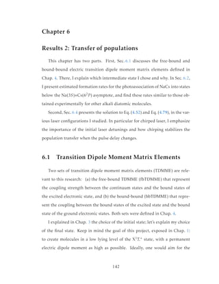
![|X,JX = 0,vX = 0 bound state, however the bbTDMME between this state and
the high-lying states of the excited electronic state are detrimental to a tran-
sition by stimulated emission. Yet, Aymar and Dulieu [19] showed (see their
Fig. 4) that for NaCs the permanent electric dipole moment is fairly constant
when the vibrational quantum number vX increases: the permanent electric
dipole moment stays close to −4.5 Debye for all vX ≤ 40.
I should choose a state in X1Σ+ not so low in the well that it would be in-
accessible by stimulated emission from the first excited electronic asymptote,
and yet no so high that its permanent electric dipole moment would be too dif-
ferent from the average value −4.5 Debye. The state |X,JX = 0,vX = 32 meets
those criteria.
Figure 6.1 p. 144 (top panel) shows the free-bound TDMMEs defined in
Eq. (4.38) between the continuum stationary scattering state chosen in Sec. 3.1
and the bound vibrational states of the A1
Σ+ state. As expected from the
Franck-Condon principle [24, Chap. 11], the fbTDMMEs are close to 0 for
bound-states that lie low in the well, but are much greater for bound states
of A1
Σ+ near dissociation. Experimentalists [22, 75] rely on the magnitude of
these bfTDMMEs to perform photoassociation spectroscopy. The bottom panel
of Fig. 6.1 displays the bound-bound TDMMEs from any |A,JA = 1,vA of the
A1
Σ+ electronic state into the state |X,0,32 . The rovibrational states |X,0,32
and |X,2,32 are so close in energy that their wave function are almost identi-
cal, yielding no significant difference between the bbTDMMEs from A1
Σ+ into
|X,0,vX = 32 or |X,2,32 . Once more, as expected from the Franck-Condon
principle, the higher vA, the lower the amplitude of the oscillations of the bbT-
DMME. With the help of Fig. 6.1, one can choose a range of intermediate states
|A,JA = 1,vA that (i) are not to close to the dissociation asymptote of the A1
Σ+
143](https://image.slidesharecdn.com/f18acd25-2ace-4766-aa5f-998434d2b6e5-150515233108-lva1-app6892/85/2015_Valladier_Stephane_Dissertation-164-320.jpg)


![this range of energy. The probability density function accumulates at the right
classical turning point with V3/2. Consequently, the overlap with the contin-
uum states of the X1Σ+ state and the corresponding fbTDMME are very small
(see Fig. 6.2), illustrating the ∆S = 0 that forbids transitions between the singlet
and the triplet.
For the purpose of my study, I chose as an intermediate state the coupled-
channel bound state |Φcc
vcc=254 . This state has TDMMEs that meet the same
criteria as those outlined when choosing a bound state for the A1
Σ+ state.
6.2 Photoassociation rates for NaCs
6.2.1 Validation of photoassociation rates obtained
For a given temperature and intensity of a continuous wave laser, the pho-
toassociation rate KPA is an experimental measure of the fbTDMMEs. The rate
KPA from the continuum at temperature T of the ground electronic state into a
bound state |Y ,vY ,J = 1 of electronic state Y with rotational quantum number
J = 1 is related to the fbTDMME through [76, Eq. (1)]
KPA(v) = 3
3λ2
th
2π
3
2
h
2
Y ,vY ,J = 1 |DY X | χX0
E=kBT /2
2
, (6.1)
where λth is the thermal de Broglie wavelength λ2
th = h
3µkBT . More details on
the theory of photoassociation appear in [69, 77, 78].
The photoassociation rate is calculated from a continuum state into a single
bound state of an excited electronic potential. Among the quantities that en-
ter the calculation of the photoassociation rate is the fbTDMME between that
continuum state and the bound state one photoassociates to [77, 78]. There-
146](https://image.slidesharecdn.com/f18acd25-2ace-4766-aa5f-998434d2b6e5-150515233108-lva1-app6892/85/2015_Valladier_Stephane_Dissertation-167-320.jpg)

![fore one can only calculate KPA’s towards the bound states of the potential one
is interested to probe, and essentially KPA is another way of representing the
fbTDMMEs, while including at the same time more experimental details. Ulti-
mately, one can not calculate more KPA than there are bound states in a given
potential.
In this section, I use Eq. (6.1) to validate my calculation of the fbTDMMEs
by comparing with the experimental results obtained in [22] for NaCs. More-
over by using similar laser intensities and sample temperature, I can also com-
pare my results for NaCs to those published in [18] for RbCs and in [79] for
LiCs.
I 5 W cm
2
T 200 ΜK
Na 3S Cs 6
2
P3 2
Computed
Approximate
Measured
10 1
100
101
102
10 14
10 13
10 12
10 11
10 10
10 9
10 8
10 7
10 6
detuning cm
1
PAratecm
3
s
Figure 6.3: (Color online) Photoassociation rate for NaCs at T = 200µK using
a continuous wave laser with intensity I = 5W/cm2 vs. detuning. Detunings
are measured below the Na(3S)+Cs(62P3/2) asymptote. The filled green circle
corresponds to the detuning closest to the experimental condition of [22].
Figures 6.3 & 6.4 show the photoassociation rates for NaCs from the contin-
uum of the X1Σ+ state state into all of the bound states of the spin-orbit coupled
A1
Σ+ −b3
Π0 manifold (down to a reasonable value of the detuning, photoasso-
ciation into states that lay low in the potential well is irrelevant). The colors are
148](https://image.slidesharecdn.com/f18acd25-2ace-4766-aa5f-998434d2b6e5-150515233108-lva1-app6892/85/2015_Valladier_Stephane_Dissertation-169-320.jpg)
![I 5 W cm
2
T 200 ΜK
Na 3S Cs 6
2
P1 2
Calculated
Approximate
100
101
102
10 14
10 13
10 12
10 11
10 10
10 9
10 8
10 7
detuning cm
1
PAratecm
3
s
Figure 6.4: (Color online) Photoassociation rate for NaCs at T = 200µK using
a continuous wave laser with intensity I = 5W/cm2 vs. detuning. Detunings are
measured below the Na(3S)+Cs(62P1/2) asymptote.
chosen to correspond to the relevant potential asymptotes, in order to remain
consistent with the graphs in Chaps. 4 & 5, and in particular Fig. 4.4, p. 109:
photoassociation rates for detunings measured below the asymptote of the V3/2
potential are in green, photoassociation rates for detunings measured below
the asymptote of the V1/2 asymptote are in magenta. Each figure is labeled
with the dissociation limit from which the detunings are measured. Both fig-
ures are obtained at a photoassociation laser intensity of I = 5W/cm2, as in [22].
In each figure, the jagged dashed line connects the successive symbols to pre-
vent the eye from perceiving the data as a scatter plot. The dashed dotted line
in the upper right portion of each graph is an estimate to the photoassociation
rate obtained from an estimate of the fbTDMME based on the approximation
formulae found in [73, 80] and based on the long-range dispersion coefficients
that govern the potential at large value of the internuclear separation. Notice
that the approximation constitutes an upper limit to the actual calculation, and
149](https://image.slidesharecdn.com/f18acd25-2ace-4766-aa5f-998434d2b6e5-150515233108-lva1-app6892/85/2015_Valladier_Stephane_Dissertation-170-320.jpg)
![that the actual results never exceed the approximate prediction. In particular
the filled data point in Fig. 6.3 reproduces within experimental uncertainty the
photoassociation rate reported in [22].
I 3.63 W cm
2
T 100 ΜK
Na 3S Cs 6
2
P1 2
Calculated
Approximate
100
101
102
10 14
10 13
10 12
10 11
10 10
10 9
10 8
10 7
10 6
detuning cm
1
PAratecm
3
s
Figure 6.5: (Color online) Photoassociation rate for NaCs at T = 100µK using
a continuous wave laser with intensity I = 3.63W/cm2 vs. detuning. Detunings
are measured below the Na(3S)+Cs(62P1/2) asymptote. The filled magenta dia-
monds corresponds to the detuning closest to the experimental condition of [18].
In Figure 6.5, I used the experimental conditions from [18]. The two filled
diamonds correspond to detunings for NaCs closest to the detunings for RbCs
used in [18]. In fact, I was able to find a detuning and intensity that yielded
the same photoassociation rate at T = 100µK for NaCs than for RbCs. Note
that for NaCs at 51cm−1 below Na(3S)+Cs(62P1/2), KPA is a minimum. Actu-
ally I set the intensity of the photoassociation laser so that the minimum KPA at
this detuning is equal between the two molecules. If I want KPA at a detuning
of 61cm−1below Na(3S)+Cs(62P1/2) (the closest maximum) to match the pub-
lished photoassociation rate of [18], I need a lower photoassociation intensitya.
aPhotoassociation rates vary linearly with the photoassociation intensity.
150](https://image.slidesharecdn.com/f18acd25-2ace-4766-aa5f-998434d2b6e5-150515233108-lva1-app6892/85/2015_Valladier_Stephane_Dissertation-171-320.jpg)
![It is worth remembering that Kerman et al. [18] do not state the actual intensity
they use to obtain the KPA’s they report; they only give the maximum photoas-
sociation intensity that their set up allows (4kW/cm2).
I 74 W cm
2
T 200 ΜK
Na 3S Cs 6
2
P3 2
10 1
100
101
102
10 15
10 14
10 13
10 12
10 11
10 10
10 9
10 8
10 7
10 6
detuning cm
1
PAratecm
3
s
Figure 6.6: (Color online) Photoassociation rate for NaCs at T = 200µK using
a continuous wave laser with intensity I = 74W/cm2 vs. detuning. Detunings
are measured below the Na(3S)+Cs(62P3/2) asymptote. The filled green circles
corresponds to the detuning closest to the experimental condition of [79].
In Figures 6.6 and 6.7, Dutta et al. [79] report a detuning of 15.08GHz ≈
0.50cm−1 below the Li(2S)+Rb(52P3/2) asymptote. In NaCs there are two bound
states below the Na(3S)+Cs(62P3/2) asymptote, one with detuning 0.371cm−1,
the other with a detuning of 0.827cm−1; these data points are marked with
filled symbols in Figs. 6.6 and 6.7. Although Dutta et al. [79] are quite spe-
cific about the intensity of their photoassociation laser, they only provide the
separate temperatures of their Li MOTa (1000µK) and their Rb MOT (200µK,
similar than the NaCs temperature in the experiments reported by the group
of Prof. Bigelow at the University of Rochester). So, I obtained PA rates for
NaCs at both temperatures: as the temperature of the mixture is bound by
aMagneto-Optical Trap
151](https://image.slidesharecdn.com/f18acd25-2ace-4766-aa5f-998434d2b6e5-150515233108-lva1-app6892/85/2015_Valladier_Stephane_Dissertation-172-320.jpg)
![I 74 W cm
2
T 1000 ΜK
Na 3S Cs 6
2
P3 2
10 1
100
101
102
10 15
10 14
10 13
10 12
10 11
10 10
10 9
10 8
10 7
detuning cm
1
PAratecm
3
s
Figure 6.7: (Color online) Photoassociation rate for NaCs at T = 1000µK using
a continuous wave laser with intensity I = 74W/cm2 vs. detuning. Detunings
are measured below the Na(3S)+Cs(62P3/2) asymptote. The filled green circles
corresponds to the detuning closest to the experimental condition of [79].
the temperature of the individual species, and photoassociation rates decrease
smoothly when the temperature increases, the NaCs photoassociation rate at
the—unreported—temperature of the LiRb mixture is within these bounds. At
both temperatures, the photoassociation rate for NaCs is larger than for LiRb.
Note that I could always lower the photoassociation laser intensity to obtain
the same rate for the two molecules. The photoassociation rate at these detun-
ings is larger for NaCs because the scattering wave function is almost in phase
with the excited state coupled-channel wave function: the oscillations of both
wave function are thus constructive thereby enhancing the value of the bound-
free transition dipole moment. A similar phenomenon might occur for LiRb
but due to the nature of the potentials, the amplitude of the constructively-
interfering lobes is smaller, yielding an overall smaller bfTDMME.
152](https://image.slidesharecdn.com/f18acd25-2ace-4766-aa5f-998434d2b6e5-150515233108-lva1-app6892/85/2015_Valladier_Stephane_Dissertation-173-320.jpg)


![6.4 Populations as functions of time
The idea here is to fiddle with the various parameters of the laser available
and attempt to achieve three goals:
1. transfer a significant (≥ 90%) portion of the population from the contin-
uum into the final state |X,0,32
2. avoid population to linger in the intermediate state(s) |A,1,vA or |Φcc
vcc
to
prevent loss of population by spontaneous emission
3. complete the population transfer within at most a few nanoseconds.
Note that choosing a spectral bandwidth uniquely determines the temporal
bandwidth and the maximum chirp rate that a filter can impart onto a laser. In
planning for the later use of adiabatic transfer, I follow the recommendation of
[16, 30, 81]: I always choose pump and Stokes chirp rates equal to each others,
lasers with identical temporal bandwidth, and intensities such that the peak
Rabi frequencies are equal.
To warm up, let’s begin with case 1-bNIu.
6.4.1 Case 1—bNIu: intuitive sequence of unchirped lasers
with narrow spectral bandwidth, without SO coupling
To generate Figure 6.9 p. 158, the laser intensities are set so the correspond-
ing Rabi frequencies are π-pulses. In the intuitive sequence (pump before
Stokes pulse), the action of each laser can be viewed independently, and the
system undergoes 2-state π-pulse transfer within each set of relevant states.
The laser intensities are also optimized to minimize oscillations of population
during the action of a given pulse.
157](https://image.slidesharecdn.com/f18acd25-2ace-4766-aa5f-998434d2b6e5-150515233108-lva1-app6892/85/2015_Valladier_Stephane_Dissertation-178-320.jpg)
![By separating the lasers as shown, the population is transferred sequentially
from one state to the other. The transfer yields 99.5% of population in |X,0,32 .
For each transfer, the optimal detuning of the laser is 0 (see Sec. 2.3.1). What
about the intermediate population in |A,1,140 ? The typical lifetimes of vibra-
tional states |A,vA > 100 are greater than 40ns [10]. Therefore, no population
should be lost from the intermediate state by spontaneous emission. Let’s now
0.
10.
20.
30.
40.
50.
60.
IntensitykW.cm2
aPump laser chirped
Pump laser regular
Stokes laser chirped
Stokes laser regular
0 1000 2000 3000 4000 5000
Time ps
0.0
0.2
0.4
0.6
0.8
1.0
Population
b
E
X0
140
A1
32
X0
32
X2
v A 140,odd
A1
v A 140,even
A1
Figure 6.9: (Color online) Population transfer as a function of time, case 1—
bNIu. Narrow spectral bandwidth of 0.5GHz, no spin-orbit effects accounted
for, unchirped lasers in intuitive sequence. The laser intensities are chosen to
obtain the simplest π-pulse as possible.
158](https://image.slidesharecdn.com/f18acd25-2ace-4766-aa5f-998434d2b6e5-150515233108-lva1-app6892/85/2015_Valladier_Stephane_Dissertation-179-320.jpg)


![vides an expression to delimit a range of values for optimal detunings
• when chirping the lasers, the sequence of π-pulses becomes insensitive to
pulse delay, which can then be reduced to minimize the duration of the
overall population transfer
• for the minimal pulse delay, the process becomes adiabatic without re-
sorting to the counterintuitive sequence.
After this first taste of adiabatic passage, let’s consider STIRAP.
6.4.3 Case 3—bNCu: STIRAP with narrow spectral bandwidth,
without SO coupling
The counterintuitive sequence is an essential requirement of STIRAP (see
Sec. 2.3.2). In the present case, the lasers are unchirped: I set the detunings to
0, which is the optimal value for STIRAP [16, 30, 32, 81]. Achieving population
transfer in the counterintuitive sequence requires a minimal pulse intensity
(Eq. (15) in [16], Eq. (58) in[81]) to reach adiabaticity. Figure 6.17 shows that
the minimal required intensity is 10 × Iπ,0, where Iπ,0 is the minimal π-pulse
intensity. Passed that value, the process is rather insensitive to changes in the
intensity.
The higher the intensity, the more stable is STIRAP with respect to the de-
lay between the pulses as shown in Fig. 6.18. Regardless of the intensity, the
optimal delay is always given by ηSTIRAP = − 1√
2ln2
∆τ, where ∆τ is the FWHM
of the intensity pulse, as derived in App. C.
To close this case, although this process yields a high final population in
|X,0,32 , the adiabatic condition is not satisfied at all times, as shown by the
169](https://image.slidesharecdn.com/f18acd25-2ace-4766-aa5f-998434d2b6e5-150515233108-lva1-app6892/85/2015_Valladier_Stephane_Dissertation-190-320.jpg)


![and 1.8% remains in the continuum state. The neighbors of |A,1,140 in energy
share the remaining 0.2% of population.
6.4.11 Case 10—BNIc: Intuitive sequence of chirped lasers with
broad spectral bandwidth, without SO coupling
The first simulation assumes all parameters to be the same as in the previ-
ous case 9—BNIu. In particular the detunings are zero, despite our knowledge
of the GRHYP. Figure 6.33 shows the population transfer in this case. First, no
population gets transferred into any of the vibrational states of X1Σ+. As the
pulse is positively chirped, the central frequency of the pump laser increases
with time, and the states above |A,1,140 in energy get successively populated.
Note that the first state to enter into resonance with the laser is |A,1,141 . How-
ever the state |A,1,146 , with the highest free-bound transition dipole moment,
gets populated first as a closer look at early times in Fig. 6.33 shows. The state
|A,1,141 then picks up population. The state |A,1,144 , which has the second
highest fbTDMME in magnitude, is third to enter the scene, immediately fol-
lowed by |A,1,143 . The states |A,1,142 and |A,1,145 remain oblivious to the
process, as they have the smallest free-bound transition dipole moment ma-
trix elements, see Tbl. 6.2 p. 192. Apart from |A,1,141 , the neighboring states
are populated in the same order as their transition dipole moment. Chirping
the laser gives priority to |A,1,141 over |A,1,vA ,vA = 143,144, but is not suf-
ficient for |A,1,141 to precede |A,1,146 in receiving population, due to the
strong value of the fbTDMME of |A,1,146 . Notice the similarity of this graph
with Fig. 5 in [82].
Let’s change the detunings using the GRHYP (Fig. 6.34) and see how the
process is modified. The state |A,1,146 still collects, however briefly, some
189](https://image.slidesharecdn.com/f18acd25-2ace-4766-aa5f-998434d2b6e5-150515233108-lva1-app6892/85/2015_Valladier_Stephane_Dissertation-210-320.jpg)


![Bibliography
[1] M. H. Anderson, J. R. Ensher, M. R. Matthews, C. E. Wieman, and E. A. Cor-
nell, Observation of Bose-Einstein condensation in a dilute atomic vapor, Science,
269(5221), 198 (1995).
[2] J. Doyle, B. Friedrich, R. Krems, and F. Masnou-Seeuws, Editorial: Quo vadis, cold
molecules?, The European Physical Journal D - Atomic, Molecular, Optical and
Plasma Physics, 31(2), 149 (2004).
[3] L. D. Carr, D. DeMille, R. V. Krems, and J. Ye, Cold and ultracold molecules: science,
technology and applications, New Journal of Physics, 11(5), 055049 (2009).
[4] R. V. Krems, Cold controlled chemistry, Physical Chemistry Chemical Physics, 10,
4079 (2008).
[5] J. J. Hudson, B. E. Sauer, M. R. Tarbutt, and E. A. Hinds, Measurement of the
Electron Electric Dipole Moment Using YbF Molecules, Physical Review Letters, 89,
023003 (2002).
[6] D. DeMille, Quantum Computation with Trapped Polar Molecules, Physical Review
Letters, 88(6), 067901 (2002).
[7] P. Rabl, D. DeMille, J. M. Doyle, M. D. Lukin, R. J. Schoelkopf, and P. Zoller,
Hybrid Quantum Processors: Molecular Ensembles as Quantum Memory for Solid
State Circuits, Physical Review Letters, 97, 033003 (2006).
[8] L. Bomble, P. Pellegrini, P. Ghesqui`ere, and M. Desouter-Lecomte, Toward scalable
information processing with ultracold polar molecules in an electric field: A numerical
investigation, Physical Review A, 82, 062323 (2010).
[9] G. Pupillo, A. Griessner, A. Micheli, M. Ortner, D.-W. Wang, and P. Zoller, Cold
Atoms and Molecules in Self-Assembled Dipolar Lattices, Physical Review Letters,
100, 050402 (2008).
[10] J. Zaharova, M. Tamanis, R. Ferber, A. N. Drozdova, E. A. Pazyuk, and A. V. Stol-
yarov, Solution of the fully-mixed-state problem: Direct deperturbation analysis of the
A1Σ+–b3Π complex in a NaCs dimer, Physical Review A, 79(1), 012508 (2009).
[11] E. Luc-Koenig and F. Masnou-Seeuws, Cold Molecules: Theory, Experiment, Ap-
plications, chapter 7: Prospects for Control of Ultracold Molecule Formation via
Photassociation with Chirped Laser Pulses, 245–290, CRC Press (2009).
[12] E. Luc-Koenig, M. Vatasescu, R. Kosloff, and F. Masnou-Seeuws, Making Ultracold
Molecules with Chirped Laser Pulses, in E. Dalimier, editor, Spectral Line Shapes
2004, volume 1 of Proceedings of the 17th International Conference on Spectral Line
Shapes, 329–336, Frontier Group (2004).
[13] C. P. Koch, E. Luc-Koenig, and F. Masnou-Seeuws, Making ultracold molecules in a
two-color pump-dump photoassociation scheme using chirped pulses, Physical Review
A, 73(3), 033408 (2006).
213](https://image.slidesharecdn.com/f18acd25-2ace-4766-aa5f-998434d2b6e5-150515233108-lva1-app6892/85/2015_Valladier_Stephane_Dissertation-234-320.jpg)
![[14] K. Winkler, F. Lang, G. Thalhammer, P. v. d. Straten, R. Grimm, and J. H. Den-
schlag, Coherent Optical Transfer of Feshbach Molecules to a Lower Vibrational State,
Physical Review Letters, 98(4), 043201 (2007).
[15] S. Ospelkaus, A. Pe’er, K.-K. Ni, J. J. Zirbel, B. Neyenhuis, S. Kotochigova, P. S.
Julienne, J. Ye, and D. S. Jin, Efficient state transfer in an ultracold dense gas of
heteronuclear molecules, Nature Physics, 4(8), 622 (2008).
[16] K. Bergmann, H. Theuer, and B. W. Shore, Coherent population transfer among
quantum states of atoms and molecules, Reviews of Modern Physics, 70(3), 1003
(1998).
[17] K. Bergmann and B. W. Shore, Molecular Dynamics and Spectroscopy by Stimulated
Emission Pumping, volume 4 of Advanced Series in Physical Chemistry, chapter 9:
Coherent Population Transfer, 315–373, World Scientific (1995).
[18] A. J. Kerman, J. M. Sage, S. Sainis, T. Bergeman, and D. DeMille, Production of Ul-
tracold, Polar RbCs∗ Molecules via Photoassociation, Physical Review Letters, 92(3),
033004 (2004).
[19] M. Aymar and O. Dulieu, Calculation of accurate permanent dipole moments of the
lowest 1,3Σ+ states of heteronuclear alkali dimers using extended basis sets, The Jour-
nal of Chemical Physics, 122(20), 204302 (2005).
[20] P. S. ˙Zuchowski and J. M. Hutson, Reactions of ultracold alkali-metal dimers, Phys-
ical Review A, 81(6), 060703 (2010).
[21] O. Docenko, M. Tamanis, J. Zaharova, R. Ferber, A. Pashov, H. Kn¨ockel, and
E. Tiemann, The coupling of the X1Σ+ and a3Σ+ states of the atom pair Na+Cs
and modelling cold collisions, Journal of Physics B: Atomic, Molecular and Opti-
cal Physics, 39(19), S929 (2006).
[22] C. Haimberger, J. Kleinert, O. Dulieu, and N. P. Bigelow, Processes in the formation
of ultracold NaCs, Journal of Physics B: Atomic, Molecular and Optical Physics,
39(19), S957 (2006).
[23] B. E. A. Saleh and M. C. Teich, Fundamentals of photonics, Wiley-Interscience,
Hoboken, N.J., 2nd. edition (2007).
[24] B. H. Bransden and C. J. Joachain, Physics of atoms and molecules, Prentice Hall,
Harlow ; Munich [u.a.] (2010).
[25] M. H. Nayfeh and M. K. Brussel, Electricity and Magnetism, Wiley, New York
(1985).
[26] D. A. Steck, Cesium D Line Data (2009). Version 2.1.2.
[27] J. R. R. Tolkien, The Lord of The Rings, Houghton Mifflin, Boston (1967).
[28] A. Messiah, Quantum mechanics, North-Holland Pub. Co. ; John Wiley, Amster-
dam; New York (1966).
214](https://image.slidesharecdn.com/f18acd25-2ace-4766-aa5f-998434d2b6e5-150515233108-lva1-app6892/85/2015_Valladier_Stephane_Dissertation-235-320.jpg)
![[29] C. Cohen-Tannoudji, B. Diu, and F. Lalo¨e, Quantum mechanics, Wiley, New York
(1977).
[30] B. W. Shore, The theory of coherent atomic excitation, John Wiley and Sons, Inc.,
New York (1990).
[31] U. Gaubatz, P. Rudecki, S. Schiemann, and K. Bergmann, Population transfer be-
tween molecular vibrational levels by stimulated Raman scattering with partially over-
lapping laser fields. A new concept and experimental results, The Journal of Chemical
Physics, 92(9), 5363 (1990).
[32] M. P. Fewell, B. W. Shore, and K. Bergmann, Coherent Population Transfer among
Three States: Full Algebraic Solutions and the Relevance of Non Adiabatic Processes to
Transfer by Delayed Pulses, Australian Journal of Physics, 50(2), 281 (1997).
[33] J. H. Van Vleck, The Coupling of Angular Momentum Vectors in Molecules, Reviews
of Modern Physics, 23, 213 (1951).
[34] H. Lefebvre-Brion and R. W. Field, The spectra and dynamics of diatomic molecules,
Elsevier Academic Press, Amsterdam; Boston (2004).
[35] H. Katˆo, Energy Levels and Line Intensities of Diatomic Molecules. Application to
Alkali Metal Molecules, Bulletin of the Chemical Society of Japan, 66(11), 3203
(1993).
[36] J. F. Ogilvie, The vibrational and rotational spectrometry of diatomic molecules, Aca-
demic Press (1998).
[37] R. J. LeRoy, Molecular Spectroscopy, Specialist periodical reports, volume 1, chapter
3 : Energy Levels of a diatomic near dissociation, 113–176 (1973).
[38] S. J. Umanski and A. I. Voronin, Asymptotic Calculation of Some Exchange Integrals,
Theoretica Chimica Acta, 12(2), 166 (1968).
[39] H. Margenau, Van der waals forces, Reviews of Modern Physics, 11(1), 1 (1939).
[40] K. M. Jones, E. Tiesinga, P. D. Lett, and P. S. Julienne, Ultracold photoassocia-
tion spectroscopy: long-range molecules and atomic scattering, Reviews of Modern
Physics, 78, 483 (2006).
[41] B. Bussery, Y. Achkar, and M. Aubert-F´econ, Long-Range Molecular States Disso-
ciating To The Three or Four Lowest Asymptotes for the Ten Heteronuclear Diatomic
Alkali Molecules, Chemical Physics, 116, 319 (1987).
[42] M. Marinescu and H. R. Sadeghpour, Long range potentials for two-species alkali-
metal atoms, Physical Review A, 59(1), 390 (1999).
[43] I. G. Kaplan, Intermolecular interactions : physical picture, computational methods,
model potentials, Wiley, Hoboken, NJ (2006).
215](https://image.slidesharecdn.com/f18acd25-2ace-4766-aa5f-998434d2b6e5-150515233108-lva1-app6892/85/2015_Valladier_Stephane_Dissertation-236-320.jpg)
![[44] M. Aymar and O. Dulieu, Calculations of transition and permanent dipole moments
of heteronuclear alkali dimers NaK, NaRb and NaCs, Molecular Physics, 105(11-12),
1733 (2007).
[45] R. J. LeRoy, LEVEL 8.0: A Computer Program for Solving the Radial Schr¨odinger
Equation for Bound and Quasibound Levels, Research Report CP-661, University of
Waterloo Chemical Physics (2007).
[46] J. Kim, Y. Lee, and A. Stolyarov, Quasi-relativistic treatment of the low-lying {KCs}
states, Journal of Molecular Spectroscopy, 256(1), 57 (2009). PRAHA2008, The
20th International Conference on High Resolution Molecular Spectroscopy.
[47] C. Haimberger, J. Kleinert, P. Zabawa, A. Wakim, and N. P. Bigelow, Formation of
ultracold, highly polar X1Σ+ NaCs molecules, New Journal of Physics, 11(5), 055042
(2009).
[48] J. Kleinert, C. Haimberger, P. J. Zabawa, and N. P. Bigelow, Trapping of Ultracold
Polar Molecules with a Thin-Wire Electrostatic Trap, Physical Review Letters, 99,
143002 (2007).
[49] P. Zabawa, A. Wakim, A. Neukirch, C. Haimberger, N. P. Bigelow, A. V. Stolyarov,
E. A. Pazyuk, M. Tamanis, and R. Ferber, Near-dissociation photoassociative produc-
tion of deeply bound NaCs molecules, Physical Review A, 82, 040501 (2010).
[50] P. F. Bernath, Spectra of atoms and molecules, Oxford University Press, New York,
2nd edition (2005).
[51] J. M. Brown and A. Carrington, Rotational spectroscopy of diatomic molecules, Cam-
bridge University Press, Cambridge; New York (2003).
[52] M. E. Rose, Elementary theory of angular momentum, Wiley, New York (1957).
[53] M. A. Morrison and G. A. Parker, A Guide to Rotations in Quantum Mechanics,
Australian Journal of Physics, 40(4), 465 (1987).
[54] M. D. Sturge, Statistical and thermal physics : fundamentals and applications, A.K.
Peters, Natick, Mass. (2003).
[55] G. Herzberg, Molecular Spectra and Molecular Structure I, volume I. Spectra of
Diatomic Molecules, Van Nostrand Reinhold Company, 2nd edition (1950).
[56] A. R. Edmonds, Angular momentum in quantum mechanics., Princeton University
Press, Princeton, N.J. (1957).
[57] J. H. Van Vleck, On σ-Type Doubling and Electron Spin in the Spectra of Diatomic
Molecules, Physical Review, 33, 467 (1929).
[58] D. Bohm, Quantum Theory, Prentice-Hall, Inc., 1 edition (1951).
[59] M. Born and R. Oppenheimer, Zur Quantentheorie der Molekeln, Annalen der
Physik, 389, 457 (1927).
216](https://image.slidesharecdn.com/f18acd25-2ace-4766-aa5f-998434d2b6e5-150515233108-lva1-app6892/85/2015_Valladier_Stephane_Dissertation-237-320.jpg)
![[60] J. O. Hornkohl and C. Parigger, Angular momentum states of the diatomic molecule,
American Journal of Physics, 64(5), 623 (1996).
[61] R. T. Pack and J. O. Hirschfelder, Energy Corrections to the Born–Oppenheimer Ap-
proximation. The Best Adiabatic Approximation, The Journal of Chemical Physics,
52(2), 521 (1970).
[62] C. Eckart, The Kinetic Energy of Polyatomic Molecules, Physical Review, 46, 383
(1934).
[63] U. Fano, Description of States in Quantum Mechanics by Density Matrix and Operator
Techniques, Reviews of Modern Physics, 29, 74 (1957).
[64] K. Blum, Density matrix theory and applications, Plenum Press, New York (1981).
[65] S. Stenholm, Foundations of laser spectroscopy, Wiley, New York (1984).
[66] J. Vala, O. Dulieu, F. Masnou-Seeuws, P. Pillet, and R. Kosloff, Coherent control of
cold-molecule formation through photoassociation using a chirped-pulsed-laser field,
Physical Review A, 63, 013412 (2000).
[67] D. J. Heinzen, Ultracold Atomic Interactions, in M. Inguscio, S. Stringari, and C. E.
Wieman, editors, Bose-Einstein condensation in atomic gases, 351–390, Interna-
tional School of Physics ”Enrico Fermi” and Societ italiana di fisica., IOS Press,
Amsterdam; Washington, DC (1998).
[68] W. C. Stwalley and H. Wang, Photoassociation of Ultracold Atoms: A New Spectro-
scopic Technique, Journal of Molecular Spectroscopy, 195(2), 194 (1999).
[69] C. Drag, Photoassociation d’atomes de cesium froids. Formation et caract´erisation d’un
nuage froid de mol´ecules diatomiques de cesium., Ph.D. thesis, [S.l.] (2000).
[70] P. S. Julienne, Cold molecules : theory, experiment, applications, chapter 6: Molecu-
lar States Near a Collision Threshold, 221–243, CRC Press, Boca Raton (2009).
[71] C. P. Koch, R. Kosloff, E. Luc-Koenig, F. Masnou-Seeuws, and A. Crubellier, Pho-
toassociation with chirped laser pulses: calculation of the absolute number of molecules
per pulse, Journal of Physics B: Atomic, Molecular and Optical Physics, 39(19),
S1017 (2006).
[72] H. Friedrich, Theoretical atomic physics, Springer-Verlag, Berlin; New York, 3rd
edition (2005).
[73] B. E. Londo˜no, J. E. Mahecha, E. Luc-Koenig, and A. Crubellier, Resonant coupling
effects on the photoassociation of ultracold Rb and Cs atoms, Physical Review A, 80,
032511 (2009).
[74] R. Stoer, Josef; Bulirsch, Introduction to numerical analysis, Springer-Verlag, New
York (1992).
217](https://image.slidesharecdn.com/f18acd25-2ace-4766-aa5f-998434d2b6e5-150515233108-lva1-app6892/85/2015_Valladier_Stephane_Dissertation-238-320.jpg)
![[75] C. Haimberger, J. Kleinert, M. Bhattacharya, and N. P. Bigelow, Formation and
detection of ultracold ground-state polar molecules, Physical Review A, 70, 021402
(2004).
[76] S. Azizi, M. Aymar, and O. Dulieu, Prospects for the formation of ultracold ground
state polar molecules from mixed alkali atom pairs, The European Physical Journal
D: Atomic, Molecular, Optical and Plasma Physics, 31(2), 195 (2004).
[77] J. L. Bohn and P. S. Julienne, Semianalytic theory of laser-assisted resonant cold col-
lisions, Physical Review A, 60, 414 (1999).
[78] P. Pillet, A. Crubellier, A. Bleton, O. Dulieu, P. Nosbaum, I. Mourachko, and
F. Masnou-Seeuws, Photoassociation in a gas of cold alkali atoms: I. Perturbative
quantum approach, Journal of Physics B: Atomic, Molecular and Optical Physics,
30(12), 2801 (1997).
[79] S. Dutta, J. Lorenz, A. Altaf, D. S. Elliott, and Y. P. Chen, Photoassociation of ultra-
cold LiRb∗
molecules: Observation of high efficiency and unitarity-limited rate satura-
tion, Physical Review A, 89, 020702 (2014).
[80] H. Wang and W. C. Stwalley, Ultracold photoassociative spectroscopy of heteronuclear
alkali-metal diatomic molecules, The Journal of Chemical Physics, 108(14), 5767
(1998).
[81] N. V. Vitanov, M. Fleischhauer, B. W. Shore, and K. Bergmann, Coherent manipu-
lation of atoms and molecules by sequential laser pulses, volume 46 of Advances In
Atomic, Molecular, and Optical Physics, 55 – 190, Academic Press (2001).
[82] E. Luc-Koenig, R. Kosloff, F. Masnou-Seeuws, and M. Vatasescu, Photoassociation
of cold atoms with chirped laser pulses: Time-dependent calculations and analysis
of the adiabatic transfer within a two-state model, Physical Review A, 70, 033414
(2004).
[83] J. R. Taylor, An introduction to error analysis : the study of uncertainties in physical
measurements, University Science Books, Sausalito, Calif. (1997).
218](https://image.slidesharecdn.com/f18acd25-2ace-4766-aa5f-998434d2b6e5-150515233108-lva1-app6892/85/2015_Valladier_Stephane_Dissertation-239-320.jpg)


![The intensity defined by Eq. (A.7) has full widtha at 1/e equal to τ
√
2. The
corresponding Full Width at Half Maximumb,c (FWHM) is ∆τ = τ
√
2 ln2.
The spectral intensity S(ν) is the square modulus of the Fourier transform
of the pulse:
S(ν) = |A(ν)|2
= A(ν)A∗
(ν), with (A.8a)
A(ν) = A0τ
√
πexp −π2
τ2
(ν − ν0)2
, [TLG pulse Fourier transform] (A.8b)
S(ν) = |A0|2
τ2
πexp −2π2
τ2
(ν − ν0)2
(A.8c)
where ν0 is the pulse’s initial frequency. The spectral width, defined as the
FWHM of the spectral intensity, is thus
∆ν =
√
2 ln2
π
1
τ
=
2 ln2
π
1
∆τ
⇔ ∆ω =
4 ln2
∆τ
(A.9)
A.1.4 Chirped Gaussian Pulse
Mathematically, multiplying a TLG pulse by a phase factor with a time de-
pendent phase suffices to define a Chirped Gaussian (CG) pulse:
A(t) = A0 exp −
t2
τ2
exp(iφ(t)), A0 ∈ C. (A.10)
The pulse is linearly chirped if the phase is quadratic in time φ(t) = at2/2τ2,a ∈
R. If the chirp parameter a is zero, the CG pulse reduces to the TLG pulse. The
general form of a linearly CG pulse is thus
A(t) = A0 exp −(1 − ia)
t2
τ2
A0 ∈ C, (A.11)
aThe full width δ at 1/e of a Gaussian f (t) centered at t0 is such that f (t0 ± δ
2 ) = f (t0)/e.
bThe FWHM of a Gaussian function f (t) centered at t0 is such that f (t0 ± ∆τ
2 ) = f (t0)/2.
cThe FWHM of the temporal envelope A(t) is ∆t = 2τ
√
ln2
222](https://image.slidesharecdn.com/f18acd25-2ace-4766-aa5f-998434d2b6e5-150515233108-lva1-app6892/85/2015_Valladier_Stephane_Dissertation-243-320.jpg)


![Appendix B
The many faces of adiabaticity in physics
The word “adiabatic” comes from the greek a (“not”) + dia (“through”) +
batos (“passable”). Something adiabatic is therefore, etymologically, something
that prevents another from passing through. An excellent illustration of an
adiabatic entity is given in [27, Book 2, end of chap. V].
B.1 Thermodynamics and Statistical Mechanics
In thermodynamics, a process is called adiabatic if it does not let any heat
pass into or out of the system. If the process is reversible, the change in heat
dQ is directly related to the change in entropy dS by dS = dQ/T . Thus if this
reversible process is adiabatic, no heat is exchanged, and the entropy stays con-
stant.
From a statistical mechanics point of view, since the entropy of the system
stays constant during this reversible adiabatic process, the multiplicity of the
macrostate of the system stays the same. Thus although the microstate of the
system may change throughout the process, the macrostate is unaffected by the
reversible adiabatic process, keeping the entropy of the system constant.
B.2 Quantum Mechanics
Messiah [28, chap. xvii, vol. II] discusses extensively the adiabatic theorem
in Quantum Mechanics. Messiah proves the adiabatic theorem by consider-
ing that the Hamiltonian of the system is explicitly time dependent, and changes
227](https://image.slidesharecdn.com/f18acd25-2ace-4766-aa5f-998434d2b6e5-150515233108-lva1-app6892/85/2015_Valladier_Stephane_Dissertation-248-320.jpg)
![slowly with time. The essential result of the adiabatic theorem is that if the
system starts in an eigenstate |ψ(t0) of the Hamiltonian H (t0) at t = t0, and
if H (t) changes slowly with time, then at t = t1 > t0, the system will be in the
eigenstate |ψ(t1) that derives from |ψ(t0) by continuity. This statement is best
illustrated in the context of STImulated Raman Adiabatic Passage (STIRAP),
which I discuss in Sec. 2.3.
Although Messiah proves the adiabatic theorem when the total hamiltonian
depends explicitly on time t and changes slowly with t, nothing in the theorem
prevents its application to a hamiltonian that changes slowly when any one of
its variable changes. Thus, I can consider the time independent Hamiltonian
of a diatomic molecule, which does depend on the internuclear separation R,
and consider that said hamiltonian varies slowly as R changes.
If H changes slowly from Ri to Ri+1, the state of the electrons at Ri+1 derives
from the state of the electrons at Ri by continuity. In this sense, Hund’s cases
states are adiabatic: they obey the adiabatic theorem where R, rather than time
t, is the key variable.
Since Hund’s cases always diagonalize He, and all Hund’s cases are adia-
batic in the sense of the adiabatic theorem, by extension, models that describe
molecular dynamics where He is diagonal are called adiabatic. On the contrary,
when the model does not diagonalize He, then the model is non-adiabatic. Non-
adiabatic models (i.e. not diagonalizing He) that diagonalize Tn(R) are some-
times called diabatic models [34].
228](https://image.slidesharecdn.com/f18acd25-2ace-4766-aa5f-998434d2b6e5-150515233108-lva1-app6892/85/2015_Valladier_Stephane_Dissertation-249-320.jpg)
![Appendix C
Optimal Pulse Delay
In this appendix I translate mathematically the condition for optimal pulse
delay expressed at the end of §V.B (p. 1011) in [16]:
“For optimum delay, the mixing angle should reach an angle of π/4
when Ωeff reaches its maximum value.”
where Ωeff(t) = Ω2
P (t) + Ω2
S(t). The expressions for the Gaussian Rabi pulses
are:
ΩP (t) = Ω0
P exp
−4ln2
t − tP
∆τP
2
= Ω0
P exp −
(t − tP )2
2σ2
P
(C.1a)
ΩS(t) = Ω0
S exp
−4ln2
t − tS
∆τS
2
= Ω0
S exp −
(t − tS)2
2σ2
S
(C.1b)
I restrict the derivation below to Rabi pulses of identical width and height [31]:
σP = σS = σ, Ω0
P = Ω0
S = Ω. First, let’s find the extrema of
Ωeff(t) = Ω0 exp −
(t − tP )2
σ2
+ exp −
(t − tS)2
σ2
1/2
= Ω0 u(t)
The extrema of Ωeff(t) are such that du
dt = 0:
du
dt
= −
2
σ2
(t − tP )exp −
(t − tP )2
σ2
+ (t − tS)exp −
(t − tS)2
σ2
The roots du
dt are the solution of a transcendental equation. However, t1/2 = tS+tP
2
is an analytic root of du/dt, since t1/2 − tP = η/2 = −(t1/2 − tS). The nature of
the extremum of Ωeff at t = t1/2 is given by the sign of dΩeff
dt t=t1/2
. Using the
229](https://image.slidesharecdn.com/f18acd25-2ace-4766-aa5f-998434d2b6e5-150515233108-lva1-app6892/85/2015_Valladier_Stephane_Dissertation-250-320.jpg)

![Thus the optimal pulse delay is |η| = σ
√
2. Since 1
2σ2 = 4ln2
∆τ2 , then in terms of
the pulse FWHM ∆τ
η = tS − tP = −
∆τ
2
√
ln2
≈ −0.6∆τ (C.7)
as reported in [31]. It is important to remember that ∆τ is the FWHM of the
Rabi pulse amplitude. The optimal pulse delay must be negative, since STIRAP
can only occur in the counterintuitive sequence, when the Stokes pulse precedes
the pump pulse.
231](https://image.slidesharecdn.com/f18acd25-2ace-4766-aa5f-998434d2b6e5-150515233108-lva1-app6892/85/2015_Valladier_Stephane_Dissertation-252-320.jpg)


![Then
vα −
2
2µ
d2
dR2
vα = Evα
δvαvα
− vα V total
α vα (E.1a)
= Evα
δvαvα
− vα V total
α vα (E.1b)
= vα −
2
2µ
d2
dR2
vα , (E.1c)
since V total
α is purely multiplicative and δvαvα
= δvαvα
. Matrix elements of the
type described in the previous equation occur both in the A and H basis. Equa-
tions E.1 show that TA and the parts of TH that contain d2
/dR2 are indeed
hermitian.
The function dγ/dR is purely multiplicative, therefore
vα
dγ
dR
2
vα = vα
dγ
dR
2
vα ,
so all diagonal blocks of TH are hermitian.
Let’s focus now on the off-diagonal blocks of TH. To finish proving that TH
is hermitian, I need to prove that
v3/2
d2
γ
dR2
+ 2
dγ
dR
∂
∂R
v1/2 = v1/2 −
d2
γ
dR2
− 2
dγ
dR
∂
∂R
v3/2 . (E.2)
Let’s recall the rule of integration by parts for the product of three well-behaved
functions f ,g, and h:
b
a
f gh dR = [f gh]b
a −
b
a
f ghdR −
b
a
f g hdR,
234](https://image.slidesharecdn.com/f18acd25-2ace-4766-aa5f-998434d2b6e5-150515233108-lva1-app6892/85/2015_Valladier_Stephane_Dissertation-255-320.jpg)


![Appendix F
Examining the coupled-channels wave functions
F.1 Introduction
In this appendix I verify the validity of the solutions to the coupled-channels
problem I set out to solve, and I show the closeness of the calculated coupled-
channels rovibrational energies with the results published in [10].
F.2 Validity of the coupled-channels solutions
Let’s recall equations (4.71) from Sec. 4.4.2.4 on p. 114, and use them to
define the operators ˆh11, ˆh12, ˆh21, and ˆh22, such that
−
2
2µ
d2
dR2
−
dγ
dR
2
+ V1/2(R) + 4
2
2µR2
ψ
[1/2]
vcc
(R)
+
2
2µ
d2
γ
dR2
+ 2
dγ
dR
d
dR
ψ
[3/2]
vcc
(R) = Ecc
vcc
ψ
[1/2]
vcc
(R), (F.1a)
−
2
2µ
d2
γ
dR2
+ 2
dγ
dR
d
dR
ψ
[1/2]
vcc
(R)
+
−
2
2µ
d2
dR2
−
dγ
dR
2
+ V3/2(R) + 4
2
2µR2
ψ
[3/2]
vcc
(R) = Ecc
vcc
ψ
[3/2]
vcc
(R). (F.1b)
⇔
ˆh11 ψ
[1/2]
vcc
+ ˆh12 ψ
[3/2]
vcc
= Ecc
vcc
ψ
[1/2]
vcc
, (F.2a)
ˆh21 ψ
[1/2]
vcc
+ ˆh22 ψ
[3/2]
vcc
= Ecc
vcc
ψ
[3/2]
vcc
. (F.2b)
The potentials V1/2 and V3/2 are defined in Eq. (4.55) p. 103, the mixing angleγ(R) is defined by its sine and cosine in Eq. (4.57) p. 104, and the coupled-
channel eigenket |Φcc
vcc
is defined in Eq. (4.70) p. 115. By plotting on the same
237](https://image.slidesharecdn.com/f18acd25-2ace-4766-aa5f-998434d2b6e5-150515233108-lva1-app6892/85/2015_Valladier_Stephane_Dissertation-258-320.jpg)
![graph the left and right hand side of Eqs. (F.2a-F.2b), I can assess whether |Φcc
vcc
is actually an eigenstate of the coupled-channel Time-Independent Schr¨odinger
Equation with eigenenergy Ecc
vcc
. If the left hand side of the equations superim-
poses on the right hand side, then |Φcc
vcc
is indeed a coupled-channel eigenstate
with energy Ecc
vcc
.
Figures F.1–F.9 below show plots of Eqs. (F.2a) and (F.2b). On each figure,
panel (a) is always a plot of Eq. (F.2a), and panel (b) is always a plot of Eq. (F.2b).
The red (resp.gray) solid line always represents the left hand side of Eq. (F.2a)
(resp.Eq. (F.2b)), while the dotted blue (resp. dashed green) line represents the
right hand side of Eq. (F.2a) (resp. Eq. (F.2b)). The legend on each figure is a
reminder of this convention. The black horizontal line is the horizontal axis,
drawn to guide the eye.
Notice that on all figures, the continuous and the discontinuous lines al-
ways superimpose nicely, no matter the vibrational energy. To reinforce the
graphical agreement of figures F.1–F.9, I plot in figures F.10–F.18 the absolute
difference between the left hand side and the right hand side of Eqs. (F.2a-F.2b).
I calculated the absolute error using error propagation techniques from Taylor
[83], given the uncertainty in the various terms that appear on the left and right
hand side of Eq. (F.1).
I also compare in Fig. F.19 the vibrational transition energiesa Ecc
vcc
− E
JX=0
vX=0
obtained from my calculation, to the experimental results reported in the sec-
ond column of Tbl. III in [10]. The difference between my results and those of
[10] is at least 0.017cm−1 for vcc = 42 and at most 2.018cm−1 for vcc = 40. Za-
harova et al. [10] include more physical effects in the model they use to analyse
their experimental data (see Sec. III of [10]) than I do in my model. This is the
most probable cause for the discrepancy.
aRemember: for the coupled-channel calculation, the rotational quantum number Jcc is 1.
238](https://image.slidesharecdn.com/f18acd25-2ace-4766-aa5f-998434d2b6e5-150515233108-lva1-app6892/85/2015_Valladier_Stephane_Dissertation-259-320.jpg)
![The graphical match of the wave functions, further supported by the small-
ness of the difference between each side of Eqs. (F.2a-F.2b) strongly suggests
that I correctly encoded the machinery to solve the coupled equations Eq. (F.1) (or
equivalently and Eq. (F.2)) and the method I chose to solve these equations produce
results in agreement with the experimental results published in [10].
239](https://image.slidesharecdn.com/f18acd25-2ace-4766-aa5f-998434d2b6e5-150515233108-lva1-app6892/85/2015_Valladier_Stephane_Dissertation-260-320.jpg)


![12000
12100
12200
12300
12400
12500
TransitionenergyEvcc
cc
EvX0
JX0
cm
1
11 980.513 46
12 029.479 47
12 066.918 48
12 082.438 49
12 134.919 50
12 160.402 51
12 189.216 52
12 236.104 53
12 257.287 54
12 294.722 55
12 331.512 56
12 360.381 57
12 395.878 58
12 427.595 59
12 465.065 60
12 491.138 61
12 528.596 62
11 980.831
12 066.157
12 158.613
12 190.558
12 236.944
12 255.595
12 296.586
12 330.796
12 359.964
12 397.736
12 426.222
12 465.579
12 527.784
A b vX 0
This work
CC vX 0
Zarahova et al. 2009
11500
11600
11700
11800
11900
11 534.716 33
11 578.092 34
11 627.015 35
11 640.208 36
11 683.456 37
11 723.409 38
11 750.263 39
11 786.512 40
11 821.609 41
11 859.996 42
11 884.846 43
11 924.039 44
11 967.841 45
11 534.24
11 638.941
11 722.473
11 749.759
11 788.53
11 820.326
11 860.013
11 886.014
11 923.433
11 968.076
A b vX 0
This work
A b vX 0
Zarahova et al. 2009
Figure F.19: (Color online) Energy level diagram comparing the transition energy
Ecc
vcc
− E
J=0
vX=0 reported in Tbl. III of [10] (right column) to the values calculated from
the coupled-channel results of this work (left, colored column). The integer num-
ber in the middle is the coupled-channel vibrational index vcc. The absolute error
is at most 2.018cm−1 for vcc = 40.
258](https://image.slidesharecdn.com/f18acd25-2ace-4766-aa5f-998434d2b6e5-150515233108-lva1-app6892/85/2015_Valladier_Stephane_Dissertation-279-320.jpg)


2015_Valladier_Stephane_Dissertation
- 1. UNIVERSITY OF OKLAHOMA GRADUATE COLLEGE PHOTOASSOCIATION AND ROVIBRATIONAL COOLING OF SODIUM CESIUM USING CHIRPED LASER PULSES AND STIMULATED RAMAN ADIABATIC PASSAGE A DISSERTATION SUBMITTED TO THE GRADUATE FACULTY in partial fulfillment of the requirements for the Degree of DOCTOR OF PHILOSOPHY By ST´EPHANE VALLADIER Norman, Oklahoma 2015
- 2. PHOTOASSOCIATION AND ROVIBRATIONAL COOLING OF SODIUM CESIUM USING CHIRPED LASER PULSES AND STIMULATED RAMAN ADIABATIC PASSAGE A DISSERTATION APPROVED FOR THE HOMER L. DODGE DEPARTMENT OF PHYSICS AND ASTRONOMY BY Dr. Gregory A. Parker, Chair Dr. Michael A. Morrison, Co-Chair Dr. Eric R. Abraham Dr. Kieran J. Mullen Dr. James P. Shaffer Dr. Wai Tak Yip
- 3. © Copyright ST´EPHANE VALLADIER 2015 All Rights Reserved.
- 4. To Victoria-St´ephanie Badino & Mireille Montet, my great-grandmother and my grandmother; To ´Elie & Hortense Granjeon, my step grandparents; To R´egis & Th´er`ese Valladier, my grandparents. To my wife Marine for your support, your love, and above all, your patience.
- 5. Acknowledgements My first and foremost thanks go to my advisor and mentor for more than nine years, Prof. Michael A. Morrison. You opened my mind to scientific re- search, and constantly reminded me of the traps and pitfalls that plague the path, while the intellectual reward, even though hard to get, was definitely worth the trouble. For your help, guidance, advice, and above all, patience: sin- cere thanks, Michael. Next I want to thank Prof. Gregory A. Parker who agreed to advise me when Prof. Morrison officially retired. Greg, your insights, sugges- tions, and warnings when dealing with numerical intricacies were extremely valuable. Thanks for your help and support through the second half of this journey. For their experimental expertise, I convey my gratitude to Profs. Abra- ham and Shaffer, who kept me aware of the realities of the laboratory, some- times easily forgotten by theorists. For accepting to jump on the wagon while it was already on the tracks, I very gratefully thank Prof. Yip. Finally, I dearly thank Prof. Mullen for his ongoing moral support and his help in making my last semester at the University of Oklahoma possible. I do not think it possible to go through Graduate School without an en- tourage of true friends. I wish this list would be exhaustive, but sadly, I only have limited space, and can not thank all of you individually as well as you deserve. Nonetheless, my friendship and gratitude go in particular to Nassima Baamara, Marine Le Faucheur, Brad C. Wilcox, Tom Akin, Sara Barber, Sean Krzyzewski, Scarlet Norberg, and Shayne Cairns. To Bobby and Allison Flesh- man, my thanks to you are “bigger in the inside than on the outside”. To my colleague in this adventure, James Dizikes, for his friendship and patience with my crazyness, for the long discussions on Physics, for his support, for the tools you developed that helped me in this work, un grand merci. iv
- 6. Although I left home to get on this adventure, home never left me. Thanks to B´ereng`ere and Pierre Quero for their unfaltering friendship, understanding, and electronic presence. Thanks to technology, my uncle Michel Valladier and his wife Annie were very often by my side, and have not the slightest idea of how much it meant to me. To my sister Diane Daunas for her unfaltering love, her moods that always cheered me up, and her help in motivating me, merci Micropuce. To my stepmother ´Eliane Granjeon, whose serenity and calm were inspiring and helpful beyond hope, thank you. To my mother Corinne Constant for her complete confidence in her son, her patience in waiting for the end of this long road, and the long hours spent a long time ago checking my homework, and always pushing me to give my best, thank you. To my father, ´Etienne Valladier. You ignited a hunger for knowledge in me that will never be satiated. I hope that I put as much care in this work as you have taught me to put in everything I do. I wish that you are as proud of this result as I am proud to have you as a father. Et dans mes grandes mains tremblantes o`u repose ma th`ese termin´ee, je haussais vers le ciel la gloire de mes parents vers les volcans de mon Velay et les collines de ma Provence. —d’apr`es Marcel Pagnol, La gloire de mon P`ere St´ephane Valladier Burbank, California, 13th March, 2015 v
- 7. Remerciements D’abord et avant tout mes remerciements s’adressent `a mon directeur de th`ese et mentor pendant plus de neuf ans, le Prof. Michael A. Morrison. Vous m’avez ouvert l’esprit `a la recherche scientifique, et m’avez constamment mis en garde contre les pi`eges et trappes qui infestent le chemin, alors que la r´e- compense intellectuelle, bien que difficile `a obtenir, valait v´eritablement la peine. Pour votre aide, vos conseils, vos avis, et par dessus tout, votre patience: sinc`eres remerciements, Michael. Ensuite je voudrais remercier le Prof. Gregory A. Parker qui accepta de me suivre quand le Prof. Morrison pris officiellement sa retraite. Greg, votre discernement, vos suggestions, et vos avertissements `a propos des subtilit´es num´eriques furent d’une grande valeur. Merci de votre aide et de votre soutien pendant la deuxi`eme moiti´e de ce parcours. Pour leur expertise dans le domaine exp´erimental, je transmets ma gratitude aux Profs. Abraham et Shaffer, qui m’ont rappel´e les r´ealit´es du laboratoire, parfois facilement oubli´ees par les th´eoriciens. Pour avoir accepter de prendre le train en marche alors qu’il ´etait d´ej`a bien en route, je remercie tr`es sinc`erement le Prof. Yip. Enfin, je remercie tr`es ch`erement le Prof. Mullen pour son soutien moral sans faille et son aide pour avoir rendu possible mon dernier semestre `a l’Universit´e d’Oklahoma. Je doute qu’il soit possible de traverser l’´Ecole Doctorale sans un solide entourage de v´eritables amis. J’aimerais que cette liste soit exhaustive, mais malheureusement, je n’ai que peu de place, et je ne pourrais jamais vous re- mercier tous autant que vous le m´eritez. Cependant, mon amiti´e et ma grati- tude s’adressent en particulier `a Nassima Baamara, Marine Le Faucheur, Brad C. Wilcox, Tom Akin, Sara Barber, Sean Krzyzewski, Scarlet Norberg, et Shayne Cairns. `A Bobby et Allison Fleshman, ma gratitude pour vous est “plus grande vi
- 8. `a l’int´erieur qu’`a l’ext´erieur”. `A mon coll`egue dans cette aventure, James Dizi- kes, pour son amiti´e et sa patience avec mes folies, pour les longues discussions de Physique, pour son soutien, pour les outils que tu as d´evelopp´es et qui m’ont aid´es dans mon travail, un grand merci. Bien qu’ayant quitt´e ma terre pour m’engager dans cette aventure, ma terre ne m’a jamais quitt´e. Merci `a B´ereng`ere et Pierre Quero pour leur amiti´e sans faille, leur compr´ehension, et leur pr´esence ´electronique. Grˆace `a la technolo- gie, mon oncle Michel Valladier et sa femme Annie furent souvent `a mes cˆot´es, et vous n’avez pas la moindre id´ee de ce que c¸a a repr´esent´e pour moi. `A ma sœur Diane Daunas pour son amour sans faille, ses humeurs qui m’ont toujours remont´e le moral, et son aide pour me motiver, merci Micropuce. `A ma belle-m`ere ´Eliane Granjeon, dont la s´er´enit´e et le calme furent une source d’inspiration et d’aide au-del`a de tout espoir, merci. `A ma m`ere Corinne Con- stant pour sa confiance totale dans son fils, sa patience en attendant la fin de cette longue route, et les longues heures pass´ees il y a longtemps `a v´erifier mes devoirs, et `a toujours me pousser `a donner le meilleur de moi-mˆeme, merci. `A mon p`ere, ´Etienne Valladier. Tu as allum´e en moi une faim de connaissance qui ne sera jamais rassasi´ee. J’esp`ere avoir mis autant de soin dans ce travail que tu m’as enseign´e `a en mettre dans tout ce que j’entreprenais. Je souhaite que tu sois aussi fier de ce r´esultat que je suis fier de t’avoir pour p`ere. Et dans mes grandes mains tremblantes o`u repose ma th`ese termin´ee, je haussais vers le ciel la gloire de mes parents vers les volcans de mon Velay et les collines de ma Provence. —d’apr`es Marcel Pagnol, La gloire de mon P`ere St´ephane Valladier Burbank, Californie, le 13 mars 2015 vii
- 9. Table of Contents Acknowledgements iv Remerciements vi Table of Contents xi List of Tables xiii List of Figures xix Abstract xx 1 Introduction 1 1.1 Ultracold polar molecules . . . . . . . . . . . . . . . . . . . . . . . . . . 1 1.2 The photoassociation process . . . . . . . . . . . . . . . . . . . . . . . . 3 1.3 Context . . . . . . . . . . . . . . . . . . . . . . . . . . . . . . . . . . . . . 3 1.4 Why NaCs? . . . . . . . . . . . . . . . . . . . . . . . . . . . . . . . . . . . 5 1.5 Here’s the menu . . . . . . . . . . . . . . . . . . . . . . . . . . . . . . . . 5 2 Background 7 2.1 Lasers . . . . . . . . . . . . . . . . . . . . . . . . . . . . . . . . . . . . . . 7 2.1.1 Continuous wave lasers . . . . . . . . . . . . . . . . . . . . . . . . 8 2.1.2 Gaussian laser pulses . . . . . . . . . . . . . . . . . . . . . . . . . 9 2.1.3 Chirped laser pulses . . . . . . . . . . . . . . . . . . . . . . . . . 13 2.2 Adiabatic Theorem . . . . . . . . . . . . . . . . . . . . . . . . . . . . . . 15 2.2.1 Adiabatic passage . . . . . . . . . . . . . . . . . . . . . . . . . . . 16 2.2.2 Condition for applicability of the adiabatic theorem . . . . . . . 17 2.3 Population transfer . . . . . . . . . . . . . . . . . . . . . . . . . . . . . . 19 2.3.1 The 2-state problem . . . . . . . . . . . . . . . . . . . . . . . . . . 19 2.3.2 The 3-state problem . . . . . . . . . . . . . . . . . . . . . . . . . . 28 2.4 Spin-orbit coupling . . . . . . . . . . . . . . . . . . . . . . . . . . . . . . 37 2.5 Ingredients for the research . . . . . . . . . . . . . . . . . . . . . . . . . 39 2.5.1 Potential energy curves . . . . . . . . . . . . . . . . . . . . . . . . 39 2.5.2 Electric dipole moment for NaCs between X1Σ+ and A1 Σ+ elec- tronic states . . . . . . . . . . . . . . . . . . . . . . . . . . . . . . 46 3 Physics 51 3.1 The system . . . . . . . . . . . . . . . . . . . . . . . . . . . . . . . . . . . 51 3.2 The interactions . . . . . . . . . . . . . . . . . . . . . . . . . . . . . . . . 56 3.2.1 Coulomb interactions . . . . . . . . . . . . . . . . . . . . . . . . . 56 3.2.2 Rotations in molecules . . . . . . . . . . . . . . . . . . . . . . . . 58 3.2.3 Spin-orbit interactions . . . . . . . . . . . . . . . . . . . . . . . . 61 3.2.4 Light matter interaction . . . . . . . . . . . . . . . . . . . . . . . 63 3.3 Born-Oppenheimer Approximation . . . . . . . . . . . . . . . . . . . . . 67 viii
- 10. 4 Mathematics 70 4.1 The model . . . . . . . . . . . . . . . . . . . . . . . . . . . . . . . . . . . 70 4.1.1 The Hamiltonian . . . . . . . . . . . . . . . . . . . . . . . . . . . 70 4.1.2 Descriptor of the system . . . . . . . . . . . . . . . . . . . . . . . 71 4.1.3 The initial conditions . . . . . . . . . . . . . . . . . . . . . . . . . 74 4.2 Equations for the reduced radial wave functions . . . . . . . . . . . . . . 79 4.2.1 Method of solution . . . . . . . . . . . . . . . . . . . . . . . . . . 79 4.2.2 Derivation . . . . . . . . . . . . . . . . . . . . . . . . . . . . . . . 80 4.3 Neglecting spin-orbit . . . . . . . . . . . . . . . . . . . . . . . . . . . . . 89 4.4 Including spin-orbit . . . . . . . . . . . . . . . . . . . . . . . . . . . . . . 100 4.4.1 The necessity to solve a coupled-channels problem . . . . . . . . 100 4.4.2 The solution to the coupled-channels problem . . . . . . . . . . 106 4.4.3 Probability amplitudes when using spin-orbit coupled channels 116 4.5 Numerical solution to the problem . . . . . . . . . . . . . . . . . . . . . 121 4.5.1 Method used . . . . . . . . . . . . . . . . . . . . . . . . . . . . . . 121 4.5.2 Necessary matrix elements . . . . . . . . . . . . . . . . . . . . . . 121 4.5.3 Test cases . . . . . . . . . . . . . . . . . . . . . . . . . . . . . . . . 122 5 Results 1: spin-orbit coupled probability density functions 129 6 Results 2: Transfer of populations 142 6.1 Transition Dipole Moment Matrix Elements . . . . . . . . . . . . . . . . 142 6.2 Photoassociation rates for NaCs . . . . . . . . . . . . . . . . . . . . . . . 146 6.2.1 Validation of photoassociation rates obtained . . . . . . . . . . . 146 6.2.2 Evaluation of spin-orbit coupling effects . . . . . . . . . . . . . . 153 6.3 A break and a breather . . . . . . . . . . . . . . . . . . . . . . . . . . . . 154 6.4 Populations as functions of time . . . . . . . . . . . . . . . . . . . . . . . 157 6.4.1 Case 1—bNIu: intuitive sequence of unchirped lasers with nar- row spectral bandwidth, without SO coupling . . . . . . . . . . . 157 6.4.2 Case 2—bNIc: intuitive sequence of chirped lasers with narrow spectral bandwidth, without SO coupling . . . . . . . . . . . . . 159 6.4.3 Case 3—bNCu: STIRAP with narrow spectral bandwidth, with- out SO coupling . . . . . . . . . . . . . . . . . . . . . . . . . . . . 169 6.4.4 Case 4—bNCc: chirped STIRAP with narrow spectral bandwidth, without SO coupling . . . . . . . . . . . . . . . . . . . . . . . . . 170 6.4.5 Case 5—bSIu: intuitive sequence of unchirped lasers with nar- row spectral bandwidth, inclusive of SO coupling . . . . . . . . 174 6.4.6 Case 6—bSIc: intuitive sequence of chirped lasers with narrow spectral bandwidth, inclusive of SO coupling . . . . . . . . . . . 176 6.4.7 Case 7—bSCu: Counterintuitive sequence of unchirped lasers with narrow spectral bandwidth, inclusive of SO coupling . . . . 179 6.4.8 Case 8—bSCc: Counterintuitive sequence of chirped lasers with narrow spectral bandwidth, inclusive of SO coupling . . . . . . . 179 6.4.9 Checkpoint . . . . . . . . . . . . . . . . . . . . . . . . . . . . . . . 183 6.4.10 Case 9—BNIu: Intuitive sequence of unchirped lasers with broad spectral bandwidth, without SO coupling . . . . . . . . . . . . . 185 ix
- 11. 6.4.11 Case 10—BNIc: Intuitive sequence of chirped lasers with broad spectral bandwidth, without SO coupling . . . . . . . . . . . . . 189 6.4.12 Case 11—BNCu: counter-intuitive sequence of unchirped lasers with broad spectral bandwidth, exclusive of SO coupling . . . . 193 6.4.13 Case 12—BNCc: counter-intuitive sequence of chirped lasers with broad spectral bandwidth, exclusive of SO coupling . . . . . . . 196 6.4.14 Case 13—BSIu: intuitive sequence of unchirped lasers with broad spectral bandwidth, inclusive of SO coupling . . . . . . . . . . . 198 6.4.15 Case 14—BSIc: intuitive sequence of chirped lasers with broad spectral bandwidth, inclusive of SO coupling . . . . . . . . . . . 201 6.4.16 Case 15—BSCu: counter-intuitive sequence of unchirped lasers with broad spectral bandwidth, inclusive of SO coupling . . . . 204 6.4.17 Case 16—BSCc: counter-intuitive sequence of chirped lasers with broad spectral bandwidth, inclusive of SO coupling . . . . . . . 205 6.4.18 Consequences of broader spectral bandwidths . . . . . . . . . . 207 7 Conclusion 210 7.1 Summary . . . . . . . . . . . . . . . . . . . . . . . . . . . . . . . . . . . . 210 7.2 Outlook . . . . . . . . . . . . . . . . . . . . . . . . . . . . . . . . . . . . . 211 Bibliography 218 A More on chirped laser pulses 219 A.1 Definitions . . . . . . . . . . . . . . . . . . . . . . . . . . . . . . . . . . . 219 A.1.1 What is a chirped pulse ? . . . . . . . . . . . . . . . . . . . . . . . 219 A.1.2 Linear chirps . . . . . . . . . . . . . . . . . . . . . . . . . . . . . . 221 A.1.3 Transform Limited Gaussian pulses . . . . . . . . . . . . . . . . . 221 A.1.4 Chirped Gaussian Pulse . . . . . . . . . . . . . . . . . . . . . . . 222 A.1.5 Summary . . . . . . . . . . . . . . . . . . . . . . . . . . . . . . . . 223 A.2 How to chirp a pulse? . . . . . . . . . . . . . . . . . . . . . . . . . . . . . 224 A.2.1 Filtering in Theory . . . . . . . . . . . . . . . . . . . . . . . . . . 224 A.2.2 Chirping a Transform-Limited Gaussian Pulse . . . . . . . . . . 224 B The many faces of adiabaticity in physics 227 B.1 Thermodynamics and Statistical Mechanics . . . . . . . . . . . . . . . . 227 B.2 Quantum Mechanics . . . . . . . . . . . . . . . . . . . . . . . . . . . . . 227 C Optimal Pulse Delay 229 D Getting the derivative of the spin-orbit mixing angle from its tangent 232 E Checking hermicity of the kinetic energy operator 233 F Examining the coupled-channels wave functions 237 F.1 Introduction . . . . . . . . . . . . . . . . . . . . . . . . . . . . . . . . . . 237 F.2 Validity of the coupled-channels solutions . . . . . . . . . . . . . . . . . 237 x
- 12. G Parameters for populations plots of chapter 6 259 G.1 case 1—bNIu . . . . . . . . . . . . . . . . . . . . . . . . . . . . . . . . . . 259 G.2 case 2—bNIc . . . . . . . . . . . . . . . . . . . . . . . . . . . . . . . . . . 260 G.3 case 3—bNCu . . . . . . . . . . . . . . . . . . . . . . . . . . . . . . . . . 261 G.4 case 4—bNCc . . . . . . . . . . . . . . . . . . . . . . . . . . . . . . . . . 262 G.5 case 5—bSIu . . . . . . . . . . . . . . . . . . . . . . . . . . . . . . . . . . 263 G.6 case 6—bSIc . . . . . . . . . . . . . . . . . . . . . . . . . . . . . . . . . . 264 G.7 case 7—bSCu . . . . . . . . . . . . . . . . . . . . . . . . . . . . . . . . . . 265 G.8 case 8—bSCc . . . . . . . . . . . . . . . . . . . . . . . . . . . . . . . . . . 266 G.9 case 9—BNIu . . . . . . . . . . . . . . . . . . . . . . . . . . . . . . . . . . 267 G.10 case 10—BNIc . . . . . . . . . . . . . . . . . . . . . . . . . . . . . . . . . 268 G.11 case 11—BNCu . . . . . . . . . . . . . . . . . . . . . . . . . . . . . . . . 269 G.12 case 12—BNCc . . . . . . . . . . . . . . . . . . . . . . . . . . . . . . . . . 270 G.13 case 13—BSIu . . . . . . . . . . . . . . . . . . . . . . . . . . . . . . . . . 272 G.14 case 14—BSIc . . . . . . . . . . . . . . . . . . . . . . . . . . . . . . . . . 274 G.15 case 15—BSCu . . . . . . . . . . . . . . . . . . . . . . . . . . . . . . . . . 275 G.16 case 16—BSCc . . . . . . . . . . . . . . . . . . . . . . . . . . . . . . . . . 277 xi
- 13. List of Tables 2.1 Rabi oscillations for a continuous wave laser: maximal population in the final state for various detunings. . . . . . . . . . . . . . . . . . . . . . . . 23 2.2 Parameters of the analytic representation of the potential energy curve of the X1Σ+ state in NaCs. . . . . . . . . . . . . . . . . . . . . . . . . . . 42 2.3 Parameters for the short-range and the long-range form of the A1 Σ+ and b3 Π electronic states potential energy curves of NaCs. . . . . . . . . . . 45 3.1 Molecular quantum numbers associated with various angular momenta. 59 4.1 Norm of the highest lying rovibrational wave functions of the A1 Σ+ state of NaCs. . . . . . . . . . . . . . . . . . . . . . . . . . . . . . . . . . . . . . 123 6.1 Four letters codes for possible combination of study parameters . . . . 156 6.2 Free-bound transition dipole moment matrix elements for the 7 vibra- tional states immediately below the configuration average asymptote Na(3S)+Cs(6P ). . . . . . . . . . . . . . . . . . . . . . . . . . . . . . . . . 192 6.3 Population in the various states involved in case 12—BNCc at the end of the process. . . . . . . . . . . . . . . . . . . . . . . . . . . . . . . . . . 196 6.4 Population in the various states involved in case 14—BSIc at the end of the process. . . . . . . . . . . . . . . . . . . . . . . . . . . . . . . . . . . . 203 6.5 Population in the various states involved in case 16—BSCc at the end of the process. . . . . . . . . . . . . . . . . . . . . . . . . . . . . . . . . . . . 207 G.1 Parameters for optimized population transfer in case 1—bNIu. . . . . . 259 G.2 Parameters for optimized population transfer in case 2—bNIc. . . . . . 260 G.3 Parameters for optimized population transfer in case 3—bNCu. . . . . . 261 G.4 Parameters for optimized population transfer in case 4—bNCc. . . . . . 262 G.5 Parameters for optimized population transfer in case 5—bSIu. . . . . . 263 G.6 Parameters for optimized population transfer in case 6—bSIc. . . . . . . 264 G.7 Parameters for optimized population transfer in case 7—bSCu. . . . . . 265 G.8 Parameters for optimized population transfer in case 6—bSIc. . . . . . . 266 G.9 Parameters for optimized population transfer in case 9—BNIu. . . . . . 267 G.10 Parameters for optimized population transfer in case 10—BNIc. . . . . 268 G.11 Parameters for optimized population transfer in case 11—BNCu. . . . . 269 G.12 Parameters for optimized population transfer in case 12—BNCc. . . . . 271 G.13 Parameters for optimized population transfer in case 13—BSIu. . . . . . 273 G.14 Parameters for optimized population transfer in case 14—BSIc. . . . . . 274 xii
- 14. G.15 Parameters for optimized population transfer in case 15—BSCu. . . . . 276 G.16 Parameters for optimized population transfer in case 14—BSIc. . . . . . 279 xiii
- 15. List of Figures 1.1 Common temperatures in Physics compared to the ultracold regime, T ≤ 1mK. . . . . . . . . . . . . . . . . . . . . . . . . . . . . . . . . . . . . 1 1.2 General photoassociation cooling process. . . . . . . . . . . . . . . . . . 4 2.1 Gaussian electric field pulse amplitude. . . . . . . . . . . . . . . . . . . 9 2.2 Gaussian electric field pulse intensity. . . . . . . . . . . . . . . . . . . . 11 2.3 Linearly up-chirped Gaussian pulse e−t2 cos((10 + 9t)t). . . . . . . . . . . 14 2.4 Linearly up-chirped Gaussian intensity with parameters relevant to the present research. . . . . . . . . . . . . . . . . . . . . . . . . . . . . . . . . 15 2.5 The 2-state problem: energy levels and states labels. . . . . . . . . . . . 20 2.6 Rabi oscillations for 3 different detunings. . . . . . . . . . . . . . . . . . 24 2.7 Population transfer for a π-pulse. . . . . . . . . . . . . . . . . . . . . . . 27 2.8 Population transfer for a near π-pulse. . . . . . . . . . . . . . . . . . . . 28 2.9 Energy configurations in the 3-state problem. . . . . . . . . . . . . . . . 29 2.10 Spherical polar coordinates and 3D Hilbert space. . . . . . . . . . . . . 34 2.11 Ideal adiabatic passage in the 3-state problem. . . . . . . . . . . . . . . . 38 2.12 Potential energy curves for the X1Σ+, A1 Σ+, and b3 Π electronic states of NaCs. . . . . . . . . . . . . . . . . . . . . . . . . . . . . . . . . . . . . . . 40 2.13 Log-log plot of modified electric transition dipole moment data. . . . . 48 2.14 Semilog plot of modified electric transition dipole moment data. . . . . 49 2.15 Linear fit residuals between the electric transition dipole moment long- range model and ab initio data. . . . . . . . . . . . . . . . . . . . . . . . . 50 2.16 Electric transition dipole moment function. . . . . . . . . . . . . . . . . 50 3.1 Definition of angles in the space-fixed frame attached to the center of mass of the nuclei of NaCs. . . . . . . . . . . . . . . . . . . . . . . . . . . 54 3.2 Maxwell-Boltzmann probability distribution of energies at T = 200µK. 55 3.3 Definition of distances between particles in a diatomic molecule. . . . . 57 4.1 X1Σ+ electronic state of NaCs with = 1 centrifugal barrier. . . . . . . . 75 4.2 NaCs Hund’s case (a) potential energy curves (PECs) for the b3 Π and A1 Σ+ electronic states, coupled by spin-orbit interactions to yield hy- brid PECs V1/2 and V3/2. . . . . . . . . . . . . . . . . . . . . . . . . . . . 104 4.3 Dependence of derivatives of the spin-orbit mixing angle γ on the inter- nuclear separation R. . . . . . . . . . . . . . . . . . . . . . . . . . . . . . 107 4.4 Definition of notation for bound states, scattering states, and asymptotic energy for the hybrid potentials energy curves V1/2(R) and V3/2(R). . . . 109 xiv
- 16. 4.5 Diagonal bound-bound matrix elements 2 2µ χv1/2 | V1/2 γ V1/2 |χv1/2 . 113 4.6 Diagonal bound-bound matrix elements 2 2µ Ξq3/2 | V3/2 γ V3/2 |Ξq3/2 . . 114 4.7 Off-diag. bound-bound matrix elements − 2 2µ Ξq3/2 | V3/2 γ V1/2 |χv1/2 . 115 4.8 Test case: 2-state problem with continuous wave laser. . . . . . . . . . . 126 4.9 Test case: 3-state problem with continuous wave laser. . . . . . . . . . . 127 4.10 Test case: 2-state problem with π-pulse laser. . . . . . . . . . . . . . . . 128 5.1 Coupled-channel probability density function for vcc = 0. . . . . . . . . 133 5.2 Coupled-channel probability density function for vcc = 3. . . . . . . . . 134 5.3 Coupled-channel probability density function for vcc = 6. . . . . . . . . 135 5.4 Coupled-channel probability density function for vcc = 75. . . . . . . . 136 5.5 Coupled-channel probability density function for vcc = 165. . . . . . . . 137 5.6 Coupled-channel probability density function for vcc = 166. . . . . . . . 138 5.7 Coupled-channel probability density function for vcc = 194. . . . . . . . 139 5.8 Coupled-channel probability density function for vcc = 195. . . . . . . . 140 5.9 Coupled-channel probability density function for vcc = 235. . . . . . . . 141 6.1 Free-bound & bound-bound transition dipole moment matrix elements between the X1Σ+ and the A1 Σ+ electronic states. . . . . . . . . . . . . . 144 6.2 Free-bound & bound-bound transition dipole moment matrix elements between the X1Σ+ and the coupled-channel states V1/2 ∼ V3/2. . . . . . . 147 6.3 Photoassociation rate for NaCs at T = 200µK, I = 5W/cm2, below the Na(3S)+Cs(62P3/2) asymptote. . . . . . . . . . . . . . . . . . . . . . . . . 148 6.4 Photoassociation rate for NaCs at T = 200µK, I = 5W/cm2, below the Na(3S)+Cs(62P1/2) asymptote. . . . . . . . . . . . . . . . . . . . . . . . . 149 6.5 Photoassociation rate for NaCs at T = 100µK, I = 3.63W/cm2, below the Na(3S)+Cs(62P1/2) asymptote. . . . . . . . . . . . . . . . . . . . . . . . . 150 6.6 Photoassociation rate for NaCs at T = 200µK, I = 74W/cm2, below the Na(3S)+Cs(62P3/2) asymptote. . . . . . . . . . . . . . . . . . . . . . . . . 151 6.7 Photoassociation rate for NaCs at T = 1000µK, I = 74W/cm2, below the Na(3S)+Cs(62P3/2) asymptote. . . . . . . . . . . . . . . . . . . . . . . . . 152 6.8 Difference between including and neglecting spin-orbit coupling when determining photoassociation rates for NaCs at T = 200µK using a con- tinuous wave laser with intensity I = 74W/cm2 vs. detuning. . . . . . . 153 6.9 Population transfer as a function of time, case 1—bNIu. . . . . . . . . . 158 6.10 Sensitivity of the final population in the final state to the laser detunings for chirped pulses in the intuitive sequence for narrow bandwidth, no SO coupling, case 2—bNIc. . . . . . . . . . . . . . . . . . . . . . . . . . . 162 xv
- 17. 6.11 Population transfer as a function of time, chirped lasers with optimized detunings, minimal π-pulse intensity, case 2—bNIc. . . . . . . . . . . . 163 6.12 Dependence of population transfer for chirped pulses on the intensity for case 2—bNIc. . . . . . . . . . . . . . . . . . . . . . . . . . . . . . . . . 164 6.13 Population transfer as a function of time, case 2—bNIc. . . . . . . . . . 165 6.14 Insensitivity of the population at the end of the process to the delay between the pulses for chirped lasers, case 2—bNIc. . . . . . . . . . . . . 166 6.15 Population transfer as a function of time for optimal time delay in case 2—bNIc. . . . . . . . . . . . . . . . . . . . . . . . . . . . . . . . . . . . . 167 6.16 Adiabatic eigenstates and local adiabatic conditions for case 2—bNIc at optimal detuning, pulse delay, and intensity. . . . . . . . . . . . . . . . . 168 6.17 Final population as a function of pulse intensities for unchirped lasers in the counterintuitive sequence (case 3—bNCu). . . . . . . . . . . . . . 170 6.18 Final population as a function of pulse delay for unchirped lasers in the counterintuitive sequence (case 3—bNCu) for 2 values of the intensity. . 171 6.19 Population as a function of pulse delay for unchirped lasers in the coun- terintuitive sequence (case 3—bNCu) for 2 values of the intensity. . . . 172 6.20 Dependence of final populations on pulse delay for the counterintuitive sequence with chirped pulses (case 4—bNCc). . . . . . . . . . . . . . . . 174 6.21 Population as a function of time in chirped STIRAP (case 4—bNCc) for an intensity of 16Iπ,0 at optimal pulse delay. . . . . . . . . . . . . . . . . 175 6.22 Population transfer as a function of time, case 5—bSIu. . . . . . . . . . 177 6.23 Sensitivity of the final population in the final state to the laser detun- ings for chirped pulses in the intuitive sequence for narrow bandwidth, including SO coupling (case 6—bSIc). . . . . . . . . . . . . . . . . . . . . 178 6.24 Populations as a function of time in chirped intuitive sequence (case 6— bSIc) for an intensity of 25Iπ,0 at optimal pulse delay. . . . . . . . . . . . 180 6.25 Population as a function of time in chirped intuitive sequence (case 7— bSCu) for an intensity of 25Iπ,0 at optimal pulse delay. . . . . . . . . . . 181 6.26 Population transfer for chirped counterintuitive sequence of lasers with narrow spectral bandwidth, accounting for spin-orbit effects, case 8— bSCc. . . . . . . . . . . . . . . . . . . . . . . . . . . . . . . . . . . . . . . 182 6.27 Adiabatic elements for case 8—bSCc. . . . . . . . . . . . . . . . . . . . . 184 6.28 Population transfer for intuitive sequence of unchirped lasers with broad spectral bandwidth (10GHz), exclusive of spin-orbit coupling, case 9— BNIu. . . . . . . . . . . . . . . . . . . . . . . . . . . . . . . . . . . . . . . 186 6.29 Dependence of final population on the detuning of the pump pulse for case 9—BNIu. . . . . . . . . . . . . . . . . . . . . . . . . . . . . . . . . . 187 xvi
- 18. 6.30 Dependence of final population on the intensity of the pump pulse for case 9—BNIu. . . . . . . . . . . . . . . . . . . . . . . . . . . . . . . . . . 188 6.31 Dependence of final population on the pulse delay for case 9—BNIu. . 188 6.32 Population transfer for intuitive sequence of unchirped lasers with broad spectral bandwidth (10GHz), exclusive of spin-orbit coupling, case 9— BNIu with optimized parameters. . . . . . . . . . . . . . . . . . . . . . . 190 6.33 Population transfer for intuitive sequence of chirped lasers with broad spectral bandwidth (10GHz), exclusive of spin-orbit coupling, case 10— BNIc. . . . . . . . . . . . . . . . . . . . . . . . . . . . . . . . . . . . . . . 191 6.34 Population transfer for intuitive sequence of chirped lasers with broad spectral bandwidth (10GHz), exclusive of spin-orbit coupling, case 10— BNIc, optimal detunings. . . . . . . . . . . . . . . . . . . . . . . . . . . . 193 6.35 Variation of final populations in vibrational states of interest as a func- tion of pulse delay for case 10—BNIc. . . . . . . . . . . . . . . . . . . . . 194 6.36 Populations with optimized parameters for case 11—BNCu. . . . . . . . 195 6.37 Populations with optimized parameters for case 12—BNCc. . . . . . . . 197 6.38 Population transfer for intuitive sequence of unchirped lasers with broad spectral bandwidth (10GHz), inclusive of spin-orbit coupling, case 13— BSIu. . . . . . . . . . . . . . . . . . . . . . . . . . . . . . . . . . . . . . . 199 6.39 Dependence of final population on the detuning of the pump pulse for case 13—BSIu. . . . . . . . . . . . . . . . . . . . . . . . . . . . . . . . . . 200 6.40 Dependence of final population on the intensity of the pump pulse for case 13—BSIu. . . . . . . . . . . . . . . . . . . . . . . . . . . . . . . . . . 200 6.41 Dependence of final population on the pulse delay for case 13—BSIu. . 201 6.42 Population transfer for intuitive sequence of unchirped lasers with broad spectral bandwidth (10GHz), exclusive of spin-orbit coupling, case 13— BSIu with optimized parameters. . . . . . . . . . . . . . . . . . . . . . . 202 6.43 Populations with optimized parameters for case 14—BSIc. . . . . . . . . 204 6.44 Populations with optimized parameters for case 15—BSCu. . . . . . . . 206 6.45 Populations with optimized parameters for case 16—BSCc. . . . . . . . 208 A.1 Linearly up-chirped Gaussian pulse U(t) = e−t2 cos(10πt + 21t2). . . . . 220 F.1 Coupled-channel wave function for vcc = 0. . . . . . . . . . . . . . . . . 240 F.2 Coupled-channel wave function for vcc = 3. . . . . . . . . . . . . . . . . 241 F.3 Coupled-channel wave function for vcc = 6. . . . . . . . . . . . . . . . . 242 F.4 Coupled-channel wave function for vcc = 75. . . . . . . . . . . . . . . . . 243 F.5 Coupled-channel wave function for vcc = 165. . . . . . . . . . . . . . . . 244 xvii
- 19. F.6 Coupled-channel wave function for vcc = 166. . . . . . . . . . . . . . . . 245 F.7 Coupled-channel wave function for vcc = 194. . . . . . . . . . . . . . . . 246 F.8 Coupled-channel wave function for vcc = 195. . . . . . . . . . . . . . . . 247 F.9 Coupled-channel wave function for vcc = 235. . . . . . . . . . . . . . . . 248 F.10 Precision check for the coupled-channel wave function for vcc = 0. . . . 249 F.11 Precision check for the coupled-channel wave function for vcc = 3. . . . 250 F.12 Precision check for the coupled-channel wave function for vcc = 6. . . . 251 F.13 Precision check for the coupled-channel wave function for vcc = 75. . . 252 F.14 Precision check for the coupled-channel wave function for vcc = 165. . . 253 F.15 Precision check for the coupled-channel wave function for vcc = 166. . . 254 F.16 Precision check for the coupled-channel wave function for vcc = 194. . . 255 F.17 Precision check for the coupled-channel wave function for vcc = 195. . . 256 F.18 Precision check for the coupled-channel wave function for vcc = 235. . . 257 F.19 Comparison of vibrational transition energies from the coupled-channel calculation to the results of Zarahova et al.(2009). . . . . . . . . . . . . . 258 G.1 Numerical search for optimal detunings in case 11—BNCu. . . . . . . . 270 G.2 Numerical search for optimal laser intensities in case 11—BNCu, for the optimal detuning from Fig. G.1. . . . . . . . . . . . . . . . . . . . . . . . 270 G.3 Numerical search for the optimal value of the pulse delay for the opti- mal detuning of Fig. G.1 and the optimal intensities Fig. G.2, case 11— BNCu. . . . . . . . . . . . . . . . . . . . . . . . . . . . . . . . . . . . . . . 271 G.4 Numerical search for optimal detunings in case 12—BNCc. . . . . . . . 272 G.5 Numerical search for optimal laser intensities in case 12—BNCc, for the optimal detuning from Fig. G.4. . . . . . . . . . . . . . . . . . . . . . . . 272 G.6 Numerical search for the optimal value of the pulse delay for the opti- mal detuning of Fig. G.4 and the optimal intensities Fig. G.5, case 12— BNCc. . . . . . . . . . . . . . . . . . . . . . . . . . . . . . . . . . . . . . . 273 G.7 Numerical search for optimal detunings in case 14—BSIc. . . . . . . . . 275 G.8 Numerical search for optimal laser intensities in case 14—BSIc, for the optimal detuning from Fig. G.7. . . . . . . . . . . . . . . . . . . . . . . . 275 G.9 Numerical search for the optimal value of the pulse delay for the opti- mal detuning of Fig. G.7 and the optimal intensities Fig. G.8, case 14— BSIc. . . . . . . . . . . . . . . . . . . . . . . . . . . . . . . . . . . . . . . . 276 G.10 Numerical search for optimal detunings in case 15—BSCu. . . . . . . . 277 G.11 Numerical search for optimal laser intensities in case 15—BSCu, for the optimal detuning from Fig. G.1. . . . . . . . . . . . . . . . . . . . . . . . 277 xviii
- 20. G.12 Numerical search for the optimal value of the pulse delay for the opti- mal detuning of Fig. G.1 and the optimal intensities Fig. G.2, case 15— BSCu. . . . . . . . . . . . . . . . . . . . . . . . . . . . . . . . . . . . . . . 278 G.13 Numerical search for optimal detunings in case 16—BSCc. . . . . . . . 278 G.14 Numerical search for optimal laser intensities in case 16—BSCc, for the optimal detuning from Fig. G.13. . . . . . . . . . . . . . . . . . . . . . . 279 G.15 Numerical search for the optimal value of the pulse delay for the op- timal detuning of Fig. G.13 and the optimal intensities Fig. G.14, case 16—BSCc. . . . . . . . . . . . . . . . . . . . . . . . . . . . . . . . . . . . 280 xix
- 21. Abstract This dissertation presents the study of how two laser pulses can bind sodium and cesium atoms at ultracold temperature (T = 200µK) into an ultracold, po- lar, diatomic molecule with a definite quantum state. A single-channel scat- tering model represents the initial continuum state, and two different models represent the intermediate state: one excluding spin-orbit coupling effects in the intermediate state, the other accounting for such effects. We calculate the A1 Σ+ − b3 Π spin-orbit coupled wave functions using a basis expansion tech- nique, and validate the results by comparing to experimentally obtained, spin- orbit coupled energy levels. The computation of photoassociation rates be- tween the continuum state and the intermediate states reveals the crucial im- portance of spin-orbit coupling. Furthermore, this study shows how the spec- tral bandwidth (narrow vs. broad), the chirping (chirped vs. unchirped), the detunings, the intensities, and the pulse delay (intuitive vs. counter-intuitive sequence) of the lasers affect the transfer of population from the continuum scattering state to a comparatively low-lying (vX = 32,JX = 0) rovibrational state of the X1Σ+ ground electronic state of NaCs. The transfer process relies either on a sequence of π-pulses, or uses stimulated Raman adiabatic passage (STIRAP). Lasers with narrow spectral bandwidth (0.5GHz) always yield a fi- nal population in |X1Σ+,vX = 32,JX = 0 higher than 95% in less than 4 ns. xx
- 22. Chapter 1 Introduction 1.1 Ultracold polar molecules Since the successful realization of Bose-Einstein condensates [1], physicists endeavored to extend cooling techniques from atoms to molecules, hoping to reach the ultracold thermal regime of a few hundred microKelvin (µK). T K 6000 K: surface of the Sun 100°C: water boils 273.15K 0°C: water freezes 77 K: nitrogenboils 2.7 K: outer space 200 ΜK: NaCs in this work 50 nK: atomic Bose Einstein condensation 10 8 10 7 10 6 10 5 10 4 10 3 10 2 10 1 100 101 102 103 104 Figure 1.1: Common temperatures in Physics compared to the ultracold regime, T ≤ 1mK. Ultracold molecules are the nexus where high-precision measurement physi- cists, controlled-chemistry scientists, and experts in quantum information pro- cessing meet [2, 3]. Krems [4] mentions that thermal motion complicates the occurrence of bimolecular reaction controlled by external fields; molecular gases in the ultracold regime would not suffer from these complications, con- 1
- 23. sequently facilitating the reaction. The drastic reduction of thermal motion in the ultracold regime grants controls of new degrees of freedom only available to molecules. Ultracold homonucleara diatomic molecules widened the horizon of physi- cal chemistry with photoassociation, a process where a laser light binds two atoms to form a molecule. Then the hope for ultracold polar heteronuclear diatomic molecules was on sight, along with many promises. Carr et al. [3] provide an extensive review of the fundamental science accessible with ultra- cold molecules, along with possible applications. For example, strong dipolar molecules are good candidates for testing fundamental symmetries, as they may be used to measure the electric dipole moment of the electron (eEDM) [5]. The existence of an eEDM would violate the parity and time-reversal symme- tries, and could explain the matter/antimatter imbalance in the observed Uni- verse. When an electron is bound to an atom, the effect of an external electric field on the eEDM is about 3 times smaller than when the electron is bound to a dipolar molecule. Thus dipolar molecules naturally increase the resolutions of the eEDM measurements. DeMille [6] proposed to use the strong dipole- dipole interaction between such molecules to build a quantum computer. A few years later, Rabl et al. [7] proposed a scheme to create quantum memory devices, paving the way to the next upgrade from current Solid State Drives (SSD) used in today’s computers. Recently, Bomble et al. [8] simulated the exe- cution of quantum algorithms using laser pulses on a register of ultracold NaCs molecules. Finally, Pupillo et al. [9] proposed to align strong dipolar molecules with an external field to create a floating lattice structure, capable to host a aAs soon as two atoms bond together, they form a molecule. If the two atomic nuclei in this diatomic molecule are identical, the molecule is homonuclear, e.g. O2, the oxygen most lifeforms on Earth breath. If the two atomic nuclei are different, the molecule is heteronuclear. Carbon monoxide, CO, is a well known heteronuclear molecule: in the USA, many states require by law that homes be equipped with CO alarms, as the gas is highly toxic to humans. 2
- 24. different atomic or molecular species that would then form a lattice gas. 1.2 The photoassociation process In order to use ultracold dipolar molecules, a scheme to create them is nec- essary. My research concerns a theoretical study of the photoassociation of the NaCs molecule from the continuum of the ground electronic Born-Oppenheimer (BO) state X1Σ+ to a superposition of rovibrational levels of the first excited BO state A1 Σ+, and subsequent stabilization to one of the low-lying rovibrational levels of the X1Σ+ state—a process called rovibrational cooling. Photoassocia- tion is triggered by a pulsed laser that excites the initial continuum state to a superposition of high-lying rovibrational levels of the A1 Σ+ state. The subse- quent wave packet propagates back and forth in the potential well of the A1 Σ+ state. Eventually, spontaneous (or stimulated) emission can populate a low- lying rovibrational level of the X1Σ+ state. The overall process is sketched in Fig. 1.2. The study also accommodates the strong spin-orbit coupling effects be- tween the b3 Π and the A1 Σ+ electronic states, and reported by Zaharova et al. [10]. In the range of excitation energy usually used in photoassociation, these relativistic effects should not be ignored. 1.3 Context Within the past decade, several groups achieved rovibrational cooling of diatomic molecules using various processes involving photoassociation. Luc- Koenig and Masnou-Seeuws [11] described rovibrational cooling of Cs2 us- ing chirped laser pulses for the photoassociation step, and relied either on 3
- 25. Low v Superposition of high lying states Photoassociation Relaxation Wave packet propagation X1 A1 Na 3s Cs 6s Na 3s Cs 6p Internuclear separation Potentialenergy Figure 1.2: General photoassociation cooling process. The photoassociation laser transfers the colliding atoms from the continuum of the ground elec- tronic state to a superposition of high-lying rovibrational states of the first excited Born-Oppenheimer (BO) electronic state. As the wave packet formed propagates to smaller internuclear separations, relaxation can occur either by spontaneous or stimulated emission. spontaneous [12] or stimulated [13] emission for the relaxation step. Winkler et al. [14] transferred ultracold 87Rb2 formed via a Feschbach resonance from a bound rovibrational state of the ground electronic state into a more deeply bound rovibrational state of that electronic state. The group of Ye at JILAa [15] populated high-lying vibrational levels of the X1Σ+ state of 40K87Rb by preparing Feschbach molecules and then using STImulated Raman Adiabatic Passage (STIRAP [16, 17]) to transfer them to the destination state. Kerman et al. [18] reported on the formation of 85Rb133Cs molecules in deeply bound states of the X1Σ+ state using a continuous-wave laser for photoassociation and spontaneous emission for relaxation. Yet, prepar- ing Feschbach molecules is technologically intricate and costly, and the relia- aFormerly known as the Joint Institute for Laboratory Astrophysics. 4
- 26. bility of spontaneous emission to reach a chosen quantum state is questionable. 1.4 Why NaCs? As mentioned above, one goal of ultracold physics is to form highly polar molecules. The sodium-cesium (NaCs) dimer has the second largest permanent electric dipole moment of all alkali dimers [Tbl. VI in 19]. This dipole moment is also fairly constant among the low-lying vibrational states in the ground elec- tronic state of NaCs [19]. ˙Zuchowski and Hutson [20, Tbl. II] showed that NaCs is quite insensitive to the reaction 2NaCs → Na2 + Cs2: once the molecule is formed it is the least likely among other heteronuclear alkali dimer to dissoci- ate when colliding with another molecule. To my knowledge, only two groups are now doing research on NaCs: the Tiemann team at Hannover [21], and the Bigelow group at Rochester [22]. Therefore proposing a new photoassociation scheme for NaCs will contribute to the field of formation of ultracold alkali dimers. 1.5 Here’s the menu This manuscript unfolds in the following manner: • Chap. 2 provides a non-exhaustive set of background topics and concepts necessary to understand the results at the end, and also the invaluable in- gredients required to do the research. These include the basics of the 2- and 3- state problems of quantum mechanics, the potential energy curves for the electronic states of the molecule, and the electric dipole moment function that partially governs the transition between the relevant elec- tronic states 5
- 27. • Chap. 3 defines the system I studied, details its relevant physical char- acteristics, and gives justifications for the models and approximations I used. • Chap. 4 sets up the mathematical description of the system and the physi- cal interactions that govern its behavior; then proceeds to derive the equa- tions one needs to solve to actually discover how the system behaves. • Chaps. 5 focuses on the probability density functions for the spin-orbit coupled channels, in particular the location of the peaks of probability depending on the energy of the coupled-channel bound state. • Chap. 6 give the solutions to the equations obtained in Chap. 4, and fi- nally, • Chap. 7 summarizes the findings of this adventure, and suggests possible extension of this work. 6
- 28. Chapter 2 Background “A beginning is the time for taking the most delicate care that the balances are correct.” —Frank Herbert, Dune 2.1 Lasers This section summarizes some aspects of the mathematical modeling of lasers relevant to this work. Saleh and Teich [23, Chap. 3 & 15]a provide in- depth information on the optical properties of laser apparati. For the purpose of this research, it suffices to remember that lasers are essentially sources of monochromatic electromagnetic fields. In this work, the term laser refers only to the time-dependent, propagating, monochromatic electromagnetic field, and never to its source. As a propagating E&M wave, laser fields are also space- dependent. I justify in Sec. 3.2.4 p. 63 why I can neglect this spatial depen- dence. Finally, only the electric part of the laser E&M field is considered. In this section, I focus on the time-dependence of the laser field. In general, the laser field # E (t), polarized in the direction ˆ is written as # E (t) = E (t)cos(ωt) ˆ (2.1) where E (t) is the amplitude and ω the angular frequency of the photons in the laser field. aSee also references therein and Bransden and Joachain [24, Chap. 15]. 7
- 29. In what follows, I examine special cases for the time dependence of E (t). Later on, I introduce chirped laser fields, where ω becomes time-dependent. 2.1.1 Continuous wave lasers In a continuous wave (cw) laser, the amplitude of the field is constant: E (t) = E0 so that # E (t) = E0 cos(ωt) ˆ. (2.2) Thus a cw laser is an electric field that points along the direction ˆ perpendic- ular to the direction of propagation, with a single definite angular frequency ω. Mathematically, the cw laser field is on since the beginning of times, and remains on until the end of times. Physically, the cw laser field interacts with a system that never experiences the on-off transition regime of the laser. The intensity I(t) of an electromagnetic wave is the time-averagea over one period T of the wave, of the magnitude of the Poynting vector #π(t): I(t) = 1 T t+T t |#π(t )|dt , (2.3) where |#π(t )| = cε0| # E (t )|2. For a cw laser with amplitude E0, the intensity is the constant I = 1 2cε0E 2 0 . Let’s now examine a special case of lasers with time-dependent amplitudes: the Gaussian laser pulses. aSee [25, p. 454]. 8
- 30. Τ' t 0 0 2 t0 2 Τ' t0 3 2 Τ' t0 1 Τ' t0 1 2 Τ' t0 t0 1 2 Τ' t0 1 Τ' t0 3 2 Τ' t0 2 Τ' Figure 2.1: Gaussian electric field pulse amplitude. The horizontal dashed line indicates the Half Maximum height, while the two vertical dashed lines mark the Full Width at Half Maximum (FWHM) ∆τ . 2.1.2 Gaussian laser pulses In a pulsed laser, the amplitude E (t) is zero long before and long after the interaction of the laser with the system: lim t→−∞ E (t) = lim t→+∞ E (t) = 0 Typical pulsed lasers have a Gaussian amplitude—see Fig. 2.1—such that E (t) = E0 exp −4ln2 t − t0 ∆τ 2 (2.4) where the pulse has maximum amplitude E0 at t = t0 and ∆τ is the Full Width at Half Maximum (FWHM) such that E (t ± ∆τ 2 ) = E0 2 . The intensity is still defined by Eq. (2.3), but a pulsed laser has a time- 9
- 31. dependent amplitude, so I(t) = 1 T t+T t |#π(t )|dt = cε0 T t+T t | # E (t )|2 dt = cε0 T t+T t |E (t )|2 cos2 (ωt)dt = cε0E 2 0 T t+T t exp −4ln2 t − t0 ∆τ 2 × 2 cos2 (ωt )dt (2.5) The integral in Eq. (2.5) has no analytic solution. However, if the period of the wave is shorter than the FWHM ∆τ , the wave oscillates over one period with- out the envelope changing significantly, see Fig. 2.2. The exponential factor may then be considered constant in the interval [0,T], and thus taken out of the integral in Eq. (2.5) when T = 2π ω ∆τ : I(t) ≈ ω∆τ 2π cε0E 2 0 exp −4ln2 t − t0 ∆τ 2 × 2 1 T t+T t cos2 (ωt )dt I(t) ≈ ω∆τ 2π cε0E 2 0 2 exp −4ln2 t − t0 ∆τ / √ 2 2 . (2.6) In this research, the angular frequency ω corresponds to the transition fre- quency between the quantum states involved. At least, ω is on the order of the 62S1/2 → 62P1/2 transition frequency of Cesium [26]: ω ≈ 2π × 3.35 × 1014 Hz. The duration of the laser pulses in this research never exceeds 10ns = 10−8 s, thus ω∆τ ≈ 2π × 3.35 × 1014 × 10−8 2π, so Eq. (2.6) applies. Under such con- dition, the intensity is also Gaussian bell shaped, with peak value I0 = cε0E 2 0 2 at t = t0 and FWHM ∆τ = ∆τ √ 2/2. The integral over time of the intensity represents the total energy per unit area provided by the pulse. Let’s write I(t) as I(t) = I0 exp − (t−t0)2 2σ2 . The Gaus- sian function is such that 99.7% of the pulse energy is carried between t0 − 3σ and t0 + 3σ. I can relate the standard deviation σ of the pulse intensity to the 10
- 32. t0 2 Τ' t0 3 2 Τ' t0 Τ' t0 Τ' 2 t0 t0 Τ' 2 t0 Τ' t0 3 2 Τ' t0 2 Τ' Τ 2 2 Τ' I t I0 I0 2 t1 t1 2 Π Ω t1 2 2 Π Ω t1 3 2 Π Ω t1 4 2 Π Ω t1 5 2 Π Ω t1 6 2 Π Ω t1 7 2 Π Ω I0 Figure 2.2: Top: Gaussian electric field pulse intensity. Solid thick black line: Gaussian envelope. The gray filling inside the envelope is actually the densely packed oscillations of the cos2(ωt) term in Eq. (2.5). These oscilla- tions are magnified in the bottom panel. The horizontal dashed line indicates the Half Maximum height, while the two vertical dashed lines mark the Full Width at Half Maximum (FWHM), which is √ 2/2 smaller than the FWHM ∆τ of the original amplitude pulse of Fig. 2.1. Bottom: The period 2π/ω of the wave is much smaller than the FWHM of the pulse. After 7 periods of the original wave, the height of the crests remains the same, thereby justifying the approximation that yields to Eq. (2.6). This figure uses ω = 2π×3.35×1014 Hz and ∆τ = 10ns. The time t1 in the bottom panel is taken 500 000 wave periods after the peak at t0. 11
- 33. FWHM ∆τ of the corresponding field amplitude pulse by identifying the rele- vant terms. Thus 3σ = 3∆τ 4 √ ln2 ≈ 0.9∆τ . (2.7) Therefore, numerically, it is sufficient to consider that a process involving Gaus- sian pulses starts ∆τ before the pulse reaches its maximum, and is over after ∆τ has elapsed since the pulse’s maximum. Finally, since the FWHM of the Gaussian function I(t) is the temporal band- width of the laser, what is the associated spectral bandwidth? First, the Fourier Transform of a Gaussian function is a Gaussian function, with different param- eters. Using the information from [23, p. 1124], the time-dependent Gaussian intensity I(t) = cε0E 2 0 2 exp −4ln2 t − t0 ∆τ 2 with FWHM ∆τ, has Fourier Transform F [I(t)] = I(ω) = cε0E 2 0 2 8πln2 ∆ω2 exp −4ln2 ω − ω0 ∆ω 2 . The spectral bandwidth ∆ω, which is also the FWHM of I(ω), relates to the temporal bandwidth through ∆ω = 4ln2 ∆τ . Thus the briefer the laser pulse, the broader its spectral bandwidth: the fre- quency resolution of the pulse decreases with its duration. Consider a very brief laser pulse, such that ∆τ ≈ 5ps, then the spectral bandwidth is ∆ω ≈ 2π × 8.8 × 1010 Hz. Suppose now the laser tuned to the transition between two quantum states |1 and |2 , with resonant frequency ω12, and all initial popula- 12
- 34. tion in state |1 . If there exists a quantum state |3 with an energy within ∆ω of state |2 , then the laser maya transfer some population to state |3 rather than |2 , an unintended consequence. In choosing the laser pulses’s characteristics in this research, I must keep this issue in mind. 2.1.3 Chirped laser pulses By definition, a laser pulse is chirped when its central frequency ω is time- dependent, ω = ω(t). A pulse is linearly chirped when its central frequency ω(t) depends linearly on time, i.e. when there exists a real constantb such that ω(t) = ω0 + t, where is the chirp rate. Linearly chirped pulses are up-chirped for > 0 (frequency increases with time) and down-chirped for < 0 (frequency decreases with time). A chirped Gaussian laser pulse field, polarized along ˆ has therefore the mathematical form # E (t) = E (t)cos(ω(t)t) ˆ, (2.8) with E (t) the Gaussian envelope defined in Eq. (2.4). Figure 2.3 shows an example of a linearly up-chirped Gaussian laser pulse. I chose the values of ω0 and to exaggerate the features created by chirping. As Fig. 2.4 shows, for the laser tuning frequency and chirp rate value rele- vant to the problem, the intensity of the laser is constant over several optical cycles. Thus, like in the unchirped case of the previous section, the tempo- ral intensity still follows a Gaussian curve. As before, if the electric field has Gaussian envelope with FWHM ∆τ , then the temporal intensity has FWHM aThe transition can be allowed by relevant selection rules, but actually ill-favored by detri- mental transition dipole moments factors. bGiven how many symbols this dissertation requires, I am running out: the character (read roomen) is a letter in the Elvish script invented by Tolkien [27, App. E]. 13
- 35. Time Pulse Amplitude Figure 2.3: Linearly up-chirped Gaussian pulse: e−t2 cos((10 + 9t)t) is the pulse amplitude, with central frequency ω(t) = 10+9t. The dashed lines indi- cate the pulse envelope. ∆τ = ∆τ √ 2/2: I(t) = cε0E 2 0 2 exp −4ln2 t − t0 ∆τ 2 . (2.9) The FWHM of the spectral intensity still defines the spectral bandwidth ∆ω of the Gaussian chirped pulse. According to the results from Appendix A and using the notations of the current sectiona, ∆ω = 4 ln2 ∆τ 1 + ∆τ2 2ln2 2 . (2.10) For a chirped Gaussian pulse, the spectral bandwidth is a function of the tem- poral bandwidth and the chirp rate. Thus the choice of 2 parameters deter- mines the third one. aDimensional reminder: the chirp rate has dimension of time−2, and the FWHM ∆τ has dimension of time, thus the sum in the square root in Eq. (2.10) is dimensionally consistent. 14
- 36. t0 2 Τ' t0 3 2 Τ' t0 Τ' t0 Τ' 2 t0 t0 Τ' 2 t0 Τ' t0 3 2 Τ' t0 2 Τ' Τ 2 2 Τ' I t I0 I0 2 t1 t1 2 Π Ω t1 2 2 Π Ω t1 3 2 Π Ω t1 4 2 Π Ω t1 5 2 Π Ω t1 6 2 Π Ω t1 7 2 Π Ω t1 8 2 Π Ω t1 9 2 Π Ω I0 Figure 2.4: Linearly up-chirped Gaussian pulse intensity. The gray filling inside the envelope is actually the function e−4ln2(t−t0 ∆τ ) 2 cos2((ω + t)t) with ∆τ = 3ns, ω = 2π × 335.048THz, and = 2π × 10GHz/ns = 6.28 × 10⁻⁵ ps−2. For these values of the parameters, the intensity is constant over a few optical cycles, as the magnification in the bottom panel shows. 2.2 Adiabatic Theorem Adiabaticity is a versatile concept in Physics, with different meanings in thermodynamics, statistical mechanics, molecular spectroscopy, and general quantum mechanics (see App. B). Here I limit the discussion of adiabaticity 15
- 37. in the context of the adiabatic theorem and adiabatic passage as presented by Messiah [28, Chap. XVII, §II.10, vol. 2], who derives the formal mathematical proof of the adiabatic theorem. The Adiabatic Theorem states that if the system starts in an eigenket |i(t0) of the Hamiltonian H (t0) at t = t0, and if H (t) changes infinitely slowly with time, then at t = t1 > t0, the system will be in the eigenket |i(t1) of H (t1) that derives from |i(t0) by continuity. Consequently, as time passes, the system makes no transition from |i(t) to any other eigenket |j(t) of H (t). 2.2.1 Adiabatic passage Consider a total hamiltonian of the form H (t) = H0 + V (t), where V (t) represents a time-dependent interaction of the system with its environment. In the absence of V (t), the system is governed solely by H0. By controlling the time variation of V (t), one controls how H (t) changes in time, and thus how its eigenstates {|j(t) }j evolve in time. In particular, one can control the evolution of the projection of the |i(t) s on the (time-independent) eigenkets of H0. Let’s now assume that at t = t0 = 0,V (t0) = 0: the eigenstates of H (t0) and H0 coincide since the two hamiltonian equal each others. Therefore, there ex- ists an eigenket |i(t0) of H (t0) that coincides at t0 = 0 with a particular eigen- ket of interest |ψ0 of H0. The point of adiabatic passage is to engineer V (t) so that at some later time t1, V (t1) = 0 and |i(t1) now coincides with an eigenket |ψ1 |ψ0 of H0. One may think of adiabatic passage as a rotation in Hilbert space of the time-dependent eigenkets {|j(t) }j of H (t). The rotation starts with the kets |j(t) ’s coinciding with the eigenbasis of H0. As time passes, V (t) reorients the 16
- 38. kets |j(t) ’s into another configuration relative to the fixed, time-independent eigenbasis of H0. 2.2.2 Condition for applicability of the adiabatic theorem In adiabatic passage, the carrier state |i(t) transfers population adiabati- cally from an initial state |ψ0 to a final state |ψ1 . The transfer is adiabatic if the adiabatic theorem applies, i.e. the hamiltonian H (t) must vary slowly with time. How slow is sufficiently slow? This is what the adiabatic approximation answers. Any rigorous implementation of the adiabatic approximation requires the determination of the eigensystem of H (t), i.e. that H (t) can be diagonalized, a condition satisfied by all hermitian operatorsa. The most general form of the adiabatic approximation appears in Messiah [28, pp. 753–754]. However, this form is impractical when engineering V (t) to achieve adiabaticity. Noting that the adiabatic theorem is mostly used with the system at t0 = 0 in a eigenket |i(t0) of H (t0), the adiabatic approximation simplifies into [28] αji(t) ωji(t) 2 1, j i, (2.11) where αji(t) = j(t) ∂ ∂t i(t) , and ωji(t) = ωj(t) − ωi(t) with ωu(t) the eigen- value of H (t) associated with |u(t) H (t)|u(t) = ωu(t)|u(t) , u = i,j. (2.12) aH (t) may not be hermitian, in which case the existence of its eigenelements must be proven by other means. Also the eigenvalues of H (t)—if they exist—may not belong to R. That’s OK: rigorously, when H is time-dependent, its eigenvalues do not represent the possible energies of the system, and they might even be non-observable. 17
- 39. Let’s show how the time-dependent potential V (t) comes into play a little more explicitly. First remember that the total time-dependent hamiltonian is H (t) = H0 + V (t), and differentiate Eq. (2.12) with respect to time for u = i: ∂ ∂t H (t)|i(t) = ∂ ∂t ( ωi(t)|i(t) ) (2.13a) ⇔ ∂H ∂t |i(t) + H (t) ∂ ∂t |i(t) = ∂ ωi(t) ∂t |i(t) + ωi(t) ∂ ∂t |i(t) . (2.13b) Now, operate on the left with j(t)| j(t) ∂H ∂t i(t) + j(t) H (t) ∂ ∂t i(t) = ∂ ωi(t) ∂t j(t)|i(t) + ωi(t) j(t) ∂ ∂t i(t) . (2.13c) Since H (t) is hermitian, j(t)|i(t) = δij and j(t)|H (t) = ωj(t) j(t)|. Thus j(t) ∂H ∂t i(t) + ωj(t) j(t) ∂ ∂t i(t) = ∂ ωi(t) ∂t δij + ωi(t) j(t) ∂ ∂t i(t) (2.13d) ⇔ j(t) ∂ ∂t i(t) = − 1 (ωj(t) − ωi(t)) j(t) ∂H ∂t i(t) (2.13e) ⇔ αji = − 1 ωji j(t) ∂H ∂t i(t) (2.13f) ⇔ αji = − 1 ωji j(t) ∂V ∂t i(t) (2.13g) Therefore the adiabatic theorem is applicable when j(t) ∂V ∂t i(t) ω2 ji(t) 2 1, j i. (2.14) To verify that any process is adiabatic requires the knowledge of the time deriva- tive of the operator V (t), and the eigenelements of the total time-dependent 18
- 40. hamiltonian H (t). In the next section, I will exploit adiabatic passage in the 3-state problem, and derive the relevant adiabatic condition for that case. 2.3 Population transfer 2.3.1 The 2-state problem This section defines the 2-state problem and presents some of its solution in certain cases. Cohen-Tannoudji et al. [29, chap. IV, p. 405] introduces the reader to the 2-state problem. The monograph by Shore [30] provides, to my knowledge, the most advanced, thorough, and complete treatment of the 2 and 3-state problems. I will focus on the latter in Sec. 2.3.2, but for the moment I shall concentrate on the former. 2.3.1.1 Presentation Consider the 2 quantum states of Fig. 2.5. The states |i and |f are eigen- states of a time-independent hamiltonian H0: H0 |u = Eu |u ,u = i,f. The goal in the 2-state problem is to tailor a time-dependent interaction V (t) to trans- fer an ensemble of particles initially in state |i to state |f . For simplicity, I will assume that V (t) has no diagonal elements, and that all non zero matrix elements are real: i V (t) i = f V (t) f = 0 (2.15a) i V (t) f = f V (t) i = Vif (t) 0. (2.15b) 19
- 41. f , Ef i , Ei Ωfi Ω Energy Figure 2.5: The 2-state problem: energy levels and states labels. The prob- lem consists in transferring the system initially in state |i into state |f using a monochromatic coherent radiation with frequency ω. The detuning ∆ is the difference between the radiation frequency and the energy separation between the 2 state: ∆ = ωfi − ω. The system is described by a ket |Ψ (t) = ai(t)|i + af (t)|f , (2.16) where Pi(t) = |ai(t)|2 represents the probability to find the system at time t in state |i , and Pf (t) = |af (t)|2 represents the probability to find the system at time t in state |f . Sometimes, one refers to Pi(t) as the population in state |i , and to Pf (t) as the population in state |f . The initial condition translates into |Ψ (t = 0) = |i , i.e. Pi(t = 0) = 1 and Pf (t = 0) = 0. From the Time-Dependent Schr¨odinger Equation using the descriptor of Eq. (2.16) and the properties of the interaction potential given by Eqs. (2.15), one obtains, in matrix form: i d dt ai af = Ei Vif (t) Vif (t) Ef ai af . (2.17) Let’s work on how to solve this equation. 20
- 42. 2.3.1.2 Rotating wave approximation and solutions to the 2-state problem The operator V (t) models the interaction between the electric dipole of the system and the electric field # E (t) of a monochromatic wave with frequency ω (see Eq. (2.1)). Thus, I may write Vif (t) = Vif E (t)cos(ωt) = Ω(t)cos(ωt), (2.18) so Eq. (2.17) now reads: i d dt ai af = Ei Ω(t)cos(ωt) Ω(t)cos(ωt) Ef ai af . (2.19) Due to the oscillatory term cos(ωt), this equation has no analytic solution [30, p. 231]. To pave the way towards a solution, let’s perform the unitary transformation ai af = e−iEit/ 0 0 e−i(Ei− ω)t/ ci cf (2.20) The unitary transformation does not change the populations, Pi(t) = |ai(t)|2 = |ci(t)|2 and Pf (t) = |af (t)|2 = |cf (t)|2. The new probability amplitudes c’s satisfy i d dt ci cf = 0 Ω(t)cos(ωt)e−iωt Ω(t)cos(ωt)e+iωt Ef − Ei − ω ci cf (2.21a) ⇔ i d dt ci cf = 0 Ω(t) 2 (1 + e−2iωt) Ω(t) 2 (e2iωt + 1) Ef − Ei − ω ci cf . (2.21b) Setting Ω(t) to a constant and ω = 0 in the latter equation, renders the interac- 21
- 43. tion V time-independent. Then, Eq. (2.21b) has analytic solutions called Rabi oscillations [29, chap. IV.C.3, p. 412] with frequency 1 (Ef − Ei)2 + 4| Ω|2. When V (t) is time-dependent such that Vif (t) = Vif E (t)cos(ωt), and the driving frequency ω is much greater thana 1 (Ef − Ei)2 + 4|Vif Emax|2, the be- havior of interest for the probability amplitude occurs over many optical cycles [30, p. 236]. In this context, the Rotating Wave Approximation (RWA) [30, p. 236] assumes that the probability amplitudes cu(t),u = i,f do not change appreciably over an optical cycle of the driving field, and thus the rapidly os- cillating term e2iωt in Eq. (2.21b) averages out over said optical cycle. In effect the RWA consists in the replacements 1 + e2iωt → 1 1 + e−2iωt → 1 It is useful to condense notations by defining the detuning ∆ of the driving field from the resonance frequency, ∆ = Ef −Ei − ω. With the RWA, Eq. (2.21b) becomes d dt ci cf = − i 2 0 Ω(t) Ω(t) 2∆ ci cf (2.22) aThe quantity Emax is the maximum value of the electric field envelope E (t). 22
- 44. ∆ (units of Ω) 0 1 2 3 4 5 Pmax f 1 0.5 0.2 0.1 0.0588 0.0385 Table 2.1: Rabi oscillations for a continuous wave laser: maximal popula- tion in the final state for various detunings. The maximal population in |f decreases as the detuning increases, according to Pmax f = 1/ 1 + ∆ Ω 2 . 2.3.1.3 Rabi oscillations for different detunings For a continuous wave laser, Ω is time-independent. Then Eq. (2.22) has analytic solutionsa for all values of the detuning ∆ ci(t) = e−i ∆ 2 t δ δcos δt 2 + i∆sin δt 2 , (2.23a) cf (t) = − iΩ δ e−i ∆ 2 t sin δt 2 , (2.23b) where δ = √ ∆2 + Ω2. The probability to find the system described by the ket |Ψ (t) in state |i or state |f at time t, i.e. the populations Pi(t) and Pf (t), are therefore Pi(t) = |ci(t)|2 = 1 δ2 δ2 cos2 δt 2 + ∆2 sin2 δt 2 , (2.24a) Pf (t) = |cf (t)|2 = Ω δ 2 sin2 δt 2 , (2.24b) In Fig. 2.6 p. 24, I plot Eqs. (2.24) for three values of the detuning ∆. The plots show that the population in each state oscillates with frequency δ = √ ∆2 + Ω2, between extrema that also depend on the detuning (see Tbl. 2.1). As the de- tuning increases, so does the frequency of the oscillations, while the maximal population in state |f decreases. The population in the final state, Pf (t) is aOne may obtain these solutions by standard methods from calculus, in particular by diag- onalizing the 2×2 matrix of Eq. (2.22). 23
- 45. 2 Π ∆0 2 2 Π ∆0 3 2 Π ∆0 4 2 Π ∆0 0.0 0.5 1.0 Probability 0 2 Π ∆1 2 2 Π ∆1 3 2 Π ∆1 4 2 Π ∆1 5 2 Π ∆1 0.0 0.5 1.0 Probability 0 2 Π ∆2 2 2 Π ∆2 3 2 Π ∆2 4 2 Π ∆2 5 2 Π ∆2 6 2 Π ∆2 7 2 Π ∆2 8 2 Π ∆2 Time 0.0 0.2 0.4 0.6 0.8 1.0 Probability Figure 2.6: Rabi oscillations for 3 different detunings. Red solid curve: population in the final state |f . Blue dashed curve: population in the ini- tial state |i . In each panel, the detuning is a multiple of Ω, ∆k = kΩ, so δk = ∆2 k + Ω2 = Ω √ k2 + 1. Top panel: zero detuning, ∆ = 0. Middle panel: ∆ = Ω. Bottom panel: ∆ = 2Ω. The vertical dashed lines mark the period for the on-resonance (∆ = 0) case: as the detuning increases, the period of the os- cillation decreases. Also, as the detuning increases, the maximum population that can be transferred in |f decreases, see also Tbl. 2.1. maximal every half-period, that is whena t = (2k + 1)π δ ,k ∈ N. An important point to keep in mind: figure 2.6 shows oscillating probabil- ak ∈ N since t ≥ 0. 24
- 46. ities. If one performs a measurement on the system at any time t, then the possible outcomes of that measurement are given by Eqs. (2.24). For example, at zero detuning (top panel in Fig. 2.6), if the system is probed at t = 22π δ0 , then there is a 100% chance that the system is in |f . By the fifth postulate of quan- tum mechanics (Cohen-Tannoudji et al. [29, p. 221]), the system is then frozen into |f . Probing the same system again at a later time—no later than the life- time of |f —will again yield Pf = 1. Population oscillations plots can not be obtained in the lab like oscillations on an oscilloscope screen, every data point must be obtained individually and the experiment restarted. Summary To achieve population transfer from |i to |f in the 2-state configu- ration with a continuous wave laser 1. the laser must be resonant with the transition |i → |f , i.e. ∆ = 0, 2. the system must be probed at any time t = (2k + 1) π Ω,k ∈ N to freeze the population in state |f . What happens with a pulsed laser? 2.3.1.4 Pulsed lasers in the 2-state problem: the necessity for π-pulses When Ω is time-dependent, then for ∆ = 0 Eq. (2.22) has analytic solutions: ci(t) = i cos t 0 Ω(t ) 2 dt (2.25a) cf (t) = −i sin t 0 Ω(t ) 2 dt , (2.25b) 25
- 47. which yields for the populations Pi(t) = cos2 t 0 Ω(t ) 2 dt (2.26a) Pf (t) = sin2 t 0 Ω(t ) 2 dt . (2.26b) The probability to find the system in |f is 1 at all instants t such that t 0 Ω(t )dt = (2k + 1)π, k ∈ N. (2.27) If Ω(t) is a pulse, lasting from t = 0 to t = tend, then according to the above condition, the pulse successfully transferred population from |i to |f if tend 0 Ω(t )dt = (2k + 1)π, k ∈ N. (2.28) The challenge is to achieve population transfer in a given amount of time: tend is therefore a constraint on the problem. Furthermore, imposing when the pro- cess ends determines the FWHM of the pulse. If ∆τ is the FWHM of a Gaus- sian pulse, then at least 99.7% of the pulse energy is transferred to the system between tp − ∆τ and tp + ∆τ (see Sec. 2.1.2, p. 9). Therefore one may choose ∆τ such that 2∆τ = tend. The only parameter of the pulse left to satisfy the condition Eq. (2.28) is the pulse amplitude. In particular, a pulse that satisfies Eq. (2.28) for k = 0 is called a π-pulse. Figure 2.7 shows the ideal case of a π-pulse and the corresponding pop- ulation transfer. Figure 2.8 shows the case of a near-π-pulse and the corre- sponding population transfer. For the pulse in Fig. 2.8, tend 0 Ω(t )dt = 3.15π. Because the pulse does not satisfy Eq. (2.28), the population in the final state reaches 1 before the pulse is over, and then decreases to its final value. The 26
- 48. 0 0.5 1 Pulseamplitude0 a 0 Τ' 2 Τ' 3 2 Τ' 2 Τ' Time 0.0 0.2 0.4 0.6 0.8 1.0 Probability b final t initial t Figure 2.7: Population transfer for a π-pulse. (a): Solid curve, pulse am- plitude Ω(t). The dashed lines mark the Full Width at Half Maximum. Note that the vertical axis is in units of Ω0. (b): Probability in each state of the 2-state problem. The population passes smoothly and completely from the initial state |i (blue dashed curve) to the final state |f (red solid curve). The transfer effectively starts after ∆τ /2, and is essentially over after 3∆τ /2. requirements of the π-pulse condition are quite constraining [16, p. 1005]. As Fig. 2.8 show, population is not fully transferred when the π-pulse condition is only approximately satisfied. 27
- 49. 0 0.5 1 1.5 2. 2.5 3. Pulseamplitude0 a 0 Τ 2 Τ 3 2 Τ 2 Τ Time 0.0 0.2 0.4 0.6 0.8 1.0 Probability b final t initial t Figure 2.8: Population transfer for a near-π pulse. (a): Solid curve, pulse amplitude Ω(t). The dashed lines mark the Full Width at Half Maximum. Note that the vertical axis is in units of Ω0. The dotted thin line represents the original π-pulse of Fig. 2.7. (b): Probability in each state of the 2-state problem. The population oscillates between the two states before reaching a steady value at the end of the process. However, because the pulse does not satisfy Eq. (2.28), the population in |f reaches 1 before the pulse is over, and then decreases to its final value. 2.3.2 The 3-state problem In the previous section, the selection rules of the interaction V (t) determine the possibility of a transition |i → |f . As V (t) represents the electric dipole- 28
- 50. i , Ei e , Ee f , Ef Energy i , Ei e , Ee f , Ef V i , Ei e , Ee f , Ef Figure 2.9: Possible ordering of energy in the 3-state problem. Left (Λ): Λ configuration, Ef < Ei < Ee. Middle (Ξ): Ξ configuration, Ei < Ee < Ef . Right (V ): V configuration, Ee < Ef < Ei. The arrows indicate the expected sequence of the transfer. The diagrams are drawn for an overall relaxation: Ef is always below Ei. Swapping the indices f and i gives the diagram for an overall excitation. electric field interaction, the strength of the transition |i → |f depends on the amplitude of the laser field and the magnitude of the electric dipole moment matrix element between |i and |f . If selection rules forbid the transition al- togethera, then one can use an intermediate state |e , for which the transitions |i → |e and |e → |f are allowed by the operator V (t), as a stepping stone be- tween |i and |f . Whether |i lies above or below |f in energy, there are three possible ways to position |e on the energy scale, as Fig. 2.9 shows. 2.3.2.1 Defining the problem In the 3-state problem, two E&M fields are present: the pump field with frequency ωP couples |i & |e , while the Stokes field with frequency ωS couples |e to |f . If V (t) is the operator representing this interaction, we shall assume a Or the matrix element i V (t) f is so small that the amplitude of the corresponding laser is unrealistic. 29
- 51. that i V i = e V e = f V f = i V f = 0. I will further assume that all non-zero matrix element of V are real, and re- member that they are time-dependent. Furthermore, the Gaussian envelopes of each laser pulse do not coincide in time. In particular, the envelopes reach their peak values at different instants. Thus, the expression for the Gaussian pulse envelopes are Ei(t) = E 0 i exp −4ln2 (t − ti) ∆τi 2 , i = P ,S, (2.29) where ti is the instant when Ei(t) peaks. I also define the pulse delay η = tS −tP . When η > 0 ⇒ tS > tP , the pump pulse peaks before the Stokes pulse (intuitive sequence). When η < 0 ⇒ tS < tP , the pump pulse peaks after the Stokes pulse (counterintuitive sequence). The descriptor of the system in the 3-state problem is |Ψ (t) = ci(t)e−iEit/ |i + ce(t)e−it(ωP +Ei/ ) |e + cf (t)e−it(ωP −ωS+Ei/ ) |f , (2.30) where the choice of phase factors sets the stage to use the RWA later. Plugging |Ψ (t) into the Time-Dependent Schr¨odinger Equation yields equations for the probability amplitudes c’s: i d dt ci ce cf = 0 i V e e−itωP 0 e V i eitωP ∆P e V f eitωS 0 f V e e−itωS (∆P − ∆S) ci ce cf , (2.31) 30
- 52. where I defined the detunings ∆P = Ee − Ei − ωP , (2.32a) ∆S = Ee − Ef − ωS. (2.32b) As in the 2-state problem, the time dependence of i V e and f V e originates from an oscillatory part and a time-dependent envelope. However, each term has its own envelope and its own oscillation frequencya: i V e = VieEP (t)cos(ωP t) = ΩP (t) 2 eiωP t + e−iωP t (2.33a) f V e = Vf eES(t)cos(ωSt) = ΩS(t) 2 eiωSt + e−iωSt (2.33b) As in the 2-state problem, I assume that the Rabi frequencies ΩP (t) and ΩS(t) are real quantities. Now I insert Eqs. (2.33) into Eq. (2.31) and invoke the RWA to obtain: d dt ci ce cf = − i 2 0 ΩP (t) 0 ΩP (t) 2∆P ΩS(t) 0 ΩS(t) 2(∆P − ∆S) H(t) ci ce cf . (2.34) Pulses in the intuitive sequence Whenb ∆P = ∆S = 0, if the pump pulse oc- curs before the Stokes pulse, and the pulses do not overlap significantly, the system undergoes Rabi oscillations between |i & |e while the pump pulse lasts. After the pump pulse is over, the Stokes pulse interacts with the system a In reality, the system interacts with the superposition EP (t) + ES(t). I give a mathemati- cally and physically more rigorous approach in Sec. 4.3, p. 89. Thanks to the Rotating Wave Approximation, the full problem reduces to the situation described in the present section. b The condition ∆P = ∆S is equivalent to Ef − Ei = ωP −ωS, i.e. the energy separation between the two photons is in resonance with the transition from |i to |f , hence the phrase two-photon resonance. 31
- 53. and triggers Rabi oscillations between |e & |f . During this intuitive sequence, if the pump (first) pulse does not satisfy the π-pulse condition of Eq. (2.28), then the population in the intermediate state |e at the end of the pump pulse, Pe(t pump end ), cannot reach 1, as in Fig. 2.8. Consequently, the Stokes (second) pulse, even if it satisfies Eq. (2.28) can only transfer into |f at best the popu- lation Pe(t pump end ). Therefore, transferring population from |i to |f through |e sequentially requires both pulses to satisfy the π-pulse condition [31]. STIRAP However, one may use adiabatic passage to successfully transfer pop- ulation from |i to |f ([16, 30–32]). Fewell et al. [32] provide the analytic ex- pressions for the time-dependent eigenstates of H(t) in Eq. (2.34) for any value of the detunings ∆P and ∆S. To gain insights relevant to this work, I confine the present discussion to the two-photon resonance case where ∆ ≡ ∆P = ∆S. The eigenvalues of H(t) when ∆P = ∆S = ∆ are ω±(t) = ∆ ± ∆2 + |ΩP (t)|2 + |ΩS(t)|2 (2.35a) ω0 = 0 (2.35b) Unless necessary, I will no longer indicate the time-dependence of ω±(t), ΩP (t), and ΩS(t). I assumed above that the Rabi frequencies were real quantities, thus the modulus bars | · | in the definition of the eigenvalues are unnecessarya. The corresponding time-dependent eigenkets are: |Ψ+(t) = ΩP ω+(ω+ − ω−) |i + ω+ ω+(ω+ − ω−) |e + ΩS ω+(ω+ − ω−) |f (2.36a) |Ψ−(t) = ΩP ω−(ω− − ω+) |i + ω− ω−(ω− − ω+) |e + ΩS ω−(ω− − ω+) |f (2.36b) aReminder: if Ω ∈ R, then |Ω|2 = Ω2. But if Ω ∈ C, then |Ω|2 Ω2, since |Ω|2 is always real, while Ω2 can be complex. 32
- 54. |Ψ0(t) = ΩS √ −ω−ω+ |i − ΩP √ −ω−ω+ |f (2.36c) Since −ω−ω+ = ΩP (t)2 +ΩS(t)2, all of the square roots above are real quantities. The eigenket |Ψ0 is the key to adiabatic passage: if the system starts in |Ψ0(t = t0) , and H(t) varies slowly with time, then at a later time t1 > t0, the system will be in |Ψ0(t = t1) . Since |Ψ0 has no component along |e , the proba- bility to find the system in |e always remains 0: the state |e is never populated. In the case of the 3-state problem, an interesting analogy helps to visualize adiabatic passage. Since H(t) is hermitian, the three eigenkets {|Ψ+ ,|Ψ− ,|Ψ0 } are orthonormal, just like {|i ,|e ,|f }. Remember how to change from carte- sian coordinates to spherical polar coordinates: the unit vectors of Fig. 2.10 are related bya ˆr = cosθ ˆZ + sinθ cosϕ ˆX + sinθ sinϕ ˆY (2.37a) ˆθ = −sinθ ˆZ + cosθ cosϕ ˆX + cosθ sinϕ ˆY (2.37b) ˆϕ = −sinϕ ˆX + cosϕ ˆY (2.37c) The Hilbert space spanned by {|i ,|e ,|f }—or equivalently by {|Ψ0 ,|Ψ+ ,|Ψ− }— is isomorphic to the familiar, everyday, 3 dimensional space R3. Thus by direct analogy, I can establish the following mapping |i ↔ ˆY Ψ+ ↔ ˆr (2.38a) |e ↔ ˆZ Ψ− ↔ ˆθ (2.38b) |f ↔ ˆX Ψ0 ↔ ˆϕ (2.38c) aExceptionally, the hats on the letters do not denote operators, they are just a standard math- ematical notation. 33
- 55. ˆX ˆY ˆZ ˆr ˆθ ˆϕ θ ϕ |f |i |e |Ψ+ |Ψ− |Ψ0 θ ϕ ⇔ Figure 2.10: Spherical polar coordinates and 3D Hilbert space. Left: Angu- lar spherical polar coordinates (θ,ϕ), along with the cartesian basis ( ˆX, ˆY , ˆZ) and the spherical polar basis (ˆr, ˆθ, ˆϕ) of R3. The vector ˆϕ is always parallel to the ( ˆX, ˆY ) plane. The vectors ˆr & ˆθ are in the meridian plane defined by the azimuth ϕ. On this figure, ˆθ is below the ( ˆX, ˆY ) plane. The dotted line extends the ˆX-axis behind the ( ˆY , ˆZ) plane. Right: The kets (|f ,|i ,|e ) of the 3D Hilbert space correspond one to one with the vectors ( ˆX, ˆY , ˆZ) of R3. Likewise, (|Ψ+ ,|Ψ− ,|Ψ0 ) correspond to (ˆr, ˆθ, ˆϕ). When ϕ = 0,|Ψ0 = |i ; when ϕ = π/2,|Ψ0 = −|f . For all values of θ,|Ψ0 is always in the (|f ,|i ) plane of the Hilbert space, thus |Ψ0 never has a component along |e . and define the angles θ and ϕ such that: cosϕ = ΩS √ −ω−ω+ sinϕ = ΩP √ −ω−ω+ tanϕ = ΩP ΩS (2.39a) cosθ = ω+ ω+ − ω− sinϕ = ω− ω− − ω+ (2.39b) Consequently, |Ψ+ = cosθ |e + sinθ cosϕ |f + sinθ sinϕ |i (2.40a) |Ψ− = −sinθ |e + cosθ cosϕ |f + cosθ sinϕ |i (2.40b) |Ψ0 = −sinϕ |f + cosϕ |i (2.40c) I may now interpret adiabatic passage as the rotation in Hilbert space of |Ψ0 from |i to −|f when ϕ varies from 0 to π/2. 34
- 56. We should now examine closely the properties of Eq. (2.39a). The angle ϕ varies from 0 to π/2 if the ratio ΩP /ΩS varies from 0 at t = t0 to +∞ at t = tend. When the Gaussian pump pulse ΩP (t) peaks before the Gaussian Stokes pulse ΩS(t) (tP < tS), then at the beginning of the process, ΩP (t) t tP ΩS(t), so tanϕ t tP 1, i.e. ϕ → t tP π/2 and |Ψ0 ≈ t tP −|f . When the pulse sequence is over, that is for t tS > tP , then ΩP (t) t tS ΩS(t) ⇒ tanϕ t tS 1 ⇒ ϕ → t tS 0 ⇒ |Ψ0 ≈ t tS |i On the contrary, when the Stokes pulse peaks before the pump pulse (tS > tP ), ΩP (t) t tS ΩS(t) ⇒ tanϕ t tS 1 ⇒ ϕ → t tS 0+ ⇒ |Ψ0 ≈ t tS |i ΩP (t) t tP ΩS(t) ⇒ tanϕ t tP 1 ⇒ ϕ → t tP π 2 + ⇒ |Ψ0 ≈ t tP −|f Thus, only when the Stokes pulse precedes the pump pulse—counterintuitive sequence—does the state |Ψ0 effectively rotate—in Hilbert space—from |i to −|f . Bergmann et al. [16, §V.B, p. 1011] define the effective Rabi frequency Ωeff(t) = Ω2 P (t) + Ω2 S(t) and state “For optimum delay, the mixing angle should reach an angle of π/4 when Ωeff reaches its maximum value.” For Gaussian pulses of identical width ∆τ and identical height Ω0, the require- ment of [16] yields the optimal pulse delay η = − ∆τ 2 √ ln2 ≈ −0.6∆τ as reported in [31] (see also Appendix C). With the counterintuitive sequence, the passage is adiabatic if the adiabatic 35
- 57. condition Eq. (2.14) is satisfied , i.e. if Ψ± d dt Ψ0 2 |ω± − ω0|2 (2.41) Using the time-dependent colatitude θ(t) and azimuth ϕ(t) of Eq. (2.39) d dt |Ψ0 = − ˙ϕ cosϕ |f − ˙ϕ sinϕ |i . (2.42) Thus, Ψ+ d dt Ψ0 = − ˙ϕ cosϕ sinθ cosϕ − ˙ϕ sinϕ sinθ sinϕ = − ˙ϕ sinθ Ψ− d dt Ψ0 = − ˙ϕ cosϕ cosθ cosϕ − ˙ϕ sinϕ cosθ sinϕ = − ˙ϕ cosθ Since ∀t |cosθ(t)| ≤ 1 and |sinθ(t)| ≤ 1, naturally | ˙ϕg(θ(t))|2 ≤ | ˙ϕ|2,g = cos,sin. Using Eq. (2.39) and the procedure from Appendix D, dϕ dt = 1 1 + ΩP ΩS 2 d dR ΩP ΩS (2.43a) = Ω2 S Ω2 S + Ω2 P · ˙ΩP ΩS − ΩP ˙ΩS Ω2 S (2.43b) = ˙ΩP ΩS − ΩP ˙ΩS Ω2 S + Ω2 P (2.43c) Therefore the transfer from |i to |f using the state |Ψ0 is adiabatic as long as, 36
- 58. at all times, ˙ΩP ΩS − ΩP ˙ΩS Ω2 S + Ω2 P 2 2∆2 + Ω2 P + Ω2 S − ∆2 + Ω2 P + Ω2 S (2.44) If at some instant t during the interaction between the external radiation and the sample, the adiabatic condition is not satisfied, then some population may pass from |Ψ0 into either |Ψ+ or |Ψ− , and thus the state |e may be temporarily populated. Fewell et al. [32] discuss more thoroughly the consequences of the adiabatic condition not being satisfied (see [32, p. 301]). To close this section, Fig. 2.11 shows the components squared of |Ψ0 along |i and |f as time passes when the lasers are in the counterintuitive sequence. The population transfer occurs mainly between the peaks of the two pulses. The time required to achieve complete transfer is thus on the order of two laser width plus the pulse delay, 2∆τ + η. 2.4 Spin-orbit coupling Spin-orbit coupling is a relativistic effect [29]: in atoms, the electrons orbit around the nucleus thanks to the electric field of the protons. According to special relativity, this orbiting motion creates a magnetic field in the reference frame of the electron. The magnetic field then couples with the spin of the electron, hence the name spin-orbit coupling. There are two ways to account for the spin-orbit effect in quantum mechan- ics: a classical approach consists in including the spin-orbit interaction hamil- tonian in the Time-Dependent Schr¨odinger Equation, while the Dirac approach consists in imposing that the equation(s) describing the dynamics of the parti- cles have relativistic invariance. In the latter case, the spin-orbit coupling term 37
- 59. 0 0.5 1 Pulseamplitude0 a Stokes Pulse Pump Pulse 0 Τ 2 tS tP tP Τ 2 2 Τ Η Time 0.0 0.2 0.4 0.6 0.8 1.0 Probability b final t initial t Figure 2.11: Ideal adiabatic passage in the 3-state problem. Top (a): Rabi pulses in the counterintuitive sequence. Bottom (b): Components squared of the adiabatic state |Ψ0 along the states |i (dashed red line) and |f (solid blue line). naturally comes out of a power series expansion in v/c of the Dirac hamiltonian [29, chap. XII], and is part of the more general fine-structure effects. van Vleck [33] derived the full expression for the spin-orbit hamiltonian in diatomic molecules. Lefebvre-Brion and Field [34, §3.4, p. 181] discuss ex- tensively the van Vleck result and the corresponding selection rules between molecular electronic states. Katˆo [35, Eq. (52 p. 3215)] derives in more de- 38
- 60. tails what electronic states actually couple through the spin-orbit interaction in molecules. In particular, the spin-orbit interaction couples only electronic states dissociating to the same asymptote. 2.5 Ingredients for the research The goal of this research is to photoassociate, at ultracold temperature, a sodium atom with a cesium atom, and then transfer the resulting molecule to a low-lying rovibrational state in the X1Σ+ electronic state of NaCs. Two types of physical quantities are mandatory for the research: the poten- tial energy curves (PECs), and the transition electric dipole moment. 2.5.1 Potential energy curves There are three PECs involved in this problem: the X1Σ+ ground elec- tronic state, and the spin orbit-coupled A1 Σ+ and b3 Π electronic states. Here I present the origin of the data, and how I combined it to construct physically valid PECs, all plotted in Fig. 2.12 on p. 40. 2.5.1.1 X1 Σ+ ground electronic state For the X1Σ+ electronic state, I used the piecewise analytic expression ob- tained by Docenko et al. in their experimental work on the X1Σ+ and a3Σ+ electronic states of NaCs [21]. Three different pieces make up the potential VX(R). First, at small internuclear separations 0 < R < RSR, the potential model is V X SR(R) = ASR + BSR R3 . (2.45a) 39
- 61. 5 10 15 20 25 30 35 40 R a0 0.02 0.01 0.00 0.01 0.02 0.03 0.04 0.05 VREh 5 10 15 20 R 4000 2000 0 2000 4000 6000 8000 10000 12000 VRcm 1 X 1 A 1 b 3 Figure 2.12: Potential energy curves for the X1Σ+, A1 Σ+, and b3 Π electronic states of NaCs. Solid horizontals: potential asymptotes, the A1 Σ+ and b3 Π states share the same asymptote. Red (inner) dotted verticals: RSR and RLR for the X1Σ+ state. Blue (outer) dotted verticals: RSR and RLR for the A1 Σ+ and b3 Π states. Dashed rectangle: range of energies and internuclear separations covered in the experiment of [10]. 40
- 62. Between R = RSR and R = RLR, Docenko et al. use the modified Dunham expres- sion [36, chap. 4] V X WR(R) = n i=0 ai R − Rm R + bRm i . (2.45b) Finally at large internuclear separations R > RLR, V X LR(R) = V X disp(R) + Vex(R) = − CX 6 R6 − CX 8 R8 − CX 10 R10 − AexRγ e−βR . (2.45c) In general, electronic state potentials behave as Vdisp(R) = V∞ − n Cn/Rn; how- ever NaCs is a heteronuclear neutral molecule, and I am only interested in elec- tronic states where the sodium atom is always in an S state, therefore according to LeRoy [37, p. 117], ∀n ≤ 5,CX n = 0 in V X disp(R). Note also that the dissociation asymptote of the X1Σ+ state serves as the origin of the energy scale—the zero of energy—thus V X ∞ = 0. Umanski and Voronin [38] provide detailed information on the exchange energy Vex(R). Figure 2.12 shows the X1Σ+ state PEC, obtained by plugging in Eqs. (2.45) the parameters of Tbl. 2.2 (reproduced from [21]). 2.5.1.2 Excited electronic states, A1 Σ+ and b3 Π Zaharova et al. [10] published parameters for an extended Morse oscilla- tor (EMO) model of the A1 Σ+ and b3 Π electronic states of NaCs. However, the EMO does not have the physically appropriate n Cn/Rn behavior [37, 39] for values of the internuclear separation R much larger than the equilibrium internuclear separation of the respective potentials. Although the EMO does not represent correctly the long range interactions in the diatomic molecule, the predictions from this model agree with experimental data for the range of 41
- 63. Short range, R ≤ 2.8435 ˚A Well range, 2.8435 ˚A < R < 10.20 ˚A A −0.121078258 × 105 cm−1 b −0.4000 B 0.278126476 × 106 cm−1 ˚A 3 Rm 0.85062906 ˚A Long range R ≥ 10.20 ˚A a0 −4954.2371cm−1 a1 0.8986226306643612cm−1 CX 6 1.555214 × 107 cm−1 ˚A 6 a2 0.1517322178913964 × 105 cm−1 CX 8 4.967239 × 108 cm−1 ˚A 8 a3 0.1091020582856565 × 105 cm−1 CX 10 1.971387 × 1010 cm−1 ˚A 10 a4 −0.2458305372316654 × 104 cm−1 Aex 2.549087 × 104 cm−1 ˚A γ a5 −0.1608232170898541 × 105 cm−1 γ 5.12271 a6 −0.8705012336065982 × 104 cm−1 β 2.17237 ˚A −1 a7 0.2188049902097992 × 105 cm−1 a8 −0.3002538575091348 × 106 cm−1 a9 −0.7869349638160045 × 106 cm−1 a10 0.3396165699038170 × 107 cm−1 a11 0.7358409786704151 × 107 cm−1 a12 −0.2637478410890963 × 108 cm−1 a13 −0.4458510225166618 × 108 cm−1 a14 0.1351336683376161 × 109 cm−1 a15 0.1762627710924772 × 109 cm−1 a16 −0.4756878196167457 × 109 cm−1 a17 −0.4474883319488960 × 109 cm−1 a18 0.1216000437881570 × 1010 cm−1 a19 0.7460756868876818 × 109 cm−1 a20 −0.2291733580271494 × 1010 cm−1 a21 −0.8708937018502138 × 109 cm−1 a22 0.3095441526749659 × 1010 cm−1 a23 0.8199544778493311 × 109 cm−1 a24 −0.2806754517994001 × 1010 cm−1 a25 −0.6963731313587832 × 109 cm−1 a26 0.1516535916964652 × 1010 cm−1 a27 0.4445582751072266 × 109 cm−1 a28 −0.3669908996749862 × 109 cm−1 a29 −0.1352434762493831 × 109 cm−1 Table 2.2: Parameters of the analytic representation for the potential energy curve of the X1Σ+ state in NaCs. Reproduced from [21]. 42
- 64. energies that Zaharova et al. studied (see dashed box in Fig. 2.12 on p. 40). In ultracold photoassociation, a laser binds the scattering atoms into a high- lying rovibrational state of an excited electronic state of the molecule [40]. The long-range tail of the PEC controls the shape of the radial wave function of such high-lying state. Therefore, an alternative to the EMO model is necessary at large values of R. Furthermore, the rightmost (respectivelya leftmost) R boundaries of the EMO model in Fig. 2.12 are not large (resp. small) enough to switch to the long- range dispersion (resp. short range) form at these values of R. Upon request, Professor Andrey Stolyarovb kindly sent me in 2009 his ab initio data for the A1 Σ+ and b3 Π electronic states of NaCs. Stolyarov’s data has the appropriate long range behavior: V q ab initio(R) ≈ R R q e V q ∞ − C q 6 R6 − C q 8 R8 − C q 10 R10 j = A1 Σ+ or b3 Π, (2.46) where j stands either for the A1 Σ+ or the b3 Π electronic state, R q e is the equi- librium separation of state j, and V q ∞ its asymptotic value. I extracted the dis- persion coefficients from the Stolyarov data using the procedure below. As the nuclei approach each others from large internuclear separation, more dispersion terms become necessary to describe the long-range tail of the poten- tial. Starting with the asymptotic value V q ∞, the model must first include a R−6 term, then R−8, then R−10, and finally the exchange term. Since the Stolyarov data stops at R = 20 ˚A, I initially modeled the potential tail with V q ∞ − C q 6/R6. This model has two parameters; to obtain statistically meaningful parameters through a least-squares regression, I need at least 5 aIt is common practice to abbreviate respectively as resp., a convention I will use from this point on. bDepartment of Chemistry, Moscow State University, Moscow, Russia. 43
- 65. data points. Among the n = 95 data points contained in the Stolyarov set, I picked the last 5: Rn−4, Rn−3, Rn−2, Rn−1, Rn, and determined V q ∞ & C q 6 using Mathematica least-squares regression. To obtain converged values of the parameters, I added the next data point when decreasing R, Rn−5, and re-ran the regression. When adding points to the regression successively in this fashion, the parameters remained rather stable, until adding new points caused a significant divergence of the parameters from their previously stable value. This divergence signals the necessity for the next term in the long-range expression. Consequently, I restarted the procedure above, with V q ∞ − C q 6/R6 − C q 8/R8. Bussery et al. [41] and Marinescu and Sadeghpour [42] calculated ab initio values of C6 and C8 for NaCs in the A1 Σ+ and b3 Π states. I retained the results from the regression that yielded a 95% confidence interval for C6 that con- tained the ab initio value of [42]. I never included C10 in the regression model: I used C10 to enforce smoothness of the piecewise potential I constructed (see below). The asymptotic value V q ∞ is necessary to run the regression, however, I discarded the fitted value, and used V q ∞ to ensure continuity of the piecewise potential. Table 2.3 gives the value of C6 and C8 from the retained regression results. Equipped with the Stolyarov data and the dispersion coefficients, and in- fluenced by the work of [21], I constructed a piecewise model potential that exploits the EMO of [10]. For R values below the leftmost Stolyarov data point, RSR, I used the decay- ing exponential suggested in [43, chap. 5] V q SR(R) = B q SRe−α q SRR j = A1 Σ+ or b3 Π. (2.47) 44
- 66. q = A1 Σ+ b3 Π R q SR ( ˚A) 2.4 2.4 B q SR (cm−1) 473510.3635544896 1.7618018556402298 × 10⁶ α q SR ( ˚A −1 ) 1.36381214805273 2.0587811904165627 R q LR ( ˚A) 20 20 V q ∞ (cm−1) 16501.744076327697 16501.817004117052 C q 6 (Eh a0 6) 17797.95844 8258.463614 C q 8 (Eh a0 8) 5.080016549 × 10⁶ 232117.7941 C q 10 (Eh a0 10) −3.424611835 × 10⁹ −1.443415004 × 10⁹ Table 2.3: Parameters for the short-range form V q SR(R) = B q SRe−α q SRR and the long-range form V q LR(R) = V q ∞ − C q 6 R6 − C q 8 R8 − C q 10 R10 of the A1 Σ+ and b3 Π electronic states potential energy curves of NaCs. For R values above the rightmost Stolyarov data point, RLR, I describe the PEC with the dispersion potential of Eq. (2.46). Between RSR and RLR, I use the Stolyarov data. Yet I substitute the EMO model for the Stolyarov data in the applicable range of R values (see dashed rectangle in Fig. 2.12 p. 40), and use a spline interpolation to smoothly connect the experimental potential to the ab initio data points. Imposing continuity of V q(R) and dV q dR at R = RSR yields B q SR and α q SR. The same constraints at R = RLR give the values of V q ∞ and C q 10. The A1 Σ+ and the b3 Π states should have the same asymptotic value: the fine structure average energy ECs avg of the cesium atom between the 62P1/2 and the 62P3/2 excited atomic states. Using the data tables from Steck [26], where the energies are measured from the ground atomic state 62S1/2, ECs avg = 3/2 j=1/2(2j + 1)ECs j 3/2 j=1/2(2j + 1) = 11547.6274568cm−1 . (2.48) 45
- 67. The parameters V A1Σ+ ∞ and V b3Π ∞ can be used to bring the asymptotic value of each potential to 0, and then ECs avg can be added to each potential so that they dissociate to the correct value. 2.5.2 Electric dipole moment for NaCs between X1 Σ+ and A1 Σ+ electronic states In this section, I discuss the adjustments I made to the electric transition dipole moment function between the X1Σ+ and the A1 Σ+ electronic states of NaCs, reported by Aymar and Dulieu [44]. The knowledge of this function is mandatory for the calculation in my research, as will become clear in Sec. 4.2.2, p. 80. The electric transition dipole moment function DAX(R) from [44] is in- volved in the calculation of matrix elementsa A,1,vA DAX(R) X,J,vX , which I perform using numerical techniques. The three integrands are discretized over three different meshes of R-values. In particular, Aymar and Dulieu [44] provide data for DAX(R) on a mesh much sparser than the grid I used with LEVEL [45] to obtain the converged wave functions χ XJ vX (R) and χA1 vA (R). Also, the data from [44] for DAX(R) extend from Rmin = 3.2a0 up to Rmax = 30.8a0. Yet, the largest right classical turning points are 38.3a0 for the X1Σ+ state, and 60.7a0 for the A1 Σ+ state, i.e. beyond Rmax. Therefore, I need to interpolate DAX(R) between the existing ab initio data points of [44]; and using the last data points as stepping stones, I need to extend DAX(R) beyond Rmax. From R = 0 to Rmin, all wave functions I calculated are essentially zero. There is no need to know DAX(R) in this region. From Rmin to Rmax, I interpolated the data with splines of order 2. A lower a The notation for the vibrational kets will become clear in chap. 4. Bear with me. 46
- 68. interpolation order yields a non smooth curve at R = 28a0, an un-physical be- havior. A higher interpolation order creates an artificial dip between the data points at R = 28a0 and R = 29.8a0. For R > Rmax, I was first inclined to use the asymptotic model published by Kim et al. [46, Eq. (5), p. 58] DLR AX(R) = D∞ 1 + 2α R3 (2.49) where D∞ is the transition dipole moment of the Cesium atom between its 62S1/2 and 62P1/2 atomic states. Kim et al. [46] use D∞ = 3.23ea0; however, the data from [44] seems to decrease at long range to the value [26] D∞ = 3.1869 ± 5.9 × 10⁻³ ea0, which I retain for my fitting procedure. Let’s transform Eq. (2.49) into ln DAX D∞ − 1 = ln(2α) − 3lnR. (2.50) If the plot of {(lnR,ln DAX D∞ − 1 )} is a straight line, then the vertical intercept yields ln(2α) and the slope of the line should be −3. Figure 2.13 shows that even for large values of R, the data does not fit a straight line. Several fits failed to converge on a value for the slope. Thus, the expression of Eq. (2.49) appears inappropriate for the data set from [44]. Instead, I came up with an expression that uses a decaying exponential DLR AX(R) = D∞ 1 + e−c1R . (2.51) 47
- 69. Aymar & Dulieu 2007 ab initio data 25. 26. 27. 28. 29. 30. 0.010 0.020 0.015 Internuclear Separation R a0 AX abinitio 11 Figure 2.13: Log-log plot of the modified data from [44], {(lnR,ln DAX D∞ − 1 )}. The slope of the dashed line is −3, as expected if the data fitted the model from [46]. Obviously, the ab initio data from [44] does not follow the dashed line, i.e. the model of Eq. (2.49): a different model is necessary. Again, the equation may be recast as ln DAX D∞ − 1 = −c1R. (2.52) Figure 2.14 is a plot of ln DAX D∞ − 1 vs. R. The plot is not a straight line: I need to improve the model with a power of R to account for the curvature of the plot. Therefore I fitted the data set {(R,ln DAX D∞ − 1 )} to −c1R−c2Rk for values of k ranging from 2 to 12. I obtained a correlation coefficient r2 = 0.9999995033 and the residuals shown in Fig. 2.14 when setting k = 8 and using the data from Aymar and Dulieu [44] from R = 26.8a0 to R = 30.8a0—the last data point. Thus, the long range model of Eq. (2.51) for the electric transition dipole 48
- 70. Aymar & Dulieu 2007 ab initio data 22 24 26 28 30 0.010 0.050 0.020 0.030 0.015 Internuclear Separation R a0 AX abinitio 11 Figure 2.14: Semilog plot of the modified data from [44], {(R,ln DAX D∞ − 1 )}. Only the vertical axis is on a logarithmic scale. The dashed line suggests that the data does not fit a straight line on this semilog plot: an additional power of R is required in the model to account for the curvature of the data. moment of NaCs between the A1 Σ+ and the X1Σ+ electronic states is: DLR AX(R) = D∞ 1 + e−c1R−c2R8 , (2.53) with D∞ = 3.1869 ea0 c1 = 0.1443298701a−1 0 c2 = 4.482932805 × 10⁻¹³ a−8 0 Figure 2.16 shows a summary of this section: the data points from Aymar and Dulieu [44], the interpolated curve, the long range model of Eq. (2.51), and the R-value where the switch occurs from the interpolated curve to the long range model. I have collected enough information on the concepts necessary to my re- search. Let’s now move on to the physics description of the system I studied and the interactions that it experiences. 49
- 71. 27 28 29 30 31 0.006 0.004 0.002 0.000 0.002 0.004 0.006 Internuclear Separation R a0 Transitiondipolemomentresidualsa.u.ea0 Figure 2.15: Linear fit residuals between the electric transition dipole mo- ment long-range model of Eq. (2.51) and the data from [44]. Horizontal solid line: uncertainty in D∞ reported in [26]. Horizontal dashed line: 0.05×uncertainty in D∞ from [26]. The residuals are confined between the dashed lines, showing the quality of the fit. Interpolation & asymptotic model Aymar & Dulieu 2007 ab initio data 10 20 30 40 50 60 3.2 3.4 3.6 3.8 4.0 4.2 4.4 5. 10. 15. 20. 25. 30. 8. 8.5 9. 9.5 10. 10.5 11. R a0 TransitionDipoleMomentAXRa.u.ea0 R AXRD Figure 2.16: Complete electric transition dipole moment function DAX(R). The vertical dashed line marks the switch from the interpolated curve to the long range model of Eq. (2.51). 50
- 72. Chapter 3 Physics 3.1 The system The system I study is the ultracold pair of 23Na (ZNa = 11) and 133Cs (ZCs = 55) scattering bosonsa along with the molecule they form through photoasso- ciation. This section provides some physical information about the system that will become highly relevant in the next chapter. How cold is ultracold? As of this writing, there are two research groups performing experiments on NaCs: the Tiemann team at Hannover [21], and the Bigelow group at Rochester [22, 47–49]. Only the Bigelow group reported studies of ultracold NaCs at temperature T = 200µK, which is the temperature of the system in my study. The study of any system in quantum mechanics requires the definition of a reference frame. The laboratory frame consists of three arbitrary, mutually orthogonal directions in space, and an arbitrary point in space to serve as an origin. The space-fixed (SF) frame has the same axes as the laboratory frame, but is centered at the center of mass of the system under study. In the particular case of this research, I attach the SF frame to the center of mass of the nuclei of the diatomic molecule. The body-fixed (BF) frame is also attached to the center of mass of the molecule, with coordinate axes chosen to take advantage of the symmetries of the molecule. In a diatomic molecule, the electrons experience the electric field of the two nuclei, which has cylindrical symmetry about the line joining the two nuclei— aAn atom is a boson if the total number of its protons, neutrons, and electrons is even (Bransden and Joachain [24, p. 114]). 51
- 73. the internuclear axis. Thus, in a diatomic molecule, the internuclear axis defines the ˆz axis of the BF frame. As the diatomic molecule is cylindrically symmetric, the direction of the ˆx and ˆy axes in the BF frame is arbitrary.a Figure 3.1 shows the SF and BF frames for NaCs, and defines the colatitude θ and the azimuth ϕ. These two angles determine the orientation of the BF frame with respect to the SF frame. Bernath [50, p. 208] discusses the trans- formation from the laboratory frame to the SF frame for a diatomic molecule. A more thorough discussion appears in [51, chap. 2]. Bransden and Joachain [24, App. 9] treat the transformation from the SF frame to the BF frame. This research considers the system in the SF frame, where only the relative motion of the atoms matters. The reduced mass µ of the nuclei becomes relevant and is defined as µ = MNaMCs MNa + MCs = 32.54570 × 10⁻²⁷ kg (3.1) In each reference frame, different bases can be used to locate a point in space or to define a vector. Consider a point P a distance d away from the center of mass in Figure 3.1. In the SF frame, the cartesian coordinates of P are (X,Y ,Z), with X2 + Y 2 + Z2 = d2, while the spherical polar coordinates are (d,θ,ϕ). The two sets are related by the familiar relations X = d sinθ cosϕ, Y = d sinθ sinϕ, Z = d cosθ. The spherical basis, which is useful when treating rotation in quantum mechan- aIn SF6 for example, the 6 fluorine atoms are the vertices of a regular octahedron centered on the sulfur atom. Thus, in the corresponding BF frame, the ˆx, ˆy, ˆz, directions are completely determined by the shape of the SF6 molecule. 52
- 74. ics, uses the = 1 spherical harmonics quantized along the ˆZ-axis of the SF frame [52, p. 63]: Y =1,m(θ,ϕ) = Y1m(θ,ϕ) = 3 4π 1/2 1 d − 1√ 2 (X + iY ) m = +1 Z m = 0 1√ 2 (X − iY ) m = −1 The coordinates of P are then labeled according to the value of the index m of the spherical harmonics: (P−1,P0,P+1). In particular, P0 is the coordinate of P along the quantization axis ˆZ in the spherical basis. Similarly, any vector #u with components (uSF X ,uSF Y ,uSF Z ) in the SF frame’s cartesian basis has com- ponents (uSF −1,uSF 0 ,uSF +1) in the corresponding spherical basis of the SF frame, where again uSF 0 is the component of #u along the quantization axis ˆZ in the spherical basis. In the BF frame, the polar axis is the internuclear axis ˆz. The cartesian components of #u are (uBF x ,uBF y ,uBF z ) and the corresponding spherical components are (uBF −1,uBF 0 ,uBF +1), where uBF 0 is the component of #u along the in- ternuclear axis ˆz. The transformation between the SF spherical basis and the BF spherical basis is extensively discussed in Rose [52] and Morrison and Parker [53]. Although the mixture of atoms is at 200µK, the temperature is sufficiently high for Maxwell-Boltzmann statistics to correctly model the probability distribu- tion of energy [54, pp. 170 & 222]. Indeed, the critical temperature Tc for Bose- Einstein condensation to occur is [54] Tc = n ζ(3/2) 2/3 2π 2 mkB , (3.2) where n is the density of particles, m the mass of the boson, and ζ the Riemann 53
- 75. ˆX ˆY ˆZ ˆz Cs Na θ ϕ Figure 3.1: Definition of angles θ and ϕ in the space-fixed frame ( ˆX, ˆY , ˆZ) attached to the center of mass of the nuclei. The ˆz axis is the internuclear axis, and defines the body-fixed frame. The cesium atom being heavier than the sodium atom, the center of mass of the diatomic molecule is closer to Cs than to Na. zeta function. The typical densities of atoms in ultracold traps is n ≈ 1011 cm−3 [47], so that Tc(Na) ≈ 0.015µK and Tc(Cs) ≈ 0.0026µK, respectively 1.3 × 10³ and 77 × 103 times below the trapping temperature. Figure 3.2 shows the Maxwell-Boltzmann probability distribution of energy for the gaseous mixture of NaCs at T = 200µK. The most probable scattering energy is Ep = kBT 2 ≈ 0.317×10⁻⁹ Eh ≈ 2.086MHz ≈ 6.96×10⁻⁵ cm−1. This is the scattering energy I am using for the initial state of my problem. Furthermore, let me show that in a gas at temperature T0 obeying Maxwell- Boltzmann statistics, approximately 99.95% of the particles have energy be- tween 0 and ε = 9kBT0. Thus, using P(E) to denote the Maxwell-Boltzmann probability distribution of energy, let’s determine ε such that ε 0 P(E)dE ≈ 99.95%: 54
- 76. 0. 0.5 1. 1.5 2. 2.5 3. 3.5 4. 4.5 5. 5.5 0 1 2 3 4 5 6 7 8 E 10 9 Eh E10 8 Eh 1 Figure 3.2: Solid red: Maxwell-Boltzmann distribution P(E) = 2 √ π √ E (kBT )3/2 e − E kBT at T = 200µK . Dashed blue: most probable scattering en- ergy Ep = kBT 2 ≈ 0.317 × 10⁻⁹ Eh ≈ 2.086MHz ≈ 6.96 × 10⁻⁵ cm−1. ε 0 P(E)dE = ε 0 2 √ π 1 kBT0 E kBT0 1/2 exp − E kBT0 dE, (3.3a) = 2 √ π xε 0 2x2 e−x2 dx, (3.3b) = 2 √ π −xe−x2 xε 0 + xε 0 e−x2 dx , (3.3c) = Erf(xε) − 2 √ π xε e−(xε)2 , (3.3d) with Erf(xε) = 2√ π xε 0 e−x2 dx. Tabulating the right-hand side of Eq. (3.3d) in Mathematica shows that xε = 3, i.e. ε = 9kBT0, yields ε 0 P(E)dE ≈ 99.95%. Since the NaCs gas is trapped at a temperature T = 200µK, 99.95% of the atoms in the gas scatter off of each other with a relative kinetic energy at most equal to ε = 9kBT = 1800µK, according to the preceding paragraph. Should the particles be treated relativistically? The total relativistic energy Etotal rel of 55
- 77. the scatterers is Etotal rel = Erest + ε ⇔ µc2 1 − v2 c2 = µc2 + ε ⇔ v c = 1 + 2µc2/ε 1 + µc2/ε , (3.4) i.e. v = 4.1 × 10⁻⁹ c (3.5) with the numbers given. Since the speed of the particles is very much smaller than the speed of light, the kinetic energy of the nuclei in the problem can therefore be treated non-relativistically. 3.2 The interactions I account for three interactions internal to the system, and one between the system and its environment. This section introduces the mathematical form of each operator representing a given interaction, along with basic notations for the relevant operators 3.2.1 Coulomb interactions The NaCs system involves 2 nuclei, ZNa = 11 electrons from the sodium atom, and ZCs = 55 electrons for the cesium atom. The Coulomb interaction causes mutual attraction between nuclei and electrons, and mutual repulsion between electrons and between nuclei. The distances between particles (see Fig. 3.3) are the only variable quantities in the Coulomb interaction. The corresponding total potential energy V (r,R), where r represents the collection of all rjCs, riNa, and rij defined in Fig. 3.3, is V (r,R) = Vnn(R) + Vne(r,R) + Vee(r). (3.6) 56
- 78. Cs Na R ¯ei ¯ej riNa rjCs rij Figure 3.3: Definition of distances between particles experiencing the Coulomb interaction. The size difference of the circles represents the differ- ence in charge and mass of the nuclei. Typically, the motion of the electrons is much faster than that of the nuclei: the dashed lines would stretch, shrink, and reorient much faster than the solid thick line can stretch or shrink. The operator Vne(r,R) represents the nucleus-electron Coulomb attraction energy Vne(r,R) = − N i=1 ZNae2 riNa + ZCse2 riCs , (3.7) with N = 66 the total number of electrons in the molecule. The operator Vee(r) represents the electron-electron Coulomb repulsion energy Vee(r,R) = N i=1 j>i e2 rij = 1 2 N i=1 N j=1 j i e2 rij (3.8) where the extra subscript below the sums guarantees that no electron inter- acts with itself. Likewise, the 1/2 prefactor removes the superfluous term ob- tained when expanding the double sum. Finally, Vnn(R) is the nucleus-nucleus Coulomb repulsion Vnn(R) = ZNaZCse2 R . (3.9) 57
- 79. 3.2.2 Rotations in molecules With the definitions of Fig. 3.1, the total kinetic energy operator of the nu- clei is defined as: Tn( # R) ≡ − 2 2µ 1 R2 ∂ ∂R R2 ∂ ∂R T (R) + 1 2µR2 − 2 1 sinθ ∂ ∂θ sinθ ∂ ∂θ + 1 sin2 θ ∂2 ∂ϕ2 # R2(θ,ϕ) (3.10) where T (R) accounts for the vibrations of the nuclei along the internuclear axis, and # R is the angular momentum operator representing the rotation of the nuclei about their center of mass. Attempting to form a Complete Set of Commuting Observables (CSCO, see Cohen-Tannoudji et al. [29]), one can express # R2 in terms of as many angular momenta of the system as possible that commute with the complete molecular hamiltonian (§3.1.2.3 p. 96 and §3.2.1.1 p. 107-108 of [34]): # R2 = ( # J − # L − # S)2 (3.11a) = # J 2 − # J 2 z + # S2 − # S2 z + ( # L 2 − # L 2 z ) − {( # J + # L − + # J − # L + ) + ( # J + # S− + # J − # S+ ) − ( # L + # S− + # L − # S+ )}, (3.11b) Let A be any vector operator appearing in Eq. (3.11b), then Az denotes the projection operator of A along the internuclear axis ˆz, and A ± = Ax ± iAy is the raising (+)/lowering (-) operator corresponding to A . The operator # J is the total angular momentum of the molecule, exclusive of nuclear spin; # L is the total electronic orbital angular momentum, and # S is the total electronic spin angular momentum. The associated quantum numbers are summarized in Tbl. 3.1. 58
- 80. Operator # J 2 # L 2 # S2 # JZ # Jz # Lz # Sz Quantum number J undefined S M Ω = |Λ + Σ| Λ Σ Table 3.1: Molecular quantum numbers associated with various angular mo- menta. The number Λ is actually the absolute value of the quantum number for # Lz (see Herzberg [55]). The cylindrical symmetry of a diatomic molecule pre- vents # L 2 to commute with other operators: its associated quantum number is undefined. The operator # J 2 always commutes with the molecular hamiltonian when nuclear spins are not conisdered, and thus is always part of any CSCO one at- tempts to construct. Lefebvre-Brion and Field [34] define the eigenkets of # J 2, which are also eigenkets of # J 2 z , using Wigner D-functions and an appropriate choice of Euler angles (see [34, §2.3.3]): π 2 θϕ JMΩ = 2J + 1 4π 1/2 D J ΩM( π 2 ,θ,ϕ). (3.12) The mathematically curious reader may use the definitions of Wigner D-functions from Edmonds [56, chap. 4] to prove that: JMΩ J M Ω = δJJ δMM δΩΩ (3.13a) JMΩ |cosθ | J M Ω = (−1)Ω+M (2J + 1)1/2 (2J + 1)1/2 × 1 J J 0 Ω −Ω 1 J J 0 M −M δMM δΩΩ (3.13b) where j1 j2 j3 m1 m2 m3 is a Wigner 3-j symbol, and δab is the Kronecker delta. The cylindrical symmetry of a diatomic molecule prevents # L 2 from com- 59
- 81. muting with other operators. Thus, the eigenstates of # L 2 are not eigenstates of other operators. Therefore, the quantum number L can neither label the electronic wave functions nor the molecular wave functions. If L were a good quantum number, then the action of # L 2 on the molecular ket would produce a term of the form Y = L(L+1). With the help of the van Vleck pure precession hypothesisa, one may approximate the value of Y without knowing L, which remains undefined. In particular, Zaharova et al. [10, p. 012508-6] used the van Vleck pure precession hypothesis to approximate Y for the Hund’s case (a) A1 Σ+ and b3 Π electronic states of NaCs, setting: A1 Σ+ # L 2 A1 Σ+ = b3 Π # L 2 b3 Π = 2. (3.14) Docenko et al. [21] do not account explicitly for the # L 2 term in the model they use to determine the X1Σ+ electronic potential energy curve from experi- ment. The X1Σ+ state dissociates to atomic states Na(32S)+Cs(62S), where the orbital angular momentum of each atom is 0. Angular momentum algebra [52, chap. III] shows that the only value of L that would be possible were L defined, would be L = 0, and so the orbital angular momentum would have zero magni- tude. Using this estimate and the van Vleck pure precession hypothesis, I can set X1Σ+ # L 2 X1Σ+ = 0. (3.15) The terms between curly braces in the second row of Eq. (3.11b) produce off- diagonal rotational couplings (see Sec. 3.1.2.3 p. 98 and Sec. 3.2.1.1 p. 107-108 aThe van Vleck pure precession hypothesis states [57, p. 488, last paragraph] that the total electronic orbital angular momentum has constant magnitude, precesses uniformly about the internuclear axis, and the moment of inertia of the diatomic molecule is independent of Ω, the quantum number representing the projection of the total angular momentum of the molecule along the internuclear axis. 60
- 82. in [34]), which only connect electronic states that dissociate to the same asymp- tote. Katˆo [35, p. 3216] provides the non zero matrix elements for these off- diagonal couplings. For NaCs dissociating to the Na(32S)+Cs(62S) asymptote, only the X1Σ+ and the a3Σ+ electronic states are possible. Using Eqs. (62–64) from [35], the off-diagonal rotational couplings of Eq. (3.11b) between X1Σ+ state and a3Σ+ are zero. For NaCs dissociating to the Na(32S)+Cs(62P ) asymp- tote, the only non-zero coupling that could occur through the operators be- tween curly braces in Eq. (3.11b), is between the A1 Σ+ and the B1Π electronic states. Following the experimental conclusion of [10, p. 012508-3], I neglect this coupling altogether. 3.2.3 Spin-orbit interactions Although Van Vleck [33] (see also [34, Eq. 3.4.1 p. 181]) derived the full form of the spin-orbit hamiltonian HSO for diatomic molecules, the form HSO = i ˆai # i · #si (3.16) suffices to determine which electronic states are coupled by the spin-orbit in- teraction. In Eq. (3.16), the sum runs only over electrons in open shells, and #si is the spin angular momentum of the i-th electron. The definition of the operator ˆai # i is ˆai # i = K α2 2 Zeff,K r3 iK × # iK (3.17) where Zeff,K is the effective charge of nucleus K experienced by the i-th electron, riK is the distance between nucleus K and electron i, and # iK is the orbital anuglar momentum of the i-th electron about nucleus K. The relevant electronic states in my research are X1Σ+, A1 Σ+, and b3 Π. Us- 61
- 83. ing the notations and procedures in [35], I retrieved the results below. The spin-orbit operator only couples electronic states that dissociate to the same asymptote, so X1Σ+ HSO A1 Σ+ = X1Σ+ HSO b3 Π = 0 (3.18a) The X1Σ+ state and a3Σ+ dissociate to the same asymptote. However, the spin-orbit operator couples Σ states only when they behave differently under a reflection through a plane containing the internuclear axis, i.e. Σ+ HSO Σ+ = 0, Σ− HSO Σ− = 0, Σ− HSO Σ+ 0, Σ+ HSO Σ− 0. In particular, X1Σ+ HSO a3Σ+ = 0. (3.18b) By the same symmetry argument, the spin-orbit operator cannot have diagonal matrix element for Σ states, X1Σ+ HSO X1Σ+ = A1 Σ+ HSO A1 Σ+ = 0. (3.18c) However, the 3ΠΩ=0 electronic state has diagonal matrix elements, since for this state Σ = −1 and Λ = 1: η(R) ≡ − b3 Π0 HSO b3 Π0 . (3.18d) The spin-orbit interaction indeed lifts the 3-fold (Ω = 0,1,2) degeneracy of the b3 Π state. 62
- 84. The only off-diagonal matrix element of the spin-orbit hamiltonian relevant to the current work is √ 2ξ(R) ≡ − A1 Σ+ HSO b3 Π (3.18e) The experimental work of Zaharova et al. [10] provides the functions η(R) and ξ(R) of Eqs. (3.18d & 3.18e). 3.2.4 Light matter interaction The interaction between light and matter is a crucial process in the Uni- verse in general. On Earth for example, the planet’s flora absorbs sunlight to fuel photosynthesis, thereby extracting carbon from atmospheric CO2, and re- leasing the dioxygen breathed my most lifeforms. Maxwell’s equations describe light as a propagating electromagnetic (E&M) wave. Einstein’s discovery of the photoelectric effect revealed the existence of the quantum of light, the photon. A Semi-Classical Model (SCM) of the light- matter interaction describes a system of particles with quantum mechanics, while representing the external E&M field classicallya. The SCM is valid if the number of photons in the interacting E&M field is far greater than the number of photons that the system may absorb or emit (see [24, chap. 4, p. 183] and Bohm [58, chap. 18, §15]). What is the minimum number of photons carried by the field in this work? Gaussian laser pulses with a peak intensity I0 and temporal full width at half aSometimes, such model is dubbed the semi-classical approximation. However, in the lit- erature, the semi-classical approximation may refer to the WKB (Wentzel, Kramers, Brillouin) approximation, unrelated to how the E&M field is modeled. 63
- 85. maximum (FWHM)a ∆τ carry a total energy per unit area of (chap. 2) E/area = I0∆τ 2 π ln2 . The lasers in this work have a peak intensity I0 at least equal to 100kW.cm−2 and a temporal FWHM τ ≈ 550ps (see Chap. 6). The experiment reported in [47] suggests that the NaCs sample occupies a spherical volume at least equal to 0.001cm3. The smallest area of the sample that the laser illuminates is the circular cross section of that spherical volume, i.e. a surface area on the order of A = 0.024cm2. Therefore the laser beam supplies the sample with a minimum total energy of E/area × A ≈ 3.25 × 10¹¹ Eh ≈ 2.14 × 10¹⁸ GHz ≈ 7.13 × 1016 cm−1 . The least energetic photons carried by the laser beams have an energy of ap- proximately 0.051 Eh ≈ 3.3 × 10⁵ GHz ≈ 11.2 × 103 cm−1, corresponding to the transition from the asymptote of the X1Σ+ state to that of the A1 Σ+ state (see Fig. 2.12). The most energetic photons have an energy of approximately 0.076 Eh ≈ 5 × 10⁵ GHz ≈ 16.7 × 103 cm−1, corresponding to the transition from the asymptote of the A1 Σ+ state to the bottom of the X1Σ+ state potential well. Thus, dividing the total energy of the laser field by the energy of a given transi- tion shows that the field carries 1012–1015 photons. The NaCs sample contains 108–109 atomic pairs: if all atomic pairs absorb (emit) one photon from the pump (Stokes) laser pulse, then the sample absorbs (emits) a maximum of 109 photons i.e. 0.1% of the minimum number of photons in the field. Therefore the quantization of the E&M field would be excessive: I can treat the number aThis is the same ∆τ as in chap. 2, i.e. the FWHM of the intensity of the laser, not its ampli- tude. 64
- 86. of photons emitted or absorbed classically, and the use of the Semi-Classical Model is justified. Cohen-Tannoudji et al. [29, Compl. AXIII, pp. 1306–1308] provide the com- plete hamiltonian for a system interacting with a—classical—electromagnetic field a, and examine the relative importance of each term in this hamiltonian. In particular, when the wavelength λ of the external E&M field is much greater than the spatial extension of the atom/molecule system, the Long Wavelength Approximation (LWA) applies [29, Compl. AXIII]: the electric field’s spatial de- pendence is negligible over the spatial extension of the system. Let’s find an estimate for the maximum spatial extension of NaCs in this project. The photoassociation reaction tends to occur [40, p. 499] at internu- clear separations on the order of the van der Waals radiusb [40, p. 499] RvdW = 1 2 2µC6 2 1/4 of the initial electronic state of the photoassociation reaction. In this research, photoassociation starts above the asymptote of the X1Σ+ and ends among the high-lying states of the A1 Σ+ state. For the X1Σ+ state, RvdW ≈ 61.61a0 ≈ 32.6 ˚A. After the photoassociation reaction, the NaCs molecule is in a high-lying state of the A1 Σ+ state, and the corresponding vibrational wave function decays ex- ponentially to zero in the classically forbidden region. Let R+ A(vmax) be the right classical turning point of NaCs in the highest vibrational wave function asee also [24, chap. 4] bThe coefficient C6 is the factor of 1/R6 in the long-range dispersion form of the potential energy curve under consideration (see chap. 2.5.1). 65
- 87. φA vmax (R) of the A1 Σ+ state. The probability P that the internuclear separation of the molecule be greater than Rmax = 1.2R+ A(vmax) isa P = +∞ Rmax |φA vmax (R)|2 dR ≈ 9%. Thus the spatial extension of the NaCs molecule in this research is smaller than Rmax ≈ 67.15a0 > RvdW. Since the wave number of the laser fields in this project never exceeds k ≈ 17000cm−1 kRmax ≈ 6 × 10⁻³ 1, so I can apply the LWA. Within the context of the LWA, the Electric Dipole Approximation (EDA) retains only the electric dipole term in the multipole expansion of the vector potential of the field. The operator Vint(t) representing the interaction between the electric field # E (t) and the system is therefore Vint(t) = − # D · # E (t) (3.19) where # D is the operator for the total electric dipole moment of the NaCs molecule. In the space-fixed frame centered on the center of mass of the nuclei (Fig. 3.1 p. 54), the total electric dipole moment is # D = e ZNa # RNa + ZCs # RCs − ZNa+ZCs j=1 #r j , where # RNa, # RCs, and #r j are the position vectors, of respectively the sodium aThe probability that the internuclear separation of the molecule will be greater than Rmax when the molecule has wave function φA vmax−1(R) is approximately 0.7%. 66
- 88. atom, the cesium atom, and the j-th electron. One may introduce the internu- clear separation vectora # R = # RNa− # RCs to write the total electric dipole moment as # D = e ZNaMCs − ZCsMNa MCs + MNa # R − ZNa+ZCs j=1 #r j . The polarization of the laser field determines the dipole selection rules ap- plicable to the problem: linear polarization gives ∆M = 0, while circular po- larization imposes ∆M = ±1. To gain physical insights into the process, while keeping the number of molecular states involved in the problem to a minimum, I chose lasers linearly polarized along the laboratory-fixed ˆZ axis (Fig. 3.1), so only the ∆M = 0 selection rule applies. 3.3 Born-Oppenheimer Approximation Compared to atoms, diatomic molecules have the additional freedom of vi- brating along their internuclear axis, and rotating about their center of mass. In their seminal paper, Born and Oppenheimer [59] showed that the dynam- ics of the electrons are approximately separable from the dynamics of the nu- clei since the electrons are much lighter (see also [34, pp. 89-90], [60, §VI], [59, 61, 62]). To approximate the total energy of the molecule ET , one starts by considering the electronic energy Eel, then one adds the contribution of the vibrational motion, Ev, and finally the weaker contribution from the rotational motion of the nuclei, Erot (Lefebvre-Brion and Field [34, p. 90]): ET ≈ Eel + Ev + Erot The separation of the molecular dynamics into an electronic and a nuclear aRemember: the center of mass of the nuclei is such that MNa # RNa + MCs # RCs = # 0 67
- 89. contributions constitutes the Born-Oppenheimer Approximation (BOA). This decoupling has 2 consequences: 1. For a given set α of quantum numbers describing the state of the electrons (see below), the wave function of the molecule can be written as a product of two wave functions, one for the nuclei and one for the electrons ψBO α,v = χv(R,θ,ϕ)Φel α (#r ;R), (3.20a) where #r denotes the set of coordinates of all electrons, and the semi-colon indicates that R is a parameter 2. The internuclear separation R being a parametera for the electronic wave function, the radial part Tn(R) of the nuclear kinetic energy operator Tn does not act on the electronic wave function Φel α Tn(R) Φel α = Φel α |Φel α Tn(R) = δαα Tn(R) . (3.20b) In the Born-Oppenheimer Approximation, the electronic wave function |Φel α is an eigenfunction of the hamiltonian Hel(#r ; R) + Vnn = Te + Vee + Vne + Vnn (3.21) where Te is the kinetic energy operator for all electrons. The R-parameterized eigenvalue corresponding to |Φel α is the Born-Oppenheimer potential energy V BO α (R), such that (Hel + Vnn) |Φel α = V BO α (R) |Φel α (3.22) In the above, since |Φel α is an eigenstate of Hel + Vnn, the set of quantum num- aAs opposed to a variable. 68
- 90. bers α corresponds to Λ,S,Σ, which are good quantum numbers for this par- ticular operator. Yet, the Born-Oppenheimer Approximation can be written for other sets of quantum numbers α: for example, if the electronic ket |Φel α is an eigenstate of Hel + Vnn + HSO, then only the quantum number Ω is ap- propriate to label the electronic states. Important: to distinguish electronic states that have the same quantum numbers, α always contains an extra label that is not necessarily a quantum number. Thus the X1Σ+ state differs from the A1 Σ+ state, although for both of them Λ = 0, S = 0, Σ = 0; and α for the X1Σ+ state is αX = {X,Λ = 0, S = 0, Σ = 0}, while α for the A1 Σ+ state is αA = {A,Λ = 0, S = 0, Σ = 0}. The Born-Oppenheimer potential energies relevant to this problem were presented in Sec. 2.5.1. The Born-Oppenheimer Approximation will come in handy in chap. 4, when deriving equations for the populations in the various rovibrational states of NaCs involved. Speaking of chap. 4, now that I have presented the basic Physics of the problem, let’s move on and do some maths. 69
- 91. Chapter 4 Mathematics 4.1 The model 4.1.1 The Hamiltonian With all the interactions listed in chap. 3, and following the recommen- dations of [34], the total hamiltonian governing the mixture of sodium and cesium atoms exposed to the external laser electric field # E (t) is H (t) = T (R) + # R2 2µR2 + Vnn + Vne + Vee + Te Hel +HSO − # D · # E (t) Vint(t) , (4.1) where T – translational kinetic energy operator for the nuclei, # R2 2µR2 – rotational kinetic energy operator for the nuclei, Vnn – nucleus-nucleus Coulomb interaction, Vne – nucleus-electron Coulomb interaction, Vee – electron-electron Coulomb interaction, Te – kinetic energy operator for the electrons, HSO – spin-orbit interaction, # D – electric dipole operator. Equation 4.1 also recalls the definition of the electronic hamiltonian Hel, nec- essary when using the Born-Oppenheimer Approximation, and of the light- matter interaction term Vint(t). 70
- 92. Two different lasers act on the system, the pump pulse and the Stokes pulse. Thus the total electric field # E (t) is the sum of the pump field and the Stokes field # E (t) = # EP (t) + # ES(t) (4.2) The hamiltonian H (t) governs 2 nuclei and a total of ZNa + ZCs = 11 + 55 = 66 electrons, and is written in the space-fixed frame. In this research, unless otherwise specified, the origin of the energy scale— the zero of energy—is taken at the asymptote of the X1Σ+electronic state. 4.1.2 Descriptor of the system All the interactions in the system being accounted for in chapter 3, I must choose a way to describe the system. There are two possibilities: either use a wave function or a density operator. The treatment via the density operator is ideal to treat the initial condition [29, Comp. EIII] (i.e. a gaseous mixture in thermal equilibrium at ultracold temperature T = 200µK), but requires to solve the quantum Liouville-von Neumann equation [63–65]. If the density operator is expressed in a basis of the relevant Hilbert space of dimension N, then solving the quantum Liouville-von Neumann equation means solving N2 coupled partial differential equations [63, 64]. When using a wave function for- malism, solving the problem means solving the Time-Dependent Schr¨odinger Equation, i.e. only N coupled partial differential equations. The density operator would also allow for the appropriate treatment of spontaneous emission, which I am not considering in my problem. A rele- vant time scale involved in the problem is the lifetime τ of the cesium atom in the 62P1/2 atomic state. If the light-matter interaction lasts longer than τ, than the cesium atom could have decayed back to its ground atomic state. Ac- 71
- 93. cording to Steck [26], the lifetime of Cs:62P1/2 is τ = 34.791(90)ns. Since the laser pulses I use in this research last at most 3ns, the laser pulses will be over before any relaxation of the cesium atom can occur. Also, according to Tbl. 3 of Zaharova et al. [10], the lifetime for the transitions from vibrational states of the A1 Σ+ state to the vibrational states of the X1Σ+ state are greater than 40ns, also longer than the duration of the pulsed lasers sequence. Therefore it is legitimate to neglect spontaneous emission. Furthermore, there exists a way to express the initial condition for the sys- tem in the density operator formalism using a linear combination of projectors over wave packets [66, p. 013412-3]. In general, a wave packet is a superpo- sition of bound states and stationary continuum states. To facilitate my un- derstanding of the underlying physics, I will simply use a wave packet. Doing so, I only have to solve the Time-Dependent Schr¨odinger Equation, that is N coupled partial differential equations. Therefore I describe the system with a time-dependent ket |Ψ (t) . The cor- responding wave function is R,θ,ϕ, #r |Ψ (t) = Ψ (R,θ,ϕ, #r ,t): Ψ (R,θ,ϕ, #r ,t) = α ∞ J=0 J M=−J 1 R Γ α JMΩ(R,t) π 2 θϕ |JMΩ Φel α (#r ;R). (4.3) In Eq. (4.3), R is the internuclear separation, the angles θ and ϕ define the ori- entation of the internuclear axis in the space-fixed frame (see Fig. 3.3), and #r denotes the set of coordinates of all electrons. I defined the angular wave func- tion π 2 θϕ |JMΩ in Eq. (3.12) on p. 59. The R-parameterized wave function Φel α (#r ;R) corresponds to the Born-Oppenheimer electronic state |Φel α defined in Sec. 3.3 on p. 67. Finally the reduced radial wave function Γ α JMΩ(R,t) (see Eq. (4.4) below) is a linear combination of the vibrational and stationary scat- tering wave functions of the Born-Oppenheimer potential energy curve that 72
- 94. corresponds to the tensor product state |JMΩ ⊗ |Φel α . Rigorously, Eq. (4.3) should contain a sum over Ω. However, the choice of a particular Hund’s case for the electronic states |Φel α ’s determines what quantum numbers make up the set α. In all Hund’s cases, J and M are always good quantum numbers For Hund’s cases (b), (d), (e), and (e’) [34, p. 103], Ω is not part of α, and so Eq. (4.3) should contain an extra J Ω=−J . For Hund’s case (c), the only good quantum number that makes up α is Ω. Thus in Hund’s case (c) the summation α reduces to J Ω=−J . Finally in Hund’s case (a), the seta α is Λ,S,Σ, and so α becomes Λ≥0S≥0 S Σ=−S . Since Ω = Λ + Σ, an extra summation over the allowed values of Ω would be superfluous. The reduced radial wave function Γ α JMΩ(R,t) is a superposition of rovibra- tional and energy normalized stationary continuum wave functions of the elec- tronic state α with rotational quantum numbers J, M, Ω: Γ α JMΩ(R,t) = v a αJMΩ v (t) R|αJMΩ,v + +∞ E∞ α a αJMΩ E (t) R|χ αJMΩ E dE (4.4) where the R|αJMΩ,v s are the rovibrational wave functions in electronic state α with vibrational quantum number v and rotational quantum numbers J,M,Ω, E∞ α is the asymptotic value of the potential energy for electronic state α (with the potential energy curves of Fig. 2.12, E∞ X = 0), and R|χ αJMΩ E s are the energy- normalized stationary scattering wave functions with energy E above the asymp- tote of the electronic state α with rotational quantum number J,M,Ω. The point of this research is to derive and solve differential equations satisfied by aGiven the above remarks, the whole set of quantum numbers in Hund’s case (a) is {J,Ω,Λ,S,Σ}. The quantum number Ω appears in the preceding set despite the redundancy originating from Ω = Λ + Σ (see [34, pp. 94 & 103]). Lefebvre-Brion and Field [34] do not in- clude the quantum number M in any of their Hund’s case basis sets since their book does not cover “problems involving laboratory-fixed electromagnetic fields” (p. 103). 73
- 95. the coefficients a’s in Eq. (4.4). Equipped with a proper descriptor for the system, I can now translate the initial physical condition into a mathematical statement. 4.1.3 The initial conditions At t = 0, when no laser has yet illuminated the sample, the system is simply a pair of atoms scattering above the asymptote of the X1Σ+ electronic state, for which Ω = 0. Thus ∀α X1Σ+, ∀{J,M,Ω}, Γ α JMΩ(R,t = 0) = 0. (4.5) The corresponding initial conditions on the expansion coefficients that appear in Eq. (4.4) are thus ∀α X1Σ+, ∀{J,M,Ω}, a αJMΩ v (t = 0) = 0, (4.6a) a αJMΩ E (t = 0) = 0. (4.6b) Equation (4.3) contains a sum over all possible quantum numbers J. For the system at T = 200µK, what values are available to the quantum numbers J,M,and Ω above the asymptote of the X1Σ+ state? Let’s first examine what partial waves are accessible to the system at this temperature ([40, p. 499], [67], [68, p. 198], [69, p. 56]). Figure 4.1 shows the potential energy curves for the X1Σ+ state VX(R) + ( +1) 2µR2 with = 0 and = 1. The horizontal long-dashed green line in Fig. 4.1 represents the scattering energy chosen in Sec. 3.1. Clearly the initial scattering energy is not sufficient to overcome the = 1 centrifugal barrier. Therefore only the s-wave ( = 0) is relevant to my problem. 74
- 96. 0 100 200 300 400 500 2 1 0 1 2 Internuclear Separation a0 Energy109 Eh Figure 4.1: Short dashed blue: X1Σ+ electronic state of NaCs with = 0. Solid red: X1Σ+ electronic state of NaCs with = 1. Long dashed green: cho- sen scattering energy E ≈ 3.2×10⁻¹⁰ Eh. The chosen scattering energy is below the = 1 rotational barrier of the X1Σ+ electronic state (solid red curve). The vertical thin dashes denote the width ∆R ≈ 187.4a0 of the rotational barrier at E. Angular momentum coupling rules between the s-wave and the X1Σ+ elec- tronic state give the possible values of the quantum numbers J and M. To obtain the possible states |JM , I need (a) to couple the states |LΛ with the kets |SΣ , (b) to rotate the quantization axis from the body-fixed internuclear axis z to the space-fixed axis Z—which is the quantization axis for the par- tial waves—and finally, (c) I need to couple the electronic angular momentum # L + # S with the angular momentum for the rotations of the nuclei # R to obtain the total angular momentum of the molecule # J . First, remember that the van Vleck pure precession hypothesis (Sec. 3.2.2) suggests L = 0 for the X1Σ+ state, for which Λ = 0,S = 0, and Σ = 0. Let’s define the total electronic angular mo- mentum # Ja ≡ # L + # S. The rules of angular momenta coupling ([29, chap. X], 75
- 97. [52, chap. III]) give: |LΛ |SΣ = L+S Ja=|L−S| LSΛΣ|JaΩ |JaΩ , (4.7) where LSΛΣ|JaΩ is the Clebsch-Gordan coefficient, anda Ω = Λ + Σ is the projection of # Ja on the body-fixed internuclear ˆz-axis. For the X1Σ+ state, ac- cording to the above: |L = 0,Λ = 0 |S = 0,Σ = 0 = 0 Ja=0 0000|Ja0 |Ja,Ω = 0 (4.8a) = 0000|00 |Ja = 0,Ω = 0 (4.8b) = |Ja = 0,Ω = 0 , (4.8c) since the Clebsch-Gordan coefficient 0000|00 equals 1. The partial wave | m is quantized along the space-fixed ˆZ-axis. To correctly couple |JaΩ and | m , I must first rotate the quantization axis of |JaΩ from the internuclear body-fixed ˆz-axis to the space-fixed ˆZ-axis. Using the passive convention (see Morrison and Parker [53]), |JaΩ BF = Ja MJa=−Ja D Ja ∗ ΩMJa (ϕ,θ,0)|JaMJa SF . (4.9) aThis Ω is the same as in Tbl. 3.1. 76
- 98. Thus in the present case, |Ja = 0,Ω = 0 BF = 0 MJa=0 D0 ∗ 0MJa (ϕ,θ,0)|0MJa SF (4.10a) = D0 ∗ 00 (ϕ,θ,0)|Ja = 0,MJa = 0 SF (4.10b) = |Ja = 0,MJa = 0 SF (4.10c) since the Wigner D0 ∗ 00 function equals 1. Now I can couple |Ja = 0,MJa = 0 with the only partial wave | m accessible to the system, the s-wave | = 0,m = 0 . Using angular momentum algebra as in Eq. (4.7) with M = MJa + m , |JaMJa | m = Ja+ J=|Ja− | JaMJa m |JM |JM (4.11a) |Ja = 0,MJa = 0 | = 0,m = 0 = 0 J=0 0000|J,M = 0 |J,M = 0 (4.11b) |Ja = 0,MJa = 0 | = 0,m = 0 = |J = 0,M = 0 . (4.11c) Consequently, the s-wave above the asymptote of the X1Σ+ state only allows the rotational quantum numbers J = 0, and M = 0. For the X1Σ+ state, Ω = 0 regardless of the accessible partial waves, since Ω originates from the coupling of # L and # S. Going back to the reduced radial wave function, the initial condi- tions for Γ X1Σ+ JM0 are Γ X1Σ+ 000 (R,t = 0) 0, and ∀J 0, Γ X1Σ+ JM0 (R,t = 0) = 0. (4.12) The above intial condition for Γ X1Σ+ JM0 yields for the corresponding expansion 77
- 99. coefficients of Eq. (4.4) ∀J 0, a X1Σ+JM0 v (t = 0) = 0, (4.13a) a X1Σ+JM0 E (t = 0) = 0. (4.13b) At t = 0, the system is unbound, so the vibrational components of Γ X1Σ+ 000 must be zero: ∀v,aX1Σ+000 v (t = 0) = 0. (4.14) In order to keep the derivation that follows as general as possiblea, I only out- line some properties that the coefficient aX1Σ+000 E must have at t = 0. At t = 0, I consider that the system is in the stationary scattering state |χX1Σ+000 Ep with energy Ep =≈ 0.317 × 10⁻⁹ Eh ≈ 2.086MHz ≈ 6.96 × 10⁻⁵ cm−1. To reflect this fact, aX1Σ+000 E (t = 0) must be a function of energy, very sharply peaked about E = Ep. Also, since all Γ ’s must be normalized for all values of t, aX1Σ+000 E (t = 0) must satisfy: +∞ E∞ X1Σ+ aX1Σ+000 E (t = 0) 2 dE = 1. (4.15) No operator in the definition Eq. (4.1) of H (t) acts on the quantum num- ber M, except the light-matter interaction term Vint(t). So for all operators in H (t) except Vint(t), ∆M = 0. The polarization of the laser light determines which selection rule on M does Vint(t) allow. I picked linearly-polarized light, so the selection rule on M for the light-matter interaction term is ∆M = 0 (see Sec. 3.2.4). Likewise, no operator in H (t) acts on the quantum number Ω, ex- cept # R2 (see Eq. (3.11b). So for all operators in H (t) except # R2, ∆Ω = 0. In Eq. (3.11b), only # J ± # L and # J ± # S give rise to the selection rule ∆Ω = ±1. aLater in this chapter (p. 92), I will discretize the integral over the continuum. One benefit is the simplification of the initial condition on the coefficient aX1Σ+000 E (t = 0). 78
- 100. However, I argued below Eq. (3.15) on p. 60 that the effects of # J ± # L and # J ± # S are negligible in my study. Therefore, the effective hamiltonian in this research has selection rules ∆M = 0 and ∆Ω = 0: M and Ω remain constant during the process. Both quantum numbers start as 0, and keep the same value throughout the whole process. Thus, I will no longer specify the quantum numbers M and Ω, and remember that they are always equal to zero, unless they are needed for clarity. 4.2 Equations for the reduced radial wave functions 4.2.1 Method of solution The system described by the wave function Eq. (4.3) and subject to the hamil- tonian Eq. (4.1), evolves according to the Time-Dependent Schr¨odinger Equa- tion i ∂ ∂t |Ψ (t) = H (t)|Ψ (t) , (4.16) subject to the initial conditions Eqs. (4.5 & 4.12), or equivalently Eqs. (4.6), (4.13), (4.14), & (4.15). To solve the problem, notice that the Hamiltonian H (t) can be split into the time-dependent term Vint(t), and the time-independent term H0 = T (R) + # R2 2µR2 + Vnn + Hel + HSO. The idea here is to first find a basis of eigenfunctions of H0 in the extended Hilbert space L2(RN ), which accounts for the R-dependence of the descriptor Ψ (R,θ,ϕ, #r ,t). Then expanding the Γ ’s over such basis of H0 will yield equations for the time-dependent expansion coefficients a’s of Eq. (4.4). In the course of the derivation, the features of the total electric field # E (t) become incrementally relevant: 79
- 101. 1. the polarization of the light is crucial when deriving equations for the Γ ’s, as it determines the selection rules for the quantum numbers J, M, and Ω between the electronic states (Eq. (4.18)); 2. the range of frequencies to which the lasers are tuned comes into play (see paragraph below Eq. (4.23)), and allows me to neglect certain dipole moment functions; 3. the general time-dependence of the tuning frequency—the chirp—enters the stage and leads to Eq. (4.42); 4. finally, the time-dependence of the lasers’ envelope appears at the very end in Eq. (4.52) and Eq. (4.79), where the chirps are taken linear. As explained in Sec. 2.1, non-chirped lasers are a limiting case of chirped lasers, and continuous-wave lasers are limiting cases of pulsed lasers. Thus the fi- nal equations Eq. (4.52) and Eq. (4.79) are valid for chirped and non-chirped, pulsed and continuous-wave lasersa. 4.2.2 Derivation The first step, covered in this section, is to obtain equations for the reduced radial wave functions Γ ’s. Plugging Eq. (4.3) into the Time-Dependent Schr¨odinger Equation Eq. (4.16) aDear reader, if you wish to include more features in this research, your best starting point is Eq. (4.17), especially if you want to use a different total electric field # E (t), or include rotational perturbations embedded in # R±. If you want to include phenomena like hyperfine structure or E&M field quantization, you need to redefine your total hamiltonian and your descriptor, and thus go back to Eq. (4.1) and Eq. (4.3). Finally, if you intend to use this work to make brownies, learn Elvish, or acquire supernatural powers, I am afraid you grabbed the wrong grimoire. 80
- 102. using the hamiltonian of Eq. (4.1) yields ∀α, J, M, Ω, i ∂ ∂t Γ α JMΩ = − 2 2µ ∂2 ∂R2 + 2 2µR2 (J(J + 1) − Ω2 ) Γ α JMΩ + 2 2µR2 α Φel α # L 2 − # L 2 z + # S2 − # S2 z Φel α Γ α JMΩ + α J M 1 2µR2 JMΩ| Φel α # R± Φel α |J M Ω Γ α J M Ω + α Φel α He + HSO Φel α Γ α JMΩ − α J M JMΩ| Φel α # D · # E (t) Φel α |J M Ω Γ α J M Ω (4.17) where # R± = # L + # S− + # L − # S+ − # J + # L − − # J − # L + − # J + # S− − # J − # S+ is neglected in what follows, as explained at the end of Sec. 3.2.2. The sum over electronic states α runs over all electronic states possiblea, including the state α. Thus the light-matter interaction term, the last term in Eq. (4.17), represents electric dipole transitions within the same electronic state and between different elec- tronic states. The lasers are linearly polarized along the space-fixed ˆZ-axis, thus # E (t) = E (t) · ˆZ. Also the amplitude of the total laser field E (t) depends neither on the angular nor the electronic coordinates but only on time, so I can aThe possible electronic states are ionization states, dissociative states, and electronic states that support bound vibrational states. 81
- 103. factor it out of all the summation terms: ∀α, J, M, Ω, i ∂ ∂t Γ α JMΩ = − 2 2µ ∂2 ∂R2 + 2 2µR2 (J(J + 1) − Ω2 ) Γ α JMΩ + 2 2µR2 α Φel α # L 2 − # L 2 z + # S2 − # S2 z Φel α Γ α JMΩ + α Φel α He + HSO Φel α Γ α JMΩ − E (t) α J M JMΩ| Φel α # D · ˆZ Φel α |J M Ω Γ α J M Ω (4.18) Without choosing a basis for the electronic states α’s, I cannot pursue the derivation. Lefebvre-Brion and Field [34, §3.2, p. 99] extensively discuss the various Hund’s coupling cases, each of them providing a convenient set of quantum numbers to identify the electronic states. Zaharova et al. [10] re- ported Hund’s case (a) potentials and spin-orbit coupling functions for NaCs, suggesting to continue the derivation using Hund’s case (a) basis, where the appropriate quantum numbers necessary to identify the electronic states are Λ, S, and Σ (defined in Tbl. 3.1)a. I can now specify the sum over electronic states α in the previous equations using the replacement rule α → Λ ≥0 S ≥0 +S Σ =−S The general electronic state ket |Φel α becomes |αΛSΣ , where the label α pre- vents confusion between different electronic states with identical sets of quan- aAt very large R values, Hund’s case (a) is usually not the most appropriate basis to use to represent the electronic states. Which Hund’s case is most appropriate for a given situation depends on the range of energies studied, and what physical interactions dominate the system in this range of energies. Using potential energy curves, a given range of energies corresponds to one (or more) range of internuclear separation. In this research, there is no ideal Hund’s case. The Hund’s case (a) is a convenient stepping stone to do the research. 82
- 104. tum numbers: |X000 characterizes the X1Σ+electronic state, while |A000 char- acterizes the A1 Σ+ state. Also, the electronic hamiltonian He is diagonal in the Hund’s case (a) basis and its eigenvalues are the Born-Oppenheimer potential energies αΛSΣ Hel + Vnn αΛSΣ = V BO α (R). (4.19) Furthermore in Hund’s case (a) basis, the operator # L 2 − # L 2 z + # S2 − # S2 z is di- agonal (Lefebvre-Brion and Field [34, §3.1.2.3]) and the R-dependent quantity 2 2µR2 αΛSΣ # L 2 αΛSΣ is usually merged with V BO α (R) or approximated us- ing the van Vleck pure precession hypothesis (see p. 60). The next step in the derivation is to determine the matrix element of the electric dipole moment JMΩ| αΛSΣ # D · ˆZ α Λ S Σ |J M Ω . Katˆo [35, p. 3209] derived the general expression to transform the electric dipole mo- ment components in the spherical basis [52, p. 63 and following] from the molecule-fixed coordinates {DBF −1 , DBF 0 , DBF +1 } to the laboratory fixed coordi- nates {DSF −1 , DSF 0 , DSF +1 }. Again the lasers in this research are linearly polarized along the ˆZ-axis, so I only need the matrix elements ofa # D · ˆZ = DSF 0 = DZ: JMΩ| αΛSΣ DZ α Λ S Σ |J M Ω ≡ JMΩ| αΛSΣ DSF 0 α Λ S Σ |J M Ω = t=0,±1 (−1)t αΛ DBF t α Λ δSS δΣΣ ×(−1)M −Ω [(2J + 1)(2J + 1)]1/2 J J 1 −M M 0 J J 1 −Ω Ω −i (4.20) The only electronic states involved in the problem are the X1Σ+, the A1 Σ+, and aIn the following equations, t is just a dummy summation index that doe snot represent any physical quantity. 83
- 105. the b3 Π states. Electric dipole transitions may only occur between states with the same spin multiplicity [35], as the Kronecker delta δSS in Eq. (4.20) shows, so the only possible transitions are X1Σ+ ↔ X1Σ+, X1Σ+ ↔ A1 Σ+, A1 Σ+ ↔ A1 Σ+, and b3 Π ↔ b3 Π. One necessary condition for J J 1 −Ω Ω −t to differ from 0 is Ω − Ω − t = 0. Since Ω = Ω = 0 for all electronic states involved, only the t = 0 spherical component DBF 0 = Dz of the dipole moment has non-zero 3-j symbols prefactors in Eq. (4.20), which reduces it to JM0| αΛSΣ DZ α Λ S Σ |J M 0 = (−1)M Dαα (R) ×[(2J + 1)(2J + 1)]1/2 J J 1 −M M 0 J J 1 0 0 0 δSS δΣΣ (4.21) where Dαα (R) = αΛ Dz α Λ is the transition dipole moment function, which depends only on the internuclear separation R as all other coordinates have been integrated over. The Wigner 3-j symbol J J 1 −M M 0 is non-zero if the selection rules ∆J = ±1 and ∆M = 0 are satisfied. Hence the only surviving terms in Eq. (4.21) are JM0| αΛSΣ DZ α Λ SΣ |J + 1,M0 = (−1)M [(2J + 1)(2J + 3)]1/2 Dαα (R) × J + 1 J 1 −M M 0 J + 1 J 1 0 0 0 (4.22a) 84
- 106. and JM0| αΛSΣ DZ α Λ SΣ |J − 1,M0 = (−1)M [(2J + 1)(2J − 1)]1/2 Dαα (R) × J − 1 J 1 −M M 0 J − 1 J 1 0 0 0 . (4.22b) Inserting Eqs. (4.22) in Eq. (4.18), remembering that only Ω = 0 is relevant, yields ∀ J, M, α ∈ {X,A,b}, i ∂ ∂t Γ α JM0 = − 2 2µ ∂2 ∂R2 + 2 2µR2 J(J + 1) + V BO α (R) Γ α JM0 + 2 2µR2 αΛSΣ # L 2 αΛSΣ − Λ2 + S(S + 1) − Σ2 Γ α JM0 + α αΛSΣ HSO α Λ S Σ Γ α JM0 +(−1)M+1 E (t) 2J + 1 α Dαα (R) 2J + 3 J + 1 J 1 −M M 0 J + 1 J 1 0 0 0 Γ α J+1M0 + 2J − 1 J − 1 J 1 −M M 0 J − 1 J 1 0 0 0 only 0 if J 0 and M ±J Γ α J−1M0 . (4.23) Within the same electronic state, an external electric field might trigger electric-dipole allowed transitions. However, neither the pump nor the Stokes laser are resonant with any transition within the X1Σ+, the A1 Σ+, or the b3 Π state. Thus the interaction of the electric field # E (t) with the permanent electric- dipole moments DXX, DAA, and Dbb is negligible compared to the interaction between # E (t) and DAX (Eq. (4.24)). I can discard from Eq. (4.23) all terms that 85
- 107. involve DXX, DAA, or Dbb. Let’s define for later DAX(R) ≡ A0 Dz X0 . (4.24) Note that DXA(R) = X0 Dz A0 = DAX(R) as the expectation value of Dz must be a real quantity. Let’s get more specific. As explained in Sec. 4.1.3, the system starts in the X1Σ+ state with J = M = Ω = 0. I drop the subscripts M and Ω, given my remark at the end of Sec. 4.1.3, and I use the equations for the matrix elements of HSO given in Sec. 3.2.3 i ∂ ∂t Γ X1Σ+ 0 = − 2 2µ ∂2 ∂R2 + 2 2µR2 × 0 + V BO X1Σ+(R) Γ X1Σ+ 0 + 2 2µR2 X000 # L 2 X000 − 02 + 0(0 + 1) − 02 Γ X1Σ+ 0 − E (t)DXA(R) √ 3 1 0 1 0 0 0 1 0 1 0 0 0 Γ A1Σ+ 1 . (4.25a) The van Vleck pure precession hypothesis (see footnote on p. 60) suggests that the expectation value of # L 2 for the X1Σ+ state is zero. Let’s simplify the nota- tion and set: VX(R) = V BO X1Σ+(R) (4.25b) The linearly polarized pump laser takes the system to the A1 Σ+ state with 86
- 108. J = 1: i ∂ ∂t Γ A1Σ+ 1 = − 2 2µ ∂2 ∂R2 + 2 2µR2 × 2 + V BO A1Σ+(R) Γ A1Σ+ 1 + 2 2µR2 (2 − 02 + 0(0 + 1) − 02 )Γ A1Σ+ 1 − √ 2ξ(R)Γ b3Π 1 −E (t)DAX(R) √ 3 √ 5 2 1 1 0 0 0 2 Γ X1Σ+ 2 + √ 1 0 1 1 0 0 0 2 Γ X1Σ+ 0 . (4.25c) where I used the van Vleck pure precession hypothesis Eq. (3.14) from Sec. 3.2.2 on p. 58. Remember that the wave functions Γ ’s are linear combinations of the vibrational wave functions and the stationary scattering wave functions avail- able in the electronic state |Φel α . An even permutation of its columns does not modify any Wigner 3-j sym- bol, and the ones above have values 2 1 1 0 0 0 = 2 15 and 0 1 1 0 0 0 = − 1 √ 3 . The linearly polarized Stokes pulse brings the system down from the A1 Σ+, J = 1 to X1Σ+ with J = 0 or J = 2. The reduced radial wave function Γ X1Σ+ 0 already describes the time-dependent distribution of probability in X1Σ+, J = 0, while the reduced radial wave function Γ X1Σ+ 2 , along with the equation below, describes the time-dependent distribution of probability in X1Σ+, J = 2: i ∂ ∂t Γ X1Σ+ 2 = − 2 2µ ∂2 ∂R2 + 2 2µR2 × 6 + VX(R) Γ X1Σ+ 2 −E (t)DXA(R) √ 5 √ 7 3 2 1 0 0 0 2 Γ A1Σ+ 3 + √ 3 1 2 1 0 0 0 2 Γ A1Σ+ 1 . (4.25d) 87
- 109. The Stokes laser is tuned to allow transitions from A1 Σ+, J = 1 back to X1Σ+, J = 0. Technically all repopulation processes between the X1Σ+ state and the A1 Σ+ state, changing J values by 1 every time, must be included in the set of equations. However, I will notice later that for lasers with a narrow spectral bandwidth (0.5GHz), neither the pump-dump nor the STIRAP process popu- late X1Σ+, J = 2. For lasers with a broader spectral bandwidth (10GHz) a small amount of repopulation occurs, but mainly back into the excited state. There- fore, I neglect all population recycling processesa that would transfer popula- tion out of X1Σ+, J = 2. The spin-orbit operator couples the J = 1 b3 Π state to the J = 1 A1 Σ+ state as already seen in Eq. (4.25c), and the relevant reduced radial wave function satisfies i ∂ ∂t Γ b3Π 1 = − 2 2µ ∂2 ∂R2 + 2 2µR2 × 2 + V BO b3Π (R) Γ b3Π 1 + 2 2µR2 × 2Γ b3Π 1 − η(R)Γ b3Π 1 − √ 2ξ(R)Γ A1Σ+ 1 . (4.25e) The b3 Π is not dipole-coupled to any other electronic states involved in the problem, as explained earlier, hence the absence of a light-matter interaction term in the previous equation. To avoid cluttering the equations that follow, I define the shorthands Γ X1Σ+ 0 = Γ X 0 Γ X1Σ+ 2 = Γ X 2 Γ A1Σ+ 1 = Γ A 1 Γ b3Π 1 = Γ b 1 aThese processes are physically and mathematically allowed but since no population enters X1Σ+, J = 2 ever, said processes do not actually occur. 88
- 110. which all depend only on the internuclear separation R and time t, and V BO A1Σ+(R) = VA(R) V BO b3Π (R) = Vb(R). Equation (4.26) on p. 90 uses the above shorthands and summarizes Eqs. (4.25) in matrix form. Equation (4.26) looks like a 4×4 system of coupled, partial, differential equa- tions, which is not a trivial thing to solve. One goal of this research is to study the influence of the spin-orbit coupling on the population transfer process. To make an actual comparison, I need to first study the effect of ignoring spin- orbit coupling on the process, then include the coupling, and examine how the conclusions change. In Sec. 4.3, I derive the general equations for the probability amplitudes in each rovibrational and stationary scattering states, when the model ignores spin-orbit coupling. Section 4.4 achieves the same goal as Sec. 4.3, but the equations I obtain for the same probability amplitudes account for spin-orbit coupling. Interestingly, although the physical content of the coefficients in the equations is different, both sets have the same mathematical structure. 4.3 Neglecting spin-orbit In this section, I neglect altogether the spin-orbit function in Eq. (4.26), then I derive equations for the probability amplitudes a’s of Eq. (4.4). Since the b3 Π electronic state is initially unoccupied, and I neglect all couplings to it, the b3 Π 89
- 112. state becomes irrelevant to the dynamics, and Eq. (4.26) reduces to: i ∂ ∂t Γ X 0 Γ X 2 Γ A 1 = − 2 2µ ∂2 ∂R2 + VX(R) 0 − √ 3 3 E (t)DAX(R) 0 − 2 2µ ∂2 ∂R2 − 6 R2 + VX(R) −2 √ 15 15 E (t)DAX(R) − √ 3 3 E (t)DAX(R) −2 √ 15 15 E (t)DAX(R) − 2 2µ ∂2 ∂R2 − 4 R2 + VA(R) Γ X 0 Γ X 2 Γ A 1 . (4.27) The reduced radial wave functions Γ ’s may be expanded over the basis of vibrational wave functions of the corresponding electronic statea Γ X 0 (R,t) = NX0−1 vX=0 aX0 vX (t) R|X,0,vX + +∞ 0 aX0 E (t) R|χX0 E dE, (4.28a) Γ X 2 (R,t) = NX2−1 vX=0 aX2 vX (t) R|X,2,vX , (4.28b) Γ A 1 (R,t) = NA1−1 vA=0 aA1 vA (t) R|A,1,vA . (4.28c) where NαJ is the number of vibrational states in electronic state α with rota- tional quantum number J. Also, the vibrational wave function R|α,J,vα has vibrational energy E αJ vα . No laser in the problem is tuned to such a frequency that the continuum of the A1 Σ+ state or the X1Σ+ J = 2 state might be populated, whence the absence of an integral over energies in Eqs. (4.28b & 4.28c). To facilitate the derivation—and later the solution—of equations for the probability amplitudes, let’s discretize the integral over continuum energies in Eq. (4.28a). First, I shall limit the range of integration from 0 to ε, since this range covers 99.95% of the continuum states accessible to the system at T = 200µK (see p. 55). Next, I consider the most general discretization—or quadrature—possible, i.e. the range of continuum energies needs not be evenly aRemember: M and Ω are not specified because they remain zero throughout the process. 91
- 113. divided, and the discretization consists in the replacement +∞ 0 aX0 E (t) R|χX0 E dE → NE i=1 aX0 Ei (t) R|χX0 Ei ∆Ei, (4.29) where the i-th interval of energy as width ∆Ei, and there are NE such intervals. A little caveat: the continuum stationary scattering kets |χX0 E are mutually or- thogonal in the Dirac sensea χX0 E |χX0 E = δ(E − E ), (4.30) whereas the discretized stationary scattering kets |χX0 Ei are mutually orthogonal in the Kronecker sense χX0 Ei |χX0 Ej = δEiEj . (4.31) I should remind the reader that in the transition dipole moment matrix ele- ments (TDMMEs) ... |DAX | ... that appear below, the brackets ... represent an integration over the internuclear separation R, and all TDMMEs are real numbers. Let’s substitute the expansions Eq. (4.28a) and Eq. (4.28c) in the first row of Eq. (4.27), multiply on the left by X,0,vX |R , integrate from R = 0 to R = +∞, and use orthonormalization of the wave functions. Then the probability amplitudes of the vibrational bound states of the X1Σ+ state, J = 0, are such aIn photoassociation processes, stationary scattering wave functions must be energy nor- malized. Thus, the energy density of states is automatically accounted for in the wave func- tion when taking matrix elements of the light-matter interaction term [70, p. 224], and so the probability of free-bound transition per unit time, obtained by Fermi’s Golden Rule, has the appropriate dimension (see [71, p. S1022], Friedrich [72, Eq. (2.137) p. 122]) 92
- 114. thata ∀vX ∈ 0,NX0 − 1 , i d dt aX0 vX (t) = EX0 vX aX0 vX − NA1−1 vA=0 √ 3 3 E (t) X,0,vX |DAX | A,1,vA aA1 vA (t), (4.32) and for the discrete scattering states ∀j ∈ 1,NE , i d dt aX0 Ej (t) = EX0 j aX0 Ej − NA1−1 vA=0 √ 3 3 E (t) χX0 Ej |DAX | A,1,vA aA1 vA (t) (4.33) Given the expansion Eq. (4.28a), the quantity |aX0 E (t)|2 dE is the probability density to find the system in the continuum of the X1Σ+ state with scattering energy between E and E + dE. However, the quantity |aX0 Ej ∆Ej|2 is the prob- ability to find the system in the stationary scattering state with wave function R|χX0 Ej . For convenience, I define ∀j ∈ 1,NE , αX0 Ej ≡ aX0 Ej ∆Ej. (4.34) After multiplying Eq. (4.33) by ∆Ej, I obtain ∀j ∈ 1,NE , i d dt αX0 Ej (t) = EX0 j αX0 Ej − NA1−1 vA=0 √ 3 3 E (t) ∆Ej χX0 Ej |DAX | A,1,vA aA1 vA (t). (4.35) The probability amplitudes of the rovibrational states of the X1Σ+ state, aAs usual, ∀v ∈ a,b means that v can be any integer between a and b with (a,b) ∈ R2. 93
- 115. J = 2, satisfy ∀vX ∈ 0,NX2 − 1 , i d dt aX2 vX (t) = EX2 vX aX2 vX − NA1−1 vA=0 2 √ 15 15 E (t) X,2,vX |DAX | A,1,vA aA1 vA (t). (4.36) The last set of equations, for the probability amplitudes of the rovibrational states of the A1 Σ+ state, originates from the last row in Eq. (4.27) when using the expansions of Eq. (4.28): ∀vA ∈ 0,NA1 − 1 , i d dt aA1 vA (t) = EA1 vA aA1 vA − NX2−1 vX=0 2 √ 15 15 E (t) A,1,vA |DAX | X,2,vX aX2 vX (t) − NX0−1 vX=0 √ 3 3 E (t) A,1,vA |DAX | X,0,vX aX0 vX (t) − NE j=1 √ 3 3 E (t) A,1,vA |DAX | χX0 Ej ∆EjαX0 Ej (t). (4.37) Equation (4.39) on p. 95 collects Eqs. (4.32), (4.35), (4.36), and (4.37) in matrix form. All diagonal blocks in Eq. (4.39) are themselves diagonal, while all off- diagonal blocks are not diagonal. To avoid cluttering the matrix, I specify only the generic term in each block, and I also define the shorthands A1 vA DX0 vX = − A,1,vA |DAX | X,0,vX = − X,0,vX |DXA | A,1,vA , (4.38a) A1 vA DX2 vX = − A,1,vA |DAX | X,2,vX = − X,2,vX |DXA | A,1,vA , (4.38b) A1 vA DX0 Ej = − A,1,vA |DAX | χX0 Ej ∆Ej = − χX0 Ej |DXA | A,1,vA ∆Ej. (4.38c) To prepare the application of the Rotating Wave Approximation (Sec. 2.3.1.2, 94
- 117. p. 21), let’s perform a unitary transformation by defining new probability am- plitudes c’s such that: cX0 Ej (t)e−iζE(t) = αX0 Ej (t), cA1 vA (t)e−iζA(t) = aA1 vA (t), (4.40a) cX0 vX (t)e−iζX(t) = aX0 vX (t), cX2 vX (t)e−iζX(t) = aX2 vX (t), (4.40b) where the phases ζ are defined in terms of an arbitrary energy E0 and the chirped frequencies of the pump (P) and Stokes (S) lasers ζE(t) = E0t , ζX(t) = E0t + (ωP (t) − ωS(t))t, ζA(t) = E0t + ωP (t)t. (4.41) The laser frequencies are time-dependent since the lasers in this study are ulti- mately chirped. To keep the derivation as generic as possible I do not yet specify a particular way of chirping. The quantity E0 serves to simplify the matrix ob- tained at the end of the derivation. For example when using only one state in the discretization of the continuum, one should choose E0 as the most probable continuum energy according to the appropriate statistical distribution, here Maxwell-Boltzmann (see Sec. 3.1 and Fig. 3.2 p. 55 therein). After performing the unitary transformation defined above, the new prob- ability amplitudes c’s satisfy Eq. (4.42) on page 97. In order for the matrix to fit in the page, I defined ω(t) = ωP (t) + ˙ωP (t)t − ωS(t) − ˙ωS(t)t, (4.43) where ˙ω denotes first-order differentiation of ω with respect to time. As for Eq. (4.39), I specified only the generic term in each block of Eq. (4.42). Note 96
- 119. that non-chirped lasers have time-independent frequencies ωP (t) = ωP and ωS(t) = ωS, (4.44) consequently ˙ωP (t) = ˙ωS(t) = 0, making non-chirped lasers a limiting case of chirped lasers. As long as the time derivative of the laser frequency ( ˙ωP (t) or ˙ωS(t) above) remains unspecified, so is the type of chirping. Thus Eq. (4.42) is valid for any chirped laser fields, in particular non-chirped lasers and linearly chirped lasers. Also Eq. (4.42) is valid for both continuous-wave and pulsed lasers (see below). I summarized in Sec. 2.3.1.2, p. 21 the Rotating Wave Approximation (RWA), which allows one to neglect highly oscillatory terms from the equations for the probability amplitudes. First remember (Sec. 2.1.3, p. 13) that each laser pulse has an electric field EP (t) = E P 0 (t) cos(ωP (t)t) = E P 0 (t) 2 (e+iωP (t)t + e−iωP (t)t ) (4.45a) ES(t) = E S 0 (t) cos(ωS(t)t) = E S 0 (t) 2 (e+iωS(t)t + e−iωS(t)t ) (4.45b) Note that if the field envelope E P 0 (t) or E S 0 (t) is made time-independent, the corresponding laser is a continuous wave (chirped, as the time-dependence of the corresponding ω is not necessarily removed) laser. The total electric field E (t) that appears in all equations so far, is the sum of each laser field. Let’s pick an example, and fully expand E (t)e+iωP (t)t = E P 0 (t) 2 e+iωP (t)t + e−iωP (t)t + E S 0 (t) 2 e+iωS(t)t + e−iωS(t)t e+iωP (t)t = E P 0 (t) 2 e+2iωP (t)t + 1 + E S 0 (t) 2 e+i(ωS(t)+ωP (t))t + e−i(ωS(t)−ωP (t))t . (4.46) 98
- 120. The idea of the RWA is that all oscillatory terms in Eq. (4.46), when averaged over the many optical cycles that the process lasts, are negligible compared to the slowly varying term E P 0 (t)/2. Thus the RWA consists in applying the following replacement rule in Eq. (4.42): E (t)e±iωP (t)t → E P 0 (t) 2 (4.47) E (t)e±iωS(t)t → E S 0 (t) 2 (4.48) Now that I have eliminated the complex exponential factors from Eq. (4.42), I can specify how the lasers are chirped. In this research, the lasers are linearly chirpeda, i.e. their instantaneous frequency is ωP (t) = ωP 0 + P t ωS(t) = ωS 0 + S t, (4.49) where P (resp. S) is the chirp rate for the pump (resp. Stokes) pulse, and ωP 0 (resp. ωS 0 ) is the initial value of the pump (resp. Stokes) pulse frequency. If the lasers were non-chirped, then P and S would be zero. The time-independent pieces of the diagonal terms in Eq. (4.42) correspond to laser frequency detun- ings from corresponding resonance. To emphasize these detunings in the final set of equations—the one I made my goal to obtain in this section—let’s first pick a vibrational index vref of a given rovibrational state in the A1 Σ+ state, and define the following detunings ∆P vA = EA1 vA − E0 − ωP 0 , ∆j = Ej − E0 , (4.50) J = 0, 2, ∆S vX,J = EA1 vref − E XJ vX − ωS 0 , ∆P vref = EA1 vref − E0 − ωP 0 (4.51) aThis is the simplest type of chirping. A more complicated chirp can be approximated a linear chirp through a Taylor expansion. 99
- 121. Equation (4.52) on page 101 implements the RWA and the above detunings into Eq. (4.42). This last set of equations is the final piece of this section, and shows that laser detunings and chirp rates couple diagonal terms, while the lasers’ amplitude envelope couple vibrational states belonging to different elec- tronic states. It is trivial to recover the time-dependent matrix H(t) of Eq. (2) in Bergmann et al. [16] from the generic expression Eq. (4.52) on p. 101, in par- ticular by setting the chirp rates P and S to zero, as the lasers in [16] are non-chirped. Analysing the TDMMEs A1 vA DX0 Ej , A1 vA DX0 vX , and A1 vA DX2 vX can reduce drastically the number of rovibrational states to involve in the problem. Indeed, too small TDMMEs are detrimental to population transfer, unless the correspond- ing laser pulse is sufficiently intense to compensate for the TDMME and yield an acceptable Rabi frequency. In chapter 6, I will show such analysis. Section 4.5 will present the method to solve Eq. (4.52). However, the inclu- sion of the spin-orbit effect gives a set of equations for probability amplitudes with the same structure as Eq. (4.52), as the next section will show. 4.4 Including spin-orbit 4.4.1 The necessity to solve a coupled-channels problem Because of the spin-orbit coupling between the A1 Σ+ state and the b3 Π state, it is no longer valid to decide which rovibrational states to include based on examination of the TDMME between the X1Σ+ state and the A1 Σ+ state. What follows exposes the necessary preliminary steps that lead to the rele- vant quantities to analyse in order to pick the proper vibrational state(s) in the A1 Σ+ − b3 Π manifold. 100
- 123. First let’s remember the 4×4 matrix of Eq. (4.26) − 2 2µ ∂2 ∂R2 + VX(R) 0 − √ 3 3 E (t)DAX(R) 0 0 − 2 2µ ∂2 ∂R2 − 6 R2 + VX(R) −2 √ 15 15 E (t)DAX(R) 0 − √ 3 3 E (t)DAX(R) −2 √ 15 15 E (t)DAX(R) − 2 2µ ∂2 ∂R2 − 4 R2 + VA(R) − √ 2ξ(R) 0 0 − √ 2ξ(R) − 2 2µ ∂2 ∂R2 − 4 R2 + Vb(R) − η(R) (4.53) I can split the 4 × 4 matrix of (4.53) in 4 terms: the nuclear kinetic energy T, the rotational energy R, the electric dipole D, and the electronic and spin-orbit term Hel . In the Hund’s case (a) basis A defined by the 4 kets {|X1Σ+,J = 0 , |X1Σ+,2 , |A1 Σ+,1 , |b3 Π,1 }, these matrices are: TA = − 2 2µ ∂2 ∂R2 0 0 0 0 ∂2 ∂R2 0 0 0 0 ∂2 ∂R2 0 0 0 0 ∂2 ∂R2 A RA = − 2 2µ 0 0 0 0 0 − 6 R2 0 0 0 0 − 4 R2 0 0 0 0 − 4 R2 A (4.54a) DA = 0 0 DAX(R) √ 3 3 0 0 0 DAX(R)2 √ 15 15 0 DAX(R) √ 3 3 DAX(R)2 √ 15 15 0 0 0 0 0 0 A (4.54b) Hel A = V BO X (R) 0 0 0 0 V BO X (R) 0 0 0 0 V BO A (R) − √ 2ξ(R) 0 0 − √ 2ξ(R) V BO b (R) − η(R) A (4.54c) 102
- 124. Diagonalizing Hel provides a new hybrida basis H. Expressing the eigenvectors of Hel in the basis A gives the passage matrix U from H to A. The eigenvalues of Hel are V BO X (R), (doubly degenerate) (4.55a) V1/2(R) = 1 2 VA + Vb0 − (VA − Vb0)2 + 8ξ2 , (4.55b) V3/2(R) = 1 2 VA + Vb0 + (VA − Vb0)2 + 8ξ2 , (4.55c) where all quantities are R-dependent, VA = V BO A , and Vb0 = V BO b (R) − η(R) to simplify the notation. With the origin of the energy scaleb at the asymptote of the X1Σ+ state potential energy curve, the asymptotic value of the V1/2(R) PEC corresponds to the transition energy of the cesium atom from the ground atomic state 62S1/2 to the first excited fine-structure state 62P1/2. Similarly, the asymptotic value of the V3/2(R) PEC corresponds to the transition energy of the cesium atom from the ground atomic state 62S1/2 to the second excited fine-structure state 62P3/2. Thus the asymptotic separation between the two PEC lim R→+∞ V3/2(R) − V1/2(R) corresponds to the 62P fine-structure splitting of the cesium atom. The passage matrix U from H to A is U = |X1Σ+,0 |X1Σ+,2 |V1/2,1 |V3/2, 1 X1Σ+,0| 1 0 0 0 X1Σ+,2| 0 1 0 0 A1Σ+,1| 0 0 cosγ −sinγ b3Π0,1| 0 0 sinγ cosγ H→A (4.56) aThis basis is hybrid because it does not correspond to any pure Hund’s case, neither is it diabatic or adiabatic since Tn is almost diagonal in H for some ranges of R and definitely non-diagonal in other ranges. bThe zero of energy. 103
- 125. NaCs b3 0 A1 V3 2 V1 2 10 20 30 40 0.025 0.030 0.035 0.040 0.045 0.050 0.055 2. 4. 6. 8. 10. 12. 14. 16. 18. 20. 22. 24. 5000. 6000. 7000. 8000. 9000. 10 000. 11 000. 12 000. Internuclear Separation a0 EnergyEh cm 1 Figure 4.2: NaCs Hund’s case (a) potential energy curves (PECs) for the b3 Π and A1 Σ+ state, coupled by spin-orbit interactions to yield hybrid PECs V1/2 and V3/2. Note the double-well of the V1/2 curve with a local maximum around 4.25 ˚A, and the smooth step of the V3/2 adiabatic curve for internuclear separations around 9.27 ˚A. The PECs are drawn using potential models constructed at the University of Okla- homa in 2012. where the mixing angle γ is defined by the trigonometric functions cosγ = √ 2ξ(R) (2ξ2(R) + (VA − V1/2)2)1/2 sinγ = (VA − V1/2) (2ξ2(R) + (VA − V1/2)2)1/2 (4.57) A similar situation and set of definitions appears in Londo˜no et al. [73]. Rotational matrix in the hybrid basis The particular shape of the matrices U and RA renders the transformation of RA into the hybrid basis H rather trivial: RH = U−1 RAU = U† RAU = − 2 2µ 0 0 0 0 0 − 6 R2 0 0 0 0 − 4 R2 0 0 0 0 − 4 R2 H = RA. (4.58) 104
- 126. The electric dipole matrix in the hybrid basis The transformation of the dipole matrix from basis A to basis H gives DH = U−1 DAU = U† DAU (4.59) DH = 0 0 − √ 3 3 DAX cosγ √ 3 3 DAX sinγ 0 0 −2 √ 15 15 DAX cosγ −2 √ 15 15 DAX sinγ − √ 3 3 DAX cosγ −2 √ 15 15 DAX cosγ 0 0 √ 3 3 DAX sinγ 2 √ 15 15 DAX sinγ 0 0 H Thus, the matrix above gives the transition dipole moment function from the X1Σ+ state to the V1/2 and V3/2 states: DX1Σ+↔V1/2 (R) = DAX(R)cosγ and DX1Σ+↔V3/2 (R) = DAX(R)sinγ. (4.60) Kinetic energy operator expressed in the hybrid basis Since the transfor- mation U depends on the internuclear separation R, the kinetic energy matrix T is no longer diagonal in the hybrid basis H (as expected, see [34, p. 94]): TH = U−1 TAU = U† TAU TH = − 2 2µ ∂2 ∂R2 0 0 0 0 ∂2 ∂R2 0 0 0 0 − dγ dR 2 + ∂2 ∂R2 − d2 γ dR2 − 2 dγ dR ∂ ∂R 0 0 d2 γ dR2 + 2 dγ dR ∂ ∂R − dγ dR 2 + ∂2 ∂R2 H . (4.61) The change of basis A → H did not decouple the electronic states: instead of the A1 Σ+ and b3 Π states coupled by √ 2ξ(R), I now have the V1/2(R) and V3/2(R) 105
- 127. states coupled by the mixing angle matrix Aγ = − 2 2µ 0 0 0 0 0 0 0 0 0 0 − dγ dR 2 − d2 γ dR2 − 2 dγ dR ∂ ∂R 0 0 d2 γ dR2 + 2 dγ dR ∂ ∂R − dγ dR 2 H . (4.62) Figure 4.3 shows the various derivatives of γ that appear in the above matrix Aγ. Appendix D explains how to obtain the derivative of the mixing angle γ without actually computing γ itself. In Appendix E, I check the hermicity of the kinetic energy operator in basis H, as it is not obvious from the expression of TH inEq. (4.61). Once I obtain the mixing angle matrix elements (MAMEs), I can solve the coupled-channels problem using a basis expansion technique. Let’s see how in the next section. 4.4.2 The solution to the coupled-channels problem 4.4.2.1 A bit of introduction Three parts make up the current section. First, I give the mathematical ex- pression of the coupled-channels problem I have to solve. Next, I explain how I can simplify the problem given the R-dependence of the functions dγ dR , dγ dR 2 , and d2 γ dR2 , and the behavior of the MAMEs. Last, I recall the basic mathematical properties of the coupled-channels eigenstates. 4.4.2.2 Formulating the coupled-channels problem The coupled-channels problem to solve involves the hybrid electronic states |V1/2 and |V3/2 , and only the rotational state |J = 1,M = 0,Ω = 0 . Since there 106
- 128. 0 1 2 3 4 5 6 dΓ dR 2 a0 2 a 2.0 1.5 1.0 0.5 0.0 dΓ dR a0 1 b 5 10 15 20 25 30 35 40 Internuclear Separation R a0 8 6 4 2 0 2 4 6 d2 Γ dR2 a0 2 c Figure 4.3: (a): Square of the first derivative of the mixing angle γ with respect to the internuclear separation R. (b): First derivative of the mixing angle γ with respect to R. The extrema occur at R ≈ 8.03a0 ≈ 4.25 ˚A and R ≈ 17.51a0 ≈ 9.27 ˚A with respective values (dγ/dR)min ≈ −2.43a0 −1 and (dγ/dR)max ≈ 0.18a0 −1. (c): Second derivative of the mixing angle γ with respect to R. All functions are smooth and continuous at all R. 107
- 129. is only one rotational state involved in the solution to this coupled-channels problem, I do not mention J, M, and Ω anymore below. In the sub-basis h = {|V1/2, J = 1 ,|V3/2, J = 1 } of H, the operators in the relevant coupled-channels portion Hcc of the total hamiltonian, Hcc = T + # R2 2µR2 + V tot + γ, (4.63) have matrices easily extracted from the ones obtained in the previous section Th = − 2 2µ d2 dR2 0 0 d2 dR2 h , Rh = − 2 2µ − 4 R2 0 0 − 4 R2 h , (4.64a) Vtot h = V1/2(R) 0 0 V3/2(R) h , Ah = 2 2µ dγ dR 2 d2 γ dR2 + 2 dγ dR ∂ ∂R − d2 γ dR2 − 2 dγ dR ∂ ∂R dγ dR 2 h . (4.64b) Notice that the matrix Ah, which corresponds to the lower-right block of Aγ in Eq. (4.62) defines the operator γ. I used LEVEL [45] to obtain the J = 1 rovibrational eigenenergies and eigen- states of the V1/2(R) and V3/2(R) states, which respectively support 146 and 114 eigenstates. Let’s define the orthonormal basis B = {|χv |V1/2 }v,{|e |V1/2 }e,{|Ξq |V3/2 }q, {|e |V1/2 }e , where v ∈ 0,145 and q ∈ 0,113 , e represents a scattering en- ergy above the asymptote e∞ = lim R→∞ V1/2(R) of V1/2(R), and e is a scattering energy above the asymptote e∞ = lim R→∞ V3/2(R) of V3/2(R). Figure 4.4 illustrates the meaning of these symbols. The various kets in B are eigenstates of the 108
- 130. 5 10 15 20 25 Internuclear Separation R a0 0.025 0.030 0.035 0.040 0.045 0.050 0.055 0.060 EnergyEh a V1 2 R e e ev Χv 5 10 15 20 25 30 Internuclear Separation R a0 b V3 2 R E E Eq q Figure 4.4: (Color online) Definition of notation for bound states, scattering states, and asymptotic energy for the hybrid potentials energy curves (a) V1/2 and (b) V3/2. The thin dotted line common to both panels is the asymptote of the A1 Σ+ state. Note that e can be greater or smaller than e∞, but always remains greater than e∞. As stated at the end of Sec. 4.1.1, the zero of energy is at the asymptote of the X1Σ+ state. corresponding time-independent, uncoupled hamiltonians: T + # R2 2µR2 + V tot |χv |V1/2 = − 2 2µ d2 dR2 + 4 2 2µR2 + V1/2(R) |χv |V1/2 = ev |χv |V1/2 (4.65a) T + # R2 2µR2 + V tot |e |V1/2 = e|e |V1/2 (4.65b) T + # R2 2µR2 + V tot |Ξq |V3/2 = − 2 2µ d2 dR2 + 4 2 2µR2 + V3/2(R) |Ξq |V3/2 = Eq |Ξq |V3/2 (4.65c) T + # R2 2µR2 + V tot |e |V3/2 = e|e |V3/2 (4.65d) 109
- 131. The coupled-channels eigenstate |Φcc vcc with eigenenergy Ecc vcc satisfies Hcc |Φcc vcc = Ecc vcc |Φcc vcc (4.66) and may be expanded over the basis B |Φcc vcc = v av,vcc |χv |V1/2 + ∞ e∞ ae,vcc |e |V1/2 de + q bq,vcc |Ξq |V3/2 + ∞ e∞ be,vcc |e |V3/2 de. (4.67) where all expansion coefficients are constants. Plugging equation 4.67 into Eq. (4.66), and using the definitions of Eqs. (4.65) yields the following system of equations for the expansion coefficients of the coupled-channels eigenstate: ∀v ∈ 0,145 , Ecc vcc av,vcc = evav,vcc + v av ,vcc χv| V1/2 γ V1/2 |χv + ∞ e∞ ae ,vcc χv| V1/2 γ V1/2 |e de + q bq ,vcc χv| V1/2 γ V3/2 |Ξq + ∞ e∞ be ,vcc χv| V1/2 γ V3/2 |e de , (4.68a) ∀q ∈ 0,113 , Ecc vcc bq,vcc = Eqbq,vcc + q bq ,vcc Ξq| V3/2 γ V3/2 |Ξq + ∞ e∞ be ,vcc Ξq| V3/2 γ V3/2 |e de + v av ,vcc Ξq| V3/2 γ V1/2 |χv + ∞ e∞ ae ,vcc Ξq| V3/2 γ V1/2 |e de , (4.68b) ∀e > e∞, Ecc vcc ae,vcc = eae,vcc + v av ,vcc e| V1/2 γ V1/2 |χv + ∞ e∞ ae ,vcc e| V1/2 γ V1/2 |e de + q bq ,vcc e| V1/2 γ V3/2 |Ξq + ∞ e∞ be ,vcc e| V1/2 γ V3/2 |e de , (4.68c) 110
- 132. ∀e > e∞, Ecc vcc be,vcc = ebe,vcc + q bq ,vcc e| V3/2 γ V3/2 |Ξq + ∞ e∞ be ,vcc e| V3/2 γ V3/2 |e de + v av ,vcc e| V3/2 γ V1/2 |χv + ∞ e∞ ae ,vcc e| V3/2 γ V1/2 |e de . (4.68d) If all the bound-continuum and continuum-continuum matrix elements of γ are ignored, obtaining the expansion coefficients amounts to diagonalize a 260× 260 matrix. 4.4.2.3 Examining the bound-bound matrix elements of γ Figures 4.5, 4.6, and 4.7 are plots of the bound-bound matrix elements of γ. Rather than showing the matrices as arrays of numbers, I chose to repre- sent the matrices as mosaics, where the tile’s position corresponds to the row- column position in the matrix, and the tile’s color corresponds to the value of the associated number. The legend on the right of each figure provides an indicator for the values of the matrix elements. In all figures, each axis corre- sponds to the value of the relevant vibrational quantum number. I reinforced the notation for the vibrational quantum number from Eq. (4.68) by adding a 1/2 or 3/2 subscript: my intent is to remind the reader to which electronic state does a given vibrational quantum number belongs. A little help with the leg- end: the closer to white a given tile is, the closer to zero the corresponding number, and so the smaller the coupling due to the operator γ between the vibrational states considered. For example, in Fig. 4.5, the matrix elements 2 2µ χ145| V1/2 γ V1/2 |χv1/2 = 2 2µ χ145 dγ dR 2 χv1/2 is extremely small for all values of v1/2 compared to other couplings: the color of the couplings al- ways stays in the white range of the legend, indicating closeness to zero and the weakness of the γ-coupling between |χ145 and any |χv1/2 . Figures 4.6 and 111
- 133. 4.7 display the same behavior for the matrix elements 2 2µ Ξq3/2 | V3/2 γ V3/2 |Ξq3/2 = 2 2µ Ξq3/2 dγ dR 2 Ξq3/2 (4.69a) and − 2 2µ Ξq3/2 | V3/2 γ V1/2 |χv1/2 = − 2 2µ Ξq3/2 d2 γ dR2 + 2 dγ dR d dR χv1/2 (4.69b) for very high values of q3/2 and v1/2. On the contrary, the darker regions in Figs. 4.5, 4.6, and 4.7 correspond to comparatively strong γ-coupling between the vibrational states. For example, the red (darkest) spot in Fig. 4.5 corre- sponds to the matrix element 2 2µ χ6 dγ dR 2 χ6 . One very important feature common to these three figures is the trend of the matrix elements. The bottom-left and top-right region of each figure are very light-colored, indicating weak γ-coupling between the very high-lying vi- brational states and the ones deep in the V1/2 or V3/2 potential well. The higher the vibrational quantum number, the whiter the corresponding row or column, i.e. the less will γ couple this particular vibrational state to other vibrational states belonging to either the same potential (Figs. 4.5 and 4.6), or the other potential (Fig. 4.7). Continuum wave functions oscillate with very small amplitude—compared to bound states—until the internuclear separation approaches the value of the right classical turning point of the highest bound statea. Given the shape of the coupling functions in Fig. 4.3 (p. 107), the continuum-continuum and bound- continuum matrix elements of γ are therefore likely to be negligible. Consequently, it seems reasonable to neglect all γ-couplings involving any aWhat Londo˜no et al. [73] call RN is somewhat greater than the rightmost classical turning point. The rightmost classical turning point is thus a good estimate for a lower bound on RN . 112
- 134. 0 5 10 15 20 25 30 35 40 45 50 55 60 65 70 75 80 85 90 95 100 105 110 115 120 125 130 135 140 145 0 5 10 15 20 25 30 35 40 45 50 55 60 65 70 75 80 85 90 95 100 105 110 115 120 125 130 135 140 145 v12 v1 2 1.25 1.00 0.75 0.50 0.25 0 0.25 0.50 0.75 1.00 1.25 1.50 1.75 6420246 Figure 4.5: (Color online) Diagonal bound-bound matrix elements 2 2µ χv1/2 | V1/2 γ V1/2 |χv1/2 = 2 2µ χv1/2 dγ dR 2 χv1/2 . The legend on the right is in atomic units ×10−5. of the continuum states that appear in Eqs. (4.68); in particular, these couplings play no role in the transfer of population to and from the X1Σ+ state. This approximation reduces the problem of finding the eigenstates of the coupled- channel Time-Independent Schr¨odinger Equation to the diagonalization of a 260 × 260 matrix. Indeed the J = 1,V1/2 potential holds 145 + 1 = 146 rovibra- tional states, and the J = 1,V3/2 potential holds 113 + 1 = 114, thus the total matrix to diagonalize has dimensions 260 × 260. Results of that operation are examined below. 113
- 135. 0 5 10 15 20 25 30 35 40 45 50 55 60 65 70 75 80 85 90 95 100 105 110 0 5 10 15 20 25 30 35 40 45 50 55 60 65 70 75 80 85 90 95 100 105 110 q32 q3 2 1.8 1.6 1.4 1.2 1.0 0.8 0.6 0.4 0.2 0 0.5 1.0 1.5 2.0 2.5 3.0 3.5 4.0 4.5 5.0 6420246 Figure 4.6: (Color online) Diagonal bound-bound matrix elements 2 2µ Ξq3/2 | V3/2 γ V3/2 |Ξq3/2 = 2 2µ Ξq3/2 dγ dR 2 Ξq3/2 . The legend on the right is in atomic units ×10−5. 4.4.2.4 Wave functions for each separated channels The diagonalization of the real, symmetric 260 × 260 matrix takes about 0.03s to run in Mathematica , and yields the coefficients {{av,vcc }v,{bq,vcc }q} de- fined for each value of vcc in Eq. (4.67). One may express the 2 components 114
- 136. 0 5 10 15 20 25 30 35 40 45 50 55 60 65 70 75 80 85 90 95 100 105 110 0 5 10 15 20 25 30 35 40 45 50 55 60 65 70 75 80 85 90 95 100 105 110 115 120 125 130 135 140 145 q32 v1 2 12 11 10 9 8 7 6 5 4 3 2 1 0 1 2 3 4 5 6 7 8 9 10 11 12 6420246 Figure 4.7: (Color online) Off-diagonal bound-bound matrix elements − 2 2µ Ξq3/2 | V3/2 γ V1/2 |χv1/2 = − 2 2µ Ξq3/2 d2 γ dR2 + 2 dγ dR d dR χv1/2 . The legend on the right is in atomic units ×10−5. coupled-channel eigenket |Φcc vcc in vector form: |Φcc vcc V1/2| ψ [1/2] vcc (R) V3/2| ψ [3/2] vcc (R) with ψ [1/2] vcc (R) = v av,vcc χv(R) ψ [3/2] vcc (R) = q bq,vcc Ξq(R). (4.70) The ket |Φcc vcc is a solution of the Time-Independent Schr¨odinger Equation with energy Ecc vcc if and only if it satisfies Eq. (4.66), or equivalently if ψ [1/2] vcc (R) and ψ [3/2] vcc (R) satisfy − 2 2µ d2 dR2 − dγ dR 2 + V1/2(R) + 4 2 2µR2 ψ [1/2] vcc (R) + 2 2µ d2 γ dR2 + 2 dγ dR d dR ψ [3/2] vcc (R) = Ecc vcc ψ [1/2] vcc (R), (4.71a) 115
- 137. and − 2 2µ d2 γ dR2 + 2 dγ dR d dR ψ [1/2] vcc (R) + − 2 2µ d2 dR2 − dγ dR 2 + V3/2(R) + 4 2 2µR2 ψ [3/2] vcc (R) = Ecc vcc ψ [3/2] vcc (R). (4.71b) In Appendix F, I verify—for certain values of vcc—that the coupled-channels eigenkets |Φcc vcc I obtained are indeed solution of the Time-Independent Schr¨odinger Equation. I discuss the features of the coupled-channels probability density functions that correspond to the chosen sample of vcc’s in chap. 5. I should now return to the quest of getting equations for the time-dependent probability amplitudes relevant to my problem. 4.4.3 Probability amplitudes when using spin-orbit coupled channels The kets and energies |Φcc vcc and Ecc vcc are solutions of the Time-Independent Schr¨odinger Equation Eq. (4.66). However the heart of the problem is to solve the time-dependent Eq. (4.26). Let’s use the coupled-channels results I obtained in the previous section (4.4.2) to derive a set of equations, similar to Eq. (4.52), that will include the physics of spin-orbit coupling embedded in |Φcc vcc and Ecc vcc . After performing the unitary transformation U of Eq. (4.56), I could use the two single-channel wave packets Γ [1/2] 1 (R,t) and Γ [3/2] 1 (R,t), each a linear combination of Γ A 1 and Γ b 1 . Yet I now have the coupled-channels kets |Φcc vcc . Thus, a 2-dimensional coupled-channels wave packet |Γ cc (t) = Ncc−1 vcc=0 acc vcc (t) |Φcc vcc , (4.72) 116
- 138. with |Φcc vcc = ψ [1/2] vcc (R)|V1/2 +ψ [3/2] vcc (R)|V3/2 , is more practical for the derivation. I only need to replace |A,1,vA by |Φcc vcc and DAX by D in Eqs. (4.32), (4.35), (4.36), and (4.37), thereby obtaining the following equations ∀vX ∈ 0,NX0 − 1 , i d dt aX0 vX (t) = EX0 vX aX0 vX − Ncc−1 vcc=0 √ 3 3 E (t) X,0,vX D Φcc vcc acc vcc (t); (4.73a) ∀j ∈ 1,NE , i d dt αX0 Ej (t) = EX0 j αX0 Ej − Ncc−1 vcc=0 √ 3 3 E (t) ∆Ej χX0 Ej D Φcc vcc acc vcc (t); (4.73b) ∀vX ∈ 0,NX2 − 1 , i d dt aX2 vX (t) = EX2 vX aX2 vX − Ncc−1 vcc=0 2 √ 15 15 E (t) X,2,vX D Φcc vcc acc vcc (t); (4.73c) and finally for the coupled-channels probability amplitudes ∀vcc ∈ 0,Ncc − 1 , i d dt acc vcc (t) = Ecc vcc acc vcc − NX2−1 vX=0 2 √ 15 15 E (t) Φcc vcc D X,2,vX aX2 vX (t) − NX0−1 vX=0 √ 3 3 E (t) Φcc vcc D X,0,vX aX0 vX (t) − NE j=1 √ 3 3 E (t) Φcc vcc D χX0 Ej ∆EjαX0 Ej (t). (4.73d) Naturally the question arises:“What are the D matrix elements ?” Let’s consider for example X,0,vX D Φcc vcc , and remember that |Φcc vcc has 2 com- ponents, one over |V1/2 and another over |V3/2 , as recalled below Eq. (4.72). 117
- 139. Since D is linear X,0,vX D Φcc vcc = X,0,vX D V1/2 |ψ [1/2] vcc + X,0,vX D V3/2 |ψ [3/2] vcc (4.74) The expression of D in the hybrid basis H gives the matrix elements of D between the relevant electronic states, thus X,0,vX D Φcc vcc = √ 3 3 X,0,vX −DAX cosγ ψ [1/2] vcc + X,0,vX DAX sinγ ψ [1/2] vcc . (4.75a) Likewise, X,2,vX D Φcc vcc = 2 √ 15 15 X,2,vX −DAX cosγ ψ [1/2] vcc + X,2,vX DAX sinγ ψ [1/2] vcc (4.75b) and χX0 Ej D Φcc vcc = √ 3 3 χX0 Ej −DAX cosγ ψ [1/2] vcc + χX0 Ej DAX sinγ ψ [1/2] vcc . (4.75c) Equations (4.75) clearly show what TDMMEs are required, and how to combine them to obtain quantities that are physically relevant to the dynamics. 118
- 140. Finally, I may define shorthands similar to those of Eqs. (4.38) cc vcc DX0 vX = Φcc vcc D X,0,vX = X,0,vX D Φcc vcc , (4.76a) cc vcc DX2 vX = Φcc vcc D X,2,vX = X,2,vX D Φcc vcc , (4.76b) cc vcc DX0 Ej = Φcc vcc D χX0 Ej ∆Ej = χX0 Ej D Φcc vcc ∆Ej. (4.76c) I can apply the same transformations from Sec. 4.3 that yielded Eq. (4.52) to Eqs. (4.73), obtaining Eq. (4.79) on page 120. I should remind the reader that ∆P vcc = Ecc vcc − E0 − ωP 0 , ∆j = Ej − E0, (4.77) J = 0, 2, ∆S vX,J = Ecc vref − E XJ vX − ωS 0 , ∆P vref = Ecc vref − E0 − ωP 0 . (4.78) The physical content of Eq. (4.79) and Eq. (4.52) is almost the same. Both equa- tions are first order differential equations for the time-dependent probability amplitudes c’s, both are written for linearly-polarized, chirped laser pulsesa. However I obtained Eq. (4.52) by neglecting spin-orbit coupling between the A1 Σ+ and the b3 Π states, while spin-orbit coupling is embedded in the transi- tion dipole moment matrix elements cc vcc D αJ vα when writing Eq. (4.79). Because both sets of equations have the same structure, I can solve them using the same algorithm. aThe limiting cases described in Secs. 4.2.1 and 4.3 for the lasers still apply. 119
- 142. 4.5 Numerical solution to the problem 4.5.1 Method used The results of Sec. 4.3 and Sec. 4.4 show that I need to solve a set of first- order, coupled, differential equations subject to the respective initial conditions Eq. (4.5) and Eq. (4.12), where the only variable is time, t. The Runge-Kutta 4 (RK4) method, an iterative procedure based on Taylor expansions [74], is well-suited to solve such systems of differential equations. In particular, the RK4 method does not require a fixed step size during the propagation, thereby easily accommodating solutions that could be rapidly oscillating. Before presenting the test cases for the Mathematica implementation of RK4, let me explain how I obtained the various matrix elements necessary to my calculation. 4.5.2 Necessary matrix elements The matrix elements we encountered in Sec. 4.3 and Sec. 4.4 have the form +∞ 0 f1(R)f2(R)f3(R)dR = +∞ 0 F(R)dR. (4.80) At least one of the three integrands above, e.g. f1(R), represents a bound state of an electronic state. Therefore f1(R) decays exponentially to zero in the clas- sically forbidden region of the potential energy curve. Thus I can restrict the integration domain in Eq. (4.80) from [0,∞) to a finite range [a,b]. I can now ap- proximate the integral using a composite version of Simpson’s Rule [74, p. 130]. Consider an even number N of subintervals [Ri,Ri+1] that divide [a,b] with 121
- 143. Ri = a + i(b − a)/N = a + ih. The composite version of Simpson’s Rule states that b a F(R)dR ≈ h 3 F(a) + N/2−1 i=1 F(R2i) + N/2 i=1 F(R2i−1) + F(b) . (4.81) The following section presents how I tested the Mathematica notebooks I wrote to use the Runge-Kutta 4 method and the composite Simpson’s Rule. 4.5.3 Test cases 4.5.3.1 Matrix Elements The simplest operator to consider for my implementation of the composite Simpson’s Rule is f2(R) = 1. When f1(R) = f3(R) = f (R), the integral in Eq. (4.80) is simply the norm of f (R). For the A1 Σ+ state highest-lying wave functions—calculated with LEVEL [45]—Table 4.1 shows their norm obtained with the composite Simpson’s Rule of Eq. (4.81). In the table, the percent relative error between the calculated norm and 1 never exceeds 5 × 10⁻⁴%. The highest percent relative error—1.1 × 10⁻⁴%—occurs for vA = 106. The test cases thus validates my implementation of the composite Simpson’s Rule when determining matrix elements. 4.5.3.2 Runge Kutta In order to solve Eq. (4.52) and Eq. (4.79), I wrote Mathematica notebooks that load all the necessary information (transition dipole moment matrix ele- ments, eigenvalues for the relevant electronic states, laser parameters,...) for the problem, and applies the Runge-Kutta 4 method [74]. To test that the im- plementation of RK4 included in Mathematica can actually solve the equa- tions of my problem, I need test cases. I am lucky that there exist analytic 122
- 144. vA EvA (Eh) EvA (cm−1) | A,1,vA |A,1,vA |2 130 0.0522816445 11474.49465 0.9999995209 131 0.05233550722 11486.31615 0.9999995381 132 0.05238371461 11496.89645 0.9999996512 133 0.05242635143 11506.25415 0.9999996525 134 0.05246357487 11514.42375 0.99999973 135 0.05249559178 11521.45065 0.9999997441 136 0.05252268603 11527.39715 0.999999793 137 0.05254519204 11532.33665 0.9999997988 138 0.05256351307 11536.35765 0.9999998439 139 0.05257809699 11539.55845 0.9999999084 140 0.0525894172 11542.04295 0.9999999518 141 0.05259798539 11543.92345 0.9999999272 142 0.05260427222 11545.30325 0.9999999832 143 0.05260865997 11546.26625 0.9999999498 144 0.05261136461 11546.85985 1.000000014 145 0.05261293518 11547.20455 0.9999999673 146 0.05261369199 11547.37065 0.9999999574 Table 4.1: Norm of the highest lying rovibrational wave functions of the A1 Σ+ state of NaCs. The norm is calculated using the composite Simpson’s Rule. The wave functions were determined using LEVEL [45]. The rovi- brational energies are measured from the asymptote of the X1Σ+ state (see Fig. 2.12, p. 40). solutions to the 2-state problem, both with continuous and pulsed laser (see Sec. 2.3.1), and to the 3-state problem with continuous wave lasers [30, p. 787]. Finally Eq. (4.52) and Eq. (4.79) can easily be reduced to the 2 or 3-state prob- lem. 123
- 145. A test case should be as simple as possible but not simpler, and as close to the actual problem to solve as possible. Let’s consider only the reduction of Eq. (4.52) into the 2-state problem, and later into the 3-state problem. Thus the spin-orbit coupling cannot be the source of any discrepancy between the numerical solutions obtained with RK4, and the analytic solutions. Another overall simplification consists in using un-chirped lasers, i.e. I set P = S = 0 in my test cases. I explained in chap. 3 that I will consider only one stationary scattering state. Thus, in Eq. (4.52), NE = 1. I choose the reference energy E0 equal to the scattering energy of the initial state, so that ∆1=0. By setting the amplitude of the Stokes pulse, E S 0 (t) to 0, I restrict the problem to the excitation of popu- lation from |χX0 E to the vibrational states of the A1 Σ+electronic state. Finally, by setting the pump pulse frequency ωP in resonance with a given transition, e.g. |χX0 E → |A,1,vA = 144 , all other vibrational states in A1 Σ+ should not be significantly populated: effectively, Eq. (4.52) reduces to i d dt cX0 E cA1 144 = 0 A1 144DX0 E √ 3 3 E P 0 (t) 2 A1 144DX0 E √ 3 3 E P 0 (t) 2 ∆P vA − 2 P t cX0 E cA1 144 , (4.82) To obtain a three state problem, it suffices to set E S 0 (t) 0 and to tune the Stokes laser to a fixed frequency ωS resonant with a relevant relaxation transi- tion, in the current case the transition |A,1,vA = 144 → |X,0,vX = 32 . In this situation, Eq. (4.52) reduces to i d dt cX0 E cX0 32 cA1 144 = 0 0 A1 144DX0 E √ 3 3 E P 0 (t) 2 0 ∆P 144 − ∆S 32 − 2( P − S )t A1 144DX0 32 √ 3 3 E S 0 (t) 2 A1 144DX0 E √ 3 3 E P 0 (t) 2 A1 144DX0 32 √ 3 3 E S 0 (t) 2 ∆P 144 − 2 P t cX0 E cX0 32 cA1 144 (4.83) 124
- 146. Figure 4.8 compares the analytic solution of Eq. (4.82) for ∆P 144 = 0 to the corresponding numerical solution I obtained with my Mathematica notebook. The top panel shows the—constant—intensity of the continuous wave pump laser. The Stokes laser is effectively off, with intensity equal to zero. The middle panel represents the populations in the states |χX0 E and |A,1,vA = 144 . Notice that the Stokes laser being off, no population gets transferred into the states |X,J,32 ,J = 0,2. Last, the bottom panel represents the absolute error between the analytic and the numerical solution. The absolute error remains belowa 10−15, i.e. Mathematica default machine precision. Therefore, the numerical and analytic solutions are in agreement: the code passes the first test case. Figure 4.9 shows the analytic and numerical solutions of Eq. (4.83) for ∆P 144 = ∆S 32 = 0. The absolute difference between the two types of solutions for all three populations calculated, always remain below 10−6. This amount of error re- mains acceptable for the populations, and I consider this test case satisfactory. To end this series of test cases, Fig. 4.10 compares the analytic and numer- ical solution of Eq. (4.82) for a Gaussian π-pulse at zero detuning. As in the case of Fig. 4.8, the absolute error is still on the order of Mathematica machine precision. This test case is also satisfactory. In this chapter I derived the key equations I need to solve my problem, Eqs. (4.52) and (4.79). Then I validated with test cases my implementation or use of the mathematical methods necessary to actually solve the problem. The next chapter will present the results of my calculations. aPopulations and absolute errors on dimensions are dimensionless 125
- 147. 0. 50. 100. 150. 200. 250. 300. IntensitykW.cm 2 aPump laser intensity Stokes laser intensity E X0 t E, ana X0 t 144 A1 t 144,ana A1 t 32 X0 t 32 X2 t 0.0 0.2 0.4 0.6 0.8 1.0 Population b 0. 2. 4. 6. 8. 10. 12. 14. 16. 18. 20. Time ns 0. 1. 2. 3. 4. 5. AbsoluteError10 15 c E X0 t E, ana X0 t 144 A1 t 144,ana A1 t Figure 4.8: (Color online) Test case: 2-state problem with continuous wave laser. Top panel (a): Laser intensities. Middle panel (b): Populations, the legend appears on panel (a) to avoid clutter. The subscripts “ana” abbrevi- ates “analytic”. Bottom panel (c): Absolute error between the numerical and analytic solutions. The error is on the order of Mathematica machine preci- sion. The graphical agreement from panel (b) is reinforced by the quantitative agreement of panel (c). 126
- 148. 0. 50. 100. 150. 200. 250. 300. IntensitykW.cm 2 aPump laser intensity Stokes laser intensity E X0 t E, ana X0 t 144 A1 t 144,ana A1 t 32 X0 t 32,ana X0 t 32 X2 t 0.0 0.2 0.4 0.6 0.8 1.0 Population b 0. 2. 4. 6. 8. 10. 12. 14. 16. 18. 20. Time ns 0. 1. 2. AbsoluteError10 6 c E X0 t E, ana X0 t 144 A1 t 144,ana A1 t 32 X0 t 32,ana X0 t Figure 4.9: (Color online) Test case: 3-state problem with continuous wave laser. Top panel (a): Laser intensities. The lasers have equal intensities, hence the 2 lines are superimposed. Middle panel (b): Populations (see also Fig. 4.8). Bottom panel (c): Absolute error between the numerical and ana- lytic solutions. 127
- 149. 0. 1. 2. 3. 4. 5. 6. 7. 8. 9. 10. IntensitykW.cm 2 aPump laser intensity Stokes laser intensity 0.0 0.2 0.4 0.6 0.8 1.0 Population b E X0 t E, ana X0 t 144 A1 t 144,ana A1 t 32 X0 t 32 X2 t 0. 0.5 1. 1.5 2. Time ns 0. 0.5 1. 1.5 2. AbsoluteError10 15 c E X0 t E, ana X0 t 144 A1 t 144,ana A1 t Figure 4.10: (Color online) Test case: 2-state problem with π-pulse laser. Top panel (a): Laser intensities. Only the pump laser is on in the 2-state problem. Middle panel (b): Populations (see also Fig. 4.8). Bottom panel (c): Absolute error between the numerical and analytic solutions. The error is on the order of Mathematica machine precision. 128
- 150. Chapter 5 Results 1: spin-orbit coupled probability density functions This chapter combines the spin-orbit wave-functions discussed in App. F to form the corresponding probability density functions (PDFs), and discusses their features, which are strikingly different from usual single-channel PDFs. Figures 5.1 to 5.9 (pp. 133–141) plot the coupled-channel probability den- sity functions (PDFs), on top of the potential energy curves, for the same values of the coupled-channel vibrational index vcc as in Figs. F.1 to F.9. The coupled- channels wave function are unit-normalized as they represent bound states, however the amplitude of the PDFs is not to scale in any of the figures. The amplitude was adjusted in each figure to display as much of the important fea- tures as possible, and these graphs should not be used to gain any quantitative information about the PDFs. The base line of the PDF matches the value of the corresponding coupled-channels vibrational energy. The top part of each figure represents the square modulus of the expansion coefficients av1/2,vcc and bq3/2,vcc , defined by Eq. (4.67), and such thata: |Φcc vcc = v av,vcc |χv |V1/2 + q bq,vcc |Ξq |V3/2 . The quantity |av1/2,vcc |2 is the probability for the system in the coupled-channel state |Φcc vcc to be found in the single-channel state |χv1/2 , while |bq3/2,vcc |2 is the probability for the system in the coupled-channel state |Φcc vcc to be found in the aI justified in Sec. 4.4.2.3 p. 111 how to neglect the part of the expansion that runs over the continuum. 129
- 151. single-channel state |Ξq3/2 . The probability density functions are calculated as |Φcc vcc |2 = ψ [1/2] vcc 2 + ψ [3/2] vcc 2 (5.1) from Eq. (4.70). For vcc = 0, figure 5.1 shows that the PDF has the expected behavior of a ground state vibrational wave function: a single, sharp peak above the mini- mum of the potential. Likewise for vcc = 3, figure 5.2 displays the same feature: the vcc = 3 vibrational energy is barely above the minimum of the A1 Σ+ state, and not yet above the potential energy crossing, thus the effect of spin-orbit coupling on this state is very small, and the bottom of the well of the A1 Σ+ state dominates the behavior of |Φcc vcc=3 . However, a bit of the probability den- sity tunnels through the local maximum at the bottom of the V1/2 potential energy curve. In figure 5.3, the vcc = 6 vibrational energy grazes the local maximum at the bottom of V1/2(R). Imagine that at this energy, the b3 Π0 and the A1 Σ+ states each have a vibrational state. The rightmost lobe of the wave function belonging to b3 Π0 would combine through the spin-orbit interaction with the leftmost lobe of the PDF belonging to A1 Σ+, thereby producing the sharp peak in the middle of the coupled-channels state |Φcc vcc=6 . In terms of the hybrid po- tentials, the top panels of Fig. 5.3 show that χv=6(R) dominates the components of |Φcc vcc=6 . Looking at panel (a) in Fig. F.3, the connection between ψ [1/2] vcc=6 and χv=6(R) appears clearly. At vcc = 75 (see Figs. F.4 and 5.4), the function ψ [1/2] vcc=75(R) belongs to the [1/2] channel and the single-channel wave function that contributes the most to ψ [1/2] vcc=75(R) is |χv1/2=55 . Since |χv1/2=55 lives on the V1/2 PEC (pink dot-dashed curve in Fig. 5.4), it exists in the relevant classically allowed region. Likewise, 130
- 152. the function ψ [3/2] vcc=75(R) belongs to the [3/2] channel and the single-channel wave function that contributes the most to ψ [3/2] vcc=75(R) is |Ξq3/2=19 , which only exists in the classically allowed region of the V3/2 PEC, i.e. within the long- dashed, dark green curve of Fig. 5.4. As the two classically allowed region do not have the same spatial extension, that difference shows more strikingly in Fig. F.4. The vcc = 75 probability density function also clearly displays a peak above each of the classical turning points at R ≈ 5.58a0,6.61a0,9.83a0, and 12.96a0. Similar features can also be seen in figures 1 & 4 published by Londo˜no et al. [73]. One must examine the cases vcc = 165 & 166 together. First notice that the dominant single-channel contributors are |χv1/2=111 and |Ξq3/2=54 in both cases. However, |Ξq3/2=54 significantly prevails in |Φcc vcc=165 . Indeed for vcc = 165, the PDF essentially equals zero around R ≈ 12.3a0, i.e. the right classical turning point of the V3/2 channel. Since |Ξq3/2=54 carries most of the probability, there is no probability left to find the system in state |Φcc vcc=165 in the classically for- bidden region of V3/2 beyond R ≈ 12.3a0. On the contrary, |χv1/2=111 prevails in |Φcc vcc=166 and becomes the main probability carrier. Thus |Φcc vcc=166 does ex- tend in the classically forbidden region of V3/2. Notice also how the dominance of |χv1/2=111 absorbs the lobe of |Ξq3/2=54 near R = 12.3a0, in contrast to the persistence of the equivalent lobe for |Φcc vcc=75 . Interferences similar to those that appear for vcc = 165 & 166 on the left of the potential avoided crossing exist on the right of said crossing for vcc = 194 & 195, which I discuss next. The PDF of vcc = 195 shows destructive interferences to the right of the po- tential avoided crossing. Constructive interferences occur immediately after. While the internuclear separation increases, the succession of destructive and constructive interferences is blurred. As |Ξq3/2=66 reaches its right classical 131
- 153. turning point on V3/2, it interferes less and less with |χv1/2=128 (see the differ- ence in oscillations in Fig. F.8), creating the jagged peaks between R = 12a0 and R = 14.5a0. Then as |Ξq3/2=66 decreases to 0 in the classically forbidden re- gion of V3/2, it no longer interferes with |χv1/2=128 , yielding a smooth PDF. The state vcc = 194 has the same dominant single-channel contributors as vcc = 195, however the contributions are swapped: |Ξq3/2=66 now dominates the coupled PDF for |Φcc vcc=194 . Consequently the interference effect of |χv1/2=128 is not as strong as for vcc = 195. In particular, the destructive interferences do not ap- pear. The constructive interference effect near R = 9a0 has a greater amplitude, and the residual interference that cause the jagged peaks of vcc = 195 are vir- tually nonexistent for vcc = 194. The structure of the vcc = 194 & 195 PDFs for NaCs is more pronounced than for the RbCs PDFs reported in in [73]. In this reference, only one constructive or destructive interference particularly stands out (see Fig. 4 therein). The last probability density figure (5.9) for vcc = 235 is quite different from the vcc = 195 case, in particular the intermediate peak disappeared. Notice that |Φcc 235 has no probability for small R values between the inner walls of the potentials. Also, above the potential avoided crossing, spin-orbit coupling causes a slight bump up from the base line on the PDF, rather than a dip down to the base line. Furthermore, for R > 9a0, the locus of the top of the arches of |Φcc 235 does not increase monotonically, the coupling between the channels causes a slight change in the slope of this locus around R = 15a0. This behavior is more pronounced for coupled-channel states with vibrational energy above the asymptote of V1/2. 132
- 154. 0 20 40 60 80 100 120 140 v1 2 0.0 0.2 0.4 0.6 0.8 1.0 Probability a vcc 0 av1 2,0 2 0 10 20 30 40 50 60 70 80 90 100 110 q3 2 b bq3 2,0 2 b3 0 A1 V3 2 V1 2 0 cc 2 5 10 15 20 25 0.03 0.04 0.05 0.06 0.07 0.08 R a0 PotentialenergyEh Figure 5.1: (Color online) Bottom—Coupled-channel probability density function for vcc = 0. Potential energy curves are in the background. The base line for the proba- bility density function matches the corresponding rovibrational energy. As the ground coupled-channel state, with rovibrational energy barely above the lowest of all po- tentials minima, the probability density function has the expected characteristic sin- gle peak centered in the middle of the well. Top—Probability for the system in the coupled-channel state |Φcc vcc=0 to be found (panel (a)) in the state |χv1/2 or (panel (b)) the state |Ξq3/2 . The dominant contribution comes from |χv1/2=0 , since |Φcc vcc=0 lies at the very bottom of the V1/2 potential energy curve. 133
- 155. 0 20 40 60 80 100 120 140 v1 2 0.0 0.2 0.4 0.6 0.8 1.0 Probability a vcc 3 av1 2,3 2 0 10 20 30 40 50 60 70 80 90 100 110 q3 2 b bq3 2,3 2 b3 0 A1 V3 2 V1 2 3 cc 2 5 10 15 20 25 0.03 0.04 0.05 0.06 0.07 0.08 R a0 PotentialenergyEh Figure 5.2: (Color online) Bottom— Coupled-channel probability density function for vcc = 3. This state has a rovibrational energy barely above the second minimum of the lowest potential, again the probability density function has the expected character- istic single peak centered in the middle of this well. Top—The dominant contribution comes from |χv1/2=3 , since |Φcc vcc=3 lies at the bottom of the second well of the V1/2 potential energy curve. See Fig. 5.1 p. 133 for additional information. 134
- 156. 0 20 40 60 80 100 120 140 v1 2 0.0 0.2 0.4 0.6 0.8 1.0 Probability a vcc 6 av1 2,6 2 0 10 20 30 40 50 60 70 80 90 100 110 q3 2 b bq3 2,6 2 b3 0 A1 V3 2 V1 2 6 cc 2 5 10 15 20 25 0.03 0.04 0.05 0.06 0.07 0.08 R a0 PotentialenergyEh Figure 5.3: (Color online) Bottom—Coupled-channel probability density function for vcc = 6. The rovibrational energy is barely grazing the local maximum of the poten- tial, producing the pronounced peak above the local maximum. Top—The dominant contribution comes from |χv1/2=6 : the energy does not yet go into the classically region of the V3/2, hence the lack of contribution from any of the |Ξv3/2 . See Fig. 5.1 p. 133 for additional information. 135
- 157. 0 20 40 60 80 100 120 140 v1 2 0.0 0.2 0.4 0.6 0.8 1.0 Probability a vcc 75 av1 2,75 2 0 10 20 30 40 50 60 70 80 90 100 110 q3 2 b bq3 2,75 2 b3 0 A1 V3 2 V1 2 75 cc 2 5 10 15 20 25 0.03 0.04 0.05 0.06 0.07 0.08 R a0 PotentialenergyEh Figure 5.4: (Color online) Bottom—Coupled-channel probability density function for vcc = 75. The probability density function resembles that of the single-channel V1/2 potential. However, the spin-orbit interaction causes the disturbance in the oscil- lations around 7a0 near the inner wall of the V3/2 potential. Top—The state |χv1/2=55 dominates the contributions from V1/2, while the state |Ξv3/2=19 is the dominant con- tribution from V3/2. The small components of the states |χv1/2=54,56 and |Ξv3/2=18,20,21 contribute to the disturbances in the region between 7a0 and 9.5a0. See Fig. 5.1 p. 133 for additional information. 136
- 158. 0 20 40 60 80 100 120 140 v1 2 0.0 0.2 0.4 0.6 0.8 1.0 Probability a vcc 165 av1 2,165 2 0 10 20 30 40 50 60 70 80 90 100 110 q3 2 b bq3 2,165 2 165 cc 2 b3 0 A1 V3 2 V1 2 5 10 15 20 25 0.03 0.04 0.05 0.06 0.07 0.08 R a0 PotentialenergyEh Figure 5.5: (Color online) Bottom—Coupled-channel probability density function for vcc = 165. Top—The state |Φcc vcc=165 is mostly dominated by |Ξq3/2=54 . The con- tribution of the |χv1/2 states near v1/2 = 111 yields the part of the probability density function below 6a0. This contribution is responsible for the interferences between 6a0 and 7.5a0. The probability density is drawn with the same scaling factor as vcc = 166 in Fig. 5.6. Vertical dashes: position of the potential avoided crossing. See Fig. 5.1 p. 133 for additional information. 137
- 159. 0 20 40 60 80 100 120 140 v1 2 0.0 0.2 0.4 0.6 0.8 1.0 Probability a vcc 166 av1 2,166 2 0 10 20 30 40 50 60 70 80 90 100 110 q3 2 b bq3 2,166 2 166 cc 2 b3 0 A1 V3 2 V1 2 5 10 15 20 25 0.03 0.04 0.05 0.06 0.07 0.08 R a0 PotentialenergyEh Figure 5.6: (Color online) Bottom—Coupled-channel probability density function for vcc = 166. Top—The state |Φcc vcc=166 is mostly dominated by |χv1/2=111 . The contri- bution of the |χv1/2=111 states yields the part of the probability density function below 6a0. The small contributions from the states near |Ξq3/2=54 are responsible for the in- terferences between 6a0 and 7.5a0. The probability density is drawn with the same scaling factor as vcc = 165 in Fig. 5.5. Vertical dashes: position of the potential avoided crossing. See Fig. 5.1 p. 133 for additional information. 138
- 160. 0 20 40 60 80 100 120 140 v1 2 0.0 0.2 0.4 0.6 0.8 1.0 Probability a vcc 194 av1 2,194 2 0 10 20 30 40 50 60 70 80 90 100 110 q3 2 b bq3 2,194 2 194 cc 2 b3 0 A1 V3 2 V1 2 5 10 15 20 25 0.03 0.04 0.05 0.06 0.07 0.08 R a0 PotentialenergyEh Figure 5.7: (Color online) Bottom—Coupled-channel probability density function for vcc = 194. This probability density function shows features similar to those re- ported by Londo˜no et al. [73]; 4 local maxima located above the corresponding classi- cal turning points, although the maximum above the inner V3/2 classical turning point is barely visible, and a irregular envelope of the probability density function. Vertical dashes: position of the potential avoided crossing. Top—The main contributions are from |χv1/2=128 and |Ξq3/2=66 . The probability density is drawn with the same scaling factor as vcc = 195 in Fig. 5.8. See Fig. 5.1 p. 133 for additional information. 139
- 161. 0 20 40 60 80 100 120 140 v1 2 0.0 0.2 0.4 0.6 0.8 1.0 Probability a vcc 195 av1 2,195 2 0 10 20 30 40 50 60 70 80 90 100 110 q3 2 b bq3 2,195 2 195 cc 2 b3 0 A1 V3 2 V1 2 5 10 15 20 25 0.03 0.04 0.05 0.06 0.07 0.08 R a0 PotentialenergyEh Figure 5.8: (Color online) Bottom—Coupled-channel probability density function for vcc = 195. This probability density function exhibits spin-orbit coupling conse- quences through the compression above the potential avoided crossing, and the jagged intermediate peak. Vertical dashes: position of the potential avoided crossing. Top— The main contributions are from |χv1/2=128 and |Ξq3/2=66 . The probability density is drawn with the same scaling factor as vcc = 194 in Fig. 5.7. See Fig. 5.1 p. 133 for addi- tional information. 140
- 162. 0 20 40 60 80 100 120 140 v1 2 0.0 0.2 0.4 0.6 0.8 1.0 Probability a vcc 235 av1 2,235 2 0 10 20 30 40 50 60 70 80 90 100 110 q3 2 b bq3 2,235 2 235 cc 2 b3 0 A1 V3 2 V1 2 5 10 15 20 25 0.03 0.04 0.05 0.06 0.07 0.08 R a0 PotentialenergyEh Figure 5.9: (Color online) Bottom—Coupled-channel probability density function for vcc = 235. The probability density function appears to belong only to V3/2. The spin-orbit coupling bulges the probability above the potential avoided crossing. For high-lying states, spin-orbit coupling replaces the local maximum in the probability density function above the right classical turning point for V3/2 with a slightly non monotonic increase of the locus of the top of the arches: the tops form a less steep slope from 13a0 to ≈ 17a0. Top—The main contribution is from |Ξq3/2=89 . Since Ecc vcc=235 > e∞, there are no contributions from the |χv1/2 states. Vertical dashes: position of the potential avoided crossing. See Fig. 5.1 p. 133 for additional information. 141
- 163. Chapter 6 Results 2: Transfer of populations This chapter has two parts. First, Sec. 6.1 discusses the free-bound and bound-bound electric transition dipole moment matrix elements defined in Chap. 4. There, I explain which intermediate state I chose and why. In Sec. 6.2, I present estimated formation rates for the photoassociation of NaCs into states below the Na(3S)+Cs(62P ) asymptote, and find these rates similar to those ob- tained experimentally for other alkali diatomic molecules. Second, Sec. 6.4 presents the solution to Eq. (4.52) and Eq. (4.79), in the var- ious laser configurations I studied. In particular for chirped laser, I emphasize the importance of the initial laser detunings and how chirping stabilizes the population transfer when the pulse delay changes. 6.1 Transition Dipole Moment Matrix Elements Two sets of transition dipole moment matrix elements (TDMME) are rele- vant to this research: (a) the free-bound TDMME (fbTDMME) that represent the coupling strength between the continuum states and the bound states of the excited electronic state, and (b) the bound-bound (bbTDMME) that repre- sent the coupling between the bound states of the excited state and the bound state of the ground electronic states. Both sets were defined in Chap. 4. I explained in Chap. 3 the choice of the initial state; let’s explain my choice of the final state. Keep in mind the goal of this project, exposed in Chap. 1: to create molecules in a low lying level of the X1Σ+ state, with a permanent electric dipole moment as high as possible. Ideally, one would aim for the 142
- 164. |X,JX = 0,vX = 0 bound state, however the bbTDMME between this state and the high-lying states of the excited electronic state are detrimental to a tran- sition by stimulated emission. Yet, Aymar and Dulieu [19] showed (see their Fig. 4) that for NaCs the permanent electric dipole moment is fairly constant when the vibrational quantum number vX increases: the permanent electric dipole moment stays close to −4.5 Debye for all vX ≤ 40. I should choose a state in X1Σ+ not so low in the well that it would be in- accessible by stimulated emission from the first excited electronic asymptote, and yet no so high that its permanent electric dipole moment would be too dif- ferent from the average value −4.5 Debye. The state |X,JX = 0,vX = 32 meets those criteria. Figure 6.1 p. 144 (top panel) shows the free-bound TDMMEs defined in Eq. (4.38) between the continuum stationary scattering state chosen in Sec. 3.1 and the bound vibrational states of the A1 Σ+ state. As expected from the Franck-Condon principle [24, Chap. 11], the fbTDMMEs are close to 0 for bound-states that lie low in the well, but are much greater for bound states of A1 Σ+ near dissociation. Experimentalists [22, 75] rely on the magnitude of these bfTDMMEs to perform photoassociation spectroscopy. The bottom panel of Fig. 6.1 displays the bound-bound TDMMEs from any |A,JA = 1,vA of the A1 Σ+ electronic state into the state |X,0,32 . The rovibrational states |X,0,32 and |X,2,32 are so close in energy that their wave function are almost identi- cal, yielding no significant difference between the bbTDMMEs from A1 Σ+ into |X,0,vX = 32 or |X,2,32 . Once more, as expected from the Franck-Condon principle, the higher vA, the lower the amplitude of the oscillations of the bbT- DMME. With the help of Fig. 6.1, one can choose a range of intermediate states |A,JA = 1,vA that (i) are not to close to the dissociation asymptote of the A1 Σ+ 143
- 165. 2000 1500 1000 500 0 500 1000 ΧE X0 XARA,vA,1e.a0.Eh 12 a ΧE X0 XA R A,140,1 1299.31 e.a0.Eh 1 2 0 20 40 60 80 100 120 140 vA 0.5 0.0 0.5 1.0 X,vX32,0XARA,vA,1e.a0 b X,32,0 XA R A,140,1 0.0822047 e.a0 Figure 6.1: (Color online) Top—Free-bound transition dipole moment matrix ele- ments between the stationary scattering state with energy E = 0.317 × 10⁻⁹ Eh, and the vibrational states of the A1 Σ+electronic state. Bottom—Bound-bound transition dipole moment matrix elements between the vibrational state |X,JX = 0,vX = 32 of X1Σ+, and the vibrational states of the A1 Σ+electronic state. The vertical dashed line marks the intermediate state chosen, vA = 140. 144
- 166. state, to prevent the pump laser pulse from exciting the scattering atoms into the continuum above A1 Σ+, (ii) that are not so far from the same asymptote that the fbTDMME is too small (iii) and finally that have a reasonable bbTD- MME with |X,JX = 0,vX = 32 . With these criteria, I chose |A,JA = 1,vA = 140 , marked by the vertical dashed line on Fig. 6.1 as the stepping stone in my process to transfer population from the continuum to |X,JX = 0,vX = 32 . The pump laser will be tuned close to the |χX0 E → |A,JA = 1,vA = 140 transition en- ergy, and the Stokes pulse close to the |A,JA = 1,vA = 140 → |X,JX = 0,vX = 32 transition energy. Figure 6.2 shows the free-bound and bound-bound transition dipole mo- ment matrix elements calculated when accounting for spin-orbit coupling ef- fect, as explained in Eq. (4.75), p. 118. The free-bound TDMMEs (top panel) increase drastically when the coupled-channel bound state energy nears either the Na(3S)+Cs(62P1/2) asymptote (vcc → 215) or the Na(3S)+Cs(62P3/2) asymp- tote (216 ≤ vcc ≤ 259). For states near a dissociation asymptote, much of the probability density accumulates around the rightmost classical turning point: thus the overlap with continuum states of the X1Σ+ state have higher values, making the fbTDMME greater than between the same continuum states and coupled-channel bound states that lie lower in energy. The probability density function for the states 210 ≤ vcc ≤ 215, very near the Na(3S)+Cs(62P1/2) asymp- tote, are significant only at large R values. Thus, the TDMME between these states and the continuum states of X1Σ+ state are comparatively large. Con- versely, the bbTDMME are very small for these values of vcc. This explains the features just below vcc = 215 in Fig. .6.2. The probability density functions for the states immediately above the Na(3S)+Cs(62P1/2) asymptote receive a nearly exclusive contribution from the V3/2 channel, which matches the b3 Π0 state in 145
- 167. this range of energy. The probability density function accumulates at the right classical turning point with V3/2. Consequently, the overlap with the contin- uum states of the X1Σ+ state and the corresponding fbTDMME are very small (see Fig. 6.2), illustrating the ∆S = 0 that forbids transitions between the singlet and the triplet. For the purpose of my study, I chose as an intermediate state the coupled- channel bound state |Φcc vcc=254 . This state has TDMMEs that meet the same criteria as those outlined when choosing a bound state for the A1 Σ+ state. 6.2 Photoassociation rates for NaCs 6.2.1 Validation of photoassociation rates obtained For a given temperature and intensity of a continuous wave laser, the pho- toassociation rate KPA is an experimental measure of the fbTDMMEs. The rate KPA from the continuum at temperature T of the ground electronic state into a bound state |Y ,vY ,J = 1 of electronic state Y with rotational quantum number J = 1 is related to the fbTDMME through [76, Eq. (1)] KPA(v) = 3 3λ2 th 2π 3 2 h 2 Y ,vY ,J = 1 |DY X | χX0 E=kBT /2 2 , (6.1) where λth is the thermal de Broglie wavelength λ2 th = h 3µkBT . More details on the theory of photoassociation appear in [69, 77, 78]. The photoassociation rate is calculated from a continuum state into a single bound state of an excited electronic potential. Among the quantities that en- ter the calculation of the photoassociation rate is the fbTDMME between that continuum state and the bound state one photoassociates to [77, 78]. There- 146
- 168. 2000 1500 1000 500 0 500 1000 ΧE X0 Rvcc cc Re.a0.Eh 12 a ΧE X0 R 254 cc R 1485.26 e.a0.Eh 1 2 0 50 100 150 200 250 vcc 0.5 0.0 0.5 1.0 X,vX32,0Rvcc cc Re.a0 b X,32,0 R 254 cc R 0.0618025 e.a0 Figure 6.2: (Color online) Top—Free-bound transition dipole moment matrix ele- ments between the stationary scattering state with energy E = 0.317 × 10⁻⁹ Eh, and the coupled-channel vibrational states of the A1 Σ+ ∼ b3 Π0 manifold, equivalent to the coupled-channels V1/2 ∼ V3/2. Bottom—Bound-bound transition dipole moment matrix elements between the vibrational state |X,JX = 0,vX = 32 of X1Σ+, and the coupled-channel vibrational states of the A1 Σ+ ∼ b3 Π0 manifold. The vertical dashed line marks the intermediate state chosen, vcc = 254. 147
- 169. fore one can only calculate KPA’s towards the bound states of the potential one is interested to probe, and essentially KPA is another way of representing the fbTDMMEs, while including at the same time more experimental details. Ulti- mately, one can not calculate more KPA than there are bound states in a given potential. In this section, I use Eq. (6.1) to validate my calculation of the fbTDMMEs by comparing with the experimental results obtained in [22] for NaCs. More- over by using similar laser intensities and sample temperature, I can also com- pare my results for NaCs to those published in [18] for RbCs and in [79] for LiCs. I 5 W cm 2 T 200 ΜK Na 3S Cs 6 2 P3 2 Computed Approximate Measured 10 1 100 101 102 10 14 10 13 10 12 10 11 10 10 10 9 10 8 10 7 10 6 detuning cm 1 PAratecm 3 s Figure 6.3: (Color online) Photoassociation rate for NaCs at T = 200µK using a continuous wave laser with intensity I = 5W/cm2 vs. detuning. Detunings are measured below the Na(3S)+Cs(62P3/2) asymptote. The filled green circle corresponds to the detuning closest to the experimental condition of [22]. Figures 6.3 & 6.4 show the photoassociation rates for NaCs from the contin- uum of the X1Σ+ state state into all of the bound states of the spin-orbit coupled A1 Σ+ −b3 Π0 manifold (down to a reasonable value of the detuning, photoasso- ciation into states that lay low in the potential well is irrelevant). The colors are 148
- 170. I 5 W cm 2 T 200 ΜK Na 3S Cs 6 2 P1 2 Calculated Approximate 100 101 102 10 14 10 13 10 12 10 11 10 10 10 9 10 8 10 7 detuning cm 1 PAratecm 3 s Figure 6.4: (Color online) Photoassociation rate for NaCs at T = 200µK using a continuous wave laser with intensity I = 5W/cm2 vs. detuning. Detunings are measured below the Na(3S)+Cs(62P1/2) asymptote. chosen to correspond to the relevant potential asymptotes, in order to remain consistent with the graphs in Chaps. 4 & 5, and in particular Fig. 4.4, p. 109: photoassociation rates for detunings measured below the asymptote of the V3/2 potential are in green, photoassociation rates for detunings measured below the asymptote of the V1/2 asymptote are in magenta. Each figure is labeled with the dissociation limit from which the detunings are measured. Both fig- ures are obtained at a photoassociation laser intensity of I = 5W/cm2, as in [22]. In each figure, the jagged dashed line connects the successive symbols to pre- vent the eye from perceiving the data as a scatter plot. The dashed dotted line in the upper right portion of each graph is an estimate to the photoassociation rate obtained from an estimate of the fbTDMME based on the approximation formulae found in [73, 80] and based on the long-range dispersion coefficients that govern the potential at large value of the internuclear separation. Notice that the approximation constitutes an upper limit to the actual calculation, and 149
- 171. that the actual results never exceed the approximate prediction. In particular the filled data point in Fig. 6.3 reproduces within experimental uncertainty the photoassociation rate reported in [22]. I 3.63 W cm 2 T 100 ΜK Na 3S Cs 6 2 P1 2 Calculated Approximate 100 101 102 10 14 10 13 10 12 10 11 10 10 10 9 10 8 10 7 10 6 detuning cm 1 PAratecm 3 s Figure 6.5: (Color online) Photoassociation rate for NaCs at T = 100µK using a continuous wave laser with intensity I = 3.63W/cm2 vs. detuning. Detunings are measured below the Na(3S)+Cs(62P1/2) asymptote. The filled magenta dia- monds corresponds to the detuning closest to the experimental condition of [18]. In Figure 6.5, I used the experimental conditions from [18]. The two filled diamonds correspond to detunings for NaCs closest to the detunings for RbCs used in [18]. In fact, I was able to find a detuning and intensity that yielded the same photoassociation rate at T = 100µK for NaCs than for RbCs. Note that for NaCs at 51cm−1 below Na(3S)+Cs(62P1/2), KPA is a minimum. Actu- ally I set the intensity of the photoassociation laser so that the minimum KPA at this detuning is equal between the two molecules. If I want KPA at a detuning of 61cm−1below Na(3S)+Cs(62P1/2) (the closest maximum) to match the pub- lished photoassociation rate of [18], I need a lower photoassociation intensitya. aPhotoassociation rates vary linearly with the photoassociation intensity. 150
- 172. It is worth remembering that Kerman et al. [18] do not state the actual intensity they use to obtain the KPA’s they report; they only give the maximum photoas- sociation intensity that their set up allows (4kW/cm2). I 74 W cm 2 T 200 ΜK Na 3S Cs 6 2 P3 2 10 1 100 101 102 10 15 10 14 10 13 10 12 10 11 10 10 10 9 10 8 10 7 10 6 detuning cm 1 PAratecm 3 s Figure 6.6: (Color online) Photoassociation rate for NaCs at T = 200µK using a continuous wave laser with intensity I = 74W/cm2 vs. detuning. Detunings are measured below the Na(3S)+Cs(62P3/2) asymptote. The filled green circles corresponds to the detuning closest to the experimental condition of [79]. In Figures 6.6 and 6.7, Dutta et al. [79] report a detuning of 15.08GHz ≈ 0.50cm−1 below the Li(2S)+Rb(52P3/2) asymptote. In NaCs there are two bound states below the Na(3S)+Cs(62P3/2) asymptote, one with detuning 0.371cm−1, the other with a detuning of 0.827cm−1; these data points are marked with filled symbols in Figs. 6.6 and 6.7. Although Dutta et al. [79] are quite spe- cific about the intensity of their photoassociation laser, they only provide the separate temperatures of their Li MOTa (1000µK) and their Rb MOT (200µK, similar than the NaCs temperature in the experiments reported by the group of Prof. Bigelow at the University of Rochester). So, I obtained PA rates for NaCs at both temperatures: as the temperature of the mixture is bound by aMagneto-Optical Trap 151
- 173. I 74 W cm 2 T 1000 ΜK Na 3S Cs 6 2 P3 2 10 1 100 101 102 10 15 10 14 10 13 10 12 10 11 10 10 10 9 10 8 10 7 detuning cm 1 PAratecm 3 s Figure 6.7: (Color online) Photoassociation rate for NaCs at T = 1000µK using a continuous wave laser with intensity I = 74W/cm2 vs. detuning. Detunings are measured below the Na(3S)+Cs(62P3/2) asymptote. The filled green circles corresponds to the detuning closest to the experimental condition of [79]. the temperature of the individual species, and photoassociation rates decrease smoothly when the temperature increases, the NaCs photoassociation rate at the—unreported—temperature of the LiRb mixture is within these bounds. At both temperatures, the photoassociation rate for NaCs is larger than for LiRb. Note that I could always lower the photoassociation laser intensity to obtain the same rate for the two molecules. The photoassociation rate at these detun- ings is larger for NaCs because the scattering wave function is almost in phase with the excited state coupled-channel wave function: the oscillations of both wave function are thus constructive thereby enhancing the value of the bound- free transition dipole moment. A similar phenomenon might occur for LiRb but due to the nature of the potentials, the amplitude of the constructively- interfering lobes is smaller, yielding an overall smaller bfTDMME. 152
- 174. 6.2.2 Evaluation of spin-orbit coupling effects Given a photoassociation intensity and a temperature of the alkali mixture, how does the photoassociation rate vary when the photoassociation laser is detuned from a given asymptote? For NaCs, one sees from Figs. 6.3 and 6.4 that the photoassociation rate changes more smoothly at small detuning (∆v < 1cm−1) below the Na(3S)+Cs(62P3/2) asymptote than below Na(3S)+Cs(62P1/2). However for 4cm−1 < ∆v < 9cm−1, the photoassociation rate is more stable for states below the Na(3S)+Cs(62P1/2) asymptote. I 74 W cm 2 T 200ΜK SO coupling: included coupled channel excluded A 1 state 0 200 400 600 10 15 10 14 10 13 10 12 10 11 10 10 10 9 10 8 10 7 10 6 detuning cm 1 PAratecm 3 s Figure 6.8: (Color online) Difference between including and neglecting spin- orbit coupling when determining photoassociation rates for NaCs at T = 200µK using a continuous wave laser with intensity I = 74W/cm2 vs. detuning. De- tunings are measured below the Na(3S)+Cs(62P ) asymptote, the dissociation asymptote of the A1 Σ+electronic state, marked by the black vertical line at zero detuning. The vertical magenta line near 370cm−1, in the middle of the plot, marks the Na(3S)+Cs(62P1/2) asymptote. From a theoretical point of view, one would first try to predict photoasso- ciation rates using Hund’s case (a) potential energy curves, notorious for not including spin-orbit effects. In such model, photoassociation occurs into vibra- tional states belonging to the A1 Σ+electronic state. However in Nature, spin- 153
- 175. orbit coupling can not be turned off. Realistic photoassociation thus aims for the spin-orbit coupled-channel bound state |Φcc vcc . Figure 6.8 compares the ra tes for photoassociation into the high-lying bound states of A1 Σ+ to the rates for photoassociation into the spin-orbit coupled-channel bound states |Φcc vcc that actually exist below the asymptote of the (purely theoretical) A1 Σ+ state. Between the Na(3S)+Cs(62P ) asymptote of the A1 Σ+electronic state and the Na(3S)+Cs(62P1/2) asymptotea, the—realistic—photoassociation rates that ac- count for spin-orbit coupling are lower than those predicted using only the A1 Σ+ state. When the detuning is such that the laser becomes resonant with the coupled-channel bound states just below the Na(3S)+Cs(62P1/2) asymp- tote, then the photoassociation rates that include spin-orbit coupling are much higher than those determined using only the A1 Σ+ state. Along with showing the difference in photoassociation rates between the two formalisms (with & without spin-orbit coupling), Figure 6.8 also shows that in Nature there are less vibrational states below the asymptote of the A1 Σ+ state than what a pure Hund’s case (a) formalism predicts, and that the density of vibrational states is quite different. 6.3 A break and a breather The part of this chapter covering the obtention of key quantities for the final calculation, is over. Before actually looking at the solutions to Eq. (4.52) and Eq. (4.79), I must explain the order of the sections that follow. I divided the study into 16 different scenarios, each identified by a four let- ters codeb 1 2 3 4 (see below and Tbl. 6.1). The underlying principle in the aOf the state I’ve called V1/2 of Fig. 4.4 bNone of the symbols 1, 2, 3, 4 have any physical meaning. They are just placeholders used solely in this section. 154
- 176. sequence of cases is to proceed from as-simple-as-possible-but-no-simpler sit- uations to more intricate ones. During such journey, I can relate the teachings from a previous case to the one under scrutiny at a given moment. The topics of Sec. 2.3.1 and 2.3.2 will now become handy. The simplest situation is to set up the lasers so that the system behaves as a 3 (or even sometimes as 2) states problem. The near dissociation (ND) vi- brational states involved are close to each other in energy. In order to favor only one of these ND states out of the many that exist below the dissociation asymptote, I ran the first block of calculations using laser pulses with a narrow spectral bandwidth of 0.5GHz. The corresponding temporal Full Width at Half Maximum (FWHM) is then 882ps. I identify this block with 1 = b. The sec- ond principal block of calculation uses laser with a broader spectral bandwidth of 10GHz, thereby exciting the vibrational states that the previous laser were trying to leave alone. Broader laser pulses are faster: the pulses now have a temporal FWHM of 62ps. Although 10GHz is below the energy separation be- tween the ND vibrational states near the chosen ones, such spectral bandwidth is sufficient for the neighboring states to affect the dynamics of the process. For calculations ran at this—comparatively—large spectral Bandwidth, 1 = B. Within a spectral bandwidth, I applied the same philosophy as when choos- ing test cases. I first examined processes where I Neglected the effects of spin- orbit coupling (cases with 2 = N), and subsequently looked at situations where I included SO effects (cases with 2 = S). The 4 combinations I just outlined span the four columns of Tbl. 6.1 I now split each column into 2 rows: the first row is for lasers in the Intuitive sequence ( 3 = I), the second row is for lasers in the Counter-intuitive sequence ( 3 = C). 155
- 177. 0.5GHz (b) 10GHz (B) No (N) SO with SO (S) No (N) SO with SO (S) Intuitive(I) unchirped(u) bNIu (1) bSIu (5) BNIu (9) BSIu (13)chirped(c) bNIc (2) bSIc (6) BNIc (10) BSIc (14) Counterintuitive(C) unchirped(u) bNCu (3) bSCu (7) BNCu (11) BSCu (15) chirped(c) bNCc (4) bSCc (8) BNCc (12) BSCc (16) Table 6.1: Four letters codes that uniquely identify the 16 situations exam- ined in this chapter. Finally each row is separated into two shelves: the top one is for unchirped lasers ( 4 = u) while the bottom shelf is for chirped lasers ( 4 = c). I summarize in Tbl. 6.1 all 16 codes for quick identification, and I also indicate the order of presentation in this manuscript. We are now ready to dive into the analysis and discussion of the solutions to Eq. (4.52) and Eq. (4.79). 156
- 178. 6.4 Populations as functions of time The idea here is to fiddle with the various parameters of the laser available and attempt to achieve three goals: 1. transfer a significant (≥ 90%) portion of the population from the contin- uum into the final state |X,0,32 2. avoid population to linger in the intermediate state(s) |A,1,vA or |Φcc vcc to prevent loss of population by spontaneous emission 3. complete the population transfer within at most a few nanoseconds. Note that choosing a spectral bandwidth uniquely determines the temporal bandwidth and the maximum chirp rate that a filter can impart onto a laser. In planning for the later use of adiabatic transfer, I follow the recommendation of [16, 30, 81]: I always choose pump and Stokes chirp rates equal to each others, lasers with identical temporal bandwidth, and intensities such that the peak Rabi frequencies are equal. To warm up, let’s begin with case 1-bNIu. 6.4.1 Case 1—bNIu: intuitive sequence of unchirped lasers with narrow spectral bandwidth, without SO coupling To generate Figure 6.9 p. 158, the laser intensities are set so the correspond- ing Rabi frequencies are π-pulses. In the intuitive sequence (pump before Stokes pulse), the action of each laser can be viewed independently, and the system undergoes 2-state π-pulse transfer within each set of relevant states. The laser intensities are also optimized to minimize oscillations of population during the action of a given pulse. 157
- 179. By separating the lasers as shown, the population is transferred sequentially from one state to the other. The transfer yields 99.5% of population in |X,0,32 . For each transfer, the optimal detuning of the laser is 0 (see Sec. 2.3.1). What about the intermediate population in |A,1,140 ? The typical lifetimes of vibra- tional states |A,vA > 100 are greater than 40ns [10]. Therefore, no population should be lost from the intermediate state by spontaneous emission. Let’s now 0. 10. 20. 30. 40. 50. 60. IntensitykW.cm2 aPump laser chirped Pump laser regular Stokes laser chirped Stokes laser regular 0 1000 2000 3000 4000 5000 Time ps 0.0 0.2 0.4 0.6 0.8 1.0 Population b E X0 140 A1 32 X0 32 X2 v A 140,odd A1 v A 140,even A1 Figure 6.9: (Color online) Population transfer as a function of time, case 1— bNIu. Narrow spectral bandwidth of 0.5GHz, no spin-orbit effects accounted for, unchirped lasers in intuitive sequence. The laser intensities are chosen to obtain the simplest π-pulse as possible. 158
- 180. study the influence of chirping the lasers. 6.4.2 Case 2—bNIc: intuitive sequence of chirped lasers with narrow spectral bandwidth, without SO coupling 6.4.2.1 Importance of detunings in chirped processes In this scenario, at first, I run the program using the maximum chirp rate possible. Then, no population was transferred in any state at all. Why? With chirped lasers, the central frequency of the laser changes with time, and thus the instant when resonance occurs is important. To find the ideal detuning in the intuitive sequence, consider the following. Transfer from the initial state to the intermediate state is most likely when the magnitudea of the coupling term in the hamiltonian is maximal, and the diagonal term for the intermediate state is equal to that maximum. Indeed this corresponds to the wave of the system being resonant with the laser wave: as sailors waiting for the tide to exit the harbour, the particles of the system only change state when the laser is maximal. For the hamiltonian of Eq. (4.52), this amounts to Ω0 P = 2(∆P vA=140 − 2 P tP ) (6.2) where Ω0 P = A1 vA=140DX0 E √ 3 3 E P 0 (tP ) , and thus the optimal detunings are ∆P vA=140 = 2 P tP ± Ω0 P 2 . (6.3) This expression, which features the Rabi frequency that couples the initial and the intermediate state, can easily be adapted for any other vibrational state aThe laser envelope, being a Gaussian, is always positive, but the transition dipole moment prefactor may be negative, hence the necessity to specify magnitude. 159
- 181. used as an intermediate. The central frequency of the laser is (Eq. (4.49)) ωP (t) = ω0,P − ∆P vA=140 + P t (6.4) and the laser is on resonance at a time tP ,res such that ωP (tP ,res) = ω0,P . Conse- quently, tP ,res = 2tP ± Ω0 P 2 P . (6.5) If the term 2tP in the above equation is the dominant term, then the ideal de- tuning corresponds to the chirped laser pulse being resonant with its central frequency at twice the peaking time. I call this generalization of the intuitive resonance condition (resonance at the peak of the pulse), the Generalized Reso- nance Hypothesis (GRHYP). The GRHYP will help later to home in on the ideal detuning value. What about the detuning of the Stokes pulse? Keeping the pictures of waves in mind, the wave of the system awaits the tide—i.e. the peak—of the Stokes pulse to be transferred from the intermediate state to the final state. The relax- ation will be most efficient if the intermediate and the final state are in phase, that is if the diagonal term of the hamiltonian for the intermediate state and for the final state are equal to each other when the Stokes laser peaks. Mathe- matically, 2 ∆P vA=140 − 2 P tS = 2 ∆P vA=140 − ∆S vX=32 − 2( P − S )tS (6.6a) ⇔ ∆S vX=32 = 2 tS, (6.6b) since here the chirp rates are equal P = S = . The Stokes pulse is resonant at a 160
- 182. time tS,res such that ωS(t) = ω0,S − ∆S vX=32 + S tS,res = ω0,S (6.7a) ⇔ tS,res = ∆S vX=32 S = 2tS (6.7b) Thus the ideal detuning of the Stokes pulse in the intuitive sequence is such that the Stokes pulse appears resonant with its transition frequency at twice its peaking time. This is a corollary of the GRHYP. Figure 6.10 shows the final population in the final state |X,0,32 as a func- tion of both detunings. The top panel shows the numerical search for optimal values of the detunings. A strong dependence of the process efficiency on the detuning of the Stokes pulse is clearly visible. For a given value of the Stokes pulse detuning ∆S, the final population in the final state is almost insensitive to the detuning of the pump pulse. The bottom panel in Fig. 6.10 represents three slices of the top panel, taken at three different values of the pump pulse detuning ∆P . Two values of ∆P correspond to the prediction of the GHRYP. The optimal value happens to be the mid-value between the GHRYP predic- tions. When ∆P is outside the range of values predicted by the GRHYP, the final population in the final step drops by a few tenths of a percent. The three curves in the bottom panel delimit the slight bump on the surface plotted in the top panel. These graphs indicate that the GRHYP correctly delimits a region of optimal detunings. In the present case the optimal detunings correspond to ∆P vA=140 = 2 tP and ∆S vX=32 = 2 tS. Figure 6.11 shows the populations when using the maximum chirp rate possible. The detunings were optimized using the GRHYP presented above. Notice that chirping the lasers decreased the efficiency of each step: for each 161
- 183. p 2y P tP P 0 2 p 2y P tP p 2y P tP P 0 2 2.6 10 6 2.8 10 6 3. 10 6 3.2 10 6 3.4 10 6 0.00 0.02 0.04 0.06 S Eh 32 X2 tfinal Figure 6.10: (Color online) Sensitivity of the final population in the final state |X,0,32 to the laser detunings for chirped pulses in the intuitive se- quence for narrow bandwidth, without spin-orbit coupling (case 2—bNIc). Top panel: numerical search in the region predicted by the GRHYP (see text). Notice the slight bump at the top of the ridge. Bottom panel: Dependence of the final population in the final state on the detuning of the Stokes pulse, for three values of the pump detuning: two are predicted by the GRHYP, the third is the middle value between those. 162
- 184. transfer, only 25% of the population from one state goes to the next, yielding a final population in the final state of 6.25%. 0. 10. 20. 30. 40. 50. 60. IntensitykW.cm 2 aPump laser chirped Pump laser regular Stokes laser chirped Stokes laser regular 0 2000 4000 6000 8000 Time ps 0.0 0.2 0.4 0.6 0.8 1.0 Population b E X0 140 A1 32 X0 32 X2 v A 140,odd A1 v A 140,even A1 Figure 6.11: (Color online) Population transfer as a function of time, case 2—bNIc. Lasers are chirped: the pulses are temporally stretched and the peak intensity decreases. The laser intensities are chosen to obtain the simplest π- pulse as possible. The detunings are optimized to yield the highest population in the intermediate state, and then in the final state, as the pulses act in the intuitive sequence. 6.4.2.2 Dependence of the transfer on intensity Once the lasers are chirped, the sensitivity of the population transfer on the intensity of the lasers is quite different from Fig. 2.8. To study such de- pendence, I turn off the Stokes laser, and examine the final population in the 163
- 185. 140 A1 tfinal 5 10 15 20 0.0 0.2 0.4 0.6 0.8 1.0 Intensity units of Π pulse intensity FinalPopulation Figure 6.12: (Color online) Dependence of population transfer for chirped pulses on the intensity for case 2—bNIc. intermediate state as a function of the intensity (Fig. 6.12). The population ex- ceeds 98% for an intensity equal to 16 times the minimum π-pulse intensity: this is the intensity I choose for later runs. I also increased the intensities to maximize the population in the final state. Figure 6.13 shows the population transfer for these increased intensities. Since the population stays in the inter- mediate state for about 2ns, let’s examine the sensitivity of the transfer to the time delay between the pulses. 6.4.2.3 Sensitivity on pulse delay With all other parameters kept constant, I plot in Fig. 6.14 p. 166 the pop- ulations at the end of the process as a function of the time delay between the pulses. The horizontal axis is labeled in units of the temporal FWHM of the laser pulses before they are chirped. Chirping the lasers makes the process insensitive to the delay between the pulses, although one may increase the fi- nal population in the final state from 98.5% to 99% by setting the delay to ≈ 0.45∆τ. Effectively one may consider that the overall duration of the process 164
- 186. 0. 0.2 0.4 0.6 0.8 1. IntensityMW.cm2 aPump laser chirped Pump laser regular Stokes laser chirped Stokes laser regular 0 2000 4000 6000 8000 Time ps 0.0 0.2 0.4 0.6 0.8 1.0 Population b E X0 140 A1 32 X0 32 X2 v A 140,odd A1 v A 140,even A1 Figure 6.13: (Color online) Population transfer as a function of time, case 2—bNIc. Lasers are chirped: the pulses are temporally stretched and the peak intensity decreases. The laser intensities are chosen to obtain the simplest π- pulse as possible. The detunings are optimized to yield the highest population in the intermediate state, and then in the final state, as the pulses act in the intuitive sequence. is equal toa 2∆τ +η, and thus Fig. 6.14 shows that the minimal duration for the process is ≈ 2.45∆τ. Being insensitive to the pulse delay, the process will be overall faster when the delay is shortest. Setting the delay between the pulses to ≈ 0.45∆τ yields aRemember that ∆τ is the FWHM of the pulse, and η the time delay between the pulses. 165
- 187. 140 A1 tfinal 32 X0 tfinal 0.5 1.0 1.5 2.0 2.5 3.0 0.0 0.2 0.4 0.6 0.8 1.0 Delay unit: incoming FWHM FinalPopulation Figure 6.14: (Color online) Insensitivity of the population at the end of the process to the delay between the pulses for chirped lasers, case 2—bNIc. The almost flat blue line of triangles rises from 98.5% to 99% at ≈ 0.45∆τ. Fig. 6.15 p. 167. The overall duration is divided by 2 from Fig. 6.13, and the intermediate state is not much populated. This figure shares many similarities with Fig. 2.11, let’s examine why. 6.4.2.4 Adiabatic passage in practice This is our first encounter with adiabatic transfer in a real situation. Com- pare the population in Fig. 6.15—the solution carrier—to the adiabatic carrier in the top panel of Fig. 6.16. At early times the solution matches almost per- fectly the adiabatic carrier. Around t ≈ 1000ps the component of the adiabatic carrier over the initial state (red long dashes) starts to lose strength to the ben- efit of the intermediate state. In what follows, I call the adiabatic companion the eigenstate of the time-dependent hamiltonian that interacts the most with the adiabatic carrier, as measured by the adiabatic condition Eq. (2.11). Here, the adiabatic ratio (middle panel) indicates a redistribution of population between the adiabatic carrier and its companion. Very small oscillations in the solution 166
- 188. 0. 0.2 0.4 0.6 0.8 1. IntensityMW.cm 2 aPump laser chirped Pump laser regular Stokes laser chirped Stokes laser regular 0 1000 2000 3000 4000 Time ps 0.0 0.2 0.4 0.6 0.8 1.0 Population b E X0 140 A1 32 X0 32 X2 v A 140,odd A1 v A 140,even A1 Figure 6.15: (Color online) Population transfer as a function of time for op- timal time delay in case 2—bNIc. The process lasts twice less time than in Fig. 6.13. The population in the intermediate state stays above 20% for less than 1ns. The population in the final state at the end of the process is 99%. carrier (Fig. 6.15, bottom panel) at t ≈ 1000ps reflect this exchange, which also happens towards the end of the process (t ≈ 3000ps), just before PX0 32 reaches a plateau. What did we learn from case 2—bNIc? • detunings are crucial to chirped-lasers sequences, and the GRHYP pro- 167
- 189. E X0 t 32 X0 t 32 X2 t 140 A1 t 0 1000 2000 3000 4000 0.0 0.2 0.4 0.6 0.8 1.0 Time ps Componentsquaredalongstate Eigenvector 35 0 1000 2000 3000 4000 0.00 0.01 0.02 0.03 0.04 Time ps AdiabaticRatio E X0 t 32 X0 t 32 X2 t 140 A1 t 0 1000 2000 3000 4000 0.0 0.2 0.4 0.6 0.8 1.0 Time ps Componentsquaredalongstate Eigenvector 36 Figure 6.16: (Color online) Adiabatic eigenstates and local adiabatic condi- tions for case 2—bNIc at optimal detuning, pulse delay, and intensity. Top panel: main adiabatic carrier (see text). Middle panel: adiabatic condition Eq. (2.11) as a function of time between the adiabatic carrier (top panel), and the companion in the bottom panel. Bottom panel: adiabatic companion, interacting with the main carrier of the top panel, and preventing the popu- lation transfer 168
- 190. vides an expression to delimit a range of values for optimal detunings • when chirping the lasers, the sequence of π-pulses becomes insensitive to pulse delay, which can then be reduced to minimize the duration of the overall population transfer • for the minimal pulse delay, the process becomes adiabatic without re- sorting to the counterintuitive sequence. After this first taste of adiabatic passage, let’s consider STIRAP. 6.4.3 Case 3—bNCu: STIRAP with narrow spectral bandwidth, without SO coupling The counterintuitive sequence is an essential requirement of STIRAP (see Sec. 2.3.2). In the present case, the lasers are unchirped: I set the detunings to 0, which is the optimal value for STIRAP [16, 30, 32, 81]. Achieving population transfer in the counterintuitive sequence requires a minimal pulse intensity (Eq. (15) in [16], Eq. (58) in[81]) to reach adiabaticity. Figure 6.17 shows that the minimal required intensity is 10 × Iπ,0, where Iπ,0 is the minimal π-pulse intensity. Passed that value, the process is rather insensitive to changes in the intensity. The higher the intensity, the more stable is STIRAP with respect to the de- lay between the pulses as shown in Fig. 6.18. Regardless of the intensity, the optimal delay is always given by ηSTIRAP = − 1√ 2ln2 ∆τ, where ∆τ is the FWHM of the intensity pulse, as derived in App. C. To close this case, although this process yields a high final population in |X,0,32 , the adiabatic condition is not satisfied at all times, as shown by the 169
- 191. 140 A1 tfinal 32 X0 tfinal 5 10 15 20 25 0.0 0.2 0.4 0.6 0.8 1.0 Intensity units of Π pulse intensity FinalPopulation Figure 6.17: (Color online) Final population as a function of pulse intensi- ties for unchirped lasers in the counterintuitive sequence (case 3—bNCu). The unit for the horizontal axis is the minimal π-pulse intensity Iπ,0. When the in- tensity of the laser exceeds 10Iπ,0, the final population is relatively insensitive to the changes in the intensity. difference between the adiabatic carrier and the solution carrier in Fig. 6.19. At the end of the process, 5.4% of population remains in the intermediate state 6.4.4 Case 4—bNCc: chirped STIRAP with narrow spectral bandwidth, without SO coupling This is the final case that deals with a narrow bandwidth and no spin-orbit coupled channels. The laser detunings are crucial to the efficiency of the pro- cess, so let’s apply the principles of the GRHYP from Sec. 6.4.2.1 to the present situation, since the lasers are chirped. The lasers are in a counterintuitive se- quence: the Stokes pulse interacts with the sample first, and the pump pulse 170
- 192. 140 A1 tfinal 32 X0 tfinal 1.5 1.0 0.5 0.0 0.2 0.4 0.6 0.8 1.0 Delay unit: optimal STIRAP delay FinalPopulation 140 A1 tfinal 32 X0 tfinal 1.5 1.0 0.5 0.0 0.2 0.4 0.6 0.8 1.0 Delay unit: optimal STIRAP delay FinalPopulation Figure 6.18: (Color online) Final population as a function of pulse delay for unchirped lasers in the counterintuitive sequence (case 3—bNCu) for 2 val- ues of the intensity. Top panel: Intensity of 10Iπ,0. Bottom panel: Intensity of 16Iπ,0. The horizontal axis is scaled to the STIRAP optimal pulse delay ηSTIRAP = − 1√ 2ln2 ∆τ, where ∆τ is the FWHM of the intensity pulse. The sensi- tivity of the process to the pulse delay decreases when the intensity increases, and ηSTIRAP optimizes the transfer in both situations. interacts last. Therefore, in applying the GRHYP, let’s solve for ∆P vA=140 in Ω0 S = 2 ∆P vA=140 − 2 P tS (6.8a) ⇔ ∆P vA=140 = 2 P tS ± Ω0 S 2 (6.8b) 171
- 193. 0. 0.2 0.4 0.6 0.8 1. IntensityMW.cm 2 aPump laser chirped Pump laser regular Stokes laser chirped Stokes laser regular 0 500 1000 1500 2000 2500 Time ps 0.0 0.2 0.4 0.6 0.8 1.0 Population b E X0 140 A1 32 X0 32 X2 v A 140,odd A1 v A 140,even A1 E X0 t 32 X0 t 32 X2 t 140 A1 t 0 500 1000 1500 2000 2500 0.0 0.2 0.4 0.6 0.8 1.0 Time ps Componentsquaredalongstate Figure 6.19: (Color online) Panel (a): Laser pulses. Panel (b):Population as a function of time in STIRAP (case 3—bNCu) for an intensity of 16Iπ,0 at optimal pulse delay. Bottom panel: Adiabatic state followed by the solution carrier for most of the transfer. where Ω0 S = A1 vA=140DX0 vX=32 √ 3 3 E S 0 (tS) . With the corollary of the GRHYP, we can deduce the detuning of the Stokes laser: the phase of the final state must equal the phase of the intermediate state when the last pulse—i.e. the pump pulse— 172
- 194. interacts with the system. Mathematically ∆P vA=140 − 2 P tP = ∆P vA=140 − ∆S vX=32 − 2( P − S )tP (6.9a) ⇔ ∆S vX=32 = 2 tP , (6.9b) since P = S = . With such detunings, the pump pulse is resonant at the time tCI P ,res = 2tS ± Ω0 S 2 P . (6.10) If the term 2tS is dominant in this expression, then the ideal pump detuning corresponds to the chirped pump laser pulse being resonant with its central frequency at twice the peaking time of the Stokes laser. The ideal detuning for the Stokes pulse, in the counterintuitive sequence, makes the Stokes pulse res- onant with its central frequency at twice the peaking time of the pump laser. Let’s look at the dependence of the final populations on the pulse delay in Fig. 6.20. The final population reaches 98.6% for a time delay equal to 0.46ηSTIRAP ≈ 0.39∆τ. Thus by putting the laser in the counterintuitive se- quence, the process has now an overall duration of 2.39∆τ, only faster 2% faster than the intuitive sequence with chirped lasers. The counterintuitive sequence efficiency decreases rather slowly: at 0.8ηSTIRAP, the process still yields 88% in the final state. To end this section, Fig. 6.21 shows the populations as a function of time for the optimal parameters discussed. The transfer nearly follows the adia- batic carrier shown in the bottom panel of the figure. The difference between the adiabatic carrier and the solution carrier has the same explanations as in Sec. 6.4.2. In the present situation though, the effects of the adiabatic condi- tion breakdown are more striking after the crossing between PX0 E (t) and PX0 32 (t). 173
- 195. 140 A1 tfinal 32 X0 tfinal 2.0 1.5 1.0 0.5 0.0 0.2 0.4 0.6 0.8 1.0 Delay unit: optimal STIRAPdelay FinalPopulation Figure 6.20: (Color online) Dependence of final populations on pulse delay for the counterintuitive sequence with chirped pulses (case 4—bNCc). The population in the |X,0,32 reaches 99.1% for a pulse delay of 0.25 × ηSTIRAP Notice that chirping the lasers leaves no remaining population in the intermediate state compared to unchirped STIRAP (Fig. 6.19). 6.4.5 Case 5—bSIu: intuitive sequence of unchirped lasers with narrow spectral bandwidth, inclusive of SO coupling I ran this scenario with the same philosophy as for case 1-bNIu : two well- separated π-pulses that succeed in transferring population into the final state. I set the time delay between the lasers to 3 temporal FWHM, and each laser has the appropriate minimal π-pulse intensity. The difference in the relevant transition dipole moment matrix elements (TDMMEs) yields different π-pulse laser intensities between the present case and case 1-bNIu (Sec. 6.4.1). The relevant TDMMEs for all cases in the first column of Tbl. 6.1, along with the 174
- 196. 0. 0.2 0.4 0.6 0.8 1. IntensityMW.cm 2 aPump laser chirped Pump laser regular Stokes laser chirped Stokes laser regular 0 500 1000 1500 2000 2500 3000 Time ps 0.0 0.2 0.4 0.6 0.8 1.0 Population b E X0 140 A1 32 X0 32 X2 v A 140,odd A1 v A 140,even A1 E X0 t 32 X0 t 32 X2 t 140 A1 t 0 500 1000 1500 2000 2500 3000 0.0 0.2 0.4 0.6 0.8 1.0 Time ps Componentsquaredalongstate Figure 6.21: (Color online) Top panel: Population as a function of time in chirped STIRAP (case 4—bNCc) for an intensity of 16Iπ,0 at optimal pulse delay. Bottom panel: Adiabatic state followed by the solution carrier for most of the transfer. corresponding minimal π-pulse intensities are A1 140DX0 E = −1299.31ea0 E−1/2 h ⇒ Iπ,P = 37.1706kW/cm2 A1 140DX0 32 = 0.0822047ea0 ⇒ Iπ,S = 52.9330kW/cm2 175
- 197. while for all cases in the second column of Tbl. 6.1, cc1 254DX0 E = −1485.26ea0 E−1/2 h ⇒ Iπ,P = 28.4512kW/cm2 cc1 254DX0 32 = 0.0618025ea0 ⇒ Iπ,S = 93.6671kW/cm2 Figure Fig. 6.22 shows the result of the calculation. The main change intro- duced by the spin-orbit coupling effects is the ratio of intensities. 6.4.6 Case 6—bSIc: intuitive sequence of chirped lasers with narrow spectral bandwidth, inclusive of SO coupling As for case 2-bNIc, where I excluded spin-orbit coupling, the initial de- tunings of the lasers prove quite important to the efficiency of the transfer. Figure 6.23 shows the numerical search for optimal detunings near the pre- diction from the GRHYP in the present case. Notice that the surface displays the same features as in Fig. 6.15, in particular the slight bump at the top of the ridge. The bottom panel of Fig. 6.23 shows the strong dependence of the final populations on the Stokes detuning, for the three values of the pump detuning indicated in the figure. Numerically the ideal detunings are almost identical between case 2-bNIc and case 6-bSIc: since the transition dipole moments are very similar, the peak Rabi amplitudes are also almost identical (see previous section). Also the peaking times of the lasers, tP and tS, are the same in cases 2-bNIc and 6-bSIc, hence the closeness of the detunings between the two cases. I ran the calculation with the same parameters as for case 5—bSIu, and en- countered the same phenomenon of efficiency reduction at minimal intensity due to chirping as described in Sec. 6.4.2 for case 2—bNIc. However, in the 176
- 198. 0. 25. 50. 75. 100. IntensitykW.cm 2 aPump laser chirped Pump laser regular Stokes laser chirped Stokes laser regular 0 1000 2000 3000 4000 5000 Time ps 0.0 0.2 0.4 0.6 0.8 1.0 Population b E X0 254 cc1 32 X0 32 X2 vcc 254,odd cc1 vcc 254,even cc1 Figure 6.22: (Color online) Population transfer as a function of time, case 5—bSIu. Narrow spectral bandwidth of 0.5GHz, spin-orbit effects accounted for, unchirped lasers in intuitive sequence. The laser intensities are chosen to obtain the simplest π-pulse as possible. present case, chirping reduced the efficiency of each single step from ≈ 100% to ≈ 20%, requiring a greater increase in the intensity to recover a transfer ef- ficiency greater than 98%. Therefore I readjusted the intensities and went on to study the dependence of the process on time delay. As for case 2—bNIc, the minimal pulse delay was ≈ 0.85∆τ. Figure 6.24 shows the population trans- fer for these optimized parameters. Again with the optimized parameters and 177
- 199. p 2yPtP P 0 2 p 2yPtP p 2yPtP P 0 2 2.6 10 6 2.8 10 6 3. 10 6 3.2 10 6 3.4 10 6 0.00 0.02 0.04 0.06 S Eh 32 X2 tfinal Figure 6.23: (Color online) Sensitivity of the final population in the final state |X,0,32 to the laser detunings for chirped pulses in the intuitive se- quence for narrow bandwidth, inclusive of spin-orbit coupling (case 6—bSIc). Top panel: numerical search in the region predicted by the GRHYP (see text). Notice the slight bump at the top of the ridge. Bottom panel: Dependence of the final population in the final state on the detuning of the Stokes pulse, for three values of the pump detuning: two are predicted by the GRHYP, the third is the middle value between those. 178
- 200. pulse overlap, the transfer is nearly adiabatic: the adiabatic carrier and the so- lution carrier are almost identical, even though the adiabatic ratio of Eq. (2.11) is on the order of 0.5% at all times. Here, including pin-orbit coupling not only changes the ratio of intensities as in the previous case, but the population in the intermediate state varies less smoothly than for case 2—bNIc. 6.4.7 Case 7—bSCu: Counterintuitive sequence of unchirped lasers with narrow spectral bandwidth, inclusive of SO coupling Here, I found numerically a set of parameters which maximizes to 94.2% the populations transferred into the final state. However, 5.4% of population gets trapped into |Φcc vcc=254 . The population transfer is also not adiabatic, as ev- idenced by the difference between the adiabatic carrier and the solution carrier shown in Fig. 6.25. From the lack of adiabaticity, I conclude that conventional STIRAP is not possible in this situation: the spin-orbit coupled states do not create a favorable adiabatic basis in the counterintuitive sequence, even though a working adiabatic basis was found for the intuitive sequence. 6.4.8 Case 8—bSCc: Counterintuitive sequence of chirped lasers with narrow spectral bandwidth, inclusive of SO cou- pling In the counterintuitive sequence when including spin-orbit effects, chirping the lasers restores the stability of adiabatic passage that we saw in the A1 Σ+ state-only case for regular STIRAP (case 3—bNCu). The optimal delay between 179
- 201. 0. 0.5 1. 1.5 2. 2.5 IntensityMW.cm 2 aPump laser chirped Pump laser regular Stokes laser chirped Stokes laser regular 0 500 1000 1500 2000 2500 3000 3500 Time ps 0.0 0.2 0.4 0.6 0.8 1.0 Population b E X0 254 cc1 32 X0 32 X2 vcc 254,odd cc1 vcc 254,even cc1 E X0 t 32 X0 t 32 X2 t 254 vcc1 t 0 500 1000 1500 2000 2500 3000 3500 0.0 0.2 0.4 0.6 0.8 1.0 Time ps Componentsquaredalongstate Figure 6.24: (Color online) Panel (a): Laser pulses. Panel (b):Populations as a function of time in chirped intuitive sequence (case 6—bSIc) for an intensity of 25Iπ,0 at optimal pulse delay η = 0.85∆τ. The necessity for higher intensi- ties is a consequence of the inclusion of spin-orbit coupling effects. Bottom panel: Adiabatic state followed by the solution carrier for most of the transfer. 180
- 202. 0. 0.5 1. 1.5 IntensityMW.cm 2 aPump laser chirped Pump laser regular Stokes laser chirped Stokes laser regular 0 500 1000 1500 2000 2500 3000 Time ps 0.0 0.2 0.4 0.6 0.8 1.0 Population b E X0 254 cc1 32 X0 32 X2 vcc 254,odd cc1 vcc 254,even cc1 Figure 6.25: (Color online) Top & middle panel: Populations as a function of time in unchirped counterintuitive sequence (case 7—bSCu) for an inten- sity of 16.5Iπ,0 at optimal pulse delay η = −0.38∆τ. The higher necessary intensities are a consequence of the inclusion of spin-orbit coupling effects. 181
- 203. the pulses is 0.5∆τ, the process is thus slightly faster than in case 6—bSIc. Figure 6.26 shows the population transfer for the optimal parameters. Figure 0. 0.5 1. 1.5IntensityMW.cm 2 aPump laser chirped Pump laser regular Stokes laser chirped Stokes laser regular 0 1000 2000 3000 4000 Time ps 0.0 0.2 0.4 0.6 0.8 1.0 Population b E X0 254 cc1 32 X0 32 X2 vcc 254,odd cc1 vcc 254,even cc1 Figure 6.26: (Color online) Optimized population transfer for chirped coun- terintuitive sequence of lasers with narrow spectral bandwidth, accounting for spin-orbit effects, case 8—bSCc. The final population in the X1Σ+ state reaches 96.2%. 6.27 shows the adiabatic carrier involved, the adiabatic condition as a function of time, and the adiabatic companion. Notice how the small adiabatic transfer actually makes the intermediate population in the solution carrier smaller than in the adiabatic carrier. The passage is better in that regard than if the solution 182
- 204. was perfectly matching the adiabatic carrier. 6.4.9 Checkpoint What have we learned so far? By chirping the lasers, one can achieve adia- batic passage in either laser sequence. The cost is an increase of the intensity, with the benefit of more stability in the procedure, and even making the pro- cedure faster. We’ve also noted the importance of detunings when chirping the lasers, and derived expressions that lead to the optimal detunings for se- quences with lasers of equal chirp rates. When studying STIRAP on spin-orbit coupled channel states, chirping the lasers helped to optimize the process. To keep making the process faster, a solution is to use lasers with smaller temporal bandwidths. The tradeoff is broader spectral bandwidths. How do the vibrational states close in energy to the chosen intermediate state affect the dynamics of the process? Such cases are described by the two rightmost columns of Tbl. 6.1. Let’s embark into those studies. 183
- 205. E X0 t 32 X0 t 32 X2 t 254 vcc1 t 0 1000 2000 3000 4000 0.0 0.2 0.4 0.6 0.8 1.0 Time ps Componentsquaredalongstate 0 1000 2000 3000 4000 0.000 0.005 0.010 0.015 0.020 Time ps AdiabaticRatio E X0 t 32 X0 t 32 X2 t 254 vcc1 t 0 1000 2000 3000 4000 0.0 0.2 0.4 0.6 0.8 1.0 Time ps Componentsquaredalongstate Figure 6.27: (Color online) Adiabatic carrier (top panel), adiabatic condition (middle panel), and adiabatic companion (bottom) for chirped counterintu- itive sequence of lasers with narrow spectral bandwidth, accounting for spin- orbit effects, case 8—bSCc. The adiabatic carrier has a stronger component over the intermediate state than the actual solution of the problem. 184
- 206. 6.4.10 Case 9—BNIu: Intuitive sequence of unchirped lasers with broad spectral bandwidth, without SO coupling Since they are not chirped, the pump and Stokes lasers are a priori resonant with their respective transitions. Yet, they are detuned from all the other tran- sitions possible. As the spectral bandwidth is now 10GHz, we should expect the vibrational states close in energy to our chosen stepping stone |A,1,140 to take part in the process. In this study, I use the same lasers as in case 1—bNIu, except that I broaden the spectral bandwidth to 10GHz. Figure 6.28 shows the corresponding population transfer. With these broader lasers still in the intu- itive sequence, the pump π-pulse fails to achieve a full photoassociation step. The state |A,1,146 has such a strong transition dipole moment matrix element with the X1Σ+ scattering state, that even though the pump laser is far detuned from the transition |χX0 E → |A,1,146 , some population transits briefly into |A,1,146 (dotted line oscillating around t = 50ps in Fig. 6.28), and prevents |A,1,140 from being fully populated by the pump pulse. Consequently, the Stokes pulse can only transfer into |X,0,32 at most the population remaining in |A,1,140 at the end of the pump pulse. The vibrational states close in energy to |A,1,140 are not the only ones to affect the overall transfer: we discussed in chap. 4 how the electric dipole selection rule allows transitions in to X1Σ+, JX = 2. Here the Stokes pulse transfers population preferably to the state with which it resonates, i.e. |X,0,32 . However, 2.2% of the total population ends up in |X,2,32 . 185
- 207. 0. 5. 10. 15. 20. 25. IntensityMW.cm2 aPump laser chirped Pump laser regular Stokes laser chirped Stokes laser regular 0 50 100 150 200 250 Time ps 0.0 0.2 0.4 0.6 0.8 1.0 Population b 146 E X0 140 A1 32 X0 32 X2 vA 140,odd A1 vA 140,even A1 Figure 6.28: (Color online) Population transfer for intuitive sequence of unchirped lasers with broad spectral bandwidth (10GHz), exclusive of spin- orbit coupling, case 9—BNIu. The strong free-bound transition dipole mo- ment matrix element between the continuum and |A,1,146 prevents the π- pulse from fully achieving photoassociation into |A,1,141 . At the end of the process, 15.9% of the population is in |X,0,32 , 2.2% in |X,2,32 , 2.5% in |A,1,140 , and the rest stayed in the continuum state. The |A,1,146 only col- lected 0.07% of the total population while disturbing the overall process. 186
- 208. With more vibrational states involved in the transfer, particularly in the pump step, the study of the influence of the detuning of the pump laser on the population transfer is now important. In Fig. 6.29, there exists a non-zero value of the detuning of the pump laser that drastically enhances the population in the final state.We will see in case 13—BSIu that the same phenomenon occurs. 140 A1 tfinal 32 X0 tfinal 32 tot tfinal 32 X2 tfinal 4. 10 6 2. 10 6 0 2. 10 6 4. 10 6 0.0 0.2 0.4 0.6 0.8 1.0 P Eh FinalPopulation Figure 6.29: (Color online) Dependence of final population on the detuning of the pump pulse for case 9—BNIu. The final population in the final state is greatly enhanced for a detuning of ∆P = −10−6 Eh. Let’s use this newly found detuning and examine the dependence of the population transfer on the intensity in Fig. 6.30. Both intensities are always chosen such that the peak Rabi frequencies of each lasers are equal, as sug- gested for STIRAP. The pattern in Fig. 6.30 is typical of general π-pulses, as explained briefly at the end of Sec. 2.3.1: whenever the intensity of the laser does not make the integral over time of the corresponding Rabi frequency an odd multiple of π, the population is not maximized. Here, the maxima do not reach 100%, and the oscillations are dampened as the intensity increases be- cause of the presence of the neighboring states: increasing the intensity also increases the coupling to these other states, which receive more population, 187
- 209. that in turn does not go into the desired intermediate and final states. 32 X0 tfinal 15 000 20 000 25 000 30 000 35 000 40 000 0.0 0.2 0.4 0.6 0.8 1.0 Intensity kW.cm 2 FinalPopulation Figure 6.30: (Color online) Dependence of final population on the intensity of the pump pulse for case 9—BNIu. The final population in the final state is maximal for the minimal π-pulse intensity. For the optimal detuning and intensity above, the process is fairly insensi- tive to the delay between the pulses, as shown in Fig. 6.31. 140 A1 tfinal 32 X0 tfinal 0.5 1.0 1.5 2.0 2.5 3.0 0.0 0.2 0.4 0.6 0.8 Delay unit: incoming FWHM FinalPopulation Figure 6.31: (Color online) Dependence of final population on the pulse delay for case 9—BNIu. The final population is comparatively high when the pulse delay is at least 1.5 FWHM of the laser. Finally, Fig. 6.32 shows the population transfer for the optimal parameters discussed above. The state |X,0,32 receives 78.1% of the total population, 10.2% go into the |X,2,32 state, 9.7% of the population is trapped in |A,1,140 , 188
- 210. and 1.8% remains in the continuum state. The neighbors of |A,1,140 in energy share the remaining 0.2% of population. 6.4.11 Case 10—BNIc: Intuitive sequence of chirped lasers with broad spectral bandwidth, without SO coupling The first simulation assumes all parameters to be the same as in the previ- ous case 9—BNIu. In particular the detunings are zero, despite our knowledge of the GRHYP. Figure 6.33 shows the population transfer in this case. First, no population gets transferred into any of the vibrational states of X1Σ+. As the pulse is positively chirped, the central frequency of the pump laser increases with time, and the states above |A,1,140 in energy get successively populated. Note that the first state to enter into resonance with the laser is |A,1,141 . How- ever the state |A,1,146 , with the highest free-bound transition dipole moment, gets populated first as a closer look at early times in Fig. 6.33 shows. The state |A,1,141 then picks up population. The state |A,1,144 , which has the second highest fbTDMME in magnitude, is third to enter the scene, immediately fol- lowed by |A,1,143 . The states |A,1,142 and |A,1,145 remain oblivious to the process, as they have the smallest free-bound transition dipole moment ma- trix elements, see Tbl. 6.2 p. 192. Apart from |A,1,141 , the neighboring states are populated in the same order as their transition dipole moment. Chirping the laser gives priority to |A,1,141 over |A,1,vA ,vA = 143,144, but is not suf- ficient for |A,1,141 to precede |A,1,146 in receiving population, due to the strong value of the fbTDMME of |A,1,146 . Notice the similarity of this graph with Fig. 5 in [82]. Let’s change the detunings using the GRHYP (Fig. 6.34) and see how the process is modified. The state |A,1,146 still collects, however briefly, some 189
- 211. 0. 10. 20. IntensityMW.cm 2 aPump laser chirped Pump laser regular Stokes laser chirped Stokes laser regular 0 50 100 150 200 250 Time ps 0.0 0.2 0.4 0.6 0.8 1.0 Population b 146 E X0 140 A1 32 X0 32 X2 v A 140,odd A1 v A 140,even A1 Figure 6.32: (Color online) Population transfer for intuitive sequence of unchirped lasers with broad spectral bandwidth (10GHz), exclusive of spin- orbit coupling, case 9—BNIu with optimized parameters. 190
- 212. 0. 5. 10. 15. 20. 25. IntensityMW.cm 2 aPump laser chirped Pump laser regular Stokes laser chirped Stokes laser regular 0 100 200 300 400 Time ps 0.0 0.2 0.4 0.6 0.8 1.0 Population b 143146 141 141 144 E X0 140 A1 32 X0 32 X2 v A 140,odd A1 v A 140,even A1 Figure 6.33: (Color online) Population transfer for intuitive sequence of chirped lasers with broad spectral bandwidth (10GHz), exclusive of spin-orbit coupling, case 10—BNIc. With the detunings set at zero, the intermediate state of interest is never populated, and thus no population is transferred to the final state. transient population. This time, the intermediate state |A,1,140 is populated. Again as time passes, the pump laser approaches resonance with |A,1,141 , which then receives some population. The detunings are chosen so that when the Stokes peaks, population is stimulated down to |X,0,32 and |X,2,32 . No- tice that any laser is indifferent to the direction of the transfer: here the Stokes 191
- 213. vA A1 vA=140DX0 E (ea0 E−1/2 h ) 146 −12717.5 145 117.779 144 4188.26 143 2628.12 142 −270.391 141 −1739.22 140 −1299.31 Table 6.2: Free-bound transition dipole moment matrix elements for the 7 vibrational states immediately below the configuration average asymptote Na(3S)+Cs(6P ). pulse re-excites some population into |A,1,141 . Indeed with the passing of time, the central frequency of the Stokes also increases with time, and eventu- ally the Stokes pulse is sufficiently near the transition |A,1,141 → |X,0,32 to trigger re-excitation into |A,1,141 . The population transfer is very sensitive to the pulse delay (Fig. 6.35). The oscillations in the final population in |X,0,32 as the time delay changes are not in phase with the oscillations in the final population in |X,2,32 . Thus although it is possible to maximize the total population in X1Σ+, one cannot minimize the population in |X,2,32 and simultaneously maximize the popu- lation in |X,0,32 . Finally a numerical search showed that for an intensity of 5 times the minimal π-pulse intensity, the total population in the X1Σ+ state reaches 44%, with 30% in |X,2,32 and 14% in |X,0,32 . Such intensity corre- sponds to ≈ 52MW/cm2 for the pump pulse, and ≈ 75MW/cm2 for the Stokes pulse. With intensities so high, the process would be unrealistic. 192
- 214. 0. 5. 10. 15. 20. 25. IntensityMW.cm 2 aPump laser chirped Pump laser regular Stokes laser chirped Stokes laser regular 0 100 200 300 400 Time ps 0.0 0.2 0.4 0.6 0.8 1.0 Population b 146 141 E X0 140 A1 32 X0 32 X2 v A 140,odd A1 v A 140,even A1 Figure 6.34: (Color online) Population transfer for intuitive sequence of chirped lasers with broad spectral bandwidth (10GHz), exclusive of spin-orbit coupling, case 10—BNIc. Optimal detunings change the final distribution of populations among the vibrational states available. 6.4.12 Case 11—BNCu: counter-intuitive sequence of unchirped lasers with broad spectral bandwidth, exclusive of SO coupling Appendix G details the numerical search for the optimal parameters (de- tunings, intensities, and pulse delay) for this case. Figure 6.36 p. 195 shows 193
- 215. 140 A1 tfinal 32 tot tfinal 32 X0 tfinal 32 X2 tfinal 0.5 1.0 0.00 0.05 0.10 0.15 0.20 0.25 Delay unit: incoming FWHM FinalPopulation Figure 6.35: (Color online) Variation of final populations in vibrational states of interest as a function of pulse delay for case 10—BNIc. This process is highly unstable compared to the ones studied so far. the population transfer with the optimized parameters. Similarly to case 9— BNIu, the broader spectral bandwidth of the laser increases the influence of the intermediate vibrational states with the strongest fbTDMME, |A,vA = 146,1 . Thus in the counter-intuitive sequence, the influence of |A,vA = 146,1 prevents the realization of an adiabatic state favorable to a full population transfer into |X,vX = 32,0 . When both laser pulses are over, only 20.7% of the population ends up in |X,vX = 32,0 (1.9% in |X,vX = 32,2 ), 2.6% of the population re- mains in |A,vA = 140,1 , and 74.7% of the population stays in the continuum. Therefore making the process faster by decreasing the temporal bandwidth of the laser, correspondingly increasing the spectral bandwidth, prevents success- ful STIRAP. For unchirped lasers, the counter-intuitive sequence transfers less population into the desired final state than the intuitive sequence. 194
- 216. 0. 10. 20. 30. 40. 50. 60. IntensityMW.cm 2 aPump laser chirped Pump laser regular Stokes laser chirped Stokes laser regular 0 50 100 150 200 Time ps 0.0 0.2 0.4 0.6 0.8 1.0 Population b 146 E X0 140 A1 32 X0 32 X2 v A 140,odd A1 v A 140,even A1 Figure 6.36: (Color online) Populations with optimized parameters for case 11—BNCu. The broad spectral bandwidth of the lasers involve the interme- diate states not resonant with the laser, but with a strong TDMME. The graph clearly shows the transient population into the state |A,vA = 146,1 , which prevents the realization of an adiabatic state favorable to the population trans- fer. 195
- 217. 6.4.13 Case 12—BNCc: counter-intuitive sequence of chirped lasers with broad spectral bandwidth, exclusive of SO coupling Appendix G details the numerical search for the optimal parameters for this case. Compared to case 11—BNCu, chirping the lasers helps to remove popula- tion from the continuum. The final population in |X,vX = 32,0 is smaller here than in case 11 (20.7%). One benefit of chirping the lasers is the higher prob- ability that the scattering atoms were photoassociated, i.e. formed a molecule. Indeed the probability to find the system elsewhere than in the continuum is 88.1%. Table 6.3 gives the probabilities at the end of the process for this case. State Pfinal(%) |χX0 E 11.9 |X,vX = 32,J = 0 10.7 |X,32,2 1.9 |A,vA = 146,1 16.3 |A,144,1 5.7 |A,143,1 6.1 |A,142,1 0.4 |A,141,1 37.3 |A,140,1 9.7 Table 6.3: Population in the various states involved in case 12—BNCc at the end of the process. 196
- 218. 0. 10. 20. 30. IntensityMW.cm 2 aPump laser chirped Pump laser regular Stokes laser chirped Stokes laser regular 0 100 200 300 400 Time ps 0.0 0.2 0.4 0.6 0.8 1.0 Population b 146 144 143 141 E X0 140 A1 32 X0 32 X2 v A 140,odd A1 v A 140,even A1 Figure 6.37: (Color online) Populations with optimized parameters for case 12—BNCc. The populations are nicely spread over the high-lying states of the A1 Σ+ state, with |A,vA = 141,1 being the most populated state. Only 10.7% of population reaches the |X,vX = 32,J = 0 . Chirping the lasers in the counter- intuitive sequence depletes the continuum much more than in the unchirped case 11—BNCu. 197
- 219. 6.4.14 Case 13—BSIu: intuitive sequence of unchirped lasers with broad spectral bandwidth, inclusive of SO cou- pling I obtained the population transfer in Fig. 6.38 by using the minimal π- pulse intensities possible, at zero detuning at first. Similarly to case 9—BNIu, (Sec. 6.4.10, p. 185) the vibrational state with the highest free-bound transition dipole moment matrix element intervenes significantly in the transfer. Also, the broader bandwidth of the laser now lets population arrive into |X,2,32 . For the same reasons as in case 9—BNIu, the influence of the detuning of the pump laser on the population transfer is important. The inclusion of spin- orbit coupling effects has not changed the fact mentioned in Sec. 6.4.10: here too there exists a non-zero value of the detuning of the pump laser that dras- tically enhances the population in the final state. The ideal detuning is now −2.8 × 10⁻⁶ Eh and yields a final population in |X,0,32 of 68.8% for the mini- mal π-pulse intensity of the laser. Figure 6.39 shows the variation of the most important final populations as a function of the detuning of the pump pulse. With the optimal detuning, the final population depends also on the inten- sity. The qualitative behavior of figure 6.40 is identical to that of Fig. 6.30. The quantitative difference originate from the difference in the free-bound transi- tion dipole moment matrix elements, already evoked in Sec. 6.4.5: the minimal π-pulse intensity is smaller in the present case, the maximum final popula- tion is smaller also, and the next optimal intensity value is also smaller. As in case 9—BNIu, I chose both intensities such that the peak Rabi frequencies of each lasers are equal. The maxima do not reach 100%, and the oscillations are dampened as the intensity increases because of the presence of the neighboring states, as explained in Sec. 6.4.5. 198
- 220. 0. 10. 20. 30. 40. IntensityMW.cm 2 aPump laser chirped Pump laser regular Stokes laser chirped Stokes laser regular 0 50 100 150 200 250 Time ps 0.0 0.2 0.4 0.6 0.8 1.0 Population b 259 E X0 254 cc1 32 X0 32 X2 vcc 254,odd cc1 vcc 254,even cc1 Figure 6.38: (Color online) Population transfer for intuitive sequence of unchirped lasers with broad spectral bandwidth (10GHz), inclusive of spin- orbit coupling, case 13—BSIu. The strong free-bound transition dipole mo- ment matrix element between the continuum and |Φcc vcc=259 prevents the π- pulse from fully achieving photoassociation into |Φcc vcc=254 . Notice also the small amount of population that transits through vcc = 258 (green dots be- tween 0 ps and 100 ps For consistency’s sake, figure 6.41 shows the robustness of the process with respect to the pulse delay. To conclude this section, Fig. 6.42 shows the popu- lation transfer for the optimal parameters discussed above. The state |X,0,32 receives 68.8% of the total population, 8.3% go into the |X,2,32 state, 7.2% 199
- 221. 254 cc1 tfinal 32 X0 tfinal 32 tot tfinal 32 X2 tfinal 6. 5. 4. 3. 2. 1. 0. 1. 0.0 0.2 0.4 0.6 0.8 1.0 P 10 6 Eh FinalPopulation Figure 6.39: (Color online) Dependence of the final population on the de- tuning of the pump pulse for case 13—BSIu. The final population in the final state is greatly enhanced for a detuning of ∆P = −2.8 × 10⁻⁶ Eh. 32 X0 tfinal 15 000 20 000 25 000 30 000 0.0 0.2 0.4 0.6 0.8 1.0 Intensity kW.cm 2 FinalPopulation Figure 6.40: (Color online) Dependence of final population on the intensity of the pump pulse for case 13—BSIu. The final population in the final state is maximal for the minimal π-pulse intensity. of the population is trapped in the intermediate state |Φcc vcc=254 , and 14.9% re- mains in the continuum state. The neighbors of |Φcc vcc=254 in energy share the remaining 0.8% of population. 200
- 222. 32 X0 tfinal 0.0 0.5 1.0 1.5 2.0 2.5 3.0 0.0 0.2 0.4 0.6 0.8 1.0 Delay unit: incoming FWHM FinalPopulation Figure 6.41: (Color online) Dependence of final population on the pulse delay for case 13—BSIu. The final population is comparatively high when the pulse delay is at least 1.5 FWHM of the laser. 6.4.15 Case 14—BSIc: intuitive sequence of chirped lasers with broad spectral bandwidth, inclusive of SO coupling I show the details of the numerical search for the optimal parameters for this case in Appendix G. Figure 6.43 shows the population transfer with pa- rameters that maximize the final population in |X,vX = 32,J = 0 . All the states that take a significant part in the transfer are also labeled. Chirping the laser distributes the total population over many more intermediate states than in the unchirped case. At the end of the process, there is only a 0.4% probability that the scattering atoms did not form a molecule. The wave function of the sys- tem consists of 2 distinct wave packets: one in the X1Σ+ state, and the other in the spin-orbit coupled-channel excited state. The final probability to find the system in the wave packet belonging to the coupled-channel excited state is 59.3%, while the total probability to find the system in the X1Σ+ state is 40.2%. The 0.1% remainder of the population is shared between the unlabeled states that belong to the spin-orbit coupled-channel excited state. The process takes 200 ps more than the unchirped case 13—BSIu for pop- 201
- 223. 0. 10. 20. 30. 40. IntensityMW.cm 2 aPump laser chirped Pump laser regular Stokes laser chirped Stokes laser regular 0 50 100 150 200 250 Time ps 0.0 0.2 0.4 0.6 0.8 1.0 Population b 259 258 E X0 254 cc1 32 X0 32 X2 vcc 254,odd cc1 vcc 254,even cc1 Figure 6.42: (Color online) Population transfer for intuitive sequence of unchirped lasers with broad spectral bandwidth (10GHz), inclusive of spin- orbit coupling, case 13—BSIu with optimized parameters. 202
- 224. ulation to accumulate in |X,vX = 32,J = 0 . The total final population in the X1Σ+ state is 40.2%, while it is 77.5% in case 13—BSIu. Moreover, in the present case, the necessary laser intensities are much higher than in case 13. Therefore, if the goal is the transfer of population into |X,vX = 32,J = 0 the parameters in case 13 are more favorable; if the goal is the spectroscopy of the high-lying coupled-channel vibrational states, experimentalists should favor the procedure of case 14. Table 6.4 gives the probabilities at the end of the process for this case. State Pfinal(%) |χX0 E 0.4 |X,vX = 32,J = 0 36.3 |X,32,2 3.9 |Φcc vcc=259 13.7 |Φcc 258 5.2 |Φcc 257 9.2 |Φcc 256 3.1 |Φcc 255 12.6 |Φcc 254 14.1 |Φcc 253 1.4 Table 6.4: Population in the various states involved in case 14—BSIc at the end of the process. The lasers being first resonant with |Φcc 254 and then with |Φcc 255 , these states are the most populatedat the end of the process. A signif- icant amount of population accumulates in |Φcc 259 because it has the largest fbTDMME. 203
- 225. 0. 20. 40. 60. 80. 100. 120. 140. 160. 180. 200. IntensityMW.cm 2 aPump laser chirped Pump laser regular Stokes laser chirped Stokes laser regular 0 100 200 300 400 Time ps 0.0 0.2 0.4 0.6 0.8 1.0 Population b 258 257 256 253 259 253 257 258 255 256 259 E X0 254 cc1 32 X0 32 X2 vcc 254,odd cc1 vcc 254,even cc1 Figure 6.43: (Color online) Populations with optimized parameters for case 14—BSIc. 6.4.16 Case 15—BSCu: counter-intuitive sequence of unchirped lasers with broad spectral bandwidth, inclusive of SO coupling As for the previous section, the details for the numerical search of the pa- rameters that maximize the final population in |X,vX = 32,J = 0 appear in Ap- pendix G. Figure 6.45 shows the resulting population for the present case. Ba- 204
- 226. sically one switches to the counter-intuitive laser sequence in hope of creat- ing and following an adiabatic state that carries all population from the initial state to the chosen final state., without populating significantly the interme- diate state. The present scheme does not achieve this goal. Similarly to case 11—BNCu, broadening the spectral width of the laser increases the effect of the intermediate bound state with the largest fbTDMME, |Φcc vcc=259 . In par- ticular, the influence of |Φcc vcc=259 prevents the occurence of an adiabatic state suitable for STIRAP. The conditions of case 15—BSCu yield less population in |X,vX = 32,J = 0 than the conditions of either case 13—BSIu or case 14—BSIc. Let’s examine what happens when we chirp the lasers with a counter intuitive sequence. 6.4.17 Case 16—BSCc: counter-intuitive sequence of chirped lasers with broad spectral bandwidth, inclusive of SO coupling Figure 6.45 shows the populations as a function of time. The numerical search for optimal parameters appears in Appendix G, as for the other cases. Compared to the previous 3 situations, case 16—BSCc yields the smallest final population in |X,vX = 32,J = 0 . However, the continuum is completely de- pleted: all of the scattering atoms are photoassociated. The final populations in the intermediate states are higher in the present case than for the intuitive sequence with chirped pulses (case 14—BSIc). A very clear distribution of the population among the intermediate state, much clearer than in case 14—BSIc, makes the process more suitable to populate the high lying coupled-channel vibrational states. Also the necessary laser intensities are much lower than in case 14. Thus, the set up of case 16 appears well adapted to the spectroscopic 205
- 227. 0. 20. 40. 60. 80. IntensityMW.cm 2 aPump laser chirped Pump laser regular Stokes laser chirped Stokes laser regular 0 50 100 150 200 Time ps 0.0 0.2 0.4 0.6 0.8 1.0 Population b 259 253 E X0 254 cc1 32 X0 32 X2 vcc 254,odd cc1 vcc 254,even cc1 Figure 6.44: (Color online) Populations with optimized parameters for case 15—BSCu. study of the states |Φcc vcc ,vcc = 253,...,259. Table 6.5 compares the final populations between the present case and case case 14—BSIc, where the lasers were in the intuitive sequence. notice that 206
- 228. State Pcounter final (%) Pintuitive final (%) |χX0 E 0 0.4 |X,vX = 32,J = 0 6.6 36.3 |X,32,2 4.1 3.9 |Φcc vcc=259 37.7 13.7 |Φcc 258 10.1 5.2 |Φcc 257 7.6 9.2 |Φcc 256 21.7 3.1 |Φcc 255 1.3 12.6 |Φcc 254 10.8 14.1 |Φcc 253 0.1 1.4 Table 6.5: Population in the various states involved in case 16—BSCc at the end of the process, and comparison with case 14—BSIc where the lasers are in the intuitive sequence. Notice how the population in |X,vX = 32,J = 0 is much smaller for lasers in the counter-intuitive sequence. 6.4.18 Consequences of broader spectral bandwidths From Sec. 6.4.10 to Sec. 6.4.17, I examined the effect on the overall process of using shorter laser pulses in the time domain, i.e. pulses with a broader spectral bandwidth than the cases studied in Sec. 6.4.1 to Sec. 6.4.8. What’s the takeaway? First with broader spectral bandwidth, the states close in energy to the ones chosen influence the process more. In particular, the on-resonance requirement valid for continuous wave lasers or laser pulses with very narrow spectral bandwidth no longer optimizes the population transfer. For unchirped pulses, a numerical search near the resonance provides the value for optimal detunings. For chirped pulses, the GRHYP provides a pair of values for the pump and Stokes detuning that can serve as a starting point for the numerical 207
- 229. 0. 10. 20. 30. 40. 50. 60. IntensityMW.cm 2 aPump laser chirped Pump laser regular Stokes laser chirped Stokes laser regular 0 100 200 300 400 Time ps 0.0 0.2 0.4 0.6 0.8 1.0 Population b 259 256 258 257 255 E X0 254 cc1 32 X0 32 X2 vcc 254,odd cc1 vcc 254,even cc1 Figure 6.45: (Color online) Populations with optimized parameters for case 16—BSCc. search of ideal detunings. Next, a broader spectral bandwidth makes the overall process much more sensitive to changes in the laser intensities. The laser intensities act as an undiscriminating magnifying lens on the whole system: when one increases the laser intensity in the hope of increasing the final population in the final state, instead the transient population in the states with the largest fbTDMME increases, effectively acting as a leak on the total wave function of the system 208
- 230. and preventing an actual increase of the final population in the final state. Last, no set up with broadband pulses provides an adiabatic state suitable for population transfer as we found in the case of narrow spectral bandwidth pulses. To close this section, using laser pulses with smaller temporal bandwidth appears as a good way to populate very high lying vibrational states of the spin-orbit coupled-channel excited electronic state. The π-pulse sequence of case 13—BSIu was the setup that transferred most of the population to the X1Σ+ ground electronic state—67.5% in |X,vX = 32,0 —and that process was over in 200 ps. This chapter has reached its final point. It is now time to draw the overall conclusions of this work. 209
- 231. Chapter 7 Conclusion “Would you tell me, please, which way I ought to go from here ?” “That depends a good deal on where you want to get to,” said the Cat. —Lewis Carroll, Alice in Wonderland 7.1 Summary The purpose of this work was to find a procedure that yields heteronuclear, polar, diatomic molecules in a low-lying vibrational state of the X1Σ+ ground electronic state, from a pair of scattering atoms at ultracold temperature, us- ing two laser pulses. In Section 6.4, I showed that certain laser configurations yield indeed a final population in the state |X1Σ+,vX = 32,J = 0 greater than 95%. A π-pulse sequence always works, and chirping the lasers increases the robustness of such sequence when the laser intensity changes. To obtain the results of chapters 5 & 6, I constructed highly accurate poten- tial energy curves, valid at all internuclear separation and based on published experimental data (see Sec. 2.5.1). Using a basis expansion technique, I obtained spin-orbit coupled-channel wave function of the A1 Σ+ −−b3 Π0 manifold (Sec. 4.4). I validated this method by comparing the coupled-channel energy levels I calculated with experimen- tal results (see Fig. F.19 p. 258). We validated the calculation of the transition dipole moment matrix ele- ments necessary to this work by comparing the corresponding photoassocia- tion rates for NaCs to those obtained experimentally for similar molecules and 210
- 232. reported in the literature (see Sec. 6.2, p. 146). After careful examination of the results in Sec. 6.4, I concluded that the overall speed of the transfer is limited: when the temporal bandwidth of the laser is decreased, the spectral bandwidth increases bringing more intermedi- ate states in the process, in turn lowering its efficiency. Nevertheless, faster lasers populate a small selection of the very high-lying states of the excited coupled-channel manifold: such procedure appears well suited for the pho- toassociation spectroscopy of these high-lying states. Let’s see what avenues may be explored now. 7.2 Outlook Like any research project, several new directions of research are now open. For example, one could include the effect of spontaneous emission in the model, and assess the consequences on the population transfer and in particular the population of the final state. Another possible line of research lies in the treatment of the initial state. I used a single-channel formalism with only one scattering wave function. Should a X1Σ+ − −a3Σ+ coupled-channel formalism be used to treat the con- tinuum, the derivation would start essentially at Eq. (4.17). Although I included the dominant spin-orbit effect in the problem, there are indirect spin-orbit coupling effects between the A1 Σ+ state and the Ω = 1, 2 components of the b3 Π. Furthermore, if one uses a coupled-channel formalism for the continuum, then the B1Π and c3Σ+ electronic states must be involved in the calculation, along with the relevant spin-orbit coupling function, which to my knowledge is unknown at the time of this writing. As I limited my work to two chirped laser pulses of identical Full Width at 211
- 233. Half Maximum and identical chirp rates, one may envision the study of proce- dures that use lasers with different FWHM and/or different chirp rates. The Generalized Resonance Hypothesis (GRHYP, Sec. 6.4.2.1, p. 159) worked rather well to predict adapted detunings for the cases involving chirped lasers with narrow spectral bandwidth. How can the GRHYP be improved to work with broader lasers? The last outstanding question is how to get from the |X1Σ+,vX = 32,J = 0 state to the lowest state of all, |X1Σ+,vX = 0,J = 0 ? Thank you, dear reader, for bearing with me until this very last sentence. 212
- 234. Bibliography [1] M. H. Anderson, J. R. Ensher, M. R. Matthews, C. E. Wieman, and E. A. Cor- nell, Observation of Bose-Einstein condensation in a dilute atomic vapor, Science, 269(5221), 198 (1995). [2] J. Doyle, B. Friedrich, R. Krems, and F. Masnou-Seeuws, Editorial: Quo vadis, cold molecules?, The European Physical Journal D - Atomic, Molecular, Optical and Plasma Physics, 31(2), 149 (2004). [3] L. D. Carr, D. DeMille, R. V. Krems, and J. Ye, Cold and ultracold molecules: science, technology and applications, New Journal of Physics, 11(5), 055049 (2009). [4] R. V. Krems, Cold controlled chemistry, Physical Chemistry Chemical Physics, 10, 4079 (2008). [5] J. J. Hudson, B. E. Sauer, M. R. Tarbutt, and E. A. Hinds, Measurement of the Electron Electric Dipole Moment Using YbF Molecules, Physical Review Letters, 89, 023003 (2002). [6] D. DeMille, Quantum Computation with Trapped Polar Molecules, Physical Review Letters, 88(6), 067901 (2002). [7] P. Rabl, D. DeMille, J. M. Doyle, M. D. Lukin, R. J. Schoelkopf, and P. Zoller, Hybrid Quantum Processors: Molecular Ensembles as Quantum Memory for Solid State Circuits, Physical Review Letters, 97, 033003 (2006). [8] L. Bomble, P. Pellegrini, P. Ghesqui`ere, and M. Desouter-Lecomte, Toward scalable information processing with ultracold polar molecules in an electric field: A numerical investigation, Physical Review A, 82, 062323 (2010). [9] G. Pupillo, A. Griessner, A. Micheli, M. Ortner, D.-W. Wang, and P. Zoller, Cold Atoms and Molecules in Self-Assembled Dipolar Lattices, Physical Review Letters, 100, 050402 (2008). [10] J. Zaharova, M. Tamanis, R. Ferber, A. N. Drozdova, E. A. Pazyuk, and A. V. Stol- yarov, Solution of the fully-mixed-state problem: Direct deperturbation analysis of the A1Σ+–b3Π complex in a NaCs dimer, Physical Review A, 79(1), 012508 (2009). [11] E. Luc-Koenig and F. Masnou-Seeuws, Cold Molecules: Theory, Experiment, Ap- plications, chapter 7: Prospects for Control of Ultracold Molecule Formation via Photassociation with Chirped Laser Pulses, 245–290, CRC Press (2009). [12] E. Luc-Koenig, M. Vatasescu, R. Kosloff, and F. Masnou-Seeuws, Making Ultracold Molecules with Chirped Laser Pulses, in E. Dalimier, editor, Spectral Line Shapes 2004, volume 1 of Proceedings of the 17th International Conference on Spectral Line Shapes, 329–336, Frontier Group (2004). [13] C. P. Koch, E. Luc-Koenig, and F. Masnou-Seeuws, Making ultracold molecules in a two-color pump-dump photoassociation scheme using chirped pulses, Physical Review A, 73(3), 033408 (2006). 213
- 235. [14] K. Winkler, F. Lang, G. Thalhammer, P. v. d. Straten, R. Grimm, and J. H. Den- schlag, Coherent Optical Transfer of Feshbach Molecules to a Lower Vibrational State, Physical Review Letters, 98(4), 043201 (2007). [15] S. Ospelkaus, A. Pe’er, K.-K. Ni, J. J. Zirbel, B. Neyenhuis, S. Kotochigova, P. S. Julienne, J. Ye, and D. S. Jin, Efficient state transfer in an ultracold dense gas of heteronuclear molecules, Nature Physics, 4(8), 622 (2008). [16] K. Bergmann, H. Theuer, and B. W. Shore, Coherent population transfer among quantum states of atoms and molecules, Reviews of Modern Physics, 70(3), 1003 (1998). [17] K. Bergmann and B. W. Shore, Molecular Dynamics and Spectroscopy by Stimulated Emission Pumping, volume 4 of Advanced Series in Physical Chemistry, chapter 9: Coherent Population Transfer, 315–373, World Scientific (1995). [18] A. J. Kerman, J. M. Sage, S. Sainis, T. Bergeman, and D. DeMille, Production of Ul- tracold, Polar RbCs∗ Molecules via Photoassociation, Physical Review Letters, 92(3), 033004 (2004). [19] M. Aymar and O. Dulieu, Calculation of accurate permanent dipole moments of the lowest 1,3Σ+ states of heteronuclear alkali dimers using extended basis sets, The Jour- nal of Chemical Physics, 122(20), 204302 (2005). [20] P. S. ˙Zuchowski and J. M. Hutson, Reactions of ultracold alkali-metal dimers, Phys- ical Review A, 81(6), 060703 (2010). [21] O. Docenko, M. Tamanis, J. Zaharova, R. Ferber, A. Pashov, H. Kn¨ockel, and E. Tiemann, The coupling of the X1Σ+ and a3Σ+ states of the atom pair Na+Cs and modelling cold collisions, Journal of Physics B: Atomic, Molecular and Opti- cal Physics, 39(19), S929 (2006). [22] C. Haimberger, J. Kleinert, O. Dulieu, and N. P. Bigelow, Processes in the formation of ultracold NaCs, Journal of Physics B: Atomic, Molecular and Optical Physics, 39(19), S957 (2006). [23] B. E. A. Saleh and M. C. Teich, Fundamentals of photonics, Wiley-Interscience, Hoboken, N.J., 2nd. edition (2007). [24] B. H. Bransden and C. J. Joachain, Physics of atoms and molecules, Prentice Hall, Harlow ; Munich [u.a.] (2010). [25] M. H. Nayfeh and M. K. Brussel, Electricity and Magnetism, Wiley, New York (1985). [26] D. A. Steck, Cesium D Line Data (2009). Version 2.1.2. [27] J. R. R. Tolkien, The Lord of The Rings, Houghton Mifflin, Boston (1967). [28] A. Messiah, Quantum mechanics, North-Holland Pub. Co. ; John Wiley, Amster- dam; New York (1966). 214
- 236. [29] C. Cohen-Tannoudji, B. Diu, and F. Lalo¨e, Quantum mechanics, Wiley, New York (1977). [30] B. W. Shore, The theory of coherent atomic excitation, John Wiley and Sons, Inc., New York (1990). [31] U. Gaubatz, P. Rudecki, S. Schiemann, and K. Bergmann, Population transfer be- tween molecular vibrational levels by stimulated Raman scattering with partially over- lapping laser fields. A new concept and experimental results, The Journal of Chemical Physics, 92(9), 5363 (1990). [32] M. P. Fewell, B. W. Shore, and K. Bergmann, Coherent Population Transfer among Three States: Full Algebraic Solutions and the Relevance of Non Adiabatic Processes to Transfer by Delayed Pulses, Australian Journal of Physics, 50(2), 281 (1997). [33] J. H. Van Vleck, The Coupling of Angular Momentum Vectors in Molecules, Reviews of Modern Physics, 23, 213 (1951). [34] H. Lefebvre-Brion and R. W. Field, The spectra and dynamics of diatomic molecules, Elsevier Academic Press, Amsterdam; Boston (2004). [35] H. Katˆo, Energy Levels and Line Intensities of Diatomic Molecules. Application to Alkali Metal Molecules, Bulletin of the Chemical Society of Japan, 66(11), 3203 (1993). [36] J. F. Ogilvie, The vibrational and rotational spectrometry of diatomic molecules, Aca- demic Press (1998). [37] R. J. LeRoy, Molecular Spectroscopy, Specialist periodical reports, volume 1, chapter 3 : Energy Levels of a diatomic near dissociation, 113–176 (1973). [38] S. J. Umanski and A. I. Voronin, Asymptotic Calculation of Some Exchange Integrals, Theoretica Chimica Acta, 12(2), 166 (1968). [39] H. Margenau, Van der waals forces, Reviews of Modern Physics, 11(1), 1 (1939). [40] K. M. Jones, E. Tiesinga, P. D. Lett, and P. S. Julienne, Ultracold photoassocia- tion spectroscopy: long-range molecules and atomic scattering, Reviews of Modern Physics, 78, 483 (2006). [41] B. Bussery, Y. Achkar, and M. Aubert-F´econ, Long-Range Molecular States Disso- ciating To The Three or Four Lowest Asymptotes for the Ten Heteronuclear Diatomic Alkali Molecules, Chemical Physics, 116, 319 (1987). [42] M. Marinescu and H. R. Sadeghpour, Long range potentials for two-species alkali- metal atoms, Physical Review A, 59(1), 390 (1999). [43] I. G. Kaplan, Intermolecular interactions : physical picture, computational methods, model potentials, Wiley, Hoboken, NJ (2006). 215
- 237. [44] M. Aymar and O. Dulieu, Calculations of transition and permanent dipole moments of heteronuclear alkali dimers NaK, NaRb and NaCs, Molecular Physics, 105(11-12), 1733 (2007). [45] R. J. LeRoy, LEVEL 8.0: A Computer Program for Solving the Radial Schr¨odinger Equation for Bound and Quasibound Levels, Research Report CP-661, University of Waterloo Chemical Physics (2007). [46] J. Kim, Y. Lee, and A. Stolyarov, Quasi-relativistic treatment of the low-lying {KCs} states, Journal of Molecular Spectroscopy, 256(1), 57 (2009). PRAHA2008, The 20th International Conference on High Resolution Molecular Spectroscopy. [47] C. Haimberger, J. Kleinert, P. Zabawa, A. Wakim, and N. P. Bigelow, Formation of ultracold, highly polar X1Σ+ NaCs molecules, New Journal of Physics, 11(5), 055042 (2009). [48] J. Kleinert, C. Haimberger, P. J. Zabawa, and N. P. Bigelow, Trapping of Ultracold Polar Molecules with a Thin-Wire Electrostatic Trap, Physical Review Letters, 99, 143002 (2007). [49] P. Zabawa, A. Wakim, A. Neukirch, C. Haimberger, N. P. Bigelow, A. V. Stolyarov, E. A. Pazyuk, M. Tamanis, and R. Ferber, Near-dissociation photoassociative produc- tion of deeply bound NaCs molecules, Physical Review A, 82, 040501 (2010). [50] P. F. Bernath, Spectra of atoms and molecules, Oxford University Press, New York, 2nd edition (2005). [51] J. M. Brown and A. Carrington, Rotational spectroscopy of diatomic molecules, Cam- bridge University Press, Cambridge; New York (2003). [52] M. E. Rose, Elementary theory of angular momentum, Wiley, New York (1957). [53] M. A. Morrison and G. A. Parker, A Guide to Rotations in Quantum Mechanics, Australian Journal of Physics, 40(4), 465 (1987). [54] M. D. Sturge, Statistical and thermal physics : fundamentals and applications, A.K. Peters, Natick, Mass. (2003). [55] G. Herzberg, Molecular Spectra and Molecular Structure I, volume I. Spectra of Diatomic Molecules, Van Nostrand Reinhold Company, 2nd edition (1950). [56] A. R. Edmonds, Angular momentum in quantum mechanics., Princeton University Press, Princeton, N.J. (1957). [57] J. H. Van Vleck, On σ-Type Doubling and Electron Spin in the Spectra of Diatomic Molecules, Physical Review, 33, 467 (1929). [58] D. Bohm, Quantum Theory, Prentice-Hall, Inc., 1 edition (1951). [59] M. Born and R. Oppenheimer, Zur Quantentheorie der Molekeln, Annalen der Physik, 389, 457 (1927). 216
- 238. [60] J. O. Hornkohl and C. Parigger, Angular momentum states of the diatomic molecule, American Journal of Physics, 64(5), 623 (1996). [61] R. T. Pack and J. O. Hirschfelder, Energy Corrections to the Born–Oppenheimer Ap- proximation. The Best Adiabatic Approximation, The Journal of Chemical Physics, 52(2), 521 (1970). [62] C. Eckart, The Kinetic Energy of Polyatomic Molecules, Physical Review, 46, 383 (1934). [63] U. Fano, Description of States in Quantum Mechanics by Density Matrix and Operator Techniques, Reviews of Modern Physics, 29, 74 (1957). [64] K. Blum, Density matrix theory and applications, Plenum Press, New York (1981). [65] S. Stenholm, Foundations of laser spectroscopy, Wiley, New York (1984). [66] J. Vala, O. Dulieu, F. Masnou-Seeuws, P. Pillet, and R. Kosloff, Coherent control of cold-molecule formation through photoassociation using a chirped-pulsed-laser field, Physical Review A, 63, 013412 (2000). [67] D. J. Heinzen, Ultracold Atomic Interactions, in M. Inguscio, S. Stringari, and C. E. Wieman, editors, Bose-Einstein condensation in atomic gases, 351–390, Interna- tional School of Physics ”Enrico Fermi” and Societ italiana di fisica., IOS Press, Amsterdam; Washington, DC (1998). [68] W. C. Stwalley and H. Wang, Photoassociation of Ultracold Atoms: A New Spectro- scopic Technique, Journal of Molecular Spectroscopy, 195(2), 194 (1999). [69] C. Drag, Photoassociation d’atomes de cesium froids. Formation et caract´erisation d’un nuage froid de mol´ecules diatomiques de cesium., Ph.D. thesis, [S.l.] (2000). [70] P. S. Julienne, Cold molecules : theory, experiment, applications, chapter 6: Molecu- lar States Near a Collision Threshold, 221–243, CRC Press, Boca Raton (2009). [71] C. P. Koch, R. Kosloff, E. Luc-Koenig, F. Masnou-Seeuws, and A. Crubellier, Pho- toassociation with chirped laser pulses: calculation of the absolute number of molecules per pulse, Journal of Physics B: Atomic, Molecular and Optical Physics, 39(19), S1017 (2006). [72] H. Friedrich, Theoretical atomic physics, Springer-Verlag, Berlin; New York, 3rd edition (2005). [73] B. E. Londo˜no, J. E. Mahecha, E. Luc-Koenig, and A. Crubellier, Resonant coupling effects on the photoassociation of ultracold Rb and Cs atoms, Physical Review A, 80, 032511 (2009). [74] R. Stoer, Josef; Bulirsch, Introduction to numerical analysis, Springer-Verlag, New York (1992). 217
- 239. [75] C. Haimberger, J. Kleinert, M. Bhattacharya, and N. P. Bigelow, Formation and detection of ultracold ground-state polar molecules, Physical Review A, 70, 021402 (2004). [76] S. Azizi, M. Aymar, and O. Dulieu, Prospects for the formation of ultracold ground state polar molecules from mixed alkali atom pairs, The European Physical Journal D: Atomic, Molecular, Optical and Plasma Physics, 31(2), 195 (2004). [77] J. L. Bohn and P. S. Julienne, Semianalytic theory of laser-assisted resonant cold col- lisions, Physical Review A, 60, 414 (1999). [78] P. Pillet, A. Crubellier, A. Bleton, O. Dulieu, P. Nosbaum, I. Mourachko, and F. Masnou-Seeuws, Photoassociation in a gas of cold alkali atoms: I. Perturbative quantum approach, Journal of Physics B: Atomic, Molecular and Optical Physics, 30(12), 2801 (1997). [79] S. Dutta, J. Lorenz, A. Altaf, D. S. Elliott, and Y. P. Chen, Photoassociation of ultra- cold LiRb∗ molecules: Observation of high efficiency and unitarity-limited rate satura- tion, Physical Review A, 89, 020702 (2014). [80] H. Wang and W. C. Stwalley, Ultracold photoassociative spectroscopy of heteronuclear alkali-metal diatomic molecules, The Journal of Chemical Physics, 108(14), 5767 (1998). [81] N. V. Vitanov, M. Fleischhauer, B. W. Shore, and K. Bergmann, Coherent manipu- lation of atoms and molecules by sequential laser pulses, volume 46 of Advances In Atomic, Molecular, and Optical Physics, 55 – 190, Academic Press (2001). [82] E. Luc-Koenig, R. Kosloff, F. Masnou-Seeuws, and M. Vatasescu, Photoassociation of cold atoms with chirped laser pulses: Time-dependent calculations and analysis of the adiabatic transfer within a two-state model, Physical Review A, 70, 033414 (2004). [83] J. R. Taylor, An introduction to error analysis : the study of uncertainties in physical measurements, University Science Books, Sausalito, Calif. (1997). 218
- 240. Appendix A More on chirped laser pulses Introduction This appendix is an extract of a term paper I wrote for Modern Optics class, and covers some theoretical points regarding chirped laser pulses. I will first define mathematically what chirped pulse are, by comparing Transform Limited Gaussian pulses to Chirped Gaussian pulses. Then I ex- amine how linear filters are used to chirp laser pulses. Notation. In this appendix, I will refer to a time-dependent signal by a script capital, as A(t), and to the corresponding frequency-dependent Fourier trans- form by a regular non-script capital, as A(ν). A.1 Definitions A.1.1 What is a chirped pulse ? An optical pulse centered at the frequency ω0 = 2πν0, with complex enve- lope A(t), has the mathematical form U(t) = A(t)exp(iω0t). (A.1) 219
- 241. Such pulse can be rewritten in terms of the phase and modulus of the complex envelope as U(t) = |A(t)|exp(iφ(t))exp(iω0t) = |A(t)|exp(i(φ(t) + ω0t)). (A.2) The instantaneous frequency ωi of the pulse is the time derivative of the total phase of U(t) ωi(t) = ω0 + d dt φ(t). (A.3) By definition, a pulse is chirped when the instantaneous frequency ωi depends on time, or equivalently when the phase of the complex envelope is not sta- tionary. Therefore a chirped pulse has a time-varying instantaneous frequency. If the range of frequencies the pulse spans is in the visible range, the pulse changes color as time passes. An example of a chirped pulse is plotted in Fig. 2.3. Time Pulse Amplitude Figure A.1: Linearly up-chirped Gaussian pulse. The functional form used to draw this plot is U(t) = e−t2 cos(10πt + 21t2). 220
- 242. A.1.2 Linear chirps A pulse is linearly chirped when its instantaneous frequency ωi depends lin- early on time, i.e. when there exists a real constant α such that ωi = ω0 + αt. (A.4) For linear chirps, the phase of the pulse’s complex envelope must depend quadrat- ically on time φ(t) = α t2 2 . (A.5) Linear chirped pulses are up-chirped for α > 0 and down-chirped for α < 0. Two kinds of pulses are worth examining: the Transform limited Gaussian pulse and the Chirped Gaussian pulse. A.1.3 Transform Limited Gaussian pulses A temporal envelope A(t) with constant phase and Gaussian amplitude A(t) = A0 exp − t2 τ2 , A0 ∈ C (A.6) defines a Transform-Limited Gaussian (TLG) pulse. The temporal intensity of a TLG pulse is itself Gaussian: I(t) = |A(t)|2 = |A0|2 exp −2 t2 τ2 . (A.7) 221
- 243. The intensity defined by Eq. (A.7) has full widtha at 1/e equal to τ √ 2. The corresponding Full Width at Half Maximumb,c (FWHM) is ∆τ = τ √ 2 ln2. The spectral intensity S(ν) is the square modulus of the Fourier transform of the pulse: S(ν) = |A(ν)|2 = A(ν)A∗ (ν), with (A.8a) A(ν) = A0τ √ πexp −π2 τ2 (ν − ν0)2 , [TLG pulse Fourier transform] (A.8b) S(ν) = |A0|2 τ2 πexp −2π2 τ2 (ν − ν0)2 (A.8c) where ν0 is the pulse’s initial frequency. The spectral width, defined as the FWHM of the spectral intensity, is thus ∆ν = √ 2 ln2 π 1 τ = 2 ln2 π 1 ∆τ ⇔ ∆ω = 4 ln2 ∆τ (A.9) A.1.4 Chirped Gaussian Pulse Mathematically, multiplying a TLG pulse by a phase factor with a time de- pendent phase suffices to define a Chirped Gaussian (CG) pulse: A(t) = A0 exp − t2 τ2 exp(iφ(t)), A0 ∈ C. (A.10) The pulse is linearly chirped if the phase is quadratic in time φ(t) = at2/2τ2,a ∈ R. If the chirp parameter a is zero, the CG pulse reduces to the TLG pulse. The general form of a linearly CG pulse is thus A(t) = A0 exp −(1 − ia) t2 τ2 A0 ∈ C, (A.11) aThe full width δ at 1/e of a Gaussian f (t) centered at t0 is such that f (t0 ± δ 2 ) = f (t0)/e. bThe FWHM of a Gaussian function f (t) centered at t0 is such that f (t0 ± ∆τ 2 ) = f (t0)/2. cThe FWHM of the temporal envelope A(t) is ∆t = 2τ √ ln2 222
- 244. from which we can calculate the Fourier transform A(ν) = A0τ π 1 − ia exp − π2τ2(ν − ν0)2 1 − ia . (A.12) The spectral intensity of the linear CG pulse is thus S(ν) = |A0|2 τ2 π √ 1 + a2 exp −2 π2τ2(ν − ν0)2 1 + a2 , (A.13) and the spectral width is ∆ν = √ 2 ln2 π √ 1 + a2 τ = 2 ln2 π √ 1 + a2 ∆τ ⇔ ∆ω = 4 ln2 ∆τ √ 1 + a2. (A.14) Note that the Parseval-Plancherel theorem remains satisfied: whether the chirped pulse is considered in the temporal or the spectral domain, the pulse carries the same total energy per unit area: +∞ −∞ I(t)dt = +∞ −∞ |A(t)|2 dt = +∞ −∞ |A(ν)|2 dν = +∞ −∞ S(ν)dν = |A0|2 τ π 2 A.1.5 Summary Knowing the basics of chirped pulses, I now turn to how pulses are chirped. I will consider the use of filters to chirp optical pulses, and shall examine the effect of a chirping filter on the two pulses described in the preceding section. 223
- 245. A.2 How to chirp a pulse? A.2.1 Filtering in Theory Within the framework of the theory of linear systems, a linear filter amounts to its transfer function H (ν). Multipying the transfer function by the Fourier transform A1(ν) of the input signal yields the Fourier transform A2(ν) of the ouput signal: A2(ν) = H (ν)A1(ν). (A.15) A chirp filter has to impart a time-dependent phase to the signal, i.e. a frequency- dependent phase on the signal’s Fourier transform. Therefore a chirp filter has the transfer function H (ν − ν0) = exp −ibπ2 (ν − ν0)2 . (A.16) A.2.2 Chirping a Transform-Limited Gaussian Pulse Let’s examine the effect of the chirp filter on a TLG pulse with temporal width τ1 and amplitude A10. Remembering the Fourier transform of the input pulse from Eq. (A.8b) A1(ν) = A10τ1 √ πexp −π2 τ2 1 (ν − ν0)2 , (A.17) the chirp filter defined in Eq. (A.16) multiplies A1(ν) and yields A2(ν) = A10τ1 √ πexp −π2 τ2 1 (ν − ν0)2 exp −ibπ2 (ν − ν0)2 (A.18a) = A10τ1 √ πexp −π2 (ν − ν0)2 (τ2 1 + ib) . (A.18b) 224
- 246. To extract the amplitude A20, the temporal width τ2, and the chirp parameter a2 of the output signal A2(ν), we need to recast A2(ν) as the Fourier transform of a chirped pulse, given by Eq. (A.12) A2(ν) = A20τ2 π 1 − ia2 exp − π2τ2 2 (ν − ν0)2 1 − ia2 . (A.19) Equating the real and imaginary parts of Eqs. A.18b and A.19, and noticing that the equations must hold for all ν, yields τ2, a2, and A20: a2 = b τ2 1 , τ2 = τ1 1 + a2 2, A20 = A10 √ 1 − ia2 . (A.20a) (A.20b) (A.20c) The spectral width of the chirped pulse described by Eq. (A.19) is obtained from Eqs. A.14 and A.20b, ∆ν2 = √ 2 ln2 π 1 + a2 2 τ2 = √ 2 ln2 πτ1 = ∆ν1. (A.21) Therefore the chirp filter has the following effects on the TLG pulse: • the pulse acquires a chirp parameter a2 = b/τ2 1 , • the temporal width of the pulse is increased by a factor 1 + a2 2 > 1, i.e. the pulse is temporally stretched, • the spectral width of the pulse remains unchanged, • the peak intensity is divided by 1 + a2 2, i.e. chirping decreases the peak intensity of the pulse. 225
- 247. Although the peak intensity decreases, the total energy contained in the TLG pulse is conserved, since the pulse is also temporally stretched. 226
- 248. Appendix B The many faces of adiabaticity in physics The word “adiabatic” comes from the greek a (“not”) + dia (“through”) + batos (“passable”). Something adiabatic is therefore, etymologically, something that prevents another from passing through. An excellent illustration of an adiabatic entity is given in [27, Book 2, end of chap. V]. B.1 Thermodynamics and Statistical Mechanics In thermodynamics, a process is called adiabatic if it does not let any heat pass into or out of the system. If the process is reversible, the change in heat dQ is directly related to the change in entropy dS by dS = dQ/T . Thus if this reversible process is adiabatic, no heat is exchanged, and the entropy stays con- stant. From a statistical mechanics point of view, since the entropy of the system stays constant during this reversible adiabatic process, the multiplicity of the macrostate of the system stays the same. Thus although the microstate of the system may change throughout the process, the macrostate is unaffected by the reversible adiabatic process, keeping the entropy of the system constant. B.2 Quantum Mechanics Messiah [28, chap. xvii, vol. II] discusses extensively the adiabatic theorem in Quantum Mechanics. Messiah proves the adiabatic theorem by consider- ing that the Hamiltonian of the system is explicitly time dependent, and changes 227
- 249. slowly with time. The essential result of the adiabatic theorem is that if the system starts in an eigenstate |ψ(t0) of the Hamiltonian H (t0) at t = t0, and if H (t) changes slowly with time, then at t = t1 > t0, the system will be in the eigenstate |ψ(t1) that derives from |ψ(t0) by continuity. This statement is best illustrated in the context of STImulated Raman Adiabatic Passage (STIRAP), which I discuss in Sec. 2.3. Although Messiah proves the adiabatic theorem when the total hamiltonian depends explicitly on time t and changes slowly with t, nothing in the theorem prevents its application to a hamiltonian that changes slowly when any one of its variable changes. Thus, I can consider the time independent Hamiltonian of a diatomic molecule, which does depend on the internuclear separation R, and consider that said hamiltonian varies slowly as R changes. If H changes slowly from Ri to Ri+1, the state of the electrons at Ri+1 derives from the state of the electrons at Ri by continuity. In this sense, Hund’s cases states are adiabatic: they obey the adiabatic theorem where R, rather than time t, is the key variable. Since Hund’s cases always diagonalize He, and all Hund’s cases are adia- batic in the sense of the adiabatic theorem, by extension, models that describe molecular dynamics where He is diagonal are called adiabatic. On the contrary, when the model does not diagonalize He, then the model is non-adiabatic. Non- adiabatic models (i.e. not diagonalizing He) that diagonalize Tn(R) are some- times called diabatic models [34]. 228
- 250. Appendix C Optimal Pulse Delay In this appendix I translate mathematically the condition for optimal pulse delay expressed at the end of §V.B (p. 1011) in [16]: “For optimum delay, the mixing angle should reach an angle of π/4 when Ωeff reaches its maximum value.” where Ωeff(t) = Ω2 P (t) + Ω2 S(t). The expressions for the Gaussian Rabi pulses are: ΩP (t) = Ω0 P exp −4ln2 t − tP ∆τP 2 = Ω0 P exp − (t − tP )2 2σ2 P (C.1a) ΩS(t) = Ω0 S exp −4ln2 t − tS ∆τS 2 = Ω0 S exp − (t − tS)2 2σ2 S (C.1b) I restrict the derivation below to Rabi pulses of identical width and height [31]: σP = σS = σ, Ω0 P = Ω0 S = Ω. First, let’s find the extrema of Ωeff(t) = Ω0 exp − (t − tP )2 σ2 + exp − (t − tS)2 σ2 1/2 = Ω0 u(t) The extrema of Ωeff(t) are such that du dt = 0: du dt = − 2 σ2 (t − tP )exp − (t − tP )2 σ2 + (t − tS)exp − (t − tS)2 σ2 The roots du dt are the solution of a transcendental equation. However, t1/2 = tS+tP 2 is an analytic root of du/dt, since t1/2 − tP = η/2 = −(t1/2 − tS). The nature of the extremum of Ωeff at t = t1/2 is given by the sign of dΩeff dt t=t1/2 . Using the 229
- 251. shorthand u(t) defined above, d2 dt2 Ωeff = Ω0 2 ¨uu − ˙u2 2 u−3/2 (C.2) d2 Ωeff dt2 t=t1/2 = Ω0 2 d2 u dt2 t=t1/2 u(t1/2) − 02 2 (u(t1/2))−3/2 (C.3) = Ω0 2 d2 u dt2 t=t1/2 × 1 u(t1/2) (C.4) The above equation shows that d2 u dt2 t=t1/2 determines the sign of dΩeff dt t=t1/2 . Let’s calculate the second derivative of u with respect to time t: d2 u dt2 = − 2 σ2 1 − 2 (t − tP )2 σ2 exp − (t − tP )2 σ2 + 1 − 2 (t − tS)2 σ2 exp − (t − tS)2 σ2 (C.5a) ¨u(t1/2) = − 2 σ2 exp − (tP − tS)2 4σ2 1 − 2 (tS − tP )2 4σ2 + 1 − 2 (tP − tS)2 4σ2 (C.5b) ¨u(t1/2) = − 4 σ2 exp − η2 4σ2 1 − η2 2σ2 (C.5c) The effective Rabi frequency Ωeff reaches a maximum at t = t1/2 if and only if dΩeff dt t=t1/2 ≤ 0, i.e. ¨u(t1/2) ≤ 0 (C.6a) ⇔ 0 ≤ 1 − η2 2σ2 (C.6b) ⇔ η2 ≤ 2σ2 (C.6c) ⇔ |η| ≤ σ √ 2 (C.6d) 230
- 252. Thus the optimal pulse delay is |η| = σ √ 2. Since 1 2σ2 = 4ln2 ∆τ2 , then in terms of the pulse FWHM ∆τ η = tS − tP = − ∆τ 2 √ ln2 ≈ −0.6∆τ (C.7) as reported in [31]. It is important to remember that ∆τ is the FWHM of the Rabi pulse amplitude. The optimal pulse delay must be negative, since STIRAP can only occur in the counterintuitive sequence, when the Stokes pulse precedes the pump pulse. 231
- 253. Appendix D Getting the derivative of the spin-orbit mixing angle from its tangent It is easy to obtain the tangent of γ from Eq. (4.57): tanγ = sinγ cosγ = VA − V1/2 √ 2ξ . Defining u(R) = VA − V1/2 √ 2ξ , then γ = arctanu. Remembering now that d dR arctanu = u 1 + u2 , one gets dγ dR = d dR arctanu = 1 1 + VA−V1/2√ 2ξ 2 d dR VA − V1/2 √ 2ξ , which is an expression for dγ/dR that does not require calculating γ explicitly. Substituting the definition for V1/2 from Eq. (4.55) leads to dγ dR = 1 1 + VA−Vb0 2 √ 2ξ + VA−Vb0 2 √ 2ξ 2 + 1 2 d dR VA − Vb0 2 √ 2ξ + VA − Vb0 2 √ 2ξ 2 + 1 , showing that the derivative of the mixing angle can be expressed solely in terms of the Hund’s case (a) potentials and the relevant spin-orbit coupling terms. This latter expression was used to obtain the three graphs of Fig. 4.3. 232
- 254. Appendix E Checking hermicity of the kinetic energy operator All operators defined in Eqs. (4.54a) are hermitian. This property is obvious for all operators that do not involve a derivative with respect to R: R, D, and Hel . A hermitian operator remains hermitian under a unitary transformation. Thus the change of basis defined by U conserves the hermicity of R, D, and Hel whether they are expressed in basis A or H. Although the hermicity of the kinetic energy operator T is trivial, the her- micity of the kinetic energy matrix T is not necessarily obvious after perform- ing a unitary transformation, even though such transformation cannot affect hermicity. Let’s prove that T of Eq. (4.54a) and Eq. (4.61) is indeed hermitian, no matter what basis it is expressed in. First consider matrix elements of the form vα − 2 2µ d2 dR2 vα , where α denotes any of the electronic states, and |vα is any vibrational state belonging to the electronic state |Φel α . The vibrational state |vα satisfies the time-independent Schr¨odinger equation (TISE): − 2 2µ d2 dR2 |vα + V total α |vα = Evα |vα , where V total α is the sum of the rotational energy and all other potential energies. 233
- 255. Then vα − 2 2µ d2 dR2 vα = Evα δvαvα − vα V total α vα (E.1a) = Evα δvαvα − vα V total α vα (E.1b) = vα − 2 2µ d2 dR2 vα , (E.1c) since V total α is purely multiplicative and δvαvα = δvαvα . Matrix elements of the type described in the previous equation occur both in the A and H basis. Equa- tions E.1 show that TA and the parts of TH that contain d2 /dR2 are indeed hermitian. The function dγ/dR is purely multiplicative, therefore vα dγ dR 2 vα = vα dγ dR 2 vα , so all diagonal blocks of TH are hermitian. Let’s focus now on the off-diagonal blocks of TH. To finish proving that TH is hermitian, I need to prove that v3/2 d2 γ dR2 + 2 dγ dR ∂ ∂R v1/2 = v1/2 − d2 γ dR2 − 2 dγ dR ∂ ∂R v3/2 . (E.2) Let’s recall the rule of integration by parts for the product of three well-behaved functions f ,g, and h: b a f gh dR = [f gh]b a − b a f ghdR − b a f g hdR, 234
- 256. and apply this expression to f (R) = R|v3/2 = ψv3/2 (R) = ψv3/2 , g(R) = dγ dR , h(r) = R|v1/2 = ψv1/2 (R) = ψv1/2 . Starting from part of the matrix element on the left hand side of Eq. (E.2): v3/2 dγ dR ∂ ∂R v1/2 = +∞ 0 ψv3/2 dγ dR ψv1/2 dR (E.3a) = ψv3/2 dγ dR ψv1/2 R=+∞ R=0 − +∞ 0 ψv3/2 dγ dR ψv1/2 dR − +∞ 0 ψv3/2 dγ dR ψv1/2 dR, (E.3b) where the quantity between square brackets is zero, since the wave functions vanish at R = 0 and R = +∞. Permuting the order of the products in the re- maining integrals yields v3/2 dγ dR ∂ ∂R v1/2 = − +∞ 0 ψv1/2 dγ dR ψv3/2 dR − +∞ 0 ψv1/2 dγ dR ψv3/2 dR (E.3c) = − v1/2 dγ dR ∂ ∂R v3/2 − v1/2 d2 γ dR2 v3/2 (E.3d) Let’s now combine Eq. (E.3d) with Eq. (E.2) v3/2 d2 γ dR2 + 2 dγ dR ∂ ∂R v1/2 = v3/2 d2 γ dR2 v1/2 + 2 v3/2 dγ dR ∂ ∂R v1/2 (E.4a) 235
- 257. v3/2 d2 γ dR2 + 2 dγ dR ∂ ∂R v1/2 = v1/2 d2 γ dR2 v3/2 − 2 v1/2 dγ dR ∂ ∂R v3/2 − 2 v1/2 d2 γ dR2 v3/2 (E.4b) = v1/2 − d2 γ dR2 − 2 dγ dR ∂ ∂R v3/2 , (E.4c) which completes the proof that TH is hermitian, as it should. First, verifying that TH is hermitian allows to check whether I did any al- gebraic mistake when passing from basis A to basis H. Second, notice that the V1/2 state holds 146 rovibrational states, and the V3/2 holds 114. If I did not re- member that T must be hermitian, I would have had to calculate (146+114)2 = 67600 matrix elements. Thanks to hermicity, I now only have to calculate 146 × (146 + 1)/2 = 10731 elements of the form v1/2 dγ dR 2 − 2 2µ ∂2 ∂R2 v1/2 , 114 × (114 + 1)/2 = 6555 v3/2 dγ dR 2 − 2 2µ ∂2 ∂R2 v3/2 , 114 × 146 = 16644 v3/2 d2 γ dR2 + 2 dγ dR ∂ ∂R v1/2 , that is 33930 matrix elements, about half what I was about to calculate before I remembered (and checked!) the hermicity of T. 236
- 258. Appendix F Examining the coupled-channels wave functions F.1 Introduction In this appendix I verify the validity of the solutions to the coupled-channels problem I set out to solve, and I show the closeness of the calculated coupled- channels rovibrational energies with the results published in [10]. F.2 Validity of the coupled-channels solutions Let’s recall equations (4.71) from Sec. 4.4.2.4 on p. 114, and use them to define the operators ˆh11, ˆh12, ˆh21, and ˆh22, such that − 2 2µ d2 dR2 − dγ dR 2 + V1/2(R) + 4 2 2µR2 ψ [1/2] vcc (R) + 2 2µ d2 γ dR2 + 2 dγ dR d dR ψ [3/2] vcc (R) = Ecc vcc ψ [1/2] vcc (R), (F.1a) − 2 2µ d2 γ dR2 + 2 dγ dR d dR ψ [1/2] vcc (R) + − 2 2µ d2 dR2 − dγ dR 2 + V3/2(R) + 4 2 2µR2 ψ [3/2] vcc (R) = Ecc vcc ψ [3/2] vcc (R). (F.1b) ⇔ ˆh11 ψ [1/2] vcc + ˆh12 ψ [3/2] vcc = Ecc vcc ψ [1/2] vcc , (F.2a) ˆh21 ψ [1/2] vcc + ˆh22 ψ [3/2] vcc = Ecc vcc ψ [3/2] vcc . (F.2b) The potentials V1/2 and V3/2 are defined in Eq. (4.55) p. 103, the mixing angleγ(R) is defined by its sine and cosine in Eq. (4.57) p. 104, and the coupled- channel eigenket |Φcc vcc is defined in Eq. (4.70) p. 115. By plotting on the same 237
- 259. graph the left and right hand side of Eqs. (F.2a-F.2b), I can assess whether |Φcc vcc is actually an eigenstate of the coupled-channel Time-Independent Schr¨odinger Equation with eigenenergy Ecc vcc . If the left hand side of the equations superim- poses on the right hand side, then |Φcc vcc is indeed a coupled-channel eigenstate with energy Ecc vcc . Figures F.1–F.9 below show plots of Eqs. (F.2a) and (F.2b). On each figure, panel (a) is always a plot of Eq. (F.2a), and panel (b) is always a plot of Eq. (F.2b). The red (resp.gray) solid line always represents the left hand side of Eq. (F.2a) (resp.Eq. (F.2b)), while the dotted blue (resp. dashed green) line represents the right hand side of Eq. (F.2a) (resp. Eq. (F.2b)). The legend on each figure is a reminder of this convention. The black horizontal line is the horizontal axis, drawn to guide the eye. Notice that on all figures, the continuous and the discontinuous lines al- ways superimpose nicely, no matter the vibrational energy. To reinforce the graphical agreement of figures F.1–F.9, I plot in figures F.10–F.18 the absolute difference between the left hand side and the right hand side of Eqs. (F.2a-F.2b). I calculated the absolute error using error propagation techniques from Taylor [83], given the uncertainty in the various terms that appear on the left and right hand side of Eq. (F.1). I also compare in Fig. F.19 the vibrational transition energiesa Ecc vcc − E JX=0 vX=0 obtained from my calculation, to the experimental results reported in the sec- ond column of Tbl. III in [10]. The difference between my results and those of [10] is at least 0.017cm−1 for vcc = 42 and at most 2.018cm−1 for vcc = 40. Za- harova et al. [10] include more physical effects in the model they use to analyse their experimental data (see Sec. III of [10]) than I do in my model. This is the most probable cause for the discrepancy. aRemember: for the coupled-channel calculation, the rotational quantum number Jcc is 1. 238
- 260. The graphical match of the wave functions, further supported by the small- ness of the difference between each side of Eqs. (F.2a-F.2b) strongly suggests that I correctly encoded the machinery to solve the coupled equations Eq. (F.1) (or equivalently and Eq. (F.2)) and the method I chose to solve these equations produce results in agreement with the experimental results published in [10]. 239
- 261. energywavefunctionEha0 12 0. 0.01 0.02 0.03 a h11Ψ0 1 2 h12Ψ0 3 2 E0Ψ0 1 2 6 8 10 12 14 16 R a0 energywavefunctionEha0 12 0. 5. 10 5 1. 10 4 b h21Ψ0 1 2 h22Ψ0 3 2 E0Ψ0 3 2 E0 0.0242013Eh 5311.56cm 1 Figure F.1: (Color online) Graphical check of the validity of the coupled-channel wave function vcc = 0 calculated with the basis expansion method. (a)—Left and right hand side of the coupled-channel Time-Independent Schr¨odinger Equation for the V1/2 channel. (b)—Same as (a) for the V3/2 channel. Note how the continuous and discon- tinuous lines superimpose, showing the Time-Independent Schr¨odinger Equation is verified. 240
- 262. energywavefunctionEha0 12 0.030 0.025 0.020 0.015 0.010 0.005 0.000 a h11Ψ3 1 2 h12Ψ3 3 2 E3Ψ3 1 2 6 8 10 12 14 16 R a0 energywavefunctionEha0 12 0. 1. 10 4 2. 10 4 3. 10 4 4. 10 4 5. 10 4 b h21Ψ3 1 2 h22Ψ3 3 2 E3Ψ3 3 2 E3 0.0253599 Eh 5565.85 cm 1 Figure F.2: (Color online) Validity of the coupled-channel wave function vcc = 3 cal- culated with the basis expansion method. 241
- 263. energywavefunctionEha0 12 0.02 0.01 0. 0.01 a h11Ψ6 1 2 h12Ψ6 3 2 E6Ψ6 1 2 6 8 10 12 14 16 R a0 energywavefunctionEha0 12 1. 10 3 0. 1. 10 3 2. 10 3 3. 10 3 b h21Ψ6 1 2 h22Ψ6 3 2 E6Ψ6 3 2 E6 0.0257854 Eh 5659.24 cm 1 Figure F.3: (Color online) Validity of the coupled-channel wave function vcc = 6 cal- culated with the basis expansion method. The vertical dashed line marks the position of the avoided crossing of the potentials. 242
- 264. energywavefunctionEha0 12 0.04 0.03 0.02 0.01 0. 0.01 0.02a h11Ψ75 1 2 h12Ψ75 3 2 E75Ψ75 1 2 6 8 10 12 14 R a0 energywavefunctionEha0 12 0.02 0.01 0. 0.01 0.02 b h21Ψ75 1 2 h22Ψ75 3 2 E75Ψ75 3 2 E75 0.0366415 Eh 8041.87 cm 1 Figure F.4: (Color online) Validity of the coupled-channel wave function vcc = 75 calculated with the basis expansion method. Vertical dashes: avoided crossing of the potentials. 243
- 265. energywavefunctionEha0 12 0.02 0.01 0. 0.01 0.02a h11Ψ165 1 2 h12Ψ165 3 2 E165Ψ165 1 2 6 8 10 12 14 R a0 energywavefunctionEha0 12 0.04 0.02 0. 0.02 0.04b h21Ψ165 1 2 h22Ψ165 3 2 E165Ψ165 3 2 E165 0.0481056 Eh 10558. cm 1 Figure F.5: (Color online) Validity of the coupled-channel wave function vcc = 165 calculated with the basis expansion method. Vertical dashes: avoided crossing of the potentials. 244
- 266. energywavefunctionEha0 12 0.06 0.04 0.02 0. 0.02 a h11Ψ166 1 2 h12Ψ166 3 2 E166Ψ166 1 2 6 8 10 12 14 16 18 20 R a0 energywavefunctionEha0 12 0.02 0.01 0. 0.01 0.02 b h21Ψ166 1 2 h22Ψ166 3 2 E166Ψ166 3 2 E166 0.0481313 Eh 10563.6 cm 1 Figure F.6: (Color online) Validity of the coupled-channel wave function vcc = 166 calculated with the basis expansion method. Vertical dashes: avoided crossing of the potentials. 245
- 267. energywavefunctionEha0 12 0.03 0.02 0.01 0. 0.01 a h11Ψ194 1 2 h12Ψ194 3 2 E194Ψ194 1 2 5.0 7.5 10.0 12.5 15.0 17.5 20.0 22.5 R a0 energywavefunctionEha0 12 0.03 0.02 0.01 0. 0.01 0.02 0.03 0.04 b h21Ψ194 1 2 h22Ψ194 3 2 E194Ψ194 3 2 E194 0.050418 Eh 11065.5 cm 1 Figure F.7: (Color online) Validity of the coupled-channel wave function vcc = 194 calculated with the basis expansion method. Vertical dashes: avoided crossing of the potentials. 246
- 268. energywavefunctionEha0 12 0.03 0.02 0.01 0. 0.01 0.02 0.03 a h11Ψ195 1 2 h12Ψ195 3 2 E195Ψ195 1 2 5.0 7.5 10.0 12.5 15.0 17.5 20.0 22.5 R a0 energywavefunctionEha0 12 0.01 0. 0.01 0.02 b h21Ψ195 1 2 h22Ψ195 3 2 E195Ψ195 3 2 E195 0.0504419 Eh 11070.7 cm 1 Figure F.8: (Color online) Validity of the coupled-channel wave function vcc = 195 calculated with the basis expansion method. Vertical dashes: avoided crossing of the potentials. 247
- 269. energywavefunctionEha0 12 0.004 0.003 0.002 0.001 0. 0.001 0.002 0.003 0.004a h11Ψ235 1 2 h12Ψ235 3 2 E235Ψ235 1 2 5 10 15 20 25 R a0 energywavefunctionEha0 12 0.05 0.04 0.03 0.02 0.01 0. 0.01 0.02 0.03 b h21Ψ235 1 2 h22Ψ235 3 2 E235Ψ235 3 2 E235 0.0526603 Eh 11557.6 cm 1 Figure F.9: (Color online) Validity of the coupled-channel wave function vcc = 235 calculated with the basis expansion method. 248
- 270. energywavefunctionEha0 12 0 1. 10 6 2. 10 6 3. 10 6 4. 10 6 5. 10 6 ah11Ψ0 1 2 h12Ψ0 3 2 E0Ψ0 1 2 Uncertainty 6 8 10 12 14 16 R a0 energywavefunctionEha0 12 0 2. 10 7 4. 10 7 6. 10 7 8. 10 7 1. 10 6 1.2 10 6 bh21Ψ0 1 2 h22Ψ0 3 2 E0Ψ0 3 2 Uncertainty Figure F.10: (Color online) Solid lines—Absolute difference between the left hand side and right hand side of Eq. (F.2a) (panel (a)) and Eq. (F.2b) (panel (b)) for vcc = 0. Dashed lines—a priori uncertainty estimate on the difference, based on the precision of the terms in Eqs. (F.2). Notice that in panel (b) the actual difference is ten times smaller than the estimate. 249
- 271. energywavefunctionEha0 12 0 2. 10 5 4. 10 5 6. 10 5 8. 10 5 1. 10 4 ah11Ψ3 1 2 h12Ψ3 3 2 E3Ψ3 1 2 Uncertainty 6 8 10 12 14 16 R a0 energywavefunctionEha0 12 0 2. 10 6 4. 10 6 6. 10 6 8. 10 6 bh21Ψ3 1 2 h22Ψ3 3 2 E3Ψ3 3 2 Uncertainty Figure F.11: (Color online) Solid lines—Absolute difference between the left hand side and right hand side of Eq. (F.2a) (panel (a)) and Eq. (F.2b) (panel (b)) for vcc = 3. The actual difference is much smaller than the estimate (dashed lines). 250
- 272. energywavefunctionEha0 12 0 1. 10 4 2. 10 4 3. 10 4 4. 10 4 5. 10 4 ah11Ψ6 1 2 h12Ψ6 3 2 E6Ψ6 1 2 Uncertainty 6 8 10 12 14 16 R a0 energywavefunctionEha0 12 0 2. 10 4 4. 10 4 6. 10 4 8. 10 4 1. 10 3 1.2 10 3 1.4 10 3 1.6 10 3 bh21Ψ6 1 2 h22Ψ6 3 2 E6Ψ6 3 2 Uncertainty Figure F.12: (Color online) Solid lines—Absolute difference between the left hand side and right hand side of Eq. (F.2a) (panel (a)) and Eq. (F.2b) (panel (b)) for vcc = 6. The actual difference is much smaller than the estimate (dashed lines); in particular in panel (b), the actual difference is crushed onto the horizontal axis. 251
- 273. energywavefunctionEha0 12 0 1. 10 4 2. 10 4 3. 10 4 ah11Ψ75 1 2 h12Ψ75 3 2 E75Ψ75 1 2 Uncertainty 6 8 10 12 14 R a0 energywavefunctionEha0 12 0 1. 10 4 2. 10 4 3. 10 4 4. 10 4 5. 10 4 bh21Ψ75 1 2 h22Ψ75 3 2 E75Ψ75 3 2 Uncertainty Figure F.13: (Color online) Solid lines—Absolute difference between the left hand side and right hand side of Eq. (F.2a) (panel (a)) and Eq. (F.2b) (panel (b)) for vcc = 75. 252
- 274. energywavefunctionEha0 12 0 0.0001 0.0002 0.0003 0.0004 0.0005 ah11 Ψ165 1 2 h12 Ψ165 3 2 E165 Ψ165 1 2 Uncertainty 5.0 7.5 10.0 12.5 15.0 17.5 20.0 22.5 R a0 energywavefunctionEha0 12 0 0.0001 0.0002 0.0003 0.0004 0.0005 bh21 Ψ165 1 2 h22 Ψ165 3 2 E165 Ψ165 3 2 Uncertainty Figure F.14: (Color online) Solid lines—Absolute difference between the left hand side and right hand side of Eq. (F.2a) (panel (a)) and Eq. (F.2b) (panel (b)) for vcc = 165. 253
- 275. energywavefunctionEha0 12 0 1. 10 4 2. 10 4 3. 10 4 ah11Ψ166 1 2 h12Ψ166 3 2 E166Ψ166 1 2 Uncertainty 6 8 10 12 14 16 R a0 energywavefunctionEha0 12 0 1. 10 4 2. 10 4 3. 10 4 4. 10 4 bh21Ψ166 1 2 h22Ψ166 3 2 E166Ψ166 3 2 Uncertainty Figure F.15: (Color online) Solid lines—Absolute difference between the left hand side and right hand side of Eq. (F.2a) (panel (a)) and Eq. (F.2b) (panel (b)) for vcc = 166. 254
- 276. energywavefunctionEha0 12 0 1. 10 4 2. 10 4 3. 10 4 ah11Ψ194 1 2 h12Ψ194 3 2 E194Ψ194 1 2 Uncertainty 5.0 7.5 10.0 12.5 15.0 17.5 20.0 22.5 R a0 energywavefunctionEha0 12 0 1. 10 4 2. 10 4 3. 10 4bh21Ψ194 1 2 h22Ψ194 3 2 E194Ψ194 3 2 Uncertainty Figure F.16: (Color online) Solid lines—Absolute difference between the left hand side and right hand side of Eq. (F.2a) (panel (a)) and Eq. (F.2b) (panel (b)) for vcc = 194. 255
- 277. energywavefunctionEha0 12 0 1. 10 4 2. 10 4 3. 10 4 4. 10 4 ah11Ψ195 1 2 h12Ψ195 3 2 E195Ψ195 1 2 Uncertainty 5.0 7.5 10.0 12.5 15.0 17.5 20.0 22.5 R a0 energywavefunctionEha0 12 0 1. 10 4 2. 10 4 bh21Ψ195 1 2 h22Ψ195 3 2 E195Ψ195 3 2 Uncertainty Figure F.17: (Color online) Solid lines—Absolute difference between the left hand side and right hand side of Eq. (F.2a) (panel (a)) and Eq. (F.2b) (panel (b)) for vcc = 195. 256
- 278. energywavefunctionEha0 12 0 1. 10 4 2. 10 4 3. 10 4 4. 10 4 5. 10 4 ah11Ψ235 1 2 h12Ψ235 3 2 E235Ψ235 1 2 Uncertainty 5.0 7.5 10.0 12.5 15.0 17.5 20.0 22.5 R a0 energywavefunctionEha0 12 0 5. 10 5 1. 10 4 1.5 10 4 bh21Ψ235 1 2 h22Ψ235 3 2 E235Ψ235 3 2 Uncertainty Figure F.18: (Color online) Solid lines—Absolute difference between the left hand side and right hand side of Eq. (F.2a) (panel (a)) and Eq. (F.2b) (panel (b)) for vcc = 235. 257
- 279. 12000 12100 12200 12300 12400 12500 TransitionenergyEvcc cc EvX0 JX0 cm 1 11 980.513 46 12 029.479 47 12 066.918 48 12 082.438 49 12 134.919 50 12 160.402 51 12 189.216 52 12 236.104 53 12 257.287 54 12 294.722 55 12 331.512 56 12 360.381 57 12 395.878 58 12 427.595 59 12 465.065 60 12 491.138 61 12 528.596 62 11 980.831 12 066.157 12 158.613 12 190.558 12 236.944 12 255.595 12 296.586 12 330.796 12 359.964 12 397.736 12 426.222 12 465.579 12 527.784 A b vX 0 This work CC vX 0 Zarahova et al. 2009 11500 11600 11700 11800 11900 11 534.716 33 11 578.092 34 11 627.015 35 11 640.208 36 11 683.456 37 11 723.409 38 11 750.263 39 11 786.512 40 11 821.609 41 11 859.996 42 11 884.846 43 11 924.039 44 11 967.841 45 11 534.24 11 638.941 11 722.473 11 749.759 11 788.53 11 820.326 11 860.013 11 886.014 11 923.433 11 968.076 A b vX 0 This work A b vX 0 Zarahova et al. 2009 Figure F.19: (Color online) Energy level diagram comparing the transition energy Ecc vcc − E J=0 vX=0 reported in Tbl. III of [10] (right column) to the values calculated from the coupled-channel results of this work (left, colored column). The integer num- ber in the middle is the coupled-channel vibrational index vcc. The absolute error is at most 2.018cm−1 for vcc = 40. 258
- 280. Appendix G Parameters for populations plots of chapter 6 This appendix gives tables of the laser parameters that lead the optimized populations for the 16 cases of Sec. 6.4. For certain cases, the details of the numerical search for the optimized parameters is also given. G.1 case 1—bNIu Unit Pump pulse Stokes pulse Intensity kW.cm−2 37.17735239 52.94266239 Bandwidth spectral GHz 0.5 0.5 temporal ps 882.5424006 882.5424006 Time delay ps 2647.63 Chirp rates GHz/ps 0 0 cm−1/ps 0 0 Transition energy Eh 0.05258941688 0.06222832894 eV 1.43103081 1.693318945 cm−1 11542.04288 13657.53955 Detuning Eh 0 0 eV 0 0 cm−1 0 0 Table G.1: Parameters for optimized population transfer in case 1—bNIu. 259
- 281. G.2 case 2—bNIc Unit Pump pulse Stokes pulse Intensity kW.cm−2 594.729 846.928 Bandwidth spectral GHz 0.5 0.5 temporal ps 1248.103 1248.103 Time delay ps 561.65 Chirp rates GHz/ps 1.77985 × 10−3 = cm−1/ps 5.93695 × 10−5 = Transition energy Eh 0.05258941688 0.06222832894 eV 1.43103081 1.693318945 cm−1 11542.04288 13657.53955 Detuning Eh 8.440532615 × 10⁻⁷ 1.147912436 × 10⁻⁶ eV 2.2296785729 × 10⁻⁵ 3.123628592 × 10⁻⁵ cm−1 0.1852482784 0.2519376586 Table G.2: Parameters for optimized population transfer in case 2—bNIc. The tem- poral bandwidth of the effective lasers differs from case 1—bNIu due to the chirping. The chirp rates of the lasers are equal. 260
- 282. G.3 case 3—bNCu Unit Pump pulse Stokes pulse Intensity kW.cm−2 594.838 847.083 Bandwidth spectral GHz 0.5 0.5 temporal ps 882.5424006 882.5424006 Time delay ps -749.562 Chirp rates GHz/ps 0 0 cm−1/ps 0 0 Transition energy Eh 0.05258941688 0.06222832894 eV 1.43103081 1.693318945 cm−1 11542.04288 13657.53955 Detuning Eh 0 0 eV 0 0 cm−1 0 0 Table G.3: Parameters for optimized population transfer in case 3—bNCu. The pulse delay is negative since the laser sequence is counter-intuitive. 261
- 283. G.4 case 4—bNCc Unit Pump pulse Stokes pulse Intensity kW.cm−2 594.734 846.936 Bandwidth spectral GHz 0.5 0.5 temporal ps 1248.103 1248.103 Time delay ps -344.79 Chirp rates GHz/ps 1.77985 × 10−3 = cm−1/ps 5.93695 × 10−5 = Transition energy Eh 0.05258941688 0.06222832894 eV 1.43103081 1.693318945 cm−1 11542.04288 13657.53955 Detuning Eh 8.440532615 × 10⁻⁷ 1.147912436 × 10⁻⁶ eV 2.2296785729 × 10⁻⁵ 3.123628592 × 10⁻⁵ cm−1 0.1852482784 0.2519376586 Table G.4: Parameters for optimized population transfer in case 4—bNCc. The tem- poral bandwidth of the effective lasers differs from case 1—bNIu due to the chirping. The chirp rates of the lasers are equal. The pulse delay is negative since the laser sequence is counter-intuitive. 262
- 284. G.5 case 5—bSIu Unit Pump pulse Stokes pulse Intensity kW.cm−2 28.446 93.650 Bandwidth spectral GHz 0.5 0.5 temporal ps 882.5424006 882.5424006 Time delay ps 2647.63 Chirp rates GHz/ps 1.77985 × 10−3 = cm−1/ps 5.93695 × 10−5 = Transition energy Eh 0.05344353723 0.06308244928 eV 1.454272606 1.716560742 cm−1 11729.5 13844.9973 Detuning Eh 0 0 eV 0 0 cm−1 0 0 Table G.5: Parameters for optimized population transfer in case 5—bSIu. 263
- 285. G.6 case 6—bSIc Unit Pump pulse Stokes pulse Intensity kW.cm−2 711.150 2341.251 Bandwidth spectral GHz 0.5 0.5 temporal ps 1248.103 1248.103 Time delay ps 750.16 Chirp rates GHz/ps 1.77985 × 10−3 = cm−1/ps 5.9369 × 10−5 = Transition energy Eh 0.05344353723 0.06308244928 eV 1.454272606 1.716560742 cm−1 11729.5 13844.9973 Detuning Eh 8.440532615 × 10⁻⁷ 1.2499 × 10⁻⁶ eV 2.2296785729 × 10⁻⁵ 3.401155 × 10⁻⁵ cm−1 0.1852482784 0.274322 Table G.6: Parameters for optimized population transfer in case 6—bSIc. The tempo- ral bandwidth of the effective lasers differs from case 5—bSIu due to the chirping. The chirp rates of the lasers are equal. 264
- 286. G.7 case 7—bSCu Unit Pump pulse Stokes pulse Intensity kW.cm−2 469.36 1545.23 Bandwidth spectral GHz 0.5 0.5 temporal ps 882.5424006 882.5424006 Time delay ps -337.30 Chirp rates GHz/ps 0 = cm−1/ps 0 = Transition energy Eh 0.05344353723 0.06308244928 eV 1.454272606 1.716560742 cm−1 11729.5 13844.9973 Detuning Eh 0 0 eV 0 0 cm−1 0 0 Table G.7: Parameters for optimized population transfer in case 7—bSCu. The pulse delay is negative since the laser sequence is counter-intuitive. 265
- 287. G.8 case 8—bSCc Unit Pump pulse Stokes pulse Intensity kW.cm−2 455.14 1498.4 Bandwidth spectral GHz 0.5 0.5 temporal ps 1248.103 1248.103 Time delay ps -449.74 Chirp rates GHz/ps 1.77985 × 10−3 = cm−1/ps 5.9369 × 10−5 = Transition energy Eh 0.05344353723 0.06308244928 eV 1.454272606 1.716560742 cm−1 11729.5 13844.9973 Detuning Eh 8.440532615 × 10⁻⁷ 1.0874 × 10⁻⁶ eV 2.22968 × 10⁻⁵ 2.9589 × 10⁻⁵ cm−1 0.1852482784 0.23865 Table G.8: Parameters for optimized population transfer in case 6—bSIc. The tempo- ral bandwidth of the effective lasers differs from case 5—bSIu due to the chirping. The chirp rates of the lasers are equal. 266
- 288. G.9 case 9—BNIu Unit Pump pulse Stokes pulse Intensity MW.cm−2 14.868 21.173 Bandwidth spectral GHz 10 10 temporal ps 44.127 44.127 Time delay ps -24.36 Chirp rates GHz/ps 0 = cm−1/ps 0 = Transition energy Eh 0.05258941688 0.06222832894 eV 1.43103081 1.693318945 cm−1 11542.04288 13657.53955 Detuning Eh −10−6 0 eV −2.72114 × 10⁻⁵ 0 cm−1 -0.21947 0 Table G.9: Parameters for optimized population transfer in case 9—BNIu. 267
- 289. G.10 case 10—BNIc Unit Pump pulse Stokes pulse Intensity MW.cm−2 14.868 21.173 Bandwidth spectral GHz 10 10 temporal ps 62.405 62.405 Time delay ps 187.2155 Chirp rates GHz/ps 0.7119 = cm−1/ps 0.02375 = Transition energy Eh 0.05258941688 0.06222832894 eV 1.43103081 1.693318945 cm−1 11542.04288 13657.53955 Detuning Eh 1.6881 × 10⁻⁶ 5.73956 × 10⁻⁵ eV 4.59357 × 10⁻⁴ 1.56181 × 10⁻³ cm−1 3.70496 12.59688 Table G.10: Parameters for optimized population transfer in case 10—BNIc. 268
- 290. G.11 case 11—BNCu Unit Pump pulse Stokes pulse Intensity MW.cm−2 35.683 50.815 Bandwidth spectral GHz 10 10 temporal ps 44.127 44.127 Time delay ps -24.36 Chirp rates GHz/ps 0 = cm−1/ps 0 = Transition energy Eh 0.05258941688 0.06222832894 eV 1.43103081 1.693318945 cm−1 11542.04288 13657.53955 Detuning Eh −6 × 10⁻⁷ 0 eV −1.632 × 10⁻⁵ 0 cm−1 -0.13168 0 Table G.11: Parameters for optimized population transfer in case 11—BNCu. 269
- 291. Figure G.1: Numerical search for optimal detunings in case 11—BNCu. 140 A1 tfinal 32 X0 tfinal 1 2 3 4 5 6 0.00 0.05 0.10 0.15 0.20 0.25 0.30 Intensity units of Π pulse intensity FinalPopulation Figure G.2: Numerical search for optimal laser intensities in case 11—BNCu, for the optimal detuning from Fig. G.1. G.12 case 12—BNCc 270
- 292. 140 A1 tfinal 32 X0 tfinal 1.5 1.0 0.5 0.0 0.00 0.05 0.10 0.15 0.20 0.25 Delay unit: optimal STIRAPdelay FinalPopulation Figure G.3: Numerical search for the optimal value of the pulse delay for the optimal detuning of Fig. G.1 and the optimal intensities Fig. G.2, case 11— BNCu. Unit Pump pulse Stokes pulse Intensity MW.cm−2 23.045 32.818 Bandwidth spectral GHz 10 10 temporal ps 62.405 62.405 Time delay ps -29.9825 Chirp rates GHz/ps 0.7119 = cm−1/ps 0.02375 = Transition energy Eh 0.05258941688 0.06222832894 eV 1.43103081 1.693318945 cm−1 11542.04288 13657.53955 Detuning Eh 1.46 × 10⁻⁵ 1.76 × 10⁻⁵ eV 3.9728 × 10⁻⁴ 4.7892 × 10⁻⁴ cm−1 3.20433 3.8627 Table G.12: Parameters for optimized population transfer in case 12—BNCc. 271
- 293. Figure G.4: Numerical search for optimal detunings in case 12—BNCc. 140 A1 tfinal 32 X0 tfinal 1 2 3 4 5 0.00 0.02 0.04 0.06 0.08 0.10 0.12 Intensity I0,P FinalPopulation Figure G.5: Numerical search for optimal laser intensities in case 12—BNCc, for the optimal detuning from Fig. G.4. G.13 case 13—BSIu 272
- 294. 140 A1 tfinal 32 X0 tfinal 3.0 2.5 2.0 1.5 1.0 0.5 0.0 0.00 0.05 0.10 0.15 0.20 0.25 Delay unit: ideal ΗSTIRAP FinalPopulation Figure G.6: Numerical search for the optimal value of the pulse delay for the optimal detuning of Fig. G.4 and the optimal intensities Fig. G.5, case 12— BNCc. Unit Pump pulse Stokes pulse Intensity MW.cm−2 11.378 37.460 Bandwidth spectral GHz 10 10 temporal ps 44.127 44.127 Time delay ps 66.191 Chirp rates GHz/ps 0 = cm−1/ps 0 = Transition energy Eh 0.05344353723 0.06308244928 eV 1.454272606 1.716560742 cm−1 11729.5 13844.9973 Detuning Eh −2.8 × 10⁻⁶ 0 eV 7.6191 × 10⁻⁵ 0 cm−1 -0.61453 0 Table G.13: Parameters for optimized population transfer in case 13—BSIu. 273
- 295. G.14 case 14—BSIc Unit Pump pulse Stokes pulse Intensity MW.cm−2 50.634 166.697 Bandwidth spectral GHz 10 10 temporal ps 62.405 62.405 Time delay ps 187.21 Chirp rates GHz/ps 0.712 = cm−1/ps 0.2375 = Transition energy Eh 0.05344353723 0.06308244928 eV 1.454272606 1.716560742 cm−1 11729.5 13844.9973 Detuning Eh 8.9 × 10⁻⁶ 5.13 × 10⁻⁵ eV 2.4218 × 10⁻⁴ 1.396 × 10⁻³ cm−1 11.259 0 Table G.14: Parameters for optimized population transfer in case 14—BSIc. The temporal bandwidth of the effective lasers differs from case 14—BSIu due to the chirping. The chirp rates of the lasers are equal. 274
- 296. Figure G.7: Numerical search for optimal detunings in case 14—BSIc. 254 cc1 tfinal 32 X0 tfinal 0 2 4 6 8 10 0.0 0.1 0.2 0.3 0.4 Intensity Units of IΠ,0 FinalPopulation Figure G.8: Numerical search for optimal laser intensities in case 14—BSIc, for the optimal detuning from Fig. G.7. G.15 case 15—BSCu 275
- 297. 32 X0 tfinal 0.0 0.5 1.0 1.5 2.0 2.5 3.0 3.5 4.0 4.5 5.0 0.0 0.1 0.2 0.3 0.4 Delay unit: incoming FWHM FinalPopulation Figure G.9: Numerical search for the optimal value of the pulse delay for the optimal detuning of Fig. G.7 and the optimal intensities Fig. G.8, case 14— BSIc. Unit Pump pulse Stokes pulse Intensity MW.cm−2 23.899 78.68 Bandwidth spectral GHz 10 10 temporal ps 44.127 44.127 Time delay ps -3.748 Chirp rates GHz/ps 0 = cm−1/ps 0 = Transition energy Eh 0.05344353723 0.06308244928 eV 1.454272606 1.716560742 cm−1 11729.5 13844.9973 Detuning Eh −1.75 × 10⁻⁶ −2.5 × 10⁻⁷ eV −4.762 × 10⁻⁵ −6.80285 × 10⁻⁶ cm−1 −0.38408 -0.054869 Table G.15: Parameters for optimized population transfer in case 15—BSCu. 276
- 298. Figure G.10: Numerical search for optimal detunings in case 15—BSCu. 32 X0 tfinal 0 2 4 6 8 10 12 14 0.00 0.02 0.04 0.06 0.08 0.10 Intensity kW.cm 2 FinalPopulation Figure G.11: Numerical search for optimal laser intensities in case 15— BSCu, for the optimal detuning from Fig. G.1. G.16 case 16—BSCc 277
- 299. 254 cc1 tfinal 32 X0 tfinal 32 tot tfinal 2.0 1.5 1.0 0.5 0.0 0.00 0.05 0.10 0.15 0.20 0.25 0.30 Delay unit: optimal STIRAPdelay FinalPopulation Figure G.12: Numerical search for the optimal value of the pulse delay for the optimal detuning of Fig. G.1 and the optimal intensities Fig. G.2, case 15— BSCu. Figure G.13: Numerical search for optimal detunings in case 16—BSCc. 278
- 300. Unit Pump pulse Stokes pulse Intensity MW.cm−2 15.360 50.571 Bandwidth spectral GHz 10 10 temporal ps 62.405 62.405 Time delay ps -42.725 Chirp rates GHz/ps 0.712 = cm−1/ps 0.2375 = Transition energy Eh 0.05344353723 0.06308244928 eV 1.454272606 1.716560742 cm−1 11729.5 13844.9973 Detuning Eh 1.575 × 10⁻⁵ 2.15 × 10⁻⁵ eV 4.28579 × 10⁻⁴ 5.85045 × 10⁻⁴ cm−1 3.45672 4.7187 Table G.16: Parameters for optimized population transfer in case 14—BSIc. The temporal bandwidth of the effective lasers differs from case 14—BSIu due to the chirp- ing. The chirp rates of the lasers are equal. 32 X0 tfinal 1 2 3 4 5 0.00 0.02 0.04 0.06 0.08 0.10 Intensity units IΠ,P, 0 FinalPopulation Figure G.14: Numerical search for optimal laser intensities in case 16— BSCc, for the optimal detuning from Fig. G.13. 279
- 301. 254 cc1 tfinal 32 X0 tfinal 32 tot tfinal 2.0 1.5 1.0 0.5 0.0 0.00 0.05 0.10 0.15 0.20 0.25 Delay unit: optimal STIRAPdelay FinalPopulation Figure G.15: Numerical search for the optimal value of the pulse delay for the optimal detuning of Fig. G.13 and the optimal intensities Fig. G.14, case 16—BSCc. 280