![IAES International Journal of Artificial Intelligence (IJ-AI)
Vol. 14, No. 2, April 2025, pp. 1096∼1105
ISSN: 2252-8938, DOI: 10.11591/ijai.v14.i2.pp1096-1105 ❒ 1096
A mixed integer nonlinear programming model for
site-specific management zone problem
Luis Eduardo Urbán-Rivero1,2
, Jonás Velasco3
1Departmento de Ingenierı́a Industrial y Operaciones, Instituto Tecnológico Autónomo de México, CDMX, México
2Universidad Politécnica Metropolitana de Hidalgo, Hidalgo, México
3CONAHCYT-Centro de Investigación en Matemáticas (CIMAT), A.C., Aguascalientes, México
Article Info
Article history:
Received Apr 26, 2024
Revised Nov 15, 2024
Accepted Dec 15, 2024
Keywords:
Agricultural optimization
MINLP model
Precision agriculture
Resource management
Site-specific management zones
ABSTRACT
Precision agriculture employs sophisticated tools to optimize decision-making
in farming, aiming to simultaneously improve crop yields and manage resources
more effectively in a context of increasing scarcity and rising costs. A key as-
pect of precision agriculture is the delineation of site-specific management zones
(SSMZs), which involves segmenting a field into areas that are homogeneous in
terms of soil physicochemical properties. The problem of delineating SSMZ
have been approached using a wide variety of methodologies, all of which,
heuristic, focus on finding feasible solutions. Until this work, there was no exact
algorithm or mathematical model that would allow for a point of comparison.
This paper introduces a novel approach to tackle the delineation of SSMZ with
orthogonal shapes through the development of a mixed integer nonlinear pro-
gramming (MINLP) model. Small instances with different scenarios show the
scope of the proposed approach and the significance of the results. It provides a
structure for the SSMZ problem with orthogonal shapes and establishes a bench-
mark for evaluating the performance of heuristic solutions, metaheuristics, or
hybrid approaches.
This is an open access article under the CC BY-SA license.
Corresponding Author:
Jonás Velasco
CONAHCYT-Centro de Investigación en Matemáticas (CIMAT), A.C.
Aguascalientes, México
Email: jvelasco@cimat.mx
1. INTRODUCTION
Precision agriculture stands at the forefront of a technological revolution in modern farming, encap-
sulating the shift towards more sustainable, efficient, and data-driven agricultural practices. This innovative
approach leverages detailed environmental and crop data, precision technology, and advanced analytics to
optimize both the quality and quantity of agricultural production [1]. The central concept within precision
agriculture is the creation of agricultural management zones, which are specific areas within larger fields that
exhibit relatively homogeneous conditions that should be managed differently from neighboring zones [2].
These zones enable the application of localized treatment strategies for water, fertilizers, and pesticides, thereby
enhancing the efficiency of resource use and minimizing environmental impacts [3]. The precision agricultural
process involves the following steps:
– Data collection: comprehensive data regarding the field is collected using various methods. This data
often includes information about soil properties (e.g., texture, organic matter, pH, and nutrient status),
topography, crop yield history, and remotely sensed data. The data is often georeferenced, meaning it is
Journal homepage: http://ijai.iaescore.com](https://image.slidesharecdn.com/2525899-250806092525-d0f4f327/85/Amixed-integer-nonlinear-programming-model-for-site-specific-management-zone-problem-1-320.jpg)
![Int J Artif Intell ISSN: 2252-8938 ❒ 1097
associated with specific geographical coordinates.
– Geostatistical analysis: this data is then analyzed using geostatistical methods to identify spatial variabil-
ity and correlation structures across the field. Geostatistical techniques such as kriging, co-kriging, or
machine learning algorithms can be used.
– Delineation of management zones: using the results of the geostatistical analysis, distinct management
zones can be identified. Each of these zones should have a relatively homogeneous set of characteristics,
allowing for differential management practices.
– Variable rate technology (VRT) implementation: with these delineated zones, different management
strategies can be applied to different areas, using VRT. This can include differential application of
fertilizers, water, pesticides, or even differential planting densities.
– Evaluation and adjustments: the effectiveness of these site-specific management zone (SSMZ) practices
is then evaluated, often through yield monitoring and soil testing. Based on the results, adjustments to
the management zones or practices may be made in subsequent seasons.
The main goal of the SSMZ approach is to enhance the efficiency of agricultural operations by allo-
cating resources where they are needed most, thereby reducing waste and potentially increasing crop yields [4].
In this paper, our focus will primarily be on the third step, which aims to provide a tool to support decision-
making within the precision agriculture process. We explore the crucial role that MINLP models play in opti-
mizing these processes, particularly in formulating and solving the complex and nonlinear problems inherent
to the delineation of management zones. MINLP models offer a robust framework for handling the dynamic
and multifactorial interactions in agricultural fields, which is essential for effective decision-making and the
implementation of precise and adaptive agricultural practices. However, the model’s capabilities are somewhat
limited by the nonconvex nature of the nonlinear constraint used to calculate homogeneity.
The power of MINLP lies in its flexibility and generality, capable of representing a vast landscape of
optimization problems with precision and depth that linear approaches and continuous models cannot achieve.
However, this power comes with increased computational complexity. Solving MINLP problems involves
navigating a search space that is not only vast due to the combinatorial nature of integer variables but also
challenging due to the presence of nonlinearities, which can introduce multiple local optima, non-convexities,
and other complexities [5].
This paper is structured as follows: section 2 reviews various methodologies used in the delineation
of management zones, exploring significant advancements and applications within precision agriculture. In
section 3, we define the problem of SSMZ delineation, establishing a framework for our subsequent analysis.
Section 4 outlines our proposed modeling approach, describing the construction of a graph-based representation
to analyze soil sample relationships. Section 5 details the experimental setup and execution of our mixed integer
nonlinear programming (MINLP) model, including a comparison of our results with existing state-of-the-art
methods. Finally, section 6 offers concluding remarks and discusses potential avenues for future research in
this area.
2. RELATED WORK
Precision agriculture has made significant strides in utilizing advanced technology and analytical
methods to optimize crop management and increase agricultural efficiency. This literature review explores
the diverse methodologies employed in the delineation of management zones, which is a critical component for
executing site-specific agricultural practices effectively. One of the primary methods for identifying manage-
ment zones involves various clustering algorithms that classify field areas based on soil or vegetation properties.
These techniques include:
– Principal component analysis (PCA) and spatial PCA: used to reduce the dimensionality of large datasets
while preserving most of the variance, helping to identify patterns that influence soil properties [6]–[8].
– Fuzzy clustering methods: such as fuzzy k-means and fuzzy c-means, which allow for a more flexible
classification of data points that may belong to multiple clusters, providing a more nuanced delineation
of management zones [9]–[13].
– Multivariate k-means, hierarchical clustering and other machine learning based methods: these methods
offer robust ways to group data based on similarities across multiple variables, suitable for complex
agricultural fields [14]–[17].
– Segmentation techniques from signal processing: recently, segmentation methods have been adapted
A mixed integer nonlinear programming model for ... (Luis E. Urbán-Rivero)](https://image.slidesharecdn.com/2525899-250806092525-d0f4f327/85/Amixed-integer-nonlinear-programming-model-for-site-specific-management-zone-problem-2-320.jpg)
![1098 ❒ ISSN: 2252-8938
from the signal processing field to agriculture, enabling the delineation of zones by analyzing spatial
continuity and discontinuity in field data [18]–[21].
In addition to clustering, operations research provides powerful tools for optimizing the configuration of
management zones:
– Binary integer programming models: in [22]–[24] these models facilitate the delineation of rectangular
management zones, simplifying the application of variable rate inputs and fitting well with conventional
agricultural equipment.
– Evolutionary computation: in [25], an estimation of distribution algorithm (EDA) is used to extend the
formation of zones with orthogonal shapes, aiming to minimize the number of zones while maximizing
homogeneity.
– Graph-based heuristics: Urbán-Rivero et al. [26] provides a characterization of orthogonal solutions
using graphs and propose a greedy algorithm that exploits this structure. The proposed graph serves as
the basis for the proposal of the nonlinear programming model in this work.
The integration of these methodologies into practical agricultural applications has seen variable
success. For instance, Haghverdi et al. [27] applied the binary integer programming model to irrigation system
design, while Zhang et al. [28] enhanced this approach by integrating semivariogram analysis to optimize grid
size and input distribution. The challenge of delineating management zones efficiently and accurately remains
a central focus, necessitating ongoing refinement of decision support systems [29]. As technology and data
collection methods evolve, the precision in precision agriculture will continue to improve, driving further ad-
vancements in this crucial area of agricultural science. In [30], a comprehensive review of the literature on
optimization can be found.
3. PROBLEM DEFINITION
We define the SSMZ delineation problem as the division of an agricultural field plot into regions that
are homogeneous in terms of certain soil properties. This follows the definition provided in [26]:
Input: An agricultural field plot M, consisting of |M| soil samples, and a parameter α ∈ [0, 1] representing
the minimum desired homogeneity across regions.
Output: The plot divided into Z = {z1, z2, . . . zk} regions, where the number of regions |Z| is minimized,
and the homogeneity H ≥ α.
The homogeneity parameter H is defined in [6] as follows:
H(M, Z) = 1 −
P
z∈Z(|z| − 1) · s2
(z)
σ2
T · (|M| − |Z|)
(1)
Here, |z| is the number of samples in region z, s2
(z) is the variance of soil properties within region z, and σ2
T is
the total variance across all samples in M. The (1) ensures that the relative variance within the chosen regions
meets the threshold α, thus guaranteeing the desired homogeneity.
4. METHODOLOGY
We construct a graph G′
= (V ′
, E′
) to represent the spatial relationships between various soil samples
taken from an agricultural field plot. Each vertex in V ′
corresponds to a distinct soil sample, and an edge is
placed between any two vertices if their respective soil samples are adjacent in the field. This adjacency is
typically defined by shared boundaries of the sampling locations. Figure 1 illustrates this graph structure, where
vertices are shown as blue circles and edges are depicted as red lines, similar to the graph-based heuristics used
in [26]. This modeling approach helps in visualizing and analyzing the connectivity and distribution of soil
characteristics across the plot.
To built a mixed-integer non-linear programming (MINLP) model, it is necessary to provide the
following definitions.
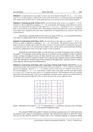
Definition 1 A spanning tree T of a graph G is a subgraph that contains all the vertices V of G. The subgraph
T is a tree, meaning it is a connected and acyclic subgraph that spans all the vertices of the original graph.
Int J Artif Intell, Vol. 14, No. 2, April 2025: 1096–1105](https://image.slidesharecdn.com/2525899-250806092525-d0f4f327/85/Amixed-integer-nonlinear-programming-model-for-site-specific-management-zone-problem-3-320.jpg)
![1100 ❒ ISSN: 2252-8938
solutions. According to the model proposed by Abdelmaguid in [31] for the minimum spanning tree problem,
to formulate the SSMZ delineation problem as a mixed integer non-linear model, it is essential to introduce
a special vertex uN into the vertex set (V = V ′
∪ {uN }) that is connected to all vertices in G′
. This vertex
uN does not carry any inherent value. Furthermore, each edge in this new graph configuration is replaced with
two directed arcs, creating a directed graph GD = (V, A). This directional aspect allows us to more precisely
control how zones are formed and connected, ensuring each tree (zone) within the forest can be uniquely
identified by color. An example of this graph configuration, GD, complete with the auxiliary vertex uN and all
its arcs, is depicted in Figure 2. This example serves to illustrate the structure and the connectivity enforced by
the inclusion of the special vertex and the conversion of edges to directed arcs, facilitating the modeling of the
SSMZ delineation problem.
4
8
12
14 15 16
1 2 3
5 6 7
9 10 11
13
17
Figure 2. Example of graph GD for a 4×4 SSMZ instance, illustrating vertex connectivity
The main objective of our model is to organize the vertices of the directed graph GD into θ distinct
trees. Each tree is designed to cover a unique set of vertices, ensuring no overlaps, while also adhering to a
specific homogeneity condition as outlined in [22]. This homogeneity condition ensures that all vertices within
any single tree exhibit similar characteristics, which is crucial for effective management zoning in agricultural
settings or other applicable fields.
In our graphical representation, depicted in Figure 3, the left side showcases a potential solution
achieved by the model. In this solution, the specially introduced vertex uN plays a pivotal role as it acts as a
common connecting point, or sink, for all possible trees. This setup ensures that all trees are interconnected
through this auxiliary vertex, facilitating the management of connectivity and homogeneity across the entire
graph. Each vertex u in the graph is assigned a color k, where the color indicates that vertex u belongs to
region k. Similarly, an arc (u, v) that is colored k in the solution represents an edge from the original graph
G′
, indicating that vertices u and v are part of the same homogeneous region or zone. The model’s flexibility
allows these connections to be directed, meaning the direction of the arc does not affect the interpretation
that both vertices belong to the same region. This aspect is illustrated further in the central and right parts of
Figure 3, where the layout of the graph and its corresponding zoning are displayed.
1
1
2 2 2
2 2
2 2
2 2 2
3
3
3
4
16 1
1
2 2 2
2 2
2 2
2 2 2
3
3
3
4
1
1
2 2 2
2 2
2 2
2 2 2
3
3
3
4
Figure 3. Graphical representation of an SSMZ solution: GD on the left, G′
in the center, and its application
in SSMZ on the right
Int J Artif Intell, Vol. 14, No. 2, April 2025: 1096–1105](https://image.slidesharecdn.com/2525899-250806092525-d0f4f327/85/Amixed-integer-nonlinear-programming-model-for-site-specific-management-zone-problem-5-320.jpg)

![1102 ❒ ISSN: 2252-8938
X
q∈δ+(u)
yu,q,k = xu,k, u ∈ V uN , k ∈ K (13)
du,k ≥ cu − z̄k u ∈ V uN , k ∈ K (14)
du,k ≥ −(cu − z̄k) u ∈ V uN , k ∈ K (15)
pu,k ≤ M · xu,k u ∈ V uN , k ∈ K (16)
pu,k ≥ du,k − M · (1 − xu,k) u ∈ V uN , k ∈ K (17)
pu,k ≤ du,k u ∈ V uN , k ∈ K (18)
Vu,k ≥ Vv,k + yu,v,k − |V | · (1 − yu,v,k), (u, v) ∈ A, u ̸= uN , v ̸= uN k ∈ K (19)
VuN ,k = 0, k ∈ K (20)
yu,v,k + yv,u,k ≤ xu,k · xv,k, (u, v) ∈ A, k ∈ K (21)
z̄k · zk =
X
u∈V vN
cu · xu,k (22)
z̄k ≤ M · rk, k ∈ K (23)
σ2
(|V {vN }| − θ) · (1 − α) ≥
X
u∈V vN
X
k∈K
(pu,k)2
(24)
The objective function (2) aims to minimize the number of colors (or spanning trees). Constraint (3)
counts the number of vertices assigned the color k. Constraint (4) ensures that each vertex is assigned exactly
one color, with the exception of the special vertex uN , which is assigned θ colors as specified in constraint (5).
Since uN is the termination point for each tree, it must be possible to enter this vertex using any employed
color, but exiting in any color is prohibited, as stipulated by constraints (6) and (7). Constraint (8) accounts for
the number of colors actually utilized. Constraints (9) to (11) allows the assignment of color k to vertices and
arcs only if color k is active, defined as being assigned to at least one vertex. Constraint (12) stipulates that an
arc can be assigned at most one color. Constraint (13) requires that for each vertex u ∈ V {uN }, there must
be an outgoing arc to any neighboring vertex v that is colored k only if vertex u also has color k. Constraints
(14) to (18) calculate the product |cu − z̄k| × xu,k. Constraints (19) and (20) function as Miller-Tucker-Zemlin
(MTZ) constraints to prevent disconnected trees sharing the same color. Constraint (21) ensures that if two
neighboring vertices are assigned color k, then at least one of the arcs connecting them must also be colored
k or remain uncolored. Otherwise, no color is assigned to the arcs between these vertices. Finally, constraints
(22) and (23) record the average value of the vertices colored k, and constraint (24) compares the homogeneity
of a solution against the threshold α.
Note that constraint (21) models the behavior of the anticoloring of the edges (ACE) since the arcs
entering or leaving a vertex u must either have the same color as u or have no color assigned. Additionally,
regardless of their orientation, these arcs are considered as edges of tree k. This ensures that the graph’s
structural integrity and coloration rules strictly align with the requirements for uniformity and connectivity
within each management zone.
5. EXPERIMENTAL RESULTS
The MINLP model was executed on a system equipped with an Intel Xeon processor featuring 24
physical cores and 128 GB of RAM, running Ubuntu 20.04. Gurobi 10.0, accessed via its Python interface,
was utilized as the solver [32]. We focused on solving instances of class 1, as well as instances based on real
data which are available in [33]. The detailed results of this work and the implementation of mixed integer non
linear model are available in [34]. The solver was configured to run for a maximum duration of 8 hours. After
this period, the best solution obtained is reported, alongside the relative distance (GAP) between this solution
Int J Artif Intell, Vol. 14, No. 2, April 2025: 1096–1105](https://image.slidesharecdn.com/2525899-250806092525-d0f4f327/85/Amixed-integer-nonlinear-programming-model-for-site-specific-management-zone-problem-7-320.jpg)
![Int J Artif Intell ISSN: 2252-8938 ❒ 1103
and its best-known upper bound. These results are compared against state-of-the-art solutions from the EDA
results as reported in [25].
In Table 1, we present the results for class 1 instances at different levels of the homogeneity threshold
α set at 0.5, 0.7, and 0.9. Here, Z∗
denotes the objective function value from the state-of-the-art solutions,
and Z represents the objective function value achieved by our model (2)–(24). Similarly, Table 2 display the
outcomes for instances with real data for α values ranging from 0.1 to 1.0.
Table 1. Results for class 1 instances
Class k α Z∗ Z GAP Time(s) α Z∗ Z GAP Time(s) α Z∗ Z GAP Time(s)
1 1 0.5 6 4 0.50 28,800.00 0.7 10 19 0.84 28,800.00 0.9 19 28 0.86 28,800.00
2 5 8 0.75 28,800.00 10 23 0.87 28,800.00 21 24 0.83 28,800.00
3 6 2 0.00 20,986.00 9 23 0.87 28,800.00 22 34 0.88 28,800.00
4 4 2 0.00 1,602.00 6 22 0.86 28,800.00 22 31 0.87 28,800.00
5 8 18 0.88 28,800.00 10 22 0.86 28,800.00 21 31 0.87 28,800.00
6 3 3 0.33 28,800.00 8 15 0.80 28,800.00 16 26 0.85 28,800.00
7 8 13 0.85 28,800.00 13 17 0.82 28,800.00 23 31 0.84 28,800.00
8 4 4 0.50 28,800.00 6 8 0.63 28,800.00 16 36 0.91 28,800.00
9 7 7 0.71 28,800.00 12 21 0.86 28,800.00 25 32 0.84 28,800.00
10 5 4 0.50 28,800.00 8 16 0.81 28,800.00 19 28 0.86 28,800.00
Table 2. Results for organic matter, Ph, phosphorus and sum of basis instances
Instance α Z∗ Time(s) Z GAP Time(s)
OM 1 40 23.28 40 0.00 26
0.9 17 22.33 34 0.91 28,800
0.8 11 22.73 24 0.88 28,800
0.7 9 22.94 29 0.90 28,800
0.6 6 23.17 31 0.90 28,800
0.5 5 23.26 3 0.00 17,626
0.4 4 23.33 3 0.00 11,128
0.3 2 23.43 2 0.00 928
0.2 2 23.47 3 0.00 1091
0.1 2 23.63 2 0.00 112
Ph 1 19 22.3 19 0.10 28800
0.9 13 22.33 19 0.10 28,800
0.8 8 23.15 14 0.79 28,800
0.7 6 23.28 14 0.79 28,800
0.6 5 23.39 6 0.50 28,800
0.5 4 23.45 4 0.25 28,800
0.4 3 23.52 4 0.25 28,800
0.3 3 23.62 3 0.00 474
0.2 2 23.6 3 0.00 487
0.1 2 23.64 2 0.00 365
Instance α Z∗ Time(s) Z GAP Time(s)
P 1 32 21.46 32 0.00 92
0.9 7 23.28 4 0.00 11,118
0.8 4 23.46 3 0.00 1,212
0.7 3 23.54 2 0.00 79
0.6 2 23.64 2 0.00 430
0.5 2 23.67 2 0.00 311
0.4 2 23.67 3 0.00 350
0.3 2 23.66 2 0.00 361
0.2 2 23.64 2 0.00 74
0.1 2 23.61 2 0.00 79
SB 1 40 23.51 40 0.00 29
0.9 14 22.6 32 0.88 28,800
0.8 9 22.94 23 0.87 28,800
0.7 5 23.16 13 0.77 28,800
0.6 3 23.35 10 0.70 28,800
0.5 3 23.43 26 0.89 28,800
0.4 2 23.54 3 0.00 992
0.3 2 23.5 2 0.00 957
0.2 2 23.57 3 0.00 560
0.1 2 23.51 2 0.00 652
In nonconvex optimization, the Karush-Kuhn-Tucker (KKT) theorem establishes that if a point
x satisfies the KKT conditions, then x is a stationary critical point of a function. However, it is crucial to
emphasize that this critical point is not guaranteed to be a global optimum. In other words, the KKT theorem
only tells us that x is a point where the function ceases to change in a feasible direction. This implies that x
could be a local optimum, a global optimum, or a saddle point. The reason we cannot guarantee that x is a
global optimum is due to the non convex nature of the model. In a nonconvex function, there can be multiple
local minima, and there is no straightforward way to determine which one is the global minimum [35].
In Table 2, some solutions (bold numbers) are identified as optimal because their GAP (optimality
gap) is equal to 0. However, as mentioned earlier, a GAP of 0 does not guarantee that the solution is a global
optimum. It is possible that these solutions are local optima that the software could not identify as such. In
some cases, these local solutions might coincide with the global optimum, but there is no way to know for sure
without further analysis.
A mixed integer nonlinear programming model for ... (Luis E. Urbán-Rivero)](https://image.slidesharecdn.com/2525899-250806092525-d0f4f327/85/Amixed-integer-nonlinear-programming-model-for-site-specific-management-zone-problem-8-320.jpg)
![1104 ❒ ISSN: 2252-8938
6. CONCLUSION AND FUTURE WORK
In this paper, we propose a MINLP model for delineation of SSMZ problem. Our MINLP model
represents a sophisticated approach to identifying optimal solutions for the SSMZ challenge. However, the
model’s capabilities are somewhat constrained by the nonconvex nature of the nonlinear constraint used for
calculating homogeneity. This nonconvexity introduces significant complexities that preclude us from defini-
tively asserting the optimality of the solutions generated by the model. Despite these challenges, the model has
demonstrated its ability to deliver the best possible solutions for smaller instances, specifically for configura-
tions involving 6×7 samples. This achievement underscores the model’s potential efficacy in more contained
scenarios. Looking forward, we recognize the need to evolve our approach to overcome the limitations posed
by the current homogeneity calculation method. We plan to explore two main avenues for advancement. First,
we intend to develop heuristics that exploit the structural aspects of the mixed-integer nonlinear program. By
designing these heuristics, we aim to bypass some of the computational intensity and nonconvexity issues,
thereby facilitating more efficient solution processes. Second, we are considering alternative methods for
calculating homogeneity that avoid nonconvex formulations and reduce computational demands. These new
methods could potentially transform the model’s applicability and scalability, making it more versatile and
effective across a broader range of scenarios.
REFERENCES
[1] T. Doerge, “Defining management zones for precision farming,” Crop Insights, vol. 8, no. 21, pp. 1–5, 1999.
[2] N. Zhang, M. Wang, and N. Wang, “Precision agriculture—a worldwide overview,” Computers and Electronics in Agriculture, vol.
36, no. 2–3, pp. 113–132, 2002, doi: 10.1016/S0168-1699(02)00096-0.
[3] R. E. Plant, “Site-specific management: The application of information technology to crop production,” Computers and Electronics
in Agriculture, vol. 30, no. 1–3, pp. 9–29, 2001, doi: 10.1016/S0168-1699(00)00152-6.
[4] D. L. Corwin, “Site-specific management and delineating management zones,” in Precision Agriculture for Sustainability and
Environmental Protection, London, England: Routledge, 2013, pp. 135–157, doi: 10.4324/9780203128329.
[5] J. Lee and S. Leyffer, Mixed integer nonlinear programming. New York: Springer, 2012, doi: 10.1007/978-1-4614-1927-3.
[6] R. A. Ortega and O. A. Santibáñez, “Determination of management zones in corn (Zea mays L.) based on soil fertility,” Computers
and Electronics in Agriculture, vol. 58, no. 1, pp. 49–59, 2007, doi: 10.1016/j.compag.2006.12.011.
[7] A. Gavioli, E. G. D. Souza, C. L. Bazzi, L. P. C. Guedes, and K. Schenatto, “Optimization of management zone delin-
eation by using spatial principal components,” Computers and Electronics in Agriculture, vol. 127, pp. 302–310, 2016, doi:
10.1016/j.compag.2016.06.029.
[8] A. M. Aggag and A. Alharbi, “Spatial analysis of soil properties and site-specific management zone delineation for the south hail
region, Saudi Arabia,” Sustainability, vol. 14, no. 23, 2022, doi: 10.3390/su142316209.
[9] N. R. Peralta, J. L. Costa, M. Balzarini, M. C. Franco, M. Córdoba, and D. Bullock, “Delineation of management zones
to improve nitrogen management of wheat,” Computers and Electronics in Agriculture, vol. 110, pp. 103–113, 2015, doi:
10.1016/j.compag.2014.10.017.
[10] M. A. Córdoba, C. I. Bruno, J. L. Costa, N. R. Peralta, and M. G. Balzarini, “Protocol for multivariate homogeneous zone delineation
in precision agriculture,” Biosystems Engineering, vol. 143, pp. 95–107, 2016, doi: 10.1016/j.biosystemseng.2015.12.008.
[11] Q. Jiang, Q. Fu, and Z. Wang, “Study on delineation of irrigation management zones based on management zone analyst software,”
in Computer and Computing Technologies in Agriculture IV, 2011, pp. 419–427, doi: 10.1007/978-3-642-18354-6 50.
[12] N. M. Betzek, E. G. D. Souza, C. L. Bazzi, K. Schenatto, and A. Gavioli, “Rectification methods for optimization of management
zones,” Computers and Electronics in Agriculture, vol. 146, pp. 1–11, 2018, doi: 10.1016/j.compag.2018.01.014.
[13] R. Srinivasan, B. N. Shashikumar, and S. K. Singh, “Mapping of soil nutrient variability and delineating site-specific management
zones using fuzzy clustering analysis in eastern coastal region, India,” Journal of the Indian Society of Remote Sensing, vol. 50, no.
3, pp. 533–547, 2022, doi: 10.1007/s12524-021-01473-9.
[14] N. Ohana-Levi et al., “A weighted multivariate spatial clustering model to determine irrigation management zones,” Computers and
Electronics in Agriculture, vol. 162, pp. 719–731, 2019, doi: 10.1016/j.compag.2019.05.012.
[15] G. Ruß and R. Kruse, “Exploratory hierarchical clustering for management zone delineation in precision agriculture,” in Advances
in Data Mining. Applications and Theoretical Aspects, 2011, pp. 161–173, doi: 10.1007/978-3-642-23184-1 13.
[16] B. B. Bantchina et al., “Corn yield prediction in site-specific management zones using proximal soil sensing, remote sensing, and
machine learning approach,” Computers and Electronics in Agriculture, vol. 225, 2024, doi: 10.1016/j.compag.2024.109329.
[17] Y. Saikai, V. Patel, and P. D. Mitchell, “Machine learning for optimizing complex site-specific management,” Computers and
Electronics in Agriculture, vol. 174, 2020, doi: 10.1016/j.compag.2020.105381.
[18] L. Zane, B. Tisseyre, S. Guillaume, and B. Charnomordic, “Within-field zoning using a region growing algorithm guided by geosta-
tistical analysis,” in Precision Agriculture 2013, Wageningen, Netherlands: Wageningen Academic Publishers, 2013, pp. 313–319,
doi: 10.3920/9789086867783 039.
[19] C. Leroux, H. Jones, A. Clenet, and B. Tisseyre, “A new approach for zoning irregularly-spaced, within-field data,” Computers and
Electronics in Agriculture, vol. 141, pp. 196–206, 2017, doi: 10.1016/j.compag.2017.07.025.
[20] M. Denora et al., “Validation of rapid and low-cost approach for the delineation of zone management based on machine learning
algorithms,” Agronomy, vol. 12, no. 1, 2022, doi: 10.3390/agronomy12010183.
[21] S. Ouazaa, C. I. Jaramillo-Barrios, N. Chaali, Y. M. Q. Amaya, J. E. C. Carvajal, and O. M. Ramos, “Towards site specific manage-
ment zones delineation in rotational cropping system: Application of multivariate spatial clustering model based on soil properties,”
Geoderma Regional, vol. 30, 2022, doi: 10.1016/j.geodrs.2022.e00564.
Int J Artif Intell, Vol. 14, No. 2, April 2025: 1096–1105](https://image.slidesharecdn.com/2525899-250806092525-d0f4f327/85/Amixed-integer-nonlinear-programming-model-for-site-specific-management-zone-problem-9-320.jpg)
![Int J Artif Intell ISSN: 2252-8938 ❒ 1105
[22] N. M. Cid-Garcia, V. Albornoz, Y. A. Rios-Solis, and R. Ortega, “Rectangular shape management zone delineation using integer
linear programming,” Computers and Electronics in Agriculture, vol. 93, pp. 1–9, 2013, doi: 10.1016/j.compag.2013.01.009.
[23] V. M. Albornoz, N. M. Cid-Garcı́a, R. Ortega, and Y. A. Rı́os-Solı́s, “A hierarchical planning scheme based on precision agriculture,”
International Series in Operations Research and Management Science, vol. 224, pp. 129–162, 2015, doi: 10.1007/978-1-4939-2483-
7 6.
[24] V. M. Albornoz and G. E. Zamora, “A precision agriculture approach for a crop rotation planning problem with adjacency con-
straints,” in Optimization Under Uncertainty in Sustainable Agriculture and Agrifood Industry, Cham: Springer International Pub-
lishing, 2024, pp. 161–178, doi: 10.1007/978-3-031-49740-7 7.
[25] J. Velasco, S. Vicencio, J. A. Lozano, and N. M. Cid-Garcia, “Delineation of site-specific management zones using estima-
tion of distribution algorithms,” International Transactions in Operational Research, vol. 30, no. 4, pp. 1703–1729, 2023, doi:
10.1111/itor.12970.
[26] L. E. Urbán-Rivero, J. Velasco, and J. R. Rodrı́guez, “A simple greedy heuristic for site specific management zone problem,” Axioms,
vol. 11, no. 7, 2022, doi: 10.3390/axioms11070318.
[27] A. Haghverdi, B. G. Leib, R. A. Washington-Allen, P. D. Ayers, and M. J. Buschermohle, “Perspectives on delineating man-
agement zones for variable rate irrigation,” Computers and Electronics in Agriculture, vol. 117, pp. 154–167, 2015, doi:
10.1016/j.compag.2015.06.019.
[28] X. Zhang, L. Jiang, X. Qiu, J. Qiu, J. Wang, and Y. Zhu, “An improved method of delineating rectangular management
zones using a semivariogram-based technique,” Computers and Electronics in Agriculture, vol. 121, pp. 74–83, 2016, doi:
10.1016/j.compag.2015.11.016.
[29] S. Wolfert, L. Ge, C. Verdouw, and M.-J. Bogaardt, “Big data in smart farming – a review,” Agricultural Systems, vol. 153, pp.
69–80, 2017, doi: 10.1016/j.agsy.2017.01.023.
[30] V. M. Albornoz, “Management zones by optimization,” Encyclopedia of Digital Agricultural Technologies, pp. 785–791, 2023, doi:
10.1007/978-3-031-24861-0 283.
[31] T. F. Abdelmaguid, “An efficient mixed integer linear programming model for the Minimum spanning tree problem,” Mathematics,
vol. 6, no. 10, 2018, doi: 10.3390/math6100183.
[32] Gurobi Optimization, “Gurobi optimizer reference manual,” Gurobi Project. 2023. Accessed: Dec. 01, 2023. [Online]. Available:
https://docs.gurobi.com/projects/optimizer/en/current/index.html
[33] N. M. Cid-Garcıa, “Instances for the EDA-SSMZ,” GitHub. 2013. [Online]. Available: https://github.com/NxtrCd/Instances-EDA-
SSMZ
[34] L. E. Urbán-Rivero, “SSMZ exact,” GitHub, 2024. [Online]. Available: https://github.com/lurbanrivero/SSMZ Exact
[35] P. Belotti, C. Kirches, S. Leyffer, J. Linderoth, J. Luedtke, and A. Mahajan, “Mixed-integer nonlinear optimization,” Acta Numerica,
vol. 22, 2013, doi: 10.1017/S0962492913000032.
BIOGRAPHIES OF AUTHORS
Luis Eduardo Urbán-Rivero received a bachelor’s degree in computer engineer-
ing at Universidad Autónoma Metropolitana Azcapotzalco in 2011 and a master’s and Ph.D. in
optimization from the same university in 2014 and 2018, respectively. He had a postdoctoral
fellowship at CIMAT Aguascalientes from 2019 to 2021. He is currently an associated full-time
Professor at Instituto Tecnológico Autónomo de México. He is a member of the Mexican Society of
Operations Research (SMIO) and the Mexican System of Researchers. He can be contacted at email:
lurbanrivero@gmail.com.
Jonás Velasco was born in Los Mochis, Sinaloa, México, in 1984. He received his B.S.
degree in industrial engineering from the Universidad de Occidente (UdeO) in 2007. He received
the M.S. and Ph.D. degrees in systems engineering from the Universidad Autónoma de Nuevo León
(UANL), México, in 2009 and 2013, respectively. He is currently a CONAHCYT Research Fellow at
the Center for Research in Mathematics (CIMAT), Aguascalientes, Mexico, where he has carried out
consulting projects for different SMEs companies related to the automotive sector. He has authored
over twenty publications. His main research interests include applied optimization, mathematical
programming, evolutionary and bio-inspired algorithms, and its applications in diverse fields such
as transportation, facility layout and location, manufacturing and production planning, logistics and
distribution. He is a member of the Mexican Society of Operations Research (SMIO) and a member
of the Mexican System of Researchers (CONAHCYT-SNII). He has served on the review boards of
diverse technical journals. He can be contacted at email: jvelasco@cimat.mx.
A mixed integer nonlinear programming model for ... (Luis E. Urbán-Rivero)](https://image.slidesharecdn.com/2525899-250806092525-d0f4f327/85/Amixed-integer-nonlinear-programming-model-for-site-specific-management-zone-problem-10-320.jpg)
Amixed integer nonlinear programming model for site-specific management zone problem
- 1. IAES International Journal of Artificial Intelligence (IJ-AI) Vol. 14, No. 2, April 2025, pp. 1096∼1105 ISSN: 2252-8938, DOI: 10.11591/ijai.v14.i2.pp1096-1105 ❒ 1096 A mixed integer nonlinear programming model for site-specific management zone problem Luis Eduardo Urbán-Rivero1,2 , Jonás Velasco3 1Departmento de Ingenierı́a Industrial y Operaciones, Instituto Tecnológico Autónomo de México, CDMX, México 2Universidad Politécnica Metropolitana de Hidalgo, Hidalgo, México 3CONAHCYT-Centro de Investigación en Matemáticas (CIMAT), A.C., Aguascalientes, México Article Info Article history: Received Apr 26, 2024 Revised Nov 15, 2024 Accepted Dec 15, 2024 Keywords: Agricultural optimization MINLP model Precision agriculture Resource management Site-specific management zones ABSTRACT Precision agriculture employs sophisticated tools to optimize decision-making in farming, aiming to simultaneously improve crop yields and manage resources more effectively in a context of increasing scarcity and rising costs. A key as- pect of precision agriculture is the delineation of site-specific management zones (SSMZs), which involves segmenting a field into areas that are homogeneous in terms of soil physicochemical properties. The problem of delineating SSMZ have been approached using a wide variety of methodologies, all of which, heuristic, focus on finding feasible solutions. Until this work, there was no exact algorithm or mathematical model that would allow for a point of comparison. This paper introduces a novel approach to tackle the delineation of SSMZ with orthogonal shapes through the development of a mixed integer nonlinear pro- gramming (MINLP) model. Small instances with different scenarios show the scope of the proposed approach and the significance of the results. It provides a structure for the SSMZ problem with orthogonal shapes and establishes a bench- mark for evaluating the performance of heuristic solutions, metaheuristics, or hybrid approaches. This is an open access article under the CC BY-SA license. Corresponding Author: Jonás Velasco CONAHCYT-Centro de Investigación en Matemáticas (CIMAT), A.C. Aguascalientes, México Email: jvelasco@cimat.mx 1. INTRODUCTION Precision agriculture stands at the forefront of a technological revolution in modern farming, encap- sulating the shift towards more sustainable, efficient, and data-driven agricultural practices. This innovative approach leverages detailed environmental and crop data, precision technology, and advanced analytics to optimize both the quality and quantity of agricultural production [1]. The central concept within precision agriculture is the creation of agricultural management zones, which are specific areas within larger fields that exhibit relatively homogeneous conditions that should be managed differently from neighboring zones [2]. These zones enable the application of localized treatment strategies for water, fertilizers, and pesticides, thereby enhancing the efficiency of resource use and minimizing environmental impacts [3]. The precision agricultural process involves the following steps: – Data collection: comprehensive data regarding the field is collected using various methods. This data often includes information about soil properties (e.g., texture, organic matter, pH, and nutrient status), topography, crop yield history, and remotely sensed data. The data is often georeferenced, meaning it is Journal homepage: http://ijai.iaescore.com
- 2. Int J Artif Intell ISSN: 2252-8938 ❒ 1097 associated with specific geographical coordinates. – Geostatistical analysis: this data is then analyzed using geostatistical methods to identify spatial variabil- ity and correlation structures across the field. Geostatistical techniques such as kriging, co-kriging, or machine learning algorithms can be used. – Delineation of management zones: using the results of the geostatistical analysis, distinct management zones can be identified. Each of these zones should have a relatively homogeneous set of characteristics, allowing for differential management practices. – Variable rate technology (VRT) implementation: with these delineated zones, different management strategies can be applied to different areas, using VRT. This can include differential application of fertilizers, water, pesticides, or even differential planting densities. – Evaluation and adjustments: the effectiveness of these site-specific management zone (SSMZ) practices is then evaluated, often through yield monitoring and soil testing. Based on the results, adjustments to the management zones or practices may be made in subsequent seasons. The main goal of the SSMZ approach is to enhance the efficiency of agricultural operations by allo- cating resources where they are needed most, thereby reducing waste and potentially increasing crop yields [4]. In this paper, our focus will primarily be on the third step, which aims to provide a tool to support decision- making within the precision agriculture process. We explore the crucial role that MINLP models play in opti- mizing these processes, particularly in formulating and solving the complex and nonlinear problems inherent to the delineation of management zones. MINLP models offer a robust framework for handling the dynamic and multifactorial interactions in agricultural fields, which is essential for effective decision-making and the implementation of precise and adaptive agricultural practices. However, the model’s capabilities are somewhat limited by the nonconvex nature of the nonlinear constraint used to calculate homogeneity. The power of MINLP lies in its flexibility and generality, capable of representing a vast landscape of optimization problems with precision and depth that linear approaches and continuous models cannot achieve. However, this power comes with increased computational complexity. Solving MINLP problems involves navigating a search space that is not only vast due to the combinatorial nature of integer variables but also challenging due to the presence of nonlinearities, which can introduce multiple local optima, non-convexities, and other complexities [5]. This paper is structured as follows: section 2 reviews various methodologies used in the delineation of management zones, exploring significant advancements and applications within precision agriculture. In section 3, we define the problem of SSMZ delineation, establishing a framework for our subsequent analysis. Section 4 outlines our proposed modeling approach, describing the construction of a graph-based representation to analyze soil sample relationships. Section 5 details the experimental setup and execution of our mixed integer nonlinear programming (MINLP) model, including a comparison of our results with existing state-of-the-art methods. Finally, section 6 offers concluding remarks and discusses potential avenues for future research in this area. 2. RELATED WORK Precision agriculture has made significant strides in utilizing advanced technology and analytical methods to optimize crop management and increase agricultural efficiency. This literature review explores the diverse methodologies employed in the delineation of management zones, which is a critical component for executing site-specific agricultural practices effectively. One of the primary methods for identifying manage- ment zones involves various clustering algorithms that classify field areas based on soil or vegetation properties. These techniques include: – Principal component analysis (PCA) and spatial PCA: used to reduce the dimensionality of large datasets while preserving most of the variance, helping to identify patterns that influence soil properties [6]–[8]. – Fuzzy clustering methods: such as fuzzy k-means and fuzzy c-means, which allow for a more flexible classification of data points that may belong to multiple clusters, providing a more nuanced delineation of management zones [9]–[13]. – Multivariate k-means, hierarchical clustering and other machine learning based methods: these methods offer robust ways to group data based on similarities across multiple variables, suitable for complex agricultural fields [14]–[17]. – Segmentation techniques from signal processing: recently, segmentation methods have been adapted A mixed integer nonlinear programming model for ... (Luis E. Urbán-Rivero)
- 3. 1098 ❒ ISSN: 2252-8938 from the signal processing field to agriculture, enabling the delineation of zones by analyzing spatial continuity and discontinuity in field data [18]–[21]. In addition to clustering, operations research provides powerful tools for optimizing the configuration of management zones: – Binary integer programming models: in [22]–[24] these models facilitate the delineation of rectangular management zones, simplifying the application of variable rate inputs and fitting well with conventional agricultural equipment. – Evolutionary computation: in [25], an estimation of distribution algorithm (EDA) is used to extend the formation of zones with orthogonal shapes, aiming to minimize the number of zones while maximizing homogeneity. – Graph-based heuristics: Urbán-Rivero et al. [26] provides a characterization of orthogonal solutions using graphs and propose a greedy algorithm that exploits this structure. The proposed graph serves as the basis for the proposal of the nonlinear programming model in this work. The integration of these methodologies into practical agricultural applications has seen variable success. For instance, Haghverdi et al. [27] applied the binary integer programming model to irrigation system design, while Zhang et al. [28] enhanced this approach by integrating semivariogram analysis to optimize grid size and input distribution. The challenge of delineating management zones efficiently and accurately remains a central focus, necessitating ongoing refinement of decision support systems [29]. As technology and data collection methods evolve, the precision in precision agriculture will continue to improve, driving further ad- vancements in this crucial area of agricultural science. In [30], a comprehensive review of the literature on optimization can be found. 3. PROBLEM DEFINITION We define the SSMZ delineation problem as the division of an agricultural field plot into regions that are homogeneous in terms of certain soil properties. This follows the definition provided in [26]: Input: An agricultural field plot M, consisting of |M| soil samples, and a parameter α ∈ [0, 1] representing the minimum desired homogeneity across regions. Output: The plot divided into Z = {z1, z2, . . . zk} regions, where the number of regions |Z| is minimized, and the homogeneity H ≥ α. The homogeneity parameter H is defined in [6] as follows: H(M, Z) = 1 − P z∈Z(|z| − 1) · s2 (z) σ2 T · (|M| − |Z|) (1) Here, |z| is the number of samples in region z, s2 (z) is the variance of soil properties within region z, and σ2 T is the total variance across all samples in M. The (1) ensures that the relative variance within the chosen regions meets the threshold α, thus guaranteeing the desired homogeneity. 4. METHODOLOGY We construct a graph G′ = (V ′ , E′ ) to represent the spatial relationships between various soil samples taken from an agricultural field plot. Each vertex in V ′ corresponds to a distinct soil sample, and an edge is placed between any two vertices if their respective soil samples are adjacent in the field. This adjacency is typically defined by shared boundaries of the sampling locations. Figure 1 illustrates this graph structure, where vertices are shown as blue circles and edges are depicted as red lines, similar to the graph-based heuristics used in [26]. This modeling approach helps in visualizing and analyzing the connectivity and distribution of soil characteristics across the plot. To built a mixed-integer non-linear programming (MINLP) model, it is necessary to provide the following definitions. Definition 1 A spanning tree T of a graph G is a subgraph that contains all the vertices V of G. The subgraph T is a tree, meaning it is a connected and acyclic subgraph that spans all the vertices of the original graph. Int J Artif Intell, Vol. 14, No. 2, April 2025: 1096–1105
- 4. Int J Artif Intell ISSN: 2252-8938 ❒ 1099 Definition 2 A spanning forest of a graph G consists of a set of disjoint subgraphs {T1, T2, . . . , Tk}, where each Ti is a tree that includes a subset of the vertices of G. Each tree Ti is a connected and acyclic subgraph of G, and the union of all the trees Ti in the spanning forest covers all the vertices of the original graph G. Definition 3 (Anticoloring of the Vertices (ACV)) An anticoloring of the vertices in a graph G = (V, E), referred to as ACV, is defined by a mapping a : V → K∪{uncolored}. This mapping ensures that if two vertices u and v are connected by an edge in E, then either a(u) = a(v), a(u) = uncolored, or a(v) = uncolored. Here, K represents the set of available colors. The designation of uncolored allows for a vertex to be adjacent to any other vertex, regardless of its color status. Furthermore, it is required that every vertex in V has a color assigned from K. Anticoloring is originally defined on the vertices of a graph. In this case, we will extend this definition to the edges of a graph and provide the version of anticoloring for edges. Definition 4 (Anticoloring of the Edges (ACE)) An anticoloring of the edges in a graph G = (V, E), re- ferred to as ACE, is defined by a mapping a′ : E → K ∪ {uncolored}. This function assigns colors to the edges such that two incident edges (edges that share a common vertex) must either be assigned the same color or remain uncolored. The set K represents the available colors, and the option uncolored provides flexibility, allowing for configurations where not all edges require a color assignment. Alongside the anticoloring of edges, it is also necessary to consider an improper vertex coloring for the graph G. In an improper vertex coloring, there are no restrictions on the assignment of colors to adjacent vertices, meaning two adjacent vertices can either share the same color or have different colors. This type of coloring is less restrictive compared to proper vertex coloring, where adjacent vertices must have different colors, thus allowing for a broader range of color assignments and applications, especially useful in scenarios where adjacency does not necessitate differentiation. Definition 5 (Anticoloring of the Edges with a non-proper Coloring of the Vertices (ACE-UCV)) An anti- coloring of the edges with a non-proper coloring of the vertices for a graph G = (V, E), denoted as ACE-UCV, involves two mappings. The first, ℓ : V → K, assigns a color to each vertex in V from the set of colors K. The second mapping, a′ : E → K ∪ {uncolored}, assigns colors to the edges such that each edge incident to a vertex u in V is either the same color as u or remains uncolored. This formulation allows for a flexible approach to coloring the graph, as there are no additional constraints on how vertices are colored relative to one another, thus permitting adjacent vertices to share the same color or have different colors. 1 2 · · · n n + 1 n + 2 · · · 2n . . . . . . ... . . . (m − 1)n + 1 (m − 1)n + 2 · · · K = mn Figure 1. Illustration of the graph G′ = (V ′ , E′ ) representing a m × n grid layout, showing vertices and edges for site-specific management zoning The concept of SSMZ on the graph G′ translates into finding a spanning forest on G′ while minimizing the number of trees, subject to a homogeneity constraint. This spanning forest induces an ACE-UCV, where each tree not only meets the ACE-UCV conditions but is also a connected subgraph, as required by SSMZ A mixed integer nonlinear programming model for ... (Luis E. Urbán-Rivero)
- 5. 1100 ❒ ISSN: 2252-8938 solutions. According to the model proposed by Abdelmaguid in [31] for the minimum spanning tree problem, to formulate the SSMZ delineation problem as a mixed integer non-linear model, it is essential to introduce a special vertex uN into the vertex set (V = V ′ ∪ {uN }) that is connected to all vertices in G′ . This vertex uN does not carry any inherent value. Furthermore, each edge in this new graph configuration is replaced with two directed arcs, creating a directed graph GD = (V, A). This directional aspect allows us to more precisely control how zones are formed and connected, ensuring each tree (zone) within the forest can be uniquely identified by color. An example of this graph configuration, GD, complete with the auxiliary vertex uN and all its arcs, is depicted in Figure 2. This example serves to illustrate the structure and the connectivity enforced by the inclusion of the special vertex and the conversion of edges to directed arcs, facilitating the modeling of the SSMZ delineation problem. 4 8 12 14 15 16 1 2 3 5 6 7 9 10 11 13 17 Figure 2. Example of graph GD for a 4×4 SSMZ instance, illustrating vertex connectivity The main objective of our model is to organize the vertices of the directed graph GD into θ distinct trees. Each tree is designed to cover a unique set of vertices, ensuring no overlaps, while also adhering to a specific homogeneity condition as outlined in [22]. This homogeneity condition ensures that all vertices within any single tree exhibit similar characteristics, which is crucial for effective management zoning in agricultural settings or other applicable fields. In our graphical representation, depicted in Figure 3, the left side showcases a potential solution achieved by the model. In this solution, the specially introduced vertex uN plays a pivotal role as it acts as a common connecting point, or sink, for all possible trees. This setup ensures that all trees are interconnected through this auxiliary vertex, facilitating the management of connectivity and homogeneity across the entire graph. Each vertex u in the graph is assigned a color k, where the color indicates that vertex u belongs to region k. Similarly, an arc (u, v) that is colored k in the solution represents an edge from the original graph G′ , indicating that vertices u and v are part of the same homogeneous region or zone. The model’s flexibility allows these connections to be directed, meaning the direction of the arc does not affect the interpretation that both vertices belong to the same region. This aspect is illustrated further in the central and right parts of Figure 3, where the layout of the graph and its corresponding zoning are displayed. 1 1 2 2 2 2 2 2 2 2 2 2 3 3 3 4 16 1 1 2 2 2 2 2 2 2 2 2 2 3 3 3 4 1 1 2 2 2 2 2 2 2 2 2 2 3 3 3 4 Figure 3. Graphical representation of an SSMZ solution: GD on the left, G′ in the center, and its application in SSMZ on the right Int J Artif Intell, Vol. 14, No. 2, April 2025: 1096–1105
- 6. Int J Artif Intell ISSN: 2252-8938 ❒ 1101 4.1. MINLP Model for SSMZ delineation problem Parameters: – V : Set of vertices (samples). – A : Set of arcs. – K: Set of colors. – cu : Measurement of soil property of sample u (vertex u). – uN : Auxiliary vertex uN ∈ V . – δ+ (u): Set of outer neighbors of vertex u. – M : A big value constant. Variables: xu,k = ( 1 If vertex u is assigned color k. 0 Otherwise. yu,v,k = ( 1 If arc u → v is assigned color k. 0 Otherwise. rk = ( 1 If color k is used. 0 Otherwise. zk = Number of vertices assigned color k. z̄k = Mean value of measurements for vertices with color k. Vu,k = Auxiliary variable to store the order of vertices assigned color k. du,k = Auxiliary variable to store the absolute difference |cu − z̄k|. pu,k = Auxiliary variable to store the product du,k · xu,k. θ = Number of used colors. min θ (2) X u∈V {uN } xu,k = zk, k ∈ K (3) X k∈K xu,k = 1, u ∈ V {uN } (4) X k∈K xuN ,k = θ (5) X u∈V {uN } yu,uN ,k = rk, k ∈ K (6) X u∈V {uN } yuN ,u,k = 0, k ∈ K (7) X k∈K rk = θ (8) xu,k ≤ rk, u ∈ V, k ∈ K (9) yu,v,k ≤ rk, (u, v) ∈ A, k ∈ K (10) rk ≤ X u∈V {uN } xu,k, k ∈ K (11) X k∈K yu,v,k ≤ 1, (u, v) ∈ A (12) A mixed integer nonlinear programming model for ... (Luis E. Urbán-Rivero)
- 7. 1102 ❒ ISSN: 2252-8938 X q∈δ+(u) yu,q,k = xu,k, u ∈ V uN , k ∈ K (13) du,k ≥ cu − z̄k u ∈ V uN , k ∈ K (14) du,k ≥ −(cu − z̄k) u ∈ V uN , k ∈ K (15) pu,k ≤ M · xu,k u ∈ V uN , k ∈ K (16) pu,k ≥ du,k − M · (1 − xu,k) u ∈ V uN , k ∈ K (17) pu,k ≤ du,k u ∈ V uN , k ∈ K (18) Vu,k ≥ Vv,k + yu,v,k − |V | · (1 − yu,v,k), (u, v) ∈ A, u ̸= uN , v ̸= uN k ∈ K (19) VuN ,k = 0, k ∈ K (20) yu,v,k + yv,u,k ≤ xu,k · xv,k, (u, v) ∈ A, k ∈ K (21) z̄k · zk = X u∈V vN cu · xu,k (22) z̄k ≤ M · rk, k ∈ K (23) σ2 (|V {vN }| − θ) · (1 − α) ≥ X u∈V vN X k∈K (pu,k)2 (24) The objective function (2) aims to minimize the number of colors (or spanning trees). Constraint (3) counts the number of vertices assigned the color k. Constraint (4) ensures that each vertex is assigned exactly one color, with the exception of the special vertex uN , which is assigned θ colors as specified in constraint (5). Since uN is the termination point for each tree, it must be possible to enter this vertex using any employed color, but exiting in any color is prohibited, as stipulated by constraints (6) and (7). Constraint (8) accounts for the number of colors actually utilized. Constraints (9) to (11) allows the assignment of color k to vertices and arcs only if color k is active, defined as being assigned to at least one vertex. Constraint (12) stipulates that an arc can be assigned at most one color. Constraint (13) requires that for each vertex u ∈ V {uN }, there must be an outgoing arc to any neighboring vertex v that is colored k only if vertex u also has color k. Constraints (14) to (18) calculate the product |cu − z̄k| × xu,k. Constraints (19) and (20) function as Miller-Tucker-Zemlin (MTZ) constraints to prevent disconnected trees sharing the same color. Constraint (21) ensures that if two neighboring vertices are assigned color k, then at least one of the arcs connecting them must also be colored k or remain uncolored. Otherwise, no color is assigned to the arcs between these vertices. Finally, constraints (22) and (23) record the average value of the vertices colored k, and constraint (24) compares the homogeneity of a solution against the threshold α. Note that constraint (21) models the behavior of the anticoloring of the edges (ACE) since the arcs entering or leaving a vertex u must either have the same color as u or have no color assigned. Additionally, regardless of their orientation, these arcs are considered as edges of tree k. This ensures that the graph’s structural integrity and coloration rules strictly align with the requirements for uniformity and connectivity within each management zone. 5. EXPERIMENTAL RESULTS The MINLP model was executed on a system equipped with an Intel Xeon processor featuring 24 physical cores and 128 GB of RAM, running Ubuntu 20.04. Gurobi 10.0, accessed via its Python interface, was utilized as the solver [32]. We focused on solving instances of class 1, as well as instances based on real data which are available in [33]. The detailed results of this work and the implementation of mixed integer non linear model are available in [34]. The solver was configured to run for a maximum duration of 8 hours. After this period, the best solution obtained is reported, alongside the relative distance (GAP) between this solution Int J Artif Intell, Vol. 14, No. 2, April 2025: 1096–1105
- 8. Int J Artif Intell ISSN: 2252-8938 ❒ 1103 and its best-known upper bound. These results are compared against state-of-the-art solutions from the EDA results as reported in [25]. In Table 1, we present the results for class 1 instances at different levels of the homogeneity threshold α set at 0.5, 0.7, and 0.9. Here, Z∗ denotes the objective function value from the state-of-the-art solutions, and Z represents the objective function value achieved by our model (2)–(24). Similarly, Table 2 display the outcomes for instances with real data for α values ranging from 0.1 to 1.0. Table 1. Results for class 1 instances Class k α Z∗ Z GAP Time(s) α Z∗ Z GAP Time(s) α Z∗ Z GAP Time(s) 1 1 0.5 6 4 0.50 28,800.00 0.7 10 19 0.84 28,800.00 0.9 19 28 0.86 28,800.00 2 5 8 0.75 28,800.00 10 23 0.87 28,800.00 21 24 0.83 28,800.00 3 6 2 0.00 20,986.00 9 23 0.87 28,800.00 22 34 0.88 28,800.00 4 4 2 0.00 1,602.00 6 22 0.86 28,800.00 22 31 0.87 28,800.00 5 8 18 0.88 28,800.00 10 22 0.86 28,800.00 21 31 0.87 28,800.00 6 3 3 0.33 28,800.00 8 15 0.80 28,800.00 16 26 0.85 28,800.00 7 8 13 0.85 28,800.00 13 17 0.82 28,800.00 23 31 0.84 28,800.00 8 4 4 0.50 28,800.00 6 8 0.63 28,800.00 16 36 0.91 28,800.00 9 7 7 0.71 28,800.00 12 21 0.86 28,800.00 25 32 0.84 28,800.00 10 5 4 0.50 28,800.00 8 16 0.81 28,800.00 19 28 0.86 28,800.00 Table 2. Results for organic matter, Ph, phosphorus and sum of basis instances Instance α Z∗ Time(s) Z GAP Time(s) OM 1 40 23.28 40 0.00 26 0.9 17 22.33 34 0.91 28,800 0.8 11 22.73 24 0.88 28,800 0.7 9 22.94 29 0.90 28,800 0.6 6 23.17 31 0.90 28,800 0.5 5 23.26 3 0.00 17,626 0.4 4 23.33 3 0.00 11,128 0.3 2 23.43 2 0.00 928 0.2 2 23.47 3 0.00 1091 0.1 2 23.63 2 0.00 112 Ph 1 19 22.3 19 0.10 28800 0.9 13 22.33 19 0.10 28,800 0.8 8 23.15 14 0.79 28,800 0.7 6 23.28 14 0.79 28,800 0.6 5 23.39 6 0.50 28,800 0.5 4 23.45 4 0.25 28,800 0.4 3 23.52 4 0.25 28,800 0.3 3 23.62 3 0.00 474 0.2 2 23.6 3 0.00 487 0.1 2 23.64 2 0.00 365 Instance α Z∗ Time(s) Z GAP Time(s) P 1 32 21.46 32 0.00 92 0.9 7 23.28 4 0.00 11,118 0.8 4 23.46 3 0.00 1,212 0.7 3 23.54 2 0.00 79 0.6 2 23.64 2 0.00 430 0.5 2 23.67 2 0.00 311 0.4 2 23.67 3 0.00 350 0.3 2 23.66 2 0.00 361 0.2 2 23.64 2 0.00 74 0.1 2 23.61 2 0.00 79 SB 1 40 23.51 40 0.00 29 0.9 14 22.6 32 0.88 28,800 0.8 9 22.94 23 0.87 28,800 0.7 5 23.16 13 0.77 28,800 0.6 3 23.35 10 0.70 28,800 0.5 3 23.43 26 0.89 28,800 0.4 2 23.54 3 0.00 992 0.3 2 23.5 2 0.00 957 0.2 2 23.57 3 0.00 560 0.1 2 23.51 2 0.00 652 In nonconvex optimization, the Karush-Kuhn-Tucker (KKT) theorem establishes that if a point x satisfies the KKT conditions, then x is a stationary critical point of a function. However, it is crucial to emphasize that this critical point is not guaranteed to be a global optimum. In other words, the KKT theorem only tells us that x is a point where the function ceases to change in a feasible direction. This implies that x could be a local optimum, a global optimum, or a saddle point. The reason we cannot guarantee that x is a global optimum is due to the non convex nature of the model. In a nonconvex function, there can be multiple local minima, and there is no straightforward way to determine which one is the global minimum [35]. In Table 2, some solutions (bold numbers) are identified as optimal because their GAP (optimality gap) is equal to 0. However, as mentioned earlier, a GAP of 0 does not guarantee that the solution is a global optimum. It is possible that these solutions are local optima that the software could not identify as such. In some cases, these local solutions might coincide with the global optimum, but there is no way to know for sure without further analysis. A mixed integer nonlinear programming model for ... (Luis E. Urbán-Rivero)
- 9. 1104 ❒ ISSN: 2252-8938 6. CONCLUSION AND FUTURE WORK In this paper, we propose a MINLP model for delineation of SSMZ problem. Our MINLP model represents a sophisticated approach to identifying optimal solutions for the SSMZ challenge. However, the model’s capabilities are somewhat constrained by the nonconvex nature of the nonlinear constraint used for calculating homogeneity. This nonconvexity introduces significant complexities that preclude us from defini- tively asserting the optimality of the solutions generated by the model. Despite these challenges, the model has demonstrated its ability to deliver the best possible solutions for smaller instances, specifically for configura- tions involving 6×7 samples. This achievement underscores the model’s potential efficacy in more contained scenarios. Looking forward, we recognize the need to evolve our approach to overcome the limitations posed by the current homogeneity calculation method. We plan to explore two main avenues for advancement. First, we intend to develop heuristics that exploit the structural aspects of the mixed-integer nonlinear program. By designing these heuristics, we aim to bypass some of the computational intensity and nonconvexity issues, thereby facilitating more efficient solution processes. Second, we are considering alternative methods for calculating homogeneity that avoid nonconvex formulations and reduce computational demands. These new methods could potentially transform the model’s applicability and scalability, making it more versatile and effective across a broader range of scenarios. REFERENCES [1] T. Doerge, “Defining management zones for precision farming,” Crop Insights, vol. 8, no. 21, pp. 1–5, 1999. [2] N. Zhang, M. Wang, and N. Wang, “Precision agriculture—a worldwide overview,” Computers and Electronics in Agriculture, vol. 36, no. 2–3, pp. 113–132, 2002, doi: 10.1016/S0168-1699(02)00096-0. [3] R. E. Plant, “Site-specific management: The application of information technology to crop production,” Computers and Electronics in Agriculture, vol. 30, no. 1–3, pp. 9–29, 2001, doi: 10.1016/S0168-1699(00)00152-6. [4] D. L. Corwin, “Site-specific management and delineating management zones,” in Precision Agriculture for Sustainability and Environmental Protection, London, England: Routledge, 2013, pp. 135–157, doi: 10.4324/9780203128329. [5] J. Lee and S. Leyffer, Mixed integer nonlinear programming. New York: Springer, 2012, doi: 10.1007/978-1-4614-1927-3. [6] R. A. Ortega and O. A. Santibáñez, “Determination of management zones in corn (Zea mays L.) based on soil fertility,” Computers and Electronics in Agriculture, vol. 58, no. 1, pp. 49–59, 2007, doi: 10.1016/j.compag.2006.12.011. [7] A. Gavioli, E. G. D. Souza, C. L. Bazzi, L. P. C. Guedes, and K. Schenatto, “Optimization of management zone delin- eation by using spatial principal components,” Computers and Electronics in Agriculture, vol. 127, pp. 302–310, 2016, doi: 10.1016/j.compag.2016.06.029. [8] A. M. Aggag and A. Alharbi, “Spatial analysis of soil properties and site-specific management zone delineation for the south hail region, Saudi Arabia,” Sustainability, vol. 14, no. 23, 2022, doi: 10.3390/su142316209. [9] N. R. Peralta, J. L. Costa, M. Balzarini, M. C. Franco, M. Córdoba, and D. Bullock, “Delineation of management zones to improve nitrogen management of wheat,” Computers and Electronics in Agriculture, vol. 110, pp. 103–113, 2015, doi: 10.1016/j.compag.2014.10.017. [10] M. A. Córdoba, C. I. Bruno, J. L. Costa, N. R. Peralta, and M. G. Balzarini, “Protocol for multivariate homogeneous zone delineation in precision agriculture,” Biosystems Engineering, vol. 143, pp. 95–107, 2016, doi: 10.1016/j.biosystemseng.2015.12.008. [11] Q. Jiang, Q. Fu, and Z. Wang, “Study on delineation of irrigation management zones based on management zone analyst software,” in Computer and Computing Technologies in Agriculture IV, 2011, pp. 419–427, doi: 10.1007/978-3-642-18354-6 50. [12] N. M. Betzek, E. G. D. Souza, C. L. Bazzi, K. Schenatto, and A. Gavioli, “Rectification methods for optimization of management zones,” Computers and Electronics in Agriculture, vol. 146, pp. 1–11, 2018, doi: 10.1016/j.compag.2018.01.014. [13] R. Srinivasan, B. N. Shashikumar, and S. K. Singh, “Mapping of soil nutrient variability and delineating site-specific management zones using fuzzy clustering analysis in eastern coastal region, India,” Journal of the Indian Society of Remote Sensing, vol. 50, no. 3, pp. 533–547, 2022, doi: 10.1007/s12524-021-01473-9. [14] N. Ohana-Levi et al., “A weighted multivariate spatial clustering model to determine irrigation management zones,” Computers and Electronics in Agriculture, vol. 162, pp. 719–731, 2019, doi: 10.1016/j.compag.2019.05.012. [15] G. Ruß and R. Kruse, “Exploratory hierarchical clustering for management zone delineation in precision agriculture,” in Advances in Data Mining. Applications and Theoretical Aspects, 2011, pp. 161–173, doi: 10.1007/978-3-642-23184-1 13. [16] B. B. Bantchina et al., “Corn yield prediction in site-specific management zones using proximal soil sensing, remote sensing, and machine learning approach,” Computers and Electronics in Agriculture, vol. 225, 2024, doi: 10.1016/j.compag.2024.109329. [17] Y. Saikai, V. Patel, and P. D. Mitchell, “Machine learning for optimizing complex site-specific management,” Computers and Electronics in Agriculture, vol. 174, 2020, doi: 10.1016/j.compag.2020.105381. [18] L. Zane, B. Tisseyre, S. Guillaume, and B. Charnomordic, “Within-field zoning using a region growing algorithm guided by geosta- tistical analysis,” in Precision Agriculture 2013, Wageningen, Netherlands: Wageningen Academic Publishers, 2013, pp. 313–319, doi: 10.3920/9789086867783 039. [19] C. Leroux, H. Jones, A. Clenet, and B. Tisseyre, “A new approach for zoning irregularly-spaced, within-field data,” Computers and Electronics in Agriculture, vol. 141, pp. 196–206, 2017, doi: 10.1016/j.compag.2017.07.025. [20] M. Denora et al., “Validation of rapid and low-cost approach for the delineation of zone management based on machine learning algorithms,” Agronomy, vol. 12, no. 1, 2022, doi: 10.3390/agronomy12010183. [21] S. Ouazaa, C. I. Jaramillo-Barrios, N. Chaali, Y. M. Q. Amaya, J. E. C. Carvajal, and O. M. Ramos, “Towards site specific manage- ment zones delineation in rotational cropping system: Application of multivariate spatial clustering model based on soil properties,” Geoderma Regional, vol. 30, 2022, doi: 10.1016/j.geodrs.2022.e00564. Int J Artif Intell, Vol. 14, No. 2, April 2025: 1096–1105
- 10. Int J Artif Intell ISSN: 2252-8938 ❒ 1105 [22] N. M. Cid-Garcia, V. Albornoz, Y. A. Rios-Solis, and R. Ortega, “Rectangular shape management zone delineation using integer linear programming,” Computers and Electronics in Agriculture, vol. 93, pp. 1–9, 2013, doi: 10.1016/j.compag.2013.01.009. [23] V. M. Albornoz, N. M. Cid-Garcı́a, R. Ortega, and Y. A. Rı́os-Solı́s, “A hierarchical planning scheme based on precision agriculture,” International Series in Operations Research and Management Science, vol. 224, pp. 129–162, 2015, doi: 10.1007/978-1-4939-2483- 7 6. [24] V. M. Albornoz and G. E. Zamora, “A precision agriculture approach for a crop rotation planning problem with adjacency con- straints,” in Optimization Under Uncertainty in Sustainable Agriculture and Agrifood Industry, Cham: Springer International Pub- lishing, 2024, pp. 161–178, doi: 10.1007/978-3-031-49740-7 7. [25] J. Velasco, S. Vicencio, J. A. Lozano, and N. M. Cid-Garcia, “Delineation of site-specific management zones using estima- tion of distribution algorithms,” International Transactions in Operational Research, vol. 30, no. 4, pp. 1703–1729, 2023, doi: 10.1111/itor.12970. [26] L. E. Urbán-Rivero, J. Velasco, and J. R. Rodrı́guez, “A simple greedy heuristic for site specific management zone problem,” Axioms, vol. 11, no. 7, 2022, doi: 10.3390/axioms11070318. [27] A. Haghverdi, B. G. Leib, R. A. Washington-Allen, P. D. Ayers, and M. J. Buschermohle, “Perspectives on delineating man- agement zones for variable rate irrigation,” Computers and Electronics in Agriculture, vol. 117, pp. 154–167, 2015, doi: 10.1016/j.compag.2015.06.019. [28] X. Zhang, L. Jiang, X. Qiu, J. Qiu, J. Wang, and Y. Zhu, “An improved method of delineating rectangular management zones using a semivariogram-based technique,” Computers and Electronics in Agriculture, vol. 121, pp. 74–83, 2016, doi: 10.1016/j.compag.2015.11.016. [29] S. Wolfert, L. Ge, C. Verdouw, and M.-J. Bogaardt, “Big data in smart farming – a review,” Agricultural Systems, vol. 153, pp. 69–80, 2017, doi: 10.1016/j.agsy.2017.01.023. [30] V. M. Albornoz, “Management zones by optimization,” Encyclopedia of Digital Agricultural Technologies, pp. 785–791, 2023, doi: 10.1007/978-3-031-24861-0 283. [31] T. F. Abdelmaguid, “An efficient mixed integer linear programming model for the Minimum spanning tree problem,” Mathematics, vol. 6, no. 10, 2018, doi: 10.3390/math6100183. [32] Gurobi Optimization, “Gurobi optimizer reference manual,” Gurobi Project. 2023. Accessed: Dec. 01, 2023. [Online]. Available: https://docs.gurobi.com/projects/optimizer/en/current/index.html [33] N. M. Cid-Garcıa, “Instances for the EDA-SSMZ,” GitHub. 2013. [Online]. Available: https://github.com/NxtrCd/Instances-EDA- SSMZ [34] L. E. Urbán-Rivero, “SSMZ exact,” GitHub, 2024. [Online]. Available: https://github.com/lurbanrivero/SSMZ Exact [35] P. Belotti, C. Kirches, S. Leyffer, J. Linderoth, J. Luedtke, and A. Mahajan, “Mixed-integer nonlinear optimization,” Acta Numerica, vol. 22, 2013, doi: 10.1017/S0962492913000032. BIOGRAPHIES OF AUTHORS Luis Eduardo Urbán-Rivero received a bachelor’s degree in computer engineer- ing at Universidad Autónoma Metropolitana Azcapotzalco in 2011 and a master’s and Ph.D. in optimization from the same university in 2014 and 2018, respectively. He had a postdoctoral fellowship at CIMAT Aguascalientes from 2019 to 2021. He is currently an associated full-time Professor at Instituto Tecnológico Autónomo de México. He is a member of the Mexican Society of Operations Research (SMIO) and the Mexican System of Researchers. He can be contacted at email: lurbanrivero@gmail.com. Jonás Velasco was born in Los Mochis, Sinaloa, México, in 1984. He received his B.S. degree in industrial engineering from the Universidad de Occidente (UdeO) in 2007. He received the M.S. and Ph.D. degrees in systems engineering from the Universidad Autónoma de Nuevo León (UANL), México, in 2009 and 2013, respectively. He is currently a CONAHCYT Research Fellow at the Center for Research in Mathematics (CIMAT), Aguascalientes, Mexico, where he has carried out consulting projects for different SMEs companies related to the automotive sector. He has authored over twenty publications. His main research interests include applied optimization, mathematical programming, evolutionary and bio-inspired algorithms, and its applications in diverse fields such as transportation, facility layout and location, manufacturing and production planning, logistics and distribution. He is a member of the Mexican Society of Operations Research (SMIO) and a member of the Mexican System of Researchers (CONAHCYT-SNII). He has served on the review boards of diverse technical journals. He can be contacted at email: jvelasco@cimat.mx. A mixed integer nonlinear programming model for ... (Luis E. Urbán-Rivero)