SlideShare a Scribd company logo
.
            PAC-Bayesian Bound
    for Gaussian Process Regression and
       Multiple Kernel Additive Model
.

                     †
                         Taiji Suzuki

                  †
                    The University of Tokyo
           Department of Mathematical Informatics


                    助教の会, 2012


                                             .      .   .   .   .   .
                                                                        1/1
Taiji Suzuki: PAC-Bayesian Bound for Gaussian Process Regression and
Multiple Kernel Additive Model.
Conference on Learning Theory (COLT2012), JMLR Workshop and
Conference Proceedings 23, pp. 8.1 – 8.20, 2012.


                                              .    .    .    .    .    .
                                                                           2/1
Outline


          .   .   .   .   .   .
                                  3/1
Outline


          .   .   .   .   .   .
                                  4/1
Non-parametric Regression

          1.5


            1


          0.5


            0


         -0.5


          -1
                0   0.1   0.2   0.3   0.4   0.5   0.6   0.7       0.8       0.9       1


                                                              .         .         .       .   .   .
                                                                                                      5/1
Sparse Additive Model


                        .   .   .   .   .   .
                                                6/1
Sparse Additive Model


                        .   .   .   .   .   .
                                                7/1
Problem Setting


                        yi = f o (xi ) + ξi , (i = 1, . . . , n),
   where f o is the true function such that E[Y |X ] = f o (X ).

   f o is well approximated by a function f ∗ with a sparse representation:

                                               ∑
                                               M
                         f o (x) ≃ f ∗ (x) =          ∗
                                                     fm (x (m) ),
                                               m=1

                                    ∗
   where only a few components of {fm }M are non-zero.
                                       m=1


                                                            .       .   .   .   .   .
                                                                                        8/1
Outline


          .   .   .   .   .   .
                                  9/1
Multiple Kernel Learning


                         (                    )2
                     1∑         ∑                ∑
                       n         M                M
                                          (m)
             min           yi −     fm (xi ) + C     ∥fm ∥Hm
            fm ∈Hm   n
                      i=1       m=1              m=1

   (Hm : Reproducing Kernel Hilbert Space (RKHS), explained later)


       Extension of Group Lasso: each group is infinite dimensional
       Sparse solution
       Reduced to finite dimensional optimization problem by the
       representer theorem (Sonnenburg et al., 2006; Rakotomamonjy
       et al., 2008; Suzuki & Tomioka, 2009)


                                                 .    .     .    .   .   .
                                                                             10 / 1
Various types of regularization
      L1 -MKL (Lanckriet et al., 2004; Bach et al., 2004):Sparse
                 ( M     )
                   ∑              ∑M
          min L        fm + C        ∥fm ∥Hm
        fm ∈Hm
                   m=1          m=1

      L2 -MKL:Dense
                ( M   )
                 ∑         ∑
                           M
          min L     fm + C   ∥fm ∥2 m
                                  H
        fm ∈Hm
                   m=1          m=1


                                                    .    .    .    .   .   .
                                                                               11 / 1
Various types of regularization
      L1 -MKL (Lanckriet et al., 2004; Bach et al., 2004):Sparse
                 ( M     )
                   ∑              ∑M
          min L        fm + C        ∥fm ∥Hm
        fm ∈Hm
                   m=1          m=1

      L2 -MKL:Dense
                ( M   )
                 ∑         ∑
                           M
          min L     fm + C   ∥fm ∥2 m
                                  H
        fm ∈Hm
                   m=1          m=1


      Elasticnet-MKL (Tomioka & Suzuki, 2009)
                  ( M    )
                   ∑           ∑M              ∑
                                               M
          min L        fm + C1    ∥fm ∥Hm + C2   ∥fm ∥2 m
                                                      H
        fm ∈Hm
                   m=1           m=1                m=1

      ℓp -MKL (Kloft et al., 2009)
                 ( M       )       ( M         )p
                                                2
                    ∑               ∑
          min L         fm + C1        ∥fm ∥Hm
                                            p
        fm ∈Hm
                   m=1             m=1
                                                     .    .   .    .   .   .
                                                                               11 / 1
Sparsity VS accuracy


   Figure : Relation between accuracy and sparsity of Elasticnet-MKL for caltech
   101                                                 .     .    .    .     .     .
                                                                                       12 / 1
Sparsity VS accuracy


   Figure : Relation between accuracy and sparsity of ℓp -MKL (Cortes et al., 2009)


                                                        .    .     .     .    .       .
                                                                                          13 / 1
Restricted Eigenvalue Condition
   To prove a fast convergence rate of MKL, we utilize the following
   condition called Restricted Eigenvalue Condition (Bickel et al., 2009;
   Koltchinskii & Yuan, 2010; Suzuki, 2011; Suzuki & Sugiyama, 2012).
   .
   Restricted Eigenvalue Condition
   .
   There exists a constant 0 < C such that

   .                             0 < C < β√d (I0 ).


                      {             ∑M
                                   ∥ m=1 fm ∥2 2 (Π)
                                              L
        βb (I ) := sup β ≥ 0 | β ≤ ∑                  ,
                                     m∈I ∥fm ∥2 2 (Π)
                                              L
                                                                                   }
                                           ∑                     ∑
                          ∀f such that b         ∥fm ∥L2 (Π) ≥         ∥fm ∥L2 (Π) .
                                           m∈I                   m∈I
                                                                  /

                                                                   c
   fm s are not totally correlated inside I0 and between I0 .and I.0 .
                                                      .                        .       .   .
                                                                                               14 / 1
We investigate a Bayesian variant of MKL.


We show a fast learning rate of it without strong conditions on the
design such as the restricted eigenvalue condition.


                                                .    .    .    .      .   .
                                                                              15 / 1
Outline


          .   .   .   .   .   .
                                  16 / 1
our research = sparse aggregated estimation + Gaussian process


   Aggregated Estimator, Exponential Screening, Model Averaging
   (Leung & Barron, 2006; Rigollet & Tsybakov, 2011)
   Gaussian Process Regression (Rasmussen & Williams, 2006; van der
   Vaart & van Zanten, 2008a; van der Vaart & van Zanten, 2008b;
   van der Vaart & van Zanten, 2011)


                                            .    .    .    .      .   .
                                                                          17 / 1
Aggregated Estimator


Aggregated Estimator
        Assume that Y ∈ Rn is generated by the following model:

                                          Y =µ+ϵ
                                             ≃ X θ0 + ϵ,

        where ϵ = (ϵ1 , . . . , ϵn )⊤ is i.i.d. realization of Gaussian noise (N (0, σ 2 )).


        We would like to estimate µ using a set of model M. Each element
        m ∈ M, we have a linear model with dimension dm :

                                              Xm θm ,

        where θm ∈ Rdm and Xm ∈ Rn×dm consists of a subset of columns of a
        design matrix. Let θm be a least squares estimator on a model m ∈ M:
                           ˆ

                                      θm = (Xm Xm )† Xm Y .
                                      ˆ      ⊤        ⊤

                                                                .     .     .     .     .      .
                                                                                                   18 / 1
Aggregated Estimator


Aggregated Estimator

        Let ˆm be an unbiased estimator of the risk rm = E∥Xm θm − µ∥2 :
            r                                                 ˆ

                          ˆm = ∥Y − Xm θm ∥2 + σ 2 (2dm − n),
                          r            ˆ

        (we can show that Eˆm = rm ). Define the aggregated estimator as
                           r
                               ∑                       ˆ
                                 m∈M πm exp(−ˆm /4)Xm θm
                                               r
                          µ=
                          ˆ     ∑                        ,
                                  m′ ∈M πm′ exp(−ˆm′ /4)
                                                 r

        a.k.a., Akaike weight (Akaike, 1978; Akaike, 1979).
        .
        Theorem (Risk bound of aggregated estimator (Leung & Barron, 2006))
        .
                        [           ]        {                }
                          1                    rm    4
                      E ∥ˆ − µ∥2 ≤ min
                            µ                     + log(1/πm ) .
        .                 n             m∈M     n    n

                                                       .    .    .    .    .   .
                                                                                   19 / 1
Aggregated Estimator


Application of the risk bound to sparse estimation (Rigollet
& Tsybakov, 2011)


                       (m)
        Let Xi,m = xi (i = 1, . . . , n, m = 1, . . . , M). Let M be all subsets of
        [M] = {1, . . . , M}, and for I ⊂ [M]
                                    (       )
                                    1 |I | |I | , (if |I | ≤ R),
                                    C 2eM
                                   
                             πI := 1 ,                 (if |I | = M),
                                   2
                                   
                                   
                                      0,               (otherwise),

        where R = rank(X ) and C is a normalization constant. Under this
                                                  ˆ
        setting, we call the aggregated estimator θ the exponential screening
        estimator, denoted by θ ˆES .


                                                           .    .     .    .     .    .
                                                                                          20 / 1
Aggregated Estimator


Application of the risk bound to sparse estimation (Rigollet
& Tsybakov, 2011)
        .
        Theorem (Rigollet and Tsybakov (2011))
        .
        Assume that ∥X:,m ∥n ≤ 1. Then we have
                               {                         (             )}
                                               R ∥θ∥0           eM
        E[∥X θES −µ∥2 ] ≤ min ∥X θ − µ∥2 + C ∧
             ˆ                                        log 1 +
        .
                    n
                          θ∈RM
                                         n
                                               n  n           ∥θ∥0 ∨ 1

        ※ Note that there is no assumption on the condition of the design X !


                                                       .     .    .    .    .   .
                                                                                    21 / 1
Aggregated Estimator


Application of the risk bound to sparse estimation (Rigollet
& Tsybakov, 2011)
        .
        Theorem (Rigollet and Tsybakov (2011))
        .
        Assume that ∥X:,m ∥n ≤ 1. Then we have
                               {                         (             )}
                                               R ∥θ∥0           eM
        E[∥X θES −µ∥2 ] ≤ min ∥X θ − µ∥2 + C ∧
             ˆ                                        log 1 +
        .
                    n
                          θ∈RM
                                         n
                                               n  n           ∥θ∥0 ∨ 1

        ※ Note that there is no assumption on the condition of the design X !
        Moreover we have
        .
        Corollary (Rigollet and Tsybakov (2011))
        .
                                     {                     }
                                                                   log(M)
            E[∥X θES − µ∥2 ] ≤ min ∥X θ − µ∥2 + φn,M (θ) + C ′′
                   ˆ        n                   n                         ,
                                θ∈RM                                  n

                                             (          )            √ (            )
                                   ∥θ∥0                      ∥θ∥ℓ1
        where φn,M (θ) = C ′ R ∧
                             n      n     log 1+ ∥θ∥0 ∨1 ∧
                                                   eM          √
                                                                n
                                                                               CM
                                                                      log 1+ ∥θ∥ℓ √n .
        .                                                    .       .    .   .   1   .   .
                                                                                              21 / 1
Aggregated Estimator


Comparison with BIC type estimator


                       {                       (                         )}
                                     2σ 2 ∥θ∥0     2 + a√       1+a
        θBIC := arg min ∥Y − X θ∥2 +
        ˆ                        n              1+       L(θ) +     L(θ)    ,
                 θ∈RM                    n         1+a           a
                             (             )
                                   eM
        where L(θ) = 2 log       ∥θ∥0 ∨1       , and a > 0 is a parameter.
        .
        Theorem (Bunea et al. (2007), Rigollet and Tsybakov (2011))
        .
        Assume that ∥X:,m ∥n ≤ 1. Then we have
                                        {                            }
                                                        1+a             C σ2
        E[∥X θBIC − µ∥2 ] ≤ (1 + a) min ∥X θ − µ∥2 + C
             ˆ        n                            n         φn,M (θ) +
                                   θ∈RM                   a              n
        .
        The exponential screening estimator gives a smaller bound.

                                                                   .    .    .   .   .   .
                                                                                             22 / 1
Aggregated Estimator


Comparison with Lasso estimator
                                            {                   }
                           ˆLasso := arg min ∥Y − X θ∥2 + λ∥θ∥ℓ1 .
                           θ                          n
                                      θ∈RM                  n

        .
        Theorem (Rigollet and Tsybakov (2011))
        .                                               √
        Assume that ∥X:,m ∥n ≤ 1. Then, if we set λ = Aσ log(M) , then we have
                                                            n
                                                    {                                 }
                                                                         ∥θ∥ℓ1 √
                       ˆLasso
                  E[∥X θ        −   µ∥2 ]
                                      n     ≤ min       ∥X θ −   µ∥2
                                                                   n   +C √     log(M) .
                                             θ∈RM                           n
        .
        The exponential screening estimator gives a smaller bound.


                                                                         .   .   .   .     .   .
                                                                                                   23 / 1
Aggregated Estimator


Comparison with Lasso estimator
                                            {                   }
                           ˆLasso := arg min ∥Y − X θ∥2 + λ∥θ∥ℓ1 .
                           θ                          n
                                      θ∈RM                  n

        .
        Theorem (Rigollet and Tsybakov (2011))
        .                                               √
        Assume that ∥X:,m ∥n ≤ 1. Then, if we set λ = Aσ log(M) , then we have
                                                            n
                                                    {                                 }
                                                                         ∥θ∥ℓ1 √
                       ˆLasso
                  E[∥X θ        −   µ∥2 ]
                                      n     ≤ min       ∥X θ −   µ∥2
                                                                   n   +C √     log(M) .
                                             θ∈RM                           n
        .
        The exponential screening estimator gives a smaller bound.
        If the restricted eigenvalue condition is satisfied, then
                                            {                                }
        E[∥X θˆLasso − µ∥2 ] ≤ (1 + a) min ∥X θ − µ∥2 + C (1 + a) ∥θ∥0 log(M) .
                          n                              n
                                      θ∈RM                       a      n
                                                                         .   .   .   .     .   .
                                                                                                   23 / 1
Gaussian Process Regression


                              Gaussian Process Regression


                                                    .   .   .   .   .   .
                                                                            24 / 1
Gaussian Process Regression


Bayes’ theorem
        Statistical model: {p(x|θ) | θ ∈ Θ}
             Prior distribution: π(θ)
                                     ∏n
             Likelihood: p(Dn |θ) = i=1 p(xi |θ)
             Posterior distribution (Bayes’ theorem):

                                                           p(Dn |θ)π(θ)
                                            p(θ|Dn ) = ∫                  .
                                                           p(Dn |θ)π(θ)dθ

                 Bayes estimator:
                                            ∫
                              g := argmin
                              ˆ            EDn :θ [R(θ, g (Dn ))]π(θ)dθ
                                     g
                                         ∫ (∫                           )
                                = argmin        R(θ, g (Dn ))p(θ|Dn )dθ p(Dn )dDn
                                     g


                                                                ∫
                 If R(θ, θ′ ) = ∥θ − θ′ ∥2 , then g (Dn ) =
                                                  ˆ                 θp(θ|Dn )dθ.
                                                                       .      .    .   .   .   .
                                                                                                   25 / 1
Gaussian Process Regression


Gaussian Process Regression

                        8


                        6


                        4


                        2


                        0


                      -2


                      -4


                      -6
                            0   0.1   0.2   0.3   0.4   0.5   0.6   0.7   0.8   0.9   1

                                                                      .    .     .    .   .   .
                                                                                                  26 / 1
Gaussian Process Regression


Gaussian Process Regression
        Gaussian process prior: a prior on a functions f = (f (x) : x ∈ X ).

                                                f ∼ GP

        means that each finite subset (f (x1 ), f (x2 ), . . . , f (xj )) (j = 1, 2, . . . )
        obeys a zero-mean multivariate normal distribution.
        We assume that supx |f (x)| < ∞ and f : Ω → ℓ∞ (X ) is tight and Borel
        measurable.

        Kernel function:

                                   k(x, x ′ ) := Ef ∼GP [f (x)f (x ′ )].

        Examples:
                 Linear kernel: k(x, x ′ ) = x ⊤ x ′ .
                 Gaussian kernel: k(x, x ′ ) = exp(−∥x − x ′ ∥2 /2σ 2 ).
                 polynomial kernel: k(x, x ′ ) = (1 + x ⊤ x ′ )d .
                                                                    .      .   .   .    .     .
                                                                                                  27 / 1
Gaussian Process Regression


Gaussian Process Prior


             4
                                                                                    1


             3
                                                                                  0.5


             2                                                                      0


             1                                                                   -0.5


             0                                                                    -1


            -1                                                                   -1.5


            -2                                                                    -2
                 0   0.1   0.2     0.3   0.4   0.5   0.6   0.7   0.8   0.9   1          0   0.1   0.2    0.3   0.4       0.5   0.6   0.7       0.8   0.9       1


                                 (a) Gaussian kernel                                                    (b) Linear kernel


                                                                                                         .           .           .         .               .       .
                                                                                                                                                                       28 / 1
Gaussian Process Regression


Estimation
        Suppose {yi }n are generated from the following model:
                     i=1

                                          yi = f o (xi ) + ξi ,

        where ξi is i.i.d. Gaussian noise N (0, σ 2 ).
        Posterior distribution: let f = (f (x1 ), . . . , f (xn )), then
                                  (              )          (            )
                            1          ∥f − Y ∥2                 1 ⊤ −1
              p(f|Dn ) = exp −n                n
                                                     exp − f K f
                            C             2σ 2                   2
                                  (                                        )
                            1        1                       −1       2
                         = exp − f − (K + σ In ) KY (K −1 +In /σ2 ) ,
                                                       2
                            C        2

        where K ∈ Rn×n is the Gram matrix (Ki,j = k(xi , xj )).


                 posterior mean: ˆ = (K + σ 2 In )−1 KY .
                                 f
                 posterior covariance: K − K (K + σ 2 In )−1 K .
                                                                  .   .   .   .   .   .
                                                                                          29 / 1
Gaussian Process Regression


Gaussian Process Posterior


             1.5                                                                   1.5


               1                                                                     1


             0.5                                                                   0.5


               0                                                                     0


            -0.5                                                                  -0.5


             -1                                                                    -1
                   0   0.1   0.2    0.3   0.4   0.5   0.6   0.7   0.8   0.9   1          0   0.1   0.2   0.3   0.4       0.5   0.6   0.7       0.8   0.9       1


                                   (c) Training Data                                               (d) Posterior Sample


                                                                                                         .           .           .         .               .       .
                                                                                                                                                                       30 / 1
Gaussian Process Regression


Gaussian Process Posterior 2


                               .   .   .   .   .   .
                                                       31 / 1
Gaussian Process Regression


Our interest


                    How fast does the posterior converge around the true?


                                                         .   .    .   .     .   .
                                                                                    32 / 1
Gaussian Process Regression


Reproducing Kernel Hilbert Space (RKHS)

        The kernel function defines Reproducing Kernel Hilbert Space (RKHS) H
        as a completion of the linear space spanned by all functions

                                         ∑
                                         I
                                    x→         αi k(xi , x),       (I = 1, 2, . . . )
                                         i=1

        relative to the RKHS norm ∥ · ∥H induced by the inner product
                 ⟨ I                               ⟩
                   ∑                 ∑
                                     J                 ∑∑
                                                       I J
                                        ′    ′
                       αi k(xi , ·),   αj k(xj , ·)  =     αi αj′ k(xi , xj′ ).
                              i=1        j=1                   H       i=1 j=1

        Reproducibility: for f ∈ H, the function value at x is recovered as

                                           f (x) = ⟨f , k(x, ·)⟩H .

        See van der Vaart and van Zanten (2008b) for more detail.
                                                                             .      .   .   .   .   .
                                                                                                        33 / 1
Gaussian Process Regression


The work by van der Vaart and van Zanten (2011)
        van der Vaart and van Zanten (2011) gave the posterior convergence rate
        for Mat´rn prior.
               e
        Mat´rn prior: for a regularity α > 0, we define
             e
                                        ∫
                                              ⊤    ′
                           k(x, x ′ ) =   e iλ (x−x ) ψ(λ)dλ,
                                             Rd

        where ψ : Rd → R is the spectral density given by
                                                    1
                                    ψ(λ) =                    .
                                             (1 + ∥λ∥2 )α+d/2

                                                                  ′
                 The support is included in a H¨lder space C α [0, 1]d for any α′ < α.
                                               o
                 The RKHS H is included in a Sobolev space W α+d/2 [0, 1]d with the
                 regularity α + d/2.

        For infinite dimensional RKHS H, the support of the prior is
        typically much larger than H.            .     .   .     .                .      .
                                                                                             34 / 1
Gaussian Process Regression


Convergence rate of posterior: Mat´rn prior
                                  e
            ˆ
        Let f be the posterior mean.
        .
        Theorem (van der Vaart and van Zanten (2011))
        .
        Let f ∗ ∈ C β [0, 1]d ∩ W β [0, 1]d for β > 0, then for Mat´rn prior, we have
                                                                   e
                                                    (    α∧β
                                                              )
                                E[∥f − f ∗ ∥2 ] ≤ O n− α+d/2 .
                                    ˆ        n
        .
                                      (       β
                                                 )
             The optimal rate is O n− β+d/2 .
                 The optimal rate is achieved only when α = β.
                              α∧β
                 The rate n− α+d/2 is tight.
                  → If f ∗ ∈ H (β = α + d/2), then GP does not achieve the optimal
                 rate.

           → Scale mixture is useful (van der Vaart & van Zanten, 2009).
                                                           .     .    .    .     .      .
                                                                                            35 / 1
Gaussian Process Regression


Summary of existing results


                 GP is optimal only in quite restrictive situations (α = β).
                         In particular, if f o ∈ H, the optimal rate can not be achieved.
                 The analysis was given only for restricted classes such as Sobolev
                 and H¨lder classes.
                      o


                                                                    .     .     .     .     .   .
                                                                                                    36 / 1
Outline


          .   .   .   .   .   .
                                  37 / 1
Bayesian-MKL = sparse aggregated estimation + Gaussian process


    Condition on design: Does not require any special conditions such
    as restricted eigenvalue condition.
    Optimality: Adaptively achieves the optimal rate for a wide class of
    true functions. In particular, even if f o ∈ H, it achieves the optimal
    rate.
    Generality: The analysis is given for a general class of spaces
    utilizing the notion of interpolation spaces and the metric entropy.


                                                 .     .    .    .     .      .
                                                                                  38 / 1
Bayesian MKL
  We estimate f o in a Bayesian manner. Let f = (f1 , . . . , fM ).
  Prior of Bayesian MKL:
                ∑           ∏∫                                      ∏
   Π(df ) =            πJ ·          GPm (dfm |λm )G(dλm ) ·          δ0 (dfm )
              J⊆{1,...,M}   m∈J   λm ∈R+                             m∈J
                                                                      /


                                                      .    .     .         .   .   .
                                                                                       39 / 1
Bayesian MKL
  We estimate f o in a Bayesian manner. Let f = (f1 , . . . , fM ).
  Prior of Bayesian MKL:
                ∑           ∏∫                                      ∏
   Π(df ) =            πJ ·          GPm (dfm |λm )G(dλm ) ·          δ0 (dfm )
              J⊆{1,...,M}   m∈J   λm ∈R+                             m∈J
                                                                      /


       GPm (·|λm ) with a scale parameter λm is a scaled Gaussian process
                                            ˜
       corresponding to the kernel function km,λm where

                                     ˜       km
                                     km,λm =    ,
                                             λm
       for some fixed kernel function km .
       G(λm ) = exp(−λm ) (Gamma distribution: conjugate prior)
       → scale mixture.
       Set all components fm for m ∈ J as 0.
                                    /
       Put a prior πJ on each sub-model J.
                                                      .    .     .         .   .   .
                                                                                       39 / 1
Bayesian MKL
  We estimate f o in a Bayesian manner. Let f = (f1 , . . . , fM ).
  Prior of Bayesian MKL:
                ∑           ∏∫                                      ∏
   Π(df ) =            πJ ·          GPm (dfm |λm )G(dλm ) ·          δ0 (dfm )
              J⊆{1,...,M}   m∈J   λm ∈R+                                   m∈J
                                                                            /


       πJ is given as
                                                   (     )−1
                                     ζ |J|         M
                               πJ = ∑ M                        ,
                                        j=1   ζj   |J|

       with some ζ ∈ (0, 1).


                                                           .       .   .         .   .   .
                                                                                             39 / 1
The estimator

   The posterior: For some constant β > 0, the posterior probability
   measure is given as
                               ( ∑n        ∑           )
                                       (y − M f (x ))2
                            exp − i=1 i βm=1 m i
          Π(df |Dn ) := ∫    ( ∑n        ∑          )        Π(df ),
                                    (y − M f (x ))2
                                             ˜
                          exp − i=1 i βm=1 m i           ˜
                                                      Π(df )

   for f = (f1 , . . . , fM ).
                                              ˆ
   The estimator: The Bayesian estimator f (Bayesian-MKL estimator) is
   given as the expectation of the posterior:
                             ∫ ∑
                               M
                       ˆ
                       f =          fm Π(df |y1 , . . . , yn ).
                              m=1


                                                          .       .   .   .   .   .
                                                                                      40 / 1
Point


        Model averaging
        Scale mixture of Gaussian process prior


                                                  .   .   .   .   .   .
                                                                          41 / 1
Outline


          .   .   .   .   .   .
                                  42 / 1
PAC-Bayesian Bound


Mean Squared Error


       We want to bound the mean squared error:

                                       1∑ o
                                         n
                        ∥f o − f ∥2 :=
                               ˆ n         (f (xi ) − f (xi ))2 ,
                                                      ˆ
                                       n
                                          i=1

             ˆ
       where f is the Bayesian estimator. We utilize a PAC-Bayesian bound.


                                                         .     .    .   .    .   .
                                                                                     43 / 1
PAC-Bayesian Bound


PAC-Bayesian Bound


       Under some conditions for the noise (explained in the next slide), we
       have the following theorem.
       .
       Theorem (Dalalyan and Tsybakov (2008))
       .
       For all probability measure ρ, we have
                            [            ] ∫                    βK(ρ, Π)
                 EY1:n |x1:n ∥f − f o ∥2 ≤ ∥f − f o ∥2 dρ(f ) +
                              ˆ        n             n                   ,
                                                                   n

       where K(ρ, Π) is the KL-divergence between ρ and Π:
                                        ∫    (    )
                                               dρ
                             K(ρ, Π) := log         dρ.
       .                                       dΠ


                                                       .     .    .    .       .   .
                                                                                       44 / 1
PAC-Bayesian Bound


Noise Condition
       Let
                                       mξ (z) := −E[ξ1 1{ξ1 ≤ z}],
       where 1{·} is the indicator function. Then we impose the following
       assumption on mξ .
       .
       Assumption
       .
       E[ξ1 ] < ∞ and the measure mξ (z)dz is absolutely continuous with
           2

       respect to the density function pξ (z) with a bounded Radon-Nikodym
       derivative, i.e., there exists a bounded function gξ : R → R+ such that
                       ∫       b                ∫       b
                                   mξ (z)dz =               gξ (z)pξ (z)dz,       ∀a, b ∈ R.
       .                   a                        a

               The Gaussian noise N (0, σ 2 ) satisfies the assumption with
               gξ (z) = σ 2 ,
               The uniform distribution on [−a, a] satisfies the assumption with
               gξ (z) = max(a2 − z 2 , 0)/2.
                                                                              .       .    .   .   .   .
                                                                                                           45 / 1
Main Result


Concentration Function


        We define the concentration function as
              (m)
         ϕf ∗ (ϵ, λm ) :=           inf
                                      ∗
                                                 ∥h∥2 m,λm − log GPm ({f : ∥f ∥n ≤ ϵ}|λm ) .
                                                    H
              m             h∈Hm :∥h−fm ∥n ≤ϵ

                                          bias                         variance

                              (m)                          ∗
        It is known that ϕf ∗ (ϵ, λm ) ∼ − log GPm ({f : ∥fm − f ∥n ≤ ϵ}|λm ) (van
                           m
        der Vaart & van Zanten, 2011; van der Vaart & van Zanten, 2008b).


                                                                   .    .     .    .    .      .
                                                                                                   46 / 1
Main Result


General Result

                             ∗                              ∗
        Let I0 := {m | fm ̸= 0}, ˇ0 := {m ∈ I0 | fm ∈ Hm }, and κ := ζ(1 − ζ).
                                     I                         /
        .
        Theorem (Convergence rate of Bayesian-MKL)
        .
        The convergence rate of Bayesian-MKL is bounded as
                           [           ]
               EY1:n |x1:n ∥f − f o ∥2 ≤ 2∥f o − f ∗ ∥2
                              ˆ      n                      n
                                 {      (                                                  )
                                   ∑                1 (m)                λm       log(λm )
               + C1 inf                   ϵ2 + ϕf ∗ (ϵm , λm ) +
                                            m                                   −
                       ϵm ,λm >0                    n m                   n           n
                                   m∈I0
                                                                       (        ) }
                                         ∑                   |I0 |       Me
                                    +              ϵm ϵm′ +        log              .
                                        m,m′ ∈ˇ0 :
                                              I
                                                              n          κ|I0 |
        .                                m̸=m′


                                                                  .      .     .     .         .   .
                                                                                                       47 / 1
Main Result


Outlook of the theorem
                              (                                               )
                                    1 (m)                          log(λm )
        Let ϵ2 = inf ϵm ,λm >0 ϵ2 + n ϕf ∗ (ϵm , λm ) +
            ˆm                  m
                                                          λm
                                                           n   −      n           and suppose
                                         m
          o     ∗
        f = f . Typically   ϵ2
                            ˆm    achieves the optimal learning rate for the single
        kernel learning.
                 ∗
             If fm ∈ Hm for all m, then we have
                                                 [                     (        )]
                               [           ]       ∑         |I0 |       Me
                    EY1:n |x1:n ∥f − f ∥n = O
                                 ˆ     o 2              2
                                                      ϵm +
                                                      ˆ            log             .
                                                              n          κ|I0 |
                                                  m∈I0

              → Optimal learning rate for MKL.
              Note that we imposed no condition on the design such as restricted
              eigenvalue condition.
                  ∗
              If fm ∈ Hm for all m ∈ I0 , then we have
                    /
                                               (      )2                     
                              [            ]      ∑                 (        )
                                                          |I0 |       Me 
                   EY1:n |x1:n ∥f − f o ∥2 = O 
                                ˆ                   ϵm +
                                                    ˆ           log             .
                                         n
                                                           n          κ|I0 |
                                                 m∈I0
                                                               .        .         .    .   .    .
                                                                                                    48 / 1
Main Result


Outline of the Proof
        Fix ϵm , λm > 0 arbitrary. Next we define a “representer” element
                                      ∗       ∗                              ∗
        hm ∈ Hm that is close to fm . If fm ∈ Hm , then set hm = fm . Otherwise,
        ˜                                                            ˜
        we take h ˜m ∈ Hm,λ such that
                              m

        ∥hm ∥2 m ,λm ≤ 2 inf h∈Hm :∥h−fm ∥n ≤ϵm ∥h∥2 m,λm . We substitute the following
         ˜
             H                          ∗
                                                    H
        “dummy” posterior into ρ:
                       ∫             GPm (dfm −hm |λm )1{∥fm −hm ∥n ≤ϵm }
                                                ˜ ˜           ˜
                   ∏ λm ≤λm ≤λm
                              ˜         GPm ({∆fm :∥∆fm ∥n ≤ϵm }|λm )
                                                                  ˜       G(dλm ) ∏
                                                                             ˜
        ρ(df ) =         2
                                                                                 ·     δ0 (dfm ).
                  m∈I0
                                    G({λm : λ2m ≤ λm ≤ λm })
                                         ˜             ˜
                                                                                   m∈I
                                                                                    / 0

        One can show that the KL-divergence betweenρ and the prior Π is
        bounded as
        1              ∑ ( 1 (m)              1     1
                                                             )
                                                                   |I0 |
                                                                             (
                                                                                Me
                                                                                      )
                     ′
          K(ρ, Π) ≤ C1        ϕ ∗ (ϵm , λm ) + λm − log (λm ) +          log            ,
        n                   n fm              n     n               n          |I0 |κ
                          m∈I0
                ′
        where  C1  is a universal constant. A key to prove this is an infinite
        dimensional extension of the Brascamp and Lieb inequality (Brascamp &
        Lieb, 1976; Harg´, 2004). Since {ϵm , λm }M are arbitrary, this gives the
                          e                        m=1
        assertion.                                        .     .     .    .  .                .
                                                                                                   49 / 1
Applications to Some Examples

Example 1: Metric Entropy Characterization
(Correctly specified)


        Define the ϵ-covering number N(BHm , ϵ, ∥ · ∥n ) as the number of
        ∥ · ∥n -norm balls covering the unit ball BHm in Hm .
        The metric entropy is its logarithm:

                                  log N(BHm , ϵ, ∥ · ∥n ).


                                                             .   .   .   .   .   .
                                                                                     50 / 1
Applications to Some Examples


Example 1: Metric Entropy Characterization

        We assume that there exits a real value 0 < sm < 1 such that

                                log N(BHm , ϵ, ∥ · ∥n ) = O(ϵ−2sm ),

        where BHm is the unit ball of the RKHS Hm .
        .
        Theorem (Correctly specified)
        . ∗
        If fm ∈ Hm for all m ∈ I0 , then we have
                                      {                          (        )}
                     [            ]     ∑              |I0 |        Me
                                              − 1+sm
                                                                             +2∥f o−f ∗ ∥2
                                                  1
          EY1:n |x1:n ∥f
                       ˆ − f o ∥2 ≤ C       n        +       log
                                n
                                                        n          |I0 |κ                n
        .                              m∈I0


        It is known that, if there is no scale mixture prior, the optimal rate
        n− 1+sm can not be achieved (Castillo, 2008).
              1


                                                               .       .   .    .     .      .
                                                                                                 51 / 1
Applications to Some Examples


Example 1: Metric Entropy Characterization (Misspecified)
        Let [L2 (Pn ), Hm ]θ,∞ be the interpolation space equipped with the norm,
                            ∥f ∥θ,∞ := sup t −θ inf {∥f − gm ∥n + t∥gm ∥Hm }.
                                (m)
                                         t>0     gm ∈Hm

        One has
                                      Hm → [L2 (Pn ), Hm ]θ,∞ → L2 (Pn ).

                                                       L2

                                                Interpolation space


                                                      Hm


                                                                      .   .   .   .   .   .
                                                                                              52 / 1
Applications to Some Examples


Example 1: Metric Entropy Characterization (Misspecified)
        Let [L2 (Pn ), Hm ]θ,∞ be the interpolation space equipped with the norm,

                            ∥f ∥θ,∞ := sup t −θ inf {∥f − gm ∥n + t∥gm ∥Hm }.
                                (m)
                                         t>0      gm ∈Hm

        One has
                                      Hm → [L2 (Pn ), Hm ]θ,∞ → L2 (Pn ).
        .
        Theorem (Misspecified)
        .
            ∗
        If fm ∈ [L2 (Pn ), Hm ]θ,∞ with 0 < θ ≤ 1, then we have
                                       (                   )2                      
                       [            ]   ∑                                 (       )
                                                                 |I0 |        Me
                                              n− 2(1+sm /θ)
                                                     1
            EY1:n |x1:n ∥f − f o ∥2 ≤C
                         ˆ                                     +       log
                                  n
                                                                 n          |I0 |κ 
                                                    m∈I0

        .                                      + 2∥f − f ∗ ∥2
                                                    o
                                                            n

        Thanks to the scale mixture prior, the estimator adaptively achieves the
        optimal rate for θ ∈ (sm , 1].                   .   .     .     .    .         .
                                                                                            52 / 1
Applications to Some Examples


Example 2: Mat´rn prior
              e

        Suppose that Xm = [0, 1]dm . The Mat´rn priors on Xm correspond to the
                                             e
        kernel function defined as
                                        ∫
                                              ⊤    ′
                                   ′
                           km (z, z ) =   e is (z−z ) ψm (s)ds,
                                           Rdm

        where ψm (s) is the spectral density given by
        ψm (s) = (1 + ∥s∥2 )−(αm +dm /2) , for a smoothness parameter αm > 0.
        .
        Theorem (Mat´rn prior, correctly specified)
                          e
        .
            ∗
        If fm ∈ Hm , then we have that
                                          {                             (        )}
                          [            ]    ∑ − 1+ 1dm        |I0 |        Me
               EY1:n |x1:n ∥f − f o ∥2 ≤C
                            ˆ                   n   2αm +dm +       log
                                     n
                                                               n          |I0 |κ
                                           m∈I0

        .                               + 2∥f o − f ∗ ∥2
                                                       n

                                                             .     .    .     .       .   .
                                                                                              53 / 1
Applications to Some Examples


Example 2: Mat´rn prior
              e


        .
        Theorem (Mat´rn prior, Misspecified)
                           e
        .
            ∗
        If fm ∈ C [0, 1]dm ∩ W βm [0, 1]dm and βm < αm + dm /2, then we have
                   βm

        that
                                         (             )2                    
                                          ∑                         (       )
                         [            ]            βm      |I0 |        Me 
              EY1:n |x1:n ∥f − f o ∥2 ≤C
                            ˆ                 n− 2βm +dm +       log
                                    n
                                                           n          |I0 |κ 
                                         m∈I0

        .                           + 2∥f o − f ∗ ∥2
                                                   n

                    ∗
        Although fm ∈ Hm , the convergence rate achieves the optimal rate
                      /
        adaptively.


                                                         .    .    .    .     .   .
                                                                                      54 / 1
Applications to Some Examples


Example 3: Group Lasso

        Xm is a finite dimensional Euclidean space: Xm = Rdm . The kernel
        function corresponding to the Gaussian process prior is km (x, x ′ ) = x ⊤ x ′ :

                                fm (x) = µ⊤ x, µ ∼ N (0, Idm ).

        .
        Theorem (Group Lasso)
        .
        If fm = µ⊤ x, then we have that
            ∗
                    m

                         [            ]  {∑                           (        )}
                                           m∈I0 dm log(n)   |I0 |        Me
              EY1:n |x1:n ∥f
                           ˆ − f o ∥2 =C                  +       log
                                    n
                                                n            n          |I0 |κ
        .                             + 2∥f o − f ∗ ∥2
                                                     n

        This is rate optimal up to log(n)-order.


                                                             .    .     .     .     .      .
                                                                                               55 / 1
Applications to Some Examples


Gaussian correlation conjecture
        We use an infinite dimensional version of the following inequality
        (Brascamp-Lieb inequality (Brascamp & Lieb, 1976; Harg´, 2004)):
                                                                  e

                                E[⟨X , ϕ⟩2 |X ∈ A] ≤ E[⟨X , ϕ⟩2 ],

        where X ∼ N (0, Σ) and A is a symmetric convex set centered on the
        origin.

        Gaussian correlation conjecture:

                                    µ(A ∩ B) ≥ µ(A)µ(B),

        where µ is any centered Gaussian measure and A and B are any two
        symmetric convex sets.

        Brascamp-Lieb inequality can be seen as an application of a particular
        case of the Gaussian correlation conjecture. See the survey by Li and
        Shao (2001) for more details.
                                                              .      .   .   .   .   .
                                                                                         56 / 1
Applications to Some Examples


Conclusion


                We developed a PAC-Bayesian bound for Gaussian process model
                and generalized it to sparse additive model.
                The optimal rate is achieved without any conditions on the design.
                We have observed that Gaussian processes with scale mixture
                adaptively achieve the minimax optimal rate on both
                correctly-specified and misspecified situations.


                                                           .    .    .    .    .     .
                                                                                         57 / 1
Akaike, H. (1978). A Bayesian analysis of the minimum AIC procedure.
  Annals of the Institute of Statistical Mathematics, 30, 9–14.
Akaike, H. (1979). A bayesian extension of the minimum aic procedure of
  autoregressive model fitting. Biometrika, 66, 237–242.
Bach, F., Lanckriet, G., & Jordan, M. (2004). Multiple kernel learning,
  conic duality, and the SMO algorithm. the 21st International
  Conference on Machine Learning (pp. 41–48).
Bickel, P. J., Ritov, Y., & Tsybakov, A. B. (2009). Simultaneous analysis
  of Lasso and Dantzig selector. The Annals of Statistics, 37, 1705–1732.
Brascamp, H. J., & Lieb, E. H. (1976). On extensions of the
  brunn-minkowski and pr´kopa-leindler theorem, including inequalities
                            e
  for log concave functions, and with an application to the diffusion
  equation. Journal of Functional Analysis, 22, 366–389.
Bunea, F., Tsybakov, A. B., & Wegkamp, M. H. (2007). Aggregation for
  gaussian regression. The Annals of Statistics, 35, 1674–1697.
Castillo, I. (2008). Lower bounds for posterior rates with Gaussian
  process priors. Electronic Journal of Statistics, 2, 1281–1299.
Cortes, C., Mohri, M., & Rostamizadeh, A. (2009). L2 regularization for
  learning kernels. the 25th Conference on Uncertainty in Artificial
  Intelligence (UAI 2009). Montr´al, Canada. .
                                   e                    .    .    .  .      .
                                                                                57 / 1
Dalalyan, A., & Tsybakov, A. B. (2008). Aggregation by exponential
  weighting sharp PAC-Bayesian bounds and sparsity. Machine Learning,
  72, 39–61.
Harg´, G. (2004). A convex/log-concave correlation inequality for
    e
  gaussian measure and an application to abstract wiener spaces.
  Probability Theory and Related Fields, 130, 415–440.
Kloft, M., Brefeld, U., Sonnenburg, S., Laskov, P., M¨ller, K.-R., & Zien,
                                                     u
  A. (2009). Efficient and accurate ℓp -norm multiple kernel learning.
  Advances in Neural Information Processing Systems 22 (pp.
  997–1005). Cambridge, MA: MIT Press.
Koltchinskii, V., & Yuan, M. (2010). Sparsity in multiple kernel learning.
  The Annals of Statistics, 38, 3660–3695.
Lanckriet, G., Cristianini, N., Ghaoui, L. E., Bartlett, P., & Jordan, M.
  (2004). Learning the kernel matrix with semi-definite programming.
  Journal of Machine Learning Research, 5, 27–72.
Leung, G., & Barron, A. R. (2006). Information theory and mixing
  least-squares regressions. IEEE Transactions on Information Theory,
  52, 3396–3410.
                                                  .    .     .    .    .     .
                                                                                 57 / 1
Li, W. V., & Shao, Q.-M. (2001). Gaussian processes: inequalities, small
   ball probabilities and applications. Stochastic Processes: Theory and
   Methods, 19, 533–597.
Rakotomamonjy, A., Bach, F., Canu, S., & Y., G. (2008). SimpleMKL.
   Journal of Machine Learning Research, 9, 2491–2521.
Rasmussen, C. E., & Williams, C. (2006). Gaussian processes for
   machine learning. MIT Press.
Rigollet, P., & Tsybakov, A. (2011). Exponential screening and optimal
   rates of sparse estimation. The Annals of Statistics, 39, 731–771.
Sonnenburg, S., R¨tsch, G., Sch¨fer, C., & Sch¨lkopf, B. (2006). Large
                     a             a              o
   scale multiple kernel learning. Journal of Machine Learning Research,
   7, 1531–1565.
Suzuki, T. (2011). Unifying framework for fast learning rate of
   non-sparse multiple kernel learning. Advances in Neural Information
   Processing Systems 24 (pp. 1575–1583). NIPS2011.
Suzuki, T., & Sugiyama, M. (2012). Fast learning rate of multiple kernel
   learning: Trade-off between sparsity and smoothness. JMLR Workshop
   and Conference Proceedings 22 (pp. 1152–1183). Fifteenth
   International Conference on Artificial Intelligence and Statistics
   (AISTATS2012).                                   .   .     .    .   .   .
                                                                               57 / 1
Applications to Some Examples

        Suzuki, T., & Tomioka, R. (2009). SpicyMKL. arXiv:0909.5026.
        Tomioka, R., & Suzuki, T. (2009). Sparsity-accuracy trade-off in MKL.
          NIPS 2009 Workshop:: Understanding Multiple Kernel Learning
          Methods. Whistler. arXiv:1001.2615.
        van der Vaart, A. W., & van Zanten, J. H. (2008a). Rates of contraction
          of posterior distributions based on Gaussian process priors. The Annals
          of Statistics, 36, 1435–1463.
        van der Vaart, A. W., & van Zanten, J. H. (2008b). Reproducing kernel
          Hilbert spaces of Gaussian priors. Pushing the Limits of Contemporary
          Statistics: Contributions in Honor of Jayanta K. Ghosh, 3, 200–222.
          IMS Collections.
        van der Vaart, A. W., & van Zanten, J. H. (2009). Adaptive Bayesian
          estimation using a Gaussian random field with inverse Gamma
          bandwidth. The Annals of Statistics, 37, 2655–2675.
        van der Vaart, A. W., & van Zanten, J. H. (2011). Information rates of
          nonparametric gaussian process methods. Journal of Machine Learning
          Research, 12, 2095–2119.

                                                        .    .    .    .     .      .
                                                                                        57 / 1

More Related Content

PDF
Jokyokai2
PDF
Stochastic Alternating Direction Method of Multipliers
PDF
FDTD Presentation
PDF
DIGITAL IMAGE PROCESSING - Day 4 Image Transform
PDF
Seridonio fachini conem_draft
PPT
PDF
Dynamic stiffness and eigenvalues of nonlocal nano beams
Jokyokai2
Stochastic Alternating Direction Method of Multipliers
FDTD Presentation
DIGITAL IMAGE PROCESSING - Day 4 Image Transform
Seridonio fachini conem_draft
Dynamic stiffness and eigenvalues of nonlocal nano beams

What's hot (20)

PDF
Autoregression
PPTX
Methods available in WIEN2k for the treatment of exchange and correlation ef...
PDF
PDF
Energy methods for damped systems
PDF
Cb25464467
PPT
Dynamic response of oscillators to general excitations
PDF
IJCER (www.ijceronline.com) International Journal of computational Engineerin...
PDF
129966863283913778[1]
PDF
NC time seminar
PDF
PDF
Eh4 energy harvesting due to random excitations and optimal design
PDF
Wien2k getting started
PDF
Goodfellow, Bengio, Couville (2016) "Deep Learning", Chap. 6
PDF
Goodfellow, Bengio, Couville (2016) "Deep Learning", Chap. 7
PDF
Vibration energy harvesting under uncertainty
PDF
Second Order Perturbations During Inflation Beyond Slow-roll
PDF
Bayesian inversion of deterministic dynamic causal models
PPTX
Localized Electrons with Wien2k
PDF
The all-electron GW method based on WIEN2k: Implementation and applications.
PDF
UCB 2012-02-28
Autoregression
Methods available in WIEN2k for the treatment of exchange and correlation ef...
Energy methods for damped systems
Cb25464467
Dynamic response of oscillators to general excitations
IJCER (www.ijceronline.com) International Journal of computational Engineerin...
129966863283913778[1]
NC time seminar
Eh4 energy harvesting due to random excitations and optimal design
Wien2k getting started
Goodfellow, Bengio, Couville (2016) "Deep Learning", Chap. 6
Goodfellow, Bengio, Couville (2016) "Deep Learning", Chap. 7
Vibration energy harvesting under uncertainty
Second Order Perturbations During Inflation Beyond Slow-roll
Bayesian inversion of deterministic dynamic causal models
Localized Electrons with Wien2k
The all-electron GW method based on WIEN2k: Implementation and applications.
UCB 2012-02-28
Ad

Viewers also liked (11)

PPT
Jokyokai
PDF
Ibis2016
PDF
Sparse estimation tutorial 2014
PDF
統計的学習理論チュートリアル: 基礎から応用まで (Ibis2012)
PDF
機械学習におけるオンライン確率的最適化の理論
PDF
Minimax optimal alternating minimization \\ for kernel nonparametric tensor l...
PDF
Kobayashi 20140409
PDF
Aishima140714
PDF
Polar符号および非対称通信路の符号化について
PDF
第8章 ガウス過程回帰による異常検知
PDF
Estimating structured vector autoregressive models
Jokyokai
Ibis2016
Sparse estimation tutorial 2014
統計的学習理論チュートリアル: 基礎から応用まで (Ibis2012)
機械学習におけるオンライン確率的最適化の理論
Minimax optimal alternating minimization \\ for kernel nonparametric tensor l...
Kobayashi 20140409
Aishima140714
Polar符号および非対称通信路の符号化について
第8章 ガウス過程回帰による異常検知
Estimating structured vector autoregressive models
Ad

Similar to PAC-Bayesian Bound for Gaussian Process Regression and Multiple Kernel Additive Model (20)

PDF
NIPS2010: optimization algorithms in machine learning
PDF
Computational Tools and Techniques for Numerical Macro-Financial Modeling
PDF
Cluster-cluster aggregation with (complete) collisional fragmentation
PDF
Cluster aggregation with complete collisional fragmentation
PDF
Estimating Future Initial Margin with Machine Learning
PDF
Research in Composites for Aero Engine Applications
PDF
k-MLE: A fast algorithm for learning statistical mixture models
PDF
Instantaneous Gelation in Smoluchwski's Coagulation Equation Revisited, Confe...
PDF
Econophysics III: Financial Correlations and Portfolio Optimization - Thomas ...
PDF
Lecture 02 internet video search
PDF
The Inverse Smoluchowski Problem, Particles In Turbulence 2011, Potsdam, Marc...
PDF
The inverse droplet coagulation problem
PDF
Matrix Chain Scheduling Algorithm
PDF
Optimal multi-configuration approximation of an N-fermion wave function
PDF
Atiyah-Guillemin-Sternberg convexity theorem.pdf
PDF
Stochastic Frank-Wolfe for Constrained Finite Sum Minimization @ Montreal Opt...
PDF
FK_icassp_2014
PDF
Program on Quasi-Monte Carlo and High-Dimensional Sampling Methods for Applie...
PDF
Integral Equations And Operator Theory Volume 59 I Gohberg Chief Editor
PDF
Design Method of Directional GenLOT with Trend Vanishing Moments
NIPS2010: optimization algorithms in machine learning
Computational Tools and Techniques for Numerical Macro-Financial Modeling
Cluster-cluster aggregation with (complete) collisional fragmentation
Cluster aggregation with complete collisional fragmentation
Estimating Future Initial Margin with Machine Learning
Research in Composites for Aero Engine Applications
k-MLE: A fast algorithm for learning statistical mixture models
Instantaneous Gelation in Smoluchwski's Coagulation Equation Revisited, Confe...
Econophysics III: Financial Correlations and Portfolio Optimization - Thomas ...
Lecture 02 internet video search
The Inverse Smoluchowski Problem, Particles In Turbulence 2011, Potsdam, Marc...
The inverse droplet coagulation problem
Matrix Chain Scheduling Algorithm
Optimal multi-configuration approximation of an N-fermion wave function
Atiyah-Guillemin-Sternberg convexity theorem.pdf
Stochastic Frank-Wolfe for Constrained Finite Sum Minimization @ Montreal Opt...
FK_icassp_2014
Program on Quasi-Monte Carlo and High-Dimensional Sampling Methods for Applie...
Integral Equations And Operator Theory Volume 59 I Gohberg Chief Editor
Design Method of Directional GenLOT with Trend Vanishing Moments

More from Taiji Suzuki (7)

PPTX
[ICLR2021 (spotlight)] Benefit of deep learning with non-convex noisy gradien...
PDF
[NeurIPS2020 (spotlight)] Generalization bound of globally optimal non convex...
PPTX
深層学習の数理:カーネル法, スパース推定との接点
PPTX
Iclr2020: Compression based bound for non-compressed network: unified general...
PDF
数学で解き明かす深層学習の原理
PPTX
深層学習の数理
PDF
はじめての機械学習
[ICLR2021 (spotlight)] Benefit of deep learning with non-convex noisy gradien...
[NeurIPS2020 (spotlight)] Generalization bound of globally optimal non convex...
深層学習の数理:カーネル法, スパース推定との接点
Iclr2020: Compression based bound for non-compressed network: unified general...
数学で解き明かす深層学習の原理
深層学習の数理
はじめての機械学習

PAC-Bayesian Bound for Gaussian Process Regression and Multiple Kernel Additive Model

  • 1. . PAC-Bayesian Bound for Gaussian Process Regression and Multiple Kernel Additive Model . † Taiji Suzuki † The University of Tokyo Department of Mathematical Informatics 助教の会, 2012 . . . . . . 1/1
  • 2. Taiji Suzuki: PAC-Bayesian Bound for Gaussian Process Regression and Multiple Kernel Additive Model. Conference on Learning Theory (COLT2012), JMLR Workshop and Conference Proceedings 23, pp. 8.1 – 8.20, 2012. . . . . . . 2/1
  • 3. Outline . . . . . . 3/1
  • 4. Outline . . . . . . 4/1
  • 5. Non-parametric Regression 1.5 1 0.5 0 -0.5 -1 0 0.1 0.2 0.3 0.4 0.5 0.6 0.7 0.8 0.9 1 . . . . . . 5/1
  • 6. Sparse Additive Model . . . . . . 6/1
  • 7. Sparse Additive Model . . . . . . 7/1
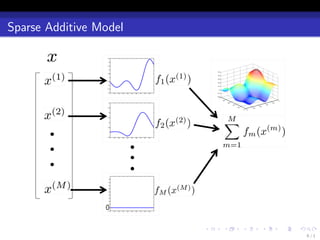
  • 8. Problem Setting yi = f o (xi ) + ξi , (i = 1, . . . , n), where f o is the true function such that E[Y |X ] = f o (X ). f o is well approximated by a function f ∗ with a sparse representation: ∑ M f o (x) ≃ f ∗ (x) = ∗ fm (x (m) ), m=1 ∗ where only a few components of {fm }M are non-zero. m=1 . . . . . . 8/1
  • 9. Outline . . . . . . 9/1
  • 10. Multiple Kernel Learning ( )2 1∑ ∑ ∑ n M M (m) min yi − fm (xi ) + C ∥fm ∥Hm fm ∈Hm n i=1 m=1 m=1 (Hm : Reproducing Kernel Hilbert Space (RKHS), explained later) Extension of Group Lasso: each group is infinite dimensional Sparse solution Reduced to finite dimensional optimization problem by the representer theorem (Sonnenburg et al., 2006; Rakotomamonjy et al., 2008; Suzuki & Tomioka, 2009) . . . . . . 10 / 1
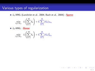
  • 11. Various types of regularization L1 -MKL (Lanckriet et al., 2004; Bach et al., 2004):Sparse ( M ) ∑ ∑M min L fm + C ∥fm ∥Hm fm ∈Hm m=1 m=1 L2 -MKL:Dense ( M ) ∑ ∑ M min L fm + C ∥fm ∥2 m H fm ∈Hm m=1 m=1 . . . . . . 11 / 1
  • 12. Various types of regularization L1 -MKL (Lanckriet et al., 2004; Bach et al., 2004):Sparse ( M ) ∑ ∑M min L fm + C ∥fm ∥Hm fm ∈Hm m=1 m=1 L2 -MKL:Dense ( M ) ∑ ∑ M min L fm + C ∥fm ∥2 m H fm ∈Hm m=1 m=1 Elasticnet-MKL (Tomioka & Suzuki, 2009) ( M ) ∑ ∑M ∑ M min L fm + C1 ∥fm ∥Hm + C2 ∥fm ∥2 m H fm ∈Hm m=1 m=1 m=1 ℓp -MKL (Kloft et al., 2009) ( M ) ( M )p 2 ∑ ∑ min L fm + C1 ∥fm ∥Hm p fm ∈Hm m=1 m=1 . . . . . . 11 / 1
  • 13. Sparsity VS accuracy Figure : Relation between accuracy and sparsity of Elasticnet-MKL for caltech 101 . . . . . . 12 / 1
  • 14. Sparsity VS accuracy Figure : Relation between accuracy and sparsity of ℓp -MKL (Cortes et al., 2009) . . . . . . 13 / 1
  • 15. Restricted Eigenvalue Condition To prove a fast convergence rate of MKL, we utilize the following condition called Restricted Eigenvalue Condition (Bickel et al., 2009; Koltchinskii & Yuan, 2010; Suzuki, 2011; Suzuki & Sugiyama, 2012). . Restricted Eigenvalue Condition . There exists a constant 0 < C such that . 0 < C < β√d (I0 ). { ∑M ∥ m=1 fm ∥2 2 (Π) L βb (I ) := sup β ≥ 0 | β ≤ ∑ , m∈I ∥fm ∥2 2 (Π) L } ∑ ∑ ∀f such that b ∥fm ∥L2 (Π) ≥ ∥fm ∥L2 (Π) . m∈I m∈I / c fm s are not totally correlated inside I0 and between I0 .and I.0 . . . . . 14 / 1
  • 16. We investigate a Bayesian variant of MKL. We show a fast learning rate of it without strong conditions on the design such as the restricted eigenvalue condition. . . . . . . 15 / 1
  • 17. Outline . . . . . . 16 / 1
  • 18. our research = sparse aggregated estimation + Gaussian process Aggregated Estimator, Exponential Screening, Model Averaging (Leung & Barron, 2006; Rigollet & Tsybakov, 2011) Gaussian Process Regression (Rasmussen & Williams, 2006; van der Vaart & van Zanten, 2008a; van der Vaart & van Zanten, 2008b; van der Vaart & van Zanten, 2011) . . . . . . 17 / 1
  • 19. Aggregated Estimator Aggregated Estimator Assume that Y ∈ Rn is generated by the following model: Y =µ+ϵ ≃ X θ0 + ϵ, where ϵ = (ϵ1 , . . . , ϵn )⊤ is i.i.d. realization of Gaussian noise (N (0, σ 2 )). We would like to estimate µ using a set of model M. Each element m ∈ M, we have a linear model with dimension dm : Xm θm , where θm ∈ Rdm and Xm ∈ Rn×dm consists of a subset of columns of a design matrix. Let θm be a least squares estimator on a model m ∈ M: ˆ θm = (Xm Xm )† Xm Y . ˆ ⊤ ⊤ . . . . . . 18 / 1
  • 20. Aggregated Estimator Aggregated Estimator Let ˆm be an unbiased estimator of the risk rm = E∥Xm θm − µ∥2 : r ˆ ˆm = ∥Y − Xm θm ∥2 + σ 2 (2dm − n), r ˆ (we can show that Eˆm = rm ). Define the aggregated estimator as r ∑ ˆ m∈M πm exp(−ˆm /4)Xm θm r µ= ˆ ∑ , m′ ∈M πm′ exp(−ˆm′ /4) r a.k.a., Akaike weight (Akaike, 1978; Akaike, 1979). . Theorem (Risk bound of aggregated estimator (Leung & Barron, 2006)) . [ ] { } 1 rm 4 E ∥ˆ − µ∥2 ≤ min µ + log(1/πm ) . . n m∈M n n . . . . . . 19 / 1
  • 21. Aggregated Estimator Application of the risk bound to sparse estimation (Rigollet & Tsybakov, 2011) (m) Let Xi,m = xi (i = 1, . . . , n, m = 1, . . . , M). Let M be all subsets of [M] = {1, . . . , M}, and for I ⊂ [M]  ( )  1 |I | |I | , (if |I | ≤ R),  C 2eM  πI := 1 , (if |I | = M), 2   0, (otherwise), where R = rank(X ) and C is a normalization constant. Under this ˆ setting, we call the aggregated estimator θ the exponential screening estimator, denoted by θ ˆES . . . . . . . 20 / 1
  • 22. Aggregated Estimator Application of the risk bound to sparse estimation (Rigollet & Tsybakov, 2011) . Theorem (Rigollet and Tsybakov (2011)) . Assume that ∥X:,m ∥n ≤ 1. Then we have { ( )} R ∥θ∥0 eM E[∥X θES −µ∥2 ] ≤ min ∥X θ − µ∥2 + C ∧ ˆ log 1 + . n θ∈RM n n n ∥θ∥0 ∨ 1 ※ Note that there is no assumption on the condition of the design X ! . . . . . . 21 / 1
  • 23. Aggregated Estimator Application of the risk bound to sparse estimation (Rigollet & Tsybakov, 2011) . Theorem (Rigollet and Tsybakov (2011)) . Assume that ∥X:,m ∥n ≤ 1. Then we have { ( )} R ∥θ∥0 eM E[∥X θES −µ∥2 ] ≤ min ∥X θ − µ∥2 + C ∧ ˆ log 1 + . n θ∈RM n n n ∥θ∥0 ∨ 1 ※ Note that there is no assumption on the condition of the design X ! Moreover we have . Corollary (Rigollet and Tsybakov (2011)) . { } log(M) E[∥X θES − µ∥2 ] ≤ min ∥X θ − µ∥2 + φn,M (θ) + C ′′ ˆ n n , θ∈RM n ( ) √ ( ) ∥θ∥0 ∥θ∥ℓ1 where φn,M (θ) = C ′ R ∧ n n log 1+ ∥θ∥0 ∨1 ∧ eM √ n CM log 1+ ∥θ∥ℓ √n . . . . . . 1 . . 21 / 1
  • 24. Aggregated Estimator Comparison with BIC type estimator { ( )} 2σ 2 ∥θ∥0 2 + a√ 1+a θBIC := arg min ∥Y − X θ∥2 + ˆ n 1+ L(θ) + L(θ) , θ∈RM n 1+a a ( ) eM where L(θ) = 2 log ∥θ∥0 ∨1 , and a > 0 is a parameter. . Theorem (Bunea et al. (2007), Rigollet and Tsybakov (2011)) . Assume that ∥X:,m ∥n ≤ 1. Then we have { } 1+a C σ2 E[∥X θBIC − µ∥2 ] ≤ (1 + a) min ∥X θ − µ∥2 + C ˆ n n φn,M (θ) + θ∈RM a n . The exponential screening estimator gives a smaller bound. . . . . . . 22 / 1
  • 25. Aggregated Estimator Comparison with Lasso estimator { } ˆLasso := arg min ∥Y − X θ∥2 + λ∥θ∥ℓ1 . θ n θ∈RM n . Theorem (Rigollet and Tsybakov (2011)) . √ Assume that ∥X:,m ∥n ≤ 1. Then, if we set λ = Aσ log(M) , then we have n { } ∥θ∥ℓ1 √ ˆLasso E[∥X θ − µ∥2 ] n ≤ min ∥X θ − µ∥2 n +C √ log(M) . θ∈RM n . The exponential screening estimator gives a smaller bound. . . . . . . 23 / 1
  • 26. Aggregated Estimator Comparison with Lasso estimator { } ˆLasso := arg min ∥Y − X θ∥2 + λ∥θ∥ℓ1 . θ n θ∈RM n . Theorem (Rigollet and Tsybakov (2011)) . √ Assume that ∥X:,m ∥n ≤ 1. Then, if we set λ = Aσ log(M) , then we have n { } ∥θ∥ℓ1 √ ˆLasso E[∥X θ − µ∥2 ] n ≤ min ∥X θ − µ∥2 n +C √ log(M) . θ∈RM n . The exponential screening estimator gives a smaller bound. If the restricted eigenvalue condition is satisfied, then { } E[∥X θˆLasso − µ∥2 ] ≤ (1 + a) min ∥X θ − µ∥2 + C (1 + a) ∥θ∥0 log(M) . n n θ∈RM a n . . . . . . 23 / 1
  • 27. Gaussian Process Regression Gaussian Process Regression . . . . . . 24 / 1
  • 28. Gaussian Process Regression Bayes’ theorem Statistical model: {p(x|θ) | θ ∈ Θ} Prior distribution: π(θ) ∏n Likelihood: p(Dn |θ) = i=1 p(xi |θ) Posterior distribution (Bayes’ theorem): p(Dn |θ)π(θ) p(θ|Dn ) = ∫ . p(Dn |θ)π(θ)dθ Bayes estimator: ∫ g := argmin ˆ EDn :θ [R(θ, g (Dn ))]π(θ)dθ g ∫ (∫ ) = argmin R(θ, g (Dn ))p(θ|Dn )dθ p(Dn )dDn g ∫ If R(θ, θ′ ) = ∥θ − θ′ ∥2 , then g (Dn ) = ˆ θp(θ|Dn )dθ. . . . . . . 25 / 1
  • 29. Gaussian Process Regression Gaussian Process Regression 8 6 4 2 0 -2 -4 -6 0 0.1 0.2 0.3 0.4 0.5 0.6 0.7 0.8 0.9 1 . . . . . . 26 / 1
  • 30. Gaussian Process Regression Gaussian Process Regression Gaussian process prior: a prior on a functions f = (f (x) : x ∈ X ). f ∼ GP means that each finite subset (f (x1 ), f (x2 ), . . . , f (xj )) (j = 1, 2, . . . ) obeys a zero-mean multivariate normal distribution. We assume that supx |f (x)| < ∞ and f : Ω → ℓ∞ (X ) is tight and Borel measurable. Kernel function: k(x, x ′ ) := Ef ∼GP [f (x)f (x ′ )]. Examples: Linear kernel: k(x, x ′ ) = x ⊤ x ′ . Gaussian kernel: k(x, x ′ ) = exp(−∥x − x ′ ∥2 /2σ 2 ). polynomial kernel: k(x, x ′ ) = (1 + x ⊤ x ′ )d . . . . . . . 27 / 1
  • 31. Gaussian Process Regression Gaussian Process Prior 4 1 3 0.5 2 0 1 -0.5 0 -1 -1 -1.5 -2 -2 0 0.1 0.2 0.3 0.4 0.5 0.6 0.7 0.8 0.9 1 0 0.1 0.2 0.3 0.4 0.5 0.6 0.7 0.8 0.9 1 (a) Gaussian kernel (b) Linear kernel . . . . . . 28 / 1
  • 32. Gaussian Process Regression Estimation Suppose {yi }n are generated from the following model: i=1 yi = f o (xi ) + ξi , where ξi is i.i.d. Gaussian noise N (0, σ 2 ). Posterior distribution: let f = (f (x1 ), . . . , f (xn )), then ( ) ( ) 1 ∥f − Y ∥2 1 ⊤ −1 p(f|Dn ) = exp −n n exp − f K f C 2σ 2 2 ( ) 1 1 −1 2 = exp − f − (K + σ In ) KY (K −1 +In /σ2 ) , 2 C 2 where K ∈ Rn×n is the Gram matrix (Ki,j = k(xi , xj )). posterior mean: ˆ = (K + σ 2 In )−1 KY . f posterior covariance: K − K (K + σ 2 In )−1 K . . . . . . . 29 / 1
  • 33. Gaussian Process Regression Gaussian Process Posterior 1.5 1.5 1 1 0.5 0.5 0 0 -0.5 -0.5 -1 -1 0 0.1 0.2 0.3 0.4 0.5 0.6 0.7 0.8 0.9 1 0 0.1 0.2 0.3 0.4 0.5 0.6 0.7 0.8 0.9 1 (c) Training Data (d) Posterior Sample . . . . . . 30 / 1
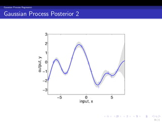
  • 34. Gaussian Process Regression Gaussian Process Posterior 2 . . . . . . 31 / 1
  • 35. Gaussian Process Regression Our interest How fast does the posterior converge around the true? . . . . . . 32 / 1
  • 36. Gaussian Process Regression Reproducing Kernel Hilbert Space (RKHS) The kernel function defines Reproducing Kernel Hilbert Space (RKHS) H as a completion of the linear space spanned by all functions ∑ I x→ αi k(xi , x), (I = 1, 2, . . . ) i=1 relative to the RKHS norm ∥ · ∥H induced by the inner product ⟨ I ⟩ ∑ ∑ J ∑∑ I J ′ ′ αi k(xi , ·), αj k(xj , ·) = αi αj′ k(xi , xj′ ). i=1 j=1 H i=1 j=1 Reproducibility: for f ∈ H, the function value at x is recovered as f (x) = ⟨f , k(x, ·)⟩H . See van der Vaart and van Zanten (2008b) for more detail. . . . . . . 33 / 1
  • 37. Gaussian Process Regression The work by van der Vaart and van Zanten (2011) van der Vaart and van Zanten (2011) gave the posterior convergence rate for Mat´rn prior. e Mat´rn prior: for a regularity α > 0, we define e ∫ ⊤ ′ k(x, x ′ ) = e iλ (x−x ) ψ(λ)dλ, Rd where ψ : Rd → R is the spectral density given by 1 ψ(λ) = . (1 + ∥λ∥2 )α+d/2 ′ The support is included in a H¨lder space C α [0, 1]d for any α′ < α. o The RKHS H is included in a Sobolev space W α+d/2 [0, 1]d with the regularity α + d/2. For infinite dimensional RKHS H, the support of the prior is typically much larger than H. . . . . . . 34 / 1
  • 38. Gaussian Process Regression Convergence rate of posterior: Mat´rn prior e ˆ Let f be the posterior mean. . Theorem (van der Vaart and van Zanten (2011)) . Let f ∗ ∈ C β [0, 1]d ∩ W β [0, 1]d for β > 0, then for Mat´rn prior, we have e ( α∧β ) E[∥f − f ∗ ∥2 ] ≤ O n− α+d/2 . ˆ n . ( β ) The optimal rate is O n− β+d/2 . The optimal rate is achieved only when α = β. α∧β The rate n− α+d/2 is tight. → If f ∗ ∈ H (β = α + d/2), then GP does not achieve the optimal rate. → Scale mixture is useful (van der Vaart & van Zanten, 2009). . . . . . . 35 / 1
  • 39. Gaussian Process Regression Summary of existing results GP is optimal only in quite restrictive situations (α = β). In particular, if f o ∈ H, the optimal rate can not be achieved. The analysis was given only for restricted classes such as Sobolev and H¨lder classes. o . . . . . . 36 / 1
  • 40. Outline . . . . . . 37 / 1
  • 41. Bayesian-MKL = sparse aggregated estimation + Gaussian process Condition on design: Does not require any special conditions such as restricted eigenvalue condition. Optimality: Adaptively achieves the optimal rate for a wide class of true functions. In particular, even if f o ∈ H, it achieves the optimal rate. Generality: The analysis is given for a general class of spaces utilizing the notion of interpolation spaces and the metric entropy. . . . . . . 38 / 1
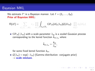
  • 42. Bayesian MKL We estimate f o in a Bayesian manner. Let f = (f1 , . . . , fM ). Prior of Bayesian MKL: ∑ ∏∫ ∏ Π(df ) = πJ · GPm (dfm |λm )G(dλm ) · δ0 (dfm ) J⊆{1,...,M} m∈J λm ∈R+ m∈J / . . . . . . 39 / 1
  • 43. Bayesian MKL We estimate f o in a Bayesian manner. Let f = (f1 , . . . , fM ). Prior of Bayesian MKL: ∑ ∏∫ ∏ Π(df ) = πJ · GPm (dfm |λm )G(dλm ) · δ0 (dfm ) J⊆{1,...,M} m∈J λm ∈R+ m∈J / GPm (·|λm ) with a scale parameter λm is a scaled Gaussian process ˜ corresponding to the kernel function km,λm where ˜ km km,λm = , λm for some fixed kernel function km . . . . . . . 39 / 1
  • 44. Bayesian MKL We estimate f o in a Bayesian manner. Let f = (f1 , . . . , fM ). Prior of Bayesian MKL: ∑ ∏∫ ∏ Π(df ) = πJ · GPm (dfm |λm )G(dλm ) · δ0 (dfm ) J⊆{1,...,M} m∈J λm ∈R+ m∈J / GPm (·|λm ) with a scale parameter λm is a scaled Gaussian process ˜ corresponding to the kernel function km,λm where ˜ km km,λm = , λm for some fixed kernel function km . G(λm ) = exp(−λm ) (Gamma distribution: conjugate prior) → scale mixture. . . . . . . 39 / 1
  • 45. Bayesian MKL We estimate f o in a Bayesian manner. Let f = (f1 , . . . , fM ). Prior of Bayesian MKL: ∑ ∏∫ ∏ Π(df ) = πJ · GPm (dfm |λm )G(dλm ) · δ0 (dfm ) J⊆{1,...,M} m∈J λm ∈R+ m∈J / GPm (·|λm ) with a scale parameter λm is a scaled Gaussian process ˜ corresponding to the kernel function km,λm where ˜ km km,λm = , λm for some fixed kernel function km . G(λm ) = exp(−λm ) (Gamma distribution: conjugate prior) → scale mixture. Set all components fm for m ∈ J as 0. / . . . . . . 39 / 1
  • 46. Bayesian MKL We estimate f o in a Bayesian manner. Let f = (f1 , . . . , fM ). Prior of Bayesian MKL: ∑ ∏∫ ∏ Π(df ) = πJ · GPm (dfm |λm )G(dλm ) · δ0 (dfm ) J⊆{1,...,M} m∈J λm ∈R+ m∈J / GPm (·|λm ) with a scale parameter λm is a scaled Gaussian process ˜ corresponding to the kernel function km,λm where ˜ km km,λm = , λm for some fixed kernel function km . G(λm ) = exp(−λm ) (Gamma distribution: conjugate prior) → scale mixture. Set all components fm for m ∈ J as 0. / Put a prior πJ on each sub-model J. . . . . . . 39 / 1
  • 47. Bayesian MKL We estimate f o in a Bayesian manner. Let f = (f1 , . . . , fM ). Prior of Bayesian MKL: ∑ ∏∫ ∏ Π(df ) = πJ · GPm (dfm |λm )G(dλm ) · δ0 (dfm ) J⊆{1,...,M} m∈J λm ∈R+ m∈J / πJ is given as ( )−1 ζ |J| M πJ = ∑ M , j=1 ζj |J| with some ζ ∈ (0, 1). . . . . . . 39 / 1
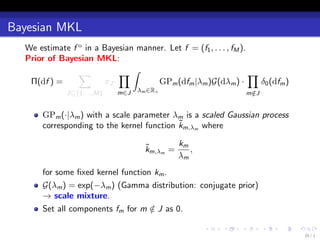
  • 48. The estimator The posterior: For some constant β > 0, the posterior probability measure is given as ( ∑n ∑ ) (y − M f (x ))2 exp − i=1 i βm=1 m i Π(df |Dn ) := ∫ ( ∑n ∑ ) Π(df ), (y − M f (x ))2 ˜ exp − i=1 i βm=1 m i ˜ Π(df ) for f = (f1 , . . . , fM ). ˆ The estimator: The Bayesian estimator f (Bayesian-MKL estimator) is given as the expectation of the posterior: ∫ ∑ M ˆ f = fm Π(df |y1 , . . . , yn ). m=1 . . . . . . 40 / 1
  • 49. Point Model averaging Scale mixture of Gaussian process prior . . . . . . 41 / 1
  • 50. Outline . . . . . . 42 / 1
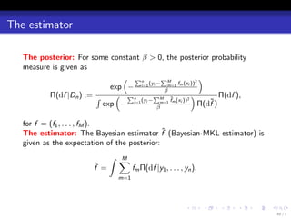
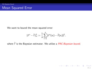
  • 51. PAC-Bayesian Bound Mean Squared Error We want to bound the mean squared error: 1∑ o n ∥f o − f ∥2 := ˆ n (f (xi ) − f (xi ))2 , ˆ n i=1 ˆ where f is the Bayesian estimator. We utilize a PAC-Bayesian bound. . . . . . . 43 / 1
  • 52. PAC-Bayesian Bound PAC-Bayesian Bound Under some conditions for the noise (explained in the next slide), we have the following theorem. . Theorem (Dalalyan and Tsybakov (2008)) . For all probability measure ρ, we have [ ] ∫ βK(ρ, Π) EY1:n |x1:n ∥f − f o ∥2 ≤ ∥f − f o ∥2 dρ(f ) + ˆ n n , n where K(ρ, Π) is the KL-divergence between ρ and Π: ∫ ( ) dρ K(ρ, Π) := log dρ. . dΠ . . . . . . 44 / 1
  • 53. PAC-Bayesian Bound Noise Condition Let mξ (z) := −E[ξ1 1{ξ1 ≤ z}], where 1{·} is the indicator function. Then we impose the following assumption on mξ . . Assumption . E[ξ1 ] < ∞ and the measure mξ (z)dz is absolutely continuous with 2 respect to the density function pξ (z) with a bounded Radon-Nikodym derivative, i.e., there exists a bounded function gξ : R → R+ such that ∫ b ∫ b mξ (z)dz = gξ (z)pξ (z)dz, ∀a, b ∈ R. . a a The Gaussian noise N (0, σ 2 ) satisfies the assumption with gξ (z) = σ 2 , The uniform distribution on [−a, a] satisfies the assumption with gξ (z) = max(a2 − z 2 , 0)/2. . . . . . . 45 / 1
  • 54. Main Result Concentration Function We define the concentration function as (m) ϕf ∗ (ϵ, λm ) := inf ∗ ∥h∥2 m,λm − log GPm ({f : ∥f ∥n ≤ ϵ}|λm ) . H m h∈Hm :∥h−fm ∥n ≤ϵ bias variance (m) ∗ It is known that ϕf ∗ (ϵ, λm ) ∼ − log GPm ({f : ∥fm − f ∥n ≤ ϵ}|λm ) (van m der Vaart & van Zanten, 2011; van der Vaart & van Zanten, 2008b). . . . . . . 46 / 1
  • 55. Main Result General Result ∗ ∗ Let I0 := {m | fm ̸= 0}, ˇ0 := {m ∈ I0 | fm ∈ Hm }, and κ := ζ(1 − ζ). I / . Theorem (Convergence rate of Bayesian-MKL) . The convergence rate of Bayesian-MKL is bounded as [ ] EY1:n |x1:n ∥f − f o ∥2 ≤ 2∥f o − f ∗ ∥2 ˆ n n { ( ) ∑ 1 (m) λm log(λm ) + C1 inf ϵ2 + ϕf ∗ (ϵm , λm ) + m − ϵm ,λm >0 n m n n m∈I0 ( ) } ∑ |I0 | Me + ϵm ϵm′ + log . m,m′ ∈ˇ0 : I n κ|I0 | . m̸=m′ . . . . . . 47 / 1
  • 56. Main Result Outlook of the theorem ( ) 1 (m) log(λm ) Let ϵ2 = inf ϵm ,λm >0 ϵ2 + n ϕf ∗ (ϵm , λm ) + ˆm m λm n − n and suppose m o ∗ f = f . Typically ϵ2 ˆm achieves the optimal learning rate for the single kernel learning. ∗ If fm ∈ Hm for all m, then we have [ ( )] [ ] ∑ |I0 | Me EY1:n |x1:n ∥f − f ∥n = O ˆ o 2 2 ϵm + ˆ log . n κ|I0 | m∈I0 → Optimal learning rate for MKL. Note that we imposed no condition on the design such as restricted eigenvalue condition. ∗ If fm ∈ Hm for all m ∈ I0 , then we have / ( )2  [ ] ∑ ( ) |I0 | Me  EY1:n |x1:n ∥f − f o ∥2 = O  ˆ ϵm + ˆ log . n n κ|I0 | m∈I0 . . . . . . 48 / 1
  • 57. Main Result Outline of the Proof Fix ϵm , λm > 0 arbitrary. Next we define a “representer” element ∗ ∗ ∗ hm ∈ Hm that is close to fm . If fm ∈ Hm , then set hm = fm . Otherwise, ˜ ˜ we take h ˜m ∈ Hm,λ such that m ∥hm ∥2 m ,λm ≤ 2 inf h∈Hm :∥h−fm ∥n ≤ϵm ∥h∥2 m,λm . We substitute the following ˜ H ∗ H “dummy” posterior into ρ: ∫ GPm (dfm −hm |λm )1{∥fm −hm ∥n ≤ϵm } ˜ ˜ ˜ ∏ λm ≤λm ≤λm ˜ GPm ({∆fm :∥∆fm ∥n ≤ϵm }|λm ) ˜ G(dλm ) ∏ ˜ ρ(df ) = 2 · δ0 (dfm ). m∈I0 G({λm : λ2m ≤ λm ≤ λm }) ˜ ˜ m∈I / 0 One can show that the KL-divergence betweenρ and the prior Π is bounded as 1 ∑ ( 1 (m) 1 1 ) |I0 | ( Me ) ′ K(ρ, Π) ≤ C1 ϕ ∗ (ϵm , λm ) + λm − log (λm ) + log , n n fm n n n |I0 |κ m∈I0 ′ where C1 is a universal constant. A key to prove this is an infinite dimensional extension of the Brascamp and Lieb inequality (Brascamp & Lieb, 1976; Harg´, 2004). Since {ϵm , λm }M are arbitrary, this gives the e m=1 assertion. . . . . . . 49 / 1
  • 58. Applications to Some Examples Example 1: Metric Entropy Characterization (Correctly specified) Define the ϵ-covering number N(BHm , ϵ, ∥ · ∥n ) as the number of ∥ · ∥n -norm balls covering the unit ball BHm in Hm . The metric entropy is its logarithm: log N(BHm , ϵ, ∥ · ∥n ). . . . . . . 50 / 1
  • 59. Applications to Some Examples Example 1: Metric Entropy Characterization We assume that there exits a real value 0 < sm < 1 such that log N(BHm , ϵ, ∥ · ∥n ) = O(ϵ−2sm ), where BHm is the unit ball of the RKHS Hm . . Theorem (Correctly specified) . ∗ If fm ∈ Hm for all m ∈ I0 , then we have { ( )} [ ] ∑ |I0 | Me − 1+sm +2∥f o−f ∗ ∥2 1 EY1:n |x1:n ∥f ˆ − f o ∥2 ≤ C n + log n n |I0 |κ n . m∈I0 It is known that, if there is no scale mixture prior, the optimal rate n− 1+sm can not be achieved (Castillo, 2008). 1 . . . . . . 51 / 1
  • 60. Applications to Some Examples Example 1: Metric Entropy Characterization (Misspecified) Let [L2 (Pn ), Hm ]θ,∞ be the interpolation space equipped with the norm, ∥f ∥θ,∞ := sup t −θ inf {∥f − gm ∥n + t∥gm ∥Hm }. (m) t>0 gm ∈Hm One has Hm → [L2 (Pn ), Hm ]θ,∞ → L2 (Pn ). L2 Interpolation space Hm . . . . . . 52 / 1
  • 61. Applications to Some Examples Example 1: Metric Entropy Characterization (Misspecified) Let [L2 (Pn ), Hm ]θ,∞ be the interpolation space equipped with the norm, ∥f ∥θ,∞ := sup t −θ inf {∥f − gm ∥n + t∥gm ∥Hm }. (m) t>0 gm ∈Hm One has Hm → [L2 (Pn ), Hm ]θ,∞ → L2 (Pn ). . Theorem (Misspecified) . ∗ If fm ∈ [L2 (Pn ), Hm ]θ,∞ with 0 < θ ≤ 1, then we have ( )2  [ ]  ∑ ( ) |I0 | Me n− 2(1+sm /θ) 1 EY1:n |x1:n ∥f − f o ∥2 ≤C ˆ + log n  n |I0 |κ  m∈I0 . + 2∥f − f ∗ ∥2 o n Thanks to the scale mixture prior, the estimator adaptively achieves the optimal rate for θ ∈ (sm , 1]. . . . . . . 52 / 1
  • 62. Applications to Some Examples Example 2: Mat´rn prior e Suppose that Xm = [0, 1]dm . The Mat´rn priors on Xm correspond to the e kernel function defined as ∫ ⊤ ′ ′ km (z, z ) = e is (z−z ) ψm (s)ds, Rdm where ψm (s) is the spectral density given by ψm (s) = (1 + ∥s∥2 )−(αm +dm /2) , for a smoothness parameter αm > 0. . Theorem (Mat´rn prior, correctly specified) e . ∗ If fm ∈ Hm , then we have that { ( )} [ ] ∑ − 1+ 1dm |I0 | Me EY1:n |x1:n ∥f − f o ∥2 ≤C ˆ n 2αm +dm + log n n |I0 |κ m∈I0 . + 2∥f o − f ∗ ∥2 n . . . . . . 53 / 1
  • 63. Applications to Some Examples Example 2: Mat´rn prior e . Theorem (Mat´rn prior, Misspecified) e . ∗ If fm ∈ C [0, 1]dm ∩ W βm [0, 1]dm and βm < αm + dm /2, then we have βm that ( )2   ∑ ( ) [ ] βm |I0 | Me  EY1:n |x1:n ∥f − f o ∥2 ≤C ˆ n− 2βm +dm + log n  n |I0 |κ  m∈I0 . + 2∥f o − f ∗ ∥2 n ∗ Although fm ∈ Hm , the convergence rate achieves the optimal rate / adaptively. . . . . . . 54 / 1
  • 64. Applications to Some Examples Example 3: Group Lasso Xm is a finite dimensional Euclidean space: Xm = Rdm . The kernel function corresponding to the Gaussian process prior is km (x, x ′ ) = x ⊤ x ′ : fm (x) = µ⊤ x, µ ∼ N (0, Idm ). . Theorem (Group Lasso) . If fm = µ⊤ x, then we have that ∗ m [ ] {∑ ( )} m∈I0 dm log(n) |I0 | Me EY1:n |x1:n ∥f ˆ − f o ∥2 =C + log n n n |I0 |κ . + 2∥f o − f ∗ ∥2 n This is rate optimal up to log(n)-order. . . . . . . 55 / 1
  • 65. Applications to Some Examples Gaussian correlation conjecture We use an infinite dimensional version of the following inequality (Brascamp-Lieb inequality (Brascamp & Lieb, 1976; Harg´, 2004)): e E[⟨X , ϕ⟩2 |X ∈ A] ≤ E[⟨X , ϕ⟩2 ], where X ∼ N (0, Σ) and A is a symmetric convex set centered on the origin. Gaussian correlation conjecture: µ(A ∩ B) ≥ µ(A)µ(B), where µ is any centered Gaussian measure and A and B are any two symmetric convex sets. Brascamp-Lieb inequality can be seen as an application of a particular case of the Gaussian correlation conjecture. See the survey by Li and Shao (2001) for more details. . . . . . . 56 / 1
  • 66. Applications to Some Examples Conclusion We developed a PAC-Bayesian bound for Gaussian process model and generalized it to sparse additive model. The optimal rate is achieved without any conditions on the design. We have observed that Gaussian processes with scale mixture adaptively achieve the minimax optimal rate on both correctly-specified and misspecified situations. . . . . . . 57 / 1
  • 67. Akaike, H. (1978). A Bayesian analysis of the minimum AIC procedure. Annals of the Institute of Statistical Mathematics, 30, 9–14. Akaike, H. (1979). A bayesian extension of the minimum aic procedure of autoregressive model fitting. Biometrika, 66, 237–242. Bach, F., Lanckriet, G., & Jordan, M. (2004). Multiple kernel learning, conic duality, and the SMO algorithm. the 21st International Conference on Machine Learning (pp. 41–48). Bickel, P. J., Ritov, Y., & Tsybakov, A. B. (2009). Simultaneous analysis of Lasso and Dantzig selector. The Annals of Statistics, 37, 1705–1732. Brascamp, H. J., & Lieb, E. H. (1976). On extensions of the brunn-minkowski and pr´kopa-leindler theorem, including inequalities e for log concave functions, and with an application to the diffusion equation. Journal of Functional Analysis, 22, 366–389. Bunea, F., Tsybakov, A. B., & Wegkamp, M. H. (2007). Aggregation for gaussian regression. The Annals of Statistics, 35, 1674–1697. Castillo, I. (2008). Lower bounds for posterior rates with Gaussian process priors. Electronic Journal of Statistics, 2, 1281–1299. Cortes, C., Mohri, M., & Rostamizadeh, A. (2009). L2 regularization for learning kernels. the 25th Conference on Uncertainty in Artificial Intelligence (UAI 2009). Montr´al, Canada. . e . . . . . 57 / 1
  • 68. Dalalyan, A., & Tsybakov, A. B. (2008). Aggregation by exponential weighting sharp PAC-Bayesian bounds and sparsity. Machine Learning, 72, 39–61. Harg´, G. (2004). A convex/log-concave correlation inequality for e gaussian measure and an application to abstract wiener spaces. Probability Theory and Related Fields, 130, 415–440. Kloft, M., Brefeld, U., Sonnenburg, S., Laskov, P., M¨ller, K.-R., & Zien, u A. (2009). Efficient and accurate ℓp -norm multiple kernel learning. Advances in Neural Information Processing Systems 22 (pp. 997–1005). Cambridge, MA: MIT Press. Koltchinskii, V., & Yuan, M. (2010). Sparsity in multiple kernel learning. The Annals of Statistics, 38, 3660–3695. Lanckriet, G., Cristianini, N., Ghaoui, L. E., Bartlett, P., & Jordan, M. (2004). Learning the kernel matrix with semi-definite programming. Journal of Machine Learning Research, 5, 27–72. Leung, G., & Barron, A. R. (2006). Information theory and mixing least-squares regressions. IEEE Transactions on Information Theory, 52, 3396–3410. . . . . . . 57 / 1
  • 69. Li, W. V., & Shao, Q.-M. (2001). Gaussian processes: inequalities, small ball probabilities and applications. Stochastic Processes: Theory and Methods, 19, 533–597. Rakotomamonjy, A., Bach, F., Canu, S., & Y., G. (2008). SimpleMKL. Journal of Machine Learning Research, 9, 2491–2521. Rasmussen, C. E., & Williams, C. (2006). Gaussian processes for machine learning. MIT Press. Rigollet, P., & Tsybakov, A. (2011). Exponential screening and optimal rates of sparse estimation. The Annals of Statistics, 39, 731–771. Sonnenburg, S., R¨tsch, G., Sch¨fer, C., & Sch¨lkopf, B. (2006). Large a a o scale multiple kernel learning. Journal of Machine Learning Research, 7, 1531–1565. Suzuki, T. (2011). Unifying framework for fast learning rate of non-sparse multiple kernel learning. Advances in Neural Information Processing Systems 24 (pp. 1575–1583). NIPS2011. Suzuki, T., & Sugiyama, M. (2012). Fast learning rate of multiple kernel learning: Trade-off between sparsity and smoothness. JMLR Workshop and Conference Proceedings 22 (pp. 1152–1183). Fifteenth International Conference on Artificial Intelligence and Statistics (AISTATS2012). . . . . . . 57 / 1
  • 70. Applications to Some Examples Suzuki, T., & Tomioka, R. (2009). SpicyMKL. arXiv:0909.5026. Tomioka, R., & Suzuki, T. (2009). Sparsity-accuracy trade-off in MKL. NIPS 2009 Workshop:: Understanding Multiple Kernel Learning Methods. Whistler. arXiv:1001.2615. van der Vaart, A. W., & van Zanten, J. H. (2008a). Rates of contraction of posterior distributions based on Gaussian process priors. The Annals of Statistics, 36, 1435–1463. van der Vaart, A. W., & van Zanten, J. H. (2008b). Reproducing kernel Hilbert spaces of Gaussian priors. Pushing the Limits of Contemporary Statistics: Contributions in Honor of Jayanta K. Ghosh, 3, 200–222. IMS Collections. van der Vaart, A. W., & van Zanten, J. H. (2009). Adaptive Bayesian estimation using a Gaussian random field with inverse Gamma bandwidth. The Annals of Statistics, 37, 2655–2675. van der Vaart, A. W., & van Zanten, J. H. (2011). Information rates of nonparametric gaussian process methods. Journal of Machine Learning Research, 12, 2095–2119. . . . . . . 57 / 1