


Ch06b entropy
- 1. Property Relationships Chapter 6 1
- 2. : The T-ds relations Apply the differential form of the first law for a closed stationary system for an internally reversible process δQint rev − δWint rev = dU δQint rev = TdS δWint rev = PdV TdS − PdV = dU 2
- 3. Divide by the mass, you get Tds = du + Pdv This equation is known as: First Gibbs equation or First Tds relationship Divide by T, .. du Pdv ds = + T T Although we get this form for internally reversible process, we still can compute ∆s for an irreversible process. This is because S is a point function. 3
- 4. Second T-ds (Gibbs) relationship Recall that… h = u + Pv Take the differential for both sides dh = du + Pdv + vdP Rearrange to find du du = dh − Pdv − vdP Substitute in the First Tds relationship Tds = du + Pdv Tds = dh − vdP Second Tds relationship, or Gibbs equation 4
- 5. dh vdP Divide by T, .. ds = − T T Thus We have two equations for ds du Pdv dh vdP ds = + ds = − T T T T To find ∆s, we have to integrate these equations. Thus we need a relation between du and T (or dh and T). Now we can find entropy change (the LHS of the entropy balance) for liquids and solids 5
- 6. Entropy Change of Liquids- 2 and Solids Solids and liquids do not change specific volume appreciably with pressure. That means that dv=0, so the first equation is the easiest to use. 0 du Pdv Thus For du ds = + solids and ds = T T liquids T , Recall also that For solids and liquids du = CdT du CdT ∴ ds = = T T 6
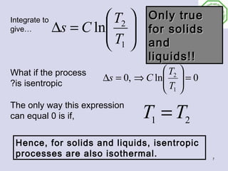
- 7. Integrate to T2 Only true give… ∆s = C ln T for solids 1 and liquids!! What if the process T2 ∆s = 0, ⇒ C ln = 0 T ?is isentropic 1 T1 = T2 The only way this expression can equal 0 is if, Hence, for solids and liquids, isentropic processes are also isothermal. 7
- 8. Example(6-7): Effect of Density of a Liquid on Entropy Liquid methane is commonly used in various cryogenic applications. The critical temperature of methane is 191 K (or -82oC), and thus methane must be maintained below 191 K to keep it in liquid phase. The properties of liquid methane at various temperatures and pressures are given next page. Determine the entropy change of liquid methane as it undergoes a process from 110 K and 1 MPa to 120 K and 5 MPa (a) using actual data for methane and (b) approximating liquid methane as an incompressible substance. What is the error involved in the later case? 8
- 9. ∆s = s 2 − s 2 = 5.145 − 4.875 = 0.270kj / kgK T2 T2 120 ∆s = C ln = Cavg ln = 3.4785 ln T T = 0.303kj / kgK 1 1 110 9
- 10. Example (6-19): Entropy generated when a hot block is dropped in a lake A 50-kg block of iron casting at 500 K is dropped in a large lake that is at 285 K. The block reaches thermal equilibrium with lake water. Assuming an average specific heat of 0.45 kJ/kg.K for the iron, determine: (a) The entropy change of the iron block, (b) The entropy change of the water lake, (c) the entropy generated during this process. 10
- 11. (a) The entropy change of the iron block, T2 285 ∆Siron = 50 × 0.45 × ln = mC ln = −12.65 kj / K T1 500 we need also to find Q coming out of the system. Q − W = ∆U Q − 0 = mC (T2 − T1 ) Q = 50 × 0.45(285 − 500) = −4838 kJ Tsurr= 285 K (b) The entropy change of the water lake, T=500K Q 4838 ∆Slake = = = 16.97 kJ / K Tlake 285 11
- 12. (c) the entropy generated during this process. Choose the iron block and the lake as the system and treat it is an isolated system. Tsurr= 285 K Thus Sg = ∆Stot = ∆Ssys + ∆Slake T=500K Sg = ∆Stot = -12.6 + 16.97 = 4.32 System boundary 12
- 13. The Entropy Change of Ideal- 3 Gases, first relation First relation The entropy change of an ideal gas can be obtained by substituting du = CvdT and P /T= R/υ into Tds relations: Tds = du + pd υ du Pd υ dT dυ ds = + ds = C v +R T T T υ integrating 2 dT υ2 1 ∫ ⇒ s2 − s1 = Cv ( T ) T +R ln υ1 13
- 14. Second relation A second relation for the entropy change of an ideal gas for a process can be obtained by substituting dh = CpdT and υ /T= R/P into Tds relations: dh vdp dT dp Tds = dh −vdp ds = − ds = C p −R T T T p integrating 2 dT P2 1 ∫ s2 − s1 = C p ( T ) T − R ln P1 14
- 15. 2 dT υ2 s2 − s1 = ∫ Cv ( T ) +R ln 1 T υ1 2 dT P2 1 ∫ s2 − s1 = C p ( T ) T − R ln P1 The integration of the first term on the RHS can be done via two methods: 1. Assume constant Cp and constant Cv (Approximate Analysis) 2. Evaluate these integrals exactly and tabulate the data (Exact Analysis) 15
- 16. Method 1: Constant specific )heats (Approximate Analysis First relation 2 dT υ2 T2 v2 s2 − s1 = ∫ Cv ( T ) +R ln ⇒ ∆s = Cv ln + R ln T v 1 T υ1 1 1 Only true for ideal gases, assuming constant heat capacities Second relation 2 dT P2 T2 P2 s2 − s1 = ∫ C p ( T ) − R ln ⇒ ∆s = C p ln − R ln T P 1 T P1 1 1 Only true for ideal gases, assuming constant heat capacities 16
- 17. Sometimes it is more convenient to calculate the change in entropy per mole, instead of per unit mass T2 v2 ∆s = s2 − s1 = Cv ln + Ru ln T v kJ/kmol. K 1 1 T2 P2 ∆s = s2 − s1 = C p ln − Ru ln T P kJ/kmol. K 1 1 Ru is the universal gas constant 17
- 18. Method 2: Variable specific heats (Exact Analysis) 2 C p dT P2 We use the second relation ∆s = ∫ 1 T − R ln P1 Wecould substitute in the equations for Cv and Cp, and perform the integrations Cp = a + bT + cT2 + dT3 But this is time consuming. Someone already did the integrations and tabulated them for us (table A-17) They assume absolute 0 as the starting point 18
- 19. The integral is expressed as: T2 dT T2 dT T1 dT ∫T1 C p (T ) T = ∫ 0 C p (T ) T − ∫ C p (T ) 0 T T2 dT ∫ = s2 − s1 0 0 Cp( T ) T1 T T dT s = ∫ 0 Where Cp( T ) 0 T is tabulated in Table A-17 Therefore P2 ∆s = s − s − R ln 0 2 0 1 unit : kJ / kg .K P1 19
- 20. Is s = f (T) only? like u for an .ideal gas Let us see Temperature dependence Pressure P2 dependence ∆s = s − s − R ln 0 2 0 1 P1 From this equation, It can be seen that the entropy of an ideal gas is not a function only of the temperature ( as was the internal energy) but also of the pressure or the specific volume. The function s° represents only the temperature- dependent part of entropy 20
- 21. How about the other relation 2 dT v2 ∆s = ∫ 1 Cv T + R ln v1 We can develop another relation for the entropy changed based on the above relation but this will require the definition of another function and tabulating it which is not practical. T dT ?= ∫ 0 Cv ( T ) T 21
- 22. 6-4 Isentropic Processes The entropy of a fixed mass can be changed by 1. Heat transfer, 2. Irreversibilities It follows that the entropy of a system will not change if we have 1. Adiabatic process, 2. Internally reversible process. Therefore, we define the following: 22
- 23. Isentropic Processes of Ideal Gases Many real processes can be modeled as isentropic Isentropic processes are the standard against which we should measure efficiency We need to develop isentropic relationships for ideal gases, just like we developed for solids and liquids 23
- 24. )Constant specific heats (1st relation Recall T2 v2 ∆s = Cv ln + R ln T v 1 1 For the isentropic case, ∆S=0. Thus R T2 v2 T2 R v2 v1 Cv Cv ln = − R ln T v ln = − ln = ln T 1 1 1 Cv v1 v 2 Recall also from ch 2, the following relations..… R = C p − Cv ⇒ R / Cv = C p / Cv − 1 = k − 1 k −1 Only applies to T2 v1 ∴ = T v ideal gases, with constant 1 2 specific heats 24
- 25. Constant specific heats (2nd )relation T2 P2 ∆s = C p ln − R ln = 0 T P 1 1 R T2 R P2 P2 Cp ln = T C ln P = ln P 1 p 1 1 k −1 Recall..… R / Cv = k − 1 or R /C p = k k −1 Only applies to T2 P2 k ideal gases, ∴ = T P with constant 1 1 specific heats 25
- 26. …Since k −1 k −1 T2 v1 T2 P2 k = T v and = T P 1 2 1 1 k −1 k −1 HENCE v1 P2 k v = P 2 1 k Which can be v1 P2 Third simplified to… = v P isentropic 2 1 relationship 26
- 27. Full form of Isentropic relations of Ideal Gases k −1 k −1 k T2 v1 T2 P2 k v1 P2 = T v = = v P T P 1 2 1 1 2 1 Compact form 1− k Tv k −1 = constant TP k = constant Pv k = constant Valid for only for 1- Ideal gas 2- Isentropic process 3- Constant specific heats 27
- 28. That works if the specific heat constants can be approximated as constant, but what if ?that’s not a good assumption We need to use the exact treatment 0 P2 ∆s = s − s − R ln 0 2 0 1 P 1 This equation is a good way to evaluate P2 property changes, s = s + R ln 0 2 0 1 P but it can be tedious if you know the 1 volume ratio instead of the pressure ratio 28
- 29. P2 s = s + R ln 0 2 0 1 P s20 is only a function 1 of temperature!!! s −s 0 0 P2 Rename the exponential term 2 = ln 1 P as Pr , (relative pressure) R 1 which is only a function of temperature, and is tabulated P2 s2 − s10 0 on the ideal gas tables = exp R P1 s2 0 s2 0 exp P2 R÷ exp R ÷ Pr 2 = P2 Pr 2 = = P1 s10 s10 Pr 1 P1 Pr 1 exp exp R÷ R÷ 29
- 30. You can use either of the following 2 equations P2 Pr 2 P2 = s = s + R ln 0 2 0 1 P P Pr1 1 1 This is good if you know the pressure ratio but how about if you know only the volume ratio In this case, we use the ideal gas law P v1 P2 v2 v2 T2 P T2 Pr1 T2 Pr1 vr 2 1 = ⇒ = 1 = = = T1 T2 v1 T1 P2 T1 Pr 2 Pr 2 T1 vr1 v2 vr 2 where vr = T / P r ∴ = v1 vr1 Remember, these relationships only hold for ideal gases and isentropic processes 30
- 31. Example (6-10): Isentropic Compression of Air in a Car Engine Air is compressed in a car engine from 22oC and 95 kPa in a reversible and adiabatic manner. If the compression ratio V1/V2 of this piston-cylinder device is 8, determine the final temperature of the air. <Answer: 662.7 K> Sol: 31