Computational materials science of polymers

This document provides an overview of computational materials science methods for modeling polymers. It discusses three main approaches for estimating the physical properties of polymers based on their chemical structure: (1) an empirical group contributions method, (2) a semi-empirical method developed by the author that uses physics-based equations calibrated with polymer standards, and (3) a newer method using coherence indexes and correlation rules. The document focuses on the semi-empirical approach and describes the development of computer software that can calculate over 60 physical properties of polymers from their chemical structure, as well as perform the inverse problem of designing polymers with target properties. Overall, the document outlines computational tools for modeling polymers from their molecular structure.


![PREFACE
Published in the journal “Chemistry and Life”, No. 2, 1981 was the article by
me, titled by the editor as “Atom plus atom plus thousand atoms”. This article
discussed the possibility of calculating some physical properties of polymers on the
basis of the chemical structure of the repeat unit (it was then possible to calculate
properties of linear polymers only). In conclusion of the article, titled “A little
fantasy”, it was written: “Therefore, many properties of polymer can be predicted, if
nothing except the structural formula of the appropriate monomer is known. It is a
great progress: nowadays already, such calculations allow chemists to be drawn
away from heavy duty to synthesize hopeless monomers. Formerly, under empirical
selection of materials, many of such monomers had to be synthesized. Nevertheless,
calculations are to be made manually still. Moreover, when they are translated into
the machinery language, chalk and blackboard traditional for any chemical dispute
can be substituted by an electronic “pencil”. A chemist will draw a formula of the
suggested monomer on the screen by it, and the computer will answer immediately if
it is useful or not to synthesize it. Another opposite task seems to be much more
absorbing. If the computer is able to calculate properties by structural formulae,
apparently, it may be taught, vice versa, to calculate the formula of a suitable
monomer (or several formulae to choose) by any, even contradictory set of properties,
given to it. In this case, it will be able to substitute the chemist in his most problematic
part of work, one is able to succeed in on the basis of experience, intuition and luck.”
That was a fantasy, and it could be hardly imagined that these ideas would be realized
at any time in neat future. However, events were developing very fast, especially after
appearance of high-power personal computers. Before discussing stages of this great
work, methods of the quantitative estimation of polymer physical properties must be
presented in brief performed on the basis of their chemical structure. At the present
time, there are three main approaches to this estimation. One of them, developed by
Van Krevelen [214], is based on the idea of so-called ‘group contributions’, according
to which the simplest empirical expressions of the additive type are written down, the
present group, existing in different polymeric units, making one and the same
contribution to the calculated characteristic (for example, glass transition temperature,
melting, etc.). As the author states, this is just an empirical approach, which allows
the physical properties of many of linear polymers to be calculated with high
accuracy.
Another approach, being developed for a long time by the author of this
preface in company with Yu.I. Matveev [28, 128] is semi-empirical. According to it,
equations for calculation of the physical properties are deduced on the basis of ideas
of physics of solids, and calibration of the method is performed with the help of
physical characteristics of polymeric standards, the properties of which are studied
well. Consequently, parameters of equations possess a definite physical sense (energy
of dispersion interaction, energy of strong intermolecular interaction, including
hydrogen bonds, Van-der-Walls volume, etc.). Application of this approach makes
possible estimation with enough accuracy of many physical characteristics of
polymers (about 60 up to now). Therefore, the number of polymers of various
structures is unlimited.
The third approach developed by J. Bicerano [133] has appeared recently. It is
based on the so-called coherence indexes, reduced in practice to a search for various](https://image.slidesharecdn.com/computationalmaterialsscienceofpolymers-141021180636-conversion-gate02/85/Computational-materials-science-of-polymers-9-320.jpg)


![Chapter I. Brief information on types of polymers and their
chemical structure
The very large number of existing polymers may be subdivided into three
main classes forming the basis of the presently accepted classification. The first class
contains a large group of carbochain polymers whose macromolecules have a skeleton
composed of carbon atoms. Typical representatively of the polymers of this class are
polyethylene, polypropylene, polyisobutylene, poly(methyl methacrylate), poly(vinyl
alcohol) and many other. A fragment of a macromolecule of the first of them is of the
following structure
[–CH2–CH2–]n
The second class is represented by a similar large group of heterochain
polymers, the main chain of macromolecules of which contains heteroatoms, in
addition to carbon atoms (for example, oxygen, nitrogen, sulfur, etc.). Numerous
polyethers and polyesters, polyamides, polyurethanes, natural proteins, etc., as well as
a large group of elemento-organic polymers relate to this class of polymers. The
chemical structure of some representatives of this class of polymers is the following:
[–CH2–CH2–O–]n Poly(ethylene oxide)
(polyether);
Poly(ethylene terephthalate)
(polyester);
Polyamide;
Polydimethylsiloxane
(elemento-organic
polymer);
Polyphosphonitrile chloride
(inorganic polymer).
CH3
C l
The third class of polymers is composed of high-molecular compounds with a
conjugated system of bonds. It includes various polyacetylenes, polyphenylenes,
polyoxadiazoles and many other compounds. The examples of these polymers are:
[–CH=CH–]n Polyacetylene
Polyphenylene
Polyoxadiazole
(CH2)2 O C
O
C O
O n
NH (C H2)6 N H C (C H2)4
O
C
O n
S i O
CH3 n
N P
C l n
n
N N
C
C
O n](https://image.slidesharecdn.com/computationalmaterialsscienceofpolymers-141021180636-conversion-gate02/85/Computational-materials-science-of-polymers-17-320.jpg)

![11
additions are possible.
Alternation of the types of addition is possible, i.e. units may be differently
attached to each other in a single macromolecule. Existence of a great number of units
in the polymeric chain and possibility of only several variants of their attachment
gives a huge number of isomers in relation to the whole macromolecule. To put it
differently, a polymer may contain (and indeed contains) not only the macromolecules
of the same chemical structure, but mixtures of a large number of macromolecules,
which, of course, makes the polymer to differ from low-molecular substances,
composed of identical molecules only.
We will not talk about a rapid increase of the number of possible isomers in
the sequence of substituted saturated hydrocarbons with the number of carbon atoms
(i.e. with propagation of the molecule); even at a small (compared with polymers)
number of them this number reaches a tremendous value. It is easy to imagine that
when the number of units becomes tens or hundreds of thousands, the number of
possible isomers becomes astronomically high [80].
Let us return to monosubstituted unsaturated hydrocarbons. When a polymeric
chain is formed during polymerization, the substituents R may dispose differently in
relation to the plane of single bonds. In one of possible cases, these substituents are
disposed irregularly in relation to the plane of single bonds; such polymers are called
irregular or atactic:
H
C
H
C
H
C
H
C
H
C
R
C
H
C
H
C
H
C
R
C
H
C
H
C
H
C
H
C
H
C
R
C
H
R
H
R
H
R
H
R
H
R
H
R
H
R
H
R
In other cases, synthesis may be performed in such a manner that substituents
would be disposed either by the same side of the plane of the main bonds
H
C
H
C
H
C
H
C
H
C
H
C
H
C
H
C
H
C
H
C
H
C
H
C
H
C
H
C
H
C
H
C
H
R
H
R
H
R
H
R
H
R
H
R
H
R
H
R
or by both sides, but with regular alternation of the substituents direction:
H
C
H
C
R
C
H
C
H
C
H
C
R
C
H
C
H
C
H
C
R
C
H
C
H
C
H
C
R
C
H
C
R
H
H
H
R
H
H
H
R
H
H
H
R
H
H
H
The polymers composed of the units with regular alternation of substituents
were called stereoregular. If the substituents are disposed on one side of the plane of
the main bonds, stereoregular polymers are called isotactic. If they are disposed on
both sides of the plane, the polymers are called syndiotactic.
The situation is more complicated with polymers synthesized from
disubstituted monomers. Already in the monomer, substituents may dispose on the
same (cis-isomer) or on both sides (trans-isomer) of the plane of the double bonds:
H
C C
R
H
R'
H
C C
R
R'
H](https://image.slidesharecdn.com/computationalmaterialsscienceofpolymers-141021180636-conversion-gate02/85/Computational-materials-science-of-polymers-19-320.jpg)

![13
polyamides), introduction of a three-functional compound into the main chain always
leads to the formation of branched polymers:
... ...
A A A A' A A A A A A A
A
A
A
A
... A A A A' A A A A A A A
It is self-evident that the polymeric body based on the branched
macromolecules will differ in the structure and properties from a substance composed
of linear macromolecules. However, we must not hurry in concluding about the type
of physical structuring of the branched polymers. At first glance, it seems that the
presence of large branches will make obstacles to denser packing of the chains, as
well as to the crystallization process or regulation of macromolecules in general.
Indeed, this is sometimes the case. In other cases, the opposite situation is observed. It
depends upon the chemical structure of the main chain and its branches, which
determines the volume of units, interaction forces between them and neighbour
chains, etc.
Recently, special attention has been paid to the structure and properties of so-called
dendric polymers, the macromolecule of which is schematically depicted in
Figure 1 [98, 212]. Below, we will discuss in more detail the influence of the types of
branchings on the properties of the resulting polymers.
Figure 1. Schematic representation of dendric polymers
Branchings may be composed in different ways. They may contain the same
units, which compose the main chain. However, ‘grafted’ polymers have become
widely used; they are formed in grafting of previously obtained chains of a definite
structure to the main chain with an extremely different structure:
... ...
B
B
B
B
...](https://image.slidesharecdn.com/computationalmaterialsscienceofpolymers-141021180636-conversion-gate02/85/Computational-materials-science-of-polymers-21-320.jpg)
![14
Sometimes, such grafting is performed many times.
We can now easily pass from the branched to three-dimensional ‘cross-linked’
polymers. This requires just an increase of the concentration of multifunctional
compounds in the polymer chain. The chains could also be cross-linked by special
curing agents, i.e. by compounds containing active groups, capable of reaction with
functional groups of the main chain or the end groups. The classic example is the
curing of epoxy resins:
CH3
O C
CH3
O CH2
CH CH2
O
CH3
... O C
CH3
O CH2
CH CH2
O
NH2
R
NH2
+
CH3
O C
CH3
CH3
O C
CH3
O CH2 CH CH2
O CH2
OH
CH CH2
OH
NH
R
NH
...
...
Further on, the second hydrogen atom is substituted, and a network is formed.
According to the classification described in ref. [202], there exist several main
...
methods of obtaining network polymers:
1) Realization of a chemical reaction between two (or more) different functional
end groups, attached to a chain of low molecular mass. As a result, a dense network
with short chains between cross-link points is formed.
2) Chemical linking of high-molecular compounds by the end groups with the
help of a low-molecular cross-linking agent. Consequently, a network with long linear
fragments between the cross-linked points is formed.
3) Formation of a network by copolymerization of two- and polyfunctional
monomers. The example of such a network is the styrene–divinylbenzene system:
... ...
CH2 CH CH2 CH CH2
... ...
CH2 CH CH2 CH CH2
4) Vulcanization of polymeric chains by involving, in the reaction, functional
groups disposed along the main chain. The reaction is performed either by the
application of a low-molecular cross-linking agent or by means of radiation and other
types of influence on the functional groups.](https://image.slidesharecdn.com/computationalmaterialsscienceofpolymers-141021180636-conversion-gate02/85/Computational-materials-science-of-polymers-22-320.jpg)
![15
Other possible (and already realized in practice) ways of producing the
network systems should also be added.
5) Formation of networks with by means of a reaction of two (or more)
heterogeneous polymers by functional groups disposed along the chain of each
polymers (i.e. in the repeating units, but not at the ends).
6) Synthesis of polymeric networks with the help of the polycyclotrimerization
reaction. For this purpose, oligomers with end groups capable of forming cycles
during the reaction [56, 79, 101, 152] are formed. The example of such a reaction is
the trimerization of two-functional oligomers (or monomers) containing cyanate end
groups. Clearly, other ways of obtaining the polymeric networks are also possible.
Recently, a new type of polymer, called ‘interpolymers’ was produced [16,
215]. The interpolymer is a system composed of two (or more) macromolecules,
heterogeneous in the chemical structure, chemically bonded to each other through the
functional groups disposed in the repeating units of the each macromolecule. A
schematic representation of the interpolymer is displayed in Figure 2.
Figure 2. Schematic representation of interpolymer.
A specific example of this system is, for example, a product of interaction
between polystyrene and polytrichlorobutadiene:
... CH2 CH ... + ... CH2 CH CCl CCl2
...
AlCl3
... ...
CH2 CH CCl CCl
The formation of interpolymers gives new possibilities of modifying the structure and
properties of polymers.
Another type of ‘two-cord’ system is the ladder polymer, the example of
which is polyphenylsylsesquioxane [113]:
... ...
CH2 CH
... ...
Si O Si
O
... Si
...
O
O
O Si O](https://image.slidesharecdn.com/computationalmaterialsscienceofpolymers-141021180636-conversion-gate02/85/Computational-materials-science-of-polymers-23-320.jpg)
![Chapter II. Packing of macromolecules and polymer
density
II.1. Increments method and basic physical assumptions
After discussing briefly the chemical structure of polymers, let us pass to the
volumetric representation of macromolecules, which is necessary for understanding
the features of structure formation in polymers. These considerations will be based on
the assumptions developed by A.I. Kitaigorodsky in organic crystal chemistry [75].
According to these assumptions, every atom is presented as a sphere with
intermolecular radius R. Values of these radii are determined from the data of X-ray
structural analysis of ideal crystals of organic substances. In this case, it is assumed
that valency-unbonded atoms, entering into an intermolecular (but not chemical)
interaction, contact each other along the borders of the spheres. This is schematically
represented in Figure 3. Then, if two identical atoms are in contact, the intermolecular
radius will be determined from the relation:
R = l/2, (II.1)
where l is the distance between mass centers of two identical valency-unbonded
atoms, which, however, are capable of intermolecular physical interaction.
Figure 3. Schematic representation of intermolecular (Van-der-Waals) interaction of two atoms
According to the same assumptions, chemical interaction between two atoms
always causes their compression, because the length of the chemical bond di is always
shorter than the sum of two intermolecular radii:
di R1 + R2. (II.2)
This is clear from Figure 4, which schematically depicts two chemically
bonded atoms. If the intermolecular radii Ri for all atoms participating in the repeat
unit, and all lengths of chemical bonds between these atoms are known, their own
(Van-der-Waals) volume of the repeat unit could be easily calculated, and a model of
this unit (or greater fragment of the macromolecule), in which the volume of each
atom is bordered by a sphere with intermolecular radius Ri, could be composed.](https://image.slidesharecdn.com/computationalmaterialsscienceofpolymers-141021180636-conversion-gate02/85/Computational-materials-science-of-polymers-24-320.jpg)


![29
of the occupied volume or, according to the terminology used in organic crystal
chemistry, the molecular packing coefficient k:
Δ
N V
ρ
V
own
k i
= =
Σ
/
A
total
M
V
i
. (II.5)
Clearly, the value of k for the same polymer will depend on temperature and
the physical state of the polymer, because the value of ρ depends on them.
Calculations performed for many amorphous bulky polymers existing in the glassy
state have indicated that the first approximation of k gives its value constant and
practically independent of the chemical structure of the polymer [41]. Passing on to
polymers with a complicated chemical structure from those with a simple one causes
no significant change of the part of the occupied volume (e.g. the value of k).
Table 4 indicates the chemical structure and numerical values of coefficients
of the molecular packing of some glassy polymers. It also shows that first
approximations of the values of k for each of them are equal, indeed. To demonstrate
this experimental fact more clearly, Figure 6 displays the dependence of density ρ of
various polymers on the relation M NA ΣΔ
Vi . In Figure 6 it is clearly seen that all
i](https://image.slidesharecdn.com/computationalmaterialsscienceofpolymers-141021180636-conversion-gate02/85/Computational-materials-science-of-polymers-37-320.jpg)


![36
(in this case, it should be taken into account that α1 + α2 + … + αn = 1).
In the reduced form, the expression (II.9) is the following:
=
Σ
=
= =k n
α
1
ρ , (II.10)
Σ
M
k k
=
k
k
k n
k
k k
M
1
ρ
α
Expressions (II.7)–(II.10) may also be used for calculating the density of
miscible blends of polymers.
Let us now examine the temperature dependences of the molecular packing
coefficients of glassy polymers. Calculation of values of k at different temperatures
are performed by formulae yielding from the expression (II.5):
Δ
N V
A
1
k T i
i
[ ( )] g G g
( )
+ −
MV T T
=
Σ
α
, (T Tg); (II.11)
Δ
N V
A
1
k T i
i
[ ( )] g L g
( )
+ −
MV T T
=
Σ
α
, (T Tg); (II.12)
where Vg is the specific volume of the polymer at the glass transition temperature Tg;
αG and αL are the volume expansion coefficients of polymers below and above the
glass transition temperature, respectively.
Figure 7. Temperature dependences of the coefficients of molecular packing k for a series of polymers:
1 – poly(n-butyl methacrylate), 2 – poly(n-propyl methacrylate), 3 – poly(ethyl methacrylate), 4 –
polystyrene, 5 – poly(methyl methacrylate), 6 – polycarbonate based on bisphenol A.
Calculations by equations (II.11) and (II.12) indicate that temperature
dependences of the molecular packing coefficients are of the form depicted in Figure
7. A remarkable property of these temperature dependences in the real equality of the
molecular packing coefficient in the first approximation for all bulky polymers at any
temperature below the glass transition point. In the second, more accurate
approximation, the molecular packing coefficient is the same for every polymer at the
glass transition temperature. This value is kg ≈ 0.667.](https://image.slidesharecdn.com/computationalmaterialsscienceofpolymers-141021180636-conversion-gate02/85/Computational-materials-science-of-polymers-44-320.jpg)


![41
Taking into account that the specific volume at the glass transition temperature
Tg equals
N V
V i
k M
i
g
A
g
g 1
ΣΔ
= ρ = , (II.13)
where ρg is the polymer density at Tg; and substituting (13) into (11) and (12), we get
g
[ 1
( )] G g
( )
T T
k
k T
+ −
=
α
, (T Tg); (II.14)
g
k
[ 1
( )] L g
( )
T T
k T
+ −
=
α
, (T Tg); (II.15)
Equations (II.14) and (II.15) can be used for obtaining relations, which
describe temperature dependences of the density of polymers ρ in the glassy and
rubbery states. For this purpose, we substitute (II.14) and (II.15) into equation (II.6):
g
ρ , (T Tg); (II.16)
[ + ( − )] ΣΔ
=
T T N Vi
i
k M
T
G g A
1
( )
α
g
[ + ( − )] ΣΔ
=
T T N Vi
i
k M
k T
L g A
1
( )
α
, (T Tg); (II.17)
Because, as it is seen from the further considerations, values of expansion
coefficients αG and αL, as well as the glass transition temperature Tg, can be
calculated from the chemical structure of the repeating polymer unit, temperature
dependences of density ρ (T) can also be calculated from relations (II.16) and (II.17).
In conclusion, let us note that the constancy of the coefficient of molecular
packing k is true only for amorphous bulky substances composed of polymers. In the
case of crystalline polymeric substances, the situation is significantly changed. If the
coefficients of molecular packing for ideal polymeric crystals are calculated with the
help of the X-ray analysis data, one can assure himself that, in spite of amorphous
ones, the coefficients of molecular packing of crystalline polymers are extremely
different. The smallest values of k are typical of aliphatic systems with volumetric
side groups, for example, for poly-4-methylpentene-1 and poly-n-butyraldehyde. The
highest coefficients of packing are typical of 1,4-trans-β-polyisoprene and poly-chloroprene.
As an example, Table 5 shows the crystallographic values of densities and
molecular packing coefficients for a series of typical crystalline polymers. It is clear
that the values of k for them vary in a wide range. Hence, crystalline polymers display
a rather wide distribution curve of the coefficients of molecular packing (Figure 8).](https://image.slidesharecdn.com/computationalmaterialsscienceofpolymers-141021180636-conversion-gate02/85/Computational-materials-science-of-polymers-49-320.jpg)

![43
composed of a polymer of the same chemical structure. This definition of the free
volume is used extremely seldom.
Let us now pass to analysis of the relationship between the free volume of
polymers, the coefficient of molecular packing and the porous structure.
The porous structure mostly defines their properties. That is why the methods
of estimation of the porous structure of polymers and its connection with such
characteristics as the coefficient of molecular packing and the free volume of polymer
must be discussed in detail. The case is that the size of micropores depends on the
method of its estimation. Clearly, interpretation of their nature and the relationship of
the characteristics of the microporous structure with the properties of polymers
significantly depends on the method of their determination.
The properties of many bulky and film polymers significantly depend on the
density of packing of macromolecules, and for such systems as sorbents, ionites, etc.,
used in gel-chromatography and production of ion exchangers, the volume of pores is
very important, together with their size distribution, specific surface.
Let us present the definition, given in ref. [68]: “Pores are emptinesses or
cavities in solids usually connected with each other. They possess various and
different form and size, determined significantly by nature and the way of obtaining
absorbents”.
Usually, the characteristics of a microporous structure are judged by
experimental data on equilibrium adsorption, capillary condensation of vapor and
mercury pressing in (mercury porosimetry) [121]. Recently, the positron annihilation
method has been used [3, 48, 110, 123, 134, 140, 155, 164, 187, 211]. This method
helps in determining the characteristics of the microporous structure, when the size of
pores is commensurable with the molecule size. Such micropores are inaccessible for
sorbate molecules and especially for mercury when mercury porosimetry is used.
Polymers and materials prepared from them possess the feature (in contrast to
mineral sorbents) that they swell during sorption of vapors of organic liquids.
Consequently, their structure changes and usual methods of calculation give no
possibility of estimating the true porous structure of the initial material. It stands to
reason that vapors of organic liquids, in which polymer does not swell, can be used in
sorption experiments. Then the parameters of the porous structure of the initial
material can be determined, but these cases are quite rare [107].
Before passing to comparison of parameters of the porous structure with the
free volume of the polymer, it should be noted that parameters of the porous structure
for the same polymer could be significantly different due to conditions of its synthesis
and further processing. For example, a film or fibers may be obtained from various
solvents [81], as well as from a solvent–precipitant mixture [97], and will display a
different microporous structure and properties. The same can be said about materials
obtained by pressing and injection molding and with the help of hydrostatic extrusion
as well. Therewith, macropores may also be formed and their total volume may be
quite high. If special synthesis methods are used, materials based on polymer
networks may be obtained, which possess a large specific surface and extremely large
pore radii [115]. Clearly, such macropores are not defined by the packing density of
macromolecules. They may be formed by loose packing of formations larger than
macromolecules or may be caused by conduction of a chemical process of the
network formation under special conditions [167].
Several more general comments should be made. Besides macropores, as
mentioned above, micropores are present in a polymeric substance, the size of which
is commensurable with the size of sorbate molecules. Clearly, in this case, sorbate](https://image.slidesharecdn.com/computationalmaterialsscienceofpolymers-141021180636-conversion-gate02/85/Computational-materials-science-of-polymers-51-320.jpg)


![46
polymer. This is observed from the fact that the same polymers produced by
polymerization in the melt are practically non-porous, and values of VE for them are
very small, and W0
max = 0.
Table 6
Parameters of porous structure and coefficients of molecular packing of a series of polymers
Polymer
VE,
cm3/g
max,
cm3/g
W0
W0,
cm3/g
Vinacc.,
cm3/g
K
Polyethylene (100% crystallinity)
–CH2–CH2–
0.26 ~0 ~0 0.26 0.736
Polyethylene (crystallinity 100%)
–CH2–CH2–
0.35 0.08 0.01 0.27 0.675
Polyisobutylene
–CH2–C(CH3)2–
0.36 ~0 ~0 0.36 0.678
Polymethylidenphthalide
CH2 C
O
C
O
Polymerization in dimethylformamide solution
Polymerization in melt
1.28
0.22
1.06
~0
0.22
0.22
0.687
0.687
Polyarylate F-1
C O O
O
C
O
C
O
C
O
Polycondensation in chlorinated bisphenol solution
pressed at 360°C and under 312.5 MPa pressure
0.82
0.24
0.58
~0
0.31
~0
0.24
0.24
0.688
0.688
Pores formed during synthesis may be closed in polymer pressing under high
pressure, and the porous polymer then becomes non-porous. Therewith, in all cases,
W0 is smaller than W0
max that indicates the absence of swelling.
For all polymers, values of Vinacc. are close to these characteristics for the
density of crystallized samples. Of special attention is the fact that independently of
the production method, the molecular packing coefficient for amorphous and semi-crystalline
polymers in their bulky part is the same and close to the average value
kavg = 0.681, which was discussed above. For a crystalline sample, the value of k is
significantly higher.
There is one more interesting point to discuss, associated with molecular
packing, namely, the change of the system volume during polymerization, i.e. at
transition from monomer to polymer.
It is well known that transition from a monomeric liquid to a solid glassy
polymer is accompanied by a significant contraction, i.e. volume decrease [76]. The
specific volume of the polymer Vp is always smaller than that of monomer Vm, and
their difference ΔV = Vp – Vm 0. One of the reasons for contraction is substitution of
longer intermolecular bonds existing in liquid monomers by shorter chemical bonds](https://image.slidesharecdn.com/computationalmaterialsscienceofpolymers-141021180636-conversion-gate02/85/Computational-materials-science-of-polymers-54-320.jpg)


![50
In the set of polyacrylates and polymethacrylates α2 grows first with the
volume of the side substituent and then decreases. Decrease of the intensity of the
effect of the dense packing of chains, apparently, depends upon steric hindrances.
Hence, it follows from the above-said that the notions of porosity and packing
density are inadequate. Porosity reflects almost always cavities greater than the
molecular size, i.e. quite large ones. As for the packing density of macromolecules
themselves, it may be judged by considering the non-porous part of the sample only.
As noted above, application of positron annihilation methods is preferable for
analyzing the microporous structure of polymers [3, 48, 110, 123, 134, 140, 155, 164,
187, 211]. With the help of these methods, qualitative and quantitative information
about the characteristics of submicropores (2–15 Å) in polymers may be obtained.
Let us discuss the results of studying annihilation of positrons in two
polymers, which are good models of the limiting characteristics of the packing density
of macromolecular chains. One of them is polyimide characterized by a highly
regular, quasi-crystalline structure, and the second is poly(1-trimethylsilyl-1-propyne)
(PTMSP) which, on the contrary, is characterized by a low coefficient of molecular
packing.
Consider structural changes in PTMSP, which appear during its long exposure
at room temperature after synthesis.
For comparison, we also display the data on annihilation of positrons for a
series of other model polymers. The chemical structures of all above-mentioned
systems are shown below.
Poly(1-trimethylsilyl-1-propyne)
CH3
C C
Si
CH3
H3C CH3
Polyisoprene
CH CH2
Polydimethylsiloxane
CH3
Polystyrene
n
Polytetraflouroethylene
[—CF2—CF2—]n
n
CH2 C
CH3
n
CH2 CH
n
Si
CH3
O](https://image.slidesharecdn.com/computationalmaterialsscienceofpolymers-141021180636-conversion-gate02/85/Computational-materials-science-of-polymers-58-320.jpg)
![51
Polyimide
O
C
C
O
N
O
C
C
N O
O n
Observation of the annihilation of positrons in PTMSP was performed with
the help of a method of detection of the lifetime spectra of positrons (measurements
were made by S.A. Tishin; data not published). Measurements were performed by a
thermostabilized spectrometer, which realizes the traditional fast–slow scheme of
detection, with a temporal photomultiplier selected and optimized due to an original
method [111].
Processing of experimental spectra was performed with the help of well-known
software ‘Resolution’ and ‘Positron FIT’.
Table 8 shows the results of separation of parameters of a long-living
component at three-component decomposition of positron lifetime spectra for
PTMSP, polyimide, polystyrene, polydimethylsiloxane and polytetrafluoroethylene.
Clearly, PTMSP possesses an anomalous long lifetime for an ortho-positronium atom,
to annihilation of which by a pick-off–decay the origin of a long-living component of
the lifetime spectrum in polymers is bound [3, 48, 110, 123, 134, 140, 155, 164, 187,
211]. Hitherto, the maximal lifetime of the long-living component, τD, was observed
in polydimethylsiloxane and teflon in solid polymers [123, 164]. Comparison with the
results of measurements in model polymers (see Table 8) indicates that neither the
presence of an unsaturated bond, nor the presence of a side group or silicon atom
separately is the explanation of so high τD for PTMSP.
Table 8
Parameters of the longest component of positron lifetime spectrum for a series of polymers and
rated values of radius R and volume V of micropores
Sample τD + 0.03, ns ID ± 0.25, % R0, Å R, Å V, Å3 E, eV
PTMSP 5.78 38.4 6.76 5.10 416.5 0.41
Polytetrafluoroethylene 4.27 21.6 6.05 4.39 265.8 0.51
Polydimethylsiloxane 3.23 41.3 5.45 3.79 170.9 0.63
Polyimide 2.77 38.1 5.14 3.48 132.1 0.71
Polystyrene (atactic) 2.05 40.5 4.56 2.90 76.9 0.90
Two suggestions about the reasons of anomalous long average lifetime of
positrons in PTMSP can be made.
First, molecular structure of the repeat unit allows a supposition that a high
concentration of bulky, low-mobile side groups creates a porous structure with the
pore size of about Van-der-Waals volume of –Si≡C3H9 side fragment.
Secondly, the size of pores may be associated with a long relaxation time of
synthesized PTMSP at room temperature. It may be suggested that the formation and
evolution of microcavities of a large size must depend on the motion of large
segments of macromolecules or even structural fragments with a long period of
regrouping.
The lifetime of an ortho-positronium atom regarding the pick-off–annihilation
allows estimation of the size of the microcavity in which it was localized before
annihilation [140]. The calculation results are also shown in Table 8.](https://image.slidesharecdn.com/computationalmaterialsscienceofpolymers-141021180636-conversion-gate02/85/Computational-materials-science-of-polymers-59-320.jpg)
![52
In line with the model [140], positronium is considered in a spherical pit
surrounded by a layer of electrons, ΔR thick. For wave functions in spherical
coordinates:
( ) ( )
−
= ⋅ ⋅
2 sin / in the pit;
0 outside the pit.
( )
0
1/ 2 1
R0 r R
r r (II.35)
The probability of positronium existence outside the limits of density will be:
R
= − +
2
sin
1
W R , (II.36)
2
0 0
( ) 1
R
R
R
where R = R0 – ΔR.
Suggesting that the rate of ortho-positronium annihilation inside the electron
layer equals 0.5 ns–1, the decomposition rate averaged over spins will be:
λD = 1/τD = 2W(R) (II.37)
with the constant ΔR = 1.66 Å, selected empirically for solids.
Let us consider the results of measurements of PTMSP films porous structure
because of their aging.
Long-term relaxation of PTMSP films was investigated with the help of
measuring positron lifetime spectra. As Table 9 and Figure 9 indicate displaying a
series of characteristics of time spectrum decomposition into three components and
the calculated radius of micropores R, and durability of samples aging, lifetime of the
long-living component decreases with growth of PTMSP exposure time at room
temperature. In practice, the intensity of the long-living component does not depend
on the relaxation time.
Table 9
Long-term relaxation of PTMSP from the data of measurement of the longest component
parameters of positron lifetime spectrum (τn is lifetime of intermediate component)
Aging time, days τD ± 0.03, ns RD ± 0.25, % τn ± 0.080, ns
13 5.78 38.40 0.687
17 5.68 37.53 0.607
24 5.72 38.09 0.678
83 5.40 38.08 0.507
210 5.09 37.91 0.453
Figure 9. Dependence of sizes R of the positron-sensitive microcavity on time of exposure tc at 25°C
for PTMSP](https://image.slidesharecdn.com/computationalmaterialsscienceofpolymers-141021180636-conversion-gate02/85/Computational-materials-science-of-polymers-60-320.jpg)
![53
The result observed is connected with slow structural relaxation but not the
‘aging’ (if by the ‘aging’ occurrence of the main chain fission is meant), because the
latter process is usually accompanied by changes in intensity ID (results of observing
long-term aging of polyethylene by the method of positron lifetime variation may be
displayed as an example, although ‘aging’ in polymers is a very specific process).
Taking into account the relation between τD and the radius of micropores in
polymers [140], it must be concluded that in long-term relaxation of PTMSP sizes of
pores decrease (see Figure 9) and, probably, the mobility of macromolecular chains
reduces due to free volume decrease.
As follows from the constancy of ID, the concentration of positronium traps is
independent of the exposure time in the studied time interval.
Let us now discuss the results of investigation of positron annihilation in
polyimide.
As the measurements have shown [48], annihilation of positrons in polyimide
is significantly different from the one usually observed in most polymers. The
annihilation spectrum in polymers is usually characterized by the presence of three or
four components with average lifetimes from 100 ps to 4 ns [54, 164, 187]. However,
the different structure of the spectrum is observed for polyimide. It displays a single,
short-term, component with τ0 = 0.388 ns (Figure 10). Time distribution is
approximated well by a single decay line, the tangent of which determines the average
lifetime.
Figure 10. Positron lifetime spectrum τ of the starting polyimide film (here N is the number of
readings in a channel)
The value of lifetime and the spectrum structure allow a supposition that
annihilation in polyimide proceeds from the positron state without forming a
positronium atom as it is typical of metals and semiconductors with high mobility of
electrons and a regular crystalline structure.
In this meaning, polyimide forms an electron structure unique for polymers,
characterized by high values and high homogeneity degree of the density function for
electrons.](https://image.slidesharecdn.com/computationalmaterialsscienceofpolymers-141021180636-conversion-gate02/85/Computational-materials-science-of-polymers-61-320.jpg)
![54
Figure 11. Lifetimes τ and intensities of components (%) in the spectra of the original sample (I) and
deformed samples of polyimide after recovery lasting for 1 (II) and 24 (III) hrs.
Table 10
Annihilation characteristics of polyimide film
Sample
Recovery
lasting, hr τ0, ps τ1, ps τ2, ps I2, %
Count rate,
k⋅10–9, s
Initial 385±5
Deformed 1 294±30 440±17 59±5 0.60±0.15
Deformed 24 361±10 531±30 9±2 0.12±0.05
In relation to interaction with positrons, the microstructure of the initial
(undistorted) polyimide film possesses no defects. However, time spectra change after
deformation (Figure 11 and Table 10). Two components instead of a single one are
observed in the deformed sample: with shorter and longer lifetimes. After recovery
(resting) during 24 hours at room temperature, an increase of lifetimes of both
components and reduction of intensity of longer-term ones are observed. The
character of changes taking place allows a supposition that the submolecular structure
of polyimide is rebuilt during deformation; intermolecular bonds break, and
microdefect free volumes enough for positron localization – are formed. In this case,
the value of the long-term component τ2 must reflect changes in the average size, and
intensity I2 – concentration of these defects. Analogous changes in the spectra were
also observed in annealing defects in metals and semiconductors. These changes are
usually analyzed with the help of a positron entrapment model. This model is
qualitatively good in reflecting changes in the time spectra observed in polyimide
deformation. Reduction of the lifetime of the short component, bound to annihilation
in the undistorted part of the polymer, depends on the high rate of capture in the
deformed sample. After partial contraction during recovery, the concentration of
defects decreases and lifetime τ2 approaches the characteristic one of the original
polymer. Therewith, the intensity of the long-term component, I2, formed due to
positron annihilation on defects, decreases, too. Growth of the lifetime τ2 may be
explained by coagulation (consolidation of small defects into larger ones) during
recovery or fast relaxation of small pores and, consequently, by growth of the average
capture radius.
As indicated in estimations, the concentration of microdefects after partial
relaxation decreases more than 7-fold. Therewith, the free volume induced by
deformation decreases by a factor of 4 [48]. The values obtained indicate that two
processes proceed – fusion of microdefects and relaxation of the smallest ones,
though, apparently, the intensity of the latter process is higher.](https://image.slidesharecdn.com/computationalmaterialsscienceofpolymers-141021180636-conversion-gate02/85/Computational-materials-science-of-polymers-62-320.jpg)
![55
Hence the one-component spectrum is typical of the original polyimide film.
In deformed samples, at least two components are observed in time spectra, which are
bound to the positron annihilation from the free state and the one localized in
micropores, formed at stretching. The lifetime increases and the intensity of the defect
component decreases during relaxation.
The results obtained with the help of the model of positron capture describe
clearly the changes of time distributions observed and allow a supposition that the
structure of the free volume during relaxation changes not only as a result of fast
recombination of the smallest pores, but also because of their consolidation with the
formation of long-term large-size microcavities.
Basing on the analysis performed in ref. [48], the following model of positron
annihilation and relaxation mechanism bound to it are suggested: before deformation
all positrons, captured in small traps with the bond energy slightly higher that the heat
energy, annihilate; after deformation, rather long (compared with the positron
diffusion length) areas occur, in which the concentration of small traps (of the size
~10 nm) decreases significantly, loosened up areas with deep centers of positron
capture are formed simultaneously in which the lifetime of positrons is longer;
relaxation happens in the way that pores formed during deformation recombine and,
moreover, increase when consolidate.
Hence, measuring the lifetime of positrons, the data on changes in structure of
the free volume occurring after polymeric film deformation may be obtained.
However, interpretation of the information obtained requires a detailed study of the
nature of components of a complex time spectrum of annihilation typical for a non-equilibrium
state of polymer. No solution of this problem with the help of one of the
positron methods was obtained [3, 110, 156]. That is why a complex study of positron
annihilation was performed [49] in deformed polyimide with the help of measuring
the lifetime of positrons and angular correlation of annihilation radiation.
Two series of experiments are described in ref. [49]. In the first series, a
polyimide film was stretched by 20%. Then, the film was set free and relaxed freely.
Lifetime spectra for the freely relaxed film were measured every 1.5 hours.
Parameters of angular distribution were determined every hour during the day.
Table 11
Change of annihilation characteristics of polyimide film depending on duration of relaxation
after deforming by 20%
Lifetime Angul Relaxation lasting ar correlation
after deforming, h τavg±1,
ps
τ1±10,
ps
I2±1.5,
% FWMH±
0.05, mrad
Γ1±0.07,
mrad
Θρ±0.07,
mrad
Iρ±1.5,
%
0 365 201 74.3 10.44 10.49 7.14 28.2
1 360 176 73.6 10.77
5 368 208 77.2 10.60
24 362 205 73.0 10.48 10.64 7.14 34.7
240 364 200 74.1 10.43 10.72 6.95 32.3
Separated 368 220 76.3
Note. τavg, τ1 and I2 are characteristics of positron lifetime spectra; FWMH is the full width on the
middle height of the full spectrum; Γ1 is FWMH of the first Gaussian; Θρ and Iρ are characteristics of
the parabolic component of the angular correlation spectrum.
In the second series of experiments, stress relaxation at deformation ε 0 = 20%
was studied. The characteristics of angular distributions were determined for films
with fixed ends. Measurements were performed with the help of a device that
performs deformation of samples directly in the measurement chamber. Stress](https://image.slidesharecdn.com/computationalmaterialsscienceofpolymers-141021180636-conversion-gate02/85/Computational-materials-science-of-polymers-63-320.jpg)
![56
relaxation curves (dependences of stress σ on time τ) and recovery curves
(dependences of deformation ε on time τ) were taken simultaneously.
The values of the positron lifetime obtained from spectra are shown in Table
11 and Figure 12. Similar to the above-described results of two-component analysis,
changes of annihilation characteristics, which then relaxed gradually to those typical
of the initial polyimide sample, were observed in the structure of the time spectrum,
approximated by three components, after deformation.
Figure 12. Positron lifetime spectrum as a function of relaxation time for freely relaxing polyimide
films (for designation see Table 11).
Three components were separated: the lifetime of the first short-term
components (170–220 ps) significantly depend on relaxation time; as displayed by
investigations [49], the lifetime of the second one (388±10 ps) is independent of or
weakly depends on the sample state. However, significant changes in the intensity of
this component are observed. The characteristics of the third component have not
changed during the experiment.
In the work cited, experiments on measuring the angular correlation were
performed (alongside the measurement of the positron lifetime). Making no detailed
analysis of the results of these measurements, note that in experiments with fixed ends
(under stress relaxation conditions) the free volume significantly increases after
deformation, and its further slow relaxation is displayed well, happened at the
sacrifice of a decrease of micropore concentration.
In most cases, changes of macro- and microparameters of the polyimide film
during stress relaxation and recovery after deformation were indicated by the method
of positron diagnostics. Non-monotonous changes in the characteristics of positron
lifetime spectra and angular distributions of annihilation photons during recovery
were observed. Two ranges of changes in positron-sensitive properties of polyimide,](https://image.slidesharecdn.com/computationalmaterialsscienceofpolymers-141021180636-conversion-gate02/85/Computational-materials-science-of-polymers-64-320.jpg)

![Chapter III. Temperature coefficient of volumetric
expansion
The thermal expansion of solids is a consequence of anharmonicity of thermal
oscillations of the substance particles. The thermal expansion of polymers has a
number of peculiarities connected with various physical transitions occurring in the
polymer as temperature is increased. To estimate experimentally the temperature
coefficient of volumetric expansion, the temperature dependence of the specific
volume of the polymer is determined. Schematically, this dependence is depicted in
Figure 13.
Figure 13. Schematic representation of the dependence of specific volume V on temperature T
(dilatometric curve) (rate of heating q1 q2 q3 q4).
This dependence as a broken line is typical of many polymers near the glass
transition temperature, Tg. At temperatures below the glass transition temperature this
dependence is flatter than in the range of temperatures above it. Hence if T Tg, the
temperature coefficient of volumetric expansion (which represents a tangent of
dilatometric dependence) is smaller than when T Tg. In the first case, the
temperature coefficient of volumetric expansion is designated as αG, and in the
second one – αL. In this connection, the specific volume of the polymeric substance
may be calculated by equations
V = Vg[1 + αG(T – Tg)], (T Tg); (III.1)
V = Vg[1 + αL(T – Tg)], (T Tg), (III.2)
where Vg is the specific volume of the polymer at the glass transition temperature; T is
temperature.
The dilatometric dependence shown in Figure 13 is rather simplified. In fact,
we are dealing not with a broken line, but with a curve called dilatometric. The
curvature of dilatometric dependences may be ambiguous. First of all, transition from
the glassy state into the rubbery one is characterized not by an abrupt fracture on the
dilatometric curve but by a smooth transition of one branch of the dilatometric curve
into another. This is clearly seen from Figure 14 which displays an experimental
dilatometric curve for polystyrene, determined near the glass transition temperature
(105°C) of this polymer. The glass transition temperature itself is determined by
intersection of tangents of two branches of the dilatometric curve. Secondly, if the](https://image.slidesharecdn.com/computationalmaterialsscienceofpolymers-141021180636-conversion-gate02/85/Computational-materials-science-of-polymers-66-320.jpg)
![59
dilatometric curve is determined in a wide temperature range, we may ensure that in
the area below the glass transition temperature it is not linear all the way, but indicates
a clear curvature.
Figure 14. Dependence of specific volume V on temperature T for polystyrene.
Figure 15. Dependence of the temperature coefficient of volumetric expansion αG on temperature T for
poly(methyl methacrylate).
According to this curve, with decreasing temperature the coefficient of volumetric (or
linear) expansion is not the constant of the polymeric substance. Figure 15 displays
the experimental temperature dependence of the coefficient of linear expansion for
poly(methyl methacrylate), determined in a wide range of temperatures [154]. It is
easy to verify that the value of αG decreases with temperature, i.e. the dilatometric
dependence at T Tg is not linear. In this case, to calculate the volume of the
polymeric substance, it is not enough to use equation (37), but it is necessary to turn
to a more general relation
= ⋅ ∂
α 1 V
, (III.3)
T
V ∂
0
G
where αG is the thermal coefficient of volumetric expansion depending on
temperature; V0 is the specific volume of the polymer near the absolute zero.
Knowing this dependence, the specific volume of a polymeric substance at any
temperature T may be calculated by equation (III.3).
Dilatometric dependences are not only of practical meaning as the ones
allowing searching of the glass transition temperature of polymers. They are also
theoretically valuable. First of all, slope changes not associated with the polymeric
substance transition from the glassy into the rubbery state are observed at some
temperatures below the glass transition temperature. These transitions occur at
temperatures below the glass transition temperature (e.g. inside the glassy state area)](https://image.slidesharecdn.com/computationalmaterialsscienceofpolymers-141021180636-conversion-gate02/85/Computational-materials-science-of-polymers-67-320.jpg)
![60
and are of a somewhat different nature as compared with the main transition. Hence,
temperatures of these transitions may be determined by the dilatometric curve.
Secondly, according to the concept developed by Boyer and Simha, and formulated
by Flory, the transition from the glassy state into the rubbery one takes place at the
temperature at which part of the free volume in the polymer becomes the same and
equal to fc = 0.025. Due to this concept, the following relation holds [205]:
(αL – αG)Tg = 0.113. (III.4)
This relation is a rough approximation, because it takes into account no
curvature of the dilatometric dependence. Taking into account this curvature enables
Simha [154] to refine the free volume concept and to determine it with higher
accuracy. However, even in this case, the concept is just a rough approximation,
although it allows a description of the glassy state–rubbery state transition.
Table 12 displays experimental values of αG for a series of glassy polymers.
The lower the glass transition temperature, the higher is the coefficient of thermal
expansion. This correlates with the Simha–Boyer concept and equation (III.4). Hence,
heat-resistant polymers displaying high glass transition temperatures possess lower
αG, and traditional polymers softening at low temperature display higher coefficients
of thermal expansion which, as a consequence, depend on the chemical structure of
the polymer.
Table 12
Calculated αG,calc and experimental αG,exp values of thermal coefficients of volumetric expansion
and the glass transition temperature Tg for a series of glassy polymers
Polymer Tg, K αG,exp⋅104, K–1 αG,calc⋅104, K–1
Poly(methyl methacrylate) 378 2.69 2.55
Poly(ethylene methacrylate) 338 2.99 2.84
Poly-n-propyl methacrylate 308 3.19 3.05
Poly-n-butyl methacrylate 293 3.34 3.22
Poly(methyl acrylate) 293 3.03 2.80
Polystyrene 378 2.50; 2.83 2.50
Polycarbonate based on bisphenol A 423 — 2.27
In ref. [35], the problems discussed above had been studied in detail for
polymer networks based on epoxy resins. Cured bulky samples were obtained using
epoxy resin ED-20, methyltetrahydrophthalic anhydride as a curing agent, and azelaic
acid (to elongate linear fragments between network cross-linked points), and oleic
acid (to obtain ‘suspended’ chains). It was found that the coefficients of molecular
packing for cured networks based on epoxy resins are higher than those for linear
polymers. This is typical of systems containing no ‘dangled’ chains (branches), i.e.
when azelaic acid is used as a co-curing agent. At room temperature, the coefficient of
molecular packing for them is almost independent of the network composition, and its
average value is kavg = 0.694, which is somewhat higher than the average value kavg =
0.681 for linear glassy polymers. Therewith, the average coefficient of molecular
packing of cured networks at their glass transition temperature is kg = 0.681, which is
also greater than kg = 0.667, typical of linear polymers. According to the data of these
measurements
(αL – αG)Tg = 0.106. (III.5)](https://image.slidesharecdn.com/computationalmaterialsscienceofpolymers-141021180636-conversion-gate02/85/Computational-materials-science-of-polymers-68-320.jpg)
![61
Calculations and measurements have also indicated that for cured epoxy resins
the fraction of the free volume, formed due to thermal expansion, is 0.078. This value
is calculated from the formula
−
V V
g 0 T
V
f =α
= , (III.6)
G g
g
where Vg and V0 are specific volumes of the polymer at the glass transition
temperature Tg and near the absolute zero, respectively.
The same value is determined from the relation
1
= 0 −
k
g
k
f , (III.7)
where kg and k0 are the coefficients of molecular packing at the glass transition
temperature Tg and near the absolute zero, respectively. For linear polymers, the value
of f equals 0.096.
As mentioned above, the thermal expansion of substances is a consequence of
anharmonicity of thermal oscillations of the substance particles. On this basis, it can
be suggested that the coefficient of thermal expansion consists of contributions of
various oscillations of these particles.
Above all, the role of a weak dispersion interaction must be taken into
account. It should be noted that every atom is characterized by self-dispersion
interaction, which depends on both the type of the atom and its surrounding atoms, i.e.
on the atoms chemically bonded with it.
In the calculation scheme [28, 43], to calculate the coefficient of thermal
expansion, it was suggested that contributions of each atom are proportional to the
part of the Van-der-Waals volume ΔVi of it in the total Van-der-Waals volume
ΣΔ
i
Vi of the repeat unit of the polymer.
Moreover, it is essential to take into account the influence of strong
intermolecular interactions, which appear in the presence of various polar groups in
the repeat unit of polymer. To them are corresponded, first of all, ester ,
C
O
O
nitrile –C≡N groups, and various halogens which substitute hydrogen atoms (–CHCl–,
–CHF–, –CF3), etc. These groups cause dipole–dipole interactions of various types.
The most significant influence is also caused by polar groups, which lead to
occurrence of hydrogen bonds. They are, for example, amide ,
NH C
O
urethane , hydroxylic –OH, acidic groups.
NH C
O
O
C
O
OH
Clearly, the energy of hydrogen bonds, similar to the dipole–dipole
interaction, will depend on the chemical structure of polar groups. Seemingly, their
contribution to the coefficient of thermal expansion must be different. However, if
different parameters to characterize the energy of strong intermolecular interaction are
introduced for each type of the dipole–dipole interaction and hydrogen bonds, this
will not only make the calculation scheme more complicated, but will also make
impossible calculations of the coefficient of thermal expansion for polymers](https://image.slidesharecdn.com/computationalmaterialsscienceofpolymers-141021180636-conversion-gate02/85/Computational-materials-science-of-polymers-69-320.jpg)
![62
containing new polar groups. That is why discussion in works [28, 43] was limited by
the first approximation, according to which contribution of any dipole–dipole
interaction is defined by the same parameter βd, independent of the chemical structure
of the polar group.
However, since the Van-der-Waals volume of each polar group is different, it
will be seen in discussion below that the contribution of each polar group to the
coefficient of thermal expansion is also different. Concerning hydrogen bonds, we
may also confine to a single parameter βh, which characterizes the energy of hydrogen
bonds.
The exception is only the class of polyamides which have a specific behavior
and require several parameters βh characterizing the energy of hydrogen bonds.
Consequently, a relation to calculate the thermal coefficient of volumetric
expansion was obtained for polymers existing in the glassy state as follows:
Σ Δ +
Σ
α V β
αG , (III.8)
Σ
Δ
=
i
i
j
j
i
i i
V
where αi are partial coefficients of thermal volumetric expansion, stipulated by weak
dispersion interaction of the i-th atom with the neighbor atoms; ΔVi is the Van-der-
Waals volume of the i-th atom; βj are parameters characterizing contribution of each
type of specific intermolecular interaction (dipole–dipole, hydrogen bonds) to the
coefficient of thermal expansion.
Let us consider the physical meaning of parameters αi which characterize the
weak dispersion interaction.
It is well known that the coefficient of volumetric expansion is described by
the relation
R
0,
i
3
γ
i i
i
r
2
δ
α = , (III.9)
where R is the universal gas constant; δi is the anharmonicity coefficient,
δ = ∂ ϕ ; ϕ is the potential of the i-th atom interaction with the adjacent ones; γi
r i
i
1
∂
r
0,
3
3
2
is the harmonic force constant,
r i
i
r
0,
2
2
∂
γ = ∂ ϕ ; r0,i is the distance between the
considered i-th atom and adjacent atoms.
To estimate the coefficient δi and the harmonic force constant γi the Lennard–
Jones potential can be used
ϕ(r) = D[(r0/r)12 – 2(r0/r)6]. (III.10)
In equation (III.10), the value D characterizes bond energy, and r0 is the
equilibrium distance between atoms, unbonded chemically, but participating in the
intermolecular interaction. Then, it may be written that](https://image.slidesharecdn.com/computationalmaterialsscienceofpolymers-141021180636-conversion-gate02/85/Computational-materials-science-of-polymers-70-320.jpg)
![63
72
D γ = ;
2
0,
i
i
i
r
756
D δ = ;
3
0,
i
i
i
r
α = 7 R
;
i D
i
16
7 = . (III.11)
i
i
R
D
16α
Table 13
Values of constants αi, βj, ai and bj for various atoms and types of intermolecular interaction
Atom or type of intermolecular
interaction Symbol αi Symbol ai⋅103,
K–1
bj⋅103,
Å3K–1
Carbon αC 0.00 aC 0.02 —
Hydrogen αH 1.92 aH 19.98 —
Oxygen in the backbone αO,m 2.21 aO,m 22.95 —
Oxygen in the side group
–O–
=O
αO,s
αO,s′
1.54
0.77
aO,s
aO,s′
16.00
8.00
—
—
Nitrogen in the backbone αN,m 0.83 aN,m 8.62 —
Nitrogen in the side group αN,s 0.61 aN,s 6.35 —
Chlorine αCl 0.39 aCl 4.01 —
Fluorine αF 0.66 aF 6.90 —
Sulfur in the backbone αS,m 0.72 aS,m 7.50 —
Sulfur in the side group αS,s 0.20 aS,s 2.04 —
Silicon in the backbone αSi,m 0.80 aSi,m 8.30 —
Silicon in the side group αSi,s 0.00 aSi,s 0.20 —
Boron in carboranes αB –0.96 aB –10.00 —
Dipole–dipole interaction* βd –5.31 bd — –55.4
Hydrogen bond** βh –13.44 bh — –139.6
Type of substitution of benzene rings***
para-metha-ortho-
βp
βm
βo
–2.41
1.54
1.54
bp
bm
bo
—
—
—
–25.6
16.0
16.0
Coefficient for polydienes β≠ 12.96 b≠ — 135.0
Aliphatic cycle βcycle –11.52 bcycle — –120.0
* Parameters βd and bd are introduced for each branching in the main or side chain; they are also
introduced in the presence of a polar group of any type; if aliphatic polymers possess two CH3-groups
or two atoms of F or Cl at carbon atom, then constant bd is neglected.
For fragments - CH – (bd = 51) - CH – (bd = 32) - CH – (bd = 51) - CH - (bd = 32)
| | | |
C – O - O – C - C – S - S – C -
|| || || ||
O O O O
the additional constant are introduced shown in brackets.
** Constant bh is introduced in the presence of a hydrogen bond of any type for all polymers, except
polyamides; for the latter, constants βh and bh are shown in Table 18.
*** Constants βp, βm, βo and bp, bm, bo are introduced at substitution of aromatic rings in para-, metha-and
ortho-positions, respectively; the number of these constants equals to the number of substituted
rings. In the case of structure, 2βp and 2bp are introduced.
The expressions (III.11) allow estimation of the energy of the dispersion
interaction for each atom. These values are shown in Table 13. They indicate that
values Di really correspond to the energies of the intermolecular interaction, but not to
energies of the chemical bond. However, if these values are estimated by other
methods [66] (designate them as Di
0), it is found that values Di differ several times
from Di
0. This happens because every atom in any low-molecular substance or](https://image.slidesharecdn.com/computationalmaterialsscienceofpolymers-141021180636-conversion-gate02/85/Computational-materials-science-of-polymers-71-320.jpg)


![66
account that, despite the seeming simplicity of this physical characteristic, its
experimental determination is rather difficult. That is the reason why greatly different
values of αG for the same polymer can be found in the literature. All calculated and
experimental values of αG shown in Table 12 characterize a part of the dilatometric
straight line which directly adjoins the glass transition temperature.
With regard to the thermal coefficient of volumetric expansion αL in the
rubbery state, as mentioned above, it can be determined with the help of relation
(III.4), although significant errors are possible in this case. The monograph [214] by
Van-Krevelen indicates another relation for estimating αL:
αL = εl/VM = εlρ/M, (III.18)
where εl = 10–3VM, VM is the molar volume (per repeat unit of a polymer);
VM = NA ΣΔ
Vi , where NA is the Avogadro number, ΣΔ
i
i
Vi is the Van-der-Waals
volume of the repeat unit; M is the molecular mass of the repeat unit; ρ is the polymer
density.
Taking into account that according to the data by Van-Krevelen VM = 1.60VW
in the rubbery state, it follows from the relation (III.18) that the coefficient of thermal
volumetric expansion for polymers in the rubbery state is the same and equals
αL ≈ 6.3⋅10–4 K–1.](https://image.slidesharecdn.com/computationalmaterialsscienceofpolymers-141021180636-conversion-gate02/85/Computational-materials-science-of-polymers-74-320.jpg)


![77
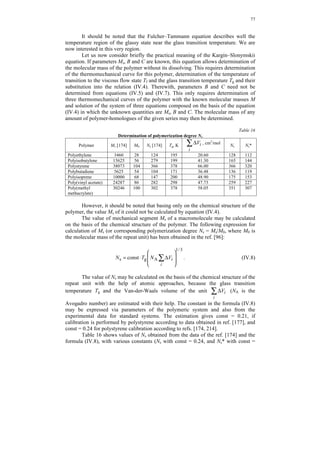
It should be noted that the Fulcher–Tammann equation describes well the
temperature region of the glassy state near the glass transition temperature. We are
now interested in this very region.
Let us now consider briefly the practical meaning of the Kargin–Slonymskii
equation. If parameters Ms, B and C are known, this equation allows determination of
the molecular mass of the polymer without its dissolving. This requires determination
of the thermomechanical curve for this polymer, determination of the temperature of
transition to the viscous flow state Tf and the glass transition temperature Tg and their
substitution into the relation (IV.4). Therewith, parameters B and C need not be
determined from equations (IV.5) and (IV.7). This only requires determination of
three thermomechanical curves of the polymer with the known molecular masses M
and solution of the system of three equations composed on the basis of the equation
(IV.4) in which the unknown quantities are Ms, B and C. The molecular mass of any
amount of polymer-homologues of the given series may then be determined.
Table 16
Determination of polymerization degree Ns
Polymer Ms [174] M0 Ns [174] Tg, K ΣΔ
i
Vi , cm3/mol Ns Ns*
Polyethylene 3460 28 124 195 20.60 128 112
Polyisobutylene 15625 56 279 199 41.30 165 144
Polystyrene 38073 104 366 378 66.00 366 320
Polybutadiene 5625 54 104 171 36.48 136 119
Polyisoprene 10000 68 147 200 48.90 175 153
Poly(vinyl acetate) 24287 86 282 298 47.73 259 227
Poly(methyl
30246 100 302 378 58.05 351 307
methacrylate)
However, it should be noted that basing only on the chemical structure of the
polymer, the value Ms of it could not be calculated by equation (IV.4).
The value of mechanical segment Ms of a macromolecule may be calculated
on the basis of the chemical structure of the polymer. The following expression for
calculation of Ms (or corresponding polymerization degree Ns = Ms/M0, where M0 is
the molecular mass of the repeat unit) has been obtained in the ref. [96]:
1/ 3
Δ ⋅ = Σi
s const g A
N T N Vi . (IV.8)
The value of Ns may be calculated on the basis of the chemical structure of the
repeat unit with the help of atomic approaches, because the glass transition
temperature Tg and the Van-der-Waals volume of the unit ΣΔ
i
Vi (NA is the
Avogadro number) are estimated with their help. The constant in the formula (IV.8)
may be expressed via parameters of the polymeric system and also from the
experimental data for standard systems. The estimation gives const = 0.21, if
calibration is performed by polystyrene according to data obtained in ref. [177], and
const = 0.24 for polystyrene calibration according to refs. [174, 214].
Table 16 shows values of Ns obtained from the data of the ref. [174] and the
formula (IV.8), with various constants (Ns with const = 0.24, and Ns* with const =](https://image.slidesharecdn.com/computationalmaterialsscienceofpolymers-141021180636-conversion-gate02/85/Computational-materials-science-of-polymers-85-320.jpg)
![78
0.21). If const = 0.21 the difference in the values obtained from the ref. [174] does not
exceed 10%.
So far, we have discussed such physical characteristics of polymers as the
glass transition temperature, the temperature of transition to the viscous flow state, the
value of the macromolecule segment, which were determined experimentally with the
help of the thermomechanical method of polymer investigation.
Definite difficulties are met when determining temperature ranges of the solid
(glassy), rubbery and viscous flow states of polymers by this method. This especially
concerns new polymers.
Let us consider generally the possible deformation behavior of polymers in
thermomechanical tests. Recall that under these conditions the sample is loaded at
increasing temperature. In most cases, the stress acts permanently during the
experiment and temperature grows linearly.
Fundamentally, the thermomechanical method of investigation allows
immediate determination of temperature ranges of all three physical states of the
polymer. However, the existence of one or another physical state and appropriate
temperature range may be determined reliably only if it is known that the polymer
studied behaves itself as a ‘classic’ one, i.e. gives the classic thermomechanical curve
depicted in Figure 18. As it is observed in the considerations below, even if the form
of the thermomechanical curve coincides with the classic one, in estimation of the
properties of a new polymer it is not yet possible to determine unambiguously the
temperature ranges of physical states and even of the states themselves.
Before we consider this point, let us discuss some procedural questions. A
question which appears most often is about the method of determination of transition
points from the thermomechanical curve. As mentioned above, the following method
is suitable: a definite strain ε0 is chosen, plotted from the temperature axis and from
the rubbery plateau. The glass transition temperature and the temperature of transition
to the viscous flow state will correspond to temperatures, at which one and the same
value ε0 of rubbery and plastic strain occur, respectively.
This method is most correct but suitable only when the thermodynamic curve
is of the classic form with abrupt bends of the curves in transition temperature ranges.
Then, the change of ε0 will not cause large shifts in determination of Tg and Tf. If
deformation develops more smoothly, then the adjusted transition points Tg and Tf
will be quite undefined. They will be sufficiently dependent on the value of ε0 (Figure
22).
That is why another method is used in practice: values of Tg and Tf are
determined by cross-points of tangents to two correspondent branches of the
thermomechanical curve (Figure 23). In this case, values of Tg and Tf are less
dependent on the shape of the thermodynamic curve, and this method is warranted for
comparative estimation of polymers.
Comparing thermomechanical curves of a series of polymers, the glass
transition point may be defined as the temperature at which deformation is developed
by the value of a specific percentage of the rubbery plateau height. Then, for each
polymer this typical deformation will display different values, because heights of the
rubbery plateau are also different.
Selection of the determination method of Tg and Tf depends on the shape of the
thermomechanical curve of polymers, and any of these methods may be chosen under
comparative estimation of their properties. Of importance is just the comparison of
several polymers to be performed always by the same method.](https://image.slidesharecdn.com/computationalmaterialsscienceofpolymers-141021180636-conversion-gate02/85/Computational-materials-science-of-polymers-86-320.jpg)


![86
measured. Schematically, this dependence is depicted in Figure 13. This dependence
as a broken line is typical of many polymers near the glass transition temperature. At
temperatures below the glass transition temperature, this dependence is more
flattened, than at temperatures above it. This is the main reason observed at the glass
transition temperature (see Figure 13). Obviously, dilatometric dependences may be
obtained at different rates of heating (or cooling) of the sample. Consequently, if the
heating rate is changed in a quite wide range, the dilatometric dependences change in
the manner depicted in Figure 13. The higher the rate of the sample heating, the
higher is temperature at which the bending is observed and, vice versa, the lower the
heating rate, the lower is temperature of the bending and the specific volume of the
sample in the bending point decreases. Hence, the glass transition temperature
depends on the rate of heating or cooling of the sample, which is associated with the
relaxation mechanism of the glass transition (see below).
It should be noted that changing the heating or cooling rate causes has a
smaller effect on the type of dilatometric curve and on the glass transition temperature
than the effect of mechanical tension on the type of the thermomechanical curve and
the glass transition temperature. To cause a significant change of the glass transition
temperature in the first case, the heating or cooling rate must be changed by many
decimal degrees, which is impossible to do in an experiment. At the same time, ten- or
hundred-fold change of the heating rate changes the glass transition temperature by
several degrees only. Meanwhile, the change of the mechanical tension by several
percents only may cause a sharp increase or abrupt decrease of the glass transition
temperature. A special role in this case is played by the rate of mechanical influence.
Analysis of these experimental facts enabled G.M. Bartenev [53] to apply the
viewpoint that mechanical and structural glass transitions must differ. By the
structural glass transition one means transition from the glassy state to the rubbery
state (and the reverse process) in the absence of mechanical tension. This transition
and its temperature are associated only with the heating and cooling rate. Mechanical
glass transition is associated with the rapid mechanical influence on the polymer and
its behavior as a solid under the rapid action of the mechanical force. As temperature
changes, the mechanical glass transition may occur at rather lower temperatures than
the structural glass transition.
Figure 33. Temperature dependence of heat capacity Cp (scheme).
In addition to the dilatometric method of determination of the glass transition
temperature, other methods are also widely used, for example, calorimetric one. In
this case, heat capacity Cp of the polymeric substance is measured, the dependence of
Cp on T is of the typical shape (Figure 33). In the area of the glassy state, heat](https://image.slidesharecdn.com/computationalmaterialsscienceofpolymers-141021180636-conversion-gate02/85/Computational-materials-science-of-polymers-94-320.jpg)
![87
capacity grows slowly with temperature, but when Tg is reached, a sharp increase of
the heat capacity is observed. When the transitional zone is passed, the heat capacity
again increases only slowly with temperature.
Apparently, dynamic mechanical analysis is used most widely. In this method,
the temperature dependences of the storage modulus E′ and the loss modulus E′′ of
the complex elasticity modulus E* = E′ + iE′′ change, as well as the loss-factor tgδE =
E′′/E′ (Figure 34). The temperature dependence of tgδE displays several maxima, with
the most intensive (and high-temperature) one associated with transition from the
glassy state to the rubbery state.
Figure 34. Temperature dependence of the mechanical loss-factor tgδE (scheme).
The temperature dependence of the dielectric loss-factor tgδε = ε′′⁄ε′, where ε′′
and ε′ are the true and the imaginary parts of the complex dielectric constant ε* = ε′ +
iε′′, looks the same (Figure 35).
Figure 35. Temperature dependence of the dielectric loss factor tgδε (scheme).
Finally, the glass transition temperature may be determined from a sharp
increase of the diffusion coefficient. Neglecting discussion of these methods of
experimental determination of Tg, let us guide the reader to special literature [5, 51,
124].](https://image.slidesharecdn.com/computationalmaterialsscienceofpolymers-141021180636-conversion-gate02/85/Computational-materials-science-of-polymers-95-320.jpg)


![91
time (time of transition) becomes extremely long, and the polymeric substance begins
to behave as a glassy solid.
This transition theory was subsequently mathematically justified by M.V.
Volkenstein and O.B. Ptitsyn, who had performed mathematical analysis of the
relaxation transition from the rubbery state to the glassy state and back, and had
adjusted conditions under which such transitions may be performed. According to this
theory
U U
1
tr,0 tr + tr
=
ln lg
RT q
RT
g
2
g
τ
, (IV.14)
where q is the rate of system cooling.
Equation (IV.14) shows that the glass transition temperature depends on the
rate of polymer cooling.
In its initial form, the Volkenstein–Ptitsyn theory does not consider the
cooperative character of thermal motion of kinetic units. As shown subsequently, such
calculation is absolutely necessary, because due to large length and flexibility of
macromolecules the local motion of any kinetic unit touches upon its neighbors. For
example, motion in the frames of a single repeat unit of a macromolecule causes
motion of the neighbor units and this is the reason for segmental mobility. Calculation
of the cooperative ability of motion of kinetic units of various sizes, performed by
Ptitsyn and Sharonov, caused refinement of the Volkenstein–Ptitsyn theory and
allowed reasonable values of the activation energy of the relaxation process to be
determined.
Figure 38. Schematic representation of thermomechanical (a) and dilatometric (b) curves in the zone
of transition from the glassy state to the rubbery state (see text) .
Analysis of a polymeric substance with the help of a non-linear model [87, 89]
shows [90] that transition from the glassy state to the rubbery state must proceed not
in a point but in some interval of temperatures which depends on the rate of heating or
cooling q. Schematically, this is shown in Figure 38, which depicts thermomechanical
and dilatometric curves in the transition area. Here Tg,1 is the temperature, at which
transition from the rubbery state to the glassy state begins at system cooling; Tg,2 is
the temperature at which this transition ends.
The results obtained in work [90] indicate that at low rates of cooling the glass
transition temperature range degenerates and the glass transition temperature only
remains. In the general case of analysis of polymer behavior in the area of T Tg,1, a
significant role is played by the cooling rate. If the cooling rate is high, temperatures](https://image.slidesharecdn.com/computationalmaterialsscienceofpolymers-141021180636-conversion-gate02/85/Computational-materials-science-of-polymers-99-320.jpg)
![92
Tg,1 and Tg,2 differ significantly, i.e. transition to the glassy state proceeds in a wide
temperature range.
In practice, the glass transition temperature range is really broadened as the
rate of cooling (or heating) increases, not in a jump-like manner, but quite smoothly.
Therewith, the temperature dependence of deformation in the transition zone becomes
more abrupt as the rate of cooling (or heating) decreases. This is clear from Figure 39,
which indicates thermomechanical curves for a series of cured compounds based on
epoxy oligomers. In accordance with the theoretical results obtained, the glass
transition temperature range windes as the heating rate increases (Figure 40).
Figure 39. Thermomechanical curves of cured epoxy compound measured under conditions of
compression. Rate of heating 0.62 (1), 1.07 (2), 2.39 (3), 4.61 (4), 6.39 (5), 9.44 (6), and
15.47 (7) deg/min. Composition of specimen: ED-20 – 1 mole, MTHPA – 0.6 mole,
azelaic acid – 0.7 mole.
Figure 40. Dependence of temperature differences ΔT = Tg,1 – Tg,2 on heating rate q: (a) correlates with
the same composition as in Figure 39; (b) corresponds to the composition of specimen: ED-
20 – 1 mole, MTHPA – 1.3 mole, oleic acid – 0.7 mole.
The nonlinear model of polymeric substances [87,89] was also used for
estimating the activation energy of γ-transition in polymers.
Estimation of many properties of polymers requires the values of the
activation energies associated with various transitions in polymeric systems. If a
polymer is considered as a linear system, then it will be a selection of activation
energies, usually associated with the motion of a definite group of atoms in a chain.
But if it is considered as a non-linear system, described by a model suggested in ref.
[87] (Figure A-6-8), we must know the activation energy of elementary acts only,
associated, for example, with a jump of atoms from one equilibrium state to another in
a rotary isomer, and which is usually associated with the activation energy of the γ-
transition. All other relaxation times stipulated by other transitions are expressed via
the desired activation energy and temperature coefficients determined by non-linear](https://image.slidesharecdn.com/computationalmaterialsscienceofpolymers-141021180636-conversion-gate02/85/Computational-materials-science-of-polymers-100-320.jpg)
![93
model parameters [269]. Hence, a temperature dependence of activation energy in the
area of α-transition may be obtained, and the Williams–Landel–Ferry formula may be
deduced, etc.
To use actively this model for calculations of particular polymeric systems, the
relation of the parameters of the model with the chemical structure of the repeat unit
must be known.
Let us demonstrate how expressions for determining activation energy which
participate in the temperature dependences of relaxation times (viscosity) may be
deduced from correlations of the ref. [269]. It is shown below that the activation
energy is linked by simple dependences with the glass transition temperature and,
therefore, it may be calculated on the basis of the chemical structure of the repeat unit.
Let us consider expressions for relaxation times τ3 and τ5 of a non-linear
model, shown in ref. [269], in the range of temperature of the onset Tg,2 and
termination Tg,1 of glass transition. With this aim in view, let us perform series
expansion of τ2/τ5 and τ2/τ3 in relation to Tg,1 and Tg,2, respectively, and confine to
terms of the smallness order one by T – Tg,1 and T – Tg,2. Then,
τ ,
( g,1 )
τ
2
5
2
5
− ⋅
g,1
T T
≈ d
⋅
dT
T T
= τ
τ
because
τ 0
and 0
2 =
T =T τ
g,1
5
τ ,
2 =
T =T τ
g,2
3
where τ2 is the relaxation time of one of elements of the model, which may be
expressed by the Arrhenius–Eiring formula.
The expressions τ2/τ5 and τ2/τ3 may be expressed via variable δ0, respectively,
as follows:
τ ,
( )g,1
δ
0
τ
2
5
2
≈ d
⋅
5 0
d
⋅ −
g,1 g,1
T T
dT
d
T T T T
= =
τ
τ δ
τ .
( )g,2
δ
0
τ
2
3
2
3
d
⋅ −
g,2 g,2
T T
dT
≈ d
⋅
dT
T T T T
= =
τ
τ
As according to ref. [269], values
τ
0 T T
g,1
2
5
d
d
=
⋅
τ
δ
and
τ
0 T T
g,2
2
3
d
d
=
⋅
τ
δ
are of
the same order of magnitude, future consideration will take into account only the
expressions τ2/τd
5, and Tg will be taken for Tg,1. Let determine ( δ ) 0
dT
at Tg,1. As
according to ref. [269],](https://image.slidesharecdn.com/computationalmaterialsscienceofpolymers-141021180636-conversion-gate02/85/Computational-materials-science-of-polymers-101-320.jpg)
![94
1
δ K 1
, 1
3
= 16
1
− ⋅
0 21
−
K
K = f e−Y , 3
1 1
K = f e−Y ,
3 3
( ) 1,3 g1,3 Y =1− 2 1−T T ,
then
K T Y T Y
1 1
−
− ⋅
1 1
−
d δ δ
2 1
0
16
= ⋅
3 g 3 g 1
0
1
1
21
3 1
K
dT
.
The relation
T T K
g,1
1
3
K
=
= 57/32, δ0 = –2.8 [269]. K1 value corresponds to the
elasticity of a chemical bond, and K3 – to the elasticity modulus of an intermolecular
bond, that is why Tg,1 = Td (to the temperature of onset of intense thermal
degradation), Tg,3 = Tm (to the melting point). Then,
7.6 1
dT T T
m g,1
T T
d g,1
−
−
−
=
=
d
m
m
0
1
1
1
g,1
T
T
T
d
T T
δ
.
τ
2
d
From ref. [269] 0.3
g,1
5
0
− ≈
⋅
T =T
d
τ
δ
may be found. Taking into account the
expression
d 0 δ
dT
and the value
τ
0 T T
g,1
2
5
d
d
=
⋅
τ
δ
, the dependence τ2/τ5 on temperature
in the area of Tg (suggesting Tg = Tg,1) may be presented as follows:
( )g
T T
d g
d
m
2.3 1
T T
τ
5 m g
m
2
1
1
1
T T
T
T
T
−
−
− ⋅
−
≈ −
τ
. (IV.15)
The expression obtained, according to ref. [269], describes the transition to the
glassy state. It may be displayed that the Bachinski formula is also reduced to an
analogous form. Actually, to describe the viscosity of liquids η, Bachinski [768] has
suggested an empirical formula:
ω
η
−
=
v
C
. (IV.16)](https://image.slidesharecdn.com/computationalmaterialsscienceofpolymers-141021180636-conversion-gate02/85/Computational-materials-science-of-polymers-102-320.jpg)
![95
Here v is the specific volume of the liquid; ω is the molecular ‘limited’ volume of the
liquid (according to Bachinski, =Σ
Mω ε i , where εi are constants of atoms forming
i
the molecule; M is the molecular mass), C is the constant. The expression (IV.16)
describes well the liquid viscosity in a wide range of temperatures and pressures, the
constant C may be found from the Camerling–Ownnes theory of similarity of
molecular systems. Bachinski has shown [768] that for many liquids the following
correlation is fulfilled:
1/ 6
CM
1/ 2 1/ 3
g
T ω
= 0.531⋅10–4, (IV.17)
Thus, the accuracy of determination of C depending on the chemical structure is
±6.2%.
Let us transform the expression (IV.16). For this purpose, let us consider the
temperature dependence of the specific volume, which may be presented in the
following form:
v = ω[1 + αv(T – Tg)], (IV.18)
where αv is the coefficient of volumetric expansion which, according to ref. [269] in
the case of the potential ‘6 – 12’, is equal to 1/42Tg. With regard to equation (IV.16),
correlation (IV.18) has the following form:
T −T
=
η
0 g
42T
g
η
, (IV.19)
where η0 = C/ω. Expression (IV.19) will be analogous to equation (IV.15) obtained
from the non-linear model, therewith, η0 = η2 = K1τ2, and η = K1τ5. But contrary to
the Bachinski formula deduced for transition from liquid to glass, the desired
expression describes the transition from the side of low temperatures (transition from
the glassy state to the rubbery state). That is why
0
T T
d g
d
m
T T
m g
m
g
2 42
1
1
1
1
η 2.3 η
−
− ⋅
−
=
T
T
T
T
. (IV.20)
From equation (IV.20) the expression for the activation energy may be
deduced. Let us estimate the following value for the real polymeric systems:
42
T T
d g
1
1
T T
m g
1
1
2.3
d
m
m
g
−
− ⋅
−
=
T
T
T
T
A . (IV.21)](https://image.slidesharecdn.com/computationalmaterialsscienceofpolymers-141021180636-conversion-gate02/85/Computational-materials-science-of-polymers-103-320.jpg)
![96
Shown in the Table are initial data (glass transition temperatures Tg, melting
points Tm, temperatures of the onset of intense thermal degradation Td), and results of
calculation of values A for a series of polymers. Values of Tg, Tm and Td are usually
taken from experimental data but, in some cases, when, for example, a polymer is not
crystallized or when its melting point lies above the temperature of onset of intense
thermal degradation and thus may not be measured experimentally, they are
calculated by the expressions shown below.
Calculation results indicate (Table 17′) that the value A falls within the range
from 24 to 82. In some cases, it becomes negative. It is typical of polymers, for which
temperature of the onset of intense thermal degradation lies near the glass transition
temperature, or the melting point and the glass transition temperature are close, i.e. for
heat-resistant polymers. As obvious, coefficients A calculated for the most of
polymers are positive that, according to equation (IV.20), correspond to positive
values of viscosity. Similar to a non-linear model of polymeric body, in which
viscosity is associated with relaxation mechanisms, according to the Mandelshtamm–
Leontovich theory, the viscosity in our expressions will be the second one, because
the non-linear model suggested [269] describes behavior of a polymeric substance by
a selection of kinetic equations. However, as the Table indicates, for some polymers
A 0. The latter means that the second viscosity of these polymers is negative. The
result obtained has a physical meaning and, as follows from ref. [768], is associated
with nonequilibrium of the medium in the range of the glass transition temperature.
This result must be analyzed in more detail.
= ⋅ Δ
*
η h E
expression (IV.20) may
With regard to η0 = C/ω and
g
2 2 exp
kT
Nl q
be presented in the form:
E *
2
Δ = ⋅
AC
ω
Nl q
h
kT
g
ln , (IV.22)
where N is the number units in the macromolecule; l is the unit size; q = exp(ΔE/kT);
ΔE* is the difference in the energies of rotary isomers.](https://image.slidesharecdn.com/computationalmaterialsscienceofpolymers-141021180636-conversion-gate02/85/Computational-materials-science-of-polymers-104-320.jpg)


![101
Considering a polymer in the glassy state as a frozen liquid and using data of
the Camerling–Ownnes theory of molecular similarity, as Bachinski has done, the
expression for C may be presented in the following form in analog to formula (IV.17):
b
CM = − 10 1/ 2 1/3
g
T
1/ 6
ω
.
Here b is the exponent value which, in the case of polymeric systems, is somewhat
dependent on chemical structure and will be found during comparison with particular
characteristics of polymers. Because
r.u.
Δ Σi
~
ω N Vi , where
r.u.
Δ Σi
Vi is the
Van-der-Walls volume of the repeating unit,
1/3
Δ Σi
~
l Vi and
C = 10 −b Tg 1/ 2 ω 1/ 3 M 1/ 6
,
*
Δ = − +
1/ 2 1/ 6
g
AT M
1/3
r.u.
E
g
2.3 27 ln
M
b
kT
. (IV.23)
If for real polymer systems logarithm is taken from Tg, M, and Mr.u., average
by polymeric systems, it is observed that fluctuations stipulated by the difference of
parameters Tg, M, and Mr.u. for particular polymeric system from average ones, give a
low error ( 10%) for determination of the activation energy ΔE* of this system. In
turn, the logarithm from average values of parameters by polymeric systems is taken
into account via constant b. That is why, expression (IV.23) may be reduced to the
form:
ΔE* = 2.3(27 – b)kTg.
In accordance with the experimental data from refs. [214], the value of b may be
estimated, which is equal to 15.7. Respectively,
ΔE* ≅ 26kTg. (IV.24)
Shown below are some calculated ( * )
ΔEcalc and experimental ( ) *
ΔEexper values
of the activation energy for a series of polymers according to the data from refs.
[214].
Polymer PEO PCTFE PE PVA Butyl
rubber
Tg, K 206 323 213 303 200
*
ΔEcalc ,
kJ/mol
44.8 70.3 46.0 65.8 45.6
*
ΔEexper ,
kJ/mol
37.7 72.7 50.3 60.8 49.9](https://image.slidesharecdn.com/computationalmaterialsscienceofpolymers-141021180636-conversion-gate02/85/Computational-materials-science-of-polymers-109-320.jpg)
![102
Deviations between *
ΔEcalc and *
ΔEexper observed do not exceed ~15%.
Considering jumps of atoms or groups of atoms along the chain in rotary
H
isomers as *diffusion of these atoms in polymer, the ratio ΔE*/d2 may be determined
by data from ref. [214] (p. 298, Figure XVIII.7), where d is the size of the groups of
atoms diffusing. But ΔE* is deduced from expression (IV.23), from which the size d
of the jumping group of atoms may be determined immediately. For example, in the
case of PS, ΔE*/d2 = 600, Tg = 378 K, ΔE* = 82.2 kJ/mol, and d = 5.7 Å that
corresponds to the group C6H5. However, jumps of a group of hydrogen atoms are
possible in PS. If sizes of these atoms are known, the activation energy may be
deduced from the expression ΔE*/d2. It is equal ΔE = 19.7 kJ/mol. From expression
(IV.24) the temperature of transition of this group of atoms Tg,1 may be estimated. If
calculated, Cg,1 = 91 K, which by the order of magnitude corresponds to the
temperature of δ-transition in PS (accurate coincidence is out of the question, because
the constant in expression (IV.24) is found for the γ-transition). Estimations
performed allows a supposition that if the repeating unit of polymer possesses side
(asymmetric) groups of atoms different by size, a δ-transition appears in such a
polymer.
Discussed above is one of the concepts of the polymeric substance transition
from the glassy state to the rubbery state and back. This concept is based on
assumption of the relaxation mechanism of transition, the time of this transition (the
relaxation time) depending on temperature and being determined by the energetic
barrier height to be overcome in order to provide with the transition. Since different
macromolecules possess different flexibility or rigidity, they are characterize by
different heights of the energetic barrier and, consequently, by different glass
transition temperatures. The more flexible the macromolecule is, the lower the height
of the energetic barrier is which characterizes the system composed of such
macromolecules.
The concept of the polymeric substance transition from the glassy state to the
rubbery state and back, based on the relaxation mechanism of transitions, is not
unique. Another concept that explains these transitions is the concept by S.N.
Zhurkov, based on acceptance of a significant role of intermolecular bonds in
polymers. Let us discuss this concept.
Every polymeric macromolecule possesses polar groups, which display
various energies of interaction with each other. They form bonds which are not
chemical, but are of the physical nature and are called intermolecular bonds. Such
bonds may be rather weak as, for example, in polyisobutylene, polypropylene,
polyethylene, and in other analogous polymers, but they may also be very strong as
for example, in polyamides, polyesters, etc. In the former case, it is spoken about
weak Van-der-Waals bonds, the energy of which is very low. In the latter case, strong
hydrogen bonds which appear due to existence of amide NH C
groups (poly-amides),
O
and strong dipole–dipole interaction which appear due to existence of ester
groups are considered. Intermolecular bonds may be stipulated by an
O
C O
existence of not only these polar groups, but also of other groups capable of strong
≡N groups (for example,
-groups (for example, in poly(vinyl alcohol), and
many others. Polar groups in neighboring macromolecules under definite conditions
may interact with each other forming cross-linked bridges between them, which are](https://image.slidesharecdn.com/computationalmaterialsscienceofpolymers-141021180636-conversion-gate02/85/Computational-materials-science-of-polymers-110-320.jpg)


![108
Besides the Zhurkov rule of plasticization, discussed above in detail, there are
many other rules. For example, because viscosity of low-molecular fluids–plasticizers
in by many decimal degrees smaller than viscosity of polymer, it is assumed that
equal volumes of the fluid may equally decrease the glass transition temperature of
the polymer:
ΔT = æ
v
+
V v
, (IV.38)
where V is the polymer volume; v is the plasticizer volume; æ is the coefficient equal
for all fluids.
Equation (IV.38) reflects the Kargin–Malinskii rule of volumetric parts. It
operates better for weak polar polymers, whereas the Zhurkov rule is more valuable
for strong polar polymers. The cases are often, when both rules are unable to describe
behavior of real polymeric systems. Let us dwell in more detail on this point below.
IV.3. Calculation of the glass transition temperature of linear polymers
This section discusses the calculation scheme for estimation of the glass
transition temperature Tg developed in works [6, 128]. According to this scheme, the
coefficients of molecular packing for polymers of various chemical structures are
approximately equal at the glass transition temperature of each of polymers, this value
kg being estimated by the value kg ≈ 0.667 for linear polymers. The coefficient of
molecular packing k0 near the absolute zero is also approximately equal for all
polymers and is 0.731.
These measurements indicate that the transition from the glassy state to the
rubbery state proceeds, when a definite part of empty volume is reached, equal fE =
1 – kg = 0.333, and expression for the glass transition temperature may be presented in
the following form:
0 g
=
−
G G
g
1 0.0906
α α
=
k k
T . (IV.39)
It should be noted that the material discussed in the present Chapter is tightly
connected with the material discussed in Chapter III. Using expressions for αG
deduced in Chapter III, it must be written down that
1
R
= , (IV.40)
0.455
1
ZD
T
g 0
Σ
where Σ
Δ
Δ
=
i
i
i
i
i i
V
V
Z D
ZD
0
0
1
1
; Z is the coordination number of the i-th atom; D0i is
the bond energy of the i-th atom with neighboring ones; ΔVi is the Van-der-Waals
volume increment of the i-th atom.](https://image.slidesharecdn.com/computationalmaterialsscienceofpolymers-141021180636-conversion-gate02/85/Computational-materials-science-of-polymers-117-320.jpg)
![109
Numerical values of 1/ZiD0i, typical of every atom and every type of
intermolecular interaction, were determined with the help of statistical treatment of
experimental data by the method of least squares. As mentioned above, the values of
bond energies obtained as a result of processing of the experimental data correspond
to energies of the intermolecular interaction. Presence of polar groups in polymers,
which causes strong intermolecular interaction, is taken into account by introduction
of special constants.
For practical calculations, it is advisable to rewrite the formula (IV.40) in the
following form:
Σ
Δ
i
Δ +
V
Tg , (IV.41)
Σ Σ
=
j
j
i
i i
i
a V b
where ai is a selection of constants, which characterizes energy of a weak dispersion
interaction as the averaged contribution of each atom into this interaction; bj is a
selection of constants, which characterizes energy of a strong specific intermolecular
interaction (dipole–dipole, hydrogen bonds, etc.).
Values ai and bj are associated with parameters αi by the following relations:
i i
= ; (IV.42)
i k k
0 / g 1 0.0906
a
α = α
−
j j
= . (IV.43)
j k k
0 / g 1 0.0906
b
β β
=
−
Using the relation (IV.41), the glass transition temperature of a tremendous
number of polymers may be calculated. This is associated with the circumstance that
the approach described is ‘atomistic’, i.e. each atom is characterized by its constant ai
(their values are shown in Table 13). As for specific intermolecular interactions
(dipole–dipole, hydrogen bonds), they are characterized by their constants bj,
independent of chemical structure of the polar group. For example, dipole–dipole
interactions of various types are characterized by the same constant bd = –55 ⋅ 10–3
Å3 K–1. The situation with hydrogen bonds in polyamides is somewhat more
complicated. This is connected with specificity of their influence on Tg in the frames
of the present class of polymers (Table 18)*.
As an example, Table 19 indicates experimental and calculated values of glass
transition temperatures for a series of model polymers, starting with polymers of a
simple chemical structure to quite complicated systems. Selections of parameters of
the relation (IV.41) are also present there.
The approach developed [6, 128] and the relation (IV.41) obtained on its basis
allow taking into account the influence of the type of unit attachment to the polymers
chain on the glass transition temperature of it. If attachment is usual (‘head-to-tail), as
* Clearly, such approach displays advantages before popular calculation method, based on group
contributions [214]. If a polymer possesses a group, which contribution into the glass transition
temperature is unknown, the calculation becomes impossible. In the same approach discussed,
contribution of any group is simply composed of the contributions of atoms composing it plus the
contribution of specific interactions, if these groups are polar.](https://image.slidesharecdn.com/computationalmaterialsscienceofpolymers-141021180636-conversion-gate02/85/Computational-materials-science-of-polymers-118-320.jpg)


![Table 19′
Experimental and calculated values of the glass transition temperature, Tg, for the broaden list of polymers, presented in the alphabetic order
No. Polymer
ΣΔ
i
Vi ,
Å3
( Σi
ai Δ Vi
+ + Σ
j
bj )⋅103
, Å3K–1
Tg, K
(exp.)
Tg, K
(calc)
References
1. Cyanoethyl cellulose 132(0 gr)
188(1 gr)
483 (1 gr);
244 (0 gr)
453 389 (1
gr); 541
(0 gr)
326
CH2
CH
CH
2. Ethyl cellulose 204(2 gr)
168(1 gr)
654 (2 gr);
449 (1 gr)
316 312 (2
gr); 374
(1 gr)
275, 327
CH2
CH
CH
CH
O
O
CH2
CH
CH
CH3
CH2 O
CH3
O
O
CH2
CH3
3. Methyl cellulose 151(1 gr)
170(2 gr)
370 (1 gr);
496 (2 gr)
423 343 (2
gr); 408
(1 gr)
326
CH2
CH
CH
CH
O
O
CH3
CH
CH
O
O
O
CH3
CH3
4. Nylon 8,6 [Poly(iminoadipoyliminooctamethylene)] 266 811 318 328 472
NH )4
C (CH2
O
C NH (CH2
)8
O
CH
CH
O
CH
O
O
OH
CH2
OH
CH2 C N
117](https://image.slidesharecdn.com/computationalmaterialsscienceofpolymers-141021180636-conversion-gate02/85/Computational-materials-science-of-polymers-129-320.jpg)
![1 2 3 4 5 6 7
5. Nylon 10 [Poly(imino-1-oxodecamethylene)] 184 580 315 317 480
NH C (CH2)9
O
6. Nylon 10,10 [Poly(iminosebacoyliminodecamethylene)] 368 1161 333, 319 317 472, 473
NH C (CH2)8 C
O
7. Nylon 10,12 [Poly(iminodecamethyleneiminododecanedioyl)] 402 1280 322 314 477
NH (CH2)10 NH C (CH2)10 C
O O
8. Nylon 10,6 [Poly(iminoadipoyliminodecamethylene)] 300 929 313 323 472
9. Nylon 11 [Poly(imino-1-oxoundecamethylene)] 201 640 315, 316,
365, 333 -
343
314 480, 668,
681, 716
NH C (CH2)10
O
10. Nylon 12 [Poly(imino-1-oxododecamethylene)] 218 699 313 - 316,
314
312 284, 475,
480, 679
NH C (CH2)11
O
11. Nylon 12,18 [Poly(iminododecamethyleneiminooctadecanedioyl)] 539 1750 323 308 477
NH (CH2)12 NH C (CH2)16
C
O
O
12. Nylon 13 [Poly(imino-1-oxotridecamethylene)] 235 756 314 311 480
NH C (CH2)12
O
NH
O
(CH2)10
NH C (CH2)4 C
O
NH
O
(CH2)10
118](https://image.slidesharecdn.com/computationalmaterialsscienceofpolymers-141021180636-conversion-gate02/85/Computational-materials-science-of-polymers-130-320.jpg)
![1 2 3 4 5 6 7
13. Nylon 14,18 [Poly(iminotetradecamethyleneiminooctadecanedioyl)] 573 1866 321 307 477
NH (CH2)14 NH C (CH2)16
C
O
O
14. Nylon 18,18 [Poly(iminooctadecanedioyliminooctadecamethylene)] 641 2102 323 305 477, 478
NH (CH2)18 NH C (CH2)16
C
O
O
15. Nylon 3 [Poly(imino-1-oxotrimethylene)] 64.7 170 384 380 469
NH )2
16. Nylon 4,6 [Poly(iminotetramethyleneiminoadipoyl)] 198 577 316 343 470
NH (CH2)4 NH C (C)4
H2
C
O
O
17. Nylon 5,6 [Poly(iminopentamethyleneiminoadipoyl)] 215 634 318 339 471, 472
NH (CH2)5 NH C (C)4
H2
C
O
O
18. Nylon 6,10 [Poly(iminohexamethyleneiminocebacoyl)] 300 929 323 323 284, 317,
320, 325
NH (CH2)6 NH C (C)8
H2
C
O
O
19. Nylon 6,12 [Poly(iminohexamethyleneiminododecanedioyl)] 334 1044 319 320 473, 477,
478
NH (CH2)6 NH C (C)H2
10
C
O
O
20. Nylon 6,7 [Poly(iminohexamethyleneiminopimeloyl)] 249 752 331 331 464, 473
NH (CH2)6 NH C (C)5
H2
C
O
O
C (CH2
O
119](https://image.slidesharecdn.com/computationalmaterialsscienceofpolymers-141021180636-conversion-gate02/85/Computational-materials-science-of-polymers-131-320.jpg)
![1 2 3 4 5 6 7
21. Nylon 6,8 [Poly(iminohexamethyleneiminosuberoyl)] 266 811 330 328 473
NH (CH2)6 NH C (C)6
H2
C
O
O
22. Nylon 6,9 [Poly(iminohexamethyleneiminoazelaoyl)] 283 868 331 326 476
NH (CH2)6 NH C (C)7
H2
C
O
O
23. Nylon 7 [Poly(imino-1-oxoheptamethylene)] 133 405 325 328 325, 473,
479, 480
NH )6
C (CH2
O
24. Nylon 7,6 [Poly(iminoadipoyliminoheptamethylene)] 249 752 318, 333 331 365, 464,
472, 473
NH )4
C (CH2
O
C NH (CH2
)7
O
25. Nylon 7,7 [Poly(iminopimeloyliminoheptamethylene)] 266 811 328 328 473
NH )5
C (CH2
O
C NH (CH2
)7
O
26. Nylon 8 [Poly(imino-1-oxooctamethylene)] 150 464 323 323 480, 680
NH )7
C (CH2
O
27. Nylon 8,10 [Poly(iminooctamethyleneiminodecanedioyl)] 334 1044 333 320 472
NH (CH2)8 NH C (C)8
H2
C
O
O
28. Nylon 8,12 [Poly(iminooctamethyleneiminododecanedioyl)] 368 1161 323 317 477
NH (CH2)8 NH C (CH2)10 C
O O
120](https://image.slidesharecdn.com/computationalmaterialsscienceofpolymers-141021180636-conversion-gate02/85/Computational-materials-science-of-polymers-132-320.jpg)
![1 2 3 4 5 6 7
29. Nylon 8,22 [Poly(iminooctamethyleneiminodocosanedioyl)] 539 1750 321 308 477
NH (CH2)8 NH C (CH2)20 C
O O
30. Nylon 9 [Poly(imino-1-oxononamethylene)] 167 522 319 320 473, 479,
480
NH C (CH2)8
O
31. Nylon 9,6 [Poly(iminoadipoyliminononamethylene)] 283 868 318 326 471
NH C (CH2)4 C
O
NH
O
(CH2)9
32. Poly(1,1,1-trifluoro-isopropyl methacrylate) 146 394 354
Vicat
softening
tempera-ture
371 589
CH3
C
C O CH
CH3
O
CF3
CH2
33. Poly(1,1,5-trihydrooctafluoroallyl-2-cyanoacrylate) 209 641 353 326 733
C
C
N
CO O
CH2
CH2
(CF2)3 CF2H
34. Poly(1,1,7-trihydrododecafluoroheptyl-2-cyanoacrylate) 264 892 330 296 733
C
C
CO O
CH2
CH2
N
(CF2)5 CF2H
121](https://image.slidesharecdn.com/computationalmaterialsscienceofpolymers-141021180636-conversion-gate02/85/Computational-materials-science-of-polymers-133-320.jpg)


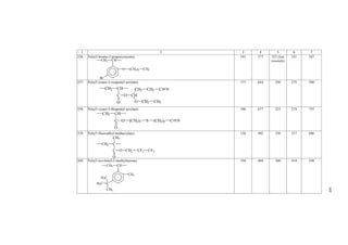


![1 2 3 4 5 6 7
245. Poly(5,7-dihydro-1,3,5,7-tetraoxobenzo[1,2-c:4,5-c']dipyrrole-2,6[1H,3H]-diyl-1,4-phenyleneoxy-
1,4phenylene)
309 476 523, 773,
653
649 298, 300-309
CO
CO
CO
246. Poly(5,7-dihydro-1,3,5,7-tetraoxobenzo[1,2-c:4,5-c']dipyrrole-2,6[1H,3H]-diyl-1,4-phenylenethio-1,4-
phenylene)
319 519 618 615 303
CO
247. Poly(5,7-dihydro-1,3,5,7-tetraoxobenzo[1,2-c:4,5-c']dipyrrole-2,6[1H,3H]-diyl-3-
methylheptamethylene)
286 709 408 403 299
CO
248. Poly(5,7-dihydro-1,3,5,7-tetraoxobenzo[1,2-c:4,5-c']dipyrrole-2,6[1H,3H]-diyl-4,4-
dimethylheptamethylene)
303 734 408 413 299
)3 C (CH2
CO
249. Poly(5,7-dihydro-1,3,5,7-tetraoxobenzo[1,2-c:4,5-c']dipyrrole-2,6[1H,3H]-diylnonamethylene) 303 844 383 359 299
CO
250. Poly(5-bromo-2-butoxystyrene) 208 667 320 312 547
CH2 CH
)3
O (CH2
Br
CH3
N O
CO
N
CO
CO
N S
CO
N
CO
CO
N (CH2
)2 CH (CH2)4
CH3
CO
N
CO
CO
N (CH2
)3
CH3
CH3
CO
N
CO
CO
N (C)9
H2
CO
N
167](https://image.slidesharecdn.com/computationalmaterialsscienceofpolymers-141021180636-conversion-gate02/85/Computational-materials-science-of-polymers-181-320.jpg)


![1 2 3 4 5 6 7
550. Poly(oxy-1,4-phenylenediphenylmethylene-1,4-phenyleneoxy-1,4-phenylenesulfonyl-1,4-phenylene) 516 1071 503 482 6
551. Poly(oxy-1,4-phenylenefluoren-9-ylidene-1,4-phenyleneoxysebacoyl) 499 1279 424 390 395
O O C (CH2
552. Poly(oxy-1,4-phenylenehexafluoro-2,2-propylidene-1,4-phenyleneoxy-1,4-phenylenecarbonyl-1,4-
phenylene]
420 917 448 458 297
CF3
553. Poly(oxy-1,4-phenyleneiminoisophthaloylimino-1,4-phenylene) 296 610 463, 554 485 308, 378,
379
O C O SO2
C
)8
O
C
O
O C O C
CF3 O
C NH
O
NH C
O
O
223](https://image.slidesharecdn.com/computationalmaterialsscienceofpolymers-141021180636-conversion-gate02/85/Computational-materials-science-of-polymers-239-320.jpg)


![1 2 3 4 5 6 7
878. Poly(vinyl trimethyl silane) 115 314 378-417 366 693
CH
CH2
H3C Si CH3
CH3
879. Poly[(1,2-diethoxycarbonyl)ethylene] 159 564 286 282 674
CH CH
C C
O O
O O
CH2 CH3
H3C CH2
880. Poly(4-acetoxybenzoyloxyethylene) 182 534 ~349 341 278, 628
CH2 CH
O C
O
O C CH3
O
881. Poly[(1-heptoxycarbonyl-1-heptoxycarbonylmethylene)ethylene] 346 1442 188, 250 240 665
O
C
CH2 C
O
CH2
C O
O
(CH2)6 CH3
(CH2)6 CH3
882. Poly[(1-methoxycarbonyl-1-methoxycarbonylmethylene)ethylene] 142 393 372 361 665
O
C
CH2 C
O
C O
O
CH3
CH2
CH3
280](https://image.slidesharecdn.com/computationalmaterialsscienceofpolymers-141021180636-conversion-gate02/85/Computational-materials-science-of-polymers-299-320.jpg)
![1 2 3 4 5 6 7
883. Poly[(1-methylcyclohexanoyloxy)ethylene] 170 482 359 353 650
CH2 CH
O
C
O
CH3
C
CH2
CH2
CH2
CH2
CH2
884. Poly[(2,2-dimethylvaleryloxy)ethylene] 165 571 283 289 650
885. Poly[(2-acetoxybenzoyloxy)ethylene] 182 534 333 341 278, 628
C
O
CH
O
C
CH3
CH2
O
O
886. Poly[(2-benzoyloxymethyl)styrene] 230 552 345 417 545
CH2 CH
CH2 O C
O
CH
O
CH2
C
C
O
H3C (CH2)2
CH3
CH3
281](https://image.slidesharecdn.com/computationalmaterialsscienceofpolymers-141021180636-conversion-gate02/85/Computational-materials-science-of-polymers-300-320.jpg)
![1 2 3 4 5 6 7
887. Poly[(2-butoxyethoxy)methylstyrene] 248 925 235 268 552
888. Poly[(2-ethylhexyloxy)ethylene] 180 779 207 231 600, 621
CH
889. Poly[(2-methoxybenzoyloxy)ethylene] 164 488 338 336 278, 628
CH2 CH
O
890. Poly[(2-methylbenzoyloxy)ethylene] 155 443 321 349 278, 580,
628, 653
O
CH2
CH2
CH CH2
CH2
CH2
CH3
CH2 CH3
C
O
O CH3
CH2 CH
O
C
O
CH3
CH2 CH
CH2 O (CH2
)2 O (CH2
)3 CH3
282](https://image.slidesharecdn.com/computationalmaterialsscienceofpolymers-141021180636-conversion-gate02/85/Computational-materials-science-of-polymers-301-320.jpg)
![1 2 3 4 5 6 7
891. Poly[(2-nitrosoethyl) methacrylate] 125 411 328 304 610
CH3
C
C
CH2
O
O
CH2
CH2 N O
892. Poly[(3-methoxybenzoyloxy)ethylene] 164 488 ~317 336 278, 628
CH2 CH
O
C
O
O CH3
893. Poly[(3-methylbenzoyloxy)ethylene] 155 443 324 349 278, 628,
653
CH2 CH
O
C
O
CH3
894. Poly[(3-nitrobenzoyloxy)ethylene] 155 439 366 353 278, 628
CH2 CH
O
C
O
NO2
283](https://image.slidesharecdn.com/computationalmaterialsscienceofpolymers-141021180636-conversion-gate02/85/Computational-materials-science-of-polymers-302-320.jpg)
![1 2 3 4 5 6 7
895. Poly[(3-trimethylsilylbenzoyloxy)ethylene] 217 573 353 378 659
CH
O
CH2
C
O
Si CH3
CH3
H3C
896. Poly[(4-dimethylaminophenyl)methylsilylenetrimethylene] 218 752 267 290 489
N CH3
H3C
Si (CH2)3
CH3
897. Poly[(4-dimethylaminophenyl)phenylsilylenetrimethylene] 276 857 325 322 489
N CH3
H3C
Si (CH2)3
284](https://image.slidesharecdn.com/computationalmaterialsscienceofpolymers-141021180636-conversion-gate02/85/Computational-materials-science-of-polymers-303-320.jpg)

![1 2 3 4 5 6 7
898. Poly[(4-methoxybenzoyloxy)ethylene] 164 488 360 336 278, 570,
628, 652,
653
CH2 CH
O
C
O
O CH3
899. Poly[(4-methylbenzoyloxy)ethylene] 155 443 343 350 278, 628,
652, 653
CH2 CH
O
C
O
CH3
900. Poly[(4-nitrobenzoyloxy)ethylene] 155 439 395 353 278, 628
CH2 CH
O
C
O
NO2
901. Poly[(4-pentadecafluoroheptyl)styrene] 306 1093 320 280 561
CH2 CH
(CF2)6 CF3
285](https://image.slidesharecdn.com/computationalmaterialsscienceofpolymers-141021180636-conversion-gate02/85/Computational-materials-science-of-polymers-305-320.jpg)
![1 2 3 4 5 6 7
902. Poly[(4-phenylbenzoyloxy)ethylene] 214 552 358 388 278, 628
CH2 CH
O
C
O
903. Poly[(4-propionyloxybenzoyloxy)ethylene] 200 571 346 350 278, 628
CH2 CH
O
C
O
O C CH2
CH3
O
904. Poly[(4-p-toluoylbutyryloxy)ethylene] 206 691 313 298 651
CH
O
905. Poly[(4-trimethylsilylbenzoyloxy)ethylene] 217 573 408 379 659, 660
CH
O
CH2
C
O
CH3
Si CH3
CH3
906. Poly[(cyclohexylmethyl)ethylene] 142 473 348 300 514
CH2 CH
CH2
CH2
CH
CH2 CH2
CH2
CH2
C
O
(CH2)3 CH3
CH2
286](https://image.slidesharecdn.com/computationalmaterialsscienceofpolymers-141021180636-conversion-gate02/85/Computational-materials-science-of-polymers-306-320.jpg)
![1 2 3 4 5 6 7
907. Poly[(cyclopentylmethyl)ethylene] 124 391 333 317 514
CH2 CH
CH2
CH2
CH
CH2
CH2
CH2
908. Poly[(heptafluoro-2-propoxy)ethylene] 131 434 ~328, 338 302 591
CH2 CH
O
F3C CF CF3
909. Poly[(methyl)phenylsilylenetrimethylene] 172 656 243 262 490
CH3
Si (CH2)3
910. Poly[(nonadecafluorodecanoyloxy)ethylene] 314 1292 253–255 243 656
CH2 CH
O
C
O
(CF2)8 CF3
911. Poly[(nonafluorovaleryloxy)ethylene] 177 670 288–293 264 656
CH2 CH
O
C
O
(CF2)3 CF3
287](https://image.slidesharecdn.com/computationalmaterialsscienceofpolymers-141021180636-conversion-gate02/85/Computational-materials-science-of-polymers-307-320.jpg)
![1 2 3 4 5 6 7
912. Poly[(pentadecafluorooctanyloxy)ethylene] 259 1040 258–263 249 656
CH2 CH
O
913. Poly[(pentafluoropropionyloxy)ethylene] 122 421 315 290 656
CH2 CH
O
914. Poly[(tert-butoxycarbonylamino)ethylene] 142 362 393 392 654
CH2 CH
NH
CH3
O C O C
CH3
CH3
915. Poly[(trifluoroacetoxy)ethylene] 94.9 297 ~319,
348
319 656, 657
CH
O
CH2
C
O
CF3
916. Poly[(undecafluorocyclohexylcarbonyloxy)ethylene] 210 652 327 321 656
CH
O
CH2
C
O
CF2
CF
CF2
CF2
CF2
CF2
C
O
(CF2)6 CF3
C
O
CF2 CF3
288](https://image.slidesharecdn.com/computationalmaterialsscienceofpolymers-141021180636-conversion-gate02/85/Computational-materials-science-of-polymers-308-320.jpg)
![1 2 3 4 5 6 7
917. Poly[2-(2-dimethylaminoethoxycarbonyl)styrene] 218 597.6 342 365 551
CH2 CH
C O
O
(CH2)2 N
CH3
CH3
918. Poly[2,2,3,3-tetramethylvaleryloxy)ethylene] 199 610 363 326 650
CH
O
C
O
CH3
CH3
C C
CH3
CH2
CH3
CH3
CH2
919. Poly[2,2,3,4-tetramethylvaleryloxy)ethylene] 199 599 323 332 650
CH
O
C
O
CH3
C CH
CH3
CH
CH3
CH3
CH3
CH2
920. Poly[2,2,4,4-tetramethylvaleryloxy)ethylene] 199 610 328 326 650
CH
O
C
O
CH3
C CH2
CH3
CH3
C CH3
CH3
CH2
289](https://image.slidesharecdn.com/computationalmaterialsscienceofpolymers-141021180636-conversion-gate02/85/Computational-materials-science-of-polymers-309-320.jpg)
![1 2 3 4 5 6 7
921. Poly[2,2-difluoro-2-(2-heptafluorotetrahydrofuranyl)ethyl acrylate] 209 739 275 Brittle
point
283 587
CH2 CH
C O
C2
HCF2
O
F F2
F2 O
F2
922. Poly[3-(4-biphenyl)styrene] 261 529 ~471
(softening
point)
493 546
CH2 CH
923. Poly[3-chloro-2,2-bis(chloromethyl)propyl acrylate] 192 608 319 316 560
CH2 CH
Cl
CH2
C O
C2
HO
C
CH2Cl
CH2
Cl
924. Poly[4-(1-ethylhexyloxymethyl)styrene] 272 1000 250 272 552
CH2 CH
CH2 O CH (CH2
)4
CH2
CH3
CH3
290](https://image.slidesharecdn.com/computationalmaterialsscienceofpolymers-141021180636-conversion-gate02/85/Computational-materials-science-of-polymers-310-320.jpg)
![1 2 3 4 5 6 7
925. Poly[4-(1-hydroxy-1-methylbutyl)styrene] 202 553 ~403
softening
point
365 567
926. Poly[4-(1-hydroxy-1-methylethyl)styrene] 168 375 ~438
softening
point
448 567
927. Poly[4-(1-hydroxy-1-methylhexyl)styrene] 236 731 ~364
softening
point
323 567
CH2 CH
OH C CH3
CH2 CH2 CH3
CH2 CH
OH C CH3
CH3
CH2 CH
OH C CH3
(CH2)4 CH3
291](https://image.slidesharecdn.com/computationalmaterialsscienceofpolymers-141021180636-conversion-gate02/85/Computational-materials-science-of-polymers-311-320.jpg)
![1 2 3 4 5 6 7
928. Poly[4-(1-hydroxy-1-methylpentyl)styrene] 219 642 356
softening
point
341 567
CH2 CH
HO C CH3
CH2)3 CH3
929. Poly[4-(1-hydroxy-1-methylpropyl)styrene] 185 464 459 399 567
930. Poly[4-(1-hydroxy-3-morpholinopropyl)styrene] 246 665 323 low
viscosity
370 567
CH2 CH
HO CH (CH2)2 N
CH2
CH2
CH2
O
CH2
(
CH2 CH
HO C CH3
CH2 CH3
292](https://image.slidesharecdn.com/computationalmaterialsscienceofpolymers-141021180636-conversion-gate02/85/Computational-materials-science-of-polymers-312-320.jpg)
![1 2 3 4 5 6 7
931. Poly[4-(1-hydroxy-3-piperidinopropyl)styrene] 254 688 327 low
viscosity
369 567
CH2 CH
HO CH (CH2)2 N
CH2
CH2
CH2
CH2
CH2
932. Poly[4-(2-hydroxybutoxymethyl)styrene] 212 656 319 323 552
CH2 CH
CH2 O CH2CH CH2
933. Poly[4-(3-morpholinopropionyl)styrene] 240 677.4 314 354 567
O C (CH2)2 N
O
CH2
CH2
CH2
CH2
CH2 CH
OH
CH3
293](https://image.slidesharecdn.com/computationalmaterialsscienceofpolymers-141021180636-conversion-gate02/85/Computational-materials-science-of-polymers-313-320.jpg)
![1 2 3 4 5 6 7
934. Poly[4-(3-piperidinopropionyl)styrene] 248 701 311 353 567
CH2 CH
CO (CH2)2 N
CH2
CH2
CH2
CH2
CH2
935. Poly[4-(4-biphenyl)styrene] 261 529 593
(softening
point)
493 546
936. Poly[4-(4-hydroxybutoxymethyl)styrene] 212 721 293 294 552
CH2 CH
CH2 O (CH2
)4 OH
937. Poly[4-(octyloxymethyl)styrene] 272 1067 231 255 552
CH2 CH
CH2 O (CH2
)7 CH3
CH2 CH
294](https://image.slidesharecdn.com/computationalmaterialsscienceofpolymers-141021180636-conversion-gate02/85/Computational-materials-science-of-polymers-314-320.jpg)
![1 2 3 4 5 6 7
938. Poly[4-(sec-butoxymethyl)styrene] 204 646 313 316 552
CH2 CH
CH3
CH2 O CH CH2
CH3
939. Poly[di(oxy-1,4-phenylene)carbonyl-1,4-phenylene] 262 630 433 416 297
O O C
O
940. Poly[di(oxy-1,4-phenylene)oxyisophthaloyl] 290 674 446 430 380
O O O C C
941. Poly[di(oxy-1,4-phenylene)sulfonyl-1,4-phenylene] 273 591 483 462 297
O O SO2
942. Poly[di(oxydimethylsilylene)-1,4-phenylenedimethylsilylene] 280 1284 210 218 451
CH3
O Si Si
Si
CH3
O
CH3
CH3
CH3
CH3
O O
295](https://image.slidesharecdn.com/computationalmaterialsscienceofpolymers-141021180636-conversion-gate02/85/Computational-materials-science-of-polymers-315-320.jpg)
![1 2 3 4 5 6 7
943. Poly[di(oxyethylene)oxy-1,4-phenylenecarbonyl-oxycarbonyl-1,4-phenylene] 294 930 314 316 350
O C
C O
O
O
O (CH2)2 O (CH2)2
944. Poly[di(oxyethylene)oxyadipoyl] 202 838 227 241 290
C (CH2)4 C O CH2 CH2 O CH2 CH2 O
O O
945. Poly[di(oxyethylene)oxyazelaoyl] 254 1081 205 235 290
C (CH2)7 C O CH2 CH2 O CH2 CH2 O
O O
946. Poly[di(oxyethylene)oxycarbonyliminohexamethyleneiminocarbonyl)] 260 916 272 284 349
(CH2)6 NH C
C
947. Poly[di(oxyethylene)oxydodecanedioyl] 339 1480 202 229 290
C (CH2)12 C O CH2 CH2 O CH2 CH2 O
O O
948. Poly[di(oxyethylene)oxyglutaryl] 185 758 226 244 290
C (CH2)3 C O CH2 CH2 O CH2 CH2 O
O O
949. Poly[di(oxyethylene)oxymalonyl] 151 602 244 251 290
C CH2 C O CH2 CH2 O CH2 CH2 O
O O
O
O (C)2 H2
O (C)2 H2
O
NH O
296](https://image.slidesharecdn.com/computationalmaterialsscienceofpolymers-141021180636-conversion-gate02/85/Computational-materials-science-of-polymers-316-320.jpg)
![1 2 3 4 5 6 7
950. Poly[di(oxyethylene)oxymethylmalonyl] 168 625 244 269 290
CH2 O C CH
O
C
CH3 O
O CH2 CH2 O CH2
951. Poly[di(oxyethylene)oxynonylmalonyl] 305 1344 214 227 290
CH2 O C CH
O
C
(
CH2)8 O
O CH2 CH2 O CH2
CH3
952. Poly[di(oxyethylene)oxyoctadecanedioyl] 441 1951 205 226 290
O CH2 C (CH2
)18
O
C
O
O CH2 CH2 O CH2
953. Poly[di(oxyethylene)oxyoxalyl] 134 521 265 257 290
CH2 O C
O
C
O
O CH2 CH2 O CH2
954. Poly[di(oxyethylene)oxypentylmalonyl] 237 987 226 240 290
CH2 O C CH
O
C
(
CH2)4 O
O CH2 CH2 O CH2
CH3
955. Poly[di(oxyethylene)oxypimeloyl] 219 920 213 238 290
CH2 O C (C)5
H2
O
C
O
O CH2 CH2 O CH2
297](https://image.slidesharecdn.com/computationalmaterialsscienceofpolymers-141021180636-conversion-gate02/85/Computational-materials-science-of-polymers-317-320.jpg)
![1 2 3 4 5 6 7
956. Poly[di(oxyethylene)oxypropylmalonyl] 185 714 235 259 290
CH2 O C CH
O
C
CH2 O
O CH2 CH2 O CH2
CH3
957. Poly[di(oxyethylene)oxysebacoyl] 271 1163 199 233 290
O CH2 CH2 O CH2 CH2 O C (CH2)8 C
O O
958. Poly[di(oxyethylene)oxysuberoyl] 237 1000 212 237 290
O CH2 CH2 O CH2 CH2 O C (CH2)6 C
O O
959. Poly[di(oxyethylene)oxysuccinyl] 168 680 244 247 290
O CH2 CH2 O CH2 CH2 O C (CH2)2 C
O O
960. Poly[di(oxymethylene)oxy-1,4-phenylenecarbonyl-oxycarbonyl-1,4-phenylene] 259 794 325 326 350
CH2 O CH2 O C O C
O O
O
961. Poly[di(oxymethylene)oxy-2,2,3,3,4,4-hexafluoropentamethylene]
–O–CH2–O–CH2–O–CH2–(CF2)3–CH2–
179 909 218 197 368
962. Poly[imino-5-tert-butylisophthaloylimino-(2,5-dimethylhexamethylene)] 341 804 422 424 444
NH C C NH CH2 (CH2)2 CH CH2
H3C C CH3
CH3
CH
O O
CH3 CH3
298](https://image.slidesharecdn.com/computationalmaterialsscienceofpolymers-141021180636-conversion-gate02/85/Computational-materials-science-of-polymers-318-320.jpg)
![1 2 3 4 5 6 7
963. Poly[imino-5-tert-butylisophthaloylimino-(3,4-dimethylhexamethylene)] 341 804 446 424 444
CH3
NH C C NH (CH2)2 CH (CH2)2
O O
H3C C CH3
CH3
CH
CH3
964. Poly[imino-5-tert-butylisophthaloyliminohexamethylene] 306 754 436 406 444
NH C C NH (CH2)6
O O
H3C C CH3
CH3
965. Poly[iminomethylene(2,5-dimethyl-1,4-phenylene)methyleneiminosuberoyl] 306 855 351 358 373
H3C
NH CH2 CH2 NH C (C)6 H2
C
H3C
O O
966. Poly[iminomethylene-1,4-phenylenemethyleneiminocarbonyl(1,3,3-trimethyl-5-oxopentamethylene)] 290 770 398 377 406
NH CH2 CH2 NH C CH
CH2
O
CH3
CH3
C CH2
CH3
C
O
299](https://image.slidesharecdn.com/computationalmaterialsscienceofpolymers-141021180636-conversion-gate02/85/Computational-materials-science-of-polymers-319-320.jpg)
![1 2 3 4 5 6 7
967. Poly[oxy(allyloxymethyl)ethylene] 117 544 195 215 330
CH
CH2
O CH2
O CH2
CH CH2
968. Poly[oxy(bromomethyl)ethylene] 82.5 311 259 265 332
CH
CH2Br
O CH2
969. Poly[oxy(butoxymethyl)ethylene] 139 662 194 210 330
CH
CH2
CH2
O
O
(CH2)3 CH3
970. Poly[oxy(chloromethyl)ethylene] 75.5 306 251, 248 247 332, 703
CH2 CH
CH2Cl
O
971. Poly[oxy(ethoxymethyl)ethylene] 104 479 212 217 330
CH2 CH
CH2
O
O CH2
CH3
972. Poly[oxy(hexyloxymethyl)ethylene] 173 840 190 206 330
O CH2 CH
CH2 O (CH2
)5 CH3
973. Poly[oxy(methoxymethyl)ethylene] 87.3 400 211 218 330
O CH2 CH
CH2 O CH3
300](https://image.slidesharecdn.com/computationalmaterialsscienceofpolymers-141021180636-conversion-gate02/85/Computational-materials-science-of-polymers-320-320.jpg)
![1 2 3 4 5 6 7
974. Poly[oxy(methyl)phenylsilylene] 129 471 187, 273 274 748
CH3
975. Poly[oxy(methyl)phenylsilyleneoxy-1,4-phenyleneisopropylidene-1,4-phenylene] 340 960 331 354 448
CH3
976. Poly[oxy-1,3-phenyleneoxy-5-(heptafluoropropyl)isophthaloyl] 293 807 394 363 431
O C
O
977. Poly[oxy-1,4-phenylene-(2-cyano)-2-phenyltrimethylene-1,4-phenylene] 306 691 416
Proposed
structure
443 377
O Si
Si O C
CH3
O
CH3
O C
O
CF2 CF2 CF3
C N
O CH2 C CH2
301](https://image.slidesharecdn.com/computationalmaterialsscienceofpolymers-141021180636-conversion-gate02/85/Computational-materials-science-of-polymers-321-320.jpg)
![1 2 3 4 5 6 7
978. Poly[oxy-1,4-phenylene-2,2-di(ethoxycarbonyl)trimethylene-1,4-phenylene] 335 1003 327 334 377
CH2
O
C
CH3
O
O CH2 C CH2
C
O
O
CH2
CH3
979. Poly[oxy-2-(1-naphthyl)-6-phenyl-1,4-phenylene] 281 562 507 500 331
O
980. Poly[oxy-2-(2-biphenylyl)-6-phenyl-1,4-phenylene] 311 641 484 485 331
O
302](https://image.slidesharecdn.com/computationalmaterialsscienceofpolymers-141021180636-conversion-gate02/85/Computational-materials-science-of-polymers-322-320.jpg)
![1 2 3 4 5 6 7
981. Poly[oxy-2-(2-chlorobenzoyloxy)trimethyleneoxy-1,4-phenyleneisopropylidene-1,4-phenylene] 406 1140 339 356 329
CH3
982. Poly[oxy-2-(4-tert-butylphenyl)-6-phenyl-1,4-phenylene] 303 634 513 478 331
O
C CH3
CH3
CH3
983. Poly[oxy-2-(chloroacetoxy)trimethyleneoxy-1,4-phenyleneisopropylidene-1,4-phenylene] 331 943 338 351 329
CH3
CH CH2 O C
O
CH2
C
O
O CH2Cl
CH3
O CH2 CH CH2 O C
O CH3
C
CH2
O
Cl
303](https://image.slidesharecdn.com/computationalmaterialsscienceofpolymers-141021180636-conversion-gate02/85/Computational-materials-science-of-polymers-323-320.jpg)
![1 2 3 4 5 6 7
984. Poly[oxy-2,2-bis(chloromethyl)trimethylene] 124 420 265 295 273, 300,
339-345
CH2Cl
O CH2 C
CH2
CH2Cl
985. Poly[oxy-2-acetoxytrimethyleneoxy-1,4-phenylenemethyl(phenyl)methylene-1,4-phenylene] 375 1014 383 370 329
CH3
CH CH2 O C
O
CH2
C
O
CH3
O
986. Poly[oxy-2-benzoyloxytrimethyleneoxy-1,4-phenylenemethyl(phenyl)methylene-1,4-phenylene] 451 1212 399 372 329
987. Poly[oxy-5-(pentadecafluoroheptyl)isophthaloyloxy-2,2,3,3,4,4-hexafluoropentamethylene] 445 1660 300 268 410
O C
O
C
CF2
O
O
CF2
CH2
CF2
CF2 CF2
CF2
CF2
CF2
CF2
CH2
CF3
CH CH2 O C
O
CH2
C
O
O
CH3
CH2
304](https://image.slidesharecdn.com/computationalmaterialsscienceofpolymers-141021180636-conversion-gate02/85/Computational-materials-science-of-polymers-324-320.jpg)

![1 2 3 4 5 6 7
989. Poly[oxy-6-phenyl-2-(m-tolyl)-1,4-phenylene] 252 506 492 498 331
990. Poly[oxy-6-phenyl-2-(p-tolyl)-1,4-phenylene] 252 506 491 498 331
991. Poly[oxycarbonyldi(oxy-1,4-phenylene)sulfonyl-1,4-phenyleneoxy-1,4-phenylene] 385 881 ~478 437 337
O C O
992. Poly[oxycarbonyloxy-1,3-(2,2,4,4-tetramethylcyclobutylene) 162 372 500, 433,
418
435 390–392
O
H3C
O
H3C
H3C CH3
O C O
O
C
CH
C
CH
H3C CH3
SO2 O
O
O
305](https://image.slidesharecdn.com/computationalmaterialsscienceofpolymers-141021180636-conversion-gate02/85/Computational-materials-science-of-polymers-326-320.jpg)
![1 2 3 4 5 6 7
993. Poly[oxycarbonyloxy-1,4-phenylene(methyl)phenylmethylene-1,4-phenylene] 297 661 449 449 384, 386
O C O
O
CH3
C
994. Poly[oxycarbonyloxy-4,6-dimethyl-1,2-phenylenemethylene-3,5-dimethyl-1,2-phenylene] 271 679 410 399 388
O C O
O
CH2
H3C CH3 H3C CH3
995. Poly[oxydi(pentafluorophenyl)silylenedi(oxydimethylsilylene)] 369 1525 231 242 446
CH3
O Si
O Si O
Si
CH3
CH3
CH3
F
F
F
F F
F
F
F
F
F
306](https://image.slidesharecdn.com/computationalmaterialsscienceofpolymers-141021180636-conversion-gate02/85/Computational-materials-science-of-polymers-327-320.jpg)
![1 2 3 4 5 6 7
996. Poly[oxymethylpentafluorophenylsilylenedi(oxydimethylsilylene)] 286 1343 190 213 446
CH3 CH3
CH3
O Si
O Si O
Si
F CH3
CH3
F
F
F
F
997. Poly[oxytri(dimethylsilyleneoxy)(methyl)phenylsilylene-1,3-phenylene(methyl)phenylsilylene)] 538 2491 231 216 372
CH3
CH3
CH3
CH3
O Si O Si O Si O Si
CH3
CH3
CH3
CH3
Si
998. Poly[penta(oxydiethylsilylene)-1,4-phenylenedimethylsilylene] 666 4215 193 158 372
CH3
CH2
CH3
CH2
CH3
CH2
CH3
CH2
Si O Si O Si O Si
CH2
CH2
CH2
CH3
Si
CH3
CH3
CH2
Si O
CH2
O
CH2
CH3
CH3 CH3
CH3
CH3
999. Poly[penta(oxydiethylsilylene)-1,4-phenyleneoxy-1,4-phenylenedimethylsilylene] 750 4438 208 169 372
CH3
CH2
CH3
CH3
Si O Si O Si O Si
CH2
CH2
CH2
CH2
CH2
CH3
Si O
CH2
CH2
O
CH2
CH2
CH3
CH3
CH3 CH3
CH3
CH3
CH3
O Si
CH3
307](https://image.slidesharecdn.com/computationalmaterialsscienceofpolymers-141021180636-conversion-gate02/85/Computational-materials-science-of-polymers-328-320.jpg)
![1 2 3 4 5 6 7
1000. Poly[tetra(oxydimethylsilylene)-1,3-phenylenedimethylsilylene] 423 2286 198 185 372
CH3
Si
CH3
CH3
CH3
CH3
Si O Si O Si O Si
CH3 CH3
O
CH3
CH3
CH3
1001. Poly[tetra(oxydimethylsilylene)-1,4-phenylenedimethylsilylene] 423 2238 201 189 372
CH3
CH3
CH3
CH3
Si O Si O Si O Si
CH3
CH3
CH3
CH3
Si
CH3
O
CH3
1002. Poly[tetra(oxydimethylsilylene)-1,4-phenyleneoxy-1,4-phenylenedimethylsilylene] 507 2449 221 207 372
CH3
Si
CH3
O
CH3
CH3
O Si O Si O Si O Si
CH3
CH3
CH3
CH3
CH3
CH3
1003. Poly[thio-1-(allyloxymethyl)ethylene] 126 581 213 217 330
CH CH2
CH2
S
O CH2
CH CH2
1004. Poly[tri(oxy-1,4-phenylene)carbonyl-1,4-phenylene] 347 848 423 409 297
O O O C
O
1005. Poly[tri(oxy-1,4-phenylene)sulfonyl-1,4-phenylene] 357 808 453 442 297
O O O SO2
308](https://image.slidesharecdn.com/computationalmaterialsscienceofpolymers-141021180636-conversion-gate02/85/Computational-materials-science-of-polymers-329-320.jpg)
![1 2 3 4 5 6 7
1006. Poly[tri(oxydimethylsilylene)-1,4-phenylenedimethylsilylene] 351 1764 211 199 372
CH3
CH3
CH3
O Si O Si O Si
CH3
CH3
CH3
CH3
Si
CH3
1007. Poly[tri(oxydimethylsilylene)oxy(methyl)-2-phenylethylsilylene] 380 2159 171 176 449
CH3
CH3
CH3
CH2
CH2
O Si O Si O Si O Si
CH3
CH3
CH3
CH3
1008. Poly[tri(oxydimethylsilylene)oxy(methyl)phenylsilylene] 344 1901 201 181 449
CH3
CH3
CH3
CH3
O Si O Si O Si O Si
CH3
CH3
CH3
1009. Poly[tri(oxydimethylsilylene)oxy(methyl)trimethylsiloxysilylene] 359 1962 148 183 449
CH3
CH3
H3C Si
CH3
O Si O Si O Si O Si
CH3
CH3
CH3
CH3
CH3
O
CH3
309](https://image.slidesharecdn.com/computationalmaterialsscienceofpolymers-141021180636-conversion-gate02/85/Computational-materials-science-of-polymers-330-320.jpg)
![1 2 3 4 5 6 7
1010. Poly[tri(oxydimethylsilylene-1,4-phenyleneoxy)-1,4-phenylenedimethylsilylene] 436 1982 236 220 372
CH3
Si
CH3
O
CH3
O Si O Si O Si
CH3
CH3
CH3
CH3
CH3
1011. Poly[tri(oxyethylene)oxycarbonyliminohexamethyleneiminocarbonyl] 304 1131 260 269 765
O (CH2)6 NH C
C NH
O
O
O (CH2)2 O (CH2)2 O (CH2)2
1012. Poly1H,1H-nonafluoro-4-oxahexyl acrylate) 204 826 224 247 587
CH2 CH
C O CH2
O
(CF2)2 O CF2
CF3
1013. Poly1H,1H-nonafluoropentyl acrylate) 194 767 236 253 589
CH2 CH
C O CH2
O
(CF2)3 CF3
1014. Polyarylate of phenolphthalein and terephthalic acid 390 677 583 576 6
O C C
C O O
O
O
CO
310](https://image.slidesharecdn.com/computationalmaterialsscienceofpolymers-141021180636-conversion-gate02/85/Computational-materials-science-of-polymers-331-320.jpg)


![320
The above-described effect of influence of chain attachment on Tg of the
polymer is also spread upon polymeric systems, composed of isomers. For example,
polyamidophenyl quinoxalines, analyzed in the study in [83], display the following
structure:
PAPQ-1
N
N
PAPQ-2
N
N
O
N
N
NH C
C NH
O
O O
n
O
N
N
O
NH
C
O
C
O NH
n
In the case of PAPQ-2, polar groups representing phenolquinoxaline cycles are
in tight contact with each other, and the intermolecular interaction occurring at the
sacrifice of these groups is displayed in the frames of the unit; then, the dipole–dipole
interaction between units of neighboring chains is not realized.
PAPQ-1 and PAPQ-2 are isomers with the same gross-formula.
Work [83] represent experiments and calculations on the determination of
glass transition temperatures of two pairs of polymers, the structure of which is shown
above. Since strong intermolecular interaction occurring at the sacrifice of separate
polar groups significantly affects Tg, it is obvious that when this interaction takes
place inside the unit, Tg of such polymers must be lower than for polymers with a
completely analogous structure, but with such disposition of polar groups in which
intermolecular interaction manifests itself between units of neighboring chains.
Calculations and experiments have confirmed that this indeed happens in this
way. When the glass transition temperature is calculated for PAPQ-1,
Σ = + + + ⋅ 1
j , and for PAPQ-2 h
b 4bp 2bh 2bd 2 b
j
2 d
Σb j = 4bp + 2b . Consequently,
j
the calculated value of Tg for PAPQ-1 is 265°C, and for PAPQ-2 it is 208°C.
Appropriate experimental values are 275 and 210°C, respectively.
At the same gross-formula of the repeat unit, the glass transition temperature
also depends on the location of separate aromatic fragments. For example, polyimides
PI-1and PI-2 possess identical gross-formulae, but display different locations of
aromatic cycles. Calculating the glass transition temperature for PI-1, it is obtained
that b 2bd 2bp
Σ j = + , and in the case of PI- b 2bd 5bp
j
Σ j = + . In accordance
j
with this, Tg for polyimide PI-1 is 238°C, and for PI- 295°C. Experimentally,
approximately the same values are obtained.](https://image.slidesharecdn.com/computationalmaterialsscienceofpolymers-141021180636-conversion-gate02/85/Computational-materials-science-of-polymers-342-320.jpg)
![321
O
N O
PI-1
O
PI-2
N
O
C
C
O
O
C
C
N
O
It should be noted that special attention must be paid to the cases when a
significant deviation in experimental and calculated data on the glass transition
temperature is observed. This may be caused by both the occurrence of a polar group
possessing a special influence on the energy of intermolecular interaction and, vice
versa, exclusion of any polar group from formation of the network of physical bonds
between neighboring chains of the polymer. In the first case, introduction of a new
constant bj is required, but it should always be remembered that the greater is the
number of constants introduced to the calculated scheme, the lower becomes its
predictive power and, in the border case, when every new polymer requires
introduction of a new constant bj, the predictive power of the calculation scheme
becomes equal to zero.
It should be also taken into account that anomalous addition of units to each
other may not weaken, but strengthen intermolecular interaction between neighboring
chains, and then the glass transition temperature will increase.
Let us now turn to the problem of plasticization rules. Let us use two
poly(ether ketones)∗ as polymers:
PAEK 1
PAEK 2
O C
C O C
O
As plasticizers, let us choose phthalic acid esters – dimethylphthalate (DMP),
dimethylterephthalate (DMTP) and dibutylphthalate (DBP):
∗ These poly(ether ketones) are produced in works [769 – 771].
O
C O
O
H3C CH3
O
O
C
O
C
C
O
C
C
N
O
O
O](https://image.slidesharecdn.com/computationalmaterialsscienceofpolymers-141021180636-conversion-gate02/85/Computational-materials-science-of-polymers-343-320.jpg)


![328
Σ Σ
=
V
k i
Σ Σ Σ
=
=
=
k i i
Δ +
Δ
=
k n
j
k i
j k
k n
k i k
a V b
T
1
1
g
α
α
, (IV.52)
where αk is the molar part of the k-th component;
ΣΔ
and
Vi
i k
Σ Δ +Σ j
are the Van-der-Waals volume and the selection of constants for
j k
i
i i b V a
the k-th component, respectively; n is the total number of components in copolymer.
In the reduced form, correlations (IV.50) and (IV.51) are the following:
=
Σ Σ
=
α
1
Σ
V
k i
Σ
=
=
Δ
Δ
=
k n
i k
k k
i
k
k n
k i k
T
V
T
1 g,
g
α
, (IV.53)
and
Σ =
1 1 β . (IV.54)
=
=
k n
k
k
Tg 1 Tg,k
Dependences (IV.49)–(IV.54) of the glass transition temperature Tg of the
copolymer on its composition are non-linear, and in the case of two-component
copolymers they look as it is schematically represented in Figure 43. These
dependences do not take into account weakening of the intermolecular interaction in
copolymer units, although this weakening must cause a decrease of the glass transition
temperature compared with the additive value.
In practice, ‘dips’ on the dependences of Tg on composition are deeper than
the ones calculated from equations (IV.49)–(IV.54) and equal ΔT = 20–30°C [78].
That is why a modified relation was suggested in the work [39], which takes this
circumstance into account:
→
+ +
Σ Σ
α α
+ Δ +
Δ +
+ +
Δ +
Δ
=
Σ Σ Σ Σ
α β α β
, (IV.55)](https://image.slidesharecdn.com/computationalmaterialsscienceofpolymers-141021180636-conversion-gate02/85/Computational-materials-science-of-polymers-350-320.jpg)
![329
α
[ ( ) ( ) ( )]
⋅ − + + − + − +
Δ +
+ Δ
→
Σ Σ
Σ
α β α α α α α α
where all designations are the same as in the formula (IV.51); 0.03 is an empirical
coefficient which takes into account decrease of strong intermolecular interactions at
copolymerization.
Figure 43. Dependences of the glass transition temperature Tg on composition α for two-component
copolymers calculated from equations (IV.49) (curve 1) and (IV.54) (curve 2)
In the reduced form, equation (IV.54) may be presented in the following form:
Σ Σ
=
α
k i
1
Σ Σ Σ Σ ( )
=
=
=
=
=
− +
k i i
Δ +
Δ
=
k n
k
k k
k n
j
k i
j k
k n
k i k
a V b
V
T
1 1
g
α 0.03 α 1 α
, (IV.56)
where αk,
ΣΔ
and
Vi
i k
Σ Δ +Σ j
are the molar part, the Van-der-Waals
j k
i
i i b V a
volume and the selection of constants for the k-th component of the copolymer,
respectively.](https://image.slidesharecdn.com/computationalmaterialsscienceofpolymers-141021180636-conversion-gate02/85/Computational-materials-science-of-polymers-351-320.jpg)
![330
To calculate the glass transition temperatures of copolymers, equations (IV.55)
and (IV.56) require no knowledge of the experimental glass transition temperatures of
homopolymers.
Another variant of the formula for calculation of the glass transition
temperature of copolymers may be deduced by combining equations (IV.41) and
(IV.55):
Σ Σ
Δ +
α α
Σ Σ Σ
α α ...
α
...
i
i n
g,2 g,
+ Δ
α
n i
[ ( ) ( ) ( )] ,
1 1 ... 1 0.03
1 1 2 2
2
2
g,1
1
1
2
2
1
1
g
+ − + − + + − ⋅
→
→
+
Δ
+ +
Δ
+
Δ
+ +
Δ
=
Σ
n n
i n
n
n
i
i
i
i
i
i
i
i
V
T
V
T
V
T
V
V V
T
α α α α α α
(IV.57)
where Tg,1, Tg,2, …, Tg,n are the glass transition temperatures of homopolymers,
composed of the components 1, 2, …, n. In the reduced form, equation (IV.57) can be
written as:
Σ Σ
Σ
=
α
k i
1
i k
Σ Σ ( )
=
=
=
=
=
+ −
Δ
Δ
=
k n
k
k k
k n
k k
i
k
k n
k i k
T
V
V
T
1 g, 1
g
α 0.03 α 1 α
. (IV.58)
Let us now discuss the influence of sequences distribution in polymers on the
glass transition temperature of them.
Imagine that the following sequences exist:
1) Diades AA and BB;
2) Triades AAA and BBB;
where A and B are the components of a copolymer. Let the molar parts of components
A and B be 0.5:0.5.
Now Tg values may be calculated for random copolymers consisting of the
sequences mentioned above.
For the random copolymer consisting of A and B components, we obtain:
Σ Σ
Δ +
Δ
α α
+ − + −
Δ
+
Δ
( ) ( ) 0.03[ A(1 A) B(1 B)]
g B
B
B
g A
A
A
B
B
A
A
g
α α α α α α
=
Σ Σ
T
V
T
V
V V
T
i
i
i
i
i
i
i
i
, (IV.59)](https://image.slidesharecdn.com/computationalmaterialsscienceofpolymers-141021180636-conversion-gate02/85/Computational-materials-science-of-polymers-352-320.jpg)
![331
where αA and αB are the molar parts of the components A and B, respectively;
A
Δ Σi
Vi and
B
Δ Σi
Vi are the Van-der-Waals volumes of the components A and
B, respectively; Tg,A and Tg,B are the calculated glass transition temperatures for
homopolymers based on the components A and B, respectively.
For instance, for copolymers of ethylene (component A) and vinyl acetate
(component B), it is obtained: Tg,A = 213 K, Tg,B = 301 K;
A
Δ Σi
Vi = 34.2 Å3,
B
Δ Σi
Vi = 79.65 Å3:
(CH2CH2)n
A
B
Then, Tg value for the random copolymer in accordance with equation (IV.59)
is equal to 250 K, when αA:αB = 0.5:0.5.
Let us now examine the case, when the copolymer composed of the same
components is the random copolymer consisting of diades AA and BB. Since Tg,AA =
Tg,A and Tg,BB = Tg,B, equation (IV.59) is reduced to the following form:
Σ Σ
Δ ⋅ +
⋅ Δ
α α
2 2
Δ
2 2
+ − + −
Δ
+
( ) ( ) 0.03[ A (1 A ) B (1 B
)]
g B
B
B
g A
A
A
B
B
A
A
g
α α α α α α
=
Σ Σ
T
V
T
V
V V
T
i
i
i
i
i
i
i
i
. (IV.60)
(It should be remembered since the molar ratio of the components A and B is 0.5:0.5,
the molar ratio of the components AA and BB is the same). Substituting all the values
into equation (IV.60), we obtain Tg = 259 K.
Let us now discuss the case when the random copolymer consists of the triades
AAA and BBB. Then, in accordance with equation (IV.59), we get:
Σ Σ
Δ ⋅ +
⋅ Δ
α α
3 3
Δ
3 3
+ − + −
Δ
+
( ) ( ) 0.03[ A (1 A ) B (1 B
)]
g B
B
B
g A
A
A
B
B
A
A
g
α α α α α α
=
Σ Σ
T
V
T
V
V V
T
i
i
i
i
i
i
i
i
. (IV.61)
( CH2 CH )m
O
C
CH3
O](https://image.slidesharecdn.com/computationalmaterialsscienceofpolymers-141021180636-conversion-gate02/85/Computational-materials-science-of-polymers-353-320.jpg)

![333
CH
R
;
CH2
C O
O
CnH2n+1
R'
C
R
CH2
where R is the hydrocarbon radical: —CnH2n+1; —O—CnH2n+1; ,
etc.
In the general case, the number of possible variants of chain branchings may
be quite high. Consider the main among them, schematically represented in Figure 44,
which depicts the backbone and possible types of branches.
Figure 44. Different types of branchings in polymers (see text).
In the simplest (but of the lowest probability) case, branches may possess
equal length and be located in each repeat unit (see Figure 44a). Another variant
corresponds to branches of the same length, regularly distributed along the backbone
in a definite number of units (see Figure 44b). The third type corresponds to the case,
when branches of various length exist, but they are regularly distributed along the
backbone in a definite number of units (see Figure 44c). Then a variant is possible
when branches of different lengths are randomly distributed along the backbone (see
Figure 44d). Two more types are to be considered. According to one of them,
branches of different lengths are randomly distributed along the backbone, and each
branch possesses one more branch of different length on it (see Figure 44e). Clearly,
this general case may include all particular cases, when branches are identical and
regularly distributed along the backbone, and secondary branches are identical or
different, etc. One more principal case consists of a tree-like branching (see Figure
44f). In this case, occurrence of every new branch causes occurrence of one more
branch.
Note that at the present time, such systems have been synthesized in practice
[82], and they are named ‘dendric polymers’ or ‘dendrimers’.
In all cases considered, branches may be of the same chemical origin in
relation to the backbone, or of a different one. The case, when branches are of a
different chemical origin in relation to the backbone corresponds to grafted polymers.](https://image.slidesharecdn.com/computationalmaterialsscienceofpolymers-141021180636-conversion-gate02/85/Computational-materials-science-of-polymers-355-320.jpg)
![334
In these systems, in most cases, a microphase separation occurs due to
thermodynamic inconsistency of the backbone and the grafted chain. Therefore, each
phase may possess, for example, its own glass transition temperature which, however,
in many cases differs from the glass transition temperature of individual components.
That is why Tg for grafted copolymers may be calculated only in the case of complete
miscibility of the initial and the grafted polymer. However, the reverse task may also
be solved – estimation of the composition of each phase by temperatures of relaxation
transitions in it, assuming that each of the phases includes a definite number of
foreign units.
Work [24] analyzes the influence of branchings of different types on the
physical characteristics of polymers.
In homopolymers, branches may be joined directly to the backbone by
substitution of one of the atoms or via a spacer of another chemical origin. Let us
consider all these variants on particular examples. Let us choose polyethylene and its
derivatives as one of the model polymers for this consideration:
Structure I
CH2 CH (CH2
( )n
CH2
CH3
CH2)
m
Let us consider the influence of branchings on the glass transition temperature
Tg. Note that if m = 0, we get the case, depicted in Figure 44a, when branches are of
the same length and distributed on each repeat unit. Let us discuss in detail calculation
of this structure. The glass transition temperature is calculated from equation (IV.41).
For the structure I, depicted above,
= Δ Σi
Vi (51.3 + 17.1n + 34.2m)Å3;
Σ Δ +Σ =
j
j
i
ai Vi b (185.34 + 80.25n + 160m)⋅10–3 Å3K–1.
Calculating values of Σj
b j , it should be taken into account that every branch
requires introduction of a single increment bd. As a consequence, we get
3
= + +
51.3 17.1 34.2
n m
(K) ⋅
T . (IV.63)
g 10
+ +
185.34 80.25 160.5
n m
The results of calculation performed in equation (IV.63), are shown in Figure
45. Clearly, if branches locate in every repeat unit (m = 0), then Tg is strongly
dependent on the number of CH2–groups in the branch. Tg sharply increases as n
decreases, when n 5.
For the case m = 0, a series of branched polymers exists, the properties of
which have been studied experimentally. For example, when m = 0 and n = 0,
polypropylene is obtained, for which the calculated value of Tg is 277 K, and the
experimental value is 263 K. If m = 0 and n = 1, we get polybutene-1 with the
calculated value of Tg of 258 K and the experimental one of 248 K. The same](https://image.slidesharecdn.com/computationalmaterialsscienceofpolymers-141021180636-conversion-gate02/85/Computational-materials-science-of-polymers-356-320.jpg)

![336
The formula for calculation of the glass transition temperature Tg deduced on
the basis of equation (IV.41) and with regard to all mentioned above, obtains the
following form for structure I
3
k k
γ β
Σ Σ
+ +
γ β
51.3 17.1 34.2
i e j e
(K) ⋅
2 2
1
2 2
+ +
=
j m
1 1
1
2 2
g 10
185.3 80.25 160.5
=
Σ Σ
=
−
=
=
−
=
=
−
=
=
−
k k
j
j
i n
i
i
j m
j
j
i n
i
i
i e j e
T
γ β
γ β
, (IV.68)
where
1
m
β = .
avg
Results of the calculation performed by formula (IV.68) are indicated in
Figure 46. The character of Tg dependence on nw is analogous to Tg dependence on n
with the only difference that the former are more smooth.
Generally, results of the calculations performed [24] for branched
polyethylene indicate that the greatest influence on the glass transition temperature is
cause by short-chain branchings, frequently located along the backbone.
Figure 46. Dependences of Tg on nw for structure I. Numbers at curves denote mavg values (see text).
Let us now turn to the next type of branchings when new branches appear on
the original branch. In this case, the structural formula of branched polyethylene is the
following
Structure II
CH2 CH (CH2
( )x
CH2
CH
CH2)
(CH2)y
( )z
CH2
CH3
CH3
n
This correlates with the scheme in Figure 44e. In this case, the formula for
calculation of Tg, deduced from equation (IV.41), obtains the following form:](https://image.slidesharecdn.com/computationalmaterialsscienceofpolymers-141021180636-conversion-gate02/85/Computational-materials-science-of-polymers-358-320.jpg)


![341
chemical structure of the system obtained is just roughly similar to that of the initial
polymer.
In conclusion of this Section, let us consider a possibility of estimating
energies of the intermolecular interaction and its components, stipulated by various
types of intermolecular interaction. Basing on the approach developed in refs. [6,
128], we obtain that the total energy of intermolecular interaction D is described by
the following correlation:
m
Δ
Σ
R V
i
a V b
D
j
j
i
i i
i
Δ +
=
Σ Σ
0.455
, (IV.74)
where m is the number of atoms in the polymer repeat unit; R is the universal gas
constant; the meaning of the rest of parameters is the same as in equation (IV.41).
For copolymers, we obtain:
=
Σ Σ =
= =
=
Σ
R V
=
k i
Σ Σ Σ
k i i
Δ +
Δ
=
k n
k
k k
k n
j
k i
j k
k n
k i k
m
a V b
D
1
1
1
0.455
α
α
α
, (IV.75)
where mk is the number of atoms in the k-th repeat unit.
Substituting equation (IV.41) into formula (IV.75), we obtain:
= g m
, (IV.76)
RT
D
0.455
and for copolymers,
Σ =
=
=
k n
k
kmk
RT
D
1
g,cop
0.455
α , (IV.77)
where Tg,cop is the glass transition temperature of the copolymer.
Energy of dispersion interaction Dd is determined from the following
expression:
m
. (IV.78)
d Σ
R V
a V
D
i
i i
i
i
Δ
Δ
=
Σ
0.455
For a statistic copolymer, we obtain:](https://image.slidesharecdn.com/computationalmaterialsscienceofpolymers-141021180636-conversion-gate02/85/Computational-materials-science-of-polymers-365-320.jpg)


![346
where
l.ch.,1
Δ Σi
Vi is the Van-der-Waals volume of the repeat unit of linear
fragments of cross-linked chains, m1 being the average amount of these units, located
between cross-linked points of the network;
*
l.ch.,1
Δ Σi
Vi is the same for the unit
linked to cross-linked point (possessing different chemical structure compared with
‘normal’ units);
l.ch.,2
Δ Σi
Vi is the Van-der-Waals volume of the repeat unit of the
linear fragment of cross-linking bridges, m2 being the amount of these units;
*
l.ch.,2
Δ Σi
Vi is the same for the unit linked to the cross-linked point.
Let us now discuss the notion of ‘cross-linked point of the network’. To
formulate this notion, equation (IV.85) was calibrated in work [30] basing on the
experimental data on the glass transition temperatures for numerous and well-characterized
network systems. Consequently, it was obtained that the following
definition of the cross-linked point must be assumed for better coincidence of
calculated and experimental data: the cross-linked point of a network is a group of
atoms which includes the atom, from which branching of chains takes place, and
neighboring atoms, chemically bonded with it, with their closest substituents. Shown
below are networks of different chemical nature, in which cross-linked points,
according to this definition, are marked by the dotted line. Basing on the present
definition of the cross-linked point and the examples displayed, it is quite easy to
identify the cross-linked point in a network of any chemical nature.
... CH2 CH2 CH CH2
CH2
CH2
CH2
...
...
...
...
CH2
... CH2 CH2 C CH2
CH2
CH2
CH2
...
CH2
CH CH ... CH2 CH CH2 CH 2
... CH CH 2
... CH CH ... CH2 CH CH2 CH CH2 CH 2](https://image.slidesharecdn.com/computationalmaterialsscienceofpolymers-141021180636-conversion-gate02/85/Computational-materials-science-of-polymers-370-320.jpg)


![352
crl.p.
Δ Σi
Vi = ΔVC,1 + 4ΔVC,10 + 8ΔVH,124 = 5.0 + 4⋅13.1 + 8⋅2.0 = 73.4 Å3;
v.
Δ Σi
Vi = ΔVC,10 + 2ΔVH,124 = 13.1 + 2⋅2.0 = 17.1 Å3.
Then
crl.p.
Δ Σi
Vi = 73.4 + 2⋅17.1(m – 2) = 50 + 34.2m.
Value
l.ch.
Σ Δ +Σ
j
j
i
ai Vi b = 2(aCΔVC,10 + aH2ΔVH,124)(m – 2) = 2(0.021⋅13.1 +
19.98⋅2⋅2.0)(m – 2)⋅10–3 = (160.39m – 320.78)⋅10–3 Å3K–1.
Value
crl.p.
Δ Σi
Ki Vi = KC(ΔVC,1 + 4ΔVC,10) + KH⋅8⋅ΔVH,124 = [1.15(5.0 + 4⋅13.1) +
2.307⋅8⋅2.0]⋅10–3 = 102.92⋅10–3 Å3K–1.
Substituting these values to equation (IV.89), we get
3
73.4
(K) ⋅
T . (IV.108)
g 10
−
160.39 217.86
=
m
Relation (IV.108) is true, when m ≥ 2. The dependence of Tg on m calculated
from this relation is depicted in Figure 53.
Figure 53. Dependence of Tg on m for the model polyethylene network with tetra-functional cross-linked
point](https://image.slidesharecdn.com/computationalmaterialsscienceofpolymers-141021180636-conversion-gate02/85/Computational-materials-science-of-polymers-377-320.jpg)

![2-group being
adhered to two neighboring cross-linked points.
Then
r.f.
Δ Σi
Vi =
crl.p.
Δ Σi
Vi = ΔVC,1 + 4⁄2ΔVC,10 + 8⁄2ΔVH,124 = 5.0 + 2⋅13.1 + 4⋅2.0 =
= 39.2 Å3;
crl.p.
Δ Σi
Ki Vi = KC⋅(ΔVC,1 + 4⁄2ΔVC,10) + KH⋅8⁄2ΔVH,124 = [1.15(5.10 + 2⋅13.1) +
2.307⋅4⋅2.0]⋅10–3 = 54.35⋅10–3 Å3K–1.
Since the present network contains no linear fragments, and for it
l.ch.
Σ Δ +Σ
j
j
i
ai Vi b = 0, softening of it may occur only as a result of its thermal
degradation, i.e. degradation by chemical bonds. Substitution of all parameters into
equation (IV.89) gives
39.2 3
Tg = Td = ⋅ 10 = 721K
.
54.34
If m = 0, the structure of the network VI obtains the form
...
C
... ...
C
... C C C
C
... ...
i.e. possesses the ideal diamond structure, for which
...
... ...
...
...
...
...
...
C
C
C
...
... ...
... ...
...
...
...
...
...
... ...
...
...](https://image.slidesharecdn.com/computationalmaterialsscienceofpolymers-141021180636-conversion-gate02/85/Computational-materials-science-of-polymers-379-320.jpg)
![354
r.f.
Δ Σi
Vi = ΔVC,1 = 5.0 Å3;
l.ch.
Σ Δ +Σ
j
j
i
ai Vi b = 0;
Δ = KC⋅ΔVC,1 = 1.15⋅10−3 Å3K–1.
Σ
Substitution of these values into equation (IV.89) gives
5.0 3
Tg = Td = ⋅ 10 = 870 K
.
5.75
Hence, the calculated temperature of onset of intense thermal degradation of diamond
is ~600°C. It is known from literature that diamond is burnt off completely when
heated up to 850–1000°C.
Let us now consider behavior of the network
Structure VII
.
...
..
... (CH 2)m - 2
CH2 CH
CH2
(CH2)m -
2 CH2
( CH2
)m-2
CH2
CH CH ... 2
... (CH2)m 2 CH2 CH CH2 (CH2)m 2 CH2 CH ...
- -
which possesses a tri-functional cross-linked point, marked by dotted lines. For this
network,
Σ
Δ = ΔVC,6 + ΔVC,10 + 7ΔVH,124 = 9.0 + 3⋅13.1 + 7⋅2.0 = 62.3 Å3;
l.ch.
Δ Σi
Vi = (ΔVC,10 + 2ΔVH,124)(m – 2) = (13.1 + 2⋅2.0)(m – 2) =
= (17.1m – 34.2) Å3;
r.f.
Δ Σi
Vi =
crl.p.
Δ Σi
Vi + 1.5
l.ch.
Δ Σi
Vi = 62.3 + 1.5(17.1m – 34.2) =
= (26.65m + 11) Å3;
Σ Σ
Δ +Σ
Δ +
l.ch. crl.p.
i
i i
j
j
i
ai Vi b K V = 1.5[(aCΔVC,10 + 2aHΔVH,124)(m – 2)l.ch. +
+ [KC(ΔVC,6 + ΔVC,10) + 7KHΔVH,124]crl.p. = {[1.5(0.021⋅13.1 + 2⋅19.98⋅2.0)×](https://image.slidesharecdn.com/computationalmaterialsscienceofpolymers-141021180636-conversion-gate02/85/Computational-materials-science-of-polymers-380-320.jpg)
![355
×(m – 2)] + 1.15(9.0 + 3⋅13.1) + 7⋅2.307⋅2.0}⋅10−3 = (120.3m – 152.76) 10−3 Å3K−1.
Substituting all obtained above values into equation (IV.94), we get
3
25.65
(K) ⋅
g 10
−
120.3 152.76
=
m
m
T . (IV.109)
The dependence of Tg on m is shown in Figure 54. It is clearly seen that Tg
abruptly decreases as m increases, i.e. as the size of linear fragments between
neighboring cross-linked points increases.
Figure 54. Dependence of Tg on m for the model polyethylene network with tri-functional cross-linked
point.
Equation (IV.109) is true at m ≥ 2. If m = 1, we obtain the network of the
following structure:
.
..
CH ...
...
... CH CH2 CH CH2 CH ...
...
... CH CH 2
CH
CH2 CH2
...
This network consists only of cross-linked points, which are its repeating
fragments; these fragments−cross-linked points are marked by dotted lines.
For this network
r.f.
Δ Σi
Vi =
crl.p.
Δ Σi
Vi = ΔVC,6 +1.5ΔVC,10 + 4ΔVH,124 =
= 9.0 + 1.5⋅13.1 + 4⋅2.0 = 36.65 Å3;](https://image.slidesharecdn.com/computationalmaterialsscienceofpolymers-141021180636-conversion-gate02/85/Computational-materials-science-of-polymers-381-320.jpg)
![356
l.ch.
Σ Δ +Σ
j
j
i
ai Vi b = 0;
crl.p.
Δ Σi
Ki Vi = KC(ΔVC,6 +1.5ΔVC,10) + KH⋅4⋅ΔVH,124 =
= [1.15(9.0 + 1.5⋅13.1) + 2.307⋅4⋅2.0]⋅10−3 = 53.41⋅10−3 Å3K.
Substituting the values obtained into equation (IV.94), we get
3
T = T = ⋅ = .
g d
36.65
10 686 K
53.41
Finally, let us consider structure VII of the network under the condition m = 0.
This network displays the form:
. ...
..
... CH CH CH ...
... CH CH CH ...
...
...
Here the branching atom is every carbon atom, so it should be written down that
crl.p.
Δ Σi
Vi = ΔVC,6 + ΔVH,124 = 9.0 + 2.0 = 11.0 Å3;
l.ch.
Σ Δ +Σ
j
j
i
ai Vi b = 0;
r.f.
Δ Σi
Ki Vi =
crl.p.
Δ Σi
Ki Vi = KC⋅ΔVC,6 + KH⋅ΔVH,124 =
= (1.15⋅9.0 + 2.307⋅3⋅2.0]⋅10−3 = 14.964⋅10−3 Å3K−1.
Substituting these values of network parameters into equation (IV.94), we
obtain
11.0 3
Tg = Td = ⋅ 10 = 735K
.
14.964
Let us now discuss the network of the third type, in which cross-liked chains
are of the same chemical structure, and cross-linking bridges are of a different one. As
an example, let us analyze the real network based on epoxy resin of the following
chemical structure [30]](https://image.slidesharecdn.com/computationalmaterialsscienceofpolymers-141021180636-conversion-gate02/85/Computational-materials-science-of-polymers-382-320.jpg)
![357
Structure VIII
... CH2 CH
CH2
CH2
The stoichiometric composition of the network conforms to 2 moles of epoxy
oligomer per mole of curing agent, diamine. The cross-linked point of the network is
marked by dotted lines.
For the repeating fragment of the network, we get:
r.f.
Δ Σi
Vi = (ΔVN,144 + 2ΔVC,56 + ΔVC,21 + 4ΔVH,124) + [2ΔVC,39 + 2ΔVC,40 + 2ΔVC,130
+ 2ΔVC,132 + 2ΔVH,125 + 6ΔVH,124 + 2ΔVC,20 + 4ΔVC,18 + ΔVH,124 + (2ΔVO,130 + 2ΔVC,40
+ ΔVC,39 + ΔVC,132 + 5ΔVH,124 + ΔVH,125 + 2ΔVC,20 + 4ΔVC,18 +4ΔVH,124)m]l.ch.,1 +
(4ΔVC,18 + ΔVC,19 + 4ΔVH,124 + 1/2ΔVC,12 + 1/2⋅2⋅ΔVH,124)l.ch.,2 = (0.9 + 2⋅14.6 + 10.2 +
4⋅2.0) + [2⋅12.2 + 2⋅16.2 + 2⋅2.7 + 2⋅5.6 + 2⋅4.7 + 6⋅2.0 + 2⋅11.6 + 4⋅12.7 + 4⋅2.0) +
(2⋅2.7 + 2⋅16.2 + 12.2 + 5.6 + 5⋅2.0 + 4.7 + 2⋅11.6 + 4⋅12.7 + 4⋅2.0)m] + (4⋅12.7 + 8.4
+ 4⋅2.0 + 1/2⋅12.6 + 1/2⋅2⋅2.0) = (300.6 + 152.3)m Å3;
l.ch.,1
Σ Δ +Σ
j
j
i
ai Vi b = aC(2ΔVC,39 + 2ΔVC,40 + 2ΔVC,20 + 4ΔVC,18) + aH(2ΔVH,125 +
ΔVH,124 + 4ΔVH,124) + aO,0(2ΔVO,130) + aO,δ(2ΔVO,132) + [aC(2ΔVC,40 + ΔVC,39 + 2ΔVC,20
+ 4ΔVC,18) + aH(5ΔVH,124 + ΔVH,125 + 4ΔVH,124) + aO,0(2ΔVO,130) + aO,s( ΔVO,132)]m +
bd⋅2 + bh⋅2 + bm + (bd + bh + bm)m = {0.021(2⋅12.2 + 2⋅16.2 + 2⋅11.6 + 4⋅12.7) +
19.98(2⋅4.7 + 6⋅2.0 + 4⋅2.0) + 22.95⋅2⋅2.7 + 16.0⋅2⋅5.6 + [0.021(2⋅16.2 + 12.2 + 2⋅11.6
+ 4⋅12.7) + 19.98(5⋅2.0 + 4.7 + 4⋅2.0) + 22.95⋅2⋅2.7 + 16.0⋅5.6]m + 2(–55.4) + 2(–
139.6) + 16.0 + (–55.4 – 139.6 + 16.0)m}⋅10–3 = (519.3 + 490.6m)⋅10–3 Å3K–1;
l.ch.,2
Σ Δ +Σ
j
j
i
ai Vi b = aC(4ΔVC,18 + ΔVC,19 + 1/2ΔVC,12) + aH(4ΔVH,124 +
1/2⋅2⋅ΔVH,124) + bp = [0.021(4⋅12.7 + 8.4 + 1/2⋅12.6) + 19.98(4⋅0.2 + 2.0) +
+ (–25.6)]⋅10–3 = 175.6⋅10–3 Å3K–1;
crl.p.
Δ Σi
Ki Vi = KNΔVN,144 + KC(2ΔVC,56 + ΔVC,21) + KH⋅4ΔVH,124 = [2.52⋅0.9 +
1.15(2⋅14.6 + 10.2) + 2.307⋅4⋅2.0]⋅10–3 = 66.1⋅10–3 Å3K–1.
Substituting all calculated values of network parameters into equation (IV.98),
we get:
OH
O O CH2 CH CH2
OH
O O
...
OH
CH2 CH CH2 O O
OH
CH2 CH CH2 O
... N ...
O
OH
CH2 N CH2 CH CH2
OH
CH2 CH CH2
m
m](https://image.slidesharecdn.com/computationalmaterialsscienceofpolymers-141021180636-conversion-gate02/85/Computational-materials-science-of-polymers-383-320.jpg)

![359
Structure IX
CH)m - 1 CH2 CH CH2 CH (CH2 CH)m ... -
1 CH 2
CH ... CH2
- -
This network is a tri-functional one, i.e. three chains yield from every cross-linked
point of it (marked by dotted lines). It possesses
Σ
Δ = ΔVC,7 + 2ΔVC,10 + ΔVC,19 + 5ΔVH,124 = 8.7 + 2⋅13.1 + 8.4 + 5⋅2.0 =
= 53.3 Å3;
l.ch.,1
Δ Σi
Vi = ΔVC,7 + ΔVC,19 + 5ΔVC,18 + 6ΔVH,124 + (ΔVC,10 + ΔVC,7 + ΔVC,19 +
5ΔVC,18 + 8ΔVH,124)(m – 1) = 8.7 + 8.4 + 5⋅12.7 + 6⋅2.0 + (13.1 + 8.7 + 8.4 + 5⋅12.7 +
8⋅2.0)(m – 1) = (109.7m – 17.1) Å3;
l.ch.,2
Δ Σi
Vi = 2ΔVC,18 + 2ΔVH,124 = 2⋅12.7 + 2⋅2.0= 29.4 Å3;
crl.p.
Δ Σi
Ki Vi = KC(2ΔVC,7 + 2ΔVC,10 + ΔVC,19) + KH⋅5ΔVH,124 = [1.15(8.7 + 2⋅13.1
+ 8.4) + 2.307⋅5⋅2.0]⋅10–3 = 72.9⋅10–3 Å3K–1;
l.ch.,1
Σ Δ +Σ
j
j
i
ai Vi b = aC(ΔVC,7 + ΔVC,19 + 5ΔVC,18) + aH6ΔVH,124 + [aC(ΔVC,10 +
ΔVC,7 + ΔVC,19 + 5ΔVC,18) + aH8ΔVH,124](m – 1) + bd/2 + bd/2⋅(m – 1) = {0.021(8.7 +
8.4 + 5⋅12.7) + 19.98⋅6⋅2.0 + [0.021(13.1 + 8.7 + 8.4 + 5⋅12.7) + 19.98⋅8⋅2.0](m – 1) +
(–55.4)/2 + (–55.4)/2⋅(m – 1)}⋅10–3 = (–80.2 + 294.0m)⋅10–3 Å3K–1;
l.ch.,2
Σ Δ +Σ
j
j
i
ai Vi b = aC2ΔVC,18 + aH2ΔVH,124 + bp/2 = (0.021⋅2⋅12.7 + 19.98⋅2.0
– 25.6/2)⋅10–3 = 67.6⋅10–3 Å3K–1.
...
...
(CH2 CH)m 1
CH CH ... CH CH2 CH (CH2 CH)m 1 2
... (CH2](https://image.slidesharecdn.com/computationalmaterialsscienceofpolymers-141021180636-conversion-gate02/85/Computational-materials-science-of-polymers-385-320.jpg)

![361
l.ch.,2
Σ Δ +Σ
j
j
i
ai Vi b = aC2ΔVC,18 + aH2ΔVH,124 + bp/2 = (0.021⋅2⋅12.7 + 19.98⋅2.0
– 25.6/2)⋅10–3 = 67.6⋅10–3 Å3K–1;
crl.p.
Δ Σi
Ki Vi = KC(2⋅1/2⋅ΔVC,10 + ΔVC,7 + ΔVC,19) + KH(2⋅1/2⋅ΔVH,124 + ΔVH,124) =
[1.15(2⋅1/2⋅13.1 + 8.7 + 8.4) + 2.307(2⋅1/2⋅2.0 + 2.0)]⋅10–3 = 48.57⋅10–3 Å3K–1.
Substituting these values into equation (IV.98), we get
= + − T .
(K) 3
g =
10 565
36.2 29.4
+
48.57 67.6
Let us now consider the influence of cross-linked points distribution along the
chains on the glass transition temperature Tg. The analysis will be performed in terms
of the cross-linking degree α. For the fragment of the network
... ...
CH2 CH
. ..
let us determine all values of parameters from equation (IV.98).
1
Δ Σi
Vi = 2ΔVC,18 + 2ΔVH,124 + ΔVC,10 + ΔVC,7 + ΔVC,19 + 3ΔVH,124 = 2⋅12.7 + 2⋅2.0
+ 13.1 + 8.7 + 8.4 + 3⋅2.0 = 65.6 Å3;
1
Σ Δ +Σ +Σ Δ
i
i i
j
j
i
ai Vi b K V = aC2ΔVC,18 + aH2ΔVH,124 + bp/2 + KC(ΔVC,10 + ΔVC,7
+ ΔVC,19) + KHΔVH,124 = [0.021⋅2⋅12.7 + 19.98⋅2⋅2.0 – 1/2⋅25.6 + 1.15(13.1 + 8.7 +
8.4) + 2.307⋅3⋅2.0]⋅10–3 = 116.2⋅10–3 Å3K–1.
Now it should be taken into account that in the repeat unit of polystyrene
... ...
CH2 CH
. ..
2*
which yields from the network cross-](https://image.slidesharecdn.com/computationalmaterialsscienceofpolymers-141021180636-conversion-gate02/85/Computational-materials-science-of-polymers-387-320.jpg)

![362
*
2
Δ Σi
Vi =
ps
Δ Σi
Vi = ΔVC,10 + ΔVC,7 + ΔVC,19 + 5ΔVC,18 + 8ΔVH,124 = 13.1 + 8.7
+ 8.4 + 5⋅12.7 + 8⋅2.0 = 109.7 Å3;
*
2
Σ Δ +Σ +Σ Δ
i
i i
j
j
i
ai Vi b K V = aC(ΔVC,7 + ΔVC,19 + 5ΔVC,18) + aH6ΔVH,124 + bd/2 +
KCΔVC,10 + KH2ΔVH,124 = [0.021(8.7 + 8.4 + 5⋅12.7) + 19.98⋅6⋅2.0 – 55.4/2 + 1.15⋅13.1
+ 2.307⋅2⋅2.0]⋅10–3 = 238.1⋅10–3 Å3K–1.
For a ‘normal’ polystyrene unit,
we obtain
ps
Δ Σi
... ...
Vi = 109.7 Å3;
ps
Σ Δ +Σ
j
j
i
ai Vi b = aC(ΔVC,10 + ΔVC,7 + ΔVC,19 + 5ΔVC,18) + aH8ΔVH,124 + bd/2 =
[0.021(13.1 + 8.7 + 8.4 + 5⋅12.7) + 19.98⋅8⋅2.0 – 55.4/2]⋅10–3 = 294.1⋅10–3 Å3K–1.
When all parameters of equation (IV.98) are calculated, let us analyze three
variants.
1) Uniform distribution of cross-links
For this case, equation (IV.98) obtains the following form:
Σ
V
Δ + + Δ +
α
Σ Σ Σ Σ Σ Σ
α α
a V b K V a V b K V
,
Σ
+ (1 − )
Δ
i
V
+ (1 − 2 )
Δ +
(K)
ps
1
ps
*
1 2
g
→
→
+
Δ + + Δ
+
Δ
=
Σ Σ
j
j
i
i i
i
i
i i
j
j
i
i i
i
i i
j
j
i
i i
i
i
a V b
T
α
α
(IV.112)
where α is the cross-linking degree equal to 1/m, which characterizes the part of
linked phenyl groups.
Substituting values of all above-determined parameters of the network into
(IV.112), we get
CH2 CH](https://image.slidesharecdn.com/computationalmaterialsscienceofpolymers-141021180636-conversion-gate02/85/Computational-materials-science-of-polymers-389-320.jpg)


![366
Σ Σ
Δ − +
α α
(1 )
V V
1 ps
+ Δ − +
1 ps
g
(1 )
(K)
Δ + + Δ
Δ
=
Σ Σ Σ Σ Σ
j
j
i
i i
i
i i
j
j
i
i i
i
i
i
i
a V b K V a V b
T
α α
. (IV.120)
Substituting all values of the network parameters into (IV.120), we obtain
3
= α ⋅ + − α
⋅
α α
65.6 (1 ) 109.7
T . (IV.121)
(K) ⋅
g 10
⋅ + − ⋅
116.2 (1 ) 294.0
Calculations performed by equation (IV.121) lead to the dependence of Tg on
α displayed in Figure 57, curve 3.
This figure also displays experimental data on the dependence of Tg on the
cross-linking degree α, taken from ref. [160].
Experimental points fit well curve 2; this testifies that cross-linked points are
distributed in the real network in a random way.
b) Influence of the cross-linked point structure on the glass transition
temperature of network
Let us discuss one more question on the influence of the chemical structure of
the network upon its glass transition temperature. In this case, networks of equal
chemical structure of linear fragments but of different structure of cross-linked points
will be discussed. For this analysis, polydimethylsiloxane networks of the following
chemical structure are suitable [27]:
Si
O
O
CH3
... CH2 Si (O
Si
Si
O
CH3
CH2
H3C
CH2
H2C
CH2
H2C
CH3
CH3
Si)n 2
CH3
O
CH3
Si
-
CH3
CH2
CH3
...
...
(A)
CH3
Si)n -
2
CH3
(B)
Si
O
O Si
CH3
... CH2 Si (O
O
CH3
CH2
H3C
CH2 CH2
CH3
O
CH3
Si
CH2
CH3
...
CH 2
H2
CH2 Si O Si CCH2
... CH3
H3C
At low values of n (high cross-linked network) synthesis is based on
...
application of individual compounds with accurately assigned value of n. That is why
at conversion close to 100%, the value of Mc in these networks is determined with
high accuracy.
Prior to analyzing the influence of the structure of cross-linked points on Tg,
let us repeat the definition of the network cross-linked point from the point of view of
its chemical structure: cross-linked point of a network is a group of atoms, including
the atom from which branching begins, plus neighboring atoms chemically bonded
with the former one with their closest substituents (therewith, another end of the](https://image.slidesharecdn.com/computationalmaterialsscienceofpolymers-141021180636-conversion-gate02/85/Computational-materials-science-of-polymers-394-320.jpg)
![367
branch may also be included into the corresponding cross-linked point, otherwise this
will be a simple branching). Then for considered networks, cross-linked points are of
the structure limited by dotted lines.
Let us determine all values of constants for these systems, included into
equation (IV.85):
r.f.
Δ Σi
Vi = 3ΔVC,106 + 3ΔVC,109 + 3ΔVC,109 + 3/2[4ΔVC,106 + 2(n – 1)3ΔVC,106] +
21ΔVH,124 + 3/3[12ΔVH,124 + 6(n – 2) ΔVH,124] + 3ΔVO,135 + 3/2[ΔVO,135 + (n –
2)ΔVO,135] + 3ΔVSi,172 + 3/2[2ΔVSi,173 + (n – 2)ΔVSi,172] = (239.85 + 108.15n) Å3;
Σ Δ +Σ
j
j
i
ai Vi b = aC{3ΔVC,109 + 3/2[4ΔVC,106 + 2(n – 2)ΔVC,106]} + aH{6ΔVH,124 +
3/2[12ΔVH,124 + 6(n – 2)ΔVH,124] + aO,03/2[ΔVO,135 + (n – 2)ΔVO,135] + aSi3/2[2ΔVSi,173
+ (n – 2)ΔVSi,172].
Substitution of all values to the present relation gives the value of
Σ Δ +Σ
j
j
i
ai Vi b = (176.0 + 721.5n)⋅10–3 Å3K–1 (therewith, 0 = Σj
b j , because
polymer contains no separate polar groups which induce strong intermolecular
interaction).
For the cross-linked point of the network (A), we get
crl.p.,A
Δ Σi
Ki Vi = KC(3ΔVC,106 + 3ΔVC,109) + KH15ΔVH,124 + KO3ΔVO,135 +
KSi3ΔVSi,172 = 252.3 Å3K−1.
Substitution of
Σ Δ +Σ
i V ,
r.f.
Δ Σi
j
j
i
ai Vi b , and
crl.p.,A
Δ Σi
Ki Vi into
equation (IV.85) gives the following dependence of the glass transition temperature Tg
of the network on the polymerization degree:
3
= +
239.8 108.1
n
T . (IV.122)
(K) ⋅
g 10
+
428.3 721.5
n
Graphically, this dependence is shown in Figure 59. For networks with tetra-functional
cross-linked pints (scheme B), it can be easily shown that the calculated
dependence of Tg on the polymerization degree n is identical to relation (IV.122),
because each value in the numerator and the denominator of this relation is multiplied
by the same number 4/3.
Let us now discuss the influence of cross-linked points structure of networks
from polydimethylsiloxane on their glass transition temperature. Reasoning from
chemical ideas, possible cross-linked points may be depicted as shown below.](https://image.slidesharecdn.com/computationalmaterialsscienceofpolymers-141021180636-conversion-gate02/85/Computational-materials-science-of-polymers-395-320.jpg)
![368
Figure 59. Dependence of Tg on 1/n for A and B structures (see text).
To calculate Tg of networks containing various cross-linked points, it is
advisable to determine first the values of
l.f.
Σ Δ +Σ
j
j
i
ai Vi b and
l.f.
Δ Σi
Vi for a
single linear fragment of the network between two neighboring cross-linked points:
l.f.
Δ Σi
Vi = 2ΔVSi,172 + 4ΔVC,106 + ΔVSi,172(n – 2) + 2ΔVC,106(n – 2)+ ΔVO,135 +
ΔVO,135(n – 2) + 12ΔVH,124 + 6ΔVH,124(n – 2);
l.f.
Δ Σi
Vi = (72.1n – 0.5) Å3;
l.f.
Σ Δ +Σ
j
j
i
ai Vi b = aC[4ΔVC,106 + 2ΔVC,106(n – 2)] + aO,0[ΔVO,135 + (n – 2)ΔVO,135]
+ aH[12ΔVH,124 + 6(n – 2)ΔVH,124] + aSi[2ΔVSi,172 + (n – 2)ΔVSi,172];
l.f.
Σ Δ +Σ
j
j
i
ai Vi b = (481n – 11.5)⋅10−3 Å3K−1.
The resultant values of
l.f.
Δ Σi
Vi and
l.f.
Σ Δ +Σ
j
j
i
ai Vi b for all
considered networks are equal.
Displayed below are possible cross-linked points of networks from
polydimethylsiloxane and relations obtained from equation (IV.85) which allow
calculation of Tg in accordance with the number of the repeat units n in linear
fragments connecting these cross-linked points.](https://image.slidesharecdn.com/computationalmaterialsscienceofpolymers-141021180636-conversion-gate02/85/Computational-materials-science-of-polymers-396-320.jpg)


![371
ΣΔ Σ Σ
Σ
Δ + −
Δ +
1.5 ( 2)
Δ =
r.f. crl.p. v. d.ch.
i
i
i
i
i
i
i
Vi V V m V , (IV.123)
where
crl.p.
Δ Σi
Vi is the Van-der-Waals volume of the network cross-linked point,
marked by dotted lines in the scheme;
v.
Δ Σi
Vi is the Van-der-Waals volume of
2
d.ch.
Δ Σi
Vi is the Van-der-Waals of the dangled chain.
Therewith,
ΣΔ Σ
Σ
−
m
2
V V 2
, (IV.124)
+ Δ
Δ =
d.ch. v. CH3
i
i
i
i
i
i V
where
CH3
Δ Σi
Vi is the Van-der-Waals volume of the end CH3
Values of
crl.p.
Δ Σi
Vi and
v.
Δ Σi
Vi were calculated above;
CH3
Δ Σi
Vi = ΔVC,13 + 3ΔVH,124 = (17.2 + 3⋅2.0) = 23.2 Å3;
Prior to further calculations, one more important note should be made.
Principally, there may not appear a situation, when a network possessing no dangled
chains, and a network containing them are of the identical structure. To put it
differently, appearance of dangled chains always implies a change in chemical
structure of the network, which affects the glass transition temperature and other
properties.
So,
r.f.
Δ Σi
Vi = 73.4 + 1.5⋅17.1(m – 2) + 17.1(m/2 – 2) + 23.2 = (11.1 + 34.2m) Å3;
l.ch.
Σ Δ +Σ
j
j
i
ai Vi b = 1.5(aCΔVC,10 + aH2ΔVH,124)(m – 2) + (aCΔVC,10 +
aH2ΔVH,124)(m/2 – 2) + (aCΔVC,13 + aH3ΔVH,124) + bd = [1.5(0.021⋅13.1 +
19.98⋅2⋅2.0)(m – 2) + (0.021⋅13.1 + 19.98⋅2⋅2.0)(m/2 – 2) + 0.021⋅17.2 + 19.98⋅3⋅2.0 +
(–55.4)]⋅10–3 = (160.4m – 336.2)⋅10–3 Å3K–1.](https://image.slidesharecdn.com/computationalmaterialsscienceofpolymers-141021180636-conversion-gate02/85/Computational-materials-science-of-polymers-399-320.jpg)

![373
In the case of this ‘break’ of network linear fragments a linear chain is formed,
and constants ai and bj instead of Ki should be used in calculation of the former cross-linked
point, i.e.
crl.p.
Σ Δ +Σ
j
j
i
ai Vi b = aC(ΔVC,1 + 4ΔVC,10) + aH8ΔVH,124 = [0.021(5.0 + 4⋅13.1) +
19.98⋅8⋅2.0]⋅10–3 = 320.9⋅10–3 Å3K–1.
Then for a network fragment between two vertical dotted lines, it should be
given:
f.
Δ Σi
Vi = 73.4 + 17.1(m – 2) + 17.1(m/2 – 2)⋅2 + 23.2⋅2 = (17.2 + 34.2m) Å3;
f.
Σ Δ +Σ
j
j
i
ai Vi b = {320.0 + 0.021[13.1(m – 2) + 13.1(m/2 – 2)2 + 17.2⋅2] +
19.98[2⋅2.0(m – 2) + 2⋅2.0(m/2 – 2)⋅2 + 6⋅2.0]}⋅10–3 = (80.2 + 160.4m)⋅10–3 Å3K–1.
Substituting all these values and previously calculated parameters of the
network into equation (IV.85), we obtain
α α 3
(IV.127)
= + + − +
(17.2 34.2 m ) (1 )(5.0 34.2 m
)
(K) ⋅
g 10
+ + − −
(80.2 160.4 m ) (1 )(160.4 m
217.86)
T
α α
or
3
= + +
α
5.0 34.2 12.2
(K) ⋅
g 10
+ −
α
160.4 m
298.1 217.86
m
T , (IV.128)
Figure 62. Dependences of Tg on α (with different m) for tetra-functional polyethylene network with
dangled chains when the formation of them reduce a quantity of cross-linked points.](https://image.slidesharecdn.com/computationalmaterialsscienceofpolymers-141021180636-conversion-gate02/85/Computational-materials-science-of-polymers-401-320.jpg)
![374
where α is a part of the former cross-linked points in the network, from which 2
broken chains yield.
Relation (IV.128) it valuable at α ≤ 0.25.
The dependence of Tg on α calculated by equation (IV.128) is shown in Figure
62. Clearly, the glass transition temperature decreases abruptly as the part of cross-linked
points with yielding two broken chains increases. The reason is that the place
of branching loses its role of the cross-linked point, and linear fragment between two
neighbor cross-linked points two-fold increases.
Let us now consider a tri-functional network with dangled chains. The scheme
of this hypothetical network based on polyethylene is shown below:
(CH2)m - 2 CH2 CH CH2
(CH2)m -
2 CH2
CH2
CH3
CH2
CH2
... CH2 CH ...
In this case, when linear chains break, the former cross-linked point with
yielding a dangled chain loses its significance as a cross-linked point, and is included
to composition of a linear fragment with a branching. For the repeating fragment of
the network bordered by two vertical dotted lines, we obtain:
f.
Δ Σi
Vi = 62.3 + 17.1m – 34.2 + 17.1(m/2 – 2) + 23.2 = (25.65m +17.1) Å3;
f.
Σ Δ +Σ
j
j
i
ai Vi b = aC[ΔVC,6 + 3ΔVC,10 + ΔVC,10(m – 2) + ΔVC,10(m/2 – 2) + ΔVC,13]
+ aH[7ΔVH,124 + 2ΔVH,124(m – 2) + 2ΔVH,124(m/2 – 2) + 3ΔVH,124] + bd = {0.021[9.0 +
3⋅13.1 + 13.1(m – 2) + 13.1(m/2 – 2) + 17.2] + 19.98[7⋅2.0 + 2⋅2.0(m – 2) + 2⋅2.0(m/2
– 2) + 3⋅2.0] – 55.4}⋅10–3 = (24.8 + 120.3m)⋅10–3 Å3K–1.
Substituting all these and previously calculated parameters of the network into
equation (IV.85), we get:
α α 3
(IV.129)
= + + − +
(17.1 25.65 m ) (1 )(11.0 25.65 m
)
(K) ⋅
g 10
+ + − −
(24.8 120.3 m ) (1 )(120.3 m
152.76)
T
α α
or
3
= + +
α
11.0 25.65 6.1
(K) ⋅
g 10
+ −
α
120.3 m
177.56 152.76
m
T , (IV.130)
where α is a part of structures with dangled chains.
...
2
( CH2
)m - 2 _...
CH3
CH2 CH ...
(CH2)m 2 CH2 CH CH2 (CH2)m 2 CH2
.. .
2 _
( )m-2
- -](https://image.slidesharecdn.com/computationalmaterialsscienceofpolymers-141021180636-conversion-gate02/85/Computational-materials-science-of-polymers-402-320.jpg)
![375
Figure 63. Dependences of Tg on α (with different m) for tri-functional polyethylene network with
dangled chains .
Figure 64 (right). Schematic representation of different defects of network (see text).
Dependences of Tg on α with different m are shown in Figure 63. As the part of
dangled chains grows, Tg abruptly decreases, especially with small m.
Considered above were hypothetical network based on polyethylene with
fragments between cross-linked points and dangled chains of the same chemical
structure. Let us now consider a system with dangled chains of a different structure
compared with backbones of the network. Such a system based on epoxy resin was
synthesized and investigated in ref. [35]. Epoxy resin ED-20 was cured by
methyltetrahydrophthalic anhydride, some part of which was substituted by oleic acid
in order to obtain a network with dangled chains. Results of calculations and
experiments performed for such networks are discussed in detail in refs. [35, 125].
Besides dangled chains, the network may also contain such defects as isolated
loops. Figure 64 displays defects of various types as branchings or isolated loops.
Cross-linked points are the only branching points, in which chains yielding from them
are joined to neighboring chains, i.e. form a cross-link. These structures are marked
by ‘+’ sign. If a chain forming no cross-link but representing a simple branch yields
from the branching point or forms an isolated loop at the sacrifice of attachment by its
end to the yielding point or another place of the same chain, these places are not also
cross-linked points (marked by ‘–’ sign).
This must be taken into account when equation (IV.85) is used for calculation
of the glass transition temperature. If a branching point is a cross-linked point (in the
sense discussed above), constants Ki must be used for calculation by equation (IV.85).
If a branching point is not the cross-linked point, for the same atoms constants ai and
bj must be substituted into equation (IV.85).
Using equation (IV.85), the amount of defects in the real network structure
may be estimated by comparing calculated and experimental values of Tg. Let us
perform such detailed analysis on the example of network based on methyl
methacrylate and 1-methoxy-1-vinyl-1-sila-2,7-dioxa-4,5-(1,2-carborano) cyclohept-ane
copolymer. Chemical structure of this polymer is shown below [67]:
CH3
C
CH2
C
CH2
O
O
CH3
CH
Si O
O O
CH2 CH2
C C
B10H10
CH3
x y
I II](https://image.slidesharecdn.com/computationalmaterialsscienceofpolymers-141021180636-conversion-gate02/85/Computational-materials-science-of-polymers-403-320.jpg)


![379
Substituting found values of
I
Δ Σi
Vi ,
II
Δ Σi
Vi ,
I
Σ Δ +Σ
j
j
i
ai Vi b ,
II
Σ Δ +Σ
j
j
i
ai Vi b ,
crl.p.
Δ Σi
Ki Vi ,
l.ch.
Σ Δ +Σ
j
j
i
ai Vi b into equation
(IV.133), we get
3
= +
96.8 112.1
n
T . (IV.134)
(K) ⋅
g 10
− +
255.8 420.5 635.6
ny n
Experimental dependences of Tg on composition of component II, taken from
ref. [20] are shown in Figure 65. It also displays calculated dependences of Tg on
concentration of the second component with different parts of acting cross-linked
points y. Calculation was performed by equation (IV.134). The Figure displays that,
for example, if the part of component II is 20%, the amount of active cross-linked
points is ~58% and of inactive – 42%. At the amount of this component of 10%, the
part of active cross-linked points is ~55%, etc. Hence, although networks obtained in
ref. [20] are high cross-linked ones, but are significantly defective. If 20% of structure
II is contained by the copolymer, the part of the sol fraction is 18.5%. Consequently, a
part of inactive cross-linked points is contained in the branched copolymer, being
washed off the system. The remaining part of inactive cross-linked points (42 – 18.5 =
23.5%) is in the network composition and forms a structure of branchings or isolated
loops type.
Figure 65. Dependences of Tg on proportion n of 1-methoxy-1-vinyl-1-sila-2,7-dioxa-4,5-(1,2-
carborano)cycloheptane; the proportion of active cross-linked points: 1 (1), 0.9 (2), 0.8 (3),
0.7 (4), 0.6 (5), 0.5 (6), 0.4 (7). The points denote the experimental values.
Let us give one more example of estimation of the network structure based on
comparison of the calculated and experimental glass transition temperatures Tg [105].
Consider ebonites as an example of this network, because various types of networks
may be realized in them, and because essential but conflicting experimental data on
their structure and mechanical properties have also been obtained. Let us calculate Tg
of polyisoprene-based ebonite. Let us assume that the amount of sulfur participating
in the reaction corresponds to a single atom of sulfur per repeat unit of isoprene.](https://image.slidesharecdn.com/computationalmaterialsscienceofpolymers-141021180636-conversion-gate02/85/Computational-materials-science-of-polymers-407-320.jpg)
![380
Several variants of formation of a network, in the composition of which structures of
four types may participate, will be considered.
.
. .
... ...
CH2 CH C
CH2
.
. .
... ...
CH2 CH C
CH2
1) ; 2) ;
S
CH3
...
S
CH3
S
...
.
. .
... ...
CH CH2 C CH2
... ...
CH CH2 C CH2
3) ; 4) .
CH3
(S)n
...
CH3
Structure 1 contains monosulfide bridges, structure 2 – disulfide bridges,
structure 3 – polysulfide ones, and structure 4 represents original units of
polyisoprene. For structure 1, all atoms are included into cross-linked points of the
Σ Δ +Σ
network. That is why for it
j
j
i
ai Vi b = 0. Then, we obtain:
1
Δ Σi
Vi = 2ΔVC,10 + ΔVC* + ΔVC** + ΔVC,13 + 8ΔVH,124 + ΔVS,157 = 92.2 Å3;
1
Δ Σi
Ki Vi = KC(2ΔVC,10 + ΔVC* + ΔVC** + ΔVC,13) + KH8ΔVH,124 + KSΔVS,157 =
136.9⋅10−3 Å3K−1.
For constants of the Van-der-Waals volume for several atoms included in the
structure of networks 1–4 are absent in Table 3, they are shown below:
S
1.76
1.54 1.54
C C
C
= 10.2 Å3; Δ ∗∗
Δ ∗
= 6.1 Å3;
= 18.9 Å3.
Δ ∗
S
1.76
1.54 1.54
C C
1.54
H
1.54
C
2.10 2.10
S S S
For structure 1, the glass transition temperature Tg calculated from equation
C
(IV.85) coincides with temperature of the onset of intense thermal degradation Td
(because all atoms are included into the cross-linked point of the network): Tg = Td =
673 K.
Consequently, if sulfur is completely consumed for polyisoprene vulcanization
in a manner that monosulfide bonds are formed only, then Tg must coincide with the
temperature of onset of intense thermal degradation, and it equals to 400°C. In
practice, ebonites possess the glass transition temperature of 60–120°C [84]. That is](https://image.slidesharecdn.com/computationalmaterialsscienceofpolymers-141021180636-conversion-gate02/85/Computational-materials-science-of-polymers-408-320.jpg)


![383
Figure 66. Calculated dependence of Tg for ebonites containing only mono- and disulfide cross-links
on the part β2 of disulfide links.
Taking into account that literature data exist on the formation of bridges only
with a limited number of sulfur atoms (the average value is assumed to be 2.6 [84]),
let us consider the question of the influence of the part of bridges of different length
(up to three sulfur atoms) upon Tg.
Designate the number of linked units as mlnk = m1 + m2 + m3, where m1, m2 and
m3 are the numbers of units linked by mono-, di- and trisulfide bridges, respectively.
The total number of units both linked and free equals mlnk + m2 + 2m3 = m1 + m2 + m3
+ m2 + 2m3 = m1 + 2m2 + 3m3. Then
m
1
β = ;
1 m 2m 3m
+ +
1 2 3
m
2
+ +
β = ;
2 m 2m 3m
1 2 3
m
3
β = ;
3 m 2m 3m
+ +
1 2 3
β = + 2
.
m m
+ +
2 3
4 2 3
m m m
1 2 3
Divide numerators and denominators of these expressions by m3
β
;
+ +
=
β
;
+ +
=
(IV.140)
β ;
+ +
=
= +
β
.
+ +
Substituting equations (IV.140) into equation (IV.136), we get
= + + + +](https://image.slidesharecdn.com/computationalmaterialsscienceofpolymers-141021180636-conversion-gate02/85/Computational-materials-science-of-polymers-411-320.jpg)


![384
Figure 67. Triangular diagram characterizing the influence of composition of network of ebonites
on Tg; the numbers at isolines denote Tg.
intensive degradation in this case, equals 400°C. The minimal value Tg = −10°C is
typical of the network containing trisulfide bridges only.
A case may also be imagined when sulfuric bridges may be of different
lengths, and a definite distribution by length exists in the real system. Such variants
were discussed in ref. [105], where the glass transition temperature of ebonites was
calculated as the value dependent on the function of distribution by lengths of cross
bridges composed of sulfur atoms. Consequently, it has been concluded that the
bridges may not contain a large number of sulfur atoms. So the statement set in
literature that the bridges are mostly formed of disulfide chains is true.](https://image.slidesharecdn.com/computationalmaterialsscienceofpolymers-141021180636-conversion-gate02/85/Computational-materials-science-of-polymers-414-320.jpg)
![Chapter V. Temperature of transition into the viscous flow
state for amorphous polymers
V.1 Estimation of temperature of transition into the viscous flow
state of polymers
Let us note once again that, in dependence on temperature, amorphous
polymer may exist in three physical states: glassy, rubbery and viscous flow. Methods
of estimation of the glass transition temperature, Tg, of polymers based on chemical
structure of the repeat unit are discussed above. Estimation of not only glass transition
temperature Tg, but also temperature of transition into the viscous flow state Tf, which
determine the temperature range of the rubbery state, by the chemical structure of
polymer is extremely desirable. Therewith, the value of Tf is necessary for processing
of polymers.
The position of Tf in relation to Tg of the polymer is closely linked with the
molecular mass of the chain M.
An attempt to estimate Tf was made in ref. [96]. It is based on application of
an expression that sets the dependence of zero (Newtonian) shear viscosity η0 on the
molecular mass M [177]:
η ρ π , (V.1)
+
RT e e
M
M
K
0 3
2 3
= −
0.5 1.5
2
1
1
M
15 M
M
M
e
where 2 2
K =ζb2N k Tπ M (b is the segment length; N0 is the number of
B
2
0
segments composing the present macromolecule; ζ is the friction coefficient of the
segment, including external and internal friction of the initial macromolecule; kB is
the Boltzmann constant); Me is the mass of the macromolecule, starting from which
entanglements of chains affect significantly the melt viscosity; R is the universal gas
constant.
According to refs. [175, 176], equation (V.2) holds in the range of Me M
5Me.
It may be shown that the value of K does not depend upon M. Actually, b2 =
n0a2, where n0 is the number of repeat units in a segment; a is the typical size of the
repeat unit; ζ = ζ0n0 (ζ0 is the friction coefficient for a single repeat unit). Then
= = =
ζ π ζ π
K b N k T M n n a N k T M
ζ π ζ π
( ) ( ) 2 2 .
B
2
0
2
= =
0 0
2
B
2
0 0 0
2 2
B
2
0
2
0 0 0
2 2
B
2
0
2
n aN k T Man N a k T Ma
(V.2)
Hence, the value of K depends upon characteristics of the repeat unit only and
is independent of the molecular mass; therewith,
2 3
a Vi , where ΣΔ
~
Δ Σi
i
Vi is
the Van-der-Waals volume of the repeat unit.](https://image.slidesharecdn.com/computationalmaterialsscienceofpolymers-141021180636-conversion-gate02/85/Computational-materials-science-of-polymers-415-320.jpg)
![386
Equation (V.2) is used in ref. [84] for determination of the temperature of
transition into the rubbery state Tf. Displaying no details of analysis, let us write down
the final expression for estimation of Tf:
( )
g
1
1 ln
0.5 3 f 1.5
1
1
3
T B
T C
X AX
= +
− +
, (V.3)
where C is a constant (C = 26); X = M/Ms, M is the molecular mass of the polymer, Ms
is the molecular mass of the mechanical segment of the macromolecule, i.e. the
molecular mass starting from which the glass transition temperature becomes
independent of M; A = Ms/Me; B = (A0.5 – 1)3 + 1/3.
As the data in ref. [177] indicate, for most polymers (polystyrene, poly-α-
methylstyrene, polyvinylacetate, polyisobutylene, polyisoprene) A ≈ 2.4. For
polyethylene only, A ≈ 5.2–6.8, and for polybutadiene, A ≈ 4.3. Calculations for
different values of A give the following constants B:
A = 2.4 → B = 0.5;
A = 4.3 → B = 1.57;
A = 5.2 → B = 2.43;
A = 6.8 → B = 4.48.
Substituting values of parameters A, B and C into equation (V.3), for the
general case we obtain:
+
−
= +
1
3
M
2.4 1
ln
1
26
1
0.5 3
s
1.5
M
s
T
g
f
M
M
B
T
. (V.4)
To use equation (V.4), it is necessary first to estimate the value of Ms. It may
be calculated with the help of equation (V.1) with regard to the condition that Ms =
Ns⋅M0, where Ns is the polymerization degree of a mechanical segment of
macromolecule; M0 is the molecular mass of the repeat unit of the polymer.
The value of Ns (or Ms) determines the transition temperature to the rubbery
state of the polymer, when Tg is yet independent of the molecular mass. However,
when N Ns (or M Ms), the polymer also transits into the glassy state, but then Tg
will depend on the molecular mass. In this case, Tg = Tf (but therewith, it should be
taken into account that Tg is lower than the true glass transition temperature).
Expression (V.4) enables Tf to be also determined for this case.
It is obvious that the border transition temperature into the viscous flow state
is limited by the temperature of onset of intense thermal degradation Td (see Chapter
VII for details). From this point of view, not at every molecular mass a polymer may
transit into the viscous flow state. Using the expression (V.4) and assuming that Tf =
Td, the maximal polymerization degree (or the maximal molecular mass) may be
determined, at which the polymer may be transited into the viscous flow state (Table
20). However, temperature ranges of the viscous flow state, obtained in this case, are
by 15–20% higher than really observed ones. This is due to the fact that due to](https://image.slidesharecdn.com/computationalmaterialsscienceofpolymers-141021180636-conversion-gate02/85/Computational-materials-science-of-polymers-416-320.jpg)
![387
polydispersity of synthetic polymers, a part of chains transits into the viscous flow
state (actually, a superposition of the viscous flow and the rubbery states is observed),
which causes overload of longer chains.
Table 20
Maximum degree of polymerization Nmax at which the polymer can be transferred from the
glassy state to the viscous flow state without degradation
Polymer Tg/Td [84] Xmax Ns Nmax
Polyethylene 0.575 ∼28 112 3136
Polyisobutylene 0.420 72 144 10368
Polystyrene 0.612 18 320 5760
Polyvinylacetate 0.716 ∼9 227 2043
Poly(methyl methacrylate) 0.506 40 307 12280
Poly(vinyl chloride) 0.630 15 230 3450
To illustrate the above-said, let us analyze some experimental data displayed
in ref. [109], in particular, by polyisobutylene and polyvinyl chloride. Analysis of the
data on polyisobutylene with the help of expression (V.4) indicates that at N 10 400
the polymer is unable to be transited into the viscous flow state. All the rest molecules
with higher polymerization degree would inevitably degrade (under the influence of
either mechanical stresses or temperature) when tried to be transited into the viscous
flow state. The latter causes the fact that long molecules disrupt due to their overload.
Broken chains may be found after thermomechanical analysis by determination of the
molecular-mass distribution.
The value of calc
Tf at N = 10 400 found with the help of expression (V.4)
equals to 181°C, whereas exp
exp
Tf − T = 61°C) is
Tf = 120°C. Reduction of Tf ( calc
f
stipulated by the fact that, according to the data from [109], longer molecules are
~50-fold overloaded because of shorter molecules transition into the viscous flow
state. If the experiment is conducted at the load of 0.07 MPa, long molecules in the
range of Tf are affected by the load of ~3.5 MPa.
Hence, if we want to obtain Tf independent of more or less disregarded
attendant factors as polydispersity with the help of thermomechanical analysis, it is
necessary to introduce additional limits for the polymerization degree of images,
therewith, setting the condition that the value of ΔT = calc
Tf exp
−T f
is smaller than the
limits of the experimental error. The polymerization degree N, up to which
polydispersity does not affect Tf, may be estimated from the empirical expression:
2.3.
NT
g ≈
N T
s f
(V.5)
The influence of polydispersity must be displayed in dynamic mechanical
tests. In this case, asymmetry of the temperature dependence of the mechanical loss
tangent in the area of the α-transition (at T Tα) is also associated with transition of
shorter chains with N Ns into the viscous flow state. A polymer possessing no low-molecular
component (N Ns) must display a symmetric maximum of losses.](https://image.slidesharecdn.com/computationalmaterialsscienceofpolymers-141021180636-conversion-gate02/85/Computational-materials-science-of-polymers-417-320.jpg)
![388
V.2 Dependence of Newtonian viscosity on molecular mass of
polymer in a wide range of its change
It is common knowledge that the reptation Doi–Edwards model has allowed
substantial developments in the rheology of concentrated solutions and melts of
polymers. Already in initial works by Doi–Edwards [225], the following law for
Newtonian viscosity η0 was obtained:
η0 ~ (M/Me)3 at M ≥ Me, (V.6)
where M is the molecular mass of the polymeric chain; Me is the molecular mass
starting from which physical entanglements between chains affect molecular motion
of the chain.
This formula was deduced only with regard to reptational motions in the
chain. Further on, with regard to fluctuation of the tube contour, in which reptational
motion proceeds, Doi [226] succeeded in refining dependence (V.6) for M/Me 1.
The form of the expression deduced by Doi
0.5 3
η M e
(V.7)
3
0 ~ 1 1.47
e
−
M
M
M
enabled the dependence of η0 on M/Me to be described for M/Me 1. However,
expression (V.7) in the range of values M/Me 20 indicates an abrupt deviation with
experimental data [226].
More accurate calculation of fluctuations of the tube contour has enabled Lin
[174, 175] to deduce an expression:
1.5
M η , (V.8)
+
M
0 3
−
e
0.5 3
e
3
e
1
~ 1 1.47
M
M
M
M
which describes the behavior of η0 down to M/Me ~ 5 or even 1, if the value of Me is
corrected in each of these areas.
As indicated in the work by Lin [174], Doi had insufficiently utilized the
possibilities of the theory. Moreover, as it will become clear below, if summation in
appropriate expressions deduced in ref. [227] is performed completely, then the
dependence η0 = f(M/Me) may be obtained within the framework of the Doi–Edwards
theory. This dependence describes efficiently the experimental data in the total area of
M/Me variation, i.e. from unit to as large as one likes value (in the area preceding the
chain rupture at shear).
As indicated in ref. [96], calculated estimation of the glass transition
temperature of polymers in the range Me M Ms requires taking into account not
only the chemical structure of the repeat unit of the polymer, but also its viscosity
depending on the molecular mass.
Obtaining reliable analytical dependences of viscosity on molecular mass is of
the utmost importance for proteins when calculating the glass transition temperature](https://image.slidesharecdn.com/computationalmaterialsscienceofpolymers-141021180636-conversion-gate02/85/Computational-materials-science-of-polymers-418-320.jpg)
![389
(specificity of proteins is so that, in contrast to synthetic polymers, many of them have
the molecular mass in the range Me M Ms).
In contrast to protein macromolecules, synthetic polymers usually possess a
wide molecular-mass distribution. The presence of low-molecular fractions causes a
change of the glass transition temperature of the system and spectra of relaxation
times of it. Hence, for both proteins and synthetic polymers, a significant role is
played by entanglements between chains (the notion of ‘entanglement’ is interpreted
below). By virtue of the fact that the molecular mass of protein macromolecules is not
large enough, entanglements affect the glass transition temperature. In this respect,
proteins occupy a special place among high-molecular compounds.
Taking into account the polymerization degree is also important for many
heat-resistant polymers, which possess no rubbery state due to low polymerization
degree N Ncr, where Ncr is the critical polymerization degree, and at heating transit
directly to the viscous flow state.
An attempt was made in ref. [772] to deduce an analytical expression, which
allows description of the dependence of Newtonian viscosity in the whole range of
changes of the molecular mass Me ≤ M ≤ Mcr. Following this work and according to
refs. [226, 227], let us write down an expression for the relaxation shear modulus:
G t = μ ( ) μ ( ) μ ( )
. (V.9)
nkTL
5
4
( ) A t B t C t
a
Here
Σ=
= + −
A 1 exp
cr
2
1 A
N
p
tp
τ
μ ,
[ ] Σ=
μ , (V.10)
= + − −
α
τ
π
8 N
n
Σ=
μ ,
= −
π n τ
0
2
C 2 2 exp
tp
1 C
where τA, τB, τC are relaxation times for motions of different types: τA is the
relaxation time of the linear chain between neighboring entanglements; τB is the
maximal relaxation time of the whole chain; τC is time of reptational motion of the
chain.
In accordance with ref. [227] expression (V.10) may be rewritten in the
following form:
[ ]Σ=
= + − −
μ α (V.11)
π τ
(α(E) is the function of transformation of a chain length element (affinor), which
depends on the stretch ratio). Then, transferring from summation to integration, under
the condition](https://image.slidesharecdn.com/computationalmaterialsscienceofpolymers-141021180636-conversion-gate02/85/Computational-materials-science-of-polymers-419-320.jpg)
![390
1
0 8
1
N
2 2 = Σ=
p π p
it may be written down
N N
0 0
8
Σ = ∫
=
1
dp
2
π p
1
2 2
p p
. (V.12)
Let us consider the range of such times t when μA(t) = 1. With regard to
expression (V.11), let us write down that
μBμC = μC + [α(E) – 1]μB′ ,
where
2
2
64
Σ
μ . (V.13)
′ = − +
p n
p n
t
, p n B
C
B 4 2 2 exp
π τ τ
In future discussion, we will be interested in the maximal Newtonian, or ‘zero’
shear viscosity η0 which, according to ref. [226], is determined as
∫ ∞
=
0
η0 G(t)dt ,
and in this case equal
( )
η α τ . (V.14)
= − Σ Σ
π τ
+
+
π
τ
τ
Because according to ref. [227],
=
N
B 2 τ τ
A
2
0
e
N
3
0
=
N
C 6 τ τ
, A
e
N
,
then
τ e
. (V.15)
0
B
C
N =
1
N
3
τ
Let us now calculate sums included in expression (V.14) with regard to
condition (V.15). In accordance with transition (V.12), let us write down](https://image.slidesharecdn.com/computationalmaterialsscienceofpolymers-141021180636-conversion-gate02/85/Computational-materials-science-of-polymers-420-320.jpg)

![. (V.20)
As indicated in ref. [227], α(E) may be presented as
( )
= + Σ αα + ,
α ε ε
α
where εαα are components of the strain tensor of the chain.](https://image.slidesharecdn.com/computationalmaterialsscienceofpolymers-141021180636-conversion-gate02/85/Computational-materials-science-of-polymers-422-320.jpg)
![392
Σ = 0
α
If a polymer is considered incompressible
εαα , then the relaxation
process τB is displayed in the non-linear area only.
With regard to volumetric compressibility (which, in fact, was made by Lin) in
1 ε δ
α
L
Σ αα = (B is a constant, which may be found from the condition
the form of B
3 L
0
of equality of the viscosity calculated by expression (V.20) and the Rous viscosity at
M = Me); fluctuations of the chain contour will contribute to the linear viscosity. But
taking into account fluctuations of the chain contour length, according to ref. [226],
causes a change of coefficient at τC, which will be taken into account by constant C.
Then expression (V.20) may be presented in the following form:
η 4 τ δ . (V.21)
+
−
3 1
N
N
N
N
L
nkTL
e
e
e
0
1
1
7
= + C
N
N
N
N
B
L
a
0
0.5
0
0.5
0
1.5
e
0
C
0
arctg
0 3
3
4
12
15
~
L t , according
Considered in ref. [226] are fluctuations of the contour length ( )
~
2 1/ 2
to which values of fluctuations are ( ( )
) δL = L t − L and are determined from the
correlation:
δL ≈ L(Me/M0)1/2.
The same work has indicated that the average contour length of the chain is
determined as follows:
~
L(t) ≡ L
.
The analogous meaning of L(t) is indicated in ref. [174]. According to this work, the
contour length of the chain is determined from the same correlations.
One more important point of the work [174] is that at time, t equal to the
correlation time of fluctuations δL(t) and designated as τB, a part of tube, which is still
in the stress state, shortens to length L0. Further on, expression for G(t) in ref. [174] is
presented in the form:
μ t
TL
= +
G t ,
C
C
B
B 5
( )
τ
μ
τ
C
t
B
a
where
0.5
δ
L
M
B = = e.
L
M
Because according to refs. [226] and [174]](https://image.slidesharecdn.com/computationalmaterialsscienceofpolymers-141021180636-conversion-gate02/85/Computational-materials-science-of-polymers-423-320.jpg)
![393
0.5
δL ,
e
0
=
M
M
L
0.5 3
M
~ 1 1.47 e
−
M
C
and taking into account that Ne/N0 = Me/M, expression (V.21), finally, may be
presented in the following form:
η ρRTπ , (V.22)
+
+
=
M
e
D
M
e
P
M
e
L
3
M
e
e
2
0 1.28
f
15 M
M
f
M
f
M
KM
where fL is the Lin function, fL(M/Me) = 1/3 (Me/M)1.5; fD is the Doi function,
fD(M/Me) = [1–1.47(Me/M)0.5]3; fP is an additional function obtained in work [767],
( )
, ρ is density.](https://image.slidesharecdn.com/computationalmaterialsscienceofpolymers-141021180636-conversion-gate02/85/Computational-materials-science-of-polymers-424-320.jpg)
![
= −
The numerical coefficient at fL(M/Me) is calculated under the condition that at
M/Me = 1, η0 from expression (V.22) coincides with the value of R
η0 from the Rouse
formula, i.e.
η = ρ π KM
.
RT
36
2
R
0
Correlation (V.22) is true at M/Me ≥ 1. In the case when M/Me 1, in equation
(V.22) it should be taken M/Me = 1 in order to transit to the Rouse expression.
Let us consider two functions ϕ(M/Me) which take into account influence of
the molecular mass (polymerization degree) on Newtonian viscosity η0:
M ϕ (V.23)
M
P 1.28
+
+
=
M
e
D
M
e
P
M
e
L
3
e e
M
f
M
f
M
f
M
M
and
ϕL(M/Me) = [fL(M/Me) + [1 – (Me/M)0.5]3](M/Me)3,
where ϕP(M/Me) is the function deduced in ref. [767]; ϕL(M/Me) is the function
deduced in refs. [174, 175].
Figure 67′ represents calculation results for the ratio ϕP(M/Me)/ϕL(M/Me)
depending on X = M/Mc in the range of variation of X: 1 ≤ X ≤ 40. A difference
between the results suggested in ref. [767] and the results by Lin is observed in the
area of high values X ~ 10. But if results obtained by the Lin formula for ϕL and by
the Doi formula for ϕD are compared, it is found that this deviation is much higher. At
X ~ 10 ϕD/ϕL = 0.676, and ϕP/ϕL = 0.935, i.e. the Lin formula overestimates ϕ in the
area of large values of X. Equation (V.23) enables data to be improved, obtained by
the Lin formula in the range of high X, and approximate them to the experimental
data.](https://image.slidesharecdn.com/computationalmaterialsscienceofpolymers-141021180636-conversion-gate02/85/Computational-materials-science-of-polymers-425-320.jpg)
![394
Figure 67′. Dependence of ϕP/ϕL on X.
Basing on expression (V.22), the calculation scheme for determination of the
transition temperature to the viscous flow state Tf, suggested in ref. [96], may be
improved. Using the same expressions presented in ref. [96], the expression for Tg/Tf
will have the following form:
[( ) ] ( )
1.5 0.5 3 1.5
,
1
3
arctg
1
9
ln 1.47 0.427 1.08 1
1
1
1
0.5
T
g
f
−
×
×
= + ′ − + + −
AX
AX
B X AX AX
T C
(V.24)
where A = Mc/Me, X = M/Mc, C = 26 [96], B′ = (A0.5 – 1.47)3 + 0.427 + 1.08A1.5(1 –
1/9A)arctg(3A)-0.5. When A = 2.4 [230], B′ =1.805. If the ratio Tg/Tf is determined at
1/A = X = 2.4-1, then Tg/Tf = 1.08 and the glass transition temperature *
Tg of polymer,
which possesses M Mc, is *
Tg = Tg/1.08 = 419 K. For example, if Tg = 180°C, then
*
Tg = 146°C. The maximal shift of Tg at N = Ne will represent ΔTg = 34°C.
Calculations by the Lin formula indicate Tg/Tf = 1.066, *
Tg = 152°C and ΔTg = 28°C.
Expressions obtained for η0 = f(N/Nc) allow a significant refinement of sought
for dependence of η0 in the area of Ne ≤ N ≤ Nc. However, when they are used for
determination of *
Tg in the area of Ne ≤ N ≤ Nc, they refine *
Tg insignificantly
compared with the Lin expression [174, 175]. That is why, in future consideration,
determining *
Tg or Tf at N Nc, more simple Lin expression may be used.
Basing on the approach considered, irregular polymeric systems may be
subdivided into three classes according to the type of transition from the glassy state
into the viscous flow state.
1. Substances of the polymeric type (polymers in their classic meaning), which
display Tg independent of the polymerization degree.](https://image.slidesharecdn.com/computationalmaterialsscienceofpolymers-141021180636-conversion-gate02/85/Computational-materials-science-of-polymers-426-320.jpg)
![395
2. Polymeric systems of the Edwards–Doi type, in which a significant role of the
reptation motion is played and Tg depends on the polymerization degree N,
therewith Ne ≤ N ≤ Nc.
3. Substances of the Rouse type – oligomeric systems with the polymerization
degree N Ne.
In the case of the Rouse substance, the Newtonian viscosity of a melt may be
presented in the following form:
.
η = ρ π = ρ ζ a
N a
36 36
2
A
2
R
0 N
M
KM
RT
a
In accordance with the principle of determination of typical temperatures
which was used by us in ref. [96], the Rouse glass transition temperature will be
determined from the condition of equality of the coefficients of viscosity at a
temperature change
1
( )
ρ ζ
a T N
R R R =
( )
T N
ρ ζ
E E E e
, (V.25)
where ρR and ρE are densities of polymer melts, included in the Rouse and the Lin
formulae, respectively; ζa and ζE are friction coefficients of chains from the same
formulae, respectively.
Suggesting that ρR = ρE, correlation (V.25) transforms to the following
equation:
ζ
. (V.26)
=
ζ
Taking into account that ζ(T) ~ exp(ΔE*/RT) and that, according to ref. [96],
ΔE* = CTg, expression (V.26) may be presented in the form:
N
T e
E
= + . (V.27)
N
1
R 1
ln
T C
′
Here
T
g
T
C′ = C ,
E
T
g
T
E
= 1.08 and C′ ≅ 28, N Ne.
Let polymer possess Nc = 360, Ne = 150, and NR = 75. Then
E g
1.025 1.067
R
T T
T = = .
Let Tg = 453 K, then TR = 409 K = 136°C, Tg = 180°C, TE = 146°C.
The value of B′ (and of A, as well) may be determined as the cross point of the
tangent appropriate to the Rouse law and the tangent appropriate to the Edwards–Doi
law for low-molecular fractions of the current polymer.](https://image.slidesharecdn.com/computationalmaterialsscienceofpolymers-141021180636-conversion-gate02/85/Computational-materials-science-of-polymers-427-320.jpg)
![396
As indicated above, a significant role in determination of Tg in the range of
N Nc is played by the parameter A = Nc/Ne. An additive scheme of determination of
Nc basing on their chemical structure of the repeat unit of the polymeric chain was
suggested in ref. [96]. Ref. [767] gives the additive scheme for determination of Ne.
Attempts to determine Ne were already made long ago – since the reptation
model had appeared. In a series of works [230, 231] Ne was estimated on the basis of
topological ideas considering cross-linked points as a consequence of chain
entanglements. Analytical expressions obtained are complicated for analysis and do
not solve the final task – setting of a correlation between Ne and the chemical
structure of the chain. Moreover, it has been already indicated in works [233, 234]
that topological cross-linked points are unable to make a significant contribution to
the thermodynamic properties of polymers because of low probability of their
appearance. The latter experimental data [229] indicate that Ne significantly depends
on temperature.
Basing on the results of works [229, 233, 234], let us suggest the following
scheme of Ne determination. First, all cross-linked points in polymer are of the
physical type and appear due to capture of one chain by a potential pit of another
chain at thermal motion of them relative to each other. Hence, a network with
physical cross-linked points appears in the polymer. Secondly, a stress σ = Eelε
appears in between cross-linked points of the chain, i.e. any fixation of parts of the
chain causes occurrence of stress between fixation points due to thermal motion (this
fact is known in the theory of the rubbery state). And, thirdly, the reptation motion
inside a tube of diameter d appears when a cross-linked point–oscillator formed by
captured unit of a neighboring chain loses its stability under the effect of applied
stress.
The points formulated above may be presented in the following form:
E ε π = , (V.28)
max
2
e max 4
f
d
where Ee is the elasticity modulus of the network, Ee = 3ρRT/Me; Me is the molecular
mass of the chain between physical cross-linked points, Me = μNe; μ is the molecular
mass of the repeat unit; d is the diameter of the tube in which the reptation proceeds;
fmax is the maximal force at which the cross-linked point–oscillator loses its stability,
and reptation motion starts.
Monograph [28] indicates solution of the problem of stability loss by an
oscillator under the effect of high intensities and, according to these data,
3
f ak T m
= − −
T
e
max B 1 1 , (V.29)
T
4
εmax = const1/ar0. (V.30)
Substituting expressions (V.29) and (V.30) into expression (V.28), we obtain:
Ne = d2/(C∞b2), (V.31)
where](https://image.slidesharecdn.com/computationalmaterialsscienceofpolymers-141021180636-conversion-gate02/85/Computational-materials-science-of-polymers-428-320.jpg)
![397
C m . (V.32)
const2
T
e
3
1 1
4
∞ = − − T
Expression (V.31) is analogous to that obtained in ref. [96]. Moreover, it
enables the meaning of parameter C∞ to be defined concretely. The dependence of C∞
on T completely indicates experimentally measured dependences of Ne on temperature
[96]. Using the Beaman rule Tg/Tm = 2/3, expression (V.32) may be presented in the
form:
2
1 1
g const
9
∞ = − − T
8
T
e
C . (V.32)
In fact, Tg/Tm may change in a wide range depending on the chemical structure
of the repeat unit, and this fact may be taken into account with the help of an
appropriate additive scheme [96].
Using formulae (V.31) and (V.33), and the expression for Ne, as well, deduced
in work [96], Nc/Ne may be presented in the form:
. (V.34)
= − −
The value of const is constant for all polymers,
l Vi , d2 is the
r.u.
Δ = Σi
3
0
cross-section square of the repeat unit.
This analysis makes it possibility to describe all three states of the polymer,
the temperature of transition from one state to another, as well as the area of N Nc
via typical temperatures. This allows approaching from new positions the
interpretation of results of acoustic spectroscopy for polydispersity polymers,
influence of short chains (N Nc) at T Tα (temperature of α-transition), for example,
β-transition.](https://image.slidesharecdn.com/computationalmaterialsscienceofpolymers-141021180636-conversion-gate02/85/Computational-materials-science-of-polymers-429-320.jpg)
![Chapter VI. Melting point of polymers
The melting point is determined as the temperature at which a polymer transits
from the crystalline state into the viscous flow state. In contrast to low-molecular
substances, in which this process proceeds in a jump-like manner, in the case of
polymers melting is observed in a temperature range. This happens due to
polydispersity of polymeric chains, their branching and imperfection of crystallites
formed. The equilibrium and experimental melting points are distinguished. The
equilibrium melting point m m
0m
T = ΔH ΔS , where ΔHm is the melting enthalpy, ΔSm
is the melting entropy. The equilibrium melting point is determined by the point of the
phase equilibrium between a monocrystal of the polymer and its melt. Since perfect
monocrystals are difficult to obtain from the polymer, the equilibrium melting point is
determined by methods of extrapolation, for example, by extrapolation of the
dependence of the experimental melting point on the size of crystallites or on the
molecular mass of the polymer.
The melting point Tm is a physical characteristic and is most difficult to
calculate. The case in point is calculation based on the chemical structure of the repeat
unit of the polymer. Let us discuss two approaches to solution of this problem. One of
them is based on estimation of the relation between the glass transition temperature Tg
and the melting point Tm. It should be noted that, according to the Beaman rule [132],
Tg/Tm ≈ 2/3. However, the detailed analysis of a large range of polymers of extremely
various structures has indicated [172] that this relation varies in a wide range,
although for a broad group of polymeric systems it is ~2/3.
The equation expressing the relation between glass transition temperature Tg
and melting point Tm is deduced in ref. [42] basing on the experimental data,
according to which the coefficient of molecular packing of a crystalline polymer at
the melting point is approximately equal to the coefficient of molecular packing of a
amorphous polymer of the same structure at the glass transition temperature, i.e.
melting of a crystalline polymer and transition of an amorphous polymer from the
glassy state into the rubbery state occurs when the same part of the empty volume is
reached.
The relation for Tg/Tm is presented in the following form [42]:
Δ
Σ
i
= Σ ( )
Σ
1
T
g
m
−
−
Δ +
A
V
V
T
j
j
i
i i
i
δ γ
. (VI.1)
Here δi = (k0 – kg)/ki (ki is the partial coefficient of packing of the i-th atom); γj are the
constants taking into calculation the contribution of strong intermolecular
interactions; A = kg/(k0 – kg) = 10.418; the meaning of the rest of designations is the
same as in equation (IV.39). Values of δi and γj are shown in Table 21.](https://image.slidesharecdn.com/computationalmaterialsscienceofpolymers-141021180636-conversion-gate02/85/Computational-materials-science-of-polymers-430-320.jpg)


![405
1 2 3 4
Poly(ethylene oxide) 339 348 314
Poly(propylene oxide) 340; 348 356 342
Poly(tetramethylene oxide) 338; 309 311 349
Poly(tetramethylene adipate) 332 314 334
Poly(trimethylene adipate) 311 315 311
Polystyrene 513; 523 509
Poly-α-vinylnaphthalene 633 625
Poly(hexamethylene adipamide) 539 539
Poly(hexamethylene sebacamide) 499; 488 494
Polyamide-6 488; 499 496
Polyamide-11 467; 455 481
Polyvinylisobutyl ether 438 497
Poly(methyl methacrylate) 433 465
Polyvinylethyl ether 417 398
Poly(dimethyl siloxane) 234 234
Melting points of copolymers cannot be described by a simple relation,
deduced from equation (VI.1) using the rule of additivity.
Another approach [29] is based on consideration of the repeat unit of the
polymer as a set of anharmonic oscillators.
According to ref [114], the free energy of an anharmonic oscillator is:
F ≤ F + ω − β −β , (VI.2)
0
2 3 2
2
a a a y
m
0 2 3
where
=
kT
F kT
2
0 ln 2sh
ω
;
ω = α ; y
2 =
ω
cth
m
0 2
m ω
2
kT
;
(m is the mass of the atom; α is the elasticity coefficient of the oscillator; β is the
coefficient of anharmonicity of the oscillator; a is the value which characterizes the
displacement of the equilibrium point of the harmonic oscillator relative to zero).
The value of a in expression (VI.2) is deduced from the condition of the
minimum of the free energy by a, i.e. when
mω2a – βa2 – β〈y2〉0 = 0. (VI.3)
The condition of stability loss of this system is considered, and the critical
temperature Tcr, at which stability is lost, is determined from the expression:
1
1
T ω
= +
B ln
cr
−
A
A
k
, (VI.4)
where](https://image.slidesharecdn.com/computationalmaterialsscienceofpolymers-141021180636-conversion-gate02/85/Computational-materials-science-of-polymers-437-320.jpg)
![406
2 2
mω m
ω
A .
2
2
=
β
η
The critical temperature Tcr is a phase transition temperature, i.e. of melting in
this case.
If the both Lennard–Jones potential, with the help of which parameters of the
equation (VI.2) are determined, and the expression for the coefficient of volumetric
expansion are used, the following correlation for estimation of the melting point may
be obtained [29]:
Σ
K V
Σ
Δ
Δ
=
i
i
i
i i
V
1
Tm
, (VI.5)
where Ki = 18.52R/(zDi) (R in the universal gas constant; z is the coordination
number; Di is the energy of intermolecular interaction occurred at the expense of the
i-th atom).
The number of values of Ki is determined by the number of atoms composing
the repeat unit. But because some of atoms participate in the composition of polar
groups with strong dipole–dipole interaction, hydrogen bonds, etc., the latter may be
taken into account by addition of a part of energy strong intermolecular interaction,
stipulated by contribution of the i-th atom, to the energy of dispersion interactions Di.
Then
i D
i
K
1
1
~
,1 ~ ;
,2 d
i i
i
D D
K
+ Δ
;
+Δ
; etc., (VI.6)
where d
ΔDi is the contribution of the i-th atom into the dipole–dipole interaction;
Δ
is the contribution of the i-th atom into hydrogen bonding; etc.
Computerized calculations performed according to equation (VI.5) by the
method of least squares have indicated [29] that for polymers, containing atoms of
carbon, hydrogen and oxygen in the repeat unit, for satisfactory calculation of the
melting point of a series of polymers basing on chemical structure of the repeating
unit, it is enough to know DH, dH
D , D0, and d
D0 parameters (Table 24); values of Di
were calculated at z = 4.
Table 24
Numerical values Ki, Di and ΔDi for hydrogen and oxygen atoms
Element Designation Ki,x⋅103, deg–1 Di, kcal/mol ΔDi, kcal/mol
Hydrogen KH
dH
K
10.42
10.03
0.88
0.92
0.04
Oxygen KO
dOK
16.5
13.3
0.56
0.70
0.14](https://image.slidesharecdn.com/computationalmaterialsscienceofpolymers-141021180636-conversion-gate02/85/Computational-materials-science-of-polymers-438-320.jpg)

![Chapter VII. Temperature of onset of intense thermal
degradation of polymers
Let us consider the characteristic of thermal stability of polymers, determined
with the help of thermogravimetric analysis. The temperature dependences of the
substance mass at continuously increasing temperature are determined with the help
of this method (thermogravimetric curves). It is common knowledge that for most of
polymers, thermogravimetric curves possess the shape schematically represented in
Figure 68. Estimating the thermal stability of a polymer, let us use the temperature of
onset of intense thermal degradation Td determined by the point of intersection of
tangents to two branches of the thermogravimetric curve (see Figure 68).
Figure 68. Schematic representation of the thermogravimetric curve and the method of evaluation of Td
value.
The correlation, indicated in ref. [88], which estimates the temperature of
onset of thermal degradation Td is deduced on the basis of consideration of valency
bound atoms as a set of anharmonic oscillators which form the repeat unit of the
polymer. At this point, approach is the same as for estimation of the glass transition
temperature Tg and the melting point Tm. But in this case, the energy of chemical
bonds but not the energy of intermolecular interaction is taken into calculations,
although the latter also displays a significant influence on the energy of dissociation
of chemical bonds. For example, it is common knowledge that the energy of
dissociation of C–C (carbon–carbon) bonds changes in the range from 30 to 90
kcal/mol [64] depending on which group contains carbon atoms, i.e. according to their
valence surrounding. The same also relates to other pairs of valence bonded atoms
(C–O, C–S, C–N, etc.).
When a polymer is heated up, its volume changes, this change being
composed of two parts: increase of the free volume and change of chemical bonds
lengths. Analysis of these changes has led to the following dependence of the
temperature of onset of intense thermal degradation Td on the parameters of the
chemical structure of the polymer [88]:](https://image.slidesharecdn.com/computationalmaterialsscienceofpolymers-141021180636-conversion-gate02/85/Computational-materials-science-of-polymers-440-320.jpg)


![413
(K) 3
d =
10 618
109.9
dH
=
K K K K
dC
⋅ + ⋅ + ⋅ + ⋅
22.2 6.0 17.5 10
C H
T
(deduction of this expression requires the data from Table 3 to be used, which indicate
Van-der-Waals volumes of atoms).
Formally, if polystyrene is considered as a substituted polyethylene, in which
one atom of hydrogen in every unit is substituted by phenyl, it may be concluded that
such substitution causes a decrease of Td. This reduction may start before the glass
transition temperature is reached. Polymers with bulky side substituents containing
polar groups behave In this manner. Polymethylidenephthalide is one of these
polymers:
CH2 C
O
C
O
The formula for calculation of the temperature of the onset of intense
degradation of polymethylidenephthalide, deduced from (VII.5), is of the following
form:
(K) 3
d =
T .
10 592
126.15
dO
=
K K K K K
dH
21.6 83.3 4 8 9.25
H
dC
C
⋅ + ⋅ + ⋅ + ⋅ + ⋅
The presence of a bulky polar grouping in a side chain induces high glass
transition temperature, equal to 390°C for this polymer. This value of Tg appears as
the result of both calculations and experiments [55]. The latter should be discussed in
more detail, because in the cases in which the intense thermal degradation starts
before the glass transition temperature is reached, direct determination of Tg becomes
impossible. In this connection the following method of determination of Tg for
polymethylidenephthalide was used in refs. [55]: a series of methylidenphtalide
copolymers with styrene, methyl methacrylate and methyl acrylate of different
compositions was synthesized. The glass transition temperature was determined for
these copolymers. Figure 69 represents dependences of Tg on the composition of these
copolymers. As the concentration of methylidenephthalide increases, Tg grows first,
but when Tg reaches values at which the intense thermal degradation starts, this
growth terminates. In this area of high concentrations of methylidenephthalide,
softening of copolymers proceeds at the sacrifice of their decomposition. At the same
time, extrapolation of dependences of Tg on composition to the 100% concentration of
methylidenephthalide results in Tg = 390°C for polymethylidenephthalide. Hence, the
onset of intense degradation of this polymer is at 300°C and, consequently, for
polymethylidenephthalide, the onset of this process is at much lower temperatures,
than the glass transition temperature.
On the contrary, in the case of weakly polar groups of polymers (polyethylene,
polydimethylsiloxane, etc.), the glass transition temperature and the melting point are
much lower than the temperature of thermal degradation. A case may be selected (on
the example of polyheteroarylenes), when the glass transition temperature and the
temperature of thermal degradation will be practically coincident.](https://image.slidesharecdn.com/computationalmaterialsscienceofpolymers-141021180636-conversion-gate02/85/Computational-materials-science-of-polymers-445-320.jpg)

![common knowledge [69] that introduction of the units mentioned prevents premature
decomposition of polyformaldehyde proceeding by the end groups. That is why,
calculation of temperature of the second decrease of the sample mass is conducted by
structure of the repeat unit. It should be noted preliminarily that polyformaldehyde is
a polar polymer, chains of which possess a strong intermolecular interaction. Then](https://image.slidesharecdn.com/computationalmaterialsscienceofpolymers-141021180636-conversion-gate02/85/Computational-materials-science-of-polymers-447-320.jpg)


![420
In the reduced form, correlation (VIII.3) may be written down as follows:
k n
Σ
k R
=
k
k k
Σ Σ
N V
=
=
=
k i
Δ
=
−
+
k n
k i k
n
n
1
A
1
avg
2
2
1
2
α
α
. (VIII.4)
Equations (VIII.1) and (VIII.2) allow sufficiently accurate estimation of the
refractive index of polymers and copolymers on the basis of their chemical structure.
However, in the case of polymers and copolymers with low glass transition
temperatures, the value of n is often somewhat underestimated. This is associated with
the fact that the coefficient of molecular packing k for such systems is somewhat
lower than the average value kavg. That is why for more accurate estimation of the
refractive index, it is desirable to take into account the temperature dependence of k,
described by equations (II.14) and (II.15). Substitution of these dependences into
expression (VIII.2) gives
g
[ + ( − )] ΣΔ
=
−
+
T T N Vi
i
Rk
n
n
G g A
2
2
1
2 1
α
, (T Tg); (VIII.5)
g
[ + ( − )] ΣΔ
=
−
+
T T N Vi
i
Rk
n
n
L g A
2
2
1
2 1
α
, (T Tg), (VIII.6)
where kg = 0.667.
Consequently, using equation (VIII.4) for copolymers, we obtain:
Σ
α
k R
=
1
g
[ ( )] Σ Σ
+ − Δ
=
=
=
k i
=
−
+
k n
k i k
k n
k
k k
T T N V
n
n
1
G g A
2
2
1
1
2
α α
, (T Tg); (VIII.7)
Σ
α
k R
=
1
g
[ ( )] Σ Σ
+ − Δ
=
=
=
k i
=
−
+
k n
k i k
k n
k
k k
T T N V
n
n
1
L g A
2
2
1
1
2
α α
, (T Tg). (VIII.8)
Table 28 displays refractive indices for a series of amorphous polymers.
Clearly, the value of n depends on the chemical structure of the polymer and increases
at transition from aliphatic polymers to aromatic ones. It is also clear that for
polymers existing in the rubbery state at room temperature (T Tg), values of 20
nD
calculated with regard to the temperature dependence of the coefficient of molecular
packing, i.e. with application of expression (VIII.5), correlate much better with](https://image.slidesharecdn.com/computationalmaterialsscienceofpolymers-141021180636-conversion-gate02/85/Computational-materials-science-of-polymers-454-320.jpg)

![422
1 2 3 4 5
38.210 1.610 1.62 356
15.497 1.467 1.49 / 1.47 253
20.126 1.467 1.49 301
34.986 1.578 1.58 353
69.983 1.585 1.58 431
117.662 1.610 1.60 582
CH2 CH
Cl
CH2 CH
O CH3
CH2 CH
O C CH3
O
CH2 CH
O
CH3
C O C
O
O
CH3
C C O
O O C
O
C
O
O
* Column 4 indicates two values of ncalc: the first of them is determined by equation (VIII.2), and the
second – by equation (VIII.6), i.e. with regard to the temperature dependence of the coefficient of
molecular packing k.
More comprehensive data on polymers, for which refractive indices were
measured, are shown in Table 28′, the experimental data in which are borrowed from
Polymer Handbook [453].
Table 28′
Average refractive indices of polymers
Polymer n (exp) n1 (calc)
1 2 3
Cellulose 1.54 1.49 (am);
1.54 (cryst)
Cellulose nitrate 1.5 – 1.514 1.52
Cellulose triacetate 1.47 – 1.48 1.48
Cellulose tripropionate 1.48 – 1.49 1.49
Ethyl cellulose 1.479 1.47
Methyl cellulose (low viscosity) 1.497 1.48
Natural rubber 1.519 –
1.52
1.51
Poly(acrolein) 1.529 1.51
Poly(acrylic acid) 1.527 1.49](https://image.slidesharecdn.com/computationalmaterialsscienceofpolymers-141021180636-conversion-gate02/85/Computational-materials-science-of-polymers-456-320.jpg)


![428
cycles of types of benzene, naphthalene, anthracene, carbonyl groups and any
molecular groupings containing double or triple bonds, i.e. groupings containing
mobile π-electrons) to the molecule.
At the present time, there exist two approaches to numerical estimation of the
stress-optical coefficient Cσ for polymers based on the chemical structure of the
repeating unit of them. The first approach suggested in ref. [36] is empirical.
On the basis of numerous experimental data, treated in the cited reference, a
correlation has been suggested that connects Cσ with the parameters of the chemical
structure of the repeat unit of the polymer:
+ Π
C
σ , (VIII.15)
Δ
Σ
= Σ
i
i
i
i
N V
C
A
where Ci are constants which characterize contributions of every atom and type of
intermolecular interaction into the stress-optical coefficient (Table 29); ΣΔ
i
Vi is the
Van-der-Waals volume of the repeat unit composed of volumes of atoms participating
in this unit; NA is the Avogadro number; Π = 0.3544⋅10−4 cm2/kG is the universal
parameter.
Table 29
Values Ci characterizing contributions of each atom and type of intermolecular interaction to the
stress-optical coefficient
Atom or type of intermolecular interaction
Symbol Ci⋅103,
MPa–1 cm3/mol
Carbon CC –2.0492
Hydrogen CH –0.5227
Oxygen in the backbone CO,b 3.1980
Oxygen in the side group CO,s –0.7568
Nitrogen in the backbone CΝ,b 7.1750
Nitrogen in the side group CΝ,s 1.3030
Chlorine CCl –3.4760
Sulfur CS –0.7900
Dipole–dipole interaction * Cd –1.6000
Hydrogen bond Ch –6.2100
p-Substitution of aromatic cycles ** Cp 1.7000
* Coefficient Cd is applied to every group of any chemical nature; if two identical groups locate at the
same atom, a single coefficient Cd must be introduced. For phenyl group, Cd = –2.15⋅10–3.
** Coefficient Cp is introduced in the case of p-substitution of aromatic cycles; the number of
coefficients Cp introduced equals to the number of aromatic cycles substituted in the p-position.
Table 30 shows values of stress-optical coefficient Cσ for a series of polymers
in the glassy state. The value of Cσ changes is extremely wide range in relation to
chemical structure of polymer – from low negative values for poly(methyl
methacrylate) and poly-α-methylstyrene to extremely high positive values typical of
aromatic polymers. High optical sensitivity of these polymers is indicated by their
structure: the presence of a large number of condensed cycles characterized by a
significant anisotropy of polarizability. As follows from Table 30, compounds
saturated by nitrogen and sulfur atoms and aromatic cycles possess the highest values](https://image.slidesharecdn.com/computationalmaterialsscienceofpolymers-141021180636-conversion-gate02/85/Computational-materials-science-of-polymers-462-320.jpg)
![429
of Cσ. A significant influence on the optical sensitivity is also caused by the type of
substitution of aromatic cycles. Para-substitution promotes increase of Cσ.
The presence of a large number of polar C=O-groups leads to a decrease of
optical sensitivity. Possessing high negative anisotropy of polarizability, this group
decreases the total positive effect. The fact that the C=O-group is the carrier of the
negative effect has been observed in ref. [206] and confirmed in ref. [100] in the study
of the opto-mechanical properties of polymers displayed in Table 30.
Table 30
Experimental and calculated values of stress-optical coefficients Cσ for a series of glassy polymers
Polymer Cσ⋅106,
Mpa-1 exper.
Cσ⋅106,
MPa-1 calc.
1 2 3
10.7 10.65
–3.3 –2.80
–2.0 –4.57
15.7 22.30
7.3 14.80
22.9 16.70
CH2 CH
CH3
CH3
C
C
CH2 C
CH2 CH
CH3
CH2 CH
Cl
Cl
CH2 CH
Cl
CH2
CH3
O](https://image.slidesharecdn.com/computationalmaterialsscienceofpolymers-141021180636-conversion-gate02/85/Computational-materials-science-of-polymers-463-320.jpg)


![433
( )
Σ Σ
Σ α σ
Σ
C V
k k i
σ , (VIII.19)
=
=
=
=
−Π Δ
k i
Δ
=
k n
k i k
k n
k i k
V
C
1
1
,
α
where Cσ,k is the stress-optical coefficient of the k-th component.
Let us now consider a semi-empirical method of estimation of the stress-optical
coefficient Cσ suggested in ref. [91]. The matter is that the calculation scheme
for determination of Cσ, described above, which enables Cσ of polymer to be
determined with high accuracy based on chemical structure of the repeating unit, does
not link Cσ with other opto-mechanical thermal parameters (elasticity modulus, glass
transition temperature, etc.). Let us first perform general analysis.
Let us consider a thin plate lying in the XOY plane. Because the light
wavelength is much less than transverse sizes of the sample, it may be considered as
an infinite plate. The light beam falls along the Z axis. Since the plate is thin, then
according to [86]
μ
1
UZZ (UXX +UYY )
−
=
μ
, (VIII.20)
where UZZ, UXX and UYY are displacements along the corresponding axes; μ is the
Poisson ratio.
When the plate is undistorted, its material represents an isotropic dielectric
with the dielectric constant ε0. When the plate is deformed, the optical symmetry of
the medium changes and, consequently, the substance becomes optically anisotropic
and may be described by introducing dielectric constant tensor εik. According to [85]
εik = ε0δik + a1Uik + a2Ullδik, (VIII.21)
where Uik is the strain tensor; a1 and a2 are opto-elastic constants.
We shall be interested in the value of εZZ which, in accordance with (VIII.21),
may be presented in the following form:
+ + −
( )
+ −
μ
1 2
μ
1 2
ε ε μ
a U U a U U
ZZ XX YY XX YY
( ).
0 1 2
= + −
ε 1 2
μ
+
μ
a a U U
1 1
1
1
1
0 2 1
XX YY
−
−
−
=
−
−
−
= −
μ
μ
μ
μ
μ
(VIII.22)
Let σYY = 0 (uniaxial deformation). Then μUXX = –UYY and
εZZ = ε0 + [a2(1 – 2μ) – a1μ]UXX; (VIII.23)
( ) XX UXX UXX EUXX
E − =
−
= 2
1 2
σ μ
, (VIII.24)
μ](https://image.slidesharecdn.com/computationalmaterialsscienceofpolymers-141021180636-conversion-gate02/85/Computational-materials-science-of-polymers-467-320.jpg)
![434
where E is the elasticity modulus.
From the system of equations (VIII.23) and (VIII.24), the dependence of εZZ
on σYY may be obtained:
1 = + − − . (VIII.25)
ZZ [( )a a ] XX
ε ε 0 1 2μ 2 μ 1 σ
E
Substituting εZZ by 2
nZZ , and ε0 by 2
n0 (where nZZ and n0 are refractive indices
in the Z direction and of isotropic substance, respectively), the stress-optical
coefficient Cσ may be found from expression (VIII.25) which, according to the
definition, will be equal:
[( ) 2 1]
= ∂
ZZ μ μ
σ σ
σ = − −
0 0
1 2
2
1
a a
n E
n
C
XX
XX
∂
=
. (VIII.26)
Using for a1 and a2 the expressions deduced in ref. [50], according to which
= ∂ 1
ε ε
( 1)( 2)
3
∂
ρ ε
6 0 0 1 + − −
a ; (VIII.27)
ρ
T
= − ∂ 2
ε ε
( 1)( 2)
3
∂
ρ ε
3 0 0 2 + − +
a , (VIII.28)
ρ
T
where ρ is the polymer density, we obtain the final expression:
( )( )( )
= + + − − ∂
μ ρ ε σ 1 2 1 3
∂
T
n n
n E
C
ρ
2
3
2
1 2
0
2
0
0
. (VIII.29)
Let us estimate the term
T
∂
∂
ρ
ε by equation (VIII.29). Let us rewrite
T
∂
∂
ε
ρ
as
ε T
. (VIII.30)
⋅ ∂
= ∂
T
∂
∂
T T
∂
∂
ρ
ε
ρ
When T Tg, it may be assumed that in a definite temperature range the
coefficient of volumetric expansion αG = const, and
∂
ε
∂
ρ
= const 0. Consequently,
expression (VIII.29) may be reduced to the following form:
*
∂
= ∂
ε
1 Π +
σ α , (VIII.31)
2 0 G
T n E
C
ρ
which is an analogue of equation (VIII.15). In expression (VIII.31)](https://image.slidesharecdn.com/computationalmaterialsscienceofpolymers-141021180636-conversion-gate02/85/Computational-materials-science-of-polymers-468-320.jpg)
![435
( 1 + μ ) ( 2 − 1 ) ( 2 +
2
)
n n
n E
* 0 0
Π = ,
0
3
where μ is the Poisson ratio; n0 is the refractive index; E is the elasticity modulus.
Because according to the above-said, in the case of amorphous polymers,
g
G
0.0962
T
α = (see Section IV.3), and for isotropic dielectric, according to ref. [85],
Σ
ε V
Σ
Δ
Δ
=
i
i
i
i i
V
ε 0 , expression (VIII.31) obtains the final form:
*
15.6 g
Cσ , (VIII.32)
0
+ Π
Δ
C V
Δ
Σ
T
= ⋅ Σ
i
i
i
i i
V
n E
where Ci = ∂ε/∂T; ΔVi are the increments of Van-der-Waals volumes of atoms.
Values of Ci are practically independent of temperature and stress, as well as
change weakly with temperature and stress in the optical range of frequencies [57,
106].
To determine Cσ, we will base on the following reasons. Because Π* is the
order zero value, and Cσ is the first order value by smallness, Ci may be presented as
Ci = Ci,0 + δCi, where Ci,0 is the order zero component, and δCi is the component of
the first order by smallness. Then determination of Cσ from expression (VIII.32) will
be reduced to solution of the system of equations
+Π′ = 0
Δ
Σ
C V
Δ
Σ
i
i
i
i i
V
δ
Δ
Σ
C V
; C
σ
V
i
i
i
i i
= ′
Δ
Σ
, (VIII.33)
where
C n E
C σ
σ′ = ;
g
0
15.6T
*
15.6T
Π′ = Π n 0
E .
g
The second equation in the system (VIII.33) is used in ref. [91] for calculation
of constants δCi for various atoms and types of intermolecular interaction. Calibration
of the method was performed on the basis of experimental values of Cσ, n0, E and Tg
for a series of amorphous polymers studied well by solving the excessive system of
equations, composed on the basis of correlation (VIII.32). Consequently, a selection
of constants δCi shown in Table 31 was obtained. Knowing these constants, the value
of Cσ′ may be determined first from expression (VIII.33), and then Cσ may be
calculated from the correlation
′ ⋅15.6 g
C T
= σ
σ . (VIII.34)
n E
C
0](https://image.slidesharecdn.com/computationalmaterialsscienceofpolymers-141021180636-conversion-gate02/85/Computational-materials-science-of-polymers-469-320.jpg)
![436
Table 31
Values of constants δCi for different atoms and types of intermolecular interaction
Element or type of molecular interaction Designations δCi⋅106, MPa-1
Carbon δCC – 0.005
Hydrogen δCH – 0.118
Oxygen in the backbone δCO,b 2.660
Oxygen in the side group δCO,s –0.700
Nitrogen in the backbone δCN,b 16.620
Nitrogen in the side group δCΝ,s 0.640
Sulfur δCS 0.740
Dipole–dipole interaction δCd 6.470
Hydrogen bond δCh –66.040
Para-substitution δCp –0.730
Metha-substitution δCm –3.410
Let us perform this analysis in detail for poly(phenyl quinoxoline)
O
N
N
C
C
N
N
C
C
which possesses the maximal stress-optical coefficient. For this polymer,
Σ Δ
i
δCi Vi = δCC(4ΔVC* + 4ΔVC,21 + 4ΔVC,19 + 2ΔVC,20 + 20ΔVC,18) + δCH,20ΔVH,124 +
δCO,bΔVO,131 + 4δCN,sΔVN,151 + 2δCd = –0.005(4⋅11.1 + 4⋅10.2 + 4⋅8.4 + 2⋅11.6 +
20⋅12.7) + (–0.118)⋅20⋅2.0 + 2.66⋅2.1 + 4⋅0.64⋅6.1 + 2⋅6.47 = 27.4 MPa–1 cm3/mol;
ΣΔ
Vi = 462.5 Å3.
i
Then
27.4 = ′σ
C = 0.0592.
462.5
Substituting the value of Cσ′ , Tg = 563 K, n0 = 1.62 and E = 1900 MPa into
expression (VIII.34), we obtain
= 0.0592 ⋅ 15.6 ⋅ 563 Cσ ⋅
103
= 169 B.
⋅
1.62 1900
The semi-empirical approach to estimation of the stress-optical coefficient Cσ
of polymers, developed in ref. [91], also enables the elasticity modulus of the linear
glassy polymer to be calculated. Using correlation (VIII.34) for the determination of
Cσ′ , it may be indicated that](https://image.slidesharecdn.com/computationalmaterialsscienceofpolymers-141021180636-conversion-gate02/85/Computational-materials-science-of-polymers-470-320.jpg)


![439
C V T
0
g
C T
0
g
15.6
15.6
V C n
C n
E
i
i
i
i i
σ
σ
σ
δ
Δ
⋅
Δ
=
′ ⋅
=
Σ
Σ
. (VIII.35)
Substituting equation (IV.41) into correlation (VIII.35) for calculation of Tg of
linear polymer, finally, we obtain:
Σ
⋅
C V
Δ +
Δ
=
Σ Σ
j
j
i
i i
i
i i
C n a V b
E
0
15.6
σ
δ
. (VIII.36)
The results of calculation of E for representatives of different classes of heat-resistant
polymers are shown in Table 32. It should be noted that the elasticity moduli
of glassy polymers at temperatures below Tg differ insignificantly from each other (for
example, two-fold difference must not be considered large, because it may be
indicated as a result of tests at different deformation rates, for samples of different
shape, for samples of the same polymer with different prehistory of production, etc.).
That is why we must proceed with caution when estimating the elasticity modulus of
linear glassy polymers.
The stress-optical coefficient Cσ is a fundamental characteristic of materials
applied to the photoelasticity method of stress investigation. According to this
method, a model of the full-scale construction is prepared from transparent optically
sensitive polymers to which appropriate loads are the applied. Consequently, a
birefringence appears in the material of the model, and one may evaluate the stress–
strain state on the basis of the construction of the pattern of fringes.
In the case of bulky models, the method of deformation freezing is quite
efficient. The essence of this method is that the model is heated up to a temperature at
which the model material transits into the rubbery state. The model is then loaded and
cooled under load down to room temperature, which for usual stress-optical materials
is approximately 80–100°C below the glass transition temperature. Strains occurring
at loading of the model and optical anisotropy are frozen. Further on, the model is
sawn into thin plates which are then studied.
Paying no attention to other varieties of the photoelasticity method of stress
investigation, let us note that successful development of these methods is possible
only by creation of new polymeric materials with the required opto-mechanical
properties. Solution of various problems requires materials of two types, elastic and
viscoelastic. Investigation of stress fields in stratified elastic media by the method of
dynamic photoelasticity requires polymeric materials with different moduli possessing
the ratio of elasticity moduli from 2 to 10 and elastic properties at both static and
dynamic loading. Such materials have appeared recently in the practice of dynamic
photoelasticity [45].](https://image.slidesharecdn.com/computationalmaterialsscienceofpolymers-141021180636-conversion-gate02/85/Computational-materials-science-of-polymers-473-320.jpg)
![440
Figure 71. Stress relaxation for specimens ED-20 + MTHPA (1), polyisocyanurate network (2) and
viscoelastic material (3) the composition of which is indicated in Figure 72
A difficulty in obtaining such materials is that all polymeric glasses
independently of the chemical structure possess nearly identical elasticity moduli of
~103 MPa. Seemingly, to obtain materials with different moduli, polymers may be
synthesized which at the experimental temperature (room, for example) would exist in
the zone of transition from the glassy state to the rubbery state. Because the elasticity
modulus decreases abruptly in this zone, a material can always be selected possessing
an acceptable elasticity modulus. However, materials in the transition zone possess
extremely viscoelastic behavior, whereas the photoelasticity method of stress
investigation require elastic materials for solving this task. These two incompatible
requirements may be fulfilled in polymer networks of a definite chemical structure by
synthesizing high cross-linked networks which, possessing extremely high rubbery
modulus, would possess low glass transition temperatures (significantly below the
room temperature). The current state of the problem in the sphere of prognosis of
properties of such systems enabled the structure of high cross-linked networks to be
predicted, which would fulfill these two conflicting requirements [46, 47].
When the above-considered approach is used, the glass transition temperature
and the elasticity modulus are predicted, and network carbofunctional organosilicon
polyisocyanurates with various but short lengths of the linear fragment were chosen as
a particular object of investigation [45, 46]:
where
O O
CH3 CH3
CH3
O
R: NH C O CH2 CH2 O CH2 Si O Si CH2 O CH2 CH2 O C NH
O O
CH3
CH3
n CH3
R
CH3
N
C C
N N
C
R R](https://image.slidesharecdn.com/computationalmaterialsscienceofpolymers-141021180636-conversion-gate02/85/Computational-materials-science-of-polymers-474-320.jpg)
![441
A significant property of these materials is that despite the values of moduli
typical of the zone of transition from the glassy state to the rubbery state, they display
rubbery, as glass or rubber, but not viscoelastic behavior as usual materials existing in
the transition zone.
Let us compare the relaxation behavior of the given materials and materials
(elastic and viscoelastic), which are usually applied to the photoelasticity method
[47]: epoxy oligomer ED-20 cured by polysebacic acid anhydride (viscoelastic
material) and oligomer ED-20 cured by methyltetrahydrophthalic anhydride (Tg =
115°C, elastic material). Existence of the transition zone (from the glassy state into
the rubbery state) of a viscoelastic material in the temperature range from –5 to 34°C
enables, changing the test temperature, comparison of the relaxation properties of
these polymers to be performed at identical values of the initial elasticity modulus.
Analyzing the data shown in Figure 71, it may be concluded that the curve of
stress relaxation for a polyisocyanurate network is similar to the relaxation curve of a
glassy polymer. The absolute value of stress decrease, when the part of low relaxation
rate for the sample of network polyisocyanurate is reached, is approximately the same
as for the glassy material (ED-20 + MTHPA) and significantly lower than for a
viscoelastic polymer.
Figure 72 indicates dependences of mechanical I(t) = ε(t)/σ and optical D(t) =
m(t)/σd creep on time: m(t) is the order interference fringes at the moment of
measurement; σ is the stress in the sample; d is the sample thickness in the
translucence direction.
Figure 72b indicates that the compliance of the viscoelastic material smoothly
increase after loading. However, in contrast to a typical viscoelastic polymer, for
silicon-containing polyisocyanurate networks (see Figure 72b) the creep process
rapidly attenuates.
Figure 72. Mechanical I(t) and optical D(t) creep curves of network polyisocyanurates at n = 6.2 (see
the structural formula in the text), σ = 1.4 MPa (a) and viscoelastic polymer based on epoxy
oligomer ED-20 cured with the mixture of polysebacic anhydride (27.3 %) in the presence of
ozelaic acid (13.8%) (b)](https://image.slidesharecdn.com/computationalmaterialsscienceofpolymers-141021180636-conversion-gate02/85/Computational-materials-science-of-polymers-475-320.jpg)
![442
Hence it may be noted that the elastic behavior, complicated only by weak
signs of viscoelasticity, is typical of carbofunctional organosilicon polyisocyanurates
synthesized in Refs. [45, 46].
Table 33 indicates the values of equilibrium elasticity moduli, obtained by
approximation of relaxation curves of stresses attracting new relaxation memory
functions (see below) which, besides high correlation coefficients, yield a series of the
physical characteristics of the material (number of microdefects, initial entropy of the
system, etc.). This Table also indicates values of the stress-related value of material
strip 1.0
σ 0 . As observed from the Table, stress-optical sensitivity n increases with the
value of the linear fragment in the sequence of polyisocyanurates differing by the
amount of dimethylsiloxane units between network cross-linked points. Obviously,
despite a decrease of the concentration of groups with high polarizability anisotropy
(isocyanurate cycle, aromatic rings), optical sensitivity increases due to an increase of
macrochain mobility, which depends on both the concentration of cross-linked points
in the network and the amount of dimethylsiloxane units possessing a low potential
energy of Si–C–Si bond rotation [52].
Table 33
Opto-mechanical properties of macrodiisocyanates networks
Static loading Dynamic loading
N
E, MPa 1.0
O σ , MPa (at 22°C) Cp, m/s Ed, MPa 1.0
O σ , MPa
1.2 866 1.26 1980 4822 2.6
2.5 283 1.14 1700 3454 2.3
3.8 149 1.08 1270 1897 2.1
5.4 0.80 1000 1140 1.8
6.2 43 0.69 800 727 1.6
The dynamic characteristics of the opto-mechanical properties of polymers
may differ significantly from statistic ones due to the influence of the time factor. For
example, under the effect of short-term pulse loads the processes associated with
recording of the optical pattern of fringes in the model last from several microseconds
to hundreds of microseconds. In this case, usual quasi-static creep and stress
relaxation tests may not reflect the essence of phenomena proceeding in the polymeric
material under dynamic influence.
Analysis of photograms indicates that longitudinal and transverse waves
spread in a rod from network polyisocyanurates at a constant rate. Values of the rate
of longitudinal wave spreading Cspr and dynamic elasticity modulus Ed calculated by
the equation 2
Ed = ρCspr , where ρ is the material density, are indicated in Table 33. It
is obvious that these materials have a wide range of values of the longitudinal wave
rate Cspr (500 … 2000 m/s) and dynamic elasticity modulus Ed (300 … 5000MPa).
Hence, optically sensitive materials based on network polyisocyanurates with
short chains between neighboring cross-linked points of the network differ
significantly from the traditionally used materials which have practically equal values
of the dynamic modulus different static elasticity modulus. This creates problems in
their application to solution of some dynamic tasks.
To estimate the viscoelastic properties of network polyisocyanurates under the
conditions of dynamic influence, let us consider pulses of fringe patterns m(t) in
different cross-sections l of rods. For comparison, values of pulses m(t) are depicted
on a single graphic (Figure 73) with a time displacement which takes into account the](https://image.slidesharecdn.com/computationalmaterialsscienceofpolymers-141021180636-conversion-gate02/85/Computational-materials-science-of-polymers-476-320.jpg)
![443
rate of wave spreading in materials. In contrast to a typical viscoelastic polymer (see
Figure 73b), an insignificant change of the shape of pulses and their duration is
typical of samples of network polyisocyanurates with n = 1, …, 9. This change is
observed at an increase of the distance passed in the rods and testifies their low
viscoelasticity under pulsed loading. Consequently, optically sensitive network
polyisocyanurates are suitable for the study of the stress–strain state of stratified
media by the dynamic photoelasticity method.
Figure 73. Change of impulses of pattern of fringes m(t) in different sections l of network
polyisocyanurates rods at n = 2.5 and l = 50 (1); 150 mm (3) (a) and viscoelastic polymer
at l = 60 (1); 100 (2); 160 mm (3) (b), the composition of which is indicated in Figure 72.
Considered above were elastic polymeric materials. However, to solve a series
of tasks, optically sensitive materials with viscoelasticity are required. Clearly, the
viscoelastic behavior is typical of the transition zone from the glassy to the rubbery
state.
The currently available photoelasticity methods of creep modeling (the
photocreep method) are based on a special selection of materials which, besides high
optical sensitivity, would possess a clearly expressed viscoelastic behavior. To solve
this problem, it is necessary to obtain polymer networks existing at test temperature in
the transition area from the glassy to the rubbery state.
Therewith, the viscoelasticity of materials increases as the test temperature
approaches glass transition temperature Tg. Therefrom, it is required to obtain a series
of polymeric materials with assigned Tg, differently spaced in relation to the test
temperature.
To predict the thermal and physical characteristics of newly synthesized epoxy
anhydridoacidic compounds used for solving the present task, the above-described
calculation scheme of determination of Tg was used for polymer networks in ref. [35].
To obtain optically sensitive polymers differing by their thermal and opto-mechanical
indices, to synthesize model materials, epoxy oligomer ED-20, curing
agent – methyltetrahydrophthalic anhydride, cocuring agents – dicarboxylic azelaic
acid and monocarboxylic oleic acid in various stoichiometric ratios were used in order
to regulate the cross-linking frequency and the molecular mass of linear fragment Ms.](https://image.slidesharecdn.com/computationalmaterialsscienceofpolymers-141021180636-conversion-gate02/85/Computational-materials-science-of-polymers-477-320.jpg)


![exceeding of refraction R by polarization P for these groups.
Let us analyze the correction, necessary to be introduced into refraction in
order to calculate polarizability of the molecule. For polar groups of various chemical
nature, polarizability is given as
Pi = Ri + ΔRi, (IX.5)
where Ri is the molar refraction of this group; ΔRi is a correction associated with the
orientation of dipoles. Values of these corrections were calculated with the help of
linear regression analysis based on comparison of refractive indices and dielectric
constants of a great number of polar polymers. The calculation itself was performed
using formulae (IX.3′) and (IX.3′′), the combination of which gave the following
expression:
Σ Σ
k R R
ε . (IX.6)
Σ
Δ
+ Δ
=
−
+
i
i
j
j
i
i
N V
A
avg
1
2
ε
Calculation results are indicated in Table 34, which gives numerical values of
ΔRi for various polar groups most often met in polymers. If these values are known,
dielectric constants for a wide range of organic polymers of various classes may be
calculated. The results of the calculations performed indicate good coincidence with
the experimental data [133, 214] (see Table 34a).
Table 34
Values ΔRi for calculation of polarizability
Group ΔRi, cm3/mol Group ΔRi, cm3/mol
3.557 21.000
C NH
O
5.371 0.845
8.728 3.900
17.085 2 1.352
C
O
O C
O
O C O
O
3.500
≡N 5.464
10.300
N
O
O
To obtain more accurate values of the dielectric constant for polymers at room
temperature, it is desirable to take into account the temperature dependence of the](https://image.slidesharecdn.com/computationalmaterialsscienceofpolymers-141021180636-conversion-gate02/85/Computational-materials-science-of-polymers-483-320.jpg)
![449
coefficient of molecular packing. This relates, first of all, to polymers existing in the
rubbery state at room temperature. According to ref. [128], the temperature
dependence k(T) for these polymers is described by the correlation:
Table 34a
Calculated and experimental values of the dielectric constant for a series of polymers
Polymer εcalc εexper Error, %
1 2 3 4
Polytetrafluoroethylene 1.98 2.00; 1.96;
2.01; 2.10
– 1.0
Poly(4-methyl-1-pentene) 2.27 2.13 6.6
Polypropylene 2.27 2.15; 2.20 3.2
Polyisobutylene 2.23 2.23 0.0
Poly(vinyl cyclohexane) 2.38 2.25 5.8
Poly(1-butene) 2.25 2.27 – 0.9
Polyethylene 2.23 2.20; 2.30 1.4
Poly(α,α,α′,α′-tetrafluoro-p-xylylene) 2.40 2.35 2.1
Polyisoprene 2.28 2.37 – 3.8
Poly(o-methyl styrene) 2.54 2.49 2.0
Poly(1,4-butadiene) 2.27 2.51 – 9.6
Poly(β-vinyl naphthalene) 2.65 2.51 5.6
Polystyrene 2.57 2.55; 2.60; 2.50 0.8
Poly(α-methyl styrene) 2.54 2.57 – 1.2
Poly(cyclohexyl methacrylate) 2.70 2.58 4.6
Polychlorotrifluoroethylene 2.70 2.80; 2.60 3.8
Poly(α-vinyl naphthalene) 2.65 2.60 1.9
Poly[oxy(2,6-dimethyl-1,4-phenylene)] 2.77 2.75; 2.65; 2.60 0.7
Poly[1,1-cyclohexane bis(4-phenyl)carbonate] 2.97 2.60 14.2
Poly(p-xylylene) 2.58 2.65 – 2.6
Poly(p-chlorostyrene) 2.88 2.82; 2.63; 2.65 2.1
Polyvinylbutyral 2.70 2.69 0.4
Ethylcellulose 2.71 2.70 0.4
Poly(isobutyl methacrylate) 2.71 2.70 0.4
Poly(dimethyl siloxane) 2.75 2.75 0.0
Poly[oxy(2,6-diphenyl-1,4-phenylene)] 2.78 2.80 – 0.7
Poly(m-chlorostyrene) 2.88 2.80 2.8
Poly(n-butyl methacrylate) 2.64 2.82 – 6.4
Poly(vinylidene chloride) 2.87 2.90; 2.92; 2.85 0.7
Bisphenol-A-polycarbonate 3.11 3.00; 3.05; 2.90 2.0
Poly(N-vinyl carbazole) 2.69 2.90 – 7.2
Poly[1,1-ethane bis(4-phenyl)carbonate] 3.18 2.90 9.6
Poly(3,4-dichlorostyrene) 3.16 2.94 7.5
Poly(chloro-p-xylylene) 2.89 2.95 – 2.0
Poly(vinyl chloride) 3.14 3.15; 3.05; 2.95 – 0.3
Poly(1,4-cyclohexylidene dimethylene terephthalate) 2.94 3.00 – 2.0
Poly(ethyl methacrylate) 2.84 2.80; 3.00; 2.90 1.4
Poly(oxy-2,2-dichloromethyltrimethylene) 3.06 3.00 2.0
Poly(p-methoxy-o-chlorostyrene) 2.94 3.08 – 4.5
Poly(methyl methacrylate) 2.94 2.94; 3.15; 3.10 0.0
Poly[thio(p-phenylene)] 2.99 3.10 – 3.5
Polyoxymethylene 2.96 2.95; 2.85; 3.10 0.3
Poly(tetramethylene terephthalate) 3.09 3.10 – 0.3
Poly(ethyl α-chloroacrylate) 3.26 3.20; 3.16; 3.10 1.9
Poly[4,4’-isopropylidene diphenoxydi(4-phenylene)sulfone] 2.93 3.18 – 7.9
Poly(ether etherketone) 3.00 3.20 – 6.2
Poly(hexamethylene sebacamide) 3.60 3.80; 3.20; –5.3](https://image.slidesharecdn.com/computationalmaterialsscienceofpolymers-141021180636-conversion-gate02/85/Computational-materials-science-of-polymers-484-320.jpg)
![450
1 2 3 4
Poly(vinyl acetate) 3.10 3.02; 3.30;
3.20; 3.22; 3.25
2.6
Poly(ethylene terephthalate) 3.29 3.40; 3.50;
3.10; 3.25
1.2
Poly(p-hydroxybenzoate) 3.25 3.28 –0.9
Poly[2,2’-(m-phenylene-5,5’-bibenzimidazole)] 2.72 3.30 -–17.6
Poly(methyl α-chloroacrylate) 3.47 3.45; 3.32; 3.40 0.6
Poly[4,4’-diphenoxydi(4-phenylene)sulfone] 3.54 3.44 2.9
Poly(hexamethylene adipamide) 4.13 4.14; 4.10;
4.00; 3.50
– 0.2
Poly[N,N’-(p,p’-oxydiphenylene)pyromellitimide] 3.39 3.50 – 3.1
Poly[4,4’-sulfondiphenoxydi(4-phenylene)sulfone] 3.72 3.80 – 2.1
Polyacrylonitrile 3.01 3.26; 3.15;
3.10; 4.00
– 2.9
= − ; Tg T.
( )g
4
g
1 3.56 10
( )
T T
k
k T
+ ⋅ −
At room temperature we obtain
= − .
( )g
g
4
1 3.56 10 298
(298)
T
k
k
+ ⋅ −
For copolymers, the equation to calculate the dielectric constant is presented in
the following form:
( )
α α α
α α α
k P P P
Δ + +
n i
+ Δ
Δ
+ + +
=
−
ε
+
Σ Σ Σ
i n
i
i
i
i
n n
N V V V
ε
...
...
1
2
2
2
1
A 1
avg 1 1 2 2 , (IX.5)
where α1, α2, …, αn are the molar parts of the components 1, 2, …, n of copolymer;
1
Δ Σi
Vi ,
2
Δ Σi
Vi , …,
ΣΔ
are the Van-der-Waals volumes of the same
i V
i n
components; P1, P2, …, Pn are polarizabilities of the components 1, 2, …, n.
In the reduced form, equation (IX.5) looks as follows:
k n
Σ
k P
=
k
k k
Σ Σ
N V
=
=
=
k i
Δ
=
−
+
k n
1
k i k
A
1
avg
1
2
α
α
ε
ε
, (IX.6)](https://image.slidesharecdn.com/computationalmaterialsscienceofpolymers-141021180636-conversion-gate02/85/Computational-materials-science-of-polymers-485-320.jpg)

![452
20.1. The same calculations have also been performed for a series of other liquids
and, therewith, the result is analogous to the former one: in all cases, the calculated
dielectric constant is significantly lower than the experimental one. Hence, even if it
is possible to calculate the density of a liquid with high accuracy, this would not lead
to proper values of the dielectric constant calculated by equation (IX.3).
It might be suggested that the value ΔRi for the same polar group contained in
polymers and low-molecular liquids must be different. The calculations performed
indicate that this is true not only for comparison of the behavior of organic liquids and
polymers, but also for comparison of liquids themselves related to the same class. For
example, contribution of OH-group to the value of ΔRi is different in the sequence of
alcohols and depends on the chemical structure of alcohol. In all cases, for liquids
related to the same class, the contribution of a polar group to the value ΔRi increases
with the Van-der-Waals volume of the liquid. Such analysis has been performed on
the basis of equation (IX.6), into which the average value of the coefficient of
molecular packing kavg for liquids of various classes is substituted, and values ΣΔ
i
Ri
are calculated from Tables shown in refs. [28] and [128].
Table 34b
Dependence of ΔRi on the Van-der-Waals volume of liquids
Class of liquids
Δ = Δ Σi
Ri f Vi
Chlorinated compounds containing 1 carbon atom 1 0.49 43.8
Δ Σi
R = − Δ + Cl Vi
Chlorinated compounds containing more than 1
carbon atom
Δ R 2 = Σi
− 0.332 Δ Cl Vi
+ 45.52
Chlorinated compounds with a double bond at
chlorine atom
Δ R C=l = −0.325ΣΔ Vi
+ 33.5
i
Alcohols
Δ = − ⋅ − ΣΔ Σ
R Vi V
0.343
2
3
1.708 10 0.761
OH
+
+ Δ +
i
i
i
Acids
Δ = ⋅ − ΣΔ Σ
R Vi V
57.0
2
3
3.75 10 0.825
COOH
+
+ Δ −
i
i
i
Esters Δ R Σi
COO = 0 . 18 Δ Vi
+ 20 . 2 Ketones Δ R CO = 0 . 525 Δ Vi
+ 8 . 25 ΣiEthers ΔRO = 29.0
Aldehydes
Δ = − ⋅ − ΣΔ Σ
R Vi V
2.648
2
3
1.67 10 0.751
COH
+
+ Δ +
i
i
i
Nitriles Δ R Σi
CN = 0 . 525 Δ Vi
+ 9 . 75 2 NO + Δ = Δ Σi
Nitrocompounds 0.667 3.64
R Vi
Therewith, experimental values of the dielectric constant ε were used, and
values ΔRi for each polar group were calculated by equation (IX.4). A total of eleven](https://image.slidesharecdn.com/computationalmaterialsscienceofpolymers-141021180636-conversion-gate02/85/Computational-materials-science-of-polymers-487-320.jpg)
![453
classes of organic liquids was analyzed, indicated in Table 34b. Therewith, for
chlorinated compounds, the influence of the chlorine atom on polarization, OH-group
– for alcohols, COOH-group – for acids, etc. was taken into account.
Figure 74′ indicates the dependence of ΔROH on the Van-der-Waals volume of
an alcohol molecule. Clearly, all points fit well the generalized curve that may be
approximated with the help of a correlation
2
Δ = − ⋅ − ΣΔ Σ
3
OH + Δ +
1.708 10 0.761 0.343
R Vi V .
i
i
i
Figure 74′. Dependence of correction ΔR to polarizability on the Van-der-Waals volume ΣΔ
i
Vi for
OH-group
Correlations for calculation of ΔRi values for all remaining classes of liquids
were obtained in an analogous manner. These correlations are shown in Table 34b. If
they are known, contribution of each polar group to the value ΔRi may be calculated
easily. These calculations were performed for a multiplicity of organic liquids (Table
35). The calculations were performed with the help of correlations indicated in Table
34b; Van-der-Waals volumes and molar refractions were determined according to the
common procedure [28, 128]. The calculations performed have indicated quite good
coincidence with experimental values of ε, which could not be obtained by other
methods. Hence, it is possible to calculate the dielectric constant of polymers and
their solvents; this may be performed on the basis of the chemical structure of the
repeat unit of a polymer or a molecule of an organic liquid.
Table 35
Values of the Van-der-Waals volume, polarizability, calculated and experimental values of
dielectric constant for a series of organic liquids
Liquids ΣΔ
i
Vi , Å3 P,
cm3/mol εcalc εexper Error, %
1 2 3 4 5 6
n-Pentane 97.40 25.29 1.932 1.844 4.80
Isopentane 97.40 25.29 1.932 1.843 4.80](https://image.slidesharecdn.com/computationalmaterialsscienceofpolymers-141021180636-conversion-gate02/85/Computational-materials-science-of-polymers-488-320.jpg)


![Chapter X. Equilibrium rubbery modulus for polymer
networks
X.1 Calculations of the equilibrium modulus
To estimate the equilibrium rubbery modulus E∞ and molecular mass of an
linear fragment Mc in the case of elastomer networks in the case of fairly sparse
cross-links, the equation of the classic rubber elasticity theory is used:
RT
c
3
M
E
= ρ ∞ , (X.1)
where ρ is the density of a cross-linked elastomer; R is the universal gas constant; T is
absolute temperature.
Application of equation (X.1) to high-crosslinked networks, the linear
fragment of which contains an extremely small number of units, down to 1 and even
lower, causes a substantial divergence between the experimental and calculated values
of E∞.
For equation (X.1) to be true for description of the properties of high-crosslinked
networks, the so-called front-factor Φ is introduced into it:
RT
∞ = Φ
c
3
M
E
ρ
. (X.2)
However, introduction of an unpredictable front-factor into equation (X.1)
does not improve the situation, because, comparing the calculated and experimental
values of E∞, we may only estimate this front-factor. In this connection, ref. [31]
indicates an attempt to obtain a generalized correlation for estimation of E∞ and Mc
which is true both for sparse and high-crosslinked networks.
Let us perform a detailed analysis of the influence of a great number of
network cross-linked points on the equilibrium rubbery modulus. Preliminarily, it
should be noted that for sparse networks, the Van-der-Waals volume of cross-linked
points is extremely lower than the Van-der-Waals volume of linear fragments. That is
why it may be neglected when the compressibility of a network system is estimated.
In the case of high-crosslinked networks, it is impossible to do this, because the total
Van-der-Waals volume of cross-linked points is approximately identical to the total
Van-der-Waals volume of linear fragments and may even exceed it.
Considering an elastomer network as a system consisted of two subsystems –
elastic and rotational-isomeric, let us analyze first the latter one. Ref. [28] indicates
that determination of the elasticity coefficient of the rotational-isomeric subsystem
requires knowing of the difference between the energies of rotational isomers, which
depends on the size of ‘molecular defects’ d
li in the polymer in the following manner:
ΔEi = 4Dia2 (lid )2 , (X.3)](https://image.slidesharecdn.com/computationalmaterialsscienceofpolymers-141021180636-conversion-gate02/85/Computational-materials-science-of-polymers-491-320.jpg)
![457
where Di is the average energy of intermolecular interaction, typical of the atom of
this type; a is the Morse potential constant:
( )
( ) = − − −1 −1
( ) 2 ϕ R D e a R r0 , (X.4)
where D is the depth of the potential trough; r0 is the equilibrium distance between
atoms in harmonic approximation.
Figure 75. ‘Cylinder of interaction’ of two hydrogen atoms (see text).
To determine the size of the molecular defect d
li , let us consider a ‘cylinder of
interaction’ (Figure 75), the notion of which was introduced in work [91]. Its volume
is composed from volumes of interacting atoms ΔVi and the volume of the defect
itself, characterized by δiΔVi:
V = ΔVi + i ΔVi cryst cryst
cyl 2 δ , (X.5)
V = ΔVi + i ΔVi amph amph
cyl 2 δ , (X.6)
δ i and amph
where ΔVi is the Van-der-Waals volume of the i-th atom; values cryst
δ i
participating in correlations (X.5) and (X.6), are discussed in detail in work [31];
therewith, cryst
Vcyl is the volume of the cylinder of interaction for a crystalline
polymer, and amph
Vcyl is the same for an amorphous polymer.
Therefrom, the defect value equals
l i i i
i
cyl
amph cryst
V V
cyl
cryst
cyl
amph
d cyl
2 2 S
V
S
− Δ
=
=
=
δ δ
, (X.7)
where ΔVi is a part of the Van-der-Waals volume of the i-th atom which is overlapped
by the Van-der-Waals volume of the atom, chemically bonded to it; digit 2 in the
denominator appears due to the equality of the amplitude of the i-th atom jump-over
to a half of the defect size; Scyl is the cross-section of the cylinder of interaction.
Let us estimate the value of d
li . For this purpose, let us consider the limiting
case when the base radius of the cylinder of interaction equals the Van-der-Waals
radius of the i-th atom. Then](https://image.slidesharecdn.com/computationalmaterialsscienceofpolymers-141021180636-conversion-gate02/85/Computational-materials-science-of-polymers-492-320.jpg)
![458
li ( i i ) Ri
d = δ amph −δ cryst 1 . (X.8)
3
For a hydrocarbon polymer, Ri = RH; the defect size is the constant value
which equal d =
li 0.053RH, where RH is the Van-der-Waals radius of the hydrogen
atom, equal to 1.17 Å. Substituting the value of d
li obtained into expression (X.3), we
obtain the value of hydrogen atom contribution to the difference of the energies of
rotational isomers: ΔEH = 4.56 kJ/mol. The value found correlates by the order of
magnitude with spectroscopic data on the difference of energies of rotational isomers.
For further analysis, let us rewrite expression (X.3) in the following form:
d 2
l
4 2 2
E D a R , (X.9)
Δ =
i
i
i i i R
where Ri is the Van-der-Waals radius of the i-th atom; d
li is the size of the defect
formed by this atom.
Ref. [28] indicates estimation of the value aRi; therewith, it was found that
aRi ≈ 6.
To estimate the contribution of the rotational-isomeric subsystem to the
temperature dependence of the elasticity modulus of the polymer in the transition
region and in the range of the rubbery state, values of d
li for various atoms and types
of the intermolecular interaction should be found.
As the calculations performed have indicated [28], melting points of polymers
Tm and the energy of intermolecular interaction Di, included in expression (X.9), for
the atom of the present type depend on the fact whether it participates in the
composition of a group of atoms performing the hydrogen bond or dipole–dipole
interaction. That is why when ΔEi is calculated by expression (X.9), the influence of
the types of specific effect mentioned will be generally displayed via the energy of
intermolecular interaction Di of the atom of this type. Therewith, as calculation
indicates, the constants amph
δ i and cryst
δ i are independent of the influence of
hydrogen bonds and dipole–dipole interaction.
For the case when the repeat unit consists of a selection of atoms of different
types, let us introduce the notion of efficient difference in the energies ΔEeff of
rotational isomers, which may be found as follows. Apply a correlation deduced in
ref. [28] to estimate the elasticity modulus of amorphous polymers:
Σ
i
Δ
Σ
Δ
=
V
i
V S
i i
l
i i i
E
κ
, (X.10)
where ΔVi is the Van-der-Waals volume of the i-th atom of a repeat unit; Si is the
Van-der-Waals surface of the i-th atom, through which the intermolecular interaction](https://image.slidesharecdn.com/computationalmaterialsscienceofpolymers-141021180636-conversion-gate02/85/Computational-materials-science-of-polymers-493-320.jpg)
![459
occurs; κi is the elasticity coefficient of the i-th atom bond; li is the characteristic size
of the bond (see Figure 75).
For the rubbery state, the denominator in expression (X.10) is equal to
ΣΔ
i ri i
V S
κ
i i
l
, where κri is the elasticity coefficient of the rotational–isomeric subsystem.
According to ref. [28], the value of κri is
RT κ = , (X.11)
(d )2
i i
ri
q l
= Δ
E
q i
i exp ; ΔEi is the difference in the energies of rotational isomers.
where RT
With regard to correlation (X.11), the denominator of equation (X.10) obtains the
form:
( )
d 2
l q S Σ Δ
i i i V
RTl
i
i i
. (X.12)
Let us introduce a value qeff so that it is determined from the condition:
( Σ l ) q S
( l ) q S
Δ = eff eff
ΣΔ
i i i V
i i
i
i i
l
V
l
eff
d 2
eff
d 2
. (X.13)
Since leff, according to correlation (X.3), is calculated from the formula
( ) 2
d 2 E
eff
eff 4D a
eff
l
= Δ ,
where Deff = αRTm, and Seff = 〈S〉 and d
leff = 〈l〉, then condition (X.13) may be reduced
to the following form:
( )
Δ
E q S
Σ eff eff
. (X.14)
2 surf
m
d 2
4
m
V
RT a l
V
l q S
i i i
l
T T
i
i i
α
Δ =
=
The left part of expression (X.14) is known, and 〈S〉 and 〈l〉 in the right part are
known, too. That is why the problem is reduced to obtaining a solution of equation of
the type b = xex, where x = ΔEeff/RTm, and b includes all the known components of
equation (X.14). On this basis, the influence of atoms of various types on ΔEeff may
be determined.
If the hydrogen atom is assumed to be the most typical one included in
polymers, and the value ΔEH appropriate to it is taken, appearance in the structure of a
repeat unit from atoms of another type with ΔEi will cause a change of ΔEeff.](https://image.slidesharecdn.com/computationalmaterialsscienceofpolymers-141021180636-conversion-gate02/85/Computational-materials-science-of-polymers-494-320.jpg)


![464
As an example, let us discuss model networks based on polydimethylsiloxane
used in ref. [188]. The network is of the following structure:
...
...
(H3C CH3)m 1
+
O
Si
O
CH3
CH3
... (O Si)m + 1 O Si
O
(Si O)m ...
+
1 CH3
(H3C CH3
)m +
1
O
Si
O
CH3
The cross-linked point of the network is marked by dotted lines. For this
network,
crl.p.
Δ Σi
Vi = ΔVSi,175 + 4ΔVO,135 = 34.7 Å3;
l.f.
Δ Σi
Vi = m(ΔVSi,172 + 2ΔVC,106 + 4ΔVO,135 + 6ΔVH,124) = 72.1 Å3;
β = 34.7/72.1 = 0.481.
Calculation of the equilibrium rubber modulus of high cross-linked networks
by equation (X.27) and the glass transition temperature Tg by equation (IV.85)
requires taking into account all details of chemical structure of the network. The point
is that when m = 0, the structure of this network obtains the form
...
...
O
H3C Si
CH3
O
CH3
CH3
...
...
O
... O Si O Si
O
Si O Si
O
Si
CH3
CH3
H3C CH3
O
O ...
O
CH3
Si
In this case, only a part of the unit remains as a linear fragment
CH3
O](https://image.slidesharecdn.com/computationalmaterialsscienceofpolymers-141021180636-conversion-gate02/85/Computational-materials-science-of-polymers-499-320.jpg)
![465
between neighboring cross-linked points, because the oxygen atom in this unit is a
component of the neighboring cross-linked point. Determining n as
0
l.f.
*
ΣΔ Σ
Δ
l.f.
i
i
i
Vi V , where
*
l.f.
Δ Σi
Vi is the Van-der-Waals volume of
group, we get n = 0.99. If m = 1, n = 1.99, etc. Of prime importance is
CH3
Si
CH3
taking into account of this fact in calculation of the glass transition temperature Tg,
which is calculated by equation (IV.85). In this case, equation (IV.85) transformed to
the formula
T , (X.37)
*
l.f.
Σ Σ Σ
Δ +
V m V V
0
Δ +
Δ +
Δ +
crl.p. l.f.
*
l.f..
0
crl.p. l.f.
g
Δ
Δ
=
Σ Σ Σ
i
i i
i
i i
i
i i
i
i
i
i
i
i
K V m a V a V
where
0
l.f.
Δ Σi
ai Vi and
*
l.f.
Δ Σi
ai Vi are series of increments for structures
CH3
Si
and , respectively (note that in the case of the network
CH3
Si
CH3
O
considered, Σj
b j = 0).
CH3
Calculation of the equilibrium rubbery modulus Enet by equation (X.27)
requires the value (El.f.)0 to be estimated first. As mentioned above, this may be
performed by two methods. The first method concludes in application of expression
(X.30), i.e. the value (El.f.)0 is determined empirically. Substituting ρ = 1.169 g/cm3,
Φ = 4, M0 = 74.15, T = 293 K into this equation, we obtain that (El.f.)0 = 230 MPa.
The second method concludes in application of expression (X.27) and
experimental value of Enet for a sparse network. If the experimental value of Enet
determined in ref. [188] is used then, basing on expression (X.27), we obtain that
(El.f.)0 = 197 MPa. Calculations of Enet by expression (X.27) using this value of (El.f.)0
give equilibrium rubbery moduli shown in Table 36. Clearly, Enet increases sharply
with shortening of the distance between neighboring cross-linked points of the
network, and for high-crosslinked network (n = 1) reaches high values. Therewith, the
glass transition temperature remains below room temperature.](https://image.slidesharecdn.com/computationalmaterialsscienceofpolymers-141021180636-conversion-gate02/85/Computational-materials-science-of-polymers-500-320.jpg)

![467
by several orders of magnitude (see Figure 76). In this connection, at first glance, it
may seem that the problem of obtaining polymers with different elasticity moduli
lying, for example, in the range from 3⋅103 MPa to 3 MPa, is quite simple: to
accomplish this, polymers possessing the glass transition temperature Tg close to room
temperature must be produced (if heteromodular materials should work at room
temperature). However, it is common knowledge that materials in the transition zone
display a clearly expressed viscoelastic behavior and, moreover, their mechanical
properties change sharply at extremely small changes, both decrease (transition to
plastic) and increase (transition to rubber), of temperature. This is the second
difficulty of obtaining heteromodular materials, which besides the wide range of
change of the elasticity modulus must possess elastic but not viscoelastic properties.
Moreover, they must retain the assigned gradient of the properties in a wide
temperature range.
Theoretically, the wide range of the elasticity modulus without applying any
plasticizers or fillers may be obtained by creating high-crosslinked network structures
containing bulky cross-linked points bonded by flexible linear chains of controlled
length (Figure 77).
Figure 77. Schematic representation of network consisting of bulky cross-linked points and short
flexible chains as linear fragments.
This yields from generalized equation (X.33) for estimation of the equilibrium
rubbery modulus E∞ for network systems.
According to equation (X.33), a high value of E∞ (or Enet) may be reached
transiting to high-crosslinked networks with bulky cross-linked points when n = 1 and
β 1. Therewith, to keep glass transition temperature Tg low, linear fragments
connecting cross-linked points must be extremely flexible. Polyisocyanurates
networks, the chemical structure of which is displayed in Chapter VIII, were
synthesized [45, 46] as the structures containing rigid bulky cross-linked points
bonded by linear flexible chains (R).
The role of a cross-linked point (marked by dotted lines) is played by
isocyanurate cycle possessing the functionality equal to three.
Short organosilicon chains, the structure of which is indicated in Chapter VIII,
were used as linear fragments.
In another method, polyisocyanurate copolymer networks were produced
[127].
The general principle of synthesis of these materials is that application of
olygomeric diols as one of the original components interacting with a diisocyanate,
2,4-toluene diisocyanate, in particular, by the urethane-forming reaction, gives first
macrodiisocyanates:](https://image.slidesharecdn.com/computationalmaterialsscienceofpolymers-141021180636-conversion-gate02/85/Computational-materials-science-of-polymers-502-320.jpg)
![468
H3C CH3
O C N N
C O
O
O
NH C O R O C HN
Industrial oligomeric rubbers with hydroxyl end groups may be used as diols.
One of them is PF-OP-15 polyether representing the oligomeric copolymer of
tetrahydrofurane and propylene oxide:
R:{ [O (CH2)4]m (O CH2 CH)n }p
m/n = 19.7/1.7; p = 1.2.
CH3
Figure 78. Dependence of calculated glass transition temperature Tg of polyisocyanurate polymers
based on diisocyanates with different structure R as dictated by the mole fraction α of
rubber PF-OP-15:
CH2 1) R: ; 2) R: ;
3) R: H C H 2 H ; 4) R: ( C H 2 ) 6 .
Macrodiisocyanates obtained from oligomeric rubbers form polymer networks
by the reaction of polycyclotrimerization in situ and copolymerize with diisocyanates
of any chemical structure (aromatic, alicyclic or aliphatic), capable of forming
polyisocyanurate networks at an acceptable rate. In reality, mixed copolymeric
structure is formed in this case. The polymer may contain a network composed of
products of homopolycyclotrimerization of oligomer and diisocyanate simultaneously](https://image.slidesharecdn.com/computationalmaterialsscienceofpolymers-141021180636-conversion-gate02/85/Computational-materials-science-of-polymers-503-320.jpg)
![469
with a network formed by interaction of the oligomer with diisocyanate producing
structures with the arbitrary disposition of linking chains.
As the excess of diisocyanate in the initial reactionary mixture increases
compared with oligomeric macrodiisocyanate, the concentration of rigid cyclic
structures in the network formed increases. Hence, the ratio of flexible (polyether) and
rigid (isocyanurate cycles with joint aromatic cycles) fragments may be changed as
desired that regulates mechanical properties in a wide range. To check the real
possibility of this regulation of polymer networks properties, calculation of Tg value
was performed preliminarily with application of equation (IV.85). Figure 78 indicates
a smooth decrease of Tg value as the part of flexible rubber fragment increases.
Calculations of the equilibrium elasticity modulus performed by equation
(X.27) indicated [127] that at low Tg (below room temperature) the equilibrium
modulus E∞ may obtain high values, intermediate between values of the moduli for
rubber and plastics. Such preliminary calculations were performed for networks with
organosilicon linear fragments [45]. Consequently, an expression was deduced for the
structure considered, which connects Tg of the network with the amount of
dimethylsiloxane units n in the linear fragment:
= 751 + 108.15
n
. (X.38)
n
T
g +
2,450 721.5
Calculations performed according to expression (X.38) are shown in Table 37,
which indicates that the glass transition temperature lies below room temperature and
decreases as the value of n increases approaching the glass transition temperature of
polydimethylsiloxane at n = 44.
Table 37 also indicates the values of equilibrium moduli, which obtain
different values in the range from 3 to 870 MPa in dependence on the value of n.
Synthesis of polymer networks with the above-discussed structure performed
confirmed correctness of the suppositions and calculations made [45, 46]. For
example, E∞ of obtained networks with organosilicon linear fragments changes in the
range from 3 to 3⋅103 MPa (Figure 79) in dependence on the length of the linear
fragment.
Table 37
Values of calculated glass transition temperatures Tg and equilibrium modulus of elasticity E∞ of
cured macrodiisocyanate depending on the number of dimethylsiloxane repeat units
n Tg, °C Ecalc, MPa Eexper, MPa
0 33
1 – 2 884 886
2 – 5 249 283
3 – 41 123 149
6 – 67 40 43
9 – 80 22 24
19 – 99 8 7
44 – 112 3 3
Of special importance for these materials is the process of microphase
separation associated with the substantially different surface energy of organosilicon
chains (21 dyn/cm) and isocyanurate cross-linked points (35 dyn/cm). Microphase
separation has been confirmed by X-ray photoelectron spectroscopy, electron
microscopy and dynamic mechanical analysis.](https://image.slidesharecdn.com/computationalmaterialsscienceofpolymers-141021180636-conversion-gate02/85/Computational-materials-science-of-polymers-504-320.jpg)

![471
containing isocyanurate cross-linked points with attached branchings, are clearly
observed. Thereby, the existence of microphase separation in the system associated
with thermodynamic incompatibility of polydimethylsiloxane fragments with
isocyanurate cross-linked points and branchings attached to them should be admitted.
Taking into account that the transition temperatures of both microphases are
shifted towards each other, the composition of microphases may be calculated basing
on the condition that the transition temperature must coincide with the glass transition
temperature of microphases of the present composition. Because the transition
temperature in the microphase generally composed of organosilicon fragments is
higher than the glass transition temperature of polydimethylsiloxane, it is obvious that
neighboring fragments are contained in the polydimethylsiloxane microphase.
To answer the question about the structure of these fragments, the glass
transition temperatures of the structures shown below have been calculated in ref.
[45]:
CH3
CH3
NH C O CH2 CH2 O CH2 Si O Si
CH2 O CH2 CH2 O C NH
O O
n
CH3
CH3
The glass transition temperature was calculated from formula (IV.41), the
step-by-step calculation of Tg for polydimethylsiloxane fragment with different n and
attached parts of chains marked by dotted lines being performed. These parts were
‘lengthened’ until the calculated glass transition temperature coincided with the
experimental temperature of the first transition. Consequently, the coincidence of
calculated and experimental values of the transition temperature was observed in the
case when polydimethylsiloxane domains contained parts of chains marked by double
dotted lines. Therewith, the structure of these parts is independent of the value n, i.e.
of the length of the organosilicon chain. This method of estimating the composition of
microdomains may be extended to any object characterized by microphase separation.
If a microphase separation proceeds in the system, then in calculation of the
equilibrium rubbery modulus the notion of the ‘network cross-linked point’ from the
viewpoint of its chemical structure must be broadened. Actually, the presence of a
rigid microphase (the above-considered one, for example, which includes
isocyanurate cross-linked points with attached branchings) enables the microphase to
play the role of a cross-linked point. Therewith, all one needs to do is to be convinced
that the glass transition temperature of this microphase is above room temperature.
The presence of this ‘macrocross-linked point’ causes a significant increase of β value
in equation (X.27) that promotes an increase of the equilibrium rubbery modulus.
Ref. [45] displays this analysis performed for the system discussed above.
Consequently, it was obtained that the glass transition temperature of rigid domains
was 33°C, and their Van-der-Waals volume equaled 751 Å3.
Taking into account that the Van-der-Waals volume of the repeat unit of
polydimethylsiloxane equals 180.15 Å3, the value β = 751/180.15 ≈ 4.2.
Experimentally, the equilibrium rubbery moduli were determined [46] with the
help of measurements of stress relaxation curves approximated with the help of a
physically proved relaxation memory function (see below).
The mechanical behavior of polyisocyanurate networks containing
organosilicon linear fragments was demonstrated above (see Figure 71). Figure 79
indicates the dependence of the elasticity modulus of polyisocyanurate networks on
the number of repeat units of polydimethylsiloxane chains linking cross-linked points.](https://image.slidesharecdn.com/computationalmaterialsscienceofpolymers-141021180636-conversion-gate02/85/Computational-materials-science-of-polymers-506-320.jpg)
![472
The elasticity modulus of such networks overlaps the range of moduli typical of the
transition zone from the glassy state to the rubbery state. However, in spite of this, the
mechanical behavior of present materials is not viscoelastic as for all polymers in the
transition zone, but elastic typical of polymeric glasses. This is proved by the form of
stress relaxation curves displayed in Figure 71.
Let us call attention once again to the mechanical behavior of polyiso-cyanurate
network with linear organosilicon fragments with n = 6.2. At these sizes of
linear chains, the initial stress σ0 is approximately coincident with σ0 for a
viscoelastic material (7.5 MPa), but mechanical behavior is significantly different
from the former one: stress relaxes fast by a low value at the initial moment of time,
and then stress decrease stops, i.e. the material behaves itself as an elastic glassy
polymer1.
Let us now turn to analysis of the properties of gradient-modulus materials
produced on the basis of oligomeric rubber PF-OP-15 and 2,4-toluylene diisocyanate.
For producing gradient-modulus materials, initial components are dosed
smoothly to ensure directed control of the chemical composition of the network in the
same sample.
Figure 81. Dependence of the elasticity modulus lgE or E on concentration of 2,4-toluylene
diisocyanate G in its mixture with oligomeric macrodiisocyanate; the concentration of G
varies along the specimen length l.
In this manner, the samples were produced in refs. [19, 129] in which the
elasticity modulus changed from 4.5 MPa (typical of rubbers) to 2000 MPa (typical of
1 It should be taken into account that there are no absolute elastic polymeric materials (excluding ideal
crystals). That is why the terms ‘elastic behavior’ and ‘elastic material’ in relation to polymers are
conditional: by elastic behavior we mean extremely slow stress relaxation.](https://image.slidesharecdn.com/computationalmaterialsscienceofpolymers-141021180636-conversion-gate02/85/Computational-materials-science-of-polymers-507-320.jpg)
![473
plastics). Therewith, this change proceeded smoothly in the same material with no
interfaces and intermediate layers.
Figure 81 displays an example of the dependence of the elasticity modulus on
the concentration of 2,4-toluylene diisocyanate in the initial mixture. It is clearly
observed that the elasticity modulus changes linearly along the sample and, hence, as
mentioned above, a smooth transition from rubber to plastic is performed with no
interfaces.
To analyze the mechanical behavior of materials obtained, stress relaxation
curves were measured for microspecimens cut off from the initial macrospecimen in
different points of the gradient (Figure 82). This Figure indicates for comparison the
stress relaxation curve for a viscoelastic material – epoxy resin ED-20 cured by
polysebacic acid anhydride in the presence of azelaic acid, for which Tg is located
near room temperature, i.e. for the same material, the relaxation behavior of which is
shown in Figure 71. Stress relaxation curves were plotted in ‘relative stress’ – time
coordinates. Relative stress was calculated as σ/σ0, where σ is the current relaxing
stress, σ0 is the initial stress developed at the moment of the end of ‘immediate’
setting of deformation.
Figure 82. Curves of relative stress relaxation σ/σ0 for polyisocyanurate networks prepared from
oligomeric macrodiisocyanate and 2,4-toluylene diisocyanate when the concentration of
the latter in percent by weight is: 1 – 6, 2 – 46, 3 – 27, respectively; 4 – epoxy oligomer
ED-20 cured with methyltetrahydrophthalic anhydride; 5 – epoxy viscoelastic polymer (the
composition is indicated in the text).
From this Figure, it is obvious that as for usual viscoelastic material the
relative stress relaxes fast down to zero, for polymer networks obtained in refs. [19,
129] a slower decrease of stress is observed, typical of polymeric glasses or rubbers
with further transition to extremely low stress relaxation.
Hence, in spite of the fact that a definite part of the material in the same
specimen possesses values of the modulus typical of the transition zone, mechanical
behavior is elastic as for glasses of rubbers but not viscoelastic typical of all polymers
in the transition zone.
Dynamic mechanical analysis indicates that tgδ for the networks obtained is
extremely low which is typical of elastic materials, despite the values of the storage
modulus E′ typical of the transition zone.
Basing on polyisocyanurate networks, films with a gradient of the elasticity
modulus perpendicular to the film surface (in direction of thin) were obtained. These](https://image.slidesharecdn.com/computationalmaterialsscienceofpolymers-141021180636-conversion-gate02/85/Computational-materials-science-of-polymers-508-320.jpg)

![Chapter XI. Description of relaxation processes in polymers
XI.1 Stress relaxation
Various variants of the memory function in the appropriate Boltzmann–
Volterra equations have been suggested to date to describe processes of stress
relaxation and creep. Combined description of these memory functions and their
resolvent is present in monograph [112]. The memory function contains three or four
parameters, moreover they usually possess a fractional exponent of time, because only
in this case experimental data may be described with a good approximation by stress
relaxation and creep.
Analysis of proposed memory functions has indicated that at proper selection
of parameters they give the course of relaxation processes with acceptable accuracy.
However, the physical meaning of these parameters is not always clear, although
attempts to disclose the physical meaning of some memory functions have been made
[74, 104]. Reference [7] suggested an approach to production of relaxation memory
functions based on consideration of thermodynamic functions and their changes
during relaxation.
Suppose that the stress relaxation proceeds as a result of interaction and
diffusion of kinetic units – relaxants. Relaxants may be various groups of atoms,
repeat units, larger fragments and the whole fragments of macromolecules. Among
relaxants are also separate elements of the free (empty) volume, i.e. microcavities,
stress concentrators, etc. Interacting with each other, these microcavities may unite,
be rearranged and diffuse in a polymeric material during relaxation, forming a
structure which promotes a decrease of relaxing stress. The polymeric material may
then be considered as the one consisting of relaxants and non-relaxants, the most part
of the sample material after ‘instantaneous’ setting of deformation consisting of
relaxants interacting with each other forming a non-relaxing material. Appearance of
particles of two types (relaxants and non-relaxants) and their diffusion cause
production of entropy in the system, which increases in the course of stress relaxation.
The production of entropy (or the rate of appearance of entropy) is determined
by the expression
dS 1
dt V
, where S is entropy, t is time, V is the volume of the system.
Relaxation memory functions were obtained in ref. [7], assuming that the driving
force of the process is production of the system (sample) entropy, which increases up
to the maximum value during stress relaxation.
It is common knowledge that if the system consists of two types of particles,
the entropy of mixing S in this system determined with the help of the Boltzmann
equation is calculated from the expression
!
m
S = k , (XI.1)
! !
ln
*
2
*
1
*
B
m m
where m* is the total number of particles (in this case, the number of relaxants and
non-relaxants per specific volume); *
m1 and *2
m are numbers of relaxants and non-](https://image.slidesharecdn.com/computationalmaterialsscienceofpolymers-141021180636-conversion-gate02/85/Computational-materials-science-of-polymers-510-320.jpg)
![476
relaxants in the specific volume, respectively; kB is the Boltzmann constant. Taking
into account that two types of particles are present, it may be written down that
*
!
m
( ) ( )
ln
! 1 !
B * *
S k
αm α m
=
−
, (XI.2)
where α is the part of relaxants in the total number of particles. Using an approximate
formula for calculating the factorial at large m*, basing on equation (XI.2), we obtain:
( )
*
m m
*
π
2
m m e
−
ln .
( ) *
( )
α m α m * α
m
*
* *
B
− −−
* * * * (1 ) (1 )
πα α π α α
2 2(1 ) 1
S k
m m m m e
=
− −
, (XI.3)
After some transformations and neglecting low components of the expression,
we obtain the following form:
S = –kBm*[αlnα + (1 – α)ln(1 – α)]. (XI.4)
The value α of changes with time t from 1 to 0.5, because at α = 0.5 the
entropy of mixing reaches its maximum.
Assume that the memory function in the Boltzmann–Volterra equation is
associated with the reverse dependence of the type
∫ ∞
1 1
= −
(τ ) T τ dτ
T S , (XI.5)
0 ( )
0
*
max
S S
where T*(τ) is the variable part of the memory function. Then, substituting expression
(XI.4) into equation (XI.5), we obtain
−
1
T , (XI.6)
+ − −
=
1
ln0.5
ln (1 ) ln(1 )
( )
0
S
B
α α α α
τ
k m
where ∫ ∞
m =
m* T*(τ )dτ .
0
Now it is necessary to indicate the dependence of α on τ (remember that α is
the part of relaxants in the total number of particles in the system). As mentioned
above, the change of α with time τ may be stipulated by two reasons: interaction of
relaxants and their transition into non-relaxants, and diffusion of kinetic units (note
that the mechanism associated with diffusion of microdefects is described in refs.
[104, 119]). Let us discuss these reasons.
Since the interaction of relaxants is complicated, it is reasonable to describe it
by the reaction equation of the n-th order. If in a usual chemical reaction, for example,
the third order is rarely observed (because this requires active collision of three
particles simultaneously), in this case, relaxants are ‘condensed’ in the sample, and
the elementary act of their interaction may include several relaxants together (for](https://image.slidesharecdn.com/computationalmaterialsscienceofpolymers-141021180636-conversion-gate02/85/Computational-materials-science-of-polymers-511-320.jpg)

![478
According to requirements on the relaxation memory function, the value α0
must be extremely low; in ref. [7] α0 was assumed to be equal to 10–10 basing on
approximation of stress relaxation curves for a series of polymers.
At low values of k*τ/β, i.e. in initial stages of relaxation, the function T1(τ) is
substantially simplified. Actually, at low k*τ/β, the value ( )β
1+ k*τ /β = 1 + k*τ.
Then
( ) ( )
* 0 * 0
k m
B 1
k k
( ) ( )
.
1
ln0.5
1
1
ln 1
1
1
1
1
1
1
ln
1
1
1
( )
* 0 * 0
0
1
−
+
+
−
+
+
−
→
→
+
−
+
−
+
= −
α
τ
α
τ
α
τ
α
τ
τ
k k
S
T
(XI.10)
After further transformations, we obtain
= − S
1 − 1
+ + −
( ) .
( ) ( )
0
1 * *
ln 1 ln 0.5
B 1 0 0
T
k m k k
τ
τ α τ α
(XI.11)
Neglecting the second summand in the braces due to its smallness, it is
obtained that
1
S
( ) .
( ) ( )
0
1 * *
ln 1
B 1 0 0
T
k m k k
τ
τ α τ α
= −
+ + −
(XI.12)
Let us integrate expression (XI.12) after some preliminary transformations:
τ τ .
(XI.13)
t S
t 1
τ +
α
∫ = − ∫ e
( ) 0
ln
*
*
0 0
0
* *
0
B 1
0
1
+ +
k
d
e
k
e
k m k k
T d
τ α τ α
Then, we obtain
( ) ( ) .
t t
∫ τ τ = − τ + α = − k t
+ α − α
ln 1
ln
ln 1
ln
0
S
( ) ln
0
0
*
*
0
S
B 1
0
0
*
*
B 1
0
1 −
k m k
e
k
k m k
T d
(XI.14)](https://image.slidesharecdn.com/computationalmaterialsscienceofpolymers-141021180636-conversion-gate02/85/Computational-materials-science-of-polymers-513-320.jpg)
![479
Let us substitute the value of ∫ t
1(τ ) τ into the Boltzmann equation:
T d
0
σ σ 0 1 1(τ ) τ , (XI.15)
− = ∫ t
T d
0
where σ0 is the initial stress appeared as a result of ‘instantaneous’ deformation.
Consequently, we obtain the relation for description of stress relaxation in the
initial part (at low values of t):
( ) .
ln 1
= + + −
σ σ σ α k t
ln 1
ln
S
0 −
0
0
*
*
0 0
B 1
α
k m k
(XI.16)
If expression (XI.16) is true, the dependence of σ on ( )
+ −
α
k t α
ln 1
ln
ln 1
0
0
*
−
must
represent a straight line, tangent of which equals
*
σ S
0 0
k m k
B 1
, and the section cut-off on
the axis of ordinates – σ0. Figure 83 displays such dependence for poly(methyl
methacrylate). It is clear that experimental points fit the straight line with high
accuracy.
Figure 83. Dependence of σ on ( )
+ −
α
k t α
ln 1
ln
ln 1
0
0
*
−
(for explanation see text). Stress relaxation for
PMMA-material under conditions of uniaxial compression when the temperature is 295 K
and the deformation is 2.2%.
Let us now consider the diffusion mechanism of relaxation. When the
continuous-time random walks of kinetic units take place, the amount of sites
occupied by them at time τ and, consequently, the part of non-relaxants 1 – α is
determined from the correlation [146]:
(1 – α) = aτb/2, (XI.17)](https://image.slidesharecdn.com/computationalmaterialsscienceofpolymers-141021180636-conversion-gate02/85/Computational-materials-science-of-polymers-514-320.jpg)


![482
t∫0
*
1 ( ) (1) and T τ dτ
Figure 84. Dependences of σ on T τ dτ
t∫0
*
2 ( ) (2). (Experiment conditions are similar
to those shown in Figure 83).
Let us now turn back to the relaxation memory function, based on the analysis
of kinetics of relaxants interaction and their transition into a non-relaxing material.
Memory function (XI.9) has been deduced from the condition that the interaction of
relaxants represents a unilateral irreversible reaction of the n-th order, i.e. it is
assumed that the relaxants interacted transit into a non-relaxing material in a way that
makes the process irreversible.
Ref. [44] discusses the interaction of relaxants by a reversible reaction of the
n-th order, i.e. it is assumed that a non-relaxing material may produce relaxants during
the process. The kinetic equation of this reaction is of the following form:
− d
α = k α n − k (1 − α ) n
. (XI.25)
dt
Equation (XI.25) is deduced under the condition that rate constants of direct
and reverse reactions are identical and equal to k. This leads to the situation when the
system transits to the equilibrium state, parts of relaxants and non-relaxants become
the same and equal to 0.5. Equation (XI.25) is integrated up to the end only in some
particular cases, for example, at n = 2. In the general case, when n is a fractional
value, only numerical integration may be performed. To find the dependence of the
transformation degree α on time t, the Runge–Kutta numerical method with automatic
selection of the integration step was used in ref. [44]. The resultant values of values α,
calculated at various small steps with respect to t, were used for computer calculations
t∫
of the values of the integral of the variable part of the memory function T τ dτ
0
*
3 ( ) ,
where
1
T τ . (XI.26)
ln0.5
1
*
3 +
− − + − + − +
( ) ln( ) (1 )ln(1 )
( )
0 0 0 0
= −
α α α α α α α α](https://image.slidesharecdn.com/computationalmaterialsscienceofpolymers-141021180636-conversion-gate02/85/Computational-materials-science-of-polymers-517-320.jpg)

![484
∫ ∞
=
0
*
3
*
m3 m3 T (τ )dτ , (XI.37)
where *
m1 and *
m3 are the quantities of inhomogeneities (relaxants) in the polymeric
material which interact with each other in the course of relaxation; *2
m is the number
of diffusing inhomogeneities in the material during stress relaxation.
If equations (XI.32)–(XI.34) describe correctly the shape of experimental
stress relaxation curves, then in coordinates σ–∫ t
*
1 ) ( τ τ , σ–∫ t
T d
0
*
2 (τ ) τ and σ–
T d
0
∫ t
*
3 (τ ) τ a straight line must be formed, tangents of which are equal to σ0S0/kBmi,
T d
0
and the section cut-off from the axis of ordinates is σ0.
To use equations (XI.32), (XI.33) and (XI.34), it is necessary to know values
of integrals ∫ t
*
1 ) ( τ τ , ∫ t
T d
0
*
2 ) ( τ τ and ∫ t
T d
0
*
3 (τ ) τ . These values depend on two pairs
T d
0
of parameters: k* and β, a and γ, respectively. These integrals have been determined
by computerized numerical methods [13, 44] at varied parameters k* and β, a and γ.
Tables 38–40 show numerical values of variable parts *( )
T1 τ , ( ) *
T2 τ and
*( )
T3 τ of relaxation memory function T1(τ), T2(τ) and T3(τ), taken from refs. [13, 44].
Basing on these values, the stress relaxation curves may be approximated in a wide
range of process time t.
According to equations (XI.32), (XI.33) and (XI.34), to process experimental
data by the root squares fitting, it is advisable to perform the following procedure.
Initially, all values of integrals ∫ t
*
1 ) ( τ τ , ∫ t
T d
0
*
2 ) ( τ τ and ∫ t
T d
0
*
3 (τ ) τ in the form of
T d
0
three dimensions are stored in the computer memory. Each dimension contains values
of integrals ∫ t
*
1 ) ( τ τ , ∫ t
T d
0
*
2 ) ( τ τ and ∫ t
T d
0
*
3 (τ ) τ at different chosen times t for each
T d
0
pair of system parameters k* and β, a and γ (dimension 1 corresponds to Table 38,
dimension 2 – to Table 39, dimension 3 – to Table 40). Every experimental
dependence σ(t) is approximated by equation (XI.32), (XI.33) or (XI.34), and values
of pairs of parameters k* and β, a and γ are automatically selected, for which the sum
of deviation squares of the experimental values from the experimental ones is
minimal, and the correlation coefficient is maximal.
Experimental checking of memory function (XI.9), (XI.18) and (XI.26) and of
the whole procedure was performed in a series of works [11, 12, 14, 38] on the
example of poly(methyl methacrylate), polyoxadiazole, polyimide, polybenzoxazole,
and other polymers.](https://image.slidesharecdn.com/computationalmaterialsscienceofpolymers-141021180636-conversion-gate02/85/Computational-materials-science-of-polymers-519-320.jpg)


![494
Figure 87. Logarithmic dependence of the minimum duration of relaxation process t on k* at which
reliable determination of β parameter is possible.
At the present time, the most wide-spread method of approximation of stress
relaxation curves in the non-linear area of mechanical behavior is the one based on the
main cubic theory by Iliyushin [73]. According to ref. [73], the relaxation modulus
Er(t) = σ(t)/ε0 is first approximated in the linear area of viscoelasticity and then, by
introduction of one more parameter and application of the same relaxation memory
function but with different parameters, relaxation curves in the non-linear area are
approximated. Another method is based on the application of equations containing a
fractional exponent of the time degree of magnitude, this index being assumed to be
dependent on the value of deformation [220] which is maintained constant during the
relaxation process. In both cases, although good coincidence of the experimental and
calculated curves is reached, the physical meaning of the introduced new parameters
is not disclosed.
In this section, let us consider an approach to description of stress relaxation
curves in the non-linear area with the help of physically stated parameters included in
the relaxation memory function (XI.9).
It should be noted that the memory function (XI.9) has been obtained on the
basis of the mixing entropy of only two types of units – relaxants and non-relaxants; if
the number of types of kinetic units making a significant contribution to the relaxation
process exceeds two, several rate constants of interaction of relaxants of various types
appear with respective several values of k*. Finally, this will lead to the appearance of
a spectrum of interaction constants, which is analogous to the spectrum of relaxation
times. However, numerous tests have indicated that to describe the stress relaxation
curves, a single rate constant of relaxants interaction k* is enough even at a significant
duration of the process t. This means that although relaxants may be of different
types, only one of them makes a substantial contribution to the relaxation process.
That is why in further discussion, transiting to the description of the approximation
procedure of relaxation dependences in the non-linear area of the mechanical behavior
of polymers, we shall use the memory function T1(τ).
The meaning of such approximation is the following [15]. Let us write down
an expression for the temperature dependence of the rate constant:
k* = k −ΔU RT , (XI.38)
* exp( / )
0
where *
k0 is the pre-exponential multiplicand; ΔU is the activation energy of the
interaction process; R is the universal gas constant; T is the absolute temperature. It is](https://image.slidesharecdn.com/computationalmaterialsscienceofpolymers-141021180636-conversion-gate02/85/Computational-materials-science-of-polymers-529-320.jpg)
![495
common knowledge that the free volume of polymers increases during their
deformation (in this case, the free volume means the empty volume, which represents
the difference between the real volume of the polymeric substance and the Van-der-
Waals volume of atoms occupied by them in the polymeric substance). At significant
deformation of solid (glassy and crystalline) polymers, the free volume increases up
to a very high value, which simplifies significantly the jump-over of kinetic units
from one position into another. This very fact leads to induced elasticity, i.e. to
induced softening of the material. That is why if we assume that the activation energy
of relaxants interaction decreases as mechanical stress increases, at quite high stress
values this may cause appearance of an excessive free volume. Based on this
phenomenon, the expression for the temperature dependence of stress relaxation time
is deduced [1, 65]. Hence, it may be presented
= − Δ −
= − Δ −
U E
RT
* exp k
exp
RT
U
k k r * 0 r 0
0
* 0
0
δσ δ ε
, (XI.39)
where Er is the relaxation modulus; ΔU0 is the initial interaction energy of relaxants;
σr is the relaxing stress; ε0 is the constant deformation; δ is the fluctuation volume in
which the elementary act of relaxants interaction proceeds.
Therewith, for the linear area of mechanical behavior when stress is not so
high yet to form an excessive free volume, let us assume the value δ = 0, i.e. the rate
constant k k ( U0 RT )
* = exp − Δ and does not depend on mechanical stress. As the
*
0
given deformation ε0 increases, a moment appears when a large excessive free volume
forms that greatly simplifies interaction of relaxants and accelerates the relaxation
process. This, from the positions considered, is the transition to the non-linear
behavior. In this case, the value k* is not constant, but becomes dependent on the
relaxation modulus according to expression (XI.39). Taking this into account, we can
approximate the stress relaxation curves in the non-linear area and carry out
simultaneous determination of excessive fluctuation volume δ, in which the
elementary act of relaxants interaction proceeds.
Before describing the procedure of approximation of relaxation curves with
the help of the suggested approach, let us rewrite the Boltzmann equation in the
following form:
t
= − ∫
( ) 0 0 (τ ) τ , (XI.40)
E t E E T d
0
where E0 is the initial modulus appearing after the ‘instantaneous’ assignment of
deformation; T(τ) is the relaxation memory function. Experiment indicates that the
best approximation of relaxation curves for glassy polymers is reached at the
application of the memory function T1(τ), which we will use in future discussion.
Substituting the memory function T1(τ) into equation (XI.40), we obtain:
t
T d
E S
= − 0 0
∫
( ) 0 (τ ) τ , (XI.41)
k m
E t E
0
*
1
B 1](https://image.slidesharecdn.com/computationalmaterialsscienceofpolymers-141021180636-conversion-gate02/85/Computational-materials-science-of-polymers-530-320.jpg)

![497
Function α participating in the integrand (XI.41) contains the relaxation
modulus Er which, as the function itself (XI.43), depends on time τ. However, at
numerical integration of the relaxation memory function (XI.9), the relaxation
modulus is taken in the area between two experimentally determined points ti and ti+1
as a constant value equal to Ei+1,exper, which, as shown below, does not affect the
approximation results.
It must be noted that it follows from equations (XI.9) and (XI.41) that at the
point τ = 0 α = 1, and the difference (α – α0) equals 0.9999999999, which is
approximated by the computer as 1 and considered as an error, because the argument
of the natural logarithm becomes 0. To eliminate this difficulty, the Boltzmann
equation may be rewritten in the following form:
t
= − ∫
( ) 1 0 (τ ) τ ,
E t E E T d
t
1
where t1 and E1 are values of time and relaxation modulus, respectively, for the initial
point of the experimental curve. Simultaneously, such presentation significantly
reduces the working time of the program, because there is no need for integration of
the steepest (starting) part of the relaxation curve.
XI.2 Sorption and swelling processes
Let us apply the above-considered apparatus for describing relaxation
phenomena in polymers to the processes of sorption and swelling. The point is that
these processes proceed not only by filling in of separate pores in a polymeric
substance, but also cause conformation rearrangements of macromolecules, i.e. are
accompanied by relaxation processes. This idea has been put forward long ago in a
series of works [63, 67, 71]. However, the detailed analysis of this process with regard
to the relaxation mechanism of sorption and swelling was performed in refs. [10, 72].
This approach makes it possible to identify mechanism of the sorption of vapors by
polymers. As mentioned above, the mechanism is associated with the fact that the
penetration of vapors of low-molecular liquids into a polymer causes a rearrangement,
sometimes significant, of submolecular organization which, in turn, affects the
kinetics of further sorption and diffusion.
Let us perform analysis on the basis of solving a system of differential
equations [120]:
∂
ν v
⋅ ν − , (XI.44)
f ν = 0
; = 0
⋅ − ∂
P
∂
x
∂
x
where f is the force affecting the diffusing particle; v is the number of diffusing
particles; ν is the velocity of movement of diffusing particles; D is the diffusion
coefficient; P is the osmotic pressure equal to (v/N)RT; N is the total number of
particles in the system; R is the universal gas constant; T is the absolute temperature.
From equation (XI.44) with regard to the expression for P, it is obtained that](https://image.slidesharecdn.com/computationalmaterialsscienceofpolymers-141021180636-conversion-gate02/85/Computational-materials-science-of-polymers-532-320.jpg)
![498
ν t
( )
= ⋅. (XI.45)
f
RT
N
D t
( )
Since the polymer is a viscoelastic medium, movement of the diffusing
particle in it, determined by its velocity v, depends on kinetic relaxation processes of
the medium. To put it differently, it is necessary to connect the rate of diffusing
particle, which becomes dependent on time, v(τ), as the particle penetrates into the
viscoelastic substance, with the force f participating in the system of equations
(XI.44).
Let us perform general analysis of sorption and swelling processes using the
hereditary Boltzmann–Volterra theory and choosing the above-mentioned memory
function for describing the creep of polymeric substances.
Because resolvents of memory function (XI.9) and (XI.18) have not as yet
been found, the same memory function (XI.9) and (XI.18) but with the parameters
different from those suitable for description of stress relaxation, may be used in the
description of creep of polymers.
With the help of memory function (XI.9) and (XI.18), creep is described by
the correlations:
ε ( ) ε 0 1 1(τ ) τ ; (XI.46)
+ = ∫ t
t T d
0
ε ( ) ε 0 1 2 (τ ) τ , (XI.47)
+ = ∫ t
t T d
0
where ε(t) is the deformation developed up to the moment of time t; ε0 is the elastic
(instantaneous) deformation.
If the process is limited by the rate of interaction of relaxants, the creep is
described by equation (XI.46), and if it is limited by diffusion of inhomogeneities in
the material, the creep is described by equation (XI.47).
Let us analyze sorption and swelling with the help of a device applied in ref.
[72] using memory functions T1(τ) and T2(τ).
The value ν will equal
d ε τ
τ
( ) [ ( )l0 ]
ν τ = , (XI.48)
d
where l0 is the initial length typical of the sample.
Using expressions (XI.46) and (XI.47), we obtain:
ν(τ) = ε0l0T1(τ) (XI.49)
or
ν(τ) = ε0l0T2(τ). (XI.50)
From correlations (XI.49) and (XI.50), we get](https://image.slidesharecdn.com/computationalmaterialsscienceofpolymers-141021180636-conversion-gate02/85/Computational-materials-science-of-polymers-533-320.jpg)
![499
l f = (XI.51)
ν τ 0 T τ
( ) 1( )
SE
or
l f = , (XI.52)
ν τ 0 T τ
( ) 2 ( )
SE
where S is the cross-section of the sample; E is the instantaneous elasticity modulus; f
is the force loading the sample.
Substituting correlations (XI.51) and (XI.52) into expression (XI.46), we
obtain
l
RT
τ 0 T τ
D = (XI.53)
( ) 1( )
SE
N
or
l
RT
τ 0 T τ
D = . (XI.54)
( ) 2 ( )
SE
N
Solving the equation of diffusion with the variable diffusion coefficient D(τ),
as it was made in ref. [72], for a plate of thickness l, the kinetic dependence of the
relative amount of sorbed substance may be calculated:
RT
π π
n
( ) ,
1
n
2 1
exp
(0)
2 1
exp
(2 1)
×
( )
2 1
(0) exp
2 1
exp
1
(2 1)
( )
M t
( )
*
2
0
*
2
2
0
*
2
*
2
2
RT
⋅ ∞
− − +
n
−
⋅
− +
+
×
− − +
⋅
− +
+
=
∞
Σ
Σ
∞
=
∞
=
f
N
n
l
f
RT
N
l
n
f t
RT
N
l
f
N
l
M n
n
n
π
π
(XI.55)
where
l
*( ) 0 T ( )d B
= ∫ + 1
0
1
SE
f t
t
τ τ (XI.56)
or
l
*( ) 0 T ( )d B
= ∫ + 2
0
2
SE
f t
t
τ τ . (XI.57)
Therewith,
l
*(0) 0 B
l
f = 1
or 2
SE
*(0) 0 B
f = , (XI.58)
SE
l
f ∞ = ( 1 + 1)
or ( 2 2 )
l
*( ) 0 A B
SE
*( ) 0 A B
f ∞ = + , (XI.59)
SE](https://image.slidesharecdn.com/computationalmaterialsscienceofpolymers-141021180636-conversion-gate02/85/Computational-materials-science-of-polymers-534-320.jpg)

![501
∫
∞ =
∫
( )
M t
∞
0
T d
*
2
0
*
2
τ τ
( )
( )
( )
τ τ
T d
M
t
, (XI.66)
where *( )
T1 τ and ( ) *
T2 τ are variable parts of memory function T1(τ) and T2(τ),
respectively.
To confirm experimentally the possibility of describing sorption with the help
of expressions (XI.65) and (XI.66), measurement of kinetics on free films and coating
based on cured epoxy resin ED-20 were performed in ref. [10].
Figure 88 indicates the kinetic curves of sorption measured on samples of
cured epoxy resins in the form of both free films and coatings on an aluminum
substrate with various types of surface treatment.
The calculation results are shown in Table 42. Calculations of the kinetic
parameters of sorption were performed by equations (XI.65) and (XI.66) using
tabulated values of integrals ∫ t
*
1 ) ( τ τ and ∫ t
T d
0
*
2 (τ ) τ , shown above. If equations
T d
0
(XI.65) and (XI.66) describe properly the process of sorption, graphs in coordinates
M(t)–∫ t
*
1 ) ( τ τ or M(t)–∫ t
T d
0
*
2 (τ ) τ must represent straight lines starting from the
T d
0
origin of coordinates, and the tangents of them are equal to *
M(∞) A1 or *
M(∞) A2 .
This requirement is fulfilled by equation (XI.64), which is clearly seen in Figure 89.
Experimental points fit well the calculated straight line in M(t)–∫ t
*
2 (τ ) τ
T d
0
coordinates which yields from the origin of coordinates. The correlation coefficient
varies from 0.998 to 0.996. Parameters of the memory function T2(τ) are shown in
Table 42.
Table 42
Kinetic parameters of sorbing processes
Parameters of memory function T2(τ)
(time in min)
Rate of change Mt/M0 at t
Type of sample D⋅10–10,
cm2/s
a γ 1 min 60 min
Free film 4.361 0.0346 0.4 0.0297 0.00395
Cover on degreased
aluminum surface
3.451 0.0209 0.5 0.0427 0.00414
Cover on treated
aluminum surface
2.707 0.1040 0.3 0.0653 0.00433
Description of kinetic curves of sorption using the memory function T1(τ)
indicated [10] the worst coincidence of the calculated and experimental values of
M(t). Remember that the memory function T1(τ) is valid if the course of the relaxation
process is limited by the rate of relaxants interaction. When this process is limited by
their diffusion in the material (i.e. self-diffusion), the memory function T2(τ) is valid.](https://image.slidesharecdn.com/computationalmaterialsscienceofpolymers-141021180636-conversion-gate02/85/Computational-materials-science-of-polymers-536-320.jpg)
![502
As the calculations performed have shown [10], in the case of sorption of vapors of
low-molecular liquids, the process is described well with the help of the memory
function T2(τ), i.e. self-diffusion of relaxants is the limiting stage of the process lying
in the basis of sorption. The Table also shows the diffusion coefficients calculated by
the usual Fick equation. Table 42 indicates the rate of change of the relative mass
overweight {d[M(t)/M(∞)]}/dt, which is calculated on the basis of correlation (XI.62):
= , (XI.67)
T τ
( )
( ) 1
*
M t
v d ( )
= * 2
2
A
dt
M
∞
where the value *
A2 is taken from Table 39. If the parameters of the memory function
*( )
T2 τ are known, it is easy to calculate v at various moments of time t.
Figure 88. Kinetic curves of water vapor sorption at p/ps = 0.08: 1 – free film of ED-20; 2 – ED-20
coating degreased aluminum foil; 3 – ED-20 coating aluminum foil processed with
γ-aminopropyltriethoxysilane.
Figure 89. Dependence of Mt/M0 on ∫ t
*
2 (τ ) τ .
T d
0](https://image.slidesharecdn.com/computationalmaterialsscienceofpolymers-141021180636-conversion-gate02/85/Computational-materials-science-of-polymers-537-320.jpg)

![Chapter XII. Solubility of polymers
XII.1 Specific cohesive energy of organic liquids and polymers
Hildebrand solubility parameter
To predict the solubility of polymers in various organic solvents, as well as for
preliminary estimation of the miscibility of polymers with each other or with
plasticizers, the characteristic as the solubility parameter δ is often used. This
characteristic has been introduced by Hildebrand for description of solutions of non-electrolytes.
The Hildebrand solubility parameters is determined from the correlation
δ = ΔE0 , (XII.1)
V
where ΔE0 = ΔH0 – RT; ΔH0 is the latent heat of liquid evaporation; R is the universal
gas constant; T is the absolute temperature; V is the molar volume of the liquid.
The square of the solubility parameter represents specific cohesive energy of
the liquid, i.e. the value of cohesive energy divided by the molar volume:
δ2 = ΔE0/V. (XII.2)
These notions are also applied to polymers, therewith, estimations are
indicated per repeat unit. In this case, the problem is that the value δ may be
experimentally determined only for low-molecular liquids evaporating without
decomposition. For polymers which cannot be evaporated without decomposition,
values of δ are determined by indirect methods or calculated from the constants of
energies for separate atoms and groups of atoms [141, 150, 206].
Taking into account the nature of molecules in liquids and polymers leads to
the following equation for calculating the specific cohesive energy [25]:
Σ
Δ
E
Σ Σ
Δ
=
Δ
= Δ
i
i
i
i
N V
i
i N V
E
A
*
A
*
δ 2 , (XII.3)
where ΔE* = kΔE0 is the cohesive energy of the liquid or repeat unit of the polymer,
reduced by the number of times by which the Van-der-Waals volume of the molecule
(or unit) is smaller than the molar volume; k is the coefficient of molecular packing of
the liquid or polymer.
The value of ΔE* is additive and is represented as ΔE* = ΣΔ
i
Ei* , where *
ΔEi
is the contribution of each atom and type of intermolecular interaction to ΔE*.
Values of *
ΔEi are shown in Table 43, which indicates the appropriate notes.
With the help of them, the solubility parameter δ may be calculated for many
polymers with different chemical structures.](https://image.slidesharecdn.com/computationalmaterialsscienceofpolymers-141021180636-conversion-gate02/85/Computational-materials-science-of-polymers-539-320.jpg)

![506
6) The constant *
ΔEh is introduced in the presence of a hydrogen bond of any type.
7) The constant *
ΔE=CCl2 takes into account the specific interaction in the presence of the
group; therewith, the constant *
ΔEd is not introduced.
8) The constant *
C
Cl
Cl
ΔEO,c takes into account appearance of polarity in stressed 3–5-component cycles
containing the heteroatom O.
9) The constant *
ΔEi is introduced at transition from normal hydrocarbons to isomers.
The experimental methods of determination of solubility parameter δ conclude
in the following. The value of intrinsic viscosity η of the polymer is evaluated in a
selection of solvents with different values of the solubility parameter. Further on,
dependences of η of the polymer on the parameter δ of solubility of the same solvent,
in which they were measured, are composed.
Figure 90 indicates the schematic representation of this dependence. The
maximum of this dependence determines the parameter of polymer solubility which,
in this case, equals the parameter of liquid solubility, in which the intrinsic viscosity
of this polymer is maximal (see Figure 90).
Figure 90. Schematic representation of dependence of intrinsic viscosity [η] of polymers in different
solvents on solubility parameter of solvent δp.
Another experimental method of estimating the value δ is the measurements of
the equilibrium swelling degree and plotting the dependence of this value on the
solubility parameter of the liquid in vapors of which the swelling degree was
measured. This dependence is analogous to the one depicted in Figure 90. It should be
noted that experimental methods of determination of δ are difficult and not always
reliable. For preliminary estimation of δ, the calculation methods are preferable.
To predict solubility of polymers, the calculated value δp for the polymer is
sometime compared with experimental values δs for solvents. If values δ for polymers
and solvents differ significantly, then no dissolution takes place. However, the
coincidence of solubility parameters of the polymer and the solvent does not yet
guarantee dissolution of the polymer in the current solvent. In practice, in the case of
coincidence of δ values, dissolution is observed in 50% of cases only (see below).](https://image.slidesharecdn.com/computationalmaterialsscienceofpolymers-141021180636-conversion-gate02/85/Computational-materials-science-of-polymers-541-320.jpg)
![507
Table 44
Parameters of solubility of a series of polymers
Name δ, cal0.5/cm1.5 ΣΔ
i
Ei* ,
cal/mol
ΣΔ
i
NA Vi ,
cm3/mol
Calc. Exper. [54]
1 Poly(methyl methacrylate) 5043 58.5 9.3 9.1; 9.5; 9.4
2 Poly(ethyl methacrylate) 5689 69.0 9.1 8.95
3 Poly-n-propyl-methacrylate 6335 79.3 8.9
4 Poly-n-butyl-methacrylate 6981 89.6 8.8
5 Poly(methyl acrylate) 4397 48.2 9.55 10.1
6 Poly(ethyl acrylate) 5043 58.5 9.3 9.4
7 Polystyrene 5500 66.0 9.1 9.1; 8.6; 8.7
8 Polyisobutylene 2584 41.6 7.9 7.95; 7.8; 8.05
9 Polyacrylonitrile 4623 32.6 11.9
10 Poly(ethylene terephthalate) 10418 102.4 10.1
11 Nylon 6,6 18210 139.2 11.4
12 Phenolphthalein and isophthalic acid
polyarylate
27189 234.7 10.7 10.8
13 Phenolphthalein and terephthalic acid
polyarylate
27189 234.7 10.7 10.7
14 Phenolphthalein and 4,4’-
diphenyldicarboxylic acid polyarylate
31397 279.2 10.6 10.4
Table 44 indicates solubility parameters δ for polymers of various chemical
structures. The chemical structure significantly affects the value δ. The presence of
strong polar groups of Cl, , C≡N types, etc. leads to increase of the
cohesive energy and, consequently, of the value δ. The solubility parameter is most
strongly increased by hydrogen bonds appearing in the presence of OH and
groups, and by aromatic cycles, as well.
For copolymers, the equation for calculating the solubility parameter is
presented in the form:
α α α
...
α α α
Σ Σ Σ
Δ + +
E E E
n i
Δ + +
n i
Δ +
Δ +
Δ
Δ
=
Σ Σ Σ
i n
i
i
i
i
i n
i
i
i
i
N V V V
δ
...
2
2
1
A 1
*
2
*
2
1
*
1
2 , (XII.4)
where α1, α2, …, αn are the molar parts of components 1, 2, …, n;
1
Δ Σi
Vi ,
2
Δ Σi
Vi , …,
ΣΔ
are the Van-der-Waals volumes of components 1, 2, …,
i V
i n
C O
O
HNC
O](https://image.slidesharecdn.com/computationalmaterialsscienceofpolymers-141021180636-conversion-gate02/85/Computational-materials-science-of-polymers-542-320.jpg)

![509
XII.2 Solubility criterion
The problem of prediction of the solubility of polymers has been urgent for
many years. One of the methods of preliminary estimation of polymer solubility
concludes in comparing values of Hildebrand solubility parameters δ for the polymer
δp and the solvent δs. Therewith, it is assumed that if the condition δp ≈ δs is fulfilled,
polymer dissolution in the given solvent may be expected. However, experience
suggests that with the help of such comparison we may only ‘neglect’ the solvents, in
which no dissolution of the given polymer proceeds. These are systems for which
δp δs or δp δs. With the help of this estimation, it is possible to shorten
significantly the list of solvents to be tested, in which the polymer may dissolve.
Estimation and experience [128] indicate that this method makes it possible, for
example, to neglect 120–130 organic liquids from the list of 160 solvents as obviously
invalid for dissolution. Therewith, the polymer is dissolved in a half of the rest of
solvents conformed to the condition δp ≈ δs.
Consequently, fulfilling the condition δp ≈ δs may not guarantee solubility of
the polymer. It is desirable to obtain a more accurate method of preliminary
estimation of polymers in relation to the solvents, for which the condition δp ≈ δs is
met. Let us consider in detail the solubility criterion suggested in refs. [32, 95], which
possesses quite high predictive force.
The feature of the problem of solubility lies in the fact that here, in contrast to
determination of some simplest properties, not only the chemical structure, but also
the particular supermolecular structure of the polymer should be taken into account.
Actually, it is common knowledge that a crystalline polymer is dissolved
much less readily than an amorphous polymer of the same chemical structure.
Oriented samples are also less soluble compared with isotropic samples. Probably, in
the case of isotropic samples of amorphous polymers, the supermolecular structure
may also be different; however, this problem is still the subject of discussion.
Presented at an International Conference in 1979 in London were experimental and
theoretical data on the absence of a ‘nodular’ structure in amorphous polymers, the
data of electron-microscopic investigations of the surface of films and chips being
added to artifacts [142]. However, it can be hardly imagined that if the surface of the
film obtained from the solution and the surface of chip of a block sample obtained
from the melt give one and the same electron-microscopic picture of globules, this
picture is the consequence of artifacts.
It is noted that the neutron scattering method is the only one that may give
direct information on this problem, although interpretation of data is not uniform. This
discussion has been continuing. Basing on results of X-ray scattering, it is stated [189]
that a level of packing regularity does also exist in amorphous polymers.
Analyzing the problem of solubility in ref. [32], the authors used the model of
the supermolecular structure developed in refs. [92, 93], in which the supermolecular
structure of amorphous polymers is modeled as globules. Therewith, an attempt was
made in these works to justify the absence of a long period at small-angle X-ray
scattering. It is also assumed that every globule consists of globules–macromolecules
[4, 102]. Supposing that both types of globules are connected with each other by bond
belts, let us discuss the most typical elementary event of dissolution, i.e.
decomposition of particles down to separate globular macromolecules, which is
schematically represented in Figure 91.](https://image.slidesharecdn.com/computationalmaterialsscienceofpolymers-141021180636-conversion-gate02/85/Computational-materials-science-of-polymers-544-320.jpg)

![511
Figure 92. Cross-section of the globule and the belt whereby the globule is linked to the other globules
of supermolecular structure (schematic).
Let us consider in more detail the forces affecting the globule and appearing
during its adhesive wetting by the solvent. According to the image in Figure 92, two
forces affect the initial globule of the supermolecular structure and the bond belt.
They are the forces determined by WA, i.e. by the surface tension of the solvent, and
the interfacial tension applied to the surface of the supermolecular structure globule,
disposing over the bond belt. The latter force strives to detach the globule from the
polymer (this happens due to different signs of curvature of these surfaces).
Determining the second force, it may be assumed that the surface to which the force
detaching the globule is applied is the tore surface (shaded in Figure 92). Therewith,
the wetting force intensity will be applied to the half of the tore surface. Because the
cross size of the linking belt is significantly smaller than the greater radius of the belt,
further on, all calculations are performed on typical sizes of the bond belt, the surface
of which is also assumed to be toroidal. Let us determine the conditions of polymer
dissolution. Figure 93 indicates a triangle, apexes of which locate in centers of
globules of the supermolecular structure. Therewith, [A′D] = [DB′] = r, [AD] = [DB]
= R, [DO] = [OE] = Rt = R/2, where r is the smaller radius of the linking tore, R is the
radius of globule of the supermolecular structure, Rt is the larger radius of the linking
tore.
Figure 93. Characteristic distances between globules (see text).
Globule 1 will be affected by the adhesive wetting force which compresses
globule to the polymer. According to the Laplace law, this force is determined from
the correlation:](https://image.slidesharecdn.com/computationalmaterialsscienceofpolymers-141021180636-conversion-gate02/85/Computational-materials-science-of-polymers-546-320.jpg)

![513
So, the second condition may be written down as follows:
*2
s
2
δ p ≤δ . (XII.16)
Let us transform expression (XII.16):
γ γ γ
*2
s γ
2 s p s-p
s
s
δ δ ρ
+ −
= , (XII.17)
where 2
*2
δ s = 3γε 4πr , *
δ s is the cohesive energy density of the solvent; * *
max
ε max
is the maximal distance between solvent molecules, which are still affected by forces
of interaction, r* is the characteristic size of the linkage of the Frenkel cluster of the
solvent, r * r
ρ = ε *
max ε max
. Making designation 2
2
s
μ = δ p δ and taking into
account that, according to refs. [147 – 149],
( )1/ 2
γ s-p = γ s +γ p − 2Φγ sγ p , (XII.18)
the condition of solubility (XII.16) may be presented in the following form:
1/ 2
γ
p 2
μ ρ , (XII.19)
s
≤ Φ
γ
where 2
s
2
μ = δ p δ ; δp and δs are Hildebrand parameters for the polymer and the
solvent, respectively; γp and γs are the surface tensions of the polymer and the solvent,
respectively;
4 ( V V
)
1/ 3
s p
( 2
V 1/3
1/3 )s
+
V
p
Φ = . (XII.20)
Here Vs and Vp are the molar volumes of the solvent and the polymer (per one unit),
respectively. Note that values Φ are of the order of unity.
Expression (XII.19) is deduced from the condition that there is no swelling of
the polymer. Let us consider another case, i.e. when polymer swells. This means that
the solvent penetrates into a cavity between globules A, B, and C (see Figure 92). In
this case, condition (XII.15) may be formally presented in the same form, however,
the effective value (γp/γs)eff will play the role of the relation γp/γs. This effective value
will be smaller than the true value γp/γs, because penetration of the solvent into the
cavity between globules causes wedging and decreases force ft necessary for
detachment of globule B.
This question is discussed in detail in ref. [32]. Consequently, the following
expression is deduced for the solubility criterion:](https://image.slidesharecdn.com/computationalmaterialsscienceofpolymers-141021180636-conversion-gate02/85/Computational-materials-science-of-polymers-548-320.jpg)
![514
μ 2ρΦ Φ − Φ2 −1+ a , (XII.21)
where a = γs-p/γs; other parameters are the same as in equation (XII.19).
Recall that 2
s
2
μ = δ p δ ; ρ is a constant; the value Φ is calculated from
formula (XII.20). It follows from expression (XII.21) that the value amin = 1 – Φ2
exists, at which dissolution is possible (for example, at Φ ≈ 0.95, amin = 0.1). Because
μ is always positive, solubility is possible at amin a 1. The maximal value μmax will
equal
μmax = 2ρΦ2. (XII.22)
Hence, according to criterion (XII.21), solubility will be observed in the case
when the right part of criterion (XII.21) is greater than the left part, both parts of the
criterion being calculated on the basis of the chemical structure of the repeat unit of
polymer and solvent molecule.
Experimental testing of the solubility criterion (XII. 21) is performed on the
example of approximately 300 systems of the polymer–solvent type. For polymeric
objects of the study, both traditional amorphous polymers (poly(methyl methacrylate),
polystyrene, polyvinylacetate, polyisobutylene, butadiene and isoprene rubbers, etc.)
and a series of heat resistant polymers of the cardo-type structure (polyarylates,
aromatic polyamides and polyimides, polyphenylquinoxaline) were chosen in ref.
[32]; about 50 organic liquids were used as solvents.
As mentioned above, solubility must be observed if calculated values
2ρΦ Φ− Φ2 −1+ a appear greater or equal to the value 2
s
2
μ = δ p δ ; therewith,
δp and δs values used may be both experimental and theoretical.
The value ρ introduced above is not determined directly. However, if the value
ρ is nearly constant, then introducing designation
β = Φ Φ − Φ2 −1+ a , (XII.23)
we obtain that
μ 2ρβ, (XII.24)
i.e. in (μ, β) coordinates, the dependence μ = 2ρβ represents a straight line yielding
from the origin of coordinates. Above it there must be a point which indicates the
absence of solubility, and below it – the presence of solubility. Calculations
performed for the mentioned number of pairs indicate (Figure 94) that points
corresponding to the case of insolubility (dark points) are usually disposed above the
mentioned line, and the points corresponded to solubility (light points) are located
below it. Hence, the range of values μ is divided into two fields, one of which
represents the field of insolubility, and another one – the field of solubility. However,
each of these fields contains certain numbers of ‘foreign’ points, the fraction of which](https://image.slidesharecdn.com/computationalmaterialsscienceofpolymers-141021180636-conversion-gate02/85/Computational-materials-science-of-polymers-549-320.jpg)


![520
1/ 3
Φ = 4 ⋅ (103 ⋅ 360.5)
= 0.9576.
( 1/ 3 2
103 +
183.6
1/ 3 )The value of the interfacial tension, calculated from formula (XII.18), equals:
γs-p = 43.1 + 39.7 – 2⋅0.9576⋅(43.1⋅39.7)1/2 = 3.58 dyn/cm.
The value of a = γs-p/γs = 3.58/26.1 = 0.0901.
Substituting all values of parameters of the polymer–solvent system into
criterion (XII.21), we obtain that
479 2
2
p
δ
δ
= = 1.374⋅0.9576⋅ 0.9576− 0.9576 −1+ 0.0901
μ ;
486.6
2
s
0.986 1.149.
According to criterion (XII.21), the present polyimide will dissolve in
nitrobenzene, which is observed in practice [6].
XII.3 Influence of molecular mass and degree of macromolecule
orientation on solubility
Solubility criterion (XII.21) is true for the case of isotropic amorphous
polymers with a globular supermolecular structure. Moreover, this criterion does not
take into account the influence of the polymerization degree of the polymer on
solubility, although it is common knowledge that it may be significant at transition to
greater molecular masses. Ref. [95] indicates the attempt to take into account the type
of supermolecular structure and the polymerization degree of polymers on their
solubility, as well as to set a connection between the Flory–Huggins theory and the
chemical structure of the polymer and the solvent.
Solubility criterion (XII.21) contains constant ρ, which is described by the
correlation:
ρ = ε r
s
, (XII.26)
p
p
max
s
max
r
ε
where p
ε max is the maximal relative deformation of intermolecular bonds in the
polymer at the moment of their rupture and polymer transition into the solvent; s
εmax
is the maximal deformation of the liquid, i.e. the deformation, at which the continuity
is distorted; rs is the typical size of the bond of Frenkel clusters in the solvent; rp is the
lower radius of the linking globule for the polymer.
Imagine that in the area of deformation the polymer and the solvent behave
themselves as elastic bodies [77] characterized by elasticity moduli Ep and Es,
respectively. Then](https://image.slidesharecdn.com/computationalmaterialsscienceofpolymers-141021180636-conversion-gate02/85/Computational-materials-science-of-polymers-555-320.jpg)
![521
( ) 2
δ 2
= E ε p 2
; ( s ) 2
p p max
2
δ 2
s = E s ε max
, (XII.27)
and the value μ will obtain the following form:
( )
( s )2
p 2
ε
p max
= = . (XII.28)
s max
2
p
δ
2
s
ε
δ
μ
E
E
At the moment of globule detachment, tensions in the globule and the solvent
are equal, i.e. s
s max
p
σ = Epε max = E ε . That is why expression (XII.24) is reduced to
the form:
2β
r
p ≤
r
s
. (XII.29)
1/2
rp = np a and s
Because p
1/2
rs = ns a (where ap and as are the sizes of repeat
units of the polymer and the solvent, respectively; np and ns are numbers of units in
the connecting globule in the polymer and of solvent molecules, respectively), then
taking into account the rotary-isomeric theory [58], we obtain
2
p exp ; (XII.30)
ΣΔ Δ
= RT
E
a V
i
i
p
2/3
p
= ΣΔ RT
2
s exp , (XII.31)
Δ
E
a V
i
i
s
2/3
s
where ΔVi,p and ΔVi,s are Van-der-Waals volumes of the i-th atoms participating in the
repeat unit of the polymer and the molecule of the solvent, respectively; ΔEp and ΔEs
are differences in the energies of rotary isomers of the polymer and the solvent. With
this regard, expression (XII.29) may be reduced to the form:
⋅β
q , (XII.32)
Δ
Δ
≤
n
2 s
Σ
Σ
s
p
1/ 2
p
i
V
i
i
i
V
n
Δ − Δ
where
exp p s .
=
E E
RT
q
2](https://image.slidesharecdn.com/computationalmaterialsscienceofpolymers-141021180636-conversion-gate02/85/Computational-materials-science-of-polymers-556-320.jpg)
![522
The value ns will be calculated (with accuracy up to a constant) from the
condition that ns equals the number of solvent molecules, which cover the connection
globule by a single layer. Then
2 / 3
V
p
Δ
p s 6
n n ; (XII.33)
s
Δ
=
V
2 / 3
V
p
s
n
s 6
1/3
p s
Δ
Δ
=
V
n n
.
Here
V Vi ;
p
Δ = Δ Σi
p
V Vi . Substituting expression (XII.33)
s
Δ = Δ Σi
s
into formula (XII.32), we obtain that
β ⋅
≤
2
n
q , (XII.34)
1/ 2
6
1/3
p
i.e.
1/ 2
6
ρ , and q by its meaning equals to μ (q = μ).
1/3
p
=
n
Taking into account that not the whole connecting globule is washed over by
the solvent (a part of it is a part of the globule–macromolecule), we may present the
expression for ρ in the following form:
= C
6 −
1
1/ 2
ρ , (XII.35)
1/3
p
n
where C is the part of the connecting globule surface washed over by the solvent. C is
the constant, and its value may be determined from the condition ρ = 0.687 at np = 24
[94] (at the polymerization degree N = 104).
Then C = 2.1, and solubility condition (XII.34) will reduce to the form
β ⋅
≤
1/ 2
6
n
1/3
p
q
The value np is the function of the polymerization degree of the polymer only.
Therefrom, it follows that the higher the molecular mass of the polymer, the worse is
its solubility.
Let np = ξN, where ξ = 0.24⋅10–3 at N = N0 = 104 [94]. Then 1/3 1/ 3
np = 0.13N
and condition of solubility (XII.35) may be presented in the form](https://image.slidesharecdn.com/computationalmaterialsscienceofpolymers-141021180636-conversion-gate02/85/Computational-materials-science-of-polymers-557-320.jpg)


![526
where μ and β are of the same meaning as in the case of the globular supermolecular
structure.
This condition differs from condition (XII.24) by the value of coefficient ρ
only. The relation ρf/ρgl, where ρgl corresponds to the polymer with the globular
supermolecular structure, may be presented in the form:
r
gl
f
ρ
f
gl
2( 1)
3
r
= π − ⋅
ρ
,
where rgl is the radius of the connecting globule; rf is the radius of the connecting
cylinder.
Because according to estimations made in ref. [94] rgl/rf ~ (1/3)0.5,
consequently,
≈
ρ
f
ρ
gl
0.82.
As a consequence, the condition of polymer solubility with the fibril structure
is stricter than for the globular structure. The same criterion is valuable, but with
lower coefficient 2ρf = 1.125:
μ ≤1.125β =1.125Φ Φ− Φ2 −1+ a . (XII.47)
Hence, the polymer with the fibrillar supermolecular structure may not
dissolve even under the condition of polymer solubility with the globular structure.](https://image.slidesharecdn.com/computationalmaterialsscienceofpolymers-141021180636-conversion-gate02/85/Computational-materials-science-of-polymers-561-320.jpg)

![528
regulation of the chemical structure of substances to ensure that they have the
necessary surface properties.
XIII.1. Surface tension of organic liquids
Let us consider the approach to analysis of influence of the chemical structure
on surface tension, suggested in ref. [34]. This analysis was based on the following
ideas. It is common knowledge that molecules of a liquid located on the surface
participate in an intermolecular interaction, different from that in the volume. If the
volumetric problem is considered (Figure 97), then at hexagonal packing of spherical
molecules present in the volume the coordination number equals 12, and on the
surface – 9, i.e. their ratio is 4/3. As the free energy decreases with the coordination
number increase, molecules strive to transit from the surface layer into the volume.
That is why the formation of a unit of new surface require consumption of energy.
Figure 97. Schematic representation of arrangement and interaction of molecules in the vertical (a)
and horizontal (b) planes.
Let us calculate first the number of molecules n located on the surface unit.
It may be easily displayed [34] that at hexagonal packing (see Figure 97) the
value n per 1 cm2 of surface will be
1016 0.2887
n = ⋅ , (XIII.2)
2
r
where r is the molecule radius, expressed in Å.
Therewith,
1/ 3
1/ 3
3 =
0.6204
Δ
4
⋅
Δ
Σ
= Σ
i
i
i
i
V
V
r , (XIII.3)
where ΔVi are Van-der-Waals volumes of atoms participating in the molecule
composition.
With regard to correlations (XIII.2) and (XIII.3), we obtain that](https://image.slidesharecdn.com/computationalmaterialsscienceofpolymers-141021180636-conversion-gate02/85/Computational-materials-science-of-polymers-563-320.jpg)

![530
3
16
V = ⋅ π = 1.2086⋅1016 Å3
occ 2
3
4
0.2887
10
r
r
(r is expressed in ångströms). The total volume of the surface layer Vtot = 2⋅1016 Å3,
and then ksrp,p = Vocc/Vtot = 0.604.
Hence, the coefficient of packing ksrf,p at the ideal packing of spheres in the
surface layer equals 0.604, whereas the appropriate coefficient kvol,p in the volume
equals 0.740.
Consequently, the part of molecules present on the surface equal ksrf/0.604,
where ksrf is the true coefficient of molecular packing in the surface layer. Then for
the value γ*, we obtain
γ . (XIII.7)
2 / 3
*
k E
srf
*
0.604
0.125
Δ
Σ
Δ
=
Σ
i
i
i
i
V
Let us now take into account the part of the cohesive energy which must be overcome
for the molecule to transit to the surface from the volume. This part α stipulated in
this transition by the coordination number change, will be determined from the
correlation:
α 1.225
. (XIII.8)
3
4
1
k k
0.740
12
0.604
9
0.740
12
srf
srf
= − ⋅
−
=
k
k
k
Then, for the surface tension of liquids, we obtain:
−
k E
γ αγ . (XIII.9)
0.207
Δ
Δ
= =
Σ
Σ
k
k
k V
i
i
i
i
srf
2 / 3
*
*
srf
*
s
0.919
1
0.74
Basing on correlation (XIII.9), ref. [34] indicates the calculation of values
ksrf/k for a great number of organic liquids of various nature. Initial data and results of
this calculation for representatives of various classes of liquids are indicated in Table
46. Clearly, for all organic liquids the value ksrf/k 1. Therewith, it was found that for
many organic liquids, especially for unitypical ones, for example, for hydrocarbons,
alcohols, etc., the value ksrf/k is approximately constant. The calculations performed
indicate [34] that for hydrocarbons, perfluorocompounds, halogen-containing
compounds, aldehydes, ketones and nitrocompounds the average value (ksrf/k)avg =
0.851. For alcohols, amides, and acids, (ksrf/k)avg = 0.954, and for nitriles (ksrf/k)avg =
0.910. The values of the coefficient of molecular packing in the surface layer are also
displayed in Table 46.](https://image.slidesharecdn.com/computationalmaterialsscienceofpolymers-141021180636-conversion-gate02/85/Computational-materials-science-of-polymers-565-320.jpg)


![534
0.0181 γ = 20.9 dyn/cm.
Σ
h E
Σ
Δ
Δ
=
i
ih
i
V
i
*
2 / 3
*
s
The contribution associated with weak dispersion interaction gives
0.0181 γ = 8.1 dyn/cm.
Σ
q E
Σ
Δ
Δ
=
i
id
i
V
i
*
2 / 3
*
s
Total surface tension γs = γsh + γsd = 29 dyn/cm, and the contribution of each
component equal 72.0 and 28.0%, respectively.
Analogously, for acetic acid γsh = 20.5, and γsd = 8.2 dyn/cm; the contribution
of each component equals 71.0 and 29.0%, respectively.
This analysis may be performed not only for hydrogen bonds, but also for
specific interactions of other types. It should be noted that according to the Fowkes
method [143] significantly different contributions of hydrogen bonding to the total
value of surface tension are obtained. For example, for formamide γsh = 19 and γsd =
58.2 dyn/cm [143]. The part of the surface tension stipulated by hydrogen bonding is
33%. According to calculations performed with the help of data from Table 46, for
formamide ΣΔ
i
Eih * = 16,423 and ΣΔ
i
Ei* = 31,739 J/mol. Then this part is
ΣΔ ΣΔ ≈
i
i
i
Eih E* * 0.52 or 52%, which is significantly higher than that obtained by
Fowkes.
Besides estimation of the surface tension γ of organic liquids, of interest is the
relationship of the value γ with the specific cohesive energy of the liquid δ2 or
solubility parameter δ. This problem has been discussed many times in the literature;
there are empirical correlations, which allow setting of this connection. For example,
the correlation is known [122]
δ = 4.1(γ/V1/3)0.43, (XIII.12)
where V is the molar volume of the liquid. The physical meaning of this correlation is
not clear and, moreover, it does not describe the properties of all organic liquids. For
example, calculation of δ for alcohols and organic acids by this correlation leads to
significantly reduced values.
With the help of correlation (XIII.11), the dependence connecting the
solubility parameter value with the surface tension may be deduced. For this purpose,
let us use correlation (XII.3), according to which solubility parameter δ is calculated.
First, correlation (XIII.11) is transformed by multiplying the numerator and
denominator by
1/ 3
Δ Σi
Vi . Then, the following expression is obtained](https://image.slidesharecdn.com/computationalmaterialsscienceofpolymers-141021180636-conversion-gate02/85/Computational-materials-science-of-polymers-569-320.jpg)

![536
where *
C1 = 7.67; *
C2 = 9.58; *
C3 = 8.56.
XIII.2. Surface tension of polymers
Let us now turn to calculations of the surface tension of solid polymers. At
first glance, it seems that the surface tension of polymers may be calculated directly
from formula (XIII.11), where ΣΔ
i
Ei* and ΣΔ
i
Vi are determined per repeat unit of
the polymer. However, some difficulties appear in this case associated with both chain
structure of the polymer and somewhat ambiguity of interpretation of the repeat unit.
Because the value ΣΔ
i
Vi participates in this correlation in the degree 2/3, and the
value ΣΔ
i
Ei* – in the first degree, then the more the number of chains n is considered
as a kinetic unit (the length of the whole chain, the segment length), the higher value
of γ will be obtained by formula (XIII.11).
The second reason is clear from the example of polyethylene and other
polymers. If for polyethylene the repeat unit is assumed in the form (CH2CH2),
then from correlation (XIII.11) we obtain γ = 14.7 dyn/cm. But if the repeat unit is
assumed in the form (CH2), then γ = 11.65 dyn/cm.
The same result is also obtained in the case of polyamides. For example, for
polyamide 6
and polyamide 6,6
(CH2)5 C NH
O n
(CH2)4 C NH (CH2)6
O
NH C
O n
when formula (XIII.11) is applied, we obtain γ = 45.9 dyn/cm (polyamide 6) and γ =
58.0 dyn/cm (polyamide 6,6). From the point of view of the gross formula, the
chemical structure of these polyamides is identical (polyamide 6,6 contains twice the
number of the same elements, which are contained in polyamide 6). Experimental
values of γ for these polyamides are approximately equal and vary in the range from
40 to 47 dyn/cm.
The above-discussed problems are analyzed in detail in ref. [33].
Consequently, the following correlation is obtained:
1/ 3
*
E
2 / 3
p
V m
C
i
i
i
i
j
Δ
Δ
=
Σ
Σ
γ , (XIII.18)
where m is the number of atoms in the repeat unit of polymer. For non-polar polymers
of the group I (hydrocarbons, perfluoropolymers, polyethers), C1n-p = 0.1277; for](https://image.slidesharecdn.com/computationalmaterialsscienceofpolymers-141021180636-conversion-gate02/85/Computational-materials-science-of-polymers-571-320.jpg)
![537
polar polymers of the group II (polyesters, polymers containing a nitrogroup, etc.),
C1p = 0.0751; for polymers containing alcohol, acidic and amide groups (all of them
are polar and indicate hydrogen bonding), C2 = 0.0476; for polymers containing
nitrile groups (all of them are polar), C3 = 0.0600. If a polymer contains aromatic
cycles (for example, polystyrene, polyphenylene, etc.), the value C4 = 0.1014.
Calculations performed due to formula (XIII.18) display (Table 47) that in the
most of cases, good coincidence of experimental and calculated values of the surface
tension γp is observed. The greatest deviations are observed for polymers which
crystallize easily; to them polyethylene oxide and polyformaldehyde, for which the
coefficient of molecular packing exceeds significantly the average value.
Table 47
Initial data and results of calculation of the surface tension of polymers
γp, exper.
[133, 214]
γp, by eq.
(XIII.18)
γp, by eqs.
(XIII.28) and
(XIII.29)
Polymer ΣΔ
i
Ei* ΣΔ
i
Vi
dyn/cm
Polyethylene 5,401 34.2 31.0-35.7 36.0 35.6
Polypropylene 14,885 51.3 29.0-29.6 38.8 39.6
Polyisobutylene 10,801 68.6 27.0-33.6 28.8 34.8
Rubber SCB 9,054 64.3 32.0 33.5 32.9
Rubber SCI 10,030 81.5 31.0 29.0 28.6
Polyvinyl fluoride 12,087 39.3 28.0-36.7 43.2 44.3
Polyvinyl chloride 11,055 49.0 39.0-41.5 34.2 36.3
Polyvinyliden fluoride 5,205 44.6 23.0-32.7 29.1 29.0
Polytrifluoroethylene 11,891 49.7 22.0-23.9 36.3 38.9
Polychlorotrifluoroethylene 10,761 65.7 31.0 27.4 30.7
Polytetrafluoroethylene 5,008 55.0 18.5-19.0 24.5 18.8
Polystyrene 22,990 109.7 33.0-43.0 40.5 38.0
Polyvinyl alcohol 23,675 41.6 37.0 46.5 61.0
Polyacrylonitrile 19,324 54.0 44.0 42.6 50.0
Polymethylacrylate 18,379 79.5 41.0 32.6 33.8
Polyamide II 51,562 201.2 31.0-33.0 34.9 31.4
Polyamide 6 38,059 116.0 40.0-47.0 45.0 39.5
Polyamide 6,6 76.118 231.5 39.3-46.0 45.2 35.1
Polyamide 10,10 97,723 368.3 28.5-32.0 36.1 29.1
Polyethyleneterephthalate 43,547 169.9 41.0-47.0 38.1 35.2
Polyethylacrylate 21,080 96.7 35.0 30.4 31.6
Poly(methyl methacrylate) 21,080 96.7 39.0-40.2 30.4 31.6
Poly(ethyl methacrylate) 23,780 113.8 33.0 29.1 30.0
Poly(vinyl acetate) 18,379 79.6 36.0 32.6 33.8
Polyformaldehyde 3,297 27.2 36.0 29.1 36.0
Poly(ethylene oxide) 5,997 43.8 43.0 32.1 43.0
Poly(propylene oxide) 8,698 60.9 32.0 33.2 31.9
For polymers, it is desirable to calculate the surface energy γp with the help of
solubility parameter δ. Clearly, from equation (XII.3) we obtain:
ΣΔ = ΣΔ
* δ 2 . (XIII.19)
i
i
i
Ei NA V
Substituting formula (XIII.19) into equation (XIII.18), we obtain](https://image.slidesharecdn.com/computationalmaterialsscienceofpolymers-141021180636-conversion-gate02/85/Computational-materials-science-of-polymers-572-320.jpg)
![538
V N
1/ 2
A
2
1/ 2
p
m
C i
i
j
δ
γ
Δ
=
Σ
(XIII.20)
or
m
V
D i
i
j
ΣΔ
= 2
γ p δ , (XIII.21)
where Dj = CjNA (Dj is the parameter which, similar to Cj, depends on affiliation of
the polymer to the given group). With regard to values of Cj shown above, it may be
stated that for non-polar polymers (hydrocarbons, polyethers, etc.), D1n-p = 0.0769.
For polar polymers containing ester and other polar groups, D1p = 0.0452. For
polymers containing hydroxyl, acidic and amide groups (strong hydrogen bonding),
D2 = 0.0287; for polymers containing nitrile groups, D3 = 0.0361. For polymers
containing aromatic cycles only (for example, polystyrene, polyphenylene, etc.), D4 =
0.061. Therewith, if the Van-der-Waals volume is expressed in Å3, and the specific
cohesive energy δ2 in J/cm3, then the surface tension calculated by formula (XIII.21)
is determined in dyn/cm.
The drawback of the calculation scheme described above concludes in the fact
that transition from one sequence of liquids or from one group of polymers to another
requires application of the own coefficient Aj or Cj in equations (XIII.11) and
(XIII.18). Difficulties in this case are associated with the fact that molecules of the
liquid or repeat units of polymers will possess larger volumes, and the relative
fraction of specific groups, by which they are separated according to the current
feature, will be small. For example, nitrile groups may be contained not only in
polyacrylonitrile, where their relative contribution to the Van-der-Waals volume and
the cohesive energy will be high, but also in other polymeric systems, where their
contribution may be rather low. Moreover, difficulties appear in the calculation of the
surface energy of copolymers, units of which belong to different classes of
homopolymers.
In this connection, ref. [37] indicates development of the calculation scheme
for estimating the surface tension of organic liquids and polymers, parameters of
which depend on the chemical structure of the organic liquid or polymer only, but not
on their belonging to any class.
In the work cited, the value of kp is expressed via the correlation:
*
2 / 3
*
Σ
Δ
Δ
=
Σ
i
i
i
i
V
E
δ . (XIII.22)
Here δ* is the specific surface cohesive energy, i.e. the cohesive energy per
specific surface. Note that this value differs from the usual density of the cohesive
energy determined by correlation (XII.3).
The following dependence connects the coefficient of molecular packing of
the liquid on its surface kp and the specific surface cohesive energy δ* [37]:](https://image.slidesharecdn.com/computationalmaterialsscienceofpolymers-141021180636-conversion-gate02/85/Computational-materials-science-of-polymers-573-320.jpg)
![539
Ksrf = –0.4112 + 0.3012 lgδ*. (XIII.23)
After substituting expression (XIII.9) into formula (XIII.23), we obtain
γ δ δ δ . (XIII.24)
* *
= *
0.0461 ⋅ lg − 0.063 ⋅ −
⋅ −
0.2768 lg 0.378
1
k k
s
Substituting expression (II.5) into formula (XIII.24), finally we get:
γ δ δ . (XIII.25)
= ⋅ − Σ Σ
⋅ − ⋅ −
Δ
Δ
i
i
i
i N V
M
N V
M
A
*
A
*
*
s
(0.2768 lg 0.378)
1
(0.0461 lg 0.063)
ρ
δ
ρ
Correlation (XIII.25) enables the surface tension of organic liquids to be
estimated with accuracy valuable for practical calculations independently of the class,
to which the current liquid belongs. Results of calculation indicate [37] that the
calculated and experimental data are in satisfactory agreement in most cases (see
Table 46).
Let us now turn to estimation of the surface energy of polymers. The initial
correlation for deducing equation (XIII.18) has the form [37]:
p 0.1532 1 0.919 γ α δ , (XIII.26)
= ⋅ ⋅ −
k srf
k
k
1/ 3
k m
*
srf
where α is the constant dependent on the polymer belonging to the class of polar or
non-polar polymers only.
Let us assume that the dependence of the coefficient of molar packing in the
surface layer ksrf on δ* is the same as for liquids. As often mentioned above, the
coefficient of molecular packing of the polymer in the volume is almost independent
of the chemical structure of polymers, and its average value kavg = 0.681 for solid
polymeric substances.
Using the dependence ksrf on δ* in the form of correlation (XIII.23) and kavg =
0.681, basing on correlation (XIII.23) we obtain:
( * )( *)
*
p 0.067761 lgδ 0.0925 1.5549 0.40671 lgδ γ =α δ ⋅ − − ⋅
1/ 3
m
. (XIII.27)
The analysis performed indicates [37] that values of α are indeed
approximately equal; for polar polymers, αavg = 2.097, and for non-polar polymers –
αavg = 3.055.
Then, the formula for calculation of the surface energy of polar polymers
changes to:
( * )( * )
*
pp 0.1421 lgδ 0.194 1.5549 0.4067 lgδ γ = δ ⋅ − − ⋅
1/ 3
m
, (XIII.28)](https://image.slidesharecdn.com/computationalmaterialsscienceofpolymers-141021180636-conversion-gate02/85/Computational-materials-science-of-polymers-574-320.jpg)
![540
and for non-polar polymers,
( * )( * )
*
pn 0.2070 lgδ 0.2826 1.5549 0.4067 lgδ γ = δ ⋅ − − ⋅
1/ 3
m
. (XIII.29)
The surface energy values calculated from formulae (XIII.28) and (XIII.29)
are displayed in Table 47. Clearly, in most cases, good correspondence between the
calculated and experimental surface energy values is observed. It should be noted that
experimental determination of the surface energy for solids, including polymers, is
rather difficult, although there are various modifications of the method for estimating
γp. That is why greatly different data on the surface energy for the same polymer may
be observed in the literature.
Correlations (XIII.28) and (XIII.29) deduced in ref. [37] enable the surface
energy of polymers of any chemical structure to be estimated regardless of their
belonging to any class of chemical compounds. This removes the difficulties typical
of calculation of the surface tension of organic liquids, mentioned above.
In conclusion, let us discuss one more connection between the surface energy
of organic liquids and polymers and the solubility parameter δ, the value of which is
determined from relation (XII.3).
Taking into account that
*
2 / 3
*
Σ
Δ
Δ
=
Σ
i
i
i
i
V
E
δ and substituting this expression
into equation (XII.3), we obtain that
1/ 3
Δ = Σi
δ δ N Vi . (XIII.30)
A
* 2
Furthermore, substituting expression (XIII.30) into formula (XIII.29) and
performing necessary transformations, we get:
δ
1/ 3 0.09221lg 0.01537lg 0.073
−
Σ
− Δ
× −
×
−
− Δ
= Δ
Σ
Σ
k
V
k
V
N V
i
i
i
i
i
i
0.554lg 0.0923lg 0.439
1
2
s A
δ
γ δ
. (XIII.31)
Correlation (XIII.31) links value of the surface tension of liquids γs with the
solubility parameter δ. According to the correlation mentioned, the value δ may be
obtained if experimental values of the surface tension of liquids are known](https://image.slidesharecdn.com/computationalmaterialsscienceofpolymers-141021180636-conversion-gate02/85/Computational-materials-science-of-polymers-575-320.jpg)


![549
3. This case is appropriate to the total miscibility of polymers, i.e. the first
polymer is ‘dissolved’ in the second one, and the second polymer is ‘dissolved’ in the
first one. The miscibility criterion obtains the form:
– at introduction of the first polymer into the second one:
δ
μ =
1 1.374 1 2ρβ
1 1
2
2
p,1
2
p,2
δ
= Φ Φ − Φ − + a ; (XIV.8)
– at introduction of the second polymer into the first one:
δ
μ =
2 1.374 1 2ρβ
2 2
2
2
p,2
2
p,1
δ
= Φ Φ− Φ − + a . (XIV.9)
In the case as the one above-mentioned, a single glass transition temperature
Tg is displayed, and the dependence of Tg on the composition of the mixture has the
shape schematically represented in Figure 98, curve 2.
Let us discuss now the behavior of a series of particular well-studied
polymeric mixtures. The first of them is the mixture of polystyrene with
poly(vinylmethyl ether):
CH2 CH CH2 CH
Polymer 1 Polymer 2.
O
CH3
The behavior of this mixture of various compositions is studied in detail in a
series of works [131, 153, 168, 198–200]. The dependence of the glass transition
temperature Tg of this mixture on the composition is displayed in Figure 99.
Figure 99. Dependence of the glass transition temperature Tg on mole fraction α of polystyrene for the
mixture of poly(vinylmethyl ether) with polystyrene (2). Dotted curve (1) represents
dependence of Tg on α on the condition, as components are completely miscible.
Clearly, as polystyrene concentration increases from 0 to 40%, the change of
Tg is extremely weak and is almost independent of the composition of the mixture.](https://image.slidesharecdn.com/computationalmaterialsscienceofpolymers-141021180636-conversion-gate02/85/Computational-materials-science-of-polymers-584-320.jpg)

![551
where α is the molar part of PVME in the mixture;
1
*
Δ Σi
Ei and
2
*
Δ Σi
Ei are
molar cohesive energies for PS and PVME, respectively;
1
Δ Σi
Vi and
2
Δ Σi
Vi
are Van-der-Waals volumes of repeat units of PS and PVME, respectively.
Substituting characteristics of polymers shown in Table 48 into correlation
(XIV.10), we obtain that
= − cal/cm3. (XIV.11)
δ α
2 22,988 14,292
mixture −
α
4.18(66.13 29.57 )
Let us now estimate the surface energy of the mixture according to equation
(XIII.39):
[ ]
α
Σ Σ
Δ − +
α α
N V V
+ − Δ
α
(1 )
E
[ ] ,
(1 )
(1 )
(1 )
1/ 3
2 1
1
*
2 / 3
2 1
A
2
*
mixture 1n 4
m m
E
C C
i
i
i
i
i
i
i
i
α α
γ α α
+ −
→
→
Δ
+
Δ
= + −
Σ
Σ
(XIV.12)
where C1n and C4 are coefficients from equation (XIII.39) for PVME (non-polar
polymer) and PS, respectively; m1 and m2 are the numbers of atoms in repeat units of
PS and PVME, respectively.
Substituting all the values from Table 48 into correlation (XIII.39), we obtain
that
= − − . (XIV.13)
γ α 22,988 14,292
α
mixture 2 / 3 1/ 3
− −
(109.8 49.1 ) (16 6 )
(0.0231 0.1046)
α α
Future analysis requires estimation of the molar volume of the mixture:
Vmixture = α53.68 + (1 – α)97.088. (XIV.14)
To calculate left and right parts of criterion (XII.21), let us use correlations
(XIV.11), (XIV.13) and (XIV.14). Therewith, let us consider a two-component
mixture, one of the components of which represents PVME, and the second one is a
mixture (microphase) of PVME/PS type with different molar part α of PVME.
Calculation results are displayed in Figure 100 in the shape of two dependences of
both parts of the criterion (XII.21) on the molar part of PVME. The cross-point of
these two dependences corresponds to the PVME concentration in the microphase at](https://image.slidesharecdn.com/computationalmaterialsscienceofpolymers-141021180636-conversion-gate02/85/Computational-materials-science-of-polymers-586-320.jpg)


![554
Let us analyze now a simpler case, when two polymers are totally miscible
with each other.
As an example of such mixture, let us consider the polystyrene (PS)–poly(2,6-
dimethyl-1,4-phenylenoxide) (PPO) system, studied well in a series of works [139,
166, 169, 197, 203, 204, 209].
Suggest that PS is the ‘solvent’ for PPO. Applying solubility criterion (XII.21)
with regard to all physical characteristics of the mixture components (see Table 48), it
is found that μ2 = 2
δ 2
2 δ 1
= 0.959; Φ = 1.0; γ1,2 = 0.0456; a = 0.001096; 2ρβ2 = 1.328
(δ1 and δ2 are solubility parameters of PS and PPO, respectively). Because μ2 2ρβ2,
then according to criterion (XII.17) PS is a good ‘solvent’ for PPO, i.e. miscibility
must be observed. It should be assumed now that PPO is the “solvent” for PS. Then μ1
= 2
δ2
1 δ 2
= 1.043; Φ = 1.0; γ1,2 = 0.0456; a = 0.00103; 2ρβ1 = 1.33. Clearly, in this
case also, the left part of criterion (XII.21) is smaller than the right part of it, i.e.
miscibility is also possible. Experiments indicate that, indeed, polymers in the present
pair are totally miscible. This leads to a description of the glass transition temperature
of the PS/PVME mixture by the same dependence on the composition as for statistic
copolymers, i.e. by correlation (IV.55). This dependence is shown in Figure 101,
which indicates that experimental points fit well the calculated curve. It should be
noted that the approach considered possesses the advantage before some other
approaches that it requires no introduction of ‘fitted’ parameters. To put it differently,
this analysis requires understanding of the chemical structure of components, based
on which all physical characteristics of polymers are calculated.
Figure 101. Dependence of the glass transition temperature Tg on the molar fraction α of poly(2,6-
dimethyl-1,4-phenyleneoxide) for the polymer blend with polystyrene.](https://image.slidesharecdn.com/computationalmaterialsscienceofpolymers-141021180636-conversion-gate02/85/Computational-materials-science-of-polymers-589-320.jpg)
![Chapter XV. Influence of the end groups on the properties
of polymers
The problem of influence of the molecular mass of the polymer and the
problem of the end groups role and their influence on the properties associated with it
has been discussed many times in the literature. For example, there are data on the
dependence of glass transition temperature Tg and melting point Tm on the molecular
mass in the shape of curves with a plateau, as well as information on other properties
dependent on the molecular mass.
As an example, Figure 21 displays the dependence of Tg on the mean
molecular mass of polystyrene. There is a series of correlations describing these
dependences, for example [144],
Tg = Tg(∞) – k/M,
where Tg(∞) is the glass transition temperature of the polymer at the molecular mass
M → ∞; k is the polymer constant.
Dependences of this kind do not describe Tg(M) curves along their length.
More complicated dependence Tg(M) is of the form [145]:
Tg = Tg(∞) – K*/(M + M*),
where K* and M* are fitted parameters. Obviously, not only glass transition
temperature Tg, but also all other properties depend on the molecular mass. Searching
for these dependences is of special interest.
This problem is of prime importance for analysis of the molecular mass
influence on the properties of propagating chains at a very low number of units n. The
circumstance that the chemical structure of end groups may significantly (and even
principally sometimes) differ from the structure of the repeat unit of the polymer is
not always taken into account in this analysis. This causes that the composition of the
dependence of a parameter of any physical property on n indicates every new value of
n nonequivalent to the former one, because the chemical structure of the averaged unit
changes with transition from n to (n + 1), etc. Only when n ≈ 10 – 20, the influence of
end groups becomes low and dependences of the properties on n approach the values
of parameters typical of the repeat unit of the polymer.
Ref. [8] indicates quantitative description of the dependences of three physical
parameters – Van-der-Waals volume, molar refraction and molar cohesive energy –
on the number of units in a polymeric chain starting from n = 1. Therewith, the
influence of the type of initiator applied to polymerization on the chemical structure
of end groups and properties of dimers, trimers, etc. followed from it, is taken into
account. Calculations were performed on the example of four polymers – poly(methyl
methacrylate) (PMMA), polystyrene (PS), poly(ethylene terephthalate) (PET) and
polycarbonate (PC) based on bisphenol A.
The following types of systems were considered:](https://image.slidesharecdn.com/computationalmaterialsscienceofpolymers-141021180636-conversion-gate02/85/Computational-materials-science-of-polymers-590-320.jpg)
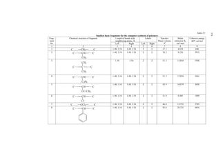
![557
PS-4
PET-1
PET-2
PC-1
PC-2
PC-3
O O
C (CH2 CH) C
n
O (CH2
HO [C H
C )2 O]
O
O
n
O (CH2
HO [C C
C )2 O]
O
n
O O
O C] n OH
O
CH3
C
CH3
H [O
O C] n O
O
CH3
C
CH3
H [O
CH3
H [O C
O C] n O
O
CH3
C
CH3
CH3
For all structures, Van-der-Waals volumes ΣΔ
i
C OH
O
OH
i V , molar refractions Σi
Ri
and molar cohesive energies ΣΔ
i
Ei* have been calculated. As an example, let us
consider in detail the calculation of these characteristics for PMMA-1 structure.
PMMA-1
Δ Σi
Vi = 3ΔVC,13 + ΔVC,1 + 2ΔVC,48 + 2ΔVC,41 + ΔVC,10 + ΔVC,6 + 18ΔVH,124
+ 2ΔVO,129 + 2ΔVO,139 + (ΔVC,10 + ΔVC,1 + ΔVC,13 + ΔVC,48 + ΔVC,41 + 8ΔVH,124 +
ΔVO,129 + ΔVO,139)(n – 2);
PMMA-1
Δ Σi
Vi = 3⋅17.2 + 5.0 + 2⋅15.9 + 2⋅20.3 + 13.1 + 9.0 + 18⋅2.0 + 2⋅3.4 +
2⋅5.8 + (13.1 + 5.0 + 17.2 + 15.9 + 20.3 + 8⋅2.0 + 3.4 + 5.8)(n – 2) = 205.5 +
(n – 2)⋅96.7 Å3.](https://image.slidesharecdn.com/computationalmaterialsscienceofpolymers-141021180636-conversion-gate02/85/Computational-materials-science-of-polymers-592-320.jpg)
;
( ) 1 - PMMA p l
C = 0.34565⋅(3⋅17.2 + 5.0 + 2⋅15.9 + 2⋅20.3 + 13.1 + 9.0) + 0.62289⋅18⋅2.0
+ 0.92998⋅(2⋅3.4 + 2⋅5.8) + [0.34565⋅(13.1 + 5.0 + 17.2 + 15.9 + 20.3) +
0.62289⋅8⋅2.0 + 0.92998⋅(3.4 + 5.8)](n – 2) = 91.8 + 43.2(n – 2) cal/(mol⋅deg).
Table 49
Values ΣΔ
i
Vi , ΣΔ
i
Ei* , Σi
Ri and Clp for PMMA-5 with different values of the
polymerization degree n
n
0
Δ Σi
Vi , Å3
0
*
Δ Σi
Ei , cal/mol
0
Σi
Ri , cm3/mol
Clp,0 ,
cal/(mol⋅deg)
1 297.0 17541 84.42 125.0
2 197.0 11292 54.50 84.5
3 163.0 9209 44.70 70.7
4 146.5 8168 39.80 63.8
5 136.6 7543 36.60 59.6
7 115.6 6363 31.60 50.3
10 107.0 5828 29.07 46.8
15 100.3 5411 27.08 44.0
20 97.0 5203 26.08 42.7](https://image.slidesharecdn.com/computationalmaterialsscienceofpolymers-141021180636-conversion-gate02/85/Computational-materials-science-of-polymers-593-320.jpg)

![560
end group possesses a significant Van-der-Waals volume, it contributes substantially
to the physical characteristics, and values
0
Δ Σi
Vi ,
0
*
Δ Σi
Ei ,
0
Σi
Ri and
Clp,0 at low n appear sharply different from asymptotic ones. The asymptote is
approached (depending on type of the end group) at n = 10–20, which is assumed
sometimes for the value of the chain segment. This situation is typical, for example,
of PMMA-4, when benzoyl peroxide is used as an initiator in polymerization of
methyl-methacrylate.
Analyzing the data obtained in ref. [8], some other regularities of the influence
of the chemical structure of end groups on the physical characteristics of the polymer
may be observed. For example, the Van-der-Waals volume of the averaged repeat unit
of the polymer is generally affected by the volume of end groups. The same may be
indicated for molar refraction. Consideration of Figure 102 confirms this conclusion.
For systems PMMA-1, PMMA-2 and PMMA-3, the Van-der-Waals volume and the
molar refraction weakly depend on n. This is clearly indicated by consideration of
curves 1–3 in Figure 102. The same may be also said about the cohesive energy of
these systems. This is associated with the fact that in the case of PMMA-1, PMMA-2
and PMMA-3, end groups do not enter any specific intermolecular interaction. That is
why they cause no significant change of the cohesive energy. In turn, the presence of
bulky end groups significantly different from the repeat unit of the polymer by the
chemical structure leads to a sharp change of all the characteristics discussed (see
Figure 102, curves 4, 5). All the above-said also relates fully to systems based on
polystyrene.
Systems containing end groups, although of small volume but possessing a
strong specific intermolecular interaction, behave themselves differently. For
example, they may be end OH-groups in the case of poly(ethylene terephthalate) and
polycarbonate. This specificity of the structure of end groups leads to different
regularities: the characteristics associated with volume and molecular refraction
change insignificantly with n; in turn, cohesive energy, in which specific
intermolecular interaction plays a highly significant role, changes greatly as n
increases. All this must be taken into account when the influence of the
polymerization degree (especially, on initial stages of the process) on the measured
physical characteristics is analyzed.
Above, we analyzed the physical characteristics of a series of polymers
dependent on the chain length. These characteristics are initial for the estimation of
the physical parameters of polymeric substances. For example, due to the Van-der-
Waals volume
0
Δ Σi
Vi and cohesive energy
0
*
Δ Σi
Ei important parameters of
the substance such as the density of cohesive energy or Hildebrand solubility
parameter may be calculated. Of interest is also the dependence of this parameter δ on
n at transition from monomer to dimer, trimer, etc.
These calculations were performed in ref. [8] for systems PMMA-4, PS-4,
PETP-1 and PC-1. Calculation results in the form of dependence of δ on n are
displayed in Figure 103. One can recognize that for some systems (PMMA-4, PS-4)
regardless of whether they contain bulky end groups or not, the solubility parameter
depends significantly on n. This is associated with the fact that the presence of end
OH-groups in these polymers causes the appearance of hydrogen bonds that requires](https://image.slidesharecdn.com/computationalmaterialsscienceofpolymers-141021180636-conversion-gate02/85/Computational-materials-science-of-polymers-595-320.jpg)

![Chapter XVI. Thermophysical properties of polymers
The thermophysical properties are heat capacity, thermal diffusivity and heat
conductivity.
XVI.1 Heat capacity
Heat capacity is the amount of heat which must be consumed for heating a
body up by 1°C. Molar heat capacity, if a mole of substance is considered, and
specific heat capacity in the case of 1 g of substance, differ. Heat capacity at constant
pressure Cp equals the rate of enthalpy change with temperature increase, and heat
capacity at constant volume Cv – the rate of internal energy change with temperature
increase.
In a quite wide temperature range, heat capacity increases linearly with
temperature, the temperature coefficient of heat capacity increase for solid polymers
possessing the average value of 3⋅10–3. At phase or physical transition of the polymer,
heat capacity changes in a jump-like manner.
For example, transition from the glassy to rubbery state indicates quite a sharp
jump-like increase of heat capacity. When the physical transition is passed, heat
capacity returns to weak growth with temperature.
The heat capacity of polymers depends on their chemical structure (Table 50).
Among polymeric hydrocarbons, the lowest heat capacity is displayed by
polyethylene and polyoxymethylene.
When hydrogen atoms are substituted by polar groups, heat capacity increases.
Also, heat capacity rapidly increases in transition from aliphatic to aromatic polymers.
Many attempts have been made to calculate the heat capacity of polymers on
the basis of the chemical structure of the repeat unit. Let us consider the method of
calculation discussed in ref. [22]. In the work cited, it is supposed that the molar heat
capacity of a polymeric substance is proportional to the Van-der-Waals volume of
atoms of the repeat unit of the polymer. To put it differently,
Cp s
=ΣC , ΔV + A s
(XVI.1)
i
i
s
p i
and
Cp l
=ΣC , ΔV + A l
, (XVI.2)
i
i
l
p i
where s
Cp and l
Cp are the molar heat capacities of the polymer in the glassy state and
the rubbery state, respectively; s
Cp,i and l
Cp,i are constants for each atom having the
meaning of heat capacities reduced to the unit Van-der-Waals volume and applicable
for the glassy state and the rubbery state, respectively; As and Al are parameters equal
to: As = 0.77 cal/(mol⋅deg), Al = 0.69 cal/(mol⋅deg).](https://image.slidesharecdn.com/computationalmaterialsscienceofpolymers-141021180636-conversion-gate02/85/Computational-materials-science-of-polymers-597-320.jpg)


![566
and transverse to the orientation axis. The thermal properties of polymers are
discussed in more detail in reviews [59, 61, 62].
Table 53
Heat conductivity λ for a series of polymers at 293 K
Polymer Structural formula λ, W/(m⋅K)
Polyethylene of:
High pressure
Low pressure
CH2CH2 0.380
0.470
Polypropylene:
Atactic
Isotactic
0.175
0.230
CH3
CH2 CH
Polystyrene 0.130
CH2 CH
Poly(vinyl chloride) 0.170
CH2 CH
Cl
CH3
Poly(methyl methacrylate) 0.190
C
C
CH2
O
O
CH3
Polytetrafluoroethylene CF2CF2 0.250
Poly(dimethyl siloxane) 0.167
CH3
Si
O
CH3](https://image.slidesharecdn.com/computationalmaterialsscienceofpolymers-141021180636-conversion-gate02/85/Computational-materials-science-of-polymers-601-320.jpg)
![Chapter XVII. Molecular design and computer synthesis of
polymers with predetermined properties
In previous sections of the book, the possibility of calculating the physical
properties of polymers on the basis on the chemical structure of the repeat unit of
linear polymers or the repeating fragment of polymer networks was demonstrated. At
the present time, the above-mentioned calculations are performed in a computer.
Therewith, main direct and reverse tasks and secondary tasks may be solved.
The direct task concludes in calculating the polymer properties from the data
on the chemical structure of the repeat unit of the polymer or a fragment of network.
The reverse task (which is more complicated) consists of predicting the
structural formula of the repeat unit of the polymer which would have a single or
several required characteristics of the physical properties.
A solution of both tasks is described in refs. [9, 17, 26, 126].
When setting and solving problems, two border approaches and a series of
intermediate approaches are possible. The first border approach concludes in
recording in computer memory a large number of polymers with different chemical
structure for which the physical characteristics mentioned above were previously
calculated. Then, computer’s role will conclude only in the search for necessary
structural formulas in the database and layout of the required information, when both
direct and reverse tasks are solved. In the case of such approach, the accuracy of
layout characteristics is close to 100%, but the predictive power for structures absent
in the database equals zero. In fact, such approach enables just to create a database.
The second border variant concludes in the following. A table of Van-der-
Waals volumes of atoms is recorded in the computer memory. A fragment of this
Table is shown as an example below.
C
H
1.54 1.08
1.54 1.54
C
1.54
1.54 1.54
C C
C
O
1.54 1.54
1.08
1.54 1.54
C C
C C C
C
1.08
1 2 3 4
1.54 1.54
C C
C
C
1.08 1.28
5 6 7 8
In principle, each of the atoms squared by dotted lines may be valently bonded
to other atoms; for the above-depicted structures, this possibility is demonstrated by
the matrix (1 – joining is possible; 0 – prohibition):
Atom, No. 1 2 3 4 5 6 7 8
1 1 1 1 1 1 0 0 0
2 1 1 1 1 1 1 0 0
3 1 1 1 1 1 0 1 0
4 1 1 1 1 1 1 0 0
5 1 1 1 1 1 0 0 1
6 0 1 0 1 0 0 0 0
7 0 0 1 0 0 0 0 0
8 0 0 0 0 1 0 0 0
C C
C
1.54
C
1.50
1.54
C
H
H
1.28
O
1.54 1.54
C O C
O
H
C](https://image.slidesharecdn.com/computationalmaterialsscienceofpolymers-141021180636-conversion-gate02/85/Computational-materials-science-of-polymers-602-320.jpg)
![568
The table representing Van-der-Waals volumes of atoms, shown in the present
monograph, contains over 200 values of volumes for atoms valently bonded with
other various atoms. The task of building a repeat unit of a polymer from all this
multiplicity of atoms, even at their limited amount in the repeat unit, is rather difficult
to be computerized, and its solution by a computer requires too much computer time
due to the appearance of a tremendous amount of variants. In the present case, we are
talking about solving the reverse problem, when polymers with given properties are to
be ‘synthesized’ using a computer.
The above-discussed situation led to the need to develop an intermediate
approach (between the border ones described) to computerized prognosis of the
physical characteristics of polymers and their computerized synthesis. This approach
concludes in preliminary summation of all constants participating in the initial
correlations for calculation of properties for separate fragments (‘basic fragment’),
from which then a repeat unit of a polymer is constructed on a computer.
The variant of the software described in ref. [17] provides constructing of
polymers, repeat units of which contain two fragments only possessing a possibility of
chemical bonding with each other. According to the method of mutual joining, all the
fragments discussed are subdivided into 8 classes:
Class Structure Class Structure
I 1.54 1.54
V
C R1 C
II 1.48 1.48
VI
C R2 C
III 1.50 1.50
VII
C O R1,2 O C
IV VIII
1.37 1.37
C O R1,2 O C
1.50 1.50
O R1,2 O
1.37 1.37
O R2 O
1.37 1.37
N R1,2 N
1.37 1.37
C R3 C
CH
OH
where R1: CH2; ; (CH2)4, etc.; R2: ;
, etc.;
O
O
C
N
O
C
N
O
C
N
O
O C
N
R3:, ; , etc.
C
C
O
O
C
O
C
O
The matrix shown below reflects possibilities of mutual joinings of the
fragments related to different classes (1 –joining is possible; 0 – prohibition):](https://image.slidesharecdn.com/computationalmaterialsscienceofpolymers-141021180636-conversion-gate02/85/Computational-materials-science-of-polymers-603-320.jpg)
![569
Fragment, No. I II III IV V VI VII VIII
I 1 0 0 0 0 0 0 0
II 0 1 0 0 0 0 0 0
III 0 0 0 0 1 0 0 0
IV 0 0 0 0 0 1 0 0
V 0 0 1 0 0 0 0 0
VI 0 0 0 1 0 0 0 0
VII 0 0 0 0 0 0 0 1
VIII 0 0 0 0 0 0 1 0
Generally, ref. [17] presents series of constants calculated for 194 fragments
(‘basic fragments’) of various chemical structures. As an example, some of them are
shown in Table 54. Dotted squares mark the chemical structure of the fragment itself;
also displayed are atoms, joined to the fragment, and lengths of chemical bonds
expressed in Å.
The possibility of joining of one of 18 fragments to another, taking into
account their belonging to different classes, is demonstrated in the following matrix
(1 – joining is possible; 0 – prohibition):
Fragment, No. 1 2 3 4 5 6 7 8 9 10 11 12 13 14 15 16 17 18
1 1 1 1 0 1 1 1 1 1 0 0 0 0 0 0 0 0 0
2 1 1 1 0 1 1 1 1 1 0 0 0 0 0 0 0 0 0
3 1 1 1 0 1 1 1 1 1 1 0 0 0 0 0 0 0 0
4 0 0 0 0 0 0 0 0 0 0 0 0 0 0 0 0 1 0
5 1 1 1 0 1 1 1 1 1 0 0 0 0 0 0 0 0 0
6 1 1 1 0 1 1 1 1 1 0 0 0 0 0 0 0 0 0
7 1 1 1 0 1 1 1 1 1 0 0 0 0 0 0 0 0 0
8 1 1 1 0 1 1 1 1 1 0 0 0 0 0 0 0 0 0
9 1 1 1 0 1 1 1 1 1 0 0 0 0 0 0 0 0 0
10 0 0 0 0 0 0 0 0 0 1 1 1 1 0 0 0 0 0
11 0 0 0 0 0 0 0 0 0 1 1 1 1 0 0 0 0 0
12 0 0 0 0 0 0 0 0 0 1 1 0 0 0 0 0 0 0
13 0 0 0 0 0 0 0 0 0 1 1 0 0 0 0 0 0 0
14 0 0 0 0 0 0 0 0 0 0 0 0 0 0 0 0 0 1
15 0 0 0 0 0 0 0 0 0 0 0 0 0 0 0 0 0 1
16 0 0 0 0 0 0 0 0 0 0 0 0 0 0 0 0 0 1
17 0 0 0 1 0 0 0 0 0 0 0 0 0 0 0 0 0 0
18 0 0 0 0 0 0 0 0 0 0 0 0 0 1 1 1 0 0
The program contemplates both the solutions of the direct task concluded in
the determination of polymer properties basing on the chemical structure of the repeat
unit and the reverse task consisted in searching for the units such that the polymer
composed from them would possess the given physico-chemical properties. Solving
the reverse task, the computer calculates a parameter of one of the required properties
using all probable variants of combinations from ‘basic fragments’ recorded by its
memory. For polymers, the property of which appears in the required interval, the
parameter of another property is calculated, after which the required polymers are also
selected, etc.
The drawback of this software is that composition of a repeat unit of a
polymer from two large ‘basic fragment’ does not embrace the tremendous amount of
probable structures. Obviously, the smaller the size of ‘basic fragments’ used for
composing the repeat unit, the more variants of polymers may be obtained due to the
great amount and multiplicity of ‘basic fragments’ in the unit and for calculating their
properties.](https://image.slidesharecdn.com/computationalmaterialsscienceofpolymers-141021180636-conversion-gate02/85/Computational-materials-science-of-polymers-604-320.jpg)
![570
That is why A.A. Askadskii, E.G. Galpern, A.L. Chistyakov, and I.V.
Stankevich [126] have created a software for computer ‘synthesis’ of polymers from
the scarcest ‘basic fragments’, i.e. those which, in principle, cannot be sectioned.
These basic fragments are shown in Table 55.
To denote the possibility of joining these small fragments, recorded in the
computer memory, to each other, definite labels are attributed to every end of ‘basic
fragments’. Note that the fragments used for composing the repeat unit possess only
20 different end groups and, consequently, 20 different labels (see Table 55), which
may interact with each other in accordance with the matrix recorded by the computer
memory:
LABELS 1 2 3 4 5 6 7 8 9 10 11 12 13 14 15 16 17 18 19 20
1 1 1 1 0 0 0 0 0 0 0 0 0 0 1 0 0 1 0 0 1
2 1 0 1 0 0 0 0 0 0 0 0 0 0 0 0 0 0 0 0 0
3 1 1 1 0 0 0 0 0 0 0 0 0 0 1 0 0 0 0 1 0
4 0 0 0 0 0 0 0 1 0 0 0 0 0 0 0 0 0 0 0 0
5 0 0 0 0 0 0 0 0 1 0 0 0 0 0 0 0 0 0 0 0
6 0 0 0 0 0 0 0 0 0 0 1 0 0 0 1 0 0 1 0 0
7 0 0 0 0 0 0 0 0 0 0 0 1 0 0 0 0 0 0 0 0
8 0 0 0 1 0 0 0 0 0 0 0 0 0 0 0 0 0 0 0 0
9 0 0 0 0 1 0 0 0 0 0 0 0 0 0 0 0 0 0 0 0
10 0 0 0 0 0 0 0 0 0 0 0 0 1 0 0 0 0 0 0 0
11 0 0 0 0 0 1 0 0 0 0 0 0 0 0 0 1 0 0 0 0
12 0 0 0 0 0 0 1 0 0 0 0 0 0 0 0 0 0 0 0 0
13 0 0 0 0 0 0 0 0 0 1 0 0 0 0 0 0 0 0 0 0
14 1 0 1 0 0 0 0 0 0 0 0 0 0 0 0 0 0 0 0 0
15 0 0 0 0 0 1 0 0 0 0 0 0 0 0 0 0 0 0 0 0
16 0 0 0 0 0 0 0 0 0 0 1 0 0 0 0 0 0 1 0 0
17 1 0 0 0 0 0 0 0 0 0 0 0 0 0 0 0 0 0 0 0
18 0 0 0 0 0 1 0 0 0 0 0 0 0 0 0 1 0 0 0 0
19 0 0 1 0 0 0 0 0 0 0 0 0 0 0 0 0 0 0 0 0
20 1 0 0 0 0 0 0 0 0 0 0 0 0 0 0 0 0 0 0 0
In this matrix, no difference is made for the given C–C bond of 1.54 Å (in
aliphatic fragments) and 1.48 Å (in aromatic fragments), because transition from one
bond to another causes only insignificant changes in the Van-der-Waals volume,
which display no substantial influence on the accuracy of calculation of physical
properties.
Figure 105. Schematic representation of construction of the combinatorial tree when constructing a
repeat unit of polymer (see text).](https://image.slidesharecdn.com/computationalmaterialsscienceofpolymers-141021180636-conversion-gate02/85/Computational-materials-science-of-polymers-605-320.jpg)


![582
As an example illustrating building of the repeat unit, Figure 105 shows a
combinatorial tree, which is composed from three fragments (‘basic fragments’) with
various end labels. The rule, according to which the formation of a bond between end
groups is permitted, or prohibited, is reflected in the matrix of their interactions.
Clearly, the quantity of probable variants of the repeat unit of the polymer increases
with every step of joining a consequent fragment.
It should be taken into account that if all ‘basic fragments’ recorded by the
computer memory participate in the composition and therewith each of them may join
to the propagating unit by both one or another ends, then 2n of variants of the repeat
unit (where n is the number of ‘basic fragments’) appear on every stage of joining of
the next fragment. Hence, this procedure represents a geometric progression with
denominator 2.
Besides direct and reverse tasks, software for prognosis of the physical
properties of polymers enables other tasks to be solved. For example, the upper and
lower ranges of the physical characteristics may be determined which, in principle,
organic polymers are able to display; for example, the lower value of the onset
temperature of intense thermal degradation of organic polymers, Td, is 150°C, and the
upper limit is 575°C. Hence, an organic polymer possessing the onset temperature of
intense thermal degradation above 575°C is difficult to produce. ‘Combination’ of
various properties in the same polymer may also be estimated, etc. (see below).
Software based on using the finest basic fragments enables calculations and
‘synthesis’ of polymers of the following classes:
1. Polyolefins, vinyl polymers, etc.
2. Polyethers and polyetherketones
3. Polyesters
4. Polyamides
5. Polysulfones, polyethersulfones
6. Polyimides
7. Polyoxadiazoles
8. Polybenzimidazoles
9. Polysulfides
10. Organosilicon polymers
11. Polycarbonates
The number of polymer classes may be increased, if necessary. This requires
introduction of a group determining affiliation of polymers to the chosen class into the
database; for example, introduction of urethane group into the database enables to
calculate properties of polyurethanes and to synthesize polyurethanes with the given
properties in a computer. The drawback of this software is that the above-mentioned
tasks may be solved only for polymers containing the basic fragments present in the
database. Although the number of polymers is great in this case, some limits do exist.
In this connection, A.A. Askadskii and A.F. Klinskikh [22] created software,
according to which the chemical structure of a polymer is ‘gathered’ not from ‘basic
fragments’, but from separate atoms. In this case, the chemical structure of a repeat
unit is displayed on the screen in the form of a structural formula of an organic
compound, as a chemist writes it down on paper. After that, the physical properties of
the polymer of the given structure are calculated and laid out immediately to the user.
Therewith, the molecular design of a polymer may be performed by changing its
chemical structure, introducing various groups, etc., and its physical characteristics
are obtained immediately. This program enables us to solve the first (direct) task only,
because when polymers are synthesized from separate atoms (but not ‘basic](https://image.slidesharecdn.com/computationalmaterialsscienceofpolymers-141021180636-conversion-gate02/85/Computational-materials-science-of-polymers-617-320.jpg)


![586
The program was tested on all compounds for which, on the one hand,
experimental data were known and, on the other hand, calculations by the method of
constants had been performed before. For example, the properties of polyolefins,
vinyl, acrylic and dienic polymers, aliphatic and aromatic polymers (including
polyamides), polyesters, polyimides, polysulfones, polyetherketones, etc. were
calculated. It has been shown that the program successfully interprets the structure of
the repeat unit in accordance with the calculation scheme of the method of constants,
and provides for required accuracy of the calculation method of 3–5%. Examples of
solving the direct, reverse and combined tasks of computerized synthesis of polymers
based on the above-described programs are indicated in Appendices 1 – 3.
Let us consider one more task, which may be solved by the above-described
software.
At present, in connection with the application of polymers to various spheres,
requirements on their physical properties have become much stricter. Problems
appear, solutions of which require polymers with a combination of a series of physical
properties, simultaneously falling within the given ranges of the values of their
characteristics. A question is raised about the combination of properties of polymers.
Described in ref. [23] is the method of its solving with the help of ‘miscibility
diagrams’, which consists of the following: assume that for a large group of polymers
values of parameters of any two physical properties (from experiment or calculation)
are known. Let us compose a diagram on which a specific point (Figure 106)
corresponds to every polymer, where the abscissa axis (X) represents the values of the
parameters of the first property, and on the ordinate axis (Y) – of the second one. All
these points are located inside some region, which may be contoured. This region is
called ‘the miscibility region’ of the mentioned physical properties for the given
group of polymers. Attention should be paid to the fact that the density of points
distribution in the region may be rather irregular. Such diagrams enable to estimate
possibility of existence of polymers with given properties without additional
consumption of labor. Actually, let the ranges (X2 – X1) and (Y2 – Y1) of values of
properties, which must be possessed by polymers, be given. If the area determined by
these ranges, falls within the miscibility region in the diagram, and some points exist
there, i.e. the polymer may exist (case I). In the opposite case, obtaining the required
polymer among polymers of these classes is of low probability (case II).
To compose miscibility diagrams of this kind, either experimental data on
various physical properties of polymers, or calculated data may be used.
Combinations of these data may also be used.
To calculate various physical properties of polymers, it is desirable to apply
the computer program suggested in ref. [17], because with the help of it the properties
of polymers either already synthesized, or the ones which may be, in fact, synthesized
are considered. This very program was used in ref. [23] for composing combination
regions of various properties of polymers. Among these properties the following were
considered: density, ρ; refractive index, n; glass transition temperature, Tg; the
relation of glass transition temperature to the melting point, Tg/Tm; the onset
temperature of intense thermal degradation, Td; the Hildebrand solubility parameter, δ
(density of cohesive energy); stress-optical coefficient Cσ.
Ref. [23] indicates 27 diagrams built on a computer, which reflect
combination of any two of the above-mentioned physical properties. Formulae, with
the help of which the connection between two given parameters of properties may be
searched, are shown in monograph [6].](https://image.slidesharecdn.com/computationalmaterialsscienceofpolymers-141021180636-conversion-gate02/85/Computational-materials-science-of-polymers-621-320.jpg)

![588
Every diagram contains a point from which these dependences start. This is
associated with the program feature [17], in which several homologues (CH2)n up
to n = 20 are set as original fragments from the total 194 ones, and the point, from
which these dependences start, characterizes polyethylene.
Other features inherent to each diagram are clearly seen in corresponding
figures. Having these diagrams, the possibility of obtaining polymers, which would
possess the necessary combination of one of several properties may be predicted. For
example, if polymers with the solubility parameter δ = 10 (cal/cm3)1/2 and Tg ≈ 300°C
should be obtained, it may be made easily, because the point corresponded to these
coordinates falls within the densest part of the diagram in Figure 107b. It would be
quite difficult to produce a polymer with the glass transition temperature Tg ~ 500°C
at the same solubility parameter, and at Tg = 600°C this becomes practically
impossible, because the point corresponding to these coordinates is out of the range of
the ‘miscibility’ region. This analysis may be easily performed for any diagram
presented in ref. [23], as well as for a set of these diagrams, which enables us to
predict the possibility of obtaining polymers with a a set of the required properties.
Clearly, that if such diagrams are composed with the help of a computer program,
according to which the polymer is composed from the finest ‘basic fragments’, the
regions of miscibility of polymers will be significantly expanded by points reflecting
properties of the very large number of polymers.](https://image.slidesharecdn.com/computationalmaterialsscienceofpolymers-141021180636-conversion-gate02/85/Computational-materials-science-of-polymers-623-320.jpg)


![597
Table A-1-3
Fragmentary composition and structural formulae of hemicelluloses
Designations of
hemicelluloses
Fragmentary composition and name
of natural biopolymer
Structural formulae of hemicelluloses
1 2 3
C1 (Fs12)3–(Fs2)42–(Fs1)23–(Fs11)5
aspen glucomannan [208]
C2 (Fs12)2–(Fs2)13–(Fs1)5–(Fs12)3
spruce glucomannan [116]
O
OH
OH
O
42 23 5
3
CH2OH
OH
O
O OH
O
OH O
OH
O
OH
CH2OH
OH
CH2OH
O
OH
CH2OH
OH O
O
OH
CH2OH
O
OH
CH2
OH O
3
O
13 5
2
CH2OH
OH
O
O OH
O
OH O
OH
O
OH
CH2OH
OH
CH2OH
O
OH
CH2OH
O
CH2OH
OH O OH
OH
O
OH
CH2OH
OH
O
O
597](https://image.slidesharecdn.com/computationalmaterialsscienceofpolymers-141021180636-conversion-gate02/85/Computational-materials-science-of-polymers-632-320.jpg)
![598
1 2 3
C3 (Fs10)19–(Fs3)125–(Fs6)5
aspen 4-0-methylglucuronoxylan
[117]
C4 Fs3–Fs10–Fs3–Fs6–Fs8–Fs15
spruce arabinoglucuronoxylan [118]
O
O OH
OH
OCH3
O
O
OH
COOH
O
O
OH O
OH
O
OH
O
OH
OH
O
125
OH 19
5
O
OH
O
O
O
OH
COOH
OH
OCH3
O
OH
OH
O
O
O O OH
OH
OH
O
O
O
OH
O
OH
OH
OH
O
O
O
O
OH
OH
OH
O
OH
OCH3
COOH
O
OH
O
OH
OH
O O
OH
598](https://image.slidesharecdn.com/computationalmaterialsscienceofpolymers-141021180636-conversion-gate02/85/Computational-materials-science-of-polymers-633-320.jpg)
![599
1 2 3
C5 Fs7–(Fs4)50–Fs7
Galactouronan from plants [130]
C6 (Fs9)8–(Fs5)21–(Fs3)52–(Fs13)15–(Fs5)3
birch xylan [118]
O
COOH
OH O
COOCH3
O
OH O
OH
COOH
O
OH
O
OH
OH
O
OH
O
OH
OH
O
OH
O
50
O
OH
O
COOCH3
O
COOCH3
OH
O
O
O COOCH3
OH
O OH
O
OH
O OH
O
O OH
O
COOCH3
OH
COOH
O
OH
H3CO
O
8
21 52
15
3
599](https://image.slidesharecdn.com/computationalmaterialsscienceofpolymers-141021180636-conversion-gate02/85/Computational-materials-science-of-polymers-634-320.jpg)
![600
1 2 3
C7 Fs16–Fs14
larch arabinogalactan [60]
C8 [Fs2–Fs1–(Fs2)4–Fs1–Fs2]48
1,4-β-D-glucomannan [2]
OH O
OH
OH
O
CH2
O
OH O
OH
CH2OH
OH O
OH
OH
OH O
OH
O
CH2
O
OH O
OH
CH2OH
OH
OH O
OH
O
CH2
O
O
O
CH2
OH O
OH
CH2OH
OH
OH O
OH
CH2OH
OH O
OH
O
CH2OH
OH OH
O
O
O
OH
CH2OH
OH
O
CH2OH
O
OH OH
O
CH2OH
O
OH OH
O
CH2OH
O
OH OH
O
CH2OH
O
OH OH
O
O
OH
CH2OH
OH
O
CH2OH
O
OH OH
48
Note: chemical formulae of hemicelluloses and the sample of 1,4-β-D-glucomannan shown in the Table were presented by Doctors of Biology V.D. Shcherbukhin and A.V.
Bolobova.
600](https://image.slidesharecdn.com/computationalmaterialsscienceofpolymers-141021180636-conversion-gate02/85/Computational-materials-science-of-polymers-635-320.jpg)


![Appendix 3. The example of solving the complex problem –
analysis of the chemical structure of phenol
formaldehyde resin
The example of solving the complex problem of polymer synthesis belongs to
the analysis of the chemical structure of one of the representatives of polymer
networks – phenol-formaldehyde resin widely applied, in particular, to production of
pressed woody articles.
Before analyzing the structure of a polymer network based on phenol
formaldehyde resin, it should be noted that although phenol formaldehyde resins
(PFR) are one of the oldest representatives of high cross-linked polymer networks,
their structure is still of great interest [201]. There is a broad list of works devoted to
the analysis of the structure and properties of PFR. However, there is still no general
point of view on the chemical structure of the network formed by these resins. The
reason is, apparently, in the fact that due to proceeding of the PFR curing the network
structure obtained may be different. Another reason is associated with the fact that
OH-groups capable of forming hydrogen bonds are present in the network structure.
These hydrogen bonds may be displayed in both intermolecular interaction of these
groups disposed in neighboring PFR chains and at the sacrifice of the same interaction
OH-groups disposed in the same repeat unit.
Figure A-3-1. Schematic representation of a network of hydrogen bonds (a) appearing between
neighboring chains and (b) within the same repeat unit.
The meaning of the notions of ‘intermolecular interaction’ and ‘intramolecular
interaction’ in the context of the approach under discussion should be explained with
the help of a simplified scheme represented in Figure A-3-1. Figure A-3-1a
demonstrates the case corresponding to the intermolecular interaction, which leads to
the formation of a network of physical (hydrogen) bonds linking chains. Clearly, the
formation of this network promotes an increase of the glass transition temperature.
The case displayed in Figure A-3-1b reflects the situation when two OH-groups are in
the same unit of the linear fragment of PFR, and hydrogen bonding then occurs in the
frames of the same unit, and the network of physical bonds between neighboring ones
is not formed. This problem was analyzed above in detail on the example of
poly(imidophenyl quinoxalines) and poly(amidophenyl quinoxalines). It stands to
reason that various types of intermolecular interaction (hydrogen bonding) causing a
significant influence on PFR properties, as it will be shown below, may coexist in
reality.
In cured PFR, according to the existing data, the following structures
(repeating fragments of the network) may exist:](https://image.slidesharecdn.com/computationalmaterialsscienceofpolymers-141021180636-conversion-gate02/85/Computational-materials-science-of-polymers-642-320.jpg)
![608
Structure 1:
CH2
CH2 CH2
OH
This structure is included only in the network the repeat unit of which is
marked by dotted lines.
The glass transition temperature of the network will be calculated using
equation (IV.85).
According to the definition of the chemical structure of the cross-linked point
of the network, the structure of the cross-linked point is formed by a selection of
atoms, including the one from which the chain is branched, and the neighboring atoms
with their substituents, as well. For structure 1 of the network, the structure of the
cross-linked point is marked by dotted lines:
CH2
OH
Clearly, the whole cross-linked point contains three such selections of atoms.
Then for the structure 1, we obtain*:
1
Δ Σi
Vi = 3(ΔVC,19 + ½ΔVC,12 + ½⋅2ΔVH,124) + 2ΔVC,18 + 2ΔVH,124 + ΔVC,20 + ΔVO,133
+ ΔVH,125 = 3(8.4 + ½⋅12.6 + ½⋅2⋅2.0) + 2⋅12.7 + 2⋅2.0 + 11.65 + 5.2 + 4.7 = 101.1 Å3;
1
Σ Δ +Σ
j
j
i
ai Vi b = aC(2ΔVC,18 + ΔVC,20) + aH(2ΔVH,124 + ΔVC,125) + aO,sΔVO,133 + bh
= [0.021(2⋅12.7 + 11.65) + 19.93(2⋅2.0 + 4.7) 7.03⋅5.2 – 139.6]⋅10–3 = 71.6⋅10–3 Å3
K–1;
1
Δ Σi
Ki Vi = KC(ΔVC,19 + ½ΔVC,12) + KH2⋅1/2ΔVH,124 = [1.15(8.4 + ½⋅12.6) +
2.307⋅2⋅1/2⋅2.0]⋅10–3 = 21.5⋅10–3 Å3K–1.
Substituting values of
Δ
Vi Σi,
1
1
Σ Δ +Σ
j
j
i
ai Vi b , and
1
Δ Σi
Ki Vi into
equation (IV.85), we obtain the following value of the glass transition temperature of
the network in the case of the ideal structure 1:
* Here and below, numbers of atoms correspond to their numbers in Table 3.](https://image.slidesharecdn.com/computationalmaterialsscienceofpolymers-141021180636-conversion-gate02/85/Computational-materials-science-of-polymers-643-320.jpg)
![609
3
101.1 ⋅
⋅ +
T = = 743 K. (A-3-1)
g 10
21.5 3 71.6
The calculated value of Tg is significantly above the range of experimental
values, Tg,exper, shown in Table A-3-1 and, consequently, the real PFR network will
differ by structure from the ideal structure 1.
Table A-3-1
Experimental values of the characteristics of cured PFR
Property name Unit Limits of measurements
Glass transition temperature, Tg,exper K 343–433
Density, ρ (exper.) g/cm3 1.24–1.33
Refractive index, n (exper.) rel. un. 1.57–1.63
Coefficient of volumetric expansion, αG (exper.) K–1 (1.80–2.25)⋅10–4
Molar heat capacity, sp
C (exper.) cal/(mol⋅deg) 29–48
Structure 2:
CH2 CH2
HO
CH2
OH
This possible structure of PFR relates to a linear polymer (the repeat unit is
marked by dotted lines).
For this structure,
ΣΔ
i
Vi = 3ΔVC,19 + 2ΔVC,18 + 1/2⋅2ΔVC,12 + ΔVC,20 + ΔVC,40 + 4⋅1/2ΔVH,124 + 2ΔVH,124
+ 2ΔVH,124 + 2ΔVH,125 + ΔVO,133 + ΔVO,132 = 3⋅8.4 + 2⋅12.7 + 1/2⋅2⋅12.6 + 11.65 + 16.0
+ 4⋅1/2⋅2.0 + 2⋅2.0 + 2⋅2.0 + 2⋅4.7 + 5.2 + 5.6 = 123.05 Å3;
Σ Δ
i
ai Vi = aC(3ΔVC,19 + 2ΔVC,18 + 1/2⋅2ΔVC,12 + ΔVC,20 + ΔVC,40) + aH(4⋅1/2ΔVH,124 +
2ΔVH,124 + 2ΔVH,124 + 2ΔVH,125) + aO,s(ΔVO,133 + ΔVO,132) = [0.021(3⋅8.4 + 2⋅12.7 +
1/2⋅2⋅12.6 + 11.65 + 16.0) + 19.98(4⋅1/2⋅2.0 + 2⋅2.0 + 2⋅2.0 + 2⋅4.7) + 7.03(5.2 +
5.6)]⋅10–3 = 505.4⋅10–3 Å3K–1.
If both OH-groups participate in the formation of hydrogen bonds between
chains (as shown in Figure A-3-1), then
Σj
j b = 2bh + bM; Σj
bj = (–139.6⋅2 + 16.0)⋅10–3 = –263.2⋅10–3 Å3K–1.
Substitution of all values of parameters into equation (IV.41) leads to the
following value of Tg of the ideal structure 2:
3
123.05 ⋅
−
T = = 508 K. (A-3-2)
g 10
505.4 263.2](https://image.slidesharecdn.com/computationalmaterialsscienceofpolymers-141021180636-conversion-gate02/85/Computational-materials-science-of-polymers-644-320.jpg)
![610
Similar to the structure 1, this value is higher than the experimental
temperature interval in which the α-transition is observed for PFR.
Structure 3:
CH2 CH2
OH
This structure forms only linear chains, the repeat unit of which is marked by
dotted lines. For structure 3, we obtain:
3
Δ Σi
Vi = 2ΔVC,19 + ΔVC,20 + 3ΔVC,18 + 1/2⋅2ΔVC,12 + 1/2⋅4ΔVH,124 + ΔVH,125 +
3ΔVH,124 + ΔVO,133 = 2⋅8.4 + 11.65 + 3⋅12.7 + 1/2⋅2⋅12.6 + 1/2⋅4⋅2.0 + 4.7 + 3⋅2.0 +
5.2 = 99.05 Å3;
3
Δ Σi
ai Vi = aC(2ΔVC,19 + ΔVC,20 + 3ΔVC,18 + 1/2⋅2ΔVC,12) + aH(1/2⋅4ΔVH,124 +
ΔVH,125 + 3ΔVH,124) + aO,s⋅ΔVO,133 = [0.021(2⋅8.4 + 11.65 + 3⋅12.7 + 1/2⋅2⋅12.6) +
19.98(1/2⋅4⋅2.0 + 4.7+ 3⋅2.0) + 7.03 5.2]⋅10–3 = 331.9⋅10–3 Å3K–1.
Σj
j b = 2bh + bM; Σj
bj = (–139.6 + 16.0)⋅10–3 = –123.6⋅10–3 Å3K–1.
Substitution of all these values of parameters into equation (IV.41) leads to the
following value of Tg of the ideal structure 3:
3
99.05 ⋅
−
T = = 476 K. (A-3-3)
g 10
331.9 123.6
This value of Tg is somewhat above the temperature range of the α-transition
for PFR.
Structure 4:
CH2 CH2
O
This structure forms a network, the repeating fragment of which is marked by
dotted lines. The structure of the cross-linked point of this network is the following
(marked by dotted lines):
H2C CH2
O](https://image.slidesharecdn.com/computationalmaterialsscienceofpolymers-141021180636-conversion-gate02/85/Computational-materials-science-of-polymers-645-320.jpg)
![611
For structure 4, we obtain:
4
Δ Σi
Vi = 2ΔVC,19 + ΔVC,20 + 1/2⋅2ΔVC,12 + 3ΔVC,18 + 3ΔVH,124 + 4⋅1/2ΔVH,124 +
ΔVO,131 = 3⋅8.4 + 11.65 + 1/2⋅2⋅12.6 + 3⋅12.7 + 3⋅2.0 + 4⋅1/2⋅2.0 + 2.1 = 91.25 Å3;
4
Δ Σi
ai Vi = aC(3ΔVC,18) + aH(3ΔVH,124) = (0.021⋅3⋅12.7 + 19.98⋅3⋅2.0)⋅10–3 =
120.7⋅10–3 Å3K–1;
Σj
bj = 0;
4
Δ Σi
Ki Vi = KC(2ΔVC,19 + ΔVC,20 + 1/2⋅2ΔVC,12) + KH⋅4⋅1/2ΔVH,124 + KOΔVO,131 =
[1.15(2⋅8.4 + 11.65 + 1/2⋅2⋅12.6) + 2.307⋅4⋅1/2⋅2.0 + 0.058⋅2.1]⋅10–3 = 56.5⋅10–3 Å3K–
1.
Substituting these values into equation (IV.85), we obtain the following value
of Tg for the ideal network, composed from the structure 4:
3
91.25 ⋅
+
T = = 515 K. (A-3-4)
g 10
56.5 120.7
Hence, the glass transition temperature of this cross-linked polymer network
would be quite high compared with Tg,exper.
Structure 5:
CH2 CH2
HO
CH2
OH
From the viewpoint of the gross-formula, this structure is identical to the
structure 2, but in the present case, hydrogen bonding appears within the single repeat
unit. Such a structure is described in ref. [99].
If hydrogen bonds are formed between neighboring OH-groups disposed
Σj
within the same repeat unit, then, as mentioned above, the physical network between
chains stipulated by hydrogen bonds is not formed. Then calculating the glass
transition temperature, the value of bj is calculated in the following way: because
Σj
this structure is linear, the constant bM must be taken into calculation when
considering the m-substitution in an aromatic cycle; moreover, there are two branches
from the aromatic cycle, which requires introduction of two constants bd. Then bj
= bM + 2bd = [16.0 – 2⋅55.4]⋅10–3 = –94.8⋅10–3 Å3K–1. Substituting values ΣΔ
i
Vi ,
Σ Δ
i
i i V a and Σj
bj into equation (IV.85), the following value of the glass transition
temperature is obtained for the structure 5:](https://image.slidesharecdn.com/computationalmaterialsscienceofpolymers-141021180636-conversion-gate02/85/Computational-materials-science-of-polymers-646-320.jpg)
![612
3
123.05 ⋅
T = = 300 K. (A-3-5)
g 10
−
505.4 94.8
This value of Tg falls below the range of the α-transition for cured PFR.
As indicated, no calculated values of the glass transition temperature of the
ideal structures of PFR discussed falls within the range of experimental values of the
glass transition temperature, Tg,exper. It may therefore be assumed that there is a more
complicated structure of cured PFR than the considered ideal ones; this has been
indicated by many investigators. Most probably, the real structure of PFR consists of
the selection of the considered ideal structures.
To state the most probablr real PFR structure, let us calculate, besides Tg, the
following characteristics of cured PFR: density ρ, refractive index n, coefficient of
volumetric expansion αG, and molar heat capacity sp
C . Selection of these character-istics
is stipulated by both their importance and sensitivity to changes of the structural
formula of the substance and the fact that for various ideal PFR structures, as the glass
transition temperature increases, values of other characteristics may increase or
decrease, which is important for search of the most probable structure of PFR by the
method of experiment design (see below).
The calculated values of PFR density for structures 1–5, obtained due to
equation (II.6), are indicated in Table A-3-2.
Table A-3-2
Calculated values of Tg, ρ, n, αG and s
Cp for the ideal structures of cured PFR
Ideal structure of PFR Tg, K ρ, g/cm3 n, rel. un. αG⋅104, K–1
s
Cp ,
cal/(mol⋅deg)
Structure 1 743 1.253 1.621 1.30 31.9
Structure 2 507 1.250 1.583 3.20 42.4
Structure 3 476 1.205 1.604 2.02 31.4
Structure 4 515 1.301 1.645 1.86 26.1
Structure 5 300 1.250 1.583 3.20 42.4
Let us calculate the refractive index n by equation (VIII.2), which contains the
molar refraction summed up from the refraction indices of separate atoms and
constants for different types of bonds (double, triple).
For structure 1, we obtain (values of Ri are taken from [28]):
R1 = 3⋅(RC + 1/2⋅RC + RH) + 2RC + 2RH + RC + RO′ + RH + 3R≠ = 3⋅(2.418 + 1/2⋅2.418
+ 1.10) + 2⋅2.418 + 2⋅1.10 + 2.418 + 1.525 + 1.10 + 3⋅1.733 = 31.459 cm3/mol.
For structure 2:
R2 = 8RC + 8RH + 2RO′ + 3R≠ = 8⋅2.418 + 8⋅1.10 + 2⋅1.525 + 3⋅1.733 = 36.393
cm3/mol.
For structure 3:
R3 = 7RC + 6RH + RO′ + 3R≠ = 7⋅2.418 + 6⋅1.10 + 1.525 + 3⋅1.733 = 30.25 cm3/mol.
For structure 4:
R4 = 7RC + 5RH + RO + 3R≠ = 7⋅2.418 + 5⋅1.10 + 1.643 + 3⋅1.733 = 29.268 cm3/mol.
For structure 5, the value R5 coincides with the value R2. Values of n for
various structures calculated by equation (VIII.2) are shown in Table A-3-2.
Heat capacity sp
C in the glassy state of the polymer was calculated by
correlation (XVI.1).](https://image.slidesharecdn.com/computationalmaterialsscienceofpolymers-141021180636-conversion-gate02/85/Computational-materials-science-of-polymers-647-320.jpg)
![613
The value αG is directly connected with the glass transition temperature Tg by
the correlation:
0.096
α = . (A-3-6)
(K)
G T
g
The calculated values of sp
C and αG for all five ideal structures are shown in
Table A-3-2.
Comparison of the calculated values of PFR characteristics for possible ideal
structures, shown in Table A-3-2, with their experimental values (see Table A-3-1)
enables us to conclude that cured PFR does not represent an ideal network, but
contains a set of structures; this set can be determined using the method of experiment
design for multi-component systems with composing simplex networks and
polynomial ‘composition – property’ models. For independent variables X of these
models, let us assume the above-considered ideal structures the combination of which
will determine the real structural composition of cured PFR: x1 for structure 1; x2 for
structure 2; x3 for structure 3; and x4 for structure 4. For the response function Y, the
following properties of cured PFR will be taken: glass transition temperature, Tg (K);
density, ρ (g/cm3); refractive index, n (rel. un.); coefficient of volumetric expansion,
αG (K–1); and molar heat capacity, sp
C (cal/(mol⋅deg)).
As indicated, instead of the ideal structure 2, the structure 5 is assumed as the
independent variable; this structure differs by the existence of hydrogen bonding of
OH-groups within the same repeat unit which, with all other characteristics being the
same, provides for lower glass transition temperatures (see Table A-3-2).
The dependence of the response functions Y on variables X will be searched
for in the form of the second order model [70]:
Y = Σβij + Σβijxixj; 1 ≤ i ≤ 4; 1 ≤ j ≤ 4, (A-3-7)
where
βi = yi; βij = 4yij – 2yi – 2yj. (A-3-8)
Design of the experiment and appropriate simplex lattice are shown in Table
A-3-3 and Figure A-3-2a, respectively.
Table A-3-3
Matrix of the experimental design and calculated values of PFR at the experimental design
Coordinates of
Point of the Calculated values of PFR
experiment design points
experiment
design x1 x2 x3 x4
Tg,
K
ρ,
g/cm3
n,
rel. un.
αG⋅104,
K–1
s
Cp ,
cal/(mol⋅deg)
y1 1 0 0 0 743 1.253 1.621 1.30 31.90
y2 0 1 0 0 300 1.250 1.583 3.20 42.40
y3 0 0 1 0 476 1.205 1.604 2.02 31.40
y4 0 0 0 1 515 1.301 1.645 1.86 26.10
y12 ½ 1/2 0 0 410 1.251 1.600 2.34 37.20
y23 0 1/2 1/2 0 359 1.232 1.594 2.67 36.90
y13 ½ 0 1/2 0 582 1.232 1.613 1.65 31.65
y14 ½ 0 0 1/2 615 1.276 1.633 1.56 29.00
y24 0 1/2 0 1/2 364 1.272 1.614 2.64 34.25
y34 0 0 1/2 1/2 494 1.254 1.624 1.94 28.75](https://image.slidesharecdn.com/computationalmaterialsscienceofpolymers-141021180636-conversion-gate02/85/Computational-materials-science-of-polymers-648-320.jpg)


![618
Figure A-3-4. Schematic representation of the search procedure for an acceptable set Ωx of ideal PFR
structures for x4 = 0. Showing domains of the acceptable sets of structures: (a)
=
for the glass transition temperature of cured PFR: (b) ρ
for the density; (c)
=
= for the refractive index; (d) G
= for the coefficient of volumetric
x1x4 0
expansion; (e)
= for the molar heat capacity; (f) 0 1 4
x x = for the ideal PFR
structures with the coordinates of vertices T1 (0.35; 0.34; 0.31; 0.00); T2 (0.34; 0.35;
0.31; 0.00); T3 (0.55; 0.45; 0.00; 0.00).
The region of acceptable selection of the ideal structures of cured PFR is
determined by consecutive sorting out of the regions const 1 4
x x = at variation of the
structure x4 content with step 0.01 from 0 to 1. Consequently, it is obtained that that
the desired region Ωx represents an improper figure and the coordinates of apexes of
this figure are shown in Figure A-3-6. Disposition of Ωx regions in the factor space of
ideal structures of PFR enables us to conclude that the real structure of cured PFR
may be represented only by the combination of linear (structures 3 and 5) and network
(structures 1 and 4) fragments of the polymeric chain; this has also been confirmed by
other investigators [99].
Figure A-3-5. Effect of the ideal structure 4 on the change of the domain Ωx of acceptable set of ideal
structures of cured PFR for the refractive index (I) and for the molar heat capacity (II) at
x4 = 0 (a); 0.2 (b); 0.4 (c).](https://image.slidesharecdn.com/computationalmaterialsscienceofpolymers-141021180636-conversion-gate02/85/Computational-materials-science-of-polymers-653-320.jpg)


![Appendix 4. Application of the approach to multicomponent
copolymers
Usually, analysis of the structure and properties of copolymers was performed
for the systems containing two components. It has been was performed much less
frequently for triple copolymers. In this appendix, applicability of the approach,
described in the present monograph, to analysis of the structure and properties of
copolymers containing from three to five copolymers will be discussed.
Simultaneously, let us compare experimental and calculated values of the physical
characteristics for both homopolymers and homopolymer-based multicomponent
copolymers.
To analyze the properties of multicomponent copolymers, six monomers are
chosen in ref. [39], used in reactions of polymerization and copolymerization: methyl
methacrylate (MMA), butyl methacrylate (BMA), butyl acrylate (BA), n-nonyl
acrylate (NA), 2-ethylhexyl acrylate (EHA), and n-heptyl acrylate (HA).
Homopolymers and copolymers based on these compounds are fully amorphous high-molecular
substances, which are easily formed in a block and suitable for
investigation of thermal and optical characteristics. Indicated in Table A-4-1 is the
composition of five copolymers synthesized in ref. [39]. Calculation of the glass
transition temperature Tg for multicomponent copolymers is performed by equations
(IV.55) and (IV.57). The first of these equations for calculation of the glass transition
temperature of copolymers requires no understanding of the experimental glass
transition temperatures of homopolymers. Equation (IV.57) contains values of glass
transition temperature of homopolymers, for calculation of Tg of copolymers
experimental values of Tg for appropriate homopolymers being used.
Table A-4-1
Composition of copolymers
Molar parts of units in copolymer
Copolymer
MMA BMA BA NA EHA HA
1 0.333 0.333 0.333
2 0.250 0.250 0.250 0.250
3 0.250 0.250 0.250 0.250
4 0.200 0.200 0.200 0.200 0.200
5 0.250 0.250 0.250 0.250
Density is calculated by equations (II.7), (A-4-1) and (A-4-2). The first of
them is approximate, obtained on the base of suggestion that the coefficient of
molecular packing is approximately the same for all polymers, and equals kavg = 0.681
for all block polymers at room temperature. However, for polymer and copolymers
existing in the rubbery state at room temperature, it is desirable to take into account
temperature dependences of the coefficient of molecular packing, k, in the density
calculation, because the difference of the real coefficient of packing for them from the
average value kavg, increases with a decrease of the glass transition temperature.
Equations (A-4-1) and (A-4-2) are obtained with regard to this circumstance and
enable, as indicated below, to calculate more accurately the density of polymers and
copolymers. For the latter, we obtain:](https://image.slidesharecdn.com/computationalmaterialsscienceofpolymers-141021180636-conversion-gate02/85/Computational-materials-science-of-polymers-656-320.jpg)

![623
M
0.667
+ − Δ
Σ Σ
Σ
=
α α
G g A k i
=
=
=
= k n
k i k
k n
k
k k
G
T N V
1
20 1
[1 (293 )]
α
ρ , 293 Tg; (A-4-1)
M
0.667
+ − Δ
Σ Σ
Σ
=
α α
L g A k i
=
=
=
= k n
k i k
k n
k
k k
G
T N V
1
20 1
[1 (293 )]
α
ρ , 293 Tg. (A-4-2)
Besides the glass transition temperature and density, the following
characteristics are calculated for copolymers: the refractive index n, the stress-optical
coefficient Cσ, temperature of the onset of intense thermal degradation Td, the
dielectric constant ε, the solubility parameter δ, the surface energy γ. Calculations
were performed using equations (VIII.3), (VII.7), (VIII.16), (IX.4), (XII.4), and
(XIII.39), respectively. First of all, let us compare the calculated and experimental
values of the properties of homopolymers. These data are indicated in Table A-4-2. In
most cases, good coincidence between experimental and calculated data is observed.
Separately, we must dwell on the calculation of such characteristic of homo- and
copolymers as density ρ, for which two values are shown in the Table. The first of
them is determined with the help of equation (II.7), and the second – by correlations
(A-4-1) and (A-4-2), which take into account the temperature dependence of the
coefficient of molecular packing. In the case of a glassy polymer (poly(methyl
methacrylate)), the calculated value of density obtained by equation (II.7) coincides
with the experimental value. For homopolymers with low glass transition
temperatures, which are in the rubbery state at room temperature, consideration of the
temperature dependence to the coefficient of molecular packing leads to lower values
of density compared with those determined on the base of the value kavg. Therewith,
the data on density values coincide with experimental ones.
The glass transition temperature, determined from equation (IV.41) with the
accuracy usual for such calculations, coincides with the experimental values. The
refractive index for homopolymers is calculated from equation (VIII.1), as well as
from equation (VIII.6), which takes into account the temperature dependence of the
coefficient of molecular packing. The latter circumstance enables us to calculate the
refractive index with high accuracy.
With regard to such characteristics as the solubility parameter, surface energy,
temperature of the onset of intense thermal degradation, the thermal coefficient of
volumetric expansion in the glassy state, and the stress-optical coefficient, they
coincide with the experimental ones with the accuracy usual for such calculations.
The properties of multi-component copolymers are indicated in Table A-4-3.
Here, the coincidence of the calculated and experimental characteristics is
approximately the same as for homopolymers. The density calculated from equation
(II.7) using the average value of the coefficient of molecular packing is somewhat
higher than the values, determined experimentally. This is stipulated by the fact that
all copolymers possess the glass transition temperature below room temperature.
Values of density ρ calculated by correlation (A-4-2) with regard to the temperature
dependence of the coefficient of molecular packing, is somewhat lower than these
calculated by equation (II.7), and coincide well with the experimental values of ρ.](https://image.slidesharecdn.com/computationalmaterialsscienceofpolymers-141021180636-conversion-gate02/85/Computational-materials-science-of-polymers-658-320.jpg)

![Appendix 5. Influence of strong intermolecular interaction
occurring between two dissimilar polymers on
their miscibility
When two or more polymers are mixed, the situation may appear when an
additional strong intermolecular interaction occurs between chains of these polymers,
which is not displayed between macromolecules of each of polymers, taken
separately. These may be hydrogen bonds or strong dipole–dipole interactions.
Analysis of the influence of these interactions on the glass transition temperature will
be shown below.
In a series of works devoted to the analysis of miscibility of polymers and the
properties of mixtures obtained, the main attention is paid to these special interactions
occurring between macromolecular chains of the mixed polymers. The scheme of this
interaction is demonstrated by the following example:
F3C CF3
O
H
O
Let us consider in detail examples of such interactions and experimental
methods of their determination. Mixtures of styrene copolymer with vinylphenylhexa-fluoromethylcarbynol
with the polymers as polycarbonate based on bisphenol A,
poly(butyl methacrylate), poly-2,6-dimethyl-1,4-phenylene oxide may represent an
example of this significant event [209]. Introduction of hydroxyl groups to the
mentioned polymer leads to the formation of hydrogen bonds between the copolymer
and polycarbonate, which causes a sharp increase of miscibility. The thermograms
obtained by the DSC method for polystyrene mixtures with polycarbonate show
clearly two glass transition temperatures indicating immiscibility of these polymers.
The situation is changed abruptly when polystyrene introduced to the mixture is
substituted by a copolymer of the above given structure: thermograms indicate the
single glass transition temperature (which indicates miscibility). Therewith, the glass
transition temperature regularly increases with the concentration of polycarbonate.
Mixtures of copolymers of the above-mentioned structure with poly(ethylene oxide)
(PEO), which represents the solid polymer, also display this effect [210]. Crystallinity
of PEO in the mixture varies in the manner by which the melting point decreases. The
formation of hydrogen bonds between PEO and copolymer has been studied in
dependence on temperature. As temperature increases, hydrogen bonds between
copolymer and PEO dissociate, but are restored when cooled down. Even in the case
of solid polymer such as PEO, the presence of hydrogen bonding between chains of](https://image.slidesharecdn.com/computationalmaterialsscienceofpolymers-141021180636-conversion-gate02/85/Computational-materials-science-of-polymers-660-320.jpg)
![626
mixed polymers improves their miscibility, suppresses crystallization, and forms one-phase
systems.
Behavior of styrene copolymer mixtures with vinylphenylhexafluoromethyl
carbynol was studied for such polymers as poly(vinyl acetate), poly(methyl
methacrylate), poly(ethyl methacrylate), poly-n-(butyl methacrylate), poly(methyl
vinyl ether), poly-2,6-dimethyl-1,4-phenylene oxide, polycarbonate based on
bisphenol A, styrene copolymer with acrylonitrile, as well as with amorphous and
solid polyesters and polyamides [193]. For these systems, hydrogen bonding
influences the miscibility of components, which has been confirmed by measurements
of the glass transition temperature, as well as by FTIR-spectroscopy. Ref. [165]
represents a detailed investigation of the miscibility of this polymer with a series of
aliphatic polyamides, such as nylon-6,12 and N,N’-dimethyl-substituted nylon-6,12.
The miscibility criterion was again assumed to be general glass transition temperature
for the mixture, therewith, the polymers were used, for which the glass transition
temperature is significantly different from that for polystyrene and copolymer. For
example, the glass transition temperature of nylon-6,12 is 46°C, and the melting point
is estimated in the range of 206–215°C. To estimate the influence of the crystallinity
degree on miscibility, besides nylon-6,12, N,N’-dimethyl-substituted nylon-6,12 was
used, as well as copolymers with different concentration of it. The main conclusions
made according to the results of ref. [165] are that hydrogen bonds between
components of the mixture are formed and these bonds dissociate at heating and occur
again at cooling down. Therewith, the introduction of a small amount of carbonyl
groups to polystyrene improved the miscibility of such immiscible polymers as
polystyrene and polyamide. Consequently, the copolymer under consideration may be
a compatibilizer.
Ref. [192] represents the study of the miscibility of substituted phenol
condensed resins with poly(methyl methacrylate) (PMMA). The following resins
were studied:
where R = H; t-butyl; NO2; Cl.
This work indicates again that formation of the hydrogen bonds between
components of the mixture plays a significant role in miscibility. Thermodynamic
parameters of dissociation of hydrogen bonds, such as enthalpy and entropy, were
determined. The most significant influence is caused by such substituents as NO2 and
Cl. All mixtures of these phenol resins with poly(methyl methacrylate) displayed the
single glass transition temperature that meant that they are miscible well. Therewith,
the dependences of the glass transition temperature on the composition were
corresponded to three different cases:
1. The glass transition temperature of mixtures is higher than the mean glass
transition temperature.
2. The glass transition temperature of mixtures is always lower than the mean glass
transition temperature.
OH
R n](https://image.slidesharecdn.com/computationalmaterialsscienceofpolymers-141021180636-conversion-gate02/85/Computational-materials-science-of-polymers-661-320.jpg)
![627
3. Dependence of the glass transition temperature on the composition is of the S-shape
in relation to the mean dependence.
The authors of ref. [192] suggest description of the mixture behavior
appropriate to the cases 1 and 2 by the following correlation:
Tg = W1Tg1 + W2Tg2 + qW1W2, (A-5-1)
where Tg1 and Tg2 are the glass transition temperatures of polymers 1 and 2,
respectively; W1 and W2 are their weight parts; the parameter q may be interpreted as
the contribution of hydrogen bonds, which may be considered as pseudo-crosslinks.
Therewith, the value of q characterizes intensity of the hydrogen bonding.
The experiments showed that when NO2 and t-butyl are used as substituents,
the values of q are negative and approximately equal by the absolute value. If
substituents are H and Cl, then the values of q are positive (all the above-said is true at
substitution of an aromatic cycle in the para-position).
Consequently, mixtures of phenol resins possessing t-butyl and NO2-groups
with poly(methyl methacrylate) display the behavior corresponding to the second
case. When there is no substitution, the behavior of the system corresponds to the
third case. Finally, when Cl is the substituent, behavior of the mixture corresponds to
the first case.
For the third case, the S-shape of dependence of the glass transition
temperature Tg on the composition may be described by the following correlation:
+
WT kW T
T +
= , (A-5-2)
g qWW
1 2
1 g1 2 g2
+
W kW
1 2
which is the most general one compared with expression (A-5-1).
Thereafter [190], correlation (A-5-2) was applied to description of the
dependence of the glass transition temperature on the weight part of the components
for mixtures of substituted phenol resins (see above) with such polymers as poly(ethyl
methacrylate) and poly(methyl methacrylate) F and t-butyl being substituents on the
phenol resin, and behavior of the mixtures based on non-substituted phenol resin was
also studied.
All three cases described above were obtained, and all parameters of equation
(A-5-2) were found.
Studied in refs. [170] and [171] was the phenomenon of hydrogen bonding
between macromolecules in mixtures of polymers by the FTIR-spectroscopy, and
using the Patterson and Robald theory [173] and by obtaining diagrams with the
lowest threshold temperature of dissolution. The solubility and miscibility of
poly(ethyl oxazoline)
( CH2 N CH2
)n
C2H5C O
were studied; poly(ethyl oxazoline) is the isomer of poly-N,N’-dimethylacrylamide
( CH2 CH
)n
CN(CH3)2
O](https://image.slidesharecdn.com/computationalmaterialsscienceofpolymers-141021180636-conversion-gate02/85/Computational-materials-science-of-polymers-662-320.jpg)
![628
To estimate the miscibility of poly(ethyl oxazoline) with other polymers, two
series of experiments were performed. In the first series, the films based on mixtures
of pairs of polymers were obtained, one of which was poly(ethyl oxazoline). In the
second series of experiments, complexes based on the same pairs of polymers were
obtained. These complexes were obtained by mixing polymeric solutions with further
separation of residue, its drying in vacuum during a long time to a constant mass. It
was found that the composition of the complex differs from that of the initial mixture,
the composition of the complex being correspondent to the ratio of polar groups
leading to a strong intermolecular interaction.
The glass transition temperature of poly(ethyl oxazoline) mixed with
polyacrylic acid is below the additive values, whereas for the complexes, the glass
transition temperature is above them. The authors associate this with the formation of
a network of physical bonds in the case of complexes.
The miscibility of poly(vinyl methyl ether) with styrene copolymers with
methyl methacrylate [136] was also studied. The threshold composition of the
copolymer, at which it is miscible with poly(vinyl methyl ether), was found. Such
copolymer must contain about 60% (mol) of polystyrene. Phase diagrams and so-called
‘windows of miscibility’ for these mixtures were obtained.
Besides the glass transition temperature, the thermal stability of mixtures was
also studied [221] (on the example of poly-p-hydroxystyrene mixtures with poly(vinyl
pyrrolidone) and poly(ethylene oxazoline)). It was found that during heating a small
loss of polyhydroxystyrene mass (6%) in the temperature range of 200–250°C is
caused by the cross-linking reaction leading to formation of ether bonds. Importance
of hydrogen bonds formation between chains of polymers is also noted.
Intermolecular complexes may be formed directly during polymerization
[135]. For example, this is manifested in photopolymerization of acrylic acid, in
which poly(ethylene oxide) is dissolved. The glass transition temperature of the
complexes exceeds not only the glass transition temperature of mixtures, but also
glass transition temperatures of the original components. These complexes are
dissolved in such solvents as dimethylformamide and dimethylsulfoxide, and
definitely swell in water and methanol; however, they do not swell in dioxane. If the
number of groups able to form hydrogen bonds is decreased by copolymerization of
acrylic acid with methyl methacrylate, the ability to complex formation is preserved,
although it is somewhat reduced.
Thermal oxidation also depends [191] on the formation of hydrogen bonds
between chains of polymers (for example, for mixtures of poly(vinyl methyl ether)
and modified polystyrene). Modified polystyrene represented a styrene copolymer
containing 2.5% (mol) of hexofluoro-2-propylstyrene, i.e. it contained hydroxyl
groups inclined to formation of hydrogen bonds. As mentioned many times above,
this circumstance provided for improved miscibility of the components in the mixture.
However, in addition, phenol groups in the copolymer caused an increase of the
system resistance to thermal oxidation, i.e. these groups acted as antioxidants. This
was expressed in an increase of the induction period of poly(vinyl methyl ether)
thermal oxidation, and the rate of the process decreased. The complex formation
described above was also observed between poly-N,N’-dimethylacrylamide and
phenoloformaldehyde resin [218]. The complexes were precipitated from solutions in
acetone, ethyl acetate and dioxane. Therewith, as before, the composition of these
complexes corresponded to the molar ratio of the components. The glass transition
temperature of complexes was higher than the glass transition temperatures of the
original components. Poly(dimethyl acrylamide) also formed complexes with](https://image.slidesharecdn.com/computationalmaterialsscienceofpolymers-141021180636-conversion-gate02/85/Computational-materials-science-of-polymers-663-320.jpg)
![629
p-methoxyphenoloformaldehyde resin, therewith the glass transition temperature
increases significantly compared with that of each of the components [216, 217].
In ref. [162] were synthesized interpenetrating networks (IPN) based on
miscible polymers – poly-1-hydroxy-2,6-methylphenylene and poly(methyl metha-crylate).
Two types of cross-linked agents were used at various temperatures:
hexamethylene tetramine and 1,3-dioxolane. As indicated in the cited work, the
intensity of hydrogen bonding in mixtures and IPN is determined by variation of the
cross-linking temperature and decrease of the concentration of groups able to form
hydrogen bonds. The concentration of these groups was varied by using methyl
methacrylate copolymer with styrene. Using FTIR-spectroscopy, it was shown that to
preserve miscibility in these mixtures, it is necessary to ensure that the value of
intermolecular interaction, stipulated by hydrogen bonds, is not lower than a definite
threshold value.
Hydrogen bonding influences the phase behavior of mixtures of polymers
[163]. Methyl methacrylate copolymers with styrene and phenoloformaldehyde resin,
in which hydroxyl groups are partially methylated, were chosen as objects for such
investigation. Miscibility diagrams were composed and so-called ‘windows of
miscibility’ were found where full miscibility and microphase separation were
observed in dependence on temperature and concentration of one of the components.
Ref. [222] studied the miscibility of mixtures of homopolymers with
copolymers. The first pair represented a mixture of poly-4-hydroxystyrene with
n-butyl acrylate copolymer with t-butyl methacrylate. The mixtures mentioned are
miscible, when butyl acrylate concentration in the copolymer is 64% or higher. The
second pair represented poly-t-butyl acrylate and styrene copolymer with 4-
hydroxystyrene. For this pair, the ‘window of miscibility’ existed at 4-hydroxystyrene
concentration in copolymer between 28 and 66% (mol). The glass transition
temperature of miscible mixtures of poly-t-butyl acrylate and styrene copolymer with
4-hydroxystyrene is significantly lower than the additive values and, which is of
special interest, it is extremely weakly dependent on the mixture composition, being
approximately equal to the glass transition temperature of copolymers themselves.
Such behavior may be explained only by the formation of hydrogen bonds between
components of the mixture, which is confirmed experimentally by IR-spectroscopy
methods.
Future development of these ideas may be observed in ref. [116], in which
hydrogen bonding of IPN, obtained from a miscible polymeric mixture of poly-1-
hydroxyl-2,6-methylenephenylene and poly(methyl methacrylate), was studied.
Copolymers of methyl methacrylate and styrene were also used in order to decrease
the amount of carbonyl groups. To obtain IPN, various cross-linking agents were
used, such as hexamethylene tetramine and 1,3-dioxolane. Cross-linking was
performed at various temperatures, by which the intensity of hydrogen bonding in
IPN was varied. The miscible mixture of the two polymers displayed thermal
reversibility in relation to hydrogen bonding. Semi-IPN and IPN prepared at
temperatures above the glass transition temperature of the mixture contained no
initial amount of hydrogen bonds after cooling down to room temperature; but when
poly(methyl methacrylate) copolymer with styrene is used instead of pure
poly(methyl methacrylate) (i.e. when the amount of carbonyl groups is reduced),
semi-IPN did not form a single phase at a significant decrease of the concentration of
these groups. However, semi-IPN and IPN synthesized at comparatively low
temperatures (below the glass transition temperature of the mixture), preserved high](https://image.slidesharecdn.com/computationalmaterialsscienceofpolymers-141021180636-conversion-gate02/85/Computational-materials-science-of-polymers-664-320.jpg)
![630
level of hydrogen bonds amount compared with the ones, synthesized at high
temperatures, and the single phase [196].
In ref. [186], the authors turned to new objects, such as polybenzimidazoles
and poly-4-vinylpyridine. The main object of investigation was poly-2,2’-(m-phenylene)-
5,5’-bibenzimidazole
NH
N
C
NH
N
C
n
All mixtures of different compositions displayed the single glass transition
temperature that testified about their miscibility of components and, therewith, the
glass transition temperature was above the additive values. As in the previous works,
the authors explain this by the formation of hydrogen bonds taking place according to
the scheme:
N
N
H H
N
N
C
C
N
( CH CH2 )n
The formation of hydrogen bonds is confirmed by experimental FTIR-spectroscopy.
The main practical conclusion which can be drawn on the basis of the works
cited is that miscibility can be improved by introduction of a small amount of
functional groups, hydroxyl ones, for example, into one of the components, which
lead to the formation of hydrogen bonds between polymers – the mixture components.
Therewith, domains of various size may be formed, and to decrease their size it is
enough, for example, to introduce 4.4% (mol) of hydroxyl groups into polystyrene so
that it would become miscible with poly-n-butyl acrylate. Preliminary investigations
of these regions of relaxation and the size of domains by the NMR method were
performed in ref. [158]. In studies [159, 178, 195, 207, 223], these investigations were
continued.
Complexes based on poly-4-hydroxystyrene and poly-N,N’-dimethyl
acrylamide were studied by the NMR 13C method with cross-polarization and sample
rotation at the magic angle. The size of inhomogeneities determined by this method
was found to be equal to ≈ 2.5 nm [207]. Further on, this investigation was performed
for IPN. It is found that, in this case, the size of aggregates is smaller than 2.2 nm
[195].
The influence of PMMA microtacticity on its miscibility with a styrene
copolymer with vinyl phenol was studied by the NMR method [159]. It was found
that syndiotactic PMMA is miscible more efficiently with the copolymer mentioned
and formed a single phase in a wide range of mixture compositions based on both](https://image.slidesharecdn.com/computationalmaterialsscienceofpolymers-141021180636-conversion-gate02/85/Computational-materials-science-of-polymers-665-320.jpg)
![631
methyl methacrylates. As indicated by the NMR method, for most composites, the
size of microinhomogeneities is about 2 nm. Investigations of this kind have also been
carried out with poly-4-vinylphenyl dimethylsilanol and its copolymers with styrene
[178, 185]. In the present case, a significant influence of hydrogen bonding between
phenolic and phosphate groups was also observed, as indicated by IR-spectroscopy,
NMR 31P and NMR 13C methods [224].
Studied in ref. [137] were mixtures of poly(ethylene oxide) and poly(butyl
methacrylate) with modified poly(butyl methacrylate) containing groups, able to form
hydrogen bonds [179 – 184]. Introduction of 4-hydroxy-4,4-bis-3-fluoromethylbutyl
group
CH3
Si
O
(CH2)3
F3C C
CF3
OH
n
even into a siloxane polymer possessing a low surface energy makes it possible
obtaining mixtures miscible with poly(ethylene oxide) and poly(butyl methacrylate).
Estimated in ref. [151] is the parameter of the polymer–polymer interaction
based on the study of diffusion of water in the mixtures. In all cases, this parameter
became more negative, which indicated better miscibility. Correlations between the
diffusion coefficient and the specific volume of the polymer were found.
It should be noted [194] that functionalization of polystyrene at the sacrifice of
introduction of fluoralkylcarbonyl or hydroxyl groups in it improves the miscibility of
polystyrene with other polymers and increases its thermal stability, oxidation
resistance, and decreases combustibility; this is evident in its mixtures with other
polymers.
The miscibility of a series of polyamides with other polymers was studied
[128, 138, 157]. In ref. [138], poly-p-phenylene terephthalamide sulfonyl was chosen
as the test sample:
HN NH CO
SO3H
CO
n
Based on its mixtures with poly(vinyl pyrrolidone), poly-4-vinylpyridine and
polyvinyl alcohol, the so-called molecular composites were obtained, in which the
rigid-chain polyamide sulfonyl was the reinforcing element. A significant influence of
hydrogen bonding between elements of the molecular composite was detected.
Therewith, for mixtures with poly(vinyl pyridine) and IPN, the glass transition
temperature was below the additive values that, according to the authors, testified
about a small number of contacts between macromolecules.
An attempt was also made to modify nylon-6 by preparing its mixtures with a
small amount of phenoloformaldehyde resin [157]. Addition of phenoloformaldehyde
resin in amounts of 1–2% increases the elasticity coefficient and decreases water
absorption. Therewith, larger spherulites were produced. Increase of the
phenoloformaldehyde resin content in the composite induces no improvement of
properties. Consequently, it is concluded that the miscibility of nylon-6 with](https://image.slidesharecdn.com/computationalmaterialsscienceofpolymers-141021180636-conversion-gate02/85/Computational-materials-science-of-polymers-666-320.jpg)
![632
phenoloformaldehyde resin is rather restricted and falls within the range up to 3% of
phenoloformaldehyde resin. The aim of the work [128] was study of the mechanism
of polymer-analogous reaction between poly(trichlorobutadiene) (PTCB) and
aliphatic diamines: t-butylamine, diethylamine and triethylamine, which model
chemical processes proceeding in separate fragments of polymeric chains during
PTCB interaction with branched poly(ethylene imine).
With the help of FTIR methods and electronic spectroscopy, it was shown that
when poly-1,1,2-trichlorobutadiene interacts with amines, hydrogen-bonded ionic
complexes with the charge transfer are formed accompanying reactions of allyl
chlorine substitution by amino group and dehydration. The contribution of each of
these processes to the total conversion of functional groups of the polymer depends on
amine nature (the N-substitution degree) and the type of solvent. The primary and
secondary amines are more inclined to form stable hydrogen-bonded complexes with
polymers, whereas the tertiary amines cause mostly dehydrochlorination of the
polymer and formation of polyene sequences of different length. Dehydrochlorination
prevails in dioxane, and substitution and complex formation – in chloroform.
Hence, for more objective prediction of the miscibility of polymers with each
other, as well as for analyzing the reasons for miscibility, special attention should be
paid not only to the properties of individual components, but also to the specific
intermolecular interaction between them.
As the results of numerous works indicate, there are several ways of
improving the miscibility of polymers:
1. Selection of polymeric pairs or modification of polymers, which are performed for
strong intermolecular interaction occurring between heterogeneous polymeric
chains (for example, hydrogen bonding). This problem will be analyzed in detail
below.
2. The second way concludes in performing chemical reactions between components
of the mixture that finally leads to obtaining of so-called interpolymers, described
in detail in ref. [215].
3. The third way concludes in introducing compatibilizers into the system, i.e. low-molecular
and high-molecular compounds possessing functional groups, which
strengthen the specific intermolecular interaction between chains. Copolymers
may also be used as compatibilizers,.
Let us discuss in more detail the problems associated with strengthening of the
specific intermolecular interaction between mixed polymers.
If such an interaction does not occur, the glass transition temperature of a
homogeneous mixture of miscible polymers is calculated from equation (IV.57). It
contains the glass transition temperatures of homopolymers based on the components
1 and 2, the values of which may be taken as both calculated and experimental for
estimating the glass transition temperature of the mixture. In another form, equation
(IV.57) is reduced to expression (IV.55), which contains sets of constants for the
components 1 and 2, associated with the energy of intermolecular interaction.
Suppose now that hydrogen bonding occurs in the case, polymer 2 is added to
polymer 1. In this case, constant bh = –140⋅10–3 Å3K–1, which characterizes the
contribution of hydrogen bonds, must be introduced to the value
1
Σ Δ +Σ
j
j
i
ai Vi b
for the component 1. For this case from equation (IV.55), we obtain:](https://image.slidesharecdn.com/computationalmaterialsscienceofpolymers-141021180636-conversion-gate02/85/Computational-materials-science-of-polymers-667-320.jpg)


![639
components (**) able to form hydrogen bonds is quite moderate and, therewith,
S-shaped dependences of the glass transition temperature of the mixtures on the
composition are formed. These dependences were observed in many works (refs.
[180, 192, 193, 209]).
Table A-5-2
Initial values of parameters for calculating the glass transition temperature of miscible (Tg,1 =
376 K, Tg,2 = 442 K) mixtures of homopolymer (1) and copolymer (2)
1
Δ Σi
Vi , Å3
2
Δ Σi
Vi , Å3
Δ , Å3K–1
Σ +Σ
Δ , Å3K–1
Σ +Σ
110 115 293 260
Figure A-5-4. Dependence of the glass transition temperature Tg on concentration of the second
component α2 for miscible mixtures of homopolymer and copolymer (see text) when:
a) hydrogen bonding between components exists; b) dipole–dipole interaction between
components prevail.
2) This case corresponds to formation of strong dipole–dipole interactions
between copolymer 2 and polymer 1.](https://image.slidesharecdn.com/computationalmaterialsscienceofpolymers-141021180636-conversion-gate02/85/Computational-materials-science-of-polymers-674-320.jpg)
![640
For calculation of the glass transition temperature, appropriate equations are
deduced from equations (A-5-7) and (A-5-8):
( )
α Δ
( − ) +
( )
α Δ α α α β
( )
α Δ
+ +
⋅ − +
+
→
→
+ − +
+
−
=
Σ Σ
Σ
Σ Σ
Σ
α Δ α α
; (A-5-9)
( )
Σ Σ
( ) ( )
α α α α β α
( )
+ − ⋅
+ Δ
→
→
+
Δ
+ − +
Δ
−
+
− Δ
=
Σ
Σ
α α
α
α
(A-5-10)
The calculation results obtained by equations (A-5-9) and (A-5-10) are
indicated in Figure A-5-4,b. Calculated dependences of Tg on the part of copolymer 2
were obtained under various parts of the component (**) in the copolymer. It should
be noted that occurrence of the S-shape of Tg dependence on the composition is
displayed only in the case, when the copolymer 2 contains a significant part of the
component (**). However, in all the cases, these dependences differ from these
obtained with no regard to occurrence of an additional dipole–dipole interaction
between components of the mixture. In relation to variations of the glass transition
temperatures occurred as a result of excessive intermolecular interaction between
components, the calculated data indicate that these interactions are of a significant
importance. The values of Tg differ from those, when no additional intermolecular
interaction occurs. Note also the important circumstance that all equations (A-5-3) –
(A-5-10) applied to the analysis of the glass transition temperature dependence on the
mixture composition displays no one ‘fitting’ parameter and, hence, all calculations
are performed on the basis of the chemical structure of the mixture components.
Let us consider behavior of a series of particular mixtures of two miscible
polymers. The first of them represents a mixture of poly-n-butyl methacrylate
(PBMA) with styrene copolymer with 4-vinylphenyl dimethylsilanol (St-VPDMS)
[180]:](https://image.slidesharecdn.com/computationalmaterialsscienceofpolymers-141021180636-conversion-gate02/85/Computational-materials-science-of-polymers-675-320.jpg)


![643
[CH2 CH]
N
These mixtures were studied in ref. [186]. It has been indicated that hydrogen
bonds are formed between residues of 4-vinylpyridine and NH-groups in PBI. This is
the reason that homogeneous mixtures based on these two polymers are formed.
Experimental dependences of the glass transition temperatures on the composition of
these mixtures, taken from ref. [186], are indicated in Figure A-5-6. Glass transition
temperatures of the mixtures exceed values of Tg for the original components.
Calculated dependences of Tg on composition, determined by equation (A-5-8), are
also indicated in Figure A-5-6. It is obvious from this figure that experimental points
fit well the calculated curve, when the molar fraction of PBI in the mixture does not
exceed 0.3. Deviation of the experimental points from the calculated curve at high
concentration of PBI is associated with the onset of poly-4-vinylpyridine degradation
at heating over 375°. Note one more time that all calculations are performed by the
equations containing no ‘fitting parameters. Hence, all the results are obtained only on
the base of chemical structure of the components of the mixture.
Figure A-5-6. Dependence of the glass transition temperature Tg on the composition α2 for miscible
mixtures of poly(vinyl pyridine) with poly(benzimidazole). 1 – calculated curve; 2 –
experimental dependence; 3 – linear dependence.
Let us make some conclusions from the above analysis. In the case of miscible
mixtures of two homopolymers, the dependence of the glass transition temperature on
the composition of the mixture may obtain different forms /shapes/. If the Van-der-
Waals volumes of the repeat unit of homopolymers are approximately equal, and no
additional strong intermolecular interaction occurs between the components, the glass
transition temperature falls below the average values. If the Van-der-Waals volume of](https://image.slidesharecdn.com/computationalmaterialsscienceofpolymers-141021180636-conversion-gate02/85/Computational-materials-science-of-polymers-678-320.jpg)

![Appendix 6. On formation of super-molecular structures in
amorphous polymers
1 Scheme of formation of the super-molecular structure
The experimental data obtained up to the present time, as well as theoretical
investigations of polymers enable us to appoint a scheme of the formation of super-molecular
structures and, yielding from this scheme, to make an attempt in future to
set a connection between the chemical structure of a polymer, its super-molecular
structure and physical properties [236]. The question about super-molecular structures
and their forms was originally formulated in ref. [237]. Further on, various models of
super-molecular structure appeared [238, 239], which allow an explanation of a series
of properties of amorphous polymers in solution, melt and solid state. Simultaneously
with model ideas, numerous experiments with obtaining super-molecular structure by
various methods were performed, with the method of electron microscopy being the
chief method. The most typical situation in amorphous polymers observed is the
picture of globules the sizes of which correspond to aggregates of tens and hundreds
of macromolecules.
Let us dwell on problems of super-molecular structure formation and
description of this process with the help of an analytical apparatus, developed in refs.
[240 – 242]. Before passing to the essence of the problem, let us note in brief the main
results of these works, which will be necessary for us for future discussion. Suggested
by Lifshitz in ref. [240] was the equation:
gˆψ = Λexp{μ*(n)/RT}Ψ, (A-6-1)
n = ψ2exp{μ*(n)/RT}, (A-6-2)
N = ∫nd 3r ,
where gˆ is the integral operator; gˆψ = ∫ g(x − x′)ψ (x′)d 3x′ ; g(x – x′) is the
conditional probability of existence of two units in points x and x′, respectively; ψ and
Λ are the characteristic function and the characteristic value of equation (A-6-1),
respectively; n(x) is the function of the smoothed density which defines the
macroscopic state of the polymeric globule; μ* is the chemical potential of the system
of broken chains; N is the total number of units of the macromolecule. Besides
description of the ‘coil – globule’ transition, this equation allows analysis of the
structure of various physical factors (temperature, solvent quality, interaction with the
solvent). Basing on the analysis of solutions of equation (A-6-1), a phase diagram of
the system of interacting particles of the polymeric macromolecule in solution was
composed (Figure A-6-1), which, further on, will be widely used for explaining the
formation of the super-molecular structure.
As the ‘starting state’, consider a diluted solution of a polymer, in which
overlapping of coils is absent, and a monomacromolecular transition is possible. It
may be either a diluted solution, specially prepared for this purpose, or a solution of
propagating chains of the polymer in the medium in which synthesis proceeds. The
synthesis may proceed both in the monomer medium and in the medium of a specially](https://image.slidesharecdn.com/computationalmaterialsscienceofpolymers-141021180636-conversion-gate02/85/Computational-materials-science-of-polymers-680-320.jpg)

![647
If a bond globule (coil) is small compared with nucleus of globules of two
initial macromolecules, i.e. r R (Figure A-6-2), an element of the super-molecular
structure of the ‘dumbbell’ type is formed. If a bond globule (coil) is comparable with
globules of original macromolecules, i.e. r ~ R (Figure A-6-2), an element of the
super-molecular structure of the ‘ellipsoid’ type is formed. The rest of elements of the
super-molecular structure will be of an intermediate type between the ellipsoid and
the dumbbell. When the element of the super-molecular structure formed interacts
with each other or with globules of macromolecules, new bond globules or coils
appear, which lead to formation of super-macromolecules composed of globules–
macromolecules.
Depending upon the size of bond globules (coils), these super-macromolecules
will possess different mobility. In the case of small bond globules (coils), their
mobility will be maximal. Consequently, the super-macromolecule forms a giant
globule representing the final element of the super-molecular structure. In the case
when bond globules are large (the original element of the super-molecular structure,
on average, approaches the ellipsoid), the mobility of separate elements of the super-macromolecule
will be low, and a drawn fibrillar super-molecular structure is
obtained. The size of the super-molecular structure will be defined by the length of
the super-macromolecule.
Let us estimate the length of a segment1 of the super-macromolecule in the
case of a fibrillar super-molecular structure (in the case of the globular super-molecular
structure, the size of the segment equals the size of the globule-macromolecule).
Making estimations, we will proceed from the assumption that the
sizes of super-macromolecular chains of globular and fibrillar super-molecular
structures are equal. The number of globules–macromolecules by radius nR and length
nL of cylinder of the fibrillar structure may be determined from the condition:
Vfib =πRfibL , Rfib = nRRmol, Lfib = 2nLRmol, Vglob = R n 3
fib
2
4 π ,
3 mol
where n is the total number of globules–macromolecules in the final element of the
super-molecular structure. From the condition Vfib = Vglob, it follows that
2 2 = 4 . (A-6-3)
nLnR 3 n
Let us deduce the second condition for nL considering a super-macromolecule,
which forms the fibrillar super-molecular structure, as the Porod–Kratki chain.
Suggest that a/L 1, where a and L are sizes of the segment and the whole super-macromolecule,
respectively. Then, according to [243], the length of the Porod–
Kratki chain will be h 2 = 2La, where L = 2nRmol, a = βRmol, and ( ) 2 1/ 2 h =2nLRmol.
Then the condition for h 2 may change to:
2nL = 2nβ . (A-6-4)
1 For the segment of super-macromolecule, we assume its part, the ends of which may travel
independently, i.e. this is the same definition as for chains of macromolecules, but in relation to
superchains.](https://image.slidesharecdn.com/computationalmaterialsscienceofpolymers-141021180636-conversion-gate02/85/Computational-materials-science-of-polymers-682-320.jpg)
![648
From conditions (A-6-3) and (A-6-4), it follows that β = 8n 9nR4 . The number
of globules–macromolecules n will be calculated on the base of the size of the super-molecular
structure globule. The calculations will be performed on the example of
polyarylate F-2, for which the electron-microscopic image of the film, taken from
refs. [4, 244], is displayed in Figure A-6-3. Let us determine the number of
macromolecules in super-globules. As indicated in Figure (A-6-3), super-globules are
principally of two types – comparatively small and homogeneous, and larger. The
former possess the radius Rcr = 125 Å, and the latter ~500–1200 Å. Polyarylate
studied has M = 40 000, and polymerization degree is equal to 90. The Van-der-Waals
volume of the repeat unit ΣΔ
i
Vi is 390.2 Å2; taking into account that the coefficient
of molecular packing in the film is ~0.695, the volume of a single unit is 390.2/
0.695 = 561 Å3. The volume of the macromolecule consisting of 90 units equals
50 860 Å3. At Rcr = 125 Å the number of macromolecules forming the super-globule
will be ~150, and at Rcr = 500 Å it is ~10 000.
Figure A-6-3. Electron–microscopic image of polyarylate F-2 film according to data from refs.
[4, 244].
The mean radius of the globule, 〈Dglob〉, determined by the microphotography
method [4, 244], is ~800 Å. The number n appropriate to it at Rmol ~ 20 Å is
n ~ 8 000. The value nR will be determined on the basis of the mean diameter of fibril
〈Dfib〉 ~ 192 Å; nR ~ 5. Then β ≅ 11. From this it is clear that the transversal size of the
fibril will be similar by order of magnitude of the segment length of the super-macromolecule.
The latter result is quite natural, because the condition a/L 1 is
true at β ≅ 11, and in this case, Dfib ~ a.
In accordance with the above-discussed ideas, the fibrillar or globular
structure may be formed by selecting the molecular mass distribution, solvent quality,
temperature solution and rigidity of molecules. To analyze the influence of the above-counted
factors on the type of super-molecular structure separately, let us consider
changing of the periphery thickness depending on the properties of macromolecules
and their solutions. According to refs. [240, 241], when passing the coil–globule
transition, the dependence of the globule density n on the coordinate x at T Tc will
obtain the form indicated in Figure A-6-4. As volumetric approximation will be
considered further, the dependence for the periphery thickness obtained below may be
also used in the temperature range T T ≤ Tc. Considering the globule consisting of](https://image.slidesharecdn.com/computationalmaterialsscienceofpolymers-141021180636-conversion-gate02/85/Computational-materials-science-of-polymers-683-320.jpg)
![649
a dense center with density nn and a periphery, let us determine the periphery
thickness as the area where density changes linearly with distance x, counted from the
dn
center border. Then, n(x) = nn x
− , where Rn is the radius of the central zone. As
dx
Rn
nn is known, and the coil density equals zero, then to determine the periphery,
dn
Rn dx
must be found. From expression (A-6-2), it may be found that
dn ψ
= .
dx
d
d
dn
n
RT
n
dx
μ
ln
*
1
2 ⋅
− ⋅
Figure A-6-4. Dependence of the globule density n on coordinate x (volumetric approximation is
cross-hatched).
For the derivative dn/dx to be independent on x, it must be taken Ψ ~ eαx.
Then,
= .
μ α
dn
d
n
RT
n
dn
dx
Rn *
1
2
− ⋅
Let us consider the initial equation (A-6-1). For the condition ψ ~ eαx to be
met in the area of the periphery, it is necessary that exp{μ*(n)/RT} = const. For the
d
2
area of periphery, let us present the operator gˆ in the form ˆ 1 2
2
g → + a , as it was
dx
made in ref. [240]. Then equation (A-6-1) will obtain the form:
(1 const) 0 2
2
2 d
ψ + −Λ ψ =
dx
α = ± Λ −
const 1
a
a , 2
and
= α = Λ const − 1
.
2
2 ( ) 2 ( )
a
n R n R
dn
dx
n n](https://image.slidesharecdn.com/computationalmaterialsscienceofpolymers-141021180636-conversion-gate02/85/Computational-materials-science-of-polymers-684-320.jpg)
![650
The dependence of the periphery density on coordinate x will be expressed as
follows:
2 ( )
( ) = − Λ − .
n const 1
x
n R
n x n n
a
The periphery thickness 2 l will be found from the conditions n(Rn) = nn/2 and n(2l) =
0, and will be equal
= a
l . (A-6-5)
const 1
2
Λ −
In the volumetric approximation, when profile of the globule is substituted by a jog,
the periphery thickness will be equal to l.
Let us estimate const in expression (A-6-5) in the volumetric approximation.
As in the volumetric approximation, according to [242],
B
4
C
1
2
Λ = + , where B and C
are the second and the third virial coefficients in the equation of the globule state, at
θ-temperature the periphery size is l = a / 2 const −1. The size of the globule Rglob is
composed of the center size Rn and the periphery size. That is why,
= + a
R Rn .
2 const 1 glob −
When T = θ, the globule transforms into a coil, Rn = 0, and 2Rglob = Na2 , i.e. the
square size of the globule equals to the mean square of the coil size (amplitude of
fluctuations). That is why, const = 1 + 1/N. Hence, when T = θ, free energy and
density of the globule, according to [242], will be equal to zero, and the periphery
thickness 2l = N1/2a. When T θ, the value 1/N may be neglected, and const ≅ 1.
1/ 2 1/ 2
When T θ, the size of the center will be
θ
−
Rn , and its density is
θ
N a aC
= −
2 b ( T
)
−
= = +
1/ 2 3
3 1/ 3
n 3
θ
4
C
N
4 ( )
3
1
3
1
N b T
a N
R
n
n
π θ
π
,
i.e. the density of the center increases as temperature decreases.
To analyze the influence of temperature, solvent quality, and chain rigidity on
the periphery thickness and, respectively, on the formation of the super-molecular
structure, let us consider expression (A-6-5) at T θ. The problem of the sequence of
effects (heating–cooling, rate of solvent elimination, etc.) on the system and hysteresis
phenomena associated with it will not be discussed. As in this temperature range
const ≅ 1, nglob = –B/2C (according to ref. [242]), the expression for the periphery
thickness may obtain the form:
a
= . (A-6-6)
n B
l
− 2 glob](https://image.slidesharecdn.com/computationalmaterialsscienceofpolymers-141021180636-conversion-gate02/85/Computational-materials-science-of-polymers-685-320.jpg)
![651
Rigid-chain polymers possessing large value of the segment, a, will be
characterized by extended periphery l, and all other factors being the same, the
fibrillar structure will be typical of them. In the limit, when the segment becomes
equal to the macromolecule by length, and the latter obtains a stick-like form, the idea
of the center becomes senseless, and the super-molecular structure may be of the
fibrillar type only. The border of rigidity, out of which globules will not be already
formed, may be determined from the phase diagram (Figure A-6-1) for the equivalent
chain, macroscopic characteristics of which coincide with the characteristics of the
original macromolecule [245].
Let us now estimate the influence of the solvent quality, all other factors being
the same (constant concentration and temperature). As virial coefficients A2 are used
in studying solutions of polymers, determined from the concentration dependence of
osmotic pressure and light scattering, to analyze the influence of the solvent quality, it
will be assumed that A2 ~ B. For the periphery to form, according to expression
(A-6-6), the value of B must be negative, i.e. a bad solvent is favorable for forming
the periphery. The worse is the thermodynamic quality of the solvent (the absolute
value of B is higher), the smaller is the periphery size. If the solvent quality is
significantly worse, the size of the periphery will be minimal and polymer will be
precipitated out as compact globules without a periphery.
The problem of formation of a super-molecular structure in a polymeric
substance obtained from the solution without precipitation of the polymer will be
largely of interest for us. It follows from expression (A-6-6) that when the film is cast
from a bad solvent (large absolute value of B), globules with periphery l of small size
will be formed. This, in its turn, will lead to formation of a globular super-molecular
structure, and the sample will possess increased friability. Experimentally, this fact is
confirmed well. When the quality of the solvent is increased (|B| → 0), the size of
periphery will increase, and the probability of formation of a fibrillar structure
increases. Therewith, samples possess better ability to deformation. When the
thermodynamic quality of the solvent is increased significantly, the value of B
becomes positive, and then the globule with center and periphery is not formed at all,
and at formation of a solid macromolecules remain in the form of coils. In this
connection, the experimental data become clear; according to these data, the addition
of a small amount of a polymer precipitator to the solution improves the mechanical
properties of films.
Let us now discuss the influence of temperature on the character of formation
of the super-molecular structure. If the absolute value of the second negative virial
coefficient B increases as temperature decreases, then the quality of the solvent
deteriorates; such solution has the upper critical temperature of dissolution.
Therewith, according to correlation (A-6-6), the size of the periphery l decreases, and
a compact globular structure will be formed during the formation of a film from the
solution. This will lead to deterioration of the mechanical properties of the film. In the
case when the absolute value of the second negative virial coefficient B increases with
temperature, the quality of the solvent deteriorates; such solvent displays the lower
critical temperature of dissolution. According to expression (A-6-6), in this case, the
size of the periphery l will also be low, which will lead to the formation of a compact
globular super-molecular structure. Consequently, in the first case, to eliminate
formation of the globular super-molecular structure and to obtain globules with
extended periphery, able to form bond globules and formation of a fibrillar structure,
the film must be cast under increased temperature. In the second case, the film must](https://image.slidesharecdn.com/computationalmaterialsscienceofpolymers-141021180636-conversion-gate02/85/Computational-materials-science-of-polymers-686-320.jpg)

![653
A diluted solution at temperatures below the θ-temperature was considered
below as the onset state for forming a super-molecular structure. Therewith, a
significant role affecting the stability of the super-molecular structure as the polymer
concentration increases is played by surface tension, appearing in both the globule
itself and in the solvent affecting the globule after the coil–globule transition. If a
‘good’ solvent at temperatures above the θ-point is taken for the onset state, formation
of the super-molecular structure is rather problematic and requires further
consideration with regard to the data obtained in ref. [246].
It should be noted that the majority of super-molecular structures were
obtained from solutions of polymers at room temperature, whereas their
θ-temperatures exceed the room temperature by 10–20° and more [247]. That is why
the mechanism of formation of a super-molecular structure discussed above may be
assumed as quite a typical one of polymers. As shown below, the mechanism of
formation of a super-molecular structure suggested may be used for explaining and
predicting the solubility of polymers.
2 Calculation method of evaluation of dimensions of elements of
super-molecular structure of polymers
The physical characteristics of polymers calculated by the approach discussed
in the monograph may be subdivided conditionally into two types. The characteristics
mainly determined by the chemical structure of the repeat unit relate to the first type.
These characteristics are the glass transition temperature, temperature of the onset of
intense thermal degradation, the refractive index, density, etc. The second type
embraces the characteristics not only by the chemical structure of the repeat unit, but
also by the geometric size of elements of the supermolecular structure. These are the
elasticity modulus, solubility, conductivity, etc. To calculate these characteristics, one
must know how to determine the geometric size of elements of the super-molecular
structure in relation to conditions of molding of the polymeric sample. In the case of
casting film samples, the super-molecular structure will depend on the chemical
structure of the solvent and the polymer, the temperature of solvent evaporation, the
rate of evaporation, adding of precipitators, etc. Before we turn to discussion of the
analysis results, several general notes must be made.
Due to its stoichiometric configuration, not every system of macromolecules is
capable of spontaneous formation of either a globular or a fibrillar structure. If we
start preparation of the sample from a solution, then the flexible chains in static
conditions counteract in size and in the corresponding region of scaling diagrams of
state the interaction of the blocks may lead to the formation of globular density
agglomerations. Semi-rigid chains, vice versa, strive to straighten as the concentration
increases, which will lead to the formation of a fibrillar super-molecular structure.
Moreover, flexible molecules in a straightening field (whatsoever in the presence of
strong gradients of rate or force) may behave themselves as rigid ones and form a
fibrillar super-molecular structure.
Selection of a bad or good solvent determines both thermodynamic and kinetic
factors. Therewith, the rate of solvent elimination (or precipitator injection) may play
the decisive role, because the system of macromolecules must manage to rearrange
itself to one or another side. Moreover, it is common knowledge that amphiphilic or
diphilic macromolecules may interact ‘in parts’ separately with the precipitator. For
example [254], when poly(methyl methacrylate) is precipitated by methanol, a fine](https://image.slidesharecdn.com/computationalmaterialsscienceofpolymers-141021180636-conversion-gate02/85/Computational-materials-science-of-polymers-688-320.jpg)
![654
suspension is formed, drying of which leads to a typically granulated (globular)
structure, because the precipitator solvates ester groups, but causes a collapse of non-polar
backbone of the chains. In contrast, saturated hydrocarbons as precipitators lead
to the formation of a continuous gel, because they precipitate, in the strict sense, only
polar groups, but not the backbone. External fields and the regularity of chains (as
well as the absolute values of the size of the repeat unit) contribute to the kinetics of
structure formation.
Following the results from ref. [94], the special attention in this Appendix will
be paid to the thermodynamic aspect of the problem of formation of super-molecular
structure proceeding at casting of a polymeric substance from solution.
Performed in ref. [255] are calculations on the determination of sizes of super-structures
appearing in block-copolymers. Analogous types of elements of super-molecular
structure may also be observed in homopolymers (according to technology
in ref. [255], lamellar; fibrillar, appropriate to the cylindrical one; globular,
appropriate to the spherical one). Let indicate that the original physical assumptions
used in calculating the size of super-structures in block-copolymers are maintained at
formation of the super-molecular structure according to the scheme discussed in ref.
[92]. That is why correlations from ref. [255], appropriately corrected, may be applied
to the determination of the size of elements of the super-molecular structure. In spite
of ref. [255], discussed below are super-molecular structures in the amorphous state of
the homopolymer.
The physical base of structure formation in block-copolymers is immiscibility
of blocks, their tendency to segregation. Therewith, morphology is determined by the
ratio of the molecular mass of blocks. In the case of forming a super-molecular
structure in homopolymers, it is based on super-macromolecules, formed from
globules – macromolecules existing below the coil – globule transition temperature2,
Tcr [92]. Below Tcr, the polymer and the solvent become immiscible, and segregation
appears (the globule presses out the solvent). We are interested in the result of
segregation at decrease of the solvent concentration, as well as in the influence of the
molecular mass on the results obtained.
When determining sizes of elements of the super-molecular structure, let
consider the final stage of appearance of the super-molecular structure, when the
concentration (volumetric part) of the solvent, cs ~ 0, and the concentration of
supermolecules, csm ~ 1. Let us consider a change of the conformational free energy
of the supermolecule of the α-type, ΔFα, where α = 1 in the case of the lamellar
structure, α = 2 in the case of the fibrillar structure, and α = 3 in the case of the
globular structure. According to ref. [255], let us confine ourselves to two summands
and write down that
ΔFα = ΔFα,s + ΔFα,e, (A-6-7)
R
2
sm
3 α ; 2
where ΔFα,e is the elastic component of the free energy; ΔFα,e = kT
H
2
2
Hsm is
the mean square distance between ends of the super-macromolecule placed into the
medium of the same super-macromolecules with concentration csm; 2
Hsm = l2M/m at
csm ~ 1 according to ref. [256], where M is the molecular mass of the
2 In ref. [244], such super-macromolecules were named ‘nails’ consisting of many twisted globules –
macromolecules.](https://image.slidesharecdn.com/computationalmaterialsscienceofpolymers-141021180636-conversion-gate02/85/Computational-materials-science-of-polymers-689-320.jpg)
![655
supermacromolecule; m and l are the mass and the size of the globule –
macromolecules; Rα is the size of the element of the super-molecular structure of the
α-type; ΔFα,s is the surface component of the free energy appearing due to the effect
of the surface tension forces of the solvent on the super-macromolecule:
ΔFα,s = γαMv Rα , (A-6-8)
where γ is the coefficient of the surface tension of the solvent; v is the specific
volume of the super-macromolecule. Influence of the solvent on the super-macromolecule
is taken into account in the value of ΔFα,s.
Reducing ΔFα to minimum by Rα, let deduce the value of
Rα =
3
1
1 2
αγ
3
v
M
3
2
m
l
kT
.
Taking into consideration that M/m = Nc, where Nc is the number of globules–
macromolecules forming the super-macromolecule, Mv = Ncl (with an accuracy of a
constant coefficient), we obtain the final expression for Rα:
αγ . (A-6-9)
Rα = l N l
kT
3
2
3
1
c
2
3
Let us discuss now in more detail the mechanism of twisting of the super-macromolecule
into a globule or a fibril in order to refine the value of the surface
tension participating in expression (A-6-9). For an example, let us consider a globular
super-molecular structure, although the result obtained may also be applied to other
types of the super-molecular structure.
Figure A-6-5. Initial stage of interaction of globules–macromolecules and formation of super-molecular
structure (the scheme is presented according to data of ref. [92]).
According to the notions developed in ref. [92], globules–macromolecules
possess a denser center and friable periphery (Figure A-6-5). When globules–
macromolecules interact, bond globules are formed in the periphery, which is clearly
observed from Figure A-6-5. If the bond globules appear on two opposite ends of
diameters of the globules–macromolecules, no motion of elements of the
supermacromolecule would appear, because forces stipulated by the surface tension
from the side of opposite hemispheres of the globule–macromolecule would be
equilibrated. But as the radii connecting centers of globules locate at an angle β, the](https://image.slidesharecdn.com/computationalmaterialsscienceofpolymers-141021180636-conversion-gate02/85/Computational-materials-science-of-polymers-690-320.jpg)
![656
value of which is random, a non-equilibrated force appears, by which the solvent acts
on elements of the supermacromolecule. The value of this force is proportional to a
non-equilibrated square equal to the doubled square cut-off from the surface of the
globule–macromolecule by the bond globule (Figure A-6-5). Hence, the surface
component of the free energy for the globule–macromolecule may be presented in the
form: (ΔFs)glob = γSbond, where Sbond = π 2
Rb.glob. ; Rb.glob. is the radius of the bond
globule.
The density of the surface component of the free energy of the globule–
macromolecule (sub-index gm), calculated per specific surface, will be equal to
ξγ
Δ
F
π
=
s
2
gm
4 R
,
where
2
R
b.glob.
ξ ; Rgm is the radius of the globule–macromolecule. From the
gm
2
1
=
R
condition of equality of the density of the surface component of the free energy on the
globule of super-molecular structure and on the globule–macromolecule (because
effect of the surface tension on the globule of super-molecular structure is composed
of effects on separate globules–macromolecules), it is obtained that
ξγ
Δ F
α Δ s
= F
=
π α π
s
2
gm
2
4 R
4 R
.
Hence, influence of the solvent on globules of the super-macromolecule may
be taken into account via the efficient coefficient of surface tension γ′, which is
γ′ = ξγ.
The value of Nc will be found from the condition of equilibrium of volumes of
a freely linked super-macromolecular chain and a globular super-molecular structure
2
c
3 2 3 2 3
c 3
N l
l l N
kT
′
= αγ
or
1
N αγ .
1 2 2
c 3
−
′
= l
kT
In the case of a globular super-molecular structure,
= .
2
R
3
kT
b
l
γ ′
Let us estimate the value of ξ for the case of the globular super-molecular
structure. If, for example, R3/l = 20 [92], l ~ 20 Å, T = 300 K, γ = 0.04 N⋅m,](https://image.slidesharecdn.com/computationalmaterialsscienceofpolymers-141021180636-conversion-gate02/85/Computational-materials-science-of-polymers-691-320.jpg)
![657
ξ =
1
800
, 2ξ =
n
b.glob. ,
N
2
R
R
=
glob
where n is the number of units in the bond globule; N is the number of units in the
macromolecule, because 2
Rb.glob. = nl2, 2
c
2
Rgm = Nl , where lc is the value of the
macromolecule segment.
Let N ≅ 10,000. Then n ≅ 24 units, and the periphery of every macromolecule
gives 12 units. In the case of fibrils, R2/l ≅ 5, and n ≅ 72 units.
These results allow refining of the model of super-molecular structure
formation. If it was suggested in ref. [92] that the fibrillar structure was formed by
elements of the ellipsoid type, it followed from the above estimations that the
dumbbell was the universal element of the super-molecular structure. As the number
of units forming the bond globule at formation of fibrillar and globular structures is
much less than the amount of units in the globule–macromolecule, a dumbbell-shape
figure is formed, when two globules–macromolecules unite.
In the case of the fibrillar structure, the bond globule is 3-fold greater. As the
bond globule contains a low number of units, it displays rather low (entropic)
elasticity almost in the whole temperature range that enables the super-macromolecule
to adhere in the required shape.
Let us estimate R3. Because γ = kT/a2 [257], where a is the typical size in the
liquid, then R3/lb.glob. = 2
2
b.glob.
l
a
, a2 = 2
Nsls , 2
lb.glob. = 2
nlun. , and R3/l = (Ns/n)(ls/lun.),
where Ns/n is the number of solvent molecules per one unit of polymer. Let us
determine the value Ns/n from the condition that the polymer unit forms a sphere, and
solvent molecules locate in the spherical layer near the sphere–unit:
2
s un. R
un.
R
un.
+ 6 12 8
3 2 3 4 8
s
2
s
R R R R R
3
s
3
s
2
s un. s
+
= + + =
R
R
R
N
n
.
Initial data and calculation results of sizes of elements of the super-molecular structure for a
series of polymers at polymerization degree N = 100
Solvent ΣΔ
i
Vi , Å3
æ R3/l R3, Å
Poly(methyl methacrylate),
un.
Δ Σi
Vi = 96.8 Å3, l = 21 Å
Chloroform 69.6 0.896 23.17 487
DCE 76.2 0.923 23.89 502
Benzene 88.2 0.969 25.14 527
Toluene 105.1 1.028 27.13 569
Dioxane 87.7 0,968 25.11 527
Polystyrene,
un.
Δ Σi
Vi = 109.7 Å3, l = 22 Å
Chloroform 69.6 0.859 22.21 488
Benzene 88.2 0.930 24.08 530
Dioxane 87.7 0.928 24.03 528](https://image.slidesharecdn.com/computationalmaterialsscienceofpolymers-141021180636-conversion-gate02/85/Computational-materials-science-of-polymers-692-320.jpg)
![658
Aromatic polyester,
un.
Δ Σi
Vi = 390.2 Å3, l = 34 Å
Chloroform 69.6 0.178 8.39 286
Dichloroethane 76.2 0.195 8.64 292
Tetrachloroethane 105.8 0.271 9.84 333
Nitrobenzene 105.1 0.269 9.81 333
Tetrahydrofuran 84.2 0.215 8.96 306
Since
2
R
s
un.
2
s
un.
=
R
l
l
, then
2
R
R
R
3 6 12 s 8
s
un.
un.
= + +
R
R
l
. The value Rs/Run.
may be presented in the form: æ = Rs/Run =
3
1
ΣΔ Σ
3
Δ
1
s un.
i
i
i
Vi V , where
s
Δ Σi
Vi and
un.
Δ Σi
Vi are the Van-der-Waals volumes of the solvent molecule
and the repeat unit of the polymer, respectively. If we assume from the experimental
2,
data that Ns/n = 20(Run/Rs)then it is obtained that
ΣΔ Σ
Δ
un. s
i
i
i
Vi V ≈ 2.2.
On a series of particular examples, let us calculate the dependence of R3/l on
æ. Initial data and calculation results for three polymers – poly(methyl methacrylate),
polystyrene, and phenolphthalein and isophthalic acid polyester – are shown in the
Table above. It is indicated that if the Van-der-Waals volumes of the repeat unit of
polymer and the solvent molecule are similar, then æ ~ 1, and the ratio of the size of
the element of the super-molecular structure R3 to the globule–macromolecule size l
(R3/l) changes in a narrow range from 22 to 27. If the Van-der-Waals volume of the
solvent molecule is significantly smaller than the volume of the repeat unit of
polymer, then æ and R3/l are significantly lower (0.18–0.27 and 8.4–9.8, respectively).
However, if the absolute size of the element of the super-molecular structure R3 is
calculated, these values are close for all polymers (see the Table). It should be noted
on this subject that electron micrographs for various amorphous polymers, observed
in numerous works, display approximate equality of these sizes, which was one of the
reasons to ascribe this structure to artifacts and to doubt in reality its existence. As
indicated by estimations for polymers of different classes made in ref. [94], this very
picture must be observed.
In the case of fibrils, from the condition of equality of the volumes of the
cylinder formed by a freely linked chain of the supermacromolecule and a fibril, we
obtain that
′
= ,
π
α γ π l 2 LN 3
2
l N l L
kT
c
2
c
4
3
2
3
where L is the length of the element of the cylinder (fibril).
γ 3
N , 2 2
2 2
1 3
2
c 3
2 −
′
= l
kT
3
l
kTl
R
= ,
γ ′](https://image.slidesharecdn.com/computationalmaterialsscienceofpolymers-141021180636-conversion-gate02/85/Computational-materials-science-of-polymers-693-320.jpg)
![659
and the ratio R2/R3 =
n
g
f
2
b.glob. g
2
b.glob. f
3
2
3
R
2
n
R
= , where ng is the number of units in the bond
globule of the globular super-molecular structure; nf is the number of units in the bond
globule of the fibrillar super-molecular structure. Basing on the experimental data
[767], it is obtained that R2/R3 ≈ 1/4 and ng/nf ≈ 1/6 (in the same solvent).
Let now determine the value of the free energy of the domain (super-macromolecule)
ΔFα. With the value of Rα calculated by equation (A-6-9), expression
(A-6-7) gives
Mv
R
F
α
α
αγ
2
Δ = 3 .
Let us now estimate free energy of globular and fibrillar super-molecular
structures:
Δ = 9γ ;
Δ = V
, V
9γ
g
R
F
3
g 2
f
R
F
2
f 2
2
n
g
f
R
2
3
n
g
f
R
2
3
ξ
g
f
R
2
3
γ
g
f
F
g
f
3
2
3
2
3
2
3
2
= = = =
Δ
Δ
n
R
n
R
R
F
ξ
γ
.
Estimations give
1
4
3
n
g =
2 6
3
2
f
⋅
=
n
, and
1
16
Δ
F
F
g =
Δ
f
1, i.e. the fibrillar structure is
energetically less profitable than the globular one in the current solvent. To obtain a
fibrillar structure, the following condition must be fulfilled:
ΔFg + ΔF ≈ ΔFf,
where ΔF may be associated with heat delivery in the case of solution or with
application of mechanical energy (in the solid state). To obtain a bond globule
appropriate to the fibrillar structure, a polymer must be exposed in the area of the
coil–globule transition temperature Tcr. The value of the bond globule must depend on
the difference of temperatures Tcr – T and the rate of evaporation of the solvent.
To obtain the desired super-molecular structure, Tcr for the given polymer–
solvent system must be known. Usually, Tcr is significantly higher than the
experiment temperature, or it rapidly shifts to the side of high temperatures at solvent
evaporation. That is why peripheries of globules–macromolecules do not manage to
penetrate into each other. If this process is decelerated artificially, formation of a
fibrillar structure may be expected.
Obtaining ratios for R3/l and R2/R3, the ratio for R2/l may be obtained:
R
n
R
2 g 9 18 12
= + +
2
R
s
un.
s
un.
f
R
R
n
l
.
Let assume that ng/nf = δg/δf, where δg is the thickness of the periphery of the
globule–macromolecule for the globular super-molecular structure; δf is the thickness](https://image.slidesharecdn.com/computationalmaterialsscienceofpolymers-141021180636-conversion-gate02/85/Computational-materials-science-of-polymers-694-320.jpg)
![660
of the periphery of the globule of macromolecule of the fibrillar super-molecular
structure.
The main factor affecting the periphery thickness is the difference of
temperatures, Tcr – T. If this value is extremely high, then δ →δg. In the general case,
if the results from refs. [92, 257, 258] are used, it may be indicated that
β − cr
T T
e
δ = δg.+ (Rα − δg) T
.
When T = Tcr, δ = Rα, and when (Tcr – T)/T→ ∞, δ →δg:
g
1
n R T T
−
+ −
= =
T
n
cr
g
f
δ
g
f
1 1 exp
β
δ
δ
α
,
=
Δ
T
R β T
δ
Δ ≅ −
T
β T
α , 7
exp 5
g cr
cr
,
cr
β
lim
7T
ΔT ≅ − .
If the initial temperature of solvent evaporation at casting of the film
corresponds to the condition ΔT ΔTlim, then the polymer will transit into the globule
state. When ΔT ΔTlim, formation of a fibrillar super-molecular structure may be
expected. Therewith, it should be taken into account that when the solvent
concentration changes, Tcr will also change, and to obtain a fibrillar structure, Tcr must
always be controlled.
Determined above were the sizes of various types of super-molecular
structure, their relation to the chemical structure of the polymer and the solvent was
stated. However, the question remains, how a globule or fibril is formed from a super-macromolecule
existing in a relatively diluted solution that activates formation of
closed forms, the process of super-molecular structure formation.
Data accumulated up to now enable to answer this question. Usually, the film
is formed in a definite volume at gradual evaporation of the solvent. Therewith,
temperature gradients occur between the solvent surface and the vessel bottom.
Moreover, gradients of surface tension forces occur on surfaces of elements of super-macromolecules.
Consequently, a convection motion occurs in the solution, and at
some concentration of the solvent, the Benar cells are formed (either spheres or
cylinders). The moment of appearance of the Benar cells is determined by the
Marangoni number, because in thickness of the solution considered a significant role
is played by gravitation–capillary effects [259]. The type of excited motion is
determined by rigidity of the chain of super-macromolecule, i.e. by the size of the
bond globule. Note that in contrast to simple viscous liquids and their mixtures, in the
case of macromolecules, only the first modes of convection motion will be excited
(rotation of the whole sphere or cylinder), because other modes of the motion cannot
be excited due to bulk of the super-macromolecular chain. This convection motion
may ascribe the shape to super-macromolecules, which they possess in the super-molecular
structure. The fact that formation of the super-molecular structure is
associated with convection motions may be observed experimentally. Introducing spin
labels into a polymer and observing the solution behavior in an alternating magnetic
field, one may observe a resonance absorption in the range of low frequencies
associated with particular motions of the super-macromolecule. This resonance](https://image.slidesharecdn.com/computationalmaterialsscienceofpolymers-141021180636-conversion-gate02/85/Computational-materials-science-of-polymers-695-320.jpg)
![661
absorption is absent in diluted solutions, appears at the moment of super-molecular
structure formation and will last up to complete evaporation of the solvent.
3 Phase state of polymers as a result of formation of the super-molecular
structure by one-cavity bond hyperboloids
To describe the amorphous state of a substance, the space of constant negative
curvature (the Lobachevski space) has been used in some works [260–262]. When
structures given in the Lobachevski space are mapped on the Euclidean plane, an
irregularity appears, usually registered by X-ray analysis. Moreover, as indicated in
ref. [263], in a space with a negative curvature crystalline lattice considered in the
harmonic approximation becomes unstable at quite high temperature – melting is
observed.
We have described the model of the super-molecular structure of polymers,
formed on the account of interaction (bonding) of globules–macromolecules via
periphery (Figure A-6-5). Application of this model to the description of solubility
[264] demanded revision of the structure formed by peripheries when globules–
macromolecules are bonded. It was found that this structure must possess the surface
of a negative curvature. Owing to this very negative curvature of the structure surface
(‘bond belt’) formed between globules of the super-molecular structure, the solvent
affects the globules by forces, which (under definite conditions) cause their
detachment.
In this Section, let us determine the curvature of the surface of the bond
structure formed between globules–macromolecules and super-molecular structures
via refinement of the structure and associate the former with parameters of the super-molecular
structure (thickness of peripheries, size of elements of super-molecular
structure, globules–macromolecules, etc.). Therewith, let us base on the results
obtained in ref. [93]. Furthermore, proceeding from particular expression for
curvature, let us analyze the influence of the parameters of the super-molecular
structure on the phase state of the polymer. Let us also determine the size of the
elementary structure (amorphone) producing the amorphous state [265]. In turn,
influence of the curvature of bond hyperboloid on the phase state of polymer appears
after potential mapping of atoms interaction (for example, the Lennard–Jones
potential) on a surface with negative curvature (the Lobachevski space).
Consequently, additional terms appear in the interaction potential, which depend on
the space curvature.
In ref. [264], the bond region of globules–macromolecules and globules of
super-molecular structure is considered as an element of a structure with negative
curvature. To perform further calculations, let us refine the shape of the surface of this
element. Let us assume that at quite good approximation (the latter fact is confirmed
by calculations of various characteristics of polymers stipulated by the super-molecular
structure) this surface may be considered as a one-cavity hyperboloid. Then
within the framework of the globule (or fibril) of the super-molecular structure, one-cavity
hyperboloids form the full surface of negative curvature when crossed [266].
Let us determine curvature K of the one-cavity hyperboloid via the sizes of the
periphery and the globule–macromolecule. Therewith, let us assume that bonding
regions between globules–macromolecules and globules of the super-molecular
structure possess the same size, because in both cases bonding is performed via the
globule–macromolecule. Figure A-6-6 depicts the one-cavity bond hyperboloid
formed by mutual penetration of peripheries of two globules–macromolecules. The
main curvature radii R1 and R2 will be respectively equal to: R1 = CB, R2 = AB. If R1](https://image.slidesharecdn.com/computationalmaterialsscienceofpolymers-141021180636-conversion-gate02/85/Computational-materials-science-of-polymers-696-320.jpg)
![662
and R2 are expressed via radii of globules – macromolecules Rgl-m and periphery
thickness l, we obtain that
Figure A-6-6. Scheme for calculating curvature of the one-cavity bond hyperboloid: 1, 2 – globules–
macromolecules 1 and 2; 3 – one-cavity bond hyperboloid; dotted lines mark borders of
peripheries of globules 1 and 2.
−
R1 = βl, R2 = Rgl-m
gl−m 4 gl−m
1
R
l
R
l . (A-6-10)
Since
l
4Rgl−m
1, then R2 ≈ lRgl−m .
The value of coefficient β will be refined in future calculations. According to the
definition, the curvature value K = 1/R1R2, where R1 and R2 are determined by
formulae (A-6-10).
In real polymeric systems, the curvature of one-cavity bond hyperboloids will
fluctuate owing to molecular-mass distribution (because the thickness of the periphery
depends on the molecular mass). That is why it is necessary to average the curvature
by quite a great number of macromolecules within the framework of the element of
the super-molecular structure and to operate with the mean curvature in future.
Let us consider now the potential of interaction of atoms forming the bond
hyperboloid in the negative curvature space. As indicated in ref. [263], critical
temperatures do not depend on the metrics selection. The most important is that the
metrics must correspond to the space with a constant negative curvature. That is why,
furthermore, conformal Euclidean metrics will be used, because in this case,
expressions for potential and appropriate calculations are simpler.](https://image.slidesharecdn.com/computationalmaterialsscienceofpolymers-141021180636-conversion-gate02/85/Computational-materials-science-of-polymers-697-320.jpg)
![663
According to ref. [263], in the present case, the potential of interaction of
atoms in the space with negative curvature is of the following form:
R
Φ = Φ + ∫Φ′
K R R dR
R
0
2
0 0 ( ) , (A-6-11)
where Φ0 is the desired potential in the absence of curvature; R0 is the coordinate at
which Φ0(R0) = 0.
Let Φ0 be described by the Lennard–Jones potential:
1 2
ξ ξ
Φ0(ξ) = D
− 12 6
.
Here ξ is the non-dimensional coordinate; ξ = R/a, a is the distance between
neighboring lattice points. Then the potential (A-6-11) in the non-dimensional system
of coordinates ξ may be presented in the following form:
ξ
Φ(ξ) = Φ0(ξ) + Ka2 ∫Φ′ ( )
ξ
ξ ξ ξ
0
2
0 d , (A-6-12)
where ξ0 is the coordinate, at which Φ0(ξ0) = 0, ξ0 = R0/a; K is the curvature of the
surface possessing negative curvature in the Lobachevski space.
Integrating equation (A-6-12), we obtain that
( )
ξ Ka Ka
D
1 2
ξ ξ ξ ξ ξ ξ
1
− −
Φ = − + −
4
0
10
0
2
4
0
10
0
2
1
12 6 4
1
10
12
4
1
10
12
. (A-6-13)
From the condition Φ0(ξ0) = 0, we obtain that 6
0 ξ = 1/2. Substituting ξ0 into
the expression for potential (A-6-13), we finally obtain that
( ) 2
ξ . (A-6-14)
4
0
Φ = − + −
10
0
2
1
12 6 4
1
10
12
1 2
Ka Ka
D
+
ξ ξ ξ ξ
From the condition Φ′(ξ) = 0, we find extreme values of the potential (A-6-
14):
− + 1
2
+
1
1
6 2
Ka
ξ ξ
= 0.
In the case, if K 0, Φ(ξ) possesses a single maximum at ξ = 1, which
coincides with the minimum of the potential Φ0(ξ). This result is not of interest. When
K 0, Φ(ξ) possesses the minimum at ξ1 = 1, and the maximum at ξ2 = 1/ a − K , if
ξ2 ξ1. When ξ2 ξ1, potential (A-6-14) possesses the maximum at ξ1 = 1 and the
minimum at ξ2:](https://image.slidesharecdn.com/computationalmaterialsscienceofpolymers-141021180636-conversion-gate02/85/Computational-materials-science-of-polymers-698-320.jpg)
![664
( ) 1 4
2
Φ ξ = − +
1 Ka
5
D
Φ ( ξ ) 1
6 3 , 2 = − ( Ka 2 )− ( Ka 2 )+
Ka
2
5
D
, ( ) Ka2
Φ ∞ →
D
.
It is clear that at ξ2 ξ1, i.e. at |Ka2| 1, the atom existing in the fields of two
neighboring atoms will possess only one state of equilibrium. When ξ2 ξ1, i.e.
|Ka2| 1, the atom existing in the field of two neighboring atoms possesses two states
of equilibrium. Therewith, if all three atoms are of the same type, or the atom located
in the point ξ = 1 interacts with similar (but of a different type, than in the point ξ = 1)
atoms located in the points ξ = 0 and ξ = 2, the difference of energies of potential pits
in points 2 ξ ′ and 2 ξ ′ (the difference in energies of rotary isomers) ΔE = 0. But if the
atom located in the point ξ = 1 interacts with different atoms located in points ξ = 0
and ξ = 2, then 1 2 2 1 ξ −ξ ′ ≠ξ ′′ −ξ and ΔE ≠ 0 (Figure A-6-7). Summing up potentials,
we will proceed from the condition that positions of the maximum of the potential
Φ(ξ) of the left and the right atoms coincide (although this condition is not
obligatory).
Figure A-6-7. Potential of interaction of the given atom (ξ1 = 1) with two neighboring atoms (ξ = 0
and ξ = 2) under two different conditions: ξ2 ξ1 (a) or ξ2 ξ1 (b).
Hence, when |Ka2| 1, summation of potentials (A-6-14) will give two states
of equilibrium for every atoms, which is typical of systems of the order–disorder type.
Systems of similar type display a phase transition of the second kind [267]. To
provide transitions of atom from one state of equilibrium into another, the presence of
defects (of the disclination type) in the polymer is necessary, the size of which
(angular values) may be determined via coefficients of molecular packing of
amorphous and crystalline states. When |Ka2| 1, summation of potentials (A-6-14)
will give only one state of equilibrium for each atom, which is typical of regular
systems of the crystal type. In such systems, the phase transition of the first order
takes place [267].
Let estimate the value β basing on the following ideas. According to formula
(A-6-10), K = ( ) 1 βl lRgl−m . If assume that a ~ 2 Å (this corresponds to two Van-der-
Waals radii of hydrogen atom), and Rgl-m ≈ 20 Å, then at Ka2 = 4 (βl 20l ) ~ 1, β2/3 ≅
l–1, β2/3 ≅ ( ) 1 lun. nper . For the globule, nper ~ 24 [94], β2/3 ≅ 1/(5lun.), lun. ~ 3 Å, β ≅
0.45, i.e. is approximately equal to the half of the periphery thickness. That is why, R1
in expression (A-6-10) may be presented in the following form: R1 = 0.5lun. nper . If
nper nf or nper ngl (where nf and ngl are the numbers of units in the bond](https://image.slidesharecdn.com/computationalmaterialsscienceofpolymers-141021180636-conversion-gate02/85/Computational-materials-science-of-polymers-699-320.jpg)
![665
hyperboloid in the case of fibrillar or globular super-molecular structure [94]), the
polymer exists in the crystalline state. On the base of data from ref. [94], let us
determine
( 2
)
3
l
2
3
4
( ) a
c
= n
c
= 3 3
4 ≅ 2.3
2
c
a
a
=
n
l
Ka
Ka
.
Since (Ka2)c = 1, (Ka2)a = 2.3 and ξ2 ≅
2
1
− Ka
≅ 0.7. The value ξ2 is appropriate to
the size of the molecular defect and may be estimated via the coefficient of molecular
packing in amorphous, ka, and crystalline, kc, state by the relation [94]:ξ2 = (kc – ka)1/3.
Usually in the crystalline state, the mean packing coefficient kc = 0.74, and in the
amorphous one ka = 0.68; then ξ2 ≅ 0.45.
Let us now determine the size of amophone3. For scattering of X-rays or
electrons on the globule–macromolecule to be fully isotropic, it is necessary that the
whole surface of the globule is overlapped by cross-sections of the rotation
hyperboloid with radius R2, i.e. 2
2
2
4πRgl−m = NπR .
M
N = − = gl − m = 4 mol
~ 40
,
4
det
2
gl m
2
2
n
l
R
R
R
2
gl m
2
gl m
2a
L = 4NR − ~ 160R − , Na ~ 12Rgl-m ~ 240 Å.
The cross size of the element of the super-molecular structure in a polymer
fibril approaches by the order of value the size of amorphone estimated above. That is
why the fibril may be approximated as a tube possessing the radius of amorphone and
filled with amorphones along the generatrix. In the globule of the super-molecular
structure, the amount of globules–macromolecules equals 3
4
π= 4
R N πR ,
3
gl 3
m gl-m
3
3
2 3
3
gl
5 10
~ ⋅
R
m ~ 16 10
3
gl-m
2 10
⋅
= ⋅
R
N
m
N
N , ~ 400
a m
,
where Nm is the number of globules–macromolecules forming the globule of the
super-molecular structure; Nam is the number of globules–macromolecules forming
the amorphone. Hence, the globule of the super-molecular structure contains ~400
amorphones.
Given here were statistical estimates of amorphone. Determining the number
of amorphones in the globule of the super-molecular structure, it was suggested that it
has the spherical shape. In reality, to determine its shape, it is necessary to find, from
the condition of dense packing of globules in the element of the super-molecular
structure, the shape of the bordering surface providing isotropic scattering of X-rays
3 The assumption used is excessive and guarantees fully isotropic scattering; more precise solution of
the problem requires determination of the amount of cross-sections and their projections appearing at
overlapping of bond hyperboloids under condition of formation of element of the super-molecular
structure.](https://image.slidesharecdn.com/computationalmaterialsscienceofpolymers-141021180636-conversion-gate02/85/Computational-materials-science-of-polymers-700-320.jpg)
![666
or electrons on globules–macromolecules. This sort of problems may be solved by a
computer.
The model of the super-molecular structure considered enables to refine the
physical meaning of elements of the nonlinear mechanical model of polymeric
substances, suggested in ref. [87]. This model is depicted in Figure A-6-8. According
to this model, relaxation processes are described by the spectrum of relaxation times,
which contains two main times (short and long) and a number of other relaxation
times dependent on these two main times. In the right part of Figure A-6-8 shown the
globule–macromolecule and radial lines connecting the center O of the globule–
macromolecule with canters of neighboring globules–macromolecules. Let us
separate the typical element, deformation of which determines the deformation
behavior of the whole polymeric substance. In Figure A-6-8, this element is marked
by the dotted line. Two thresholds may be indicated in the mentioned element: one
threshold (OA) includes a bond hyperboloid, and another one (OB) does not include it.
Therewith, OA ≠ OB, but taking into account the small thickness of the periphery, it
may be assumed that OA ≈ OB, i.e. the supposition about equal lengths of elements in
the nonlinear mechanical model made in ref. [87], may be assumed to be true.
Figure A-6-8. Element of super-molecular structure (right) and nonlinear mechanical model of
polymeric body appropriate to it (See text).
Let us estimate the angle β between the axis lines of elements of the super-molecular
structure (pairs of bonded globules). This may be made proceeding from
the following ideas. In the case of spatial contacts, β = 4π/n, where n is the number of
globules present in the first spherical layer near the present globule–macromolecule of
the radius Rgl-m. Let us determine the value of n from the following expression:
n = ( )
2
3
gl m
3
+ −
− 2 − − − +
R R R gl m
gl m i
8 6 12
R
R
gl m
R
R
R
3
= +
i i i
,
where Ri is the radius of the i-th globule present in the spherical layer near the globule
of radius Rgl-m. In the general case, Rgl-m/Ri is a random value, because Ri may obtain
values depended on molecular mass and molecular-mass distribution.
Let us estimate values of n and β from different border cases. When
Rgl-m/Ri = 1, n = 26, β = π/6;
Rgl-m/Ri → 0, n = 8, β = π/2;](https://image.slidesharecdn.com/computationalmaterialsscienceofpolymers-141021180636-conversion-gate02/85/Computational-materials-science-of-polymers-701-320.jpg)
![667
Rgl-m/Ri → ∞, n → ∞, β = 0.
Suggesting these cases to be equally probable, let us calculate the value of β as
〈β〉 =
1 π π = π
+ + 2
.
9
0
3 6 2
Hence, 〈β〉 corresponds to Rgl-m/Ri ~ 1 (more accurate, to Rgl-m/Ri = 0.63).
The model of the super-molecular structure suggested allows complete
definition of the physical meaning of relaxation mechanisms of the Alexandrov–
Lazurkin elements, participating in the nonlinear model: one mechanism associated
with long relaxation times takes place in bond hyperboloids and may be described
with the help of the order–disorder system in the isomeric approximation by
Volkenstein. The second mechanism with shorter relaxation times is analogous to the
mechanism associated with stagnation of internal rotation and is developed in the
globule–macromolecule itself (the Bresler–Frenkel mechanism).
So, one of the main relaxation times (the short one) is typical of the globule of
super-molecular structure of a positive curvature (corresponds to the time in
ferroelectric of the mixing type), and the second one is typical of the bond
hyperboloid with a negative curvature (long time in the system of the order–disorder
type).
The time and frequency dependences of polymer behavior in the transitional
region can be described satisfactorily with the help of the Isakovich–Chaban [268,
269] and Irzhak–Rozenberg–Rostiashvili [270] models. In the one-dimensional case,
it follows from these models that the main relaxation process is stipulated by the
mutual diffusion of five to seven atoms. In the case of the model of the suggested
super-molecular structure, these regions of rearrangement of atoms may be concretely
defined – they must proceed in the bond hyperboloids.](https://image.slidesharecdn.com/computationalmaterialsscienceofpolymers-141021180636-conversion-gate02/85/Computational-materials-science-of-polymers-702-320.jpg)


Computational materials science of polymers
- 1. COMPUTATIONAL MATERIALS SCIENCE OF POLYMERS
- 3. COMPUTATIONAL MATERIALS SCIENCE OF POLYMERS
- 4. CAMBRIDGE INTERNATIONAL SCIENCE PUBLISHING
- 5. Published by Cambridge International Science Publishing 7 Meadow Walk, Great Abington, Cambridge CB1 6AZ, UK http://www.cisp-publishing.com First published January 2003 © A A Askadskii © Cambridge International Science Publishing Conditions of sale All rights reserved. No part of this publication may be reproduced or transmitted in any form or by any means, electronic or mechanical, including photocopy, recording, or any information storage and retrieval system, without permission in writing from the publisher British Library Cataloguing in Publication Data A catalogue record for this book is available from the British Library ISBN 1 898326 6 22 Production Irina Stupak Printed by Antony Rowe Ltd, Chippenham, Wiltshire, Great Britain
- 6. About the Author Andrey Aleksandrovich Askadskii is a Professor of Chemistry at the In-stitute of Organo-Element Compounds of the Russian Academy of Sciences. He holds M.S. in Civil Engineering from the Moscow Civil Engineering Institute (1959), M.S. in Chemistry from the Mendeleev Institute of Chemical Technology (1962) and Ph.D. in Physics of Polymers (1968). The main scientific interests of the author are: the development of a physical approach to the quantitative evaluation of the physical properties of linear and network polymers on the basis of their chemical structure; development of computer programs for calculating the properties of poly-mers and low-molecular liquids and also computer synthesis of polymers with the required properties; experimental examination of the structure of properties of heat-resistant aromatic polymers of different grades; development of new methods of experimental and theoretical analysis of the relaxation proper-ties of polymer materials; production of new types of polymers; production and examination of electrically conducting polymer materials on the basis of heat-resistant polymers and organo-element compounds; development of gradient polymer materials with a variable modulus of elasticity within the limits of the same material and retaining elastic (not viscoelastic) proper-ties at any point of the gradient material. Prof Askadskii is the author of more than 400 scientific studies and 20 books, six of which have been published abroad.
- 7. Contents Preface Introduction 3 Chapter I. Brief information on types of polymes and their chemical structure 9 Chapter II. Packing of macromolecules and polymers density 16 II.1. Increments method and basic physical assumption 16 Chapter III. Temperature coefficient of volumetric expansion 58 Chapter IV. Glass transition temperature of polymers 67 IV.I. Thermomechanical and other methods of evaluation of the glass transition temperature of polymers 67 IV.2. Mechanism of glass transition 88 IV.3. Calculation of the glass transition temperature of linear polymers 108 IV.4. Influence of plasticization on the glass transition temperature of polymers 322 IV.5. Calculation of the glass transition 343 Chapter V. Temperature of transition into the viscous flow state for amorphous polymers 385 V.1. Estimation of temperature of transition into the viscous flow state of polymers 385 V.2. Dependence of Newtonian viscosity on molecular mass of polymer in a wide range of its change 388 Chapter VI. Melting point of polymers 398 Chapter VII. Temperature of onset of intense thermal degradation of polymers 408 Chapter VIII. Optical and opto-mechanical properties of polymers 418 VIII.1. Refractive index 418 VIII. 2. Stress-optical coefficient 426 Chapter IX. Dielectric constant of polymers and organic solvents 445 Chapter X. Equilibrium rubber modulus for polymer networks 456 X.1. Calculation of the equilibrium modulus 456 X.2. Heteromodular and gradient-modulus polymers 466 Chapter XI. Description of relaxation processes in polymers 475 XI.1. Stress relaxation 475 XI. 2. Sorption and swelling processes 497 Chapter XII. Solubility of polymers 504 XII.1. Specific cohesive energy of organic liquids and polymers. Hildebrand solubility parameter 504 XII.2. Solubility criterion 509 XII.3. Influence of molecular mass and degree of macromolecule orientation on solubility 520 Chapter XIII. Surface properties of organic liquids and polymers 527 XIII.1. Surface tension of organic liquids 528 XIII.2. Surface tension of polymers 536 Chapter XIV. Miscibility of polymers 547 Chapter XV. Influence of the end groups on the properties of polymers 555 Chapter XVI. Thermophysical properties of polymers 562 XVI.1. Heat capacity 562 XVI.2. Thermal diffusivity and heat conductivity 564
- 8. Chapter XVII. Molecular design and computer synthesis of polymers with predermined properties 567 Appendix 1. Examples of solution of direct problems of polymers synthesis 589 Appendix 2. Examples of solving the reverse problem of polymer synthesis 602 Appendix 3. The example of solving the complex problem – analysis of the chemical structure of phenol formaldehyde resin 607 Appendix 4. Application of the approach to multicomponent copolymers 621 Appendix 5. Influence of strong intermolecular interaction occurring between two dissimilar polymers on their miscibility 625 Appendix 6. On formation of super-molecular structure in amorphous polymers 645 1. Scheme of formation of the super-molecular structure 645 2. Calculation method of evaluation of dimensions of elements of super-molecular structure of polymers 3. Phase state of polymers as a result of formation of the super-molecular structure by one-cavity bond hyperboloids 653 References 669 Index 689
- 9. PREFACE Published in the journal “Chemistry and Life”, No. 2, 1981 was the article by me, titled by the editor as “Atom plus atom plus thousand atoms”. This article discussed the possibility of calculating some physical properties of polymers on the basis of the chemical structure of the repeat unit (it was then possible to calculate properties of linear polymers only). In conclusion of the article, titled “A little fantasy”, it was written: “Therefore, many properties of polymer can be predicted, if nothing except the structural formula of the appropriate monomer is known. It is a great progress: nowadays already, such calculations allow chemists to be drawn away from heavy duty to synthesize hopeless monomers. Formerly, under empirical selection of materials, many of such monomers had to be synthesized. Nevertheless, calculations are to be made manually still. Moreover, when they are translated into the machinery language, chalk and blackboard traditional for any chemical dispute can be substituted by an electronic “pencil”. A chemist will draw a formula of the suggested monomer on the screen by it, and the computer will answer immediately if it is useful or not to synthesize it. Another opposite task seems to be much more absorbing. If the computer is able to calculate properties by structural formulae, apparently, it may be taught, vice versa, to calculate the formula of a suitable monomer (or several formulae to choose) by any, even contradictory set of properties, given to it. In this case, it will be able to substitute the chemist in his most problematic part of work, one is able to succeed in on the basis of experience, intuition and luck.” That was a fantasy, and it could be hardly imagined that these ideas would be realized at any time in neat future. However, events were developing very fast, especially after appearance of high-power personal computers. Before discussing stages of this great work, methods of the quantitative estimation of polymer physical properties must be presented in brief performed on the basis of their chemical structure. At the present time, there are three main approaches to this estimation. One of them, developed by Van Krevelen [214], is based on the idea of so-called ‘group contributions’, according to which the simplest empirical expressions of the additive type are written down, the present group, existing in different polymeric units, making one and the same contribution to the calculated characteristic (for example, glass transition temperature, melting, etc.). As the author states, this is just an empirical approach, which allows the physical properties of many of linear polymers to be calculated with high accuracy. Another approach, being developed for a long time by the author of this preface in company with Yu.I. Matveev [28, 128] is semi-empirical. According to it, equations for calculation of the physical properties are deduced on the basis of ideas of physics of solids, and calibration of the method is performed with the help of physical characteristics of polymeric standards, the properties of which are studied well. Consequently, parameters of equations possess a definite physical sense (energy of dispersion interaction, energy of strong intermolecular interaction, including hydrogen bonds, Van-der-Walls volume, etc.). Application of this approach makes possible estimation with enough accuracy of many physical characteristics of polymers (about 60 up to now). Therefore, the number of polymers of various structures is unlimited. The third approach developed by J. Bicerano [133] has appeared recently. It is based on the so-called coherence indexes, reduced in practice to a search for various
- 10. 2 correlations of physical properties with many rules of obtaining coefficients of correlation dependencies. Discussed in the present monograph are principles of the approach, developed by A.A. Askadskii and Yu.I. Matveev, special attention being paid particularly to computer realization of the current calculation method for physical properties of polymers. The first computer software has been composed by E.G. Galpern, I.V. Stankevich and A.L. Chistyakov - investigators of quantum chemistry laboratory of A.N. Nesmeyanov Institute of Organo-Element Compounds, RAS. Initially, computer “synthesis” of polymers by this software was performed from so-called large procurements representing residues of monomers, involved into the synthesis reaction. In the second variant, computer synthesis was performed from smallest procurements, from which the repeat unit of the polymer was constructed. This broadens significantly capabilities of the software for solving both direct (calculation of the polymer properties from its chemical structure) and reverse task (computer ‘synthesis’ of polymers with preliminarily programmed /assigned/ properties, the ranges of which were set in the computer), because the amount of ‘synthesized’ olymers has increased sharply. Then principally new software was composed by A.F. Klinskikh, in which chemical structure of the repeat unit was ‘constructed’from atoms. Thus, the user needs just to depict chemical structure of the polymer on the computer screen as chemist does it on the paper, and computer lays out all physical properties of polymers, involved in the software (all about 60). This software also provides for calculation of a sequence of properties of low-molecular weight organic compounds, as well as, which is very important, properties of polymeric networks. Solution of the reverse task is also provided. Of special importance is the possibility to calculate properties of copolymers and their mixtures, to predict solubility and compatibility of polymers, to construct dependencies of properties on temperature, molecular mass, crystallinity degree, microtacticity (of special importance are dependences of glass transition temperature and temperature of transition into the viscous flow state on molecular mass). It stands to reason that not all the problems are solved. Accuracy of the calculation and various predictions of polymers behavior at dissolution and mixing with each other must be increased, calculation schemes to estimate new properties of polymers must be developed, and their computer realization must be performed, etc. It is obvious that the present monograph possesses some drawbacks. The authors will be thankful for any notes on the point of the book.
- 11. 3 INTRODUCTION As mentioned above, the approach to estimation of the physical properties of polymers, discussed in the monograph, is semi-empirical. When estimating the thermal characteristics of polymers, such as glass transition temperature, melting point, it is supposed that the repeat unit is composed of a set of anharmonic oscillators representing atomic pairs, linked by intermolecular physical bonds. The critical temperature of this set of anharmonic oscillators is that determines the above-mentioned two transition temperatures. The thermal expansion coefficient is also closely related to these characteristics. In the case of a characteristic as the temperature of the onset of intensive thermal degradation, the polymeric unit is considered as a set of anharmonic oscillators representing atomic pairs, linked by chemical bonds. The critical temperature of such a set of oscillators characterizes the temperature of the onset of intensive thermal degradation at the given rate of heating (clearly at a different rate of heating, the temperature of the onset of intensive thermal degradation will be different, i.e. kinetic effects play a significant role in this case). At first glance, it may seem strange that thermal degradation is considered here not as a kinetic, which is conventional, but as an original phase transition, at which, however, the initial substance cannot be obtained from the products of thermal decomposition by simple cooling down. Equations for calculating other physical characteristics are based on physical approaches, discussed in detail below, and we will not consider them in this part. Common for all these equations is summarizing the sequence of atomic constants, which characterize contributions to the energy of intermolecular interaction, chemical bonds energy, Van-der-Waals volume, etc. Strictly speaking, the present approach cannot be named additive in the common sense of the word, because the calculated properties are not additive in relation to atoms and groups, which compose the repeat unit of polymer. Here additivity is applied to the characteristics which are really additive (Van-der- Waals volume, molecular mass, intermolecular interaction energy, etc.). The approach being described allows calculation of their properties of the unlimited number of polymers and conduction of the computer synthesis of polymers with assigned properties with the help of software created and described in the monograph that is not possible using other existing programs. As mentioned above, the approach discussed in the monograph is semi-empirical, calibration of the method being based on the so-called polymeric standards, the properties of which are studied in detail and common. Let us consider the essence of calibration on an example of the equation calculating glass transition temperature of a linear polymer, Tg: Σ Δ i Δ + V T , Σ Σ = j j i i i i g a V b
- 12. 4 where ai are atomic constants; bj are constants bound to the energy of strong intermolecular interaction (dipole-dipole, hydrogen bonds), occurred between polymeric chains at the sacrifice of polar groups existing in them; ΣΔ i Vi is the Van-der- Waals volume of the polymer repeat unit, summarized from Van-der-Waals volumes of atoms participating in the composition of the unit. Reduce the equation to the following view: Σ Δ +Σ = ΣΔ i i j j g i i i V T a V b 1 . Basing on this equation, the excessive system of linear equations is composed as follows: ......................................................................................................................... Σ Δ + Δ + + Δ + α + β + + γ = Δ Σ Δ + Δ + + Δ + α +β + + γ = Δ Δ + Δ + + Δ + α +β + + γ = Δ Σ . 1 ... ... ; 1 ... ... ; 1 ... ... 1 , 1 ,1 2 ,2 , 1 2 ,1 2 1 2,1 2 2,2 2, 2 1 2 2 2 ,1 1 1 1,1 2 1,2 1, 1 1 1 2 1 i i m g m m n m n m m m k i i g n n k i i g n n k V T a V a V a V b b b V T a V a V a V b b b V T a V a V a V b b b Then the matrix of coefficients at the unknowns of this excessive system of equations: Δ Δ Δ Δ Δ Δ Δ Δ Δ = α β γ α β γ α β γ and the column matrix of free terms of these equations Δ Δ Δ = Σ Σ Σ are composed. Further on, a transposed matrix à is composed and multiplied by the initial one – ÃA, as well as by the column matrix – ÃB. All this results in obtaining a
- 13. 5 canonic system of equations. This canonic system is solved, for example, by the Gauss method. The whole procedure of calibration is performed by standard software. Without considering features of such regressive analysis, let us note only that polymers, selected for calibrating the method, must possess experimental values of analyzed physical characteristics in broadest range, and the chemical structure of polymeric standards must be sufficiently different. Usually, an excessive system composed of 30–0 equations is to be solved, which corresponds to 30–40 polymers. Next, the properties of other polymers are calculated from the coefficients obtained. In this case, the energy of weak dispersion interaction, strong dipole–dipole interactions and hydrogen bonds, their relative part and many other physical parameters of the system are determined. We are coming now to a brief description of the contents of individual chapters of the monographs. The first chapter discusses the data of modern classification of polymers and their chemical structure. Of the outstanding importance, induced by the features of the chemical structure and the application field, are interpolymers, dendric and staircase (ladder) polymers. The second chapter discusses the approach to computerized materials technology of polymers on the atomic–olecular level, based on the method of increments. The increments of various atoms and main groups of them are calculated. The main physical ideas about structure of macromolecules of polymers and parameters determining it are displayed. The method for calculating such an important characteristic of the polymer structure, as the coefficient of molecular packing, is given. A connection between the free volume of the polymer, the coefficient of molecular packing and parameters of its porous structures is established. For experimental determination of characteristics of the microporous structure of polymers, the method of positron annihilation, the application of which indicated structural changes in polymers in their relaxation, is used. With consideration of weak dispersion and strong (dipole–dipole and hydrogen bonds), the third chapter gives formulae for calculating the thermal coefficient of the volume expansion in dependence on the chemical structure of the polymer. In this case, the type of atoms in the polymeric chain and type of the intermolecular interaction are estimated by a limited number of corresponding increments, numerical values of which are determined. The fourth chapter describes in detail the thermomechanical method of determination of the glass transition temperature and fluidity of polymers, features of interpreting thermomechanical curves for amorphous and crystalline polymers are analyzed, the calculation method of determination of the mechanical segment from the chemical structure of the polymer is displayed. Two main concepts of the mechanism of vitrification processes of polymers, relaxation and intermolecular, are discussed. The ‘atomistic approach’ which is more universal than the widespread so-called ‘group contributions method’ to calculation of polymer properties from their chemical structure, is considered. This approach was used for deriving an analytical expression to calculate the glass transition temperature of linear and network polymers from their chemical structure. The influence of types of linear polymers branching and the number of units between cross-link points, type and structure of these points, existence and type of the network defects for network polymers on the glass transition temperature of the polymers is analyzed. Given in the fifth chapter is the method for calculating the fluidity temperature of amorphous polymers and the temperature range of the rubbery state of polymers
- 14. 6 from their chemical structure, and conditions of appearance of the rubbery state in a polymer depending on its molecular mass, as well, which is important for processing of polymers. The sixth chapter describes two approaches to calculating the melting point of polymers from the chemical structure of the repeat unit. The first approach is based on the experimental fact of closeness in parts of the empty volume in melting of a crystalline polymer and in transition of an amorphous polymer of the same structure from the glassy-like into the high-elastic state. The second approach is based on the consideration of the repeat unit of a polymer as a selection of anharmonic oscillators. Discussed in the seventh chapter is the most important characteristic of thermal resistance of polymers — initial temperature of their intensive thermal degradation. The formula to calculate this temperature based on the chemical structure of the polymer was deduced, and necessity to take into account the resulting products of thermal degradation which starts with the decay of end groups in polymer macromolecules, are indicated. In the eighth chapter, Lorenz–Lorentz equations are used for deriving equations for calculation of the refractive index of polymers and copolymers from their chemical structure. To obtain the stress-optical coefficient, empirical and semi-empirical approaches are established, in which the contribution of each atom and the type of intermolecular interaction are estimated by an appropriate increment. Using the dependencies obtained for the stress-optical coefficient on the chemical structure of the repeat unit of the polymer, the contribution of various atoms and polar groups to the value of this coefficient is estimated, and a polymer with the properties unique for the method of dynamic photo-elasticity is proposed. The ninth chapter displays a scheme for calculating the dielectric constant of polymers and organic liquids with respect to their chemical structure which is important for both synthesis of polymers with the required dielectric constant and prognosis of polymer solubility in organic liquids. Taking into account not only the contribution of various polar groups to the dielectric constant of polymers and liquids, but also different contributions of a polar group in the present class of liquids resulted in the previously unobtainable agreement in the experimental and calculated values of the dielectric constant for a broad spectrum of organic polymers and liquids. Based on the notion of network polymers as an elastic and rotational–isomeric subsystem and taking into account its structure as linear fragments and cross-linked points, the tenth chapter indicates the deduction of formulae for calculating the equilibrium rubbery modulus and molecular mass of a linear fragment between neighboring cross-linked points. Further analysis of the resultant dependencies allowed the formulation of conditions for obtaining a polymer with unique (unusual) properties – different modulus and gradient polymers characterized by large changes of the equilibrium rubbery modulus within the same article. Existence of these unique properties is confirmed experimentally for synthesized network of polyisocyanurates. The eleventh chapter describes the derivation of analytical expressions for relaxation memory functions, necessary for determining the stress relaxation and creep of the polymers. In this case, the production of entropy of a relaxing system is represented by transition of relaxants (kinetic units of a polymer of different nature) into non-relaxants by means of their interaction or diffusion, the mechanism of interaction of relaxants in stress relaxation being found predominant. The apparatus created for description of relaxation events in polymers is applied in description of sorption and swelling processes. Thus, contrary to stress relaxation, the mechanism of relaxants diffusion is predominant in sorption.
- 15. 7 The twelfth chapter is devoted to the problem of increasing the accuracy of prediction of polymer solubility in organic liquids. It is shown that the predictive ability of the solubility criterion, calculated with respect to the chemical structure of the polymer and the solvent, sharply increases with consideration for the type of supermolecular structure of the polymer and the degree of its polymerization. Based on the chemical structure of the matter, the thirteenth chapter gives a calculation method for the most important property of organic liquids and polymers, i.e. surface tension. Contrary to the additive scheme for summation of parachors which characterizes the contribution of separate atoms to the surface tension, the approach developed allows estimation of the contribution of polar groups and specific intermolecular interaction to the surface tension value and connection of it with the solubility parameter and density of cohesion energy in substances. Invoking the idea of solubility of a single homopolymer in another one, the fourteenth chapter suggests a criterion for estimating the compatibility of polymers basing on the data of the chemical structure of separate components. The analysis of application of the criterion for compatible, partially compatible or incompatible polymers indicates its high predictive ability. On the example of the calculation of the Van-der-Waals volume, molar refraction, heat capacity and other properties of a number of polymers, chapter fifteen displays the role of the chemical structure of macromolecule end groups and importance of their calculation in the study of regularities of changes in the polymer properties on their molecular mass. The sixteenth chapter indicates a method for calculating the molar heat capacity with respect to the chemical structure of polymers. The method is based on a supposition that the contribution of each atom to heat capacity is proportional to its Van-der-Waals volume. It is noted that the heat capacity, thermal diffusivity and heat conductivity of polymers depend not only on their chemical structure, but also on the physical and phase states of the polymeric body. The seventeenth chapter describes methodological ways of solving the direct problem of computerized determination of the physical characteristics of polymers and low-molecular liquids with respect to their chemical structure and the reverse one — computer synthesis of polymers with the given set of properties. These problems are solved by the methods of fragments and separate atoms. The corresponding software which allows calculation of more than 50 chemical properties of linear and network polymers and copolymers, and a number of the most important properties of low molecular weight liquids, as well, is developed. Discussed is the method of depicting diagrams of polymer properties compatibility, application of which may significantly simplify solution of the direct and, especially, reverse problems of computational materials sciences. Appendices demonstrate abilities of the approach, described in the monograph, to determine the properties of some natural polymers (the example of solving the direct problem of polymers synthesis) with respect to their chemical structure (Appendix 1); to search for chemical structures of polyetherketones (the example of solving the reverse problem of polymer synthesis), the properties of which must lie in a given range (Appendix 2); to solve a mixed problem of polymers synthesis on the example of analyzing the chemical structure of phenoloformaldehyde resin, when the direct problem — estimation of the properties of the ideal structures of such resin with respect to their chemical formulae — and the reverse one — searching for a combination of structures with which the chemical formula of phenoloformaldehyde resin obtained provides experimentally observed values of its
- 16. 8 properties — are solved consecutively (Appendix 3); to analyze the structure and properties of copolymers, composed of from three to five comonomers (Appendix 4); and the influence of a strong intermolecular interaction appearing between two heterogeneous polymers on their compatibility is analyzed (Appendices 5 and 6).
- 17. Chapter I. Brief information on types of polymers and their chemical structure The very large number of existing polymers may be subdivided into three main classes forming the basis of the presently accepted classification. The first class contains a large group of carbochain polymers whose macromolecules have a skeleton composed of carbon atoms. Typical representatively of the polymers of this class are polyethylene, polypropylene, polyisobutylene, poly(methyl methacrylate), poly(vinyl alcohol) and many other. A fragment of a macromolecule of the first of them is of the following structure [–CH2–CH2–]n The second class is represented by a similar large group of heterochain polymers, the main chain of macromolecules of which contains heteroatoms, in addition to carbon atoms (for example, oxygen, nitrogen, sulfur, etc.). Numerous polyethers and polyesters, polyamides, polyurethanes, natural proteins, etc., as well as a large group of elemento-organic polymers relate to this class of polymers. The chemical structure of some representatives of this class of polymers is the following: [–CH2–CH2–O–]n Poly(ethylene oxide) (polyether); Poly(ethylene terephthalate) (polyester); Polyamide; Polydimethylsiloxane (elemento-organic polymer); Polyphosphonitrile chloride (inorganic polymer). CH3 C l The third class of polymers is composed of high-molecular compounds with a conjugated system of bonds. It includes various polyacetylenes, polyphenylenes, polyoxadiazoles and many other compounds. The examples of these polymers are: [–CH=CH–]n Polyacetylene Polyphenylene Polyoxadiazole (CH2)2 O C O C O O n NH (C H2)6 N H C (C H2)4 O C O n S i O CH3 n N P C l n n N N C C O n
- 18. 10 An interesting group of chelate polymers possessing various elements in their composition, able to form coordination bonds (usually, they are depicted by arrows), also relates to this class. The elementary unit of these polymers is often complex, for example: H3C CH3 The most widely used type of material in the large group of polymeric materials are still the materials based on the representatives of the first class of polymers which are carbochain high-molecular compounds. The most valuable materials could be produced from carbochain polymers, for example, synthetic rubbers, plastics, fibers, films, etc. Historically, these polymers have been implemented in practice first (production of phenoloformaldehyde resins, synthetic rubber, organic glass, etc.). Many of carbochain polymers became subsequently the classic objects for investigation and creation of a theory of the mechanical behaviour of polymeric substances (for example, polyisobutylene, poly(methyl methacrylate), poly-propylene, phenoloformaldehyde resin, etc.). Subsequently, materials based on heterochain polymers – polyamide and polyester fibers, films, varnishes, coatings and other materials and articles – became widespread. This has given impetus to investigating the properties and formation of notions, in particular, of anisotropic substances possessing extremely different properties in different directions. A special place in the sequence of these polymers is devoted to high-molecular elemento-organic compounds. Finally, the representatives of the third class – polymers with conjugated system of bonds – were used for the preparation of conducting materials. Considering in general terms the chemical structure of polymers of different classes, we have discussed the structural formula of the repeating unit in the macromolecule. However, the existence of many such units in the macromolecule immediately complicates the situation. Let us begin, for example, with an assumption that each unit in the elementary act of macromolecule growth may be differently attached to the neighbouring one; in this case, we are talking about the ‘head-to-head’, ‘tail-to-tail’ or ‘head-to-tail’ addition. Various variants of the unit addition to the propagating macromolecule are possible for asymmetric monomers of the type which possess R substituents on one of carbon atoms. Here, variants of ‘head-to-head’ ... ... and “head-to-tail” H3C O P O O CH3 Zn O P O O C H2 C H R CH2 CH CH CH2 CH2 CH CH CH2 R R R R ... ... CH2 CH CH2 CH CH2 CH R R R
- 19. 11 additions are possible. Alternation of the types of addition is possible, i.e. units may be differently attached to each other in a single macromolecule. Existence of a great number of units in the polymeric chain and possibility of only several variants of their attachment gives a huge number of isomers in relation to the whole macromolecule. To put it differently, a polymer may contain (and indeed contains) not only the macromolecules of the same chemical structure, but mixtures of a large number of macromolecules, which, of course, makes the polymer to differ from low-molecular substances, composed of identical molecules only. We will not talk about a rapid increase of the number of possible isomers in the sequence of substituted saturated hydrocarbons with the number of carbon atoms (i.e. with propagation of the molecule); even at a small (compared with polymers) number of them this number reaches a tremendous value. It is easy to imagine that when the number of units becomes tens or hundreds of thousands, the number of possible isomers becomes astronomically high [80]. Let us return to monosubstituted unsaturated hydrocarbons. When a polymeric chain is formed during polymerization, the substituents R may dispose differently in relation to the plane of single bonds. In one of possible cases, these substituents are disposed irregularly in relation to the plane of single bonds; such polymers are called irregular or atactic: H C H C H C H C H C R C H C H C H C R C H C H C H C H C H C R C H R H R H R H R H R H R H R H R In other cases, synthesis may be performed in such a manner that substituents would be disposed either by the same side of the plane of the main bonds H C H C H C H C H C H C H C H C H C H C H C H C H C H C H C H C H R H R H R H R H R H R H R H R or by both sides, but with regular alternation of the substituents direction: H C H C R C H C H C H C R C H C H C H C R C H C H C H C R C H C R H H H R H H H R H H H R H H H The polymers composed of the units with regular alternation of substituents were called stereoregular. If the substituents are disposed on one side of the plane of the main bonds, stereoregular polymers are called isotactic. If they are disposed on both sides of the plane, the polymers are called syndiotactic. The situation is more complicated with polymers synthesized from disubstituted monomers. Already in the monomer, substituents may dispose on the same (cis-isomer) or on both sides (trans-isomer) of the plane of the double bonds: H C C R H R' H C C R R' H
- 20. 12 Synthesis of macromolecules from cis-isomers leads to the formation of erythro-diisotactic polymers R C R' C R C R' C R C R' C R C R' C R C R' C H H H H H H H H H H and trans-isomers give treo-diisotactic polymers R C R' C R C R' C R C R' C H H H H H H H C R' C H C R' C H C R' C H C R' C H C R' C H C R' C H C R' C H C R' C R H R H R H R H R H R H R H R H Needless to say, other more complex modifications are also possible, which immediately cause a change of properties of polymeric materials. The materials composed from stereoregular polymers are often easily crystallized so that gives their physical structure and properties can be regulated. Here we meet for the first time a modification of the properties of polymeric materials, which is caused by practically any change in the chemical structure of macromolecules and the physical structure of the polymeric substance. Physical modification is often indicated by a change of the chemical structure, and sometimes is completely defined by it. One of the main methods of modification is the synthesis of copolymers, when not a single but several monomers participate in the reaction. That is why the macromolecule becomes composed from different units. These units may alternate continuously: –A–B–A–B–A–B–A–B–A–B– the alternating copolymer; but, most often, they are arranged irregularly: –A–A–B–A–B–B–A–A–A–B– the random copolymer. The units may also be linked in separate blocks which are the linked to each other: –A–A–A–A–A–B–B–B–B–B– the block-copolymer. Obviously, each block may contain a different number of units. This is immediately shown up in the properties of the future polymeric substance. In this case, the copolymerization process becomes regulated. Running ahead, recall that mechanical mixtures of polymers and copolymers of the same molar composition may often possess rather different properties, but sometimes they are practically identical. The considered schemes of addition of units during macromolecule growth indicate the only case of copolymerization of two types of monomers. Even if many combinations are realized in these simplest cases, their number grows immeasurably when three or more monomers (or types of units) are used All the above-discussed chains of polymers represent linear formations. However, branched macromolecular chains could be easily synthesized. For this purpose, it is even unnecessary to introduce multifunctional compounds into the chain composition. Branching also occurs in polymerization of unsaturated hydrocarbons with no functional groups. If no special steps are taken, the products of polymerization of ethylene, propylene, isobutylene and other similar compounds will always contain some amount of chains branched from the main chain. Concerning the products of polycondensation (see the above discussion on polyesters and
- 21. 13 polyamides), introduction of a three-functional compound into the main chain always leads to the formation of branched polymers: ... ... A A A A' A A A A A A A A A A A ... A A A A' A A A A A A A It is self-evident that the polymeric body based on the branched macromolecules will differ in the structure and properties from a substance composed of linear macromolecules. However, we must not hurry in concluding about the type of physical structuring of the branched polymers. At first glance, it seems that the presence of large branches will make obstacles to denser packing of the chains, as well as to the crystallization process or regulation of macromolecules in general. Indeed, this is sometimes the case. In other cases, the opposite situation is observed. It depends upon the chemical structure of the main chain and its branches, which determines the volume of units, interaction forces between them and neighbour chains, etc. Recently, special attention has been paid to the structure and properties of so-called dendric polymers, the macromolecule of which is schematically depicted in Figure 1 [98, 212]. Below, we will discuss in more detail the influence of the types of branchings on the properties of the resulting polymers. Figure 1. Schematic representation of dendric polymers Branchings may be composed in different ways. They may contain the same units, which compose the main chain. However, ‘grafted’ polymers have become widely used; they are formed in grafting of previously obtained chains of a definite structure to the main chain with an extremely different structure: ... ... B B B B ...
- 22. 14 Sometimes, such grafting is performed many times. We can now easily pass from the branched to three-dimensional ‘cross-linked’ polymers. This requires just an increase of the concentration of multifunctional compounds in the polymer chain. The chains could also be cross-linked by special curing agents, i.e. by compounds containing active groups, capable of reaction with functional groups of the main chain or the end groups. The classic example is the curing of epoxy resins: CH3 O C CH3 O CH2 CH CH2 O CH3 ... O C CH3 O CH2 CH CH2 O NH2 R NH2 + CH3 O C CH3 CH3 O C CH3 O CH2 CH CH2 O CH2 OH CH CH2 OH NH R NH ... ... Further on, the second hydrogen atom is substituted, and a network is formed. According to the classification described in ref. [202], there exist several main ... methods of obtaining network polymers: 1) Realization of a chemical reaction between two (or more) different functional end groups, attached to a chain of low molecular mass. As a result, a dense network with short chains between cross-link points is formed. 2) Chemical linking of high-molecular compounds by the end groups with the help of a low-molecular cross-linking agent. Consequently, a network with long linear fragments between the cross-linked points is formed. 3) Formation of a network by copolymerization of two- and polyfunctional monomers. The example of such a network is the styrene–divinylbenzene system: ... ... CH2 CH CH2 CH CH2 ... ... CH2 CH CH2 CH CH2 4) Vulcanization of polymeric chains by involving, in the reaction, functional groups disposed along the main chain. The reaction is performed either by the application of a low-molecular cross-linking agent or by means of radiation and other types of influence on the functional groups.
- 23. 15 Other possible (and already realized in practice) ways of producing the network systems should also be added. 5) Formation of networks with by means of a reaction of two (or more) heterogeneous polymers by functional groups disposed along the chain of each polymers (i.e. in the repeating units, but not at the ends). 6) Synthesis of polymeric networks with the help of the polycyclotrimerization reaction. For this purpose, oligomers with end groups capable of forming cycles during the reaction [56, 79, 101, 152] are formed. The example of such a reaction is the trimerization of two-functional oligomers (or monomers) containing cyanate end groups. Clearly, other ways of obtaining the polymeric networks are also possible. Recently, a new type of polymer, called ‘interpolymers’ was produced [16, 215]. The interpolymer is a system composed of two (or more) macromolecules, heterogeneous in the chemical structure, chemically bonded to each other through the functional groups disposed in the repeating units of the each macromolecule. A schematic representation of the interpolymer is displayed in Figure 2. Figure 2. Schematic representation of interpolymer. A specific example of this system is, for example, a product of interaction between polystyrene and polytrichlorobutadiene: ... CH2 CH ... + ... CH2 CH CCl CCl2 ... AlCl3 ... ... CH2 CH CCl CCl The formation of interpolymers gives new possibilities of modifying the structure and properties of polymers. Another type of ‘two-cord’ system is the ladder polymer, the example of which is polyphenylsylsesquioxane [113]: ... ... CH2 CH ... ... Si O Si O ... Si ... O O O Si O
- 24. Chapter II. Packing of macromolecules and polymer density II.1. Increments method and basic physical assumptions After discussing briefly the chemical structure of polymers, let us pass to the volumetric representation of macromolecules, which is necessary for understanding the features of structure formation in polymers. These considerations will be based on the assumptions developed by A.I. Kitaigorodsky in organic crystal chemistry [75]. According to these assumptions, every atom is presented as a sphere with intermolecular radius R. Values of these radii are determined from the data of X-ray structural analysis of ideal crystals of organic substances. In this case, it is assumed that valency-unbonded atoms, entering into an intermolecular (but not chemical) interaction, contact each other along the borders of the spheres. This is schematically represented in Figure 3. Then, if two identical atoms are in contact, the intermolecular radius will be determined from the relation: R = l/2, (II.1) where l is the distance between mass centers of two identical valency-unbonded atoms, which, however, are capable of intermolecular physical interaction. Figure 3. Schematic representation of intermolecular (Van-der-Waals) interaction of two atoms According to the same assumptions, chemical interaction between two atoms always causes their compression, because the length of the chemical bond di is always shorter than the sum of two intermolecular radii: di R1 + R2. (II.2) This is clear from Figure 4, which schematically depicts two chemically bonded atoms. If the intermolecular radii Ri for all atoms participating in the repeat unit, and all lengths of chemical bonds between these atoms are known, their own (Van-der-Waals) volume of the repeat unit could be easily calculated, and a model of this unit (or greater fragment of the macromolecule), in which the volume of each atom is bordered by a sphere with intermolecular radius Ri, could be composed.
- 25. 17 Figure 4. Schematic representation of two chemically bonded atoms. Figure 5. Model of polyethylene chain fragment. Table 1 shows intermolecular radii of some widespread atoms, which compose the majority of polymers. Table 1 Van-der-Waals radii R of different atoms Atom R, nm Atom R, nm C 0.180 Si 0.210 H 0.117 Sn 0.210 O 0.136 As 0.200 N 0.157 S 0.180 F 0.150 P 0.190 Cl 0.178 Pb 0.220 Br 0.195 B 0.165 I 0.221 Ti 0.200 Table 2 displays bond lengths of various combinations of atoms, also characteristic for most of existing polymers. If these values are known, the volume of the repeat unit of any polymer may be calculated. To conduct this, the own volume of each atom participating in the repeat unit should be preliminarily determined. It is calculated from the formula Δ = 3 π 3 −Σ π 2 − (3 ), 1 Vi R hi R hi (II.3) 3 4 i where ΔVi is the increment of the own (Van-der-Waals) volume of the present atom; R is the intermolecular radius of this atom; hi is the height of the sphere segment, cut off from the present atom by a neighbor one, chemically bonded to it. The value hi is calculated from relation
- 26. 18 + − h = R − , (II.4) 2 2 2 R d R 2 i i i i d where Ri is the intermolecular radius of a neighbor valency-bonded atom; di is the length of the chemical bond (see Figure 4). Table 2 Chemical bond length di for same pairs of atoms Bond* di, nm Bond* di, nm Bond* di, nm C–C 0.154 C–F 0.134 O–F 0.161 C–C 0.148 C–F 0.131 O=N 0.120 C=C 0.140 C–Cl 0.177 O=S 0.144 C=C 0.134 C–Cl 0.164 O=P 0.145 C=C 0.119 C–Br 0.194 N–P 0.165 C–H 0.108 C–Br 0.185 N–P 0.163 C–O 0.150 C–I 0.221 N–P 0.158 C–O 0.137 C–I 0.205 S–S 0.210 C–N 0.140 C–B 0.173 S–As 0.221 C–N 0.137 C–Sn 0.215 S=As 0.208 C=N 0.131 C–As 0.196 Si–Si 0.232 C=N 0.127 C–Pb 0.220 P–F 0.155 0.134 H–O 0.108 P–Cl 0.201 C ≡N 0.116 H–S 0.133 P–S 0.181 C–S 0.176 H–N 0.108 B–B 0.177 C–S 0.156 H–B 0.108 Sn–Cl 0.235 C–Si 0.188 O–S 0.176 As–Cl 0.216 C–Si 0.168 O–Si 0.164 As–As 0.242 * If the same pair of atoms is linked by a single bond, the longer bond corresponds to attachment of this atom to an aliphatic carbon atom; the shorter bond corresponds to attachment of the same atom to an aromatic carbon atom. Increments of the volumes of various atoms and atomic groups are shown in Table 3. Obviously, the volume of the given atom depends on its surrounding, i.e. on the type of atoms chemically bonded to it. The greater the volume of the neighbor, chemically bonded atom and the shorter the length of the chemical bond, the greater is the compression of the given atom. When increments of the volumes, ΔVi, of all the atoms entering into the repeat unit of polymers are determined, the relative part of the occupied volume in the total volume of the polymeric substance may be calculated. In the case of polymer, calculations would be appropriate to conduct basing on molar volumes of the repeat unit, because polymers are always polydispersional (i.e. they contain macromolecules of various length), and also because at long lengths of the macromolecule the influence of end groups may be neglected. Then, the own molar volume will equal own = AΣΔ , V N Vi and the total molar volume Vtotal = M/ρ, ρ is density of the i polymeric substance; M is the molecular mass of the repeat unit; NA is the Avogadro number. Numerous experiments and calculations show that in all cases the condition Vown Vtotal is fulfilled. Hence, in the first approximation, the volume of the polymeric substance could be divided into two parts: the own (Van-der-Waals) volume of atoms, which they occupy in a solid, and the volume of spaces determined as the difference of Vtotal and Vown. Of interest is determination of the part C N
- 27. 19 Table 3 Van-der-Waals volumes of atoms
- 28. 20
- 29. 21
- 30. 22
- 31. 23
- 32. 24
- 33. 25
- 34. 26
- 35. 27
- 36. 28
- 37. 29 of the occupied volume or, according to the terminology used in organic crystal chemistry, the molecular packing coefficient k: Δ N V ρ V own k i = = Σ / A total M V i . (II.5) Clearly, the value of k for the same polymer will depend on temperature and the physical state of the polymer, because the value of ρ depends on them. Calculations performed for many amorphous bulky polymers existing in the glassy state have indicated that the first approximation of k gives its value constant and practically independent of the chemical structure of the polymer [41]. Passing on to polymers with a complicated chemical structure from those with a simple one causes no significant change of the part of the occupied volume (e.g. the value of k). Table 4 indicates the chemical structure and numerical values of coefficients of the molecular packing of some glassy polymers. It also shows that first approximations of the values of k for each of them are equal, indeed. To demonstrate this experimental fact more clearly, Figure 6 displays the dependence of density ρ of various polymers on the relation M NA ΣΔ Vi . In Figure 6 it is clearly seen that all i
- 38. 30 Table 4 Values of the coefficients of molecular packing for some glassy and semi-crystalline polymers Structural formula of the repeat unit of polymer Van-der-Waals volume of the unit, cm3/mol Packing coefficient k 41.6 0.678 32.6 0.682 58.5 0.684 69.1 0.680 144.3 0.679 234.7 0.679 263.1 0.680 277.5 0.688 56.4 0.685 C H 3 H C C CH2 N CH3 C C CH2 O CH3 O CH3 C C CH2 O C2H5 O C O O CH3 C CH3 O O O O O CH2 CH CH CH2 C O C O C O C O (CH2)8 C O C C O O C NH NH C C HN C C H 3 C H 2 C O O
- 39. 31 —CH2—CH=CH—CH2— 59.1 0.654 74.3 0.659 100 0.699 97.8 0.708 110.3 0.693 269.0 0.692 CH2 (CH2)5 NH C O CH3 O —CF2—CF2— 43.9 0.753 72.4 0.663 —CH2—CHF— 33.8 0.700 54.9 0.666 —CH2—CCl2— 58.7 0.654 —CH2—CF2— 36.0 0.744 123.1 0.641 134.3 0.664 CH2 CH C CH3 CH2 CH CH H2C CH2 HC CH2 N CH2 C O C C O N C C O N O CH2 CH O C CH3 O CH2 CH O CH3 CH3 CH2 C C O O CH CH3 CH3 CH3 CH2 C C O O C4H9
- 40. 32 168.3 0.651 120.0 0.607 85.9 0.696 163.0 0.687 88.8 0.705 111.6 0.669 115.5 0.657 65.6 0.638 89.3 0.650 40.0 0.681 CH3 CH2 C C O O C6H13 CH3 Si O CH2 CH2 CF3 C O CH2 CH2 CH2 CH3 N CH2 CH N CH2 CH N H2C C O H2C CH2 CH2 CH Cl CH2 CH CH3 CH2 CH S CH3 CH2 CH C O O C2H5 O CH2 C O
- 41. 33 69.9 0.684 172.5 0.740 70.6 0.677 —CH2—O— 21.3 0.752 126.1 0.616 118.5 0.667 53.0 0.733 150.8 0.679 103.0 0.620 76.2 0.568 F CH3 CH2 CH2 C2H5 CH3 —CH2—CH2—S— 46.4 0.680 144.4 0.692 227.7 0.693 O CH CH3 CH2 C O C O C O NH NH CH2 CH C O O CH3 CH3 Si O CH2 CH C O O C4H9 C Cl CF2 CH2 C C O O CH CH2 CH2 CH2 Si O C2H5 Si O CH3 (CH2)2 O C O C O O O C O O
- 42. 34 154.1 0.696 157.0 0.721 —CH2—CH2— 30.2 0.682 46.3 0.666 99.6 0.665 262.1 0.726 Figure 6. Dependence of density ρ on ΣΔ the values of ρ determined experimentally fit well the same linear dependence on the relation of atoms mass on their volume. In accordance with Equation (II.5), the tangent of this straight line represents the molecular packing coefficient which, in the case of amorphous bulky systems, serves as an universal constant. If it is true, the polymer density ρ may be calculated from the equation kM A ρ , (II.6) ΣΔ = N Vi i O C O O SO2 CH2 CH CH3 CH2 CH CH2 NH C O O (CH2)4 O C NH O
- 43. 35 that yields directly from Equation (II.5) under the condition kavg = const. In the case of amorphous bulky polymers, kavg = 0.681. For silicon-containing polymers, the average coefficient of molecular packing is 0.603. Hence, a change of the polymer chemical structure is unable to cause a significant effect on the part of the occupied volume in amorphous polymeric substance, and the value of density, ρ, itself depends on the relation of mass and the Van-der-Walls volume of the repeat unit only. Obviously, here we are dealing with true bulky substances of the amorphous structure. In reality, a polymeric substance with any porosity may be formed, and the coefficient k will have extremely different values. However, in this case, the notion of the packing density, quantitatively estimated by the value of k, loses its usual meaning and must be calculated for pore walls material only. We return to this problem below when discuss parameters of the porous structure of polymers, determined by the sorption method. For copolymers, equation (II.6) has the form ( ) α α α α α α k M M M Δ + + n i Δ + Δ + + + = Σ Σ Σ i n i i i i n n N V V V ρ ... ... 2 2 1 A 1 avg 1 1 2 2 , (II.7) where α1, α2, …, αn are molar parts of the components 1, 2, …, n; M1, M2, …, Mn are molecular masses of the repeat units of the same components; 1 Δ Σi Vi , 2 Δ Σi Vi , …, ΣΔ are their Van-der-Waals volumes. Vi i n In the reduced form, expression (II.7) is: k n Σ k M = k k k Σ Σ N V = = = k i Δ = k n 1 k i k A 1 avg α α ρ , (II.8) where αk, Mk, ΣΔ are the molar part, the molecular mass, and the Van-der- Vi i k Waals volume of the k-th component, respectively. If we want to express the density of copolymer via densities ρ1, ρ2, …, ρn of homopolymers based on the components 1, 2, …, n, expression (II.7) changes to the following form: = + + + α α ... α M M M n n n M M M n n ρ α ρ α 1 ρ α ρ 2 + + ... + 2 2 1 1 1 1 2 2 , (II.9)
- 44. 36 (in this case, it should be taken into account that α1 + α2 + … + αn = 1). In the reduced form, the expression (II.9) is the following: = Σ = = =k n α 1 ρ , (II.10) Σ M k k = k k k n k k k M 1 ρ α Expressions (II.7)–(II.10) may also be used for calculating the density of miscible blends of polymers. Let us now examine the temperature dependences of the molecular packing coefficients of glassy polymers. Calculation of values of k at different temperatures are performed by formulae yielding from the expression (II.5): Δ N V A 1 k T i i [ ( )] g G g ( ) + − MV T T = Σ α , (T Tg); (II.11) Δ N V A 1 k T i i [ ( )] g L g ( ) + − MV T T = Σ α , (T Tg); (II.12) where Vg is the specific volume of the polymer at the glass transition temperature Tg; αG and αL are the volume expansion coefficients of polymers below and above the glass transition temperature, respectively. Figure 7. Temperature dependences of the coefficients of molecular packing k for a series of polymers: 1 – poly(n-butyl methacrylate), 2 – poly(n-propyl methacrylate), 3 – poly(ethyl methacrylate), 4 – polystyrene, 5 – poly(methyl methacrylate), 6 – polycarbonate based on bisphenol A. Calculations by equations (II.11) and (II.12) indicate that temperature dependences of the molecular packing coefficients are of the form depicted in Figure 7. A remarkable property of these temperature dependences in the real equality of the molecular packing coefficient in the first approximation for all bulky polymers at any temperature below the glass transition point. In the second, more accurate approximation, the molecular packing coefficient is the same for every polymer at the glass transition temperature. This value is kg ≈ 0.667.
- 45. Table 5 Coefficients of molecular packing k for a series of crystalline polymers Name Type of elementary cell Chemical formula ρ, g/cm3 k 1 2 3 4 5 Polyethylene Rhombic Pseudo-monoclinic Triclinic CH2CH2 1.000 1.014 0.965 1.013 0.736 0.746 0.710 0.745 Polypropylene: - isotactic - syndiotactic Monoclinic Monoclinic 0.936 0.910 0.693 0.674 1,2-poly(butadiene): - isotactic - syndiotactic Rhombic Rhombohedral 0.963 0.960 0.692 0.690 CH2 CH CH3 CH2 CH CH CH2 1,4-trans-poly(butadiene) Pseudo-hexagonal CH2CH=CHCH2 1.020 0.733 1,4-cis-poly(butadiene) Monoclinic CH2CH=CHCH2 1.010 0.726 1,4-cis-polyisoprene Monoclinic 1.000 0.725 CH2 CH C CH2 CH3 Polychloroprene Rhombic 1.657 0.893 CH2 CH C CH2 Cl Poly(ethylene terephthalate) Triclinic 1.455 0.776 Poly(hexamethylene terephthalate) O CH2 CH2 O C O C O Triclinic 1.131 0.652 O C O C O O (CH2)6 37
- 46. 38 1 2 3 4 5 Poly(ethylene isophthalate) Triclinic 1.358 0.724 O C O CH2 C O O CH2 Poly(ethylene adipate) Triclinic 1.274 0.782 Polyamide 6,6: α-isomer β-isomer Triclinic Triclinic 1.240 1.248 0.764 0.769 O (CH2 )2 O C (CH2 )4 O C O C O (CH2)4 C HN O (CH2)6 NH Polyamide 6,10 Triclinic 1.157 0.740 C O (CH2)8 C HN O (CH2)6 NH Polyamide 6 Monoclinic 1.230 0.758 C O HN (CH2)5 Polyamide 11 Triclinic 1.192 0.789 C O HN (CH2)10 Poly-4-methylpentene-1 Tetragonal 0.813 0.598 CH2 CH CH2 CH CH3 CH3 38
- 47. 39 1 2 3 4 5 Polyvinylchloride Rhombic Monoclinic 1.440 1.455 0.680 0.687 Polytetrafluoroethylene Pseudo-hexagonal Hexagonal CH2 CH Cl –CF2–CF2– 2.400 2.360 0.794 0.781 Polyvinylfluoride Hexagonal 1.440 0.742 CH2 CH F Poly(vinyl alcohol) Monoclinic 1.350 0.770 CH2 CH OH Polyacrylonitrile Rhombic 1.110 0.677 Poly(methyl methacrylate) isotactic CH2 CH C N Pseudo-rhombic 1.230 0.719 C H 3 C H 2 C C O O C H 3 Polystyrene Rhombohedral 1.120 0.711 CH2 CH Polyoxymethylene Hexagonal –CH2–O– 1.506 0.808 Polyethylene oxide Hexagonal –CH2–CH2–O– 1.205 0.723 39
- 48. 40 1 2 3 4 5 Polypropylene oxide Rhombic 1.102 1.154 0.663 CH2 CH O 0.694 CH3 40
- 49. 41 Taking into account that the specific volume at the glass transition temperature Tg equals N V V i k M i g A g g 1 ΣΔ = ρ = , (II.13) where ρg is the polymer density at Tg; and substituting (13) into (11) and (12), we get g [ 1 ( )] G g ( ) T T k k T + − = α , (T Tg); (II.14) g k [ 1 ( )] L g ( ) T T k T + − = α , (T Tg); (II.15) Equations (II.14) and (II.15) can be used for obtaining relations, which describe temperature dependences of the density of polymers ρ in the glassy and rubbery states. For this purpose, we substitute (II.14) and (II.15) into equation (II.6): g ρ , (T Tg); (II.16) [ + ( − )] ΣΔ = T T N Vi i k M T G g A 1 ( ) α g [ + ( − )] ΣΔ = T T N Vi i k M k T L g A 1 ( ) α , (T Tg); (II.17) Because, as it is seen from the further considerations, values of expansion coefficients αG and αL, as well as the glass transition temperature Tg, can be calculated from the chemical structure of the repeating polymer unit, temperature dependences of density ρ (T) can also be calculated from relations (II.16) and (II.17). In conclusion, let us note that the constancy of the coefficient of molecular packing k is true only for amorphous bulky substances composed of polymers. In the case of crystalline polymeric substances, the situation is significantly changed. If the coefficients of molecular packing for ideal polymeric crystals are calculated with the help of the X-ray analysis data, one can assure himself that, in spite of amorphous ones, the coefficients of molecular packing of crystalline polymers are extremely different. The smallest values of k are typical of aliphatic systems with volumetric side groups, for example, for poly-4-methylpentene-1 and poly-n-butyraldehyde. The highest coefficients of packing are typical of 1,4-trans-β-polyisoprene and poly-chloroprene. As an example, Table 5 shows the crystallographic values of densities and molecular packing coefficients for a series of typical crystalline polymers. It is clear that the values of k for them vary in a wide range. Hence, crystalline polymers display a rather wide distribution curve of the coefficients of molecular packing (Figure 8).
- 50. 42 Figure 8. Curve of distribution of the coefficients of molecular packing k for crystalline polymers. II.2. Relationship between free volume of polymers, coefficient of molecular packing and porous structure Before we start discussing the relationship between the above-mentioned physical characteristics, the term of the ‘free volume’ must be discussed in brief. There are three definitions of the free volume: 1) The free volume represents the difference between the true molar volume of the substance, VM, and its Van-der-Waals molar volume ΣΔ NA Vi : i Δ = − ΣΔ = − ΣΔ V VM NA Vi M /ρ NA V . (II.18) i i i The value of ΔV obtained in this way is often called ‘the empty volume’. Clearly, the empty volume depends on temperature, because the molar volume also depends on it: VM = M/ρ. Substituting this relation into equations (II.16) and (II.17), we obtain: ( ) − + − 1 G g Δ ( ) = ΣΔ 1 g A k T T V T N V i i α , (T Tg); (II.19) ( ) 1 − + − T T L g Δ ( ) = ΣΔ 1 g V T N V A k i i α , (T Tg); (II.20) Relations (II.19) and (II.20) describe the temperature dependences of the empty volume. 2) The free volume represents the difference between the volumes of the substance at the absolute zero and at the assigned temperature; to put it differently, the free volume represents an excessive volume occurring as a result of thermal expansion of the substance. This definition of the free volume is most valuable. Moreover, the present free volume is subdivided into the free volume of fluctuation and the expansion volume. 3) The free volume represents the difference between the volume of polymeric substance at the assigned temperature and the volume of the ideal crystal
- 51. 43 composed of a polymer of the same chemical structure. This definition of the free volume is used extremely seldom. Let us now pass to analysis of the relationship between the free volume of polymers, the coefficient of molecular packing and the porous structure. The porous structure mostly defines their properties. That is why the methods of estimation of the porous structure of polymers and its connection with such characteristics as the coefficient of molecular packing and the free volume of polymer must be discussed in detail. The case is that the size of micropores depends on the method of its estimation. Clearly, interpretation of their nature and the relationship of the characteristics of the microporous structure with the properties of polymers significantly depends on the method of their determination. The properties of many bulky and film polymers significantly depend on the density of packing of macromolecules, and for such systems as sorbents, ionites, etc., used in gel-chromatography and production of ion exchangers, the volume of pores is very important, together with their size distribution, specific surface. Let us present the definition, given in ref. [68]: “Pores are emptinesses or cavities in solids usually connected with each other. They possess various and different form and size, determined significantly by nature and the way of obtaining absorbents”. Usually, the characteristics of a microporous structure are judged by experimental data on equilibrium adsorption, capillary condensation of vapor and mercury pressing in (mercury porosimetry) [121]. Recently, the positron annihilation method has been used [3, 48, 110, 123, 134, 140, 155, 164, 187, 211]. This method helps in determining the characteristics of the microporous structure, when the size of pores is commensurable with the molecule size. Such micropores are inaccessible for sorbate molecules and especially for mercury when mercury porosimetry is used. Polymers and materials prepared from them possess the feature (in contrast to mineral sorbents) that they swell during sorption of vapors of organic liquids. Consequently, their structure changes and usual methods of calculation give no possibility of estimating the true porous structure of the initial material. It stands to reason that vapors of organic liquids, in which polymer does not swell, can be used in sorption experiments. Then the parameters of the porous structure of the initial material can be determined, but these cases are quite rare [107]. Before passing to comparison of parameters of the porous structure with the free volume of the polymer, it should be noted that parameters of the porous structure for the same polymer could be significantly different due to conditions of its synthesis and further processing. For example, a film or fibers may be obtained from various solvents [81], as well as from a solvent–precipitant mixture [97], and will display a different microporous structure and properties. The same can be said about materials obtained by pressing and injection molding and with the help of hydrostatic extrusion as well. Therewith, macropores may also be formed and their total volume may be quite high. If special synthesis methods are used, materials based on polymer networks may be obtained, which possess a large specific surface and extremely large pore radii [115]. Clearly, such macropores are not defined by the packing density of macromolecules. They may be formed by loose packing of formations larger than macromolecules or may be caused by conduction of a chemical process of the network formation under special conditions [167]. Several more general comments should be made. Besides macropores, as mentioned above, micropores are present in a polymeric substance, the size of which is commensurable with the size of sorbate molecules. Clearly, in this case, sorbate
- 52. 44 molecules cannot penetrate into these micropores (it is assumed that for sorbate molecules to penetrate into pores, the volume of the latter must be several times greater than that of penetrating molecules). Since sorbate molecules may be different, i.e. may possess different sizes, parameters of the porous structure determined from the sorption data will depend on types and sizes of molecules of sorbed substances. That is why such terms as ‘porosity to nitrogen’, ‘porosity to benzene’, etc. have been introduced. Of interest is that the sorption method of determination of the porous structure of polymeric substances cannot be used in the case when a substance contains quite large macropores. This is associated with the fact that under conditions of polymolecular adsorption, when many molecular layers are formed on walls of macropores, their fusion becomes difficult, i.e. capillary condensation is absent. Then, the total volume of pores calculated by the amount of sorbate penetrated into the polymeric substance will be smaller than the true volume of macropores. Starting the analysis of relationship between the physical characteristics of the polymeric substance and its microporous structure, let us introduce some definitions and designations: Ssp is the specific surface of micropores, W0 is the total volume of pores, W0 max is the maximal volume of pores accessible for sorbate molecules of any size (per gram of the substance), VF is the free volume (in the present case, the volume of expansion), VE is the ‘empty volume’ (see above), VT is the specific volume of the polymeric substance at given temperature, VW is the Van-der-Waals volume (per gram of the substance), Vid.cr. is the specific volume of the ideal crystal or bulky amorphous polymer (a bulky amorphous polymer is the one in which no sorbate molecule can penetrate into its pores). Let us write down some relations connecting these characteristics: VF = VT – V0; (II.21) VE = VT – VW. (II.22) Next, let connect these characteristics with the coefficient of molecular packing k (see above): k = VW/VT; 1 – k = VE/VT. (II.23) As mentioned above, there are so-called non-porous sorbents (for example, crystalline substances), into which no molecules of sorbate can penetrate without swelling. Clearly, that for such substances W0 max = 0. At the same time, as seen from the data in Table 5, coefficients of molecular packing of crystals fall within the range from 0.64 to 0.89. Taking into account that the coefficient of molecular packing, by definition, represents a part of the occupied (Van-der-Waals) volume, it can be said that the part of empty (but inaccessible) volume is 1 – k = 0.11–0.36. This empty volume is inaccessible for even small sorbate molecules to penetrate in; let mark it as Vinacc.. Then the volume of the ideal crystal (or bulky amorphous polymer, Vblk) can be written down as Vid.cr. = VW + Vinacc.; Vblk = VW + Vinacc.. (II.24) The volume of the real polymeric substance (which contains micropores accessible for a sorbate) will be summed up from three parts: VT = VW + Vinacc. + W0 max. (II.25) Then W0 max = VT – Vid.cr.; W0 max = VT – Vblk. (II.26)
- 53. 45 The coefficient of molecular packing in the bulky part of the polymer will be determined from the relation = . (II.27) max W V V W T 0 k − In the case of estimation of the density of macromolecule packing for the real polymeric substance containing micropores accessible for sorbate molecules, the coefficient of molecular packing, k, should be calculated by the relation W V = , (II.28) V W T 0 k − where W0 is the total volume of micropores (per gram of the substance), determined on the basis of sorption measurements. The value of W0 max that represents the difference between the specific volume of the substance at the given temperature and volume of the true bulky substance is conceptually identical to the porosity factor P = 1/ρs – 1/ρt, where ρs is the apparent density; ρt is the true density. Therewith, ρs represents the density of the substance at the current temperature, affected by the pores existing in it. It is best to measure the apparent density of substances with the proper geometrical shape, because when using no solvents ρs can be found by dividing the substance weight by its volume. If the apparent density of substances with the improper shape is measured, the pycnometric or dilatometric method can be used. The difficulty is in selection of a liquid that does not wet the surface of the substance and does not penetrate deep into it. The true density ρt represents density of the bulky part of the substance containing no pores. It is best to measure the density of the ideal crystal, because it can be calculated on the basis of crystalline lattice parameters. In the case of amorphous and partly crystalline substances, the method of gradient tubes may be used applying liquids penetrating well into pores. However, it should be taken into account that a mixture of two liquids is used for creation of the density gradient in the tube, each of which may possess different wettability and penetrability into pores. The picture is then distorted, and the determined density is not true. The relations shown above can be estimated unambiguously if a polymer swells in the sorbate, used for estimation of the porous structure of the polymer. If the experiment indicates that W0 is greater than W0 max, this indicates that the volume of vapors absorbed by the polymer is greater than the volume of pores existing in it, i.e. the polymer swells during sorption. Let us now consider the experimental and calculated data on determination of the parameters of the polymer structure and coefficients of their molecular packing. These data are shown in Table 6. For ideal polyethylene crystallites, VE = Vinacc. and W0 max = 0. The coefficient of molecular packing is quite high. For semi-crystalline polyethylene, the empty volume, VE, is greater than in the case of the ideal crystal and, therewith, a part of it is accessible for penetration of small sorbate molecules. However, the total volume of pores determined by methanol sorption equals 0.01 cm3/g. The molecular packing coefficient for the bulky part of such polyethylene is significantly lower than for the ideal crystal. Polymers in the rubbery state (polyisobutylene, for example) also possess comparatively low values of free volumes and are practically non-porous sorbents (VE = Vinacc.). Contrary to this, polymers produced by polycondensation or polymerization in solution display immensely high values of W0 max. In this synthesis method, pores are formed due to elimination of the solvent, distributed in the volume of the synthesized
- 54. 46 polymer. This is observed from the fact that the same polymers produced by polymerization in the melt are practically non-porous, and values of VE for them are very small, and W0 max = 0. Table 6 Parameters of porous structure and coefficients of molecular packing of a series of polymers Polymer VE, cm3/g max, cm3/g W0 W0, cm3/g Vinacc., cm3/g K Polyethylene (100% crystallinity) –CH2–CH2– 0.26 ~0 ~0 0.26 0.736 Polyethylene (crystallinity 100%) –CH2–CH2– 0.35 0.08 0.01 0.27 0.675 Polyisobutylene –CH2–C(CH3)2– 0.36 ~0 ~0 0.36 0.678 Polymethylidenphthalide CH2 C O C O Polymerization in dimethylformamide solution Polymerization in melt 1.28 0.22 1.06 ~0 0.22 0.22 0.687 0.687 Polyarylate F-1 C O O O C O C O C O Polycondensation in chlorinated bisphenol solution pressed at 360°C and under 312.5 MPa pressure 0.82 0.24 0.58 ~0 0.31 ~0 0.24 0.24 0.688 0.688 Pores formed during synthesis may be closed in polymer pressing under high pressure, and the porous polymer then becomes non-porous. Therewith, in all cases, W0 is smaller than W0 max that indicates the absence of swelling. For all polymers, values of Vinacc. are close to these characteristics for the density of crystallized samples. Of special attention is the fact that independently of the production method, the molecular packing coefficient for amorphous and semi-crystalline polymers in their bulky part is the same and close to the average value kavg = 0.681, which was discussed above. For a crystalline sample, the value of k is significantly higher. There is one more interesting point to discuss, associated with molecular packing, namely, the change of the system volume during polymerization, i.e. at transition from monomer to polymer. It is well known that transition from a monomeric liquid to a solid glassy polymer is accompanied by a significant contraction, i.e. volume decrease [76]. The specific volume of the polymer Vp is always smaller than that of monomer Vm, and their difference ΔV = Vp – Vm 0. One of the reasons for contraction is substitution of longer intermolecular bonds existing in liquid monomers by shorter chemical bonds
- 55. 47 formed between monomer molecules in the polymer. Therewith, the own Van-der- Waals volumes of atoms decrease owing to their ‘compressing’ (see above). Nevertheless, this is not the only reason of contraction. It follows from consideration of the experimentally determined specific volumes that there is another reason for contraction, which is more dense packing of polymeric chains compared with the packing of monomeric molecules. This is indicated by the fact that the packing coefficients of polymers are always greater than those of their monomers (kp km). Let the total contraction, ΔVtotal, be presented as a sum of two values: ΔV1, which is the contraction stipulated by substitution of intermolecular bonds by chemical ones, and ΔV2, which is the contraction involved by more dense packing of chains, ΔVtotal = ΔV1 + ΔV2, (II.29) and each of the summands estimated. To do this, values of the specific volume of a polymer should be calculated on the assumption that it displays the packing coefficient, the same as the monomer km, i.e. A p m N p k V M V i i Δ ′ = ⋅ Σ , (II.30) where p Δ Σi Vi is the Van-der-Waals volume of atoms in the repeat unit of the polymer; M is the molecular mass of the unit. Values of Vp′ for some polymers, calculated in this way, are shown in Table 7. They are always greater than experimentally measured values of specific volumes of the polymer, Vp. The difference between Vp′ and Vm is ΔV1 = Vp′ – Vm, (II.31) and the remaining part of the contraction is calculated by the formula ΔV2 = ΔVtotal – V1. (II.32) Relative parts of contraction are determined from the relations: α1 = ΔV1/ΔVtotal; (II.33) α2 = ΔV2/ΔVtotal. (II.34) The data shown in Table 7 indicate that in all the cases the smaller part of contraction depends upon opening of double bonds, and the greater part — on dense packing of polymer chains. Therewith, the chemical structure of a monomer and an appropriate polymer significantly affects the values of α1 and α2.
- 56. 49 Table 7 Changes in volume of the system as a result of polymerization Polymer (monomer) Vm, cm3/g Vn, cm3/g V′n, cm3/g Vtotal, cm3/g ΔV1, cm3/g ΔV2, cm3/g α1, % α2, % 1 2 3 4 5 6 7 8 9 1.068 0.855 0.968 0.213 0.080 0.133 37.6 62.4 1.102 0.890 1.031 0.212 0.071 0.141 33.5 66.5 1.109 0.928 1.045 0.181 0.064 0.117 35.4 64.6 1.046 0.815 0.951 0.231 0.095 0.136 41.1 58.9 1.082 0.873 1.000 0.209 0.082 0.127 39.2 60.8 CH3 CH2 C C O O CH3 CH3 CH2 C C O O C2H5 CH3 CH2 C C O O C3H7 CH2 CH C O O CH3 CH2 CH C O O C2H5 48
- 57. 50 1 2 3 4 5 6 7 8 9 1.098 0.952 1.036 0.146 0.062 0.084 42.5 57.5 1.073 0.841 0.976 0.232 0.097 0.135 41.8 58.2 1.104 0.942 1.028 0.162 0.076 0.086 46.9 53.1 CH2 CH C O O C4H9 CH2 CH O C CH3 O CH2 CH 49
- 58. 50 In the set of polyacrylates and polymethacrylates α2 grows first with the volume of the side substituent and then decreases. Decrease of the intensity of the effect of the dense packing of chains, apparently, depends upon steric hindrances. Hence, it follows from the above-said that the notions of porosity and packing density are inadequate. Porosity reflects almost always cavities greater than the molecular size, i.e. quite large ones. As for the packing density of macromolecules themselves, it may be judged by considering the non-porous part of the sample only. As noted above, application of positron annihilation methods is preferable for analyzing the microporous structure of polymers [3, 48, 110, 123, 134, 140, 155, 164, 187, 211]. With the help of these methods, qualitative and quantitative information about the characteristics of submicropores (2–15 Å) in polymers may be obtained. Let us discuss the results of studying annihilation of positrons in two polymers, which are good models of the limiting characteristics of the packing density of macromolecular chains. One of them is polyimide characterized by a highly regular, quasi-crystalline structure, and the second is poly(1-trimethylsilyl-1-propyne) (PTMSP) which, on the contrary, is characterized by a low coefficient of molecular packing. Consider structural changes in PTMSP, which appear during its long exposure at room temperature after synthesis. For comparison, we also display the data on annihilation of positrons for a series of other model polymers. The chemical structures of all above-mentioned systems are shown below. Poly(1-trimethylsilyl-1-propyne) CH3 C C Si CH3 H3C CH3 Polyisoprene CH CH2 Polydimethylsiloxane CH3 Polystyrene n Polytetraflouroethylene [—CF2—CF2—]n n CH2 C CH3 n CH2 CH n Si CH3 O
- 59. 51 Polyimide O C C O N O C C N O O n Observation of the annihilation of positrons in PTMSP was performed with the help of a method of detection of the lifetime spectra of positrons (measurements were made by S.A. Tishin; data not published). Measurements were performed by a thermostabilized spectrometer, which realizes the traditional fast–slow scheme of detection, with a temporal photomultiplier selected and optimized due to an original method [111]. Processing of experimental spectra was performed with the help of well-known software ‘Resolution’ and ‘Positron FIT’. Table 8 shows the results of separation of parameters of a long-living component at three-component decomposition of positron lifetime spectra for PTMSP, polyimide, polystyrene, polydimethylsiloxane and polytetrafluoroethylene. Clearly, PTMSP possesses an anomalous long lifetime for an ortho-positronium atom, to annihilation of which by a pick-off–decay the origin of a long-living component of the lifetime spectrum in polymers is bound [3, 48, 110, 123, 134, 140, 155, 164, 187, 211]. Hitherto, the maximal lifetime of the long-living component, τD, was observed in polydimethylsiloxane and teflon in solid polymers [123, 164]. Comparison with the results of measurements in model polymers (see Table 8) indicates that neither the presence of an unsaturated bond, nor the presence of a side group or silicon atom separately is the explanation of so high τD for PTMSP. Table 8 Parameters of the longest component of positron lifetime spectrum for a series of polymers and rated values of radius R and volume V of micropores Sample τD + 0.03, ns ID ± 0.25, % R0, Å R, Å V, Å3 E, eV PTMSP 5.78 38.4 6.76 5.10 416.5 0.41 Polytetrafluoroethylene 4.27 21.6 6.05 4.39 265.8 0.51 Polydimethylsiloxane 3.23 41.3 5.45 3.79 170.9 0.63 Polyimide 2.77 38.1 5.14 3.48 132.1 0.71 Polystyrene (atactic) 2.05 40.5 4.56 2.90 76.9 0.90 Two suggestions about the reasons of anomalous long average lifetime of positrons in PTMSP can be made. First, molecular structure of the repeat unit allows a supposition that a high concentration of bulky, low-mobile side groups creates a porous structure with the pore size of about Van-der-Waals volume of –Si≡C3H9 side fragment. Secondly, the size of pores may be associated with a long relaxation time of synthesized PTMSP at room temperature. It may be suggested that the formation and evolution of microcavities of a large size must depend on the motion of large segments of macromolecules or even structural fragments with a long period of regrouping. The lifetime of an ortho-positronium atom regarding the pick-off–annihilation allows estimation of the size of the microcavity in which it was localized before annihilation [140]. The calculation results are also shown in Table 8.
- 60. 52 In line with the model [140], positronium is considered in a spherical pit surrounded by a layer of electrons, ΔR thick. For wave functions in spherical coordinates: ( ) ( ) − = ⋅ ⋅ 2 sin / in the pit; 0 outside the pit. ( ) 0 1/ 2 1 R0 r R r r (II.35) The probability of positronium existence outside the limits of density will be: R = − + 2 sin 1 W R , (II.36) 2 0 0 ( ) 1 R R R where R = R0 – ΔR. Suggesting that the rate of ortho-positronium annihilation inside the electron layer equals 0.5 ns–1, the decomposition rate averaged over spins will be: λD = 1/τD = 2W(R) (II.37) with the constant ΔR = 1.66 Å, selected empirically for solids. Let us consider the results of measurements of PTMSP films porous structure because of their aging. Long-term relaxation of PTMSP films was investigated with the help of measuring positron lifetime spectra. As Table 9 and Figure 9 indicate displaying a series of characteristics of time spectrum decomposition into three components and the calculated radius of micropores R, and durability of samples aging, lifetime of the long-living component decreases with growth of PTMSP exposure time at room temperature. In practice, the intensity of the long-living component does not depend on the relaxation time. Table 9 Long-term relaxation of PTMSP from the data of measurement of the longest component parameters of positron lifetime spectrum (τn is lifetime of intermediate component) Aging time, days τD ± 0.03, ns RD ± 0.25, % τn ± 0.080, ns 13 5.78 38.40 0.687 17 5.68 37.53 0.607 24 5.72 38.09 0.678 83 5.40 38.08 0.507 210 5.09 37.91 0.453 Figure 9. Dependence of sizes R of the positron-sensitive microcavity on time of exposure tc at 25°C for PTMSP
- 61. 53 The result observed is connected with slow structural relaxation but not the ‘aging’ (if by the ‘aging’ occurrence of the main chain fission is meant), because the latter process is usually accompanied by changes in intensity ID (results of observing long-term aging of polyethylene by the method of positron lifetime variation may be displayed as an example, although ‘aging’ in polymers is a very specific process). Taking into account the relation between τD and the radius of micropores in polymers [140], it must be concluded that in long-term relaxation of PTMSP sizes of pores decrease (see Figure 9) and, probably, the mobility of macromolecular chains reduces due to free volume decrease. As follows from the constancy of ID, the concentration of positronium traps is independent of the exposure time in the studied time interval. Let us now discuss the results of investigation of positron annihilation in polyimide. As the measurements have shown [48], annihilation of positrons in polyimide is significantly different from the one usually observed in most polymers. The annihilation spectrum in polymers is usually characterized by the presence of three or four components with average lifetimes from 100 ps to 4 ns [54, 164, 187]. However, the different structure of the spectrum is observed for polyimide. It displays a single, short-term, component with τ0 = 0.388 ns (Figure 10). Time distribution is approximated well by a single decay line, the tangent of which determines the average lifetime. Figure 10. Positron lifetime spectrum τ of the starting polyimide film (here N is the number of readings in a channel) The value of lifetime and the spectrum structure allow a supposition that annihilation in polyimide proceeds from the positron state without forming a positronium atom as it is typical of metals and semiconductors with high mobility of electrons and a regular crystalline structure. In this meaning, polyimide forms an electron structure unique for polymers, characterized by high values and high homogeneity degree of the density function for electrons.
- 62. 54 Figure 11. Lifetimes τ and intensities of components (%) in the spectra of the original sample (I) and deformed samples of polyimide after recovery lasting for 1 (II) and 24 (III) hrs. Table 10 Annihilation characteristics of polyimide film Sample Recovery lasting, hr τ0, ps τ1, ps τ2, ps I2, % Count rate, k⋅10–9, s Initial 385±5 Deformed 1 294±30 440±17 59±5 0.60±0.15 Deformed 24 361±10 531±30 9±2 0.12±0.05 In relation to interaction with positrons, the microstructure of the initial (undistorted) polyimide film possesses no defects. However, time spectra change after deformation (Figure 11 and Table 10). Two components instead of a single one are observed in the deformed sample: with shorter and longer lifetimes. After recovery (resting) during 24 hours at room temperature, an increase of lifetimes of both components and reduction of intensity of longer-term ones are observed. The character of changes taking place allows a supposition that the submolecular structure of polyimide is rebuilt during deformation; intermolecular bonds break, and microdefect free volumes enough for positron localization – are formed. In this case, the value of the long-term component τ2 must reflect changes in the average size, and intensity I2 – concentration of these defects. Analogous changes in the spectra were also observed in annealing defects in metals and semiconductors. These changes are usually analyzed with the help of a positron entrapment model. This model is qualitatively good in reflecting changes in the time spectra observed in polyimide deformation. Reduction of the lifetime of the short component, bound to annihilation in the undistorted part of the polymer, depends on the high rate of capture in the deformed sample. After partial contraction during recovery, the concentration of defects decreases and lifetime τ2 approaches the characteristic one of the original polymer. Therewith, the intensity of the long-term component, I2, formed due to positron annihilation on defects, decreases, too. Growth of the lifetime τ2 may be explained by coagulation (consolidation of small defects into larger ones) during recovery or fast relaxation of small pores and, consequently, by growth of the average capture radius. As indicated in estimations, the concentration of microdefects after partial relaxation decreases more than 7-fold. Therewith, the free volume induced by deformation decreases by a factor of 4 [48]. The values obtained indicate that two processes proceed – fusion of microdefects and relaxation of the smallest ones, though, apparently, the intensity of the latter process is higher.
- 63. 55 Hence the one-component spectrum is typical of the original polyimide film. In deformed samples, at least two components are observed in time spectra, which are bound to the positron annihilation from the free state and the one localized in micropores, formed at stretching. The lifetime increases and the intensity of the defect component decreases during relaxation. The results obtained with the help of the model of positron capture describe clearly the changes of time distributions observed and allow a supposition that the structure of the free volume during relaxation changes not only as a result of fast recombination of the smallest pores, but also because of their consolidation with the formation of long-term large-size microcavities. Basing on the analysis performed in ref. [48], the following model of positron annihilation and relaxation mechanism bound to it are suggested: before deformation all positrons, captured in small traps with the bond energy slightly higher that the heat energy, annihilate; after deformation, rather long (compared with the positron diffusion length) areas occur, in which the concentration of small traps (of the size ~10 nm) decreases significantly, loosened up areas with deep centers of positron capture are formed simultaneously in which the lifetime of positrons is longer; relaxation happens in the way that pores formed during deformation recombine and, moreover, increase when consolidate. Hence, measuring the lifetime of positrons, the data on changes in structure of the free volume occurring after polymeric film deformation may be obtained. However, interpretation of the information obtained requires a detailed study of the nature of components of a complex time spectrum of annihilation typical for a non-equilibrium state of polymer. No solution of this problem with the help of one of the positron methods was obtained [3, 110, 156]. That is why a complex study of positron annihilation was performed [49] in deformed polyimide with the help of measuring the lifetime of positrons and angular correlation of annihilation radiation. Two series of experiments are described in ref. [49]. In the first series, a polyimide film was stretched by 20%. Then, the film was set free and relaxed freely. Lifetime spectra for the freely relaxed film were measured every 1.5 hours. Parameters of angular distribution were determined every hour during the day. Table 11 Change of annihilation characteristics of polyimide film depending on duration of relaxation after deforming by 20% Lifetime Angul Relaxation lasting ar correlation after deforming, h τavg±1, ps τ1±10, ps I2±1.5, % FWMH± 0.05, mrad Γ1±0.07, mrad Θρ±0.07, mrad Iρ±1.5, % 0 365 201 74.3 10.44 10.49 7.14 28.2 1 360 176 73.6 10.77 5 368 208 77.2 10.60 24 362 205 73.0 10.48 10.64 7.14 34.7 240 364 200 74.1 10.43 10.72 6.95 32.3 Separated 368 220 76.3 Note. τavg, τ1 and I2 are characteristics of positron lifetime spectra; FWMH is the full width on the middle height of the full spectrum; Γ1 is FWMH of the first Gaussian; Θρ and Iρ are characteristics of the parabolic component of the angular correlation spectrum. In the second series of experiments, stress relaxation at deformation ε 0 = 20% was studied. The characteristics of angular distributions were determined for films with fixed ends. Measurements were performed with the help of a device that performs deformation of samples directly in the measurement chamber. Stress
- 64. 56 relaxation curves (dependences of stress σ on time τ) and recovery curves (dependences of deformation ε on time τ) were taken simultaneously. The values of the positron lifetime obtained from spectra are shown in Table 11 and Figure 12. Similar to the above-described results of two-component analysis, changes of annihilation characteristics, which then relaxed gradually to those typical of the initial polyimide sample, were observed in the structure of the time spectrum, approximated by three components, after deformation. Figure 12. Positron lifetime spectrum as a function of relaxation time for freely relaxing polyimide films (for designation see Table 11). Three components were separated: the lifetime of the first short-term components (170–220 ps) significantly depend on relaxation time; as displayed by investigations [49], the lifetime of the second one (388±10 ps) is independent of or weakly depends on the sample state. However, significant changes in the intensity of this component are observed. The characteristics of the third component have not changed during the experiment. In the work cited, experiments on measuring the angular correlation were performed (alongside the measurement of the positron lifetime). Making no detailed analysis of the results of these measurements, note that in experiments with fixed ends (under stress relaxation conditions) the free volume significantly increases after deformation, and its further slow relaxation is displayed well, happened at the sacrifice of a decrease of micropore concentration. In most cases, changes of macro- and microparameters of the polyimide film during stress relaxation and recovery after deformation were indicated by the method of positron diagnostics. Non-monotonous changes in the characteristics of positron lifetime spectra and angular distributions of annihilation photons during recovery were observed. Two ranges of changes in positron-sensitive properties of polyimide,
- 65. 57 associated with ‘fast’ and ‘slow’ relaxation processes, were separated, and differences in the type of relaxation of the polymer microporous structure depending upon the condition of deformation and ‘rest’ were observed. The effects observed are stipulated by formation of areas of the local ‘defrosting’ of molecular mobility. All these experimental facts indicate that the microporous structure of the polymer is rearranged during stress relaxation; this is expressed by the redistribution of the sizes of micropores and their merging. Hence the method of positron annihilation allows not only estimation of the microporous structure of polymers, but also following its change under mechanical loading.
- 66. Chapter III. Temperature coefficient of volumetric expansion The thermal expansion of solids is a consequence of anharmonicity of thermal oscillations of the substance particles. The thermal expansion of polymers has a number of peculiarities connected with various physical transitions occurring in the polymer as temperature is increased. To estimate experimentally the temperature coefficient of volumetric expansion, the temperature dependence of the specific volume of the polymer is determined. Schematically, this dependence is depicted in Figure 13. Figure 13. Schematic representation of the dependence of specific volume V on temperature T (dilatometric curve) (rate of heating q1 q2 q3 q4). This dependence as a broken line is typical of many polymers near the glass transition temperature, Tg. At temperatures below the glass transition temperature this dependence is flatter than in the range of temperatures above it. Hence if T Tg, the temperature coefficient of volumetric expansion (which represents a tangent of dilatometric dependence) is smaller than when T Tg. In the first case, the temperature coefficient of volumetric expansion is designated as αG, and in the second one – αL. In this connection, the specific volume of the polymeric substance may be calculated by equations V = Vg[1 + αG(T – Tg)], (T Tg); (III.1) V = Vg[1 + αL(T – Tg)], (T Tg), (III.2) where Vg is the specific volume of the polymer at the glass transition temperature; T is temperature. The dilatometric dependence shown in Figure 13 is rather simplified. In fact, we are dealing not with a broken line, but with a curve called dilatometric. The curvature of dilatometric dependences may be ambiguous. First of all, transition from the glassy state into the rubbery one is characterized not by an abrupt fracture on the dilatometric curve but by a smooth transition of one branch of the dilatometric curve into another. This is clearly seen from Figure 14 which displays an experimental dilatometric curve for polystyrene, determined near the glass transition temperature (105°C) of this polymer. The glass transition temperature itself is determined by intersection of tangents of two branches of the dilatometric curve. Secondly, if the
- 67. 59 dilatometric curve is determined in a wide temperature range, we may ensure that in the area below the glass transition temperature it is not linear all the way, but indicates a clear curvature. Figure 14. Dependence of specific volume V on temperature T for polystyrene. Figure 15. Dependence of the temperature coefficient of volumetric expansion αG on temperature T for poly(methyl methacrylate). According to this curve, with decreasing temperature the coefficient of volumetric (or linear) expansion is not the constant of the polymeric substance. Figure 15 displays the experimental temperature dependence of the coefficient of linear expansion for poly(methyl methacrylate), determined in a wide range of temperatures [154]. It is easy to verify that the value of αG decreases with temperature, i.e. the dilatometric dependence at T Tg is not linear. In this case, to calculate the volume of the polymeric substance, it is not enough to use equation (37), but it is necessary to turn to a more general relation = ⋅ ∂ α 1 V , (III.3) T V ∂ 0 G where αG is the thermal coefficient of volumetric expansion depending on temperature; V0 is the specific volume of the polymer near the absolute zero. Knowing this dependence, the specific volume of a polymeric substance at any temperature T may be calculated by equation (III.3). Dilatometric dependences are not only of practical meaning as the ones allowing searching of the glass transition temperature of polymers. They are also theoretically valuable. First of all, slope changes not associated with the polymeric substance transition from the glassy into the rubbery state are observed at some temperatures below the glass transition temperature. These transitions occur at temperatures below the glass transition temperature (e.g. inside the glassy state area)
- 68. 60 and are of a somewhat different nature as compared with the main transition. Hence, temperatures of these transitions may be determined by the dilatometric curve. Secondly, according to the concept developed by Boyer and Simha, and formulated by Flory, the transition from the glassy state into the rubbery one takes place at the temperature at which part of the free volume in the polymer becomes the same and equal to fc = 0.025. Due to this concept, the following relation holds [205]: (αL – αG)Tg = 0.113. (III.4) This relation is a rough approximation, because it takes into account no curvature of the dilatometric dependence. Taking into account this curvature enables Simha [154] to refine the free volume concept and to determine it with higher accuracy. However, even in this case, the concept is just a rough approximation, although it allows a description of the glassy state–rubbery state transition. Table 12 displays experimental values of αG for a series of glassy polymers. The lower the glass transition temperature, the higher is the coefficient of thermal expansion. This correlates with the Simha–Boyer concept and equation (III.4). Hence, heat-resistant polymers displaying high glass transition temperatures possess lower αG, and traditional polymers softening at low temperature display higher coefficients of thermal expansion which, as a consequence, depend on the chemical structure of the polymer. Table 12 Calculated αG,calc and experimental αG,exp values of thermal coefficients of volumetric expansion and the glass transition temperature Tg for a series of glassy polymers Polymer Tg, K αG,exp⋅104, K–1 αG,calc⋅104, K–1 Poly(methyl methacrylate) 378 2.69 2.55 Poly(ethylene methacrylate) 338 2.99 2.84 Poly-n-propyl methacrylate 308 3.19 3.05 Poly-n-butyl methacrylate 293 3.34 3.22 Poly(methyl acrylate) 293 3.03 2.80 Polystyrene 378 2.50; 2.83 2.50 Polycarbonate based on bisphenol A 423 — 2.27 In ref. [35], the problems discussed above had been studied in detail for polymer networks based on epoxy resins. Cured bulky samples were obtained using epoxy resin ED-20, methyltetrahydrophthalic anhydride as a curing agent, and azelaic acid (to elongate linear fragments between network cross-linked points), and oleic acid (to obtain ‘suspended’ chains). It was found that the coefficients of molecular packing for cured networks based on epoxy resins are higher than those for linear polymers. This is typical of systems containing no ‘dangled’ chains (branches), i.e. when azelaic acid is used as a co-curing agent. At room temperature, the coefficient of molecular packing for them is almost independent of the network composition, and its average value is kavg = 0.694, which is somewhat higher than the average value kavg = 0.681 for linear glassy polymers. Therewith, the average coefficient of molecular packing of cured networks at their glass transition temperature is kg = 0.681, which is also greater than kg = 0.667, typical of linear polymers. According to the data of these measurements (αL – αG)Tg = 0.106. (III.5)
- 69. 61 Calculations and measurements have also indicated that for cured epoxy resins the fraction of the free volume, formed due to thermal expansion, is 0.078. This value is calculated from the formula − V V g 0 T V f =α = , (III.6) G g g where Vg and V0 are specific volumes of the polymer at the glass transition temperature Tg and near the absolute zero, respectively. The same value is determined from the relation 1 = 0 − k g k f , (III.7) where kg and k0 are the coefficients of molecular packing at the glass transition temperature Tg and near the absolute zero, respectively. For linear polymers, the value of f equals 0.096. As mentioned above, the thermal expansion of substances is a consequence of anharmonicity of thermal oscillations of the substance particles. On this basis, it can be suggested that the coefficient of thermal expansion consists of contributions of various oscillations of these particles. Above all, the role of a weak dispersion interaction must be taken into account. It should be noted that every atom is characterized by self-dispersion interaction, which depends on both the type of the atom and its surrounding atoms, i.e. on the atoms chemically bonded with it. In the calculation scheme [28, 43], to calculate the coefficient of thermal expansion, it was suggested that contributions of each atom are proportional to the part of the Van-der-Waals volume ΔVi of it in the total Van-der-Waals volume ΣΔ i Vi of the repeat unit of the polymer. Moreover, it is essential to take into account the influence of strong intermolecular interactions, which appear in the presence of various polar groups in the repeat unit of polymer. To them are corresponded, first of all, ester , C O O nitrile –C≡N groups, and various halogens which substitute hydrogen atoms (–CHCl–, –CHF–, –CF3), etc. These groups cause dipole–dipole interactions of various types. The most significant influence is also caused by polar groups, which lead to occurrence of hydrogen bonds. They are, for example, amide , NH C O urethane , hydroxylic –OH, acidic groups. NH C O O C O OH Clearly, the energy of hydrogen bonds, similar to the dipole–dipole interaction, will depend on the chemical structure of polar groups. Seemingly, their contribution to the coefficient of thermal expansion must be different. However, if different parameters to characterize the energy of strong intermolecular interaction are introduced for each type of the dipole–dipole interaction and hydrogen bonds, this will not only make the calculation scheme more complicated, but will also make impossible calculations of the coefficient of thermal expansion for polymers
- 70. 62 containing new polar groups. That is why discussion in works [28, 43] was limited by the first approximation, according to which contribution of any dipole–dipole interaction is defined by the same parameter βd, independent of the chemical structure of the polar group. However, since the Van-der-Waals volume of each polar group is different, it will be seen in discussion below that the contribution of each polar group to the coefficient of thermal expansion is also different. Concerning hydrogen bonds, we may also confine to a single parameter βh, which characterizes the energy of hydrogen bonds. The exception is only the class of polyamides which have a specific behavior and require several parameters βh characterizing the energy of hydrogen bonds. Consequently, a relation to calculate the thermal coefficient of volumetric expansion was obtained for polymers existing in the glassy state as follows: Σ Δ + Σ α V β αG , (III.8) Σ Δ = i i j j i i i V where αi are partial coefficients of thermal volumetric expansion, stipulated by weak dispersion interaction of the i-th atom with the neighbor atoms; ΔVi is the Van-der- Waals volume of the i-th atom; βj are parameters characterizing contribution of each type of specific intermolecular interaction (dipole–dipole, hydrogen bonds) to the coefficient of thermal expansion. Let us consider the physical meaning of parameters αi which characterize the weak dispersion interaction. It is well known that the coefficient of volumetric expansion is described by the relation R 0, i 3 γ i i i r 2 δ α = , (III.9) where R is the universal gas constant; δi is the anharmonicity coefficient, δ = ∂ ϕ ; ϕ is the potential of the i-th atom interaction with the adjacent ones; γi r i i 1 ∂ r 0, 3 3 2 is the harmonic force constant, r i i r 0, 2 2 ∂ γ = ∂ ϕ ; r0,i is the distance between the considered i-th atom and adjacent atoms. To estimate the coefficient δi and the harmonic force constant γi the Lennard– Jones potential can be used ϕ(r) = D[(r0/r)12 – 2(r0/r)6]. (III.10) In equation (III.10), the value D characterizes bond energy, and r0 is the equilibrium distance between atoms, unbonded chemically, but participating in the intermolecular interaction. Then, it may be written that
- 71. 63 72 D γ = ; 2 0, i i i r 756 D δ = ; 3 0, i i i r α = 7 R ; i D i 16 7 = . (III.11) i i R D 16α Table 13 Values of constants αi, βj, ai and bj for various atoms and types of intermolecular interaction Atom or type of intermolecular interaction Symbol αi Symbol ai⋅103, K–1 bj⋅103, Å3K–1 Carbon αC 0.00 aC 0.02 — Hydrogen αH 1.92 aH 19.98 — Oxygen in the backbone αO,m 2.21 aO,m 22.95 — Oxygen in the side group –O– =O αO,s αO,s′ 1.54 0.77 aO,s aO,s′ 16.00 8.00 — — Nitrogen in the backbone αN,m 0.83 aN,m 8.62 — Nitrogen in the side group αN,s 0.61 aN,s 6.35 — Chlorine αCl 0.39 aCl 4.01 — Fluorine αF 0.66 aF 6.90 — Sulfur in the backbone αS,m 0.72 aS,m 7.50 — Sulfur in the side group αS,s 0.20 aS,s 2.04 — Silicon in the backbone αSi,m 0.80 aSi,m 8.30 — Silicon in the side group αSi,s 0.00 aSi,s 0.20 — Boron in carboranes αB –0.96 aB –10.00 — Dipole–dipole interaction* βd –5.31 bd — –55.4 Hydrogen bond** βh –13.44 bh — –139.6 Type of substitution of benzene rings*** para-metha-ortho- βp βm βo –2.41 1.54 1.54 bp bm bo — — — –25.6 16.0 16.0 Coefficient for polydienes β≠ 12.96 b≠ — 135.0 Aliphatic cycle βcycle –11.52 bcycle — –120.0 * Parameters βd and bd are introduced for each branching in the main or side chain; they are also introduced in the presence of a polar group of any type; if aliphatic polymers possess two CH3-groups or two atoms of F or Cl at carbon atom, then constant bd is neglected. For fragments - CH – (bd = 51) - CH – (bd = 32) - CH – (bd = 51) - CH - (bd = 32) | | | | C – O - O – C - C – S - S – C - || || || || O O O O the additional constant are introduced shown in brackets. ** Constant bh is introduced in the presence of a hydrogen bond of any type for all polymers, except polyamides; for the latter, constants βh and bh are shown in Table 18. *** Constants βp, βm, βo and bp, bm, bo are introduced at substitution of aromatic rings in para-, metha-and ortho-positions, respectively; the number of these constants equals to the number of substituted rings. In the case of structure, 2βp and 2bp are introduced. The expressions (III.11) allow estimation of the energy of the dispersion interaction for each atom. These values are shown in Table 13. They indicate that values Di really correspond to the energies of the intermolecular interaction, but not to energies of the chemical bond. However, if these values are estimated by other methods [66] (designate them as Di 0), it is found that values Di differ several times from Di 0. This happens because every atom in any low-molecular substance or
- 72. 64 polymer is in intermolecular interaction not with a single atom, but with several atoms, with which it coordinates. Then, it should be written: Di = zDi 0, (III.12) where z is the coordination number. In this case, the total average energy of the weak dispersion interaction is determined from the relation zD0, where Σ V Σ ( Δ ) Δ = i i i i i D V D 0, 0 1 . (III.13) For copolymers, equation (III.8) gives: Σ Σ Σ Σ α α β α α β ... , ... + Δ + V V 2 Σ Σ Δ + α α V V 2 1 1 2 2 1 1 G Σ Σ + Δ + α α β n i i + Δ n i j n i n j i i i i i j j i i i j j i i i V V → → + + Δ + + Δ + = Σ α α (III.14) where α1, α2, …, αn are molar parts of the components 1, 2, …, n (do not mix these values up with the values αi present in brackets in the expressions); 1 Σ Δ +Σ j j i αi Vi β , 2 Σ Δ +Σ j j i αi Vi β , …, Σα Δ +Σβ j represent the j n i i i V selection of constants αi, βj for the components 1, 2, …, n of copolymer; 1 Δ Σi Vi , 2 Δ Σi Vi , …, ΣΔ are Van-der-Waals volumes of the repeat units of these Vi i n components. In reduced form, the relation (III.14) can be written as follows:
- 73. 65 Σ Σ Σ α α β k i i α . (III.15) = Σ Σ = = = k i Δ Δ + = k n k i k k n j k i j k V V 1 1 G α If it is advisable to express the thermal coefficient of volumetric expansion αG of the copolymer via analogous coefficients αG,1, αG,2, …, αG,n for appropriate homopolymers, the substitution of (III.8) into (III.14) gives: Σ Σ Σ Δ + + Δ + α α α α α α V V V n n i Δ + + n i i n + Δ i i i i i n i i i i V V V Δ Δ = Σ Σ Σ α α α α ... ... 2 2 1 1 G, 2 2 G,2 1 1 G,1 G , (III.16) where α1, α2, …, αn are the molar parts of the components 1, 2, …, n of the copolymer. In reduced form, the relation (III.16) becomes k n Σ Σ V α α G, k k i 1 k i k α . (III.17) = Σ Σ = = = V k i Δ Δ = k n 1 k i k G α It should be noted that the dependence of αG on the copolymer composition α is not linear but has a curvature dependent on the energy of intermolecular interaction of components and their Van-der-Waals volume (Figure 16). Figure 16. Schematic representation of the dependence of the thermal coefficient of volumetric expansion αG on the composition of copolymer α . The calculated values of the coefficients of thermal expansion of a series of polymers in the glassy state are shown in Table 12. Generally, it should be taken into
- 74. 66 account that, despite the seeming simplicity of this physical characteristic, its experimental determination is rather difficult. That is the reason why greatly different values of αG for the same polymer can be found in the literature. All calculated and experimental values of αG shown in Table 12 characterize a part of the dilatometric straight line which directly adjoins the glass transition temperature. With regard to the thermal coefficient of volumetric expansion αL in the rubbery state, as mentioned above, it can be determined with the help of relation (III.4), although significant errors are possible in this case. The monograph [214] by Van-Krevelen indicates another relation for estimating αL: αL = εl/VM = εlρ/M, (III.18) where εl = 10–3VM, VM is the molar volume (per repeat unit of a polymer); VM = NA ΣΔ Vi , where NA is the Avogadro number, ΣΔ i i Vi is the Van-der-Waals volume of the repeat unit; M is the molecular mass of the repeat unit; ρ is the polymer density. Taking into account that according to the data by Van-Krevelen VM = 1.60VW in the rubbery state, it follows from the relation (III.18) that the coefficient of thermal volumetric expansion for polymers in the rubbery state is the same and equals αL ≈ 6.3⋅10–4 K–1.
- 75. Chapter IV. Glass transition temperature of polymers IV.1. Thermomechanical and other methods of evaluation of the glass transition temperature of polymers The thermomechanical method of studying polymers is one of the most widespread methods of experimental determination of glass transition temperature Tg. This method has been developed by V.A. Kargin and T.I. Sogolova. The essence of the method is the following. A polymeric substance is subjected to a permanent or variable load. Therewith, its deformation at each temperature and selected time of the load effect is recorded. It is known that if a polymeric sample is subjected to a constant stress, creep develops in it. Graphically, this looks as depicted in Figure 17. To perform these experiments under comparable conditions, deformation must be measured during a strictly constant time of observation, which may be any but advisable so that reading of deformation would performed on the second, flattened part of the creep curve. Having performed such an experiment at different temperature, a temperature dependence of deformation may be plotted which, in the general case, will be the same as depicted in Figure 18. Before we proceed to consideration of features of the graphic in Figure 18, note that an analogous curve may also be obtained in the case, when the sample is subjected to effect of a low constant force, and temperature rises permanently with time. Such a view of thermomechanical tests is most widespread at present, with temperature usually increasing in accordance with a linear law T = T0 + αt, (IV.1) where T0 is the temperature of the onset of the experiment; t is time; α is the rate of temperature growth with time. Figure 17. Schematic representation of creep (dependence of deformation ε on time t at constant stress). Usually, the standard rate of temperature growth is from 1.5 to 4 deg/min. This method of thermomechanical investigation is more suitable for the apparatus, although it gives less information than the first one. This concerns especially the cases when fine structural transformations occurring in the sample at heating are studied by the thermomechanical method. We will return to this question below, and let us now consider the thermomechanical curve of the ideal polymer displaying no structural
- 76. 68 transformations at heating. Such a curve is shown in Figure 18, and it is obtained in the case when an experiment starts from rather low temperatures. Figure 18. Schematic representation of the thermomechanical curve (dependence of deformation ε on temperature T) on which I is the glassy state of polymer, II is the rubbery state of polymer and III is the viscous flow state of polymer. In this temperature range, deformation of the sample is small and increases insignificantly with temperature. When the temperature definite for each polymer is reached, deformation begins growing rapidly. If the load is low, increase of deformation proceeds not infinitely but ends quite fast. A plateau occurs on the curve, which is called ‘the rubber-like plateau’. The extent of this plateau on the temperatre axis may be quite long and, as indicated below, it depends on the molecular mass of the polymer. Further heating induces again a sharp increase of deformation, and the polymer sample spreads. The thermomechanical curve depicted in Figure 18 clearly divides the temperature area of the test into three intervals. In the first of them, the polymer is in the solid, glassy state (if it is amorphous). In this state, deformation is rather low and grows only slowly with temperature: the polymer behaves itself almost like low-molecular substances. The first sharp increase on the thermomechanical curve is connected with the polymer transition from the solid glassy state into the rubbery state. This state is characterized by acquiring rubbery properties by the polymer, i.e. it possesses the ability to develop high reversible deformations under low stress. This state is typical only for polymers, and it is not displayed in the case of low-molecular weight solids. At further heating, a sharp increase of deformation is connected with occurrence of the viscous flow state, for which viscous flowing of the polymeric substance is typical. Appropriate temperatures of transitions from the glassy state to the rubbery state and from the rubbery state into the viscous flow state have received the names ‘the glass transition temperature’ and ‘the flow temperature’. Before we discuss the nature of each of the physical states of polymers, note that depending on the chemical structure of the polymer, i.e. on flexibility or rigidity of its macromolecules, the glass transition temperature may obtain different values. At the present time, there are polymers which display the glass transition temperature from –123 to 600°C. An example of the first of them is polydimethylsiloxane with the following formula: CH3 Si O CH3 n
- 77. 69 An example of the second one is polynaphthoylenebenzimidazole of the following chemical structure: ... N N C C O C C N N ... Synthesis of polymers with the lowest possible glass transition temperatures is of great importance for obtaining polymers resistant to cold. Synthesis of polymers with the highest possible glass transition temperature is of the same importance for obtaining solid heat-resistant polymers, capable of service at increased temperatures and stresses. Many polymers, applied at present, possess glass transition temperatures lying inside this broad interval. Shown in Table 14 are some of them and, considering these data, the influence of the chemical structure of polymers on their glass transition temperature could be easily imagined. It should be noted that transition from the glassy state into the rubbery state appears not at a definitely stated temperature but in some temperature range which may be several tens of degrees wide. This is quite clear because the transition considered is not the phase transition (such as melting, for example) but represents a physical transition from one phase to another, keeping one of the phases. In the case of amorphous glassy substances, this phase is liquid with no regard to the aggregate state of the polymeric substance – glassy (solid), rubbery or viscous flow state. Fundamentally, every polymer, if its molecular mass is quite high, may exist in one of the three physical states. Rubbers differ from plastics by the only thing that the glass transition temperature of polymers, on which they are based, is below room temperature, and for plastics – above room temperature. However, if a rubber is cooled down to temperatures below the glass transition point (for example, to –80°C), then a rubber-like substance becomes solid and behaves itself similar to usual glassy polymers. Vice versa, if a solid glassy polymer (for example, poly(methyl-methacrylate)) is heated up to a temperature above its glass transition point (above 100°C), it becomes a rubber-like material and behaves itself as usual rubber at room temperature. Hence, the subdivision of polymeric substances into rubber-like and solid glassy ones is rather conditional and has been formed historically. Table 14 Glass transition temperature Tg of representatives of various series of polymers Name Structural formula Tg, K 1 2 3 1,4-polybutadiene –CH2–CH=CH–CH2– 170 Polydimethylsiloxane 150 CH3 Si O CH3 1,4-polyisoprene 202 C CH2 CH CH3 CH2
- 78. 70 1 2 3 CH3 Polyisobutylene 199 C CH2 CH3 Polyvinylmethyl ether 258 CH2 CH O CH3 Polyvinylethyl ether 248 CH2 CH O C2H5 Polyvinylacetate 298 CH2 CH O C O CH3 Polyvinylchloride 355 CH2 CH Cl Poly(methyl methacrylate) 378 CH3 CH2 C C O O CH3 Poly(ethyl methacrylate) 338 CH3 CH2 C C O O C2H5 Poly(hexyl methacrylate) 268 CH3 CH2 C C O O C6H13 CH2 CH Poly(methyl acrylate) 293 C O CH2 CH O CH3 Poly(butyl acrylate) 233 C O CH2 CH O C4H9 Polystyrene 378
- 79. 71 1 2 3 Poly(vinyl alcohol) 358 Poly(ethylene terephthalate) 353 Polyacrylonitrile 418 Polyacrylamide 426 Polycarbonate based on bisphenol A 422 Polyester based on sebacic acid and phenolphthalein 368 Polyester based on isophthalic acid and phenolphthalein 543 Polyamide based on sebacic acid and aniline-phthalein 451 Polyimide based on pyromellitic dianhydride and aniline-phthalein 783 CH2 CH OH C O C O O (CH2)2 O CH2 CH C N CH2 CH C NH2 O CH3 O C CH3 O C O C (C)8 H2 O C O O C O C O O C (C)8 H2 O C NH O C O C O NH C O O C O C O O C O CO CO N CO CO N C O C O
- 80. 72 A polymer cannot exist in the gaseous state, because it is much easier to disrupt a chains of macromolecules than to overcome total forces of intermolecular interaction: polymer chains are extremely long and possess numerous intermolecular bonds between neighboring chains; that is why it is impossible to transfer the polymer to the gaseous state without decomposing it. It was mentioned above that in each of three physical states the polymer may exist only if its molecular mass is quite large. Then, at heating up a solid plastic, it transforms consequently from the solid glassy state to the rubbery state, and then — to the viscous flow state (Figure 18). If the molecular mass of the polymer is low, it is transferred from the glassy state directly to the viscous flow state, and the thermomechanical curve has the form schematically represented in Figure 19. Such a curve is also typical for low-molecular weight substances. Hence, the rubbery state is typical for polymers only and is not displayed by low-molecular weight substances. Figure 19. Schematic representation of thermomechanical curve for a polymer with small molecular mass on which I is the glassy state of polymer and II is the viscous flow state of polymer. Figure 20. Schematic representation of a series of thermomechanical curves for polymers having different molecular mass M1 M2 M3 M4 M5 M6 . Now it is necessary to determine the molecular mass at which the polymer begins displaying the rubbery state. To accomplish this, let us consider a series of thermomechanical curves of polymer-homologues with various molecular masses. Figure 20 represents schematically such a series; it is clearly seen that with growth of the molecular mass the glass transition temperature increases at first and then practically stops changing. The molecular mass, at which this change stops, is the segment molecular mass. From this molecular mass, the polymer begins indicating the
- 81. 73 rubbery state. This is quite clear, because the segment is that part of a macromolecule the ends of which are able to slide independently. Consequently, if a macromolecule is longer than the segment length, thermal motion may be performed in its separate places only, not touching the macromolecule as a whole. This causes typical rubbery properties, whereas high reversible deformations without significant mechanical stresses are typical for the polymer. This is the rubbery state. Clearly, if the molecular mass of the polymer exceeds the segment value, its further increase cannot cause growth of the glass transition temperature, because motion of segments as separate parts of macromolecules is not displayed yet. On the contrary, the temperature of polymer transition to the viscous flow state grows permanently with molecular mass, because flow is nothing but slide of separate molecules relative to each other on the whole. It is clear that the longer macromolecule is, the greater is the heat energy required for moving macromolecules relative to each other, i.e. to induce flow. That is why the temperature of transition into the viscous flow state increases permanently with molecular mass. Therefore, it is absolutely clear that the value of the mechanical segment can be determined with the help of the thermomechanical method. This value will be correspond to the molecular mass at which the rubbery state occurs, and exceeding of which may not increase of the glass transition temperature. Figure 21 represents the dependence of the glass transition temperature on molecular mass Mp for polystyrene. This dependence confirms the validity of the above discussion and is described well by some relations, the most widespread among which is the Flory equation Tg = Tg,∞ – α/M, (IV.2) where Tg,∞ is the glass transition temperature at molecular mass tending to infinity; α is a parameter; and the equation = − β g g,∞ 1 1 T T M , (IV.3) where β is a parameter. Figure 21. Dependence of the glass transition temperature Tg on molecular mass Mp for polystyrene. Let us now discuss experimental and calculation methods of determination of the mechanical segment value, i.e. molecular mass Ms, starting from which the
- 82. 74 rubbery state occurs. As mentioned above, one of suitable methods of experimental determination of the mechanical segment value is the thermomechanical method. Considering again Figure 20, it may be said that the molecular mass of the segment determined by the thermomechanical method equals M3. The value of the segment depends on the chemical structure of the macromolecule, and the more rigid macromolecule is, the higher the value of its segment is. The lowest value of the segment is displayed by flexible macromolecules, which display quite free rotation of separate units relative to each other. Table 15 shows molecular masses of segments for macromolecules of various polymers. It is clearly seen from this Table that in dependence on the chemical structure of polymers, their macromolecules display absolutely different sizes of segments. The shortest segment is typical for polyisobutylene macromolecules, and the longest for polyarylate macromolecules1. The most rigid-chain polymers possess extremely large mechanical segments and, in many cases, the value of this segment equals the length of a macromolecule. In other words, no separate parts could be moved in such macromolecules, not touching the whole macromolecule. Since when heating such a polymer macromolecules of the polymer move relative to each other as a whole, the temperature of transition to the viscous flow state and the glass transition temperature coincide for it, because the fluidity of polymers by definition is sliding of separate molecules relative to each other. One more interesting feature is noteworthy, clearly seen in Table 15. Different polymers possessing, however, absolutely the same backbone and differing by side substituents only, display different segment lengths. At first glance, this contradicts the fact that the flexibility of macromolecules is not a consequence of their deflection, but the result of rotation of separate units relative to ordinary bonds, i.e. the bonds which link the backbone atoms (in the present case, they are carbon atoms in polyisobutylene, polyethylene, polystyrene, etc.). However, this contradiction is just apparent. Freedom (or restriction) of rotation of separate groups relative to each other depends not only on the macromolecule backbone, but also on type of its side substituents. The more bulky and polar the substituent is, all other factors being the same, rotation of separate units is restricted. Hence, we must consider not only backbone rigidity, but also kinetic rigidity associated with the restriction of rotation, occurring due to the presence of bulky side substituents. In this respect, polystyrene is typical; it has a phenyl ring as a side substituent in the repeat unit. Consequently, this polymer possesses a larger mechanical segment compared with the other polymers shown in Table 15. Now, it is necessary to relate the molecular mass of the segment with the parameters of the chemical structure of the polymer and with its typical temperatures – the glass transition temperature and the temperature of transition into the viscous flow state. However, first of all, we must agree on the method of determining these temperatures. If such a determination is performed thermomechanically, it is very important to choose a method of obtaining these temperatures from the thermomechanical curve. The theory of the thermomechanical method, developed by V.A. Kargin and G.L. Slonymskii, states that the glass transition temperature and the temperature of transition to the viscous flow state must be determined in the manner depicted in Figure 22. A value of deformation ε0 is chosen, plotted on the x-coordinate and in 1 Mechanical segment of macromolecules, the point of our discussion, must not be identified with the Kuhn segment, which characterizes flexibility of isolated chain and is determined from behavior of macromolecules in solution.
- 83. 75 relation to the height of the rubbery plateau. A line parallel to the abscissa axis is then drawn and points of intersection of these lines with the thermomechanical curve give the required glass transition temperature to the viscous flow states. Hence, according to this definition, the glass transition temperature is the temperature at which deformation under the effect of a specific load develops by the value ε0. The temperature of transition to the viscous flow state is the temperature at which irreversible deformation (flow) changes by the same value ε0. The value ε0 may be chosen arbitrarily, but it must not be too high in order not to exceed the rubbery plateau height. In practice, a specific fraction of the rubbery plateau height is taken for the value ε0. Table 15 Values of molecular mass of a segment Ms for different polymers determined by the thermomechanical method Polymer Ms Polyisobutylene 1000–1200 CH3 C CH3 CH2 Polyvinylchloride 12000 C Cl CH2 Polystyrene 30000–40000 CH2 C Poly(ether ketone) 200 000 CH3 C O C O O Polyarylate F-1 300 000 C O O C O C O C O O CH3 The Kargin–Slonymskii theory based on the consideration of deformation of a polymeric body model with the calculation of temperature change leads to the following relation:
- 84. 76 ( − ) ( ) f g B T T f g = + , (IV.4) lg lg s C T T M M + − where M is the molecular mass of the polymer; Ms is the molecular mass of the segment; Tf is the temperature of transition to the viscous flow state; Tg is the glass transition temperature; B and C are parameters of the polymer. Figure 22. Evaluation of temperatures Tg and Tf according to the value ε0 chosen on the thermomechanical curve in accordance with Kargin–Slonymskii’s theory . Equation (IV.4) links the molecular mass of the polymer with the molecular mass of the segment and the difference of the temperature of transition into the viscous flow state and the glass transition temperature (Tf – Tg). Not dwelling on the practical meaning of this equation yet, note that its parameters B and C have a clear physical meaning. The parameter B is determined from the relation: σt lg 0 η ε B = , (IV.5) 0 0 where σ is the constant stress applied to the sample during the thermomechanical test; t0 is loading time; ε0 is the deformation at which Tg and Tf values are determined (its meaning is clearly seen from Figure 22); η0 is the pre-exponential multiplicand in the Fulcher–Tammann equation which links the viscosity of the system with temperature. This equation has the form: A η =η e T − T , (IV.6) 0 0 where η is the viscosity of the system at temperature T expressed in Kelvin degrees; η0 is the pre-exponential multiplicand; A and T0 are parameters of the material. Hence, all the values composing the parameter B are determined. The constant C in equation (IV.4) is found from the relation A C = 0.434 . (IV.7) B
- 85. 77 It should be noted that the Fulcher–Tammann equation describes well the temperature region of the glassy state near the glass transition temperature. We are now interested in this very region. Let us now consider briefly the practical meaning of the Kargin–Slonymskii equation. If parameters Ms, B and C are known, this equation allows determination of the molecular mass of the polymer without its dissolving. This requires determination of the thermomechanical curve for this polymer, determination of the temperature of transition to the viscous flow state Tf and the glass transition temperature Tg and their substitution into the relation (IV.4). Therewith, parameters B and C need not be determined from equations (IV.5) and (IV.7). This only requires determination of three thermomechanical curves of the polymer with the known molecular masses M and solution of the system of three equations composed on the basis of the equation (IV.4) in which the unknown quantities are Ms, B and C. The molecular mass of any amount of polymer-homologues of the given series may then be determined. Table 16 Determination of polymerization degree Ns Polymer Ms [174] M0 Ns [174] Tg, K ΣΔ i Vi , cm3/mol Ns Ns* Polyethylene 3460 28 124 195 20.60 128 112 Polyisobutylene 15625 56 279 199 41.30 165 144 Polystyrene 38073 104 366 378 66.00 366 320 Polybutadiene 5625 54 104 171 36.48 136 119 Polyisoprene 10000 68 147 200 48.90 175 153 Poly(vinyl acetate) 24287 86 282 298 47.73 259 227 Poly(methyl 30246 100 302 378 58.05 351 307 methacrylate) However, it should be noted that basing only on the chemical structure of the polymer, the value Ms of it could not be calculated by equation (IV.4). The value of mechanical segment Ms of a macromolecule may be calculated on the basis of the chemical structure of the polymer. The following expression for calculation of Ms (or corresponding polymerization degree Ns = Ms/M0, where M0 is the molecular mass of the repeat unit) has been obtained in the ref. [96]: 1/ 3 Δ ⋅ = Σi s const g A N T N Vi . (IV.8) The value of Ns may be calculated on the basis of the chemical structure of the repeat unit with the help of atomic approaches, because the glass transition temperature Tg and the Van-der-Waals volume of the unit ΣΔ i Vi (NA is the Avogadro number) are estimated with their help. The constant in the formula (IV.8) may be expressed via parameters of the polymeric system and also from the experimental data for standard systems. The estimation gives const = 0.21, if calibration is performed by polystyrene according to data obtained in ref. [177], and const = 0.24 for polystyrene calibration according to refs. [174, 214]. Table 16 shows values of Ns obtained from the data of the ref. [174] and the formula (IV.8), with various constants (Ns with const = 0.24, and Ns* with const =
- 86. 78 0.21). If const = 0.21 the difference in the values obtained from the ref. [174] does not exceed 10%. So far, we have discussed such physical characteristics of polymers as the glass transition temperature, the temperature of transition to the viscous flow state, the value of the macromolecule segment, which were determined experimentally with the help of the thermomechanical method of polymer investigation. Definite difficulties are met when determining temperature ranges of the solid (glassy), rubbery and viscous flow states of polymers by this method. This especially concerns new polymers. Let us consider generally the possible deformation behavior of polymers in thermomechanical tests. Recall that under these conditions the sample is loaded at increasing temperature. In most cases, the stress acts permanently during the experiment and temperature grows linearly. Fundamentally, the thermomechanical method of investigation allows immediate determination of temperature ranges of all three physical states of the polymer. However, the existence of one or another physical state and appropriate temperature range may be determined reliably only if it is known that the polymer studied behaves itself as a ‘classic’ one, i.e. gives the classic thermomechanical curve depicted in Figure 18. As it is observed in the considerations below, even if the form of the thermomechanical curve coincides with the classic one, in estimation of the properties of a new polymer it is not yet possible to determine unambiguously the temperature ranges of physical states and even of the states themselves. Before we consider this point, let us discuss some procedural questions. A question which appears most often is about the method of determination of transition points from the thermomechanical curve. As mentioned above, the following method is suitable: a definite strain ε0 is chosen, plotted from the temperature axis and from the rubbery plateau. The glass transition temperature and the temperature of transition to the viscous flow state will correspond to temperatures, at which one and the same value ε0 of rubbery and plastic strain occur, respectively. This method is most correct but suitable only when the thermodynamic curve is of the classic form with abrupt bends of the curves in transition temperature ranges. Then, the change of ε0 will not cause large shifts in determination of Tg and Tf. If deformation develops more smoothly, then the adjusted transition points Tg and Tf will be quite undefined. They will be sufficiently dependent on the value of ε0 (Figure 22). That is why another method is used in practice: values of Tg and Tf are determined by cross-points of tangents to two correspondent branches of the thermomechanical curve (Figure 23). In this case, values of Tg and Tf are less dependent on the shape of the thermodynamic curve, and this method is warranted for comparative estimation of polymers. Comparing thermomechanical curves of a series of polymers, the glass transition point may be defined as the temperature at which deformation is developed by the value of a specific percentage of the rubbery plateau height. Then, for each polymer this typical deformation will display different values, because heights of the rubbery plateau are also different. Selection of the determination method of Tg and Tf depends on the shape of the thermomechanical curve of polymers, and any of these methods may be chosen under comparative estimation of their properties. Of importance is just the comparison of several polymers to be performed always by the same method.
- 87. 79 Figure 23. Evaluation of temperatures Tg and Tf by the points of intersection of tangents to two branches of thermomechanical curve. Let us now describe deformation of polymers during thermomechanical tests. Very often, especially in the initial estimation, a polymer is tested as a powder. The powder may only be compressed, and as it is placed in a special cell, compression is close to the hydrostatic one. First of all, it should be taken into account that a powder-like polymer is not yet a polymeric material, but its basis only. As a result of the thermomechanical test, the substance disposed beyond the punch is characterized, which transmits the load to the sample. That is why we obtain the thermodynamic curve of not a polymeric material, but of a polymer powder. Since the powder may be not densely packed in the cell (not due to the fault of a scientist, but because of its properties), and in connection with probable existence of small amounts of solvent and by-products of the reaction, the shape of the thermomechanical curve may be significantly distorted. That is why estimation of physical states of the polymer on powder samples is of the most ‘rough’ type, especially in the case of new, unknown polymers. Even if the thermomechanical curve is of the classic shape (see Figure 18) and consists of three parts, the statement that the polymer displays all three physical states transiting from one into another at heating should be neglected. It should be taken into account that growth of deformation in a powder sample may be caused by secondary reasons. When the thermomechanical curve is determined, it is best to take a look on the last branch of it. If it exists in the temperature range in which thermal and thermooxidative degradation does not penetrate deep enough, flowing of polymers may be discussed. To be certain that development of a large deformation (up to 100% at compression) is caused by flow and not by deep degradation of the polymer, thermogravimetric analysis (TGA) must be performed (thermogravimetric curve must be obtained) simultaneously. This is most important in the case of heat-resistant polymers for which high strains start to develop in the temperature range from 600 to 800°C. So, this deformation, caused by deep thermal degradation of the polymer, may be erroneously assumed to be the flow. It should also be taken into account that besides degradation, network formation may also occur during thermomechanical tests. These two processes always coexist at polymer heating, but one of them proceeds with much higher rate and defines direction of the whole process. Structuring may be displayed in formation of cross-links between chains of the
- 88. 80 polymer, cycle formation, etc. Consequently, the started flowing of polymer will be stopped, and a plateau appears on the thermomechanical curve, analogous by its shape to the plateau of the rubbery state for linear polymers. That is why the existence of the plateau (more correct, retarded deformation) is not the point to state that the polymer in the present temperature range is in the rubbery state. Ensuring that large deformation in the last region of the thermomechanical curve is cause by polymer flow, it should be attempted to transfer it into a bulky sample by any of existing methods (for example, by hot pressing). After that the sample is again thermomechanically tested. If the shape of the repeated thermomechanical curve is close to the initial one (obtained for the powder sample), chemical changes, possibly occurring during processing, are insufficient. Now we should only ensure that the plateau on the thermomechanical curve reflects the rubbery state, and is not caused by secondary reasons. One of the typical features of the rubbery deformation is its complete reversibility, as well as the ability to be expressed at very low loads (remind that the rubbery modulus is usually three-four decimal degrees lower than the modulus of elasticity for a glassy polymer). When a plateau is found on the thermomechanical curve, it must be checked if deformation is reversible in this temperature range. This is performed by regular loading of the sample, with this load exceeding the initial one, sometimes several times. If at application of additional load deformation increases sharply and recovers fast after its removal, a reversibility may be considered. This is reflected in Figure 24. If values of additional load and additional reversible deformation caused by it are known, the rubbery modulus may be easily calculated dividing the additional load by the deformation increment (Eel = Δσ/Δε). Ensuring that the elasticity modulus is of the smallest value (below ~1 MPa), it may be stated that the polymer in the plateau area is really in the rubbery state. For rigid-chain polymers, the elasticity modulus will be significantly higher (~10 MPa), and it is most important here to check reversibility of deformation in the plateau area. Therewith, it is often observed that a part of additional deformation is reversible (rubbery), and the rest of it is irreversible (plastic). In this case, the elasticity modulus is determined by division of Δσ by the increment of the reversible part of deformation, and it is hardly possible to speak about the true rubbery state. Figure 24. Checking of reversibility of deformation in the zone of the supposed rubbery-like plateau (see text)
- 89. 81 Figure 25. A lever mechanism with a variable arm for ensuring constant tension in the course of creep process (scheme). All the above-said is true when thermomechanical tests are also performed under the effect of elongating tension. Secondary effects at elongation may not distort the picture so significantly, as in the case of compression. As thermomechanical investigations are performed at low elongation and the classic thermomechanical curve is obtained, it must only be assured that the plateau reflects the true rubbery. Checking is performed in an analogous way: an additional load is applied, and reversibility of deformation is checked after its removal. If deformation is reversible, it is rubbery. In thermomechanical tests on elongation, the tension should be constant. Contrary to tests on compression, some difficulties are faced here. The cross-section of the sample decreases at deformation and, consequently, stress in it grows under the effect of constant force. To compensate the stress increment caused by developed deformation, the load is transmitted to the sample via a lever mechanism with a variable arm (Figure 25). The arm decreases as deformation is developed, and the load decreases consequently so that the stress in the sample remains constant. After making sure that the plateau on the thermomechanical curve reflects the rubbery state, it can be said with confidence transition to the rubbery state has taken place. The transition ‘point’ is determined by the above-described methods. Until now, we have discussed the thermomechanical curve of semi-crystalline polymers, which is of the classic form and displays three physical states and two transitional temperature areas between them. It should be taken into account that the thermomechanical curve of crystalline polymers may be of the analogous shape (see Figure 18). Besides thermomechanical investigations, X-ray analysis must be performed in order to confirm semi-crystallinity of the sample. Neglecting so far transitions in crystalline polymers, let us discuss separate cases of behavior of semi-crystalline polymers under thermomechanical conditions of tests. It may be immediately noticed that classic thermomechanical curves are not always observed. Deviations of the thermomechanical curve shape from the classic one are caused by different reasons. For example, the thermomechanical curve of a semi-crystalline polymer is often of the shape shown in Figure 19. It is absolutely obvious that this polymer displays no viscous flow state. It is also obvious that
- 90. 82 deformation of the sample (under compression) does not reach 100% and, consequently, it is burnt off at high temperatures, and the remaining part is distributed below the punch and prevents it from reaching the bottom. We should also carefully treat the temperature range, in which deformation grows sharply. If deformation near the onset of the horizontal plateau is completely reversible, it is of the rubbery type. However, it may not be stated without additional experiments that the polymer transits to the rubbery state, and the curve uplift points out the glass transition temperature. It is entirely probable that at this temperature chains of the polymer are intensively cross-linked, which therewith deforms, but subsequently loses meltability and solubility. That is why besides thermomechanical tests, thermogravimetric analysis is obligatory. Sometimes a polymer gives the classic thermomechanical curve, the last branch of which is in the area of very high temperatures (700–800°C). Clearly, development of large deformations in this area is caused not by viscous flow, but by intensive thermal degradation. In this case, it must not be said about the temperature of transition into the viscous flow state and the transition into the viscous flow state. It is specially obvious in the cases, when the thermomechanical curve is of the shape depicted in Figure 26. Distortion of the rubbery plateau (if it exists for the polymer tested) is caused by thermal degradation proceeding, excretion of gas products, etc. Figure 26. Thermomechanical curve of polymer undergoing thermal degradation during the course of measurement (scheme). Figure 27. Appearance of ‘negative’ deformation on the thermomechanical curve (see text). Under compression, the thermomechanical curve may also be of the shape depicted in Figure 27. In this case, decrease and even appearance of ‘negative’ deformation is caused by increase of the sample height, as a result of which the punch transmitting the load to the sample is slightly lifted. This event may be caused by
- 91. 83 elimination of residual solvent at heating up powder-like or bulky samples, excretion of gas products of degradation, etc. In such a case, determination of the true glass transition temperature and the temperature of transition into the viscous flow state is quite difficult. One of the reasons for the appearance of negative deformation may be the following. Preparing for thermomechanical tests, a polymer powder is pressed at room temperature, which is usually well below the glass transition area. Consequently, the polymer is subjected to the induced elastic deformation. Temperature grows during thermomechanical tests and when it reaches the glass transition area, the induced elastic deformation rapidly becomes reversible. The sample expands and, if the test is performed under compression at low loading, ‘negative’ deformation appears on the thermomechanical curve. The higher the pressure applied to the polymer powder at tableting, the greater the negative deformation is and the greater is the distortion of the shape of thermomechanical curve. In this case, the glass transition temperature corresponds to the lowering and not uplifting branch of the thermomechanical curve. In thermomechanical tests of polymers with elongation, deformation also decreases sometimes as temperature grows (Figure 28). The sample contraction may occur as a result of cross-linking, ring formation, etc., proceeding during the test. Figure 28. Decreasing of deformation on the thermomechanical curve determining under conditions of tension (see text). In most cases, the thermomechanical curve consists of two (see Figure 19) and not three parts. Usually, this is associated with the insufficient molecular mass of the polymer and with the fact that the polymer transits from the glassy state to the viscous flow one without reaching the rubbery state. Rising of the appropriate branch of the thermomechanical curve defines the temperature of transition into the viscous flow state, and it may be said that the glass transition (softening) and temperatures of transition into the viscous flow state coincide. When the second branch of the thermomechanical curve lies in the area of high temperatures, it should be confirmed that no degradation of the polymer happens in this area, and sharp increase of deformation is really associated with the polymer flowing and not with its degradation. In the latter case, softening and flowing are not yet reached, and the polymer exists in the glassy state in the whole possible temperature range. When transitions from the glassy state to the rubbery state and from the rubbery state to the viscous flow state are expressed clearly on the thermomechanical curve (in temperature ranges of transitions the deformation sharply increases), transition temperatures Tg and Tf can be easily measured. However, the thermomechanical curve is often of the shape depicted in Figure 29. This thermomechanical curve cannot help in determination of the glass transition
- 92. 84 temperature: the transition is seriously ‘blurred’. That is why other methods should be used. Transitions from the glassy state to the rubbery state and from the rubbery state to the viscous flow state, and the melting point of polymers as well can be determined by dilatometric, calorimetric, and optical methods; it is appropriate to use also dynamic mechanical methods of investigation, etc. (see below). Figure 29. Thermomechanical curve with ‘blurred’ transition (scheme). Let us now turn to crystalline polymers. In some cases, the shape of thermomechanical curves of crystalline polymers differs from that of the same curves for semi-crystalline polymers and, in other cases, they nearly coincide. It is impossible to answer the question as to whether a polymer is semi-crystalline or crystalline with the help of only the thermomechanical method of investigation. An X-ray pattern should be obtained first, and then data of the X-ray structural analysis must be compared with the results of the thermomechanical study. Crystalline polymers may be obtained directly during synthesis and further process-ing. For crystalline polymers, the thermomechanical curve may be of the shape depicted in Figure 30. If a polymer is quite extensively crystallized, the rubbery state is nearly completely suppressed, and the polymer displays no significant deformations in a wide temperature range. When transited to the melting point, deformation grows sharply and reaches the maximal value. Figure 30. Thermomechanical curve of well-crystallized polymer (scheme). The thermomechanical curve in Figure 30 corresponds to the case in which the rubbery deformation is completely suppressed by crystallization. Under real conditions, semi-crystalline areas exist in the crystalline polymer, which behave themselves at heating as a semi-crystalline polymer. During thermomechanical investigation of semi-crystalline polymers in the glass transition range, deformation will increase with further formation of a plateau (Figure 31). However, the rubbery plateau will not be of the same height as for pure semi-crystalline polymers of the
- 93. 85 same structure. It will be significantly lower depending on the crystallinity degree. In any case, the glass transition temperature and the temperature of transition to the viscous flow state can be determined for the semi-crystalline polymer. Figure 31. Thermomechanical curve of semi-crystalline polymer (scheme). Particular emphasis should be placed on polymers, which easily crystallize during the thermomechanical test. It is then best to perform the experiment with a regular load2. Figure 32. Schematic representation of the thermomechanical curve for a semi-crystalline polymer determined at periodic variation of load (see text). Rapid crystallization of a semi-crystalline polymer occurs at temperatures above Tg. That is why the semi-crystalline polymer capable of rapid crystallization in the glassy state behaves itself similar to the normal semi-crystalline polymer only slightly crystallized. In the thermomechanical test, it gives a low deformation up to the glass transition temperature. Passing through this temperature, the polymer develops a large rubber deformation (Figure 32, curve 2). However, crystallization at T Tg makes the polymer rigid, and if the load is applied regularly, the deformation decreases abruptly (see Figure 32, curve 2). Once the polymer has been deeply crystallized, its deformation is not yet different from the deformation of the preliminarily crystallized polymer (see Figure 32, curve 1). The temperature of transition to the viscous flow states will also coincide (see Figure 32). Let us now discuss briefly other methods of experimental estimation of the glass transition temperature of polymers. One of them is the dilatometric method in which the dependence of the specific volume of the polymer on temperature is 2 In all the cases, when more fine investigations are performed by the thermomechanical method, the load is best to be applied regularly, giving rest to the sample, i.e. a possibility to recover deformation after load removal. Then all effects of the glass transition, crystallization, etc. will be displayed more clearly.
- 94. 86 measured. Schematically, this dependence is depicted in Figure 13. This dependence as a broken line is typical of many polymers near the glass transition temperature. At temperatures below the glass transition temperature, this dependence is more flattened, than at temperatures above it. This is the main reason observed at the glass transition temperature (see Figure 13). Obviously, dilatometric dependences may be obtained at different rates of heating (or cooling) of the sample. Consequently, if the heating rate is changed in a quite wide range, the dilatometric dependences change in the manner depicted in Figure 13. The higher the rate of the sample heating, the higher is temperature at which the bending is observed and, vice versa, the lower the heating rate, the lower is temperature of the bending and the specific volume of the sample in the bending point decreases. Hence, the glass transition temperature depends on the rate of heating or cooling of the sample, which is associated with the relaxation mechanism of the glass transition (see below). It should be noted that changing the heating or cooling rate causes has a smaller effect on the type of dilatometric curve and on the glass transition temperature than the effect of mechanical tension on the type of the thermomechanical curve and the glass transition temperature. To cause a significant change of the glass transition temperature in the first case, the heating or cooling rate must be changed by many decimal degrees, which is impossible to do in an experiment. At the same time, ten- or hundred-fold change of the heating rate changes the glass transition temperature by several degrees only. Meanwhile, the change of the mechanical tension by several percents only may cause a sharp increase or abrupt decrease of the glass transition temperature. A special role in this case is played by the rate of mechanical influence. Analysis of these experimental facts enabled G.M. Bartenev [53] to apply the viewpoint that mechanical and structural glass transitions must differ. By the structural glass transition one means transition from the glassy state to the rubbery state (and the reverse process) in the absence of mechanical tension. This transition and its temperature are associated only with the heating and cooling rate. Mechanical glass transition is associated with the rapid mechanical influence on the polymer and its behavior as a solid under the rapid action of the mechanical force. As temperature changes, the mechanical glass transition may occur at rather lower temperatures than the structural glass transition. Figure 33. Temperature dependence of heat capacity Cp (scheme). In addition to the dilatometric method of determination of the glass transition temperature, other methods are also widely used, for example, calorimetric one. In this case, heat capacity Cp of the polymeric substance is measured, the dependence of Cp on T is of the typical shape (Figure 33). In the area of the glassy state, heat
- 95. 87 capacity grows slowly with temperature, but when Tg is reached, a sharp increase of the heat capacity is observed. When the transitional zone is passed, the heat capacity again increases only slowly with temperature. Apparently, dynamic mechanical analysis is used most widely. In this method, the temperature dependences of the storage modulus E′ and the loss modulus E′′ of the complex elasticity modulus E* = E′ + iE′′ change, as well as the loss-factor tgδE = E′′/E′ (Figure 34). The temperature dependence of tgδE displays several maxima, with the most intensive (and high-temperature) one associated with transition from the glassy state to the rubbery state. Figure 34. Temperature dependence of the mechanical loss-factor tgδE (scheme). The temperature dependence of the dielectric loss-factor tgδε = ε′′⁄ε′, where ε′′ and ε′ are the true and the imaginary parts of the complex dielectric constant ε* = ε′ + iε′′, looks the same (Figure 35). Figure 35. Temperature dependence of the dielectric loss factor tgδε (scheme). Finally, the glass transition temperature may be determined from a sharp increase of the diffusion coefficient. Neglecting discussion of these methods of experimental determination of Tg, let us guide the reader to special literature [5, 51, 124].
- 96. 88 IV.2. Mechanism of glass transition The mechanism of glass transition has been studied for many years, but there is no general viewpoint on the glass transition mechanism. That is why we shall consider main common viewpoints on this mechanism. Note that these viewpoints do not contradict to each other. First of all, let us consider the concept of the relaxation mechanism of glass transition, put forward by A.P. Alexandrov, Yu.S. Lazurkin, P.P. Kobeko, and G.I. Gurevich. Let us preliminarily note once again that transition to the glassy state and the opposite transition to the rubbery state are not phase transitions of the first and the second kind (remember that according to the Erenfest definition, the phase transition of the first kind is the phase transition at which thermodynamic functions display a sharp jump at the transition temperature, and the derivative of the temperature dependence of the thermodynamic function is ruptured). The phase transition of the second kind is the transition at which temperature dependences of thermodynamic functions at the transition temperature change smoothly, and a sharp jump at the transition temperature is displayed only by first derivatives of these functions. Externally, in the case of polymers, some temperature dependences of thermodynamic functions look as if they were typical of transition of the second kind. For example, the temperature dependence of the specific volume (dilatometric curve) possesses a bend at the glass transition temperature by which this temperature is identified (see Figure 13). However, this resemblance is only superficial, because the transition considered is not associated with appearance of a new phase, as in the case of melting or crystallization from the melt, but is the transition from one physical state to another keeping the unique liquid phase. Hence, by the phase state solid glass represents a liquid, like elastomers and flowing polymers. They differ only by the aggregate state, representing the unique liquid phase. Figure 36. Location of kinetic unit in the minimum of potential energy (scheme). Let us now turn to consideration of the relaxation mechanism of glass transition. Let us begin description of this mechanism from low-molecular substances. Each molecule of such substance occupies a definite location in space and oscillates due to thermal fluctuations, i.e. as a result of exceeding the average temperature by the temperature of the present point. To transit to another location in space, a definite amount of energy should be consumed. Let the kinetic unit (atom or molecule) exist in the location, when the potential energy of it is minimal. This case, displayed in Figure 36, corresponds to the stable equilibrium. To transit the kinetic unit to a new state of equilibrium, it is necessary to overcome some energetic barrier, which is the real transition energy and is called the potential barrier. Hence, the potential barrier is the energy, which must be spent by the kinetic unit in order to transit to a new location. Let us consider the composition of this barrier.
- 97. 89 Every thermodynamic system is characterized by the value of the free energy or isobaric–isothermal potential F: F = U – TS, (IV.9) where U is the internal energy of the system; T is absolute temperature; S is entropy. The value of the free energy U is composed of the energy of translation of particles, the energy of their rotation, and the oscillation energy of particles in relation to their equilibrium. Concerning entropy, according to the Boltzman definition, it equals S = kBlnW, (IV.10) where kB is the Boltzman constant; W is the thermodynamic probability of existence of the system. The notion of entropy as a statistic characteristic is best demonstrated on the example of various conformations of macromolecules. Let us consider one of the border cases, a completely stretched chain (Figure 37,a). Clearly, such chain may possess only a single conformation, and the distance between its ends h will be equal to the full length of the macromolecule. Probability of existence of this conformation is extremely low, because it just the single one. But if we take a globular chain structure (see Figure 37,b), it will obtain a multiplicity of conformation at the same distance between its ends, i.e. its elements may locate differently in space keeping this distance constant. The shorter this distance h (down to some limit), the more conformations of the macromolecule may be composed and greater is the probability of existence of the macromolecule in this (globular) form. Since according to the Boltzman definition entropy is proportional to the logarithm of thermodynamic probability, it will increase with decrease of the distance between macromolecule ends. According to the second law of thermodynamics, a spontaneous process always proceeds with entropy increase. That is why thermal motion in the case of flexible macromolecules causes their coiling. Figure 37. Schematic representation of straightened (a) and coiled (b) polymer chain (h is the distance between the chain ends). Turning back to the system composed of small molecules, note that transiting of kinetic unit from one state into another both the internal energy and entropy will change. Change of the free energy will be determined from the relation ΔF = ΔU – TΔS, (IV.11)
- 98. 90 where ΔU is the change of the free energy; ΔS is the change of entropy. The probability of the given kinetic unit being in a specific position in space depends on its energy and absolute temperature. This probability is determined by the relation W = ν0e–E/RT, (IV.12) where ν0 is the self frequency of oscillation of atoms or molecules; E is the energy of the particle; R is the universal gas constant; T is the absolute temperature. Equation (IV.12) is used in cases when calculation is performed per mole of the substance. If the calculation is performed per molecule, kB (the Boltzman constant) should be introduced instead of R. These values are connected by the relation kB = R/NA, where NA = 6.023⋅1023 mol–1 (the Avogadro number). It is common knowledge that the fundamental frequency of oscillation of atoms in solids is ~1013 Hz, and the oscillation period is determined from the relation τ0 = 1/ν0. It is of interest that the time of settled life of an atom in this location is 10–10–10–11 s. Considering transition of a polymer from the glassy state to the rubbery state, let us introduce such characteristic as the time of this transition. This time τtr is determined from the relation eUtr RT τ tr =τ tr,0 , (IV.13) where τtr,0 is a pre-exponential multiplicand which represents the value reversible to the fundamental frequency of oscillations of atoms; Utr is the energy, which must be spent to perform the transition. The smaller τtr is, the faster the transition is, i.e. the higher is temperature and the lower is transition energy Utr, the easier the transition conduction is. Let us consider a rubbery polymeric body, cooled down at a definite rate of temperature change. If the time of transition of structural elements (kinetic units) from one state to another is short at a definite temperature, such transition is fast and change of the structure will proceed immediately after the temperature change. It may be said that if the transition time τtr is much shorter than the observation time τobs, then the transition will proceed very fast and the equilibrium state of structure of the polymeric body is reached very rapidly immediately after the temperature change. The heat energy, characterized by the RT product, decreases with temperature, and the relaxation time (see equation (IV.13)) grows significantly. However, if it remains shorter than the time of system observation, the transition proceeds quite rapidly. Further decrease of temperature will lead to a sharp increase of τtr and to fulfillment of the condition τobs ≈ τtr, and then τobs τtr. This corresponds to the case when the observation time becomes much shorter than the transition time. Clearly, this transition cannot be observed, although it proceeds. The transition proceeds so slowly that observation of it becomes difficult. That is why the polymeric substance becomes solid, i.e. transits to the glassy state. It should be noted once again that the structure of the polymeric substance at this transition is in fact not equilibrium. It is somehow frozen in the state preliminary to the transition. If we could manage to observe the transition for a very long time, it would be noted that this transition proceeds, although very slowly. Hence, according to these notions, the transition from the rubbery state into the glassy state is the relaxation process and is associated with the fact that at temperatures definite for every polymer the relaxation
- 99. 91 time (time of transition) becomes extremely long, and the polymeric substance begins to behave as a glassy solid. This transition theory was subsequently mathematically justified by M.V. Volkenstein and O.B. Ptitsyn, who had performed mathematical analysis of the relaxation transition from the rubbery state to the glassy state and back, and had adjusted conditions under which such transitions may be performed. According to this theory U U 1 tr,0 tr + tr = ln lg RT q RT g 2 g τ , (IV.14) where q is the rate of system cooling. Equation (IV.14) shows that the glass transition temperature depends on the rate of polymer cooling. In its initial form, the Volkenstein–Ptitsyn theory does not consider the cooperative character of thermal motion of kinetic units. As shown subsequently, such calculation is absolutely necessary, because due to large length and flexibility of macromolecules the local motion of any kinetic unit touches upon its neighbors. For example, motion in the frames of a single repeat unit of a macromolecule causes motion of the neighbor units and this is the reason for segmental mobility. Calculation of the cooperative ability of motion of kinetic units of various sizes, performed by Ptitsyn and Sharonov, caused refinement of the Volkenstein–Ptitsyn theory and allowed reasonable values of the activation energy of the relaxation process to be determined. Figure 38. Schematic representation of thermomechanical (a) and dilatometric (b) curves in the zone of transition from the glassy state to the rubbery state (see text) . Analysis of a polymeric substance with the help of a non-linear model [87, 89] shows [90] that transition from the glassy state to the rubbery state must proceed not in a point but in some interval of temperatures which depends on the rate of heating or cooling q. Schematically, this is shown in Figure 38, which depicts thermomechanical and dilatometric curves in the transition area. Here Tg,1 is the temperature, at which transition from the rubbery state to the glassy state begins at system cooling; Tg,2 is the temperature at which this transition ends. The results obtained in work [90] indicate that at low rates of cooling the glass transition temperature range degenerates and the glass transition temperature only remains. In the general case of analysis of polymer behavior in the area of T Tg,1, a significant role is played by the cooling rate. If the cooling rate is high, temperatures
- 100. 92 Tg,1 and Tg,2 differ significantly, i.e. transition to the glassy state proceeds in a wide temperature range. In practice, the glass transition temperature range is really broadened as the rate of cooling (or heating) increases, not in a jump-like manner, but quite smoothly. Therewith, the temperature dependence of deformation in the transition zone becomes more abrupt as the rate of cooling (or heating) decreases. This is clear from Figure 39, which indicates thermomechanical curves for a series of cured compounds based on epoxy oligomers. In accordance with the theoretical results obtained, the glass transition temperature range windes as the heating rate increases (Figure 40). Figure 39. Thermomechanical curves of cured epoxy compound measured under conditions of compression. Rate of heating 0.62 (1), 1.07 (2), 2.39 (3), 4.61 (4), 6.39 (5), 9.44 (6), and 15.47 (7) deg/min. Composition of specimen: ED-20 – 1 mole, MTHPA – 0.6 mole, azelaic acid – 0.7 mole. Figure 40. Dependence of temperature differences ΔT = Tg,1 – Tg,2 on heating rate q: (a) correlates with the same composition as in Figure 39; (b) corresponds to the composition of specimen: ED- 20 – 1 mole, MTHPA – 1.3 mole, oleic acid – 0.7 mole. The nonlinear model of polymeric substances [87,89] was also used for estimating the activation energy of γ-transition in polymers. Estimation of many properties of polymers requires the values of the activation energies associated with various transitions in polymeric systems. If a polymer is considered as a linear system, then it will be a selection of activation energies, usually associated with the motion of a definite group of atoms in a chain. But if it is considered as a non-linear system, described by a model suggested in ref. [87] (Figure A-6-8), we must know the activation energy of elementary acts only, associated, for example, with a jump of atoms from one equilibrium state to another in a rotary isomer, and which is usually associated with the activation energy of the γ- transition. All other relaxation times stipulated by other transitions are expressed via the desired activation energy and temperature coefficients determined by non-linear
- 101. 93 model parameters [269]. Hence, a temperature dependence of activation energy in the area of α-transition may be obtained, and the Williams–Landel–Ferry formula may be deduced, etc. To use actively this model for calculations of particular polymeric systems, the relation of the parameters of the model with the chemical structure of the repeat unit must be known. Let us demonstrate how expressions for determining activation energy which participate in the temperature dependences of relaxation times (viscosity) may be deduced from correlations of the ref. [269]. It is shown below that the activation energy is linked by simple dependences with the glass transition temperature and, therefore, it may be calculated on the basis of the chemical structure of the repeat unit. Let us consider expressions for relaxation times τ3 and τ5 of a non-linear model, shown in ref. [269], in the range of temperature of the onset Tg,2 and termination Tg,1 of glass transition. With this aim in view, let us perform series expansion of τ2/τ5 and τ2/τ3 in relation to Tg,1 and Tg,2, respectively, and confine to terms of the smallness order one by T – Tg,1 and T – Tg,2. Then, τ , ( g,1 ) τ 2 5 2 5 − ⋅ g,1 T T ≈ d ⋅ dT T T = τ τ because τ 0 and 0 2 = T =T τ g,1 5 τ , 2 = T =T τ g,2 3 where τ2 is the relaxation time of one of elements of the model, which may be expressed by the Arrhenius–Eiring formula. The expressions τ2/τ5 and τ2/τ3 may be expressed via variable δ0, respectively, as follows: τ , ( )g,1 δ 0 τ 2 5 2 ≈ d ⋅ 5 0 d ⋅ − g,1 g,1 T T dT d T T T T = = τ τ δ τ . ( )g,2 δ 0 τ 2 3 2 3 d ⋅ − g,2 g,2 T T dT ≈ d ⋅ dT T T T T = = τ τ As according to ref. [269], values τ 0 T T g,1 2 5 d d = ⋅ τ δ and τ 0 T T g,2 2 3 d d = ⋅ τ δ are of the same order of magnitude, future consideration will take into account only the expressions τ2/τd 5, and Tg will be taken for Tg,1. Let determine ( δ ) 0 dT at Tg,1. As according to ref. [269],
- 102. 94 1 δ K 1 , 1 3 = 16 1 − ⋅ 0 21 − K K = f e−Y , 3 1 1 K = f e−Y , 3 3 ( ) 1,3 g1,3 Y =1− 2 1−T T , then K T Y T Y 1 1 − − ⋅ 1 1 − d δ δ 2 1 0 16 = ⋅ 3 g 3 g 1 0 1 1 21 3 1 K dT . The relation T T K g,1 1 3 K = = 57/32, δ0 = –2.8 [269]. K1 value corresponds to the elasticity of a chemical bond, and K3 – to the elasticity modulus of an intermolecular bond, that is why Tg,1 = Td (to the temperature of onset of intense thermal degradation), Tg,3 = Tm (to the melting point). Then, 7.6 1 dT T T m g,1 T T d g,1 − − − = = d m m 0 1 1 1 g,1 T T T d T T δ . τ 2 d From ref. [269] 0.3 g,1 5 0 − ≈ ⋅ T =T d τ δ may be found. Taking into account the expression d 0 δ dT and the value τ 0 T T g,1 2 5 d d = ⋅ τ δ , the dependence τ2/τ5 on temperature in the area of Tg (suggesting Tg = Tg,1) may be presented as follows: ( )g T T d g d m 2.3 1 T T τ 5 m g m 2 1 1 1 T T T T T − − − ⋅ − ≈ − τ . (IV.15) The expression obtained, according to ref. [269], describes the transition to the glassy state. It may be displayed that the Bachinski formula is also reduced to an analogous form. Actually, to describe the viscosity of liquids η, Bachinski [768] has suggested an empirical formula: ω η − = v C . (IV.16)
- 103. 95 Here v is the specific volume of the liquid; ω is the molecular ‘limited’ volume of the liquid (according to Bachinski, =Σ Mω ε i , where εi are constants of atoms forming i the molecule; M is the molecular mass), C is the constant. The expression (IV.16) describes well the liquid viscosity in a wide range of temperatures and pressures, the constant C may be found from the Camerling–Ownnes theory of similarity of molecular systems. Bachinski has shown [768] that for many liquids the following correlation is fulfilled: 1/ 6 CM 1/ 2 1/ 3 g T ω = 0.531⋅10–4, (IV.17) Thus, the accuracy of determination of C depending on the chemical structure is ±6.2%. Let us transform the expression (IV.16). For this purpose, let us consider the temperature dependence of the specific volume, which may be presented in the following form: v = ω[1 + αv(T – Tg)], (IV.18) where αv is the coefficient of volumetric expansion which, according to ref. [269] in the case of the potential ‘6 – 12’, is equal to 1/42Tg. With regard to equation (IV.16), correlation (IV.18) has the following form: T −T = η 0 g 42T g η , (IV.19) where η0 = C/ω. Expression (IV.19) will be analogous to equation (IV.15) obtained from the non-linear model, therewith, η0 = η2 = K1τ2, and η = K1τ5. But contrary to the Bachinski formula deduced for transition from liquid to glass, the desired expression describes the transition from the side of low temperatures (transition from the glassy state to the rubbery state). That is why 0 T T d g d m T T m g m g 2 42 1 1 1 1 η 2.3 η − − ⋅ − = T T T T . (IV.20) From equation (IV.20) the expression for the activation energy may be deduced. Let us estimate the following value for the real polymeric systems: 42 T T d g 1 1 T T m g 1 1 2.3 d m m g − − ⋅ − = T T T T A . (IV.21)
- 104. 96 Shown in the Table are initial data (glass transition temperatures Tg, melting points Tm, temperatures of the onset of intense thermal degradation Td), and results of calculation of values A for a series of polymers. Values of Tg, Tm and Td are usually taken from experimental data but, in some cases, when, for example, a polymer is not crystallized or when its melting point lies above the temperature of onset of intense thermal degradation and thus may not be measured experimentally, they are calculated by the expressions shown below. Calculation results indicate (Table 17′) that the value A falls within the range from 24 to 82. In some cases, it becomes negative. It is typical of polymers, for which temperature of the onset of intense thermal degradation lies near the glass transition temperature, or the melting point and the glass transition temperature are close, i.e. for heat-resistant polymers. As obvious, coefficients A calculated for the most of polymers are positive that, according to equation (IV.20), correspond to positive values of viscosity. Similar to a non-linear model of polymeric body, in which viscosity is associated with relaxation mechanisms, according to the Mandelshtamm– Leontovich theory, the viscosity in our expressions will be the second one, because the non-linear model suggested [269] describes behavior of a polymeric substance by a selection of kinetic equations. However, as the Table indicates, for some polymers A 0. The latter means that the second viscosity of these polymers is negative. The result obtained has a physical meaning and, as follows from ref. [768], is associated with nonequilibrium of the medium in the range of the glass transition temperature. This result must be analyzed in more detail. = ⋅ Δ * η h E expression (IV.20) may With regard to η0 = C/ω and g 2 2 exp kT Nl q be presented in the form: E * 2 Δ = ⋅ AC ω Nl q h kT g ln , (IV.22) where N is the number units in the macromolecule; l is the unit size; q = exp(ΔE/kT); ΔE* is the difference in the energies of rotary isomers.
- 105. 97 Table 17′ Initial data and calculated results of value A for a series of polymers Polymer Tg, K Tm, K (exper./calc.) Td, K Tg/Tm Tg/Tm Tm/Td A 1 2 3 4 5 6 7 8 263 449/451 673 0.583 0.391 0.667 39.1 378 513/509 618 0.743 0.612 0.824 46.6 249 405/413 664 0.603 0.375 0.622 46.5 302 508/500 678 0.605 0.445 0.737 35.2 453 633/625 588 0.724 0.770 1.06 -21.5 205 332/314 663 0.654 0.309 0.474 71.4 CH2 CH CH3 CH2 CH CH2 CH C2H5 CH2 CH CH3 CH3 CH2 CH CH2 CH O (CH2)4 O C (CH2)4 C O O 97
- 106. 98 1 2 3 4 5 6 7 8 214 311/315 659 0.679 0.325 0.478 77.6 254 359/387 704 0.655 0.361 0.550 64.1 260 417/398 704 0.653 0.369 0.565 62.2 150 234/234 771 0.640 0.194 0.303 82.2 O (CH2)3 O C (CH2)4 C CH O O CH2 CH2 CH3 CH O CH3 CH2 CH3 Si O CH3 CH2CH2 213 410/410 713 0.519 0.575 0.299 37.8 246 438/397 651 0.620 0.379 0.609 50.9 CH O CH2 CH3 CH2CH2O 206 339/348 794 0.592 0.259 0.438 60.4 198 348/356 742 0.556 0.267 0.480 50.5 (CH2)4O 194 309/311 721 0.622 0.269 0.431 67.4 CH2 CH CH3 CH2 CH O CH3 O 98
- 107. 99 1 2 3 4 5 6 7 8 318 433/465 629 0.682 0.506 0.739 47.6 223 323/334 655 0.667 0.340 0.510 71.2 351 530/539 621 0.651 0.565 0.868 23.7 323 499/494 622 0.654 0.519 0.794 35.1 323; 348 499/496 621 0.651 0.520 0.799 34.0 319 467/481 653 0.662 0.488 0.737 42.5 298 /458 640 0.651 0.716 0.466 44.8 C C O O CH3 CH3 CH2 (CH2)4 (C H2 )4 (C H2 )6 N H (CH2)8 (CH2)6 NH C O (CH2)2 O C NH (CH2)5 C O NH (CH2)10 CH O C CH2 O C O O CH3 O C N H O C O C NH O C O 99
- 108. 100 1 2 3 4 5 6 7 8 199 /300 713 0.663 0.420 0.279 78.6 620 /801 667 0.774 0.930 1.200 –180.9 CH3 CH2 C CH3 C O O C O C O C O O 100
- 109. 101 Considering a polymer in the glassy state as a frozen liquid and using data of the Camerling–Ownnes theory of molecular similarity, as Bachinski has done, the expression for C may be presented in the following form in analog to formula (IV.17): b CM = − 10 1/ 2 1/3 g T 1/ 6 ω . Here b is the exponent value which, in the case of polymeric systems, is somewhat dependent on chemical structure and will be found during comparison with particular characteristics of polymers. Because r.u. Δ Σi ~ ω N Vi , where r.u. Δ Σi Vi is the Van-der-Walls volume of the repeating unit, 1/3 Δ Σi ~ l Vi and C = 10 −b Tg 1/ 2 ω 1/ 3 M 1/ 6 , * Δ = − + 1/ 2 1/ 6 g AT M 1/3 r.u. E g 2.3 27 ln M b kT . (IV.23) If for real polymer systems logarithm is taken from Tg, M, and Mr.u., average by polymeric systems, it is observed that fluctuations stipulated by the difference of parameters Tg, M, and Mr.u. for particular polymeric system from average ones, give a low error ( 10%) for determination of the activation energy ΔE* of this system. In turn, the logarithm from average values of parameters by polymeric systems is taken into account via constant b. That is why, expression (IV.23) may be reduced to the form: ΔE* = 2.3(27 – b)kTg. In accordance with the experimental data from refs. [214], the value of b may be estimated, which is equal to 15.7. Respectively, ΔE* ≅ 26kTg. (IV.24) Shown below are some calculated ( * ) ΔEcalc and experimental ( ) * ΔEexper values of the activation energy for a series of polymers according to the data from refs. [214]. Polymer PEO PCTFE PE PVA Butyl rubber Tg, K 206 323 213 303 200 * ΔEcalc , kJ/mol 44.8 70.3 46.0 65.8 45.6 * ΔEexper , kJ/mol 37.7 72.7 50.3 60.8 49.9
- 110. 102 Deviations between * ΔEcalc and * ΔEexper observed do not exceed ~15%. Considering jumps of atoms or groups of atoms along the chain in rotary H isomers as *diffusion of these atoms in polymer, the ratio ΔE*/d2 may be determined by data from ref. [214] (p. 298, Figure XVIII.7), where d is the size of the groups of atoms diffusing. But ΔE* is deduced from expression (IV.23), from which the size d of the jumping group of atoms may be determined immediately. For example, in the case of PS, ΔE*/d2 = 600, Tg = 378 K, ΔE* = 82.2 kJ/mol, and d = 5.7 Å that corresponds to the group C6H5. However, jumps of a group of hydrogen atoms are possible in PS. If sizes of these atoms are known, the activation energy may be deduced from the expression ΔE*/d2. It is equal ΔE = 19.7 kJ/mol. From expression (IV.24) the temperature of transition of this group of atoms Tg,1 may be estimated. If calculated, Cg,1 = 91 K, which by the order of magnitude corresponds to the temperature of δ-transition in PS (accurate coincidence is out of the question, because the constant in expression (IV.24) is found for the γ-transition). Estimations performed allows a supposition that if the repeating unit of polymer possesses side (asymmetric) groups of atoms different by size, a δ-transition appears in such a polymer. Discussed above is one of the concepts of the polymeric substance transition from the glassy state to the rubbery state and back. This concept is based on assumption of the relaxation mechanism of transition, the time of this transition (the relaxation time) depending on temperature and being determined by the energetic barrier height to be overcome in order to provide with the transition. Since different macromolecules possess different flexibility or rigidity, they are characterize by different heights of the energetic barrier and, consequently, by different glass transition temperatures. The more flexible the macromolecule is, the lower the height of the energetic barrier is which characterizes the system composed of such macromolecules. The concept of the polymeric substance transition from the glassy state to the rubbery state and back, based on the relaxation mechanism of transitions, is not unique. Another concept that explains these transitions is the concept by S.N. Zhurkov, based on acceptance of a significant role of intermolecular bonds in polymers. Let us discuss this concept. Every polymeric macromolecule possesses polar groups, which display various energies of interaction with each other. They form bonds which are not chemical, but are of the physical nature and are called intermolecular bonds. Such bonds may be rather weak as, for example, in polyisobutylene, polypropylene, polyethylene, and in other analogous polymers, but they may also be very strong as for example, in polyamides, polyesters, etc. In the former case, it is spoken about weak Van-der-Waals bonds, the energy of which is very low. In the latter case, strong hydrogen bonds which appear due to existence of amide NH C groups (poly-amides), O and strong dipole–dipole interaction which appear due to existence of ester groups are considered. Intermolecular bonds may be stipulated by an O C O existence of not only these polar groups, but also of other groups capable of strong ≡N groups (for example, -groups (for example, in poly(vinyl alcohol), and many others. Polar groups in neighboring macromolecules under definite conditions may interact with each other forming cross-linked bridges between them, which are
- 111. 103 quite strong. Recall that we are dealing not with chemical bonds, but with physical ones. Schematically, it is represented in Figure 41. Figure 41. Schematic representation of a network of physical (intermolecular) bonds. It is necessary to pay attention to one more very important circumstance. Contrary to chemical bonds, intermolecular bonds are rather weak. Energy necessary for dissociation them is by a decimal degree lower than that for chemical bonds. Recall that the energy of chemical bonds dissociation is of several tens of kcal/mol, and that of intermolecular bonds is several kcal/mol. The strongest bonds are displayed by amide, ester, hydroxyl and some other groups. However, the energy of dissociation of intermolecular bonds formed by these groups does not exceed ten kcal/mol (in fact, this energy is lower). Hence, intermolecular bonds are not stable, but decompose permanently under the effect of thermal fluctuations and are formed in new places. They somewhat migrate along the polymeric chain and in doing so link not strictly specified chains of macromolecules, but the chains, in which they appear at the current moment. However, at each definite temperature the amount of intermolecular bonds existing simultaneously is much the same for polymers of a definite chemical structure. It may be said that under equivalent consideration, intermolecular bonds act in definite places of macromolecules forming a peculiar network and making impossible their motion in relation to each other. Taking into account that, in fact, macromolecular bonds are formed and dissociate permanently under the effect of thermal fluctuations, an equilibrium may be shifted to one or another side, i.e. to the side of formation or dissociation of intermolecular bonds. As with usual chemical reaction, the equilibrium shifts to the side of decomposition of intermolecular bonds as temperature increases, and to the side of their formation as temperature decreases. When polymeric substance existing in the rubbery state is cooled, the amount of forming intermolecular bonds grows permanently. When a definite temperature is reached, the amount of bridge bonds formed reaches the value enough for fixing separate macromolecules relative to each other and allowing not translation mobility of them. Therewith, vibration mobility remains. Formation of a quite frequent and strong network of intermolecular bonds with polymer cooling down to a definite temperature promotes a definite loss of mobility of macromolecules at this temperature, and the polymeric substance as a whole becomes solid, i.e. transits to the glassy state. Temperature, at which this phenomenon is observed, is the glass transition temperature. When polymeric substance in the glassy state is heated, the equilibrium shifts to the side of intermolecular bond decomposition. When the process of their dissociation is carried far enough, macromolecules obtain translation mobility, and the polymeric substance softens, i.e. transits to the rubbery state. According to the concept considered, this is the nature of transition of polymeric substance from the rubbery state to the glassy state and back.
- 112. 104 To perform this transition, a definite number of intermolecular bonds must be formed in each polymeric substance with no dependence on their chemical structure. Designate this number as x. Concentration of active groups in the polymer, capable of formation of intermolecular bonds, are designated as N. In this case, taking into account that intermolecular bonds dissociate and are formed permanently in other places, and that an equilibrium between the number of formed and dissociated bonds exists, to describe this process, a common equation of chemical kinetics describing equilibrium process may be used: x↔ 2(N – 2x). (IV.25) Left part of the equation includes the number of intermolecular bonds formed at a definite temperature; right part of it in brackets represents the number of active groups remained, capable of forming these bonds. Digit two appears in brackets, because formation of each bond consumes two active groups. This is also the reason of appearance of two before brackets. Since the reaction considered is equilibrium, the law of mass action may be applied to it, according to which the relation of concentration of the substance formed to concentration of the initial substance is a constant value, equal to the equilibrium constant. Therewith, stoichiometric coefficients of the reaction equation are included in indices of degrees of corresponding concentrations. Hence, in the present case ( ) N x − = , (IV.26) eq 2 2 k x where keq is the equilibrium constant. According to Arrhenius, temperature dependence of the equilibrium constant is described by the following relation E = − eq * RT , (IV.27) k A e where A* is a steric factor; E is the bond energy (in this case, the intermolecular bonds energy); R is the universal gas constant; T is absolute temperature. Substituting (IV.27) into (IV.26), we get E ( ) RT x = N − 2x 2 A* e . (IV.28) Equation (IV.28) associates the number of intermolecular bonds formed with the number of active groups capable of formation of these bonds and with temperature. To clear up the mechanism of glass transition, it is necessary to interlock a part of polar groups one way or another in order to exclude them from the interaction. Interlocking may be performed by different methods, for example, by an insignificant change of the chemical structure of the macromolecule or by introducing small molecules of low-molecular substances acting as plasticizers. They may be introduced by sorption of gaseous small molecules of a sorbate by polymer. Assume that n of such small molecules were introduced into a polymeric substance, so that the same number of polar groups were interlocked. In this case, (IV.28) will be written as:
- 113. 105 E ( 2 )2 * RT1 x = N − x − n A e , (IV.29) where n is the number of solvent molecules. To fulfill the equilibrium condition and the number of intermolecular bonds formed to become x again, temperature must be changes, i.e. it must be decreased to decrease the value in brackets in the right part of equation (IV.29). That is why, T is substituted by T1 in this equation. Solving jointly the system of equations (IV.28) and (IV.29), we obtain the following relation T T − . (IV.30) T T E R n N x 1 1 2 2ln 1 = ⋅ − − In equation (IV.30) T correlates with the glass transition temperature of the original non-plasticized polymer, and T1
- 114. plasticized polymer, because by the condition x is the number of intermolecular bonds necessary for formation of a firm spatial network. When this network is formed, the polymer transits to the glassy state. Equation (IV.30) may be used for description of transition of a polymer from the solid state to the rubbery state, when a definite amount of plasticizer is introduced into it. However, this equation may be simplified significantly. First, assume that the number of intermolecular bonds is significantly smaller than the total number of polar groups capable of intermolecular interaction (as experiments have indicated, such happens indeed in practice: to obtain a firm network of intermolecular bonds and to ‘cure’ the polymer, it is necessary to fix no more than 10% of polar groups). In other words, the condition is fulfilled: N 2x. (IV.31) Let us introduce the second assumption, namely, operation with a small number of plasticizer molecules (clearly, such assumption might be not introduced). Then it will be written that n/N 1. (IV.32) Taking the logarithm of the equation (IV.30) and taking into account that under the condition (IV.32) ln(1 – n/N) = –n/N, we get = ⋅ T − T . (IV.33) T T E R n N 1 2 1 If a low amount of plasticizer molecules is introduced into the polymer, the glass transition temperatures of the initial and plasticized polymers will not be significantly different. So it may be assumed that T ≈ T1 and 2 T −T = Δ 1 1 T T T T . Under these conditions, the relation (IV.33) will obtain the form
- 115. 106 n = ⋅ Δ . (IV.34) 2 2 T T E R N Therefrom, Δ = 2 nRT 2 (IV.35) EN T or ΔT = αn, (IV.36) where 2RT 2 α = . (IV.37) EN Equation (IV.36) reflects the Zhurkov rule of molar parts. According to this rule, decrease of the glass transition temperature of plasticized polymer compared with the glass transition temperature of the initial polymer is proportional to the molar part of introduced plasticizer. This rule means that independent of chemical structure, depression of the glass transition temperature is the same, if equal molar parts of plasticizer are introduced. This is quite clear, because according to the present concept, solidification of polymer (transition from the rubbery state to the glassy state) proceeds at formation of equal amount of intermolecular bonds. If a part of polar groups is eliminated from the process in one way or another, then decrease of the glass transition temperature will depend only on the amount of these groups, but not on chemical structure of interlocking molecules. Table 17 Values of energies of intermolecular interaction for various polar groups Polymer Group E, kcal/mol Poly(methyl methacrylate) 2.25 C O O CH3 Polyacrylonitrile –C≡N 2.22 Polyisobutylene –CH3 0.67 Polyethylene –CH2– 0.32 Experiments and calculations performed by S.N. Zhurkov et al, lead to values of energies of the intermolecular interaction for various groups, shown in Table 17. This Table indicates clearly that energies of the intermolecular interaction are low, by a decimal degree lower than energies of chemical bonds. The highest energy of intermolecular interaction is displayed by hydrogen bonds and by bonds appeared at the sacrifice of interaction of carbonyl groups with nitrile groups, as well. The lowest energy of intermolecular interaction (Van-der-Waals forces) is typical of 2 The higher the energy of intermolecular interaction is, the greater amount of thermal energy is required for overcoming these bonds and the higher the glass transition temperature of polymers possessing strong intermolecular bonds is. The lower the energy of intermolecular interaction is, the lower the amount of thermal
- 116. 107 energy is required to failure these bonds and the lower the temperature of polymer transition from the glassy state to the rubbery state is. Polymers such as polyethylene, polyisobutylene, polypropylene, etc. display low glass transition temperatures. In turn, polymers such as polyesters, polyamides, polyvinyl alcohol, polyacrylonitrile, etc., which possess strong intermolecular interaction, display higher glass transition temperatures. Clearly, this consideration neglects skeleton rigidity of the macromolecule, i.e. possibility or impossibility for separate groups in the main chain to rotate around the ordinary bonds. Besides, this factor may be decisive and cause a very significant influence on the glass transition temperature of the polymer. One more important circumstance is noteworthy. In the case of glass transition of low-molecular liquids, molecules of which contain polar groups, all of them may interact with each other, because no steric hindrances for this exist. In the case of the glass transition of polymers, macromolecules are denuded of this possibility due to their great length. Only in an ideal polymer crystal, free from any distortions and dislocations, polar groups in the repeating units are capable of complete interaction with each other. At the glass transition of a polymeric liquid (i.e. at transition from the viscous flow state or the rubbery state to the glassy state), structure of the polymer is far from the ideal crystal. That is why, due to steric hindrances, only a part of polar groups may enter the intermolecular interaction. According to tests on measurements of heat capacity of polymeric substances at temperature change, it was found that only a small part of polar groups enters the intermolecular interaction during polymer cooling down to the glass transition temperature. The amount of these groups is ~10% of the total number of groups capable of intermolecular interaction. And even this small amount of interacting groups is enough for the polymeric substance to transit from the rubbery state to the glassy state due to formation of a spatial network of intermolecular bonds. Formation of these bonds at polymer cooling and their dissociation at its heating may be detected by direct methods of physical study. The first among them is the IR-spectroscopy method, with the help of which it was clearly displayed that at polymer cooling down to the glass transition temperature or polymer heating above this temperature an intensive formation or dissociation of intermolecular bonds proceeds. So detailed consideration of this concept is associated with the circumstance that in the subsequent discussion describing calculation methods of estimation of the glass transition temperature of polymers Tg various variants of appearance of the intermolecular interaction will be considered, which affect on calculated values of Tg. Actually, intermolecular interaction between polar groups located in neighboring chains causes formation of a physical network of intermolecular bonds. However, such interaction may also be performed between polar groups, located in the same repeating unit of the macromolecule. Then these groups are excluded from the interaction between the neighboring chains, and the glass transition temperature decreases. The same effect will also be observed at an anomalous addition of monomers during polymerization or copolymerization (‘head-to-head’ or ‘tail-to-tail’ attachment). In this case, intermolecular interaction is performed between polar groups located in neighboring repeating units of the same chain; clearly, therewith they are excluded from the interaction between neighboring chains, which causes a decrease of the glass transition temperature. All these points will analyzed in detail below.
- 117. 108 Besides the Zhurkov rule of plasticization, discussed above in detail, there are many other rules. For example, because viscosity of low-molecular fluids–plasticizers in by many decimal degrees smaller than viscosity of polymer, it is assumed that equal volumes of the fluid may equally decrease the glass transition temperature of the polymer: ΔT = æ v + V v , (IV.38) where V is the polymer volume; v is the plasticizer volume; æ is the coefficient equal for all fluids. Equation (IV.38) reflects the Kargin–Malinskii rule of volumetric parts. It operates better for weak polar polymers, whereas the Zhurkov rule is more valuable for strong polar polymers. The cases are often, when both rules are unable to describe behavior of real polymeric systems. Let us dwell in more detail on this point below. IV.3. Calculation of the glass transition temperature of linear polymers This section discusses the calculation scheme for estimation of the glass transition temperature Tg developed in works [6, 128]. According to this scheme, the coefficients of molecular packing for polymers of various chemical structures are approximately equal at the glass transition temperature of each of polymers, this value kg being estimated by the value kg ≈ 0.667 for linear polymers. The coefficient of molecular packing k0 near the absolute zero is also approximately equal for all polymers and is 0.731. These measurements indicate that the transition from the glassy state to the rubbery state proceeds, when a definite part of empty volume is reached, equal fE = 1 – kg = 0.333, and expression for the glass transition temperature may be presented in the following form: 0 g = − G G g 1 0.0906 α α = k k T . (IV.39) It should be noted that the material discussed in the present Chapter is tightly connected with the material discussed in Chapter III. Using expressions for αG deduced in Chapter III, it must be written down that 1 R = , (IV.40) 0.455 1 ZD T g 0 Σ where Σ Δ Δ = i i i i i i V V Z D ZD 0 0 1 1 ; Z is the coordination number of the i-th atom; D0i is the bond energy of the i-th atom with neighboring ones; ΔVi is the Van-der-Waals volume increment of the i-th atom.
- 118. 109 Numerical values of 1/ZiD0i, typical of every atom and every type of intermolecular interaction, were determined with the help of statistical treatment of experimental data by the method of least squares. As mentioned above, the values of bond energies obtained as a result of processing of the experimental data correspond to energies of the intermolecular interaction. Presence of polar groups in polymers, which causes strong intermolecular interaction, is taken into account by introduction of special constants. For practical calculations, it is advisable to rewrite the formula (IV.40) in the following form: Σ Δ i Δ + V Tg , (IV.41) Σ Σ = j j i i i i a V b where ai is a selection of constants, which characterizes energy of a weak dispersion interaction as the averaged contribution of each atom into this interaction; bj is a selection of constants, which characterizes energy of a strong specific intermolecular interaction (dipole–dipole, hydrogen bonds, etc.). Values ai and bj are associated with parameters αi by the following relations: i i = ; (IV.42) i k k 0 / g 1 0.0906 a α = α − j j = . (IV.43) j k k 0 / g 1 0.0906 b β β = − Using the relation (IV.41), the glass transition temperature of a tremendous number of polymers may be calculated. This is associated with the circumstance that the approach described is ‘atomistic’, i.e. each atom is characterized by its constant ai (their values are shown in Table 13). As for specific intermolecular interactions (dipole–dipole, hydrogen bonds), they are characterized by their constants bj, independent of chemical structure of the polar group. For example, dipole–dipole interactions of various types are characterized by the same constant bd = –55 ⋅ 10–3 Å3 K–1. The situation with hydrogen bonds in polyamides is somewhat more complicated. This is connected with specificity of their influence on Tg in the frames of the present class of polymers (Table 18)*. As an example, Table 19 indicates experimental and calculated values of glass transition temperatures for a series of model polymers, starting with polymers of a simple chemical structure to quite complicated systems. Selections of parameters of the relation (IV.41) are also present there. The approach developed [6, 128] and the relation (IV.41) obtained on its basis allow taking into account the influence of the type of unit attachment to the polymers chain on the glass transition temperature of it. If attachment is usual (‘head-to-tail), as * Clearly, such approach displays advantages before popular calculation method, based on group contributions [214]. If a polymer possesses a group, which contribution into the glass transition temperature is unknown, the calculation becomes impossible. In the same approach discussed, contribution of any group is simply composed of the contributions of atoms composing it plus the contribution of specific interactions, if these groups are polar.
- 119. 110 schematically represented in Figure 42a, the intermolecular interaction may be performed between neighboring polymer chains with formation of a physical network of intermolecular bonds (see Figure 41). But if a part of chains displays an anomalous attachment (for example, ‘head-to-head’), as schematically represented in Figure 42b, the intermolecular interaction will proceed between two polar groups, located in neighboring units in the same chain. Obviously, then these polar groups are excluded from formation of the physical network between neighboring chains (see Figure 42b). Table 18 Values of constants βj and bj
- 120. Polyamide type βj⋅103, Å3K–1 bj⋅103, Å3K–1 Aromatic polyamides –11.5 –119 Aliphatic polyamides of all types* –20.4 –212 Aliphatic – aromatic polyamides containing CH2-groups** –14.0 – 145 Aliphatic – aromatic polyamides based on iso-, terephthalic acid and metha-, para-phenylene diamine, containing an even number –18.1 –188 CH2-groups** Aliphatic – aromatic polyamides based on iso-, terephthalic acid and metha-, para-phenylene diamine containing an odd number of CH2-groups** 16.3 –169 * When the number (n 2
- 121. n 5, additional constants CH2 b = –23.0 are introduced in amount m(n – 5), where m
- 122. the repeating unit. ** When the number (n 2 e repeating unit n 6, additional constants CH2 b = – 23.0 are introduced in amount (n – 6). Figure 42. Nature of intermolecular interaction in case of molecules ‘head-to-tail’ (a) and ‘head-to-head’ (b) joined . Since strong intermolecular interactions are taken into calculation in the relation (IV.41) by parameters bj, clearly, it should be presented that Σ Δ V Δ + − Σ Σ = j j i i i i i a V b T (1 ) g γ , (IV.44) where γ is the part of anomalously joined chains. According to the relation (IV.44), the glass transition temperature of polymer with anomalous attachment of chains will be decreased. It will be displayed on a particular example below.
- 123. 111 Table 19 Van-der-Waals volumes of the repeating units ΣΔ i Vi , values Σ Δ i i i V a , and Σj bj and the glass transition temperatures Tg for a series of polymers Polymer ΣΔ Tg i Vi , Å3 Σ Δ i ai Vi ⋅103, Å3K−1 Σj bj ⋅103, Å3K−1 Calc. Exp. 1 2 3 4 5 6 81.3 319 81.5 203 200 22 79.0 279 81.5 219 225 71.8 478 0 150 150 51.2 239 –55.4 279 258; 293 68.3 319 0 214 199 68.3 319 –45.7 250 248 CH2 CH C CH2 CH3 CH3 Si O CH3 CH2 CH CH3 CH3 CH2 C CH3 CH2 CH C2H5 111
- 124. 112 1 2 3 4 5 6 60.7 295 –55.4 253 258 77.8 375 –55.4 244 248 111.9 534 –36.0 225 221 48.9 199 –55.4 341 355 22 63.7 238 0 268 256 96.4 422 –166.2 377 378 113.5 502.0 –166.2 338 338 147.6 661.0 –146.7 287 293 CH2 CH O CH3 CH2 CH O C2H5 CH2 CH O C4H9 CH2 CH Cl CH3 CH2 C C O O CH3 CH3 CH2 C C O O C2H5 CH3 CH2 C C O O C4H9 112
- 125. 113 1 2 3 4 5 6 181.8 820.0 –127 262 268 41.5 309.0 –195.0 365 358 166 578.4 –136.4 375 353 54.0 183 –55.4 422 418 231.8 1121 –428 335 325 116 560 –214 335 335 64.3 363 –210 421 426 CH3 CH2 C C O O C6H13 C O C O O (CH2)2 O C O (CH2)4 C NH O (CH2)6 NH C O (CH2)5 NH CH2 CH C O NH2 CH2 CH OH CH2 CH N 113
- 126. 114 1 2 3 4 5 6 109.8 320 –27.7 376 378 127 399 –83.1 401 435 60.2 356 –195.0 374 379; 439 238.8 771 –162.0 431 422 451.1 1480 –300.5 382 363 CH2 CH CH3 CH2 C CH2 CH C O OH CH3 O C CH3 O C O C (C)8 H2 O C O O C O C O O 114
- 127. 115 1 2 3 4 5 6 465.4 1163 –351.3 573 593 437.3 1060 –242 535 543 395.5 1066 –453.3 646 653 519.9 1331 –298.4 503 500 C O O C O O C O C O C O O C HN O C O C O C O NH N O C C O CH3 O C CH3 O C C N O O C O O C 115
- 128. 116 1 2 3 4 5 6 368.1 1133 –468 553 560 262.3 692 –76.8 416 420 389.7 1003 –326.1 576 583 O S O O O S O O C O O C O O C O C O C O O 116
- 129. Table 19′ Experimental and calculated values of the glass transition temperature, Tg, for the broaden list of polymers, presented in the alphabetic order No. Polymer ΣΔ i Vi , Å3 ( Σi ai Δ Vi + + Σ j bj )⋅103 , Å3K–1 Tg, K (exp.) Tg, K (calc) References 1. Cyanoethyl cellulose 132(0 gr) 188(1 gr) 483 (1 gr); 244 (0 gr) 453 389 (1 gr); 541 (0 gr) 326 CH2 CH CH 2. Ethyl cellulose 204(2 gr) 168(1 gr) 654 (2 gr); 449 (1 gr) 316 312 (2 gr); 374 (1 gr) 275, 327 CH2 CH CH CH O O CH2 CH CH CH3 CH2 O CH3 O O CH2 CH3 3. Methyl cellulose 151(1 gr) 170(2 gr) 370 (1 gr); 496 (2 gr) 423 343 (2 gr); 408 (1 gr) 326 CH2 CH CH CH O O CH3 CH CH O O O CH3 CH3 4. Nylon 8,6 [Poly(iminoadipoyliminooctamethylene)] 266 811 318 328 472 NH )4 C (CH2 O C NH (CH2 )8 O CH CH O CH O O OH CH2 OH CH2 C N 117
- 130. 1 2 3 4 5 6 7 5. Nylon 10 [Poly(imino-1-oxodecamethylene)] 184 580 315 317 480 NH C (CH2)9 O 6. Nylon 10,10 [Poly(iminosebacoyliminodecamethylene)] 368 1161 333, 319 317 472, 473 NH C (CH2)8 C O 7. Nylon 10,12 [Poly(iminodecamethyleneiminododecanedioyl)] 402 1280 322 314 477 NH (CH2)10 NH C (CH2)10 C O O 8. Nylon 10,6 [Poly(iminoadipoyliminodecamethylene)] 300 929 313 323 472 9. Nylon 11 [Poly(imino-1-oxoundecamethylene)] 201 640 315, 316, 365, 333 - 343 314 480, 668, 681, 716 NH C (CH2)10 O 10. Nylon 12 [Poly(imino-1-oxododecamethylene)] 218 699 313 - 316, 314 312 284, 475, 480, 679 NH C (CH2)11 O 11. Nylon 12,18 [Poly(iminododecamethyleneiminooctadecanedioyl)] 539 1750 323 308 477 NH (CH2)12 NH C (CH2)16 C O O 12. Nylon 13 [Poly(imino-1-oxotridecamethylene)] 235 756 314 311 480 NH C (CH2)12 O NH O (CH2)10 NH C (CH2)4 C O NH O (CH2)10 118
- 131. 1 2 3 4 5 6 7 13. Nylon 14,18 [Poly(iminotetradecamethyleneiminooctadecanedioyl)] 573 1866 321 307 477 NH (CH2)14 NH C (CH2)16 C O O 14. Nylon 18,18 [Poly(iminooctadecanedioyliminooctadecamethylene)] 641 2102 323 305 477, 478 NH (CH2)18 NH C (CH2)16 C O O 15. Nylon 3 [Poly(imino-1-oxotrimethylene)] 64.7 170 384 380 469 NH )2 16. Nylon 4,6 [Poly(iminotetramethyleneiminoadipoyl)] 198 577 316 343 470 NH (CH2)4 NH C (C)4 H2 C O O 17. Nylon 5,6 [Poly(iminopentamethyleneiminoadipoyl)] 215 634 318 339 471, 472 NH (CH2)5 NH C (C)4 H2 C O O 18. Nylon 6,10 [Poly(iminohexamethyleneiminocebacoyl)] 300 929 323 323 284, 317, 320, 325 NH (CH2)6 NH C (C)8 H2 C O O 19. Nylon 6,12 [Poly(iminohexamethyleneiminododecanedioyl)] 334 1044 319 320 473, 477, 478 NH (CH2)6 NH C (C)H2 10 C O O 20. Nylon 6,7 [Poly(iminohexamethyleneiminopimeloyl)] 249 752 331 331 464, 473 NH (CH2)6 NH C (C)5 H2 C O O C (CH2 O 119
- 132. 1 2 3 4 5 6 7 21. Nylon 6,8 [Poly(iminohexamethyleneiminosuberoyl)] 266 811 330 328 473 NH (CH2)6 NH C (C)6 H2 C O O 22. Nylon 6,9 [Poly(iminohexamethyleneiminoazelaoyl)] 283 868 331 326 476 NH (CH2)6 NH C (C)7 H2 C O O 23. Nylon 7 [Poly(imino-1-oxoheptamethylene)] 133 405 325 328 325, 473, 479, 480 NH )6 C (CH2 O 24. Nylon 7,6 [Poly(iminoadipoyliminoheptamethylene)] 249 752 318, 333 331 365, 464, 472, 473 NH )4 C (CH2 O C NH (CH2 )7 O 25. Nylon 7,7 [Poly(iminopimeloyliminoheptamethylene)] 266 811 328 328 473 NH )5 C (CH2 O C NH (CH2 )7 O 26. Nylon 8 [Poly(imino-1-oxooctamethylene)] 150 464 323 323 480, 680 NH )7 C (CH2 O 27. Nylon 8,10 [Poly(iminooctamethyleneiminodecanedioyl)] 334 1044 333 320 472 NH (CH2)8 NH C (C)8 H2 C O O 28. Nylon 8,12 [Poly(iminooctamethyleneiminododecanedioyl)] 368 1161 323 317 477 NH (CH2)8 NH C (CH2)10 C O O 120
- 133. 1 2 3 4 5 6 7 29. Nylon 8,22 [Poly(iminooctamethyleneiminodocosanedioyl)] 539 1750 321 308 477 NH (CH2)8 NH C (CH2)20 C O O 30. Nylon 9 [Poly(imino-1-oxononamethylene)] 167 522 319 320 473, 479, 480 NH C (CH2)8 O 31. Nylon 9,6 [Poly(iminoadipoyliminononamethylene)] 283 868 318 326 471 NH C (CH2)4 C O NH O (CH2)9 32. Poly(1,1,1-trifluoro-isopropyl methacrylate) 146 394 354 Vicat softening tempera-ture 371 589 CH3 C C O CH CH3 O CF3 CH2 33. Poly(1,1,5-trihydrooctafluoroallyl-2-cyanoacrylate) 209 641 353 326 733 C C N CO O CH2 CH2 (CF2)3 CF2H 34. Poly(1,1,7-trihydrododecafluoroheptyl-2-cyanoacrylate) 264 892 330 296 733 C C CO O CH2 CH2 N (CF2)5 CF2H 121
- 134. 1 2 3 4 5 6 7 35. Poly(1,1-dichloro-2-fluoroethylene) 68.9 205 ~320 Low molecular weight 336 646 CCl2 CH F 36. Poly(1,1-difluoro-2-trifluoromethoxyethylene) 86.6 318 263–273 272 445 CH O CF3 CF2 37. Poly(1,1-dihydrotrifluoroethyl-2-cyanoacrylate) 132 314 373 420 733 C C N CO O CH2 CH2 CF3 38. Poly(1,1-dimethylsilazane) 76.1 409 191 186 491, 492 CH3 Si NH CH3 39. Poly(1,1-dimethyltetramethylene) 102 366 253 279 539 CH3 C (CH2)3 CH3 40. Poly(1,1-dimethyltrimethylene) 85.3 288 263 296 539-542 CH3 C (CH2)2 CH3 122
- 135. 1 2 3 4 5 6 7 41. Poly(1,2-butadiene) 64.2 240 266, 269 268 734 42. Poly(1,2-dimethyl-1-butenylene) 98.3 426 262 231 498 CH3 43. Poly(1,3,4-oxadiazolediyl-1,4-phenylene-3,3-phthalidylidene-1,4-phenylene) 306 494 653 620 296 N N 45. Poly(1,3,4-oxadiazolediyl-1,4-phenyleneoxy-1,4-phenyleneisopropylidene-1,4-phenyleneoxy-1,4- phenylene) 418 931 453 449 297 CH3 N N 46. Poly(1,3-dimethylbutyl acrylate) 165 579 258 Brittle point 285 582 CH2 CH CH CH2 C C CH2 CH2 CH3 C O CO C O C O C O CH3 C O C CH2 CH C O CH CH2 O CH3 CH3 CH CH3 123
- 136. 1 2 3 4 5 6 7 47. Poly(1,3-dioxa-2-propyl-4,6-cyclohexylenemethylene) 144 498 322 289 273, 324 CH2 CH2 HC CH O O CH CH2 CH2 CH3 48. Poly(1,4,7-trioxy-3,3,5,5-tetrafluoroheptamethylene-5-pentyloxyisophthaloyl) 324 1232 287 263 328 CH2 O C C O CF2 O O CH2 CF2 O O (CH2 )4 CH3 49. Poly(1,4,7-trioxy-3,3,5,5-tetrafluoroheptamethylenecarbonyl-1,3-phenylene-hexafluorotrimethylene- 1,3-phenylenecarbonyl) 387 1363 303 284 328 O C (CF2)3 C O CH2 O O CH2 CF2 O CF2 50. Poly(1,4,7-trioxy-3,3,5,5-tetrafluoroheptamethyleneisophthaloyl) 230 816 301 282 328 O CH2 CF2 O CF2 C 51. Poly(1,4-butadiene) –CH2–CH=CH–CH2– 64.2 375 166, 171 171 735, 736 CH2 O C O O 52. Poly(1-ethyl-1-butenylene) 98.3 489 197 201 507, 507 C CH CH2 CH2 CH2 CH3 124
- 137. 1 2 3 4 5 6 7 53. Poly(17-fluoroalkyl methacrylate) 321 1239 310 259 686 CH3 C C CH2 O O CH2 (CF2)7 CF3 54. Poly(1-bromo-1-butenylene) 86.0 368 241 234 662 CH2 C CH CH2 Br 55. Poly(1-butyl-1-butenylene) 132 667 192 198 504 CH2 C CH CH2 (CH2)3 CH3 56. Poly(1-decyl-1-butenylene) 235 1205 220 195 273 CH2 C CH CH2 ( CH2)9 CH3 57. Poly(1-ethyl-1-methyltetramethylene) 119 454 ~250 262 525 CH3 C (CH2)3 CH2 CH3 58. Poly(1H,1H,3H-hexafluorobutyl acrylate) 162 623 251 260 589 CH2 CH O C CH2 CF2 CHF CF3 O 125
- 138. 1 2 3 4 5 6 7 59. Poly(1H,1H,5H-octafluoropentyl acrylate) 189 724 238 261 589 C O CF2H 60. Poly(1H,1H,5H-octafluoropentyl methacrylate) 206 696 309 296 603 61. Poly(1H,1H,7H-dodecafluoroheptyl methacrylate) 261 946 286 276 603 C 62. Poly(1H,1H,9H-hexadecafluorononyl methacrylate) 316 1197 258 264 603 63. Poly(1H,1H,-pentadecafluorooctyl acrylate) 277 1145 256 Crystalline 242 589 C C CH2 O O CH2 CH3 (CF2)3 CF2H O C CH2 (CF2)5 CH2 CH3 O CF2H C C CH2 O O CH2 CH3 (CF2)7 CF2H CH2 CH O C CH2 O (CF2)6 CF3 CH2 CH CH2 (CF2)3 O 126
- 139. 1 2 3 4 5 6 7 64. Poly(1H,1H-heptafluorobutyl acrylate) 167 645 243 259 315, 589, 590 O C CH2 65. Poly(1H,1H-heptafluorobutyl methacrylate) syndiotactic 184 523 ~330 352 (syndio) 602 66. Poly(1H,1H-pentafluoropropyl acrylate) 139 519 247 268 589 O C CH2 CF2 CF3 67. Poly(1-heptene) 119 538 226 221 509 ( 68. Poly(1-heptyl-1-butenylene) 184 939 190 196 286, 505 69. Poly(1-isopropyl-1-butenylene) 115 502 221 229 504, 505, 507 CH2 CH O (CF2)2 CF3 C C CH2 O O CH2 CH3 (CF2)2 CF3 CH2 CH O CH2 CH CH2)4 CH3 C CH CH2 CH2 (CH2)6 CH3 C CH CH2 CH2 CH H3C CH3 127
- 140. 1 2 3 4 5 6 7 70. Poly(1-methyloctamethylene) 154 664 215 232 538 CH (CH2)7 CH3 71. Poly(1-pentenylene) –CH=CH–(CH2)3– 81.3 457 159, 183 178 502, 508 72. Poly(1-phenyl-1-butenylene) 140 509 283 low molecular wieght 275 499 C CH CH2 CH2 73. Poly(1-propyl-1-butenylene) 115 578 196 199 504 C CH CH2 CH2 CH2 CH2 CH3 74. Poly(1-tert-butyl-1-butenylene) 132 528 293 250 286, 396, 505, 506 C CH CH2 CH2 C CH3 H3C CH3 75. Poly(2,2-dimethylbutoxyethylene) 146 537 282 272 624 CH O CH2 CH2 CH3 C CH2 CH3 CH3 128
- 141. 1 2 3 4 5 6 7 76. Poly(2,3,3,3-tetrafluoropropylene) 71.9 240 315 300 291 CH2 CF CF3 77. Poly(2,3,4,5,6-pentafluorostyrene) 135 371 378 364 291 CH2 CH F F F F F 78. Poly(2,4,6-trimethylstyrene) 160 366 435 softening point 437 287 CH2 CH CH3 CH3 H3C 79. Poly(2,4-dichlorostyrene) 137 338 406 405 548, 557 CH2 CH Cl Cl 129
- 142. 1 2 3 4 5 6 7 80. Poly(2,4-diisopropylstyrene) 211 548 ~435 385 287 CH2 CH CH3 CH CH3 H3C CH CH3 CH2 CH 81. Poly(2,4-dimethylstyrene) 143 340 385 420 300, 548, 555, 563, 574 CH3 CH3 82. Poly(2,5-dichlorostyrene) 137 338 379 405 280, 548, 558 CH2 CH Cl Cl CH2 CH 83. Poly(2,5-fluorostyrene) 120 307 374 391 287 F F 130
- 143. 1 2 3 4 5 6 7 84. Poly(2,5-diisopropylstyrene) 211 548 441 385 287 CH2 CH CH3 CH H3C CH3 CH H3C 85. Poly(2,5-dimethylstyrene) 143 340 416 420 548 CH2 CH CH3 H3C 86. Poly(2,6-dichlorostyrene) 137 338 440 405 287, 494, 559 CH2 CH Cl Cl 87. Poly(2,6-xylenyl methacrylate) 188 431 440 437 701 CH3 C C O O CH2 CH3 CH3 131
- 144. 1 2 3 4 5 6 7 88. Poly(2-bromoethyl methacrylate) 135 380 325 355 560 CH3 C C O CH2 (CH2)2 Br O 89. Poly(2-butoxycarbonylstyrene) 206 624.6 339 330 551 CH2 CH C O O (CH2)3 CH3 90. Poly(2-butoxymethylstyrene) 204 711 340 287 545 CH2 CH CH2 O (CH2 )3 CH3 91. Poly(2-carboxystyrene) 135 349 450 388 556 CH2 CH C OH O 92. Poly(2-chloro-1,4,4-trifluoro-1-butenylene) 94.5 372 256 254 500 C C CH2 CF2 Cl F 132
- 145. 1 2 3 4 5 6 7 93. Poly(2-chlorobenzoyloxyethylene) 152 425 335 355 278, 628, 653 CH O CH2 O C Cl 94. Poly(2-chloroethyl methacrylate) 128 374 365 342 361 CH3 C C O CH2 (CH2)2 Cl O 95. Poly(2-chlorostyrene) 124 302 392 410 548 CH2 CH Cl 96. Poly(2-cyclohexylethylethylene) 159 562 313 283 514 CH2 CH CH2 CH2 CH2 CH CH2 CH2 CH2 CH2 97. Poly(2-decanehydronaphthyl methacrylate) 226 518 418 436 706 O C O CH2 CH3 C CH2 CH CH2 CH2 CH CH2 CH CH2 CH2 CH2 133
- 146. 1 2 3 4 5 6 7 98. Poly(2-ethoxycarbonylphenyl acrylate) 200 617 303 325 560 C 99. Poly(2-ethoxycarbonylstyrene) 172 444.6 391 387 551 100. Poly(2-ethoxymethylstyrene) 170 531 347 low viscosity 320 545 101. Poly(2-ethyl-1,3-dioxa-4,6-cyclohexylenemethylene) 126 406 345 310 273 CH2 102. Poly(2-ethyl-2-methylpropylene terephthalate) 234 659 340, 328- 338 355 723 C H2 C H O O O C O C 2H5 CH2 CH C O O CH2 CH3 CH2 CH CH2 O CH2 CH3 CH O CH O CH CH2 CH2 CH3 CH2 O C C O O C CH2 O CH2 CH3 H3C 134
- 147. 1 2 3 4 5 6 7 103. Poly(2-ethylhexyl methacrylate) 216 797 263 Brittle point 271 581 CH3 C O C CH2 CH CH2 O (CH2)3 CH2 CH3 CH3 104. Poly(2-ethylstyrene) 143 404 376 354 555 CH2 CH CH2 CH3 105. Poly(2-fluoro-5-methylstyrene) 131 337 384 389 562 CH2 CH F H3C 106. Poly(2-hexyloxycarbonylstyrene) 240 801.6 318 299 551 CH2 CH C O O (CH2)5 CH3 107. Poly(2-hydroxyethyl methacrylate) 121 346 358 350 690 CH3 CH2 C O C O CH2 CH2 OH 135
- 148. 1 2 3 4 5 6 7 108. Poly(2-hydroxymethylstyrene) 134 327 433 410 273 CH2 CH CH2 OH 109. Poly(2-hydroxypropyl methacrylate) 138 433 (80% isotactic), 369 (atactic), 357 (58% syndio) 328, 359, 311 (80% isotactic), 393 (58% syndiotactic) 319(80% isotactic), 374 (atactic), 387 (58% syndiotact.) 560, 604- 606, 663 CH3 C C CH2 O O CH2 CH CH3 OH 110. Poly(2-isobutoxycarbonylstyrene) 206 548.6 400 376 551 CH2 CH C O O CH2 CH CH3 CH3 111. Poly(2-isopentyloxycarbonylstyrene) 223 637.6 341 350 551 CH2 CH C O O CH2 CH2 CH CH3 CH3 136
- 149. 1 2 3 4 5 6 7 112. Poly(2-isopentyloxymethylstyrene) 221 725 351 (low viscosity) 305 545 113. Poly(4-isopentyloxystyrene) 204 636 ~330 321 553 CH3 114. Poly(2-isopropoxycarbonylstyrene) 189 469.6 419 402 551 CH3 115. Poly(2-isopropoxymethylstyrene) 187 555 361 (low viscosity) 337 545 CH2 CH O (CH2 )2 CH CH3 CH2 CH C O O CH CH3 CH2 CH CH2 O (CH2 )2 CH CH3 CH3 CH2 CH CH3 CH2 O CH CH3 137
- 150. 1 2 3 4 5 6 7 116. Poly(2-isopropyl-1,3-dioxa-4,6-cyclohexylenemethylene) 144 424 329 340 273 CH2 117. Poly(2-methoxycarbonylphenyl acrylate) 182 534 319 341 560 O CH3 118. Poly(2-methoxycarbonylstyrene) 155 421 403 (low viscosity) 368 556 119. Poly(2-methoxyethyl acrylate) 123 496 223 248 587 120. Poly(2-methoxymethylstyrene) 153 451 362 (low viscosity) 339 545 CH O CH O CH CH2 CH3 CH CH3 CH2 CH O C O C O CH2 CH C O O CH3 CH2 CH C O CH2 O CH2 O CH3 CH2 CH CH2 O CH3 138
- 151. 1 2 3 4 5 6 7 121. Poly(2-methoxystyrene) 136 363 ~348 375 568 122. Poly(2-methyl-1,3-dioxa-4,6-cyclohexylenemethylene) 109 318 355 343 273 CH2 123. Poly(2-methylbutyl acrylate) 148 556 241 Brittle point 266 582, 706 124. Poly(2-methylpentyl acrylate) 165 645 235 Brittle point 256 582 125. Poly(α-methylstyrene) 126 314 293, 371- 375, 453, 443, 455 401 670, 671, 689, 697, 709, 726 CH2 CH O CH3 CH O CH O CH CH2 CH3 CH2 CH C O CH2 O CH CH2 CH3 CH3 CH2 CH C O CH2 O CH CH2 CH2 CH3 CH3 CH3 CH2 C 139
- 152. 1 2 3 4 5 6 7 126. Poly(2-methylstyrene) 126 315 409 400 282, 548, 555, 563, 568 CH2 CH CH3 127. Poly(2-naphthyl acrylate) 183 487 358 376 585 CH2 CH C O O 128. Poly(2-octyl acrylate) 199 833 228 Brittle point 239 582 CH2 CH CH3 CH (CH2)5 C O O CH3 129. Poly(2-octyloxystyrene) 255 977 286 261 575 CH2 CH O (CH2 )7 CH3 130. Poly(2-pentyloxycarbonylstyrene) 223 712 365 313 551 CH2 CH C O O (CH2)4 CH3 140
- 153. 1 2 3 4 5 6 7 131. Poly(2-pentyloxymethylstyrene) 221 798 320 277 545 132. Poly(2-phenethyloxymethylstyrene) 246 730 336 low viscosity 337 545 133. Poly(2-phenoxycarbonylstyrene) 213 462 397 (low viscosity) 461 556 134. Poly(2-propoxycarbonylstyrene) 189 533.6 381 354 551 135. Poly(2-propoxymethylstyrene) 187 621 370 low viscosity 301 545 CH2 CH CH2 O (CH2 )4 CH3 CH2 CH CH2 O CH2 CH2 CH2 CH C O O CH2 CH C O O CH2 CH2 CH3 CH2 CH CH2 O CH2 CH2 CH3 141
- 154. 1 2 3 4 5 6 7 136. Poly(2-tert-butylaminoethyl methacrylate) 194 647 306 300 560, 597 CH3 C C O CH2 (CH2)2 NH O CH3 C CH3 CH3 137. Poly(2-tert-butylphenyl acrylate) 206 563 345 367 585 CH2 CH O C O C CH3 H3C CH3 138. Poly(3,3,3-trifluoropropylene) 66.7 217 300 307 291, 620, 647, 648 CH2 CH CF3 139. Poly(3,3-dimethyl-3-phenylpropionyloxyethylene) 206 609 293 338 650 CH O CH2 C CH2 O CH3 C CH3 140. Poly(3,3-dimethylbutyl methacrylate) 182 553 318 329 599, 706 C O C CH2 CH2 CH2 CH3 CH3 C O CH3 CH3 142
- 156. 1 2 3 4 5 6 7 141. Poly(3,3-phthalidylidene-1,4-phenyleneoxy-5-tert-butylisophthaloyloxy-1,4-phenylene) 457 870 552 525 313 C O CO O C C O O C O CH3 CH3 H3C 142. Poly(3,3-phthalidylidene-1,4-phenyleneoxycarbonyloxy-1,4-phenylene) 296 550 513, 538 538 313, 323 C O CO O C O O 143. Poly(3,3-phthalidylidene-1,4-phenyleneoxyisophthaloyloxy-1,4-phenylene) 390 720 591, 543 542 6, 313 C O CO O C C O O O 144. Poly(3,4-dichlorostyrene) 137 338 401 405 548, 558 CH2 CH Cl Cl 143
- 157. 1 2 3 4 5 6 7 145. Poly(3,4-dimethylbenzoylethylene) 162 411 315 346 267 CH2 CH C O CH3 CH3 146. Poly(3,4-dimethylstyrene) 143 340 384 420 548 CH2 CH CH3 CH3 147. Poly(3,5,5-trimethylhexyl methacrylate) 233 747 274 312 601 CH3 O CH2 C C O CH2 CH2 CH CH2 CH3 CH3 C CH3 CH3 148. Poly(3,5-dimethylstyrene) 143 340 377 420 563 CH2 CH H3C CH3 144
- 158. 1 2 3 4 5 6 7 149. Poly(3-bromobenzoyloxyethylene) 159 436 331 365 278, 628 CH2 CH O O C Br 150. Poly(3-chlorobenzoyloxyethylene) 151 428 338 352 278, 628, 653 CH O CH2 O C Cl 151. Poly(3-chlorostyrene) 124 302 363 410 548 CH2 CH Cl 152. Poly(3-cyclohexylpropylethylene) 176 652 248 270 511 CH2 CH2 CH2 CH2 CH2 CH CH2 CH2 CH2 CH CH2 153. Poly(3-dimethylaminophenyl acrylate) 184 505 320 364 560 CH C CH2 O O N CH3 H3C 145
- 159. 1 2 3 4 5 6 7 154. Poly(3-ethoxycarbonylphenyl acrylate) 200 617 297 324 560 C 155. Poly(3-ethylstyrene) 143 404 ~303 354 555 156. Poly(3-fluoroalkyl α-fluoroacrylate) 117 311 398 376 686 F 157. Poly(3-fluoroalkyl methacrylate) 129 369 355 349 686 CH3 CH2 C O CH2 CF3 158. Poly(3-hydroxybutyrate) 121 451 277, 278, 223 268 685, 718, 724 CH2 CH O O O C O C2H5 CH2 CH CH2 CH3 CH2 C O C O CH2 CF3 C O CH2 CH O O C (CH2)3 OH 146
- 160. 1 2 3 4 5 6 7 159. Poly(3-hydroxymethylstyrene) 134 327 398 410 273 160. Poly(3-methoxybutyl acrylate) 157 611 217 257 594 C (CH2 161. Poly(3-methoxycarbonylphenyl acrylate) 182 534 311 341 560 C 162. Poly(3-methoxypropyl acrylate) 140 586 198 239 587 CH2 CH C O (CH2)3 163. Poly(3-methylbutyl acrylate) 148 556 228 Brittle point 266 582 CH2 CH CH2 OH CH2 CH O O )2 CH O CH3 CH3 CH2 CH O O C O O CH3 O CH3 O CH2 CH C O CH2 O CH2 CH CH3 CH3 147
- 161. 1 2 3 4 5 6 7 164. Poly(3-methylstyrene) 126 315 370 400 548, 555, 563, 572 CH2 CH CH3 165. Poly(3-oxabutyl methacrylate) 157 561 289 280 596, 597 CH3 CH2 C O C O (CH2)3 O CH3 166. Poly(3-pentyl acrylate) 148 565 267, 257 262 560, 582 CH2 167. Poly(4-acetylstyrene) 145 363.4 389 399 544 CH2 CH C CH3 O 168. Poly(4-benzoylbutyryloxyethylene) 208 632 318 329 651 CH2 CH O C (CH2 O )3 C O CH2 CH O C O CH CH2 CH3 CH3 148
- 162. 1 2 3 4 5 6 7 169. Poly(4-benzoylstyrene) 204 528 371 386 544 170. Poly(4-biphenyl acrylate) 213 539 383 395 578 CH2 C H O C O 171. Poly(4-bromo-3-methoxybenzoylethylene) 175 476 317 329 627 172. Poly(4-bromobenzoyloxyethylene) 159 436 365 365 278, 628, 652, 653 CH2 CH O C CH2 CH C O O Br CH3 CH2 CH O O C Br 149
- 163. 1 2 3 4 5 6 7 173. Poly(4-bromostyrene) 131 310 391, 414- 430 423 548-550, 668 CH2 CH Br 174. Poly(4-butoxycarbonylphenyl acrylate) 234 909 286 257 560 CH2 CH C O C O(CH2)3 O O CH3 175. Poly(4-butoxycarbonylphenylmethacrylamide) 254 669 401 softening point 380 611 CH3 C C NH O CH2 C O O (CH2)3 CH3 176. Poly(4-butoxycarbonylstyrene) 206 625 349 330 544 CH2 CH O C O (CH2)3 CH3 177. Poly(4-butoxymethylstyrene) 204 711 283 287 552 CH2 CH CH2 O (CH2)3 CH3 150
- 164. 1 2 3 4 5 6 7 178. Poly(4-butoxystyrene) 187 621 ~320 301 552, 553 CH2 CH 179. Poly(4-butylstyrene) 178 586 279 304 552, 553, 555 180. Poly(4-butylyloxybenzoyloxyethylene) 217 715 334 303 278, 628 CH2 CH O 181. Poly(4-carboxyphenylmethacrylamide) 183 284 473 (Softening point) 527 (decom-position) 611 O (CH2)3 CH3 CH2 CH (CH2)3 CH3 CH3 C C NH CH2 O C OH O C O O (CH2 )2 CH3 151
- 165. 1 2 3 4 5 6 7 182. Poly(4-carboxystyrene) 135 293 386 388 544 CH2 CH COOH CH 183. Poly(4-chloro-2-methylstyrene) 140 354 418 396 548 Cl CH2 CH3 184. Poly(4-chloro-3-fluorostyrene) 129 324 395 398 548 CH Cl F CH2 186. Poly(4-chloro-3-methylstyrene) 140 354 387 396 548 CH Cl CH3 CH2 152
- 166. 1 2 3 4 5 6 7 187. Poly(4-chlorobenzoylethylene) 142 372 310, 362 333 627, 628 CH2 CH O C Cl 188. Poly(4-chlorobenzoyloxyethylene) 151 428 357 352 278, 628, 652, 653 CH O CH2 O C Cl 189. Poly(4-chlorostyrene) 124 302 383, 388- 401 410 287, 548- 550, 667 CH2 CH Cl 190. Poly(4-cyanobutyl acrylate) 150 624 233-238 240 754 CH C O CH2 (CH2)4 O C N 191. Poly(4-cyclohexylbutyryloxyethylene) 204 731 ~263 279 650 CH O CH2 C CH2 O CH2 (CH2)2 CH CH2 CH2 CH2 CH2 153
- 167. 1 2 3 4 5 6 7 192. Poly(4-decylstyrene) 280 1120 208 250 554 CH2 CH (CH2)9 CH3 193. Poly(4-dimethylaminocarbonylstyrene) 174 437 398 398 544 CH2 CH O C N CH3 CH3 194. Poly(4-dodecylstyrene) 314 1138 221 276 554 CH2 CH (CH2)11 CH3 195. Poly(4-ethoxybenzoyloxyethylene) 181 568 343 319 278, 628 CH O C O CH2 CH3 CH2 O 154
- 168. 1 2 3 4 5 6 7 196. Poly(4-ethoxycarbonylphenyl acrylate) 200 617 310 324 766 CH2 CH C O CO O O C2H5 197. Poly(4-ethoxycarbonylphenylmethacrylamide) 220 491 441 (Softening point) 448 611 CH3 C C NH CH2 O C O O CH2 CH3 198. Poly(4-ethoxycarbonylstyrene) 172 445 367 387 544 CH2 CH C O O CH2 CH3 199. Poly(4-ethoxystyrene) 153 442 ~359 346 553 CH2 CH O CH2 CH3 200. Poly(4-ethylbenzoylethylene) 162 476 325 305 627, 628 CH2 CH O C CH2 CH3 155
- 169. 1 2 3 4 5 6 7 201. Poly(4-ethylstyrene) 143 404 300, 351 354 552, 554, 555 202. Poly(4-fluoroalkyl α-fluoroacrylate) 139 390 368 356 686 F C CF2 203. Poly(4-fluoroalkyl methacrylate) 151 448 353 337 686 CH3 CH2 C 204. Poly(4-fluorostyrene) 115 286 368 402 548-550, 563-565 CH2 CH CH2 CH3 CH2 C O CH2 O CF2H C O O CH2 CF2 CF2H CH2 CH F 156
- 170. 1 2 3 4 5 6 7 205. Poly(4-hexadecylstyrene) 382 1175 278 325 554 CH2 CH (CH2)15 CH3 206. Poly(4-hexanoylstyrene) 213 721.4 339 295 544 C H2 C H O C (C H2 )4 C H3 207. Poly(4-hexyloxycarbonylstyrene) 240 801.6 339 299 554 C H2 C H O C O (C H2 )5 C H3 208. Poly(4-hexyloxymethylstyrene) 238 888 253 268 552 C H2 C H C H2 O (C H2 )5 C H3 157
- 171. 1 2 3 4 5 6 7 209. Poly(4-hexylstyrene) 212 765 246 277 554 CH2 CH (CH2)5 CH3 210. Poly(4-isobutoxycarbonylstyrene) 206 549 363 376 544 CH2 CH CH3 C O O CH2 CH CH3 211. Poly(4-isopropoxycarbonylstyrene) 189 470 368 402 544 CH2 CH CH3 O C O CH CH3 212. Poly(4-isopropylbenzoyloxyethylene) 189 520 342 363 278, 628 CH2 CH O C O CH3 CH CH3 158
- 172. 1 2 3 4 5 6 7 213. Poly(4-methoxy-2-methylstyrene) 152 386 ~358, 363 394 568 CH2 CH CH3 O CH3 214. Poly(4-methoxycarbonylphenyl methacrylate) 200 482 379 415 560 C C CH2 O O 215. Poly(4-methoxycarbonylphenylmethacrylamide) 202 410 453 (Softening point) 493 611 CH3 C C NH CH2 O C O O CH3 216. Poly(4-methoxycarbonylstyrene) 155 421 386 368 544 CH2 CH O C O CH3 C O O CH3 CH3 159
- 173. 1 2 3 4 5 6 7 217. Poly(4-methoxymethylstyrene) 153 451 350 339 552 CH2 CH CH2 O CH3 218. Poly(4-methoxystyrene) 136 363 386 375 553, 568- 570, 672 CH2 CH O CH3 219. Poly(4-methylstyrene) 126 315 366, 374, 382 400 548, 555, 569, 572, 573, 708 CH2 CH CH3 220. Poly(4-morpholinocabonylstyrene) 206 509 400 405 544 CH2 CH O C N CH2 CH2 CH2 O CH2 160
- 174. 1 2 3 4 5 6 7 221. Poly(4-nonadecyl styrene) 434 1206 305 360 273 CH2 CH (CH2)18 CH3 222. Poly(4-nonylstyrene) 263 1031 220 255 554 CH2 CH (CH2)8 CH3 223. Poly(4-octadecylstyrene) 417 1198 305 348 554 CH2 CH (CH2)17 CH3 224. Poly(4-octanoylstyrene) 247 843 323 293 544 CH2 CH O C (C)6 H2 CH3 161
- 175. 1 2 3 4 5 6 7 225. Poly(4-octylstyrene) 246 943 228 261 554 CH2 CH (CH2)7 CH3 226. Poly(4-p-anisoylstyrene) 211 521 376 405 544 CH2 CH O CH3 227. Poly(4-phenoxystyrene) 194 515 ~373 (softening point) 377 287 CH2 CH O 228. Poly(4-phenyl styrene) 185 423 434 437 571, 576 CH2 CH 162
- 176. 1 2 3 4 5 6 7 229. Poly(4-phenylacetylstyrene) 221 561 351 393 544 CH2 CH C CH2 O 230. Poly(4-piperidinocarbonylstyrene) 214 534 387 401 544 CH2 CH CO N CH2 CH2 CH2 CH2 CH2 231. Poly(4-propionylstyrene) 170 453 375 375 544 C H2 C H O C C H2 C H3 232. Poly(4-propoxycarbonylstyrene) 189 534 365 354 544 C H2 C H O C O C H2 C H2 C H3 163
- 177. 1 2 3 4 5 6 7 233. Poly(4-propoxymethylstyrene) 187 621 295 301 552 C H2 C H C H2 O C H2 C H2 C H3 234. Poly(4-propoxystyrene) 170 531 343 320 553 C H2 C H O C H2 C H2 C H3 CH2 CH 235. Poly(4-p-toluoylstyrene) 220 524 372 420 544 H3C C O 236. Poly(4-sec-butylstyrene) 178 511 359 348 555 C H2 C H C H3 C H C H2 C H3 164
- 178. 1 2 3 4 5 6 7 237. Poly(4-tert-butylbenzoylethylene) 196 515 377 344 628 C H2 C H C O H3C C C H3 C H3 238. Poly(4-tert-butylbenzoyloxyethylene) 206 572 374 360 278, 628, 655 CH2 CH 239. Poly(4-tert-butylcyclohexyl methacrylate) 238 607 356, 403- 451 392 758, 760 C H3 C C O CH2 O C H2 C H C H2 C H2 C H3 C H C C H3 C H2 C H3 240. Poly(4-tert-butylphenyl acrylate) 206 563 344 366 585 C H2 C H C O C O C H3 C H 3 C H3 C O C H3C CH3 CH3 O 165
- 180. 1 2 3 4 5 6 7 241. Poly(4-tert-butylstyrene) 178 446 399–404 399 666 C H 2 C H C H 3 C C H3 C H3 242. Poly(4-tetradecylstyrene) 348 1156 237 301 554 CH2 CH (CH2)13 CH3 243. Poly(4-valerylstyrene) 196 631 343 311 544 CH2 CH O C (C)H2 3 CH3 244. Poly(4-vinyl phenol) 127 236 429 494 714 CH2 CH OH 166
- 181. 1 2 3 4 5 6 7 245. Poly(5,7-dihydro-1,3,5,7-tetraoxobenzo[1,2-c:4,5-c']dipyrrole-2,6[1H,3H]-diyl-1,4-phenyleneoxy- 1,4phenylene) 309 476 523, 773, 653 649 298, 300-309 CO CO CO 246. Poly(5,7-dihydro-1,3,5,7-tetraoxobenzo[1,2-c:4,5-c']dipyrrole-2,6[1H,3H]-diyl-1,4-phenylenethio-1,4- phenylene) 319 519 618 615 303 CO 247. Poly(5,7-dihydro-1,3,5,7-tetraoxobenzo[1,2-c:4,5-c']dipyrrole-2,6[1H,3H]-diyl-3- methylheptamethylene) 286 709 408 403 299 CO 248. Poly(5,7-dihydro-1,3,5,7-tetraoxobenzo[1,2-c:4,5-c']dipyrrole-2,6[1H,3H]-diyl-4,4- dimethylheptamethylene) 303 734 408 413 299 )3 C (CH2 CO 249. Poly(5,7-dihydro-1,3,5,7-tetraoxobenzo[1,2-c:4,5-c']dipyrrole-2,6[1H,3H]-diylnonamethylene) 303 844 383 359 299 CO 250. Poly(5-bromo-2-butoxystyrene) 208 667 320 312 547 CH2 CH )3 O (CH2 Br CH3 N O CO N CO CO N S CO N CO CO N (CH2 )2 CH (CH2)4 CH3 CO N CO CO N (CH2 )3 CH3 CH3 CO N CO CO N (C)9 H2 CO N 167
- 182. 1 2 3 4 5 6 7 251. Poly(5-bromo-2-ethoxystyrene) 174 487 353 357 547 252. Poly(5-bromo-2-isopentyloxystyrene) 225 680 310 (low viscosity) 331 547 253. Poly(5-bromo-2-isopropoxystyrene) 191 511 308 374 547 254. Poly(5-bromo-2-methoxystyrene) 157 408 359 385 547 255. Poly(5-bromo-2-pentyloxystyrene) 225 755 322 (low viscosity) 298 547 CH2 CH O CH Br CH3 CH3 CH2 CH O CH2 CH3 Br CH2 CH O CH3 Br CH2 CH )4 O (CH2 Br CH3 CH2 CH O (CH2 )2 CH Br CH3 CH3 168
- 183. 1 2 3 4 5 6 7 256. Poly(5-bromo-2-propoxystyrene) 191 577 327 (low viscosity) 331 547 CH2 CH O (C)2 H2 Br CH3 257. Poly(5-cyano-3-oxapentyl acrylate) 177 644 250 275 580 258. Poly(5-cyano-3-thiapentyl acrylate) 186 677 223 274 755 )2 C N 259. Poly(5-fluoroalkyl methacrylate) 156 492 350 317 686 CH3 C C CH2 O O CH2 CF2 CF3 260. Poly(5-tert-butyl-2-methylstyrene) 194 469 360 414 548 CH2 CH CH3 H3C C CH3 H3C CH C O CH2 (CH2)3 O S (CH2 CH C O CH2 CH O CH2 O CH2 CH2 C CH3 N 169
- 184. 1 2 3 4 5 6 7 261. Poly(6-cyano-3-thiahexyl acrylate) 203 769 215 264 755 )3 C N 262. Poly(6-cyano-4-thiahexyl acrylate) 203 769 215 264 755 263. Poly(7,7,8,8-tetrafluoro-3,6-dioxaoctyl acrylate) 204 823 233 248 587 CH2 CH C O (CH2 )2 O O (CH2 )2 O CF2 CF2H 264. Poly(8-cyano-7-thiaoctyl acrylate) 237 944 214 251 755 265. Poly(8-fluoroalkyl methacrylate) 206 696 320 296 686 C C CH2 O O CH2 CH3 (CF2)3 CF2H CH C O CH2 (CH2)3 O S (CH2 CH C O CH2 (CH2)4 O S (CH2 )2 C N CH C O CH2 (CH2)7 O S CH2 C N 170
- 185. 1 2 3 4 5 6 7 266. Poly(9-iodononylethylene) 223 858 267 260 649 CH CH2)8 CH2 ( CH2I 267. Poly(α,β,β-trifluorostyrene) 125 303 513 413 287, 291, 295, 566 CF2 CF 268. Poly(acenaphthylene) 143 210 487-618; 628-649 682 287, 494, 751-753, 759 CH CH 269. Poly(allyl-2-cyanoacrylate) 129 335 395 385 728 C 270. Poly(allyloxyethyl-2-cyanoacrylate) 173 551 330 314 729 C C N CO O CH2 (CH2)2 O CH2 CH CH2 271. Poly(allyloxyisopropyl-2-cyanoacrylate) 190 576 304 330 732 C C CO O CH2 CH2 N CH O CH3 CH2 CH CH2 C CO O CH2 CH2 N CH CH2 171
- 186. 1 2 3 4 5 6 7 272. Poly(aniline) 87.7 247 373 355 761 273. Poly(benzoylethylene) 128 390 314, 347 329 627, 628 274. Poly(benzoyloxyethylene) 138 391 344 353 278, 398, 568, 580, 628, 652, 653 275. Poly(benzylethylene) 127 381 333 333 511, 514, 661 CH2 CH 276. Poly(butoxyethylene) 112 498 218, 217 225 588, 600, 620-624, 709 )3 CH3 277. Poly(butyl chloroacrylate) 145 472 330 Vicat softening point 307 599 NH CH2 CH O C CH2 CH O O C CH2 CH O (CH2 C C O (CH2)3 CH2 Cl O CH3 CH2 172
- 187. 1 2 3 4 5 6 7 278. Poly(butyl cyanoacrylate) 150 457 358 328 613 C C N C O (CH2)3 CH2 O CH3 279. Poly(butylene 2,6-naphthalate) 245 706 321 347 725 C O (CH2 )4 O O C O 280. Poly(butylene adipate) 193 785 223 246 699 (CH2)4 C O (CH2)4 C O O O 281. Poly(butylene isophthalate) 200 643 291 311 699 C O (CH2 )4 O O C O 282. Poly(butylene terephthalate) 200 602 304 332 699 C 283. Poly(butylethylene) 102 449 223 227 509-513 CH CH2)3 CH2 ( CH3 C O O (CH2)4 O O 173
- 188. 1 2 3 4 5 6 7 284. Poly(butylimino-2,2,3,3,4,4-hexafluoropentamethylenebutyliminoadipoyl) 383 1508 283–288 254 481 CH2 N C (C)4 H2 (CF2)3 N CH2 ( ( O O CH2)3 CH2)3 CH3 CH3 C 285. Poly(butyliminohexafluoroglutarylbutyliminohexamethylene) 383 1508 ~293 Brittle point 252 481 286. Poly(butylthioethylene) 121 476 253 254 600 CH2 CH )3 CH3 S (CH2 287. Poly(butyryliminoethylene) 116 358 ~303 324 750 CH 288. Poly(carbonyl-1,3-phenylenecarbonyloxy-1,3-phenyleneoxy) 206 500 405 412 6 C C O O O O 289. Poly(carbonyl-1,3-phenylenecarbonyloxy-1,4-phenylene-1,4-phenyleneoxy) 282 594 480 475 6 C C O O O O ( N C (C2 )3 FCH2)3 CH3 C N O O (CH2)6 CH2)3 CH3 ( C (CH2NH )2 CH3 O CH2 174
- 189. 1 2 3 4 5 6 7 290. Poly(carbonyl-1,4-phenylenecarbonyloxy-1,4-phenylene-(methyl)phenylmethylene-1,4-phenyleneoxy) 391 788 483-493 496 6 CH3 291. Poly(carbonyl-1,4-phenylenecarbonyloxy-1,4-phenylene-1,4-phenyleneoxy) 282 552 540 511 6 C 292. Poly(carbonyl-1,4-phenylenesulfonyl-1,4-phenylenecarbonyloxy-1,4-phenylene-3,3-phthalidylidene- 1,4-phenylene) 494 834 598 592 6 293. Poly(carbonyl-1,4-phenylenesulfonyl-1,4-phenylenecarbonyloxy-1,4-phenylenediphenylmethylene- 1,4-phenyleneoxy) 554 1053 563 526 6 C C O C O O O C O O C CO O O C SO2 O C SO2 C O C O O O C O O O O 175
- 190. 1 2 3 4 5 6 7 294. Poly(carbonyl-1,4-phenylenesulfonyl-1,4-phenylenecarbonyloxy-1,4-phenyleneisopropylidene-1,4- phenyleneoxy) 437 837 518 522 6 CH3 C SO2 C O C O O O CH3 295. Poly(chlorotrifluoroethylene) 64.5 210 ~325, 373 307 283, 286, 325, 360, 397, 399, 413, 415, 476, 523, 608, 629-645 CF CF2 Cl 296. Poly(cyclodecyl methacrylate) 238 773 331 308 706 CH3 C C CH2 O CH2 O CH CH2 CH2 CH2 CH2 CH2 CH2 CH2 CH2 297. Poly(cyclododecyl methacrylate) 272 932 329 292 706 CH3 C C CH2 O CH2 O CH CH2 CH2 CH2 CH2 CH2 CH2 CH2 CH2 CH2 CH2 298. Poly(cyclohexanoyloxyethylene) 153 464 349 330 650 CH O CH2 C O CH2 CH CH2 CH2 CH2 CH2 176
- 191. 1 2 3 4 5 6 7 299. Poly(cyclohexyl acrylate) 153 532 292 288 583 CH C CH2 O O CH2 CH CH2 CH2 CH2 CH2 300. Poly(cyclohexyl chloroacrylate) 167 413 387 Vicat softening point 404 599 Cl C C O CH2 CH CH2 O CH2 CH2 CH2 CH2 301. Poly(cyclohexyl methacrylate) 170 456 384 373 742 CH3 C C O CH2 CH2 CH2 302. Poly(cyclohexylacetoxyethylene) 170 552 298 308 650 CH O C CH2 O CH2 CH2 CH2 CH2 CH2 CH CH2 303. Poly(cyclohexylethylene) 124 326 393, 406 380 514-520 CH2 CH CH H2C CH2 CH2 H2C H2C CH CH2 CH2 CH2 O 177
- 192. 1 2 3 4 5 6 7 304. Poly(cyclohexyloxyethylene) 134 438 354 306 624 CH2 305. Poly(cyclooctyl methacrylate) 204 614 346 332 706 CH3 CH2 CH2 306. Poly(cyclooctylmethyl methacrylate) 221 695 326 318 706 CH2 O CH2 CH2 C 307. Poly(cyclopentylethylene) 107 301 348 355 514 CH2 CH2 CH 308. Poly(decyl methacrylate) 250 1050 203 238 277, 581, 596, 756 CH2 CH O CH CH2 CH2 CH2 CH2 C C CH2 O O CH CH2 CH2 CH2 CH2 CH2 CH CH2 CH2 CH2 CH2 CH2 O CH2 CH3 C CH2 CH CH2 CH2 C H3 C C O CH2 O (C H2 )9 C H3 178
- 193. 1 2 3 4 5 6 7 309. Poly(decyl-2-cyanoacrylate) 253 996 192 254 731 C C N CO O CH2 (CH2)9 CH3 310. Poly(decyloxyethylene) 214 1034 ~183, 211 207 600, 620, 622, 623 CH2 CH O (CH2)9 CH3 311. Poly(diethylaminoethyl methacrylate) 194 649 289-297 299 597 CH3 C C O CH2 (CH2)2 N O CH2 CH2 CH3 CH3 312. Poly(diethylsiloxane) 106 757 134; 138- 140 140 740, 741 C2H5 Si 313. Poly(dimethylaminoethyl methacrylate) 160 489 292 327 560 C 314. Poly(dimethylsilylenemethylene) 80.7 504 173, 186 160 493, 711 CH3 Si CH2 CH3 O C2H5 O C CH2 CH2 CH2 CH3 N CH3 O CH3 179
- 194. 1 2 3 4 5 6 7 315. Poly(dimethylsilylenetrimethylene) 115 665 203 173 490 CH3 316. Poly(di-p-tolylsilylenetrimethylene) 263 809 311 325 489 CH3 317. Poly(dithiodecamethylene) –S–S–(CH2)10– 208 967 208 215 461 318. Poly(dithioethylene) –S–S–CH2–CH2– 71.3 330 246 216 351, 352 319. Poly(dithiohexamethylene) –S–S–(CH2)6– 140 649 199 216 351 320. Poly(dithiomethylene-1,4-phenylenemethylene) 147 465 296 316 352, 461 321. Poly(dithiopentamethylene) –S–S–(CH2)5– 123 572 201 215 351 Si (CH2)3 CH3 Si (CH2)3 CH3 S S CH2 CH2 180
- 195. 1 2 3 4 5 6 7 322. Poly(dodecafluorobutoxyethylene) 174 713 263–273 244 445 CF 323. Poly(dodecyl acrylate) 267 1094 270 Brittle point 244 581, 586 CH2 CH C O (C2 HO )11 CH3 324. Poly(dodecyl methacrylate) 284 1229 208 conflicting data 231 273, 581, 598, 600, 601 325. Poly(ehter ether ketone) 262 630 420, 425, 418, 430, 405, 431 416 684, 700, 702, 709, 715 O C O O 326. Poly(ether imide) 1 604 1250 483 483 738, 739 O CH3 C O C C N O O O C C N O O CH3 327. Poly(ether imide) 10 478 988 515 484 738, 739 O C O C N O O O C O O N C O CF2 CF2 CF2 CF2 CF3 C O (C2 )11 HC CH3 CH2 CH3 O 181
- 196. 1 2 3 4 5 6 7 328. Poly(ether imide) 11 562 1203 488 467 738, 739 O O C 329. Poly(ether imide) 12 478 1028 500 465 738, 739 O O C 330. Poly(ether imide) 13 646 1462 487 442 738, 739 O C 331. Poly(ether imide) 14 572 1246 485 459 738, 739 O C C O N O S O O C C N O O 332. Poly(ether imide) 15 488 1030 499 474 738, 739 O C O N C O S O C C N O O O O N C O C O C N O O O N C O C O C N O O O N C O O O O O C C N O O 182
- 197. 1 2 3 4 5 6 7 333. Poly(ether imide) 16 488 1073 482 455 738, 739 O C C O N O S O O C C N O 334. Poly(ether imide) 17 564 1165 530 484 738, 739 O C C O N O S O O C C N O 335. Poly(ether imide) 18 656 1505 451 436 738, 739 O C C O N O O O S O C C N O O 336. Poly(ether imide) 19 582 1143 533 509 738, 739 O C C O N O O O C C O N O SO2 337. Poly(ether imide) 2 520 1074 488 484 738, 739 C O C C N C O C N O O O O CH3 CH3 183
- 198. 1 2 3 4 5 6 7 338. Poly(ether imide) 20 498 969 538 514 738, 739 O C C O N O O C C O N O SO2 339. Poly(ether imide) 21 394 812 528 485 738, 739 O O C 340. Poly(ether imide) 22 666 1402 402 475 738, 739 O C C O N O O O O C C O N O SO2 341. Poly(ether imide) 23 572 1184 483 483 738, 739 O C C O N O O C O O C C N O O 342. Poly(ether imide) 24 487 1008 512 483 738, 739 O C O N C O C O C C N O O O C N C C N O O O O 184
- 199. 1 2 3 4 5 6 7 343. Poly(ether imide) 25 656 1442 467 455 738, 739 O C C O N O O O O C O C C N O O 344. Poly(ether imide) 26 504 1330 401 379 738, 739 O CO CO N O O CO CO N (C)6 H2 345. Poly(ether imide) 27 572 1246 507 459 738, 739 O CO CO N S O CO CO N O 346. Poly(ether imide) 28 488 1073 504 455 738, 739 O CO CO N S O CO CO N 347. Poly(ether imide) 29 656 1505 475 436 738, 739 O CO CO N S O CO CO N O O 185
- 200. 1 2 3 4 5 6 7 348. Poly(ether imide) 3 562 1246 472 451 738, 739 O O C C N O C O C O O N O O 349. Poly(ether imide) 30 582 1143 540 509 738, 739 O CO CO N SO2 O CO CO N O 350. Poly(ether imide) 31 498 969 539 514 738, 739 O CO CO N SO2 O CO CO N 351. Poly(ether imide) 32 666 1402 503 475 738, 739 O CO CO N O O SO2 N CO CO O 352. Poly(ether imide) 33 487 1008 521 483 738, 739 O CO CO N CO O CO CO N 186
- 201. 1 2 3 4 5 6 7 353. Poly(ether imide) 34 394 855 514 461 738, 739 CO 354. Poly(ether imide) 35 562 1286 466 437 738, 739 O CO CO CO O N N CO O O 355. Poly(ether imide) 36 553 1122 550 493 738, 739 N CO CO O O N CO CO O 356. Poly(ether imide) 37 469 862 548 544 738, 739 N CO CO O N CO CO O 357. Poly(ether imide) 38 638 1381 497 462 738, 739 N CO CO O O O N CO CO O O CO CO N N CO O 187
- 202. 1 2 3 4 5 6 7 358. Poly(ether imide) 39 562 1203 512 467 738, 739 O 359. Poly(ether imide) 4 478 1028 482 465 738, 739 O O C O C O N O O C C O N 360. Poly(ether imide) 40 478 1028 505 465 738, 739 O CO CO N O O CO CO N 361. Poly(ether imide) 41 646 1462 471 442 738, 739 O CO CO N O O CO CO N O O 362. Poly(ether imide) 42 597 1164 549 513 737 CO CO C N CO O O N CO CF3 CF3 CO CO N O O CO CO N O 188
- 203. 1 2 3 4 5 6 7 363. Poly(ether imide) 43 597 1164 529 513 737 O CF3 C CF3 CO CO O N CO CO N 364. Poly(ether imide) 44 597 1164 491 513 737 O CO CO N O CF3 C CF3 N CO CO 365. Poly(ether imide) 45 597 1164 529 513 737 N CO CO O O CF3 C N CF3 CO CO 366. Poly(ether imide) 46 478 988 536 484 738, 739 N CO CO O N CO CO O O 367. Poly(ether imide) 47 394 812 532 485 738, 739 N CO CO O N CO CO O 189
- 204. 1 2 3 4 5 6 7 368. Poly(ether imide) 48 562 1246 487 451 738, 739 CO CO 369. Poly(ether imide) 49 478 1047 499 465 738, 739 N CO CO O O O CO CO N 370. Poly(ether imide) 5 394 855 497 461 738, 739 O C O C O N O O C C O N 371. Poly(ether imide) 50 683 1444 503 473 737 O CO CO N O N CO CO O O 372. Poly(ether imide) 51 598 1189 554 503 737 N CO CO O O N CO CO CH2 H3C H3C CH3 CH3 N CO O N CO O O O 190
- 205. 1 2 3 4 5 6 7 373. Poly(ether imide) 52 598 1189 538 503 737 N CO CO O CH3 N CO CO CH2 H3C H3C CH3 O 374. Poly(ether imide) 53 598 1189 545 503 737 CH3 N CO CO CH2 H3C H3C CH3 O O CO CO N 375. Poly(ether imide) 54 581 1107 581 525 737 H3C H3C O CH3 N CH3 CO CO O CO CO N 376. Poly(ether imide) 55 471 975 523 483 737 N CO CO O CF3 CO CO N O 191
- 206. 1 2 3 4 5 6 7 377. Poly(ether imide) 56 471 975 523 483 737 378. Poly(ether imide) 57 471 975 508 483 737 N CO CO O O CO CO N CF3 379. Poly(ether imide) 58 692 1401 526 494 737 N CO CO O O N CO CO CH3 CH3 C C CH3 CH3 380. Poly(ether imide) 59 692 1401 519 494 737 CO CO N O O CH3 C C CH3 CH3 CH3 CO CO N 381. Poly(ether imide) 6 562 1286 403 437 738, 739 O C O O N C O O O O C O N C O CO CO N O CO CO N CF3 192
- 208. 1 2 3 4 5 6 7 382. Poly(ether imide) 60 692 1401 519 494 737 CO CO N O N CO CO CH3 CH3 C C CH3 CH3 O O O 383. Poly(ether imide) 61 608 1310 502 464 737 O O CO CO N N CO CO 384. Poly(ether imide) 62 608 1310 501 464 737 CO CO N O N CO CO O O O O O 385. Poly(ether imide) 63 608 1351 481 450 737 CO CO N N CO CO O O 386. Poly(ether imide) 64 683 1444 500 473 737 CO CO N O N CO CO O O O 387. Poly(ether imide) 65 439 916 533 479 737 N CO CO O O N CO CO 193
- 209. 1 2 3 4 5 6 7 388. Poly(ether imide) 66 439 916 528 479 737 CO 389. Poly(ether imide) 67 439 916 503 479 737 CO CO N O O CO CO N 390. Poly(ether imide) 68 439 916 527 479 737 CO CO N O N CO CO O O 391. Poly(ether imide) 69 523 1092 513 479 737 N CO CO O N CO CO O 392. Poly(ether imide) 7 553 1122 502 493 738, 739 C O C N O O O C C N O O O CO CO N O N CO O 194
- 210. 1 2 3 4 5 6 7 393. Poly(ether imide) 70 523 1092 508 479 737 CO 394. Poly(ether imide) 71 523 1092 522 479 737 CO CO N O O CO CO N O O O 395. Poly(ether imide) 72 523 1092 518 479 737 O CO CO N N CO CO 396. Poly(ether imide) 73 523 1134 499 461 737 N CO CO O O N CO CO O 397. Poly(ether imide) 74 523 1134 498 461 737 CO CO N O CO O CO O N CO CO N O N CO O O 195
- 211. 1 2 3 4 5 6 7 399. Poly(ether imide) 75 523 1134 494 461 737 CO 400. Poly(ether imide) 76 565 1137 538 497 737 N CO CO O O N CO CO CH3 C CH3 401. Poly(ether imide) 77 565 1137 509 497 737 CO CO N O O CH3 C CH3 CO CO N 402. Poly(ether imide) 78 565 1137 520 497 737 CO CO N O N CO CO CH3 C CH3 O 403. Poly(ether imide) 79 656 1442 489 455 738, 739 O CO CO N CO O O N CO CO O O CO CO N O N CO O 196
- 212. 1 2 3 4 5 6 7 404. Poly(ether imide) 8 469 946 520 496 738, 739 O C O C N O O O C C N O CH3 405. Poly(ether imide) 80 604 1251 508 483 738, 739 O CO CO N C O CO CO N O CH3 CH3 406. Poly(ether imide) 81 520 1075 509 484 738, 739 O CO CO N C O CO CO N CH3 CH3 407. Poly(ether imide) 82 612 1246 503 491 738, 739 C O CH2 CH3 N CO CO N CO CO O CH3 408. Poly(ether imide) 83 577 1378 408 397 738, 739 CH3 N (CH2)6 CO CO C O N CO CO O 197
- 213. 1 2 3 4 5 6 7 409. Poly(ether imide) 84 683 1444 500 473 738, 739 CO 410. Poly(ether imide) 85 683 1444 504 473 766 CO CO N O N CO CO O O O 411. Poly(ether imide) 9 638 1381 478 462 738, 739 O O C C N O O O O O C C N O 412. Poly(ethyl chloroacrylate) 111 294 366 Vicat softening point 377 588, 599, 614, 615 Cl CH2 C C O O CH2 CH3 413. Poly(ethyl ethacrylate) 131 427 300 307 560 CH2 CH2 C C O O CH3 CH2 CH3 414. Poly(ethyl ethoxycarbonyl methacrylate) 176 553 325 318 613 CH2 CH2 C C O O C O O CH2 CH3 CH2 CH3 O CO CO N O N CO O O 198
- 214. 1 2 3 4 5 6 7 415. Poly(ethyl-2-cyanoacrylate) 116 279 422 416 730 C C N CO O CH2 CH2 CH3 416. Poly(ethyl-2-propylene) 85.3 297 268 287 526 CH2 CH2 C CH3 CH3 417. Poly(ethylene 2,6-naphthalate) 211 548 398 385 725 C (CH2)2 O C O O O 418. Poly(ethylene 2,6-naphthalenedicarboxylate) 211 548 398 385 699, 727 O O 419. Poly(ethylimino-2,2,3,3,4,4-hexafluoropentamethyleneethyliminoadipoyl) 315 1150 293 274 481 CH2 N C (C)4 H2 (CF2)3 N CH2 CH2 CH2 CH3 CH3 C O O 420. Poly(ethyliminohexafluoroglutarylethyliminohexamethylene) 315 1150 ~278 274 481 N C (CH2 O )6 N C CH2 (CF2)3 O CH2 CH3 CH3 C (CH2)2 O C O 199
- 215. 1 2 3 4 5 6 7 421. Poly(ethylthioethylene) 86.5 297 266 291 601 422. Poly(formyloxyethylene) 62.3 207 310 (~60% syndio) 301 501 CH2 CH O 423. Poly(glycidyl methacrylate) 128 391 347, 336 327 687, 705 424. Poly(hexafluoromethoxyethylene) 91.8 340 268 270 445 CF2 CF O CF3 425. Poly(hexyl hexyloxycarbonyl methacrylate) 312 1268 269 246 612 CH2 CH2 C O (CH2)5 CH3 426. Poly(hexylethylene) 137 634 208 - 228 216 496, 509, 512 CH2 CH S CH2 CH3 O C H C C CH2 O O CH2 CH3 CH CH2 O C O C O O (CH2)5 CH3 CH2 CH ( CH2)5 CH3 200
- 216. 1 2 3 4 5 6 7 427. Poly(hexyloxyethylene) 146 676 199 216 600, 620- 624, 709 CH2 CH 428. Poly(imino-1,3-phenyleneiminoisophthaloyl) 212 436 553, 513 486 378, 474, 486 C O NH NH C O 429. Poly(imino-1,3-phenyleneiminosebacoyl) 273 713 383 383 485 C O NH NH C (CH2)8 O 430. Poly(imino-1,3-phenyleneiminoterephthaloyl) 212 394 500 538 378 C O NH NH C O 431. Poly(imino-1,4-phenyleneiminoisophthaloyl) 212 394 500 538 378 C NH NH C O O 432. Poly(imino-1,4-phenyleneiminoterephthaloyl) 212 353 618, 580 - 600 601 378, 379 NH NH C C O O 433. Poly(imino-1,5-naphthyleneiminoterephthaloyl) 258 459 578 562 379 C O NH NH C O O (CH2)5 CH3 201
- 217. 1 2 3 4 5 6 7 434. Poly(imino-1-methyl-3-oxotrimethylene) 81.8 201 369 407 469 CH2 C O NH CH CH3 435. Poly(imino-1-oxoethylene-1,4-phenylene-2-oxoethyleneiminooctadecamethylene) 478 1354 351 353 478 NH C CH2 CH2 C NH O O (CH2)18 436. Poly(imino-1-oxotrimethylene-1,4-phenylene-3-oxotrimethyleneiminododecamethylene) 392 1107 358 354 478 NH C CH2 CH2 437. Poly(imino-1-oxotrimethylene-1,4-phenylene-3-oxotrimethyleneiminooctadecamethylene) 512 1467 338 349 478 NH C CH2 CH2 O CH2 CH2 C NH O (CH2)18 438. Poly(imino-1-oxotrimethylenefluoren-9-ylidene-3-oxotrimethyleneiminotrimethylenefluoren-9- ylidenetrimethylene) 543 1278 438 425 285 NH C (CH2)2 C (CH2)2 C NH (CH2)3 C (CH2)3 O O 439. Poly(imino-2,2,4-trimethylpentamethyleneiminoadipoyl) 266 826 338 322 406 NH C (CH2)4 O C O CH3 CH3 CH2 CH CH2 C CH2 CH3 NH 440. Poly(imino-2,2-dimethylpentamethyleneiminoazelaoyl) 300 992 336 302 483 CH3 NH CH2 C (CH2)3 NH C (CH2)7 C CH3 O O O CH2 CH2 C NH O (CH2)11 202
- 218. 1 2 3 4 5 6 7 441. Poly(imino-2,2-dimethylpentamethyleneiminodipoyl) 249 801 350 311 483 CH3 NH CH2 C (CH2)3 NH C (CH2)4 C CH3 O O 442. Poly(imino-2,2-dimethylpentamethyleneiminopimeloyl) 266 878 344 303 483 CH3 NH CH2 C (CH2)3 NH C (CH2)5 C CH3 O O 443. Poly(imino-2,2-dimethylpentamethyleneiminoterephthaloyl) 256 531 430 481 375 C C O CH3 444. Poly(imino-5-methylisophthaloyliminohexamethylene) 255 627 393 407 334 C NH (CH2 )6 O NH C O CH3 445. Poly(imino-5-tert-butylisophthaloyliminomethylene-1,3-phenylenemethylene) 313 749 465 418 444 NH C C NH CH2 O O CH2 C H3C CH3 CH3 O NH CH2 C (CH2)3 NH CH3 203
- 219. 1 2 3 4 5 6 7 446. Poly(imino-5-tert-butylisophthaloyliminomethylene-1,4-phenylenemethylene) 313 708 477 442 444 CH2 NH C C NH CH2 O O H3C C CH3 CH3 447. Poly(iminoadipoyliminomethylene-2,5-dimethyl-1,4-phenylenemethylene) 272 696 343 391 373 NH C (CH2)4 C NH H3C 448. Poly(iminoadipoyliminotrimethylenefluoren-9-ylidenetrimethylene) 388 1057 393 367 285, 317 NH C (CH2)4 C NH O O (CH2)3 C (C)3 H2 449. Poly(iminoadipoyliminotrimethylenemethyliminotrimethylene) 261 906 278 288 464 NH C (C)4 H2 C NH (CH2)3 N (CH2 O O )3 CH3 450. Poly(iminocarbonyl-1,4-phenylene-2-oxoethyleneiminohexamethylene) 256 656 377 390 482 NH C CH2 C NH (CH2 O )6 O O O CH2 CH2 H3C 204
- 220. 1 2 3 4 5 6 7 451. Poly(iminoethylene-1,4-phenyleneethyleneimino-1,11-dioxoundecamethylene) 358 994 369 360 478 NH (CH2)2 (CH2)2 NH C (C)9 H2 C O O 452. Poly(iminoethylene-1,4-phenyleneethyleneimino-1,14-dioxotetradecamethylene) 409 1127 366 363 478 NH (CH2)2 (CH2)2 NH C (CH2)12 C O O 453. Poly(iminoethylene-1,4-phenyleneethyleneimino-1,16-dioxohexadecamethylene) 443 1241 358 357 478 NH (CH2)2 (CH2)2 NH C (CH2)14 C O O 454. Poly(iminoethylene-1,4-phenyleneethyleneimino-1,18-dioxooctadecamethylene) 478 1354 348 353 478 NH (CH2)2 (CH2)2 NH C (CH2)16 C O O 455. Poly(iminoethylene-1,4-phenyleneethyleneiminosebacoyl) 341 900 378 379 478 NH (CH2)2 (CH2)2 NH C (C)8 H2 C O O 456. Poly(iminoglutarylimino-2,2-dimethylpentamethylene) 232 721 355 322 483 NH C (CH2)3 C NH O O CH2 C (C)3 H2 CH3 CH3 205
- 221. 1 2 3 4 5 6 7 457. Poly(iminohexamethyleneimino-1-oxotrimethylenefluoren-9-ylidene-3-oxotrimethylene) 388 1057 395 367 285, 317 NH (CH2)6 NH C (CH2)2 C (C)2 H2 C O O 458. Poly(iminohexamethyleneimino-4-methylpimeloyl) 249 752 323 331 476 NH (CH2)6 NH C (CH2)5 C O O 459. Poly(iminohexamethyleneiminocarbonyl-1,4-phenylene-2,2-butylidene-1,4-phenylenecarbonyl) 382 1000 427-437 382 318 CH3 NH C C C O NH (CH2)6 O CH2 CH3 460. Poly(iminoisophthaloylimino-1,4-phenylenemethylene-1,4-phenylene) 304 608 500 500 378 C NH CH2 O NH C O 461. Poly(iminoisophthaloylimino-2,2-dimethylpentamethylene) 256 572 426 447 375 NH C C NH CH2 O O CH3 C (CH2 )3 CH3 462. Poly(iminoisophthaloylimino-3,4-dimethylhexamethylene) 273 652 398 419 444 NH C C NH (CH2)2 O O CH CH CH3 (CH2)2 CH3 206
- 222. 1 2 3 4 5 6 7 463. Poly(iminoisophthaloylimino-4,4'-biphenylylene) 288 529 558 544 378, 379 NH C C NH O O 464. Poly(iminoisophthaloyliminohexamethylene) 239 604 390 396 285, 317, 357, 484 NH C C NH (CH2)6 O O 465. Poly(iminoisophthaloyliminomethylene-1,3-phenylenemethylene) 246 599 438 411 285, 317, 444 NH C C NH CH2 O O CH2 466. Poly(iminoisophthaloyliminooctamethylene) 273 717 388 381 485 NH C C NH (CH2)8 O O 467. Poly(iminoisophthaloyliminotrimethylenefluoren-9-ylidenetrimethylene) 395 828 448 477 285, 317 C C NH )3 (CH2)3 C (CH2 O NH O 468. Poly(iminomethylene-1,3-cyclohexylenemethyleneimino-5-tert-butylisophthaloyl) 329 715 473 460 444 C O NH C O CH CH2 C CH2 CH2 CH CH2 CH2 CH2 CH3 NH H3C CH3 207
- 223. 1 2 3 4 5 6 7 469. Poly(iminomethylene-1,3-phenylenemethyleneimino-1-oxotrimethylenefluoren-9-ylidene-3- oxotrimethylene) 395 914 423 432 285, 317 C CH2 NH C (CH2)2 C (CH2)2 470. Poly(iminomethylene-1,3-phenylenemethyleneiminoadipoyl) 239 689 346 347 285 NH CH2 C (CH2 )4 C O O NH CH2 471. Poly(iminomethylene-1,3-phenylenemethyleneiminocarbonyl-2,2'-biphenylenecarbonyl) 321 757 432 424 285 CH2 NH C O NH CH2 C O 472. Poly(iminomethylene-1,4-phenylenemethyleneiminododecanedioyl) 341 897 378 380 463, 478 NH CH2 CH2 NH C (C)H2 10 C O O 473. Poly(iminomethylene-1,4-phenylenemethyleneiminooctadecanedioyl) 443 1234 348 359 478 NH CH2 CH2 NH C (CH2)16 C O O 474. Poly(iminomethylene-1,4-phenylenemethyleneiminopentadecanedioyl) 392 1104 363 355 478 NH CH2 CH2 NH C (CH2)13 C O O NH CH2 O O 208
- 224. 1 2 3 4 5 6 7 475. Poly(iminomethylene-1,4-phenylenemethyleneiminotridecanedioyl) 358 992 373 361 478 NH CH2 CH2 NH C (CH2)11 C O O 476. Poly(iminomethylene-1,4-phenylenemethyleneiminoundecanedioyl) 324 878 380 369 463, 478 NH CH2 CH2 NH C (CH2)9 C O O 477. Poly(iminomethylene-5-tert-butyl-1,3-phenylenemethyleneiminoadipoyl) 306 841 382 364 444 NH CH2 CH2 NH C C (CH2)4 CH3 C H3C O O CH3 478. Poly(iminomethylene-5-tert-butyl-1,3-phenylenemethyleneiminoisophthaloyl) 313 749 461 418 444 C O NH C O CH2 H3C C CH3 CH2 NH CH3 479. Poly(iminooctamethyleneimino-1-oxoethylene-1,4-phenylene-2-oxoethylene) 307 783 383 392 478 NH C CH2 CH2 C O (CH2)8 O NH 209
- 225. 1 2 3 4 5 6 7 480. Poly(iminooxalylimino-2,2-dimethylpentamethylene) 181 482 382 376 483 CH3 C C NH CH2 C CH2 CH2 CH2 NH O O CH3 481. Poly(iminopentamethyleneiminocarbonyl-1,4-phenylene-2-oxoethylene) 239 648 376 369 482 NH (CH2)5 NH C CH2 C O O 482. Poly(iminoterephthaloylimino-1,4,4-trimethylheptamethylene) 307 751 423 409 488 CH3 (CH2)2 C (C)3 H2 CH3 CH3 CH NH C C NH O O 483. Poly(iminoterephthaloylimino-1,4-phenylenemethylene-1,4-phenylene) 304 566 500 537 378 NH C C NH O O CH2 484. Poly(iminoterephthaloylimino-2,2,4-trimethylheptamethylene) 307 751 418 409 361, 406 CH3 CH2 CH (CH2)3 CH3 NH C C NH C O O CH2 CH3 485. Poly(iminoterephthaloylimino-2,4,4-trimethylheptamethylene) 307 751 421, 432 409 406 CH2 C (C)3 H2 CH3 NH C C NH CH O O CH2 CH3 CH3 210
- 226. 1 2 3 4 5 6 7 486. Poly(iminoterephthaloylimino-3-ethylhexamethylene) 273 713 403 383 406 NH C C NH (CH2)2 CH O O CH2 (CH2)3 CH3 487. Poly(iminoterephthaloylimino-3-isopropylhexamethylene) 290 727 416 399 406 NH C C NH (CH2)2 CH O O CH (CH2)3 H3C CH3 488. Poly(iminoterephthaloylimino-4,4'-biphenylylene) 288 488 613 590 378, 379 NH C C NH O O 489. Poly(iminoterephthaloylimino-4,4-dimethylheptamethylene) 290 690 425 420 406 CH3 NH C C NH (CH2)3 C O O (CH2)3 CH3 490. Poly(iminoterephthaloyliminododecamethylene) 341 900 393 379 484, 487 NH C C NH (CH2)12 O O 491. Poly(iminoterephthaloyliminohexamethylene) 239 561 413 426 406 NH C C NH (CH2)6 O O 211
- 227. 1 2 3 4 5 6 7 492. Poly(iminoterephthaloyliminomethylene-2,5-dimethyl-1,4-phenylenemethylene) 279 564 498 495 373 NH C C NH CH2 O O CH2 H3C H3C 493. Poly(iminoterephthaloyliminononamethylene) 290 769 388 377 406 NH C C NH (CH2)9 O O 494. Poly(iminotetramethyleneiminocarbonyl-1,4-phenylene-2,2-butylidene-1,4-phenylenecarbonyl) 348 841 446-455 414 318 CH3 NH C C C O NH (CH2)4 O CH2 CH3 495. Poly(iminotetramethyleneiminocarbonyl-1,4-phenylene-2-oxoethylene) 222 568 357 391 482 NH (CH2)4 NH C CH2 C O O 496. Poly(iminotrimethylenefluoren-9-ylidenetrimethyleneiminosebacoyl) 456 1373 358 332 285, 317 NH (CH2)3 C (C)3 H2 NH C (CH2)8 O C O 212
- 228. 1 2 3 4 5 6 7 497. Poly(isobutoxyethylene) 112 424 254 264 273, 333, 495, 588, 600, 620, 622-626 CH3 498. Poly(isobutyl acrylate) 131 466 249 Brittle point, 230 281 582, 706 C CH 499. Poly(isobutyl chloroacrylate) 145 398 363 364 588, 617 Cl CH2 C CH3 500. Poly(isobutyl methacrylate) 148 440 (random), 530 (iso) 326, 337 (random), 281 (isotactic) 336 random), 279 (iso) 506, 581, 583, 596, 607, 706, 710 CH3 501. Poly(isobutylethylene) 102 375 302, 297 - 333 272 281, 524, 527-537 CH2 CH O CH2 CH CH3 CH2 CH O CH2 O CH3 CH3 C O O CH2 CH CH3 CH2 CH CH2 CH CH3 CH3 C C CH2 O O CH2 CH CH3 CH3 213
- 229. 1 2 3 4 5 6 7 502. Poly(isohexylethylene) 137 557 239 246 511 503. Poly(isonicotinoyloxyethylene) 135 364 372 371 278, 370, 658 CH2 CH O 504. Poly(isopentylethylene) 119 465 259 256 511 CH3 CH 505. Poly(isopropoxyethylene) 94.9 344 270, 261 276 588, 600, 620, 624, 709 506. Poly(isopropyl acrylate) 114 388 267-270 294 506, 582, 583 CH2 CH CH2 CH2 CH2 CH CH3 CH3 C O N CH2 CH CH2 CH2 CH3 CH2 CH O CH CH3 CH3 CH2 CH O C O CH3 CH CH3 214
- 230. 1 2 3 4 5 6 7 507. Poly(isopropyl chloroacrylate) 128 318 363 Vicat softening point 402 588, 599 Cl CH2 C CH3 CH 508. Poly(isopropyl methacrylate) 131 428 (iso), 314 (syndio) 300 (isotactic), 358 (syndiotac-tic) 306 (iso), 417 (syndio) 706 CH3 509. Poly(isopropylethylene) 85.3 287 323 297 514, 521, 528, 534 510. Poly(isopropylimino-2,2,3,3,4,4-hexafluoropentamethyleneisopropyliminoadipoyl) 349 1195 303-308 292 481 511. Poly(isopropyliminohexafluoroglutarylisopropyliminohexamethylene) 349 1195 ~293 292 481 512. Poly(methoxyethylene) 60.7 240 242, 246, 228, 245, 248, 251 253 273, 333, 577, 600, 691, 694, 696, 704, 709, 719 C O O CH3 CH2 CH CH CH3 CH3 N CH2 (CF2)3 CH2 N C (CH2)4 C CH CH3 H3C CH CH3 CH3 O O N C (CF2)3 C N (CH2)6 CH O CH CH3 CH3 H3C CH3 O CH2 CH O CH3 C C CH2 O O CH CH3 CH3 215
- 231. 1 2 3 4 5 6 7 513. Poly(methyl chloroacrylate) 94.2 216 413 Vicat softening point 437 599 Cl C C O CH2 CH3 O 514. Poly(methyl fluoroacrylate) 84.5 198 404 426 579, 618 F C C O CH2 CH3 O 515. Poly(methyl fluoromethacrylate) 112 289 357 387 579, 616 CF3 C C O CH2 CH3 O 516. Poly(methyl methacrylate) 96.4 301 (iso), 224 (syndio) 311, 323 (isotactic), 378 (syndio-tactic) 320 (iso), 431 (syndio) 766 CH3 C C CH2 O O CH3 517. Poly(methyl phenylacrylate) 155 364 391, 397 426 619 CH2 C O C O CH3 216
- 232. 1 2 3 4 5 6 7 517. Poly(methylimino-2,2,3,3,4,4-hexafluoropentamethylenemethyliminoadipoyl) 281 989 298-303 (Brittle point) 284 481 (CF2)3 N C (C2 )4 HC CH3 O CH2 N CH2 CH3 O 518. Poly(methyliminohexafluoroglutarylmethyliminohexamethylene) 281 989 298-303 284 481 N C (CF2)3 C N (CH2)6 CH3 O O CH3 519. Poly(methylphenylsilylenemethylene) 138 496 301 278 707 Si CH2 CH3 520. Poly(N-butylacrylamide) 133 437 319 304 757 CH C NH CH2 O (CH2)3 CH3 521. Poly(N-carbazolylethylene) 186 407 500, 357, 423, 481 457 273, 362, 495, 595, 669, 698 CH2 CH N 522. Poly(N-dodecylacrylamide) 270 1154 198-320 234 580, 757 CH C NH CH2 O (CH2)11 CH3 217
- 233. 1 2 3 4 5 6 7 523. Poly(neopentyl methacrylate) 165 465 299-312 355 664, 706 CH3 524. Poly(neopentylethylene) 119 399 332 softening point, crystalline sample 298 511 H3C CH3 525. Poly(heptyl acrylate) 182 630 213 Brittle point 225 580, 706 526. Poly(nicotinoyloxyethylene) 135 364 360 371 278, 658 CH2 CH O 527. Poly(nonyl acrylate) 216 986 215 Britte point, 184 219 580, 706 C C CH2 O O CH2 CH3 C CH3 CH3 CH CH2 CH2 C CH3 C O N CH2 CH (CH2)8 CH3 C O O CH2 CH O C O C7H15 218
- 234. 1 2 3 4 5 6 7 528. Poly(nonylethylene) 188 900 236 209 512 CH CH2)8 CH2 ( CH3 529. Poly(n-pentyl acrylate) 148 630 216 235 706 CH2 CH O C O (C)H2 4 CH3 530. Poly(N-sec-butylacrylamide) 133 373 390 357 580 531. Poly(N-tert-butylacrylamide) 133 307 401 433 580 CH3 532. Poly(N-tert-butylmethacrylamide) 150 331 433 453 579 CH3 C C NH O CH2 C CH3 CH3 CH3 533. Poly(octafluoro-4-methyl-1-butenylene) 123 436 270 282 291 CF CF CF2 CF CF3 CH C NH CH2 O CH CH2 CH3 CH3 CH C NH CH2 O C CH3 CH3 219
- 236. 1 2 3 4 5 6 7 534. Poly(octamethyene p,p'-dibenzoate) 344 1055 315 326 722 C C O (CH2)8 O O O CH2 CH 535. Poly(octyl acrylate) 199 896 208 Brittle point 222 580, 592, 706 (CH2)7 CH3 C O O 536. Poly(octyloxyethylene) 180 853 194 211 600, 620-623 CH2 CH O (CH2)7 CH3 537. Poly(oxy-tert-butylethylene) 112 394 308 284 333-336 O CH2 CH C CH3CH3 CH3 538. Poly(oxy-1,1-dimethylethylene) 77.8 401 204 194 333 CH3 C CH2 O CH3 539. Poly(oxy-1,2-dimethylethylene) 77.8 290 277 268 333 CH3 O CH CH CH3 220
- 237. 1 2 3 4 5 6 7 540. Poly(oxy-1,3-phenylenecarbonyloxycarbonyl-1,3-phenyleneoxytetramethylene) 284 956 293 297 350 O O (CH2)4 C O C O O 541. Poly(oxy-1,3-phenylenehexafluorotrimethylene-1,3-phenyleneoxycarbonyl-1,3- phenylenehexafluorotrimethylene-1,3-phenylenecarbonyl) 521 1598 345 326 314 O (CF2)3 O C (CF2)3 C O O 542. Poly(oxy-1,3-phenyleneoxyisophthaloyl) 206 500 411 412 380, 409, 426, 432-434 O O C C O O 543. Poly(oxy-1,4-phenylene(methyl)phenylmethylene-1,4-phenyleneoxy-1,4-phenylenesulfonyl-1,4- phenylene) 458 962 476 473 6 CH3 O C O SO2 544. Poly(oxy-1,4-phenylene-3,3-phthalidylidene-1,4-phenyleneoxy-1,4-phenylenesulfonyl-1,4-phenylene) 456 851 543-553 536 6 C O O CO O SO2 221
- 238. 1 2 3 4 5 6 7 545. Poly(oxy-1,4-phenylene-9,9-anthronylidene-1,4-phenyleneoxyterephthaloyl) 455 753 627 604 6 O O C C 546. Poly(oxy-1,4-phenylenecarbonyl-1,4-phenyleneoxy-1,4-phenyleneisopropylidene-1,4-phenylene) 389 894 428 435 297 CH3 O C O C O CH3 547. Poly(oxy-1,4-phenylenecarbonyl-1,4-phenyleneoxy-1,4-phenylenesulfonyl-1,4-phenylene) 366 787 478 465 6 O CO O SO2 548. Poly(oxy-1,4-phenylenecarbonylimino-1,4-phenylenesulfonyl-1,4-phenyleneiminocarbonyl-1,4- phenylene) 400 726 571 551 376 C NH SO2 NH C O O O 549. Poly(oxy-1,4-phenylenecarbonylimino-2,2-dimethylpentamethyleneiminocarbonyl-1,4-phenylene) 340 833 428 408 375 CH3 O C NH CH2 C (C)3 H2 NH C CH3 O O C O O CO 222
- 239. 1 2 3 4 5 6 7 550. Poly(oxy-1,4-phenylenediphenylmethylene-1,4-phenyleneoxy-1,4-phenylenesulfonyl-1,4-phenylene) 516 1071 503 482 6 551. Poly(oxy-1,4-phenylenefluoren-9-ylidene-1,4-phenyleneoxysebacoyl) 499 1279 424 390 395 O O C (CH2 552. Poly(oxy-1,4-phenylenehexafluoro-2,2-propylidene-1,4-phenyleneoxy-1,4-phenylenecarbonyl-1,4- phenylene] 420 917 448 458 297 CF3 553. Poly(oxy-1,4-phenyleneiminoisophthaloylimino-1,4-phenylene) 296 610 463, 554 485 308, 378, 379 O C O SO2 C )8 O C O O C O C CF3 O C NH O NH C O O 223
- 240. 1 2 3 4 5 6 7 554. Poly(oxy-1,4-phenyleneisopropylidene-1,4-phenyleneoxy-1,4-phenyleneazo-1,4-phenylene) 389 960 448 405 297 N N CH3 O C O CH3 555. Poly(oxy-1,4-phenyleneisopropylidene-1,4-phenyleneoxy-1,4-phenylenecarbonyl-1,4-phenylene) 389 894 433 435 6 CH3 O C O CO CH3 556. Poly(oxy-1,4-phenyleneisopropylidene-1,4-phenyleneoxy-1,4-phenylenecarbonyl-1,4- phenylenecarbonyl-1,4-phenylene) 482 1090 438 442 6 CH3 O C O C C CH3 O O 557. Poly(oxy-1,4-phenyleneisopropylidene-1,4-phenyleneoxy-1,4-phenylenesulfonyl-1,4-phenylene) 399 854 458, 463- 473 467 6 CH3 O C O SO2 CH3 558. Poly(oxy-1,4-phenyleneisopropylidene-1,4-phenyleneoxy-1,4- phenylenesulfonylmethyliminotetramethylenemethyliminosulfonyl-1,4-phenylene) 555 1394 393 398 297 CH3 CH3 C O SO2 N (CH2)4 CH3 N CH3 SO2 O 559. Poly(oxy-1,4-phenyleneisopropylidene-1,4-phenyleneoxy-1,4-phenyleneterephthaloyl-1,4-phenylene) 482 1090 438 442 297 CH3 O C O C C CH3 O O 224
- 241. 1 2 3 4 5 6 7 560. Poly(oxy-1,4-phenyleneisopropylidene-1,4-phenyleneoxy-1,4-phenylenethionyl-1,4-phenylene) 394 940 438 419 6 CH3 O C O S O CH3 561. Poly(oxy-1,4-phenylenemethylene-1,4-phenyleneoxy-1,4-phenylenesulfonyl-1,4-phenylene) 365 806 453 453 6 O CH2 O SO2 562. Poly(oxy-1,4-phenyleneoxy-1,4-phenyleneoxy-1,4-phenylenesulfonyl-1,4-phenylene) 357 808 453 442 6 O O O SO2 563. Poly(oxy-1,4-phenyleneoxy-1,4-phenyleneoxyterephthaloyl) 290 633 423 458 6 C C 564. Poly(oxy-1,4-phenylenesulfonyl-1,4-phenylene) 188 373 487 504 297, 322, 381–383 O SO2 565. Poly(oxy-1,4-phenylenesulfonyl-1,4-phenyleneoxy-1,4-phenylenecarbonyl-1,4-phenylene) 366 787 478 465 297 O SO2 O C O O O O O O 225
- 242. 1 2 3 4 5 6 7 566. Poly(oxy-1,4-phenylenesulfonyl-1,4-phenyleneoxy-1,4-phenylenecyclohexylidene-1,4-phenylene) 438 948 478 462 297 O SO2 O C H2C CH2 H2C CH2 CH2 567. Poly(oxy-1,4-phenylenesulfonyl-1,4-phenyleneoxy-1,4-phenylenediphenylmethylene-1,4-phenylene) 516 1081 503 482 297 O SO2 O C 568. Poly(oxy-1,4-phenylenesulfonyl-1,4-phenyleneoxy-1,4-phenyleneisopropylidene-1,4-phenylene) 399 854 449 467 292, 297, 361, 369 CH3 O SO2 O C CH3 569. Poly(oxy-1,4-phenylenesulfinyl-1,4-phenyleneoxy-1,4-phenyleneisopropylidene-1,4-phenylene) 394 940 438 419 297 O S O C O CH3 CH3 226
- 243. 1 2 3 4 5 6 7 570. Poly(oxy-1,4-phenylenesulfonyl-1,4-phenyleneoxy-1,4-phenylenemethylene-1,4-phenylene) 365 806 453 453 319 571. Poly(oxy-1,4-phenylenesulfonyl-1,4-phenyleneoxy-1,4-phenylenemethylphenylmethylene-1,4- phenylene) 458 962 473 476 297 CH3 572. Poly(oxy-1,4-phenylenesulfonyl-1,4-phenyleneoxy-1,4-phenylenesulfonyl-1,4-phenylene) 377 748 518 504 6 573. Poly(oxy-1,4-phenylenesulfonyl-1,4-phenyleneoxy-1,4-phenylenethio-1,4-phenylene) 367 850 448 432 297 574. Poly(oxy-1,4-phenylenesulfonyl-1,4-phenyleneoxy-2,6-dimethyl-1,4-phenyleneisopropylidene-3,5- dimethyl-1,4-phenylene) 465 951 508 489 297 O SO2 O CH2 O SO2 O C O SO2 O SO2 O SO2 O S CH3 O SO2 O C CH3 H3C H3C CH3 CH3 227
- 244. 1 2 3 4 5 6 7 575. Poly(oxy-1,4-phenylenesulfonyl-1,4-phenyleneoxyterephthaloyl) 310 574 522 540 380 O SO2 O C C O O 576. Poly(oxy-1,4-phenylenesulfonyl-2,7-naphthylenesulfonyl-1,4-phenylene) 338 637 523 531 322 O SO2 SO2 577. Poly(oxy-1,4-phenylenesulfonyl-4,4'-biphenylylenesulfonyl-1,4-phenylene) 368 665 533 553 322 O SO2 SO2 578. Poly(oxy-1,4-phenylenethio-1,4-phenyleneoxy-1,4-phenylenesulfonyl-1,4-phenylene) 367 850 448 432 6 O S O SO2 579. Poly(oxy-1-methyltrimethylene) 77.8 346 223 225 364 CH O CH2 CH3 CH2 580. Poly(oxy-2,2,2-trichloroethylethylene) 122 473 271 258 338 CH CH2 CCl3 O CH2 228
- 245. 1 2 3 4 5 6 7 581. Poly(oxy-2,2,3,3,4,4,5,5-octafluorohexamethyleneoxycarbonyliminohexamethylene-iminocarbonyl) 326 1199 271 272 745, 746 O CH2 (CF2)4 CH2 O C NH 582. Poly(oxy-2,2,3,3,4,4,5,5-octafluorohexamethyleneoxy-3,6-dithiaoctanedioyl) 339 1534 ~235 Brittle point 221 421 CH2 (CF2)4 CH2 O S (CH2)2 S (CH2 583. Poly(oxy-2,2,3,3,4,4-hexafluoropentamethyleneoxy3,6-dithiaoctanedioyl) 312 1412 ~233 221 421 CH2 (CF2)3 CH2 O S (CH2)2 S (CH2 584. Poly(oxy-2,2,3,3,4,4-hexafluoropentamethyleneoxy-4,4'-octafluorobiphenylylene) 326 1025 314 318 357 585. Poly(oxy-2,2,3,3,4,4-hexafluoropentamethyleneoxyadipoyl) 241 1000 216 241 309-422 O CH2 (CF2)3 CH2 (CH2)4 586. Poly(oxy-2,2,3,3,4,4-hexafluoropentamethyleneoxycarbonyl-1,3-phenylenedecafluoropentamethylene- 1,3-phenylenecarbonyl) 460 1655 301 278 314 NH C O (CH2)6 O O C (CH2)2 O )2 C O O C (CH2)2 O )2 C O F F F F O F CH2 F (CF2)3 F CH2 F O C O O C O O CH2 (CF2)3 CH2 O C (CF2)5 C O O 229
- 246. 1 2 3 4 5 6 7 587. Poly(oxy-2,2,3,3,4,4-hexafluoropentamethyleneoxycarbonyl-1,3-phenylenehexafluorotrimethylene- 1,3-phenylenecarbonyl) 405 1406 290 288 314 O CH2 (CF2)3 CH2 O C (CF2)3 C O O 588. Poly(oxy-2,2,3,3,4,4-hexafluoropentamethyleneoxycarbonyl-3,3'-biphenylylenecarbonyl) 324 1035 318 313 314 O C C O CH2 O O CH2 (CF2)3 589. Poly(oxy-2,2,3,3,4,4-hexafluoropentamethyleneoxymethylene-1,4-phenylenemethylene) 272 1058 247 257 358 O CH2 (CF2)4 CH2 O CH2 CH2 590. Poly(oxy-2,2,4,4-tetramethyl-1,3-cyclobutyleneoxycarbonyl-trans-1,4-cyclohexylenecarbonyl) 271 642 442 422 279 CH2 H3C CH3 591. Poly(oxy-2,6-dimethyl-1,4-phenyleneisopropylidene-3,5-dimethyl-1,4-phenyleneoxysebacoyl) 460 1281 318 359 404 H3C O H3C C CH3 O CH3 CH3 CH3 C (C)8 H2 O C O O C CH CH2 CH CH2 CH2 CH C C CH H3C O CH3 C O O 230
- 247. 1 2 3 4 5 6 7 592. Poly(oxy-2,6-diphenyl-1,4-phenylene) 236 483 493, 498 489 447, 450, 546, 673 O 593. Poly(oxy-2,6-diphenyl-1,4-phenylenemethylene-3,5-diphenyl-1,4-phenyleneoxysebacoyl) 663 1842 365 360 404 O CH2 )8 O C (CH2 O C O 594. Poly(oxy-2-acetoxytrimethyleneoxy-1,4-phenylene) 190 642 322 296 329 O CH2 CH CH2 O O O C CH3 595. Poly(oxy-2-acetoxytrimethyleneoxy-1,4-phenylene-1-ethyl-1,3-cyclohexylene-1,4-phenylene) 390 1114 380 350 329 CH CH2 O C O CH2 C O O CH3 CH2 H2C CH2 CH CH2 CH3 CH2 231
- 248. 1 2 3 4 5 6 7 596. Poly(oxy-2-acetoxytrimethyleneoxy-1,4-phenyleneisopropylidene-1,4-phenylene) 317 906 333 350 329 CH3 CH CH2 O C O CH2 O C CH3 O CH3 597. Poly(oxy-2-acetoxytrimethyleneoxy-1,4-phenylenesulfonyl-1,4-phenylene) 294 799 403 368 329 CH2 CH CH2 O SO2 O O O C CH3 598. Poly(oxy-2-acetoxytrimethyleneoxy-2,6-dichloro-1,4-phenyleneisopropylidene-3,5-dichloro-1,4- phenylene) 372 944 373 394 276 CH3 Cl CH2 O C CH CH3 CH2 Cl O Cl Cl O C O CH3 599. Poly(oxy-2-benzoyloxytrimethyleneoxy-1,4-phenyleneisopropylidene-1,4-phenylene) 375 1036 338 362 276 CH CH2 O C O CH2 C O O CH3 CH3 232
- 249. 1 2 3 4 5 6 7 600. Poly(oxy-2-butenylene oxycarbonyliminohexamethyleneiminocarbonyl) cis-trans 247 918 234, 228 269 408, 427 CH2 CH CH CH2 O C NH (CH2)6 NH C O O O 601. Poly(oxy-2-bytenyleneoxysebacoyl) cis, trans 257 1163 232 221 408 (CH2)8 C O O C O O CH2 HC CH CH2 602. Poly(oxy-2-ethyl-2-chloromethyltrimethylene) 127 472 ~293 269 363 CH2 CH3 O CH2 C CH2 CH2 Cl 603. Poly(oxy-2-hydroxytrimethyleneoxy-1,4-phenylene) 152 492 333 309 359 O CH2 CH CH2 O OH 604. Poly(oxy-2-hydroxytrimethyleneoxy-1,4-phenylene-1,3,3-trimethyltrimethylene-1,4-phenylene) 330 940 348 351 359 CH3 C CH CH2 CH3 CH3 CH CH2 O OH O CH2 605. Poly(oxy-2-hydroxytrimethyleneoxy-1,4-phenylene-1-ethyl-1,4-cyclohexylene-1,4-phenylene) 352 964 413 365 359 O CH2 CH CH2 O OH C CH2 CH2 H2C CH3 CH2 CH2 CH 233
- 250. 1 2 3 4 5 6 7 606. Poly(oxy-2-hydroxytrimethyleneoxy-1,4-phenylene-1-methyl-1,4-cyclohexyleneisopropylidene-1,4- phenylene) 386 1003 408 385 359 CH3 C H3C CH CH2 CH2 CH2 C CH2 CH CH2 O OH O CH2 CH3 607. Poly(oxy-2-hydroxytrimethyleneoxy-1,4-phenyleneisobutylidene-1,4-phenylene) 296 836 368 354 359 CH3 C CH3 CH2 CH CH2 O OH O CH2 608. Poly(oxy-2-hydroxytrimethyleneoxy-1,4-phenyleneisopropylidene-1,4-phenylene) 279 756 373 369 359 CH3 O CH2 CH CH2 O C OH CH3 609. Poly(oxy-2-hydroxytrimethyleneoxy-1,4-phenylenemethyl(phenyl)methylene-1,4-phenylene) 337 862 388 391 329 CH3 O CH2 CH CH2 O C OH 610. Poly(oxy-2-hydroxytrimethyleneoxy-1,4-phenylenemethylene-1,4-phenylene) 245 708 353 346 359 O CH2 CH CH2 O CH2 OH 234
- 252. 1 2 3 4 5 6 7 611. Poly(oxy-2-hydroxytrimethyleneoxy-1,4-phenylenesulfonyl-1,4-phenylene) 256 648 428 395 329 CH2 CH CH2 O SO2 OH O 612. Poly(oxy-2-hydroxytrimethyleneoxy-2,6-dichloro-1,4-phenyleneisopropylidene-3,5-dichloro-1,4- phenylene) 334 793 388 421 359 CH3 Cl CH CH2 O C CH3 CH2 Cl O Cl Cl OH 613. Poly(oxy-2-hydroxytrimethyleneoxy-2-chloro-1,4-phenyleneisopropylidene-3-chloro-1,4-phenylene) 306 939 358 326 359 CH3 Cl CH CH2 O C CH3 O CH2 Cl OH 614. Poly(oxy-2-pentyloxyisophthaloyloxy-2,2,3,3,4,4-hexafluoropentamethylene) 342 1276 290 268 424 O C O C O CH2 O CH2)4 O CF2 CH3 CF2 CF2 CH2 ( 235
- 253. 1 2 3 4 5 6 7 615. Poly(oxy-2-propionyloxytrimethyleneoxy-1,4-phenyleneisopropylidene-1,4-phenylene) 334 997 331 335 329 CH3 CH CH2 O C CH2 O CH3 C O O CH2 CH3 616. Poly(oxy-3,3',5,5'-tetramethyl-4,4'-biphenylylenesebacoyl) 410 1155 330 355 404 H3C CH3 O O C (CH2)8 O C H3C CH3 O 617. Poly(oxy-3,3',5,5'-tetraphenyl-4,4'-biphenylylenesebacoyl) 646 1587 371 407 404 O C (CH2 )8 O C O O 618. Poly(oxy-3-heptafluoropropylglutaryloxy-2,2,3,3,4,4,5,5-octafluorohexamethylene) 311 1239 ~248 251 421 O C CH2 O CH CH2 C O O CH2 (CF2)4 CH2 CF2 CF2 CF3 236
- 254. 1 2 3 4 5 6 7 619. Poly(oxy-3-heptafluoropropylglutaryloxy-2,2,3,3,4,4-hexafluoropentamethylene) 311 1224 243 - 248 254 421 O C 620. Poly(oxy-3-oxotrimethyleneiminomethylene-2,5-dimethyl-1,4-phenylenemethyleneimino-1- oxotrimethylene) 281 749 353 375 373 H3C O (CH2)2 C NH CH2 CH2 NH C (CH2)2 O O H3C 621. Poly(oxy-4,4'-biphenylyleneoxy-1,4-phenylenesulfonyl-1,4-phenylene) 348 725 503 480 297 O O SO2 622. Poly(oxy-4-pentyloxyisophthaloyloxy-2,2,3,3,4,4-hexafluoropentamethylene) 342 1276 282 268 424 O C O CH2 O (CH2)4 CH3 CF2 CF2 CF2 CH2 O C O 623. Poly(oxy-5-butyl-1,3-phenyleneoxyisophthaloyl) 274 794 359 345 409 O O C C O O (CH2)3 CH3 CH2 C O CH2 CH O CF2 CF2 CF3 O CH2 (CF2)3 CH2 237
- 255. 1 2 3 4 5 6 7 624. Poly(oxy-5-ethyl-1,3-phenyleneoxyisophthaloyl) 240 615 395 390 409 O O C C O CH2 CH3 O 625. Poly(oxy-5-hexyl-1,3-phenyleneoxyisophthaloyl) 308 972 335 317 409 O C O C O ( CH2)5 CH3 O 626. Poly(oxy-5-methyl-1,3-phenyleneoxyisophthaloyl) 223 526 426 424 409 O O C O O C O CH3 627. Poly(oxy-5-nonyl-1,3-phenyleneoxy-2-fluoroisophthaloyl) 364 1260 307 289 430 O O C C O CH2)8 CH3 F O ( 238
- 256. 1 2 3 4 5 6 7 628. Poly(oxy-5-nonyl-1,3-phenyleneoxy-5-fluoroisophthaloyl) 364 1260 293 289 334 O O C C O ( F CH2)8 CH3 O 629. Poly(oxy-5-nonyl-1,3-phenyleneoxyisophthaloyl) 359 1238 304 290 409 O O C C O ( CH2)8 CH3 O 630. Poly(oxy-5-octyl-1,3-phenyleneoxyisophthaloyl) 342 1152 314 297 409 O O C C O ( CH2)7 CH3 O 631. Poly(oxy-5-oxopentamethyleneiminomethylene-1,4-phenylenemethyleneimino-1-oxopentamethylene) 316 972 343 325 374 O (CH2)4 C NH CH2 CH2 NH C (CH2)4 O O 239
- 257. 1 2 3 4 5 6 7 632. Poly(oxy-5-pentyloxyisophthaloyloxy-1,4-phenylenemethylene-1,4-phenylene) 393 1092 383 360 380 O C C O O O O CH2 (CH2)4 CH3 633. Poly(oxy-5-pentyloxyisophthaloyloxy-1,4-phenylenesulfonyl-1,4-phenylene) 404 1033 443 391 380 O C C O SO2 O O O (CH2)4 CH3 634. Poly(oxy-5-pentyloxyisophthaloyloxy-2,2,3,3,4,4-hexafluoropentamethylene) 342 1276 243 268 424 O C C O CH2 (CF2)3 O O O CH2 (CH2)4 CH3 635. Poly(oxy-5-pentyloxyisophthaloyloxy-4,4'-biphenylene) 376 1011 411 372 380 O C O C O O O (CH2)4 CH3 240
- 258. 1 2 3 4 5 6 7 636. Poly(oxy-5-propyl-1,3-phenyleneoxyisophthaloyl) 257 704 394 365 409 O O C CH2 CH2 O CH3 C O 637. Poly(oxy-5-tridecyl-1,3-phenyleneoxyisophthaloyl) 428 1597 291 268 409 O C O C O O ( CH2)12 CH3 638. Poly(oxy-5-undecyl-1,3-phenyleneoxyisophthaloyl) 393 1419 295 277 409 O C O C O O ( CH2)10 CH3 639. Poly(oxyadipoyloxy-1,4-phenyleneisopropylidene-1,4-phenylene) 326 865 341 377 407 O C O (CH2)4 C O O CH3 C CH3 241
- 259. 1 2 3 4 5 6 7 640. Poly(oxyadipoyloxy-2,6-dimethyl-1,4-phenyleneisopropylidene-3,5-dimethyl-1,4-phenylene) 392 961 366 408 404 O C O CH3 641. Poly(oxyadipoyloxy-3,3',5,5'-tetramethyl-4,4-biphenylylene) 341 832 381 410 404 CH3 H3C O C O (CH2)4 C 642. Poly(oxyadipoyloxydecamethylene) 295 1261 217 234 290, 406 O C O (CH2)10 643. Poly(oxybutylene) –O–(CH2)4– 77.8 374 185 208 709 644. Poly(oxybutylethylene) 112 533 203 210 330 645. Poly(oxycarbonyl-1,3-phenyleneoxy-1,3-phenylenecarbonyloxy-2,2,3,3,4,4- hexafluoropentamethylene) 332 1114 293 298 314 (CH2)4 C O O H3C H3C C CH3 CH3 CH3 (CH2)4 C O O O CH2 CH (CH2)3 CH3 O C O C O CH2 (CF2)3 CH2 O O CH3 H3C O O 242
- 260. 1 2 3 4 5 6 7 646. Poly(oxycarbonyl-1,4-cyclohexylenecarbonyloxy-1,4-phenyleneisopropylidene-1,4-phenylene) trans 348 825 423 422 279 CH3 O C CH3 CH C O CH2 CH2 CH2 CH2 O C CH O 647. Poly(oxycarbonyl-1,5-dimethylpentamethylene) 148 523 240 283 676 CH3 O C CH (CH2)3 CH O CH3 648. Poly(oxycarbonyl-2,6-naphthylenecarbonyloxydecamethylene) 348 1188 287 293 411 C C O O (CH2)10 O O 649. Poly(oxycarbonyl-3-methylpentamethylene) 131 498 220 263 675 O C (CH2)2 CH (CH2)2 O CH3 650. Poly(oxycarbonylimino-1,4-phenylenemethylene-1,4-phenyleneiminocarbonyloxyhexadecamethylene) 521 1541 313 338 441 O C NH CH2 NH C O O (CH2)16 O 651. Poly(oxycarbonylimino-4-methyl-1,3-phenyleneiminocarbonyloxynonamethylene) 326 970 335 336 442 O C NH O NH C O (CH2)9 CH3 O 243
- 261. 1 2 3 4 5 6 7 652. Poly(oxycarbonylimino-4-methyl-1,3-phenyleneiminocarbonyloxyoctamethylene) 309 909 337 340 442 O C NH O NH C O (CH2)8 CH3 O 653. Poly(oxycarbonyliminomethylene-1,4-phenylenemethyleneiminocarbonyloxydecamethylene) 360 1094 322 329 441 O C NH CH2 CH2 NH C O (CH2)10 O O 654. Poly(oxycarbonyliminomethylene-1,4-phenylenemethyleneiminocarbonyloxydodecamethylene) 394 1220 318 323 441 O C NH CH2 CH2 NH C O (CH2)12 O O 655. Poly(oxycarbonyliminomethylene-1,4-phenylenemethyleneiminocarbonyloxy-hexadecamethylene) 463 1475 320 314 441 O C NH CH2 CH2 NH C O (CH2)16 O O 656. Poly(oxycarbonylneopentylenesulfonylneopentylene) 227 672 323 338 316 CH3 CH3 C CH2 C CH2 SO2 CH2 C CH2 O O CH3 CH3 657. Poly(oxycarbonyloxy-1,3-phenylenehexafluorotrimethylene-1,3-phenylene) 270 882 319 306 314 O C O O (CF2)3 244
- 262. 1 2 3 4 5 6 7 658. Poly(oxycarbonyloxy-1,4-phenylene-2,2-butylidene-1,4-phenylene) 256 643 407 398 385, 394 CH3 659. Poly(oxycarbonyloxy-1,4-phenylene-2,2-pentylidene-1,4-phenylene) 273 732 410 373 384 CH3 660. Poly(oxycarbonyloxy-1,4-phenylenebenzylidene-1,4-phenylene) 280 636 394 440 385, 388 661. Poly(oxycarbonyloxy-1,4-phenylenecyclohexylidene-1,4-phenylene) 278 650 448 428 384, 385, 388 O C O C CH2 CH3 O O C O O C CH2 CH2 CH3 O C O CH O O C O C O H2C CH2 H3C CH2 CH2 245
- 263. 1 2 3 4 5 6 7 662. Poly(oxycarbonyloxy-1,4-phenyleneethylidene-1,4-phenylene) 222 530 403 419 388 O C O CH O CH3 663. Poly(oxycarbonyloxy-1,4-phenylenehexafluoro-2,2-propylidene-1,4-phenylene) 270 577 449 468 387 CF3 O C O C O CF3 664. Poly(oxycarbonyloxy-1,4-phenyleneisobutylidene-1,4-phenylene) 256 643 422 398 388 CH3 O C O C O CH2 CH3 665. Poly(oxycarbonyloxy-1,4-phenyleneisopropylidene-1,3-phenyleneisopropylidene-1,4-phenylene) 365 859 393 425 388 CH3 O C O C O CH3 CH3 C CH3 666. Poly(oxycarbonyloxy-1,4-phenylenemethylene-1,4-phenylene) 205 506 420 405 388, 402 O C O O CH2 667. Poly(oxycarbonyloxy-1,4-phenylenethio-1,4-phenylene) 207 551 ~383 376 402 O C O S O 246
- 264. 1 2 3 4 5 6 7 668. Poly(oxycarbonyloxy-2,2,3,3,4,4,5,5-octafluorohexamethylene) 182 816 232 223 389 O C O O CH2 CF2 CF2 CF2 CF2 CH2 669. Poly(oxycarbonyloxy-2,6-dichloro-1,4-phenyleneisopropylidene-3,5-dichloro-1,4-phenylene) 294 593 453, 493, 504 496 384, 386, 387 O C O O CH3 C CH3 Cl Cl Cl Cl 670. Poly(oxycarbonyloxy-2-chloro-1,4-phenylenecyclohexylidene-3-chloro-1,4-phenylene) 305 723 443 - 452 422 385 Cl Cl C H2C CH2 H2C CH2 CH2 671. Poly(oxycarbonyloxy-2-chloro-6-methyl-1,4-phenyleneisopropylidene-3-chloro-5-methyl-1,4- phenylene) 299 676 427 442 385 O Cl H3C CH3 C Cl CH3 CH3 O C O 672. Poly(oxycarbonyloxy-2-isopropyl-1,4-phenyleneisopropylidene-1,4-phenylene) 289 682 385 424 388 O C O C O CH CH3 CH3 CH3 CH3 O C O O 247
- 266. 1 2 3 4 5 6 7 673. Poly(oxycarbonyloxy-2-methoxy-1,4-phenyleneisopropylidene-1,4-phenylene) 265 625 418 424 388 674. Poly(oxycarbonyloxy-2-methyl-1,4-phenylenecyclohexylidene-3-methyl-1,4-phenylene) 311 697 408 446 385, 393 675. Poly(oxycarbonyloxy-2-methyl-1,4-phenyleneisopropylidene-1,4-phenylene) 255 577 413 442 388 676. Poly(oxycarbonyloxy-2-methyl-1,4-phenyleneisopropylidene-3-methyl-1,4-phenylene) 272 714 368, 373, 418, 363 - 383 381 384-386, 393 O C O C O O CH3 H3C O C O O H3C C CH3 H2C CH2 H2C CH2 CH2 O C O C O CH3 CH3 H3C O C O O H3C CH3 C CH3 CH3 248
- 267. 1 2 3 4 5 6 7 677. Poly(oxycarbonyloxy-3-methyl-1,4-phenylenebenzylidene-2-methyl-1,4-phenylene) 313 685 455 457 385 CH3 H3C O C O CH O 678. Poly(oxycarbonyloxyhexamethylene) 140 633 230 low molecular wieght sample 221 389 O C O O (CH2)6 679. Poly(oxydecamethyleneoxycarbonylimino-1,4-phenylenemethylene-1,4-phenyleneiminocarbonyl) 419 1167 321 359 441, 442 O (CH2)10 O C NH CH2 NH C O O 700. Poly(oxydecylethylene) 214 1070 232 200 330, 333 CH2 CH ( CH2)9 CH3 O 701. Poly(oxydimethylsilylene-1,3-phenylenehexafluorotrimethylene-1,3-phenylenedimethylsilylene) 365 1393 265 262 314 CH3 O Si CH3 CH3 (CF2)3 Si CH3 249
- 268. 1 2 3 4 5 6 7 702. Poly(oxydimethylsilylene-1,3-phenylenetetrafluoroethylene-1,3-phenylenedimethylsilylene) 338 1271 271 266 450 CH3 CH3 O Si (CF2)2 Si CH3 CH3 703. Poly(oxydimethylsilylene-1,4-phenyleneoxy-1,4-phenylenedimethylsilylene) 292 1021 293 286 371 CH3 Si CH3 O CH3 O Si CH3 704. Poly(oxydimethylsilylene-2,4,5,6-tetrafluorophenylenedimethylsilylene) 228 946 245 241 446 CH3 CH3 F F O Si Si CH3 CH3 F F 705. Poly(oxydimethylsilyleneoxydimethylsilylene-2,4,5,6-tetrafluorophenylenedimethylsilylene) 300 1429 212 210 446 CH3 CH3 F F O Si Si CH3 Si CH3 O CH3 CH3 F F 706. Poly(oxydimethylsilyleneoxypentyleneoxyisophthaloyloxyneopentylenedimethylsilylene) 446 2084 221 214 428 C O CH2 C CH2 Si O CH3 CH3 CH3 CH3 O Si O (CH2 )5 O C CH3 O CH3 250
- 269. 1 2 3 4 5 6 7 707. Poly(oxydimethylsilyleneoxypentyleneoxyterephthaloyloxyneopentylenedimethylsilylene) 446 2046 238 218 429 CH3 CH3 CH3 O Si O (CH2)5 O C C O CH2 C CH2 Si CH3 O O CH3 CH3 708. Poly(oxydiphenoxymethyleneoxy-1,4-phenyleneisopropylidene-1,4-phenylene) 407 998 365 408 405 O CH3 O C O C O CH3 709. Poly(oxydiphenoxymethyleneoxy-3,3'-dimethyl-4,4'-biphenylene) 390 920 398 424 405 CH3 O C O CH3 O O 710. Poly(oxydiphenoxymethyleneoxy-4,4'-biphenylene) 356 868 385 410 405 O O C O O 251
- 270. 1 2 3 4 5 6 7 711. Poly(oxydiphenylsilylene-1,3-phenylene) 261 765 ~331 341 295 O Si 712. Poly(oxydiphenylsilyleneoxydimethylsilylene-1,4-phenylenedimethylsilylene) 354 1378 ~273 286 451 CH3 Si CH3 O CH3 O Si CH3 Si 713. Poly(oxydodecamethyleneoxycarbonylimino-1,4-phenylenemethylene-1,4-phenyleneiminocarbonyl) 453 1291 316 351 441 O (CH2)12 O C NH CH2 NH C 714. Poly(oxyethylenedithioethylene) –O–(CH2)2–S–S–(CH2)2– 115 542 220 212 351, 352 O O 715. Poly(oxyethyleneoxycarbonyl-1,4-cyclohexylenecarbonyl) trans 181 586 291 309 279 O CH2 CH2 O C CH O CH2 CH2 CH2 CH2 CH C O 252
- 271. 1 2 3 4 5 6 7 716. Poly(oxyethyleneoxycarbonyl-1,4-phenylene-sec-butylidene-1,4-phenylenecarbonyl) 309 840 380 368 318 O CH2 CH2 O C CH CH2 O CH3 CH2 C O 717. Poly(oxyethyleneoxycarbonyl-2,6-naphthylenecarbonyl) 211 548 386 385 411, 412 O C O O CH2 CH2 C O 718. Poly(oxyethyleneoxycarbonyl-2,7-naphthylenecarbonyl) 211 548 392 385 412 O CH2 CH2 O C C O O 719. Poly(oxyethyleneoxycarbonylimino-1,4-phenylene ethylene-1,4-phenyleneiminocarbonyl) 299 726 390 412 443 O (CH2)2 O C NH (CH2)2 NH C O O 720. Poly(oxyethyleneoxycarbonylimino-1,4-phenylene methylene-1,4-phenyleneiminocarbonyl) 282 664 412, 366 425 442, 443 O (CH2)2 O C NH CH2 NH C O O 721. Poly(oxyethyleneoxycarbonylimino-1,4-phenylene tetramethylene-1,4-phenyleneiminocarbonyl) 333 852 379 391 443 O (CH2)2 O C NH (CH2)4 NH C O O 253
- 272. 1 2 3 4 5 6 7 722. Poly(oxyethyleneoxyisophthaloyl) 166 485 324 342 412 (CH2)2 O C C O O 723. Poly(oxyethylenetetrathioethylene) –O–(CH2)2–S–S–S–S–(CH2)2– 153 733 233 209 351 O 724. Poly(oxyethylethylene) 77.8 355 203 219 330 CH2 CH CH2 O CH3 725. Poly(oxyethylidene) 43.7 186 243 235 353, 354 O CH CH3 726. Poly(oxyglutaryloxy-2,2,3,3,4,4,5,5-octafluorohexamethylene) 251 1041 218 - 223 241 421 727. Poly(oxyglutaryloxy-2,2,3,3,4,4-hexafluoropentamethylene) 224 918 218 – 223 244 421 728. Poly(oxyheptamethyleneoxycarbonylimino-1,4-phenylenemethylene-1,4-phenyleneiminocarbonyl) 368 979 357 376 442 O (CH2)7 O C NH CH2 NH C O O 729. Poly(oxyhexamethyleneoxycarbonyl-2,6-naphthylenecarbonyl) 279 866 317 322 411 O C O (CH2)6 C O O O C O (CH2)3 C O O CH2 (CF2)4 CH2 O C O (CH2)3 C O O CH2 (CF2)3 CH2 254
- 273. 1 2 3 4 5 6 7 730. Poly(oxyhexamethyleneoxycarbonyliminomethylene-1,4-phenylenemethyleneiminocarbonyl) 292 846 329 345 441 O (CH2)6 O C NH O 731. Poly(oxyhexylethylene) 146 712 206 205 330 O CH2 CH ( CH2)5 CH3 732. Poly(oxyisophthaloyl) 122 298 403 410 414, 440 O C C O O 733. Poly(oxyisophthaloyloxy-1,4-phenylenebenzylidene-1,4-phenylene) 374 806 433, 513 464 288, 291, 425 O C CH O C O O 734. Poly(oxyisophthaloyloxy-1,4-phenyleneisopropylidene-1,4-phenylene) 333 722 462 461 313, 403, 404, 426 CH3 C CH3 O C O C O O 735. Poly(oxyisophthaloyloxy-1,4-phenylenemethylene-1,4-phenylene) 298 673 423 443 380 O C CH2 O C O O CH2 NH C O CH2 255
- 274. 1 2 3 4 5 6 7 736. Poly(oxyisophthaloyloxy-2,2,3,3,4,4-hexafluoropentamethylene) 248 858 298 289 410, 424 O C C O CH2 O O (CF2)3 CH2 737. Poly(oxyisophthaloyloxy-2,6-dimethyl-1,4-phenyleneisopropylidene-3,5-dimethyl-1,4-phenylene) 399 819 498 487 404 H3C O CH3 C CH3 CH3 O C C O O H3C CH3 738. Poly(oxyisophthaloyloxy-2,6-dimethyl-1,4-phenylenemethylene-3,5-dimethyl-1,4-phenylene) 365 772 461 473 403 H3C O H3C CH2 CH3 CH3 O C O C O 739. Poly(oxyisophthaloyloxy-2-methyl-1,4-phenyleneisopropylidene-3-methyl-1,4-phenylene) 366 882 438 415 401 H3C O CH3 C CH3 CH3 O C C O O 740. Poly(oxyisophthaloyloxy-2-methyl-1,4-phenylenemethylene-3-methyl-1,4-phenylene) 332 723 418 459 403 H3C O CH2 CH3 O C C O O 256
- 275. 1 2 3 4 5 6 7 741. Poly(oxyisophthaloyloxy-4,4'-biphenylylene) 282 594 437, 583, 480 475 309, 423 742. Poly(oxymethyl-3,3,3-trifluoropropylsilylene) 121 644 193 188 420, 422, 447, 747 CH3 743. Poly(oxymethylene-1,3-phenylenemethyleneoxy-2,2,3,3,4,4-hexafluoropentamethylene) 245 980 238 250 358 O CH2 CH2 O CH2 (CF2)3 CH2 744. Poly(oxymethylene-1,3-phenylenemethyleneoxycarbonylimino-1,4-phenylenemethylene-1,4- phenyleneiminocarbonyl) 357 838 379 426 444 745. Poly(oxymethylene-1,4-cyclohexylenemethyleneoxycarbonyl-trans-1,4-cyclohexylenecarbonyl) 271 863 325 314 279 CH2 CH2 O CH2 CH 746. Poly(oxymethylene-1,4-phenyleneoxy-1,4-phenylenemethyleneoxy-2,2,3,3,4,4- hexafluoropentamethylene) 329 1154 279 285 358 O C C O O O O Si CH2 CH2 CF3 CH2 O C NH CH2 NH C O O O CH2 O C CH O CH2 CH2 CH2 CH2 CH C CH2 O CH CH2 CH2 CH2 O CH2(CF2)3 CH2 O O CH2 257
- 276. 1 2 3 4 5 6 7 747. Poly(oxymethylene-5-tert-butyl-1,3-phenylenemethyleneoxycarbonylimino-1,4-phenylenemethylene- 1,4-phenyleneiminocarbonyl) 425 993 387 428 444 CH2 O C NH CH2 NH C O O CH2 H3C C CH3 O CH3 748. Poly(oxymethyleneoxy-1,4-phenylenecarbonyloxycarbonyl-1,4-phenylene) 233 635 357 367 350 O CH2 O C O C O O 749. Poly(oxymethyleneoxy-2,2,3,3,4,4,5,5-octafluorohexamethylene) –O–CH2–O–CH2–(CF2)4–CH2– 180 874 220 206 367 750. Poly(oxymethyleneoxy-2,2,3,3,4,4-hexafluoropentamethylene) –O–CH2–O–CH2–(CF2)3–CH2– 153 750 220 204 367 751. Poly(oxymethyleneoxyethylenedithioethylene) –O–CH2–O–(CH2)2–S–S–(CH2)2– 142 707 214 201 351, 352, 366 752. Poly(oxymethyleneoxytetramethylenedithiotetramethylene) –O–CH2–O–(CH2)4–S–S–(CH2)4– 210 1123 197 187 351 753. Poly(oxymethylpentafluorophenylsilylene) 154 550 248 280 446 CH3 O Si F F F F F 258
- 277. 1 2 3 4 5 6 7 754. Poly(oxymethylpentafluorophenylsilyleneoxydimethylsilylene) 226 1027 208 220 446 CH3 O Si CH3 Si CH3 O F F F F F 755. Poly(oxyneopentyleneoxycarbonyl-1,4-cyclohexylenecarbonyl) trans 232 826 303 281 279 CH3 CH2 O CH2 C CH2 O C CH O CH3 CH2 CH2 CH C CH2 O 756. Poly(oxyneopentyleneoxyterephthaloyl) 217 682 341 318 279 CH3 CH2 C CH2 O C C O O O CH3 757. Poly(oxyneopentylenesulfonylneopentyleneoxycarbonyliminohexamethyleneiminocarbonyl) 381 1140 303 334 316 CH3 CH3 O CH2 C CH2 SO2 CH2 C CH2 O C NH (CH2)6 NH C CH3 CH3 O O 758. Poly(oxynonamethyleneoxycarbonyimino-1,4-phenylenemethylene-1,4-phenyleneiminocarbonyl) 402 1104 345 364 442 (CH2)9 O C NH CH2 NH C O O O 259
- 278. 1 2 3 4 5 6 7 759. Poly(oxyoctamethyleneoxycarbonylimino-1,4-phenylenemethylene-1,4-phenyleneiminocarbonyl) 385 1041 352 370 442 (CH2)8 O C NH CH2 NH C O O O 760. Poly(oxypentamethyleneoxy-1,4-phenylenecarbonyloxycarbonyl-1,4-phenylene) 301 953 326 316 350 O (CH2)5 O C O C O O 761. Poly(oxypentamethyleneoxyadipoyl) 210 864 204 243 290 O (CH2)5 O C (C)H2 4 C O O 762. Poly(oxypentamethyleneoxycarbonylimino-1,4-phenylenemethylene-1,4-phenyleneiminocarbonyl) 333 852 368 391 442 (CH2)5 O C NH CH2 NH C O O O 763. Poly(oxypentamethyleneoxycarbonylimino-4-methyl-1,3-phenyleneiminocarbonyl) 258 721 325 358 442 (CH2)5 O C NH O NH C CH3 O O 764. Poly(oxypentamethyleneoxycarbonyl-2,6-naphthylenecarbonyl) 262 787 311 333 411 O C O O (CH2)5 C O 260
- 279. 1 2 3 4 5 6 7 765. Poly(oxypentamethyleneoxyterephthaloyl) 217 682 283, 318 318 306, 310, 311, 312 C 766. Poly(oxypimeloyloxy-2,6-dimethyl-1,4-phenyleneisopropylidene-3,5-dimethyl-1,4-phenylene) 409 1041 357 393 404 O C O CH3 767. Poly(oxypimeloyloxy-3,3',5,5'-tetramethyl-4,4'-biphenylylene) 358 913 369 392 404 O C O 768. Poly(oxypropylene) 60.7 266 198, 201 228 330, 333, 688 O C O O (CH2)5 O (CH2)5 C O O H3C H3C C CH3 CH3 CH3 (CH2)5 C O O H3C H3C CH3 CH3 CH2 CH O CH3 261
- 281. 1 2 3 4 5 6 7 769. Poly(oxyterephthaloyloxy-1,4-phenylene-9,9-anthronylidene-1,4-phenylene) 455 753 570, 627 604 395 C O C 770. Poly(oxyterephthaloyloxy-1,4-phenylenebenzylidene-1,4-phenylene) 374 763 473 490 425 C O CH O O C O 771. Poly(oxyterephthaloyloxy-1,4-phenylenefluoren-9-ylidene-1,4-phenylene) 437 776 654, 590 563 395 C C O O O C O 772. Poly(oxyterephthaloyloxy-1,4-phenylenehexafluoroisopropylidene-1,4-phenylene) 364 704 534 517 439 C O C O O C O CF3 CF3 C O O C O O 262
- 282. 1 2 3 4 5 6 7 773. Poly(oxyterephthaloyloxy-1,4-phenyleneisopropylidene-1,4-phenylene) 333 681 478 489 400, 403, 404, 407, 426, 435, 438, 439 774. Poly(oxyterephthaloyloxy-2,6-dimethyl-1,4-phenyleneisopropylidene-3,5-dimethyl-1,4-phenylene) 399 778 498 513 404 CH3 O C 775. Poly(oxyterephthaloyloxy-2-chloro-1,4-phenyleneisopropylidene-3-chloro-1,4-phenylene) 360 865 463, 413 416 436 Cl Cl CH3 776. Poly(oxyterephthaloyloxy-2-isopropyl-1,4-phenyleneisopropylidene-3-isopropyl-1,4-phenylene) 434 1048 403, 413 414 289, 293, 294, 436 CH3 CH CH CH3 777. Poly(oxyterephthaloyloxy-2-methyl-1,4-phenyleneisopropylidene-3-methyl-1,4-phenylene) 366 839 ~428, 461 436 401, 417, 436 C O C O O C O CH3 CH3 O C C O O O C CH3 O C C O O O C CH3 CH3 CH3 CH3 H3C C CH3 CH3 CH3 C O O O C O H3C H3C C CH3 CH3 CH3 C O O O 263
- 283. 1 2 3 4 5 6 7 778. Poly(oxyterephthaloyloxy-2-sec-butyl-1,4-phenylene-isopropylidene-3-sec-butyl-1,4-phenylene) 468 1225 373 382 436 O C C O O O CH3 C CH2 CH CH3 CH2 CH CH3 CH3 CH3 CH3 779. Poly(oxyterephthaloyloxydecamethylene) 302 1079 298, 268 280 274, 416, 417 O C C O O O (CH2)10 780. Poly(oxyterephthaloyloxyheptamethylene) 251 839 276 299 417 O C C O O O (CH2)7 781. Poly(oxyterephthaloyloxyhexamethylene) 234 762 318, 264 307 274, 416, 417 C O O (CH2)6 O C O 782. Poly(oxyterephthaloyloxymethylene-1,4-cyclohexylenemethylene) 70% trans 256 721 358 355 279, 437 CH2 O CH2 CH CH CH2 CH2 CH2 CH2 O C C O O 264
- 284. 1 2 3 4 5 6 7 783. Poly(oxyterephthaloyloxyneopentylenesulfonylneopentylene) 330 878 378 376 316 O C C O O O CH3 CH2 C CH2 SO2 CH3 CH3 CH2 C CH2 CH3 784. Poly(oxyterephthaloyloxynonamethylene) 285 1000 308, 270 285 274, 416, 417 O C 785. Poly(oxyterephthaloyloxyoctamethylene) 268 921 318 291 416 O C 786. Poly(oxyterephthaloyloxypentamethylene) 217 682 318 318 274, 416 O C 787. Poly(oxytetrafluoroethylene) −O−CF2−CF2− 64.4 330 225 195 356, 357 788. Poly(oxytetramethylene) −O−(CH2)4− 77.8 374 189, 178 208 346, 347, 348, 695 789. Poly(oxytetramethylenedithiotetramethylene) −O−(CH2)4−S−S−(CH2)4− 183 863 197 212 351, 352 790. Poly(oxytetramethyleneoxy-1,4-phenylenecarbonyloxycarbonyl-1,4-phenylene) 284 874 348 325 350 O (CH2)4 O C O C O O C O O (CH2)9 O C O O (CH2)8 O C O O (CH2)5 O 265
- 285. 1 2 3 4 5 6 7 791. Poly(oxytetramethyleneoxy-1,4-phenyleneisopropylidene-1,4-phenyleneoxy-1,4-phenylenesulfonyl- 1,4-phenyleneoxy-1,4-phenyleneisopropylidene-1,4-phenylene) 687 1735 413 396 297 CH3 O O (CH2)4 O C C 792. Poly(oxytetramethyleneoxycarbonylimino-1,4-phenylenemethylene-1,4-phenyleneiminocarbonyl) 316 788 382 401 442 793. Poly(oxytetramethyleneoxycarbonyl-1,4-cyclohexylenecarbonyl) 215 824 263 261 279 O C CH CH 794. Poly(oxytetramethyleneoxycarbonyl-2,6-napthylenecarbonyl) 245 706 349 347 411 795. Poly(oxytetramethyleneoxysebacoyl) 261 1106 216 236 273, 408, 427 O (CH2)4 O )8 C 796. Poly(oxytetramethyleneoxyterephthaloyl) 200 602 290, 353 332 274, 279, 416, 417 O SO2 CH3 CH3 CH3 (CH2)4 O C NH CH2 NH C O O O O (CH2)4 O C O C O C (CH2 O O C O O O (CH2 )4 O C CH2 CH2 (CH2)4 CH2 O CH2 O C O 266
- 286. 1 2 3 4 5 6 7 797. Poly(oxytrimethylene) −O−(CH2)3− 60.7 295 195 206 347, 362, 363 798. Poly(oxytrimethyleneoxy-1,3-phenylenecarbonyl-oxycarbonyl-1,3-phenylene) 267 878 326 304 350 O (CH2)3 O C O C O O 799. Poly(oxytrimethyleneoxy-1,4-phenylenecarbonyloxycarbonyl-1,4-phenylene) 267 795 368 336 350 O (CH2)3 O C O C O O 800. Poly(oxytrimethyleneoxyadipoyl) 176 707 214 249 290 (CH2)3 O C (CH2 )4 O C O O 701. Poly(oxytrimethyleneoxycarbonylimino-1,4-phenylenemethylene-1,4-phenyleneiminocarbonyl) 299 726 392 412 442 (CH2)3 O C NH CH2 NH C O O O 802. Poly(oxytrimethyleneoxycarbonylimino-4-methyl-1,3-phenyleneiminocarbonyl) 207 570 345, 213 363 442, 744 803. Poly(oxytrimethyleneoxycarbonyl-1,4-cyclohexylenecarbonyl) trans 198 744 267 266 279 CH2 O C CH CH2 (CH2)3 CH2 O CH CH2 O C O (CH2)3 O C NH O NH C O O CH3 267
- 287. 1 2 3 4 5 6 7 804. Poly(oxytrimethyleneoxycarbonyl-2,6-napthylenecarbonyl) 228 626 346 364 411 805. Poly(oxytrimethyleneoxyterephthaloyl) 183 523 368, 308 350 279, 321, 416, 417 C 806. Poly(pentabromobenzyl acrylate) 260 585 453 445 712 C O 807. Poly(pentachlorophenyl acrylate) 207 456 420 454 560 C O 808. Poly(pentyl methacrylate) 165 604 268 Brittle point 273 581, 706 O (CH2)3 O C O C O (CH2)3 O C O O O CH2 CH CH2 O Br Br Br Br Br CH2 CH O Cl Cl Cl Cl Cl CH3 C C CH2 O O (CH2)4 CH3 268
- 288. 1 2 3 4 5 6 7 809. Poly(pentylethylene) 137 620 242 221 509 CH CH2)4 CH2 ( CH3 810. Poly(perfluorostyrene) 150 326 467 460 291 CF2 CF F F F F F 811. Poly(phenyl acrylate) 138 380 330 363 560, 585 CH2 CH C O O 812. Poly(phenyl ethyl acrylate) 172 558 270 308 560 CH2 CH C O O (CH2)2 813. Poly(phenylene sulfide) 94.4 260 359, 383, 353, 365 363 692, 709, 713, 720 S 814. Poly(pentyloxyethylene) 129 586 207 220 600, 621 CH2 CH O (CH2)4 CH3 269
- 289. 1 2 3 4 5 6 7 815. Poly(p-phenylene terephthalamide) Kevlar 212 353 508, 580 - 600 601 709 NH C 816. Poly(propoxyethylene) 94.9 409 224 232 588, 621 CH2 CH 817. Poly(propionyloxyethylene) 96.4 353 283 273 650 CH O 818. Poly(propyl acrylate) 114 452 236 Brittle point, 228 252 589, 706 )2 819. Poly(propyl chloroacrylate) 128 383 344 Vicat softening point 334 588, 599 C NH O O O CH2 CH2 CH3 CH2 CH C O (CH2 O CH3 C C O CH2 Cl CH2 O CH2 CH3 C O CH2 CH3 CH2 270
- 290. 1 2 3 4 5 6 7 820. Poly(propylethylene) 85.3 363 233 235 362, 496, 503, 509, 510, 512, 522, 528, 543 821. Poly(2,4,5-trimethylstyrene) 160 366 409 softening point 437 287 822. Poly(sec-butoxyethylene) 112 434 253 258 600, 620 823. Poly(sec-butyl acrylate) conventional 131 476 251, 253, 256 275 582, 583 C CH CH2 CH3 824. Poly(sec-butyl chloroacrylate) 145 407 347 Vicat softening point 356 599 CH CH2 CH2 CH2 CH3 CH2 CH CH3 CH3 H3C CH2 CH O CH CH2 CH3 CH3 CH2 CH O O CH3 Cl CH2 C C O O CH CH2 CH3 CH3 271
- 291. 1 2 3 4 5 6 7 825. Poly(sulfonyl-1,2-cyclohexylene) 118 300 401 393 316 SO2 CH CH 826. Poly(sulfonyl-1,3-cyclohexylene) 118 300 381 393 316 827. Poly(sulfonyl-1,3-phenyleneiminoadipoylimino-1,3-phenylene) 309 724 413 427 467, 468 828. Poly(sulfonyl-1,3-phenyleneiminoadipoylimino-1,4-phenylene) 309 681 467 453 467, 468 829. Poly(sulfonyl-1,3-phenyleneiminoazelaoylimino-1,3-phenylene) 360 940 398 383 467, 468 830. Poly(sulfonyl-1,3-phenyleneiminocarbonyl-1,4-naphthylenecarbonylimino-1,3-phenylene) 362 674 573 softening point 537 376 CH CH2 CH2 CH CH2 CH2 SO2 C NH O NH C (CH2)4 O SO2 C NH O NH C (CH2)4 O SO2 C NH O NH C (CH2)7 O SO2 NH C O SO2 C NH O H2C CH2 H2C CH2 272
- 292. 1 2 3 4 5 6 7 831. Poly(sulfonyl-1,3-phenyleneiminododecanedioylimino-1,3-phenylene) 412 1111 380 371 467, 468 832. Poly(sulfonyl-1,3-phenyleneiminosebacoylimino-1,3-phenylene) 377 997 385 378 467, 468 833. Poly(sulfonyl-1,3-phenyleneiminosuberoylimino-1,3-phenylene) 343 884 398 388 467, 468 834. Poly(sulfonyl-1,4-phenyleneimino-2-methoxyisophthaloylimino-1,4-phenylene) 342 621 568 - 583 551 376 835. Poly(sulfonyl-1,4-phenyleneiminoazelaoylimino-1,4-phenylene) 360 857 451 420 467, 468 NH C (CH2)7 C NH 836. Poly(sulfonyl-1,4-phenyleneiminocarbonyl-1,4-naphthylenecarbonylimino-1,4-phenylene) 362 591 573 softening point 613 376 C NH O NH C (CH2)10 O SO2 C NH O NH C (CH2)8 O SO2 C NH O NH C (CH2)6 O SO2 C NH O NH C O SO2 O CH3 SO2 O O SO2 NH C C NH O O 273
- 293. 1 2 3 4 5 6 7 837. Poly(sulfonyl-1,4-phenyleneiminocarbonyl-1,4-phenylenemethylene-1,4-phenylenecarbonylimino-1,4- phenylene) 408 723 573 softening point 564 376 C NH O NH C CH2 O SO2 838. Poly(sulfonyl-1,4-phenyleneiminododecanedioylimino-1,4-phenylene) 412 1027 433 401 467, 468 SO2 NH C (CH2)10 O C NH O 839. Poly(sulfonyl-1,4-phenyleneiminopimeloylimino-1,4-phenylene) 326 721 436 452 467, 468 SO2 NH C (CH2)5 O C NH O 840. Poly(sulfonyl-1,4-phenyleneiminosebacloylimino-1,4-phenylene) 377 913 444 413 467, 468 SO2 NH C (CH2)8 O C NH O 841. Poly(sulfonyl-1,4-phenyleneiminosuberoylimino-1,4-phenylene) 343 800 453 429 467, 468 SO2 NH C (CH2)6 O C NH O 842. Poly(sulfonyl-1,4-phenyleneiminoterephthaloyl-1,4-phenylenecarbonylimino-1,4-phenylene) 410 707 590 580 376 SO2 NH C C O O C NH O 274
- 294. 1 2 3 4 5 6 7 843. Poly(sulfonyl-1,4-phenylenemethylene-1,4-phenylene) 196 371 497 529 383 SO2 CH2 844. Poly(terephthaloyloxy-2-methyl-1,4-phenyleneisopropylidene-3-methyl-1,4-phenyleneoxy) 366 839 436 423 6 H3C CH3 CH3 C C O C O O O CH3 845. Poly(tert-butyl acrylate) 131 411 380, 316, 346, 313, 304 319 560, 583, 584, 706, 709 CH2 CH C O C O CH3 CH3 CH3 846. Poly(tert-butylethylene) 102 311 337 Highly crystalline sample softening point 328 511 CH2 CH C CH3 H3C CH3 847. Poly(tetradecyl acrylate) 301 1115 297 Brittle point 270 277, 581 CH2 CH O C O (C)H2 13 CH3 848. Poly(tetradecyl methacrylate) 318 1325 201-264 240 593 CH3 C C CH2 O O (CH2)13 CH3 275
- 295. 1 2 3 4 5 6 7 849. Poly(tetradecylethylene) 273 1026 246 266 509, 512, 521 CH CH2)13 CH2 ( CH3 850. Poly(tetrathiodecamethylene) −S−S−S−S−(CH2)10− 246 1159 197 212 461 851. Poly(tetrathioethylene) −S−S−S−S−(CH2)2− 109 717 249 212 351, 352 852. Poly(tetrathiomethylene-1,4-phenylenemethylene) 184 848 276 284 461 S S S S CH2 CH2 853. Poly(thio-1,2-cyclohexylene) 109 405 256, 228 269 452, 453 S 854. Poly(thio-1,3-cyclohexylene) 109 405 221 269 453 CH2 S CH CH2 CH CH2 CH2 855. Poly(thio-11-oxoundecamethyleneiminoethylene-1,4-phenyleneethyleneimino-1-oxoundecamethylene) 564 1790 331 315 463 S (CH2)10 C NH (CH2)2 (CH2)2 NH C (CH2)10 O O CH CH H2C CH2 H2C CH2 276
- 296. 1 2 3 4 5 6 7 856. Poly(thio-1-ethylethylene) 86.5 399 218 217 330 857. Poly(thio-1-methyl-3-oxotrimethylene) 88.1 301 285 293 466 858. Poly(thio-1-methyltrimethylene) 86.5 388 214 223 462 859. Poly(thio-2,2-dimethylene) Poly(thioisobutylene) 86.5 333.2 259 260 677 CH3 860. Poly(thio-2-ethyl-2-methyltrimethylene) 121 504 ~223 240 316 CH3 CH2 CH2 861. Poly(thio-3-methyl-6-oxohexamethylene) 139 539 293 258 465 862. Poly(thiodifluoromethylene) −S−CF2− 45.7 250 155 183 456-458 863. Poly(thiomethylene) −S−CH2− 35.3 205 218 172 454 S CH2 CH CH2 CH3 S CH CH2 C CH3 O S CH2 CH2 CH CH3 S CH2 C CH3 S CH2 C CH3 S (CH2)2 CH (CH2)2 C CH3 O 277
- 297. 1 2 3 4 5 6 7 864. Poly(thioneopentylene) 104 414 233 251 316, 453 CH3 865. Poly(thiopropylene) 69.5 309 226 225 330, 454, 455 866. Poly(thiotrimethylene) −S−(CH2)3− 69.5 364 ~228 191 453, 459, 460 867. Poly(tridecanolactone) 233 1031 237 226 763 868. Poly(triethylene glycol p,p'-dibenzoate) 329 1006 293 327 721 869. Poly(trifluoroethylene) 49.7 171 304 291 445 CF2 CH 870. Poly(trimethylsilyl methacrylate) 159 416 (random), 489 (iso), 365 (sindio) 341 (iso), 400 (sindio) 382 (random), 325 (iso), 436 (sindio) 609 S CH2 C CH2 CH3 S CH2 CH CH3 C O O (CH2)12 C O C O O CH2 CH2 O CH2 CH2 O CH2 CH2 O F CH3 C C O O CH2 CH3 Si CH3 CH3 278
- 298. 1 2 3 4 5 6 7 871. Poly(trithiodecamethylene) −S−S−S−(CH2)10− 227 1064 203 213 461 872. Poly(trithiomethylene-1,4-phenylenemethylene) 165 555 291 297 461 S S S CH2 CH2 873. Poly(ureylene-1,4-phenylenemethylene-1,4-phenyleneureylenedecamethylene) 424 1317 319 322 441 NH C NH CH2 NH O C NH O (CH2)10 874. Poly(ureylene-1,4-phenylenemethylene-1,4-phenyleneureylenedodecamethylene) 458 1427 324 321 441 NH C NH CH2 NH O C NH O (CH2)12 875. Poly(ureylene-1,4-phenylenemethylene-1,4-phenyleneureyleneoctadecamethylene) 560 1767 321 317 441 NH C NH CH2 NH O C NH O (CH2)18 876. Poly(ureylenehexamethyleneureylene-1,4-phenylenemethylene-1,4-phenylene) 355 1086 328 327 441 NH C NH CH2 O NH C NH (CH2)6 O 877. Poly(ureyleneoctamethyleneureylene-1,4-phenylenemethylene-1,4-phenylene) 389 1201 323 324 441 NH C NH CH2 O NH C NH (CH2)8 O 279
- 299. 1 2 3 4 5 6 7 878. Poly(vinyl trimethyl silane) 115 314 378-417 366 693 CH CH2 H3C Si CH3 CH3 879. Poly[(1,2-diethoxycarbonyl)ethylene] 159 564 286 282 674 CH CH C C O O O O CH2 CH3 H3C CH2 880. Poly(4-acetoxybenzoyloxyethylene) 182 534 ~349 341 278, 628 CH2 CH O C O O C CH3 O 881. Poly[(1-heptoxycarbonyl-1-heptoxycarbonylmethylene)ethylene] 346 1442 188, 250 240 665 O C CH2 C O CH2 C O O (CH2)6 CH3 (CH2)6 CH3 882. Poly[(1-methoxycarbonyl-1-methoxycarbonylmethylene)ethylene] 142 393 372 361 665 O C CH2 C O C O O CH3 CH2 CH3 280
- 300. 1 2 3 4 5 6 7 883. Poly[(1-methylcyclohexanoyloxy)ethylene] 170 482 359 353 650 CH2 CH O C O CH3 C CH2 CH2 CH2 CH2 CH2 884. Poly[(2,2-dimethylvaleryloxy)ethylene] 165 571 283 289 650 885. Poly[(2-acetoxybenzoyloxy)ethylene] 182 534 333 341 278, 628 C O CH O C CH3 CH2 O O 886. Poly[(2-benzoyloxymethyl)styrene] 230 552 345 417 545 CH2 CH CH2 O C O CH O CH2 C C O H3C (CH2)2 CH3 CH3 281
- 301. 1 2 3 4 5 6 7 887. Poly[(2-butoxyethoxy)methylstyrene] 248 925 235 268 552 888. Poly[(2-ethylhexyloxy)ethylene] 180 779 207 231 600, 621 CH 889. Poly[(2-methoxybenzoyloxy)ethylene] 164 488 338 336 278, 628 CH2 CH O 890. Poly[(2-methylbenzoyloxy)ethylene] 155 443 321 349 278, 580, 628, 653 O CH2 CH2 CH CH2 CH2 CH2 CH3 CH2 CH3 C O O CH3 CH2 CH O C O CH3 CH2 CH CH2 O (CH2 )2 O (CH2 )3 CH3 282
- 302. 1 2 3 4 5 6 7 891. Poly[(2-nitrosoethyl) methacrylate] 125 411 328 304 610 CH3 C C CH2 O O CH2 CH2 N O 892. Poly[(3-methoxybenzoyloxy)ethylene] 164 488 ~317 336 278, 628 CH2 CH O C O O CH3 893. Poly[(3-methylbenzoyloxy)ethylene] 155 443 324 349 278, 628, 653 CH2 CH O C O CH3 894. Poly[(3-nitrobenzoyloxy)ethylene] 155 439 366 353 278, 628 CH2 CH O C O NO2 283
- 303. 1 2 3 4 5 6 7 895. Poly[(3-trimethylsilylbenzoyloxy)ethylene] 217 573 353 378 659 CH O CH2 C O Si CH3 CH3 H3C 896. Poly[(4-dimethylaminophenyl)methylsilylenetrimethylene] 218 752 267 290 489 N CH3 H3C Si (CH2)3 CH3 897. Poly[(4-dimethylaminophenyl)phenylsilylenetrimethylene] 276 857 325 322 489 N CH3 H3C Si (CH2)3 284
- 305. 1 2 3 4 5 6 7 898. Poly[(4-methoxybenzoyloxy)ethylene] 164 488 360 336 278, 570, 628, 652, 653 CH2 CH O C O O CH3 899. Poly[(4-methylbenzoyloxy)ethylene] 155 443 343 350 278, 628, 652, 653 CH2 CH O C O CH3 900. Poly[(4-nitrobenzoyloxy)ethylene] 155 439 395 353 278, 628 CH2 CH O C O NO2 901. Poly[(4-pentadecafluoroheptyl)styrene] 306 1093 320 280 561 CH2 CH (CF2)6 CF3 285
- 306. 1 2 3 4 5 6 7 902. Poly[(4-phenylbenzoyloxy)ethylene] 214 552 358 388 278, 628 CH2 CH O C O 903. Poly[(4-propionyloxybenzoyloxy)ethylene] 200 571 346 350 278, 628 CH2 CH O C O O C CH2 CH3 O 904. Poly[(4-p-toluoylbutyryloxy)ethylene] 206 691 313 298 651 CH O 905. Poly[(4-trimethylsilylbenzoyloxy)ethylene] 217 573 408 379 659, 660 CH O CH2 C O CH3 Si CH3 CH3 906. Poly[(cyclohexylmethyl)ethylene] 142 473 348 300 514 CH2 CH CH2 CH2 CH CH2 CH2 CH2 CH2 C O (CH2)3 CH3 CH2 286
- 307. 1 2 3 4 5 6 7 907. Poly[(cyclopentylmethyl)ethylene] 124 391 333 317 514 CH2 CH CH2 CH2 CH CH2 CH2 CH2 908. Poly[(heptafluoro-2-propoxy)ethylene] 131 434 ~328, 338 302 591 CH2 CH O F3C CF CF3 909. Poly[(methyl)phenylsilylenetrimethylene] 172 656 243 262 490 CH3 Si (CH2)3 910. Poly[(nonadecafluorodecanoyloxy)ethylene] 314 1292 253–255 243 656 CH2 CH O C O (CF2)8 CF3 911. Poly[(nonafluorovaleryloxy)ethylene] 177 670 288–293 264 656 CH2 CH O C O (CF2)3 CF3 287
- 308. 1 2 3 4 5 6 7 912. Poly[(pentadecafluorooctanyloxy)ethylene] 259 1040 258–263 249 656 CH2 CH O 913. Poly[(pentafluoropropionyloxy)ethylene] 122 421 315 290 656 CH2 CH O 914. Poly[(tert-butoxycarbonylamino)ethylene] 142 362 393 392 654 CH2 CH NH CH3 O C O C CH3 CH3 915. Poly[(trifluoroacetoxy)ethylene] 94.9 297 ~319, 348 319 656, 657 CH O CH2 C O CF3 916. Poly[(undecafluorocyclohexylcarbonyloxy)ethylene] 210 652 327 321 656 CH O CH2 C O CF2 CF CF2 CF2 CF2 CF2 C O (CF2)6 CF3 C O CF2 CF3 288
- 309. 1 2 3 4 5 6 7 917. Poly[2-(2-dimethylaminoethoxycarbonyl)styrene] 218 597.6 342 365 551 CH2 CH C O O (CH2)2 N CH3 CH3 918. Poly[2,2,3,3-tetramethylvaleryloxy)ethylene] 199 610 363 326 650 CH O C O CH3 CH3 C C CH3 CH2 CH3 CH3 CH2 919. Poly[2,2,3,4-tetramethylvaleryloxy)ethylene] 199 599 323 332 650 CH O C O CH3 C CH CH3 CH CH3 CH3 CH3 CH2 920. Poly[2,2,4,4-tetramethylvaleryloxy)ethylene] 199 610 328 326 650 CH O C O CH3 C CH2 CH3 CH3 C CH3 CH3 CH2 289
- 310. 1 2 3 4 5 6 7 921. Poly[2,2-difluoro-2-(2-heptafluorotetrahydrofuranyl)ethyl acrylate] 209 739 275 Brittle point 283 587 CH2 CH C O C2 HCF2 O F F2 F2 O F2 922. Poly[3-(4-biphenyl)styrene] 261 529 ~471 (softening point) 493 546 CH2 CH 923. Poly[3-chloro-2,2-bis(chloromethyl)propyl acrylate] 192 608 319 316 560 CH2 CH Cl CH2 C O C2 HO C CH2Cl CH2 Cl 924. Poly[4-(1-ethylhexyloxymethyl)styrene] 272 1000 250 272 552 CH2 CH CH2 O CH (CH2 )4 CH2 CH3 CH3 290
- 311. 1 2 3 4 5 6 7 925. Poly[4-(1-hydroxy-1-methylbutyl)styrene] 202 553 ~403 softening point 365 567 926. Poly[4-(1-hydroxy-1-methylethyl)styrene] 168 375 ~438 softening point 448 567 927. Poly[4-(1-hydroxy-1-methylhexyl)styrene] 236 731 ~364 softening point 323 567 CH2 CH OH C CH3 CH2 CH2 CH3 CH2 CH OH C CH3 CH3 CH2 CH OH C CH3 (CH2)4 CH3 291
- 312. 1 2 3 4 5 6 7 928. Poly[4-(1-hydroxy-1-methylpentyl)styrene] 219 642 356 softening point 341 567 CH2 CH HO C CH3 CH2)3 CH3 929. Poly[4-(1-hydroxy-1-methylpropyl)styrene] 185 464 459 399 567 930. Poly[4-(1-hydroxy-3-morpholinopropyl)styrene] 246 665 323 low viscosity 370 567 CH2 CH HO CH (CH2)2 N CH2 CH2 CH2 O CH2 ( CH2 CH HO C CH3 CH2 CH3 292
- 313. 1 2 3 4 5 6 7 931. Poly[4-(1-hydroxy-3-piperidinopropyl)styrene] 254 688 327 low viscosity 369 567 CH2 CH HO CH (CH2)2 N CH2 CH2 CH2 CH2 CH2 932. Poly[4-(2-hydroxybutoxymethyl)styrene] 212 656 319 323 552 CH2 CH CH2 O CH2CH CH2 933. Poly[4-(3-morpholinopropionyl)styrene] 240 677.4 314 354 567 O C (CH2)2 N O CH2 CH2 CH2 CH2 CH2 CH OH CH3 293
- 314. 1 2 3 4 5 6 7 934. Poly[4-(3-piperidinopropionyl)styrene] 248 701 311 353 567 CH2 CH CO (CH2)2 N CH2 CH2 CH2 CH2 CH2 935. Poly[4-(4-biphenyl)styrene] 261 529 593 (softening point) 493 546 936. Poly[4-(4-hydroxybutoxymethyl)styrene] 212 721 293 294 552 CH2 CH CH2 O (CH2 )4 OH 937. Poly[4-(octyloxymethyl)styrene] 272 1067 231 255 552 CH2 CH CH2 O (CH2 )7 CH3 CH2 CH 294
- 315. 1 2 3 4 5 6 7 938. Poly[4-(sec-butoxymethyl)styrene] 204 646 313 316 552 CH2 CH CH3 CH2 O CH CH2 CH3 939. Poly[di(oxy-1,4-phenylene)carbonyl-1,4-phenylene] 262 630 433 416 297 O O C O 940. Poly[di(oxy-1,4-phenylene)oxyisophthaloyl] 290 674 446 430 380 O O O C C 941. Poly[di(oxy-1,4-phenylene)sulfonyl-1,4-phenylene] 273 591 483 462 297 O O SO2 942. Poly[di(oxydimethylsilylene)-1,4-phenylenedimethylsilylene] 280 1284 210 218 451 CH3 O Si Si Si CH3 O CH3 CH3 CH3 CH3 O O 295
- 316. 1 2 3 4 5 6 7 943. Poly[di(oxyethylene)oxy-1,4-phenylenecarbonyl-oxycarbonyl-1,4-phenylene] 294 930 314 316 350 O C C O O O O (CH2)2 O (CH2)2 944. Poly[di(oxyethylene)oxyadipoyl] 202 838 227 241 290 C (CH2)4 C O CH2 CH2 O CH2 CH2 O O O 945. Poly[di(oxyethylene)oxyazelaoyl] 254 1081 205 235 290 C (CH2)7 C O CH2 CH2 O CH2 CH2 O O O 946. Poly[di(oxyethylene)oxycarbonyliminohexamethyleneiminocarbonyl)] 260 916 272 284 349 (CH2)6 NH C C 947. Poly[di(oxyethylene)oxydodecanedioyl] 339 1480 202 229 290 C (CH2)12 C O CH2 CH2 O CH2 CH2 O O O 948. Poly[di(oxyethylene)oxyglutaryl] 185 758 226 244 290 C (CH2)3 C O CH2 CH2 O CH2 CH2 O O O 949. Poly[di(oxyethylene)oxymalonyl] 151 602 244 251 290 C CH2 C O CH2 CH2 O CH2 CH2 O O O O O (C)2 H2 O (C)2 H2 O NH O 296
- 317. 1 2 3 4 5 6 7 950. Poly[di(oxyethylene)oxymethylmalonyl] 168 625 244 269 290 CH2 O C CH O C CH3 O O CH2 CH2 O CH2 951. Poly[di(oxyethylene)oxynonylmalonyl] 305 1344 214 227 290 CH2 O C CH O C ( CH2)8 O O CH2 CH2 O CH2 CH3 952. Poly[di(oxyethylene)oxyoctadecanedioyl] 441 1951 205 226 290 O CH2 C (CH2 )18 O C O O CH2 CH2 O CH2 953. Poly[di(oxyethylene)oxyoxalyl] 134 521 265 257 290 CH2 O C O C O O CH2 CH2 O CH2 954. Poly[di(oxyethylene)oxypentylmalonyl] 237 987 226 240 290 CH2 O C CH O C ( CH2)4 O O CH2 CH2 O CH2 CH3 955. Poly[di(oxyethylene)oxypimeloyl] 219 920 213 238 290 CH2 O C (C)5 H2 O C O O CH2 CH2 O CH2 297
- 318. 1 2 3 4 5 6 7 956. Poly[di(oxyethylene)oxypropylmalonyl] 185 714 235 259 290 CH2 O C CH O C CH2 O O CH2 CH2 O CH2 CH3 957. Poly[di(oxyethylene)oxysebacoyl] 271 1163 199 233 290 O CH2 CH2 O CH2 CH2 O C (CH2)8 C O O 958. Poly[di(oxyethylene)oxysuberoyl] 237 1000 212 237 290 O CH2 CH2 O CH2 CH2 O C (CH2)6 C O O 959. Poly[di(oxyethylene)oxysuccinyl] 168 680 244 247 290 O CH2 CH2 O CH2 CH2 O C (CH2)2 C O O 960. Poly[di(oxymethylene)oxy-1,4-phenylenecarbonyl-oxycarbonyl-1,4-phenylene] 259 794 325 326 350 CH2 O CH2 O C O C O O O 961. Poly[di(oxymethylene)oxy-2,2,3,3,4,4-hexafluoropentamethylene] –O–CH2–O–CH2–O–CH2–(CF2)3–CH2– 179 909 218 197 368 962. Poly[imino-5-tert-butylisophthaloylimino-(2,5-dimethylhexamethylene)] 341 804 422 424 444 NH C C NH CH2 (CH2)2 CH CH2 H3C C CH3 CH3 CH O O CH3 CH3 298
- 319. 1 2 3 4 5 6 7 963. Poly[imino-5-tert-butylisophthaloylimino-(3,4-dimethylhexamethylene)] 341 804 446 424 444 CH3 NH C C NH (CH2)2 CH (CH2)2 O O H3C C CH3 CH3 CH CH3 964. Poly[imino-5-tert-butylisophthaloyliminohexamethylene] 306 754 436 406 444 NH C C NH (CH2)6 O O H3C C CH3 CH3 965. Poly[iminomethylene(2,5-dimethyl-1,4-phenylene)methyleneiminosuberoyl] 306 855 351 358 373 H3C NH CH2 CH2 NH C (C)6 H2 C H3C O O 966. Poly[iminomethylene-1,4-phenylenemethyleneiminocarbonyl(1,3,3-trimethyl-5-oxopentamethylene)] 290 770 398 377 406 NH CH2 CH2 NH C CH CH2 O CH3 CH3 C CH2 CH3 C O 299
- 320. 1 2 3 4 5 6 7 967. Poly[oxy(allyloxymethyl)ethylene] 117 544 195 215 330 CH CH2 O CH2 O CH2 CH CH2 968. Poly[oxy(bromomethyl)ethylene] 82.5 311 259 265 332 CH CH2Br O CH2 969. Poly[oxy(butoxymethyl)ethylene] 139 662 194 210 330 CH CH2 CH2 O O (CH2)3 CH3 970. Poly[oxy(chloromethyl)ethylene] 75.5 306 251, 248 247 332, 703 CH2 CH CH2Cl O 971. Poly[oxy(ethoxymethyl)ethylene] 104 479 212 217 330 CH2 CH CH2 O O CH2 CH3 972. Poly[oxy(hexyloxymethyl)ethylene] 173 840 190 206 330 O CH2 CH CH2 O (CH2 )5 CH3 973. Poly[oxy(methoxymethyl)ethylene] 87.3 400 211 218 330 O CH2 CH CH2 O CH3 300
- 321. 1 2 3 4 5 6 7 974. Poly[oxy(methyl)phenylsilylene] 129 471 187, 273 274 748 CH3 975. Poly[oxy(methyl)phenylsilyleneoxy-1,4-phenyleneisopropylidene-1,4-phenylene] 340 960 331 354 448 CH3 976. Poly[oxy-1,3-phenyleneoxy-5-(heptafluoropropyl)isophthaloyl] 293 807 394 363 431 O C O 977. Poly[oxy-1,4-phenylene-(2-cyano)-2-phenyltrimethylene-1,4-phenylene] 306 691 416 Proposed structure 443 377 O Si Si O C CH3 O CH3 O C O CF2 CF2 CF3 C N O CH2 C CH2 301
- 322. 1 2 3 4 5 6 7 978. Poly[oxy-1,4-phenylene-2,2-di(ethoxycarbonyl)trimethylene-1,4-phenylene] 335 1003 327 334 377 CH2 O C CH3 O O CH2 C CH2 C O O CH2 CH3 979. Poly[oxy-2-(1-naphthyl)-6-phenyl-1,4-phenylene] 281 562 507 500 331 O 980. Poly[oxy-2-(2-biphenylyl)-6-phenyl-1,4-phenylene] 311 641 484 485 331 O 302
- 323. 1 2 3 4 5 6 7 981. Poly[oxy-2-(2-chlorobenzoyloxy)trimethyleneoxy-1,4-phenyleneisopropylidene-1,4-phenylene] 406 1140 339 356 329 CH3 982. Poly[oxy-2-(4-tert-butylphenyl)-6-phenyl-1,4-phenylene] 303 634 513 478 331 O C CH3 CH3 CH3 983. Poly[oxy-2-(chloroacetoxy)trimethyleneoxy-1,4-phenyleneisopropylidene-1,4-phenylene] 331 943 338 351 329 CH3 CH CH2 O C O CH2 C O O CH2Cl CH3 O CH2 CH CH2 O C O CH3 C CH2 O Cl 303
- 324. 1 2 3 4 5 6 7 984. Poly[oxy-2,2-bis(chloromethyl)trimethylene] 124 420 265 295 273, 300, 339-345 CH2Cl O CH2 C CH2 CH2Cl 985. Poly[oxy-2-acetoxytrimethyleneoxy-1,4-phenylenemethyl(phenyl)methylene-1,4-phenylene] 375 1014 383 370 329 CH3 CH CH2 O C O CH2 C O CH3 O 986. Poly[oxy-2-benzoyloxytrimethyleneoxy-1,4-phenylenemethyl(phenyl)methylene-1,4-phenylene] 451 1212 399 372 329 987. Poly[oxy-5-(pentadecafluoroheptyl)isophthaloyloxy-2,2,3,3,4,4-hexafluoropentamethylene] 445 1660 300 268 410 O C O C CF2 O O CF2 CH2 CF2 CF2 CF2 CF2 CF2 CF2 CF2 CH2 CF3 CH CH2 O C O CH2 C O O CH3 CH2 304
- 326. 1 2 3 4 5 6 7 989. Poly[oxy-6-phenyl-2-(m-tolyl)-1,4-phenylene] 252 506 492 498 331 990. Poly[oxy-6-phenyl-2-(p-tolyl)-1,4-phenylene] 252 506 491 498 331 991. Poly[oxycarbonyldi(oxy-1,4-phenylene)sulfonyl-1,4-phenyleneoxy-1,4-phenylene] 385 881 ~478 437 337 O C O 992. Poly[oxycarbonyloxy-1,3-(2,2,4,4-tetramethylcyclobutylene) 162 372 500, 433, 418 435 390–392 O H3C O H3C H3C CH3 O C O O C CH C CH H3C CH3 SO2 O O O 305
- 327. 1 2 3 4 5 6 7 993. Poly[oxycarbonyloxy-1,4-phenylene(methyl)phenylmethylene-1,4-phenylene] 297 661 449 449 384, 386 O C O O CH3 C 994. Poly[oxycarbonyloxy-4,6-dimethyl-1,2-phenylenemethylene-3,5-dimethyl-1,2-phenylene] 271 679 410 399 388 O C O O CH2 H3C CH3 H3C CH3 995. Poly[oxydi(pentafluorophenyl)silylenedi(oxydimethylsilylene)] 369 1525 231 242 446 CH3 O Si O Si O Si CH3 CH3 CH3 F F F F F F F F F F 306
- 328. 1 2 3 4 5 6 7 996. Poly[oxymethylpentafluorophenylsilylenedi(oxydimethylsilylene)] 286 1343 190 213 446 CH3 CH3 CH3 O Si O Si O Si F CH3 CH3 F F F F 997. Poly[oxytri(dimethylsilyleneoxy)(methyl)phenylsilylene-1,3-phenylene(methyl)phenylsilylene)] 538 2491 231 216 372 CH3 CH3 CH3 CH3 O Si O Si O Si O Si CH3 CH3 CH3 CH3 Si 998. Poly[penta(oxydiethylsilylene)-1,4-phenylenedimethylsilylene] 666 4215 193 158 372 CH3 CH2 CH3 CH2 CH3 CH2 CH3 CH2 Si O Si O Si O Si CH2 CH2 CH2 CH3 Si CH3 CH3 CH2 Si O CH2 O CH2 CH3 CH3 CH3 CH3 CH3 999. Poly[penta(oxydiethylsilylene)-1,4-phenyleneoxy-1,4-phenylenedimethylsilylene] 750 4438 208 169 372 CH3 CH2 CH3 CH3 Si O Si O Si O Si CH2 CH2 CH2 CH2 CH2 CH3 Si O CH2 CH2 O CH2 CH2 CH3 CH3 CH3 CH3 CH3 CH3 CH3 O Si CH3 307
- 329. 1 2 3 4 5 6 7 1000. Poly[tetra(oxydimethylsilylene)-1,3-phenylenedimethylsilylene] 423 2286 198 185 372 CH3 Si CH3 CH3 CH3 CH3 Si O Si O Si O Si CH3 CH3 O CH3 CH3 CH3 1001. Poly[tetra(oxydimethylsilylene)-1,4-phenylenedimethylsilylene] 423 2238 201 189 372 CH3 CH3 CH3 CH3 Si O Si O Si O Si CH3 CH3 CH3 CH3 Si CH3 O CH3 1002. Poly[tetra(oxydimethylsilylene)-1,4-phenyleneoxy-1,4-phenylenedimethylsilylene] 507 2449 221 207 372 CH3 Si CH3 O CH3 CH3 O Si O Si O Si O Si CH3 CH3 CH3 CH3 CH3 CH3 1003. Poly[thio-1-(allyloxymethyl)ethylene] 126 581 213 217 330 CH CH2 CH2 S O CH2 CH CH2 1004. Poly[tri(oxy-1,4-phenylene)carbonyl-1,4-phenylene] 347 848 423 409 297 O O O C O 1005. Poly[tri(oxy-1,4-phenylene)sulfonyl-1,4-phenylene] 357 808 453 442 297 O O O SO2 308
- 330. 1 2 3 4 5 6 7 1006. Poly[tri(oxydimethylsilylene)-1,4-phenylenedimethylsilylene] 351 1764 211 199 372 CH3 CH3 CH3 O Si O Si O Si CH3 CH3 CH3 CH3 Si CH3 1007. Poly[tri(oxydimethylsilylene)oxy(methyl)-2-phenylethylsilylene] 380 2159 171 176 449 CH3 CH3 CH3 CH2 CH2 O Si O Si O Si O Si CH3 CH3 CH3 CH3 1008. Poly[tri(oxydimethylsilylene)oxy(methyl)phenylsilylene] 344 1901 201 181 449 CH3 CH3 CH3 CH3 O Si O Si O Si O Si CH3 CH3 CH3 1009. Poly[tri(oxydimethylsilylene)oxy(methyl)trimethylsiloxysilylene] 359 1962 148 183 449 CH3 CH3 H3C Si CH3 O Si O Si O Si O Si CH3 CH3 CH3 CH3 CH3 O CH3 309
- 331. 1 2 3 4 5 6 7 1010. Poly[tri(oxydimethylsilylene-1,4-phenyleneoxy)-1,4-phenylenedimethylsilylene] 436 1982 236 220 372 CH3 Si CH3 O CH3 O Si O Si O Si CH3 CH3 CH3 CH3 CH3 1011. Poly[tri(oxyethylene)oxycarbonyliminohexamethyleneiminocarbonyl] 304 1131 260 269 765 O (CH2)6 NH C C NH O O O (CH2)2 O (CH2)2 O (CH2)2 1012. Poly1H,1H-nonafluoro-4-oxahexyl acrylate) 204 826 224 247 587 CH2 CH C O CH2 O (CF2)2 O CF2 CF3 1013. Poly1H,1H-nonafluoropentyl acrylate) 194 767 236 253 589 CH2 CH C O CH2 O (CF2)3 CF3 1014. Polyarylate of phenolphthalein and terephthalic acid 390 677 583 576 6 O C C C O O O O CO 310
- 332. 1 2 3 4 5 6 7 1015. Polyamide of 1,7-bis(aminophenoxy)naphthalene and dicarboxylic acid 303 564 412–536 537 717 NH C O C NH O 1016. Polyamide of adipic acid and anilinephthalein 389 745 522 483 6 C NH NH C CO O C (CH2 )4 O O 1017. Polyamide of anilinefluorene and terephthalic acid 443 711 643 623 6 NH C C C O O NH 1018. Polyamide of anilinephthalein and isophthalic acid 396 655 588 605 6 C C NH NH O O CO O C 311
- 333. 1 2 3 4 5 6 7 1019. Polyamide of anilinphthalein and terephthalic acid 396 613 633 646 6 NH C C C O O NH O CO 1020. Polyamide of diphenylphthalidedicarboxylic acid and 1,4-phenylenediamine 396 613 643 646 6 C C NH NH O C O CO O 1021. Polyamide of diphenylphthalidedicarboxylic acid and anilinephthalein 579 872 646 664 6 C C NH O C O CO O C CO O NH 1022. Polyamide of diphenylphthalidedicarboxylic acid and benzidine 471 746 643-653 631 6 C C NH O O CO O C NH 312
- 334. 1 2 3 4 5 6 7 1023. Polyamide of phenolanthrone and terephthalic acid 461 689 683 669 6 NH C C C O O NH C O 1024. Polyamide of sebacic acid and anilinephthalein 457 1018 435 449 6 C NH NH C CO O C (CH2 )8 O O 1025. Polyamide of 4,4'-diphenyloxidedicarboxylic acid and anilinephthalein 480 829 600 579 6 C NH NH O CO O C C O O 313
- 335. 1 2 3 4 5 6 7 1026. Polyarylate of 4,4'-diphenyloxidedicarboxylic acid and phenolphthalein 474 894 573–593 530 6 O C O O C CO O O C O 1027. Polyarylate of Bisphenol A and isophthalic acid 333 722 457 461 683 C C O O CH3 O C O CH3 1028. Polyarylate of diphenylphthalidedicarboxylic acid and 4,4'-diphenyleneoxide 474 894 585 530 6 C O C O O CO O C O O 1029. Polyarylate of diphenylphthalidedicarboxylic acid and bisphenol A 516 940 543 549 6 C C O C O O CO O C CH3 CH3 314
- 336. 1 2 3 4 5 6 7 1030. Polyarylate of diphenylphthalidedicarboxylic acid and resorcin 390 720 543 542 6 O O C C C O O CO O 1031. Polyarylate of phenolanthrone and terephthalic acid 455 754 627 604 6 O C C C O O O C O 1032. Polyarylate of phenolfluorene and 4,4'-diphenyldicarboxylic acid 513 911 587 563 6 O O C C O C O 1033. Polyarylate of phenolfluorene and isophthalic acid 437 817 543 535 6 C O C O O C O 315
- 337. 1 2 3 4 5 6 7 1034. Polyarylate of phenolfruorene and terephthalic acid 437 776 590 563 6 O C C C O O O 1035. Polyarylate of phenolphthalein and 4,4-diphenyldicarboxylic acid 465 812 603 573 6 O C O C CO O O C O 1036. Polyarylate of phenolphthalein and diphenylphthalidedicarboxylic acid 573 936 583–598, 613 612 6 C O CO O C O C CO O O C O 1037. Polyarylate of phenolphthalein and isophthalic acid 390 720 543 542 6 C O O CO O C O C O 316
- 338. 1 2 3 4 5 6 7 1038. Poly(carbonyl-1,4-phehylenesulfonyl-1,4-phenylenecarbonyloxy-1,4- -9-ylidene-1,4- phenyleneoxy) 541 933 623 580 6 O C SO2 C O O C O 1039. Polyester of phenolphthalein and adipic acid 383 861 433 445 6 C O O CO )4 O C (CH2 O C O 1040. Polyester of sebacic acid and phenolphthalein 452 1180 373 383 6 )8 C O O C (CH2 O O C O CO 1041. Polyimide of anilinefluorene and 3,3',4,4'-tetracarboxydiphenyl 532 830 687-703 641 6 N C CO CO CO CO N 317
- 339. 1 2 3 4 5 6 7 1042. Polyimide of 4,4'-diaminodiphenyloxide and 3,3',4,4'-tetracarboxydiphenylhexafluoroisopropylene 467 840 586–592 556 6 O CF3 CO C CO CF3 N CO CO N 1043. Polyimide of anilineanthrone and 3,3',4,4'-tetracarboxydiphenyloxide 558 889 623–673 628 6 N CO CO CO O CO N C CO 1044. Polyimide of anilinefluorene and 3,3',4,4'-benzophenonetetracarboxylic acid 550 893 623–673 616 6 1045. Polyimide of anilinephthalein and 3,3',4,4'-tetracarboxydiphenyloxide 493 814 623–664 606 6 CO O C N O C C O C O C N O O N CO CO CO CO CO N C 318
- 340. 1 2 3 4 5 6 7 1046. Polyparabanic acid 1 229 398 563–573 576 766 O N CO CO N CO 1047. Polyparabanic acid 2 237 395 563–573 600 766 CH2 N CO CO N CO 1048. Polypyromelliteimide of anilinefluorene 456 619 723–788 737 6 C N CO CO CO CO N 1049. Polypyromelliteimide of anilinephthalein 409 520 789 787 6 C CO O CO CO N CO CO N 1050. Polysulfone of Bisphenol A and diphenylene sulfone 399 854 459 467 683 O SO2 CH3 O C CH3 319
- 342. 320 The above-described effect of influence of chain attachment on Tg of the polymer is also spread upon polymeric systems, composed of isomers. For example, polyamidophenyl quinoxalines, analyzed in the study in [83], display the following structure: PAPQ-1 N N PAPQ-2 N N O N N NH C C NH O O O n O N N O NH C O C O NH n In the case of PAPQ-2, polar groups representing phenolquinoxaline cycles are in tight contact with each other, and the intermolecular interaction occurring at the sacrifice of these groups is displayed in the frames of the unit; then, the dipole–dipole interaction between units of neighboring chains is not realized. PAPQ-1 and PAPQ-2 are isomers with the same gross-formula. Work [83] represent experiments and calculations on the determination of glass transition temperatures of two pairs of polymers, the structure of which is shown above. Since strong intermolecular interaction occurring at the sacrifice of separate polar groups significantly affects Tg, it is obvious that when this interaction takes place inside the unit, Tg of such polymers must be lower than for polymers with a completely analogous structure, but with such disposition of polar groups in which intermolecular interaction manifests itself between units of neighboring chains. Calculations and experiments have confirmed that this indeed happens in this way. When the glass transition temperature is calculated for PAPQ-1, Σ = + + + ⋅ 1 j , and for PAPQ-2 h b 4bp 2bh 2bd 2 b j 2 d Σb j = 4bp + 2b . Consequently, j the calculated value of Tg for PAPQ-1 is 265°C, and for PAPQ-2 it is 208°C. Appropriate experimental values are 275 and 210°C, respectively. At the same gross-formula of the repeat unit, the glass transition temperature also depends on the location of separate aromatic fragments. For example, polyimides PI-1and PI-2 possess identical gross-formulae, but display different locations of aromatic cycles. Calculating the glass transition temperature for PI-1, it is obtained that b 2bd 2bp Σ j = + , and in the case of PI- b 2bd 5bp j Σ j = + . In accordance j with this, Tg for polyimide PI-1 is 238°C, and for PI- 295°C. Experimentally, approximately the same values are obtained.
- 343. 321 O N O PI-1 O PI-2 N O C C O O C C N O It should be noted that special attention must be paid to the cases when a significant deviation in experimental and calculated data on the glass transition temperature is observed. This may be caused by both the occurrence of a polar group possessing a special influence on the energy of intermolecular interaction and, vice versa, exclusion of any polar group from formation of the network of physical bonds between neighboring chains of the polymer. In the first case, introduction of a new constant bj is required, but it should always be remembered that the greater is the number of constants introduced to the calculated scheme, the lower becomes its predictive power and, in the border case, when every new polymer requires introduction of a new constant bj, the predictive power of the calculation scheme becomes equal to zero. It should be also taken into account that anomalous addition of units to each other may not weaken, but strengthen intermolecular interaction between neighboring chains, and then the glass transition temperature will increase. Let us now turn to the problem of plasticization rules. Let us use two poly(ether ketones)∗ as polymers: PAEK 1 PAEK 2 O C C O C O As plasticizers, let us choose phthalic acid esters – dimethylphthalate (DMP), dimethylterephthalate (DMTP) and dibutylphthalate (DBP): ∗ These poly(ether ketones) are produced in works [769 – 771]. O C O O H3C CH3 O O C O C C O C C N O O O
- 344. 322 O O CH3 , , O C C O O O CH3 CH3 O DMP DMTP DBP Dependence of the glass transition temperature for PAEK 1 on the plasticizer is shown below: Glass transition temperature, K Spl, % (mass) DMP DMTP DBP 0 380 380 380 2.5 365 364 369 5.0 355 347 365 10.0 345 341 364 15.0 339 * 364 20.0 330 * 364 Dependence of the glass transition temperature for PAEK 2 on the plasticizer concentration is the following: Glass transition temperature, K Spl, % (mass) DMP DMTP DBP 0 470 470 470 2.5 425 417 441 5.0 408 394 426 10.0 387 380 415 15.0 362 * 406 20.0 353 * 403 * - dimethylterephthalate is crystallized out of the polymer. IV.4. Influence of plasticization on the glass transition temperature of polymers Let us analyze the changing effect of the part of the plasticizer introduced into polymer on the glass transition temperature of the plasticized system. As mentioned above, there are two fundamental concepts for description of these dependences and two regularities corresponded to them: the Zhurkov rule of molar parts and the Kargin–Malinskii rule of volumetric parts. According to the Zhurkov rule, decrease of the glass transition temperature is proportional to the molar part of the plasticizer introduced, i.e. when it is fulfilled, the dependence of the glass transition temperature on the molar part of the plasticizer must be linear. The experiments performed indicated∗ that dependence Tg(α) is not linear for all studied systems. ∗ Author’s data, not published. C C O O O (CH2)3 (CH2)3 CH3 CH3 C C O O CH3
- 345. 323 According to the Kargin–Malinskii rule, decrease of the glass transition temperature during plasticization is proportional to the volumetric part of the plasticizer in the polymer (æ), i.e. Tg(æ) must be linear. The experimental data for systems considered give no linear dependence. Hence, both rules do not describe the real behavior of the given polymer– plasticizer systems. Let us consider a possibility to describe the dependence of the glass transition temperature on the part of plasticizer, basing on the notions and calculation schemes, discussed above. According to the given ideas, the glass transition temperature of a linear polymer is described by correlation (IV.41). If the plasticizer molecule interacts with polar groups of the polymer and screens them, then the specific intermolecular interaction between polymer chains cannot be displayed. Then, because these groups are excluded from the intermolecular interaction, constants βj must be excluded from equation (IV.41), and this exclusion must be made in proportion to the molar part of the plasticizer introduced. The quantity of parameters βj excluded depends on the quantity of dipole–dipole interactions displayed by the given polar group of the polymer, as well as on the number of polar groups contained in the plasticizer molecule. In the general form, we obtain the following equation: Δ V Σ = Σ Σ g , (IV.45) V a β mb nα T d j j i i i i i Δ + − where m is the quantity of parameters bd related to a single polar group of the polymer; n is the quantity of polar groups in the plasticizer molecule; α is the molar part of the plasticizer. The value of m is determined according to the rules discussed above. In the case of poly(arylether ketone) based on phenolphthalein (PAEK 2), m = 2.5; for diane poly(arylether ketone) (PAEK 1), m = 2. With regard to the plasticizers applied, dimethylphthalate and dibutylphthalate, for them n = 2. Then, equation (IV.45) is reduced to the form: for PAEK 2, Δ Σ = Σ Σ V T , (IV.46) β 2.5 2α g Δ + − ⋅ d j j i i i i i V a b and for PAEK 1, Δ Σ = Σ Σ V T . (IV.47) β 2 2α g Δ + − ⋅ d j j i i i i i V a b Calculations performed by equations (IV.46) and (IV.47) lead to a decrease of the glass transition temperature of the plasticized sample compared with the original
- 346. 324 polymer. However, the above-considered reason for decrease of the glass transition temperature is not unique. The second reason may be trivial and associated with the so-called effect of dilution. It is meant that a polymer with a relatively high softening temperature is diluted by the plasticizer with a much lower softening temperature. If the polymer and the plasticizer are miscible, the system may be considered analogous to a two-component mixture of polymers, fully miscible with each other (the mixture possesses general glass transition temperature at any composition). Then the phase diagram (Tg–composition) for the mixture of polymer and plasticizer may be calculated by correlation (IV.59) applied to estimation of the glass transition temperature of mixtures of miscible polymers. In this case, the correlation is reduced to the form: Σ Σ Δ + Δ α α + Δ + Δ ( ) ( ) p pl g pl pl pl g p p p pl pl p p g α α 0.06α α = Σ Σ T V T V V V T i i i i i i i i , (IV.48) where p Δ Σi Vi and pl Δ Σi Vi are Van-der-Waals volumes of the repeat unit of polymer and the plasticizer molecule, respectively; (Tg)p and (Tg)pl are the glass transition temperature of the polymer and the softening temperature of plasticizer, respectively. Let us consider results of calculation (Figure 42′) performed by equations (IV.46), (IV.47) and (IV.48) for plasticized systems PAEK 1 and PAEK 2. Clearly, the dependence of the glass transition obtained by equation (IV.48) with regard to the dilution influence is much deeper than the one calculated by equations (IV.46) and (IV.47) with regard to screening of polar groups of the polymer by plasticizer molecules. However, both dependences give no values of depression of the glass transition temperature, coincident to experimental ones. Hence, taking into account each mechanism of plasticization separately does not enable adequate description of the real behavior of the plasticized system. However, if the effects of ‘dilution’ and ‘screening’ are summed up, the obtained dependence of the glass transition temperature on the plasticizer concentration is close to the experimental one in the area of plasticizer concentration, when it is miscible with the polymer. Calculated data are shown below. Calculated glass transition temperatures for plasticized PAEK 1 Glass transition temperature Tg, K Cpf, % (mass) DMP DBP Exp. Calc. (dil. + scr.) Exp. Calc. (dil. + scr.) 2.5 365 367 368 366 5.0 355 355 365 352 10.0 345 333 364 327 15.0 339 313 364 305 20.0 330 296 364 285
- 347. 325 Calculated values of glass transition temperature for plasticized PAEK 2 Glass transition temperature Tg, K Cpf, % (mass) DMP DBP Exp. Calc. (dil. + scr.) Exp. Calc. (dil. + scr.) 2.5 425 448 441 447 5.0 408 428 426 425 10.0 384 393 415 387 15.0 362 363 406 353 20.0 253 336 403 323 Figure 42′. Calculated dependence of glass transition of PAEK-11 (a, b) and PAEK-21 (c, d) on the content of dimethylphthalate (a, c) and dibutylphthalate (b, d) . Discussing the PAEK 2–DBP system, it may be noted that starting from 7– 10% (mass) of dibutylphthalate concentration in the system, clear separation, displayed in appearance of film dimness, begins. From this point, decrease of the glass transition temperature is decelerated and, consequently, an abrupt deviation from the calculated dependence appears (Figure 42′d). Using dimethylphthalate as a plasticizer for PAEK 2, the plasticizer is much better joined with polymer. No signs of separation are observed in the range of concentrations considered (0–20% (mass)). In this case, the calculated dependence of the glass transition temperature on the plasticizer concentration, obtained by summation of temperature depressions of dilution and screening effects of polar groups, is close to the experimental one throughout the length (Figure 42′c).
- 348. 326 Note that the present analysis requires no introduction of any fitting parameters and is based only on the chemical structure of the plasticizer and the polymer. It may be mentioned in passing that comparing the calculated and experimental data, the system composition (the part of plasticizer), at which miscibility fails (PAEK 2–DBP, Figure 42′e), may be determined,. Concerning the case of PAEK 1 and PAEK 2 plasticization by dimethylterephthalate, in the present case, such analysis cannot be performed completely. This is associated with the circumstance that dimethylterephthalate is a crystalline substance, and only the melting point is known for it. The dilution effect may not be calculated, because, on the one hand, a mixture of crystalline and amorphous substance exists and, on the other hand, although crystallinity of DMTP is lost at low concentrations and its glass transition temperature is unknown. In this case, the only depression of the glass transition temperature associated with screening of polar groups in the polymer may be estimated. Clearly, the values of depressions calculated by equations (IV.46), (IV.47) coincide with the analogous values calculated for dimethylphthalate. Hence, description of the plasticizer influence on the glass transition temperature is quite complicated and, for adequate description, both mechanisms of plasticization must be taken into account. Let us now turn to description of copolymers. For copolymers, the relation (IV.41) is transformed to the form: Σ Σ Δ + α α V V + Δ + Σ Σ Σ Σ α α a V b a V b j j n Σ + Δ V n i + Δ + n i i i i n j j i i i j j i i i i i i i a V b T → → + + Δ + + + Δ = Σ Σ α α ... ... 2 2 1 1 2 2 1 1 g , (IV.49) where α1, α2, …, αn are the molar parts of the components 1, 2, …, n; 1 Δ Σi Vi , 2 Δ Σi Vi , …, ΣΔ are the Van-der-Waals volumes of the repeat units of the Vi i n components 1, 2, …, n; 1 Σ Δ +Σ j j i ai Vi b , 2 Σ Δ +Σ j j i ai Vi b , …, Σ Δ +Σ j are selections of constants for the components 1, 2, …, n j n i i i b V a (remember that α1 + α2 + … + αn = 1).
- 349. 327 Correlation (IV.49) always leads to non-linear dependences of Tg on the polymer composition. If we want to express Tg of the copolymer via the glass transition of appropriate homopolymers, then using correlations (IV.41) and (IV.49), it may be written + Σ Σ Σ Δ + + α α α n i Δ ... + + Δ + Δ + Δ Δ = Σ Σ Σ i i n n α α α n i i i i i n i i i i T V T V T V V V V T 2 g,2 g, 2 g,1 1 1 2 2 1 1 g ... , (IV.50) where Tg,1, Tg,2, …, Tg,n are glass transition temperatures of homopolymers, prepared from the components 1, 2, …, n. In another form, the relation (IV.50) may be presented as follows: 1 1 1 = + + + , (IV.51) β β β n T T T T g,n 2 g,2 1 g g,1 1 ... where Δ + + n i i n Σ α + Δ i i i i i V i V V V Δ Δ = Σ Σ Σ α α α β ... 2 2 1 1 1 1 1 ; Δ + + n i i n Σ α + Δ i i i i i V i V V V Δ Δ = Σ Σ Σ α α α β ... 2 2 1 1 2 1 2 ; ……………………………………………………… Δ + + n i i n Σ α + Δ i i i i V i i n n V V V Δ Δ = Σ Σ Σ α α α β ... 2 2 1 1 1 . Hence, coefficients β1, β2, …, βn by their meaning are parts of the Van-der- Waals volumes of the units 1, 2, …, n. In the reduced form, relation (IV.49) is presented in the form:
- 350. 328 Σ Σ = V k i Σ Σ Σ = = = k i i Δ + Δ = k n j k i j k k n k i k a V b T 1 1 g α α , (IV.52) where αk is the molar part of the k-th component; ΣΔ and Vi i k Σ Δ +Σ j are the Van-der-Waals volume and the selection of constants for j k i i i b V a the k-th component, respectively; n is the total number of components in copolymer. In the reduced form, correlations (IV.50) and (IV.51) are the following: = Σ Σ = α 1 Σ V k i Σ = = Δ Δ = k n i k k k i k k n k i k T V T 1 g, g α , (IV.53) and Σ = 1 1 β . (IV.54) = = k n k k Tg 1 Tg,k Dependences (IV.49)–(IV.54) of the glass transition temperature Tg of the copolymer on its composition are non-linear, and in the case of two-component copolymers they look as it is schematically represented in Figure 43. These dependences do not take into account weakening of the intermolecular interaction in copolymer units, although this weakening must cause a decrease of the glass transition temperature compared with the additive value. In practice, ‘dips’ on the dependences of Tg on composition are deeper than the ones calculated from equations (IV.49)–(IV.54) and equal ΔT = 20–30°C [78]. That is why a modified relation was suggested in the work [39], which takes this circumstance into account: → + + Σ Σ α α + Δ + Δ + + + Δ + Δ = Σ Σ Σ Σ α β α β , (IV.55)
- 351. 329 α [ ( ) ( ) ( )] ⋅ − + + − + − + Δ + + Δ → Σ Σ Σ α β α α α α α α where all designations are the same as in the formula (IV.51); 0.03 is an empirical coefficient which takes into account decrease of strong intermolecular interactions at copolymerization. Figure 43. Dependences of the glass transition temperature Tg on composition α for two-component copolymers calculated from equations (IV.49) (curve 1) and (IV.54) (curve 2) In the reduced form, equation (IV.54) may be presented in the following form: Σ Σ = α k i 1 Σ Σ Σ Σ ( ) = = = = = − + k i i Δ + Δ = k n k k k k n j k i j k k n k i k a V b V T 1 1 g α 0.03 α 1 α , (IV.56) where αk, ΣΔ and Vi i k Σ Δ +Σ j are the molar part, the Van-der-Waals j k i i i b V a volume and the selection of constants for the k-th component of the copolymer, respectively.
- 352. 330 To calculate the glass transition temperatures of copolymers, equations (IV.55) and (IV.56) require no knowledge of the experimental glass transition temperatures of homopolymers. Another variant of the formula for calculation of the glass transition temperature of copolymers may be deduced by combining equations (IV.41) and (IV.55): Σ Σ Δ + α α Σ Σ Σ α α ... α ... i i n g,2 g, + Δ α n i [ ( ) ( ) ( )] , 1 1 ... 1 0.03 1 1 2 2 2 2 g,1 1 1 2 2 1 1 g + − + − + + − ⋅ → → + Δ + + Δ + Δ + + Δ = Σ n n i n n n i i i i i i i i V T V T V T V V V T α α α α α α (IV.57) where Tg,1, Tg,2, …, Tg,n are the glass transition temperatures of homopolymers, composed of the components 1, 2, …, n. In the reduced form, equation (IV.57) can be written as: Σ Σ Σ = α k i 1 i k Σ Σ ( ) = = = = = + − Δ Δ = k n k k k k n k k i k k n k i k T V V T 1 g, 1 g α 0.03 α 1 α . (IV.58) Let us now discuss the influence of sequences distribution in polymers on the glass transition temperature of them. Imagine that the following sequences exist: 1) Diades AA and BB; 2) Triades AAA and BBB; where A and B are the components of a copolymer. Let the molar parts of components A and B be 0.5:0.5. Now Tg values may be calculated for random copolymers consisting of the sequences mentioned above. For the random copolymer consisting of A and B components, we obtain: Σ Σ Δ + Δ α α + − + − Δ + Δ ( ) ( ) 0.03[ A(1 A) B(1 B)] g B B B g A A A B B A A g α α α α α α = Σ Σ T V T V V V T i i i i i i i i , (IV.59)
- 353. 331 where αA and αB are the molar parts of the components A and B, respectively; A Δ Σi Vi and B Δ Σi Vi are the Van-der-Waals volumes of the components A and B, respectively; Tg,A and Tg,B are the calculated glass transition temperatures for homopolymers based on the components A and B, respectively. For instance, for copolymers of ethylene (component A) and vinyl acetate (component B), it is obtained: Tg,A = 213 K, Tg,B = 301 K; A Δ Σi Vi = 34.2 Å3, B Δ Σi Vi = 79.65 Å3: (CH2CH2)n A B Then, Tg value for the random copolymer in accordance with equation (IV.59) is equal to 250 K, when αA:αB = 0.5:0.5. Let us now examine the case, when the copolymer composed of the same components is the random copolymer consisting of diades AA and BB. Since Tg,AA = Tg,A and Tg,BB = Tg,B, equation (IV.59) is reduced to the following form: Σ Σ Δ ⋅ + ⋅ Δ α α 2 2 Δ 2 2 + − + − Δ + ( ) ( ) 0.03[ A (1 A ) B (1 B )] g B B B g A A A B B A A g α α α α α α = Σ Σ T V T V V V T i i i i i i i i . (IV.60) (It should be remembered since the molar ratio of the components A and B is 0.5:0.5, the molar ratio of the components AA and BB is the same). Substituting all the values into equation (IV.60), we obtain Tg = 259 K. Let us now discuss the case when the random copolymer consists of the triades AAA and BBB. Then, in accordance with equation (IV.59), we get: Σ Σ Δ ⋅ + ⋅ Δ α α 3 3 Δ 3 3 + − + − Δ + ( ) ( ) 0.03[ A (1 A ) B (1 B )] g B B B g A A A B B A A g α α α α α α = Σ Σ T V T V V V T i i i i i i i i . (IV.61) ( CH2 CH )m O C CH3 O
- 354. 332 Substituting all the parameters into equation (IV.61), we obtain that Tg = 262 K. Of course, in principle, any copolymer may be ‘constructed’ of arbitrary sequences. For example, they may be the following: AAA, ABBA, BBB, ABAB, BBBA, etc. In this case, the equation for calculating the glass transition temperature is reduced to the form: Σ Σ Σ Δ + Δ + α α α V V V Σ Σ Σ ABBA AAA α α α ( ) ( ) ( ) Σ Σ Σ Δ + Δ + + Δ → α α α V V V AAAB ABAB ( ) ( ) ( ) , BBB BBBA g BBBA BBBA g AAAB AAAB g ABAB ABAB BBBA BBBA AAAB AAAB ABAB ABAB g BBB BBB g ABBA ABBA g AAA AAA BBB BBB ABBA ABBA AAA AAA g T V T V T V T V T V T V T i i i i i i i i i i i i i i i i i i i i i i i i Δ + Δ + Δ → + Δ + Δ + Δ + Δ = Σ Σ Σ α α α (IV.62) where αAAA, αABBA, αBBB, αABAB, αAAAB, and αBBBA are the molar parts of the sequences AAA, ABBA, BBB, ABAB, AAAB, and BBBA; AAA Δ Σi Vi , ABBA Δ Σi Vi , BBB Δ Σi Vi , ABAB Δ Σi Vi , AAAB Δ Σi Vi , and BBBA Δ Σi Vi are the Van-der-Waals volumes of the same sequences, respectively; Tg,AAA, Tg,ABBA, Tg,BBB, Tg,ABAB, Tg,AAAB, and Tg,BBBA are the glass transition temperatures of homopolymers based on the components AAA, ABBA, BBB, ABAB, AAAB, and BBBA. Obviously, the molar parts of all the sequences cannot be arbitrary, because the molar parts of the original components A and B are given. Consequently, the way of looking at the problem of influence of the sequences distribution is the following: 1) Using the above approach, all the sequences are drawn as homopolymers and Tg values are calculated for them. 2) The properties of the copolymer containing the given parts of the sequences are calculated; it should be only remembered that original components are taken in the given proportions, and the molar parts of the sequences must correspond to the molar parts of original components. Let us now consider the influence of chain branchings on the glass transition temperature. Branchings of chains are observed quite often and are either a consequence of side processes proceeding in the course of synthesis of linear polymers, or are created purposefully for modification of properties. For example, branches may already be contained in the structure of monomers of the following type:
- 355. 333 CH R ; CH2 C O O CnH2n+1 R' C R CH2 where R is the hydrocarbon radical: —CnH2n+1; —O—CnH2n+1; , etc. In the general case, the number of possible variants of chain branchings may be quite high. Consider the main among them, schematically represented in Figure 44, which depicts the backbone and possible types of branches. Figure 44. Different types of branchings in polymers (see text). In the simplest (but of the lowest probability) case, branches may possess equal length and be located in each repeat unit (see Figure 44a). Another variant corresponds to branches of the same length, regularly distributed along the backbone in a definite number of units (see Figure 44b). The third type corresponds to the case, when branches of various length exist, but they are regularly distributed along the backbone in a definite number of units (see Figure 44c). Then a variant is possible when branches of different lengths are randomly distributed along the backbone (see Figure 44d). Two more types are to be considered. According to one of them, branches of different lengths are randomly distributed along the backbone, and each branch possesses one more branch of different length on it (see Figure 44e). Clearly, this general case may include all particular cases, when branches are identical and regularly distributed along the backbone, and secondary branches are identical or different, etc. One more principal case consists of a tree-like branching (see Figure 44f). In this case, occurrence of every new branch causes occurrence of one more branch. Note that at the present time, such systems have been synthesized in practice [82], and they are named ‘dendric polymers’ or ‘dendrimers’. In all cases considered, branches may be of the same chemical origin in relation to the backbone, or of a different one. The case, when branches are of a different chemical origin in relation to the backbone corresponds to grafted polymers.
- 356. 334 In these systems, in most cases, a microphase separation occurs due to thermodynamic inconsistency of the backbone and the grafted chain. Therefore, each phase may possess, for example, its own glass transition temperature which, however, in many cases differs from the glass transition temperature of individual components. That is why Tg for grafted copolymers may be calculated only in the case of complete miscibility of the initial and the grafted polymer. However, the reverse task may also be solved – estimation of the composition of each phase by temperatures of relaxation transitions in it, assuming that each of the phases includes a definite number of foreign units. Work [24] analyzes the influence of branchings of different types on the physical characteristics of polymers. In homopolymers, branches may be joined directly to the backbone by substitution of one of the atoms or via a spacer of another chemical origin. Let us consider all these variants on particular examples. Let us choose polyethylene and its derivatives as one of the model polymers for this consideration: Structure I CH2 CH (CH2 ( )n CH2 CH3 CH2) m Let us consider the influence of branchings on the glass transition temperature Tg. Note that if m = 0, we get the case, depicted in Figure 44a, when branches are of the same length and distributed on each repeat unit. Let us discuss in detail calculation of this structure. The glass transition temperature is calculated from equation (IV.41). For the structure I, depicted above, = Δ Σi Vi (51.3 + 17.1n + 34.2m)Å3; Σ Δ +Σ = j j i ai Vi b (185.34 + 80.25n + 160m)⋅10–3 Å3K–1. Calculating values of Σj b j , it should be taken into account that every branch requires introduction of a single increment bd. As a consequence, we get 3 = + + 51.3 17.1 34.2 n m (K) ⋅ T . (IV.63) g 10 + + 185.34 80.25 160.5 n m The results of calculation performed in equation (IV.63), are shown in Figure 45. Clearly, if branches locate in every repeat unit (m = 0), then Tg is strongly dependent on the number of CH2–groups in the branch. Tg sharply increases as n decreases, when n 5. For the case m = 0, a series of branched polymers exists, the properties of which have been studied experimentally. For example, when m = 0 and n = 0, polypropylene is obtained, for which the calculated value of Tg is 277 K, and the experimental value is 263 K. If m = 0 and n = 1, we get polybutene-1 with the calculated value of Tg of 258 K and the experimental one of 248 K. The same
- 357. 335 convergence typical of the present method is also observed for other polymers at m = 0 and n = 2 and 6. Figure 45. Dependences of the glass transition temperature Tg on n for structure I. Numbers at curves denote m values (see text). If branches are less frequent (m 0), influence of the number of units in the branching on Tg decreases and, when branches become rather rare (m = 10), the branching length does not practically affect Tg (note, by the way, that when m → ∞, this correlates with a star-like polymer). Let us now consider the case when branches in polyethylene are randomly distributed along the backbone, these branches being of different lengths. Assume that the value of m adheres to the random distribution m m F(m) =1− e avg (m ≥ 0) , (IV.64) where mavg is the average value of m. The function of density distribution is of the following form avg 1 avg ( ) m m e m f m − = . (IV.65) Assume also that the polymerization degree of branches is distributed by the Flory law q(n) = γ2ne–γn, (IV.66) where γ = 1 ; nw is the weighted mean value of n. nw For future calculations assume that the border value n = 10. Then the number of units in a branch will be determined from the correlation = i nk = − Σ n i e i = i 1 2 2 br γ γ . (IV.67)
- 358. 336 The formula for calculation of the glass transition temperature Tg deduced on the basis of equation (IV.41) and with regard to all mentioned above, obtains the following form for structure I 3 k k γ β Σ Σ + + γ β 51.3 17.1 34.2 i e j e (K) ⋅ 2 2 1 2 2 + + = j m 1 1 1 2 2 g 10 185.3 80.25 160.5 = Σ Σ = − = = − = = − = = − k k j j i n i i j m j j i n i i i e j e T γ β γ β , (IV.68) where 1 m β = . avg Results of the calculation performed by formula (IV.68) are indicated in Figure 46. The character of Tg dependence on nw is analogous to Tg dependence on n with the only difference that the former are more smooth. Generally, results of the calculations performed [24] for branched polyethylene indicate that the greatest influence on the glass transition temperature is cause by short-chain branchings, frequently located along the backbone. Figure 46. Dependences of Tg on nw for structure I. Numbers at curves denote mavg values (see text). Let us now turn to the next type of branchings when new branches appear on the original branch. In this case, the structural formula of branched polyethylene is the following Structure II CH2 CH (CH2 ( )x CH2 CH CH2) (CH2)y ( )z CH2 CH3 CH3 n This correlates with the scheme in Figure 44e. In this case, the formula for calculation of Tg, deduced from equation (IV.41), obtains the following form:
- 359. 337 = + + + +
- 360. ⋅ . (IV.69) + + + + −
- 361. The meaning of designations x, y, z, and m is seen from the structural formula of branched polyethylene. Note that if x + y + z = 0 and m = 0, this corresponds to a polymer of the following structure ... CH CH2 CH ... CH3 CH3 For this polymer, the calculated glass transition temperature is 294 K, and experimental 302 K. Analysis of equation (IV.69) indicates that Tg depends only on the sum (x + y + z) and the value m. Figure 47a shows dependences of Tg on (x + y + z) at various values of m, i.e. at various frequencies of branches, determined by the value 1/m. Here the influence of branches is approximately the same as in the previous cases. However, the appearance of secondary branches causes a sharper increase of the glass transition temperature, which is most clearly displayed at short and frequent (m = 0) branchings. Let us consider tree-like branchings. In the case of polyethylene with a tri-functional cross-linked point, the chemical structure of such system is shown below: Structure III ... CH CH2 ( )n CH2 CH CH2 ( )n CH CH2 ( )n ... CH (CH2)n . .. ... When determining Σj ... (CH2)n CH CH2 (CH2)n ... CH2 CH (CH2)n ... ( )n CH (CH2)n CH ... ... ... b j , it should be taken into account that every new branch causes a necessity of introducing the increment bd, and its influence becomes most noticeable when the shortest branches exist. If these branches are of the same length (n =const), the formula for calculation of the glass transition temperature, deduced from equation (IV.31), obtains the following form: 3 = + 17.1 n 11.0 (K) ⋅ T . (IV.70) g 10 − 80.25 n 15.25 The dependence of Tg on n, calculated by equation (IV.70), is indicated in Figure 47b (curve 1). It is clearly observed that if tree-like branchings exist, Tg of the system changes must more significantly than in all previous cases. When branches become shortest (n = 1), Tg reaches 160°C. This is much higher than Tg of the original polyethylene. The reason for such a sharp increase of Tg is that at short branchings the
- 362. 338 chemical structure of the polymer significantly differs from the chemical structure of polyethylene, the role of dipole–dipole interaction increasing. Consider another variant, when branches are distributed by lengths according to the Flory law. In this case, the formula for calculation of Tg deduced from (IV.41) obtains the following form: 3 + k Σ = γ γ 17.1 i e 110 (K) ⋅ 1 2 2 1 2 2 g 10 − 80.25 15.25 = Σ = − = = − k i n i i i n i i i e T γ γ , (IV.71) and the results of calculations performed by equation (IV.71) are shown in Figure 47b (curve 2). It may be noted that when branches are distributed by lengths, dependence of Tg on nw is weaker than with branches of the same length. Clearly, comparison is set at n = nw . Let us now discuss branchings of the same chemical origin as the backbone, but joined to it by untying of another chemical structure. As an example, let us consider the structure of the branched polymer, displayed below: Structure IV ... CH2 CH (CH2 O CH2)m CH2 ... ( )n CH2 CH3 A particular case of this system (m = 0) represents a selection of vinyl ethers with different values of n. For this case, the formula for calculation of Tg is of the following form 3 = + 78.1 17.1 (K) ⋅ g 10 + 289.4 80.25 n n T (IV.72) Figure 47. Dependences of Tg on (x + y + z) for structure II (a) and dependences of Tg on n (1) and nw (2) for structure III (b). Numbers at curves denote m values (see text) .
- 363. 339 and calculations by equation (IV.72) lead to the dependence of Tg on n depicted in Figure 48. This dependence is analogous to the above-described ones. Therewith, concordance of the calculated and experimental values of Tg usual for the present method is also observed in this case. Figure 48. Dependence of Tg on n for structure IV. If branches are distributed by lengths and randomly located along the backbone, the formula for calculation of Tg transforms to: 3 k k γ β Σ 2 2 Σ + + γ β 78.1 17.1 34.2 i e j e 1 1 (K) ⋅ g 10 2 2 + + 289.4 80.25 160.5 = j m 1 1 = Σ Σ = − = = − = = − = = − k k j j i n i i j m j j i n i i i e j e T γ β γ β . (IV.73) In the general case, the dependence of Tg on the average number of CH2– groups in branches at various values of m looks as depicted in Figure 49. The character of these dependences is also analogous to that considered above for branched polyethylene. Figure 49. Dependences of Tg on nw for structure IV. Numbers at curves denote m values (see text).
- 364. 340 In conclusion, let us consider a series of organic glasses based on polymethacrylates. The general formula of these systems is of the following form: Structure V CH3 CH2 C ... C ... O CH2 O (CH2)n CH3 The formula for calculation of Tg for polymethacrylates, deduced from equation (IV.41), is of the form 3 = + 113.85 17.1 n (K) ⋅ T . g 10 + 355.0 80.25 n The dependence of Tg on the length of side branch n is shown in Figure 50. As the branch length increases, the glass transition temperature abruptly decreases and transition from the glassy state to the rubbery state is observed. Figure 50. Dependences of Tg on n for structure V. In summary, several conclusions on the influence of branchings on the glass transition temperature Tg can be made. The first conclusion is that as the length of branches increases, the properties of polymers change insignificantly and approach the properties of homopolymers of the chemical structure identical to branches. This is true in the case when branches located in each repeat unit. If the branches are less frequent and distributed along the backbone of the polymer is a random way, their influence on properties is more significant, if their chemical nature differs from that of the backbone. The highest influence on the physical properties is exerted by short branchings. For the glass transition temperature, the influence of short branchings is formally taken into account by introduction of constants bd to the formula (IV.41) in the case of every new branching. This influence is associated with increase of chain rigidity and occurrence of an additional intermolecular interaction, when a branch containing a polar group is joined. It should also be noted that existence of a great number of short-chain branches brings about a qualitative change of the chemical structure of the polymer. If short-chain branchings are of the tree-like form, the
- 365. 341 chemical structure of the system obtained is just roughly similar to that of the initial polymer. In conclusion of this Section, let us consider a possibility of estimating energies of the intermolecular interaction and its components, stipulated by various types of intermolecular interaction. Basing on the approach developed in refs. [6, 128], we obtain that the total energy of intermolecular interaction D is described by the following correlation: m Δ Σ R V i a V b D j j i i i i Δ + = Σ Σ 0.455 , (IV.74) where m is the number of atoms in the polymer repeat unit; R is the universal gas constant; the meaning of the rest of parameters is the same as in equation (IV.41). For copolymers, we obtain: = Σ Σ = = = = Σ R V = k i Σ Σ Σ k i i Δ + Δ = k n k k k k n j k i j k k n k i k m a V b D 1 1 1 0.455 α α α , (IV.75) where mk is the number of atoms in the k-th repeat unit. Substituting equation (IV.41) into formula (IV.75), we obtain: = g m , (IV.76) RT D 0.455 and for copolymers, Σ = = = k n k kmk RT D 1 g,cop 0.455 α , (IV.77) where Tg,cop is the glass transition temperature of the copolymer. Energy of dispersion interaction Dd is determined from the following expression: m . (IV.78) d Σ R V a V D i i i i i Δ Δ = Σ 0.455 For a statistic copolymer, we obtain:
- 366. 342 k n Σ Σ = Σ α R V k i 1 k i k k n k k Σ Σ = = = = = k i i Δ Δ = k n k k i k m a V D 1 1 d 0.455 α α . (IV.79) The energy of the dipole–dipole and hydrogen bonds is determined from the formula: Δ − Δ + Δ Σ = − = Σ Σ Σ + i i i j j i i i i i a V b a V mR V D D D 1 1 dd h d 0.455 . (IV.80) The ratio of the dispersion interaction in the total intermolecular interaction equals: Σ Δ Σ = + i b i i j j a V D D d 1 . (IV.81) For statistic copolymers, we obtain: j b Σ Σ = i i i k d 1 1 k n k α k j k k n k k a V D D Δ = + Σ Σ = = = 1 α . (IV.82) The ratio of dipole–dipole and H-bonding interaction in total intermolecular interaction may be determined from the following expression: Σ Σ Σ Δ + Σ a V b Σ b Δ = − Δ D + = − = − i i i j j i j i i j i i i a V a V D D D dd h 1 d 1 , (IV.83) which for statistic polymers is reduced to the form: ( ) k n Σ = b dd h 1 Σ ( ) = = + = Δ = − k n k α k i k k k j k a V D D 1 α . (IV.84)
- 367. 343 Hence, using the above-described approach, not only the glass transition temperature of polymers and copolymers may be estimated, but also such important characteristics as total energy of intermolecular interaction and its components, stipulated by various types of the intermolecular interaction (weak dispersion interaction, strong dipole– dipole interaction, and hydrogen bonds), may be determined. Running ahead, let us note that such estimation is also correct for polymer networks, which are analyzed below. IV.5. Calculation of the glass transition temperature of polymer networks It is experimentally determined that the glass transition temperature, as well as many other properties of network systems, depends on the number of the repeat units between cross-linked points m in the way as schematically represented in Figure 51. If the network is not dense, its glass transition temperature depends only slightly on m, but when the number of the repeating units in chains between neighboring cross-linked points decreases significantly, the glass transition temperature increases sharply and reaches extremely high values. Tests and calculations indicate that the glass transition temperature begins increasing, when the number of units in linear fragments binding cross-linked points becomes smaller than 4–5. This is the vary value of m, at which it may be said about the transition from rarefied to frequent networks. Figure 51. Schematic representation of dependence of the glass transition temperature Tg of networks on the number of repeat units m in linear fragments between cross-linked points. Let us consider two border cases: 1) Network is extremely sparse; this correlates with the case of m → 0. In this case, the properties of networks do not practically differ from the properties of a linear polymer of the same chemical structure. Consequently, the glass transition temperature Tg may be calculated from equation (IV.41). 2) Network is extremely frequent and consists of cross-linked points only (the notion of the ‘network cross-linked point’ will be discussed in detail below). In this border case, the network may soften at heating only at the sacrifice of its thermal degradation by chemical bonds in cross-linked points. The softening temperature of this network, or more precisely the temperature of onset of intensive thermal degradation, may be calculated from equation (VII.5).
- 368. 344 In most cases, real networks respond to the intermediate variant, because they contain quite long but finite linear fragments between cross-linked points. Calculation of the influence of both these linear fragments and network cross-linked points on the glass transition temperature has led to the following equation, which represents the generalized form of equations (IV.41) and (VII.5). Σ Δ + + = Σ Σ Σ Δ Δ , (IV.85) where Δ is the Van-der-Waals volume of the repeating fragment of the Σ network; l.ch. Σ Δ +Σ j j i ai Vi b is a selection of constants for linear chains participating in the repeating fragment of the network; Δ is a selection Σ of constants for the network cross-linked point. This equation takes into account both border cases of extremely rarefied and extremely frequent networks, and intermediate cases. Actually, if a network consists of linear fragments only, influence of cross-linked points may be neglected and Δ → 0; equation (IV.85) transforms into (IV.41). On the contrary, in a Σ network is the most frequent, i.e. consists of cross-linked points only, equation (IV.75) transits into (VII.5). In all intermediate cases, both summands from the denominator of equation (IV.85) act. Figure 52. Schematic representation of networks of different types: (a) network consisting of fragments of polymer chains of the same chemical structure and possessing tetra-functional cross-linked point; (b) network consisting of fragments of polymer chains of the same chemical structure but possessing tri-functional cross-linked point; (c) network consisting of linear chains of the same chemical structure and cross-links of different chemical structure possessing tri-functional cross-linked point. Let us consider now two the most important questions. Question one is connected with estimation of the Van-der-Waals volume of the repeating fragment of
- 369. 345 the network. Let us analyze several variants of networks, schematically represented in Figure 52. The network depicted in Figure 52a possesses a tetra-functional cross-linked point (four chains yield from each cross-linked point, all chains possessing the same chemical structure). For this network, the Van-der-Waals volume of the repeating fragment of the network is calculated as crl.p. * ΣΔ Σ Σ Σ Δ + Δ + Δ − = 2( 2) 4 r.f. l.ch. l.ch. i i i i i i i Vi m V V V , (IV.86) where l.ch. Δ Σi Vi is the Van-der-Waals volume of the repeat unit in linear chains connecting cross-linked points; crl.p. Δ Σi Vi is the Van-der-Waals volume of the network cross-linked point; * l.ch. Δ Σi Vi is the Van-der-Waals volume of the unit of the linear fragment, linked to the cross-linked point (this unit is of somewhat different chemical structure compared with ‘normal’ units). Another variant reflects the case when the network possesses a tri-functional cross-linked point which links linear chains of the same chemical structure (see Figure 52b). For this network, the formula for calculation of the Van-der-Waals volume of the repeating fragment obtains the form: crl.p. * ΣΔ Σ Σ Σ Δ + Δ + Δ − = ( 2) 3 3 2 r.f. l.ch. l.ch. i i i i i i i Vi m V V V , (IV.87) where designations are the same as in equation (IV.86). One more type of the network is depicted in Figure 52c. This network is composed of cross-linked chains of the same chemical nature and cross-linking bridges of different chemical nature. In this case, the formula for calculation of the Van-der-Waals volume of the repeating fragment of the network obtains the form: crl.p. Σ Σ Σ Δ + V m V V * Δ + Δ − = Δ + l.ch.,2 l.ch.,2 →+ 2 − Δ * l.ch.,1 l.ch.,1 1 r.f. 2 2 ( 2) 2 → + Δ Σ Σ Σ i i i i i i i i i i i i V V V m , (IV.88)
- 370. 346 where l.ch.,1 Δ Σi Vi is the Van-der-Waals volume of the repeat unit of linear fragments of cross-linked chains, m1 being the average amount of these units, located between cross-linked points of the network; * l.ch.,1 Δ Σi Vi is the same for the unit linked to cross-linked point (possessing different chemical structure compared with ‘normal’ units); l.ch.,2 Δ Σi Vi is the Van-der-Waals volume of the repeat unit of the linear fragment of cross-linking bridges, m2 being the amount of these units; * l.ch.,2 Δ Σi Vi is the same for the unit linked to the cross-linked point. Let us now discuss the notion of ‘cross-linked point of the network’. To formulate this notion, equation (IV.85) was calibrated in work [30] basing on the experimental data on the glass transition temperatures for numerous and well-characterized network systems. Consequently, it was obtained that the following definition of the cross-linked point must be assumed for better coincidence of calculated and experimental data: the cross-linked point of a network is a group of atoms which includes the atom, from which branching of chains takes place, and neighboring atoms, chemically bonded with it, with their closest substituents. Shown below are networks of different chemical nature, in which cross-linked points, according to this definition, are marked by the dotted line. Basing on the present definition of the cross-linked point and the examples displayed, it is quite easy to identify the cross-linked point in a network of any chemical nature. ... CH2 CH2 CH CH2 CH2 CH2 CH2 ... ... ... ... CH2 ... CH2 CH2 C CH2 CH2 CH2 CH2 ... CH2 CH CH ... CH2 CH CH2 CH 2 ... CH CH 2 ... CH CH ... CH2 CH CH2 CH CH2 CH 2
- 371. 347 CH2 N CH2 N CH2 OH CH CH OH CH2 CH2 O O O O CH2 CH2 OH CH CH OH CH2 CH2 ... ... CH3 CH3 O CH3 ... Si Si ... Analyzed below are various variants of networks and examples of calculations of their glass transition temperatures Tg are given. Let us now dwell on estimation of value of the molecular mass of the averaged fragment between neighboring cross-linked points. This estimation may be performed on the basis of the chemical structure of the network and the experimentally determined glass transition temperature. For this purpose, the experimental value of Tg must be substituted to equation (IV.85), and the equation must be solved by m. Let us perform this analysis in general for various types of networks depicted in Figure 52. Let consider first the network depicted in Figure 52a; four chains yield from each cross-linked points of this network. Therewith, all linear fragments are of the same chemical structure of the repeat unit. Then, considering the repeating fragment of the network, it should be written on the basis of equations (IV.85) and (IV.86): T , (IV.89) crl.p. Σ Σ Σ Δ + m V V V * Δ + − Δ 2( 2) 4 Δ + + Δ + l.ch. l.ch. crl.p. * l.ch. l.ch. g − Δ + 2( 2) 4 = Σ Σ Σ Σ Σ i i i j j i i i j j i i i i i i i i i m a V b a V b K V where l.ch. Σ Δ +Σ j j i ai Vi b is a selection of constants for the repeat unit of linear intercross-linked chains; * l.ch. Σ Δ +Σ j j i ai Vi b is the same for border chains linked ... ... Si O O O Si Si CH3 CH3 CH3 CH3 CH3 ... ... CH3 O CH2 O CH2 ... ... ...
- 372. 348 to cross-linked points; crl.p. Δ Σi Ki Vi is a selection of constants for the network cross-linked point; other designations are the same as in formula (IV.86). The molecular mass of linear chains between cross-linked points Mc may be determined as 1 Mc = (m− 2)M + 2M *+ M , (IV.90) 2 crl.p. where M is the molecular mass of the ‘normal’ unit; M* is the molecular mass of the unit linked to the cross-linked point; Mcrl.p. is the molecular mass of the cross-linked point. Denote: ΣΔ V A i i = l.ch. ΣΔ Σ + 1 Δ ; V V B Σ Δ +Σ 2 ; a V b C i i i i = crl.p. 2 l.ch. j j i i i = l.ch. ; Σ Σ Δ +Σ + 1 Δ 2 a V b K V D . (IV.91) i i i j j i i i = crl.p. 2 * l.ch. Then, after some transformations, equations (IV.89) and (IV.90) obtain the form: B T D g 2 ; (IV.92) T C A m − − − = g 1 = . (IV.93) 2 crl.p. − B T D M + + g g c M 2M * M − T C A Let us now analyze a network with tri-functional cross-linked points with the same chemical structure of chain units yielding from the cross-linked point (see Figure 52b). For the repeating fragment of this network, it should be written: Σ Σ Σ Δ Δ Δ + + − + + + + − = Σ Σ Σ Σ Σ Δ Δ Δ , (IV.94) where all designations are the same as in equation (IV.89). Then ; (IV.95) − − − =
- 373. 349 where B Vi V ; crl.p. * = ΣΔ Σ Δ + 1 l.ch. i i i D ai Vi b K V . (IV.96) crl.p. * Σ Σ = Δ +Σ Δ + 1 l.ch. i i i j j i Therefrom, crl.p. 3 2 − B T D 1 g 1 M m M M M + + = − + + = . (IV.97) g 3 2 crl.p. 3 2 c ( 2) 2 * M 2M * M − T C A The third variant of the network depicted in Figure 52c consists of linear chains, cross-linked by chains of a different chemical structure; the cross-linked point of the network is tri-functional. For this network, the dependence of Tg on the composition is of the following form: Σ Σ Σ Δ + m V V V Δ + Σ Σ Σ Σ Σ m a V b a V b K V * Δ + + Δ + Σ Σ Σ + 1 Δ Δ + + Δ + l.ch.,2 l.ch.,2 − Δ ( 2) 2 − Δ + ( 2) 2 + − Δ + 2 − Δ + crl.p. 3 * l.ch.,2 l.ch.,2 2 crl.p. * l.ch.,1 l.ch.,1 2 crl.p. 3 2 * l.ch.,1 l.ch.,1 1 g 2 2 2 2 → → + + = Σ Σ Σ Σ j j i i i j j i i i i i i i i i i i i j j i i i j j i i i i i i i i i a V b a V b m V V V m T , (IV.98) where m1 and m2 are the numbers of ‘normal’ units of cross-linked chains and cross-linking bridges between neighboring cross-linked points. All parameters with index * relate to chains linked to the cross-linked points. The relation between m1 and m2 is detected from the molar ratio of components 1 and 2: m1/m2 = q1/q2, where q1 and q2 are numbers of moles of components 1 and 2, respectively. Substituting this relation into equation (IV.98), we get − 2 − − ( − 2 − ) − B A A T D C C 2 1 2 g 2 2 1 − = → + 1 − g 1 2 2 − − 1 + + 1 g 1 2 → 2 1 2 2 − + 1 1 2 2 2 2 2 2 2 2 2 m q T C C q q q T C C A A q q q A A q , (IV.99)
- 374. 350 where A Vi ; l.ch.,1 Δ = Σi 1 A Vi ; l.ch.,2 Δ = Σi 2 Δ Δ Δ Δ ; = Σ Σ Σ Σ + + + C ai Vi b ; l.ch.,1 = Σ Δ +Σ 1 j j i C ai Vi b ; l.ch.,2 = Σ Δ +Σ 2 j j i * = Σ Δ +Σ Σ Σ Σ Δ + 2 2 + Δ + D ai Vi b K V a V b . crl.p. l.ch.,2 * l.ch.,1 j j i i i i i i j j i Let us introduce designations: q q 1 A * = C 1 + A 2 ; 1 2 q = − − + + 2 B B A A A ; * 2 2 1 2 2 1 A 2 q q 1 C = C + . (IV.100) D =D −C + 2 ; 2 q 1 * 2 2 C 2 q * 1 C 2 q Then we obtain * * B T D * * 2 g g m 1 T C A − − − = . (IV.101) In a network composed of heterogeneous chain fragments, located between cross-linked points, it is advisable to determine two values of Mc (Mc,1 which is the molecular mass of the chain fragment between cross-linked points for cross-linked chains, and Mc,2 which is the same for cross-linking bridges). Therewith, Mc,1 = (m1 – 2)M1 + 2M1* + Mcrl.p.,1; (IV.102) 2 m q Mc,2 = (m2 – 2)M2 + 2M2* + Mcrl.p.,2 = 1 − 2 1 q + 2M2* + Mcrl.p.,2, (IV.103) where Mcrl.p.,1 is the molecular mass of the part of the cross-linked point adhered to cross-linked chains (black circles in Figure 52c); Mcrl.p.,2 is the molecular mass of the part of the cross-linked point adhered to cross-linking bridges (white circles in Figure 52c). Therewith, the value Mcrl.p.,1 + Mcrl.p.,2 is equal to the molecular mass of the whole cross-linked point, Mcrl.p.. Then, considering (IV.101), expressions (IV.102) and (IV.103) become of the following form = ; (IV.104) crl.p.,1 * − M + + 1 1 * * B T D g g c,1 2 − * * M M M T C A ( ) 2 crl.p.,2 M + * − + * * B T D q c,2 2 2 2 g g 1 2 * * M M M M T C A q − − = . (IV.105)
- 375. 351 The average value of molecular mass Mavg of the chain between network cross-linked points may be calculated from the equation Mavg = αMc,1 + (1 – α)Mc,2, (IV.106) where α = q1/(q1 + q2). Let us now discuss in detail the procedure of calculating Tg and Mc for all three variants. The first of them correlated with a network with a tetra-functional cross-linked point and chains of the same chemical structure yielding from it. As the simplest example, let us analyze the hypothetical network based on polyethylene Structure VI ... ( )m-2 CH2 CH2 C CH2 CH2 - - CH2 ( )m-2 CH2 CH2 - - ... For this network, the Van-der-Waals volume of the repeating fragment will be determined from the relation ΣΔV Σ V Σ V m − Δ + 2 ( 2) Δ = r.f. crl.p. v. i i i i i i , (IV.107) where crl.p. Δ Σi Vi is the Van-der-Waals volume of the cross-linked point (marked by dotted lines); v. Δ Σi Vi is the Van-der-
- 376. 2-group. Therewith∗, ∗ Numbers of atoms correspond to those given in Table 3. ... ... ... ... ... ... ... ... C CH2 ... C ... (CH2)m 2 ... C CH C ... CH2 (CH2)m 2 (CH2)m 2 2 CH2 ... C CH2 C CH2 (CH2)m 2 CH2 ...
- 377. 352 crl.p. Δ Σi Vi = ΔVC,1 + 4ΔVC,10 + 8ΔVH,124 = 5.0 + 4⋅13.1 + 8⋅2.0 = 73.4 Å3; v. Δ Σi Vi = ΔVC,10 + 2ΔVH,124 = 13.1 + 2⋅2.0 = 17.1 Å3. Then crl.p. Δ Σi Vi = 73.4 + 2⋅17.1(m – 2) = 50 + 34.2m. Value l.ch. Σ Δ +Σ j j i ai Vi b = 2(aCΔVC,10 + aH2ΔVH,124)(m – 2) = 2(0.021⋅13.1 + 19.98⋅2⋅2.0)(m – 2)⋅10–3 = (160.39m – 320.78)⋅10–3 Å3K–1. Value crl.p. Δ Σi Ki Vi = KC(ΔVC,1 + 4ΔVC,10) + KH⋅8⋅ΔVH,124 = [1.15(5.0 + 4⋅13.1) + 2.307⋅8⋅2.0]⋅10–3 = 102.92⋅10–3 Å3K–1. Substituting these values to equation (IV.89), we get 3 73.4 (K) ⋅ T . (IV.108) g 10 − 160.39 217.86 = m Relation (IV.108) is true, when m ≥ 2. The dependence of Tg on m calculated from this relation is depicted in Figure 53. Figure 53. Dependence of Tg on m for the model polyethylene network with tetra-functional cross-linked point
- 378. 353 If m = 1 or m = 0, the situation changes. When m = 1, the structure of the network VI looks as follows ... C CH2 ... C C C CH2 CH2 CH2 ... ... C This network consists of cross-linked point
- 379. 2-group being adhered to two neighboring cross-linked points. Then r.f. Δ Σi Vi = crl.p. Δ Σi Vi = ΔVC,1 + 4⁄2ΔVC,10 + 8⁄2ΔVH,124 = 5.0 + 2⋅13.1 + 4⋅2.0 = = 39.2 Å3; crl.p. Δ Σi Ki Vi = KC⋅(ΔVC,1 + 4⁄2ΔVC,10) + KH⋅8⁄2ΔVH,124 = [1.15(5.10 + 2⋅13.1) + 2.307⋅4⋅2.0]⋅10–3 = 54.35⋅10–3 Å3K–1. Since the present network contains no linear fragments, and for it l.ch. Σ Δ +Σ j j i ai Vi b = 0, softening of it may occur only as a result of its thermal degradation, i.e. degradation by chemical bonds. Substitution of all parameters into equation (IV.89) gives 39.2 3 Tg = Td = ⋅ 10 = 721K . 54.34 If m = 0, the structure of the network VI obtains the form ... C ... ... C ... C C C C ... ... i.e. possesses the ideal diamond structure, for which ... ... ... ... ... ... ... ... C C C ... ... ... ... ... ... ... ... ... ... ... ... ... ...
- 380. 354 r.f. Δ Σi Vi = ΔVC,1 = 5.0 Å3; l.ch. Σ Δ +Σ j j i ai Vi b = 0; Δ = KC⋅ΔVC,1 = 1.15⋅10−3 Å3K–1. Σ Substitution of these values into equation (IV.89) gives 5.0 3 Tg = Td = ⋅ 10 = 870 K . 5.75 Hence, the calculated temperature of onset of intense thermal degradation of diamond is ~600°C. It is known from literature that diamond is burnt off completely when heated up to 850–1000°C. Let us now consider behavior of the network Structure VII . ... .. ... (CH 2)m - 2 CH2 CH CH2 (CH2)m - 2 CH2 ( CH2 )m-2 CH2 CH CH ... 2 ... (CH2)m 2 CH2 CH CH2 (CH2)m 2 CH2 CH ... - - which possesses a tri-functional cross-linked point, marked by dotted lines. For this network, Σ Δ = ΔVC,6 + ΔVC,10 + 7ΔVH,124 = 9.0 + 3⋅13.1 + 7⋅2.0 = 62.3 Å3; l.ch. Δ Σi Vi = (ΔVC,10 + 2ΔVH,124)(m – 2) = (13.1 + 2⋅2.0)(m – 2) = = (17.1m – 34.2) Å3; r.f. Δ Σi Vi = crl.p. Δ Σi Vi + 1.5 l.ch. Δ Σi Vi = 62.3 + 1.5(17.1m – 34.2) = = (26.65m + 11) Å3; Σ Σ Δ +Σ Δ + l.ch. crl.p. i i i j j i ai Vi b K V = 1.5[(aCΔVC,10 + 2aHΔVH,124)(m – 2)l.ch. + + [KC(ΔVC,6 + ΔVC,10) + 7KHΔVH,124]crl.p. = {[1.5(0.021⋅13.1 + 2⋅19.98⋅2.0)×
- 381. 355 ×(m – 2)] + 1.15(9.0 + 3⋅13.1) + 7⋅2.307⋅2.0}⋅10−3 = (120.3m – 152.76) 10−3 Å3K−1. Substituting all obtained above values into equation (IV.94), we get 3 25.65 (K) ⋅ g 10 − 120.3 152.76 = m m T . (IV.109) The dependence of Tg on m is shown in Figure 54. It is clearly seen that Tg abruptly decreases as m increases, i.e. as the size of linear fragments between neighboring cross-linked points increases. Figure 54. Dependence of Tg on m for the model polyethylene network with tri-functional cross-linked point. Equation (IV.109) is true at m ≥ 2. If m = 1, we obtain the network of the following structure: . .. CH ... ... ... CH CH2 CH CH2 CH ... ... ... CH CH 2 CH CH2 CH2 ... This network consists only of cross-linked points, which are its repeating fragments; these fragments−cross-linked points are marked by dotted lines. For this network r.f. Δ Σi Vi = crl.p. Δ Σi Vi = ΔVC,6 +1.5ΔVC,10 + 4ΔVH,124 = = 9.0 + 1.5⋅13.1 + 4⋅2.0 = 36.65 Å3;
- 382. 356 l.ch. Σ Δ +Σ j j i ai Vi b = 0; crl.p. Δ Σi Ki Vi = KC(ΔVC,6 +1.5ΔVC,10) + KH⋅4⋅ΔVH,124 = = [1.15(9.0 + 1.5⋅13.1) + 2.307⋅4⋅2.0]⋅10−3 = 53.41⋅10−3 Å3K. Substituting the values obtained into equation (IV.94), we get 3 T = T = ⋅ = . g d 36.65 10 686 K 53.41 Finally, let us consider structure VII of the network under the condition m = 0. This network displays the form: . ... .. ... CH CH CH ... ... CH CH CH ... ... ... Here the branching atom is every carbon atom, so it should be written down that crl.p. Δ Σi Vi = ΔVC,6 + ΔVH,124 = 9.0 + 2.0 = 11.0 Å3; l.ch. Σ Δ +Σ j j i ai Vi b = 0; r.f. Δ Σi Ki Vi = crl.p. Δ Σi Ki Vi = KC⋅ΔVC,6 + KH⋅ΔVH,124 = = (1.15⋅9.0 + 2.307⋅3⋅2.0]⋅10−3 = 14.964⋅10−3 Å3K−1. Substituting these values of network parameters into equation (IV.94), we obtain 11.0 3 Tg = Td = ⋅ 10 = 735K . 14.964 Let us now discuss the network of the third type, in which cross-liked chains are of the same chemical structure, and cross-linking bridges are of a different one. As an example, let us analyze the real network based on epoxy resin of the following chemical structure [30]
- 383. 357 Structure VIII ... CH2 CH CH2 CH2 The stoichiometric composition of the network conforms to 2 moles of epoxy oligomer per mole of curing agent, diamine. The cross-linked point of the network is marked by dotted lines. For the repeating fragment of the network, we get: r.f. Δ Σi Vi = (ΔVN,144 + 2ΔVC,56 + ΔVC,21 + 4ΔVH,124) + [2ΔVC,39 + 2ΔVC,40 + 2ΔVC,130 + 2ΔVC,132 + 2ΔVH,125 + 6ΔVH,124 + 2ΔVC,20 + 4ΔVC,18 + ΔVH,124 + (2ΔVO,130 + 2ΔVC,40 + ΔVC,39 + ΔVC,132 + 5ΔVH,124 + ΔVH,125 + 2ΔVC,20 + 4ΔVC,18 +4ΔVH,124)m]l.ch.,1 + (4ΔVC,18 + ΔVC,19 + 4ΔVH,124 + 1/2ΔVC,12 + 1/2⋅2⋅ΔVH,124)l.ch.,2 = (0.9 + 2⋅14.6 + 10.2 + 4⋅2.0) + [2⋅12.2 + 2⋅16.2 + 2⋅2.7 + 2⋅5.6 + 2⋅4.7 + 6⋅2.0 + 2⋅11.6 + 4⋅12.7 + 4⋅2.0) + (2⋅2.7 + 2⋅16.2 + 12.2 + 5.6 + 5⋅2.0 + 4.7 + 2⋅11.6 + 4⋅12.7 + 4⋅2.0)m] + (4⋅12.7 + 8.4 + 4⋅2.0 + 1/2⋅12.6 + 1/2⋅2⋅2.0) = (300.6 + 152.3)m Å3; l.ch.,1 Σ Δ +Σ j j i ai Vi b = aC(2ΔVC,39 + 2ΔVC,40 + 2ΔVC,20 + 4ΔVC,18) + aH(2ΔVH,125 + ΔVH,124 + 4ΔVH,124) + aO,0(2ΔVO,130) + aO,δ(2ΔVO,132) + [aC(2ΔVC,40 + ΔVC,39 + 2ΔVC,20 + 4ΔVC,18) + aH(5ΔVH,124 + ΔVH,125 + 4ΔVH,124) + aO,0(2ΔVO,130) + aO,s( ΔVO,132)]m + bd⋅2 + bh⋅2 + bm + (bd + bh + bm)m = {0.021(2⋅12.2 + 2⋅16.2 + 2⋅11.6 + 4⋅12.7) + 19.98(2⋅4.7 + 6⋅2.0 + 4⋅2.0) + 22.95⋅2⋅2.7 + 16.0⋅2⋅5.6 + [0.021(2⋅16.2 + 12.2 + 2⋅11.6 + 4⋅12.7) + 19.98(5⋅2.0 + 4.7 + 4⋅2.0) + 22.95⋅2⋅2.7 + 16.0⋅5.6]m + 2(–55.4) + 2(– 139.6) + 16.0 + (–55.4 – 139.6 + 16.0)m}⋅10–3 = (519.3 + 490.6m)⋅10–3 Å3K–1; l.ch.,2 Σ Δ +Σ j j i ai Vi b = aC(4ΔVC,18 + ΔVC,19 + 1/2ΔVC,12) + aH(4ΔVH,124 + 1/2⋅2⋅ΔVH,124) + bp = [0.021(4⋅12.7 + 8.4 + 1/2⋅12.6) + 19.98(4⋅0.2 + 2.0) + + (–25.6)]⋅10–3 = 175.6⋅10–3 Å3K–1; crl.p. Δ Σi Ki Vi = KNΔVN,144 + KC(2ΔVC,56 + ΔVC,21) + KH⋅4ΔVH,124 = [2.52⋅0.9 + 1.15(2⋅14.6 + 10.2) + 2.307⋅4⋅2.0]⋅10–3 = 66.1⋅10–3 Å3K–1. Substituting all calculated values of network parameters into equation (IV.98), we get: OH O O CH2 CH CH2 OH O O ... OH CH2 CH CH2 O O OH CH2 CH CH2 O ... N ... O OH CH2 N CH2 CH CH2 OH CH2 CH CH2 m m
- 384. 358 3 = + 300.6 152.3 (K) − g 10 + + + 519.3 490.6 m 175.6 66.1 m T . (IV.110) If m = 0, we obtain the structure of cured epoxy resin based on diglycidyl ether of corresponding bisphenol HO OH For this resin, the calculated value of Tg,calc = 395 K; the experimental value is Tg,exp = 396 K. Figure 55. Dependence of Tg,calc on m for the cured epoxy resin (see text). Figure 55 depicts the dependence of Tg on m, calculated by formula (IV.110). When the linear fragment of the network decreases, the glass transition temperature increases, especially intensive, when m→ 0. Let us now consider the influence of structure features of polymeric networks and their defects on the glass transition temperature Tg. a) Influence of cross-links distribution in the network on the glass transition temperature Let us analyze first the influence of cross-links distribution along the chains upon the glass transition temperature of the network. As a well-studied model network, a system based on polystyrene cross-linked by divinylbenzene is chosen. This network displays the structure:
- 385. 359 Structure IX CH)m - 1 CH2 CH CH2 CH (CH2 CH)m ... - 1 CH 2 CH ... CH2 - - This network is a tri-functional one, i.e. three chains yield from every cross-linked point of it (marked by dotted lines). It possesses Σ Δ = ΔVC,7 + 2ΔVC,10 + ΔVC,19 + 5ΔVH,124 = 8.7 + 2⋅13.1 + 8.4 + 5⋅2.0 = = 53.3 Å3; l.ch.,1 Δ Σi Vi = ΔVC,7 + ΔVC,19 + 5ΔVC,18 + 6ΔVH,124 + (ΔVC,10 + ΔVC,7 + ΔVC,19 + 5ΔVC,18 + 8ΔVH,124)(m – 1) = 8.7 + 8.4 + 5⋅12.7 + 6⋅2.0 + (13.1 + 8.7 + 8.4 + 5⋅12.7 + 8⋅2.0)(m – 1) = (109.7m – 17.1) Å3; l.ch.,2 Δ Σi Vi = 2ΔVC,18 + 2ΔVH,124 = 2⋅12.7 + 2⋅2.0= 29.4 Å3; crl.p. Δ Σi Ki Vi = KC(2ΔVC,7 + 2ΔVC,10 + ΔVC,19) + KH⋅5ΔVH,124 = [1.15(8.7 + 2⋅13.1 + 8.4) + 2.307⋅5⋅2.0]⋅10–3 = 72.9⋅10–3 Å3K–1; l.ch.,1 Σ Δ +Σ j j i ai Vi b = aC(ΔVC,7 + ΔVC,19 + 5ΔVC,18) + aH6ΔVH,124 + [aC(ΔVC,10 + ΔVC,7 + ΔVC,19 + 5ΔVC,18) + aH8ΔVH,124](m – 1) + bd/2 + bd/2⋅(m – 1) = {0.021(8.7 + 8.4 + 5⋅12.7) + 19.98⋅6⋅2.0 + [0.021(13.1 + 8.7 + 8.4 + 5⋅12.7) + 19.98⋅8⋅2.0](m – 1) + (–55.4)/2 + (–55.4)/2⋅(m – 1)}⋅10–3 = (–80.2 + 294.0m)⋅10–3 Å3K–1; l.ch.,2 Σ Δ +Σ j j i ai Vi b = aC2ΔVC,18 + aH2ΔVH,124 + bp/2 = (0.021⋅2⋅12.7 + 19.98⋅2.0 – 25.6/2)⋅10–3 = 67.6⋅10–3 Å3K–1. ... ... (CH2 CH)m 1 CH CH ... CH CH2 CH (CH2 CH)m 1 2 ... (CH2
- 386. 360 Substituting all calculated values of network parameters into equation (IV.98), we get 3 = + 64.6 109.7 m (K) − T . (IV.111) g 10 + 60.3 294.0 m Formula (IV.111) is true under the condition m ≥ 1. The dependence of Tg on m calculated from formula (IV.111) is depicted in Figure 56 (note that when m → ∞, we get the calculated value of Tg for linear polystyrene, which equal 373 K). It is seen that the glass transition temperature sharply increases as the number of polystyrene units between neighboring cross-links decreases, when the number of these units (m – 1) → 0. When m = 0, the network structure IX is of the following composition . .. ... ... CH2 CH CH2 CH CH2 CH ... ... ... ... CH2 CH CH2 CH CH2 CH ... that corresponds to 100% cross-linking. Cross-linked point of this network is marked by dotted lines. It possesses Σ Δ = 2⋅1/2⋅ΔVC,10 + ΔVC,7 + 2⋅2/2⋅ΔVH,124 + ΔVH,124 + ΔVC,19 = 2⋅1/2⋅13.1 + 8.7 + 2⋅2/2⋅2.0 + 2.0 + 8.4 = 36.2 Å3; The value of l.ch.,1 Σ Δ +Σ j j i ai Vi b = 0, because all atoms in cross-linked chains are included in cross-linked points composition. l.ch.,2 Δ Σi Vi = 2ΔVC,18 + 2ΔVH,124 = 2⋅12.7 + 2⋅2.0= 29.4 Å3;
- 387. 361 l.ch.,2 Σ Δ +Σ j j i ai Vi b = aC2ΔVC,18 + aH2ΔVH,124 + bp/2 = (0.021⋅2⋅12.7 + 19.98⋅2.0 – 25.6/2)⋅10–3 = 67.6⋅10–3 Å3K–1; crl.p. Δ Σi Ki Vi = KC(2⋅1/2⋅ΔVC,10 + ΔVC,7 + ΔVC,19) + KH(2⋅1/2⋅ΔVH,124 + ΔVH,124) = [1.15(2⋅1/2⋅13.1 + 8.7 + 8.4) + 2.307(2⋅1/2⋅2.0 + 2.0)]⋅10–3 = 48.57⋅10–3 Å3K–1. Substituting these values into equation (IV.98), we get = + − T . (K) 3 g = 10 565 36.2 29.4 + 48.57 67.6 Let us now consider the influence of cross-linked points distribution along the chains on the glass transition temperature Tg. The analysis will be performed in terms of the cross-linking degree α. For the fragment of the network ... ... CH2 CH . .. let us determine all values of parameters from equation (IV.98). 1 Δ Σi Vi = 2ΔVC,18 + 2ΔVH,124 + ΔVC,10 + ΔVC,7 + ΔVC,19 + 3ΔVH,124 = 2⋅12.7 + 2⋅2.0 + 13.1 + 8.7 + 8.4 + 3⋅2.0 = 65.6 Å3; 1 Σ Δ +Σ +Σ Δ i i i j j i ai Vi b K V = aC2ΔVC,18 + aH2ΔVH,124 + bp/2 + KC(ΔVC,10 + ΔVC,7 + ΔVC,19) + KHΔVH,124 = [0.021⋅2⋅12.7 + 19.98⋅2⋅2.0 – 1/2⋅25.6 + 1.15(13.1 + 8.7 + 8.4) + 2.307⋅3⋅2.0]⋅10–3 = 116.2⋅10–3 Å3K–1. Now it should be taken into account that in the repeat unit of polystyrene ... ... CH2 CH . .. 2* which yields from the network cross-
- 388. 2 lines) is included into the cross-linked point composition. Then, for this polystyrene unit, we get:
- 389. 362 * 2 Δ Σi Vi = ps Δ Σi Vi = ΔVC,10 + ΔVC,7 + ΔVC,19 + 5ΔVC,18 + 8ΔVH,124 = 13.1 + 8.7 + 8.4 + 5⋅12.7 + 8⋅2.0 = 109.7 Å3; * 2 Σ Δ +Σ +Σ Δ i i i j j i ai Vi b K V = aC(ΔVC,7 + ΔVC,19 + 5ΔVC,18) + aH6ΔVH,124 + bd/2 + KCΔVC,10 + KH2ΔVH,124 = [0.021(8.7 + 8.4 + 5⋅12.7) + 19.98⋅6⋅2.0 – 55.4/2 + 1.15⋅13.1 + 2.307⋅2⋅2.0]⋅10–3 = 238.1⋅10–3 Å3K–1. For a ‘normal’ polystyrene unit, we obtain ps Δ Σi ... ... Vi = 109.7 Å3; ps Σ Δ +Σ j j i ai Vi b = aC(ΔVC,10 + ΔVC,7 + ΔVC,19 + 5ΔVC,18) + aH8ΔVH,124 + bd/2 = [0.021(13.1 + 8.7 + 8.4 + 5⋅12.7) + 19.98⋅8⋅2.0 – 55.4/2]⋅10–3 = 294.1⋅10–3 Å3K–1. When all parameters of equation (IV.98) are calculated, let us analyze three variants. 1) Uniform distribution of cross-links For this case, equation (IV.98) obtains the following form: Σ V Δ + + Δ + α Σ Σ Σ Σ Σ Σ α α a V b K V a V b K V , Σ + (1 − ) Δ i V + (1 − 2 ) Δ + (K) ps 1 ps * 1 2 g → → + Δ + + Δ + Δ = Σ Σ j j i i i i i i i j j i i i i i i j j i i i i i a V b T α α (IV.112) where α is the cross-linking degree equal to 1/m, which characterizes the part of linked phenyl groups. Substituting values of all above-determined parameters of the network into (IV.112), we get CH2 CH
- 390. 363 α α T 3 . (IV.113) = ⋅ + − ⋅ α α α 65.6 (1 ) 109.7 (K) ⋅ g 10 ⋅ + ⋅ + − ⋅ 116.2 238.1 (1 2 ) 294.0 Formula (IV.113) is true under the condition 0 α ≤ 0.5. If α 0.5, no free units of polystyrene remains, and formula (IV.113) reduces to the form α α T 3 . (IV.114) = ⋅ + − ⋅ α α 65.6 (1 ) 109.7 (K) ⋅ g 10 ⋅ + − ⋅ 116.2 (1 ) 238.1 When α = 0, we obtain the calculated glass transition temperature of linear polystyrene. The dependence of Tg on the cross-linking degree α determined with the help of equations (IV.113) and (IV.114) is shown in Figure 57, curve 1. Figure 57. Dependence of Tg on the cross-linking degree α for the polystyrene and divinylbenzene network: 1 – uniform distribution of cross-linked points; 2 – irregular distribution of cross-linked points; 3 – the most ununiform distribution of cross-linked points. The points denote Tg values detected experimentally. Figure 57 indicates that the dependence of Tg on the cross-linking degree α consists of two parts – with fast and slow increase of Tg. This is caused by a specific influence of network cross-linked points upon Tg, which is indicated by the above analysis. 2) A random distribution of cross-links It is common knowledge that the function of distribution by distances for a random field of points fitting a straight line is the following = − − / avg , (IV.115) ( ) 1 l l F l e where l is the distance between two neighboring points, and in the case under consideration – the distance between cross-linked points; lavg is the average distance. Turning to the polymerization degree m, we get = − − / avg . (IV.116) ( ) 1 m m F m e
- 391. 364 If cross-linked points are located alongside each other ... CH2 CH CH2 CH CH2 CH CH2 CH CH2 CH CH2 CH ... ... CH2 CH CH2 CH CH2 CH CH2 CH CH2 CH CH2 CH ...
- 392. 2 in the scheme) and simultaneously included into the cross-linked point composition will be lower than in the case, when cross-linked points are separated by linear fragments: ... CH2 CH CH2 CH CH2 CH CH2 CH CH2 CH CH2 CH ... ... CH2 CH CH2 CH CH2 CH CH2 CH CH2 CH CH2 CH ... Consequently, the value of * α ai Vi b K V decreases by the 2 Σ Δ +Σ +Σ Δ i i i j j i value proportional to the amount of cross-links located alongside each other. Then α ai Vi b increases by the same value. ps ) 1 ( − Σ Δ +Σ j j i Since we are interested in cross-linked points located alongside each other, = − − . Then, taking into account that mavg = 1/α, we get F(m) at m = 1 is avg 1/ (1) 1 m F e F(1) = 1 – e–α. (IV.117) Then equation (IV.103) in the second summand in the denominator will obtain α – α(1 – e–α) = α/eα, and in the third summand, 1 – 2α + α(1 – e–α) = 1 – α – α/eα instead of (1 – 2α). When substitutions are made, we get
- 393. 365 Σ V α α α Δ + + Δ + Σ Σ Σ Σ Σ Σ a V b K V , e Σ a V b K V + (1 − ) Δ V + (1 − − / ) Δ + (K) ps ps * 1 1 2 g → → + Δ + + Δ + Δ = Σ Σ j j i i i i i i i i j j i i i i i i j j i i i i i e a V b T α α α α α (IV.118) Substituting all calculated values of the network parameters into equation (IV.118), we get 3 = α ⋅ + − α ⋅ 65.6 (1 ) 109.7 T . (IV.119) (K) ⋅ g 10 α α α α α α ⋅ + ⋅ + − − ⋅ 116.2 238.1 (1 / e ) 294.0 e Formula (IV.119) is valuable under the condition (α + α/eα) ≤ 1; this conditionally correlates with α ≤ 0.66. If (α + α/eα) ≥ 1, no free units of polystyrene remain, and formula (IV.119) transits into equation (IV.114). The dependence of Tg on α obtained with the help of (IV.119) and (IV.114) is depicted in Figure 57, curve 2. 3) The most ununiform distribution of cross-linked points. This distribution corresponds to the case when a large number of cross-linked points locates alongside each other and form significant sequences of cross-linked points linked by linear fragments of polystyrene chains (see scheme in Figure 58). Figure 58. Hypothetical case of the most ununiform distribution of cross-linked points of network (scheme). At this distribution of cross-linked points, the amount of polystyrene units linked to the cross-linked point becomes small, and it may be written that
- 394. 366 Σ Σ Δ − + α α (1 ) V V 1 ps + Δ − + 1 ps g (1 ) (K) Δ + + Δ Δ = Σ Σ Σ Σ Σ j j i i i i i i j j i i i i i i i a V b K V a V b T α α . (IV.120) Substituting all values of the network parameters into (IV.120), we obtain 3 = α ⋅ + − α ⋅ α α 65.6 (1 ) 109.7 T . (IV.121) (K) ⋅ g 10 ⋅ + − ⋅ 116.2 (1 ) 294.0 Calculations performed by equation (IV.121) lead to the dependence of Tg on α displayed in Figure 57, curve 3. This figure also displays experimental data on the dependence of Tg on the cross-linking degree α, taken from ref. [160]. Experimental points fit well curve 2; this testifies that cross-linked points are distributed in the real network in a random way. b) Influence of the cross-linked point structure on the glass transition temperature of network Let us discuss one more question on the influence of the chemical structure of the network upon its glass transition temperature. In this case, networks of equal chemical structure of linear fragments but of different structure of cross-linked points will be discussed. For this analysis, polydimethylsiloxane networks of the following chemical structure are suitable [27]: Si O O CH3 ... CH2 Si (O Si Si O CH3 CH2 H3C CH2 H2C CH2 H2C CH3 CH3 Si)n 2 CH3 O CH3 Si - CH3 CH2 CH3 ... ... (A) CH3 Si)n - 2 CH3 (B) Si O O Si CH3 ... CH2 Si (O O CH3 CH2 H3C CH2 CH2 CH3 O CH3 Si CH2 CH3 ... CH 2 H2 CH2 Si O Si CCH2 ... CH3 H3C At low values of n (high cross-linked network) synthesis is based on ... application of individual compounds with accurately assigned value of n. That is why at conversion close to 100%, the value of Mc in these networks is determined with high accuracy. Prior to analyzing the influence of the structure of cross-linked points on Tg, let us repeat the definition of the network cross-linked point from the point of view of its chemical structure: cross-linked point of a network is a group of atoms, including the atom from which branching begins, plus neighboring atoms chemically bonded with the former one with their closest substituents (therewith, another end of the
- 395. 367 branch may also be included into the corresponding cross-linked point, otherwise this will be a simple branching). Then for considered networks, cross-linked points are of the structure limited by dotted lines. Let us determine all values of constants for these systems, included into equation (IV.85): r.f. Δ Σi Vi = 3ΔVC,106 + 3ΔVC,109 + 3ΔVC,109 + 3/2[4ΔVC,106 + 2(n – 1)3ΔVC,106] + 21ΔVH,124 + 3/3[12ΔVH,124 + 6(n – 2) ΔVH,124] + 3ΔVO,135 + 3/2[ΔVO,135 + (n – 2)ΔVO,135] + 3ΔVSi,172 + 3/2[2ΔVSi,173 + (n – 2)ΔVSi,172] = (239.85 + 108.15n) Å3; Σ Δ +Σ j j i ai Vi b = aC{3ΔVC,109 + 3/2[4ΔVC,106 + 2(n – 2)ΔVC,106]} + aH{6ΔVH,124 + 3/2[12ΔVH,124 + 6(n – 2)ΔVH,124] + aO,03/2[ΔVO,135 + (n – 2)ΔVO,135] + aSi3/2[2ΔVSi,173 + (n – 2)ΔVSi,172]. Substitution of all values to the present relation gives the value of Σ Δ +Σ j j i ai Vi b = (176.0 + 721.5n)⋅10–3 Å3K–1 (therewith, 0 = Σj b j , because polymer contains no separate polar groups which induce strong intermolecular interaction). For the cross-linked point of the network (A), we get crl.p.,A Δ Σi Ki Vi = KC(3ΔVC,106 + 3ΔVC,109) + KH15ΔVH,124 + KO3ΔVO,135 + KSi3ΔVSi,172 = 252.3 Å3K−1. Substitution of Σ Δ +Σ i V , r.f. Δ Σi j j i ai Vi b , and crl.p.,A Δ Σi Ki Vi into equation (IV.85) gives the following dependence of the glass transition temperature Tg of the network on the polymerization degree: 3 = + 239.8 108.1 n T . (IV.122) (K) ⋅ g 10 + 428.3 721.5 n Graphically, this dependence is shown in Figure 59. For networks with tetra-functional cross-linked pints (scheme B), it can be easily shown that the calculated dependence of Tg on the polymerization degree n is identical to relation (IV.122), because each value in the numerator and the denominator of this relation is multiplied by the same number 4/3. Let us now discuss the influence of cross-linked points structure of networks from polydimethylsiloxane on their glass transition temperature. Reasoning from chemical ideas, possible cross-linked points may be depicted as shown below.
- 396. 368 Figure 59. Dependence of Tg on 1/n for A and B structures (see text). To calculate Tg of networks containing various cross-linked points, it is advisable to determine first the values of l.f. Σ Δ +Σ j j i ai Vi b and l.f. Δ Σi Vi for a single linear fragment of the network between two neighboring cross-linked points: l.f. Δ Σi Vi = 2ΔVSi,172 + 4ΔVC,106 + ΔVSi,172(n – 2) + 2ΔVC,106(n – 2)+ ΔVO,135 + ΔVO,135(n – 2) + 12ΔVH,124 + 6ΔVH,124(n – 2); l.f. Δ Σi Vi = (72.1n – 0.5) Å3; l.f. Σ Δ +Σ j j i ai Vi b = aC[4ΔVC,106 + 2ΔVC,106(n – 2)] + aO,0[ΔVO,135 + (n – 2)ΔVO,135] + aH[12ΔVH,124 + 6(n – 2)ΔVH,124] + aSi[2ΔVSi,172 + (n – 2)ΔVSi,172]; l.f. Σ Δ +Σ j j i ai Vi b = (481n – 11.5)⋅10−3 Å3K−1. The resultant values of l.f. Δ Σi Vi and l.f. Σ Δ +Σ j j i ai Vi b for all considered networks are equal. Displayed below are possible cross-linked points of networks from polydimethylsiloxane and relations obtained from equation (IV.85) which allow calculation of Tg in accordance with the number of the repeat units n in linear fragments connecting these cross-linked points.
- 397. 369 = + 144.2 n 33.7 (1) 3 (K) ⋅ g 10 + 962 n 11.3 T = + 108.15 n 52.9 (2) 3 (K) ⋅ g 10 + 721.5 n 46.5 T = + 72.1 n 66.1 (3) 3 (K) ⋅ g 10 + 481 n 72.6 T = + 72.1 n 58.1 (4) 3 (K) ⋅ g 10 + 481 n 61.2 T = + 72.1 n 49.3 (5) 3 (K) ⋅ g 10 + 481 n 48.8 T ... .. . H3C 3 Si CHO CH3 ... Si O Si O O H3C 3 Si CHCH3 CH3 CH3 ... Si O Si O O CH3 CH3 Si CH3 CH3 ... Si ... CH3 Si H3C CH3 .. . CH3 CH3 ... Si O Si O CH2 CH3 CH3 Si ... CH3 CH3 CH3 CH2 Si CH3 ... Si O O Si ... CH3 CH3 CH3 CH3 ... Si O Si O CH2 CH3 CH3 Si ... CH3 CH3 CH3 ... Si O O Si ... Si CH3 CH3 CH3 CH3 CH3 ... Si O Si O CH3 CH3 Si ... CH3 CH3 CH3 ... Si O O Si ... Si CH3 CH3 CH3 According to the relation described above, dependences of Tg of networks on the number n of polydimethylsiloxane units are shown in Figure 60. It is obvious that the structure of a cross-linked point affects significantly Tg only if n = 1÷4 (α = 0.25 – 1). As the distance between cross-linked points increases, the role of the latter decreases abruptly, and already at n = 10 the glass transition temperature for all networks approaches Tg of polydimethylsiloxane, which equals 150 K.
- 398. 370 Figure 60. Dependences of Tg of networked polydimethylsiloxanes on 1/n for different types of cross-linked points. Designations 1–5 of cross-linked points in the Figure correspond to their designations in the text. c) Influence of dangled chains and other defects of network on the glass transition temperature of polymer networks Among the multitude of various variants of dangled chains, let us consider two of them in detail. The first variant is a modification of network I, when a part of cross-link bridges is ‘broken’ in halves: ... ... ... C CH2 ( )m-2 CH2 CH2 ... ... ... ... C CH2 (CH2)m - 2 CH2 C CH2 (CH2)m CH2 C ... - 2 CH2 2 ( CH2 )m - 2 _CH3 ... CH3 2 ( CH2 )m - 2 _CH2 ... ... ... ... C CH2 (CH2)m - 2 CH2 C CH2 (CH2)m CH2 C ... - 2 CH2 ... ... In this case, the cross-linked point of the network is kept, but it becomes tri-functional (in the present example, as it is obvious from the scheme, chemical structure of a cross-linked point also remains unchanged). The repeating fragment of the present structure consists of the repeating fragment of tri-functional network and dangled chain. Then for the Van-der-Waals volume, it may be written down that
- 399. 371 ΣΔ Σ Σ Σ Δ + − Δ + 1.5 ( 2) Δ = r.f. crl.p. v. d.ch. i i i i i i i Vi V V m V , (IV.123) where crl.p. Δ Σi Vi is the Van-der-Waals volume of the network cross-linked point, marked by dotted lines in the scheme; v. Δ Σi Vi is the Van-der-Waals volume of 2 d.ch. Δ Σi Vi is the Van-der-Waals of the dangled chain. Therewith, ΣΔ Σ Σ − m 2 V V 2 , (IV.124) + Δ Δ = d.ch. v. CH3 i i i i i i V where CH3 Δ Σi Vi is the Van-der-Waals volume of the end CH3 Values of crl.p. Δ Σi Vi and v. Δ Σi Vi were calculated above; CH3 Δ Σi Vi = ΔVC,13 + 3ΔVH,124 = (17.2 + 3⋅2.0) = 23.2 Å3; Prior to further calculations, one more important note should be made. Principally, there may not appear a situation, when a network possessing no dangled chains, and a network containing them are of the identical structure. To put it differently, appearance of dangled chains always implies a change in chemical structure of the network, which affects the glass transition temperature and other properties. So, r.f. Δ Σi Vi = 73.4 + 1.5⋅17.1(m – 2) + 17.1(m/2 – 2) + 23.2 = (11.1 + 34.2m) Å3; l.ch. Σ Δ +Σ j j i ai Vi b = 1.5(aCΔVC,10 + aH2ΔVH,124)(m – 2) + (aCΔVC,10 + aH2ΔVH,124)(m/2 – 2) + (aCΔVC,13 + aH3ΔVH,124) + bd = [1.5(0.021⋅13.1 + 19.98⋅2⋅2.0)(m – 2) + (0.021⋅13.1 + 19.98⋅2⋅2.0)(m/2 – 2) + 0.021⋅17.2 + 19.98⋅3⋅2.0 + (–55.4)]⋅10–3 = (160.4m – 336.2)⋅10–3 Å3K–1.
- 400. 372 Substituting all values calculated above into equation (IV.85), we get α α 3 (IV.125) = + + − + (11.1 34.2 m ) (1 )(5.0 34.2 m ) (K) ⋅ g 10 − + + − − (160.4 m 336.2 102.9) (1 )(160.4 m 217.86) T α α or 3 = + + α 5.0 34.2 6.1 (K) ⋅ g 10 − − α 160.4 m 15.44 217.86 m T . (IV.126) Equation (IV.126) is valuable up to α ≤ 5, because at m ≥ 2 break of every linear chain forms two cross-linked points of the network, from which dangled chains yield. The dependence of the glass transition temperature Tg on α determined by formula (IV.126) is displayed in Figure 61. It is obvious that Tg grows weakly with α, the slope of this dependence decreasing as the number of units between cross-links m increases. At first glance, it may seem that appearance of network defects as dangled chains must cause a decrease but not an increase of Tg. However, it should be taken into account that in this particular case, appearance of dangled chains does not decrease the number of cross-linked points and even change their chemical structure. Moreover, appearance of every branching requires introduction of the constant bd that promotes increase of Tg. Figure 61. Dependences of Tg on α (with different m) for tetra-functional polyethylene network with dangled chains and constant numbers of cross-linked points. In the case when a cross-linked point loses is original meaning due to chains ‘break’, i.e. it is no more the cross-linked point of the network, the glass transition temperature obviously decreases. This type of the network is shown below: CH3 2 ( CH2 )m - 2 _CH2 ... C CH2 (CH2)m 2 CH2 C CH2 (CH2)m CH2 C ... 2 CH2 ... ... ... ... ... - -
- 401. 373 In the case of this ‘break’ of network linear fragments a linear chain is formed, and constants ai and bj instead of Ki should be used in calculation of the former cross-linked point, i.e. crl.p. Σ Δ +Σ j j i ai Vi b = aC(ΔVC,1 + 4ΔVC,10) + aH8ΔVH,124 = [0.021(5.0 + 4⋅13.1) + 19.98⋅8⋅2.0]⋅10–3 = 320.9⋅10–3 Å3K–1. Then for a network fragment between two vertical dotted lines, it should be given: f. Δ Σi Vi = 73.4 + 17.1(m – 2) + 17.1(m/2 – 2)⋅2 + 23.2⋅2 = (17.2 + 34.2m) Å3; f. Σ Δ +Σ j j i ai Vi b = {320.0 + 0.021[13.1(m – 2) + 13.1(m/2 – 2)2 + 17.2⋅2] + 19.98[2⋅2.0(m – 2) + 2⋅2.0(m/2 – 2)⋅2 + 6⋅2.0]}⋅10–3 = (80.2 + 160.4m)⋅10–3 Å3K–1. Substituting all these values and previously calculated parameters of the network into equation (IV.85), we obtain α α 3 (IV.127) = + + − + (17.2 34.2 m ) (1 )(5.0 34.2 m ) (K) ⋅ g 10 + + − − (80.2 160.4 m ) (1 )(160.4 m 217.86) T α α or 3 = + + α 5.0 34.2 12.2 (K) ⋅ g 10 + − α 160.4 m 298.1 217.86 m T , (IV.128) Figure 62. Dependences of Tg on α (with different m) for tetra-functional polyethylene network with dangled chains when the formation of them reduce a quantity of cross-linked points.
- 402. 374 where α is a part of the former cross-linked points in the network, from which 2 broken chains yield. Relation (IV.128) it valuable at α ≤ 0.25. The dependence of Tg on α calculated by equation (IV.128) is shown in Figure 62. Clearly, the glass transition temperature decreases abruptly as the part of cross-linked points with yielding two broken chains increases. The reason is that the place of branching loses its role of the cross-linked point, and linear fragment between two neighbor cross-linked points two-fold increases. Let us now consider a tri-functional network with dangled chains. The scheme of this hypothetical network based on polyethylene is shown below: (CH2)m - 2 CH2 CH CH2 (CH2)m - 2 CH2 CH2 CH3 CH2 CH2 ... CH2 CH ... In this case, when linear chains break, the former cross-linked point with yielding a dangled chain loses its significance as a cross-linked point, and is included to composition of a linear fragment with a branching. For the repeating fragment of the network bordered by two vertical dotted lines, we obtain: f. Δ Σi Vi = 62.3 + 17.1m – 34.2 + 17.1(m/2 – 2) + 23.2 = (25.65m +17.1) Å3; f. Σ Δ +Σ j j i ai Vi b = aC[ΔVC,6 + 3ΔVC,10 + ΔVC,10(m – 2) + ΔVC,10(m/2 – 2) + ΔVC,13] + aH[7ΔVH,124 + 2ΔVH,124(m – 2) + 2ΔVH,124(m/2 – 2) + 3ΔVH,124] + bd = {0.021[9.0 + 3⋅13.1 + 13.1(m – 2) + 13.1(m/2 – 2) + 17.2] + 19.98[7⋅2.0 + 2⋅2.0(m – 2) + 2⋅2.0(m/2 – 2) + 3⋅2.0] – 55.4}⋅10–3 = (24.8 + 120.3m)⋅10–3 Å3K–1. Substituting all these and previously calculated parameters of the network into equation (IV.85), we get: α α 3 (IV.129) = + + − + (17.1 25.65 m ) (1 )(11.0 25.65 m ) (K) ⋅ g 10 + + − − (24.8 120.3 m ) (1 )(120.3 m 152.76) T α α or 3 = + + α 11.0 25.65 6.1 (K) ⋅ g 10 + − α 120.3 m 177.56 152.76 m T , (IV.130) where α is a part of structures with dangled chains. ... 2 ( CH2 )m - 2 _... CH3 CH2 CH ... (CH2)m 2 CH2 CH CH2 (CH2)m 2 CH2 .. . 2 _ ( )m-2 - -
- 403. 375 Figure 63. Dependences of Tg on α (with different m) for tri-functional polyethylene network with dangled chains . Figure 64 (right). Schematic representation of different defects of network (see text). Dependences of Tg on α with different m are shown in Figure 63. As the part of dangled chains grows, Tg abruptly decreases, especially with small m. Considered above were hypothetical network based on polyethylene with fragments between cross-linked points and dangled chains of the same chemical structure. Let us now consider a system with dangled chains of a different structure compared with backbones of the network. Such a system based on epoxy resin was synthesized and investigated in ref. [35]. Epoxy resin ED-20 was cured by methyltetrahydrophthalic anhydride, some part of which was substituted by oleic acid in order to obtain a network with dangled chains. Results of calculations and experiments performed for such networks are discussed in detail in refs. [35, 125]. Besides dangled chains, the network may also contain such defects as isolated loops. Figure 64 displays defects of various types as branchings or isolated loops. Cross-linked points are the only branching points, in which chains yielding from them are joined to neighboring chains, i.e. form a cross-link. These structures are marked by ‘+’ sign. If a chain forming no cross-link but representing a simple branch yields from the branching point or forms an isolated loop at the sacrifice of attachment by its end to the yielding point or another place of the same chain, these places are not also cross-linked points (marked by ‘–’ sign). This must be taken into account when equation (IV.85) is used for calculation of the glass transition temperature. If a branching point is a cross-linked point (in the sense discussed above), constants Ki must be used for calculation by equation (IV.85). If a branching point is not the cross-linked point, for the same atoms constants ai and bj must be substituted into equation (IV.85). Using equation (IV.85), the amount of defects in the real network structure may be estimated by comparing calculated and experimental values of Tg. Let us perform such detailed analysis on the example of network based on methyl methacrylate and 1-methoxy-1-vinyl-1-sila-2,7-dioxa-4,5-(1,2-carborano) cyclohept-ane copolymer. Chemical structure of this polymer is shown below [67]: CH3 C CH2 C CH2 O O CH3 CH Si O O O CH2 CH2 C C B10H10 CH3 x y I II
- 404. 376 Under the thermal effect upon the copolymer, the cycle in structure II transforms into a linear structure, and a network of the following chemical structure is formed: CH3 x y I II According to the definition of the cross-linked point given above, its chemical structure in the present network is the following: ... ... O O ... Let us calculate values of ΣΔ i Vi , Σ Δ +Σ j j i ai Vi b and Σ Δ i Ki Vi for the present network. For structure I, I Δ Σi Vi = ΔVC,10 + ΔVC,13 + ΔVC,1 + ΔVC,48 + ΔVC,41 + 8ΔVH,124 + ΔVO,129 + ΔVO,139 = 96.8 Å3. For structure II, II Δ Σi Vi = ΔVC,10 + ΔVC,41 + ΔVC* + 2ΔVC,40 + 2ΔVC,117 + 10ΔVH,124 + 10ΔVH,128 + 3ΔVO* + ΔVSi,174 + 6ΔVB,185 + 4ΔVB,184 = 208.8 Å3. Increments of the Van-der-Waals volume for atoms marked by ‘*’ sign are absent in Table 3, so they are displayed below: = 8.0 Å3; Δ ∗ Δ ∗ = 1.95 Å3; Δ = 30.1 Å3. C CH2 C CH2 O O CH3 CH Si O CH2 O C C B10H10 CH2 O CH3 CH2 CH Si ... O ... C 1.54 C H C Si 1.88 1.08 1.54 1.64 1.50 Si O C O 1.64 1.64 1.88 O Si C 1.64 O
- 405. 377 Let us now calculate values of Σ Δ +Σ j j i ai Vi b for the ideal network with the structure shown above. For structure I, I Σ Δ +Σ j j i ai Vi b = aC(ΔVC,10 + ΔVC,13 + ΔVC,1 + ΔVC,48 + ΔVC,41) + aH(8ΔVH,124) + aO,sΔVO,129 + aO′′,s ΔVO,139 + 3bd = 255.8⋅10–3 Å3K–1. For structure II, II Σ Δ +Σ j j i ai Vi b = aC(2ΔVC,40 + 2ΔVC,117 + ΔVC,41) + aH(7ΔVH,124 + 10ΔVH,128) + aB(6ΔVB,185 + 4ΔVB,184) + bd = 401.0⋅10–3 Å3K–1. Let us now calculate crl.p. Δ Σi Ki Vi for cross-linked point of the network with structure displayed above. crl.p. Δ Σi Ki Vi = KC(ΔVC,10 + ΔVC*) + KH(3ΔVH,124) + KdO(3ΔVO*) + KSi(ΔVSi*) = 69.9⋅10–3 Å3K–1. Let us consider in the general form dependence of the glass transition temperature on chemical structure of the network taking into account that it possesses defects in the structure and branchings displayed in Figure 64. As noted above, if a branch forms no cross-link, then, though chemical structure of the cross-linked point in the branching point is the same as in the case of the cross-link formation, this cross-linked point loses its role, and constants ai and bj instead of Ki must be used for it in calculation by equation (IV.85). The equation (IV.85) is rewritten in the form: T , (IV.131) V + Δ − + Σ Δ + l.ch. crl.p. crl.p. g ) 1 ( Δ + Δ = Σ Σ Σ Σ Σ j j i i i i i i j j i i i i i a V b y K V y a V b where y is a part of branching points acting as cross-linked points. Comparing calculated and experimental glass transition temperatures, the value of y may be found from the relation, deduced from equation (IV.131) .
- 406. 378 + Δ − Σ Σ Σ Σ Σ V a V b a V b l.ch. crl.p. Δ − Δ + + Δ + crl.p. l.ch. 1 g,exp Δ = Σ Σ Σ j j i i i i i i j j i i i j j i i i i i K V a V b T y , where Tg,exp is the experimental glass transition temperature. If to form a network copolymers are used, as it takes place in this case, the situation becomes more complicated. Assume that one of components of copolymer does not form a network. Then in the ideal case (100% of cross-linking) + Σ Σ Δ Δ + + + − + − = Σ Σ Σ Σ Σ Δ Δ Δ (IV.132) (n is the part of structure II). If a part of branching points are not cross-linked points, then Δ Σ Σ Σ Σ Σ + + Δ Δ Δ − + + Σ + − + + → + + − = Σ Σ Σ Δ Δ (IV.133) where y is the part of active cross-linked points. To calculate the part of active y and inactive (1 – y) cross-linked points, Σ Δ +Σ equation (IV.133) will be used. First, let us calculate the value of j j i ai Vi b : crl.p.,II Σ Δ +Σ j j i ai Vi b = aC(ΔVC,10 + ΔVC*) + aH(3ΔVH,124) + aO,0(2ΔVO*) + aO,sΔVO* + aSiΔVSi* = 490.4⋅10–3 Å3K–1.
- 407. 379 Substituting found values of I Δ Σi Vi , II Δ Σi Vi , I Σ Δ +Σ j j i ai Vi b , II Σ Δ +Σ j j i ai Vi b , crl.p. Δ Σi Ki Vi , l.ch. Σ Δ +Σ j j i ai Vi b into equation (IV.133), we get 3 = + 96.8 112.1 n T . (IV.134) (K) ⋅ g 10 − + 255.8 420.5 635.6 ny n Experimental dependences of Tg on composition of component II, taken from ref. [20] are shown in Figure 65. It also displays calculated dependences of Tg on concentration of the second component with different parts of acting cross-linked points y. Calculation was performed by equation (IV.134). The Figure displays that, for example, if the part of component II is 20%, the amount of active cross-linked points is ~58% and of inactive – 42%. At the amount of this component of 10%, the part of active cross-linked points is ~55%, etc. Hence, although networks obtained in ref. [20] are high cross-linked ones, but are significantly defective. If 20% of structure II is contained by the copolymer, the part of the sol fraction is 18.5%. Consequently, a part of inactive cross-linked points is contained in the branched copolymer, being washed off the system. The remaining part of inactive cross-linked points (42 – 18.5 = 23.5%) is in the network composition and forms a structure of branchings or isolated loops type. Figure 65. Dependences of Tg on proportion n of 1-methoxy-1-vinyl-1-sila-2,7-dioxa-4,5-(1,2- carborano)cycloheptane; the proportion of active cross-linked points: 1 (1), 0.9 (2), 0.8 (3), 0.7 (4), 0.6 (5), 0.5 (6), 0.4 (7). The points denote the experimental values. Let us give one more example of estimation of the network structure based on comparison of the calculated and experimental glass transition temperatures Tg [105]. Consider ebonites as an example of this network, because various types of networks may be realized in them, and because essential but conflicting experimental data on their structure and mechanical properties have also been obtained. Let us calculate Tg of polyisoprene-based ebonite. Let us assume that the amount of sulfur participating in the reaction corresponds to a single atom of sulfur per repeat unit of isoprene.
- 408. 380 Several variants of formation of a network, in the composition of which structures of four types may participate, will be considered. . . . ... ... CH2 CH C CH2 . . . ... ... CH2 CH C CH2 1) ; 2) ; S CH3 ... S CH3 S ... . . . ... ... CH CH2 C CH2 ... ... CH CH2 C CH2 3) ; 4) . CH3 (S)n ... CH3 Structure 1 contains monosulfide bridges, structure 2 – disulfide bridges, structure 3 – polysulfide ones, and structure 4 represents original units of polyisoprene. For structure 1, all atoms are included into cross-linked points of the Σ Δ +Σ network. That is why for it j j i ai Vi b = 0. Then, we obtain: 1 Δ Σi Vi = 2ΔVC,10 + ΔVC* + ΔVC** + ΔVC,13 + 8ΔVH,124 + ΔVS,157 = 92.2 Å3; 1 Δ Σi Ki Vi = KC(2ΔVC,10 + ΔVC* + ΔVC** + ΔVC,13) + KH8ΔVH,124 + KSΔVS,157 = 136.9⋅10−3 Å3K−1. For constants of the Van-der-Waals volume for several atoms included in the structure of networks 1–4 are absent in Table 3, they are shown below: S 1.76 1.54 1.54 C C C = 10.2 Å3; Δ ∗∗ Δ ∗ = 6.1 Å3; = 18.9 Å3. Δ ∗ S 1.76 1.54 1.54 C C 1.54 H 1.54 C 2.10 2.10 S S S For structure 1, the glass transition temperature Tg calculated from equation C (IV.85) coincides with temperature of the onset of intense thermal degradation Td (because all atoms are included into the cross-linked point of the network): Tg = Td = 673 K. Consequently, if sulfur is completely consumed for polyisoprene vulcanization in a manner that monosulfide bonds are formed only, then Tg must coincide with the temperature of onset of intense thermal degradation, and it equals to 400°C. In practice, ebonites possess the glass transition temperature of 60–120°C [84]. That is
- 409. 381 why it must be assumed that besides monosulfide bridges, di- and, probably, polysulfide ones must occur. Let us calculate Tg for a network system possessing various types of the bridges between polyisoprene chains. For structure 2, 2 Δ Σi Vi = 2ΔVC,10 + ΔVC* + ΔVC** + ΔVC,13 + 8ΔVH,124 + ΔVS,164 = 111.1 Å3; 2 Δ Σi Ki Vi = KC(2ΔVC,10 + ΔVC* + ΔVC** + ΔVC,13) + KH8ΔVH,124 + KSΔVS,164 = 172.8⋅10−3 Å3K−1. For structure 3, 3 Δ Σi Vi = 2ΔVC,10 + ΔVC* + ΔVC** + ΔVC,13 + 8ΔVH,124 + ΔVS,164 + (n – 2)ΔVS*; 3 Δ Σi Vi = (73.3 + 18.9n) Å3; 3 Δ Σi Ki Vi = 172.8⋅10−3 Å3K−1; 3 Σ Δ +Σ j j i ai Vi b = (n – 2)aSΔVS*; 3 Δ Σi ai Vi = (141.7n – 283.5)⋅10−3 Å3K−1; For structure 4, 4 Δ Σi Vi = 2ΔVC,10 + ΔVC,16 + ΔVC,15 + ΔVC,13 + 8ΔVH,124 = 81.5 Å3; 4 Σ Δ +Σ j j i ai Vi b = aC(2ΔVC,10 + ΔVC,16 + ΔVC,15 + ΔVC,13) + aH8ΔVH,124 + bd + b≠ = 400.7⋅10−3 Å3K−1. Let us deduce a relation binding Tg of ebonite to molar parts of bridges containing mono-, di- and polysulfide groups. Let β1, β2, …, βn be molar parts of cross-linked points (bridges) containing mono-, di- and n-sulfide groups. At assigned stoiciometric relation between sulfur S and polyisoprene, occurrence of a single disulfide bond leads to unlinking of one polyisoprene unit. Occurrence of a trisulfide bond causes appearance of two unlinked polyisoprene units, etc. Consequently, the part β1 of unlinked polyisoprene units will be equal to Σ = i n = + + + − = − β1 β 2 2β3 ... ( n 1)β n ( i 1)β i . (IV.135) = i 2
- 410. 382 Then, on the basis of the above considerations and equation (IV.135), we get Σ Σ Σ β Δ β Δ β Δ Σ Σ Σ β Δ β Δ β Δ Σ Σ Δ β = + + + Σ Σ Σ Σ = = = − + − → → + + + + + + + + = Δ Δ β (IV.136) Therewith, it is taken into account that Σ = = − i n i ( 1)β = 1 – β1 – β2 – … – βn = i i 2 1 – Σ = i n = i i 1 β . Let us consider some particular cases. Assume that the network is formed only of mono- and disulfide bonds. Then . Σ Σ Σ Δ − − + β β β β (1 ) V V V + (1 − − ) Δ + 4 1 2 2 Δ + + 2 Δ 1 1 4 1 2 2 2 1 1 g Δ Δ = Σ Σ Σ Σ j j i i i i i i i i i i i i i i i K V K V a V b T β β β β (IV.137) Taking into account β2 = 1 – β1 – β2, finally, we get . Σ Σ Σ − Δ β β β (1 2 ) − Δ (1 ) 4 Δ + Δ + V V V + 2 Δ + 2 + 2 Δ 1 2 4 2 2 2 1 2 g = Σ Σ Σ Σ j j i i i i i i i i i i i i i i i K V K V a V b T β β β (IV.138) Equation (IV.138) binds Tg of the ebonite network with the molar part β2 of disulfide bridges. Substituting numerical values of all increments into this equation, we obtain = + β 92.2 8.2 3 T 10 . (IV.139) 136.9 299.7 2 2 g ⋅ + β The dependence of Tg on β2 is shown in Figure 66. As the part of disulfide bonds increases, Tg smoothly decreases and at β2 = 0.5 (disulfide bridges exist only) becomes equal 60°C.
- 411. 383 Figure 66. Calculated dependence of Tg for ebonites containing only mono- and disulfide cross-links on the part β2 of disulfide links. Taking into account that literature data exist on the formation of bridges only with a limited number of sulfur atoms (the average value is assumed to be 2.6 [84]), let us consider the question of the influence of the part of bridges of different length (up to three sulfur atoms) upon Tg. Designate the number of linked units as mlnk = m1 + m2 + m3, where m1, m2 and m3 are the numbers of units linked by mono-, di- and trisulfide bridges, respectively. The total number of units both linked and free equals mlnk + m2 + 2m3 = m1 + m2 + m3 + m2 + 2m3 = m1 + 2m2 + 3m3. Then m 1 β = ; 1 m 2m 3m + + 1 2 3 m 2 + + β = ; 2 m 2m 3m 1 2 3 m 3 β = ; 3 m 2m 3m + + 1 2 3 β = + 2 . m m + + 2 3 4 2 3 m m m 1 2 3 Divide numerators and denominators of these expressions by m3 β ; + + = β ; + + = (IV.140) β ; + + = = + β . + + Substituting equations (IV.140) into equation (IV.136), we get = + + + +
- 412. ⋅ . (IV.141) + + + +
- 413. Let us now consider a triangle (Figure 67), analogous to the Gibbs triangle, on the sides of which parts of bridges with various bonds are plotted, and isolines represent levels of equal Tg. Clearly, Tg of ebonites may change in an extremely wide range at the existence of mono-, di- and trisulfide bridges. The maximum softening temperature (monosulfide bonds only exist), coincident with the temperature of
- 414. 384 Figure 67. Triangular diagram characterizing the influence of composition of network of ebonites on Tg; the numbers at isolines denote Tg. intensive degradation in this case, equals 400°C. The minimal value Tg = −10°C is typical of the network containing trisulfide bridges only. A case may also be imagined when sulfuric bridges may be of different lengths, and a definite distribution by length exists in the real system. Such variants were discussed in ref. [105], where the glass transition temperature of ebonites was calculated as the value dependent on the function of distribution by lengths of cross bridges composed of sulfur atoms. Consequently, it has been concluded that the bridges may not contain a large number of sulfur atoms. So the statement set in literature that the bridges are mostly formed of disulfide chains is true.
- 415. Chapter V. Temperature of transition into the viscous flow state for amorphous polymers V.1 Estimation of temperature of transition into the viscous flow state of polymers Let us note once again that, in dependence on temperature, amorphous polymer may exist in three physical states: glassy, rubbery and viscous flow. Methods of estimation of the glass transition temperature, Tg, of polymers based on chemical structure of the repeat unit are discussed above. Estimation of not only glass transition temperature Tg, but also temperature of transition into the viscous flow state Tf, which determine the temperature range of the rubbery state, by the chemical structure of polymer is extremely desirable. Therewith, the value of Tf is necessary for processing of polymers. The position of Tf in relation to Tg of the polymer is closely linked with the molecular mass of the chain M. An attempt to estimate Tf was made in ref. [96]. It is based on application of an expression that sets the dependence of zero (Newtonian) shear viscosity η0 on the molecular mass M [177]: η ρ π , (V.1) + RT e e M M K 0 3 2 3 = − 0.5 1.5 2 1 1 M 15 M M M e where 2 2 K =ζb2N k Tπ M (b is the segment length; N0 is the number of B 2 0 segments composing the present macromolecule; ζ is the friction coefficient of the segment, including external and internal friction of the initial macromolecule; kB is the Boltzmann constant); Me is the mass of the macromolecule, starting from which entanglements of chains affect significantly the melt viscosity; R is the universal gas constant. According to refs. [175, 176], equation (V.2) holds in the range of Me M 5Me. It may be shown that the value of K does not depend upon M. Actually, b2 = n0a2, where n0 is the number of repeat units in a segment; a is the typical size of the repeat unit; ζ = ζ0n0 (ζ0 is the friction coefficient for a single repeat unit). Then = = = ζ π ζ π K b N k T M n n a N k T M ζ π ζ π ( ) ( ) 2 2 . B 2 0 2 = = 0 0 2 B 2 0 0 0 2 2 B 2 0 2 0 0 0 2 2 B 2 0 2 n aN k T Man N a k T Ma (V.2) Hence, the value of K depends upon characteristics of the repeat unit only and is independent of the molecular mass; therewith, 2 3 a Vi , where ΣΔ ~ Δ Σi i Vi is the Van-der-Waals volume of the repeat unit.
- 416. 386 Equation (V.2) is used in ref. [84] for determination of the temperature of transition into the rubbery state Tf. Displaying no details of analysis, let us write down the final expression for estimation of Tf: ( ) g 1 1 ln 0.5 3 f 1.5 1 1 3 T B T C X AX = + − + , (V.3) where C is a constant (C = 26); X = M/Ms, M is the molecular mass of the polymer, Ms is the molecular mass of the mechanical segment of the macromolecule, i.e. the molecular mass starting from which the glass transition temperature becomes independent of M; A = Ms/Me; B = (A0.5 – 1)3 + 1/3. As the data in ref. [177] indicate, for most polymers (polystyrene, poly-α- methylstyrene, polyvinylacetate, polyisobutylene, polyisoprene) A ≈ 2.4. For polyethylene only, A ≈ 5.2–6.8, and for polybutadiene, A ≈ 4.3. Calculations for different values of A give the following constants B: A = 2.4 → B = 0.5; A = 4.3 → B = 1.57; A = 5.2 → B = 2.43; A = 6.8 → B = 4.48. Substituting values of parameters A, B and C into equation (V.3), for the general case we obtain: + − = + 1 3 M 2.4 1 ln 1 26 1 0.5 3 s 1.5 M s T g f M M B T . (V.4) To use equation (V.4), it is necessary first to estimate the value of Ms. It may be calculated with the help of equation (V.1) with regard to the condition that Ms = Ns⋅M0, where Ns is the polymerization degree of a mechanical segment of macromolecule; M0 is the molecular mass of the repeat unit of the polymer. The value of Ns (or Ms) determines the transition temperature to the rubbery state of the polymer, when Tg is yet independent of the molecular mass. However, when N Ns (or M Ms), the polymer also transits into the glassy state, but then Tg will depend on the molecular mass. In this case, Tg = Tf (but therewith, it should be taken into account that Tg is lower than the true glass transition temperature). Expression (V.4) enables Tf to be also determined for this case. It is obvious that the border transition temperature into the viscous flow state is limited by the temperature of onset of intense thermal degradation Td (see Chapter VII for details). From this point of view, not at every molecular mass a polymer may transit into the viscous flow state. Using the expression (V.4) and assuming that Tf = Td, the maximal polymerization degree (or the maximal molecular mass) may be determined, at which the polymer may be transited into the viscous flow state (Table 20). However, temperature ranges of the viscous flow state, obtained in this case, are by 15–20% higher than really observed ones. This is due to the fact that due to
- 417. 387 polydispersity of synthetic polymers, a part of chains transits into the viscous flow state (actually, a superposition of the viscous flow and the rubbery states is observed), which causes overload of longer chains. Table 20 Maximum degree of polymerization Nmax at which the polymer can be transferred from the glassy state to the viscous flow state without degradation Polymer Tg/Td [84] Xmax Ns Nmax Polyethylene 0.575 ∼28 112 3136 Polyisobutylene 0.420 72 144 10368 Polystyrene 0.612 18 320 5760 Polyvinylacetate 0.716 ∼9 227 2043 Poly(methyl methacrylate) 0.506 40 307 12280 Poly(vinyl chloride) 0.630 15 230 3450 To illustrate the above-said, let us analyze some experimental data displayed in ref. [109], in particular, by polyisobutylene and polyvinyl chloride. Analysis of the data on polyisobutylene with the help of expression (V.4) indicates that at N 10 400 the polymer is unable to be transited into the viscous flow state. All the rest molecules with higher polymerization degree would inevitably degrade (under the influence of either mechanical stresses or temperature) when tried to be transited into the viscous flow state. The latter causes the fact that long molecules disrupt due to their overload. Broken chains may be found after thermomechanical analysis by determination of the molecular-mass distribution. The value of calc Tf at N = 10 400 found with the help of expression (V.4) equals to 181°C, whereas exp exp Tf − T = 61°C) is Tf = 120°C. Reduction of Tf ( calc f stipulated by the fact that, according to the data from [109], longer molecules are ~50-fold overloaded because of shorter molecules transition into the viscous flow state. If the experiment is conducted at the load of 0.07 MPa, long molecules in the range of Tf are affected by the load of ~3.5 MPa. Hence, if we want to obtain Tf independent of more or less disregarded attendant factors as polydispersity with the help of thermomechanical analysis, it is necessary to introduce additional limits for the polymerization degree of images, therewith, setting the condition that the value of ΔT = calc Tf exp −T f is smaller than the limits of the experimental error. The polymerization degree N, up to which polydispersity does not affect Tf, may be estimated from the empirical expression: 2.3. NT g ≈ N T s f (V.5) The influence of polydispersity must be displayed in dynamic mechanical tests. In this case, asymmetry of the temperature dependence of the mechanical loss tangent in the area of the α-transition (at T Tα) is also associated with transition of shorter chains with N Ns into the viscous flow state. A polymer possessing no low-molecular component (N Ns) must display a symmetric maximum of losses.
- 418. 388 V.2 Dependence of Newtonian viscosity on molecular mass of polymer in a wide range of its change It is common knowledge that the reptation Doi–Edwards model has allowed substantial developments in the rheology of concentrated solutions and melts of polymers. Already in initial works by Doi–Edwards [225], the following law for Newtonian viscosity η0 was obtained: η0 ~ (M/Me)3 at M ≥ Me, (V.6) where M is the molecular mass of the polymeric chain; Me is the molecular mass starting from which physical entanglements between chains affect molecular motion of the chain. This formula was deduced only with regard to reptational motions in the chain. Further on, with regard to fluctuation of the tube contour, in which reptational motion proceeds, Doi [226] succeeded in refining dependence (V.6) for M/Me 1. The form of the expression deduced by Doi 0.5 3 η M e (V.7) 3 0 ~ 1 1.47 e − M M M enabled the dependence of η0 on M/Me to be described for M/Me 1. However, expression (V.7) in the range of values M/Me 20 indicates an abrupt deviation with experimental data [226]. More accurate calculation of fluctuations of the tube contour has enabled Lin [174, 175] to deduce an expression: 1.5 M η , (V.8) + M 0 3 − e 0.5 3 e 3 e 1 ~ 1 1.47 M M M M which describes the behavior of η0 down to M/Me ~ 5 or even 1, if the value of Me is corrected in each of these areas. As indicated in the work by Lin [174], Doi had insufficiently utilized the possibilities of the theory. Moreover, as it will become clear below, if summation in appropriate expressions deduced in ref. [227] is performed completely, then the dependence η0 = f(M/Me) may be obtained within the framework of the Doi–Edwards theory. This dependence describes efficiently the experimental data in the total area of M/Me variation, i.e. from unit to as large as one likes value (in the area preceding the chain rupture at shear). As indicated in ref. [96], calculated estimation of the glass transition temperature of polymers in the range Me M Ms requires taking into account not only the chemical structure of the repeat unit of the polymer, but also its viscosity depending on the molecular mass. Obtaining reliable analytical dependences of viscosity on molecular mass is of the utmost importance for proteins when calculating the glass transition temperature
- 419. 389 (specificity of proteins is so that, in contrast to synthetic polymers, many of them have the molecular mass in the range Me M Ms). In contrast to protein macromolecules, synthetic polymers usually possess a wide molecular-mass distribution. The presence of low-molecular fractions causes a change of the glass transition temperature of the system and spectra of relaxation times of it. Hence, for both proteins and synthetic polymers, a significant role is played by entanglements between chains (the notion of ‘entanglement’ is interpreted below). By virtue of the fact that the molecular mass of protein macromolecules is not large enough, entanglements affect the glass transition temperature. In this respect, proteins occupy a special place among high-molecular compounds. Taking into account the polymerization degree is also important for many heat-resistant polymers, which possess no rubbery state due to low polymerization degree N Ncr, where Ncr is the critical polymerization degree, and at heating transit directly to the viscous flow state. An attempt was made in ref. [772] to deduce an analytical expression, which allows description of the dependence of Newtonian viscosity in the whole range of changes of the molecular mass Me ≤ M ≤ Mcr. Following this work and according to refs. [226, 227], let us write down an expression for the relaxation shear modulus: G t = μ ( ) μ ( ) μ ( ) . (V.9) nkTL 5 4 ( ) A t B t C t a Here Σ= = + − A 1 exp cr 2 1 A N p tp τ μ , [ ] Σ= μ , (V.10) = + − − α τ π 8 N n Σ= μ , = − π n τ 0 2 C 2 2 exp tp 1 C where τA, τB, τC are relaxation times for motions of different types: τA is the relaxation time of the linear chain between neighboring entanglements; τB is the maximal relaxation time of the whole chain; τC is time of reptational motion of the chain. In accordance with ref. [227] expression (V.10) may be rewritten in the following form: [ ]Σ= = + − − μ α (V.11) π τ (α(E) is the function of transformation of a chain length element (affinor), which depends on the stretch ratio). Then, transferring from summation to integration, under the condition
- 420. 390 1 0 8 1 N 2 2 = Σ= p π p it may be written down N N 0 0 8 Σ = ∫ = 1 dp 2 π p 1 2 2 p p . (V.12) Let us consider the range of such times t when μA(t) = 1. With regard to expression (V.11), let us write down that μBμC = μC + [α(E) – 1]μB′ , where 2 2 64 Σ μ . (V.13) ′ = − + p n p n t , p n B C B 4 2 2 exp π τ τ In future discussion, we will be interested in the maximal Newtonian, or ‘zero’ shear viscosity η0 which, according to ref. [226], is determined as ∫ ∞ = 0 η0 G(t)dt , and in this case equal ( ) η α τ . (V.14) = − Σ Σ π τ + + π τ τ Because according to ref. [227], = N B 2 τ τ A 2 0 e N 3 0 = N C 6 τ τ , A e N , then τ e . (V.15) 0 B C N = 1 N 3 τ Let us now calculate sums included in expression (V.14) with regard to condition (V.15). In accordance with transition (V.12), let us write down
- 421. 391 64 1 Σ ∫ ∫ 2 2 2 2 e + → 4 2 2 2 e + 0 0 1 1 2 0 0 1 3 1 1 3 N N n N N p dpdn n p n N N π p n p . Transiting to new variables x = 1/p and y = 1/n, let us calculate the integral ∫ . (V.16) 0 2 e N e 0 0 0.5 0 0.5 e 0 1/ 1 2 1 N 2 e 0 2 1 3 1 3 arctg 1 3 1 3 0 x N N N xN N x N N x N y y dy N + ⋅ = − + + 1 N Taking into account that e 2 0 3 0 x N N 1, integral (V.16) may be presented in the following form: ∫ x . (V.17) N 0.5 N N x N N x N 1 2 e N y y dy e 0 0.5 e 0 1/ 1 2 0 2 1 3 arctg 1 3 1 3 0 ⋅ = − + + With regard to expression (V.17), let us calculate the integral 0.5 e 0 0.5 N N ∫ ∫ e N 0 1.5 − 3 1 0 e 1/ 1 1/ 1 2 1 N 2 e 0 2 2 1 3 arctg 3 1 4 7 12 3 0 0 = + + N N N x N y x y dy N N . (V.18) Analogously, the sum at τC may be calculated, which equals N 8 1 0 3 2 4 4 Σ → ∫ = n n 1 dn π n . (V.19) Substituting values of sums (V.18) and (V.19) into expression (V.14), we obtain: η α τ τ ( ) + − = − +
- 422. . (V.20) As indicated in ref. [227], α(E) may be presented as ( ) = + Σ αα + , α ε ε α where εαα are components of the strain tensor of the chain.
- 423. 392 Σ = 0 α If a polymer is considered incompressible εαα , then the relaxation process τB is displayed in the non-linear area only. With regard to volumetric compressibility (which, in fact, was made by Lin) in 1 ε δ α L Σ αα = (B is a constant, which may be found from the condition the form of B 3 L 0 of equality of the viscosity calculated by expression (V.20) and the Rous viscosity at M = Me); fluctuations of the chain contour will contribute to the linear viscosity. But taking into account fluctuations of the chain contour length, according to ref. [226], causes a change of coefficient at τC, which will be taken into account by constant C. Then expression (V.20) may be presented in the following form: η 4 τ δ . (V.21) + − 3 1 N N N N L nkTL e e e 0 1 1 7 = + C N N N N B L a 0 0.5 0 0.5 0 1.5 e 0 C 0 arctg 0 3 3 4 12 15 ~ L t , according Considered in ref. [226] are fluctuations of the contour length ( ) ~ 2 1/ 2 to which values of fluctuations are ( ( ) ) δL = L t − L and are determined from the correlation: δL ≈ L(Me/M0)1/2. The same work has indicated that the average contour length of the chain is determined as follows: ~ L(t) ≡ L . The analogous meaning of L(t) is indicated in ref. [174]. According to this work, the contour length of the chain is determined from the same correlations. One more important point of the work [174] is that at time, t equal to the correlation time of fluctuations δL(t) and designated as τB, a part of tube, which is still in the stress state, shortens to length L0. Further on, expression for G(t) in ref. [174] is presented in the form: μ t TL = + G t , C C B B 5 ( ) τ μ τ C t B a where 0.5 δ L M B = = e. L M Because according to refs. [226] and [174]
- 424. 393 0.5 δL , e 0 = M M L 0.5 3 M ~ 1 1.47 e − M C and taking into account that Ne/N0 = Me/M, expression (V.21), finally, may be presented in the following form: η ρRTπ , (V.22) + + = M e D M e P M e L 3 M e e 2 0 1.28 f 15 M M f M f M KM where fL is the Lin function, fL(M/Me) = 1/3 (Me/M)1.5; fD is the Doi function, fD(M/Me) = [1–1.47(Me/M)0.5]3; fP is an additional function obtained in work [767], ( ) , ρ is density.
- 425. = − The numerical coefficient at fL(M/Me) is calculated under the condition that at M/Me = 1, η0 from expression (V.22) coincides with the value of R η0 from the Rouse formula, i.e. η = ρ π KM . RT 36 2 R 0 Correlation (V.22) is true at M/Me ≥ 1. In the case when M/Me 1, in equation (V.22) it should be taken M/Me = 1 in order to transit to the Rouse expression. Let us consider two functions ϕ(M/Me) which take into account influence of the molecular mass (polymerization degree) on Newtonian viscosity η0: M ϕ (V.23) M P 1.28 + + = M e D M e P M e L 3 e e M f M f M f M M and ϕL(M/Me) = [fL(M/Me) + [1 – (Me/M)0.5]3](M/Me)3, where ϕP(M/Me) is the function deduced in ref. [767]; ϕL(M/Me) is the function deduced in refs. [174, 175]. Figure 67′ represents calculation results for the ratio ϕP(M/Me)/ϕL(M/Me) depending on X = M/Mc in the range of variation of X: 1 ≤ X ≤ 40. A difference between the results suggested in ref. [767] and the results by Lin is observed in the area of high values X ~ 10. But if results obtained by the Lin formula for ϕL and by the Doi formula for ϕD are compared, it is found that this deviation is much higher. At X ~ 10 ϕD/ϕL = 0.676, and ϕP/ϕL = 0.935, i.e. the Lin formula overestimates ϕ in the area of large values of X. Equation (V.23) enables data to be improved, obtained by the Lin formula in the range of high X, and approximate them to the experimental data.
- 426. 394 Figure 67′. Dependence of ϕP/ϕL on X. Basing on expression (V.22), the calculation scheme for determination of the transition temperature to the viscous flow state Tf, suggested in ref. [96], may be improved. Using the same expressions presented in ref. [96], the expression for Tg/Tf will have the following form: [( ) ] ( ) 1.5 0.5 3 1.5 , 1 3 arctg 1 9 ln 1.47 0.427 1.08 1 1 1 1 0.5 T g f − × × = + ′ − + + − AX AX B X AX AX T C (V.24) where A = Mc/Me, X = M/Mc, C = 26 [96], B′ = (A0.5 – 1.47)3 + 0.427 + 1.08A1.5(1 – 1/9A)arctg(3A)-0.5. When A = 2.4 [230], B′ =1.805. If the ratio Tg/Tf is determined at 1/A = X = 2.4-1, then Tg/Tf = 1.08 and the glass transition temperature * Tg of polymer, which possesses M Mc, is * Tg = Tg/1.08 = 419 K. For example, if Tg = 180°C, then * Tg = 146°C. The maximal shift of Tg at N = Ne will represent ΔTg = 34°C. Calculations by the Lin formula indicate Tg/Tf = 1.066, * Tg = 152°C and ΔTg = 28°C. Expressions obtained for η0 = f(N/Nc) allow a significant refinement of sought for dependence of η0 in the area of Ne ≤ N ≤ Nc. However, when they are used for determination of * Tg in the area of Ne ≤ N ≤ Nc, they refine * Tg insignificantly compared with the Lin expression [174, 175]. That is why, in future consideration, determining * Tg or Tf at N Nc, more simple Lin expression may be used. Basing on the approach considered, irregular polymeric systems may be subdivided into three classes according to the type of transition from the glassy state into the viscous flow state. 1. Substances of the polymeric type (polymers in their classic meaning), which display Tg independent of the polymerization degree.
- 427. 395 2. Polymeric systems of the Edwards–Doi type, in which a significant role of the reptation motion is played and Tg depends on the polymerization degree N, therewith Ne ≤ N ≤ Nc. 3. Substances of the Rouse type – oligomeric systems with the polymerization degree N Ne. In the case of the Rouse substance, the Newtonian viscosity of a melt may be presented in the following form: . η = ρ π = ρ ζ a N a 36 36 2 A 2 R 0 N M KM RT a In accordance with the principle of determination of typical temperatures which was used by us in ref. [96], the Rouse glass transition temperature will be determined from the condition of equality of the coefficients of viscosity at a temperature change 1 ( ) ρ ζ a T N R R R = ( ) T N ρ ζ E E E e , (V.25) where ρR and ρE are densities of polymer melts, included in the Rouse and the Lin formulae, respectively; ζa and ζE are friction coefficients of chains from the same formulae, respectively. Suggesting that ρR = ρE, correlation (V.25) transforms to the following equation: ζ . (V.26) = ζ Taking into account that ζ(T) ~ exp(ΔE*/RT) and that, according to ref. [96], ΔE* = CTg, expression (V.26) may be presented in the form: N T e E = + . (V.27) N 1 R 1 ln T C ′ Here T g T C′ = C , E T g T E = 1.08 and C′ ≅ 28, N Ne. Let polymer possess Nc = 360, Ne = 150, and NR = 75. Then E g 1.025 1.067 R T T T = = . Let Tg = 453 K, then TR = 409 K = 136°C, Tg = 180°C, TE = 146°C. The value of B′ (and of A, as well) may be determined as the cross point of the tangent appropriate to the Rouse law and the tangent appropriate to the Edwards–Doi law for low-molecular fractions of the current polymer.
- 428. 396 As indicated above, a significant role in determination of Tg in the range of N Nc is played by the parameter A = Nc/Ne. An additive scheme of determination of Nc basing on their chemical structure of the repeat unit of the polymeric chain was suggested in ref. [96]. Ref. [767] gives the additive scheme for determination of Ne. Attempts to determine Ne were already made long ago – since the reptation model had appeared. In a series of works [230, 231] Ne was estimated on the basis of topological ideas considering cross-linked points as a consequence of chain entanglements. Analytical expressions obtained are complicated for analysis and do not solve the final task – setting of a correlation between Ne and the chemical structure of the chain. Moreover, it has been already indicated in works [233, 234] that topological cross-linked points are unable to make a significant contribution to the thermodynamic properties of polymers because of low probability of their appearance. The latter experimental data [229] indicate that Ne significantly depends on temperature. Basing on the results of works [229, 233, 234], let us suggest the following scheme of Ne determination. First, all cross-linked points in polymer are of the physical type and appear due to capture of one chain by a potential pit of another chain at thermal motion of them relative to each other. Hence, a network with physical cross-linked points appears in the polymer. Secondly, a stress σ = Eelε appears in between cross-linked points of the chain, i.e. any fixation of parts of the chain causes occurrence of stress between fixation points due to thermal motion (this fact is known in the theory of the rubbery state). And, thirdly, the reptation motion inside a tube of diameter d appears when a cross-linked point–oscillator formed by captured unit of a neighboring chain loses its stability under the effect of applied stress. The points formulated above may be presented in the following form: E ε π = , (V.28) max 2 e max 4 f d where Ee is the elasticity modulus of the network, Ee = 3ρRT/Me; Me is the molecular mass of the chain between physical cross-linked points, Me = μNe; μ is the molecular mass of the repeat unit; d is the diameter of the tube in which the reptation proceeds; fmax is the maximal force at which the cross-linked point–oscillator loses its stability, and reptation motion starts. Monograph [28] indicates solution of the problem of stability loss by an oscillator under the effect of high intensities and, according to these data, 3 f ak T m = − − T e max B 1 1 , (V.29) T 4 εmax = const1/ar0. (V.30) Substituting expressions (V.29) and (V.30) into expression (V.28), we obtain: Ne = d2/(C∞b2), (V.31) where
- 429. 397 C m . (V.32) const2 T e 3 1 1 4 ∞ = − − T Expression (V.31) is analogous to that obtained in ref. [96]. Moreover, it enables the meaning of parameter C∞ to be defined concretely. The dependence of C∞ on T completely indicates experimentally measured dependences of Ne on temperature [96]. Using the Beaman rule Tg/Tm = 2/3, expression (V.32) may be presented in the form: 2 1 1 g const 9 ∞ = − − T 8 T e C . (V.32) In fact, Tg/Tm may change in a wide range depending on the chemical structure of the repeat unit, and this fact may be taken into account with the help of an appropriate additive scheme [96]. Using formulae (V.31) and (V.33), and the expression for Ne, as well, deduced in work [96], Nc/Ne may be presented in the form: . (V.34) = − − The value of const is constant for all polymers, l Vi , d2 is the r.u. Δ = Σi 3 0 cross-section square of the repeat unit. This analysis makes it possibility to describe all three states of the polymer, the temperature of transition from one state to another, as well as the area of N Nc via typical temperatures. This allows approaching from new positions the interpretation of results of acoustic spectroscopy for polydispersity polymers, influence of short chains (N Nc) at T Tα (temperature of α-transition), for example, β-transition.
- 430. Chapter VI. Melting point of polymers The melting point is determined as the temperature at which a polymer transits from the crystalline state into the viscous flow state. In contrast to low-molecular substances, in which this process proceeds in a jump-like manner, in the case of polymers melting is observed in a temperature range. This happens due to polydispersity of polymeric chains, their branching and imperfection of crystallites formed. The equilibrium and experimental melting points are distinguished. The equilibrium melting point m m 0m T = ΔH ΔS , where ΔHm is the melting enthalpy, ΔSm is the melting entropy. The equilibrium melting point is determined by the point of the phase equilibrium between a monocrystal of the polymer and its melt. Since perfect monocrystals are difficult to obtain from the polymer, the equilibrium melting point is determined by methods of extrapolation, for example, by extrapolation of the dependence of the experimental melting point on the size of crystallites or on the molecular mass of the polymer. The melting point Tm is a physical characteristic and is most difficult to calculate. The case in point is calculation based on the chemical structure of the repeat unit of the polymer. Let us discuss two approaches to solution of this problem. One of them is based on estimation of the relation between the glass transition temperature Tg and the melting point Tm. It should be noted that, according to the Beaman rule [132], Tg/Tm ≈ 2/3. However, the detailed analysis of a large range of polymers of extremely various structures has indicated [172] that this relation varies in a wide range, although for a broad group of polymeric systems it is ~2/3. The equation expressing the relation between glass transition temperature Tg and melting point Tm is deduced in ref. [42] basing on the experimental data, according to which the coefficient of molecular packing of a crystalline polymer at the melting point is approximately equal to the coefficient of molecular packing of a amorphous polymer of the same structure at the glass transition temperature, i.e. melting of a crystalline polymer and transition of an amorphous polymer from the glassy state into the rubbery state occurs when the same part of the empty volume is reached. The relation for Tg/Tm is presented in the following form [42]: Δ Σ i = Σ ( ) Σ 1 T g m − − Δ + A V V T j j i i i i δ γ . (VI.1) Here δi = (k0 – kg)/ki (ki is the partial coefficient of packing of the i-th atom); γj are the constants taking into calculation the contribution of strong intermolecular interactions; A = kg/(k0 – kg) = 10.418; the meaning of the rest of designations is the same as in equation (IV.39). Values of δi and γj are shown in Table 21.
- 431. 399 Table 21 Values of parameters δi and γi of various atoms and types of intermolecular interaction Atom or type of intermolecular interaction Designation δi γi, Å3 Silicon δSi 0.0840 Carbon δC 0.08685 Hydrogen δH 0.0740 Oxygen in the backbone δO,b 0.0621 Oxygen in a branch δO,s 0.0963 Nitrogen in the backbone δΝ,b – 0.0212 Dipole–dipole interaction γd -0.0727 Hydrogen bond γh -0.0188 p-Substitution -0.100 Hydrogen bonds in polyamides: Aromatic polyamides 0.422 Even aliphatic polyamides 0.392 Even–odd aliphatic polyamides 0.392 Odd aliphatic polyamides 0.467 Aliphatic–aromatic polyamides containing an even 0.445 number of –CH2-groups Aliphatic–aromatic polyamides containing an odd number of –CH2-groups 0.544 Aliphatic–aromatic polyamides based on iso-, terephthalic acids and p, m-phenylenediamines containing –CH2-groups only 0.445 In many cases, calculations performed by equation (VI.1) indicate good coincidence with experiment. To increase the accuracy of calculations, it is advisable to know group contributions Σ( Δ )+Σ j j i δ i Vi γ of polymeric groups, from which many polymers are composed. These group contributions are obtained by summing up values of δ iΔVi for atoms participating in the current group. Then values of γj typical of each polar group and type of substitution in aromatic cycles, and small readjustments, which increase accuracy of the calculation, as well, are added to the sum. The readjustments are deduced by comparing experimental and calculated values of Tm for a series of polymeric standards. Values of Σ( Δ )+Σ j j i δ i Vi γ for a series of atomic groups are shown in Table 22. Table 22 Corrected values of quantities Σ( Δ )+Σ j j i δ i Vi γ for a series of basic fragments (See text) Chemical structure of a fragment and neighboring atoms bonded to it Σ( Δ )+Σ j j i δ i Vi γ 1 2 2 1.434 2.795 4.302 C...... .......C CH CH3 C H3 C ...... C .......C C H3
- 432. 400 1 2 4.228 3.652 2.702 C...... .......C CH C2H5 C...... .......C CH O CH3 C...... .......C CH Cl 2 3.770 7.889 9.177 1.576 3.064 4.623 8.175 6.745 6.645 C...... CH .......C CH3 C...... C .......C C...... C .......C O C...... CH .......O CH3 C H3 C ...... .......O C C H3 C...... CH .......O C...... .......O C...... .......O 2 1.972
- 433. 401 1 2 7.028 6.928 9.826 CH3 0.211 0.168 0.153 6.567 6.467 6.671 6.571 6.724 6.624 6.849 6.749 O...... .......O O...... .......O O...... .......O CH3 S...... .......C S...... .......C S...... .......S S...... .......S S...... .......N S...... .......N S...... .......O S...... .......O
- 434. 402 1 2 1.338 12.000 9.455 13.290 5.997 6.463 6.263 8.630 C O N N CF3 2 1.703 0.130 2 1.573 2.083 2.039 1.856 6.619 C...... .......C C C C O O O C...... C .......C C O O C...... C .......C C...... C .......C CF3 C...... .......C C...... .......C C...... .......C NH N C 1.54 1.50 C...... C O .......C O 1.54 1.37 C...... C O .......C O C...... C .......N O C...... .......N
- 435. 403 1 2 6.519 2.403 6.902 6.802 6.776 6.676 16.646 9.882 9.600 8.912 O...... .......N 1.37 1.54 C...... NHC .......C O O...... .......N O...... .......N N...... .......N N...... .......N O O C N N C...... .......C C C C O O O...... .......C C C N O O C...... .......C C C N O O O...... .......C NH N C
- 436. 404 1 2 9.704 8.734 5.986 .......C O C C N O .......C NH N C C H3 O ...... S i .......O C H3 0.042 2.541 2.049 10.685 10.172 O...... C .......O O C...... N .......C CH3 N...... .......N C...... .......C 2 2.048 S...... S...... Application of these values enables the melting point to be calculated with high accuracy. This is indicated by Table 23, which displays experimental values of Tm for a series of polymers, as well as the calculated values obtained with the application of atomic and group contributions. Table 23 Experimental and calculated values of melting point Tm for a series of polymers Polymer Tm, K experimental Tm, K calculated by equation (VI.1) Tm, K calculated by equation (VI.5) 1 2 3 4 Polyethylene 410 410 Polypropylene 449 451 421 Polybutene 405 413 418 Poly-4-methylpentene-1 508 500 504 Poly(ethylene adipate) 323 334 321
- 437. 405 1 2 3 4 Poly(ethylene oxide) 339 348 314 Poly(propylene oxide) 340; 348 356 342 Poly(tetramethylene oxide) 338; 309 311 349 Poly(tetramethylene adipate) 332 314 334 Poly(trimethylene adipate) 311 315 311 Polystyrene 513; 523 509 Poly-α-vinylnaphthalene 633 625 Poly(hexamethylene adipamide) 539 539 Poly(hexamethylene sebacamide) 499; 488 494 Polyamide-6 488; 499 496 Polyamide-11 467; 455 481 Polyvinylisobutyl ether 438 497 Poly(methyl methacrylate) 433 465 Polyvinylethyl ether 417 398 Poly(dimethyl siloxane) 234 234 Melting points of copolymers cannot be described by a simple relation, deduced from equation (VI.1) using the rule of additivity. Another approach [29] is based on consideration of the repeat unit of the polymer as a set of anharmonic oscillators. According to ref [114], the free energy of an anharmonic oscillator is: F ≤ F + ω − β −β , (VI.2) 0 2 3 2 2 a a a y m 0 2 3 where = kT F kT 2 0 ln 2sh ω ; ω = α ; y 2 = ω cth m 0 2 m ω 2 kT ; (m is the mass of the atom; α is the elasticity coefficient of the oscillator; β is the coefficient of anharmonicity of the oscillator; a is the value which characterizes the displacement of the equilibrium point of the harmonic oscillator relative to zero). The value of a in expression (VI.2) is deduced from the condition of the minimum of the free energy by a, i.e. when mω2a – βa2 – β〈y2〉0 = 0. (VI.3) The condition of stability loss of this system is considered, and the critical temperature Tcr, at which stability is lost, is determined from the expression: 1 1 T ω = + B ln cr − A A k , (VI.4) where
- 438. 406 2 2 mω m ω A . 2 2 = β η The critical temperature Tcr is a phase transition temperature, i.e. of melting in this case. If the both Lennard–Jones potential, with the help of which parameters of the equation (VI.2) are determined, and the expression for the coefficient of volumetric expansion are used, the following correlation for estimation of the melting point may be obtained [29]: Σ K V Σ Δ Δ = i i i i i V 1 Tm , (VI.5) where Ki = 18.52R/(zDi) (R in the universal gas constant; z is the coordination number; Di is the energy of intermolecular interaction occurred at the expense of the i-th atom). The number of values of Ki is determined by the number of atoms composing the repeat unit. But because some of atoms participate in the composition of polar groups with strong dipole–dipole interaction, hydrogen bonds, etc., the latter may be taken into account by addition of a part of energy strong intermolecular interaction, stipulated by contribution of the i-th atom, to the energy of dispersion interactions Di. Then i D i K 1 1 ~ ,1 ~ ; ,2 d i i i D D K + Δ ; +Δ ; etc., (VI.6) where d ΔDi is the contribution of the i-th atom into the dipole–dipole interaction; Δ is the contribution of the i-th atom into hydrogen bonding; etc. Computerized calculations performed according to equation (VI.5) by the method of least squares have indicated [29] that for polymers, containing atoms of carbon, hydrogen and oxygen in the repeat unit, for satisfactory calculation of the melting point of a series of polymers basing on chemical structure of the repeating unit, it is enough to know DH, dH D , D0, and d D0 parameters (Table 24); values of Di were calculated at z = 4. Table 24 Numerical values Ki, Di and ΔDi for hydrogen and oxygen atoms Element Designation Ki,x⋅103, deg–1 Di, kcal/mol ΔDi, kcal/mol Hydrogen KH dH K 10.42 10.03 0.88 0.92 0.04 Oxygen KO dOK 16.5 13.3 0.56 0.70 0.14
- 439. 407 Table 23 displays calculated values of Tm for a series of polymers containing atoms of carbon, hydrogen and oxygen in the repeat unit. In spite of quite good convergence of the calculated and experimental data, it should be noted that the present method is of limited application.
- 440. Chapter VII. Temperature of onset of intense thermal degradation of polymers Let us consider the characteristic of thermal stability of polymers, determined with the help of thermogravimetric analysis. The temperature dependences of the substance mass at continuously increasing temperature are determined with the help of this method (thermogravimetric curves). It is common knowledge that for most of polymers, thermogravimetric curves possess the shape schematically represented in Figure 68. Estimating the thermal stability of a polymer, let us use the temperature of onset of intense thermal degradation Td determined by the point of intersection of tangents to two branches of the thermogravimetric curve (see Figure 68). Figure 68. Schematic representation of the thermogravimetric curve and the method of evaluation of Td value. The correlation, indicated in ref. [88], which estimates the temperature of onset of thermal degradation Td is deduced on the basis of consideration of valency bound atoms as a set of anharmonic oscillators which form the repeat unit of the polymer. At this point, approach is the same as for estimation of the glass transition temperature Tg and the melting point Tm. But in this case, the energy of chemical bonds but not the energy of intermolecular interaction is taken into calculations, although the latter also displays a significant influence on the energy of dissociation of chemical bonds. For example, it is common knowledge that the energy of dissociation of C–C (carbon–carbon) bonds changes in the range from 30 to 90 kcal/mol [64] depending on which group contains carbon atoms, i.e. according to their valence surrounding. The same also relates to other pairs of valence bonded atoms (C–O, C–S, C–N, etc.). When a polymer is heated up, its volume changes, this change being composed of two parts: increase of the free volume and change of chemical bonds lengths. Analysis of these changes has led to the following dependence of the temperature of onset of intense thermal degradation Td on the parameters of the chemical structure of the polymer [88]:
- 441. 409 Σ Σ Δ Δ = i V i i x i V T i α 42 1 d , (VII.1) where α xi is the partial coefficient of volumetric expansion of the i-th atom, appeared at the sacrifice of the change chemical bonds lengths; ΔVi is the Van-der-Waals volume of the i-th atom; ΣΔ i Vi is the Van-der-Waals volume of the repeat unit of the polymer. Therewith α β , (VII.2) i x R = 3 γ i d 0 2 where β is the coefficient of anharmonicity, β = − ∂ ζ ; γ is a force constant, 0 3 3 1 2 d ∂d 2 2 ∂d γ = ∂ ζ ; ζ is the potential of chemical interaction. All values are given for the i-th atom, chemically bonded with other atoms. To estimate the energy of dissociation of chemical bonds, let us use the Morse potential ( ) − − − ( ) 1 1 = − − ( ) 2 ζ d E e a d d0 , (VII.3) where d is the distance between chemically bonded atoms; d0 is the equilibrium distance; E is the energy of dissociation of chemical bonds. Taking into account expression (VII.3), 3 α . (VII.4) i R i x ad E = 4 0 Then Σ Td , (VII.5) Σ Δ V Δ = i i i i i K V where R = 31.5 . (VII.6) ( )i i ad E K 0 In the case of dissociation by C–H bonds, the values of constants are d0 = 0.108, Eavg = 396 J/mol, a = 0.0266 nm–1. Values of Ki are shown in Table 25.
- 442. 410 Table 25 Conventional symbols and numeric values of constants Ki Atom or group Designation of constant Ki⋅103, Å3K–1 Note 1 2 3 4 Carbon KC 1.150 — Carbon dC K 1.920 Suitable for carbon atom participating in a polar group Hydrogen KH 2.307 — Hydrogen dH K 0.556 Suitable for hydrogen atom participating in a polar group Oxygen KO 0.058 — Oxygen dO K 1.572 Suitable for oxygen atom participating in a polar group K 2.520 Suitable for nitrogen atom Nitrogen dN participating in a polar group Nitrogen d KN,c 0.411 Suitable for nitrogen atom participating in a heterocycle Sulfur KS 1.900 — Sulfur d KS 6.300 Suitable for sulfur atom participating in a polar group Fluorine KF 1.360 — Chlorine d Cl K 2.500 Suitable for chlorine atom participating in a polar group Hydrogen bond at the sacrifice of OH-group h KOH 3.450 Suitable in the presence of hydrogen bond at the sacrifice of OH-group Hydrogen bond at the sacrifice of NHCO-group h KNHCO 2.200 Suitable in the presence of hydrogen bond at the sacrifice of NHCO-group Because atoms may participate in the composition of polar groups possessing a specific intermolecular interaction, their contribution to thermal stability will be different from the contribution of the same atoms possessing only weak Van-der- Waals interaction. For example, polymers may contain the following polar groups: CH3; C O ; C O O ; C NH ; N N O When Td is calculated by equation (VII.5), taking into account of the intermolecular interaction is performed in the following way. If the atom considered is not a participant of the polar group, its parameter Ki is multiplied by the appropriate Van-der-Waals volume. But if the atom is included into the polar group, its parameter Ki is designated as h Ki or d Ki (h is the hydrogen bond, d is the dipole–dipole interaction), and h Ki or d Ki is multiplied only by the appropriate Van-der-Waals volume, i.e. contribution of the atom into the Van-der- Waals interaction is not taken into account as the significantly weaker value. For representatives of various classes of polymers, examples of calculation of Td values are shown in Table 26. O OH; OH; C N; C O NH C O O ; C O C ; S ; O Cl; O CH2 .
- 443. 411 Table 26 Calculated and experimental values of temperatures of onset of intense thermal degradation Td in inert medium for a series of polymers Chemical structure of the repeat unit 3 10 ⋅ Δ Σi Ki Vi , Å3/K ΣΔ i Vi , Å3 Td, K Exper. Td, K Calc. 1 2 3 4 5 CH2CH2 48.6 34.2 713 704 81.4 51.5 673 673 186.1 115.6 623; 633; 643 621 372.6 231.2 593; 653 621 241.0 166.1 663 688 177.6 109.9 633 618 164.3 96.4 600– 623 588 213.1 126.15 563 591 CH3 CH2 CH C (CH2 )5 NH CH3 CF2CF2 70.8 54.9 773 775 95.0 54.1 570 569 606.0 396 683 653 1 2 3 4 5 O C (CH2 )4 C O NH O (CH2)6 NH O (CH2 )2 O C O C O CH2 CH C C CH2 O O CH3 CH2 C O C O CH2 CH C N C C HN O O C O C O NH
- 444. 412 570.0 389.5 728 683 777.0 513.0 733; 728 660 527.0 381.0 753 723 668.0 437.4 663; 653; 658 655 C C O O O C N C C O C O O N C N C O O C C O N N C C N N C O O O O O S C O C O O CH3 C O CH3 Equation (VII.5) allows not only estimation of the temperature of onset of O N C O O intense thermal degradation of the polymer at its heating in an inert medium, but also makes it possible to solve a series of other problems. For example, for some time it was not clear whether intense thermal degradation may be started at temperatures below the glass transition temperature Tg. To put it differently, must the polymer at heating first transit from the glassy state into the rubbery state or into the viscous flow state in order to make possible thermal degradation, or may the latter also proceed in the glassy state? For many polymers, the temperature of onset of intense degradation is indeed above the glass transition temperature or the melting point. However, in a number of cases, degradation starts at temperatures below the glass transition temperature or the melting point. The latter is stipulated by the fact that stability of a chemical bond depends crucially on dipole–dipole interactions and hydrogen bonds. Let us discuss this in more detail. If at the same backbone a polymer possesses polar groups in its composition which occupy a significant Van-der-Waals volume compared with other atoms, not participating in the composition of these groups, this polymer possesses a lower temperature of thermal degradation. Let us show it on the example of polystyrene CH2 CH In the case of polystyrene, existence of a bulky polar phenyl group leads to the following expression for calculation of Td by expression (VII.5):
- 445. 413 (K) 3 d = 10 618 109.9 dH = K K K K dC ⋅ + ⋅ + ⋅ + ⋅ 22.2 6.0 17.5 10 C H T (deduction of this expression requires the data from Table 3 to be used, which indicate Van-der-Waals volumes of atoms). Formally, if polystyrene is considered as a substituted polyethylene, in which one atom of hydrogen in every unit is substituted by phenyl, it may be concluded that such substitution causes a decrease of Td. This reduction may start before the glass transition temperature is reached. Polymers with bulky side substituents containing polar groups behave In this manner. Polymethylidenephthalide is one of these polymers: CH2 C O C O The formula for calculation of the temperature of the onset of intense degradation of polymethylidenephthalide, deduced from (VII.5), is of the following form: (K) 3 d = T . 10 592 126.15 dO = K K K K K dH 21.6 83.3 4 8 9.25 H dC C ⋅ + ⋅ + ⋅ + ⋅ + ⋅ The presence of a bulky polar grouping in a side chain induces high glass transition temperature, equal to 390°C for this polymer. This value of Tg appears as the result of both calculations and experiments [55]. The latter should be discussed in more detail, because in the cases in which the intense thermal degradation starts before the glass transition temperature is reached, direct determination of Tg becomes impossible. In this connection the following method of determination of Tg for polymethylidenephthalide was used in refs. [55]: a series of methylidenphtalide copolymers with styrene, methyl methacrylate and methyl acrylate of different compositions was synthesized. The glass transition temperature was determined for these copolymers. Figure 69 represents dependences of Tg on the composition of these copolymers. As the concentration of methylidenephthalide increases, Tg grows first, but when Tg reaches values at which the intense thermal degradation starts, this growth terminates. In this area of high concentrations of methylidenephthalide, softening of copolymers proceeds at the sacrifice of their decomposition. At the same time, extrapolation of dependences of Tg on composition to the 100% concentration of methylidenephthalide results in Tg = 390°C for polymethylidenephthalide. Hence, the onset of intense degradation of this polymer is at 300°C and, consequently, for polymethylidenephthalide, the onset of this process is at much lower temperatures, than the glass transition temperature. On the contrary, in the case of weakly polar groups of polymers (polyethylene, polydimethylsiloxane, etc.), the glass transition temperature and the melting point are much lower than the temperature of thermal degradation. A case may be selected (on the example of polyheteroarylenes), when the glass transition temperature and the temperature of thermal degradation will be practically coincident.
- 446. 414 Hence, when analyzing the influence of the chemical structure of polymers on their thermal characteristics and when predicting the polymer properties, it should be taken into account that one and the same groupings may cause the opposite influence on various thermal characteristics. Figure 69. Dependences of Tg on the molar part α of styrene (1), methyl methacrylate (2) and methyl acrylate (3) for the copolymers of these components with methylidenephthalide. Of special attention is the case when degradation of a polymer starts from dissociation by end groups. If this dissociation does not lead to formation of the same end groups, as mentioned above, calculation of the value must be performed on the basis of the chemical structure of the repeat unit of the polymer. In this case, if dissociation of end groups, which proceeds easier than decomposition in the polymer backbone, leads to formation of the same end groups, the calculation must be performed on the basis of the chemical structure of end groups only. In this case, polyformaldehyde decomposition is typical: HO CH2 O (CH2 O)n ... Calculation of Td by the structure of end groups (marked by dotted lines) leads to the following value: (K) 3 d,1 = T 10 447 . 39.4 h OH = K K K dH 25.1 4 10.3 dC ⋅ + ⋅ + ⋅ This value coincides well with the experimental value of Td, determined by the first change of the mass of polyformaldehyde under conditions of thermogravimetric analysis (Figure 70). This analysis was performed for a sample stabilized by 22
- 447. common knowledge [69] that introduction of the units mentioned prevents premature decomposition of polyformaldehyde proceeding by the end groups. That is why, calculation of temperature of the second decrease of the sample mass is conducted by structure of the repeat unit. It should be noted preliminarily that polyformaldehyde is a polar polymer, chains of which possess a strong intermolecular interaction. Then
- 448. 415 (K) 3 d,2 = T 10 583 . 32.5 hO = K K K dH 25.1 4 3.4 dC ⋅ + ⋅ + ⋅ Figure 70.
- 449. 22 groups. (The experiment was performed in the medium of argon at the heating rate of 5 deg/min). This value coincides also well with the experimental value, determined from the thermogravimetric curve (see Figure 70). Hence, analysis of the influence of the chemical structure on thermal degradation of a polymer makes it possible to perform scanning by various polar groups existing both on the ends of macromolecules and in the repeat units. Therewith, it may occur that the temperature of decomposition of these groups is lower than the onset temperature of intense thermal degradation of the whole polymer. It is advisable to perform further scanning with regard to chemical transformations of these groups at polymer heating. Clearly, such calculation analysis is unable to substitute completely experimental studies of thermal degradation of polymers, which is extremely complicated. In the case of copolymers, equation (VII.5) obtains the form: Σ Σ Σ Δ + + Δ + α α ... α V V V n i Δ + + n i i i n + Δ i i i i i i i n i i i i K V K V K V T Δ Δ = Σ Σ Σ α α ... α 2 2 1 1 2 2 1 1 d , (VII.7) where α1, α2, …, αn are the molar parts of components 1, 2, …, n; 1 Δ Σi Vi , 2 Δ Σi Vi , …, ΣΔ are the Van-der-Waals volumes of these components; Vi i n 1 Δ Σi Ki Vi , 2 Δ Σi Ki Vi , …, Σ Δ are the series of constants for Ki Vi i n components 1, 2, …, n. In the reduced form, correlation (VII.7) becomes
- 450. 416 k n Σ Σ = V α k i k i k Σ Σ = = = K V k i i Δ Δ = k n k i k T 1 1 d α . (VII.8) If it is desirable to express the temperature of onset of intense thermal degradation via analogous values for homopolymers composed of components 1, 2, …, n, then, according to equation (VII.5) and expression (VII.7), it may be written that: i Σ Σ Σ Δ + + α α ... α Δ + V V V n i i n n n i i i i i n i i i i T V T V T V T 2 d,2 d, 2 d,1 1 1 2 2 1 1 d ... Δ + + Δ + Δ Δ = Σ Σ Σ α α α , (VII.9) where Td,1, Td,2, …, Td,n are temperatures of onset of intense thermal degradation of homopolymers synthesized from components 1, 2, …, n. In the reduced form, expression (VII.9) is the following: = Σ Σ = α 1 Σ V k i Σ = = Δ Δ = k n i k k k i k k n k i k T V T 1 d, d α . (VII.10) In a different form, correlation (VII.7) looks as follows: 1 1 1 = β + β + + β , (VII.11) n 2 T T n d,1 Td,2 Td, 1 d 1 ... where Σ α β ; = i V 1 Σ Σ = i 1 V k i Δ Δ = k n 1 k i k 1 α
- 451. 417 Σ α β ; = i V 2 Σ Σ = 2 i V k i Δ Δ = k n 1 k i k 2 α ………………………… Σ α β . = V n i i n Σ Σ = V k i Δ Δ = k n 1 k i k n α
- 452. Chapter VIII. Optical and opto-mechanical properties of polymers VIII.1 Refractive index The refractive index is the most important optical property of polymers. This characteristic is directly associated with the dielectric constant of the substance. In the general case, three molecular processes contribute to the statistic dielectric constant: orientation of constant momenta in a field, the relative displacement of positive and negative ions inside the molecule and the displacement of electrons in relation to nuclei. These three processes describe orientational, atomic and electron polarization, respectively. In the area of sound frequencies, the dielectric constant is usually independent of frequency. As frequency increases, orientational polarization falls behind the field and finally has no effect on the dielectric constant. Usually, this transition proceeds in the area of radio frequencies. At much higher frequencies, usually in the infrared range, another type of transition is observed, when the frequency of influence approaches self frequencies of ion oscillations or exceeds them. In the optical range, the contribution of orientational polarization is negligible; the contribution of atomic polarization may also be neglected. In this range, not the dielectric constant ε but refractive index n is measured, the square of which equals ε under the condition that both these values are determined at one and the same frequency. The refractive index somewhat changes with frequency in the optical range which is associated with a gradual approximation to self frequencies of oscillation of electrons existing in the ultraviolet range. The simplest method, in which an attempt is made to take into account electrostatic interactions between molecules, is the method of the local Lorentz field. The Lorentz calculation of the local field intensity is also valid at optical frequencies under the same conditions, as in the statistic case, if the wavelength of the alternative field is long compared with the lattice spacing. As applied to polymers, this means that the wavelength must be long compared with the size of the elementary cell (or approximately comparable with the average distance between atoms of neighboring macromolecules). A change of the refractive index n in dependence on density at the current frequency with the Lorentz correction adheres to the following law: R 2 n ⋅ M = + n − 1 2 ρ 2 . (VIII.1) This expression represents the Lorenz–Lorentz formula, which is the optical analogue to the Clausius–Mossotti formula (see below). In equation (VIII.1), M is the molecular mass (of the repeat unit, in the case of polymers); ρ is density; R is molecular refraction. In the case of glassy polymers, the value of ρ is calculated by the formula (II.6), substitution of which into equation (VIII.1) gives
- 453. 419 Σ Σ = = Δ ⋅ − + i i i i N V i i R m A r k n n avg A 2 2 1 2 , (VIII.2) where NA is the Avogadro number; kavg is the average coefficient of molecular packing (for bulky monolith bodies, kavg = 0.681; for films, kavg = 0.695); mi is the number of atoms of the i-th type in the repeat unit; ri is the specific refraction of atoms of the i-th type; Ai is the atomic mass; ΔVi are increments of Van-der-Waals volumes of atoms participating in the repeat unit of polymer. Molecular refraction R is the additive value and is composed of refractions Ri of separate atoms and constants for types of chemical bonds (double, triple). Some values of Ri, required for calculations, are shown in Table 27 composed according to the data by Eisenlore for the wavelength of 0.5893 μm (D). To calculate the refractive index n of copolymers, equation (VIII.2) has the form: ( ) α α α k R R R Δ + + n i + Δ Δ + + + = − + Σ Σ Σ i n i i i i n n N V V V n n α α ... α ... 1 2 2 2 1 A 1 avg 1 1 2 2 2 2 , (VIII.3) where α1, α2, …, αn are the molar parts of the components 1, 2, …, n; R1, R2, …, Rn are the molar refractions of homopolymers based on components 1, 2, …, n; 1 Δ Σi Vi , 2 Δ Σi Vi , …, ΣΔ are their Van-der-Waals volumes. Vi i n Table 27 Atomic refractions of series of atoms in organic compounds according to the data by Eisenlore Atoms, atomic groups and features of structure Symbol RD, cm3/mol Carbon RC 2.418 Hydrogen RH 1.100 Oxygen: In OH In ethers * In CO RO– RO RO= 1.525 1.643 2.211 Chlorine RCl 5.967 Bromine RBr 8.865 Iodine RI 13.900 Double C=C bond R= 1.733 Triple C≡C bond R≡ 2.398 Nitrogen: In primary amines In secondary amines In tertiary amines In imides (tertiary) In nitriles ** H2NC R RHN(C)2 RN(C)3 RC–N=C RN≡C 2.322 2.502 2.840 3.776 3.118 * As well as in α-oxides, no constant being introduced for the tertiary oxide cycle. ** Values of nitrogen atomic refraction in imides and nitriles include constants for double and triple carbon–nitrogen bonds.
- 454. 420 In the reduced form, correlation (VIII.3) may be written down as follows: k n Σ k R = k k k Σ Σ N V = = = k i Δ = − + k n k i k n n 1 A 1 avg 2 2 1 2 α α . (VIII.4) Equations (VIII.1) and (VIII.2) allow sufficiently accurate estimation of the refractive index of polymers and copolymers on the basis of their chemical structure. However, in the case of polymers and copolymers with low glass transition temperatures, the value of n is often somewhat underestimated. This is associated with the fact that the coefficient of molecular packing k for such systems is somewhat lower than the average value kavg. That is why for more accurate estimation of the refractive index, it is desirable to take into account the temperature dependence of k, described by equations (II.14) and (II.15). Substitution of these dependences into expression (VIII.2) gives g [ + ( − )] ΣΔ = − + T T N Vi i Rk n n G g A 2 2 1 2 1 α , (T Tg); (VIII.5) g [ + ( − )] ΣΔ = − + T T N Vi i Rk n n L g A 2 2 1 2 1 α , (T Tg), (VIII.6) where kg = 0.667. Consequently, using equation (VIII.4) for copolymers, we obtain: Σ α k R = 1 g [ ( )] Σ Σ + − Δ = = = k i = − + k n k i k k n k k k T T N V n n 1 G g A 2 2 1 1 2 α α , (T Tg); (VIII.7) Σ α k R = 1 g [ ( )] Σ Σ + − Δ = = = k i = − + k n k i k k n k k k T T N V n n 1 L g A 2 2 1 1 2 α α , (T Tg). (VIII.8) Table 28 displays refractive indices for a series of amorphous polymers. Clearly, the value of n depends on the chemical structure of the polymer and increases at transition from aliphatic polymers to aromatic ones. It is also clear that for polymers existing in the rubbery state at room temperature (T Tg), values of 20 nD calculated with regard to the temperature dependence of the coefficient of molecular packing, i.e. with application of expression (VIII.5), correlate much better with
- 455. 421 experimental values of 20 nD . Therewith, values of the glass transition temperature Tg determined by equation (IV.41) and values of the coefficients of volumetric expansion αG and αL determined by correlations (III.8) and (III.5) were used for calculation. Table 28 nD,exp and calculated 20 Molar refractions R, experimental 20 nD,calc values of the refractive indices for a series of amorphous polymers Polymer Σi Ri , cm3/mol 20 nD,exp 20 nD,calc * Tg,calc, K 1 2 3 4 5 20.126 1.479 1.49 / 1.47 282 24.744 1.469 1.49 / 1.47 267 33.980 1.466 1.50 / 1.48 242 24.744 1.490 1.490 377 29.362 1.485 1.50 / 1.49 338 38.598 1.483 1.50 / 1.49 287 44.233 1.568 1.56 378 33.343 1.591 1.60 376 37.961 1.587 1.59 401 CH C O CH2 O CH3 CH C O CH2 O C2H5 CH C O CH2 O C4H9 C C O CH2 O CH3 CH3 C C O O C C O CH2 CH2 O C4H9 CH3 CH3 C C O CH2 O CH2 CH C2H5 CH3 CH3 CH2 C
- 456. 422 1 2 3 4 5 38.210 1.610 1.62 356 15.497 1.467 1.49 / 1.47 253 20.126 1.467 1.49 301 34.986 1.578 1.58 353 69.983 1.585 1.58 431 117.662 1.610 1.60 582 CH2 CH Cl CH2 CH O CH3 CH2 CH O C CH3 O CH2 CH O CH3 C O C O O CH3 C C O O O C O C O O * Column 4 indicates two values of ncalc: the first of them is determined by equation (VIII.2), and the second – by equation (VIII.6), i.e. with regard to the temperature dependence of the coefficient of molecular packing k. More comprehensive data on polymers, for which refractive indices were measured, are shown in Table 28′, the experimental data in which are borrowed from Polymer Handbook [453]. Table 28′ Average refractive indices of polymers Polymer n (exp) n1 (calc) 1 2 3 Cellulose 1.54 1.49 (am); 1.54 (cryst) Cellulose nitrate 1.5 – 1.514 1.52 Cellulose triacetate 1.47 – 1.48 1.48 Cellulose tripropionate 1.48 – 1.49 1.49 Ethyl cellulose 1.479 1.47 Methyl cellulose (low viscosity) 1.497 1.48 Natural rubber 1.519 – 1.52 1.51 Poly(acrolein) 1.529 1.51 Poly(acrylic acid) 1.527 1.49
- 457. 423 1 2 3 Poly(acrylonitrile) 1.52 (1.5187) 1.49 Poly(allyl mathacrylate) 1.5196 1.51 Poly(N-allyl methacrylamide) 1.5476 1.53 Poly(N-benzyl methacrylamide) 1.5965 1.57 Poly(n-butyl methacrylate) 1.483 1.49 Poly(benzyl methacrylate) 1.5680 1.56 Poly(bornyl methacrylate) 1.5059 1.53 Poly(2-bromoethyl methacrylate) 1.5426 1.53 Poly(p-bromophenyl methacrylate) 1.5964 1.58 Poly(2-bromo-4-trifluoromethylstyrene) 1.5 1.55 Poly(1,2-butadiene) 1.5000 1.53 Poly(1,3-butadiene) 1.5154 1.51 Poly(butene) (isotactic) 1.5125 1.50 Poly(butyl acrylate) 1.4631 – 1.466 1.48 Poly(sec-butyl α-bromoacrylate) 1.542 1.53 Poly(sec-butyl α-chloroacrylate) 1.500 1.52 Poly(2-tert-butyl-1,3-butadiene) 1.5060 1.51 Poly(tert-butyl methacrylate) 1.4638 1.50 Poly(butylmercaptyl methacrylate) 1.5390 1.56 Poly(N-butyl methacrylamide) 1.5135 1.52 Poly(o-chlorobenzyl mathacrylate) 1.5823 1.57 Poly(2-chloro-1-(chloromethyl)ethyl methacrylate) 1.5270 1.53 Poly(2-chlorocyclohexyl methacrylate) 1.5179 1.53 Poly(o-chlorodiphenylmethyl methacrylate) 1.6040 1.59 Poly(2-chloroethyl α-chloroacrylate) 1.533 1.53 Poly(2-chloroethyl methacrylate) 1.517 1.52 Poly(1-(o-chlorophenyl)ethyl methacrylate) 1.5624 1.56 Poly(chloroprene) 1.554- 1.558 1.54 Poly(o-chlorostyrene) 1.6098 1.62 Poly(m-cresyl methacrylate) 1.5683 1.55 Poly(o-cresyl methacrylate) 1.5707 1.55 Poly(cyclohexyl α-bromoacrylate) 1.542 1.55 Poly(cyclohexyl α-chloroacrylate) 1.532 1.53 Poly(cyclohexyl α-ethoxyacrylate) 1.4969 1.51 Poly(cyclohexyl methacrylate) 1.5066 1.52 Poly(p-cyclohexylphenyl methacrylate) 1.5575 1.56 Poly(1-decene) 1.4730 1.49 Poly(2-decyl-1,3-butadiene) 1.4899 1.50 Poly(2,3-dibromopropyl methacrylate) 1.5739 1.56 Poly(1,3-dibromopropyl methacrylate) 1.5270 1.53 Poly(2,6-dichlorostyrene) 1.6248 1.63 Poly(2-diethylaminoethyl methacrylate) 1.5174 1.52 Poly(1,1-diethylpropyl methacrylate) 1.4889 1.51 Poly(2,3-dimethylbutadiene) (methyl rubber) 1.525 1.51 Poly(1,2-diphenylethyl methacrylate) 1.5816 1.58 Poly(diphenylmethyl methacrylate) 1.5933 1.58 Poly(p-divinylbenzene) 1.6150 1.61 Poly(dodecyl methacrylate) 1.4740 1.49 Poly(2-ethoxyethyl acrylate) 1.471 1.46 Poly(2-ethoxyethyl methacrylate) 1.4833 1.48 Poly(3-ethoxypropyl acrylate) 1.465 1.47 Poly(ethyl acrylate) 1.4685 1.47 Poly(ethyl α-chloroacrylate) 1.502 1.51
- 458. 424 1 2 3 Poly(ethyl methacrylate) 1.485 1.50 Poly(ethylene) (density 0.914 g/cm3) (density 0.94 – 0.945 g/cm3) (density 0.965 g/cm3) 1.51 1.52–1.53 1.545 1.49 1.52 1.54 Poly(ethylmercaptyl methacrylate) 1.547 1.54 Poly(2-fluoroethyl methacrylate) 1.4768 1.47 Poly(4-fluoro-2-trifluoromethylstyrene) 1.46 1.51 Poly(2-(heptafluorobutoxy)ethyl acrylate) 1.390 1.40 Poly(heptafluorobutyl acrylate) 1.367 1.39 Poly(2-heptyl-1,3-butadiene) 1.5000 1.50 Poly(hexadecyl methacrylate) 1.4750 1.50 Poly(2,2,3,3,4,4-hexafluorobutyl acrylate) 1.392 1.41 Poly(n-hexyl methacrylate) 1.4813 1.49 Poly(2-hydroxyethyl methacrylate) 1.5119 1.49 Poly(iminoadipoyliminohexamethylene) (Nylon 6,6) 1.53 1.52 Poly(iminoadipoyliminotetramethylene) 1.53 1.52 Poly(imino(1-oxohexamethylene)) (Nylon 6) 1.53 1.52 Polyisobutene 1.505–1.51 1.49 Poly(isobutyl methacrylate) 1.477 1.50 Polyisoprene 1.521 1.51 Poly(2-isopropyl-1,3-butadiene) 1.5028 1.51 Poly(isopropyl methacrylate) 1.4728 1.50 Poly(p-isopropylstyrene) 1.554 1.58 Poly(methacrylonitrile) 1.52 1.49 Poly(p-methoxybenzyl methacrylate) 1.552 1.54 Poly(2-methoxyethyl acrylate) 1.463 1.46 Poly((N-2-methoxyethyl)methacrylamide) 1.5246 1.51 Poly(4-methoxy-2-methylstyrene) 1.5868 1.57 Poly(o-methoxyphenyl methacrylate) 1.5705 1.54 Poly(methoxypropyl acrylate) 1.471 1.46 Poly(o-methoxystyrene) 1.5932 1.57 Poly(p-methoxystyrene) 1.5967 1.57 Poly(methyl acrylate) 1.472 – 1.480 1.46 Poly(methyl α-bromoacrylate) 1.5672 1.54 Poly(methyl α-chloroacrylate) 1.517 1.51 Poly(methyl methacrylate) 1.4893 1.49 Poly(N-methyl-methacrylamide) 1.5398 1.52 Poly(4-methyl-1-pentene) 1.459 – 1.465 1.51 Poly(1-methylcyclohexyl methacrylate) 1.5111 1.52 Poly(2-methylcyclohexyl methacrylate) 1.5028 1.52 Poly(3-methylcyclohexyl methacrylate) 1.4947 1.52 Poly(4-methylcyclohexyl methacrylate) 1.4975 1.52 Poly(o-methylstyrene) 1.5874 1.60 Poly(α-naphthyl methacrylate) 1.6410 1.59 Poly(β-naphthyl methacrylate) 1.6298 1.59 Poly(m-nitrobenzyl methacrylate) 1.5845 1.57 Poly(2-nitro-2-methylpropyl methacrylate) 1.4868 1.53 Poly(nonafluoropentyl acrylate) 1.360 1.37 Poly(octafluoropentyl acrylate) 1.380 1.38 Poly(oxycarbonyloxybis(1,4-(3,5-dichlorophenylene))) 1.6056 1.61 Poly(oxycarbonyloxy1,4-(2,6-dichloro)phenylene-isopropylidene-1,4- 1.6056 1.60 (2,6-dichloro)phenylene) Poly(oxycarbonyloxy1,4-phenylene-1,3-dimethylbutylidene-1,4- phenylene) 1.5671 1.57 Poly(oxycarbonyloxy1,4-phenylene-1-methyl-butylidene-1,4-phenylene) 1.5745 1.57
- 459. 425 1 2 3 Poly(oxycarbonyloxy1,4-phenylene-1-propylbutylidene-1,4-phenylene) 1.5602 1.57 Poly(oxycarbonyloxy1,4-phenylene-sec-butylidene-1,4-phenylene) 1.5827 1.57 Poly(oxycarbonyloxy1,4-phenylenebutylidene-1,4-phenylene) 1.5792 1.57 Poly(oxycarbonyloxy1,4-phenylenecyclohexylidene-1,4-phenylene) 1.5900 1.58 Poly(oxycarbonyloxy1,4-phenylenediphenyl-methylene-1,4-phenylene) 1.6539 1.61 Poly(oxycarbonyloxy1,4-phenyleneethylidene-1,4-phenylene) 1.5937 1.58 Poly(oxycarbonyloxy1,4-phenyleneisobutylidene-1,4-phenylene) 1.5702 1.57 Poly(oxycarbonyloxy1,4-phenyleneisopropylidene-1,4-phenylene) 1.5850 1.58 Poly(oxy-2,6-dimethylphenylene) 1.575 1.59 Poly(oxydimethylsilylene) (poly(dimethyl siloxane)) 1.43 1.41 Poly(oxyethylene) (high molecular weight) 1.4563 1.45 Poly(oxyethyleneoxymaleoyl) (poly(ethylene maleate) 1.4840 1.46 Poly(oxyethyleneoxysuccinoyl) (poly(ethylene succinate)) 1.4744 1.46 Poly(oxyethyleneoxyterephthaloyl) (amorphous) (poly(ethylene 1.5750 1.54 terephthalate)) Poly(oxymethylene) 1.48 1.42 Poly(oxy-1-oxopentamethylene) 1.465 1.47 Poly(oxypropylene) 1.4495 1.46 Poly(pentachlorophenyl methacrylate) 1.608 1.61 Poly(pentadecafuorooctyl acrylate) 1.339 1.35 Poly(pentafluoropropyl acrylate) 1.385 1.39 Poly(pentafluorovinyl propionate) 1.364 1.37 Poly(1-phenyl-n-amyl methacrylate) 1.5396 1.55 Poly(phenyl α-bromoacrylate) 1.612 1.59 Poly(phenyl methacrylate) 1.5706 1.56 Poly(1-phenylallyl methacrylate) 1.5573 1.56 Poly(1-phenylcyclohexyl methacrylate) 1.5645 1.56 Poly(1-phenylethyl methacrylate) 1.5487 1.55 Poly(2-phenylethyl methacrylate) 1.5592 1.55 Poly(N-(2-phenylethyl)methacrylate) 1.5857 1.57 Poly(2-(phenylsulfonyl)ethyl methacrylate) 1.5682 1.56 Poly(n-propyl methacrylate) 1.484 1.50 Poly(propylene) (density 0.9075 g/cm3) 1.5030 1.51 Poly(styrene) 1.59 – 1.592 1.60 Poly(tetradecyl methacrylate) 1.4746 1.49 Poly(tetrafluoro-3-(heptafluoropropoxy)propyl acrylate) 1.346 1.36 Poly(tetrafluoro-3-(pentafluoroethoxy)propyl acrylate) 1.348 1.36 Poly(tetrafluoro-3-(trifluoromethoxy)propyl acrylate) 1.360 1.37 Poly(2-(1,1,2,2-tetrafluoroethoxy)ethyl acrylate) 1.412 1.41 Poly(tetrafluoroethylene) 1.35 – 1.38 1.31 Poly(2,2,2-trifluoro-1-methylethyl methacrylate) 1.4185 1.45 Poly(trifluorochloroethylene) 1.42 – 1.43 1.42 Poly(2-trifluoroethoxy)ethyl acrylate) 1.419 1.42 Poly(trifluoroethyl acrylate) 1.407 1.41 Poly(trifluoroethyl methacrylate) 1.437 1.44 Poly(trifluoroisopropyl methacrylate) 1.4177 1.45 Poly(trifluorovinyl acetate) 1.375 1.40 Poly(3,3,5-trimethylcyclohexyl methacrylate) 1.485 1.52 Poly(undecafluorohexyl acrylate) 1.356 1.36 Poly(vinyl acetate) 1.4665 1.49 Poly(vinyl alcohol) 1.49 – 1.53 1.50 Poly(vinyl benzoate) 1.5775 1.58 Poly(vinyl butyl ether) 1.4563 1.48 Poly(viny sec-butyl ether) (isotactic) 1.4740 1.48 Poly(vinyl butyral) 1.48 – 1.49 1.50 Poly(vinyl chloride) 1.54 – 1.55 1.57
- 460. 426 1 2 3 Poly(vinyl chloroacetate) 1.512 1.54 Poly(vinyl decyl ether) 1.4628 1.48 Poly(vinyl dodecyl ether) 1.4640 1.48 Poly(vinyl ethyl ether) 1.4540 1.47 Poly(vinyl-2-ethylhexyl ether) 1.4626 1.49 Poly(vinyl formal) 1.50 1.50 Poly(vinyl hexyl ether) 1.4591 1.48 Poly(vinyl isobutyl ether) 1.4507 1.48 Poly(vinyl methyl ether) 1.467 1.47 Poly(vinyl methyl ether) (isotactic) 1.4700 1.47 Poly(vinyl octyl ether) 1.4613 1.48 Poly(vinyl pentyl ether) 1.4581 1.48 Poly(vinyl phenyl sulfide) 1.6568 1.67 Poly(vinyl propionate) 1.4665 1.48 Poly(vinylcarbazole) 1.683 1.64 Poly(vinylfuran) 1.55 1.56 Poly(vinylidene chloride) 1.60 – 1.63 1.57 Poly(vinylidene fluoride) 1.42 1.38 Poly(vinylnaphthalene) 1.6818 1.63 Poly(1-vinyl-2-pyrrolidone) 1.53 1.55 Poly(N-vinylphthalimide) 1.6200 1.60 Poly(2-vinyltetrahydrofuran) 1.55 1.53 Poly(2-vinylthiophene) 1.6376 1.65 VIII.2 Stress-optical coefficient Polymeric materials have been used widely in the photoelasticity method of investigation of stresses. This method is based on the phenomenon of birefringence, found by D. Brüster, which appears in transparent optically isotropic materials under deformation and is stipulated by anisotropy of the refraction index in the mutually perpendicular directions. In the case of glassy polymers, the first consequence of applied load is the variation of interatomic distances and valence angles in a polymeric chain. These changes determine the instaneous elastic deformation. Elastic deformation is associated with the mobility of atoms composing chains of macromolecules within a statistical segment of a macrochain. Occurrence of the birefringence and its value at deformation of polymers existing in the glassy state are generally stipulated by the dislocation of electronic shells of atoms and electronic clouds forming chemical bonds, as well as by distortion of the valence angles that leads to anisotropy of polarizability of elementary units of macromolecules. In the glassy state, birefringence may also be associated sometimes with the elastic orientation of optically anisotropic macromolecules or their parts (for example, mobile side methyl groups in polyacrylates and fluoride groups in poly(methacrylate) esters near their equilibrium state. Therewith, the so-called elastic component of birefringence occurs, which reaches its maximum almost immediately after the load application. In the case of the ideal elastic body, total birefringence would be controlled by elastic deformation, because under these conditions elastically deformed polymer would exist in the equilibrium state. However, it should be noted that the behavior of real polymeric substances differs from the elastic one. The change of deformation and values of birefringence with time is typical of them even in the glassy state.
- 461. 427 For optically sensitive polymeric materials that are in the glassy state, the experimental Wertheim law is applicable up to certain stress levels. This law connects the optical retardation δ at any point of the polymeric model existing in the plane-stress state with the difference of the main principal stresses σ1 and σ2 acting in the plane model in the same point, and thickness of the model d: δ = Cσ(σ1 – σ2)d (VIII.9) or Δn = n1 – n2 = Cσ(σ1 – σ2)d, (VIII.10) where Cσ is the stress-optical coefficient; Δn is the birefringence; n1 and n2 are refractive indices along and perpendicular to the optical axis. Introducing the light wavelength λ into equation (VIII.10), a correlation is obtained which connects birefringence with the fringe order: = σ − C d (σ1 σ 2 ) m , (VIII.11) λ where m is the fringe order for a given wavelength λ. Coefficient Cσ is usually considered to be independent of the wavelength, but as more accurate investigation has indicated, it is not true. In practice of the photoelasticity method, to characterize he optical sensitivity of polymeric materials, another value – the stress-related value of material strip 1.0 σ 0 – is used. This value equals σ 1.0 = λ 0 . (VIII.12) Cσ d In the case of a linear dependence between stress and strain, birefringence may be expressed via strain. Then, the dependence is reduced to the following form: δ = Cε(ε1 – ε2)d, (VIII.13) where Cε is the strain-optical coefficient of the material; ε1 and ε2 are the principal strains. Both optical coefficients are connected with each other by the correlation: λ = C σ E ε = C , (VIII.14) μ + 1.0 0 1 ε where μ is the Poisson ratio; E is the elasticity modulus; 0 . 10 ε is the strain-related value of material strip. Since the value of birefringence of a polymer in the glassy state, in a definite range, is proportional to the anisotropy of polarizability of the elementary unit bonds, the increase of polarizability anisotropy of macromolecules and, consequently, the optical sensitivity of the polymer may be achieved by introduction into the starting monomer or oligomer of groups with high polarizability anisotropy (such as aromatic
- 462. 428 cycles of types of benzene, naphthalene, anthracene, carbonyl groups and any molecular groupings containing double or triple bonds, i.e. groupings containing mobile π-electrons) to the molecule. At the present time, there exist two approaches to numerical estimation of the stress-optical coefficient Cσ for polymers based on the chemical structure of the repeating unit of them. The first approach suggested in ref. [36] is empirical. On the basis of numerous experimental data, treated in the cited reference, a correlation has been suggested that connects Cσ with the parameters of the chemical structure of the repeat unit of the polymer: + Π C σ , (VIII.15) Δ Σ = Σ i i i i N V C A where Ci are constants which characterize contributions of every atom and type of intermolecular interaction into the stress-optical coefficient (Table 29); ΣΔ i Vi is the Van-der-Waals volume of the repeat unit composed of volumes of atoms participating in this unit; NA is the Avogadro number; Π = 0.3544⋅10−4 cm2/kG is the universal parameter. Table 29 Values Ci characterizing contributions of each atom and type of intermolecular interaction to the stress-optical coefficient Atom or type of intermolecular interaction Symbol Ci⋅103, MPa–1 cm3/mol Carbon CC –2.0492 Hydrogen CH –0.5227 Oxygen in the backbone CO,b 3.1980 Oxygen in the side group CO,s –0.7568 Nitrogen in the backbone CΝ,b 7.1750 Nitrogen in the side group CΝ,s 1.3030 Chlorine CCl –3.4760 Sulfur CS –0.7900 Dipole–dipole interaction * Cd –1.6000 Hydrogen bond Ch –6.2100 p-Substitution of aromatic cycles ** Cp 1.7000 * Coefficient Cd is applied to every group of any chemical nature; if two identical groups locate at the same atom, a single coefficient Cd must be introduced. For phenyl group, Cd = –2.15⋅10–3. ** Coefficient Cp is introduced in the case of p-substitution of aromatic cycles; the number of coefficients Cp introduced equals to the number of aromatic cycles substituted in the p-position. Table 30 shows values of stress-optical coefficient Cσ for a series of polymers in the glassy state. The value of Cσ changes is extremely wide range in relation to chemical structure of polymer – from low negative values for poly(methyl methacrylate) and poly-α-methylstyrene to extremely high positive values typical of aromatic polymers. High optical sensitivity of these polymers is indicated by their structure: the presence of a large number of condensed cycles characterized by a significant anisotropy of polarizability. As follows from Table 30, compounds saturated by nitrogen and sulfur atoms and aromatic cycles possess the highest values
- 463. 429 of Cσ. A significant influence on the optical sensitivity is also caused by the type of substitution of aromatic cycles. Para-substitution promotes increase of Cσ. The presence of a large number of polar C=O-groups leads to a decrease of optical sensitivity. Possessing high negative anisotropy of polarizability, this group decreases the total positive effect. The fact that the C=O-group is the carrier of the negative effect has been observed in ref. [206] and confirmed in ref. [100] in the study of the opto-mechanical properties of polymers displayed in Table 30. Table 30 Experimental and calculated values of stress-optical coefficients Cσ for a series of glassy polymers Polymer Cσ⋅106, Mpa-1 exper. Cσ⋅106, MPa-1 calc. 1 2 3 10.7 10.65 –3.3 –2.80 –2.0 –4.57 15.7 22.30 7.3 14.80 22.9 16.70 CH2 CH CH3 CH3 C C CH2 C CH2 CH CH3 CH2 CH Cl Cl CH2 CH Cl CH2 CH3 O
- 464. 430 1 2 3 24.5 10.10 57.5 43.9 111.0 105.0 161.0 160.0 90 77.3 150.0 143.0 93 83.0 CH3 C C CH2 CH N C O C O O CH3 CH3 O N N C C N N C C C C HN O O C O C O NH C C O O O O C O C O S N N C C N N C C O O CH2 O O CH2
- 465. 431 1 2 3 77.4 66.4 62.0 60.1 C NH NH O C C NH NH O Using equation (VIII.15), the contribution of each group to the stress-optical coefficient may be estimated quantitatively. This contribution is characterized by the value of Σ ΣΔ i i i Ci NA V , with the higher value of Cσ corresponding to the lower absolute value of Σ ΣΔ i i i Ci NA V , because this relation is negative. A sequence of separate groups is formed due to the contribution Σ ΣΔ i i i Ci NA V ⋅107 to the stress-optical coefficient: O N N ; –145.2 –157.5 –166.8 –223.4 –315.9 –323.3 –336.0 –345.7 –348.3 –486.4 The calculation scheme considered for determination the stress-optical coefficient enables the expected optical sensitivity of the polymer to be estimated and is of a definite meaning for synthesis of polymers applicable in the photoelasticity method of investigation of stresses. For copolymers, equation (VIII.15) obtains the following form: C O C C O C O ; O C C C C O O O ; C C N C C N O O O O ; ; C ; ; C C O ; C C O; O C . O
- 466. 432 σ , (VIII.16) Σ Σ Σ α α α C C C n i + ... + Δ ... 2 + 2 Δ 1 A 1 2 2 1 1 +Π n i Δ + + + = Σ Σ Σ i n i i i i i n i i i i N V V V C α α α where α1, α2, …, αn are the molar parts of the components 1, 2, …, n; 1 Σi Ci , 2 Σi Ci , …, Σ are series of constants for the components 1, 2, …, n; Ci i n 1 Δ Σi Vi , 2 Δ Σi Vi , …, ΣΔ are Van-der-Waals volumes of the Vi i n components 1, 2, …, n; NA is the Avogadro number. In the reduced form, equation (VIII.16) obtains the form: σ , (VIII.17) k n Σ Σ = C α k i k i k N V 1 A 1 + Π k i Δ = Σ Σ = = = k n k i k C α where αk, Σ and Ci i k ΣΔ are the molar part, the series of constants and the Vi i k Van-der-Waals volume of the k-th element, respectively. If it is desired to express the stress-optical coefficient for copolymers via stress-optical coefficients of the components, equation (VIII.16) changes to: ( ) ( ) Σ Σ Δ Π − + −Π Δ α α C V C V σ σ Σ Σ Δ + α α V V ( ) , ... ... + −Π Δ C V , 2 2 1 1 2 2 ,2 1 1 ,1 i n n i i n + Δ n i i n i i i i i i i V C → → + + Δ + + = Σ Σ α α σ σ (VIII.18) where Cσ,1, Cσ,2, …, Cσ,n are stress-optical coefficient of the components 1, 2, …, n. In the reduced form, equation (VIII.18) obtains the following form:
- 467. 433 ( ) Σ Σ Σ α σ Σ C V k k i σ , (VIII.19) = = = = −Π Δ k i Δ = k n k i k k n k i k V C 1 1 , α where Cσ,k is the stress-optical coefficient of the k-th component. Let us now consider a semi-empirical method of estimation of the stress-optical coefficient Cσ suggested in ref. [91]. The matter is that the calculation scheme for determination of Cσ, described above, which enables Cσ of polymer to be determined with high accuracy based on chemical structure of the repeating unit, does not link Cσ with other opto-mechanical thermal parameters (elasticity modulus, glass transition temperature, etc.). Let us first perform general analysis. Let us consider a thin plate lying in the XOY plane. Because the light wavelength is much less than transverse sizes of the sample, it may be considered as an infinite plate. The light beam falls along the Z axis. Since the plate is thin, then according to [86] μ 1 UZZ (UXX +UYY ) − = μ , (VIII.20) where UZZ, UXX and UYY are displacements along the corresponding axes; μ is the Poisson ratio. When the plate is undistorted, its material represents an isotropic dielectric with the dielectric constant ε0. When the plate is deformed, the optical symmetry of the medium changes and, consequently, the substance becomes optically anisotropic and may be described by introducing dielectric constant tensor εik. According to [85] εik = ε0δik + a1Uik + a2Ullδik, (VIII.21) where Uik is the strain tensor; a1 and a2 are opto-elastic constants. We shall be interested in the value of εZZ which, in accordance with (VIII.21), may be presented in the following form: + + − ( ) + − μ 1 2 μ 1 2 ε ε μ a U U a U U ZZ XX YY XX YY ( ). 0 1 2 = + − ε 1 2 μ + μ a a U U 1 1 1 1 1 0 2 1 XX YY − − − = − − − = − μ μ μ μ μ (VIII.22) Let σYY = 0 (uniaxial deformation). Then μUXX = –UYY and εZZ = ε0 + [a2(1 – 2μ) – a1μ]UXX; (VIII.23) ( ) XX UXX UXX EUXX E − = − = 2 1 2 σ μ , (VIII.24) μ
- 468. 434 where E is the elasticity modulus. From the system of equations (VIII.23) and (VIII.24), the dependence of εZZ on σYY may be obtained: 1 = + − − . (VIII.25) ZZ [( )a a ] XX ε ε 0 1 2μ 2 μ 1 σ E Substituting εZZ by 2 nZZ , and ε0 by 2 n0 (where nZZ and n0 are refractive indices in the Z direction and of isotropic substance, respectively), the stress-optical coefficient Cσ may be found from expression (VIII.25) which, according to the definition, will be equal: [( ) 2 1] = ∂ ZZ μ μ σ σ σ = − − 0 0 1 2 2 1 a a n E n C XX XX ∂ = . (VIII.26) Using for a1 and a2 the expressions deduced in ref. [50], according to which = ∂ 1 ε ε ( 1)( 2) 3 ∂ ρ ε 6 0 0 1 + − − a ; (VIII.27) ρ T = − ∂ 2 ε ε ( 1)( 2) 3 ∂ ρ ε 3 0 0 2 + − + a , (VIII.28) ρ T where ρ is the polymer density, we obtain the final expression: ( )( )( ) = + + − − ∂ μ ρ ε σ 1 2 1 3 ∂ T n n n E C ρ 2 3 2 1 2 0 2 0 0 . (VIII.29) Let us estimate the term T ∂ ∂ ρ ε by equation (VIII.29). Let us rewrite T ∂ ∂ ε ρ as ε T . (VIII.30) ⋅ ∂ = ∂ T ∂ ∂ T T ∂ ∂ ρ ε ρ When T Tg, it may be assumed that in a definite temperature range the coefficient of volumetric expansion αG = const, and ∂ ε ∂ ρ = const 0. Consequently, expression (VIII.29) may be reduced to the following form: * ∂ = ∂ ε 1 Π + σ α , (VIII.31) 2 0 G T n E C ρ which is an analogue of equation (VIII.15). In expression (VIII.31)
- 469. 435 ( 1 + μ ) ( 2 − 1 ) ( 2 + 2 ) n n n E * 0 0 Π = , 0 3 where μ is the Poisson ratio; n0 is the refractive index; E is the elasticity modulus. Because according to the above-said, in the case of amorphous polymers, g G 0.0962 T α = (see Section IV.3), and for isotropic dielectric, according to ref. [85], Σ ε V Σ Δ Δ = i i i i i V ε 0 , expression (VIII.31) obtains the final form: * 15.6 g Cσ , (VIII.32) 0 + Π Δ C V Δ Σ T = ⋅ Σ i i i i i V n E where Ci = ∂ε/∂T; ΔVi are the increments of Van-der-Waals volumes of atoms. Values of Ci are practically independent of temperature and stress, as well as change weakly with temperature and stress in the optical range of frequencies [57, 106]. To determine Cσ, we will base on the following reasons. Because Π* is the order zero value, and Cσ is the first order value by smallness, Ci may be presented as Ci = Ci,0 + δCi, where Ci,0 is the order zero component, and δCi is the component of the first order by smallness. Then determination of Cσ from expression (VIII.32) will be reduced to solution of the system of equations +Π′ = 0 Δ Σ C V Δ Σ i i i i i V δ Δ Σ C V ; C σ V i i i i i = ′ Δ Σ , (VIII.33) where C n E C σ σ′ = ; g 0 15.6T * 15.6T Π′ = Π n 0 E . g The second equation in the system (VIII.33) is used in ref. [91] for calculation of constants δCi for various atoms and types of intermolecular interaction. Calibration of the method was performed on the basis of experimental values of Cσ, n0, E and Tg for a series of amorphous polymers studied well by solving the excessive system of equations, composed on the basis of correlation (VIII.32). Consequently, a selection of constants δCi shown in Table 31 was obtained. Knowing these constants, the value of Cσ′ may be determined first from expression (VIII.33), and then Cσ may be calculated from the correlation ′ ⋅15.6 g C T = σ σ . (VIII.34) n E C 0
- 470. 436 Table 31 Values of constants δCi for different atoms and types of intermolecular interaction Element or type of molecular interaction Designations δCi⋅106, MPa-1 Carbon δCC – 0.005 Hydrogen δCH – 0.118 Oxygen in the backbone δCO,b 2.660 Oxygen in the side group δCO,s –0.700 Nitrogen in the backbone δCN,b 16.620 Nitrogen in the side group δCΝ,s 0.640 Sulfur δCS 0.740 Dipole–dipole interaction δCd 6.470 Hydrogen bond δCh –66.040 Para-substitution δCp –0.730 Metha-substitution δCm –3.410 Let us perform this analysis in detail for poly(phenyl quinoxoline) O N N C C N N C C which possesses the maximal stress-optical coefficient. For this polymer, Σ Δ i δCi Vi = δCC(4ΔVC* + 4ΔVC,21 + 4ΔVC,19 + 2ΔVC,20 + 20ΔVC,18) + δCH,20ΔVH,124 + δCO,bΔVO,131 + 4δCN,sΔVN,151 + 2δCd = –0.005(4⋅11.1 + 4⋅10.2 + 4⋅8.4 + 2⋅11.6 + 20⋅12.7) + (–0.118)⋅20⋅2.0 + 2.66⋅2.1 + 4⋅0.64⋅6.1 + 2⋅6.47 = 27.4 MPa–1 cm3/mol; ΣΔ Vi = 462.5 Å3. i Then 27.4 = ′σ C = 0.0592. 462.5 Substituting the value of Cσ′ , Tg = 563 K, n0 = 1.62 and E = 1900 MPa into expression (VIII.34), we obtain = 0.0592 ⋅ 15.6 ⋅ 563 Cσ ⋅ 103 = 169 B. ⋅ 1.62 1900 The semi-empirical approach to estimation of the stress-optical coefficient Cσ of polymers, developed in ref. [91], also enables the elasticity modulus of the linear glassy polymer to be calculated. Using correlation (VIII.34) for the determination of Cσ′ , it may be indicated that
- 471. 437 Table 32 Opto-mechanical properties of a series of heat-resistant aromatic polymers Structure of the repeating unit Tg, K ′ ΣΔ Cσ⋅106, MPa-1 E, MPa n Cσ Vi , i MPa-1⋅cm3/mol Calc. Exper. Calc. Exper. Calc. 1 2 3 4 5 6 7 8 563 27.4 169.0 161.1 1810 1900 1.62 788 2017.0 120.7 111.2 3120 3100 1.62 O N N N N C C N O O C C N O O O C O C 437
- 472. 438 1 2 3 4 5 6 7 8 593 12.940 88.1 92.7 2200 2190 1.60 543 10.600 72.8 72.8 1640 1630 1.63 630 7.813 80.2 77.4 1260 1260 1.64 C C O O O C O C O O C O C O O O S O C N H N H O C C O 438
- 473. 439 C V T 0 g C T 0 g 15.6 15.6 V C n C n E i i i i i σ σ σ δ Δ ⋅ Δ = ′ ⋅ = Σ Σ . (VIII.35) Substituting equation (IV.41) into correlation (VIII.35) for calculation of Tg of linear polymer, finally, we obtain: Σ ⋅ C V Δ + Δ = Σ Σ j j i i i i i i C n a V b E 0 15.6 σ δ . (VIII.36) The results of calculation of E for representatives of different classes of heat-resistant polymers are shown in Table 32. It should be noted that the elasticity moduli of glassy polymers at temperatures below Tg differ insignificantly from each other (for example, two-fold difference must not be considered large, because it may be indicated as a result of tests at different deformation rates, for samples of different shape, for samples of the same polymer with different prehistory of production, etc.). That is why we must proceed with caution when estimating the elasticity modulus of linear glassy polymers. The stress-optical coefficient Cσ is a fundamental characteristic of materials applied to the photoelasticity method of stress investigation. According to this method, a model of the full-scale construction is prepared from transparent optically sensitive polymers to which appropriate loads are the applied. Consequently, a birefringence appears in the material of the model, and one may evaluate the stress– strain state on the basis of the construction of the pattern of fringes. In the case of bulky models, the method of deformation freezing is quite efficient. The essence of this method is that the model is heated up to a temperature at which the model material transits into the rubbery state. The model is then loaded and cooled under load down to room temperature, which for usual stress-optical materials is approximately 80–100°C below the glass transition temperature. Strains occurring at loading of the model and optical anisotropy are frozen. Further on, the model is sawn into thin plates which are then studied. Paying no attention to other varieties of the photoelasticity method of stress investigation, let us note that successful development of these methods is possible only by creation of new polymeric materials with the required opto-mechanical properties. Solution of various problems requires materials of two types, elastic and viscoelastic. Investigation of stress fields in stratified elastic media by the method of dynamic photoelasticity requires polymeric materials with different moduli possessing the ratio of elasticity moduli from 2 to 10 and elastic properties at both static and dynamic loading. Such materials have appeared recently in the practice of dynamic photoelasticity [45].
- 474. 440 Figure 71. Stress relaxation for specimens ED-20 + MTHPA (1), polyisocyanurate network (2) and viscoelastic material (3) the composition of which is indicated in Figure 72 A difficulty in obtaining such materials is that all polymeric glasses independently of the chemical structure possess nearly identical elasticity moduli of ~103 MPa. Seemingly, to obtain materials with different moduli, polymers may be synthesized which at the experimental temperature (room, for example) would exist in the zone of transition from the glassy state to the rubbery state. Because the elasticity modulus decreases abruptly in this zone, a material can always be selected possessing an acceptable elasticity modulus. However, materials in the transition zone possess extremely viscoelastic behavior, whereas the photoelasticity method of stress investigation require elastic materials for solving this task. These two incompatible requirements may be fulfilled in polymer networks of a definite chemical structure by synthesizing high cross-linked networks which, possessing extremely high rubbery modulus, would possess low glass transition temperatures (significantly below the room temperature). The current state of the problem in the sphere of prognosis of properties of such systems enabled the structure of high cross-linked networks to be predicted, which would fulfill these two conflicting requirements [46, 47]. When the above-considered approach is used, the glass transition temperature and the elasticity modulus are predicted, and network carbofunctional organosilicon polyisocyanurates with various but short lengths of the linear fragment were chosen as a particular object of investigation [45, 46]: where O O CH3 CH3 CH3 O R: NH C O CH2 CH2 O CH2 Si O Si CH2 O CH2 CH2 O C NH O O CH3 CH3 n CH3 R CH3 N C C N N C R R
- 475. 441 A significant property of these materials is that despite the values of moduli typical of the zone of transition from the glassy state to the rubbery state, they display rubbery, as glass or rubber, but not viscoelastic behavior as usual materials existing in the transition zone. Let us compare the relaxation behavior of the given materials and materials (elastic and viscoelastic), which are usually applied to the photoelasticity method [47]: epoxy oligomer ED-20 cured by polysebacic acid anhydride (viscoelastic material) and oligomer ED-20 cured by methyltetrahydrophthalic anhydride (Tg = 115°C, elastic material). Existence of the transition zone (from the glassy state into the rubbery state) of a viscoelastic material in the temperature range from –5 to 34°C enables, changing the test temperature, comparison of the relaxation properties of these polymers to be performed at identical values of the initial elasticity modulus. Analyzing the data shown in Figure 71, it may be concluded that the curve of stress relaxation for a polyisocyanurate network is similar to the relaxation curve of a glassy polymer. The absolute value of stress decrease, when the part of low relaxation rate for the sample of network polyisocyanurate is reached, is approximately the same as for the glassy material (ED-20 + MTHPA) and significantly lower than for a viscoelastic polymer. Figure 72 indicates dependences of mechanical I(t) = ε(t)/σ and optical D(t) = m(t)/σd creep on time: m(t) is the order interference fringes at the moment of measurement; σ is the stress in the sample; d is the sample thickness in the translucence direction. Figure 72b indicates that the compliance of the viscoelastic material smoothly increase after loading. However, in contrast to a typical viscoelastic polymer, for silicon-containing polyisocyanurate networks (see Figure 72b) the creep process rapidly attenuates. Figure 72. Mechanical I(t) and optical D(t) creep curves of network polyisocyanurates at n = 6.2 (see the structural formula in the text), σ = 1.4 MPa (a) and viscoelastic polymer based on epoxy oligomer ED-20 cured with the mixture of polysebacic anhydride (27.3 %) in the presence of ozelaic acid (13.8%) (b)
- 476. 442 Hence it may be noted that the elastic behavior, complicated only by weak signs of viscoelasticity, is typical of carbofunctional organosilicon polyisocyanurates synthesized in Refs. [45, 46]. Table 33 indicates the values of equilibrium elasticity moduli, obtained by approximation of relaxation curves of stresses attracting new relaxation memory functions (see below) which, besides high correlation coefficients, yield a series of the physical characteristics of the material (number of microdefects, initial entropy of the system, etc.). This Table also indicates values of the stress-related value of material strip 1.0 σ 0 . As observed from the Table, stress-optical sensitivity n increases with the value of the linear fragment in the sequence of polyisocyanurates differing by the amount of dimethylsiloxane units between network cross-linked points. Obviously, despite a decrease of the concentration of groups with high polarizability anisotropy (isocyanurate cycle, aromatic rings), optical sensitivity increases due to an increase of macrochain mobility, which depends on both the concentration of cross-linked points in the network and the amount of dimethylsiloxane units possessing a low potential energy of Si–C–Si bond rotation [52]. Table 33 Opto-mechanical properties of macrodiisocyanates networks Static loading Dynamic loading N E, MPa 1.0 O σ , MPa (at 22°C) Cp, m/s Ed, MPa 1.0 O σ , MPa 1.2 866 1.26 1980 4822 2.6 2.5 283 1.14 1700 3454 2.3 3.8 149 1.08 1270 1897 2.1 5.4 0.80 1000 1140 1.8 6.2 43 0.69 800 727 1.6 The dynamic characteristics of the opto-mechanical properties of polymers may differ significantly from statistic ones due to the influence of the time factor. For example, under the effect of short-term pulse loads the processes associated with recording of the optical pattern of fringes in the model last from several microseconds to hundreds of microseconds. In this case, usual quasi-static creep and stress relaxation tests may not reflect the essence of phenomena proceeding in the polymeric material under dynamic influence. Analysis of photograms indicates that longitudinal and transverse waves spread in a rod from network polyisocyanurates at a constant rate. Values of the rate of longitudinal wave spreading Cspr and dynamic elasticity modulus Ed calculated by the equation 2 Ed = ρCspr , where ρ is the material density, are indicated in Table 33. It is obvious that these materials have a wide range of values of the longitudinal wave rate Cspr (500 … 2000 m/s) and dynamic elasticity modulus Ed (300 … 5000MPa). Hence, optically sensitive materials based on network polyisocyanurates with short chains between neighboring cross-linked points of the network differ significantly from the traditionally used materials which have practically equal values of the dynamic modulus different static elasticity modulus. This creates problems in their application to solution of some dynamic tasks. To estimate the viscoelastic properties of network polyisocyanurates under the conditions of dynamic influence, let us consider pulses of fringe patterns m(t) in different cross-sections l of rods. For comparison, values of pulses m(t) are depicted on a single graphic (Figure 73) with a time displacement which takes into account the
- 477. 443 rate of wave spreading in materials. In contrast to a typical viscoelastic polymer (see Figure 73b), an insignificant change of the shape of pulses and their duration is typical of samples of network polyisocyanurates with n = 1, …, 9. This change is observed at an increase of the distance passed in the rods and testifies their low viscoelasticity under pulsed loading. Consequently, optically sensitive network polyisocyanurates are suitable for the study of the stress–strain state of stratified media by the dynamic photoelasticity method. Figure 73. Change of impulses of pattern of fringes m(t) in different sections l of network polyisocyanurates rods at n = 2.5 and l = 50 (1); 150 mm (3) (a) and viscoelastic polymer at l = 60 (1); 100 (2); 160 mm (3) (b), the composition of which is indicated in Figure 72. Considered above were elastic polymeric materials. However, to solve a series of tasks, optically sensitive materials with viscoelasticity are required. Clearly, the viscoelastic behavior is typical of the transition zone from the glassy to the rubbery state. The currently available photoelasticity methods of creep modeling (the photocreep method) are based on a special selection of materials which, besides high optical sensitivity, would possess a clearly expressed viscoelastic behavior. To solve this problem, it is necessary to obtain polymer networks existing at test temperature in the transition area from the glassy to the rubbery state. Therewith, the viscoelasticity of materials increases as the test temperature approaches glass transition temperature Tg. Therefrom, it is required to obtain a series of polymeric materials with assigned Tg, differently spaced in relation to the test temperature. To predict the thermal and physical characteristics of newly synthesized epoxy anhydridoacidic compounds used for solving the present task, the above-described calculation scheme of determination of Tg was used for polymer networks in ref. [35]. To obtain optically sensitive polymers differing by their thermal and opto-mechanical indices, to synthesize model materials, epoxy oligomer ED-20, curing agent – methyltetrahydrophthalic anhydride, cocuring agents – dicarboxylic azelaic acid and monocarboxylic oleic acid in various stoichiometric ratios were used in order to regulate the cross-linking frequency and the molecular mass of linear fragment Ms.
- 478. 444 Figure 74. Dependence of the stress-related values of material strip reduced to the specific stress m/σ on loading time t. Formula of compositions is: 1) ED-20 – 1 mole, methyltetrahydrophthalic anhydride (MTHPA) – 1.4 mole, oleic acid – 0.6 mole; 2) ED-20 – 1 mole, MTHPA – 0.2 mole, azelaic acid – 0.9 mole; 3) ED-20 – 1 mole, MTHPA – 1.6 mole, oleic acid – 0.4 mole Consequently, a set of polymer networks was obtained, the glass transition temperatures of which are close to room temperature. Obviously, materials based on these networks possessed clearly expressed viscoelasticity. Such polymers possess the ability to creep in an extremely wide range of absolute values of compliance and process rates. This also causes the clearly indicated time dependence of the stress-related values of material strip reduced to specific stress (Figure 74).
- 479. Chapter IX. Dielectric constant of polymers and organic solvents Calculations of the dielectric constant of polymers from their chemical structure is an important problem both from the point of view of directed synthesis of polymers with the given dielectric constant and for estimation of the polarity (magnetic momentum) of the repeat unit of the polymer that is also of a significant meaning for predicting polymer solubility in organic solvents. That is why it is also worthwhile to perform quantitative estimation of the dielectric constant for organic liquids which are solvents for polymers. It must be noted immediately that the problem of calculation of the dielectric constant of organic liquids is more complicated than of polymers. This is associated with the circumstance that the coefficient of molecular packing for amorphous polymers is approximately identical and depends only slightly on the chemical structure of the polymer. As mentioned above, in the first approximation, the coefficient of molecular packing for glassy amorphous polymers at room temperature is estimated by the value 0.681. In more accurate approximation, the coefficient of molecular packing is approximately identical for all polymers at their glass transition temperatures Tg; this value is kg = 0.667. As shown below, this enables accurate calculations of dielectric constant ε to be performed for polymers at room temperature. For organic liquids, their coefficient of molecular packing significantly depends on the chemical structure; the coefficient of molecular packing for organic liquids varies in the range from 0.45 to 0.705. This circumstance makes it difficult to calculate the density (or molar volume) of a liquid, which is necessary for further calculation of the dielectric constant. It is common knowledge that the relationship between polarization vector P and the vector of electric field intensity E in vacuum and in a dielectric is of the following form: D = E + 4πP = εE, where D is the vector of electric field density. The theory leads to the following expression for the dielectric constant in the case of non-polar dielectrics: Σ − α n α β 1 , Σ = + i i i i i i i n ε 1 where ni is the concentration of atoms, ions or molecules of the i-th type; α is the polarizability of these structural elements; βi is the factor taking into account the dipole–dipole interaction. It is common knowledge that the dielectric constant of a homogeneous dielectric ε indicates how many times the value of electric field intensity E decreases inside the dielectric compared with the value of external field E0: E0 E = . ε
- 480. 446 Macroscopic field E is the vector sum, E = E0 + Ei, of the external field E0 and the field Ei stipulated by the substance polarization P in the external field: Ei = –4πP. In weak fields, polarization is proportional to the macroscopic field P = χE, where χ is the macroscopic susceptibility of the substance. Therefrom, with regard to the above-considered equations, we obtain the well-known connection of macroscopic characteristics: ε = 1 + 4πχ. (IX.1) At microscopic description, the value of polarization is determined by microscopic polarizability =Σ χ 0 niαi (ni is the concentration and αi is the i polarizability of structural elements of the substance) and the value of local field Eloc: P = χ0Eloc, where the local field equals Eloc = E + βP. The coefficient of depolarization β for isotropic dielectric equals to 4π/3. A connection between macroscopic χ and microscopic χ0 polarizabilities may be deduced from the above-considered correlations: = . 0 χ χ 0 − 1 βχ The formula connecting the dielectric constant with microscopic polarizability (the Clausius–Mossotti formula) may be also deduced: π χ 4 π niαi 4 = = Σ − ε + i ε 3 3 1 2 0 . (IX.2) Electron polarizability αel in the range of optical frequencies equals: f k Σ − = 0 α , k k D e m 2 2 0 2 el ω ω where ωD = 3.2⋅1015 rad/s is the frequency corresponding to D – the sodium bend; ω0,k and f0,k are the frequency and strength of oscillators for the electron spectrum of the substance associated with the 0 → k transition. By the order of magnitude, electron polarizability αel is 10–24 cm3. The appropriate contribution in equation (IX.2) is of the following form:
- 481. 447 π α ρ Σ ( ) = Σ i i i i i R M n 4 el 3 , where ρ is density; M is molecular mass; Ri is the molar refraction of the i-th structural element (in the case of polymers, calculation is performed per a repeat unit). Orientational polarizability αdip in weak fields associated with the rotation of constant dipoles d, equals: 2 d B α = . dip 3 k T At room temperature, for dipoles d ≅ 1D the value of αdip also equals approximately 10–24 cm3. The appropriate contribution to the Clausius–Mossotti formula, associated with the presence of polar groups in the structure, will be presented in the following form: Σ ( ) = ΣΔ j j π α ρ i i i P M n 4 dip 3 , where the sum by j is summed up by all polar groups of structural elements. Finally, equation (IX.2) will have the following form: ⋅ =Σ +ΣΔ − ε + j j i Ri P M 1 ε 2 ρ . (IX.3) In the case of polymers, calculation is performed per a repeat unit. Taking into account that the density of polymers may be calculated by equation (II.6), we reduce it to the following expression, suitable for calculation of the dielectric constant: k P A ε avg . (IX.4) ΣΔ = − + N Vi i 1 2 ε The value of molar polarizability P is additive and is composed of polarizabilities of atoms, as well as polarizability constants associated with the presence of various types of chemical bonds (double, triple) and other features of the structure of molecules. In this case, the situation is the same as with estimation of the molar refraction. For non-polar dielectrics, the dielectric constant is stipulated by deformation polarizability only and, according to the Maxwell correlation, is practically coincident with the square of the refractive index in the area of high frequencies ε ≈ n2. For these polymers (polyethylene, polytetrafluoroethylene, polybutadiene, etc.), the molar refraction R is practically coincident with the molar polarization P. For polar dielectrics, the situation is more complicated. Under the effect of an electric field the orientation of constant dipoles proceeds in them. These dipoles occur at the expense of the presence of polar groups in the polymer, for example, such as
- 482. 448
- 483. exceeding of refraction R by polarization P for these groups. Let us analyze the correction, necessary to be introduced into refraction in order to calculate polarizability of the molecule. For polar groups of various chemical nature, polarizability is given as Pi = Ri + ΔRi, (IX.5) where Ri is the molar refraction of this group; ΔRi is a correction associated with the orientation of dipoles. Values of these corrections were calculated with the help of linear regression analysis based on comparison of refractive indices and dielectric constants of a great number of polar polymers. The calculation itself was performed using formulae (IX.3′) and (IX.3′′), the combination of which gave the following expression: Σ Σ k R R ε . (IX.6) Σ Δ + Δ = − + i i j j i i N V A avg 1 2 ε Calculation results are indicated in Table 34, which gives numerical values of ΔRi for various polar groups most often met in polymers. If these values are known, dielectric constants for a wide range of organic polymers of various classes may be calculated. The results of the calculations performed indicate good coincidence with the experimental data [133, 214] (see Table 34a). Table 34 Values ΔRi for calculation of polarizability Group ΔRi, cm3/mol Group ΔRi, cm3/mol 3.557 21.000 C NH O 5.371 0.845 8.728 3.900 17.085 2 1.352 C O O C O O C O O 3.500 ≡N 5.464 10.300 N O O To obtain more accurate values of the dielectric constant for polymers at room temperature, it is desirable to take into account the temperature dependence of the
- 484. 449 coefficient of molecular packing. This relates, first of all, to polymers existing in the rubbery state at room temperature. According to ref. [128], the temperature dependence k(T) for these polymers is described by the correlation: Table 34a Calculated and experimental values of the dielectric constant for a series of polymers Polymer εcalc εexper Error, % 1 2 3 4 Polytetrafluoroethylene 1.98 2.00; 1.96; 2.01; 2.10 – 1.0 Poly(4-methyl-1-pentene) 2.27 2.13 6.6 Polypropylene 2.27 2.15; 2.20 3.2 Polyisobutylene 2.23 2.23 0.0 Poly(vinyl cyclohexane) 2.38 2.25 5.8 Poly(1-butene) 2.25 2.27 – 0.9 Polyethylene 2.23 2.20; 2.30 1.4 Poly(α,α,α′,α′-tetrafluoro-p-xylylene) 2.40 2.35 2.1 Polyisoprene 2.28 2.37 – 3.8 Poly(o-methyl styrene) 2.54 2.49 2.0 Poly(1,4-butadiene) 2.27 2.51 – 9.6 Poly(β-vinyl naphthalene) 2.65 2.51 5.6 Polystyrene 2.57 2.55; 2.60; 2.50 0.8 Poly(α-methyl styrene) 2.54 2.57 – 1.2 Poly(cyclohexyl methacrylate) 2.70 2.58 4.6 Polychlorotrifluoroethylene 2.70 2.80; 2.60 3.8 Poly(α-vinyl naphthalene) 2.65 2.60 1.9 Poly[oxy(2,6-dimethyl-1,4-phenylene)] 2.77 2.75; 2.65; 2.60 0.7 Poly[1,1-cyclohexane bis(4-phenyl)carbonate] 2.97 2.60 14.2 Poly(p-xylylene) 2.58 2.65 – 2.6 Poly(p-chlorostyrene) 2.88 2.82; 2.63; 2.65 2.1 Polyvinylbutyral 2.70 2.69 0.4 Ethylcellulose 2.71 2.70 0.4 Poly(isobutyl methacrylate) 2.71 2.70 0.4 Poly(dimethyl siloxane) 2.75 2.75 0.0 Poly[oxy(2,6-diphenyl-1,4-phenylene)] 2.78 2.80 – 0.7 Poly(m-chlorostyrene) 2.88 2.80 2.8 Poly(n-butyl methacrylate) 2.64 2.82 – 6.4 Poly(vinylidene chloride) 2.87 2.90; 2.92; 2.85 0.7 Bisphenol-A-polycarbonate 3.11 3.00; 3.05; 2.90 2.0 Poly(N-vinyl carbazole) 2.69 2.90 – 7.2 Poly[1,1-ethane bis(4-phenyl)carbonate] 3.18 2.90 9.6 Poly(3,4-dichlorostyrene) 3.16 2.94 7.5 Poly(chloro-p-xylylene) 2.89 2.95 – 2.0 Poly(vinyl chloride) 3.14 3.15; 3.05; 2.95 – 0.3 Poly(1,4-cyclohexylidene dimethylene terephthalate) 2.94 3.00 – 2.0 Poly(ethyl methacrylate) 2.84 2.80; 3.00; 2.90 1.4 Poly(oxy-2,2-dichloromethyltrimethylene) 3.06 3.00 2.0 Poly(p-methoxy-o-chlorostyrene) 2.94 3.08 – 4.5 Poly(methyl methacrylate) 2.94 2.94; 3.15; 3.10 0.0 Poly[thio(p-phenylene)] 2.99 3.10 – 3.5 Polyoxymethylene 2.96 2.95; 2.85; 3.10 0.3 Poly(tetramethylene terephthalate) 3.09 3.10 – 0.3 Poly(ethyl α-chloroacrylate) 3.26 3.20; 3.16; 3.10 1.9 Poly[4,4’-isopropylidene diphenoxydi(4-phenylene)sulfone] 2.93 3.18 – 7.9 Poly(ether etherketone) 3.00 3.20 – 6.2 Poly(hexamethylene sebacamide) 3.60 3.80; 3.20; –5.3
- 485. 450 1 2 3 4 Poly(vinyl acetate) 3.10 3.02; 3.30; 3.20; 3.22; 3.25 2.6 Poly(ethylene terephthalate) 3.29 3.40; 3.50; 3.10; 3.25 1.2 Poly(p-hydroxybenzoate) 3.25 3.28 –0.9 Poly[2,2’-(m-phenylene-5,5’-bibenzimidazole)] 2.72 3.30 -–17.6 Poly(methyl α-chloroacrylate) 3.47 3.45; 3.32; 3.40 0.6 Poly[4,4’-diphenoxydi(4-phenylene)sulfone] 3.54 3.44 2.9 Poly(hexamethylene adipamide) 4.13 4.14; 4.10; 4.00; 3.50 – 0.2 Poly[N,N’-(p,p’-oxydiphenylene)pyromellitimide] 3.39 3.50 – 3.1 Poly[4,4’-sulfondiphenoxydi(4-phenylene)sulfone] 3.72 3.80 – 2.1 Polyacrylonitrile 3.01 3.26; 3.15; 3.10; 4.00 – 2.9 = − ; Tg T. ( )g 4 g 1 3.56 10 ( ) T T k k T + ⋅ − At room temperature we obtain = − . ( )g g 4 1 3.56 10 298 (298) T k k + ⋅ − For copolymers, the equation to calculate the dielectric constant is presented in the following form: ( ) α α α α α α k P P P Δ + + n i + Δ Δ + + + = − ε + Σ Σ Σ i n i i i i n n N V V V ε ... ... 1 2 2 2 1 A 1 avg 1 1 2 2 , (IX.5) where α1, α2, …, αn are the molar parts of the components 1, 2, …, n of copolymer; 1 Δ Σi Vi , 2 Δ Σi Vi , …, ΣΔ are the Van-der-Waals volumes of the same i V i n components; P1, P2, …, Pn are polarizabilities of the components 1, 2, …, n. In the reduced form, equation (IX.5) looks as follows: k n Σ k P = k k k Σ Σ N V = = = k i Δ = − + k n 1 k i k A 1 avg 1 2 α α ε ε , (IX.6)
- 486. 451 where αk and ΣΔ are the molar part and the Van-der-Waals volume of the k-th Vi i k component, respectively; Pk is its polarizability. It is desirable to express the dielectric constant of a copolymer via dielectric constants of the components, then equation (IX.5) may be rewritten in the following form: + α ε − Σ Σ V V , Σ Σ Δ + α α V V 1 2 ... ... 1 2 1 2 1 2 2 2 1 1 2 2 2 2 α ε 1 − 1 1 1 i n + − α ε n ε + Δ n i i n i n n i i i i i i i i V V Δ + → → + + Δ + + Δ + Δ + = − + Σ Σ α ε ε ε ε (IX.7) where ε1, ε2, …, εn are dielectric constants of the components 1, 2, …, n. In the reduced form, equation (IX.7) becomes the following: − α ε Σ k Σ ε 1 2 ε , (IX.8) = k k Σ Σ = = = k i Δ Δ + = − + k n k i k k n i k i k V V 1 1 1 2 α ε where αk is the molar part of the k-th element; ΣΔ is the Van-der-Waals Vi i k volume of the k-th element. To estimate the dielectric constant of organic liquids which are solvents of polymers, let us now turn to the calculation scheme. As mentioned above, the coefficient of molecular packing for organic liquids depends significantly on the chemical structure and is not a constant value. That is why calculation of the dielectric constant by formula (IX.3) is difficult, because the density of the liquid can not be calculated with acceptable accuracy. However, this is not the main reason why the dielectric constant of liquids may not be estimated with the help of the Clausius–Mossotti equation with acceptable accuracy. For example, if the value ε is calculated for such a solvent as n-propyl alcohol and the value ΔRi is assumed the same as for polymers, we will get the following numerical values: ΔRi = 3.3 cm3/mol, ρexper = 0.799 g/cm3, ΣΔ i Vi = 70.65 Å3, ΣΔ i Ri = 17.579 cm3/mol, P = 21.079 cm3/mol. Substituting these values into equation (IX.3), we obtain ε = 2.17, which is by the order of magnitude lower than the experimental value, which equals
- 487. 452 20.1. The same calculations have also been performed for a series of other liquids and, therewith, the result is analogous to the former one: in all cases, the calculated dielectric constant is significantly lower than the experimental one. Hence, even if it is possible to calculate the density of a liquid with high accuracy, this would not lead to proper values of the dielectric constant calculated by equation (IX.3). It might be suggested that the value ΔRi for the same polar group contained in polymers and low-molecular liquids must be different. The calculations performed indicate that this is true not only for comparison of the behavior of organic liquids and polymers, but also for comparison of liquids themselves related to the same class. For example, contribution of OH-group to the value of ΔRi is different in the sequence of alcohols and depends on the chemical structure of alcohol. In all cases, for liquids related to the same class, the contribution of a polar group to the value ΔRi increases with the Van-der-Waals volume of the liquid. Such analysis has been performed on the basis of equation (IX.6), into which the average value of the coefficient of molecular packing kavg for liquids of various classes is substituted, and values ΣΔ i Ri are calculated from Tables shown in refs. [28] and [128]. Table 34b Dependence of ΔRi on the Van-der-Waals volume of liquids Class of liquids Δ = Δ Σi Ri f Vi Chlorinated compounds containing 1 carbon atom 1 0.49 43.8 Δ Σi R = − Δ + Cl Vi Chlorinated compounds containing more than 1 carbon atom Δ R 2 = Σi − 0.332 Δ Cl Vi + 45.52 Chlorinated compounds with a double bond at chlorine atom Δ R C=l = −0.325ΣΔ Vi + 33.5 i Alcohols Δ = − ⋅ − ΣΔ Σ R Vi V 0.343 2 3 1.708 10 0.761 OH + + Δ + i i i Acids Δ = ⋅ − ΣΔ Σ R Vi V 57.0 2 3 3.75 10 0.825 COOH + + Δ − i i i Esters Δ R Σi COO = 0 . 18 Δ Vi + 20 . 2 Ketones Δ R CO = 0 . 525 Δ Vi + 8 . 25 ΣiEthers ΔRO = 29.0 Aldehydes Δ = − ⋅ − ΣΔ Σ R Vi V 2.648 2 3 1.67 10 0.751 COH + + Δ + i i i Nitriles Δ R Σi CN = 0 . 525 Δ Vi + 9 . 75 2 NO + Δ = Δ Σi Nitrocompounds 0.667 3.64 R Vi Therewith, experimental values of the dielectric constant ε were used, and values ΔRi for each polar group were calculated by equation (IX.4). A total of eleven
- 488. 453 classes of organic liquids was analyzed, indicated in Table 34b. Therewith, for chlorinated compounds, the influence of the chlorine atom on polarization, OH-group – for alcohols, COOH-group – for acids, etc. was taken into account. Figure 74′ indicates the dependence of ΔROH on the Van-der-Waals volume of an alcohol molecule. Clearly, all points fit well the generalized curve that may be approximated with the help of a correlation 2 Δ = − ⋅ − ΣΔ Σ 3 OH + Δ + 1.708 10 0.761 0.343 R Vi V . i i i Figure 74′. Dependence of correction ΔR to polarizability on the Van-der-Waals volume ΣΔ i Vi for OH-group Correlations for calculation of ΔRi values for all remaining classes of liquids were obtained in an analogous manner. These correlations are shown in Table 34b. If they are known, contribution of each polar group to the value ΔRi may be calculated easily. These calculations were performed for a multiplicity of organic liquids (Table 35). The calculations were performed with the help of correlations indicated in Table 34b; Van-der-Waals volumes and molar refractions were determined according to the common procedure [28, 128]. The calculations performed have indicated quite good coincidence with experimental values of ε, which could not be obtained by other methods. Hence, it is possible to calculate the dielectric constant of polymers and their solvents; this may be performed on the basis of the chemical structure of the repeat unit of a polymer or a molecule of an organic liquid. Table 35 Values of the Van-der-Waals volume, polarizability, calculated and experimental values of dielectric constant for a series of organic liquids Liquids ΣΔ i Vi , Å3 P, cm3/mol εcalc εexper Error, % 1 2 3 4 5 6 n-Pentane 97.40 25.29 1.932 1.844 4.80 Isopentane 97.40 25.29 1.932 1.843 4.80
- 489. 454 1 2 3 4 5 6 n-Hexane 114.00 29.31 1.945 1.890 2.90 Cyclohexane 102.00 27.71 1.990 2.023 – 1.60 n-Heptane 132.00 34.53 1.941 1.924 0.90 n-Octane 149.00 39.14 1.947 1.948 – 0.05 n-Nonane 166.00 43.76 1.951 1.972 – 1.20 n-Decane 183.00 48.38 1.950 1.991 – 2.10 Benzene 88.24 26.31 2.261 2.284 – 1.00 Toluene 105.00 30.93 2.240 2.379 (25°) – 5.80 o-Xylene 121.00 35.54 2.568 2.568 0.00 m-Xylene 121.00 35.54 2.374 2.374 0.00 p-Xylene 121.00 35.54 2.270 2.270 0.00 Ethylbenzene 122.00 35.54 2.220 2.412 – 8.00 Naphthalene 134.00 41.65 2.339 2.540 (85°) – 7.90 Isopropylbenzene 139.00 40.16 2.207 2.380 – 7.30 Styrene 118.00 35.08 2.256 2.430 (25°) – 7.20 Chlorobenzene 102.00 35.07 4.160 5.621 – 26.00 Bromobenzene 109.00 34.07 5.400 5.400 0.00 Ethylbromide 68.02 19.20 9.380 9.390 – 0.10 1,2-Dibromoethane 89.83 26.97 4.780 4.780 0.00 Methyliodide 64.68 19.62 7.000 7.000 0.00 Ethyliodide 81.75 24.24 7.820 7.820 0.00 Cyclohexanol 110.00 32.79 14.790 15.000 – 1.40 Methanol 36.51 11.90 32.660 32.630 – 0.70 Ethanol 53.58 16.52 26.610 24.300 8.80 n-Propanol 70.65 21.14 21.440 20.100 6.01 n-Butanol 87.72 25.75 17.580 17.100 2.28 Isobutanol 87.72 25.75 17.580 17.700 – 1.10 n-Pentanol 105.00 30.37 14.630 13.900 4.80 n-Hexanol 122.00 34.99 12.500 13.300 – 6.40 n-Octanol 150.00 44.23 10.450 10.340 0.80 Acetic acid 55.16 17.24 6.240 6.150 0.70 Butyric acid 89.29 26.47 2.890 2.970 – 2.60 Isovaleric acid 106.00 31.09 2.650 2.640 0.20 n-Valeric acid 106.00 31.09 2.650 2.660 – 0.60 Methyl formate 57.29 21.82 9.640 8.500 13.10 Ethyl formate 74.36 26.44 7.170 7.160 – 0.10 Methyl acetate 74.36 26.44 7.170 6.680 7.10 Ethyl acetate 91.43 31.05 6.090 6.020 1.00 n-Propyl acetate 109.00 35.67 5.450 5.690 – 4.30 Ethyl propyonate 109.00 35.67 5.450 5.650 – 3.60 n-Butyl acetate 126.00 40.29 5.080 5.010 1.20 Acetone 64.84 21.44 22.550 20.700 8.90 Methyl ethylketone 81.91 26.05 18.920 18.510 2.20 Diethylketone 98.98 30.67 17.070 17.000 0.40 Cyclohexanone 104.00 33.09 17.930 18.300 – 2.00 Diethyl ether 89.86 25.87 4.400 4.335 1.50 Dipropyl ether 124.00 3.410 3.390 (26°) 0.60 Diisopropyl ether 124.00 35.11 4.880 3.880 25.80 Dibutyl ether 158.00 3.030 3.060 (25°) – 1.00 Diamyl ether 192.00 2.810 2.770 (25°) 1.40 Diisoamyl ether 192.00 2.810 2.820 0.30 Butylethyl ether 124.00 3.410 3.060 (25°) 11.40 Ethanale 47.77 23.410 21.100 10.90 Propyonale 64.84 18.000 18.500 2.70 Butynale 81.91 14.720 13.400 9.80 Nitromethane 46.19 39.050 35.870 (30°) 8.90
- 490. 455 1 2 3 4 5 6 Nitroethane 63.26 30.540 28.060 (30°) 8.80 1-Nitropropane 80.33 27.080 23.240 (30°) 16.50 2-Nitropropane 80.33 26.760 25.520 (30°) 4.90 Nitrile acetate 48.96 16.72 40.780 37.500 8.70 Nitrile propyonate 66.03 21.34 25.240 27.200 – 7.20 Nitrile butyrate 83.09 25.95 20.450 20.300 0.70 Nitrile pentanate 100.00 30.57 18.110 17.400 4.10 Nitrile isoheptanate 117.00 35.19 16.730 15.500 7.90
- 491. Chapter X. Equilibrium rubbery modulus for polymer networks X.1 Calculations of the equilibrium modulus To estimate the equilibrium rubbery modulus E∞ and molecular mass of an linear fragment Mc in the case of elastomer networks in the case of fairly sparse cross-links, the equation of the classic rubber elasticity theory is used: RT c 3 M E = ρ ∞ , (X.1) where ρ is the density of a cross-linked elastomer; R is the universal gas constant; T is absolute temperature. Application of equation (X.1) to high-crosslinked networks, the linear fragment of which contains an extremely small number of units, down to 1 and even lower, causes a substantial divergence between the experimental and calculated values of E∞. For equation (X.1) to be true for description of the properties of high-crosslinked networks, the so-called front-factor Φ is introduced into it: RT ∞ = Φ c 3 M E ρ . (X.2) However, introduction of an unpredictable front-factor into equation (X.1) does not improve the situation, because, comparing the calculated and experimental values of E∞, we may only estimate this front-factor. In this connection, ref. [31] indicates an attempt to obtain a generalized correlation for estimation of E∞ and Mc which is true both for sparse and high-crosslinked networks. Let us perform a detailed analysis of the influence of a great number of network cross-linked points on the equilibrium rubbery modulus. Preliminarily, it should be noted that for sparse networks, the Van-der-Waals volume of cross-linked points is extremely lower than the Van-der-Waals volume of linear fragments. That is why it may be neglected when the compressibility of a network system is estimated. In the case of high-crosslinked networks, it is impossible to do this, because the total Van-der-Waals volume of cross-linked points is approximately identical to the total Van-der-Waals volume of linear fragments and may even exceed it. Considering an elastomer network as a system consisted of two subsystems – elastic and rotational-isomeric, let us analyze first the latter one. Ref. [28] indicates that determination of the elasticity coefficient of the rotational-isomeric subsystem requires knowing of the difference between the energies of rotational isomers, which depends on the size of ‘molecular defects’ d li in the polymer in the following manner: ΔEi = 4Dia2 (lid )2 , (X.3)
- 492. 457 where Di is the average energy of intermolecular interaction, typical of the atom of this type; a is the Morse potential constant: ( ) ( ) = − − −1 −1 ( ) 2 ϕ R D e a R r0 , (X.4) where D is the depth of the potential trough; r0 is the equilibrium distance between atoms in harmonic approximation. Figure 75. ‘Cylinder of interaction’ of two hydrogen atoms (see text). To determine the size of the molecular defect d li , let us consider a ‘cylinder of interaction’ (Figure 75), the notion of which was introduced in work [91]. Its volume is composed from volumes of interacting atoms ΔVi and the volume of the defect itself, characterized by δiΔVi: V = ΔVi + i ΔVi cryst cryst cyl 2 δ , (X.5) V = ΔVi + i ΔVi amph amph cyl 2 δ , (X.6) δ i and amph where ΔVi is the Van-der-Waals volume of the i-th atom; values cryst δ i participating in correlations (X.5) and (X.6), are discussed in detail in work [31]; therewith, cryst Vcyl is the volume of the cylinder of interaction for a crystalline polymer, and amph Vcyl is the same for an amorphous polymer. Therefrom, the defect value equals l i i i i cyl amph cryst V V cyl cryst cyl amph d cyl 2 2 S V S − Δ = = = δ δ , (X.7) where ΔVi is a part of the Van-der-Waals volume of the i-th atom which is overlapped by the Van-der-Waals volume of the atom, chemically bonded to it; digit 2 in the denominator appears due to the equality of the amplitude of the i-th atom jump-over to a half of the defect size; Scyl is the cross-section of the cylinder of interaction. Let us estimate the value of d li . For this purpose, let us consider the limiting case when the base radius of the cylinder of interaction equals the Van-der-Waals radius of the i-th atom. Then
- 493. 458 li ( i i ) Ri d = δ amph −δ cryst 1 . (X.8) 3 For a hydrocarbon polymer, Ri = RH; the defect size is the constant value which equal d = li 0.053RH, where RH is the Van-der-Waals radius of the hydrogen atom, equal to 1.17 Å. Substituting the value of d li obtained into expression (X.3), we obtain the value of hydrogen atom contribution to the difference of the energies of rotational isomers: ΔEH = 4.56 kJ/mol. The value found correlates by the order of magnitude with spectroscopic data on the difference of energies of rotational isomers. For further analysis, let us rewrite expression (X.3) in the following form: d 2 l 4 2 2 E D a R , (X.9) Δ = i i i i i R where Ri is the Van-der-Waals radius of the i-th atom; d li is the size of the defect formed by this atom. Ref. [28] indicates estimation of the value aRi; therewith, it was found that aRi ≈ 6. To estimate the contribution of the rotational-isomeric subsystem to the temperature dependence of the elasticity modulus of the polymer in the transition region and in the range of the rubbery state, values of d li for various atoms and types of the intermolecular interaction should be found. As the calculations performed have indicated [28], melting points of polymers Tm and the energy of intermolecular interaction Di, included in expression (X.9), for the atom of the present type depend on the fact whether it participates in the composition of a group of atoms performing the hydrogen bond or dipole–dipole interaction. That is why when ΔEi is calculated by expression (X.9), the influence of the types of specific effect mentioned will be generally displayed via the energy of intermolecular interaction Di of the atom of this type. Therewith, as calculation indicates, the constants amph δ i and cryst δ i are independent of the influence of hydrogen bonds and dipole–dipole interaction. For the case when the repeat unit consists of a selection of atoms of different types, let us introduce the notion of efficient difference in the energies ΔEeff of rotational isomers, which may be found as follows. Apply a correlation deduced in ref. [28] to estimate the elasticity modulus of amorphous polymers: Σ i Δ Σ Δ = V i V S i i l i i i E κ , (X.10) where ΔVi is the Van-der-Waals volume of the i-th atom of a repeat unit; Si is the Van-der-Waals surface of the i-th atom, through which the intermolecular interaction
- 494. 459 occurs; κi is the elasticity coefficient of the i-th atom bond; li is the characteristic size of the bond (see Figure 75). For the rubbery state, the denominator in expression (X.10) is equal to ΣΔ i ri i V S κ i i l , where κri is the elasticity coefficient of the rotational–isomeric subsystem. According to ref. [28], the value of κri is RT κ = , (X.11) (d )2 i i ri q l = Δ E q i i exp ; ΔEi is the difference in the energies of rotational isomers. where RT With regard to correlation (X.11), the denominator of equation (X.10) obtains the form: ( ) d 2 l q S Σ Δ i i i V RTl i i i . (X.12) Let us introduce a value qeff so that it is determined from the condition: ( Σ l ) q S ( l ) q S Δ = eff eff ΣΔ i i i V i i i i i l V l eff d 2 eff d 2 . (X.13) Since leff, according to correlation (X.3), is calculated from the formula ( ) 2 d 2 E eff eff 4D a eff l = Δ , where Deff = αRTm, and Seff = 〈S〉 and d leff = 〈l〉, then condition (X.13) may be reduced to the following form: ( ) Δ E q S Σ eff eff . (X.14) 2 surf m d 2 4 m V RT a l V l q S i i i l T T i i i α Δ = = The left part of expression (X.14) is known, and 〈S〉 and 〈l〉 in the right part are known, too. That is why the problem is reduced to obtaining a solution of equation of the type b = xex, where x = ΔEeff/RTm, and b includes all the known components of equation (X.14). On this basis, the influence of atoms of various types on ΔEeff may be determined. If the hydrogen atom is assumed to be the most typical one included in polymers, and the value ΔEH appropriate to it is taken, appearance in the structure of a repeat unit from atoms of another type with ΔEi will cause a change of ΔEeff.
- 495. 460 Therewith, this change depends on the weight coefficient of this atom in the repeat unit. The value ΔEeff will either increase or decrease: ΔEeff ΔEH, if ΔEi ΔEH, and ΔEeff ΔEH, if ΔEi ΔEH. Let us now consider the influence of the cross-linking degree on the elasticity modulus of a polymer network existing in the rubbery state. Representing the polymer network as a mixture of linear fragments and cross-linked points, let us write down that 1/Enet = γ/El.f. + (1 – γ)/Ecrl.p., or = , (X.15) l.f. E crl.p. l.f. net (1 ) E E E γ + −γ where El.f. and Ecrl.p. are the moduli for linear fragments and cross-linked points, respectively; γ is the concentration of linear fragments. Because equation (X.15) was deduced by summing up compressibilities of linear fragments of the polymeric chain and cross-linked points, consequently, = Δ Σ Σ Δ γ , where i i i Vi V l.f. l.f. Δ Σi Vi is the Van-der-Waals volume of the linear fragment; ΣΔ i Vi is the Van-der-Waals volume of the repeating fragment of the polymer network. As regards the notion of the cross-linked point from the present viewpoint, it was formulated above: the cross-linked point of a network is a group of atoms consisted of the atom, from which branching starts, plus neighboring atoms, chemically bonded to the former one, and their nearest substituents. The value Σ Σ Δ Δ i i i Vi V l.f. may be reduced to the following form: crl.p. Σ n V 0 Δ + l.f. 0 l.f. l.f. Δ Δ = V Δ Δ Σ Σ Σ Σ i i i i i i i i i i n V V V , (X.16) where 0 l.f. Δ Σi Vi is the Van-der-Waals volume of the repeat unit of the linear fragment; n is the number of repeat units per single cross-linked point. Introducing designations ξ = El.f./Ecrl.p. and 0 β Vi V , = ΣΔ Σ Δ crl.p. l.f. i i i where El.f. is the elasticity modulus of the linear polymer; Ecrl.p. is the elasticity
- 496. 461 modulus of a polymer network consisted of cross-linked points only; crl.p. Δ Σi Vi is the Van-der-Waals volume of the network cross-linked point, we reduce to the following correlation: γ = n/(n + β), and expression (X.15) is transformed to the form: βξ l.f. . (X.17) β β γ γ ξ + + n + = + − = n n E E (1 ) net Since the polymer composed of cross-linked points only has the modulus many orders of magnitude higher than the modulus of the linear elastomer, then ξ 1, and for high-crosslinked networks ξ β. That is why the second term in expression (X.17) may be neglected. Therefrom, we obtain that + β = n n E net E l.f. . (X.18) Let us turn back to efficient values leff, qeff, d leff and Seff. Taking into account that the elasticity modulus of the rotational-isomeric subsystem is proportional to the mean-statistic number of chains n concluded in linear fragments between cross-linked points, correlation (X.10) may be reduced to the form: l RT (l )q S n E eff eff d eff eff l.f. = , (X.19) and for the case of n0 = 1 and temperature T0, the rotational-isomeric modulus of such a hypothetical polymer equals: l RT ( ) ( eff ) 0 eff E = . (X.20) 0 eff d 2 eff l.f. 0 l q S Taking the ratio of these moduli, we obtain 0 eff E l.f. = , (X.21) q T ( ) eff l.f. 0 0 nq T E = Δ E 0 eff eff exp q eff eff exp and where RT Δ = RT 0 E q . Substituting this expression into correlation (X.18), we obtain: 0 eff E net = + β . (X.22) q T ( ) 2 0 eff l.f. 0 q T n n E
- 497. 462 For practical calculations, it should be taken into account that the repeating fragment of the network consists of nΦ/2 of repeat units. That is why expression (X.22) with regard to functionality Φ must be reduced to the form: = + β . (X.23) net 2 E ( ) ( ) 0 eff eff T 0 2 l.f. 0 q q T n n E Φ Let us analyze in more detail equation (X.23) comparing it with equation (X.1) of the classical rubber elasticity theory. Clearly, these equations are analogous, equation (X.23) describing the modulus of both high-crosslinked and sparse networks. Actually, writing down n = Mmix/M0, from equation (X.23) we obtain: ( ) ( ) 0 eff M M c 0 q T = , (X.24) ( ) 2 0 eff c 0 net l.f. 0 / 2 / q T M M E E + β Φ where M0 is the molecular mass of the repeat unit. For sparse networks, β Mc/M0. Then ( ) 0 eff = . (X.25) eff 0 T c 0 net l.f. 0 2 q q T M M E E Φ Comparing expressions (X.1) and (X.25), we obtain that 3 M q R T q ( ) 0 0 eff 0 eff l.f. 0 2 E = Φ . (X.26) If measurements of the modulus are performed at T = T0, then qeff = 0 qeff , and equation (X.23) is reduced to the form: = 2( + β ) . (X.27) ( ) mix l.f. 0 2 n n E E Φ In the presence of large chain fragments between cross-linked points (sparse networks) the condition β n is fulfilled, and equation (X.27) is reduced to the correlation: = 2 ( ) net l.f. 0 (X.28) n E E Φ 0 T0 T = qeff q and M0n = Mc, we obtain: and, with regard to correlations eff E = ρ , (X.29) c net 3 M RT
- 498. 463 i.e. correlation (X.29) is entirely in agreement with equation (X.1). Correlation (X,27) is applicable to practical calculations of the modulus of high-crosslinked networks, the value (El.f.)0 being calculated either by equation (X.26) or determined from experimental data on the equilibrium modulus for sparse networks, when n 1. Let us perform a series of transformations. When T = T0 and 0 qeff = qeff , expression (X.29) obtains the form E = ρ Φ . (X.30) ( ) R T 0 3 l.f. 0 2 M Then from correlations (X.30) and (X.27) we obtain: E = ρ + β . (X.31) 2 RT n 0 net 3 ( ) M n Taking into account that Mc = M0n, we obtain from expression (X.31) that RT n M n E c net = 3ρ ( + β ) . (X.32) Dividing the numerator and the denominator of expression (X.32) by n, we reduce it to the form: ρ RT n + β n E = . (X.33) c net 3 ( ) M or RT n n net c 3 ( ) E M = ρ + β . (X.34) For a sparse network, β 1 and n 1, that is why β/n → 0, and generalized equation (X.33) is transformed into usual equation (X.1). To estimate the value Mc for the case of high-crosslinked networks, expression (X.34) may be used. Preliminarily, for convenience, it may be transformed with regard to n = Mc/M0 to the following form: + c 0 c net 3 1 M M M RT E β ρ = . (X.35) Then from equation (X.35) we get: 3 RT 3 RT (3 RT 4 E M ) net net 0 c 2 E M ρ + ρ ρ + β = . (X.36) For the sparse networks, β → 0 and expression (X.36) transforms to equation (X.1).
- 499. 464 As an example, let us discuss model networks based on polydimethylsiloxane used in ref. [188]. The network is of the following structure: ... ... (H3C CH3)m 1 + O Si O CH3 CH3 ... (O Si)m + 1 O Si O (Si O)m ... + 1 CH3 (H3C CH3 )m + 1 O Si O CH3 The cross-linked point of the network is marked by dotted lines. For this network, crl.p. Δ Σi Vi = ΔVSi,175 + 4ΔVO,135 = 34.7 Å3; l.f. Δ Σi Vi = m(ΔVSi,172 + 2ΔVC,106 + 4ΔVO,135 + 6ΔVH,124) = 72.1 Å3; β = 34.7/72.1 = 0.481. Calculation of the equilibrium rubber modulus of high cross-linked networks by equation (X.27) and the glass transition temperature Tg by equation (IV.85) requires taking into account all details of chemical structure of the network. The point is that when m = 0, the structure of this network obtains the form ... ... O H3C Si CH3 O CH3 CH3 ... ... O ... O Si O Si O Si O Si O Si CH3 CH3 H3C CH3 O O ... O CH3 Si In this case, only a part of the unit remains as a linear fragment CH3 O
- 500. 465 between neighboring cross-linked points, because the oxygen atom in this unit is a component of the neighboring cross-linked point. Determining n as 0 l.f. * ΣΔ Σ Δ l.f. i i i Vi V , where * l.f. Δ Σi Vi is the Van-der-Waals volume of group, we get n = 0.99. If m = 1, n = 1.99, etc. Of prime importance is CH3 Si CH3 taking into account of this fact in calculation of the glass transition temperature Tg, which is calculated by equation (IV.85). In this case, equation (IV.85) transformed to the formula T , (X.37) * l.f. Σ Σ Σ Δ + V m V V 0 Δ + Δ + Δ + crl.p. l.f. * l.f.. 0 crl.p. l.f. g Δ Δ = Σ Σ Σ i i i i i i i i i i i i i i i K V m a V a V where 0 l.f. Δ Σi ai Vi and * l.f. Δ Σi ai Vi are series of increments for structures CH3 Si and , respectively (note that in the case of the network CH3 Si CH3 O considered, Σj b j = 0). CH3 Calculation of the equilibrium rubbery modulus Enet by equation (X.27) requires the value (El.f.)0 to be estimated first. As mentioned above, this may be performed by two methods. The first method concludes in application of expression (X.30), i.e. the value (El.f.)0 is determined empirically. Substituting ρ = 1.169 g/cm3, Φ = 4, M0 = 74.15, T = 293 K into this equation, we obtain that (El.f.)0 = 230 MPa. The second method concludes in application of expression (X.27) and experimental value of Enet for a sparse network. If the experimental value of Enet determined in ref. [188] is used then, basing on expression (X.27), we obtain that (El.f.)0 = 197 MPa. Calculations of Enet by expression (X.27) using this value of (El.f.)0 give equilibrium rubbery moduli shown in Table 36. Clearly, Enet increases sharply with shortening of the distance between neighboring cross-linked points of the network, and for high-crosslinked network (n = 1) reaches high values. Therewith, the glass transition temperature remains below room temperature.
- 501. 466 Table 36 Values of β, Enet and Tg for polydimethylsiloxane networks M n β Emix, MPa Tg, K 1 0.99 0.482 148.0 183 1 1.99 0.241 61.5 166 2 2.99 0.160 38.2 161 3 3.99 0.120 27.6 158 4 4.99 0.096 21.6 156 6 6.99 0.069 15.0 154 9 9.99 0.048 10.3 153 X.2 Heteromodular and gradient-modulus polymers Concluding this Chapter, let us consider application of calculation schemes which allow estimation of the glass transition temperature Tg and the equilibrium rubbery modulus E∞ to create polymeric materials with unusual properties. The case in point is the production of elastic polymeric materials of two types: 1) heteromodular ones, displaying the elasticity modulus constant for every sample, which changes in a very wide range when transiting from sample to sample; 2) gradient-modulus ones displaying the elasticity modulus changing smoothly in the frames of the same sample along the assigned direction, therewith, the material possesses no layers or interfaces. In the latter case, it is necessary to obtain a smooth transition from rubber to plastic or vice versa in the volume of the same material that enables heteromodular constructions to be created without using traditional methods of bonding – gluing, welding, etc. Complexity of realization of this idea is associated with two main features of polymeric material behavior, which must be clarified. Figure 76 schematically shows the temperature dependence of the elasticity modulus for a typical polymer: unfortunately, in the glassy state range, the elasticity modulus weakly depends on the chemical structure of the polymer and varies in the range (2–3)⋅103 MPa. This the first difficulty of obtaining heteromodular and gradient-modulus materials. Figure 76. Schematic representation of dependence of elasticity modulus E on temperature T. In the area of transition from the glassy state into the rubbery state, the elasticity modulus decreases abruptly in a narrow range of temperature (ΔT = 20–30°)
- 502. 467 by several orders of magnitude (see Figure 76). In this connection, at first glance, it may seem that the problem of obtaining polymers with different elasticity moduli lying, for example, in the range from 3⋅103 MPa to 3 MPa, is quite simple: to accomplish this, polymers possessing the glass transition temperature Tg close to room temperature must be produced (if heteromodular materials should work at room temperature). However, it is common knowledge that materials in the transition zone display a clearly expressed viscoelastic behavior and, moreover, their mechanical properties change sharply at extremely small changes, both decrease (transition to plastic) and increase (transition to rubber), of temperature. This is the second difficulty of obtaining heteromodular materials, which besides the wide range of change of the elasticity modulus must possess elastic but not viscoelastic properties. Moreover, they must retain the assigned gradient of the properties in a wide temperature range. Theoretically, the wide range of the elasticity modulus without applying any plasticizers or fillers may be obtained by creating high-crosslinked network structures containing bulky cross-linked points bonded by flexible linear chains of controlled length (Figure 77). Figure 77. Schematic representation of network consisting of bulky cross-linked points and short flexible chains as linear fragments. This yields from generalized equation (X.33) for estimation of the equilibrium rubbery modulus E∞ for network systems. According to equation (X.33), a high value of E∞ (or Enet) may be reached transiting to high-crosslinked networks with bulky cross-linked points when n = 1 and β 1. Therewith, to keep glass transition temperature Tg low, linear fragments connecting cross-linked points must be extremely flexible. Polyisocyanurates networks, the chemical structure of which is displayed in Chapter VIII, were synthesized [45, 46] as the structures containing rigid bulky cross-linked points bonded by linear flexible chains (R). The role of a cross-linked point (marked by dotted lines) is played by isocyanurate cycle possessing the functionality equal to three. Short organosilicon chains, the structure of which is indicated in Chapter VIII, were used as linear fragments. In another method, polyisocyanurate copolymer networks were produced [127]. The general principle of synthesis of these materials is that application of olygomeric diols as one of the original components interacting with a diisocyanate, 2,4-toluene diisocyanate, in particular, by the urethane-forming reaction, gives first macrodiisocyanates:
- 503. 468 H3C CH3 O C N N C O O O NH C O R O C HN Industrial oligomeric rubbers with hydroxyl end groups may be used as diols. One of them is PF-OP-15 polyether representing the oligomeric copolymer of tetrahydrofurane and propylene oxide: R:{ [O (CH2)4]m (O CH2 CH)n }p m/n = 19.7/1.7; p = 1.2. CH3 Figure 78. Dependence of calculated glass transition temperature Tg of polyisocyanurate polymers based on diisocyanates with different structure R as dictated by the mole fraction α of rubber PF-OP-15: CH2 1) R: ; 2) R: ; 3) R: H C H 2 H ; 4) R: ( C H 2 ) 6 . Macrodiisocyanates obtained from oligomeric rubbers form polymer networks by the reaction of polycyclotrimerization in situ and copolymerize with diisocyanates of any chemical structure (aromatic, alicyclic or aliphatic), capable of forming polyisocyanurate networks at an acceptable rate. In reality, mixed copolymeric structure is formed in this case. The polymer may contain a network composed of products of homopolycyclotrimerization of oligomer and diisocyanate simultaneously
- 504. 469 with a network formed by interaction of the oligomer with diisocyanate producing structures with the arbitrary disposition of linking chains. As the excess of diisocyanate in the initial reactionary mixture increases compared with oligomeric macrodiisocyanate, the concentration of rigid cyclic structures in the network formed increases. Hence, the ratio of flexible (polyether) and rigid (isocyanurate cycles with joint aromatic cycles) fragments may be changed as desired that regulates mechanical properties in a wide range. To check the real possibility of this regulation of polymer networks properties, calculation of Tg value was performed preliminarily with application of equation (IV.85). Figure 78 indicates a smooth decrease of Tg value as the part of flexible rubber fragment increases. Calculations of the equilibrium elasticity modulus performed by equation (X.27) indicated [127] that at low Tg (below room temperature) the equilibrium modulus E∞ may obtain high values, intermediate between values of the moduli for rubber and plastics. Such preliminary calculations were performed for networks with organosilicon linear fragments [45]. Consequently, an expression was deduced for the structure considered, which connects Tg of the network with the amount of dimethylsiloxane units n in the linear fragment: = 751 + 108.15 n . (X.38) n T g + 2,450 721.5 Calculations performed according to expression (X.38) are shown in Table 37, which indicates that the glass transition temperature lies below room temperature and decreases as the value of n increases approaching the glass transition temperature of polydimethylsiloxane at n = 44. Table 37 also indicates the values of equilibrium moduli, which obtain different values in the range from 3 to 870 MPa in dependence on the value of n. Synthesis of polymer networks with the above-discussed structure performed confirmed correctness of the suppositions and calculations made [45, 46]. For example, E∞ of obtained networks with organosilicon linear fragments changes in the range from 3 to 3⋅103 MPa (Figure 79) in dependence on the length of the linear fragment. Table 37 Values of calculated glass transition temperatures Tg and equilibrium modulus of elasticity E∞ of cured macrodiisocyanate depending on the number of dimethylsiloxane repeat units n Tg, °C Ecalc, MPa Eexper, MPa 0 33 1 – 2 884 886 2 – 5 249 283 3 – 41 123 149 6 – 67 40 43 9 – 80 22 24 19 – 99 8 7 44 – 112 3 3 Of special importance for these materials is the process of microphase separation associated with the substantially different surface energy of organosilicon chains (21 dyn/cm) and isocyanurate cross-linked points (35 dyn/cm). Microphase separation has been confirmed by X-ray photoelectron spectroscopy, electron microscopy and dynamic mechanical analysis.
- 505. 470 Figure 79. Logarithmic dependence of the elasticity modulus E on a number of dimethylsiloxane units n in linear fragment. Generally speaking, the microphase separation may proceed both in linear block-copolymers or mixtures of polymers and in networks. In these cases, two clearly expressed maxima are observed on the temperature dependence of mechanical loss factor tgδ. Figure 80 represents the temperature dependence of mechanical loss factor tgδ for bulky samples of considered polyisocyanurates possessing different lengths of linear organosilicon fragments. The low-temperature peak is shifted to the side of low temperatures with increasing length of the linear fragment, approaching Tg of polydimethylsiloxane. The high-temperature maximum associated with devitrification of the whole system does not practically depend on the value n starting from n = 2. Figure 80. Temperature dependence of the mechanical loss-factor tgδ for bulky specimens of polyisocyanurate networks with different length of linear organosilicon fragments n: 1 – 1.2; 2 – 2.1; 3 – 3.2; 4 – 5.4; 5 – 9.2; 6 – 22 . Hence, two transition temperatures, one of which may be related to the devitrification temperature of the polydimethylsiloxane microphase in the polymeric network and the second – to the devitrification temperature of a microphase
- 506. 471 containing isocyanurate cross-linked points with attached branchings, are clearly observed. Thereby, the existence of microphase separation in the system associated with thermodynamic incompatibility of polydimethylsiloxane fragments with isocyanurate cross-linked points and branchings attached to them should be admitted. Taking into account that the transition temperatures of both microphases are shifted towards each other, the composition of microphases may be calculated basing on the condition that the transition temperature must coincide with the glass transition temperature of microphases of the present composition. Because the transition temperature in the microphase generally composed of organosilicon fragments is higher than the glass transition temperature of polydimethylsiloxane, it is obvious that neighboring fragments are contained in the polydimethylsiloxane microphase. To answer the question about the structure of these fragments, the glass transition temperatures of the structures shown below have been calculated in ref. [45]: CH3 CH3 NH C O CH2 CH2 O CH2 Si O Si CH2 O CH2 CH2 O C NH O O n CH3 CH3 The glass transition temperature was calculated from formula (IV.41), the step-by-step calculation of Tg for polydimethylsiloxane fragment with different n and attached parts of chains marked by dotted lines being performed. These parts were ‘lengthened’ until the calculated glass transition temperature coincided with the experimental temperature of the first transition. Consequently, the coincidence of calculated and experimental values of the transition temperature was observed in the case when polydimethylsiloxane domains contained parts of chains marked by double dotted lines. Therewith, the structure of these parts is independent of the value n, i.e. of the length of the organosilicon chain. This method of estimating the composition of microdomains may be extended to any object characterized by microphase separation. If a microphase separation proceeds in the system, then in calculation of the equilibrium rubbery modulus the notion of the ‘network cross-linked point’ from the viewpoint of its chemical structure must be broadened. Actually, the presence of a rigid microphase (the above-considered one, for example, which includes isocyanurate cross-linked points with attached branchings) enables the microphase to play the role of a cross-linked point. Therewith, all one needs to do is to be convinced that the glass transition temperature of this microphase is above room temperature. The presence of this ‘macrocross-linked point’ causes a significant increase of β value in equation (X.27) that promotes an increase of the equilibrium rubbery modulus. Ref. [45] displays this analysis performed for the system discussed above. Consequently, it was obtained that the glass transition temperature of rigid domains was 33°C, and their Van-der-Waals volume equaled 751 Å3. Taking into account that the Van-der-Waals volume of the repeat unit of polydimethylsiloxane equals 180.15 Å3, the value β = 751/180.15 ≈ 4.2. Experimentally, the equilibrium rubbery moduli were determined [46] with the help of measurements of stress relaxation curves approximated with the help of a physically proved relaxation memory function (see below). The mechanical behavior of polyisocyanurate networks containing organosilicon linear fragments was demonstrated above (see Figure 71). Figure 79 indicates the dependence of the elasticity modulus of polyisocyanurate networks on the number of repeat units of polydimethylsiloxane chains linking cross-linked points.
- 507. 472 The elasticity modulus of such networks overlaps the range of moduli typical of the transition zone from the glassy state to the rubbery state. However, in spite of this, the mechanical behavior of present materials is not viscoelastic as for all polymers in the transition zone, but elastic typical of polymeric glasses. This is proved by the form of stress relaxation curves displayed in Figure 71. Let us call attention once again to the mechanical behavior of polyiso-cyanurate network with linear organosilicon fragments with n = 6.2. At these sizes of linear chains, the initial stress σ0 is approximately coincident with σ0 for a viscoelastic material (7.5 MPa), but mechanical behavior is significantly different from the former one: stress relaxes fast by a low value at the initial moment of time, and then stress decrease stops, i.e. the material behaves itself as an elastic glassy polymer1. Let us now turn to analysis of the properties of gradient-modulus materials produced on the basis of oligomeric rubber PF-OP-15 and 2,4-toluylene diisocyanate. For producing gradient-modulus materials, initial components are dosed smoothly to ensure directed control of the chemical composition of the network in the same sample. Figure 81. Dependence of the elasticity modulus lgE or E on concentration of 2,4-toluylene diisocyanate G in its mixture with oligomeric macrodiisocyanate; the concentration of G varies along the specimen length l. In this manner, the samples were produced in refs. [19, 129] in which the elasticity modulus changed from 4.5 MPa (typical of rubbers) to 2000 MPa (typical of 1 It should be taken into account that there are no absolute elastic polymeric materials (excluding ideal crystals). That is why the terms ‘elastic behavior’ and ‘elastic material’ in relation to polymers are conditional: by elastic behavior we mean extremely slow stress relaxation.
- 508. 473 plastics). Therewith, this change proceeded smoothly in the same material with no interfaces and intermediate layers. Figure 81 displays an example of the dependence of the elasticity modulus on the concentration of 2,4-toluylene diisocyanate in the initial mixture. It is clearly observed that the elasticity modulus changes linearly along the sample and, hence, as mentioned above, a smooth transition from rubber to plastic is performed with no interfaces. To analyze the mechanical behavior of materials obtained, stress relaxation curves were measured for microspecimens cut off from the initial macrospecimen in different points of the gradient (Figure 82). This Figure indicates for comparison the stress relaxation curve for a viscoelastic material – epoxy resin ED-20 cured by polysebacic acid anhydride in the presence of azelaic acid, for which Tg is located near room temperature, i.e. for the same material, the relaxation behavior of which is shown in Figure 71. Stress relaxation curves were plotted in ‘relative stress’ – time coordinates. Relative stress was calculated as σ/σ0, where σ is the current relaxing stress, σ0 is the initial stress developed at the moment of the end of ‘immediate’ setting of deformation. Figure 82. Curves of relative stress relaxation σ/σ0 for polyisocyanurate networks prepared from oligomeric macrodiisocyanate and 2,4-toluylene diisocyanate when the concentration of the latter in percent by weight is: 1 – 6, 2 – 46, 3 – 27, respectively; 4 – epoxy oligomer ED-20 cured with methyltetrahydrophthalic anhydride; 5 – epoxy viscoelastic polymer (the composition is indicated in the text). From this Figure, it is obvious that as for usual viscoelastic material the relative stress relaxes fast down to zero, for polymer networks obtained in refs. [19, 129] a slower decrease of stress is observed, typical of polymeric glasses or rubbers with further transition to extremely low stress relaxation. Hence, in spite of the fact that a definite part of the material in the same specimen possesses values of the modulus typical of the transition zone, mechanical behavior is elastic as for glasses of rubbers but not viscoelastic typical of all polymers in the transition zone. Dynamic mechanical analysis indicates that tgδ for the networks obtained is extremely low which is typical of elastic materials, despite the values of the storage modulus E′ typical of the transition zone. Basing on polyisocyanurate networks, films with a gradient of the elasticity modulus perpendicular to the film surface (in direction of thin) were obtained. These
- 509. 474 films formed from high-crosslinked polymer networks, possess good mechanical properties (strength of 50 MPa and ultimate elongation of 90%). Hence, obtaining of gradient-modulus materials allows us to avoid the main drawback of high-crosslinked polymer networks – their brittleness.
- 510. Chapter XI. Description of relaxation processes in polymers XI.1 Stress relaxation Various variants of the memory function in the appropriate Boltzmann– Volterra equations have been suggested to date to describe processes of stress relaxation and creep. Combined description of these memory functions and their resolvent is present in monograph [112]. The memory function contains three or four parameters, moreover they usually possess a fractional exponent of time, because only in this case experimental data may be described with a good approximation by stress relaxation and creep. Analysis of proposed memory functions has indicated that at proper selection of parameters they give the course of relaxation processes with acceptable accuracy. However, the physical meaning of these parameters is not always clear, although attempts to disclose the physical meaning of some memory functions have been made [74, 104]. Reference [7] suggested an approach to production of relaxation memory functions based on consideration of thermodynamic functions and their changes during relaxation. Suppose that the stress relaxation proceeds as a result of interaction and diffusion of kinetic units – relaxants. Relaxants may be various groups of atoms, repeat units, larger fragments and the whole fragments of macromolecules. Among relaxants are also separate elements of the free (empty) volume, i.e. microcavities, stress concentrators, etc. Interacting with each other, these microcavities may unite, be rearranged and diffuse in a polymeric material during relaxation, forming a structure which promotes a decrease of relaxing stress. The polymeric material may then be considered as the one consisting of relaxants and non-relaxants, the most part of the sample material after ‘instantaneous’ setting of deformation consisting of relaxants interacting with each other forming a non-relaxing material. Appearance of particles of two types (relaxants and non-relaxants) and their diffusion cause production of entropy in the system, which increases in the course of stress relaxation. The production of entropy (or the rate of appearance of entropy) is determined by the expression dS 1 dt V , where S is entropy, t is time, V is the volume of the system. Relaxation memory functions were obtained in ref. [7], assuming that the driving force of the process is production of the system (sample) entropy, which increases up to the maximum value during stress relaxation. It is common knowledge that if the system consists of two types of particles, the entropy of mixing S in this system determined with the help of the Boltzmann equation is calculated from the expression ! m S = k , (XI.1) ! ! ln * 2 * 1 * B m m where m* is the total number of particles (in this case, the number of relaxants and non-relaxants per specific volume); * m1 and *2 m are numbers of relaxants and non-
- 511. 476 relaxants in the specific volume, respectively; kB is the Boltzmann constant. Taking into account that two types of particles are present, it may be written down that * ! m ( ) ( ) ln ! 1 ! B * * S k αm α m = − , (XI.2) where α is the part of relaxants in the total number of particles. Using an approximate formula for calculating the factorial at large m*, basing on equation (XI.2), we obtain: ( ) * m m * π 2 m m e − ln . ( ) * ( ) α m α m * α m * * * B − −− * * * * (1 ) (1 ) πα α π α α 2 2(1 ) 1 S k m m m m e = − − , (XI.3) After some transformations and neglecting low components of the expression, we obtain the following form: S = –kBm*[αlnα + (1 – α)ln(1 – α)]. (XI.4) The value α of changes with time t from 1 to 0.5, because at α = 0.5 the entropy of mixing reaches its maximum. Assume that the memory function in the Boltzmann–Volterra equation is associated with the reverse dependence of the type ∫ ∞ 1 1 = − (τ ) T τ dτ T S , (XI.5) 0 ( ) 0 * max S S where T*(τ) is the variable part of the memory function. Then, substituting expression (XI.4) into equation (XI.5), we obtain − 1 T , (XI.6) + − − = 1 ln0.5 ln (1 ) ln(1 ) ( ) 0 S B α α α α τ k m where ∫ ∞ m = m* T*(τ )dτ . 0 Now it is necessary to indicate the dependence of α on τ (remember that α is the part of relaxants in the total number of particles in the system). As mentioned above, the change of α with time τ may be stipulated by two reasons: interaction of relaxants and their transition into non-relaxants, and diffusion of kinetic units (note that the mechanism associated with diffusion of microdefects is described in refs. [104, 119]). Let us discuss these reasons. Since the interaction of relaxants is complicated, it is reasonable to describe it by the reaction equation of the n-th order. If in a usual chemical reaction, for example, the third order is rarely observed (because this requires active collision of three particles simultaneously), in this case, relaxants are ‘condensed’ in the sample, and the elementary act of their interaction may include several relaxants together (for
- 512. 477 example, fusion of several microcavities into a single one). Therewith, the reaction order may be fractional. For this case, the following kinetic equation is true: kcn dc = τ d , (XI.7) where k is the reaction constant; c is the concentration. Integrating (XI.7) from τ = 0 to t, we obtain that c ( 1 1 1( 1) )1 0 0 + − − = c − n k n c n τ , where c0 is the initial concentration of relaxants of any type (assume for ease that these concentrations are equal for different types of relaxants). Then 1 = = , (XI.8) ( )β c0 k* τ β α 1 / c + k* = kcn− ; where 1 0 1 1 − = n β ; n is the reaction order. To obtain the relaxation memory function, it is necessary to substitute expression (XI.8) into equation (XI.6). Therewith, it should be taken into account that at the end of deformation the fraction of relaxants is not 1, but somewhat smaller, equal to 1 – α0. Taking into account all the above-mentioned, we obtain 1 1 ( ) ( ) β β k k 1 1 0 k m ( ) ( ) . 1 ln0.5 1 / ln 1 1 / 1 1 1 / ln 1 / 1 ( ) 0 * 0 * 0 * 0 * B 1 1 − + + − + + − → → + − + − + = − α τ β α τ β α τ β α τ β τ β β k k S T (XI.9) The function T1(τ) is of the physical sense only under the condition that 1 * ( ) 0.5 1 / ≥ + β k τ β . Hence, the memory function T1(τ) contains four parameters: k* = kcn− ; A = 0 ; 1 S k m B 1 0 1 1 − = n β and α0.
- 513. 478 According to requirements on the relaxation memory function, the value α0 must be extremely low; in ref. [7] α0 was assumed to be equal to 10–10 basing on approximation of stress relaxation curves for a series of polymers. At low values of k*τ/β, i.e. in initial stages of relaxation, the function T1(τ) is substantially simplified. Actually, at low k*τ/β, the value ( )β 1+ k*τ /β = 1 + k*τ. Then ( ) ( ) * 0 * 0 k m B 1 k k ( ) ( ) . 1 ln0.5 1 1 ln 1 1 1 1 1 1 1 ln 1 1 1 ( ) * 0 * 0 0 1 − + + − + + − → → + − + − + = − α τ α τ α τ α τ τ k k S T (XI.10) After further transformations, we obtain = − S 1 − 1 + + − ( ) . ( ) ( ) 0 1 * * ln 1 ln 0.5 B 1 0 0 T k m k k τ τ α τ α (XI.11) Neglecting the second summand in the braces due to its smallness, it is obtained that 1 S ( ) . ( ) ( ) 0 1 * * ln 1 B 1 0 0 T k m k k τ τ α τ α = − + + − (XI.12) Let us integrate expression (XI.12) after some preliminary transformations: τ τ . (XI.13) t S t 1 τ + α ∫ = − ∫ e ( ) 0 ln * * 0 0 0 * * 0 B 1 0 1 + + k d e k e k m k k T d τ α τ α Then, we obtain ( ) ( ) . t t ∫ τ τ = − τ + α = − k t + α − α ln 1 ln ln 1 ln 0 S ( ) ln 0 0 * * 0 S B 1 0 0 * * B 1 0 1 − k m k e k k m k T d (XI.14)
- 514. 479 Let us substitute the value of ∫ t 1(τ ) τ into the Boltzmann equation: T d 0 σ σ 0 1 1(τ ) τ , (XI.15) − = ∫ t T d 0 where σ0 is the initial stress appeared as a result of ‘instantaneous’ deformation. Consequently, we obtain the relation for description of stress relaxation in the initial part (at low values of t): ( ) . ln 1 = + + − σ σ σ α k t ln 1 ln S 0 − 0 0 * * 0 0 B 1 α k m k (XI.16) If expression (XI.16) is true, the dependence of σ on ( ) + − α k t α ln 1 ln ln 1 0 0 * − must represent a straight line, tangent of which equals * σ S 0 0 k m k B 1 , and the section cut-off on the axis of ordinates – σ0. Figure 83 displays such dependence for poly(methyl methacrylate). It is clear that experimental points fit the straight line with high accuracy. Figure 83. Dependence of σ on ( ) + − α k t α ln 1 ln ln 1 0 0 * − (for explanation see text). Stress relaxation for PMMA-material under conditions of uniaxial compression when the temperature is 295 K and the deformation is 2.2%. Let us now consider the diffusion mechanism of relaxation. When the continuous-time random walks of kinetic units take place, the amount of sites occupied by them at time τ and, consequently, the part of non-relaxants 1 – α is determined from the correlation [146]: (1 – α) = aτb/2, (XI.17)
- 515. 480 where 0 b 1; a is a constant. In the case, if b = 1, correlation (XI.17) corresponds to the Fick diffusion: 1/ 2 4 α τ D − = 1 l π , where l is the sample size; D is the diffusion coefficient; i.e. 1/ 2 4 = D a . π l Substituting correlation (XI.17) into equation (XI.6), we obtain − 1 S T , (XI.18) 2 τ γ τ γ + − τ γ − τ γ = − 1 ln0.5 ln (1 )ln(1 ) ( ) 0 B 2 τ k m a a a a where γ = b/2. The function T2(τ) is of the physical meaning only under the condition, if aτγ ≤ 0.5. The memory function (XI.18) contains three parameters: 0 S A = − , a and k m B 2 γ. It represents a function with a non-essential singularity at τ = 0. At low values of aτγ the function T2(τ) may be simplified. In this case, correlation (XI.18) will be reduced to the form: − T . (XI.19) − = − 1 ln0.5 1 S 2 γ γ τ τ (ln 1) ( ) 0 B 2 τ k m a a Neglecting the second summand in the square brackets, we obtain 2 . (XI.20) = − a e a S 0 k m T γ 1 τ γ τ τ ln ( ) B 2 After a series of preliminary transformations, let us integrate correlation (XI.20): t t γ γ τ S ∫ = − ∫ − e a d a e e 0 k m a a T d τ γ γ τ τ γ τ τ 0 1 B 2 0 2 ln ( ) . Let us make variable substitution: τ γ x ; a = e ex τ γ = ; a γ τ 1/ = ex a . Then
- 516. 481 τ τ . (XI.21) ln S ∫ 2 ( ) ∫ 2 1 1/ 1 0 B 2 0 − = − x x t dx xe a x x k m a T d γ γ In what follows we obtain that τ τ . (XI.22) ln S e ∫ 2 ( ) ∫ 2 1 1/ 2 1/ 1 0 1/ B 2 0 − − = − x x t dx x x k m a T d γ γ γ γ Taking into account the x1 = 0 and at e x γ 2 = , we get − − 1/ 1 1/ 1 0 = − − a S e ∫ γ ( ) li 1 , τ τ t 1/ B 2 0 2 γ γ γ γ e k m a T d t (XI.23) where li is the integral logarithm. t∫ Substituting the value of T τ dτ 0 2( ) into the Boltzmann equation (XI.15), we deduce the correlation describing stress relaxation in the initial section of the relaxation curve under the condition that atγ 1: − − 1/ 1 γ γ σ σ σ t = + − a li 1 , 1/ S e B 2 1/ 1 0 0 0 γ γ γ e k m a (XI.24) If correlation (XI.24) is fulfilled in σ– − − γ γ 1 1/ 1 a li t e , we obtain the straight line, the tangent of which equals S e − γ σ γ 1/ γ B 2 1/ 1 0 0 k m a , and the section cut-off from the axis of ordinates equal to σ0. If the limiting stage of relaxation is interaction of relaxants and transition of them into a non-relaxing material, memory function (XI.9) or reduced expression (XI.16) on the initial part must act. If the limiting stage of the process is diffusion of non-relaxants formed, memory function (XI.18) or reduced expression (XI.24) in the initial part must act. t∫ As an example, Figure 84 shows dependences of σ on T τ dτ 0 1( ) and on T τ dτ t∫ 0 2( ) . Clearly, in this case, the memory function T1(τ)represents better the stress relaxation for poly(methyl methacrylate).
- 517. 482 t∫0 * 1 ( ) (1) and T τ dτ Figure 84. Dependences of σ on T τ dτ t∫0 * 2 ( ) (2). (Experiment conditions are similar to those shown in Figure 83). Let us now turn back to the relaxation memory function, based on the analysis of kinetics of relaxants interaction and their transition into a non-relaxing material. Memory function (XI.9) has been deduced from the condition that the interaction of relaxants represents a unilateral irreversible reaction of the n-th order, i.e. it is assumed that the relaxants interacted transit into a non-relaxing material in a way that makes the process irreversible. Ref. [44] discusses the interaction of relaxants by a reversible reaction of the n-th order, i.e. it is assumed that a non-relaxing material may produce relaxants during the process. The kinetic equation of this reaction is of the following form: − d α = k α n − k (1 − α ) n . (XI.25) dt Equation (XI.25) is deduced under the condition that rate constants of direct and reverse reactions are identical and equal to k. This leads to the situation when the system transits to the equilibrium state, parts of relaxants and non-relaxants become the same and equal to 0.5. Equation (XI.25) is integrated up to the end only in some particular cases, for example, at n = 2. In the general case, when n is a fractional value, only numerical integration may be performed. To find the dependence of the transformation degree α on time t, the Runge–Kutta numerical method with automatic selection of the integration step was used in ref. [44]. The resultant values of values α, calculated at various small steps with respect to t, were used for computer calculations t∫ of the values of the integral of the variable part of the memory function T τ dτ 0 * 3 ( ) , where 1 T τ . (XI.26) ln0.5 1 * 3 + − − + − + − + ( ) ln( ) (1 )ln(1 ) ( ) 0 0 0 0 = − α α α α α α α α
- 518. 483 Hence, we get three relaxation memory functions T1(τ), T2(τ) and T3(τ), therewith S ( ) *( ) T = − ⋅ ; (XI.27) 1 τ T 1 τ 0 k m B 1 S ( ) *( ) T = − ⋅ ; (XI.28) 2 τ T 2 τ 0 k m B 2 S ( ) *( ) T = − ⋅ , (XI.29) 3 τ T 3 τ 0 k m B 3 where *( ) T1 τ , ( ) * T2 τ and ( ) * T3 τ are variable parts of memory function T1(τ),T2(τ) and T3(τ), respectively. These variable parts of the relaxation memory function are described by correlations: 1 T τ , (XI.30) ln0.5 1 * 1 − − − + − + − + ( ) ln( ) (1 )ln(1 ) ( ) 0 0 0 0 = − α α α α α α α α α 1 = ; where (1 + k* τ / β ) β 1 T . (XI.31) ln0.5 1 *( ) 2 − = − τ γ τ γ + − τ γ − τ γ ln (1 ) ln(1 ) τ a a a a The variable part of the memory function T3(τ) is described by correlation (XI.26). Substituting memory function T1(τ), T2(τ) and T3(τ) into the Boltzmann equation, we obtain: t T d σ σ σ S 0 (τ ) τ ; (XI.32) = − 0 0 ∫ k m 0 * 1 B 1 t T d σ σ σ S 0 (τ ) τ ; (XI.33) = − 0 0 ∫ k m 0 * 2 B 2 t T d σ σ σ S 0 (τ ) τ . (XI.34) = − 0 0 ∫ k m 0 * 3 B 3 In equations (XI.32)–(XI.34) ∫ ∞ = 0 * 1 * m1 m1 T (τ )dτ ; (XI.35) ∫ ∞ = 0 * 2 * m2 m2 T (τ )dτ ; (XI.36)
- 519. 484 ∫ ∞ = 0 * 3 * m3 m3 T (τ )dτ , (XI.37) where * m1 and * m3 are the quantities of inhomogeneities (relaxants) in the polymeric material which interact with each other in the course of relaxation; *2 m is the number of diffusing inhomogeneities in the material during stress relaxation. If equations (XI.32)–(XI.34) describe correctly the shape of experimental stress relaxation curves, then in coordinates σ–∫ t * 1 ) ( τ τ , σ–∫ t T d 0 * 2 (τ ) τ and σ– T d 0 ∫ t * 3 (τ ) τ a straight line must be formed, tangents of which are equal to σ0S0/kBmi, T d 0 and the section cut-off from the axis of ordinates is σ0. To use equations (XI.32), (XI.33) and (XI.34), it is necessary to know values of integrals ∫ t * 1 ) ( τ τ , ∫ t T d 0 * 2 ) ( τ τ and ∫ t T d 0 * 3 (τ ) τ . These values depend on two pairs T d 0 of parameters: k* and β, a and γ, respectively. These integrals have been determined by computerized numerical methods [13, 44] at varied parameters k* and β, a and γ. Tables 38–40 show numerical values of variable parts *( ) T1 τ , ( ) * T2 τ and *( ) T3 τ of relaxation memory function T1(τ), T2(τ) and T3(τ), taken from refs. [13, 44]. Basing on these values, the stress relaxation curves may be approximated in a wide range of process time t. According to equations (XI.32), (XI.33) and (XI.34), to process experimental data by the root squares fitting, it is advisable to perform the following procedure. Initially, all values of integrals ∫ t * 1 ) ( τ τ , ∫ t T d 0 * 2 ) ( τ τ and ∫ t T d 0 * 3 (τ ) τ in the form of T d 0 three dimensions are stored in the computer memory. Each dimension contains values of integrals ∫ t * 1 ) ( τ τ , ∫ t T d 0 * 2 ) ( τ τ and ∫ t T d 0 * 3 (τ ) τ at different chosen times t for each T d 0 pair of system parameters k* and β, a and γ (dimension 1 corresponds to Table 38, dimension 2 – to Table 39, dimension 3 – to Table 40). Every experimental dependence σ(t) is approximated by equation (XI.32), (XI.33) or (XI.34), and values of pairs of parameters k* and β, a and γ are automatically selected, for which the sum of deviation squares of the experimental values from the experimental ones is minimal, and the correlation coefficient is maximal. Experimental checking of memory function (XI.9), (XI.18) and (XI.26) and of the whole procedure was performed in a series of works [11, 12, 14, 38] on the example of poly(methyl methacrylate), polyoxadiazole, polyimide, polybenzoxazole, and other polymers.
- 520. 485 Table 38 Values of ∫ t * 1 (τ ) τ T d 0 t β = 0.2 β = 0.3 β = 0.4 β = 0.5 β = 0.6 β = 0.7 β = 0.8 1 2 3 4 5 6 7 8 k∗ = 0.1 0.5 17.57 17.52 17.49 17.47 17.46 17.45 17.45 1 19.06 18.93 18.86 18.82 18.80 18.78 18.76 2 20.62 20.34 20.20 20.11 20.05 20.01 19.98 3 21.56 21.14 20.92 20.78 20.69 20.63 20.57 4 22.22 21.66 21.37 21.19 21.06 20.98 20.91 5 22.73 22.03 21.67 21.45 21.30 21.19 21.10 6 23.13 22.31 21.88 21.62 21.44 21.31 21.22 9 23.98 22.82 22.22 21.86 21.62 21.45 21.33 15 24.88 23.21 22.39 21.94 21.66 21.47 21.34 30 25.70 23.31 22.39 21.94 21.66 21.47 21.34 45 25.87 23.31 22.39 21.94 21.66 21.47 21.34 60 25.88 23.31 22.39 21.94 21.66 21.47 21.34 90 25.90 23.31 22.39 21.94 21.66 21.47 21.34 120 25.90 23.31 22.39 21.94 21.66 21.47 21.34 180 25.90 23.31 22.39 21.94 21.66 21.47 21.34 240 25.90 23.31 22.39 21.94 21.66 21.47 21.34 300 25.90 23.31 22.39 21.94 21.66 21.47 21.34 360 25.90 23.31 22.39 21.94 21.66 21.47 21.34 720 25.90 23.31 22.39 21.94 21.66 21.47 21.34 1,440 25.90 23.31 22.39 21.94 21.66 21.47 21.34 2,880 25.90 23.31 22.39 21.94 21.66 21.47 21.34 5,760 25.90 32.31 22.39 21.94 21.66 21.47 21.34 10,080 25.90 23.31 22.39 21.94 21.66 21.47 21.34 100,000 25.90 23.31 22.39 21.94 21.66 21.47 21.34 k∗ = 0.01 0.5 133.5 133.4 133.4 133.4 133.4 133.4 133.4 1 144.6 144.5 144.5 144.4 144.4 144.4 144.4 2 156.8 156.6 156.5 156.4 156.4 156.3 156.3 3 164.5 164.2 164.0 163.9 163.8 163.8 163.7 4 170.2 169.7 169.5 169.3 169.3 169.2 169.1 5 174.8 174.1 173.8 173.6 173.5 173.4 173.3 6 178.6 177.8 177.4 177.1 177.0 176.9 176.8 9 187.3 186.0 185.4 185.0 184.8 184.6 184.4 15 198.6 196.5 195.4 194.7 194.3 193.9 193.7 30 214.7 210.3 208.1 206.7 205.8 205.1 204.6 45 223.1 217.5 214.2 212.1 210.7 209.7 208.9 60 230.3 222.0 217.6 215.0 213.2 211.9 210.9 90 238.9 227.2 221.2 217.6 215.2 213.5 212.2 120 244.3 229.7 222.4 218.2 215.4 213.5 212.2 180 250.7 231.6 222.8 218.2 215.4 213.5 212.2 240 254.0 231.9 222.8 218.2 215.4 213.5 212.2 300 255.9 232.0 222.8 218.2 215.4 213.5 212.2 360 257.1 232.0 222.8 218.2 215.4 213.5 212.2 720 258.0 232.0 222.8 218.2 215.4 213.5 212.2 1,440 258.1 232.0 222.8 218.2 215.4 213.5 212.2 2,880 258.1 232.0 222.8 218.2 215.4 213.5 212.2 5,760 258.1 232.0 222.8 218.2 215.4 213.5 212.2 10,080 258.1 232.0 222.8 218.2 215.4 213.5 212.2 100,000 258.1 232.0 222.8 218.2 215.4 213.5 212.2
- 521. 486 1 2 3 4 5 6 7 8 k∗ = 0.001 0.5 1,027 1,027 1,027 1,027 1,027 1,027 1,027 1 1,110 1,110 1,110 1,110 1,110 1,110 1,110 2 1,201 1,200 1,200 1,200 1,200 1,200 1,200 3 1,258 1,257 1,257 1,257 1,257 1,257 1,257 4 1,300 1,299 1,299 1,299 1,299 1,299 1,299 5 1,334 1,333 1,333 1,333 1,333 1,332 1,332 6 1,362 1,361 1,361 1,361 1,361 1,360 1,360 9 1,427 1,426 1,426 1,425 1,425 1,425 1,425 15 1,514 1,513 1,512 1,511 1,511 1,511 1,510 30 1,644 1,640 1,639 1,637 1,637 1,636 1,636 45 1,724 1,719 1,716 1,714 1,713 1,712 1,711 60 1,784 1,776 1,772 1,769 1,768 1,767 1,766 90 1,872 1,860 1,853 1,849 1,847 1,845 1,844 120 1,936 1,919 1,910 1,905 1,901 1,899 1,897 180 2,027 2,001 1,988 1,980 1,974 1,970 1,967 240 2,093 2,059 2,041 2,029 2,022 2,017 2,013 300 2,145 2,101 2,079 2,065 2,055 2,049 2,043 360 2,188 2,136 2,109 2,092 2,081 2,073 2,067 720 2,341 2,244 2,194 2,163 2,142 2,127 2,116 1,440 2,472 2,308 2,227 2,182 2,154 2,135 2,121 2,880 2,556 2,319 2,227 2,182 2,154 2,135 2,121 5,760 2,578 2,319 2,227 2,182 2,154 2,135 2,121 10,080 2,579 2,319 2,227 2,182 2,154 2,135 2,121 100,000 2,579 2,319 2,227 2,182 2,154 2,135 2,121 k∗ = 0.0001 0.5 7,900 7,900 7,900 7,900 7,900 7,900 7,900 1 8,556 8,556 8,556 8,556 8,556 8,556 8,556 2 9,256 9,256 9,256 9,256 9,256 9,256 9,256 3 9,692 9,692 9,692 9,692 9,692 9,692 9,692 4 10,010 10,010 10,010 10,010 10,010 10,010 10,010 5 10,270 10,270 10,270 10,270 10,270 10,270 10,270 6 10480 10,480 10,480 10,480 10,480 10,480 10,480 9 10970 10,970 10,970 10,970 10,970 10,970 10,970 15 11,620 11,620 11,620 11,620 11,620 11,620 11,620 30 12,570 12,570 12,570 12,570 12,570 12,570 12,570 45 13,170 13,160 13,160 13,160 13,160 13,160 13,160 60 13,610 13,600 13,600 13,600 13,600 13,600 13,600 90 14,270 14,260 14,260 14,260 14,260 14,260 14,260 120 14,760 14,750 14,740 14,740 14,740 14,740 14,740 180 15,470 15,450 15,440 15,440 15,440 15,440 15,440 240 16,000 15,980 15,900 15,950 15,950 15,950 15,950 300 16,430 16,390 16,380 16,360 16,360 16,350 16,350 360 16,800 16,760 16,730 16,720 16,710 16,700 16,700 720 18,230 18,130 18,080 18,050 18,030 18,020 18,010 1,440 19,760 19,560 19,460 19,390 19,350 19,320 19,300 2,880 21,360 20,940 20,720 20,590 20,500 20,440 20,390 5,760 22,930 22,130 21,170 21,450 21,280 21,150 21,060 10,080 24,090 22,820 22,170 21,780 21,520 21,340 21,210 100,000 24,090 22,820 22,170 21,780 21,520 21,340 21,210 k∗ = 0.00001 0.5 59,840 59,840 59,840 59,840 59,840 59,840 59,840 1 65,230 65,230 65,230 65,230 65,230 65,230 65,230 2 70,910 70,910 70,910 70,910 70,910 70,910 70,910 3 74,420 74,420 74,420 74,420 74,420 74,420 74,420 4 76,970 76,970 76,970 76,970 76,970 76,970 76,970
- 522. 487 1 2 3 4 5 6 7 8 5 78,990 78,990 78,990 78,990 78,990 78,990 78,990 6 80,670 80,670 80,670 80,670 80,670 80,670 80,670 9 84,500 84,500 84,500 84,500 84,500 84,500 84,500 15 89,610 89,610 89,610 89,610 89,610 89,610 89,610 30 96,900 96,900 96,900 96,900 96,900 96,900 96,900 45 101,400 101,400 101,400 101,400 101,400 101,400 101,400 60 104,700 104,700 104,700 104,700 104,700 104,700 104,700 90 109,700 109,700 109,700 109,700 109,700 109,700 109,700 120 113,300 113,300 113,300 113,300 113,300 113,300 113,300 180 118,600 118,600 118,600 118,600 118,600 118,600 118,600 240 122,500 122,500 122,500 122,500 122,500 122,500 122,500 300 125,700 125,600 125,600 125,600 125,600 125,600 125,600 360 128,400 128,400 128,300 128,300 128,300 128,300 128,300 720 139,000 139,000 138,900 138,900 138,900 138,900 138,900 1,400 150,800 150,600 150,500 150,500 150,500 150,400 150,400 2,880 163,600 163,200 163,100 162,900 162,900 162,800 162,800 5,760 177,500 176,800 176,400 176,200 176,000 175,900 175,800 10,080 189,700 188,300 187,500 187,100 186,800 186,600 186,500 100,000 189,700 188,300 187,500 187,100 186,800 186,600 186,500 Table 39 Values of ∫ t * 2 (τ ) τ T d 0 t a = 0.315 a = 0.284 a= 0.252 a= 0.220 a= 0.189 a= 0.158 1 2 3 4 5 6 7 γ = 0.1 0.5 0.144 0.189 0.247 0.323 0.421 0.556 1 0.236 0.317 0.425 0.567 0.750 1.003 2 0.375 0.523 0.722 0.984 1.326 1.799 3 0.494 0.693 0.977 1.353 1.844 2.527 4 0.576 0.843 1.205 1.691 2.327 3.213 5 0.656 0.977 1.417 2.007 2.784 3.867 6 0.727 1.099 1.614 2.307 3.220 4.498 9 0.900 1.418 2.144 3.132 4.443 6.283 15 1.142 1.915 3.029 4.567 6.628 9.541 30 1.464 2.754 4.711 7.492 11.285 16.700 45 1.609 3.303 5.991 9.902 15.300 23.070 60 1.675 3.693 7.036 12.000 18.930 28.960 90 1.707 4.198 8.684 15.590 25.410 39.780 120 4.488 9.948 18.640 31.180 49.680 180 4.745 11.780 23.670 41.320 67.710 240 4.808 13.030 27.780 50.190 84.090 300 13.910 31.250 58.160 99.290 360 14.540 34.240 65.440 113.600 720 15.850 46.290 100.100 187.100 1,440 56.880 146.400 301.100 2,880 61.700 200.800 470.700 5,760 252.000 707.900 10,080 277.400 948.100 100,000 1694.000 t a = 0.199 a = 0.169 a= 0.139 a= 0.1096 a = 0.0798 a = 0.050 γ = 0.2 0.5 0.521 0.660 0.860 1.127 1.601 2.577 1 0.837 1.081 1.431 1.913 2.757 4.493 2 1.316 1.744 2.353 3.221 4.721 7.811
- 523. 488 1 2 3 4 5 6 7 3 1.694 2.285 3.130 4.349 6.447 10.780 4 2.011 2.754 3.819 5.368 8.031 13.530 5 2.286 3.173 4.448 6.310 9.514 16.130 6 2.531 3.555 5.029 7.195 10.920 18.620 9 3.133 4.536 6.574 9.596 14.800 25.590 15 3.979 6.047 9.097 13.680 21.610 38.090 30 5.124 8.530 13.740 21.740 35.740 65.000 45 5.647 10.10 17.140 28.180 47.660 88.580 60 5.885 11.17 19.830 33.650 58.250 110.100 90 6.003 12.47 23.910 42.770 76.860 149.300 120 13.13 26.800 50.270 93.160 185.000 180 13.56 30.800 62.200 121.300 249.300 240 33.160 71.460 145.300 307.400 300 34.570 78.930 166.800 361.000 360 35.390 85.090 186.000 411.200 720 106.500 274.300 667.700 1,440 117.800 382.800 1063.000 2,880 493.300 1649.000 5,760 567.100 2471.000 10,080 3310.000 100,000 t a = 0.126 a = 0.104 a = 0.0819 a = 0.0598 a = 0.378 a = 0.0157 γ = 0.3 0.5 1.219 1.488 1.913 2.621 4.064 9.064 1 1.901 2.362 3.076 4.265 6.680 15.020 2 2.914 3.697 4.894 6.888 10.940 24.870 3 3.701 4.762 6.381 9.080 14.560 33.380 4 4.358 5.673 7.677 11.020 17.810 41.120 5 4.926 6.478 8.841 12.790 20.810 48.330 6 5.429 7.204 9.908 14.430 23.620 55.140 9 6.664 9.049 12.690 18.800 31.240 73.880 15 8.396 11.830 17.110 26.030 44.240 106.600 30 10.750 16.240 24.900 39.720 70.200 174.900 45 11.830 30.350 50.350 50.220 91.380 233.100 60 12.320 20.650 34.500 58.900 109.800 285.400 90 12.560 22.600 40.450 72.860 141.400 379.000 120 23.440 44.460 83.880 168.300 462.800 180 23.780 49.180 100.500 213.600 611.800 240 51.430 112.600 251.300 744.400 300 52.390 121.700 283.800 865.600 360 52.690 128.700 312.400 978.300 720 147.500 436.300 1545.000 1,440 568.700 2401.000 2,880 669.000 3650.000 5,760 5383.000 10,080 7146.000 100,000 12981.00 t a = 0.079 a = 0.0642 a = 0.0494 a = 0.0346 a = 0.0198 A = 0.005 γ = 0.4 0.5 2.456 3.007 3.858 5.370 8.928 29.87 1 3.712 4.583 5.928 8.310 13.890 46.81 2 5.526 6.904 9.030 12.790 21.560 73.33 3 6.909 8.710 11.490 16.400 27.850 95.35 4 8.053 10.230 13.590 19.540 33.370 114.80 5 9.036 11.560 15.450 22.340 38.360 132.70 6 9.902 12.740 17.140 24.910 42.970 149.30
- 524. 489 1 2 3 4 5 6 7 9 12.020 15.720 21.450 31.620 55.220 193.90 15 14.970 20.110 28.120 42.360 75.440 269.50 30 18.990 26.900 39.410 61.830 114.100 420.50 45 20.870 30.870 46.970 76.130 114.400 544.70 60 21.750 33.380 52.530 87.580 170.100 654.10 90 22.210 36.050 60.110 105.300 212.900 845.60 120 37.060 64.860 118.700 248.400 1014.00 180 69.760 137.600 305.900 1306.00 240 71.490 150.300 352.000 1562.00 300 71.860 158.900 390.500 1792.00 360 164.900 423.400 2004.00 720 175.000 553.900 3047.00 1,440 664.600 4571.00 2,880 706.500 6734.00 5,760 9665.00 10,080 12595.00 100,000 t a = 0.05 a = 0.0403 a = 0.0306 a = 0.0209 a = 0.0113 a = 0.00158 γ = 0.5 0.5 4.738 5.767 7.420 10.42 17.95 102.4 1 6.850 8.384 10.830 15.28 26.42 150.4 2 9.792 12.080 15.710 22.33 38.84 221.1 3 11.980 14.870 19.450 27.80 28.60 277.2 4 13.760 17.170 22.570 32.42 56.93 325.4 5 15.280 19.160 25.290 36.50 64.34 368.6 6 16.600 20.910 27.740 40.17 71.08 408.1 9 19.810 25.250 33.850 49.57 88.57 511.9 15 24.230 31.510 43.030 64.13 116.40 681.0 30 30.180 40.870 57.930 89.34 167.30 1003.0 45 32.950 46.140 67.480 107.00 205.50 1258.0 60 34.250 49.370 74.220 120.70 236.90 1476.0 90 34.920 52.580 82.960 141.10 287.60 1850.0 120 53.600 87.970 155.60 328.10 2169.0 180 92.330 174.80 391.20 2713.0 240 93.240 186.20 439.50 3178.0 300 193.00 478.00 3590.0 360 196.90 509.70 3965.0 720 620.30 5757.0 1,440 680.20 8281.0 2,880 11745.0 5,760 16307.0 10,080 20775.0 100.000 34975.0 Table 40 Values of ∫ t * 3 (τ ) τ T d 0 t β = 0.2 β = 0.3 β = 0.4 β = 0.5 β = 0.6 β = 0.7 β = 0.8 1 2 3 4 5 6 7 8 K∗ = 0.1 0.5 17.570 17.52 17.49 17.47 17.460 17.45 17.45 1 19.060 18.94 18.87 18.83 18.800 18.78 18.77 2 20.740 20.47 20.32 20.23 20.180 20.13 20.11 3 21.700 21.29 21.06 20.93 20.840 20.78 20.73 4 22.370 21.82 21.52 21.35 21.230 21.15 21.10
- 525. 490 1 2 3 4 5 6 7 8 5 22.880 22.20 21.84 21.62 21.480 21.38 21.32 6 23.290 22.48 22.06 21.80 21.640 21.53 21.46 9 24.170 23.02 22.45 22.12 21.910 21.77 21.68 15 25.150 23.50 22.73 22.31 22.060 21.90 21.79 30 26.140 23.79 22.85 22.38 22.104 21.93 21.82 45 26.400 23.81 22.85 22.38 22.105 21.93 21.82 60 26.470 23.81 22.85 22.38 22.105 21.93 21.82 90 26.516 23.81 22.85 22.38 22.105 21.93 21.82 120 26.520 23.81 22.85 22.38 22.105 21.93 21.82 180 26.521 23.81 22.85 22.38 22.105 21.93 21.82 240 26.521 23.81 22.85 22.38 22.105 21.93 21.82 300 26.521 23.81 22.85 22.38 22.105 21.93 21.82 360 26.521 23.81 22.85 22.38 22.105 21.93 21.82 720 26.521 23.81 22.85 22.38 22.105 21.93 21.82 1,440 26.521 23.81 22.85 22.38 22.105 21.93 21.82 2,880 26.521 23.81 22.85 22.38 22.105 21.93 21.82 5,760 26.521 23.81 22.85 22.38 22.105 21.93 21.82 10,080 26.521 23.81 22.85 22.38 22.105 21.93 21.82 100,000 26.521 23.81 22.85 22.38 22.105 21.93 21.82 k∗ = 0.01 0.5 133.50 133.40 133.40 133.40 133.40 133.40 133.40 1 144.69 144.53 144.50 144.48 144.47 144.46 144.45 2 157.73 157.44 157.36 157.29 157.26 157.23 157.21 3 165.29 165.17 165.02 164.91 164.85 164.80 164.77 4 171.35 170.79 170.57 170.42 170.33 170.26 170.21 5 175.93 175.23 174.94 174.74 174.62 174.54 174.47 6 179.75 178.91 178.54 178.30 178.15 178.04 177.96 9 188.68 187.39 186.79 186.42 186.17 186.00 185.87 15 200.54 198.35 197.29 196.63 196.20 195.89 195.67 30 217.70 213.32 211.11 209.76 208.87 208.26 207.81 45 227.25 220.82 216.55 215.57 214.29 213.41 212.78 60 233.75 225.43 221.22 218.71 217.10 216.01 215.23 90 242.53 230.88 225.14 221.83 219.76 218.38 217.42 120 248.07 233.66 226.82 223.00 220.67 219.14 218.09 180 254.85 236.25 228.08 223.76 221.21 219.56 218.44 240 258.50 237.11 228.36 223.88 221.28 219.61 218.48 300 260.62 237.41 228.42 223.90 221.29 219.61 218.48 360 261.90 237.52 228.43 223.91 221.29 219.61 218.48 720 265.01 237.69 228.45 223.91 221.29 219.61 218.48 1,440 265.38 237.69 228.45 223.91 221.29 219.61 218.48 2,880 265.39 237.69 228.45 223.91 221.29 219.61 218.48 5,760 265.39 237.69 228.45 223.91 221.29 219.61 218.48 10,080 265.39 237.69 228.45 223.91 221.29 219.61 218.48 100,000 265.39 237.69 228.45 223.91 221.29 219.61 218.48 k∗ = 0.001 0.5 1,027 1,027 1,027 1,027 1,027 1,027 1,027 1 1111.5 1111.6 1111.5 1111.4 1111.3 1111.3 1111.2 2 1209.9 1209.6 1209.4 1209.3 1209.1 1209.0 1208.2 3 1268.4 1268.0 1267.7 1267.5 1267.3 1267.2 1267.0 4 1311.2 1310.7 1310.3 1310.1 1309.8 1309.7 1309.5 5 1345.4 1344.7 1344.3 1344.0 1343.8 1343.6 1343.4 6 1373.9 1373.2 1372.7 1372.4 1372.1 1371.9 1371.7 9 1441.2 1440.0 1439.3 1438.9 1438.6 1438.3 1438.1 15 1532.3 1530.4 1529.3 1528.6 1528.2 1527.8 1527.5 30 1669.9 1666.1 1664.0 1662.7 1661.8 1661.2 1660.7 45 1752.6 1746.7 1743.5 1741.6 1740.3 1739.4 1738.6
- 526. 491 1 2 3 4 5 6 7 8 60 1813.0 1805.0 1800.6 1798.0 1796.3 1795.1 1794.1 90 1902.3 1889.8 1883.2 1879.2 1876.6 1874.7 1873.2 120 1966.9 1949.9 1940.9 1935.5 1932.0 1929.4 1927.5 180 2061.3 2035.3 2021.6 2013.4 2007.9 2004.0 2001.1 240 2128.4 2093.6 2075.3 2064.3 2056.9 2051.8 2048.0 300 2180.5 2137.0 2114.2 2100.4 2091.3 2084.9 2080.3 360 2222.8 2170.9 2143.7 2127.3 2116.5 2109.0 2103.5 720 2390.4 2293.4 2244.0 2215.0 2196.5 2184.0 2175.1 1,440 2536.4 2373.2 2296.8 2255.0 2229.6 2212.9 2201.4 2,880 2638.6 2405.2 2310.7 2262.7 2234.6 2216.7 2204.5 5,760 2685.1 2409.8 2311.4 2262.9 2234.7 2216.8 2204.5 10,080 2692.0 2409.9 2311.4 2262.9 2234.7 2216.8 2204.5 100,000 2692.5 2409.9 2311.4 2262.9 2234.7 2216.8 2204.5 k∗ = 0.0001 0.5 7900.0 7900.0 7900.0 7900.0 7900.0 7900.0 7900.0 1 8543.0 8543.0 8543.0 8543.0 8543.0 8543.0 8543.0 2 9257.0 9257.0 9257.0 9257.0 9257.0 9257.0 9257.0 3 9696.1 9696.1 9696.1 9696.1 9696.1 9696.1 9696.1 4 10020.0 10020.0 10020.0 10020.0 10020.0 10020.0 10020.0 5 10279.0 10279.0 10279.0 10279.0 10279.0 10279.0 10279.0 6 10496.0 10496.0 10496.0 10496.0 10496.0 10496.0 10496.0 9 11003.0 11003.0 11003.0 11003.0 11003.0 11003.0 11003.0 15 11682.0 11682.0 11682.0 11682.0 11682.0 11682.0 11682.0 30 12705.0 12700.0 12699.0 12699.0 12699.0 12699.0 12699.0 45 13318.0 13310.0 13309.0 13308.0 13308.0 13308.0 13308.0 60 13768.0 13758.0 13756.0 13755.0 13754.0 13754.0 13753.0 90 14439.0 14425.0 14421.0 14419.0 14418.0 14417.0 14416.0 120 14932.0 14914.0 14909.0 14905.0 14903.0 14902.0 14901.0 180 15668.0 15642.0 15633.0 15627.0 15623.0 15621.0 15620.0 240 16208.0 16174.0 16161.0 16153.0 16148.0 16145.0 16142.0 300 16639.0 16597.0 16580.0 16569.0 16562.0 16558.0 16554.0 360 16999.0 16949.0 16928.0 16914.0 16906.0 16900.0 16896.0 720 18531.0 18429.0 18381.0 18351.0 18332.0 18319.0 18303.0 1,440 20172.0 19963.0 19860.0 19796.0 19755.0 19726.0 19704.0 2,880 21886.0 21465.0 21252.0 21122.0 21037.0 20978.0 20934.0 5,760 23592.0 22789.0 22382.0 22139.0 21983.0 21877.0 21801.0 10,080 24827.0 23555.0 22936.0 22583.0 22363.0 22218.0 22117.0 100,000 26080.0 24104.0 23243.0 22789.0 22520.0 22348.0 22230.0 K∗ = 0.00001 0.5 59,840 59,840 59,840 59,840 59,840 59,840 59,840 1 65,248 65,248 65,248 65,248 65,248 65,248 65,248 2 71,358 71,358 71,358 71,358 71,358 71,358 71,358 3 74,932 74,931 74,931 74,931 74,931 74,931 74,931 4 77,514 77,514 77,514 77,514 77,514 77,514 77,514 5 79,553 79,553 79,553 79,553 79,553 79,553 79,553 6 81,247 81,246 81,246 81,246 81,246 81,246 81,2476 9 85,191 85,190 85,190 85,190 85,189 85,189 85,189 15 90,455 90,454 90,453 90,453 90,453 90,452 90,452 30 98,281 98,278 98,277 98,277 98,276 98,276 98,276 45 102,922 102,918 102,916 102,915 102,915 102,914 102,914 60 106,304 106,300 106,297 106,295 106,294 105,294 106,293 90 111,320 111,313 111,309 111,307 111,305 111,304 111303 120 114,985 114,975 114,970 114,967 114,965 114,963 114,962 180 120,433 120,417 120,409 120,404 120,401 120,398 120,397 240 124,422 124,401 124,390 124,383 124,379 124,376 124,373 300 127,605 127,577 127,563 127,554 127,549 127,545 127,542
- 527. 492 1 2 3 4 5 6 7 8 360 130,268 130,233 130,216 130,206 130,199 130,194 130,190 720 141,656 141,581 141,544 141,522 141,507 141,496 141,488 1,440 154,141 153,980 153,899 153,850 153,818 153,795 153,778 2,880 167,823 167,475 167,298 167,192 167,121 167,071 167,033 5,760 182,744 181,990 181,608 181,377 181,223 181,113 181,032 10,080 195,357 193,966 193,256 192,826 195,538 192,335 192,184 100,000 211,967 209,097 207,617 206,718 206,120 205,700 205,393 Calculation results are shown in Table 41 and in Figure 85. Clearly, the memory function T1(τ) displays the course of stress relaxation better than T2(τ) does. Therewith, the correlation coefficient is close to 1. Consequently, in this case, the limiting stage of the process in the initial stage of the stress relaxation curve is the interaction of relaxants and their transition into a non-relaxing material. Table 41 also shows that the value k*, proportional to the rate constant of interaction k, is constant at different temperatures. The main contribution to the rate of relaxation is made by the value kBmi/S0, proportional to the number of kinetic units mi which cause relaxation. These values naturally decrease as temperature increases. Naturally, more accurate determination of parameters of memory functions T1(τ) and T2(τ) requires longer experiments. Figure 85. Dependences of σ on ∫ t * 1 ) ( τ τ (a) and ∫ t T d 0 * 2 (τ ) τ (b) for bulky specimens of PMMA T d 0 (deformation is 2.2%) at T, K: 294 (1), 313 (2), 323 (3) and 333 (4) Table 41 Values of parameters k*, β, Ai = σ0S0/(kBmi ), kBmi/S0, a,γ, memory functions Tl(τ) and T2(τ), initial stresses σ0, and correlation coefficients r for poly(methyl methacrylate) with deformation equal to ε0 = 2.2% T1(τ); k*=0,0001 min-1; β = 0.2 T2(τ); a = 0.05 min-1; γ = 0.5 T, K Al⋅104, MPa σ0, MPa k m B 1 S 0 r A2, MPa σ0, MPa k m B 2 S 0 r 294 1.6 49.64 310,250 0.998 2.272 40.39 17.78 0.991 313 2.3 52.29 227,350 0.999 3.197 39.33 12.30 0.995 323 1.8 38.25 212,500 0.999 2.465 28.20 14.44 0.991 333 2.3 39.25 170,650 0.999 3.177 26.31 8.28 0.991
- 528. 493 In conclusion, one practical problem should be discussed, which is associated with the reliability of determination of relaxation parameters by approximation of stress relaxation curves. For this purpose, let us consider dependences of ∫ t * (τ ) τ on lgt for the k T d 0 * 3 memory function T*(τ )dτ 3 , shown in Figure 86. Clearly, for every chosen value the rate constants of the reaction k* for different values of β in initial stages coincide first, and then diverge. The duration of the relaxation process, at which divergence of these curves depends on k*: the higher this value is, the shorter is duration of the process of the onset of divergence of ∫ t * (τ ) τ dependences on t. This area of t and k* k T d 0 * 3 (cross-hatched in Figure 87) characterizes the duration of the relaxation process, which must be realized in the experiment in order to obtain reliable values of β which characterize the reaction order n, because β = 1/(n – 1). The experiment performed at shorter values of t, allows no reliable determination of the reaction order. Such experiment enables us to determine the rate constant only. For example, if the rate constant equals 0.1 min–1, the duration of a relaxation process performed in experiments must exceed 2 min; at k* = 0.01 min–1 this duration is already 60 min, etc. Figure 86. Dependences of ∫ t * (τ ) τ on lgt when k* = 0.1 (1); 0.01 (2); 0.001 (3); 0.0001 (4), k T d 0 * 3 and 0.00001 (5). Hence, the minimal time, during which the stress relaxation experiment must be conducted for reliable determination of the process parameters, may be determined with the help of Figure 87. Actually, a reduction of the rate constant of the process must cause a significant increase of the experiment duration. The above-discussed procedure of approximation of stress relaxation curves σ(t) is true for the case of linear mechanical behavior of polymeric materials, when the parameters of the process are independent of its duration and deformation value. We should dwell on the possibility of description of non-linear relaxation processes, which are most typical of polymeric materials, even at low strains.
- 529. 494 Figure 87. Logarithmic dependence of the minimum duration of relaxation process t on k* at which reliable determination of β parameter is possible. At the present time, the most wide-spread method of approximation of stress relaxation curves in the non-linear area of mechanical behavior is the one based on the main cubic theory by Iliyushin [73]. According to ref. [73], the relaxation modulus Er(t) = σ(t)/ε0 is first approximated in the linear area of viscoelasticity and then, by introduction of one more parameter and application of the same relaxation memory function but with different parameters, relaxation curves in the non-linear area are approximated. Another method is based on the application of equations containing a fractional exponent of the time degree of magnitude, this index being assumed to be dependent on the value of deformation [220] which is maintained constant during the relaxation process. In both cases, although good coincidence of the experimental and calculated curves is reached, the physical meaning of the introduced new parameters is not disclosed. In this section, let us consider an approach to description of stress relaxation curves in the non-linear area with the help of physically stated parameters included in the relaxation memory function (XI.9). It should be noted that the memory function (XI.9) has been obtained on the basis of the mixing entropy of only two types of units – relaxants and non-relaxants; if the number of types of kinetic units making a significant contribution to the relaxation process exceeds two, several rate constants of interaction of relaxants of various types appear with respective several values of k*. Finally, this will lead to the appearance of a spectrum of interaction constants, which is analogous to the spectrum of relaxation times. However, numerous tests have indicated that to describe the stress relaxation curves, a single rate constant of relaxants interaction k* is enough even at a significant duration of the process t. This means that although relaxants may be of different types, only one of them makes a substantial contribution to the relaxation process. That is why in further discussion, transiting to the description of the approximation procedure of relaxation dependences in the non-linear area of the mechanical behavior of polymers, we shall use the memory function T1(τ). The meaning of such approximation is the following [15]. Let us write down an expression for the temperature dependence of the rate constant: k* = k −ΔU RT , (XI.38) * exp( / ) 0 where * k0 is the pre-exponential multiplicand; ΔU is the activation energy of the interaction process; R is the universal gas constant; T is the absolute temperature. It is
- 530. 495 common knowledge that the free volume of polymers increases during their deformation (in this case, the free volume means the empty volume, which represents the difference between the real volume of the polymeric substance and the Van-der- Waals volume of atoms occupied by them in the polymeric substance). At significant deformation of solid (glassy and crystalline) polymers, the free volume increases up to a very high value, which simplifies significantly the jump-over of kinetic units from one position into another. This very fact leads to induced elasticity, i.e. to induced softening of the material. That is why if we assume that the activation energy of relaxants interaction decreases as mechanical stress increases, at quite high stress values this may cause appearance of an excessive free volume. Based on this phenomenon, the expression for the temperature dependence of stress relaxation time is deduced [1, 65]. Hence, it may be presented = − Δ − = − Δ − U E RT * exp k exp RT U k k r * 0 r 0 0 * 0 0 δσ δ ε , (XI.39) where Er is the relaxation modulus; ΔU0 is the initial interaction energy of relaxants; σr is the relaxing stress; ε0 is the constant deformation; δ is the fluctuation volume in which the elementary act of relaxants interaction proceeds. Therewith, for the linear area of mechanical behavior when stress is not so high yet to form an excessive free volume, let us assume the value δ = 0, i.e. the rate constant k k ( U0 RT ) * = exp − Δ and does not depend on mechanical stress. As the * 0 given deformation ε0 increases, a moment appears when a large excessive free volume forms that greatly simplifies interaction of relaxants and accelerates the relaxation process. This, from the positions considered, is the transition to the non-linear behavior. In this case, the value k* is not constant, but becomes dependent on the relaxation modulus according to expression (XI.39). Taking this into account, we can approximate the stress relaxation curves in the non-linear area and carry out simultaneous determination of excessive fluctuation volume δ, in which the elementary act of relaxants interaction proceeds. Before describing the procedure of approximation of relaxation curves with the help of the suggested approach, let us rewrite the Boltzmann equation in the following form: t = − ∫ ( ) 0 0 (τ ) τ , (XI.40) E t E E T d 0 where E0 is the initial modulus appearing after the ‘instantaneous’ assignment of deformation; T(τ) is the relaxation memory function. Experiment indicates that the best approximation of relaxation curves for glassy polymers is reached at the application of the memory function T1(τ), which we will use in future discussion. Substituting the memory function T1(τ) into equation (XI.40), we obtain: t T d E S = − 0 0 ∫ ( ) 0 (τ ) τ , (XI.41) k m E t E 0 * 1 B 1
- 531. 496 where *( ) T1 τ is the variable part of the memory function T1(τ), described by equation (XI.30). For the case of stress relaxation in the non-linear area of mechanical behavior, β U E k* 0 r 0 0 exp β δ ε τ α − Δ − + = RT 1 1 . (XI.42) It follows from comparison of equations (XI.8) and (XI.42) that the component k* exp(− ΔU RT ) 0 , independent of the relaxation modulus Er, corresponds to k* in equation (XI.8) for the linear part of the mechanical behavior. Hence, it may be indicated that β δ ε τ E k* exp r 0 β α + = RT 1 1 . (XI.43) The procedure of approximation is concluded in determination of the value δ, at which the value of function ϕ(δ), which is the sum of the squares of deviations, is minimal: n ( ) Σ= = − i Ei Ei 1 2 ϕ (δ ) ,calc ,exper , where n is the number of experimental points; Ei,calc and Ei,exper are the values of the relaxation modulus calculated by equation (XI.42) and determined experimentally, respectively. The calculation algorithm is the following. The values of relaxation moduli for the experimental stress relaxation curves are stored in the computer sequentially in the ascending order of deformation values ε0. Each introduced curve, except the first one, is compared with the previously introduced curve. If every value of the modulus of the newly introduced curve at one and the same relaxation time is lower than that of the averaged curve, and the mean arithmetic value of relative deviations exceeds 10%, such a curve is assumed to be related to the non-linear area of the mechanical behavior. Then, for the averaged curve, the relaxation parameters for the linear area are calculated by the above-described method and, basing on them, approximation of the case related to the non-linear area is performed. Search for the minimum of the function ϕ(δ) is conducted by the method of the reverse variable step, and integration of the relaxation memory function is performed by the Simpson method with the given accuracy (usually, 0.001%).
- 532. 497 Function α participating in the integrand (XI.41) contains the relaxation modulus Er which, as the function itself (XI.43), depends on time τ. However, at numerical integration of the relaxation memory function (XI.9), the relaxation modulus is taken in the area between two experimentally determined points ti and ti+1 as a constant value equal to Ei+1,exper, which, as shown below, does not affect the approximation results. It must be noted that it follows from equations (XI.9) and (XI.41) that at the point τ = 0 α = 1, and the difference (α – α0) equals 0.9999999999, which is approximated by the computer as 1 and considered as an error, because the argument of the natural logarithm becomes 0. To eliminate this difficulty, the Boltzmann equation may be rewritten in the following form: t = − ∫ ( ) 1 0 (τ ) τ , E t E E T d t 1 where t1 and E1 are values of time and relaxation modulus, respectively, for the initial point of the experimental curve. Simultaneously, such presentation significantly reduces the working time of the program, because there is no need for integration of the steepest (starting) part of the relaxation curve. XI.2 Sorption and swelling processes Let us apply the above-considered apparatus for describing relaxation phenomena in polymers to the processes of sorption and swelling. The point is that these processes proceed not only by filling in of separate pores in a polymeric substance, but also cause conformation rearrangements of macromolecules, i.e. are accompanied by relaxation processes. This idea has been put forward long ago in a series of works [63, 67, 71]. However, the detailed analysis of this process with regard to the relaxation mechanism of sorption and swelling was performed in refs. [10, 72]. This approach makes it possible to identify mechanism of the sorption of vapors by polymers. As mentioned above, the mechanism is associated with the fact that the penetration of vapors of low-molecular liquids into a polymer causes a rearrangement, sometimes significant, of submolecular organization which, in turn, affects the kinetics of further sorption and diffusion. Let us perform analysis on the basis of solving a system of differential equations [120]: ∂ ν v ⋅ ν − , (XI.44) f ν = 0 ; = 0 ⋅ − ∂ P ∂ x ∂ x where f is the force affecting the diffusing particle; v is the number of diffusing particles; ν is the velocity of movement of diffusing particles; D is the diffusion coefficient; P is the osmotic pressure equal to (v/N)RT; N is the total number of particles in the system; R is the universal gas constant; T is the absolute temperature. From equation (XI.44) with regard to the expression for P, it is obtained that
- 533. 498 ν t ( ) = ⋅. (XI.45) f RT N D t ( ) Since the polymer is a viscoelastic medium, movement of the diffusing particle in it, determined by its velocity v, depends on kinetic relaxation processes of the medium. To put it differently, it is necessary to connect the rate of diffusing particle, which becomes dependent on time, v(τ), as the particle penetrates into the viscoelastic substance, with the force f participating in the system of equations (XI.44). Let us perform general analysis of sorption and swelling processes using the hereditary Boltzmann–Volterra theory and choosing the above-mentioned memory function for describing the creep of polymeric substances. Because resolvents of memory function (XI.9) and (XI.18) have not as yet been found, the same memory function (XI.9) and (XI.18) but with the parameters different from those suitable for description of stress relaxation, may be used in the description of creep of polymers. With the help of memory function (XI.9) and (XI.18), creep is described by the correlations: ε ( ) ε 0 1 1(τ ) τ ; (XI.46) + = ∫ t t T d 0 ε ( ) ε 0 1 2 (τ ) τ , (XI.47) + = ∫ t t T d 0 where ε(t) is the deformation developed up to the moment of time t; ε0 is the elastic (instantaneous) deformation. If the process is limited by the rate of interaction of relaxants, the creep is described by equation (XI.46), and if it is limited by diffusion of inhomogeneities in the material, the creep is described by equation (XI.47). Let us analyze sorption and swelling with the help of a device applied in ref. [72] using memory functions T1(τ) and T2(τ). The value ν will equal d ε τ τ ( ) [ ( )l0 ] ν τ = , (XI.48) d where l0 is the initial length typical of the sample. Using expressions (XI.46) and (XI.47), we obtain: ν(τ) = ε0l0T1(τ) (XI.49) or ν(τ) = ε0l0T2(τ). (XI.50) From correlations (XI.49) and (XI.50), we get
- 534. 499 l f = (XI.51) ν τ 0 T τ ( ) 1( ) SE or l f = , (XI.52) ν τ 0 T τ ( ) 2 ( ) SE where S is the cross-section of the sample; E is the instantaneous elasticity modulus; f is the force loading the sample. Substituting correlations (XI.51) and (XI.52) into expression (XI.46), we obtain l RT τ 0 T τ D = (XI.53) ( ) 1( ) SE N or l RT τ 0 T τ D = . (XI.54) ( ) 2 ( ) SE N Solving the equation of diffusion with the variable diffusion coefficient D(τ), as it was made in ref. [72], for a plate of thickness l, the kinetic dependence of the relative amount of sorbed substance may be calculated: RT π π n ( ) , 1 n 2 1 exp (0) 2 1 exp (2 1) × ( ) 2 1 (0) exp 2 1 exp 1 (2 1) ( ) M t ( ) * 2 0 * 2 2 0 * 2 * 2 2 RT ⋅ ∞ − − + n − ⋅ − + + × − − + ⋅ − + + = ∞ Σ Σ ∞ = ∞ = f N n l f RT N l n f t RT N l f N l M n n n π π (XI.55) where l *( ) 0 T ( )d B = ∫ + 1 0 1 SE f t t τ τ (XI.56) or l *( ) 0 T ( )d B = ∫ + 2 0 2 SE f t t τ τ . (XI.57) Therewith, l *(0) 0 B l f = 1 or 2 SE *(0) 0 B f = , (XI.58) SE l f ∞ = ( 1 + 1) or ( 2 2 ) l *( ) 0 A B SE *( ) 0 A B f ∞ = + , (XI.59) SE
- 535. 500 where 1 1 ) ( τ τ d T A or ∫ ∞ ∫ ∞ = 0 = 0 A1 T2 (τ )dτ . RT Because f *(t) 1 N , then on the basis of equation (XI.55) it may be written that * * = − (0) ( ) f f t M t ∞ f f (0) ( ) ( ) ( ) * * − ∞ M . (XI.60) Substituting expressions (XI.56), (XI.58) or (XI.57), (XI.59) into equation (XI.60), we obtain, respectively: T d 1 0 1( ) ( ) M t ( ) A M t∫ = ∞ τ τ (XI.61) or T d 2 0 2 ( ) ( ) M t ( ) A M t∫ = ∞ τ τ . (XI.62) In the case of desorption or syneresis, kinetic equations are reduced to the form: t T d ( ) τ τ (XI.63) = − ∫ M t M 0 1 0 1 ( ) or t T d ( ) τ τ , (XI.64) = − ∫ M t M 0 2 0 1 ( ) where M0 is the initial mass of the swelling sample. Taking into account that relaxation memory function (XI.9) and (XI.18) contain constant values, which may be taken out of the integral, we obtain from expressions ((XI.61) and (XI.62): ∫ ∞ = ∫ ( ) M t ∞ 0 T d * 1 0 * 1 τ τ ( ) ( ) ( ) τ τ T d M t (XI.65) or
- 536. 501 ∫ ∞ = ∫ ( ) M t ∞ 0 T d * 2 0 * 2 τ τ ( ) ( ) ( ) τ τ T d M t , (XI.66) where *( ) T1 τ and ( ) * T2 τ are variable parts of memory function T1(τ) and T2(τ), respectively. To confirm experimentally the possibility of describing sorption with the help of expressions (XI.65) and (XI.66), measurement of kinetics on free films and coating based on cured epoxy resin ED-20 were performed in ref. [10]. Figure 88 indicates the kinetic curves of sorption measured on samples of cured epoxy resins in the form of both free films and coatings on an aluminum substrate with various types of surface treatment. The calculation results are shown in Table 42. Calculations of the kinetic parameters of sorption were performed by equations (XI.65) and (XI.66) using tabulated values of integrals ∫ t * 1 ) ( τ τ and ∫ t T d 0 * 2 (τ ) τ , shown above. If equations T d 0 (XI.65) and (XI.66) describe properly the process of sorption, graphs in coordinates M(t)–∫ t * 1 ) ( τ τ or M(t)–∫ t T d 0 * 2 (τ ) τ must represent straight lines starting from the T d 0 origin of coordinates, and the tangents of them are equal to * M(∞) A1 or * M(∞) A2 . This requirement is fulfilled by equation (XI.64), which is clearly seen in Figure 89. Experimental points fit well the calculated straight line in M(t)–∫ t * 2 (τ ) τ T d 0 coordinates which yields from the origin of coordinates. The correlation coefficient varies from 0.998 to 0.996. Parameters of the memory function T2(τ) are shown in Table 42. Table 42 Kinetic parameters of sorbing processes Parameters of memory function T2(τ) (time in min) Rate of change Mt/M0 at t Type of sample D⋅10–10, cm2/s a γ 1 min 60 min Free film 4.361 0.0346 0.4 0.0297 0.00395 Cover on degreased aluminum surface 3.451 0.0209 0.5 0.0427 0.00414 Cover on treated aluminum surface 2.707 0.1040 0.3 0.0653 0.00433 Description of kinetic curves of sorption using the memory function T1(τ) indicated [10] the worst coincidence of the calculated and experimental values of M(t). Remember that the memory function T1(τ) is valid if the course of the relaxation process is limited by the rate of relaxants interaction. When this process is limited by their diffusion in the material (i.e. self-diffusion), the memory function T2(τ) is valid.
- 537. 502 As the calculations performed have shown [10], in the case of sorption of vapors of low-molecular liquids, the process is described well with the help of the memory function T2(τ), i.e. self-diffusion of relaxants is the limiting stage of the process lying in the basis of sorption. The Table also shows the diffusion coefficients calculated by the usual Fick equation. Table 42 indicates the rate of change of the relative mass overweight {d[M(t)/M(∞)]}/dt, which is calculated on the basis of correlation (XI.62): = , (XI.67) T τ ( ) ( ) 1 * M t v d ( ) = * 2 2 A dt M ∞ where the value * A2 is taken from Table 39. If the parameters of the memory function *( ) T2 τ are known, it is easy to calculate v at various moments of time t. Figure 88. Kinetic curves of water vapor sorption at p/ps = 0.08: 1 – free film of ED-20; 2 – ED-20 coating degreased aluminum foil; 3 – ED-20 coating aluminum foil processed with γ-aminopropyltriethoxysilane. Figure 89. Dependence of Mt/M0 on ∫ t * 2 (τ ) τ . T d 0
- 538. 503 Hence, the method of description of the kinetic curves of sorption, which takes into account the relaxation type of this process, enables kinetic dependences to be approximated with high accuracy using the new relaxation memory function. If the Fick equation with the constant diffusion coefficient is used for this purpose, the adequate description cannot be carried out, and the process may be approximated only over a short initial period of time.
- 539. Chapter XII. Solubility of polymers XII.1 Specific cohesive energy of organic liquids and polymers Hildebrand solubility parameter To predict the solubility of polymers in various organic solvents, as well as for preliminary estimation of the miscibility of polymers with each other or with plasticizers, the characteristic as the solubility parameter δ is often used. This characteristic has been introduced by Hildebrand for description of solutions of non-electrolytes. The Hildebrand solubility parameters is determined from the correlation δ = ΔE0 , (XII.1) V where ΔE0 = ΔH0 – RT; ΔH0 is the latent heat of liquid evaporation; R is the universal gas constant; T is the absolute temperature; V is the molar volume of the liquid. The square of the solubility parameter represents specific cohesive energy of the liquid, i.e. the value of cohesive energy divided by the molar volume: δ2 = ΔE0/V. (XII.2) These notions are also applied to polymers, therewith, estimations are indicated per repeat unit. In this case, the problem is that the value δ may be experimentally determined only for low-molecular liquids evaporating without decomposition. For polymers which cannot be evaporated without decomposition, values of δ are determined by indirect methods or calculated from the constants of energies for separate atoms and groups of atoms [141, 150, 206]. Taking into account the nature of molecules in liquids and polymers leads to the following equation for calculating the specific cohesive energy [25]: Σ Δ E Σ Σ Δ = Δ = Δ i i i i N V i i N V E A * A * δ 2 , (XII.3) where ΔE* = kΔE0 is the cohesive energy of the liquid or repeat unit of the polymer, reduced by the number of times by which the Van-der-Waals volume of the molecule (or unit) is smaller than the molar volume; k is the coefficient of molecular packing of the liquid or polymer. The value of ΔE* is additive and is represented as ΔE* = ΣΔ i Ei* , where * ΔEi is the contribution of each atom and type of intermolecular interaction to ΔE*. Values of * ΔEi are shown in Table 43, which indicates the appropriate notes. With the help of them, the solubility parameter δ may be calculated for many polymers with different chemical structures.
- 540. 505 Table 43 Values * ΔEi for different atoms and types of intermolecular interaction Atom and type of intermolecular interaction Designation * ΔEi , cal/mol 1 2 3 Carbon *C ΔE 550.7 Hydrogen *H ΔE 47.7 Oxygen *O ΔE 142.6 Nitrogen *N ΔE 1205.0 Fluorine *F ΔE 24.2 Sulfur * ΔES 1750.0 Chlorine * Cl E Δ –222.7 Bromine * ΔEBr 583.0 Iodine * ΔEI 1700.0 Double bond *≠ ΔE –323.0 Aromatic cycle (skeleton) ΔΕ* 713.0 Dipole–dipole interaction * ΔEd 1623.0 Dipole–dipole interaction in non-polar aprotic solvents of: amide type dimethylsulfoxide type * ΔEa,N * ΔEa,S 1623.0 2600.0 Hydrogen bond * ΔEh 3929.0 Specific interactions in the presence of =CCl2 group * ΔE=CCl2 2600.0 In stressed three-five-component cycles in the presence of O atom * ΔEO,c 2430.0 Hydrocarbon radical isomerism * ΔEi – 412.0 Notes: 1) The constant *≠ ΔE is introduced in the presence of double bonds, not participating in polar groups. 2) The constant ΔE* is introduced in the presence of aromatic cycles in the amount appropriate to these cycles. 3) The constant * ΔEd is introduced in all the cases in the presence of a polar group of any type; in the case of chlorinated compounds in the presence of two and more Cl atoms, added to the same carbon atom, two * ΔEd should be introduced. 4) The constant * ΔEa,N is introduced at the calculation of δ for dipolar aprotic solvents of the amide type; therewith, the usual dipole–dipole interaction at the sacrifice of polar groups is taken into account by introduction of the appropriate amount of constants. 5) The same as for the previous case, but for solvents of the dimethylsulfoxide type.
- 541. 506 6) The constant * ΔEh is introduced in the presence of a hydrogen bond of any type. 7) The constant * ΔE=CCl2 takes into account the specific interaction in the presence of the group; therewith, the constant * ΔEd is not introduced. 8) The constant * C Cl Cl ΔEO,c takes into account appearance of polarity in stressed 3–5-component cycles containing the heteroatom O. 9) The constant * ΔEi is introduced at transition from normal hydrocarbons to isomers. The experimental methods of determination of solubility parameter δ conclude in the following. The value of intrinsic viscosity η of the polymer is evaluated in a selection of solvents with different values of the solubility parameter. Further on, dependences of η of the polymer on the parameter δ of solubility of the same solvent, in which they were measured, are composed. Figure 90 indicates the schematic representation of this dependence. The maximum of this dependence determines the parameter of polymer solubility which, in this case, equals the parameter of liquid solubility, in which the intrinsic viscosity of this polymer is maximal (see Figure 90). Figure 90. Schematic representation of dependence of intrinsic viscosity [η] of polymers in different solvents on solubility parameter of solvent δp. Another experimental method of estimating the value δ is the measurements of the equilibrium swelling degree and plotting the dependence of this value on the solubility parameter of the liquid in vapors of which the swelling degree was measured. This dependence is analogous to the one depicted in Figure 90. It should be noted that experimental methods of determination of δ are difficult and not always reliable. For preliminary estimation of δ, the calculation methods are preferable. To predict solubility of polymers, the calculated value δp for the polymer is sometime compared with experimental values δs for solvents. If values δ for polymers and solvents differ significantly, then no dissolution takes place. However, the coincidence of solubility parameters of the polymer and the solvent does not yet guarantee dissolution of the polymer in the current solvent. In practice, in the case of coincidence of δ values, dissolution is observed in 50% of cases only (see below).
- 542. 507 Table 44 Parameters of solubility of a series of polymers Name δ, cal0.5/cm1.5 ΣΔ i Ei* , cal/mol ΣΔ i NA Vi , cm3/mol Calc. Exper. [54] 1 Poly(methyl methacrylate) 5043 58.5 9.3 9.1; 9.5; 9.4 2 Poly(ethyl methacrylate) 5689 69.0 9.1 8.95 3 Poly-n-propyl-methacrylate 6335 79.3 8.9 4 Poly-n-butyl-methacrylate 6981 89.6 8.8 5 Poly(methyl acrylate) 4397 48.2 9.55 10.1 6 Poly(ethyl acrylate) 5043 58.5 9.3 9.4 7 Polystyrene 5500 66.0 9.1 9.1; 8.6; 8.7 8 Polyisobutylene 2584 41.6 7.9 7.95; 7.8; 8.05 9 Polyacrylonitrile 4623 32.6 11.9 10 Poly(ethylene terephthalate) 10418 102.4 10.1 11 Nylon 6,6 18210 139.2 11.4 12 Phenolphthalein and isophthalic acid polyarylate 27189 234.7 10.7 10.8 13 Phenolphthalein and terephthalic acid polyarylate 27189 234.7 10.7 10.7 14 Phenolphthalein and 4,4’- diphenyldicarboxylic acid polyarylate 31397 279.2 10.6 10.4 Table 44 indicates solubility parameters δ for polymers of various chemical structures. The chemical structure significantly affects the value δ. The presence of strong polar groups of Cl, , C≡N types, etc. leads to increase of the cohesive energy and, consequently, of the value δ. The solubility parameter is most strongly increased by hydrogen bonds appearing in the presence of OH and groups, and by aromatic cycles, as well. For copolymers, the equation for calculating the solubility parameter is presented in the form: α α α ... α α α Σ Σ Σ Δ + + E E E n i Δ + + n i Δ + Δ + Δ Δ = Σ Σ Σ i n i i i i i n i i i i N V V V δ ... 2 2 1 A 1 * 2 * 2 1 * 1 2 , (XII.4) where α1, α2, …, αn are the molar parts of components 1, 2, …, n; 1 Δ Σi Vi , 2 Δ Σi Vi , …, ΣΔ are the Van-der-Waals volumes of components 1, 2, …, i V i n C O O HNC O
- 543. 508 n; 1 * Δ Σi Ei , 2 * Δ Σi Ei , …, ΣΔ * are the cohesive energies of components Ei i n 1, 2, …, n; NA is the Avogadro number. In the reduced form, equation (XII.4) is the following: k n Σ Σ E α k i k i k δ , (XII.5) = Σ Σ N V = = = k i Δ Δ = k n 1 k i k A 1 * 2 α where αk and ΣΔ are the molar part and the Van-der-Waals volume of the Vi i k k-th component, respectively; ΣΔ * is its cohesive energy. Ei i k If it is desirable to express the solubility parameter via the solubility parameters of the components of the copolymer, it should be written down: Σ Σ Σ Δ + + Δ + α δ α δ ... α δ V V V n n i Δ + + n i i n + Δ i i i i i n i i i i V V V Δ Δ = Σ Σ Σ α α α δ ... 2 2 1 1 2 2 2 2 2 1 2 1 1 2 , (XII.6) where δ1, δ2, …, δn are solubility parameters of the components 1, 2, …, n. In the reduced form, this equation is presented as k n Σ Σ = V 2 α δ k k i 1 k i k δ , (XII.7) Σ Σ = = = V k i Δ Δ = k n 1 k i k 2 α where αk, ΣΔ , and δk are the molar part, the Van-der-Waals volume and the Vi i k solubility parameter for the k-th component, respectively.
- 544. 509 XII.2 Solubility criterion The problem of prediction of the solubility of polymers has been urgent for many years. One of the methods of preliminary estimation of polymer solubility concludes in comparing values of Hildebrand solubility parameters δ for the polymer δp and the solvent δs. Therewith, it is assumed that if the condition δp ≈ δs is fulfilled, polymer dissolution in the given solvent may be expected. However, experience suggests that with the help of such comparison we may only ‘neglect’ the solvents, in which no dissolution of the given polymer proceeds. These are systems for which δp δs or δp δs. With the help of this estimation, it is possible to shorten significantly the list of solvents to be tested, in which the polymer may dissolve. Estimation and experience [128] indicate that this method makes it possible, for example, to neglect 120–130 organic liquids from the list of 160 solvents as obviously invalid for dissolution. Therewith, the polymer is dissolved in a half of the rest of solvents conformed to the condition δp ≈ δs. Consequently, fulfilling the condition δp ≈ δs may not guarantee solubility of the polymer. It is desirable to obtain a more accurate method of preliminary estimation of polymers in relation to the solvents, for which the condition δp ≈ δs is met. Let us consider in detail the solubility criterion suggested in refs. [32, 95], which possesses quite high predictive force. The feature of the problem of solubility lies in the fact that here, in contrast to determination of some simplest properties, not only the chemical structure, but also the particular supermolecular structure of the polymer should be taken into account. Actually, it is common knowledge that a crystalline polymer is dissolved much less readily than an amorphous polymer of the same chemical structure. Oriented samples are also less soluble compared with isotropic samples. Probably, in the case of isotropic samples of amorphous polymers, the supermolecular structure may also be different; however, this problem is still the subject of discussion. Presented at an International Conference in 1979 in London were experimental and theoretical data on the absence of a ‘nodular’ structure in amorphous polymers, the data of electron-microscopic investigations of the surface of films and chips being added to artifacts [142]. However, it can be hardly imagined that if the surface of the film obtained from the solution and the surface of chip of a block sample obtained from the melt give one and the same electron-microscopic picture of globules, this picture is the consequence of artifacts. It is noted that the neutron scattering method is the only one that may give direct information on this problem, although interpretation of data is not uniform. This discussion has been continuing. Basing on results of X-ray scattering, it is stated [189] that a level of packing regularity does also exist in amorphous polymers. Analyzing the problem of solubility in ref. [32], the authors used the model of the supermolecular structure developed in refs. [92, 93], in which the supermolecular structure of amorphous polymers is modeled as globules. Therewith, an attempt was made in these works to justify the absence of a long period at small-angle X-ray scattering. It is also assumed that every globule consists of globules–macromolecules [4, 102]. Supposing that both types of globules are connected with each other by bond belts, let us discuss the most typical elementary event of dissolution, i.e. decomposition of particles down to separate globular macromolecules, which is schematically represented in Figure 91.
- 545. 510 Figure 91. Schematic representation of polymer surface and elementary event of dissolution. Here, the case of an uneven surface is shown (for example, a powder or a film with surface roughness), when the load is applied from the side of the solvent to the globule belt by which it is connected with neighboring globules, and detachment of the globule from the polymeric substance and its transition into the solvent proceeds at the sacrifice of bond belt rupture. It should be noted that to estimate the solubility of polymers, it is necessary to consider the change of free energy, i.e. to take into account both energetic and entropic components. In this case, we will consider only amorphous polymers composed of macromolecular globules, which keep their form in solution. In this particular case, conformational selection is maintained, and the change of entropy at transition of macromolecules into the solution will be slightly different from the ideal case only due to the difference in sizes of solvent molecules and macromolecular globules. That is why in this case, in the first approximation, the entropy change at dissolution may be neglected. When analyzing the solubility of crystalline polymers or amorphous non-globular polymers with flexible macromolecules, the entropic component of free energy may be significant, and the energetic criterion considered is changed. Let us dwell on the physical assumptions used in determination of the solubility conditions. When a polymer sample is immersed into a solvent, the globules which exist on the sample surface will be detached first. Let us consider forces affecting the globules. Figure 92 indicates the globule cross-section and the belt of the globule bonding it to other globules of the supermolecular structure of the polymer. At the moment of the polymer dipping into solvent, the solid (globule)–liquid interface is formed. Formation of the unit of this surface includes work WA determined by the process of adhesive wetting: WA = γs-p – (γp + γs), (XII.8) where γp and γs are surface tensions of the polymer and the solvent, respectively; γs-p is interfacial tension. Therewith, WA represents the work of adhesion, i.e. the work required for separation of the surfaces (restoration of the initial state). The work of adhesion induces occurrence of forces affecting the globule of the supermolecular structure; these forces depending on the size and sign of curvature of the surfaces which form the globule and the bond belt. These forces lead to detachment of the globule from the rest of the polymer sample. But as soon as this detachment happens, and the globule transits into the solvent, a fresh (new) surface of another globule, which was closed, is formed. It is also wetted by the solvent, and the same forces appear. When this globule is detached, the situation is repeated: new surfaces of the previously screened globules are formed and due to the effect of wetting forces they are subsequently transferred into the solvent.
- 546. 511 Figure 92. Cross-section of the globule and the belt whereby the globule is linked to the other globules of supermolecular structure (schematic). Let us consider in more detail the forces affecting the globule and appearing during its adhesive wetting by the solvent. According to the image in Figure 92, two forces affect the initial globule of the supermolecular structure and the bond belt. They are the forces determined by WA, i.e. by the surface tension of the solvent, and the interfacial tension applied to the surface of the supermolecular structure globule, disposing over the bond belt. The latter force strives to detach the globule from the polymer (this happens due to different signs of curvature of these surfaces). Determining the second force, it may be assumed that the surface to which the force detaching the globule is applied is the tore surface (shaded in Figure 92). Therewith, the wetting force intensity will be applied to the half of the tore surface. Because the cross size of the linking belt is significantly smaller than the greater radius of the belt, further on, all calculations are performed on typical sizes of the bond belt, the surface of which is also assumed to be toroidal. Let us determine the conditions of polymer dissolution. Figure 93 indicates a triangle, apexes of which locate in centers of globules of the supermolecular structure. Therewith, [A′D] = [DB′] = r, [AD] = [DB] = R, [DO] = [OE] = Rt = R/2, where r is the smaller radius of the linking tore, R is the radius of globule of the supermolecular structure, Rt is the larger radius of the linking tore. Figure 93. Characteristic distances between globules (see text). Globule 1 will be affected by the adhesive wetting force which compresses globule to the polymer. According to the Laplace law, this force is determined from the correlation:
- 547. 512 s p s-p s p s-p f R . (XII.9) 2 gl t γ γ γ π γ γ γ π + − = + − = R R Moreover, the force ft is applied to the bond belt striving to detach the globule from the substance: ( )s p s-p 2 sin γ γ γ π θ + − f Rr . (XII.10) t t 1 1 2 = ⋅ − r R θ =π , then Since Rt = R/2, 6 2 ( )t s p s-p 1 1 π γ +γ −γ f Rr . (XII.11) = − r R For the globule to detach from the supermolecular structure, two conditions must be fulfilled. The first condition is that the detaching force applied from the side of the solvent, ft, must be greater than fgl which compresses the globule to the substance, i.e. ( ) 0 8 r γ γ γ . (XII.12) s p s-p 3 + − − R For globules, 8r/3R 1. That is why condition (XII.12) may be presented in the following form: γs + γp γs-p. (XII.13) The second condition is formed in the following manner: the work performed by the surface tension forces of the solvent A must exceed the energy of rupture of intermolecular bonds in the bond belt, i.e. specific cohesive energy of the polymer 2 δ p would be lower or equal to the work of the solvent on rupture of the linking tore, related to the specific volume of the linking tore *2 δ p . The value A may be presented in the form: A = (ft – fgl)εmaxr, and ( ) R r = + − − . (XII.14) *2 A r p V π ε δ γ γ γ 4 8 3 max s p s-p t Because 8r/3R 1, expression (XII.14) transforms to: ( ) ε πr *2 s = + − . (XII.15) δ γ γ γ 3 max 4 s p s-p
- 548. 513 So, the second condition may be written down as follows: *2 s 2 δ p ≤δ . (XII.16) Let us transform expression (XII.16): γ γ γ *2 s γ 2 s p s-p s s δ δ ρ + − = , (XII.17) where 2 *2 δ s = 3γε 4πr , * δ s is the cohesive energy density of the solvent; * * max ε max is the maximal distance between solvent molecules, which are still affected by forces of interaction, r* is the characteristic size of the linkage of the Frenkel cluster of the solvent, r * r ρ = ε * max ε max . Making designation 2 2 s μ = δ p δ and taking into account that, according to refs. [147 – 149], ( )1/ 2 γ s-p = γ s +γ p − 2Φγ sγ p , (XII.18) the condition of solubility (XII.16) may be presented in the following form: 1/ 2 γ p 2 μ ρ , (XII.19) s ≤ Φ γ where 2 s 2 μ = δ p δ ; δp and δs are Hildebrand parameters for the polymer and the solvent, respectively; γp and γs are the surface tensions of the polymer and the solvent, respectively; 4 ( V V ) 1/ 3 s p ( 2 V 1/3 1/3 )s + V p Φ = . (XII.20) Here Vs and Vp are the molar volumes of the solvent and the polymer (per one unit), respectively. Note that values Φ are of the order of unity. Expression (XII.19) is deduced from the condition that there is no swelling of the polymer. Let us consider another case, i.e. when polymer swells. This means that the solvent penetrates into a cavity between globules A, B, and C (see Figure 92). In this case, condition (XII.15) may be formally presented in the same form, however, the effective value (γp/γs)eff will play the role of the relation γp/γs. This effective value will be smaller than the true value γp/γs, because penetration of the solvent into the cavity between globules causes wedging and decreases force ft necessary for detachment of globule B. This question is discussed in detail in ref. [32]. Consequently, the following expression is deduced for the solubility criterion:
- 549. 514 μ 2ρΦ Φ − Φ2 −1+ a , (XII.21) where a = γs-p/γs; other parameters are the same as in equation (XII.19). Recall that 2 s 2 μ = δ p δ ; ρ is a constant; the value Φ is calculated from formula (XII.20). It follows from expression (XII.21) that the value amin = 1 – Φ2 exists, at which dissolution is possible (for example, at Φ ≈ 0.95, amin = 0.1). Because μ is always positive, solubility is possible at amin a 1. The maximal value μmax will equal μmax = 2ρΦ2. (XII.22) Hence, according to criterion (XII.21), solubility will be observed in the case when the right part of criterion (XII.21) is greater than the left part, both parts of the criterion being calculated on the basis of the chemical structure of the repeat unit of polymer and solvent molecule. Experimental testing of the solubility criterion (XII. 21) is performed on the example of approximately 300 systems of the polymer–solvent type. For polymeric objects of the study, both traditional amorphous polymers (poly(methyl methacrylate), polystyrene, polyvinylacetate, polyisobutylene, butadiene and isoprene rubbers, etc.) and a series of heat resistant polymers of the cardo-type structure (polyarylates, aromatic polyamides and polyimides, polyphenylquinoxaline) were chosen in ref. [32]; about 50 organic liquids were used as solvents. As mentioned above, solubility must be observed if calculated values 2ρΦ Φ− Φ2 −1+ a appear greater or equal to the value 2 s 2 μ = δ p δ ; therewith, δp and δs values used may be both experimental and theoretical. The value ρ introduced above is not determined directly. However, if the value ρ is nearly constant, then introducing designation β = Φ Φ − Φ2 −1+ a , (XII.23) we obtain that μ 2ρβ, (XII.24) i.e. in (μ, β) coordinates, the dependence μ = 2ρβ represents a straight line yielding from the origin of coordinates. Above it there must be a point which indicates the absence of solubility, and below it – the presence of solubility. Calculations performed for the mentioned number of pairs indicate (Figure 94) that points corresponding to the case of insolubility (dark points) are usually disposed above the mentioned line, and the points corresponded to solubility (light points) are located below it. Hence, the range of values μ is divided into two fields, one of which represents the field of insolubility, and another one – the field of solubility. However, each of these fields contains certain numbers of ‘foreign’ points, the fraction of which
- 550. 515 is about 15%. Generally, the number of dark and light points is approximately equal, and the value 2 s 2 μ = δ p δ varies around unity. Figure 94. Dependence of μ on β for different pairs of the ‘polymer–solvent’ type (for explanation see text). The dotted line in Figure 94, corresponding to the dependence μ = 2ρβ, is traced in the manner that the number of ‘foreign’ points above and below the straight line would be minimal and approximately equal. If these conditions are fulfilled, the value 2ρ = 1.374. Figure 94 indicates immediately that if the only condition δs ≈ δp is fulfilled, dissolution may be observed in 50% of cases only. Consequently, for systems in which the condition δs ≈ δp is fulfilled, according to criterion (XII.19) or (XII. 21), solubility may be predicted with higher accuracy equal to 85%. Taking into account that real non-solvents are preliminarily neglected, for which δs δp and δs δp, the predictive strength of the criterion may be considered high. Usually, solubility is observed when the surface tension of the solvent is close to the surface tension of the polymer; the interfacial tension is then low and the value a is also low. But if the equality δs ≈ δp is fulfilled, the surface tension of the solvent is significantly lower than the surface tension of the polymer, the relation of the interfacial tension to the surface tension of the solvent is high, a becomes high, and β becomes low. Points in the diagram (see Figure 94) appears in the left upper field. Hence, two factors promote the increase of β value: equality of the molar volumes of the solvent and the repeat unit and the equality of the surface tensions of the polymer and the solvent. In its turn, according to Figure 94, the increased value β promotes the polymer solubility. It has been assumed for a long time that the like must dissolve in the like. However, no acceptable definition of such substances has been presented as yet. From the point of view of the solubility criterion expressed by expression (XII.19) or (XII. 21), these substances may be considered as the ones possessing similar densities of the cohesive energy (the Hildebrand solubility parameter δ), molar volumes and surface tension coefficients. In this case, solubility and miscibility are usually observed.
- 551. 516 Figure 94 indicates that some exclusions do also exist. For example, in the case of polyarylate, according to criterion (XII. 21), there should be no dissolution in chloroform, and cyclohexanol must dissolve the polymer. In practice, the situation is opposite: chloroform dissolves efficiently many heat-resistant polymers, and cyclohexanol – not. These very exclusions form the main part of distortion of criterion (XII. 21). Apparently, in the case of chloroform, dissolution proceeds practically without swelling, which confirms the preliminary experiments. Other possible reasons of deviations from criterion (XII. 21) will be analyzed below. According to the above-discussed ideas, estimation of the solubility of the polymer with the given chemical structure in one or another solvent concludes in the following facts. For this polymer and solvent, values of the solubility parameter δ are calculated from formula (XII.3). Then the value of the surface energy for polymers, γp, is calculated by equation (XIII.18) or equations (XIII.28) and (XIII.29). It is also possible to calculate γp with the help of a parachor using equation (XIII.1). The molar volume of the repeat unit of the polymer, necessary for this purpose, is determined as ΣΔ i N V V i = , (XII.25) avg A p k where kavg = 0.681. If polymer density, dp, is known, then Vp = M/dp, where M is the molecular mass of the repeat unit. The surface tension for the solvent, γs, may be assumed as both experimental and calculated from formula (XIII.11). The value Φ is calculated from formula (XII.20). Values of Vs and Vp required for this purpose are determined from correlations Vp = M/dp and Vs = M/ds, where ds and dp are densities of the solvent and the polymer, respectively. After that, the value of the interfacial tension, γs-p, is calculated from equation (XII.13), and then – the value a = γs-p/γs. Further on, the value 1.347Φ Φ − Φ2 −1+ a is calculated, and the result is compared with μ = δ 2 δ 2 p s . If μ 1.347Φ Φ − Φ2 −1+ a , then dissolution of the polymer in the current solvent may be expected with 85% probability. Let us indicate an example of calculation for the poly(methyl methacrylate)– benzene system. C O C O C O O C O CH3 C Polymer Solvent C CH2 O CH3 O
- 552. 517 First, it is necessary to determine solubility parameters for the polymer, δp, and the solvent, δs. For the polymer, p * Δ Σi Ei = 5 *C E Δ + 8 *H E Δ + 2 *O ΔE + * ΔEd = 5⋅550.7 + 8⋅47.7 + 2⋅142.6 + 1623 = 5043.3 cal/mol = 21,081 J/mol (all values * ΔEi are taken from Table 43). p Δ Σi Vi = ΔVC,10 + ΔVC,13 + ΔVC,1 + ΔVC,49 + ΔVC,41 + ΔVO,139 + ΔVO,129 + 8ΔVH,124 = 13.1 +17.2 + 5.0 + 15.9 + 20.3 + 5.8 + 3.4 + 8⋅2.0 = 96.7 Å3 (all numbers of atoms correspond to the numbers in Table 3). Substituting calculated values of p * Δ Σi Ei and p Δ Σi Vi into equation (XII.3), we obtain that δ 2 21,081 p = 362 J/cm3; δp = 19.0 (J/cm3)1/2. = 0.6023 96.7 ⋅ For the solvent, s * Δ Σi Ei = 6 *C E Δ + 6 *H ΔE + ΔE* = 6⋅550.7 + 6⋅47.7 + 713 = 4303 cal/cm3 = 17,988 J/ cm3. s Δ Σi Vi = 6ΔVC,18 + 6ΔVH,124 = 6⋅12.7 + 6⋅2.0 = 88.2 Å3. According to these parameters, from equation (XII.3) we obtain that δ 2 17,988 p = 338.6 J/cm3; δs = 18.4 (J/cm3)1/2. = 0.6023 88.2 ⋅ It is clear that δs ≈ δp, and it may be suggested that poly(methyl methacrylate) is soluble in benzene. The surface tensions of the polymer and the solvent should then be calculated. Substituting values of p * Δ Σi Ei and p Δ Σi Vi , and m = 15 (the number of atoms in the repeat unit of poly(methyl methacrylate)) into equation (XIII.22), we obtain that poly(methyl methacrylate) relates to polar groups of the type 1): = 21,081 = p 2 / 3 1/ 3 γ 0.0751 30.5 dyn/cm. ⋅ (96.7) 15
- 553. 518 For benzene, according to expression (XIII.11), we obtain 17,988 = = s 2 / 3 γ 0.0287 26.1 dyn/cm. (88.2) The molar volume of benzene Vs = 89 cm3/mol; the molar volume of poly(methyl methacrylate), according to equation (XII.25), equals 0.6023 ⋅ 96.7 V = = 85.5 cm3/mol. 0.681 p Now it is necessary to calculate the value of Φ. According to equation (XII.20), it indicates 1/ 3 Φ = 4 ⋅ (89 ⋅ 85.5) = 1. ( 1/ 3 2 89 + 85.5 1/ 3 )Further on, interfacial tension is calculated from formula (XII.18): γs-p = 26.1 + 30.5 – 2⋅1⋅(26.1⋅30.5)1/2 = 0.17 dyn/cm. The value of a = γs-p/γs = 0.17/26.1 = 0.00656. Substituting all values of parameters of the polymer–sovlent system obtained into criterion (XII.21), we obtain that 362 2 2 p δ δ = = 1.374⋅1.0⋅ 1.0 − 1.0 −1+ 0.00656 μ ; 338.6 2 s 1.069 1.263 Because the left part of criterion (XII.21) is smaller than the right part of it, then poly(methyl methacrylate) must dissolve in benzene, which is observed in reality. Let us display one more example of calculation for a more complicated polymer–solvent system. As a polymer, let us choose anilinphthalein polypyromellitimide, and nitrobenzene – as a solvent: N O Polymer Solvent O O N C O C O C C O C C N O O
- 554. 519 For the polymer, p * Δ Σi E Δ + 14 *H Ei = 30 *C E Δ + 6 *O ΔE + 2 * ΔEd + 4 ΔE* = 30⋅550.7 + ΔEN + 3 * 14⋅47.7 + 6⋅142.6 + 2⋅1205 + 3⋅1623 + 4⋅713 = 28,175 cal/mol = 117,733 J/mol; p Δ Σi Vi = 4ΔVC,64 + 8ΔVC,19 + 14ΔVC,18 + 2ΔVC,21 + ΔVC,34 + ΔVC,49 + 14ΔVH,124 + 5ΔVO,139 + ΔVO,129 + 2ΔVH,144 = 4⋅14.1 + 8⋅8.4 + 14⋅12.7 + 2⋅10.2 + 7.9 + 15.7 + 14⋅2.0 + 5⋅5.8 + 3.4 + 2⋅0.9 = 407.6 Å3. In accordance with equation (XII.3), we obtain: δ 2 117,773 p = 479.7 J/cm3; δp = 21.9 (J/cm3)1/2. = 0.6023 407.6 ⋅ For the solvent, p * Δ Σi E Δ + 5 *H Ei = 6 *C ΔE + * ΔEN + 2 *O ΔE + ΔE* + * ΔEd = 6⋅550.7 + 5⋅47.7 + 1205 + 2⋅142.6 + 713 + 1623 = 7,369 cal/mol = 30,802 J/mol; p Δ Σi Vi = 5ΔVC,18 + ΔVC,21 + 5ΔVH,124 + ΔVH,150 + 2ΔVO,140 = 5⋅12.7 + 10.2 + 5⋅2.0 + 7.0 + 2⋅7.2 = 105.1 Å3. According to equation (XII.3), we obtain: δ 2 30,802 s = 486.6 J/cm3; δs = 22.06 (J/cm3)1/2. = 0.6023 105.1 ⋅ It is clear that δs ≈ δp, i.e. the present polyimide, principally, may dissolve in nitrobenzene. Then, the surface tension of the polymer and the solvent is calculated. The number of the atoms in the repeat unit of the present polyimide m = 52. Substituting all parameters of polyimide into equation (XIII.18), we obtain that = 117,773 = p 2 / 3 1/ 3 γ 0.0751 43.1 dyn/cm. ⋅ (407.6) 52 According to expression (XIII.11), for nitrobenzene we get: 30,802 = = s 2 / 3 γ 0.0287 39.7 dyn/cm. (105.1) The molar volume of nitrobenzene Vs = 103 cm3/mol; the molar volume Vp of polyimide, according to equation (XII.25), equals = 0.6023 ⋅ 407.6 V = 360.5 cm3/mol. 0.681 p Let us calculate the value of Φ by equation (XII.20):
- 555. 520 1/ 3 Φ = 4 ⋅ (103 ⋅ 360.5) = 0.9576. ( 1/ 3 2 103 + 183.6 1/ 3 )The value of the interfacial tension, calculated from formula (XII.18), equals: γs-p = 43.1 + 39.7 – 2⋅0.9576⋅(43.1⋅39.7)1/2 = 3.58 dyn/cm. The value of a = γs-p/γs = 3.58/26.1 = 0.0901. Substituting all values of parameters of the polymer–solvent system into criterion (XII.21), we obtain that 479 2 2 p δ δ = = 1.374⋅0.9576⋅ 0.9576− 0.9576 −1+ 0.0901 μ ; 486.6 2 s 0.986 1.149. According to criterion (XII.21), the present polyimide will dissolve in nitrobenzene, which is observed in practice [6]. XII.3 Influence of molecular mass and degree of macromolecule orientation on solubility Solubility criterion (XII.21) is true for the case of isotropic amorphous polymers with a globular supermolecular structure. Moreover, this criterion does not take into account the influence of the polymerization degree of the polymer on solubility, although it is common knowledge that it may be significant at transition to greater molecular masses. Ref. [95] indicates the attempt to take into account the type of supermolecular structure and the polymerization degree of polymers on their solubility, as well as to set a connection between the Flory–Huggins theory and the chemical structure of the polymer and the solvent. Solubility criterion (XII.21) contains constant ρ, which is described by the correlation: ρ = ε r s , (XII.26) p p max s max r ε where p ε max is the maximal relative deformation of intermolecular bonds in the polymer at the moment of their rupture and polymer transition into the solvent; s εmax is the maximal deformation of the liquid, i.e. the deformation, at which the continuity is distorted; rs is the typical size of the bond of Frenkel clusters in the solvent; rp is the lower radius of the linking globule for the polymer. Imagine that in the area of deformation the polymer and the solvent behave themselves as elastic bodies [77] characterized by elasticity moduli Ep and Es, respectively. Then
- 556. 521 ( ) 2 δ 2 = E ε p 2 ; ( s ) 2 p p max 2 δ 2 s = E s ε max , (XII.27) and the value μ will obtain the following form: ( ) ( s )2 p 2 ε p max = = . (XII.28) s max 2 p δ 2 s ε δ μ E E At the moment of globule detachment, tensions in the globule and the solvent are equal, i.e. s s max p σ = Epε max = E ε . That is why expression (XII.24) is reduced to the form: 2β r p ≤ r s . (XII.29) 1/2 rp = np a and s Because p 1/2 rs = ns a (where ap and as are the sizes of repeat units of the polymer and the solvent, respectively; np and ns are numbers of units in the connecting globule in the polymer and of solvent molecules, respectively), then taking into account the rotary-isomeric theory [58], we obtain 2 p exp ; (XII.30) ΣΔ Δ = RT E a V i i p 2/3 p = ΣΔ RT 2 s exp , (XII.31) Δ E a V i i s 2/3 s where ΔVi,p and ΔVi,s are Van-der-Waals volumes of the i-th atoms participating in the repeat unit of the polymer and the molecule of the solvent, respectively; ΔEp and ΔEs are differences in the energies of rotary isomers of the polymer and the solvent. With this regard, expression (XII.29) may be reduced to the form: ⋅β q , (XII.32) Δ Δ ≤ n 2 s Σ Σ s p 1/ 2 p i V i i i V n Δ − Δ where exp p s . = E E RT q 2
- 557. 522 The value ns will be calculated (with accuracy up to a constant) from the condition that ns equals the number of solvent molecules, which cover the connection globule by a single layer. Then 2 / 3 V p Δ p s 6 n n ; (XII.33) s Δ = V 2 / 3 V p s n s 6 1/3 p s Δ Δ = V n n . Here V Vi ; p Δ = Δ Σi p V Vi . Substituting expression (XII.33) s Δ = Δ Σi s into formula (XII.32), we obtain that β ⋅ ≤ 2 n q , (XII.34) 1/ 2 6 1/3 p i.e. 1/ 2 6 ρ , and q by its meaning equals to μ (q = μ). 1/3 p = n Taking into account that not the whole connecting globule is washed over by the solvent (a part of it is a part of the globule–macromolecule), we may present the expression for ρ in the following form: = C 6 − 1 1/ 2 ρ , (XII.35) 1/3 p n where C is the part of the connecting globule surface washed over by the solvent. C is the constant, and its value may be determined from the condition ρ = 0.687 at np = 24 [94] (at the polymerization degree N = 104). Then C = 2.1, and solubility condition (XII.34) will reduce to the form β ⋅ ≤ 1/ 2 6 n 1/3 p q The value np is the function of the polymerization degree of the polymer only. Therefrom, it follows that the higher the molecular mass of the polymer, the worse is its solubility. Let np = ξN, where ξ = 0.24⋅10–3 at N = N0 = 104 [94]. Then 1/3 1/ 3 np = 0.13N and condition of solubility (XII.35) may be presented in the form
- 558. 523 2.1 N ≤ ⋅β 1/ 6 q . (XII.36) Because calculations of all constants in correlation (XII.36) were performed for N = 104, and for real polymers N may display different values, in more general form, expression (XII.36) must be present as follows: β 4 1/ 6 10 374 . 1 q , (XII.37) ≤ N where 2.1/(104)1/6 = 1.374 is the value of the coefficient at β in expression (XII.37) at N = 104. The value N0 corresponded to 2ρ = 1.374 is obtained from the graphic shown in Figure 94, which is depicted with no regard to molecular masses of the polymers analyzed. Within the framework of the present approach, this value must correspond to some average polymerization degree N0, at which the polymer solubility in various solvents must be estimated experimentally. Because the polymerization degree N of real polymers may differ from N0, condition (XII.37) will finally change to: β 1/ 6 N 1.374 0 q . (XII.38) ≤ N Hence, even if the polymer has the globular supermolecular structure, the condition of its solubility depends on the polymerization degree. For the solubility condition to be fulfilled in the form of expression (XII.20), the whole polymer– solvent system must be reduced by molecular weights, i.e. the solubility criterion must be presented in the form: μ* ≤ 1.374β, (XII.39) where μ* = μ(N/N0)1/6 (μ is of the same meaning as before, i.e. 2 s 2 μ =δ p δ ). To illustrate the influence of the polymerization degree on solubility of polymers, Figure 95 indicates the curve of dependence of μ*/μ on (N/N0)1/6. If the real polymerization degree N N0, the solubility increases, and vice versa. In some cases, taking into account the polymer molecular mass improves the predictive power of the criterion.
- 559. 524 Figure 95. Dependence of μ*/μ on (N/N0)1/6. Up to now, analysis of the solubility criterion was performed for amorphous polymers with the globular supermolecular structure. However, it is common knowledge that the factor as orientation affects solubility of polymers. For example, polyvinyl alcohol is well soluble in water, but fibers formed from this polymer are quite stable in water. That is why the solubility criterion in the form of expression (XII.21) may not be applied to prediction of the solubility of polymeric substances with stretched macromolecules. In this connection, let us discuss the problem of changing of criterion (XII.21) at the transition to the fibril structure. Let us confine ourselves to the case when fibrils touch by the generatrix. In contrast with ‘connecting globules’, connection of the fibril with other fibrils is performed via ‘connecting cylinders’ (oriented polymer), which are considered above in detail. Figure 96 indicates the cross-section of fibrils and the scheme of application of forces in it. Figure 96. Cross-section of fibrils and schematic representation of surface forces applied. According to the Laplace law, the force ff clamping down the given fibril in relation to other ones equals γ +γ −γ f R L s p s-p f 2 p f = , (XII.40) R where 2Rp is the distance between connecting cylinders of fibrils (see Figure 96); Lf is the length of the connecting cylinder generatrix, equal to the fibril length. Taking into account that Rp = R/2, the expression for ff will be presented in the following form: ff = Lf(γs + γp – γs-p). (XII.41)
- 560. 525 Here γs-p is the coefficient of the interfacial tension of the polymer–solvent type. The force fc applied to the connecting cylinder from the side of the solvent and striving to detach the fibril equals θ γ γ γ π = + − f ( s p s-p ) s p s-p 2 sin π γ γ γ f r L , (XII.42) c f f 2 + − = ⋅ L R where rf is the radius of the connecting cylinder; θ = 60° (see Figure 96). The first condition of detachment, according to which fc – ff 0, has the same form as in the case of the globular structure (see above) γ s +γ p γ s-p . This condition is always fulfilled. The second condition of detachment is associated with the work of detachment: A (f f ) p r = c − f εmax , (XII.43) performed by forces of the surface tension of the solvent; p εmax is the deformation at break of the connecting cylinder. This work must exceed the energy of disruption of intermolecular bonds. The work of the solvent consumed for disruption of connective cylinders and related to the volume of two connecting cylinders should be presented in the following form: ( ) (2 c ) * 2 δ s = A V . (XII.44) Here Vc is the volume of the connecting cylinder, equal to Vc = πr2Lf. Using expressions (XII.41) and (XII.42), we obtain ( ) * 2 s γ s p s-p s f 2 s γ γ γ δ δ ρ + − = , (XII.45) where ( ) s δ * 2 s = 3γ s ε s max 4πr ; 2( 1) 3 r s f p max ρ ε s max f = ⋅ ⋅ π − ε r . Consequently, the second condition may be presented in the following form: ( * )2 2 δ s ≤ δ s or μ ≤ ρfβ, (XII.46)
- 561. 526 where μ and β are of the same meaning as in the case of the globular supermolecular structure. This condition differs from condition (XII.24) by the value of coefficient ρ only. The relation ρf/ρgl, where ρgl corresponds to the polymer with the globular supermolecular structure, may be presented in the form: r gl f ρ f gl 2( 1) 3 r = π − ⋅ ρ , where rgl is the radius of the connecting globule; rf is the radius of the connecting cylinder. Because according to estimations made in ref. [94] rgl/rf ~ (1/3)0.5, consequently, ≈ ρ f ρ gl 0.82. As a consequence, the condition of polymer solubility with the fibril structure is stricter than for the globular structure. The same criterion is valuable, but with lower coefficient 2ρf = 1.125: μ ≤1.125β =1.125Φ Φ− Φ2 −1+ a . (XII.47) Hence, the polymer with the fibrillar supermolecular structure may not dissolve even under the condition of polymer solubility with the globular structure.
- 562. Chapter XIII. Surface properties of organic liquids and polymers It is important to know the surface tension value and be able to predict it on the basis of the chemical structure of the substance is important, because many individual properties of liquids and solids, as well as miscibility and solubility of them in each other, depend on the surface tension of liquids and surface energy of solids. Among existing methods of calculation of surface tension, the most wide-spread is the additive scheme based on summing up of parachors which characterize the contribution of separate atoms to surface tension. The calculation is performed by the formula 4 4 P i = = Σ V P V i γ , (XIII.1) where P is the total parachor of the molecule (or the repeat unit of the polymer); Pi are parachors typical of every atom. Values of atomic parachors Pi, as well as constants which characterize contribution of various types of bonds (double, triple) and cycles (three-component, four-component, etc.) to the general parachor of the substance, are indicated in Table 45. Table 45 Values of atomic parachors Pi and parachors for a series of constants Pj Atom Pi Constants Pj C 4.8 Double bond 23.2 H 17.1 O 20.0 Triple bond 46.4 O2* 60.0 N 12.5 Three-component cycle 16.7 S 48.2 Four-component cycle 11.6 F 27.5 Five-component cycle 8.5 Cl 54.3 Br 68.0 I 91.0 Six-component cycle 6.1 * For two oxygen atoms participating in the ester group. C O O Formula (XIII.1) enables the value γ to be calculated with high accuracy for organic liquids and polymers. However, the physical meaning of values Pi participating in correlation (XIII.1) is not clear yet. This makes it difficult to analyze the influence of the weak Van-der-Waals interaction and strong polar groups on formation of some surface properties of organic liquids and polymers. This problem is quite important, because analysis of such an influence on the quantitative level allows
- 563. 528 regulation of the chemical structure of substances to ensure that they have the necessary surface properties. XIII.1. Surface tension of organic liquids Let us consider the approach to analysis of influence of the chemical structure on surface tension, suggested in ref. [34]. This analysis was based on the following ideas. It is common knowledge that molecules of a liquid located on the surface participate in an intermolecular interaction, different from that in the volume. If the volumetric problem is considered (Figure 97), then at hexagonal packing of spherical molecules present in the volume the coordination number equals 12, and on the surface – 9, i.e. their ratio is 4/3. As the free energy decreases with the coordination number increase, molecules strive to transit from the surface layer into the volume. That is why the formation of a unit of new surface require consumption of energy. Figure 97. Schematic representation of arrangement and interaction of molecules in the vertical (a) and horizontal (b) planes. Let us calculate first the number of molecules n located on the surface unit. It may be easily displayed [34] that at hexagonal packing (see Figure 97) the value n per 1 cm2 of surface will be 1016 0.2887 n = ⋅ , (XIII.2) 2 r where r is the molecule radius, expressed in Å. Therewith, 1/ 3 1/ 3 3 = 0.6204 Δ 4 ⋅ Δ Σ = Σ i i i i V V r , (XIII.3) where ΔVi are Van-der-Waals volumes of atoms participating in the molecule composition. With regard to correlations (XIII.2) and (XIII.3), we obtain that
- 564. 529 n . (XIII.3) 0.75 10 2 / 3 16 ⋅ Δ = Σi Vi Let us calculate the cohesive energy e* accounted for one molecule. According to the approach for estimating the solubility parameter (see above), the cohesive energy accounted for one mole of the substance equals E k ΣΔ i* , where i * ΔEi are molar constants displaying the meaning of the energy of intermolecular interaction for each type of atoms and separate polar groups participating in the molecule or the repeat unit of the polymer (values of * ΔEi are shown in Table 43); k is the coefficient of molecular packing in the volume of the substance considered. Then 0.166 * 1016 A * * ⋅ ⋅ Δ = Δ = Σ Σ k E kN E e i i i i . (XIII.5) In formula (XIII.5), the value e* is expressed in ergs, and ΣΔ i Ei* – in Joules. The cohesive energy γ*, which would be possessed by all molecules in the volume located in the surface layer of 1 cm2 square equals ne* and, according to correlations (XIII.4) and (XIII.5), equals γ . (XIII.6) 2 / 3 * E * * 0.125 Δ Σ Δ = Σ i i i i k V The value of γ* significantly exceeds the value of surface tension, because the formation of a specific new surface requires overcoming of not the whole cohesive energy, but just a part of it, because in the surface layer the molecule possesses the coordination number different from zero. Figure 97b indicates that approximately 1/4 part of the cohesive energy is consumed for the molecule yield from the volume to the surface, because in this case the coordination number changes from 12 to 9. Moreover, it should be taken into account that packing of molecules in the surface layer is not perfect, as it is observed from Figure 97b. Let us designate the true coefficient of molecules packing in the surface layer as ksrf. For future calculations, let us determine the coefficient of packing ksrf,p in the surface layer at the ideal hexagonal packing of spheres. To determine the maximum possible occupied volume Vocc, let us multiply the number of molecules n in the specific surface layer by the volume of a single molecule:
- 565. 530 3 16 V = ⋅ π = 1.2086⋅1016 Å3 occ 2 3 4 0.2887 10 r r (r is expressed in ångströms). The total volume of the surface layer Vtot = 2⋅1016 Å3, and then ksrp,p = Vocc/Vtot = 0.604. Hence, the coefficient of packing ksrf,p at the ideal packing of spheres in the surface layer equals 0.604, whereas the appropriate coefficient kvol,p in the volume equals 0.740. Consequently, the part of molecules present on the surface equal ksrf/0.604, where ksrf is the true coefficient of molecular packing in the surface layer. Then for the value γ*, we obtain γ . (XIII.7) 2 / 3 * k E srf * 0.604 0.125 Δ Σ Δ = Σ i i i i V Let us now take into account the part of the cohesive energy which must be overcome for the molecule to transit to the surface from the volume. This part α stipulated in this transition by the coordination number change, will be determined from the correlation: α 1.225 . (XIII.8) 3 4 1 k k 0.740 12 0.604 9 0.740 12 srf srf = − ⋅ − = k k k Then, for the surface tension of liquids, we obtain: − k E γ αγ . (XIII.9) 0.207 Δ Δ = = Σ Σ k k k V i i i i srf 2 / 3 * * srf * s 0.919 1 0.74 Basing on correlation (XIII.9), ref. [34] indicates the calculation of values ksrf/k for a great number of organic liquids of various nature. Initial data and results of this calculation for representatives of various classes of liquids are indicated in Table 46. Clearly, for all organic liquids the value ksrf/k 1. Therewith, it was found that for many organic liquids, especially for unitypical ones, for example, for hydrocarbons, alcohols, etc., the value ksrf/k is approximately constant. The calculations performed indicate [34] that for hydrocarbons, perfluorocompounds, halogen-containing compounds, aldehydes, ketones and nitrocompounds the average value (ksrf/k)avg = 0.851. For alcohols, amides, and acids, (ksrf/k)avg = 0.954, and for nitriles (ksrf/k)avg = 0.910. The values of the coefficient of molecular packing in the surface layer are also displayed in Table 46.
- 566. 531 Because for some series of organic liquids the value ksrf/k plays the role of a constant, then correlation (XIII.9) may be reduced to the form: 2 / 3 * * s Σ Δ Δ = Σ i i i i V E γ A , (XIII.10) where A = 0.207⋅(ksrf/k)⋅(1 – 0.919⋅ksrf/k). Taking into account the above-displayed values of ksrf/k, the following expression for calculation of the surface tension of organic liquids may be presented: 2 / 3 * * s Σ Δ Δ = Σ i i i i j V E γ A . (XIII.11) For hydrocarbons, perfluorocompounds, halogen-containing compounds, esters, aldehydes, ketones and nitrocompounds (group I), A1 = 0.0287; for alcohols, amides, and acids (group II), A2 = 0.0181; for nitriles (group III), A3 = 0.0229. Recall that * ΔEi is expressed in Joules, ΔVi – Å3, and then, with indicated coefficients Aj, the value γs is expressed in dyn/cm. Table 46 Initial data and results of calculation of the surface tension of a series of organic liquids γ, dyn/cm Compound ΣΔ Ei *, i J/mol , 2 / 3 * Δ Σi Vi Å3 k ksrf Exper. Calc. 1 2 3 4 5 6 7 Hydrocarbons n-Pentane 13,903 21.30 0.510 0.453 16.03 17.960 Isopentane 12,180 21.40 0.510 0.447 15.00 17.330 n-Hexane 16,603 23.70 0.527 0.462 18.41 19.895 Cyclohexane 16,206 21.90 0.567 0.443 25.12 23.760 n-Heptane 19,303 25.90 0.541 0.469 20.21 21.604 n-Octane 22,003 28.20 0.549 0.472 21.75 22.700 Isooctane 20,281 28.20 0.545 0.479 18.85 21.710 n-Nonane 24,704 30.30 0.558 0.479 22.91 23.940 n-Decane 27,404 32.30 0.571 0.489 23.92 25.900 n-Tetradecane 38,209 39.90 0.589 0.506 26.96 28.770 Benzene 19,186 19.80 0.597 0.501 28.78 29.760 Toluene 20,687 22.30 0.592 0.489 28.53 28.680 n-Xylene 23,391 24.70 0.610 0.960 30.03 30.650 m-Xylene 23,391 24.70 0.600 0.515 26.63 29.740 o-Xylene 23,391 24.70 0.595 0.499 28.31 29.250 Ethylbenzene 23,391 24.60 0.598 0.514 29.04 29.599 Isopropylbenzene 24,369 26.80 0.596 0.490 28.20 28.790
- 567. 532 1 2 3 4 5 6 7 Perfluorocompounds n-Perfluoropentane 12,724 29.50 0.574 0.523 9.87 16.904 n-Perfluoroheptane 15,228 32.80 0.551 0.478 12.60 17.330 n-Perfluorooctane 17,732 35.90 0.571 0.493 13.60 18.680 Halogen-containing compounds Dichloromethane 14,408 15.14 0.554 0.458 28.12 24.800 Chloroform 13,275 17.60 0.555 0.424 27.16 23.600 Tetrachlorocarbon 12,147 19.87 0.553 0.350 26.75 20.900 Ethyl chloride 11,453 15.52 0.527 0.423 22.18 20.500 1,1-Dichloroethane 17,109 17.94 0.544 0.475 24.75 23.800 1,2-Dichloroethane 17,109 17.94 0.579 0.455 32.23 28.010 1,1,1-Trichloroethane 15,976 20.24 0.555 0.440 25.77 23.700 Tetrachloroethane 28,416 22.40 0.607 0.518 36.04 34.230 Isobutyl chloride 15,132 20.96 0.550 0.458 21.99 22.160 cis-Dichloroethylene 15,357 17.20 0.571 0.468 28.00 26.090 trans-Dichloroethylene 15,357 17.20 0.563 0.484 25.00 25.195 Trichloroethylene 18,313 19.57 0.582 0.472 29.50 28.600 Tetrachloroethylene 21,268 21.70 0.605 0.481 32.26 30.720 Chlorobenzene 23,642 21.80 0.605 0.479 33.19 32.600 Bromobenzene 27,011 23.00 0.634 0.522 36.34 36.790 Iodobenzene 31,688 24.60 0.661 0.558 37.65 41.753 Bromoform 23,379 20.73 0.650 0.609 31.68 38.000 Ethyl bromide 14,822 16.70 0.542 0.470 24.15 22.520 1,2-Dibromoethane 23,843 20.05 0.628 0.497 38.91 36.800 Ethyliodide 19,491 18.41 0.590 0.535 28.10 30.400 Alcohols Glycol 39,840 15.50 0.659 0.625 46.49 51.900 Glycerol 59,557 19.41 0.705 0.660 62.29 71.100 Cyclohexanol 33,443 22.96 0.658 0.576 34.37 44.600 Methanol 20,118 11.02 0.544 0.539 22.55 33.100 Ethanol 22,819 14.10 0.565 0.558 22.32 23.600 n-Propanol 25,511 17.20 0.563 0.547 23.70 23.930 n-Butanol 28,219 19.77 0.578 0.562 24.57 29.200 Isobutyl alcohol 26,497 19.77 0.573 0.564 22.98 28.300 n-Amyl alcohol 30,919 22.30 0.587 0.559 25.68 30.820 n-Hexanol 33,624 24.70 0.590 0.564 24.48 31.460 n-Octanol 39,024 21.90 0.597 0.557 27.53 32.840 Acids Acetic 23,015 14.60 0.589 0.566 27.42 30.450 Butyric 28,420 20.00 0.587 0.556 26.96 30.700 Isovaleric 29,398 22.80 0.597 0.563 25.31 32.640 n-Valeric 31,120 22.50 0.519 0.555 27.35 31.680 Esters Methyl formiate 13,376 14.90 0.567 0.490 24.62 25.696 Ethyl formiate 16,076 17.80 0.565 0.495 23.84 25.510 Methyl acetate 16,076 17.80 0.565 0.490 24.49 25.510 Ethyl acetate 18,781 20.40 0.565 0.499 23.75 25.650 n-Propyl acetate 21,481 22.87 0.573 0.505 24.28 26.770 Isopropyl acetate 19,758 22.90 0.567 0.498 22.35 25.350 Ethyl propyonate 21,481 22.87 0.573 0.505 24.27 26.770 n-Butyl acetate 24,181 25.20 0.577 0.506 25.20 27.430 Amyl acetate 26,882 27.40 0.584 0.511 25.88 28.470 Ethyl isovaleate 25,159 27.00 0.570 0.504 23.77 26.350 Diethyl carbonate 22,075 24.20 0.593 0.502 26.44 28.550 Aldehydes and ketones Benzaldehyde 27,672 22.50 0.636 0.513 39.70 37.890 Acetaldehyde 12,782 13.20 0.509 0.468 23.32 24.900
- 568. 533 1 2 3 4 5 6 7 Acetone 15,483 16.30 0.534 0.478 24.60 21.299 Methylethylketone 18,183 18.98 0.556 0.491 25.18 24.690 Diethylketone 20,883 21.50 0.570 0.503 25.18 26.660 Cyclohexanon 23,186 22.10 0.575 0.450 35.62 27.850 Ethers Diethyl ether 11,796 20.20 0.521 0.411 16.49 18.270 1,4-Dioxane 25,564 19.70 0.614 0.540 33.70 35.590 Amines, amides Aniline 30,008 21.50 0.658 0.541 43.31 43.230 Pyridine 17,514 18.50 0.595 0.403 37.25 29.700 Formamide 31,739 12.30 0.640 0.585 58.35 43.700 Nitriles Acetonitrile 17,021 13.50 0.565 0.514 29.10 26.210 Propyonitrile 19,725 16.40 0.565 0.546 27.25 26.390 n-Valeonitrile 25,126 21.70 0.589 0.532 27.44 30.600 Capronitrile 27,826 24.00 0.592 0.533 27.87 31.080 Methacrylonitrile 20,674 18.50 0.574 0.529 24.40 27.990 Nitrocompounds Nitromethane 15,913 12.86 0.518 0.428 36.98 35.500 Nitroethane 18,613 15.88 0.534 0.433 32.06 33.600 2-Nitropropane 19,592 18.70 0.547 0.471 29.12 32.900 Nitrobenzene 31,199 22.30 0.615 0.506 43.35 39.700 Calculations performed by formula (XIII.11) indicate quite good agreement of the calculated and experimental values of γ, deviations being approximately the same as in calculations with the help of parachors. Correlation (XIII.11) enables the contribution of separate groups and specific intermolecular interaction to the surface tension to be estimated. For example, usually, of interest is the contribution of hydrogen bonds made in formation of the surface properties of organic liquids. Let us estimate such contribution on the example of alcohols and acids. For this purpose, let us transform correlation (XIII.11) to the following form: 0.0181 γ , = Σ Σ Σ i Δ + Δ Δ id i ih i i E E V * * 2 / 3 * s where ΣΔ i Eih * is the contribution of hydrogen bonds to cohesive energy; ΣΔ =ΣΔ −ΣΔ i ih i i i Eid E E* * * is the contribution of weak dispersion interaction to cohesive energy. For ethanol, ΣΔ i E Δ + 6 *H Ei* = 2 *C ΔE + ΣΔ E Δ + *O i Eih * = 2⋅550.7 + 6⋅47.7 + 142.6 + 3929 = 5,460 cal/mol = 22,820 J/mol, and ΣΔ i Eih * = 16,423 J/mol. Then a part of the surface tension stipulated by hydrogen bonding will be determined as
- 569. 534 0.0181 γ = 20.9 dyn/cm. Σ h E Σ Δ Δ = i ih i V i * 2 / 3 * s The contribution associated with weak dispersion interaction gives 0.0181 γ = 8.1 dyn/cm. Σ q E Σ Δ Δ = i id i V i * 2 / 3 * s Total surface tension γs = γsh + γsd = 29 dyn/cm, and the contribution of each component equal 72.0 and 28.0%, respectively. Analogously, for acetic acid γsh = 20.5, and γsd = 8.2 dyn/cm; the contribution of each component equals 71.0 and 29.0%, respectively. This analysis may be performed not only for hydrogen bonds, but also for specific interactions of other types. It should be noted that according to the Fowkes method [143] significantly different contributions of hydrogen bonding to the total value of surface tension are obtained. For example, for formamide γsh = 19 and γsd = 58.2 dyn/cm [143]. The part of the surface tension stipulated by hydrogen bonding is 33%. According to calculations performed with the help of data from Table 46, for formamide ΣΔ i Eih * = 16,423 and ΣΔ i Ei* = 31,739 J/mol. Then this part is ΣΔ ΣΔ ≈ i i i Eih E* * 0.52 or 52%, which is significantly higher than that obtained by Fowkes. Besides estimation of the surface tension γ of organic liquids, of interest is the relationship of the value γ with the specific cohesive energy of the liquid δ2 or solubility parameter δ. This problem has been discussed many times in the literature; there are empirical correlations, which allow setting of this connection. For example, the correlation is known [122] δ = 4.1(γ/V1/3)0.43, (XIII.12) where V is the molar volume of the liquid. The physical meaning of this correlation is not clear and, moreover, it does not describe the properties of all organic liquids. For example, calculation of δ for alcohols and organic acids by this correlation leads to significantly reduced values. With the help of correlation (XIII.11), the dependence connecting the solubility parameter value with the surface tension may be deduced. For this purpose, let us use correlation (XII.3), according to which solubility parameter δ is calculated. First, correlation (XIII.11) is transformed by multiplying the numerator and denominator by 1/ 3 Δ Σi Vi . Then, the following expression is obtained
- 570. 535 Σ Σ Δ Δ E V Σ Δ = i i i i i i V A 1/ 3 * γ s . (XIII.13) Substituting correlation (XII.3) into formula (XIII.13), we obtain γs = A⋅0.6023 1/ 3 Δ Σi Vi δ2. (XIII.14) In correlation (XIII.14), values of ΔVi are expressed in ångströms, δ2 – in J/cm3. Taking into account that A displays several different values for various different groups of organic liquids, we obtain the correlation: γs = Bj 1/ 3 Δ Σi Vi δ2, (XIII.15) where Bj = 0.6023⋅Aj. For liquids from the group I, B1 = 0.0172, from the group II – B2 = 0.0109, from the group III – B3 = 0.0138. To determine the value γ by correlation (XIII.15), both the calculated and experimental values of δ may be used. The results of calculation of γ performed with application of experimental values of δ are shown in Table 46. Clearly, the experimental values γexper and calculated values γcalc coincide quite well. The opposite task (which is more important) may also be solved, i.e. values of the solubility parameters δ may be calculated from the experimental value of surface tension. For this purpose, let us transform correlation (XIII.15) to the following form (with regard to the fact that N V Vk AΣΔ i = ): i 1/ 2 δ γ s . (XIII.16) 1/ 3 (0.6023)1/ 6 = Bj 1/ 2 k 1/ 6 V ⋅ Clearly, correlation (XIII.16) by its form is similar to empirical formula (XIII.12). However, the multiplicand before the value (γs/V1/3) is not constant but depends upon the chemical structure of organic liquids, because the coefficient of packing k depends on it. In the first approximation, it may be assumed that for groups of organic compounds considered above the values of k vary in a narrow range, and their average value may be applied. The calculations performed indicate that for the group I of organic liquids kavg,1 = 0.580, for the group II – kavg,2 = 0.601, and for the group III – kavg,3 = 0.586. Then basing on formula (XIII.16), we obtain: 1/ 2 = δ * γ s , (XIII.17) 1/ 3 V C j
- 571. 536 where * C1 = 7.67; * C2 = 9.58; * C3 = 8.56. XIII.2. Surface tension of polymers Let us now turn to calculations of the surface tension of solid polymers. At first glance, it seems that the surface tension of polymers may be calculated directly from formula (XIII.11), where ΣΔ i Ei* and ΣΔ i Vi are determined per repeat unit of the polymer. However, some difficulties appear in this case associated with both chain structure of the polymer and somewhat ambiguity of interpretation of the repeat unit. Because the value ΣΔ i Vi participates in this correlation in the degree 2/3, and the value ΣΔ i Ei* – in the first degree, then the more the number of chains n is considered as a kinetic unit (the length of the whole chain, the segment length), the higher value of γ will be obtained by formula (XIII.11). The second reason is clear from the example of polyethylene and other polymers. If for polyethylene the repeat unit is assumed in the form (CH2CH2), then from correlation (XIII.11) we obtain γ = 14.7 dyn/cm. But if the repeat unit is assumed in the form (CH2), then γ = 11.65 dyn/cm. The same result is also obtained in the case of polyamides. For example, for polyamide 6 and polyamide 6,6 (CH2)5 C NH O n (CH2)4 C NH (CH2)6 O NH C O n when formula (XIII.11) is applied, we obtain γ = 45.9 dyn/cm (polyamide 6) and γ = 58.0 dyn/cm (polyamide 6,6). From the point of view of the gross formula, the chemical structure of these polyamides is identical (polyamide 6,6 contains twice the number of the same elements, which are contained in polyamide 6). Experimental values of γ for these polyamides are approximately equal and vary in the range from 40 to 47 dyn/cm. The above-discussed problems are analyzed in detail in ref. [33]. Consequently, the following correlation is obtained: 1/ 3 * E 2 / 3 p V m C i i i i j Δ Δ = Σ Σ γ , (XIII.18) where m is the number of atoms in the repeat unit of polymer. For non-polar polymers of the group I (hydrocarbons, perfluoropolymers, polyethers), C1n-p = 0.1277; for
- 572. 537 polar polymers of the group II (polyesters, polymers containing a nitrogroup, etc.), C1p = 0.0751; for polymers containing alcohol, acidic and amide groups (all of them are polar and indicate hydrogen bonding), C2 = 0.0476; for polymers containing nitrile groups (all of them are polar), C3 = 0.0600. If a polymer contains aromatic cycles (for example, polystyrene, polyphenylene, etc.), the value C4 = 0.1014. Calculations performed due to formula (XIII.18) display (Table 47) that in the most of cases, good coincidence of experimental and calculated values of the surface tension γp is observed. The greatest deviations are observed for polymers which crystallize easily; to them polyethylene oxide and polyformaldehyde, for which the coefficient of molecular packing exceeds significantly the average value. Table 47 Initial data and results of calculation of the surface tension of polymers γp, exper. [133, 214] γp, by eq. (XIII.18) γp, by eqs. (XIII.28) and (XIII.29) Polymer ΣΔ i Ei* ΣΔ i Vi dyn/cm Polyethylene 5,401 34.2 31.0-35.7 36.0 35.6 Polypropylene 14,885 51.3 29.0-29.6 38.8 39.6 Polyisobutylene 10,801 68.6 27.0-33.6 28.8 34.8 Rubber SCB 9,054 64.3 32.0 33.5 32.9 Rubber SCI 10,030 81.5 31.0 29.0 28.6 Polyvinyl fluoride 12,087 39.3 28.0-36.7 43.2 44.3 Polyvinyl chloride 11,055 49.0 39.0-41.5 34.2 36.3 Polyvinyliden fluoride 5,205 44.6 23.0-32.7 29.1 29.0 Polytrifluoroethylene 11,891 49.7 22.0-23.9 36.3 38.9 Polychlorotrifluoroethylene 10,761 65.7 31.0 27.4 30.7 Polytetrafluoroethylene 5,008 55.0 18.5-19.0 24.5 18.8 Polystyrene 22,990 109.7 33.0-43.0 40.5 38.0 Polyvinyl alcohol 23,675 41.6 37.0 46.5 61.0 Polyacrylonitrile 19,324 54.0 44.0 42.6 50.0 Polymethylacrylate 18,379 79.5 41.0 32.6 33.8 Polyamide II 51,562 201.2 31.0-33.0 34.9 31.4 Polyamide 6 38,059 116.0 40.0-47.0 45.0 39.5 Polyamide 6,6 76.118 231.5 39.3-46.0 45.2 35.1 Polyamide 10,10 97,723 368.3 28.5-32.0 36.1 29.1 Polyethyleneterephthalate 43,547 169.9 41.0-47.0 38.1 35.2 Polyethylacrylate 21,080 96.7 35.0 30.4 31.6 Poly(methyl methacrylate) 21,080 96.7 39.0-40.2 30.4 31.6 Poly(ethyl methacrylate) 23,780 113.8 33.0 29.1 30.0 Poly(vinyl acetate) 18,379 79.6 36.0 32.6 33.8 Polyformaldehyde 3,297 27.2 36.0 29.1 36.0 Poly(ethylene oxide) 5,997 43.8 43.0 32.1 43.0 Poly(propylene oxide) 8,698 60.9 32.0 33.2 31.9 For polymers, it is desirable to calculate the surface energy γp with the help of solubility parameter δ. Clearly, from equation (XII.3) we obtain: ΣΔ = ΣΔ * δ 2 . (XIII.19) i i i Ei NA V Substituting formula (XIII.19) into equation (XIII.18), we obtain
- 573. 538 V N 1/ 2 A 2 1/ 2 p m C i i j δ γ Δ = Σ (XIII.20) or m V D i i j ΣΔ = 2 γ p δ , (XIII.21) where Dj = CjNA (Dj is the parameter which, similar to Cj, depends on affiliation of the polymer to the given group). With regard to values of Cj shown above, it may be stated that for non-polar polymers (hydrocarbons, polyethers, etc.), D1n-p = 0.0769. For polar polymers containing ester and other polar groups, D1p = 0.0452. For polymers containing hydroxyl, acidic and amide groups (strong hydrogen bonding), D2 = 0.0287; for polymers containing nitrile groups, D3 = 0.0361. For polymers containing aromatic cycles only (for example, polystyrene, polyphenylene, etc.), D4 = 0.061. Therewith, if the Van-der-Waals volume is expressed in Å3, and the specific cohesive energy δ2 in J/cm3, then the surface tension calculated by formula (XIII.21) is determined in dyn/cm. The drawback of the calculation scheme described above concludes in the fact that transition from one sequence of liquids or from one group of polymers to another requires application of the own coefficient Aj or Cj in equations (XIII.11) and (XIII.18). Difficulties in this case are associated with the fact that molecules of the liquid or repeat units of polymers will possess larger volumes, and the relative fraction of specific groups, by which they are separated according to the current feature, will be small. For example, nitrile groups may be contained not only in polyacrylonitrile, where their relative contribution to the Van-der-Waals volume and the cohesive energy will be high, but also in other polymeric systems, where their contribution may be rather low. Moreover, difficulties appear in the calculation of the surface energy of copolymers, units of which belong to different classes of homopolymers. In this connection, ref. [37] indicates development of the calculation scheme for estimating the surface tension of organic liquids and polymers, parameters of which depend on the chemical structure of the organic liquid or polymer only, but not on their belonging to any class. In the work cited, the value of kp is expressed via the correlation: * 2 / 3 * Σ Δ Δ = Σ i i i i V E δ . (XIII.22) Here δ* is the specific surface cohesive energy, i.e. the cohesive energy per specific surface. Note that this value differs from the usual density of the cohesive energy determined by correlation (XII.3). The following dependence connects the coefficient of molecular packing of the liquid on its surface kp and the specific surface cohesive energy δ* [37]:
- 574. 539 Ksrf = –0.4112 + 0.3012 lgδ*. (XIII.23) After substituting expression (XIII.9) into formula (XIII.23), we obtain γ δ δ δ . (XIII.24) * * = * 0.0461 ⋅ lg − 0.063 ⋅ − ⋅ − 0.2768 lg 0.378 1 k k s Substituting expression (II.5) into formula (XIII.24), finally we get: γ δ δ . (XIII.25) = ⋅ − Σ Σ ⋅ − ⋅ − Δ Δ i i i i N V M N V M A * A * * s (0.2768 lg 0.378) 1 (0.0461 lg 0.063) ρ δ ρ Correlation (XIII.25) enables the surface tension of organic liquids to be estimated with accuracy valuable for practical calculations independently of the class, to which the current liquid belongs. Results of calculation indicate [37] that the calculated and experimental data are in satisfactory agreement in most cases (see Table 46). Let us now turn to estimation of the surface energy of polymers. The initial correlation for deducing equation (XIII.18) has the form [37]: p 0.1532 1 0.919 γ α δ , (XIII.26) = ⋅ ⋅ − k srf k k 1/ 3 k m * srf where α is the constant dependent on the polymer belonging to the class of polar or non-polar polymers only. Let us assume that the dependence of the coefficient of molar packing in the surface layer ksrf on δ* is the same as for liquids. As often mentioned above, the coefficient of molecular packing of the polymer in the volume is almost independent of the chemical structure of polymers, and its average value kavg = 0.681 for solid polymeric substances. Using the dependence ksrf on δ* in the form of correlation (XIII.23) and kavg = 0.681, basing on correlation (XIII.23) we obtain: ( * )( *) * p 0.067761 lgδ 0.0925 1.5549 0.40671 lgδ γ =α δ ⋅ − − ⋅ 1/ 3 m . (XIII.27) The analysis performed indicates [37] that values of α are indeed approximately equal; for polar polymers, αavg = 2.097, and for non-polar polymers – αavg = 3.055. Then, the formula for calculation of the surface energy of polar polymers changes to: ( * )( * ) * pp 0.1421 lgδ 0.194 1.5549 0.4067 lgδ γ = δ ⋅ − − ⋅ 1/ 3 m , (XIII.28)
- 575. 540 and for non-polar polymers, ( * )( * ) * pn 0.2070 lgδ 0.2826 1.5549 0.4067 lgδ γ = δ ⋅ − − ⋅ 1/ 3 m . (XIII.29) The surface energy values calculated from formulae (XIII.28) and (XIII.29) are displayed in Table 47. Clearly, in most cases, good correspondence between the calculated and experimental surface energy values is observed. It should be noted that experimental determination of the surface energy for solids, including polymers, is rather difficult, although there are various modifications of the method for estimating γp. That is why greatly different data on the surface energy for the same polymer may be observed in the literature. Correlations (XIII.28) and (XIII.29) deduced in ref. [37] enable the surface energy of polymers of any chemical structure to be estimated regardless of their belonging to any class of chemical compounds. This removes the difficulties typical of calculation of the surface tension of organic liquids, mentioned above. In conclusion, let us discuss one more connection between the surface energy of organic liquids and polymers and the solubility parameter δ, the value of which is determined from relation (XII.3). Taking into account that * 2 / 3 * Σ Δ Δ = Σ i i i i V E δ and substituting this expression into equation (XII.3), we obtain that 1/ 3 Δ = Σi δ δ N Vi . (XIII.30) A * 2 Furthermore, substituting expression (XIII.30) into formula (XIII.29) and performing necessary transformations, we get: δ 1/ 3 0.09221lg 0.01537lg 0.073 − Σ − Δ × − × − − Δ = Δ Σ Σ k V k V N V i i i i i i 0.554lg 0.0923lg 0.439 1 2 s A δ γ δ . (XIII.31) Correlation (XIII.31) links value of the surface tension of liquids γs with the solubility parameter δ. According to the correlation mentioned, the value δ may be obtained if experimental values of the surface tension of liquids are known
- 576. 541 (estimation is performed by the method of inspection). This is of importance because the surface tension of liquids can be measured quite easily, and the solubility parameter associated with the latent heat of evaporation of the liquid is more difficult to calculate. It is especially difficult for polymers, because their solubility parameter may be determined by indirect methods only – by measurements of swelling in different solvents, viscosity of solutions, etc. It should be noted that the possibility of estimating the surface energy of polymers experimentally is also important, because their surface energy is related by simple correlations with cohesive energy and sublimation energy. Various situations may appear when calculating the surface energy of copolymers or homogeneous mixtures. If components of a copolymer relate to the same group of substances (according to the above-mentioned classification), then, as the value Cj is identical for them, correlation (XIII.18) applied to copolymers obtains the form: Σ Σ Δ + α α E E Σ Σ Σ Δ + + Δ + α α α V V V + Δ E i n n i α ( ... ), ... ... 1/ 3 1 1 2 2 * 2 / 3 2 2 1 1 2 * 2 1 * 1 p n n n i i n i i i i i i i i j m m m C α α α γ × + + + → → × Δ + + Δ = Σ , (XIII.32) where α1, α2, …, αn are molar parts of the components 1, 2, …, n; 1 * Δ ΣiEi , 2 * Δ Σi Ei , …, ΣΔ * are values of the cohesive energy for the components 1, Ei i n 2, …, n; 1 Δ Σi Vi , 2 Δ Σi Vi , …, ΣΔ are their Van-der-Waals volumes; Vi i n m1, m2, …, mn are numbers of atoms in repeat units of the components 1, 2, …, n. In the reduced form, correlation (XIII.32) gives γ . (XIII.33) 1/ 3 E α k i k i k 1 k n Σ Σ 2 / 3 1 1 * p k i Δ Δ = = Σ Σ Σ = = = = = k n k k k k n k i k j V m C α α If it is desirable to express the surface energy of a copolymer via the surface energies of homopolymers γp,1, γp,2, …, γp,n obtained from components 1, 2, …, n, then equation (XIII.32) is reduced to the following form:
- 577. 542 Σ Σ Δ + α γ α γ V m V m Σ Σ Σ Δ + + Δ + α α α V V V + Δ V m n α γ n n i n i ( ... ). ... ... 1/ 3 1 1 2 2 1/ 3 2 / 3 p, 2 / 3 2 2 1 1 1/ 3 2 2 / 3 2 2 p,2 1/ 3 1 2 / 3 1 1 p,1 p n n i n i n i i i i i i i i j m m m C α α α γ × + + + → → × Δ + + Δ = Σ , (XIII.34) In the reduced form, correlation (XIII.34) looks as follows: γ . (XIII.35) 1/ 3 V m 1 α γ k k i 2 / 3 1 k n Σ Σ 1 1/ 3 2 / 3 p, p k i Δ Δ = = k Σ Σ Σ = = = = = k n k k k k n k i k k i k j V m C α α If all components of the copolymer relate to different groups of substances (they possess different values of Cj), then correlation (XIII.32) for this copolymer (on the example of a double copolymer) is presented in the form: ( ) Σ Σ Δ + α α E E ( )1/ 3 1 1 2 2 2 / 3 2 + 2 Δ 1 1 2 * 2 1 * 1 p 1 ,I 2 ,II V V m m C C i i i i i i i i j j α α α α γ α α + Δ Δ = + Σ Σ (XIII.36) or ( ) V m C α γ Σ Σ Σ Δ + α α V V + Δ → V m C ( ) . 1/ 3 1 1 2 2 ,II 1/ 3 2 2 / 3 2 2 p,2 2 / 3 2 2 1 1 ,I 1/ 3 1 2 / 3 1 1 p,1 p 1 ,I 2 ,II m m C C j i i i i i i j i i j j α α α γ γ α α × + → × Δ + Δ = + Σ (XIII.37) In the case of a multicomponent copolymer, various situations may appear: a part of components may belong to the same group of substances, and the rest belongs to another group. In the general case, we obtain:
- 578. 543 Cj = α1Cj,1 + α2Cj,2 + … + αnCj,n, (XIII.38) where Cj,1 is the value of Cj for the group of substances, to which component 1 belongs (it may be Cj,I, Cj,II, Cj,III, or Cj,IV); Cj,2, …, Cj,n is the same for components 2, …, n. Then, with regard to equation (XIII.38), correlation (XIII.33) obtains the form: γ α , (XIII.39) 1/ 3 E α k i k i k 1 k n Σ Σ 2 / 3 1 1 * p , 1 k i Δ Δ = Σ Σ Σ Σ = = = = = = = = k n k k k k n k i k k n k k j k V m C α α and correlation (XIII.35) is reduced to γ α . (XIII.40) 1/ 3 V m C α γ k k i = = = k n 1 2 / 3 = Σ Σ 1 , 1 1/ 3 2 / 3 p, p , 1 k i Δ Δ = Σ Σ Σ Σ = = = = k k k k n k i k j k k n k k i k k n k k j k V m C α α The above-described correlations for calculation of the surface energy of copolymers are not quite suitable, because affiliation of the polymer to some group must be taken into account every time. That is why, for computer realization of the method, it is desirable to express values Cj via the surface energies of copolymer components. From equation (XIII.18) we obtain that V m Σ Σ Δ Δ = i i i i j E C * 1/ 3 2 / 3 γ p . Then for the copolymer, we obtain: + + V m Σ Δ Δ V m γ + Σ Δ Δ = Σ Σ ... 2 * 1/ 3 2 2 / 3 2 p2 2 1 * 1/ 3 1 2 / 3 1 p1 p 1 i i i i i i i i E E α γ γ α
- 579. 544 Σ Σ Δ + Σ γ α α Δ + α α + + Δ E E E α n i V V ( ) , V m ... i n i + + Δ ... ... 1/ 3 1 1 2 2 2 / 3 * 2 2 1 1 2 * 2 1 * 1 * 1/ 3 2 / 3 p, n n n i i n i n i i i i i i i i i n n i n n V m m m E α α α α α + + + → → + Δ + Δ ⋅ Δ Δ Σ Σ Σ Σ Σ (XIII.41) where all designations are identical to the above-considered formulae. In the reduced form, correlation (XIII.41) will have the form: γ α . (XIII.42) 1/ 3 E γ α k i k i k 1 k n Σ Σ 2 / 3 1 1 * Σ V m k i 1 * 1/ 3 2 / 3 p p k i Δ Δ ⋅ Δ Δ = Σ Σ Σ Σ Σ = = = = = = = = k n k k k k n k i k k n k i i k k i k k V m E α α Let us show an example of calculation of the surface energy for polyvinyl alcohol copolymer with poly(vinyl acetate): CH2 CH OH CH2 CH O C CH3 O Polyvinyl alcohol (PVA) Poly(vinyl acetate) (PVAc) For PVA we obtain ΣΔ i Ei* = 2 *C E Δ + 4 *H E Δ + *O ΔE + * ΔEh = 2⋅550.7 + 4⋅47.7 + 142.6 + 3929 = 5,363.8 cal/mol = 22,420.6 J/mol. ΣΔ i Vi = ΔVC,10 + ΔVC,39 + ΔVH,125 + ΔVH,124 + ΔVO,132 = 13.1 + 12.2 + 3⋅2.0 + 4.7 + 5.6 = 41.6 Å3. The number of atoms m in the repeat unit of PVA equals 7. Substituting values ΣΔ i Ei* , ΣΔ i Vi , and m into equation (XIII.18) and taking into account that the present polymer belongs to group II of polar polymers (C2 = 0.0476), we obtain that
- 580. 545 22,420.6 γ = = 46.5 dyn/cm. p 2 / 3 1/ 3 (41.6) 7 0.0476 ⋅ For PVAc we obtain: ΣΔ Ei* = 4 C i *E Δ + 6 *H E Δ + 2 *O ΔE + * ΔEd = 4⋅550.7 + 6⋅47.7 + 2⋅142.6 + 1623 = 4,397 cal/mol = 18,380 J/mol. ΣΔ i Vi = ΔVC,10 + ΔVC,39 + ΔVC,48 + ΔVC,13 + 6ΔVH,124 + ΔVO,129 + ΔVO,139 = 13.1 + 12.2 + 15.9 + 17.2 + 6⋅2.0 + 3.4 + 5.8 = 79.6 Å3. The number of atoms m in the repeat unit of PVAc equals 12. Using equation (XIII.18) and taking into account that PVAc belongs to polar polymers from group I (Cp1 = 0.0751), we obtain that 18,380 γ = = 32.6 dyn/cm. p 2 / 3 1/ 3 (79.6) 12 0.0751 ⋅ To calculate γp of the copolymer, let us first use correlation (XIII.36); assume that the molar part of PVA α1 = 0.4, and for PVAc – α2 = 0.6. Substituting all parameters of the copolymer into correlation (XIII.36), we obtain: γ = ⋅ + ⋅ 0.4 ⋅ 22,420.6 + 0.6 ⋅ 18,380 = 37.0 dyn/cm. p 2 / 3 1/ 3 (0.4 41.6 0.6 79.6) (0.4 7 0.6 12) (0.4 0.0476 0.6 0.0751) ⋅ + ⋅ ⋅ ⋅ + ⋅ Let us now use correlation (XIII.37): γ = ⋅ + ⋅ 0.4 ⋅ 46.5 ⋅ 41.6 ⋅ 7 / 0.0476 + 37.0 dyn/cm. 2 / 3 1/ 3 → ⋅ ⋅ ⋅ 0.6 32.6 79.6 12 / 0.0751 (0.4 7 0.6 12) (0.4 41.6 0.6 79.6) (0.4 0.0476 0.6 0.0751) 1/ 3 2 / 3 2 / 3 1/ 3 p = × ⋅ + ⋅ → ⋅ + ⋅ × Let us now consider the surface energy of a triple copolymer based on acrylonitrile, butadiene and styrene (ABS–plastic): –CH2–CH=CH–CH2– CH2 CH C N Polyacrylonitrile (PAN) Polybutadiene (PB) Polystyrene (PS) For PAN, ΣΔ i Ei* = 3 *C E Δ + 3 *HΔE + * ΔEN + * ΔEd = 3⋅550.7 + 3⋅47.7 + 1205 + 1623 = 4623.2 cal/mol = 19,325 J/mol. CH2 CH
- 581. 546 ΣΔ i Vi = ΔVC,10 + ΔVC,6 + ΔVC,71 + 3ΔVH,124 + ΔVN,154 = 13.1 + 9.0 + 15.9 + 3⋅2.0 + 10 = 54 Å3. PAN belongs to polymers of group III, because it contains a nitrile group (C3 = 0.060). The number of atoms, m, in the repeat unit of PAN equals 7. For it, according to formula (XIII.18), we obtain that 19,325 γ = = 42.4 dyn/cm. p 2 / 3 1/ 3 54 7 0.060 ⋅ For PB, ΣΔ i Ei* = 4 *C E Δ + 6 *H E Δ + *≠ ΔE = 4⋅550.7 + 6⋅47.7 – 323 = 2,166 cal/mol = 9,054 J/mol. ΣΔ i Vi = 2ΔVC,10 + 2ΔVC,16 + 6ΔVH,124 = 2⋅13.1 + 2⋅13.1 + 6⋅2.0 = 64.4 Å3. PB belongs to non-polar polymers of the group I (C1n = 0.1277); for it, m = 10. Application of formula (XIII.18) leads to the following result: 9,054 γ = = 33.4 dyn/cm. p 2 / 3 1/ 3 (64.4) 10 0.1277 ⋅ For PS, ΣΔ i Ei* = 8 *C ΔE + ΔE* = 8⋅550.7 + 8⋅47.7 + 713 = 5,500 cal/mol = 22,991 E Δ + 8 *H J/mol. ΣΔ i Vi = ΔVC,10 + ΔVC,7 + ΔVC,19 + 5ΔVC,18 + 8ΔVH,124 = 13.1 + 8.7 + 8.4 + 5⋅12.7 + 8⋅2.0 = 109.7 Å3. PS belongs to group IV of polymers (C4 = 0.1014); for it, m = 16. Substitution of all values of PS parameters into formula (XIII.18) gives 22,991 γ = = 40.4 dyn/cm. p 2 / 3 1/ 3 (109.7) 16 0.1014 ⋅ Calculating the surface energy of the copolymer, we assume that the part of PAN units α1 = 0.3, the part of PB α2 = 0.2, and the part of PS α3 = 0.5. Then it is obtained from equation (XIII.37) that γ = ⋅ + ⋅ + ⋅ ⋅ ⋅ ⋅ + 40.9 dyn/cm. 0.3 42.4 54 7 / 0.06 (0.3 54 0.2 64.4 0.5 109.7) (0.3 0.06 0.2 0.1277 0.5 0.1014) 2 / 3 1/ 3 2 / 3 1/ 3 → ⋅ ⋅ ⋅ + ⋅ ⋅ ⋅ 0.2 33.4 64.4 10 / 0.1277 0.5 40.4 109.7 16 / 0.1014 1/ 3 (0.3 7 0.2 10 0.5 16) 2 / 3 2 / 3 1/ 3 p = × ⋅ + ⋅ + ⋅ → ⋅ + ⋅ + ⋅ ×
- 582. Chapter XIV. Miscibility of polymers The problem of miscibility of polymers is one of the most important problems at present. The point is is that new polymeric materials are now created, as a rule, not by synthesizing new polymers, but by composing mixtures of the known polymers. Therewith, it is essential to consider not only mixed composites, into which components of the mixture are injected in comparable amounts, but also the introduction of microadditions of polymers, their surface modification, etc. There are also problems appearing in this case, such as microphase separation, facilities to control the composition and size of microphases, etc. Having no way of discussing numerous publications which have appeared recently in this field, let us analyze one of possible ways of predicting the miscibility of polymers and estimating the composition of microphases. One of possible ways of looking at the problem of predicting the miscibility of polymers is the application of criterion (XII.21), which is intended for analyzing the solubility of polymers. Therewith, if one polymer is introduced in small amounts into another polymer, the former of them is considered as the ‘polymer’ and the latter – as the ‘solvent’ when criterion (XII.21) is applied. In principle, the following variants are probable. 1. When criterion (XII.21) is used, it turns out that, in all cases, the left part of the criterion is greater than the right part, i.e. total incompatibility takes place. Under all cases we mean those when the first polymer is introduced in small quantities into the second one and, vice versa, the second polymer is introduced in small quantities into the first one. Then the criterion of the miscibility of polymers obtains the form: at introduction of the first polymer into the second one: δ μ = 1 1.374 1 2ρβ 1 1 2 2 p,1 2 p,2 δ = Φ Φ− Φ − + a ; (XIV.1) at introduction of the second polymer into the first one: δ μ = = Φ Φ − Φ − + a ; (XIV.2) 2 1.374 1 2ρβ 2 2 2 2 p,2 2 p,1 δ where δp,1 and δp,2 are the solubility parameters of polymers 1 and 2, respectively; ( ) ( 1/ 3 )2 Φ = , (XIV.3) p,2 1/ 3 p,1 1/ 3 ⋅ 4 V p,1 V p,2 V V + where Vp,1 and Vp,2 are the molar volumes of polymers 1 and 2, respectively; a1 = γp,1;p,2/γp,2; (XIV.4) a2 = γp,1;p,2/γp,1, where
- 583. 548 γp,1;p,2 = γp,1 + γp,2 – 2Φ(γp,1⋅γp,2)1/2, (XIV.5) where γp,1 and γp,2 are values of the surface energy for polymers 1 and 2, respectively. Criteria (XIV.1) and (XIV.2) mean that the polymers display total incompatibility. 2. When small quantities of the first polymer are introduced into the second one, criterion (XII.21) indicates that they are miscible, i.e. δ μ = 1 1.374 1 2ρβ 1 1 2 2 p,1 2 p,2 δ = Φ Φ − Φ − + a . (XIV.6) However, when the second polymer is introduced into the first one, it may appear that miscibility is not observed, i.e. δ μ = 2 1.374 1 2ρβ 2 2 2 2 p,2 2 p,1 δ = Φ Φ − Φ − + a . (XIV.7) This, at first glance, a paradoxic conclusion is indicated, indeed, which will be shown below. Here, it should also be noted that, usually, the miscibility of two polymers is judged by the glass transition temperature of their mixture. A single glass transition temperature is typical of totally miscible polymers and lies between the glass transition temperatures of original components. A mixture of totally incompatible polymers display two glass transition temperatures, each of which is identical to the glass transition temperature of the original component. For partial miscibility, when both components are present in different quantities in the microphase, two glass transition temperatures are also indicated but, compared with the glass transition temperatures of original components, they are shifted towards each other. For the case under consideration, when the first polymer is combined with the second one, the dependence of the glass transition temperature on the composition is of the shape schematically represented in Figure 98, curve 1. This form of the curve will be explained below on the example of a ‘polymer 1–polymer 2’ specific system. Figure 98. Schematic representation of dependence of the glass transition temperature Tg on the composition of the mixture α: 1 – partially miscible polymers; 2 – totally miscible polymers.
- 584. 549 3. This case is appropriate to the total miscibility of polymers, i.e. the first polymer is ‘dissolved’ in the second one, and the second polymer is ‘dissolved’ in the first one. The miscibility criterion obtains the form: – at introduction of the first polymer into the second one: δ μ = 1 1.374 1 2ρβ 1 1 2 2 p,1 2 p,2 δ = Φ Φ − Φ − + a ; (XIV.8) – at introduction of the second polymer into the first one: δ μ = 2 1.374 1 2ρβ 2 2 2 2 p,2 2 p,1 δ = Φ Φ− Φ − + a . (XIV.9) In the case as the one above-mentioned, a single glass transition temperature Tg is displayed, and the dependence of Tg on the composition of the mixture has the shape schematically represented in Figure 98, curve 2. Let us discuss now the behavior of a series of particular well-studied polymeric mixtures. The first of them is the mixture of polystyrene with poly(vinylmethyl ether): CH2 CH CH2 CH Polymer 1 Polymer 2. O CH3 The behavior of this mixture of various compositions is studied in detail in a series of works [131, 153, 168, 198–200]. The dependence of the glass transition temperature Tg of this mixture on the composition is displayed in Figure 99. Figure 99. Dependence of the glass transition temperature Tg on mole fraction α of polystyrene for the mixture of poly(vinylmethyl ether) with polystyrene (2). Dotted curve (1) represents dependence of Tg on α on the condition, as components are completely miscible. Clearly, as polystyrene concentration increases from 0 to 40%, the change of Tg is extremely weak and is almost independent of the composition of the mixture.
- 585. 550 This dependence is not described by equation (IV.55) valid for statistic copolymers and homogenous mixtures of polymers (curve 1). Let us analyze in detail the miscibility of polystyrene (PS) and poly(vinylmethyl ether) (PVME) with the help of criterion (XII.21). Suppose first that PS is the ‘solvent’ for PVME. The initial characteristics necessary for the application of criterion (XII.21) are shown in Table 48. Substituting values of these characteristics into equation (XIV.20), we obtain that μ2= 0.684 1.218 = 2ρβ2. Table 48 Initial data for estimating compatibility of a series of polmers: polystyrene (PS), poly(vinylmethyl ether) (PVME) and poly(2,6-dimethyl-1,4-phenylene oxide) (PPO) Physical characteristics PS PVME PPO Solubility parameter δ, (cal/cm3)1/2 9.12 7.54 8.93 Surface energy γ, dyn/cm 41.6 33.4 44.4 Molar volume V, cm3/mol 97.08 60.7 103.75 Cohesive energy ΣΔ i Ei* , J/mol 22988 8696 23587 Van-der-Waals volume ΣΔ i Vi , Å3 109.8 60.7 117.4 Glass transition temperature Tg , K 373 245 Hence, because the left part of the miscibility criterion is smaller than the right part, then PVME is ‘dissolved’ well in PS. Suggest now that PVME is the ‘solvent’ for PS. Then, with the help of miscibility criterion (XIV.1) we obtain that μ1= 1.462 1.175 = 2ρβ1. Because the left part of the criterion is greater than the right part, this means that poly(vinylmethyl ether) is not ‘dissolved’ in polystyrene. That is why when PS is injected into PVME, a microphase separation should be expected. However, because PS is the ‘solvent’ for PVME, a part of PVME will be miscible with PS. Consequently, two microphases will be formed, one of which contains PVME, and the second – a mixture of PVME with PS. When the PVME concentration in the second microphase increases, miscibility of this microphase with PVME is improved and at a definite concentration of PVME, the second microphase will be miscible with PVME. Let us determine this critical concentration of PVME. For this purpose, let us write down the correlation for calculating the solubility parameter of the current mixture of polymers. Basing on equation (XII.3), we obtain that δ , (XIV.10) α α α α Σ Σ Δ − + E E (1 ) + − Δ Δ Δ = Σ Σ 2 1 A 1 * 2 * 2 mixture (1 ) i i i i i i i i N V V
- 586. 551 where α is the molar part of PVME in the mixture; 1 * Δ Σi Ei and 2 * Δ Σi Ei are molar cohesive energies for PS and PVME, respectively; 1 Δ Σi Vi and 2 Δ Σi Vi are Van-der-Waals volumes of repeat units of PS and PVME, respectively. Substituting characteristics of polymers shown in Table 48 into correlation (XIV.10), we obtain that = − cal/cm3. (XIV.11) δ α 2 22,988 14,292 mixture − α 4.18(66.13 29.57 ) Let us now estimate the surface energy of the mixture according to equation (XIII.39): [ ] α Σ Σ Δ − + α α N V V + − Δ α (1 ) E [ ] , (1 ) (1 ) (1 ) 1/ 3 2 1 1 * 2 / 3 2 1 A 2 * mixture 1n 4 m m E C C i i i i i i i i α α γ α α + − → → Δ + Δ = + − Σ Σ (XIV.12) where C1n and C4 are coefficients from equation (XIII.39) for PVME (non-polar polymer) and PS, respectively; m1 and m2 are the numbers of atoms in repeat units of PS and PVME, respectively. Substituting all the values from Table 48 into correlation (XIII.39), we obtain that = − − . (XIV.13) γ α 22,988 14,292 α mixture 2 / 3 1/ 3 − − (109.8 49.1 ) (16 6 ) (0.0231 0.1046) α α Future analysis requires estimation of the molar volume of the mixture: Vmixture = α53.68 + (1 – α)97.088. (XIV.14) To calculate left and right parts of criterion (XII.21), let us use correlations (XIV.11), (XIV.13) and (XIV.14). Therewith, let us consider a two-component mixture, one of the components of which represents PVME, and the second one is a mixture (microphase) of PVME/PS type with different molar part α of PVME. Calculation results are displayed in Figure 100 in the shape of two dependences of both parts of the criterion (XII.21) on the molar part of PVME. The cross-point of these two dependences corresponds to the PVME concentration in the microphase at
- 587. 552 which the miscibility of PVME with this microphase appears. This threshold concentration αcr = 0.62. The Van-der-Waals volume of the mixture with the threshold concentration of PVME will equal th Δ Σi Vi = 60.7⋅0.62 + 109.8⋅0.38 = 79.36 Å3. Figure 100. Dependences of μ (2) and 2ρβ (1) on the molar fraction α of poly(vinylmethyl ether) within microphase (for explanation see text). Now the glass transition temperature of the mixture with the threshold concentration of PVME may be calculated. For this purpose, let us use equation (IV.55): + Δ Σ Σ Σ 2 th (1 th ) 0.03 g,1 1 Δ − g,1 1 α g,2 2 th 2 1 1 th g,th + − ⋅ Δ + Δ − Δ Δ = Σ Σ Σ α α α T V T V T V V V V T i i i i i i i i i i i i . (XIV.15) Substituting all parameters of the system from Table 48 into correlation (XIV.15) and taking into account that αth = 0.62, we obtain that Tg,th = 284 K. Now the dependence of glass transition temperature Tg on the composition of the mixture consisting of PVME and ‘critical’ mixture, i.e. a mixture consisting of PS and PVME with the critical concentration αth of PVME equal to 0.62, may be determined. Using equation (IV.55) for this purpose, we obtain that
- 588. 553 2 (1 ) 0.03 + Δ Σ Σ Σ g,th th Δ − g,th th α g,2 2 2 th th g,th + − ⋅ Δ + Δ − Δ Δ = Σ Σ Σ α α α T V T V T V V V V T i i i i i i i i i i i i , (XIV.16) where α is the molar part of PVME. Correlation (XIV.16) is true only in the range of α from 1 down to 0.62. The curve composed in accordance with correlation (XIV.16) is shown in Figure 99 (curve 2). Clearly, experimental points fit well this dependence. To describe the second part of the dependence of Tg on the composition of PVME/PS mixture (inside the range of α from 0.62 down to 0), it is necessary first to determine the Van-der-Waals volume of the mixture, for which Tg = 284 K: ΣΔ = ΣΔ Σ Σ Δ + 0.62 0.38 0.62 0.38 Δ + i i i i 2 2 1 i i i Vi V V V ; ΣΔ i Vi = 67.8 Å3. Now, the dependence of Tg on the composition of the mixture, one of the components of which represents PS, and the second – the microphase with Tg = 284 K (see above), may be described. For this system, we obtain that α T , (XIV.17) 2 (1 ) 0.03 67.8 248 109.8 67.8 373 248 (109.8 67.8) 67.8 g + + ′ − ′ ⋅ ′ − ′ − + = α α α where α′ is the molar part of PS on the scale from 1 down to 0.38. To determine the true molar part of PS in the mixture, it should be presented: (1 – α) = 0.38 + α′⋅0.62, where α is the molar part of PVME, and (1 – α) is the molar part of PS in the total mixture. Substituting α′ = (1−α ) − 0.38 into correlation (XIV.17), we find that the 0.62 correlation obtained describes well the second part of dependence of Tg in the range of α from 0 to 0.62 on the composition of the mixture at high concentration of PS (see Figure 99). Hence, solubility criterion (XII.21) may be successfully applied to description of the dependence of glass transition temperature Tg of the polymer system, in which one of polymers ‘dissolves’ well the second one, but the first polymer is badly ‘dissolved’ in the second one.
- 589. 554 Let us analyze now a simpler case, when two polymers are totally miscible with each other. As an example of such mixture, let us consider the polystyrene (PS)–poly(2,6- dimethyl-1,4-phenylenoxide) (PPO) system, studied well in a series of works [139, 166, 169, 197, 203, 204, 209]. Suggest that PS is the ‘solvent’ for PPO. Applying solubility criterion (XII.21) with regard to all physical characteristics of the mixture components (see Table 48), it is found that μ2 = 2 δ 2 2 δ 1 = 0.959; Φ = 1.0; γ1,2 = 0.0456; a = 0.001096; 2ρβ2 = 1.328 (δ1 and δ2 are solubility parameters of PS and PPO, respectively). Because μ2 2ρβ2, then according to criterion (XII.17) PS is a good ‘solvent’ for PPO, i.e. miscibility must be observed. It should be assumed now that PPO is the “solvent” for PS. Then μ1 = 2 δ2 1 δ 2 = 1.043; Φ = 1.0; γ1,2 = 0.0456; a = 0.00103; 2ρβ1 = 1.33. Clearly, in this case also, the left part of criterion (XII.21) is smaller than the right part of it, i.e. miscibility is also possible. Experiments indicate that, indeed, polymers in the present pair are totally miscible. This leads to a description of the glass transition temperature of the PS/PVME mixture by the same dependence on the composition as for statistic copolymers, i.e. by correlation (IV.55). This dependence is shown in Figure 101, which indicates that experimental points fit well the calculated curve. It should be noted that the approach considered possesses the advantage before some other approaches that it requires no introduction of ‘fitted’ parameters. To put it differently, this analysis requires understanding of the chemical structure of components, based on which all physical characteristics of polymers are calculated. Figure 101. Dependence of the glass transition temperature Tg on the molar fraction α of poly(2,6- dimethyl-1,4-phenyleneoxide) for the polymer blend with polystyrene.
- 590. Chapter XV. Influence of the end groups on the properties of polymers The problem of influence of the molecular mass of the polymer and the problem of the end groups role and their influence on the properties associated with it has been discussed many times in the literature. For example, there are data on the dependence of glass transition temperature Tg and melting point Tm on the molecular mass in the shape of curves with a plateau, as well as information on other properties dependent on the molecular mass. As an example, Figure 21 displays the dependence of Tg on the mean molecular mass of polystyrene. There is a series of correlations describing these dependences, for example [144], Tg = Tg(∞) – k/M, where Tg(∞) is the glass transition temperature of the polymer at the molecular mass M → ∞; k is the polymer constant. Dependences of this kind do not describe Tg(M) curves along their length. More complicated dependence Tg(M) is of the form [145]: Tg = Tg(∞) – K*/(M + M*), where K* and M* are fitted parameters. Obviously, not only glass transition temperature Tg, but also all other properties depend on the molecular mass. Searching for these dependences is of special interest. This problem is of prime importance for analysis of the molecular mass influence on the properties of propagating chains at a very low number of units n. The circumstance that the chemical structure of end groups may significantly (and even principally sometimes) differ from the structure of the repeat unit of the polymer is not always taken into account in this analysis. This causes that the composition of the dependence of a parameter of any physical property on n indicates every new value of n nonequivalent to the former one, because the chemical structure of the averaged unit changes with transition from n to (n + 1), etc. Only when n ≈ 10 – 20, the influence of end groups becomes low and dependences of the properties on n approach the values of parameters typical of the repeat unit of the polymer. Ref. [8] indicates quantitative description of the dependences of three physical parameters – Van-der-Waals volume, molar refraction and molar cohesive energy – on the number of units in a polymeric chain starting from n = 1. Therewith, the influence of the type of initiator applied to polymerization on the chemical structure of end groups and properties of dimers, trimers, etc. followed from it, is taken into account. Calculations were performed on the example of four polymers – poly(methyl methacrylate) (PMMA), polystyrene (PS), poly(ethylene terephthalate) (PET) and polycarbonate (PC) based on bisphenol A. The following types of systems were considered:
- 591. 556 PMMA-1 PMMA-2 PMMA-3 PMMA-4 PMMA-5 PS-1 PS-2 PS-3 (CH2 C)n 2 CH2 CH3 (CH2 C)n 2 CH C C O OCH3 CH3 C O OCH3 CH3 C CH C OCH3 O - CH3 (CH2 C)n 2 CH C C C H3C CH3 C O OCH3 CH3 C O OCH3 O OCH3 - CH3 C CH (CH2 C)n 1 CH2 C O O OCH3 CH3 C O OCH3 - CH3 O (CH2 C) C C C O O OCH3 n H3C CH (CH2 CH)n- 2 CH2 CH2 H3C CH (CH2 CH)n- 2 CH CH O H3C CH (CH2 CH)n - 1 C CH3 C CH C H3C CH3 C O OCH3 CH3 C O OCH3 O OCH3 -
- 592. 557 PS-4 PET-1 PET-2 PC-1 PC-2 PC-3 O O C (CH2 CH) C n O (CH2 HO [C H C )2 O] O O n O (CH2 HO [C C C )2 O] O n O O O C] n OH O CH3 C CH3 H [O O C] n O O CH3 C CH3 H [O CH3 H [O C O C] n O O CH3 C CH3 CH3 For all structures, Van-der-Waals volumes ΣΔ i C OH O OH i V , molar refractions Σi Ri and molar cohesive energies ΣΔ i Ei* have been calculated. As an example, let us consider in detail the calculation of these characteristics for PMMA-1 structure. PMMA-1 Δ Σi Vi = 3ΔVC,13 + ΔVC,1 + 2ΔVC,48 + 2ΔVC,41 + ΔVC,10 + ΔVC,6 + 18ΔVH,124 + 2ΔVO,129 + 2ΔVO,139 + (ΔVC,10 + ΔVC,1 + ΔVC,13 + ΔVC,48 + ΔVC,41 + 8ΔVH,124 + ΔVO,129 + ΔVO,139)(n – 2); PMMA-1 Δ Σi Vi = 3⋅17.2 + 5.0 + 2⋅15.9 + 2⋅20.3 + 13.1 + 9.0 + 18⋅2.0 + 2⋅3.4 + 2⋅5.8 + (13.1 + 5.0 + 17.2 + 15.9 + 20.3 + 8⋅2.0 + 3.4 + 5.8)(n – 2) = 205.5 + (n – 2)⋅96.7 Å3.
- 593. 558 PMMA-1 * Δ Σi E + 18Δ *H Ei = 10Δ *C E + 4Δ *O E + 2Δ * E + 8Δ *H Ed (5Δ *C O E + 2Δ E *+ Δ * Ed )(n – 2); PMMA-1 * Δ Σi Ei = 10⋅550.7 + 18⋅47.7 + 4⋅142.6 + 2⋅1623 + (5⋅550.7 + 8⋅47.7 + 2⋅142.6 + 1623)(n – 2) = 10,182 + (n – 2)⋅5,043 cal/mol = 42,561 + (n – 2)⋅21,080 J/mol. PMMA-1 Σi Ri = 10RC + 18RH + 2RO + 2RO= + (5RC + 8RH + RO + RO=)(n – 2); PMMA-1 Σi Ri = 10⋅2.418 + 18⋅1.100 + 2⋅1.643 + 2⋅2.211 + (5⋅2.418 + 8⋅1.100 + 1.643 + 2.211)(n – 2) = 51.688 + (n – 2)⋅24.744 cm3/mol. Besides these characteristics, let us also calculate heat capacity in the liquid state Cpl . For PMMA-1, we obtain: ( ) 1 - PMMA p l C = Cpl ,C ⋅(3ΔVC,13 + ΔVC,1 + 2ΔVC,48 + 2ΔVC,41 + ΔVC,10 + ΔVC,6) + Cl p,H ⋅18VH,124 + Cl p,O ⋅(2ΔVO,129 + 2ΔVO,139) + [ Cl p,C (ΔVC,10 + ΔVC,1 + ΔVC,13 + ΔVC,48 + ΔVC,41) + Cpl ,H ⋅8ΔVH,124 + Cpl ,O ⋅(ΔVO,129 + ΔVO,139)](n – 2); ( ) 1 - PMMA p l C = 0.34565⋅(3⋅17.2 + 5.0 + 2⋅15.9 + 2⋅20.3 + 13.1 + 9.0) + 0.62289⋅18⋅2.0 + 0.92998⋅(2⋅3.4 + 2⋅5.8) + [0.34565⋅(13.1 + 5.0 + 17.2 + 15.9 + 20.3) + 0.62289⋅8⋅2.0 + 0.92998⋅(3.4 + 5.8)](n – 2) = 91.8 + 43.2(n – 2) cal/(mol⋅deg). Table 49 Values ΣΔ i Vi , ΣΔ i Ei* , Σi Ri and Clp for PMMA-5 with different values of the polymerization degree n n 0 Δ Σi Vi , Å3 0 * Δ Σi Ei , cal/mol 0 Σi Ri , cm3/mol Clp,0 , cal/(mol⋅deg) 1 297.0 17541 84.42 125.0 2 197.0 11292 54.50 84.5 3 163.0 9209 44.70 70.7 4 146.5 8168 39.80 63.8 5 136.6 7543 36.60 59.6 7 115.6 6363 31.60 50.3 10 107.0 5828 29.07 46.8 15 100.3 5411 27.08 44.0 20 97.0 5203 26.08 42.7
- 594. 559 Analogous calculations were also performed for all other structures. Then values obtained for ΣΔ i Vi , ΣΔ i Ei* , Σi Ri and Clp were recalculated for a single unit of polymer by simple division by n, and dependences 0 ΣΔ Σ Δ = i i i Vi n V ; 0 ΣΔ Σ Δ = * * i i i Ei n E , 0 Σ Σ = i i i Ri n R and Cl n Clp = p,0 on the number of units n have been plotted. These dependences for PMMA with various end groups are presented in Figure 102. Table 49 showing values of 0 Δ Σi Vi , 0 * Δ Σi Ei , 0 Σi Ri and Clp,0 depended on n for PMMA-5, is also displayed as an example. Figure 102. Dependences of (a), Δ Σ (b), Δ Σ (c) and Cpl ,0 (d) as a Σ function of degree of polymerization n for poly(methyl methacrylate). Numbers of curves correspond to the numbers of PMMA specimens (see text). Curves in Figure 102 and Table 49 clearly display that dependences of the Van-der-Waals volume, the cohesive energy, the molar refraction and heat capacity represent by shape the curves asymptotically approaching values 0 Δ Σi Vi , 0 * Δ Σi Ei , 0 Σi Ri and Clp,0 typical of the repeat unit of the polymer. Therewith, the shape of curves is different for different end groups of the polymer. In some cases, when end groups make no significant contribution into the characteristics considered, even at low n values of 0 Δ Σi Vi , 0 * Δ Σi Ei , 0 Σi Ri and Clp,0 differ insignificantly from asymptotic one, typical of the current chain. In the case, when the
- 595. 560 end group possesses a significant Van-der-Waals volume, it contributes substantially to the physical characteristics, and values 0 Δ Σi Vi , 0 * Δ Σi Ei , 0 Σi Ri and Clp,0 at low n appear sharply different from asymptotic ones. The asymptote is approached (depending on type of the end group) at n = 10–20, which is assumed sometimes for the value of the chain segment. This situation is typical, for example, of PMMA-4, when benzoyl peroxide is used as an initiator in polymerization of methyl-methacrylate. Analyzing the data obtained in ref. [8], some other regularities of the influence of the chemical structure of end groups on the physical characteristics of the polymer may be observed. For example, the Van-der-Waals volume of the averaged repeat unit of the polymer is generally affected by the volume of end groups. The same may be indicated for molar refraction. Consideration of Figure 102 confirms this conclusion. For systems PMMA-1, PMMA-2 and PMMA-3, the Van-der-Waals volume and the molar refraction weakly depend on n. This is clearly indicated by consideration of curves 1–3 in Figure 102. The same may be also said about the cohesive energy of these systems. This is associated with the fact that in the case of PMMA-1, PMMA-2 and PMMA-3, end groups do not enter any specific intermolecular interaction. That is why they cause no significant change of the cohesive energy. In turn, the presence of bulky end groups significantly different from the repeat unit of the polymer by the chemical structure leads to a sharp change of all the characteristics discussed (see Figure 102, curves 4, 5). All the above-said also relates fully to systems based on polystyrene. Systems containing end groups, although of small volume but possessing a strong specific intermolecular interaction, behave themselves differently. For example, they may be end OH-groups in the case of poly(ethylene terephthalate) and polycarbonate. This specificity of the structure of end groups leads to different regularities: the characteristics associated with volume and molecular refraction change insignificantly with n; in turn, cohesive energy, in which specific intermolecular interaction plays a highly significant role, changes greatly as n increases. All this must be taken into account when the influence of the polymerization degree (especially, on initial stages of the process) on the measured physical characteristics is analyzed. Above, we analyzed the physical characteristics of a series of polymers dependent on the chain length. These characteristics are initial for the estimation of the physical parameters of polymeric substances. For example, due to the Van-der- Waals volume 0 Δ Σi Vi and cohesive energy 0 * Δ Σi Ei important parameters of the substance such as the density of cohesive energy or Hildebrand solubility parameter may be calculated. Of interest is also the dependence of this parameter δ on n at transition from monomer to dimer, trimer, etc. These calculations were performed in ref. [8] for systems PMMA-4, PS-4, PETP-1 and PC-1. Calculation results in the form of dependence of δ on n are displayed in Figure 103. One can recognize that for some systems (PMMA-4, PS-4) regardless of whether they contain bulky end groups or not, the solubility parameter depends significantly on n. This is associated with the fact that the presence of end OH-groups in these polymers causes the appearance of hydrogen bonds that requires
- 596. 561 introduction of constants * ΔEh which take into account the contribution of the energy of hydrogen bonds to total cohesive energy. As n increases, the contribution of these bonds becomes weaker and at n = 10 – 20 is almost negligible. Figure 103. Dependence of solubility parameter δ on the degree of polymerization n for PS-4 (1), PMMA-4 (2), PC-1 (3) and PET-1 (4). Besides the solubility parameter, of special interest is also consideration of the influence of the chemical structure of end groups on surface tension. Figure 104 indicates the dependence of the surface tension on polymerization degree n for PMMA-5. Obviously, the surface tension decreases as n increases, striving to the border value typical for PMMA. Figure 104. Dependence of the surface tension γp as a function of the degree of polymerization n for PMMA-5. Hence, consideration of the influence of the chemical structure of end groups of polymers on their molecular characteristics and macroscopic properties indicates that this influence may be quite different. The presence of the effect of bulky end groups affects mainly the Van-der-Waals volume of the ‘averaged’ unit, cohesive energy and molar refraction. The presence of groups (of the hydroxyl type) with small volume but possessing specific intermolecular interaction has a strong effect on the cohesive energy and solubility parameter, as well as on surface tension, with a small influence on the Van-der-Waals volume and molar refraction. Considering the dependence of any physical properties on the chain length n, these factors must be taken into account.
- 597. Chapter XVI. Thermophysical properties of polymers The thermophysical properties are heat capacity, thermal diffusivity and heat conductivity. XVI.1 Heat capacity Heat capacity is the amount of heat which must be consumed for heating a body up by 1°C. Molar heat capacity, if a mole of substance is considered, and specific heat capacity in the case of 1 g of substance, differ. Heat capacity at constant pressure Cp equals the rate of enthalpy change with temperature increase, and heat capacity at constant volume Cv – the rate of internal energy change with temperature increase. In a quite wide temperature range, heat capacity increases linearly with temperature, the temperature coefficient of heat capacity increase for solid polymers possessing the average value of 3⋅10–3. At phase or physical transition of the polymer, heat capacity changes in a jump-like manner. For example, transition from the glassy to rubbery state indicates quite a sharp jump-like increase of heat capacity. When the physical transition is passed, heat capacity returns to weak growth with temperature. The heat capacity of polymers depends on their chemical structure (Table 50). Among polymeric hydrocarbons, the lowest heat capacity is displayed by polyethylene and polyoxymethylene. When hydrogen atoms are substituted by polar groups, heat capacity increases. Also, heat capacity rapidly increases in transition from aliphatic to aromatic polymers. Many attempts have been made to calculate the heat capacity of polymers on the basis of the chemical structure of the repeat unit. Let us consider the method of calculation discussed in ref. [22]. In the work cited, it is supposed that the molar heat capacity of a polymeric substance is proportional to the Van-der-Waals volume of atoms of the repeat unit of the polymer. To put it differently, Cp s =ΣC , ΔV + A s (XVI.1) i i s p i and Cp l =ΣC , ΔV + A l , (XVI.2) i i l p i where s Cp and l Cp are the molar heat capacities of the polymer in the glassy state and the rubbery state, respectively; s Cp,i and l Cp,i are constants for each atom having the meaning of heat capacities reduced to the unit Van-der-Waals volume and applicable for the glassy state and the rubbery state, respectively; As and Al are parameters equal to: As = 0.77 cal/(mol⋅deg), Al = 0.69 cal/(mol⋅deg).
- 598. 563 Table 50 Calculated and experimental values of molar heat capacities for a series of polymers s Cp , cal/(mol⋅deg) l Polymer Cp , cal/(mol⋅deg) Calc. Experimental Calc. Experimental Polyethylene 11.02 10.4; 11.1; 11.8; 10.15 14.7 15.1 Polypropylene 16.9 15.7; 16.5 21.7 21.6 Polyisobutylene 22.8 22.4 28.8 26.4 Poly-4-methylpentene-1 34.6 33.6 Polybutadiene 20.0 21.0 26.3 24.3 Polyisoprene 25.8 25.7 33.3 31.3 Polystyrene 32.4 30.5; 29.3 43.0 42.6 Polyoxymethylene 8.8 10.2; 8.9 13.2 15.0 Polyoxytetramethylene 26.4 28.2 34.1 35.7 Polyoxypropylene 19.8 19.7 26.0 26.5 Poly(vinyl chloride) 16.2 14.4; 13.8; 16.2; 18.1 18.1 Poly(chlorotrifluoroethylene) 25.4 25.0; 23.3 Poly(tetrafluoroethylene) 23.4 23.0; 21.1 23.0 23.0 Poly(vinyl alcohol) 16.3 13.6; 15.4 Poly(vinyl acetate) 27.2 30.2; 23.6 37.0 39.5 Poly(methyl methacrylate) 33.1 33.0; 32.0 44.0 43.5 Poly(acrylonitrile) 15.5 15.9 Polyamide-6 40.2 39.1; 39.2 59.4 57.8 Polyamide-6,6 81.1 79.0; 76.6 Polyamide-6,10 104.7 107 146.2 147.0 Poly(ethylene terephthalate) 52.9 52.0; 52.2 73.3 71.0 Polycarbonate based on bisphenol A 72.7 72.4; 71.0 97.6 97.8 Poly(propylene sulfone) 29.4 29.4 38.8 38.8 Poly-2,6-dimethyl-1,4-phenyleneoxide 35.1 36.4; 34.9 47.0 50.5 Table 51 Values s Cp and l Cp for different atoms Atom Designation Numerical value, cal/(mol⋅deg) Å3 Designation Numerical value, cal/(mol⋅deg) Å3 Carbon CsC 0.232030 ClC 0.345646 Hydrogen CHs 0.714129 CHl 0.622889 Oxygen CsO 0.634726 ClO 0.929977 Nitrogen CNs 0.314997 CNl 2.099874 Fluorine CsF 0.543367 CFl 0.444909 Chlorine CsCl 0.368819 ClCl 0.284693 Sulfur Cs S 0.273109 ClS 0.303031 Values of s Cp,i and l Cp,i were obtained by regression analysis with the help of solving the excessive system of equations deduced on the basis of correlation (XVI.1) or (XVI.2) using the experimental data on heat capacity for well-studied polymers (so-called polymeric standards–polyethylene, polystyrene, poly(methyl methacrylate), etc.).
- 599. 564 Values of s Cp,i and l Cp,i obtained for each atom are shown in Table 51. With the help of these values and Van-der-Waals volumes displayed in Table 3, molar heat capacities s Cp and l Cp may be calculated for many polymers. Satisfactory accuracy of calculation is clear from Table 50. For copolymers, equations (XVI.1) and (XVI.2) are reduced to the following form: = Σ Δ Σ Σ , s p A V C V C V C C + α1 , α ... α i s , (XVI.3) + + s n p i Δ i n + Δ i i s p i i i s p i 2 2 , 1 = Σ Δ Σ Σ , l p A V C V C V C C + α1 , α ... α i l , (XVI.4) + + l n p i Δ i n + Δ i i l p i i i l p i 2 2 , 1 where α1, α2, …, αn are the molar parts of the components 1, 2, …, n; , s Cp i V , 1 Δ Σi i , l Cp i V , 1 Δ Σi i s Cp i V , 2 , Δ Σi i l Cp i V , …, 2 , Δ Σi i Σ , Δ , Cp s i V i i n Σ , Δ Cp l i V i i n are the sets of constants for the components 1, 2, …, n, respectively. If it is required to express the heat capacity of a copolymer via the heat capacity of homopolymers based on the components 1, 2, …, n, it should be written down that Cp s =α1C s s s p ,1 +α2C p ,2 +...+α n C p , n , (XVI.5) Cp l =α1C l l l p ,1 +α2C p ,2 + ... +α n C p , n , (XVI.6) where s Cp,1, s Cp,2 , …, s Cp,n are the molar heat capacities of polymers based on the components 1, 2, …, n in the glassy state; l Cp,1, l Cp,2 , …, l Cp,n are the molar heat capacities of polymers based on the components 1, 2, …, n in the rubbery state. XVI.2 Thermal diffusivity and heat conductivity Thermal diffusivity is a characteristic that describes the rate of temperature propagation under the effect of heat flow under non-stationary temperature conditions. This characteristic is determined from the correlation: α λ = , (XVI.7) ρ Cp where λ is heat conductivity; Cp is the specific heat capacity under constant pressure; ρ is polymer density.
- 600. 565 For solid (glassy and crystalline) polymers, thermal diffusivity decreases slowly with temperature increase. However, when a polymer transits from the glassy to the rubbery state, thermal diffusivity decreases abruptly. Thermal diffusivity depends on the chemical structure of the polymer, as well as on the crystallinity degree, molecular mass and pressure. Table 52 shows the values of thermal diffusivity for a series of polymers with different chemical structures. Table 52 Thermal diffusivity α for a series of polymers at 293 K Polymer Structural formula α⋅107, m2/sec High pressure polyethylene CH2CH2 1.40 Polyisoprene 0.90 CH C CH2 CH3 CH2 Poly(ethylene oxide) CH2CH2O 0.90 Poly(dimethyl siloxane) 1.08 CH3 Si O CH3 CH2 CH Polystyrene 0.99 Poly(vinyl chloride) 1.21 CH2 CH Cl Poly(methyl methacrylate) 1.19 CH3 C C CH2 O O CH3 Heat conductivity represents the capability of polymeric substances for heat transfer from more heated substances to less heated ones. The coefficient of heat conductivity λ represents the proportionality coefficient between the heat flow and the temperature gradient. Heat conductivity is associated with the propagation and dissipation of elastic waves caused by thermal oscillations of particles in the substance. At temperatures approaching the absolute zero, heat conductivity also strives to zero. The heat conductivity of polymers depends on their chemical structure in the frame of one and the same physical state. For amorphous glassy polymers, heat conductivity is somewhat lower than for crystalline polymers. The temperature dependence of heat conductivity is affected by the chemical structure of the polymer. For one series of polymers, the slope of this dependence is positive, and for another one – negative. In the area of physical transition from the glassy to rubbery state, a low maximum of heat conductivity is observed. Table 53 shows heat conductivity values for a series of polymers with different chemical structures, from which the type of the effect of the chemical structure on heat conductivity is clear. Of special meaning is the anisotropy of the heat conductivity of polymers. This property is typical of oriented polymeric systems, in which heat conductivity is different along
- 601. 566 and transverse to the orientation axis. The thermal properties of polymers are discussed in more detail in reviews [59, 61, 62]. Table 53 Heat conductivity λ for a series of polymers at 293 K Polymer Structural formula λ, W/(m⋅K) Polyethylene of: High pressure Low pressure CH2CH2 0.380 0.470 Polypropylene: Atactic Isotactic 0.175 0.230 CH3 CH2 CH Polystyrene 0.130 CH2 CH Poly(vinyl chloride) 0.170 CH2 CH Cl CH3 Poly(methyl methacrylate) 0.190 C C CH2 O O CH3 Polytetrafluoroethylene CF2CF2 0.250 Poly(dimethyl siloxane) 0.167 CH3 Si O CH3
- 602. Chapter XVII. Molecular design and computer synthesis of polymers with predetermined properties In previous sections of the book, the possibility of calculating the physical properties of polymers on the basis on the chemical structure of the repeat unit of linear polymers or the repeating fragment of polymer networks was demonstrated. At the present time, the above-mentioned calculations are performed in a computer. Therewith, main direct and reverse tasks and secondary tasks may be solved. The direct task concludes in calculating the polymer properties from the data on the chemical structure of the repeat unit of the polymer or a fragment of network. The reverse task (which is more complicated) consists of predicting the structural formula of the repeat unit of the polymer which would have a single or several required characteristics of the physical properties. A solution of both tasks is described in refs. [9, 17, 26, 126]. When setting and solving problems, two border approaches and a series of intermediate approaches are possible. The first border approach concludes in recording in computer memory a large number of polymers with different chemical structure for which the physical characteristics mentioned above were previously calculated. Then, computer’s role will conclude only in the search for necessary structural formulas in the database and layout of the required information, when both direct and reverse tasks are solved. In the case of such approach, the accuracy of layout characteristics is close to 100%, but the predictive power for structures absent in the database equals zero. In fact, such approach enables just to create a database. The second border variant concludes in the following. A table of Van-der- Waals volumes of atoms is recorded in the computer memory. A fragment of this Table is shown as an example below. C H 1.54 1.08 1.54 1.54 C 1.54 1.54 1.54 C C C O 1.54 1.54 1.08 1.54 1.54 C C C C C C 1.08 1 2 3 4 1.54 1.54 C C C C 1.08 1.28 5 6 7 8 In principle, each of the atoms squared by dotted lines may be valently bonded to other atoms; for the above-depicted structures, this possibility is demonstrated by the matrix (1 – joining is possible; 0 – prohibition): Atom, No. 1 2 3 4 5 6 7 8 1 1 1 1 1 1 0 0 0 2 1 1 1 1 1 1 0 0 3 1 1 1 1 1 0 1 0 4 1 1 1 1 1 1 0 0 5 1 1 1 1 1 0 0 1 6 0 1 0 1 0 0 0 0 7 0 0 1 0 0 0 0 0 8 0 0 0 0 1 0 0 0 C C C 1.54 C 1.50 1.54 C H H 1.28 O 1.54 1.54 C O C O H C
- 603. 568 The table representing Van-der-Waals volumes of atoms, shown in the present monograph, contains over 200 values of volumes for atoms valently bonded with other various atoms. The task of building a repeat unit of a polymer from all this multiplicity of atoms, even at their limited amount in the repeat unit, is rather difficult to be computerized, and its solution by a computer requires too much computer time due to the appearance of a tremendous amount of variants. In the present case, we are talking about solving the reverse problem, when polymers with given properties are to be ‘synthesized’ using a computer. The above-discussed situation led to the need to develop an intermediate approach (between the border ones described) to computerized prognosis of the physical characteristics of polymers and their computerized synthesis. This approach concludes in preliminary summation of all constants participating in the initial correlations for calculation of properties for separate fragments (‘basic fragment’), from which then a repeat unit of a polymer is constructed on a computer. The variant of the software described in ref. [17] provides constructing of polymers, repeat units of which contain two fragments only possessing a possibility of chemical bonding with each other. According to the method of mutual joining, all the fragments discussed are subdivided into 8 classes: Class Structure Class Structure I 1.54 1.54 V C R1 C II 1.48 1.48 VI C R2 C III 1.50 1.50 VII C O R1,2 O C IV VIII 1.37 1.37 C O R1,2 O C 1.50 1.50 O R1,2 O 1.37 1.37 O R2 O 1.37 1.37 N R1,2 N 1.37 1.37 C R3 C CH OH where R1: CH2; ; (CH2)4, etc.; R2: ; , etc.; O O C N O C N O C N O O C N R3:, ; , etc. C C O O C O C O The matrix shown below reflects possibilities of mutual joinings of the fragments related to different classes (1 –joining is possible; 0 – prohibition):
- 604. 569 Fragment, No. I II III IV V VI VII VIII I 1 0 0 0 0 0 0 0 II 0 1 0 0 0 0 0 0 III 0 0 0 0 1 0 0 0 IV 0 0 0 0 0 1 0 0 V 0 0 1 0 0 0 0 0 VI 0 0 0 1 0 0 0 0 VII 0 0 0 0 0 0 0 1 VIII 0 0 0 0 0 0 1 0 Generally, ref. [17] presents series of constants calculated for 194 fragments (‘basic fragments’) of various chemical structures. As an example, some of them are shown in Table 54. Dotted squares mark the chemical structure of the fragment itself; also displayed are atoms, joined to the fragment, and lengths of chemical bonds expressed in Å. The possibility of joining of one of 18 fragments to another, taking into account their belonging to different classes, is demonstrated in the following matrix (1 – joining is possible; 0 – prohibition): Fragment, No. 1 2 3 4 5 6 7 8 9 10 11 12 13 14 15 16 17 18 1 1 1 1 0 1 1 1 1 1 0 0 0 0 0 0 0 0 0 2 1 1 1 0 1 1 1 1 1 0 0 0 0 0 0 0 0 0 3 1 1 1 0 1 1 1 1 1 1 0 0 0 0 0 0 0 0 4 0 0 0 0 0 0 0 0 0 0 0 0 0 0 0 0 1 0 5 1 1 1 0 1 1 1 1 1 0 0 0 0 0 0 0 0 0 6 1 1 1 0 1 1 1 1 1 0 0 0 0 0 0 0 0 0 7 1 1 1 0 1 1 1 1 1 0 0 0 0 0 0 0 0 0 8 1 1 1 0 1 1 1 1 1 0 0 0 0 0 0 0 0 0 9 1 1 1 0 1 1 1 1 1 0 0 0 0 0 0 0 0 0 10 0 0 0 0 0 0 0 0 0 1 1 1 1 0 0 0 0 0 11 0 0 0 0 0 0 0 0 0 1 1 1 1 0 0 0 0 0 12 0 0 0 0 0 0 0 0 0 1 1 0 0 0 0 0 0 0 13 0 0 0 0 0 0 0 0 0 1 1 0 0 0 0 0 0 0 14 0 0 0 0 0 0 0 0 0 0 0 0 0 0 0 0 0 1 15 0 0 0 0 0 0 0 0 0 0 0 0 0 0 0 0 0 1 16 0 0 0 0 0 0 0 0 0 0 0 0 0 0 0 0 0 1 17 0 0 0 1 0 0 0 0 0 0 0 0 0 0 0 0 0 0 18 0 0 0 0 0 0 0 0 0 0 0 0 0 1 1 1 0 0 The program contemplates both the solutions of the direct task concluded in the determination of polymer properties basing on the chemical structure of the repeat unit and the reverse task consisted in searching for the units such that the polymer composed from them would possess the given physico-chemical properties. Solving the reverse task, the computer calculates a parameter of one of the required properties using all probable variants of combinations from ‘basic fragments’ recorded by its memory. For polymers, the property of which appears in the required interval, the parameter of another property is calculated, after which the required polymers are also selected, etc. The drawback of this software is that composition of a repeat unit of a polymer from two large ‘basic fragment’ does not embrace the tremendous amount of probable structures. Obviously, the smaller the size of ‘basic fragments’ used for composing the repeat unit, the more variants of polymers may be obtained due to the great amount and multiplicity of ‘basic fragments’ in the unit and for calculating their properties.
- 605. 570 That is why A.A. Askadskii, E.G. Galpern, A.L. Chistyakov, and I.V. Stankevich [126] have created a software for computer ‘synthesis’ of polymers from the scarcest ‘basic fragments’, i.e. those which, in principle, cannot be sectioned. These basic fragments are shown in Table 55. To denote the possibility of joining these small fragments, recorded in the computer memory, to each other, definite labels are attributed to every end of ‘basic fragments’. Note that the fragments used for composing the repeat unit possess only 20 different end groups and, consequently, 20 different labels (see Table 55), which may interact with each other in accordance with the matrix recorded by the computer memory: LABELS 1 2 3 4 5 6 7 8 9 10 11 12 13 14 15 16 17 18 19 20 1 1 1 1 0 0 0 0 0 0 0 0 0 0 1 0 0 1 0 0 1 2 1 0 1 0 0 0 0 0 0 0 0 0 0 0 0 0 0 0 0 0 3 1 1 1 0 0 0 0 0 0 0 0 0 0 1 0 0 0 0 1 0 4 0 0 0 0 0 0 0 1 0 0 0 0 0 0 0 0 0 0 0 0 5 0 0 0 0 0 0 0 0 1 0 0 0 0 0 0 0 0 0 0 0 6 0 0 0 0 0 0 0 0 0 0 1 0 0 0 1 0 0 1 0 0 7 0 0 0 0 0 0 0 0 0 0 0 1 0 0 0 0 0 0 0 0 8 0 0 0 1 0 0 0 0 0 0 0 0 0 0 0 0 0 0 0 0 9 0 0 0 0 1 0 0 0 0 0 0 0 0 0 0 0 0 0 0 0 10 0 0 0 0 0 0 0 0 0 0 0 0 1 0 0 0 0 0 0 0 11 0 0 0 0 0 1 0 0 0 0 0 0 0 0 0 1 0 0 0 0 12 0 0 0 0 0 0 1 0 0 0 0 0 0 0 0 0 0 0 0 0 13 0 0 0 0 0 0 0 0 0 1 0 0 0 0 0 0 0 0 0 0 14 1 0 1 0 0 0 0 0 0 0 0 0 0 0 0 0 0 0 0 0 15 0 0 0 0 0 1 0 0 0 0 0 0 0 0 0 0 0 0 0 0 16 0 0 0 0 0 0 0 0 0 0 1 0 0 0 0 0 0 1 0 0 17 1 0 0 0 0 0 0 0 0 0 0 0 0 0 0 0 0 0 0 0 18 0 0 0 0 0 1 0 0 0 0 0 0 0 0 0 1 0 0 0 0 19 0 0 1 0 0 0 0 0 0 0 0 0 0 0 0 0 0 0 0 0 20 1 0 0 0 0 0 0 0 0 0 0 0 0 0 0 0 0 0 0 0 In this matrix, no difference is made for the given C–C bond of 1.54 Å (in aliphatic fragments) and 1.48 Å (in aromatic fragments), because transition from one bond to another causes only insignificant changes in the Van-der-Waals volume, which display no substantial influence on the accuracy of calculation of physical properties. Figure 105. Schematic representation of construction of the combinatorial tree when constructing a repeat unit of polymer (see text).
- 606. 571 Table 54 Chemical structure and sets of constants for various fragments Frag-ment No. Class Chemical structure of fragment Σi Vi , Å3 M Σ( Δ + ) i ai Vi bi ⋅103, Å3K−1 Σ Δ i Ki Vi ⋅103, Å3K−1 Σ( Δ + ) i δ i Vi γ i , Å Σi Ri , cm3/mol Σi Ei* , cal/mol Σi Ci ⋅103, (cm3/mol)⋅MPa−1 1 2 3 4 5 6 7 8 9 10 11 1 I 17.1 14 80.2 24.3 1.434 4.618 646 –3.090 1.54 1.54 C CH2 C 2 I 43.9 44 129.0 62.3 3.122 10.879 3058 –9.458 1.54 1.54 C C CH O CH3 3 I 79.6 86 195.2 129.5 6.778 15.290 6020 –17.871 CH3 1.54 1.54 C C C C O CH3 O 4 VI 82.1 76 135.8 100.7 7.028 24.107 4208 –12.686 1.37 1.37 O O 5 I 24.5 30 33.9 54.2 2.076 6.143 4718 –10.061 1.54 1.54 C C CH OH 6 I 124.9 144 449 194.4 10.440 31.016 7502 –16.618 1.54 1.54 C C C O (CH2)4 O C O O 571
- 607. 572 1 2 3 4 5 6 7 8 9 10 11 7 I 131.0 164 231.8 191.6 11.090 36.651 9126 –16.926 1.54 1.54 C C C O O C O O 1.54 1.54 8 I 128.9 142 216.2 226.9 9.911 34.934 14334 –17.106 C C C HN (CH2)4 NH C O O 9 I 136.5 162 208.0 226.4 10.655 40.570 15958 –19.113 1.54 C 1.54 C C HN O NH C O 10 II 75.6 76 135.7 96.2 6.463 24.107 4208 –12.686 1.48 1.48 C C 11 II 159.8 168 319.6 200.0 14.521 49.864 8559 –22.174 1.48 1.48 C C O 12 II 130.6 164 273.4 190.6 11.047 36.651 9126 –18.626 C C 1.54 1.54 C O O O C O 572
- 608. 573 1 2 3 4 5 6 7 8 9 10 11 13 II 1.48 1.48 162.7 170 376.6 274.4 12.736 44.170 15626 –23.295 C C C HN (CH2)6 NH C O O 14 III 163.1 184 395.4 199.0 14.786 51.500 8701 –18.976 1.50 1.50 C C O O 15 III 3.4 16 78 0.20 0.211 1.643 143 +3.198 1.50 1.50 C O C 16 III 87.5 108 259.7 103 7.363 27.393 4494 –6.290 1.50 1.50 C O O C 17 IV 86.3 108 273 103 7.288 27.393 4494 –7.990 1.37 C 1.37 C O O 18 V 74.6 56 321 104.9 6.318 18.472 2584 –12.378 1.54 1.54 C (CH2)4 C 573
- 609. 574 Table 55 Smallest basic fragments for the computer synthesis of polymers Frag- Chemical structure of fragment Length of bonds with Labels ment neighboring atoms, Å No. Left Right Left Right Van-der- Waals volume, Å3 Molar refraction Ri, cm3/mol Cohesive energy ΔΕ*, cal/mol 1 2 3 4 5 6 7 8 9 1 C……CH2……C 1.48; 1.54 1.48; 1.54 I I 17.1 4.618 646 2 1.48; 1.54 1.48; 1.54 2 2 34.2 9.236 2915 C C CH CH3 3 1.54 1.54 2 2 51.3 13.854 1938 CH3 C C C CH3 4 1.48; 1.54 1.48; 1.54 2 2 51.3 13.854 3561 C C CH C2H5 5 1.48; 1.54 1.48; 1.54 2 2 43.9 10.879 3058 C C CH O CH3 6 1.48; 1.54 1.48; 1.54 2 2 31.9 9.485 1999 C C CH Cl 7 C……CCl2……C 1.48; 1.54 1.48; 1.54 2 2 46.8 12.752 2705 8 1.48; 1.54 1.48; 1.54 2 2 92.6 28.725 4854 C CH C 574
- 610. 575 1 2 3 4 5 6 7 8 9 9 1.48; 1.54 1.48; 1.54 2 2 109.8 33.343 7123 CH3 C C C 10 1.48; 1.54 1.48; 1.54 2 2 18.6 4.629 693 C C C O 11 1.48; 1.54 1.48; 1.54 2 2 108.9 32.797 7218 C C C C O O 12 1.48; 1.54 1.48; 1.54 2 2 155.2 40.234 8966 C C C 13 1.48; 1.54 1.48; 1.54 2 2 81.1 14.694 1797 CF3 C C C CF3 14 1.48 1.48 3 3 75.6 24.107 4208 C C 575
- 611. 576 1 2 3 4 5 6 7 8 9 15 1.48 1.48 3 3 75.6 24.107 4208 C C 16 1.54 1.54 2 2 54.6 13.399 6084 N C C C O N C 17 1.48 1.48 3 3 100.3 33.127 8791 NH N C C 18 C……CH2……O 1.54 1.50 1 4 20.2 4.618 646 19 1.54 1.50 2 4 37.8 9.236 2915 C O CH CH3 CH3 20 1.54 1.50 2 4 54.9 13.854 3561 C O C CH3 21 1.54 1.50 2 4 96.2 24.725 4854 C CH O 22 1.48 1.37 3 5 78.8 24.107 4208 C O C 576
- 612. 577 1 2 3 4 5 6 7 8 9 23 1.48 1.37 3 5 78.8 24.107 4208 C O 24 O……CH2……O 1.50 1.50 4 4 23.3 4.618 646 25 1.37 1.37 5 5 82.1 24.107 4208 O O 26 1.37 1.37 5 5 82.1 24.107 4208 O O CH3 27 1.37 1.37 5 5 115.5 33.343 8746 O O CH3 28 C……O……C 1.50 1.50 8 8 3.4 1.643 143 29 C……O……C 1.37 1.50 9 8 2.7 1.643 143 30 C……O……C 1.37 1.37 9 9 2.1 1.643 143 31 1.54 1.50 2 8 25.1 6.272 2460 C C C O O C C C O O 32 1.54 1.37 2 9 24.4 6.272 2460 33 C……CH2……N 1.54 1.37 1 6 18.6 4.618 646 34 C N 1.54 1.37 2 6 20.1 4.629 2316 C O 577
- 613. 578 1 2 3 4 5 6 7 8 9 35 1.48 1.37 3 6 77.4 24.107 4208 C N 36 1.48 1.37 3 6 77.4 24.107 4208 C N 37 1.37 1.48; 1.54 11 14 28.4 8.231 5875 C NHC C O 38 1.37 1.37 5 6 80.6 24.107 4208 O N 39 1.37 1.37 5 6 80.6 24.107 4208 O N 40 1.37 1.37 6 6 79.2 24.107 4208 N N 41 1.37 1.37 6 6 79.2 24.107 4208 N N 42 C……NH……C 1.37 1.37 11 11 8.5 3.602 1253 43 1.76 1.48 7 3 76.8 24.107 4208 S C 578
- 614. 579 1 2 3 4 5 6 7 8 9 44 1.76 1.48 7 3 76.8 24.107 4208 S C 45 1.76 1.76 7 7 78.0 24.107 4208 S S 46 1.76 1.76 7 7 78.0 24.107 4208 S S 47 1.76 1.37 7 6 78.6 24.107 4208 S N 48 1.76 1.37 7 6 78.6 24.107 4208 S N 49 1.76 1.37 7 5 80.0 24.107 4208 S O 50 1.76 1.37 7 5 80.0 24.107 4208 S O 51 C……S……C 1.76 1.76 12 12 16.5 8.00 1750 52 1.76 1.76 12 12 26.1 8.870 3656 O C S C O 579
- 615. 580 1 2 3 4 5 6 7 8 9 53 1.37 1.37 11 11 144.6 46.103 12542 O C C C C N O C C N O O 54 1.37 1.37 11 11 190.2 61.441 15553 O C O N N C C C C C O O O 55 1.37 1.37 5 11 113.4 35.105 8375 C C N O C O 56 1.48 1.37 3 11 110.1 35.105 8375 O C C N O C C 57 1.37 1.48 3 5 103.4 33.126 8791 NH N C C O 580
- 616. 581 1 2 3 4 5 6 7 8 9 58 1.76 1.37 7 11 111.3 35.105 8375 O C C N O C S 59 1.76 1.48 7 3 101.3 33.127 8791 NH N C C S CH3 60 1.64 1.64 13 13 71.6 O Si O CH3 61 Si……O……Si 1.64 1.64 10 10 0.5 62 1.50 1.50 4 4 24.8 4.629 2316 O O C O C N C 63 1.37 1.37 11 11 25.6 8.558 1899 CH3 64 1.37 1.37 6 6 124.8 39.445 7219 N N 65 1.48 1.48 3 3 121.2 39.445 7219 C C 66 C……CF2……C 1.48; 1.54 1.48; 1.54 1 1 27.1 4.898 599 581
- 617. 582 As an example illustrating building of the repeat unit, Figure 105 shows a combinatorial tree, which is composed from three fragments (‘basic fragments’) with various end labels. The rule, according to which the formation of a bond between end groups is permitted, or prohibited, is reflected in the matrix of their interactions. Clearly, the quantity of probable variants of the repeat unit of the polymer increases with every step of joining a consequent fragment. It should be taken into account that if all ‘basic fragments’ recorded by the computer memory participate in the composition and therewith each of them may join to the propagating unit by both one or another ends, then 2n of variants of the repeat unit (where n is the number of ‘basic fragments’) appear on every stage of joining of the next fragment. Hence, this procedure represents a geometric progression with denominator 2. Besides direct and reverse tasks, software for prognosis of the physical properties of polymers enables other tasks to be solved. For example, the upper and lower ranges of the physical characteristics may be determined which, in principle, organic polymers are able to display; for example, the lower value of the onset temperature of intense thermal degradation of organic polymers, Td, is 150°C, and the upper limit is 575°C. Hence, an organic polymer possessing the onset temperature of intense thermal degradation above 575°C is difficult to produce. ‘Combination’ of various properties in the same polymer may also be estimated, etc. (see below). Software based on using the finest basic fragments enables calculations and ‘synthesis’ of polymers of the following classes: 1. Polyolefins, vinyl polymers, etc. 2. Polyethers and polyetherketones 3. Polyesters 4. Polyamides 5. Polysulfones, polyethersulfones 6. Polyimides 7. Polyoxadiazoles 8. Polybenzimidazoles 9. Polysulfides 10. Organosilicon polymers 11. Polycarbonates The number of polymer classes may be increased, if necessary. This requires introduction of a group determining affiliation of polymers to the chosen class into the database; for example, introduction of urethane group into the database enables to calculate properties of polyurethanes and to synthesize polyurethanes with the given properties in a computer. The drawback of this software is that the above-mentioned tasks may be solved only for polymers containing the basic fragments present in the database. Although the number of polymers is great in this case, some limits do exist. In this connection, A.A. Askadskii and A.F. Klinskikh [22] created software, according to which the chemical structure of a polymer is ‘gathered’ not from ‘basic fragments’, but from separate atoms. In this case, the chemical structure of a repeat unit is displayed on the screen in the form of a structural formula of an organic compound, as a chemist writes it down on paper. After that, the physical properties of the polymer of the given structure are calculated and laid out immediately to the user. Therewith, the molecular design of a polymer may be performed by changing its chemical structure, introducing various groups, etc., and its physical characteristics are obtained immediately. This program enables us to solve the first (direct) task only, because when polymers are synthesized from separate atoms (but not ‘basic
- 618. 583 fragments’), the number of variants is so high that they cannot be realized on a computer of any power. This program enables to calculate the properties of polymers and copolymers, and polymer networks, listed below: 1. Molecular mass of the repeat unit; 2. Molar volume at room temperature; 3. Temperature dependence of the molar volume; 4. Dependence of molar volume on crystallinity degree; 5. The Van-der-Waals volume; 6. Density at room temperature; 7. Dependence of density on crystallinity degree; 8. Temperature dependence of density; 9. Thermal expansion value in the given temperature range; 10. The Hildebrand parameter of solubility; 11. Surface energy; 12. Refractive index at room temperature; 13. Temperature dependence of refractive index; 14. Dielectric constant at room temperature; 15. Birefringence; 16. Dipole moment; 17. Stress-optical coefficient in the glassy state; 18. Glass transition temperature; 19. Dependence of glass transition temperature on molecular mass; 20. Temperature of the onset of intense thermal degradation; 21. Dependence of temperature of polymer transition to the viscous-flow state on molecular mass; 22. Coefficient of volumetric expansion in the glassy state; 23. Coefficient of volumetric expansion in the rubbery state; 24. Molar heat capacity under constant pressure in the glassy state at room temperature; 25. Molar heat capacity under constant pressure in the rubbery state at room temperature; 26. Temperature dependence of molar heat capacity in the glassy state and the rubbery state; 27. Specific heat capacity at room temperature under constant pressure in the glassy state; 28. Specific heat capacity at room temperature under constant pressure in the rubbery state; 29. Jump of molar heat capacity at transition from the glassy state to the rubbery state; 30. Jump of specific heat capacity at transition from the glassy state to the rubbery state; 31. Total energy of intermolecular interaction; 32. Energy of dispersion interaction; 33. Energy of strong dipole–dipole interaction and hydrogen bonds; 34. The part of energy of dispersion interaction in total energy of intermolecular interaction; 35. The part of energy of dipole–dipole interaction and hydrogen bonds in total energy of intermolecular interaction; 36. Molar refraction; 37. Molar polarizability;
- 619. 584 38. Total cohesive energy; 39. The part of cohesive energy stipulated by hydrogen bonds; 40. The part of cohesive energy stipulated by dipole–dipole interaction; 41. The part of cohesive energy stipulated by dispersion interaction; 42. Permeability by oxygen; 43. Permeability by carbon dioxide; 44. Permeability by nitrogen; 45. Interface tension on the polymer–solvent interface; 46. Interface tension on the polymer–polymer interface; 47. Elasticity modulus in the area of rubber-like plateau; 48. Value of mechanical segment (molecular mass or polymerization degree, at which the rubbery state is displayed); 49. Activation energy of low-temperature γ-transition; 50. Newtonian viscosity of polymeric melts; 51. Prediction of solubility of polymers in organic solvents; 52. Influence of molecular mass on solubility; 53. Influence of orientation degree on solubility; 54. Prediction of miscibility of polymers. For low-molecular liquids, calculation of the properties listed below is involved in the program: 1. Molecular mass; 2. Molar volume; 3. The Van-der-Waals volume; 4. Density; 5. The Hildebrand parameter of solubility; 6. Surface tension; 7. Refractive index; 8. Dielectric constant; 9. Molar heat capacity in the solid state; 10. Molar heat capacity in the liquid state; 11. Molar refraction; 12. Molar polarizability; 13. Total cohesive energy; 14. The part of cohesive energy stipulated by hydrogen bonds; 15. The part of cohesive energy stipulated by dipole–dipole interaction; 16. The part of cohesive energy stipulated by dispersion interaction. Let us now turn to the principles of computer realization of the method of atomic constants. Preliminarily, it should be noted that practical validity of this method for solving the problem of searching for structures of the repeat unit providing required physicochemical properties of polymer is obvious. For example, in the frames of the method of constants, the values of typical temperatures (glass transition, degradation and melting) of polymers may be calculated and structures fulfilling the requirements on the total complex of the above-mentioned properties may be found. The structures found may form the base for applying software of computer planning of organic synthesis (CPOS). Let us consider in greater detail the calculation scheme of the method of constants on the example of calculation of the glass transition temperature of polymer Tg by the chemical formula of its repeat unit. Tg is calculated from equation (IV.39). The algorithm involves: 1) analysis of the structure by atoms and bonds; 2) separation of groups of atoms responsible for dipole–dipole interaction and hydrogen
- 620. 585 bonds (including various cases of hydrogen bonding typical of polyamides); 3) determination of ortho-, metha- and para-substitutions for aromatic cycles in the main chain; 4) determination of double ‘carbon–carbon’ bonds in the main chain. As these rules are not in contradiction with each other, they assume a formalized description providing computer realization of the algorithm. Analogous analysis is performed in calculation of all other properties of polymers, networks and organic liquids. Computerization of the method of atomic constants is based on modularity, developed, compatible Windows-interface and conformity with CPOS programs. First two principles are well known and common. That is why let us dwell on the third principle. Being the original object for CPOS application, the structure of the target compound such be such as to ensure the required physico-chemical properties. Because searching for such structure is one of the tasks in the method of constants, coordinated description of structures in the method of constants and CPOS must be provided. Main blocks for CPOS programs are tables of atoms and the table of connectivity, which sets a selection of atoms and types of bonds in structure of the compound. For realization of the method of constants, it has been assumed desirable to form such tables for each calculated formula of the repeat unit. Of special attention was solution of the problem of user communication with the program. To depict the structure of the repeat unit of polymer, the planar (two-dimensional) image of disposition of atoms linked by definite types of bonds was used. If necessary, correspondence to linear Wiswesser formulae or to the writing form by Morgan is set with the help of tables of atoms and connectivity. The problem of the unambiguous interpretation of the structure of the repeat unit displayed on the screen is also important. For this purpose, control of the existence of data on atoms, groups of atoms and bonds in the database is used in the program. The program represents an assembly of modules providing: 1) the regime of editing the structure analyzed (entering, deleting and transposition of symbols of atoms, groups of atoms, data files recording on disk and reading from disk with the structure, etc.); 2) Analysis of the structure, the calculation of parameters and treatment of structural errors. Separation of modules of the second group enables to make the program easily transmitted between various systems. In practice, the program is used since 1994, first applied to DOS, and at present – to Windows’98. Figure 106. Schematic representation of the region of possible existence for two properties of polymers (see text).
- 621. 586 The program was tested on all compounds for which, on the one hand, experimental data were known and, on the other hand, calculations by the method of constants had been performed before. For example, the properties of polyolefins, vinyl, acrylic and dienic polymers, aliphatic and aromatic polymers (including polyamides), polyesters, polyimides, polysulfones, polyetherketones, etc. were calculated. It has been shown that the program successfully interprets the structure of the repeat unit in accordance with the calculation scheme of the method of constants, and provides for required accuracy of the calculation method of 3–5%. Examples of solving the direct, reverse and combined tasks of computerized synthesis of polymers based on the above-described programs are indicated in Appendices 1 – 3. Let us consider one more task, which may be solved by the above-described software. At present, in connection with the application of polymers to various spheres, requirements on their physical properties have become much stricter. Problems appear, solutions of which require polymers with a combination of a series of physical properties, simultaneously falling within the given ranges of the values of their characteristics. A question is raised about the combination of properties of polymers. Described in ref. [23] is the method of its solving with the help of ‘miscibility diagrams’, which consists of the following: assume that for a large group of polymers values of parameters of any two physical properties (from experiment or calculation) are known. Let us compose a diagram on which a specific point (Figure 106) corresponds to every polymer, where the abscissa axis (X) represents the values of the parameters of the first property, and on the ordinate axis (Y) – of the second one. All these points are located inside some region, which may be contoured. This region is called ‘the miscibility region’ of the mentioned physical properties for the given group of polymers. Attention should be paid to the fact that the density of points distribution in the region may be rather irregular. Such diagrams enable to estimate possibility of existence of polymers with given properties without additional consumption of labor. Actually, let the ranges (X2 – X1) and (Y2 – Y1) of values of properties, which must be possessed by polymers, be given. If the area determined by these ranges, falls within the miscibility region in the diagram, and some points exist there, i.e. the polymer may exist (case I). In the opposite case, obtaining the required polymer among polymers of these classes is of low probability (case II). To compose miscibility diagrams of this kind, either experimental data on various physical properties of polymers, or calculated data may be used. Combinations of these data may also be used. To calculate various physical properties of polymers, it is desirable to apply the computer program suggested in ref. [17], because with the help of it the properties of polymers either already synthesized, or the ones which may be, in fact, synthesized are considered. This very program was used in ref. [23] for composing combination regions of various properties of polymers. Among these properties the following were considered: density, ρ; refractive index, n; glass transition temperature, Tg; the relation of glass transition temperature to the melting point, Tg/Tm; the onset temperature of intense thermal degradation, Td; the Hildebrand solubility parameter, δ (density of cohesive energy); stress-optical coefficient Cσ. Ref. [23] indicates 27 diagrams built on a computer, which reflect combination of any two of the above-mentioned physical properties. Formulae, with the help of which the connection between two given parameters of properties may be searched, are shown in monograph [6].
- 622. 587 Figure 107. Combination diagrams of Td and Tg (a), δ and Tg (b), δ and n (c) (see text). As an example, Figure 107 shows miscibility diagrams of the following properties of polymers: glass transition temperature, Tg, and the onset temperature of intense thermal degradation, Td; Tg and solubility parameter, δ; refractive index, n, and δ. Let us consider several features of these and other similar diagrams. All regions of miscibility display different density. This means that there are sub-regions of miscibility exist containing the main bulk of polymers, and from these very sub-regions the chemical structure of polymers may be most easily chosen, which would fit the two given properties. All the diagrams display the presence of clearly expressed dependences of one property on another. Each of these dependencies characterizes definite series of polymers, for example, polyesters, polyamides, polyimides, etc.
- 623. 588 Every diagram contains a point from which these dependences start. This is associated with the program feature [17], in which several homologues (CH2)n up to n = 20 are set as original fragments from the total 194 ones, and the point, from which these dependences start, characterizes polyethylene. Other features inherent to each diagram are clearly seen in corresponding figures. Having these diagrams, the possibility of obtaining polymers, which would possess the necessary combination of one of several properties may be predicted. For example, if polymers with the solubility parameter δ = 10 (cal/cm3)1/2 and Tg ≈ 300°C should be obtained, it may be made easily, because the point corresponded to these coordinates falls within the densest part of the diagram in Figure 107b. It would be quite difficult to produce a polymer with the glass transition temperature Tg ~ 500°C at the same solubility parameter, and at Tg = 600°C this becomes practically impossible, because the point corresponding to these coordinates is out of the range of the ‘miscibility’ region. This analysis may be easily performed for any diagram presented in ref. [23], as well as for a set of these diagrams, which enables us to predict the possibility of obtaining polymers with a a set of the required properties. Clearly, that if such diagrams are composed with the help of a computer program, according to which the polymer is composed from the finest ‘basic fragments’, the regions of miscibility of polymers will be significantly expanded by points reflecting properties of the very large number of polymers.
- 624. Appendix 1. Examples of solution of direct problems of polymer synthesis Let us consider solution of the direct problem of estimation of the properties of polymers based on their chemical structure on an example of natural polymers. The specific features of these polymers are the following: 1) These polymers contain cyclic non-aromatic structures with a large number of OH-groups able to form hydrogen bonds. 2) Hydrogen bonds in these polymers may be formed both between neighboring chains and in the range of a single chain, and even in a single repeat unit. The scheme representing these interactions is shown in Figure 41. The presence of interchain and intrachain (including intra-unit) hydrogen bonds depends on the steric factor – dislocation of OH-groups in relation to the plane of circles. 3) Many high-molecular compounds, including cellulose, degrade thermally at heating before the process of devitrification is onset. Consequently, the glass transition temperature (the most important characteristic for polymers) may not be determined experimentally. 4) Many natural high-molecular compounds possess different units, i.e. contain fragments of different chemical nature in their chains. In this Section, we will discuss application of the approach developed for estimating the physical properties of polymers based on their chemical structure to natural high-molecular compounds, which possess quite complicated but well studied chemical structure. Table A-1-1 indicates chemical structures of 16 fragments of hemicelluloses structures, most often met in the structure of natural polymers. Of special attention is the fact that in some cases, despite the identical gross-formula, these fragments included in polymeric chains involve different physical properties of natural polymers. For example, for structures Fs1 and Fs2, gross-formulae are identical, but in the structure of Fs2 fragment OH-groups disposed at one side of the circle plane may form hydrogen bonds between each other. Hence, they participate in the formation of bonds between neighboring chains. This circumstance influences the glass transition temperature and some other properties of polymers containing these fragments. Let consider in greater detail the influence of the chemical structure of the above-mentioned natural polymers on their glass transition temperature. The glass transition temperature is calculated from equation (IV.39). Calculating the glass transition temperature from this equation, all fine features of the structure of the polymeric unit should be taken into account. If hydrogen bonds are formed between chains of the polymer (as a result, a physical network is formed at the sacrifice of intermolecular bonds), then parameter bh = –140⋅10–3 Å3K–1 should be introduced into equation (IV.39). In the case if OH-groups in the repeat unit are disposed in the manner that hydrogen bonds are formed between them in the range of the same unit, then the network of physical intermolecular bonds between chains is not formed (see Figure A-3-1,b), and for other groups, constants bd instead of bh must be introduced into equation (IV.39), which are introduced for every branching from the main chain of the polymer. The use of this approximation leads to values of the glass transition temperature and all other properties, which are displayed in Table A-1-2. It is clearly
- 625. 590 observed that at the identical gross-formula the glass transition temperature of the structure Fs1 (541 K) is much higher than for the structure Fs2 (319 K). Therewith, such important characteristic of polymers as Mc (molecular mass of the mechanical segment of macromolecule, at which the rubbery state appears) is also changed. Saturation of the structure of hemicelluloses by OH- and COOH-groups leads to a sharp increase of the glass transition temperature, if these groups are capable of forming hydrogen bonds between chains of polymers. If hydrogen bonds are formed inside the repeat unit, the glass transition temperature is abruptly decreased. Let us consider in brief some other properties. The densities of solid samples are approximately equal, the lowest density being possessed by the structure Fs5, in which only a single OH-group is present. Consequently, this structure possesses the highest onset temperature of intense thermal degradation. It should be noted that, in some cases, the onset temperature of intense thermal degradation lies below the glass transition temperature or is close to it, which is the reason that experimental determination of Tg for natural polymers is rather difficult. The surface energy for 16 calculated structures changes in quite wide ranges, the lowest surface energy being typical of the structure Fs5 containing the smallest number of OH-groups, and the highest value is typical of the structure Fs8 containing the greatest number of these groups. Dielectric constants are approximately equal, the solubility parameter is quite high compared with synthetic polymers, refractive indices are approximately equal, and the temperature coefficient of volumetric expansion in the glassy state significantly depends upon the chemical structure of the fragment and changes antibatically to the glass transition temperature. Further on, let us consider the properties of hemicelluloses composed from the above-mentioned fragments. The chemical composition of 8 hemicelluloses and disposition of fragments in them are shown in Table A-1-3. The main properties of hemicelluloses of the given composition are shown in Table A-1-4. All properties were calculated on the basis of the molar content of fragments. Actually, the glass transition temperature of hemicelluloses of various chemical structures varies from 332 to 517 K, and the onset temperature of intense thermal degradation – from 517 to 580 K. The main characteristics indicated in Table A-1-4 show that the values of these temperatures for hemicelluloses C4 are very similar. Of special attention is the extremely low permeability of films from hemicelluloses to various gases. Experimental testing of the calculation results was performed on the basis of 1,4-β-D-glucomannan, the structure of which (F8) is shown on Table A-1-3. The thermomechanical curve for the initial preparation containing an uncontrolled amount of water is shown in Figure A-1-1. After drying in vacuum at a temperature of 80°C during two hours, the form of the thermomechanical curve changed a little (Figure A- 1-2). The form of Debye patterns (Figure A-1-3) also changes during such thermal processing in vacuum. They indicate that the glucomannan specimens studied were practically amorphous. The calculated value of the glass transition temperature (356 K) with the accuracy, typical of such calculations, coincides with the experimental value which, according to the thermomechanical curve (see Figure A-1-2), is 333 K. It is not inconcievable that after further drying the glass transition temperature might be somewhat increased. The second peak of deformation on the thermomechanical curve appears at a temperature close to the temperature of intense thermal degradation and is probably associated with it.
- 626. 591 Needless to say that the results of all the calculations performed may be considered only as preliminary ones, and in future they must be related to not only with the primary, but also with the secondary structure of chemicelluoses. Table A-1-1 Chemical formulae of the fragments of hemicellulose structures Designation of structures fragments Chemical formulae of structures fragments 1 2 Fs1 Fs2 Fs3 Fs4 Fs5 Fs6 O CH2OH OH OH O O CH2OH O OH HO O OH OH O COOCH3 O OH OH O O COOCH3 OH O O OH O O OH OH HO O
- 627. 592 1 2 Fs7 Fs8 Fs9 Fs10 O COOH OH O OH OH HO O O O O O O OH O O COOCH3 COOCH3 HO O O OH OH OH OH OCH3 HO O O OH COOH O OH O
- 628. 593 1 2 Fs11 Fs12 Fs13 Fs14 O OH CH2 O OH OH O HO CH2OH O HO O CH2OH OH O CH2OH OH OH OH O O O O OH O OH O OH H3CO COOH O CH2OH CH2OH HO OH O O HO OH O OH CH2 OH HO O O
- 629. 594 1 2 Fs15 Fs16 OCH3 COOH OH O CH2 O OH Table A-1-2 O O O OH OH O OH O OH O O HO HO OH CH2 CH2OH OH CH2 O HO CH2OH OH O OH O HO O O OH Properties of hemicellulose structure fragments O OH OH O O OH OH HO O Values of properties of structures fragments Designation of structures properties MM Vm, cm3/mol ΣΔ i Vi , Å3 ρ, g/cm3 Tg, K Td, K Fs1 162 116 132 1.39 541 556 Fs2 162 116 132 1.39 319 556 Fs3 132 95 107 1.40 511 571 Fs4 190 135 152 1.41 459 585 Fs5 174 128 145 1.36 403 607 Fs6 264 189 214 1.40 574 527 Fs7 308 212 240 1.45 641 520 Fs8 250 174 197 1.44 427 520 Fs9 348 256 290 1.36 436 570 Fs10 322 229 259 1.41 518 530 Fs11 324 233 263 1.39 431 511 Fs12 324 233 263 1.39 432 511 Fs13 322 229 259 1.41 518 530 Fs14 486 349 395 1.39 388 525 Fs15 454 324 367 1.40 552 517 Fs16 929 661 748 1.41 437 513 Values of properties of structures fragments Designation of structures properties γ, dyn/cm E*, kcal/mol αh, rel. un. αdd, rel. un. αd, rel. un. ε, rel. un. E, kcal/mol Fs1 45.5 23.9 0.72 0.00 0.28 3.36 49.6 Fs2 45.5 23.9 0.72 0.00 0.28 3.36 49.6 Fs3 54.8 18.2 0.63 0.07 0.30 3.34 37.96
- 630. 595 Fs4 46.4 21.5 0.54 0.11 0.35 3.49 46.15 Fs5 37.9 16.8 0.34 0.21 0.44 3.33 38.76 Fs6 53.0 35.2 0.66 0.03 0.31 3.34 85.22 Fs7 58.9 43.3 0.67 0.05 0.28 3.56 103.60 Fs8 62.1 37.8 0.61 0.13 0.26 3.45 90.93 Fs9 36.5 32.3 0.36 0.18 0.46 3.33 83.85 Fs10 49.9 39.7 0.58 0.09 0.33 3.43 90.52 Fs11 45.5 47.8 0.72 0.00 0.28 3.36 109.43 Fs12 45.5 47.8 0.72 0.00 0.28 3.36 109.43 Fs13 49.9 39.7 0.58 0.09 0.33 3.43 90.52 Fs14 45.5 71.7 0.72 0.00 0.28 3.36 158.65 Fs15 50.3 56.7 0.61 0.06 0.33 3.40 137.33 Fs16 46.6 139.1 0.70 0.03 0.27 3.38 321.32 Values of properties Designation of of structures fragments structures properties Edd+h, kcal/mol Ed, kcal/mol δ, (cal/cm3)1/2 n, rel. un. ΔU, kcal/mol αG⋅104, K–4 Fs1 37.60 12.0 14.30 1.49 27.9 1.78 Fs2 22.20 12.0 14.30 1.49 27.9 3.01 Fs3 27.70 10.26 13.85 1.49 26.4 1.88 Fs4 30.18 15.97 12.65 1.48 23.7 2.09 Fs5 21.53 17.23 11.43 1.48 20.8 2.38 Fs6 64.07 21.15 13.63 1.49 29.7 1.67 Fs7 80.77 22.83 14.29 1.48 33.1 1.50 Fs8 39.00 18.74 14.72 1.48 34.7 1.43 Fs9 48.40 35.45 11.23 1.48 22.6 2.20 Fs10 63.65 26.87 13.16 1.48 26.8 1.85 Fs11 84.83 24.60 14.34 1.49 30.8 2.22 Fs12 84.83 24.60 14.34 1.49 30.8 2.22 Fs13 63.65 26.87 13.16 1.48 26.8 1.85 Fs14 70.17 36.61 14.34 1.49 29.8 1.66 Fs15 99.57 37.76 13.23 1.48 28.5 1.74 Fs16 157.40 69.68 14.51 1.49 31.9 1.55 Designation Values of properties of structures fragments of structures αL⋅104, nl, 1 properties K−rel. un. sp C , cal/(mol⋅deg) Clp , cal/(mol⋅deg) R, cm3/mol Ml Fs1 4.46 467 52.7 67.6 33.37 79034 Fs2 4.46 487 52.7 67.6 33.37 46602 Fs3 4.71 431 41.5 54.0 27.23 56980 Fs4 5.25 435 57.6 76.1 38.12 82740 Fs5 5.97 376 52.3 69.5 36.59 65434 Fs6 4.20 609 83.8 107.3 54.45 160900 Fs7 3.76 707 95.7 123.7 60.61 217850 Fs8 3.59 693 77.9 100.3 49.83 110198 Fs9 5.52 512 105.4 138.3 73.18 178375 Fs10 4.65 586 99.9 129.4 65.30 188853 Fs11 4.04 678 106.1 134.5 66.74 219817 Fs12 4.04 678 106.1 134.5 66.74 219817 Fs13 4.65 586 99.9 129.4 65.30 188853 Fs14 4.18 750 159.5 201.3 100.11 245324 Fs15 4.37 700 142.1 182.7 92.57 318105 Fs16 3.90 995 302.7 381.4 189.45 653567 Designation of Values of properties of structures fragments structures P, Cσ, μ, P O2 , properties cm3/mol B D DU CO2 P , DU N2 P , DU Fs1 51.2 104 1.55 0.03 0.07 0.00 Fs2 51.2 104 1.55 0.03 0.07 0.00
- 631. 596 Fs3 41.4 132 1.39 0.04 0.09 0.01 Fs4 61.1 91 1.70 0.22 0.56 0.03 Fs5 56.0 104 1.63 1.38 4.12 0.24 Fs6 82.9 108 1.99 0.11 0.27 0.02 Fs7 97.8 99 2.16 0.02 0.03 0.00 Fs8 78.3 113 1.93 0.00 0.00 0.00 Fs9 112.0 95 2.32 3.17 10.23 0.60 Fs10 102.5 108 2.21 0.11 0.26 0.02 Fs11 102.3 95 2.21 0.03 0.07 0.00 Fs12 102.3 95 2.21 0.03 0.07 0.00 Fs13 102.5 108 2.21 0.11 0.26 0.02 Fs14 153.5 98 2.72 0.03 0.07 0.00 Fs15 144.0 101 2.63 0.15 0.37 0.02 Fs16 292.6 96 3.76 0.01 0.03 0.00 Note: MM is the molecular mass; Vm is the molar volume; ΣΔ i Vi is the Van-der-Waals volume; ρ is the density; Tg is the glass transition temperature; Td is the onset temperature of intense thermal degradation; γ is the surface energy; E* is the cohesive energy; αh is the relation of hydrogen bonds energy to total cohesive energy; αdd is the relation of dipole–dipole interaction energy to total cohesive energy; αd is the relation of dispersion interaction energy to total cohesive energy; ε is the dielectric constant; E is the total energy of intermolecular interaction; Edd+h is the energy of dipole–dipole interaction and hydrogen bonds; Ed is the energy of dispersion interaction; δ is the solubility parameter; n is the refractive index; ΔU is the activation energy of low-temperature γ-transition; αG is the coefficient of thermal expansion in the glassy state; αL is the coefficient of thermal expansion in the rubbery state; nl is the polymerization degree of the polymer when the rubbery state appears; sp C is the molar heat capacity in the glassy state; Cpl is the molar heat capacity in the rubbery state; R is the molar refraction; Ml is the molecular mass of polymer when the rubbery state appears; P is the polarizability; Cσ is the stress-optical coefficient; μ is the dipole moment; O2 P , CO2 P , N2 P are the permeabilities by oxygen, carbon dioxide and nitrogen, respectively (the unit of measurement of permeability 1 DU = 0.45⋅10–10 cm2⋅s–1⋅atm–1). ε ε Figure A-1-1. Thermomechanical curve of initial 1,4-β-D-glucomannan.
- 632. 597 Table A-1-3 Fragmentary composition and structural formulae of hemicelluloses Designations of hemicelluloses Fragmentary composition and name of natural biopolymer Structural formulae of hemicelluloses 1 2 3 C1 (Fs12)3–(Fs2)42–(Fs1)23–(Fs11)5 aspen glucomannan [208] C2 (Fs12)2–(Fs2)13–(Fs1)5–(Fs12)3 spruce glucomannan [116] O OH OH O 42 23 5 3 CH2OH OH O O OH O OH O OH O OH CH2OH OH CH2OH O OH CH2OH OH O O OH CH2OH O OH CH2 OH O 3 O 13 5 2 CH2OH OH O O OH O OH O OH O OH CH2OH OH CH2OH O OH CH2OH O CH2OH OH O OH OH O OH CH2OH OH O O 597
- 633. 598 1 2 3 C3 (Fs10)19–(Fs3)125–(Fs6)5 aspen 4-0-methylglucuronoxylan [117] C4 Fs3–Fs10–Fs3–Fs6–Fs8–Fs15 spruce arabinoglucuronoxylan [118] O O OH OH OCH3 O O OH COOH O O OH O OH O OH O OH OH O 125 OH 19 5 O OH O O O OH COOH OH OCH3 O OH OH O O O O OH OH OH O O O OH O OH OH OH O O O O OH OH OH O OH OCH3 COOH O OH O OH OH O O OH 598
- 634. 599 1 2 3 C5 Fs7–(Fs4)50–Fs7 Galactouronan from plants [130] C6 (Fs9)8–(Fs5)21–(Fs3)52–(Fs13)15–(Fs5)3 birch xylan [118] O COOH OH O COOCH3 O OH O OH COOH O OH O OH OH O OH O OH OH O OH O 50 O OH O COOCH3 O COOCH3 OH O O O COOCH3 OH O OH O OH O OH O O OH O COOCH3 OH COOH O OH H3CO O 8 21 52 15 3 599
- 635. 600 1 2 3 C7 Fs16–Fs14 larch arabinogalactan [60] C8 [Fs2–Fs1–(Fs2)4–Fs1–Fs2]48 1,4-β-D-glucomannan [2] OH O OH OH O CH2 O OH O OH CH2OH OH O OH OH OH O OH O CH2 O OH O OH CH2OH OH OH O OH O CH2 O O O CH2 OH O OH CH2OH OH OH O OH CH2OH OH O OH O CH2OH OH OH O O O OH CH2OH OH O CH2OH O OH OH O CH2OH O OH OH O CH2OH O OH OH O CH2OH O OH OH O O OH CH2OH OH O CH2OH O OH OH 48 Note: chemical formulae of hemicelluloses and the sample of 1,4-β-D-glucomannan shown in the Table were presented by Doctors of Biology V.D. Shcherbukhin and A.V. Bolobova. 600
- 636. 601 Table A-1-4 Properties of hemicelluloses Designa- Properties of hemicelluloses tions of hemicel-luloses ΣΔ i Vi , Å3 ρ, g/cm3 Tg, K Td, K αG⋅10–4, K-1 δ, (cal/cm3) 1/2 γ, dyn/cm O2 P , DU CO2 P , DU N2 P , DU C1 146 1.39 332 546 2.90 14.3 45.5 0.03 0.07 0.00 C2 160 1.39 367 538 2.62 14.3 45.5 0.03 0.07 0.00 C3 130 1.40 499 557 1.92 13.7 53.4 0.05 0.12 0.01 C4 211 1.41 517 530 1.83 13.6 53.3 0.05 0.11 0.01 C5 156 1.42 464 580 2.07 12.8 47.2 0.19 0.47 0.03 C6 154 1.38 435 566 2.21 12.8 47.0 0.21 0.54 0.03 C7 571 1.40 419 517 1.62 14.5 46.2 0.02 0.04 0.00 C8 1,052 1.39 356 556 2.70 14.3 45.5 0.03 0.07 0.00 Note: Designations of properties of hemicelluloses correspond to those used in Table A-1-2. Figure A-1-2. Thermomechanical curve of dry 1,4-β-D-glucomannan. Figure A-1-3. Debye patterns of powder-like initial (a) and dry (b) specimens of 1,4-β-D glucomannan
- 637. Appendix 2. Examples of solving the reverse problem of polymer synthesis The reverse task concludes in synthesis, i.e. in finding a chemical formula or formulae of polymers whose properties must fall within the given range. Let poly(ether ketones) be required to be synthesized possessing the glass transition temperature above 493 K and simultaneously with the melting point below 653 K (the latter is important for successful processing). There are no limits on the values of the rest of properties (solubility parameter, density, dielectric constant, refractive index). The given task will be solved with the help of the program operating with the finest basic fragments. Let us select the number of basic fragments in repeat units, equal to 7. The solution of the given task yields the chemical formulae of poly(ether ketones), shown in Table A-2-1 (450 000 structures were calculated, from which only 24 structures fell within the required range of properties). Let us widen a little the range of properties by introduction of the lower border for the glass transition temperature, equal to 483 K. In this case, from the same number of calculated structures 84 structures of poly(ether ketones) were selected, the chemical formulae of which are shown in Table A-2-2.
- 638. 603 Table A-2-1 Chemical formulae of poly(ether ketones) with the glass transition temperature Tg above 493 K and the melting point Tm below 653 K Properties of poly(ether ketones) Numbers of poly(ether ketones) structures Tg, K Tm, K δ, (cal/cm3)1/2 ρ, g/cm3 ε, rel. un. n, rel. un. Chemical formulae of poly(ether ketones) 1 2 3 4 5 6 7 8 1 495 632 9.78 1.24 2.95 1.62 −COpC6H4OpC6H4phtC10H6mC6H4− 2 495 632 9.78 1.24 2.95 1.62 −COpC6H4OpC6H4phtmC6H4ClOH6− 3 498 652 9.63 1.20 2.83 1.59 −COpC6H4OpC6H4flClOH6mC6H4− 4 498 652 9.63 1.20 2.83 1.59 −COpC6H4OpC6H4flmC6H4C10H6− 5 495 632 9.78 1.24 2.95 1.62 −COpC6H4OpC6H4C10H6phtmC6H4− 6 498 652 9.63 1.20 2.83 1.59 −COpC6H4OpC6H4C10H6flmC6H4− 7 495 632 9.78 1.24 2.95 1.62 −COpC6H4OpC6H4mC6H4phtC10H6− 8 498 652 9.63 1.20 2.83 1.59 −COpC6H4OpC6H4mC6H4flC10H6− 9 495 632 9.78 1.24 2.95 1.62 −COC10H6phtpC6H4ΟpC6H4mC6H4− 10 495 632 9.78 1.24 2.95 1.62 −COC10H6phtmC6H4pC6H4ΟpC6H4− 11 498 652 9.63 1.20 2.83 1.59 −COC10H6flpC6H4ΟpC6H4mC6H4− 12 498 652 9.63 1.20 2.83 1.59 −COC10H6flmC6H4pC6H4ΟpC6H4− 13 495 632 9.78 1.24 2.95 1.62 −COC10H6pC6H4ΟpC6H4phtmC6H4− 14 498 652 9.63 1.20 2.83 1.59 −COC10H6pC6H4ΟpC6H4flmC6H4− 15 495 632 9.78 1.24 2.95 1.62 −COC10H6mC6H4phtpC6H4ΟpC6H4− 16 498 652 9.63 1.20 2.83 1.59 −COC10H6mC6H4flpC6H4ΟpC6H4− 17 495 632 9.78 1.24 2.95 1.62 −COmC6H4phtpC6H4ΟpC6H4C10H6− 18 495 632 9.78 1.24 2.95 1.62 −COmC6H4phtC10H6pC6H4ΟpC6H4− 19 489 652 9.63 1.20 2.83 1.59 −COmC6H4flpC6H4ΟpC6H4C10H6− 20 498 652 9.63 1.20 2.83 1.59 −COmC6H4flC10H6pC6H4ΟpC6H4− 21 495 632 9.78 1.24 2.95 1.62 −COmC6H4pC6H4ΟpC6H4phtC10H6− 22 498 652 9.63 1.20 2.83 1.59 −COmC6H4pC6H4ΟpC6H4flC10H6− 23 495 632 9.78 1.24 2.95 1.62 −COmC6H4C10H6phtpC6H4ΟpC6H4− 24 498 652 9.63 1.20 2.83 1.59 −COmC6H4C10H6flpC6H4ΟpC6H4− Note: Designations are the same as in the Note to Table A-2-2. 603
- 639. 604 Table A-2-2 Chemical formulae of poly(ether ketones) with the glass transition temperature Tg above 483 K and the melting point Tm below 653 K Properties of poly(ether ketones) Numbers of poly(ether ketones) structures Tg, K Tm, K δ, (cal/cm 3)1/2 ρ, g/cm3 ε, rel. un. n, rel. un. Chemical formulae of poly(ether ketones) 1 2 3 4 5 6 7 8 1 489 626 9.71 1.24 2.96 1.62 −COmC6H4ΟpC6H4phtmC6H4pC6H4− 2 489 626 9.71 1.24 2.96 1.62 −COmC6H4ΟpC6H4phtpC6H4mC6H4− 3 493 648 9.55 1.19 2.83 1.58 −COmC6H4ΟpC6H4flmC6H4pC6H4− 4 493 648 9.55 1.19 2.83 1.58 −COmC6H4ΟpC6H4flmC6H4pC6H4− 5 489 626 9.71 1.24 2.96 1.62 −COmC6H4ΟpC6H4mC6H4phtpC6H4− 6 493 648 9.55 1.19 2.83 1.58 −COmC6H4ΟpC6H4mC6H4flpC6H4− 7 489 626 9.71 1.24 2.96 1.62 −COmC6H4ΟpC6H4pC6H4phtmC6H4− 8 493 648 9.55 1.19 2.83 1.58 −COmC6H4ΟpC6H4pC6H4flmC6H4− 9 489 626 9.71 1.24 2.96 1.62 −COpC6H4ΟmC6H4phtmC6H4pC6H4− 10 489 626 9.71 1.24 2.96 1.62 −COpC6H4ΟmC6H4phtpC6H4mC6H4− 11 493 648 9.55 1.19 2.83 1.58 −COpC6H4ΟmC6H4flmC6H4pC6H4− 12 493 648 9.55 1.19 2.83 1.58 −COpC6H4ΟmC6H4flpC6H4mC6H4− 13 498 626 9.71 1.24 2.96 1.62 −COpC6H4ΟmC6H4mC6H4phtpC6H4− 14 493 648 9.55 1.19 2.83 1.58 −COpC6H4ΟmC6H4mC6H4flpC6H4− 15 489 626 9.71 1.24 2.96 1.62 −COpC6H4ΟmC6H4pC6H4phtmC6H4− 16 493 648 9.55 1.19 2.83 1.58 −COpC6H4ΟmC6H4pC6H4flmC6H4− 17 495 632 9.78 1.24 2.95 1.62 −COpC6H4ΟpC6H4phtC10H6mC6H4− 18 495 632 9.78 1.24 2.95 1.62 −COpC6H4ΟpC6H4phtmC6H4C10H6− 19 498 550 9.71 1.24 2.96 1.62 −COpC6H4ΟpC6H4phtmC6H4mC6H4− 20 498 652 9.63 1.20 2.83 1.59 −COpC6H4ΟpC6H4flC10H6mC6H4− 21 498 652 9.63 1.20 2.83 1.59 −COpC6H4ΟpC6H4flmC6H4C10H6− 22 493 578 9.55 1.19 2.83 1.58 −COpC6H4ΟpC6H4flmC6H4mC6H4− 23 495 632 9.78 1.24 2.95 1.62 −COpC6H4ΟpC6H4C10H6phbmC6H4− 24 498 652 9.63 1.20 2.83 1.59 −COpC6H4ΟpC6H4C10H6flmC6H4− 25 495 632 9.78 1.24 2.95 1.62 −COpC6H4ΟpC6H4mC6H4phtC10H6− 26 489 550 9.71 1.24 2.96 1.62 −COpC6H4ΟpC6H4mC6H4phtmC6H4− 604
- 640. 605 1 2 3 4 5 6 7 8 27 498 652 9.63 1.20 2.83 1.59 −COpC6H4ΟpC6H4mC6H4flC10H6− 28 493 578 9.55 1.19 2.83 1.58 −COpC6H4ΟpC6H4mC6H4flmC6H4− 29 495 632 9.78 1.24 2.95 1.62 −COC10H6phtpC6H4OpC6H4mC6H4− 30 495 632 9.78 1.24 2.95 1.62 −COC10H6phtmC6H4pC6H4OpC6H4− 31 498 652 9.63 1.20 2.83 1.59 −COC10H6flpC6H4ΟpC6H4mC6H4− 32 498 652 9.63 1.20 2.83 1.59 −COC10H6flmC6H4pC6H4OpC6H4− 33 495 632 9.78 1.24 2.95 1.62 −COC10H6pC6H4ΟpC6H4phtmC6H4− 34 498 652 9.63 1.20 2.83 1.59 −COC10H6pC6H4ΟpC6H4flmC6H4− 35 495 632 9.78 1.24 2.95 1.62 −COC10H6mC6H4phtpC6H4OpC6H4− 36 498 652 6.63 1.20 2.83 1.59 −COC10H6mC6H4flpC6H4OpC6H4− 37 489 626 9.71 1.24 2.96 1.62 −COmC6H4phtmC6H4ΟpC6H4pC6H4− 38 489 626 9.71 1.24 2.96 1.62 −COmC6H4phtpC6H4ΟmC6H4pC6H4− 39 495 632 9.78 1.24 2.95 1.62 −COmC6H4phtpC6H4ΟpC6H4C10H6− 40 480 550 9.71 1.24 2.96 1.62 −COmC6H4phtpC6H4ΟpC6H4mC6H4− 41 495 632 9.78 1.24 2.95 1.62 −COmC6H4phtC10H6pC6H4ΟpC6H4− 42 489 550 9.71 1.24 2.96 1.62 −COmC6H4phtmC6H4pC6H4ΟpC6H4− 43 489 626 9.71 1.24 2.96 1.62 −COmC6H4phtpC6H4mC6H4ΟpC6H4− 44 489 626 9.71 1.24 2.96 1.62 −COmC6H4phtpC6H4pC6H4ΟmC6H4− 45 493 648 9.55 1.19 2.83 1.58 −COmC6H4flmC6H4ΟpC6H4pC6H4− 46 493 648 9.55 1.19 2.83 1.58 −COmC6H4flpC6H4ΟmC6H4pC6H4− 47 498 652 9.63 1.20 2.83 1.59 −COmC6H4flpC6H4ΟpC6H4C10H6− 48 493 578 9.55 1.19 2.83 1.58 −COmC6H4flpC6H4ΟpC6H4mC6H4− 49 498 652 9.63 1.20 2.83 1.59 −COmC6H4flC10H6pC6H4ΟpC6H4− 50 493 578 9.55 1.19 2.83 1.58 −COmC6H4flmC6H4pC6H4ΟpC6H4− 51 493 648 9.55 1.19 2.83 1.58 −COmC6H4flpC6H4mC6H4ΟpC6H4− 52 493 648 9.55 1.19 2.83 1.58 −COmC6H4flpC6H4pC6H4ΟmC6H4− 53 489 626 9.71 1.24 2.96 1.62 −COmC6H4mC6H4ΟpC6H4phtpC6H4− 54 493 648 9.55 1.19 2.83 1.58 −COmC6H4mC6H4ΟpC6H4flpC6H4− 55 489 626 9.71 1.24 2.96 1.62 −COmC6H4pC6H4ΟmC6H4phtpC6H4− 56 493 648 9.55 1.19 2.83 1.58 −COmC6H4pC6H4ΟmC6H4flpC6H4− 57 495 632 9.78 1.24 2.95 1.62 −COmC6H4pC6H4ΟpC6H4phtC10H6− 605
- 641. 606 1 2 3 4 5 6 7 8 58 489 550 9.71 1.24 2.96 1.62 −COmC6H4pC6H4ΟpC6H4phtmC6H4− 59 498 652 9.63 1.20 2.83 1.59 −COmC6H4pC6H4ΟpC6H4flC10H6− 60 493 578 9.55 1.19 2.83 1.58 −COmC6H4pC6H4ΟpC6H4flmC6H4− 61 495 632 9.78 1.24 2.95 1.62 −COmC6H4C10H6phtpC6H4OpC6H4− 62 498 652 9.63 1.20 2.83 1.59 −COmC6H4C10H6flpC6H4OpC6H4− 63 489 550 9.71 1.24 2.96 1.62 −COmC6H4mC6H4phtpC6H4OpC6H4− 64 493 578 9.55 1.19 2.83 1.58 −COmC6H4mC6H4flpC6H4OpC6H4− 65 489 626 9.71 1.24 2.96 1.62 −COmC6H4pC6H4phtmC6H4OpC6H4− 66 489 626 9.71 1.24 2.96 1.62 −COmC6H4pC6H4phtpC6H4OmC6H4− 67 493 648 9.55 1.19 2.83 1.58 −COmC6H4mC6H4flmC6H4OpC6H4− 68 493 648 9.55 1.19 2.83 1.58 −COmC6H4pC6H4flpC6H4OmC6H4− 69 489 626 9.71 1.24 2.96 1.62 −COpC6H4phtmC6H4ΟpC6H4mC6H4− 70 489 626 9.71 1.24 2.96 1.62 −COpC6H4phtpC6H4ΟmC6H4mC6H4− 71 489 626 9.71 1.24 2.96 1.62 −COpC6H4phtmC6H4mC6H4ΟpC6H4− 72 489 626 9.71 1.24 2.96 1.62 −COpC6H4phtmC6H4pC6H4ΟmC6H4− 73 493 648 9.55 1.19 2.83 1.58 −COpC6H4flmC6H4ΟpC6H4mC6H4− 74 493 648 9.55 1.19 2.83 1.58 −COpC6H4flpC6H4ΟmC6H4mC6H4− 75 493 648 9.55 1.19 2.83 1.58 −COpC6H4flmC6H4mC6H4ΟpC6H4− 76 493 648 9.55 1.19 2.83 1.58 −COpC6H4flmC6H4pC6H4ΟmC6H4− 77 489 626 9.71 1.24 2.96 1.62 −COpC6H4mC6H4ΟpC6H4phtmC6H4− 78 493 648 9.55 1.19 2.83 1.58 −COpC6H4mC6H4ΟpC6H4flmC6H4− 79 489 626 9.71 1.24 2.96 1.62 −COpC6H4pC6H4ΟmC6H4phtmC6H4− 80 493 648 9.55 1.19 2.83 1.58 −COpC6H4pC6H4ΟmC6H4flmC6H4− 81 489 626 9.71 1.24 2.96 1.62 −COpC6H4mC6H4phtmC6H4OpC6H4− 82 489 626 9.71 1.24 2.96 1.62 −COpC6H4mC6H4phtpC6H4OmC6H4− 83 493 648 9.55 1.19 2.83 1.58 −COpC6H4mC6H4flmC6H4ΟpC6H4− 84 493 648 9.55 1.19 2.83 1.58 −COpC6H4mC6H4flpC6H4OmC6H4− Note: 1) The following designations of the basic fragments are used in chemical formulae of poly(ether ketones): C C –pht– , –fl– , –mC6H4– , –pC6H4– . C O O 2) Tg is the glass transition temperature; Tm is the melting point; δ is the solubility parameter; ρ is the density; ε is the dielectric constant; n is the refractive index. 606
- 642. Appendix 3. The example of solving the complex problem – analysis of the chemical structure of phenol formaldehyde resin The example of solving the complex problem of polymer synthesis belongs to the analysis of the chemical structure of one of the representatives of polymer networks – phenol-formaldehyde resin widely applied, in particular, to production of pressed woody articles. Before analyzing the structure of a polymer network based on phenol formaldehyde resin, it should be noted that although phenol formaldehyde resins (PFR) are one of the oldest representatives of high cross-linked polymer networks, their structure is still of great interest [201]. There is a broad list of works devoted to the analysis of the structure and properties of PFR. However, there is still no general point of view on the chemical structure of the network formed by these resins. The reason is, apparently, in the fact that due to proceeding of the PFR curing the network structure obtained may be different. Another reason is associated with the fact that OH-groups capable of forming hydrogen bonds are present in the network structure. These hydrogen bonds may be displayed in both intermolecular interaction of these groups disposed in neighboring PFR chains and at the sacrifice of the same interaction OH-groups disposed in the same repeat unit. Figure A-3-1. Schematic representation of a network of hydrogen bonds (a) appearing between neighboring chains and (b) within the same repeat unit. The meaning of the notions of ‘intermolecular interaction’ and ‘intramolecular interaction’ in the context of the approach under discussion should be explained with the help of a simplified scheme represented in Figure A-3-1. Figure A-3-1a demonstrates the case corresponding to the intermolecular interaction, which leads to the formation of a network of physical (hydrogen) bonds linking chains. Clearly, the formation of this network promotes an increase of the glass transition temperature. The case displayed in Figure A-3-1b reflects the situation when two OH-groups are in the same unit of the linear fragment of PFR, and hydrogen bonding then occurs in the frames of the same unit, and the network of physical bonds between neighboring ones is not formed. This problem was analyzed above in detail on the example of poly(imidophenyl quinoxalines) and poly(amidophenyl quinoxalines). It stands to reason that various types of intermolecular interaction (hydrogen bonding) causing a significant influence on PFR properties, as it will be shown below, may coexist in reality. In cured PFR, according to the existing data, the following structures (repeating fragments of the network) may exist:
- 643. 608 Structure 1: CH2 CH2 CH2 OH This structure is included only in the network the repeat unit of which is marked by dotted lines. The glass transition temperature of the network will be calculated using equation (IV.85). According to the definition of the chemical structure of the cross-linked point of the network, the structure of the cross-linked point is formed by a selection of atoms, including the one from which the chain is branched, and the neighboring atoms with their substituents, as well. For structure 1 of the network, the structure of the cross-linked point is marked by dotted lines: CH2 OH Clearly, the whole cross-linked point contains three such selections of atoms. Then for the structure 1, we obtain*: 1 Δ Σi Vi = 3(ΔVC,19 + ½ΔVC,12 + ½⋅2ΔVH,124) + 2ΔVC,18 + 2ΔVH,124 + ΔVC,20 + ΔVO,133 + ΔVH,125 = 3(8.4 + ½⋅12.6 + ½⋅2⋅2.0) + 2⋅12.7 + 2⋅2.0 + 11.65 + 5.2 + 4.7 = 101.1 Å3; 1 Σ Δ +Σ j j i ai Vi b = aC(2ΔVC,18 + ΔVC,20) + aH(2ΔVH,124 + ΔVC,125) + aO,sΔVO,133 + bh = [0.021(2⋅12.7 + 11.65) + 19.93(2⋅2.0 + 4.7) 7.03⋅5.2 – 139.6]⋅10–3 = 71.6⋅10–3 Å3 K–1; 1 Δ Σi Ki Vi = KC(ΔVC,19 + ½ΔVC,12) + KH2⋅1/2ΔVH,124 = [1.15(8.4 + ½⋅12.6) + 2.307⋅2⋅1/2⋅2.0]⋅10–3 = 21.5⋅10–3 Å3K–1. Substituting values of Δ Vi Σi, 1 1 Σ Δ +Σ j j i ai Vi b , and 1 Δ Σi Ki Vi into equation (IV.85), we obtain the following value of the glass transition temperature of the network in the case of the ideal structure 1: * Here and below, numbers of atoms correspond to their numbers in Table 3.
- 644. 609 3 101.1 ⋅ ⋅ + T = = 743 K. (A-3-1) g 10 21.5 3 71.6 The calculated value of Tg is significantly above the range of experimental values, Tg,exper, shown in Table A-3-1 and, consequently, the real PFR network will differ by structure from the ideal structure 1. Table A-3-1 Experimental values of the characteristics of cured PFR Property name Unit Limits of measurements Glass transition temperature, Tg,exper K 343–433 Density, ρ (exper.) g/cm3 1.24–1.33 Refractive index, n (exper.) rel. un. 1.57–1.63 Coefficient of volumetric expansion, αG (exper.) K–1 (1.80–2.25)⋅10–4 Molar heat capacity, sp C (exper.) cal/(mol⋅deg) 29–48 Structure 2: CH2 CH2 HO CH2 OH This possible structure of PFR relates to a linear polymer (the repeat unit is marked by dotted lines). For this structure, ΣΔ i Vi = 3ΔVC,19 + 2ΔVC,18 + 1/2⋅2ΔVC,12 + ΔVC,20 + ΔVC,40 + 4⋅1/2ΔVH,124 + 2ΔVH,124 + 2ΔVH,124 + 2ΔVH,125 + ΔVO,133 + ΔVO,132 = 3⋅8.4 + 2⋅12.7 + 1/2⋅2⋅12.6 + 11.65 + 16.0 + 4⋅1/2⋅2.0 + 2⋅2.0 + 2⋅2.0 + 2⋅4.7 + 5.2 + 5.6 = 123.05 Å3; Σ Δ i ai Vi = aC(3ΔVC,19 + 2ΔVC,18 + 1/2⋅2ΔVC,12 + ΔVC,20 + ΔVC,40) + aH(4⋅1/2ΔVH,124 + 2ΔVH,124 + 2ΔVH,124 + 2ΔVH,125) + aO,s(ΔVO,133 + ΔVO,132) = [0.021(3⋅8.4 + 2⋅12.7 + 1/2⋅2⋅12.6 + 11.65 + 16.0) + 19.98(4⋅1/2⋅2.0 + 2⋅2.0 + 2⋅2.0 + 2⋅4.7) + 7.03(5.2 + 5.6)]⋅10–3 = 505.4⋅10–3 Å3K–1. If both OH-groups participate in the formation of hydrogen bonds between chains (as shown in Figure A-3-1), then Σj j b = 2bh + bM; Σj bj = (–139.6⋅2 + 16.0)⋅10–3 = –263.2⋅10–3 Å3K–1. Substitution of all values of parameters into equation (IV.41) leads to the following value of Tg of the ideal structure 2: 3 123.05 ⋅ − T = = 508 K. (A-3-2) g 10 505.4 263.2
- 645. 610 Similar to the structure 1, this value is higher than the experimental temperature interval in which the α-transition is observed for PFR. Structure 3: CH2 CH2 OH This structure forms only linear chains, the repeat unit of which is marked by dotted lines. For structure 3, we obtain: 3 Δ Σi Vi = 2ΔVC,19 + ΔVC,20 + 3ΔVC,18 + 1/2⋅2ΔVC,12 + 1/2⋅4ΔVH,124 + ΔVH,125 + 3ΔVH,124 + ΔVO,133 = 2⋅8.4 + 11.65 + 3⋅12.7 + 1/2⋅2⋅12.6 + 1/2⋅4⋅2.0 + 4.7 + 3⋅2.0 + 5.2 = 99.05 Å3; 3 Δ Σi ai Vi = aC(2ΔVC,19 + ΔVC,20 + 3ΔVC,18 + 1/2⋅2ΔVC,12) + aH(1/2⋅4ΔVH,124 + ΔVH,125 + 3ΔVH,124) + aO,s⋅ΔVO,133 = [0.021(2⋅8.4 + 11.65 + 3⋅12.7 + 1/2⋅2⋅12.6) + 19.98(1/2⋅4⋅2.0 + 4.7+ 3⋅2.0) + 7.03 5.2]⋅10–3 = 331.9⋅10–3 Å3K–1. Σj j b = 2bh + bM; Σj bj = (–139.6 + 16.0)⋅10–3 = –123.6⋅10–3 Å3K–1. Substitution of all these values of parameters into equation (IV.41) leads to the following value of Tg of the ideal structure 3: 3 99.05 ⋅ − T = = 476 K. (A-3-3) g 10 331.9 123.6 This value of Tg is somewhat above the temperature range of the α-transition for PFR. Structure 4: CH2 CH2 O This structure forms a network, the repeating fragment of which is marked by dotted lines. The structure of the cross-linked point of this network is the following (marked by dotted lines): H2C CH2 O
- 646. 611 For structure 4, we obtain: 4 Δ Σi Vi = 2ΔVC,19 + ΔVC,20 + 1/2⋅2ΔVC,12 + 3ΔVC,18 + 3ΔVH,124 + 4⋅1/2ΔVH,124 + ΔVO,131 = 3⋅8.4 + 11.65 + 1/2⋅2⋅12.6 + 3⋅12.7 + 3⋅2.0 + 4⋅1/2⋅2.0 + 2.1 = 91.25 Å3; 4 Δ Σi ai Vi = aC(3ΔVC,18) + aH(3ΔVH,124) = (0.021⋅3⋅12.7 + 19.98⋅3⋅2.0)⋅10–3 = 120.7⋅10–3 Å3K–1; Σj bj = 0; 4 Δ Σi Ki Vi = KC(2ΔVC,19 + ΔVC,20 + 1/2⋅2ΔVC,12) + KH⋅4⋅1/2ΔVH,124 + KOΔVO,131 = [1.15(2⋅8.4 + 11.65 + 1/2⋅2⋅12.6) + 2.307⋅4⋅1/2⋅2.0 + 0.058⋅2.1]⋅10–3 = 56.5⋅10–3 Å3K– 1. Substituting these values into equation (IV.85), we obtain the following value of Tg for the ideal network, composed from the structure 4: 3 91.25 ⋅ + T = = 515 K. (A-3-4) g 10 56.5 120.7 Hence, the glass transition temperature of this cross-linked polymer network would be quite high compared with Tg,exper. Structure 5: CH2 CH2 HO CH2 OH From the viewpoint of the gross-formula, this structure is identical to the structure 2, but in the present case, hydrogen bonding appears within the single repeat unit. Such a structure is described in ref. [99]. If hydrogen bonds are formed between neighboring OH-groups disposed Σj within the same repeat unit, then, as mentioned above, the physical network between chains stipulated by hydrogen bonds is not formed. Then calculating the glass transition temperature, the value of bj is calculated in the following way: because Σj this structure is linear, the constant bM must be taken into calculation when considering the m-substitution in an aromatic cycle; moreover, there are two branches from the aromatic cycle, which requires introduction of two constants bd. Then bj = bM + 2bd = [16.0 – 2⋅55.4]⋅10–3 = –94.8⋅10–3 Å3K–1. Substituting values ΣΔ i Vi , Σ Δ i i i V a and Σj bj into equation (IV.85), the following value of the glass transition temperature is obtained for the structure 5:
- 647. 612 3 123.05 ⋅ T = = 300 K. (A-3-5) g 10 − 505.4 94.8 This value of Tg falls below the range of the α-transition for cured PFR. As indicated, no calculated values of the glass transition temperature of the ideal structures of PFR discussed falls within the range of experimental values of the glass transition temperature, Tg,exper. It may therefore be assumed that there is a more complicated structure of cured PFR than the considered ideal ones; this has been indicated by many investigators. Most probably, the real structure of PFR consists of the selection of the considered ideal structures. To state the most probablr real PFR structure, let us calculate, besides Tg, the following characteristics of cured PFR: density ρ, refractive index n, coefficient of volumetric expansion αG, and molar heat capacity sp C . Selection of these character-istics is stipulated by both their importance and sensitivity to changes of the structural formula of the substance and the fact that for various ideal PFR structures, as the glass transition temperature increases, values of other characteristics may increase or decrease, which is important for search of the most probable structure of PFR by the method of experiment design (see below). The calculated values of PFR density for structures 1–5, obtained due to equation (II.6), are indicated in Table A-3-2. Table A-3-2 Calculated values of Tg, ρ, n, αG and s Cp for the ideal structures of cured PFR Ideal structure of PFR Tg, K ρ, g/cm3 n, rel. un. αG⋅104, K–1 s Cp , cal/(mol⋅deg) Structure 1 743 1.253 1.621 1.30 31.9 Structure 2 507 1.250 1.583 3.20 42.4 Structure 3 476 1.205 1.604 2.02 31.4 Structure 4 515 1.301 1.645 1.86 26.1 Structure 5 300 1.250 1.583 3.20 42.4 Let us calculate the refractive index n by equation (VIII.2), which contains the molar refraction summed up from the refraction indices of separate atoms and constants for different types of bonds (double, triple). For structure 1, we obtain (values of Ri are taken from [28]): R1 = 3⋅(RC + 1/2⋅RC + RH) + 2RC + 2RH + RC + RO′ + RH + 3R≠ = 3⋅(2.418 + 1/2⋅2.418 + 1.10) + 2⋅2.418 + 2⋅1.10 + 2.418 + 1.525 + 1.10 + 3⋅1.733 = 31.459 cm3/mol. For structure 2: R2 = 8RC + 8RH + 2RO′ + 3R≠ = 8⋅2.418 + 8⋅1.10 + 2⋅1.525 + 3⋅1.733 = 36.393 cm3/mol. For structure 3: R3 = 7RC + 6RH + RO′ + 3R≠ = 7⋅2.418 + 6⋅1.10 + 1.525 + 3⋅1.733 = 30.25 cm3/mol. For structure 4: R4 = 7RC + 5RH + RO + 3R≠ = 7⋅2.418 + 5⋅1.10 + 1.643 + 3⋅1.733 = 29.268 cm3/mol. For structure 5, the value R5 coincides with the value R2. Values of n for various structures calculated by equation (VIII.2) are shown in Table A-3-2. Heat capacity sp C in the glassy state of the polymer was calculated by correlation (XVI.1).
- 648. 613 The value αG is directly connected with the glass transition temperature Tg by the correlation: 0.096 α = . (A-3-6) (K) G T g The calculated values of sp C and αG for all five ideal structures are shown in Table A-3-2. Comparison of the calculated values of PFR characteristics for possible ideal structures, shown in Table A-3-2, with their experimental values (see Table A-3-1) enables us to conclude that cured PFR does not represent an ideal network, but contains a set of structures; this set can be determined using the method of experiment design for multi-component systems with composing simplex networks and polynomial ‘composition – property’ models. For independent variables X of these models, let us assume the above-considered ideal structures the combination of which will determine the real structural composition of cured PFR: x1 for structure 1; x2 for structure 2; x3 for structure 3; and x4 for structure 4. For the response function Y, the following properties of cured PFR will be taken: glass transition temperature, Tg (K); density, ρ (g/cm3); refractive index, n (rel. un.); coefficient of volumetric expansion, αG (K–1); and molar heat capacity, sp C (cal/(mol⋅deg)). As indicated, instead of the ideal structure 2, the structure 5 is assumed as the independent variable; this structure differs by the existence of hydrogen bonding of OH-groups within the same repeat unit which, with all other characteristics being the same, provides for lower glass transition temperatures (see Table A-3-2). The dependence of the response functions Y on variables X will be searched for in the form of the second order model [70]: Y = Σβij + Σβijxixj; 1 ≤ i ≤ 4; 1 ≤ j ≤ 4, (A-3-7) where βi = yi; βij = 4yij – 2yi – 2yj. (A-3-8) Design of the experiment and appropriate simplex lattice are shown in Table A-3-3 and Figure A-3-2a, respectively. Table A-3-3 Matrix of the experimental design and calculated values of PFR at the experimental design Coordinates of Point of the Calculated values of PFR experiment design points experiment design x1 x2 x3 x4 Tg, K ρ, g/cm3 n, rel. un. αG⋅104, K–1 s Cp , cal/(mol⋅deg) y1 1 0 0 0 743 1.253 1.621 1.30 31.90 y2 0 1 0 0 300 1.250 1.583 3.20 42.40 y3 0 0 1 0 476 1.205 1.604 2.02 31.40 y4 0 0 0 1 515 1.301 1.645 1.86 26.10 y12 ½ 1/2 0 0 410 1.251 1.600 2.34 37.20 y23 0 1/2 1/2 0 359 1.232 1.594 2.67 36.90 y13 ½ 0 1/2 0 582 1.232 1.613 1.65 31.65 y14 ½ 0 0 1/2 615 1.276 1.633 1.56 29.00 y24 0 1/2 0 1/2 364 1.272 1.614 2.64 34.25 y34 0 0 1/2 1/2 494 1.254 1.624 1.94 28.75
- 649. 614 Figure A-3-2. Designation of responses at the points of simplex lattice: a) experimental design points; b) control design points. As indicated by the diagram, the experimental design points with the single index, yi, are located in the tetrahedron apexes, with two indices, yij – in the middle of the tetrahedron edges possessing apexes, i and j. Therewith, values of the response functions Tg, ρ, n, αG, and sp C in the points of the experimental design yi, located in the apexes of the tetrahedron, are calculated by equations (IV.85), (II.6), (VIII.2), (XVI.1) and (A-3-6), and in intermediate points of the experiment, i.e. with two or more indices at y, by the equations: – for the glass transition temperature, ; 5 + Δ Σ Σ Σ α α α V V V Σ Σ Σ Σ Σ α α α α V b K V V b 5 + Δ + Δ + Δ Σ V α + Δ 4 4 4 5 5 3 3 1 1 1 4 4 3 3 1 1 g + Δ + Δ + Δ + → → + + Δ + Δ + + = Σ Σ Σ Σ Σ j j i i i i i i j j i i i i i j j i i i i i i j j i i i i i i i i i V b K V V b T α α α α (A-3-9) – for the density, ( ) ρ ; (A-3-10) α α α α N Vi V V V + Δ + Δ + Δ Δ + + + = Σ Σ Σ Σ 5 5 4 4 3 3 1 A 1 0.681 1 1 3 3 4 4 5 5 i i i i i i i M M M M α α α α – for the refractive index, ( ) 2 0.681 α α α α N Vi V V V + Δ + Δ + Δ Δ + + + = − + Σ Σ Σ Σ 5 5 4 4 3 3 1 A 1 1 1 3 3 4 4 5 5 n 2 1 2 i i i i i i i R R R R n α α α α ; (A-3-11) – for the molar heat capacity,
- 650. 615 + Δ + Δ = Δ Σ Σ Σ α α α C C V C V C V 0 ; 5 + Δ 5 , 4 4 , 3 3 , 1 1 , C V C i i s p i i i s p i i i s p i i i s p i sp + + Σ α (A-3-12) C 1C ,1 3C ,3 4C ,4 5C ,5 C0 sp sp sp sp sp =α +α +α +α + . The coefficient of volumetric expansion is calculated by correlation (A-3-6), the value Tg being determined from equation (A-3-9). In correlations (A-3-9) – (A-3- 12), α1, α3, α4, and α5 are the molar parts of the structures 1, 3, 4, and 5, respectively; therewith, α1 = x1, α3 = x3, α4 = x4, and α5 = x5. Using the response values in the design points shown in Table A-3-3 and equations (A-3-8) for calculation of the coefficient β for the second order model (A-3- 7), polynomial models for cured PFR are found, in which insignificant coefficients are neglected: – for the glass transition temperature, K: Tg = 743x1 + 300x2 + 476x3 + 515x4 – 446x1x2 – 116x1x3 – – 56x1x4 – 116x2x3 – 174x2x4; (A-3-13) – for the density, g/cm3: ρ = 1.253x1 + 1.250x2 + 1.205x3 + 1.301x4 + 0.012x1x3 + + 0.018x2x3 – 0.014x2x4; (A-3-14) – for the refractive index, rel. un.: n = 1.621x1 + 1.583x2 + 1.604x3 + 1.646x4 – 0.009x1x2; (A-3-15) – for the coefficient of volumetric expansion, K–1: αG = (1.3x1 + 3.2x2 + 2.02x3 + 1.86x4 + 0.36x1x2 + + 0.24x2x3 + 0.44x2x4)⋅10–4; (A-3-16) – for the molar heat capacity, cal/(mol⋅deg): sp C = 31.9x1 + 42.4x2 + 31.4x3 + 26.1x4 + 0.2x1x2. (A-3-17) Using polynomial models (A-3-13) – (A-3-17) obtained and equations (IV.85), (II.6), (VIII.2), (XVI.1), and (A-3-6) in the control design points shown in Figure A-3-2b (the design point with three indices, yijk, locates in the middle of the tetrahedron designe with apexes i, j and k), the properties of cured PFR are calculated. As indicated in Table A-3-2, the relative error of the properties prognosis for cured PFR does not exceed 1.7%, which is quite acceptable for application to polynomial models both in order to determine the real structure of cured PFR and the degree of influence of the ideal structure type on the PFR properties. In particular, indicated as an example in Figure A-3-3 is graphic interpretation of the polynomial model of the glass transition temperature for PFR (A-3-13) in the area of change of
- 651. 616 Table A-3-4 Errors of the predicted properties of cured PFRs Coordinates of control design points Values of PFR properties in control design points Relative error of the predicted properties of Control design PFR, % points x1 x2 x3 x4 Tg/T ′g ρ/ρ′ n/n′ (αG/αG′)⋅104 s ′ p s Cp C δTg δρ δn δαG δ s Cp y123 1/3 1/3 1/3 0 428 431 1.238 1.259 1.603 1.602 2.240 2.235 35.23 35.23 – 0.7 – 1.7 0.1 0.2 0 y124 1/3 1/3 0 1/3 436 442 1.265 1.266 1.617 1.615 2.200 2.200 33.47 33.47 – 1.4 – 0.1 0.1 0 0 y134 1/3 0 1/3 1/3 559 558 1.253 1.254 1.623 1.624 1.720 1.714 29.80 29.80 0.2 – 0.1 0.1 0.4 0 y234 0 1/3 1/3 1/3 394 397 1.252 1.253 1.611 1.611 2.440 2.436 33.3 33.3 – 0.8 – 0.1 0 0.2 0 Notes: 1. Shown in the numerator are properties of PFR calculated by equations (109), (6), (VII.2), (XVI.1), and (A-3-6). The denominator indicates the properties calculated by polynomial models (A-3-13) – (A-3-17). 2. Relative error of the predicted properties of PFR is calculated by the formula: ⋅100% − ′ y y ijk ijk y . ′ δ = ijk ijjk y 616
- 652. 617 the ideal structures 1, 3 and 5 ratio (in the absence of the ideal structure 4). As indicated, isolines of the glass transition temperature of PFR represent straight lines, suggesting that contributions of separate ideal structures into formation of properties of the real desired PFR structure are additive and, the more so, the glass transition of PFR is preferably determined by the relative concentration of the ideal structures 1 and 5. Figure A-3-3. Isolines of the glass transition temperature Tg of PFR in the region of ideal structures x1, x2 and x3 (x4 = 0). Searching for the real structure of cured PFR includes the determination of the Σi ratio between contents of the ideal structures 1, 3, 4, and 5, at which border conditions on the experimental values of the resin properties, indicated in Table A-3-1, are fulfilled. The acceptable selection of these ideal structures Ωx (at xi = 1, 0 ≤ xi ≤ 1, i = 1− 4 ) is set on in the following sequence. When the concentration of the structure 4 is fixed (x4 = const) for every tested property of the resin (Tg, ρ, n, αG, and sp C ), regions of acceptable selections of the remaining three ideal structures are determined in the plane of change of variables x1, x2 and x3. The desired value const 1 4 x x = is obtained by the consequent superimposition of these regions. The example of this procedure at x4 = const is indicated in Figure A-3-4. As indicated, such indices of cured PFR as the refractive index (Figure A-3-4c) and the molar heat capacity (Figure A-3-4e) cause no influence on the formation of the region of the acceptable selection of the ideal structures 0 1 4 x x = (Figure A-3-4d). Apparently, the influence of these characteristics of PFR is evident only for ideal structure 4 and increases with the concentration of the latter (Figure A-3-5).
- 653. 618 Figure A-3-4. Schematic representation of the search procedure for an acceptable set Ωx of ideal PFR structures for x4 = 0. Showing domains of the acceptable sets of structures: (a) = for the glass transition temperature of cured PFR: (b) ρ for the density; (c) = = for the refractive index; (d) G = for the coefficient of volumetric x1x4 0 expansion; (e) = for the molar heat capacity; (f) 0 1 4 x x = for the ideal PFR structures with the coordinates of vertices T1 (0.35; 0.34; 0.31; 0.00); T2 (0.34; 0.35; 0.31; 0.00); T3 (0.55; 0.45; 0.00; 0.00). The region of acceptable selection of the ideal structures of cured PFR is determined by consecutive sorting out of the regions const 1 4 x x = at variation of the structure x4 content with step 0.01 from 0 to 1. Consequently, it is obtained that that the desired region Ωx represents an improper figure and the coordinates of apexes of this figure are shown in Figure A-3-6. Disposition of Ωx regions in the factor space of ideal structures of PFR enables us to conclude that the real structure of cured PFR may be represented only by the combination of linear (structures 3 and 5) and network (structures 1 and 4) fragments of the polymeric chain; this has also been confirmed by other investigators [99]. Figure A-3-5. Effect of the ideal structure 4 on the change of the domain Ωx of acceptable set of ideal structures of cured PFR for the refractive index (I) and for the molar heat capacity (II) at x4 = 0 (a); 0.2 (b); 0.4 (c).
- 654. 619 For the quantitative estimation of the properties of PFR containing various types of structures, let us substitute all calculated parameters into equations (A-3-13) – (A-3-17). Consequently, we obtain the following expressions for calculation of the glass transition temperature Tg, density ρ, refractive index n, coefficient of volumetric expansion αG, and molar heat capacity sp C : 3 = α ⋅ + α ⋅ + α ⋅ + α ⋅ α α α α 101.1 123.05 99.05 91.25 ⋅ ⋅ + ⋅ + ⋅ + ⋅ 1 5 3 4 T ; (A-3-18) g 10 136.1 410.6 208.3 177.2 1 5 3 4 ( ) ( ) ρ α α α α 3 ; (A-3-19) = ⋅ + ⋅ + ⋅ + ⋅ 0.681 112 136 106 105 ⋅ 1 5 3 4 10 ⋅ + ⋅ + ⋅ + ⋅ α α α α 0.6023 101.1 123.05 99.05 91.25 1 5 3 4 ( ) ( ) 3 = α ⋅ + α ⋅ + α ⋅ + α ⋅ 0.681 31.459 36.393 30.25 29.268 1 1 5 3 4 ⋅ 1 5 3 4 2 n 2 10 0.6023 101.1 123.05 99.05 91.25 2 ⋅ + ⋅ + ⋅ + ⋅ − + α α α α n ; (A-3-20) αG = 0.0096/Tg; (A-3-21) sp C = α1⋅31.9 + α5⋅42.4 + α3⋅31.4 + α4⋅26.1, (A-3-22) where α1, α3, α4, and α5 are the molar parts of the structures 1, 3, 4 and 5, respectively. One of the possible relations between relative content of ideal structures, responded to the region of admissible selection (Figure A-3-6) has the following form: α1 = 0.345, α5 = 0.345, α3 = 0.2, and α4 = 0.11. Figure A-3-6. Coordinates of vetrices of the domain of admissible set of ideal structures Ωx for cured PFR: T1 (0.35; 0.34; 0.31; 0.00); T2 (0.34; 0.35; 0.31; 0.00); T3 (0.55; 0.45; 0.00; 0.00); T4 (0.00; 0.22; 0.13; 0.65). Substituting these values into correlations (A-3-18) – (A-3-22), for the real network we obtain: Tg = 429 K; ρ = 1.248 g/cm3; n = 1.6057; αG = 2.238⋅10–4 K–1; sp C = 34.8 cal/(mol⋅deg); as indicated (see Figure A-3-3), all these values fall within the range of experimental values.
- 655. 620 Taking into account the presence of a narrow region of the acceptable set of ideal structures for cured PFR (see Figure A-3-6), it may be concluded that the real structure of the network obtained is close to the most probable one. Hence, the approach described in the Section IV.4, combined with the method of experiment design, enables, firstly, to made definite conclusions about the structure of cross-linked systems, basing on the comparison of experimental and calculated characteristics of the network. Secondly, the examined problem of the analysis of phenol formaldehyde resin structure relates to the mixed problem, because the direct problem is solved in the initial stage – the properties of ideal structures of PFR are determined by their chemical structure. In the second stage of investigations, solution of the reverse problem is considered – the chemical structure of PFR is searched, which provides for the desirable set of properties of this resin. In this case, such set of properties is given by their experimental values shown in Table A-3-1. In the present example, note also the application of the approach to solving the reverse problem of polymers synthesis, different from the one described in Appendix 2.
- 656. Appendix 4. Application of the approach to multicomponent copolymers Usually, analysis of the structure and properties of copolymers was performed for the systems containing two components. It has been was performed much less frequently for triple copolymers. In this appendix, applicability of the approach, described in the present monograph, to analysis of the structure and properties of copolymers containing from three to five copolymers will be discussed. Simultaneously, let us compare experimental and calculated values of the physical characteristics for both homopolymers and homopolymer-based multicomponent copolymers. To analyze the properties of multicomponent copolymers, six monomers are chosen in ref. [39], used in reactions of polymerization and copolymerization: methyl methacrylate (MMA), butyl methacrylate (BMA), butyl acrylate (BA), n-nonyl acrylate (NA), 2-ethylhexyl acrylate (EHA), and n-heptyl acrylate (HA). Homopolymers and copolymers based on these compounds are fully amorphous high-molecular substances, which are easily formed in a block and suitable for investigation of thermal and optical characteristics. Indicated in Table A-4-1 is the composition of five copolymers synthesized in ref. [39]. Calculation of the glass transition temperature Tg for multicomponent copolymers is performed by equations (IV.55) and (IV.57). The first of these equations for calculation of the glass transition temperature of copolymers requires no understanding of the experimental glass transition temperatures of homopolymers. Equation (IV.57) contains values of glass transition temperature of homopolymers, for calculation of Tg of copolymers experimental values of Tg for appropriate homopolymers being used. Table A-4-1 Composition of copolymers Molar parts of units in copolymer Copolymer MMA BMA BA NA EHA HA 1 0.333 0.333 0.333 2 0.250 0.250 0.250 0.250 3 0.250 0.250 0.250 0.250 4 0.200 0.200 0.200 0.200 0.200 5 0.250 0.250 0.250 0.250 Density is calculated by equations (II.7), (A-4-1) and (A-4-2). The first of them is approximate, obtained on the base of suggestion that the coefficient of molecular packing is approximately the same for all polymers, and equals kavg = 0.681 for all block polymers at room temperature. However, for polymer and copolymers existing in the rubbery state at room temperature, it is desirable to take into account temperature dependences of the coefficient of molecular packing, k, in the density calculation, because the difference of the real coefficient of packing for them from the average value kavg, increases with a decrease of the glass transition temperature. Equations (A-4-1) and (A-4-2) are obtained with regard to this circumstance and enable, as indicated below, to calculate more accurately the density of polymers and copolymers. For the latter, we obtain:
- 657. 622 Table A-4-2 Calculated and experimental characteristics of homopolymers* Homopolymer ρ, g/cm3 Tg, K N ε δ, (J/cm3)1/2 γ, dyn/cm αG⋅104, K-1 Td, K Cσ, B PMMA 1.17 −1.23 1.17;1.17 378 377 1.49;1.55 1.49 3.10 2.94 18.6 19.0 39.0 − 40.2 31.0 2.70 2.55 623 629 3.30 − 2.85 − PBMA 1.06 1.09;1.06 300 287 1.48 1.50 2.82 2.71 17.7 −18.4 18.2 − 27.2 − 3.05 − 627 − 16.6 PBA 1.04 1.11;1.05 221 242 1.47 1.50 − 2.76 18.2 −18.4 18.4 30.7 28.0 2.80 3.05 − 627 − 32.2 PNA − 1.04; 0.97 215 219 − 1.51 − 2.58 − 17.5 − 25.3 − 3.05 − 626 − 40.5 PEHA − 1.05; 0.99 − 242 − 1.51 − 2.60 − 17.5 − 3.05 − 626 − 39.4 PHA − 1.06; 0.99 220 225 − 1.51 − 2.63 − 17.7 − 26.1 − 3.05 − 626 − 38.1 Notes: 1. * - shown in the numerator are experimental values of physical characteristics; indicated in the denominator are calculated values. In the case calculated ρ values, the first of them was obtained by equation (II.7), and the second – by equations (A-4-1) and (A-4-2); 2. ρ is the density; Tg is the glass transition temperature; n is the refractive index; ε is the dielectric constant; δ is the solubility parameter; γ is the surface energy; αG is the thermal coefficient of volumetric expansion in the glassy state; Cσ is the stress-optical coefficient. 622
- 658. 623 M 0.667 + − Δ Σ Σ Σ = α α G g A k i = = = = k n k i k k n k k k G T N V 1 20 1 [1 (293 )] α ρ , 293 Tg; (A-4-1) M 0.667 + − Δ Σ Σ Σ = α α L g A k i = = = = k n k i k k n k k k G T N V 1 20 1 [1 (293 )] α ρ , 293 Tg. (A-4-2) Besides the glass transition temperature and density, the following characteristics are calculated for copolymers: the refractive index n, the stress-optical coefficient Cσ, temperature of the onset of intense thermal degradation Td, the dielectric constant ε, the solubility parameter δ, the surface energy γ. Calculations were performed using equations (VIII.3), (VII.7), (VIII.16), (IX.4), (XII.4), and (XIII.39), respectively. First of all, let us compare the calculated and experimental values of the properties of homopolymers. These data are indicated in Table A-4-2. In most cases, good coincidence between experimental and calculated data is observed. Separately, we must dwell on the calculation of such characteristic of homo- and copolymers as density ρ, for which two values are shown in the Table. The first of them is determined with the help of equation (II.7), and the second – by correlations (A-4-1) and (A-4-2), which take into account the temperature dependence of the coefficient of molecular packing. In the case of a glassy polymer (poly(methyl methacrylate)), the calculated value of density obtained by equation (II.7) coincides with the experimental value. For homopolymers with low glass transition temperatures, which are in the rubbery state at room temperature, consideration of the temperature dependence to the coefficient of molecular packing leads to lower values of density compared with those determined on the base of the value kavg. Therewith, the data on density values coincide with experimental ones. The glass transition temperature, determined from equation (IV.41) with the accuracy usual for such calculations, coincides with the experimental values. The refractive index for homopolymers is calculated from equation (VIII.1), as well as from equation (VIII.6), which takes into account the temperature dependence of the coefficient of molecular packing. The latter circumstance enables us to calculate the refractive index with high accuracy. With regard to such characteristics as the solubility parameter, surface energy, temperature of the onset of intense thermal degradation, the thermal coefficient of volumetric expansion in the glassy state, and the stress-optical coefficient, they coincide with the experimental ones with the accuracy usual for such calculations. The properties of multi-component copolymers are indicated in Table A-4-3. Here, the coincidence of the calculated and experimental characteristics is approximately the same as for homopolymers. The density calculated from equation (II.7) using the average value of the coefficient of molecular packing is somewhat higher than the values, determined experimentally. This is stipulated by the fact that all copolymers possess the glass transition temperature below room temperature. Values of density ρ calculated by correlation (A-4-2) with regard to the temperature dependence of the coefficient of molecular packing, is somewhat lower than these calculated by equation (II.7), and coincide well with the experimental values of ρ.
- 659. 624 Table A-4-3 Physical characteristics of homopolymers* Copolymer Van-der-Waals volume, Å ρ, g/cm3 n Cσ, B Tg, K Td, K 1 125 1.09 1.12;1.08 − 1.50 − 15.5 298 273;268 563 627 2 148 1.04 1.09;1.03 − 1.50 − 21.6 237 247;243 573 627 3 143 1.04 1.09;1.04 − 1.50 − 21.3 233 258;255 570 627 4 158 1.02 1.08;1.02 − 1.50 − 25.2 240 244;240 610 627 5 139 1.06 1.10;1.04 − 1.50 − 21.0 243 252;247 570 627 Notes: 1. * Indicated in the numerator are experimental values, and in the denominator – calculated ones; for density ρ, the first value is obtained from equation (II.7), and the second – from equation (A- 4-2); for Tg, the first value is calculated by equation (IV.55), and the second – by correlation (IV.57), using experimental values of Tg for homopolymers. 2. ρ is the density; n is the refractive index; Cσ is the stress-optical coefficient; Tg is the glass transition temperature; Td is the onset temperature of intense thermal degradation. For all copolymers, the refractive index n is approximately the same, and is associated with the close values of the refractive index for all homopolymers, mentioned above. The stress-optical coefficient is also almost identical for all copolymers, excluding the copolymer 1 with increased concentration of MMA units possessing a negative value of Cσ. The glass transition temperature of copolymers indicated in Table A-4-3 is calculated by equations (IV.55) and (IV.57). The former requires no understanding of experimental values of the glass transition temperature of homopolymers, and the latter uses these values. By and large good coincidence of calculated and experimental values of Td is observed. In most cases, when experimental values of Tg for homopolymers are used and substituted to equation (IV.57), correspondence of the calculation to the experiment becomes somewhat better. As for temperature of the onset of rapid thermal degradation Td, good coincidence is observed for the copolymer 4, for which the error is 2.7%. For other copolymers, the calculated values deviated from the experimental ones for this characteristic by 50° to higher values which gives 8%. This phenomenon has not as yet been explained. It should be taken into account only that the characteristic such as the dependence of the temperature of the onset of intense thermal degradation on the presence of admixtures and other reasons is stronger. The calculated values of this characteristic are determined for the ideal polymeric system. Hence, the possibility of predicting various characteristics of multi-component copolymers is obvious. Therewith, the approach used does not require any experimentally determined values. The prognosis is performed on the basis of only the chemical structure of the multi-component copolymer.
- 660. Appendix 5. Influence of strong intermolecular interaction occurring between two dissimilar polymers on their miscibility When two or more polymers are mixed, the situation may appear when an additional strong intermolecular interaction occurs between chains of these polymers, which is not displayed between macromolecules of each of polymers, taken separately. These may be hydrogen bonds or strong dipole–dipole interactions. Analysis of the influence of these interactions on the glass transition temperature will be shown below. In a series of works devoted to the analysis of miscibility of polymers and the properties of mixtures obtained, the main attention is paid to these special interactions occurring between macromolecular chains of the mixed polymers. The scheme of this interaction is demonstrated by the following example: F3C CF3 O H O Let us consider in detail examples of such interactions and experimental methods of their determination. Mixtures of styrene copolymer with vinylphenylhexa-fluoromethylcarbynol with the polymers as polycarbonate based on bisphenol A, poly(butyl methacrylate), poly-2,6-dimethyl-1,4-phenylene oxide may represent an example of this significant event [209]. Introduction of hydroxyl groups to the mentioned polymer leads to the formation of hydrogen bonds between the copolymer and polycarbonate, which causes a sharp increase of miscibility. The thermograms obtained by the DSC method for polystyrene mixtures with polycarbonate show clearly two glass transition temperatures indicating immiscibility of these polymers. The situation is changed abruptly when polystyrene introduced to the mixture is substituted by a copolymer of the above given structure: thermograms indicate the single glass transition temperature (which indicates miscibility). Therewith, the glass transition temperature regularly increases with the concentration of polycarbonate. Mixtures of copolymers of the above-mentioned structure with poly(ethylene oxide) (PEO), which represents the solid polymer, also display this effect [210]. Crystallinity of PEO in the mixture varies in the manner by which the melting point decreases. The formation of hydrogen bonds between PEO and copolymer has been studied in dependence on temperature. As temperature increases, hydrogen bonds between copolymer and PEO dissociate, but are restored when cooled down. Even in the case of solid polymer such as PEO, the presence of hydrogen bonding between chains of
- 661. 626 mixed polymers improves their miscibility, suppresses crystallization, and forms one-phase systems. Behavior of styrene copolymer mixtures with vinylphenylhexafluoromethyl carbynol was studied for such polymers as poly(vinyl acetate), poly(methyl methacrylate), poly(ethyl methacrylate), poly-n-(butyl methacrylate), poly(methyl vinyl ether), poly-2,6-dimethyl-1,4-phenylene oxide, polycarbonate based on bisphenol A, styrene copolymer with acrylonitrile, as well as with amorphous and solid polyesters and polyamides [193]. For these systems, hydrogen bonding influences the miscibility of components, which has been confirmed by measurements of the glass transition temperature, as well as by FTIR-spectroscopy. Ref. [165] represents a detailed investigation of the miscibility of this polymer with a series of aliphatic polyamides, such as nylon-6,12 and N,N’-dimethyl-substituted nylon-6,12. The miscibility criterion was again assumed to be general glass transition temperature for the mixture, therewith, the polymers were used, for which the glass transition temperature is significantly different from that for polystyrene and copolymer. For example, the glass transition temperature of nylon-6,12 is 46°C, and the melting point is estimated in the range of 206–215°C. To estimate the influence of the crystallinity degree on miscibility, besides nylon-6,12, N,N’-dimethyl-substituted nylon-6,12 was used, as well as copolymers with different concentration of it. The main conclusions made according to the results of ref. [165] are that hydrogen bonds between components of the mixture are formed and these bonds dissociate at heating and occur again at cooling down. Therewith, the introduction of a small amount of carbonyl groups to polystyrene improved the miscibility of such immiscible polymers as polystyrene and polyamide. Consequently, the copolymer under consideration may be a compatibilizer. Ref. [192] represents the study of the miscibility of substituted phenol condensed resins with poly(methyl methacrylate) (PMMA). The following resins were studied: where R = H; t-butyl; NO2; Cl. This work indicates again that formation of the hydrogen bonds between components of the mixture plays a significant role in miscibility. Thermodynamic parameters of dissociation of hydrogen bonds, such as enthalpy and entropy, were determined. The most significant influence is caused by such substituents as NO2 and Cl. All mixtures of these phenol resins with poly(methyl methacrylate) displayed the single glass transition temperature that meant that they are miscible well. Therewith, the dependences of the glass transition temperature on the composition were corresponded to three different cases: 1. The glass transition temperature of mixtures is higher than the mean glass transition temperature. 2. The glass transition temperature of mixtures is always lower than the mean glass transition temperature. OH R n
- 662. 627 3. Dependence of the glass transition temperature on the composition is of the S-shape in relation to the mean dependence. The authors of ref. [192] suggest description of the mixture behavior appropriate to the cases 1 and 2 by the following correlation: Tg = W1Tg1 + W2Tg2 + qW1W2, (A-5-1) where Tg1 and Tg2 are the glass transition temperatures of polymers 1 and 2, respectively; W1 and W2 are their weight parts; the parameter q may be interpreted as the contribution of hydrogen bonds, which may be considered as pseudo-crosslinks. Therewith, the value of q characterizes intensity of the hydrogen bonding. The experiments showed that when NO2 and t-butyl are used as substituents, the values of q are negative and approximately equal by the absolute value. If substituents are H and Cl, then the values of q are positive (all the above-said is true at substitution of an aromatic cycle in the para-position). Consequently, mixtures of phenol resins possessing t-butyl and NO2-groups with poly(methyl methacrylate) display the behavior corresponding to the second case. When there is no substitution, the behavior of the system corresponds to the third case. Finally, when Cl is the substituent, behavior of the mixture corresponds to the first case. For the third case, the S-shape of dependence of the glass transition temperature Tg on the composition may be described by the following correlation: + WT kW T T + = , (A-5-2) g qWW 1 2 1 g1 2 g2 + W kW 1 2 which is the most general one compared with expression (A-5-1). Thereafter [190], correlation (A-5-2) was applied to description of the dependence of the glass transition temperature on the weight part of the components for mixtures of substituted phenol resins (see above) with such polymers as poly(ethyl methacrylate) and poly(methyl methacrylate) F and t-butyl being substituents on the phenol resin, and behavior of the mixtures based on non-substituted phenol resin was also studied. All three cases described above were obtained, and all parameters of equation (A-5-2) were found. Studied in refs. [170] and [171] was the phenomenon of hydrogen bonding between macromolecules in mixtures of polymers by the FTIR-spectroscopy, and using the Patterson and Robald theory [173] and by obtaining diagrams with the lowest threshold temperature of dissolution. The solubility and miscibility of poly(ethyl oxazoline) ( CH2 N CH2 )n C2H5C O were studied; poly(ethyl oxazoline) is the isomer of poly-N,N’-dimethylacrylamide ( CH2 CH )n CN(CH3)2 O
- 663. 628 To estimate the miscibility of poly(ethyl oxazoline) with other polymers, two series of experiments were performed. In the first series, the films based on mixtures of pairs of polymers were obtained, one of which was poly(ethyl oxazoline). In the second series of experiments, complexes based on the same pairs of polymers were obtained. These complexes were obtained by mixing polymeric solutions with further separation of residue, its drying in vacuum during a long time to a constant mass. It was found that the composition of the complex differs from that of the initial mixture, the composition of the complex being correspondent to the ratio of polar groups leading to a strong intermolecular interaction. The glass transition temperature of poly(ethyl oxazoline) mixed with polyacrylic acid is below the additive values, whereas for the complexes, the glass transition temperature is above them. The authors associate this with the formation of a network of physical bonds in the case of complexes. The miscibility of poly(vinyl methyl ether) with styrene copolymers with methyl methacrylate [136] was also studied. The threshold composition of the copolymer, at which it is miscible with poly(vinyl methyl ether), was found. Such copolymer must contain about 60% (mol) of polystyrene. Phase diagrams and so-called ‘windows of miscibility’ for these mixtures were obtained. Besides the glass transition temperature, the thermal stability of mixtures was also studied [221] (on the example of poly-p-hydroxystyrene mixtures with poly(vinyl pyrrolidone) and poly(ethylene oxazoline)). It was found that during heating a small loss of polyhydroxystyrene mass (6%) in the temperature range of 200–250°C is caused by the cross-linking reaction leading to formation of ether bonds. Importance of hydrogen bonds formation between chains of polymers is also noted. Intermolecular complexes may be formed directly during polymerization [135]. For example, this is manifested in photopolymerization of acrylic acid, in which poly(ethylene oxide) is dissolved. The glass transition temperature of the complexes exceeds not only the glass transition temperature of mixtures, but also glass transition temperatures of the original components. These complexes are dissolved in such solvents as dimethylformamide and dimethylsulfoxide, and definitely swell in water and methanol; however, they do not swell in dioxane. If the number of groups able to form hydrogen bonds is decreased by copolymerization of acrylic acid with methyl methacrylate, the ability to complex formation is preserved, although it is somewhat reduced. Thermal oxidation also depends [191] on the formation of hydrogen bonds between chains of polymers (for example, for mixtures of poly(vinyl methyl ether) and modified polystyrene). Modified polystyrene represented a styrene copolymer containing 2.5% (mol) of hexofluoro-2-propylstyrene, i.e. it contained hydroxyl groups inclined to formation of hydrogen bonds. As mentioned many times above, this circumstance provided for improved miscibility of the components in the mixture. However, in addition, phenol groups in the copolymer caused an increase of the system resistance to thermal oxidation, i.e. these groups acted as antioxidants. This was expressed in an increase of the induction period of poly(vinyl methyl ether) thermal oxidation, and the rate of the process decreased. The complex formation described above was also observed between poly-N,N’-dimethylacrylamide and phenoloformaldehyde resin [218]. The complexes were precipitated from solutions in acetone, ethyl acetate and dioxane. Therewith, as before, the composition of these complexes corresponded to the molar ratio of the components. The glass transition temperature of complexes was higher than the glass transition temperatures of the original components. Poly(dimethyl acrylamide) also formed complexes with
- 664. 629 p-methoxyphenoloformaldehyde resin, therewith the glass transition temperature increases significantly compared with that of each of the components [216, 217]. In ref. [162] were synthesized interpenetrating networks (IPN) based on miscible polymers – poly-1-hydroxy-2,6-methylphenylene and poly(methyl metha-crylate). Two types of cross-linked agents were used at various temperatures: hexamethylene tetramine and 1,3-dioxolane. As indicated in the cited work, the intensity of hydrogen bonding in mixtures and IPN is determined by variation of the cross-linking temperature and decrease of the concentration of groups able to form hydrogen bonds. The concentration of these groups was varied by using methyl methacrylate copolymer with styrene. Using FTIR-spectroscopy, it was shown that to preserve miscibility in these mixtures, it is necessary to ensure that the value of intermolecular interaction, stipulated by hydrogen bonds, is not lower than a definite threshold value. Hydrogen bonding influences the phase behavior of mixtures of polymers [163]. Methyl methacrylate copolymers with styrene and phenoloformaldehyde resin, in which hydroxyl groups are partially methylated, were chosen as objects for such investigation. Miscibility diagrams were composed and so-called ‘windows of miscibility’ were found where full miscibility and microphase separation were observed in dependence on temperature and concentration of one of the components. Ref. [222] studied the miscibility of mixtures of homopolymers with copolymers. The first pair represented a mixture of poly-4-hydroxystyrene with n-butyl acrylate copolymer with t-butyl methacrylate. The mixtures mentioned are miscible, when butyl acrylate concentration in the copolymer is 64% or higher. The second pair represented poly-t-butyl acrylate and styrene copolymer with 4- hydroxystyrene. For this pair, the ‘window of miscibility’ existed at 4-hydroxystyrene concentration in copolymer between 28 and 66% (mol). The glass transition temperature of miscible mixtures of poly-t-butyl acrylate and styrene copolymer with 4-hydroxystyrene is significantly lower than the additive values and, which is of special interest, it is extremely weakly dependent on the mixture composition, being approximately equal to the glass transition temperature of copolymers themselves. Such behavior may be explained only by the formation of hydrogen bonds between components of the mixture, which is confirmed experimentally by IR-spectroscopy methods. Future development of these ideas may be observed in ref. [116], in which hydrogen bonding of IPN, obtained from a miscible polymeric mixture of poly-1- hydroxyl-2,6-methylenephenylene and poly(methyl methacrylate), was studied. Copolymers of methyl methacrylate and styrene were also used in order to decrease the amount of carbonyl groups. To obtain IPN, various cross-linking agents were used, such as hexamethylene tetramine and 1,3-dioxolane. Cross-linking was performed at various temperatures, by which the intensity of hydrogen bonding in IPN was varied. The miscible mixture of the two polymers displayed thermal reversibility in relation to hydrogen bonding. Semi-IPN and IPN prepared at temperatures above the glass transition temperature of the mixture contained no initial amount of hydrogen bonds after cooling down to room temperature; but when poly(methyl methacrylate) copolymer with styrene is used instead of pure poly(methyl methacrylate) (i.e. when the amount of carbonyl groups is reduced), semi-IPN did not form a single phase at a significant decrease of the concentration of these groups. However, semi-IPN and IPN synthesized at comparatively low temperatures (below the glass transition temperature of the mixture), preserved high
- 665. 630 level of hydrogen bonds amount compared with the ones, synthesized at high temperatures, and the single phase [196]. In ref. [186], the authors turned to new objects, such as polybenzimidazoles and poly-4-vinylpyridine. The main object of investigation was poly-2,2’-(m-phenylene)- 5,5’-bibenzimidazole NH N C NH N C n All mixtures of different compositions displayed the single glass transition temperature that testified about their miscibility of components and, therewith, the glass transition temperature was above the additive values. As in the previous works, the authors explain this by the formation of hydrogen bonds taking place according to the scheme: N N H H N N C C N ( CH CH2 )n The formation of hydrogen bonds is confirmed by experimental FTIR-spectroscopy. The main practical conclusion which can be drawn on the basis of the works cited is that miscibility can be improved by introduction of a small amount of functional groups, hydroxyl ones, for example, into one of the components, which lead to the formation of hydrogen bonds between polymers – the mixture components. Therewith, domains of various size may be formed, and to decrease their size it is enough, for example, to introduce 4.4% (mol) of hydroxyl groups into polystyrene so that it would become miscible with poly-n-butyl acrylate. Preliminary investigations of these regions of relaxation and the size of domains by the NMR method were performed in ref. [158]. In studies [159, 178, 195, 207, 223], these investigations were continued. Complexes based on poly-4-hydroxystyrene and poly-N,N’-dimethyl acrylamide were studied by the NMR 13C method with cross-polarization and sample rotation at the magic angle. The size of inhomogeneities determined by this method was found to be equal to ≈ 2.5 nm [207]. Further on, this investigation was performed for IPN. It is found that, in this case, the size of aggregates is smaller than 2.2 nm [195]. The influence of PMMA microtacticity on its miscibility with a styrene copolymer with vinyl phenol was studied by the NMR method [159]. It was found that syndiotactic PMMA is miscible more efficiently with the copolymer mentioned and formed a single phase in a wide range of mixture compositions based on both
- 666. 631 methyl methacrylates. As indicated by the NMR method, for most composites, the size of microinhomogeneities is about 2 nm. Investigations of this kind have also been carried out with poly-4-vinylphenyl dimethylsilanol and its copolymers with styrene [178, 185]. In the present case, a significant influence of hydrogen bonding between phenolic and phosphate groups was also observed, as indicated by IR-spectroscopy, NMR 31P and NMR 13C methods [224]. Studied in ref. [137] were mixtures of poly(ethylene oxide) and poly(butyl methacrylate) with modified poly(butyl methacrylate) containing groups, able to form hydrogen bonds [179 – 184]. Introduction of 4-hydroxy-4,4-bis-3-fluoromethylbutyl group CH3 Si O (CH2)3 F3C C CF3 OH n even into a siloxane polymer possessing a low surface energy makes it possible obtaining mixtures miscible with poly(ethylene oxide) and poly(butyl methacrylate). Estimated in ref. [151] is the parameter of the polymer–polymer interaction based on the study of diffusion of water in the mixtures. In all cases, this parameter became more negative, which indicated better miscibility. Correlations between the diffusion coefficient and the specific volume of the polymer were found. It should be noted [194] that functionalization of polystyrene at the sacrifice of introduction of fluoralkylcarbonyl or hydroxyl groups in it improves the miscibility of polystyrene with other polymers and increases its thermal stability, oxidation resistance, and decreases combustibility; this is evident in its mixtures with other polymers. The miscibility of a series of polyamides with other polymers was studied [128, 138, 157]. In ref. [138], poly-p-phenylene terephthalamide sulfonyl was chosen as the test sample: HN NH CO SO3H CO n Based on its mixtures with poly(vinyl pyrrolidone), poly-4-vinylpyridine and polyvinyl alcohol, the so-called molecular composites were obtained, in which the rigid-chain polyamide sulfonyl was the reinforcing element. A significant influence of hydrogen bonding between elements of the molecular composite was detected. Therewith, for mixtures with poly(vinyl pyridine) and IPN, the glass transition temperature was below the additive values that, according to the authors, testified about a small number of contacts between macromolecules. An attempt was also made to modify nylon-6 by preparing its mixtures with a small amount of phenoloformaldehyde resin [157]. Addition of phenoloformaldehyde resin in amounts of 1–2% increases the elasticity coefficient and decreases water absorption. Therewith, larger spherulites were produced. Increase of the phenoloformaldehyde resin content in the composite induces no improvement of properties. Consequently, it is concluded that the miscibility of nylon-6 with
- 667. 632 phenoloformaldehyde resin is rather restricted and falls within the range up to 3% of phenoloformaldehyde resin. The aim of the work [128] was study of the mechanism of polymer-analogous reaction between poly(trichlorobutadiene) (PTCB) and aliphatic diamines: t-butylamine, diethylamine and triethylamine, which model chemical processes proceeding in separate fragments of polymeric chains during PTCB interaction with branched poly(ethylene imine). With the help of FTIR methods and electronic spectroscopy, it was shown that when poly-1,1,2-trichlorobutadiene interacts with amines, hydrogen-bonded ionic complexes with the charge transfer are formed accompanying reactions of allyl chlorine substitution by amino group and dehydration. The contribution of each of these processes to the total conversion of functional groups of the polymer depends on amine nature (the N-substitution degree) and the type of solvent. The primary and secondary amines are more inclined to form stable hydrogen-bonded complexes with polymers, whereas the tertiary amines cause mostly dehydrochlorination of the polymer and formation of polyene sequences of different length. Dehydrochlorination prevails in dioxane, and substitution and complex formation – in chloroform. Hence, for more objective prediction of the miscibility of polymers with each other, as well as for analyzing the reasons for miscibility, special attention should be paid not only to the properties of individual components, but also to the specific intermolecular interaction between them. As the results of numerous works indicate, there are several ways of improving the miscibility of polymers: 1. Selection of polymeric pairs or modification of polymers, which are performed for strong intermolecular interaction occurring between heterogeneous polymeric chains (for example, hydrogen bonding). This problem will be analyzed in detail below. 2. The second way concludes in performing chemical reactions between components of the mixture that finally leads to obtaining of so-called interpolymers, described in detail in ref. [215]. 3. The third way concludes in introducing compatibilizers into the system, i.e. low-molecular and high-molecular compounds possessing functional groups, which strengthen the specific intermolecular interaction between chains. Copolymers may also be used as compatibilizers,. Let us discuss in more detail the problems associated with strengthening of the specific intermolecular interaction between mixed polymers. If such an interaction does not occur, the glass transition temperature of a homogeneous mixture of miscible polymers is calculated from equation (IV.57). It contains the glass transition temperatures of homopolymers based on the components 1 and 2, the values of which may be taken as both calculated and experimental for estimating the glass transition temperature of the mixture. In another form, equation (IV.57) is reduced to expression (IV.55), which contains sets of constants for the components 1 and 2, associated with the energy of intermolecular interaction. Suppose now that hydrogen bonding occurs in the case, polymer 2 is added to polymer 1. In this case, constant bh = –140⋅10–3 Å3K–1, which characterizes the contribution of hydrogen bonds, must be introduced to the value 1 Σ Δ +Σ j j i ai Vi b for the component 1. For this case from equation (IV.55), we obtain:
- 668. 633 T , (A-5-3) + Δ Σ Σ α α V V Δ 2 2 1 2 0.03 2 2 h i i 1 1 2 2 2 1 1 g ⋅ + + Δ + Δ + + = Σ Σ Σ Σ α α α α α j j i j j i i i i i i i a V b b a V b because a part of repeat units of the polymer 1 appeared bonded to the component 2 by hydrogen bonds. This equation was deduced on the basis of the assumption that two repeat units are linked by hydrogen bonds, one of them being belonged to the polymer 1, and the second – to the polymer 2. Taking into account equation (IV.57) and the expression α1 = (1 – α2), it should be written down that − Δ ( 1 ) + Δ Σ Σ α α Δ Δ (1 ) 2(1 ) 2(1 ) 0.03 2 2 g,2 2 2 2 2 g,1 1 2 2 2 1 2 g + − ⋅ + − + − = Σ Σ α α α α α α T V b T V V V T i i h i i i i i i , (A-5-4) where Tg,1 and Tg,2 are the glass transition temperatures (calculated or experimental) for the components 1 and 2, respectively. Let us now analyze the dependence of the glass transition temperature on the mixture composition, reflected by equations (A-5-3) and (A-5-4). Three different cases will be considered: 1) The Van-der-Waals volumes of repeat unit of polymers 1 and 2 are approximately equal: 1 Δ Σi Vi ≈ 2 Δ Σi Vi . 2) The Van-der-Waals volume of repeat unit of the polymer 1 is significantly lower than for the polymer 2: 1 Δ Σi Vi 2 Δ Σi Vi . 3) The Van-der-Waals volume of repeat unit of the polymer 1 is significantly higher than for the polymer 2: 1 Δ Σi Vi 2 Δ Σi Vi . Initial values of 1 Δ Σi Vi , 2 Δ Σi Vi , Tg,1, Tg,2, 1 Σ Δ +Σ j j i ai Vi b , and 2 Σ Δ +Σ j j i ai Vi b for the mixtures corresponded to all three cases mentioned are shown in Table A-5-1. Indicated in Figure A-5-1,a are dependences of the glass transition temperature of mixtures on the content of component 2 for the case, when 1 Δ Σi Vi ≈ 2 Δ Σi Vi . Therewith, these values vary in a wide range. When the Van-der- Waals volume of the repeat units is low, the value of 2 Σ Δ +Σ j j i ai Vi b is also
- 669. 634 low, therewith, the cases are considered when the glass transition temperature is practically the same for both components of the mixture. Since the value bh, which characterizes the influence of hydrogen bonds on Tg, is quite high, it may be observed from equations (A-5-3) and (A-5-4) that the smaller is the Van-der-Waals volume, the more the glass transition temperature exceeds the value appropriate to the usual case, at which additional specific interaction between components is absent. This affects the run of Tg dependences on α2, indicated in Figure A-5-1,a. When the Van-der-Waals volume of repeat units of both components increases, the effect of additional interaction decreases, and the glass transition temperature of the mixture is just a little higher than the value of Tg calculated by equations (IV.55) and (IV.57). Table A-5-1 Initial values of parameters for calculation of the glass transition temperature of miscible mixtures of homopolymers Figure Number of curve in Figure A-5-1 1 Δ Σi Vi , Å3 2 Δ Σi Vi , Å3 Δ , Σ +Σ Å3K–1 Δ , Σ +Σ Å3K–1 A-5-1a 1 2 3 4 110 250 350 450 115 260 360 460 293 665 931 1197 260 588 814 1041 A-5-1b 1 2 3 4 105 105 105 105 240 340 440 540 279 279 279 279 543 769 995 1222 A-5-1c 1 2 3 4 225 340 440 540 115 115 115 115 598 904 1170 1436 260 260 260 260 Note: Tg,1 = 376 K; Tg,2 = 442 K. Figure A-5-1,b is appropriate to the case, when 1 Δ Σi Vi Δ ΣiVi . Here 2 the glass transition temperature is significantly higher than the value of Tg calculated by expression (A-5-3). It should be noted that even if additional hydrogen bonding is absent, the glass transition temperature of the mixture exceeds the value of Tg calculated on the basis of the molar parts of components. Figure A-5-1,c describes the situation when 1 Δ Σi Vi 2 Δ Σi Vi . In this case, influence of the additional hydrogen bonding decreases, because the total energy of dispersion interaction significantly exceeds the energy of hydrogen bonds. Such situation also appears in the cases, when the excessive intermolecular interaction between components at their mixing is the dipole–dipole interaction, occurred owing to the presence of polar groups in the repeat unit. In this case, the value bh in equations (A-5-3) and (A-5-4) is substituted by the value bd:
- 670. 635 Figure A-5-1. Dependence of the glass transition temperature Tg on concentration of the second component α2 for miscible mixtures of two polymers when formation of hydrogen bonding between them takes place: a) 1 Δ Σi Vi ≈ 2 Δ Σi Vi ; b) 1 Δ Σi Vi 2 Δ Σi Vi ; c) 1 Δ Σi Vi 2 Δ Σi Vi ; numbers on curves correspond to the numbers in the curves shown in Table A-5-1. The curves 1’– 4’ correspond to the situation when no additional hydrogen bonding between the components takes place.
- 671. 636 T ; (A-5-5) Σ Σ Δ + α α V V + Δ + 2 2 1 2 0.03 2 d i i 2 1 1 2 2 2 1 1 g ⋅ + Δ + + Δ = Σ Σ Σ Σ α α α α α j j i j j i i i i i i i a V b b a V b ( 1 ) Σ Σ Δ + − Δ α α (1 ) 2(1 ) 2(1 ) 0.03 2 2 g,2 2 2 2 2 g,1 1 2 2 2 1 2 g + − ⋅ Δ + − + Δ − = Σ Σ α α α α α α T V b T V V V T i i d i i i i i i . (A-5-6) When 1 Δ Σi Vi ≈ 2 Δ Σi Vi , the influence of additional intermolecular interaction on the dependence of Tg on the composition is also displayed, but it appears significantly lower than at occurrence of hydrogen bonds between components (Figure A-5-2,a). The reason is that the value bd, characterizing influence of the dipole–dipole interaction on the glass transition temperature, is lower by the absolute value than the value bh. If the Van-der-Waals volume of the component 2 is significantly higher than that of the component 1, positive deviation of Tg values from the average values also takes place, however, the effect is not so high as in the case of occurrence of hydrogen bonds (Figure A-5-2,b). If the Van-der-Waals volume of the repeat unit of the component 1 is much higher than of the component 2, the influence of additional intermolecular interaction is not so high, and dependences of the glass transition temperatures on the composition are quite close to those calculated by equation (IV.55), i.e. with no regard to additional intermolecular interaction between components. This is clearly indicated in Figure A-5-2,c. It is common knowledge that besides the dependences of glass transition temperatures on the composition of the mixtures with maxima (curve 1) and minima (curve 2), the S-shaped dependences are encountered quite often (curve 3) (Figure A- 5-3). This is associated with the fact that one of the components of the mixture represents a copolymer containing a limited number of polar groups, able to form hydrogen bonds. Let us consider this situation in more detail. Suppose that a copolymer contains a limited amount of repeat units capable of hydrogen bonding (copolymer 2). For example, copolymer 2 may be presented in the form: (CH2 CH)m (CH2 CH)n OH (*) (**)
- 672. 637 Figure A-5-2. Similar to the situation in Figure A-5-1 but with occurrence of additional dipole–dipole interaction between components.
- 673. 638 Let us designate the molar part of the repeat unit (**) as β. Suppose that the counter-polymer (polymer 1) is able to form hydrogen bonds with the repeat unit (**), contained in the copolymer 2. Applying these designations, equations (A-5-3) and (A- 5-4) are reduced to the following forms: ( ) − Δ α ( − ) Δ + ( ) α α α α β a V b b 1 2 1 2 ( ) ; 2 1 0.03 1 2 2 + Δ 2 α + Δ + 2 2 2 2 2 2 1 2 1 2 g ⋅ − + → → + − + + = Σ Σ Σ Σ Σ Σ α α α j j i i i i i h j j i i i i i a V b V V T ; (A-5-7) ( ) Σ Σ ( ) ( ) α α α α β α ( ) + − ⋅ + Δ → → + Δ + − + Δ − + − Δ = Σ Σ α α α α . (A-5-8) Figure A-5-3. Schematic representation of typical deviation of the glass transition temperature from its average values for the mixtures of miscible polymers (see text). As above, let us discuss a series of cases: 1) The Van-der-Waals volume of the repeat unit is approximately the same. Initial values of all parameters necessary for the calculation are shown in Table A-5-2. During calculation, let us vary content of the component (**) for the copolymer 2. Calculation results are shown in Figure A-5-4,a. Clearly, the part of the
- 674. 639 components (**) able to form hydrogen bonds is quite moderate and, therewith, S-shaped dependences of the glass transition temperature of the mixtures on the composition are formed. These dependences were observed in many works (refs. [180, 192, 193, 209]). Table A-5-2 Initial values of parameters for calculating the glass transition temperature of miscible (Tg,1 = 376 K, Tg,2 = 442 K) mixtures of homopolymer (1) and copolymer (2) 1 Δ Σi Vi , Å3 2 Δ Σi Vi , Å3 Δ , Å3K–1 Σ +Σ Δ , Å3K–1 Σ +Σ 110 115 293 260 Figure A-5-4. Dependence of the glass transition temperature Tg on concentration of the second component α2 for miscible mixtures of homopolymer and copolymer (see text) when: a) hydrogen bonding between components exists; b) dipole–dipole interaction between components prevail. 2) This case corresponds to formation of strong dipole–dipole interactions between copolymer 2 and polymer 1.
- 675. 640 For calculation of the glass transition temperature, appropriate equations are deduced from equations (A-5-7) and (A-5-8): ( ) α Δ ( − ) + ( ) α Δ α α α β ( ) α Δ + + ⋅ − + + → → + − + + − = Σ Σ Σ Σ Σ Σ α Δ α α ; (A-5-9) ( ) Σ Σ ( ) ( ) α α α α β α ( ) + − ⋅ + Δ → → + Δ + − + Δ − + − Δ = Σ Σ α α α α (A-5-10) The calculation results obtained by equations (A-5-9) and (A-5-10) are indicated in Figure A-5-4,b. Calculated dependences of Tg on the part of copolymer 2 were obtained under various parts of the component (**) in the copolymer. It should be noted that occurrence of the S-shape of Tg dependence on the composition is displayed only in the case, when the copolymer 2 contains a significant part of the component (**). However, in all the cases, these dependences differ from these obtained with no regard to occurrence of an additional dipole–dipole interaction between components of the mixture. In relation to variations of the glass transition temperatures occurred as a result of excessive intermolecular interaction between components, the calculated data indicate that these interactions are of a significant importance. The values of Tg differ from those, when no additional intermolecular interaction occurs. Note also the important circumstance that all equations (A-5-3) – (A-5-10) applied to the analysis of the glass transition temperature dependence on the mixture composition displays no one ‘fitting’ parameter and, hence, all calculations are performed on the basis of the chemical structure of the mixture components. Let us consider behavior of a series of particular mixtures of two miscible polymers. The first of them represents a mixture of poly-n-butyl methacrylate (PBMA) with styrene copolymer with 4-vinylphenyl dimethylsilanol (St-VPDMS) [180]:
- 676. 641 (CH2 CH)m (CH2 CH)n H3C Si CH3 OH Firstly, it is necessary to calculate glass transition temperatures for St-VPDMS copolymer at different concentration of VPDMS. Such calculations were performed by equation (IV.55), and their results are presented in Table A-5-3. Good coincidence of calculated and experimental data is observed. For further calculations of glass transition temperatures of PBMA mixtures with the given copolymer, it is necessary to know values of and Σ Δ +Σ determined Σ Δ +Σ from equation (IV.55). It is also necessary to determine the same values for copolymers of all compositions. These values are also shown in Table A-5-3. They were used for future calculation of the glass transition temperature of a series of PBMA and St-VPDMS mixtures of different compositions. Indicated in Figure A-5-5 are the calculation results for two mixtures in the form of dependences of the glass transition temperature on the composition. These dependences for miscible mixtures containing St-VPDMS-34 and St-VPDMS-9 were obtained by equation (A-5-7). For every mixture, quite good coincidence with the experimental data is observed (see Figure A-5-5,a and b). Table A-5-3 Parameters of copolymers of styrene with vinylphenyldimethylsilanol Designations The part of VPDMS, % (mol) Tg (exp.), ºC Tg (calc.), ºC ΣΔVi , Å3 × Σ Δ +Σ ×103, Å3K-1 PS 100 105 103 110 293 PBMA 100 29 19 148 516 PVPDMS-2 1.9 97 103 111 295 PVPDMS-4 4.1 98 103 113 301 PVPDMS-9 8.7 98 103 116 309 PVPDMS-P 11.4 99 103 117 311 PVPDMS-18 18.2 101 104 122 324 PVPDMS-34 33.9 115 109 133 348 PVPDMS-60 60.0 121 122 151 382 PVPDMS-100 100 153 178 418 Moreover, let us analyze dependence of Tg on composition for PBMA mixture with St-VPDMS-9 with the help o equation (A-5-8). Therewith, let us also introduce experimental data into this equation. Consequently, we obtain a good coincidence of calculated and experimental data (see Figure A-5-5,c). Note that glass transition temperatures of mixtures are below the average values, when concentration of modified styrene (i.e. St-VPDMS) in the mixture is low. In the case, when concentration of this component in the mixture increases, glass transition
- 677. 642 temperatures exceed the average values. Such exceeding is explained by formation of a great amount of hydrogen bonds between components at their mixing. Figure A-5-5. Dependence of the glass transition temperature Tg on the mole fraction of copolymer α2 for miscible mixtures of PS with VPDMS/PBMA: a) PVPDMS-34; b) PVPDMS-9. 1 – calculated curve; 2 – experimental dependence; 3 – linear dependence. Let us now consider behavior of another mixture obtained at the mixing of poly-(2,2’-m-phenylene-5,5’-bibenzimidazol) (PBI): N and poly-4-vinylpyridine: N NH NH
- 678. 643 [CH2 CH] N These mixtures were studied in ref. [186]. It has been indicated that hydrogen bonds are formed between residues of 4-vinylpyridine and NH-groups in PBI. This is the reason that homogeneous mixtures based on these two polymers are formed. Experimental dependences of the glass transition temperatures on the composition of these mixtures, taken from ref. [186], are indicated in Figure A-5-6. Glass transition temperatures of the mixtures exceed values of Tg for the original components. Calculated dependences of Tg on composition, determined by equation (A-5-8), are also indicated in Figure A-5-6. It is obvious from this figure that experimental points fit well the calculated curve, when the molar fraction of PBI in the mixture does not exceed 0.3. Deviation of the experimental points from the calculated curve at high concentration of PBI is associated with the onset of poly-4-vinylpyridine degradation at heating over 375°. Note one more time that all calculations are performed by the equations containing no ‘fitting parameters. Hence, all the results are obtained only on the base of chemical structure of the components of the mixture. Figure A-5-6. Dependence of the glass transition temperature Tg on the composition α2 for miscible mixtures of poly(vinyl pyridine) with poly(benzimidazole). 1 – calculated curve; 2 – experimental dependence; 3 – linear dependence. Let us make some conclusions from the above analysis. In the case of miscible mixtures of two homopolymers, the dependence of the glass transition temperature on the composition of the mixture may obtain different forms /shapes/. If the Van-der- Waals volumes of the repeat unit of homopolymers are approximately equal, and no additional strong intermolecular interaction occurs between the components, the glass transition temperature falls below the average values. If the Van-der-Waals volume of
- 679. 644 the unit of homopolymer 1 is significantly smaller than that of homopolymer 2, positive deviations of the glass transition temperature from the average value take place even if the additional intermolecular interactions are absent. But if such interactions take place, a positive deviation of Tg values from the average values always takes place. In the case of homopolymer mixtures with a copolymer containing a limited amount of polar groups, capable for strong intermolecular interaction with other components (dipole–dipole interaction, hydrogen bonds), dependences of Tg on the composition are S-shaped. All the mentioned features of behavior of such miscible mixtures may be described with the help of the equations mentioned above, which allow estimation of the properties of the mixtures based on the chemical structure of the components. It is self-evident that the present approach cannot pretend to be general, and more general investigations are required to take into account the influence of various specific interactions and fine features of the structure of components of mixtures on their thermomechanical behavior.
- 680. Appendix 6. On formation of super-molecular structures in amorphous polymers 1 Scheme of formation of the super-molecular structure The experimental data obtained up to the present time, as well as theoretical investigations of polymers enable us to appoint a scheme of the formation of super-molecular structures and, yielding from this scheme, to make an attempt in future to set a connection between the chemical structure of a polymer, its super-molecular structure and physical properties [236]. The question about super-molecular structures and their forms was originally formulated in ref. [237]. Further on, various models of super-molecular structure appeared [238, 239], which allow an explanation of a series of properties of amorphous polymers in solution, melt and solid state. Simultaneously with model ideas, numerous experiments with obtaining super-molecular structure by various methods were performed, with the method of electron microscopy being the chief method. The most typical situation in amorphous polymers observed is the picture of globules the sizes of which correspond to aggregates of tens and hundreds of macromolecules. Let us dwell on problems of super-molecular structure formation and description of this process with the help of an analytical apparatus, developed in refs. [240 – 242]. Before passing to the essence of the problem, let us note in brief the main results of these works, which will be necessary for us for future discussion. Suggested by Lifshitz in ref. [240] was the equation: gˆψ = Λexp{μ*(n)/RT}Ψ, (A-6-1) n = ψ2exp{μ*(n)/RT}, (A-6-2) N = ∫nd 3r , where gˆ is the integral operator; gˆψ = ∫ g(x − x′)ψ (x′)d 3x′ ; g(x – x′) is the conditional probability of existence of two units in points x and x′, respectively; ψ and Λ are the characteristic function and the characteristic value of equation (A-6-1), respectively; n(x) is the function of the smoothed density which defines the macroscopic state of the polymeric globule; μ* is the chemical potential of the system of broken chains; N is the total number of units of the macromolecule. Besides description of the ‘coil – globule’ transition, this equation allows analysis of the structure of various physical factors (temperature, solvent quality, interaction with the solvent). Basing on the analysis of solutions of equation (A-6-1), a phase diagram of the system of interacting particles of the polymeric macromolecule in solution was composed (Figure A-6-1), which, further on, will be widely used for explaining the formation of the super-molecular structure. As the ‘starting state’, consider a diluted solution of a polymer, in which overlapping of coils is absent, and a monomacromolecular transition is possible. It may be either a diluted solution, specially prepared for this purpose, or a solution of propagating chains of the polymer in the medium in which synthesis proceeds. The synthesis may proceed both in the monomer medium and in the medium of a specially
- 681. 646 selected solvent (then, in the first case, the amount of macromolecules formed at the onset of the reaction will be low, and the solution may be considered diluted). The solution temperature T will be lower than some critical temperature Tc (which will be determined below), but is greater than the triple point T (Figure A-6-1). Then, macromolecules with molecular mass above the BA line (Figure A-6-1) will transit into the globular state with a dense center and loose ‘periphery’, and macromolecules with the molecular weight below the BA line will remain in the coil state. Figure A-6-1. Phase diagram of a system of interacting particles (beads) of the chain in solution. EDC lines separate the area of globule without periphery, EDBA – globules with periphery, CBA – the coil. T is the temperature of the triple point; Tcr is the critical temperature of broken chains. Figure A-6-2. Scheme of formation of the initial element of super-molecular structure: 1, 2 – centers of globules of macromolecules; 3, 4 – peripheries of globules of macromolecules; 5 – bond globule (or coil). To solve the task set, let us limit by the volumetric approximation when the density of a macromolecule at the nucleus–periphery interface changes jump-like to zero (periphery density). Let us discuss an interaction of two such globules with the periphery when they approach each other due to diffusion motion or sedimentation (interaction of coils is out of interest for us, because in this case either globules with a periphery may appear, if the total number of units in coils will appear above the coil– globule transition on the phase diagram, or a coil with higher molecular weight is formed, i.e. the problem is reduced to the same cases, which will be discussed below). When peripheries of globules of two macromolecules interpenetrate, units of peripheries will interact with each other. Therewith, the following variants are possible. If the total number of units in peripheries under given temperature is above the coil–globule phase transition line (Figure A-6-1), a bond globule with periphery is formed (Figure A-6-2). If the total number of units in peripheries is low and appears below the phase transition line, a bond coil is formed at the capture of periphery units of one globule by periphery units of another one, which at a future decrease of temperature transits either to the bond globule with the periphery or to the bond globule without the periphery (Figure A-6-1). Hence, in any case, the initial element forming the super-molecular structure will be two globules connected with each other by a globule or a bond coil. Depending on the size of the globule center and bond globule (or coil), these elements of super-molecular structure in the limit form two most typical types of elements of the super-molecular structure.
- 682. 647 If a bond globule (coil) is small compared with nucleus of globules of two initial macromolecules, i.e. r R (Figure A-6-2), an element of the super-molecular structure of the ‘dumbbell’ type is formed. If a bond globule (coil) is comparable with globules of original macromolecules, i.e. r ~ R (Figure A-6-2), an element of the super-molecular structure of the ‘ellipsoid’ type is formed. The rest of elements of the super-molecular structure will be of an intermediate type between the ellipsoid and the dumbbell. When the element of the super-molecular structure formed interacts with each other or with globules of macromolecules, new bond globules or coils appear, which lead to formation of super-macromolecules composed of globules– macromolecules. Depending upon the size of bond globules (coils), these super-macromolecules will possess different mobility. In the case of small bond globules (coils), their mobility will be maximal. Consequently, the super-macromolecule forms a giant globule representing the final element of the super-molecular structure. In the case when bond globules are large (the original element of the super-molecular structure, on average, approaches the ellipsoid), the mobility of separate elements of the super-macromolecule will be low, and a drawn fibrillar super-molecular structure is obtained. The size of the super-molecular structure will be defined by the length of the super-macromolecule. Let us estimate the length of a segment1 of the super-macromolecule in the case of a fibrillar super-molecular structure (in the case of the globular super-molecular structure, the size of the segment equals the size of the globule-macromolecule). Making estimations, we will proceed from the assumption that the sizes of super-macromolecular chains of globular and fibrillar super-molecular structures are equal. The number of globules–macromolecules by radius nR and length nL of cylinder of the fibrillar structure may be determined from the condition: Vfib =πRfibL , Rfib = nRRmol, Lfib = 2nLRmol, Vglob = R n 3 fib 2 4 π , 3 mol where n is the total number of globules–macromolecules in the final element of the super-molecular structure. From the condition Vfib = Vglob, it follows that 2 2 = 4 . (A-6-3) nLnR 3 n Let us deduce the second condition for nL considering a super-macromolecule, which forms the fibrillar super-molecular structure, as the Porod–Kratki chain. Suggest that a/L 1, where a and L are sizes of the segment and the whole super-macromolecule, respectively. Then, according to [243], the length of the Porod– Kratki chain will be h 2 = 2La, where L = 2nRmol, a = βRmol, and ( ) 2 1/ 2 h =2nLRmol. Then the condition for h 2 may change to: 2nL = 2nβ . (A-6-4) 1 For the segment of super-macromolecule, we assume its part, the ends of which may travel independently, i.e. this is the same definition as for chains of macromolecules, but in relation to superchains.
- 683. 648 From conditions (A-6-3) and (A-6-4), it follows that β = 8n 9nR4 . The number of globules–macromolecules n will be calculated on the base of the size of the super-molecular structure globule. The calculations will be performed on the example of polyarylate F-2, for which the electron-microscopic image of the film, taken from refs. [4, 244], is displayed in Figure A-6-3. Let us determine the number of macromolecules in super-globules. As indicated in Figure (A-6-3), super-globules are principally of two types – comparatively small and homogeneous, and larger. The former possess the radius Rcr = 125 Å, and the latter ~500–1200 Å. Polyarylate studied has M = 40 000, and polymerization degree is equal to 90. The Van-der-Waals volume of the repeat unit ΣΔ i Vi is 390.2 Å2; taking into account that the coefficient of molecular packing in the film is ~0.695, the volume of a single unit is 390.2/ 0.695 = 561 Å3. The volume of the macromolecule consisting of 90 units equals 50 860 Å3. At Rcr = 125 Å the number of macromolecules forming the super-globule will be ~150, and at Rcr = 500 Å it is ~10 000. Figure A-6-3. Electron–microscopic image of polyarylate F-2 film according to data from refs. [4, 244]. The mean radius of the globule, 〈Dglob〉, determined by the microphotography method [4, 244], is ~800 Å. The number n appropriate to it at Rmol ~ 20 Å is n ~ 8 000. The value nR will be determined on the basis of the mean diameter of fibril 〈Dfib〉 ~ 192 Å; nR ~ 5. Then β ≅ 11. From this it is clear that the transversal size of the fibril will be similar by order of magnitude of the segment length of the super-macromolecule. The latter result is quite natural, because the condition a/L 1 is true at β ≅ 11, and in this case, Dfib ~ a. In accordance with the above-discussed ideas, the fibrillar or globular structure may be formed by selecting the molecular mass distribution, solvent quality, temperature solution and rigidity of molecules. To analyze the influence of the above-counted factors on the type of super-molecular structure separately, let us consider changing of the periphery thickness depending on the properties of macromolecules and their solutions. According to refs. [240, 241], when passing the coil–globule transition, the dependence of the globule density n on the coordinate x at T Tc will obtain the form indicated in Figure A-6-4. As volumetric approximation will be considered further, the dependence for the periphery thickness obtained below may be also used in the temperature range T T ≤ Tc. Considering the globule consisting of
- 684. 649 a dense center with density nn and a periphery, let us determine the periphery thickness as the area where density changes linearly with distance x, counted from the dn center border. Then, n(x) = nn x − , where Rn is the radius of the central zone. As dx Rn nn is known, and the coil density equals zero, then to determine the periphery, dn Rn dx must be found. From expression (A-6-2), it may be found that dn ψ = . dx d d dn n RT n dx μ ln * 1 2 ⋅ − ⋅ Figure A-6-4. Dependence of the globule density n on coordinate x (volumetric approximation is cross-hatched). For the derivative dn/dx to be independent on x, it must be taken Ψ ~ eαx. Then, = . μ α dn d n RT n dn dx Rn * 1 2 − ⋅ Let us consider the initial equation (A-6-1). For the condition ψ ~ eαx to be met in the area of the periphery, it is necessary that exp{μ*(n)/RT} = const. For the d 2 area of periphery, let us present the operator gˆ in the form ˆ 1 2 2 g → + a , as it was dx made in ref. [240]. Then equation (A-6-1) will obtain the form: (1 const) 0 2 2 2 d ψ + −Λ ψ = dx α = ± Λ − const 1 a a , 2 and = α = Λ const − 1 . 2 2 ( ) 2 ( ) a n R n R dn dx n n
- 685. 650 The dependence of the periphery density on coordinate x will be expressed as follows: 2 ( ) ( ) = − Λ − . n const 1 x n R n x n n a The periphery thickness 2 l will be found from the conditions n(Rn) = nn/2 and n(2l) = 0, and will be equal = a l . (A-6-5) const 1 2 Λ − In the volumetric approximation, when profile of the globule is substituted by a jog, the periphery thickness will be equal to l. Let us estimate const in expression (A-6-5) in the volumetric approximation. As in the volumetric approximation, according to [242], B 4 C 1 2 Λ = + , where B and C are the second and the third virial coefficients in the equation of the globule state, at θ-temperature the periphery size is l = a / 2 const −1. The size of the globule Rglob is composed of the center size Rn and the periphery size. That is why, = + a R Rn . 2 const 1 glob − When T = θ, the globule transforms into a coil, Rn = 0, and 2Rglob = Na2 , i.e. the square size of the globule equals to the mean square of the coil size (amplitude of fluctuations). That is why, const = 1 + 1/N. Hence, when T = θ, free energy and density of the globule, according to [242], will be equal to zero, and the periphery thickness 2l = N1/2a. When T θ, the value 1/N may be neglected, and const ≅ 1. 1/ 2 1/ 2 When T θ, the size of the center will be θ − Rn , and its density is θ N a aC = − 2 b ( T ) − = = + 1/ 2 3 3 1/ 3 n 3 θ 4 C N 4 ( ) 3 1 3 1 N b T a N R n n π θ π , i.e. the density of the center increases as temperature decreases. To analyze the influence of temperature, solvent quality, and chain rigidity on the periphery thickness and, respectively, on the formation of the super-molecular structure, let us consider expression (A-6-5) at T θ. The problem of the sequence of effects (heating–cooling, rate of solvent elimination, etc.) on the system and hysteresis phenomena associated with it will not be discussed. As in this temperature range const ≅ 1, nglob = –B/2C (according to ref. [242]), the expression for the periphery thickness may obtain the form: a = . (A-6-6) n B l − 2 glob
- 686. 651 Rigid-chain polymers possessing large value of the segment, a, will be characterized by extended periphery l, and all other factors being the same, the fibrillar structure will be typical of them. In the limit, when the segment becomes equal to the macromolecule by length, and the latter obtains a stick-like form, the idea of the center becomes senseless, and the super-molecular structure may be of the fibrillar type only. The border of rigidity, out of which globules will not be already formed, may be determined from the phase diagram (Figure A-6-1) for the equivalent chain, macroscopic characteristics of which coincide with the characteristics of the original macromolecule [245]. Let us now estimate the influence of the solvent quality, all other factors being the same (constant concentration and temperature). As virial coefficients A2 are used in studying solutions of polymers, determined from the concentration dependence of osmotic pressure and light scattering, to analyze the influence of the solvent quality, it will be assumed that A2 ~ B. For the periphery to form, according to expression (A-6-6), the value of B must be negative, i.e. a bad solvent is favorable for forming the periphery. The worse is the thermodynamic quality of the solvent (the absolute value of B is higher), the smaller is the periphery size. If the solvent quality is significantly worse, the size of the periphery will be minimal and polymer will be precipitated out as compact globules without a periphery. The problem of formation of a super-molecular structure in a polymeric substance obtained from the solution without precipitation of the polymer will be largely of interest for us. It follows from expression (A-6-6) that when the film is cast from a bad solvent (large absolute value of B), globules with periphery l of small size will be formed. This, in its turn, will lead to formation of a globular super-molecular structure, and the sample will possess increased friability. Experimentally, this fact is confirmed well. When the quality of the solvent is increased (|B| → 0), the size of periphery will increase, and the probability of formation of a fibrillar structure increases. Therewith, samples possess better ability to deformation. When the thermodynamic quality of the solvent is increased significantly, the value of B becomes positive, and then the globule with center and periphery is not formed at all, and at formation of a solid macromolecules remain in the form of coils. In this connection, the experimental data become clear; according to these data, the addition of a small amount of a polymer precipitator to the solution improves the mechanical properties of films. Let us now discuss the influence of temperature on the character of formation of the super-molecular structure. If the absolute value of the second negative virial coefficient B increases as temperature decreases, then the quality of the solvent deteriorates; such solution has the upper critical temperature of dissolution. Therewith, according to correlation (A-6-6), the size of the periphery l decreases, and a compact globular structure will be formed during the formation of a film from the solution. This will lead to deterioration of the mechanical properties of the film. In the case when the absolute value of the second negative virial coefficient B increases with temperature, the quality of the solvent deteriorates; such solvent displays the lower critical temperature of dissolution. According to expression (A-6-6), in this case, the size of the periphery l will also be low, which will lead to the formation of a compact globular super-molecular structure. Consequently, in the first case, to eliminate formation of the globular super-molecular structure and to obtain globules with extended periphery, able to form bond globules and formation of a fibrillar structure, the film must be cast under increased temperature. In the second case, the film must
- 687. 652 be cast at reduced temperature. Then, according to expression (A-6-6), the absolute value of B will be lower, and the size of periphery l will be greater. It is common knowledge that when the transitions occurs (glass transition temperature, melting point and temperature of degradation), the super-molecular structures weakly affect the appropriate critical temperatures. However, if the problems of plasticization and transfer (diffusion, conductivity, etc.) are considered, the contribution of the super-molecular structure may appear decisive. For example, let us consider plasticization of polymer. According to existing notions, plasticization is subdivided into two types: intrastructural one (by Zhurkov and Kargin–Malinski) and interstructural one (by Kozlov). Reasoning from the above-developed notions on the super-molecular structure, plasticization via the globule center corresponds to the intrastructural plasticization, when the plasticizer penetrating into the globule center, changes the temperature of the coil–globule transition (more accurately, the glass transition temperature). Therewith, the glass transition temperature will change smoothly with the concentration of the plasticizer, because in most cases (especially, in globular super-molecular structures), the volume of the globule center significantly exceeds the periphery volume. In the case of interstructural plasticization, the process of plasticization proceeds at the sacrifice of peripheries, because the plasticizer does not penetrate inside the center. Therewith, peripheries of those globules will be saturated by the plasticizers, which are located on the surface of superglobules. As the volume of these peripheries represents a small part of the volume of the superglobule center, saturation of the periphery by a plasticizer will proceed faster than in the case of intrastructural plasticization, which is observed experimentally and is indicated by an abrupt decrease of the glass transition temperature. The mechanism of interstructural plasticization suggested enables plasticiz-ation and anti-plasticization phenomena to be explained. As the elasticity modulus decreases during plasticization at the given temperature, within the framework of the model of the super-molecular structure considered this event may be explained by the fact that the periphery extends under the effect of the plasticizer, and the contribution of the more dense center to the elastic properties decreases. When anti-plasticization proceeds, the periphery thickness decreases first, contribution of the center to the elastic properties increases, and the elasticity modulus increases. Further increase of the plasticizer concentration indicates the same effect of it as in the case of plasticization. Doping of polymer (for example, polyacetylene by doping components I2 and AsF5) is, apparently, analogous to interstructural plasticization. That is why in spite of the low concentration of the dopant components in proportion to the total volume of the polymer, 100% doping of the periphery appears, and the total conductivity of the polymer will be determined by the conductivity of I2 and AsF5 vapors multiplied by the concentration of these components in the polymer (because the doped periphery represents a mixture of ‘gases’ of units and doping components). Therewith, transition to the dielectric state will proceed due to collapse of the periphery. Consequently, atoms of doping components appear disseminated in the solid matrix. Due to the same reasons, the diffusion coefficient of the polymer will be equal to the diffusion coefficient of gas of the penetrating substance multiplied by the concentration of peripheries. When temperature decreases, the coefficient of diffusion similar to conductivity must display a minimum in the temperature range of the metal–dielectric transition.
- 688. 653 A diluted solution at temperatures below the θ-temperature was considered below as the onset state for forming a super-molecular structure. Therewith, a significant role affecting the stability of the super-molecular structure as the polymer concentration increases is played by surface tension, appearing in both the globule itself and in the solvent affecting the globule after the coil–globule transition. If a ‘good’ solvent at temperatures above the θ-point is taken for the onset state, formation of the super-molecular structure is rather problematic and requires further consideration with regard to the data obtained in ref. [246]. It should be noted that the majority of super-molecular structures were obtained from solutions of polymers at room temperature, whereas their θ-temperatures exceed the room temperature by 10–20° and more [247]. That is why the mechanism of formation of a super-molecular structure discussed above may be assumed as quite a typical one of polymers. As shown below, the mechanism of formation of a super-molecular structure suggested may be used for explaining and predicting the solubility of polymers. 2 Calculation method of evaluation of dimensions of elements of super-molecular structure of polymers The physical characteristics of polymers calculated by the approach discussed in the monograph may be subdivided conditionally into two types. The characteristics mainly determined by the chemical structure of the repeat unit relate to the first type. These characteristics are the glass transition temperature, temperature of the onset of intense thermal degradation, the refractive index, density, etc. The second type embraces the characteristics not only by the chemical structure of the repeat unit, but also by the geometric size of elements of the supermolecular structure. These are the elasticity modulus, solubility, conductivity, etc. To calculate these characteristics, one must know how to determine the geometric size of elements of the super-molecular structure in relation to conditions of molding of the polymeric sample. In the case of casting film samples, the super-molecular structure will depend on the chemical structure of the solvent and the polymer, the temperature of solvent evaporation, the rate of evaporation, adding of precipitators, etc. Before we turn to discussion of the analysis results, several general notes must be made. Due to its stoichiometric configuration, not every system of macromolecules is capable of spontaneous formation of either a globular or a fibrillar structure. If we start preparation of the sample from a solution, then the flexible chains in static conditions counteract in size and in the corresponding region of scaling diagrams of state the interaction of the blocks may lead to the formation of globular density agglomerations. Semi-rigid chains, vice versa, strive to straighten as the concentration increases, which will lead to the formation of a fibrillar super-molecular structure. Moreover, flexible molecules in a straightening field (whatsoever in the presence of strong gradients of rate or force) may behave themselves as rigid ones and form a fibrillar super-molecular structure. Selection of a bad or good solvent determines both thermodynamic and kinetic factors. Therewith, the rate of solvent elimination (or precipitator injection) may play the decisive role, because the system of macromolecules must manage to rearrange itself to one or another side. Moreover, it is common knowledge that amphiphilic or diphilic macromolecules may interact ‘in parts’ separately with the precipitator. For example [254], when poly(methyl methacrylate) is precipitated by methanol, a fine
- 689. 654 suspension is formed, drying of which leads to a typically granulated (globular) structure, because the precipitator solvates ester groups, but causes a collapse of non-polar backbone of the chains. In contrast, saturated hydrocarbons as precipitators lead to the formation of a continuous gel, because they precipitate, in the strict sense, only polar groups, but not the backbone. External fields and the regularity of chains (as well as the absolute values of the size of the repeat unit) contribute to the kinetics of structure formation. Following the results from ref. [94], the special attention in this Appendix will be paid to the thermodynamic aspect of the problem of formation of super-molecular structure proceeding at casting of a polymeric substance from solution. Performed in ref. [255] are calculations on the determination of sizes of super-structures appearing in block-copolymers. Analogous types of elements of super-molecular structure may also be observed in homopolymers (according to technology in ref. [255], lamellar; fibrillar, appropriate to the cylindrical one; globular, appropriate to the spherical one). Let indicate that the original physical assumptions used in calculating the size of super-structures in block-copolymers are maintained at formation of the super-molecular structure according to the scheme discussed in ref. [92]. That is why correlations from ref. [255], appropriately corrected, may be applied to the determination of the size of elements of the super-molecular structure. In spite of ref. [255], discussed below are super-molecular structures in the amorphous state of the homopolymer. The physical base of structure formation in block-copolymers is immiscibility of blocks, their tendency to segregation. Therewith, morphology is determined by the ratio of the molecular mass of blocks. In the case of forming a super-molecular structure in homopolymers, it is based on super-macromolecules, formed from globules – macromolecules existing below the coil – globule transition temperature2, Tcr [92]. Below Tcr, the polymer and the solvent become immiscible, and segregation appears (the globule presses out the solvent). We are interested in the result of segregation at decrease of the solvent concentration, as well as in the influence of the molecular mass on the results obtained. When determining sizes of elements of the super-molecular structure, let consider the final stage of appearance of the super-molecular structure, when the concentration (volumetric part) of the solvent, cs ~ 0, and the concentration of supermolecules, csm ~ 1. Let us consider a change of the conformational free energy of the supermolecule of the α-type, ΔFα, where α = 1 in the case of the lamellar structure, α = 2 in the case of the fibrillar structure, and α = 3 in the case of the globular structure. According to ref. [255], let us confine ourselves to two summands and write down that ΔFα = ΔFα,s + ΔFα,e, (A-6-7) R 2 sm 3 α ; 2 where ΔFα,e is the elastic component of the free energy; ΔFα,e = kT H 2 2 Hsm is the mean square distance between ends of the super-macromolecule placed into the medium of the same super-macromolecules with concentration csm; 2 Hsm = l2M/m at csm ~ 1 according to ref. [256], where M is the molecular mass of the 2 In ref. [244], such super-macromolecules were named ‘nails’ consisting of many twisted globules – macromolecules.
- 690. 655 supermacromolecule; m and l are the mass and the size of the globule – macromolecules; Rα is the size of the element of the super-molecular structure of the α-type; ΔFα,s is the surface component of the free energy appearing due to the effect of the surface tension forces of the solvent on the super-macromolecule: ΔFα,s = γαMv Rα , (A-6-8) where γ is the coefficient of the surface tension of the solvent; v is the specific volume of the super-macromolecule. Influence of the solvent on the super-macromolecule is taken into account in the value of ΔFα,s. Reducing ΔFα to minimum by Rα, let deduce the value of Rα = 3 1 1 2 αγ 3 v M 3 2 m l kT . Taking into consideration that M/m = Nc, where Nc is the number of globules– macromolecules forming the super-macromolecule, Mv = Ncl (with an accuracy of a constant coefficient), we obtain the final expression for Rα: αγ . (A-6-9) Rα = l N l kT 3 2 3 1 c 2 3 Let us discuss now in more detail the mechanism of twisting of the super-macromolecule into a globule or a fibril in order to refine the value of the surface tension participating in expression (A-6-9). For an example, let us consider a globular super-molecular structure, although the result obtained may also be applied to other types of the super-molecular structure. Figure A-6-5. Initial stage of interaction of globules–macromolecules and formation of super-molecular structure (the scheme is presented according to data of ref. [92]). According to the notions developed in ref. [92], globules–macromolecules possess a denser center and friable periphery (Figure A-6-5). When globules– macromolecules interact, bond globules are formed in the periphery, which is clearly observed from Figure A-6-5. If the bond globules appear on two opposite ends of diameters of the globules–macromolecules, no motion of elements of the supermacromolecule would appear, because forces stipulated by the surface tension from the side of opposite hemispheres of the globule–macromolecule would be equilibrated. But as the radii connecting centers of globules locate at an angle β, the
- 691. 656 value of which is random, a non-equilibrated force appears, by which the solvent acts on elements of the supermacromolecule. The value of this force is proportional to a non-equilibrated square equal to the doubled square cut-off from the surface of the globule–macromolecule by the bond globule (Figure A-6-5). Hence, the surface component of the free energy for the globule–macromolecule may be presented in the form: (ΔFs)glob = γSbond, where Sbond = π 2 Rb.glob. ; Rb.glob. is the radius of the bond globule. The density of the surface component of the free energy of the globule– macromolecule (sub-index gm), calculated per specific surface, will be equal to ξγ Δ F π = s 2 gm 4 R , where 2 R b.glob. ξ ; Rgm is the radius of the globule–macromolecule. From the gm 2 1 = R condition of equality of the density of the surface component of the free energy on the globule of super-molecular structure and on the globule–macromolecule (because effect of the surface tension on the globule of super-molecular structure is composed of effects on separate globules–macromolecules), it is obtained that ξγ Δ F α Δ s = F = π α π s 2 gm 2 4 R 4 R . Hence, influence of the solvent on globules of the super-macromolecule may be taken into account via the efficient coefficient of surface tension γ′, which is γ′ = ξγ. The value of Nc will be found from the condition of equilibrium of volumes of a freely linked super-macromolecular chain and a globular super-molecular structure 2 c 3 2 3 2 3 c 3 N l l l N kT ′ = αγ or 1 N αγ . 1 2 2 c 3 − ′ = l kT In the case of a globular super-molecular structure, = . 2 R 3 kT b l γ ′ Let us estimate the value of ξ for the case of the globular super-molecular structure. If, for example, R3/l = 20 [92], l ~ 20 Å, T = 300 K, γ = 0.04 N⋅m,
- 692. 657 ξ = 1 800 , 2ξ = n b.glob. , N 2 R R = glob where n is the number of units in the bond globule; N is the number of units in the macromolecule, because 2 Rb.glob. = nl2, 2 c 2 Rgm = Nl , where lc is the value of the macromolecule segment. Let N ≅ 10,000. Then n ≅ 24 units, and the periphery of every macromolecule gives 12 units. In the case of fibrils, R2/l ≅ 5, and n ≅ 72 units. These results allow refining of the model of super-molecular structure formation. If it was suggested in ref. [92] that the fibrillar structure was formed by elements of the ellipsoid type, it followed from the above estimations that the dumbbell was the universal element of the super-molecular structure. As the number of units forming the bond globule at formation of fibrillar and globular structures is much less than the amount of units in the globule–macromolecule, a dumbbell-shape figure is formed, when two globules–macromolecules unite. In the case of the fibrillar structure, the bond globule is 3-fold greater. As the bond globule contains a low number of units, it displays rather low (entropic) elasticity almost in the whole temperature range that enables the super-macromolecule to adhere in the required shape. Let us estimate R3. Because γ = kT/a2 [257], where a is the typical size in the liquid, then R3/lb.glob. = 2 2 b.glob. l a , a2 = 2 Nsls , 2 lb.glob. = 2 nlun. , and R3/l = (Ns/n)(ls/lun.), where Ns/n is the number of solvent molecules per one unit of polymer. Let us determine the value Ns/n from the condition that the polymer unit forms a sphere, and solvent molecules locate in the spherical layer near the sphere–unit: 2 s un. R un. R un. + 6 12 8 3 2 3 4 8 s 2 s R R R R R 3 s 3 s 2 s un. s + = + + = R R R N n . Initial data and calculation results of sizes of elements of the super-molecular structure for a series of polymers at polymerization degree N = 100 Solvent ΣΔ i Vi , Å3 æ R3/l R3, Å Poly(methyl methacrylate), un. Δ Σi Vi = 96.8 Å3, l = 21 Å Chloroform 69.6 0.896 23.17 487 DCE 76.2 0.923 23.89 502 Benzene 88.2 0.969 25.14 527 Toluene 105.1 1.028 27.13 569 Dioxane 87.7 0,968 25.11 527 Polystyrene, un. Δ Σi Vi = 109.7 Å3, l = 22 Å Chloroform 69.6 0.859 22.21 488 Benzene 88.2 0.930 24.08 530 Dioxane 87.7 0.928 24.03 528
- 693. 658 Aromatic polyester, un. Δ Σi Vi = 390.2 Å3, l = 34 Å Chloroform 69.6 0.178 8.39 286 Dichloroethane 76.2 0.195 8.64 292 Tetrachloroethane 105.8 0.271 9.84 333 Nitrobenzene 105.1 0.269 9.81 333 Tetrahydrofuran 84.2 0.215 8.96 306 Since 2 R s un. 2 s un. = R l l , then 2 R R R 3 6 12 s 8 s un. un. = + + R R l . The value Rs/Run. may be presented in the form: æ = Rs/Run = 3 1 ΣΔ Σ 3 Δ 1 s un. i i i Vi V , where s Δ Σi Vi and un. Δ Σi Vi are the Van-der-Waals volumes of the solvent molecule and the repeat unit of the polymer, respectively. If we assume from the experimental 2, data that Ns/n = 20(Run/Rs)then it is obtained that ΣΔ Σ Δ un. s i i i Vi V ≈ 2.2. On a series of particular examples, let us calculate the dependence of R3/l on æ. Initial data and calculation results for three polymers – poly(methyl methacrylate), polystyrene, and phenolphthalein and isophthalic acid polyester – are shown in the Table above. It is indicated that if the Van-der-Waals volumes of the repeat unit of polymer and the solvent molecule are similar, then æ ~ 1, and the ratio of the size of the element of the super-molecular structure R3 to the globule–macromolecule size l (R3/l) changes in a narrow range from 22 to 27. If the Van-der-Waals volume of the solvent molecule is significantly smaller than the volume of the repeat unit of polymer, then æ and R3/l are significantly lower (0.18–0.27 and 8.4–9.8, respectively). However, if the absolute size of the element of the super-molecular structure R3 is calculated, these values are close for all polymers (see the Table). It should be noted on this subject that electron micrographs for various amorphous polymers, observed in numerous works, display approximate equality of these sizes, which was one of the reasons to ascribe this structure to artifacts and to doubt in reality its existence. As indicated by estimations for polymers of different classes made in ref. [94], this very picture must be observed. In the case of fibrils, from the condition of equality of the volumes of the cylinder formed by a freely linked chain of the supermacromolecule and a fibril, we obtain that ′ = , π α γ π l 2 LN 3 2 l N l L kT c 2 c 4 3 2 3 where L is the length of the element of the cylinder (fibril). γ 3 N , 2 2 2 2 1 3 2 c 3 2 − ′ = l kT 3 l kTl R = , γ ′
- 694. 659 and the ratio R2/R3 = n g f 2 b.glob. g 2 b.glob. f 3 2 3 R 2 n R = , where ng is the number of units in the bond globule of the globular super-molecular structure; nf is the number of units in the bond globule of the fibrillar super-molecular structure. Basing on the experimental data [767], it is obtained that R2/R3 ≈ 1/4 and ng/nf ≈ 1/6 (in the same solvent). Let now determine the value of the free energy of the domain (super-macromolecule) ΔFα. With the value of Rα calculated by equation (A-6-9), expression (A-6-7) gives Mv R F α α αγ 2 Δ = 3 . Let us now estimate free energy of globular and fibrillar super-molecular structures: Δ = 9γ ; Δ = V , V 9γ g R F 3 g 2 f R F 2 f 2 2 n g f R 2 3 n g f R 2 3 ξ g f R 2 3 γ g f F g f 3 2 3 2 3 2 3 2 = = = = Δ Δ n R n R R F ξ γ . Estimations give 1 4 3 n g = 2 6 3 2 f ⋅ = n , and 1 16 Δ F F g = Δ f 1, i.e. the fibrillar structure is energetically less profitable than the globular one in the current solvent. To obtain a fibrillar structure, the following condition must be fulfilled: ΔFg + ΔF ≈ ΔFf, where ΔF may be associated with heat delivery in the case of solution or with application of mechanical energy (in the solid state). To obtain a bond globule appropriate to the fibrillar structure, a polymer must be exposed in the area of the coil–globule transition temperature Tcr. The value of the bond globule must depend on the difference of temperatures Tcr – T and the rate of evaporation of the solvent. To obtain the desired super-molecular structure, Tcr for the given polymer– solvent system must be known. Usually, Tcr is significantly higher than the experiment temperature, or it rapidly shifts to the side of high temperatures at solvent evaporation. That is why peripheries of globules–macromolecules do not manage to penetrate into each other. If this process is decelerated artificially, formation of a fibrillar structure may be expected. Obtaining ratios for R3/l and R2/R3, the ratio for R2/l may be obtained: R n R 2 g 9 18 12 = + + 2 R s un. s un. f R R n l . Let assume that ng/nf = δg/δf, where δg is the thickness of the periphery of the globule–macromolecule for the globular super-molecular structure; δf is the thickness
- 695. 660 of the periphery of the globule of macromolecule of the fibrillar super-molecular structure. The main factor affecting the periphery thickness is the difference of temperatures, Tcr – T. If this value is extremely high, then δ →δg. In the general case, if the results from refs. [92, 257, 258] are used, it may be indicated that β − cr T T e δ = δg.+ (Rα − δg) T . When T = Tcr, δ = Rα, and when (Tcr – T)/T→ ∞, δ →δg: g 1 n R T T − + − = = T n cr g f δ g f 1 1 exp β δ δ α , = Δ T R β T δ Δ ≅ − T β T α , 7 exp 5 g cr cr , cr β lim 7T ΔT ≅ − . If the initial temperature of solvent evaporation at casting of the film corresponds to the condition ΔT ΔTlim, then the polymer will transit into the globule state. When ΔT ΔTlim, formation of a fibrillar super-molecular structure may be expected. Therewith, it should be taken into account that when the solvent concentration changes, Tcr will also change, and to obtain a fibrillar structure, Tcr must always be controlled. Determined above were the sizes of various types of super-molecular structure, their relation to the chemical structure of the polymer and the solvent was stated. However, the question remains, how a globule or fibril is formed from a super-macromolecule existing in a relatively diluted solution that activates formation of closed forms, the process of super-molecular structure formation. Data accumulated up to now enable to answer this question. Usually, the film is formed in a definite volume at gradual evaporation of the solvent. Therewith, temperature gradients occur between the solvent surface and the vessel bottom. Moreover, gradients of surface tension forces occur on surfaces of elements of super-macromolecules. Consequently, a convection motion occurs in the solution, and at some concentration of the solvent, the Benar cells are formed (either spheres or cylinders). The moment of appearance of the Benar cells is determined by the Marangoni number, because in thickness of the solution considered a significant role is played by gravitation–capillary effects [259]. The type of excited motion is determined by rigidity of the chain of super-macromolecule, i.e. by the size of the bond globule. Note that in contrast to simple viscous liquids and their mixtures, in the case of macromolecules, only the first modes of convection motion will be excited (rotation of the whole sphere or cylinder), because other modes of the motion cannot be excited due to bulk of the super-macromolecular chain. This convection motion may ascribe the shape to super-macromolecules, which they possess in the super-molecular structure. The fact that formation of the super-molecular structure is associated with convection motions may be observed experimentally. Introducing spin labels into a polymer and observing the solution behavior in an alternating magnetic field, one may observe a resonance absorption in the range of low frequencies associated with particular motions of the super-macromolecule. This resonance
- 696. 661 absorption is absent in diluted solutions, appears at the moment of super-molecular structure formation and will last up to complete evaporation of the solvent. 3 Phase state of polymers as a result of formation of the super-molecular structure by one-cavity bond hyperboloids To describe the amorphous state of a substance, the space of constant negative curvature (the Lobachevski space) has been used in some works [260–262]. When structures given in the Lobachevski space are mapped on the Euclidean plane, an irregularity appears, usually registered by X-ray analysis. Moreover, as indicated in ref. [263], in a space with a negative curvature crystalline lattice considered in the harmonic approximation becomes unstable at quite high temperature – melting is observed. We have described the model of the super-molecular structure of polymers, formed on the account of interaction (bonding) of globules–macromolecules via periphery (Figure A-6-5). Application of this model to the description of solubility [264] demanded revision of the structure formed by peripheries when globules– macromolecules are bonded. It was found that this structure must possess the surface of a negative curvature. Owing to this very negative curvature of the structure surface (‘bond belt’) formed between globules of the super-molecular structure, the solvent affects the globules by forces, which (under definite conditions) cause their detachment. In this Section, let us determine the curvature of the surface of the bond structure formed between globules–macromolecules and super-molecular structures via refinement of the structure and associate the former with parameters of the super-molecular structure (thickness of peripheries, size of elements of super-molecular structure, globules–macromolecules, etc.). Therewith, let us base on the results obtained in ref. [93]. Furthermore, proceeding from particular expression for curvature, let us analyze the influence of the parameters of the super-molecular structure on the phase state of the polymer. Let us also determine the size of the elementary structure (amorphone) producing the amorphous state [265]. In turn, influence of the curvature of bond hyperboloid on the phase state of polymer appears after potential mapping of atoms interaction (for example, the Lennard–Jones potential) on a surface with negative curvature (the Lobachevski space). Consequently, additional terms appear in the interaction potential, which depend on the space curvature. In ref. [264], the bond region of globules–macromolecules and globules of super-molecular structure is considered as an element of a structure with negative curvature. To perform further calculations, let us refine the shape of the surface of this element. Let us assume that at quite good approximation (the latter fact is confirmed by calculations of various characteristics of polymers stipulated by the super-molecular structure) this surface may be considered as a one-cavity hyperboloid. Then within the framework of the globule (or fibril) of the super-molecular structure, one-cavity hyperboloids form the full surface of negative curvature when crossed [266]. Let us determine curvature K of the one-cavity hyperboloid via the sizes of the periphery and the globule–macromolecule. Therewith, let us assume that bonding regions between globules–macromolecules and globules of the super-molecular structure possess the same size, because in both cases bonding is performed via the globule–macromolecule. Figure A-6-6 depicts the one-cavity bond hyperboloid formed by mutual penetration of peripheries of two globules–macromolecules. The main curvature radii R1 and R2 will be respectively equal to: R1 = CB, R2 = AB. If R1
- 697. 662 and R2 are expressed via radii of globules – macromolecules Rgl-m and periphery thickness l, we obtain that Figure A-6-6. Scheme for calculating curvature of the one-cavity bond hyperboloid: 1, 2 – globules– macromolecules 1 and 2; 3 – one-cavity bond hyperboloid; dotted lines mark borders of peripheries of globules 1 and 2. − R1 = βl, R2 = Rgl-m gl−m 4 gl−m 1 R l R l . (A-6-10) Since l 4Rgl−m 1, then R2 ≈ lRgl−m . The value of coefficient β will be refined in future calculations. According to the definition, the curvature value K = 1/R1R2, where R1 and R2 are determined by formulae (A-6-10). In real polymeric systems, the curvature of one-cavity bond hyperboloids will fluctuate owing to molecular-mass distribution (because the thickness of the periphery depends on the molecular mass). That is why it is necessary to average the curvature by quite a great number of macromolecules within the framework of the element of the super-molecular structure and to operate with the mean curvature in future. Let us consider now the potential of interaction of atoms forming the bond hyperboloid in the negative curvature space. As indicated in ref. [263], critical temperatures do not depend on the metrics selection. The most important is that the metrics must correspond to the space with a constant negative curvature. That is why, furthermore, conformal Euclidean metrics will be used, because in this case, expressions for potential and appropriate calculations are simpler.
- 698. 663 According to ref. [263], in the present case, the potential of interaction of atoms in the space with negative curvature is of the following form: R Φ = Φ + ∫Φ′ K R R dR R 0 2 0 0 ( ) , (A-6-11) where Φ0 is the desired potential in the absence of curvature; R0 is the coordinate at which Φ0(R0) = 0. Let Φ0 be described by the Lennard–Jones potential: 1 2 ξ ξ Φ0(ξ) = D − 12 6 . Here ξ is the non-dimensional coordinate; ξ = R/a, a is the distance between neighboring lattice points. Then the potential (A-6-11) in the non-dimensional system of coordinates ξ may be presented in the following form: ξ Φ(ξ) = Φ0(ξ) + Ka2 ∫Φ′ ( ) ξ ξ ξ ξ 0 2 0 d , (A-6-12) where ξ0 is the coordinate, at which Φ0(ξ0) = 0, ξ0 = R0/a; K is the curvature of the surface possessing negative curvature in the Lobachevski space. Integrating equation (A-6-12), we obtain that ( ) ξ Ka Ka D 1 2 ξ ξ ξ ξ ξ ξ 1 − − Φ = − + − 4 0 10 0 2 4 0 10 0 2 1 12 6 4 1 10 12 4 1 10 12 . (A-6-13) From the condition Φ0(ξ0) = 0, we obtain that 6 0 ξ = 1/2. Substituting ξ0 into the expression for potential (A-6-13), we finally obtain that ( ) 2 ξ . (A-6-14) 4 0 Φ = − + − 10 0 2 1 12 6 4 1 10 12 1 2 Ka Ka D + ξ ξ ξ ξ From the condition Φ′(ξ) = 0, we find extreme values of the potential (A-6- 14): − + 1 2 + 1 1 6 2 Ka ξ ξ = 0. In the case, if K 0, Φ(ξ) possesses a single maximum at ξ = 1, which coincides with the minimum of the potential Φ0(ξ). This result is not of interest. When K 0, Φ(ξ) possesses the minimum at ξ1 = 1, and the maximum at ξ2 = 1/ a − K , if ξ2 ξ1. When ξ2 ξ1, potential (A-6-14) possesses the maximum at ξ1 = 1 and the minimum at ξ2:
- 699. 664 ( ) 1 4 2 Φ ξ = − + 1 Ka 5 D Φ ( ξ ) 1 6 3 , 2 = − ( Ka 2 )− ( Ka 2 )+ Ka 2 5 D , ( ) Ka2 Φ ∞ → D . It is clear that at ξ2 ξ1, i.e. at |Ka2| 1, the atom existing in the fields of two neighboring atoms will possess only one state of equilibrium. When ξ2 ξ1, i.e. |Ka2| 1, the atom existing in the field of two neighboring atoms possesses two states of equilibrium. Therewith, if all three atoms are of the same type, or the atom located in the point ξ = 1 interacts with similar (but of a different type, than in the point ξ = 1) atoms located in the points ξ = 0 and ξ = 2, the difference of energies of potential pits in points 2 ξ ′ and 2 ξ ′ (the difference in energies of rotary isomers) ΔE = 0. But if the atom located in the point ξ = 1 interacts with different atoms located in points ξ = 0 and ξ = 2, then 1 2 2 1 ξ −ξ ′ ≠ξ ′′ −ξ and ΔE ≠ 0 (Figure A-6-7). Summing up potentials, we will proceed from the condition that positions of the maximum of the potential Φ(ξ) of the left and the right atoms coincide (although this condition is not obligatory). Figure A-6-7. Potential of interaction of the given atom (ξ1 = 1) with two neighboring atoms (ξ = 0 and ξ = 2) under two different conditions: ξ2 ξ1 (a) or ξ2 ξ1 (b). Hence, when |Ka2| 1, summation of potentials (A-6-14) will give two states of equilibrium for every atoms, which is typical of systems of the order–disorder type. Systems of similar type display a phase transition of the second kind [267]. To provide transitions of atom from one state of equilibrium into another, the presence of defects (of the disclination type) in the polymer is necessary, the size of which (angular values) may be determined via coefficients of molecular packing of amorphous and crystalline states. When |Ka2| 1, summation of potentials (A-6-14) will give only one state of equilibrium for each atom, which is typical of regular systems of the crystal type. In such systems, the phase transition of the first order takes place [267]. Let estimate the value β basing on the following ideas. According to formula (A-6-10), K = ( ) 1 βl lRgl−m . If assume that a ~ 2 Å (this corresponds to two Van-der- Waals radii of hydrogen atom), and Rgl-m ≈ 20 Å, then at Ka2 = 4 (βl 20l ) ~ 1, β2/3 ≅ l–1, β2/3 ≅ ( ) 1 lun. nper . For the globule, nper ~ 24 [94], β2/3 ≅ 1/(5lun.), lun. ~ 3 Å, β ≅ 0.45, i.e. is approximately equal to the half of the periphery thickness. That is why, R1 in expression (A-6-10) may be presented in the following form: R1 = 0.5lun. nper . If nper nf or nper ngl (where nf and ngl are the numbers of units in the bond
- 700. 665 hyperboloid in the case of fibrillar or globular super-molecular structure [94]), the polymer exists in the crystalline state. On the base of data from ref. [94], let us determine ( 2 ) 3 l 2 3 4 ( ) a c = n c = 3 3 4 ≅ 2.3 2 c a a = n l Ka Ka . Since (Ka2)c = 1, (Ka2)a = 2.3 and ξ2 ≅ 2 1 − Ka ≅ 0.7. The value ξ2 is appropriate to the size of the molecular defect and may be estimated via the coefficient of molecular packing in amorphous, ka, and crystalline, kc, state by the relation [94]:ξ2 = (kc – ka)1/3. Usually in the crystalline state, the mean packing coefficient kc = 0.74, and in the amorphous one ka = 0.68; then ξ2 ≅ 0.45. Let us now determine the size of amophone3. For scattering of X-rays or electrons on the globule–macromolecule to be fully isotropic, it is necessary that the whole surface of the globule is overlapped by cross-sections of the rotation hyperboloid with radius R2, i.e. 2 2 2 4πRgl−m = NπR . M N = − = gl − m = 4 mol ~ 40 , 4 det 2 gl m 2 2 n l R R R 2 gl m 2 gl m 2a L = 4NR − ~ 160R − , Na ~ 12Rgl-m ~ 240 Å. The cross size of the element of the super-molecular structure in a polymer fibril approaches by the order of value the size of amorphone estimated above. That is why the fibril may be approximated as a tube possessing the radius of amorphone and filled with amorphones along the generatrix. In the globule of the super-molecular structure, the amount of globules–macromolecules equals 3 4 π= 4 R N πR , 3 gl 3 m gl-m 3 3 2 3 3 gl 5 10 ~ ⋅ R m ~ 16 10 3 gl-m 2 10 ⋅ = ⋅ R N m N N , ~ 400 a m , where Nm is the number of globules–macromolecules forming the globule of the super-molecular structure; Nam is the number of globules–macromolecules forming the amorphone. Hence, the globule of the super-molecular structure contains ~400 amorphones. Given here were statistical estimates of amorphone. Determining the number of amorphones in the globule of the super-molecular structure, it was suggested that it has the spherical shape. In reality, to determine its shape, it is necessary to find, from the condition of dense packing of globules in the element of the super-molecular structure, the shape of the bordering surface providing isotropic scattering of X-rays 3 The assumption used is excessive and guarantees fully isotropic scattering; more precise solution of the problem requires determination of the amount of cross-sections and their projections appearing at overlapping of bond hyperboloids under condition of formation of element of the super-molecular structure.
- 701. 666 or electrons on globules–macromolecules. This sort of problems may be solved by a computer. The model of the super-molecular structure considered enables to refine the physical meaning of elements of the nonlinear mechanical model of polymeric substances, suggested in ref. [87]. This model is depicted in Figure A-6-8. According to this model, relaxation processes are described by the spectrum of relaxation times, which contains two main times (short and long) and a number of other relaxation times dependent on these two main times. In the right part of Figure A-6-8 shown the globule–macromolecule and radial lines connecting the center O of the globule– macromolecule with canters of neighboring globules–macromolecules. Let us separate the typical element, deformation of which determines the deformation behavior of the whole polymeric substance. In Figure A-6-8, this element is marked by the dotted line. Two thresholds may be indicated in the mentioned element: one threshold (OA) includes a bond hyperboloid, and another one (OB) does not include it. Therewith, OA ≠ OB, but taking into account the small thickness of the periphery, it may be assumed that OA ≈ OB, i.e. the supposition about equal lengths of elements in the nonlinear mechanical model made in ref. [87], may be assumed to be true. Figure A-6-8. Element of super-molecular structure (right) and nonlinear mechanical model of polymeric body appropriate to it (See text). Let us estimate the angle β between the axis lines of elements of the super-molecular structure (pairs of bonded globules). This may be made proceeding from the following ideas. In the case of spatial contacts, β = 4π/n, where n is the number of globules present in the first spherical layer near the present globule–macromolecule of the radius Rgl-m. Let us determine the value of n from the following expression: n = ( ) 2 3 gl m 3 + − − 2 − − − + R R R gl m gl m i 8 6 12 R R gl m R R R 3 = + i i i , where Ri is the radius of the i-th globule present in the spherical layer near the globule of radius Rgl-m. In the general case, Rgl-m/Ri is a random value, because Ri may obtain values depended on molecular mass and molecular-mass distribution. Let us estimate values of n and β from different border cases. When Rgl-m/Ri = 1, n = 26, β = π/6; Rgl-m/Ri → 0, n = 8, β = π/2;
- 702. 667 Rgl-m/Ri → ∞, n → ∞, β = 0. Suggesting these cases to be equally probable, let us calculate the value of β as 〈β〉 = 1 π π = π + + 2 . 9 0 3 6 2 Hence, 〈β〉 corresponds to Rgl-m/Ri ~ 1 (more accurate, to Rgl-m/Ri = 0.63). The model of the super-molecular structure suggested allows complete definition of the physical meaning of relaxation mechanisms of the Alexandrov– Lazurkin elements, participating in the nonlinear model: one mechanism associated with long relaxation times takes place in bond hyperboloids and may be described with the help of the order–disorder system in the isomeric approximation by Volkenstein. The second mechanism with shorter relaxation times is analogous to the mechanism associated with stagnation of internal rotation and is developed in the globule–macromolecule itself (the Bresler–Frenkel mechanism). So, one of the main relaxation times (the short one) is typical of the globule of super-molecular structure of a positive curvature (corresponds to the time in ferroelectric of the mixing type), and the second one is typical of the bond hyperboloid with a negative curvature (long time in the system of the order–disorder type). The time and frequency dependences of polymer behavior in the transitional region can be described satisfactorily with the help of the Isakovich–Chaban [268, 269] and Irzhak–Rozenberg–Rostiashvili [270] models. In the one-dimensional case, it follows from these models that the main relaxation process is stipulated by the mutual diffusion of five to seven atoms. In the case of the model of the suggested super-molecular structure, these regions of rearrangement of atoms may be concretely defined – they must proceed in the bond hyperboloids.
- 703. 669 References 1. A.P. Alexandrov, Proc. I and II Conf. on High-Molecular Compounds, Moscow-Leningrad, Izd. AN SSSR, 1945, pp. 49-59. (Rus) 2. O.V. Anulov, G.V. Baryishnikov, N.I. Shimanova, N.M. Mestechkina, and V.D. Shcherbukhin, Appl. Biochem. And Microbiol., 1995, vol. 31(1), pp. 87-91. (Rus) 3. P.U. Arifov, S.A. Tishin, A.V. Shevchenko, and V.A. Tishin, Vysokomol. Soedin., 1987, vol. B29(1), pp. 59-63. (Rus) 4. A.A. Askadskii, Physicochemistry of polyarylates. Moscow, Khimia, 1968, 214 p. (Rus) 5. A.A. Askadskii, Deformation of polymers. Moscow, Khimia, 1973, 448 p. (Rus) 6. A.A. Askadskii, Structure and properties of heat-resistant polymers. Moscow, Khimia, 1981, 320 p. (Rus) 7. A.A. Askadskii, Mechan. Comp. Mater., 1987, No. 3, pp. 403-409. (Rus) 8. A.A. Askadskii, Vysokomol. Soedin., 1989, vol. A31(10), pp. 2141-2148. (Rus) 9. A.A. Askadskii, Mechan. Composite Mater., 1990, No. 6, pp. 963-977. (Rus) 10. A.A. Askadskii, V.A. Arslanbekov, T.A. Andryushchenko, Yu.I. Matveev, and A.L. Blumenfeld, Vysokomol. Soedin., 1989, vol. A31(8), pp. 1616-1623. (Rus) 11. A.A. Askadskii, R.B. Banyavichus, Z.S. Vikhauskas, A.I. Marma, and A.L. Blumenfeld, Vysokomol. Soedin., 1988, vol. A30(8), pp. 1684-1689. (Rus) 12. A.A. Askadskii, V.A. Beloshenko, K.A. Byichko, V.V. Shaposhnikova, A.V. Samoryadov, O.V. Kovriga, S.N. Salazkin, V.A. Sergeev, V.G. Slobodina, and Ya.V. Genin, Vysokomol. Soedin., 1994, vol. A36(7), pp. 1143-1147. (Rus) 13. A.A. Askadskii, A.L. Blumenfeld, E.G. Galpern, and A.L. Chistyakov, Vysokomol. Soedin., vol. A36(7), pp. 1143-1147. (Rus) 14. A.A. Askadskii, K.A. Byichko, O.V. Kovriga, S.V. Tsutsuran, R.B. Shleifman, and V.V. Kurashev, Vysokomol. Soedin., 1991, vol. A33(11), pp. 2477-2486. (Rus) 15. A.A. Askadskii, and M.P. Valetskii, Mechan. Composite Mater., 1990, No. 3, pp. 441-446. (Rus) 16. A.A. Askadskii, and I.I. Vointseva, Vysokomol. Soedin., 1987, vol. A29(12), pp. 2654-2669. (Rus) 17. A.A. Askadskii, E.G. Galpern, T.P. Matveeva, A.L. Chistyakov, and G.L. Slonimskii, Vysokomol. Soedin., 1987, vol. A29(11), pp. 2433-2440. (Rus) 18. A.A. Askadskii, E.G. Galpern, G.V. Surov, V.V. Bulatov, G.L. Slonimskii, and V.V. Korshak, Vysokomol. Soedin., 1989, vol. B31(4), pp. 308-317. (Rus) 19. A.A. Askadskii, L.M. Goleneva, and K.A. Byichko, Vysokomol. Soedin., 1995, vol. A37(5), pp. 829-841. (Rus) 20. A.A. Askadskii, V.V. Kazantsva, O.A. Melnik, K.A. Byichko, A.A. Sakharova, G.L. Slonymskii, and T.M. Frunze, Vysokomol. Soedin., 1988, vol. A30(6), pp. 1285-1293. (Rus) 21. A.A. Askadskii, A.I. Kitaigorodskii, and G.L. Slonimskii, Vysokomol. Soedin., Vysokomol. Soedin., 1975, vol. A17(10), pp. 2293-2300. (Rus) 22. A.A. Askadskii, and A.F. Klinskikh, Plasticheskie Massy, 1998, No. 4, pp. 29-33. (Rus) 23. A.A. Askadskii, and A.F. Klinskikh, Vysokomol. Soedin., 1999, vol. A41(1), pp. 83-85. (Rus) 24. A.A. Askadskii, and O.V. Kovriga, Vysokomol. Soedin., 1991, vol. A33(9), pp. 1945-1955. (Rus) 25. A.A. Askadskii, L.K. Kolmakova, A.A. Tager, G.L. Slonymskii, and V.V. Korshak, Vysokomol. Soedin., 1977, vol. A19(5), pp. 1004-1013. (Rus) 26. A.A. Askadskii, and V.I. Kondrashchenko, Vysokomol. Soedin., 1997, vol. A39(10), pp. 1625- 1634. (Rus) 27. A.A. Askadskii, V.M. Litvinov. A.A. Zhdanov, and G.L. Slonymskii, Vysokomol. Soedin., 1985, vol. A27(11), pp. 2408-2414. (Rus) 28. A.A. Askadskii, and Yu.I. Matveev, Chemical structure and physical properties of polymers. Moscow, Khimia, 1983, 248 p. (Rus) 29. A.A. Askadskii, Yu.I. Matveev, G.L. Slonymskii, and V.V. Korshak, Doklady AN SSSR, 1978, vol. 238(3), pp. 592-595. (Rus) 30. A.A. Askadskii, Yu.I. Matveev, A.V. Pastukhov, B.A. Rozenberg, T.I. Ponomareva, N.A. Shchegolevskaya, and A.S. Marshalkovich, Vysokomol. Soedin., 1983, vol. A25(1), pp. 56-71). (Rus) 31. A.A. Askadskii, Yu.I. Matveev, and T.P. Matveeva, Vysokomol. Soedin., 1988, vol. A30(12), pp. 2542-2550. (Rus)
- 704. 670 32. A.A. Askadskii, Yu.I. Matveev, and M.S. Motevosyan, Vysokomol. Soedin., 1990, vol. A32(10), pp. 2157-2166. (Rus) 33. A.A. Askadskii, M.S. Motevosyan, and G.L. Slonymskii, Dep. VINITI, No. 6949-C, Dep. IEOC October 2, 1985, Moscow, 26 p. (Rus) 34. A.A. Askadskii, M.S. Motevosyan, and G.L. Slonymskii, Vysokomol. Soedin., 1987, vol. A29(4), pp. 753-760. (Rus) 35. A.A. Askadskii, A.V. Pastukhov, and A.S. Marshalkovich, Vysokomol. Soedin., 1984, vol. A26(1), pp. 160-171. (Rus) 36. A.A. Askadskii, S.N. Prozorova, and G.L. Slonymskii, Vysokomol. Soedin., 1976, vol. A18(3), pp. 636-647. (Rus) 37. A.A. Askadskii, and T.R. Razmadze, Vysokomol. Soedin., 1991, vol. A33(5), pp. 1141-1148. (Rus) 38. A.A. Askadskii, T.R. Razmadze, S.N. Salazkin, V.A. Sergeev, A.V. Samoryadov, K.A. Byichko, O.V. Kovriga, T.M. Babchinitser, and A. Varada Ragulu, Vysokomol. Soedin., 1991, vol. A33(6), pp. 1239-1250. (Rus) 39. A.A. Askadskii, A.A. Sakharova, O.A. Melnik, and V.V. Kazantseva, Vysokomol. Soedin., 1997, vol. A39(7), pp. 1160-1165. (Rus) 40. A.A. Askadskii, and G.L. Slonymskii, Vysokomol. Soedin., 1971, vol. A13(8), pp. 1917-1919. (Rus) 41. A.A. Askadskii, G.L. Slonymskii, and A.I. Kitaigorodskii, Vysokomol. Soedin., 1974, vol. A16(2), pp. 424-430. (Rus) 42. A.A. Askadskii, G.L. Slonymskii, Yu.I, Matveev, and V.V. Korshak, Doklady AN SSSR, 1975, vol. 224(3), pp. 612-615. (Rus) 43. A.A. Askadskii, G.L. Slonymskii, Yu.I, Matveev, and V.V. Korshak, Vysokomol. Soedin., 1976, vol. A18(9), pp. 2067-2074. (Rus) 44. A.A. Askadskii, G.V. Surov, V.V. Nemchinov, A.L. Blumenfeld, and Z.S. Vikhauskas, Vysokomol. Soedin., 1989, vol. A31(6), pp. 1320-1327. (Rus) 45. A.A. Askadskii, G.V. Surov, V.A. Pankratov, Ts.M. Frenkel, A.A. Zhdanov, L.I. Makarova, A.S. Marshalkovich, and L.G. Radchenko, Vysokomol. Soedin., 1990, vol. A32(7), pp. 1517-1527. (Rus) 46. A.A. Askadskii, G.V. Surov, V.A. Pankratov, Ts.M. Frenkel, L.I. Makarov, A.A. Zhdanov, I.V. Blagodetskikh, and A.V. Pastukhov, Vysokomol. Soedin., 1990, vol. A32(7), pp. 1528-1534. (Rus) 47. A.A. Askadskii, G.V. Surov, A.S. Marshalkovich, V.V. Dvalishvili, V.A. Pankratov, and Ts.M. Frenkel, Mechan. Composite Mater., 1991, No. 1, pp. 3-8. (Rus) 48. A.A. Askadskii, S.A. Tishin, V.V. Kazantseva, and O.V. Kovriga, Vysokomol. Soedin., 1990, vol. A32(12), pp. 2437-2445. (Rus) 49. A.A. Askadskii, S.A. Tishin, M.I. Tsapovetskii, V.V. Kazantseva, O.V. Kovriga, and V.A. Tishin, Vysokomol. Soedin., 1992, vol. A34(12), pp. 62-72. (Rus) 50. Yu.S. Barash, J. Exper. And Theor. Phys., 1980, vol. 79(6), pp. 2271-2281. (Rus) 51. G.M. Bartenev, and Yu.V. Zelenev, Physics and Mechanics of Polymers. Moscow, Vysshaya Shkola, 1983, 391 p. (Rus) 52. G.M. Bartenev, and S.Ya. Frenkel, Physics of polymers. Ed. A.M. Elyashevich, Leningrad, Khimia, 1990, 432 p. (Rus) 53. G.M. Bartenev, and A.G. Barteneva, Relaxation properties of polymers. Moscow, Khimia, 1992, 383 p. (Rus) 54. A.Z. Varisov, Yu.N. Kuznetsov, E.P. Prokopiev, and A.I. Filipiev, Uspekhi Khimii, 1981, vol. 50(10), pp. 1892-1923. (Rus) 55. S.V. Vinogradova, S.N. Salazkin, G.Sh. Chelidze, G.L. Slonymskii, A.A. Askadskii, K.A. Bychko, L.I. Komarova, I.V. Zhuravleva, and V.V. Korshak, Plasticheskie Massy, 1971, No. 8, pp. 10-13. (Rus) 56. S.V. Vinogradova, V.A. Pankratov, Ts.M. Frenkel, L.F. Larina, L.I. Komarova, and V.V. Korshak, Vysokomol. Soedin., 1981, vol. A23(6), pp. 1238-1243. (Rus) 57. M.V. Volkenstein, Molecular optics. Moscow-Leningrad, Gos. Izd. Tekhn. I Teor. Lit., 1951, 744 p. (Rus) 58. M.V. Volkenstein, Configuration statistics of polymeric chains. Moscow-Leningrad, Izd. AN SSSR, Leningrad dept., 1959, 466 p. (Rus) 59. B. Vunderlich, and G. Baur, Heat capacity of linear polymers (Transl. From Engl. And Germ.). Moscow, Mir, 1972, 238 p. (Rus) 60. Hemicelluloses. Ed. V.S. Gromov and M.S. Dudkin, Riga, Zinatne, 1991, 488 p. (Rus)
- 705. 671 61. Yu.K. Godovskii, Thermophysical methods of polymers study. Moscow, Khimia, 1976, 216 p. (Rus) 62. Yu.K. Godovskii, Thermophysics of polymers. Moscow, Khimia, 1982, 280 p. (Rus) 63. V.E. Gul, Colloid. Zh., 1953, vol. 15(3), pp. 170-177. (Rus) 64. L.V. Gurvich, G.V. Karachentsev, V.N. Kondratiev, Yu.A. Lebedev, V.A. Medvedev, V.K. Potapov, and Yu.S. Khodeev, Energies of chemical bonds break. Ionization potentials and affinity to electron. Moscow, Nauka, 1974, 351 p. (Rus) 65. G.I. Gurevich, Zh. Tekhn. Fiz., 1947, vol. 17(12), pp. 1491-1502. (Rus) 66. V.G. Dashevskii, Conformation of organic molecules. Moscow, Khimia, 1974, 432 p. (Rus) 67. B.A. Dogadkin, and V.E. Gul, Doklady AN SSSR, 1950, vol. 70(6), pp. 1017-1019. (Rus) 68. M.M. Dubinin, Surface and porosity of adsorbents. In: Main Problems of the theory of physical adsorption. Proc. I-st All-Union Conf. on Theor. Problems of Adsorption. Moscow, Nauka, 1970, pp. 251-269. (Rus) 69. N.S. Enikolopov, and S.A. Volfson, Chemistry and technology of polyformaldehyde. Moscow, Khimia, 1968, 279 p. (Rus) 70. I.G. Zedginidze, Planning of experiment for study of multi-component systems. Moscow, Nauka, 1976, 390 p. (Rus) 71. P.I. Zubov, Mechanism of formation of protein jellies. Doctor Thesis, Moscow, L.Ya. Karpov SICPI, 1949, 174 p. (Rus) 72. P.I. Zubov, Yu.I. Matveev, A.A. Askadskii, and T.A. Andryushchenko, Vysokomol. Soedin., 1980, vol. A22(6), pp. 1347-1358. (Rus) 73. A.A. Iliushin, and B.E. Pobedrya, Grounds of mathematical theory of thermal viscoelasticity. Moscow, Nauka, 1970, 280 p. (Rus) 74. V.A. Kabanov, Doklady AN SSSR, 1970, vol. 195(2), pp. 402-405. (Rus) 75. A.I. Kitaigorodskii, Organic crystallochemistry. Moscow, Izd. AN SSSR, 1955, 558 p. (Rus) 76. V.S. Klimenkov, V.A. Kargin, and A.I. Kitaigorodskii, Zh. Fiz. Khim., 1953, vol. 27(8), pp. 1217-1227. (Rus) 77. M.I. Kornfeld, Elasticity and strength of liquids. Moscow-Leningrad, Gos. Izd. Tekhn. Teor. Lit., 1951, 108 p. (Rus) 78. V.V. Korshak, Heterochain structure of polymers. Moscow, Nauka, 1977, 301 p. (Rus) 79. V.V. Korshak, S.V. Vinogradova, G.L. Slonymskii, V.A. Pankratov, A.A. Askadskii, Ts.M. Frenkel, L.F. Larina, and K.A. Bychko, Vysokomol. Soedin., 1981, vol. A23(6), pp. 1244-1251. (Rus) 80. V.V. Korshak, and A.A. Askadskii, Doklady AN SSSR, 1986, vol. 289(6), pp. 1412-1416. (Rus) 81. V.V. Korshak, G.L. Slonymskii, A.A. Askadskii, A.L. Rusanov, T.V. Lekae, and M.S. Matevosyan, Vysokomol. Soedin., 1989, vol. A31(1), pp. 34-39. (Rus) 82. V.G. Krasovskii, N.A. Sadovskii, O.B. Gorbatsevich, A.M. Muzafarov, V.D. Myakushev, M.N. Il’ina, I.I. Dubovik, T.V. Strelkova, and V.S. Papkov, Vysokomol. Soedin., 1994, vol. A36(4), pp. 714-720. (Rus) 83. E.S. Krongauz, N.M. Belomoina, A.A. Askadskii, V.V. Kazantseva, K.A. Bychko, G.L. Slonymskii, and V.V. Korshak, Vysokomol. Soedin., 1986, vol. A28(7), pp. 1473-1478. (Rus) 84. A.S. Kuzminskii, and L.V. Borkova, Zh. Fiz. Khim., 1958, vol. 32(9), pp. 2051-2060. (Rus) 85. L.D. Landau, and E.M. Lifshits, Theoretical physics. Vol. 8. Electrodynamics of continuum. 2nd Ed., improved and added by E.M. Lifshits and L.P. Pitaevskii, Moscow, Nauka, 1982, 623 p. (Rus) 86. L.D. Landau, and E.M. Lifshits, Theoretical physics. Vol. 7. Elasticity theory. 4th Ed., Moscow, Nauka, 1987, 246 p. (Rus) 87. Yu.I. Matveev, and A.A. Askadskii, Vysokomol. Soedin., 1981, vol. A23(6), pp. 1347-1357. (Rus) 88. Yu.I. Matveev, A.A. Askadskii, I.V. Zhuravleva, G.L. Slonymskii, and V.V. Korshak, Vysokomol. Soedin., 1981, vol. A23(9), pp. 2013-2026. (Rus) 89. Yu.I. Matveev, and A.A. Askadskii, Vysokomol. Soedin., 1982, vol. A24(6), pp. 1295-1303. (Rus) 90. Yu.I. Matveev, and A.A. Askadskii, Vysokomol. Soedin., 1985, vol. A27(11), pp. 2357-2362. (Rus) 91. T.P. Matveeva, Yu.I. Matveev, and A.A. Askadskii, Mechan. Composite Mater., 1986, No. 2, pp. 201-206. (Rus) 92. Yu.I. Matveev, and A.A. Askadskii, Vysokomol. Soedin., 1986, vol. A28(7), pp. 1365-1372. (Rus) 93. Yu.I. Matveev, and A.A. Askadskii, Vysokomol. Soedin., 1989, vol. A31(3), pp. 617-622. (Rus)
- 706. 672 94. Yu.I. Matveev, and A.A. Askadskii, Vysokomol. Soedin., 1989, vol. A31(3), pp. 526-532. (Rus) 95. Yu.I. Matveev, and A.A. Askadskii, Vysokomol. Soedin., 1994, vol. A36(3), pp. 436-443. (Rus) 96. Yu.I. Matveev, and A.A. Askadskii, Vysokomol. Soedin., 1993, vol. A35(1), pp. 63-67. (Rus) 97. M.S. Matevosyan, A.A. Askadskii, and G.L. Slonymskii, Vysokomol. Soedin., 1987, vol. A29(4), pp. 761-767. (Rus) 98. A.M. Muzafarov, E.A. Rebrov, and V.S. Papkov, Uspekhi Khimii, 1991, vol. 60(7), pp. 1596- 1612. (Rus) 99. A.F. Nikolaev, Synthetic polymers and plastics on their base. 2nd Ed., Moscow-Leningrad, Khimia, Leningrad dept., 1966, 768 p. (Rus) 100. R.S. Norkina, S.I. Sokolov, and N.A. Shchegolevskaya, Izv. VUZov, Khimia i Khim. Tekhnol., 1964, vol. 7(4), pp. 645-650. (Rus) 101. V.A. Pankratov, A.A. Askadskii, M.M. Patsuria, Yu.S. Kochergin, S.V. Vinogradova, G.L. Slonymskii, and V.V. Korshak, Vysokomol. Soedin., 1977, vol. A19(1), pp. 142-148. (Rus) 102. G.L. Slonymskii, V.V. Korshak, S.V. Vinogradova, A.I. Kitaigorodskii, A.A. Askadskii, S.N. Salazkin, and E.M. Belavtseva, Vysokomol. Soedin., 1967, vol. A9(2), pp. 851-854. (Rus) 103. G.L. Slonymskii, V.V. Korshak, A.I. Mzhelskii, A.A. Askadskii, Ya.S. Vygodskii, and S.V. Vinogradova, Doklady AN SSSR, 1968, vol. 182(4), pp. 851-854. (Rus) 104. G.L. Slonymskii, and V.O. Shestopal, Vysokomol. Soedin., 1978, vol. A20(8), pp. 1712-1721. (Rus) 105. G.L. Slonymskii, and A.A. Askadskii, Vysokomol. Soedin., 1986, vol. A28(5), pp. 1014-1022. (Rus) 106. T.A. Speranskaya, and L.N. Tarutina, Optical properties of polymers. Leningrad, Khimia, Leningrad dept., 1976, 136 p. (Rus) 107. A.A. Tager, M.V. Tsilipotkina, and A.I. Suvorova, Doklady AN SSSR, 1958, vol. 120(3), pp. 570-572. (Rus) 108. A.A. Tager, and L.K. Kolmakova, Vysokomol. Soedin., 1980, vol. A22(3), pp. 483-496. (Rus) 109. B.Ya. Teitelbaum, Thermomechanical analysis of polymers. Moscow, Nauka, 1979, 234 p. (Rus) 110. S.A. Tishin, V.A. Tishin, and B.A. Shpilevskii, Mechan. Composite Mater., 1990, No. 1, pp. 3-8. (Rus) 111. S.A. Tishin, Appl. and Tech. Exper., 1990, No. 5, pp. 171-174. (Rus) 112. Yu.S. Urzhumtsev, and R.D. Maksimov, Prognosis of deformation of polymeric materials. Riga, Zinatne, 1975, 416 p. (Rus) 113. Achievements in the field of synthesis of elementorganic polymers. pp. 143-231. V.V.Korshak, A.I. Kirilin et al.; Ed. V.V. Korshak, Nesmeyanov’s Institute of Organo-Element Compounds, AS USSR. Moscow, Nauka, 1988, 319 p. (Rus) 114. R.F. Feinman, Statistic mechanics: the course of lectures. (Transl. From Engl.) Ed. Prof. D.N. Zubarev, 2nd Ed., Moscow, Mir, 1978, 407 p. (Rus) 115. M.V. Tsilipotkina, A.A. Tager, O.V. Nechaeva, A.V. Vasiliev, L.M. Bykova, S.M. Bulygina, V.A. Vasnev, and S.N. Salazkin, Vysokomol. Soedin., 1972, vol. A14(9), pp. 2053-2057. (Rus) 116. V.I. Sharkov, N.I. Kuibina, and Yu.P. Solovieva, J. Appl. Chem., 1965, vol. 35(5), pp. 1119- 1128. (Rus) 117. V.I. Sharkov, N.I. Kuibina, and Yu.P. Solovieva, J. Appl. Chem., 1967, vol. 40(11), pp. 2609- 2611. (Rus) 118. V.I. Sharkov, and N.I. Kuibina, Chemistry of Hemicelluloses. Moscow, Lesnaya Promyshlennost’, 1972, 440 p. (Rus) 119. V.O. Shestopal, Phys. Solids, 1970, vol. 12(1), pp. 291-294. (Rus) 120. A. Einstein, Collection of scientific works. Vol. 3. Works on kinetic theory, theory of radiation and grounds of quantum mechanics. Moscow, Nauka, 1966, 631 p. (Rus) 121. Experimental methods in adsorption and molecular chromatography. Ed. A.V. Kiselev and V.P. Dreving, Moscow, Izd. Moscow Univ., 1973, 433 p. (Rus) 122. Encyclopedia of polymers. Vol. I. 1043 p., Moscow, Sov. Enci