Concise Notes on tree and graph data structure

114/05/01 CS201 1
CS201: Data Structures and
Discrete Mathematics I
Introduction to trees and graphs

114/05/01 CS201 3
What is a tree?
• Trees are structures used to represent hierarchical
relationship
• Each tree consists of nodes and edges
• Each node represents an object
• Each edge represents the relationship between two
nodes.
edge
node

114/05/01 CS201 4
Some applications of Trees
President
VP
Personnel
VP
Marketing
Director
Customer
Relation
Director
Sales
Organization Chart
+
* 5
3 2
Expression Tree

114/05/01 CS201 5
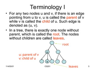
Terminology I
• For any two nodes u and v, if there is an edge
pointing from u to v, u is called the parent of v
while v is called the child of u. Such edge is
denoted as (u, v).
• In a tree, there is exactly one node without
parent, which is called the root. The nodes
without children are called leaves.
u
v
root
u: parent of v
v: child of u
leaves

114/05/01 CS201 6
Terminology II
• In a tree, the nodes without children are
called leaves. Otherwise, they are called
internal nodes.
internal nodes
leaves

114/05/01 CS201 7
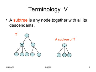
Terminology III
• If two nodes have the same parent, they are
siblings.
• A node u is an ancestor of v if u is parent of v or
parent of parent of v or …
• A node v is a descendent of u if v is child of v or
child of child of v or …
u
v w
x
v and w are siblings
u and v are ancestors of x
v and x are descendents of u

114/05/01 CS201 8
Terminology IV
• A subtree is any node together with all its
descendants.
v v
T
A subtree of T

114/05/01 CS201 9
Terminology V
• Level of a node n: number of nodes on the path from
root to node n
• Height of a tree: maximum level among all of its node
n
Level 1
Level 2
Level 3
Level 4
height=4

114/05/01 CS201 10
Binary Tree
• Binary Tree: Tree in which every node has at
most 2 children
• Left child of u: the child on the left of u
• Right child of u: the child on the right of u
u
x y
z
w
v
x: left child of u
y: right child of u
w: right child of v
z: left child of w

114/05/01 CS201 11
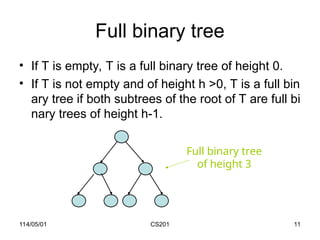
Full binary tree
• If T is empty, T is a full binary tree of height 0.
• If T is not empty and of height h >0, T is a full bin
ary tree if both subtrees of the root of T are full bi
nary trees of height h-1.
Full binary tree
of height 3

114/05/01 CS201 12
Property of binary tree (I)
• A full binary tree of height h has 2h
-1
nodes
No. of nodes = 20
+ 21
+ … + 2(h-1)
= 2h
– 1
Level 1: 20
nodes
Level 2: 21
nodes
Level 3: 22
nodes

114/05/01 CS201 13
Property of binary tree (II)
• Consider a binary tree T of height h. The
number of nodes of T  2h
-1
Reason: you cannot have more nodes than
a full binary tree of height h.

114/05/01 CS201 14
Property of binary tree (III)
• The minimum height of a binary tree with n
nodes is log(n+1)
By property (II), n  2h
-1
Thus, 2h
 n+1
That is, h  log2 (n+1)

114/05/01 CS201 15
Binary Tree ADT
binary
binary
tree
tree
setLeft, setRight
getElem
getLeft, getRight
isEmpty, isFull,
isComplete
setElem
makeTree

114/05/01 CS201 16
Representation of a Binary Tree
• An array-based representation
• A reference-based representation

114/05/01 CS201 17
An array-based representation
–1: empty tree
d
b f
a c e
nodeNum item leftChild rightChild
0 d 1 2
1 b 3 4
2 f 5 -1
3 a -1 -1
4 c -1 -1
5 e -1 -1
6 ? ? ?
7 ? ? ?
8 ? ? ?
9 ? ? ?
... ..... ..... ....
0
6
free
root

114/05/01 CS201 18
Reference Based
Representation
NULL: empty tree left right
element
d
b f
a c
d
b f
a c
You can code this with a
class of three fields:
Object element;
BinaryNode left;
BinaryNode right;

114/05/01 CS201 19
Tree Traversal
• Given a binary tree, we may like to do
some operations on all nodes in a binary
tree. For example, we may want to double
the value in every node in a binary tree.
• To do this, we need a traversal algorithm
which visits every node in the binary tree.

114/05/01 CS201 20
Ways to traverse a tree
• There are three main ways to traverse a tree:
– Pre-order:
• (1) visit node, (2) recursively visit left subtree, (3) recursively
visit right subtree
– In-order:
• (1) recursively visit left subtree, (2) visit node, (3) recursively
right subtree
– Post-order:
• (1) recursively visit left subtree, (2) recursively visit right subtr
ee, (3) visit node
– Level-order:
• Traverse the nodes level by level
• In different situations, we use different traversal
algorithm.

114/05/01 CS201 21
Examples for expression tree
• By pre-order, (prefix)
+ * 2 3 / 8 4
• By in-order, (infix)
2 * 3 + 8 / 4
• By post-order, (postfix)
2 3 * 8 4 / +
• By level-order,
+ * / 2 3 8 4
• Note 1: Infix is what we read!
• Note 2: Postfix expression can be computed
efficiently using stack
+
* /
2 3 8 4

114/05/01 CS201 22
Pre-order
Algorithm pre-order(BTree x)
If (x is not empty) {
print x.getItem(); // you can do other things!
pre-order(x.getLeftChild());
pre-order(x.getRightChild());
}

114/05/01 CS201 23
Pre-order example
Pre-order(a);
a
b c
d
Print a;
Pre-order(b);
Pre-order(c);
Print b;
Pre-order(d);
Pre-order(null);
Print c;
Pre-order(null);
Pre-order(null);
Print d;
Pre-order(null);
Pre-order(null);
a b d c

114/05/01 CS201 24
Time complexity of Pre-order
Traversal
• For every node x, we will call
pre-order(x) one time, which performs
O(1) operations.
• Thus, the total time = O(n).

114/05/01 CS201 25
In-order and post-order
Algorithm in-order(BTree x)
in-order(x.getLeftChild());
in-order(x.getRightChild());
}
Algorithm post-order(BTree x)
post-order(x.getLeftChild());
post-order(x.getRightChild());
}

114/05/01 CS201 26
In-order example
In-order(a);
a
b c
d
In-order(b);
Print a;
In-order(c);
In-order(d);
Print b;
In-order(null);
In-order(null);
Print c;
In-order(null);
In-order(null);
Print d;
In-order(null);
d b a c

114/05/01 CS201 27
Post-order example
Post-order(a);
a
b c
d
Post-order(b);
Post-order(c);
Print a;
Post-order(d);
Post-order(null);
Print b;
Post-order(null);
Print c;
Post-order(null);
Post-order(null);
Post-order(null);
Print d;
d b c a

114/05/01 CS201 28
Time complexity for in-order and
post-order
• Similar to pre-order traversal, the time
complexity is O(n).

114/05/01 CS201 29
Level-order
• Level-order traversal requires a queue!
Algorithm level-order(BTree t)
Queue Q = new Queue();
BTree n;
Q.enqueue(t); // insert pointer t into Q
while (! Q.empty()){
n = Q.dequeue(); //remove next node from the front of Q
if (!n.isEmpty()){
print n.getItem(); // you can do other things
Q.enqueue(n.getLeft()); // enqueue left subtree on rear of Q
Q.enqueue(n.getRight()); // enqueue right subtree on rear of Q
};
};

114/05/01 CS201 30
Time complexity of Level-order
traversal
• Each node will enqueue and dequeue one
time.
• For each node dequeued, it only does one
print operation!
• Thus, the time complexity is O(n).

114/05/01 CS201 31
General tree implementation
struct TreeNode
{
Object element
TreeNode *firstChild
TreeNode *nextsibling
}
because we do not know how many children a
node has in advance.
• Traversing a general tree is similar to traversing
a binary tree
A
G
F
D
C
B E

114/05/01 CS201 32
Summary
• We have discussed
– the tree data-structure.
– Binary tree vs general tree
– Binary tree ADT
• Can be implemented using arrays or references
– Tree traversal
• Pre-order, in-order, post-order, and level-order

114/05/01 CS201 34
What is a graph?
• Graphs represent the relationships among data
items
• A graph G consists of
– a set V of nodes (vertices)
– a set E of edges: each edge connects two nodes
• Each node represents an item
• Each edge represents the relationship between
two items
node
edge

114/05/01 CS201 35
Examples of graphs
H
H
C H
H
Molecular Structure
Server 1
Server 2
Terminal 1
Terminal 2
Computer Network
Other examples: electrical and communication networks,
airline routes, flow chart, graphs for planning projects

114/05/01 CS201 36
Formal Definition of graph
• The set of nodes is denoted as V
• For any nodes u and v, if u and v are
connected by an edge, such edge is denoted
as (u, v)
• The set of edges is denoted as E
• A graph G is defined as a pair (V, E)
v
u
(u, v)

114/05/01 CS201 37
Adjacent
• Two nodes u and v are said to be adjacent
if (u, v)  E
v
w
u
(u, v)
u and v are adjacent
v and w are not adjacent

114/05/01 CS201 38
Path and simple path
• A path from v1 to vk is a sequence of node
s v1, v2, …, vk that are connected by edges
(v1, v2), (v2, v3), …, (vk-1, vk)
• A path is called a simple path if every nod
e appears at most once.
v1
v2
v4
v3
v5
- v2, v3, v4, v2, v1 is a path
- v2, v3, v4, v5 is a path, also it
is a simple path

114/05/01 CS201 39
Cycle and simple cycle
• A cycle is a path that begins and ends at
the same node
• A simple cycle is a cycle if every node
appears at most once, except for the first
and the last nodes
v1
v2
v4
v3
v5
- v2, v3, v4, v5 , v3, v2 is a cycle
- v2, v3, v4, v2 is a cycle, it is
also a simple cycle

114/05/01 CS201 40
Connected graph
• A graph G is connected if there exists path
between every pair of distinct nodes;
otherwise, it is disconnected
v1
v4
v3
v5
v2
This is a connected graph because there exists
path between every pair of nodes

114/05/01 CS201 41
Example of disconnected graph
v1
v4
v3
v5
v2
This is a disconnected graph because there does not
exist path between some pair of nodes, says, v1 and
v7
v7
v6
v8
v9

114/05/01 CS201 42
Connected component
• If a graph is disconnect, it can be partitioned into
a number of graphs such that each of them is
connected. Each such graph is called a
connected component.
v1
v4
v3
v5
v2 v7
v6
v8
v9

114/05/01 CS201 43
Complete graph
• A graph is complete if each pair of distinct
nodes has an edge
Complete graph
with 3 nodes
Complete graph
with 4 nodes

114/05/01 CS201 44
Subgraph
• A subgraph of a graph G =(V, E) is a grap
h H = (U, F) such that U  V and
F  E.
v1
v4
v3
v5
v2
G
v4
v3
v5
v2
H

114/05/01 CS201 45
Weighted graph
• If each edge in G is assigned a weight, it is
called a weighted graph
Houston
Chicago 1000
2000
3500
New York

114/05/01 CS201 46
Directed graph (digraph)
• All previous graphs are undirected graph
• If each edge in E has a direction, it is called a directed
edge
• A directed graph is a graph where every edges is a
directed edge
Directed edge
Houston
Chicago 1000
2000 3500
New York

114/05/01 CS201 47
More on directed graph
• If (x, y) is a directed edge, we say
– y is adjacent to x
– y is successor of x
– x is predecessor of y
• In a directed graph, directed path, directed
cycle can be defined similarly
y
x

114/05/01 CS201 48
Multigraph
• A graph cannot have duplicate edges.
• Multigraph allows multiple edges and self
edge (or loop).
Multiple edge
Self edge

114/05/01 CS201 49
Property of graph
• A undirected graph that is connected and
has no cycle is a tree.
• A tree with n nodes have exactly n-1
edges.
• A connected undirected graph with n
nodes must have at least n-1 edges.

114/05/01 CS201 50
Implementing Graph
• Adjacency matrix
– Represent a graph using a two-dimensional
array
• Adjacency list
– Represent a graph using n linked lists where
n is the number of vertices

114/05/01 CS201 51
Adjacency matrix for directed graph
v1
v4
v3
v5
v2
G
1 2 3 4 5
v1 v2 v3 v4 v5
1 v1 0 1 0 0 0
2 v2 0 0 0 1 0
3 v3 0 1 0 1 0
4 v4 0 0 0 0 0
5 v5 0 0 1 1 0
Matrix[i][j] = 1 if (vi, vj)E
0 if (vi, vj)E

114/05/01 CS201 52
Adjacency matrix for weighted
undirected graph
v1
v4
v3
v5
v2
G
1 2 3 4 5
v1 v2 v3 v4 v5
1 v1 ∞ 5 ∞ ∞ ∞
2 v2 5 ∞ 2 4 ∞
3 v3 0 2 ∞ 3 7
4 v4 ∞ 4 3 ∞ 8
5 v5 ∞ ∞ 7 8 ∞
Matrix[i][j] = w(vi, vj) if (vi, vj)E or (vj, vi)E
∞ otherwise
5
2
3 7
8
4

114/05/01 CS201 53
Adjacency list for directed graph
v1
v4
v3
v5
v2
G
1 v1  v2
2 v2  v4
3 v3  v2  v4
4 v4
5 v5  v3  v4

114/05/01 CS201 54
Adjacency list for weighted
undirected graph
v1
v4
v3
v5
v2
G
5
2
3 7
8
4
1 v1  v2(5)
2 v2  v1(5)  v3(2)  v4(4)
3 v3  v2(2)  v4(3)  v5(7)
4 v4  v2(4)  v3(3)  v5(8)
5 v5  v3(7)  v4(8)

114/05/01 CS201 55
Pros and Cons
• Adjacency matrix
– Allows us to determine whether there is an
edge from node i to node j in O(1) time
• Adjacency list
– Allows us to find all nodes adjacent to a given
node j efficiently
– If the graph is sparse, adjacency list requires
less space

114/05/01 CS201 56
Problems related to Graph
• Graph Traversal
• Topological Sort
• Spanning Tree
• Minimum Spanning Tree
• Shortest Path

114/05/01 CS201 57
Graph Traversal Algorithm
• To traverse a tree, we use tree traversal
algorithms like pre-order, in-order, and post-
order to visit all the nodes in a tree
• Similarly, graph traversal algorithm tries to visit
all the nodes it can reach.
• If a graph is disconnected, a graph traversal that
begins at a node v will visit only a subset of
nodes, that is, the connected component
containing v.

114/05/01 CS201 58
Two basic traversal algorithms
• Two basic graph traversal algorithms:
– Depth-first-search (DFS)
• After visit node v, DFS strategy proceeds along a
path from v as deeply into the graph as possible
before backing up
– Breadth-first-search (BFS)
• After visit node v, BFS strategy visits every node a
djacent to v before visiting any other nodes

114/05/01 CS201 59
Depth-first search (DFS)
• DFS strategy looks similar to pre-order. From a given no
de v, it first visits itself. Then, recursively visit its unvisite
d neighbours one by one.
• DFS can be defined recursively as follows.
Algorithm dfs(v)
print v; // you can do other things!
mark v as visited;
for (each unvisited node u adjacent to v)
dfs(u);

114/05/01 CS201 60
DFS example
• Start from v3
v1
v4
v3
v5
v2
G
v3
1
v2
2
v1
3
v4
4
v5
5
x
x
x
x x

114/05/01 CS201 61
Non-recursive version of DFS
algorithm
Algorithm dfs(v)
s.createStack();
s.push(v);
mark v as visited;
while (!s.isEmpty()) {
let x be the node on the top of the stack s;
if (no unvisited nodes are adjacent to x)
s.pop(); // blacktrack
else {
select an unvisited node u adjacent to x;
s.push(u);
mark u as visited;
}
}

114/05/01 CS201 62
Non-recursive DFS example
v1
v4
v3
v5
v2
G
visit stack
v3 v3
v2 v3, v2
v1 v3, v2, v1
backtrack v3, v2
v4 v3, v2, v4
v5 v3, v2, v4 , v5
backtrack v3, v2, v4
backtrack v3, v2
backtrack v3
backtrack empty
x
x
x
x x

114/05/01 CS201 63
Breadth-first search (BFS)
• BFS strategy looks similar to level-order. From a
given node v, it first visits itself. Then, it visits ev
ery node adjacent to v before visiting any other n
odes.
– 1. Visit v
– 2. Visit all v’s neigbours
– 3. Visit all v’s neighbours’ neighbours
– …
• Similar to level-order, BFS is based on a queue.

114/05/01 CS201 64
Algorithm for BFS
Algorithm bfs(v)
q.createQueue();
q.enqueue(v);
mark v as visited;
while(!q.isEmpty()) {
w = q.dequeue();
for (each unvisited node u adjacent to w) {
q.enqueue(u);
mark u as visited;
}
}

114/05/01 CS201 65
BFS example
• Start from v5
v5
1
v3
2
v4
3
v2
4
v1
5
v1
v4
v3
v5
v2
G
x
Visit Queue
(front to
back)
v5 v5
empty
v3 v3
v4 v3, v4
v4
v2 v4, v2
v2
empty
v1 v1
empty
x
x
x x

114/05/01 CS201 66
Topological order
• Consider the prerequisite structure for courses:
• Each node x represents a course x
• (x, y) represents that course x is a prerequisite to course y
• Note that this graph should be a directed graph without cycles
(called a directed acyclic graph).
• A linear order to take all 5 courses while satisfying all prerequisites
is called a topological order.
• E.g.
– a, c, b, e, d
– c, a, b, e, d
b d
e
c
a

114/05/01 CS201 67
Topological sort
• Arranging all nodes in the graph in a topological
order
Algorithm topSort
n = |V|;
for i = 1 to n {
select a node v that has no successor;
aList.add(1, v);
delete node v and its edges from the graph;
}
return aList;

114/05/01 CS201 68
Example
b d
e
c
a
1. d has no
successor!
Choose d!
a
5. Choose a!
The topological
order is
a,b,c,e,d
2. Both b and e have
no successor!
Choose e!
b
e
c
a
3. Both b and c have
no successor!
Choose c!
b
c
a
4. Only b has no
successor!
Choose b!
b
a

114/05/01 CS201 69
Topological sort algorithm 2
• This algorithm is based on DFS
Algorithm topSort2
s.createStack();
for (all nodes v in the graph) {
if (v has no predecessors) {
s.push(v);
mark v as visited;
}
}
while (!s.isEmpty()) {
let x be the node on the top of the stack s;
if (no unvisited nodes are adjacent to x) { // i.e. x has no unvisited successor
aList.add(1, x);
s.pop(); // blacktrack
} else {
select an unvisited node u adjacent to x;
s.push(u);
mark u as visited;
}
}
return aList;

114/05/01 CS201 70
Spanning Tree
• Given a connected undirected graph G, a
spanning tree of G is a subgraph of G that
contains all of G’s nodes and enough of its
edges to form a tree.
v1
v4
v3
v5
v2
Spanning
tree Spanning tree is not unique!

114/05/01 CS201 71
DFS spanning tree
• Generate the spanning tree edge during the DF
S traversal.
Algorithm dfsSpanningTree(v)
mark v as visited;
for (each unvisited node u adjacent to v) {
mark the edge from u to v;
dfsSpanningTree(u);
}
• Similar to DFS, the spanning tree edges can be generate
d based on BFS traversal.

114/05/01 CS201 72
Example of generating spanning
tree based on DFS
v1
v4
v3
v5
v2
G
stack
v3 v3
v2 v3, v2
v1 v3, v2, v1
backtrack v3, v2
v4 v3, v2, v4
v5 v3, v2, v4 , v5
backtrack v3, v2, v4
backtrack v3, v2
backtrack v3
backtrack empty
x
x
x
x x

114/05/01 CS201 73
Minimum Spanning Tree
• Consider a connected undirected graph where
– Each node x represents a country x
– Each edge (x, y) has a number which measures the
cost of placing telephone line between country x and
country y
• Problem: connecting all countries while
minimizing the total cost
• Solution: find a spanning tree with minimum total
weight, that is, minimum spanning tree

114/05/01 CS201 74
Formal definition of minimum
spanning tree
• Given a connected undirected graph G.
• Let T be a spanning tree of G.
• cost(T) = eTweight(e)
• The minimum spanning tree is a spanning tree T
which minimizes cost(T)
v1
v4
v3
v5
v2
5
2
3 7
8
4
Minimum
spanning
tree

114/05/01 CS201 75
Prim’s algorithm (I)
Start from v5, find the
minimum edge attach to
v5
v2
v1
v4
v3
v5
5 2
3 7
8
4
Find the minimum
edge attach to v3 and
v5
v2
v1
v4
v3
v5
5 2
3 7
8
4
Find the minimum
edge attach to v2, v3
and v5
v2
v1
v4
v3
v5
5 2
3 7
8
4
v2
v1
v4
v3
v5
5 2
3 7
8
4
v2
v1
v4
v3
v5
5 2
3 7
8
4
Find the minimum edge
attach to v2, v3 , v4 and v5

114/05/01 CS201 76
Prim’s algorithm (II)
Algorithm PrimAlgorithm(v)
• Mark node v as visited and include it in the mini
mum spanning tree;
• while (there are unvisited nodes) {
– find the minimum edge (v, u) between a visited node v
and an unvisited node u;
– mark u as visited;
– add both v and (v, u) to the minimum spanning tree;
}

114/05/01 CS201 77
Shortest path
• Consider a weighted directed graph
– Each node x represents a city x
– Each edge (x, y) has a number which represent the
cost of traveling from city x to city y
• Problem: find the minimum cost to travel from
city x to city y
• Solution: find the shortest path from x to y

114/05/01 CS201 78
Formal definition of shortest
path
• Given a weighted directed graph G.
• Let P be a path of G from x to y.
• cost(P) = ePweight(e)
• The shortest path is a path P which minimizes c
ost(P)
v2
v1
v4
v3
v5
5
2
3 4
8
4 Shortest Path

114/05/01 CS201 79
Dijkstra’s algorithm
• Consider a graph G, each edge (u, v) has
a weight w(u, v) > 0.
• Suppose we want to find the shortest path
starting from v1 to any node vi
• Let VS be a subset of nodes in G
• Let cost[vi] be the weight of the shortest
path from v1 to vi that passes through
nodes in VS only.

114/05/01 CS201 80
Example for Dijkstra’s algorithm
v2
v1
v4
v3
v5
5
2
3 4
8
4
v VS cost[v1] cost[v2] cost[v3] cost[v4] cost[v5]
1 [v1] 0 5 ∞ ∞ ∞

114/05/01 CS201 81
v2
v1
v4
v3
v5
5
2
3 4
8
4
1 [v1] 0 5 ∞ ∞ ∞
2 v2 [v1, v2] 0 5 ∞ 9 ∞

114/05/01 CS201 82
v2
v1
v4
v3
v5
5
2
3 4
8
4
1 [v1] 0 5 ∞ ∞ ∞
2 v2 [v1, v2] 0 5 ∞ 9 ∞
3 v4 [v1, v2, v4] 0 5 12 9 17

114/05/01 CS201 83
v2
v1
v4
v3
v5
5
2
3 4
8
4
1 [v1] 0 5 ∞ ∞ ∞
2 v2 [v1, v2] 0 5 ∞ 9 ∞
3 v4 [v1, v2, v4] 0 5 12 9 17
4 v3 [v1, v2, v4, v3] 0 5 12 9 16
5 v5 [v1, v2, v4, v3, v5] 0 5 12 9 16

114/05/01 CS201 84
Dijkstra’s algorithm
Algorithm shortestPath()
n = number of nodes in the graph;
for i = 1 to n
cost[vi] = w(v1, vi);
VS = { v1 };
for step = 2 to n {
find the smallest cost[vi] s.t. vi is not in VS;
include vi to VS;
for (all nodes vj not in VS) {
if (cost[vj] > cost[vi] + w(vi, vj))
cost[vj] = cost[vi] + w(vi, vj);
}
}

114/05/01 CS201 85
Summary
• Graphs can be used to represent many real-life
problems.
• There are numerous important graph algorithms.
• We have studied some basic concepts and
algorithms.
– Graph Traversal
– Topological Sort
– Spanning Tree
– Minimum Spanning Tree
– Shortest Path

Concise Notes on tree and graph data structure

More Related Content

Similar to Concise Notes on tree and graph data structure (20)

Recently uploaded (20)

Concise Notes on tree and graph data structure

Editor's Notes