![Logistic Regression
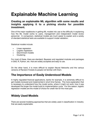
For logistic regression the result of the combination is then input into a sigmoid to
obtain the maximum likelihood estimator for the probabilities of a 0 or 1 outcome.
(1)
usually written as:
(2)
Linear Regression
In some cases, the more simpler linear regression model is used.
(3)
where:
Mathematical Programming
Mathematical programming is another approach that is used to estimate a linear model. One
formulation is:
(4)
subject to:
(5)
(6)
(7)
where:
G0 and G1 are the sets of observations with an outcome of 0 or 1 respectively.
probability(y = 1) = exp(X * b)/(1.0 + exp(X * b))
p(y = 1) = 1.0/(1.0 + exp(−1.0 * X * b)
y = X * b
y ∈ [−1,1]
min z =
∑
i
ei
∑
j
(xi,j * wj) + ei > = 0 ∀i ∈ G1
∑
j
(xi,j * wj) − ei > = 0 ∀i ∈ G0
∑
j
wj = 1
Page of2 16](https://image.slidesharecdn.com/explainableml2-190719050403/85/Creating-an-Explainable-Machine-Learning-Algorithm-2-320.jpg)


Creating an Explainable Machine Learning Algorithm
- 1. Explainable Machine Learning Creating an explainable ML algorithm with some results and insights applying it to a picking stocks for possible investment. One of the major roadblocks in getting ML models into use is the difficulty in explaining how the ML model works to users, management and independent model review personnel. In comparison, statistical models are much easier to explain and a variety of standard statistical tests are available to support model validation. Statistical models include: • Linear regression • Logistic regression • Discriminant models • Clustering For most of these, there are standard, Bayesian and regulated modules and packages in SAS, R, Python, etc. that are widely accepted and easy to use. On the other hand, it is more difficult to explain Neural Networks and the various versions of Random Forests to people not familiar with them. The Importance of Easily Understood Models In highly regulated financial applications, banks for example, it is extremely difficult to get models reviewed and implemented in short time frames. The more explanation that is necessary to understand how the model works, where it might not work, how it was developed the longer the model build to implementation cycle. For this reason, logistic regression models are the model of choice for credit risk for the most part. Widely Used Models There are several modeling approaches that are widely used in classification in industry that are easily explainable. Page of1 16
- 2. Logistic Regression For logistic regression the result of the combination is then input into a sigmoid to obtain the maximum likelihood estimator for the probabilities of a 0 or 1 outcome. (1) usually written as: (2) Linear Regression In some cases, the more simpler linear regression model is used. (3) where: Mathematical Programming Mathematical programming is another approach that is used to estimate a linear model. One formulation is: (4) subject to: (5) (6) (7) where: G0 and G1 are the sets of observations with an outcome of 0 or 1 respectively. probability(y = 1) = exp(X * b)/(1.0 + exp(X * b)) p(y = 1) = 1.0/(1.0 + exp(−1.0 * X * b) y = X * b y ∈ [−1,1] min z = ∑ i ei ∑ j (xi,j * wj) + ei > = 0 ∀i ∈ G1 ∑ j (xi,j * wj) − ei > = 0 ∀i ∈ G0 ∑ j wj = 1 Page of2 16
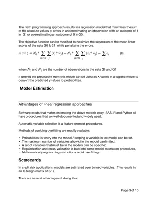
- 3. The math programming approach results in a regression model that minimizes the sum of the absolute values of errors in underestimating an observation with an outcome of 1 in G1 or overestimating an outcome of 0 in G0. The objective function can be modified to maximize the separation of the mean linear scores of the sets G0 & G1 while penalizing the errors. (8) where and are the number of observations in the sets G0 and G1. If desired the predictions from this model can be used as X values in a logistic model to convert the predicted y values to probabilities. Model Estimation Advantages of linear regression approaches Software exists that makes estimating the above models easy. SAS, R and Python all have procedures that are well-documented and widely used. Automatic variable selection is a feature on most procedures. Methods of avoiding overfitting are readily available: • Probabilities for entry into the model / keeping a variable in the model can be set. • The maximum number of variables allowed in the model can limited. • A set of variables that must be in the models can be specified. • Regularization and cross-validation is built into some model estimation procedures. • Mathematical programming restrictions avoid overfitting. Scorecards In credit risk applications, models are estimated over binned variables. This results in an X design matrix of 0/1s. There are several advantages of doing this: max z = N0 * ∑ i∈G1 ∑ j (xi * wj) − N1 * ∑ i∈G0 ∑ j (xi * wj) − ∑ i ei N0 N1 Page of3 16
- 4. • Character variables can be grouped together by similar outcome probabilities. • Missing data for any of the variables can be explicitly modeled in a 0/1 column of the X matrix. • Continuous variables are grouped together into bins over intervals. This allows for the slope to change and for step changes in the predictors. • The model weights can be transformed to integers then applied to the binned x variables in a simple to understand way to generate the score. • For example, if age is in a scorecard: • If age is below 23 subtract 10 points. • If age is above 40 add 5. • The binned categories for a given x variable can be used to generate a transformed x variable by running a regression model on the bins of the variable. This can be used to transform a character variable with many categories into 1 predictor variable. Usage Scorecards estimated with logistic regression are used or can be used in a variety of industries to manage risk. • Financial institutions for application scoring. • Financial institution for fraud modeling. • Survival modeling. • Stock picking. • Gambling - picking the horses or winners of matches. • Managing bookings and no-shows in the transportation and hospitality industries. • Customer churn. • Political vote prediction. • etc. A Role for ML? So, given the wide use and acceptance models that produce an easily understandable linear score which may or may not be transformed into a probability or scorecard what role is there for ML in an environment that values explainability? At first glance, it would seem that ML might add value in a couple of areas: Binning: if the predictor variables are binned a ML algorithm could be programmed to do the binning in a manner that is beneficial to the goal of producing a model with the ability to generate good predictions. However, in many cases the binning produced by a modeler or an algorithm is overridden by project sponsors due to the desire to manage a particular segment or past experience. Page of4 16
- 5. Feature selection: modeling software does an acceptable job on this task. Most apply a greedy-type algorithm based on variables currently in the model to pick the next variable in or remove a variable from the model. Variables that must be in the model can also be specified. In the statistical models limited restrictions on weights are available. Some algorithms use the 1-norm to limit the number of predictors in a model. Bayesian approaches can also be used to limit the number of predictors or the magnitude of weights. ML might be used then to select features in a non-sequential manner learning which features are best in combination. However, there exists another area where an explainable ML model might add value. It is illustrated well by looking at a gambling problem. Going to the Races Are Horse Race Bettors More Sophisticated Than Bankers? Bettors at race tracks take information (data) into consideration when placing their bets. It may include: • Pole position of the horse Page of5 16 QUEUEING AT THE BETTING WINDOWS AT THE TRACK
- 6. • Jockey and horse past performances • Number of horses in the race • Type of race • Length of race • Odds on the payoff • Kelly Criterion Research has shown that in the US the betting pool on the favorites that generates the odds is a fairly accurate estimation of winning probabilities (see Ziemba) even after the noise that is added to the above list by bettors who bet on horses’ names or jockey colors, etc. are factored in. In the bulleted list above there is one item that isn’t quite like the others. Sophisticated gamblers use the Kelly Criterion to decide whether and how much to bet. Kelly bet formula (9) where: f is the fraction of the available cash pool to bet p is the probability of winning b is the amount lost in the odds ratio given a loss g is the amount of profit in the odds ratio given a win The Kelly bet formula maximizes the rate of growth of the bettor’s cash pool given the known probability of winning and the known payoff odds to bet, g/b. If f < 0, no bet is made, the Kelly bettor would be betting the wrong side of the odds. Any betting strategy with betting > f will lead to gambler’s ruin. Sophisticated bettors who use the Kelly Criteria or bet some fraction of f factor in the payoff to their decision. This strategy isn’t built into most scorecard building processes used by financial institutions. Usually models are built that have 2 components, one for the probability of outcomes and the other for the gain or loss associated with the outcome. ML Model Objectives A useful ML model that might be implemented by those with a bias towards explainability would have the following features: f = p − (1 − p) * b/g Page of6 16
- 7. 1. Easily understood. A scorecard with integer weights is significantly more easily explained and understood than a neural network or random forest. 2. Do something linear regression models don’t do. For example, combine both the probability of financial gain with the expected gain or loss. 3. Flexibility. The algorithm should be flexible enough handle different objectives, constraints, hyper parameters, etc. Possible Applications Marketing / Credit Application Scoring / Account Management Marketing models could be improved by incorporating budget constraints into the model and the expected return and any risk into the objective function. Credit card holders fall into categories of usage: • Revolvers — those who carry a balance from statement to statement • Transactors — those who pay off the outstanding balance every month • Dormants — those who have a card but do not use it • Defaulters — those who use the credit but do not pay the balance • Fraudsters — those who apply for credit cards but have no intention to pay their balance. The usual models that are built are probability of default models. These can be either for account management or to make the accept / reject decision in application scoring. It isn’t difficult to see that a model that incorporates the expected profit / loss in account management or application scoring would be beneficial. Changing the limit on credit cards and lines of credit are other examples. Additionally, application scoring might be improved in the case where the application scorecard is under development (a process that might take a year in a bank) but a second score is desired to be applied to determine a subset of applications to reject of a given size while minimizing the financial effect on profitability. Repeated Actions with Costs, Benefits and Constraints Operational constraints enter into some decisions. For example fraud referrals and stock picking. Possible fraudulent transactions may be referred to the fraud operations department. Typically, there will be an upper limit on the number of transactions that may be worked Page of7 16
- 8. in a day while there is a cost / benefit relationship between rejecting transactions and preventing fraud that portfolio managers emphasize. Some problems require making a decision over sequential time periods. For example, every Friday picking 10 stocks to highlight for an investors report. One More Possible Advantage of an ML Model Every observation is important in the statistical and mathematical programming approaches. Regression models use all the observations available to estimate or validate the model based on the likelihood function and any penalty functions. Likewise with the mathematical programming approach where the objective function is evaluated over all the observations. It is possible to design a ML model that only concentrates on learning features to include in a scorecard and the weights that optimizes a more specific objective function. Picking Stocks — Example Statement of the Problem Maximize the expected return over a 13 week (1 quarter) performance period by picking 10 stocks to invest in over a 10-week period of picks using a scorecard over available data where the weights in the card are integers. (10) subject to: (11) where: (12) (13) is the total number of observations at week t. t is the week the observation is from. max z = ∑ t ( ∑ i∈t ( ∑ j (xi,t * wj > cutofft) * profiti,t)) ∑ i∈t ( ∑ j (xi,t * wj > cutofft)) > = 10 ∀ t cutofft = percentile(scoresi,t,100 − (1/Nt)) scorei = ∑ j (xi * wj) ∀i Nt Page of8 16
- 9. Exclusions: Stocks with current prices < $8. Financial stocks due to too many investment funds present in the data set. ML Tasks The algorithm will have to accomplish 4 tasks. 1. Transform the feature values into binned data. 2. Select a set of the features from (1) for possible model inclusion. 3. Determine a good performing set of features for the model. 4. Estimate a good performing set of integer weights. Learning At each iteration, the algorithm will then generate a guess solution based on solutions it remembers, submit it to the oracle for evaluation (compute the profit on the picks), decide whether or not to remember the solution, if the memory is full decide which solution to purge and replace with the current solution. This is where the opportunity to get creative and experiment is. So as not to ruin it for those who would like to design an algorithm the details of the learning given are limited to the paragraph above. Several different approaches can be implemented including the popular population evolutionary algorithms or search procedures over the combinations. Hyperparameters: Page of9 16 LEARNING FLOWCHART
- 10. Binning. The number of bins is set at 4 + 1 if missing values are present. A minimum of 5% of the observations in the model sample have to fall in a bin for it to be a valid bin. Max Iterations: Stop after 5000 iterations are performed. Other Stopping: Stop when the number of different combinations of features in the memory falls below a certain level. Stop if 100 iterations are performed with no improvement in the objective function. Data • Stock feature and performance history • Snapshot • Weekly at Friday close • Snapshots taken at 13 individual weeks • Exclusions • Stocks from the financial sector -- Banks, Investment funds • Stocks with a price < $8 at the snapshot point • The price history is affected significantly by reverse splits • Features • 37 candidate features • Technical / Fundamental / Valuation / General • Performance History • Performance Measure • Return or percent change in Price 13 weeks after the snapshot • Model Test Segmentation • 10% of the stocks are held out as a validation sample chosen by Ticker symbol • Model sample: 22,852 — Validation sample: 2,903 Page of10 16
- 11. Results Population mean return: 8.9% Model picks return: 32.6% Validation picks return: 17.9% These plots show returns over weeks sampled and the overall return distribution. Overall distribution of % Return Sample Returns Picks in blue show significantly less risk than the stocks that aren’t picked (in red) on the sample of stock performances the model was built on. The validation which is significantly smaller still shows increased returns while at the same time reduced risk of loss of investment funds. Both the model and validation plots are based on the pooled pick of 10 stocks each week. The learning algorithm only sees the results of the model sample observations. Because of this it isn’t unreasonable to expect the validation sample to perform at a lower level. It has to go deeper into the score distribution. Picking the top 10 scoring stocks each week in the sample results in a densities that indicate a higher performance than the validation sample performance might be possible. Page of11 16
- 12. The score distribution is peaked at slightly less than 0. It is important to remember that the only scores taken into consideration in the ML optimization are the top 10 each of the 10 weeks in the population sample. In spite of that, the score distribution is spread from -200 to 300. The second plot shows the value of the objective function for the model sample and the validation sample. The validation sample is shown for informative purposes. It does not enter into the decision to stop the model iterations. Page of12 16
- 13. Expectation Plots The observations in the model sample are binned with cuts at each 5%. For each bin the average score, probability of profit, average gain and average loss are plotted. The average gain and loss are scaled by dividing by the maximum average gain to allow plotting all 3 values on the same scale. The model sample illustrates that the algorithm is performing as designed. The highest score bin has the best performance as indicated by having both the highest probability of a gain and the largest spread between average gain and average loss. Key: Probabilty Loss Gain The plot illustrates a problem that exists in building a model to maximize stock investment returns. Often the highest returns are look a lot like the most risky investments. The validation sample has more volatile expectations, but the same observations can be made. The best performance is at the high end although there is a slight reversal in the upper percentiles. Page of13 16
- 14. Expected Margin by Score The expected margin within each of the bins is computed from the values above. (14) The model sample margin shows an almost linear pattern in the margin by score bin. The validation sample has a lot more noise, but in general the model performs well on the validation sample. margin = probgain * averagegain − probloss * averageloss Page of14 16
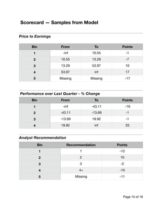
- 15. Scorecard — Samples from Model Price to Earnings Performance over Last Quarter - % Change Analyst Recommendation Bin From To Points 1 -inf 10.55 -1 2 10.55 13.29 -7 3 13.29 53.97 10 4 53.97 inf 17 5 Missing Missing -17 Bin From To Points 1 -inf -43.11 -19 2 -43.11 -13.69 -1 3 -13.69 19.92 -1 4 19.92 inf 33 Bin Recommendation Points 1 1 -12 2 2 10 3 3 -2 4 4+ -10 5 Missing -11 Page of15 16
- 16. Conclusions It is possible to build an easily explainable Machine Learning model in the form of a scorecard that will improve decisions. The objective function can be specified to target the area of operation and constraints instead of using a loss function that is applied to all the data. Both probability and profit can be built into the objective function. An algorithm to accomplish this task can be set up to output a model in the form of an easily understandable scorecard allowing end users to check if the model agrees with their experience. As the model learns, the solution set that is remembered can be used to provide an ensemble of predictions if so desired. End user input can be easily incorporated via binning boundaries or restrictions. The algorithm does not follow a greedy approach of selecting one predictor (regression) or making one partition (decision trees) then making successive decisions on feature selection based on those already made but explores combinations of the candidate feature set remembering those with the best performance. As a bonus, solving targeted problems may result in a solution that rank orders well enough over the entire population. Questions If you have any questions, suggestions for applications, or a problem and its data that you would like to see if an algorithm like this would provide a solution for please feel free to email me at bill.fite@miner3.com Page of16 16