Credit Default Models

Credit Default Models
Swati Mital
swati.mital@maths.ox.ac.uk
Professional Risk Managers’ International Association
May 4, 2016
Mital, Swati (PRMIA) Credit Default Models May 4, 2016 1 / 31

Credit Risk
What is Credit Risk?
Credit Risk is the risk that the value of the portfolio changes due to
changes in the credit quality of the ”obligors” due to defaults or rating
downgrade.
Products: Loans, Sovereign Bonds, Corporate Bonds and Credit
Derivatives. Ignore Equity. We focus on corporate credit models not retail
scoring models.
Why model Credit Risk?
Measure Risk in porfolio of credit risky instruments
Compute Regulatory Capital
Compute Economic Capital
Perform Risk Adjusted comparison of diﬀerent porfolios

Agenda
Focus on, broadly speaking, four types of Credit Default Models
Merton’s Structural Model
Extension to Merton’s Model (KMV Model)
Ratings based Model
Multivariate Factor Models
We also have a brief section on
Reduced Form Model (Bernoulli Mixture Model)
Finally, we cover Copulas and how they are used for Default Modelling
Default Modelling with Copulas

Notations
Let the time interval be ﬁxed [0, T]. Let τi be time to default for obligor i.
Let Yi = 1τi ≤T be the default indicator.
Then, we can represent the probability of default for obligor i as,
PDi = P(Yi = 1) = 1 − P(Yi = 0) = P(τi ≤ T) (1)
Let EADi be the exposure at default and LGDi be the loss given default.
Then the default loss on a porfolio is,
Default Loss =
n
i=1
EADi × Yi × LGDi (2)
Since Yi is a Bernoulli r.v., E[Yi ] = PDi . This gives us the Expected value
of the default loss. However, we are interested in diﬀerent quantiles of the
loss distribution function.

Structural Models
In 1974, Merton showed how the Black Scholes Option Pricing theory can
be used to estimate a firm’s probability of default and credit spreads.
Assumptions in Merton’s structural Credit Risk Model:
Firm value, Vt, is financed by equity, St, and, debt, Bt
Vt = St + Bt, 0 ≤ t ≤ T (3)
Debt is a single zero coupon bond with face value B and time to
maturity T
Default occurs when the value of the firm, VT , goes below the
outstanding debt, B. This can be determined from the firm’s balance
sheet.

Structural Models
Hence, at time T if VT ≥ B, then the shareholders receive ST = VT − B
and there is no default. But if VT < B, then a default event occurs and
shareholders receive nothing, i.e., ST = 0.
The equity of a firm is a call option on it’s assets with Strike, B.
The debt of a firm is long a risk-free asset, B, and short a put (to the
equity holders) on the firm.
In Option Analogy terms, this can be expressed as,
ST = (VT − B)+
BT = B − (B − VT )+ (4)

Default Probability under Structural Model
We assume that the ﬁrm’s asset value, Vt, follows Geometric Brownian
Motion, Vt = V0exp (µv − σ2
v
2 )t + σv Wt .
We can compute the probability of default, P(VT < B), also known as,
”Distance to Default”, as
P(VT < B) = P V0exp (µv −
σ2
v
2
)T + σv WT < B
= P

WT <
ln B
V0
− (µv − σ2
v
2 )T
σv


= Φ


ln B
V0
− (µv − σ2
v
2 )T
σv
√
T


= δT
(5)

Diagrammatic Representation
Figure: Merton Structural Model (source: Crouhy et al., A comparative analysis
of current credit risk models, Journal of Banking and Finance, 2000 [59-117])

Variables in the Structural Model
In Merton’s model, we link the ﬁrm’s equity value, St, which is observed in
the market, and equity volatility, σe, to the otherwise unobservable asset
value, Vt and asset volatility, σv . The price of equity can be computed
using the Black-Scholes price of a call option on Vt with strike B.
St = CBS
(t, Vt, σv , r, T, B) = VtΦ(d1) − B exp−r(T−t)
Φ(d2)
d1 =
ln Vt
B + (r + σ2
v
2 )(T − t)
σv (T − t)
d2 = d1 − σv (T − t)
σe =
Vt
St
Φ(d1)σv
(6)
Hence, given, St, σe, r, and B we can solve for the Distance to Default,
δT .

Credit Spreads in Merton’s Model
Merton’s model can also be used to compute the credit spread above the
yield of a risk-free bond.
Let Pr (t, T) be the price of a risk-free zero coupon bond maturing at time
T. Let Pd (t, T) be the price of a corporate risky bond maturing at time
T. Then, we can deﬁne the credit spread on their yields, assuming
continuous compounding, as,
spread(t, T) =
1
T − t
ln
Pd (t, T)
Pr (t, T)
(7)
In Merton’s model the price of ﬁrm’s debt can be computed as a
discounted value of default-free debt, B, and a Black-Scholes price of a
short put option on Vt with strike, B. This gives,
Pd (t, T) = Pr (t, T)Φ(d2) +
Vt
B
Φ(d1) (8)
Plugging this back into Equation 7 gives us the formula for the credit
spread.

Evaluation of Merton’s Model
Advantages
Credit Risk of a firm is connected to underlying structural variables.
Intuitive Economic Explanation and Endogenous explanation of credit
defaults.
Option Analogy allows for easy implementation.
Disadvantages
Too Simplistic: Equity as Call option, Debt matures at same time.
Only applicable if a firm has tradable equity and a good estimate of
debt level. Not extendable for private firms or sovereigns.
Assumes that two equally leveraged firms with identical market
capitalization and asset volatility are of equal risk.
Underestimate credit spreads for short time to maturity that is
empirically difficult to explain.

KMV Extension of Merton’s Model
KMV (now Moody’s KMV) model was developed in 1990s and it focused
on modelling defaults by extending the Merton Model.
Mapped Distance to Default to historical default rates using
proprietary database.
Removed the need to model credit risk using Option Theory.
KMV model is only focused on modelling default and not the credit
spreads.

Dynamics of the KMV Model - EDF
One of the central ideas in the KMV model is the Expected Default
Frequency (EDF). This is the one-year probability of default of an obligor.
Going back to Merton’s model the EDF would be,
EDFMerton = 1 − Φ
ln V0
B + (µv − σ2
v
2 )
σv
(9)
In KMV model, the EDF has similar structure to the Merton model but
the function 1 − Φ is replaced with an estimated KMV function. The
variable µv is ignored and the V0 and σv are backed out from the
observable value of equity of the ﬁrm.
The default boundary, B, is 1
2 of short-term debt (< 1 year) and
100% of long-term debt.
Floor on the Estimated 1 year default probability of 40% and a ceiling
of 0.01%.

Dynamics of the KMV Model - DD
The other central idea in the KMV model is the Distance to Default (DD).
To put it simply, a higher DD means a ﬁrm is less likely to default than a
lower DD.
The DD is mapped to EDF using empirical proprietary KMV
database. Firms with equal DD have equal EDF.
DD in the KMV model can be expressed by the following equation,
DD =
(V0 − F)
σv V0
(10)
where F is the default threshold.
Relationship between EDF and DD. (Source: Moody’s/KMV)

Ratings Based Models
Credit Rating measures the credit quality of a firm at any given point in
time. The Ratings based model computes the probabilities of this rating
changing. These migration probabilities are supplied by Rating Agencies
(for e.g., Moody’s, Standard and Poor’s). JP Morgan CreditMetrics is a
popular ratings based credit risk model.
In the KMV model the fundamental state variable was DD, in the
Ratings Migration approach the state variable is the Credit Rating.
Firms with equal Credit Rating have equal migration probabilities.
Rating agencies have huge database that cover a wide range of firms
including sovereigns.
Rating agencies focus on ”through the cycle” credit ratings causing
less fluctuations as opposed to KMV which is ”point in time”.
Rating agencies are slow to react to credit events leading to a lag
from the market spreads.

An Example Ratings Migration Matrix
One year Transition Probability Matrix taken from Moody’s. (Source:
Elton E, Gruber M, Agrawal D, Explaining the Rate Spread on Corporate
Bonds, Journal of Finance 2001)

Migration Model in Firm Value Model
Popular way to embed a migration model inside a ﬁrm value model.
Suppose we are given transition probabilities by the rating agencies
for n rating classes. Denote pj where 0 ≤ j ≤ n as the probability for
a given ﬁrm to be in rating class j. We then select rating migration
thresholds −∞ = d0 < d1 < .... < dn < dn+1 = ∞ such that
P(dj−1 < Vt < dj ) = pj ∀j.
If we assume that the asset process, Vt, has log normal distribution
(Merton’s assumption), then we can compute the thresholds using
standard normal distribution as,
d1 = ZCCC = Φ−1
(pdef )
d2 = ZB = Φ−1
(pdef + pCCC )
d3 = ZBB = Φ−1
(pdef + pCCC + pB)
...
(11)

Multivariate Firm Value Model
Here we extend Merton’s ideas into something that can be used on a large
portfolio by using factors for modelling dependence.
Consider a portfolio of n firms over a time period [0, T]. Assume
T = 1.
Let Yi denote default indicator. So, Yi = 1 indicates that a default
event has taken place and Yi = 0 means there is no default.
The default of the company is driven by some latent variable Xi ,
generally assumed to be normally distributed, which if it lies below a
threshold di , a default occurs. Therefore, we can write the default
probability as,
P(Yi = 1) = P(Xi ≤ di ) = F(di ) (12)
Model default dependence between the different firms in the portfolio
by making the Xi correlated, i.e., to make the asset values dependent.

Generic Factor Model
Let X = (X1 X2... Xn)T , then the random vector X is driven by a set of
(p << n) factors to reduce the dimensionality of the correlation matrix. A
generic factor model can be expressed as,
X = α + βT
F + (13)
α ∈ Rn is a vector of constants that can be thought of as the global
factor affecting all firms.
F ∈ Rp is a random vector of (systematic or economic) factors.
βT ∈ Rn×p is the factor loading on the p factors since each Xi load
differently on each factor.
∈ Rn is a random vector of (idiosyncratic) terms and are hence
uncorrelated with mean zero.
cov(F, ) = 0

Gaussian Linear Factor Model
Since the ﬁrm value model descends from Merton model, we assume that
X has a multivariate normal distribution.
Let F ∼ N(0, Ω)
Let ∼ N(0, Γ)
Then, X ∼ N(α, βT
Ωβ + Γ)
cov(Xi , Xj ) = βT
i Ωβj
For majority of credit risk models, since actual asset values of the company
are unobservable, the factors are derived by observing the equity returns.

One Factor Vasicek Model
This is a special case where, Xi = βi F + 1 − β2
i i , and F, i have
standard normal distribution. Therefore, X ∼ N(0, 1). If all the factor
loadings are identical then we get a homogeneous model,
Xi =
√
ρF + 1 − ρ i (14)
where ρ = var(βi F) = β2
i ∀i is the systematic variance but also the asset
correlation parameter since it is the correlation of the critical variables.
corr(Xj , Xk) =
βj
T
Ωβk
βj
T
Ωβj + Γjj βk
T
Ωβk + Γkk
=
βj
2
βj
2
+ (1 − β2
j ) βk
2
+ (1 − β2
k)
= ρ
(15)

Bernoulli Mixture Model
We start with a portfolio of n ﬁrms and a p-dimensional factor vector
Θ = (θ1, θ2, ..., θp). In a Bernoulli Mixture Model, the probability of
default conditional on these factors is given by,
P(Yi = 1|Θ = Θ) = pi (Θ) (16)
such that the joint probability of the default indicators conditional on the
factors is given by,
P(Y1 = y1, Y2 = y2, ..., Yn = yn|Θ = Θ) =
n
i=1
pi (Θ)yi
(1 − pi (Θ))1−yi
(17)
And, hence, the default indicators of the n ﬁrms are independent
conditional on the factor vector with their joint default probability given by,
P(Y1 = 1, Y2 = 1, ..., Yn = 1|Θ) =
n
i=1
pi (Θ) (18)

Gaussian Firm Value Model as a Mixture Model
We now see that the Gaussian Firm Value Model is, in fact, also a
Bernoulli Mixture Model with Θ = F. And the conditional probability of
the default for a ﬁrm is given as,
P(Yi = 1|F) = P(Xi < di |F)
= P(αi + βi
T
F + i < di |F)
= P( i < di − βi
T
F − αi )
= Φ
di − βi
T
F − αi
σ i
= Φ
Φ−1(pi ) − βi
T
F − αi
σ i
(19)

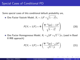
Special Cases of Conditional PD
Some special cases of this conditional default probability are,
One Factor Vasicek Model, Xi = βi F + 1 − β2
i i
P(Yi = 1|F) = Φ

Φ−1(pi ) − βi F
1 − β2
i

 (20)
One Factor Homogeneous Model, Xi =
√
ρF +
√
1 − ρ i (used in Basel
II IRB approach)
P(Yi = 1|F) = Φ
Φ−1(pi ) −
√
ρF
√
1 − ρ
(21)

Copulas
Deﬁnition
Let C be a copula function. Then C : [0, 1]n → [0, 1] such that there are
random variables U1, U2, ..., Un that take values on [0, 1] whose joint
cumulative distribution function is C.
C(u1, u2, ..., un) = P(U1 ≤ u1, U2 ≤ u2, ..., Un ≤ un) (22)
Multivariate Distribution using Copula
Consider a vector of random variables (X1, X2, ..., Xn) such that their
univariate marginal distribution functions are (F1(x1), F2(x2), ..., Fn(xn)).
Then the Copula function results in their multivariate joint distribution,
C(F1(x1), F2(x2), ..., Fn(xn)) = F(x1, x2, ..., xn) (23)
Sklar’s Theorem established that any multivariate distribution F can be
written in this form using a Copula Function.

Copula Functions
Gaussian and t-copula are two of the most common Copula functions used
in Credit Default Models. We define them as follows,
Gaussian Copula
Let Φn be Multivariate Normal Distribution, then we can define the
Gaussian Copula as,
C(u1, u2, ..., un) = Φn(Φ−1
(u1), Φ−1
(u2), ..., Φ−1
(un), ρ) (24)
Student’s t Copula
Let Tν and tν be the multivariate and univariate Student’s t distribution
with ν degrees of freedom.Then, we define the Student’s t Copula as,
C(u1, u2, ..., un) = Tν(t−1
ν (u1), t−1
ν (u2), ..., t−1
ν (un), ρ) (25)

Default Correlation Models
Modelling default dependence for credit portfolios using Copulas was
popularized by Li in [2]. We build our framework with the following
assumptions.
We have n firms and we want to model their default correlations over
a fixed time period [0, T].
We have the marginal distribution of survival times, Si , for each of
these firms. Denote this by Fi (s) = P(Si ≤ s).
Then Copulas are one of the ways to model the joint distribution
function of the survival times,
F(s1, s2, ..., sn) = C(F1(s1), F2(s2), ..., Fn(sn), ρ) (26)
Therefore, for C = Φn, the joint default probability is given by,
P(S1 < T, ..., Sn < T) = Φn(Φ−1
(F1(S1)), ..., Φ−1
(Fn(Sn)), ρ) (27)
For C = Tν, the joint default probability is,
P(S1 < T, ..., Sn < T) = Tν(t−1
ν (F1(S1)), ..., t−1
ν (Fn(Sn)), ρ) (28)

Factor Model with Gaussian Copula
Let us look again at the One-Factor Vasicek Model covered earlier. We
know that the default probability is given by Fi (Si ) = P(Si < T) = pi and
the joint default probability distribution is given as,
P(Y1 = 1, ..., Yn = 1) = Φn(Φ−1
(p1), ..., Φ−1
(pn), ρ) (29)
In the factor model, the defaults are conditionally independent on the
systematic factors, Q, and therefore the latent variables,
Xi =
√
βi Q + 1 − β2
i i , have conditional joint default probability given
by the copula function,
C(p1, p2, ..., pn) =
+∞
−∞


n
i=1
Φ

Φ−1(pi ) − βi Q
1 − β2
i



 φ(y)dy (30)

Conclusions
We have looked at the dynamics of diﬀerent credit default models starting
from Firm Value models to Multivariate Factor Models.
All sophisticated banks have advanced IRB models for computing
Default Risk on credit portfolios. Generally, multifactor model with
copula dependence structure is well understood and widely
implemented.
We discussed the dynamics of diﬀerent credit risk models. One of the
other big challenges is in the calibration of these models. For
example: factor selection, factor weights, correlation structure etc.
In order to compute the distribution of default loss, Monte Carlo
techniques are typically used. There are many computational
challenges in a Monte Carlo simulation especially for non-linear
products that require full revaluation.

Reference (1/2)
McNeil AJ, Frey R and Embrechts P: Quantitative Risk Management:
Concepts, Techniques and Tools (Revised Edition). Princeton
University Press., 2015
Crouhy M., Galai D., Mark R: A Comparative analysis of current
credit risk models, 2000
Crosbie, P: Modeling Default Risk, Moody’s KMV Technical
Document, 2002
Kealhofer, S. and Bohn, J.: Portfolio management of default risk,
Moody’s KMV Technical Document, 2001

Reference (2/2)
Rutkowski, M. and Tarca, S., Regulatory Capital Modelling for Credit
Risk, University of Sydney, 2014
Li, D. X. On default correlation: A copula function approach. Journal
of Fixed In- come 9(4), 43–54., 2000.
Tarashev N. and Zhu H., Speciﬁcation and Calibration Errors in
Measures of Portfolio Credit Risk: The Case of the ASRF Model,
Bank of International Settlements

Credit Default Models

More Related Content

What's hot (20)

Viewers also liked (20)

Similar to Credit Default Models (20)

Recently uploaded (20)

Credit Default Models