Data Structures and Agorithm: DS 22 Analysis of Algorithm.pptx

International Islamic University H-10, Islamabad, Pakistan
Data Structure
Lecture No. 22
Analysis of Algorithm
Engr. Rashid Farid Chishti
http://youtube.com/rfchishti
http://sites.google.com/site/chishti

 An algorithm is a set of instructions to be followed to solve a problem.
 There can be more than one solution (more than one algorithm) to solve a
given problem.
 An algorithm can be implemented using different programming languages
on different platforms.
 An algorithm must be correct. It should correctly solve the problem.
 e.g. For sorting, this algorithm should work even if the input is already
sorted, or it contains repeated elements.
 Once we have a correct algorithm for a problem, we have to determine the
efficiency of that algorithm.
 Program: An Implementation of Algorithm in some programming language
 Data Structure: Organization of data needed to solve the problem
Algorithm

 There are two aspects of algorithmic performance:
 Time
 Instructions take time.
 How fast does the algorithm perform ?
 What affects its runtime ?
 Space
 Data structures take space (RAM)
 What kind of data structures can be used ?
 How does choice of data structure affect the runtime ?
 We will focus on time:
 How to estimate the time required for an algorithm ?
 How to reduce the time required ?
Efficiency of an Algorithm

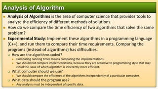
 Analysis of Algorithms is the area of computer science that provides tools to
analyze the efficiency of different methods of solutions.
 How do we compare the time efficiency of two algorithms that solve the same
problem?
 Experimental Study: Implement these algorithms in a programming language
(C++), and run them to compare their time requirements. Comparing the
programs (instead of algorithms) has difficulties.
 How are the algorithms coded?
 Comparing running times means comparing the implementations.
 We should not compare implementations, because they are sensitive to programming style that may
cloud the issue of which algorithm is inherently more efficient.
 What computer should we use?
 We should compare the efficiency of the algorithms independently of a particular computer.
 What data should the program use?
 Any analysis must be independent of specific data.
Analysis of Algorithm

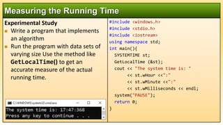
Experimental Study
 Write a program that implements
an algorithm
 Run the program with data sets of
varying size Use the method like
GetLocalTime() to get an
accurate measure of the actual
running time.
Measuring the Running Time
#include <windows.h>
#include <stdio.h>
#include <iostream>
using namespace std;
int main(){
SYSTEMTIME st;
GetLocalTime (&st);
cout << "The system time is: "
<< st.wHour <<":"
<< st.wMinute <<":"
<< st.wMilliseconds << endl;
system("PAUSE");
return 0;
}

#include <windows.h>
#include <stdio.h>
#include <iostream>
using namespace std;
long double factorial(long double n){
if (n < 0) // if n is negative
exit(-1); // close the program
long double f = 1;
while (n > 1)
f *= n--;
return f;
}
int main(){
LARGE_INTEGER t1, t2, t3;
long double n, answer;
cout << "Enter a positive integer: ";// 170
cin >> n;
QueryPerformanceCounter(&t1);
answer = factorial(n);
QueryPerformanceCounter(&t2);
t3.QuadPart = t2.QuadPart - t1.QuadPart;
cout << n << "! = " << answer << endl;
cout << "Time taken = "
<< t3.QuadPart <<" nano seconds"
<< endl;
system("PAUSE");
return 0;
}

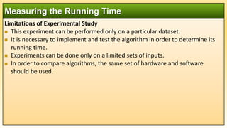
Limitations of Experimental Study
 This experiment can be performed only on a particular dataset.
 It is necessary to implement and test the algorithm in order to determine its
running time.
 Experiments can be done only on a limited sets of inputs.
 In order to compare algorithms, the same set of hardware and software
should be used.

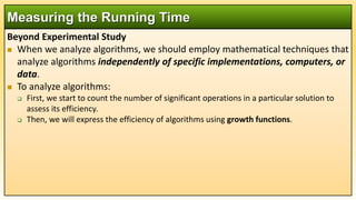
Beyond Experimental Study
 When we analyze algorithms, we should employ mathematical techniques that
analyze algorithms independently of specific implementations, computers, or
data.
 To analyze algorithms:
 First, we start to count the number of significant operations in a particular solution to
assess its efficiency.
 Then, we will express the efficiency of algorithms using growth functions.

 Each operation in an algorithm (or a program) has a cost.
 Each operation takes a certain of time.
count = count + 1; // take a certain amount of time, but it is constant
 A sequence of operations:
count = count + 1; Cost: c1
sum = sum + count; Cost: c2
Total Cost = c1 + c2
 Example 1: Simple If-Statement
 Total Cost
= c1 + c2+max(c3,c4)
The Execution Time of an Algorithm
Simple if Statement Cost Running Time
int abs_value; C1 1
if ( n < 0 ) C2 1
abs_value = -n; C3 1
else
abs_value = n; C4 1

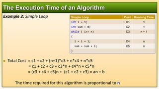
Example 2: Simple Loop
 Total Cost = c1 + c2 + (n+1)*c3 + n*c4 + n*c5
= c1 + c2 + c3 + c3*n + c4*n + c5*n
= (c3 + c4 + c5)n + (c1 + c2 + c3) = an + b
The time required for this algorithm is proportional to n
Simple Loop Cost Running Time
int i = 1; C1 1
int sum = 0; C2 1
while ( i<= n) C3 n + 1
{
i = i + 1; C4 n
sum = sum + i; C5 n
}

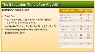
Example 3: Nested Loop
 Total Cost
= c1 + c2 + (n+1)*c3 + n*c4 + n*(n+1)*c5
+ n*n*c6 + n*n*c7 + n*c8
= (c5+c6+c7)n2 + (c3+c4+c5+c8)n + (c1+c2+c3)
 The time required for this algorithm is
proportional to n2
Nested Loop Cost Running
Time
int i = 1; C1 1
int sum = 0; C2 1
while ( i<= n) C3 n + 1
{
int j = 1; C4 n
while ( j<= n) C5 n*(n+1)
{
sum = sum + i; C6 n*n
j = j + 1; C7 n*n
}
i = i + 1; C8 n
}

 Loops: The running time of a loop is at most the running time of the
statements inside of that loop times the number of iterations.
 Nested Loops: Running time of a nested loop containing a statement in the
inner most loop is the running time of statement multiplied by the product of
the sized of all loops.
 Consecutive Statements: Just add the running times of those consecutive
statements.
 If Else: Never more than the running time of the test plus the larger of running
times of S1 and S2.
General Rules for Estimation

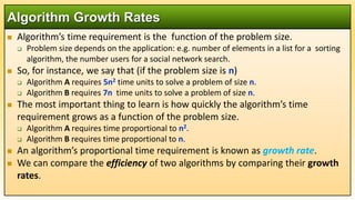
 Algorithm’s time requirement is the function of the problem size.
 Problem size depends on the application: e.g. number of elements in a list for a sorting
algorithm, the number users for a social network search.
 So, for instance, we say that (if the problem size is n)
 Algorithm A requires 5n2 time units to solve a problem of size n.
 Algorithm B requires 7n time units to solve a problem of size n.
 The most important thing to learn is how quickly the algorithm’s time
requirement grows as a function of the problem size.
 Algorithm A requires time proportional to n2.
 Algorithm B requires time proportional to n.
 An algorithm’s proportional time requirement is known as growth rate.
 We can compare the efficiency of two algorithms by comparing their growth
rates.
Algorithm Growth Rates

Algorithm Growth Rates
Graph of time requirements as
a function of the problem size n
Common Growth Rates
Function Growth Rate
Name
c Constant
log2 N Logarithmic
log2 N Log-squared
N Linear
N log2 N Log-linear
N2 Quadratic
N3 Cubic
2N Exponential
2

Running Time for Small Inputs
Running
time
Input size (x = n)
x3 2x x2
log2(x)

Running Time for Large Inputs
Running
time
Input size (x = n)
x.log2(x)
x
x2
2x x3

 Searching a number from array,
 (Best Case) The number found is at index 0
 (Worst Case) The Number was Not Fount or the number found is at index N-1, Where N
is the size of an array.
 (Average Case) The number found is at index between 1 and N-1
Best, Average and Worst Case
0
1
2
3
4
5
6
A B C D E F G
Running
Time
(ms)
- - - - - - - - - - - - - - - - - - - - - - - - - - - - - - - - - - Worst Case
- - - - - - - - - - - - - - - - - - - - - - - - - - - - - - - - - - Best Case
}Average Case
dataset

 Asymptotic notation of an algorithm is a mathematical representation of its
complexity.
 There are three types of Asymptotic Notations...
 Big - O (O)
 Big - Omega (Ω)
 Big - Theta (θ)
 Big - Oh Notation (O): Big Oh notation is used to define the upper bound of an
algorithm in terms of Time Complexity. It provides us with an asymptotic
upper bound.
 That means Big - Oh notation always indicates the maximum time required by
an algorithm for all input values.
 That means Big Oh notation describes the worst case of an algorithm time
complexity.
Asymptotic Notations

 f(n) is your algorithm runtime, and g(n) is an arbitrary time complexity. you are
trying to relate to your algorithm.
 f(n) is O(g(n)), if for some real constants c (c > 0) and number n0 , f(n) ≤ c g(n)
for every input size n (n > n0).
 O(g(n))
= { f(n): there exist positive constants c and n0
such that 0 ≤ f(n) ≤ cg(n) for all n ≥ n0 }
 f(n) = O(g(n)) means f(n) grows slower than or
equal to c g(n)
 If an Algo A requires time proportional to n2, it is O(n2).
 If an Algo A requires time proportional to n, it is O(n).
Big - Oh Notation (O)

f(n) = 7n2 + 2n + 4
f(n) = 5n2 + 6n + 4
g(n) = 8n2
n0 = 4

 To Simply the analysis of running time by getting the rid of details which may
be affected by specific implementation hardware.
 Capturing the Essence: how the running time of an algorithm increases with
the size of the input in the limit.
 Two Basic Rules:
 Drop all lower order terms
 Drop all constants
f(n) = 5n2 + 6n + 10
= 5n2 + 6n + 10
= 5n2 + 10
= 5n2 + 10
= n2
f(n) = 7n2 + 2n + 4
= 7n2 + 2n + 4
= 7n2 + 4
= 7n2 + 4
= n2

 If an algorithm requires f(n) = n2-3n+10 seconds to solve a problem size n. If
constants k and n0 exist such that
k*n2 >= n2-3n+10 for all n >= n0 .
the algorithm is order n2 (In fact, k is 2 and n0 is 2)
2*n2 >= n2-3n+10 for all n >= 2 .
Thus, the algorithm requires no more than k*n2 time units for n >= n0 ,
So it is O(n2)

n0 = 2
K=2

Show 2x + 17 is O(2x)
2x + 17 ≤ 2x + 2x = 2*2x for x > 5
Hence k = 2 and n0 = 5
2*2x
n0 = 5

 Big Omega notation is used to define the lower bound of an algorithm in terms
of Time Complexity.
 That means Big-Omega notation always indicates the minimum time required
by an algorithm for all input values.
 That means Big-Omega notation describes the
best case of an algorithm time complexity.
 It provides us with an asymptotic lower bound.
 f(n) is Ω(g(n)), if for some real constants c (c > 0)
and number n0 (n0 > 0), f(n) ≥ c g(n) for every
input size n (n > n0)
 f(n) = Ω(g(n)) means f(n) grows faster than or
equal to g(n)
Big - Omega Notation (Ω)

 Big - Theta notation is used to define the average bound of an algorithm in
terms of Time Complexity and denote the asymptotically tight bound
(Sandwich between best case and worst case)
 That means Big - Theta notation always
indicates the average time required by an
algorithm for all input values.
 That means Big - Theta notation describes the
average case of an algorithm time complexity.
 function f(n) as time complexity of an algorithm
and g(n) is the most significant term.
If C1 g(n) ≤ f(n) ≤ C2 g(n)
for all n ≥ n0 , C1 > 0, C2 > 0 and n0 ≥ 1
Then we can represent f(n) as θ(g(n)).
Big - Theta Notation (θ)
Average
Worst
Best
}
}

Big - Theta Notation (θ)
g(n) = 8n2
g(n) = 7n2
Show f(n) = 7n2 + 1 is 𝚹(n2)
You need to show f(n) is O(n2) and f(n) is Ω(n2)
f(n) is O(n2) because 7n2 + 1 ≤ 7n2 + n2 ∀ n ≥ 1
 k1 = 8 n0 = 1
f(n) is Ω (n2) because 7n2 + 1 ≥ 7n2 ∀n ≥ 0
 k2 = 7 n0 = 0
Pick the largest n0 to satisfy both conditions naturally
 k1 = 8, k2 = 7, n0 = 1
k1 = 8
n0 = 1
n0 = 0

Common Asymptotic Notations
Complexity Terminology
O (n!) Factorial
O (2n), n>1 Exponential
O (nb) Polynomial
O (n2) Quadratic
O (n log2 n) Linearithmic
O (n) Linear
O (log2 n) Logarithmic
O (1) Constant
Complexity
Dataset Size (n)
Running
Time
(sec)
2
2

Complexity Function:
F(n) = C1*1 + C2*1 + Max(C3,C4)*1
= (C1+C2+C3)1 = 1 (a fixed value)
So algorithm complexity is O(1)
Running Time Analysis Example 1
Simple if Statement Cost Running Time
int abs_value; C1 1
if ( n < 0 ) C2 1
abs_value = -n; C3 1
else
abs_value = n; C4 1

F(n) = C1 + C2 + (n+1)*C3 + n*C4 + n*C5
= (C3+C4+C5)*n + (C1+C2+C3) = an+b = n
So algorithm complexity is O(n)
Simple Loop Cost Running Time
int i = 1; C1 1
int sum = 0; C2 1
while ( i<= n) C3 n + 1
{
i = i +1; C4 n
sum = sum +1; C5 n
}

F(n) = c1 + c2 + (n+1)*c3 + n*c4 + n*(n+1)c5
+ n*n*c6 + n*n*c7 + n*c8
= (c5+c6+c7)*n2 + (c3+c4+c5+c8)*n + (c1+c2+c3)
= a*n2 + b*n + c
So algorithm complexity is O(n2)
Nested Loop Cost Running
Time
int i = 1; C1 1
int sum = 0; C2 1
while ( i<= n) C3 n + 1
{
int j = 1; C4 n
while ( j<= n) C5 n*(n+1)
{
sum = sum +1; C6 n*n
j = j + 1; C7 n*n
}
i = i + 1; C8 n
}

 Some mathematical equalities are:
Some Mathematical Facts
2
2
)
1
(
*
...
2
1
2
1
n
n
n
n
i
n
i









3
6
)
1
2
(
*
)
1
(
*
...
4
1
3
1
2
2 n
n
n
n
n
i
n
i










1
2
2
...
2
1
0
2
1
0
1











n
i
n
n
i

T(n) = c1*(n+1) + c2*( ) + c3* ( ) + c4*( )
= a*n3 + b*n2 + c*n + d
So, the growth-rate function for
this algorithm is O(n3)
Nested Loop Cost Running Time
for (int i=1; i<=n; i++) C1 n+1
for (int j=1; j<=i; j++) C2
for (int k=1; k<=j; k++) C3
x = x+1; C4



n
j
j
1
)
1
(

 

n
j
j
k
k
1 1
)
1
(

 
n
j
j
k
k
1 1



n
j
j
1
)
1
( 
 

n
j
j
k
k
1 1
)
1
( 
 
n
j
j
k
k
1 1

Data Structures and Agorithm: DS 22 Analysis of Algorithm.pptx

More Related Content

Similar to Data Structures and Agorithm: DS 22 Analysis of Algorithm.pptx (20)

More from RashidFaridChishti (20)

Recently uploaded (20)

Data Structures and Agorithm: DS 22 Analysis of Algorithm.pptx

Editor's Notes