


Data Structures using Python(generic elective).pptx
- 1. GE- Data Structures using Python Binary Trees- Unit-4
- 2. Tree Binary Search Tree AVL Trees 2
- 3. Text Books Introduction to Algorithms: Thomas H. Cormen, Charles E. Leiserson, Ronald L. Rivest, Clifford Stein, 3rd Edition. M T Goodrich, Roberto Tamassia, Algorithm Design, John Wiley, 2002. 3
- 4. Learning Outcomes Will enable students to choose appropriate data structures for designing solutions to specific problems. In depth understanding of advanced paradigms and data structures to solve algorithmic problems. Able to analyse efficiency and proofs of correctness. 4
- 5. Pre-requisites Understanding of basic data structure concepts Any one programming language like C, C++, Java etc. 5
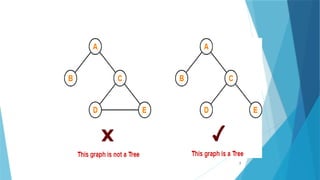
- 6. Trees Tree is a non-linear data structure which organizes data in a hierarchical structure. It is a connected graph without any circuits. If in a graph, there is one and only one path between every pair of vertices, then graph is called as a tree. 6
- 7. 7
- 8. Properties There is one and only one path between every pair of vertices in a tree. A tree with n vertices has exactly (n-1) edges. A graph is a tree if and only if it is minimally connected. Any connected graph with n vertices and (n-1) edges is a tree. 8
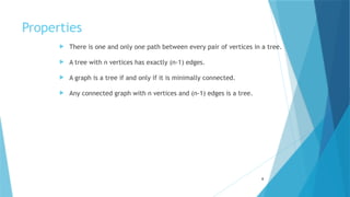
- 10. 10 Root Node The first node from where the tree originates is called as a root node.
- 11. 11 Edges The connecting link between any two nodes is called as an edge.
- 12. 12 Parent Node The node which has a branch from it to any other node is called as a parent node.
- 13. 13 Child Node The node which is a descendant of some node is called as a child node.
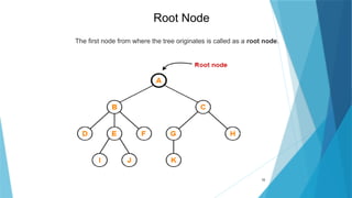
- 14. 14 Siblings Node Nodes which belong to the same parent are called as siblings.
- 15. 15 Degree of Node Degree of a node is the total number of children of that node. Degree of a tree is the highest degree of a node among all the nodes in the tree.
- 16. 16 Here, nodes A, B, C, E and G are internal nodes. Internal Node The node which has at least one child is called as an internal node/ Non-terminal nodes.
- 17. 17 Here, nodes D, I, J, F, K and H are leaf nodes. Leaf Node The node which does not have any child is called as a leaf node/Terminal Node
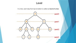
- 18. 18 Level In a tree, each step from top to bottom is called as level of a tree.
- 19. 19 Height of Node Total number of edges that lies on the longest path from any leaf node to a particular node.
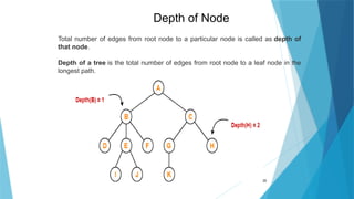
- 20. 20 Depth of Node Total number of edges from root node to a particular node is called as depth of that node. Depth of a tree is the total number of edges from root node to a leaf node in the longest path.
- 21. 21 Sub trees In a tree, each child from a node forms a subtree recursively. Every child node forms a subtree on its parent node.
- 22. 22 Forest A forest is a set of disjoint trees.
- 23. Binary Tree Binary tree is a special tree data structure in which each node can have at most 2 children. Each node has either 0 child or 1 child or 2 children. 23
- 24. 24
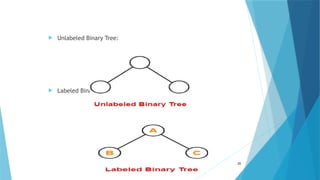
- 25. Unlabeled Binary Tree: Labeled Binary Tree: 25
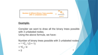
- 26. 26 Example- Consider we want to draw all the binary trees possible with 3 unlabeled nodes. Using the above formula, we have- Number of binary trees possible with 3 unlabeled nodes = 2 x 3 C3 / (3 + 1) = 6 C3 / 4 = 5
- 27. 27
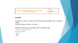
- 28. 28 Example- Consider we want to draw all the binary trees possible with 3 labeled nodes. Using the above formula, we have- Number of binary trees possible with 3 labeled nodes = { 2 x 3 C3 / (3 + 1) } x 3! = { 6 C3 / 4 } x 6 = 5 x 6 = 30
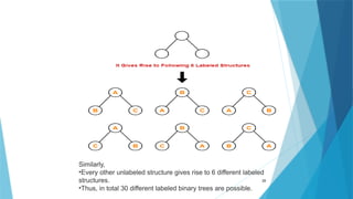
- 29. 29 Similarly, •Every other unlabeled structure gives rise to 6 different labeled structures. •Thus, in total 30 different labeled binary trees are possible.
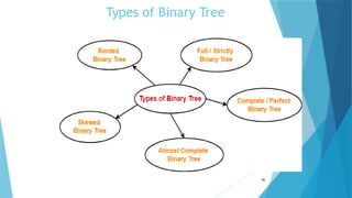
- 30. Types of Binary Tree 30
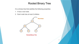
- 31. 31 It is a binary tree that satisfies the following properties: 1. It has a root node. 2. Each node has at most 2 children Rooted Binary Tree
- 32. 32 Full Binary Tree Full/Strictly Binary Tree A binary tree in which every node has either 0 or 2 children
- 33. 33 Complete Binary Tree A complete binary tree is a binary tree in which every internal node has exactly 2 children and all the leaf nodes are at same level Complete Binary Tree
- 34. 34 Almost Complete Binary Tree An almost complete binary tree is a binary tree in which all the levels are completely filled except possibly last level. The last level must be strictly filled from left to right. Almost Complete Binary Tree
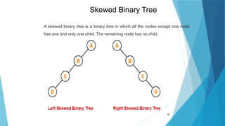
- 35. 35 A skewed binary tree is a binary tree in which all the nodes except one node has one and only one child. The remaining node has no child. Skewed Binary Tree
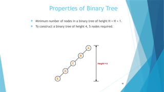
- 36. Properties of Binary Tree Minimum number of nodes in a binary tree of height H = H + 1. To construct a binary tree of height 4, 5 nodes required. 36
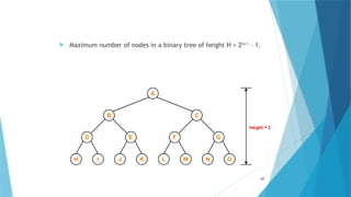
- 37. Maximum number of nodes in a binary tree of height H = 2H+1 – 1. 37
- 38. Total Number of leaf nodes in a Binary Tree = Total Number of nodes with 2 children + 1 38 Here, •Number of leaf nodes = 3 •Number of nodes with 2 children = 2
- 39. Maximum number of nodes at any level ‘L’ in a binary tree = 2L. Maximum number of nodes at level-2 in a binary tree = 22 = 4 39
- 40. 40
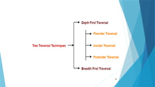
- 41. Depth First Traversal Following three traversal techniques fall under Depth First Traversal- Pre order Traversal In order Traversal Post order Traversal 41
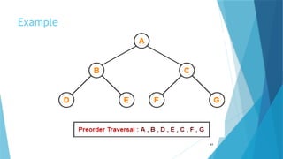
- 42. Pre order Traversal Algorithm : Visit the root Traverse the left sub tree i.e. call Preorder (left sub tree) Traverse the right sub tree i.e. call Preorder (right sub tree) Root → Left → Right 42
- 43. Example 43
- 44. In order Traversal Algorithm- Traverse the left sub tree i.e. call Inorder (left sub tree) Visit the root Traverse the right sub tree i.e. call Inorder (right sub tree) Left → Root → Right 44
- 45. Example 45
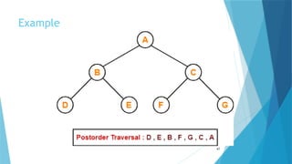
- 46. Post order Traversal Algorithm- Traverse the left sub tree i.e. call Postorder (left sub tree) Traverse the right sub tree i.e. call Postorder (right sub tree) Visit the root Left → Right → Root 46
- 47. Example 47
- 48. Breadth First 48 • Breadth First Traversal of a tree prints all the nodes of a tree level by level. • Also called as Level Order Traversal.
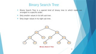
- 49. Binary Search Tree Binary Search Tree is a special kind of binary tree in which nodes are arranged in a specific order. Only smaller values in its left sub tree. Only larger values in its right sub tree. 49
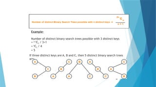
- 50. 50 Example- Number of distinct binary search trees possible with 3 distinct keys = 2×3 C3 / 3+1 = 6 C3 / 4 = 5 If three distinct keys are A, B and C, then 5 distinct binary search trees are-
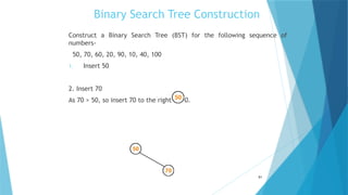
- 51. Binary Search Tree Construction Construct a Binary Search Tree (BST) for the following sequence of numbers- 50, 70, 60, 20, 90, 10, 40, 100 1. Insert 50 2. Insert 70 As 70 > 50, so insert 70 to the right of 50. 51
- 52. Insert 60 As 60 > 50, so insert 60 to the right of 50. As 60 < 70, so insert 60 to the left of 70. • Insert 20 As 20 < 50, so insert 20 to the left of 50. 52
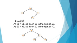
- 53. 53 • Insert 90 As 90 > 50, so insert 90 to the right of 50. As 90 > 70, so insert 90 to the right of 70.
- 54. Insert 10 As 10 < 50, so insert 10 to the left of 50. As 10 < 20, so insert 10 to the left of 20. • Insert 40 As 40 < 50, so insert 40 to the left of 50. As 40 > 20, so insert 40 to the right of 20. 54
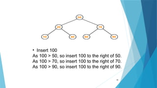
- 55. 55 • Insert 100 As 100 > 50, so insert 100 to the right of 50. As 100 > 70, so insert 100 to the right of 70. As 100 > 90, so insert 100 to the right of 90.
- 56. 56
- 57. BST Traversal A binary search tree is traversed in exactly the same way a binary tree is traversed. In other words, BST traversal is same as binary tree traversal. 57
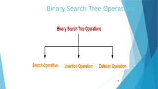
- 58. Binary Search Tree Operations 58
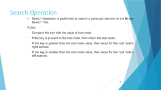
- 59. Search Operation Search Operation is performed to search a particular element in the Binary Search Tree. Rules: • Compare the key with the value of root node. • If the key is present at the root node, then return the root node. • If the key is greater than the root node value, then recur for the root node’s right subtree. • If the key is smaller than the root node value, then recur for the root node’s left subtree. 59
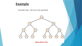
- 60. Example 60 Consider Key = 45 has to be searched
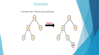
- 61. Insertion Operation Insertion Operation is performed to insert an element in the Binary Search Tree. Rules: The insertion of a new key always takes place as the child of some leaf node. • Search the key to be inserted from the root node till some leaf node is reached. • Once a leaf node is reached, insert the key as child of that leaf node. 61
- 62. Example 62 Consider Key = 40 has to be searched
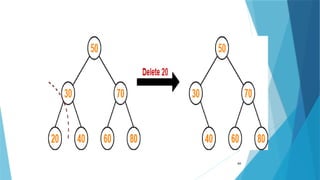
- 63. Deletion Operation Deletion Operation is performed to delete a particular element from the Binary Search Tree. Case-01: Deletion Of A Node Having No Child (Leaf Node)- Example- Consider the following example where node with value = 20 is deleted from the BST 63
- 64. 64
- 65. Case-02: Deletion Of A Node Having Only One Child- Consider the following example where node with value = 30 is deleted from the BST- 65
- 66. 66
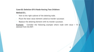
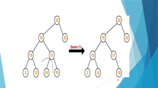
- 67. Case-03: Deletion Of A Node Having Two Children- Method-01: • Visit to the right subtree of the deleting node. • Pluck the least value element called as inorder successor. • Replace the deleting element with its inorder successor. Example- Consider the following example where node with value = 15 is deleted from the BST- 67
- 68. 68
- 69. Method-02: • Visit to the left subtree of the deleting node. • Pluck the greatest value element called as in order predecessor. • Replace the deleting element with its inorder predecessor. Consider the following example where node with value = 15 is deleted from the BST- 69
- 70. 70
- 71. Time Complexity • Time complexity of all BST Operations = O(h). Here, h = Height of binary search tree Worst Case- The binary search tree is a skewed binary search tree. • Height of the binary search tree becomes n. • So, Time complexity of BST Operations = O(n). 71
- 72. 72
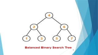
- 73. In best case, • The binary search tree is a balanced binary search tree. • Height of the binary search tree becomes log(n). • So, Time complexity of BST Operations = O(logn). 73
- 74. 74
- 75. Balanced Searched Tree It is a tree that automatically keeps its height small for a sequence of insertions and deletions. A balanced binary tree is one in which no leaf nodes are 'too far' from the root. Also called as height balanced Tree in which the difference between the height of the left subtree and right subtree is not more than m. m is balance factor equal to 1. 75
- 76. Applications Self-balancing binary search trees can be used in a natural way to construct and maintain ordered lists, such as priority queues. They can also be used for associative arrays; key-value pairs are simply inserted with an ordering based on the key alone. 76
- 77. Need Balancing the tree makes for better search times O(log(n)) as opposed to O(n). As we know that most of the operations on Binary Search Trees proportional to height of the Tree, So it is desirable to keep height small. It ensure that search time strict to O(log(n)) of complexity. 77
- 78. Examples: • AVL Trees (Adelso-Velskii and Landis) • 2-3 Trees • B-trees • Red-black Trees 78
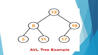
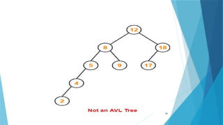
- 79. AVL Tree AVL trees are special kind of binary search trees. In AVL trees, height of left subtree and right subtree of every node differs by at most one. AVL trees are also called as self-balancing binary search trees. 79
- 80. 80
- 81. 81
- 82. Balance Factor Balance factor of a node = Height of its left subtree – Height of its right subtree. In AVL tree, Balance factor of every node is either 0 or 1 or -1. 82
- 83. AVL Tree Operations 1. Search Operation 2. Insertion Operation 3. Deletion Operation 83
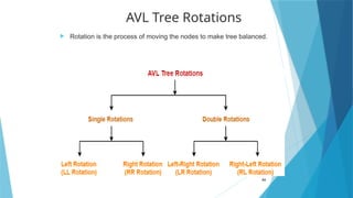
- 84. AVL Tree Rotations Rotation is the process of moving the nodes to make tree balanced. 84
- 85. Cases Of Imbalance And Their Balancing Using Rotation Operations 85
- 86. 86
- 87. 87
- 88. 88
- 89. RR Rotation RR rotation is an anticlockwise rotation, which is applied on the edge below a node having balance factor -2 89 In above example, node A has balance factor -2 because a node C is inserted in the right subtree of A right subtree. We perform the RR rotation on the edge below A.
- 90. LL Rotation LL rotation((is clockwise rotation, which is applied on the edge below a node having balance factor 2. 90 In above example, node C has balance factor 2 because a node A is inserted in the left subtree of C left subtree. We perform the LL rotation on the edge below A.
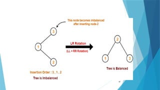
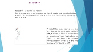
- 91. LR Rotation LR rotation = RR rotation + LL rotation, first RR rotation is performed on subtree and then LL rotation is performed on full tree, Full tree - the first node from the path of inserted node whose balance factor is other than -1, 0, or 1. 91 A node B has been inserted into the right subtree of A the left subtree of C, because of which C has become an unbalanced node having balance factor 2. This case is L R rotation where: Inserted node is in the right subtree of left subtree of C
- 92. 92 As LR rotation = RR + LL rotation, hence RR (anticlockwise) on subtree rooted at A is performed first. By doing RR rotation, node A, has become the left subtree of B. After performing RR rotation, node C is still unbalanced, i.e., having balance factor 2, as inserted node A is in the left of left of C Now we perform LL clockwise rotation on full tree, i.e. on node C. node C has now become the right subtree of node B, A is left subtree of B Balance factor of each node is now either -1, 0, or 1, i.e. BST is balanced now.
- 93. RL Rotation RL rotation = LL rotation +RR rotation, first LL rotation is performed on subtree and then RR rotation is performed on full tree Full tree - the first node from the path of inserted node whose balance factor is other than -1, 0, or 1. 93 A node B has been inserted into the left subtree of C the right subtree of A, because of which A has become an unbalanced node having balance factor - 2. This case is RL rotation where: Inserted node is in the left subtree of right subtree of A
- 94. 94 As RL rotation = LL rotation + RR rotation, hence, LL (clockwise) on subtree rooted at C is performed first. By doing RR rotation, node C has become the right subtree of B. After performing LL rotation, node A is still unbalanced, i.e. having balance factor -2, which is because of the right-subtree of the right-subtree node A. Now we perform RR rotation (anticlockwise rotation) on full tree, i.e. on node A. node C has now become the right subtree of node B, and node A has become the left subtree of B. Balance factor of each node is now either -1, 0, or 1, i.e., BST is balanced now.
- 95. 95 Delete the node 60 from the AVL tree shown in the following image.
- 96. 96
- 97. 97 Delete Node 55 from the AVL tree shown in the following image.
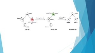
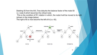
- 98. 98 Deleting 55 from the AVL Tree disturbs the balance factor of the node 50 i.e. node A which becomes the critical node. This is the condition of R1 rotation in which, the node A will be moved to its right (shown in the image below). The right of B is now become the left of A (i.e. 45).
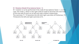
- 99. 99 R-1 Rotation (Node B has balance factor -1) R-1 rotation is to be performed if the node B has balance factor -1. In this case, the node C, which is the right child of node B, becomes the root node of the tree with B and A as its left and right children respectively. The sub-trees T1, T2 becomes the left and right sub-trees of B whereas, T3, T4 become the left and right sub-trees of A.
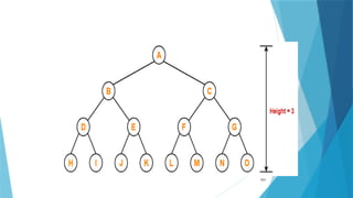
- 100. AVL Tree Properties 1. Maximum possible number of nodes in AVL tree of height H = 2H+1 – 1 e.g. Maximum possible number of nodes in AVL tree of height-3 = 23+1 – 1 = 16 – 1 = 15 100
- 101. 101
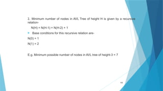
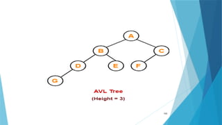
- 102. 2. Minimum number of nodes in AVL Tree of height H is given by a recursive relation- N(H) = N(H-1) + N(H-2) + 1 Base conditions for this recursive relation are- N(0) = 1 N(1) = 2 E.g. Minimum possible number of nodes in AVL tree of height-3 = 7 102
- 103. 103
- 104. 3. Minimum possible height of AVL Tree using N nodes = log ⌊ 2N⌋ Example- Minimum possible height of AVL Tree using 8 nodes = log28 ⌊ ⌋ = log223 ⌊ ⌋ = 3log22 ⌊ ⌋ = 3 ⌊ ⌋ = 3 104
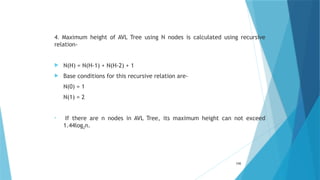
- 105. 4. Maximum height of AVL Tree using N nodes is calculated using recursive relation- N(H) = N(H-1) + N(H-2) + 1 Base conditions for this recursive relation are- N(0) = 1 N(1) = 2 • If there are n nodes in AVL Tree, its maximum height can not exceed 1.44log2n. 105
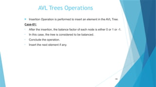
- 106. AVL Trees Operations Insertion Operation is performed to insert an element in the AVL Tree. Case-01: • After the insertion, the balance factor of each node is either 0 or 1 or -1. • In this case, the tree is considered to be balanced. • Conclude the operation. • Insert the next element if any. 106
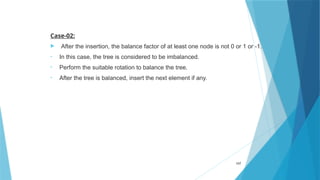
- 107. Case-02: After the insertion, the balance factor of at least one node is not 0 or 1 or -1. • In this case, the tree is considered to be imbalanced. • Perform the suitable rotation to balance the tree. • After the tree is balanced, insert the next element if any. 107
- 108. Rules To Remember 1. After inserting an element in the existing AVL tree, Balance factor of only those nodes will be affected that lies on the path from the newly inserted node to the root node. 2. To check whether the AVL tree is still balanced or not after the insertion, • There is no need to check the balance factor of every node. • Check the balance factor of only those nodes that lies on the path from the newly inserted node to the root node. 108
- 109. 109 3. After inserting an element in the AVL tree, •If tree becomes imbalanced, then there exists one particular node in the tree by balancing which the entire tree becomes balanced automatically. •To re balance the tree, balance that particular node.
- 110. To find that particular node, • Traverse the path from the newly inserted node to the root node. • Check the balance factor of each node that is encountered while traversing the path. • The first encountered imbalanced node will be the node that needs to be balanced. 110
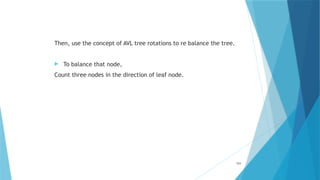
- 111. Then, use the concept of AVL tree rotations to re balance the tree. To balance that node, Count three nodes in the direction of leaf node. 111
- 112. Construct AVL Tree for the following sequence of numbers- 50 , 20 , 60 , 10 , 8 , 15 , 32 , 46 , 11 , 48 112
- 113. Solution 113 Step-01: Insert 50 Step-02: Insert 20 •As 20 < 50, so insert 20 in 50’s left sub tree. Step-03: Insert 60 •As 60 > 50, so insert 60 in 50’s right sub tree.
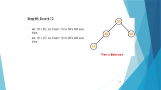
- 114. Step-04: Insert 10 • As 10 < 50, so insert 10 in 50’s left sub tree. • As 10 < 20, so insert 10 in 20’s left sub tree. 114
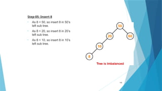
- 115. Step-05: Insert 8 • As 8 < 50, so insert 8 in 50’s left sub tree. • As 8 < 20, so insert 8 in 20’s left sub tree. • As 8 < 10, so insert 8 in 10’s left sub tree. 115
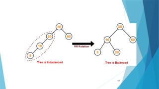
- 116. To balance the tree, Find the first imbalanced node on the path from the newly inserted node (node 8) to the root node. The first imbalanced node is node 20. Now, count three nodes from node 20 in the direction of leaf node. Then, use AVL tree rotation to balance the tree. 116
- 117. 117
- 118. Step-06: Insert 15 • As 15 < 50, so insert 15 in 50’s left sub tree. • As 15 > 10, so insert 15 in 10’s right sub tree. • As 15 < 20, so insert 15 in 20’s left sub tree. 118
- 119. To balance the tree, Find the first imbalanced node on the path from the newly inserted node (node 15) to the root node. The first imbalanced node is node 50. Now, count three nodes from node 50 in the direction of leaf node. Then, use AVL tree rotation to balance the tree. 119
- 120. 120
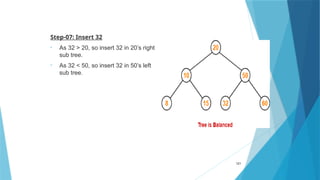
- 121. Step-07: Insert 32 • As 32 > 20, so insert 32 in 20’s right sub tree. • As 32 < 50, so insert 32 in 50’s left sub tree. 121
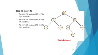
- 122. Step-08: Insert 46 • As 46 > 20, so insert 46 in 20’s right sub tree. • As 46 < 50, so insert 46 in 50’s left sub tree. • As 46 > 32, so insert 46 in 32’s right sub tree. 122
- 123. Step-09: Insert 11 • As 11 < 20, so insert 11 in 20’s left sub tree. • As 11 > 10, so insert 11 in 10’s right sub tree. • As 11 < 15, so insert 11 in 15’s left sub tree. 123
- 124. Step-10: Insert 48 • As 48 > 20, so insert 48 in 20’s right sub tree. • As 48 < 50, so insert 48 in 50’s left sub tree. • As 48 > 32, so insert 48 in 32’s right sub tree. • As 48 > 46, so insert 48 in 46’s right sub tree. 124
- 125. To balance the tree, Find the first imbalanced node on the path from the newly inserted node (node 48) to the root node. The first imbalanced node is node 32. Now, count three nodes from node 32 in the direction of leaf node. Then, use AVL tree rotation to balance the tree. 125