SlideShare a Scribd company logo
Dynamic Path Planning
FOLLOW THE GAP METHOD [FGM] FOR MOBILE ROBOTS
Presented by: Vikrant Kumar M. Tech. MED CIM 133569
Robotics – Control & Intelligence – Path
Planning – Dynamic Path Planning
Robotics &
Automation
Programming and
Intelligence
Control &
Intelligence
Controller Design Sensors for Robot
Motion Planning
and Control
Path Planning
Static Path
Planning
Dynamic Path
Planning
Mechanical
Design
Mobile Robot Navigation
• Global Navigation – from knowledge of goal point
• Local Navigation – from knowledge of near by objects
in path
• Personal Navigation – continuous updating of current
position
Robot’s ability to safely move towards the Goal using its knowledge and
sensorial information of the surrounding environment.
Three terms important in navigation are:
Static Path Planning
• Probabilistic Roadmap (PRM) - Two phase navigation:
• Learning phase
• Query phase
• Visibility Graph – navigating at the boundary of obstacles,
turning at corners only, finding shortest straight line path.
Based on a map and goal location, finding a geometric path.
Methods
Dynamic Path Planning
• Bug Algorithms
• Artificial Potential Field (APF) Algorithm
• Harmonic Potential Field (HPF) Algorithm
• Virtual Force Field (VFF) method
• Virtual Field Histogram (VFH) method
• Follow the Gap Method (FGM)
Aim is of avoiding unexpected obstacles along the robot’s trajectory to reach the goal.
Methods
Some terms of concern
• Point Robot Approach
• Field of view of Robot
• Non-holonomic constraints
Point Robot Approach
• Robot and Obstacles are assumed circular.
• Radius of robot is added to radius of obstacles
• The Robot is reduced to a point, while Obstacles are equally enlarged.
Field of view
• The sector region within the range of robot’s sensors to get
information of environment.
• Two quantitative measures of field of view:
• End angles of the sector on right and left sides.
• Radius of the sector.
Nonholonomic Constraints
• If the vector space of the possible motion directions of a mechanical
system is restricted
• And the restriction can not be converted into an algebraic relation
between configuration variables.
• Can be visualized as, inability of a car like vehicle to move sideways, it
is bound to follow an arc to reach a lateral co-ordinate.
Nonholonomic Constraints and Field of View
of Robot
Nonholonomic Constraint
Field of View
Bug Algorithms
• Common sense approach of moving directly to goal.
• Contour the obstacle when found, until moving straight to goal is
possible again.
• Path chosen – often too long
• Robot prone to move close to obstacles
Possible paths with Bug Algorithm
Artificial Potential Field (APF)
• Presently very popular
• Obstacles represent “repulsive potential”
• Goal represent “attractive Potential”
• Main drawback –
• Robot gets trapped in local minima.
• The Method Ignores nonholonomic constraints
APF contd..
APF contd..
• Main drawback –
• Robot gets trapped in local minima.
• The Method Ignores nonholonomic constraints
Harmonic Potential Field (HPF)
• An HPF is generated using a Laplace boundary value problem (BVP).
• HPF approach may be configured to operate in a model-based and/or
sensor-based mode
• It can also be made to accommodate a variety of constraints.
• the robot must know the map of the whole environment .
• contradicts reactiveness and local planning properties of obstacle
avoidance.
Virtual Force Field method (VFF)
• 2D Cartesian histogram grid for obstacle representation.
• Each cell has certainty value of confidence, that an obstacle is present there.
• Then APF is applied.
• Problems of APF method still exist in VFF
VFF contd…
Virtual Field Histogram (VFH)
• Uses a 2D Cartesian histogram grid like in VFF.
• Reduces it to a one dimensional polar histogram around the robot's
momentary location.
• Selects lowest polar obstacle density sector
• steers the robot in that direction
• very much goal oriented since it always selects the sector which is in the
same direction as the goal.
• selected sector can be the wrong one in some cases.
• does not consider nonholonomic constraints of robots
VFH Confidence value and 1D polar histogram
Follow the Gap Method (FGM)
• Point Robot Approach
• Obstacle representation
• Construction a gap array among obstacles.
• Determination of maximum gap, considering the Goal point location.
• Calculation of angle to Center of Maximum gap
• Robot proceeds to center of maximum gap.
Problem Definition
• The Algorithm
• Should find a purely reactive heading to achieve goal co-ordinates
• Should avoiding obstacles with as large distance as possible
• Should consider measurement and nonholonomic constraints
• for obstacle avoidance must collaborate with global planner
• Goal point – obtained from the global planner
• Obstacle co-ordinates - change with time
Point Robot Approach
Xrob = Abscissa of robot point
Yrob = Ordinate of robot point
Rrob = Robot circle’s radius
Xobsn = Abscissa of nth obstacle
Yobsn = Ordinate of nth obstacle
Robsn = nth obstacle’s circle’s radius
Distance to Obstacle
Distance of nth obstacle from robot
d = ((Xobsn – Xrob)2 + (Yobsn – Yrob)2)1/2
Using Pythogoras theorem
dn2 + (Robsn + Rrob)2 = d2
Or, dn = ((Xobsn – Xrob)2 + (Yobsn – Yrob)2 – (Robsn + Rrob)2)1/2
Obstacle Representation
• Two parameter representation
• Φ obs_l_1 – Border left angle of obstacle 1
• Φ obs_r_1 -- Border right angle of obstacle 1
• Φ obs_l_1 – Border left angle of obstacle 2
• Φ obs_l_1 – Border right angle of obstacle 2
Φobs_l_1
Φobs_r_1
Φobs_l_2
Φobs_r_2
Obst.
1
Obst.
2
Gap Border Evaluation
If, 𝑑𝑛ℎ𝑜𝑙 < 𝑑𝑓𝑜𝑣 => 𝛷𝑙𝑖𝑚 = 𝛷𝑛ℎ𝑜𝑙
Else if, 𝑑𝑛ℎ𝑜𝑙 ≥ 𝑑𝑓𝑜𝑣 => 𝛷𝑙𝑖𝑚 = 𝛷𝑓𝑜𝑣
In order to understand which boundary is active for a
boundary obstacle, decision rule are illustrated as
follows:
Gap boarder parameters
• 1. Φlim: Gap border angle
• 2. Φnhol: Border angle coming from nonholonomic constraint
• 3. Φfov: Border angle coming from field of view
• 4. dnhol: Nearest distance between nonholonomic constraint arc and
obstacle border
• 5. dfov: Nearest distance between field of view line and obstacle border
Gap border parameters
.
Construction of gap array
Robot
Goal
Gap 4
Gap 2
Gap 3
Field of View
Gap 1
Gap 5
 N + 1 gaps for N obstacles
Gap array and Maximum Gap
• Gap[N+1] = [(Φlim_l – Φobs1_l)(Φobs1_r – Φobs2_l)……(Φobs(n-
1)_r –Φobs(n-1)_l)(Φobsn_r – Φlim_r)]
• Maximum gap is determined with a sorting algorithm in program.
Gap array and Maximum Gap
Gap Center angle Calculation
Gap center angle
• The gap center angle (φgap_c ) is found in terms of the measurable d1,
d2, φ1, φ2 parameters
Calculation of final heading angle
• Final angle is Combination of angle of center of maximum gap and
Goal point angle.
• Determined by fusing weighted average function of gap center angle
and goal angle.
• α is the weight to obstacle gap.
• α acts as tuning parameter for FGM.
• ß weight to goal point (assumed 1 for simplicity)
• dmin is minimum distance to the approaching obstacle.
Final Heading Angle
Role of α value
• Weightage to gap angle is α/dmin
• α makes the path goal oriented or gap oriented.
• For α= 0, φfinal is equal to φgoal
• Increasing values of alpha brings φfinal closer to φgap_c and vice
versa
Relation of final angle with α
Comparison - FGM with APF on local minima
FGM and APF on local minima
• FGM the robot can reach goal point while avoiding obstacles
• In APF method, robot gets stuck because of the local minimum where
all vectors from the obstacles and goal point zero each other
• FGM selects the first calculated gap value if there are equal maximum
gaps.
• This provides FGM to move if at least one gap exists.
Comparison of Safety and Travel length
• From table below, FGM is 23% safer than the FGM-basic and 40%
safer than the APF in terms of the norm of the defined metric while
the total distance traveled values are almost the same
Dead end Scenario
• A dead-end scenario of U-shaped obstacles is a problem for FGM as it
is for APF as both are more sort of local planners.
• It needs upper level of intelligence.
• Can be solved by approaches like Virtual Obstacle Method, Multiple
Goal Point method etc.
Advantages of FGM
• Single tuning parameter (α) in weightage to gap center angle
(α/dmin)
• No local minima problem like earlier algorithms
• Considers nonholonomic constraints for the robot.
• Only feasible trajectories are generated, lesser ambiguity to decision,
lesser computation time.
• Field of view of robot is taken into account.
• Robot does not move in unmeasured directions.
• Passage through maximum gap center – Safest path.
Limitation of FGM
Remedy
• Unable to come out of dead-end-scenario
• Hybridizing FGM with local planner techniques like virtual
obstacles, virtual goal point method etc.
Conclusion
• Dynamic path planning literature and algorithms were explained.
• Follow the Gap Method(FGM) was explained in detail.
• Major Contribution from FGM:
• Single tuning parameter
• No local minima problem
• Consideration to field of view and nonholonomic constraints.
• Consideration to safety in trajectory planning.
Thank You!

More Related Content

PPTX
Evolutionary computing - soft computing
PPTX
Evolutionary Computing
PDF
Robotics for Path Planning
PPTX
Self-organizing map
PPTX
Topological Data Analysis.pptx
PPT
Path Planning And Navigation
PDF
Path Planning for Mobile Robots
PDF
Robotics or Robot Technology
Evolutionary computing - soft computing
Evolutionary Computing
Robotics for Path Planning
Self-organizing map
Topological Data Analysis.pptx
Path Planning And Navigation
Path Planning for Mobile Robots
Robotics or Robot Technology

What's hot (20)

PDF
Motion Planning
PPTX
Robotics and Autoamtion_ manipulators, actuators and end effectors
PPTX
Steepest descent method
PDF
Control engineering module 1 part-a 18me71
PPTX
Machine learning session4(linear regression)
PDF
Robot Manipulation Basics
PPTX
Self Organizing Maps
PPT
Knowledge Based Genetic Algorithm for Robot Path Planning
PDF
Path Planning for Mobile Robot Navigation Using Voronoi Diagram and Fast Marc...
PPTX
Lecture 09: Localization and Mapping III
PPT
Chapter 2 robot kinematics
PPT
Artificial Intelligence -- Search Algorithms
PPTX
Robotics ch 4 robot dynamics
PPT
Geometric modeling111431635 geometric-modeling-glad (1)
PDF
Gradient descent method
PDF
RMV Mechanics
PPTX
Robot programming , accuracy ,repeatability and application
PPTX
Uncertain Knowledge and Reasoning in Artificial Intelligence
PPT
Introduction to robotics
PPTX
Graphics Kernel System (GKS).pptx
Motion Planning
Robotics and Autoamtion_ manipulators, actuators and end effectors
Steepest descent method
Control engineering module 1 part-a 18me71
Machine learning session4(linear regression)
Robot Manipulation Basics
Self Organizing Maps
Knowledge Based Genetic Algorithm for Robot Path Planning
Path Planning for Mobile Robot Navigation Using Voronoi Diagram and Fast Marc...
Lecture 09: Localization and Mapping III
Chapter 2 robot kinematics
Artificial Intelligence -- Search Algorithms
Robotics ch 4 robot dynamics
Geometric modeling111431635 geometric-modeling-glad (1)
Gradient descent method
RMV Mechanics
Robot programming , accuracy ,repeatability and application
Uncertain Knowledge and Reasoning in Artificial Intelligence
Introduction to robotics
Graphics Kernel System (GKS).pptx
Ad

Similar to Dynamic Path Planning (20)

PDF
Iaetsd modified artificial potential fields algorithm for mobile robot path ...
PPT
Path Planning And Navigation
PDF
A Path Planning Technique For Autonomous Mobile Robot Using Free-Configuratio...
PPT
AI Robotics
PPT
16355694.ppt
PDF
IRJET- Path Finder with Obstacle Avoidance Robot
PDF
DM986-Week 9 -Part 1-Path Planning and Obstacle Avoidance.pdf
DOCX
Lecture 11 Navigation Dr. Giorgos A. Demetrio.docx
PDF
Optimally Learnt, Neural Network Based Autonomous Mobile Robot Navigation System
PDF
Design of Mobile Robot Navigation system using SLAM and Adaptive Tracking Con...
PDF
K017655963
PPTX
Real-time Obstacle Avoidance Algorithm for Mobile Robots
PDF
Pranav_Shah_Report
PPT
khelchandra project on ai
PDF
DESIGN AND IMPLEMENTATION OF PATH PLANNING ALGORITHM
PDF
PDF
A Global Integrated Artificial Potential Field/Virtual Obstacles Path Plannin...
PDF
Novel Navigation Strategy Study on Autonomous Mobile Robots
PDF
Implementation of D* Path Planning Algorithm with NXT LEGO Mindstorms Kit for...
PDF
Design and implementation of path planning algorithm for wheeled mobile robot...
Iaetsd modified artificial potential fields algorithm for mobile robot path ...
Path Planning And Navigation
A Path Planning Technique For Autonomous Mobile Robot Using Free-Configuratio...
AI Robotics
16355694.ppt
IRJET- Path Finder with Obstacle Avoidance Robot
DM986-Week 9 -Part 1-Path Planning and Obstacle Avoidance.pdf
Lecture 11 Navigation Dr. Giorgos A. Demetrio.docx
Optimally Learnt, Neural Network Based Autonomous Mobile Robot Navigation System
Design of Mobile Robot Navigation system using SLAM and Adaptive Tracking Con...
K017655963
Real-time Obstacle Avoidance Algorithm for Mobile Robots
Pranav_Shah_Report
khelchandra project on ai
DESIGN AND IMPLEMENTATION OF PATH PLANNING ALGORITHM
A Global Integrated Artificial Potential Field/Virtual Obstacles Path Plannin...
Novel Navigation Strategy Study on Autonomous Mobile Robots
Implementation of D* Path Planning Algorithm with NXT LEGO Mindstorms Kit for...
Design and implementation of path planning algorithm for wheeled mobile robot...
Ad

Dynamic Path Planning

  • 1. Dynamic Path Planning FOLLOW THE GAP METHOD [FGM] FOR MOBILE ROBOTS Presented by: Vikrant Kumar M. Tech. MED CIM 133569
  • 2. Robotics – Control & Intelligence – Path Planning – Dynamic Path Planning Robotics & Automation Programming and Intelligence Control & Intelligence Controller Design Sensors for Robot Motion Planning and Control Path Planning Static Path Planning Dynamic Path Planning Mechanical Design
  • 3. Mobile Robot Navigation • Global Navigation – from knowledge of goal point • Local Navigation – from knowledge of near by objects in path • Personal Navigation – continuous updating of current position Robot’s ability to safely move towards the Goal using its knowledge and sensorial information of the surrounding environment. Three terms important in navigation are:
  • 4. Static Path Planning • Probabilistic Roadmap (PRM) - Two phase navigation: • Learning phase • Query phase • Visibility Graph – navigating at the boundary of obstacles, turning at corners only, finding shortest straight line path. Based on a map and goal location, finding a geometric path. Methods
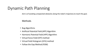
  • 5. Dynamic Path Planning • Bug Algorithms • Artificial Potential Field (APF) Algorithm • Harmonic Potential Field (HPF) Algorithm • Virtual Force Field (VFF) method • Virtual Field Histogram (VFH) method • Follow the Gap Method (FGM) Aim is of avoiding unexpected obstacles along the robot’s trajectory to reach the goal. Methods
  • 6. Some terms of concern • Point Robot Approach • Field of view of Robot • Non-holonomic constraints
  • 7. Point Robot Approach • Robot and Obstacles are assumed circular. • Radius of robot is added to radius of obstacles • The Robot is reduced to a point, while Obstacles are equally enlarged.
  • 8. Field of view • The sector region within the range of robot’s sensors to get information of environment. • Two quantitative measures of field of view: • End angles of the sector on right and left sides. • Radius of the sector.
  • 9. Nonholonomic Constraints • If the vector space of the possible motion directions of a mechanical system is restricted • And the restriction can not be converted into an algebraic relation between configuration variables. • Can be visualized as, inability of a car like vehicle to move sideways, it is bound to follow an arc to reach a lateral co-ordinate.
  • 10. Nonholonomic Constraints and Field of View of Robot Nonholonomic Constraint Field of View
  • 11. Bug Algorithms • Common sense approach of moving directly to goal. • Contour the obstacle when found, until moving straight to goal is possible again. • Path chosen – often too long • Robot prone to move close to obstacles
  • 12. Possible paths with Bug Algorithm
  • 13. Artificial Potential Field (APF) • Presently very popular • Obstacles represent “repulsive potential” • Goal represent “attractive Potential” • Main drawback – • Robot gets trapped in local minima. • The Method Ignores nonholonomic constraints
  • 15. APF contd.. • Main drawback – • Robot gets trapped in local minima. • The Method Ignores nonholonomic constraints
  • 16. Harmonic Potential Field (HPF) • An HPF is generated using a Laplace boundary value problem (BVP). • HPF approach may be configured to operate in a model-based and/or sensor-based mode • It can also be made to accommodate a variety of constraints. • the robot must know the map of the whole environment . • contradicts reactiveness and local planning properties of obstacle avoidance.
  • 17. Virtual Force Field method (VFF) • 2D Cartesian histogram grid for obstacle representation. • Each cell has certainty value of confidence, that an obstacle is present there. • Then APF is applied. • Problems of APF method still exist in VFF
  • 19. Virtual Field Histogram (VFH) • Uses a 2D Cartesian histogram grid like in VFF. • Reduces it to a one dimensional polar histogram around the robot's momentary location. • Selects lowest polar obstacle density sector • steers the robot in that direction • very much goal oriented since it always selects the sector which is in the same direction as the goal. • selected sector can be the wrong one in some cases. • does not consider nonholonomic constraints of robots
  • 20. VFH Confidence value and 1D polar histogram
  • 21. Follow the Gap Method (FGM) • Point Robot Approach • Obstacle representation • Construction a gap array among obstacles. • Determination of maximum gap, considering the Goal point location. • Calculation of angle to Center of Maximum gap • Robot proceeds to center of maximum gap.
  • 22. Problem Definition • The Algorithm • Should find a purely reactive heading to achieve goal co-ordinates • Should avoiding obstacles with as large distance as possible • Should consider measurement and nonholonomic constraints • for obstacle avoidance must collaborate with global planner • Goal point – obtained from the global planner • Obstacle co-ordinates - change with time
  • 23. Point Robot Approach Xrob = Abscissa of robot point Yrob = Ordinate of robot point Rrob = Robot circle’s radius Xobsn = Abscissa of nth obstacle Yobsn = Ordinate of nth obstacle Robsn = nth obstacle’s circle’s radius
  • 24. Distance to Obstacle Distance of nth obstacle from robot d = ((Xobsn – Xrob)2 + (Yobsn – Yrob)2)1/2 Using Pythogoras theorem dn2 + (Robsn + Rrob)2 = d2 Or, dn = ((Xobsn – Xrob)2 + (Yobsn – Yrob)2 – (Robsn + Rrob)2)1/2
  • 25. Obstacle Representation • Two parameter representation • Φ obs_l_1 – Border left angle of obstacle 1 • Φ obs_r_1 -- Border right angle of obstacle 1 • Φ obs_l_1 – Border left angle of obstacle 2 • Φ obs_l_1 – Border right angle of obstacle 2 Φobs_l_1 Φobs_r_1 Φobs_l_2 Φobs_r_2 Obst. 1 Obst. 2
  • 26. Gap Border Evaluation If, 𝑑𝑛ℎ𝑜𝑙 < 𝑑𝑓𝑜𝑣 => 𝛷𝑙𝑖𝑚 = 𝛷𝑛ℎ𝑜𝑙 Else if, 𝑑𝑛ℎ𝑜𝑙 ≥ 𝑑𝑓𝑜𝑣 => 𝛷𝑙𝑖𝑚 = 𝛷𝑓𝑜𝑣 In order to understand which boundary is active for a boundary obstacle, decision rule are illustrated as follows:
  • 27. Gap boarder parameters • 1. Φlim: Gap border angle • 2. Φnhol: Border angle coming from nonholonomic constraint • 3. Φfov: Border angle coming from field of view • 4. dnhol: Nearest distance between nonholonomic constraint arc and obstacle border • 5. dfov: Nearest distance between field of view line and obstacle border
  • 29. Construction of gap array Robot Goal Gap 4 Gap 2 Gap 3 Field of View Gap 1 Gap 5  N + 1 gaps for N obstacles
  • 30. Gap array and Maximum Gap • Gap[N+1] = [(Φlim_l – Φobs1_l)(Φobs1_r – Φobs2_l)……(Φobs(n- 1)_r –Φobs(n-1)_l)(Φobsn_r – Φlim_r)] • Maximum gap is determined with a sorting algorithm in program.
  • 31. Gap array and Maximum Gap
  • 32. Gap Center angle Calculation
  • 33. Gap center angle • The gap center angle (φgap_c ) is found in terms of the measurable d1, d2, φ1, φ2 parameters
  • 34. Calculation of final heading angle • Final angle is Combination of angle of center of maximum gap and Goal point angle. • Determined by fusing weighted average function of gap center angle and goal angle. • α is the weight to obstacle gap. • α acts as tuning parameter for FGM. • ß weight to goal point (assumed 1 for simplicity) • dmin is minimum distance to the approaching obstacle.
  • 36. Role of α value • Weightage to gap angle is α/dmin • α makes the path goal oriented or gap oriented. • For α= 0, φfinal is equal to φgoal • Increasing values of alpha brings φfinal closer to φgap_c and vice versa
  • 37. Relation of final angle with α
  • 38. Comparison - FGM with APF on local minima
  • 39. FGM and APF on local minima • FGM the robot can reach goal point while avoiding obstacles • In APF method, robot gets stuck because of the local minimum where all vectors from the obstacles and goal point zero each other • FGM selects the first calculated gap value if there are equal maximum gaps. • This provides FGM to move if at least one gap exists.
  • 40. Comparison of Safety and Travel length
  • 41. Comparison of Safety and Travel length • From table below, FGM is 23% safer than the FGM-basic and 40% safer than the APF in terms of the norm of the defined metric while the total distance traveled values are almost the same
  • 42. Dead end Scenario • A dead-end scenario of U-shaped obstacles is a problem for FGM as it is for APF as both are more sort of local planners. • It needs upper level of intelligence. • Can be solved by approaches like Virtual Obstacle Method, Multiple Goal Point method etc.
  • 43. Advantages of FGM • Single tuning parameter (α) in weightage to gap center angle (α/dmin) • No local minima problem like earlier algorithms • Considers nonholonomic constraints for the robot. • Only feasible trajectories are generated, lesser ambiguity to decision, lesser computation time. • Field of view of robot is taken into account. • Robot does not move in unmeasured directions. • Passage through maximum gap center – Safest path.
  • 44. Limitation of FGM Remedy • Unable to come out of dead-end-scenario • Hybridizing FGM with local planner techniques like virtual obstacles, virtual goal point method etc.
  • 45. Conclusion • Dynamic path planning literature and algorithms were explained. • Follow the Gap Method(FGM) was explained in detail. • Major Contribution from FGM: • Single tuning parameter • No local minima problem • Consideration to field of view and nonholonomic constraints. • Consideration to safety in trajectory planning.