SlideShare a Scribd company logo
RS/GIS Training
Geometric Fundamentals
1. GEOMETRIC FUNDAMENTALS OF MAPPING
1.1 THE MATHEMATICAL FIGURE OF THE EARTH
1.2 THE GEOID AS REFERENCESURFACE FOR HEIGHTS
1.3 APPROXIMATIONS OF THE EARTH’S FIGURE
1.3.1 Ellipsoid
1.3.2 Sphere
1.4 THE ELLIPSOID AS REFERENCE SURFACE FOR LOCATIONS
1.4.1 Local Reference Ellipsoids
1.4.2 Global Reference Ellipsoids
1.5 CONCLUSION ON REFERENCE SURFACES
1.6 SPATIAL COORINATE SYSTEMS
1.6.1 Ellipsoidal Geographic Coordinates
1.6.2 Geocentric Coordinates
1.6.3 Transformation of Spatial Coordinates
1.6.3.1 Spatial Geographic Coordinates to Geocentric Coordinates
1.6.3.2 Geocentric Coordinates to Spatial Geographic Coordinates
1.7 PLANE COORDINATE SYSTEMS
1.7.1 Cartesian Coordinates
1.7.2 Polar Coordinates
1.7.3 Transformation of Plane Coordinates
1.7.3.1 Polar Coordinates to Cartesian Coordinates
1.7.3.2 Cartesian Coordinates to Polar Coordinates
1.7.3.3 Cartesian Coordinates to Cartesian Coordinates
1.7.3.4 Cartesian Coordinates to Cartesian Coordinates with Scale Change
1.8 UNITS OF MEASUREMENTS
1.8.1 Units of Angles
1.8.2 Units for Lengths
1.8.3 Units for Areas
1.9 THE MAP SCALE
1. GEOMETRIC FUNDAMENTALS OF MAPPING
by Alfred MEHLBREUER
1.1 The Mathematical Figure of the Earth
The earth’s surface as we know it is anything but uniform. Only part of it,
the oceans, can be treated as reasonably uniform. But the surface or
topography of the land masses show large vertical variations between
mountains and valleys which make it impossible to approximate the shape
of the earth with any reasonably simple mathematical model.
We can simplify matters by the idealization of expanding the oceans below
the land masses and make the assumption that the water can flow freely
also there. If we then neglect tidal and current effects on this”global
ocean”, the resultant water surface is remaining affected only by
gravity.This has a certain consequence on the shape of this surface
because the direction of gravity - more commonly known as plumb line -
is dependent on the mass distribution in side the earth. Due to
irregularities or mass anomalies in this distribution the “global ocean” is
forced to be an undulated surface. This surface is called the GEOID or the
“mathematical figure of the earth”. The plumb line through any surface
point is always perpendicular to it (see also Spirit Leveling).
If the earth was of uniform density and the earth’s topography didn’t exist,
the geoid would have the shape of an oblate ellipsoid centered on the
earth’s center of mass.
Unfortunately, the situation is not this simple. Where mass deficiency
exists, the geoid will dip below the mean ellipsoid. Conversely, where a
mss surplus exist, the geoid will rise above the mean ellipsoid. These
influences cause the geoid to deviate from a mean ellipsoidal shape by up
to + 100 meters (see figure 1.1). The deviation between the geoid and an
ellipsoid is called the geoid undulation or geoid height. The biggest
presently known undulations are the minimum in the Indian Ocean
with N =-100 meters and the maximum in the northern part of the Atlantic
Ocean with N = +70 meters.
The Geoid as Reference Surface for
Heights
1.2
Surveying observations are usually made with instruments leveled by means of spirit
bubbles. Since these bubbles follow the influence of the earth’s gravity the observations
are made relative to the geoid. As a consequence, the geoid is well suited to be a natural
reference surface for land surveying.
In order to establish the geoid as reference, the ocean’s water level is registered t coastal
places over several years using tide gauges (mareographs). Variations of the sea level
with time, as long as they are periodic, are largely eliminated by averaging the
registrations. The resulting water level represents n approximation to the geoid and is
called the Mean Sea Level (MSL). Every nation or groups of nations have established
those observation points which are normally located close to the area of concern. For the
Netherlands the geodetic tide gauge station is in Amsterdam, for France in Marseille, for
Greece in Salonika, etc.
Starting from these stations the heights of points on the earth’s surface can be measured
using spirit leveling techniques (see land surveying). Since all the height values within a
country are related to a particular reference point, care must be taken when using
heights from another system. This might be the case in the border area of of adjacent
nations. Even within the territory of a state, heights may differ depending on to which
tide gauge they are related. As an example, the MSL from the Atlantic to the Pacific coast
of the USA increases by 0.6 to 0.7 m.
GIS/RS Training
ApproximationEarth’s1.3
The curvature of the geoid displays discontinuities at abrupt density variations inside the
earth. Consequently, the geoid is not an analytic surface and it is thereby not suitable as
a reference surface for determination of locations. If we are to carry out computations of
positions, distances, directions, etc. on the earth’s surface, we need to have some
mathematical reference frame. The most convenient geometric reference is the oblate
ellipsoid as it provides a relatively simple figure which fits the geoid to first order
approximation. For small scale mapping purposes we can also use the sphere which fits
the geoid to second order approximation.
1.3.1 Ellipsoid
An ellipsoid is formed when an ellipse is rotated about its minor axis. This ellipse which
defines an ellipsoid or spheroid is called a meridian ellipse (Note that ellipsoid and
spheroid are being treated s equivalent and interchangeable words.)
The shape of an ellipsoid may be defined in a number of ways, but in geodetic practice
the definition is usually by its semi-major axis and flattening. Flattening F is dependent
on both the semi-major axis a and the semi-major axis b.
F=(a-b)/a= (a-b/a)
The ellipsoid may also be defined by its semi-minor axis b and eccentricity e
which is given by:
e = ( 1 - ( b /a )) = ( a - b ) / a = 2f - f
Given one axis and any one of the other three parameters, the other two can be
derived.
Typical values of the parameters for an ellipsoid are:
a = 6378135.00m b = 6356750.52m
f = 1/289.26 e = 0.08181881066
This ellipsoid is often used with global satellite surveying
applications.
Pole
Pole
Equator plane
Semi major axis a
The meridian ellipse
1.3.2 Sphere
As can be seen from the dimensions of the earth ellipsoid, the semi-major axis a and
the semi-minor axis b differ only by a bit more than 21 km. A better impression on the
earth’s dimensions my be achieved if we refer to a more “human scale”. For this we
can use the quotient given by the flattening f. Considering a sphere of approximately
6 m in diameter (r =298.26cm) then the ellipsoid is derived by compressing the sphere
at each pole by 1 cm only. This compression is rather small when compared to the
dimension of the semi-major axis a. The consequence is, that instead of using the
ellipsoid, the sphere might be sufficient for certain mapping tasks.
To get an indication when the second order approximation can be applied, the
following case shall be discussed: The Russian World Map “Karth Mira” maps the
earth at scale 1:2,500,000. One of the sheets is London; it covers the area of 12 W to
12 E and 48 N to 60 N. If we use the dimensions of the above mentioned ellipsoid then
the distance between the two parallels is dE = 1335644.81 m. On a sphere of
r = 6378135.00 m, which corresponds to the semi-major axis of the ellipsoid, we get a
distance of ds = 1335833.47 m. The difference dE - dS becomes 188.66 m which is 0.08
mm at the scale 1;2,500,000. When we assume the smallest plottable line on a map is
+ 0.2 mm then a sphere instead of an ellipsoid can be used in this case.
However, it should be noted that another result will be achieved if we use a sphere
with different radius. How different spheres can be derived from the same ellipsoid is
shown by the following list:
r = 6378135.00 m (corresponds to the semi-major axis of the ellipsoid)
r = 6356750.52 m (corresponds to the semi-minor axis of the ellipsoid)
r = 6367442.76 m (average of semi-major and semi-minor axis)
r = 6370998.85 m (sphere with the equal volume than the ellipsoid)
r = 6371005.25 m (sphere with the equal surface than the ellipsoid)
Taking into account those variations, 1:5,000,000 is recommended in practice as the
largest scale at which the spherical approximation can be made.
1.4 The Ellipsoid as Reference Surface for Location
1.4.1 Local Reference Ellipsoids
It is important to realize that topographic maps are drawn and geodetic positions are
defined with respect to a reference datum (also referred to as geodetic datum).
In the United States we use the North American Datum, in Japan the Tokyo datum, in
some European countries the European Datum, in Germany the Potsdam Datum, etc.
A reference datum is defined by the size and shape of an ellipsoid as well as a
position (called the datum) at which latitude and longitude are known. Those
geometric models have been established to fit the geoid well over the area of local
interest, which in the past was never larger than a continent. As a consequence, the
differences between the geoid and the reference ellipsoid may be ignored. This
allows accurate maps to be drawn in the vicinity of the datum.
Figure 1.3 shows that a position on the geoid will have a different set of latitude and
longitude coordinates in each reference datum. In this figure the North American
datum is extrapolated to Europe. Even though the datum fits the geoid in the North
American continent well, it does not fit the European geoid. Conversely, if the
European datum were extrapolated to the North American continent, this similar
result is found.
Widely in use are the following ellipsoids generally named after their generator.
Name (Date a (m) b (m) f Used in
Delamber (1810) 6376985. 6355598. 1:308.64 Belgium
Airy (1830) 6377563. 6356257. 1:299.32 Great Britain
Bessel (1841) 6377397. 6356079. 1:299.15 Central Europe,
Chile, Indonesia
Clarke (1866) 6378274. 6356651. 1:294.97 North America, Philippines
Clarke (1880) 6378316. 6356582. 1:1:293.47 France Parts of Africa
Helmert (1906) 6378200. 6256818. 1:298.3 Egypt
Hayford (1909) 6378388. 6356912. 1:297.0 Argentina, Denmark
Krassowski (1940) 6378245. 6356863. 1:298.3 USSR, Eastern Europe
AFRICA
S.AMERICA
N.AMERICA EUROPE
N N
1.4.2 Global Reference Ellipsoids
With increasing demands for global surveying results we register several activities to
establish also global reference ellipsoids. Especially the International Union for Geodesy and
Geophysics (IUGG) is involved in establishing those reference figures. The motivation is to
make geodetic results mutually comparable and to provide coherent result also to other
disciplines like astronomy and geophysics.
In 1924 in Madrid, the general assembly of the IUGG introduced the ellipsoid determined by
Hayford 1909 as the International Ellipsoid. In contrary to local reference ellipsoids which
apply only to a region or local area of the earth’s surface., global reference systems
approximating the geoid as a mean earth ellipsoid. However, according to present
knowledge, the values for this earth model only give an insufficient approximation.
At the general assembly 1967 of the IUGG in Luzern, the 1924 reference system was replaced
by the Geodetic Reference System 1967 9GRS 1967). It represents a good approximation (as
of 1967) to the mean earth figure. The geometric ellipsoidal parameters a, b and f are given in
the table below. The Geodetic Reference System 1967 no longer represents the size and
shape of the earth to an adequate accuracy. Consequently, it was replaced by the Geodetic
Reference System 1980 (see table).
It can be expected that the increasing amount of global observations and better accuracies
some other international reference ellipsoids will be established in the future. Nowadays,
geodesists are able to measure the Earth-as-a-whole with the aid of artificial satellites.
However, a re-adjustment of all existing local geodetic survey reference systems is not to be
expected for the time being due to the great efforts in applying coordinate transformation
and changing existing maps. Local reference systems retain their practical importance for
national mapping activities.
Name (Date) a(m) b(m) f
International (1924) 6378388. 6356912. 1:297.000
GRS 1967 6378160. 6356775. 1:298.247
GRS 1980 6378137. 6356752. 1:298.257
1.5 Conclusion on Reference Surfaces
In summary, when speaking of the size and shape of the earth and positions on it, there are
three surfaces to be considered:
 The topography - the physical surface of the earth.
 The goid - the level surface (also a physical reality).
 The ellipsoid - the reference frame for computations.
Surveying observations are made on the earth surface relative to the geoid. Before using
observations in geodetic computation, they must be corrected for locational differences
between the geoid and the reference ellipsoid. These corrections are small and may for
some purposes be ignored if a reference ellipsoid is chosen so as to closely fit the geoid in
the area of concern (see figure 1.4)
Note that the Geoid in only used as reference surface for height measurements.
Locations are defined with respect to a reference ellipsoid or a sphere.
A sphere as earth model can be used for maps at scale 1:5,000,000 and smaller.
EARTH’S SURFACE
GEIOD
ELLIPSOID
Geoid separation
(Undulation)
SEA SURFACE
The Three relevant surfaces for mapping.
1.6 Spatial Coordinate Systems
1.6.1 Ellipsoidal Geographic Coordinate System
The most widely used global coordinate system consists of lines of geographic longitude
and latitude. Lines of equal latitude are called parallels. They form circles on the surface of
the ellipsoid. Lines of equal longitude are called meridians and they form ellipses (meridian
ellipses) on the ellipsoid.
The latitude of a point P is the angle between the ellipsoidal normal through P and the
equatorial plan. Latitude is zero on the equator ( = 0) and increases towards the two poles
to maximum values of = +90 (N90) at the North Pole and = -90 (S 90 ) at the South Pole.
The longitude is the angle between the meridian ellipse which passes through Greenwich
and the meridian ellipse containing the point in question. It is measured in the equatorial
plane from the meridian of Greenwich = 0 wither eastwards through =+ 180 (E180) or
westwards through = - 180 (W180 ).
Latitude and longitude representing the geographic coordinates of a point P. They are
always given in angular units (e.g. City hall Enschede: = 52 13’ 13.5” N, = 6 53’,50.8” E).
Spatial geographic coordinates ( , ,h ) are obtained by introducing the ellipsoidal height h
to the system. The ellipsoidal height of a point is the vertical distance of the point in
question above the ellipsoid. It is measured in distance units along the ellipsoidal normal
from the point to the ellipsoid surface.
Pole
Greenwich
Equator
P
h
P
The concept of geographic coordinates can also be applied to a sphere as the reference
surface. However, there is significant difference between the ellipsoidal and the spherical
geographic latitude.
The concept of latitude on the latitude on the ellipsoid might become clearer if we look at
the meridian plane through P (see figure 1.6). If a spherical rather than an ellipsoidal figure
were being used, the latitude of P’ would be the angle at the center of the sphere. This is
because the normal to the surface of the sphere will always pass through its center. Using
an ellipsoidal figure, the normal through P’ will not pass through the center of the ellipsoid,
and the latitude is given by the angle between this normal and the equatorial plane. The
angle is given by the angle between this normal and the equatorial plane. The angle is
called the geocentric latitude, and it is often used as an intermediate quantity in
calculations with the ellipsoid.
Semi minor axis
b.
Sphere
Semi minor axis a
tangent
P
P
ellipsoid
1.6.2 Geocentric Coordinates ( X,Y,Z)
An alternative and often more convenient method of defining a position is with spatial
cartesian coordinates (figure 1.7). The system has its origin at the mass-center of the earth
with the x and y axis in the plane of the equator. The three axes are mutually orthogonal and
form a right-handed system.
It should be noted that the rotational (spin) axis of the earth changes its position with the
time (catchword: polar motion). Due to this the mean position of the pole in the year 1903
(based on observations between 1900 and 1905) was used to define the so-called “
“Conventional International Origin”(CIO).
Z
CIO
Greenwich
EquatorX
Y
P
Zp
Yp Xp
1.6.3 Transformation of Spatial Coordinates
Like already mentioned with the geoid as local reference surface for heights, care must be
taken when using data from another height system. This might be the case in the border
area of adjacent nations (see 1.2). Something similar comes up when using geographic
coordinates related to different reference datums. The way in which local datums are
established is based on convenience and best fit over a certain area of the earth’s surface.
These datums are seldom geocentric of correct scale, or oriented exactly to the CIO pole
and the Greenwich meridian. However, the problem of non-similarity of adjacent systems
can be solved by transforming the coordinates.
Many types of datum transformations have been developed over the years. They range from
simple similarity transformations between two sets of plane coordinates to more complex
formulae taking into account three dimensional transformations are typically only valid over
a very limited area. Three dimensional transformations are more suitable for larger areas as
they are typically global in concept and enable solutions for heights as well as planimetric
positions.
The complete three dimensional transformation involves seven parameters that relate
corresponding coordinates in the two ellipsoidal systems. There are three translation
parameters to relate the origins of the two system (dX, dY, dZ), three rotation parameters to
relate the orientation of the two system ( x, y, z), and one scale parameter (s) to account for
any difference in scale between the two systems.
Transformation between local reference datums is a geodetic problem. Consequently,
cartographers will normally not been involved but might be asked to assist in preparing for
transformation.
1.6.3.1 Spatial Geographic Coordinates to Geocentric Coordinates
Datum transformations are usually carried out using geocentric coordinates rather than
geographic coordinates. The use of geographic coordinates would necessitate the use of an
associated ellipsoid.The geocentric coordinates (X, Y, Z) of a point P known in geographic
coordinates ( ) on an ellipsoid of semi major axis a, and semi minor axis b, may be
calculated by using the formulae:
Y = p * cos *sin
Z = p * ( 1 - e ) * sin
The parameter p(rho) is the radius of the curvature in the prime vertical (east-west direction)
while e is the eccentricity (see 1.3.1). Rho can be computed by using the formulae:
N = p = a / (1 - e *
M
If a point P is situated at a height h above the ellipsoid, its geocentric coordinates are given
by:
X = (p+h) * cos * cos
Y = (p+h) * cos * sin
Z = (p*(1-e ) + h) * sin
1.6.3.2 Geocentric Coordinates to Spatial Geographic Coordinates
The inverse computation of ( ) from (X,Y,Z ) is carried out as follows (refer also to
figure 1.8)
=
=
h =
The following substitutions are used within the formulae:
p
=
=
e =
e =
(tan
The inverse determination of the parameters , , and h can be solved without interation.
However, the solution gives good results for earth bound stations while stations of distant
space need an interation to achieve greater accuracy.
1.7 Plane Coordinate Systems:
A flat map has only two dimensions, width (left to right) and length (bottom to top). Transforming the three
dimensional earth body into a two dimensional map is subject of map projections. Here, like in several
other cartographic applications, two dimensional coordinates are needed to describe the location of any
point in an unambiguous and unique manner.
1.7.1 Cartesian Coordinates
One possibility of defining a point in a plane is to use plane rectangular coordinates. This is a system of
intersecting perpendicular lines which contains two principal axes, called the x- and y- axis. The horizontal
axis is usually referred to as the x-axis and the vertical the y - axis (Note that the x-axis is sometimes called
Easting and the y-axis Northing). The intersection of the x- and y-axis forms the origin. The plane is marked
at intervals by equally spaced coordinate lines.
Any location P on the map can now be precisely and objectively specified by
giving its two numerical coordinates xp and yp.
Y
-X Origin
-Y X
P1 (2.32, 2.55)
P2 (5.77, 1.55)
Normally, the coordinates xp = 0 and yp = 0 are given to the origin. However, sometimes large positive
values are added to the origin coordinates. This is to avoid negative values for the x- and y- coordinates in
case the origin of the coordinate system is located inside the area of interest. The point which has then the
coordinates xp=0 and yp = 0 is called the false origin.
Rectangular coordinates are also called cartesian coordinates after Descartes, a French mathematician of
the seventeenth century. He devised a system for geometric interpretation of algebraic relationship which
formed the basis for the development of a branch of mathematics called “analytic geometry”.
1.7.2 Polar Coordinates
Another possibility of defining a point in a plane is by polar coordinates. This is the distance d from the
origin to the point concerned and the angle a between a fixed (or zero) direction and the direction to the
point (see figure 1.10) The angle a is called azimuth or bearing and is counted clockwise. It is given in
angular units while the distance d is expressed in length units.
Bearings are always related to a fixed direction (initial bearing) or a datum line. In principle, this reference
line can be chosen freely.However, in practice three different directions are widely in use:
True North, Grid North and Magnetic North. The corresponding bearings are called: true bearing or
geodetic bearing, grid bearing and magnetic or compass bearing (see lectures on Land Surveying).
Polar coordinates are often used in land surveying. For some types of surveying instruments it is
advantageous to make use of this coordinate system.Especially the development of precise remote
distance measurement techniques has led to the virtually universal preference for the polar
coordinate method in detail survey.
Plain polar coordinates (a, d)
Origin
Initial bearing
a
1.7.3 Transformation of Plane Coordinates
As cartographers you are most probably concerned in your day to day work wilth going from one two
dimensional coordinate system to the other. This includes the transformation of polar coordinates
delivered by a surveyor into cartesian map coordinates or the transformation from one plane
rectangular system to another adjacent system. No matter how, you should be prepared to carry out
successfully simple two dimensional transformations. In the following sections some of these typical
tasks will be discussed.
1.7.3.1 Polar Coordinates to Cartesian Coordinates
Known: a , d
Unknown: xp, yp
Assumption: There is no difference in scale (length units) between the two systems.
Condition: The origins of the two coordinate systems are identical (x0=0, y0 = 0).
The orientation (angle between zero direction and y- coordinate axis) is zero.
X
Origin
a
d
P
SIMPLE CASE OF TRANSFORMING POLAR
COORDINATES TO ARTESIAN COORDINATES.Y
The simple case of transforming polar coordinates to cartesian coordinates you will hardly find in
practice. For a more realistic case a translation (shift) and a rotation parameter has to be introduced to
transform one system to the other.
Known: a, d, x0, y0,
Unknown: Xp, yp
Assumption: There is no difference in scale (length units) between the two systems.
The origins of the two coordinate systems are not identical.
The orientation (angle between zero direction and y-coordinate axis) is unequal zero.
X
Y
Origin
a d
P
Origin 2
y0
X0
1.7.3.2 Cartesian Coordinates to Polar Coordinates
Known: xp, yp
Unknown: a, d
Assumption: There is no difference in scale (length units) between the two systems.
Condition: The orientation (angle between zero direction and y - coordinate axis) us zero.
XOrigin
a
d
P
Y
The more realistic case again makes use of a translation (shift) and rotation for transformation.
Known; xp, yp, xo, yo,
Known; a, d.
Assumption; There is no difference in scale (length units) between the two systems.
The origins of the two coordinate systems are not identical.
The orientation (angle between zero direction and y-coordinate axis) is unequal zero.
Origin
a d
P
Origin 2
y0
X0 Xp
Initial Bearing
Y
yp
1.7.3.3 Cartesian Coordinates to Cartesian Coordinates
With this kind of plane coordinate transformation the cartographer will quite often come in touch with.
The task is to transform the coordinates from one plane rectangular system to another system which
might be translated (shifted) and/or rotated against the first one. Typical applications are:
 The transformation from one grid system to an adjacent coordinate system
in case a map is located in the overlapping part of two grid systems and
both shall be represented on the map (see also: map projections).
 The transformation of digitizer coordinates x and y to map coordinates X
and Y. A map that is fixed on a digitizer table can only be digitizer in the
digitizer coordinate system. However, the fixed map is normally slightly
rotated against this system. The resulting digitizer coordinates might
consequently be transformed to achieve a certain map
coordinate system (see also:digitizing from graphic documents).
Known: xp, yp, X0, Y0, a
Unknown: Xp, Yp
Assumption: There is no difference in scale (length units) between the two
systems.
The origins of the two coordinate systems are not identical.
The orientation (angle between two corresponding coordinates axes) is
unequal zero.
Transformation of cartesian coordinates to
cartesian coordinates.Y
Y0
Origin 1 X0
X
Xp = X0 + xp* cos a - yp*sin a
Yp = Y0 + xp* sin a + yp*cos a
If we assume the shift-values X0 and Y0 and
also the rotation A are unknown, then we can
calculate the transformation coefficients X0, Y0
a1 and a2 by using the coordinates of two
control points. Those points are known in
both the first (x,y) and the second coordinate
system (X,Y). In this case a system of four
simultaneous equations with four unknowns
has to be solved..
1.7.3.4 Cartesian Coordinates to Cartesian Coordinates
with Scale Change
This kind of transformation will be needed to correct additionally for scale changes
between the two plane rectangular coordinate systems. Differences in scale, I.e. length units
may occur when one of the coordinate system is in meter and the other in feet.
Consequently, scale differences are existing but might be regular, I.e. similar in x- and y-
direction. More serious is the non similar scale change caused by shrinkage of paper maps
which undergo humidity based changes more in one direction than the other. Consequently,
the scale factor along the x-axis is different from that along the y- axis.
The first problem can be solved by applying a conformal transformation which changes the
size and position of any geometric element but maintains its form. The problem of non
regular shrinkage can be solved by applying an affine transformation.
Origin 1 X
Y
Y0
X0
Y0
Origin 2
p
x
Xp
1
Transformation of a cartesian coordinates.
Y
Y0
Origin 1 X0
X
The general statement of the
conformal transformation is:
Xp = X0 + b1*xp - b2*yp
Yp = Y0 + b2*xp + b1*yp
Where:
b1 = s*cos a
and
b2 = s*sin a
If we assume the shift-value X0 and Y0, the common scale factor s in x- and y-
direction and also the rotation q are unknown, the we can calculate the
transformation coefficients X0, Y0, b1 and b2 by using the coordinates of two
control points only.
The number of control points will change when we apply an affine transformation.
If we assume the shift-values X0 and Y0 and Y0, the scale factors sx and sy in x-
and y- direction and also the rotation a are unknown, then we can calculate the six
transformation coefficients X0, Y0, c1, c2, c3 and c4 by using the coordinates of
three control points. Every control point delivers two equations for X and Y each.
Consequently, a system of six simultaneous equations with six unknowns has to
be solved.
For the conformal transformation at least two control points are needed when the
four transformation parameters have to be calculated, while for the affine
transformation at least three control points are necessary, If there are more than
the minimum number of control points available (so called redundant information)
then we usually apply techniques of Least Squares Adjustment. This enables us to
introduce all the information which is available to get a more stable or better
result. Least squares adjustment is usually already integrated in digitizer software
(see: digitizing from graphic documents).
1.8 Units of Measurements
Measurements are taken in units. A measurement without indicating the unit
applied makes no sense. In cartography, three groups of unit have to be
distinguished according to the basic measurements which can be taken from
maps. These are units for angles, units for lengths and units for areas.
1.8.1 Units for Angles
Angles are usually indicated in one of the four following ways:
• In degrees, based on a division of the full circle into 360 units.
• In grades, based on a division of the full circle in to 400 units.
• In radians, based on a division of the full circle into 2 units (6.283185).
• In mils, based on a division of the full circle into 6400 units.
The division of the circumference of a circle in degree is an ancient way of
indicating angle measurements which is still in use today with mathematics. It is
originally based upon moon cycles, lasting 30 days. Twelve moons
(months)elapsed a year of 360 days or a full circle. Consequently, all circles were
divided accordingly. Degrees are units of the so called sexagesimal system in
which the base unit is divided in to 60 minutes (‘), and one minute into 60 seconds
(“). A right angle counts 90 degrees.
The decimal system of dividing the circumference of a circle in grades was
introduced into science after the French Revolution. It overcomes some
inconvenience in handling the sexagesimal system, namely when adding or
subtracting non-decimal numbers. In the decimal system, the full circle is divided
in 100 centigrades ( C ), one centigrade in 100 decimilligrades (cc). A right angle
counts 100 grades. The big advantage of this system is that one can express an
A decimal number which definitely simplifies computations. The decimal system is
widely in use in land surveying.
A radian is based on the mathematical constant 2 which is the circumference of
a circle with the radius 1. Radians are often used to transform angles from one
system to another. A right angle counts /2 which is 1.5707963 radians. One radian
is the angle which corresponds to the circumference distance 1 in a circle with the
radius1.
The unit mils is mainly known from military applications; it is hardly used by the
civilians doing cartometric measurements. However, to be able to understand
military language, one has to know the relations. A right angle is 1600 mils.
degrees grades radians mils
1 degree 1 0.9 1.7453*10 -2 17.77777
1 grade 1.111111 1 1.5708*10-2 16
1 radian 57.29578 63.661975 1 1018.5916
1 mil 5.625*10-2 6.25*10-2 9.817*10-4 1
1.8.2 Units for Lengths
Most countries of the world are either “going metric”, or have already done so.
The decimal nature of the metric system, and thus the simple relationship of the
units used in the system, make computations easier in the metric system than
they are in the British imperial system. The metric system has been in operation
already in France since the French Revolution, and many European countries have
adopted the system by the time the first Metric Convention was set up in 1875 to
establish international standards of measurements. In 1960 an international
conference on weights and measures adopted what has become known as the
“standard International Metric system (S.I). For length measurements the base unit
of the S.I. System is the metre.
British Imperial System
12 inches = 1foot
3 feet = 1 yard
51/2 yard = 1 rod (pole or perch)
4 rods = 1 chain
22 yards = 1 chain
80 chains = 1 mile
1760 yards = 1 mile
63360 inches = 1 mile
Metric System
10 millimetres = 1centimetre (cm)
10 centimetres = 1 decimetre (dm
10 decimetres = 1 metre (m)
100centimetres = 1 metre
1000 metres = 1 kilometre (km)
100000 centimetres = 1 kilometre
The S.I system also forms the basis of the metric
conversion of topographic maps in many parts of the
world. Metrication of topographic maps means that all
units of measurement will appear in metric terms. Thus,
the scale of the map will be metric, the grid referencing
system will be in metres rather than in yards, and
heights will also be shown in metres. In most of those
countries where the British imperial system was used
almost exclusively for topographic mapping, this
change-over, for practical reasons, must be a gradual
process since finance and time are two major
limitations. However, conversion is well underway in
Great Britain, Australia, some countries in Africa and
Canada, to give a few examples.
1.8.3 Units for Areas
Area measurements are based on linear measures. Also in the case, the metric
system is much easier to handle than the British imperial system. If the metric
system is replacing the imperial system, it is consequent to change also to
metric area measures. However, since the British system is still in use, a
conversion table is given next page.
1.9 The Map Scale
Scale is a ratio. It is the ratio between a distance measured on a map and the corresponding
distance measured on the reference surface (ellipsoid or sphere). To state that a map has a
scale of one inch to one mile means that every inch measured on the map represents a
distance of one mile on the reference surface.
Scale is usually expressed in one or more of the three following ways:
• As a word statement such as one inch to one hundred yards.
• As a numerical proportion, for example, 1:50000.
• As a linear relationship or as graphic line scale.
The verbal type of scale expression is associated almost entirely with maps using the
British Imperial system of linear measurement (in inches, yards, and miles, for example).
Metric scales can be, of course, also easily expressed in the form of a statement but this is
not so commonly in use. However, a verbal expression of a scale is the least useful method
when reading a map, irrespective of the measurement system which is being used (imperial
or metric). It is difficult to measure distances directly from the map using a verbal scale.
The numerical proportion of map distance to real world distance is more often used. Both
the numerator and the denominator must be expressed in the same units. In the example
1:50000, one unit on the map represents 50000 of the same units on the reference surface.
Scale in this form is with numerical scales it is important to ensure that map distance and
distance on the reference surface are stated in terms of the same measurement system.
Distances measured on the map are transformed to real world distances by multiplying
them with the denominator.
The graphic line scale is the most useful method of representing scale on maps, for actual
distances can be measured directly from the map. Straight line distances can be determined
by a ruler or even by means of a paper strip on which tick marks can be indicated. This
distance is then compared with the linear scale and the ground distance may be read easily.
To determine the distance along a road or a river (or a similar curved line) a series of steps
or sub-points is established. Very useful for this action is using a pair of dividers. The
distances between each set of points is determined separately, noted and cumulative total
kept.
Some confusion often surrounds the terms small and large map scale. To clarify the matter
one should remember the meaning of scale which is a ratio or quotient. One divided by
twenty five thousand (1:250,000) gives a larger result than one divided by one hundred
thousand (1:100,000). Consequently, scale 1:250,000 is larger than scale 1:1000000 has a
larger scale than a map with scale of 1:100000.
A large scale map depicts a comparatively small area of land. As a consequence, they are
especially useful when detail has to be shown. A cadastral map is always in a large scale as
fields, houses and other relevant features have to be represented completely and with their
true location. A small scale map depicts a comparatively large area of land . A common
example of a small scale map is that of a state or country as is found in an atlas. Obviously
the amount of detail that can be shown on such a map is limited and features such as roads
and railways are drawn out of all proportion of their actual size.
An often made mistake is assuming the map scale as being generally valid for the entire
map sheet. This generalized assumption is not correct.
The transformation of the reference surface (ellipsoid, sphere) to the map plane is always
connected with geometrical distortions. For example, a projection that preserves the
size
Of areas distorts at the same time their shapes. It is not possible for a map to preserve both
- size and shape - at the same time. Something comparable we have with equidistant
projections. Although they are able to preserve distances, they are never equidistant
everywhere. The geometrical property equidistance can only be achieved for certain
locations or along certain lines. A map may be equidistant along the meridians but is not so
along the parallels (see map projections). As a consequence, the indicated scale (nominal
map scale) is only valid along the meridians. A map user should be aware of this especially
when computations are to be made on the basis of measurements taken from small scale
maps.
When maps show the whole globe, the map maker sometimes replaces the standard
graphic scale with a variable graphic scale. The scale may change systematically in north-
south and east-west directions. To use such a variable scale, you first have to decide in
what latitude-longitude zone you want to determine a distance, and then depict the distance
from the graphic scale.
The situation is different for large scale maps which depict a comparatively small area of
land. Though the geometric property equidistance along certain lines is also valid for these
maps, the resulting distortions are smaller due to the larger scale. They may become so
small that they cannot be measured any longer when using a ruler. This is generally the
case with topographic maps. In this case we can assume the map scale as being valid for
the entire map sheet.
In some books a definition of map scale is given which is not precise enough. It is written
that the map scale is the ratio between a distance measured on a map and the
corresponding distance measured on the ground (the physical earth surface). This
inaccurate as in reality a distance on the physical earth surface differes from that on the
geometrical reference surface. From figure 1.18 can be seen that the distance d on the
Plateau is longer than the corresponding distance d on the ellipsoid. Consequently, maps
with slightly different scales would have to be produced for coastal plain regions and high
mountaineous regions. To avoid this methodical and practical confusion every distance
measured in land surveying is reduced to the ellipsoid (see land surveying). This means, a
distance measured on the map and multiplied by the scale denominator gives as result the
corresponding distance on the reference surface and not on the earth surface. However, it
should be noted that for most practical cases the difference between the calculated
distance and the actual distance on the ground is so small that it can be neglected.

More Related Content

DOCX
Latitude
PPT
7 8.math projection (2)
PPT
datum
PPTX
PPTX
Geospatial reference-systems
PPTX
Geodetic systems (earth, ellipsoid)
PPTX
Surveying geodesy ajith sir
PDF
Ge152 lecture2 terrestrial reference systems_2nd_sem2013-2014_s_reyes
Latitude
7 8.math projection (2)
datum
Geospatial reference-systems
Geodetic systems (earth, ellipsoid)
Surveying geodesy ajith sir
Ge152 lecture2 terrestrial reference systems_2nd_sem2013-2014_s_reyes

What's hot (20)

PDF
2018 GIS in the Rockies Workshop: Coordinate Systems and Projections
PPTX
Earth Coordinate Systems
PDF
Projections and coordinate system
PPTX
Coordinate systems
PPT
Geodetic systems
PDF
International spheroid[1]
PPTX
Coordinate systems
PPTX
GIS Map Projection
PDF
Basics of geodesy
PPTX
Geodesy University Course
PPTX
Geographic coordinate system & map projection
PPTX
Map projections
PPTX
Introduction to MAPS,Coordinate System and Projection System
PPTX
GEOID-DETERMINAION
PPT
Basic of Geodesy
PPTX
2017 PLSC Track: Fundamentals of Coordinate Systems
PPT
Map projection
PPTX
Family of cylindrical map projection
PPTX
Map projection
PPTX
Map Projection
2018 GIS in the Rockies Workshop: Coordinate Systems and Projections
Earth Coordinate Systems
Projections and coordinate system
Coordinate systems
Geodetic systems
International spheroid[1]
Coordinate systems
GIS Map Projection
Basics of geodesy
Geodesy University Course
Geographic coordinate system & map projection
Map projections
Introduction to MAPS,Coordinate System and Projection System
GEOID-DETERMINAION
Basic of Geodesy
2017 PLSC Track: Fundamentals of Coordinate Systems
Map projection
Family of cylindrical map projection
Map projection
Map Projection
Ad

Similar to GIS/RS Training (20)

PDF
Basic Geodesy.pdf
PPTX
GEODESY Module IV.pptx info about geodesy
PPTX
ELLIPSOID GEOMETRY TYPES OF LATITUDES OF ELLIPSOID.pptx
PDF
inroduction to geodesy
PPTX
TYBSC IT PGIS Unit III Chapter I Spatial Referencing and Positioning
PPT
proyecciones cartográficas utm para realizar transformaciones
PPT
presentación básica de conceptos de geodesia clásica para georeferenciación
PPTX
Introduction to Geodesy-Types, Shape of earth
PDF
PDF
Combined gis 2(GEOGRAPHIC INFORMATION SYSTEM)
PDF
Coordinate System.pdf
PDF
basic geodesy.pdf
PPTX
Basic Geodesy.pptx .........................
PDF
Gravity & magnetic methods in geology
PPTX
Types of Ellipsoid
PPT
Earth_model...2.ppt
PDF
Geodesy md. yousuf gazi
PPTX
Geodesy is the science of accurately measuring and understanding the Earth's ...
PPT
GIS_lec 2_Different_Spatial coordinate system.ppt
PDF
Geodesy - Definition, Types, Uses and Applications
Basic Geodesy.pdf
GEODESY Module IV.pptx info about geodesy
ELLIPSOID GEOMETRY TYPES OF LATITUDES OF ELLIPSOID.pptx
inroduction to geodesy
TYBSC IT PGIS Unit III Chapter I Spatial Referencing and Positioning
proyecciones cartográficas utm para realizar transformaciones
presentación básica de conceptos de geodesia clásica para georeferenciación
Introduction to Geodesy-Types, Shape of earth
Combined gis 2(GEOGRAPHIC INFORMATION SYSTEM)
Coordinate System.pdf
basic geodesy.pdf
Basic Geodesy.pptx .........................
Gravity & magnetic methods in geology
Types of Ellipsoid
Earth_model...2.ppt
Geodesy md. yousuf gazi
Geodesy is the science of accurately measuring and understanding the Earth's ...
GIS_lec 2_Different_Spatial coordinate system.ppt
Geodesy - Definition, Types, Uses and Applications
Ad

Recently uploaded (20)

PPTX
UNIT 4 Total Quality Management .pptx
PPTX
Lesson 3_Tessellation.pptx finite Mathematics
PPTX
web development for engineering and engineering
PPTX
UNIT-1 - COAL BASED THERMAL POWER PLANTS
PPT
Project quality management in manufacturing
PPTX
M Tech Sem 1 Civil Engineering Environmental Sciences.pptx
PPTX
MCN 401 KTU-2019-PPE KITS-MODULE 2.pptx
PDF
PRIZ Academy - 9 Windows Thinking Where to Invest Today to Win Tomorrow.pdf
PDF
Evaluating the Democratization of the Turkish Armed Forces from a Normative P...
PPTX
Sustainable Sites - Green Building Construction
PDF
keyrequirementskkkkkkkkkkkkkkkkkkkkkkkkkkkkkkkkkkkkk
PPT
Mechanical Engineering MATERIALS Selection
PDF
Mitigating Risks through Effective Management for Enhancing Organizational Pe...
PPTX
CARTOGRAPHY AND GEOINFORMATION VISUALIZATION chapter1 NPTE (2).pptx
PDF
BMEC211 - INTRODUCTION TO MECHATRONICS-1.pdf
PDF
The CXO Playbook 2025 – Future-Ready Strategies for C-Suite Leaders Cerebrai...
PDF
PPT on Performance Review to get promotions
PPTX
Foundation to blockchain - A guide to Blockchain Tech
PDF
Digital Logic Computer Design lecture notes
PPTX
Welding lecture in detail for understanding
UNIT 4 Total Quality Management .pptx
Lesson 3_Tessellation.pptx finite Mathematics
web development for engineering and engineering
UNIT-1 - COAL BASED THERMAL POWER PLANTS
Project quality management in manufacturing
M Tech Sem 1 Civil Engineering Environmental Sciences.pptx
MCN 401 KTU-2019-PPE KITS-MODULE 2.pptx
PRIZ Academy - 9 Windows Thinking Where to Invest Today to Win Tomorrow.pdf
Evaluating the Democratization of the Turkish Armed Forces from a Normative P...
Sustainable Sites - Green Building Construction
keyrequirementskkkkkkkkkkkkkkkkkkkkkkkkkkkkkkkkkkkkk
Mechanical Engineering MATERIALS Selection
Mitigating Risks through Effective Management for Enhancing Organizational Pe...
CARTOGRAPHY AND GEOINFORMATION VISUALIZATION chapter1 NPTE (2).pptx
BMEC211 - INTRODUCTION TO MECHATRONICS-1.pdf
The CXO Playbook 2025 – Future-Ready Strategies for C-Suite Leaders Cerebrai...
PPT on Performance Review to get promotions
Foundation to blockchain - A guide to Blockchain Tech
Digital Logic Computer Design lecture notes
Welding lecture in detail for understanding

GIS/RS Training

  • 2. 1. GEOMETRIC FUNDAMENTALS OF MAPPING 1.1 THE MATHEMATICAL FIGURE OF THE EARTH 1.2 THE GEOID AS REFERENCESURFACE FOR HEIGHTS 1.3 APPROXIMATIONS OF THE EARTH’S FIGURE 1.3.1 Ellipsoid 1.3.2 Sphere 1.4 THE ELLIPSOID AS REFERENCE SURFACE FOR LOCATIONS 1.4.1 Local Reference Ellipsoids 1.4.2 Global Reference Ellipsoids 1.5 CONCLUSION ON REFERENCE SURFACES 1.6 SPATIAL COORINATE SYSTEMS 1.6.1 Ellipsoidal Geographic Coordinates 1.6.2 Geocentric Coordinates 1.6.3 Transformation of Spatial Coordinates 1.6.3.1 Spatial Geographic Coordinates to Geocentric Coordinates 1.6.3.2 Geocentric Coordinates to Spatial Geographic Coordinates
  • 3. 1.7 PLANE COORDINATE SYSTEMS 1.7.1 Cartesian Coordinates 1.7.2 Polar Coordinates 1.7.3 Transformation of Plane Coordinates 1.7.3.1 Polar Coordinates to Cartesian Coordinates 1.7.3.2 Cartesian Coordinates to Polar Coordinates 1.7.3.3 Cartesian Coordinates to Cartesian Coordinates 1.7.3.4 Cartesian Coordinates to Cartesian Coordinates with Scale Change 1.8 UNITS OF MEASUREMENTS 1.8.1 Units of Angles 1.8.2 Units for Lengths 1.8.3 Units for Areas 1.9 THE MAP SCALE
  • 4. 1. GEOMETRIC FUNDAMENTALS OF MAPPING by Alfred MEHLBREUER 1.1 The Mathematical Figure of the Earth The earth’s surface as we know it is anything but uniform. Only part of it, the oceans, can be treated as reasonably uniform. But the surface or topography of the land masses show large vertical variations between mountains and valleys which make it impossible to approximate the shape of the earth with any reasonably simple mathematical model. We can simplify matters by the idealization of expanding the oceans below the land masses and make the assumption that the water can flow freely also there. If we then neglect tidal and current effects on this”global ocean”, the resultant water surface is remaining affected only by gravity.This has a certain consequence on the shape of this surface because the direction of gravity - more commonly known as plumb line - is dependent on the mass distribution in side the earth. Due to irregularities or mass anomalies in this distribution the “global ocean” is forced to be an undulated surface. This surface is called the GEOID or the “mathematical figure of the earth”. The plumb line through any surface point is always perpendicular to it (see also Spirit Leveling). If the earth was of uniform density and the earth’s topography didn’t exist, the geoid would have the shape of an oblate ellipsoid centered on the earth’s center of mass.
  • 5. Unfortunately, the situation is not this simple. Where mass deficiency exists, the geoid will dip below the mean ellipsoid. Conversely, where a mss surplus exist, the geoid will rise above the mean ellipsoid. These influences cause the geoid to deviate from a mean ellipsoidal shape by up to + 100 meters (see figure 1.1). The deviation between the geoid and an ellipsoid is called the geoid undulation or geoid height. The biggest presently known undulations are the minimum in the Indian Ocean with N =-100 meters and the maximum in the northern part of the Atlantic Ocean with N = +70 meters.
  • 6. The Geoid as Reference Surface for Heights 1.2 Surveying observations are usually made with instruments leveled by means of spirit bubbles. Since these bubbles follow the influence of the earth’s gravity the observations are made relative to the geoid. As a consequence, the geoid is well suited to be a natural reference surface for land surveying. In order to establish the geoid as reference, the ocean’s water level is registered t coastal places over several years using tide gauges (mareographs). Variations of the sea level with time, as long as they are periodic, are largely eliminated by averaging the registrations. The resulting water level represents n approximation to the geoid and is called the Mean Sea Level (MSL). Every nation or groups of nations have established those observation points which are normally located close to the area of concern. For the Netherlands the geodetic tide gauge station is in Amsterdam, for France in Marseille, for Greece in Salonika, etc. Starting from these stations the heights of points on the earth’s surface can be measured using spirit leveling techniques (see land surveying). Since all the height values within a country are related to a particular reference point, care must be taken when using heights from another system. This might be the case in the border area of of adjacent nations. Even within the territory of a state, heights may differ depending on to which tide gauge they are related. As an example, the MSL from the Atlantic to the Pacific coast of the USA increases by 0.6 to 0.7 m.
  • 8. ApproximationEarth’s1.3 The curvature of the geoid displays discontinuities at abrupt density variations inside the earth. Consequently, the geoid is not an analytic surface and it is thereby not suitable as a reference surface for determination of locations. If we are to carry out computations of positions, distances, directions, etc. on the earth’s surface, we need to have some mathematical reference frame. The most convenient geometric reference is the oblate ellipsoid as it provides a relatively simple figure which fits the geoid to first order approximation. For small scale mapping purposes we can also use the sphere which fits the geoid to second order approximation. 1.3.1 Ellipsoid An ellipsoid is formed when an ellipse is rotated about its minor axis. This ellipse which defines an ellipsoid or spheroid is called a meridian ellipse (Note that ellipsoid and spheroid are being treated s equivalent and interchangeable words.) The shape of an ellipsoid may be defined in a number of ways, but in geodetic practice the definition is usually by its semi-major axis and flattening. Flattening F is dependent on both the semi-major axis a and the semi-major axis b. F=(a-b)/a= (a-b/a)
  • 9. The ellipsoid may also be defined by its semi-minor axis b and eccentricity e which is given by: e = ( 1 - ( b /a )) = ( a - b ) / a = 2f - f Given one axis and any one of the other three parameters, the other two can be derived.
  • 10. Typical values of the parameters for an ellipsoid are: a = 6378135.00m b = 6356750.52m f = 1/289.26 e = 0.08181881066 This ellipsoid is often used with global satellite surveying applications. Pole Pole Equator plane Semi major axis a The meridian ellipse
  • 11. 1.3.2 Sphere As can be seen from the dimensions of the earth ellipsoid, the semi-major axis a and the semi-minor axis b differ only by a bit more than 21 km. A better impression on the earth’s dimensions my be achieved if we refer to a more “human scale”. For this we can use the quotient given by the flattening f. Considering a sphere of approximately 6 m in diameter (r =298.26cm) then the ellipsoid is derived by compressing the sphere at each pole by 1 cm only. This compression is rather small when compared to the dimension of the semi-major axis a. The consequence is, that instead of using the ellipsoid, the sphere might be sufficient for certain mapping tasks. To get an indication when the second order approximation can be applied, the following case shall be discussed: The Russian World Map “Karth Mira” maps the earth at scale 1:2,500,000. One of the sheets is London; it covers the area of 12 W to 12 E and 48 N to 60 N. If we use the dimensions of the above mentioned ellipsoid then the distance between the two parallels is dE = 1335644.81 m. On a sphere of r = 6378135.00 m, which corresponds to the semi-major axis of the ellipsoid, we get a distance of ds = 1335833.47 m. The difference dE - dS becomes 188.66 m which is 0.08 mm at the scale 1;2,500,000. When we assume the smallest plottable line on a map is + 0.2 mm then a sphere instead of an ellipsoid can be used in this case.
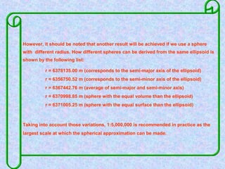
  • 12. However, it should be noted that another result will be achieved if we use a sphere with different radius. How different spheres can be derived from the same ellipsoid is shown by the following list: r = 6378135.00 m (corresponds to the semi-major axis of the ellipsoid) r = 6356750.52 m (corresponds to the semi-minor axis of the ellipsoid) r = 6367442.76 m (average of semi-major and semi-minor axis) r = 6370998.85 m (sphere with the equal volume than the ellipsoid) r = 6371005.25 m (sphere with the equal surface than the ellipsoid) Taking into account those variations, 1:5,000,000 is recommended in practice as the largest scale at which the spherical approximation can be made.
  • 13. 1.4 The Ellipsoid as Reference Surface for Location 1.4.1 Local Reference Ellipsoids It is important to realize that topographic maps are drawn and geodetic positions are defined with respect to a reference datum (also referred to as geodetic datum). In the United States we use the North American Datum, in Japan the Tokyo datum, in some European countries the European Datum, in Germany the Potsdam Datum, etc. A reference datum is defined by the size and shape of an ellipsoid as well as a position (called the datum) at which latitude and longitude are known. Those geometric models have been established to fit the geoid well over the area of local interest, which in the past was never larger than a continent. As a consequence, the differences between the geoid and the reference ellipsoid may be ignored. This allows accurate maps to be drawn in the vicinity of the datum. Figure 1.3 shows that a position on the geoid will have a different set of latitude and longitude coordinates in each reference datum. In this figure the North American datum is extrapolated to Europe. Even though the datum fits the geoid in the North American continent well, it does not fit the European geoid. Conversely, if the European datum were extrapolated to the North American continent, this similar result is found.
  • 14. Widely in use are the following ellipsoids generally named after their generator. Name (Date a (m) b (m) f Used in Delamber (1810) 6376985. 6355598. 1:308.64 Belgium Airy (1830) 6377563. 6356257. 1:299.32 Great Britain Bessel (1841) 6377397. 6356079. 1:299.15 Central Europe, Chile, Indonesia Clarke (1866) 6378274. 6356651. 1:294.97 North America, Philippines Clarke (1880) 6378316. 6356582. 1:1:293.47 France Parts of Africa Helmert (1906) 6378200. 6256818. 1:298.3 Egypt Hayford (1909) 6378388. 6356912. 1:297.0 Argentina, Denmark Krassowski (1940) 6378245. 6356863. 1:298.3 USSR, Eastern Europe
  • 16. 1.4.2 Global Reference Ellipsoids With increasing demands for global surveying results we register several activities to establish also global reference ellipsoids. Especially the International Union for Geodesy and Geophysics (IUGG) is involved in establishing those reference figures. The motivation is to make geodetic results mutually comparable and to provide coherent result also to other disciplines like astronomy and geophysics. In 1924 in Madrid, the general assembly of the IUGG introduced the ellipsoid determined by Hayford 1909 as the International Ellipsoid. In contrary to local reference ellipsoids which apply only to a region or local area of the earth’s surface., global reference systems approximating the geoid as a mean earth ellipsoid. However, according to present knowledge, the values for this earth model only give an insufficient approximation. At the general assembly 1967 of the IUGG in Luzern, the 1924 reference system was replaced by the Geodetic Reference System 1967 9GRS 1967). It represents a good approximation (as of 1967) to the mean earth figure. The geometric ellipsoidal parameters a, b and f are given in the table below. The Geodetic Reference System 1967 no longer represents the size and shape of the earth to an adequate accuracy. Consequently, it was replaced by the Geodetic Reference System 1980 (see table). It can be expected that the increasing amount of global observations and better accuracies some other international reference ellipsoids will be established in the future. Nowadays, geodesists are able to measure the Earth-as-a-whole with the aid of artificial satellites. However, a re-adjustment of all existing local geodetic survey reference systems is not to be expected for the time being due to the great efforts in applying coordinate transformation and changing existing maps. Local reference systems retain their practical importance for national mapping activities.
  • 17. Name (Date) a(m) b(m) f International (1924) 6378388. 6356912. 1:297.000 GRS 1967 6378160. 6356775. 1:298.247 GRS 1980 6378137. 6356752. 1:298.257
  • 18. 1.5 Conclusion on Reference Surfaces In summary, when speaking of the size and shape of the earth and positions on it, there are three surfaces to be considered:  The topography - the physical surface of the earth.  The goid - the level surface (also a physical reality).  The ellipsoid - the reference frame for computations. Surveying observations are made on the earth surface relative to the geoid. Before using observations in geodetic computation, they must be corrected for locational differences between the geoid and the reference ellipsoid. These corrections are small and may for some purposes be ignored if a reference ellipsoid is chosen so as to closely fit the geoid in the area of concern (see figure 1.4) Note that the Geoid in only used as reference surface for height measurements. Locations are defined with respect to a reference ellipsoid or a sphere. A sphere as earth model can be used for maps at scale 1:5,000,000 and smaller.
  • 19. EARTH’S SURFACE GEIOD ELLIPSOID Geoid separation (Undulation) SEA SURFACE The Three relevant surfaces for mapping.
  • 20. 1.6 Spatial Coordinate Systems 1.6.1 Ellipsoidal Geographic Coordinate System The most widely used global coordinate system consists of lines of geographic longitude and latitude. Lines of equal latitude are called parallels. They form circles on the surface of the ellipsoid. Lines of equal longitude are called meridians and they form ellipses (meridian ellipses) on the ellipsoid. The latitude of a point P is the angle between the ellipsoidal normal through P and the equatorial plan. Latitude is zero on the equator ( = 0) and increases towards the two poles to maximum values of = +90 (N90) at the North Pole and = -90 (S 90 ) at the South Pole. The longitude is the angle between the meridian ellipse which passes through Greenwich and the meridian ellipse containing the point in question. It is measured in the equatorial plane from the meridian of Greenwich = 0 wither eastwards through =+ 180 (E180) or westwards through = - 180 (W180 ). Latitude and longitude representing the geographic coordinates of a point P. They are always given in angular units (e.g. City hall Enschede: = 52 13’ 13.5” N, = 6 53’,50.8” E). Spatial geographic coordinates ( , ,h ) are obtained by introducing the ellipsoidal height h to the system. The ellipsoidal height of a point is the vertical distance of the point in question above the ellipsoid. It is measured in distance units along the ellipsoidal normal from the point to the ellipsoid surface.
  • 22. The concept of geographic coordinates can also be applied to a sphere as the reference surface. However, there is significant difference between the ellipsoidal and the spherical geographic latitude. The concept of latitude on the latitude on the ellipsoid might become clearer if we look at the meridian plane through P (see figure 1.6). If a spherical rather than an ellipsoidal figure were being used, the latitude of P’ would be the angle at the center of the sphere. This is because the normal to the surface of the sphere will always pass through its center. Using an ellipsoidal figure, the normal through P’ will not pass through the center of the ellipsoid, and the latitude is given by the angle between this normal and the equatorial plane. The angle is given by the angle between this normal and the equatorial plane. The angle is called the geocentric latitude, and it is often used as an intermediate quantity in calculations with the ellipsoid. Semi minor axis b. Sphere Semi minor axis a tangent P P ellipsoid
  • 23. 1.6.2 Geocentric Coordinates ( X,Y,Z) An alternative and often more convenient method of defining a position is with spatial cartesian coordinates (figure 1.7). The system has its origin at the mass-center of the earth with the x and y axis in the plane of the equator. The three axes are mutually orthogonal and form a right-handed system. It should be noted that the rotational (spin) axis of the earth changes its position with the time (catchword: polar motion). Due to this the mean position of the pole in the year 1903 (based on observations between 1900 and 1905) was used to define the so-called “ “Conventional International Origin”(CIO). Z CIO Greenwich EquatorX Y P Zp Yp Xp
  • 24. 1.6.3 Transformation of Spatial Coordinates Like already mentioned with the geoid as local reference surface for heights, care must be taken when using data from another height system. This might be the case in the border area of adjacent nations (see 1.2). Something similar comes up when using geographic coordinates related to different reference datums. The way in which local datums are established is based on convenience and best fit over a certain area of the earth’s surface. These datums are seldom geocentric of correct scale, or oriented exactly to the CIO pole and the Greenwich meridian. However, the problem of non-similarity of adjacent systems can be solved by transforming the coordinates. Many types of datum transformations have been developed over the years. They range from simple similarity transformations between two sets of plane coordinates to more complex formulae taking into account three dimensional transformations are typically only valid over a very limited area. Three dimensional transformations are more suitable for larger areas as they are typically global in concept and enable solutions for heights as well as planimetric positions. The complete three dimensional transformation involves seven parameters that relate corresponding coordinates in the two ellipsoidal systems. There are three translation parameters to relate the origins of the two system (dX, dY, dZ), three rotation parameters to relate the orientation of the two system ( x, y, z), and one scale parameter (s) to account for any difference in scale between the two systems. Transformation between local reference datums is a geodetic problem. Consequently, cartographers will normally not been involved but might be asked to assist in preparing for transformation.
  • 25. 1.6.3.1 Spatial Geographic Coordinates to Geocentric Coordinates Datum transformations are usually carried out using geocentric coordinates rather than geographic coordinates. The use of geographic coordinates would necessitate the use of an associated ellipsoid.The geocentric coordinates (X, Y, Z) of a point P known in geographic coordinates ( ) on an ellipsoid of semi major axis a, and semi minor axis b, may be calculated by using the formulae: Y = p * cos *sin Z = p * ( 1 - e ) * sin The parameter p(rho) is the radius of the curvature in the prime vertical (east-west direction) while e is the eccentricity (see 1.3.1). Rho can be computed by using the formulae: N = p = a / (1 - e * M If a point P is situated at a height h above the ellipsoid, its geocentric coordinates are given by: X = (p+h) * cos * cos Y = (p+h) * cos * sin Z = (p*(1-e ) + h) * sin
  • 26. 1.6.3.2 Geocentric Coordinates to Spatial Geographic Coordinates The inverse computation of ( ) from (X,Y,Z ) is carried out as follows (refer also to figure 1.8) = = h = The following substitutions are used within the formulae: p = = e = e = (tan The inverse determination of the parameters , , and h can be solved without interation. However, the solution gives good results for earth bound stations while stations of distant space need an interation to achieve greater accuracy.
  • 27. 1.7 Plane Coordinate Systems: A flat map has only two dimensions, width (left to right) and length (bottom to top). Transforming the three dimensional earth body into a two dimensional map is subject of map projections. Here, like in several other cartographic applications, two dimensional coordinates are needed to describe the location of any point in an unambiguous and unique manner. 1.7.1 Cartesian Coordinates One possibility of defining a point in a plane is to use plane rectangular coordinates. This is a system of intersecting perpendicular lines which contains two principal axes, called the x- and y- axis. The horizontal axis is usually referred to as the x-axis and the vertical the y - axis (Note that the x-axis is sometimes called Easting and the y-axis Northing). The intersection of the x- and y-axis forms the origin. The plane is marked at intervals by equally spaced coordinate lines.
  • 28. Any location P on the map can now be precisely and objectively specified by giving its two numerical coordinates xp and yp. Y -X Origin -Y X P1 (2.32, 2.55) P2 (5.77, 1.55)
  • 29. Normally, the coordinates xp = 0 and yp = 0 are given to the origin. However, sometimes large positive values are added to the origin coordinates. This is to avoid negative values for the x- and y- coordinates in case the origin of the coordinate system is located inside the area of interest. The point which has then the coordinates xp=0 and yp = 0 is called the false origin. Rectangular coordinates are also called cartesian coordinates after Descartes, a French mathematician of the seventeenth century. He devised a system for geometric interpretation of algebraic relationship which formed the basis for the development of a branch of mathematics called “analytic geometry”. 1.7.2 Polar Coordinates Another possibility of defining a point in a plane is by polar coordinates. This is the distance d from the origin to the point concerned and the angle a between a fixed (or zero) direction and the direction to the point (see figure 1.10) The angle a is called azimuth or bearing and is counted clockwise. It is given in angular units while the distance d is expressed in length units. Bearings are always related to a fixed direction (initial bearing) or a datum line. In principle, this reference line can be chosen freely.However, in practice three different directions are widely in use: True North, Grid North and Magnetic North. The corresponding bearings are called: true bearing or geodetic bearing, grid bearing and magnetic or compass bearing (see lectures on Land Surveying). Polar coordinates are often used in land surveying. For some types of surveying instruments it is advantageous to make use of this coordinate system.Especially the development of precise remote distance measurement techniques has led to the virtually universal preference for the polar coordinate method in detail survey.
  • 30. Plain polar coordinates (a, d) Origin Initial bearing a
  • 31. 1.7.3 Transformation of Plane Coordinates As cartographers you are most probably concerned in your day to day work wilth going from one two dimensional coordinate system to the other. This includes the transformation of polar coordinates delivered by a surveyor into cartesian map coordinates or the transformation from one plane rectangular system to another adjacent system. No matter how, you should be prepared to carry out successfully simple two dimensional transformations. In the following sections some of these typical tasks will be discussed. 1.7.3.1 Polar Coordinates to Cartesian Coordinates Known: a , d Unknown: xp, yp Assumption: There is no difference in scale (length units) between the two systems. Condition: The origins of the two coordinate systems are identical (x0=0, y0 = 0). The orientation (angle between zero direction and y- coordinate axis) is zero.
  • 32. X Origin a d P SIMPLE CASE OF TRANSFORMING POLAR COORDINATES TO ARTESIAN COORDINATES.Y
  • 33. The simple case of transforming polar coordinates to cartesian coordinates you will hardly find in practice. For a more realistic case a translation (shift) and a rotation parameter has to be introduced to transform one system to the other. Known: a, d, x0, y0, Unknown: Xp, yp Assumption: There is no difference in scale (length units) between the two systems. The origins of the two coordinate systems are not identical. The orientation (angle between zero direction and y-coordinate axis) is unequal zero. X Y Origin a d P Origin 2 y0 X0
  • 34. 1.7.3.2 Cartesian Coordinates to Polar Coordinates Known: xp, yp Unknown: a, d Assumption: There is no difference in scale (length units) between the two systems. Condition: The orientation (angle between zero direction and y - coordinate axis) us zero. XOrigin a d P Y
  • 35. The more realistic case again makes use of a translation (shift) and rotation for transformation. Known; xp, yp, xo, yo, Known; a, d. Assumption; There is no difference in scale (length units) between the two systems. The origins of the two coordinate systems are not identical. The orientation (angle between zero direction and y-coordinate axis) is unequal zero. Origin a d P Origin 2 y0 X0 Xp Initial Bearing Y yp
  • 36. 1.7.3.3 Cartesian Coordinates to Cartesian Coordinates With this kind of plane coordinate transformation the cartographer will quite often come in touch with. The task is to transform the coordinates from one plane rectangular system to another system which might be translated (shifted) and/or rotated against the first one. Typical applications are:  The transformation from one grid system to an adjacent coordinate system in case a map is located in the overlapping part of two grid systems and both shall be represented on the map (see also: map projections).  The transformation of digitizer coordinates x and y to map coordinates X and Y. A map that is fixed on a digitizer table can only be digitizer in the digitizer coordinate system. However, the fixed map is normally slightly rotated against this system. The resulting digitizer coordinates might consequently be transformed to achieve a certain map coordinate system (see also:digitizing from graphic documents). Known: xp, yp, X0, Y0, a Unknown: Xp, Yp Assumption: There is no difference in scale (length units) between the two systems. The origins of the two coordinate systems are not identical. The orientation (angle between two corresponding coordinates axes) is unequal zero.
  • 37. Transformation of cartesian coordinates to cartesian coordinates.Y Y0 Origin 1 X0 X Xp = X0 + xp* cos a - yp*sin a Yp = Y0 + xp* sin a + yp*cos a
  • 38. If we assume the shift-values X0 and Y0 and also the rotation A are unknown, then we can calculate the transformation coefficients X0, Y0 a1 and a2 by using the coordinates of two control points. Those points are known in both the first (x,y) and the second coordinate system (X,Y). In this case a system of four simultaneous equations with four unknowns has to be solved..
  • 39. 1.7.3.4 Cartesian Coordinates to Cartesian Coordinates with Scale Change This kind of transformation will be needed to correct additionally for scale changes between the two plane rectangular coordinate systems. Differences in scale, I.e. length units may occur when one of the coordinate system is in meter and the other in feet. Consequently, scale differences are existing but might be regular, I.e. similar in x- and y- direction. More serious is the non similar scale change caused by shrinkage of paper maps which undergo humidity based changes more in one direction than the other. Consequently, the scale factor along the x-axis is different from that along the y- axis. The first problem can be solved by applying a conformal transformation which changes the size and position of any geometric element but maintains its form. The problem of non regular shrinkage can be solved by applying an affine transformation.
  • 41. Transformation of a cartesian coordinates. Y Y0 Origin 1 X0 X The general statement of the conformal transformation is: Xp = X0 + b1*xp - b2*yp Yp = Y0 + b2*xp + b1*yp Where: b1 = s*cos a and b2 = s*sin a
  • 42. If we assume the shift-value X0 and Y0, the common scale factor s in x- and y- direction and also the rotation q are unknown, the we can calculate the transformation coefficients X0, Y0, b1 and b2 by using the coordinates of two control points only. The number of control points will change when we apply an affine transformation.
  • 43. If we assume the shift-values X0 and Y0 and Y0, the scale factors sx and sy in x- and y- direction and also the rotation a are unknown, then we can calculate the six transformation coefficients X0, Y0, c1, c2, c3 and c4 by using the coordinates of three control points. Every control point delivers two equations for X and Y each. Consequently, a system of six simultaneous equations with six unknowns has to be solved. For the conformal transformation at least two control points are needed when the four transformation parameters have to be calculated, while for the affine transformation at least three control points are necessary, If there are more than the minimum number of control points available (so called redundant information) then we usually apply techniques of Least Squares Adjustment. This enables us to introduce all the information which is available to get a more stable or better result. Least squares adjustment is usually already integrated in digitizer software (see: digitizing from graphic documents). 1.8 Units of Measurements Measurements are taken in units. A measurement without indicating the unit applied makes no sense. In cartography, three groups of unit have to be distinguished according to the basic measurements which can be taken from maps. These are units for angles, units for lengths and units for areas.
  • 44. 1.8.1 Units for Angles Angles are usually indicated in one of the four following ways: • In degrees, based on a division of the full circle into 360 units. • In grades, based on a division of the full circle in to 400 units. • In radians, based on a division of the full circle into 2 units (6.283185). • In mils, based on a division of the full circle into 6400 units. The division of the circumference of a circle in degree is an ancient way of indicating angle measurements which is still in use today with mathematics. It is originally based upon moon cycles, lasting 30 days. Twelve moons (months)elapsed a year of 360 days or a full circle. Consequently, all circles were divided accordingly. Degrees are units of the so called sexagesimal system in which the base unit is divided in to 60 minutes (‘), and one minute into 60 seconds (“). A right angle counts 90 degrees. The decimal system of dividing the circumference of a circle in grades was introduced into science after the French Revolution. It overcomes some inconvenience in handling the sexagesimal system, namely when adding or subtracting non-decimal numbers. In the decimal system, the full circle is divided in 100 centigrades ( C ), one centigrade in 100 decimilligrades (cc). A right angle counts 100 grades. The big advantage of this system is that one can express an
  • 45. A decimal number which definitely simplifies computations. The decimal system is widely in use in land surveying. A radian is based on the mathematical constant 2 which is the circumference of a circle with the radius 1. Radians are often used to transform angles from one system to another. A right angle counts /2 which is 1.5707963 radians. One radian is the angle which corresponds to the circumference distance 1 in a circle with the radius1. The unit mils is mainly known from military applications; it is hardly used by the civilians doing cartometric measurements. However, to be able to understand military language, one has to know the relations. A right angle is 1600 mils. degrees grades radians mils 1 degree 1 0.9 1.7453*10 -2 17.77777 1 grade 1.111111 1 1.5708*10-2 16 1 radian 57.29578 63.661975 1 1018.5916 1 mil 5.625*10-2 6.25*10-2 9.817*10-4 1
  • 46. 1.8.2 Units for Lengths Most countries of the world are either “going metric”, or have already done so. The decimal nature of the metric system, and thus the simple relationship of the units used in the system, make computations easier in the metric system than they are in the British imperial system. The metric system has been in operation already in France since the French Revolution, and many European countries have adopted the system by the time the first Metric Convention was set up in 1875 to establish international standards of measurements. In 1960 an international conference on weights and measures adopted what has become known as the “standard International Metric system (S.I). For length measurements the base unit of the S.I. System is the metre. British Imperial System 12 inches = 1foot 3 feet = 1 yard 51/2 yard = 1 rod (pole or perch) 4 rods = 1 chain 22 yards = 1 chain 80 chains = 1 mile 1760 yards = 1 mile 63360 inches = 1 mile Metric System 10 millimetres = 1centimetre (cm) 10 centimetres = 1 decimetre (dm 10 decimetres = 1 metre (m) 100centimetres = 1 metre 1000 metres = 1 kilometre (km) 100000 centimetres = 1 kilometre
  • 47. The S.I system also forms the basis of the metric conversion of topographic maps in many parts of the world. Metrication of topographic maps means that all units of measurement will appear in metric terms. Thus, the scale of the map will be metric, the grid referencing system will be in metres rather than in yards, and heights will also be shown in metres. In most of those countries where the British imperial system was used almost exclusively for topographic mapping, this change-over, for practical reasons, must be a gradual process since finance and time are two major limitations. However, conversion is well underway in Great Britain, Australia, some countries in Africa and Canada, to give a few examples.
  • 48. 1.8.3 Units for Areas Area measurements are based on linear measures. Also in the case, the metric system is much easier to handle than the British imperial system. If the metric system is replacing the imperial system, it is consequent to change also to metric area measures. However, since the British system is still in use, a conversion table is given next page.
  • 49. 1.9 The Map Scale Scale is a ratio. It is the ratio between a distance measured on a map and the corresponding distance measured on the reference surface (ellipsoid or sphere). To state that a map has a scale of one inch to one mile means that every inch measured on the map represents a distance of one mile on the reference surface. Scale is usually expressed in one or more of the three following ways: • As a word statement such as one inch to one hundred yards. • As a numerical proportion, for example, 1:50000. • As a linear relationship or as graphic line scale. The verbal type of scale expression is associated almost entirely with maps using the British Imperial system of linear measurement (in inches, yards, and miles, for example). Metric scales can be, of course, also easily expressed in the form of a statement but this is not so commonly in use. However, a verbal expression of a scale is the least useful method when reading a map, irrespective of the measurement system which is being used (imperial or metric). It is difficult to measure distances directly from the map using a verbal scale. The numerical proportion of map distance to real world distance is more often used. Both the numerator and the denominator must be expressed in the same units. In the example 1:50000, one unit on the map represents 50000 of the same units on the reference surface. Scale in this form is with numerical scales it is important to ensure that map distance and distance on the reference surface are stated in terms of the same measurement system. Distances measured on the map are transformed to real world distances by multiplying them with the denominator.
  • 50. The graphic line scale is the most useful method of representing scale on maps, for actual distances can be measured directly from the map. Straight line distances can be determined by a ruler or even by means of a paper strip on which tick marks can be indicated. This distance is then compared with the linear scale and the ground distance may be read easily. To determine the distance along a road or a river (or a similar curved line) a series of steps or sub-points is established. Very useful for this action is using a pair of dividers. The distances between each set of points is determined separately, noted and cumulative total kept. Some confusion often surrounds the terms small and large map scale. To clarify the matter one should remember the meaning of scale which is a ratio or quotient. One divided by twenty five thousand (1:250,000) gives a larger result than one divided by one hundred thousand (1:100,000). Consequently, scale 1:250,000 is larger than scale 1:1000000 has a larger scale than a map with scale of 1:100000. A large scale map depicts a comparatively small area of land. As a consequence, they are especially useful when detail has to be shown. A cadastral map is always in a large scale as fields, houses and other relevant features have to be represented completely and with their true location. A small scale map depicts a comparatively large area of land . A common example of a small scale map is that of a state or country as is found in an atlas. Obviously the amount of detail that can be shown on such a map is limited and features such as roads and railways are drawn out of all proportion of their actual size. An often made mistake is assuming the map scale as being generally valid for the entire map sheet. This generalized assumption is not correct. The transformation of the reference surface (ellipsoid, sphere) to the map plane is always connected with geometrical distortions. For example, a projection that preserves the size
  • 51. Of areas distorts at the same time their shapes. It is not possible for a map to preserve both - size and shape - at the same time. Something comparable we have with equidistant projections. Although they are able to preserve distances, they are never equidistant everywhere. The geometrical property equidistance can only be achieved for certain locations or along certain lines. A map may be equidistant along the meridians but is not so along the parallels (see map projections). As a consequence, the indicated scale (nominal map scale) is only valid along the meridians. A map user should be aware of this especially when computations are to be made on the basis of measurements taken from small scale maps. When maps show the whole globe, the map maker sometimes replaces the standard graphic scale with a variable graphic scale. The scale may change systematically in north- south and east-west directions. To use such a variable scale, you first have to decide in what latitude-longitude zone you want to determine a distance, and then depict the distance from the graphic scale. The situation is different for large scale maps which depict a comparatively small area of land. Though the geometric property equidistance along certain lines is also valid for these maps, the resulting distortions are smaller due to the larger scale. They may become so small that they cannot be measured any longer when using a ruler. This is generally the case with topographic maps. In this case we can assume the map scale as being valid for the entire map sheet. In some books a definition of map scale is given which is not precise enough. It is written that the map scale is the ratio between a distance measured on a map and the corresponding distance measured on the ground (the physical earth surface). This inaccurate as in reality a distance on the physical earth surface differes from that on the geometrical reference surface. From figure 1.18 can be seen that the distance d on the
  • 52. Plateau is longer than the corresponding distance d on the ellipsoid. Consequently, maps with slightly different scales would have to be produced for coastal plain regions and high mountaineous regions. To avoid this methodical and practical confusion every distance measured in land surveying is reduced to the ellipsoid (see land surveying). This means, a distance measured on the map and multiplied by the scale denominator gives as result the corresponding distance on the reference surface and not on the earth surface. However, it should be noted that for most practical cases the difference between the calculated distance and the actual distance on the ground is so small that it can be neglected.