


![The Text Classification Problem
A classifier can be formally defined
D: a collection of documents
C = {c1, c2, . . . , cL}: a set of L classes with their respective labels
a text classifier is a binary function F : D × C → {0, 1},
which assigns to each pair [dj , cp], dj ∈ D and cp ∈ C, a
value of
1, if dj is a member of class cp
0, if dj is not a member of class cp
Broad definition, admits supervised and unsupervised
algorithms
For high accuracy, use supervised algorithm
multi-label: one or more labels are assigned to each
document
single-label: a single class is assigned to each document
p. 7](https://image.slidesharecdn.com/irtunitiiijm-250816110819-9a93c3af/85/Information-Storage-and-Retrieval-Techniques-Unit-III-7-320.jpg)
![The Text Classification Problem
Classification function F
defined as binary function of document-class pair [dj , cp]
can be modified to compute degree of membership of dj in cp
documents as candidates for membership in class cp
candidates sorted by decreasing values of F(dj , cp)
p. 8](https://image.slidesharecdn.com/irtunitiiijm-250816110819-9a93c3af/85/Information-Storage-and-Retrieval-Techniques-Unit-III-8-320.jpg)


![Naive Text Classification
Text Classification by Direct Match
1. Input:
D: collection of documents to classify
C = {c1, c2, . . . , cL}: set of L classes with their labels
2. Represent
each document dj by a weighted vector d→j
each class cp by a weighted vector →cp (use the labels)
3. For each document dj ∈ D do
retrieve classes cp ∈ C whose labels contain terms of dj
for each pair [dj , cp] retrieved, compute vector ranking as
j p
sim(d , c ) = d
→
j
• c
→
p
|d→j | × |
c→p|
associate dj classes cp with highest values of sim(dj , cp)
p. 29](https://image.slidesharecdn.com/irtunitiiijm-250816110819-9a93c3af/85/Information-Storage-and-Retrieval-Techniques-Unit-III-29-320.jpg)

![Supervised Algorithms
Depend on a training set
Ðt ⊂ Ð: subset of training documents
7 : Ðt × C → {0, 1}: training set function
Assigns to each pair [dj , cp], dj ∈ Ðt and cp ∈ C a value of
1, if dj ∈ cp, according to judgement of human
specialists 0, if dj /
∈ cp, according to judgement of
human specialists
Training set function 7 is used to fine tune the classifier
p. 31](https://image.slidesharecdn.com/irtunitiiijm-250816110819-9a93c3af/85/Information-Storage-and-Retrieval-Techniques-Unit-III-31-320.jpg)


![Classification of Documents
Sdj ,cp
kNN: to each document-class pair [dj, cp] assign a score
Σ
= similarity(dj , dt) × 7 (dt, cp)
dt ∈Nk (dj )
where
Nk (dj ): set of the k nearest neighbors of dj in training set
similarity(dj , dt): cosine formula of Vector model (for instance)
7 (dt, cp): training set function returns
1, if dt belongs to class cp
0, otherwise
Classifier assigns to dj class(es) cp with highest
score(s)
p. 55](https://image.slidesharecdn.com/irtunitiiijm-250816110819-9a93c3af/85/Information-Storage-and-Retrieval-Techniques-Unit-III-55-320.jpg)


![Classification of Documents
plus signs: terms of
training docs in class cp
minus signs: terms of
training docs outside
class cp
Classifier assigns to each document-class [dj, cp] a
score
S(dj , cp) = |→cp − d→j |
Classes with highest scores are assigned to dj
p. 61](https://image.slidesharecdn.com/irtunitiiijm-250816110819-9a93c3af/85/Information-Storage-and-Retrieval-Techniques-Unit-III-61-320.jpg)


![Naive Bayes
Probabilistic classifiers
assign to each document-class pair [dj , cp] a probability P (cp|
d→j )
→
p j
P (c |d ) =
→
p j p
P (c ) × P (d |c )
j
P (d→
)
P (d→j ): probability that randomly selected doc is d→j
P (cp): probability that randomly selected doc is in class cp
assign to new and unseen docs classes with highest probability
estimates
p. 65](https://image.slidesharecdn.com/irtunitiiijm-250816110819-9a93c3af/85/Information-Storage-and-Retrieval-Techniques-Unit-III-65-320.jpg)

![Naive Bayes Classifier
To each pair [dj, cp], the classifier assigns a score
j p
S(d , c ) =
→
p j
P (c |d )
p j
P (c |
d→ )
P (cp|d→j ): probability that document dj belongs to class cp
P (cp|d→j ): probability that document dj does not belong to
cp P (cp|d→j ) + P (cp|d→j ) = 1
p. 67](https://image.slidesharecdn.com/irtunitiiijm-250816110819-9a93c3af/85/Information-Storage-and-Retrieval-Techniques-Unit-III-67-320.jpg)


![Multinomial Naive Bayes Classifier
Prior document probability given by
→
j
P (d ) =
L
Σ
p=1
→
P (d |
prior j p p
c ) × P (c )
where
Pprior(d→j |cp)
=
Y
ki ∈d
→j
P (ki|cp) ×
Y
ki/
∈d→j
[1 − P
(k
i p
|c )]
i p
P (k |c ) =
1 +
Σ
j j
d |d Ð
∈ Λk
∈d
t i j
P (cp|dj )
2 +
Σ
dj
Ð
∈ t
P (cp|dj )
=
1 + ni,p
2 + np
p. 72](https://image.slidesharecdn.com/irtunitiiijm-250816110819-9a93c3af/85/Information-Storage-and-Retrieval-Techniques-Unit-III-72-320.jpg)

![Multinomial Naive Bayes Classifier
Multinomial probabilistic term distribution
j p j
P (d→ |c ) =
F ! ×
Y
ki ∈dj
i p
[P (k |c )]f i , j
f i,j !
Σ
Fj = fi,j
ki ∈dj
Fj : a measure of document length
Term probabilities estimated from training set Ðt
P (ki|cp) =
Σ
d
Ð
∈
j t i,j p j
f P (c |d )
Σ Σ
p. 74
∀ki dj
Ð
∈ t
fi , j P (cp|dj )](https://image.slidesharecdn.com/irtunitiiijm-250816110819-9a93c3af/85/Information-Storage-and-Retrieval-Techniques-Unit-III-74-320.jpg)


![SVM Technique – Formalization
Let,
7 = {. . . , [cj, →zj ], [cj+1, →zj +1 ], . . .}: the training set
cj : class associated with point →zj representing doc dj
Then,
SVM Optimization Problem:
maximize m = 2/|w→ |
subject to
w→ →zj + b ≥ +1 if cj
= ca w→ →zj + b ≤ −1
if cj = cb
Support vectors: vectors that make equation equal to
either +1 or -1 p. 95](https://image.slidesharecdn.com/irtunitiiijm-250816110819-9a93c3af/85/Information-Storage-and-Retrieval-Techniques-Unit-III-95-320.jpg)


![Stacking-based Classifiers
With each document-class pair [dj, cp] in training set
associate predictions made by distinct classifiers
Instead of predicting class of document dj
predict the classifier that best predicts the class of dj , or
combine predictions of base classifiers to produce better results
Advantage: errors of a base classifier can be
counter-balanced by hits of others
p. 109](https://image.slidesharecdn.com/irtunitiiijm-250816110819-9a93c3af/85/Information-Storage-and-Retrieval-Techniques-Unit-III-109-320.jpg)


![Term-Class Incidence Table
Feature selection
dependent on statistics on term occurrences inside docs and
classes
Let
Ðt : subset composed of all training documents
Nt : number of documents in Ðt
ti : number of documents from Ðt that contain term ki
C = {c1, c2, . . . , cL}: set of all L classes
7 : Ðt × C → [0, 1]: a training set function
p. 114](https://image.slidesharecdn.com/irtunitiiijm-250816110819-9a93c3af/85/Information-Storage-and-Retrieval-Techniques-Unit-III-114-320.jpg)


![Feature Selection by Tf-Idf Weights
wi,j : tf-idf weight associated with pair [ki, dj ]
Kt h : threshold on tf-idf weights
Feature Selection by TF-IDF Weights
retain all terms ki for which wi , j ≥ Kt h
discard all others
recompute doc representations to
consider only terms retained
Experiments suggest that this feature selection allows
reducing dimensionality of space by a factor of 10 with
no loss in effectiveness
p. 118](https://image.slidesharecdn.com/irtunitiiijm-250816110819-9a93c3af/85/Information-Storage-and-Retrieval-Techniques-Unit-III-118-320.jpg)


![Contingency Table
Let
Ð: collection of documents
Ðt : subset composed of training documents
Nt : number of documents in Ðt
C = {c1, c2, . . . , cL}: set of all L classes
Further let
7 : Ðt × C → [0, 1]: training set function
nt : number of docs from training set Ðt in class cp
F : Ð × C → [0, 1]: text classifiier function
nf : number of docs from training set assigned to class cp by the
classifier
p. 131](https://image.slidesharecdn.com/irtunitiiijm-250816110819-9a93c3af/85/Information-Storage-and-Retrieval-Techniques-Unit-III-131-320.jpg)


![Basic Concepts
Basic inverted index
Vocabulary ni
to 2
do 3
is 1
be 4
or 1
not 1
I 2
am 2
what 1
think 1
therefore 1
da 1
let 1
it 1
Occurrences as inverted lists
[1,4],[2,2]
[1,2],[3,3],[4,3]
[1,2]
[1,2],[2,2],[3,2],[4,2]
[2,1]
[2,1]
[2,2],[3,2]
[2,2],[3,1]
[2,1]
[3,1]
[3,1]
[4,3]
[4,2]
[4,2]
To do is to be.
To be is to do. To be or not to be.
I am what I am.
I think therefore I am.
Do be do be do.
d1
d2
d3
Do do do, da da da.
Let it be, let it be.
p. 9
d4](https://image.slidesharecdn.com/irtunitiiijm-250816110819-9a93c3af/85/Information-Storage-and-Retrieval-Techniques-Unit-III-166-320.jpg)


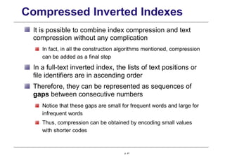
![Full Inverted Indexes
In the case of multiple documents, we need to store one
occurrence list per term-document pair
Vocabulary ni
to 2
do 3
is 1
be 4
or 1
not 1
I 2
am 2
what 1
think 1
therefore 1
da 1
let 1
it 1
Occurrences as full inverted lists
[1,4,[1,4,6,9]],[2,2,[1,5]]
[1,2,[2,10]],[3,3,[6,8,10]],[4,3,
[1,2,3]]
[1,2,[3,8]]
[1,2,[5,7]],[2,2,[2,6]],[3,2,[7,9]],
[4,2,[9,12]]
[2,1,[3]]
[2,1,[4]]
[2,2,[7,10]],[3,2,[1,4]]
[2,2,[8,11]],[3,1,[5]]
[2,1,[9]]
[3,1,[2]]
[3,1,[3]]
[4,3,[4,5,6]]
[4,2,[7,10]]
[4,2,[8,11]]
To do is to be.
To be is to do. To be or not to be.
I am what I am.
I think therefore I am.
Do be do be do.
d1
d2
d3
Do do do, da da da.
Let it be, let it be.
p. 12
d4](https://image.slidesharecdn.com/irtunitiiijm-250816110819-9a93c3af/85/Information-Storage-and-Retrieval-Techniques-Unit-III-169-320.jpg)


![Construction for Large Texts
How to merge a large suffix array LA for blocks
1, 2,... ,i − 1 with the small suffix array SA for block i?
The solution is to determine how many elements of LA
are to be placed between the elements in S A
The information is stored in a counter array C: C[j] tells how
many suffixes of LA lie between SA[j] and SA[j + 1]
Once C is computed, LA and SA are easily merged:
(1) append the first C[0] elements of LA
(2) append SA[1]
(3) append the next C[1] elements of LA
(4) append SA[2]
(5) append the next C[2] elements of LA
(6) append SA[3]
(7) .... etc
p. 86](https://image.slidesharecdn.com/irtunitiiijm-250816110819-9a93c3af/85/Information-Storage-and-Retrieval-Techniques-Unit-III-243-320.jpg)
![Construction for Large Texts
The remaining point is how to compute the counter
array C
This is done without accessing LA: the text corresponding to
LA is sequentially read into main memory
Each suffix of that text is searched for in SA (in main
memory)
Once we determine that the text suffix lies between
SA[j] and SA[j + 1], we increment C[j]
Notice that this same algorithm can be used for index
maintenance
p. 87](https://image.slidesharecdn.com/irtunitiiijm-250816110819-9a93c3af/85/Information-Storage-and-Retrieval-Techniques-Unit-III-244-320.jpg)


![Compressed Suffix Arrays
An important problem of suffix arrays is their high space
requirement
Consider again the suffix array of the Figure below, and
call it A[1, n]
20
1 2 3 4 5 6 7 8 9 10 11 12 13 14 15 16 17 18 19 20
m i s s i n g m i s s i s s i p p i $
20 8 7 19 5 16 2 13 10 1 9 6 18 17 4 15 12 3 14 11
1 2 3 4 5 6 7 8 10
9 12
11 13 14 15 16 17 18 19
The values at A[15..17] are 4, 15, 12
The same sequence is found, displaced by one value,
at A[18..20], and further displaced at A[7..9]
p. 90](https://image.slidesharecdn.com/irtunitiiijm-250816110819-9a93c3af/85/Information-Storage-and-Retrieval-Techniques-Unit-III-247-320.jpg)

![Using Function Ψ
One way to exhibit the suffix array regularities is by
means of a function called Ψ and defined so that
A[Ψ(i)] = A[i] + 1,
except when A[i] = n, in which case A[Ψ(i)] = 1
That is, Ψ(i) tells where in A is the value that follows the
current one
p. 92](https://image.slidesharecdn.com/irtunitiiijm-250816110819-9a93c3af/85/Information-Storage-and-Retrieval-Techniques-Unit-III-249-320.jpg)


![Using Function Ψ
What is most interesting is that the characters of T can
be obtained without accessing T
Therefore, T can be actually deleted and any substring
of it can be obtained just from Ψ
However, this is rarely sufficient, as one usually wants
to know the text positions where the pattern P occurs,
not the interval in A
Yet, we do not have A in order to display the positions of
the occurrences, A[i] for sp ≤ i ≤ ep
p. 95](https://image.slidesharecdn.com/irtunitiiijm-250816110819-9a93c3af/85/Information-Storage-and-Retrieval-Techniques-Unit-III-252-320.jpg)
![Using Function Ψ
To be able to locate those occurrences in T , we sample
A at regular intervals of T :
Every s-th character in T , record the suffix array position pointing
to that text position
That is, for each text position of the form 1 + j · s, let
A[i] = 1 + j · s
Then we store the pair (i, A[i]) in a dictionary
searchable by its first component
Finally, we should also be able to display any text
substring, as we plan to discard T
Note that we already know how to obtain the characters
of T starting at text position A[i], given i
p. 96](https://image.slidesharecdn.com/irtunitiiijm-250816110819-9a93c3af/85/Information-Storage-and-Retrieval-Techniques-Unit-III-253-320.jpg)
![The Burrows-Wheeler Transform
A radically different method for compressing is by
means of the Burrows-Wheeler Transform (BWT)
The BWT of T can be obtained by just
concatenating the characters that precede each
suffix in A
That is, tA [ i ] − 1 or tn if A[i] = 1
For example, the BWT of T = missing
mississippi$ is T bwt = ignpssmsm$ ipisssiii
It turns out that the BWT tends to group equal
characters into runs
Further, there are large zones where few different
characters appear
p. 97](https://image.slidesharecdn.com/irtunitiiijm-250816110819-9a93c3af/85/Information-Storage-and-Retrieval-Techniques-Unit-III-254-320.jpg)


![Simple Strings: Horspool
Horspool’s algorithm is in the fortunate position of
being very simple to understand and program
It is the fastest algorithm in many situations, especially
when searching natural language texts
Horspool’s algorithm uses the previous idea to shift the
window in a smarter way
A table d indexed by the characters of the alphabet is
precomputed:
d[c] tells how many positions can the window be shifted if the final
character of the window is c
In other words, d[c] is the distance from the end of the
pattern to the last occurrence of c in P , excluding the
occurrence of pm
p. 103](https://image.slidesharecdn.com/irtunitiiijm-250816110819-9a93c3af/85/Information-Storage-and-Retrieval-Techniques-Unit-III-260-320.jpg)

![Simple Strings: Horspool
Pseudocode for Horspool’s string matching algorithm
Horspool (T = t1t2 ... tn, P = p1p2 ... pm)
p. 105
j ← 1 ... m − 1 do d[pj ] ← m −
j
i ← 0
while i ≤ n − m do
j ← 1
(1) for c ∈ Σ do d[c]
← m
(2) for
(3)
(4)
(5)
(6)
(7)
(8)
while j ≤ m ∧ ti +j = pj do j ← j + 1
if j > m then report an occurrence at text position i +1
i ← i + d[ti+m]](https://image.slidesharecdn.com/irtunitiiijm-250816110819-9a93c3af/85/Information-Storage-and-Retrieval-Techniques-Unit-III-262-320.jpg)


![Small alphabets and long patterns
Pseudocode for the agrep’s algorithm to match long
patterns over small alphabets (simplified)
Agrep (T = t1t2 ... tn , P = p1p2 ... pm , q, h( ), N )
p. 109
(1) for i ∈ [1, N ] do d[i] ← m − q +1
(2) for j ← 0 ... m − q do d[h(pj+1pj+2 ... pj+q )] ← m −
q − j
(3) i ← 0
(4) while i ≤ n − m do
(5) s ← d[h(ti+m−q+1ti+m−q+2 ... ti+m)]
(6) if s > 0 then i ← i + s
(7) else
(8) j ← 1
(9)
(10)
(11)
while j ≤ m ∧ ti + j = pj do j ← j +1
if j > m then report an occurrence at text position i +1
i ← i +1](https://image.slidesharecdn.com/irtunitiiijm-250816110819-9a93c3af/85/Information-Storage-and-Retrieval-Techniques-Unit-III-266-320.jpg)

![Automata
Figure below shows, on top, a NFA to search for the
pattern P = abracadabra
The initial self-loop matches any character
Each table column corresponds to an edge of the automaton
B[a] = 0 1 1 0 1 0 1 0 1 1 0
B[b] = 1 0 1 1 1 1 1 1 0 1 1
B[r] = 1 1 0 1 1 1 1 1 1 0 1
B[c] = 1 1 1 1 0 1 1 1 1 1 1
B[d] = 1 1 1 1 1 1 0 1 1 1 1
B[*] = 1 1 1 1 1 1 1 1 1 1 1
p. 111
b r
a a a
a b a
d r
c](https://image.slidesharecdn.com/irtunitiiijm-250816110819-9a93c3af/85/Information-Storage-and-Retrieval-Techniques-Unit-III-268-320.jpg)


![Bit-parallelism and Shift-And
The simplest bit-parallel algorithm permits matching
single strings, and it is called Shift-And
The algorithm builds a table B which, for each
character, stores a bit mask bm ... b1
The mask in B[c] has the i-th bit set if and only if pi =
c
The state of the search is kept in a machine
word
D = dm ... d1, where di is set if the state i is
active
Therefore, a match is reported whenever dm = 1
Note that state number zero is not represented
in D
because it is always active and then can be left
p. 115](https://image.slidesharecdn.com/irtunitiiijm-250816110819-9a93c3af/85/Information-Storage-and-Retrieval-Techniques-Unit-III-272-320.jpg)
![Bit-parallelism and Shift-And
Pseudocode for the Shift-And algorithm
Shift-And (T = t1t2 ... tn , P = p1p2 ... pm )
(1) for c ∈ Σ do B[c] ← 0
(2) for j ← 1 ... m do B[pj ] ← B[pj ] | (1 << (j − 1))
(3) D ← 0
(4) for i ← 1 ... n do
(5) D ← ((D << 1) | 1) & B[ti ]
(6) if D & (1 << (m − 1)) /= 0
(7) then report an occurrence at text position i − m +1
There must be sufficient bits in the computer word to
store one bit per pattern position
For longer patterns, in practice we can search for p1p2 ... pw,
and
directly check the occurrences of this prefix for the complete
p. 116](https://image.slidesharecdn.com/irtunitiiijm-250816110819-9a93c3af/85/Information-Storage-and-Retrieval-Techniques-Unit-III-273-320.jpg)


![Extending Shift-And
Figure below shows pseudocode for a Shift-And
extension that handles all these cases
Shift-And-Extended (T = t1t2 ... tn , m, B[ ], A, S)
(1) I ← (A >> 1) & (A ^ (A >> 1))
(2) F ← A & (A ^ (A >> 1))
(3) D ← 0
(4) for i ← 1 ... n do
(5) D ← (((D << 1) | 1) | (D & S)) & B[ti ]
(6) Df ← D | F
(7) D ← D | (A & ((∼ (Df − I)) ^ Df ))
(8) if D & (1 << (m − 1)) /= 0
(9) then report an occurrence at text position i − m +1
p. 120](https://image.slidesharecdn.com/irtunitiiijm-250816110819-9a93c3af/85/Information-Storage-and-Retrieval-Techniques-Unit-III-277-320.jpg)


![Suffix Automata
Pseudocode for BNDM algorithm:
BNDM (T = t1t2 ... tn , P = p1p2 ... pm )
(1) for c ∈ Σ do B[c] ← 0
(2) for j ← 1 ... m do B[pj ] ← B[pj ] | (1 << (m − j))
(3) i ← 0
(4) while i ≤ n − m do
(5) j ← m − 1
(6) D ← B[ti + m ]
(7) while j > 0 ∧ D /= 0 do
(8) D ← (D << 1) & B[ti + j ]
(9) j ← j − 1
(10) if D /= 0 then report an occurrence at text
position i +1
(11) i ← i + j +1
p. 125](https://image.slidesharecdn.com/irtunitiiijm-250816110819-9a93c3af/85/Information-Storage-and-Retrieval-Techniques-Unit-III-282-320.jpg)


![Interlaced Shift-And
Pseudocode for Interlaced Shift-And algorithm with
sampling step q (simplified):
Interlaced-Shift-And (T = t1t2 ... tn , P = p1p2 ... pm , q)
(1) for c ∈ Σ do B[c] ← 0
(2) for j ← 1 ... m do B[pj ] ← B[pj ] | (1 << (j − 1))
(3) S ← (1 << q) − 1
(4) D ← 0
(5) for i ← 1 ... [n/q♩ do
(6) D ← ((D << q) | S) & B[tq ·i ]
(7) if D & (S << ([m/q♩ · q − q)) /= 0
(8) then run Shift-And over tq · i − m +1 ... tq·i+q−1
p. 128](https://image.slidesharecdn.com/irtunitiiijm-250816110819-9a93c3af/85/Information-Storage-and-Retrieval-Techniques-Unit-III-285-320.jpg)


![Multiple Patterns
Several of the algorithms for single string matching can
be extended to handle multiple strings
P = {P1, P2, . . . , Pr}
For example, we can extend Horspool so that d[c] is the
minimum over the di[c] values of the individual patterns Pi
To compute each di we must truncate Pi to the length of
the shortest pattern in P, and that length will be m
Other variants that perform well are extensions of
BNDM
Yet, bit-parallel algorithms are not useful for this
case
p. 132](https://image.slidesharecdn.com/irtunitiiijm-250816110819-9a93c3af/85/Information-Storage-and-Retrieval-Techniques-Unit-III-289-320.jpg)

![Dynamic Programming
The classical solution to approximate string matching is
based on dynamic programming
A matrix C[0..m, 0..n] is filled column by column, where
C[i, j] represents the minimum number of errors
needed to match p1p2 ... pi to some suffix of t1t2 ... tj
This is computed as follows:
C[0, j] = 0,
C[i, 0] = i,
C[i, j] = if (pi = tj ) then C[i − 1,j − 1]
else 1 + min(C[i − 1, j], C[i, j − 1], C[i − 1,j −
1]),
p. 134
where a match is reported at text positions j such that
C[m, j] ≤ k](https://image.slidesharecdn.com/irtunitiiijm-250816110819-9a93c3af/85/Information-Storage-and-Retrieval-Techniques-Unit-III-291-320.jpg)


![Dynamic Programming
Figure below gives the pseudocode for this variant
Approximate-DP (T = t1 t2 ... tn , P = p1p2 ... pm , k)
p. 137
C[i] ← i
(1) for i ← 0 . . . m do
(2) last ← k +1
(3) for j ← 1 . . . n do
(4) pC, nC ← 0
(5) for i ← 1 ... last do
(6) if pi = tj then nC ← pC
(7) else
(8)
(9)
(10)
(11)
(12)
(13)
(14)
(15)
(16)
if pC < nC then nC ← pC
if C[i] < nC then nC ← C[i]
nC ← nC +1
pC ← C[i]
C[i] ← nC
if nC ≤ k
then if last = m then report an
occurrence ending at position i
else last ← last +1
else while C[last − 1] > k do
last ← last − 1](https://image.slidesharecdn.com/irtunitiiijm-250816110819-9a93c3af/85/Information-Storage-and-Retrieval-Techniques-Unit-III-294-320.jpg)


![Automata and Bit-parallelism
Pseudocode for approximate string matching using the
Shift-And algorithm
Approximate-Shift-And (T = t1t2 ... tn , P = p1p2 ... pm , k)
(1) for c ∈ Σ do B[c] ← 0
(2) for j ← 1 ... m do B[pj ] ← B[pj ] | (1 << (j − 1))
(3) for i ← 0 ... k do Di ← (1 << i) − 1
(4) for j ← 1 ... n do
(5) pD ← D0
(6) nD, D0 ← ((D0 << 1) | 1) & B[ti ]
(7) for i ← 1 ... k do
(8) nD ← ((Di << 1) & B[ti ]) | pD | ((pD | nD) << 1) | 1
(9) pD ← Di , Di ← nD
(10) if nD & (1 << (m − 1)) /= 0
(11) then report an occurrence ending at position i
p. 140](https://image.slidesharecdn.com/irtunitiiijm-250816110819-9a93c3af/85/Information-Storage-and-Retrieval-Techniques-Unit-III-297-320.jpg)


![Searching Compressed Text
The Figure below illustrates the previous example
p. 145
separator
United States
any
V
(
Unnited 100
state 001
unates 101
unite 100
ocabulary B[ ] table
alphabet)
States
n
, n 010
010
UNITED
United
100
100
001](https://image.slidesharecdn.com/irtunitiiijm-250816110819-9a93c3af/85/Information-Storage-and-Retrieval-Techniques-Unit-III-302-320.jpg)


Information Storage and Retrieval Techniques Unit III
- 1. Modern Information Retrieval p. 1 Chapter 8 Text Classification Introduction A Characterization of Text Classification Unsupervised Algorithms Supervised Algorithms Feature Selection or Dimensionality Reduction Evaluation Metrics Organizing the Classes - Taxonomies
- 2. Introduction Ancient problem for librarians storing documents for later retrieval With larger collections, need to label the documents assign an unique identifier to each document does not allow findings documents on a subject or topic To allow searching documents on a subject or topic group documents by common topics name these groups with meaningful labels each labeled group is call a class p. 2
- 3. Introduction Text classification process of associating documents with classes if classes are referred to as categories process is called text categorization we consider classification and categorization the same process Related problem: partition docs into subsets, no labels since each subset has no label, it is not a class instead, each subset is called a cluster the partitioning process is called clustering we consider clustering as a simpler variant of text classification p. 3
- 4. Introduction Text classification a means to organize information Consider a large engineering company thousands of documents are produced if properly organized, they can be used for business decisions to organize large document collection, text classification is used Text classification key technology in modern enterprises p. 4
- 5. Machine Learning Machine Learning algorithms that learn patterns in the data patterns learned allow making predictions relative to new data learning algorithms use training data and can be of three types supervised learning unsupervised learning semi-supervised learning p. 5
- 6. Machine Learning Supervised learning training data provided as input training data: classes for input documents Unsupervised learning no training data is provided Examples: neural network models independent component analysis clustering Semi-supervised learning small training data combined with larger amount of unlabeled data p. 6
- 7. The Text Classification Problem A classifier can be formally defined D: a collection of documents C = {c1, c2, . . . , cL}: a set of L classes with their respective labels a text classifier is a binary function F : D × C → {0, 1}, which assigns to each pair [dj , cp], dj ∈ D and cp ∈ C, a value of 1, if dj is a member of class cp 0, if dj is not a member of class cp Broad definition, admits supervised and unsupervised algorithms For high accuracy, use supervised algorithm multi-label: one or more labels are assigned to each document single-label: a single class is assigned to each document p. 7
- 8. The Text Classification Problem Classification function F defined as binary function of document-class pair [dj , cp] can be modified to compute degree of membership of dj in cp documents as candidates for membership in class cp candidates sorted by decreasing values of F(dj , cp) p. 8
- 9. Text Classification Algorithms Unsupervised algorithms we discuss p. 9
- 10. Text Classification Algorithms Supervised algorithms depend on a training set set of classes with examples of documents for each class examples determined by human specialists training set used to learn a classification function p. 10
- 11. Text Classification Algorithms The larger the number of training examples, the better is the fine tuning of the classifier Overfitting: classifier becomes specific to the training examples To evaluate the classifier use a set of unseen objects commonly referred to as test set p. 11
- 12. Text Classification Algorithms Supervised classification algorithms we discuss p. 12
- 14. Clustering Input data set of documents to classify not even class labels are provided Task of the classifier separate documents into subsets (clusters) automatically separating procedure is called clustering p. 14
- 15. Clustering Clustering of hotel Web pages in Hawaii p. 15
- 16. Clustering To obtain classes, assign labels to clusters p. 16
- 17. Clustering Class labels can be generated automatically but are different from labels specified by humans usually, of much lower quality thus, solving the whole classification problem with no human intervention is hard If class labels are provided, clustering is more effective p. 17
- 18. K-means Clustering Input: number K of clusters to be generated Each cluster represented by its documents centroid K-Means algorithm: partition docs among the K clusters each document assigned to cluster with closest centroid recompute centroids repeat process until centroids do not change p. 18
- 19. K-means in Batch Mode Batch mode: all documents classified before recomputing centroids Let document dj be represented as vector d→j d→j = (w1,j, w2,j, . . . , wt,j ) where wi , j : weight of term ki in document dj t: size of the vocabulary p. 19
- 20. K-means in Batch Mode 1. Initial step. select K docs randomly as centroids (of the K clusters) △→ p = d→j 2. Assignment Step. assign each document to cluster with closest centroid distance function computed as inverse of the similarity similarity between dj and cp, use cosine formula j p sim(d , c ) = △→ p • d→j |△→ p| × | d→j | p. 20
- 21. K-means in Batch Mode 3. Update Step. recompute centroids of each cluster cp △ → p 1 = size(cp) Σ d→j ∈cp → dj 4. Final Step. repeat assignment and update steps until no centroid changes p. 21
- 22. K-means Online Recompute centroids after classification of each individual doc 1. Initial Step. select K documents randomly use them as initial centroids 2. Assignment Step. For each document dj repeat assign document dj to the cluster with closest centroid recompute the centroid of that cluster to include dj 3. Final Step. Repeat assignment step until no centroid changes. It is argued that online K-means works better than batch K-means p. 22
- 23. Bisecting K-means Algorithm build a hierarchy of clusters at each step, branch into two clusters Apply K-means repeatedly, with K=2 1. Initial Step. assign all documents to a single cluster 2. Split Step. select largest cluster apply K-means to it, with K = 2 3. Selection Step. if stop criteria satisfied (e.g., no cluster larger than pre-defined size), stop execution go back to Split Step p. 23
- 24. Hierarchical Clustering Goal: to create a hierarchy of clusters by either decomposing a large cluster into smaller ones, or agglomerating previously defined clusters into larger ones p. 24
- 25. Hierarchical Clustering General hierarchical clustering algorithm 1. Input a set of N documents to be clustered an N × N similarity (distance) matrix 2. Assign each document to its own cluster N clusters are produced, containing one document each 3. Find the two closest clusters merge them into a single cluster number of clusters reduced to N − 1 4. Recompute distances between new cluster and each old cluster 5. Repeat steps 3 and 4 until one single cluster of size N is produced p. 25
- 26. Hierarchical Clustering Step 4 introduces notion of similarity or distance between two clusters Method used for computing cluster distances defines three variants of the algorithm single-link complete-link average-link p. 26
- 27. Hierarchical Clustering dist(cp, cr): distance between two clusters cp and cr dist(dj, dl): distance between docs dj and dl Single-Link Algorithm dist(cp, cr) = min dist(dj, dl) ∀ dj ∈cp ,dl ∈cr Complete-Link Algorithm dist(cp, cr) = max ∀ dj ∈cp ,dl ∈cr dist(dj, dl) p r p. 27 dist(c , c ) = Average-Link Algorithm 1 np + nr Σ Σ dj ∈cp dl ∈cr dist(dj, dl)
- 28. Naive Text Classification Classes and their labels are given as input no training examples Naive Classification Input: collection D of documents set C = {c1, c2, . . . , cL} of L classes and their labels Algorithm: associate one or more classes of C with each doc in D match document terms to class labels permit partial matches improve coverage by defining alternative class labels i.e., synonyms p. 28
- 29. Naive Text Classification Text Classification by Direct Match 1. Input: D: collection of documents to classify C = {c1, c2, . . . , cL}: set of L classes with their labels 2. Represent each document dj by a weighted vector d→j each class cp by a weighted vector →cp (use the labels) 3. For each document dj ∈ D do retrieve classes cp ∈ C whose labels contain terms of dj for each pair [dj , cp] retrieved, compute vector ranking as j p sim(d , c ) = d → j • c → p |d→j | × | c→p| associate dj classes cp with highest values of sim(dj , cp) p. 29
- 31. Supervised Algorithms Depend on a training set Ðt ⊂ Ð: subset of training documents 7 : Ðt × C → {0, 1}: training set function Assigns to each pair [dj , cp], dj ∈ Ðt and cp ∈ C a value of 1, if dj ∈ cp, according to judgement of human specialists 0, if dj / ∈ cp, according to judgement of human specialists Training set function 7 is used to fine tune the classifier p. 31
- 32. Supervised Algorithms The training phase of a classifier p. 32
- 33. Supervised Algorithms To evaluate the classifier, use a test set subset of docs with no intersection with training set classes to documents determined by human specialists Evaluation is done in a two steps process use classifier to assign classes to documents in test set compare classes assigned by classifier with those specified by human specialists p. 33
- 34. Supervised Algorithms Classification and evaluation processes p. 34
- 35. Supervised Algorithms Once classifier has been trained and validated can be used to classify new and unseen documents if classifier is well tuned, classification is highly effective p. 35
- 37. Decision Trees Training set used to build classification rules organized as paths in a tree tree paths used to classify documents outside training set rules, amenable to human interpretation, facilitate interpretation of results p. 37
- 38. Basic Technique Consider the small relational database below Id Play Outlook Temperature Humidity Windy Training set 1 yes rainy cool normal false 2 no rainy cool normal true 3 yes overcast hot high false 4 no sunny mild high false 5 yes rainy cool normal false 6 yes sunny cool normal false 7 yes rainy cool normal false 8 yes sunny hot normal false 9 yes overcast mild high true 10 no sunny mild high true Test Instance 11 ? sunny cool high false Decision Tree (DT) allows predicting values of a given attribute p. 38
- 39. Basic Technique DT to predict values of attribute Play Given: Outlook, Humidity, Windy p. 39
- 40. Basic Technique Internal nodes → attribute names Edges → attribute values Traversal of DT → value for attribute “Play”. (Outlook = sunny) ∧ (Humidity = high) → (Play = no) Id Play Outlook Temperature Humidity Windy p. 40 Test Instance 11 ? sunny cool high false
- 41. Basic Technique Predictions based on seen instances New instance that violates seen patterns will lead to erroneous prediction Example database works as training set for building the decision tree p. 41
- 42. The Splitting Process DT for a database can be built using recursive splitting strategy Goal: build DT for attribute Play select one of the attributes, other than Play, as root use attribute values to split tuples into subsets for each subset of tuples, select a second splitting attribute repeat p. 42
- 43. The Splitting Process Step by step splitting process p. 43
- 44. The Splitting Process Strongly affected by order of split attributes depending on order, tree might become unbalanced Balanced or near-balanced trees are more efficient for predicting attribute values Rule of thumb: select attributes that reduce average path length p. 44
- 45. Classification of Documents For document classification with each internal node associate an index term with each leave associate a document class with the edges associate binary predicates that indicate presence/absence of index term p. 45
- 46. Classification of Documents V : a set of nodes Tree T = (V, E, r): an acyclic graph on V where E ⊆ V × V is the set of edges Let edge(vi, vj ) ∈ E vi is the father node vj is the child node r ∈ V is called the root of T I: set of all internal nodes I: set of all leaf nodes p. 46
- 47. Classification of Documents Define K = {k1, k2, . . . , kt}: set of index terms of a doc collection C: set of all classes P : set of logical predicates on the index terms DT = (V, E; r; lI , lL, lE ): a six-tuple where (V ; E; r): a tree whose root is r lI : I → K: a function that associates with each internal node of the tree one or more index terms lL : I → C: a function that associates with each non-internal (leaf) node a class cp ∈ C lE : E → P : a function that associates with each edge of the tree a logical predicate from P p. 47
- 48. Classification of Documents Decision tree model for class cp can be built using a recursive splitting strategy first step: associate all documents with the root second step: select index terms that provide a good separation of the documents third step: repeat until tree complete p. 48
- 49. Classification of Documents Terms ka, kb, kc, and kh have been selected for first split p. 49
- 50. Classification of Documents To select splitting terms use information gain or entropy Selection of terms with high information gain tends to increase number of branches at a given level, and reduce number of documents in each resultant subset yield smaller and less complex decision trees p. 50
- 51. Classification of Documents Problem: missing or unknown values appear when document to be classified does not contain some terms used to build the DT not clear which branch of the tree should be traversed Solution: delay construction of tree until new document is presented for classification build tree based on features presented in this document, avoiding the problem p. 51
- 52. The kNN Classifier p. 52
- 53. The kNN Classifier kNN (k-nearest neighbor): on-demand or lazy classifier lazy classifiers do not build a classification model a priori classification done when new document dj is presented based on the classes of the k nearest neighbors of dj determine the k nearest neighbors of dj in a training set use the classes of these neighbors to determine a class for dj p. 53
- 54. The kNN Classifier An example of a 4-NN classification process p. 54
- 55. Classification of Documents Sdj ,cp kNN: to each document-class pair [dj, cp] assign a score Σ = similarity(dj , dt) × 7 (dt, cp) dt ∈Nk (dj ) where Nk (dj ): set of the k nearest neighbors of dj in training set similarity(dj , dt): cosine formula of Vector model (for instance) 7 (dt, cp): training set function returns 1, if dt belongs to class cp 0, otherwise Classifier assigns to dj class(es) cp with highest score(s) p. 55
- 56. Classification of Documents Problem with kNN: performance classifier has to compute distances between document to be classified and all training documents another issue is how to choose the “best” value for k p. 56
- 57. The Rocchio Classifier p. 57
- 58. The Rocchio Classifier Rocchio relevance feedback modifies user query based on user feedback produces new query that better approximates the interest of the user can be adapted to text classification Interpret training set as feedback information terms that belong to training docs of a given class cp are said to provide positive feedback terms that belong to training docs outside class cp are said to provide negative feedback Feedback information summarized by a centroid vector New document classified by distance to centroid p. 58
- 59. Basic Technique Each document dj represented as a weighted term vector d→j d→j = (w1,j, w2,j, . . . , wt,j ) wi , j : weight of term ki in document dj t: size of the vocabulary p. 59
- 60. Classification of Documents Rochio classifier for a class cp is computed as a centroid given by p →c = β np → dj — γ Σ Σ Nt − np dj ∈cp dl/∈cp → dl where np : number of documents in class cp Nt : total number of documents in the training set terms of training docs in class cp: positive weights terms of docs outside class cp: negative weights p. 60
- 61. Classification of Documents plus signs: terms of training docs in class cp minus signs: terms of training docs outside class cp Classifier assigns to each document-class [dj, cp] a score S(dj , cp) = |→cp − d→j | Classes with highest scores are assigned to dj p. 61
- 62. Rocchio in a Query Zone For specific domains, negative feedback might move the centroid away from the topic of interest p. 62
- 63. Rocchio in a Query Zone To reduce this effect, decrease number of negative feedback docs use only most positive docs among all docs that provide negative feedback these are usually referred to as near-positive documents Near-positive documents are selected as follows →cp+ : centroid of the training documents that belong to class cp training docs outside cp: measure their distances to →cp+ smaller distances to centroid: near-positive documents p. 63
- 64. The Probabilistic Naive Bayes Classifier p. 64
- 65. Naive Bayes Probabilistic classifiers assign to each document-class pair [dj , cp] a probability P (cp| d→j ) → p j P (c |d ) = → p j p P (c ) × P (d |c ) j P (d→ ) P (d→j ): probability that randomly selected doc is d→j P (cp): probability that randomly selected doc is in class cp assign to new and unseen docs classes with highest probability estimates p. 65
- 66. Naive Bayes Classifier For efficiency, simplify computation of P (d→j |cp) most common simplification: independence of index terms classifiers are called Naive Bayes classifiers Many variants of Naive Bayes classifiers best known is based on the classic probabilistic model doc dj represented by vector of binary weights p. 66 d → j = (w1,j, w2 , j , . . . , wt , j ) wi,j = 1 0 if term ki occurs in document dj otherwise
- 67. Naive Bayes Classifier To each pair [dj, cp], the classifier assigns a score j p S(d , c ) = → p j P (c |d ) p j P (c | d→ ) P (cp|d→j ): probability that document dj belongs to class cp P (cp|d→j ): probability that document dj does not belong to cp P (cp|d→j ) + P (cp|d→j ) = 1 p. 67
- 68. Naive Bayes Classifier Applying Bayes, we obtain j p S(d , c ) ∼ → P (d | j p c ) j p P (d→ |c ) Independence assumption Y ki ∈d →j P (ki|cp) × Y ki/ ∈d→j P (ki|cp) P (d→j |cp) = P (d→j |cp) = Y ki ∈d →j P (ki|cp) × Y ki/ ∈d→j P (ki|cp) p. 68
- 69. Naive Bayes Classifier Equation for the score S(dj , cp) Σ ki i,j w log piP 1 − piP + log 1 − q iP qiP piP qiP S(dj , cp) ∼ = P (ki|cp) = P (ki|cp) piP : probability that ki belongs to doc randomly selected from cp qiP : probability that ki belongs to doc randomly selected from outside cp p. 69
- 70. Naive Bayes Classifier Estimate piP and qiP from set Ðt of training docs iP p = 1 + Σ j j d |d D ∈ ∧k ∈d t i j P (cp|dj ) 2 + Σ dj D ∈ t P (cp|dj ) = 1 + ni,p 2 + np iP q = 1 + Σ j j d |d D ∈ ∧k ∈d t i j P (cp|dj ) 2 + Σ dj D ∈ t P (cp|dj ) = 1 + (ni − ni,p) 2 + (Nt − np) ni , p , ni , np , Nt : see probabilistic model P (cp|dj ) ∈ {0, 1} and P (cp|dj ) ∈ {0, 1}: given by training set Binary Independence Naive Bayes classifier assigns to each doc dj classes with higher S(dj , cp) scores p. 70
- 71. Multinomial Naive Bayes Classifier Naive Bayes classifier: term weights are binary Variant: consider term frequency inside docs To classify doc dj in class cp → p j P (c |d ) = → P (c ) × P (d | p j p c ) j P (d→ ) P (d→j ): prior document probability P (cp): prior class probability p P (c ) = Σ d j ∈Dt p j P (c |d ) = np Nt Nt P (cp|dj ) ∈ {0, 1}: given by training set of size Nt p. 71
- 72. Multinomial Naive Bayes Classifier Prior document probability given by → j P (d ) = L Σ p=1 → P (d | prior j p p c ) × P (c ) where Pprior(d→j |cp) = Y ki ∈d →j P (ki|cp) × Y ki/ ∈d→j [1 − P (k i p |c )] i p P (k |c ) = 1 + Σ j j d |d Ð ∈ Λk ∈d t i j P (cp|dj ) 2 + Σ dj Ð ∈ t P (cp|dj ) = 1 + ni,p 2 + np p. 72
- 73. Multinomial Naive Bayes Classifier These equations do not consider term frequencies To include term frequencies, modify P (d→j |cp) consider that terms of doc dj ∈ cp are drawn from known distribution each single term draw Bernoulli trial with probability of success given by P (ki|cp) each term ki is drawn as many times as its doc frequency fi , j p. 73
- 74. Multinomial Naive Bayes Classifier Multinomial probabilistic term distribution j p j P (d→ |c ) = F ! × Y ki ∈dj i p [P (k |c )]f i , j f i,j ! Σ Fj = fi,j ki ∈dj Fj : a measure of document length Term probabilities estimated from training set Ðt P (ki|cp) = Σ d Ð ∈ j t i,j p j f P (c |d ) Σ Σ p. 74 ∀ki dj Ð ∈ t fi , j P (cp|dj )
- 75. The SVM Classifier p. 75
- 76. SVM Basic Technique – Intuition Support Vector Machines (SVMs) a vector space method for binary classification problems documents represented in t-dimensional space find a decision surface (hyperplane) that best separate documents of two classes new document classified by its position relative to hyperplane p. 76
- 77. SVM Basic Technique – Intuition Simple 2D example: training documents linearly separable p. 77
- 78. SVM Basic Technique – Intuition Line s—The Decision Hyperplane maximizes distances to closest docs of each class it is the best separating hyperplane Delimiting Hyperplanes parallel dashed lines that delimit region where to look for a solution p. 78
- 79. SVM Basic Technique – Intuition Lines that cross the delimiting hyperplanes candidates to be selected as the decision hyperplane lines that are parallel to delimiting hyperplanes: best candidates Support vectors: documents that belong to, and define, the delimiting hyperplanes p. 79
- 80. SVM Basic Technique – Intuition Our example in a 2-dimensional system of coordinates p. 80
- 81. SVM Basic Technique – Intuition Let, Hw : a hyperplane that separates docs in classes ca and cb ma : distance of Hw to the closest document in class ca mb : distance of Hw to the closest document in class cb ma + mb : margin m of the SVM The decision hyperplane maximizes the margin m p. 81
- 82. SVM Basic Technique – Intuition Hyperplane r : x − 4 = 0 separates docs in two sets its distances to closest docs in either class is 1 thus, its margin m is 2 Hyperplane s : y + x − 7 = 0 √ has margin equal to 3 2 maximum for this case s is the decision hyperplane p. 82
- 83. Lines and Hyperplanes in the Rn Let R n refer to an n-dimensional space with origin in O generic point Z is represented as →z = (z1, z2, . . . , zn) zi, 1 ≤ i ≤ n, are real variables Similar notation to refer to specific fixed points such as A, B, H, P , and Q p. 83
- 84. Lines and Hyperplanes in the Rn Line s in the direction of a vector w→ that contains a given point P Parametric equation for this line s : →z = tw→ + p→ where −∞ < t < +∞ p. 84
- 85. Lines and Hyperplanes in the Rn Hyperplane Hw that contains a point H and is perpendicular to a given vector w→ Its normal equation is Hw : (→z − →h)w→ = 0 Can be rewritten as Hw : →zw→ + k = 0 where w→ and k = −→hw→ need to be determined p. 85
- 86. Lines and Hyperplanes in the Rn P : projection of point A on hyperplane Hw AP : distance of point A to hyperplane Hw Parametric equation of line determined by A and P line(AP ) : →z = tw→ + →a where −∞ < t < +∞ p. 86
- 87. Lines and Hyperplanes in the Rn For point P specifically p→ = tpw→ + →a where tp is value of t for point P Since P ∈ Hw ( tpw→ + →a)w→ + k = 0 Solving for tp, →aw p. 87
- 88. Lines and Hyperplanes in the Rn Substitute tp into Equation of point P →a − p→ = →aw→ + k w→ |w→ | × | w→ | Since w→ /|w→ | is a unit vector AP = |→a − p→| = →aw → + k | w → | p. 88
- 89. Lines and Hyperplanes in the Rn How signs vary with regard to a hyperplane Hw region above Hw : points →z that make →zw→ + k positive region below Hw : points →z that make →zw→ + k negative p. 89
- 90. SVM Technique – Formalization The SVM optimization problem: given support vectors such as →a and →b, find hyperplane Hw that maximizes margin m p. 90
- 91. SVM Technique – Formalization b (belongs to delimiting hyperplane Hb) O: origin of the coordinate system point A: a doc from class ca (belongs to delimiting hyperplane Ha ) point B: a doc from class c Hw is determined by a point H (represented by →h) and by a perpendicular vector w→ neither →h nor w→ are known a priori p. 91
- 92. SVM Technique – Formalization P : projection of point A on hyperplane Hw AP : distance of point A to hyperplane Hw AP = →aw → + k | w → | to BQ: distance of point B hyperplane Hw →bw→ + k BQ = − | w→ | p. 92
- 93. SVM Technique – Formalization Margin m of the SVM m = AP + BQ is independent of size of w→ Vectors w→ of varying sizes maximize m Impose restrictions on |w→ | →aw→ + k = 1 →bw→ + k = −1 p. 93
- 94. SVM Technique – Formalization Restrict solution to hyperplanes that split margin m in the middle Under these conditions, m = + 1 1 |w→ | | w→ | m = 2 | w → | p. 94
- 95. SVM Technique – Formalization Let, 7 = {. . . , [cj, →zj ], [cj+1, →zj +1 ], . . .}: the training set cj : class associated with point →zj representing doc dj Then, SVM Optimization Problem: maximize m = 2/|w→ | subject to w→ →zj + b ≥ +1 if cj = ca w→ →zj + b ≤ −1 if cj = cb Support vectors: vectors that make equation equal to either +1 or -1 p. 95
- 96. SVM Technique – Formalization Let us consider again our simple example case Optimization problem: maximize m = 2/| w→ | subject to w→ · (5, 5) + b = +1 w→ · (1, 3) + b = −1 p. 96
- 97. SVM Technique – Formalization If we represent vector w→ as (x, y) then |w→ | = √ x 2 + y2 m = 3 √ 2: distance between delimiting hyperplanes Thus, 2 / √ x 2 + y2 p. 97 3 √ 2 = 5x + 5y + b = +1 x + 3y + b = −1
- 98. SVM Technique – Formalization Maximum of 2/|w→ | b = −21/9 x = 1/3, y = 1/3 equation of decision hyperplane (1/3, 1/3) · (x, y) + (−21/9) = 0 or y + x − 7 = 0 p. 98
- 99. Classification of Documents Classification of doc dj (i.e., →zj ) decided by f (→zj ) = sign(w→ →zj + b) f (→zj ) = ” + ” : dj belongs to class ca f (→zj ) = ” − ” : dj belongs to class cb SVM classifier might enforce margin to reduce errors a new document dj is classified in class ca: only if w→ →zj + b > 1 in class cb: only if w→ →zj + b < −1 p. 99
- 100. SVM with Multiple Classes SVMs can only take binary decisions a document belongs or not to a given class With multiple classes reduce the multi-class problem to binary classification natural way: one binary classification problem per class To classify a new document dj run classification for each class each class cp paired against all others classes of dj : those with largest margins p. 100
- 101. SVM with Multiple Classes Another solution consider binary classifier for each pair of classes cp and cq all training documents of one class: positive examples all documents from the other class: negative examples p. 101
- 102. Non-Linearly Separable Cases SVM has no solutions when there is no hyperplane that separates the data points into two disjoint sets This condition is known as non-linearly separable case In this case, two viable solutions are soft margin approach: allow classifier to make few mistakes kernel approach: map original data into higher dimensional space (where mapped data is linearly separable) p. 102
- 103. Soft Margin Approach Allow classifier to make a few mistakes maximize m = subject to 2 | w → | + γ Σ j ej w→ →zj + k ≥ +1 - ej , if cj = ca if cj = cb w→ →zj + k ≤ −1 + ej , ∀j, ej ≥ 0 Optimization is now trade-off between margin width amount of error parameter γ balances importance of these two factors p. 103
- 104. Kernel Approach Compute max margin in transformed feature space minimize m = subject to 1 2 2 ∗ | w→ | f (w→ , →zj ) + k ≥ +1, f (w→ , →zj ) + k ≤ −1, if cj = ca if cj = cb Conventional SVM case f (w→ , →zj ) = w→ →zj , the kernel, is dot product of input vectors Transformed SVM case the kernel is a modified map function polynomial kernel: f (w→ , →xj ) = (w→ →xj + 1)d radial basis function: f (w→ , →xj ) = exp(λ ∗ |w→ →xj |2), λ > 0 sigmoid: f (w→ , →xj ) = tanh(ρ(w→ →xj ) + c), for ρ > 0 and c < 0 p. 104
- 106. Ensemble Classifiers Combine predictions of distinct classifiers to generate a new predictive score Ideally, results of higher precision than those yielded by constituent classifiers Two ensemble classification methods: stacking boosting p. 106
- 108. Stacking-based Classifiers Stacking method: learn function that combines predictions of individual classifiers p. 108
- 109. Stacking-based Classifiers With each document-class pair [dj, cp] in training set associate predictions made by distinct classifiers Instead of predicting class of document dj predict the classifier that best predicts the class of dj , or combine predictions of base classifiers to produce better results Advantage: errors of a base classifier can be counter-balanced by hits of others p. 109
- 110. Boosting-based Classifiers Boosting: classifiers to be combined are generated by several iterations of a same learning technique Focus: missclassified training documents At each interaction each document in training set is given a weight weights of incorrectly classified documents are increased at each round After n rounds outputs of trained classifiers are combined in a weighted sum weights are the error estimates of each classifier p. 110
- 111. Boosting-based Classifiers Variation of AdaBoost algorithm (Yoav Freund et al) AdaBoost let 7 : Ðt × C be the training set function; let Nt be the training set size and M be the number of iterations; p. 111 N t initialize the weight wj of each document dj as wj = 1 ; for k = 1 to M { learn the classifier function F k from the training set; d j |dj misclassified j estimate weighted error: errk = Σ w / Σ N t i=1 wj ; 1 2 compute a classifier weight: αk = × log k 1−err errk ; for all correctly classified examples ej : wj ← wj × e− α k ; for all incorrectly classified examples ej : wj ← wj × eα k ; normalize the weights wj so that they sum up to 1; }
- 112. Feature Selection or Dimensionality Reduction p. 112
- 113. Feature Selection Large feature space might render document classifiers impractical Classic solution select a subset of all features to represent the documents called feature selection reduces dimensionality of the documents representation reduces overfitting p. 113
- 114. Term-Class Incidence Table Feature selection dependent on statistics on term occurrences inside docs and classes Let Ðt : subset composed of all training documents Nt : number of documents in Ðt ti : number of documents from Ðt that contain term ki C = {c1, c2, . . . , cL}: set of all L classes 7 : Ðt × C → [0, 1]: a training set function p. 114
- 115. Term-Class Incidence Table Term-class incidence table Case Docs in cp Docs not in cp Total Docs that contain ki ni,p n i − ni,p ni Docs that do not contain ki np − ni,p Nt − ni − (np − ni , p ) Nt − ni All docs np Nt − np Nt ni,p: # docs that contain ki and are classified in cp ni − ni,p: # docs that contain ki but are not in class cp np: total number of training docs in class cp np − ni,p: number of docs from cp that do not contain ki p. 115
- 116. Term-Class Incidence Table Given term-class incidence table above, define Probability that Probability that i j i ni N t i j i k ∈ d : P (k ) = k / ∈ d : P (k ) = N −n t i N t Probability that dj ∈ cp: P (cp) = np N t j p p N −n t p N t i j j p i p c : P (k , c ) n i , p N t i j j p i p c : P (k , c ) = n −n p i , p N t i j j Probability that k Probability that k Probability that k Probability that p i p c : P (k , c ) = n −n i i , p N t i Probability that d / ∈ c : P (c ) = ∈ / ∈ ∈ / ∈ j j d and d ∈ d and d ∈ d and d / ∈ k d and / ∈ p i p p. 116 d c : P (k , c ) = t i p i , p N −n −(n −n ) N t
- 117. Feature Selection by Doc Frequenc Let Kt h be a threshold on term document frequencies Feature Selection by Term Document Frequency retain all terms ki for which ni ≥ Kt h discard all others recompute doc representations to consider only terms retained Even if simple, method allows reducing dimensionality of space with basically no loss in effectiveness p. 117
- 118. Feature Selection by Tf-Idf Weights wi,j : tf-idf weight associated with pair [ki, dj ] Kt h : threshold on tf-idf weights Feature Selection by TF-IDF Weights retain all terms ki for which wi , j ≥ Kt h discard all others recompute doc representations to consider only terms retained Experiments suggest that this feature selection allows reducing dimensionality of space by a factor of 10 with no loss in effectiveness p. 118
- 119. Feature Selection by Mutual Inform Mutual information relative entropy between distributions of two random variables If variables are independent, mutual information is zero knowledge of one of the variables does not allow inferring anything about the other variable p. 119
- 120. Mutual Information Mutual information across all classes i p I(k , c ) = log P (ki, cp) P (ki)P (cp) ni,p = log N t ni Nt × np Nt That is, MI(ki , C) = L Σ p=1 P (cp) I(ki , cp) = L Σ p=1 np Nt p. 120 ni,p log N t ni Nt × np Nt
- 121. Mutual Information Alternative: maximum term information over all classes Im a x (ki , C) = maxL p=1 p=1 = maxL log I(ki , cp) ni,p Nt ni Nt × np N t Kt h : threshold on entropy Feature Selection by Entropy retain all terms ki for which MI(ki , C) ≥ Kt h discard all others recompute doc representations to consider only terms retained p. 121
- 122. Feature Selection: Information Gain Mutual information uses probabilities associated with the occurrence of terms in documents Information Gain complementary metric considers probabilities associated with absence of terms in docs balances the effects of term/document occurrences with the effects of term/document absences p. 122
- 123. Information Gain Information gain of term ki over set C of all classes IG(ki , C) = H(C) − H(C|ki) − H(C|¬ki) H(C): entropy of set of classes C H(C|ki): conditional entropies of C in the presence of term ki H(C|¬ki): conditional entropies of C in the absence of term ki IG(ki , C): amount of knowledge gained about C due to the fact that ki is known p. 123
- 124. Information Gain Recalling the expression for entropy, we can write IG(ki , C) = − L Σ p=1 P (cp) log P (cp) , L Σ p=1 , —− P (ki, cp) log P (cp| ki) —− L Σ p=1 p. 124 P (ki, cp) log P (cp|ki)
- 125. Information Gain Applying Bayes rule IG(ki , C) = − L Σ p=1 P (cp) log P (cp) − P (ki, cp) log P (k , c ) i p P (ki) — i p P (k , c ) log i p P (k , c ) P (ki) Substituting previous probability definitions p. 125 IG(ki , C) = − L Σ p=1 Nt p log p Nt — n n n Nt i,p log i,p ni — n n − n p i,p Nt lo g np − ni , p Nt − ni
- 126. Information Gain Kt h : threshold on information gain Feature Selection by Information Gain retain all terms ki for which IG(ki , C) ≥ Kt h discard all others recompute doc representations to consider only terms retained p. 126
- 127. Feature Selection using Chi Square Statistical metric defined as χ2 (ki , cp) = 2 Nt (P (ki, cp)P (¬ki, ¬cp) − P (ki, ¬cp)P (¬ki, cp)) P (ki) P (¬ki) P (cp) P (¬cp) quantifies lack of independence between ki and cp Using probabilities previously defined χ2 (ki , cp) = 2 Nt (ni ,p (Nt − ni − np + ni , p ) − (ni − ni , p ) (np − ni,p)) np (Nt − np ) ni (Nt − ni ) 2 Nt (Nt ni , p − np ni ) = np ni (Nt − np )(Nt − ni ) p. 127
- 128. Chi Square χ2 avg Compute either average or max chi square L Σ p=1 2 p i p (ki) = P (c ) χ (k , c ) χ2 (ki) = maxL max p=1 χ2 (ki , cp) Kt h : threshold on chi square Feature Selection by Chi Square retain all terms ki for which χ2 (ki) ≥ Kt h avg discard all others recompute doc representations to consider only terms retained p. 128
- 130. Evaluation Metrics Evaluation important for any text classification method key step to validate a newly proposed classification method p. 130
- 131. Contingency Table Let Ð: collection of documents Ðt : subset composed of training documents Nt : number of documents in Ðt C = {c1, c2, . . . , cL}: set of all L classes Further let 7 : Ðt × C → [0, 1]: training set function nt : number of docs from training set Ðt in class cp F : Ð × C → [0, 1]: text classifiier function nf : number of docs from training set assigned to class cp by the classifier p. 131
- 132. Contingency Table Apply classifier to all documents in training set Contingency table is given by Case T (dj , cp) = 1 T (dj , cp) = 0 Total F(dj , cp) = 1 n f , t n f − n f , t nf F(dj , cp) = 0 n t − n f , t Nt − n f − nt + nf , t Nt − nf All docs nt Nt − nt Nt nf , t : number of docs that both the training and classifier functions assigned to class cp nt − nf , t : number of training docs in class cp that were miss-classified The remaining quantities are calculated analogously p. 132
- 133. Accuracy and Error Accuracy and error metrics, relative to a given class cp Acc(cp) = nf , t + (Nt − nf − nt + nf , t ) Nt (nf − nf , t ) + (nt − nf , t ) Nt Err(cp) = Acc(cp) + Err(cp) = 1 These metrics are commonly used for evaluating classifiers p. 133
- 134. Accuracy and Error Accuracy and error have disadvantages consider classification with only two categories cp and cr assume that out of 1,000 docs, 20 are in class cp a classifier that assumes all docs not in class cp accuracy = 98% error = 2% which erroneously suggests a very good classifier p. 134
- 135. Accuracy and Error Consider now a second classifier that correctly predicts 50% of the documents in cp T (dj , cp) = 1 T (dj , cp) = 0 F(dj , cp) = 1 10 0 10 F(dj , cp) = 0 10 980 990 all docs 20 980 1,000 In this case, accuracy and error are given by Acc(cp) = Err(cp) = 10 + 980 1, 000 = 99% 10 + 0 = 1% 1, 000 p. 135
- 136. Accuracy and Error This classifier is much better than one that guesses that all documents are not in class cp However, its accuracy is just 1% better, it increased from 98% to 99% This suggests that the two classifiers are almost equivalent, which is not the case. p. 136
- 137. Precision and Recall Variants of precision and recall metrics in IR Precision P and recall R relative to a class cp p P (c ) = p R(c ) = n n f,t f,t nf nt Precision is the fraction of all docs assigned to class cp by the classifier that really belong to class cp Recall is the fraction of all docs that belong to class cp that were correctly assigned to class cp p. 137
- 138. Precision and Recall Consider again the classifier illustrated below T (dj , cp) = 1 T (dj , cp) = 0 F(dj , cp) = 1 10 0 10 F(dj , cp) = 0 10 980 990 all docs 20 980 1,000 Precision and recall figures are given by P (cp) 1 0 = = 100% 10 1 0 R(cp) = 20 = 50% p. 138
- 139. Precision and Recall Precision and recall computed for every category in set C great number of values makes tasks of comparing and evaluating algorithms more difficult Often convenient to combine precision and recall into a single quality measure one of the most commonly used such metric: F-measure p. 139
- 140. F-measure F-measure is defined as Fα(cp) = (α2 + 1)P (cp)R(cp) α2P (cp) + R(cp) α: relative importance of precision and recall when α = 0, only precision is considered when α = ∞, only recall is considered when α = 0.5, recall is half as important as precision when α = 1, common metric called F1-measure 1 p F (c ) = 2P (cp)R(cp) P (cp) + R(cp) p. 140
- 141. F-measure Consider again the the classifier illustrated below T (dj , cp) = 1 T (dj , cp) = 0 F(dj , cp) = 1 10 0 10 F(dj , cp) = 0 10 980 990 all docs 20 980 1,000 For this example, we write p. 141 1 p F (c ) = 2 ∗ 1 ∗ 0.5 1 + 0.5 ~ 67%
- 142. F1 Macro and Micro Averages Also common to derive a unique F1 value average of F1 across all individual categories Two main average functions Micro-average F 1, or micF1 Macro-average F1, or macF1 p. 142
- 143. F1 Macro and Micro Averages Macro-average F1 across all categories macF1 = p=1 Σ | C| F1(cp) |C| Micro-average F1 across all categories micF1 = 2PR P + R P = Σ p c C ∈ nf,t Σ cp C ∈ n f R = Σ p c C ∈ nf,t Σ p. 143 cp C ∈ nt
- 144. F1 Macro and Micro Averages In micro-average F1 every single document given the same importance In macro-average F1 every single category is given the same importance captures the ability of the classifier to perform well for many classes Whenever distribution of classes is skewed both average metrics should be considered p. 144
- 145. Cross-Validation Cross-validation standard method to guarantee statistical validation of results build k different classifiers: Ψ1, Ψ2, . . . , Ψk for this, divide training set Ðt into k disjoint sets (folds) of sizes Nt 1 , Nt 2 , . . . , Nt k classifier Ψi training, or tuning, done on Ðt minus the ith fold testing done on the ith fold p. 145
- 146. Cross-Validation Each classifier evaluated independently using precision-recall or F1 figures Cross-validation done by computing average of the k measures Most commonly adopted value of k is 10 method is called ten-fold cross-validation p. 146
- 147. Standard Collections Reuters-21578 most widely used reference collection constituted of news articles from Reuters for the year 1987 collection classified under several categories related to economics (e.g., acquisitions, earnings, etc) contains 9,603 documents for training and 3,299 for testing, with 90 categories co-occuring in both training and test class proportions range from 1,88% to 29,96% in the training set and from 1,7% to 32,95% in the testing set p. 147
- 148. Standard Collections Reuters: Volume 1 (RCV1) and Volume 2 (RCV2) RCV1 another collection of news stories released by Reuters contains approximately 800,00 documents documents organized in 103 topical categories expected to substitute previous Reuters-21578 collection RCV2 modified version of original collection, with some corrections p. 148
- 149. Standard Collections OHSUMED another popular collection for text classification subset of Medline, containing medical documents (title or title + abstract) 23 classes corresponding to MesH diseases are used to index the documents p. 149
- 150. Standard Collections 20 NewsGroups third most used collection approximately 20,000 messages posted to Usenet newsgroups partitioned (nearly) evenly across 20 different newsgroups categories are the newsgroups themselves p. 150
- 151. Standard Collections Other collections WebKB hypertext collection ACM-DL a subset of the ACM Digital Library samples of Web Directories such as Yahoo and ODP p. 151
- 152. Organizing the Classes Taxonomies p. 152
- 153. Taxonomies Labels provide information on semantics of each class Lack of organization of classes restricts comprehension and reasoning Hierarchical organization of classes most appealing to humans hierarchies allow reasoning with more generic concepts also provide for specialization, which allows breaking up a larger set of entities into subsets p. 153
- 154. Taxonomies To organize classes hierarchically use specialization generalization sibling relations Classes organized hierarchicall y compose a taxonomy relations among classes can be used to fine tune the classifier taxonomies make more sense when built for a specific domain of knowledge p. 154
- 155. Taxonomies Geo-referenced taxonomy of hotels in Hawaii p. 155
- 156. Taxonomies Taxonomies are built manually or semi-automatically Process of building a taxonomy: p. 156
- 157. Taxonomies Manual taxonomies tend to be of superior quality better reflect the information needs of the users Automatic construction of taxonomies needs more research and development Once a taxonomy has been built documents can be classified according to its concepts can be done manually or automatically automatic classification is advanced enough to work well in practice p. 157
- 158. Modern Information Retrieval Chapter 9 Indexing and Searching with Gonzalo Navarro Introduction Inverted Indexes Signature Files Suffix Trees and Suffix Arrays Sequential Searching Multi-dimensional Indexing p. 1
- 159. Introduction Although efficiency might seem a secondary issue compared to effectiveness, it can rarely be neglected in the design of an IR system Efficiency in IR systems: to process user queries with minimal requirements of computational resources As we move to larger-scale applications, efficiency becomes more and more important For example, in Web search engines that index terabytes of data and serve hundreds or thousands of queries per second p. 2
- 160. Introduction Index: a data structure built from the text to speed up the searches In the context of an IR system that uses an index, the efficiency of the system can be measured by: Indexing time: Time needed to build the index Indexing space: Space used during the generation of the index Index storage: Space required to store the index Query latency: Time interval between the arrival of the query and the generation of the answer Query throughput: Average number of queries processed per second p. 3
- 161. Introduction When a text is updated, any index built on it must be updated as well Current indexing technology is not well prepared to support very frequent changes to the text collection Semi-static collections: collections which are updated at reasonable regular intervals (say, daily) Most real text collections, including the Web, are indeed semi-static For example, although the Web changes very fast, the crawls of a search engine are relatively slow For maintaining freshness, incremental indexing is used p. 4
- 163. Basic Concepts Inverted index: a word-oriented mechanism for indexing a text collection to speed up the searching task The inverted index structure is composed of two elements: the vocabulary and the occurrences The vocabulary is the set of all different words in the text For each word in the vocabulary the index stores the documents which contain that word (inverted index) p. 6
- 164. Basic Concepts Term-document matrix: the simplest way to represent the documents that contain each word of the vocabulary Vocabulary ni to 2 do 3 is 1 be 4 or 1 not 1 I 2 am 2 what 1 think 1 therefore 1 da 1 let 1 it 1 d1 d2 d3 d4 4 2 - - 2 - 3 3 2 - - - 2 2 2 2 - 1 - - - 1 - - - 2 2 - - 2 1 - - 1 - - - - 1 - - - 1 - - - - 3 - - - 2 - - - 2 To do is to be. To be is to do. To be or not to be. I am what I am. I think therefore I am. Do be do be do. d1 d2 d3 Do do do, da da da. Let it be, let it be. p. 7 d4
- 165. Basic Concepts The main problem of this simple solution is that it requires too much space As this is a sparse matrix, the solution is to associate a list of documents with each word The set of all those lists is called the occurrences p. 8
- 166. Basic Concepts Basic inverted index Vocabulary ni to 2 do 3 is 1 be 4 or 1 not 1 I 2 am 2 what 1 think 1 therefore 1 da 1 let 1 it 1 Occurrences as inverted lists [1,4],[2,2] [1,2],[3,3],[4,3] [1,2] [1,2],[2,2],[3,2],[4,2] [2,1] [2,1] [2,2],[3,2] [2,2],[3,1] [2,1] [3,1] [3,1] [4,3] [4,2] [4,2] To do is to be. To be is to do. To be or not to be. I am what I am. I think therefore I am. Do be do be do. d1 d2 d3 Do do do, da da da. Let it be, let it be. p. 9 d4
- 167. Inverted Indexes Full Inverted Indexes p. 10
- 168. Full Inverted Indexes The basic index is not suitable for answering phrase or proximity queries Hence, we need to add the positions of each word in each document to the index (full inverted index) In theory, there is no difference between theory and practice. In practice, there is. 1 4 12 18 21 24 35 43 50 54 64 67 77 83 35 24 54 67 4 43 between difference practice theory Text p. 11 Occurrences Vocabulary
- 169. Full Inverted Indexes In the case of multiple documents, we need to store one occurrence list per term-document pair Vocabulary ni to 2 do 3 is 1 be 4 or 1 not 1 I 2 am 2 what 1 think 1 therefore 1 da 1 let 1 it 1 Occurrences as full inverted lists [1,4,[1,4,6,9]],[2,2,[1,5]] [1,2,[2,10]],[3,3,[6,8,10]],[4,3, [1,2,3]] [1,2,[3,8]] [1,2,[5,7]],[2,2,[2,6]],[3,2,[7,9]], [4,2,[9,12]] [2,1,[3]] [2,1,[4]] [2,2,[7,10]],[3,2,[1,4]] [2,2,[8,11]],[3,1,[5]] [2,1,[9]] [3,1,[2]] [3,1,[3]] [4,3,[4,5,6]] [4,2,[7,10]] [4,2,[8,11]] To do is to be. To be is to do. To be or not to be. I am what I am. I think therefore I am. Do be do be do. d1 d2 d3 Do do do, da da da. Let it be, let it be. p. 12 d4
- 170. Full Inverted Indexes The space required for the vocabulary is rather small Heaps’ law: the vocabulary grows as O(nβ ), where n is the collection size β is a collection-dependent constant between 0.4 and 0.6 For instance, in the TREC-3 collection, the vocabulary of 1 gigabyte of text occupies only 5 megabytes This may be further reduced by stemming and other normalization techniques p. 13
- 171. Full Inverted Indexes The occurrences demand much more space The extra space will be O(n) and is around 40% of the text size if stopwords are omitted 80% when stopwords are indexed Document-addressing indexes are smaller, because only one occurrence per file must be recorded, for a given word Depending on the document (file) size, document-addressing indexes typically require 20% to 40% of the text size p. 14
- 172. Full Inverted Indexes To reduce space requirements, a technique called block addressing is used The documents are divided into blocks, and the occurrences point to the blocks where the word appears Block 1 Block 2 Block 3 Block 4 p. 15 This is a text. A text has many words. Words are made from letters. letters made many text words 4... 4... 2... 1, 2... 3... Vocabulary Occurrences Inverted Index Text
- 173. Full Inverted Indexes The Table below presents the projected space taken by inverted indexes for texts of different sizes p. 16 Index granularity Single document (1 MB) Small collection (200 MB) Medium collection (2 GB) Addressing words 45% 73% 36% 64% 35% 63% Addressing documents 19% 26% 18% 32% 26% 47% Addressing 64K blocks 27% 41% 18% 32% 5% 9% Addressing 256 blocks 18% 25% 1.7% 2.4% 0.5% 0.7%
- 174. Full Inverted Indexes The blocks can be of fixed size or they can be defined using the division of the text collection into documents The division into blocks of fixed size improves efficiency at retrieval time This is because larger blocks match queries more frequently and are more expensive to traverse This technique also profits from locality of reference That is, the same word will be used many times in the same context and all the references to that word will be collapsed in just one reference p. 17
- 175. Single Word Queries The simplest type of search is that for the occurrences of a single word The vocabulary search can be carried out using any suitable data structure Ex: hashing, tries, or B-trees The first two provide O(m) search cost, where m is the length of the query We note that the vocabulary is in most cases sufficiently small so as to stay in main memory The occurrence lists, on the other hand, are usually fetched from disk p. 18
- 176. Multiple Word Queries If the query has more than one word, we have to consider two cases: conjunctive (AND operator) queries disjunctive (OR operator) queries Conjunctive queries imply to search for all the words in the query, obtaining one inverted list for each word Following, we have to intersect all the inverted lists to obtain the documents that contain all these words For disjunctive queries the lists must be merged The first case is popular in the Web due to the size of the document collection p. 19
- 177. List Intersection The most time-demanding operation on inverted indexes is the merging of the lists of occurrences Thus, it is important to optimize it Consider one pair of lists of sizes m and n respectively, stored in consecutive memory, that needs to be intersected If m is much smaller than n, it is better to do m binary searches in the larger list to do the intersection If m and n are comparable, Baeza-Yates devised a double binary search algorithm It is O(log n) if the intersection is trivially empty It requires less than m + n comparisons on average p. 20
- 178. List Intersection When there are more than two lists, there are several possible heuristics depending on the list sizes If intersecting the two shortest lists gives a very small answer, might be better to intersect that to the next shortest list, and so on The algorithms are more complicated if lists are stored non-contiguously and/or compressed p. 21
- 179. Phrase and Proximity Queries Context queries are more difficult to solve with inverted indexes The lists of all elements must be traversed to find places where all the words appear in sequence (for a phrase), or appear close enough (for proximity) these algorithms are similar to a list intersection algorithm Another solution for phrase queries is based on indexing two-word phrases and using similar algorithms over pairs of words however the index will be much larger as the number of word pairs is not linear p. 22
- 180. More Complex Queries Prefix and range queries are basically (larger) disjunctive queries In these queries there are usually several words that match the pattern Thus, we end up again with several inverted lists and we can use the algorithms for list intersection p. 23
- 181. More Complex Queries To search for regular expressions the data structures built over the vocabulary are rarely useful The solution is then to sequentially traverse the vocabulary, to spot all the words that match the pattern Such a sequential traversal is not prohibitively costly because it is carried out only on the vocabulary p. 24
- 182. Boolean Queries In boolean queries, a query syntax tree is naturally defined OR translation AND syntax syntactic Normally, for boolean queries, the search proceeds in three phases: the first phase determines which documents to match the second determines the likelihood of relevance of the documents matched the final phase retrieves the exact positions of the matches to allow highlighting them during browsing, if required p. 25
- 183. Boolean Queries Once the leaves of the query syntax tree find the classifying sets of documents, these sets are further operated by the internal nodes of the tree Under this scheme, it is possible to evaluate the syntax tree in full or lazy form In the full evaluation form, both operands are first completely obtained and then the complete result is generated In lazy evaluation, the partial results from operands are delivered only when required, and then the final result is recursively generated p. 26
- 184. Boolean Queries Processing the internal nodes of the query syntax tree In (a) full evaluation is used In (b) we show lazy evaluation in more detail AND 1 OR 2 4 4 3 AND OR 2 4 4 3 AND OR 3 4 4 7 AND OR 4 6 7 AND 4 6 OR 6 7 AND 6 OR 7 AND OR 2 3 7 2 4 6 1 4 6 AND p. 27 1 4 6 2 3 4 6 7 4 6 b) a)
- 186. Ranking How to find the top-k documents and return them to the user when we have weight-sorted inverted lists? If we have a single word query, the answer is trivial as the list can be already sorted by the desired ranking For other queries, we need to merge the lists p. 29
- 187. Ranking Suppose that we are searching the disjunctive query “to do” on the collection below To do is to be. To be is to do. To be or not to be. I am what I am. I think therefore I am. Do be do be do. d1 d2 d3 Do do do, da da da. Let it be, let it be. d4 As our collection is very small, let us assume that we are interested in the top-2 ranked documents We can use the following heuristic: we process terms in idf order (shorter lists first), and each term is processed in tf order (simple ranking order) p. 30
- 188. Ranking Ranking-in-the-vector-model( query terms t ) if wd,t < tadd then break then psim ← wd,t × wq,t/Wd if d ∈ Pd(i) then Pw (i) ← Pw (i)+ psim elif psim > minj (Pw (j)) n ← minj (Pw (j)) elif c ≤ C then n ← c c ← c +1 1. Create P as C-candidate similarities initialized to (Pd , Pw )= (0, 0) 2.Sort the query terms t by decreasing weight 03 c ← 1 4. for each sorted term t in the query do 5. Compute the value of the threshold tadd 6.Retrieve the inverted list for t, Lt 07 for each document d in Lt do 08 09 10 11 11 11 12 13 14 15 if n ≤ C then P (n) ← (d, psim) 16 return the top-k documents according to Pw This is a variant of Persin’s algorithm We use a priority queue P of C document candidates where we will compute partial similarities p. 31
- 189. Internal Algorithms Building an index in internal memory is a relatively simple and low-cost task A dynamic data structure to hold the vocabulary (B-tree, hash table, etc.) is created empty Then, the text is scanned and each consecutive word is searched for in the vocabulary If it is a new word, it is inserted in the vocabulary before proceeding p. 32
- 190. Internal Algorithms A large array is allocated where the identifier of each consecutive text word is stored A full-text inverted index for a sample text with the incremental algorithm: Vocabulary trie p. 33 This is a text. A text has many words. Words are made from letters. 1 6 9 11 17 19 24 28 33 40 46 50 55 60 Text "d" "a" "n" letters: 60 made: 50 many: 28 text: 11, 19 words: 33, 40 "l" "m" "t" "w"
- 191. Internal Algorithms A full-text inverted index for a sample text with a sorting algorithm: In theory, there is no difference between theory and practice. In practice, there is. 1 4 12 18 21 24 35 43 50 54 64 67 77 83 4:4 2:24 1:35 4:43 3:54 3:67 1:35 2:24 3:54 3:67 4:4 4:43 35 p. 34 24 54 67 4 43 sort identify headers 1 2 3 4 collect identifiers difference practice theory between Occurrences Vocabulary Text
- 192. Internal Algorithms An alternative to avoid this sorting is to separate the lists from the beginning In this case, each vocabulary word will hold a pointer to its own array (list) of occurrences, initially empty A non trivial issue is how the memory for the many lists of occurrences should be allocated A classical list in which each element is allocated individually wastes too much space Instead, a scheme where a list of blocks is allocated, each block holding several entries, is preferable p. 35
- 193. Internal Algorithms Once the process is completed, the vocabulary and the lists of occurrences are written on two distinct disk files The vocabulary contains, for each word, a pointer to the position of the inverted list of the word This allows the vocabulary to be kept in main memory at search time in most cases p. 36
- 194. External Algorithms All the previous algorithms can be extended by using them until the main memory is exhausted At this point, the partial index Ii obtained up to now is written to disk and erased from main memory These indexes are then merged in a hierarchical fashion p. 37
- 195. External Algorithms Merging the partial indexes in a binary fashion Rectangles represent partial indexes, while rounded rectangles represent merging operations Level 1 (initial dump p. 38 Level 2 Level 3 Level 4 (final index) 1 2 3 5 6 7 4 I–1 I–3 I–5 I–1..2 I–1..4 I–5..8 I–3..4 I–5..6 I–7..8 I–2 I–4 I–6 I–7 I–8 I–1..8
- 196. External Algorithms In general, maintaining an inverted index can be done in three different ways: Rebuild If the text is not that large, rebuilding the index is the simplest solution Incremental updates We can amortize the cost of updates while we search That is, we only modify an inverted list when needed Intermittent merge New documents are indexed and the resultant partial index is merged with the large index This in general is the best solution p. 39
- 198. Compressed Inverted Indexes It is possible to combine index compression and text compression without any complication In fact, in all the construction algorithms mentioned, compression can be added as a final step In a full-text inverted index, the lists of text positions or file identifiers are in ascending order Therefore, they can be represented as sequences of gaps between consecutive numbers Notice that these gaps are small for frequent words and large for infrequent words Thus, compression can be obtained by encoding small values with shorter codes p. 41
- 199. Compressed Inverted Indexes A coding scheme for this case is the unary code In this method, each integer x > 0 is coded as (x − 1) 1-bits followed by a 0-bit A better scheme is the Elias-γ code, which represents a number x > 0 by a concatenation of two parts: 1. a unary code for 1+ [log2 x♩ 2. a code of [log2 x♩ bits that represents the number x − 2[log2 x ♩ in binary Another coding scheme is the Elias-δ code Elias-δ concatenates parts (1) and (2) as above, yet part (1) is not represented in unary but using Elias-γ instead p. 42
- 200. Compressed Inverted Indexes Example codes for integers Gap x Unary Elias-γ Elias-δ Golomb (b = 3) 1 0 0 0 00 2 10 100 1000 010 3 110 101 1001 011 4 1110 11000 10100 100 5 11110 11001 10101 1010 6 111110 11010 10110 1011 7 1111110 11011 10111 1100 8 11111110 1110000 11000000 11010 9 111111110 1110001 11000001 11011 10 1111111110 1110010 11000010 11100 Note: Golomb codes will be explainedIndleaxintgeanrd Searching, Modern Information Retrieval, Addison Wesley, 2010 – p. 43
- 201. Compressed Inverted Indexes In general, Elias-γ for an arbitrary integer x > 0 requires 1+ 2[log2 x♩ bits Elias-δ requires 1+ 2[log2 log2 2x♩ + [log2 x♩ bits For small values of x Elias-γ codes are shorter than Elias-δ codes, and the situation is reversed as x grows Thus the choice depends on which values we expect to encode p. 44
- 202. Compressed Inverted Indexes Golomb presented another coding method that can be parametrized to fit smaller or larger gaps For some parameter b, let q and r be the quotient and remainder, respectively, of dividing x − 1 by b I.e., q = [(x − 1)/b♩ and r = (x − 1) − q · b Then x is coded by concatenating the unary representation of q +1 the binary representation of r, using either [log2 b♩ or [log2 b| bits p. 45
- 203. Compressed Inverted Indexes If r < 2[log2 b♩−1 then r uses [log2 b♩ bits, and the representation always starts with a 0-bit Otherwise it uses [log2 b| bits where the first bit is 1 and the remaining bits encode the value r − 2[log2 b♩−1 in [log2 b♩ binary digits For example, For b = 3 there are three possible remainders, and those are coded as 0, 10, and 11, for r = 0, r = 1, and r = 2, respectively For b = 5 there are five possible remainders r, 0 through 4, and these are assigned the codes 00, 01, 100, 101, and 110 p. 46
- 204. Compressed Inverted Indexes To encode the lists of occurrences using Golomb codes, we must define the parameter b for each list Golomb codes usually give better compression than either Elias-γ or Elias-δ However they need two passes to be generated as well as information on terms statistics over the whole document collection For example, in the TREC-3 collection, the average number of bits per list entry for each method is Golomb = 5.73 Elias-δ = 6.19 Elias-γ = 6.43 This represents a five-fold reduction in space compared to a plain inverted index representation p. 47
- 205. Compressed Inverted Indexes Let us now consider inverted indexes for ranked search In this case the documents are sorted by decreasing frequency of the term or other similar type of weight Documents that share the same frequency can be sorted in increasing order of identifiers This will permit the use of gap encoding to compress most of each list p. 48
- 207. Structural Queries Let us assume that the structure is marked in the text using tags The idea is to make the index take the tags as if they were words After this process, the inverted index contains all the information to answer structural queries p. 50
- 208. Structural Queries Consider the query: select structural elements of type A that contain a structure of type B The query can be translated into finding <A> followed by <B> without </A> in between The positions of those tags are obtained with the full-text index Many queries can be translated into a search for tags plus validation of the sequence of occurrences In many cases this technique is efficient and its integration into an existing text database is simpler p. 51
- 210. Signature Files Signature files are word-oriented index structures based on hashing They pose a low overhead, at the cost of forcing a sequential search over the index Since their search complexity is linear, it is suitable only for not very large texts Nevertheless, inverted indexes outperform signature files for most applications p. 53
- 211. Structure A signature divides the text in blocks of b words each, and maps words to bit masks of B bits This mask is obtained by bit-wise ORing the signatures of all the words in the text block Block 1 Block 2 Block 3 Block 4 This is a text. A text has many words. Words are made from letters. 000101 p. 54 110101 100100 101101 h(text) = 000101 h(many) = 110000 h(words) = 100100 h(made) = 001100 h(letters) = 100001 Text Text signature Signature function
- 212. Structure If a word is present in a text block, then its signature is also set in the bit mask of the text block Hence, if a query signature is not in the mask of the text block, then the word is not present in the text block However, it is possible that all the corresponding bits are set even though the word is not there This is called a false drop A delicate part of the design of a signature file is: to ensure the probability of a false drop is low, and to keep the signature file as short as possible p. 55
- 213. Structure The hash function is forced to deliver bit masks which have at least t bits set A good model assumes that t bits are randomly set in the mask (with possible repetition) p. 56
- 215. Searching Searching a single word is made by comparing its bit mask W with the bit masks Bi of all the text blocks Whenever (W & Bi = W ), where & is the bit-wise AND, the text block may contain the word Hence, an online traversal must be performed to verify if the word is actually there This traversal cannot be avoided as in inverted indexes (except if the risk of a false match is accepted) p. 58
- 216. Searching This scheme is more efficient to search phrases and reasonable proximity queries This is because all the words must be present in a block in order for that block to hold the phrase or the proximity query Hence, the bit-wise OR of all the query masks is searched, so that all their bits must be present This reduces the probability of false drops Some care has to be exercised at block boundaries, to avoid missing a phrase which crosses a block limit To search phrases of j words or proximities of up to j words, consecutive blocks must overlap in j − 1 words This is the only indexing scheme which improves in phrase searching p. 59
- 218. Construction The construction of a signature file is rather easy: The text is simply cut in blocks, and for each block an entry of the signature file is generated Adding text is also easy, since it is only necessary to keep adding records to the signature file Text deletion is carried out by deleting the appropriate bit masks p. 61
- 219. Compression There are many alternative ways to compress signature files All of them are based on the fact that only a few bits are set in the whole file Compression ratios near 70% are reported p. 62
- 220. Suffix Trees and Suffix Arrays p. 63
- 221. Suffix Trees and Suffix Arrays Inverted indexes are by far the preferred choice to implement IR systems However, they work if the vocabulary is not too large, otherwise their efficiency would drastically drop This condition holds in many languages (particularly Western languages), but not in all For example, Finnish and German are languages that concatenate short particles to form long words Usually, there is no point in querying for those long words, but by the particles that form them p. 64
- 222. Suffix Trees and Suffix Arrays Suffix trees and suffix arrays enable indexed searching for any text substring matching a query string These indexes regard the text as one long string, and each position in the text is considered as a text suffix For example, if the text is missing mississippi, the suffixes are missing mississippi issing mississippi ssing mississippi .. ppi pi i p. 65
- 223. Suffix Trees and Suffix Arrays Structure p. 66
- 224. Structure A trie over a set of strings P = {P1 ,... , Pr} is a tree-shaped DFA that recognizes P1 | ... | Pr Hence looking for a string in P is equivalent to determining whether the DFA recognizes the string A suffix trie is, in essence, a trie data structure built over all the suffixes of a text T = t1t2 ... tn , tn , ‘$’ The pointers to the suffixes ti ... tn are stored at the final states p. 67
- 225. Structure To reduce the number of nodes in such a trie, the suffix trie removes all unary paths that finish at a leaf. The suffix trie for the text missing mississippi is 1 2 3 4 5 6 7 8 9 10 11 12 13 14 15 16 17 18 19 20 m i s s i n g m i s s i s s i p p i $ 14 11 4 12 p s n i s i p 18 17 19 5 16 s s s i i s n $ p 6 1 9 7 20 8 n s g $ n m i i p s n 2 13 10 s p 15 i p s n 3 p. 68
- 226. Structure Suffix tree: to further reduce the space requirement, all the remaining unary paths can be compressed 1 2 3 4 5 6 7 8 9 10 11 12 13 14 15 16 17 18 19 20 si m i s s i n g m i s s i s s i p p i $ 14 11 4 12 p s n i s 4 15 12 p s n p s n 3 14 11 i i p 18 17 i p 18 17 19 5 16 s s s i i s n $ p 6 1 9 7 20 8 n s g $ n m i 19 5 16 n $ p 6 7 20 8 g $ n i ssi missi p s n 2 13 10 1 9 n s i p s n 2 13 10 s p 15 p s i p s n 3 p. 69
- 227. Structure The problem with suffix trees is their space Depending on the implementation, a suffix tree takes 10 to 20 times the space of the text itself For example, the suffix tree of a text of 1 gigabyte would need at least 10 gigabytes of space In addition, suffix trees do not perform well in secondary memory p. 70
- 228. Structure Suffix arrays provide essentially the same functionality of suffix trees with much lower space requirements A suffix array of T is defined as an array pointing to all the suffixes of T , where suffixes have been lexicographically sorted (that is, the leaves of the suffix trie from left to right) The suffix array for the text missing mississippi: 20 1 2 3 4 5 6 7 8 9 10 11 12 13 14 15 16 17 18 19 20 m i s s i n g m i s s i s s i p p i $ p. 71 20 8 7 19 5 16 2 13 10 1 9 6 18 17 4 15 12 3 14 11 1 2 3 4 5 6 7 8 10 9 12 11 13 14 15 16 17 18 19
- 229. Structure A suffix array takes typically 4 times the text size, which makes it appealing for longer texts In exchange, suffix arrays are slightly slower than suffix trees In some papers suffix trees and arrays are called PAT trees and arrays p. 72
- 230. Suffix Trees and Suffix Arrays Searching for Simple Strings p. 73
- 231. Searching for Simple Strings The main property that permits finding substrings equal to a given pattern string P = p1p2 ... pm is as follows: Every text substring is a prefix of a text suffix The main idea is then to descend in the trie by following the characters of P There are three possible outcomes: There might be no path in the trie spelling out P : then P does not occur in T We find P before reaching a leaf: then P appears in all the positions stored in the leaves under that path Maybe we arrive at a leaf before reading P completely: in this case we have to keep comparing in the text pointed by the leaf to know if P is in the text or not p. 74
- 232. Searching for Simple Strings If the search is carried out on a suffix tree instead, then the edges are labeled by strings Yet, all the strings labeling edges that depart from a given node differ in their first character Therefore, at each node, there is at most one edge to follow p. 75
- 233. Searching for Simple Strings Pseudocode for a suffix tree search p. 76 Suffix-Tree-Search (S, P = p1 p2 ... pm) S ' 1 if there is an edge S 1 −→s ∧ p' j ← 0 = pi then while j < s ∧ i + j ≤ m ∧ p' j+1 (1) i ← 1 (2) while true do (3) if S is a leaf pointing to j then (4) if pi ... pm = tj + i − 1 ... tj + m − 1 (5) then return S (6) else return null p' ...p' (7) (8) (9) (10) (11) (12) (13) (14) = pi+j do j ← j +1 i ← i + j if i > m then return S' if j < s then return null S ← S' else return null
- 234. Searching for Simple Strings Searching in a suffix array is slightly different We perform a binary search with indirect comparisons 20 1 2 3 4 5 6 7 8 9 10 11 12 13 14 15 16 17 18 19 20 m i s s i n g m i s s i s s i p p i $ 20 8 7 19 5 16 2 13 10 1 9 6 18 17 4 15 12 3 14 11 1 2 3 4 5 6 7 8 10 9 12 11 13 14 15 16 17 18 19 Note that each step in this binary search requires comparing P against a text suffix p. 77
- 235. Suffix Trees and Suffix Arrays Searching for Complex Patterns p. 78
- 236. Searching for Complex Patterns Searching for a complex pattern using a suffix trie it is not a trivial task Assume for example we wish to search for a certain regular expression We build the corresponding non-deterministic finite automaton without adding the initial self-loop We will detect all the text suffixes that start with a string matching the regular expression p. 79
- 237. Searching for Complex Patterns For this sake, the algorithm begins at the trie root For each child of a node c, the automaton is fed with c and the algorithm recursively enters the subtree When the recursion returns from the subtree, the original automaton state before feeding it with c is restored The process is repeated for each children of c The search stops in three possible forms: The automaton runs out of active states The automaton arrives at a final state We arrive at a trie leaf and we keep searching in the suffix referenced there p. 80
- 238. Searching for Complex Patterns Indexed approximate string matching with tolerance k is also possible using the same idea Approximate searching on a trie cannot exceed depth m + k, and thus the time is independent on the text size for short enough patterns For longer patterns the exponential dependence on m becomes apparent in the search time Suffix trees are able to perform other complex searches that we have not considered Some examples are: Find the longest substring in the text that appears more than once Find the most common substring of a fixed length p. 81
- 239. Suffix Trees and Suffix Arrays Construction p. 82
- 240. Construction A simple way to generate a suffix array is to lexicographically sort all the pointed suffixes To compare two suffix array entries in this sorting, the corresponding text positions must be accessed There are several much stronger sorting algorithms for suffix arrays The main idea: if we know that ti+1 ... tn < tj +1 ... tn and ti = tj , then we directly infer that ti ... tn < tj ... tn Different algorithms build on this idea in different ways p. 83
- 241. Suffix Trees and Suffix Arrays Construction for Large Texts p. 84
- 242. Construction for Large Texts When the data is not in main memory, algorithms for secondary memory construction are required We present an algorithm that splits the text into blocks that can be sorted in main memory For each block, it builds the suffix array of the block in main memory, and merges it with the rest of the suffix array already built for the preceding text: (1) build the suffix array for block 1 (2) build the suffix array for block 2 (3) merge the suffix array for block 2 with that of block 1 (4) build the suffix array for block 3 (5) merge the suffix array for block 3 with that of block 1+2 (6) .... etc p. 85
- 243. Construction for Large Texts How to merge a large suffix array LA for blocks 1, 2,... ,i − 1 with the small suffix array SA for block i? The solution is to determine how many elements of LA are to be placed between the elements in S A The information is stored in a counter array C: C[j] tells how many suffixes of LA lie between SA[j] and SA[j + 1] Once C is computed, LA and SA are easily merged: (1) append the first C[0] elements of LA (2) append SA[1] (3) append the next C[1] elements of LA (4) append SA[2] (5) append the next C[2] elements of LA (6) append SA[3] (7) .... etc p. 86
- 244. Construction for Large Texts The remaining point is how to compute the counter array C This is done without accessing LA: the text corresponding to LA is sequentially read into main memory Each suffix of that text is searched for in SA (in main memory) Once we determine that the text suffix lies between SA[j] and SA[j + 1], we increment C[j] Notice that this same algorithm can be used for index maintenance p. 87
- 245. Construction for Large Texts A step of the suffix array construction for large texts: (a) the local suffix array S A is built (b) the counters C are computed (c) suffix arrays S A and LA are merged C SA SA C LA SA small text a) b) small text small suffix array counters c) small suffix array final suffix array long text counters small text small suffix array long suffix array p. 88
- 246. Suffix Trees and Suffix Arrays Compressed Suffix Arrays p. 89
- 247. Compressed Suffix Arrays An important problem of suffix arrays is their high space requirement Consider again the suffix array of the Figure below, and call it A[1, n] 20 1 2 3 4 5 6 7 8 9 10 11 12 13 14 15 16 17 18 19 20 m i s s i n g m i s s i s s i p p i $ 20 8 7 19 5 16 2 13 10 1 9 6 18 17 4 15 12 3 14 11 1 2 3 4 5 6 7 8 10 9 12 11 13 14 15 16 17 18 19 The values at A[15..17] are 4, 15, 12 The same sequence is found, displaced by one value, at A[18..20], and further displaced at A[7..9] p. 90
- 248. Compressed Suffix Arrays 20 1 2 3 4 5 6 7 8 9 10 11 12 13 14 15 16 17 18 19 20 m i s s i n g m i s s i s s i p p i $ 20 8 7 19 5 16 2 13 10 1 9 6 18 17 4 15 12 3 14 11 1 2 3 4 5 6 7 8 10 9 12 11 13 14 15 16 17 18 19 A compressor can realize that every time it has seen si, the next character it will see is s and then i This is related to k-th order compression By exploiting these regularities, the suffix array of a compressible text can also be compressed Manipulating a suffix array in compressed form is indeed slower than using the uncompressed suffix array There is not much development on using suffix array indexes (compressed or not) on disk p. 91
- 249. Using Function Ψ One way to exhibit the suffix array regularities is by means of a function called Ψ and defined so that A[Ψ(i)] = A[i] + 1, except when A[i] = n, in which case A[Ψ(i)] = 1 That is, Ψ(i) tells where in A is the value that follows the current one p. 92
- 250. Using Function Ψ Function Ψ computed for the example suffix array, and diff(i) = Ψ(i) − Ψ(i − 1) T 1 2 3 4 5 6 7 8 9 10 11 12 13 14 15 16 17 18 19 20 1 2 3 4 5 6 7 8 9 10 11 12 13 14 15 16 17 18 19 20 m i s s i n g m i s s i s s i p p i $ 20 8 7 19 5 16 2 13 10 1 9 6 18 17 4 15 12 3 14 11 10 11 2 1 12 14 18 19 20 7 9 3 4 13 5 6 8 15 16 17 10 1 – 9 – 1 11 2 4 1 1 – 13 2 – 6 1 9 – 8 1 2 7 1 1 $ g i m n p s A diff We indicate the areas of the arrays where the suffixes start with the same character p. 93
- 251. Using Function Ψ T 1 2 3 4 5 6 7 8 9 10 11 12 13 14 15 16 17 18 19 20 1 2 3 4 5 6 7 8 9 10 11 12 13 14 15 16 17 18 19 20 m i s s i n g m i s s i s s i p p i $ 20 8 7 19 5 16 2 13 10 1 9 6 18 17 4 15 12 3 14 11 10 11 2 1 12 14 18 19 20 7 9 3 4 13 5 6 8 15 16 17 10 1 – 9 – 1 11 2 4 1 1 – 13 2 – 6 1 9 – 8 1 2 7 1 1 $ g i m n p s A diff Several properties of Ψ are apparent from the figure and not difficult to prove: First, Ψ is increasing within the areas where the suffixes start with the same character Second, in the areas where the regularities we pointed out before arise, it holds Ψ(i) − Ψ(i − 1) = 1 p. 94
- 252. Using Function Ψ What is most interesting is that the characters of T can be obtained without accessing T Therefore, T can be actually deleted and any substring of it can be obtained just from Ψ However, this is rarely sufficient, as one usually wants to know the text positions where the pattern P occurs, not the interval in A Yet, we do not have A in order to display the positions of the occurrences, A[i] for sp ≤ i ≤ ep p. 95
- 253. Using Function Ψ To be able to locate those occurrences in T , we sample A at regular intervals of T : Every s-th character in T , record the suffix array position pointing to that text position That is, for each text position of the form 1 + j · s, let A[i] = 1 + j · s Then we store the pair (i, A[i]) in a dictionary searchable by its first component Finally, we should also be able to display any text substring, as we plan to discard T Note that we already know how to obtain the characters of T starting at text position A[i], given i p. 96
- 254. The Burrows-Wheeler Transform A radically different method for compressing is by means of the Burrows-Wheeler Transform (BWT) The BWT of T can be obtained by just concatenating the characters that precede each suffix in A That is, tA [ i ] − 1 or tn if A[i] = 1 For example, the BWT of T = missing mississippi$ is T bwt = ignpssmsm$ ipisssiii It turns out that the BWT tends to group equal characters into runs Further, there are large zones where few different characters appear p. 97
- 256. Sequential Searching In general the sequential search problem is: Given a text T = t1t2 ... tn and a pattern denoting a set of strings P, find all the occurrences of the strings of P in T Exact string matching: the simplest case, where the pattern denotes just a single string P = p1p2 ... pm This problem subsumes many of the basic queries, such as word, prefix, suffix, and substring search We assume that the strings are sequences of characters drawn from an alphabet Σ of size σ p. 99
- 258. Simple Strings: Brute Force The brute force algorithm: Try out all the possible pattern positions in the text and checks them one by one More precisely, the algorithm slides a window of length m across the text, ti+1ti+2 ... ti + m for 0 ≤ i ≤ n − m Each window denotes a potential pattern occurrence that must be verified Once verified, the algorithm slides the window to the next position p. 101
- 259. Simple Strings: Brute Force A sample text and pattern searched for using brute force T P T P a d a b r a a b r a c a b r a c a b r a c a d a b r a r a b r a c a d a b a a b r a c a d a b r a a b r a c a d a b r a The first text window is abracabraca After verifying that it does not match P , the window is shifted by one position p. 102
- 260. Simple Strings: Horspool Horspool’s algorithm is in the fortunate position of being very simple to understand and program It is the fastest algorithm in many situations, especially when searching natural language texts Horspool’s algorithm uses the previous idea to shift the window in a smarter way A table d indexed by the characters of the alphabet is precomputed: d[c] tells how many positions can the window be shifted if the final character of the window is c In other words, d[c] is the distance from the end of the pattern to the last occurrence of c in P , excluding the occurrence of pm p. 103
- 261. Simple Strings: Horspool P T P a b r a c a d a b r a The Figure repeats the previous example, now also applying Horspool’s shift a b r a c a b r a c a d a b r a T a b r a c a b r a c a d a b r a a b r a c a d a b r a a b r a c a d a b r a a b r a c a d a b r a a b r a c a d a b r a a b r a c a d p. 104 a b r a
- 262. Simple Strings: Horspool Pseudocode for Horspool’s string matching algorithm Horspool (T = t1t2 ... tn, P = p1p2 ... pm) p. 105 j ← 1 ... m − 1 do d[pj ] ← m − j i ← 0 while i ≤ n − m do j ← 1 (1) for c ∈ Σ do d[c] ← m (2) for (3) (4) (5) (6) (7) (8) while j ≤ m ∧ ti +j = pj do j ← j + 1 if j > m then report an occurrence at text position i +1 i ← i + d[ti+m]
- 263. Small alphabets and long patterns When searching for long patterns over small alphabets Horspool’s algorithm does not perform well Imagine a computational biology application where strings of 300 nucleotides over the four-letter alphabet {A, C, G, T} are sought This problem can be alleviated by considering consecutive pairs of characters to shift the window On other words, we can align the pattern with the last pair of window characters, ti + m − 1 ti + m In the previous example, we would shift by 42 = 16 positions on average p. 106
- 264. Small alphabets and long patterns In general we can shift using q characters at the end of the window: which is the best value for q? We cannot shift by more than m, and thus σq ≤ m seems to be a natural limit If we set q = logσ m, the average search time will be O(n logσ (m)/m) Actually, this average complexity is optimal, and the choice for q we derived is close to correct It can be analytically shown that, by choosing q = 2 logσ m, the average search time achieves the optimal O(n logσ (m)/m) p. 107
- 265. Small alphabets and long patterns This technique is used in the agrep software A hash function is chosen to map q-grams (strings of length q) onto an integer range Then the distance from each q-gram of P to the end of P is recorded in the hash table For the q-grams that do not exist in P , distance m − q + 1 is used p. 108
- 266. Small alphabets and long patterns Pseudocode for the agrep’s algorithm to match long patterns over small alphabets (simplified) Agrep (T = t1t2 ... tn , P = p1p2 ... pm , q, h( ), N ) p. 109 (1) for i ∈ [1, N ] do d[i] ← m − q +1 (2) for j ← 0 ... m − q do d[h(pj+1pj+2 ... pj+q )] ← m − q − j (3) i ← 0 (4) while i ≤ n − m do (5) s ← d[h(ti+m−q+1ti+m−q+2 ... ti+m)] (6) if s > 0 then i ← i + s (7) else (8) j ← 1 (9) (10) (11) while j ≤ m ∧ ti + j = pj do j ← j +1 if j > m then report an occurrence at text position i +1 i ← i +1
- 267. Automata and Bit-Parallelism Horspool’s algorithm, as well as most classical algorithms, does not adapt well to complex patterns We now show how automata and bit-parallelism permit handling many complex patterns p. 110
- 268. Automata Figure below shows, on top, a NFA to search for the pattern P = abracadabra The initial self-loop matches any character Each table column corresponds to an edge of the automaton B[a] = 0 1 1 0 1 0 1 0 1 1 0 B[b] = 1 0 1 1 1 1 1 1 0 1 1 B[r] = 1 1 0 1 1 1 1 1 1 0 1 B[c] = 1 1 1 1 0 1 1 1 1 1 1 B[d] = 1 1 1 1 1 1 0 1 1 1 1 B[*] = 1 1 1 1 1 1 1 1 1 1 1 p. 111 b r a a a a b a d r c
- 269. Automata It can be seen that the NFA in the previous Figure accepts any string that finishes with P = ‘abracadabra’ The initial state is always active because of the self- loop that can be traversed by any character Note that several states can be simultaneously active For example, after reading ‘abra’, NFA states 0, 1, and 4 will be active p. 112
- 270. Bit-parallelism and Shift-And Bit-parallelism takes advantage of the intrinsic parallelism of bit operations Bit masks are read right to left, so that the first bit of bm ... b1 is b1 Bit masks are handled with operations like: | to denote the bit-wise or & to denote the bit-wise and, and ^ to denote the bit-wise xor Unary operation ‘∼’ complements all the bits p. 113
- 271. Bit-parallelism and Shift-And In addition: mask << i means shifting all the bits in mask by i positions to the left, entering zero bits from the right mask >> i is analogous Finally, it is possible to operate bit masks as numbers, for example adding or subtracting them p. 114
- 272. Bit-parallelism and Shift-And The simplest bit-parallel algorithm permits matching single strings, and it is called Shift-And The algorithm builds a table B which, for each character, stores a bit mask bm ... b1 The mask in B[c] has the i-th bit set if and only if pi = c The state of the search is kept in a machine word D = dm ... d1, where di is set if the state i is active Therefore, a match is reported whenever dm = 1 Note that state number zero is not represented in D because it is always active and then can be left p. 115
- 273. Bit-parallelism and Shift-And Pseudocode for the Shift-And algorithm Shift-And (T = t1t2 ... tn , P = p1p2 ... pm ) (1) for c ∈ Σ do B[c] ← 0 (2) for j ← 1 ... m do B[pj ] ← B[pj ] | (1 << (j − 1)) (3) D ← 0 (4) for i ← 1 ... n do (5) D ← ((D << 1) | 1) & B[ti ] (6) if D & (1 << (m − 1)) /= 0 (7) then report an occurrence at text position i − m +1 There must be sufficient bits in the computer word to store one bit per pattern position For longer patterns, in practice we can search for p1p2 ... pw, and directly check the occurrences of this prefix for the complete p. 116
- 274. Extending Shift-And Shift-And can deal with much more complex patterns than Horspool The simplest case is that of classes of characters: This is the case, for example, when one wishes to search in case-insensitive fashion, or one wishes to look for a whole word Let us now consider a more complicated pattern Imagine that we search for neighbour, but we wish the u to be optional (accepting both English and American style) The Figure below shows an NFA that does the task using an ε-transition 0 1 2 3 4 5 6 7 8 9 e p. 117 i n g b r h u o
- 275. Extending Shift-And Another feature in complex patterns is the use of wild cards, or more generally repeatable characters Those are pattern positions that can appear once or more times, consecutively, in the text For example, we might want to catch all the transfer records in a banking log p. 118
- 276. Extending Shift-And As another example, we might look for well known, yet there might be a hyphen or one or more spaces For instance ‘well known’, ‘well known’, ‘well- known’, ‘well - known’, ‘well n known’, and so on sep 2 3 4 5 6 7 8 9 10 0 sep 1 e l w k p. 119 w n n l o
- 277. Extending Shift-And Figure below shows pseudocode for a Shift-And extension that handles all these cases Shift-And-Extended (T = t1t2 ... tn , m, B[ ], A, S) (1) I ← (A >> 1) & (A ^ (A >> 1)) (2) F ← A & (A ^ (A >> 1)) (3) D ← 0 (4) for i ← 1 ... n do (5) D ← (((D << 1) | 1) | (D & S)) & B[ti ] (6) Df ← D | F (7) D ← D | (A & ((∼ (Df − I)) ^ Df )) (8) if D & (1 << (m − 1)) /= 0 (9) then report an occurrence at text position i − m +1 p. 120
- 278. Faster Bit-Parallel Algorithms There exist some algorithms that can handle complex patterns and still skip text characters (like Horspool) For instance, Suffix Automata and Interlaced Shift-And algorithms Those algorithms run progressively slower as the pattern gets more complex p. 121
- 279. Suffix Automata The suffix automaton of a pattern P is an automaton that recognizes all the suffixes of P Below we present a non-deterministic suffix automaton for P = ‘abracadabra’ 10 9 7 6 5 4 3 2 1 0 11 8 b r a a a a b a d r c I p. 122
- 280. Suffix Automata To search for pattern P , the suffix automaton of Pre v (the reversed pattern) is built The algorithm scans the text window backwards and feeds the characters into the suffix automaton of P rev If the automaton runs out of active states after scanning ti + m ti + m − 1 ... ti+j , this means that ti+jti+j+1 ... ti + m is not a substring of P Thus, no occurrence of P can contain this substring, and the window can be safely shifted past ti+j If, instead, we reach the beginning of the window and the automaton still has active states, this means that the window is equal to the pattern p. 123
- 281. Suffix Automata The need to implement the suffix automaton and make it deterministic makes the algorithm more complex An attractive variant, called BNDM, implements the suffix automaton using bit-parallelism It achieves improved performance when the pattern is not very long say, at most twice the number of bits in the computer word p. 124
- 282. Suffix Automata Pseudocode for BNDM algorithm: BNDM (T = t1t2 ... tn , P = p1p2 ... pm ) (1) for c ∈ Σ do B[c] ← 0 (2) for j ← 1 ... m do B[pj ] ← B[pj ] | (1 << (m − j)) (3) i ← 0 (4) while i ≤ n − m do (5) j ← m − 1 (6) D ← B[ti + m ] (7) while j > 0 ∧ D /= 0 do (8) D ← (D << 1) & B[ti + j ] (9) j ← j − 1 (10) if D /= 0 then report an occurrence at text position i +1 (11) i ← i + j +1 p. 125
- 283. Interlaced Shift-And Another idea to achieve optimal average search time is to read one text character out of q To fix ideas, assume P = neighborhood and q = 3 If we read one text position out of 3, and P occurs at some text window ti+1ti+2 ... ti + m then we will read either ‘ngoo’, ‘ehro’, or ‘ibhd’ at the window Therefore, it is sufficient to search simultaneously for the three subsequences of P p. 126
- 284. Interlaced Shift-And Now the initial state can activate the first q positions of P , and the bit-parallel shifts are by q positions A non-deterministic suffix automaton for interlaced searching of P = ‘neighborhood’ with q = 3 is: 2 p. 127 3 4 5 6 7 8 9 10 11 12 0 1 o r h o o d n e g i h b
- 285. Interlaced Shift-And Pseudocode for Interlaced Shift-And algorithm with sampling step q (simplified): Interlaced-Shift-And (T = t1t2 ... tn , P = p1p2 ... pm , q) (1) for c ∈ Σ do B[c] ← 0 (2) for j ← 1 ... m do B[pj ] ← B[pj ] | (1 << (j − 1)) (3) S ← (1 << q) − 1 (4) D ← 0 (5) for i ← 1 ... [n/q♩ do (6) D ← ((D << q) | S) & B[tq ·i ] (7) if D & (S << ([m/q♩ · q − q)) /= 0 (8) then run Shift-And over tq · i − m +1 ... tq·i+q−1 p. 128
- 286. Regular Expressions The first part in processing a regular expression is to build an NFA from it There are different NFA construction methods We present the more traditional Thompson’s technique as it is simpler to explain p. 129
- 287. Regular Expressions Th ( E’) Th ( E . E’) = Th ( E ) Th ( E’) Th ( E ) Recursive Thompson’s construction of an NFA from a regular expression Th ( ) = Th ( a ) = a p. 130 Th ( E ) Th ( E | E’) = Th ( E * ) =
- 288. Regular Expressions Once the NFA is built we add a self-loop (traversable by any character) at the initial state Another alternative is to make the NFA deterministic, converting it into a DFA However the number of states can grow non linearly, even exponentially in the worst case p. 131
- 289. Multiple Patterns Several of the algorithms for single string matching can be extended to handle multiple strings P = {P1, P2, . . . , Pr} For example, we can extend Horspool so that d[c] is the minimum over the di[c] values of the individual patterns Pi To compute each di we must truncate Pi to the length of the shortest pattern in P, and that length will be m Other variants that perform well are extensions of BNDM Yet, bit-parallel algorithms are not useful for this case p. 132
- 290. Approximate Searching A simple string matching problem where not only a string P must be reported, but also text positions where P occurs with at most k ‘errors’ Different definitions of what is an error can be adopted The simplest definition is the Hamming distance that allows just substitutions of characters A very popular one corresponds to the so-called Levenshtein or edit distance: A error is the deletion, insertion, or substitution of a single character This model is simple enough to permit fast searching, being useful for most IR scenarios This can be extended to approximate pattern matching p. 133
- 291. Dynamic Programming The classical solution to approximate string matching is based on dynamic programming A matrix C[0..m, 0..n] is filled column by column, where C[i, j] represents the minimum number of errors needed to match p1p2 ... pi to some suffix of t1t2 ... tj This is computed as follows: C[0, j] = 0, C[i, 0] = i, C[i, j] = if (pi = tj ) then C[i − 1,j − 1] else 1 + min(C[i − 1, j], C[i, j − 1], C[i − 1,j − 1]), p. 134 where a match is reported at text positions j such that C[m, j] ≤ k
- 292. Dynamic Programming The dynamic programming algorithm to search for ‘colour’ in the text kolorama with k = 2 errors k o l o r a m a 0 0 0 0 0 0 0 0 0 c 1 1 1 1 1 1 1 1 1 o 2 2 1 2 1 2 2 2 2 l 3 3 2 1 2 2 3 3 3 o 4 4 3 2 1 2 3 4 4 u 5 5 4 3 2 2 3 4 5 r 6 6 5 4 3 2* 3 4 5 The starred entry indicates a position finishing an approximate occurrence p. 135
- 293. Dynamic Programming The previous algorithm requires O(mn) time Several extensions of it have been presented that achieve O(kn) time A simple O(kn) algorithm is obtained by computing each column only up to the point where one knows that all the subsequent cell values will exceed k The memory needed can also be reduced to O(kn) p. 136
- 294. Dynamic Programming Figure below gives the pseudocode for this variant Approximate-DP (T = t1 t2 ... tn , P = p1p2 ... pm , k) p. 137 C[i] ← i (1) for i ← 0 . . . m do (2) last ← k +1 (3) for j ← 1 . . . n do (4) pC, nC ← 0 (5) for i ← 1 ... last do (6) if pi = tj then nC ← pC (7) else (8) (9) (10) (11) (12) (13) (14) (15) (16) if pC < nC then nC ← pC if C[i] < nC then nC ← C[i] nC ← nC +1 pC ← C[i] C[i] ← nC if nC ≤ k then if last = m then report an occurrence ending at position i else last ← last +1 else while C[last − 1] > k do last ← last − 1
- 295. Automata and Bit-parallelism p. 138 c c o o o o l l u r r u Approximate string matching can also be expressed as an NFA search Figure below depicts an NFA for approximate string matching for the pattern ‘colour’ with two errors c o l o u r no errors 1 error 2 errors
- 296. Automata and Bit-parallelism Although the search phase is O(n), the NFA tends to be large (O(kn)) A better solution, based on bit-parallelism, is an extension of Shift-And We can simulate k + 1 Shift-And processes while taking care of vertical and diagonal arrows as well p. 139
- 297. Automata and Bit-parallelism Pseudocode for approximate string matching using the Shift-And algorithm Approximate-Shift-And (T = t1t2 ... tn , P = p1p2 ... pm , k) (1) for c ∈ Σ do B[c] ← 0 (2) for j ← 1 ... m do B[pj ] ← B[pj ] | (1 << (j − 1)) (3) for i ← 0 ... k do Di ← (1 << i) − 1 (4) for j ← 1 ... n do (5) pD ← D0 (6) nD, D0 ← ((D0 << 1) | 1) & B[ti ] (7) for i ← 1 ... k do (8) nD ← ((Di << 1) & B[ti ]) | pD | ((pD | nD) << 1) | 1 (9) pD ← Di , Di ← nD (10) if nD & (1 << (m − 1)) /= 0 (11) then report an occurrence ending at position i p. 140
- 298. Filtration Frequently it is easier to tell that a text position cannot match than to ensure that it matches with k errors Filtration is based on applying a fast filter over the text, which hopefully discards most of the text positions Then we can apply an approximate search algorithm over the areas that could not be discarded A simple and fast filter: Split the pattern into k +1 pieces of about the same length Then we can run a multi-pattern search algorithm for the pieces If piece pj ... pj' appears in ti ... ti' , then we run an approximate string matching algorithm over ti − j + 1 − k ... ti − j + m + k p. 141
- 299. Searching Compressed Text An extension of traditional compression mechanisms gives a very powerful way of matching much more complex patterns Let us start with phrase queries that can be searched for by compressing each of its words and searching the compressed text for the concatenated string of target symbols This is true as long as the phrase is made up of simple words, each of which can be translated into one codeword, and we want the separators to appear exactly as in the query p. 142
- 300. Searching Compressed Text A more robust search mechanism is based in word patterns For example, we may wish to search for: Any word matching ‘United’ in case-insensitive form and permitting two errors Then a separator And then any word matching ‘States’ in case-insensitive form and permitting two errors This search problem can be modeled by means of an automaton over codewords p. 143
- 301. Searching Compressed Text Let C be the set of different codewords created by the compressor We can take C as an alphabet and see the compressed text as a sequence of atomic symbols over C Our pattern has three positions, each denoting a class of characters: The first is the set of codewords corresponding to words that match ‘United’ in case-insensitive form and allowing two errors The second is the set of codewords for separators and is an optional class The third is like the first but for the word ‘States’ p. 144
- 302. Searching Compressed Text The Figure below illustrates the previous example p. 145 separator United States any V ( Unnited 100 state 001 unates 101 unite 100 ocabulary B[ ] table alphabet) States n , n 010 010 UNITED United 100 100 001
- 303. Searching Compressed Text This process can be used to search for much more complex patterns Assume that we wish to search for ‘the number of elements successfully classified’, or something alike Many other phrases can actually mean more or less the same, for example: the number of elements classified with success the elements successfully classified the number of elements we successfully classified the number of elements that were successfully classified the number of elements correctly classified the number of elements we could correctly classify ... p. 146
- 304. Searching Compressed Text To recover from linguistic variants as shown above we must resort to word-level approximate string matching In this model, we permit a limited number of missing, extra, or substituted words For example, with 3 word-level errors we can recover from all the variants in the example above p. 147
- 306. Multi-dimensional Indexing In multimedia data, we can represent every object by several numerical features For example, imagine an image from where we can extract a color histogram, edge positions, etc One way to search in this case is to map these object features into points in a multi-dimensional space Another approach is to have a distance function for objects and then use a distance based index The main mapping methods form three main classes: R∗-trees and the rest of the R-tree family, linear quadtrees, grid-files p. 149
- 307. Multi-dimensional Indexing The R-tree-based methods seem to be most robust for higher dimensions The R-tree represents a spatial object by its minimum bounding rectangle (MBR) Data rectangles are grouped to form parent nodes, which are recursively grouped, to form grandparent nodes and, eventually, a tree hierarchy Disk pages are consecutive byte positions on the surface of the disk that are fetched with one disk access The goal of the insertion, split, and deletion routines is to give trees that will have good clustering p. 150
- 308. Multi-dimensional Indexing Figure below illustrates data rectangles (in black), organized in an R-tree with fanout 3 p. 151
- 309. Multi-dimensional Search A range query specifies a region of interest, requiring all the data regions that intersect it To answer this query, we first retrieve a superset of the qualifying data regions: We compute the MBR of the query region, and then we recursively descend the R-tree, excluding the branches whose MBRs do not intersect the query MBR Thus, the R-tree will give us quickly the data regions whose MBR intersects the MBR of the query region The retrieved data regions will be further examined for intersection with the query region p. 152
- 310. Multi-dimensional Search The data structure of the R-tree for the previous figure is (fanout = 3) p. 153