SlideShare a Scribd company logo
UNIT IV
Instance Based Learning and Genetic Algorithm
Contents
Introduction – k-Nearest Neighbor Learning – Locally Weighted Regression -
Radial Basis Functions - Case-Based Reasoning. Genetic Algorithms – Example
– Hypothesis Space Search – Genetic Programming - Models of Evolution and
Learning – Parallelizing Genetic Algorithms.
Introduction
● Instance-based learning methods simply store the training examples
● Generalizing beyond these examples is postponed until a new instance must be
classified
● Instance-based methods are sometimes referred to as "lazy" learning
methods because they delay processing until a new instance must be
classified.
Advantages
● A key advantage of this kind of delayed, or lazy, learning is that instead of
estimating the target function once for the entire instance space, these
methods can estimate it locally and differently for each new instance to be
classified.
● Instance-based learning methods such as nearest neighbor and locally weighted
regression are conceptually straightforward approaches to approximating real-valued or
discrete-valued target functions.
● Learning in these algorithms consists of simply storing the presented training data.
● When a new query instance is encountered, a set of similar related instances is
retrieved from memory and used to classify the new query instance.
Disadvantages
● One disadvantage of instance-based approaches is that the cost of classifying new
instances can be high
● A second disadvantage to many instance-based approaches, especially nearest neighbor
approaches, is that they typically consider all attributes of the instances when
attempting to retrieve similar training examples from memory.
k-NEAREST NEIGHBOUR LEARNING
● The most basic instance-based method is the k-Nearest Neighbour. This algorithm
assumes all instances correspond to points in the n-dimensional space
● The nearest neighbors of an instance are defined in terms of the standard
Euclidean distance.
● More precisely, let an arbitrary instance x be described by the feature vector
● In nearest-neighbor learning the target function may be either discrete-
valued or real-valued.
● The K-Nearest Neighbour algorithm for approximating a discrete-valued
target function is given in Table
Instance Learning and Genetic Algorithm by Dr.C.R.Dhivyaa Kongu Engineering College
● The diagram on the right side of Figure 8.1 shows the shape of this decision
surface induced by 1-NEAREST NEIGHBOUR over the entire instance space.
● The decision surface is a combination of convex polyhedra surrounding each
of the training examples.
● For every training example, the polyhedron indicates the set of query points
whose classification will be completely determined by that training example.
● Query points outside the polyhedron are closer to some other training
example.
● This kind of diagram is often called the Voronoi diagram of the set of
Continuous values (real-valued)
Distance-Weighted Nearest Neighbour Algorithm
● One obvious refinement to the k-Nearest Neighbour Algorithm is to
weight the contribution of each of the k neighbors according to their
distance to the query point xq, giving greater weight to closer neighbors.
● For example, in the algorithm of Table 8.1, which approximates discrete-
valued target functions, we might weight the vote of each neighbor
according to the inverse square of its distance from xq.
Instance Learning and Genetic Algorithm by Dr.C.R.Dhivyaa Kongu Engineering College
Distance-weight for Real-Valued target functions
Remarks on k-Nearest Neighbour Algorithm
● The distance-weighted k-Nearest Neighbour Algorithm is a highly
effective inductive inference method for many practical problems.
● It is robust to noisy training data and quite effective when it is provided
a sufficiently large set of training data.
What is the inductive bias of k-Nearest Neighbour?
● The inductive bias corresponds to an assumption that the classification
of an instance xq, will be most similar to the classification of other
instances that are nearby in Euclidean distance.
Practical issue in applying k-Nearest Neighbour algorithm
● One practical issue in applying K-NN algorithm is that the distance between
instances is calculated based on all attributes of the instance
● To see the effect of this policy, consider applying k-Nearest Neighbour to a
problem in which each instance is described by 20 attributes, but where only
2 of these attributes are relevant to determining the classification for the
particular target function
● As a result, the similarity metric used by k-NN depending on all 20
attributes-will be misleading
● The distance between neighbors will be dominated by the large number of
irrelevant attributes.
● This difficulty, which arises when many irrelevant attributes are present, is
sometimes referred to as the curse of dimensionality
Approach to overcoming this problem
● One interesting approach to overcoming this problem is to weight each
attribute differently when calculating the distance between two
instances.
● This corresponds to stretching the axes in the Euclidean space,
shortening the axes that correspond to less relevant attributes, and
lengthening the axes that correspond to more relevant attributes.
● The amount by which each axis should be stretched can be determined
automatically using a cross-validation approach
● An even more drastic alternative is to completely eliminate the least
relevant attributes from the instance space
● The efficient cross-validation methods are defined for selecting relevant
subsets of the attributes for k-NN algorithms.
● In particular, they explore methods based on leave-one-out cross
validation, in which the set of m training instances is repeatedly divided
into a training set of size m - 1 and test set of size 1, in all possible ways.
● This leave-one out approach is easily implemented in k-NN algorithms
because no additional training effort is required each time the training
set is redefined.
LOCALLY WEIGHTED REGRESSION
● The nearest-neighbor approaches can be thought of as approximating the
target function f (x) at the single query point x = xq.
● Locally weighted regression is a generalization of this approach.
● It constructs an explicit approximation to f over a local region
surrounding xq.
● Locally weighted regression uses nearby or distance-weighted training
examples to form this local approximation to f.
● For example, we might approximate the target function in the
neighborhood surrounding x, using a linear function, a quadratic function,
a multilayer neural network, or some other functional form.
● The phrase "locally weighted regression" is called
○ local because the function is approximated based a only on data
near the query point,
○ weighted because the contribution of each training example is
weighted by its distance from the query point, and
○ regression because this is the term used widely in the statistical
learning community for the problem of approximating real-valued
functions.
● Given a new query instance xq, the general approach in locally weighted
regression is to construct an approximation that fits the training
examples in the neighborhood surrounding xq.
● This approximation is then used to calculate the value (xq), which is
output as the estimated target value for the query instance.
● The description of may then be deleted, because a different local
approximation will be calculated for each distinct query instance.
Locally Weighted Linear Regression
● Let us consider the case of locally weighted regression in which the
target function f is approximated near xq, using a linear function of the
form
● we derived methods to choose weights that minimize the squared error
summed over the set D of training examples
● which led us to the gradient descent training rule
How shall we modify this procedure to derive a local approximation rather than a global
one?
● The simple way is to redefine the error criterion E to emphasize fitting the local
training examples.
● Three possible criteria are given below
Instance Learning and Genetic Algorithm by Dr.C.R.Dhivyaa Kongu Engineering College
● This approach requires computation that grows linearly with the number of
training examples.
● Criterion three is a good approximation to criterion two and has the advantage
that computational cost is independent of the total number of training examples;
its cost depends only on the number k of neighbors considered.
● If we choose criterion three above and rederive the gradient descent rule using
the same style of argument
Remarks on Locally Weighted Regression
● In most cases, the target function is approximated by a constant, linear,
or quadratic function.
● More complex functional forms are not often found because
(1) the cost of fitting more complex functions for each query instance is
prohibitively high, and
(2) these simple approximations model the target function quite well over
a sufficiently small subregion of the instance space
Radial Basis Functions
● One approach to function approximation that is closely related to distance-
weighted regression and also to artificial neural networks is learning with radial
basis functions
● In this approach, the learned hypothesis is a function of the form
It is common to choose each function Ku(d (xu, x)) to be a Gaussian function centered at
the point xu with some variance
Example
● Given a set of training examples of the target function, RBF networks are typically
trained in a two-stage process.
● First, the number k of hidden units is determined and each hidden unit u is
defined by choosing the values of xu and that define its kernel function
Ku(d(xu, x)).
● Second, the weights wu are trained to maximize the fit of the network to the
training data, using the global error criterion.
● Because the kernel functions are held fixed during this second stage, the linear
weight values wu can be trained very efficiently.
● To summarize, radial basis function networks provide a global approximation to the
target function, represented by a linear combination of many local kernel functions.
● The value for any given kernel function is non-negligible only when the input x falls into
the region defined by its particular center and width.
● Thus, the network can be viewed as a smooth linear combination of many local
approximations to the target function.
● One key advantage to RBF networks is that they can be trained much more efficiently
than feedforward networks trained with BACKPROPAGATION.
● This follows from the fact that the input layer and the output layer of an RBF are
trained separately.
Case-Based Reasoning
● Instance-based methods such as k-Nearest Neighbour and locally
weighted regression share three key properties.
○ First, they are lazy learning methods in that they defer the decision of how
to generalize beyond the training data until a new query instance is observed.
○ Second, they classify new query instances by analyzing similar instances while
ignoring instances that are very different from the query.
○ Third, they represent instances as real-valued points in an n-dimensional
Euclidean space.
● Case-based reasoning (CBR) is a learning paradigm based on the
first two of these principles, but not the third
● CBR has been applied to problems such as
○ conceptual design of mechanical devices based on a stored library of
previous designs,
○ reasoning about new legal cases based on previous rulings , and solving
planning and
○ scheduling problems by reusing and combining portions of previous
solutions to similar problems
● The CADET system (CAse-based DEsign Tool) employs case based reasoning
to assist in the conceptual design of simple mechanical devices such as water
faucets.
● It uses a library containing approximately 75 previous designs and design
fragments to suggest conceptual designs to meet the specifications of new
design problems.
● Each instance stored in memory (e.g., a water pipe) is represented by
describing both its structure and its qualitative function.
● New design problems are then presented by specifying the desired function
and requesting the corresponding structure.
● This problem setting is illustrated in the below Figure
FIGURE
A stored case and a new problem.
The top half of the figure describes a
typical design fragment in the case
library of CADET.
The function is represented by the
graph of qualitative dependencies
among the T-junction variables
(described in the text).
The bottom half of the figure shows a
typical design problem.
● The top half of the figure shows the description of a typical stored case called a
T-junction pipe.
● Its function is represented in terms of the qualitative relationships among the
waterflow levels and temperatures at its inputs and outputs.
● In the functional description at its right, an arrow with a "+" label indicates that
the variable at the arrowhead increases with the variable at its tail.
● For example, the output waterflow Q3 increases with increasing input waterflow
Q1.
● Similarly, a "-" label indicates that the variable at the head decreases with the
variable at the tail.
● The bottom half of this figure depicts a new design problem described by its
desired function.
● This particular function describes the required behavior of one type of water
faucet.
● Here Qc refers to the flow of cold water into the faucet, Qh to the input flow of
hot water, and Qm to the single mixed flow out of the faucet.
● Similarly, Tc, Th, and Tm refer to the temperatures of the cold water, hot
water, and mixed water respectively.
● The variable Ct denotes the control signal for temperature that is input to the
faucet, and Cf denotes the control signal for waterflow
● Given this functional specification for the new design problem, CADET searches
its library for stored cases whose functional descriptions match the design
problem.
● If an exact match is found, indicating that some stored case implements exactly
the desired function, then this case can be returned as a suggested solution to the
design problem.
● If no exact match occurs, CADET may find cases that match various subgraphs of
the desired functional specification
● CADET searches for subgraph isomorphisms between the two function graphs, so
that parts of a case can be found to match parts of the design specification.
● Furthermore, the system may elaborate the original function specification graph in
order to create functionally equivalent graphs that may match still more cases.
● It uses a rewrite rule that allows it to rewrite the influence
This rewrite rule can be interpreted as stating that if B must increase with A, then it
is sufficient to find some other quantity x such that B increases with x, and x increases
with A.
Difference between case-based reasoning and instance-based approach
● Instances or cases may be represented by rich symbolic descriptions, such as the
function graphs used in CADET
● Multiple retrieved cases may be combined to form the solution to the new problem
which is knowledge-based reasoning rather than statistical methods.
● Case -based reasoning is search-intensive problem-solving methods.
● Similarity metric can be modified based on suitability of the retrieved case
Genetic Algorithms
Instance Learning and Genetic Algorithm by Dr.C.R.Dhivyaa Kongu Engineering College
Genetic Algorithms
● Genetic algorithms (GAS) provide a learning method motivated by an analogy to biological
evolution
● A genetic algorithm is a heuristic search method used in artificial intelligence and computing.
● It is used for finding optimized solutions to search problems based on the theory of natural
selection and evolutionary biology.
● GAS generate successor hypotheses by repeatedly mutating and recombining parts of the best
currently known hypotheses
● At each step, a collection of hypotheses called the current population is updated by replacing
some fraction of the population by offspring of the most fit current hypotheses
The popularity of GAS is motivated by a number of factors including:
● Evolution is known to be a successful, robust method for adaptation within
biological systems.
● GAS can search spaces of hypotheses containing complex interacting parts, where
the impact of each part on overall hypothesis fitness may be difficult to model.
● Genetic algorithms are easily parallelized and can take advantage of the
decreasing costs of powerful computer hardware.
● The problem addressed by GAs is to search a space of candidate hypotheses to identify
the best hypothesis.
● In GAs the "best hypothesis" is defined as the one that optimizes a predefined
numerical measure for the problem at hand, called the hypothesis Fitness
Although different implementations of genetic algorithms vary in their details, they typically
share the following structure
● The algorithm operates by iteratively updating a pool of hypotheses, called the
population.
● On each iteration, all members of the population are evaluated according to the fitness
function.
● A new population is then generated by probabilistically selecting the most fit individuals
from the current population.
● Some of these selected individuals are carried forward into the next generation
population intact.
● Others are used as the basis for creating new offspring individuals by applying genetic
operations such as crossover and mutation.
Instance Learning and Genetic Algorithm by Dr.C.R.Dhivyaa Kongu Engineering College
1.Representing Hypotheses
● Hypotheses in GAS are often represented by bit strings, so that they can be easily
manipulated by genetic operators such as mutation and crossover.
● The hypotheses represented by these bit strings can be quite complex
● To see how if-then rules can be encoded by bit strings, first consider how we might use
a bit string to describe a constraint on the value of a single attribute.
● To pick an example,
○ Consider the attribute Outlook, which can take on any of the three values
■ Sunny, Overcast, or Rain
○ One obvious way to represent a constraint on Outlook is to use a bit string of
length three, in which each bit position corresponds to one of its three possible
values.
● Example,
○ The string 010 represents the constraint that Outlook must take on the
second of these values, or Outlook = Overcast.
○ Similarly, the string 011 represents the more general constraint that allows
two possible values, or (Outlook = Overcast v Rain).
○ Note 11 1 represents the most general possible constraint, indicating that we
don't care which of its possible values the attribute takes on.
● Given this method for representing constraints on a single attribute, conjunctions
of constraints on multiple attributes can easily be represented by concatenating
the corresponding bit strings
● For example, consider a second attribute, Wind, that can take on the value Strong
or Weak
● A rule precondition such as
It can then be represented by the following bit string of length five:
● Rule postconditions (such as PlayTennis = yes) can be represented in a similar
fashion
● where the first three bits describe the "don't care" constraint on Outlook, the
next two bits describe the constraint on Wind, and the final two bits describe the
rule postcondition (here we assume PlayTennis can take on the values Yes or No).
● In designing a bit string encoding for some hypothesis space, it is useful to
arrange for every syntactically legal bit string to represent a well-defined
hypothesis.
● To illustrate, note in the rule encoding in the above paragraph the bit string 11 1
10 11 represents a rule whose postcondition does not constrain the target
attribute PlayTennis.
● If we wish to avoid considering this hypothesis, we may employ a different
encoding (e.g., allocate just one bit to the PlayTennis postcondition to indicate
whether the value is Yes or No)
2.Genetic Operators
● The generation of successors in a GA is determined by a set of operators that
recombine and mutate selected members of the current population
● The two most common operators are
○ Crossover and
○ Mutation
Crossover operator
● It produces two new offspring from two parent strings, by copying selected bits from
each parent.
● The bit at position i in each offspring is copied from the bit at position i in one of the
two parents.
● The choice of which parent contributes the bit for position i is determined by an
additional string called the crossover mask.
Instance Learning and Genetic Algorithm by Dr.C.R.Dhivyaa Kongu Engineering College
Single-point crossover operator
● Consider the topmost of the two offspring in this case.
● This offspring takes its first five bits from the first parent and its remaining six bits
from the second parent, because the crossover mask 11111000000 specifies these
choices for each of the bit positions.
● The second offspring uses the same crossover mask, but switches the roles of the two
parents.
● Therefore, it contains the bits that were not used by the first offspring.
● In single-point crossover, the crossover mask is always constructed so that it begins
with a string containing n contiguous 1s, followed by the necessary number of 0s to
Two-point crossover
● In two-point crossover, offspring are created by substituting intermediate segments of
one parent into the middle of the second parent string.
● Put another way, the crossover mask is a string beginning with n0 zeros, followed by a
contiguous string of n1 ones, followed by the necessary number of zeros to complete the
string.
● Each time the two-point crossover operator is applied, a mask is generated by randomly
choosing the integers n0 and n1.
● In the given example, the offspring are created using a mask for which no = 2 and n 1 =
5.
Uniform crossover
● It combines bits sampled uniformly from the two parents, as illustrated in example.
● In this case the crossover mask is generated as a random bit string with each bit
chosen at random and independent of the others.
Mutation operator
● The mutation operator produces small random changes to the bit string by choosing a
single bit at random, then changing its value.
● Mutation is often performed after crossover has been applied as in our prototypical
algorithm
3.Fitness Function and Selection
● The fitness function defines the criterion for ranking potential hypotheses and for
probabilistically selecting them for inclusion in the next generation population.
● If the task is to learn classification rules, then the fitness function typically has a
component that scores the classification accuracy of the rule over a set of provided
training examples.
● The fitness function may measure the overall performance of the resulting procedure
rather than performance of individual rules.
Fitness proportionate selection or roulette wheel selection
● The probability that a hypothesis will be selected is given by the ratio of its fitness to
the fitness of other members of the current population
Tournament selection
● The two hypotheses are first chosen at random from the current population.
● With some predefined probability p the more fit of these two is then selected, and with
probability (1 - p) the less fit hypothesis is selected.
● Tournament selection often yields a more diverse population than fitness proportionate
selection
Rank selection
● The hypotheses in the current population are first sorted by fitness.
● The probability that a hypothesis will be selected is then proportional to its rank in this
sorted list, rather than its fitness.
AN ILLUSTRATIVE EXAMPLE
● A genetic algorithm can be viewed as a general optimization method that searches a large
space of candidate objects seeking one that performs best according to the fitness
function.
● Although not guaranteed to find an optimal object, GAS often succeed in finding an object
with high fitness.
● GAS have been applied to a number of optimization problems outside machine learning,
including problems such as circuit layout and job-shop scheduling.
● Within machine learning, they have been applied both to function-approximation problems
and to tasks such as choosing the network topology for artificial neural network learning
systems.
Example:
● To illustrate the use of GAs for concept learning, we briefly summarize the GABIL system
described by DeJong et al. (1993).
● GABIL is a genetic algorithm-based concept learner (or attribute classifier).
● GABIL uses a GA to learn boolean concepts represented by a disjunctive set of
propositional rules.
● In experiments reported by DeJong et al. (1993),
○ the parameter r, which determines the fraction of the parent population replaced by
crossover, was set to 0.6.
○ The parameter m, which determines the mutation rate, was set to 0.001.
○ The population size p was varied from 100 to 1000, depending on the specific learning
task.
Representation
● Each hypothesis in GABIL corresponds to a disjunctive set of propositional rules
● Consider a hypothesis space in which rule preconditions are conjunctions of constraints
over two boolean attributes, a1 and a2.
● The rule postcondition is described by a single bit that indicates the predicted value of
the target attribute c.
● The hypothesis consisting of the two rules
Genetic operators
● GABIL uses the standard mutation operator in which a single bit is chosen at random
and replaced by its complement.
● The crossover operator that it uses is a fairly standard extension to the two-point
crossover operator
● To perform a crossover operation on two parents, two crossover points are first
chosen at random in the first parent string.
● Let d1 (d2) denote the distance from the leftmost (rightmost) of these two
crossover points to the rule boundary immediately to its left.
● The crossover points in the second parent are now randomly chosen, subject to the
constraint that they must have the same d1 and d2 value
● For example, if the two parent strings are
where "[" and "]" indicate crossover points, then d1 = 1 and d2 = 3.
● Hence the allowed pairs of crossover points for the second parent include the pairs of bit
positions (1,3), (1,8), and (6,8).
● If the pair (1,3) happens to be chosen
Fitness function
● The fitness of each hypothesized rule set is based on its classification accuracy over
the training data.
● In particular, the function used to measure fitness is
Extensions
● DeJong et al. (1993) also explore two interesting extensions to the basic design of
GABIL.
● In one set of experiments they explored the addition of two new genetic operators
that were motivated by the generalization operators common in many symbolic
learning methods
Add Alternative
● It generalizes the constraint on a specific attribute by changing a 0 to a 1 in the
substring corresponding to the attribute.
● For example, if the constraint on an attribute is represented by the string 10010,
this operator might change it to 101 10.
Drop condition
● The second operator, Drop condition performs a more drastic generalization step, by
replacing all bits for a particular attribute by a 1.
● This operator corresponds to generalizing the rule by completely dropping the
constraint on the attribute
In a second experiment, the bit-string representation for hypotheses was extended to
include two bits that determine which of these operators may be applied to the
hypothesis.
where the final two bits indicate in this case that the AddAlternative operator may be applied to
this bit string, but that the Dropcondition operator may not
HYPOTHESIS SPACE SEARCH
● GAs employ a randomized beam search method to seek a maximally fit hypothesis.
● This search is quite different from that of other learning methods
● In contrast, the GA search can move much more abruptly, replacing a parent hypothesis by
an offspring that may be radically different from the parent.
● One practical difficulty in some GA applications is the problem of crowding.
● Crowding is a phenomenon in which some individual that is more highly fit than others in
the population quickly reproduces, so that copies of this individual and very similar
individuals take over a large fraction of the population
● The negative impact of crowding is that it reduces the diversity of the population,
thereby slowing further progress by the GA.
Several strategies have been explored for reducing crowding.
● One approach is to alter the selection function, using criteria such as tournament selection
or rank selection in place of fitness proportionate roulette wheel selection.
● A related strategy is "fitness sharing," in which the measured fitness of an individual is
reduced by the presence of other, similar individuals in the population.
● A third approach is to restrict the kinds of individuals allowed to recombine to form
offspring.
○ For example, by allowing only the most similar individuals to recombine, we can
encourage the formation of clusters of similar individuals, or multiple "subspecies"
within the population.
○ A related approach is to spatially distribute individuals and allow only nearby
individuals to recombine
Population Evolution and the Schema Theorem
● It is interesting to ask whether one can mathematically characterize the
evolution over time of the population within a GA.
● The schema theorem of Holland (1975) provides one such characterization.
● It is based on the concept of schemas, or patterns that describe sets of bit
strings.
● To be precise, a schema is any string composed of 0s, 1s, and *'s.
● Each schema represents the set of bit strings containing the indicated 0s and
1s, with each "*" interpreted as a "don't care."
● For example, the schema 0*10 represents the set of bit strings that includes
exactly 0010 and 01 10.
● An individual bit string can be viewed as a representative of each of the different
schemas that it matches. For example, the bit string 0010 can be thought of as a
representative of 24 distinct schemas including 00**, O* 10, ****, etc.
● Similarly, a population of bit strings can be viewed in terms of the set of schemas
that it represents and the number of individuals associated with each of these
schema.
● The schema theorem characterizes the evolution of the population within a GA in
terms of the number of instances representing each schema
● Let m(s, t) denote the number of instances of schema s in the population at time t
● The schema theorem describes the expected value of m(s, t + 1) in terms of m(s,
t) and other properties of the schema, population, and GA algorithm parameters
● The evolution of the population in the GA depends on
○ the selection step,
○ the recombination step, and
○ the mutation step
Selection step
● Let us start by considering just the effect of the selection step.
● Let f (h) denote the fitness of the individual bit string h
● f(t) denote the average fitness of all individuals in the population at time t.
● Let n be the total number of individuals in the population
● Let indicate that the individual h is both a representative of schema s
and a member of the population at time t.
● Finally, denote the average fitness of instances of schema s in the
● We are interested in calculating the expected value of m(s, t + 1), which we denote
E[m(s, t + 1)].
● We can calculate E[m (s, t + I)] using the probability distribution
● Now if we select one member for the new population according to this probability
distribution, then the probability that we will select a representative of schema s
is
● The above gives the probability that a single hypothesis selected by the GA
will be an instance of schema s.
● Therefore, the expected number of instances of s resulting from the n
independent selection steps that create the entire new generation is just n
times this probability
● The equation states that the expected number of instances of schema s at
generation t + 1 is proportional to the average fitness i(s, t) of instances of this
schema at time t , and inversely proportional to the average fitness f(t) of all
members of the population at time t.
Crossover and mutation steps
● While the above analysis considered only the selection step of the GA, the
crossover and mutation steps must be considered as well.
● The full schema theorem thus provides a lower bound on the expected frequency
of schema s, as follows
● Here, pc is the probability that the single-point crossover operator will be applied
to an arbitrary individual
● pm is the probability that an arbitrary bit of an arbitrary individual will be
mutated by the mutation operator.
● o(s) is the number of defined bits in schema s, where 0 and 1 are defined bits, but
* is not.
● d(s) is the distance between the leftmost and rightmost defined bits in s.
● Finally, l is the length of the individual bit strings in the population
● leftmost term in Equation describes the effect of the selection step
● The middle term describes the effect of the single-point crossover operator
● The rightmost term describes the probability that an arbitrary individual
representing schema s will still represent schema s following application of the
mutation operator
GENETIC PROGRAMMING
● Genetic programming (GP) is a form of evolutionary computation in which
the individuals in the evolving population are computer programs rather
than bit strings.
● Koza (1992) describes the basic genetic programming approach and
presents a broad range of simple programs that can be successfully
learned by GP.
1.Representing Programs
● Programs manipulated by a GP are typically represented by trees corresponding to
the parse tree of the program.
● Each function call is represented by a node in the tree, and the arguments to the
function are given by its descendant nodes
● For example, Figure illustrates this tree representation for the function
● To apply genetic programming to a particular domain, the user must define the
primitive functions to be considered (e.g., exponential),as well
as the terminals (e.g., x, y, constants such as 2).
● As in a genetic algorithm, the prototypical genetic programming algorithm
maintains a population of individuals (in this case, program trees).
● On each iteration, it produces a new generation of individuals using selection,
crossover, and mutation.
● The fitness of a given individual program in the population is typically determined
by executing the program on a set of training data
● Crossover operations are performed by replacing a randomly chosen subtree of one
parent program by a subtree from the other parent program.
Crossover operation applied to two
parent program trees (top).
Crossover points (nodes shown in
bold at top) are chosen at random.
The subtrees rooted at these
crossover points are then exchanged to
create children trees (bottom).
2.Illustrative Example
● One illustrative example presented by Koza (1992) involves learning an
algorithm for stacking the blocks shown in Figure
● The task is to develop a general algorithm for stacking the blocks into a
single stack that spells the word "universal," independent of the initial
configuration of blocks in the world.
● The actions available for manipulating blocks allow moving only a single block
at a time.
● In particular, the top block on the stack can be moved to the table surface,
or a block on the table surface can be moved to the top of the stack.
Instance Learning and Genetic Algorithm by Dr.C.R.Dhivyaa Kongu Engineering College
● In Koza's formulation, the primitive functions used to compose programs for
this task include the following three terminal arguments:
○ CS (current stack), which refers to the name of the top block on the
stack, or F if there is no current stack.
○ TB (top correct block), which refers to the name of the topmost block on
the stack, such that it and those blocks beneath it are in the correct
order.
○ NN (next necessary), which refers to the name of the next block needed
above TB in the stack, in order to spell the word "universal," or F if no
more blocks are needed.
● In addition to these terminal arguments, the program language in this
application included the following primitive functions:
○ (MS x) (move to stack), if block x is on the table, this operator moves x
to the top of the stack and returns the value T. Otherwise, it does
nothing and returns the value F.
○ (MT x) (move to table), if block x is somewhere in the stack, this moves
the block at the top of the stack to the table and returns the value T.
Otherwise, it returns the value F.
○ (EQ x y) (equal), which returns T if x equals y, and returns F otherwise.
○ (NOT x), which returns T if x = F, and returns F if x = T.
○ (DU x y) (do until), which executes the expression x repeatedly until
expression y returns the value T.
○ To allow the system to evaluate the fitness of any given program, Koza
provided a set of 166 training example problems representing a broad variety
of initial block configurations, including problems of differing degrees of
difficulty.
○ The fitness of any given program was taken to be the number of these
examples solved by the algorithm.
○ The population was initialized to a set of 300 random programs. After 10
generations, the system discovered the following program, which solves all 166
problems.
(EQ (DU (MT CS)(NOT CS)) (DU (MS NN)(NOT NN)) )
○ Notice this program contains a sequence of two DU, or "Do Until" statements.
○ The first repeatedly moves the current top of the stack onto the table, until
the stack becomes empty.
○ The second "Do Until" statement then repeatedly moves the next necessary
block from the table onto the stack.
○ The role played by the top level EQ expression here is to provide a
syntactically legal way to sequence these two "Do Until" loops.
3.Remarks on Genetic Programming
● Genetic programming extends genetic algorithms to the evolution of complete computer
programs.
● Despite the huge size of the hypothesis space it must search, genetic programming has been
demonstrated to produce intriguing results in a number of applications.
● While the above example of GP search is fairly simple, Koza et al. (1996) summarize the use of
a GP in several more complex tasks such as designing electronic filter circuits and classifying
segments of protein molecules
● In most cases, the performance of genetic programming depends crucially on the choice of
representation and on the choice of fitness function.
● For this reason, an active area of current research is aimed at the automatic discovery and
incorporation of subroutines that improve on the original set of primitive functions, thereby
allowing the system to dynamically alter the primitives from which it constructs individuals
MODELS OF EVOLUTION AND LEARNING
● In many natural systems, individual organisms learn to adapt significantly
during their lifetime.
● At the same time, biological and social processes allow their species to
adapt over a time frame of many generation
● Models of Evolution and Learning
○ Lamarckian Evolution
○ Baldwin Effect
1.Lamarckian Evolution
● Lamarck was a scientist who, in the late nineteenth century, proposed that evolution
over many generations was directly influenced by the experiences of individual
organisms during their lifetime.
● In particular, he proposed that experiences of a single organism directly affected the
genetic makeup of their offspring:
● If an individual learned during its lifetime to avoid some toxic food, it could pass this
trait on genetically to its offspring, which therefore would not need to learn the trait.
● The Lamarckian theory states the characteristic individual acquire during their
lifetime pass them to their children.
● According to Lamarck’s theory, learning is an important part of the evolution of
species
● This is an attractive conjecture, because it would presumably allow for
more efficient evolutionary progress than a generate-and-test process
that ignores the experience gained during an individual's lifetime.
● Despite the attractiveness of this theory, current scientific evidence
overwhelmingly contradicts Lamarck's model.
● The currently accepted view is that the genetic makeup of an individual
is, in fact, unaffected by the lifetime experience of one's biological
parents.
● Despite this apparent biological fact, recent computer studies have
shown that Lamarckian processes can sometimes improve the
effectiveness of computerized genetic algorithms
2.Baldwin Effect
1. Although Lamarckian evolution is not an accepted model of biological evolution, other
mechanisms have been suggested by which individual learning can alter the course of evolution.
2. One such mechanism is called the Baldwin effect, after J. M. Baldwin (1896), who first
suggested the idea.
The Baldwin effect is based on the following observations:
1. If a species is evolving in a changing environment, there will be evolutionary pressure to favor
individuals with the capability to learn during their lifetime.
For example, if a new predator appears in the environment, then individuals capable of
learning to avoid the predator will be more successful than individuals who cannot learn.
In effect, the ability to learn allows an individual to perform a small local search during its
lifetime to maximize its fitness.
In contrast, non learning individuals whose fitness is fully determined by their genetic makeup
will operate at a relative disadvantage.
2. Those individuals who are able to learn many traits will rely less strongly on their genetic
code to "hard-wire" traits.
As a result, these individuals can support a more diverse gene pool, relying on individual
learning to overcome the "missing" or "not quite optimized" traits in the genetic code.
This more diverse gene pool can, in turn, support more rapid evolutionary adaptation.
Thus, the ability of individuals to learn can have an indirect accelerating effect on the rate
of evolutionary adaptation for the entire population.
Thus, the Baldwin effect provides an indirect mechanism for individual learning to positively
impact the rate of evolutionary progress.
By increasing survivability and genetic diversity of the species, individual learning supports
more rapid evolutionary progress
PARALLELIZING GENETIC ALGORITHMS
● GAs are naturally suited to parallel implementation, and a number of
approaches to parallelization have been explored
Coarse grain approaches
● Coarse grain approaches to parallelization subdivide the population into
somewhat distinct groups of individuals, called demes.
● Each deme is assigned to a different computational node, and a standard GA
search is performed at each node.
● Communication and cross-fertilization between demes occurs on a less
frequent basis than within demes.
● Transfer between demes occurs by a migration process, in which individuals
from one deme are copied or transferred to other demes.
● This process is modeled after the kind of cross-fertilization that might occur between
physically separated subpopulations of biological species.
● One benefit of such approaches is that it reduces the crowding problem often
encountered in nonparallel GAS, in which the system falls into a local optimum due to
the early appearance of a genotype that comes to dominate the entire population
Fine-grained approaches
● In contrast to coarse-grained parallel implementations of GAS, fine-grained
implementations typically assign one processor per individual in the population.
● Recombination then takes place among neighboring individuals.
● Several different types of neighborhoods have been proposed, ranging from planar grid
to torus

More Related Content

PPTX
Instance based learning
PPT
Artificial Intelligence
PPT
Poggi analytics - distance - 1a
PPT
Instance Based Learning in Machine Learning
PPTX
Essential of ML 2nd Lecture IIT Kharagpur
PDF
Di35605610
PDF
KNN,Weighted KNN,Nearest Centroid Classifier,Locally Weighted Regression
Instance based learning
Artificial Intelligence
Poggi analytics - distance - 1a
Instance Based Learning in Machine Learning
Essential of ML 2nd Lecture IIT Kharagpur
Di35605610
KNN,Weighted KNN,Nearest Centroid Classifier,Locally Weighted Regression

Similar to Instance Learning and Genetic Algorithm by Dr.C.R.Dhivyaa Kongu Engineering College (20)

PDF
Lecture 6 - Classification Classification
DOC
DagdelenSiriwardaneY..
PPTX
Nearest neighbors
PPTX
Instance Based Learning in machine learning
PPTX
3a-knn.pptxhggmtdu0lphm0kultkkkkkkkkkkkk
PPTX
Data Mining Lecture_10(b).pptx
PDF
k-nearest neighbour Machine Learning.pdf
PPTX
k-Nearest Neighbors with brief explanation.pptx
PDF
Machine Learning and Data Mining: 13 Nearest Neighbor and Bayesian Classifiers
PPTX
MachineLearningGlobalAcademyofTechnologySlides
PDF
ML MODULE 4.pdf
PDF
KNN presentation.pdf
PDF
Natural Language Processing of applications.pdf
PPTX
k-nearest neighbour Machine Learning.pptx
PDF
09_dm1_knn_2022_23.pdf
PPT
K nearest neighbors s machine learning method
PPTX
Statistical Machine Learning unit3 lecture notes
PDF
K nearest neighbours
Lecture 6 - Classification Classification
DagdelenSiriwardaneY..
Nearest neighbors
Instance Based Learning in machine learning
3a-knn.pptxhggmtdu0lphm0kultkkkkkkkkkkkk
Data Mining Lecture_10(b).pptx
k-nearest neighbour Machine Learning.pdf
k-Nearest Neighbors with brief explanation.pptx
Machine Learning and Data Mining: 13 Nearest Neighbor and Bayesian Classifiers
MachineLearningGlobalAcademyofTechnologySlides
ML MODULE 4.pdf
KNN presentation.pdf
Natural Language Processing of applications.pdf
k-nearest neighbour Machine Learning.pptx
09_dm1_knn_2022_23.pdf
K nearest neighbors s machine learning method
Statistical Machine Learning unit3 lecture notes
K nearest neighbours
Ad

More from Dhivyaa C.R (19)

PPTX
Database Connectivity MYSQL by Dr.C.R.Dhivyaa Kongu Engineering College
PPTX
Regular expressions, Session and Cookies by Dr.C.R.Dhivyaa Kongu Engineering ...
PPTX
Object Oriented PHP by Dr.C.R.Dhivyaa Kongu Engineering College
PPTX
String handling and arrays by Dr.C.R.Dhivyaa Kongu Engineering College
PPTX
Basics of PHP by Dr.C.R.Dhivyaa Kongu Engineering College
PPTX
Learning sets of Rules by Dr.C.R.Dhivyaa Kongu Engineering College
PPTX
Artificial Neural Network by Dr.C.R.Dhivyaa Kongu Engineering College
PPTX
Bayesian Learning by Dr.C.R.Dhivyaa Kongu Engineering College
PPTX
Machine Learning Introduction by Dr.C.R.Dhivyaa Kongu Engineering College
PPTX
Unit v -Construction and Evaluation
PPTX
Unit iv -Documenting and Implementation of Software Architecture
PPTX
Unit iii-Architecture in the lifecycle
PPTX
Unit v-Distributed Transaction and Replication
PPTX
Unit iv -Transactions
PPTX
Unit iii-Synchronization
PPTX
Inter process communication by Dr.C.R.Dhivyaa, Assistant Professor,Kongu Engi...
PPTX
Quality attributes in software architecture by Dr.C.R.Dhivyaa, Assistant prof...
PPTX
Software architecture by Dr.C.R.Dhivyaa, Assistant Professor,Kongu Engineerin...
PPTX
Distributed computing by Dr.C.R.Dhivyaa, Assistant Professor, Kongu Engineeri...
Database Connectivity MYSQL by Dr.C.R.Dhivyaa Kongu Engineering College
Regular expressions, Session and Cookies by Dr.C.R.Dhivyaa Kongu Engineering ...
Object Oriented PHP by Dr.C.R.Dhivyaa Kongu Engineering College
String handling and arrays by Dr.C.R.Dhivyaa Kongu Engineering College
Basics of PHP by Dr.C.R.Dhivyaa Kongu Engineering College
Learning sets of Rules by Dr.C.R.Dhivyaa Kongu Engineering College
Artificial Neural Network by Dr.C.R.Dhivyaa Kongu Engineering College
Bayesian Learning by Dr.C.R.Dhivyaa Kongu Engineering College
Machine Learning Introduction by Dr.C.R.Dhivyaa Kongu Engineering College
Unit v -Construction and Evaluation
Unit iv -Documenting and Implementation of Software Architecture
Unit iii-Architecture in the lifecycle
Unit v-Distributed Transaction and Replication
Unit iv -Transactions
Unit iii-Synchronization
Inter process communication by Dr.C.R.Dhivyaa, Assistant Professor,Kongu Engi...
Quality attributes in software architecture by Dr.C.R.Dhivyaa, Assistant prof...
Software architecture by Dr.C.R.Dhivyaa, Assistant Professor,Kongu Engineerin...
Distributed computing by Dr.C.R.Dhivyaa, Assistant Professor, Kongu Engineeri...
Ad

Recently uploaded (20)

PPTX
M Tech Sem 1 Civil Engineering Environmental Sciences.pptx
PDF
composite construction of structures.pdf
PDF
Evaluating the Democratization of the Turkish Armed Forces from a Normative P...
PPTX
UNIT-1 - COAL BASED THERMAL POWER PLANTS
PPTX
additive manufacturing of ss316l using mig welding
PDF
BMEC211 - INTRODUCTION TO MECHATRONICS-1.pdf
PDF
Operating System & Kernel Study Guide-1 - converted.pdf
PDF
Structs to JSON How Go Powers REST APIs.pdf
PPTX
CARTOGRAPHY AND GEOINFORMATION VISUALIZATION chapter1 NPTE (2).pptx
PPTX
UNIT 4 Total Quality Management .pptx
PPTX
bas. eng. economics group 4 presentation 1.pptx
PPTX
KTU 2019 -S7-MCN 401 MODULE 2-VINAY.pptx
PDF
keyrequirementskkkkkkkkkkkkkkkkkkkkkkkkkkkkkkkkkkkkk
PPTX
MET 305 2019 SCHEME MODULE 2 COMPLETE.pptx
PPTX
Construction Project Organization Group 2.pptx
PPTX
FINAL REVIEW FOR COPD DIANOSIS FOR PULMONARY DISEASE.pptx
PDF
Arduino robotics embedded978-1-4302-3184-4.pdf
PPTX
web development for engineering and engineering
PPTX
Lesson 3_Tessellation.pptx finite Mathematics
PDF
Well-logging-methods_new................
M Tech Sem 1 Civil Engineering Environmental Sciences.pptx
composite construction of structures.pdf
Evaluating the Democratization of the Turkish Armed Forces from a Normative P...
UNIT-1 - COAL BASED THERMAL POWER PLANTS
additive manufacturing of ss316l using mig welding
BMEC211 - INTRODUCTION TO MECHATRONICS-1.pdf
Operating System & Kernel Study Guide-1 - converted.pdf
Structs to JSON How Go Powers REST APIs.pdf
CARTOGRAPHY AND GEOINFORMATION VISUALIZATION chapter1 NPTE (2).pptx
UNIT 4 Total Quality Management .pptx
bas. eng. economics group 4 presentation 1.pptx
KTU 2019 -S7-MCN 401 MODULE 2-VINAY.pptx
keyrequirementskkkkkkkkkkkkkkkkkkkkkkkkkkkkkkkkkkkkk
MET 305 2019 SCHEME MODULE 2 COMPLETE.pptx
Construction Project Organization Group 2.pptx
FINAL REVIEW FOR COPD DIANOSIS FOR PULMONARY DISEASE.pptx
Arduino robotics embedded978-1-4302-3184-4.pdf
web development for engineering and engineering
Lesson 3_Tessellation.pptx finite Mathematics
Well-logging-methods_new................

Instance Learning and Genetic Algorithm by Dr.C.R.Dhivyaa Kongu Engineering College

  • 1. UNIT IV Instance Based Learning and Genetic Algorithm
  • 2. Contents Introduction – k-Nearest Neighbor Learning – Locally Weighted Regression - Radial Basis Functions - Case-Based Reasoning. Genetic Algorithms – Example – Hypothesis Space Search – Genetic Programming - Models of Evolution and Learning – Parallelizing Genetic Algorithms.
  • 3. Introduction ● Instance-based learning methods simply store the training examples ● Generalizing beyond these examples is postponed until a new instance must be classified ● Instance-based methods are sometimes referred to as "lazy" learning methods because they delay processing until a new instance must be classified. Advantages ● A key advantage of this kind of delayed, or lazy, learning is that instead of estimating the target function once for the entire instance space, these methods can estimate it locally and differently for each new instance to be classified.
  • 4. ● Instance-based learning methods such as nearest neighbor and locally weighted regression are conceptually straightforward approaches to approximating real-valued or discrete-valued target functions. ● Learning in these algorithms consists of simply storing the presented training data. ● When a new query instance is encountered, a set of similar related instances is retrieved from memory and used to classify the new query instance. Disadvantages ● One disadvantage of instance-based approaches is that the cost of classifying new instances can be high ● A second disadvantage to many instance-based approaches, especially nearest neighbor approaches, is that they typically consider all attributes of the instances when attempting to retrieve similar training examples from memory.
  • 5. k-NEAREST NEIGHBOUR LEARNING ● The most basic instance-based method is the k-Nearest Neighbour. This algorithm assumes all instances correspond to points in the n-dimensional space ● The nearest neighbors of an instance are defined in terms of the standard Euclidean distance. ● More precisely, let an arbitrary instance x be described by the feature vector
  • 6. ● In nearest-neighbor learning the target function may be either discrete- valued or real-valued. ● The K-Nearest Neighbour algorithm for approximating a discrete-valued target function is given in Table
  • 9. ● The diagram on the right side of Figure 8.1 shows the shape of this decision surface induced by 1-NEAREST NEIGHBOUR over the entire instance space. ● The decision surface is a combination of convex polyhedra surrounding each of the training examples. ● For every training example, the polyhedron indicates the set of query points whose classification will be completely determined by that training example. ● Query points outside the polyhedron are closer to some other training example. ● This kind of diagram is often called the Voronoi diagram of the set of
  • 11. Distance-Weighted Nearest Neighbour Algorithm ● One obvious refinement to the k-Nearest Neighbour Algorithm is to weight the contribution of each of the k neighbors according to their distance to the query point xq, giving greater weight to closer neighbors. ● For example, in the algorithm of Table 8.1, which approximates discrete- valued target functions, we might weight the vote of each neighbor according to the inverse square of its distance from xq.
  • 14. Remarks on k-Nearest Neighbour Algorithm ● The distance-weighted k-Nearest Neighbour Algorithm is a highly effective inductive inference method for many practical problems. ● It is robust to noisy training data and quite effective when it is provided a sufficiently large set of training data. What is the inductive bias of k-Nearest Neighbour? ● The inductive bias corresponds to an assumption that the classification of an instance xq, will be most similar to the classification of other instances that are nearby in Euclidean distance.
  • 15. Practical issue in applying k-Nearest Neighbour algorithm ● One practical issue in applying K-NN algorithm is that the distance between instances is calculated based on all attributes of the instance ● To see the effect of this policy, consider applying k-Nearest Neighbour to a problem in which each instance is described by 20 attributes, but where only 2 of these attributes are relevant to determining the classification for the particular target function ● As a result, the similarity metric used by k-NN depending on all 20 attributes-will be misleading ● The distance between neighbors will be dominated by the large number of irrelevant attributes. ● This difficulty, which arises when many irrelevant attributes are present, is sometimes referred to as the curse of dimensionality
  • 16. Approach to overcoming this problem ● One interesting approach to overcoming this problem is to weight each attribute differently when calculating the distance between two instances. ● This corresponds to stretching the axes in the Euclidean space, shortening the axes that correspond to less relevant attributes, and lengthening the axes that correspond to more relevant attributes. ● The amount by which each axis should be stretched can be determined automatically using a cross-validation approach
  • 17. ● An even more drastic alternative is to completely eliminate the least relevant attributes from the instance space ● The efficient cross-validation methods are defined for selecting relevant subsets of the attributes for k-NN algorithms. ● In particular, they explore methods based on leave-one-out cross validation, in which the set of m training instances is repeatedly divided into a training set of size m - 1 and test set of size 1, in all possible ways. ● This leave-one out approach is easily implemented in k-NN algorithms because no additional training effort is required each time the training set is redefined.
  • 18. LOCALLY WEIGHTED REGRESSION ● The nearest-neighbor approaches can be thought of as approximating the target function f (x) at the single query point x = xq. ● Locally weighted regression is a generalization of this approach. ● It constructs an explicit approximation to f over a local region surrounding xq. ● Locally weighted regression uses nearby or distance-weighted training examples to form this local approximation to f. ● For example, we might approximate the target function in the neighborhood surrounding x, using a linear function, a quadratic function, a multilayer neural network, or some other functional form.
  • 19. ● The phrase "locally weighted regression" is called ○ local because the function is approximated based a only on data near the query point, ○ weighted because the contribution of each training example is weighted by its distance from the query point, and ○ regression because this is the term used widely in the statistical learning community for the problem of approximating real-valued functions.
  • 20. ● Given a new query instance xq, the general approach in locally weighted regression is to construct an approximation that fits the training examples in the neighborhood surrounding xq. ● This approximation is then used to calculate the value (xq), which is output as the estimated target value for the query instance. ● The description of may then be deleted, because a different local approximation will be calculated for each distinct query instance.
  • 21. Locally Weighted Linear Regression ● Let us consider the case of locally weighted regression in which the target function f is approximated near xq, using a linear function of the form ● we derived methods to choose weights that minimize the squared error summed over the set D of training examples
  • 22. ● which led us to the gradient descent training rule How shall we modify this procedure to derive a local approximation rather than a global one? ● The simple way is to redefine the error criterion E to emphasize fitting the local training examples. ● Three possible criteria are given below
  • 24. ● This approach requires computation that grows linearly with the number of training examples. ● Criterion three is a good approximation to criterion two and has the advantage that computational cost is independent of the total number of training examples; its cost depends only on the number k of neighbors considered. ● If we choose criterion three above and rederive the gradient descent rule using the same style of argument
  • 25. Remarks on Locally Weighted Regression ● In most cases, the target function is approximated by a constant, linear, or quadratic function. ● More complex functional forms are not often found because (1) the cost of fitting more complex functions for each query instance is prohibitively high, and (2) these simple approximations model the target function quite well over a sufficiently small subregion of the instance space
  • 26. Radial Basis Functions ● One approach to function approximation that is closely related to distance- weighted regression and also to artificial neural networks is learning with radial basis functions ● In this approach, the learned hypothesis is a function of the form
  • 27. It is common to choose each function Ku(d (xu, x)) to be a Gaussian function centered at the point xu with some variance Example
  • 28. ● Given a set of training examples of the target function, RBF networks are typically trained in a two-stage process. ● First, the number k of hidden units is determined and each hidden unit u is defined by choosing the values of xu and that define its kernel function Ku(d(xu, x)). ● Second, the weights wu are trained to maximize the fit of the network to the training data, using the global error criterion. ● Because the kernel functions are held fixed during this second stage, the linear weight values wu can be trained very efficiently.
  • 29. ● To summarize, radial basis function networks provide a global approximation to the target function, represented by a linear combination of many local kernel functions. ● The value for any given kernel function is non-negligible only when the input x falls into the region defined by its particular center and width. ● Thus, the network can be viewed as a smooth linear combination of many local approximations to the target function. ● One key advantage to RBF networks is that they can be trained much more efficiently than feedforward networks trained with BACKPROPAGATION. ● This follows from the fact that the input layer and the output layer of an RBF are trained separately.
  • 30. Case-Based Reasoning ● Instance-based methods such as k-Nearest Neighbour and locally weighted regression share three key properties. ○ First, they are lazy learning methods in that they defer the decision of how to generalize beyond the training data until a new query instance is observed. ○ Second, they classify new query instances by analyzing similar instances while ignoring instances that are very different from the query. ○ Third, they represent instances as real-valued points in an n-dimensional Euclidean space. ● Case-based reasoning (CBR) is a learning paradigm based on the first two of these principles, but not the third
  • 31. ● CBR has been applied to problems such as ○ conceptual design of mechanical devices based on a stored library of previous designs, ○ reasoning about new legal cases based on previous rulings , and solving planning and ○ scheduling problems by reusing and combining portions of previous solutions to similar problems
  • 32. ● The CADET system (CAse-based DEsign Tool) employs case based reasoning to assist in the conceptual design of simple mechanical devices such as water faucets. ● It uses a library containing approximately 75 previous designs and design fragments to suggest conceptual designs to meet the specifications of new design problems. ● Each instance stored in memory (e.g., a water pipe) is represented by describing both its structure and its qualitative function. ● New design problems are then presented by specifying the desired function and requesting the corresponding structure.
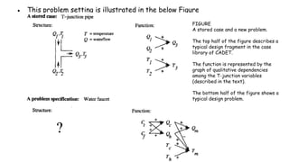
  • 33. ● This problem setting is illustrated in the below Figure FIGURE A stored case and a new problem. The top half of the figure describes a typical design fragment in the case library of CADET. The function is represented by the graph of qualitative dependencies among the T-junction variables (described in the text). The bottom half of the figure shows a typical design problem.
  • 34. ● The top half of the figure shows the description of a typical stored case called a T-junction pipe. ● Its function is represented in terms of the qualitative relationships among the waterflow levels and temperatures at its inputs and outputs. ● In the functional description at its right, an arrow with a "+" label indicates that the variable at the arrowhead increases with the variable at its tail. ● For example, the output waterflow Q3 increases with increasing input waterflow Q1. ● Similarly, a "-" label indicates that the variable at the head decreases with the variable at the tail.
  • 35. ● The bottom half of this figure depicts a new design problem described by its desired function. ● This particular function describes the required behavior of one type of water faucet. ● Here Qc refers to the flow of cold water into the faucet, Qh to the input flow of hot water, and Qm to the single mixed flow out of the faucet. ● Similarly, Tc, Th, and Tm refer to the temperatures of the cold water, hot water, and mixed water respectively. ● The variable Ct denotes the control signal for temperature that is input to the faucet, and Cf denotes the control signal for waterflow
  • 36. ● Given this functional specification for the new design problem, CADET searches its library for stored cases whose functional descriptions match the design problem. ● If an exact match is found, indicating that some stored case implements exactly the desired function, then this case can be returned as a suggested solution to the design problem. ● If no exact match occurs, CADET may find cases that match various subgraphs of the desired functional specification ● CADET searches for subgraph isomorphisms between the two function graphs, so that parts of a case can be found to match parts of the design specification. ● Furthermore, the system may elaborate the original function specification graph in order to create functionally equivalent graphs that may match still more cases.
  • 37. ● It uses a rewrite rule that allows it to rewrite the influence This rewrite rule can be interpreted as stating that if B must increase with A, then it is sufficient to find some other quantity x such that B increases with x, and x increases with A.
  • 38. Difference between case-based reasoning and instance-based approach ● Instances or cases may be represented by rich symbolic descriptions, such as the function graphs used in CADET ● Multiple retrieved cases may be combined to form the solution to the new problem which is knowledge-based reasoning rather than statistical methods. ● Case -based reasoning is search-intensive problem-solving methods. ● Similarity metric can be modified based on suitability of the retrieved case
  • 41. Genetic Algorithms ● Genetic algorithms (GAS) provide a learning method motivated by an analogy to biological evolution ● A genetic algorithm is a heuristic search method used in artificial intelligence and computing. ● It is used for finding optimized solutions to search problems based on the theory of natural selection and evolutionary biology. ● GAS generate successor hypotheses by repeatedly mutating and recombining parts of the best currently known hypotheses ● At each step, a collection of hypotheses called the current population is updated by replacing some fraction of the population by offspring of the most fit current hypotheses
  • 42. The popularity of GAS is motivated by a number of factors including: ● Evolution is known to be a successful, robust method for adaptation within biological systems. ● GAS can search spaces of hypotheses containing complex interacting parts, where the impact of each part on overall hypothesis fitness may be difficult to model. ● Genetic algorithms are easily parallelized and can take advantage of the decreasing costs of powerful computer hardware.
  • 43. ● The problem addressed by GAs is to search a space of candidate hypotheses to identify the best hypothesis. ● In GAs the "best hypothesis" is defined as the one that optimizes a predefined numerical measure for the problem at hand, called the hypothesis Fitness Although different implementations of genetic algorithms vary in their details, they typically share the following structure ● The algorithm operates by iteratively updating a pool of hypotheses, called the population. ● On each iteration, all members of the population are evaluated according to the fitness function. ● A new population is then generated by probabilistically selecting the most fit individuals from the current population. ● Some of these selected individuals are carried forward into the next generation population intact. ● Others are used as the basis for creating new offspring individuals by applying genetic operations such as crossover and mutation.
  • 45. 1.Representing Hypotheses ● Hypotheses in GAS are often represented by bit strings, so that they can be easily manipulated by genetic operators such as mutation and crossover. ● The hypotheses represented by these bit strings can be quite complex ● To see how if-then rules can be encoded by bit strings, first consider how we might use a bit string to describe a constraint on the value of a single attribute. ● To pick an example, ○ Consider the attribute Outlook, which can take on any of the three values ■ Sunny, Overcast, or Rain ○ One obvious way to represent a constraint on Outlook is to use a bit string of length three, in which each bit position corresponds to one of its three possible values.
  • 46. ● Example, ○ The string 010 represents the constraint that Outlook must take on the second of these values, or Outlook = Overcast. ○ Similarly, the string 011 represents the more general constraint that allows two possible values, or (Outlook = Overcast v Rain). ○ Note 11 1 represents the most general possible constraint, indicating that we don't care which of its possible values the attribute takes on. ● Given this method for representing constraints on a single attribute, conjunctions of constraints on multiple attributes can easily be represented by concatenating the corresponding bit strings
  • 47. ● For example, consider a second attribute, Wind, that can take on the value Strong or Weak ● A rule precondition such as It can then be represented by the following bit string of length five: ● Rule postconditions (such as PlayTennis = yes) can be represented in a similar fashion
  • 48. ● where the first three bits describe the "don't care" constraint on Outlook, the next two bits describe the constraint on Wind, and the final two bits describe the rule postcondition (here we assume PlayTennis can take on the values Yes or No). ● In designing a bit string encoding for some hypothesis space, it is useful to arrange for every syntactically legal bit string to represent a well-defined hypothesis. ● To illustrate, note in the rule encoding in the above paragraph the bit string 11 1 10 11 represents a rule whose postcondition does not constrain the target attribute PlayTennis. ● If we wish to avoid considering this hypothesis, we may employ a different encoding (e.g., allocate just one bit to the PlayTennis postcondition to indicate whether the value is Yes or No)
  • 49. 2.Genetic Operators ● The generation of successors in a GA is determined by a set of operators that recombine and mutate selected members of the current population ● The two most common operators are ○ Crossover and ○ Mutation Crossover operator ● It produces two new offspring from two parent strings, by copying selected bits from each parent. ● The bit at position i in each offspring is copied from the bit at position i in one of the two parents. ● The choice of which parent contributes the bit for position i is determined by an additional string called the crossover mask.
  • 51. Single-point crossover operator ● Consider the topmost of the two offspring in this case. ● This offspring takes its first five bits from the first parent and its remaining six bits from the second parent, because the crossover mask 11111000000 specifies these choices for each of the bit positions. ● The second offspring uses the same crossover mask, but switches the roles of the two parents. ● Therefore, it contains the bits that were not used by the first offspring. ● In single-point crossover, the crossover mask is always constructed so that it begins with a string containing n contiguous 1s, followed by the necessary number of 0s to
  • 52. Two-point crossover ● In two-point crossover, offspring are created by substituting intermediate segments of one parent into the middle of the second parent string. ● Put another way, the crossover mask is a string beginning with n0 zeros, followed by a contiguous string of n1 ones, followed by the necessary number of zeros to complete the string. ● Each time the two-point crossover operator is applied, a mask is generated by randomly choosing the integers n0 and n1. ● In the given example, the offspring are created using a mask for which no = 2 and n 1 = 5.
  • 53. Uniform crossover ● It combines bits sampled uniformly from the two parents, as illustrated in example. ● In this case the crossover mask is generated as a random bit string with each bit chosen at random and independent of the others. Mutation operator ● The mutation operator produces small random changes to the bit string by choosing a single bit at random, then changing its value. ● Mutation is often performed after crossover has been applied as in our prototypical algorithm
  • 54. 3.Fitness Function and Selection ● The fitness function defines the criterion for ranking potential hypotheses and for probabilistically selecting them for inclusion in the next generation population. ● If the task is to learn classification rules, then the fitness function typically has a component that scores the classification accuracy of the rule over a set of provided training examples. ● The fitness function may measure the overall performance of the resulting procedure rather than performance of individual rules. Fitness proportionate selection or roulette wheel selection ● The probability that a hypothesis will be selected is given by the ratio of its fitness to the fitness of other members of the current population
  • 55. Tournament selection ● The two hypotheses are first chosen at random from the current population. ● With some predefined probability p the more fit of these two is then selected, and with probability (1 - p) the less fit hypothesis is selected. ● Tournament selection often yields a more diverse population than fitness proportionate selection Rank selection ● The hypotheses in the current population are first sorted by fitness. ● The probability that a hypothesis will be selected is then proportional to its rank in this sorted list, rather than its fitness.
  • 56. AN ILLUSTRATIVE EXAMPLE ● A genetic algorithm can be viewed as a general optimization method that searches a large space of candidate objects seeking one that performs best according to the fitness function. ● Although not guaranteed to find an optimal object, GAS often succeed in finding an object with high fitness. ● GAS have been applied to a number of optimization problems outside machine learning, including problems such as circuit layout and job-shop scheduling. ● Within machine learning, they have been applied both to function-approximation problems and to tasks such as choosing the network topology for artificial neural network learning systems.
  • 57. Example: ● To illustrate the use of GAs for concept learning, we briefly summarize the GABIL system described by DeJong et al. (1993). ● GABIL is a genetic algorithm-based concept learner (or attribute classifier). ● GABIL uses a GA to learn boolean concepts represented by a disjunctive set of propositional rules. ● In experiments reported by DeJong et al. (1993), ○ the parameter r, which determines the fraction of the parent population replaced by crossover, was set to 0.6. ○ The parameter m, which determines the mutation rate, was set to 0.001. ○ The population size p was varied from 100 to 1000, depending on the specific learning task.
  • 58. Representation ● Each hypothesis in GABIL corresponds to a disjunctive set of propositional rules ● Consider a hypothesis space in which rule preconditions are conjunctions of constraints over two boolean attributes, a1 and a2. ● The rule postcondition is described by a single bit that indicates the predicted value of the target attribute c. ● The hypothesis consisting of the two rules
  • 59. Genetic operators ● GABIL uses the standard mutation operator in which a single bit is chosen at random and replaced by its complement. ● The crossover operator that it uses is a fairly standard extension to the two-point crossover operator ● To perform a crossover operation on two parents, two crossover points are first chosen at random in the first parent string. ● Let d1 (d2) denote the distance from the leftmost (rightmost) of these two crossover points to the rule boundary immediately to its left. ● The crossover points in the second parent are now randomly chosen, subject to the constraint that they must have the same d1 and d2 value
  • 60. ● For example, if the two parent strings are where "[" and "]" indicate crossover points, then d1 = 1 and d2 = 3.
  • 61. ● Hence the allowed pairs of crossover points for the second parent include the pairs of bit positions (1,3), (1,8), and (6,8). ● If the pair (1,3) happens to be chosen
  • 62. Fitness function ● The fitness of each hypothesized rule set is based on its classification accuracy over the training data. ● In particular, the function used to measure fitness is
  • 63. Extensions ● DeJong et al. (1993) also explore two interesting extensions to the basic design of GABIL. ● In one set of experiments they explored the addition of two new genetic operators that were motivated by the generalization operators common in many symbolic learning methods Add Alternative ● It generalizes the constraint on a specific attribute by changing a 0 to a 1 in the substring corresponding to the attribute. ● For example, if the constraint on an attribute is represented by the string 10010, this operator might change it to 101 10.
  • 64. Drop condition ● The second operator, Drop condition performs a more drastic generalization step, by replacing all bits for a particular attribute by a 1. ● This operator corresponds to generalizing the rule by completely dropping the constraint on the attribute In a second experiment, the bit-string representation for hypotheses was extended to include two bits that determine which of these operators may be applied to the hypothesis. where the final two bits indicate in this case that the AddAlternative operator may be applied to this bit string, but that the Dropcondition operator may not
  • 65. HYPOTHESIS SPACE SEARCH ● GAs employ a randomized beam search method to seek a maximally fit hypothesis. ● This search is quite different from that of other learning methods ● In contrast, the GA search can move much more abruptly, replacing a parent hypothesis by an offspring that may be radically different from the parent. ● One practical difficulty in some GA applications is the problem of crowding. ● Crowding is a phenomenon in which some individual that is more highly fit than others in the population quickly reproduces, so that copies of this individual and very similar individuals take over a large fraction of the population ● The negative impact of crowding is that it reduces the diversity of the population, thereby slowing further progress by the GA.
  • 66. Several strategies have been explored for reducing crowding. ● One approach is to alter the selection function, using criteria such as tournament selection or rank selection in place of fitness proportionate roulette wheel selection. ● A related strategy is "fitness sharing," in which the measured fitness of an individual is reduced by the presence of other, similar individuals in the population. ● A third approach is to restrict the kinds of individuals allowed to recombine to form offspring. ○ For example, by allowing only the most similar individuals to recombine, we can encourage the formation of clusters of similar individuals, or multiple "subspecies" within the population. ○ A related approach is to spatially distribute individuals and allow only nearby individuals to recombine
  • 67. Population Evolution and the Schema Theorem ● It is interesting to ask whether one can mathematically characterize the evolution over time of the population within a GA. ● The schema theorem of Holland (1975) provides one such characterization. ● It is based on the concept of schemas, or patterns that describe sets of bit strings. ● To be precise, a schema is any string composed of 0s, 1s, and *'s. ● Each schema represents the set of bit strings containing the indicated 0s and 1s, with each "*" interpreted as a "don't care." ● For example, the schema 0*10 represents the set of bit strings that includes exactly 0010 and 01 10.
  • 68. ● An individual bit string can be viewed as a representative of each of the different schemas that it matches. For example, the bit string 0010 can be thought of as a representative of 24 distinct schemas including 00**, O* 10, ****, etc. ● Similarly, a population of bit strings can be viewed in terms of the set of schemas that it represents and the number of individuals associated with each of these schema. ● The schema theorem characterizes the evolution of the population within a GA in terms of the number of instances representing each schema ● Let m(s, t) denote the number of instances of schema s in the population at time t ● The schema theorem describes the expected value of m(s, t + 1) in terms of m(s, t) and other properties of the schema, population, and GA algorithm parameters
  • 69. ● The evolution of the population in the GA depends on ○ the selection step, ○ the recombination step, and ○ the mutation step Selection step ● Let us start by considering just the effect of the selection step. ● Let f (h) denote the fitness of the individual bit string h ● f(t) denote the average fitness of all individuals in the population at time t. ● Let n be the total number of individuals in the population ● Let indicate that the individual h is both a representative of schema s and a member of the population at time t. ● Finally, denote the average fitness of instances of schema s in the
  • 70. ● We are interested in calculating the expected value of m(s, t + 1), which we denote E[m(s, t + 1)]. ● We can calculate E[m (s, t + I)] using the probability distribution ● Now if we select one member for the new population according to this probability distribution, then the probability that we will select a representative of schema s is
  • 71. ● The above gives the probability that a single hypothesis selected by the GA will be an instance of schema s. ● Therefore, the expected number of instances of s resulting from the n independent selection steps that create the entire new generation is just n times this probability
  • 72. ● The equation states that the expected number of instances of schema s at generation t + 1 is proportional to the average fitness i(s, t) of instances of this schema at time t , and inversely proportional to the average fitness f(t) of all members of the population at time t. Crossover and mutation steps ● While the above analysis considered only the selection step of the GA, the crossover and mutation steps must be considered as well. ● The full schema theorem thus provides a lower bound on the expected frequency of schema s, as follows
  • 73. ● Here, pc is the probability that the single-point crossover operator will be applied to an arbitrary individual ● pm is the probability that an arbitrary bit of an arbitrary individual will be mutated by the mutation operator. ● o(s) is the number of defined bits in schema s, where 0 and 1 are defined bits, but * is not. ● d(s) is the distance between the leftmost and rightmost defined bits in s. ● Finally, l is the length of the individual bit strings in the population ● leftmost term in Equation describes the effect of the selection step ● The middle term describes the effect of the single-point crossover operator ● The rightmost term describes the probability that an arbitrary individual representing schema s will still represent schema s following application of the mutation operator
  • 74. GENETIC PROGRAMMING ● Genetic programming (GP) is a form of evolutionary computation in which the individuals in the evolving population are computer programs rather than bit strings. ● Koza (1992) describes the basic genetic programming approach and presents a broad range of simple programs that can be successfully learned by GP.
  • 75. 1.Representing Programs ● Programs manipulated by a GP are typically represented by trees corresponding to the parse tree of the program. ● Each function call is represented by a node in the tree, and the arguments to the function are given by its descendant nodes
  • 76. ● For example, Figure illustrates this tree representation for the function ● To apply genetic programming to a particular domain, the user must define the primitive functions to be considered (e.g., exponential),as well as the terminals (e.g., x, y, constants such as 2). ● As in a genetic algorithm, the prototypical genetic programming algorithm maintains a population of individuals (in this case, program trees). ● On each iteration, it produces a new generation of individuals using selection, crossover, and mutation. ● The fitness of a given individual program in the population is typically determined by executing the program on a set of training data
  • 77. ● Crossover operations are performed by replacing a randomly chosen subtree of one parent program by a subtree from the other parent program. Crossover operation applied to two parent program trees (top). Crossover points (nodes shown in bold at top) are chosen at random. The subtrees rooted at these crossover points are then exchanged to create children trees (bottom).
  • 78. 2.Illustrative Example ● One illustrative example presented by Koza (1992) involves learning an algorithm for stacking the blocks shown in Figure ● The task is to develop a general algorithm for stacking the blocks into a single stack that spells the word "universal," independent of the initial configuration of blocks in the world. ● The actions available for manipulating blocks allow moving only a single block at a time. ● In particular, the top block on the stack can be moved to the table surface, or a block on the table surface can be moved to the top of the stack.
  • 80. ● In Koza's formulation, the primitive functions used to compose programs for this task include the following three terminal arguments: ○ CS (current stack), which refers to the name of the top block on the stack, or F if there is no current stack. ○ TB (top correct block), which refers to the name of the topmost block on the stack, such that it and those blocks beneath it are in the correct order. ○ NN (next necessary), which refers to the name of the next block needed above TB in the stack, in order to spell the word "universal," or F if no more blocks are needed.
  • 81. ● In addition to these terminal arguments, the program language in this application included the following primitive functions: ○ (MS x) (move to stack), if block x is on the table, this operator moves x to the top of the stack and returns the value T. Otherwise, it does nothing and returns the value F. ○ (MT x) (move to table), if block x is somewhere in the stack, this moves the block at the top of the stack to the table and returns the value T. Otherwise, it returns the value F. ○ (EQ x y) (equal), which returns T if x equals y, and returns F otherwise. ○ (NOT x), which returns T if x = F, and returns F if x = T.
  • 82. ○ (DU x y) (do until), which executes the expression x repeatedly until expression y returns the value T. ○ To allow the system to evaluate the fitness of any given program, Koza provided a set of 166 training example problems representing a broad variety of initial block configurations, including problems of differing degrees of difficulty. ○ The fitness of any given program was taken to be the number of these examples solved by the algorithm. ○ The population was initialized to a set of 300 random programs. After 10 generations, the system discovered the following program, which solves all 166 problems.
  • 83. (EQ (DU (MT CS)(NOT CS)) (DU (MS NN)(NOT NN)) ) ○ Notice this program contains a sequence of two DU, or "Do Until" statements. ○ The first repeatedly moves the current top of the stack onto the table, until the stack becomes empty. ○ The second "Do Until" statement then repeatedly moves the next necessary block from the table onto the stack. ○ The role played by the top level EQ expression here is to provide a syntactically legal way to sequence these two "Do Until" loops.
  • 84. 3.Remarks on Genetic Programming ● Genetic programming extends genetic algorithms to the evolution of complete computer programs. ● Despite the huge size of the hypothesis space it must search, genetic programming has been demonstrated to produce intriguing results in a number of applications. ● While the above example of GP search is fairly simple, Koza et al. (1996) summarize the use of a GP in several more complex tasks such as designing electronic filter circuits and classifying segments of protein molecules ● In most cases, the performance of genetic programming depends crucially on the choice of representation and on the choice of fitness function. ● For this reason, an active area of current research is aimed at the automatic discovery and incorporation of subroutines that improve on the original set of primitive functions, thereby allowing the system to dynamically alter the primitives from which it constructs individuals
  • 85. MODELS OF EVOLUTION AND LEARNING ● In many natural systems, individual organisms learn to adapt significantly during their lifetime. ● At the same time, biological and social processes allow their species to adapt over a time frame of many generation ● Models of Evolution and Learning ○ Lamarckian Evolution ○ Baldwin Effect
  • 86. 1.Lamarckian Evolution ● Lamarck was a scientist who, in the late nineteenth century, proposed that evolution over many generations was directly influenced by the experiences of individual organisms during their lifetime. ● In particular, he proposed that experiences of a single organism directly affected the genetic makeup of their offspring: ● If an individual learned during its lifetime to avoid some toxic food, it could pass this trait on genetically to its offspring, which therefore would not need to learn the trait. ● The Lamarckian theory states the characteristic individual acquire during their lifetime pass them to their children. ● According to Lamarck’s theory, learning is an important part of the evolution of species
  • 87. ● This is an attractive conjecture, because it would presumably allow for more efficient evolutionary progress than a generate-and-test process that ignores the experience gained during an individual's lifetime. ● Despite the attractiveness of this theory, current scientific evidence overwhelmingly contradicts Lamarck's model. ● The currently accepted view is that the genetic makeup of an individual is, in fact, unaffected by the lifetime experience of one's biological parents. ● Despite this apparent biological fact, recent computer studies have shown that Lamarckian processes can sometimes improve the effectiveness of computerized genetic algorithms
  • 88. 2.Baldwin Effect 1. Although Lamarckian evolution is not an accepted model of biological evolution, other mechanisms have been suggested by which individual learning can alter the course of evolution. 2. One such mechanism is called the Baldwin effect, after J. M. Baldwin (1896), who first suggested the idea. The Baldwin effect is based on the following observations: 1. If a species is evolving in a changing environment, there will be evolutionary pressure to favor individuals with the capability to learn during their lifetime. For example, if a new predator appears in the environment, then individuals capable of learning to avoid the predator will be more successful than individuals who cannot learn. In effect, the ability to learn allows an individual to perform a small local search during its lifetime to maximize its fitness. In contrast, non learning individuals whose fitness is fully determined by their genetic makeup will operate at a relative disadvantage.
  • 89. 2. Those individuals who are able to learn many traits will rely less strongly on their genetic code to "hard-wire" traits. As a result, these individuals can support a more diverse gene pool, relying on individual learning to overcome the "missing" or "not quite optimized" traits in the genetic code. This more diverse gene pool can, in turn, support more rapid evolutionary adaptation. Thus, the ability of individuals to learn can have an indirect accelerating effect on the rate of evolutionary adaptation for the entire population. Thus, the Baldwin effect provides an indirect mechanism for individual learning to positively impact the rate of evolutionary progress. By increasing survivability and genetic diversity of the species, individual learning supports more rapid evolutionary progress
  • 90. PARALLELIZING GENETIC ALGORITHMS ● GAs are naturally suited to parallel implementation, and a number of approaches to parallelization have been explored Coarse grain approaches ● Coarse grain approaches to parallelization subdivide the population into somewhat distinct groups of individuals, called demes. ● Each deme is assigned to a different computational node, and a standard GA search is performed at each node. ● Communication and cross-fertilization between demes occurs on a less frequent basis than within demes. ● Transfer between demes occurs by a migration process, in which individuals from one deme are copied or transferred to other demes.
  • 91. ● This process is modeled after the kind of cross-fertilization that might occur between physically separated subpopulations of biological species. ● One benefit of such approaches is that it reduces the crowding problem often encountered in nonparallel GAS, in which the system falls into a local optimum due to the early appearance of a genotype that comes to dominate the entire population Fine-grained approaches ● In contrast to coarse-grained parallel implementations of GAS, fine-grained implementations typically assign one processor per individual in the population. ● Recombination then takes place among neighboring individuals. ● Several different types of neighborhoods have been proposed, ranging from planar grid to torus