


![IR Models
An IR model is a quadruple [D, Q, F , R(qi, dj )]
where
1. D is a set of logical views for the documents in the collection
2. Q is a set of logical views for the user queries
3. F is a framework for modeling documents and queries
4. R(qi, dj ) is a ranking function
Q
D
q
d
R(d ,q
)
p. 6](https://image.slidesharecdn.com/irtunitiijm-241211141702-b2d054d5/85/JM-Information-Retrieval-Techniques-Unit-II-6-320.jpg)


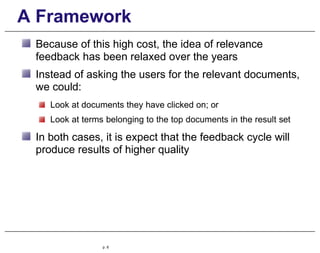
![The Boolean Model
This approach works even if the vocabulary of the
collection includes terms not in the query
Consider that the vocabulary is given by
V = {ka, kb, kc, kd}
Then, a document dj that contains only terms ka, kb,
and kc is represented by c(dj ) = (1, 1, 1, 0)
The query [q = ka
∧ (kb ∨ ¬kc)] is represented
in
p. 19
disjunctive normal form as
qDNF
= (1, 1, 1, 0) ∨ (1, 1, 1,
1) ∨
(1, 1, 0, 0) ∨ (1, 1, 0, 1)
∨
(1, 0, 0, 0) ∨ (1, 0, 0, 1)](https://image.slidesharecdn.com/irtunitiijm-241211141702-b2d054d5/85/JM-Information-Retrieval-Techniques-Unit-II-19-320.jpg)


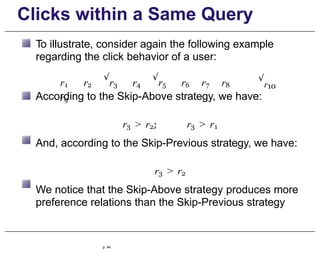
![Ranking Formula
iR
p
=
If information on the contingency table were available
for a given query, we could write
ri
R
qiR = ni −ri
N −R
Then, the equation for ranking computation in the
probabilistic model could be rewritten as
Σ
sim(dj , q) ~ log
ki[q,dj ]
×
ri N − n − R +
r
i i
R − ri ni − ri
p. 74
where ki[q, dj ] is a short notation for ki ∈ q ∧ ki ∈
dj](https://image.slidesharecdn.com/irtunitiijm-241211141702-b2d054d5/85/JM-Information-Retrieval-Techniques-Unit-II-74-320.jpg)
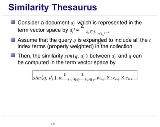
![Ranking Formula
In the previous formula, we are still dependent on an
estimation of the relevant dos for the query
For handling small values of ri, we add 0.5 to each
of the terms in the formula above, which changes
sim(dj , q) into
Σ
ki[q,dj ]
i i
ri + 0.5 N − n − R + r +
0.5
R − ri + 0.5 ni − ri +
0.5
log ×
This formula is considered as the classic ranking
equation for the probabilistic model and is known as the
Robertson-Sparck Jones Equation
p. 75](https://image.slidesharecdn.com/irtunitiijm-241211141702-b2d054d5/85/JM-Information-Retrieval-Techniques-Unit-II-75-320.jpg)
![Ranking Formula
The previous equation cannot be computed without
estimates of ri and R
One possibility is to assume R = ri = 0, as a way
to boostrap the ranking equation, which leads to
j
sim(d , q)
~
Σ
ki[q,dj ] lo
g
i
N −n +0.5
ni+0.5
This equation provides an idf-like ranking computation
In the absence of relevance information, this is the
equation for ranking in the probabilistic model
p. 76](https://image.slidesharecdn.com/irtunitiijm-241211141702-b2d054d5/85/JM-Information-Retrieval-Techniques-Unit-II-76-320.jpg)

![Ranking Example
The ranking computation led to negative weights
because of the term “do”
Actually, the probabilistic ranking equation produces
negative terms whenever ni > N/2
One possible artifact to contain the effect of negative
weights is to change the previous equation to:
Σ
sim(dj , q) ~
log ki[q,dj ]
N +
0.5
ni +
0.5
By doing so, a term that occurs in all documents
(ni = N ) produces a weight equal to zero
p. 78](https://image.slidesharecdn.com/irtunitiijm-241211141702-b2d054d5/85/JM-Information-Retrieval-Techniques-Unit-II-78-320.jpg)


![Ranking Computation
The ranking computation is based on the vector model,
but adopts termsets instead of index terms
Given a query q, let
{S1, S2, . . .} be the set of all termsets originated from q
Ni be the number of documents in which termset Si occurs
N be the total number of documents in the collection
Fi , j be the frequency of termset Si in document dj
For each pair [Si, dj ] we compute a weight Wi , j given
by
Wi,j =
(
i,j
(1 + log F ) log(1
+ 0
N
Ni
) if Fi , j >
0
Fi , j = 0
We also compute a Wi,q value for each pair [Si,
q]
p. 98](https://image.slidesharecdn.com/irtunitiijm-241211141702-b2d054d5/85/JM-Information-Retrieval-Techniques-Unit-II-98-320.jpg)


![Fuzzy Set Theory
A fuzzy subset A of a universe of discourse U is
characterized by a membership function
µA : U → [0, 1]
This function associates with each element u of U a
number µA(u) in the interval [0, 1]
The three most commonly used operations on fuzzy
sets are:
the complement of a fuzzy set
the union of two or more fuzzy sets
the intersection of two or more fuzzy sets
p. 123](https://image.slidesharecdn.com/irtunitiijm-241211141702-b2d054d5/85/JM-Information-Retrieval-Techniques-Unit-II-123-320.jpg)


![Key Idea
As before, let wi,j be the weight associated with [ki, dj ]
and V = {k1, k2, . . ., kt} be the set of all terms
If the wi,j weights are binary, all patterns of occurrence
of terms within docs can be represented by minterms:
(k1, k2, k3, . . . , kt)
.
p. 135
m1 = (0, 0, 0, . . . , 0)
m2 = (1, 0, 0, . . . , 0)
m3 = (0, 1, 0, . . . , 0)
m4 = (1, 1, 0, . . . , 0)
m2t
.
= (1, 1, 1, . . . , 1)
For instance, m2 indi-
cates documents in which
solely the term k1 occurs](https://image.slidesharecdn.com/irtunitiijm-241211141702-b2d054d5/85/JM-Information-Retrieval-Techniques-Unit-II-135-320.jpg)


![Latent Semantic Indexing
The idea here is to map documents and queries into a
dimensional space composed of concepts
Let
t: total number of index terms
N : number of documents
M = [mi j ]: term-document matrix t × N
To each element of M is assigned a weight wi,j
associated with the term-document pair [ki, dj ]
The weight wi , j can be based on a tf-idf weighting scheme
p. 147](https://image.slidesharecdn.com/irtunitiijm-241211141702-b2d054d5/85/JM-Information-Retrieval-Techniques-Unit-II-147-320.jpg)
![Latent Semantic Indexing
The matrix M = [mi j ] can be decomposed into
three components using singular value
decomposition
M = K · S · DT
were
K is the matrix of eigenvectors derived from C = M ·
MT
D T is the matrix of eigenvectors derived from MT · M
S is an r × r diagonal matrix of singular values where
r = min(t, N ) is the rank of M
p. 148](https://image.slidesharecdn.com/irtunitiijm-241211141702-b2d054d5/85/JM-Information-Retrieval-Techniques-Unit-II-148-320.jpg)
![Computing an Example
Let MT = [mi j ] be given
by
K1 K2 K3 q • dj
d1
2 0 1 5
d2
1 0 0 1
d3
0 1 3 11
d4
2 0 0 2
d5
1 2 4 17
d6
1 2 0 5
d7
0 5 0 10
q 1 2 3
Compute the matrices K, S, and Dt
p. 149](https://image.slidesharecdn.com/irtunitiijm-241211141702-b2d054d5/85/JM-Information-Retrieval-Techniques-Unit-II-149-320.jpg)


![BM1, BM11 and BM15 Formulas
Introduction of these three factors led to various BM
(Best Matching) formulas, as follows:
B M 1 j
sim (d , q) ~
Σ
ki [q,dj ]
lo
g
i
N − n +
0.5
ni +
0.5
simB M 15 j j,q
(d , q) ~ G
+
Σ
k i [q,dj ]
F i,j i,q
× F ×
lo
g
i
N − n +
0.5
ni +
0.5
simB M 11 j j,q
(d , q) ~ G
+
Σ
k i [q,dj ]
F
'
i,j i,q
× F
×
lo
g
i
N − n +
0.5
ni +
0.5
p. 171
where ki[q, dj ] is a short notation for ki ∈ q Λ ki ∈
dj](https://image.slidesharecdn.com/irtunitiijm-241211141702-b2d054d5/85/JM-Information-Retrieval-Techniques-Unit-II-171-320.jpg)

![BM1, BM11 and BM15 Formulas
These considerations lead to simpler equations as
follows
B M 1 j
sim (d , q) ~
Σ
k i [q,dj ]
lo
g
i
N − n +
0.5
ni +
0.5
simB M 15 j
(d , q) ~
Σ
k i [q,dj ]
(K1 + 1)fi , j
(K1 +
fi , j )
× lo
g
i
N − n +
0.5 i
n +
0.5
simB M 11 j
(d , q) ~
Σ
k i [q,dj ]
(K1 + 1)fi , j
K 1 len(dj )
avg_doclen + fi,j
× lo
g
i
N − n +
0.5
ni +
0.5
p. 173](https://image.slidesharecdn.com/irtunitiijm-241211141702-b2d054d5/85/JM-Information-Retrieval-Techniques-Unit-II-173-320.jpg)
![BM25 Ranking Formula
BM25: combination of the BM11 and BM15
The motivation was to combine the BM11 and BM25
term frequency factors as follows
Bi,j =
(K1 +
1)fi,j
K1
h
len(dj )
(1 − b) + bavg_doclen
i
+ f i,j
where b is a constant with values in the interval [0,
1]
If b = 0, it reduces to the BM15 term frequency
factor If b = 1, it reduces to the BM11 term
frequency factor
For values of b between 0 and 1, the equation provides a
combination of BM11 with BM15
p. 174](https://image.slidesharecdn.com/irtunitiijm-241211141702-b2d054d5/85/JM-Information-Retrieval-Techniques-Unit-II-174-320.jpg)
![BM25 Ranking Formula
The ranking equation for the BM25 model can then be
written as
Σ
simB M 25(dj, q) ~
B ki[q,dj ]
i,j × lo
g
i
N − n +
0.5
ni +
0.5
where K1 and b are empirical constants
K1 = 1 works well with real collections
b should be kept closer to 1 to emphasize the document length
normalization effect present in the BM11 formula
For instance, b = 0.75 is a reasonable assumption
Constants values can be fine tunned for particular collections
through proper experimentation
p. 175](https://image.slidesharecdn.com/irtunitiijm-241211141702-b2d054d5/85/JM-Information-Retrieval-Techniques-Unit-II-175-320.jpg)


![Bernoulli Process
j i j
P (q|M ) = P (k |
M ) ki∈q
ki/∈q
where P (ki|Mj ) are term probabilities
This is analogous to the expression for ranking
computation in the classic probabilistic model
×
The first application of languages models to IR was due
to Ponte & Croft. They proposed a Bernoulli process for
generating the query, as we now discuss
Given a document dj , let Mj be a reference to
a language model for that document
If we assume independence of index terms, we can
compute P (q|Mj ) using a multivariate Bernoulli
process:
Y Y [1 − P (ki|
Mj )]
p. 197](https://image.slidesharecdn.com/irtunitiijm-241211141702-b2d054d5/85/JM-Information-Retrieval-Techniques-Unit-II-197-320.jpg)


![Bernoulli process
j R i j
P (q|M ) = P (k |
M ) ki∈q ki/∈q
which computes the probability of generating the query
from the language (document) model
This is the basic formula for ranking computation in a
language model based on a Bernoulli process for
generating the query
×
Substituting into original P (q|Mj ) Equation, we obtain
Y Y
[1 − PR (ki |
Mj )]
p. 205](https://image.slidesharecdn.com/irtunitiijm-241211141702-b2d054d5/85/JM-Information-Retrieval-Techniques-Unit-II-205-320.jpg)


![Divergence from Randomness
Given these assumptions, the weight wi,j of a term ki in
a document dj is defined as
wi,j = [− log P (ki|C)] × [1 − P (ki|dj )]
Two term distributions are considered: in the collection
and in the subset of docs in which it occurs
The rank R(dj , q) of a document dj with regard to
a query q is then computed as
R(dj , q) =
Σ
k i ∈ q fi,q × wi,j
where fi, q is the frequency of term ki in the query
p. 210](https://image.slidesharecdn.com/irtunitiijm-241211141702-b2d054d5/85/JM-Information-Retrieval-Techniques-Unit-II-210-320.jpg)


![Reference Collections
Reference collections, which are based on the
foundations established by the Cranfield experiments,
constitute the most used evaluation method in IR
A reference collection is composed of:
A set D of pre-selected documents
A set I of information need descriptions used for testing
A set of relevance judgements associated with each pair [im ,
dj ],
im ∈ I and dj ∈ D
The relevance judgement has a value of 0 if
document
dj is non-relevant to im , and 1 otherwise
These judgements are produced by human
specialists
p. 9](https://image.slidesharecdn.com/irtunitiijm-241211141702-b2d054d5/85/JM-Information-Retrieval-Techniques-Unit-II-272-320.jpg)


![F-Measure: Harmonic Mean
The function F assumes values in the interval [0, 1]
It is 0 when no relevant documents have been retrieved
and is 1 when all ranked documents are relevant
Further, the harmonic mean F assumes a high value
only when both recall and precision are high
To maximize F requires finding the best possible
compromise between recall and precision
Notice that setting b = 1 in the formula of the E-measure
yields
F (j) = 1 − E(j)
p. 36](https://image.slidesharecdn.com/irtunitiijm-241211141702-b2d054d5/85/JM-Information-Retrieval-Techniques-Unit-II-299-320.jpg)


![Discounted Cumulated Gain
Consider that the results of the queries are graded on a
scale 0–3 (0 for non-relevant, 3 for strong relevant
docs)
For instance, for queries q1 and q2, consider that the
graded relevance scores are as follows:
Rq1 =
Rq2 =
{ [d3, 3], [d5, 3], [d9, 3], [d25, 2], [d39, 2],
[d44, 2], [d56, 1], [d71, 1], [d89, 1], [d123,
1] }
{ [d3, 3], [d56, 2], [d129, 1] }
That is, while document d3 is highly relevant to query q1,
document d56 is just mildly relevant
p. 45](https://image.slidesharecdn.com/irtunitiijm-241211141702-b2d054d5/85/JM-Information-Retrieval-Techniques-Unit-II-308-320.jpg)


![Discounted Cumulated Gain
In formal terms, we define
Given the gain vector Gj for a test query qj , the CGj
associated with it is defined as
Gj [1] if i = 1;
CGj [i] =
Gj [i] + CGj [i − 1] otherwise
where CGj [i] refers to the cumulated gain at the ith position
of the ranking for query qj
p. 48](https://image.slidesharecdn.com/irtunitiijm-241211141702-b2d054d5/85/JM-Information-Retrieval-Techniques-Unit-II-311-320.jpg)

![Discounted Cumulated Gain
More formally,
Given the gain vector Gj for a test query qj , the vector DCGj
associated with it is defined as
p. 50
j
DCG [i]
=
j
G [1] if i =
1;
G j [i]
log2 i + DCGj [i − 1] otherwise
where DCGj [i] refers to the discounted cumulated gain at the
ith position of the ranking for query qj](https://image.slidesharecdn.com/irtunitiijm-241211141702-b2d054d5/85/JM-Information-Retrieval-Techniques-Unit-II-313-320.jpg)

![DCG Curves
To produce CG and DCG curves over a set of test
queries, we need to average them over all queries
Given a set of Nq queries, average CG[i] and
DCG[i]
over all queries are computed as follows
CG[i] =
N q
CGj
[i]
;
DCG[i] =
Σ Σ N q
j = 1 Nq j = 1
DCGj [i]
Nq
For instance, for the example queries q1 and q2, these
averages are given by
CG = (0.5, 0.5, 2.0, 2.0, 2.0, 3.5, 3.5, 4.0, 4.0, 5.0, 5.0, 5.0, 5.0, 5.0,
8.0)
DCG = (0.5, 0.5, 1.5, 1.5, 1.5, 2.1, 2.1, 2.2, 2.2, 2.5, 2.5, 2.5, 2.5, 2.5,
3.3)
p. 52](https://image.slidesharecdn.com/irtunitiijm-241211141702-b2d054d5/85/JM-Information-Retrieval-Techniques-Unit-II-315-320.jpg)


![Ideal CG and DCG Metrics
Further, average ICG and average IDCG scores can
be computed as follows
ICG[i] =
N q
j=1 Nq
ICGj
[i]
;
IDCG[i] =
Σ Σ N q
j=1
IDCGj [i]
Nq
For instance, for the example queries q1 and q2, ICG
and IDCG vectors are given by
ICG = (3.0, 5.5, 7.5, 8.5, 9.5, 10.5, 11.0, 11.5, 12.0, 12.5, 12.5, 12.5, 12.5, 12.5,
12.5)
IDCG = (3.0, 5.5, 6.8, 7.3, 7.7, 8.1, 8.3, 8.4, 8.6, 8.7, 8.7, 8.7, 8.7, 8.7, 8.7)
By comparing the average CG and DCG curves for an
algorithm with the average ideal curves, we gain insight
on how much room for improvement there is
p. 57](https://image.slidesharecdn.com/irtunitiijm-241211141702-b2d054d5/85/JM-Information-Retrieval-Techniques-Unit-II-320-320.jpg)
![Normalized DCG
Precision and recall figures can be directly compared to
the ideal curve of 100% precision at all recall levels
DCG figures, however, are not build relative to any ideal
curve, which makes it difficult to compare directly DCG
curves for two distinct ranking algorithms
This can be corrected by normalizing the DCG metric
Given a set of Nq test queries, normalized CG and DCG
metrics are given by
ICG[i]
NCG[i] = CG[i]
; NDCG[i] = DCG[i]
IDCG[i]
p. 58](https://image.slidesharecdn.com/irtunitiijm-241211141702-b2d054d5/85/JM-Information-Retrieval-Techniques-Unit-II-321-320.jpg)


![BPREF
Given an information need I, let
R A : ranking computed by an IR system A relatively to I
sA , j : position of document dj in R A
[(J − R) ∧ A]|R|: set composed of the first |R|
documents in R A
that have been judged as non-relevant
p. 68](https://image.slidesharecdn.com/irtunitiijm-241211141702-b2d054d5/85/JM-Information-Retrieval-Techniques-Unit-II-331-320.jpg)
![BPREF
Define
C(RA , dj ) = {dk | dk ∈ [(J − R) ∩ A]|
R|
∧ sA,k < sA,j }
as a counter of the non-relevant docs that appear
before dj in R A
Then, the BREF of ranking R A is given by
Bpref (RA ) =
1
|R|
Σ
dj ∈(R∩A) 1
−
A j
C(R ,d )
min(|R|, |(J−R)∩A|)
p. 69](https://image.slidesharecdn.com/irtunitiijm-241211141702-b2d054d5/85/JM-Information-Retrieval-Techniques-Unit-II-332-320.jpg)
![BPREF
For each relevant document dj in the ranking, Bpref
accumulates a weight
This weight varies inversely with the number of judged
non-relevant docs that precede each relevant doc dj
For instance, if all |R| documents from [(J −
R) ∧ A]|R|
precede dj in the ranking, the weight
accumulated is 0
If no documents from [(J − R) ∧ A]|R| precede dj in
the ranking, the weight accumulated is 1
After all weights have been accumulated, the sum is
normalized by |R|
p. 70](https://image.slidesharecdn.com/irtunitiijm-241211141702-b2d054d5/85/JM-Information-Retrieval-Techniques-Unit-II-333-320.jpg)


![BPREF-10
This metric ensures that a minimum of 10 preference
relations are available, as follows
Let [(J − R) ∧ A]|R|+10 be the set composed of the
first
|R| + 10 documents from (J − R) ∧ A in the ranking
Define
C1 0 (RA , dj ) = {dk | dk ∈ [(J − R) ∩ A)]|R|+10
¨
∧ s A ,k < s A , j }
¨
Then,
Bpref
10 A
(R ) = 1
|R|
Σ
d j ∈(R∩A) 1 −
C1 0 ( R A , d j )
min(|R|+10, |(J−R)∩A|)
p. 73](https://image.slidesharecdn.com/irtunitiijm-241211141702-b2d054d5/85/JM-Information-Retrieval-Techniques-Unit-II-336-320.jpg)


![The Spearman Coefficient
Let us consider the fraction
Σ K
j=1 (s1,j − s2,j )2
K×(K2 −1)
3
Its value is
0 when the two rankings are in perfect agreement
+1 when they are in perfect disagreement
If we multiply the fraction by 2, its value shifts to the
range [0, +2]
If we now subtract the result from 1, the resultant value
shifts to the range [−1, +1]
p. 82](https://image.slidesharecdn.com/irtunitiijm-241211141702-b2d054d5/85/JM-Information-Retrieval-Techniques-Unit-II-345-320.jpg)


![The Kendall Tau Coefficient
When we think of rank correlations, we think of how two
rankings tend to vary in similar ways
To illustrate, consider two documents dj and dk and
their positions in the rankings R 1 and R2
Further, consider the differences in rank positions for
these two documents in each ranking, i.e.,
s1,k
s2,k
—
—
s1,j
s2,j
If these differences have the same sign, we say that the
document pair [dk, dj ] is concordant in both rankings
If they have different signs, we say that the document
pair is discordant in the two rankings
p. 87](https://image.slidesharecdn.com/irtunitiijm-241211141702-b2d054d5/85/JM-Information-Retrieval-Techniques-Unit-II-350-320.jpg)
![The Kendall Tau Coefficient
Consider the top 5 documents in rankings R 1 and R2
documents
s1,j s2,j s i,j − s2,j
d123
1 2 -1
d84
2 3 -1
d56
3 1 +2
d6
4 5 -1
d8
5 4 +1
The ordered document pairs in ranking R 1 are
[d123, d84], [d123, d56],
[d123, d6], [d123, d8],
[d84, d56], [d84, d6], [d84,
d8],
[d56, d6], [d56, d8],
[d6, d8]
p. 88
2
for a total of 1 × 5 × 4, or 10 ordered pairs](https://image.slidesharecdn.com/irtunitiijm-241211141702-b2d054d5/85/JM-Information-Retrieval-Techniques-Unit-II-351-320.jpg)
![The Kendall Tau Coefficient
Repeating the same exercise for the top 5 documents in
ranking R2 , we obtain
[d56, d123], [d56, d84], [d56, d8], [d56,
d6],
[d123, d84], [d123, d8],
[d84, d8], [d84, d6],
[d123, d6],
[d8, d6]
We compare these two sets of ordered pairs looking for
concordant and discordant pairs
p. 89](https://image.slidesharecdn.com/irtunitiijm-241211141702-b2d054d5/85/JM-Information-Retrieval-Techniques-Unit-II-352-320.jpg)


![Unbiased Clickthrough Data
The algorithm below achieves the effect of mixing
rankings Y A and Y B
Input: Y A = (a1, a2, . . .), Y B = (b1, b2, . . .).
Output: a combined ranking Y.
combine_ranking(YA , Y B , ka , kb, Y)
{ if (ka = kb) {
if (YA [ka + 1] /
∈ Y)
{ Y := Y + YA [ka + 1]
}
combine_ranking(YA , Y B , ka + 1,
kb, Y)
} else {
if (YB [kb + 1] /
∈ Y)
{ Y := Y + Y B [kb + 1]
p. 142](https://image.slidesharecdn.com/irtunitiijm-241211141702-b2d054d5/85/JM-Information-Retrieval-Techniques-Unit-II-405-320.jpg)


![Association Clusters
For a given query q, let
DA: local document set, i.e., set of documents retrieved by q
NA: number of documents in D5
V5: local vocabulary, i.e., set of all distinct words in D5
fi , j : frequency of occurrence of a term ki in a document dj
∈ D5
MA=[mij ]: term-document matrix with V5 rows and N5
columns
mi j =fi , j : an element of matrix MA
MT : transpose of MA
A
The matrix
Cl = Ml MT
p. 58
l
is a local term-term correlation
matrix](https://image.slidesharecdn.com/irtunitiijm-241211141702-b2d054d5/85/JM-Information-Retrieval-Techniques-Unit-II-465-320.jpg)


![Metric Clusters
An alternative is to normalize the correlation factor
For instance,
c'u,v = cu,v
total number of [ku, kv ] pairs
considered
In this case the local metric matrix Cl is said to be
normalized
p. 66](https://image.slidesharecdn.com/irtunitiijm-241211141702-b2d054d5/85/JM-Information-Retrieval-Techniques-Unit-II-473-320.jpg)


![Global Statistical Thesaurus
A document clustering algorithm that produces small
and tight clusters is the complete link algorithm:
1. Initially, place each document in a distinct cluster
2. Compute the similarity between all pairs of clusters
3. Determine the pair of clusters [Cu, Cv ] with the
highest inter-cluster similarity
4. Merge the clusters Cu and Cv
5. Verify a stop criterion (if this criterion is not met then go back to
step 2)
6. Return a hierarchy of clusters
p. 98](https://image.slidesharecdn.com/irtunitiijm-241211141702-b2d054d5/85/JM-Information-Retrieval-Techniques-Unit-II-505-320.jpg)


![Global Statistical Thesaurus
Given that the thesaurus classes have been built, they
can be used for query expansion
For this, an average term weight wtC for each thesaurus
class C is computed as follows
Σ |C|
wtC = i=1
wi,C
|
C|
where
|C| is the number of terms in the thesaurus class C, and
wi , C is a weight associated with the term-class pair [ki,
C]
p. 103](https://image.slidesharecdn.com/irtunitiijm-241211141702-b2d054d5/85/JM-Information-Retrieval-Techniques-Unit-II-510-320.jpg)
JM Information Retrieval Techniques Unit II
- 1. Modern Information Retrieval Chapter 3 Modeling Part I: Classic Models Introduction to IR Models Basic Concepts The Boolean Model Term Weighting The Vector Model Probabilistic Model p. 1
- 2. IR Models Modeling in IR is a complex process aimed at producing a ranking function Ranking function: a function that assigns scores to documents with regard to a given query This process consists of two main tasks: The conception of a logical framework for representing documents and queries The definition of a ranking function that allows quantifying the similarities among documents and queries p. 2
- 3. Modeling and Ranking IR systems usually adopt index terms to index and retrieve documents Index term: In a restricted sense: it is a keyword that has some meaning on its own; usually plays the role of a noun In a more general form: it is any word that appears in a document Retrieval based on index terms can be implemented efficiently Also, index terms are simple to refer to in a query Simplicity is important because it reduces the effort of query formulation p. 3
- 4. Introduction documents information need Information retrieval process index terms match ranking 3 1 2 ... docs terms query terms p. 4
- 5. Introduction A ranking is an ordering of the documents that (hopefully) reflects their relevance to a user query Thus, any IR system has to deal with the problem of predicting which documents the users will find relevant This problem naturally embodies a degree of uncertainty, or vagueness p. 5
- 6. IR Models An IR model is a quadruple [D, Q, F , R(qi, dj )] where 1. D is a set of logical views for the documents in the collection 2. Q is a set of logical views for the user queries 3. F is a framework for modeling documents and queries 4. R(qi, dj ) is a ranking function Q D q d R(d ,q ) p. 6
- 7. A Taxonomy of IR Models p. 7
- 8. Retrieval: Ad Hoc x Filtering Ad Hoc Retrieval: Collection Q1 Q3 Q2 Q4 p. 8
- 9. Retrieval: Ad Hoc x Filtering Filtering documents stream user 2 user 1 p. 9
- 10. Basic Concepts Each document is represented by a set of representative keywords or index terms An index term is a word or group of consecutive words in a document A pre-selected set of index terms can be used to summarize the document contents However, it might be interesting to assume that all words are index terms (full text representation) p. 10
- 11. Basic Concepts Let, t be the number of index terms in the document collection ki be a generic index term Then, The vocabulary V = {k1, . . . , kt} is the set of all distinct index terms in the collection p. 11 k k k k V=
- 12. Basic Concepts Documents and queries can be represented by patterns of term co-occurrences V= Each of these patterns of term co-occurence is called a term conjunctive component For each document dj (or query q) we associate a unique term conjunctive component c(dj ) (or c(q)) p. 12
- 13. The Term-Document Matrix The occurrence of a term ki in a document dj establishes a relation between ki and dj A term-document relation between ki and dj can be quantified by the frequency of the term in the document In matrix form, this can written as d1 d2 1,1 f1,2 p. 13 k1 k2 k3 f f f 2,1 2,2 f3,1 f3,2 where each fi , j element stands for the frequency of term ki in document dj
- 14. Basic Concepts Logical view of a document: from full text to a set of index terms p. 14
- 15. The Boolean Model p. 15
- 16. The Boolean Model Simple model based on set theory and boolean algebra Queries specified as boolean expressions quite intuitive and precise semantics neat formalism example of query q = ka ∧ (kb ∨ ¬kc) Term-document frequencies in the term-document matrix are all binary wi j ∈ {0, 1}: weight associated with pair (ki, dj ) wiq ∈ {0, 1}: weight associated with pair (ki, q) p. 16
- 17. The Boolean Model A term conjunctive component that satisfies a query q is called a query conjunctive component c(q) A query q rewritten as a disjunction of those components is called the disjunct normal form qDNF To illustrate, consider query q = ka ∧ (kb ∨ ¬kc) vocabulary V = {ka, kb, kc} Then q DNF = (1, 1, 1) ∨ (1, 1, 0) ∨ (1, 0, 0) c(q): a conjunctive component for q p. 17
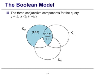
- 18. The Boolean Model Kc p. 18 The three conjunctive components for the query q = ka ∧ (kb ∨ ¬kc) Ka Kb (1,1,1)
- 19. The Boolean Model This approach works even if the vocabulary of the collection includes terms not in the query Consider that the vocabulary is given by V = {ka, kb, kc, kd} Then, a document dj that contains only terms ka, kb, and kc is represented by c(dj ) = (1, 1, 1, 0) The query [q = ka ∧ (kb ∨ ¬kc)] is represented in p. 19 disjunctive normal form as qDNF = (1, 1, 1, 0) ∨ (1, 1, 1, 1) ∨ (1, 1, 0, 0) ∨ (1, 1, 0, 1) ∨ (1, 0, 0, 0) ∨ (1, 0, 0, 1)
- 20. The Boolean Model The similarity of the document dj to the query q is defined as j sim(d , q) = ( 1 if ∃c(q) | c(q) = c(dj ) 0 otherwise The Boolean model predicts that each document is either relevant or non-relevant p. 20
- 21. Drawbacks of the Boolean Model Retrieval based on binary decision criteria with no notion of partial matching No ranking of the documents is provided (absence of a grading scale) Information need has to be translated into a Boolean expression, which most users find awkward The Boolean queries formulated by the users are most often too simplistic The model frequently returns either too few or too many documents in response to a user query p. 21
- 23. Term Weighting The terms of a document are not equally useful for describing the document contents In fact, there are index terms which are simply vaguer than others There are properties of an index term which are useful for evaluating the importance of the term in a document For instance, a word which appears in all documents of a collection is completely useless for retrieval tasks p. 23
- 24. Term Weighting To characterize term importance, we associate a weight wi,j > 0 with each term ki that occurs in the document dj If ki that does not appear in the document dj , then wi , j = 0. The weight wi,j quantifies the importance of the index term ki for describing the contents of document dj These weights are useful to compute a rank for each document in the collection with regard to a given query p. 24
- 25. Term Weighting Let, ki be an index term and dj be a document V = {k1, k2, ..., kt} be the set of all index terms wi , j ≥ 0 be the weight associated with (ki, dj ) Then we define d→j = (w1,j, w2,j, ..., wt,j ) as a weighted vector that contains the weight wi,j of each term ki ∈ V in the document dj k k k . k w w w . w V d p. 25
- 26. Term Weighting The weights wi,j can be computed using the frequencies of occurrence of the terms within documents Let fi , j be the frequency of occurrence of index term ki in the document dj The total frequency of occurrence Fi of term ki in the collection is defined as i p. 26 N Σ F = f j=1 i,j where N is the number of documents in the collection
- 27. Term Weighting The document frequency ni of a term ki is the number of documents in which it occurs Notice that ni ≤ Fi. For instance, in the document collection below, the values fi , j , Fi and ni associated with the term do are f (do, d1) = 2 f (do, d2) = 0 f (do, d3) = 3 f (do, d4) = 3 F (do) = 8 n(do) = 3 To do is to be. To be is to do. To be or not to be. I am what I am. I think therefore I am. Do be do be do. d1 d2 d3 Do do do, da da da. Let it be, let it be. p. 27 d4
- 28. Term-term correlation matrix For classic information retrieval models, the index term weights are assumed to be mutually independent This means that wi , j tells us nothing about wi+1,j This is clearly a simplification because occurrences of index terms in a document are not uncorrelated For instance, the terms computer and network tend to appear together in a document about computer networks In this document, the appearance of one of these terms attracts the appearance of the other Thus, they are correlated and their weights should reflect this correlation. p. 28
- 29. Term-term correlation matrix To take into account term-term correlations, we can compute a correlation matrix Let M→ = (mi j ) be a term-document matrix t × N where m ij = wi,j The matrix C→ = M→ M→ t is a term-term correlation matrix u,v c = Each element cu,v ∈ C expresses a correlation between terms ku and kv, given by Σ dj wu,j × wv,j Higher the number of documents in which the terms ku and kv co-occur, stronger is this correlation p. 29
- 30. Term-term correlation matrix Term-term correlation matrix for a sample collection d1 d2 k1 k2 k3 k1 k2 k3 w w 1,1 w1,2 2,1 w2,2 w3,1 w3,2 M 1 d d2 " w1,1 w2,1 w3,1 w1,2 w2,2 w3,2 M T # × ` ˛ ¸ x p. 30 ⇓ k2 w1,1w2,1 + w1,2w2,2 w2,1w2,1 + w2,2w2,2 w3,1w2,1 + w3,2w2,2 k3 k1 k2 k3 w1,1w1,1 k1 + w w 1,2 1,2 w1,1w3,1 + w1,2w3,2 w2,1w3,1 + w2,2w3,2 w3,1w3,1 + w3,2w3,2 w2,1w1,1 + w w 2,2 1,2 w3,1w1,1 + w3,2w1,2
- 32. TF-IDF Weights TF-IDF term weighting scheme: Term frequency (TF) Inverse document frequency (IDF) Foundations of the most popular term weighting scheme in IR p. 32
- 33. Term-term correlation matrix Luhn Assumption. The value of wi,j is proportional to the term frequency fi , j That is, the more often a term occurs in the text of the document, the higher its weight This is based on the observation that high frequency terms are important for describing documents Which leads directly to the following tf weight formulation: tfi,j = fi,j p. 33
- 34. Term Frequency (TF) Weights A variant of tf weight used in the literature is i,j tf = ( i,j f i,j 1 + log f if > 0 0 otherwise where the log is taken in base 2 The log expression is a the preferred form because it makes them directly comparable to idf weights, as we later discuss p. 34
- 35. Term Frequency (TF) Weights Log tf weights tfi , j for the example collection Vocabulary 1 to 2 do 3 is 4 be 5 or 6 not 7 I 8 am 9 what 10 think 11 therefore 12 da 13 let 14 it tfi,1 tfi,2 tfi,3 tfi,4 3 2 - - 2 - 2.585 2.585 2 - - - 2 2 2 2 - 1 - - - 1 - - - 2 2 - - 2 1 - - 1 - - - - 1 - - - 1 - - - - 2.585 - - - 2 - - - 2 p. 35
- 36. Inverse Document Frequency We call document exhaustivity the number of index terms assigned to a document The more index terms are assigned to a document, the higher is the probability of retrieval for that document If too many terms are assigned to a document, it will be retrieved by queries for which it is not relevant Optimal exhaustivity. We can circumvent this problem by optimizing the number of terms per document Another approach is by weighting the terms differently, by exploring the notion of term specificity p. 36
- 37. Inverse Document Frequency Specificity is a property of the term semantics A term is more or less specific depending on its meaning To exemplify, the term beverage is less specific than the terms tea and beer We could expect that the term beverage occurs in more documents than the terms tea and beer Term specificity should be interpreted as a statistical rather than semantic property of the term Statistical term specificity. The inverse of the number of documents in which the term occurs p. 37
- 38. Inverse Document Frequency Terms are distributed in a text according to Zipf’s Law Thus, if we sort the vocabulary terms in decreasing order of document frequencies we have n(r) ∼ r−α where n(r) refer to the rth largest document frequency and α is an empirical constant That is, the document frequency of term ki is an exponential function of its rank. n(r) = Cr− α where C is a second empirical constant p. 38
- 39. Inverse Document Frequency Setting α = 1 (simple approximation for english collections) and taking logs we have log n(r) = log C − log r For r = 1, we have C = n(1), i.e., the value of C is the largest document frequency This value works as a normalization constant An alternative is to do the normalization assuming C = N , where N is the number of docs in the collection log r ∼ log N − log n(r) p. 39
- 40. Inverse Document Frequency Let ki be the term with the rth largest document frequency, i.e., n(r) = ni. Then, N idfi = log ni where idfi is called the inverse document frequency of term ki Idf provides a foundation for modern term weighting schemes and is used for ranking in almost all IR systems p. 40
- 41. Inverse Document Frequency Idf values for example collection term ni idfi = log(N/ni) 1 to 2 1 2 do 3 0.415 3 is 1 2 4 be 4 0 5 or 1 2 6 not 1 2 7 I 2 1 8 am 2 1 9 what 1 2 10 think 1 2 11 therefore 1 2 12 da 1 2 13 let 1 2 14 it 1 2 p. 41
- 42. TF-IDF weighting scheme The best known term weighting schemes use weights that combine idf factors with term frequencies Let wi,j be the term weight associated with the term ki and the document dj Then, we define wi,j = p. 42 ( (1 + log fi , j ) × log if f i,j > 0 N ni 0 otherwise which is referred to as a tf-idf weighting scheme
- 43. TF-IDF weighting scheme Tf-idf weights of all terms present in our example document collection d1 d2 d3 d4 1 to 3 2 - - 2 do 0.830 - 1.073 1.073 3 is 4 - - - 4 be - - - - 5 or - 2 - - 6 not - 2 - - 7 I - 2 2 - 8 am - 2 1 - 9 what - 2 - - 10 think - - 2 - 11 therefore - - 2 - 12 da - - - 5.170 13 let - - - 4 14 it - - - 4 p. 43
- 44. Variants of TF-IDF Several variations of the above expression for tf-idf weights are described in the literature For tf weights, five distinct variants are illustrated below tf weight binary {0,1} raw frequency f i , j log normalization 1 + log fi , j double normalization 0.5 0.5 + 0.5 f i , j m a x i f i , j double normalization K f i , j K + (1 − K) m a x i f i , j p. 44
- 45. Variants of TF-IDF Five distinct variants of idf weight idf weight unary 1 inverse frequency log N n i inv frequency smooth log(1 + N ) n i inv frequeny max log(1 + m a x i n i ) n i probabilistic inv frequency log N − n i n i p. 45
- 46. Variants of TF-IDF Recommended tf-idf weighting schemes p. 46 weighting scheme document term weight query term weight 1 N fi , j ∗ log n i (0.5 + 0.5 f i , q ) ∗ log N m a x i f i , q n i 2 1 + log fi , j log(1 + N ) n i 3 N (1 + log fi , j ) ∗ log n i N (1 + log fi , q ) ∗ log n i
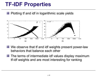
- 47. TF-IDF Properties Consider the tf, idf, and tf-idf weights for the Wall Street Journal reference collection To study their behavior, we would like to plot them together While idf is computed over all the collection, tf is computed on a per document basis. Thus, we need a representation of tf based on all the collection, which is provided by the term collection frequency Fi This reasoning leads to the following tf and idf term weights: N Σ p. 47 tf = 1 + log f i i,j j=1 i N idf = log ni
- 48. TF-IDF Properties Plotting tf and idf in logarithmic scale yields We observe that tf and idf weights present power-law behaviors that balance each other The terms of intermediate idf values display maximum tf-idf weights and are most interesting for ranking p. 48
- 49. Document Length Normalization Document sizes might vary widely This is a problem because longer documents are more likely to be retrieved by a given query To compensate for this undesired effect, we can divide the rank of each document by its length This procedure consistently leads to better ranking, and it is called document length normalization p. 49
- 50. Document Length Normalization Methods of document length normalization depend on the representation adopted for the documents: Size in bytes: consider that each document is represented simply as a stream of bytes Number of words: each document is represented as a single string, and the document length is the number of words in it Vector norms: documents are represented as vectors of weighted terms p. 50
- 51. Document Length Normalization Documents represented as vectors of weighted terms Each term of a collection is associated with an orthonormal unit vector →ki in a t-dimensional space For each term ki of a document dj is associated the term vector component wi , j × →ki p. 51
- 52. Document Length Normalization The document representation d→j is a vector composed of all its term vector components d→j = (w1,j, w2,j, ..., wt,j ) The document length is given by the norm of this vector, which is computed as follows , |d→j | = t p. 52 u Σ , w2 i i,j
- 53. Document Length Normalization Three variants of document lengths for the example collection d1 d2 d3 d4 size in bytes 34 37 41 43 number of words 10 11 10 12 vector norm 5.068 4.899 3.762 7.738 p. 53
- 54. The Vector Model p. 54
- 55. The Vector Model Boolean matching and binary weights is too limiting The vector model proposes a framework in which partial matching is possible This is accomplished by assigning non-binary weights to index terms in queries and in documents Term weights are used to compute a degree of similarity between a query and each document The documents are ranked in decreasing order of their degree of similarity p. 55
- 56. The Vector Model For the vector model: The weight wi , j associated with a pair (ki, dj ) is positive and non-binary The index terms are assumed to be all mutually independent They are represented as unit vectors of a t-dimensionsal space (t is the total number of index terms) The representations of document dj and query q are t-dimensional vectors given by d→j = (w1j, w2j, . . . , wt j ) →q = (w1q, w2q, . . . , wtq ) p. 56
- 57. The Vector Model Similarity between a document dj and a query q j i d q cos(θ) = d→j •→q |d→j |×| →q| j sim(d , q) = Σ t i=1 i,j w ×wi,q q Σ t i=1 w2 i,j × q Σ t j=1 w2 i,q Since wij > 0 and wiq > 0, we have 0 ≤ sim(dj , q) ≤ 1 p. 57
- 58. The Vector Model Weights in the Vector model are basically tf-idf weights wi,q N = (1 + log fi, q ) × log n i wi,j N = (1 + log fi , j ) × log n i These equations should only be applied for values of term frequency greater than zero If the term frequency is zero, the respective weight is also zero p. 58
- 59. The Vector Model Document ranks computed by the Vector model for the query “to do” (see tf-idf weight values in Slide 43) doc rank computation rank d1 1∗3+0.415∗0.830 5.068 0.660 d2 1∗2+0.415∗0 4.899 0.408 d3 1∗0+0.415∗1.073 3.762 0.118 d4 1∗0+0.415∗1.073 7.738 0.058 p. 59
- 60. The Vector Model Advantages: term-weighting improves quality of the answer set partial matching allows retrieval of docs that approximate the query conditions cosine ranking formula sorts documents according to a degree of similarity to the query document length normalization is naturally built-in into the ranking Disadvantages: It assumes independence of index terms p. 60
- 62. Probabilistic Model The probabilistic model captures the IR problem using a probabilistic framework Given a user query, there is an ideal answer set for this query Given a description of this ideal answer set, we could retrieve the relevant documents Querying is seen as a specification of the properties of this ideal answer set But, what are these properties? p. 62
- 63. Probabilistic Model An initial set of documents is retrieved somehow The user inspects these docs looking for the relevant ones (in truth, only top 10-20 need to be inspected) The IR system uses this information to refine the description of the ideal answer set By repeating this process, it is expected that the description of the ideal answer set will improve p. 63
- 64. Probabilistic Ranking Principle The probabilistic model Tries to estimate the probability that a document will be relevant to a user query Assumes that this probability depends on the query and document representations only The ideal answer set, referred to as R, should maximize the probability of relevance But, How to compute these probabilities? What is the sample space? p. 64
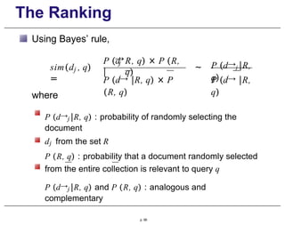
- 65. The Ranking Let, R be the set of relevant documents to query q R be the set of non-relevant documents to query q P (R|d→j ) be the probability that dj is relevant to the query q P (R|d→j ) be the probability that dj is non- relevant to q The similarity sim(dj , q) can be defined as j sim(d , q) = → P (R| d j ) j p. 65 P (R| d→ )
- 66. The Ranking Using Bayes’ rule, j sim(d , q) = → j P (d | R, q) × P (R, q) j P (d→ |R, q) × P (R, q) ~ P (d→j |R, q) j P (d→ |R, q) where P (d→j |R, q) : probability of randomly selecting the document dj from the set R P (R, q) : probability that a document randomly selected from the entire collection is relevant to query q P (d→j |R, q) and P (R, q) : analogous and complementary p. 66
- 67. The Ranking Assuming that the weights wi,j are all binary and assuming independence among the index terms: j sim(d , q) ∼ ( i i,j k |w =1 i P (k |R, q)) × ( Q Q i i,j k |w =0 i P (k |R, q)) ( Q ki |wi , j =1 i P (k | R, q)) × ( Q ki |wi , j =0 i P (k |R, q)) where P (ki|R, q): probability that the term ki is present in a document randomly selected from the set R P (ki|R, q): probability that ki is not present in a document randomly selected from the set R probabilities with R: analogous to the ones just described p. 67
- 68. The Ranking To simplify our notation, let us adopt the following conventions piR = P (ki| R, q) qiR = P (ki| R, q) Since P (ki|R, q) + P (ki|R, q) = 1 P (ki|R, q) + P (ki|R, q) = 1 we can write: j sim(d , q) ∼ i i,j k |w =1 ( piR i i,j k |w =0 iR ) × ( (1 − p )) Q p. 68 ki |wi , j =1 ( qiR) × ( Q ki |wi , j =0(1 − qiR))
- 69. The Ranking Taking logarithms, we write p. 69 sim(dj , q) ∼ log Y ki |wi , j =1 piR + log Y ki |wi , j =0 (1 − piR) — log Y ki |wi , j =1 qiR − log Y ki |wi , j =0 (1 − qiR)
- 70. The Ranking sim(dj , q) ∼ log p. 70 ki |wi , j =1 ki |wi , j =0 piR + log Summing up terms that cancel each other, we obtain Y Y (1 − pir) —lo g —lo g + log Y ki |wi , j =1 (1 − pir) + log Y ki |wi , j =1 (1 − pir) Y ki |wi , j =1 qiR − log Y ki |wi , j =0 (1 − qiR) Y ki |wi , j =1 (1 − qiR) − log Y ki |wi , j =1 (1 − qiR)
- 71. The Ranking Using logarithm operations, we obtain sim(dj , q) ∼ log Y ki |wi , j =1 piR (1 − piR) + log Y ki iR (1 − p ) + log Y ki |wi , j =1 iR (1 − q ) qiR — log Y ki iR (1 − q ) Notice that two of the factors in the formula above are a function of all index terms and do not depend on document dj . They are constants for a given query and can be disregarded for the purpose of ranking p. 71
- 72. The Ranking Further, assuming that 6 ki / ∈ q, piR = qiR and converting the log products into sums of logs, we finally obtain sim(dj , q) ~ Σ ki∈q∧ki∈dj lo g pi R 1−pi R + log 1−qi R qiR which is a key expression for ranking computation in the probabilistic model p. 72
- 73. Term Incidence Contingency Table Let, N be the number of documents in the collection ni be the number of documents that contain term ki R be the total number of relevant documents to query q ri be the number of relevant documents that contain term ki Based on these variables, we can build the following contingency table relevant non-relevant all docs docs that contain ki ri ni − ri ni docs that do not contain ki R − ri N − ni − (R − ri) N − ni all docs R N − R N p. 73
- 74. Ranking Formula iR p = If information on the contingency table were available for a given query, we could write ri R qiR = ni −ri N −R Then, the equation for ranking computation in the probabilistic model could be rewritten as Σ sim(dj , q) ~ log ki[q,dj ] × ri N − n − R + r i i R − ri ni − ri p. 74 where ki[q, dj ] is a short notation for ki ∈ q ∧ ki ∈ dj
- 75. Ranking Formula In the previous formula, we are still dependent on an estimation of the relevant dos for the query For handling small values of ri, we add 0.5 to each of the terms in the formula above, which changes sim(dj , q) into Σ ki[q,dj ] i i ri + 0.5 N − n − R + r + 0.5 R − ri + 0.5 ni − ri + 0.5 log × This formula is considered as the classic ranking equation for the probabilistic model and is known as the Robertson-Sparck Jones Equation p. 75
- 76. Ranking Formula The previous equation cannot be computed without estimates of ri and R One possibility is to assume R = ri = 0, as a way to boostrap the ranking equation, which leads to j sim(d , q) ~ Σ ki[q,dj ] lo g i N −n +0.5 ni+0.5 This equation provides an idf-like ranking computation In the absence of relevance information, this is the equation for ranking in the probabilistic model p. 76
- 77. Ranking Example Document ranks computed by the previous probabilistic ranking equation for the query “to do” doc rank computation rank d1 log 4−2+0.5 + log 4−3+0.5 2+0.5 3+0.5 - 1.222 d2 log 4−2+0.5 2+0.5 0 d3 log 4−3+0.5 3+0.5 - 1.222 d4 log 4−3+0.5 3+0.5 - 1.222 p. 77
- 78. Ranking Example The ranking computation led to negative weights because of the term “do” Actually, the probabilistic ranking equation produces negative terms whenever ni > N/2 One possible artifact to contain the effect of negative weights is to change the previous equation to: Σ sim(dj , q) ~ log ki[q,dj ] N + 0.5 ni + 0.5 By doing so, a term that occurs in all documents (ni = N ) produces a weight equal to zero p. 78
- 79. Ranking Example Using this latest formulation, we redo the ranking computation for our example collection for the query “to do” and obtain doc rank computation rank d1 log 4+0.5 + log 4+0.5 2+0.5 3+0.5 1.210 d2 log 4+0.5 2+0.5 0.847 d3 log 4+0.5 3+0.5 0.362 d4 log 4+0.5 3+0.5 0.362 p. 79
- 80. Estimaging ri and R Our examples above considered that ri = R = 0 An alternative is to estimate ri and R performing an initial search: select the top 10-20 ranked documents inspect them to gather new estimates for ri and R remove the 10-20 documents used from the collection rerun the query with the estimates obtained for ri and R Unfortunately, procedures such as these require human intervention to initially select the relevant documents p. 80
- 81. Improving the Initial Ranking Consider the equation sim(dj , q) ~ Σ ki∈q∧ki∈dj log piR 1 − piR + log 1 − q iR qiR How obtain the probabilities piR and qiR ? Estimates based on assumptions: pi R = 0.5 n i N qi R = where ni is the number of docs that contain ki Use this initial guess to retrieve an initial ranking Improve upon this initial ranking p. 81
- 82. Improving the Initial Ranking Substituting piR and qiR into the previous Equation, we obtain: Σ sim(dj , q) ~ log ki∈q∧ki∈dj N − ni ni That is the equation used when no relevance information is provided, without the 0.5 correction factor Given this initial guess, we can provide an initial probabilistic ranking After that, we can attempt to improve this initial ranking as follows p. 82
- 83. Improving the Initial Ranking iR p = We can attempt to improve this initial ranking as follows Let D : set of docs initially retrieved Di : subset of docs retrieved that contain ki Reevaluate estimates: D i D qiR = ni −Di N −D This process can then be repeated recursively p. 83
- 84. Improving the Initial Ranking sim(dj , q) ~ Σ ki∈q∧ki∈dj lo g N − ni ni To avoid problems with D = 1 and Di = 0: iR D + 1 Di + 0.5 p = ; q iR ni − Di + 0.5 = N − D + 1 Also, p. 84 Di + n i D + 1 piR = N ; i i n − D + ni qiR = N N − D + 1
- 85. Pluses and Minuses Advantages: Docs ranked in decreasing order of probability of relevance Disadvantages: need to guess initial estimates for piR method does not take into account tf factors the lack of document length normalization p. 85
- 86. Comparison of Classic Models Boolean model does not provide for partial matches and is considered to be the weakest classic model There is some controversy as to whether the probabilistic model outperforms the vector model Croft suggested that the probabilistic model provides a better retrieval performance However, Salton et al showed that the vector model outperforms it with general collections This also seems to be the dominant thought among researchers and practitioners of IR. p. 86
- 87. Modern Information Retrieval Modeling Part II: Alternative Set and Vector Models Set-Based Model Extended Boolean Model Fuzzy Set Model The Generalized Vector Model Latent Semantic Indexing Neural Network for IR p. 87
- 88. Alternative Set Theoretic Models Set-Based Model Extended Boolean Model Fuzzy Set Model p. 88
- 90. Set-Based Model This is a more recent approach (2005) that combines set theory with a vectorial ranking The fundamental idea is to use mutual dependencies among index terms to improve results Term dependencies are captured through termsets, which are sets of correlated terms The approach, which leads to improved results with various collections, constitutes the first IR model that effectively took advantage of term dependence with general collections p. 90
- 91. Termsets Termset is a concept used in place of the index terms A termset Si = {ka, kb, ..., kn} is a subset of the terms in the collection If all index terms in Si occur in a document dj then we say that the termset Si occurs in dj There are 2t termsets that might occur in the documents of a collection, where t is the vocabulary size However, most combinations of terms have no semantic meaning Thus, the actual number of termsets in a collection is far smaller than 2t p. 91
- 92. Termsets Let t be the number of terms of the collection Then, the set VS = {S1, S2, ..., S2t } is the vocabulary- set of the collection To illustrate, consider the document collection below To do is to be. To be is to do. To be or not to be. I am what I am. I think therefore I am. Do be do be do. d1 d2 d3 Do do do, da da da. Let it be, let it be. p. 92 d4
- 93. Termsets To simplify notation, let us define ka = to kd = be kg = I kj = think km = let kb = do ke = or kh = am kk = therefore kn = it kc = is kf = not ki = what kl = da Further, let the letters a...n refer to the index terms ka...kn , respectively a d e f a d g h i g h a b c a d a d c a b d 1 g j k g h b d b d b d3 d2 b b b l l l m n d m n d p. 93 d4
- 94. Termsets Consider the query q as “to do be it”, i.e. q = {a, b, d, n} For this query, the vocabulary-set is as below Termset Set of Terms Documents Sa {a} {d1 , d2} Sb {b} {d1 , d3 , d4} Sd {d} {d1 , d2 , d3 , d4} Sn {n} {d4 } Sab {a, b} {d1 } Sad {a, d} {d1 , d2} Sbd {b, d} {d1 , d3 , d4} Sbn {b, n} {d4 } Sabd {a, b, d} {d1 } Sbdn {b, d, n} {d4 } p. 94 Notice that there are 11 termsets that occur in our collection, out of the maximum of 15 termsets that can be formed with the terms in q
- 95. Termsets At query processing time, only the termsets generated by the query need to be considered A termset composed of n terms is called an n-termset Let Ni be the number of documents in which Si occurs An n-termset Si is said to be frequent if Ni is greater than or equal to a given threshold This implies that an n-termset is frequent if and only if all of its (n − 1)-termsets are also frequent Frequent termsets can be used to reduce the number of termsets to consider with long queries p. 95
- 96. Termsets Let the threshold on the frequency of termsets be 2 To compute all frequent termsets for the query q = {a, b, d, n} we proceed as follows 1. Compute the frequent 1-termsets and their inverted lists: Sa = {d1, d2} Sb = {d1, d3, d4} Sd = {d1, d2, d3, d4} 2. Combine the inverted lists to compute frequent 2-termsets: Sa d = {d1, d2} Sbd = {d1, d3, d4} 3. Since there are no frequent 3- termsets, stop a d e f a d g h i g h a b c a d a d c a b d 1 g j k g h b d b d b d2 d3 b b b l l l m n d m n d d4 p. 96
- 97. Termsets Notice that there are only 5 frequent termsets in our collection Inverted lists for frequent n-termsets can be computed by starting with the inverted lists of frequent 1-termsets Thus, the only indice that is required are the standard inverted lists used by any IR system This is reasonably fast for short queries up to 4-5 terms p. 97
- 98. Ranking Computation The ranking computation is based on the vector model, but adopts termsets instead of index terms Given a query q, let {S1, S2, . . .} be the set of all termsets originated from q Ni be the number of documents in which termset Si occurs N be the total number of documents in the collection Fi , j be the frequency of termset Si in document dj For each pair [Si, dj ] we compute a weight Wi , j given by Wi,j = ( i,j (1 + log F ) log(1 + 0 N Ni ) if Fi , j > 0 Fi , j = 0 We also compute a Wi,q value for each pair [Si, q] p. 98
- 99. Ranking Computation Consider query q = {a, b, d, n} document d1 = ‘‘a b c a d a d c a b’’ Termset Weight Sa Sb Sd Sn Sab Sad Sbd Sbn Sdn Wa,1 Wb,1 Wd,1 Wn,1 Wab,1 Wad,1 Wbd,1 Wbn,1 p. 99 (1 + log 4) ∗ log(1 + 4/2) = 4.75 (1 + log 2) ∗ log(1 + 4/3) = 2.44 (1 + log 2) ∗ log(1 + 4/4) = 2.00 0 ∗ log(1 + 4/1) = 0.00 (1 + log 2) ∗ log(1 + 4/1) = 4.64 (1 + log 2) ∗ log(1 + 4/2) = 3.17 (1 + log 2) ∗ log(1 + 4/3) = 2.44 0 ∗ log(1 + 4/1) = 0.00 0 ∗ log(1 + 4/1) = 0.00 (1 + log 2) ∗ log(1 + 4/1) = 4.64 0 ∗ log(1 + 4/1) = 0.00
- 100. Ranking Computation A document dj and a query q are represented as vectors in a 2t-dimensional space of termsets d→j = (W1 , j , W2,j, . . . , W2t ,j ) →q = (W1,q, W2,q, . . . , W2t,q ) The rank of dj to the query q is computed as follows j sim(d , q) = d→j • →q |d→ | × |→q| = j j Σ Si i,j W × Wi,q |d→ | × |→q| For termsets that are not in the query q, Wi,q = 0 p. 100
- 101. Ranking Computation The document norm |d→j | is hard to compute in the space of termsets Thus, its computation is restricted to 1-termsets Let again q = {a, b, d, n} and d1 The document norm in terms of 1-termsets is given by q |d→1| = W 2 a,1 + W2 2 + W + W2 b,1 c,1 d,1 √ = 4.75 p. 101 2 + 2.442 + 4.642 + 2.002 = 7.35
- 102. Ranking Computation To compute the rank of d1, we need to consider the seven termsets Sa, Sb, Sd, Sab, Sad, Sbd, and Sabd The rank of d1 is then given by sim(d1, q) = p. 102 (Wa,1 ∗ Wa,q + Wb,1 ∗ Wb,q + Wd,1 ∗ Wd,q + Wab,1 ∗ Wab,q + Wad,1 ∗ Wad,q + Wbd,1 ∗ Wbd,q + Wabd,1 ∗ Wabd,q ) /|d→1| = (4.75 ∗ 1.58 + 2.44 ∗ 1.22 + 2.00 ∗ 1.00 + 4.64 ∗ 2.32 + 3.17 ∗ 1.58 + 2.44 ∗ 1.22 + 4.64 ∗ 2.32)/7.35 = 5.71
- 103. Closed Termsets The concept of frequent termsets allows simplifying the ranking computation Yet, there are many frequent termsets in a large collection The number of termsets to consider might be prohibitively high with large queries To resolve this problem, we can further restrict the ranking computation to a smaller number of termsets This can be accomplished by observing some properties of termsets such as the notion of closure p. 103
- 104. Closed Termsets The closure of a termset Si is the set of all frequent termsets that co-occur with Si in the same set of docs Given the closure of Si , the largest termset in it is called a closed termset and is referred to as Φi We formalize, as follows Let Di ⊆ C be the subset of all documents in which termset Si occurs and is frequent Let S(Di ) be a set composed of the frequent termsets that occur in all documents in Di and only in those p. 104
- 105. Closed Termsets Then, the closed termset SΦi satisfies the following property / ESj ∈ S(Di ) | SΦi ⊂ Sj Frequent and closed termsets for our example collection, considering a minimum threshold equal to 2 frequency(Si) frequent termset closed termset 4 d d 3 b, bd bd 2 a, ad ad 2 g, h, gh, ghd ghd p. 105
- 106. Closed Termsets Closed termsets encapsulate smaller termsets occurring in the same set of documents The ranking sim(d1, q) of document d1 with regard to query q is computed as follows: d1 =’’a b c a d a d c a b ’’ q = {a, b, d, n} minimum frequency threshold = 2 p. 106 sim(d1, q) = (Wd,1 ∗ Wd,q + Wab,1 ∗ Wab,q + Wad,1 ∗ Wad,q + Wbd,1 ∗ Wbd,q + Wabd,1 ∗ Wabd,q )/|d→1| = (2.00 ∗ 1.00 + 4.64 ∗ 2.32 + 3.17 ∗ 1.58 + 2.44 ∗ 1.22 + 4.64 ∗ 2.32)/7.35 = 4.28
- 107. Closed Termsets Thus, if we restrict the ranking computation to closed termsets, we can expect a reduction in query time Smaller the number of closed termsets, sharper is the reduction in query processing time p. 107
- 108. Extended Boolean Model p. 108
- 109. Extended Boolean Model In the Boolean model, no ranking of the answer set is generated One alternative is to extend the Boolean model with the notions of partial matching and term weighting This strategy allows one to combine characteristics of the Vector model with properties of Boolean algebra p. 109
- 110. The Idea Consider a conjunctive Boolean query given by q = kx ∧ ky For the boolean model, a doc that contains a single term of q is as irrelevant as a doc that contains none However, this binary decision criteria frequently is not in accordance with common sense An analogous reasoning applies when one considers purely disjunctive queries p. 110
- 111. The Idea When only two terms x and y are considered, we can plot queries and docs in a two-dimensional space A document dj is positioned in this space through the adoption of weights wx, j and wy,j p. 111
- 112. The Idea These weights can be computed as normalized tf-idf factors as follows x,j w = f x,j maxx f x,j × idfx maxi idfi where fx , j is the frequency of term kx in document dj idfi is the inverse document frequency of term ki , as before To simplify notation, let wx , j = x and wy , j = y d→j = (wx , j , wy , j ) as the point dj = (x, y) p. 112
- 113. The Idea For a disjunctive query qor = kx ∨ ky, the point (0, 0) is the least interesting one This suggests taking the distance from (0, 0) as a measure of similarity sim(qor, d) = r 2 x + y 2 2 p. 113
- 114. The Idea For a conjunctive query qand = kx ∧ ky, the point (1, 1) is the most interesting one This suggests taking the complement of the distance from the point (1, 1) as a measure of similarity sim(qa n d , d) = 1 − r (1 − x) 2 + (1 − y) 2 2 p. 114
- 115. The Idea sim(qor, d) = r 2 x + y 2 2 sim(qand, d) = 1 − r (1 − x) 2 + (1 − y) 2 2 p. 115
- 116. Generalizing the Idea We can extend the previous model to consider Euclidean distances in a t-dimensional space This can be done using p-norms which extend the notion of distance to include p-distances, where 1 ≤ p ≤ ∞ A generalized conjunctive query is given by qand = k1 ∧p ∧p k2 . . . ∧p km A generalized disjunctive query is given by ∨p ∨p p. 116 qor = k1 k2 . . . ∨p km
- 117. Generalizing the Idea The query-document similarities are now given by or j sim(q , d ) = p p p x1 +x2 +...+xm m 1 p sim(qand, dj ) = 1 − 1 2 m (1−x ) +(1−x ) +...+(1−x ) p p p m 1 p where each xi stands for a weight wi,d If p = 1 then (vector-like) j sim(qor, dj ) = sim(qand, d ) = 1 x +...+xm m If p = ∞ then (Fuzzy like) sim(qor, dj ) = max(xi) sim(qand, dj ) = min(xi ) p. 117
- 118. Properties By varying p, we can make the model behave as a vector, as a fuzzy, or as an intermediary model The processing of more general queries is done by grouping the operators in a predefined order For instance, consider the query q = (k1 ∧p k2) ∨p k3 k1 and k2 are to be used as in a vectorial retrieval while the presence of k3 is required The similarity sim(q, dj ) is computed as sim(q, d) = 1 − 1 p 2 (1−x ) +(1−x )p 2 1 p p + x p 3 2 1 p p. 118
- 119. Conclusions Model is quite powerful Properties are interesting and might be useful Computation is somewhat complex However, distributivity operation does not hold for ranking computation: q1 = (k1 V k2) Λ k3 q2 = (k1 Λ k3) V (k2 Λ k3) sim(q1, dj ) /= sim(q2, dj ) p. 119
- 120. Fuzzy Set Model p. 120
- 121. Fuzzy Set Model Matching of a document to a query terms is approximate or vague This vagueness can be modeled using a fuzzy framework, as follows: each query term defines a fuzzy set each doc has a degree of membership in this set This interpretation provides the foundation for many IR models based on fuzzy theory In here, we discuss the model proposed by Ogawa, Morita, and Kobayashi p. 121
- 122. Fuzzy Set Theory Fuzzy set theory deals with the representation of classes whose boundaries are not well defined Key idea is to introduce the notion of a degree of membership associated with the elements of the class This degree of membership varies from 0 to 1 and allows modelling the notion of marginal membership Thus, membership is now a gradual notion, contrary to the crispy notion enforced by classic Boolean logic p. 122
- 123. Fuzzy Set Theory A fuzzy subset A of a universe of discourse U is characterized by a membership function µA : U → [0, 1] This function associates with each element u of U a number µA(u) in the interval [0, 1] The three most commonly used operations on fuzzy sets are: the complement of a fuzzy set the union of two or more fuzzy sets the intersection of two or more fuzzy sets p. 123
- 124. Fuzzy Set Theory Let, U be the universe of discourse A and B be two fuzzy subsets of U A be the complement of A relative to U u be an element of U Then, µA(u) = 1 − µA(u) µA ∪ B (u) = max(µA(u), µB (u)) µA ∩ B (u) = min(µA(u), µB (u)) p. 124
- 125. Fuzzy Information Retrieval Fuzzy sets are modeled based on a thesaurus, which defines term relationships A thesaurus can be constructed by defining a term-term correlation matrix C Each element of C defines a normalized correlation factor ci,l between two terms ki and kl i,l c = ni,l ni + nl − ni,l where ni : number of docs which contain ki nl : number of docs which contain kl ni , l : number of docs which contain both ki and kl p. 125
- 126. Fuzzy Information Retrieval i,j µ = 1 − We can use the term correlation matrix C to associate a fuzzy set with each index term ki In this fuzzy set, a document dj has a degree of membership µi,j given by Y kl ∈ dj (1 − ci,l) The above expression computes an algebraic sum over all terms in dj A document dj belongs to the fuzzy set associated with ki, if its own terms are associated with ki p. 126
- 127. Fuzzy Information Retrieval If dj contains a term kl which is closely related to ki, we have ~ 1 ci,l µi,j ~ 1 and ki is a good fuzzy index for dj p. 127
- 128. Fuzzy IR: An Example Da Db cc cc cc D = cc + cc + cc q 1 2 3 Dc Consider the query q = ka Λ (kb V ¬kc) The disjunctive normal form of q is composed of 3 conjunctive components (cc), as follows: →qdnf = (1, 1, 1) + (1, 1, 0) + (1, 0, 0) = cc1 + cc2 + cc3 Let Da, Db and Dc be the fuzzy sets associated with the terms ka, kb and kc, respectively p. 128
- 129. Fuzzy IR: An Example Da Db cc cc cc D = cc + cc + cc q 1 2 3 Dc Let µa,j , µb,j , and µc,j be the degrees of memberships of document dj in the fuzzy sets Da, Db, and Dc. Then, cc1 = cc2 = cc3 p. 129 µa,jµb,jµc,j µa,jµb,j (1 − µc,j ) µa,j (1 − µb,j )(1 − µc,j )
- 130. Fuzzy IR: An Example Da Db cc cc cc D = cc + cc + cc q 1 2 3 Dc µq,j p. 130 = µcc1+cc2+cc3,j 3 Y i cc ,j = 1 − (1 − µ ) i=1 = 1 − (1 − µa,jµb,jµc,j ) × (1 − µa,jµb,j (1 − µc,j )) × (1 − µa,j (1 − µb,j )(1 − µc,j ))
- 131. Conclusions Fuzzy IR models have been discussed mainly in the literature associated with fuzzy theory They provide an interesting framework which naturally embodies the notion of term dependencies Experiments with standard test collections are not available p. 131
- 132. Alternative Algebraic Models Generalized Vector Model Latent Semantic Indexing Neural Network Model p. 132
- 133. Generalized Vector Model p. 133
- 134. Generalized Vector Model Classic models enforce independence of index terms For instance, in the Vector model A set of term vectors {→k1, →k2, . . ., →kt } are linearly independent Frequently, this is interpreted as 6i ,j ⇒ →ki • →kj = 0 In the generalized vector space model, two index term vectors might be non-orthogonal p. 134
- 135. Key Idea As before, let wi,j be the weight associated with [ki, dj ] and V = {k1, k2, . . ., kt} be the set of all terms If the wi,j weights are binary, all patterns of occurrence of terms within docs can be represented by minterms: (k1, k2, k3, . . . , kt) . p. 135 m1 = (0, 0, 0, . . . , 0) m2 = (1, 0, 0, . . . , 0) m3 = (0, 1, 0, . . . , 0) m4 = (1, 1, 0, . . . , 0) m2t . = (1, 1, 1, . . . , 1) For instance, m2 indi- cates documents in which solely the term k1 occurs
- 136. Key Idea For any document dj , there is a minterm mr that includes exactly the terms that occur in the document Let us define the following set of minterm vectors m→ r, 1, 2, . . . , 2t m→ 1 = (1, 0, . . . , 0) m→ 2 = (0, 1, . . . , 0) p. 136 . . = (0, 0, . . . , 1) m → 2t Notice that we can associate each unit vector m→ r with a minterm mr , and that m→ i • m→ j = 0 for all i /= j
- 137. Key Idea Pairwise orthogonality among the m→ r vectors does not imply independence among the index terms On the contrary, index terms are now correlated by the m→ r vectors For instance, the vector m→ 4 is associated with the minterm m4 = (1, 1, . . . , 0) This minterm induces a dependency between terms k1 and k2 Thus, if such document exists in a collection, we say that the minterm m4 is active The model adopts the idea that co-occurrence of terms induces dependencies among these terms p. 137
- 138. Forming the Term Vectors Let on(i, mr ) return the weight {0, 1} of the index term ki in the minterm mr The vector associated with the term ki is computed as: → k i = Σ ∀r on(i, m ) c m→ r i,r r q Σ ∀r r on(i, m ) c2 i,r ci,r = Σ dj | c(dj )=mr wi,j Notice that for a collection of size N , only N minterms affect the ranking (and not 2t) p. 138
- 139. Dependency between Index Terms A degree of correlation between the terms ki and kj can now be computed as: → → i j k • k = Σ ∀r This degree of correlation sums up the dependencies between ki and kj induced by the docs in the collection on(i, mr ) × ci,r × on(j, mr ) × c j,r p. 139
- 140. The Generalized Vector Model An Example K1 K2 K3 d2 d4 d6 d5 d1 d7 d3 K1 K2 K3 d1 2 0 1 d2 1 0 0 d3 0 1 3 d4 2 0 0 d5 1 2 4 d6 1 2 0 d7 0 5 0 q 1 2 3 p. 140
- 141. Computation of ci,r K1 K2 K3 d1 2 0 1 d2 1 0 0 d3 0 1 3 d4 2 0 0 d5 1 2 4 d6 0 2 2 d7 0 5 0 q 1 2 3 K1 K2 K3 d1 = m6 1 0 1 d2 = m2 1 0 0 d3 = m7 0 1 1 d4 = m2 1 0 0 d5 = m8 1 1 1 d6 = m7 0 1 1 d7 = m3 0 1 0 q = m8 1 1 1 c1,r c2,r c3,r m1 0 0 0 m2 3 0 0 m3 0 5 0 m4 0 0 0 m5 0 0 0 m6 2 0 1 m7 0 3 5 m8 1 2 4 p. 141
- 142. Computation of −→ ki − → k 1 = 2 6 8 (3m→ +2m→ +m→ ) √ 32+22+12 − → k 2 = 3 7 8 (5m→ +3m→ +2m→ ) √ 5+3+2 − → k 3 = 6 7 8 (1m→ +5m→ +4m→ ) √ 1+5+4 c1,r c2,r c3,r m1 0 0 0 m2 3 0 0 m3 0 5 0 m4 0 0 0 m5 0 0 0 m6 2 0 1 m7 0 3 5 m8 1 2 4 p. 142
- 143. Computation of Document Vectors −→ d1 = 2 −→ k1 + −→ k3 −→ d2 = −→ k1 −→ d3 = −→ k2 + 3 −→ k3 −→ d4 = −→ d5 = −→ k1 + 2 −→ k 2 + 4 −→ k 3 −→ d6 = 2 −→ k2 + 2 −→ k3 −→ d7 = 5 −→ k2 −→q = −→ k1 + 2 →− k2 + 3 →− k3 K1 K2 K3 d1 2 0 1 d2 1 0 0 d3 0 1 3 d4 2 0 0 d5 1 2 4 d6 0 2 2 d7 0 5 0 q 1 2 3 p. 143
- 144. Conclusions Model considers correlations among index terms Not clear in which situations it is superior to the standard Vector model Computation costs are higher Model does introduce interesting new ideas p. 144
- 145. Latent Semantic Indexing p. 145
- 146. Latent Semantic Indexing Classic IR might lead to poor retrieval due to: unrelated documents might be included in the answer set relevant documents that do not contain at least one index term are not retrieved Reasoning: retrieval based on index terms is vague and noisy The user information need is more related to concepts and ideas than to index terms A document that shares concepts with another document known to be relevant might be of interest p. 146
- 147. Latent Semantic Indexing The idea here is to map documents and queries into a dimensional space composed of concepts Let t: total number of index terms N : number of documents M = [mi j ]: term-document matrix t × N To each element of M is assigned a weight wi,j associated with the term-document pair [ki, dj ] The weight wi , j can be based on a tf-idf weighting scheme p. 147
- 148. Latent Semantic Indexing The matrix M = [mi j ] can be decomposed into three components using singular value decomposition M = K · S · DT were K is the matrix of eigenvectors derived from C = M · MT D T is the matrix of eigenvectors derived from MT · M S is an r × r diagonal matrix of singular values where r = min(t, N ) is the rank of M p. 148
- 149. Computing an Example Let MT = [mi j ] be given by K1 K2 K3 q • dj d1 2 0 1 5 d2 1 0 0 1 d3 0 1 3 11 d4 2 0 0 2 d5 1 2 4 17 d6 1 2 0 5 d7 0 5 0 10 q 1 2 3 Compute the matrices K, S, and Dt p. 149
- 150. Latent Semantic Indexing In the matrix S, consider that only the s largest singular values are selected Keep the corresponding columns in K and DT The resultant matrix is called Ms and is given by s s s M = K · S · DT s where s, s < r, is the dimensionality of a reduced concept space The parameter s should be large enough to allow fitting the characteristics of the data small enough to filter out the non-relevant representational details p. 150
- 151. Latent Ranking The relationship between any two documents in s can be obtained from the MT · Ms matrix given by M T s · Ms = (Ks s s · S · D ) T T s s · K · S · DT s s s T s s s = D · S · K · K · S · DT s s s s = D · S · S · DT s T = (Ds · Ss) · (Ds · Ss) In the above matrix, the (i, j) element quantifies the relationship between documents di and dj p. 151
- 152. Latent Ranking The user query can be modelled as a pseudo-document in the original M matrix Assume the query is modelled as the document numbered 0 in the M matrix s The matrix MT · Ms quantifies the relationship between any two documents in the reduced concept space The first row of this matrix provides the rank of all the documents with regard to the user query p. 152
- 153. Conclusions Latent semantic indexing provides an interesting conceptualization of the IR problem Thus, it has its value as a new theoretical framework From a practical point of view, the latent semantic indexing model has not yielded encouraging results p. 153
- 154. Neural Network Model p. 154
- 155. Neural Network Model Classic IR: Terms are used to index documents and queries Retrieval is based on index term matching Motivation: Neural networks are known to be good pattern matchers p. 155
- 156. Neural Network Model The human brain is composed of billions of neurons Each neuron can be viewed as a small processing unit A neuron is stimulated by input signals and emits output signals in reaction A chain reaction of propagating signals is called a spread activation process As a result of spread activation, the brain might command the body to take physical reactions p. 156
- 157. Neural Network Model A neural network is an oversimplified representation of the neuron interconnections in the human brain: nodes are processing units edges are synaptic connections the strength of a propagating signal is modelled by a weight assigned to each edge the state of a node is defined by its activation level depending on its activation level, a node might issue an output signal p. 157
- 158. Neural Network for IR A neural network model for information retrieval p. 158
- 159. Neural Network for IR Three layers network: one for the query terms, one for the document terms, and a third one for the documents Signals propagate across the network First level of propagation: Query terms issue the first signals These signals propagate across the network to reach the document nodes Second level of propagation: Document nodes might themselves generate new signals which affect the document term nodes Document term nodes might respond with new signals of their own p. 159
- 160. Quantifying Signal Propagation Normalize signal strength (MAX = 1) Query terms emit initial signal equal to 1 Weight associated with an edge from a query term node ki to a document term node ki: i,q wi,q w = q Σ t i=1 2 wi,q Weight associated with an edge from a document term node ki to a document node dj : i,j w = wi,j q Σ p. 160 t 2 i = 1 wi,j
- 161. Quantifying Signal Propagation After the first level of signal propagation, the activation level of a document node dj is given by: t Σ i=1 i,q i,j w w = Σ t i=1 wi,q wi,j q Σ t i=1 w2 i,q × q Σ t i=1 2 wi,j which is exactly the ranking of the Vector model New signals might be exchanged among document term nodes and document nodes A minimum threshold should be enforced to avoid spurious signal generation p. 161
- 162. Conclusions Model provides an interesting formulation of the IR problem Model has not been tested extensively It is not clear the improvements that the model might provide p. 162
- 163. Modern Information Retrieval Chapter 3 Modeling Part III: Alternative Probabilistic Models BM25 Language Models Divergence from Randomness Belief Network Models Other Models p. 163
- 164. BM25 (Best Match 25) p. 164
- 165. BM25 (Best Match 25) BM25 was created as the result of a series of experiments on variations of the probabilistic model A good term weighting is based on three principles inverse document frequency term frequency document length normalization The classic probabilistic model covers only the first of these principles This reasoning led to a series of experiments with the Okapi system, which led to the BM25 ranking formula p. 165
- 166. BM1, BM11 and BM15 Formulas At first, the Okapi system used the Equation below as ranking formula sim(dj , q) ~ Σ ki∈q∧ki∈dj N − ni + 0.5 log ni + 0.5 which is the equation used in the probabilistic model, when no relevance information is provided It was referred to as the BM1 formula (Best Match 1) p. 166
- 167. BM1, BM11 and BM15 Formulas The first idea for improving the ranking was to introduce a term-frequency factor Fi , j in the BM1 formula This factor, after some changes, evolved to become F i,j = S1 × f i,j K 1 + f i,j where fi , j is the frequency of term ki within document dj K1 is a constant setup experimentally for each collection S1 is a scaling constant, normally set to S1 = (K1 + 1) If K1 = 0, this whole factor becomes equal to 1 and bears no effect in the ranking p. 167
- 168. BM1, BM11 and BM15 Formulas The next step was to modify the Fi , j factor by adding document length normalization to it, as follows: ' Fi , j = S1 × f i,j × 1 j K len(d ) avg_doclen + f i,j where len(dj ) is the length of document dj (computed, for instance, as the number of terms in the document) avg_doclen is the average document length for the collection p. 168
- 169. BM1, BM11 and BM15 Formulas Next, a correction factor Gj,q dependent on the document and query lengths was added Gj,q = K2 avg_doclen − len(dj ) × len(q) × avg_doclen + len(dj ) where len(q) is the query length (number of terms in the query) K2 is a constant p. 169
- 170. BM1, BM11 and BM15 Formulas A third additional factor, aimed at taking into account term frequencies within queries, was defined as Fi,q = S3 × fi,q K3 + fi,q where fi , q is the frequency of term ki within query q K3 is a constant S3 is an scaling constant related to K3 , normally set to S3 = (K3 + 1) p. 170
- 171. BM1, BM11 and BM15 Formulas Introduction of these three factors led to various BM (Best Matching) formulas, as follows: B M 1 j sim (d , q) ~ Σ ki [q,dj ] lo g i N − n + 0.5 ni + 0.5 simB M 15 j j,q (d , q) ~ G + Σ k i [q,dj ] F i,j i,q × F × lo g i N − n + 0.5 ni + 0.5 simB M 11 j j,q (d , q) ~ G + Σ k i [q,dj ] F ' i,j i,q × F × lo g i N − n + 0.5 ni + 0.5 p. 171 where ki[q, dj ] is a short notation for ki ∈ q Λ ki ∈ dj
- 172. BM1, BM11 and BM15 Formulas Experiments using TREC data have shown that BM11 outperforms BM15 Further, empirical considerations can be used to simplify the previous equations, as follows: Empirical evidence suggests that a best value of K2 is 0, which eliminates the Gj,q factor from these equations Further, good estimates for the scaling constants S1 and S3 are K1 + 1 and K3 + 1, respectively Empirical evidence also suggests that making K3 very large is better. As a result, the Fi,q factor is reduced simply to fi,q For short queries, we can assume that fi,q is 1 for all terms p. 172
- 173. BM1, BM11 and BM15 Formulas These considerations lead to simpler equations as follows B M 1 j sim (d , q) ~ Σ k i [q,dj ] lo g i N − n + 0.5 ni + 0.5 simB M 15 j (d , q) ~ Σ k i [q,dj ] (K1 + 1)fi , j (K1 + fi , j ) × lo g i N − n + 0.5 i n + 0.5 simB M 11 j (d , q) ~ Σ k i [q,dj ] (K1 + 1)fi , j K 1 len(dj ) avg_doclen + fi,j × lo g i N − n + 0.5 ni + 0.5 p. 173
- 174. BM25 Ranking Formula BM25: combination of the BM11 and BM15 The motivation was to combine the BM11 and BM25 term frequency factors as follows Bi,j = (K1 + 1)fi,j K1 h len(dj ) (1 − b) + bavg_doclen i + f i,j where b is a constant with values in the interval [0, 1] If b = 0, it reduces to the BM15 term frequency factor If b = 1, it reduces to the BM11 term frequency factor For values of b between 0 and 1, the equation provides a combination of BM11 with BM15 p. 174
- 175. BM25 Ranking Formula The ranking equation for the BM25 model can then be written as Σ simB M 25(dj, q) ~ B ki[q,dj ] i,j × lo g i N − n + 0.5 ni + 0.5 where K1 and b are empirical constants K1 = 1 works well with real collections b should be kept closer to 1 to emphasize the document length normalization effect present in the BM11 formula For instance, b = 0.75 is a reasonable assumption Constants values can be fine tunned for particular collections through proper experimentation p. 175
- 176. BM25 Ranking Formula Unlike the probabilistic model, the BM25 formula can be computed without relevance information There is consensus that BM25 outperforms the classic vector model for general collections Thus, it has been used as a baseline for evaluating new ranking functions, in substitution to the classic vector model p. 176
- 178. Language Models Language models are used in many natural language processing applications Ex: part-of-speech tagging, speech recognition, machine translation, and information retrieval To illustrate, the regularities in spoken language can be modeled by probability distributions These distributions can be used to predict the likelihood that the next token in the sequence is a given word These probability distributions are called language models p. 178
- 179. Language Models A language model for IR is composed of the following components A set of document language models, one per document dj of the collection A probability distribution function that allows estimating the likelihood that a document language model Mj generates each of the query terms A ranking function that combines these generating probabilities for the query terms into a rank of document dj with regard to the query p. 179
- 180. Statistical Foundation Let S be a sequence of r consecutive terms that occur in a document of the collection: S = k1 , k2, . . . , kr An n-gram language model uses a Markov process to assign a probability of occurrence to S: r Y Pn(S) = P (k | i=1 where n is the order of the Markov process The occurrence of a term depends on observing the n − 1 terms that precede it in the text i i−1 i−2 i−(n−1) k , k , . . . , k ) p. 180
- 181. Statistical Foundation Unigram language model (n = 1): the estimatives are based on the occurrence of individual words Bigram language model (n = 2): the estimatives are based on the co-occurrence of pairs of words Higher order models such as Trigram language models (n = 3) are usually adopted for speech recognition Term independence assumption: in the case of IR, the impact of word order is less clear As a result, Unigram models have been used extensively in IR p. 181
- 182. Multinomial Process Ranking in a language model is provided by estimating P (q|Mj ) Several researchs have proposed the adoption of a multinomial process to generate the query According to this process, if we assume that the query terms are independent among themselves (unigram model), we can write: Y P (q|M ) = P (k | p. 182 j i j ki∈q M )
- 183. Multinomial Process By taking logs on both sides Σ ki∈q i log P (q|Mj ) = log P (k | j M ) Σ = log P∈ (ki |Mj ) + ki∈qΛdj Σ ki ∈qΛчdj log P/∈(ki| Mj ) = Σ lo g ∈ i j P (k | M ) /∈ i j P (k | M ) ki∈qΛdj ki∈q Σ /∈ i j + log P(k | M ) where P∈ and P/∈ are two distinct probability distributions: The first is a distribution for the query terms in the document The second is a distribution for the query terms not in the document p. 183
- 184. Multinomial Process For the second distribution, statistics are derived from all the document collection Thus, we can write P/∈(ki|Mj ) = αj P (ki|C) where αj is a parameter associated with document dj and P (ki|C) is a collection C language model p. 184
- 185. Multinomial Process P (ki|C) can be estimated in different ways For instance, Hiemstra suggests an idf-like estimative: P (ki|C) = ni Σ i ni where ni is the number of docs in which ki occurs Miller, Leek, and Schwartz suggest P (ki|C) = Fi Σ p. 185 i Fi where Fi = Σ j fi , j
- 186. Multinomial Process Thus, we obtain j log P (q|M ) = Σ k i ∈q∧dj lo g P∈(ki|Mj ) αj P (ki|C) q j + n log α + Σ k i ∈q i log P (k | C) ~ Σ k i ∈q∧dj lo g P∈(ki|Mj ) αj P (ki|C) p. 186 q + n log α j where nq stands for the query length and the last sum was dropped because it is constant for all documents
- 187. Multinomial Process The ranking function is now composed of two separate parts The first part assigns weights to each query term that appears in the document, according to the expression lo g ∈ i j P (k | M ) αj P (ki| C) This term weight plays a role analogous to the tf plus idf weight components in the vector model Further, the parameter αj can be used for document length normalization p. 187
- 188. Multinomial Process The second part assigns a fraction of probability mass to the query terms that are not in the document—a process called smoothing The combination of a multinomial process with smoothing leads to a ranking formula that naturally includes tf , idf , and document length normalization That is, smoothing plays a key role in modern language modeling, as we now discuss p. 188
- 189. Smoothing In our discussion, we estimated P/∈(ki|Mj ) using P (ki| C) to avoid assigning zero probability to query terms not in document dj This process, called smoothing, allows fine tuning the ranking to improve the results. One popular smoothing technique is to move some mass probability from the terms in the document to the terms not in the document, as follows: P (ki|Mj ) = p. 189 ( s ∈ P (k | i j αj P (ki| C) M ) if ki ∈ dj otherwi se where Ps (ki |Mj ) is the smoothed distribution for terms in ∈ document dj
- 190. Smoothing Since Σ i P (ki|Mj ) = 1, we can write ki ∈dj ki/∈dj s ∈ P (k | Σ Σ M ) + α P (k i j j i|C) = 1 That is, p. 190 αj = 1 − Σ k ∈d i j s ∈ P (k | i j M ) 1 − Σ ki ∈dj i P (k | C)
- 191. Smoothing Under the above assumptions, the smoothing j s ∈ parameter α is also a function of P (k | i j M ) As a result, distinct smoothing methods can be s ∈ obtained through distinct specifications of P (k | i j M ) Examples of smoothing methods: Jelinek-Mercer Method Bayesian Smoothing using Dirichlet Priors p. 191
- 192. Jelinek-Mercer Method The idea is to do a linear interpolation between the document frequency and the collection frequency distributions: s ∈ P (k | i j M , λ) = (1 − λ) f i,j Σ i f i,j + λ Fi Σ i Fi where 0 ≤ λ ≤ 1 It can be shown that αj = λ Thus, the larger the values of λ, the larger is the effect of smoothing p. 192
- 193. Dirichlet smoothing In this method, the language model is a multinomial distribution in which the conjugate prior probabilities are given by the Dirichlet distribution This leads to s P∈(ki|Mj, λ) = i,j f + λ Fi Σ i Fi Σ i i,j f + λ As before, closer is λ to 0, higher is the influence of the term document frequency. As λ moves towards 1, the influence of the term collection frequency increases p. 193
- 194. Dirichlet smoothing Contrary to the Jelinek-Mercer method, this influence is always partially mixed with the document frequency It can be shown that j α = λ Σ i i,j f + λ As before, the larger the values of λ, the larger is the effect of smoothing p. 194
- 195. Smoothing Computation In both smoothing methods above, computation can be carried out efficiently All frequency counts can be obtained directly from the index The values of αj can be precomputed for each document Thus, the complexity is analogous to the computation of a vector space ranking using tf-idf weights p. 195
- 196. Applying Smoothing to Ranking The IR ranking in a multinomial language model is computed as follows: s ∈ compute P (k | i j M ) using a smoothing method i compute P (k |C) using Σ n or ni Fi Σ i i F i i compute αj from the Equation αj = 1 − Σ ki ∈dj ∈ P s (ki | Mj ) 1 − Σ k ∈d i j P (ki |C) compute the ranking using the formula p. 196 Σ log P (q|Mj ) = log ki∈qΛdj s P (k | i j M ) ∈ αj P (ki| C) + nq log αj
- 197. Bernoulli Process j i j P (q|M ) = P (k | M ) ki∈q ki/∈q where P (ki|Mj ) are term probabilities This is analogous to the expression for ranking computation in the classic probabilistic model × The first application of languages models to IR was due to Ponte & Croft. They proposed a Bernoulli process for generating the query, as we now discuss Given a document dj , let Mj be a reference to a language model for that document If we assume independence of index terms, we can compute P (q|Mj ) using a multivariate Bernoulli process: Y Y [1 − P (ki| Mj )] p. 197
- 198. Bernoulli process A simple estimate of the term probabilities is P (ki|Mj ) = f i,j Σ l f l,j which computes the probability that term ki will be produced by a random draw (taken from dj ) However, the probability will become zero if ki does not occur in the document Thus, we assume that a non-occurring term is related to dj with the probability P (ki|C) of observing ki in the whole collection C p. 198
- 199. Bernoulli process P (ki|C) can be estimated in different ways For instance, Hiemstra suggests an idf-like estimative: P (ki|C) = ni Σ l nl where ni is the number of docs in which ki occurs Miller, Leek, and Schwartz suggest P (ki|C) = Fi Σ l Fl i Σ where F = f j i,j This last equation for P (ki|C) is adopted here p. 199
- 200. Bernoulli process As a result, we redefine P (ki|Mj ) as follows: , P (ki|Mj ) = , , f i,j Σ i f i , j if fi , j > 0 Fi , Σ i Fi if fi , j = 0 In this expression, P (ki|Mj ) estimation is based only on the document dj when fi , j > 0 This is clearly undesirable because it leads to instability in the model p. 200
- 201. Bernoulli process This drawback can be accomplished through an average computation as follows i P (k ) = Σ i j|k ∈dj P (ki| Mj ) ni That is, P (ki) is an estimate based on the language models of all documents that contain term ki However, it is the same for all documents that contain term ki That is, using P (ki) to predict the generation of term ki by the Mj involves a risk p. 201
- 202. Bernoulli process i,j p. 202 i f = P (k ) × To fix this, let us define the average frequency fi , j of term ki in document dj as Σ i f i,j
- 203. Bernoulli process The risk Ri , j associated with using fi , j can be quantified by a geometric distribution: Ri,j = 1 × f i,j ! ! 1 + f 1 + f i,j i,j f i,j For terms that occur very frequently in the collection, fi , j 0 and Ri , j ~ 0 For terms that are rare both in the document and in the collection, fi , j ~ 1, fi , j ~ 1, and Ri , j ~ 0.25 p. 203
- 204. Bernoulli process Let us refer the probability of observing term ki according to the language model Mj as PR (ki |Mj ) We then use the risk factor Ri , j to compute PR (ki | Mj ), as follows PR (ki |Mj ) = , , P (ki|Mj )(1−Ri , j ) × P (ki)Ri,j , , F if fi , j > 0 i Σ i Fi otherwi se In this formulation, if Ri , j ~ 0 then PR (ki |Mj ) is basically a function of P (ki|Mj ) Otherwise, it is a mix of P (ki) and P (ki| Mj ) p. 204
- 205. Bernoulli process j R i j P (q|M ) = P (k | M ) ki∈q ki/∈q which computes the probability of generating the query from the language (document) model This is the basic formula for ranking computation in a language model based on a Bernoulli process for generating the query × Substituting into original P (q|Mj ) Equation, we obtain Y Y [1 − PR (ki | Mj )] p. 205
- 206. Divergence from Randomness p. 206
- 207. Divergence from Randomness A distinct probabilistic model has been proposed by Amati and Rijsbergen The idea is to compute term weights by measuring the divergence between a term distribution produced by a random process and the actual term distribution Thus, the name divergence from randomness The model is based on two fundamental assumptions, as follows p. 207
- 208. Divergence from Randomness First assumption: Not all words are equally important for describing the content of the documents Words that carry little information are assumed to be randomly distributed over the whole document collection C Given a term ki , its probability distribution over the whole collection is referred to as P (ki|C) The amount of information associated with this distribution is given by — log P (ki|C) By modifying this probability function, we can implement distinct notions of term randomness p. 208
- 209. Divergence from Randomness Second assumption: A complementary term distribution can be obtained by considering just the subset of documents that contain term ki This subset is referred to as the elite set The corresponding probability distribution, computed with regard to document dj , is referred to as P (ki|dj ) Smaller the probability of observing a term ki in a document dj , more rare and important is the term considered to be Thus, the amount of information associated with the term in the elite set is defined as 1 − P (ki|dj ) p. 209
- 210. Divergence from Randomness Given these assumptions, the weight wi,j of a term ki in a document dj is defined as wi,j = [− log P (ki|C)] × [1 − P (ki|dj )] Two term distributions are considered: in the collection and in the subset of docs in which it occurs The rank R(dj , q) of a document dj with regard to a query q is then computed as R(dj , q) = Σ k i ∈ q fi,q × wi,j where fi, q is the frequency of term ki in the query p. 210
- 211. Random Distribution To compute the distribution of terms in the collection, distinct probability models can be considered For instance, consider that Bernoulli trials are used to model the occurrences of a term in the collection To illustrate, consider a collection with 1,000 documents and a term ki that occurs 10 times in the collection Then, the probability of observing 4 occurrences of term ki in a document is given by P (ki|C) = p. 211 10 1 1 1 − 4 1000 1000 4 6 which is a standard binomial distribution
- 212. Random Distribution In general, let p = 1/N be the probability of observing a term in a document, where N is the number of docs The probability of observing fi , j occurrences of term ki in document dj is described by a binomial distribution: Fi f i,j P (ki|C) = p f i ,j F i − f i , j × (1 − p) Define p. 212 λi = p × Fi and assume that p → 0 when N → ∞, but that
- 213. Random Distribution Under these conditions, we can aproximate the binomial distribution by a Poisson process, which yields P (ki|C) = e−λi λ fi ,j i f i,j ! p. 213
- 214. Random Distribution — log P (ki|C) = − log −λ i e λ i f ,j i i,j f ! The amount of information associated with term ki in the collection can then be computed as ! ≈ −fi , j log λi + λi log e + log(fi , j !) i,j ≈ f log i,j i + λ + f 1 λi 12fi , j + 1 i,j — f log e 1 + log(2πfi,j ) 2 in which the logarithms are in base 2 and the factorial term fi , j ! was approximated by the Stirling’s formula i,j √ f ! ≈ 2π f p. 214 i,j (f +0.5) i,j e i ,j −1 −f e(12fi , j +1)
- 215. Random Distribution Another approach is to use a Bose-Einstein distribution and approximate it by a geometric distribution: P (ki|C) ≈ p × pf i , j where p = 1/(1 + λi ) The amount of information associated with term ki in the collection can then be computed as — log P (ki|C) ≈ − log i,j × — f log λi 1 1 + λi 1 + λi p. 215 which provides a second form of computing the term distribution over the whole collection
- 216. Distribution over the Elite Set The amount of information associated with term distribution in elite docs can be computed by using Laplace’s law of succession 1 1 − P (ki|dj ) = f i , j + 1 Another possibility is to adopt the ratio of two Bernoulli processes, which yields 1 − P (ki|dj ) = Fi + 1 ni × (fi , j + 1) p. 216 where ni is the number of documents in which the term occurs, as before
- 217. Normalization These formulations do not take into account the length of the document dj . This can be done by normalizing the term frequency fi , j Distinct normalizations can be used, such as f ' i,j = f i,j avg_doclen × len(dj ) p. 217 or f ' i,j i,j × = f log 1 + avg_doclen len(dj ) where avg_doclen is the average document length in the collection and len(dj ) is the length of document dj
- 218. Normalization To compute wi,j weights using normalized term frequencies, just substitute the factor fi , j by fi ' ,j In here we consider that a same normalization is applied for computing P (ki|C) and P (ki|dj ) By combining different forms of computing P (ki|C) and P (ki|dj ) with different normalizations, various ranking formulas can be produced p. 218
- 219. Bayesian Network Models p. 219
- 220. Bayesian Inference One approach for developing probabilistic models of IR is to use Bayesian belief networks Belief networks provide a clean formalism for combining distinct sources of evidence Types of evidences: past queries, past feedback cycles, distinct query formulations, etc. In here we discuss two models: Inference network, proposed by Turtle and Croft Belief network model, proposed by Ribeiro-Neto and Muntz Before proceeding, we briefly introduce Bayesian networks p. 220
- 221. Bayesian Networks Bayesian networks are directed acyclic graphs (DAGs) in which the nodes represent random variables the arcs portray causal relationships between these variables the strengths of these causal influences are expressed by conditional probabilities The parents of a node are those judged to be direct causes for it This causal relationship is represented by a link directed from each parent node to the child node The roots of the network are the nodes without parents p. 221
- 222. Bayesian Networks Let xi be a node in a Bayesian network G Γx i be the set of parent nodes of xi The influence of Γxi on xi can be specified by any set of functions Fi(xi, Γxi ) that satisfy Σ ∀xi p. 222 i i xi F (x , Γ ) = 1 0 ≤ Fi(xi, Γxi ) ≤ 1 where xi also refers to the states of the random variable associated to the node xi
- 223. Bayesian Networks A Bayesian network for a joint probability distribution P (x1, x2, x3, x4, x5) p. 223
- 224. Bayesian Networks The dependencies declared in the network allow the natural expression of the joint probability distribution P (x1, x2 , x3 , x4 , x5) = P (x1)P (x2|x1)P (x3|x1)P (x4|x2, x3)P (x5|x3) The probability P (x1) is called the prior probability for the network It can be used to model previ- ous knowledge about the se- mantics of the application p. 224
- 225. Inference Network Model p. 225
- 226. Inference Network Model An epistemological view of the information retrieval problem Random variables associated with documents, index terms and queries A random variable associated with a document dj represents the event of observing that document The observation of dj asserts a belief upon the random variables associated with its index terms p. 226
- 227. Inference Network Model An inference network for information retrieval Nodes of the network documents (dj ) index terms (ki) queries (q, q1, and q2) user information need (I) p. 227
- 228. Inference Network Model The edges from dj to the nodes ki indicate that the observation of dj increase the belief in the variables ki dj has index terms k2, ki, and kt q has index terms k1, k2, and ki q1 and q2 model boolean formulation q1 = (k1 Λ k2) V ki) I = (q V q1) p. 228
- 229. Inference Network Model Let →k = (k1, k2, . . . , kt) a t-dimensional vector ki ∈ {0, 1}, then k has 2t possible states Define → on(i, k) = ( 1 if ki = 1 according to →k 0 otherwise Let dj ∈ {0, 1} and q ∈ {0, 1} The ranking of dj is a measure of how much evidential support the observation of dj provides to the query p. 229
- 230. Inference Network Model The ranking is computed as P (q Λ dj ) where q and dj are short representations for q = 1 and dj = 1, respectively dj stands for a state where dj = 1 and 6l/=j ⇒ dl = 0, because we observe one document at a time Σ P (q Λ dj ) = P (q ∀ →k j Λ d |k) × → → P (k) Σ = P (q ∀ →k j → Λ d Λ k) Σ = P (q| d ∀ →k j → × j → Λ k) P (d Λ k) Σ → → × × j j = P (q|k) P (k|d ) P (d ) ∀→k P (q Λ dj ) = 1 − P (q Λ dj ) p. 230
- 231. Inference Network Model The observation of dj separates its children index term nodes making them mutually independent This implies that P (→k|dj ) can be computed in product form which yields P (q Λ dj ) = Σ ∀ →k → P (q| k) × j P (d ) × Y ∀i| on(i,→k)=1 P (ki| dj ) × Y ∀i| on(i,→k)=0 P (ki|dj ) where P (ki|dj ) = 1 − P (ki| dj ) p. 231
- 232. Prior Probabilities The prior probability P (dj ) reflects the probability of observing a given document dj In Turtle and Croft this probability is set to 1/N , where N is the total number of documents in the system: 1 1 P (dj ) = N P (dj ) = 1 − N To include document length normalization in the model, we could also write P (dj ) as follows: j P (d ) = 1 → j |d | P (dj ) = 1 − P (dj ) p. 232 where |d→j | stands for the norm of the vector d→j
- 233. Network for Boolean Model How an inference network can be tuned to subsume the Boolean model? First, for the Boolean model, the prior probabilities are given by: 1 1 P (dj ) = N P (dj ) = 1 − N Regarding the conditional probabilities P (ki|dj ) and P (q|→k), the specification is as follows ( 1 if ki ∈ dj 0 otherwise P (ki|dj ) = P (ki|dj ) = p. 233 1 − P (ki| dj )
- 234. Network for Boolean Model We can use P (ki|dj ) and P (q|→k) factors to compute the evidential support the index terms provide to q: ( 1 if c(q) = c(→k) 0 otherwise P (q|→k)= P (q|→k)= 1 − P (q| →k) where c(q) and c(→k) are the conjunctive components associated with q and →k, respectively By using these definitions in P (q Λ dj ) and P (q Λ dj ) equations, we obtain the Boolean form of retrieval p. 234
- 235. Network for TF-IDF Strategies For a tf-idf ranking strategy Prior probability P (dj ) reflects the importance of document normalization j P (d ) = 1 → j |d | P (dj ) = 1 − P (dj ) p. 235
- 236. Network for TF-IDF Strategies For the document-term beliefs, we write: P (ki|dj ) = α + (1 − α) × fi , j × idf i P (ki|dj ) = 1 − P (ki|dj ) where α varies from 0 to 1, and empirical evidence suggests that α = 0.4 is a good default value Normalized term frequency and inverse document frequency: f i , j = f i,j maxi fi , j log N p. 236 idf i = n i log N
- 237. Network for TF-IDF Strategies For the term-query beliefs, we write: Σ ki∈q i,j × wq P (q|→k)= f P (q|→k)= 1 − P (q| →k) p. 237 where wq is a parameter used to set the maximum belief achievable at the query node
- 238. Network for TF-IDF Strategies By substituting these definitions into P (q Λ dj ) and P (q Λ dj ) equations, we obtain a tf-idf form of ranking We notice that the ranking computed by the inference network is distinct from that for the vector model However, an inference network is able to provide good retrieval performance with general collections p. 238
- 239. Combining Evidential Sources In Figure below, the node q is the standard keyword-based query formulation for I The second query q1 is a Boolean-like query formulation for the same information need p. 239
- 240. Combining Evidential Sources Let I = q V q1 In this case, the ranking provided by the inference network is computed as P (I Λ dj ) = Σ → k → P (I| k) × → P (k| j × j d ) P (d ) = Σ →k which might yield a retrieval performance which surpasses that of the query nodes in isolation ( Turtle and Croft) 1 p. 240 → → (1 − P (q|k) P (q |k)) × → j P (k|d ) × j P (d )
- 241. Belief Network Model p. 241
- 242. Belief Network Model The belief network model is a variant of the inference network model with a slightly different network topology As the Inference Network Model Epistemological view of the IR problem Random variables associated with documents, index terms and queries Contrary to the Inference Network Model Clearly defined sample space Set-theoretic view p. 242
- 243. Belief Network Model By applying Bayes’ rule, we can write p. 243 P (dj |q) = P (dj Λ q)/P (q) P (dj |q) ~ Σ ∀→k because P (q) is a constant for all documents in the collection j × → → P (d Λ q|k) P (k)
- 244. Belief Network Model Instantiation of the index term variables separates the nodes q and d making them mutually independent: Σ ∀→k To complete the belief network we need to specify the conditional probabilities P (q|→k) and P (dj |→k) Distinct specifications of these probabilities allow the modeling of different ranking strategies j P (dj |q) ~ P (d | k) × → → P (q| k) × → P (k) p. 244
- 245. Belief Network Model For the vector model, for instance, we define a vector →ki given by →ki = →k| on(i, →k) = 1 Λ 6j /=i on(i, →k) = 0 The motivation is that tf-idf ranking strategies sum up the individual contributions of index terms We proceed as follows → , wi,q , q Σ w2 t i=1 i,q if →k = →ki Λ on(i, →q) = 1 otherwise 0 P (q|k) = P (q|→k) p. 245 = 1 − P (q| →k)
- 246. Belief Network Model Further, define j P (d | → k) = , wi,j , q Σ w2 t i=1 i , j if →k = →ki Λ on(i, d→j ) = 1 otherwise 0 P (dj |→k) = 1 − P (dj |→k) Then, the ranking of the retrieved documents coincides with the ranking ordering generated by the vector model p. 246
- 247. Computational Costs In the inference network model only the states which have a single document active node are considered Thus, the cost of computing the ranking is linear on the number of documents in the collection However, the ranking computation is restricted to the documents which have terms in common with the query The networks do not impose additional costs because the networks do not include cycles p. 247
- 248. Other Models Hypertext Model Web-based Models Structured Text Retrieval Multimedia Retrieval Enterprise and Vertical Search p. 248
- 250. The Hypertext Model Hypertexts provided the basis for the design of the hypertext markup language (HTML) Written text is usually conceived to be read sequentially Sometimes, however, we are looking for information that cannot be easily captured through sequential reading For instance, while glancing at a book about the history of the wars, we might be interested in wars in Europe In such a situation, a different organization of the text is desired p. 250
- 251. The Hypertext Model The solution is to define a new organizational structure besides the one already in existence One way to accomplish this is through hypertexts, that are high level interactive navigational structures A hypertext consists basically of nodes that are correlated by directed links in a graph structure p. 251
- 252. The Hypertext Model Two nodes A and B might be connected by a directed link lA B which correlates the texts of these two nodes In this case, the reader might move to the node B while reading the text associated with node A When the hypertext is large, the user might lose track of the organizational structure of the hypertext To avoid this problem, it is desirable that the hypertext include a hypertext map In its simplest form, this map is a directed graph which displays the current node being visited p. 252
- 253. The Hypertext Model Definition of the structure of the hypertext should be accomplished in a domain modeling phase After the modeling of the domain, a user interface design should be concluded prior to implementation Only then, can we say that we have a proper hypertext structure for the application at hand p. 253
- 255. Web-based Models The first Web search engines were fundamentally IR engines based on the models we have discussed here The key differences were: the collections were composed of Web pages (not documents) the pages had to be crawled the collections were much larger This third difference also meant that each query word retrieved too many documents As a result, results produced by these engines were frequently dissatisfying p. 255
- 256. Web-based Models A key piece of innovation was missing—the use of link information present in Web pages to modify the ranking There are two fundamental approaches to do this namely, PageRank and Hubs-Authorities Such approaches are covered in Chapter 11 of the book (Web Retrieval) p. 256
- 257. Structured Text Retrieval p. 257
- 258. Structured Text Retrieval All the IR models discussed here treat the text as a string with no particular structure However, information on the structure might be important to the user for particular searches Ex: retrieve a book that contains a figure of the Eiffel tower in a section whose title contains the term “France” The solution to this problem is to take advantage of the text structure of the documents to improve retrieval Structured text retrieval are discussed in Chapter 13 of the book p. 258
- 260. Multimedia Retrieval Multimedia data, in the form of images, audio, and video, frequently lack text associated with them The retrieval strategies that have to be applied are quite distinct from text retrieval strategies However, multimedia data are an integral part of the Web Multimedia retrieval methods are discussed in great detail in Chapter 14 of the book p. 260
- 261. Enterprise and Vertical Search p. 261
- 262. Enterprise and Vertical Search Enterprise search is the task of searching for information of interest in corporate document collections Many issues not present in the Web, such as privacy, ownership, permissions, are important in enterprise search In Chapter 15 of the book we discuss in detail some enterprise search solutions p. 262
- 263. Enterprise and Vertical Search A vertical collection is a repository of documents specialized in a given domain of knowledge To illustrate, Lexis-Nexis offers full-text search focused on the area of business and in the area of legal Vertical collections present specific challenges with regard to search and retrieval p. 263
- 264. Modern Information Retrieval Chapter 4 Retrieval Evaluation The Cranfield Paradigm Retrieval Performance Evaluation Evaluation Using Reference Collections Interactive Systems Evaluation Search Log Analysis using Clickthrough Data p. 1
- 265. Introduction To evaluate an IR system is to measure how well the system meets the information needs of the users This is troublesome, given that a same result set might be interpreted differently by distinct users To deal with this problem, some metrics have been defined that, on average, have a correlation with the preferences of a group of users Without proper retrieval evaluation, one cannot determine how well the IR system is performing compare the performance of the IR system with that of other systems, objectively Retrieval evaluation is a critical and integral component of any modern IR system p. 2
- 266. Introduction Systematic evaluation of the IR system allows answering questions such as: a modification to the ranking function is proposed, should we go ahead and launch it? a new probabilistic ranking function has just been devised, is it superior to the vector model and BM25 rankings? for which types of queries, such as business, product, and geographic queries, a given ranking modification works best? Lack of evaluation prevents answering these questions and precludes fine tunning of the ranking function p. 3
- 267. Introduction Retrieval performance evaluation consists of associating a quantitative metric to the results produced by an IR system This metric should be directly associated with the relevance of the results to the user Usually, its computation requires comparing the results produced by the system with results suggested by humans for a same set of queries p. 4
- 268. The Cranfield Paradigm p. 5
- 269. The Cranfield Paradigm Evaluation of IR systems is the result of early experimentation initiated in the 50’s by Cyril Cleverdon The insights derived from these experiments provide a foundation for the evaluation of IR systems Back in 1952, Cleverdon took notice of a new indexing system called Uniterm, proposed by Mortimer Taube Cleverdon thought it appealing and with Bob Thorne, a colleague, did a small test He manually indexed 200 documents using Uniterm and asked Thorne to run some queries This experiment put Cleverdon on a life trajectory of reliance on experimentation for evaluating indexing systems p. 6
- 270. The Cranfield Paradigm Cleverdon obtained a grant from the National Science Foundation to compare distinct indexing systems These experiments provided interesting insights, that culminated in the modern metrics of precision and recall Recall ratio: the fraction of relevant documents retrieved Precision ration: the fraction of documents retrieved that are relevant For instance, it became clear that, in practical situations, the majority of searches does not require high recall Instead, the vast majority of the users require just a few relevant answers p. 7
- 271. The Cranfield Paradigm The next step was to devise a set of experiments that would allow evaluating each indexing system in isolation more thoroughly The result was a test reference collection composed of documents, queries, and relevance judgements It became known as the Cranfield-2 collection The reference collection allows using the same set of documents and queries to evaluate different ranking systems The uniformity of this setup allows quick evaluation of new ranking functions p. 8
- 272. Reference Collections Reference collections, which are based on the foundations established by the Cranfield experiments, constitute the most used evaluation method in IR A reference collection is composed of: A set D of pre-selected documents A set I of information need descriptions used for testing A set of relevance judgements associated with each pair [im , dj ], im ∈ I and dj ∈ D The relevance judgement has a value of 0 if document dj is non-relevant to im , and 1 otherwise These judgements are produced by human specialists p. 9
- 273. Precision and Recall p. 10
- 274. Precision and Recall Consider, I: an information request R: the set of relevant documents for I A: the answer set for I, generated by an IR system R ∩ A: the intersection of the sets R and A p. 11
- 275. Precision and Recall The recall and precision measures are defined as follows Recall is the fraction of the relevant documents (the set R) which has been retrieved i.e., Recall = |R ∩ A| |R| Precision is the fraction of the retrieved documents (the set A) which is relevant i.e., Precision = |R ∩ A| |A| p. 12
- 276. Precision and Recall The definition of precision and recall assumes that all docs in the set A have been examined However, the user is not usually presented with all docs in the answer set A at once User sees a ranked set of documents and examines them starting from the top Thus, precision and recall vary as the user proceeds with their examination of the set A Most appropriate then is to plot a curve of precision versus recall p. 13
- 277. Precision and Recall Consider a reference collection and a set of test queries Let Rq1 be the set of relevant docs for a query q1: Rq1 = {d3, d5, d9, d25, d39, d44, d56, d71, d89, d123} Consider a new IR algorithm that yields the following answer to q1 (relevant docs are marked with a bullet): 01. d123 • 06. d9 • 11. d38 02. d84 07. d511 12. d48 03. d56 • 08. d129 13. d250 04. d6 09. d187 14. d113 05. d8 10. d25 • 15. d3 • p. 14
- 278. Precision and Recall If we examine this ranking, we observe that The document d123, ranked as number 1, is relevant This document corresponds to 10% of all relevant documents Thus, we say that we have a precision of 100% at 10% recall The document d56, ranked as number 3, is the next relevant At this point, two documents out of three are relevant, and two of the ten relevant documents have been seen Thus, we say that we have a precision of 66.6% at 20% recall p. 15 01. d123 • 06. d9 • 11. d38 02. d84 07. d511 12. d48 03. d56 • 08. d129 13. d250 04. d6 09. d187 14. d113 05. d8 10. d25 • 15. d3 •
- 279. Precision and Recall If we proceed with our examination of the ranking generated, we can plot a curve of precision versus recall as follows: p. 16
- 280. Precision and Recall Consider now a second query q2 whose set of relevant answers is given by Rq2 = {d3, d56, d129} The previous IR algorithm processes the query q2 and returns a ranking, as follows 01. d425 06. d615 11. d193 02. d87 07. d512 12. d715 03. d56 • 08. d129 • 13. d810 04. d32 09. d4 14. d5 05. d124 10. d130 15. d3 • p. 17
- 281. Precision and Recall If we examine this ranking, we observe The first relevant document is d56 It provides a recall and precision levels equal to 33.3% The second relevant document is d129 It provides a recall level of 66.6% (with precision equal to 25%) The third relevant document is d3 It provides a recall level of 100% (with precision equal to 20%) p. 18 01. d425 06. d615 11. d193 02. d87 07. d512 12. d715 03. d56 • 08. d129 • 13. d810 04. d32 09. d4 14. d5 05. d124 10. d130 15. d3 •
- 282. Precision and Recall The precision figures at the 11 standard recall levels are interpolated as follows Let rj , j ∈ {0, 1, 2, . . . , 10}, be a reference to the j-th standard recall level Then, P (rj ) = max∀r | r j ≤r P (r) In our last example, this interpolation rule yields the precision and recall figures illustrated below p. 19
- 283. Precision and Recall In the examples above, the precision and recall figures have been computed for single queries Usually, however, retrieval algorithms are evaluated by running them for several distinct test queries To evaluate the retrieval performance for Nq queries, we average the precision at each recall level as follows j P (r ) = Nq Σ i=1 i j P (r ) Nq where P (rj ) is the average precision at the recall level rj Pi (rj ) is the precision at recall level rj for the i-th query p. 20
- 284. Precision and Recall To illustrate, the figure below illustrates precision-recall figures averaged over queries q1 and q2 p. 21
- 285. Precision and Recall Average precision-recall curves are normally used to compare the performance of distinct IR algorithms The figure below illustrates average precision-recall curves for two distinct retrieval algorithms p. 22
- 286. Precision-Recall Appropriateness Precision and recall have been extensively used to evaluate the retrieval performance of IR algorithms However, a more careful reflection reveals problems with these two measures: First, the proper estimation of maximum recall for a query requires detailed knowledge of all the documents in the collection Second, in many situations the use of a single measure could be more appropriate Third, recall and precision measure the effectiveness over a set of queries processed in batch mode Fourth, for systems which require a weak ordering though, recall and precision might be inadequate p. 23
- 287. Single Value Summaries Average precision-recall curves constitute standard evaluation metrics for information retrieval systems However, there are situations in which we would like to evaluate retrieval performance over individual queries The reasons are twofold: First, averaging precision over many queries might disguise important anomalies in the retrieval algorithms under study Second, we might be interested in investigating whether a algorithm outperforms the other for each query In these situations, a single precision value can be used p. 24
- 288. P@5 and P@10 In the case of Web search engines, the majority of searches does not require high recall Higher the number of relevant documents at the top of the ranking, more positive is the impression of the users Precision at 5 (P@5) and at 10 (P@10) measure the precision when 5 or 10 documents have been seen These metrics assess whether the users are getting relevant documents at the top of the ranking or not p. 25
- 289. P@5 and P@10 To exemplify, consider again the ranking for the example query q1 we have been using: 01. d123 • 06. d9 • 11. d38 02. d84 07. d511 12. d48 03. d56 • 08. d129 13. d250 04. d6 09. d187 14. d113 05. d8 10. d25 • 15. d3 • For this query, we have P@5 = 40% and P@10 = 40% Further, we can compute P@5 and P@10 averaged over a sample of 100 queries, for instance These metrics provide an early assessment of which algorithm might be preferable in the eyes of the users p. 26
- 290. MAP: Mean Average Precision The idea here is to average the precision figures obtained after each new relevant document is observed For relevant documents not retrieved, the precision is set to 0 To illustrate, consider again the precision-recall curve for the example query q1 The mean average precision (MAP) for q1 is given by MAP1 = 1 + 0.66 + 0.5 + 0.4 + 0.33 + 0 + 0 + 0 + 0 + 0 1 0 p. 27 = 0.28
- 291. R-Precision Let R be the total number of relevant docs for a given query The idea here is to compute the precision at the R-th position in the ranking For the query q1, the R value is 10 and there are 4 relevants among the top 10 documents in the ranking Thus, the R-Precision value for this query is 0.4 The R-precision measure is a useful for observing the behavior of an algorithm for individual queries Additionally, one can also compute an average R-precision figure over a set of queries However, using a single number to evaluate a algorithm over several queries might be quite imprecise p. 28
- 292. Precision Histograms The R-precision computed for several queries can be used to compare two algorithms as follows Let, RPA (i) : R-precision for algorithm A for the i-th query RPB (i) : R-precision for algorithm B for the i-th query Define, for instance, the difference RPA / B (i) = RPA (i) − RPB (i) p. 29
- 293. Precision Histograms Figure below illustrates the RPA / B (i) values for two retrieval algorithms over 10 example queries The algorithm A performs better for 8 of the queries, while the algorithm B performs better for the other 2 queries p. 30
- 294. MRR: Mean Reciprocal Rank MRR is a good metric for those cases in which we are interested in the first correct answer such as Question-Answering (QA) systems Search engine queries that look for specific sites URL queries Homepage queries p. 31
- 295. MRR: Mean Reciprocal Rank Let, Ri : ranking relative to a query qi Sc o r r e c t (Ri ): position of the first correct answer in R i Sh : threshold for ranking position Then, the reciprocal rank RR(Ri ) for query qi is given by RR(Ri ) = ( 1 S correct ( R i) 0 if Sc o r re c t (Ri ) ≤ Sh otherwise The mean reciprocal rank (MRR) for a set Q of Nq queries is given by MRR(Q) = Σ N q i i R R ( R ) p. 32
- 296. The E-Measure A measure that combines recall and precision The idea is to allow the user to specify whether he is more interested in recall or in precision The E measure is defined as follows E(j) = 1 − 1 + b2 b2 + 1 r(j) P (j) where r(j) is the recall at the j-th position in the ranking P (j) is the precision at the j-th position in the ranking b ≥ 0 is a user specified parameter E(j) is the E metric at the j-th position in the ranking p. 33
- 297. The E-Measure The parameter b is specified by the user and reflects the relative importance of recall and precision If b = 0 E(j) = 1 − P (j) low values of b make E(j) a function of precision If b → ∞ limb → ∞ E(j) = 1 − r(j) high values of b make E(j) a function of recal For b = 1, the E-measure becomes the F-measure p. 34
- 298. F-Measure: Harmonic Mean The F-measure is also a single measure that combines recall and precision F (j) = 2 1 + 1 r(j) P (j) where r(j) is the recall at the j-th position in the ranking P (j) is the precision at the j-th position in the ranking F (j) is the harmonic mean at the j-th position in the ranking p. 35
- 299. F-Measure: Harmonic Mean The function F assumes values in the interval [0, 1] It is 0 when no relevant documents have been retrieved and is 1 when all ranked documents are relevant Further, the harmonic mean F assumes a high value only when both recall and precision are high To maximize F requires finding the best possible compromise between recall and precision Notice that setting b = 1 in the formula of the E-measure yields F (j) = 1 − E(j) p. 36
- 300. Summary Table Statistics Single value measures can also be stored in a table to provide a statistical summary For instance, these summary table statistics could include the number of queries used in the task the total number of documents retrieved by all queries the total number of relevant docs retrieved by all queries the total number of relevant docs for all queries, as judged by the specialists p. 37
- 301. User-Oriented Measures Recall and precision assume that the set of relevant docs for a query is independent of the users However, different users might have different relevance interpretations To cope with this problem, user-oriented measures have been proposed As before, consider a reference collection, an information request I, and a retrieval algorithm to be evaluated with regard to I, let R be the set of relevant documents and A be the set of answers retrieved p. 38
- 302. User-Oriented Measures K: set of documents known to the user K ∩ R ∩ A: set of relevant docs that have been retrieved and are known to the user (R ∩ A) − K: set of relevant docs that have been retrieved but are not known to the user p. 39
- 303. User-Oriented Measures The coverage ratio is the fraction of the documents known and relevant that are in the answer set, that is coverage = |K ∩ R ∩ A| |K ∩ R| The novelty ratio is the fraction of the relevant docs in the answer set that are not known to the user novelty = |(R ∩ A) − K| |R ∩ A| p. 40
- 304. User-Oriented Measures A high coverage indicates that the system has found most of the relevant docs the user expected to see A high novelty indicates that the system is revealing many new relevant docs which were unknown Additionally, two other measures can be defined relative recall: ratio between the number of relevant docs found and the number of relevant docs the user expected to find recall effort: ratio between the number of relevant docs the user expected to find and the number of documents examined in an attempt to find the expected relevant documents p. 41
- 305. DCG — Discounted Cumulated Gain p. 42
- 306. Discounted Cumulated Gain Precision and recall allow only binary relevance assessments As a result, there is no distinction between highly relevant docs and mildly relevant docs These limitations can be overcome by adopting graded relevance assessments and metrics that combine them The discounted cumulated gain (DCG) is a metric that combines graded relevance assessments effectively p. 43
- 307. Discounted Cumulated Gain When examining the results of a query, two key observations can be made: highly relevant documents are preferable at the top of the ranking than mildly relevant ones relevant documents that appear at the end of the ranking are less valuable p. 44
- 308. Discounted Cumulated Gain Consider that the results of the queries are graded on a scale 0–3 (0 for non-relevant, 3 for strong relevant docs) For instance, for queries q1 and q2, consider that the graded relevance scores are as follows: Rq1 = Rq2 = { [d3, 3], [d5, 3], [d9, 3], [d25, 2], [d39, 2], [d44, 2], [d56, 1], [d71, 1], [d89, 1], [d123, 1] } { [d3, 3], [d56, 2], [d129, 1] } That is, while document d3 is highly relevant to query q1, document d56 is just mildly relevant p. 45
- 309. Discounted Cumulated Gain Given these assessments, the results of a new ranking algorithm can be evaluated as follows Specialists associate a graded relevance score to the top 10-20 results produced for a given query q This list of relevance scores is referred to as the gain vector G Considering the top 15 docs in the ranking produced for queries q1 and q2, the gain vectors for these queries are: G1 = (1, 0, 1, 0, 0, 3, 0, 0, 0, 2, 0, 0, 0, 0, 3) G2 = (0, 0, 2, 0, 0, 0, 0, 1, 0, 0, 0, 0, 0, 0, 3) p. 46
- 310. Discounted Cumulated Gain By summing up the graded scores up to any point in the ranking, we obtain the cumulated gain (CG) For query q1, for instance, the cumulated gain at the first position is 1, at the second position is 1+0, and so on Thus, the cumulated gain vectors for queries q1 and q2 are given by CG1 = (1, 1, 2, 2, 2, 5, 5, 5, 5, 7, 7, 7, 7, 7, 10) CG2 = (0, 0, 2, 2, 2, 2, 2, 3, 3, 3, 3, 3, 3, 3, 6) For instance, the cumulated gain at position 8 of CG1 is equal to 5 p. 47
- 311. Discounted Cumulated Gain In formal terms, we define Given the gain vector Gj for a test query qj , the CGj associated with it is defined as Gj [1] if i = 1; CGj [i] = Gj [i] + CGj [i − 1] otherwise where CGj [i] refers to the cumulated gain at the ith position of the ranking for query qj p. 48
- 312. Discounted Cumulated Gain We also introduce a discount factor that reduces the impact of the gain as we move upper in the ranking A simple discount factor is the logarithm of the ranking position If we consider logs in base 2, this discount factor will be log2 2 at position 2, log2 3 at position 3, and so on By dividing a gain by the corresponding discount factor, we obtain the discounted cumulated gain (DCG) p. 49
- 313. Discounted Cumulated Gain More formally, Given the gain vector Gj for a test query qj , the vector DCGj associated with it is defined as p. 50 j DCG [i] = j G [1] if i = 1; G j [i] log2 i + DCGj [i − 1] otherwise where DCGj [i] refers to the discounted cumulated gain at the ith position of the ranking for query qj
- 314. Discounted Cumulated Gain For the example queries q1 and q2, the DCG vectors are given by DCG1 = (1.0, 1.0, 1.6, 1.6, 1.6, 2.8, 2.8, 2.8, 2.8, 3.4, 3.4, 3.4, 3.4, 3.4, 4.2) DCG2 = (0.0, 0.0, 1.3, 1.3, 1.3, 1.3, 1.3, 1.6, 1.6, 1.6, 1.6, 1.6, 1.6, 1.6, 2.4) Discounted cumulated gains are much less affected by relevant documents at the end of the ranking By adopting logs in higher bases the discount factor can be accentuated p. 51
- 315. DCG Curves To produce CG and DCG curves over a set of test queries, we need to average them over all queries Given a set of Nq queries, average CG[i] and DCG[i] over all queries are computed as follows CG[i] = N q CGj [i] ; DCG[i] = Σ Σ N q j = 1 Nq j = 1 DCGj [i] Nq For instance, for the example queries q1 and q2, these averages are given by CG = (0.5, 0.5, 2.0, 2.0, 2.0, 3.5, 3.5, 4.0, 4.0, 5.0, 5.0, 5.0, 5.0, 5.0, 8.0) DCG = (0.5, 0.5, 1.5, 1.5, 1.5, 2.1, 2.1, 2.2, 2.2, 2.5, 2.5, 2.5, 2.5, 2.5, 3.3) p. 52
- 316. DCG Curves Then, average curves can be drawn by varying the rank positions from 1 to a pre-established threshold p. 53
- 317. Ideal CG and DCG Metrics Recall and precision figures are computed relatively to the set of relevant documents CG and DCG scores, as defined above, are not computed relatively to any baseline This implies that it might be confusing to use them directly to compare two distinct retrieval algorithms One solution to this problem is to define a baseline to be used for normalization This baseline are the ideal CG and DCG metrics, as we now discuss p. 54
- 318. Ideal CG and DCG Metrics For a given test query q, assume that the relevance assessments made by the specialists produced: n3 documents evaluated with a relevance score of 3 n2 documents evaluated with a relevance score of 2 n1 documents evaluated with a score of 1 n0 documents evaluated with a score of 0 The ideal gain vector IG is created by sorting all relevance scores in decreasing order, as follows: IG = (3, . . . , 3, 2, . . . , 2, 1, . . . , 1, 0, . . . , 0) For instance, for the example queries q1 and q2, we have IG1 = (3, 3, 3, 2, 2, 2, 1, 1, 1, 1, 0, 0, 0, 0, 0) IG2 = (3, 2, 1, 0, 0, 0, 0, 0, 0, 0, 0, 0, 0, 0, 0) p. 55
- 319. Ideal CG and DCG Metrics Ideal CG and ideal DCG vectors can be computed analogously to the computations of CG and DCG For the example queries q1 and q2, we have ICG1 = (3, 6, 9, 11, 13, 15, 16, 17, 18, 19, 19, 19, 19, 19, 19) ICG2 = (3, 5, 6, 6, 6, 6, 6, 6, 6, 6, 6, 6, 6, 6, 6) The ideal DCG vectors are given by p. 56 IDCG1 = (3.0, 6.0, 7.9, 8.9, 9.8, 10.5, 10.9, 11.2, 11.5, 11.8, 11.8, 11.8, 11.8, 11.8, 11.8) IDCG2 = (3.0, 5.0, 5.6, 5.6, 5.6, 5.6, 5.6, 5.6, 5.6, 5.6, 5.6, 5.6, 5.6, 5.6, 5.6)
- 320. Ideal CG and DCG Metrics Further, average ICG and average IDCG scores can be computed as follows ICG[i] = N q j=1 Nq ICGj [i] ; IDCG[i] = Σ Σ N q j=1 IDCGj [i] Nq For instance, for the example queries q1 and q2, ICG and IDCG vectors are given by ICG = (3.0, 5.5, 7.5, 8.5, 9.5, 10.5, 11.0, 11.5, 12.0, 12.5, 12.5, 12.5, 12.5, 12.5, 12.5) IDCG = (3.0, 5.5, 6.8, 7.3, 7.7, 8.1, 8.3, 8.4, 8.6, 8.7, 8.7, 8.7, 8.7, 8.7, 8.7) By comparing the average CG and DCG curves for an algorithm with the average ideal curves, we gain insight on how much room for improvement there is p. 57
- 321. Normalized DCG Precision and recall figures can be directly compared to the ideal curve of 100% precision at all recall levels DCG figures, however, are not build relative to any ideal curve, which makes it difficult to compare directly DCG curves for two distinct ranking algorithms This can be corrected by normalizing the DCG metric Given a set of Nq test queries, normalized CG and DCG metrics are given by ICG[i] NCG[i] = CG[i] ; NDCG[i] = DCG[i] IDCG[i] p. 58
- 322. Normalized DCG For instance, for the example queries q1 and q2, NCG and NDCG vectors are given by NCG = NDCG = (0.17, 0.09, 0.27, 0.24, 0.21, 0.33, 0.32, 0.35, 0.33, 0.40, 0.40, 0.40, 0.40, 0.40, 0.64) (0.17, 0.09, 0.21, 0.20, 0.19, 0.25, 0.25, 0.26, 0.26, 0.29, 0.29, 0.29, 0.29, 0.29, 0.38) The area under the NCG and NDCG curves represent the quality of the ranking algorithm Higher the area, better the results are considered to be Thus, normalized figures can be used to compare two distinct ranking algorithms p. 59
- 323. Discussion on DCG Metrics CG and DCG metrics aim at taking into account multiple level relevance assessments This has the advantage of distinguishing highly relevant documents from mildly relevant ones The inherent disadvantages are that multiple level relevance assessments are harder and more time consuming to generate p. 60
- 324. Discussion on DCG Metrics Despite these inherent difficulties, the CG and DCG metrics present benefits: They allow systematically combining document ranks and relevance scores Cumulated gain provides a single metric of retrieval performance at any position in the ranking It also stresses the gain produced by relevant docs up to a position in the ranking, which makes the metrics more imune to outliers Further, discounted cumulated gain allows down weighting the impact of relevant documents found late in the ranking p. 61
- 325. BPREF — Binary Preferences p. 62
- 326. BPREF The Cranfield evaluation paradigm assumes that all documents in the collection are evaluated with regard to each query This works well with small collections, but is not practical with larger collections The solution for large collections is the pooling method This method compiles in a pool the top results produced by various retrieval algorithms Then, only the documents in the pool are evaluated The method is reliable and can be used to effectively compare the retrieval performance of distinct systems p. 63
- 327. BPREF A different situation is observed, for instance, in the Web, which is composed of billions of documents There is no guarantee that the pooling method allows reliably comparing distinct Web retrieval systems The key underlying problem is that too many unseen docs would be regarded as non-relevant In such case, a distinct metric designed for the evaluation of results with incomplete information is desirable This is the motivation for the proposal of the BPREF metric, as we now discuss p. 64
- 328. BPREF Metrics such as precision-recall and P@10 consider all documents that were not retrieved as non-relevant For very large collections this is a problem because too many documents are not retrieved for any single query One approach to circumvent this problem is to use preference relations These are relations of preference between any two documents retrieved, instead of using the rank positions directly This is the basic idea used to derive the BPREF metric p. 65
- 329. BPREF Bpref measures the number of retrieved docs that are known to be non-relevant and appear before relevant docs The measure is called Bpref because the preference relations are binary The assessment is simply whether document dj is preferable to document dk, with regard to a given information need To illustrate, any relevant document is preferred over any non-relevant document for a given information need p. 66
- 330. BPREF J: set of all documents judged by the specialists with regard to a given information need R: set of docs that were found to be relevant J − R: set of docs that were found to be non- relevant p. 67
- 331. BPREF Given an information need I, let R A : ranking computed by an IR system A relatively to I sA , j : position of document dj in R A [(J − R) ∧ A]|R|: set composed of the first |R| documents in R A that have been judged as non-relevant p. 68
- 332. BPREF Define C(RA , dj ) = {dk | dk ∈ [(J − R) ∩ A]| R| ∧ sA,k < sA,j } as a counter of the non-relevant docs that appear before dj in R A Then, the BREF of ranking R A is given by Bpref (RA ) = 1 |R| Σ dj ∈(R∩A) 1 − A j C(R ,d ) min(|R|, |(J−R)∩A|) p. 69
- 333. BPREF For each relevant document dj in the ranking, Bpref accumulates a weight This weight varies inversely with the number of judged non-relevant docs that precede each relevant doc dj For instance, if all |R| documents from [(J − R) ∧ A]|R| precede dj in the ranking, the weight accumulated is 0 If no documents from [(J − R) ∧ A]|R| precede dj in the ranking, the weight accumulated is 1 After all weights have been accumulated, the sum is normalized by |R| p. 70
- 334. BPREF Bpref is a stable metric and can be used to compare distinct algorithms in the context of large collections, because The weights associated with relevant docs are normalized The number of judged non-relevant docs considered is equal to the maximum number of relevant docs p. 71
- 335. BPREF-10 Bpref is intended to be used in the presence of incomplete information Because that, it might just be that the number of known relevant documents is small, even as small as 1 or 2 In this case, the metric might become unstable Particularly if the number of preference relations available to define N (RA , J, R, dj ) is too small Bpref-10 is a variation of Bpref that aims at correcting this problem p. 72
- 336. BPREF-10 This metric ensures that a minimum of 10 preference relations are available, as follows Let [(J − R) ∧ A]|R|+10 be the set composed of the first |R| + 10 documents from (J − R) ∧ A in the ranking Define C1 0 (RA , dj ) = {dk | dk ∈ [(J − R) ∩ A)]|R|+10 ¨ ∧ s A ,k < s A , j } ¨ Then, Bpref 10 A (R ) = 1 |R| Σ d j ∈(R∩A) 1 − C1 0 ( R A , d j ) min(|R|+10, |(J−R)∩A|) p. 73
- 337. Rank Correlation Metrics p. 74
- 338. Rank Correlation Metrics Precision and recall allow comparing the relevance of the results produced by two ranking functions However, there are situations in which we cannot directly measure relevance we are more interested in determining how differently a ranking function varies from a second one that we know well In these cases, we are interested in comparing the relative ordering produced by the two rankings This can be accomplished by using statistical functions called rank correlation metrics p. 75
- 339. Rank Correlation Metrics Let rankings R 1 and R2 A rank correlation metric yields a correlation coefficient C(R1 , R2 ) with the following properties: −1 ≤ C(R1 , R2 ) ≤ 1 if C(R1 , R2 ) = 1, the agreement between the two rankings is perfect i.e., they are the same. if C(R1 , R2 ) = −1, the disagreement between the two rankings is perfect i.e., they are the reverse of each other. if C(R1 , R2 ) = 0, the two rankings are completely independent. increasing values of C(R1 , R2 ) imply increasing agreement between the two rankings. p. 76
- 340. The Spearman Coefficient p. 77
- 341. The Spearman Coefficient The Spearman coefficient is likely the mostly used rank correlation metric It is based on the differences between the positions of a same document in two rankings Let s1 , j be the position of a document dj in ranking R1 and s2 , j be the position of dj in ranking R2 p. 78
- 342. The Spearman Coefficient Consider 10 example documents retrieved by two distinct rankings R 1 and R2 . Let s1 , j and s2,j be the document position in these two rankings, as follows: p. 79 documents s1,j s2,j s i,j − s2,j (s1,j − s2,j )2 d123 1 2 -1 1 d84 2 3 -1 1 d56 3 1 +2 4 d6 4 5 -1 1 d8 5 4 +1 1 d9 6 7 -1 1 d511 7 8 -1 1 d129 8 10 -2 4 d187 9 6 +3 9 d25 10 9 +1 1 Sum of Square Distances 24
- 343. The Spearman Coefficient By plotting the rank positions for R 1 and R2 in a 2-dimensional coordinate system, we observe that there is a strong correlation between the two rankings p. 80
- 344. The Spearman Coefficient To produce a quantitative assessment of this correlation, we sum the squares of the differences for each pair of rankings If there are K documents ranked, the maximum value for the sum of squares of ranking differences is given by K × (K2 − 1) 3 Let K = 10 If the two rankings were in perfect disagreement, then this value is (10 × (102 − 1))/3, or 330 On the other hand, if we have a complete agreement the sum is 0 p. 81
- 345. The Spearman Coefficient Let us consider the fraction Σ K j=1 (s1,j − s2,j )2 K×(K2 −1) 3 Its value is 0 when the two rankings are in perfect agreement +1 when they are in perfect disagreement If we multiply the fraction by 2, its value shifts to the range [0, +2] If we now subtract the result from 1, the resultant value shifts to the range [−1, +1] p. 82
- 346. The Spearman Coefficient This reasoning suggests defining the correlation between the two rankings as follows Let s1 , j and s2,j be the positions of a document dj in two rankings R 1 and R2 , respectively Define S(R1 , R2 ) = 1 − 6 × Σ K j=1 (s1,j −s2,j )2 K×(K2 −1) where S(R1 , R2 ) is the Spearman rank correlation coefficient K indicates the size of the ranked sets p. 83
- 347. The Spearman Coefficient For the rankings in Figure below, we have S(R1 , R2 ) = 1 − 6 × 24 10 × (102 − 1) 990 p. 84 144 = 1 − = 0.854 documents s1,j s2,j s i,j − s2,j (s1,j − s2,j )2 d123 1 2 -1 1 d84 2 3 -1 1 d56 3 1 +2 4 d6 4 5 -1 1 d8 5 4 +1 1 d9 6 7 -1 1 d511 7 8 -1 1 d129 8 10 -2 4 d187 9 6 +3 9 d25 10 9 +1 1 Sum of Square Distances 24
- 348. The Kendall Tau Coefficient p. 85
- 349. The Kendall Tau Coefficient It is difficult to assign an operational interpretation to Spearman coefficient One alternative is to use a coefficient that has a natural and intuitive interpretation, as the Kendall Tau coefficient p. 86
- 350. The Kendall Tau Coefficient When we think of rank correlations, we think of how two rankings tend to vary in similar ways To illustrate, consider two documents dj and dk and their positions in the rankings R 1 and R2 Further, consider the differences in rank positions for these two documents in each ranking, i.e., s1,k s2,k — — s1,j s2,j If these differences have the same sign, we say that the document pair [dk, dj ] is concordant in both rankings If they have different signs, we say that the document pair is discordant in the two rankings p. 87
- 351. The Kendall Tau Coefficient Consider the top 5 documents in rankings R 1 and R2 documents s1,j s2,j s i,j − s2,j d123 1 2 -1 d84 2 3 -1 d56 3 1 +2 d6 4 5 -1 d8 5 4 +1 The ordered document pairs in ranking R 1 are [d123, d84], [d123, d56], [d123, d6], [d123, d8], [d84, d56], [d84, d6], [d84, d8], [d56, d6], [d56, d8], [d6, d8] p. 88 2 for a total of 1 × 5 × 4, or 10 ordered pairs
- 352. The Kendall Tau Coefficient Repeating the same exercise for the top 5 documents in ranking R2 , we obtain [d56, d123], [d56, d84], [d56, d8], [d56, d6], [d123, d84], [d123, d8], [d84, d8], [d84, d6], [d123, d6], [d8, d6] We compare these two sets of ordered pairs looking for concordant and discordant pairs p. 89
- 353. The Kendall Tau Coefficient Let us mark with a C the concordant pairs and with a D the discordant pairs For ranking R1 , we have C, D, C, C, D, C, C, C, C, D For ranking R2 , we have D, D, C, C, C, C, C, C, C, D p. 90
- 354. The Kendall Tau Coefficient That is, a total of 20, i.e., K ( K — 1), ordered pairs are produced jointly by the two rankings Among these, 14 pairs are concordant and 6 pairs are discordant The Kendall Tau coefficient is defined as τ (Y1 , Y2 ) = P (Y1 = Y2 ) — P (Y1 /= Y2 ) In our example 14 6 τ (Y1 , Y2 ) = 20 — 20 = p. 91
- 355. The Kendall Tau Coefficient Let, ∆(Y1, Y2 ): number of discordant document pairs in Y1 and Y2 K( K — 1) — ∆(Y1, Y2 ): number of concordant document pairs in Y1 and Y2 Then, P (Y1 = Y2 ) = P (Y1 /= Y2 ) = K ( K — 1) — ∆(Y1 , Y2 ) K ( K — 1) ∆(Y1 , Y2 ) K ( K — 1) which yields τ (Y1 , Y2 ) = 1 — × 2 ∆(R ,R ) 1 2 K(K −1) p. 92
- 356. The Kendall Tau Coefficient 2 × 6 For the case of our previous example, we have ∆(Y1, Y2 ) = 6 K = 5 Thus, τ (Y1 , Y2 ) = 1 — 5(5 — 1) = 0.4 as before The Kendall Tau coefficient is defined only for rankings over a same set of elements Most important, it has a simpler algebraic structure than the Spearman coefficient p. 93
- 358. Reference Collections With small collections one can apply the Cranfield evaluation paradigm to provide relevance assessments With large collections, however, not all documents can be evaluated relatively to a given information need The alternative is consider only the top k documents produced by various ranking algorithms for a given information need This is called the pooling method The method works for reference collections of a few million documents, such as the TREC collections p. 95
- 359. The TREC Collections p. 96
- 360. The TREC Conferences TREC is an yearly promoted conference dedicated to experimentation with large test collections For each TREC conference, a set of experiments is designed The research groups that participate in the conference use these experiments to compare their retrieval systems As with most test collections, a TREC collection is composed of three parts: the documents the example information requests (called topics) a set of relevant documents for each example information request p. 97
- 361. The Document Collections The main TREC collection has been growing steadily over the years The TREC-3 collection has roughly 2 gigabytes The TREC-6 collection has roughly 5.8 gigabytes It is distributed in 5 CD-ROM disks of roughly 1 gigabyte of compressed text each Its 5 disks were also used at the TREC-7 and TREC-8 conferences The Terabyte test collection introduced at TREC-15, also referred to as GOV2, includes 25 million Web documents crawled from sites in the “.gov” domain p. 98
- 362. The Document Collections TREC documents come from the following sources: WSJ → Wall Street Journal AP → Associated Press (news wire) ZIFF → Computer Selects (articles), Ziff- Davis FR → Federal Register DOE → US DOE Publications (abstracts) SJMN → San Jose Mercury News PAT → US Patents FT → Financial Times CR → Congressional Record FBIS → Foreign Broadcast Information Service LAT → LA Times p. 99
- 363. The Document Collections Contents of TREC-6 disks 1 and 2 p. 100 Disk Contents Size Mb Number Docs Words/Doc. (median) Words/Doc. (mean) 1 WSJ, 1987-1989 267 98,732 245 434.0 AP, 1989 254 84,678 446 473.9 ZIFF 242 75,180 200 473.0 FR, 1989 260 25,960 391 1315.9 DOE 184 226,087 111 120.4 2 WSJ, 1990-1992 242 74,520 301 508.4 AP, 1988 237 79,919 438 468.7 ZIFF 175 56,920 182 451.9 FR, 1988 209 19,860 396 1378.1
- 364. The Document Collections Contents of TREC-6 disks 3-6 p. 101 Disk Contents Size Mb Number Docs Words/Doc. (median) Words/Doc. (mean) 3 SJMN, 1991 287 90,257 379 453.0 AP, 1990 237 78,321 451 478.4 ZIFF 345 161,021 122 295.4 PAT , 1993 243 6,711 4,445 5391.0 4 FT, 1991-1994 564 210,158 316 412.7 FR, 1994 395 55,630 588 644.7 CR, 1993 235 27,922 288 1373.5 5 FBIS 470 130,471 322 543.6 LAT 475 131,896 351 526.5 6 FBIS 490 120,653 348 581.3
- 365. The Document Collections Documents from all subcollections are tagged with SGML to allow easy parsing Some structures are common to all documents: The document number, identified by <DOCNO> The field for the document text, identified by <TEXT> Minor structures might be different across subcollections p. 102
- 366. The Document Collections An example of a TREC document in the Wall Street Journal subcollection <doc> <docno> WSJ880406-0090 </docno> <hl> AT&T Unveils Services to Upgrade Phone Networks Under Global Plan </hl> <author> Janet Guyon (WSJ Staff) </author> <dateline> New York </dateline> <text> American Telephone & Telegraph Co introduced the first of a new generation of phone services with broad . . . </text> </doc> p. 103
- 367. The TREC Web Collections A Web Retrieval track was introduced at TREC-9 The VLC2 collection is from an Internet Archive crawl of 1997 WT2g and WT10g are subsets of the VLC2 collection .GOV is from a crawl of the .gov Internet done in 2002 .GOV2 is the result of a joint NIST/UWaterloo effort in 2004 p. 104 Collection # Docs Avg Doc Size Collection Size VLC2 (WT100g) 18,571,671 5.7 KBytes 100 GBytes WT2g 247,491 8.9 KBytes 2.1 GBytes WT10g 1,692,096 6.2 KBytes 10 GBytes .GOV 1,247,753 15.2 KBytes 18 GBytes .GOV2 27 million 15 KBytes 400 GBytes
- 368. Information Requests Topics Each TREC collection includes a set of example information requests Each request is a description of an information need in natural language In the TREC nomenclature, each test information request is referred to as a topic p. 105
- 369. Information Requests Topics An example of an information request is the topic numbered 168 used in TREC-3: <top> <num> Number: 168 <title> Topic: Financing AMTRAK <desc> Description: A document will address the role of the Federal Government in financing the operation of the National Railroad Transportation Corporation (AMTRAK) <narr> Narrative: A relevant document must provide information on the government’s responsibility to make AMTRAK an economically viable entity. It could also discuss the privatization of AMTRAK as an alternative to continuing government subsidies. Documents comparing government subsidies given to air and bus transportation with those provided to AMTRAK would also be relevant </top> p. 106
- 370. Information Requests Topics The task of converting a topic into a system query is considered to be a part of the evaluation procedure The number of topics prepared for the first eight TREC conferences is 450 p. 107
- 371. The Relevant Documents The set of relevant documents for each topic is obtained from a pool of possible relevant documents This pool is created by taking the top K documents (usually, K = 100) in the rankings generated by various retrieval systems The documents in the pool are then shown to human assessors who ultimately decide on the relevance of each document This technique of assessing relevance is called the pooling method and is based on two assumptions: First, that the vast majority of the relevant documents is collected in the assembled pool Second, that the documents which are not in the pool can be considered to be not relevant p. 108
- 372. The Benchmark Tasks The TREC conferences include two main information retrieval tasks Ad hoc task: a set of new requests are run against a fixed document database routing task: a set of fixed requests are run against a database whose documents are continually changing For the ad hoc task, the participant systems execute the topics on a pre-specified document collection For the routing task, they receive the test information requests and two distinct document collections The first collection is used for training and allows the tuning of the retrieval algorithm The second is used for testing the tuned retrieval algorithm p. 109
- 373. The Benchmark Tasks Starting at the TREC-4 conference, new secondary tasks were introduced At TREC-6, secondary tasks were added in as follows: Chinese — ad hoc task in which both the documents and the topics are in Chinese Filtering — routing task in which the retrieval algorithms has only to decide whether a document is relevant or not Interactive — task in which a human searcher interacts with the retrieval system to determine the relevant documents NLP — task aimed at verifying whether retrieval algorithms based on natural language processing offer advantages when compared to the more traditional retrieval algorithms based on index terms p. 110
- 374. The Benchmark Tasks Other tasks added in TREC-6: Cross languages — ad hoc task in which the documents are in one language but the topics are in a different language High precision — task in which the user of a retrieval system is asked to retrieve ten documents that answer a given information request within five minutes Spoken document retrieval — intended to stimulate research on retrieval techniques for spoken documents Very large corpus — ad hoc task in which the retrieval systems have to deal with collections of size 20 gigabytes p. 111
- 375. The Benchmark Tasks The more recent TREC conferences have focused on new tracks that are not well established yet The motivation is to use the experience at these tracks to develop new reference collections that can be used for further research At TREC-15, the main tracks were question answering, genomics, terabyte, enterprise, spam, legal, and blog p. 112
- 376. Evaluation Measures at TREC At the TREC conferences, four basic types of evaluation measures are used: Summary table statistics — this is a table that summarizes statistics relative to a given task Recall-precision averages — these are a table or graph with average precision (over all topics) at 11 standard recall levels Document level averages — these are average precision figures computed at specified document cutoff values Average precision histogram — this is a graph that includes a single measure for each separate topic p. 113
- 378. INEX Collection INitiative for the Evaluation of XML Retrieval It is a test collection designed specifically for evaluating XML retrieval effectiveness It is of central importance for the XML community p. 115
- 379. Reuters, OHSUMED, NewsGroups Reuters A reference collection composed of news articles published by Reuters It contains more than 800 thousand documents organized in 103 topical categories. OHSUMED A reference collection composed of medical references from the Medline database It is composed of roughly 348 thousand medical references, selected from 270 journals published in the years 1987-1991 p. 116
- 380. Reuters, OHSUMED, NewsGroups NewsGroups Composed of thousands of newsgroup messages organized according to 20 groups These three collections contain information on categories (classes) associated with each document Thus, they are particularly suitable for the evaluation of text classification algorithms p. 117
- 381. NTCIR Collections NII Test Collection for IR Systems It promotes yearly workshops code-named NTCIR Workshops For these workshops, various reference collections composed of patents in Japanese and English have been assembled To illustrate, the NTCIR-7 PATMT (Patent Translation Test) collection includes: 1.8 million translated sentence pairs (Japanese-English) 5,200 test sentence pairs 124 queries human judgements for the translation results p. 118
- 382. CLEF Collections CLEF is an annual conference focused on Cross-Language IR (CLIR) research and related issues For supporting experimentation, distinct CLEF reference collections have been assembled over the years p. 119
- 383. Other Small Test Collections Many small test collections have been used by the IR community over the years They are no longer considered as state of the art test collections, due to their small sizes Collection Subject Num Docs Num Queries ADI Information Science 82 35 CACM Computer Science 3200 64 ISI Library Science 1460 76 CRAN Aeronautics 1400 225 LISA Library Science 6004 35 MED Medicine 1033 30 NLM Medicine 3078 155 NPL Elec Engineering 11,429 100 TIME General Articles 423 83 p. 120
- 384. Other Small Test Collections Another small test collection of interest is the Cystic Fibrosis (CF) collection It is composed of: 1,239 documents indexed with the term ‘cystic fibrosis’ in the MEDLINE database 100 information requests, which have been generated by an expert with research experience with cystic fibrosis Distinctively, the collection includes 4 separate relevance scores for each relevant document p. 121
- 385. User Based Evaluation p. 122
- 386. User Based Evaluation User preferences are affected by the characteristics of the user interface (UI) For instance, the users of search engines look first at the upper left corner of the results page Thus, changing the layout is likely to affect the assessment made by the users and their behavior Proper evaluation of the user interface requires going beyond the framework of the Cranfield experiments p. 123
- 387. Human Experimentation in the Lab Evaluating the impact of UIs is better accomplished in laboratories, with human subjects carefully selected The downside is that the experiments are costly to setup and costly to be repeated Further, they are limited to a small set of information needs executed by a small number of human subjects However, human experimentation is of value because it complements the information produced by evaluation based on reference collections p. 124
- 389. Side-by-Side Panels A form of evaluating two different systems is to evaluate their results side by side Typically, the top 10 results produced by the systems for a given query are displayed in side-by-side panels Presenting the results side by side allows controlling: differences of opinion among subjects influences on the user opinion produced by the ordering of the top results p. 126
- 390. Side-by-Side Panels Side by side panels for Yahoo! and Google Top 5 answers produced by each search engine, with regard to the query “information retrieval evaluation” p. 127
- 391. Side-by-Side Panels The side-by-side experiment is simply a judgement on which side provides better results for a given query By recording the interactions of the users, we can infer which of the answer sets are preferred to the query Side by side panels can be used for quick comparison of distinct search engines p. 128
- 392. Side-by-Side Panels In a side-by-side experiment, the users are aware that they are participating in an experiment Further, a side-by-side experiment cannot be repeated in the same conditions of a previous execution Finally, side-by-side panels do not allow measuring how much better is system A when compared to system B Despite these disadvantages, side-by-side panels constitute a dynamic evaluation method that provides insights that complement other evaluation methods p. 129
- 393. A/B Testing & Crowdsourcing p. 130
- 394. A/B Testing A/B testing consists of displaying to selected users a modification in the layout of a page The group of selected users constitute a fraction of all users such as, for instance, 1% The method works well for sites with large audiences By analysing how the users react to the change, it is possible to analyse if the modification proposed is positive or not A/B testing provides a form of human experimentation, even if the setting is not that of a lab p. 131
- 395. Crowdsourcing There are a number of limitations with current approaches for relevance evaluation For instance, the Cranfield paradigm is expensive and has obvious scalability issues Recently, crowdsourcing has emerged as a feasible alternative for relevance evaluation Crowdsourcing is a term used to describe tasks that are outsourced to a large group of people, called “workers” It is an open call to solve a problem or carry out a task, one which usually involves a monetary value in exchange for such service p. 132
- 396. Crowdsourcing To illustrate, crowdsourcing has been used to validate research on the quality of search snippets One of the most important aspects of crowdsourcing is to design the experiment carefully It is important to ask the right questions and to use well-known usability techniques Workers are not information retrieval experts, so the task designer should provide clear instructions p. 133
- 397. Amazon Mechanical Turk Amazon Mechanical Turk (AMT) is an example of a crowdsourcing platform The participants execute human intelligence tasks, called HITs, in exchange for small sums of money The tasks are filed by requesters who have an evaluation need While the identity of participants is not known to requesters, the service produces evaluation results of high quality p. 134
- 398. Evaluation using Clickthrough Data p. 135
- 399. Evaluation w/ Clickthrough Data Reference collections provide an effective means of evaluating the relevance of the results set However, they can only be applied to a relatively small number of queries On the other side, the query log of a Web search engine is typically composed of billions of queries Thus, evaluation of a Web search engine using reference collections has its limitations p. 136
- 400. Evaluation w/ Clickthrough Data One very promising alternative is evaluation based on the analysis of clickthrough data It can be obtained by observing how frequently the users click on a given document, when it is shown in the answer set for a given query This is particularly attractive because the data can be collected at a low cost without overhead for the user p. 137
- 401. Biased Clickthrough Data To compare two search engines A and B , we can measure the clickthrough rates in rankings Y A and Y B To illustrate, consider that a same query is specified by various users in distinct moments in time We select one of the two search engines randomly and show the results for this query to the user By comparing clickthrough data over millions of queries, we can infer which search engine is preferable p. 138
- 402. Biased Clickthrough Data However, clickthrough data is difficult to interpret To illustrate, consider a query q and assume that the users have clicked on the answers 2, 3, and 4 in the ranking Y A , and on the answers 1 and 5 in the ranking Y B In the first case, the average clickthrough rank position is (2+3+4)/3, which is equal to 3 In the second case, it is (1+5)/2, which is also equal to 3 The example shows that clickthrough data is difficult to analyze p. 139
- 403. Biased Clickthrough Data Further, clickthrough data is not an absolute indicator of relevance That is, a document that is highly clicked is not necessarily relevant Instead, it is preferable with regard to the other documents in the answer Further, since the results produced by one search engine are not relative to the other, it is difficult to use them to compare two distinct ranking algorithms directly The alternative is to mix the two rankings to collect unbiased clickthrough data, as follows p. 140
- 404. Unbiased Clickthrough Data To collect unbiased clickthrough data from the users, we mix the result sets of the two ranking algorithms This way we can compare clickthrough data for the two rankings To mix the results of the two rankings, we look at the top results from each ranking and mix them p. 141
- 405. Unbiased Clickthrough Data The algorithm below achieves the effect of mixing rankings Y A and Y B Input: Y A = (a1, a2, . . .), Y B = (b1, b2, . . .). Output: a combined ranking Y. combine_ranking(YA , Y B , ka , kb, Y) { if (ka = kb) { if (YA [ka + 1] / ∈ Y) { Y := Y + YA [ka + 1] } combine_ranking(YA , Y B , ka + 1, kb, Y) } else { if (YB [kb + 1] / ∈ Y) { Y := Y + Y B [kb + 1] p. 142
- 406. Unbiased Clickthrough Data Notice that, among any set of top r ranked answers, the number of answers originary from each ranking differs by no more than 1 By collecting clickthrough data for the combined ranking, we further ensure that the data is unbiased and reflects the user preferences p. 143
- 407. Unbiased Clickthrough Data Under mild conditions, it can be shown that Ranking Y A contains more relevant documents than ranking Y B only if the clickthrough rate for Y A is higher than the clickthrough rate for YB . Most important, under mild assumptions, the comparison of two ranking algorithms with basis on the combined ranking clickthrough data is consistent with a comparison of them based on relevance judgements collected from human assessors. This is a striking result that shows the correlation between clicks and the relevance of results p. 144
- 408. Modern Information Retrieval p. 1 Chapter 5 Relevance Feedback and Query Expansion Introduction A Framework for Feedback Methods Explicit Relevance Feedback Explicit Feedback Through Clicks Implicit Feedback Through Local Analysis Implicit Feedback Through Global Analysis Trends and Research Issues
- 409. Introduction Most users find it difficult to formulate queries that are well designed for retrieval purposes Yet, most users often need to reformulate their queries to obtain the results of their interest Thus, the first query formulation should be treated as an initial attempt to retrieve relevant information Documents initially retrieved could be analyzed for relevance and used to improve initial query p. 2
- 410. Introduction The process of query modification is commonly referred as relevance feedback, when the user provides information on relevant documents to a query, or query expansion, when information related to the query is used to expand it We refer to both of them as feedback methods Two basic approaches of feedback methods: explicit feedback, in which the information for query reformulation is provided directly by the users, and implicit feedback, in which the information for query reformulation is implicitly derived by the system p. 3
- 411. A Framework for Feedback Methods p. 4
- 412. A Framework Consider a set of documents Dr that are known to be relevant to the current query q In relevance feedback, the documents in Dr are used to transform q into a modified query qm However, obtaining information on documents relevant to a query requires the direct interference of the user Most users are unwilling to provide this information, particularly in the Web p. 5
- 413. A Framework Because of this high cost, the idea of relevance feedback has been relaxed over the years Instead of asking the users for the relevant documents, we could: Look at documents they have clicked on; or Look at terms belonging to the top documents in the result set In both cases, it is expect that the feedback cycle will produce results of higher quality p. 6
- 414. A Framework A feedback cycle is composed of two basic steps: Determine feedback information that is either related or expected to be related to the original query q and Determine how to transform query q to take this information effectively into account The first step can be accomplished in two distinct ways: Obtain the feedback information explicitly from the users Obtain the feedback information implicitly from the query results or from external sources such as a thesaurus p. 7
- 415. A Framework In an explicit relevance feedback cycle, the feedback information is provided directly by the users However, collecting feedback information is expensive and time consuming In the Web, user clicks on search results constitute a new source of feedback information A click indicate a document that is of interest to the user in the context of the current query Notice that a click does not necessarily indicate a document that is relevant to the query p. 8
- 417. A Framework In an implicit relevance feedback cycle, the feedback information is derived implicitly by the system There are two basic approaches for compiling implicit feedback information: local analysis, which derives the feedback information from the top ranked documents in the result set global analysis, which derives the feedback information from external sources such as a thesaurus p. 10
- 418. Implicit Feedback Information p. 11
- 419. Explicit Relevance Feedback p. 12
- 420. Explicit Relevance Feedback In a classic relevance feedback cycle, the user is presented with a list of the retrieved documents Then, the user examines them and marks those that are relevant In practice, only the top 10 (or 20) ranked documents need to be examined The main idea consists of selecting important terms from the documents that have been identified as relevant, and enhancing the importance of these terms in a new query formulation p. 13
- 421. Explicit Relevance Feedback Expected effect: the new query will be moved towards the relevant docs and away from the non-relevant ones Early experiments have shown good improvements in precision for small test collections Relevance feedback presents the following characteristics: it shields the user from the details of the query reformulation process (all the user has to provide is a relevance judgement) it breaks down the whole searching task into a sequence of small steps which are easier to grasp p. 14
- 422. The Rocchio Method p. 15
- 423. The Rocchio Method Documents identified as relevant (to a given query) have similarities among themselves Further, non-relevant docs have term-weight vectors which are dissimilar from the relevant documents The basic idea of the Rocchio Method is to reformulate the query such that it gets: closer to the neighborhood of the relevant documents in the vector space, and away from the neighborhood of the non-relevant documents p. 16
- 424. The Rocchio Method Let us define terminology regarding the processing of a given query q, as follows: Dr : set of relevant documents among the documents retrieved Nr : number of documents in set Dr Dn : set of non-relevant docs among the documents retrieved Nn : number of documents in set Dn Cr : set of relevant docs among all documents in the collection N : number of documents in the collection α, β, γ: tuning constants p. 17
- 425. The Rocchio Method Consider that the set Cr is known in advance Then, the best query vector for distinguishing the relevant from the non-relevant docs is given by 1 →qopt = r |C | → 6d ∈C 1 d→j − r N − |C | Σ Σ → 6d /∈C j r j r d → j where |Cr | refers to the cardinality of the set Cr d→j is a weighted term vector associated with document dj , and →qopt is the optimal weighted term vector for query q p. 18
- 426. The Rocchio Method However, the set Cr is not known a priori To solve this problem, we can formulate an initial query and to incrementally change the initial query vector p. 19
- 427. The Rocchio Method There are three classic and similar ways to calculate the modified query →qm as follows, p. 20 m Standard_Rocchio : →q = α →q + β Nr j ∀d→ ∈D r d → j — γ Σ Σ Nn j ∀d→ ∈D n d → j Ide_Regular : →qm = α →q + β Σ ∀d→j ∈Dr d → j — γ Σ ∀d→j ∈Dn d → j Ide_Dec_Hi : →qm = α →q + β Σ ∀d→j ∈Dr d → j — γ max_rank(Dn ) where max_rank(Dn) is the highest ranked non-relevant doc
- 428. The Rocchio Method Three different setups of the parameters in the Rocchio formula are as follows: α = 1, proposed by Rocchio α = β = γ = 1, proposed by Ide γ = 0, which yields a positive feedback strategy The current understanding is that the three techniques yield similar results The main advantages of the above relevance feedback techniques are simplicity and good results Simplicity: modified term weights are computed directly from the set of retrieved documents Good results: the modified query vector does reflect a portion of the intended query semantics (observed experimentally) p. 21
- 429. Relevance Feedback for the Probabilistic Model p. 22
- 430. A Probabilistic Method The probabilistic model ranks documents for a query q according to the probabilistic ranking principle The similarity of a document dj to a query q in the probabilistic model can be expressed as Σ sim(dj , q) α log ki∈q∧ki∈dj P (ki| R) 1 − P (ki| R) P (ki| R) 1 − P (ki|R) + log where P (ki |R) stands for the probability of observing the term ki in the set R of relevant documents P (ki |R) stands for the probability of observing the term ki in the set R of non-relevant docs p. 23
- 431. A Probabilistic Method Initially, the equation above cannot be used because P (ki|R) and P (ki|R) are unknown Different methods for estimating these probabilities automatically were discussed in Chapter 3 With user feedback information, these probabilities are estimated in a slightly different way For the initial search (when there are no retrieved documents yet), assumptions often made include: P (ki |R) is constant for all terms ki (typically 0.5) the term probability distribution P (ki |R) can be approximated by the distribution in the whole collection p. 24
- 432. A Probabilistic Method These two assumptions yield: i P (ki|R) = 0.5 P (k |R) = ni N where ni stands for the number of documents in the collection that contain the term ki Substituting into similarity equation, we obtain initial sim (dj, q) = Σ ki∈q∧ki∈dj N − ni log ni For the feedback searches, the accumulated statistics on relevance are used to evaluate P (ki|R) and P (ki| R) p. 25
- 433. A Probabilistic Method Let nr,i be the number of documents in set Dr that contain the term ki Then, the probabilities P (ki|R) and P (ki|R) can be approximated by P (ki|R) = nr,i Nr i P (k |R) = ni − nr,i N − Nr Using these approximations, the similarity equation can rewritten as j sim(d , q) = Σ k i ∈q∧ki∈dj lo g nr,i N r − nr,i n i − nr,i p. 26 N − Nr − (ni − nr, i ) + log
- 434. A Probabilistic Method Notice that here, contrary to the Rocchio Method, no query expansion occurs The same query terms are reweighted using feedback information provided by the user The formula above poses problems for certain small values of Nr and nr,i For this reason, a 0.5 adjustment factor is often added to the estimation of P (ki|R) and P (ki|R): i P (k | R) = r,i n + 0.5 Nr + 1 i P (k |R) = ni − nr,i + 0.5 N − Nr + 1 p. 27
- 435. A Probabilistic Method The main advantage of this feedback method is the derivation of new weights for the query terms The disadvantages include: document term weights are not taken into account during the feedback loop; weights of terms in the previous query formulations are disregarded; and no query expansion is used (the same set of index terms in the original query is reweighted over and over again) Thus, this method does not in general operate as effectively as the vector modification methods p. 28
- 436. Evaluation of Relevance Feedback p. 29
- 437. Evaluation of Relevance Feedback Consider the modified query vector →qm produced by expanding →q with relevant documents, according to the Rocchio formula Evaluation of →qm: Compare the documents retrieved by →qm with the set of relevant documents for →q In general, the results show spectacular improvements However, a part of this improvement results from the higher ranks assigned to the relevant docs used to expand →q into q→m Since the user has seen these docs already, such evaluation is unrealistic p. 30
- 438. The Residual Collection A more realistic approach is to evaluate →qm considering only the residual collection We call residual collection the set of all docs minus the set of feedback docs provided by the user Then, the recall-precision figures for →qm tend to be lower than the figures for the original query vector →q This is not a limitation because the main purpose of the process is to compare distinct relevance feedback strategies p. 31
- 439. Explicit Feedback Through Clicks p. 32
- 440. Explicit Feedback Through Clicks Web search engine users not only inspect the answers to their queries, they also click on them The clicks reflect preferences for particular answers in the context of a given query They can be collected in large numbers without interfering with the user actions The immediate question is whether they also reflect relevance judgements on the answers Under certain restrictions, the answer is affirmative as we now discuss p. 33
- 441. Eye Tracking Clickthrough data provides limited information on the user behavior One approach to complement information on user behavior is to use eye tracking devices Such commercially available devices can be used to determine the area of the screen the user is focussed in The approach allows correctly detecting the area of the screen of interest to the user in 60-90% of the cases Further, the cases for which the method does not work can be determined p. 34
- 442. Eye Tracking Eye movements can be classified in four types: fixations, saccades, pupil dilation, and scan paths Fixations are a gaze at a particular area of the screen lasting for 200-300 milliseconds This time interval is large enough to allow effective brain capture and interpretation of the image displayed Fixations are the ocular activity normally associated with visual information acquisition and processing That is, fixations are key to interpreting user behavior p. 35
- 443. Relevance Judgements To evaluate the quality of the results, eye tracking is not appropriate This evaluation requires selecting a set of test queries and determining relevance judgements for them This is also the case if we intend to evaluate the quality of the signal produced by clicks p. 36
- 444. User Behavior Eye tracking experiments have shown that users scan the query results from top to bottom The users inspect the first and second results right away, within the second or third fixation Further, they tend to scan the top 5 or top 6 answers thoroughly, before scrolling down to see other answers p. 37
- 445. User Behavior Percentage of times each one of the top results was viewed and clicked on by a user, for 10 test tasks and 29 subjects (Thorsten Joachims et al) p. 38
- 446. User Behavior We notice that the users inspect the top 2 answers almost equally, but they click three times more in the first This might be indicative of a user bias towards the search engine That is, that the users tend to trust the search engine in recommending a top result that is relevant p. 39
- 447. User Behavior This can be better understood by presenting test subjects with two distinct result sets: the normal ranking returned by the search engine and a modified ranking in which the top 2 results have their positions swapped Analysis suggest that the user displays a trust bias in the search engine that favors the top result That is, the position of the result has great influence on the user’s decision to click on it p. 40
- 448. Clicks as a Metric of Preferences Thus, it is clear that interpreting clicks as a direct indicative of relevance is not the best approach More promising is to interpret clicks as a metric of user preferences For instance, a user can look at a result and decide to skip it to click on a result that appears lower In this case, we say that the user prefers the result clicked on to the result shown upper in the ranking This type of preference relation takes into account: the results clicked on by the user the results that were inspected and not clicked on p. 41
- 449. Clicks within a Same Query To interpret clicks as user preferences, we adopt the following definitions Given a ranking function R(qi, dj ), let rk be the kth ranked result That is, r1, r2, r3 stand for the first, the second, and the third top results, respectively Further, let √ rk indicate that the user has clicked on the kt h result Define a preference function rk > rk − n , 0 < k − n < k, that states that, according to the click actions of the user, the kth top result is preferrable to the (k − n)th result p. 42
- 450. Clicks within a Same Query To illustrate, consider the following example regarding the click behavior of a user: √ r3 √ r5 r1 r2 r4 r6 r7 r8 r9 √ r10 This behavior does not allow us to make definitive statements about the relevance of results r3, r5, and r10 However, it does allow us to make statements on the relative preferences of this user Two distinct strategies to capture the preference relations in this case are as follows. Skip-Above: if √ rk then rk > rk − n , for all rk − n that was not clicked Skip-Previous: if √ rk and rk−1 has not been clicked then rk p. 43 > rk−1
- 451. Clicks within a Same Query To illustrate, consider again the following example regarding the click behavior of a user: r1 r2 √ r3 r4 √ r5 r6 r7 r8 r9 √ r10 According to the Skip-Above strategy, we have: r3 > r2; r3 > r1 And, according to the Skip-Previous strategy, we have: r3 > r2 We notice that the Skip-Above strategy produces more preference relations than the Skip-Previous strategy p. 44
- 452. Clicks within a Same Query Empirical results indicate that user clicks are in agreement with judgements on the relevance of results in roughly 80% of the cases Both the Skip-Above and the Skip-Previous strategies produce preference relations If we swap the first and second results, the clicks still reflect preference relations, for both strategies If we reverse the order of the top 10 results, the clicks still reflect preference relations, for both strategies Thus, the clicks of the users can be used as a strong indicative of personal preferences Further, they also can be used as a strong indicative of the relative relevance of the results for a given query p. 45
- 453. Clicks within a Query Chain The discussion above was restricted to the context of a single query However, in practice, users issue more than one query in their search for answers to a same task The set of queries associated with a same task can be identified in live query streams This set constitute what is referred to as a query chain The purpose of analysing query chains is to produce new preference relations p. 46
- 454. Clicks within a Query Chain To illustrate, consider that two result sets in a same query chain led to the following click actions: √ s2 s3 s4 s5 5 6 r7 r8 r9 r10 s6 s7 s8 s9 r1 r2 r3 r4 r r s1 √ where s10 rj refers to an answer in the first result set sj refers to an answer in the second result set In this case, the user only clicked on the second and fifth answers of the second result set p. 47
- 455. Clicks within a Query Chain Two distinct strategies to capture the preference relations in this case, are as follows Top-One-No-Click-Earlier: if ∃ sk | √ sk then sj > r1, for j ≤ 10. Top-Two-No-Click-Earlier: if ∃ sk | √ sk then sj > r1 and sj > r2, for j ≤ 10 According the first strategy, the following preferences are produced by the click of the user on result s2: s1 > r1; s2 > r1; s3 > r1; s4 > r1; s5 > r1; . . . According the second strategy, we have: s1 > r1; s2 > r1; s3 > r1; s4 > r1; s5 > r1; . . . s1 > r2; s2 > r2; s3 > r2; s4 > r2; s5 > r2; . . . p. 48
- 456. Clicks within a Query Chain We notice that the second strategy produces twice more preference relations than the first These preference relations must be compared with the relevance judgements of the human assessors The following conclusions were derived: Both strategies produce preference relations in agreement with the relevance judgements in roughly 80% of the cases Similar agreements are observed even if we swap the first and second results Similar agreements are observed even if we reverse the order of the results p. 49
- 457. Clicks within a Query Chain These results suggest: The users provide negative feedback on whole result sets (by not clicking on them) The users learn with the process and reformulate better queries on the subsequent iterations p. 50
- 459. Click-based Ranking Click through information can be used to improve the ranking This can be done by learning a modified ranking function from click-based preferences One approach is to use support vector machines (SVMs) to learn the ranking function p. 52
- 460. Click-based Ranking In this case, preference relations are transformed into inequalities among weighted term vectors representing the ranked documents These inequalities are then translated into an SVM optimization problem The solution of this optimization problem is the optimal weights for the document terms The approach proposes the combination of different retrieval functions with different weights p. 53
- 461. Implicit Feedback Through Local Analysis p. 54
- 462. Local analysis Local analysis consists in deriving feedback information from the documents retrieved for a given query q This is similar to a relevance feedback cycle but done without assistance from the user Two local strategies are discussed here: local clustering and local context analysis p. 55
- 464. Local Clustering Adoption of clustering techniques for query expansion has been a basic approach in information retrieval The standard procedure is to quantify term correlations and then use the correlated terms for query expansion Term correlations can be quantified by using global structures, such as association matrices However, global structures might not adapt well to the local context defined by the current query To deal with this problem, local clustering can be used, as we now discuss p. 57
- 465. Association Clusters For a given query q, let DA: local document set, i.e., set of documents retrieved by q NA: number of documents in D5 V5: local vocabulary, i.e., set of all distinct words in D5 fi , j : frequency of occurrence of a term ki in a document dj ∈ D5 MA=[mij ]: term-document matrix with V5 rows and N5 columns mi j =fi , j : an element of matrix MA MT : transpose of MA A The matrix Cl = Ml MT p. 58 l is a local term-term correlation matrix
- 466. Association Clusters Each element cu,v ∈ Cl expresses a correlation between terms ku and kv This relationship between the terms is based on their joint co-occurrences inside documents of the collection Higher the number of documents in which the two terms co-occur, stronger is this correlation Correlation strengths can be used to define local clusters of neighbor terms Terms in a same cluster can then be used for query expansion We consider three types of clusters here: association clusters, metric clusters, and scalar clusters. p. 59
- 467. Association Clusters cu,v = An association cluster is computed from a local correlation matrix Cl For that, we re-define the correlation factors cu,v between any pair of terms ku and kv, as follows: Σ dj ∈Dl u,j f × f v,j In this case the correlation matrix is referred to as a local association matrix The motivation is that terms that co-occur frequently inside documents have a synonymity association p. 60
- 468. Association Clusters The correlation factors cu,v and the association matrix Cl are said to be unnormalized An alternative is to normalize the correlation factors: c'u,v = cu,v cu,u + cv,v − cu,v In this case the association matrix Cl is said to be normalized p. 61
- 469. Association Clusters Given a local association matrix Cl , we can use it to build local association clusters as follows Let Cu(n) be a function that returns the n largest factors cu,v ∈ Cl , where v varies over the set of local terms and v /= u Then, Cu(n) defines a local association cluster, a neighborhood, around the term ku Given a query q, we are normally interested in finding clusters only for the |q| query terms This means that such clusters can be computed efficiently at query time p. 62
- 470. Metric Clusters Association clusters do not take into account where the terms occur in a document However, two terms that occur in a same sentence tend to be more correlated A metric cluster re-defines the correlation factors cu,v as a function of their distances in documents p. 63
- 471. Metric Clusters Let ku(n, j) be a function that returns the nth occurrence of term ku in document dj Further, let r(ku(n, j), kv(m, j)) be a function that computes the distance between the nth occurrence of term ku in document dj ; and the mth occurrence of term kv in document dj We define, cu,v = Σ Σ Σ dj ∈Dl n m 1 r(ku(n, j), kv(m, j)) In this case the correlation matrix is referred to as a local metric matrix p. 64
- 472. Metric Clusters Notice that if ku and kv are in distinct documents we take their distance to be infinity Variations of the above expression for cu,v have been reported in the literature, such as 1/r2(ku(n, j), kv (m, j)) The metric correlation factor cu,v quantifies absolute inverse distances and is said to be unnormalized Thus, the local metric matrix Cl is said to be unnormalized p. 65
- 473. Metric Clusters An alternative is to normalize the correlation factor For instance, c'u,v = cu,v total number of [ku, kv ] pairs considered In this case the local metric matrix Cl is said to be normalized p. 66
- 474. Scalar Clusters The correlation between two local terms can also be defined by comparing the neighborhoods of the two terms The idea is that two terms with similar neighborhoods have some synonymity relationship In this case we say that the relationship is indirect or induced by the neighborhood We can quantify this relationship comparing the neighborhoods of the terms through a scalar measure For instance, the cosine of the angle between the two vectors is a popular scalar similarity measure p. 67
- 475. Scalar Clusters Let →su = (cu,x1 , su , x 2 , . . . , su , x n ): vector of neighborhood correlation values for the term ku →sv = (cv,y1 , cv,y2 , . . . , cv, y m ): vector of neighborhood correlation values for term kv Define, cu,v = →su · →sv |→su | × |→sv | In this case the correlation matrix Cl is referred to as a local scalar matrix p. 68
- 476. Scalar Clusters The local scalar matrix Cl is said to be induced by the neighborhood Let Cu(n) be a function that returns the n largest cu,v values in a local scalar matrix Cl , v /= u Then, Cu(n) defines a scalar cluster around term ku p. 69
- 477. Neighbor Terms Terms that belong to clusters associated to the query terms can be used to expand the original query Such terms are called neighbors of the query terms and are characterized as follows A term kv that belongs to a cluster Cu(n), associated with another term ku, is said to be a neighbor of ku Often, neighbor terms represent distinct keywords that are correlated by the current query context p. 70
- 478. Neighbor Terms Consider the problem of expanding a given user query q with neighbor terms One possibility is to expand the query as follows For each term ku ∈ q, select m neighbor terms from the cluster Cu(n) and add them to the query This can be expressed as follows: qm = q ∪ {kv|kv ∈ Cu(n), ku ∈ q} Hopefully, the additional neighbor terms kv will retrieve new relevant documents p. 71
- 479. Neighbor Terms The set Cu(n) might be composed of terms obtained using correlation factors normalized and unnormalized Query expansion is important because it tends to improve recall However, the larger number of documents to rank also tends to lower precision Thus, query expansion needs to be exercised with great care and fine tuned for the collection at hand p. 72
- 480. Local Context Analysis p. 73
- 481. Local Context Analysis The local clustering techniques are based on the set of documents retrieved for a query A distinct approach is to search for term correlations in the whole collection Global techniques usually involve the building of a thesaurus that encodes term relationships in the whole collection The terms are treated as concepts and the thesaurus is viewed as a concept relationship structure The building of a thesaurus usually considers the use of small contexts and phrase structures p. 74
- 482. Local Context Analysis Local context analysis is an approach that combines global and local analysis It is based on the use of noun groups, i.e., a single noun, two nouns, or three adjacent nouns in the text Noun groups selected from the top ranked documents are treated as document concepts However, instead of documents, passages are used for determining term co-occurrences Passages are text windows of fixed size p. 75
- 483. Local Context Analysis More specifically, the local context analysis procedure operates in three steps First, retrieve the top n ranked passages using the original query Second, for each concept c in the passages compute the similarity sim(q, c) between the whole query q and the concept c Third, the top m ranked concepts, according to sim(q, c), are added to the original query q A weight computed as 1 − 0.9 × i/m is assigned to each concept c, where i: position of c in the concept ranking m: number of concepts to add to q The terms in the original query q might be stressed by p. 76
- 484. Local Context Analysis Of these three steps, the second one is the most complex and the one which we now discuss The similarity sim(q, c) between each concept c and the original query q is computed as follows ki∈q sim(q, c) = Q δ + i c log(f (c,k )×idf ) log n idfi where n is the number of top ranked passages considered p. 77
- 485. Local Context Analysis The function f (c, ki) quantifies the correlation between the concept c and the query term ki and is given by i f (c, k ) = n Σ i,j pf × pf c,j j=1 where pfi , j is the frequency of term ki in the j-th passage; and pfc , j is the frequency of the concept c in the j-th passage Notice that this is the correlation measure defined for association clusters, but adapted for passages p. 78
- 486. Local Context Analysis The inverse document frequency factors are computed as idfi = idfc = 5 log10 N/npi max(1, ) 5 log10 N/npc max(1, ) where N is the number of passages in the collection npi is the number of passages containing the term ki ; and npc is the number of passages containing the concept c The idfi factor in the exponent is introduced to emphasize infrequent query terms p. 79
- 487. Local Context Analysis The procedure above for computing sim(q, c) is a non-trivial variant of tf-idf ranking It has been adjusted for operation with TREC data and did not work so well with a different collection Thus, it is important to have in mind that tuning might be required for operation with a different collection p. 80
- 488. Implicit Feedback Through Global Analysis p. 81
- 489. Global Context Analysis The methods of local analysis extract information from the local set of documents retrieved to expand the query An alternative approach is to expand the query using information from the whole set of documents—a strategy usually referred to as global analysis procedures We distinguish two global analysis procedures: Query expansion based on a similarity thesaurus Query expansion based on a statistical thesaurus p. 82
- 490. Query Expansion based on a Similarity Thesaurus p. 83
- 491. Similarity Thesaurus We now discuss a query expansion model based on a global similarity thesaurus constructed automatically The similarity thesaurus is based on term to term relationships rather than on a matrix of co-occurrence Special attention is paid to the selection of terms for expansion and to the reweighting of these terms Terms for expansion are selected based on their similarity to the whole query p. 84
- 492. Similarity Thesaurus A similarity thesaurus is built using term to term relationships These relationships are derived by considering that the terms are concepts in a concept space In this concept space, each term is indexed by the documents in which it appears Thus, terms assume the original role of documents while documents are interpreted as indexing elements p. 85
- 493. Similarity Thesaurus Let, t: number of terms in the collection N : number of documents in the collection fi , j : frequency of term ki in document dj tj : number of distinct index terms in document dj Then, t itfj = log t p. 86 j is the inverse term frequency for document dj (analogous to inverse document frequency)
- 494. Similarity Thesaurus Within this framework, with each term ki is associated a vector →ki given by →ki = (wi,1, wi,2, . . . , wi,N ) These weights are computed as follows i,j w = (0.5+0.5 f i , j m a x j ( f i , j ) ) itfj r Σ N l=1 (0.5+0.5 f i ,l ma x l ( fi , l ) )2 itf 2 j where maxj (fi , j ) computes the maximum of all fi , j factors for the i-th term p. 87
- 495. Similarity Thesaurus The relationship between two terms ku and kv is computed as a correlation factor cu,v given by c = k → → u,v u v Σ 6 dj u,j · k = w × w v,j The global similarity thesaurus is given by the scalar term-term matrix composed of correlation factors cu,v This global similarity thesaurus has to be computed only once and can be updated incrementally p. 88
- 496. Similarity Thesaurus Given the global similarity thesaurus, query expansion is done in three steps as follows First, represent the query in the same vector space used for representing the index terms Second, compute a similarity sim(q, kv ) between each term kv correlated to the query terms and the whole query q Third, expand the query with the top r ranked terms according to sim(q, kv ) p. 89
- 497. Similarity Thesaurus For the first step, the query is represented by a vector →q given by Σ → →q = w k i,q i ki∈q where wi,q is a term-query weight computed using the equation for wi,j , but with →q in place of d→j For the second step, the similarity sim(q, kv) is computed as → p. 90 v v sim(q, k ) = →q · k = Σ ki∈q i,q w × ci,v
- 498. Similarity Thesaurus A term kv might be closer to the whole query centroid qC than to the individual query terms Thus, terms selected here might be distinct from those selected by previous global analysis methods p. 91
- 499. Similarity Thesaurus For the third step, the top r ranked terms are added to the query q to form the expanded query qm To each expansion term kv in query qm is assigned a weight wv,qm given by wv,qm sim(q, kv ) = Σ ki∈q wi,q The expanded query qm is then used to retrieve new documents This technique has yielded improved retrieval performance (in the range of 20%) with three different collections p. 92
- 500. Similarity Thesaurus Consider a document dj which is represented in the → term vector space by dj = Σ k ∈d i j wi,j→ ki Assume that the query q is expanded to include all the t index terms (properly weighted) in the collection Then, the similarity sim(q, dj ) between dj and q can be computed in the term vector space by sim(q, dj ) α Σ k v ∈dj Σ k u ∈ q wv,j × wu,q × cu,v p. 93
- 501. Similarity Thesaurus The previous expression is analogous to the similarity formula in the generalized vector space model Thus, the generalized vector space model can be interpreted as a query expansion technique The two main differences are the weights are computed differently only the top r ranked terms are used p. 94
- 502. Query Expansion based on a Statistical Thesaurus p. 95
- 503. Global Statistical Thesaurus We now discuss a query expansion technique based on a global statistical thesaurus The approach is quite distinct from the one based on a similarity thesaurus The global thesaurus is composed of classes that group correlated terms in the context of the whole collection Such correlated terms can then be used to expand the original user query p. 96
- 504. Global Statistical Thesaurus To be effective, the terms selected for expansion must have high term discrimination values This implies that they must be low frequency terms However, it is difficult to cluster low frequency terms due to the small amount of information about them To circumvent this problem, documents are clustered into classes The low frequency terms in these documents are then used to define thesaurus classes p. 97
- 505. Global Statistical Thesaurus A document clustering algorithm that produces small and tight clusters is the complete link algorithm: 1. Initially, place each document in a distinct cluster 2. Compute the similarity between all pairs of clusters 3. Determine the pair of clusters [Cu, Cv ] with the highest inter-cluster similarity 4. Merge the clusters Cu and Cv 5. Verify a stop criterion (if this criterion is not met then go back to step 2) 6. Return a hierarchy of clusters p. 98
- 506. Global Statistical Thesaurus The similarity between two clusters is defined as the minimum of the similarities between two documents not in the same cluster To compute the similarity between documents in a pair, the cosine formula of the vector model is used As a result of this minimality criterion, the resultant clusters tend to be small and tight p. 99
- 507. Global Statistical Thesaurus Cu Cv Cz Consider that the whole document collection has been clustered using the complete link algorithm Figure below illustrates a portion of the whole cluster hierarchy generated by the complete link algorithm 0.11 p. 100 0.15 where the inter-cluster similarities are shown in the ovals
- 508. Global Statistical Thesaurus The terms that compose each class of the global thesaurus are selected as follows Obtain from the user three parameters: TC: threshold class NDC: number of documents in a class MIDF: minimum inverse document frequency Paramenter TC determines the document clusters that will be used to generate thesaurus classes Two clusters Cu and Cv are selected, when TC is surpassed by sim(Cu , Cv) p. 101
- 509. Global Statistical Thesaurus Use NDC as a limit on the number of documents of the clusters For instance, if both Cu +v and Cu +v + z are selected then the parameter NDC might be used to decide between the two MIDF defines the minimum value of IDF for any term which is selected to participate in a thesaurus class p. 102
- 510. Global Statistical Thesaurus Given that the thesaurus classes have been built, they can be used for query expansion For this, an average term weight wtC for each thesaurus class C is computed as follows Σ |C| wtC = i=1 wi,C | C| where |C| is the number of terms in the thesaurus class C, and wi , C is a weight associated with the term-class pair [ki, C] p. 103
- 511. Global Statistical Thesaurus This average term weight can then be used to compute a thesaurus class weight wC as C | C| wtC w = × 0.5 The above weight formulations have been verified through experimentation and have yielded good results p. 104