MATLAB INTRODUCTION

MATLAB
An Introduction

Krishna K. Mohbey
NIT Bhopal

1

INTRODUCTION TO MATLAB
 MATLAB stands for MATrix LABoratory.

 What is MATLAB?
 MATLAB

provides a language and environment for
numerical computation, data analysis,visualisation and
algorithm development

 MATLAB provides functions that operate on
 Integer, real and complex numbers
 Vectors and matrices
 Structures

2

MATLAB FUNCTIONALITY
 Built-in Functionality includes
 Matrix manipulation and linear algebra
 Data analysis
 Graphics and visualisation
 …and hundreds of other functions
 Add-on toolboxes include
 Image processing
 Signal Processing
 Optimization
 Genetic Algorithms
 …and many more toolboxes

MATLAB
Typical uses include:
•
•
•
•
•
•

Math and computation
Algorithm development
Modelling, simulation, and prototyping
Data analysis, exploration, and visualization
Scientific and engineering graphics
Application development, including Graphical User Interface
building

4

Why MATLAB
A good choice for vision program development because:
•
•
•
•
•
•

Easy to Use
Quick to learn,
Good documentation
A Big library for functions
Excellent display capabilities
Widely used for teaching and research in universities and industry

5

MATLAB Components
MATLAB consists :
•
•

The MATLAB language
A high-level matrix/array language with control flow statements, functions,
data structures, input/output, and object-oriented programming features.

•
•

The MATLAB working environment
The set of tools and facilities that you work with as the MATLAB user or
programmer, including tools for developing, managing, debugging, and
profiling

•
•

Handle Graphics
It includes high-level commands for two-dimensional and threedimensional data visualization, image processing, animation, and
presentation graphics.

•

…(cont’d)
6

MATLAB Components
…
•
•

MATLAB function library.
A vast collection of functions like sum, sine, cosine, and complex
arithmetic, to more sophisticated functions like matrix inverse, matrix Eigen
values, Bessel functions, and fast Fourier transforms as well as special
image processing related functions

•
•

The MATLAB Application Program Interface (API)
A library that allows you to write C and Fortran programs that interact with
MATLAB. It include facilities for calling routines from MATLAB (dynamic
linking), calling MATLAB as a computational engine, and for reading and
writing MAT-files.

7

MATLAB
Some facts for a first impression
•

MATLAB is an interpreted language, no compilation needed

•

MATLAB does not need any variable declarations, no dimension
statements, no packaging, no storage allocation, no pointers

•

Programs can be run step by step, with full access to all variables,
functions etc.

8

MATLAB
MATLAB has an interactive environment
 Commands are interpreted one line at a time
 Commands may be scripted to create your own functions

or procedures

 Variables are created when they are used
 Variables are typed, but variable names may be reused for

different types

Connecting to MATLAB
C/C++
Java
Perl

Excel / COM

File I/O

10

Deploying with MATLAB

COM

Excel

11

MATLAB Toolboxes
MATLAB has a number of add-on software
modules, called toolbox , that perform
more specialized computations.

12

MATLAB Toolboxes
 Statistics Toolbox

 Optimization Toolbox
 Database Toolbox

 Parallel Computing Toolbox
 Image Processing Toolbox
 Bioinformatics Toolbox

 Fuzzy Logic Toolbox

 Neural Network Toolbox

 Data Acquisition Toolbox








MATLAB Report Generator
Signal Processing
Communications
System Identification
Wavelet Filter Design
Control System
Robust Control
13

Matlab Screen
 Command Window
 type commands

 Current Directory
 View folders and m-files
 Workspace
 View program variables
 Double click on a variable
 to see it in the Array Editor
 Command History

 view past commands

 save a whole session

using diary

14

WINDOW COMPONENTS
 Command Prompt – MATLAB commands are entered here.

 Workspace – Displays any variables created (Matrices, Vectors,

Singles, etc.)
 Command History - Lists all commands previously entered.

 Double clicking on a variable in the

Workspace will open an Array
Editor.
 This will give you an Excel-like
view of your data.

15

MATLAB Help
• MATLAB Help is an extremely
powerful
assistance
to
learning MATLAB
• Help not only contains the
theoretical background, but
also
shows
demos
for
implementation
• MATLAB Help can be opened
by using the HELP pull-down
menu

16

MATLAB Help (cont.)
• Any command description can
be found by typing the
command in the search field

• As
shown
above,
the
command to take square root
(sqrt) is searched
• We can also utilize MATLAB
Help from the command
window as shown

17

STARTING AND STOPPING MATLAB
 To Start

 select

 Start->Programs->MATLAB R2007a

OR

To get started, type one of these commands:
helpwin, helpdesk, or demo

 To stop (nicely)
 Select File -> Exit MATLAB
Or

type quit in the MATLAB command window

MATLAB Special Variables
1.

7.

ans
pi
eps
inf
NaN
i and j
realmin

8.

realmax

2.
3.

4.
5.
6.

Default variable name for results
Value of 
Smallest incremental number
Infinity
Not a number e.g. 0/0
i = j = square root of -1
The smallest usable positive real
number
The largest usable positive real
number

19

Some Useful MATLAB commands
 who

 whos
 help

 lookfor
 what

 clear

 clear x y
 clc

List known variables
List known variables plus their size
>> help sqrt
Help on using sqrt
>> lookfor sqrt Search for
keyword sqrt in m-files
>> what a: List MATLAB files in a:
Clear all variables from work space
Clear variables x and y from work space
Clear the command window

20

Some Useful MATLAB commands
 what

 dir
 ls

 type test

 delete test
 cd a:

 chdir a:

 pwd

 which test

List all m-files in current directory
List all files in current directory
Same as dir
Display test.m in command window
Delete test.m
Change directory to a:
Same as cd
Show current directory
Display directory path to ‘closest’ test.m

21

To clear a variable
» who

Your variables are:
D
NRe

ans
mu

rho
v

» clear D
» who
Your variables are:

NRe
»

ans

mu

rho

v
22

To clear variables
» who
Your variables are:

NRe

ans

mu

rho

v

» clear
» who
»

23

Complex Numbers
»i
ans =
0 + 1.0000i

» c1 = 2+3i
c1 =
2.0000 + 3.0000i
»

24

Other MATLAB symbols
>>
...
,
%
;
:

prompt
continue statement on next line
separate statements and data
start comment which ends at end of line
(1) suppress output
(2) used as a row separator in a matrix
specify range

25

MATLAB Arithmetic Operators
1. Addition
2. Subtraction

+
-

a+b
a-b

3. Multiplication

* or .*

a*b

or

a.*b

4. Division /
5.
or

or
or

a/b
ba

or
or

a./b
b.a

6. Assignment

=

./
.

a=b

(assign b to a)

- (unary)
+ (unary)

26

MATLAB Relational Operators
 MATLAB supports six relational operators.

Less Than

<

Less Than or Equal
Greater Than
Greater Than or Equal
Equal To
Not Equal To

<=
>
>=
==
~=

27

MATLAB Logical Operators
 MATLAB supports three logical operators.

not
and
or

~
&
|

% highest precedence
% equal precedence with or
% equal precedence with and

Power Operators
Power

^
a^b

or .^
or a.^b

28

VARIABLES, VECTORS AND MATRICES
Variables Names
 Variable names must start with a letter followed by letters, digits, and

underscores.
 Reserved names are IF, WHILE, ELSE, END, SUM, etc.
 Variable names ARE case sensitive
 Variable names can contain up to 63 characters (as of MATLAB 6.5
and newer)

Variables Value


This is the data the is associated to the variable; the data is accessed
by using the name.

29

Variables
 No need for types. i.e.,
int a;
double b;
float c;

 All variables are created with double precision unless

specified and they are matrices.
Example:
>>x=5;
>>x1=2;

 After these statements, the variables are 1x1 matrices

with double precision
30

SINGLE VALUES
 Singletons

 To assign a value to a variable use

the equal symbol ‘=‘
>> A = 32

 To find out the value of a variable

simply type the name in

31

SINGLE VALUES
 To make another variable equal to one

already entered
>> B = A
 The new variable is not updated as you

change the original value
Note: using ; suppresses output

32

SINGLE VALUES
 The value of two variables can be added together,

and the result displayed…
>> A = 10
>> A + A

 …or the result can be stored in another

variable
>> A = 10
>> B = A + A

33

VECTORS
A vector is a list of numbers

 Use square brackets [] to contain the numbers

To create a row vector use ‘,’ to separate the content

34

A Column Vector
 A matrix with only one column is called a column vector.

A column vector can be created in MATLAB as follows
(note the semicolons):

» colvec = [13 ; 45 ; -2]

colvec =
13
45
-2

35

Column Vectors
 To create a column vector use ‘;’ to separate the content

36

A Row Vector
 A matrix with only one row is called a row vector. A row

vector can be created in MATLAB as follows (note the
commas):
» rowvec = [12 , 14 , 63]
rowvec =
12

14

63

37

VECTORS
 A row vector can be converted into a column vector

by using the transpose operator ‘

38

MATRICES
 You can create matrices (arrays) of any size using a

combination of the methods for creating vectors
 List the numbers using ‘,’ to separate each column

and then ‘;’ to define a new row

39

MATRICES
 You can also use built in functions to create a matrix
>> A = zeros(2, 4)
creates a matrix called A with 2 rows and 4 columns
containing the value 0
>> A = zeros(5) or >> A = zeros(5, 5)
creates a matrix called A with 5 rows and 5 columns

 You can also use:

>> ones(rows, columns)
>> rand(rows, columns)

Note: MATLAB always refers to the first value as the
number of Rows then the second as the number of
Columns
40

A Scalar
 A matrix with only one row AND one column is a scalar. A

scalar can be created in MATLAB as follows:
» x=23
x=
23

41

MATLAB Matrices
 A matrix can be created in MATLAB as follows (note the

commas AND semicolons):
» matrix = [1 , 2 , 3 ; 4 , 5 ,6 ; 7 , 8 , 9]
matrix =
1
4
7

2
5
8

3
6
9

42

Extracting a Sub-Matrix
 A portion of a matrix can be extracted and stored in a

smaller matrix by specifying the names of both matrices
and the rows and columns to extract. The syntax is:
sub_matrix = matrix ( r1 : r2 , c1 : c2 ) ;
where r1 and r2 specify the beginning and ending rows
and c1 and c2 specify the beginning and ending columns
to be extracted to make the new matrix.

43

MATLAB Matrices
 A column vector can be  Here we extract column 2 of

extracted from a matrix. As
an example we create a
matrix below:

the matrix and
column vector:

» m=[1,2,3;4,5,6;7,8,9]

a

» coltwo=m( : , 2)

m=
1
4
7

make

coltwo =
2
5
8

3
6
9

2
5
8
44

MATLAB Matrices
 A row vector can be extracted  Here we extract row 2 of the

from a matrix. As an example
we create a matrix below:
» mat=[1,2,3;4,5,6;7,8,9]

» rowvec=mat (2 : 2 , 1 : 3)

mat =
1
4
7

matrix and make a row vector.
Note that the 2:2 specifies the
second row and the 1:3 specifies
which columns of the row.

2
5
8

3
6
9

rowvec =
4

5

6

45

Special Matrices
1 0 0
0 1 0 
eye (3)  

0 0 1 


1 1 1
1 1 1
ones (3)  

1 1 1



0 0 
0 0 
zeros(3,2)  

0 0 



1 1 1 1
ones(2,4)  

1 1 1 1

46

Concatenation of Matrices
 x = [1 2], y = [4 5]

A = [ x y]
1 2 4 5
B = [x ; y]
12
45
47

Matrices Operations

Given A and B:

Addition

Subtraction

Product

Transpose

48

Matrix Addition
» a=3;
» b=[1, 2, 3;4, 5, 6]
b=
1 2 3
4 5 6
» c= b+a
% Add a to each element of b
c=
4 5 6
7 8 9

49

Matrix Subtraction
» a=3;
» b=[1, 2, 3;4, 5, 6]
b=
1 2 3
4 5 6
» c = b - a %Subtract a from each element of b
c=
-2 -1 0
1 2 3

50

Matrix Multiplication
» a=3;
» b=[1, 2, 3; 4, 5, 6]
b=
1 2 3
4 5 6
» c = a * b % Multiply each element of b by a
c=
3 6 9
12 15 18

51

Matrix Division
» a=3;
» b=[1, 2, 3; 4, 5, 6]
b=
1 2 3
4 5 6
»c=b/a
% Divide each element of b by a
c=
0.3333 0.6667 1.0000
1.3333 1.6667 2.0000

52

The use of “.” – “Element” Operation

Given A:

Divide each
element of A by 2

Multiply each
element of A by
3

Square each
element of A

53

ACCESSING MATRIX ELEMENTS
 An Element is a single number within a matrix or vector
 To access elements of a matrix type the matrices’ name

followed by round brackets containing a reference to
the row and column number:
>> Variable_Name(Row_Number, Column_Number)

NOTE: In Excel you reference a value by Column, Row.
In MATLAB you reference a value by Row, Column
54

ACCESSING MATRIX ELEMENTS

1st

2nd

Excel

2n

MATLAB

1st

d

 To access Subject 3’s result for Test 3
 In Excel (Column, Row):

D3
 In MATLAB (Row, Column):
>> results(3, 4)

55

CHANGING MATRIX ELEMENTS
 The referenced element can also be changed
>> results(3, 4) = 10
or
>> results(3,4) = results(3,4) * 100

56

ACCESSING MATRIX ROWS
 You can also access multiple values from a Matrix

using the : symbol

 To access all columns of a row enter:

>> Variable_Name(RowNumber, :)

57

ACCESSING MATRIX COLUMNS
 To access all rows of a column


>> Variable_Name(:, ColumnNumber)

58

CHANGING MATRIX ROWS OR COLUMNS
 These reference methods can be used to change

the values of multiple matrix elements

 To change all of the values in a row or column to

zero use

>> results(:, 3) = 0

>> results(:, 5) = results(:, 3) + results(:, 4)

59

CHANGING MATRIX ROWS OR COLUMNS
 To overwrite a row or column with new values
>> results(3, :) = [10, 1, 1, 1]
>> results(:, 3) = [1; 1; 1; 1; 1; 1; 1]

NOTE: Unless you are overwriting with a single value the data entered must
be of the same size as the matrix part to be overwritten.

60

ACCESSING MULTIPLE ROWS, COLUMNS
 To access consecutive Rows or

Columns use : with start and
end points:

 Multiple Rows:

>> Variable_Name(start:end, :)

 Multiple Columns:

>> Variable_Name(:, start:end)

61

ACCESSING MULTIPLE ROWS, COLUMNS
 To access multiple non

consecutive Rows or Columns
use a vector of indexes (using
square brackets [])
 Multiple Rows:

>>Variable_Name([index1, index2, etc.], :)

 Multiple Columns:

>>Variable_Name(:, [index1, index2, etc.])

62

CHANGING MULTIPLE ROWS, COLUMNS
 The same referencing can be used to change

multiple Rows or Columns
>> results([3,6], :) = 0

>> results(3:6, :) = 0

63

Control Statement
 if

 for

 while

 break
 ….

64

Control Structures
 If Statement Syntax
if (Condition_1)
Matlab Commands
elseif (Condition_2)
Matlab Commands
elseif (Condition_3)
Matlab Commands
else
Matlab Commands
end

Some Dummy Examples
if ((a>3) & (b==5))
Some Matlab Commands;
end

if (a<3)
elseif (b~=5)
end
if (a<3)
else
End
65

if statements
if
condition

false

if
condition

statements

if A>10
% computations;
end

false

true

true

statements (1)

statements (2)

if A>10
% computations;
else
% computations;
end

 Can include multiple statements

 Statements can also include other if statements

(can nest if statements inside if statements)
 Be careful not to overlap (crossover) if statements!

66

if-elseif statement
if
condition
true

statements (1)

false

elseif
condition

false

…

elseif
condition

false

else

true

statements (2)

statements (n)

statements (n+1)

if A>10
% computations;
elseif A<10
% computations;
else
% computations
end

 Can have several elseif conditions…

 Else is optional and executes if all other tests fail
67

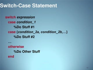
Switch-Case Statement
switch expression
case condition_1
%Do Stuff #1
case {condition_2a, condition_2b,…}
%Do Stuff #2
…
otherwise
%Do Other Stuff
end

68

Control Structures
Some Dummy Examples

 For loop syntax
for i=Index_Array
Matlab Commands
end

for i=1:100
end
for j=1:3:200
end
for m=13:-0.2:-21
end
for k=[0.1 0.3 -13 12 7 -9.3]
End
69

for loop
for
j=1:10

done

for j=1:10
% computations;
end

computations






Repeats for specified number of times
ALWAYS executes computation loop at least once!!!
Can use + or – increments
Can escape (BREAK) out of computational loop
70

Control Structures
 While Loop Syntax
Dummy Example

while (condition)
Matlab Commands
end

while ((a>3) & (b==5))
end

71

while loop
initialize k
while
k<10

done

k=0;
while k<10
% computations;
k=k+1;
end

computations
change k

 Will do computational loop ONLY if while condition is met
 Be careful to initialize while variable

 Can loop forever if while variable is not updated within loop!!!
72

What are we interested in?
 Matlab is too broad for our purposes in this course.

Series of
Matlab
commands

Input
Output
capability

Matlab
m-files
functions

Command
Line

Command
execution like
DOS command
window

mat-files

Data
storage/
loading
73

M-Files
 Script file: a collection of MATLAB

commands
 Function file: a definition file for one function

74

Script Files
 Any valid sequence of MATLAB commands

can be in the script files.
 Variables defined/used in script files are

global, i.e., they present in the workspace.

75

Using Script M-files
» what
M-files in the current directory
C:WINDOWSDesktopMatlab-Tutorials
abc abc1
» abc
1
3
5
.
.
.

File Name

79

Writing User Defined Functions
 Functions are m-files which can be executed by specifying

some inputs and supply some desired outputs.
 The code telling the Matlab that an m-file is actually a function
is
function out1=functionname(in1)
function out1=functionname(in1,in2,in3)
function [out1,out2]=functionname(in1,in2)

 You should write this command at the beginning of the m-file

and you should save the m-file with a file name same as the
function name

80

 Examples

 Write a function : out=squarer (A, ind)



Which takes the square of the input matrix if the input
indicator is equal to 1
And takes the element by element square of the input
matrix if the input indicator is equal to 2

Same Name

81

 Another function which takes an input array and returns the sum and product of

its elements as outputs

 The function sumprod(.) can be called from command window or an m-file as

82

Built-in Functions
Trigonometric
functions
Exponential
functions
Complex
functions
Rounding and
Remainder
functions

sin, cos, tan, sin, acos, atan, sinh,
cosh, tanh, asinh, acosh, atanh,
sec, cot, …
exp, log, log10, sqrt
abs, angle, imag, real, conj
floor, ceil, round, mod, rem, sign

83

Built-in Functions
•

sum – Sums the content of the variable passed

•

prod – Multiplies the content of the variable passed

•

mean – Calculates the mean of the variable passed

•

median – Calculates the median of the variable passed

•

mode – Calculates the Mode of the variable passed

•

std – Calculates the standard deviation of the variable passed

•

sqrt – Calculates the square root of the variable passed

•

max – Finds the maximum of the data

•

min – Finds the minimum of the data

•

size – Gives the size of the variable passed

84

MATLAB Logical Functions
 MATLAB also supports some logical functions.

xor (exclusive or) True is returned as 1, false as 0.
any (x)
returns 1 if any element of x is nonzero
all (x)
returns 1 if all elements of x are nonzero
isnan (x)
returns 1 at each NaN in x
isinf (x)
returns 1 at each infinity in x
finite (x)
returns 1 at each finite value in x

85

Mathematical Functions
» x=sqrt(2)/2
x=
0.7071
» y=sin(x)
y=

0.6496
»

86

FUNCTIONS
 Passing a vector to a function like sum, mean, std will

calculate the property within the vector
>> sum([1,2,3,4,5])
= 15
>> mean([1,2,3,4,5])
=3

87

FUNCTIONS
 When passing matrices the property, by default, will

be calculated over the columns

88

FUNCTIONS
 More usefully you can

now take the mean
and
standard
deviation of the data,
and add them to the
array

89

FUNCTIONS
 You can find the maximum and minimum of some

data using the max and min functions
>> max(results)
>> min(results)

90

Standard Deviation and Variance
 Standard deviation is calculated using the std() function
 std(X) : Calcuate the standard deviation of vector x

 If x is a matrix, std() will return the standard deviation of each column

 Variance (defined as the square of the standard deviation) is calculated

using the var() function
 var(X) : Calcuate the variance of vector x

X = [1 5 9;7 15 22]
s = std(X)
s = 4.2426 7.0711 9.1924

Reading Data from files
 MATLAB supports reading an entire file and creating a matrix

of the data with one statement.
>> load mydata.dat;

% loads file into matrix.

% The matrix may be a scalar, a vector, or a
% matrix with multiple rows and columns. The
% matrix will be named mydata.

>> size (mydata)

>> length (myvector)

% size will return the number
% of rows and number of
% columns in the matrix
% length will return the total
% no. of elements in myvector
92

MATLAB Demo
 Demonstrations are invaluable since they give an indication

of the MATLAB capabilities.
 A comprehensive set are available by typing the command

>>demo in MATLAB prompt.

93

MATLAB Graphics
 One of the best things about MATLAB is interactive
graphics

 “plot” is the one you will be using most often

 Many other 3D plotting functions -- plot3, mesh, surfc,
etc.

 Use “help plot” for plotting options
 To get a new figure, use “figure”

 logarithmic plots available using semilogx, semilogy and
loglog

94

Plotting Commands
plot(x,y) defaults to a blue line
plot(x,y,’ro’) uses red circles
plot(x,y,’g*’) uses green asterisks
If you want to put two plots on the same graph,
use “hold on”
plot(a,b,’r:’)
hold on
plot(a,c,’ko’)

(red dotted line)
(black circles)

95

Color, Symbols, and Line Types
 Use “help plot” to find available Specifiers
Colors

Symbols

Line Types

b

blue

.

point

-

solid

g

green

o

circle

:

dotted

r

red

x

x-mark

-.

dashdot

c

cyan

+

plus

--

dashed

m

magenta

*

star

y

yellow

s

square

k

black

d

diamond

v

triangle (down)

^

triangle (up)

<

triangle (left)

>

triangle (right)

p

pentagram

h

hexagram
96

PLOTTING
 A basic plot
>> x = [0:0.1:2*pi]
>> y = sin(x)
>> plot(x, y, ‘r.-’)

1
0.8
0.6
0.4
0.2
0
-0.2
-0.4
-0.6
-0.8
-1

0

1

2

3

4

5

6

7

97

PLOTTING
 Plotting a matrix

 MATLAB will treat each column as a different set of data
0.9
0.8
0.7
0.6
0.5
0.4
0.3
0.2
0.1

1

2

3

4

5

6

7

8

9

10

98

PLOTTING
 Some other functions that are helpful to create plots:
 hold on and hold off
 title

 legend
 axis

 xlabel
 ylabel

99

PLOTTING
>> x = [0:0.1:2*pi];
>> y = sin(x);
Sin Plots
2

>> plot(x, y, 'b*-')

sin(x)
2*sin(x)

1.5

>> hold on
1

>> plot(x, y*2, ‘r.-')
y

>> title('Sin Plots');

0.5
0
-0.5

>> legend('sin(x)', '2*sin(x)');
-1

>> axis([0 6.2 -2 2])
>> xlabel(‘x’);

-1.5
-2

0

1

2

3
x

4

5

6

>> ylabel(‘y’);
>> hold off

100

PLOTTING
 Plotting data
0.9
0.8
0.7
0.6
0.5
0.4

>> results = rand(10, 3)
>> plot(results, 'b*')
>> hold on
>> plot(mean(results, 2), ‘r.-’)

0.3
0.2
0.1

1

2

3

4

5

6

7

8

9

10

101

Plot Properties
Example
XLABEL X-axis label.

 XLABEL('text') adds text

beside the X-axis on the
current axis.

...
xlabel('x
values');
ylabel('y
values');

YLABEL Y-axis label.

 YLABEL('text') adds text

beside the Y-axis on the
current axis.

Hold
Example
HOLD Hold current graph.

 HOLD ON holds the current

plot and all axis properties so
that subsequent graphing
commands add to the existing
graph.

 HOLD OFF returns to the

default mode

 HOLD, by itself, toggles the

hold state.

...
hold on;
y2 = x + 2;

plot(x, y2,
'g+:');

Subplot
SUBPLOT Create axes in tiled
positions.
 SUBPLOT(m,n,p), or

SUBPLOT(mnp), breaks the Figure
window into an m-by-n matrix of
small axes

Example
x = [-3 -2 -1 0 1 2 3];
y1 = (x.^2) -1;
% Plot y1 on the top
subplot(2,1,1);
plot(x, y1,'bo-.');
xlabel('x values');
ylabel('y values');
% Plot y2 on the bottom
subplot(2,1,2);
y2 = x + 2;
plot(x, y2, 'g+:');

Figure
FIGURE Create figure window.
 FIGURE, by itself, creates a

new figure window, and
returns its handle.

Example
x = [-3 -2 -1 0 1 2 3];
y1 = (x.^2) -1;
% Plot y1 in the 1st Figure
plot(x, y1,'bo-.');
xlabel('x values');
ylabel('y values');
% Plot y2 in the 2nd Figure
figure
y2 = x + 2;
plot(x, y2, 'g+:');105

Surface Plot
x = 0:0.1:2;
y = 0:0.1:2;
[xx, yy] = meshgrid(x,y);
zz=sin(xx.^2+yy.^2);
surf(xx,yy,zz)
xlabel('X axes')
ylabel('Y axes')

106

3 D Surface Plot
contourf-colorbar-plot3-waterfall-contour3-mesh-surf

107

Histograms
• Histograms are useful for showing the pattern of the

whole data set
• Allows the shape of the distribution to be easily
visualized

108

Histograms
 Matlab hist(y,m) command will generate a frequency

histogram of vector y distributed among m bins
 Also can use hist(y,x) where x is a vector defining the bin
centers

Example:
>>b=sin(2*pi*t)
>>hist(b,[-1 -0.75 0 0.25 0.5 0.75 1]);

>>hist(b,10);

40

45
40

35

35

30

30

25

25

20
20

15
15

10

10

5

5
0
-1

-0.8

-0.6

-0.4

-0.2

0

0.2

0.4

0.6

0.8

1

0
-1.5

-1

-0.5

0

0.5

1

1.5

109

Histograms
 The histc function is a bit more powerful and allows bin

edges to be defined

[n, bin] = histc(x, binrange)
x = statistical distribution
binrange = the range of bins to plot eg: [1:1:10]
n = the number of elements in each bin from vector x
bin = the bin number each element of x belongs
 Use the bar function to plot the histogram

110

Histograms

Example:
>> test = round(rand(100,1)*10)
>> histc(test,[1:1:10])
>> Bar(test)
14

12

10

8

6

4

2

0

1

2

3

4

5

6

7

8

9

10

111

Image Processing Toolbox
 The Image Processing Toolbox is a collection of functions

that extend the capability of the MATLAB ® numeric
computing environment. The toolbox supports a wide
range of image processing operations, including:
 Geometric operations

 Neighborhood and block operations
 Linear filtering and filter design
 Transforms

 Image analysis and enhancement
 Binary image operations

 Region of interest operations

112

Images in MATLAB
• MATLAB can import/export
several image formats:
– BMP (Microsoft Windows
Bitmap)
– GIF (Graphics Interchange
Files)
– HDF (Hierarchical Data Format)
– JPEG (Joint Photographic
Experts Group)
– PCX (Paintbrush)
– PNG (Portable Network
Graphics)
– TIFF (Tagged Image File
Format)
– XWD (X Window Dump)
– raw-data and other types of
image data

• Data types in MATLAB
– Double (64-bit double-precision
floating point)
– Single (32-bit single-precision
floating point)
– Int32 (32-bit signed integer)
– Uint32 (32-bit unsigned integer)

113

MATLAB Image Types

 Indexed images

 Intensity images
 Binary images

 RGB images

: m-by-3 color map
: [0,1] or uint8
: {0,1}
: m-by-n-by-3

114

Image Display
 image

- create and display image object
 imagesc - scale and display as image
 imshow - display image
 colorbar - display colorbar
 getimage- get image data from axes
 truesize - adjust display size of image
 zoom
- zoom in and zoom out of 2D plot

115

Image Conversion










Gray2ind
im2bw
Im2double
Im2uint8
Im2uint16
Ind2gray
mat2gray
rgb2gray
rgb2ind

- intensity image to index image
- image to binary
- image to double precision
- image to 8-bit unsigned integers
- image to 16-bit unsigned integers
- indexed image to intensity image
- matrix to intensity image
- RGB image to grayscale
- RGB image to indexed image

116

Indexed Images
» [x,map] = imread('trees.tif');
» imshow(x,map);

117

Intensity Images
» image = ind2gray(x,map);
» imshow(image);

118

Binary Images
» imshow(edge(image));

119

IMAGE ENHANCEMENT
 Adjust intensity
 imadjust

>>im2 = histeq(im);
>>imshow(im2)

 histeq

 Noise removal
 linear filtering

 median filtering

 adaptive filtering

121

MATLAB INTRODUCTION

More Related Content

What's hot (20)

Viewers also liked (20)

Similar to MATLAB INTRODUCTION (20)

Recently uploaded (20)

MATLAB INTRODUCTION