Lecture 2 Basic Concepts of Optimal Design and Optimization Techniques final1.pptx

Lecture 2-a:
Introduction to Optimal Design
&
Optimization Techniques
17/11/2022
Subject Name : Advanced Machine
Design

Lecture 2-a:
Outline
17/11/2022
 Introduction
 Conventional Versus Optimum
Design Process
 Optimum Design Problem
Formulation
 Classification of Optimization
Problems
 Classical Optimization Techniques

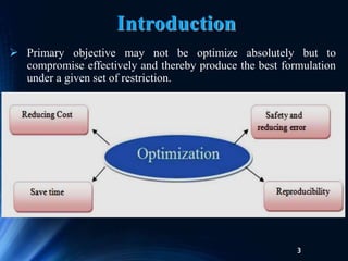
 Primary objective may not be optimize absolutely but to
compromise effectively and thereby produce the best formulation
under a given set of restriction.
3
Introduction

Introduction
10/11/2022
 Optimization is the act of obtaining the best result under given
circumstances. Optimize is defined as to make perfect, effective
or as functional as possible.
 Optimization can be defined as the process of finding the
conditions that give the maximum or minimum of value a
function.
 Optimization is a component of design process. The design of
systems can be formulated as problems of optimization where a
measure of performance is to be optimized while satisfying all
the constraints.
 In design, construction, and maintenance of any engineering
system, engineers have to take many technological and
managerial decisions at several stages. The ultimate goal of all
such decisions is either to minimize the effort required or to
maximize the desired benefit.

5
Introduction
 If a point x* corresponds to the minimum value of the function f
(x), the same point also corresponds to the maximum value of the
negative of the function, -f (x).
 Thus optimization can be taken to
mean minimization since the
maximum of a function can be
found by seeking the minimum of
the negative of the same function. In
addition, the following operations
on the objective function will not
change the optimum solution x*:
1. Multiplication (or division) of f (x) by a positive constant c.
2. Addition (or subtraction) of a positive constant c to (or from) f (x).

6
 Unconstrained: In unconstrained optimization problems there are no restrictions.
The making of the hardest tablet is the unconstrained optimization problem.
 Constrained: The constrained problem involved in it, is to make the hardest tablet
possible, but it must disintegrate in less than 15 minutes.
 Independent variables: The independent variables are under the control of the
formulator. These might include the compression force or the die cavity filling or the
mixing time.
 Dependent variables: The dependent variables are the responses or the
characteristics that are developed due to the independent variables. The more the
variables that are present in the system the more the complications that are involved
in the optimization.
Introduction

7
 The optimum seeking methods are also known as mathematical
programming techniques and are generally studied as a part of operations
research. Operations research is a branch of mathematics concerned with
the application of scientific methods and techniques to decision making
problems and with establishing the best or optimal solutions. The
beginnings of the subject of operations research can be traced to the early
period of World War II.
Introduction
 Mathematical programming techniques are useful in finding the minimum of a
function of several variables under a prescribed set of constraints.
 Stochastic process techniques can be used to analyze problems described by a set of
random variables having known probability distributions.
 Statistical methods enable one to analyze the experimental data and build empirical
models to obtain the most accurate representation of the physical situation.
 Modern Optimization Methods: also sometimes called nontraditional
optimization methods, have emerged as powerful and popular methods for solving
complex engineering optimization problems in recent years. These methods
include: genetic algorithms & simulated annealing method.

Introduction
8
 In recent years several new optimization methods that do not fall in
the area of traditional mathematical programming can be labeled as
metaheuristic optimization methods. All the metaheuristic
optimization methods have the following features:
(i) They use stochastic or probabilistic ideas in various steps;
(ii) They are intuitive or trial and error based, or heuristic in nature;
(iii) They all use strategies that imitate the behavior or characteristics of
some species such as bees, bats, birds, cuckoos, and fireflies;
(iv) They all tend to find the global optimum solution; and
(v) They are most likely to find an optimum solution, but not
necessarily all the time.
 Genetic algorithms are computerized search and optimization algorithms based on
the mechanics of natural genetics and natural selection.
 Simulated annealing method is based on the mechanics of the cooling process of
molten metals through annealing.
 Particle swarm optimization algorithm mimics the behavior of social organisms such
as a colony or swarm of insects (for example, ants, termites, bees, and wasps), a
flock of birds, and a school of fish.

 Ant colony optimization is based on the cooperative behavior of ant
colonies, which are able to find the shortest path from their nest to a
food source.
 Neural network methods are based on the immense computational
power of the nervous system to solve perceptional problems in the
presence of a massive amount of sensory data through its parallel
processing capability.
 Fuzzy optimization methods were developed to solve optimization
problems involving design data, objective function, and constraints
stated in imprecise form involving vague and linguistic descriptions
9
Introduction
 A class of methods, termed Metaheuristic Algorithms, are being
developed for the solution of optimization problems include
techniques such as the firefly, harmony search, bee, cuckoo, bat, crow,
teaching-learning, passing-vehicle, and salp swarm algorithms.

Introduction
10/11/2022
Table 1.1 lists various mathematical
programming techniques together with other
well-defined areas of operations research,
including the new class of methods termed
metaheuristic optimization methods. The
classification given in Table 1.1 is not unique;
it is given mainly for convenience.

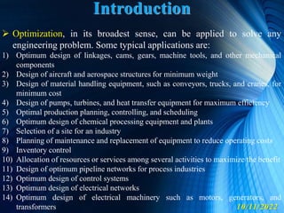
10/11/2022
 Optimization, in its broadest sense, can be applied to solve any
engineering problem. Some typical applications are:
1) Optimum design of linkages, cams, gears, machine tools, and other mechanical
components
2) Design of aircraft and aerospace structures for minimum weight
3) Design of material handling equipment, such as conveyors, trucks, and cranes, for
minimum cost
4) Design of pumps, turbines, and heat transfer equipment for maximum efficiency
5) Optimal production planning, controlling, and scheduling
6) Optimum design of chemical processing equipment and plants
7) Selection of a site for an industry
8) Planning of maintenance and replacement of equipment to reduce operating costs
9) Inventory control
10) Allocation of resources or services among several activities to maximize the benefit
11) Design of optimum pipeline networks for process industries
12) Optimum design of control systems
13) Optimum design of electrical networks
14) Optimum design of electrical machinery such as motors, generators, and
transformers
Introduction

13
 The conventional design procedures aim at finding an acceptable
or adequate design which merely satisfies the functional and
other requirements of the problem.
 In general, there will be more than one acceptable design, and
the purpose of optimization is to choose the best one of the many
acceptable designs available.
 Thus a criterion has to be chosen for comparing the different
alternative acceptable designs and for selecting the best one.
 The criterion with respect to which the design is optimized,
when expressed as a function of the design variables, is known
as the objective function.
Conventional Versus Optimum
Design Process

14
Design Process
Fig 1.4 Comparison of: (a)
conventional design method; and (b)
optimum design method.
It is important to note
that:
 Both methods are
iterative, as indicated
by a loop between
blocks 6 and 3.
 Both methods have
some blocks that
require similar
calculations and
others that require
different calculations.

15
• In block 4, the conventional design method checks to ensure that the
performance criteria are met, whereas the optimum design method checks for
satisfaction of all of the constraints for the problem formulated in block 0.
• In block 6, the conventional design method updates the design based on the
designer’s experience and intuition and other information gathered from one
or more trial designs; the optimum design method uses optimization concepts
and procedures to update the current design.
• In civil engineering, the objective is usually taken as the minimization of the
cost.
• In mechanical engineering, the maximization of the mechanical efficiency is
the obvious choice of an objective function.
• In aerospace structural design problems, the objective function for
minimization is generally taken as weight.
• In some situations, there may be more than one criterion to be satisfied
simultaneously. An optimization problem involving multiple objective
functions is known as a multiobjective programming problem.
Conventional Versus Optimum Design Process

16
 With multiple objectives there arises a possibility of conflict, and
one simple way to handle the problem is to construct an overall
objective function as a linear combination of the conflicting
multiple objective functions.
 Thus, if f1 (X) and f2 (X) denote two objective functions,
construct a new (overall) objective function for optimization as:
where 1 and 2 are constants whose values indicate the relative
importance of one objective function to the other.
𝑓(X) = 𝛼1𝑓1(X) + 𝛼2𝑓2(X)
Design Process

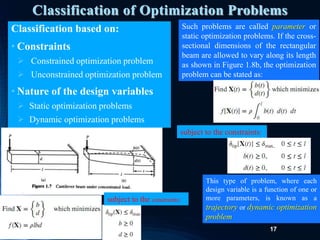
17
Classification of Optimization Problems
Classification based on:
• Constraints
 Constrained optimization problem
 Unconstrained optimization problem
• Nature of the design variables
 Static optimization problems
 Dynamic optimization problems
subject to the constraints:
Such problems are called parameter or
static optimization problems. If the cross-
sectional dimensions of the rectangular
beam are allowed to vary along its length
as shown in Figure 1.8b, the optimization
problem can be stated as:
subject to the constraints:
This type of problem, where each
design variable is a function of one or
more parameters, is known as a
trajectory or dynamic optimization
problem

18
• Physical structure of the problem
• Optimal control problems
• Non-optimal control problems
• Nature of the equations involved
• Nonlinear programming problem
• Geometric programming problem
• Quadratic programming problem
• Linear programming problem

19
• Permissable values of the design variables
• Integer programming problems
• Real valued programming problems
• Deterministic nature of the variables
• Stochastic programming problem
• Deterministic programming problem

20
• Separability of the functions
• Separable programming problems
• Non-separable programming problems
• Number of the objective functions
• Single objective programming problem
• Multiobjective programming problem

21
An optimization or a mathematical programming problem can be stated as
follows.
• f0 : Rn R: objective function
• x=(x1,…..,xn): design variables (unknowns of the problem, they must be
linearly independent)
• gi : Rn R: (i=1,…,m): inequality constraints
• The problem is a constrained optimization problem
minimize 𝑓0(𝑥)
subject to 𝑔𝑖(𝑥) ≤ 𝑏𝑖, 𝑖 = 1, . . . . , 𝑚
where X is an n-dimensional vector called the design vector, f (X) is termed the objective
function, and gj (X) and lj (X) are known as inequality and equality constraints, respectively.
Some optimization problems do not involve any constraints
Optimum Design Problem Formulation

22
Optimum Design Problem
Formulation
Design problems have:
 An objective (a goal) to be achieved
 Some constraints within which the objective/goal must be achieved
 Some criteria by which a good solution is recognized
 Constraints set specific (usually quantitative) targets or limits
 Criteria are more flexible and might be used for judging between different
design proposals, each of which meets the specific constraint targets.

23
 It is generally accepted that the proper definition and formulation of a
problem take more than 50% of the total effort needed to solve it.
Therefore, it is critical to follow well-defined procedures for formulating
design optimization problems.
 The importance of properly formulating a design optimization problem
must be stressed because the optimum solution will be only as good as the
formulation. For example:
 If we forget to include a critical constraint in the formulation, the
optimum solution will most likely violate it.
 Also, if we have too many constraints, or if they are inconsistent, there
may be no solution for the problem.
 However, once the problem is properly formulated, good software is
usually available to solve it.
 It is important to note that the process of developing a proper formulation
for optimum design of practical problems is iterative in itself.
Formulation

24
Formulation
Initial design
problem statement
Seek info
Interpret
Summarize
Review
Customer needs?
Competition?
continue
Obtain instructor approval
probe
Engineering Design
Specification
Gain
consensus
Functional requirements?
Targets? Constraints?
Evaluation criteria?
revise
Preliminary problem formulation
Literature, Surveys
Market Studies
Focus Groups
Observation Studies
Benchmark Studies
Formulating process

25
 Formulation of an optimum design problem implies translating a descriptive
statement of the problem into a well-defined mathematical statement. For most
design optimization problems, we will use the following five-step procedure to
formulate the problem:
 Step 1: Project/problem description: The statement describes the overall
objectives of the project and the requirements to be met. This is also called
the statement of work. Care should always be exercised in defining and
developing expressions for the constraints.
 Step 2: Data and information collection: To develop a mathematical
formulation for the problem, gather information on material properties,
performance requirements, resource limits, cost of raw materials, analysis
procedures (FEM), analysis tools (ABAQUS) and so forth. In many cases,
the project statement is vague, and assumptions about modeling of the
problem need to be made in order to formulate and solve it.
 Step 3: Definition of design variables: to identify a set of variables that
describe the system, called the design variables. In general, these are
referred to as optimization variables or simply variables that are regarded as
free because we should be able to assign any value to them. Different
values for the variables produce different designs. Design variables – a set
of parameters that describes the system (dimensions, material, load, …)

26
To summarize, the following considerations should be given in
identifying design variables for a problem:
 Generally, the design variables should be independent of each other.
If they are not, there must be some equality constraints between
them (explained later in several examples).
 All options of identifying design variables should be investigated. A
minimum number of design variables is required to properly
formulate a design optimization problem.
 Designate as many independent parameters as possible as at the
beginning. Later, some of the design variables can be eliminated by
assigning numerical values.
 A numerical value should be given to each identified design
variable to determine if a trial design of the system is specified.
Formulation

27
Step 4: Optimization criterion: The question is how do we quantify this statement
and designate a design as better than another (cost, profit, weight, deflection, stress,
….). For this, a criterion has to be chosen for comparing the different alternative
acceptable designs and for selecting the best one.
The criterion with respect to which the design is optimized, when expressed as a
function of the design variables, is known as the criterion or merit or objective
function.
The criterion must be a scalar function whose numerical value can be obtained once a
design is specified; that is, it must be a function of the design variable vector x. Such a
criterion is usually called an objective function for the optimum design problem, and it
needs to be maximized or minimized depending on problem requirements.
A criterion that is to be minimized is usually called a cost function in engineering
literature.
It is emphasized that a valid objective function must be influenced directly or
indirectly by the variables of the design problem; otherwise, it is not a meaningful
objective function.
In some situations, two or more objective functions may be identified, these are called
multiobjective design optimization problems.

28
 Step 4: Optimization criterion or Objective Function:
1. It must be a scalar function whose numerical values could be
obtained once a design is specified.
2. It must be a function of design variables, f (x).
3. The objective function is minimized or maximized
(minimize cost, maximize profit, minimize weight,
maximize ride quality of a vehicle, minimize the cost of
manufacturing, ….)
4. Multi-objective functions; minimize the weight of a
structure and at the same time minimize the deflection or
stress at a certain point.

29
• Objective Function Surfaces: the locus of all points satisfying f
(X) = c = constant is a forms a hypersurface in the design space,
and for each value of c there corresponds a different member of a
family of surfaces. These surfaces, called objective function
surfaces, are shown in a hypothetical two-dimensional design
space in the figure below.

30
• Once the objective function surfaces are drawn along with the
constraint surfaces, the optimum point can be determined without
much difficulty.
• But the main problem is that as the number of design variables
exceeds two or three, the constraint and objective function surfaces
become complex even for visualization and the problem has to be
solved purely as a mathematical problem.

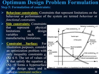
31
 Step 5: Formulation of constraints: in many practical
problems, the design variables cannot be chosen arbitrarily;
rather, they have to satisfy certain specified functional and other
requirements. All restrictions placed on the design are
collectively called constraints. The restrictions that must be
satisfied to produce an acceptable design are collectively called
design constraints.
 Constraints that represent limitations on the behavior or
performance of the system are termed behavior or functional
constraints.
 Constraints that represent physical limitations (i.e.; there can be
upper and lower bounds due to manufacturing limitations) on design
variables, such as availability, fabricability, and transportability,
are known as geometric or side constraints.

32
 Side constraints: Constraints
that represent physical
limitations on design
variables such as
manufacturing limitations.
 Constraint Surface: For
illustration purposes, consider
an optimization problem with
only inequality constraints gj
(X)  0. The set of values of
X that satisfy the equation gj
(X) =0 forms a hypersurface
in the design space and is
called a constraint surface.
Step 5: Formulation of constraints:
 Behaviour constraints: Constraints that represent limitations on the
behaviour or performance of the system are termed behaviour or
functional constraints.

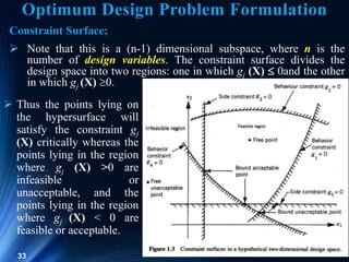
33
Constraint Surface;
 Note that this is a (n-1) dimensional subspace, where n is the
number of design variables. The constraint surface divides the
design space into two regions: one in which gj (X)  0and the other
in which gj (X) 0.
 Thus the points lying on
the hypersurface will
satisfy the constraint gj
(X) critically whereas the
points lying in the region
where gj (X) >0 are
infeasible or
unacceptable, and the
points lying in the region
where gj (X) < 0 are
feasible or acceptable.

34
Constraint Surface:
 In the below figure, a hypothetical two dimensional design space is
depicted where the infeasible region is indicated by hatched lines. A design
point that lies on one or more than one constraint surface is called a bound
point, and the associated constraint is called an active constraint.
 Design points that do not lie on
any constraint surface are known
as free points.
 Depending on whether a
particular design point belongs to
the acceptable or unacceptable
regions, it can be identified as one
of the following four types:
1) Free and acceptable point
2) Free and unacceptable point
3) Bound and acceptable point
4) Bound and unacceptable point

35
Problem Formulation
Design Constraints
Feasible Design
A design meeting all the requirements is called a feasible
(acceptable) design. An infeasible design does not meet one
or more requirements
Implicit & Explicit Constraints
All restrictions placed on a design are collectively called
constraints. Some constraints are explicit (obvious, provided)
such as min. and max. values of design variables, some are
implicit (derived, deduced) which are usually more complex
such as deflection of a structure.

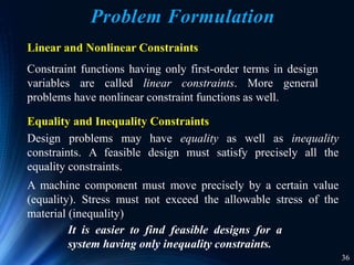
36
Linear and Nonlinear Constraints
Constraint functions having only first-order terms in design
variables are called linear constraints. More general
problems have nonlinear constraint functions as well.
A machine component must move precisely by a certain value
(equality). Stress must not exceed the allowable stress of the
material (inequality)
It is easier to find feasible designs for a
system having only inequality constraints.
Design problems may have equality as well as inequality
constraints. A feasible design must satisfy precisely all the
equality constraints.
Equality and Inequality Constraints
Problem Formulation

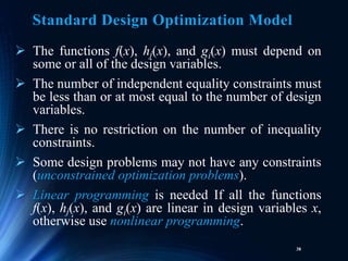
37
Standard Design Optimization Model
The standard design optimization model is defined as
follows: Find an n-vector x = (x1, x2, …., xn) of design
variables to minimize an objective function
subject to the p equality constraints
and the m inequality constraints

38
 The functions f(x), hj(x), and gi(x) must depend on
some or all of the design variables.
 The number of independent equality constraints must
be less than or at most equal to the number of design
variables.
 There is no restriction on the number of inequality
constraints.
 Some design problems may not have any constraints
(unconstrained optimization problems).
 Linear programming is needed If all the functions
f(x), hj(x), and gi(x) are linear in design variables x,
otherwise use nonlinear programming.
Standard Design Optimization Model

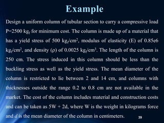
39
Design a uniform column of tubular section to carry a compressive load
P=2500 kgf for minimum cost. The column is made up of a material that
has a yield stress of 500 kgf/cm2, modulus of elasticity (E) of 0.85e6
kgf/cm2, and density () of 0.0025 kgf/cm3. The length of the column is
250 cm. The stress induced in this column should be less than the
buckling stress as well as the yield stress. The mean diameter of the
column is restricted to lie between 2 and 14 cm, and columns with
thicknesses outside the range 0.2 to 0.8 cm are not available in the
market. The cost of the column includes material and construction costs
and can be taken as 5W + 2d, where W is the weight in kilograms force
and d is the mean diameter of the column in centimeters.
Example

40
The design variables are the mean
diameter (d) and tube thickness (t):
The objective function to be
minimized is given by:
X =
𝑥1
𝑥2
=
𝑑
𝑡
𝑓(X) = 5𝑊 + 2𝑑 = 5𝜌𝑙𝜋𝑑𝑡 + 2𝑑 = 9.82𝑥1𝑥2 + 2𝑥1
Example

• The behaviour constraints can be expressed as:
1. Stress induced ≤ yield stress
2. Stress induced ≤ buckling stress
• The induced stress is given by:
41
induced stress = 𝜎i =
𝑃
𝜋𝑑𝑡
=
2500
𝜋𝑥1𝑥2
Example

42
• The buckling stress for a pin connected column is given by:
where I is the second moment of area of the cross section
of the column given by:
buckling stress = 𝜎b =
Euler buckling load
cross − sectional area
=
𝜋2
𝐸𝐼
𝑙2𝜋𝑑𝑡
𝐼 =
𝜋
64
(𝑑𝑜
4 − 𝑑𝑖
4
) =
𝜋
64
(𝑑𝑜
2 + 𝑑𝑖
2
)(𝑑𝑜 + 𝑑𝑖)(𝑑𝑜 − 𝑑𝑖)
=
𝜋
64
(𝑑 + 𝑡)2 + (𝑑 − 𝑡)2 (𝑑 + 𝑡) + (𝑑 − 𝑡) (𝑑 + 𝑡) − (𝑑 − 𝑡)
=
𝜋
8
𝑑𝑡(𝑑2
+ 𝑡2
) =
𝜋
8
𝑥1𝑥2(𝑥1
2
+ 𝑥2
2
)
Example

43
• Thus, the behaviour constraints can be restated as:
• The side constraints are given by:
𝑔1(X) =
2500
𝜋𝑥1𝑥2
− 500 ≤ 0
𝑔2(X) =
2500
𝜋𝑥1𝑥2
−
𝜋2(0.85 × 106)(𝑥1
2
+ 𝑥2
2
)
8(250)2
≤ 0
2 ≤ 𝑑 ≤ 14
0.2 ≤ 𝑡 ≤ 0.8
Example

44
• The side constraints can be expressed in standard form as:
𝑔3(X) = −𝑥1 + 2 ≤ 0
𝑔4(X) = 𝑥1 − 14 ≤ 0
𝑔5(X) = −𝑥2 + 0.2 ≤ 0
𝑔6(X) = 𝑥2 − 0.8 ≤ 0
Example

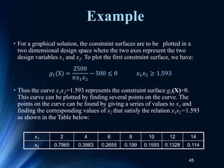
45
• For a graphical solution, the constraint surfaces are to be plotted in a
two dimensional design space where the two axes represent the two
design variables x1 and x2. To plot the first constraint surface, we have:
• Thus the curve x1x2=1.593 represents the constraint surface g1(X)=0.
This curve can be plotted by finding several points on the curve. The
points on the curve can be found by giving a series of values to x1 and
finding the corresponding values of x2 that satisfy the relation x1x2=1.593
as shown in the Table below:
𝑔1(X) =
2500
𝜋𝑥1𝑥2
− 500 ≤ 0 𝑥1𝑥2 ≥ 1.593
x1 2 4 6 8 10 12 14
x2 0.7965 0.3983 0.2655 0.199 0.1593 0.1328 0.114
Example

46
Example
• The infeasible region
represented by g1(X)>0
or x1x2< 1.593 is shown
by hatched lines. These
points are plotted and a
curve P1Q1 passing
through all these points
is drawn as shown:

47
• Similarly the second
constraint g2(X) < 0 can be
expressed as:
• The points lying on the
constraint surface g2 (X)=0
can be obtained as follows
(These points are plotted as
Curve P2Q2:
𝑥1𝑥2(𝑥1
2
+ 𝑥2
2
) ≥ 47.3
x1 2 4 6 8 10 12 14
x2 2.41 0.716 0.219 0.0926 0.0473 0.0274 0.0172
Example

48
• The plotting of side
constraints is simple since
they represent straight lines.
• After plotting all the six
constraints, the feasible
region is determined as the
bounded area ABCDEA
𝑥1𝑥2(𝑥1
2
+ 𝑥2
2
) ≥ 47.3
Example

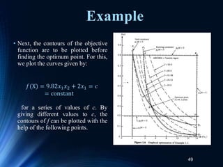
49
• Next, the contours of the objective
function are to be plotted before
finding the optimum point. For this,
we plot the curves given by:
for a series of values of c. By
giving different values to c, the
contours of f can be plotted with the
help of the following points.
𝑓(X) = 9.82𝑥1𝑥2 + 2𝑥1 = 𝑐
= constant
Example

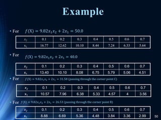
50
Example
• For
• For
• For
• For
𝑓(X) = 9.82𝑥1𝑥2 + 2𝑥1 = 50.0
x2 0.1 0.2 0.3 0.4 0.5 0.6 0.7
x1 16.77 12.62 10.10 8.44 7.24 6.33 5.64
𝑓(X) = 9.82𝑥1𝑥2 + 2𝑥1 = 40.0
x2 0.1 0.2 0.3 0.4 0.5 0.6 0.7
x1 13.40 10.10 8.08 6.75 5.79 5.06 4.51
𝑓(X) = 9.82𝑥1𝑥2 + 2𝑥1 = 31.58 (passing through the corner point C)
x2 0.1 0.2 0.3 0.4 0.5 0.6 0.7
x1 10.57 7.96 6.38 5.33 4.57 4 3.56
𝑓(X) = 9.82𝑥1𝑥2 + 2𝑥1 = 26.53 (passing through the corner point B)
x2 0.1 0.2 0.3 0.4 0.5 0.6 0.7
x1 8.88 6.69 5.36 4.48 3.84 3.36 2.99

51
Design of a Two-bar Structure
The problem is to design a two-member bracket to support a force W
without structural failure. Since the bracket will be produced in large
quantities, the design objective is to minimize its mass while also
satisfying certain fabrication and space limitation.

Ken Youssefi 52
Problem Formulation
In formulating the design problem, we need to define structural
failure more precisely. Member forces F1 and F2 can be used to
define failure condition.
Apply equilibrium conditions;
Σ Fy = 0
Σ Fx = 0

53
Problem Formulation
Represent all the design variables for a problem in the vector x.
x3 = outer diameter of member 1
x4 = inner diameter of member 1
x1 = height h of the truss
x2 = span s of the truss

54
Problem Formulation
Objective Function
Mass is selected as the objective function
Mass = ( density )( area )( length )
x1 = height h of the truss

55
Constraints for the example problem are: member stress shall not
exceed the allowable stress, and various limitations on design
variables shall be met.
Constraint on stress
σ (applied) < σ (allowable)
Problem Formulation

56
Problem Formulation
Finally, the constraints on design variables are written as
Where xil and xiu are the minimum and maximum
values for the ith design variable. These constraints are
necessary to impose fabrication and physical space
limitations.

57
The problem can be summarized as follows
Find design variables x1, x2, x3, x4, x5, and x6 to minimize the
objective function,
subject to the constraints of the equations x1 = height h of the truss
Problem Formulation

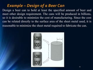
58
Example – Design of a Beer Can
Design a beer can to hold at least the specified amount of beer and
meet other design requirement. The cans will be produced in billions,
so it is desirable to minimize the cost of manufacturing. Since the cost
can be related directly to the surface area of the sheet metal used, it is
reasonable to minimize the sheet metal required to fabricate the can.

59
Fabrication, handling, aesthetic, shipping considerations and customer
needs impose the following restrictions on the size of the can:
1. The diameter of the can should be no more
than 8 cm. Also, it should not be less than 3.5
cm.
2. The height of the can should be no more than
18 cm and no less than 8 cm.
3. The can is required to hold at least 400 ml of
fluid.

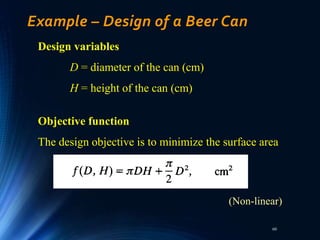
60
Design variables
D = diameter of the can (cm)
H = height of the can (cm)
Objective function
The design objective is to minimize the surface area
(Non-linear)

61
The constraints must be formulated in terms of design variables.
The first constraint is that the can must hold at least 400 ml of fluid.
The problem has two independent design variable and five
explicit constraints. The objective function and first constraint
are nonlinear in design variable whereas the remaining
constraints are linear.
(Non-linear)
The other constraints on the size of the can are:
(linear)

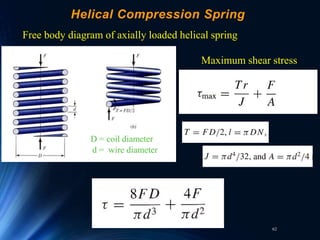
62
Helical Compression Spring
Free body diagram of axially loaded helical spring
D = coil diameter
d = wire diameter
Maximum shear stress

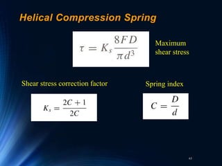
63
Shear stress correction factor Spring index
Maximum
shear stress

64
Deflection
The total strain energy, torsional and shear components
Total strain
energy

65
Castigliano’s theorem – deflection is the partial derivative of
the total strain energy.
Spring rate
Linear relationship

66
Helical spring end conditions
N (total) = Na (active number of coils) + Ni (inactive number of coils)

67
Example of unconstraint optimization problem
Design a compression spring of minimum weight, given the
following data:

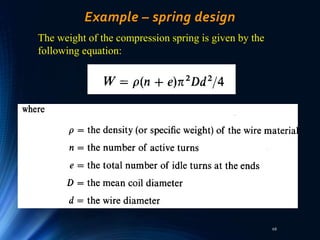
68
Example – spring design
The weight of the compression spring is given by the
following equation:

69
The equation can be expressed in terms of the
spring index C = D/d
The maximum shear stress and the deflection in the
spring are given by the following equations

Ken Youssefi 70
Substituting all of the equations into the weight equation, we
obtain the following expression in terms of spring index C:
The plot of the
objective function
W vs. C, the
spring index

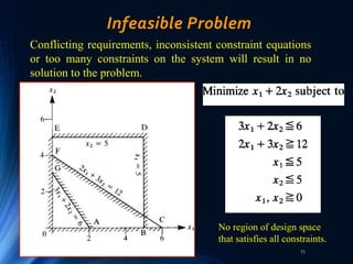
71
Infeasible Problem
Conflicting requirements, inconsistent constraint equations
or too many constraints on the system will result in no
solution to the problem.
No region of design space
that satisfies all constraints.

72
Optimization using graphical method
A wall bracket is to be designed to support a load of W. The bracket
should not fail under the load.
W = 1.2 MN
h = 30 cm
s = 40 cm
1
2

73
Problem Formulation
Design variables:
Objective function:
Stress constraints:
Where forces on bar 1 and bar 2 are:

75
Numerical Methods for Non-linear
Optimization
Graphical and analytical methods are inappropriate for many
complicated engineering design problems.
1. The number of design variables and constraints can be large.
2. The functions for the design problem can be highly nonlinear.
3. In many engineering applications, objective and/or constraint
functions can be implicit in terms of design variables.

76
Structural Optimization
Structural optimization is an automated synthesis of a mechanical
component based on structural properties.
For this optimization, a geometric modeling tool to represent the
shape, a structural analysis tool to solve the problem, and an
optimization algorithms to search for the optimum design are needed.
Structural Optimization
Geometric Modeling Structural Analysis Optimization
Finite element
modeling
Finite element
analysis
Nonlinear programming
algorithm

77
Structural Optimization Categories
 Size Optimization
Deals with parameters that do not alter the location of nodal points in
the numerical problem, keeps a design’s shape and topology
unchanged while changing dimensions of the design.
 Shape Optimization
Deals with parameters that describe the boundary position in the
numerical model. Design variables control the shape of the design.
The process requires re-meshing of the model and results in freeform
shapes
 Topology Optimization
The goal of topology optimization is to determine where to place or
add material and where to remove material. The optimization could
determine where to place ribs to stiffen the structure.

78
Optimization Categories
 Size and configuration optimization of a truss, design
variables are the cross sectional areas and nodal coordinates
of the truss.
 The truss could also be optimized for material.
 The topology or connectivity of the truss is fixed.

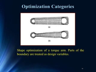
79
Shape optimization of a torque arm. Parts of the
boundary are treated as design variables.

80
 Topology optimization can be performed by using genetic
algorithm.
 Optimum shapes of the cross section of a beam for plastic
(b), aluminum (c), and steel (d)

81
Examples
Design of civil engineering structures
• variables: width and height of member cross-sections
• constraints: limit stresses, maximum and minimum dimensions
• objective: minimum cost or minimum weight
Analysis of statistical data and building empirical models
from measurements
• variables: model parameters
• Constraints: physical upper and lower bounds for model
parameters
• Objective: prediction error

82
Geometric Programming
• A geometric programming problem (GMP) is one in which the
objective function and constraints are expressed as posynomials in X.

83
Quadratic Programming Problem
• A quadratic programming problem is a nonlinear programming problem with a
quadratic objective function and linear constraints. It is usually formulated as
follows:
subject to
where c, qi,Qij, aij, and bj are constants.
𝐹(X) = 𝑐 +
𝑖=1
𝑛
𝑞𝑖 𝑥𝑖 +
𝑖=1
𝑛
𝑗=1
𝑛
𝑄𝑖𝑗 𝑥𝑖𝑥𝑗
𝑖=1
𝑛
𝑎𝑖𝑗 𝑥𝑖 = 𝑏𝑗, 𝑗 = 1,2, ⋯ , 𝑚
𝑥𝑖 ≥ 0, 𝑖 = 1,2, ⋯ , 𝑛

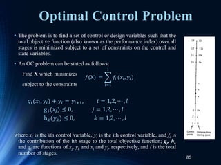
84
Optimal Control Problem
• An optimal control (OC) problem
is a mathematical programming
problem involving a number of
stages, where each stage evolves
from the preceding stage in a
prescribed manner.
• It is usually described by two
types of variables: the control
(design) and the state variables.
The control variables define the
system and govern the evolution
of the system from one stage to
the next, and the state variables
describe the behaviour or status of
the system in any stage.

85
Optimal Control Problem
• The problem is to find a set of control or design variables such that the
total objective function (also known as the performance index) over all
stages is minimized subject to a set of constraints on the control and
state variables.
• An OC problem can be stated as follows:
Find X which minimizes
subject to the constraints
where xi is the ith control variable, yi is the ith control variable, and fi is
the contribution of the ith stage to the total objective function; gj, hk
and qi are functions of xj, yk and xi and yi, respectively, and l is the total
number of stages.
𝑓(X) =
i=1
l
𝑓𝑖 (𝑥𝑖, 𝑦𝑖)
𝑞𝑖(𝑥𝑖, 𝑦𝑖) + 𝑦𝑖 = 𝑦𝑖+1, 𝑖 = 1,2, ⋯ , 𝑙
g𝑗(𝑥𝑗) ≤ 0, 𝑗 = 1,2, ⋯ , 𝑙
h𝑘(𝑦𝑘) ≤ 0, 𝑘 = 1,2, ⋯ , 𝑙

86
Integer Programming Problem
• If some or all of the design variables x1,x2,..,xn of an
optimization problem are restricted to take on only integer (or
discrete) values, the problem is called an integer programming
problem.
• If all the design variables are permitted to take any real value,
the optimization problem is called a real-valued programming
problem.

87
Stochastic Programming Problem
•A stochastic programming problem is an optimization
problem in which some or all of the parameters
(design variables and/or preassigned parameters) are
probabilistic (nondeterministic or stochastic).
•In other words, stochastic programming deals with the
solution of the optimization problems in which some
of the variables are described by probability
distributions.

88
Separable Programming Problem
• A function f (x) is said to be separable if it can be expressed
as the sum of n single variable functions, f1(x1),
f2(x2),….,fn(xn), that is,
• A separable programming problem is one in which the
objective function and the constraints are separable and can
be expressed in standard form as:
Find X which minimizes
subject to
𝑓(X) =
𝑖=1
𝑛
𝑓𝑖 𝑥𝑖
𝑓(X) =
𝑖=1
𝑛
𝑓𝑖 (𝑥𝑖)
𝑔𝑗(X) =
𝑖=1
𝑛
𝑔𝑖𝑗 (𝑥𝑖) ≤ 𝑏𝑗, 𝑗 = 1,2, ⋯ , 𝑚

89
Multiobjective Programming
Problem
• A multiobjective programming problem can be stated as follows:
Find X which minimizes f1 (X), f2 (X),…., fk (X)
subject to
where f1 , f2,…., fk denote the objective functions to be minimized
simultaneously.
𝑔𝑗(X) ≤ 0, 𝑗 = 1,2, . . . , 𝑚

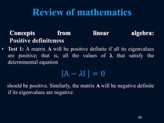
90
Review of mathematics
Concepts from linear algebra:
Positive definiteness
• Test 1: A matrix A will be positive definite if all its eigenvalues
are positive; that is, all the values of  that satisfy the
determinental equation
should be positive. Similarly, the matrix A will be negative definite
if its eigenvalues are negative.
A − 𝜆I = 0

91
Positive definiteness
• Test 2: Another test that can be used to find the positive definiteness
of a matrix A of order n involves evaluation of the determinants
• The matrix A will be positive definite if and only if all the values A1,
A2, A3,An are positive
• The matrix A will be negative definite if and only if the sign of Aj is (-
1)j for j=1,2,,n
• If some of the Aj are positive and the remaining Aj are zero, the matrix
A will be positive semidefinite
𝐴 = 𝑎11
𝐴2 =
𝑎11 𝑎12
𝑎21 𝑎22
𝐴3 =
𝑎11 𝑎12 𝑎13
𝑎21 𝑎22 𝑎23
𝑎31 𝑎32 𝑎33
𝐴3
=
𝑎11 𝑎12 𝑎13 ⋯ 𝑎1𝑛
𝑎21 𝑎22 𝑎23 ⋯ 𝑎2𝑛
𝑎31 𝑎32 𝑎33 ⋯ 𝑎3𝑛
⋮
𝑎𝑛1 𝑎𝑛2 𝑎𝑛3 ⋯ 𝑎𝑛𝑛

92
Negative definiteness
• Equivalently, a matrix is negative-definite if all its
eigenvalues are negative
• It is positive-semidefinite if all its eigenvalues are all
greater than or equal to zero
• It is negative-semidefinite if all its eigenvalues are all
less than or equal to zero

93
Concepts from linear algebra:
Nonsingular matrix: The determinant of the matrix is not zero.
Rank: The rank of a matrix A is the order of the largest
nonsingular square submatrix of A, that is, the largest submatrix
with a determinant other than zero.
Review of Mathematics

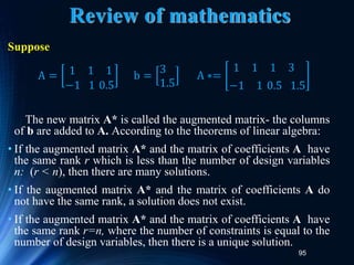
94
Solutions of a linear problem
Minimize f(x)=cTx
Subject to g(x): Ax=b
Side constraints: x ≥0
• The existence of a solution to this problem depends on the rows of
A.
• If the rows of A are linearly independent, then there is a unique
solution to the system of equations.
• If det(A) is zero, that is, matrix A is singular, there are either no
solutions or infinite solutions.

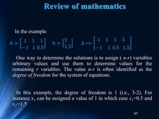
95
Suppose
The new matrix A* is called the augmented matrix- the columns
of b are added to A. According to the theorems of linear algebra:
• If the augmented matrix A* and the matrix of coefficients A have
the same rank r which is less than the number of design variables
n: (r < n), then there are many solutions.
• If the augmented matrix A* and the matrix of coefficients A do
not have the same rank, a solution does not exist.
• If the augmented matrix A* and the matrix of coefficients A have
the same rank r=n, where the number of constraints is equal to the
number of design variables, then there is a unique solution.
A = 1 1 1
−1 1 0.5
b =
3
1.5
A ∗=
1 1 1 3
−1 1 0.5 1.5

96
In the example
The largest square submatrix is a 2 x 2 matrix (since m = 2
and m < n). Taking the submatrix which includes the first two
columns of A, the determinant has a value of 2 and therefore
is nonsingular. Thus the rank of A is 2 (r = 2). The same
columns appear in A* making its rank also 2. Since
r < n, infinitely many solutions exist.
A = 1 1 1
−1 1 0.5
b =
3
1.5
A ∗=
1 1 1 3
−1 1 0.5 1.5

97
In the example
One way to determine the solutions is to assign ( n-r) variables
arbitrary values and use them to determine values for the
remaining r variables. The value n-r is often identified as the
degree of freedom for the system of equations.
In this example, the degree of freedom is 1 (i.e., 3-2). For
instance x3 can be assigned a value of 1 in which case x1=0.5 and
x2=1.5
A = 1 1 1
−1 1 0.5
b =
3
1.5
A ∗=
1 1 1 3
−1 1 0.5 1.5

98
Homework
What is the solution of the system given below?
Hint: Determine the rank of the matrix of the coefficients and
the augmented matrix.
𝑔1: 𝑥1 + 𝑥2 = 2
𝑔2: −𝑥1 + 𝑥2 = 1
𝑔3: 𝑥1 + 2𝑥2 = 1

Lecture 2 Basic Concepts of Optimal Design and Optimization Techniques final1.pptx

More Related Content

What's hot (20)

Similar to Lecture 2 Basic Concepts of Optimal Design and Optimization Techniques final1.pptx (20)

More from Khalil Alhatab (20)

Recently uploaded (20)

Lecture 2 Basic Concepts of Optimal Design and Optimization Techniques final1.pptx