SlideShare a Scribd company logo
DA 5230 – Statistical & Machine Learning
Lecture 9 – Decision Trees and Ensemble
Methods
Maninda Edirisooriya
manindaw@uom.lk
Decision Tree (DT)
• Tree-like ML modelling structure
• Each node is relevant to a
categorical feature and branch
to classes of that feature
• During prediction, data is moved
from root and passed down till it
meets a leaf
• Leaf node decides the final
prediction
BMI > 80
Age > 35
Smoking
Vegetarian Exercise
True False
True False
Cardiovascular Disease Predictor
Root Node
Internal Node
Leaf Node
Disease Healthy Disease Healthy
Disease Healthy
True
False True
False
True False
Decision Trees
• Suppose you have got a binary classification problem with 3
independent binary categorical variables X1, X2, X3, and 1 dependent
variable Y
• You can draw a decision tree starting from one of the X variables
• If this X variable cannot classify the training dataset perfectly, add
another X variable as a child node to the tree branches where there
are misclassifications (or not Pure)
• Even after adding the second X variable, if there are some
misclassifications in the branches, you can add the third X variable as
well OR you can add the third variable as the second node of the root
Decision Trees
You will be able to draw several trees like that, depending on the
training set and the X variables (note that outputs are not shown here)
Depth
1
Root X1
X2 X3
Depth
1
Root X1
X2 Depth
2
Depth
1
Root X1
X2
X3
Root
X1
Optimizing Decision Trees
• In order to find the maximum Purity of the classification you will have
to try with many decision trees
• As the number of parameters (nodes and their classes) are different
in each of the decision tree, there is no optimization algorithm to
minimize the error (or impurity)
• Known algorithms to find the globally optimum Decision Tree are
computationally expensive (problem known as a NP-hard Problem)
• Therefore, heuristic techniques are used to get better performance
out of Decision Trees
CART Algorithm
• CART (Classification And Regression Tree) is one of the best heuristic
Decision Tree algorithms
• There are 2 key decisions to be taken in the CART algorithm
1. How to select the X variable to be selected to split on each node?
2. What is the stopping criteria of splitting?
• Decision 1 is taken based on the basis of maximizing the Purity of
classification on the selected node
• Decision 2 is taken based on the basis either on,
• Reduction of purity added with new nodes
• Increased computational/memory complexity of new nodes
Stopping Criteria of Splitting
Splitting to a new node (being a leaf node) can be stopped with one of
the following criteria
• When all the data in the current node belongs to a one Y class
• Adding a new node exceeds the maximum depth of the tree
• Impurity reduction is less than a pre-defined threshold
• Number of data in the current node is lesser than a pre-defined
threshold
Adding a New Node (Splitting)
• A new node is added to a tree node, only when that branch has data
belongs to more than a one Y class (i.e. when impurity is there)
• When a new node is added, the total impurity of the new node
branches should be lesser than the current node
• Therefore, the new node is selected which has the capability of
increasing the purity (or reducing the impurity) as much as possible
• There are mainly 2 measurements to evaluate the impurity reduction,
1. Gini Index
2. Entropy
3. Variance (in Regression Trees)
Gini Index
• Gini Index (or Gini Impurity) is a well-known measure to evaluate the
value of discrimination between classes based on frequency
• Gini Impurity is defined as,
Gini Impurity = 1 - ෌𝐢=𝟏
𝐜
𝐏𝐢
𝟐
• Where,
• C is the number of Y classes and
• Pi is the data proportion of ith class
• Pi =
𝑵𝒖𝒎𝒃𝒆𝒓 𝒐𝒇 𝒅𝒂𝒕𝒂 𝒊𝒏 𝒊𝒕𝒉 𝒄𝒍𝒂𝒔𝒔 𝒐𝒇 𝒕𝒉𝒆 𝒏𝒐𝒅𝒆
𝑻𝒐𝒕𝒂𝒍 𝒏𝒖𝒎𝒃𝒆𝒓 𝒐𝒇 𝒅𝒂𝒕𝒂 𝒊𝒏 𝒕𝒉𝒆 𝒏𝒐𝒅𝒆
Entropy
• Entropy is a measure of randomness or chaos in a system
• Entropy is defined as,
Entropy = H = - ෌𝐢=𝟏
𝐜
𝐏𝐢 𝐥𝐨𝐠𝟐(𝐏𝐢)
• Where,
• C is the number of Y classes and
• Pi is the data proportion of ith class
• Pi =
𝑵𝒖𝒎𝒃𝒆𝒓 𝒐𝒇 𝒅𝒂𝒕𝒂 𝒊𝒏 𝒊𝒕𝒉 𝒄𝒍𝒂𝒔𝒔 𝒐𝒇 𝒕𝒉𝒆 𝒏𝒐𝒅𝒆
𝑻𝒐𝒕𝒂𝒍 𝒏𝒖𝒎𝒃𝒆𝒓 𝒐𝒇 𝒅𝒂𝒕𝒂 𝒊𝒏 𝒕𝒉𝒆 𝒏𝒐𝒅𝒆
• Entropy value is generally given as a negative value
• For 100% purely classified nodes, entropy is zero
Gini Impurity and Entropy vs. Proportion
Source: https://zerowithdot.com/decision-tree/
Classification Geometry
• Unlike many other Classifiers
(e.g. Logistic Classifier) Decision
Trees have Linear Hyperplanes
perpendicular to their axes
• This makes it difficult a DT to
define a diagonal decision
boundaries
• But this simplicity makes the
algorithm faster
Age = X1
BMI = X2
35
80
Age > 35
BMI > 35
Convert Continuous Features to Categorical
• Some of the X variables (e.g.: BMI) can be continuous
• They have to be converted to categorical variables to apply to DTs
• To convert a continuous variable to a binary categorical variable,
• Consider all the possible splits using all the data points as split points
• Calculate total entropy for each of the cases
• Select the case with the least entropy as the splitting point
• Encode all the data values with the new binary categorical variable
• Now you can apply this new feature to DTs
Bias-Variance Metrics of DT
• With sufficient number of X variables a DT can almost purely classify
(with 100% accuracy) for the training set
• But that kind of DT may not fit enough for test data
• Therefore, such a DT is generally considered a High Variance
(overfitting) and Low Bias ML algorithm
• However, we can increase regularization and make much smaller DTs
that have Lower Variance (which may somewhat increase the Bias)
Decision Tree Regularization
Following are some of the regularization techniques used to reduce its high
variance
1. Having a minimum limit for data points per node – will avoid adding new nodes
just for small amount of data to be classified
2. Having a maximum depth – will avoid having larger overfitting trees
3. Having a maximum number of nodes - will avoid having larger overfitting trees
4. Having a minimum decrease in loss - will avoid adding new nodes just for small
amount of purity improvement
5. Pruning the tree for misclassifications with validation data set (a special test
set) – will avoid having larger overfitting trees
• However, the variance can be hugely reduced when many different DTs are used
together
• This is known as making Ensemble Models
• This is possible, as computation cost for a DT is very small due to its simplicity
1. he validation set
Ensemble Methods
• Ensemble methods involve in combining multiple ML models that
produces a stronger model than any of its individual constituent
models
• Leverage the concept of the “Wisdom of the Crowd” where the
collective decision making of people brings much accurate decisions
than any individual person
• There are several main types of ensemble models
1. Bagging
2. Boosting
3. Stacking (combining heterogenous ML algorithms)
Bootstrapping
• Bootstrapping is a resampling technique used in statistics and ML
• The idea is to use the dataset as a data distribution where every
sample collected from the dataset is collected randomly with
replacement
• “With Replacement” means, when a datapoint is collected to the sample
from the distribution, the same data point is available in the distribution, to
be taken again as a new datapoint, to the sample
• In other words, the sample taken from the training dataset, can contain the
same data point as multiple copies
• This technique helps to increase the amount of training data without
actually increasing the given data
Bootstrapping
Source: https://dgarcia-eu.github.io/SocialDataScience/2_SocialDynamics/025_Bootstrapping/Bootstrapping.html
E.g.:
Bagging
• Bagging stands for Bootstrapping and Aggregating
• In this ensemble method, multiple models are built, where each
model is trained with Bootstrapped data from the original training
dataset
• As all the resultant models are similar in predictive power to each
other, they are averaged (aggregated) to get a prediction
• When it is a classification problem voting is used to get the
aggregation
Random Forrest
• Random Forrest use a modified version of the Bagging algorithm with
Decision Trees
• Instead of using all the X variables for any model in the ensemble,
Random Forrest selects a smaller subset of the available X variables
• For larger number of X variables this is generally 𝐍𝐮𝐦𝐛𝐞𝐫 𝐨𝐟 𝐗 𝐯𝐚𝐫𝐢𝐚𝐛𝐥𝐞𝐬
• This algorithm has significantly less variance with almost no increase
in bias compared to an individual DT
• Random Forrest can be used with unscaled data and get faster results
• Random Forrest is used as a way for Feature Selection as well
Random Forrest
Source: https://www.javatpoint.com/machine-learning-random-forest-algorithm
E.g.:
Boosting
• Though DTs are generally considered as high variance ML algorithms,
it is possible to get highly regularized DTs that are low in variance but
higher in bias
• It was found that combining many such high bias DTs can make a low
bias ensemble model, with very little increase in variance, which is
known as Boosting
• There are many Boosting algorithms such as AdaBoost, Gradient
Boosting Machines (GBM), Light GBM and XGBoost
XGBoost
• Like in Bagging, XGBoost also samples data for each of the individual
DT by Bootstrapping
• But unlike in bagging, in XGBoost, each of the new DT is generated
sequentially, after evaluating earlier DT model with data
• When selecting data to train a new DT, data that failed to classify with
the earlier DT are given higher priority
• The idea is to generate new DTs to classify the data that were not
possible to classify with previous DTs
• XGBoost has even more advanced features for tuning in its
implementation than Random Forrest
XGBoost
Source: https://www.geeksforgeeks.org/xgboost/
E.g.:
Decision Tree - Advantages
• DT ensembles are very fast at learning compared to alternatives like
Neural Networks
• Feature scaling does not significantly impact the learning
performance in DT ensemble models
• Smaller DT ensembles have higher interpretability
• Helps to Feature Selection
• There are lesser hyperparameters to be tuned compared to Neural
Networks
Decision Tree - Disadvantages
• DT ensembles cannot learn highly deeper insights like Neural
Networks
• DTs or DT ensembles are not that capable of Transfer Learn (transfer
the knowledge learnt from one larger generic model to another new
one) its knowledge
One Hour Homework
• Officially we have one more hour to do after the end of the lecture
• Therefore, for this week’s extra hour you have a homework
• DT ensembles are actually the most widely used ML algorithms in
competitions specially with non-pre-processed datasets
• As Random Forrest and XGBoost can work well at the first shot it is very
important to practice them with real world datasets
• On the other hand these algorithms can be used as the feature selection
algorithms
• Good Luck!
Questions?

More Related Content

PDF
Cyber Attack Analysis
PPTX
Cloud with Cyber Security
DOCX
resume-normal
DOC
Dss digital signature standard and dsa algorithm
PPTX
OSI Security Architecture
PPTX
Clusters techniques
PDF
Link prediction 방법의 개념 및 활용
PPTX
Ubiquitous networking
Cyber Attack Analysis
Cloud with Cyber Security
resume-normal
Dss digital signature standard and dsa algorithm
OSI Security Architecture
Clusters techniques
Link prediction 방법의 개념 및 활용
Ubiquitous networking

What's hot (20)

PPTX
Virus and its CounterMeasures -- Pruthvi Monarch
PPTX
Introduction to Big Data/Machine Learning
PPTX
Classification and Clustering
PPT
Digital Signature.ppt
PPT
Cluster analysis
PPTX
Community detection in social networks
PPT
Fog computing provide security to data in cloud ppt
PPTX
Linear models and multiclass classification
PPT
Elgamal Digital Signature
PDF
Matrix Factorization
PPTX
Tools and methods used in cyber crime
PPTX
Tdm probabilistic models (part 2)
PPTX
Cyber security and Hacking
PDF
Python: The Complete Reference by Martin C. Brown
PPTX
getting started with numpy and pandas.pptx
PPT
2.5 backpropagation
PDF
Public Key Cryptography
PPT
Vpn presentation
PPTX
cybersecurity
Virus and its CounterMeasures -- Pruthvi Monarch
Introduction to Big Data/Machine Learning
Classification and Clustering
Digital Signature.ppt
Cluster analysis
Community detection in social networks
Fog computing provide security to data in cloud ppt
Linear models and multiclass classification
Elgamal Digital Signature
Matrix Factorization
Tools and methods used in cyber crime
Tdm probabilistic models (part 2)
Cyber security and Hacking
Python: The Complete Reference by Martin C. Brown
getting started with numpy and pandas.pptx
2.5 backpropagation
Public Key Cryptography
Vpn presentation
cybersecurity
Ad

Similar to Lecture 9 - Decision Trees and Ensemble Methods, a lecture in subject module Statistical & Machine Learning (20)

PPTX
[Women in Data Science Meetup ATX] Decision Trees
PDF
Machine Learning Unit-5 Decesion Trees & Random Forest.pdf
PPTX
Machine learning session6(decision trees random forrest)
PPTX
learning using decision trees_machine.pptx
PPTX
Decision-trees basic decryptions DT .pptx
PPTX
Decision Tree in Machine learning with random forest and classification
PDF
Machine learning in science and industry — day 2
PPTX
Unit 2-ML.pptx
PDF
Decision tree
PDF
22PCOAM16 ML Unit 3 Full notes PDF & QB.pdf
PDF
22PCOAM16 _ML_Unit 3 Notes & Question bank
PPT
classification in data warehouse and mining
PPT
Ensemble Learning in Machine Learning.ppt
PPTX
Decision Tree Machine Learning Detailed Explanation.
PPTX
Intro to ml_2021
PPTX
Ai & Machine learning - 31140523010 - BDS302.pptx
DOCX
Classification Using Decision Trees and RulesChapter 5.docx
PDF
XGBoost @ Fyber
PPTX
About decision tree induction which helps in learning
PPTX
Decision Tree.pptx
[Women in Data Science Meetup ATX] Decision Trees
Machine Learning Unit-5 Decesion Trees & Random Forest.pdf
Machine learning session6(decision trees random forrest)
learning using decision trees_machine.pptx
Decision-trees basic decryptions DT .pptx
Decision Tree in Machine learning with random forest and classification
Machine learning in science and industry — day 2
Unit 2-ML.pptx
Decision tree
22PCOAM16 ML Unit 3 Full notes PDF & QB.pdf
22PCOAM16 _ML_Unit 3 Notes & Question bank
classification in data warehouse and mining
Ensemble Learning in Machine Learning.ppt
Decision Tree Machine Learning Detailed Explanation.
Intro to ml_2021
Ai & Machine learning - 31140523010 - BDS302.pptx
Classification Using Decision Trees and RulesChapter 5.docx
XGBoost @ Fyber
About decision tree induction which helps in learning
Decision Tree.pptx
Ad

More from Maninda Edirisooriya (20)

PDF
Lecture - 10 Transformer Model, Motivation to Transformers, Principles, and ...
PDF
Lecture 11 - Advance Learning Techniques
PDF
Lecture 9 - Deep Sequence Models, Learn Recurrent Neural Networks (RNN), GRU ...
PDF
Extra Lecture - Support Vector Machines (SVM), a lecture in subject module St...
PDF
Lecture 11 - KNN and Clustering, a lecture in subject module Statistical & Ma...
PDF
Lecture 10 - Model Testing and Evaluation, a lecture in subject module Statis...
PDF
Lecture 8 - Feature Engineering and Optimization, a lecture in subject module...
PDF
Lecture 7 - Bias, Variance and Regularization, a lecture in subject module St...
PDF
Lecture 6 - Logistic Regression, a lecture in subject module Statistical & Ma...
PDF
Lecture 5 - Gradient Descent, a lecture in subject module Statistical & Machi...
PDF
Lecture 4 - Linear Regression, a lecture in subject module Statistical & Mach...
PDF
Lecture 3 - Exploratory Data Analytics (EDA), a lecture in subject module Sta...
PDF
Lecture 2 - Introduction to Machine Learning, a lecture in subject module Sta...
PDF
Analyzing the effectiveness of mobile and web channels using WSO2 BAM
PDF
WSO2 BAM - Your big data toolbox
PDF
Training Report
PDF
GViz - Project Report
PPTX
PPT
Hafnium impact 2008
PPTX
Lecture - 10 Transformer Model, Motivation to Transformers, Principles, and ...
Lecture 11 - Advance Learning Techniques
Lecture 9 - Deep Sequence Models, Learn Recurrent Neural Networks (RNN), GRU ...
Extra Lecture - Support Vector Machines (SVM), a lecture in subject module St...
Lecture 11 - KNN and Clustering, a lecture in subject module Statistical & Ma...
Lecture 10 - Model Testing and Evaluation, a lecture in subject module Statis...
Lecture 8 - Feature Engineering and Optimization, a lecture in subject module...
Lecture 7 - Bias, Variance and Regularization, a lecture in subject module St...
Lecture 6 - Logistic Regression, a lecture in subject module Statistical & Ma...
Lecture 5 - Gradient Descent, a lecture in subject module Statistical & Machi...
Lecture 4 - Linear Regression, a lecture in subject module Statistical & Mach...
Lecture 3 - Exploratory Data Analytics (EDA), a lecture in subject module Sta...
Lecture 2 - Introduction to Machine Learning, a lecture in subject module Sta...
Analyzing the effectiveness of mobile and web channels using WSO2 BAM
WSO2 BAM - Your big data toolbox
Training Report
GViz - Project Report
Hafnium impact 2008

Recently uploaded (20)

PDF
SM_6th-Sem__Cse_Internet-of-Things.pdf IOT
PPTX
Engineering Ethics, Safety and Environment [Autosaved] (1).pptx
PPTX
M Tech Sem 1 Civil Engineering Environmental Sciences.pptx
PDF
PPT on Performance Review to get promotions
PPTX
CH1 Production IntroductoryConcepts.pptx
PDF
Embodied AI: Ushering in the Next Era of Intelligent Systems
PPT
Project quality management in manufacturing
PDF
composite construction of structures.pdf
PPTX
UNIT-1 - COAL BASED THERMAL POWER PLANTS
PDF
keyrequirementskkkkkkkkkkkkkkkkkkkkkkkkkkkkkkkkkkkkk
PDF
PRIZ Academy - 9 Windows Thinking Where to Invest Today to Win Tomorrow.pdf
PPTX
CYBER-CRIMES AND SECURITY A guide to understanding
PDF
Arduino robotics embedded978-1-4302-3184-4.pdf
PPTX
OOP with Java - Java Introduction (Basics)
PPTX
UNIT 4 Total Quality Management .pptx
PPTX
Foundation to blockchain - A guide to Blockchain Tech
PPTX
MCN 401 KTU-2019-PPE KITS-MODULE 2.pptx
PDF
Structs to JSON How Go Powers REST APIs.pdf
PDF
Mohammad Mahdi Farshadian CV - Prospective PhD Student 2026
PPTX
MET 305 2019 SCHEME MODULE 2 COMPLETE.pptx
SM_6th-Sem__Cse_Internet-of-Things.pdf IOT
Engineering Ethics, Safety and Environment [Autosaved] (1).pptx
M Tech Sem 1 Civil Engineering Environmental Sciences.pptx
PPT on Performance Review to get promotions
CH1 Production IntroductoryConcepts.pptx
Embodied AI: Ushering in the Next Era of Intelligent Systems
Project quality management in manufacturing
composite construction of structures.pdf
UNIT-1 - COAL BASED THERMAL POWER PLANTS
keyrequirementskkkkkkkkkkkkkkkkkkkkkkkkkkkkkkkkkkkkk
PRIZ Academy - 9 Windows Thinking Where to Invest Today to Win Tomorrow.pdf
CYBER-CRIMES AND SECURITY A guide to understanding
Arduino robotics embedded978-1-4302-3184-4.pdf
OOP with Java - Java Introduction (Basics)
UNIT 4 Total Quality Management .pptx
Foundation to blockchain - A guide to Blockchain Tech
MCN 401 KTU-2019-PPE KITS-MODULE 2.pptx
Structs to JSON How Go Powers REST APIs.pdf
Mohammad Mahdi Farshadian CV - Prospective PhD Student 2026
MET 305 2019 SCHEME MODULE 2 COMPLETE.pptx

Lecture 9 - Decision Trees and Ensemble Methods, a lecture in subject module Statistical & Machine Learning

  • 1. DA 5230 – Statistical & Machine Learning Lecture 9 – Decision Trees and Ensemble Methods Maninda Edirisooriya manindaw@uom.lk
  • 2. Decision Tree (DT) • Tree-like ML modelling structure • Each node is relevant to a categorical feature and branch to classes of that feature • During prediction, data is moved from root and passed down till it meets a leaf • Leaf node decides the final prediction BMI > 80 Age > 35 Smoking Vegetarian Exercise True False True False Cardiovascular Disease Predictor Root Node Internal Node Leaf Node Disease Healthy Disease Healthy Disease Healthy True False True False True False
  • 3. Decision Trees • Suppose you have got a binary classification problem with 3 independent binary categorical variables X1, X2, X3, and 1 dependent variable Y • You can draw a decision tree starting from one of the X variables • If this X variable cannot classify the training dataset perfectly, add another X variable as a child node to the tree branches where there are misclassifications (or not Pure) • Even after adding the second X variable, if there are some misclassifications in the branches, you can add the third X variable as well OR you can add the third variable as the second node of the root
  • 4. Decision Trees You will be able to draw several trees like that, depending on the training set and the X variables (note that outputs are not shown here) Depth 1 Root X1 X2 X3 Depth 1 Root X1 X2 Depth 2 Depth 1 Root X1 X2 X3 Root X1
  • 5. Optimizing Decision Trees • In order to find the maximum Purity of the classification you will have to try with many decision trees • As the number of parameters (nodes and their classes) are different in each of the decision tree, there is no optimization algorithm to minimize the error (or impurity) • Known algorithms to find the globally optimum Decision Tree are computationally expensive (problem known as a NP-hard Problem) • Therefore, heuristic techniques are used to get better performance out of Decision Trees
  • 6. CART Algorithm • CART (Classification And Regression Tree) is one of the best heuristic Decision Tree algorithms • There are 2 key decisions to be taken in the CART algorithm 1. How to select the X variable to be selected to split on each node? 2. What is the stopping criteria of splitting? • Decision 1 is taken based on the basis of maximizing the Purity of classification on the selected node • Decision 2 is taken based on the basis either on, • Reduction of purity added with new nodes • Increased computational/memory complexity of new nodes
  • 7. Stopping Criteria of Splitting Splitting to a new node (being a leaf node) can be stopped with one of the following criteria • When all the data in the current node belongs to a one Y class • Adding a new node exceeds the maximum depth of the tree • Impurity reduction is less than a pre-defined threshold • Number of data in the current node is lesser than a pre-defined threshold
  • 8. Adding a New Node (Splitting) • A new node is added to a tree node, only when that branch has data belongs to more than a one Y class (i.e. when impurity is there) • When a new node is added, the total impurity of the new node branches should be lesser than the current node • Therefore, the new node is selected which has the capability of increasing the purity (or reducing the impurity) as much as possible • There are mainly 2 measurements to evaluate the impurity reduction, 1. Gini Index 2. Entropy 3. Variance (in Regression Trees)
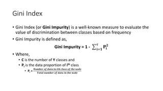
  • 9. Gini Index • Gini Index (or Gini Impurity) is a well-known measure to evaluate the value of discrimination between classes based on frequency • Gini Impurity is defined as, Gini Impurity = 1 - ෌𝐢=𝟏 𝐜 𝐏𝐢 𝟐 • Where, • C is the number of Y classes and • Pi is the data proportion of ith class • Pi = 𝑵𝒖𝒎𝒃𝒆𝒓 𝒐𝒇 𝒅𝒂𝒕𝒂 𝒊𝒏 𝒊𝒕𝒉 𝒄𝒍𝒂𝒔𝒔 𝒐𝒇 𝒕𝒉𝒆 𝒏𝒐𝒅𝒆 𝑻𝒐𝒕𝒂𝒍 𝒏𝒖𝒎𝒃𝒆𝒓 𝒐𝒇 𝒅𝒂𝒕𝒂 𝒊𝒏 𝒕𝒉𝒆 𝒏𝒐𝒅𝒆
  • 10. Entropy • Entropy is a measure of randomness or chaos in a system • Entropy is defined as, Entropy = H = - ෌𝐢=𝟏 𝐜 𝐏𝐢 𝐥𝐨𝐠𝟐(𝐏𝐢) • Where, • C is the number of Y classes and • Pi is the data proportion of ith class • Pi = 𝑵𝒖𝒎𝒃𝒆𝒓 𝒐𝒇 𝒅𝒂𝒕𝒂 𝒊𝒏 𝒊𝒕𝒉 𝒄𝒍𝒂𝒔𝒔 𝒐𝒇 𝒕𝒉𝒆 𝒏𝒐𝒅𝒆 𝑻𝒐𝒕𝒂𝒍 𝒏𝒖𝒎𝒃𝒆𝒓 𝒐𝒇 𝒅𝒂𝒕𝒂 𝒊𝒏 𝒕𝒉𝒆 𝒏𝒐𝒅𝒆 • Entropy value is generally given as a negative value • For 100% purely classified nodes, entropy is zero
  • 11. Gini Impurity and Entropy vs. Proportion Source: https://zerowithdot.com/decision-tree/
  • 12. Classification Geometry • Unlike many other Classifiers (e.g. Logistic Classifier) Decision Trees have Linear Hyperplanes perpendicular to their axes • This makes it difficult a DT to define a diagonal decision boundaries • But this simplicity makes the algorithm faster Age = X1 BMI = X2 35 80 Age > 35 BMI > 35
  • 13. Convert Continuous Features to Categorical • Some of the X variables (e.g.: BMI) can be continuous • They have to be converted to categorical variables to apply to DTs • To convert a continuous variable to a binary categorical variable, • Consider all the possible splits using all the data points as split points • Calculate total entropy for each of the cases • Select the case with the least entropy as the splitting point • Encode all the data values with the new binary categorical variable • Now you can apply this new feature to DTs
  • 14. Bias-Variance Metrics of DT • With sufficient number of X variables a DT can almost purely classify (with 100% accuracy) for the training set • But that kind of DT may not fit enough for test data • Therefore, such a DT is generally considered a High Variance (overfitting) and Low Bias ML algorithm • However, we can increase regularization and make much smaller DTs that have Lower Variance (which may somewhat increase the Bias)
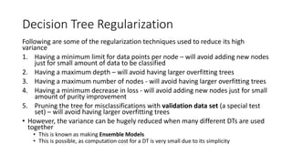
  • 15. Decision Tree Regularization Following are some of the regularization techniques used to reduce its high variance 1. Having a minimum limit for data points per node – will avoid adding new nodes just for small amount of data to be classified 2. Having a maximum depth – will avoid having larger overfitting trees 3. Having a maximum number of nodes - will avoid having larger overfitting trees 4. Having a minimum decrease in loss - will avoid adding new nodes just for small amount of purity improvement 5. Pruning the tree for misclassifications with validation data set (a special test set) – will avoid having larger overfitting trees • However, the variance can be hugely reduced when many different DTs are used together • This is known as making Ensemble Models • This is possible, as computation cost for a DT is very small due to its simplicity 1. he validation set
  • 16. Ensemble Methods • Ensemble methods involve in combining multiple ML models that produces a stronger model than any of its individual constituent models • Leverage the concept of the “Wisdom of the Crowd” where the collective decision making of people brings much accurate decisions than any individual person • There are several main types of ensemble models 1. Bagging 2. Boosting 3. Stacking (combining heterogenous ML algorithms)
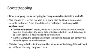
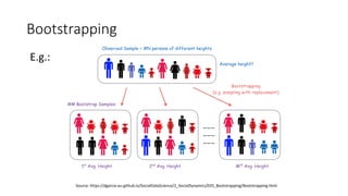
  • 17. Bootstrapping • Bootstrapping is a resampling technique used in statistics and ML • The idea is to use the dataset as a data distribution where every sample collected from the dataset is collected randomly with replacement • “With Replacement” means, when a datapoint is collected to the sample from the distribution, the same data point is available in the distribution, to be taken again as a new datapoint, to the sample • In other words, the sample taken from the training dataset, can contain the same data point as multiple copies • This technique helps to increase the amount of training data without actually increasing the given data
  • 19. Bagging • Bagging stands for Bootstrapping and Aggregating • In this ensemble method, multiple models are built, where each model is trained with Bootstrapped data from the original training dataset • As all the resultant models are similar in predictive power to each other, they are averaged (aggregated) to get a prediction • When it is a classification problem voting is used to get the aggregation
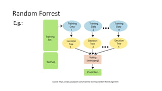
  • 20. Random Forrest • Random Forrest use a modified version of the Bagging algorithm with Decision Trees • Instead of using all the X variables for any model in the ensemble, Random Forrest selects a smaller subset of the available X variables • For larger number of X variables this is generally 𝐍𝐮𝐦𝐛𝐞𝐫 𝐨𝐟 𝐗 𝐯𝐚𝐫𝐢𝐚𝐛𝐥𝐞𝐬 • This algorithm has significantly less variance with almost no increase in bias compared to an individual DT • Random Forrest can be used with unscaled data and get faster results • Random Forrest is used as a way for Feature Selection as well
  • 22. Boosting • Though DTs are generally considered as high variance ML algorithms, it is possible to get highly regularized DTs that are low in variance but higher in bias • It was found that combining many such high bias DTs can make a low bias ensemble model, with very little increase in variance, which is known as Boosting • There are many Boosting algorithms such as AdaBoost, Gradient Boosting Machines (GBM), Light GBM and XGBoost
  • 23. XGBoost • Like in Bagging, XGBoost also samples data for each of the individual DT by Bootstrapping • But unlike in bagging, in XGBoost, each of the new DT is generated sequentially, after evaluating earlier DT model with data • When selecting data to train a new DT, data that failed to classify with the earlier DT are given higher priority • The idea is to generate new DTs to classify the data that were not possible to classify with previous DTs • XGBoost has even more advanced features for tuning in its implementation than Random Forrest
  • 25. Decision Tree - Advantages • DT ensembles are very fast at learning compared to alternatives like Neural Networks • Feature scaling does not significantly impact the learning performance in DT ensemble models • Smaller DT ensembles have higher interpretability • Helps to Feature Selection • There are lesser hyperparameters to be tuned compared to Neural Networks
  • 26. Decision Tree - Disadvantages • DT ensembles cannot learn highly deeper insights like Neural Networks • DTs or DT ensembles are not that capable of Transfer Learn (transfer the knowledge learnt from one larger generic model to another new one) its knowledge
  • 27. One Hour Homework • Officially we have one more hour to do after the end of the lecture • Therefore, for this week’s extra hour you have a homework • DT ensembles are actually the most widely used ML algorithms in competitions specially with non-pre-processed datasets • As Random Forrest and XGBoost can work well at the first shot it is very important to practice them with real world datasets • On the other hand these algorithms can be used as the feature selection algorithms • Good Luck!