SlideShare a Scribd company logo
T-Tests and ANOVA
Olaniyi Taiwo
Disclaimer
• This presentation contains materials adapted or referenced from
various online sources. These materials are included solely for
educational and informational purposes. I do not claim ownership or
original authorship of the content sourced from external references,
and full credit is due to the respective authors and creators of these
works.
Research
Title and
Question
Literature
Review
Research
Hypo
Approach
and
Designs
Sample
size
Sampling
Variables
and
Measure-
ment
Data
collection
Data
Analysis
Report /
Presentati
ons
RESEARCH
PROCESS
Variables
• A variable is a characteristic that may assume more than one set of
values to which a numerical measure can be assigned
• Variable is a characteristic that changes.
• This differs from a constant, which does not change but remains the
same.
Quantitative
Continuous
Discrete
Qualitative
Ordinal
Nominal
Measurement Scales
• Measurement scales are used to quantify numeric values of variables
or observations
There are 4 types of measurement scales:
• Nominal Scale
• Ordinal Scale
• Interval Scale
• Ratio Scale
The Hierarchy of Measurement Scales
Nominal
Interval
Ratio
Attributes are only named; weakest
Attributes can be ordered
Distance is meaningful
Absolute zero
Ordinal
Types of Data
Data
Quantitative
or Numeric
Continuous Data Discrete Data
Qualitative or
Categorical
Nominal Data Ordinal Data
Last Class
Sample vs. Population
Inferential Statistics
▪ Inferential statistics allows researchers to make decisions or
inferences by interpreting data patterns
▪ Inferential statistics can be classified as either Estimation or
Hypothesis testing.
Lecture slides to increase understanding of statistics by all category of researchers
Correlation
• A correlation typically evaluates three aspects of the relationship:
• the direction
• the form
• the degree
• How to study correlation
• Scatter Diagram Method
• Karl Pearson’s Correlation
• Spearman’s Rank correlation coefficient
• Correlation Coefficient (r) and Coefficient of determination (r2)
Chi-Square
• Chi-square analysis is primarily used to deal with categorical
(frequency) data
• Steps in tests of Hypothesis
1. Determine the appropriate test
2. Establish the level of significance: α
3. Formulate the statistical hypothesis
4. Calculate the test statistic
5. Determine the degree of freedom
6. Compare computed test statistic against a tabled/critical value
2
2 ( )
O E
E

−
= 
Today
• Understanding and interpreting T-tests
• Understanding and interpreting ANOVA
Lecture slides to increase understanding of statistics by all category of researchers
T - Tests
Objectives
• Determine when the t-test is appropriate to use
• Discuss the assumptions for t-tests
• Select the appropriate form of t-test for use in a given situation
• Understand the role of the F-statistic in determining which
independent sample t-test to use in SPSS
• Interpret t-test analyses
• Parametric test used to compare means of two group
• Data must be continuous, and the variable(s) of interest must be
normally distributed
• Compares the means of two groups; it cannot compare more than
two
• So when your research question requires the comparison of more
than two groups the t-test is not the correct test to use
• Please note that the t-test can also be used with only one group
• Used with small samples (≤ 30) - theoretical.
• For large samples (N>100) can use z to test hypotheses about means
• The null hypothesis can be expressed as
H0 = x1 = x2, or that the means of the two groups are equal
• The t-test yields a t-statistic, which can help you determine the
confidence intervals associated with a given statistical hypothesis
about the mean of a population (or about the means of two
populations)
Assumptions
• The distribution must be close to normal (so the data are continuous)
• The grouping variable must be categorical and dichotomous
• t statistic is used to estimate the magnitude of difference in the
means of two groups; the bigger the t statistic, the greater the
difference and the more significant the difference
• To have a mean, the variable must be at least approximately
normal; therefore, categorical variables, whether nominal or
ordinal, cannot be compared using the t-test
• t statistic helps determine confidence intervals associated with a
statistical hypothesis about the mean of a population or the means
of two populations
• significance is based on the confidence interval
• sample size influences the interpretation of the t statistic, but not
the interpretation of the 95% confidence interval
Variations of the t-test
• One Sample t-test
• Paired Samples t-test or Dependent t-test
• Independent Samples t-test
Variations of the t-test
• One Sample t-test
• Paired Samples t-test or Dependent t-test
• Independent Samples t-test
One Sample t-test
• Used to evaluate whether the population mean of a test variable
is different from a constant
• A major decision in using the one sample t-test is choosing the
test value (or constant)
• The test value usually represents a neutral point
• Those above the constant are given a label, those below are also
given a label while those on the neutral point are without a label
• The test value or constant may be:
• Midpoint on the test variable
• Average value of test variable based on past research
• Chance level of performance of the test variable
Formula for one sample t-test
• (x̄) = The sample mean.
• (μ) = The population mean.
• (s) = The sample standard
deviation
• (n) = Number of
observations
Lecture slides to increase understanding of statistics by all category of researchers
Class example
• Prof. Morenike wants to improve the number of scientific publications
by members of MWH WhatsApp platform. In the past among MWH
members, data indicate that the average paper publication was 100
per year. After a training on research methodology and data analysis,
the recent publication data (taken from a sample of 25 participants)
indicates an average publication of 130, with a standard deviation of
15. Did the training work? Test your hypothesis at a 5% alpha level.
• Step 1: Write your null hypothesis statement
• Step 2: Write your alternate hypothesis. This is the one you’re
testing. You think there is a difference (that the mean publication
increased), so: H1: x > 100. (one-tail) or H1: x ≠ 100 (two-tail)
• Step 3: Identify the following information you’ll need to calculate the
test statistic. The question should give you these items:
• The sample mean(x̄). This is given in the question as 130.
• The population mean(μ). Given as 100 (from past data).
• The sample standard deviation(s) = 15.
• Number of observations(n) = 25.
• Step 4: Insert the items from above into the t score formula.
• Step 5: Find the t-table value. You need two values to find this:
• The alpha level: given as 5% in the question.
• The degrees of freedom, which is the number of items in the sample (n - 1)
: 25 – 1 = 24.
• Step 6: Find the t-table value for one and two tails
• Decision rule (If calculated t is greater than Table t then reject Ho)
• Interpret
The sample mean(x̄). This is given in the question as 130.
The population mean(μ). Given as 100 (from past data).
The sample standard deviation(s) = 15.
Number of observations(n) = 25.
Lecture slides to increase understanding of statistics by all category of researchers
SPSS example
• Dr Lawal wants to test a research question about the knowledge of
mathematics in a group of students in a class in a high-brow
environment. He hypothesizes that the average math score of these
students is higher than the average for their age and class in the
population. He samples a 100 students in the school at the high brow
area, gives a standard mathematics exam and scores them
• So there are 100 students and 100 scores
• He then conducts a one-sample t-test. (using a test value of 50)
SPSS demonstration with SPSS exam data set
One-Sample Statistics
N Mean Std. Deviation Std. Error
Mean
Scores of Mathematics
exam
100 59.765 21.6848 2.1685
One-Sample Test
Test Value = 50
t df Sig. (2-tailed) Mean
Difference
95% Confidence Interval of
the Difference
Lower Upper
Scores of
Mathematics Exam
4.503 99 .000 9.7650 5.462 14.068
Lecture slides to increase understanding of statistics by all category of researchers
Variations of the t-test
• One Sample t-test
• Paired Samples t-test or Dependent t-test
• Independent Samples t-test
Paired (correlated/dependent) Sample t-Test
• Each case must have scores on two variables for a paired sample t-test
• The paired sample t-test evaluates whether the mean of the difference
between these two variables is different from the population
• It is applicable to two types of studies
• Repeated measures
• With intervention
• Without intervention
• Matched subjects designs
• With intervention
• Without intervention
• For repeated measure design, a participant is assessed on two
occasions or under two conditions on a single measure
• Repeated tests of the same person: This can be weights measured
before and after 6 months for people on a diet (intervention)
• Knowledge before and after for people data analysis class
(intervention).
• A group of people are asked to compare their preference – (on a
measured scale) for healthcare if they prefer Doctor A or B OR Buhari
and Tinubu (no intervention)
• Most of the characteristics between measurements are constant,
such as gender and ethnicity
• For matched subject design, or matched-pairs design uses two
treatment conditions and pairs subjects based on common variables
• Example include parents following their ward or child to a clinic and
being accessed on their experience – like fear scale (no intervention)
• Investigating whether husbands and wives with infertility problems
feel equally anxious using the Infertility Anxiety Measure (no
intervention)
• You want to check the effects of a new BP drug A. You match 40
selected people with similar BP readings into pairs (20 pairs). A
member of the pair is randomized to used drug A, the other uses
existing drug B over 3 months (intervention)
• Each participant pair is a case and has scores on two variables – the
score obtained by one participant under one condition and the score
obtained by the other participant under the other condition
• Assumptions:
• The distribution is close to normal (so the data are continuous)
• Grouping variable is categorical and dichotomous
• Groups are not independent
• Examples of groups that are not independent:
• Repeated tests of the same individual
• Different parts of the same individual (two legs, two eyes)
• Identical twins with identical genes
• Different parts of the same person: This could be comparing drops
using 2 eyes, or lotion using 2 legs, or left side to the right side of
the mouth.
• Since those 2 eyes or 2 legs and the teeth belong to one person,
there is very little difference between groups other than the
treatment that was assigned
Example of how to calculate paired t-test
manually
• Eleven (11) students were told to do push-ups. The number was
recorded for each person. After one hour and a big bottle of
Lucozade Boost, they were told to repeat the push-ups, and the
number of push-ups after the drink was noted for each student.
• The researcher wants to see if Lucozade boost has any statistically
significant effect on the number of push-ups the students can do
after consumption.
• Table of his findings is on the next slide
Research findings:
Sample Research question
• What is the effect of a big bottle of Lucozade boost on the mean
(average) number of push-ups students can do before and after
consumption?
Statistical Hypotheses
• H0: A = B versus H1: A  B
• There is no statistically significant difference in the mean push-ups of
students before and after drinking a large bottle of Lucozade boost
• There is a statistically significant difference in the mean push-ups of
students before and after drinking a large bottle of Lucozade boost
Decision rule
228
.
2
10
1
11
1
scores
difference
of
number
)
1
(
05
.

=
=
−
=
−
=
−
=
=
crit
t
N
df

Calculate test statistic
Formula for calculating Paired sample t-score where:
D = difference between matched scores
N = number of pairs of scores
• Step 1: Subtract each Y score
from each X score (Note that
X - Y = D)
• Step 2: Add up all of the
values from Step 1. Set this
number aside for a moment
• Step 3: Square the
differences from Step1
[i.e (X – Y)2 = D2]
• Step 4: Add up all of the
squared differences from
Step 3
• Step 5: Use the formula to
calculate t-score
• Step 6: Subtract 1 from the
sample size to get the
degrees of freedom. We
have 11 items, so 11-1 = 10.
• Step 7: Find the p-value in the t-
table, using the degrees of
freedom in Step 6. If you don’t
have a specified alpha level, use
0.05 (5%). For this sample
problem, with df=10, the t-value
is 2.228. (next slide)
• Step 8: Compare your t-table
value from Step 7 (2.228) to
your calculated t-value (-2.74).
The calculated t-value is greater
than the table value at an alpha
level of .05. The p-value is less
than the alpha level: p <.05.
• We can reject the null
hypothesis that there is no
difference between means.
• Note: You can ignore the minus sign
when comparing the two t-values, as
± indicates the direction; the p-value
remains the same for both directions.
• It would be useful to calculate a
confidence interval for the mean
difference to tell us within what limits
the true difference is likely to lie.
95% confidence interval for the true mean difference is:
d ± t∗ sd
√n or, equivalently d ± (t∗ × SE( d))
where t∗ is the 2.5% point of the t-distribution on n − 1 degrees
of freedom.
t Test for Dependent Samples: CLASS WORK
Hypothesis Testing
1. State the research question.
2. State the statistical hypothesis.
3. Set decision rule.
4. Calculate the test statistic.
5. Decide if result is significant.
6. Interpret result as it relates to your research question.
The t Test for Dependent Samples: An
Example
• State the research hypothesis/question.
• Does listening to a pro-socialized medicine lecture change
an individual’s attitude toward socialized medicine?
• State the statistical hypotheses.
0
:
0
:

=
D
A
D
O
H
H


The t Test for Dependent Samples:
An Example
• Set the decision rule.
365
.
2
7
1
8
1
scores
difference
of
number
05
.

=
=
−
=
−
=
=
crit
t
df

The t Test for Dependent Samples
• Calculate the test statistic.
The t Test for Dependent Samples
• Decide if your results are significant.
• Reject H0, -4.73 > -2.365
• Ignore the “-” sign
• Interpret your results.
• After the pro-socialized medicine lecture, individuals’ attitudes
toward socialized medicine were significantly more positive than
before the lecture.
Above example using spss (Class work)
Paired Samples Statistics
Mean N Std.
Deviation
Std. Error
Mean
Pair 1
Before
Speech
3.6250 8 1.06066 .37500
After Speech
5.6250 8 1.40789 .49776
Paired Samples Correlations
N Correlation Sig.
Pair 1
Before Speech & After
Speech
8 .562 .147
Paired Samples Test
Paired Differences t df Sig. (2-
tailed)
Mean Std.
Deviation
Std. Error
Mean
95% Confidence Interval
of the Difference
Lower Upper
Pair 1
Before Speech -
After Speech
-2.00000 1.19523 .42258 -2.99924 -1.00076 -4.733 7 .002
Sample SPSS Output and Interpretation:
1. SPSS reports the mean and standard deviation of the difference scores for each pair of variables. The
mean is the difference between the sample means. It should be close to zero if the populations means
are equal.
2. The mean difference between exams 1 and 2 is not statistically significant at α = 0.05. This is because
‘Sig. (2-tailed)’ or p > 0.05.
3. The 95% confidence interval includes zero: a zero mean difference is well within the range of likely
population outcomes.
• The interpretation of this is based on the 95% confidence interval.
• SPSS subtracts the first measurement from the second and
calculates the 95% confidence interval of the difference between
the two paired groups.
• If the two groups were significantly different you would not expect
the lower and upper values to have different signs (negative and
positive). The different signs mean that there is a 0 in the
confidence interval.
• That means that in at least some of the samples there was no
difference between the before and after measurements.
• There are many different names for a t test for related samples.
• Dependent t test,
• Repeated samples t test,
• Paired samples t test,
• Correlated samples t test,
• Within subjects t test, and
• Within groups t test
• There are many advantages of a related samples t test.
1. First, you need fewer participants than you do for a t test for
independent samples.
2. You are able to study changes over time.
3. It also reduces the impact of individual differences.
4. And lastly, it is more powerful, or more sensitive, than a t test for
independent samples
• There are also some disadvantages.
1. The first disadvantage is called carryover effects. And these can
occur when the participant's response in the second treatment is
altered by the lingering after effects of the first treatment
2. The second disadvantage of a related samples t test is called
progressive error. And this can occur when the participant's
performance changes consistently over time due to fatigue or
practice
Variations of the t-test
• One Sample t-test
• Paired Samples t-test or Dependent t-test
• Independent Samples t-test
Independent Sample t-test
• This test evaluates the difference between the mean of two
independent or unrelated groups
• With an independent sample t-test, each case must have scores on
two variables: the grouping variable and the test variable
• The grouping variable divides the cases in two mutually exclusive
groups or categories
• The test variable describes each case on some quantitative
measurement
• This test is also known as:
• Independent t Test
• Independent Measures t Test
• Independent Two-sample t Test
• Student t Test
• Two-Sample t Test
• Uncorrelated Scores t Test
• Unpaired t Test
• Unrelated t Test
Sample questions for independent sample T-tests
• Used extensively in experiments when you want to check a measure
in one group against the other (active agent Vs placebo)
• To compare the average score of the knowledge of research
methodology among Class A and Class B
• To compare fear level (measured in a scale) among those seen by a
particular dentist compared to another dentist
• Or how long it takes to have remission from a skin blister among
some patients using ointment A compared to those using ointment B
• The t-test evaluates whether the population mean of the test variable in
one group differs from the population mean of the test variable in the
second group
• Assumptions
• Test variable is normally distributed in each of the two population
• There are equal variances of the test variable (homogeneity)
• The cases represent random sample from population
• Scores of the test variables are independent of each other
Variation of independent sample t-test
There are two types of t-test that can be used on independent
groups. The decision on which to use is based on whether the
variances are equal or significantly different.
• Pooled t-test: meets all of the assumptions listed on previous slide,
and in addition, the variances of the two independent groups are
essentially equal.
• Separate t-test: meets all of the same assumptions listed on
previous slide and, in addition, the variances of the two
independent groups are unequal or unknown.
• Unfortunately, just like you cannot judge whether two means are
different by just looking at the data set, you cannot judge whether
two variances are equal or different without performing a statistical
test.
• The test statistic you use to compare variances is the F-statistic
(Levene’s Test for Equality of Variances)
• Recall that the Independent Samples t Test requires the assumption
of homogeneity of variance -- i.e., both groups have the same
variance.
• SPSS conveniently includes a test for the homogeneity of variance,
called Levene's Test, whenever you run an independent samples T
test.
• The hypotheses for Levene’s test are:
• H0: σ1
2 - σ2
2 = 0 ("the population variances of group 1 and 2 are
equal")
H1: σ1
2 - σ2
2 ≠ 0 ("the population variances of group 1 and 2 are not
equal")
• This implies that if we reject the null hypothesis of Levene's Test, it
suggests that the variances of the two groups are not equal; i.e., that
the homogeneity of variances assumption is violated.
F-statistic
• The F-statistic is similar to the t-statistic in that it compares groups
• Whereas the t-statistic is used to evaluate the differences in the
mean of 2 groups, the F-statistic evaluates differences in the
variance
• The interpretation of the F-statistic is similar to the interpretation of
the t-statistic, but is usually done based on the p-value rather than
the confidence interval
• The null hypothesis associated with the F-statistic is that there is no
difference between the variances of the two groups
• If the p-value or significance level is 0.05 or smaller you can reject
the null hypothesis and assume that the groups have significantly
different variances
• If the p-value is greater than 0.05 you cannot reject the null
hypothesis and you assume the variances are equal
Sample SPSS output
Lecture slides to increase understanding of statistics by all category of researchers
Sample SPSS output
Independent Samples Test
Levene's Test
for Equality of
Variances t-test for Equality of Means
F Sig. t df Sig. (2-tailed)
Mean
Difference
Std. Error
Difference
95% Confidence Interval of the
Difference
Lower Upper
histidin Equal
variances
assumed
5.743 .096 5.096 3 .015 83.500 16.385 31.355 135.645
Equal
variances
not assumed
6.418 2.296 .016 83.500 13.010 33.907 133.093
There are two steps to the interpretation of this output:
• First you look at the columns labeled Levene’s Test for Equality of
Variances.
• In those columns you will see the F-statistic and the significance of
that statistic.
• Since the significance is greater than 0.05 you cannot reject the null
hypothesis and you can assume that the variances are equal.
• Then, using that information you can use the row Equal variances
assumed, which gives you the result of the paired t-test.
• Again, the interpretation of this is based on the 95% confidence
interval.
• Here you see that upper and lower values have the same positive
value so the confidence interval does not cross 0 and you can reject
the null hypothesis of no difference in the means..
Sample SPSS output
Independent Samples Test
Levene's Test
for Equality of
Variances t-test for Equality of Means
F Sig. t df Sig. (2-tailed)
Mean
Difference
Std. Error
Difference
95% Confidence Interval of the
Difference
Lower Upper
histidin Equal
variances
assumed
5.743 .096 5.096 3 .015 83.500 16.385 31.355 135.645
Equal
variances
not assumed
6.418 2.296 .016 83.500 13.010 33.907 133.093
How to report t-tests
• Values to report: means (M) and standard deviations (SD) for each
group, t value (t), degrees of freedom (in parentheses next to t),
and significance level (p).
• Examples
• Women (M = 3.66, SD = .40) reported significantly higher levels of
happiness than men (M = 3.20, SD = .32), t(1) = 5.44, p < .05.
• Men (M = 4.05, SD = .50) and women (M = 4.11, SD = .55) did not
differ significantly on levels of political agreement, t(1) = 1.03, p =
n.s.
Reporting a significant single sample t-test (μ ≠ μ0):
• Students taking statistics courses in Chemistry at the University of
Lagos reported studying more hours for tests (M = 121, SD = 14.2)
than did Unilag students in general, t(33) = 2.10, p = .034.
Reporting a significant t-test for dependent groups (μ1 ≠ μ2):
• Results indicate a significant preference for Meat pie (M = 3.45, SD
= 1.11) over chicken pie (M = 3.00, SD = .80), t(15) = 4.00, p = .001.
Reporting a significant t-test for independent groups (μ1 ≠
μ2):
• Unilag students taking statistics courses in Psychology had higher IQ
scores (M = 121, SD = 14.2) than did those taking statistics courses
in Chemistry (M = 117, SD = 10.3), t(44) = 1.23, p = .09.
• Over a two-day period, participants drank significantly fewer drinks
in the experimental group (M= 0.667, SD = 1.15) than did those in
the control group (M= 8.00, SD= 2.00), t(4) = -5.51, p=.005.
Lecture slides to increase understanding of statistics by all category of researchers
Non parametric variants of t-tests
• Where data is not normally distributed, statistical analyses that
assume a normal distribution may be inappropriate.
• This is especially a concern where the sample size is small (<50 in
total).
• Variables that are discrete (take only integer values) or have an upper
or lower limit are by definition non-normal.
• For one sample T tests that do not fulfil the normality assumption,
use the Wilcoxin One Sample Signed Rank T Test
• For 2 Related samples that do not fulfil the normality assumption,
use the McNemar test.
• For 2-Independent Groups, use Mann-Whitney U-test
• For Related Ordinal Data, i.e. ordered categorical or quantitative
variables that are not plausibly normal, the suggested procedure is to
use the Wilcoxon procedure
Summary
• A t-test is a parametric test used to compare the means of two
samples
• There are different t-tests we can use based on the assumptions we
can make – paired, pooled, and separate
• To test your null hypothesis you need to know the type of t-test to
use, the number of observations, the means of the two groups (or
with pairs, the difference between the pairs), and the variances of
the two groups
• Single sample t – we have only 1 group; want to test against a
hypothetical mean.
• Dependent (Paired) t – we have two means. Either same people in
both groups, or people are related, e.g., husband-wife, left hand-
right hand.
• Independent samples t – we have 2 means, 2 groups; no relation
between groups, e.g., people randomly assigned to a single group.
Lecture slides to increase understanding of statistics by all category of researchers
• You need to compare the variances of your groups using the F-
statistic to chose between the pooled or separate tests
ANOVA
• ANOVA is short for ANalysis Of VAriance
• The purpose of ANOVA is to determine whether the mean differences
that are obtained for sample data are sufficiently large to justify a
conclusion that there are mean differences between the populations
from which the samples were obtained.
• The difference between ANOVA and t tests is that ANOVA can be
used in situations where there are two or more means being
compared, whereas the t tests are limited to situations where only
two means are involved.
Assumptions for ANOVA
• ASSUMPTION 1: The dependent variable is normally distributed for
each of the populations as defined by the different levels of the factor
• ASSUMPTION 2: The variances of the dependent variable are the
same for all populations
• ASSUMPTION 3: The cases represent random samples from the
populations and the scores on the test variable are independent of
each other
Sample research questions for ANOVA
• Is there a difference in average pain levels during tooth extraction
among patients given 3 types of Local Anesthesia?
• Are there differences in children’s weight by type of school (Public vs.
missionary vs. private)?
• Experiment to check the effects of caffeine on reading time among
students.
• 45 volunteers from a university to participate. Randomly assigns an
equal number of students to three groups: placebo (group 1), mild
doses of caffeine (group 2), and heavy doses of caffeine (group 3).
• Before study, the average number of study hours for all the students
was taken over 2 months. The intervention over the next 2 months
with a cup of coffee or placebo every night and average hours of
study was documented again.
Lecture slides to increase understanding of statistics by all category of researchers
The basic ANOVA situation
**Two variables: 1 Categorical, 1 Quantitative
Main Question: Do the (means of) the quantitative variables
depend on which group (given by categorical variable) the
individual is in?
If categorical variable has only 2 values:
• 2-sample t-test
ANOVA allows for 3 or more groups
• Analysis of variance is necessary to protect researchers from
excessive risk of a Type I error in situations where a study is
comparing more than two population means.
• E.g., caffeine study with 3 populations taking coffee:
• Population 1 - No caffeine
• Population 2 - Mild dose
• Population 3 - Heavy dose
Lecture slides to increase understanding of statistics by all category of researchers
• We have at least 3 means to test, e.g.,
• H0: 1 = 2 = 3.
• Could take them 2 at a time, but really want to test all 3 (or more) at
once.
• Although each t test can be done with a specific α-level (risk of Type I
error), the α-levels accumulate over a series of tests so that the final
experiment-wise α-level can be quite large
• ANOVA allows researcher to evaluate all of the mean differences in a
single hypothesis test using a single α-level and, thereby, keeps the
risk of a Type I error under control no matter how many different
means are being compared
Example of an ANOVA situation
Subjects: 25 patients with blisters
Treatments: Treatment A, Treatment B, Placebo (categorical)
Measurement: Number of days until blisters heal (quantitative)
Data [and means]:
• A: 5,6,6,7,7,8,9,10 [7.25]
• B: 7,7,8,9,9,10,10,11 [8.875]
• P: 7,9,9,10,10,10,11,12,13 [10.11]
Are these differences significant?
Informal Investigation
Graphical investigation:
• side-by-side box plots
• multiple histograms
ANOVA determines P-value from the F statistic
Side by Side Boxplots
What does ANOVA do?
At its simplest ANOVA tests the following hypotheses:
H0: The means of all the groups are equal. 1 = 2 = 3.
Ha: Not all the means are equal
• doesn’t say how or which ones differ.
• Can follow up with “multiple comparisons”
Note: we usually refer to the sub-populations as “groups” when doing
ANOVA.
Assumptions of ANOVA
• Each group is approximately normal
· check this by looking at histograms and/or normal quantile plots, or
use assumptions
· can handle some non-normality, but not severe outliers
Normality Check
We should check for normality using:
• assumptions about population
• histograms for each group
• normal quantile (or QQ) plot for each group
With such small data sets, there really isn’t a really good way to
check normality from data, but we make the common assumption
that physical measurements of people tend to be normally
distributed.
Lecture slides to increase understanding of statistics by all category of researchers
• The test statistic for ANOVA is an F-ratio, which is a ratio of two
sample variances.
• In the context of ANOVA, the sample variances are called mean
squares, or MS values.
Recall example of an ANOVA situation
Subjects: 25 patients with blisters
Treatments: Treatment A, Treatment B, Placebo (categorical)
Measurement: Number of days until blisters heal (quantitative)
Data [and means]:
• A: 5,6,6,7,7,8,9,10 [7.25]
• B: 7,7,8,9,9,10,10,11 [8.875]
• P: 7,9,9,10,10,10,11,12,13 [10.11]
Notation for ANOVA
• n = number of individuals all together (25)
• I = number of groups (3)
• = mean for the entire data set is (??)
Group A has
• nA = # of individuals in group A
• xAw = value for individual w in group A
• = mean for group A
• sA = standard deviation for group A
A
x
A
x
Number of individuals all together (25)
Group A Group B Group P
N = 8 N = 8 N = 9
How ANOVA works
ANOVA measures two sources of variation in the data and compares
their relative sizes
• variation BETWEEN groups
• for each data value look at the difference between its group
mean and the overall mean
• variation WITHIN groups
• for each data value we look at the difference between that
value and the mean of its group
( )2
A
Aw x
x −
( )2
x
xA −
The ANOVA F-statistic is a ratio of the Between Group
Variation divided by the Within Group Variation:
MSW
MSB
Within
Between
F =
=
• The top of the F-ratio MSbetween measures the size of mean differences
between samples.
• The bottom of the ratio MSwithin measures the magnitude of
differences that would be expected without any outside effects.
MSW
MSB
Within
Between
F =
=
• A large value for the F-ratio indicates that the obtained sample mean
differences are greater than would be expected if the samples had no
outside effect.
• A large F is evidence against H0, since it indicates that there is more
difference between groups than within groups.
• F is another distribution like z and t. There are tables of F used for
significance testing.
126
The Logic and the Process of Analysis of Variance
• The two components of the F-ratio can be described as follows:
• Between-Treatments Variability: MSbetween measures the size of the
differences between the sample means. For example, suppose that
three treatments, each with a sample of n = 5 subjects, have means of
M1 = 1, M2 = 2, and M3 = 3.
• Notice that the three means are different; that is, they are variable.
127
The Logic and the Process of ANOVA (cont.)
• By computing the variance for the three means we can measure
the size of the differences
• Although it is possible to compute a variance for the set of
sample means, it usually is easier to use the total, T, for each
sample instead of the mean, and compute variance for the set of
T values.
128
The Logic and the Process of ANOVA (cont.)
Logically, the differences (or variance) between means can be
caused by two sources:
1. Outside or Treatment Effects: If the treatments have different
effects, this could cause the mean for one treatment to be
higher (or lower) than the mean for another treatment.
2. Chance or Sampling Error: If there is no treatment effect at all,
you would still expect some differences between samples.
Mean differences from one sample to another are an example
of random, unsystematic sampling error.
Group A Group B Group P
N = 8 N = 8 N = 9
130
The Logic and the Process of ANOVA (cont.)
• Within-Treatments Variability: MSwithin measures the size of the
differences that exist inside each of the samples.
• Because all the individuals in a sample receive exactly the same
treatment, any differences (or variance) within a sample cannot
be caused by different treatments.
Group A Group B Group P
N = 8 N = 8 N = 9
132
The Logic and the Process of ANOVA
Thus, these differences are caused by only one source:
Chance or Error: The unpredictable differences that exist between
individual scores are not caused by any systematic factors and are
considered to be random, chance, or error.
133
The Logic and the Process of ANOVA (cont.)
• Considering these sources of variability, the structure of the F-ratio
becomes,
treatment effect + chance/error
F = ──────────────────────
chance/error
134
The Logic and the Process of ANOVA (cont.)
• When the null hypothesis is true and there are no differences
between treatments, the F-ratio is balanced.
• That is, when the "treatment effect" is zero, the top and bottom
of the F-ratio are measuring the same variance.
• In this case, you should expect an F-ratio near 1.00. When the
sample data produce an F-ratio near 1.00, we will conclude that
there is no significant treatment effect.
135
The Logic and the Process of ANOVA (cont.)
• On the other hand, a large treatment effect will produce a large
value for the F-ratio. Thus, when the sample data produce a
large F-ratio we will reject the null hypothesis and conclude that
there are significant differences between treatments.
• To determine whether an F-ratio is large enough to be
significant, you must select an α-level, find the df values for the
numerator and denominator of the F-ratio, and consult the F-
distribution table to find the critical value.
In Summary,
Lecture slides to increase understanding of statistics by all category of researchers
A sample class question:
• Do students' performance in exams vary depending on where they
live? – Research Question
• Independent variable: Where students live eg, Ikoyi, Ojota and Badagry
• Dependent variable : Performance in exams (standard quiz)
Ho: There is no difference in the mean score of students based on different
residence i.e. mean of Ikoyi = mean of Ojota = mean of Badagry
Ha: There is a difference in the mean score of students based on different
residence i.e. mean of Ikoyi ≠ mean of Ojota ≠ mean of Badagry
(Each score is over 10)
• Ikoyi – scores of 3 students in tests:
3, 2, 1
• Ojota – scores of 3 students in tests:
5, 3, 4
• Badagry – scores of 3 students in tests:
5, 6, 7
Manual procedure for computing 1-way ANOVA for
independent samples
• Step 1: Complete the table
• Calculate the sum in each group
• Calculate the mean in each group
Ikoyi
A
Ojota
B
Badagry
C
3 5 5
2 3 6
1 4 7
Manual procedure for computing 1-way ANOVA for
independent samples
• Step 1: Complete the table
• Calculate the sum in each group
• Calculate the mean in each group
Ikoyi
A
Ojota
B
Badagry
C
3 5 5
2 3 6
1 4 7
Total 6 12 18
Manual procedure for computing 1-way ANOVA for
independent samples
• Step 1: Complete the table
• Calculate the sum in each group
• Calculate the mean in each group
• Mean for A = 6/3 = 2
• Mean for B = 12/3 = 4
• Mean for C = 18/3 = 6
Ikoyi
A
Ojota
B
Badagry
C
3 5 5
2 3 6
1 4 7
Total 6 12 18
Mean 2 4 6
Procedure for computing 1-way ANOVA for
independent samples
• Step 2: Calculate the Grand mean
X =
=
= 6 + 12 + 18 = 4
9
Or the mean of group A + mean of group B + mean of group C
k (number of groups)
= 2 + 4 + 6 = 12/3 = 4
3
(X)
N
(XA+XB+XC)
N
Ikoyi
A
Ojota
B
Badagry
C
3 5 5
2 3 6
1 4 7
Total 6 12 18
Mean 2 4 6
x
Procedure for computing 1-way ANOVA for independent
samples
• Step 3: Compute total Sum of Squares
SStotal= (every value – grand mean)2
This is done for each value in all the
groups and added together to give the SStotal
= (3-4)2 + (2-4)2 + (1-4)2 + (5-4)2 + (3-4)2 + (4-4)2
+ (5-4)2 + (6-4)2 + (7-4)2
= 1 + 4 + 9 + 1 + 1 + 0 + 1 + 4 +9 = 30
SStotal= 30, dftotal = 8
Degree of freedom = (N – 1) = 9 – 1 = 8 (Recall that “N” is the
number of sample size from ALL the population i.e. 3 students
each from the different location)
Ikoyi
A
Ojota
B
Badagry
C
3 5 5
2 3 6
1 4 7
Total 6 12 18
Mean 2 4 6
Grand mean = 4
Procedure for computing 1-way ANOVA for
independent samples
• Step 4: Compute between groups
Sum of Squares
• Compare the means of EACH group with
the grand mean
i.e for group A = (mean of grp A – grand mean)2
for the number of variables in the group
This is the same as the value multiplied by
the number of variables in each group.
The same for grp B and Group C
SSbet = Total sum of all the values i.e value for Grp A + value for
Grp B + value for Grp C etc
Ikoyi
A
Ojota
B
Badagry
C
3 5 5
2 3 6
1 4 7
Total 6 12 18
Mean 2 4 6
Grand mean = 4
Procedure for computing 1-way ANOVA for
independent samples
SSbet = Total sum of all the values i.e value for
Grp A + value for Grp B + value for Grp C
= (2-4)2 + (2-4)2 + (2-4)2 + (4-4)2 + (4-4)2 + (4-4)2
+ (6-4)2 + (6-4)2 + (6-4)2
= 4 + 4 + 4 + 0 + 0 + 0 + 4 + 4 + 4 = 24
SSbet = 24, dfbet = 2
Degree of freedom = (k – 1) = 3 – 1 = 2 (Recall that “K” is the
number of categories of the population)
Ikoyi
A
Ojota
B
Badagry
C
3 5 5
2 3 6
1 4 7
Total 6 12 18
Mean 2 4 6
Grand mean = 4
Procedure for computing 1-way ANOVA for
independent samples
• Step 5: Compute within groups Sum of Squares
• Note that: SStotal= SSwit + SSbet therefore,
SSwit= SStotal – SSbet
= 30 – 24 = 6
or
Compare the values in EACH group with the
group mean and square them
= (3-2)2 + (2-2)2 + (1-2)2 + (5-4)2 + (3-4)2 + (4-4)2
+ (5-6)2 + (6-6)2 + (7-6)2
= 1 + 0 + 1 + 1 + 1 + 0 + 1 + 0 + 1 = 6
SSwit= 6, dfwit = 6
Degree of freedom = (N – k) = 9 – 3 = 6
Ikoyi
A
Ojota
B
Badagry
C
3 5 5
2 3 6
1 4 7
Total 6 12 18
Mean 2 4 6
Grand mean = 4
Procedure for computing 1-way ANOVA for
independent samples
• Step 6: Determine the d.f. for each sum of squares
dftotal= (N - 1) = 8
dfbet= (k - 1) = 2
dfwit= (N - k) = 6
N = total number of records
K = number of groups
Recall,
Systematic
Variance
(between means)
Error
Variance
(within means)
Procedure for computing 1-way ANOVA for
independent samples
• Step 7/8: Estimate the Variances & Compute F
=
=
SSbet
dfbet
SSwit
dfwit
MSbetween
MSwithin
MSW
MSB
Within
Between
F =
=
MSW
MSB
Within
Between
F =
=
SSbet
dfbet
SSwit
dfwit
= = 24/2
6/6
F = 12
In Summary (The formula)
MSW
MSB
F
DF
SS
MS
SST
SSB
SSW
x
x
n
x
x
SSB
df
s
x
x
SSW
DFT
s
x
x
SST
groups
i
i
obs
i
i
groups
i
obs
i
ij
obs
ij
=
=
=
+
−
=
−
=
=
−
=
=
−
=





;
;
)
(
)
(
)
(
)
(
)
(
)
(
2
2
2
2
2
2
Procedure for computing 1-way ANOVA for
independent samples
• Step 9: Consult F distribution table (it has 2 sides: d1 and d2)
d1 is your df for the numerator (i.e. systematic variance) dfbetween
d2 is your df for the denominator (i.e. error variance) dfwithin
F – Table
d1 = 2 and d2 = 6
• A large F is evidence against H0, since it indicates that there is more
difference between groups than within groups
• Calculated F- ratio was 12
• Reading from F-Table at 0.05 level was 5.14
• Conclusion: reject H0
Ho: There is no difference in the mean score of students based on different
residence i.e. mean of Ikoyi = mean of Ojota = mean of Badagry
Ha: There is a difference in the mean score of students based on different
residence i.e. mean of Ikoyi ≠ mean of Ojota ≠ mean of Badagry
Independent 1-way ANOVA: SPSS Output
ANOVA
Maths
Sum of Squares df Mean Square F Sig.
Between Groups 24.000 2 12.000 12.000 .008
Within Groups 6.000 6 1.000
Total 30.000 8
The computation of F statistic is illustrated in the following table, called ANOVA table.
Source of variance Degrees of freedom Sum of squares Mean square F ratio
Between k-1 SSB MSB=BSS/ (k-1) MSB/MSW
Within n-k SSW MSW=WSS/(n-k)
Total n-1 SST
158
Analysis of Variance and Post Tests
• The null hypothesis for ANOVA states that for the general population
there are no mean differences among the treatments being
compared; H0: μ1 = μ2 = μ3 = . . .
• When the null hypothesis is rejected, the conclusion is that there are
significant mean differences.
• However, the ANOVA simply establishes that differences exist, it does
not indicate exactly which groups, intervention, categories or
treatments are different.
• If the t-test is significant, you have a difference in population means.
• If the F-test is significant, you have a difference in population means.
But you don’t know where.
• With 3 means, could be A=B>C or A>B>C or A>B=C.
160
Analysis of Variance and Post Tests
• With more than two treatments, this creates a problem.
• Specifically, you must follow the ANOVA with additional tests, called
post tests, to determine exactly which treatments are different and
which are not.
• The Scheffe test and Tukey’s HSD are examples of post tests.
• HSD means honestly significant difference
• These tests are done after an ANOVA where H0 is rejected with more
than two treatment conditions. The tests compare the treatments,
two at a time, to test the significance of the mean differences.
Multiple Comparisons
Dependent Variable: Maths
Tukey HSD
(I) Location (J) Location Mean
Difference
(I-J)
Std.
Error
Sig. 95% Confidence Interval
Lower
Bound
Upper
Bound
Ikoyi Ojota -2.00000 .81650 .109 -4.5052 .5052
Badagry -4.00000* .81650 .006 -6.5052 -1.4948
Ojota Ikoyi 2.00000 .81650 .109 -.5052 4.5052
Badagry -2.00000 .81650 .109 -4.5052 .5052
Badagry Ikoyi 4.00000* .81650 .006 1.4948 6.5052
Ojota 2.00000 .81650 .109 -.5052 4.5052
*. The mean difference is significant at the 0.05 level.
Mean of Ikoyi = 2. Ojota = 4 and Badagry = 6
POST-HOC TEST
One-Way Analysis of Variance with SPSS
• Select an independent variable with three or more levels and a
dependent variable.
• Develop the null hypothesis and the alternative hypothesis for main
effects.
• Using SPSS, calculate an ANOVA. Include a post hoc test.
• Report on the p value and the confidence interval.
• Interpret the confidence interval.
• Decide whether to reject or retain the null hypothesis based on main
effects and/or post-hoc statistical tests.
How to report ANOVA
• A one-way between subjects ANOVA was conducted to
compare the effect of (IV)______________ on
(DV)_______________ in _________________,
__________________, and __________________
conditions.”
• There was a significant (not a significant) effect of IV
____________ on DV ______________ at the p<.05 level for
the three conditions [F(df1, df2) = ___, p = ____].
Lecture slides to increase understanding of statistics by all category of researchers
For our class example:
There was a significant effect of the location of residence on the
performance of students at p < .05 [F(2, 6) = 12, p = .008]
ANOVA
Maths
Sum of Squares df Mean Square F Sig.
Between Groups 24.000 2 12.000 12.000 .008
Within Groups 6.000 6 1.000
Total 30.000 8
• The Kruskal-Wallis test is a nonparametric (distribution free) test, and
is used when the assumptions of one-way ANOVA are not met.
• Both the Kruskal-Wallis test and one-way ANOVA assess for significant
differences on a continuous dependent variable by a categorical
independent variable (with two or more groups)
• The most common use of the Kruskal–Wallis test is when you have
one nominal variable and one measurement variable, an experiment
that you would usually analyze using one-way ANOVA, but the
measurement variable does not meet the normality assumption of a
one-way ANOVA
Next Class
• Quantitative Data Analysis Lecture 4
• Regressions.
• Contingency Table Analysis
Sample SPSS Analysis
• I have a sample SPSS data with the following variables
• Age:Continuous
• Sex: Nominal (Binary)
• Basic Metabolic Index (BMI): Continuous
• Lipid Level: Continuous
• Stroke: Nominal (Binary)
• Hypertension: Nominal (Binary)
• Educational Level: Ordinal
• Income per day: Continuous
Comparison Tests
Differences among group means
Statistical tests Predictor variable Outcome variable Sample research question
Paired t-test • Categorical
• 1 predictor
• Quantitative
• Groups come from
the same
population
What is the difference in the average
knowledge of the choice of data analysis
before and after this lecture in this group
Independent sample t-
test
• Categorical
• 1 predictor
• Quantitative
• Groups come from
different
populations
What is the difference in the average
knowledge of the choice of data analysis
in group A and group B
ANOVA • Categorical
• 1 or more predictor
• Quantitative
• 1 outcome
What is the difference in average pain
levels during tooth removal among
patients given 3 types of Local
Anesthesia
Statistical tests Predictor variable Outcome variable Sample research question
One Sample T-
Test
• Continuous • Quantitative
• One population
Is there an improvement in lipids
after a vegetarian diet over 3
days? Cut off of 200
Paired t-test • Categorical
• 1 predictor
• Quantitative
• Groups come
from the same
population
What is the difference in the
average basic metabolic index
(BMI) before and after this
lecture in this group
Independent
sample t-test
• Categorical
• 1 predictor
• Quantitative
• Groups come
from different
populations
What is the difference in the
average basic metabolic index
(BMI) after this lecture in males
and females
Analysis of Variance (ANOVA)
Statistical tests Predictor variable Outcome variable Sample research question
ANOVA • Categorical
• 1 or more
predictor
• Quantitative
• 1 outcome
What is the difference in baseline
BMI among the different
Educational level
•Thank you

More Related Content

PPTX
Student t test
PPT
students_t_test.ppt
PPT
students_t_test.ppt vvvvvvvvvvvvvvvvvvvvvvv
PPT
students_t_test.ppt
PPTX
PPTX
ARM Module 5. Advanced research methodology
PPTX
PDF
Application of Statistical and mathematical equations in Chemistry Part 2
Student t test
students_t_test.ppt
students_t_test.ppt vvvvvvvvvvvvvvvvvvvvvvv
students_t_test.ppt
ARM Module 5. Advanced research methodology
Application of Statistical and mathematical equations in Chemistry Part 2

Similar to Lecture slides to increase understanding of statistics by all category of researchers (20)

PPTX
Test of Difference Between Means.pptx Test of Difference Between Means.pptx
PPTX
Analysis of Quantitative Data Parametric and non-parametric tests.pptx
PPTX
PPT
Research_Methodology_Lecture_literature_review.ppt
PPTX
Data analysis
PPTX
Hypothesis Testing - Test Statistics (2025 spring).pptx
PPTX
Hypothesis Testing Hypothesis Testing Hypothesis Testing Hypothesis Testing
PPTX
t-test Parametric test Biostatics and Research Methodology
DOC
Str t-test1
PPTX
t test for statistics 1st sem mba sylabus
PPTX
Basic Statistics Until Regression in SPSS
PDF
jhghgjhgjhgjhfhcgjfjhvjhjgjkggjhgjhgjhfjgjgfgfhgfhg
PDF
t Test- Thiyagu
PPTX
Hypothesis testing basics in the field of statistics
PPT
bio statistics for clinical research
PPT
1 ANOVA.ppt
PPTX
tests of significance
PPTX
Test of Difference Between Means.pptx Test of Difference Between Means.pptx
Analysis of Quantitative Data Parametric and non-parametric tests.pptx
Research_Methodology_Lecture_literature_review.ppt
Data analysis
Hypothesis Testing - Test Statistics (2025 spring).pptx
Hypothesis Testing Hypothesis Testing Hypothesis Testing Hypothesis Testing
t-test Parametric test Biostatics and Research Methodology
Str t-test1
t test for statistics 1st sem mba sylabus
Basic Statistics Until Regression in SPSS
jhghgjhgjhgjhfhcgjfjhvjhjgjkggjhgjhgjhfjgjgfgfhgfhg
t Test- Thiyagu
Hypothesis testing basics in the field of statistics
bio statistics for clinical research
1 ANOVA.ppt
tests of significance
Ad

More from kabiruabubakar3 (11)

PPTX
DRUG INTERRACTIONS, LECTURE NOTES FOR PHARMACY STUDENTS
PPTX
PARASITIC DISEASES. PPT. A LECTURE DELIVERED TO UNDERGRADUATE STUDENTS
PDF
Pattern_of_Chronic_Suppurative_Otitis_Me.pdf
PPTX
medicinal chemistry power point lecture for undergraduates
PPTX
Introductory lectures for pharmacy students
PPTX
SYSTEMATIC REVIEW: A STEP-BY-STEP APPROACH
PPTX
Centrality of N-Methyl D Aspartate receptors in ameliorating the cognitive sy...
PPTX
Asthma and Cough, PHARMACOLOGY OF DISEASE AFFECTING THE RESPIRATORY SYSTEM
PPTX
CENTRAL NERVOUS SYSTEM PHARMACOLOGY,ANTIEPILEPTIC DRUGS
PPTX
Chemotherapy of Bacterial disease and classification of antibiotics
PPTX
PCH gmb.pptx
DRUG INTERRACTIONS, LECTURE NOTES FOR PHARMACY STUDENTS
PARASITIC DISEASES. PPT. A LECTURE DELIVERED TO UNDERGRADUATE STUDENTS
Pattern_of_Chronic_Suppurative_Otitis_Me.pdf
medicinal chemistry power point lecture for undergraduates
Introductory lectures for pharmacy students
SYSTEMATIC REVIEW: A STEP-BY-STEP APPROACH
Centrality of N-Methyl D Aspartate receptors in ameliorating the cognitive sy...
Asthma and Cough, PHARMACOLOGY OF DISEASE AFFECTING THE RESPIRATORY SYSTEM
CENTRAL NERVOUS SYSTEM PHARMACOLOGY,ANTIEPILEPTIC DRUGS
Chemotherapy of Bacterial disease and classification of antibiotics
PCH gmb.pptx
Ad

Recently uploaded (20)

PPTX
Institutional Correction lecture only . . .
PPTX
Cell Structure & Organelles in detailed.
PDF
The Lost Whites of Pakistan by Jahanzaib Mughal.pdf
PDF
Classroom Observation Tools for Teachers
PDF
Anesthesia in Laparoscopic Surgery in India
PPTX
Final Presentation General Medicine 03-08-2024.pptx
PDF
2.FourierTransform-ShortQuestionswithAnswers.pdf
PPTX
1st Inaugural Professorial Lecture held on 19th February 2020 (Governance and...
PDF
ANTIBIOTICS.pptx.pdf………………… xxxxxxxxxxxxx
PDF
TR - Agricultural Crops Production NC III.pdf
PDF
Basic Mud Logging Guide for educational purpose
PDF
grade 11-chemistry_fetena_net_5883.pdf teacher guide for all student
PPTX
Renaissance Architecture: A Journey from Faith to Humanism
PDF
Microbial disease of the cardiovascular and lymphatic systems
PPTX
Introduction_to_Human_Anatomy_and_Physiology_for_B.Pharm.pptx
PDF
Saundersa Comprehensive Review for the NCLEX-RN Examination.pdf
PDF
Pre independence Education in Inndia.pdf
PDF
O7-L3 Supply Chain Operations - ICLT Program
PPTX
IMMUNITY IMMUNITY refers to protection against infection, and the immune syst...
PDF
Black Hat USA 2025 - Micro ICS Summit - ICS/OT Threat Landscape
Institutional Correction lecture only . . .
Cell Structure & Organelles in detailed.
The Lost Whites of Pakistan by Jahanzaib Mughal.pdf
Classroom Observation Tools for Teachers
Anesthesia in Laparoscopic Surgery in India
Final Presentation General Medicine 03-08-2024.pptx
2.FourierTransform-ShortQuestionswithAnswers.pdf
1st Inaugural Professorial Lecture held on 19th February 2020 (Governance and...
ANTIBIOTICS.pptx.pdf………………… xxxxxxxxxxxxx
TR - Agricultural Crops Production NC III.pdf
Basic Mud Logging Guide for educational purpose
grade 11-chemistry_fetena_net_5883.pdf teacher guide for all student
Renaissance Architecture: A Journey from Faith to Humanism
Microbial disease of the cardiovascular and lymphatic systems
Introduction_to_Human_Anatomy_and_Physiology_for_B.Pharm.pptx
Saundersa Comprehensive Review for the NCLEX-RN Examination.pdf
Pre independence Education in Inndia.pdf
O7-L3 Supply Chain Operations - ICLT Program
IMMUNITY IMMUNITY refers to protection against infection, and the immune syst...
Black Hat USA 2025 - Micro ICS Summit - ICS/OT Threat Landscape

Lecture slides to increase understanding of statistics by all category of researchers

  • 2. Disclaimer • This presentation contains materials adapted or referenced from various online sources. These materials are included solely for educational and informational purposes. I do not claim ownership or original authorship of the content sourced from external references, and full credit is due to the respective authors and creators of these works.
  • 4. Variables • A variable is a characteristic that may assume more than one set of values to which a numerical measure can be assigned • Variable is a characteristic that changes. • This differs from a constant, which does not change but remains the same. Quantitative Continuous Discrete Qualitative Ordinal Nominal
  • 5. Measurement Scales • Measurement scales are used to quantify numeric values of variables or observations There are 4 types of measurement scales: • Nominal Scale • Ordinal Scale • Interval Scale • Ratio Scale
  • 6. The Hierarchy of Measurement Scales Nominal Interval Ratio Attributes are only named; weakest Attributes can be ordered Distance is meaningful Absolute zero Ordinal
  • 7. Types of Data Data Quantitative or Numeric Continuous Data Discrete Data Qualitative or Categorical Nominal Data Ordinal Data
  • 10. Inferential Statistics ▪ Inferential statistics allows researchers to make decisions or inferences by interpreting data patterns ▪ Inferential statistics can be classified as either Estimation or Hypothesis testing.
  • 13. Correlation • A correlation typically evaluates three aspects of the relationship: • the direction • the form • the degree • How to study correlation • Scatter Diagram Method • Karl Pearson’s Correlation • Spearman’s Rank correlation coefficient • Correlation Coefficient (r) and Coefficient of determination (r2)
  • 14. Chi-Square • Chi-square analysis is primarily used to deal with categorical (frequency) data • Steps in tests of Hypothesis 1. Determine the appropriate test 2. Establish the level of significance: α 3. Formulate the statistical hypothesis 4. Calculate the test statistic 5. Determine the degree of freedom 6. Compare computed test statistic against a tabled/critical value 2 2 ( ) O E E  − = 
  • 15. Today • Understanding and interpreting T-tests • Understanding and interpreting ANOVA
  • 18. Objectives • Determine when the t-test is appropriate to use • Discuss the assumptions for t-tests • Select the appropriate form of t-test for use in a given situation • Understand the role of the F-statistic in determining which independent sample t-test to use in SPSS • Interpret t-test analyses
  • 19. • Parametric test used to compare means of two group • Data must be continuous, and the variable(s) of interest must be normally distributed • Compares the means of two groups; it cannot compare more than two • So when your research question requires the comparison of more than two groups the t-test is not the correct test to use
  • 20. • Please note that the t-test can also be used with only one group • Used with small samples (≤ 30) - theoretical. • For large samples (N>100) can use z to test hypotheses about means • The null hypothesis can be expressed as H0 = x1 = x2, or that the means of the two groups are equal
  • 21. • The t-test yields a t-statistic, which can help you determine the confidence intervals associated with a given statistical hypothesis about the mean of a population (or about the means of two populations)
  • 22. Assumptions • The distribution must be close to normal (so the data are continuous) • The grouping variable must be categorical and dichotomous
  • 23. • t statistic is used to estimate the magnitude of difference in the means of two groups; the bigger the t statistic, the greater the difference and the more significant the difference • To have a mean, the variable must be at least approximately normal; therefore, categorical variables, whether nominal or ordinal, cannot be compared using the t-test
  • 24. • t statistic helps determine confidence intervals associated with a statistical hypothesis about the mean of a population or the means of two populations • significance is based on the confidence interval • sample size influences the interpretation of the t statistic, but not the interpretation of the 95% confidence interval
  • 25. Variations of the t-test • One Sample t-test • Paired Samples t-test or Dependent t-test • Independent Samples t-test
  • 26. Variations of the t-test • One Sample t-test • Paired Samples t-test or Dependent t-test • Independent Samples t-test
  • 27. One Sample t-test • Used to evaluate whether the population mean of a test variable is different from a constant • A major decision in using the one sample t-test is choosing the test value (or constant) • The test value usually represents a neutral point • Those above the constant are given a label, those below are also given a label while those on the neutral point are without a label
  • 28. • The test value or constant may be: • Midpoint on the test variable • Average value of test variable based on past research • Chance level of performance of the test variable
  • 29. Formula for one sample t-test • (x̄) = The sample mean. • (μ) = The population mean. • (s) = The sample standard deviation • (n) = Number of observations
  • 31. Class example • Prof. Morenike wants to improve the number of scientific publications by members of MWH WhatsApp platform. In the past among MWH members, data indicate that the average paper publication was 100 per year. After a training on research methodology and data analysis, the recent publication data (taken from a sample of 25 participants) indicates an average publication of 130, with a standard deviation of 15. Did the training work? Test your hypothesis at a 5% alpha level.
  • 32. • Step 1: Write your null hypothesis statement • Step 2: Write your alternate hypothesis. This is the one you’re testing. You think there is a difference (that the mean publication increased), so: H1: x > 100. (one-tail) or H1: x ≠ 100 (two-tail) • Step 3: Identify the following information you’ll need to calculate the test statistic. The question should give you these items: • The sample mean(x̄). This is given in the question as 130. • The population mean(μ). Given as 100 (from past data). • The sample standard deviation(s) = 15. • Number of observations(n) = 25.
  • 33. • Step 4: Insert the items from above into the t score formula. • Step 5: Find the t-table value. You need two values to find this: • The alpha level: given as 5% in the question. • The degrees of freedom, which is the number of items in the sample (n - 1) : 25 – 1 = 24. • Step 6: Find the t-table value for one and two tails • Decision rule (If calculated t is greater than Table t then reject Ho) • Interpret
  • 34. The sample mean(x̄). This is given in the question as 130. The population mean(μ). Given as 100 (from past data). The sample standard deviation(s) = 15. Number of observations(n) = 25.
  • 36. SPSS example • Dr Lawal wants to test a research question about the knowledge of mathematics in a group of students in a class in a high-brow environment. He hypothesizes that the average math score of these students is higher than the average for their age and class in the population. He samples a 100 students in the school at the high brow area, gives a standard mathematics exam and scores them • So there are 100 students and 100 scores • He then conducts a one-sample t-test. (using a test value of 50)
  • 37. SPSS demonstration with SPSS exam data set One-Sample Statistics N Mean Std. Deviation Std. Error Mean Scores of Mathematics exam 100 59.765 21.6848 2.1685 One-Sample Test Test Value = 50 t df Sig. (2-tailed) Mean Difference 95% Confidence Interval of the Difference Lower Upper Scores of Mathematics Exam 4.503 99 .000 9.7650 5.462 14.068
  • 39. Variations of the t-test • One Sample t-test • Paired Samples t-test or Dependent t-test • Independent Samples t-test
  • 40. Paired (correlated/dependent) Sample t-Test • Each case must have scores on two variables for a paired sample t-test • The paired sample t-test evaluates whether the mean of the difference between these two variables is different from the population • It is applicable to two types of studies • Repeated measures • With intervention • Without intervention • Matched subjects designs • With intervention • Without intervention
  • 41. • For repeated measure design, a participant is assessed on two occasions or under two conditions on a single measure • Repeated tests of the same person: This can be weights measured before and after 6 months for people on a diet (intervention) • Knowledge before and after for people data analysis class (intervention). • A group of people are asked to compare their preference – (on a measured scale) for healthcare if they prefer Doctor A or B OR Buhari and Tinubu (no intervention) • Most of the characteristics between measurements are constant, such as gender and ethnicity
  • 42. • For matched subject design, or matched-pairs design uses two treatment conditions and pairs subjects based on common variables • Example include parents following their ward or child to a clinic and being accessed on their experience – like fear scale (no intervention) • Investigating whether husbands and wives with infertility problems feel equally anxious using the Infertility Anxiety Measure (no intervention)
  • 43. • You want to check the effects of a new BP drug A. You match 40 selected people with similar BP readings into pairs (20 pairs). A member of the pair is randomized to used drug A, the other uses existing drug B over 3 months (intervention) • Each participant pair is a case and has scores on two variables – the score obtained by one participant under one condition and the score obtained by the other participant under the other condition
  • 44. • Assumptions: • The distribution is close to normal (so the data are continuous) • Grouping variable is categorical and dichotomous • Groups are not independent • Examples of groups that are not independent: • Repeated tests of the same individual • Different parts of the same individual (two legs, two eyes) • Identical twins with identical genes
  • 45. • Different parts of the same person: This could be comparing drops using 2 eyes, or lotion using 2 legs, or left side to the right side of the mouth. • Since those 2 eyes or 2 legs and the teeth belong to one person, there is very little difference between groups other than the treatment that was assigned
  • 46. Example of how to calculate paired t-test manually • Eleven (11) students were told to do push-ups. The number was recorded for each person. After one hour and a big bottle of Lucozade Boost, they were told to repeat the push-ups, and the number of push-ups after the drink was noted for each student. • The researcher wants to see if Lucozade boost has any statistically significant effect on the number of push-ups the students can do after consumption. • Table of his findings is on the next slide
  • 48. Sample Research question • What is the effect of a big bottle of Lucozade boost on the mean (average) number of push-ups students can do before and after consumption?
  • 49. Statistical Hypotheses • H0: A = B versus H1: A  B • There is no statistically significant difference in the mean push-ups of students before and after drinking a large bottle of Lucozade boost • There is a statistically significant difference in the mean push-ups of students before and after drinking a large bottle of Lucozade boost
  • 51. Calculate test statistic Formula for calculating Paired sample t-score where: D = difference between matched scores N = number of pairs of scores
  • 52. • Step 1: Subtract each Y score from each X score (Note that X - Y = D) • Step 2: Add up all of the values from Step 1. Set this number aside for a moment
  • 53. • Step 3: Square the differences from Step1 [i.e (X – Y)2 = D2] • Step 4: Add up all of the squared differences from Step 3
  • 54. • Step 5: Use the formula to calculate t-score • Step 6: Subtract 1 from the sample size to get the degrees of freedom. We have 11 items, so 11-1 = 10.
  • 55. • Step 7: Find the p-value in the t- table, using the degrees of freedom in Step 6. If you don’t have a specified alpha level, use 0.05 (5%). For this sample problem, with df=10, the t-value is 2.228. (next slide) • Step 8: Compare your t-table value from Step 7 (2.228) to your calculated t-value (-2.74). The calculated t-value is greater than the table value at an alpha level of .05. The p-value is less than the alpha level: p <.05. • We can reject the null hypothesis that there is no difference between means.
  • 56. • Note: You can ignore the minus sign when comparing the two t-values, as ± indicates the direction; the p-value remains the same for both directions. • It would be useful to calculate a confidence interval for the mean difference to tell us within what limits the true difference is likely to lie. 95% confidence interval for the true mean difference is: d ± t∗ sd √n or, equivalently d ± (t∗ × SE( d)) where t∗ is the 2.5% point of the t-distribution on n − 1 degrees of freedom.
  • 57. t Test for Dependent Samples: CLASS WORK
  • 58. Hypothesis Testing 1. State the research question. 2. State the statistical hypothesis. 3. Set decision rule. 4. Calculate the test statistic. 5. Decide if result is significant. 6. Interpret result as it relates to your research question.
  • 59. The t Test for Dependent Samples: An Example • State the research hypothesis/question. • Does listening to a pro-socialized medicine lecture change an individual’s attitude toward socialized medicine? • State the statistical hypotheses. 0 : 0 :  = D A D O H H  
  • 60. The t Test for Dependent Samples: An Example • Set the decision rule. 365 . 2 7 1 8 1 scores difference of number 05 .  = = − = − = = crit t df 
  • 61. The t Test for Dependent Samples • Calculate the test statistic.
  • 62. The t Test for Dependent Samples • Decide if your results are significant. • Reject H0, -4.73 > -2.365 • Ignore the “-” sign • Interpret your results. • After the pro-socialized medicine lecture, individuals’ attitudes toward socialized medicine were significantly more positive than before the lecture.
  • 63. Above example using spss (Class work) Paired Samples Statistics Mean N Std. Deviation Std. Error Mean Pair 1 Before Speech 3.6250 8 1.06066 .37500 After Speech 5.6250 8 1.40789 .49776 Paired Samples Correlations N Correlation Sig. Pair 1 Before Speech & After Speech 8 .562 .147 Paired Samples Test Paired Differences t df Sig. (2- tailed) Mean Std. Deviation Std. Error Mean 95% Confidence Interval of the Difference Lower Upper Pair 1 Before Speech - After Speech -2.00000 1.19523 .42258 -2.99924 -1.00076 -4.733 7 .002
  • 64. Sample SPSS Output and Interpretation: 1. SPSS reports the mean and standard deviation of the difference scores for each pair of variables. The mean is the difference between the sample means. It should be close to zero if the populations means are equal. 2. The mean difference between exams 1 and 2 is not statistically significant at α = 0.05. This is because ‘Sig. (2-tailed)’ or p > 0.05. 3. The 95% confidence interval includes zero: a zero mean difference is well within the range of likely population outcomes.
  • 65. • The interpretation of this is based on the 95% confidence interval. • SPSS subtracts the first measurement from the second and calculates the 95% confidence interval of the difference between the two paired groups. • If the two groups were significantly different you would not expect the lower and upper values to have different signs (negative and positive). The different signs mean that there is a 0 in the confidence interval. • That means that in at least some of the samples there was no difference between the before and after measurements.
  • 66. • There are many different names for a t test for related samples. • Dependent t test, • Repeated samples t test, • Paired samples t test, • Correlated samples t test, • Within subjects t test, and • Within groups t test
  • 67. • There are many advantages of a related samples t test. 1. First, you need fewer participants than you do for a t test for independent samples. 2. You are able to study changes over time. 3. It also reduces the impact of individual differences. 4. And lastly, it is more powerful, or more sensitive, than a t test for independent samples
  • 68. • There are also some disadvantages. 1. The first disadvantage is called carryover effects. And these can occur when the participant's response in the second treatment is altered by the lingering after effects of the first treatment 2. The second disadvantage of a related samples t test is called progressive error. And this can occur when the participant's performance changes consistently over time due to fatigue or practice
  • 69. Variations of the t-test • One Sample t-test • Paired Samples t-test or Dependent t-test • Independent Samples t-test
  • 70. Independent Sample t-test • This test evaluates the difference between the mean of two independent or unrelated groups • With an independent sample t-test, each case must have scores on two variables: the grouping variable and the test variable • The grouping variable divides the cases in two mutually exclusive groups or categories • The test variable describes each case on some quantitative measurement
  • 71. • This test is also known as: • Independent t Test • Independent Measures t Test • Independent Two-sample t Test • Student t Test • Two-Sample t Test • Uncorrelated Scores t Test • Unpaired t Test • Unrelated t Test
  • 72. Sample questions for independent sample T-tests • Used extensively in experiments when you want to check a measure in one group against the other (active agent Vs placebo) • To compare the average score of the knowledge of research methodology among Class A and Class B • To compare fear level (measured in a scale) among those seen by a particular dentist compared to another dentist • Or how long it takes to have remission from a skin blister among some patients using ointment A compared to those using ointment B
  • 73. • The t-test evaluates whether the population mean of the test variable in one group differs from the population mean of the test variable in the second group • Assumptions • Test variable is normally distributed in each of the two population • There are equal variances of the test variable (homogeneity) • The cases represent random sample from population • Scores of the test variables are independent of each other
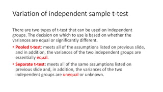
  • 74. Variation of independent sample t-test There are two types of t-test that can be used on independent groups. The decision on which to use is based on whether the variances are equal or significantly different. • Pooled t-test: meets all of the assumptions listed on previous slide, and in addition, the variances of the two independent groups are essentially equal. • Separate t-test: meets all of the same assumptions listed on previous slide and, in addition, the variances of the two independent groups are unequal or unknown.
  • 75. • Unfortunately, just like you cannot judge whether two means are different by just looking at the data set, you cannot judge whether two variances are equal or different without performing a statistical test. • The test statistic you use to compare variances is the F-statistic (Levene’s Test for Equality of Variances)
  • 76. • Recall that the Independent Samples t Test requires the assumption of homogeneity of variance -- i.e., both groups have the same variance. • SPSS conveniently includes a test for the homogeneity of variance, called Levene's Test, whenever you run an independent samples T test.
  • 77. • The hypotheses for Levene’s test are: • H0: σ1 2 - σ2 2 = 0 ("the population variances of group 1 and 2 are equal") H1: σ1 2 - σ2 2 ≠ 0 ("the population variances of group 1 and 2 are not equal") • This implies that if we reject the null hypothesis of Levene's Test, it suggests that the variances of the two groups are not equal; i.e., that the homogeneity of variances assumption is violated.
  • 78. F-statistic • The F-statistic is similar to the t-statistic in that it compares groups • Whereas the t-statistic is used to evaluate the differences in the mean of 2 groups, the F-statistic evaluates differences in the variance • The interpretation of the F-statistic is similar to the interpretation of the t-statistic, but is usually done based on the p-value rather than the confidence interval
  • 79. • The null hypothesis associated with the F-statistic is that there is no difference between the variances of the two groups • If the p-value or significance level is 0.05 or smaller you can reject the null hypothesis and assume that the groups have significantly different variances • If the p-value is greater than 0.05 you cannot reject the null hypothesis and you assume the variances are equal
  • 82. Sample SPSS output Independent Samples Test Levene's Test for Equality of Variances t-test for Equality of Means F Sig. t df Sig. (2-tailed) Mean Difference Std. Error Difference 95% Confidence Interval of the Difference Lower Upper histidin Equal variances assumed 5.743 .096 5.096 3 .015 83.500 16.385 31.355 135.645 Equal variances not assumed 6.418 2.296 .016 83.500 13.010 33.907 133.093
  • 83. There are two steps to the interpretation of this output: • First you look at the columns labeled Levene’s Test for Equality of Variances. • In those columns you will see the F-statistic and the significance of that statistic. • Since the significance is greater than 0.05 you cannot reject the null hypothesis and you can assume that the variances are equal.
  • 84. • Then, using that information you can use the row Equal variances assumed, which gives you the result of the paired t-test. • Again, the interpretation of this is based on the 95% confidence interval. • Here you see that upper and lower values have the same positive value so the confidence interval does not cross 0 and you can reject the null hypothesis of no difference in the means..
  • 85. Sample SPSS output Independent Samples Test Levene's Test for Equality of Variances t-test for Equality of Means F Sig. t df Sig. (2-tailed) Mean Difference Std. Error Difference 95% Confidence Interval of the Difference Lower Upper histidin Equal variances assumed 5.743 .096 5.096 3 .015 83.500 16.385 31.355 135.645 Equal variances not assumed 6.418 2.296 .016 83.500 13.010 33.907 133.093
  • 86. How to report t-tests • Values to report: means (M) and standard deviations (SD) for each group, t value (t), degrees of freedom (in parentheses next to t), and significance level (p). • Examples • Women (M = 3.66, SD = .40) reported significantly higher levels of happiness than men (M = 3.20, SD = .32), t(1) = 5.44, p < .05. • Men (M = 4.05, SD = .50) and women (M = 4.11, SD = .55) did not differ significantly on levels of political agreement, t(1) = 1.03, p = n.s.
  • 87. Reporting a significant single sample t-test (μ ≠ μ0): • Students taking statistics courses in Chemistry at the University of Lagos reported studying more hours for tests (M = 121, SD = 14.2) than did Unilag students in general, t(33) = 2.10, p = .034. Reporting a significant t-test for dependent groups (μ1 ≠ μ2): • Results indicate a significant preference for Meat pie (M = 3.45, SD = 1.11) over chicken pie (M = 3.00, SD = .80), t(15) = 4.00, p = .001.
  • 88. Reporting a significant t-test for independent groups (μ1 ≠ μ2): • Unilag students taking statistics courses in Psychology had higher IQ scores (M = 121, SD = 14.2) than did those taking statistics courses in Chemistry (M = 117, SD = 10.3), t(44) = 1.23, p = .09. • Over a two-day period, participants drank significantly fewer drinks in the experimental group (M= 0.667, SD = 1.15) than did those in the control group (M= 8.00, SD= 2.00), t(4) = -5.51, p=.005.
  • 92. Non parametric variants of t-tests • Where data is not normally distributed, statistical analyses that assume a normal distribution may be inappropriate. • This is especially a concern where the sample size is small (<50 in total). • Variables that are discrete (take only integer values) or have an upper or lower limit are by definition non-normal.
  • 93. • For one sample T tests that do not fulfil the normality assumption, use the Wilcoxin One Sample Signed Rank T Test • For 2 Related samples that do not fulfil the normality assumption, use the McNemar test. • For 2-Independent Groups, use Mann-Whitney U-test • For Related Ordinal Data, i.e. ordered categorical or quantitative variables that are not plausibly normal, the suggested procedure is to use the Wilcoxon procedure
  • 94. Summary • A t-test is a parametric test used to compare the means of two samples • There are different t-tests we can use based on the assumptions we can make – paired, pooled, and separate • To test your null hypothesis you need to know the type of t-test to use, the number of observations, the means of the two groups (or with pairs, the difference between the pairs), and the variances of the two groups
  • 95. • Single sample t – we have only 1 group; want to test against a hypothetical mean. • Dependent (Paired) t – we have two means. Either same people in both groups, or people are related, e.g., husband-wife, left hand- right hand. • Independent samples t – we have 2 means, 2 groups; no relation between groups, e.g., people randomly assigned to a single group.
  • 97. • You need to compare the variances of your groups using the F- statistic to chose between the pooled or separate tests
  • 98. ANOVA
  • 99. • ANOVA is short for ANalysis Of VAriance • The purpose of ANOVA is to determine whether the mean differences that are obtained for sample data are sufficiently large to justify a conclusion that there are mean differences between the populations from which the samples were obtained.
  • 100. • The difference between ANOVA and t tests is that ANOVA can be used in situations where there are two or more means being compared, whereas the t tests are limited to situations where only two means are involved.
  • 101. Assumptions for ANOVA • ASSUMPTION 1: The dependent variable is normally distributed for each of the populations as defined by the different levels of the factor • ASSUMPTION 2: The variances of the dependent variable are the same for all populations • ASSUMPTION 3: The cases represent random samples from the populations and the scores on the test variable are independent of each other
  • 102. Sample research questions for ANOVA • Is there a difference in average pain levels during tooth extraction among patients given 3 types of Local Anesthesia? • Are there differences in children’s weight by type of school (Public vs. missionary vs. private)?
  • 103. • Experiment to check the effects of caffeine on reading time among students. • 45 volunteers from a university to participate. Randomly assigns an equal number of students to three groups: placebo (group 1), mild doses of caffeine (group 2), and heavy doses of caffeine (group 3). • Before study, the average number of study hours for all the students was taken over 2 months. The intervention over the next 2 months with a cup of coffee or placebo every night and average hours of study was documented again.
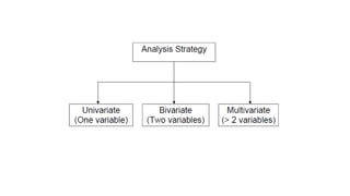
  • 105. The basic ANOVA situation **Two variables: 1 Categorical, 1 Quantitative Main Question: Do the (means of) the quantitative variables depend on which group (given by categorical variable) the individual is in? If categorical variable has only 2 values: • 2-sample t-test ANOVA allows for 3 or more groups
  • 106. • Analysis of variance is necessary to protect researchers from excessive risk of a Type I error in situations where a study is comparing more than two population means. • E.g., caffeine study with 3 populations taking coffee: • Population 1 - No caffeine • Population 2 - Mild dose • Population 3 - Heavy dose
  • 108. • We have at least 3 means to test, e.g., • H0: 1 = 2 = 3. • Could take them 2 at a time, but really want to test all 3 (or more) at once. • Although each t test can be done with a specific α-level (risk of Type I error), the α-levels accumulate over a series of tests so that the final experiment-wise α-level can be quite large
  • 109. • ANOVA allows researcher to evaluate all of the mean differences in a single hypothesis test using a single α-level and, thereby, keeps the risk of a Type I error under control no matter how many different means are being compared
  • 110. Example of an ANOVA situation Subjects: 25 patients with blisters Treatments: Treatment A, Treatment B, Placebo (categorical) Measurement: Number of days until blisters heal (quantitative) Data [and means]: • A: 5,6,6,7,7,8,9,10 [7.25] • B: 7,7,8,9,9,10,10,11 [8.875] • P: 7,9,9,10,10,10,11,12,13 [10.11] Are these differences significant?
  • 111. Informal Investigation Graphical investigation: • side-by-side box plots • multiple histograms ANOVA determines P-value from the F statistic
  • 112. Side by Side Boxplots
  • 113. What does ANOVA do? At its simplest ANOVA tests the following hypotheses: H0: The means of all the groups are equal. 1 = 2 = 3. Ha: Not all the means are equal • doesn’t say how or which ones differ. • Can follow up with “multiple comparisons” Note: we usually refer to the sub-populations as “groups” when doing ANOVA.
  • 114. Assumptions of ANOVA • Each group is approximately normal · check this by looking at histograms and/or normal quantile plots, or use assumptions · can handle some non-normality, but not severe outliers
  • 115. Normality Check We should check for normality using: • assumptions about population • histograms for each group • normal quantile (or QQ) plot for each group With such small data sets, there really isn’t a really good way to check normality from data, but we make the common assumption that physical measurements of people tend to be normally distributed.
  • 118. • The test statistic for ANOVA is an F-ratio, which is a ratio of two sample variances. • In the context of ANOVA, the sample variances are called mean squares, or MS values.
  • 119. Recall example of an ANOVA situation Subjects: 25 patients with blisters Treatments: Treatment A, Treatment B, Placebo (categorical) Measurement: Number of days until blisters heal (quantitative) Data [and means]: • A: 5,6,6,7,7,8,9,10 [7.25] • B: 7,7,8,9,9,10,10,11 [8.875] • P: 7,9,9,10,10,10,11,12,13 [10.11]
  • 120. Notation for ANOVA • n = number of individuals all together (25) • I = number of groups (3) • = mean for the entire data set is (??) Group A has • nA = # of individuals in group A • xAw = value for individual w in group A • = mean for group A • sA = standard deviation for group A A x A x
  • 121. Number of individuals all together (25) Group A Group B Group P N = 8 N = 8 N = 9
  • 122. How ANOVA works ANOVA measures two sources of variation in the data and compares their relative sizes • variation BETWEEN groups • for each data value look at the difference between its group mean and the overall mean • variation WITHIN groups • for each data value we look at the difference between that value and the mean of its group ( )2 A Aw x x − ( )2 x xA −
  • 123. The ANOVA F-statistic is a ratio of the Between Group Variation divided by the Within Group Variation: MSW MSB Within Between F = =
  • 124. • The top of the F-ratio MSbetween measures the size of mean differences between samples. • The bottom of the ratio MSwithin measures the magnitude of differences that would be expected without any outside effects. MSW MSB Within Between F = =
  • 125. • A large value for the F-ratio indicates that the obtained sample mean differences are greater than would be expected if the samples had no outside effect. • A large F is evidence against H0, since it indicates that there is more difference between groups than within groups. • F is another distribution like z and t. There are tables of F used for significance testing.
  • 126. 126 The Logic and the Process of Analysis of Variance • The two components of the F-ratio can be described as follows: • Between-Treatments Variability: MSbetween measures the size of the differences between the sample means. For example, suppose that three treatments, each with a sample of n = 5 subjects, have means of M1 = 1, M2 = 2, and M3 = 3. • Notice that the three means are different; that is, they are variable.
  • 127. 127 The Logic and the Process of ANOVA (cont.) • By computing the variance for the three means we can measure the size of the differences • Although it is possible to compute a variance for the set of sample means, it usually is easier to use the total, T, for each sample instead of the mean, and compute variance for the set of T values.
  • 128. 128 The Logic and the Process of ANOVA (cont.) Logically, the differences (or variance) between means can be caused by two sources: 1. Outside or Treatment Effects: If the treatments have different effects, this could cause the mean for one treatment to be higher (or lower) than the mean for another treatment. 2. Chance or Sampling Error: If there is no treatment effect at all, you would still expect some differences between samples. Mean differences from one sample to another are an example of random, unsystematic sampling error.
  • 129. Group A Group B Group P N = 8 N = 8 N = 9
  • 130. 130 The Logic and the Process of ANOVA (cont.) • Within-Treatments Variability: MSwithin measures the size of the differences that exist inside each of the samples. • Because all the individuals in a sample receive exactly the same treatment, any differences (or variance) within a sample cannot be caused by different treatments.
  • 131. Group A Group B Group P N = 8 N = 8 N = 9
  • 132. 132 The Logic and the Process of ANOVA Thus, these differences are caused by only one source: Chance or Error: The unpredictable differences that exist between individual scores are not caused by any systematic factors and are considered to be random, chance, or error.
  • 133. 133 The Logic and the Process of ANOVA (cont.) • Considering these sources of variability, the structure of the F-ratio becomes, treatment effect + chance/error F = ────────────────────── chance/error
  • 134. 134 The Logic and the Process of ANOVA (cont.) • When the null hypothesis is true and there are no differences between treatments, the F-ratio is balanced. • That is, when the "treatment effect" is zero, the top and bottom of the F-ratio are measuring the same variance. • In this case, you should expect an F-ratio near 1.00. When the sample data produce an F-ratio near 1.00, we will conclude that there is no significant treatment effect.
  • 135. 135 The Logic and the Process of ANOVA (cont.) • On the other hand, a large treatment effect will produce a large value for the F-ratio. Thus, when the sample data produce a large F-ratio we will reject the null hypothesis and conclude that there are significant differences between treatments. • To determine whether an F-ratio is large enough to be significant, you must select an α-level, find the df values for the numerator and denominator of the F-ratio, and consult the F- distribution table to find the critical value.
  • 138. A sample class question: • Do students' performance in exams vary depending on where they live? – Research Question • Independent variable: Where students live eg, Ikoyi, Ojota and Badagry • Dependent variable : Performance in exams (standard quiz) Ho: There is no difference in the mean score of students based on different residence i.e. mean of Ikoyi = mean of Ojota = mean of Badagry Ha: There is a difference in the mean score of students based on different residence i.e. mean of Ikoyi ≠ mean of Ojota ≠ mean of Badagry
  • 139. (Each score is over 10) • Ikoyi – scores of 3 students in tests: 3, 2, 1 • Ojota – scores of 3 students in tests: 5, 3, 4 • Badagry – scores of 3 students in tests: 5, 6, 7
  • 140. Manual procedure for computing 1-way ANOVA for independent samples • Step 1: Complete the table • Calculate the sum in each group • Calculate the mean in each group Ikoyi A Ojota B Badagry C 3 5 5 2 3 6 1 4 7
  • 141. Manual procedure for computing 1-way ANOVA for independent samples • Step 1: Complete the table • Calculate the sum in each group • Calculate the mean in each group Ikoyi A Ojota B Badagry C 3 5 5 2 3 6 1 4 7 Total 6 12 18
  • 142. Manual procedure for computing 1-way ANOVA for independent samples • Step 1: Complete the table • Calculate the sum in each group • Calculate the mean in each group • Mean for A = 6/3 = 2 • Mean for B = 12/3 = 4 • Mean for C = 18/3 = 6 Ikoyi A Ojota B Badagry C 3 5 5 2 3 6 1 4 7 Total 6 12 18 Mean 2 4 6
  • 143. Procedure for computing 1-way ANOVA for independent samples • Step 2: Calculate the Grand mean X = = = 6 + 12 + 18 = 4 9 Or the mean of group A + mean of group B + mean of group C k (number of groups) = 2 + 4 + 6 = 12/3 = 4 3 (X) N (XA+XB+XC) N Ikoyi A Ojota B Badagry C 3 5 5 2 3 6 1 4 7 Total 6 12 18 Mean 2 4 6 x
  • 144. Procedure for computing 1-way ANOVA for independent samples • Step 3: Compute total Sum of Squares SStotal= (every value – grand mean)2 This is done for each value in all the groups and added together to give the SStotal = (3-4)2 + (2-4)2 + (1-4)2 + (5-4)2 + (3-4)2 + (4-4)2 + (5-4)2 + (6-4)2 + (7-4)2 = 1 + 4 + 9 + 1 + 1 + 0 + 1 + 4 +9 = 30 SStotal= 30, dftotal = 8 Degree of freedom = (N – 1) = 9 – 1 = 8 (Recall that “N” is the number of sample size from ALL the population i.e. 3 students each from the different location) Ikoyi A Ojota B Badagry C 3 5 5 2 3 6 1 4 7 Total 6 12 18 Mean 2 4 6 Grand mean = 4
  • 145. Procedure for computing 1-way ANOVA for independent samples • Step 4: Compute between groups Sum of Squares • Compare the means of EACH group with the grand mean i.e for group A = (mean of grp A – grand mean)2 for the number of variables in the group This is the same as the value multiplied by the number of variables in each group. The same for grp B and Group C SSbet = Total sum of all the values i.e value for Grp A + value for Grp B + value for Grp C etc Ikoyi A Ojota B Badagry C 3 5 5 2 3 6 1 4 7 Total 6 12 18 Mean 2 4 6 Grand mean = 4
  • 146. Procedure for computing 1-way ANOVA for independent samples SSbet = Total sum of all the values i.e value for Grp A + value for Grp B + value for Grp C = (2-4)2 + (2-4)2 + (2-4)2 + (4-4)2 + (4-4)2 + (4-4)2 + (6-4)2 + (6-4)2 + (6-4)2 = 4 + 4 + 4 + 0 + 0 + 0 + 4 + 4 + 4 = 24 SSbet = 24, dfbet = 2 Degree of freedom = (k – 1) = 3 – 1 = 2 (Recall that “K” is the number of categories of the population) Ikoyi A Ojota B Badagry C 3 5 5 2 3 6 1 4 7 Total 6 12 18 Mean 2 4 6 Grand mean = 4
  • 147. Procedure for computing 1-way ANOVA for independent samples • Step 5: Compute within groups Sum of Squares • Note that: SStotal= SSwit + SSbet therefore, SSwit= SStotal – SSbet = 30 – 24 = 6 or Compare the values in EACH group with the group mean and square them = (3-2)2 + (2-2)2 + (1-2)2 + (5-4)2 + (3-4)2 + (4-4)2 + (5-6)2 + (6-6)2 + (7-6)2 = 1 + 0 + 1 + 1 + 1 + 0 + 1 + 0 + 1 = 6 SSwit= 6, dfwit = 6 Degree of freedom = (N – k) = 9 – 3 = 6 Ikoyi A Ojota B Badagry C 3 5 5 2 3 6 1 4 7 Total 6 12 18 Mean 2 4 6 Grand mean = 4
  • 148. Procedure for computing 1-way ANOVA for independent samples • Step 6: Determine the d.f. for each sum of squares dftotal= (N - 1) = 8 dfbet= (k - 1) = 2 dfwit= (N - k) = 6 N = total number of records K = number of groups
  • 150. Systematic Variance (between means) Error Variance (within means) Procedure for computing 1-way ANOVA for independent samples • Step 7/8: Estimate the Variances & Compute F = = SSbet dfbet SSwit dfwit MSbetween MSwithin MSW MSB Within Between F = =
  • 152. In Summary (The formula) MSW MSB F DF SS MS SST SSB SSW x x n x x SSB df s x x SSW DFT s x x SST groups i i obs i i groups i obs i ij obs ij = = = + − = − = = − = = − =      ; ; ) ( ) ( ) ( ) ( ) ( ) ( 2 2 2 2 2 2
  • 153. Procedure for computing 1-way ANOVA for independent samples • Step 9: Consult F distribution table (it has 2 sides: d1 and d2) d1 is your df for the numerator (i.e. systematic variance) dfbetween d2 is your df for the denominator (i.e. error variance) dfwithin
  • 154. F – Table d1 = 2 and d2 = 6
  • 155. • A large F is evidence against H0, since it indicates that there is more difference between groups than within groups • Calculated F- ratio was 12 • Reading from F-Table at 0.05 level was 5.14 • Conclusion: reject H0 Ho: There is no difference in the mean score of students based on different residence i.e. mean of Ikoyi = mean of Ojota = mean of Badagry Ha: There is a difference in the mean score of students based on different residence i.e. mean of Ikoyi ≠ mean of Ojota ≠ mean of Badagry
  • 156. Independent 1-way ANOVA: SPSS Output ANOVA Maths Sum of Squares df Mean Square F Sig. Between Groups 24.000 2 12.000 12.000 .008 Within Groups 6.000 6 1.000 Total 30.000 8
  • 157. The computation of F statistic is illustrated in the following table, called ANOVA table. Source of variance Degrees of freedom Sum of squares Mean square F ratio Between k-1 SSB MSB=BSS/ (k-1) MSB/MSW Within n-k SSW MSW=WSS/(n-k) Total n-1 SST
  • 158. 158 Analysis of Variance and Post Tests • The null hypothesis for ANOVA states that for the general population there are no mean differences among the treatments being compared; H0: μ1 = μ2 = μ3 = . . . • When the null hypothesis is rejected, the conclusion is that there are significant mean differences. • However, the ANOVA simply establishes that differences exist, it does not indicate exactly which groups, intervention, categories or treatments are different.
  • 159. • If the t-test is significant, you have a difference in population means. • If the F-test is significant, you have a difference in population means. But you don’t know where. • With 3 means, could be A=B>C or A>B>C or A>B=C.
  • 160. 160 Analysis of Variance and Post Tests • With more than two treatments, this creates a problem. • Specifically, you must follow the ANOVA with additional tests, called post tests, to determine exactly which treatments are different and which are not. • The Scheffe test and Tukey’s HSD are examples of post tests. • HSD means honestly significant difference
  • 161. • These tests are done after an ANOVA where H0 is rejected with more than two treatment conditions. The tests compare the treatments, two at a time, to test the significance of the mean differences.
  • 162. Multiple Comparisons Dependent Variable: Maths Tukey HSD (I) Location (J) Location Mean Difference (I-J) Std. Error Sig. 95% Confidence Interval Lower Bound Upper Bound Ikoyi Ojota -2.00000 .81650 .109 -4.5052 .5052 Badagry -4.00000* .81650 .006 -6.5052 -1.4948 Ojota Ikoyi 2.00000 .81650 .109 -.5052 4.5052 Badagry -2.00000 .81650 .109 -4.5052 .5052 Badagry Ikoyi 4.00000* .81650 .006 1.4948 6.5052 Ojota 2.00000 .81650 .109 -.5052 4.5052 *. The mean difference is significant at the 0.05 level. Mean of Ikoyi = 2. Ojota = 4 and Badagry = 6 POST-HOC TEST
  • 163. One-Way Analysis of Variance with SPSS • Select an independent variable with three or more levels and a dependent variable. • Develop the null hypothesis and the alternative hypothesis for main effects. • Using SPSS, calculate an ANOVA. Include a post hoc test. • Report on the p value and the confidence interval. • Interpret the confidence interval. • Decide whether to reject or retain the null hypothesis based on main effects and/or post-hoc statistical tests.
  • 164. How to report ANOVA • A one-way between subjects ANOVA was conducted to compare the effect of (IV)______________ on (DV)_______________ in _________________, __________________, and __________________ conditions.” • There was a significant (not a significant) effect of IV ____________ on DV ______________ at the p<.05 level for the three conditions [F(df1, df2) = ___, p = ____].
  • 166. For our class example: There was a significant effect of the location of residence on the performance of students at p < .05 [F(2, 6) = 12, p = .008] ANOVA Maths Sum of Squares df Mean Square F Sig. Between Groups 24.000 2 12.000 12.000 .008 Within Groups 6.000 6 1.000 Total 30.000 8
  • 167. • The Kruskal-Wallis test is a nonparametric (distribution free) test, and is used when the assumptions of one-way ANOVA are not met. • Both the Kruskal-Wallis test and one-way ANOVA assess for significant differences on a continuous dependent variable by a categorical independent variable (with two or more groups)
  • 168. • The most common use of the Kruskal–Wallis test is when you have one nominal variable and one measurement variable, an experiment that you would usually analyze using one-way ANOVA, but the measurement variable does not meet the normality assumption of a one-way ANOVA
  • 169. Next Class • Quantitative Data Analysis Lecture 4 • Regressions. • Contingency Table Analysis
  • 170. Sample SPSS Analysis • I have a sample SPSS data with the following variables • Age:Continuous • Sex: Nominal (Binary) • Basic Metabolic Index (BMI): Continuous • Lipid Level: Continuous • Stroke: Nominal (Binary) • Hypertension: Nominal (Binary) • Educational Level: Ordinal • Income per day: Continuous
  • 171. Comparison Tests Differences among group means Statistical tests Predictor variable Outcome variable Sample research question Paired t-test • Categorical • 1 predictor • Quantitative • Groups come from the same population What is the difference in the average knowledge of the choice of data analysis before and after this lecture in this group Independent sample t- test • Categorical • 1 predictor • Quantitative • Groups come from different populations What is the difference in the average knowledge of the choice of data analysis in group A and group B ANOVA • Categorical • 1 or more predictor • Quantitative • 1 outcome What is the difference in average pain levels during tooth removal among patients given 3 types of Local Anesthesia
  • 172. Statistical tests Predictor variable Outcome variable Sample research question One Sample T- Test • Continuous • Quantitative • One population Is there an improvement in lipids after a vegetarian diet over 3 days? Cut off of 200 Paired t-test • Categorical • 1 predictor • Quantitative • Groups come from the same population What is the difference in the average basic metabolic index (BMI) before and after this lecture in this group Independent sample t-test • Categorical • 1 predictor • Quantitative • Groups come from different populations What is the difference in the average basic metabolic index (BMI) after this lecture in males and females
  • 173. Analysis of Variance (ANOVA) Statistical tests Predictor variable Outcome variable Sample research question ANOVA • Categorical • 1 or more predictor • Quantitative • 1 outcome What is the difference in baseline BMI among the different Educational level