SlideShare a Scribd company logo
FLUID KINEMATICS
MODULE 2
INTRODUCTION
 Fluids have a tendency to move or flow even if there exists a very small shear stress.
 The study of velocity and acceleration of a flowing fluid and the description and visualization
of the fluid motion are dealt with fluid kinematics.
Methods of describing fluid motion
 Two Methods:
1. Eulerian Method:
 concerned with field of flow.
 The properties (pressure, velocity, density etc.) are expressed as function of space and time.
F = f(x, y, z, t)
2. Lagrangian Method:
 follows an individual particle( or given mass) flowing through the flow field and thus
determines the fluid properties of individual particles or masses as a function of time like
p(t), v(t) etc.
 A fluid consists of large number of particles, therefore it is convenient to use the
Eulerian method for describing the fluid motion.
System and control volume
 SYSTEM :
 It refers to a fixed, identifiable quantity of mass in space:
 Three types of system: open system, closed system, isolated system.
 SURROUNDING:
 All other matter around the system is called surrounding
 BOUNDARY:
 The system boundaries forming a closed surface separates the system from
surrounding.
 The system boundary may be fixed or movable but there is no mass transfer occurs
across the system boundaries.
Example:
Consider a piston cylinder assembly:
• If the assembly is heated from out side, the
gas expands and the piston moves.
• Alternatively the gas in the cylinder can be
compressed by moving the piston.
• Although heat and work have transferred
through the boundary but there is no mass
transfer across the boundary.
 In case of fluid flow in pipes, channels, nozzles etc. it is difficult to focus attention
on fixed identifiable quantity of mass.
 It is convenient to focus attention on a volume, in a flow field, through which the
fluid flows. This volume is called control volume.
 Control volume:
 May be defined as an arbitrary volume in a flow field through which the fluid
flows
 The geometric boundary of the control volume is called control surface, that
may be real or imaginary or may beat rest or in motion.
Example:
Control volume for fluid flow in a pipe:
• The inside surface of pipe forms real
control surface.
• The vertical portions of control volume
are imaginary.
Points to remember:
• The size and shape of control volume can
be chosen arbitrarily.
• The location of control surface affects the
computational procedure
Types of fluid flow


Visual description of fluid pattern
 While dealing with fluid flow problems, it is often advantageous to obtain a
visual representation of a flow field.
 The pattern of flow can be visualized in many different ways.
 Photographs
 Colored dyes
 flakes
 Hydrogen bubbles etc.
Path lines are the trajectories that individual fluid particles follow. These can be thought of as "recording" the
path of a fluid element in the flow over a certain period. The direction the path takes will be determined by the
streamlines of the fluid at each moment in time.
Timelines are the lines formed by a set of fluid particles that were marked at a previous instant in time,
creating a line or a curve that is displaced in time as the particles move.
Streamlines are a family of curves that are
instantaneously tangent to the velocity vector
of the flow. These show the direction a
massless fluid element will travel in at any
point in time.
There can be no flow across a streamline
Streak lines are the locus of points of all the
fluid particles that have passed continuously
through a particular spatial point in the past.
Dye steadily injected into the fluid at a fixed
point extends along a streak line.
 Stream tube:
 A typical set of neighboring streamlines that forms a passage through which
the fluid flows is called stream tube.
 No flow is possible across a stream tube except through its ends.
 The stream tube need not be a solid and are fluid surface.
 Stream filament:
 It is a stream tube with its cross section sufficiently small so that variation of
velocity over it may be considered negligible.
Velocity field

Acceleration of fluid particle in a velocity field

Streamline patterns and corresponding convective accelerations.

Therefore, ………………(1)
………………(2)
………………(3)
So, the total acceleration is obtained by combining the acceleration given by the above three equations
………………(4)
………………(5)
Mass conservation(continuity Equation along
a stream tube
• The principle of mass conservation is valid for a flowing fluid.
• In a fixed region of flow constituting a control volume, mass of fluid entering the volume per unit time
must be equal to the mass of fluid leaving the control volume per unit time plus (or minus) the increase
(or decrease) of mass of fluid in the control volume per unit time.
• But for steady flow there can not be any change in mass within the control volume
Consider a stream tube of varying cross section
Differential equation of mass conservation
………………………….……………………(1)
………………………….……………………(2)
………………………….……………………(3)
Now total rate of mass flow to the control volume
………….……………………(4)
…………………………(5)
This equation is called the continuity equation in Cartesian coordinates.
In vector form
…………………………(6)
In cylindrical polar coordinates the continuity equation can be written as
…………………………(7)
…………….………….(8)
…………….………….(9)
…………….………….(10)
Consider a transparent plane parallel and at a unit distance from the board.
Module 2 of fluid machines - Kinematics of fluids
The partial derivative of the stream function with respect to any direction gives the
velocity component at 90o
anticlockwise to that direction.
The stream function is only defined for two dimensional in compressible flow, for which the continuity
equation can be written as
Putting the values of u and v from equation 1 and 2, we will get
This shows that the stream function always satisfies the continuity equation.
In polar coordinates
…………….(3)
…………….(4)
Fluid displacements
An infinitesimal element of fluid may move in fluid such
that the elements undergoes following basic
displacements.
1. Translation:
The elements moves bodily without being rotated or
deformed
2. Rotation:
Planes( top, base and sides of element) and medians as
well as diagonal of the element may change as a result of
their rotation about any one (or all three) of the
coordinate axes.
4. Linear deformation:
Shapes of the elements gets changed without change
in orientation of the element. The planes ( top, base
and sides of the element) as well as the median lines
of the elements are displaced while remaining parallel
to their original position.
3. Angular deformation:
It involves a distortion of the fluid element in which planes
that were initially perpendicular to each other are no longer
so.
Fluid rotation
• Counter clock wise rotation is considered to be positive.
• If the fluid particles in a flow region have rotation about any axis the flow is called
rotational flow or vortex flow.
• If the fluid particles in a flow region do not have rotation about any axis the flow is called
irrotational flow
………………………(A)
Consider the motion of a fluid particle in xy-plane
Derivation of expression for Rotation
The angular velocity of the line OA can be written as
and
Now, the rotation of fluid element about z-axis a per definition of rotation can be written as
Similarly the rotation of fluid element
about x and y axis can be found out as
………………………….(1)
………………………….(2)
………………………….(3)
Hence from equation A
………………………….(B)
In vector form
………………………….(C)
Another measure of rotation of fluid element is vorticity which is equal to twice the rotation
………………………….(4)
………………………….(5)
………………………….(6)
………………………….(D)
Angular deformation
here
And,
So,
Circulation
For closed curve OACB
Or,
Or,
This means circulation per unit area is equal to the vorticity or twice the rotation
The circulation around the closed curve ABPCA is given by:
Or,
Where,
vs is the component of velocity along ds
Or,
Or,
Or,
Substituting the value of u, v and w in continuity equation we will get
Now vorticity,
Since,
Flow Nets
• To check the squareness of a grid one can join
the diagonals of all the squares, the diagonals
also should result into a grid of squares
Combination of flow patterns
The magnitude or velocity components of the
resultant motion are given by the algebraic sum
of those for the constituent motion.
Example:
Q1
Module 2 of fluid machines - Kinematics of fluids
The Acceleration Field of a Fluid
 Velocity is a vector function of position and time and thus
has three components u, v, and w, each a scalar field in
itself.
 This is the most important variable in fluid mechanics:
Knowledge of the velocity vector field is nearly
equivalent to solving a fluid flow problem.
 The acceleration vector field a of the flow is derived
from Newton’s second law by computing the total time
derivative of the velocity vector:
36
 Since each scalar component (u, v , w) is a function of
the four variables (x, y, z, t), we use the chain rule to
obtain each scalar time derivative. For example,
 But, by definition, dx/dt is the local velocity
component u, and dy/dt =v , and dz/dt = w.
 The total time derivative of u may thus be written as
follows, with exactly similar expressions for the time
derivatives of v and w:
The Acceleration Field of a Fluid
37
 Summing these into a vector, we obtain the total
acceleration
:
The Acceleration Field of a Fluid
38
 The term δV/δt is called the local acceleration, which
vanishes if the flow is steady-that is, independent of
time.
 The three terms in parentheses are called the convective
acceleration, which arises when the particle moves
through regions of spatially varying velocity, as in a nozzle
or diffuser.
 The gradient operator is given by:
The Acceleration Field of a Fluid
39
Example 1. Acceleration field
Given the eulerian velocity vector field
find the total acceleration of a particle.
Solution step 2: In a similar manner, the convective acceleration
terms, are
40
Solution step 2: In a similar manner, the
convective acceleration terms, are
41
Example 2. Acceleration field
 An idealized velocity field is given by the formula
 Is this flow field steady or unsteady? Is it two- or three
dimensional? At the point (x, y, z) = (1, 1, 0), compute
the acceleration vector.
Solution
 The flow is unsteady because time t appears explicitly in
the components.
 The flow is three-dimensional because all three velocity
components are nonzero.
 Evaluate, by differentiation, the acceleration vector at (x, y,
z)
= (−1, +1, 0).
42
Example 2.
Acceleration field
43
Exercise 1
 The velocity in a certain two-dimensional flow field is
given by the equation
where the velocity is in m/s when x, y, and t are in meter and
seconds, respectively.
1. Determine expressions for the local and convective
components of acceleration in the x and y directions.
2. What is the magnitude and direction of the velocity and
the acceleration at the point x = y = 2 m at the time t = 0?
44
The Differential Equation of Mass Conservation
 Conservation of mass, often called the continuity relation,
states that the fluid mass cannot change.
 We apply this concept to a very small region. All the basic
differential equations can be derived by considering
either an elemental control volume or an elemental
system.
 We choose an infinitesimal fixed control volume (dx, dy,
dz), as in shown in fig below, and use basic control volume
relations.
 The flow through each side of the element is approximately
one-dimensional, and so the appropriate mass
conservation relation to use here is
45
 The element is so small that the volume integral
simply reduces to a differential term:
The Differential Equation of Mass
Conservation
46
The Differential Equation of Mass Conservation
 The mass flow terms occur on all six faces, three inlets and
three outlets.
 Using the field or continuum concept where all fluid
properties are considered to be uniformly varying
functions of time and position, such as ρ= ρ (x, y, z, t).
 Thus, if T is the temperature on the left face of the
element,
the right face will have a slightly different temperature
 For mass conservation, if ρu is known on the left face, the
value of this product on the right face is
47
 Introducing these terms into the main relation
 Simplifying gives
The Differential Equation of Mass
Conservation
48
 enables us to rewrite the equation of continuity in
a compact form
 so that the compact form of the continuity relation
is
The Differential Equation of Mass Conservation
 The vector gradient operator
49
Incompressible Flow
 A special case that affords great simplification is
incompressible flow, where the density changes are
regardless of whether the
negligible. Then
flow is steady or unsteady,
 The result
 is valid for steady or unsteady incompressible flow. The
two coordinate forms are
The Differential Equation of Mass Conservation
50
The Differential Equation of Mass Conservation
 The criterion for incompressible flow is
 where Ma = V/a is the dimensionless Mach number of
the flow.
 For air at standard conditions, a flow can thus be
considered incompressible if the velocity is less than
about 100 m/s.
51
Example 3
 Consider the steady, two-dimensional velocity field given by
 Verify that this flow field is incompressible.
Solution
 Analysis. The flow is two-dimensional, implying no z component of
velocity and no variation of u or v with z.
 The components of velocity in the x and y directions respectively are
 To check if the flow is incompressible, we see if the
incompressible continuity equation is satisfied:
 So we see that the incompressible continuity equation is indeed
satisfied. Hence the flow field is incompressible.
24
Example 4
 Consider the following steady, three-dimensional velocity
field in Cartesian coordinates:
where a, b, c, and d are constants. Under what conditions is
this flow field incompressible?
Solution
Condition for incompressibility:
 Thus to guarantee incompressibility, constants a and c must
satisfy the following relationship:
a = −3c
53
Example 5
 An idealized incompressible flow has the proposed three-
dimensional velocity distribution
 Find the appropriate form of the function f(y) which
satisfies the continuity relation.
 Solution: Simply substitute the given velocity components
into the incompressible continuity equation:
54
Example 6
 For a certain incompressible flow field it is suggested that the
velocity components are given by the equations
Is this a physically possible flow field? Explain.
55
Example 7
 For a certain incompressible, two-dimensional flow
field the velocity component in the y direction is given
by the equation
 Determine the velocity in the x direction so that
the continuity equation is satisfied.
56
Example 7 -
solution
57
Example 8
 The radial velocity component in an incompressible, two
dimensional flow field is
 Determine the corresponding tangential velocity
component, required to satisfy conservation of mass.
Solution.
 The continuity equation for incompressible steady flow
in cylindrical coordinates is given by
58
Example 8
59
The Stream Function
 Consider the simple case of incompressible, two-dimensional
flow in the xy-plane.
 The continuity equation in Cartesian coordinates reduces to
(1)
 A clever variable transformation enables us to rewrite this
equation (Eq. 1) in terms of one dependent variable (ψ)
instead of two dependent variables (u and v).
 We define the stream function ψ as
(2)
60
 Substitution of Eq. 2 into Eq. 1 yields
 which is identically satisfied for any smooth function ψ(x, y).
What have we gained by this transformation?
 First, as already mentioned, a single variable (ψ) replaces two
variables (u and v)—once ψ is known, we can generate both u and v
via Eq. 2 and we are guaranteed that the solution satisfies continuity,
Eq. 1.
 Second, it turns out that the stream function has useful
physical significance . Namely, Curves of constant ψ are
streamlines of the flow.
The Stream Function
61
 This is easily proven by
considering a streamline in
the xy-plane
The Stream Function
Curves of constant stream function
represent streamlines of the flow
62
 Along a line of constant ψ we
have dψ = 0 so that
 and, therefore, along a line
of constant ψ
The Stream Function
 The change in the value of ψ as
we move from one point (x, y) to
a nearby point (x + dx, y + dy)
is given by the relationship:
63
 Along a streamline:
 where we have applied Eq. 2, the definition of ψ. Thus along
a
streamline:
 But for any smooth function ψ of two variables x and y, we
know by the chain rule of mathematics that the total change
of ψ from point (x, y) to another point (x + dx, y + dy) some
infinitesimal distance away is
The Stream Function
64
 Total change of ψ:
 By comparing the above two equations we see that dψ = 0
along a streamline;
The Stream Function
65
 and the velocity components,
and
can be related to
the stream function, through the
equations
The Stream Function
 In cylindrical coordinates the continuity equation for
incompressible, plane, two dimensional flow reduces to
66
The Differential Equation of Linear Momentum
 Using the same elemental control volume as in mass
conservation, for which the appropriate form of the
linear momentum relation is
67
 The momentum fluxes occur on all six faces, three
inlets and three outlets.
The Differential Equation of Linear Momentum
 Again the element is so small that the volume integral
simply reduces to a derivative term:
68
 A simplification occurs if we split up the term in
brackets as follows:
 The term in brackets on the right-hand side is seen to be
the equation of continuity, which vanishes identically
The Differential Equation of Linear Momentum
 Introducing these terms
69
 Thus now we have
 This equation points out that the net force on the control
volume must be of differential size and proportional to
the element volume.
The Differential Equation of Linear Momentum
 The long term in parentheses on the right-hand side is the
total acceleration of a particle that instantaneously
occupies the control volume:
70
The Differential Equation of Linear Momentum
 These forces are of two types, body forces and surface
forces.
 Body forces are due to external fields (gravity,
magnetism, electric potential) that act on the entire mass
within the element.
 The only body force we shall consider is gravity.
 The gravity force on the differential mass ρ dx dy dz
within
the control volume is
 The surface forces are due to the stresses on the sides of the
control surface. These stresses are the sum of hydrostatic
pressure plus viscous stresses τij that arise from motion with
velocity gradients
71
The Differential Equation of
Linear Momentum
72
Fig. Elemental Cartesian fixed
control volume showing the
surface forces in the x direction
only.
 Splitting into pressure plus viscous stresses
 where dv = dx dy dz.
 Similarly we can derive the y and z forces per unit volume
on the control surface
The Differential Equation of Linear Momentum
 The net surface force in the x direction is given by
73
 The net vector surface force can be written
as
The Differential Equation of
Linear Momentum
74
 is the viscous stress tensor acting on the element
 The surface force is thus the sum of the pressure
gradient vector and the divergence of the viscous stress
tensor
The Differential Equation of Linear Momentum
 In divergence form
75
 In words
The Differential Equation of Linear Momentum
 The basic differential momentum equation for an
infinitesimal element is thus
76
 This is the differential momentum equation in its full glory,
and it is valid for any fluid in any general motion,
particular fluids being characterized by particular viscous
stress terms.
The Differential Equation of Linear Momentum
 the component equations are
77
Newtonian Fluid: Navier-Stokes Equations
 For a newtonian fluid, the viscous stresses are
proportional to the element strain rates and the coefficient
of viscosity.
 where μ is the viscosity coefficient
 Substitution gives the differential momentum equation for a
newtonian fluid with constant density and viscosity:
78
 These are the incompressible flow Navier-Stokes
equations named after C. L. M. H. Navier (1785–1836) and
Sir George G. Stokes (1819–1903), who are credited with
their derivation.
Newtonian Fluid: Navier-
Stokes Equations
79
Inviscid Flow
 Shearing stresses develop in a moving fluid because of
the viscosity of the fluid.
 We know that for some common fluids, such as air and
water, the viscosity is small, therefore it seems reasonable
to assume that under some circumstances we may be able
to simply neglect the effect of viscosity (and thus
shearing stresses).
 Flow fields in which the shearing stresses are assumed to
be negligible are said to be inviscid, nonviscous, or
frictionless.
 For fluids in which there are no shearing stresses the
normal stress at a point is independent of direction—that
is σxx = σyy = σzz.
80
Euler’s Equations of Motion
 For an inviscid flow in which all the shearing stresses are
zero and the Euler’s equation of motion is written as
 In vector notation Euler’s equations can be expressed as
Inviscid Flow
81
Vorticity and Irrotationality
 The assumption of zero fluid angular velocity, or
irrotationality, is a very useful simplification.
 Here we show that angular velocity is associated with
the curl of the local velocity vector.
 The differential relations for deformation of a fluid
element can be derived by examining the Fig. below.
 Two fluid lines AB and BC, initially perpendicular at time t,
move and deform so that at t + dt they have slightly
different lengths A’B’ and B’C’ and are slightly off the
perpendicular by angles dα and dβ.
82
Vorticity and
Irrotationality
83
 But from the fig. dα and dβ are each directly related
to velocity derivatives in the limit of small dt:
 Substitution results
Vorticity and Irrotationality
 We define the angular velocity ωz about the z axis as the
average rate of counterclockwise turning of the two lines:
84
is thus one-half the curl of
 The vector
the velocity vector
 A vector twice as large is called the vorticity
Vorticity and
Irrotationality
85
Vorticity and Irrotationality
 Many flows have negligible or zero vorticity and are
called
irrotational.
 Example. For a certain two-dimensional flow field the
velocity is given by the equation
 Is this flow irrotational?
Solution.
 For the prescribed velocity field
86
Vorticity and
Irrotationality
87
Velocity Potential
 The velocity components of irrotational flow can be
expressed in terms of a scalar function (
ϕ x, y, z, t) as
 where ϕ is called the velocity potential.
 In vector form, it can be written as
 so that for an irrotational flow the velocity is expressible
as the gradient of a scalar function .
ϕ
 The velocity potential is a consequence of the
irrotationality of the flow field, whereas the stream
function is a consequence of conservation of mass
88
Velocity Potential
 It is to be noted, however, that the velocity potential can
be defined for a general three-dimensional flow, whereas
the stream function is restricted to two-dimensional
flows.
 For an incompressible fluid we know from conservation of
mass that
 and therefore for incompressible, irrotational flow (with
) it follows that
89
Velocity
Potential
 This differential equation arises in
many different areas of engineering
and physics and is called
Laplace’s equation. Thus,
inviscid, incompressible,
irrotational flow fields are
governed by Laplace’s equation.
 This type of flow is commonly called
a potential flow.
 Potential flows are irrotational flows.
That is, the vorticity is zero
throughout. If vorticity is present
(e.g., boundary layer, wake), then the
flow cannot be described by Laplace’s
equation.
64
Velocity Potential
 For some problems it will be convenient to use cylindrical
coordinates, r,θ, and z. In this coordinate system the
gradient operator is
91
Velocity
Potential
92
Example 1
 The two-dimensional flow of a nonviscous, incompressible fluid
in the vicinity of the corner of Fig. is described by the stream
function
 where ψ has units of m2/s when r is in meters. Assume the fluid
density is 103 kg/m3 and the x–y plane is horizontal that is, there
is no difference in elevation between points (1) and (2).
FIND
a) Determine, if possible, the corresponding velocity potential.
b) If the pressure at point (1) on the wall is 30 kPa, what is
the pressure at point (2)?
93
Example 1
Solution
 The radial and tangential velocity components can be
obtained from the stream function as
94
Solution
95
96
97
98
Source and Sink
 Consider a fluid flowing radially outward from a line
through the origin perpendicular to the x–y plane as is
shown in Fig. Let m be the volume rate of flow
emanating from the line (per unit length), and therefore to
satisfy conservation of mass
 or
99
 It follows that
 If m is positive, the flow is radially outward, and the flow
is considered to be a source flow. If m is negative, the flow
is toward the origin, and the flow is considered to be a sink
flow. The flowrate, m, is the strength of the source or sink.
Source and Sink
 A source or sink represents a purely radial flow.
 Since the flow is a purely radial flow, ,
the corresponding velocity potential can be
obtained by integrating the equations
100
 To yield
 The streamlines (lines of ψ = constant ) are radial lines, and
the equipotential lines (lines of = constant) are
ϕ
concentric circles centered at the origin.
Source and Sink
 The stream function for the source can be obtained
by integrating the relationships
101
Example 2
 A nonviscous, incompressible fluid flows between wedge-
shaped walls into a small opening as shown in Fig. The
velocity potential (in ft/s2), which approximately
describes this flow is
 Determine the volume rate of flow (per unit length) into
the
opening.
102
The negative sign indicates that the flow is toward the
opening,
that is, in the negative radial direction
103
Vortex
82
 We next consider a flow field in which the streamlines are
concentric circles—that is, we interchange the velocity
potential and stream function for the source. Thus, let
and
where K is a constant. In this
case the streamlines are
concentric circles with
and
This result indicates that the tangential velocity varies
inversely with the distance from the origin
 A mathematical concept commonly associated with
vortex motion is that of circulation. The circulation, Γ, is
defined as the line integral of the tangential component
of the velocity taken around a closed curve in the flow
field. In equation form, Γ, can be expressed as
83
Circulation
where the integral sign
means that the integration
is taken around a closed
curve, C, in the
counterclockwise
direction, and ds is a
differential length along
the curve
,
 This result indicates that for an irrotational flow the
circulation will generally be zero.
 However, for the free vortex with , the
circulation around the circular path of radius r is
 which shows that the circulation is nonzero.
 However, for irrotational flows the circulation around any path
that does not include a singular point will be zero.
84
Circulation
 For an irrotational flow
Circulation
 The velocity potential and stream function for the free
vortex are commonly expressed in terms of the circulation
as
and
107

More Related Content

PPT
Introduction to FLUID MECHANICS & KINEMATICS
PDF
Fluid Kinematics fluid dynamics mechanical
PPTX
Motion of fluid particles and streams
PPTX
Fluid mechanics - Motion of Fluid Particles and Stream
PDF
Fluid mechanics notes for gate
PPT
Module-3_FLUID KINEMATICS AND DYNAMICS.ppt
PPTX
Fluid_Kinematics_Presentation_6666.pptxx
Introduction to FLUID MECHANICS & KINEMATICS
Fluid Kinematics fluid dynamics mechanical
Motion of fluid particles and streams
Fluid mechanics - Motion of Fluid Particles and Stream
Fluid mechanics notes for gate
Module-3_FLUID KINEMATICS AND DYNAMICS.ppt
Fluid_Kinematics_Presentation_6666.pptxx

Similar to Module 2 of fluid machines - Kinematics of fluids (20)

PDF
Chapter 4. diffrential
PPT
5. fm 5 fluid flow co 2 adam
PDF
Chapter four fluid mechanics
PDF
Fluid Kinematics PDF of the university of Lagos Nigeria
PPTX
flow pattern OF A FLUID PARTICLES .pptx
PPT
Lecture14c
PPTX
Fluid kinematics
PPTX
fluid kinematicspresentation by pritika prajapati
PPT
Fluid Mechanics and Hydraulics_Lec 02_fluid dynamics_Omeaga.ppt
PPTX
Fluid kinematics
PPT
6. fm 6 vorti cons co 2 adam
PDF
Fluid dynamics
PDF
Review of basic Aerodynamics.pdf
PDF
lecture 2.pdf
PPTX
FLUID DYNAMICS [EQUATIONS OF MOTION].pptx
PPTX
Chapter 4 Flowing Fluids Pressure Variations (1).pptx
PPT
FluidKinematics.ppt
PDF
Fluid Mechanics: Fluid Kinematics and Compressible Flow
Chapter 4. diffrential
5. fm 5 fluid flow co 2 adam
Chapter four fluid mechanics
Fluid Kinematics PDF of the university of Lagos Nigeria
flow pattern OF A FLUID PARTICLES .pptx
Lecture14c
Fluid kinematics
fluid kinematicspresentation by pritika prajapati
Fluid Mechanics and Hydraulics_Lec 02_fluid dynamics_Omeaga.ppt
Fluid kinematics
6. fm 6 vorti cons co 2 adam
Fluid dynamics
Review of basic Aerodynamics.pdf
lecture 2.pdf
FLUID DYNAMICS [EQUATIONS OF MOTION].pptx
Chapter 4 Flowing Fluids Pressure Variations (1).pptx
FluidKinematics.ppt
Fluid Mechanics: Fluid Kinematics and Compressible Flow
Ad

Recently uploaded (20)

PPTX
Sustainable Sites - Green Building Construction
PDF
Evaluating the Democratization of the Turkish Armed Forces from a Normative P...
PDF
July 2025 - Top 10 Read Articles in International Journal of Software Enginee...
PPTX
MET 305 2019 SCHEME MODULE 2 COMPLETE.pptx
PPTX
Construction Project Organization Group 2.pptx
PDF
composite construction of structures.pdf
PPTX
Foundation to blockchain - A guide to Blockchain Tech
PDF
Mohammad Mahdi Farshadian CV - Prospective PhD Student 2026
PPTX
UNIT-1 - COAL BASED THERMAL POWER PLANTS
PDF
PRIZ Academy - 9 Windows Thinking Where to Invest Today to Win Tomorrow.pdf
PPT
Project quality management in manufacturing
PPTX
Engineering Ethics, Safety and Environment [Autosaved] (1).pptx
PPT
CRASH COURSE IN ALTERNATIVE PLUMBING CLASS
PDF
Enhancing Cyber Defense Against Zero-Day Attacks using Ensemble Neural Networks
PDF
R24 SURVEYING LAB MANUAL for civil enggi
PDF
The CXO Playbook 2025 – Future-Ready Strategies for C-Suite Leaders Cerebrai...
PDF
PPT on Performance Review to get promotions
PDF
SM_6th-Sem__Cse_Internet-of-Things.pdf IOT
PDF
TFEC-4-2020-Design-Guide-for-Timber-Roof-Trusses.pdf
PDF
BMEC211 - INTRODUCTION TO MECHATRONICS-1.pdf
Sustainable Sites - Green Building Construction
Evaluating the Democratization of the Turkish Armed Forces from a Normative P...
July 2025 - Top 10 Read Articles in International Journal of Software Enginee...
MET 305 2019 SCHEME MODULE 2 COMPLETE.pptx
Construction Project Organization Group 2.pptx
composite construction of structures.pdf
Foundation to blockchain - A guide to Blockchain Tech
Mohammad Mahdi Farshadian CV - Prospective PhD Student 2026
UNIT-1 - COAL BASED THERMAL POWER PLANTS
PRIZ Academy - 9 Windows Thinking Where to Invest Today to Win Tomorrow.pdf
Project quality management in manufacturing
Engineering Ethics, Safety and Environment [Autosaved] (1).pptx
CRASH COURSE IN ALTERNATIVE PLUMBING CLASS
Enhancing Cyber Defense Against Zero-Day Attacks using Ensemble Neural Networks
R24 SURVEYING LAB MANUAL for civil enggi
The CXO Playbook 2025 – Future-Ready Strategies for C-Suite Leaders Cerebrai...
PPT on Performance Review to get promotions
SM_6th-Sem__Cse_Internet-of-Things.pdf IOT
TFEC-4-2020-Design-Guide-for-Timber-Roof-Trusses.pdf
BMEC211 - INTRODUCTION TO MECHATRONICS-1.pdf
Ad

Module 2 of fluid machines - Kinematics of fluids

  • 2. INTRODUCTION  Fluids have a tendency to move or flow even if there exists a very small shear stress.  The study of velocity and acceleration of a flowing fluid and the description and visualization of the fluid motion are dealt with fluid kinematics. Methods of describing fluid motion  Two Methods: 1. Eulerian Method:  concerned with field of flow.  The properties (pressure, velocity, density etc.) are expressed as function of space and time. F = f(x, y, z, t) 2. Lagrangian Method:  follows an individual particle( or given mass) flowing through the flow field and thus determines the fluid properties of individual particles or masses as a function of time like p(t), v(t) etc.  A fluid consists of large number of particles, therefore it is convenient to use the Eulerian method for describing the fluid motion.
  • 3. System and control volume  SYSTEM :  It refers to a fixed, identifiable quantity of mass in space:  Three types of system: open system, closed system, isolated system.  SURROUNDING:  All other matter around the system is called surrounding  BOUNDARY:  The system boundaries forming a closed surface separates the system from surrounding.  The system boundary may be fixed or movable but there is no mass transfer occurs across the system boundaries. Example: Consider a piston cylinder assembly: • If the assembly is heated from out side, the gas expands and the piston moves. • Alternatively the gas in the cylinder can be compressed by moving the piston. • Although heat and work have transferred through the boundary but there is no mass transfer across the boundary.
  • 4.  In case of fluid flow in pipes, channels, nozzles etc. it is difficult to focus attention on fixed identifiable quantity of mass.  It is convenient to focus attention on a volume, in a flow field, through which the fluid flows. This volume is called control volume.  Control volume:  May be defined as an arbitrary volume in a flow field through which the fluid flows  The geometric boundary of the control volume is called control surface, that may be real or imaginary or may beat rest or in motion. Example: Control volume for fluid flow in a pipe: • The inside surface of pipe forms real control surface. • The vertical portions of control volume are imaginary. Points to remember: • The size and shape of control volume can be chosen arbitrarily. • The location of control surface affects the computational procedure
  • 5. Types of fluid flow 
  • 6.
  • 7. Visual description of fluid pattern  While dealing with fluid flow problems, it is often advantageous to obtain a visual representation of a flow field.  The pattern of flow can be visualized in many different ways.  Photographs  Colored dyes  flakes  Hydrogen bubbles etc. Path lines are the trajectories that individual fluid particles follow. These can be thought of as "recording" the path of a fluid element in the flow over a certain period. The direction the path takes will be determined by the streamlines of the fluid at each moment in time. Timelines are the lines formed by a set of fluid particles that were marked at a previous instant in time, creating a line or a curve that is displaced in time as the particles move. Streamlines are a family of curves that are instantaneously tangent to the velocity vector of the flow. These show the direction a massless fluid element will travel in at any point in time. There can be no flow across a streamline Streak lines are the locus of points of all the fluid particles that have passed continuously through a particular spatial point in the past. Dye steadily injected into the fluid at a fixed point extends along a streak line.
  • 8.  Stream tube:  A typical set of neighboring streamlines that forms a passage through which the fluid flows is called stream tube.  No flow is possible across a stream tube except through its ends.  The stream tube need not be a solid and are fluid surface.  Stream filament:  It is a stream tube with its cross section sufficiently small so that variation of velocity over it may be considered negligible.
  • 9. Velocity field  Acceleration of fluid particle in a velocity field
  • 10.
  • 11. Streamline patterns and corresponding convective accelerations.
  • 12.
  • 13. Therefore, ………………(1) ………………(2) ………………(3) So, the total acceleration is obtained by combining the acceleration given by the above three equations ………………(4) ………………(5)
  • 14. Mass conservation(continuity Equation along a stream tube • The principle of mass conservation is valid for a flowing fluid. • In a fixed region of flow constituting a control volume, mass of fluid entering the volume per unit time must be equal to the mass of fluid leaving the control volume per unit time plus (or minus) the increase (or decrease) of mass of fluid in the control volume per unit time. • But for steady flow there can not be any change in mass within the control volume Consider a stream tube of varying cross section
  • 15. Differential equation of mass conservation ………………………….……………………(1) ………………………….……………………(2) ………………………….……………………(3)
  • 16. Now total rate of mass flow to the control volume ………….……………………(4) …………………………(5) This equation is called the continuity equation in Cartesian coordinates. In vector form …………………………(6) In cylindrical polar coordinates the continuity equation can be written as …………………………(7)
  • 18. Consider a transparent plane parallel and at a unit distance from the board.
  • 20. The partial derivative of the stream function with respect to any direction gives the velocity component at 90o anticlockwise to that direction. The stream function is only defined for two dimensional in compressible flow, for which the continuity equation can be written as Putting the values of u and v from equation 1 and 2, we will get This shows that the stream function always satisfies the continuity equation. In polar coordinates …………….(3) …………….(4)
  • 21. Fluid displacements An infinitesimal element of fluid may move in fluid such that the elements undergoes following basic displacements. 1. Translation: The elements moves bodily without being rotated or deformed 2. Rotation: Planes( top, base and sides of element) and medians as well as diagonal of the element may change as a result of their rotation about any one (or all three) of the coordinate axes.
  • 22. 4. Linear deformation: Shapes of the elements gets changed without change in orientation of the element. The planes ( top, base and sides of the element) as well as the median lines of the elements are displaced while remaining parallel to their original position. 3. Angular deformation: It involves a distortion of the fluid element in which planes that were initially perpendicular to each other are no longer so.
  • 23. Fluid rotation • Counter clock wise rotation is considered to be positive. • If the fluid particles in a flow region have rotation about any axis the flow is called rotational flow or vortex flow. • If the fluid particles in a flow region do not have rotation about any axis the flow is called irrotational flow ………………………(A)
  • 24. Consider the motion of a fluid particle in xy-plane Derivation of expression for Rotation The angular velocity of the line OA can be written as and
  • 25. Now, the rotation of fluid element about z-axis a per definition of rotation can be written as Similarly the rotation of fluid element about x and y axis can be found out as ………………………….(1) ………………………….(2) ………………………….(3) Hence from equation A ………………………….(B) In vector form ………………………….(C)
  • 26. Another measure of rotation of fluid element is vorticity which is equal to twice the rotation ………………………….(4) ………………………….(5) ………………………….(6) ………………………….(D)
  • 28. Circulation For closed curve OACB Or, Or, This means circulation per unit area is equal to the vorticity or twice the rotation
  • 29. The circulation around the closed curve ABPCA is given by: Or, Where, vs is the component of velocity along ds Or, Or,
  • 30. Or, Substituting the value of u, v and w in continuity equation we will get Now vorticity, Since,
  • 31. Flow Nets • To check the squareness of a grid one can join the diagonals of all the squares, the diagonals also should result into a grid of squares
  • 32. Combination of flow patterns The magnitude or velocity components of the resultant motion are given by the algebraic sum of those for the constituent motion.
  • 36. The Acceleration Field of a Fluid  Velocity is a vector function of position and time and thus has three components u, v, and w, each a scalar field in itself.  This is the most important variable in fluid mechanics: Knowledge of the velocity vector field is nearly equivalent to solving a fluid flow problem.  The acceleration vector field a of the flow is derived from Newton’s second law by computing the total time derivative of the velocity vector: 36
  • 37.  Since each scalar component (u, v , w) is a function of the four variables (x, y, z, t), we use the chain rule to obtain each scalar time derivative. For example,  But, by definition, dx/dt is the local velocity component u, and dy/dt =v , and dz/dt = w.  The total time derivative of u may thus be written as follows, with exactly similar expressions for the time derivatives of v and w: The Acceleration Field of a Fluid 37
  • 38.  Summing these into a vector, we obtain the total acceleration : The Acceleration Field of a Fluid 38
  • 39.  The term δV/δt is called the local acceleration, which vanishes if the flow is steady-that is, independent of time.  The three terms in parentheses are called the convective acceleration, which arises when the particle moves through regions of spatially varying velocity, as in a nozzle or diffuser.  The gradient operator is given by: The Acceleration Field of a Fluid 39
  • 40. Example 1. Acceleration field Given the eulerian velocity vector field find the total acceleration of a particle. Solution step 2: In a similar manner, the convective acceleration terms, are 40
  • 41. Solution step 2: In a similar manner, the convective acceleration terms, are 41
  • 42. Example 2. Acceleration field  An idealized velocity field is given by the formula  Is this flow field steady or unsteady? Is it two- or three dimensional? At the point (x, y, z) = (1, 1, 0), compute the acceleration vector. Solution  The flow is unsteady because time t appears explicitly in the components.  The flow is three-dimensional because all three velocity components are nonzero.  Evaluate, by differentiation, the acceleration vector at (x, y, z) = (−1, +1, 0). 42
  • 44. Exercise 1  The velocity in a certain two-dimensional flow field is given by the equation where the velocity is in m/s when x, y, and t are in meter and seconds, respectively. 1. Determine expressions for the local and convective components of acceleration in the x and y directions. 2. What is the magnitude and direction of the velocity and the acceleration at the point x = y = 2 m at the time t = 0? 44
  • 45. The Differential Equation of Mass Conservation  Conservation of mass, often called the continuity relation, states that the fluid mass cannot change.  We apply this concept to a very small region. All the basic differential equations can be derived by considering either an elemental control volume or an elemental system.  We choose an infinitesimal fixed control volume (dx, dy, dz), as in shown in fig below, and use basic control volume relations.  The flow through each side of the element is approximately one-dimensional, and so the appropriate mass conservation relation to use here is 45
  • 46.  The element is so small that the volume integral simply reduces to a differential term: The Differential Equation of Mass Conservation 46
  • 47. The Differential Equation of Mass Conservation  The mass flow terms occur on all six faces, three inlets and three outlets.  Using the field or continuum concept where all fluid properties are considered to be uniformly varying functions of time and position, such as ρ= ρ (x, y, z, t).  Thus, if T is the temperature on the left face of the element, the right face will have a slightly different temperature  For mass conservation, if ρu is known on the left face, the value of this product on the right face is 47
  • 48.  Introducing these terms into the main relation  Simplifying gives The Differential Equation of Mass Conservation 48
  • 49.  enables us to rewrite the equation of continuity in a compact form  so that the compact form of the continuity relation is The Differential Equation of Mass Conservation  The vector gradient operator 49
  • 50. Incompressible Flow  A special case that affords great simplification is incompressible flow, where the density changes are regardless of whether the negligible. Then flow is steady or unsteady,  The result  is valid for steady or unsteady incompressible flow. The two coordinate forms are The Differential Equation of Mass Conservation 50
  • 51. The Differential Equation of Mass Conservation  The criterion for incompressible flow is  where Ma = V/a is the dimensionless Mach number of the flow.  For air at standard conditions, a flow can thus be considered incompressible if the velocity is less than about 100 m/s. 51
  • 52. Example 3  Consider the steady, two-dimensional velocity field given by  Verify that this flow field is incompressible. Solution  Analysis. The flow is two-dimensional, implying no z component of velocity and no variation of u or v with z.  The components of velocity in the x and y directions respectively are  To check if the flow is incompressible, we see if the incompressible continuity equation is satisfied:  So we see that the incompressible continuity equation is indeed satisfied. Hence the flow field is incompressible. 24
  • 53. Example 4  Consider the following steady, three-dimensional velocity field in Cartesian coordinates: where a, b, c, and d are constants. Under what conditions is this flow field incompressible? Solution Condition for incompressibility:  Thus to guarantee incompressibility, constants a and c must satisfy the following relationship: a = −3c 53
  • 54. Example 5  An idealized incompressible flow has the proposed three- dimensional velocity distribution  Find the appropriate form of the function f(y) which satisfies the continuity relation.  Solution: Simply substitute the given velocity components into the incompressible continuity equation: 54
  • 55. Example 6  For a certain incompressible flow field it is suggested that the velocity components are given by the equations Is this a physically possible flow field? Explain. 55
  • 56. Example 7  For a certain incompressible, two-dimensional flow field the velocity component in the y direction is given by the equation  Determine the velocity in the x direction so that the continuity equation is satisfied. 56
  • 58. Example 8  The radial velocity component in an incompressible, two dimensional flow field is  Determine the corresponding tangential velocity component, required to satisfy conservation of mass. Solution.  The continuity equation for incompressible steady flow in cylindrical coordinates is given by 58
  • 60. The Stream Function  Consider the simple case of incompressible, two-dimensional flow in the xy-plane.  The continuity equation in Cartesian coordinates reduces to (1)  A clever variable transformation enables us to rewrite this equation (Eq. 1) in terms of one dependent variable (ψ) instead of two dependent variables (u and v).  We define the stream function ψ as (2) 60
  • 61.  Substitution of Eq. 2 into Eq. 1 yields  which is identically satisfied for any smooth function ψ(x, y). What have we gained by this transformation?  First, as already mentioned, a single variable (ψ) replaces two variables (u and v)—once ψ is known, we can generate both u and v via Eq. 2 and we are guaranteed that the solution satisfies continuity, Eq. 1.  Second, it turns out that the stream function has useful physical significance . Namely, Curves of constant ψ are streamlines of the flow. The Stream Function 61
  • 62.  This is easily proven by considering a streamline in the xy-plane The Stream Function Curves of constant stream function represent streamlines of the flow 62
  • 63.  Along a line of constant ψ we have dψ = 0 so that  and, therefore, along a line of constant ψ The Stream Function  The change in the value of ψ as we move from one point (x, y) to a nearby point (x + dx, y + dy) is given by the relationship: 63
  • 64.  Along a streamline:  where we have applied Eq. 2, the definition of ψ. Thus along a streamline:  But for any smooth function ψ of two variables x and y, we know by the chain rule of mathematics that the total change of ψ from point (x, y) to another point (x + dx, y + dy) some infinitesimal distance away is The Stream Function 64
  • 65.  Total change of ψ:  By comparing the above two equations we see that dψ = 0 along a streamline; The Stream Function 65
  • 66.  and the velocity components, and can be related to the stream function, through the equations The Stream Function  In cylindrical coordinates the continuity equation for incompressible, plane, two dimensional flow reduces to 66
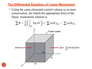
  • 67. The Differential Equation of Linear Momentum  Using the same elemental control volume as in mass conservation, for which the appropriate form of the linear momentum relation is 67
  • 68.  The momentum fluxes occur on all six faces, three inlets and three outlets. The Differential Equation of Linear Momentum  Again the element is so small that the volume integral simply reduces to a derivative term: 68
  • 69.  A simplification occurs if we split up the term in brackets as follows:  The term in brackets on the right-hand side is seen to be the equation of continuity, which vanishes identically The Differential Equation of Linear Momentum  Introducing these terms 69
  • 70.  Thus now we have  This equation points out that the net force on the control volume must be of differential size and proportional to the element volume. The Differential Equation of Linear Momentum  The long term in parentheses on the right-hand side is the total acceleration of a particle that instantaneously occupies the control volume: 70
  • 71. The Differential Equation of Linear Momentum  These forces are of two types, body forces and surface forces.  Body forces are due to external fields (gravity, magnetism, electric potential) that act on the entire mass within the element.  The only body force we shall consider is gravity.  The gravity force on the differential mass ρ dx dy dz within the control volume is  The surface forces are due to the stresses on the sides of the control surface. These stresses are the sum of hydrostatic pressure plus viscous stresses τij that arise from motion with velocity gradients 71
  • 72. The Differential Equation of Linear Momentum 72 Fig. Elemental Cartesian fixed control volume showing the surface forces in the x direction only.
  • 73.  Splitting into pressure plus viscous stresses  where dv = dx dy dz.  Similarly we can derive the y and z forces per unit volume on the control surface The Differential Equation of Linear Momentum  The net surface force in the x direction is given by 73
  • 74.  The net vector surface force can be written as The Differential Equation of Linear Momentum 74
  • 75.  is the viscous stress tensor acting on the element  The surface force is thus the sum of the pressure gradient vector and the divergence of the viscous stress tensor The Differential Equation of Linear Momentum  In divergence form 75
  • 76.  In words The Differential Equation of Linear Momentum  The basic differential momentum equation for an infinitesimal element is thus 76
  • 77.  This is the differential momentum equation in its full glory, and it is valid for any fluid in any general motion, particular fluids being characterized by particular viscous stress terms. The Differential Equation of Linear Momentum  the component equations are 77
  • 78. Newtonian Fluid: Navier-Stokes Equations  For a newtonian fluid, the viscous stresses are proportional to the element strain rates and the coefficient of viscosity.  where μ is the viscosity coefficient  Substitution gives the differential momentum equation for a newtonian fluid with constant density and viscosity: 78
  • 79.  These are the incompressible flow Navier-Stokes equations named after C. L. M. H. Navier (1785–1836) and Sir George G. Stokes (1819–1903), who are credited with their derivation. Newtonian Fluid: Navier- Stokes Equations 79
  • 80. Inviscid Flow  Shearing stresses develop in a moving fluid because of the viscosity of the fluid.  We know that for some common fluids, such as air and water, the viscosity is small, therefore it seems reasonable to assume that under some circumstances we may be able to simply neglect the effect of viscosity (and thus shearing stresses).  Flow fields in which the shearing stresses are assumed to be negligible are said to be inviscid, nonviscous, or frictionless.  For fluids in which there are no shearing stresses the normal stress at a point is independent of direction—that is σxx = σyy = σzz. 80
  • 81. Euler’s Equations of Motion  For an inviscid flow in which all the shearing stresses are zero and the Euler’s equation of motion is written as  In vector notation Euler’s equations can be expressed as Inviscid Flow 81
  • 82. Vorticity and Irrotationality  The assumption of zero fluid angular velocity, or irrotationality, is a very useful simplification.  Here we show that angular velocity is associated with the curl of the local velocity vector.  The differential relations for deformation of a fluid element can be derived by examining the Fig. below.  Two fluid lines AB and BC, initially perpendicular at time t, move and deform so that at t + dt they have slightly different lengths A’B’ and B’C’ and are slightly off the perpendicular by angles dα and dβ. 82
  • 84.  But from the fig. dα and dβ are each directly related to velocity derivatives in the limit of small dt:  Substitution results Vorticity and Irrotationality  We define the angular velocity ωz about the z axis as the average rate of counterclockwise turning of the two lines: 84
  • 85. is thus one-half the curl of  The vector the velocity vector  A vector twice as large is called the vorticity Vorticity and Irrotationality 85
  • 86. Vorticity and Irrotationality  Many flows have negligible or zero vorticity and are called irrotational.  Example. For a certain two-dimensional flow field the velocity is given by the equation  Is this flow irrotational? Solution.  For the prescribed velocity field 86
  • 88. Velocity Potential  The velocity components of irrotational flow can be expressed in terms of a scalar function ( ϕ x, y, z, t) as  where ϕ is called the velocity potential.  In vector form, it can be written as  so that for an irrotational flow the velocity is expressible as the gradient of a scalar function . ϕ  The velocity potential is a consequence of the irrotationality of the flow field, whereas the stream function is a consequence of conservation of mass 88
  • 89. Velocity Potential  It is to be noted, however, that the velocity potential can be defined for a general three-dimensional flow, whereas the stream function is restricted to two-dimensional flows.  For an incompressible fluid we know from conservation of mass that  and therefore for incompressible, irrotational flow (with ) it follows that 89
  • 90. Velocity Potential  This differential equation arises in many different areas of engineering and physics and is called Laplace’s equation. Thus, inviscid, incompressible, irrotational flow fields are governed by Laplace’s equation.  This type of flow is commonly called a potential flow.  Potential flows are irrotational flows. That is, the vorticity is zero throughout. If vorticity is present (e.g., boundary layer, wake), then the flow cannot be described by Laplace’s equation. 64
  • 91. Velocity Potential  For some problems it will be convenient to use cylindrical coordinates, r,θ, and z. In this coordinate system the gradient operator is 91
  • 93. Example 1  The two-dimensional flow of a nonviscous, incompressible fluid in the vicinity of the corner of Fig. is described by the stream function  where ψ has units of m2/s when r is in meters. Assume the fluid density is 103 kg/m3 and the x–y plane is horizontal that is, there is no difference in elevation between points (1) and (2). FIND a) Determine, if possible, the corresponding velocity potential. b) If the pressure at point (1) on the wall is 30 kPa, what is the pressure at point (2)? 93
  • 94. Example 1 Solution  The radial and tangential velocity components can be obtained from the stream function as 94
  • 96. 96
  • 97. 97
  • 98. 98
  • 99. Source and Sink  Consider a fluid flowing radially outward from a line through the origin perpendicular to the x–y plane as is shown in Fig. Let m be the volume rate of flow emanating from the line (per unit length), and therefore to satisfy conservation of mass  or 99
  • 100.  It follows that  If m is positive, the flow is radially outward, and the flow is considered to be a source flow. If m is negative, the flow is toward the origin, and the flow is considered to be a sink flow. The flowrate, m, is the strength of the source or sink. Source and Sink  A source or sink represents a purely radial flow.  Since the flow is a purely radial flow, , the corresponding velocity potential can be obtained by integrating the equations 100
  • 101.  To yield  The streamlines (lines of ψ = constant ) are radial lines, and the equipotential lines (lines of = constant) are ϕ concentric circles centered at the origin. Source and Sink  The stream function for the source can be obtained by integrating the relationships 101
  • 102. Example 2  A nonviscous, incompressible fluid flows between wedge- shaped walls into a small opening as shown in Fig. The velocity potential (in ft/s2), which approximately describes this flow is  Determine the volume rate of flow (per unit length) into the opening. 102
  • 103. The negative sign indicates that the flow is toward the opening, that is, in the negative radial direction 103
  • 104. Vortex 82  We next consider a flow field in which the streamlines are concentric circles—that is, we interchange the velocity potential and stream function for the source. Thus, let and where K is a constant. In this case the streamlines are concentric circles with and This result indicates that the tangential velocity varies inversely with the distance from the origin
  • 105.  A mathematical concept commonly associated with vortex motion is that of circulation. The circulation, Γ, is defined as the line integral of the tangential component of the velocity taken around a closed curve in the flow field. In equation form, Γ, can be expressed as 83 Circulation where the integral sign means that the integration is taken around a closed curve, C, in the counterclockwise direction, and ds is a differential length along the curve
  • 106. ,  This result indicates that for an irrotational flow the circulation will generally be zero.  However, for the free vortex with , the circulation around the circular path of radius r is  which shows that the circulation is nonzero.  However, for irrotational flows the circulation around any path that does not include a singular point will be zero. 84 Circulation  For an irrotational flow
  • 107. Circulation  The velocity potential and stream function for the free vortex are commonly expressed in terms of the circulation as and 107