SlideShare a Scribd company logo
Design and          Consumer
                                      Re - design
      Receipt and
                                                          Feedback
      Test of                                                      Distribution
      Materials
Suppliers of


Equipment


                                           Assembly
Materials


                         Production                   Inspection
and


                                                                      Customer
                    Tests of Processes , Machines , Methods ,
                    Costs                                                 s
                    Production Viewed as a System

   “ I believe this Diagram made the difference in Japan….
   the greatest way I accomplished anything there was
   through this diagram ”
                                             W. Edwards
   Deming

       Foundation of Modern Operations
       Management
A META Group Study
Energy                   30 crores per hour
Telecommunication         20 crores per hour
Manufacturing             17.5 crores per hour
Financial                 15 crores per hour
Information Technology    15 crores per hour
Insurance                       12.5 crores per
hour
Retail                   10 crores per hour
Pharmaceutical           7.5 crores per hour
Evolution of Operations Management
        Pre – Industrial Revolution Era
• Hunting
  • Planned approach towards slaying and hunting living
    creatures in defence or for consumption
• Agriculture
  • Organising and coordinating groups of people to carry
    out tasks in the fields
• Military Operations
  • Regimented organisation of groups of people
    established to protect a settlement from tyranny or
    conquer
• Creation of Professions
  • Essentially artisans who developed and passed on
    ‘trade secrets’ within their immediate families
  • Handcrafting products or services for individual
    customers
• Guilds
  • Structured group of people involved with the same
Evolution of Operations Management
            Industrial Revolution
Harnessing of Steam Energy
 • James Watt

The First ‘Steam Engine’
  • George Stevenson

The First Steam Machine
  • Ginning Machines by Eli Whitney

Division of labour
  • Economist Adam Smith conceives Division of
    Labour

Interchangeable parts
  • Eli Whitney invents interchangeability of parts
Evolution of Operations Management
                 Industrial Revolution
Principles of Scientific
Management
 • Fredrick W. Taylor

Time and Motion Studies
 • Frank and Lillian Gilbreth

Activity Scheduling
 • Henry Gantt

The Moving Assembly Line
 • Henry Ford
Evolution of Operations Management
The Focus
• Work Breakdown Structures
• One best Way of carrying out Processes
• Piece Rate System
The Outcomes
• The Meteoric Rise of Financial Accounting
• Extensive interest in Advertising and Branding
The rise of Motivational Theorists
• Elton Mayo
• Abraham Maslow
• Fredrick Herzberg
• Douglas McGregor
Evolution of Operations Management
             The Return of
             Operations
The Quality Revolution in Japan
   • W. Edwards Deming and Joseph M. Juran
The Development of the Toyota Production System
   • Eigi Toyoda , Taichi Ohno and Shiego Shengo


Modern Trends in Operations
  • Business Process Reengineering
  • Six Sigma
Operations in Today’s
         World
The Internet Revolution
•E – Commerce
•E – Businesses
  B2B
    OEMs or ‘First Fit’ Businesses
  B2C
    Franchises
  C2B
    Consultation
  C2C
    eBay,Portals,etc

Globalisation of trade
Globalisation of Operations ( Development of the
Virtual Organisation )
Definition of Operations Management
Operations Management is the system of Selecting ,
Designing , Running and Improving all transformational
processes
Transformational processes
include :
      Governmental – Creating and Running Societal
      Structures
      Physical – Manufacturing
      Exchange – Retail Operations , Banks
      Locational – Logistics and Transportation
      Physiological – Healthcare and Hospitality
      Psychological – Entertainment
      Informational – Communication , Interpretation
      Educational – Structured Knowledge Transfer
Production is the outcome of the combination of different
transformational processes ( operations ) aimed at meeting
desired Customer needs .
Production Management aims at achieving Production in
the most efficient and effective manner .
Organisation
                                   s

                   Governmental


                       Physica
                       l


                      Exchange
                                                          s


                      Locationa
                      l


Processes
                                                          Operation


Transformational
                   Physiological


                   Psychologica
                   l


                   Informationa
                   l


                    Educational


                                                  Productio
                                                  n
The Need for Operations Management in
               today’s World

In the ever changing Business Scenario in today’s
 fast developing world where we are witnessing

• Incessant Fragmentation of Markets
• Highly Informed and Vocal Customers
• Creation of Disruptive Technologies resulting in
  Specialised Knowledge
• Volatile Inter – Organisational Relationships
Objectives of Operations
 Management

Strategy – Gaining a Competitive Edge

Processes and Systems – Alignment of Back-
end activities

Quality – Scientific Methods to Create and
Deliver Products / Services

Improvement – A Constant effort to challenge
the Status Quo / Obvious
• Topic 1 – Introduction to Operations Management

• Topic 2 – Facility Location

• Topic 3 – Facility ( Plant ) Layout

• Topic 4 – Production Planning and Control

• Topic 5 – Materials Handling

• Topic 6 – Work Study

• Topic 7 – Systematic Maintenance

• Topic 8 – Quality Management

• Topic 9 – Modern Techniques in Operations Management
Regional Location Factors

•   Busine ss climate
•   Proximity to customers
•   Numbe r of customers
•   Availab ility of sites
•   Land cost
•   Constr uction / leasin g costs
•   Infrastructure (e.g., roads , water, sewer s)
•   Financial service s
•   Community incent ives
•   Community services
•   Govern menta l Incent ive
•   Govern ment regula tions
•   Environ mental regula tions
Regional Location
                       Factors


•   Labour (availability, education, cost, and unions)
•   Modes and Quality of transportation
•   Transportation costs
•   Local business regulations
•   Government services (e.g., Chamber of
    Commerce)
•   Raw material availability
•   Commercial travel
•   Climate
•   Quality of life
•   Taxes
•   Proximity of suppliers
•   Education system
Global Location
           Factors
•   Government stability
•   Government regulations
•   Political and economic systems
•   Economic stability and growth
•   Exchange rates
•   Culture
•   Climate
•   Export import regulations
•   Duties and tariffs
•   Raw material availability
•   Number and proximity of suppliers
Global Location
            Factors
•   Transportation and distribution system
•   Labour cost and education
•   Available technology
•   Commercial travel
•   Technical expertise
•   Cross-border trade regulations
•   Group trade agreements
Types of
           Facilities
Heavy-manufacturing facilities

 Large, require a lot of space, and are expensive

Light-industry facilities

 Smaller ( as compared to Large Industries ),
 cleaner plants and usually less costly

Retail and service facilities

 Smallest and least costly
Location Analysis
   Techniques
Multiattribute Preference Theory (     Location
 Rating Factor ) for Local Sites
• Is used when choices are available
• Has no ‘scientific’ basis – just an ‘agreed upon’
  weighted technique

               Attribute         Weight
         Labour Force           0.30
         Proximity to           0.20
       Customers
         Wage Rates             0.15
         Proximity to           0.15
       Suppliers
         Environment            0.10
         Modes of Transport     0.05
         Community Support      0.05
Location Analysis
     Techniques
Guidelines for Scores :
Labour Force
                                   75 –
            Highly Skilled       100
                                      50 –
            Adequately Skilled
                                 75
                                      25 –
            Semi Skilled         50
            Unskilled                 0 – 25
Location Analysis
       Techniques
Guidelines for Scores :
Proximity to Customers

                               75 –
      Within 15 kilometres
                             100
      Between 15 to 30            50 –
   kilometres                75
      Between 30 to 50            25 –
   kilometres                50
      Above 50 kilometres         0 – 25
Location Analysis
    Techniques
Guidelines for Scores :
Wage Rates


                                      75 –
       Upto 10 % of total cost
                                    100
       Between 10 – 15 % of total        50 –
     cost                           75
       Between 15 – 20 % of total        25 –
     cost                           50
       Above 20 % of total cost          0 – 25
Location Analysis
    Techniques
Guidelines for Scores :
Proximity to Suppliers


                                  75 –
         Within 15 kilometres
                                100
         Between 15 to 30            50 –
      kilometres                75
         Between 30 to 50            25 –
      kilometres                50
         Above 50 kilometres         0 – 25
Location Analysis Techniques
Guidelines for Scores :
Environment

                                             75 –
  Conducive to Ceaseless Productive Work
                                           100
                                                50 –
  Conducive to Productive Work over 25 %   75
                                                25 –
  Conducive to Productive Work for a day
                                           50
   Conducive to Productive Work for less
                                                0 – 25
than a day
Location Analysis
     Techniques
Guidelines for Scores :
Modes of Transport

  Access to any two modes of transport at      75 –
any given moment                             100
  Access to any one mode of transport at          50 –
any given moment                             75
  Need to plan a day in advance for any           25 –
mode of transport                            50
   Need to plan more than a day in advance
                                                  0 – 25
for any mode of transport
Location Analysis
     Techniques
Guidelines for Scores :
Community Support

  Extremely harmonious relationships with     75 –
communities in close proximity              100

  Have Legal relationships with                  50 –
communities in close proximity              75

  Have dispassionate relationships with          25 –
communities in close proximity              50

  Have hostile relationships with
                                                 0 – 25
communities in close proximity
Exampl
 e
A company wanting to relocate its operations has assessed
three sites and have tabulated the following results

             Attribute          Site 1     Site 2      Site 3
      Labour Force                70         60         90
     Proximity to
                                  80         90         75
   Customers
      Wage Rates                  60         95         70
     Proximity to                 75         80         80
   Suppliers
      Environment                 65         90         95
      Modes of Transport          85         90         65
      Community Support           80         65         90

Which Site qualifies based on the Multiattribute Preference
Theory ?
Using Weights ascribed we
           get


                             Wei  Si    Sit    Sit
          Attribute
                            ght te 1   e 2    e 3
                            0.3
    Labour Force                  70    60     90
                            0
    Proximity to            0.2   80    90     75
  Customers                 0
                            0.1
    Wage Rates                    60    95     70
                            5
    Proximity to            0.1   75    80     80
  Suppliers                 5
                            0.1
    Environment                   65    90     95
                            0
Weighted
Scores
     Scores : Site 1 – 72.00 ; Site 2 – 79.00 ; Site 3
     – 81.75

        Attribute              Site 1     Site 2         Site 3
    Labour Force               21.00      18.00          27.00
   Proximity to                16.00      18.00          15.00
 Customers
    Wage Rates                 9.00       14.25          10.50
   Proximity to
                               11.25      12.00          12.00
 Suppliers
    Environment                6.50        9.00          9.50
   Modes of                    4.25        4.50          3.25
 Transport
           Site 3 – The preferred
    Community
           location       4.00             3.25          4.50
Typical Attributes that an MNC looks for in a
Global Operations Site


              Attribute              Weight
     Political Stability              0.25
     Economic Growth                  0.20
     Port Facilities                  0.13
     Airline Support                  0.10
     Trade Regulations                0.08
     Duties and Tariffs               0.08
     Container Support                0.07
    Transportation /                  0.05
  Distribution
     Area Roads                        0.02
Centre of Gravity Technique

   Normally used in computing location of sites for
        Warehouses / Distribution Centres

Current Location is set as ( 0 , 0 ) on a Cartesian
Plane

Average Annual Despatch Loads to different sites
are indicated in parenthesis

Distribution Site co-ordinates are computed
accordingly

A Pictorial Representation in the form of a Graph
is drawn
y


                                    2 (x 2 , y 2 ),
   y2
                                    W2

                  1 (x 1 , y 1 ),
   y1             W1


                                                 3 (x 3 , y 3 ),
   y3
                                                 W3


                          x1            x2             x3
                                                                   x
Current Site of
Operations
Co-ordinates of New Location ( x , y ) are computed
                      thus


               (x 1 )(W 1 ) + (x 2 )(W 2 ) + (x 3 )(W 3 )
      x=
                          W1 + W2 + W3


               (y 1 )(W 1 ) + (y 2 )(W 2 ) + (y 3 )(W 3 )
       y=
                          W1 + W2 + W3
Example
                                                       A            B      C      D
                   y                                x 200           100 250     500
                                                    y 200           500 600     300
             700
                                                    Wt 70             100 130
                               C
                                                    60
             600                      (130)
                       B
             500             (100)
Kilometres


             400
                                                       D
             300                                             (60)
                              A
             200                   (70)

             100


              0        100    200     300     400      500    600    700    x

                                          Kilometres
Co-ordinates of New Location ( x , y ) are computed
                           thus


         (200)(70) + (100)(100) + (250)(130) +
x=                                                =   240
                       (500)(60)

                  70 + 100 + 130+ 60


        (200)(70) + (500)(100) + (600)(130) +
y=                                               =    444
                      (300)(60)

                 70 + 100 + 130+ 60
Location of the Warehouse

                 y

            70
            0            C
            60              (130)
            0    B (100)
Kilometre


            50                 ( 240 , 444 )
            0
            40
            0                                D
s


            30                                   (60)
            0         A
             200         (70)

            10
            0
                                                             x
             0       100    20   30 40 50         60    70
                            0    0 Kilometre
                                      0   0       0     0
                                   s
Load Distance
                                   Technique
                         Variation of the Centre of Gravity
                         Technique
     Used when Options available for Sites

     Use of the Straight Line concept ( Based on Geometric Distance
     Formula )
                                             n
                                    LD =
                                           ∑     li di

                                           i= 1
LD =        load-distance value
li    =     load expressed as a weight being despatched
di =                   distance between proposed site and
location i
     di =   (x i - x) 2 + (y i -             (x,y) = coordinates of proposed site
     y) 2
                                           (x i , y i) = coordinates of existing facility
Suppliers

        A     B     C
    D
x     200 100 250
 500
y     200 500 600
 300Potential Sites
Wt Site X100 130
       70     Y
  601    360 180
    2       420 450
    3       250 400
A               B      C              D                      Potential Sites
x 200              100 250             500                      Site   X      Y
y 200              500 600             300                      1      360    180
Wt 70                100 130                                    2      420    450
60                                                              3      250    400

Computing distances for Site 1


                                                  dC =        (x C - x 1 ) 2 + (y C - y 1 ) 2
dA =     (x A - x 1 ) 2 + (y A - y 1 ) 2
                                                        =      (250-360) 2 + (600-180) 2
   =     (200-360) 2 + (200-180) 2
                                                        = 434.16
   = 161.2
dB =     (x B - x 1 ) + (y B - y 1 )
                     2                 2         dD =       (x D - x 1 ) 2 + (y D - y 1 ) 2

   =      (100-360) + (500-180)
                          2                  2     =         (500-360) 2 + (300-180) 2

   = 412.3                                         = 184.31
                           Load Distance =
       (70)*(161.2)+(100)*(412.3)+(130)*(434.16)+(60)*(184.31)
                             =
                         120019.2
A            B      C           D                         Potential Sites
x 200           100 250          500                         Site   X      Y
y 200           500 600          300                         1      360    180
Wt 70             100 130                                    2      420    450
60                                                           3      250    400
Computing for Site 2


                                                 dC =   (xC – x2)2 + (yC – y2)2
dA =   (xA – x2)2 + (yA – y2)2
                                                   =    (250-420)2 + (600-450)2
  =    (200-420)2 + (200-450)2
           = 333.02                                          = 226.71

dB =   (xB – x2)2 + (yB – y2)2                   dD =   (xD – x2)2 + (yD – y2)2

   =    (100-420) + (500-450)
                   2             2                 =    (500-420)2 + (300-450)2

           = 323.88                                            = 170

   Load Distance = (70)*(333.02)+(100)*(323.88)+(130)*(226.71)+(60)*(170)
                                     = 97036.8
A             B      C           D                          Potential Sites
x 200            100 250          500                          Site   X      Y
y 200            500 600          300                          1      360    180
Wt 70              100 130                                     2      420    450
60                                                             3      250    400

Computing for Site 3


dA =    (xA – x3)2 + (yA – y3)2                    dC =   (xC – x3)2 + (yC – y3)2

 =     (200-250)2 + (200-400)2                        =    (250-250)2 + (600-400)2

               = 206.19                                              = 200

dB =    (xB – x3) + (yB – y3)
                 2            2                   dD =    (xD – x3)2 + (yD – y3)2

 =     (100-250)2 + (500-400)2                        =    (500-250)2 + (300-400)2

               = 180.27                                          = 269.25
       Load Distance = (70)*(206.19)+(100)*(180.27)+(130)*(200)+(60)*(269.25)
                                   = 74614.8
Facility Layouts
     Definition of Facility
            Layout
 Planned arrangement of areas within a facility
 commensurate with the product to be realised or
 service to be delivered
Objectives of Facility
Layout
 •   Optimise material-handling ( transaction ) costs
 •   Utilise space efficiently
 •   Utilise manpowe r efficiently
 •   Work around bottlenecks
 •   Facilitate interaction
 •   Reduce cycle time
 •   Reduce customer turnaround time
 •   Eliminate redundant movement
 •   Increase capacity
 •   Provide for entries, exits, placement of material ( in all
     stages of realisation ), finished goods, and people
Facility Layouts
Objectives of Facility Layout ( continued )

•   Incorporate safety and security measures
•   Promote product and service Quality
•   Facilitate proper maintenance activities
•   Provide for visual control
•   Provide for flexibility to adapt to changing conditions
Different Organisational Layout
            Representations


•   Departmental Layout
•   Material Flow Layout
•   Equipment Layout
•   Transportation and Handling Layout
•   Utilities Layout
•   Communication Channel Layout
Basic Types of Layouts
Fixed-position layouts
 are used where product cannot be moved
  Used for Large Products and Projects
  Usually ‘one-of-a-kind’ products or projects

Process layouts
 group similar activities together according to process or
 function they perform
  Traditional Type of Layout
  Suitable for Mass Production

Product layouts
 arrange activities in line according to sequence of
 operations for a particular product or service
  Modern Approach toward Creating Layouts
  More inclined towards Mass Customisation
Fixed-position layouts

Typically manufacture of Construction Projects ,
Rocket Launchers , Space Shuttles , Aircrafts ,
Ships , Surgeries , “Events”

Equipment, workers, materials, other resources
brought to site

Highly skilled labour
Process Layout - Bookstore


Video CDs                    Audio CDs ,
              Cassettes
  , DVDs                       DVDs

                             Technical
Cookbooks     Billing and      and
             Information    Management
                              Section

Children’s    Entry and        Coffee
 Books       display area      Shop
Process Layout - Manufacture


Lathe Section   Milling Section               Drilling Section

                 M        M               D   D       D          D
 L       L

                 M        M               D   D       D          D
 L       L

                 G        G          G        P
 L       L

                 G        G          G        P
 L       L
                                               Painting Department
                 Grinding and Finishing

 L       L
                     Receiving and            A        A             A
                       Shipping                     Assembly

                 Product A                        Product B
Product Layout - Manufacture


In                              Out

        Product A

In                              Out


        Product B

In                              Out


        Product C
Comparisons between Product and Process Layouts


          Product Layout                    Process Layout

• Sequential arrangement of        • Functional Grouping of
  Activities                         Activities

• Intermittent work                • Continuous work

• Adaptable Machinery              • General Purpose Machinery

• Workers are extensively cross-   • Workers are trained in a
  trained                            particular process

• Occupy smaller areas             • Occupy larger areas

• Highly flexible lines            • Largely Rigid

• Lesser travel time               • More travel time
Designing Layouts
Relationship Diagramming

 • based on location preference between areas

 • used when quantitative data is not available

 • Schematic diagram that uses weighted lines
   to denote location preference
Use of a grid called “Muther’s grid”
Muther’s Grid

Different Sections / Areas in
an organisation
                                Extent of their
                                Interactions /
                                Relationships
A    Absolutely necessary
                             E   Especially important
                             I   Important
                             O   Okay
                             U   Unimportant
                             X   Undesirable
      Production
                         O
         Offices             A
                         U         I
        Stockroom            O          E
                         A        X           A
Shipping and receiving       U          U
                         U        O
        Locker room          O
                         O
         Toolroom
Original layout


    Offices        Locker       Shipping
                    room           and
                                receiving


Stockroom     Toolroo           Production
                m
                                             A
                                             E
                                             I
                                             O
                                             U
                                             X
Relationship diagram of original layout


     Offices                Locker      Shipping and
                             room         receiving


                                                         A
                                                         E
Stockroom              Toolroom           Production     I
                                                         O
                                                         U
                                                         X
Production – 2 ‘Absolutely Necessary’ transactions ;
1 ‘Especially Important’ transaction ;
1 ‘Important’ transaction ;
1 ‘Okay’ transaction

Therefore Production needs to be centrally located
with the other departments around it .
Solution 1                  A
                                         E
                                         I
                                         O
                                         U
            Stockroom                    X


  Offices

                          Shipping and
                            receiving


Toolroom

            Production    Locker room
Solution 2               A
                                           E
                                            I
                                           O
                                           U
               Stockroom                   X


                                 Locker room
  Offices


Shipping and   Production      Toolroom
 receiving
Block Diagramming
Purpose is to minimise nonadjacent loads
Used when quantitative data is available

Steps :
• Create load summary chart
• Calculate composite (two way) movements
• Develop trial layouts minimising number
  of nonadjacent loads
Load Summary Chart

                      T
                      o

           1     2         3    4    5

       1   -    100       50    -    -

       2   -     -        200   50   -
From
       3   60    -         -    40   50

       4   -    100        -    -    60

       5   -     50        -    -    -
Composite Movements

Movement   Total Load
2 ↔3       200
2 ↔4       150
1 ↔3       110
1 ↔2       100
4 ↔5       60
3 ↔5       50
2 ↔5       50
3 ↔4       40
1 ↔4       0
1 ↔5       0
Arranged in a 2x3 Grid


1            2               3


4            5
110


      100            200
1                2         3


                     50
       0


            50
    15


       60
4                5


             40
Blocks Rearranged with Non-adjacent loads
              cancelled out


        100                    150
1                     2               4


                200


                                          60
      11
         0


                          40
                      3              5
                               50
Cellular Layouts

Identify outputs with similar flow paths
Group processes into cells based on output
Arrange cells so transactions are minimised
Locate shared processes at point of use
Original Machine Layout


4        6        7         9


     5                 8


     2            10          12


1        3             11
Original Process Layout
             Outputs


4       6               7         9


    5                        8


    2                   10        12


1       3                    11


A   B   C      Inputs
Determine Flow Logic


A : 1 – 2 – 4 – 8 – 10
B : 5 – 7 – 11 – 12
C:3–6–9
D : 1 – 2 – 4 – 8 – 10
E : 5 – 6 – 12
F:1–4–8
G : 3 – 6 – 9 – 12
H : 7 – 11 – 12
Part Routing Matrix
                         Workstations
  Pro                                                                 V
ducts                                            1       1       1 alue
        1   2    3   4   5   6   7   8   9
                                             0       1       2
   A    X   X        X               X           X
   B                     X       X                       X       X
   C             X           X           X
   D    X   X        X               X           X
   E                     X   X                                   X
   F    X            X               X
  G              X           X           X                       X
   H                             X                       X       X
 Valu
 e
Create Binary Algorithm
The procedure works like this :
• Assign a value to each column ‘k’ , where the
  value is 2 N-k N = total number of workstations ; k =
  chronological workstation number
• For each row obtain a sum by adding the 2 N-k
  values
• Rearrange the rows in the decreasing order of the
  sums obtained
• Assign a value to each row ‘k’ where the value is
  2 M-k M = total number of products ; k =
  chronological ( rearranged ) sequence number of
  the product
• For each column obtain a sum by adding the
  values
• Rearrange the columns in decreasing order of the
  sums obtained
Part Routing Matrix
                                          Workstations
  Pro                                                                                              V
ducts                                                                         1       1       1 alue
          1    2    3        4        5           6       7       8   9
                                                                          0       1       2
           2   1                 2                                1                               3
   A    048 024             56                                6
                                                                              4
                                                                                                348
                                          1               3                                       1
   B                                 28               2
                                                                                      2       1
                                                                                                63
                        5                         6                                               5
   C               12                         4
                                                                      8
                                                                                                84
           2   1                 2                                1                               3
   D    048 024             56                                6
                                                                              4
                                                                                                348
                                          1       6                                               1
   E                                 28       4
                                                                                              1
                                                                                                93
           2                     2                                1                               2
   F    048                 56                                6                                 320
                        5                         6                                               5
  G                12                         4
                                                                      8                       1
Part Routing Matrix
                                          Workstations
  Pro                                                                                              V
ducts                                                                         1       1       1 alue
          1    2    3        4        5           6       7       8   9
                                                                          0       1       2
           2   1                 2                                1                               3
   A    048 024             56                                6
                                                                              4
                                                                                                348
           2   1                 2                                1                               3
   D    048 024             56                                6
                                                                              4
                                                                                                348
           2                     2                                1                               2
   F    048                 56                                6                                 320
                        5                         6                                               5
  G                12                         4
                                                                      8                       1
                                                                                                85
                        5                         6                                               5
   C               12                         4
                                                                      8
                                                                                                84
                                          1       6                                               1
   E                                 28       4
                                                                                              1
                                                                                                93
                                          1               3                                       1
   B                                 28               2
                                                                                      2       1
Part Routing Matrix
                         Workstations
  Pro                                                                 V
ducts                                            1       1       1 alue
        1   2    3   4   5   6   7   8   9
                                             0       1       2
   A    X   X        X               X           X
   D    X   X        X               X           X
   F    X            X               X
  G              X           X           X                       X
   C             X           X           X
   E                     X   X                                   X
   B                     X       X                       X       X
   H                             X                       X       X
 Valu
 e
Part Routing Matrix
                                   Workstations
  Pro                                                                                      V
ducts                                                                 1       1       1 alue
           1   2        3     4    5       6   7     8        9
                                                                  0       1       2
            1   1              1                      1              1
   A
         28 28              28                     28             28
            6   6              6                      6              6
   D
          4   4              4                      4              4
            3                  3                      3
   F
          2                  2                      2
                        1                  1                  1                       1
   G
                    6                  6                  6                       6
   C                    8                  8                  8
   E                               4       4                                          4
   B                               2           2                              2       2
   H                                           1                              1       1
  Valu     2   1        2     2            2         2        2       1               2
Part Routing Matrix
                               Workstations
  Pro                                                                               V
ducts                          1                               1               1 alue
          1   4    8   2               6       3       9           5   7
                           0                               2               1
           1   1   1   1   1
   A
        28 28 28 28 28
           6   6   6   6   6
   D
         4   4   4   4   4
           3   3   3
   F
         2   2   2
                                       1       1       1       1
  G
                                   6       6       6       6
   C                                   8       8       8
   E                                   4                       4   4
   B                                                           2   2   2       2
   H                                                           1       1       1
Part Routing Matrix
                            Workstations
 Prod
ucts                        1                   1               1
        1   4   8   2           6   3   9           5   7
                        0                   2               1
  A     X   X   X   X       X
  D     X   X   X   X       X
  F     X   X   X
  G                             X   X   X       X
  C                             X   X   X
  E                             X               X   X
  B                                             X   X   X       X
  H                                             X       X       X
Revised Layout

                        Outputs


         8      10                9       12


                                                   11

4   Cell 1          Cell 2        6       Cell 3

                                                   7


         2      1                 3       5


                             A    B   C
                         Inputs
Flow Logic


A:5–6–8
B:5–6–8–9
C:2–4–5–7
D:1–3
E:5–6
F:1–3–4
G:4–5–6–8-9
H:2–4–7
Part Routing Matrix
                     Workstations
Produ                                            V
cts     1    2   3   4    5    6    7   8   9 alue

 A                        X    X        X
 B                        X    X        X   X
 C           X       X    X         X
 D      X        X
  E                       X    X
  F     X        X   X
 G                   X    X    X        X   X
 H           X       X              X
Value
Part Routing Matrix
                            Workstations
Produ                                                        V
cts      1     2        3       4       5   6   7   8   9 alue

                                        1                       2
 A                                          8       2
                                    6                       6
                                        1                       2
 B                                          8       2   1
                                    6                       7
                1               3       1                      1
 C                                              4
              28            2       6                       80
          2             6                                      3
 D
        56          4                                       20
                                        1                      2
  E                                         8
                                    6                        4
          2             6       3                              3
  F
        56          4       2                               52
                                3       1                      5
 G                                          8       2   1
Part Routing Matrix
                            Workstations
Produ                                                        V
cts      1     2        3       4       5   6   7   8   9 alue

          2             6       3                              3
  F
        56          4       2                               52
          2             6                                      3
 D
        56          4                                       20
                1               3       1                      1
 C                                              4
              28            2       6                       80
                1               3                              1
 H                                              4
              28            2                               64
                                3       1                      5
 G                                          8       2   1
                            2       6                        9
                                        1                      2
 B                                          8       2   1
                                    6                        7
                                        1                      2
 A                                          8       2
Part Routing Matrix
                     Workstations
Produ                                            V
cts     1    2   3   4    5    6    7   8   9 alue

  F     X        X   X
 D      X        X
 C           X       X    X         X
 H           X       X              X
 G                   X    X    X        X   X
 B                        X    X        X   X
 A                        X    X        X
  E                       X    X
Value
Part Routing Matrix
                               Workstations
Produ                                                              V
cts       1        2     3        4       5   6       7   8   9 alue

           1              1     1
  F
        28             28     28
           6              6
 D
         4              4
                   3              3       3           3
 C
               2              2       2           2
                   1              1                   1
 H
               6              6                   6
 G                                8       8   8           8   8
 B                                        4   4           4   4
 A                                        2   2           2
  E                                       1   1
          1        4     1        1       4   1       4   1   1
Part Routing Matrix
                              Workstations
Produ                                                              V
cts       1      3        4       2       7       5   6   8   9 alue

           1      1     1
  F
        28     28     28
           6      6
 D
         4      4
                          3       3       3       3
 C
                      2       2       2       2
                          1       1       1
 H
                      6       6       6
 G                        8                       8   8   8   8
 B                                                4   4   4   4
 A                                                2   2   2
  E                                               1   1
Part Routing Matrix
                       Workstations
Produc
 ts      1     3   4   2    7    5    6   8   9

  F      X     X   X
  D      X     X
  C                X   X    X    X
  H                X   X    X
  G                X             X    X   X   X
  B                              X    X   X   X
  A                              X    X   X
  E                              X    X
Value
Part Routing Matrix
                       Workstations
Produc
 ts      1     3   4   2    7    5    6   8   9

  F      X     X   X
  D      X     X
  C                X   X    X    X
  H                X   X    X
  G                X             X    X   X   X
  B                              X    X   X   X
  A                              X    X   X
  E                              X    X
Value
1   3


2   4   7


5   6   8   9
Direction of part movement within cell


                                            HM

                                                                  VM

                                                            Worker 3
      Paths of three workers                                               VM
      moving within cell
                                  L
      Material movement


                                                 Worker 2
S = Saw                                                                         G
L = Lathe
HM = Horizontal milling machine   L
VM = Vertical milling machine
G = Grinder                                                                Final
                                                                        inspection


                                                                        Finished
                                                                          part
                                  S                    Worker 1


                                                                           Out
                                  In
Service Layouts
• Usually process layouts respond to
  customer needs
• Minimise flow of customers or
  transactions
• Retailing tries to maximise customer
  exposure to products
• Layouts must be aesthetically pleasing
Types of Layouts for Service Organisations


              Freeflow Layout
Types of Layouts for Service Organisations


                Grid Layout
Types of Layouts for Service Organisations


               Spine Layout
Types of Layouts for Service Organisations


               Loopy Layout
Types of Production Processes
          Criteria for Selection of Processes

Nature of the Inputs and Outputs
  Perishable and Non – Perishable
Quantum of Production
  One – of
  Few Numbers
  Mass
Nature of Operations
  Continuous Processes
  Intermittent Processes
Capacity of the Plant
 Restrictions in Space , Equipment , Labour , Technology
Types of Production Processes
                  Types of Processes
Jobbing / Project Type Method
 This method is used where , although the Processes
  remain the same , the outputs are unique in nature .
 Example : Construction Projects , Film Making , Job
  Shops

Features of this Approach
• One – of or Very Small Quantity of Production
• Highly Skilled Workforce
• General Purpose Equipment
• Unbalanced Processing
• High Cost of Production
Types of Production Processes
                   Types of Processes
Batch Type Approach
  This method is used where a limited amount of products
   ( batches ) are produced at a time either continuously or
   intermittently .
  Example : Chemicals , Pharmaceuticals , Paints , Foods
   and some types of metal items

Features of this Approach
  • Fixed Quantities Produced
  • Semi – Skilled Workforce
  • General Purpose Equipment
  • Balanced Processing
  • Low Cost of Production
Types of Production Processes
                   Types of Processes
Mass Production
  This method is used where a very large amount of
   products ( batches ) are produced at a time either
   continuously .
  Example : Engineered Products , Fertilisers

Features of this Approach
  • Very Large Quantities Produced
  • Semi – Skilled Workforce
  • General Purpose Equipment
  • Very High Flows
  • Low Cost of Production
Types of Production Processes
                  Types of Processes

Process Based Production
  This method is used where Bulk items are produced
  Example : Sugar , Aluminium , Zinc , Iron and Steel

Features of this Approach
  • Bulk Items Produced
  • Semi – Skilled Workforce
  • General Purpose Equipment
  • Very High Flows
  • Low Cost of Production
Ways of Doing Work
                                           PRODUCT MIX


                                One of    Low Volume       High Volume   Mass

                                 Project Job
                  Jumbled
                                    Shop
PROCESS PATTERN


                  Jumbled But
                                               Batch
                  Dominant
                                                       K

                                                             Line
                  Line Flow

                  Continuous                                        Continuous
                  Flow
Production Planning and Control
          Introduction


• Coordination of materials function
  with suppliers
• Efficient utilisation of people and
  machines
• Efficient flow of materials within the
  organisation
The “Seepok” Model

                     Production
            Inputs                    Outputs

Suppliers                                       Customers


     S          I       P         O             C
Decision Support
• PPC system does not make decisions
  but provides support for decision
  making
• Managers make decisions
Software for Decision Support
• Software not only to support decision
  makers but also make some of the
  decisions
 •   Expert Systems
 •   Neural Networks
 •   Algorithms
 •   Evolutionary Programming
 •   Genetic Programming
 •   Tabu Search
 •   Simulated Annealing
Activities
• Materials Planning
• Purchasing
• Raw Material Inventory Control
• Capacity Planning
• Scheduling Machine and People
• Work-in-Process (WIP) Inventory
  Control
• Coordinate Customer Orders
• Finished Goods Inventory Control
Ill-effects of a lack of PPC

•   poor customer service
•   excessive inventories
•   low equipment and people utilisation
•   high rate of part obsolescence
•   large number of expediters
Specification                      Inventory
                        Work Study
        s                            Management


            Production Planning and Control


Routing   Loading Scheduling Despatching Expediting


                   Production Plan
Routing


• Determine the Processes to be followed
• Determine the Sequence of the Processes
• Determine the Flow of Materials / Activities
Loading


• Determine the Number of Workstations
• Determine their operational characteristics ( speeds ,
  capabilities )
• Selection of Workstations
• Creating a Contingency Plan
Scheduling


• Determining the exact time at which the Operations
  will materialise
• Timing the arrival of material ( finished / semi-finished
  part at different workstations )
• Usually done on a ‘Gantt Chart’
Despatching


• Creating Work Orders
• Creating Shop Travellers
• Issuing Authorisations
Expediting


• Creating Routine Reports
• Creating Check Points
• Follow up
Production Planning and Control
        General Framework
              Resources                                         Demand
               Planning                                        Management


Rough-Cut Capacity
    Planning                    Master Production Scheduling


            Detailed Capacity                         Detailed Material
                Planning                                 Planning


                                      Material and
                                     Capacity Plans


             Work Order                                    Purchase
                                                            Order
Demand Management

•   Forecasting
•   Order Processing
•   Order Acceptance
•   Order Confirmation
Resource Planning


•   Long-Range Capacity Requirements
•   Number of Plants
•   Number of Workstations
•   Number of Employees
•   Shifts
•   Overtime
Production Planning

Plans for Product Families
Master Planning Schedule ( MPS )

           Anatomy of a Plan
                      Annual Plan
                   Quarterly Plan
                  Monthly Plan


                   Fortnightly Plan


          Fixed          Could be subject to minor changes
Rough-Cut Capacity Planning

Capacity Requirement Planning for
Master Production Scheduling
• Open Orders
• Planned Orders
• Resource Profiles
Detailed Materials Planning
       Materials Requirements Planning

Inputs :
• Master Production Schedule (MPS)
• Bill of Materials (BOM)
• Inventory Status
• Leadtime (LT)
Bill of Material (BOM)

Shows the constituent components and how
many of those are required to build the
composite part
Product Structures and Parts

                         C        Finished Product


Manufactured
   Part

               A        Sub Assembly         B


               X                      X              Y


                    Purchased Parts
Single Level Bill of Material
  2 units of component X are used to make 1 unit of item A


  Level 0         Parent              A

 Level 1        Component             X      X2


Indented Bill of Material ( BOM ) for A is

                         Lev       Part ( nos
                    el         )
                         0         A( 1 )
                         1         X ( 2 )
Single Level Bill of Material
   2 units of component X and 1 component of Y are used to
   make 1 unit of item B


  Level 0         Parent            B

 Level 1        Component           X        X2
 Level 1        Component           Y        X1

Indented Bill of Material ( BOM ) for B is

                          Lev
                                  Part ( nos )
                     el
                          0       B(1)
                          1       X(2)
                          1       Y(1)
Single Level Bill of Material

  Level 0       Parent           C

 Level 1      Component          A    X2
 Level 1      Component          B    X3

    2 units of component A and 3 components of B are used to
    make 1 unit of item C
Indented Bill of Material ( BOM ) for C is


                        Lev
                               Part ( nos )
                   el
                        0      C(1)
                        1      A(2)
                        1      B(3)
Multi Level Bill of Material


Level 0      Parent          C


Level 1        2xA                   3xB


Level 2        2xX                2xX      1xY
Summary Bill of Material

                     Cumulati   Summary BOM for C
Level    Part
                ve
0        C           1
1        A           2               X   10
2        X           4               Y   3
1        B           3
2        X           6
2        Y           3
Create a BOM for a Two layered McDonald’s
                       Maharaja Mac

                                  Sesame Seed Top bun


             Bottom Bun Sub Assembly                     Middle Bun Sub Assembly


Bottom Bun        Patty      Sauce      Lettuce         Cheese         Patty   Onions


                                                          Middle Bun
Inventory Status
On Hand (OH) Quantity
What is physically available in the warehouse

On Order or Scheduled Receipt (SR)
What has been ordered but not received ( transitory )

Allocated Inventory (AI)
What is in the warehouse but reserved for existing
orders (i.e., not available to be used for incoming
orders)
Leadtime

Time between placing an order and receiving the parts
Parts could be
• Purchased – Dependant on Vendor
• Manufactured or assembled in house – Dependant
  on Process / Manufacturing Personnel
Leadtime Offsetting


1.Front Schedule Approach
 Schedule as early as possible
 Advantage: Minimise risk of shortage
 Disadvantage: Higher Inventory Levels
2.Back Schedule Approach
 Schedule as late as possible
 Advantage: Minimise Inventory
 Disadvantage: Higher Risk of Shortage
Important Terms / Conventions used in MRP
Gross Requirements – Derived from the MPS of the Parent
Part

Scheduled Receipts – On Order or Scheduled to be
received

On Hand – Physical Available Inventory

Allocated Inventory – Inventory scheduled to be used

Nett Requirements – Actual Quantities Required

Planned Order Receipts – Offset time when Materials are
needed

Planned Order Releases – Offset Time when materials need
to be ordered ( function of lead time )
MRP Matrix

                                    Week Number
  Heading
                               1    2    3   4        5
  Gross                                   12    10    10
                              85    95
Requirements                             0     0     0
  Scheduled                    17
Receipts                      5
  On Hand                45
  Allocated Inventory    20
  Nett Requirements
  Planned Order
Receipts
  Planned Order
Releases
MRP Matrix

                                    Week Number
  Heading
                               1    2    3   4        5
  Gross                                   12    10    10
                              85    95
Requirements                             0     0     0
  Scheduled                    17
Receipts                      5
                               11
  On Hand                45
                              5
  Allocated Inventory    20
  Nett Requirements            0
  Planned Order
Receipts
  Planned Order
MRP Matrix

                                    Week Number
  Heading
                               1    2    3   4        5
  Gross                                   12    10    10
                              85    95
Requirements                             0     0     0
  Scheduled                    17
Receipts                      5
                               11
  On Hand                45         20
                              5
  Allocated Inventory    20
  Nett Requirements            0    0
  Planned Order
Receipts
  Planned Order
MRP Matrix
                                        Week Number
  Heading
                                    1    2   3   4           5
  Gross                             8       9     1     1     1
Requirements                    5       5       20    00    00
  Scheduled                       1
Receipts                        75
                            4     1         2
  On Hand
                        5       15      0
                            2
  Allocated Inventory
                        0
                                                  1
  Nett Requirements                 0       0
                                                00
  Planned Order                                  1
MRP Matrix

                                        Week Number
  Heading
                                    1    2   3   4           5
  Gross                             8       9     1     1     1
Requirements                    5       5       20    00    00
  Scheduled                       1
Receipts                        75
                            4     1         2
  On Hand
                        5       15      0
                            2
  Allocated Inventory
                        0
                                                  1     1
  Nett Requirements                 0       0
                                                00    00
  Planned Order                                  1     1
MRP Matrix

                                        Week Number
  Heading
                                    1    2   3   4           5
  Gross                             8       9     1     1     1
Requirements                    5       5       20    00    00
  Scheduled                       1
Receipts                        75
                            4     1         2
  On Hand
                        5       15      0
                            2
  Allocated Inventory
                        0
                                                  1     1     1
  Nett Requirements                 0       0
                                                00    00    00
  Planned Order                                  1     1     1
Detailed Capacity Planning
    Capacity Requirements Planning

Creates a load profile
Identifies under-loads and over-loads
Inputs
 Planned order releases
 Routing file
 Open orders file
Routing File


Inputs
• Flow Time
• Cycle Time
• Number of Workstations
• Capabilities of Work Stations
Scheduling

Last stage of planning before production
occurs
Specifies when labour, equipment, facilities
are needed to produce a product or provide
a service
Objectives in Scheduling
Meet customer due dates
Minimise response time
Minimise completion time
Minimise time in the system
Minimise overtime
Minimise work-in-process inventory
Shop Floor Control
Loading
 Check availability of material, machines and labour

Sequencing
 Release work orders to shop and issue despatch
 lists for individual machines

Monitoring
 Maintain progress reports on each job until it is
 complete
Loading

Process of assigning work to limited
resources
Perform work on most efficient resources
Assignment Method
Perform row reductions
  subtract minimum value in each row from all other row
  values
Perform column reductions
  subtract minimum value in each column from all other
  column values
Cross out all zeros in matrix
  use minimum number of horizontal and vertical lines to
  cover all the 0s
If number of lines equals number of rows in matrix then
optimum solution has been found. Make assignments where
zeros appear
Else modify matrix
  subtract minimum uncrossed value from all uncrossed
  values
  add it to all cells where two lines intersect
  other values in matrix remain unchanged
Repeat steps 3 through 5 until optimum solution is reached
Example

          Time taken for completing
 Name             the task
           1      2      3      4
Duryodh
  an
          10      5      6     10
Dushyas
  an
           6      2      4      6
Jarasan
 dha
           7      6      5      6
Jayadra
 tha
           9      5      4     10
Step 1 - Row Reduction

          Time taken for completing
 Name             the task
           1      2      3      4
Duryodh
  an
           5      0      1      5
Dushyas
  an
           4      0      2      4
Jarasan
 dha
           2      1      0      1
Jayadra
 tha
           5      1      0      6
Step 2 - Column Reduction

          Time taken for completing
 Name             the task
           1      2      3      4
Duryodh
  an
           3      0      1      4
Dushyas
  an
           2      0      2      3
Jarasan
 dha
           0      1      0      0
Jayadra
 tha
           3      1      0      5
Step 3 - Cover all Zeros
             Time taken for completing
   Name              the task
               1      2       3       4
 Duryodh
    an
               3        0      1      4
 Dushyas
    an
               2        0      2      3
  Jarasan
   dha
               0        1      0      0
  Jayadra
Number of Lines = 3 ; Number of Rows = 4
   tha
               3        1      0      5
             Modify Matrix
Step 4 - Modify the Matrix
                          Time taken for completing
                 Name            the task
                          1       2      3       4
                 Duryod
                          3       0      1       4
                 han
                 Dushy
                          2       0      2       3
                asan
                 Jarasa
                          0       1      0       0
                ndha
                 Jayadr
                          3       1      0       5
                atha


Take the lowest value in the ‘uncovered’ cells ( in this
case = 2 ) and reduce the column to which it belongs
Add this value to the values of the intersecting cells
as shown
Step 5 - Select the
              Tasks
           Time taken for completing
 Name              the task
            1      2      3      4
Duryodh
  an
            1      0      1      4
Dushyas
  an
            0      0      2      3
Jarasan
 dha
            0      3      2      0
Jayadra
 tha
            1      1      0      5
Example

          Time taken for completing
 Name             the task
           1      2      3      4
Duryodh
  an
          10      5      6     10
Dushyas
  an
           6      2      4      6
Jarasan
 dha
           7      6      5      6
Jayadra
 tha
           9      5      4     10
Example

          Time taken for completing
 Name             the task
          1       2      3      4
Savani    20     90     40     10
Vidheya   40     45     50     35
Antara    30     70     35     25
Amala     60     45     70     40
Step 1 - Row Reduction

          Time taken for completing
 Name             the task
          1       2      3      4
Savani    10     80     30      0
Vidheya   5      10     15      0
Antara    5      45     10      0
Amala     20      5     30      0
Step 2 - Column Reduction

          Time taken for completing
 Name             the task
          1       2      3      4
Savani    5      75     20      0
Vidheya   0       5      5      0
Antara    0      40      0      0
Amala     15      0     20      0
Step 3 - Cover all Zeros

           Time taken for completing
 Name              the task
           1         2       3       4
Savani     5        75      20       0
Vidheya    0         5       5       0
Antara     0        40       0       0
Amala      15        0      20       0
  Number of lines = Number of Rows
Step 4 - Select the
               Tasks
            Time taken for completing
 Name               the task
             1      2      3      4
Savani       5     75     20      0
Vidheya      0      5      5      0
Antara       0     40      0      0
Amala        15     0     20      0
Step 5 - Assign
               Jobs
           Time taken for completing
 Name              the task
            1     2      3      4
Savani     20     90     40     10
Vidheya    40     45     50     35
Antara     30     70     35     25
Amala      60     45     70     40
Sequencing

Prioritise jobs assigned to a resource
Standardised Sequencing Rules
Sequencing Rules

FCFS - first-come, first-served
LCFS - last come, first served
DDATE - earliest due date
CUSTPR - highest customer priority
SETUP - similar required setups
SLACK - smallest slack
CR - critical ratio
SPT - shortest processing time
LPT - longest processing time
Sequencing Jobs Through Two Serial
                Processes
Johnson’s Rule
List time required to process each job at each machine. Set
up a one-dimensional matrix to represent desired sequence
with number of slots equal to number of jobs.

Select smallest processing time at either machine. If that
time is on machine 1, put the job as near to beginning of
sequence as possible.

If smallest time occurs on machine 2, put the job as near to
the end of the sequence as possible.

Remove job from list.

Repeat steps 2-4 until all slots in matrix are filled and all
jobs are sequenced.
Johnson’s Rule

                      Jobs
Machi
nes       A   B       C       D       E       F

 M1       4   8       3       6       7       5
 M2       6   3       7       2       8       4


      C   A       F       E       B       D
1 2 3 4 5 6 7 8 9 1 1 1 1 1 1 1 1 1 1 2 2 2 2 2 2 2 2 2 2 3 3 3 3 3
                        0 1 2 3 4 5 6 7 8 9 0 1 2 3 4 5 6 7 8 9 0 1 2 3 4 5
 Machi   C       A        F           E              B             D
ne 1
 Machi               C           A         F             E        B        D
ne 2
Example

                              Jobs
Machin
 es
             A        B        C     D    E

 M1          10       12       8     15   16
 M2          3        2        4     1    5
 M3          5        6        4     7    3
 M4          14       7       12     8    10


         C        A       E    D     B
Machin          Machin          Machin        Machine
                                                                                   IDLE TIME
Sequenc       e1              e2              e3             4
 e            I     O         I     O         I     O       I     O        M       M       M       M
          N       UT      N       UT      N       UT    N       UT    1        2       3       4
                                      1       1             1                              1       1
  C           0       8       8                    16            28        -       8
                                  2       2             6                              2       6
                      1       1       2       2             2
  A           8                                    26            42        -       6       5       -
                  8       8       1       1             8
              1       3       3       3       3             4                      1       1
  E                                                42            52        -                       -
          8       4       4       9       9             2                      3       3
              3       4       4       5       5             5                      1
  D                                                57            65        -               8       5
          4       9       9       0       0             7                      0
              4       6       6       6       6             6                      1
  B                                                69            76        -               6       4
          9       1       1       3       3             9                      1
                                                                           N       4       4       2
                                                                      IL       8       4       5
The Heuristic Method


                                  Jobs
      Machines
                     A       B        C        D
         M1          4        3          1     3
         M2          3        7          2     4
         M3          7        2          4     3
         M4          8        5          7     2

Add the time taken on Machines 1 and 2 to create a
‘new’ Machine
Compute similarly for Machines 3 and 4
Example


                           Jobs
Machi
nes
            A         B        C      D

 M1         7         10          3   7

 M2         15        7        11     5


        C         A        B      D
Machin          Machin          Machin        Machine
                                                                             IDLE TIME
 Sequ       e1              e2              e3             4
ence        I     O         I     O         I     O       I    OU       M        M       M       M
        N       UT      N       UT      N       UT    N       T     1        2       3       4
  C         0       1       1       3       3    7        7   14         -       1       3       7
                                                          1
  A         1       5       5       8       8    15           23         -       2       1       1
                                                      5
                                    1       1             2
  B         5       8       8                    17           28         -       -       -       -
                                5       5             3
                    1       1       1       1             2
  D         8                                    22           30         -       -       2       -
                1       5       9       9             8
                                                                         N
                                                                                 3       6       8
                                                                    IL
Example

The following 6 jobs have the following Processing Times and
Due Dates . Compare which of the following sequencing
methods will be best suited for these jobs : FCFS , LCFS ,
DDATE , SPT


                  J      Process       Due Date
                obs    ing Time    ( from now )
                   A        2             6
                   B        5             9
                   C        3             8
                   D        4            12
                   E        1            10
                   F        7            11
                   G        6            13
Solution
FCFS – First Come First Served


                                  Due
            Job   Processin                   Total
                            Date ( from               Delay
           s      g Time                  Flow Time
                              now )
            A         2            6           2       0
            B         5            9           7       0
            C         3            8           10      2
            D         4           12           14      2
            E         1           10           15      5
            F         7           11           22      11
            G         6           13           28      15


                  Average Flow Time = 14
                  Average Delay = 5
Solution
LCFS – Last Come First Served


                                  Due
            Job   Processin                   Total
                            Date ( from               Delay
           s      g Time                  Flow Time
                              now )
            G         6           13           6       0
            F         7           11           13      2
            E         1           10           14      4
            D         4           12           18      6
            C         3            8           21      13
            B         5            9           26      17
            A         2            6           28      22


                  Average Flow Time = 18
                  Average Delay = 9.14
Solution
DDATE – Earliest Due Date


                                  Due
            Job   Processin                   Total
                            Date ( from               Delay
           s      g Time                  Flow Time
                              now )
            A         2            6           2       0
            C         3            8           5       0
            B         5            9           10      1
            E         1           10           11      1
            F         7           11           18      7
            D         4           12           22      10
            G         6           13           28      15

                  Average Flow Time = 13.7
                  Average Delay = 4.85
Solution
SPT – Shortest Processing Time

                                  Due
            Job   Processin                   Total
                            Date ( from               Delay
           s      g Time                  Flow Time
                              now )
            E         1           10           1       0
            A         2            6           3       0
            C         3            8           6       0
            D         4           12           10      0
            B         5            9           15      6
            G         6           13           21      8
            F         7           11           28      17


                  Average Flow Time = 12
                  Average Delay = 4.42
Comparing the Methods of Sequencing with their
Average Flow Time and Average Delays we get :

FCFS – 14 , 5
LCFS – 18 , 9.14
DDATE – 13.7 , 4.85
SPT – 12 , 4.42


 SPT , with the least Average Flow Time and Least
 Average Delay , is the chosen method .
Material Handling

  Definition of Material Handling

The efficient and effective method of facilitating a
controlled flow of product between locations and
storing thereafter constitutes the activity of Material
Handling
* the term product includes hardware , software , a
combination thereof , people and information
Objectives of Material Handling


• To eliminate product damage
• To enhance product flow
• To optimise operating costs ( high volumes at lower
  time frames )
• To ensure asset protection
• To ensure safety
Anatomy of Material Handling
The Logical flow of materials in a facility

Receiving        Sorting              Storage   Pick-up


                           Processing

                            Packaging


                             Shipping
Important terms in Material Handling


• Distribution – The function of transporting finished goods in
  a safe condition to a separate storage facility or to the
  customer

• Storage – The act of safekeeping of goods and preserving
  them in a usable condition until they are required by
  another facility , workstation or the Customer

• Logistics – Combines the above activities and includes the
  flow of related information
Types of Product Movement ( flow )

Horizontal Product Movement
This movement takes place at a single level or elevation

 • between workstations
 • between functional areas
 • between adjacent structures
 • within a warehouse

either at floor level , above floor level or overhead in the
same facility or location
Types of Product Movement ( flow )


Vertical Product Movement
This movement takes place at multiple levels or
elevations

   •   between workstations
   •   between functional areas
   •   between adjacent structures
   •   within a warehouse

either at floor level , above the floor level , or overhead at
the same facility location
Types of Transportation Concepts
The different types of Transportation Concepts are
based on the following

  •   The Power Source
  •   Weight and Load Carrying Capacity
  •   Required Travel Space or Path
  •   Volume handled
  •   Ability to load and unload the goods
Types of Transportation Concepts
   Above Floor Non powered Transportation
                  Concept
These require Gravity Force or Human Power to
facilitate product flow between locations
Horizontal
This concept is applied at a single level or elevation .
Commonly used methods are
  • Gradients ( from a higher level to lower level )
  • Ropeways
  • Chain-Pulley Blocks
  • Movable Frames
  • Weight Differentials
  • Wheels
Types of Transportation Concepts
   Above Floor Non powered Transportation
                  Concept
Vertical
This concept is applied at multiple levels or
elevations . Commonly used methods are
  • Gradients ( from a higher level to lower level )
  • Ropeways
  • Chain-Pulley Blocks
  • Weight Differentials
  • Wheels
Types of Transportation Concepts
       Above Floor Powered Transportation
                    Concept
These require an Electric Motor , Fuel Powered Motor ,
Air Pressure or Vacuum to propel a load carrying
surface or product to facilitate product flow between
locations

Horizontal

This concept is applied at a single level or elevation .
 Commonly used methods are
•Trolleys ( Electric Powered , Air Cushioned , Pneumatic ,
 Hydraulic )
•Caddie Cars ( usually Electric Powered )
•Pipes ( Vacuum powered )
Types of Transportation Concepts
     Above Floor Powered Transportation
                  Concept

Vertical
This concept is applied at multiple levels or
  elevations . Commonly used methods are
• Lifts ( Electric Powered , Pneumatic , Hydraulic )
• Cable Cars ( usually Electric Powered )
• Pipes ( Vacuum powered )
Types of Transportation Concepts
      In Floor Non Powered Transportation
                    Concept

These have a travel path that is embedded in the floor
  and utilise Gravity or Human Power to facilitate
  product flow between locations
Horizontal
This concept is applied at a single level or elevation .
  Commonly used methods are
• Trolleys on Rails
• Cars on Specially Designed trenches
• Gradient enabled Conduits
Types of Transportation Concepts
     In Floor Non Powered Transportation
                   Concept

Vertical
This concept is applied at multiple levels or
  elevations . Commonly used methods are
• Light Trolleys with Wall Scaling Rails
• Gradient enabled Conduits
Types of Transportation Concepts
    In Floor Powered Transportation Concept


These have a travel path that is embedded in the
  floor and require Electric Powered Motor and Fuel
  Powered Motor Trolleys besides Air Pressure to
  facilitate product flow between locations.
Horizontal
This concept is applied at a single level or elevation .
  Commonly used methods are
• Mini Trains on Rails
• Cars on Specially Designed trenches
• Vacuum Conduits
Types of Transportation Concepts
   In Floor Powered Transportation Concept


Vertical
This concept is applied at multiple levels or elevations .
  Commonly used methods are
• Elevators
• Escalators
• Vacuum Conduits
Types of Transportation Concepts
     Overhead Non Powered Transportation
                   Concept

These are unique in characteristics in this that the
 travel path is above the floor level . These require
 Gravity or Employee power to facilitate product flow
 between locations. The support for the travel path is
 from the ceiling , the wall or from the floor with stands
 or racks . These facilitate movement from a higher to a
 lower gradient only .

• Slides
• Tubes or pipes
• Suspended Platforms
Types of Transportation Concepts
  Overhead Powered Transportation Concept

These also have the travel path above the floor level .
  These require Electric Power , Air Pressure or
  vacuum to propel the load carrying surface or the
  product to facilitate flow between locations.
Horizontal
Used for a single level or elevation
• Conveyor Belts or Lines
• Tubes or pipes ( vacuum powered )
• Powered Platforms ( suspended )
Types of Transportation Concepts
Overhead Powered Transportation Concept

 Vertical
 Used for multiple levels or elevations
 • Conveyor Belts or Lines
 • Tubes or pipes ( vacuum powered )
 • Powered Platforms ( suspended )
Types of Transportation Concepts
   Fixed Travel Path Transportation Concept


These are Load Carrying Surfaces that follow an
  orderly sequence or travel path through the facility .
  These are powered by an Electric Motor , air pressure
  or vacuum or computerised .
• Assembly lines
• Trains or Cars
• Fork lifts
Types of Transportation Concepts
      Variable Travel Path Transportation
                   Concept
These are Load Carrying Surfaces that do not follow
  an orderly sequence or travel path through the
  facility . These are powered by an Electric Motor or
  Fuel Powered Motors and are driven by employees .
• Cars
• Fork lifts
Operations management siib
Types of Activities
There are two types of activities in each of the Product
Transportation concepts

•Static Activities
•Dynamic Activities

Static Activities
Static activities occur at a Workstation ( either at
origination or at the culmination ) before the load
carrying surface or the load is readied for
transportation
Types of Activities

Dynamic Activities
Dynamic activities occur at a workstation ( as before )
and during the transportation process ( as found fit ) at
the instant the load carrying surface or the load is
readied for transportation
Types of Activities

Static Activities
These activities include
• Compiling necessary information
• Presenting the information in a comprehendible form
  ( to a person or a machine )
• Issuing Authorisations accordingly
Types of Activities
Dynamic Activities
These activities include
• Readying the Product and / or the Load Carrying
  Surface
• Loading the Product / Surface
• Despatching the Product / Surface
  • manually
  • mechanised
  • automated
• Traversing the Path
• Diverting wherever necessary
• Ensuring correct halts
• Unloading
• Run Out
Concept Design Parameters
These Parameters include
• Product Dimensions ( length , width , height , weight
  , shape )
• Product Quantities ( Volumes )
• Product Mix ( based on processing , shapes ,
  dimensions , despatch )
• Open Space required for the Product or Load
  Carrying Surface
• Customer or Workstation ‘working’ space
• Fragility of the Product
• Crushability of the Product
Concept Design Parameters
•   Transportation or traversed distance
•   Orientation of Traversed Distance
•   Goodness of Traversed Distance
•   Effort of the Traversed Distance
•   Number of Pickup and Delivery Points
•   Location of Pickup and Delivery Points
•   Loading and Unloading Methods
•   Production Method
•   Number of trips in a defined time bucket
•   Geographic Location of Facility and Safety
    Measures
What is Quality ?
Usual Responses

• Inspection
• Responsibility of the Quality Control Department
• Measurement Activity
• Statistics
• Technical Activity
• Support Function
Different Definitions of
               Quality
Quality is conformance to requirements
                               - Phillip B. Crosby
Quality is defined as fitness for purpose . To be fit for
purpose , the product/service must have features that satisfy
customer needs and must be delivered free of deficiencies.
                                - Joseph M. Juran
The total composite product and service characteristics
of marketing , engineering , manufacture , and maintenance
 through which the product and the service in use will
meet the expectations of the customer
                                - Armand V. Feigenbaum
A product or a service possesses Quality if it helps
someone live better materially and /or otherwise and
enjoys a large and sustainable market
                               - W. Edwards Deming
     ...degree to which a set of inherent characteristics fulfils
                                                 requirements
Quality Management


“ A people focussed management system
that aims at continual increase in customer
satisfaction at continually lower cost ,
working horizontally across functions and
departments , involving all employees and
processes , top to bottom , extending forwards
 and backwards to include the Supply chain
as well as the Customer chain . ”
SP
                             N


                                                N
                            IO


                                                  EC
                          CT


                                                     I
                                                     FIC
                        PE
                      INS


                                                       AT
                                                          IO
                                 PRODUCTION
     Specificati      A commitment that has to be met implying “satisfied
on                 requirements”
     Productio        An effort that is carried out to meet these
n                  requirements
                       An act carried out to assess the effectiveness of the
     Inspection
                   efforts to meet these requirements

                            SHEWHART CYCLE
1. Idea for placing importance on Quality
2. Responsibility for Quality
3. Research
4. Standards for Designing and
   Improvement of Products
5. Economy of Manufacturing
6. Inspection of Products
7. Expansion of Sales Channels
8. Improvement
1.Design the Product (with appropriate Tests)


4.Test it in Service,
through Market                                 2.Make it, test it in the
Research, find out what       Customer         Production Line and
the user thinks of it, and                     in the Laboratory
why the non-user has not
bought it

                         3. Put it on the Market

                         THE DEMING WHEEL
                                               the user and
           manufacturer                        the non user
Act - Adopt the change     Plan a change or a
,                          test aimed at
or abandon it ,            improvement
or run through the
cycle again


Study the
results .                Do - Carry out the
What went                change or test
wrong?                   ( preferably on a small
What did we              scale )
learn?
Statistical Methods


What is a Control Chart?
A Control Chart is a statistical tool used to
distinguish between process variation
resulting from common causes and variation
resulting from special causes.
Statistical Methods

         What Are the Control Chart Types?
• X-Bar and R Chart
• Individual X and Moving Range Chart
Other Control Chart types:
• nP Chart
• c Chart
• p Chart
• u Chart
Control Chart Decision Tree

     Are you                                             YES   Use XmR
                      NO   Data are      Is sample
     charting                                                  chart for
                           variables     Size equal
     attribute                                                 variables
                             Data           to 1?
     data?                                                       data


          YES
                                               NO


   Use XmR for                         For sample size
Attributes data or                     between 2 and
other control chart                     15, use X-Bar
       types                             and R Chart
Control Chart used where the Sample size is the Same
                     nP Chart


 UCL = nP + 3

 LCL = nP -
 3

      nP = Average Number of Rejections
      P = Overall Proportion of Rejects
Example
A lot of 50 pieces were being produced per worker per
day in a factory . The following rejects were observed
every day for each worker . Draw a Control Chart and
state your conclusions .

                                      Day
              Workers
                            1     2         3   4
            Worker 1        9     11        7   8
            Worker 2        6     11    11      9
            Worker 3       12     7         5   5
            Worker 4       11     10    13      9
            Worker 5       14     8         9   11
            Worker 6        4     11    12      12
nP = Average Rejections = Total number of
  Rejections / Total number of attempts
  = 225 / 24 = 9.38

  P = Overall Proportion of Rejects = Total number of
  Rejections / total number produced
  = 225 / 24*50 = 225 / 1200 = 0.188

 Now
 UCL = nP + 3                   LCL = nP -
                                3
= 9.38 + 3                      = 9.38 - 3

= 9.38 + 3(2.76)                = 9.38 - 3(2.76)
= 9.38 + 8.27                   = 9.38 - 8.27
= 17.66                         = 1.11
Operations management siib
Control Chart used where the Bulk Sample is
                         the Same
                          c Chart
                   c = Average Number of Blemishes

     UCL = c + 3                                           LCL = c - 3

An officer from the NHAI provided the following data for the number of
potholes found for every 10 kilometres over a stretch of 150 kilometres
on the Mumbai Nasik Highway . Draw a c Chart and state your
conclusions
      Samp                                             1       1       1       1       1       1
              1    2   3   4   5   6   7   8   9
le                                                 0       1       2       3       4       5
      Potho
              2    4   1   1   4   5   2   1   2       3       4       3       5       2       1
les
c = Average Number of Blemishes = Total number of
blemishes / Total number of Samples
= 40 / 15 = 2.667

                                    LCL = c - 3
  UCL = c + 3

   = 2.667 + 3                      = 2.667 - 3

   = 2.667 + 4.889                  = 2.667 – 4.889

   = 7.567                          = -2.222
                                    LCL = 0
Operations management siib
XmR Chart

                Steps in drawing an XmR Chart
•   Decide what are the data to be collected
•   Collect Data
•   Arrange data in their chronological sequence
•   Calculate Average ( X bar )
•   Compute Moving Range ( MR )
•   Calculate Average Moving Range ( MR bar )
•   Substitute in the formulae
•   UCL = Xbar+2.66(MRbar)
•   LCL = Xbar-2.66(MRbar)
XmR Chart
 Example

               1  2  3  4                      5/      6/      7/   8          9/   1
     Date
             /8 /8 /8 /8                      8       8       8   /8          8   0/8
     Minut       1       2       1        1       1       2       1       1       1       1
es           9       2       6        8       9       3       8       5       9       8
XmR Chart
                    Calculating MR bar
Compute differences between successive values arranged
in their chronological sequence and take the modulus of
those values ( MR )
Calculate the average of the differences (MR bar)
Example
                   1        2        3        4       5/       6/       7/        8       9/      1
      Date
              /8       /8       /8       /8       8        8        8        /8       8        0/8
      Minut        1        2        1        1       1        2        1         1       1        1
 es           9        2        6        8        9        3        8        5        9        8
      Range
                            3        6        2       1        4        5         3       4        1
 sAverage = 187 / 10 = 18.7 ; MRbar = 29 / 9 = 3.2
XmR Chart

              Steps in drawing an XmR Chart
Substituting in the formulae
UCL = Xbar+2.66(MRbar) = 18.7+2.66(3.2) = 27.27
LCL = Xbar-2.66(MRbar) = 18.7-2.66(3.2) = 10.13
Plotting the Chart we get…
Operations management siib
Constructing an X – bar and R Chart


Step 1 - Determine the data to be collected.
Step 2 - Collect and enter data by subgroup
Step 3 - Calculate and enter subgroup averages
Step 4 - Calculate and enter subgroup ranges
Step 5 - Calculate grand mean
Step 6 - Calculate average of subgroup ranges
Step 7 - Calculate UCL and LCL for subgroup averages
Step 8 - Select scales and plot
Step 9 - Document the chart
Average X =     X1 + X2 + X3 +…..+Xn
                      n
Where X is the average
and X1… are the individual values in the subgroup
n is the total values in the subgroup

X=   X1 + X2 + X3 + ……+Xn
             n
Range R = Largest value in each Subgroup – Smallest
value in each Subgroup

Average R = R1 + R2 + R3 +…..+Rn
                   n

Where R is the average Range and R1… are the individual
Ranges of the subgroups n is the total number of
n    A2
                                         3   1.023
                                         4   0.729
UCL = Xdbar + A2 Rbar
                                         5   0.577
LCL = Xdbar – A2 Rbar
                                         6   0.483
Use value of A2 based on number of
                                         7   0.419
values in subgroup = n
                                         8   0.373
                                         9   0.337
                                         1
                                             0.308
                                     0
                                         1
                                             0.285
                                     1
                                         1
                                             0.266
                                     2
                                         1
                                             0.249
Subgr
            1         2       3          4     5     6     7        8    9
oup
          15    1              1      15    1        14     15    1      14.
  X1
        .3   4.4            5.3     .0   5.3       .9     .6   4.0      0
          14    1              1      14    1        15     16    1      15.
  X2
        .9   5.5            5.1     .8   6.4       .3     .4   5.8      2
          15    1              1      16    1        14     15    1      13.
  X3
        .0   4.8            5.3     .0   7.2       .9     .3   6.4      6
          15   1               1      15   1         16     15    1      15.
  X4
Averag  .21 5.6
             15             8.5
                              1     .6
                                     15 5.5
                                          15       .5
                                                    15    .3
                                                           15. 6.41     014.
 es    5.36     .04        5.82    .36       .98   .34    52   5.58     56
          16    1              1      15   1         15     15    1      15.
 X5
Range   .41. 4.9
               1.             3.
                            4.9      1. 5.5
                                    .4    1.       .11.   .0
                                                           1.4 5.32.    01.6
 s      5       2           6     2     9      6                4
                          Grand Average = 15.40
                          Range Average = 1.82
Operations management siib
Factors in Job Design
Task analysis
  • how tasks fit together to form a job
Worker analysis
  • determining worker capabilities and
    responsibilities for a job
Environment analysis
  • physical characteristics and location of a job
Ergonomics
  • optimising number of limb and eye movements
    to complete the task
Technology and automation
  • replacing the human element in the task to be
    performed
Task Analysis
•   Description of tasks to be performed
•   Task sequence
•   Function of tasks
•   Frequency of tasks
•   Criticality of tasks
•   Relationship with other jobs/tasks
•   Performance requirements
•   Information requirements
•   Control requirements
•   Error possibilities
•   Tasks duration(s)
•   Equipment requirements
Worker Analysis
•   Capability requirements
•   Performance requirements
•   Evaluation
•   Skill level
•   Job training
•   Physical requirements
•   Mental stress
•   Boredom / Fatigue
•   Motivation
•   Number of workers
•   Level of responsibility
•   Monitoring level
•   Quality responsibility
•   Empowerment level
Environmental Analysis

•   Workplace location
•   Process location
•   Temperature and humidity
•   Lighting
•   Ventilation
•   Safety
•   Logistics
•   Space requirements
•   Noise
•   Vibration
Three Aspects of Job Instructions

• Knowledge of “Supposed to do”
• Knowledge of “Is Doing”
• Knowledge of “Regulating the Process”
Different Types of Process Charts


•   Outline Process Chart
•   Flow Process Chart ( Man , Material , Equipment )
•   Two Handed Process Chart
•   Multiple Activity Chart
Worker-Machine Multiple Activity Chart

             Job : Photo ID Cards                 Date : 3/2/2013
            Operator            Time (min)        Photo Machine

   Key in Customer Data on        2.6
                                                Idle
Card                           minutes

                                  0.4
   Feed Data Card in                            Accept Card
                               minutes
   Position Customer for          1.0           Idle
photo                          minutes
                                  0.6           Begin Photo
   Take Picture
                               minutes       process

                                  3.4           Photo / Card
   Idle                        minutes       processed

   Inspect Card and Trim          1.2
                                                Idle
edges                          minutes
Worker-Machine Time Chart

                   Summary
        Operator          Photo Machine
                    %                     %
        Time                 Time

Work      5.8       63         4.8        52

Idle      3.4       37         4.4        48

Total     9.2       100        9.2        100
Work Measurement

• Determining how long it takes to do a job
  ( in manufacture and in service )
• Time studies
 • Standard time
   • is time required by an average worker to perform a
     job once
   • incentive piece-rate wage system was based on
     time study ( now used for improvement purposes
     only )
Work Measurement

1.   Establish standard job method
2.   Break down job into elements
3.   Study job
4.   Rate worker’s performance (RF)
5.   Compute average time (t)
Work Measurement
6.Compute normal time
   Normal Time = (Elemental average) x (rating factor)


                     Nt = (t )(RF)
7.Compute standard time

           Normal Cycle Time = NT = ΣNt

 Standard Time = (normal cycle time) x (1 + allowance
 factor)

                  ST = (NT)(1 + AF)
Computation of Standard Time


           Normal Time                                    Standard Time


                                     Relaxation
                                     Allowance

                         Process                  Contingency
                         Allowance                Allowance

                Rating                                    Special
                Factor                                    Allowance

                                                                      Policy
Observed Time                                                         Allowance
Performing a Time Study
                                               Time Study Observation Sheet

Identification of operation                      Sandwich Assembly                                  Date         6/2

                                        Operator                         Approval                         Observer

                                                              Cycles                                        Summary
                                   1      2       3     4     5     6      7        8    9    10    Σt       t    RF   Nt
  Grasp and lay out bread     t   .04    .05     .05   .04   .06   .05    .06   .06     .07   .05   .53    .053 1.05 .056
1 slices
                              R .04     .38     .72    1.05 1.40 1.76 2.13 2.50 2.89 3.29
  Spread mayonnaise           t .07     .06     .07    .08   .07   .07   .08    .10     .09   .08   .77    .077 1.00 .077
2 on both slices
                              R .11      .44    .79    1.13 1.47 1.83 2.21 2.60 2.98 3.37

  Place ham, cheese,          t   .12   .11     .14    .12   .13   .13    .13   .12     .14   .14   1.28 1.28 1.10 .141
3
  and lettuce on bread        R .23     .55     .93    1.25 1.60 1.96 2.34 2.72 3.12 3.51
  Place top on sandwich,      t .10     .12     .08    .09   .11   .11    .10   .10     .12   .10   1.03 1.03 1.10 .113
4 Slice, and stack
                              R .33      .67 1.01 1.34 1.71 2.07 2.44 2.82 3.24 3.61
Performing a Time Study
Average element time = t     =     Σt =    0.53   = 0.053
                                   10       10


   Normal time = (Elemental average)(rating factor)
        Nt = ( t )(RF) = (0.053)(1.05) = 0.056


     Normal Cycle Time = NT = Σ Nt = 0.387

     ST = (NT) (1 + AF) = (0.387)(1+0.15) = 0.445 min
Performing a Time Study

How many sandwiches can be made in 2 hours?


       120 min        = 269.7 or 270 sandwiches
 0.445 min/sandwich
Performing a Time Study
 Example

                                Cycles
              Job
           Element         1      2      3   4

                                   0.  0.    0.
                1         0.16
                                12    33   15
                                   0.  0.    0.
                2          0.6
                                 6    59   61
                                   0.  0.    0.
                3         0.33
                                37    35   35
                                   0.  0.    0.
                4          0.5
Operator is Rated at 110 % Compute 49
                                 5         51
                                      Standard Time
Allowable Factor is 9.1 %     Compute Output in 8 hours
Fatigue Factor is 10 %
Learning Curves
Illustrates improvement rate of workers as
a job is repeated
Processing time per unit decreases by a
constant percentage each time output
doubles
 Processing time per unit


                            Units produced
Learning Curves


Time required for the nth unit =               tn = t1nb
 where:
    tn =     time required for nth unit produced
    t1 =     time required for first unit produced
    n=       cumulative number of units produced
           loger
   b=              where r is the learning curve percentage
           loge2    (decimal coefficient)
Learning Curve Example

A Process designed to assemble Computers had the
following attributes.
t1 = 18 hours
learning rate = 80%
What is time taken for 9th, 18th, 36th units?

t9 = (18)(9)ln(0.8)/ln 2 = (18)(9)-0.322
   = (18)/(9)0.322 = (18)(0.493) = 8.874hrs
t18= (18)(18)ln(0.8)/ln 2 = (18)(0.394) = 7.092hrs
t36= (18)(36)ln(0.8)/ln 2 = (18)(0.315) = 5.674hrs
Learning Curve for Mass Production Job
   Processing time per unit


                                              I
                                                  End of improvement


Standard
time


                                             Units produced
Example
The following times in minutes were observed for different
steps carried out to complete a job . The following factors
were considered besides the Rating factors mentioned in the
table .
Relaxation Allowance was 10 % . Special Allowance was 5 % .
Calculate Standard time .
Calculate standard output in 8 hours . Suppose one of the
operators makes 100 jobs in 6 hours – what is his efficiency ?

                       Elemental
            Elem                            Rating
                   Average Time in
            ent                            Factor
                      minutes
            Step
                    0.20                  5%
        1
            Step
                    0.08                  10 %
        2
Maintaining and Improving
           Equipment

Maintenance
 • Often viewed as an ‘Overhead Cash
    Pit’
 • Largely : Breakdown Repair
 • Highly understaffed
 • Carried out in haste
Maintaining and Improving
               Equipment
Breakdown Maintenance
 • Finding the Breakdown
 • Remedying the Breakdown
 • Shuffling to make up for lost time
Outcomes :
 • Unnecessary Capital Investment
 • Large Inventories of finished / semi-finished
   product
 • Large Inventories of Spares
Equipment Problems

Machine Malfunction
 • Machine Deterioration resulting in
   shortened machine life
 • Machine Inefficiency resulting in eventual
   high costs
 • Incorrect output – Scrap and Rework
Equipment Problems

Machine Breakdown
 • Safety Hazards resulting in Injuries
 • Idled workers resulting in High
   Inventories
 • Idled Facilities resulting in Schedule
   delays
Preventive Maintenance
The practice of tending to equipment so
that it is never idle because of a malfunction
or a breakdown thus being in a state of
optimal operation at all times
Maintainability
Maintainability is the effort and cost of
performing maintenance .
There are two measures of maintainability
 • Mean Time To Repair ( MTTR )
 • Mean Time Between Failures ( MTBF )
Mean Time To Repair ( MTTR )

MTTR = Σ ( Downtime for Repair ) /
Number of Repairs
Downtime for repair includes :

  •    Waiting for repair Personnel
  •    Diagnose Problem
  •    Locate necessary Spares
  •    Remedy the problem ( Repair )
  •    Test the Equipment
  •    Handover to owner
Mean Time Between Failures ( MTBF )

      MTBF = Total Running Time /
      Total Number of Failures
MTBF is used to estimate Reliability of an item
expressed as a function of time
So Reliability R(t) = e-λT

where

λ = 1 / MTBF ( failure rate )
T = Specified time
e = Naperian Logarithm ( 2.718 )
Example
Twenty Machines are operated for 100 hours .
One Machine fails at 60 hours and another
machine fails at 70 hours . The rest of the
eighteen machines run for the complete 100
hours . Calculate MTBF .

Total Running Time for the machines is

18 ( 100 ) + 60 + 70 = 1930 hours

Total Number of Failures = 2

So MTBF = 1930 / 2 = 965 hours
Example
For the same example what would be the
reliability of the machine at
a)500 hours
b)900 hours
   λ = 1 / MTBF = 1 / 965 = 0.0010362

   So by the formula

   R ( 500 ) = e -0.0010362(500) = 0.596 or 60 %

   And

   R ( 900 ) = e -0.0010362(900) = 0.394 or 40 %
Example
For the same example suppose there is a
component that helps the machine revert to a
reliability of 100 % , when should it be replaced so
that the machine performance does not slip below
90 %
    Reliability R(t) = e-λT where

    R(t) = 0.9

    So , substituting we get

    0.9 = e -0.0010362(T)

    Solving by transposing , T = 109.2 hours
    (101.7)
Availability
Availability is the proportion of time the
equipment is actually available to perform
work out of the time it should be available to
perform work

Taking into account MTBF and MTTR

The total time of running of a machine in a
given period of time is MTTR + MTBF
Time it is available is MTBF

So Availability ( A ) = MTBF / ( MTBF + MTTR )
Relationship between Availability and MTTR + MTBF

      MTTR      MTBF


         MTTR = 5 ; MTBF = 15 ; A = 75%
    MTTR      MTBF


           MTTR = 5 ; MTBF = 20 ; A = 80%

 MTTR         MTBF


         MTTR = 2 ; MTBF = 20 ; A = 90%
Availability
Availability can also be given as
A = Actual Running Time / Planned Running
Time

where

Planned Running Time = Total Plant Time –
Planned Downtime

Actual Running Time = Planned Running Time
– All other Downtime
Availability
Planned Downtime includes
  • Meals
  • Rest Breaks
  • Scheduled Preventive Maintenance

All other Downtime includes
 • Setup Time
 • Equipment Breakdown
 • Unavailability of Material
Example
A plant working in 2 shifts of 8 hours each has
2 hours of planned downtime per shift . On an
average it has been observed that 110 minutes
are consumed for set up of the machine and 75
minutes for breakdown / malfunction .
Calculate Availability

 Planned Running Time = 16 – 2(2) hours = 12
 hours = 720 minutes

 Actual Running Time = 720 – 110 – 75 = 535
 minutes
Efficiency
Efficiency is a measure of how well an
equipment performs when it’s running . There
are two components of efficiency

Rate Efficiency
Speed Efficiency

Rate Efficiency =

Actual Production Volume x Actual Cycle
Time / Actual Running Time
Example
If in 535 minutes it has been observed that 830
units have been produced but the actual cycle
time for each unit is 0.6 what is the rate
efficiency of the equipment ?

 Rate Efficiency = Actual Production Volume x
 Actual Cycle Time / Actual Running time

 = 830 x 0.6 / 535 = 498 / 535 = 0.9308

 = 93 %
Efficiency
Speed Efficiency

The Ratio of Designed Cycle Time to Actual
Cycle Time is called as Speed Efficiency of the
Equipment

Speed Efficiency = Designed Cycle Time /
Actual Cycle Time

Example
If designed cycle time is 0.5 per unit for
previous example
Efficiency
Performance Efficiency

Performance Efficiency = RE x SE

 = 0.9308 x 0.8333 = 0.7756 = 77 %
Yield
Yield is also termed as Quality Rate and is
expressed as a ratio of

Good Units Produced / Total Units Produced

Example

If the equipment under consideration produces
800 good units out of 830 units , Yield is given
as

 800 / 830 = 0.9639 = 96 %
Overall Equipment
        Effectiveness ( OEE )
OEE = Availability x Performance Efficiency x
Yield

Example

For the equipment under consideration , OEE

 = 0.7431 x 0.7756 x 0.9639 = 0.55

 55 %
The Need for something
                "New"
• Operators accepted chronic stoppages as
  ‘inevitable’
• Operators suffered from an attitude of “I operate
  – you clean and fix”
• The relation between the chronic stoppages and
  equipment components was not explored fully
• Maintenance Operators were not trained in the
  Science of Investigation and Remedy of
  Equipment Problems
• Slight Defects were often ignored

       TPM = Total Productive Maintenance
TPM
First implemented at Toyota Motor Company in 1962

The Mission
Advanced Products for an Advancing Society

The Policy

  • Aim for World-class Quality
  • Corporate Growth through Product Leadership
  • Product Development through Technological
    Research
  • Greater Efficiency through Greater Flexibility
  • Revitalise the Corporation through Employee
    Talent
The Need for TPM
The Purpose

The purpose of TPM is not only to keep the equipment in
a state of optimal operation at all times – but also to
tailor the equipment so that it becomes robust enough
to withstand any changes in it’s vicinity and flexible
enough to be adaptable in the wake of technological
advances

The Philosophy

We are all responsible for our Equipment
TPM Policy and Objectives

• To Maximise Overall Equipment Effectiveness
  through Total Employee Involvement
• To continually improve reliability and maintainability
  of equipment resulting in higher productivity and
  Quality
• To maximise economy of operation for the entire life
  of the Equipment
• To continually enhance skills and expertise of all
  employees ( with relation to their equipment )
• To continually enhance the work environment and
  enrich jobs
Eight Steps to TPM

1.   Conduct Initial Cleaning
2.   Address causes of Dirty Equipment
3.   Reduce the number of ‘Hard-to-Clean’ areas
4.   Document and Standardise Maintenance
     Activities
5.   Familiarise Operators with Optimal operating
     conditions
6.   Develop Diagnostic Skills and Cultivate
     Autonomy
7.   Organise and Manage the entire Workspace
8.   Strive for Continual Improvement
Conduct Initial Cleaning

• Get rid of all debris and prevent accelerated
  deterioration
• Identify hidden problems made apparent by cleaning
  and correct them
• Familiarise Operators with the nuances of equipment
  operation
             Cleaning is Inspection
Causes of Dirty Equipment
• Prevent Scattering of dust and contaminants
  wherever possible
• Prevent dirt from adhering to different parts of the
  equipment
• Work on Improving Equipment

        Localise scattering of Debris
Work on Hard-to-Clean Areas

• Design better methods for continual cleaning
• Work on creating ‘Visual Controls’
• Make equipment more ‘transparent’

     Hard to Clean is Hard to Inspect
Standardise Maintenance Activities

• Enlist factors of Deterioration
• Draft provisional standards of cleaning , inspecting
  and maintenance
• Study the structure and function of the Equipment
  thoroughly

              Adhere and Empower
Develop Operating Conditions
• Learn of Equipment Optimal Performance Parameters
• Work with experts to learn of Equipment Deterioration
• Document relationship of deterioration to
  surroundings and effects of deterioration
• Work on establishing early warning signals

              Establish Conditions
Develop Diagnostic Skills
• Create Checklists and Use them appropriately
• Improve Operational Reliability and Clarify Abnormal
  conditions
• Establish and Document appropriate Corrective and
  Preventive Measures

               Control Conditions
Manage Entire Workspace
• Standardise and Document Workshop Housekeeping
  Procedures
• Facilitate an All-encompassing Companywide
  Maintenance Programme
• Establish the 5S System
• Cover all areas and all assets in the organisation

              Manage Conditions
Improve Continually
• Train each and every person in the organisation in
  TPM
• Record and Analyse Equipment Data continually and
  facilitate organised feedback
• Relate Maintenance Goals to Company Goals
• Integrate Equipment Management into Long term and
  Annual Organisational Plans

    Transcend Performance Standards
5 SS Process
               5 Technique


The 5 - S practice is a technique used to maintain a
 “Quality Culture” in an organisation.

The name stands for 5 Japanese words

• Seiri
• Seiton
• Seiso
• Seiketsu
• Shitsuke
5 S Process
                 整理 – Seiri = Sort
 Arrange and discard unnecessary items

• Have all unnecessary items been removed ?
• Is it clear why the unnecessary items were there in the
  first place ?
• Are all loose wires tied up and bundled ?
• Have all hoses / pipes been grouped ?
• Are all walkways clearly outlined ?
5 S Process
            整頓 – Seiton = Straighten
Everything has a place and everything in it's place

• Have special Areas been designated for different
  items ?
• Are things put away after use ?
• Have all joints been tightened / fastened ?
• Are all workstations , drawers , shelves and
  cleaning implements kept in an orderly fashion ?
• Are any visual indicators used to indicate things
  out of place ?
5 S Process
                   清掃 – Seiso = Scrub
      Clean all areas / remove dust and grime


•   Are all workstations free from dry dust and wet dust ?
•   Are all relevant fixtures , jigs , tools clean ?
•   Are the work areas clean ?
•   Are suitable ventilation equipment / exhausts clean ?
5 S Process
         清潔 – Seiketsu - Standardise
      Standardise the above three activities

• Have procedures been written for the above three
  activities ?
• Have instructions for cleanliness and 'everything
  in it's place' been given ?
• Are regular checks being carried out ?
• Is maintenance a part of activities being carried
  out ?
5 S Process
        躾 – Shitsuke - Systemise
      Systemise all of the above activities

• Have all of these disciplines been extended for
  personal activities ?
• Have all office spaces been assigned 5S
  activities ?
• How often are audits carried out
  companywide ?
• What are the improvements being carried out ?
Seiri

              Typical Activities           Location   Action by

Throw away things that are not needed
Deal with causes of dirt leaks and noise
Organise cleaning the floors and
housecleaning
Treat defects, leakage and breakage
Organise the storage of parts and files
Policy of “One-is-best”
- one set of tools/stationery
- one page form/memo
- one day processing
- one stop service for customer
- one location file
Seiton


                    Typical                         Location Action by
                    Activities
Everything has a clearly designated name and
place
30-second retrieval and storage
Filing standards and control
Zoning and placement marks
Eliminate covers and locks
First in, first out arrangement
Neat notice boards (also remove obsolete notices)
Easy-to-read notices (including zoning)
Straight-line and right angle layout
Functional placement for materials, parts, tools
etc
Seiso


              Typical Activities         Location   Action by


Individual cleaning responsibility
assigned
Make cleaning and inspection easier
Regular cleaning campaigns
Cleaning inspections and correct minor
problems
Clean even the places most people do
not notice
Seiketsu


                   Typical Activities               Location   Action by
Transparency ( e.g. glass covers for see-through)
Inspection “OK” marks or labels
Danger zones marked on meters and switches
‘Danger’ warning signs and marks
Fire extinguisher and ‘Exit’ signs
Directional markings on pipes, gangways etc
Open and shut directional labels on switches etc
Colour-coded pipes
Foolproofing (Poka-yoke) practices
Responsibility labels
Electrical/telephone wire management
Colour coding - paper, files, containers etc
Prevent noise and vibration
Department/office labels and name plates
Park-like environment (garden office/factory)
Shitsuke


             Typical Activities            Location   Action by

All-together cleaning
Practice pick-up of components and waste
Wear your safety helmet/gloves/shoes etc
Public-space 5-S management
Practice dealing with emergencies
Execute in individual responsibility
Good telephone and communication
practices
Design and follow the 5-S manual
Seeing-is-believing: check for 5-S
environment
Mistake proofing


Mistake proofing is a scientific technique for
improvement of operating systems including
materials, machines and methods with an aim of
preventing problems due to human error

The term “error” means a sporadic deviation from
standard procedures resulting from loss of memory,
perception or motion.
Defect Vs errors

It is important to understand that defects
and errors are not the same thing.
A defect is the result of an error, or an
error is the cause of defects as explained
below.


         Cause         Result

         Error        Defect
Prevention of defects


            Cause              Intermediate result       End result

              Machine                         Take
  Work                                                        zero
                or          Detect error    corrective
Procedure                                                    defect
            human error                       action


                   Modify work             Analyse for
                   procedure to            preventive
                prevent such errors          action
Types of Error
• Error in memory of PLAN : Error of forgetting the sequence/
  contents operations required or restricted in standard
  procedures.

• Error in memory of EXECUTION : Errors of forgetting the
  sequence/contents of operations having been finished.

• Error in PERCEPTION of type : Error of selecting the wrong
  object in type or quantity.

• Error in perception of MOVEMENT : Error of
  misunderstanding/misjudging the shape, position, direction or
  other characteristics of the objects.
• Error in motion of HOLDING : Error in failing to hold objects.
• Error in motion of CHANGING : Errors of failing to change the
  shape , position , direction , or other characteristics of object
  according to the standard.
Human error provoking
                       situations


•   Complex design
•   Inadequately written standards
•   Too many parts
•   Mix up
•   Too many steps
•   Specifications or critical conditions
•   Too many adjustments
•   Frequent repetition
Examples of mistake
        proofing


Finger print ID lock is an excellent example of
mistake proofing. There's no need to fumble for
your keys in the dark any more. The Fingerprint
ID Door Lock is a cylindrical lock combined with
a security bolt that will let you into the house
using just your finger. It reads your unique
fingerprint and only allows entry to prints it
recognises.
Examples of mistake proofing


Gas pumps are equipped with hose
couplings that break away and quickly
shutoff the flow of petrol.
Examples of mistake proofing


Automobiles controls have a mistake proofing
device to ensure that the key in the on position
before allowing the driver to shift out of park ( for
automatic gears ).The keys can not be removed
until the car is in park.
Examples of mistake
      proofing


3.5 inch diskette can not be inserted unless
diskette is oriented correctly.This is as far as
diskette can be inserted upside-down.
The beveled corner of the diskette pushes a
stop in the disk drive out of the way allowing
diskette to be inserted.This feature,along with
the fact that the diskette is not square,prohibit
incorrect orientation.
Examples of mistake proofing


  Electronic car locks can have
  three mistake proofing devices:
• Ensures that no door is left
  unlocked.
• Door automatically locks when
  car exceeds a predetermined
  speed
• Lock won’t operate when door is
  open and engine is running.
Examples of mistake proofing


New lawn mowers are required to
have a safety bar on the handle
that must be pulled back in order
to start the engine.If you let go of
the safety bar,the mowers blade
stops in 3 seconds or less.This is
an adaptation of the”dead man
switch” from railroad locomotives.
Examples of mistake proofing


Retail stores use electronic
article    surveillance   to
ensure that no one walks
away      without     making
payment.

More Related Content

PPTX
Plant location & layout
PPT
Om lect 04_a(r0-aug08)_facility location & layout_mms_sies
PPTX
Plant layout and its types
PPTX
Plant location and layout in any industry
PPT
INDUSTRIAL ENGINEERING - PLANT LAYOUT
PDF
Production vs operations management
PPTX
Plant location and lay out planning
PPT
S ch6
Plant location & layout
Om lect 04_a(r0-aug08)_facility location & layout_mms_sies
Plant layout and its types
Plant location and layout in any industry
INDUSTRIAL ENGINEERING - PLANT LAYOUT
Production vs operations management
Plant location and lay out planning
S ch6

What's hot (18)

PPTX
Plant layout design for safety aspect
PDF
Process choice and layout decisions in manufacturing and services
PPT
Production
PPT
plant layout for services
PPTX
Types of layout (ali)
PPT
plant location
PPTX
Capacity planning ppt
PPTX
Industiral engineering (ie)
PPT
Plant layout ppt by me
PPT
Production & operations management
PPTX
Unit 1
PPTX
Facility layout
PPTX
4.types of manufacturing system and layouts
DOCX
Project On Facility Layout
PPTX
Intro to production management and plant layout
PPT
Production and Operations Mangement
PPTX
Ms ii unit ppt by DURGA PRASAD NAVULLA (jntuk)
PPTX
Plant location and layout of an industry
Plant layout design for safety aspect
Process choice and layout decisions in manufacturing and services
Production
plant layout for services
Types of layout (ali)
plant location
Capacity planning ppt
Industiral engineering (ie)
Plant layout ppt by me
Production & operations management
Unit 1
Facility layout
4.types of manufacturing system and layouts
Project On Facility Layout
Intro to production management and plant layout
Production and Operations Mangement
Ms ii unit ppt by DURGA PRASAD NAVULLA (jntuk)
Plant location and layout of an industry
Ad

Viewers also liked (20)

PPTX
Plant Layout Algorithm
PPT
3 layout-and-flow
PPTX
Prstcn dsnmd
PPSX
Block Diagramming
PPTX
Design of Production and Service Systems - Facilities
DOC
Types of dressings
PPTX
Activity diagram model
PPTX
Activity diagram tutorial
PPTX
Activity diagram
PPT
PPTX
Structure activity relationship main
PDF
Activity diagram-UML diagram
PPT
Woundcare
PPT
Heizer 09
PPTX
Wound management
PPTX
Wound dressing
PPT
Layout strategies
PPT
Wounds
PPT
Process design layout
PPT
Activity Diagram
Plant Layout Algorithm
3 layout-and-flow
Prstcn dsnmd
Block Diagramming
Design of Production and Service Systems - Facilities
Types of dressings
Activity diagram model
Activity diagram tutorial
Activity diagram
Structure activity relationship main
Activity diagram-UML diagram
Woundcare
Heizer 09
Wound management
Wound dressing
Layout strategies
Wounds
Process design layout
Activity Diagram
Ad

Similar to Operations management siib (20)

PPTX
Ops management lecture 1 introduction
PPTX
Introduction To Operations Management.pptx
DOC
Pom full
PPT
Ch 1 introduction_om
PPTX
Production and Operations management Introduction
PPT
Operations management
PPTX
The leandrive
PPTX
The value chain development approach in the LIVES project
PPTX
PPTX
ISBR_EB_OM_M1.pptx
PPT
Introduction to Operations -PPT.ppt
PPTX
01 operations management_Operations Management
PDF
Lean practitioner transactional_pune
PPTX
Lean system in services industry presentation ahmed adel
PPTX
Aminullah Assagaf_P1-Ch.1_ Introduction & Suppl Ch Mng_32.pptx
PDF
Reverse Logistics Comes of Age
PPTX
Managing Operations, Quality and Productivity by nabeel
PPTX
introduction_module1.pptx
PPTX
Webinar: How to get localization and testing for medical devices done right
PPT
Costof quality
Ops management lecture 1 introduction
Introduction To Operations Management.pptx
Pom full
Ch 1 introduction_om
Production and Operations management Introduction
Operations management
The leandrive
The value chain development approach in the LIVES project
ISBR_EB_OM_M1.pptx
Introduction to Operations -PPT.ppt
01 operations management_Operations Management
Lean practitioner transactional_pune
Lean system in services industry presentation ahmed adel
Aminullah Assagaf_P1-Ch.1_ Introduction & Suppl Ch Mng_32.pptx
Reverse Logistics Comes of Age
Managing Operations, Quality and Productivity by nabeel
introduction_module1.pptx
Webinar: How to get localization and testing for medical devices done right
Costof quality

Operations management siib

  • 1. Design and Consumer Re - design Receipt and Feedback Test of Distribution Materials Suppliers of Equipment Assembly Materials Production Inspection and Customer Tests of Processes , Machines , Methods , Costs s Production Viewed as a System “ I believe this Diagram made the difference in Japan…. the greatest way I accomplished anything there was through this diagram ” W. Edwards Deming Foundation of Modern Operations Management
  • 2. A META Group Study Energy 30 crores per hour Telecommunication 20 crores per hour Manufacturing 17.5 crores per hour Financial 15 crores per hour Information Technology 15 crores per hour Insurance 12.5 crores per hour Retail 10 crores per hour Pharmaceutical 7.5 crores per hour
  • 3. Evolution of Operations Management Pre – Industrial Revolution Era • Hunting • Planned approach towards slaying and hunting living creatures in defence or for consumption • Agriculture • Organising and coordinating groups of people to carry out tasks in the fields • Military Operations • Regimented organisation of groups of people established to protect a settlement from tyranny or conquer • Creation of Professions • Essentially artisans who developed and passed on ‘trade secrets’ within their immediate families • Handcrafting products or services for individual customers • Guilds • Structured group of people involved with the same
  • 4. Evolution of Operations Management Industrial Revolution Harnessing of Steam Energy • James Watt The First ‘Steam Engine’ • George Stevenson The First Steam Machine • Ginning Machines by Eli Whitney Division of labour • Economist Adam Smith conceives Division of Labour Interchangeable parts • Eli Whitney invents interchangeability of parts
  • 5. Evolution of Operations Management Industrial Revolution Principles of Scientific Management • Fredrick W. Taylor Time and Motion Studies • Frank and Lillian Gilbreth Activity Scheduling • Henry Gantt The Moving Assembly Line • Henry Ford
  • 6. Evolution of Operations Management The Focus • Work Breakdown Structures • One best Way of carrying out Processes • Piece Rate System The Outcomes • The Meteoric Rise of Financial Accounting • Extensive interest in Advertising and Branding The rise of Motivational Theorists • Elton Mayo • Abraham Maslow • Fredrick Herzberg • Douglas McGregor
  • 7. Evolution of Operations Management The Return of Operations The Quality Revolution in Japan • W. Edwards Deming and Joseph M. Juran The Development of the Toyota Production System • Eigi Toyoda , Taichi Ohno and Shiego Shengo Modern Trends in Operations • Business Process Reengineering • Six Sigma
  • 8. Operations in Today’s World The Internet Revolution •E – Commerce •E – Businesses B2B OEMs or ‘First Fit’ Businesses B2C Franchises C2B Consultation C2C eBay,Portals,etc Globalisation of trade Globalisation of Operations ( Development of the Virtual Organisation )
  • 9. Definition of Operations Management Operations Management is the system of Selecting , Designing , Running and Improving all transformational processes Transformational processes include : Governmental – Creating and Running Societal Structures Physical – Manufacturing Exchange – Retail Operations , Banks Locational – Logistics and Transportation Physiological – Healthcare and Hospitality Psychological – Entertainment Informational – Communication , Interpretation Educational – Structured Knowledge Transfer Production is the outcome of the combination of different transformational processes ( operations ) aimed at meeting desired Customer needs . Production Management aims at achieving Production in the most efficient and effective manner .
  • 10. Organisation s Governmental Physica l Exchange s Locationa l Processes Operation Transformational Physiological Psychologica l Informationa l Educational Productio n
  • 11. The Need for Operations Management in today’s World In the ever changing Business Scenario in today’s fast developing world where we are witnessing • Incessant Fragmentation of Markets • Highly Informed and Vocal Customers • Creation of Disruptive Technologies resulting in Specialised Knowledge • Volatile Inter – Organisational Relationships
  • 12. Objectives of Operations Management Strategy – Gaining a Competitive Edge Processes and Systems – Alignment of Back- end activities Quality – Scientific Methods to Create and Deliver Products / Services Improvement – A Constant effort to challenge the Status Quo / Obvious
  • 13. • Topic 1 – Introduction to Operations Management • Topic 2 – Facility Location • Topic 3 – Facility ( Plant ) Layout • Topic 4 – Production Planning and Control • Topic 5 – Materials Handling • Topic 6 – Work Study • Topic 7 – Systematic Maintenance • Topic 8 – Quality Management • Topic 9 – Modern Techniques in Operations Management
  • 14. Regional Location Factors • Busine ss climate • Proximity to customers • Numbe r of customers • Availab ility of sites • Land cost • Constr uction / leasin g costs • Infrastructure (e.g., roads , water, sewer s) • Financial service s • Community incent ives • Community services • Govern menta l Incent ive • Govern ment regula tions • Environ mental regula tions
  • 15. Regional Location Factors • Labour (availability, education, cost, and unions) • Modes and Quality of transportation • Transportation costs • Local business regulations • Government services (e.g., Chamber of Commerce) • Raw material availability • Commercial travel • Climate • Quality of life • Taxes • Proximity of suppliers • Education system
  • 16. Global Location Factors • Government stability • Government regulations • Political and economic systems • Economic stability and growth • Exchange rates • Culture • Climate • Export import regulations • Duties and tariffs • Raw material availability • Number and proximity of suppliers
  • 17. Global Location Factors • Transportation and distribution system • Labour cost and education • Available technology • Commercial travel • Technical expertise • Cross-border trade regulations • Group trade agreements
  • 18. Types of Facilities Heavy-manufacturing facilities Large, require a lot of space, and are expensive Light-industry facilities Smaller ( as compared to Large Industries ), cleaner plants and usually less costly Retail and service facilities Smallest and least costly
  • 19. Location Analysis Techniques Multiattribute Preference Theory ( Location Rating Factor ) for Local Sites • Is used when choices are available • Has no ‘scientific’ basis – just an ‘agreed upon’ weighted technique Attribute Weight Labour Force 0.30 Proximity to 0.20 Customers Wage Rates 0.15 Proximity to 0.15 Suppliers Environment 0.10 Modes of Transport 0.05 Community Support 0.05
  • 20. Location Analysis Techniques Guidelines for Scores : Labour Force 75 – Highly Skilled 100 50 – Adequately Skilled 75 25 – Semi Skilled 50 Unskilled 0 – 25
  • 21. Location Analysis Techniques Guidelines for Scores : Proximity to Customers 75 – Within 15 kilometres 100 Between 15 to 30 50 – kilometres 75 Between 30 to 50 25 – kilometres 50 Above 50 kilometres 0 – 25
  • 22. Location Analysis Techniques Guidelines for Scores : Wage Rates 75 – Upto 10 % of total cost 100 Between 10 – 15 % of total 50 – cost 75 Between 15 – 20 % of total 25 – cost 50 Above 20 % of total cost 0 – 25
  • 23. Location Analysis Techniques Guidelines for Scores : Proximity to Suppliers 75 – Within 15 kilometres 100 Between 15 to 30 50 – kilometres 75 Between 30 to 50 25 – kilometres 50 Above 50 kilometres 0 – 25
  • 24. Location Analysis Techniques Guidelines for Scores : Environment 75 – Conducive to Ceaseless Productive Work 100 50 – Conducive to Productive Work over 25 % 75 25 – Conducive to Productive Work for a day 50 Conducive to Productive Work for less 0 – 25 than a day
  • 25. Location Analysis Techniques Guidelines for Scores : Modes of Transport Access to any two modes of transport at 75 – any given moment 100 Access to any one mode of transport at 50 – any given moment 75 Need to plan a day in advance for any 25 – mode of transport 50 Need to plan more than a day in advance 0 – 25 for any mode of transport
  • 26. Location Analysis Techniques Guidelines for Scores : Community Support Extremely harmonious relationships with 75 – communities in close proximity 100 Have Legal relationships with 50 – communities in close proximity 75 Have dispassionate relationships with 25 – communities in close proximity 50 Have hostile relationships with 0 – 25 communities in close proximity
  • 27. Exampl e A company wanting to relocate its operations has assessed three sites and have tabulated the following results Attribute Site 1 Site 2 Site 3 Labour Force 70 60 90 Proximity to 80 90 75 Customers Wage Rates 60 95 70 Proximity to 75 80 80 Suppliers Environment 65 90 95 Modes of Transport 85 90 65 Community Support 80 65 90 Which Site qualifies based on the Multiattribute Preference Theory ?
  • 28. Using Weights ascribed we get Wei Si Sit Sit Attribute ght te 1 e 2 e 3 0.3 Labour Force 70 60 90 0 Proximity to 0.2 80 90 75 Customers 0 0.1 Wage Rates 60 95 70 5 Proximity to 0.1 75 80 80 Suppliers 5 0.1 Environment 65 90 95 0
  • 29. Weighted Scores Scores : Site 1 – 72.00 ; Site 2 – 79.00 ; Site 3 – 81.75 Attribute Site 1 Site 2 Site 3 Labour Force 21.00 18.00 27.00 Proximity to 16.00 18.00 15.00 Customers Wage Rates 9.00 14.25 10.50 Proximity to 11.25 12.00 12.00 Suppliers Environment 6.50 9.00 9.50 Modes of 4.25 4.50 3.25 Transport Site 3 – The preferred Community location 4.00 3.25 4.50
  • 30. Typical Attributes that an MNC looks for in a Global Operations Site Attribute Weight Political Stability 0.25 Economic Growth 0.20 Port Facilities 0.13 Airline Support 0.10 Trade Regulations 0.08 Duties and Tariffs 0.08 Container Support 0.07 Transportation / 0.05 Distribution Area Roads 0.02
  • 31. Centre of Gravity Technique Normally used in computing location of sites for Warehouses / Distribution Centres Current Location is set as ( 0 , 0 ) on a Cartesian Plane Average Annual Despatch Loads to different sites are indicated in parenthesis Distribution Site co-ordinates are computed accordingly A Pictorial Representation in the form of a Graph is drawn
  • 32. y 2 (x 2 , y 2 ), y2 W2 1 (x 1 , y 1 ), y1 W1 3 (x 3 , y 3 ), y3 W3 x1 x2 x3 x Current Site of Operations
  • 33. Co-ordinates of New Location ( x , y ) are computed thus (x 1 )(W 1 ) + (x 2 )(W 2 ) + (x 3 )(W 3 ) x= W1 + W2 + W3 (y 1 )(W 1 ) + (y 2 )(W 2 ) + (y 3 )(W 3 ) y= W1 + W2 + W3
  • 34. Example A B C D y x 200 100 250 500 y 200 500 600 300 700 Wt 70 100 130 C 60 600 (130) B 500 (100) Kilometres 400 D 300 (60) A 200 (70) 100 0 100 200 300 400 500 600 700 x Kilometres
  • 35. Co-ordinates of New Location ( x , y ) are computed thus (200)(70) + (100)(100) + (250)(130) + x= = 240 (500)(60) 70 + 100 + 130+ 60 (200)(70) + (500)(100) + (600)(130) + y= = 444 (300)(60) 70 + 100 + 130+ 60
  • 36. Location of the Warehouse y 70 0 C 60 (130) 0 B (100) Kilometre 50 ( 240 , 444 ) 0 40 0 D s 30 (60) 0 A 200 (70) 10 0 x 0 100 20 30 40 50 60 70 0 0 Kilometre 0 0 0 0 s
  • 37. Load Distance Technique Variation of the Centre of Gravity Technique Used when Options available for Sites Use of the Straight Line concept ( Based on Geometric Distance Formula ) n LD = ∑ li di i= 1 LD = load-distance value li = load expressed as a weight being despatched di = distance between proposed site and location i di = (x i - x) 2 + (y i - (x,y) = coordinates of proposed site y) 2 (x i , y i) = coordinates of existing facility
  • 38. Suppliers A B C D x 200 100 250 500 y 200 500 600 300Potential Sites Wt Site X100 130 70 Y 601 360 180 2 420 450 3 250 400
  • 39. A B C D Potential Sites x 200 100 250 500 Site X Y y 200 500 600 300 1 360 180 Wt 70 100 130 2 420 450 60 3 250 400 Computing distances for Site 1 dC = (x C - x 1 ) 2 + (y C - y 1 ) 2 dA = (x A - x 1 ) 2 + (y A - y 1 ) 2 = (250-360) 2 + (600-180) 2 = (200-360) 2 + (200-180) 2 = 434.16 = 161.2 dB = (x B - x 1 ) + (y B - y 1 ) 2 2 dD = (x D - x 1 ) 2 + (y D - y 1 ) 2 = (100-360) + (500-180) 2 2 = (500-360) 2 + (300-180) 2 = 412.3 = 184.31 Load Distance = (70)*(161.2)+(100)*(412.3)+(130)*(434.16)+(60)*(184.31) = 120019.2
  • 40. A B C D Potential Sites x 200 100 250 500 Site X Y y 200 500 600 300 1 360 180 Wt 70 100 130 2 420 450 60 3 250 400 Computing for Site 2 dC = (xC – x2)2 + (yC – y2)2 dA = (xA – x2)2 + (yA – y2)2 = (250-420)2 + (600-450)2 = (200-420)2 + (200-450)2 = 333.02 = 226.71 dB = (xB – x2)2 + (yB – y2)2 dD = (xD – x2)2 + (yD – y2)2 = (100-420) + (500-450) 2 2 = (500-420)2 + (300-450)2 = 323.88 = 170 Load Distance = (70)*(333.02)+(100)*(323.88)+(130)*(226.71)+(60)*(170) = 97036.8
  • 41. A B C D Potential Sites x 200 100 250 500 Site X Y y 200 500 600 300 1 360 180 Wt 70 100 130 2 420 450 60 3 250 400 Computing for Site 3 dA = (xA – x3)2 + (yA – y3)2 dC = (xC – x3)2 + (yC – y3)2 = (200-250)2 + (200-400)2 = (250-250)2 + (600-400)2 = 206.19 = 200 dB = (xB – x3) + (yB – y3) 2 2 dD = (xD – x3)2 + (yD – y3)2 = (100-250)2 + (500-400)2 = (500-250)2 + (300-400)2 = 180.27 = 269.25 Load Distance = (70)*(206.19)+(100)*(180.27)+(130)*(200)+(60)*(269.25) = 74614.8
  • 42. Facility Layouts Definition of Facility Layout Planned arrangement of areas within a facility commensurate with the product to be realised or service to be delivered Objectives of Facility Layout • Optimise material-handling ( transaction ) costs • Utilise space efficiently • Utilise manpowe r efficiently • Work around bottlenecks • Facilitate interaction • Reduce cycle time • Reduce customer turnaround time • Eliminate redundant movement • Increase capacity • Provide for entries, exits, placement of material ( in all stages of realisation ), finished goods, and people
  • 43. Facility Layouts Objectives of Facility Layout ( continued ) • Incorporate safety and security measures • Promote product and service Quality • Facilitate proper maintenance activities • Provide for visual control • Provide for flexibility to adapt to changing conditions
  • 44. Different Organisational Layout Representations • Departmental Layout • Material Flow Layout • Equipment Layout • Transportation and Handling Layout • Utilities Layout • Communication Channel Layout
  • 45. Basic Types of Layouts Fixed-position layouts are used where product cannot be moved Used for Large Products and Projects Usually ‘one-of-a-kind’ products or projects Process layouts group similar activities together according to process or function they perform Traditional Type of Layout Suitable for Mass Production Product layouts arrange activities in line according to sequence of operations for a particular product or service Modern Approach toward Creating Layouts More inclined towards Mass Customisation
  • 46. Fixed-position layouts Typically manufacture of Construction Projects , Rocket Launchers , Space Shuttles , Aircrafts , Ships , Surgeries , “Events” Equipment, workers, materials, other resources brought to site Highly skilled labour
  • 47. Process Layout - Bookstore Video CDs Audio CDs , Cassettes , DVDs DVDs Technical Cookbooks Billing and and Information Management Section Children’s Entry and Coffee Books display area Shop
  • 48. Process Layout - Manufacture Lathe Section Milling Section Drilling Section M M D D D D L L M M D D D D L L G G G P L L G G G P L L Painting Department Grinding and Finishing L L Receiving and A A A Shipping Assembly Product A Product B
  • 49. Product Layout - Manufacture In Out Product A In Out Product B In Out Product C
  • 50. Comparisons between Product and Process Layouts Product Layout Process Layout • Sequential arrangement of • Functional Grouping of Activities Activities • Intermittent work • Continuous work • Adaptable Machinery • General Purpose Machinery • Workers are extensively cross- • Workers are trained in a trained particular process • Occupy smaller areas • Occupy larger areas • Highly flexible lines • Largely Rigid • Lesser travel time • More travel time
  • 51. Designing Layouts Relationship Diagramming • based on location preference between areas • used when quantitative data is not available • Schematic diagram that uses weighted lines to denote location preference Use of a grid called “Muther’s grid”
  • 52. Muther’s Grid Different Sections / Areas in an organisation Extent of their Interactions / Relationships
  • 53. A Absolutely necessary E Especially important I Important O Okay U Unimportant X Undesirable Production O Offices A U I Stockroom O E A X A Shipping and receiving U U U O Locker room O O Toolroom
  • 54. Original layout Offices Locker Shipping room and receiving Stockroom Toolroo Production m A E I O U X
  • 55. Relationship diagram of original layout Offices Locker Shipping and room receiving A E Stockroom Toolroom Production I O U X
  • 56. Production – 2 ‘Absolutely Necessary’ transactions ; 1 ‘Especially Important’ transaction ; 1 ‘Important’ transaction ; 1 ‘Okay’ transaction Therefore Production needs to be centrally located with the other departments around it .
  • 57. Solution 1 A E I O U Stockroom X Offices Shipping and receiving Toolroom Production Locker room
  • 58. Solution 2 A E I O U Stockroom X Locker room Offices Shipping and Production Toolroom receiving
  • 59. Block Diagramming Purpose is to minimise nonadjacent loads Used when quantitative data is available Steps : • Create load summary chart • Calculate composite (two way) movements • Develop trial layouts minimising number of nonadjacent loads
  • 60. Load Summary Chart T o 1 2 3 4 5 1 - 100 50 - - 2 - - 200 50 - From 3 60 - - 40 50 4 - 100 - - 60 5 - 50 - - -
  • 61. Composite Movements Movement Total Load 2 ↔3 200 2 ↔4 150 1 ↔3 110 1 ↔2 100 4 ↔5 60 3 ↔5 50 2 ↔5 50 3 ↔4 40 1 ↔4 0 1 ↔5 0
  • 62. Arranged in a 2x3 Grid 1 2 3 4 5
  • 63. 110 100 200 1 2 3 50 0 50 15 60 4 5 40
  • 64. Blocks Rearranged with Non-adjacent loads cancelled out 100 150 1 2 4 200 60 11 0 40 3 5 50
  • 65. Cellular Layouts Identify outputs with similar flow paths Group processes into cells based on output Arrange cells so transactions are minimised Locate shared processes at point of use
  • 66. Original Machine Layout 4 6 7 9 5 8 2 10 12 1 3 11
  • 67. Original Process Layout Outputs 4 6 7 9 5 8 2 10 12 1 3 11 A B C Inputs
  • 68. Determine Flow Logic A : 1 – 2 – 4 – 8 – 10 B : 5 – 7 – 11 – 12 C:3–6–9 D : 1 – 2 – 4 – 8 – 10 E : 5 – 6 – 12 F:1–4–8 G : 3 – 6 – 9 – 12 H : 7 – 11 – 12
  • 69. Part Routing Matrix Workstations Pro V ducts 1 1 1 alue 1 2 3 4 5 6 7 8 9 0 1 2 A X X X X X B X X X X C X X X D X X X X X E X X X F X X X G X X X X H X X X Valu e
  • 70. Create Binary Algorithm The procedure works like this : • Assign a value to each column ‘k’ , where the value is 2 N-k N = total number of workstations ; k = chronological workstation number • For each row obtain a sum by adding the 2 N-k values • Rearrange the rows in the decreasing order of the sums obtained • Assign a value to each row ‘k’ where the value is 2 M-k M = total number of products ; k = chronological ( rearranged ) sequence number of the product • For each column obtain a sum by adding the values • Rearrange the columns in decreasing order of the sums obtained
  • 71. Part Routing Matrix Workstations Pro V ducts 1 1 1 alue 1 2 3 4 5 6 7 8 9 0 1 2 2 1 2 1 3 A 048 024 56 6 4 348 1 3 1 B 28 2 2 1 63 5 6 5 C 12 4 8 84 2 1 2 1 3 D 048 024 56 6 4 348 1 6 1 E 28 4 1 93 2 2 1 2 F 048 56 6 320 5 6 5 G 12 4 8 1
  • 72. Part Routing Matrix Workstations Pro V ducts 1 1 1 alue 1 2 3 4 5 6 7 8 9 0 1 2 2 1 2 1 3 A 048 024 56 6 4 348 2 1 2 1 3 D 048 024 56 6 4 348 2 2 1 2 F 048 56 6 320 5 6 5 G 12 4 8 1 85 5 6 5 C 12 4 8 84 1 6 1 E 28 4 1 93 1 3 1 B 28 2 2 1
  • 73. Part Routing Matrix Workstations Pro V ducts 1 1 1 alue 1 2 3 4 5 6 7 8 9 0 1 2 A X X X X X D X X X X X F X X X G X X X X C X X X E X X X B X X X X H X X X Valu e
  • 74. Part Routing Matrix Workstations Pro V ducts 1 1 1 alue 1 2 3 4 5 6 7 8 9 0 1 2 1 1 1 1 1 A 28 28 28 28 28 6 6 6 6 6 D 4 4 4 4 4 3 3 3 F 2 2 2 1 1 1 1 G 6 6 6 6 C 8 8 8 E 4 4 4 B 2 2 2 2 H 1 1 1 Valu 2 1 2 2 2 2 2 1 2
  • 75. Part Routing Matrix Workstations Pro V ducts 1 1 1 alue 1 4 8 2 6 3 9 5 7 0 2 1 1 1 1 1 1 A 28 28 28 28 28 6 6 6 6 6 D 4 4 4 4 4 3 3 3 F 2 2 2 1 1 1 1 G 6 6 6 6 C 8 8 8 E 4 4 4 B 2 2 2 2 H 1 1 1
  • 76. Part Routing Matrix Workstations Prod ucts 1 1 1 1 4 8 2 6 3 9 5 7 0 2 1 A X X X X X D X X X X X F X X X G X X X X C X X X E X X X B X X X X H X X X
  • 77. Part Routing Matrix Workstations Prod ucts 1 1 1 1 4 8 2 6 3 9 5 7 0 2 1 A X X X X X D X X X X X F X X X G X X X X C X X X E X X X B X X X X H X X X
  • 78. Revised Layout Outputs 8 10 9 12 11 4 Cell 1 Cell 2 6 Cell 3 7 2 1 3 5 A B C Inputs
  • 80. Part Routing Matrix Workstations Produ V cts 1 2 3 4 5 6 7 8 9 alue A X X X B X X X X C X X X X D X X E X X F X X X G X X X X X H X X X Value
  • 81. Part Routing Matrix Workstations Produ V cts 1 2 3 4 5 6 7 8 9 alue 1 2 A 8 2 6 6 1 2 B 8 2 1 6 7 1 3 1 1 C 4 28 2 6 80 2 6 3 D 56 4 20 1 2 E 8 6 4 2 6 3 3 F 56 4 2 52 3 1 5 G 8 2 1
  • 82. Part Routing Matrix Workstations Produ V cts 1 2 3 4 5 6 7 8 9 alue 2 6 3 3 F 56 4 2 52 2 6 3 D 56 4 20 1 3 1 1 C 4 28 2 6 80 1 3 1 H 4 28 2 64 3 1 5 G 8 2 1 2 6 9 1 2 B 8 2 1 6 7 1 2 A 8 2
  • 83. Part Routing Matrix Workstations Produ V cts 1 2 3 4 5 6 7 8 9 alue F X X X D X X C X X X X H X X X G X X X X X B X X X X A X X X E X X Value
  • 84. Part Routing Matrix Workstations Produ V cts 1 2 3 4 5 6 7 8 9 alue 1 1 1 F 28 28 28 6 6 D 4 4 3 3 3 3 C 2 2 2 2 1 1 1 H 6 6 6 G 8 8 8 8 8 B 4 4 4 4 A 2 2 2 E 1 1 1 4 1 1 4 1 4 1 1
  • 85. Part Routing Matrix Workstations Produ V cts 1 3 4 2 7 5 6 8 9 alue 1 1 1 F 28 28 28 6 6 D 4 4 3 3 3 3 C 2 2 2 2 1 1 1 H 6 6 6 G 8 8 8 8 8 B 4 4 4 4 A 2 2 2 E 1 1
  • 86. Part Routing Matrix Workstations Produc ts 1 3 4 2 7 5 6 8 9 F X X X D X X C X X X X H X X X G X X X X X B X X X X A X X X E X X Value
  • 87. Part Routing Matrix Workstations Produc ts 1 3 4 2 7 5 6 8 9 F X X X D X X C X X X X H X X X G X X X X X B X X X X A X X X E X X Value
  • 88. 1 3 2 4 7 5 6 8 9
  • 89. Direction of part movement within cell HM VM Worker 3 Paths of three workers VM moving within cell L Material movement Worker 2 S = Saw G L = Lathe HM = Horizontal milling machine L VM = Vertical milling machine G = Grinder Final inspection Finished part S Worker 1 Out In
  • 90. Service Layouts • Usually process layouts respond to customer needs • Minimise flow of customers or transactions • Retailing tries to maximise customer exposure to products • Layouts must be aesthetically pleasing
  • 91. Types of Layouts for Service Organisations Freeflow Layout
  • 92. Types of Layouts for Service Organisations Grid Layout
  • 93. Types of Layouts for Service Organisations Spine Layout
  • 94. Types of Layouts for Service Organisations Loopy Layout
  • 95. Types of Production Processes Criteria for Selection of Processes Nature of the Inputs and Outputs Perishable and Non – Perishable Quantum of Production One – of Few Numbers Mass Nature of Operations Continuous Processes Intermittent Processes Capacity of the Plant Restrictions in Space , Equipment , Labour , Technology
  • 96. Types of Production Processes Types of Processes Jobbing / Project Type Method This method is used where , although the Processes remain the same , the outputs are unique in nature . Example : Construction Projects , Film Making , Job Shops Features of this Approach • One – of or Very Small Quantity of Production • Highly Skilled Workforce • General Purpose Equipment • Unbalanced Processing • High Cost of Production
  • 97. Types of Production Processes Types of Processes Batch Type Approach This method is used where a limited amount of products ( batches ) are produced at a time either continuously or intermittently . Example : Chemicals , Pharmaceuticals , Paints , Foods and some types of metal items Features of this Approach • Fixed Quantities Produced • Semi – Skilled Workforce • General Purpose Equipment • Balanced Processing • Low Cost of Production
  • 98. Types of Production Processes Types of Processes Mass Production This method is used where a very large amount of products ( batches ) are produced at a time either continuously . Example : Engineered Products , Fertilisers Features of this Approach • Very Large Quantities Produced • Semi – Skilled Workforce • General Purpose Equipment • Very High Flows • Low Cost of Production
  • 99. Types of Production Processes Types of Processes Process Based Production This method is used where Bulk items are produced Example : Sugar , Aluminium , Zinc , Iron and Steel Features of this Approach • Bulk Items Produced • Semi – Skilled Workforce • General Purpose Equipment • Very High Flows • Low Cost of Production
  • 100. Ways of Doing Work PRODUCT MIX One of Low Volume High Volume Mass Project Job Jumbled Shop PROCESS PATTERN Jumbled But Batch Dominant K Line Line Flow Continuous Continuous Flow
  • 101. Production Planning and Control Introduction • Coordination of materials function with suppliers • Efficient utilisation of people and machines • Efficient flow of materials within the organisation
  • 102. The “Seepok” Model Production Inputs Outputs Suppliers Customers S I P O C
  • 103. Decision Support • PPC system does not make decisions but provides support for decision making • Managers make decisions
  • 104. Software for Decision Support • Software not only to support decision makers but also make some of the decisions • Expert Systems • Neural Networks • Algorithms • Evolutionary Programming • Genetic Programming • Tabu Search • Simulated Annealing
  • 105. Activities • Materials Planning • Purchasing • Raw Material Inventory Control • Capacity Planning • Scheduling Machine and People • Work-in-Process (WIP) Inventory Control • Coordinate Customer Orders • Finished Goods Inventory Control
  • 106. Ill-effects of a lack of PPC • poor customer service • excessive inventories • low equipment and people utilisation • high rate of part obsolescence • large number of expediters
  • 107. Specification Inventory Work Study s Management Production Planning and Control Routing Loading Scheduling Despatching Expediting Production Plan
  • 108. Routing • Determine the Processes to be followed • Determine the Sequence of the Processes • Determine the Flow of Materials / Activities
  • 109. Loading • Determine the Number of Workstations • Determine their operational characteristics ( speeds , capabilities ) • Selection of Workstations • Creating a Contingency Plan
  • 110. Scheduling • Determining the exact time at which the Operations will materialise • Timing the arrival of material ( finished / semi-finished part at different workstations ) • Usually done on a ‘Gantt Chart’
  • 111. Despatching • Creating Work Orders • Creating Shop Travellers • Issuing Authorisations
  • 112. Expediting • Creating Routine Reports • Creating Check Points • Follow up
  • 113. Production Planning and Control General Framework Resources Demand Planning Management Rough-Cut Capacity Planning Master Production Scheduling Detailed Capacity Detailed Material Planning Planning Material and Capacity Plans Work Order Purchase Order
  • 114. Demand Management • Forecasting • Order Processing • Order Acceptance • Order Confirmation
  • 115. Resource Planning • Long-Range Capacity Requirements • Number of Plants • Number of Workstations • Number of Employees • Shifts • Overtime
  • 116. Production Planning Plans for Product Families Master Planning Schedule ( MPS ) Anatomy of a Plan Annual Plan Quarterly Plan Monthly Plan Fortnightly Plan Fixed Could be subject to minor changes
  • 117. Rough-Cut Capacity Planning Capacity Requirement Planning for Master Production Scheduling • Open Orders • Planned Orders • Resource Profiles
  • 118. Detailed Materials Planning Materials Requirements Planning Inputs : • Master Production Schedule (MPS) • Bill of Materials (BOM) • Inventory Status • Leadtime (LT)
  • 119. Bill of Material (BOM) Shows the constituent components and how many of those are required to build the composite part
  • 120. Product Structures and Parts C Finished Product Manufactured Part A Sub Assembly B X X Y Purchased Parts
  • 121. Single Level Bill of Material 2 units of component X are used to make 1 unit of item A Level 0 Parent A Level 1 Component X X2 Indented Bill of Material ( BOM ) for A is Lev Part ( nos el ) 0 A( 1 ) 1 X ( 2 )
  • 122. Single Level Bill of Material 2 units of component X and 1 component of Y are used to make 1 unit of item B Level 0 Parent B Level 1 Component X X2 Level 1 Component Y X1 Indented Bill of Material ( BOM ) for B is Lev Part ( nos ) el 0 B(1) 1 X(2) 1 Y(1)
  • 123. Single Level Bill of Material Level 0 Parent C Level 1 Component A X2 Level 1 Component B X3 2 units of component A and 3 components of B are used to make 1 unit of item C Indented Bill of Material ( BOM ) for C is Lev Part ( nos ) el 0 C(1) 1 A(2) 1 B(3)
  • 124. Multi Level Bill of Material Level 0 Parent C Level 1 2xA 3xB Level 2 2xX 2xX 1xY
  • 125. Summary Bill of Material Cumulati Summary BOM for C Level Part ve 0 C 1 1 A 2 X 10 2 X 4 Y 3 1 B 3 2 X 6 2 Y 3
  • 126. Create a BOM for a Two layered McDonald’s Maharaja Mac Sesame Seed Top bun Bottom Bun Sub Assembly Middle Bun Sub Assembly Bottom Bun Patty Sauce Lettuce Cheese Patty Onions Middle Bun
  • 127. Inventory Status On Hand (OH) Quantity What is physically available in the warehouse On Order or Scheduled Receipt (SR) What has been ordered but not received ( transitory ) Allocated Inventory (AI) What is in the warehouse but reserved for existing orders (i.e., not available to be used for incoming orders)
  • 128. Leadtime Time between placing an order and receiving the parts Parts could be • Purchased – Dependant on Vendor • Manufactured or assembled in house – Dependant on Process / Manufacturing Personnel
  • 129. Leadtime Offsetting 1.Front Schedule Approach Schedule as early as possible Advantage: Minimise risk of shortage Disadvantage: Higher Inventory Levels 2.Back Schedule Approach Schedule as late as possible Advantage: Minimise Inventory Disadvantage: Higher Risk of Shortage
  • 130. Important Terms / Conventions used in MRP Gross Requirements – Derived from the MPS of the Parent Part Scheduled Receipts – On Order or Scheduled to be received On Hand – Physical Available Inventory Allocated Inventory – Inventory scheduled to be used Nett Requirements – Actual Quantities Required Planned Order Receipts – Offset time when Materials are needed Planned Order Releases – Offset Time when materials need to be ordered ( function of lead time )
  • 131. MRP Matrix Week Number Heading 1 2 3 4 5 Gross 12 10 10 85 95 Requirements 0 0 0 Scheduled 17 Receipts 5 On Hand 45 Allocated Inventory 20 Nett Requirements Planned Order Receipts Planned Order Releases
  • 132. MRP Matrix Week Number Heading 1 2 3 4 5 Gross 12 10 10 85 95 Requirements 0 0 0 Scheduled 17 Receipts 5 11 On Hand 45 5 Allocated Inventory 20 Nett Requirements 0 Planned Order Receipts Planned Order
  • 133. MRP Matrix Week Number Heading 1 2 3 4 5 Gross 12 10 10 85 95 Requirements 0 0 0 Scheduled 17 Receipts 5 11 On Hand 45 20 5 Allocated Inventory 20 Nett Requirements 0 0 Planned Order Receipts Planned Order
  • 134. MRP Matrix Week Number Heading 1 2 3 4 5 Gross 8 9 1 1 1 Requirements 5 5 20 00 00 Scheduled 1 Receipts 75 4 1 2 On Hand 5 15 0 2 Allocated Inventory 0 1 Nett Requirements 0 0 00 Planned Order 1
  • 135. MRP Matrix Week Number Heading 1 2 3 4 5 Gross 8 9 1 1 1 Requirements 5 5 20 00 00 Scheduled 1 Receipts 75 4 1 2 On Hand 5 15 0 2 Allocated Inventory 0 1 1 Nett Requirements 0 0 00 00 Planned Order 1 1
  • 136. MRP Matrix Week Number Heading 1 2 3 4 5 Gross 8 9 1 1 1 Requirements 5 5 20 00 00 Scheduled 1 Receipts 75 4 1 2 On Hand 5 15 0 2 Allocated Inventory 0 1 1 1 Nett Requirements 0 0 00 00 00 Planned Order 1 1 1
  • 137. Detailed Capacity Planning Capacity Requirements Planning Creates a load profile Identifies under-loads and over-loads Inputs Planned order releases Routing file Open orders file
  • 138. Routing File Inputs • Flow Time • Cycle Time • Number of Workstations • Capabilities of Work Stations
  • 139. Scheduling Last stage of planning before production occurs Specifies when labour, equipment, facilities are needed to produce a product or provide a service
  • 140. Objectives in Scheduling Meet customer due dates Minimise response time Minimise completion time Minimise time in the system Minimise overtime Minimise work-in-process inventory
  • 141. Shop Floor Control Loading Check availability of material, machines and labour Sequencing Release work orders to shop and issue despatch lists for individual machines Monitoring Maintain progress reports on each job until it is complete
  • 142. Loading Process of assigning work to limited resources Perform work on most efficient resources
  • 143. Assignment Method Perform row reductions subtract minimum value in each row from all other row values Perform column reductions subtract minimum value in each column from all other column values Cross out all zeros in matrix use minimum number of horizontal and vertical lines to cover all the 0s If number of lines equals number of rows in matrix then optimum solution has been found. Make assignments where zeros appear Else modify matrix subtract minimum uncrossed value from all uncrossed values add it to all cells where two lines intersect other values in matrix remain unchanged Repeat steps 3 through 5 until optimum solution is reached
  • 144. Example Time taken for completing Name the task 1 2 3 4 Duryodh an 10 5 6 10 Dushyas an 6 2 4 6 Jarasan dha 7 6 5 6 Jayadra tha 9 5 4 10
  • 145. Step 1 - Row Reduction Time taken for completing Name the task 1 2 3 4 Duryodh an 5 0 1 5 Dushyas an 4 0 2 4 Jarasan dha 2 1 0 1 Jayadra tha 5 1 0 6
  • 146. Step 2 - Column Reduction Time taken for completing Name the task 1 2 3 4 Duryodh an 3 0 1 4 Dushyas an 2 0 2 3 Jarasan dha 0 1 0 0 Jayadra tha 3 1 0 5
  • 147. Step 3 - Cover all Zeros Time taken for completing Name the task 1 2 3 4 Duryodh an 3 0 1 4 Dushyas an 2 0 2 3 Jarasan dha 0 1 0 0 Jayadra Number of Lines = 3 ; Number of Rows = 4 tha 3 1 0 5 Modify Matrix
  • 148. Step 4 - Modify the Matrix Time taken for completing Name the task 1 2 3 4 Duryod 3 0 1 4 han Dushy 2 0 2 3 asan Jarasa 0 1 0 0 ndha Jayadr 3 1 0 5 atha Take the lowest value in the ‘uncovered’ cells ( in this case = 2 ) and reduce the column to which it belongs Add this value to the values of the intersecting cells as shown
  • 149. Step 5 - Select the Tasks Time taken for completing Name the task 1 2 3 4 Duryodh an 1 0 1 4 Dushyas an 0 0 2 3 Jarasan dha 0 3 2 0 Jayadra tha 1 1 0 5
  • 150. Example Time taken for completing Name the task 1 2 3 4 Duryodh an 10 5 6 10 Dushyas an 6 2 4 6 Jarasan dha 7 6 5 6 Jayadra tha 9 5 4 10
  • 151. Example Time taken for completing Name the task 1 2 3 4 Savani 20 90 40 10 Vidheya 40 45 50 35 Antara 30 70 35 25 Amala 60 45 70 40
  • 152. Step 1 - Row Reduction Time taken for completing Name the task 1 2 3 4 Savani 10 80 30 0 Vidheya 5 10 15 0 Antara 5 45 10 0 Amala 20 5 30 0
  • 153. Step 2 - Column Reduction Time taken for completing Name the task 1 2 3 4 Savani 5 75 20 0 Vidheya 0 5 5 0 Antara 0 40 0 0 Amala 15 0 20 0
  • 154. Step 3 - Cover all Zeros Time taken for completing Name the task 1 2 3 4 Savani 5 75 20 0 Vidheya 0 5 5 0 Antara 0 40 0 0 Amala 15 0 20 0 Number of lines = Number of Rows
  • 155. Step 4 - Select the Tasks Time taken for completing Name the task 1 2 3 4 Savani 5 75 20 0 Vidheya 0 5 5 0 Antara 0 40 0 0 Amala 15 0 20 0
  • 156. Step 5 - Assign Jobs Time taken for completing Name the task 1 2 3 4 Savani 20 90 40 10 Vidheya 40 45 50 35 Antara 30 70 35 25 Amala 60 45 70 40
  • 157. Sequencing Prioritise jobs assigned to a resource Standardised Sequencing Rules
  • 158. Sequencing Rules FCFS - first-come, first-served LCFS - last come, first served DDATE - earliest due date CUSTPR - highest customer priority SETUP - similar required setups SLACK - smallest slack CR - critical ratio SPT - shortest processing time LPT - longest processing time
  • 159. Sequencing Jobs Through Two Serial Processes Johnson’s Rule List time required to process each job at each machine. Set up a one-dimensional matrix to represent desired sequence with number of slots equal to number of jobs. Select smallest processing time at either machine. If that time is on machine 1, put the job as near to beginning of sequence as possible. If smallest time occurs on machine 2, put the job as near to the end of the sequence as possible. Remove job from list. Repeat steps 2-4 until all slots in matrix are filled and all jobs are sequenced.
  • 160. Johnson’s Rule Jobs Machi nes A B C D E F M1 4 8 3 6 7 5 M2 6 3 7 2 8 4 C A F E B D
  • 161. 1 2 3 4 5 6 7 8 9 1 1 1 1 1 1 1 1 1 1 2 2 2 2 2 2 2 2 2 2 3 3 3 3 3 0 1 2 3 4 5 6 7 8 9 0 1 2 3 4 5 6 7 8 9 0 1 2 3 4 5 Machi C A F E B D ne 1 Machi C A F E B D ne 2
  • 162. Example Jobs Machin es A B C D E M1 10 12 8 15 16 M2 3 2 4 1 5 M3 5 6 4 7 3 M4 14 7 12 8 10 C A E D B
  • 163. Machin Machin Machin Machine IDLE TIME Sequenc e1 e2 e3 4 e I O I O I O I O M M M M N UT N UT N UT N UT 1 2 3 4 1 1 1 1 1 C 0 8 8 16 28 - 8 2 2 6 2 6 1 1 2 2 2 A 8 26 42 - 6 5 - 8 8 1 1 8 1 3 3 3 3 4 1 1 E 42 52 - - 8 4 4 9 9 2 3 3 3 4 4 5 5 5 1 D 57 65 - 8 5 4 9 9 0 0 7 0 4 6 6 6 6 6 1 B 69 76 - 6 4 9 1 1 3 3 9 1 N 4 4 2 IL 8 4 5
  • 164. The Heuristic Method Jobs Machines A B C D M1 4 3 1 3 M2 3 7 2 4 M3 7 2 4 3 M4 8 5 7 2 Add the time taken on Machines 1 and 2 to create a ‘new’ Machine Compute similarly for Machines 3 and 4
  • 165. Example Jobs Machi nes A B C D M1 7 10 3 7 M2 15 7 11 5 C A B D
  • 166. Machin Machin Machin Machine IDLE TIME Sequ e1 e2 e3 4 ence I O I O I O I OU M M M M N UT N UT N UT N T 1 2 3 4 C 0 1 1 3 3 7 7 14 - 1 3 7 1 A 1 5 5 8 8 15 23 - 2 1 1 5 1 1 2 B 5 8 8 17 28 - - - - 5 5 3 1 1 1 1 2 D 8 22 30 - - 2 - 1 5 9 9 8 N 3 6 8 IL
  • 167. Example The following 6 jobs have the following Processing Times and Due Dates . Compare which of the following sequencing methods will be best suited for these jobs : FCFS , LCFS , DDATE , SPT J Process Due Date obs ing Time ( from now ) A 2 6 B 5 9 C 3 8 D 4 12 E 1 10 F 7 11 G 6 13
  • 168. Solution FCFS – First Come First Served Due Job Processin Total Date ( from Delay s g Time Flow Time now ) A 2 6 2 0 B 5 9 7 0 C 3 8 10 2 D 4 12 14 2 E 1 10 15 5 F 7 11 22 11 G 6 13 28 15 Average Flow Time = 14 Average Delay = 5
  • 169. Solution LCFS – Last Come First Served Due Job Processin Total Date ( from Delay s g Time Flow Time now ) G 6 13 6 0 F 7 11 13 2 E 1 10 14 4 D 4 12 18 6 C 3 8 21 13 B 5 9 26 17 A 2 6 28 22 Average Flow Time = 18 Average Delay = 9.14
  • 170. Solution DDATE – Earliest Due Date Due Job Processin Total Date ( from Delay s g Time Flow Time now ) A 2 6 2 0 C 3 8 5 0 B 5 9 10 1 E 1 10 11 1 F 7 11 18 7 D 4 12 22 10 G 6 13 28 15 Average Flow Time = 13.7 Average Delay = 4.85
  • 171. Solution SPT – Shortest Processing Time Due Job Processin Total Date ( from Delay s g Time Flow Time now ) E 1 10 1 0 A 2 6 3 0 C 3 8 6 0 D 4 12 10 0 B 5 9 15 6 G 6 13 21 8 F 7 11 28 17 Average Flow Time = 12 Average Delay = 4.42
  • 172. Comparing the Methods of Sequencing with their Average Flow Time and Average Delays we get : FCFS – 14 , 5 LCFS – 18 , 9.14 DDATE – 13.7 , 4.85 SPT – 12 , 4.42 SPT , with the least Average Flow Time and Least Average Delay , is the chosen method .
  • 173. Material Handling Definition of Material Handling The efficient and effective method of facilitating a controlled flow of product between locations and storing thereafter constitutes the activity of Material Handling * the term product includes hardware , software , a combination thereof , people and information
  • 174. Objectives of Material Handling • To eliminate product damage • To enhance product flow • To optimise operating costs ( high volumes at lower time frames ) • To ensure asset protection • To ensure safety
  • 175. Anatomy of Material Handling The Logical flow of materials in a facility Receiving Sorting Storage Pick-up Processing Packaging Shipping
  • 176. Important terms in Material Handling • Distribution – The function of transporting finished goods in a safe condition to a separate storage facility or to the customer • Storage – The act of safekeeping of goods and preserving them in a usable condition until they are required by another facility , workstation or the Customer • Logistics – Combines the above activities and includes the flow of related information
  • 177. Types of Product Movement ( flow ) Horizontal Product Movement This movement takes place at a single level or elevation • between workstations • between functional areas • between adjacent structures • within a warehouse either at floor level , above floor level or overhead in the same facility or location
  • 178. Types of Product Movement ( flow ) Vertical Product Movement This movement takes place at multiple levels or elevations • between workstations • between functional areas • between adjacent structures • within a warehouse either at floor level , above the floor level , or overhead at the same facility location
  • 179. Types of Transportation Concepts The different types of Transportation Concepts are based on the following • The Power Source • Weight and Load Carrying Capacity • Required Travel Space or Path • Volume handled • Ability to load and unload the goods
  • 180. Types of Transportation Concepts Above Floor Non powered Transportation Concept These require Gravity Force or Human Power to facilitate product flow between locations Horizontal This concept is applied at a single level or elevation . Commonly used methods are • Gradients ( from a higher level to lower level ) • Ropeways • Chain-Pulley Blocks • Movable Frames • Weight Differentials • Wheels
  • 181. Types of Transportation Concepts Above Floor Non powered Transportation Concept Vertical This concept is applied at multiple levels or elevations . Commonly used methods are • Gradients ( from a higher level to lower level ) • Ropeways • Chain-Pulley Blocks • Weight Differentials • Wheels
  • 182. Types of Transportation Concepts Above Floor Powered Transportation Concept These require an Electric Motor , Fuel Powered Motor , Air Pressure or Vacuum to propel a load carrying surface or product to facilitate product flow between locations Horizontal This concept is applied at a single level or elevation . Commonly used methods are •Trolleys ( Electric Powered , Air Cushioned , Pneumatic , Hydraulic ) •Caddie Cars ( usually Electric Powered ) •Pipes ( Vacuum powered )
  • 183. Types of Transportation Concepts Above Floor Powered Transportation Concept Vertical This concept is applied at multiple levels or elevations . Commonly used methods are • Lifts ( Electric Powered , Pneumatic , Hydraulic ) • Cable Cars ( usually Electric Powered ) • Pipes ( Vacuum powered )
  • 184. Types of Transportation Concepts In Floor Non Powered Transportation Concept These have a travel path that is embedded in the floor and utilise Gravity or Human Power to facilitate product flow between locations Horizontal This concept is applied at a single level or elevation . Commonly used methods are • Trolleys on Rails • Cars on Specially Designed trenches • Gradient enabled Conduits
  • 185. Types of Transportation Concepts In Floor Non Powered Transportation Concept Vertical This concept is applied at multiple levels or elevations . Commonly used methods are • Light Trolleys with Wall Scaling Rails • Gradient enabled Conduits
  • 186. Types of Transportation Concepts In Floor Powered Transportation Concept These have a travel path that is embedded in the floor and require Electric Powered Motor and Fuel Powered Motor Trolleys besides Air Pressure to facilitate product flow between locations. Horizontal This concept is applied at a single level or elevation . Commonly used methods are • Mini Trains on Rails • Cars on Specially Designed trenches • Vacuum Conduits
  • 187. Types of Transportation Concepts In Floor Powered Transportation Concept Vertical This concept is applied at multiple levels or elevations . Commonly used methods are • Elevators • Escalators • Vacuum Conduits
  • 188. Types of Transportation Concepts Overhead Non Powered Transportation Concept These are unique in characteristics in this that the travel path is above the floor level . These require Gravity or Employee power to facilitate product flow between locations. The support for the travel path is from the ceiling , the wall or from the floor with stands or racks . These facilitate movement from a higher to a lower gradient only . • Slides • Tubes or pipes • Suspended Platforms
  • 189. Types of Transportation Concepts Overhead Powered Transportation Concept These also have the travel path above the floor level . These require Electric Power , Air Pressure or vacuum to propel the load carrying surface or the product to facilitate flow between locations. Horizontal Used for a single level or elevation • Conveyor Belts or Lines • Tubes or pipes ( vacuum powered ) • Powered Platforms ( suspended )
  • 190. Types of Transportation Concepts Overhead Powered Transportation Concept Vertical Used for multiple levels or elevations • Conveyor Belts or Lines • Tubes or pipes ( vacuum powered ) • Powered Platforms ( suspended )
  • 191. Types of Transportation Concepts Fixed Travel Path Transportation Concept These are Load Carrying Surfaces that follow an orderly sequence or travel path through the facility . These are powered by an Electric Motor , air pressure or vacuum or computerised . • Assembly lines • Trains or Cars • Fork lifts
  • 192. Types of Transportation Concepts Variable Travel Path Transportation Concept These are Load Carrying Surfaces that do not follow an orderly sequence or travel path through the facility . These are powered by an Electric Motor or Fuel Powered Motors and are driven by employees . • Cars • Fork lifts
  • 196. Types of Activities There are two types of activities in each of the Product Transportation concepts •Static Activities •Dynamic Activities Static Activities Static activities occur at a Workstation ( either at origination or at the culmination ) before the load carrying surface or the load is readied for transportation
  • 197. Types of Activities Dynamic Activities Dynamic activities occur at a workstation ( as before ) and during the transportation process ( as found fit ) at the instant the load carrying surface or the load is readied for transportation
  • 198. Types of Activities Static Activities These activities include • Compiling necessary information • Presenting the information in a comprehendible form ( to a person or a machine ) • Issuing Authorisations accordingly
  • 199. Types of Activities Dynamic Activities These activities include • Readying the Product and / or the Load Carrying Surface • Loading the Product / Surface • Despatching the Product / Surface • manually • mechanised • automated • Traversing the Path • Diverting wherever necessary • Ensuring correct halts • Unloading • Run Out
  • 200. Concept Design Parameters These Parameters include • Product Dimensions ( length , width , height , weight , shape ) • Product Quantities ( Volumes ) • Product Mix ( based on processing , shapes , dimensions , despatch ) • Open Space required for the Product or Load Carrying Surface • Customer or Workstation ‘working’ space • Fragility of the Product • Crushability of the Product
  • 201. Concept Design Parameters • Transportation or traversed distance • Orientation of Traversed Distance • Goodness of Traversed Distance • Effort of the Traversed Distance • Number of Pickup and Delivery Points • Location of Pickup and Delivery Points • Loading and Unloading Methods • Production Method • Number of trips in a defined time bucket • Geographic Location of Facility and Safety Measures
  • 202. What is Quality ? Usual Responses • Inspection • Responsibility of the Quality Control Department • Measurement Activity • Statistics • Technical Activity • Support Function
  • 203. Different Definitions of Quality Quality is conformance to requirements - Phillip B. Crosby Quality is defined as fitness for purpose . To be fit for purpose , the product/service must have features that satisfy customer needs and must be delivered free of deficiencies. - Joseph M. Juran The total composite product and service characteristics of marketing , engineering , manufacture , and maintenance through which the product and the service in use will meet the expectations of the customer - Armand V. Feigenbaum A product or a service possesses Quality if it helps someone live better materially and /or otherwise and enjoys a large and sustainable market - W. Edwards Deming ...degree to which a set of inherent characteristics fulfils requirements
  • 204. Quality Management “ A people focussed management system that aims at continual increase in customer satisfaction at continually lower cost , working horizontally across functions and departments , involving all employees and processes , top to bottom , extending forwards and backwards to include the Supply chain as well as the Customer chain . ”
  • 205. SP N N IO EC CT I FIC PE INS AT IO PRODUCTION Specificati A commitment that has to be met implying “satisfied on requirements” Productio An effort that is carried out to meet these n requirements An act carried out to assess the effectiveness of the Inspection efforts to meet these requirements SHEWHART CYCLE
  • 206. 1. Idea for placing importance on Quality 2. Responsibility for Quality 3. Research 4. Standards for Designing and Improvement of Products 5. Economy of Manufacturing 6. Inspection of Products 7. Expansion of Sales Channels 8. Improvement
  • 207. 1.Design the Product (with appropriate Tests) 4.Test it in Service, through Market 2.Make it, test it in the Research, find out what Customer Production Line and the user thinks of it, and in the Laboratory why the non-user has not bought it 3. Put it on the Market THE DEMING WHEEL the user and manufacturer the non user
  • 208. Act - Adopt the change Plan a change or a , test aimed at or abandon it , improvement or run through the cycle again Study the results . Do - Carry out the What went change or test wrong? ( preferably on a small What did we scale ) learn?
  • 209. Statistical Methods What is a Control Chart? A Control Chart is a statistical tool used to distinguish between process variation resulting from common causes and variation resulting from special causes.
  • 210. Statistical Methods What Are the Control Chart Types? • X-Bar and R Chart • Individual X and Moving Range Chart Other Control Chart types: • nP Chart • c Chart • p Chart • u Chart
  • 211. Control Chart Decision Tree Are you YES Use XmR NO Data are Is sample charting chart for variables Size equal attribute variables Data to 1? data? data YES NO Use XmR for For sample size Attributes data or between 2 and other control chart 15, use X-Bar types and R Chart
  • 212. Control Chart used where the Sample size is the Same nP Chart UCL = nP + 3 LCL = nP - 3 nP = Average Number of Rejections P = Overall Proportion of Rejects
  • 213. Example A lot of 50 pieces were being produced per worker per day in a factory . The following rejects were observed every day for each worker . Draw a Control Chart and state your conclusions . Day Workers 1 2 3 4 Worker 1 9 11 7 8 Worker 2 6 11 11 9 Worker 3 12 7 5 5 Worker 4 11 10 13 9 Worker 5 14 8 9 11 Worker 6 4 11 12 12
  • 214. nP = Average Rejections = Total number of Rejections / Total number of attempts = 225 / 24 = 9.38 P = Overall Proportion of Rejects = Total number of Rejections / total number produced = 225 / 24*50 = 225 / 1200 = 0.188 Now UCL = nP + 3 LCL = nP - 3 = 9.38 + 3 = 9.38 - 3 = 9.38 + 3(2.76) = 9.38 - 3(2.76) = 9.38 + 8.27 = 9.38 - 8.27 = 17.66 = 1.11
  • 216. Control Chart used where the Bulk Sample is the Same c Chart c = Average Number of Blemishes UCL = c + 3 LCL = c - 3 An officer from the NHAI provided the following data for the number of potholes found for every 10 kilometres over a stretch of 150 kilometres on the Mumbai Nasik Highway . Draw a c Chart and state your conclusions Samp 1 1 1 1 1 1 1 2 3 4 5 6 7 8 9 le 0 1 2 3 4 5 Potho 2 4 1 1 4 5 2 1 2 3 4 3 5 2 1 les
  • 217. c = Average Number of Blemishes = Total number of blemishes / Total number of Samples = 40 / 15 = 2.667 LCL = c - 3 UCL = c + 3 = 2.667 + 3 = 2.667 - 3 = 2.667 + 4.889 = 2.667 – 4.889 = 7.567 = -2.222 LCL = 0
  • 219. XmR Chart Steps in drawing an XmR Chart • Decide what are the data to be collected • Collect Data • Arrange data in their chronological sequence • Calculate Average ( X bar ) • Compute Moving Range ( MR ) • Calculate Average Moving Range ( MR bar ) • Substitute in the formulae • UCL = Xbar+2.66(MRbar) • LCL = Xbar-2.66(MRbar)
  • 220. XmR Chart Example 1 2 3 4 5/ 6/ 7/ 8 9/ 1 Date /8 /8 /8 /8 8 8 8 /8 8 0/8 Minut 1 2 1 1 1 2 1 1 1 1 es 9 2 6 8 9 3 8 5 9 8
  • 221. XmR Chart Calculating MR bar Compute differences between successive values arranged in their chronological sequence and take the modulus of those values ( MR ) Calculate the average of the differences (MR bar) Example 1 2 3 4 5/ 6/ 7/ 8 9/ 1 Date /8 /8 /8 /8 8 8 8 /8 8 0/8 Minut 1 2 1 1 1 2 1 1 1 1 es 9 2 6 8 9 3 8 5 9 8 Range 3 6 2 1 4 5 3 4 1 sAverage = 187 / 10 = 18.7 ; MRbar = 29 / 9 = 3.2
  • 222. XmR Chart Steps in drawing an XmR Chart Substituting in the formulae UCL = Xbar+2.66(MRbar) = 18.7+2.66(3.2) = 27.27 LCL = Xbar-2.66(MRbar) = 18.7-2.66(3.2) = 10.13 Plotting the Chart we get…
  • 224. Constructing an X – bar and R Chart Step 1 - Determine the data to be collected. Step 2 - Collect and enter data by subgroup Step 3 - Calculate and enter subgroup averages Step 4 - Calculate and enter subgroup ranges Step 5 - Calculate grand mean Step 6 - Calculate average of subgroup ranges Step 7 - Calculate UCL and LCL for subgroup averages Step 8 - Select scales and plot Step 9 - Document the chart
  • 225. Average X = X1 + X2 + X3 +…..+Xn n Where X is the average and X1… are the individual values in the subgroup n is the total values in the subgroup X= X1 + X2 + X3 + ……+Xn n Range R = Largest value in each Subgroup – Smallest value in each Subgroup Average R = R1 + R2 + R3 +…..+Rn n Where R is the average Range and R1… are the individual Ranges of the subgroups n is the total number of
  • 226. n A2 3 1.023 4 0.729 UCL = Xdbar + A2 Rbar 5 0.577 LCL = Xdbar – A2 Rbar 6 0.483 Use value of A2 based on number of 7 0.419 values in subgroup = n 8 0.373 9 0.337 1 0.308 0 1 0.285 1 1 0.266 2 1 0.249
  • 227. Subgr 1 2 3 4 5 6 7 8 9 oup 15 1 1 15 1 14 15 1 14. X1 .3 4.4 5.3 .0 5.3 .9 .6 4.0 0 14 1 1 14 1 15 16 1 15. X2 .9 5.5 5.1 .8 6.4 .3 .4 5.8 2 15 1 1 16 1 14 15 1 13. X3 .0 4.8 5.3 .0 7.2 .9 .3 6.4 6 15 1 1 15 1 16 15 1 15. X4 Averag .21 5.6 15 8.5 1 .6 15 5.5 15 .5 15 .3 15. 6.41 014. es 5.36 .04 5.82 .36 .98 .34 52 5.58 56 16 1 1 15 1 15 15 1 15. X5 Range .41. 4.9 1. 3. 4.9 1. 5.5 .4 1. .11. .0 1.4 5.32. 01.6 s 5 2 6 2 9 6 4 Grand Average = 15.40 Range Average = 1.82
  • 229. Factors in Job Design Task analysis • how tasks fit together to form a job Worker analysis • determining worker capabilities and responsibilities for a job Environment analysis • physical characteristics and location of a job Ergonomics • optimising number of limb and eye movements to complete the task Technology and automation • replacing the human element in the task to be performed
  • 230. Task Analysis • Description of tasks to be performed • Task sequence • Function of tasks • Frequency of tasks • Criticality of tasks • Relationship with other jobs/tasks • Performance requirements • Information requirements • Control requirements • Error possibilities • Tasks duration(s) • Equipment requirements
  • 231. Worker Analysis • Capability requirements • Performance requirements • Evaluation • Skill level • Job training • Physical requirements • Mental stress • Boredom / Fatigue • Motivation • Number of workers • Level of responsibility • Monitoring level • Quality responsibility • Empowerment level
  • 232. Environmental Analysis • Workplace location • Process location • Temperature and humidity • Lighting • Ventilation • Safety • Logistics • Space requirements • Noise • Vibration
  • 233. Three Aspects of Job Instructions • Knowledge of “Supposed to do” • Knowledge of “Is Doing” • Knowledge of “Regulating the Process”
  • 234. Different Types of Process Charts • Outline Process Chart • Flow Process Chart ( Man , Material , Equipment ) • Two Handed Process Chart • Multiple Activity Chart
  • 235. Worker-Machine Multiple Activity Chart Job : Photo ID Cards Date : 3/2/2013 Operator Time (min) Photo Machine Key in Customer Data on 2.6 Idle Card minutes 0.4 Feed Data Card in Accept Card minutes Position Customer for 1.0 Idle photo minutes 0.6 Begin Photo Take Picture minutes process 3.4 Photo / Card Idle minutes processed Inspect Card and Trim 1.2 Idle edges minutes
  • 236. Worker-Machine Time Chart Summary Operator Photo Machine % % Time Time Work 5.8 63 4.8 52 Idle 3.4 37 4.4 48 Total 9.2 100 9.2 100
  • 237. Work Measurement • Determining how long it takes to do a job ( in manufacture and in service ) • Time studies • Standard time • is time required by an average worker to perform a job once • incentive piece-rate wage system was based on time study ( now used for improvement purposes only )
  • 238. Work Measurement 1. Establish standard job method 2. Break down job into elements 3. Study job 4. Rate worker’s performance (RF) 5. Compute average time (t)
  • 239. Work Measurement 6.Compute normal time Normal Time = (Elemental average) x (rating factor) Nt = (t )(RF) 7.Compute standard time Normal Cycle Time = NT = ΣNt Standard Time = (normal cycle time) x (1 + allowance factor) ST = (NT)(1 + AF)
  • 240. Computation of Standard Time Normal Time Standard Time Relaxation Allowance Process Contingency Allowance Allowance Rating Special Factor Allowance Policy Observed Time Allowance
  • 241. Performing a Time Study Time Study Observation Sheet Identification of operation Sandwich Assembly Date 6/2 Operator Approval Observer Cycles Summary 1 2 3 4 5 6 7 8 9 10 Σt t RF Nt Grasp and lay out bread t .04 .05 .05 .04 .06 .05 .06 .06 .07 .05 .53 .053 1.05 .056 1 slices R .04 .38 .72 1.05 1.40 1.76 2.13 2.50 2.89 3.29 Spread mayonnaise t .07 .06 .07 .08 .07 .07 .08 .10 .09 .08 .77 .077 1.00 .077 2 on both slices R .11 .44 .79 1.13 1.47 1.83 2.21 2.60 2.98 3.37 Place ham, cheese, t .12 .11 .14 .12 .13 .13 .13 .12 .14 .14 1.28 1.28 1.10 .141 3 and lettuce on bread R .23 .55 .93 1.25 1.60 1.96 2.34 2.72 3.12 3.51 Place top on sandwich, t .10 .12 .08 .09 .11 .11 .10 .10 .12 .10 1.03 1.03 1.10 .113 4 Slice, and stack R .33 .67 1.01 1.34 1.71 2.07 2.44 2.82 3.24 3.61
  • 242. Performing a Time Study Average element time = t = Σt = 0.53 = 0.053 10 10 Normal time = (Elemental average)(rating factor) Nt = ( t )(RF) = (0.053)(1.05) = 0.056 Normal Cycle Time = NT = Σ Nt = 0.387 ST = (NT) (1 + AF) = (0.387)(1+0.15) = 0.445 min
  • 243. Performing a Time Study How many sandwiches can be made in 2 hours? 120 min = 269.7 or 270 sandwiches 0.445 min/sandwich
  • 244. Performing a Time Study Example Cycles Job Element 1 2 3 4 0. 0. 0. 1 0.16 12 33 15 0. 0. 0. 2 0.6 6 59 61 0. 0. 0. 3 0.33 37 35 35 0. 0. 0. 4 0.5 Operator is Rated at 110 % Compute 49 5 51 Standard Time Allowable Factor is 9.1 % Compute Output in 8 hours Fatigue Factor is 10 %
  • 245. Learning Curves Illustrates improvement rate of workers as a job is repeated Processing time per unit decreases by a constant percentage each time output doubles Processing time per unit Units produced
  • 246. Learning Curves Time required for the nth unit = tn = t1nb where: tn = time required for nth unit produced t1 = time required for first unit produced n= cumulative number of units produced loger b= where r is the learning curve percentage loge2 (decimal coefficient)
  • 247. Learning Curve Example A Process designed to assemble Computers had the following attributes. t1 = 18 hours learning rate = 80% What is time taken for 9th, 18th, 36th units? t9 = (18)(9)ln(0.8)/ln 2 = (18)(9)-0.322 = (18)/(9)0.322 = (18)(0.493) = 8.874hrs t18= (18)(18)ln(0.8)/ln 2 = (18)(0.394) = 7.092hrs t36= (18)(36)ln(0.8)/ln 2 = (18)(0.315) = 5.674hrs
  • 248. Learning Curve for Mass Production Job Processing time per unit I End of improvement Standard time Units produced
  • 249. Example The following times in minutes were observed for different steps carried out to complete a job . The following factors were considered besides the Rating factors mentioned in the table . Relaxation Allowance was 10 % . Special Allowance was 5 % . Calculate Standard time . Calculate standard output in 8 hours . Suppose one of the operators makes 100 jobs in 6 hours – what is his efficiency ? Elemental Elem Rating Average Time in ent Factor minutes Step 0.20 5% 1 Step 0.08 10 % 2
  • 250. Maintaining and Improving Equipment Maintenance • Often viewed as an ‘Overhead Cash Pit’ • Largely : Breakdown Repair • Highly understaffed • Carried out in haste
  • 251. Maintaining and Improving Equipment Breakdown Maintenance • Finding the Breakdown • Remedying the Breakdown • Shuffling to make up for lost time Outcomes : • Unnecessary Capital Investment • Large Inventories of finished / semi-finished product • Large Inventories of Spares
  • 252. Equipment Problems Machine Malfunction • Machine Deterioration resulting in shortened machine life • Machine Inefficiency resulting in eventual high costs • Incorrect output – Scrap and Rework
  • 253. Equipment Problems Machine Breakdown • Safety Hazards resulting in Injuries • Idled workers resulting in High Inventories • Idled Facilities resulting in Schedule delays
  • 254. Preventive Maintenance The practice of tending to equipment so that it is never idle because of a malfunction or a breakdown thus being in a state of optimal operation at all times
  • 255. Maintainability Maintainability is the effort and cost of performing maintenance . There are two measures of maintainability • Mean Time To Repair ( MTTR ) • Mean Time Between Failures ( MTBF )
  • 256. Mean Time To Repair ( MTTR ) MTTR = Σ ( Downtime for Repair ) / Number of Repairs Downtime for repair includes : • Waiting for repair Personnel • Diagnose Problem • Locate necessary Spares • Remedy the problem ( Repair ) • Test the Equipment • Handover to owner
  • 257. Mean Time Between Failures ( MTBF ) MTBF = Total Running Time / Total Number of Failures MTBF is used to estimate Reliability of an item expressed as a function of time So Reliability R(t) = e-λT where λ = 1 / MTBF ( failure rate ) T = Specified time e = Naperian Logarithm ( 2.718 )
  • 258. Example Twenty Machines are operated for 100 hours . One Machine fails at 60 hours and another machine fails at 70 hours . The rest of the eighteen machines run for the complete 100 hours . Calculate MTBF . Total Running Time for the machines is 18 ( 100 ) + 60 + 70 = 1930 hours Total Number of Failures = 2 So MTBF = 1930 / 2 = 965 hours
  • 259. Example For the same example what would be the reliability of the machine at a)500 hours b)900 hours λ = 1 / MTBF = 1 / 965 = 0.0010362 So by the formula R ( 500 ) = e -0.0010362(500) = 0.596 or 60 % And R ( 900 ) = e -0.0010362(900) = 0.394 or 40 %
  • 260. Example For the same example suppose there is a component that helps the machine revert to a reliability of 100 % , when should it be replaced so that the machine performance does not slip below 90 % Reliability R(t) = e-λT where R(t) = 0.9 So , substituting we get 0.9 = e -0.0010362(T) Solving by transposing , T = 109.2 hours (101.7)
  • 261. Availability Availability is the proportion of time the equipment is actually available to perform work out of the time it should be available to perform work Taking into account MTBF and MTTR The total time of running of a machine in a given period of time is MTTR + MTBF Time it is available is MTBF So Availability ( A ) = MTBF / ( MTBF + MTTR )
  • 262. Relationship between Availability and MTTR + MTBF MTTR MTBF MTTR = 5 ; MTBF = 15 ; A = 75% MTTR MTBF MTTR = 5 ; MTBF = 20 ; A = 80% MTTR MTBF MTTR = 2 ; MTBF = 20 ; A = 90%
  • 263. Availability Availability can also be given as A = Actual Running Time / Planned Running Time where Planned Running Time = Total Plant Time – Planned Downtime Actual Running Time = Planned Running Time – All other Downtime
  • 264. Availability Planned Downtime includes • Meals • Rest Breaks • Scheduled Preventive Maintenance All other Downtime includes • Setup Time • Equipment Breakdown • Unavailability of Material
  • 265. Example A plant working in 2 shifts of 8 hours each has 2 hours of planned downtime per shift . On an average it has been observed that 110 minutes are consumed for set up of the machine and 75 minutes for breakdown / malfunction . Calculate Availability Planned Running Time = 16 – 2(2) hours = 12 hours = 720 minutes Actual Running Time = 720 – 110 – 75 = 535 minutes
  • 266. Efficiency Efficiency is a measure of how well an equipment performs when it’s running . There are two components of efficiency Rate Efficiency Speed Efficiency Rate Efficiency = Actual Production Volume x Actual Cycle Time / Actual Running Time
  • 267. Example If in 535 minutes it has been observed that 830 units have been produced but the actual cycle time for each unit is 0.6 what is the rate efficiency of the equipment ? Rate Efficiency = Actual Production Volume x Actual Cycle Time / Actual Running time = 830 x 0.6 / 535 = 498 / 535 = 0.9308 = 93 %
  • 268. Efficiency Speed Efficiency The Ratio of Designed Cycle Time to Actual Cycle Time is called as Speed Efficiency of the Equipment Speed Efficiency = Designed Cycle Time / Actual Cycle Time Example If designed cycle time is 0.5 per unit for previous example
  • 269. Efficiency Performance Efficiency Performance Efficiency = RE x SE = 0.9308 x 0.8333 = 0.7756 = 77 %
  • 270. Yield Yield is also termed as Quality Rate and is expressed as a ratio of Good Units Produced / Total Units Produced Example If the equipment under consideration produces 800 good units out of 830 units , Yield is given as 800 / 830 = 0.9639 = 96 %
  • 271. Overall Equipment Effectiveness ( OEE ) OEE = Availability x Performance Efficiency x Yield Example For the equipment under consideration , OEE = 0.7431 x 0.7756 x 0.9639 = 0.55 55 %
  • 272. The Need for something "New" • Operators accepted chronic stoppages as ‘inevitable’ • Operators suffered from an attitude of “I operate – you clean and fix” • The relation between the chronic stoppages and equipment components was not explored fully • Maintenance Operators were not trained in the Science of Investigation and Remedy of Equipment Problems • Slight Defects were often ignored TPM = Total Productive Maintenance
  • 273. TPM First implemented at Toyota Motor Company in 1962 The Mission Advanced Products for an Advancing Society The Policy • Aim for World-class Quality • Corporate Growth through Product Leadership • Product Development through Technological Research • Greater Efficiency through Greater Flexibility • Revitalise the Corporation through Employee Talent
  • 274. The Need for TPM The Purpose The purpose of TPM is not only to keep the equipment in a state of optimal operation at all times – but also to tailor the equipment so that it becomes robust enough to withstand any changes in it’s vicinity and flexible enough to be adaptable in the wake of technological advances The Philosophy We are all responsible for our Equipment
  • 275. TPM Policy and Objectives • To Maximise Overall Equipment Effectiveness through Total Employee Involvement • To continually improve reliability and maintainability of equipment resulting in higher productivity and Quality • To maximise economy of operation for the entire life of the Equipment • To continually enhance skills and expertise of all employees ( with relation to their equipment ) • To continually enhance the work environment and enrich jobs
  • 276. Eight Steps to TPM 1. Conduct Initial Cleaning 2. Address causes of Dirty Equipment 3. Reduce the number of ‘Hard-to-Clean’ areas 4. Document and Standardise Maintenance Activities 5. Familiarise Operators with Optimal operating conditions 6. Develop Diagnostic Skills and Cultivate Autonomy 7. Organise and Manage the entire Workspace 8. Strive for Continual Improvement
  • 277. Conduct Initial Cleaning • Get rid of all debris and prevent accelerated deterioration • Identify hidden problems made apparent by cleaning and correct them • Familiarise Operators with the nuances of equipment operation Cleaning is Inspection
  • 278. Causes of Dirty Equipment • Prevent Scattering of dust and contaminants wherever possible • Prevent dirt from adhering to different parts of the equipment • Work on Improving Equipment Localise scattering of Debris
  • 279. Work on Hard-to-Clean Areas • Design better methods for continual cleaning • Work on creating ‘Visual Controls’ • Make equipment more ‘transparent’ Hard to Clean is Hard to Inspect
  • 280. Standardise Maintenance Activities • Enlist factors of Deterioration • Draft provisional standards of cleaning , inspecting and maintenance • Study the structure and function of the Equipment thoroughly Adhere and Empower
  • 281. Develop Operating Conditions • Learn of Equipment Optimal Performance Parameters • Work with experts to learn of Equipment Deterioration • Document relationship of deterioration to surroundings and effects of deterioration • Work on establishing early warning signals Establish Conditions
  • 282. Develop Diagnostic Skills • Create Checklists and Use them appropriately • Improve Operational Reliability and Clarify Abnormal conditions • Establish and Document appropriate Corrective and Preventive Measures Control Conditions
  • 283. Manage Entire Workspace • Standardise and Document Workshop Housekeeping Procedures • Facilitate an All-encompassing Companywide Maintenance Programme • Establish the 5S System • Cover all areas and all assets in the organisation Manage Conditions
  • 284. Improve Continually • Train each and every person in the organisation in TPM • Record and Analyse Equipment Data continually and facilitate organised feedback • Relate Maintenance Goals to Company Goals • Integrate Equipment Management into Long term and Annual Organisational Plans Transcend Performance Standards
  • 285. 5 SS Process 5 Technique The 5 - S practice is a technique used to maintain a “Quality Culture” in an organisation. The name stands for 5 Japanese words • Seiri • Seiton • Seiso • Seiketsu • Shitsuke
  • 286. 5 S Process 整理 – Seiri = Sort Arrange and discard unnecessary items • Have all unnecessary items been removed ? • Is it clear why the unnecessary items were there in the first place ? • Are all loose wires tied up and bundled ? • Have all hoses / pipes been grouped ? • Are all walkways clearly outlined ?
  • 287. 5 S Process 整頓 – Seiton = Straighten Everything has a place and everything in it's place • Have special Areas been designated for different items ? • Are things put away after use ? • Have all joints been tightened / fastened ? • Are all workstations , drawers , shelves and cleaning implements kept in an orderly fashion ? • Are any visual indicators used to indicate things out of place ?
  • 288. 5 S Process 清掃 – Seiso = Scrub Clean all areas / remove dust and grime • Are all workstations free from dry dust and wet dust ? • Are all relevant fixtures , jigs , tools clean ? • Are the work areas clean ? • Are suitable ventilation equipment / exhausts clean ?
  • 289. 5 S Process 清潔 – Seiketsu - Standardise Standardise the above three activities • Have procedures been written for the above three activities ? • Have instructions for cleanliness and 'everything in it's place' been given ? • Are regular checks being carried out ? • Is maintenance a part of activities being carried out ?
  • 290. 5 S Process 躾 – Shitsuke - Systemise Systemise all of the above activities • Have all of these disciplines been extended for personal activities ? • Have all office spaces been assigned 5S activities ? • How often are audits carried out companywide ? • What are the improvements being carried out ?
  • 291. Seiri Typical Activities Location Action by Throw away things that are not needed Deal with causes of dirt leaks and noise Organise cleaning the floors and housecleaning Treat defects, leakage and breakage Organise the storage of parts and files Policy of “One-is-best” - one set of tools/stationery - one page form/memo - one day processing - one stop service for customer - one location file
  • 292. Seiton Typical Location Action by Activities Everything has a clearly designated name and place 30-second retrieval and storage Filing standards and control Zoning and placement marks Eliminate covers and locks First in, first out arrangement Neat notice boards (also remove obsolete notices) Easy-to-read notices (including zoning) Straight-line and right angle layout Functional placement for materials, parts, tools etc
  • 293. Seiso Typical Activities Location Action by Individual cleaning responsibility assigned Make cleaning and inspection easier Regular cleaning campaigns Cleaning inspections and correct minor problems Clean even the places most people do not notice
  • 294. Seiketsu Typical Activities Location Action by Transparency ( e.g. glass covers for see-through) Inspection “OK” marks or labels Danger zones marked on meters and switches ‘Danger’ warning signs and marks Fire extinguisher and ‘Exit’ signs Directional markings on pipes, gangways etc Open and shut directional labels on switches etc Colour-coded pipes Foolproofing (Poka-yoke) practices Responsibility labels Electrical/telephone wire management Colour coding - paper, files, containers etc Prevent noise and vibration Department/office labels and name plates Park-like environment (garden office/factory)
  • 295. Shitsuke Typical Activities Location Action by All-together cleaning Practice pick-up of components and waste Wear your safety helmet/gloves/shoes etc Public-space 5-S management Practice dealing with emergencies Execute in individual responsibility Good telephone and communication practices Design and follow the 5-S manual Seeing-is-believing: check for 5-S environment
  • 296. Mistake proofing Mistake proofing is a scientific technique for improvement of operating systems including materials, machines and methods with an aim of preventing problems due to human error The term “error” means a sporadic deviation from standard procedures resulting from loss of memory, perception or motion.
  • 297. Defect Vs errors It is important to understand that defects and errors are not the same thing. A defect is the result of an error, or an error is the cause of defects as explained below. Cause Result Error Defect
  • 298. Prevention of defects Cause Intermediate result End result Machine Take Work zero or Detect error corrective Procedure defect human error action Modify work Analyse for procedure to preventive prevent such errors action
  • 299. Types of Error • Error in memory of PLAN : Error of forgetting the sequence/ contents operations required or restricted in standard procedures. • Error in memory of EXECUTION : Errors of forgetting the sequence/contents of operations having been finished. • Error in PERCEPTION of type : Error of selecting the wrong object in type or quantity. • Error in perception of MOVEMENT : Error of misunderstanding/misjudging the shape, position, direction or other characteristics of the objects. • Error in motion of HOLDING : Error in failing to hold objects. • Error in motion of CHANGING : Errors of failing to change the shape , position , direction , or other characteristics of object according to the standard.
  • 300. Human error provoking situations • Complex design • Inadequately written standards • Too many parts • Mix up • Too many steps • Specifications or critical conditions • Too many adjustments • Frequent repetition
  • 301. Examples of mistake proofing Finger print ID lock is an excellent example of mistake proofing. There's no need to fumble for your keys in the dark any more. The Fingerprint ID Door Lock is a cylindrical lock combined with a security bolt that will let you into the house using just your finger. It reads your unique fingerprint and only allows entry to prints it recognises.
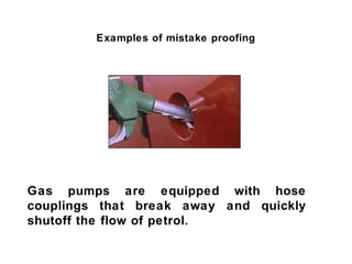
  • 302. Examples of mistake proofing Gas pumps are equipped with hose couplings that break away and quickly shutoff the flow of petrol.
  • 303. Examples of mistake proofing Automobiles controls have a mistake proofing device to ensure that the key in the on position before allowing the driver to shift out of park ( for automatic gears ).The keys can not be removed until the car is in park.
  • 304. Examples of mistake proofing 3.5 inch diskette can not be inserted unless diskette is oriented correctly.This is as far as diskette can be inserted upside-down. The beveled corner of the diskette pushes a stop in the disk drive out of the way allowing diskette to be inserted.This feature,along with the fact that the diskette is not square,prohibit incorrect orientation.
  • 305. Examples of mistake proofing Electronic car locks can have three mistake proofing devices: • Ensures that no door is left unlocked. • Door automatically locks when car exceeds a predetermined speed • Lock won’t operate when door is open and engine is running.
  • 306. Examples of mistake proofing New lawn mowers are required to have a safety bar on the handle that must be pulled back in order to start the engine.If you let go of the safety bar,the mowers blade stops in 3 seconds or less.This is an adaptation of the”dead man switch” from railroad locomotives.
  • 307. Examples of mistake proofing Retail stores use electronic article surveillance to ensure that no one walks away without making payment.