

![3
TRACTIVE EFFORT AND RESISTANCE
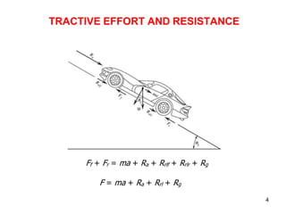
• These are the opposing forces that determine straight-line
performance of road vehicles.
• Tractive effort is simply the force available at the roadway
surface to perform work (expressed in lbs [N]).
• Resistance (expressed in lbs [N]) is defined as the force
impeding vehicle motion.
• Three major sources of vehicle resistance are:
– Aerodynamic
– Rolling (originates from the roadway surface-tire interface)
– Grade or gravitational](https://image.slidesharecdn.com/1-231229200549-109fcd66/85/-3-320.jpg)


![11
EXAMPLE 1
A 8.9 kN car has a drag coefficient of 0.40, frontal area 2.0 m2
and an available tractive effort of 1.135 kN. Determine the
maximum grade that the car can ascend at an elevation 1500 m
(ρ = 1.0567 kg/m3) on a paved surface while maintaining a
maximum speed of 110 km/h.
[see whiteboard and pages 15 - 16]](https://image.slidesharecdn.com/1-231229200549-109fcd66/85/-11-320.jpg)
![12
EXAMPLE 2
If the car in the previous example was travelling at a speed of 90
km/h on 1% down grade, determine the maximum rate of
acceleration it can attain.
[see whiteboard]](https://image.slidesharecdn.com/1-231229200549-109fcd66/85/-12-320.jpg)


![17
EXAMPLE 3
An 11.0-kN car is designed with 3.05 m wheelbase. The center
of gravity is located 550 mm above the pavement and 1.00 m
behind the front axle. If the coefficient of road adhesion is 0.6,
what is the maximum tractive effort that can be developed if the
car is (a) front-wheel-drive and (b) rear-wheel-drive?
[see whiteboard and page 18]](https://image.slidesharecdn.com/1-231229200549-109fcd66/85/-17-320.jpg)

![23
EXAMPLE 4
Calculate the minimum coefficient of road adhesion to ensure
that a car will not slide given that the car is front-wheel driven
with the braking force produced at tire-pavement contact
point is 2.1 kN, the car speed is 90 km/h, its weight is 8.7 kN
and the length of its wheel base is 1.95 m with its center of
gravity is at distance 0.90 m from the front axle and at height
0.55 m above roadway surface.
[see whiteboard]](https://image.slidesharecdn.com/1-231229200549-109fcd66/85/-23-320.jpg)
عرض تقديمي لتصميم طريق وكيفية ابعاد الطريق
- 1. CIV 331 Highway Engineering Course Instructor Dr. Essam Dabbour, P. Eng. Presentation 02
- 2. 2 ROAD-VEHICLE PERFORMANCE • Roadway design is governed by two main factors: – Vehicle capabilities • acceleration/deceleration • braking • cornering – Human capabilities • perception/reaction times • eyesight (range, height above roadway) • Performance of road vehicles forms the basis for roadway design guidelines such as: – length of acceleration / deceleration lanes – maximum grades – stopping-sight distances / passing-sight distances – timing of traffic signals
- 3. 3 TRACTIVE EFFORT AND RESISTANCE • These are the opposing forces that determine straight-line performance of road vehicles. • Tractive effort is simply the force available at the roadway surface to perform work (expressed in lbs [N]). • Resistance (expressed in lbs [N]) is defined as the force impeding vehicle motion. • Three major sources of vehicle resistance are: – Aerodynamic – Rolling (originates from the roadway surface-tire interface) – Grade or gravitational
- 4. 4 TRACTIVE EFFORT AND RESISTANCE Ff + Fr = ma + Ra + Rrlf + Rrlr + Rg F = ma + Ra + Rrl + Rg
- 5. 5 AERODYNAMIC RESISTANCE • It can have significant impacts on vehicle performance, particularly at high speeds. • It can be determined using the following equation: 2 2 V A C R f D a Where: Ra = aerodynamic resistance in lb (N) ρ (rho) = air density in slugs/ft3 (kg/m3) CD = coefficient of drag (unitless) Af = frontal area of vehicle in ft2 (m2) V = vehicle speed in ft/s (m/s)
- 6. 6 AERODYNAMIC RESISTANCE (Cont’d) • Air density is a function of both elevation and temperature (see Table 2.1 in the textbook). • The drag coefficient is measured from empirical data, either from wind tunnel experiments or actual field tests (it has dropped from about 0.5 to mid 0.2’s for sedan type vehicles, but still in 0.4 – 0.5 range for SUVs and trucks). 2005 Honda Insight (CD = 0.25) 1967 Volkswagen Beetle (CD = 0.46) 2003 Hummer H2 (CD = 0.57) 2010 Toyota Prius (CD = 0.25)
- 7. 7 AERODYNAMIC RESISTANCE (Cont’d) • As power is the product of force and speed, the power needed to overcome aerodynamic resistance can be determined using the following equation: • The force required to overcome aerodynamic resistance increases with the square of the speed while the corresponding power increases with the cube of the speed (double the speed requires 4 times the force and 8 times the power). 3 2 V A C P f D Ra
- 8. 8 ROLLING RESISTANCE • Refers to the resistance generated from the interaction between the tires and the roadway surface: – Primary source (about 90%) of this resistance is the deformation of the tire as it passes over the roadway surface. – Tire penetration/roadway surface compression (about 4%) – Tire slippage and air circulation around tire & wheel (about 6%) • Factors affecting rolling resistance (Rrl ): – Rigidity of tire and roadway surface – Tire inflation pressure and temperature – Vehicle speed
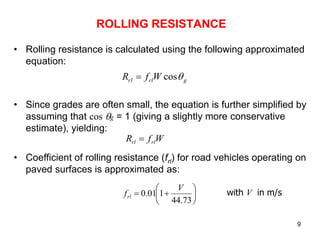
- 9. 9 ROLLING RESISTANCE • Rolling resistance is calculated using the following approximated equation: • Since grades are often small, the equation is further simplified by assuming that cos g = 1 (giving a slightly more conservative estimate), yielding: • Coefficient of rolling resistance (frl) for road vehicles operating on paved surfaces is approximated as: g rl rl W f R cos W f R rl rl 73 . 44 1 01 . 0 V frl with V in m/s
- 10. 10 GRADE RESISTANCE • The grade resistance is the component of the vehicle weight acting parallel to the roadway surface. • As highway grades are usually small: g g W R sin WG Rg g g tan sin
- 11. 11 EXAMPLE 1 A 8.9 kN car has a drag coefficient of 0.40, frontal area 2.0 m2 and an available tractive effort of 1.135 kN. Determine the maximum grade that the car can ascend at an elevation 1500 m (ρ = 1.0567 kg/m3) on a paved surface while maintaining a maximum speed of 110 km/h. [see whiteboard and pages 15 - 16]
- 12. 12 EXAMPLE 2 If the car in the previous example was travelling at a speed of 90 km/h on 1% down grade, determine the maximum rate of acceleration it can attain. [see whiteboard]
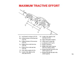
- 14. 14 MAXIMUM TRACTIVE EFFORT (Cont’d) • No matter how much force a vehicle’s engine produces at the roadway surface, there is a point beyond which additional force will not accelerate the vehicle further but rather it will just result in the spinning of tires. • To determine that maximum tractive effort, the normal load on the rear axle (Wr) is determined by summing the moments about point A: • Since the grade is usually small then cosθ = 1 and the above equations becomes: L Wh mah Wl h R W g g f a r sin cos ) ( rl f r R F L h W L l W
- 15. 15 MAXIMUM TRACTIVE EFFORT (Cont’d) • From the basics of physics, the maximum tractive force is the product of the normal force (Wr) multiplied by the coefficient of road adhesion (µ); and therefore, the maximum tractive force for a rear-wheel-drive vehicle is: • Similarly, by summing moments about point B, it can be shown that for a front-wheel-drive vehicle: L h L h f l W F R F L h W L l F rl f rl f / 1 / ) ( max max max L h L h f l W F rl r / 1 / max
- 16. 16 TYPICAL VALUES OF COEFFICIENT OF ROAD ADHESION Pavement Coefficient of Road Adhesion Maximum Slide Good, dry 1.00 0.80 Good, wet 0.90 0.60 Poor, dry 0.80 0.55 Poor, wet 0.60 0.30 Packed snow or ice 0.25 0.10
- 17. 17 EXAMPLE 3 An 11.0-kN car is designed with 3.05 m wheelbase. The center of gravity is located 550 mm above the pavement and 1.00 m behind the front axle. If the coefficient of road adhesion is 0.6, what is the maximum tractive effort that can be developed if the car is (a) front-wheel-drive and (b) rear-wheel-drive? [see whiteboard and page 18]
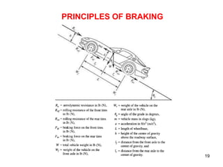
- 18. 18 PRINCIPLES OF BRAKING • For roadway design and traffic analysis, vehicle braking characteristics are the most important aspect of vehicle performance. • Braking performance is a key factor to the determination of: – stopping-sight distance, which is one of the foundations of roadway design – the length of the yellow interval for traffic signals
- 20. 20 PRINCIPLES OF BRAKING • Taking moments about the front and rear axles, and assuming cos g = 1 for small roadway grades, the normal loads on the front and rear axles are given by the following equations: • Also, from summing forces along the vehicle’s longitudinal axis gives: g a r f W R ma h Wl L W sin 1 g a f r W R ma h Wl L W sin 1 g a rl b W R ma W f F sin where: Fb = Fbf + Fbr
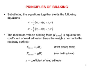
- 21. 21 PRINCIPLES OF BRAKING • Substituting the equations together yields the following equations : • The maximum vehicle braking force (Fb max) is equal to the coefficient of road adhesion times the weights normal to the roadway surface: W f F h Wl L W rl b r f 1 W f F h Wl L W rl b f r 1 r max br W F = coefficient of road adhesion f max bf W F (front braking force) (rear braking force)
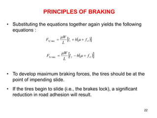
- 22. 22 PRINCIPLES OF BRAKING • Substituting the equations together again yields the following equations : • To develop maximum braking forces, the tires should be at the point of impending slide. • If the tires begin to slide (i.e., the brakes lock), a significant reduction in road adhesion will result. rl r bf f h l L W F max rl f br f h l L W F max
- 23. 23 EXAMPLE 4 Calculate the minimum coefficient of road adhesion to ensure that a car will not slide given that the car is front-wheel driven with the braking force produced at tire-pavement contact point is 2.1 kN, the car speed is 90 km/h, its weight is 8.7 kN and the length of its wheel base is 1.95 m with its center of gravity is at distance 0.90 m from the front axle and at height 0.55 m above roadway surface. [see whiteboard]