SlideShare a Scribd company logo
“HASHING”
Prepared By
Prof. Anand N. Gharu
(Assistant Professor)
Computer Dept.
15 January 2024
CLASS : SE COMPUTER 2019
SUBJECT : DSA (SEM-II)
: I
Note: The material to prepare this presentation has been taken from internet and are
generated only
for students reference and not for commercial 1
SYLLABUS
Hash Table- Concepts-hash table, hash function, basic operations,
bucket, collision, probe, synonym, overflow, open hashing, closed
hashing, perfect hash function, load density, full table, load factor,
rehashing, issues in hashing, hash functions- properties of good
hash function, division, multiplication, extraction, mid-square,
folding and universal, Collision resolution strategies- open
addressing and chaining, Hash table overflow- open addressing and
chaining, extendible hashing, closed addressing and separate
chaining.
Skip List- representation, searching and operations- insertion,
removal
SYLLABUS
INTRODUCTIO
N
UNIT-I
HASHING
1. Hashing is finding an address where the data is
to be stored as well as located using a key with
the help of the algorithmic function.
2. Hashing is a method of directly computing the
address of the record with the help of a
key by using a suitable mathematical
function called the hash function
3. A hash table is an array-based structure used to
store <key, information> pairs
INTRODUCTION
INTRODUCTION
4. Hash Table: A hash table is a data structure that
stores records in an array, called a hash table. A
Hash table can be used for quick insertion and
searching.
key
Hash(key) Address
Fig 11.1:Hashing Concept
• The resulting address is used as the basis
for storing and retrieving records and this
address is called as home address of the record
• For array to store a record in a hash table,
hash function is applied to the key of the
record being stored, returning an index
within the range of the hash table
• The item is then stored in the table of that
index position
INTRODUCTION
• Hashing is a well-known technique to search any
particular element among several elements.
• It minimizes the number of comparisons while performing
the search.
Advantage-
1. Hashing is extremely efficient.
2. The time taken by it to perform the search does not depend upon
the total number of elements.
3. It completes the search with constant time complexity O(1).
Hashing
• Hashing Mechanism -
1. An array data structure called as Hash table is used to store the
data items.
2. Based on the hash key value, data items are inserted into the hash table.
• Hash Key Value -
3. Hash key value is a special value that serves as an index for a
data item.
4. It indicates where the data item should be be stored in the hash table.
5. Hash key value is generated using a hash function.
Hashing
• Hashing Mechanism :
Hashing
• Hash Fuction :
1. Hash function takes the data item as an input and returns a small
integer value as an output.
2. The small integer value is called as a hash value.
3. Hash value of the data item is then used as an index for storing it
into the hash table.
Types of Hash Functions-
There are various types of hash functions available such as-
4. Mid Square Hash Function
5. Division Hash Function
6. Folding Hash Function etc
It depends on the user which hash function he wants to use.
Hashing
• A hash table is a data structure that stores records in an array,
called a hash table. A Hash table can be used for quick insertion
and searching.
HASH
TABLE
• Hash table is one of the most important data structures that
uses a special function known as a hash function that maps
a given value with a key to access the elements faster.
• A Hash table is a data structure that stores some
information, and the information has basically two main
components, i.e., key and value. The hash table can be
implemented with the help of an associative array. The
efficiency of mapping depends upon the efficiency of the
hash function used for mapping.
HASH
TABLE
Here, are pros/benefits of using hash tables:
1. Hash tables have high performance when looking up data,
inserting, and deleting existing values.
2. The time complexity for hash tables is constant regardless
of the number of items in the table.
3. They perform very well even when working with
large datasets.
ADVANTAGES OF HASH
TABLE
Here, are cons of using hash tables:
1. You cannot use a null value as a key.
2. Collisions cannot be avoided when generating keys using.
hash functions. Collisions occur when a key that is
already in use is generated.
3. If the hashing function has many collisions, this can lead
to performance decrease.
DISAVANTAGES OF HASH
TABLE
Here, are the Operations supported by Hash tables:
1. Insertion – this Operation is used to add an element to the
hash table
2. Searching – this Operation is used to search for elements
in the hash table using the key
3. Deleting – this Operation is used to delete elements from
the hash table
OPERATIONS OF HASH
TABLE
Real-world Applications
In the real-world, hash tables are used to store data for
1. Databases
2. Associative arrays
3. Sets
4. Memory cache
APPLICATIONS OF HASH
TABLE
a)Easy to compute : It should be easy to compute and must not become
an algorithm in itself.
b)Uniform distribution : It should provide a uniform distribution across
the hash table and should not result in clustering.
c)Less collisions :
Collisions occur when pairs of elements are mapped to
the same hash value. These should be avoided.
d) Be easy and quick to compute.
CHARACTRISTICS OF HASH
FUNCTION
1) Hash function should be simple to computer.
2) Number of collision should be less
2) The hash function uses all the input data.
3)The hash function "uniformly" distributes
the data across the entire set of possible hash values.
4)The hash function generates very different hash values
for similar strings.
PROPERTIES OF HASH
FUNCTION
• A function that maps a key into the range [0 to Max − 1], the
result of which is used as an index (or address) to hash table for
storing and retrieving record
• The address generated by hashing function is called as home
address
• All home addresses address to particular area of memory and that
area is called as prime area
HASH
FUNCTION
• Bucket is an index position in hash table that can store more than
one record
• When the same index is mapped with two keys, then both
the records are stored in the same bucket
BUCKE
T
• The result of two keys hashing into the same address is
called
collision
COLLISION
• Each calculation of an address and test for success is
known as
Probe.
PROBE
• Keys those hash to the same address are called synonyms
SYNONYMS
• The result of more keys hashing to the same address and if there
is no room in the bucket, then it is said that overflow has occurred
• Collision and overflow are synonymous when the bucket is
of size 1
OVERFLOW
• A perfect hash function h for a set S is a hash function that
maps distinct elements in S to a set of m integers, with no
collisions.
• A perfect hash function with values in a limited range can be used
for efficient lookup operations, by placing keys from S (or other
associated values) in a table indexed by the output of the function.
Perfect Hash
Function
• Advantages :
1. A perfect hash function with values in a limited range
can be used for efficient lookup operations.
2. No need to apply collision resolution techniques.
Perfect Hash
Function
Load factor is defined as (m/n) where n is the total size of the hash
table and m is the preferred number of entries which can be inserted
before a increment in size of the underlying data structure is
required.
If Load factor (α) = constant, then time complexity of Insert,
Search, Delete = Θ(1)
LOAD FACTOR
• Load Factor: The ratio of the number of items in a
table to the table’s size is called the load factor.
• Load Density : The identifier density of a hash table
is the ratio n/T,
• where n is the number of identifiers in the table.
The loading density or loading factor of a hash table
is a=n /(sb).
• T is total number of possible element.
Load factor and Load
density
• Load Density : The identifier density of a hash table
is the ratio n/T,
• Example :
• Consider the hash table with b = 26 buckets and s = 2.
We have n = 10 distinct identifiers, each representing
a C library function.
• This table has a loading factor, a, of 10/52 = 0.19
Load factor and Load
density
• Hashing is one of the searching techniques that uses a constant
time. The time complexity in hashing is O(1). Till now, we read
the two techniques for searching, i.e., linear search and binary search
• The worst time complexity in linear search is O(n), and O(logn)
in binary search. In both the searching techniques, the searching
depends upon the number of elements but we want the technique
that takes a constant time. So, hashing technique came that
provides a constant time.
• In Hashing technique, the hash table and hash function are
used. Using the hash function, we can calculate the address at
which the value can be stored.
HASHING
• The main idea behind the hashing is to create the (key/value)
pairs. If the key is given, then the algorithm computes the index at
which the value would be stored. It can be written as:
• Index = hash(key)
HASHING/HASH
FUNCTION
a) Division Method
b) Multiplication Method
c) Extraction Method
d) Mid square method
e) Folding
f) Universal Method
TYPES OF HASH
FUNCTION
There are three ways of calculating the hash function:
1. Division method
2. Folding method
3. Mid square method
In the division method, the hash function can be defined as:
h(ki) = ki % m;
where m is the size of the hash table.
For example, if the key value is 6 and the size of the hash table is 10.
When we apply the hash function to key 6 then the index would be:
h(6) = 6%10 = 6
The index is 6 at which the value is stored.
TYPES OF HASH
FUNCTION
1. Division Method:
This is the most simple and easiest method to generate a hash value. The
hash function divides the value k by M and then uses the remainder
obtained.
Formula:
h(K) = k mod M
Here,
k is the key value, and
M is the size of the hash table.
TYPES OF HASH
FUNCTION
Example:
k = 12345
M = 95
h(12345) = 12345 mod 95
= 90
k = 1276
M = 11
h(1276) = 1276 mod 11
= 0
2. The mid square method is a very good hashing method.
It involves two steps to compute the hash value-
Square the value of the key k i.e. k2
Extract the middle r digits as the hash value.
Formula:
h(K) = h(k x k)
Here,
k is the key value.
TYPES OF HASH
FUNCTION
Example:
Suppose the hash table has 100 memory locations.
So r = 2 because two digits are required to map the
key to the memory location.
k = 60
k x k = 60 x 60
= 3600 (mid 60 for k=60)
h(60) = 60
The hash value obtained is 60
3. Digit Folding Method : This method involves two steps:
Divide the key-value k into a number of parts i.e. k1, k2, k3,….,kn, where each
part has the same number of digits except for the last part that can have lesser
digits than the other parts.
Add the individual parts. The hash value is obtained by ignoring the last carry if
any.
Formula:
k = k1, k2, k3, k4, ….., kn
s = k1+ k2 + k3 + k4 +….+ kn
h(K)= s
Here,
s is obtained by adding the
TYPES OF HASH
FUNCTION
3. Digit Folding Method :
Example:
k = 12345
k1 = 12, k2 = 34, k3 = 5
s = k1 + k2 + k3
= 12 + 34 + 5
= 51
h(K) = 51
TYPES OF HASH
FUNCTION
4. Multiplication method :
This method involves the following steps:
• Choose a constant value A such that 0 < A < 1.
• Multiply the key value with A.
• Extract the fractional part of kA.
• Multiply the result of the above step by the size of the hash table
i.e. M.
• The resulting hash value is obtained by taking the floor of
the result obtained in step 4.
TYPES OF HASH
FUNCTION
4. Multiplication method :
Formula:
h(K) = floor (M (kA mod 1))
Here,
M is the size of the hash table.
k is the key value.
A is a constant value.
Where "k A mod 1" means the fractional part of k A, that is, k A -
⌊k A⌋.
TYPES OF HASH
FUNCTION
4. Multiplication method :
Example:
k = 12345
A = 0.357840
M = 100
h(12345) = floor[ 100 (12345*0.357840 mod
1)]
= floor[ 100 (4417.5348 mod 1) ]
= floor[ 100 (0.5348) ]
= floor[ 53.48 ]
= 53
TYPES OF HASH
FUNCTION
• Collision in Hashing-
In hashing,
1. Hash function is used to compute the hash value for a key.
2. Hash value is then used as an index to store the key in the hash
table.
3. Hash function may return the same hash value for two or more
keys.
“When the hash value of a key maps to an already occupied
bucket of the hash table, it is called as a Collision”
Collision in Hashing
When the two different values have the same value, then the problem occurs
between the two values, known as a collision. In the above example, the value is
stored at index 6. If the key value is 26, then the index would be:
h(26) = 26%10 = 6
Therefore, two values are stored at the same index, i.e., 6, and this leads to the
collision problem. To resolve these collisions, we have some techniques known
as collision techniques.
The following are the collision techniques:
Open Hashing: It is also known as closed addressing.
Closed Hashing: It is also known as open addressing.
COLLISION
In Hashing, collision resolution techniques are classified as-
Collision Resolution
Techniques
Separate Chaining
(Open hashing/External hashing)
The first Collision Resolution or Handling technique, " Open
Hashing ", is popularly known as Separate Chaining. This is a
technique which is used to implement an array as a linked list known
as a chain. It is one of the most used techniques by programmers to
handle collisions. Basically, a linked list data structure is used to
implement the Separate Chaining technique. When a number of
elements are hashed into the index of a single slot, then they are
inserted into a singly-linked list. This singly-linked list is the linked
list which we refer to as a chain in the Open Hashing technique.
OPEN HASHING
n Open Hashing, one of the methods used to resolve the collision is
known as a chaining method.
OPEN HASHING
1. Separate Chaining (hashing with chaining/open hashing)
To handle the collision,
2. This technique creates a linked list to the slot for which collision
occurs.
3. The new key is then inserted in the linked list.
4. These linked lists to the slots appear like chains.
5. That is why, this technique is called as separate chaining
Collision Resolution Techniques
For Searching-
• In worst case, all the keys might map to the same bucket of
the hash table.
• In such a case, all the keys will be present in a single linked list.
• Sequential search will have to be performed on the linked list to
perform the search.
• So, time taken for searching in worst case is O(n).
For Deletion-
• In worst case, the key might have to be searched first and
then deleted.
• In worst case, time taken for searching is O(n).
• So, time taken for deletion in worst case is O(n).
Collision Resolution Techniques
Advantages:
1) Simple to implement.
2)Hash table never fills up, we can always add more elements to
the chain.
3) Less sensitive to the hash function or load factors.
4)It is mostly used when it is unknown
how many and how frequently keys may be inserted or
deleted. .
Collision Resolution
Techniques
Disadvantages:
1)Cache performance of chaining is not good as keys are
stored using a linked list. Open addressing provides better
cache performance as everything is stored in the same table.
2) Wastage of Space (Some Parts of hash table are never used)
3)If the chain becomes long, then search time can become O(n)
in the worst case.
4) Uses extra space for links
Collision Resolution
Techniques
Collision Resolution Techniques
Using the hash function ‘key mod 7’, insert the following
sequence of keys in the hash table-
50, 700, 76, 85, 92, 73 and 101.
Use separate chaining technique for collision resolution.
Step-01:
Draw an empty hash table.
For the given hash function, the
possible range of hash values is [0, 6].
So, draw an empty hash table consisting
of 7 buckets as-
Collision Resolution Techniques
Using the hash function ‘key mod 7’, insert the
following sequence of keys in the hash table-
50, 700, 76, 85, 92, 73 and 101.
Use separate chaining technique for collision resolution.
Step-02:
Insert the given keys in the hash table one
by one.
The first key to be inserted in the hash table
= 50.
Bucket of the hash table to which key 50
maps = 50 mod 7 = 1.
So, key 50 will be inserted in bucket-1 of
the hash table as-
Collision Resolution Techniques
Using the hash function ‘key mod 7’, insert the
following sequence of keys in the hash table-
50, 700, 76, 85, 92, 73 and 101.
Use separate chaining technique for collision resolution.
Step-03:
The next key to be inserted in the hash table
= 700.
Bucket of the hash table to which key 700
maps = 700 mod 7 = 0.
So, key 700 will be inserted in bucket-0 of
the hash table as-
Collision Resolution Techniques
Using the hash function ‘key mod 7’, insert the
following sequence of keys in the hash table-
50, 700, 76, 85, 92, 73 and 101.
Use separate chaining technique for collision resolution.
Step-04:
The next key to be inserted in the hash table
= 76.
Bucket of the hash table to which key 76
maps = 76 mod 7 = 6.
So, key 76 will be inserted in bucket-6 of
the hash table as-
Collision Resolution Techniques
Using the hash function ‘key mod 7’, insert the following
sequence of keys in the hash table-
50, 700, 76, 85, 92, 73 and 101.
Use separate chaining technique for collision resolution.
Step-05:
The next key to be inserted in the hash table = 85.
Bucket of the hash table to which key 85 maps = 85
mod 7 = 1.
Since bucket-1 is already occupied, so
collision occurs.
Separate chaining handles the collision by creating
a linked list to bucket-1.
So, key 85 will be inserted in bucket-1 of the
hash table as-
Collision Resolution Techniques
Using the hash function ‘key mod 7’, insert the following
sequence of keys in the hash table-
50, 700, 76, 85, 92, 73 and 101.
Use separate chaining technique for collision resolution.
Step-06 :
The next key to be inserted in the hash table =
92.
Bucket of the hash table to which key 92 maps
= 92 mod 7 = 1.
Since bucket-1 is already occupied,
so collision occurs.
Separate chaining handles the collision by
creating a linked list to bucket-1.
So, key 92 will be inserted in bucket-1 of the
hash table as-
Collision Resolution Techniques
Using the hash function ‘key mod 7’, insert the following
sequence of keys in the hash table-
50, 700, 76, 85, 92, 73 and 101.
Use separate chaining technique for collision resolution.
Step-07 :
The next key to be inserted in the hash table =
73.
Bucket of the hash table to which key 73 maps
= 73 mod 7 = 3.
So, key 73 will be inserted in bucket-3 of the
hash table as-
Collision Resolution Techniques
Using the hash function ‘key mod 7’, insert the following
sequence of keys in the hash table-
50, 700, 76, 85, 92, 73 and 101.
Use separate chaining technique for collision resolution.
Step-08 :
The next key to be inserted in the hash table =
101.
Bucket of the hash table to which key
101 maps = 101 mod 7 = 3.
Since bucket-3 is already occupied,
so collision occurs.
Separate chaining handles the collision by
creating a linked list to bucket-3.
So, key 101 will be inserted in bucket-3 of the
hash table as-
Using the hash function ‘key mod 7’, insert the following
sequence of keys in the hash table-
50, 700, 76, 85, 92, 73 and 101.
Use separate chaining technique for collision resolution.
Collision Resolution Techniques
Let's first understand the chaining to resolve the collision.
Suppose we have a list of key values
A = 3, 2, 9, 6, 11, 13, 7, 12 where m = 10, and h(k) = 2k+3
In this case, we cannot directly use h(k) = ki/m as h(k) = 2k+3
The index of key value 3 is:
index = h(3) = (2(3)+3)%10 = 9
The value 3 would be stored at the index 9.
The index of key value 2 is:
index = h(2) = (2(2)+3)%10 = 7
The value 2 would be stored at the index 7.
OPEN HASHING
The index of key value 9 is:
index = h(9) = (2(9)+3)%10 = 1
The value 9 would be stored at the index 1.
The index of key value 6 is:
index = h(6) = (2(6)+3)%10 = 5
The value 6 would be stored at the index 5.
The index of key value 11 is:
index = h(11) = (2(11)+3)%10 = 5
The value 11 would be stored at the index 5.
OPEN HASHING
The index of key value 13 is:
index = h(13) = (2(13)+3)%10 = 9
The value 13 would be stored at index 9.
The index of key value 7 is:
index = h(7) = (2(7)+3)%10 = 7
The value 7 would be stored at index 7.
The index of key value 12 is:
index = h(12) = (2(12)+3)%10 = 7
The value 7 would be stored at index 7.
OPEN HASHING
OPEN HASHING
OPEN HASHING
OPEN HASHING
Let us say that we have a sequence of numbers { 437, 325, 175,
199, 171, 189, 127, 509} and a hash function H(X) = X mod 10
Let us see the results of separate chaining hash table.
OPEN HASHING
In Closed hashing, three techniques are used to resolve the
collision:
1. Linear probing
2. Quadratic probing
3. Double Hashing technique
CLOSED HASHING
PROBING
Method Description
Just like the name suggests, this method
searches for empty slots linearly starting
from
Linear probing
the position where the collision occurred
and moving forward. If the end of the list
is reached and no empty slot is found.
The probing starts at the beginning of the
list.
Quadratic
probing
This method uses quadratic polynomial
expressions to find the next available free
slot.
Double
Hashing
This technique uses a secondary
hash function algorithm to find the
next free available slot.
Open addressing
(Close hashing/Internal
hashing)
In open addressing,
1. Unlike separate chaining, all the keys are stored inside the hash
table.
2. No key is stored outside the hash table.
Techniques used for open addressing are-
3. Linear Probing
4. Quadratic Probing
5. Double Hashing
Open Addressing
Operations In open addressing,
1. Insert Operation-
• Hash function is used to compute the hash value for a key to be inserted.
• Hash value is then used as an index to store the key in the hash table.
In case of collision,
• Probing is performed until an empty bucket is found.
• Once an empty bucket is found, the key is inserted.
• Probing is performed in accordance with the technique used for
open addressing.
Open Addressing
Operations In open addressing,
Search Operation-
To search any particular key,
• Its hash value is obtained using the hash function used.
• Using the hash value, that bucket of the hash table is checked.
• If the required key is found, the key is searched.
• Otherwise, the subsequent buckets are checked until the required key or
an empty bucket is found.
• The empty bucket indicates that the key is not present in the hash table.
Open Addressing
Operations In open addressing,
Search Operation-
• The key is first searched and then deleted.
• After deleting the key, that particular bucket is marked
as “deleted”.
Open Addressing
1. Linear Probing-
2. When collision occurs, we linearly probe for the next bucket.
3. We keep probing until an empty bucket is found.
Advantage-
4. It is easy to compute.
Disadvantage-
5. The main problem with linear probing is clustering.
6. Many consecutive elements form groups.
7. Then, it takes time to search an element or to find an empty bucket.
Open Addressing Techniques
1. Linear Probing -
Let us consider a simple hash function as “key mod 7” and a sequence
of keys as 50, 700, 76, 85, 92, 73, 101.
Linear Probing
Linear probing is one of the forms of open addressing. As we know
that each cell in the hash table contains a key-value pair, so when the
collision occurs by mapping a new key to the cell already
occupied by another key, then linear probing technique searches
for the closest free locations and adds a new key to that empty
cell. In this case, searching is performed sequentially, starting from
the position where the collision occurs till the empty cell is not
found.
CLOSED HASHING
Let's understand the linear probing through an example.
Consider the above example for the linear probing:
A = 3, 2, 9, 6, 11, 13, 7, 12 where m = 10, and h(k) = 2k+3
The key values 3, 2, 9, 6 are stored at the indexes 9, 7, 1, 5 respectively.
The calculated index value of 11 is 5 which is already occupied by another
key value, i.e., 6. When linear probing is applied, the nearest empty cell to
the index 5 is 6; therefore, the value 11 will be added at the index 6.
The next key value is 13. The index value associated with this key value is
9 when hash function is applied. The cell is already filled at index 9. When
linear probing is applied, the nearest empty cell to the index 9 is 0;
therefore, the value 13 will be added at the index 0
CLOSED HASHING
Let us consider a simple hash function as “key mod 7” and a
sequence of keys as 50, 700, 76, 85, 92, 73, 101.
LINEAR PROBING
Let us consider a simple hash function as “key mod 30” and a
sequence of keys as 3, 1, 63, 5, 11, 15, 18, 16, 46.
LINEAR PROBING
Chaining
( with
/without
In collision handling method chaining is a concept which introduces
an additional field with data i.e. chain. A separate chain table is
maintained for colliding data. When collision occurs, we store the
second colliding data by linear probing method. The address
of this colliding data can be stored with the first colliding element in
the chain table, without replacement.
Chaining Without Replacement
For example, consider elements:
131, 3, 4, 21, 61, 6, 71, 8, 9
Chaining Without Replacement
For example, consider elements:
Identifier is 11, 32, 41, 54, 33. Hash function: f(x) = X mod 10 and
Table size = 10
Chaining With Replacement
For example, consider elements:
Identifier is 11, 32, 41, 54, 33.
Hash function: f(x) = X mod 10 and Table size = 10
Chaining Without Replacement
Chaining With Replacement
2. Quadratic Probing-
• When collision occurs, we probe for i2‘th bucket in ith iteration.
• We keep probing until an empty bucket is found.
Open Addressing Techniques
Quadratic Probing
• In case of linear probing, searching is performed linearly. In contrast,
quadratic probing is an open addressing technique that uses
quadratic polynomial for searching until a empty slot is found.
• It can also be defined as that it allows the insertion ki at first free
location from (u+i2)%m where i=0 to m-1.
h´ = (𝑥) = 𝑥 𝑚𝑜𝑑 𝑚
ℎ(𝑥, 𝑖) = ( ´(
ℎ 𝑥) + 𝑖2)𝑚𝑜𝑑 𝑚
We can put some other quadratic equations also using some constants
The value of i = 0, 1, . . ., m – 1. So we start from i = 0, and increase this
until we get one free space. So initially when i = 0, then the h(x, i) is same
as h´(x).
CLOSED HASHING
CLOSED HASHING
CLOSED HASHING
mod 7”
Let us consider a simple hash function as “key
and sequence of keys as 50, 700, 76, 85, 92, 73, 101
If the slot hash(x) % S is full, then we try (hash(x) + 1*1) % S.
If (hash(x) + 1*1) % S is also full, then we try (hash(x) + 2*2) %
S.
If (hash(x) + 2*2) % S is also full, then we try (hash(x) + 3*3) %
S.
This process is repeated for all the values of i until an empty slot
is found.
QUADRATIC PROBING
QUADRATIC PROBING
Example: Let us consider table Size = 7, hash function as Hash(x) = x % 7
and collision resolution strategy to be f(i) = i2 . Insert = 22, 30, and 50.
QUADRATIC PROBING
Using Linear probing and Quadratic probing, insert the following values in
the hash table of size 10.Show how many collisions occur in each iterations
28, 55, 71, 67, 11, 10, 90, 44 (Linear Probing)
QUADRATIC PROBING
Using Linear probing and Quadratic probing, insert the following values in
the hash table of size 10.Show how many collisions occur in each iterations
28, 55, 71, 67, 11, 10, 90, 44
3. Double Hashing-
• We use another hash function hash2(x) and look for i * hash2(x)
bucket in ith iteration.
• It requires more computation time as two hash functions need to
be computed.
• Double hashing is a collision resolving technique in Open
Addressed Hash tables. Double hashing uses the idea of applying
a second hash function to key when a collision occurs.
Open Addressing Techniques
Double hashing : It is a collision resolving technique in Open
Addressed Hash tables. Double hashing uses the idea of applying a
second hash function to key when a collision occurs.
Advantages of Double hashing
1. The advantage of Double hashing is that it is one of the best form
of records
of probing, producing a uniform
distribution throughout a hash table.
2. This technique does not yield any clusters.
3. It is one of effective method for resolving collisions
DOUBLE HASHING
Double hashing : A good second Hash function
is:
1. It must never evaluate to zero
2. Must make sure that all cells can be probed
CLOSED HASHING
Double hashing :
Double hashing can be done using :
(hash1(key) + i * hash2(key)) % TABLE_SIZE
Here hash1() and hash2() are hash functions and TABLE_SIZE
is size of hash table.
(We repeat by increasing i when collision occurs)
First hash function is typically hash1(key) = key %
TABLE_SIZE
A popular second hash function is : hash2(key) = PRIME – (key %
PRIME) where PRIME is a prime smaller than the TABLE_SIZE.
CLOSED HASHING
CLOSED HASHING
CLOSED HASHING
CLOSED HASHING
CLOSED HASHING
CLOSED HASHING
DOUBLE HASHING
EXAMPLE
Double Hashing Example :
Imagine you need to store some items inside a hash table
of size 20. The values given are: (16, 8, 63, 9, 27, 37, 48,
5, 69, 34, 1).
h1(n)=n%20
h2(n)=n%13
n h(n, i) =
(h1 (n) +
ih2(n)) mod
Open Vs Close Hashing
Separate Chaining Open Addressing
Keys are stored inside the hash table as
well as outside the hash table.
All the keys are stored only inside the
hash table.
The number of keys to be stored in the
hash table can even exceed the size of
the hash table.
The number of keys to be stored in the
hash table can never exceed the size of
the hash table.
Deletion is easier. Deletion is difficult.
Extra space is required for the pointers
to store the keys outside the hash table. No extra space is required.
Cache performance is poor.
This is because of linked lists which
store the keys outside the hash table.
Cache performance is better.
This is because here no linked lists are
used.
Some buckets of the hash table are
never used which leads to wastage of
space.
Buckets may be used even if no key
maps to those particular buckets.
Rehashing is a collision resolution technique.
Rehashing is a technique in which the table is resized, i.e., the size of
table is doubled by creating a new table. It is preferable is the total size
of table is a prime number. There are situations in which the rehashing is
required.
• When table is completely full
• With quadratic probing when the table is filled half.
• When insertions fail due to overflow.
In such situations, we have to transfer entries from old table to the new
table by re computing their positions using hash functions
Rehashing
Rehashing
As the name suggests, rehashing means hashing again.
Basically, when the load factor increases to more than its pre-
defined value (default value of load factor is 0.75), the
complexity increases. So to overcome this, the size of the
array is increased (doubled) and all the values are hashed
again and stored in the new double sized array to maintain a
low load factor and low complexity.
Rehashing
Why rehashing?
Rehashing is done because whenever key value pairs are
inserted into the map, the load factor increases, which implies
that the time complexity also increases as explained above.
This might not give the required time complexity of O(1).
Hence, rehash must be done, increasing the size of the
bucketArray so as to reduce the load factor and the time
complexity
Rehashing
How Rehashing is done?
Rehashing can be done as follows:
• For each addition of a new entry to the map, check the
load factor.
• If it’s greater than its pre-defined value (or default value of 0.75
if not given), then Rehash.
• For Rehash, make a new array of double the previous size and
make it the new bucket array.
• Then traverse to each element in the old bucket Array and call
the insert() for each so as to insert it into the new larger
bucket array.
Rehashing
• Hash Collisions: Hashing can produce the same hash value
for different keys, leading to hash collisions. To handle
collisions, we need to use collision resolution techniques
like chaining or open addressing.
• Hash Function Quality: The quality of the hash function
determines the efficiency of the hashing algorithm. A poor-
quality hash function can lead to more collisions, reducing
the performance of the hashing algorithm.
ISSUES IN HASHING
1. The dynamic hashing method is used to overcome the
problems of static hashing like bucket overflow.
2. In this method, data buckets grow or shrink as the records
increases or decreases. This method is also known
as Extendable hashing method.
it
allows in
poor
3. Thismethod makes hashing dynamic,
i.e., insertion or deletion without
resulting performance.
Extensible/Extendible Hashing
• How to search a key
1. First, calculate the hash address of the key.
2. Check how many bits are used in the directory, and these
bits are called as i.
3. Take the least significant i bits of the hash address.
This gives an index of the directory.
4. Now using the index, go to the directory and find bucket
address where the record might be.
Extensible/Extendible Hashing
• How to insert a new record
1. Firstly, you have to follow the same procedure
for retrieval, ending up in some bucket.
2. If there is still space in that bucket, then place the record
in it.
3. If the bucket is full, then we will split the bucket
and redistribute the records.
Extensible/Extendible Hashing
into buckets,
• For example :
Consider the following grouping of keys
depending on the prefix of their hash address:
Extensible/Extendible Hashing
The last two bits of 2 and 4 are 00. So it will go into bucket B0. The
last two bits of 5 and 6 are 01, so it will go into bucket B1. The last
two bits of 1 and 3 are 10, so it will go into bucket B2. The last two
bits of 7 are 11, so it will go into B3.
Extensible/Extendible Hashing
Insert key 9 with hash address 10001 into the above structure:
1. Since key 9 has hash address 10001, it must go into the first bucket.
But bucket B1 is full, so it will get split.
2. The splitting will separate 5, 9 from 6 since last three bits of 5, 9 are
001, so it will go into bucket B1, and the last three bits of 6 are 101, so
it will go into bucket B5.
3. Keys 2 and 4 are still in B0. The record in B0 pointed by the 000 and
100 entry because last two bits of both the entry are 00.
4. Keys 1 and 3 are still in B2. The record in B2 pointed by the 010 and
110 entry because last two bits of both the entry are 10.
5. Key 7 are still in B3. The record in B3 pointed by the 111 and 011
entry because last two bits of both the entry are 11.
Extensible/Extendible Hashing
Advantages of Extensible Hashing
1. In this method, the performance does not decrease as the
data
grows in the system. It simply increases the size of memory
to accommodate the data.
2. In this method, memory is well utilized as it grows and shrinks
with the data. There will not be any unused memory lying.
3. This method is good for the dynamic database where data grows
and shrinks frequently
Disadvantages of Extensible Hashing
1. In this method, if the data size increases then the bucket size is
also increased.
2. In this case, the bucket overflow situation will also occur. But it
might take little time to reach this situation than static
hashing.
1. A skip list is a probabilistic data structure.
2. The skip list is used to store a sorted list of elements or
data with a linked list.
3. It allows the process of the elements or data to view
efficiently. In one single step, it skips several
elements of the entire list, which is why it is known as a
skip list.
Skip List
4. The skip list is an extended version of the linked list.
5. It allows the user to search, remove, and insert the element
very quickly.
6. It consists of a base list that includes a set of elements
which maintains the link hierarchy of the
subsequent elements.
Skip List
Skip list structure
It is built in two layers: The lowest layer and Top layer.
The lowest layer of the skip list is a common sorted linked
list, and the top layers of the skip list are like an "express line"
where the elements are skipped.
Skip List
• Let's take an example to understand the working of the skip list. In this
example, we have 14 nodes, such that these nodes are divided into
two layers, as shown in the diagram.
• The lower layer is a common line that links all nodes, and the top layer is
an express line that links only the main nodes, as you can see in
the diagram.
• Suppose you want to find 47 in this example. You will start the search from
the first node of the express line and continue running on the express
line until you find a node that is equal a 47 or more than 47.
• You can see in the example that 47 does not exist in the express line, so
you search for a node of less than 47, which is 40. Now, you go to the
normal line with the help of 40, and search the 47, as shown in the
diagram.
Skip List
Skip List
Skip List Basic Operations
There are the following types of operations in the skip list.
1. Insertion operation: It is used to add a new node to a particular
location in a specific situation.
2. Deletion operation: It is used to delete a node in a
specific situation.
3. Search Operation: The search operation is used to
search a particular node in a skip list.
Skip List
Example 1: Create a skip list, we want to insert these following
keys in the empty skip list.
Step 1: Insert 6 with level 1
1. 6 with level 1.
2. 29 with level 1.
3. 22 with level 4.
4. 9 with level 3.
5. 17 with level 1.
6. 4 with level 2.
Skip List
Example 1: Create a skip list, we want to insert these following
keys in the empty skip list.
Step 2: Insert 29 with level 1
1. 6 with level 1.
2. 29 with level 1.
3. 22 with level 4.
4. 9 with level 3.
5. 17 with level 1.
6. 4 with level 2.
Skip List
Example 1: Create a skip list, we want to insert these following
keys in the empty skip list.
Step 3: Insert 22 with level 4
1. 6 with level 1.
2. 29 with level 1.
3. 22 with level 4.
4. 9 with level 3.
5. 17 with level 1.
6. 4 with level 2.
Skip List
Example 1: Create a skip list, we want to insert these following
keys in the empty skip list.
Step 4: Insert 9 with level 3
1. 6 with level 1.
2. 29 with level 1.
3. 22 with level 4.
4. 9 with level 3.
5. 17 with level 1.
6. 4 with level 2.
Skip List
Example 1: Create a skip list, we want to insert these following
keys in the empty skip list.
Step 5: Insert 17 with level 1
1. 6 with level 1.
2. 29 with level 1.
3. 22 with level 4.
4. 9 with level 3.
5. 17 with level 1.
6. 4 with level 2.
Skip List
Example 1: Create a skip list, we want to insert these following
keys in the empty skip list.
Step 6: Insert 4 with level 2
1. 6 with level 1.
2. 29 with level 1.
3. 22 with level 4.
4. 9 with level 3.
5. 17 with level 1.
6. 4 with level 2.
Skip List
Example 2: Consider this example where we want to search for
key 17.
Skip List
Example 2: Consider this example where we want to search for
key 17.
Skip List
1. If you want to insert a new node in the skip list, then it will insert
the node very fast because there are no rotations in the skip list.
2. The skip list is simple to implement as compared to the hash
table and the binary search tree.
3. It is very simple to find a node in the list because it stores the
nodes in sorted form.
4. The skip list algorithm can be modified very easily in a more
specific structure, such as indexable skip lists, trees, or priority
queues.
5. The skip list is a robust and reliable list.
Advantages of Skip List
1. It requires more memory than the balanced tree.
2. Reverse searching is not allowed.
3. The skip list searches the node much slower than the linked list.
Disadvantages of Skip List
1. Skiplist are used in distributed applications. In
distributed
systems, the nodes of skip list represents the computer systems
and pointers represent network connection.
2. Skip list are used for implementing highly scalable concurrent
priority queues with less lock contention (struggle for having a
lock on a data item)
Applications of Skip List
class. (
median
ordered
3. It is alsoused with the QMap
template
Value-based template class that provides a dictionary)
4. Theindexing of the skip list is used in
running
problems.
5. skipdb is an open-source database format
using key/value pairs.
Applications of Skip List
1. https://www.javatpoint.com/double-hashing-in-java
2. https://www.scaler.com/topics/quadratic-probing/
3. https://www.geeksforgeeks.org/quadratic-probing-in-hashing/
4. https://www.bucketstudy.com/2021/09/DSA01.html
5. https://www.upgrad.com/blog/hashing-in-data-structure/
6. https://quescol.com/data-structure/linear-probing
7. https://prac-code.blogspot.com/2013/06/chaining-without-
replacement.html
8. https://www.geeksforgeeks.org/open-addressing-collision-
handling-technique-in-hashing/
References
9.https://www.ques10.com/p/32048/using-linear-probing-
and- quadratic-probing-insert-/
10. https://dev.to/aws-builders/intro-into-hashing-3nf6
References
THANK YOU!!!
My Blog :
https://anandgharu.wordpress.com/
Email : gharu.anand@gmail.com

More Related Content

PPTX
unit-1-dsa-hashing-2022_compressed-1-converted.pptx
PPTX
Hashing and Collision Advanced data structure and algorithm
PPTX
Hashing And Hashing Tables
PPTX
hashing in data structure for Btech.pptx
PPTX
hashing in data structure for Btech .pptx
PPTX
hashing in data structure for engineering.pptx
PPTX
hashing in data strutures advanced in languae java
PPTX
Hashing
unit-1-dsa-hashing-2022_compressed-1-converted.pptx
Hashing and Collision Advanced data structure and algorithm
Hashing And Hashing Tables
hashing in data structure for Btech.pptx
hashing in data structure for Btech .pptx
hashing in data structure for engineering.pptx
hashing in data strutures advanced in languae java
Hashing

Similar to unit-1-data structure and algorithms-hashing-2024-1 (1).pptx (20)

PPTX
Data Structures-Topic-Hashing, Collision
PPTX
VCE Unit 04vv.pptx
PPTX
asdfew.pptx
PPTX
Ts project Hash based inventory system
PPTX
Presentation.pptx
PDF
Hash pre
PPTX
GRAPHS, BREADTH FIRST TRAVERSAL AND DEPTH FIRST TRAVERSAL
PPTX
Working with python Nice PPT must try very good
PPTX
Hash based inventory system
PPTX
Hashing
PPT
DS Lecture - 6 (Hashing) introduction.ppt
PPTX
hashing in data structures and its applications
PPTX
Hashing techniques, Hashing function,Collision detection techniques
PPTX
Hashing Introduction , hash functions and techniques
PPTX
Hashing data
PPTX
PPT
Chapter 12 ds
PPTX
introduction to trees,graphs,hashing
PPTX
Hash in datastructures by using the c language.pptx
Data Structures-Topic-Hashing, Collision
VCE Unit 04vv.pptx
asdfew.pptx
Ts project Hash based inventory system
Presentation.pptx
Hash pre
GRAPHS, BREADTH FIRST TRAVERSAL AND DEPTH FIRST TRAVERSAL
Working with python Nice PPT must try very good
Hash based inventory system
Hashing
DS Lecture - 6 (Hashing) introduction.ppt
hashing in data structures and its applications
Hashing techniques, Hashing function,Collision detection techniques
Hashing Introduction , hash functions and techniques
Hashing data
Chapter 12 ds
introduction to trees,graphs,hashing
Hash in datastructures by using the c language.pptx
Ad

More from pritimalkhede (6)

PPTX
unit-2-data structure and algorithms-tree-2024-1.pptx
PDF
DATABASEMANAGMENTSYSTEMSPPUunit1final.pdf
PPTX
Unit 3 Network layer and protocols.pptx
PPTX
subnetting and subnet masks Compute.pptx
PPTX
COMPUTER NETORKING PHYSICAL LAYER NOTTES
PPTX
Fundamentals of Computer Networking.pptx
unit-2-data structure and algorithms-tree-2024-1.pptx
DATABASEMANAGMENTSYSTEMSPPUunit1final.pdf
Unit 3 Network layer and protocols.pptx
subnetting and subnet masks Compute.pptx
COMPUTER NETORKING PHYSICAL LAYER NOTTES
Fundamentals of Computer Networking.pptx
Ad

Recently uploaded (20)

PPTX
Geodesy 1.pptx...............................................
PDF
R24 SURVEYING LAB MANUAL for civil enggi
PPTX
CARTOGRAPHY AND GEOINFORMATION VISUALIZATION chapter1 NPTE (2).pptx
PPTX
OOP with Java - Java Introduction (Basics)
PDF
Model Code of Practice - Construction Work - 21102022 .pdf
PDF
PPT on Performance Review to get promotions
PPTX
UNIT 4 Total Quality Management .pptx
PDF
Mitigating Risks through Effective Management for Enhancing Organizational Pe...
PDF
Evaluating the Democratization of the Turkish Armed Forces from a Normative P...
PDF
Well-logging-methods_new................
PPTX
Engineering Ethics, Safety and Environment [Autosaved] (1).pptx
PPTX
KTU 2019 -S7-MCN 401 MODULE 2-VINAY.pptx
PDF
SM_6th-Sem__Cse_Internet-of-Things.pdf IOT
DOCX
573137875-Attendance-Management-System-original
PPTX
UNIT-1 - COAL BASED THERMAL POWER PLANTS
PDF
keyrequirementskkkkkkkkkkkkkkkkkkkkkkkkkkkkkkkkkkkkk
PPTX
web development for engineering and engineering
PPTX
Welding lecture in detail for understanding
PPTX
additive manufacturing of ss316l using mig welding
PPTX
IOT PPTs Week 10 Lecture Material.pptx of NPTEL Smart Cities contd
Geodesy 1.pptx...............................................
R24 SURVEYING LAB MANUAL for civil enggi
CARTOGRAPHY AND GEOINFORMATION VISUALIZATION chapter1 NPTE (2).pptx
OOP with Java - Java Introduction (Basics)
Model Code of Practice - Construction Work - 21102022 .pdf
PPT on Performance Review to get promotions
UNIT 4 Total Quality Management .pptx
Mitigating Risks through Effective Management for Enhancing Organizational Pe...
Evaluating the Democratization of the Turkish Armed Forces from a Normative P...
Well-logging-methods_new................
Engineering Ethics, Safety and Environment [Autosaved] (1).pptx
KTU 2019 -S7-MCN 401 MODULE 2-VINAY.pptx
SM_6th-Sem__Cse_Internet-of-Things.pdf IOT
573137875-Attendance-Management-System-original
UNIT-1 - COAL BASED THERMAL POWER PLANTS
keyrequirementskkkkkkkkkkkkkkkkkkkkkkkkkkkkkkkkkkkkk
web development for engineering and engineering
Welding lecture in detail for understanding
additive manufacturing of ss316l using mig welding
IOT PPTs Week 10 Lecture Material.pptx of NPTEL Smart Cities contd

unit-1-data structure and algorithms-hashing-2024-1 (1).pptx

  • 1. “HASHING” Prepared By Prof. Anand N. Gharu (Assistant Professor) Computer Dept. 15 January 2024 CLASS : SE COMPUTER 2019 SUBJECT : DSA (SEM-II) : I Note: The material to prepare this presentation has been taken from internet and are generated only for students reference and not for commercial 1
  • 3. Hash Table- Concepts-hash table, hash function, basic operations, bucket, collision, probe, synonym, overflow, open hashing, closed hashing, perfect hash function, load density, full table, load factor, rehashing, issues in hashing, hash functions- properties of good hash function, division, multiplication, extraction, mid-square, folding and universal, Collision resolution strategies- open addressing and chaining, Hash table overflow- open addressing and chaining, extendible hashing, closed addressing and separate chaining. Skip List- representation, searching and operations- insertion, removal SYLLABUS
  • 6. 1. Hashing is finding an address where the data is to be stored as well as located using a key with the help of the algorithmic function. 2. Hashing is a method of directly computing the address of the record with the help of a key by using a suitable mathematical function called the hash function 3. A hash table is an array-based structure used to store <key, information> pairs INTRODUCTION
  • 7. INTRODUCTION 4. Hash Table: A hash table is a data structure that stores records in an array, called a hash table. A Hash table can be used for quick insertion and searching. key Hash(key) Address Fig 11.1:Hashing Concept
  • 8. • The resulting address is used as the basis for storing and retrieving records and this address is called as home address of the record • For array to store a record in a hash table, hash function is applied to the key of the record being stored, returning an index within the range of the hash table • The item is then stored in the table of that index position INTRODUCTION
  • 9. • Hashing is a well-known technique to search any particular element among several elements. • It minimizes the number of comparisons while performing the search. Advantage- 1. Hashing is extremely efficient. 2. The time taken by it to perform the search does not depend upon the total number of elements. 3. It completes the search with constant time complexity O(1). Hashing
  • 10. • Hashing Mechanism - 1. An array data structure called as Hash table is used to store the data items. 2. Based on the hash key value, data items are inserted into the hash table. • Hash Key Value - 3. Hash key value is a special value that serves as an index for a data item. 4. It indicates where the data item should be be stored in the hash table. 5. Hash key value is generated using a hash function. Hashing
  • 12. • Hash Fuction : 1. Hash function takes the data item as an input and returns a small integer value as an output. 2. The small integer value is called as a hash value. 3. Hash value of the data item is then used as an index for storing it into the hash table. Types of Hash Functions- There are various types of hash functions available such as- 4. Mid Square Hash Function 5. Division Hash Function 6. Folding Hash Function etc It depends on the user which hash function he wants to use. Hashing
  • 13. • A hash table is a data structure that stores records in an array, called a hash table. A Hash table can be used for quick insertion and searching. HASH TABLE
  • 14. • Hash table is one of the most important data structures that uses a special function known as a hash function that maps a given value with a key to access the elements faster. • A Hash table is a data structure that stores some information, and the information has basically two main components, i.e., key and value. The hash table can be implemented with the help of an associative array. The efficiency of mapping depends upon the efficiency of the hash function used for mapping. HASH TABLE
  • 15. Here, are pros/benefits of using hash tables: 1. Hash tables have high performance when looking up data, inserting, and deleting existing values. 2. The time complexity for hash tables is constant regardless of the number of items in the table. 3. They perform very well even when working with large datasets. ADVANTAGES OF HASH TABLE
  • 16. Here, are cons of using hash tables: 1. You cannot use a null value as a key. 2. Collisions cannot be avoided when generating keys using. hash functions. Collisions occur when a key that is already in use is generated. 3. If the hashing function has many collisions, this can lead to performance decrease. DISAVANTAGES OF HASH TABLE
  • 17. Here, are the Operations supported by Hash tables: 1. Insertion – this Operation is used to add an element to the hash table 2. Searching – this Operation is used to search for elements in the hash table using the key 3. Deleting – this Operation is used to delete elements from the hash table OPERATIONS OF HASH TABLE
  • 18. Real-world Applications In the real-world, hash tables are used to store data for 1. Databases 2. Associative arrays 3. Sets 4. Memory cache APPLICATIONS OF HASH TABLE
  • 19. a)Easy to compute : It should be easy to compute and must not become an algorithm in itself. b)Uniform distribution : It should provide a uniform distribution across the hash table and should not result in clustering. c)Less collisions : Collisions occur when pairs of elements are mapped to the same hash value. These should be avoided. d) Be easy and quick to compute. CHARACTRISTICS OF HASH FUNCTION
  • 20. 1) Hash function should be simple to computer. 2) Number of collision should be less 2) The hash function uses all the input data. 3)The hash function "uniformly" distributes the data across the entire set of possible hash values. 4)The hash function generates very different hash values for similar strings. PROPERTIES OF HASH FUNCTION
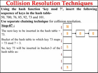
  • 21. • A function that maps a key into the range [0 to Max − 1], the result of which is used as an index (or address) to hash table for storing and retrieving record • The address generated by hashing function is called as home address • All home addresses address to particular area of memory and that area is called as prime area HASH FUNCTION
  • 22. • Bucket is an index position in hash table that can store more than one record • When the same index is mapped with two keys, then both the records are stored in the same bucket BUCKE T
  • 23. • The result of two keys hashing into the same address is called collision COLLISION
  • 24. • Each calculation of an address and test for success is known as Probe. PROBE
  • 25. • Keys those hash to the same address are called synonyms SYNONYMS
  • 26. • The result of more keys hashing to the same address and if there is no room in the bucket, then it is said that overflow has occurred • Collision and overflow are synonymous when the bucket is of size 1 OVERFLOW
  • 27. • A perfect hash function h for a set S is a hash function that maps distinct elements in S to a set of m integers, with no collisions. • A perfect hash function with values in a limited range can be used for efficient lookup operations, by placing keys from S (or other associated values) in a table indexed by the output of the function. Perfect Hash Function
  • 28. • Advantages : 1. A perfect hash function with values in a limited range can be used for efficient lookup operations. 2. No need to apply collision resolution techniques. Perfect Hash Function
  • 29. Load factor is defined as (m/n) where n is the total size of the hash table and m is the preferred number of entries which can be inserted before a increment in size of the underlying data structure is required. If Load factor (α) = constant, then time complexity of Insert, Search, Delete = Θ(1) LOAD FACTOR
  • 30. • Load Factor: The ratio of the number of items in a table to the table’s size is called the load factor. • Load Density : The identifier density of a hash table is the ratio n/T, • where n is the number of identifiers in the table. The loading density or loading factor of a hash table is a=n /(sb). • T is total number of possible element. Load factor and Load density
  • 31. • Load Density : The identifier density of a hash table is the ratio n/T, • Example : • Consider the hash table with b = 26 buckets and s = 2. We have n = 10 distinct identifiers, each representing a C library function. • This table has a loading factor, a, of 10/52 = 0.19 Load factor and Load density
  • 32. • Hashing is one of the searching techniques that uses a constant time. The time complexity in hashing is O(1). Till now, we read the two techniques for searching, i.e., linear search and binary search • The worst time complexity in linear search is O(n), and O(logn) in binary search. In both the searching techniques, the searching depends upon the number of elements but we want the technique that takes a constant time. So, hashing technique came that provides a constant time. • In Hashing technique, the hash table and hash function are used. Using the hash function, we can calculate the address at which the value can be stored. HASHING
  • 33. • The main idea behind the hashing is to create the (key/value) pairs. If the key is given, then the algorithm computes the index at which the value would be stored. It can be written as: • Index = hash(key) HASHING/HASH FUNCTION
  • 34. a) Division Method b) Multiplication Method c) Extraction Method d) Mid square method e) Folding f) Universal Method TYPES OF HASH FUNCTION
  • 35. There are three ways of calculating the hash function: 1. Division method 2. Folding method 3. Mid square method In the division method, the hash function can be defined as: h(ki) = ki % m; where m is the size of the hash table. For example, if the key value is 6 and the size of the hash table is 10. When we apply the hash function to key 6 then the index would be: h(6) = 6%10 = 6 The index is 6 at which the value is stored. TYPES OF HASH FUNCTION
  • 36. 1. Division Method: This is the most simple and easiest method to generate a hash value. The hash function divides the value k by M and then uses the remainder obtained. Formula: h(K) = k mod M Here, k is the key value, and M is the size of the hash table. TYPES OF HASH FUNCTION Example: k = 12345 M = 95 h(12345) = 12345 mod 95 = 90 k = 1276 M = 11 h(1276) = 1276 mod 11 = 0
  • 37. 2. The mid square method is a very good hashing method. It involves two steps to compute the hash value- Square the value of the key k i.e. k2 Extract the middle r digits as the hash value. Formula: h(K) = h(k x k) Here, k is the key value. TYPES OF HASH FUNCTION Example: Suppose the hash table has 100 memory locations. So r = 2 because two digits are required to map the key to the memory location. k = 60 k x k = 60 x 60 = 3600 (mid 60 for k=60) h(60) = 60 The hash value obtained is 60
  • 38. 3. Digit Folding Method : This method involves two steps: Divide the key-value k into a number of parts i.e. k1, k2, k3,….,kn, where each part has the same number of digits except for the last part that can have lesser digits than the other parts. Add the individual parts. The hash value is obtained by ignoring the last carry if any. Formula: k = k1, k2, k3, k4, ….., kn s = k1+ k2 + k3 + k4 +….+ kn h(K)= s Here, s is obtained by adding the TYPES OF HASH FUNCTION
  • 39. 3. Digit Folding Method : Example: k = 12345 k1 = 12, k2 = 34, k3 = 5 s = k1 + k2 + k3 = 12 + 34 + 5 = 51 h(K) = 51 TYPES OF HASH FUNCTION
  • 40. 4. Multiplication method : This method involves the following steps: • Choose a constant value A such that 0 < A < 1. • Multiply the key value with A. • Extract the fractional part of kA. • Multiply the result of the above step by the size of the hash table i.e. M. • The resulting hash value is obtained by taking the floor of the result obtained in step 4. TYPES OF HASH FUNCTION
  • 41. 4. Multiplication method : Formula: h(K) = floor (M (kA mod 1)) Here, M is the size of the hash table. k is the key value. A is a constant value. Where "k A mod 1" means the fractional part of k A, that is, k A - ⌊k A⌋. TYPES OF HASH FUNCTION
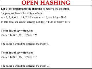
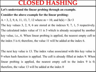
  • 42. 4. Multiplication method : Example: k = 12345 A = 0.357840 M = 100 h(12345) = floor[ 100 (12345*0.357840 mod 1)] = floor[ 100 (4417.5348 mod 1) ] = floor[ 100 (0.5348) ] = floor[ 53.48 ] = 53 TYPES OF HASH FUNCTION
  • 43. • Collision in Hashing- In hashing, 1. Hash function is used to compute the hash value for a key. 2. Hash value is then used as an index to store the key in the hash table. 3. Hash function may return the same hash value for two or more keys. “When the hash value of a key maps to an already occupied bucket of the hash table, it is called as a Collision” Collision in Hashing
  • 44. When the two different values have the same value, then the problem occurs between the two values, known as a collision. In the above example, the value is stored at index 6. If the key value is 26, then the index would be: h(26) = 26%10 = 6 Therefore, two values are stored at the same index, i.e., 6, and this leads to the collision problem. To resolve these collisions, we have some techniques known as collision techniques. The following are the collision techniques: Open Hashing: It is also known as closed addressing. Closed Hashing: It is also known as open addressing. COLLISION
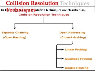
  • 45. In Hashing, collision resolution techniques are classified as- Collision Resolution Techniques
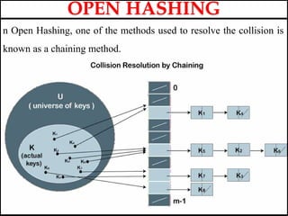
  • 47. The first Collision Resolution or Handling technique, " Open Hashing ", is popularly known as Separate Chaining. This is a technique which is used to implement an array as a linked list known as a chain. It is one of the most used techniques by programmers to handle collisions. Basically, a linked list data structure is used to implement the Separate Chaining technique. When a number of elements are hashed into the index of a single slot, then they are inserted into a singly-linked list. This singly-linked list is the linked list which we refer to as a chain in the Open Hashing technique. OPEN HASHING
  • 48. n Open Hashing, one of the methods used to resolve the collision is known as a chaining method. OPEN HASHING
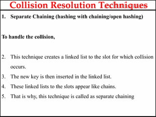
  • 49. 1. Separate Chaining (hashing with chaining/open hashing) To handle the collision, 2. This technique creates a linked list to the slot for which collision occurs. 3. The new key is then inserted in the linked list. 4. These linked lists to the slots appear like chains. 5. That is why, this technique is called as separate chaining Collision Resolution Techniques
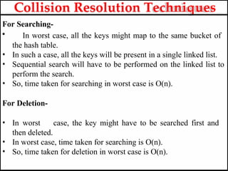
  • 50. For Searching- • In worst case, all the keys might map to the same bucket of the hash table. • In such a case, all the keys will be present in a single linked list. • Sequential search will have to be performed on the linked list to perform the search. • So, time taken for searching in worst case is O(n). For Deletion- • In worst case, the key might have to be searched first and then deleted. • In worst case, time taken for searching is O(n). • So, time taken for deletion in worst case is O(n). Collision Resolution Techniques
  • 51. Advantages: 1) Simple to implement. 2)Hash table never fills up, we can always add more elements to the chain. 3) Less sensitive to the hash function or load factors. 4)It is mostly used when it is unknown how many and how frequently keys may be inserted or deleted. . Collision Resolution Techniques
  • 52. Disadvantages: 1)Cache performance of chaining is not good as keys are stored using a linked list. Open addressing provides better cache performance as everything is stored in the same table. 2) Wastage of Space (Some Parts of hash table are never used) 3)If the chain becomes long, then search time can become O(n) in the worst case. 4) Uses extra space for links Collision Resolution Techniques
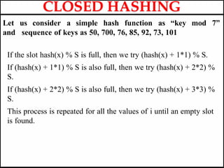
  • 53. Collision Resolution Techniques Using the hash function ‘key mod 7’, insert the following sequence of keys in the hash table- 50, 700, 76, 85, 92, 73 and 101. Use separate chaining technique for collision resolution. Step-01: Draw an empty hash table. For the given hash function, the possible range of hash values is [0, 6]. So, draw an empty hash table consisting of 7 buckets as-
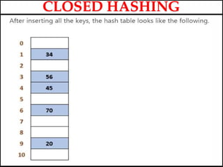
  • 54. Collision Resolution Techniques Using the hash function ‘key mod 7’, insert the following sequence of keys in the hash table- 50, 700, 76, 85, 92, 73 and 101. Use separate chaining technique for collision resolution. Step-02: Insert the given keys in the hash table one by one. The first key to be inserted in the hash table = 50. Bucket of the hash table to which key 50 maps = 50 mod 7 = 1. So, key 50 will be inserted in bucket-1 of the hash table as-
  • 55. Collision Resolution Techniques Using the hash function ‘key mod 7’, insert the following sequence of keys in the hash table- 50, 700, 76, 85, 92, 73 and 101. Use separate chaining technique for collision resolution. Step-03: The next key to be inserted in the hash table = 700. Bucket of the hash table to which key 700 maps = 700 mod 7 = 0. So, key 700 will be inserted in bucket-0 of the hash table as-
  • 56. Collision Resolution Techniques Using the hash function ‘key mod 7’, insert the following sequence of keys in the hash table- 50, 700, 76, 85, 92, 73 and 101. Use separate chaining technique for collision resolution. Step-04: The next key to be inserted in the hash table = 76. Bucket of the hash table to which key 76 maps = 76 mod 7 = 6. So, key 76 will be inserted in bucket-6 of the hash table as-
  • 57. Collision Resolution Techniques Using the hash function ‘key mod 7’, insert the following sequence of keys in the hash table- 50, 700, 76, 85, 92, 73 and 101. Use separate chaining technique for collision resolution. Step-05: The next key to be inserted in the hash table = 85. Bucket of the hash table to which key 85 maps = 85 mod 7 = 1. Since bucket-1 is already occupied, so collision occurs. Separate chaining handles the collision by creating a linked list to bucket-1. So, key 85 will be inserted in bucket-1 of the hash table as-
  • 58. Collision Resolution Techniques Using the hash function ‘key mod 7’, insert the following sequence of keys in the hash table- 50, 700, 76, 85, 92, 73 and 101. Use separate chaining technique for collision resolution. Step-06 : The next key to be inserted in the hash table = 92. Bucket of the hash table to which key 92 maps = 92 mod 7 = 1. Since bucket-1 is already occupied, so collision occurs. Separate chaining handles the collision by creating a linked list to bucket-1. So, key 92 will be inserted in bucket-1 of the hash table as-
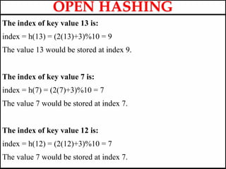
  • 59. Collision Resolution Techniques Using the hash function ‘key mod 7’, insert the following sequence of keys in the hash table- 50, 700, 76, 85, 92, 73 and 101. Use separate chaining technique for collision resolution. Step-07 : The next key to be inserted in the hash table = 73. Bucket of the hash table to which key 73 maps = 73 mod 7 = 3. So, key 73 will be inserted in bucket-3 of the hash table as-
  • 60. Collision Resolution Techniques Using the hash function ‘key mod 7’, insert the following sequence of keys in the hash table- 50, 700, 76, 85, 92, 73 and 101. Use separate chaining technique for collision resolution. Step-08 : The next key to be inserted in the hash table = 101. Bucket of the hash table to which key 101 maps = 101 mod 7 = 3. Since bucket-3 is already occupied, so collision occurs. Separate chaining handles the collision by creating a linked list to bucket-3. So, key 101 will be inserted in bucket-3 of the hash table as-
  • 61. Using the hash function ‘key mod 7’, insert the following sequence of keys in the hash table- 50, 700, 76, 85, 92, 73 and 101. Use separate chaining technique for collision resolution. Collision Resolution Techniques
  • 62. Let's first understand the chaining to resolve the collision. Suppose we have a list of key values A = 3, 2, 9, 6, 11, 13, 7, 12 where m = 10, and h(k) = 2k+3 In this case, we cannot directly use h(k) = ki/m as h(k) = 2k+3 The index of key value 3 is: index = h(3) = (2(3)+3)%10 = 9 The value 3 would be stored at the index 9. The index of key value 2 is: index = h(2) = (2(2)+3)%10 = 7 The value 2 would be stored at the index 7. OPEN HASHING
  • 63. The index of key value 9 is: index = h(9) = (2(9)+3)%10 = 1 The value 9 would be stored at the index 1. The index of key value 6 is: index = h(6) = (2(6)+3)%10 = 5 The value 6 would be stored at the index 5. The index of key value 11 is: index = h(11) = (2(11)+3)%10 = 5 The value 11 would be stored at the index 5. OPEN HASHING
  • 64. The index of key value 13 is: index = h(13) = (2(13)+3)%10 = 9 The value 13 would be stored at index 9. The index of key value 7 is: index = h(7) = (2(7)+3)%10 = 7 The value 7 would be stored at index 7. The index of key value 12 is: index = h(12) = (2(12)+3)%10 = 7 The value 7 would be stored at index 7. OPEN HASHING
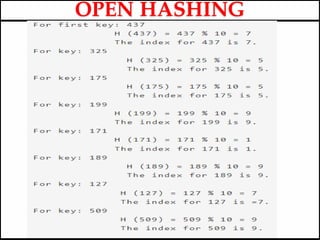
  • 67. OPEN HASHING Let us say that we have a sequence of numbers { 437, 325, 175, 199, 171, 189, 127, 509} and a hash function H(X) = X mod 10 Let us see the results of separate chaining hash table.
  • 69. In Closed hashing, three techniques are used to resolve the collision: 1. Linear probing 2. Quadratic probing 3. Double Hashing technique CLOSED HASHING
  • 70. PROBING Method Description Just like the name suggests, this method searches for empty slots linearly starting from Linear probing the position where the collision occurred and moving forward. If the end of the list is reached and no empty slot is found. The probing starts at the beginning of the list. Quadratic probing This method uses quadratic polynomial expressions to find the next available free slot. Double Hashing This technique uses a secondary hash function algorithm to find the next free available slot.
  • 72. In open addressing, 1. Unlike separate chaining, all the keys are stored inside the hash table. 2. No key is stored outside the hash table. Techniques used for open addressing are- 3. Linear Probing 4. Quadratic Probing 5. Double Hashing Open Addressing
  • 73. Operations In open addressing, 1. Insert Operation- • Hash function is used to compute the hash value for a key to be inserted. • Hash value is then used as an index to store the key in the hash table. In case of collision, • Probing is performed until an empty bucket is found. • Once an empty bucket is found, the key is inserted. • Probing is performed in accordance with the technique used for open addressing. Open Addressing
  • 74. Operations In open addressing, Search Operation- To search any particular key, • Its hash value is obtained using the hash function used. • Using the hash value, that bucket of the hash table is checked. • If the required key is found, the key is searched. • Otherwise, the subsequent buckets are checked until the required key or an empty bucket is found. • The empty bucket indicates that the key is not present in the hash table. Open Addressing
  • 75. Operations In open addressing, Search Operation- • The key is first searched and then deleted. • After deleting the key, that particular bucket is marked as “deleted”. Open Addressing
  • 76. 1. Linear Probing- 2. When collision occurs, we linearly probe for the next bucket. 3. We keep probing until an empty bucket is found. Advantage- 4. It is easy to compute. Disadvantage- 5. The main problem with linear probing is clustering. 6. Many consecutive elements form groups. 7. Then, it takes time to search an element or to find an empty bucket. Open Addressing Techniques
  • 77. Open Addressing Techniques 1. Linear Probing - Let us consider a simple hash function as “key mod 7” and a sequence of keys as 50, 700, 76, 85, 92, 73, 101.
  • 78. Linear Probing Linear probing is one of the forms of open addressing. As we know that each cell in the hash table contains a key-value pair, so when the collision occurs by mapping a new key to the cell already occupied by another key, then linear probing technique searches for the closest free locations and adds a new key to that empty cell. In this case, searching is performed sequentially, starting from the position where the collision occurs till the empty cell is not found. CLOSED HASHING
  • 79. Let's understand the linear probing through an example. Consider the above example for the linear probing: A = 3, 2, 9, 6, 11, 13, 7, 12 where m = 10, and h(k) = 2k+3 The key values 3, 2, 9, 6 are stored at the indexes 9, 7, 1, 5 respectively. The calculated index value of 11 is 5 which is already occupied by another key value, i.e., 6. When linear probing is applied, the nearest empty cell to the index 5 is 6; therefore, the value 11 will be added at the index 6. The next key value is 13. The index value associated with this key value is 9 when hash function is applied. The cell is already filled at index 9. When linear probing is applied, the nearest empty cell to the index 9 is 0; therefore, the value 13 will be added at the index 0 CLOSED HASHING
  • 80. Let us consider a simple hash function as “key mod 7” and a sequence of keys as 50, 700, 76, 85, 92, 73, 101. LINEAR PROBING
  • 81. Let us consider a simple hash function as “key mod 30” and a sequence of keys as 3, 1, 63, 5, 11, 15, 18, 16, 46. LINEAR PROBING
  • 83. In collision handling method chaining is a concept which introduces an additional field with data i.e. chain. A separate chain table is maintained for colliding data. When collision occurs, we store the second colliding data by linear probing method. The address of this colliding data can be stored with the first colliding element in the chain table, without replacement. Chaining Without Replacement
  • 84. For example, consider elements: 131, 3, 4, 21, 61, 6, 71, 8, 9 Chaining Without Replacement
  • 85. For example, consider elements: Identifier is 11, 32, 41, 54, 33. Hash function: f(x) = X mod 10 and Table size = 10 Chaining With Replacement
  • 87. For example, consider elements: Identifier is 11, 32, 41, 54, 33. Hash function: f(x) = X mod 10 and Table size = 10 Chaining Without Replacement
  • 92. 2. Quadratic Probing- • When collision occurs, we probe for i2‘th bucket in ith iteration. • We keep probing until an empty bucket is found. Open Addressing Techniques
  • 93. Quadratic Probing • In case of linear probing, searching is performed linearly. In contrast, quadratic probing is an open addressing technique that uses quadratic polynomial for searching until a empty slot is found. • It can also be defined as that it allows the insertion ki at first free location from (u+i2)%m where i=0 to m-1. h´ = (𝑥) = 𝑥 𝑚𝑜𝑑 𝑚 ℎ(𝑥, 𝑖) = ( ´( ℎ 𝑥) + 𝑖2)𝑚𝑜𝑑 𝑚 We can put some other quadratic equations also using some constants The value of i = 0, 1, . . ., m – 1. So we start from i = 0, and increase this until we get one free space. So initially when i = 0, then the h(x, i) is same as h´(x). CLOSED HASHING
  • 95. CLOSED HASHING mod 7” Let us consider a simple hash function as “key and sequence of keys as 50, 700, 76, 85, 92, 73, 101 If the slot hash(x) % S is full, then we try (hash(x) + 1*1) % S. If (hash(x) + 1*1) % S is also full, then we try (hash(x) + 2*2) % S. If (hash(x) + 2*2) % S is also full, then we try (hash(x) + 3*3) % S. This process is repeated for all the values of i until an empty slot is found.
  • 97. QUADRATIC PROBING Example: Let us consider table Size = 7, hash function as Hash(x) = x % 7 and collision resolution strategy to be f(i) = i2 . Insert = 22, 30, and 50.
  • 98. QUADRATIC PROBING Using Linear probing and Quadratic probing, insert the following values in the hash table of size 10.Show how many collisions occur in each iterations 28, 55, 71, 67, 11, 10, 90, 44 (Linear Probing)
  • 99. QUADRATIC PROBING Using Linear probing and Quadratic probing, insert the following values in the hash table of size 10.Show how many collisions occur in each iterations 28, 55, 71, 67, 11, 10, 90, 44
  • 100. 3. Double Hashing- • We use another hash function hash2(x) and look for i * hash2(x) bucket in ith iteration. • It requires more computation time as two hash functions need to be computed. • Double hashing is a collision resolving technique in Open Addressed Hash tables. Double hashing uses the idea of applying a second hash function to key when a collision occurs. Open Addressing Techniques
  • 101. Double hashing : It is a collision resolving technique in Open Addressed Hash tables. Double hashing uses the idea of applying a second hash function to key when a collision occurs. Advantages of Double hashing 1. The advantage of Double hashing is that it is one of the best form of records of probing, producing a uniform distribution throughout a hash table. 2. This technique does not yield any clusters. 3. It is one of effective method for resolving collisions DOUBLE HASHING
  • 102. Double hashing : A good second Hash function is: 1. It must never evaluate to zero 2. Must make sure that all cells can be probed CLOSED HASHING
  • 103. Double hashing : Double hashing can be done using : (hash1(key) + i * hash2(key)) % TABLE_SIZE Here hash1() and hash2() are hash functions and TABLE_SIZE is size of hash table. (We repeat by increasing i when collision occurs) First hash function is typically hash1(key) = key % TABLE_SIZE A popular second hash function is : hash2(key) = PRIME – (key % PRIME) where PRIME is a prime smaller than the TABLE_SIZE. CLOSED HASHING
  • 109. DOUBLE HASHING EXAMPLE Double Hashing Example : Imagine you need to store some items inside a hash table of size 20. The values given are: (16, 8, 63, 9, 27, 37, 48, 5, 69, 34, 1). h1(n)=n%20 h2(n)=n%13 n h(n, i) = (h1 (n) + ih2(n)) mod
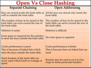
  • 110. Open Vs Close Hashing Separate Chaining Open Addressing Keys are stored inside the hash table as well as outside the hash table. All the keys are stored only inside the hash table. The number of keys to be stored in the hash table can even exceed the size of the hash table. The number of keys to be stored in the hash table can never exceed the size of the hash table. Deletion is easier. Deletion is difficult. Extra space is required for the pointers to store the keys outside the hash table. No extra space is required. Cache performance is poor. This is because of linked lists which store the keys outside the hash table. Cache performance is better. This is because here no linked lists are used. Some buckets of the hash table are never used which leads to wastage of space. Buckets may be used even if no key maps to those particular buckets.
  • 111. Rehashing is a collision resolution technique. Rehashing is a technique in which the table is resized, i.e., the size of table is doubled by creating a new table. It is preferable is the total size of table is a prime number. There are situations in which the rehashing is required. • When table is completely full • With quadratic probing when the table is filled half. • When insertions fail due to overflow. In such situations, we have to transfer entries from old table to the new table by re computing their positions using hash functions Rehashing
  • 113. As the name suggests, rehashing means hashing again. Basically, when the load factor increases to more than its pre- defined value (default value of load factor is 0.75), the complexity increases. So to overcome this, the size of the array is increased (doubled) and all the values are hashed again and stored in the new double sized array to maintain a low load factor and low complexity. Rehashing
  • 114. Why rehashing? Rehashing is done because whenever key value pairs are inserted into the map, the load factor increases, which implies that the time complexity also increases as explained above. This might not give the required time complexity of O(1). Hence, rehash must be done, increasing the size of the bucketArray so as to reduce the load factor and the time complexity Rehashing
  • 115. How Rehashing is done? Rehashing can be done as follows: • For each addition of a new entry to the map, check the load factor. • If it’s greater than its pre-defined value (or default value of 0.75 if not given), then Rehash. • For Rehash, make a new array of double the previous size and make it the new bucket array. • Then traverse to each element in the old bucket Array and call the insert() for each so as to insert it into the new larger bucket array. Rehashing
  • 116. • Hash Collisions: Hashing can produce the same hash value for different keys, leading to hash collisions. To handle collisions, we need to use collision resolution techniques like chaining or open addressing. • Hash Function Quality: The quality of the hash function determines the efficiency of the hashing algorithm. A poor- quality hash function can lead to more collisions, reducing the performance of the hashing algorithm. ISSUES IN HASHING
  • 117. 1. The dynamic hashing method is used to overcome the problems of static hashing like bucket overflow. 2. In this method, data buckets grow or shrink as the records increases or decreases. This method is also known as Extendable hashing method. it allows in poor 3. Thismethod makes hashing dynamic, i.e., insertion or deletion without resulting performance. Extensible/Extendible Hashing
  • 118. • How to search a key 1. First, calculate the hash address of the key. 2. Check how many bits are used in the directory, and these bits are called as i. 3. Take the least significant i bits of the hash address. This gives an index of the directory. 4. Now using the index, go to the directory and find bucket address where the record might be. Extensible/Extendible Hashing
  • 119. • How to insert a new record 1. Firstly, you have to follow the same procedure for retrieval, ending up in some bucket. 2. If there is still space in that bucket, then place the record in it. 3. If the bucket is full, then we will split the bucket and redistribute the records. Extensible/Extendible Hashing
  • 120. into buckets, • For example : Consider the following grouping of keys depending on the prefix of their hash address: Extensible/Extendible Hashing
  • 121. The last two bits of 2 and 4 are 00. So it will go into bucket B0. The last two bits of 5 and 6 are 01, so it will go into bucket B1. The last two bits of 1 and 3 are 10, so it will go into bucket B2. The last two bits of 7 are 11, so it will go into B3. Extensible/Extendible Hashing
  • 122. Insert key 9 with hash address 10001 into the above structure: 1. Since key 9 has hash address 10001, it must go into the first bucket. But bucket B1 is full, so it will get split. 2. The splitting will separate 5, 9 from 6 since last three bits of 5, 9 are 001, so it will go into bucket B1, and the last three bits of 6 are 101, so it will go into bucket B5. 3. Keys 2 and 4 are still in B0. The record in B0 pointed by the 000 and 100 entry because last two bits of both the entry are 00. 4. Keys 1 and 3 are still in B2. The record in B2 pointed by the 010 and 110 entry because last two bits of both the entry are 10. 5. Key 7 are still in B3. The record in B3 pointed by the 111 and 011 entry because last two bits of both the entry are 11. Extensible/Extendible Hashing
  • 124. Advantages of Extensible Hashing 1. In this method, the performance does not decrease as the data grows in the system. It simply increases the size of memory to accommodate the data. 2. In this method, memory is well utilized as it grows and shrinks with the data. There will not be any unused memory lying. 3. This method is good for the dynamic database where data grows and shrinks frequently
  • 125. Disadvantages of Extensible Hashing 1. In this method, if the data size increases then the bucket size is also increased. 2. In this case, the bucket overflow situation will also occur. But it might take little time to reach this situation than static hashing.
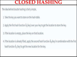
  • 126. 1. A skip list is a probabilistic data structure. 2. The skip list is used to store a sorted list of elements or data with a linked list. 3. It allows the process of the elements or data to view efficiently. In one single step, it skips several elements of the entire list, which is why it is known as a skip list. Skip List
  • 127. 4. The skip list is an extended version of the linked list. 5. It allows the user to search, remove, and insert the element very quickly. 6. It consists of a base list that includes a set of elements which maintains the link hierarchy of the subsequent elements. Skip List
  • 128. Skip list structure It is built in two layers: The lowest layer and Top layer. The lowest layer of the skip list is a common sorted linked list, and the top layers of the skip list are like an "express line" where the elements are skipped. Skip List
  • 129. • Let's take an example to understand the working of the skip list. In this example, we have 14 nodes, such that these nodes are divided into two layers, as shown in the diagram. • The lower layer is a common line that links all nodes, and the top layer is an express line that links only the main nodes, as you can see in the diagram. • Suppose you want to find 47 in this example. You will start the search from the first node of the express line and continue running on the express line until you find a node that is equal a 47 or more than 47. • You can see in the example that 47 does not exist in the express line, so you search for a node of less than 47, which is 40. Now, you go to the normal line with the help of 40, and search the 47, as shown in the diagram. Skip List
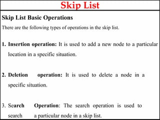
  • 131. Skip List Basic Operations There are the following types of operations in the skip list. 1. Insertion operation: It is used to add a new node to a particular location in a specific situation. 2. Deletion operation: It is used to delete a node in a specific situation. 3. Search Operation: The search operation is used to search a particular node in a skip list. Skip List
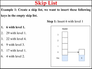
  • 132. Example 1: Create a skip list, we want to insert these following keys in the empty skip list. Step 1: Insert 6 with level 1 1. 6 with level 1. 2. 29 with level 1. 3. 22 with level 4. 4. 9 with level 3. 5. 17 with level 1. 6. 4 with level 2. Skip List
  • 133. Example 1: Create a skip list, we want to insert these following keys in the empty skip list. Step 2: Insert 29 with level 1 1. 6 with level 1. 2. 29 with level 1. 3. 22 with level 4. 4. 9 with level 3. 5. 17 with level 1. 6. 4 with level 2. Skip List
  • 134. Example 1: Create a skip list, we want to insert these following keys in the empty skip list. Step 3: Insert 22 with level 4 1. 6 with level 1. 2. 29 with level 1. 3. 22 with level 4. 4. 9 with level 3. 5. 17 with level 1. 6. 4 with level 2. Skip List
  • 135. Example 1: Create a skip list, we want to insert these following keys in the empty skip list. Step 4: Insert 9 with level 3 1. 6 with level 1. 2. 29 with level 1. 3. 22 with level 4. 4. 9 with level 3. 5. 17 with level 1. 6. 4 with level 2. Skip List
  • 136. Example 1: Create a skip list, we want to insert these following keys in the empty skip list. Step 5: Insert 17 with level 1 1. 6 with level 1. 2. 29 with level 1. 3. 22 with level 4. 4. 9 with level 3. 5. 17 with level 1. 6. 4 with level 2. Skip List
  • 137. Example 1: Create a skip list, we want to insert these following keys in the empty skip list. Step 6: Insert 4 with level 2 1. 6 with level 1. 2. 29 with level 1. 3. 22 with level 4. 4. 9 with level 3. 5. 17 with level 1. 6. 4 with level 2. Skip List
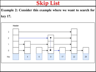
  • 138. Example 2: Consider this example where we want to search for key 17. Skip List
  • 139. Example 2: Consider this example where we want to search for key 17. Skip List
  • 140. 1. If you want to insert a new node in the skip list, then it will insert the node very fast because there are no rotations in the skip list. 2. The skip list is simple to implement as compared to the hash table and the binary search tree. 3. It is very simple to find a node in the list because it stores the nodes in sorted form. 4. The skip list algorithm can be modified very easily in a more specific structure, such as indexable skip lists, trees, or priority queues. 5. The skip list is a robust and reliable list. Advantages of Skip List
  • 141. 1. It requires more memory than the balanced tree. 2. Reverse searching is not allowed. 3. The skip list searches the node much slower than the linked list. Disadvantages of Skip List
  • 142. 1. Skiplist are used in distributed applications. In distributed systems, the nodes of skip list represents the computer systems and pointers represent network connection. 2. Skip list are used for implementing highly scalable concurrent priority queues with less lock contention (struggle for having a lock on a data item) Applications of Skip List
  • 143. class. ( median ordered 3. It is alsoused with the QMap template Value-based template class that provides a dictionary) 4. Theindexing of the skip list is used in running problems. 5. skipdb is an open-source database format using key/value pairs. Applications of Skip List
  • 144. 1. https://www.javatpoint.com/double-hashing-in-java 2. https://www.scaler.com/topics/quadratic-probing/ 3. https://www.geeksforgeeks.org/quadratic-probing-in-hashing/ 4. https://www.bucketstudy.com/2021/09/DSA01.html 5. https://www.upgrad.com/blog/hashing-in-data-structure/ 6. https://quescol.com/data-structure/linear-probing 7. https://prac-code.blogspot.com/2013/06/chaining-without- replacement.html 8. https://www.geeksforgeeks.org/open-addressing-collision- handling-technique-in-hashing/ References
  • 146. THANK YOU!!! My Blog : https://anandgharu.wordpress.com/ Email : gharu.anand@gmail.com