


![Fundamental Concepts and Definitions ____________________________________________ 39
1.14 Write Boyle’s law and Charle's law.
1.15 Determine the absolute pressure of gas in a tank if the pressure gauge mounted on tank reads 120 kPa
pressure. [221.3 kPa]
1.16 What shall be the volume of a fluid having its specific gravity as 0.0006 and mass as 10 kg?
[16.67 m3
]
1.17 Determine the pressure of compressed air in an air vessel, if the manometer mounted on it shows a
pressure of 3 m of mercury. Assume density of mercury to be 13.6 × 10³ kg/m3 and atmospheric
pressure as 101 kPa. [501.25 kPa]
1.18 Calculate the kinetic energy of a satellite revolving around the earth with a speed of 1 km/s. Assume
acceleration due to gravity as 9.91 m/s2 and gravitational force of 5 kN. [254.8 MJ]
1.19 If the gauge pressure of oil in a tube is 6.275 kPa and oil’s specific gravity is 0.8, then determine depth
of oil inside tube. [80 cm]
1.20 Determine the work required for displacing a block by 50 m and a force of 5 kN. [250 kJ]
1.21 Determine the barometer reading in millimetres of Hg if the vacuum measured on a condenser is 74.5
cm of Hg and absolute pressure is 2.262 kPa. [760mm]
1.22 Determine the absolute pressures for the following;
(i) Gauge pressure of 1.4 MPa
(ii) Vacuum pressure of 94.7 kPa
Take barometric pressure as 77.2 cm of Hg and density of mercury as 13.6 × 10³ kg/m3.
[1.5 MPa, 8.3 kPa]
1.23 Determine the pressure acting upon surface of a vessel at 200 m deep from surface of sea. Take
barometric pressure as 101 kPa and specific gravity of sea water as 1.025. [2.11 MPa]
1.24 A vacuum gauge gives pressure in a vessel as 0.1 bar, vacuum. Find absolute pressure within vessel
in bars. Take atmospheric pressure as 76 cm of mercury column, g = 9.8 m/s2
, density of mercury
= 13.6 g/cm3. [0.91 bar]
1.25 Determine the work done upon a spring having spring constant of 50 kN/m. Spring is stretched to 0.1
m from its unstretched length of 0.05 m. [0.0625 kJ]
1.26 Determine the mass of oxygen contained in a tank of 0.042 m3 at 298 K and 1.5 × 10⁷ Pa considering it
as perfect gas. Also determine the mass using compressibility charts. [8.25, 8.84]
1.27 What will be specific volume of water vapour at 1 MPa and 523 K, if it behaves as ideal gas? Also
determine the same considering generalized compressibility chart. [0.241 m3/kg, 0.234 m3/kg]
1.28 Calculate the pressure of CO2 gas at 27ºC and 0.004 m3/kg treating it as ideal gas. Also determine the
pressure using Van der Waals equation of state. [14.17 MPa, 6.9 MPa]
1.29 Determine molecular weight and gas constant for a mixture of gases having 65% N2, 35% CO2 by mole.
[33.6 kg/k mol. 0.247 kJ/kg . K]
1.30 Considering air as a mixture of 78% N2, 22% O2 by volume determine gas constant, molecular weight,
Cp and Cv for air at 25ºC. [0.2879 kJ/kg . K, 28.88 kg/K mol, 1.0106 kJ/kg . K, 0.722 kJ/kg . K]
1.31 What minimum volume of tank shall be required to store 8 kmol and 4 kmol of O2 and CO2 respectively
at 0.2 MPa, 27ºC ? [149.7 m3]
1.32 Two tanks A and B containing O2 and CO2 have volumes of 2 m3 and 4 m3 respectively. Tank A is at 0.6
MPa, 37ºC and tank B is at 0.1 MPa and 17ºC. Two tanks are connected through some pipe so as to
allow for adiabatic mixing of two gases. Determine final pressure and temperature of mixture.
[0.266 MPa, 30.6ºC]
1.33 Determine the molecular weight and gas constant for some gas having CP = 1.968 kJ/kg . K, Cv = 1.507
kJ/kg . K. [18.04 kg/kmol, 0.461 kJ/kg . K]](https://image.slidesharecdn.com/fdocuments-220624061338-6551ed4f/85/Applied-thermodynamics-onkar-singh-new-pdf-56-320.jpg)


![82 _________________________________________________________ Applied Thermodynamics
Solution:
Let mass of steam to be supplied per kg of water lifted be ‘m’ kg. Applying law of energy conservation
upon steam injector, for unit mass of water lifted.
Energy with steam entering + Energy with water entering = Energy with mixture leaving + Heat loss
to surroundings.
2
2
(50)
(720 10 4.18)
2
m
+ × ×
+ 1 × [(24.6 × 103 × 4.18) + (9.81 × 2)]
K.E. Enthalpy Enthalpy P.E
= (1 + m)
2
3 (25)
(100 10 4.18)
2
× × +
+ [m × 12 × 103 × 4.18]
Enthalpy K.E Heat loss
m [3010850] + [102847.62] = (1 + m) . (418312.5) + m[50160]
Upon solving, m = 0.124 kg steam/kg of water
Steam supply rate = 0.124 kg/s per kg of water. Ans.
12. An inelastic flexible balloon is inflated from initial empty state to a volume of 0.4 m3 with H2
available from hydrogen cylinder. For atmospheric pressure of 1.0313 bar determine the amount of work
done by balloon upon atmosphere and work done by atmosphere.
Solution:
Balloon after being inflated
Balloon initially empty
Fig. 3.34
Here let us assume that the pressure is always equal to atmospheric pressure as balloon is flexible,
inelastic and unstressed and no work is done for stretching balloon during its filling. Figure 3.34 shows
the boundary of system before and after filling balloon by firm line and dotted line respectively.
Displacement work, W =
cylinder
.
p dV
∫ +
balloon
.
p dV
∫
.
p dV
∫ = 0 as cylinder shall be rigid.
= 0 + p · ∆V
= 0 + 1.013 × 105 × 0.4
= 40.52 kJ
Work done by system upon atmosphere = 40.52 kJ
Work done by atmosphere = – 40.52 kJ Ans.
13. In a steam power plant 5 kW of heat is supplied in boiler and turbine produces 25% of heat added
while 75% of heat added is rejected in condenser. Feed water pump consumes 0.2% of this heat added
](https://image.slidesharecdn.com/fdocuments-220624061338-6551ed4f/85/Applied-thermodynamics-onkar-singh-new-pdf-99-320.jpg)


![90 _________________________________________________________ Applied Thermodynamics
20. An evacuated bottle of 0.5 m3 volume is slowly filled from atmospheric air at 1.0135 bars until the
pressure inside the bottle also becomes 1.0135 bar. Due to heat transfer, the temperature of air inside the
bottle after filling is equal to the atmospheric air temperature. Determine the amount of heat transfer.
[U.P.S.C., 1994]
Solution:
Final system boundary
after filling
Evacuated bottle
Initial system boundary
Valve
Initial system boundary
P = 1.0135 bar
atm
Fig. 3.41
Displacement work; W = 1.0135 × 105 × (0 – 0.5)
W = – 0.50675 × 10⁵ Nm
Heat transfer, Q = 0.50675 × 10⁵ Nm
Heat transfer = 0.50675 × 10⁵ Nm Ans.
21. A compressed air bottle of 0.3 m3 volume contains air at 35 bar, 40°C. This air is used to drive a
turbogenerator sypplying power to a device which consumes 5 W. Calculate the time for which the
device can be operated if the actual output of the turbogenerator is 60% of the maximum theoretical
output. The ambient pressure to which the tank pressure has fallen is 1 bar. For air,
p
C
Cv
= 1.4.
[U.P.S.C. 1993]
Solution:
Here turbogenerator is fed with compressed air from a compressed air bottle. Pressure inside bottle
gradually decreases from 35 bar to 1 bar. Expansion from 35 bar to 1 bar occurs isentropically. Thus,
for the initial and final states of pressure, volume, temperature and mass inside bottle being given as P1,
V1, T1 & m1 and P2, V2, T2 & m2 respectively. It is transient flow process similar to emptying of the
bottle.
1
2
1
P
T
γ
γ
−
=
2
1
T
T , Given: P1 = 35 bar, T1 = 40°C or 313 K
V1 = 0.3 m3; V2 = 0.3 m3
P2 = 1 bar.](https://image.slidesharecdn.com/fdocuments-220624061338-6551ed4f/85/Applied-thermodynamics-onkar-singh-new-pdf-107-320.jpg)
![First Law of Thermodynamics _____________________________________________________ 91
T2 = T1
1
2
1
P
T
γ
γ
−
T2 = 113.22 K
By perfect gas law, initial mass in bottle, m1 =
1 1
1
PV
RT =
2
35 10 0.3
0.287 313
× ×
×
m1 = 11.68 kg
Final mass in bottle, m2 =
2 2
2
PV
RT =
2
1 10 0.3
0.287 113.22
× ×
×
m2 = 0.923 kg
Energy available for running turbo generator or work;
W + (m1 – m2) h2 = m1 u1 – m2 u2
W = (m1u1 – m2u2) – (m1 – m2) h2
= (m1 cv T1 – m2 cv T2) – (m1 – m2) · cp · T2
Taking cv = 0.718 kJ/kg . K and cP = 1.005 kJ/kg · K
W = {(11.68 × 0.718 × 313) – (0.923 × 0.718 × 113.22)}
– {(11.68 – 0.923) × 1.005 × 113.22}
W = 1325.86 kJ
This is the maximum work that can be had from the emptying of compressed air bottle between
given pressure limits.
Turbogenerator’s actual output = 5 kJ/s
Input to turbogenerator =
5
0.6
= 8.33 kJ/s.
Time duration for which turbogenerator can be run;
∆t =
1325.86
8.33
∆t = 159.17 sec.
Duration ≈ 160 seconds Ans.
22. 3 kg of air at 1.5 bar pressure and 77°C temperature at state 1 is compressed polytropically to state
2 at pressure 7.5 bar, index of compression being 1.2. It is then cooled at constant temperature to its
original state 1. Find the net work done and heat transferred. [U.P.S.C. 1992]
Solution:
Different states as described in the problem are denoted as 1, 2 and 3 and shown on p-V diagram.
Process 1-2 is polytropic process with index 1.2
So,
2
1
T
T =
1
2
1
n
n
P
P
−
or, T2 = T1
1
2
1
n
n
P
P
−
](https://image.slidesharecdn.com/fdocuments-220624061338-6551ed4f/85/Applied-thermodynamics-onkar-singh-new-pdf-108-320.jpg)

![First Law of Thermodynamics _____________________________________________________ 93
Work during process 2-3,
W2–3 = P2 (V3 – V2)
= 7.5 × 10⁵ (0.402 – 0.526)
= – 93 kJ
Work during process 3-1,
W3–1 = P3V3 ln
1
3
V
V
= 7.5 × 105 × 0.402 × ln
2.01
0.402
W3–1 = 485.25 kJ
Net work, Wnet = W1–2 + W2–3 + W3–1
= – 463.56 – 93 + 485.25
Network = – 71.31 kJ Ans.
–ve work shows work done upon the system. Since it is the cycle, so
Wnet = Qnet
φ dW = φ dQ = – 71.31 kJ
Heat transferred from system = 71.31 kJ Ans.
23. A compressed air bottle of volume 0.15 m3 contains air at 40 bar and 27°C. It is used to drive a
turbine which exhausts to atmosphere at 1 bar. If the pressure in the bottle is allowed to fall to 2 bar,
determine the amount of work that could be delivered by the turbine. [U.P.S.C. 1998]
Solution:
cp = 1.005 kJ/kg . K, cv = 0.718 kJ/kg K, γ = 1.4
Initial mass of air in bottle ⇒ m1 =
2
1 1
1
40 10 0.15
0.287 300
p V
RT
× ×
=
×
m1 = 6.97 kg
Final mass of air in bottle ⇒ m2 =
2 2
2
p V
RT
2
1
T
T =
1
2
1
P
P
γ
γ
−
, m2 =
2
2 10 0.15
0.287 127.36
× ×
×
=
1.4 1
1.4
2
40
−
, m2 = 0.821 kg.
T2 = 127.36 K
Energy available for running of turbine due to emptying of bottle,
= (m1 cv T1 – m2 cv T2) – (m1 – m2) · cp · T2
= {(6.97 × 0.718 × 300) – (0.821 × 0.718 × 127.36)}
– {(6.97 – 0.821) × 1.005 × 127.35}
= 639.27 kJ.
Work available from turbine = 639.27 kJ Ans.](https://image.slidesharecdn.com/fdocuments-220624061338-6551ed4f/85/Applied-thermodynamics-onkar-singh-new-pdf-110-320.jpg)
![94 _________________________________________________________ Applied Thermodynamics
-:-4+15-
3.1 Define the first law of thermodynamics. Also give supporting mathematical expression for it.
3.2 How the first law of thermodynamics is applied to a closed system undergoing a non-cyclic process?
3.3 Show that internal energy is a property.
3.4 Explain the following :
(a) Free expansion
(b) Polytropic process
(c) Hyperbolic process
Also obtain expressions for work in each case.
3.5 Show that for a polytropic process.
Q =
1
n
γ
γ
−
−
W
where Q and W are heat and work interactions and n is polytropic index.
3.6 Derive the steady flow energy equation.
3.7 Explain a unsteady flow process.
3.8 Show that for a given quantity of air supplied with a definite amount of heat at constant volume, the
rise in pressure shall be directly proportional to initial absolute pressure and inversely proportional to
initial absolute temperature.
3.9 How much work is done when 0.566 m3
of air initially at a pressure of 1.0335 bar and temperature of 7°C
undergoes an increase in pressure upto 4.13 bar in a closed vessel? [0]
3.10 An ideal gas and a steel block are initially having same volumes at same temperature and pressure.
Pressure on both is increased isothermally to five times of its initial value. Show with the help of P–V
diagram, whether the quantities of work shall be same in two processes or different. If different then
which one is greater. Assume processes to be quasi-static.
3.11 An inventor has developed an engine getting 1055 MJ from fuel and rejecting 26.375 MJ in exhaust
and delivering 25 kWh of mechanical work. Is this engine possible? [No]
3.12 For an ideal gas the pressure is increased isothermally to ‘n’ times its initial value. How high would the
gas be raised if the same amount of work were done in lifting it? Assume process to be quasi-static.
3.13 A system’s state changes from a to b as shown on P–V diagram
a
c b
d
P
V
Fig. 3.43
Along path ‘acb’ 84.4 kJ of heat flows into the system and system does 31.65 kJ of work. Determine
heat flow into the system along path ‘adb’ if work done is 10.55 kJ. When system returns from ‘b’ to
‘a’ following the curved path then work done on system is 21.1 kJ. How much heat is absorbed or
rejected? If internal energy at ‘a’ and ‘d’ are 0 and 42.2 kJ, find the heat absorbed in processes ‘ad’ and
‘db’. [63.3 kJ, – 73.85 kJ, 52.75 kJ, 10.55 kJ]
3.14 A tank contains 2.26 m3 of air at a pressure of 24.12 bar. If air is cooled until its pressure and temperature
becomes 13.78 bar and 21.1°C respectively. Determine the decrease of internal energy.
[– 5857.36 kJ]](https://image.slidesharecdn.com/fdocuments-220624061338-6551ed4f/85/Applied-thermodynamics-onkar-singh-new-pdf-111-320.jpg)
![First Law of Thermodynamics _____________________________________________________ 95
3.15 Water in a rigid, insulating tank is set in rotation and left. Water comes to rest after some time due to
viscous forces. Considering the tank and water to constitute the system answer the following.
(i) Is any work done during the process of water coming to rest?
(ii) Is there a flow of heat?
(iii) Is there any change in internal energy (U)?
(iv) Is there any change in total energy (E)? [No, No, Yes, No]
3.16 Fuel-air mixture in a rigid insulated tank is burnt by a spark inside causing increase in both temperature
and pressure. Considering the heat energy added by spark to be negligible, answer the following :
(i) Is there a flow of heat into the system?
(ii) Is there any work done by the system?
(iii) Is there any change in internal energy (U) of system?
(iv) Is there any change in total energy (E) of system? [No, No, No, No]
3.17 Calculate the work if in a closed system the pressure changes as per relation p = 300 . V + 1000 and
volume changes from 6 to 4 m3. Here pressure ‘p’ is in Pa and volume ‘V’ is in m3. [– 5000J]
3.18 Hydrogen from cylinder is used for inflating a balloon to a volume of 35m3 slowly. Determine the work
done by hydrogen if the atmospheric pressure is 101.325 kPa. [3.55 MJ]
3.19 Show that the work done by an ideal gas is mRT1, if gas is heated from initial temperature T1 to twice
of initial temperature at constant volume and subsequently cooled isobarically to initial state.
3.20 Derive expression for work done by the gas in following system. Piston-cylinder device shown has a
gas initially at pressure and volume given by P1, V1. Initially the spring does not exert any force on
piston. Upon heating the gas, its volume gets doubled and pressure becomes P2.
Fig. 3.44 Piston-cylinder arrangement
3.21 An air compressor with pressure ratio of 5, compresses air to
1
4
th of the initial volume. For inlet
temperature to be 27°C determine temperature at exit and increase in internal energy per kg of air.
[101.83°C, 53.7 kJ/kg]
3.22 In a compressor the air enters at 27°C and 1 atm and leaves at 227°C and 1 MPa. Determine the work
done per unit mass of air assuming velocities at entry and exit to be negligible. Also determine the
additional work required, if velocities are 10 m/s and 50 m/s at inlet and exit respectively.
[200.9 kJ/kg, 202.1 kJ/kg]
3.23 Turbojet engine flies with velocity of 270 m/s at the altitude where ambient temperature is –15°C. Gas
temperature at nozzle exit is 873 K and fuel air ratio is 0.019. Corresponding enthalpy values for air and
gas at inlet and exit are 260 kJ/kg and 912 kJ/kg respectively. Combustion efficiency is 95% and
calorific value of fuel is 44.5 MJ/kg. For the heat losses from engine amounting to 21 kJ/kg of air
determine the velocity of gas jet at exit. [613.27 m/s]
3.24 Oxygen at 3MPa and 300°C flowing through a pipe line is tapped out to fill an empty insulated rigid
tank. Filling continues till the pressure equilibrium is not attained. What shall be the temperature of the
oxygen inside the tank? If γ = 1.39. [662.5°C]
3.25 Determine work done by fluid in the thermodynamic cycle comprising of following processes :
(a) Unit mass of fluid at 20 atm and 0.04 m3 is expanded by the law PV1.5 = constant, till volume gets
doubled.
(b) Fluid is cooled isobarically to its original volume.
(c) Heat is added to fluid till its pressure reaches to its original pressure, isochorically. [18.8 kJ]](https://image.slidesharecdn.com/fdocuments-220624061338-6551ed4f/85/Applied-thermodynamics-onkar-singh-new-pdf-112-320.jpg)
![96 _________________________________________________________ Applied Thermodynamics
3.26 An air vessel has capacity of 10 m3 and has air at 10 atm and 27°C. Some leakage in the vessel causes
air pressure to drop sharply to 5 atm till leak is repaired. Assuming process to be of reversible adiabatic
type determine the mass of air leaked. [45.95 kg]
3.27 Atmospheric air leaks into a cylinder having vacuum. Determine the final temperature in cylinder when
inside pressure equals to atmospheric pressure, assuming no heat transferred to or from air in cylinder.
[144.3°C]
3.28 Determine the power available from a steam turbine with following details;
Steam flow rate = 1 kg/s
Velocity at inlet and exit = 100 m/s and 150 m/s
Enthalpy at inlet and exit = 2900 kJ/kg, 1600 kJ/kg
Change in potential energy may be assumed negligible. [1293.75 kW]
3.29 Determine the heat transfer in emptying of a rigid tank of 1m3 volume containing air at 3 bar and 27°C
initially. Air is allowed to escape slowly by opening a valve until the pressure in tank drops to 1 bar
pressure. Consider escape of air in tank to follow polytropic process with index n = 1.2 [76.86 kJ]
3.30 A pump is used for pumping water from lake at height of 100 m consuming power of 60 kW. Inlet pipe
and exit pipe diameters are 150 mm and 180 mm respectively. The atmospheric temperature is 293 K.
Determine the temperature of water at exit of pipe. Take specific heat of water as 4.18 kJ/kg.K
[293.05K]
3.31 Air at 8 bar, 100°C flows in a duct of 15 cm diameter at rate of 150 kg/min. It is then throttled by a valve
upto 4 bar pressure. Determine the velocity of air after throttling and also show that enthalpy remains
constant before and after throttling. [37.8 m/s]
3.32 Determine the power required by a compressor designed to compress atmospheric air (at 1 bar, 20°C)
to 10 bar pressure. Air enters compressor through inlet area of 90cm2 with velocity of 50 m/s and
leaves with velocity of 120 m/s from exit area of 5 cm2. Consider heat losses to environment to be 10%
of power input to compressor. [50.4 kW]](https://image.slidesharecdn.com/fdocuments-220624061338-6551ed4f/85/Applied-thermodynamics-onkar-singh-new-pdf-113-320.jpg)


![Second Law of Thermodynamics ___________________________________________________ 117
1
2
Q
Q =
298.15
272.15
Thus COPHP = 11.47
Also COPHP =
1
Q
W
, Substituting Q1
therefore W= 10.89 MJ/h
or, W= 3.02 kW
Minimum power required = 3.02 kW Ans.
6. A cold storage plant of 40 tonnes of refrigeration capacity runs with its performance just
1
4
th of its
Carnot COP. Inside temperature is –15ºC and atmospheric temperature is 35ºC. Determine the power
required to run the plant. [Take : One ton of refrigeration as 3.52 kW]
Solution:
Cold storage plant can be considered as a refrigerator operating
between given temperatures limits.
Capacity of plant = Heat to be extracted = 140.8 kW
Carnot COP of plant =
( )
308
258.15
1
1
−
= 5.18
Actual COP =
5.18
4
= 1.295
Also actual COP =
2
Q
W
, hence W = 108.73 kW.
Power required = 108.73 kW Ans.
7. What would be maximum efficiency of engine that can be had between the temperatures of 1150ºC
and 27ºC ?
Solution:
Highest efficiency is that of Carnot engine, so let us find the Carnot cycle efficiency for given temperature
limits.
η = 1 –
273 27
273 1150
+
+
η = 0.7891 or 78.91% Ans.
8. A domestic refrigerator maintains temperature of – 8ºC when the atmospheric air temperature is 27ºC.
Assuming the leakage of 7.5 kJ/min from outside to refrigerator determine power required to run this
refrigerator. Consider refrigerator as Carnot refrigerator.
Solution:
Here heat to be removed continuously from refrigerated space shall be 7.5 kJ/min or 0.125 kJ/s.
For refrigerator, C.O.P. shall be,
Fig. 4.22
Fig. 4.23
25ºC
HP
Q1 = 125 MJ/ h
W
Q2
–1ºC
35°C
R
Q1
W
Q2 = 140.8 kW
–15°C](https://image.slidesharecdn.com/fdocuments-220624061338-6551ed4f/85/Applied-thermodynamics-onkar-singh-new-pdf-134-320.jpg)


![120 _________________________________________________________ Applied Thermodynamics
800 K
HE
Q1
W
Q2
T, K
R
Q3
Q4
280 K
Fig. 4.26
From above two
Q
W
may be equated,
280
280
T −
=
800
800
T
−
Temperature, T = 414.8 K
Efficiency of engine =
800 414.8
800
−
= 0.4815 Ans.
C.O.P. of refrigerator =
280
414.8 280
−
= 2.077 Ans.
11. 0.5 kg of air executes a Carnot power cycle having a thermal efficiency of 50%. The heat transfer
to the air during isothermal expansion is 40 kJ. At the beginning of the isothermal expansion the
pressure is 7 bar and the volume is 0.12 m3. Determine the maximum and minimum temperatures for the
cycle in Kelvin, the volume at the end of isothermal expansion in m3, and the work and heat transfer for
each of the four processes in kJ. For air cP = 1.008 kJ/kg . K, cv= 0.721 kJ/kg. K. [U.P.S.C. 1993]
Solution:
Given : ηcarnot = 0.5, m = 0.5 kg
P2 = 7 bar, V2 = 0.12 m3
Let thermodynamic properties be denoted with respect to salient states;
Carnot efficiency ηCarnot = 1 – 1
2
T
T
1
2
4
3
40 kJ
T
S
Fig. 4.27](https://image.slidesharecdn.com/fdocuments-220624061338-6551ed4f/85/Applied-thermodynamics-onkar-singh-new-pdf-137-320.jpg)

![122 _________________________________________________________ Applied Thermodynamics
Maximum temperature of cycle = 585.36 kJ
Minimum temperature of cycle = 292.68 kJ
Volume at the end of isothermal expansion = 0.1932 m3
12. A reversible engine as shown in figure during a cycle of operation draws 5 mJ from the 400 K
reservoir and does 840 kJ of work. Find the amount and direction of heat interaction with other reservoirs.
[U.P.S.C. 1999]
HE
Q2
Q3
200 K 300 K 400 K
Q1 = 5 mJ
W = 840 kJ
Fig. 4.28
Solution:
Let us assume that heat engine rejects Q2 and Q3 heat to reservoir at 300 K and 200 K respectively. Let
us assume that there are two heat engines operating between 400 K and 300 K temperature reservoirs
and between 400 K and 200 K temperature reservoirs. Let each heat engine receive 1
Q′ and 1
Q′′ from
reservoir at 400 K as shown below:
400 K
HE'
Q'1
W = 840 kJ
Q2
HE'
Q3
300 K 300 K
Q" Q' Q" Q = 5
1 1 1 1
, + = MJ
Fig. 4.29 Assumed arrangement
Thus, Q′1 + Q′′1 = Q1 = 5 × 10³ kJ
also,
1
2
Q
Q
′
=
400
300
, or, Q′1 =
4
3
Q2
and
1
3
Q
Q
′′
=
400
200
or, Q′′1= 2Q3
Substituting Q′1 and Q′′1
4
3
Q2 + 2Q3 = 5000
Also from total work output, Q′1 + Q′′1 – Q2 – Q3 = W
5000 – Q2 – Q3 = 840
Q2 + Q3 = 4160
Q3 = 4160 – Q2](https://image.slidesharecdn.com/fdocuments-220624061338-6551ed4f/85/Applied-thermodynamics-onkar-singh-new-pdf-139-320.jpg)
![Second Law of Thermodynamics ___________________________________________________ 123
Substituting Q3,
4
3
Q2 + 2(4160 – Q2) = 5000
4
3
Q2 – 2 Q2 = 5000 – 8320
2
2
3
Q
−
= – 3320
Q2 = 4980 kJ
and Q3 = – 820 kJ
Negative sign with Q3 shows that the assumed direction of heat Q3 is not correct and actually Q3
heat will flow from reservoir to engine. Actual sign of heat transfers and magnitudes are as under:
HE
Q2 = 4980 kJ
Q3 = 820 kJ
200 K 300 K 400 K
Q1 = 5 mJ
W = 840 kJ
Fig 4.30
Q2 = 4980 kJ, from heat engine
Q3 = 820 kJ, to heat engine Ans.
13. A heat pump working on a reversed Carnot cycle takes in energy from a reservoir maintained at 3ºC
and delivers it to another reservoir where temperature is 77ºC. The heat pump drives power for it's
operation from a reversible engine operating within the higher and lower temperature limits of 1077ºC
and 77ºC. For 100 kJ/s of energy supplied to the reservoir at 77ºC, estimate the energy taken from the
reservoir at 1077ºC. [U.P.S.C. 1994]
Solution:
Arrangement for heat pump and heat engine operating together is shown here. Engine and pump both
reject heat to the reservoir at 77ºC (350 K).
For heat engine.
ηE = 1 –
350
1350
=
1
W
Q
0.7407 =
1 2
1
Q Q
Q
−
0.7407 = 1 –
2
1
Q
Q
Q2 = 0.2593 Q1
For heat pump
COPHP =
4
4 3
Q
Q Q
−
Fig. 4.31
77 °C
or
350 K
HP
Q4
Q3
HE
Q1
3°C
or
276 K
1077 °C
or
1350 K
Q2
W](https://image.slidesharecdn.com/fdocuments-220624061338-6551ed4f/85/Applied-thermodynamics-onkar-singh-new-pdf-140-320.jpg)


![Second Law of Thermodynamics ___________________________________________________ 129
4.6 Why Carnot cycle is a theoretical cycle? Explain.
4.7 Show that coefficient of performance of heat pump and refrigerator can be related as;
COPRef = COPHP – 1
4.8 State Carnot theorem. Also prove it.
4.9 Show that the efficiencies of all reversible heat engines operating between same temperature limits are
same.
4.10 Show that efficiency af an irreversible engine is always less than the efficiency of reversible engine
operating between same temperature limits.
4.11 Assume an engine to operate on Carnot cycle with complete reversibility except that 10% of work is
required to overcome friction. For the efficiency of reversible cycle being 30%, what shall be the
efficiency of assumed engine.
For same magnitude of energy required to overcome friction, if machine operated as heat pump, then
what shall be ratio between refrigerating effect and work required. [27%, 2.12]
4.12 A Carnot engine operating between certain temperature limits has an efficiency of 30%. Determine the
ratio of refrigerating effect and work required for operating the cycle as a heat pump between the same
temperature limits. [2.33]
4.13 An inventor claims to have developed an engine that takes in 1055 mJ at a temperature of 400K and
rejects 42.2 MJ at a temperature of 200 K while delivering 15kWh of mechanical work. Check whether
engine is feasible or not. [Engine satisfies Ist law but violates 2nd law]
4.14 Determine which of the following is the most effective way to increase Carnot engine efficiency
(i) To increase T2 while keeping T1 fixed.
(ii) To decrease T1 while keeping T2 fixed. [If T1 is decreased]
4.15 A refrigerator has COP one half as great as that of a Carnot refrigerator operating between reservoirs
at temperatures of 200 K and 400 K, and absorbs 633 KJ from low temperature reservoir. How much
heat is rejected to the high temperature reservoir? [1899 kJ]
4.16 Derive a relationship between COP of a Carnot refrigerator and the efficiency of same refrigerator
when operated as an engine.
Is a Carnot engine having very high efficiency suited as refrigerator?
4.17 Calculate COP of Carnot refrigerator and Carnot heat pump, if the efficiency of the Carnot engine
between same temperature limits is 0.17. [5, 6]
4.18 For the reversible heat engines operating in series, as shown in figure 4.36. Show the following, if work
output is twice that of second.
3T2 = T1 + 2T3
HE1
Q1
W1
Q2
HE2
Q3
W2
T2
T3
T1
Fig. 4.36
4.19 A domestic refrigerator is intended to freeze water at 0ºC while water is available at 20ºC. COP of
refrigerator is 2.5 and power input to run it is 0.4 kW. Determine capacity of refrigerator if it takes 14
minutes to freeze. Take specific heat of water as 4.2 kJ/kg. ºC. [10 kg]](https://image.slidesharecdn.com/fdocuments-220624061338-6551ed4f/85/Applied-thermodynamics-onkar-singh-new-pdf-146-320.jpg)
![130 _________________________________________________________ Applied Thermodynamics
4.20 A cold storage plant of 49.64 hp power rating removes 7.4 MJ/min and discharges heat to atmospheric
air at 30ºC. Determine the temperature maintained inside the cold storage. [–40ºC]
4.21 A house is to be maintained at 21ºC from inside during winter season and at 26ºC during summer. Heat
leakage through the walls, windows and roof is about 3 × 10³ kJ/hr per degree temperature difference
between the interior of house and environment temperature. A reversible heat pump is proposed for
realizing the desired heating/cooling. What minimum power shall be required to run the heat pump in
reversed cycle if outside temperature during summer is 36ºC? Also find the lowest environment
temperature during winter for which the inside of house can be maintained at 21ºC. [0.279 kW, 11ºC]
4.22 Estimate the minimum power requirement of a heat pump for maintaining a commercial premises at 22ºC
when environment temperature is –5ºC. The heat load on pump is 1 × 10⁷ kJ/day.
4.23 A reversible engine having 50% thermal efficiency operates between a reservoir at 1527ºC and a
reservoir at some temperature T. Determine temperature T in K.
4.24 A reversible heat engine cycle gives output of 10 kW when 10 kJ of heat per cycle is supplied from a
source at 1227ºC. Heat is rejected to cooling water at 27ºC. Estimate the minimum theoretical number of
cycles required per minute. [75]
4.25 Some heat engine A and a reversible heat engine B operate between same two heat reservoirs. Engine
A has thermal efficiency equal to two-third of that of reversible engine B. Using second law of
thermodynamics show that engine A shall be irreversible engine.
4.26 Show that the COP of a refrigeration cycle operating between two reservoirs shall be, COPref =
max
1
1
η
−
, if ηmax refers to thermal efficiency of a reversible engine operating between same
temperature limits.
4.27 A heat pump is used for maintaining a building at 20ºC. Heat loss through roofs and walls is at the rate
of 6 × 10⁴ kJ/h. An electric motor of 1 kW rating is used for driving heat pump. On some day when
environment temperature is 0ºC, would it be possible for pump to maintain building at desired
temperature? [No]
4.28 Three heat engines working on carnot cycle produce work output in proportion of 5 : 4 : 3 when
operating in series between two reservoirs at 727°C and 27°C. Determine the temperature of intermediate
reservoirs. [435.34°C,202°C]
4.29 Determine the power required for running a heat pump which has to maintain temperature of 20°C
when atmospheric temperature is –10°C. The heat losses through the walls of room are 650 W per unit
temperature difference of inside room and atmosphere. [2 kW]
4.30 A heat pump is run between reservoirs with temperatures of 7°C and 77°C. Heat pump is run by a
reversible heat engine which takes heat from reservoir at 1097°C and rejects heat to reservoir at 77°C.
Determine the heat supplied by reservoir at 1097°C if the total heat supplied to reservoir at 77°C is
100 kW. [25.14 kW]
4.31 A refrigerator is used to maintain temperature of 243K when ambient temperature is 303K. A heat
engine working between high temperature reservoir of 200°C and ambient temperature is used to run
this refrigerator. Considering all processes to be reversible, determine the ratio of heat transferred from
high temperature reservoir to heat transferred from refrigerated space. [0.69]](https://image.slidesharecdn.com/fdocuments-220624061338-6551ed4f/85/Applied-thermodynamics-onkar-singh-new-pdf-147-320.jpg)


![Entropy _______________________________________________________________________ 155
= – 0.01254 kJ/kg . K
or s1 – s2 = 0.01254 kJ/kg .K
It means s2 > s1 hence the assumption that flow is from 1 to 2 is correct as from second law of
thermodynamics the entropy increases in a process i.e. s2 ≥ s1.
Hence flow occurs from 1 to 2 i.e. from 0.5 MPa, 400 K to 0.3 MPa & 350 K Ans.
16. An ideal gas is heated from temperature T1 to T2 by keeping its volume constant. The gas is expanded
back to it's initial temperature according to the law pv
n
= constant. If the entropy change in the two
processes are equal, find the value of ‘n’ in terms of adiabatic index γ. [U.P.S.C. 1997]
Solution:
During constant volume process change in entropy ∆S12 = mcv . ln
2
1
T
T
Change in entropy during polytropic process, ∆S23 = mcv 1
n
n
γ −
−
ln
2
1
T
T
Since the entropy change is same, so
∆S12 = ∆S23
mcv ln
2
1
T
T = mcv 1
n
n
γ −
−
ln
2
1
T
T
or
1
2
n
γ +
= Ans.
17. A closed system executed a reversible cycle 1–2–3–4–5–6–1 consisting of six processes. During
processes 1–2 and 3–4 the system receives 1000 kJ and 800 kJ of heat, respectively at constant temperatures
of 500 K and 400 K, respectively. Processes 2–3 and 4–5 are adiabatic expansions in which the steam
temperature is reduced from 500 K to 400 K and from 400 K to 300 K respectively. During process 5–6
the system rejects heat at a temperature of 300 K. Process 6–1 is an adiabatic compression process.
Determine the work done by the system during the cycle and thermal efficiency of the cycle.
[U.P.S.C. 1995]
Solution:
T
S
500 K
400 K
300 K
Q56
1 2
3 4
5
6
Q34 = 800 kJ
Q12 = 1000 kJ
Fig. 5.13
Heat added = Q12 + Q14
Total heat added = 1800 kJ](https://image.slidesharecdn.com/fdocuments-220624061338-6551ed4f/85/Applied-thermodynamics-onkar-singh-new-pdf-172-320.jpg)


![162 _________________________________________________________ Applied Thermodynamics
HE 840 kJ
20 K 400 K
300 K
5 mJ
0.82 mJ
4.98 mJ
Fig. 5.15
5.13 Using second law of thermodynamics check the following and also indicate nature of cycle.
(i) Heat engine receiving 1000 kJ of heat from a reservoir at 500 K and rejecting 700 kJ heat to a sink
at 27ºC.
(ii) Heat engine receiving 1000 kJ of heat from a reservoir at 500 K and rejecting 600 kJ of heat to a sink
at 27ºC.
(i) Possible, irreversible cycle
(ii) Possible, reversible cycle
5.14 Determine the change in entropy of air during it's heating in a perfectly insulated rigid tank having 5
kg of air at 2 atm. Air is heated from 40ºC to 80ºC temperature.
5.15 Calculate change in entropy of air during the process in which a heat engine rejects 1500 kJ of heat to
atmosphere at 27ºC during its operation. [5 kJ/K]
5.16 Determine the final temperature and total entropy change during a process in which metal piece of 5
kg at 200ºC falls into an insulated tank containing 125 kg of water at 20ºC. Specific heat of metal = 0.9
kJ/kg.K, Specific heat of water = 4.184 kJ/kg.K. [21.53ºC, 0.592 kJ/K]
5.17 Show that for air undergoing isentropic expansion process;
ds = p
d dp
c c
p
+ v
v
v
5.18 Determine the change in entropy of air, if it is heated in a rigid tank from 27ºC to 150ºC at low pressure.
[246.8 J/kg.K]
5.19 An electrical resistance of 100 ohm is maintained at constant temperature of 27ºC by a continuously
flowing cooling water. What is the change in entropy of the resistor in a time interval of one minute ?
[0]
5.20 A water tank of steel is kept exposed to sun. Tank has capacity of 10 m3 and is full of water. Mass of
steel tank is 50 kg and during bright sun temperature of water is 35ºC and by the evening water cools
down to 30ºC. Estimate the entropy change during this process. Take specific heat for steel as 0.45 kJ/
kg.K and water as 4.18 kJ/kg.K. [5.63 kJ/K]
5.21 Heat engine operating on Carnot cycle has a isothermal heat addition process in which 1 MJ heat is
supplied from a source at 427ºC. Determine change in entropy of (i) working fluid, (ii) source, (iii) total
entropy change in process. [1.43 kJ/K, – 1.43 kJ/K, 0]
5.22 A system operating in thermodynamic cycle receives Q1 heat at T1 temperature and rejects Q2
at temperature T2. Assuming no other heat transfer show that the net work developed per cycle is
given as,
1 2
cycle 1 2 gen
1 1
1 ·
Q T
W Q T S
T T
= + − −
](https://image.slidesharecdn.com/fdocuments-220624061338-6551ed4f/85/Applied-thermodynamics-onkar-singh-new-pdf-179-320.jpg)
![Entropy _______________________________________________________________________ 163
where Sgen is amount of entropy produced per cycle due to irreversibilities in the system.
5.23 A rigid tank contains 5 kg of ammonia at 0.2 MPa and 298 K. Ammonia is then cooled until its pressure
drops to 80 kPa. Determine the difference in entropy of ammonia between initial and final state.
[–14.8 kJ/K]
5.24 Determine the change in entropy in each of the processes of a thermodynamic cycle having following
processes;
(i) Constant pressure cooling from 1 to 2, P1 = 0.5 MPa, V1 = 0.01 m3
(ii) Isothermal heating from 2 to 3, P3 = 0.1 MPa, T3 = 25ºC, V3 = 0.01 m3
(iii) Constant volume heating from 3 to 1.
Take Cp = 1 kJ/kg . K for perfect gas as fluid.
[–0.0188 kJ/kg . K, 0.00654 kJ/kg . K, 0.0134 kJ/kg . K]
5.25 Conceptualize some toys that may approach close to perpetual motion machines. Discuss them in
detail.
5.26 Heat is added to air at 600 kPa, 110°C to raise its temperature to 650°C isochorically. This 0.4 kg air is
subsequently expanded polytropically up to initial temperature following index of 1.32 and finally
compressed isothermally up to original volume. Determine the change in entropy in each process and
pressure at the end of each process. Also show processes on p-V and T-s diagram, Assume
Cv = 0.718 kJ/kg.K, R = 0.287 kJ/kg.K [0.2526 kJ/K, 0.0628 kJ/K, 0.3155 kJ/K
1445 kPa, 38.45 kPa]
5.27 Air expands reversibly in a piston-cylinder arrangement isothermally at temperature of 260°C while its
volume becomes twice of original. Subsequently heat is rejected isobarically till volume is similar to
original. Considering mass of air as 1 kg and process to be reversible determine net heat interaction
and total change in entropy. Also show processes on T-s diagram.
[– 161.8 kJ/kg, – 0.497 kJ/kg.K]
5.28 Ethane gas at 690 kPa, 260°C is expanded isentropically up to pressure of 105 kPa, 380K. Considering
initial volume of ethane as 0.06 m3 determine the work done if it behaves like perfect gas.
Also determine the change in entropy and heat transfer if the same ethane at 105 kPa, 380K is
compressed up to 690 kPa following p.V. 1.4 = constant. [0.8608 kJ/K, 43.57 kJ]
5.29 Determine the net change in entropy and net flow of heat from or to the air which is initially at 105 kPa,
15°C. This 0.02 m3 air is heated isochorically till pressure becomes 420 kPa and then cooled isobarically
back up to original temperature. [– 0.011kJ/K, – 6.3 kJ]
5.30 Air initially at 103 kPa, 15°C is heated through reversible isobaric process till it attains temperature of
300°C and is subsequently cooled following reversible isochoric process up to 15°C temperature.
Determine the net heat interaction and net entropy change. [101.9 kJ, 0.246 kJ/K]
5.31 Calculate the entropy change when 0.05 kg of carbon dioxide is compressed from 1 bar, 15°C to 830 kPa
pressure and 0.004m3 volume. Take Cp = 0.88 kJ/kg.K. This final state may be attained following
isobaric and isothermal process. [0.0113 kJ/K]
5.32 Two insulated tanks containing 1 kg air at 200 kPa, 50°C and 0.5 kg air at 100 kPa, 80°C are connected
through pipe with valve. Valve is opened to allow mixing till the equilibrium. Calculate the amount of
entropy produced. [0.03175 kJ/K]](https://image.slidesharecdn.com/fdocuments-220624061338-6551ed4f/85/Applied-thermodynamics-onkar-singh-new-pdf-180-320.jpg)


![192 _________________________________________________________ Applied Thermodynamics
Finally, internal energy of wet steam
U2 = mh2 – p2V2
Here V2 = m·x·vg at 419.61 kPa
= 0.456 × 0.4435 × 0.628
= 0.127 m3
Hence U2 = (0.628 × 1582.8) – (419.61 × 0.127)
U2 = 940.71 kJ
Change in internal energy = U2 – U1.
Change in internal energy = 547.21 kJ Ans.
Work done = P · (V2 – V1)
= 419.61 × (0.127 – 6.28 × 10⁻⁴)
Work done = 53.03 kJ
Work done = 53.03 kJ Ans.
17. In a separating and throttling calorimeter the total quantity of steam passed was 40 kg and 2.2 kg
of water was collected from separator. Steam pressure before throttling was 1.47 MPa and temperature
and pressure after throttling are 120°C and 107.88 kPa. Determine the dryness fraction of steam before
entering to calorimeter. Specific heat of superheated steam may be considered as 2.09 kJ/kg.K.
Separating
calorimeter
Throttling
calorimeter
1.47 MPa
40 kg
2.2 kg
107.88 kPa
120 °C
2 3
Fig. 6.27
Solution:
Consider throttling calorimeter alone,
Degree of superheat = 120 – 101.8 = 18.2°C
Enthalpy of superheated steam = (2673.95 + (18.2 × 2.09))
= 2711.988 kJ/kg
Enthalpy before throttling = Enthalpy after throttling
840.513 + x2.1951.02 = 2711.988
or x2 = 0.9592
For separating calorimeter alone, dryness fraction, x1 =
40 2.2
40
−
x1 = 0.945
Overall dryness fraction = (x1.x2) = (0.945 × 0.9592)
= 0.9064
Dryness fraction : 0.9064 Ans.
18. A rigid vessel is divided into two parts A and B by means of frictionless, perfectly conducting piston.
Initially, part A contains 0.4 m3 of air (ideal gas) at 10 bar pressure and part B contains 0.4 m3 of wet
steam at 10 bar. Heat is now added to both parts until all the water in part B is evaporated. At this
condition the pressure in part B is 15 bar. Determine the initial quality of steam in part B and the total
amount of heat added to both parts. [U.P.S.C. 1995]](https://image.slidesharecdn.com/fdocuments-220624061338-6551ed4f/85/Applied-thermodynamics-onkar-singh-new-pdf-209-320.jpg)
![Thermodynamic Properties of Pure Substance ________________________________________ 193
Solution:
Here heat addition to part B shall cause evaporation of water and subsequently the rise in pressure.
Final, part B has dry steam at 15 bar. In order to have equilibrium the part A shall also have pressure of
15 bar. Thus, heat added
Q = V(P2 – P1)
= 0.4(15 – 10) × 102
Q = 200 kJ
Final enthalpy of dry steam at 15 bar, h2 = hg at 15 bar
h2 = 2792.2 kJ/kg
Let initial dryness fraction be x1. Initial enthalpy,
h1 = hf at 10bar + x1·hfg at 10 bar
h1 = 762.83 + x1·2015.3
Heat balance yields,
h1 + Q = h2
(762.83 + x1·2015.3) + 200 = 2792.2
x1 = 0.907
Heat added = 200 kJ
Initial quality = 0.907 Ans.
19. A piston-cylinder contains 3 kg of wet steam at 1.4 bar. The initial volume is 2.25 m3. The steam is
heated until its’ temperature reaches 400°C. The piston is free to move up or down unless it reaches the
stops at the top. When the piston is up against the stops the cylinder volume is 4.65 m3. Determine the
amounts of work and heat transfer to or from steam. [U.P.S.C. 1994]
Solution:
From steam table, specific volume of steam at 1.4 bar = 1.2455 m3/kg
= vg at 1.4 bar
Specific volume of wet steam in cylinder, v1 =
2.25
3
= 0.75 m3/kg
Dryness fraction of initial steam, x1 =
0.75
1.2455
= 0.602
Initial enthalpy of wet steam, h1 = hf at 1.4 bar + x1 · hfg at 1.4 bar
= 457.99 + (0.602 × 2232.3) ⇒ h1 = 1801.83 kJ/kg
At 400°C specific volume of steam, v2 =
4.65
3
= 1.55 m3/kg
For specific volume of 1.55 m3/kg at 400°C the pressure can be seen from the steam table. From
superheated steam tables the specific volume of 1.55 m3/kg lies between the pressure of 0.10 MPa
(specific volume 3.103 m3/kg at 400°C) and 0.20 MPa (specific volume 1.5493 m3/kg at 400°C). Actual
pressure can be obtained by interpolation;
P2 = 0.10 +
0.20 0.10
(1.5493 3.103)
−
−
× (1.55 – 3.103)
P2 = 0.199 MPa ≈ 0.20 MPa
Saturation pressure at 0.20 MPa = 120.23°C](https://image.slidesharecdn.com/fdocuments-220624061338-6551ed4f/85/Applied-thermodynamics-onkar-singh-new-pdf-210-320.jpg)
![194 _________________________________________________________ Applied Thermodynamics
Finally the degree of superheat = 400 – 120.23
= 279.77°C
Final enthalpy of steam at 0.20 MPa and 400°C, h2= 3276.6 kJ/kg
Heat added during process = m (h2 – h1)
= 3 × (3276.6 – 1801.83)
∆Q = 4424.31 kJ
Internal energy of initial wet steam, u1 = uf at 1.4 bar + x1.ufg at 1.4 bar
u1 = 457.84 + (0.607 × 2059.34)
u1 = 1707.86 kJ/kg
Internal energy of final state,
u2 = uat 0.2 MPa, 400°C
u2 = 2966.7 kJ/kg
Change in internal energy ⇒ ∆U = m(u2 – u1)
= 3 × (2966.7 – 1707.86)
∆U = 3776.52 kJ
From first law of thermodynamics,
Work done ∆W = ∆Q – ∆U
= 4424.31 – 3776.52
Work done, ∆W = 647.79 kJ
Heat transfer = 4424.31 kJ
Work transfer = 647.79 kJ Ans.
20. An insulated vessel is divided into two compartments connected by a valve. Initially, one compart-
ment contains steam at 10 bar, 500°C, and the other is evacuated. The valve is opened and the steam is
allowed to fill the entire volume, achieving a final pressure of 1 bar. Determine the final temperature, in
°C, the percentage of the vessel volume initially occupied by steam and the amount of entropy produced,
in kJ/kg. K. [U.P.S.C. 1993]
Solution:
Here throttling process is occurring therefore enthalpy before and after expansion remains same. Let
initial and final states be given by 1 and 2. Initial enthalpy, from steam table.
h1 at 10 bar and 500°C = 3478.5 kJ/kg
s1 at 10 bar and 500°C = 7.7622 kJ/kg.K
v1 at 10 bar and 500°C = 0.3541 m3/kg
Finally pressure becomes 1 bar so the final enthalpy at this pressure (of 1 bar) is also 3478.5 kJ/kg
which lies between superheat temperature of 400°C and 500°C at 1 bar. Let temperature be T2,
hat 1 bar, 400°C = 3278.2 kJ/kg
hat 1 bar, 500°C = 3488.1 kJ/kg
h2 = 3478.5 = hat 1 bar, 400°C +
at 1 bar,500ºC at 1bar,400ºC
( )
(500 400)
h h
−
−
(T2 – 400)](https://image.slidesharecdn.com/fdocuments-220624061338-6551ed4f/85/Applied-thermodynamics-onkar-singh-new-pdf-211-320.jpg)


![200 _________________________________________________________ Applied Thermodynamics
6.5 Derive the expression for enthalpy change during steam generation from feed water to superheated
steam.
6.6 Discuss the throttling calorimeter for dryness fraction measurement.
6.7 Give a neat sketch of “separating and throttling calorimeter” for dryness fraction measurement.
6.8 Sketch the throttling and superheating processes on h–s and T–S diagrams.
6.9 Determine the final condition of steam if it is passed through a reducing valve which lowers the
pressure from 2 MPa to 1 MPa. Assume initial state of steam to be 15% wet. [0.87]
6.10 Determine the final condition of steam, workdone, heat transferred and change in entropy if 0.5 kg of
steam at 1 MPa and 0.8 dry is heated at constant pressure until its volume gets doubled.
[408.6°C, 77.5 kJ, 453.5 kJ, 0.895 kJ/K]
6.11 Determine the state of substance if 3346 kJ of heat is added to wet steam in a closed rigid vessel of 3m3
volume containing 5 kg of wet steam at a pressure of 200 kPa till its pressure become 304 kPa. [Dry]
6.12 Complete the following table from steam table.
Pressure Temperature Enthalpy Quality Specific volume Entropy
(MPa) (°C) (kJ/kg) (x) (m3/kg) (kJ/kg.K)
(a) 1 – – – – 6.5865
(b) – 250.4 – 0 – –
(c) 10 – – 0.8 – –
(d) 20 700 – – – –
(e) 15 800 – – – –
(a) 179.9°C, 762.8 kJ/kg, 1, 0.1944 m3/kg.
(b) 4 MPa, 1087.31 kJ/kg, 1.252 m3/kg, 2.7964 kJ/kg.K
(c) 311.06°C, 2461.33 kJ/kg, 0.01442 m3/kg, 5.1632 kJ/kg.K
(d) 3809 kJ/kg, 1, 0.02113 m3/kg, 6.7993 kJ/kg.
(e) 4092.4 kJ/kg, 1, 0.0321 m3
/kg, 7.204 kJ/kg.K.
6.13 Determine the pressure in a rigid vessel and volume of rigid vessel if it contains 500 kg of water at 65°C.
[25 kPa, 0.51 m3]
6.14 Estimate the change in volume of water and the total heat required for its’ vaporization in a boiler
producing saturated steam at 75 kPa. One kg feed water is supplied to boiler as saturated water.
[2.22 m3
, 2.28 MJ]
6.15 Determine enthalpy, entropy and specific volume for following cases
(i) Steam at 4 MPa and 80% wet. (ii) Steam at 10 MPa and 550°C.
(iii) Steam at 8 MPa and 295°C.
Also estimate the above properties using Mollier diagram and quantify the percentage variation
[1430.13 kJ/kg, 3.45 kJ/kg.K, 0.011 m3/kg]
[3500.9 kJ/kg, 6.76 kJ/kg.K, 0.036 m3
/kg]
[2758 kJ/kg, 5.74 kJ/kg.K, 0.024 m3/kg]
6.16 Determine the temperature of steam at 20 MPa if its specific volume is 0.0155m3/kg. [520°C]
6.17 Steam undergoes reversible adiabatic expansion in steam turbine from 500 kPa, 300°C to 50 kPa.
Determine the work output per kg of steam turbine and quality of steam leaving steam turbine.
[357.64 kJ/kg, 0.98]
6.18 Steam flowing through two pipelines at 0.5 MPa are mixed together so as to result in a mixture flowing
at 2.2 kg/s and mass flow ratio of two is 0.8. One stream has quality of 0.8. Determine the temperature
of second stream so as to result in the final mixture having dryness fraction of 0.994.
[300°C approx.]
6.19 A steam turbine operates with isentropic efficiency of 90%. Turbine handles 6 kg/s of steam at 0.980
MPa and 200°C and leaves at 0.294 MPa. Determine the power developed in hp and change of entropy
from inlet to exit. [1660 hp, 0.050 kJ/kg.K]](https://image.slidesharecdn.com/fdocuments-220624061338-6551ed4f/85/Applied-thermodynamics-onkar-singh-new-pdf-217-320.jpg)
![Thermodynamic Properties of Pure Substance ________________________________________ 201
6.20 A boiler is fed with water velocity of 2m/s, 1.96 MPa, 100°C. Steam is produced at 400°C temperature
and comes out with velocity of 50 m/s. Determine the rate at which heat should be supplied per kg of
steam for above operation of boiler. [2824.8 kJ/kg]
6.21 A steam nozzle is supplied steam at 1 MPa, 200°C and 100 m/s. Expansion upto 0.3 MPa occurs in the
nozzle. Assuming isentropic efficiency of nozzle to be 0.9 determine final steam velocity.
6.22 Combined separating and throttling calorimeter is used to determine quality of steam. Following
observations are made;
Steam inlet pressure = 1.4 MPa
Pressure after throttling = 0.1 MPa
Temperature after throttling = 120°C
Water collected in separator = 0.45 kg
Steam condensed after throttling = 6.75 kg
Take specific heat of superheated steam = 2.1 kJ/kg.K
Also find the limiting quality of steam to be measured by above throttling calorimeter alone assuming
that separating calorimeter is not there. [0.90, 0.94]
6.23 Steam at 400kPa, dryness fraction of 0.963 is isentropically compressed till it becomes dry saturated.
This one kg steam is then heated isobarically till the initial volume is attained and subsequently steam
is restored to initial state following isochoric cooling. Determine the net work and net heat interac-
tions. Also show processes on T-s diagram. [29.93 kJ/kg, 29.93 kJ/kg]
6.24 Wet steam at 1 MPa, 0.125m3 volume and enthalpy of 1814 kJ is throttled up to 0.7 bar pressure.
Determine the final state of steam, initial mass and dryness fraction considering cp = 2.1 kJ/kg.K
[101.57°C, 0.675kg, 0.953]
6.25 Steam initially at 5 bar, 0.6 dry is isochorically heated till its pressure becomes 10 bar. This 15 kg steam
is expanded up to 3 bar following pv1.3
= constant. Subsequently steam is cooled at constant pressure
till its dryness fraction becomes half of that existed after second process. Determine the heat, work
and entropy change in three processes.
[I process: 13.38 MJ, 0, 30,285 kJ/K.
II process: – 1.25MJ, 2.73 MJ, – 2.99kJ/K
III process: – 15.22 MJ, – 1.28 MJ, 37.4 kJ/K]
6.26 Determine the heat transfer and change in entropy in each process when steam at 20 bar, 250°C
expands till it reaches 4 bar following pv1.35 = constant and subsequently heated at constant volume
till its pressure becomes 8 bar. [– 319.36 kJ/kg, & – 0.725 kJ/kg.K
764.95kJ/kg & 1.65 kJ/kg.K]
6.27 A closed vessel of 0.6 m3 initially has steam at 15 bar, 250°C. Steam is blown off till pressure drops up
to 4 bar. Subsequently vessel is cooled at constant pressure till it becomes 3 bar. Considering the
expansion of gas to be isentropic during blow-off determine heat transferred during cooling process.
[– 620.38 kJ]
6.28 Determine the heat transferred when steam is taken out isobarically from a boiler tank till boiler is left
with 80% water only. Volume of boiler tank is 10m3 and initially it has equal volumes of steam and water
at 10 bar. [1.75 × 10⁶ kJ]
6.29 Determine the temperature of steam at 1.5 MPa having mass of 50 gm and stored in vessel with volume
of 0.0076 m3
. Vessel is cooled until pressure in vessel becomes 1.1 MPa. Determine the temperature at
which steam will be just dry saturated during cooling process. Also determine the final dryness
fraction and total heat rejected. [250°C, 191.6°C, 0.85, 18.63 kJ]
6.30 Calculate the dryness fraction of steam after throttling when it is throttled from 1.4 MPa to 1 MPa &
423K.
Also determine the final condition of steam if this pressure drop takes place in closed vessel of 0.56 m3
volume and heat is lost by conduction and radiation. [0.98, 0.298]](https://image.slidesharecdn.com/fdocuments-220624061338-6551ed4f/85/Applied-thermodynamics-onkar-singh-new-pdf-218-320.jpg)


![Availability and General Thermodynamic Relations __________________________________ 209
Availability associated with work : Let us consider a control system initially at dead state. Control
system has adiabatic compression occurring in it due to work interaction with some other system. – W
work is done on control system and it attains some final state, ‘f ’. Availability in this case shall be the
maximum work available from the combined system of control system and environment as control
system returns to the dead state.
If the work W is done by the control system as it returns from final state ‘f ’ to dead state and the
change in volume Vf to V0 takes place by displacing the environment (pdV work), then availability
associated with work,
Aw = ∆Aw = [W – p0(Vf – V0)]
In case no boundary work is there, then Vf = V0
Aw = W = ∆Aw
Here it is also the availability change as system is returning to dead state. In case there is availability
loss due to internal irreversibilities then change in availability,
Aw = [W – p0(Vf – V0)] – I = ∆Aw
Similarly, availability associated with kinetic energy and potential energy can be given as,
2
1
2
KE
A mV
= ; availability with K.E.
and PE
A mgz
= ; availability with P.E.
Generalized availability equation : A general availability equation for a control system having
heat and work interactions with other systems can be obtained using earlier formulations. Let us consider
a control system interacting with other systems and also having irreversibilities causing availability
destruction in it. For elemental change during a process the energy balance can be given as,
dE = δQ – δW.
Total entropy change, dS =
Q
T
δ
+ δSirrev
where T is temperature on control surface having δQ heat transfer and δSirrev is entropy generated due
to irreversibilities
Energy equation can be rewritten as,
dE + p0dV = δQ – δW + p0dV
Entropy equation can be rewritten as,
T0 dS =
0
·
Q T
T
δ
+ T0.δSirrev
Combining modified forms of energy and entropy equations by subtracting one from other,
dE + p0dV – T0·dS = δQ – δW + p0dV –
0
·
Q T
T
δ
– T0·δSirrev
dE + p0dV – T0·dS =
0
1
T
T
−
·δQ – (δW – p0
. dV) – T0·δSirrev](https://image.slidesharecdn.com/fdocuments-220624061338-6551ed4f/85/Applied-thermodynamics-onkar-singh-new-pdf-226-320.jpg)


![236 _________________________________________________________ Applied Thermodynamics
Change in entropy of system =
1050
(273 800)
+ = 0.9786 kJ/kg · K
Change in entropy of surroundings =
·(800 30)
(273 30)
p
c
− −
+
=
1.1 770
303
− ×
= – 2.7954 kJ/kg · K
Loss of available energy = 303 (– 2.7954 + 0.9786)
= – 550.49 kJ/kg
Loss of available energy = 550.49 kJ/kg
Ratio of lost available exhaust gas energy to engine work =
550.49
1050
=
0.524
1
Ans.
7. 10 kg of water undergoes transformation from initial saturated vapour at 150ºC, velocity of 25 m/s
and elevation of 10 m to saturated liquid at 20ºC, velocity of 10 m/s and elevation of 3 m. Determine
the availability for initial state, final state and change of availability considering environment to be at
0.1 MPa and 25ºC and g = 9.8 m/s2.
Solution:
Let us consider velocities and elevations to be given in reference to environment. Availability is given by
A = m
(u – u0) + P0(v – v0) – T0(s – s0) +
2
2
C
+ gz
Dead state of water, u0 = 104.88 kJ/kg
v0 = 1.003 × 10⁻³ m3/kg
s0 = 0.3674 kJ/kg · K
For initial state of saturated vapour at 150ºC.
u1 = 2559.5 kJ/kg, v1 = 0.3928 m3/kg, s1 = 6.8379 kJ/kg · K
For final state of saturated liquid at 20ºC,
u2 = 83.95 kJ/kg, v2 = 0.001002 m3/kg, s2 = 0.2966 kJ/kg · K
Substituting in the expression for availability
Initial state availability,
A1 = 10 × [(2559.5 – 104.88) + (0.1 × 103 × (0.3928 – 0.001003) – (298.15 ×
(6.8379 – 0.3674)) +
2
3
(25)
10
2
−
×
+ (9.81 × 10 × 10–3)]
A1 = 5650.28 kJ
Final state availability
A2 = 10[(83.95 – 104.88 + (0.1 × 103 × (0.001002 – 0.001003)) – (298.15 ×
(0.2966 – 0.3674)) +
2
3
(10)
10
2
−
×
+ (9.81 × 3 × 10–3)
](https://image.slidesharecdn.com/fdocuments-220624061338-6551ed4f/85/Applied-thermodynamics-onkar-singh-new-pdf-253-320.jpg)
![Availability and General Thermodynamic Relations __________________________________ 237
A2 = 2.5835 kJ ; 2.58 kJ
Change in availability, ∆A = A2 – A1
= 2.58 – 5650.28
= – 5647.70 kJ
Initialavailability = 5650.28 kJ
Finalavailability = 2.58 kJ
Change in availability = Decrease by 5647.70 kJ Ans.
8. A steam turbine has steam flowing at steady rate of 5 kg/s entering at 5 MPa and 500ºC and leaving
at 0.2 MPa and 140ºC. During flow through turbine a heat loss of 600 kJ/s occurs to the environment at
1 atm and 25ºC. Determine
(i) the availability of steam at inlet to turbine,
(ii) the turbine output
(iii) the maximum possible turbine output, and
(iv) the irreversibility
Neglect the changes in kinetic energy and potential energy during flow.
Solution:
Let inlet and exit states of turbine be denoted as 1 and 2.
At inlet to turbine,
p1 = 5 MPa, T1 = 500ºC, h1 = 3433.8 kJ/kg, s1 = 6.9759 kJ/kg · K
At exit from turbine.
p2 = 0.2 MPa, T2 = 140ºC, h2 = 2748 kJ/kg, s2 = 7.228 kJ/kg · K
At dead state,
p0 = 101.3 kPa, T0 = 25ºC, h0 = 104.96 kJ/kg, s0 = 0.3673 kJ/kg · K
Availability of steam at inlet, A1 = m[(h1 – h0) – T0 (s1 – s0)]
A1 = 5 [(3433.8 – 104.96) – 298.15 (6.9759 – 0.3673)]
A1 = 6792.43 kJ
Availability of steam at inlet = 6792.43 kJ Ans.
Applying first law of thermodynamics
Q + mh1 = mh2 + W.
W = m(h1 – h2) – Q
= 5(3433.8 – 2748) – 600
W = 2829 kJ/s
Turbine output = 2829 kW Ans.
Maximum possible turbine output will be available when irreversibility is zero.
Wrev = Wmax = A1 – A2
= m [(h1 – h2) – T0(s1 – s2)]
= 5[(3433.8 – 2748) – 298.15 (6.9759 – 7.228)]
Wmax = 3053.18 kJ/s
Maximum output = 3053.18 kW Ans.](https://image.slidesharecdn.com/fdocuments-220624061338-6551ed4f/85/Applied-thermodynamics-onkar-singh-new-pdf-254-320.jpg)

![Availability and General Thermodynamic Relations __________________________________ 239
Here, sif and vfg both are positive quantities so the ratio
sif
v fg
is also positive and hence difference of
slopes between sublimation line and vaporization line is positive. Thus, it shows that slope of sublimation
line and vaporization line are different.
10. Obtain the expression for change in internal energy of gas obeying the Vander Waals equation of
state.
Solution:
Van der Waals equation of state can be given as under,
2
a
p
v
+
(v – b) = RT ⇒ p = 2
RT a
v b v
−
−
⇒
RT
v b
−
= p + 2
a
v
Differentiating this equation of state, partially w.r.t. T at constant volume,
v
p
T
∂
∂
=
R
v b
−
General expression for change in internal energy can be given as under,
du = Cv dT +
v
p
T p
T
∂
−
∂
dv
Substituting in the expression for change in internal energy
du = Cv · dT + ·
( )
R
T p
v b
−
−
dv
Substituting for
RT
v b
−
is expression of du,
du = Cv · dT + 2
a
p p
v
+ −
dv
du = Cv · dT + 2
a
v
dv
The change in internal energy between states 1 and 2,
2
1
du
∫ = u2 – u1 =
2
1 v
C
∫ dT – a
2 1
1 1
v v
−
∫
2
2 1 1
2 1
1 1
– = . – –
v
u u C dT a
v v Ans.
11. 500 kJ of heat is removed from a constant temperature heat reservoir maintained at 835 K. Heat is
received by a system at constant temperature of 720 K. Temperature of the surroundings, the lowest
available temperature is 280 K. Determine the net loss of available energy as a result of this irreversible
heat transfer. [U.P.S.C. 1992]](https://image.slidesharecdn.com/fdocuments-220624061338-6551ed4f/85/Applied-thermodynamics-onkar-singh-new-pdf-256-320.jpg)
![240 _________________________________________________________ Applied Thermodynamics
Solution:
Here, T0 = 280 K, i.e surrounding temperature.
Availability for heat reservoir = T0 · ∆Sreservoir
= 280 ×
500
835
= 167.67 kJ/kg · K
Availability for system = T0 · ∆Ssystem
= 280 ×
500
720
= 194.44 kJ/kg · K
Net loss of available energy = (167.67 – 194.44)
= – 26.77 kJ/kg · K
Loss of available energy = 26.77 kJ/kg · K Ans.
12. Steam flows through an adiabatic steady flow turbine. The enthalpy at entrance is 4142 kJ/kg and
at exit 2585 kJ/kg. The values of flow availability of steam at entrance and exit are 1787 kJ/kg and 140
kJ/kg respectively, dead state temperature T0 is 300 K, determine per kg of steam, the actual work, the
maximum possible work for the given change of state of steam and the change in entropy of steam.
Neglect changes in kinetic and potential energy. [U.P.S.C. 1993]
Solution:
Here dead state is given as 300 K and the maximum possible work for given change of state of steam
can be estimated by the difference of flow availability as given under:
Wmax = 1787 – 140 = 1647 kJ/kg
Actual work from turbine, Wactual = 4142 – 2585
Actual work = 1557 kJ/kg
Actual work = 1557 kJ/kg
Maximum possible work = 1647 kJ/kg Ans.
13. What shall be second law efficiency of a heat engine having efficiency of 0.25 and working between
reservoirs of 500ºC and 20ºC?
Solution:
Reversible engine efficiency, ηrev = 1 –
min
max
T
T
= 1 –
293
773
= 0.6209
Second law efficiency =
rev
η
η =
0.25
0.6209
= 0.4026 or 40.26%
= 40.26% Ans.
14. An adiabatic cylinder of volume 10 m3 is divided into two compartments A and B each of volume
6 m3 and 4 m3 respectively, by a thin sliding partition. Initially the compartment A is filled with air at
6 bar and 600 K, while there is a vacuum in the compartment B. Air expands and fills both the
compartments.Calculate the loss in available energy. Assume atmosphere is at 1 bar and 300 K.
[U.P.S.C. 1997]](https://image.slidesharecdn.com/fdocuments-220624061338-6551ed4f/85/Applied-thermodynamics-onkar-singh-new-pdf-257-320.jpg)

![242 _________________________________________________________ Applied Thermodynamics
P = P(v, T) =
RT
v
By cyclic relation,
· · 1
T p v
P v T
v T P
∂ ∂ ∂
= −
∂ ∂ ∂
Let us find the three partial derivatives separately and then substitute.
T
P
v
∂
∂
= 2
, ,
v
p
RT v R T v
p p P R
v
− ∂ ∂
= =
∂ ∂
Substituting
2
· ·
RT R v
P R
v
−
=
RT
Pv
−
= – 1 Hence proved.
16. A heat engine is working between 700º C and 30ºC. The temperature of surroundings is 17ºC. Engine
receives heat at the rate of 2×10⁴ kJ/min and the measured output of engine is 0.13 MW. Determine the
availability, rate of irreversibility and second law efficiency of engine.
Solution:
Availability or reversible work, Wrev = ηrev · Q1 =
303
1
573
−
× 2 × 104
= 1.38 × 10⁴ kJ/min
Rate of irreversibility, I = Wrev – Wuseful
=
4
3
1.38 10
0.13 10
60
×
− ×
= 100 kJ/s
Second law efficiency =
useful
rev
W
W
=
3
4
0.13 10
1.38 10
60
×
×
= 0.5652 or 56.52%
Availability = 1.38 × 10⁴ kJ/min,
Rate of irreversibility = 100 kW, Second law efficiency = 56.52% Ans.
17. A rigid tank contains air at 1.5 bar and 60ºC. The pressure of air is raised to 2.5 bar by transfer of
heat from a constant temperature reservoir at 400ºC. The temperature of surroundings is 27ºC. Determine
per kg of air, the loss of available energy due to heat transfer. [U.P.S.C. 1998]
Solution:
Loss of available energy = Irreversibility = T0 · ∆Sc
T0 = 300 K, ∆Sc = ∆Ss + ∆Se
Change in entropy of system = ∆Ss](https://image.slidesharecdn.com/fdocuments-220624061338-6551ed4f/85/Applied-thermodynamics-onkar-singh-new-pdf-259-320.jpg)
![Availability and General Thermodynamic Relations __________________________________ 243
Change in entropy of environment/surroundings = ∆Se
Here heat addition process causing rise in pressure from 1.5 bar to 2.5 bar occurs isochorically. Let
initial and final states be given by subscript 1 and 2.
1 2
1 2
P P
T T
= , T1 = 333 K, T2 = ?, P1 = 1.5 bar, P2 = 2.5 bar
T2 =
2.5 333
1.5
×
= 555 K
Heat addition to air in tank,
Q = m · cp · ∆T = 1× 1.005 × (555 – 333)
Q = 223.11 kJ/kg
∆Ss =
1
Q
T =
223.11
333
= 0.67 kJ/kg · K
∆Se =
reservoir
Q
T
−
=
223.11
673
−
= – 0.332 kJ/kg · K
∆Sc = 0.67 – 0.332
∆Sc = 0.338 kJ/kg · K
Loss of available energy = 300 × (0.338)
= 101.4 kJ/kg
Loss of available energy = 101.4 kJ/kg Ans.
18. Using the Maxwell relation derive the following T · ds equation, T · ds = Cp · dT – T·
p
v
T
∂
∂
dp
[U.P.S.C. 1998]
Solution:
Let s = s(T, p)
ds =
p
s
T
∂
∂
· dT +
T
s
p
∂
∂
· dp
or, T·ds = T·
p
s
T
∂
∂
·dT + T·
T
s
p
∂
∂
· dp
Using Maxwell’s relation,
T
s
p
∂
∂
= –
p
v
T
∂
∂
and T·
p
s
T
∂
∂
= Cp
Substitution yields,
· · · ·
p
p
v
T ds C dT T p
T
∂
= − ∂
∂
Hence proved](https://image.slidesharecdn.com/fdocuments-220624061338-6551ed4f/85/Applied-thermodynamics-onkar-singh-new-pdf-260-320.jpg)


![248 _________________________________________________________ Applied Thermodynamics
Exit stream availability is equal to the exit absolute availability.
Wrev = 1514.59 – 157.19 = 1357.4 kJ/kg
Irreversibility = Wrev – W = 1357.4 – 1000 = 357.4 kJ/kg
This irreversibility is in fact the availability loss.
Inlet stream availability = 1514.59 kJ/kg
Exit stream availability = 157.19 kJ/kg
Irreversibility = 357.4 kJ/kg Ans.
-:-4+15-
7.1 Define ‘available energy’ and ‘unavailable energy’.
7.2 What do you understand by second law efficiency? How does it differ from first law efficiency?
7.3 What is meant by a dead state? Discuss its’ importance.
7.4 Define availability. Obtain an expression for availability of closed system.
7.5 Differentiate between useful work and maximum useful work in reference to the availability.
7.6 What do you understand by Gibbs function? How does it differ from the availability function?
7.7 Describe the Helmholtz function.
7.8 What are Maxwell relations? Discuss their significance?
7.9 Describe Clapeyron equation.
7.10 What do you understand by Joule-Thomson coefficient? Explain.
7.11 Describe chemical potential.
7.12 Write short notes on the following:
(i) Clapeyron-Clausius equation,
(ii) Volume expansivity
(iii) Fugacity,
(iv) Second law analysis of engineering systems.
7.13 Determine the loss of availability when 1 kg air at 260ºC is reversibly and isothermally expanded from
0.145 m3 initial volume to 0.58 m3 final volume. [70.56 kJ/kg]
7.14 Determine the entropy generation and decrease in available energy when a heat source of 727ºC
transfers heat to a body at 127ºC at the rate of 8.35 MJ/min. Consider the temperature of sink as 27ºC.
[12.54 kJ/K · min, 3762 kJ]
7.15 Determine the available energy of furnace having the gases getting cooled from 987ºC to 207ºC at
constant temperature while the temperature of surroundings is 22ºC. [–518.1 kJ/kg]
7.16 Determine the available amount of energy removed and the entropy increase of universe when 5 kg air
at 1.38 bar, 500 K is cooled down to 300 K isobarically. The temperature of surroundings may be taken
as 4ºC. [–268.7 kJ. 3.316 kJ/K]
7.17 Determine the entropy change, unavailable energy and available energy for the process in which 2 kg
air is heated isobarically so as to cause increase in its temperature from 21ºC to 315ºC. Take T0 = 10ºC.
[1.393 kJ/K, 394.2 kJ, 196.6 kJ]
7.18 Steam enters in a steam turbine at 60 bar, 500ºC and leaves at 0.1 bar, 0.89 dry with a flow rate of 3.2652
× 104 kg/hr. Determine the loss of available energy. [1286.2 kJ/s]
7.19 Determine the available portion of heat removed from 2.5 kg air being cooled from 2.1 bar, 205ºC to 5ºC
at constant volume. The heat is rejected to surroundings at – 4ºC. [– 97.2 kJ]](https://image.slidesharecdn.com/fdocuments-220624061338-6551ed4f/85/Applied-thermodynamics-onkar-singh-new-pdf-265-320.jpg)
![Availability and General Thermodynamic Relations __________________________________ 249
7.20 Prove that heat is an inexact differential. {Q (T, s)}.
7.21 Derive an expression for change in entropy of a gas obeying Vander Waals equation of state.
7.22 Determine the coefficient of thermal expansion and coefficient of isothermal compressibility for a gas
obeying Vander Waals equation of state.
7.23 Determine the second law efficiency of a heat engine operating between 700ºC and 30ºC. The heat
engine has efficiency of 0.40. [55.74%]
7.24 Determine the amount of heat that can be converted to the useful work if total heat at 1000 kJ is
available at 500ºC. The temperature of environment is 17ºC. [624.84 kJ]
7.25 Determine the change in availability of air contained in an insulated vessel of 20 × 103 cm3. The initial
state of air is 1 bar. 40ºC. The air is heated so as to arrive at temperature of 150ºC. The temperature of
surrounding environment may be considered as 20ºC. [0.027 kJ]
7.26 Determine the enthalpy of vaporization of water at 50ºC using the Clapeyron equation.
[2396.44 kJ/kg]
7.27 Determine the % variation in the enthalpy of vaporization of steam at 500 kPa using Clapeyron
equation as compared to value in steam table. [0.201%]
7.28 Air enters a compressor at 40ºC, 500 kPa for being compressed upto 2000 kPa. Consider the compression
to be at constant temperature without internal irreversibilities. Air flows into compressor at 6 kg/min.
Neglecting the changes in kinetic energy and potential energy determine the availability transfers
accompanying heat and work and irreversibility. Take T0 = 25ºC, P0 = 1 bar. The control volume may be
taken as under,
(i) Control volume comprises of compressor alone
(ii) Control volume comprises of compressor and its immediate surroundings so that heat transfer
occurs at T0.
[(i) – 0.597 kJ/s, –12.46 kJ/s, 0.597 kJ/s
(ii) 0 kJ/s, –12.46 kJ/s, 0.597 kJ/s]
7.29 Steam expands in a cylinder from 22 bar, 450ºC to 4.5 bar, 250ºC. The environment may be considered
to be at 1 bar, 25ºC. Determine
(i) the availability of steam at inlet, exit and change in availability.
(ii) the irreversibilities in the expansion process. [196 kJ, 132 kJ, –64 kJ, 5.5 kJ]
7.30 In a steam power cycle steam enters at 60 bar, 500ºC into turbine and leaves at 0.04 bar. The isentropic
efficiency of turbine is 85% and that of pump is 70%. Considering the environment to have T0 = 25ºC,
P0
=1 bar, determine the second law efficiency of constituent components i.e. boiler, turbine, condenser
and pump. [67.6%, 99%, 84.4%, 65%]](https://image.slidesharecdn.com/fdocuments-220624061338-6551ed4f/85/Applied-thermodynamics-onkar-singh-new-pdf-266-320.jpg)


![Vapour Power Cycles ___________________________________________________________ 301
Thermal efficiency η =
add
net
w
q = 0.4503 or 45.03%
% Increase in thermal efficiency due to reheating =
0.4503 0.4478
0.4478
−
× 100
= 0.56%
Thermal efficiency of reheat cycle = 45.03%
% Increase in efficiency due to reheating = 0.56% Ans.
13. In a binary vapour cycle working on mercury and steam, the mercury vapour is generated dry
saturated at 8.45 bar and expanded upto 0.07 bar in mercury turbine. The condenser or mercury cycle is
used for generating steam at 40 bar, 0.98 dry. The steam is superheated separately upto 450ºC and then
supplied into steam turbine for being expanded upto 0.075 bar. Two closed feed water heaters are used
by bleeding out steam at 8 bar and 1 bar so as to provide feed water leaving at 150ºC and 90ºC
respectively. Condensate leaves feed water heater as saturated liquid at respective pressures and is mixed
with the hot feed water leaving the respective feed heater. The turbine running on mercury has capability
of converting 85% of available heat into work. The enthalpies of mercury may be taken as,
enthalpy of dry saturated vapour at 8.45 bar = 349 kJ/kg
enthalpy after isentropic expansion to 0.07 bar = 234.5 kJ/kg
enthalpy of saturated liquid at 0.07 bar = 35 kJ/kg
Assume feed water to enter at 150ºC into mercury condenser. Neglect pump work for getting efficiency.
Determine the steam generation rate per kg of mercury and efficiency of cycle.
Solution:
For mercury cycle,
Insentropic heat drop = 349 – 234.5 = 114.5 kJ/kg Hg
Actual heat drop = 0.85 × 114.5 = 97.325 kJ/kg Hg
Heat rejected in condenser = [349 – 97.325 – 35]
= 216.675 kJ/kg
Heat added in boiler = 349 – 35 = 314 kJ/kg
For steam cycle,
Enthalpy of steam generated = hat 40 bar, 0.98 dry = 2767.13 kJ/kg
Enthalpy of steam at inlet to steam turbine h2 = h at 40 bar, 450ºC = 3330.3 kJ/kg
Entropy of steam at inlet to steam turbine, s2 = 6.9363 kJ/kg · K
Therefore, heat added in condenser of mercury cycle
= hat 40 bar, 0.98 dry – hfeed at 40 bar
= 2767.13 – 4.18 × 150 = 2140.13 kJ/kg
Therefore, mercury required per kg of steam =
2140.13
Heat rejected in condenser
= 2140.13
216.675
= 9.88 kg per kg of steam
For isentropic expansion, s2 = s3 = s4 = s5 = 6.9363 kJ/kg · K
State 3 lies in superheated region, by interpolation the state can be given by, temperature 227.07ºC at 8
bar, h3 = 2899.23 kJ/kg](https://image.slidesharecdn.com/fdocuments-220624061338-6551ed4f/85/Applied-thermodynamics-onkar-singh-new-pdf-318-320.jpg)


![306 _________________________________________________________ Applied Thermodynamics
= 1023.175 kJ/kg steam generated
Heat transferred per kg steam generated = 1023.175 kJ/kg steam generated Ans.
For state 10 at exit of LPT, s10 = s3 = s2 = 6.3615 kJ/kg · K
Let dryness fraction be x10
s10 = 6.3615 = sƒ at 0.075 bar + x10 · sƒg at 0.075 bar
⇒ x10 = 0.754
⇒ h10 = hf at 0.075 bar + x10 · hfg at 0.075 bar
h10 = 1982.91
Net work output, neglecting pump work per kg of steam generated,
wnet = (h2 – h3) × 1 + 0.4315 × (h3 – h10)
= 555.76 + 182.11
wnet = 737.87 kJ/kg steam generated
Heat added in boiler per kg steam generated, qadd = (h2 – h1)
= (2960.7 – 4.18 × 68.425)
qadd = 2674.68 kJ/kg
Thermal efficiency =
net
add
w
q = 0.2758 or 27.58%
Thermal efficiency = 27.58% Ans.
16. In a steam power plant operating on Rankine cycle, the steam enters the turbine at 70 bar and 550ºC
with a velocity of 30 m/s. It discharges to the condenser at 0.20 bar with a velocity 90 m/s. If the steam
flow rate is 35 kg/s, find the thermal efficiency and net power produced. [U.P.S.C. 1992]
Solution:
From steam tables, h1 = 3530.9 kJ/kg, s1 = 6.9486 kJ/kg · K
Assuming isentropic expansion in nozzle, s1 = s2 = 6.9486 kJ/kg · K
Boiler
4
1
Steam
Turbine
0.20 bar 2
Condenser
Condensate extraction
and feed pump
3
(a)
70 bar, 550°C, 35 kg/s
s
T
3 2
4
1
0.02 bar
70 bar
550°
(b)
Fig. 8.48 Schematic and representation on T-s diagram](https://image.slidesharecdn.com/fdocuments-220624061338-6551ed4f/85/Applied-thermodynamics-onkar-singh-new-pdf-323-320.jpg)

![308 _________________________________________________________ Applied Thermodynamics
The correct amount of steam is bled for feed heating at exit from the HP stage. Calculate the mass of
steam bled per kg of steam passing through the HP stage and the amount of heat supplied in the boiler
per second for an output of 10 MW. Neglect pump work, [U.P.S.C. 1993]
Solution:
Boiler
1
HPT LPT
Condenser
2
7 6
5 4
3
Feed pump
CEP
S
T
4
2
7
1
10 kPa
10 MPa
3
6
5
2 MPa
Fig. 8.49 Possible arrangement and T-s representation
From steam tables:
h1 = 3625.3 kJ/kg, s1 = 6.9029 kJ/kg · K
Due to isentropic expansion, s1 = s2 = s3 = 6.9029 kJ/kg · K
At state 2, i.e. at pressure of 2 MPa and entropy 6.9029 kJ/kg · K.
By interpolating state for s2 between 2 MPa, 300ºC and 2 MPa, 350ºC from steam tables,
h2 = 3105.08 kJ/kg
For state 3, i.e. at pressure of 0.01 MPa entropy, s3 lies in wet region as s3 < sg at 0.01 MPa. Let dryness
fraction be x3 at this state
s3 = sƒ at 0.01 MPa + x3 · sƒg at 0.01 MPa
6.9029 = 0.6493 + x3 × 7.5009
x3 = 0.834
Enthalpy at state 3, h3 = hf at 0.01 MPa + x3 · hƒg at 0.01 MPa
= 191.83 + (0.834 × 2392.8)
h3 = 2187.43 kJ/kg
Let the mass of steam bled be mb per kg of steam from exit of HP for regenerative feed heating.
Considering state at exit from feed heater being saturated liquid the enthalpy at exit of feed heater
will be, hƒ at 2 MPa.
h6 = hƒ at 2 MPa = 908.79 kJ/kg
For adiabatic mixing in feed heater, for one kg of steam leaving boiler, the heat balance yields,
(1 – mb) · h5 + mb · h2 = h6
While neglecting pump work,
h5 = h4 = hƒ at 0.01 MPa = 191.83 kJ/kg
Substituting in heat balance on the feed heater,
(1 – mb) · 191.83 + mb · 3105.08 = 908.79](https://image.slidesharecdn.com/fdocuments-220624061338-6551ed4f/85/Applied-thermodynamics-onkar-singh-new-pdf-325-320.jpg)
![Vapour Power Cycles ___________________________________________________________ 309
mb = 0.246 kg per kg of steam entering HP turbine
Steam bled per kg of steam passing through HP stage = 0.246 kg Ans.
Let mass of steam leaving boiler be m kg/s.
Output = 10 × 103 = m(h1 – h2) + m(1 – mb) (h2 – h3)
10 × 103 = m{(3625.3 – 3105.08) + (1 – 0.246) (3105.08 – 2187.43)}
m = 8.25 kg/s
Neglecting pump work, h7 = h6 = 908.79 kJ/kg
Heat supplied to boiler, Q7–1 = m(h1 – h7)
Q7–1 = 8.25 (3625.3 – 908.79)
= 22411.208 kJ/s
Heat added = 22411.21 kJ/s Ans.
18. Steam enters the first stage of a turbine at 100 bar, 500ºC and expands isentropically to 10 bar. It is
then reheated to 500ºC and expanded in the second stage to the condenser pressure of 0.1 bar. Steam is
bled from the first stage at 20 bar and fed to a closed feed water heater. Feed water leaves the closed
heater at 100 bar, 200ºC (enthalpy = 856.8 kJ/kg), while the condensate is supplied to the open heater
into which steam is bled at 4 bar pressure. Saturated liquid at 4 bar exits from the open heater and enters
the closed heater. The net output of the turbine is 50 MW. Assuming the turbine and pump processes to
be isentropic, determine the mass of steam bled at each feed water heater per kg of steam entering the
first stage, the mass of steam entering the first stage per second, and the thermal efficiency.
[U.P.S.C. 1995]
Solution:
From steam table, at inlet to first stage of turbine,
h1 = hat 100 bar, 500ºC = 3373.7 kJ/kg
s1 = sat 100 bar, 500ºC = 6.5966 kJ/kg · K
Boiler
1 kg
HPT
Condenser
5 4'
4
1 kg
LPT
FP
1 kg
9
10
7
OFWH
11
CFWH 7'
8
6
3
2
1
(1 – )
m6
(1 – – )
m m
6 8
CEP
m6
m8
m6
S
T
3
2
4
100 bar
0.1 bar
500 °C
20 bar
10 bar
4 bar
4'
11
10
5 9
7
8
6
1
7'
Fig. 8.50 Arrangement and T-s representation](https://image.slidesharecdn.com/fdocuments-220624061338-6551ed4f/85/Applied-thermodynamics-onkar-singh-new-pdf-326-320.jpg)


![328 _________________________________________________________ Applied Thermodynamics
8.9 Compare performance of regenerative cycle with simple Rankine cycle.
8.10 What do you understand by binary vapour power cycles?
8.11 Discuss advantages of binary vapour cycles over single vapour cycle.
8.12 What is mixed pressure turbine?
8.13 Describe pass out turbines and back pressure turbines.
8.14 Discuss briefly the factors limiting thermal efficiency of a steam power plant.
8.15 Describe combined heat and power cycles.
8.16 A steam engine working on Rankine cycle operates between 1.96 MPa, 250ºC and 13.7 kPa. If engine
consumes steam at the rate of 0.086 kg per second, determine Rankine cycle efficiency, neglecting
pump work. Also, find Rankine cycle efficiency considering pump work. [58.8%]
8.17 In a steam power plant working on boiler pressure of 80 bar and condenser pressure of 0.075 bar
determine cycle efficiency considering it to work on Carnot cycle. [44.9%]
8.18 A reheat cycle operates between 80 bar and 0.075 bar. Temperature of steam entering turbine is 600ºC
and first stage of expansion is carried out till the steam becomes dry saturated. Subsequently steam is
reheated upto the initial temperature at inlet. Neglecting pump work determine efficiency and specific
steam consumption in kg/hp·hr. [42.5%, 141 kg/hp-hr]
8.19 A steam turbine installation of 60 MW capacity has steam entering turbine at 7 MPa, 500ºC with steam
bleeding at 2 MPa and 0.2 MPa for feed heating. Remaining steam at 2 MPa is reheated upto 480ºC.
Steam finally leaves turbine at 36 mm Hg (absolute). Give layout, mass fraction of steam bled out per
kg of steam generated, cycle efficiency and mass flow rate of steam entering turbine.
[0.159, 0.457, 46.58 kg/s]
8.20 In a steam turbine steam enters at 1.4 MPa, 320ºC and exhausts at 175 kPa. Determine the steam flow
rate considering turbine internal efficiency of 70% and load requirement of 800 kW. [2.6 kg/s]
8.21 During trial of turbine in steam power plant the steam is found to enter turbine at 2.1 MPa, 260ºC with
flow rate of 226 kg/s. Mechanical efficiency is 95% and turbine output is 100 MW. The exhaust
pressure is 140 kPa and condensate temperature is 70ºC.
Unfortunately the old boiler fails and is to be replaced by another boiler generating steam at 4.9 MPa,
320ºC. This unit may drive an additional turbine with an internal efficiency of 90% which exhausts at
2.1 MPa. A part of exhaust is reheated to above trial conditions, including flow rate and remainder
heats feed water to 205ºC. Determine (a) total plant output, (b) new total steam flow rate, kg/s, (c) old
turbine internal efficiency, (d) the overall thermal efficiency. [14.9 MW, 293 kg/s, 94.3%, 22.9%]
8.22 A steam turbine has steam entering at 40 bar, 450ºC and leaving at 0.06 bar. Turbine develops 4000 hp
at 3000 rpm with expansion occurring in two stages and reheating in between at 2 bar and both stages
give equal output. The stages have efficiency ratio of 0.8. Determine thermal efficiency of cycle.
[32.2%]
8.23 A regenerative cycle has steam supplied at 28 bar, 300ºC in first stage. A steam fraction is bled out at
3 bar for feed heating. The feed heater drains are pumped into feed line downstream of heater at the
same temperature as the bled steam. The steam expansion may be considered isentropic throughout.
Condenser works at 0.15 bar. Determine mass of steam bled per kg of steam generated and thermal
efficiency. Also give layout and T-s diagram. [0.143 kg/kg steam generated, 31.2%]
8.24 A steam power plant has steam generated at 140 bar, 400ºC and throttled to 70 bar before supplied to
turbine. Steam expands isentropically to the pressure of 15 bar and at this pressure some quantity of
steam is bled out for feed heating which leaves as condensate at 40ºC. Remaining steam is reheated at
constant pressure by mixing it with the throttled steam taken from boiler in such amount that the
resultant mixture has temperature of 250ºC. This mixture then expands isentropically upto condenser](https://image.slidesharecdn.com/fdocuments-220624061338-6551ed4f/85/Applied-thermodynamics-onkar-singh-new-pdf-345-320.jpg)
![Vapour Power Cycles ___________________________________________________________ 329
pressure of 0.075 bar. Determine horse power developed by turbine for steam generation rate of 50
ton/hr. Also give layout and T-s diagram. [14400 hp]
8.25 Steam is required for process heating at 3 bar, dry saturated along with power output of 1 MW. A back
pressure turbine with 70% internal efficiency is used for this purpose. For the steam supplied at the
rate of 2.78 kg/s determine the pressure and temperature of steam to be generated from boiler.
[37.3 bar, 344ºC]
8.26 A steam turbine has steam being generated at 30 bar, 400ºC for being expanded upto 0.04 bar with
bleeding of some steam at 3 bar for feed heating in closed feed water heater. Feed water leaves feed
heater at 130ºC and the condensate leaving feed heater as saturated liquid is sent to drain cooler
where it gets cooled to 27ºC and finally discharged in hotwell. Condensate from condenser is also
discharged in hotwell from where feed water is picked by a pump and passed through drain cooler and
subsequently closed feed water heater. Assuming no losses and negligible pump work determine the
thermal efficiency of cycle and mass of steam bled out per kg of steam generated. Draw layout and T-
s diagram. [38.82%, 0.167 kg/kg steam]
8.27 In a steam turbine plant steam enters turbine at 20 bar, 250ºC and leaves at 0.05 bar. During expansion
some amount of steam is bled out at 5 bar, 1.5 bar and 0.3 bar for feed heating in closed feed water
heaters. Condensate leaves each feed heater as saturated liquid and is passed through traps into next
feed heater at lower pressure. Combined drain at 0.3 bar is cooled in drain cooler upto condenser
temperature and then put into hot well which also collects condensate coming from condenser,
Determine,
(a) the masses of steam bled per kg of steam generated
(b) the thermal efficiency of cycle
(c) the net work output per kg of steam generated
(d) the layout and T-s diagram. Neglect pump work.
[0.088 kg, 0.0828 kg, 0.046 kg, 35.63%, 807 kJ/kg ]
8.28 A binary vapour power cycle works on mercury and steam such that dry saturated mercury vapour at
4.5 bar is supplied to mercury turbine and leaves at 0.04 bar. Steam is generated as dry saturated at 15
bar and supplied to steam turbine for being expanded upto condenser pressure of 0.04 bar. Determine
thermal efficiency of cycle. For mercury take,
hƒ at 4.5 bar = 62.93 kJ/kg, hg at 4.5 bar = 355.98 kJ/kg,
vf at 0.04 bar = 0.0000765 m3
/kg
hƒ at 0.04 bar
= 29.98 kJ/kg, hg at 0.04 bar
= 329.85 kJ/kg
sg at 4.5 bar = 0.5397 kJ/kg · K, sg at 0.04 bar = 0.6925 kJ/kg · K,
sƒ at 0.04 bar = 0.0808 kJ/kg · K](https://image.slidesharecdn.com/fdocuments-220624061338-6551ed4f/85/Applied-thermodynamics-onkar-singh-new-pdf-346-320.jpg)


![372 _________________________________________________________ Applied Thermodynamics
Using adiabatic formulations
1
5
4
V
V
γ −
′
=
4
5
'
T
T
{here V5 = V1}
or T5 = 2929.5 ×
0.4
0.172
1.06
T5 = 1415.4 K
Heat rejected in process 5 – 1, Q5–1 = cv (T5 –T1)
= 0.71 (1415.4 – 373.15)
Q5–1 = 739.99 kJ
Efficiency of mixed cycle =
1700 739.99
1700
−
= 0.5647 or 56.47%
ηOtto cycle = 50.83%; ηmixed cycle = 56.47% Ans.
4. In an air standard Brayton cycle the minimum and maximum temperature are 300 K and 1200 K,
respectively. The pressure ratio is that which maximizes the net work developed by the cycle per unit mass
of air flow. Calculate the compressor and turbine work, each in kJ/kg air, and thermal efficiency of the
cycle. [U.P.S.C. 1994]
Solution:
Maximum temperature, T3 = 1200 K
Minimum temperature, T1 = 300 K
Optimum pressure ratio for maximum work output,
rp =
2( 1)
max
min
T
T
γ
γ −
rp =
2( 1)
3
1
T
T
γ
γ −
rp = 11.3
2
1
p
p = rp = 11.3, For process 1–2,
2
1
T
T =
1
2
1
−
P
T
γ
γ
T2 = 300 · ( )
1.4 1
1.4
11.3
−
T2 = 600.21 K
For process 3–4,
3
4
T
T
=
1
3
4
P
P
γ
γ
−
=
1
2
1
P
P
γ
γ
−
, ⇒ T4 = 599.79 K](https://image.slidesharecdn.com/fdocuments-220624061338-6551ed4f/85/Applied-thermodynamics-onkar-singh-new-pdf-389-320.jpg)
![Gas Power Cycles ______________________________________________________________ 373
Heat supplied, Q23 = cp (T3 – T2) = 602.79 kJ/kg
T
S
P = P
2 3
3
2
1
4
P = P
1 4
Fig. 9.33
Compressor work, WC = cp ·(T2 – T1) = 1.005 × (600.21 – 300) = 301.71 kJ/kg
Turbine work WT = cp · (T3 – T4) = 1.005 (1200 – 599.79) = 603.21 kJ/kg
Thermal efficiency =
Net work
Heat supplied =
23
T c
W W
Q
−
=
603.21– 301.71
602.79
= 0.5002
Compressor work = 301.71 kJ/kg, Turbine work = 603.21 kJ/kg,
Thermal efficiency = 50.02% Ans.
5. A gas turbine unit receives air at 1 bar, 300 K and compresses it adiabatically to 6.2 bar. The
compressor efficiency is 88%. The fuel has a heating value of 44186 kJ/kg and the fuel-air ratio is
0.017 kg fuel/kg of air. The turbine internal efficiency is 90%. Calculate the work of turbine and
compressor per kg of air compressed and thermal efficiency. For products of combustion cp = 1.147 kJ/
kg K, γ = 1.33. [U.P.S.C. 1992]
Solution:
Gas turbine cycle is shown by 1–2–3–4 on T-S diagram,
Given:
P1 = 1 bar, P2 = P3 = 6.2 bar, F/A ratio = 0.017
T1 = 300 K, ηcompr. = 88%, ηturb = 90%
Heating value of fuel = 44186 kJ/kg
For process 1–2 being isentropic,
2
1
T
T =
1
2
1
P
P
γ
γ
−
T2 = 505.26 K
Considering compressor efficiency, ηcompr =
2 1
2 1
'
T T
T T
−
− , 0.88 =
2
(505.26 300)
( 300)
'
T
−
−
Actual temperature after compression, T'
2 = 533.25 K
During process 2–3 due to combustion of unit mass of air compressed the energy balance shall be as
under,
Heat added = mf × Heating value
Fig. 9.34
T
S
6.2 bar
3
2
1
4
1 bar
2'
4'
300 K](https://image.slidesharecdn.com/fdocuments-220624061338-6551ed4f/85/Applied-thermodynamics-onkar-singh-new-pdf-390-320.jpg)


![Gas Power Cycles ______________________________________________________________ 377
3(1 )
2
p
r
γ
γ
−
=
1
5 isen,c isen, T
·
T
T η η ⇒ rp =
2
3(1 )
1
5 isen, c isen, T
.
·
T
T
γ
γ
η η
−
rp, opt =
2
3(1 )
1
5 isen, c isen, T
·
T
T
γ
γ
η η
−
Substituting known values,
rp, opt =
2 1.4
3(1 1.4)
300
1200 0.85 0.90
×
−
× ×
= 13.6
Overall optimum pressure ratio = 13.6 Ans.
7. An air compressor has eight stages of equal pressure 1.35. The flow rate through the compressor and
its’ overall efficiency are 50 kg/s and 82% respectively. If the air enters the compressor at a pressure of
1 bar and temperature of 313 K, determine;
(i) State of air at the exit of compressor
(ii) Polytropic or small stage efficiency
(iii) Efficiency of each stage
(iv) Power required to drive the compressor assuming overall efficiency as 90%.
[U.P.S.C. 1992]
Solution:
(i) Theoretically state of air at exit can be determined by the given stage pressure ratio of 1.35. Let
pressure at inlet to first stage be P1 and subsequent intermediate pressure be P2, P3, P4, P5, P6, P7, P8,
and exit pressure being P9.
Therefore,
2
1
P
P =
3 5 6 7 8 9
4
2 3 4 5 6 7 8
P P P P P P
P
P P P P P P P
= = = = = = = 1.35
or
9
1
P
P
= (1.35)8 = 11.03
Theoretically, the temperature at exit of compressor can be predicted considering isentropic compression
of air (γ = 1.4)
9
1
T
T =
1
9
1
P
P
γ
γ
−
= ( )
0.4
1.4
11.03
T9 = 621.9 K
Considering overall efficiency of compression 82% the actual temperature at compressor exit can be
obtained
9 1
9, actual 1
T T
T T
−
−
= 0.82](https://image.slidesharecdn.com/fdocuments-220624061338-6551ed4f/85/Applied-thermodynamics-onkar-singh-new-pdf-394-320.jpg)


![394 _________________________________________________________ Applied Thermodynamics
Thus, efficiency is seen to increase in combined cycle upto 57.77% as compared to gas turbine offering
48.21% efficiency.
Overall efficiency = 57.77%
Steam per kg of air = 0.119 kg steam/kg air Ans.
16. In an I.C. engine operating on the dual cycle (limited pressure cycle), the temperature of the working
fluid (air) at the beginning of compression is 27ºC. The ratio of the maximum and minimum pressures of
the cycle is 70 and the compression ratio is 15. The amount of heat added at constant volume and at
constant pressure are equal. Compute the air standard thermal efficiency of the cycle. State three main
reasons why the actual thermal efficiency is different from the theoretical value.
[U.P.S.C. 1993]
Solution:
T1 = 27ºC = 300 K
4
1
P
P
=
3
1
P
P
= 70
Compression ratio, 1
2
V
V
= 15 =
1
3
V
V
Heat added at constant volume = Heat added at constant pressure
Q23 = Q34
m · cv(T3 – T2) = m · cp·(T4 – T3)
(T3 – T2) = γ ·(T4 – T3)
For process 1–2;
2
1
T
T =
1
2
1
P
P
γ
γ
−
2
1
T
T =
1
1
2
V
V
γ −
2
300
T
= (15)0.4
T2 = 886.25
and
2
1
P
P
=
1
2
V
V
γ
= (15)1.4
P2 = P1 · (15)1.4
P2 = 44.3 P1
For process 2–3
2
3
P
P =
2
3
T
T
Fig. 9.46
V
P
1
5
4
3
2](https://image.slidesharecdn.com/fdocuments-220624061338-6551ed4f/85/Applied-thermodynamics-onkar-singh-new-pdf-411-320.jpg)

![396 _________________________________________________________ Applied Thermodynamics
Air standard thermal efficiency = 0.6529
Air standard thermal efficiency = 65.29% Ans.
Actual thermal efficiency may be different from theoretical efficiency due to following reasons;
(a) Air standard cycle analysis considers air as the working fluid while in actual cycle it is not air
throughout the cycle. Actual working fluid which are combustion products do not behave as
perfect gas.
(b) Heat addition does not occur isochorically in actual process. Also combustion is accompanied by
inefficiency such as incomplete combustion, dissociation of combustion products, etc.
(c) Specific heat variation occurs in actual processes where as in air standard cycle analysis specific
heat variation is neglected. Also during adiabatic process theoretically no heat loss occurs while
actually these processes are accompanied by heat losses.
-:-4+15-
9.1 What do you mean by air standard cycles? Discuss its’ significance.
9.2 Derive the expression for Carnot cycle efficiency.
9.3 Discuss limitations of Carnot cycle and explain Otto cycle, Diesel cycle and Dual cycle in light of these
limitations.
9.4 Derive expression for efficiency of Otto cycle, Dual cycle and Diesel cycle.
9.5 What is meant by mean effective pressure? Discuss its’ relevance.
9.6 Obtain expressions for mean effective pressure of Otto cycle, Diesel cycle and Dual cycle.
9.7 Discuss gas turbine cycles. Obtain efficiency of Brayton cycle.
9.8 What are possible modifications in gas turbine cycle? Explain.
9.9 Explain different irreversibilities and losses in gas turbine cycle.
9.10 Define polytropic efficiency and its significance mathematically for compressors.
9.11 Obtain optimum pressure ratio condition for minimum compressor work requirement in two stage
perfect intercooled compression.
9.12 Compare the influence of reheating, regeneration and intercooling on performance of gas turbine
cycle.
9.13 Discuss Ericsson cycle and obtain its efficiency.
9.14 Obtain efficiency of Stirling cycle.
9.15 Write short notes on compressor and turbine efficiencies.
9.16 An Otto cycle operates between maximum and minimum pressures of 600 kPa and 100 kPa. The
minimum and maximum temperatures in the cycle are 27ºC and 1600 K. Determine thermal efficiency of
cycle and also show it on T-s and P-V diagram. [48%]
9.17 In an air standard Carnot cycle operating between temperatures of 57ºC and 1327ºC, determine the
heat added if cycle efficiency is 79.4% and the minimum pressure of cycle is 100 kPa. [300 kJ/kg]
9.18 Determine air standard efficiency for a diesel engine having L/D ratio of 1.6 and bore as 25 cm. Take the
clearance volume and pressure at end of suction as 1.2 litres and 1 atm. respectively. Also obtain mean
effective pressure. Volume after combustion is 1.8 times clearance volume. [63.5, 6 bar]
9.19 An engine operates on Dual cycle with a compression ratio of 15. At the end of suction the air is
available at 1 atm and 27ºC. Total heat added is 430 kJ/kg. Heat supply is in ratio of (0.536:1) for heat
supply at constant volume and constant pressure. Determine cycle efficiency and mean effective
pressure. [65%, 0.342 MPa]
9.20 A regenerative cycle has heat exchanger effectiveness of 75% and pressure ratio of 4 with compression
occurring in two stages of equal pressure ratio with intercooling back to initial temperature of 15ºC.
Maximum temperature in cycle is 650º C and expansion occurs with efficiency of 0.88. Compression
process has isentropic efficiency of 0.85 in each stage. Considering air as working fluid throughout
the cycle determine efficiency of cycle. [34.6%]](https://image.slidesharecdn.com/fdocuments-220624061338-6551ed4f/85/Applied-thermodynamics-onkar-singh-new-pdf-413-320.jpg)
![Gas Power Cycles ______________________________________________________________ 397
9.21 A gas turbine installation has intercooling, regeneration and reheating with air entering compressor at
100 kPa, 290 K and compressed to 0.41 MPa. Subsequently it is cooled until temperature drops to 13ºC
in intercooler and finally compressed to 0.75 MPa. Regenerator effectiveness is 0.70 and turbine inlet
temperature (TIT) is 1350 K and expands to 0.41 MPa where it is reheated upto 1350 K. The exhaust
pressure is 0.1 MPa. Determine overall efficiency considering expansion and compression processes
to be of isentropic type. Take air as working fluid throughout. [54.3%]
9.22 In an actual gas turbine the compressor requires 300 kJ/kg of work to quadruple the inlet pressure. For
inlet air temperature of 100ºC determine, the compressor exit air temperature and compressor efficiency.
[671.6 K, 60.6%]
9.23 In a gas turbine installation the exhaust from gas turbine is sent for process heating at 200 kPa.
Turbine produces power just sufficient to drive the compressor. Turbine inlet temperature is 815ºC
and air is supplied to compressor at 1 bar, 17ºC. Determine compressor pressure ratio for air as working
fluid throughout. [3]
9.24 A Brayton cycle producing 75 kW is designed for maximum work. The compressor inlet conditions are
100 kPa and 27ºC. Compression ratio is 5.5. For air standard Brayton cycle determine the turbine inlet
temperature, cycle efficiency and air flow rate. [794 K, 38.6%, 0.631 kg/s]
9.25 A gas turbine cycle has reheating and heat exchanger employed. The air is supplied at 1 bar, 15ºC into
compressor where it is compressed upto 4 bar with isentropic efficiency of 82%. Turbine inlet
temperature is 700ºC and expansion occurs in two stages with equal pressure ratio upto 1 bar. The
reheating between two stages occurs upto 700ºC. Isentropic efficiency of expansion is 85%. Exhaust
from low pressure turbine is passed into a heat exchanger having 0.75 effectiveness. Heat exchanger
heats the discharge from compressor before being supplied to combustion chamber. Considering air
as woking fluid throughout determine cycle efficiency. [32.1%]
9.26 In a gas turbine plant air is supplied at 1 bar, 290 K to compressor having isentropic efficiency of 0.84
and pressure ratio of 5. The air flow rate to compressor is 111600 kg/hr. Compressed air is passed
through a heat exchanger and it leaves exchanger at 360ºC, from where it is supplied to combustion
chamber. Fuel having calorific value of 41800 kJ/kg is supplied at the rate of 890 kg/hr in combustion
chamber. The combustion products expand from 4.7 bar to 1.95 bar, 410ºC in turbine. Take cp air = 1.0032
kJ/kg K, γair = 1.4, cp comb, products = 1.1286 kJ/kg K, γcomb, products = 1.34. Determine hp developed.
[3000 hp]
9.27 Show that the necessary condition for positive work output from an open cycle gas turbine can be
given by,
ηc × ηT × Tmax > Tmin .
1
r
γ
γ
−
The simple gas turbine cycle has compressor with isentropic efficiency of ηc and pressure ratio of ‘r’.
Turbine has isentropic efficiency of ηT and expansion ratio similar to that of compressor. The maximum
and minimum temperature are Tmax and Tmin and air is working fluid throughout with γ as ratio of
specific heat.
9.28 In a gas turbine installation based on Brayton cycle the highest and lowest temperatures are
TH and TL respectively. The pressure ratio and heat input from high temperature reservoir
vary such that temperature TH and TL remain constant. Show that the expression for net
maximum work output is, Wmax =
2
. 1
H
P L
L
T
C T
T
−
.
9.29 A gas turbine installation has double stage compressor and double stage turbine having
pressure ratio across each stage as 8:1 in both compressor and turbine. Pressure at inlet to
compressor is 1 bar and temperature entering each compressor is 293K and temperature](https://image.slidesharecdn.com/fdocuments-220624061338-6551ed4f/85/Applied-thermodynamics-onkar-singh-new-pdf-414-320.jpg)
![398 _________________________________________________________ Applied Thermodynamics
entering each turbine is 1373K. Considering ideal regenerator in cycle determine cycle
thermal efficiency and turbine work output.
[0.613, 1.235 MJ/kg]
9.30 An ideal Stirling cycle running on hydrogen works between temperature of 723°C and 23°C
while highest and lowest pressure are 30 bar and 5 bar respectively. Considering it to be
closed cycle determine the heat transfer to regenerator per cycle, net work per cycle and
cycle efficiency.
[3.67 MJ, 0.85 MJ, 70%]
9.31 An ideal Eriscsson cycle is running on helium. Helium is at 1.5 bar, 500°C at the start of
compression process and expansion process occurs at a pressure of 35 bar. Temperature
of low temperature reservoir is 298 K. Determine the thermal efficiency and net work of
cycle.
[61.5%, 31.075MJ]
9.32 Determine thermal efficiency of cycle, backwork ratio and net power produced from a gas
turbine installation having compressor admitting air at 1 bar, 300K & 5 m3
/s volume
flow rate. Air is compressed in two stages up to 12 bar with intercooling to 300K between
stages at a pressure of 350 kPa. Turbine inlet temperature is 1127 °C and expanssion occurs
in two stages with reheat to 1340K between stages at a pressure of 3.5 bar. Compressor
and turbine stage efficiencies are 87% and 85% respectively. Also find the % gain in
efficiency if a regenerator with effectiveness of 80% is employed in plant. Show the process
on T-S diagram.
[29.8%, 0.441, 2.17 MW, 59.66%]
9.33 A gas turbine runs at pressure ratio of 7 and maximum temperature of 1000K. Air enters
compressor at temperature of 288 K. The isentropic efficiency of turbine and compressor
are 90% & 85% respectively. Find the percentage reduction in efficiency compared to ideal
Brayton cycle. Also find net work output and back work ratio of gas turbine. Show the
processes on T-S diagram. [32.85%, 132.5 kJ/kg, 0.656]](https://image.slidesharecdn.com/fdocuments-220624061338-6551ed4f/85/Applied-thermodynamics-onkar-singh-new-pdf-415-320.jpg)


![Fuels and Combustion __________________________________________________________ 407
In any fuel containing carbon (C), hydrogen (H2), oxygen (O) and sulphur (S) the higher calorific
value of fuel can be estimated using respective calorific values for constituents. In the fuel oxygen is not
present in free form but is associated with hydrogen.
H2 + O ® H2O
(2) (16) (18)
On mass basis, 1 kg (H2) + 8 kg (O) ® 9 kg (H2O)
1
8
kg (H2) + 1 kg (O) ®
9
8
kg (H2O)
Above chemical equation indicates that with every unit mass of oxygen,
1
8
of oxygen mass shall be
the mass of hydrogen associated with it. Thus, the free hydrogen available for oxidation (combustion)
shall be only H
O
-
8
e j where H refers to hydrogen mass and O refers to oxygen mass.
The higher calorific value of fuel can thus be given as under using the mass fractions of constitu-
ent elements known. If percentage mass fractions of fuel constituents are given by C, H, O and S then.
H.C.V. of fuel =
1
100
[8100·C + 34,400 H
O
-
8
e j + 2220·S] kcal/kg
Lower calorific value of fuel can be given by,
L.C.V. of fuel = (H.C.V. of fuel) – (Heat carried by water vapour formed per kg of fuel burnt)
The amount of latent heat carried depends upon the pressure at which evaporation takes place
and quantity of water vapour formed. Generally, the evaporation is considered to take place at saturation
temperature of 15°C and the latent heat of water vapour at this saturation temperature is 588.76 kcal/kg.
During combustion of fuel the water shall be formed due to hydrogen present in fuel, therefore mass of
water vapour can be given by the mass fraction of hydrogen. Thus,
L.C.V. of fuel = H.C.V. of fuel
H
( ) -
´ ´
FH IK
9 588 76
100
.
{ }, kcal/kg
10.7 COMBUSTION ANALYSIS
From earlier discussions it is seen how the combustion of a fuel can be written in the form of chemical
reactions for the oxidation of different elements constituting fuel. Based on chemical reactions the mass
of oxygen required per kg of element can be estimated. From these the oxygen requirement per kg of
fuel constituents and subsequently mass of air required for the estimated oxygen requirement can be
known. Let us see how air required for complete burning of a fuel having 85.5% carbon, 12.3%
hydrogen and 2.2% ash is calculated;
Mass of oxygen required for constituents;
1 kg of carbon shall require
8
3
kg of oxygen
1 kg of hydrogen shall require 8 kg of oxygen
Ash shall not undergo oxidation.](https://image.slidesharecdn.com/fdocuments-220624061338-6551ed4f/85/Applied-thermodynamics-onkar-singh-new-pdf-424-320.jpg)


![414 _________________________________________________________ Applied Thermodynamics
Solution:
Combustion equation for the coal (100 kg of coal) can be given as under;
86
12
C
6
1
H
5
16
O
2
14
N
1
32
S
× + × + × + × + ×
FH IK + n(O2 + 3.76 N2) ®
a × CO2 + b × SO2 + d × N2 + e × H2O
From above equation C, H, O, S, N can be equated on both the sides as under,
C; 7.16 = a
H; 6 = 2e
O; (0.3125 + 2n) = 2a + 2b + e
N; (0.1429 + 3.76 ´ 2n) = 2d
S; 0.03125 = b
Solving we get a = 7.16
b = 0.03125
d = 32.163
e = 3
n = 8.535
Amount of air required shall be [8.535 ´ (4.76)] kg mol per 100 kg of coal.
Air-fuel ratio =
8 4 76 28
100
.535 . .97
´ ´
= 11.77 kg air per kg of fuel
Air-fuel ratio = 11.77 Ans.
2. One kg C8H18 fuel is supplied to an engine with 13 kg of air. Determine the percentage by
volume of CO2 in dry exhaust gas considering exhaust gas to consist of CO2, CO and N2.
Solution:
Combustion equation in mol. basis for one kg of fuel supplied shall be as under.
1
114
(C8H18) + n(0.21 O2 + 0.79 N2) “ ® a × CO2 + b × CO + d × N2 + e × H2O
Equating the coefficients on both sides,
C;
8
114
= 0.0702 = a + b
O2; 0.21 n = a +
b e
2 2
+
H;
18
114
= 0.1579 = 2e
N2; 0.79 n = d. Also it is given that 13 kg of air per kg of fuel is supplied, therefore
n =
13
28.97
= 0.4487
Solving above following are available,
a = 0.0393
b = 0.0309](https://image.slidesharecdn.com/fdocuments-220624061338-6551ed4f/85/Applied-thermodynamics-onkar-singh-new-pdf-431-320.jpg)


![Fuels and Combustion __________________________________________________________ 433
It yields,
a = 1
b = 22.56
d = 2
e = 4
Now the combustion equation with 200% excess air shall be;
With 200% excess air; Ans.
CH4 + 6(O2 + 3.76N2) ® CO2 + 22.56N2 + 2H2O + 4O2
When there is 20% less air then actual air supplied will be 20% less than 100% theoretical air. Due
to less than theoretical air supplied there will be incomplete combustion and CO will be present with
combustion products.
CH4 + 0.8 ´ 2 (O2 + 3.76N2) ® aCO2 + bCO + dN2 + eH2O
Equating C, H2, O2 and N2 we get
C; a + b = 1
O2; a +
b e
2 2
+ = 1.6
H2; e = 2
N2; d = 1.2 ´ 3.76 = 4.512
It yields,
a = 0.2
b = 0.8
d = 4.512
e = 2
Hence for 20% less air the combustion equation shall be as under
For 20% less air.
CH4 + 1.6 (O2 + 3.76N2) ® 0.2CO2 + 0.8CO + 4.512N2 + 2H2O Ans.
16. Determine the adiabatic flame temperature for the combustion of carbon monoxide (CO) with
150 percent theoretical amount of oxygen to form CO2. The reactants enter the steady flow reactor at
25°C, 1 atm and the products are CO2 and excess O2. Enthalpy of O2, CO and CO2 are 0 kJ/kg mole,
– 110418 kJ/kg and – 393,137 kJ/kg mole respectively. The constant pressure specific heats of CO2 and O2
at 1 atm, may be assumed to be 56.43 and 36.5 kJ/kg mole K, respectively.[U.P.S.C. 1993]
Solution:
Combustion equation of carbon monoxide yields,
2CO +
3
2
O2 ® 2CO2 +
1
2
O2
Since the process is adiabatic so the total enthalpy of reactants and products shall remain same,
Enthalpy of reactants = 2 (– 110,418) +
1
2
(0)
= – 220,836 kJ/kg × mole](https://image.slidesharecdn.com/fdocuments-220624061338-6551ed4f/85/Applied-thermodynamics-onkar-singh-new-pdf-450-320.jpg)
![434 _________________________________________________________ Applied Thermodynamics
Enthalpy of products for adiabatic flame temperature to be T°K.
= [2 (– 393,137) + (56.43 × (T – 298)) + (
1
2
× 36.5 × (T – 298))]
Enthalpy of reactants = Enthalpy of products
– 220,836 = [2 × (– 393,137) + (56.43 × (T – 298)) + (
1
2
× 36.5 × (T – 298))}
T = 7869.48 K
. Adiabatic flame temperature = 7869.48 K Ans
-:-4+15-
10.1 What do you understand by fuel?
10.2 Describe different types of fuel.
10.3 What do you mean by endothermic and exothermic reactions? Explain.
10.4 Describe proximate analysis and ultimate analysis and their relevance.
10.5 What is meant by stoichiometric air-fuel ratio?
10.6 Describe calorific values of fuel and its’ measurement.
10.7 What is excess air?
10.8 Explain working of Orsat analyzer for flue gas analysis.
10.9 Describe fuel cells.
10.10 Define adiabatic flame temperature.
10.11 A coal sample has 90% carbon, 3.3% hydrogen, 3% oxygen, 0.8% nitrogen. 0.9% sulphur and 2%
ash. For 50% excess air supply determine percentage composition of dry flue gases by volume
and minimum oxygen required.
[13% CO2, 7.1.% O2, 80% N2, minimum oxygen = 2.64 kg]
10.12 A coal sample has 85% carbon, 6% hydrogen, 6% oxygen and 3% ash by mass. What will be the
minimum quantity of air required per kg of coal? Take air to have 23% O2 and 77% N2 by mass.
[11.70 kg]
10.13 For a hydrocarbon fuel having 84.8% carbon, 15.2% hydrogen by mass determine the
stoichiometric air-fuel ratio. Also obtain the volumetric composition of combustion products with
15% excess air being supplied. [15.11, 12.51% CO2, 2.89% O2, 84.60% N2]
10.14 For a coal fuel sample having 86% carbon, 4% hydrogen, 4.5% oxygen and 5.5% ash by mass
determine minimum air required per kg of coal. Also find volumetric composition of combustion
products when the actual air supplied for combustion is 1.5 times the minimum air required for
complete combustion.
[11.16 kg air/kg of fuel, 12.52% CO2, 80.47% N2, 7.01% O2]
10.15 During the combustion of coal having 22% carbon, 3.5% hydrogen, 6.5% oxygen and remaining
ash by mass, the dry flue gas has volumetric composition of 8% CO2, 1.5% CO, 80.5% N2 and
10% O2. Calculate the minimum air required per kg of coal and % excess air. Consider air to have
23% and 77% of oxygen and nitrogen respectively by mass. [3.48 kg air, 43.3% excess air]
10.16 A liquid fuel has 86% C and 14% H2 by mass. During combustion actual air supplied is 10% less
than the theoretically required for complete combustion. Obtain the volumetric composition of dry
flue gases considering that all hydrogen gets burnt and carbon gets burnt to form carbon
monoxide and carbon dioxide with no free carbon left. [11.39% CO2, 4.78% CO, 83.82% N2]](https://image.slidesharecdn.com/fdocuments-220624061338-6551ed4f/85/Applied-thermodynamics-onkar-singh-new-pdf-451-320.jpg)
![Fuels and Combustion __________________________________________________________ 435
10.17 A producer gas sample has 2% CH4, 2% O2, 14% H2, 22% CO, 5% CO2 and 55% N2 by volume.
Determine the minimum air requirement per m3
of gas and the volumetric analysis of combustion
products for 40% excess air supply. Take air to have 21% oxygen by volume.
[0.952 m3
air, 14.7% CO2, 81.25% N2, 4.05% O2]
10.18 Determine air fuel ratio and percentage excess air for a liquid fuel sample whose ultimate analysis
shows 85% carbon and 15% hydrogen. It produces dry exhaust gases having 11.5% CO2, 1.2%
CO, 0.9% O2, 86% N2 by volume after combustion. [15.07, 12.47% excess air]
10.19 C10 H22 is burnt with air fuel ratio of 13 by mass. Combustion is such that complete of hydrogen
burns into water and there is no free oxygen and no free carbon. Also the carbon dioxide and
carbon monoxide are present in combustion products. Determine volumetric analysis of
combustion products. [7.68% CO2, 6.25% CO, 15.32% H2O, 70.75% N2]
10.20 A hydrocarbon fuel has 86% carbon and 14% hydrogen. The heat evolved by 1 kg carbon burning
to CO2 is 33800 kJ and 1 kg hydrogen burning is 142000 kJ. For 25% of excess air supply determine
the mass of air required and higher calorific value. [18.52 kg air, 48948 kJ/kg fuel]
10.21 Determine air fuel ratio for combustion of C3H8 (Propane) with 200 percent theoretical air supplied.
[31.62]
10.22 Transform the volumetric analysis as given into gravimetric analysis. 15% CO, 2.2% CO, 1.6% O2,
81.2% N2. [21.6% CO2, 2.2% CO, 1.7% O2, 74.5% N2]
10.23 A coal sample has 66% C, 5.9% H2, 1% S, 19.9% O2, 1.5% N2, 5.6% ash by mass and calorific value
of 29000 kJ/kg. When this coal is burnt with 30% excess air the temperature of flue gases leaving
is 300°C and ambient temperature is 17°C. Considering combustion to be complete and partial
pressure of moisture to be 0.07 bar in flue gases and energy accompanied being 3075 kJ/kg of steam,
determine,
(i) the air-fuel ratio by mass.
(ii) the volumetric analysis of combustion products.
(iii) the heat carried away by flue gases as percentage of heat released by coal.
[11.55, 19.37% O2, 4.25% H2O, 0.16% SO2, 4.91% O2, 71.31% N2, 17.36%]
10.24 Determine the higher and lower calorific values of gas at atmospheric pressure and 15°C using
the following observations from a gas calorimeter for any fixed time.
Atmospheric pressure = 76 cm Hg
Gas burnt = 0.015 m3
Cooling water collected = 11 kg
Condensate collected = 0.01 kg
Cooling water temperature rise = 6°C
Gas pressure above atmosphere = 4.2 cm of water
Gas temperature = 17°C
Latent heat of steam at atmospheric pressure = 2440 kJ/kg
Density of mercury = 13600 kg/m3
.
[Higher calorific value = 18470 kJ/m3
, Lower calorific value = 18445.6 kJ/m3
]
10.25 Determine the net and gross calorific values per kg of mixture at constant pressure for
stoichiometric mixture of air and C6H6 (benzene) vapour at 25°C. Enthalpy of combustion for C6H6
at 25°C is – 3169500 kJ/kmol and the water is present in vapour phase in the combustion products.
[2861 kJ/kg, 2981 kJ/kg]](https://image.slidesharecdn.com/fdocuments-220624061338-6551ed4f/85/Applied-thermodynamics-onkar-singh-new-pdf-452-320.jpg)


![502 _________________________________________________________ Applied Thermodynamics
Fraction of energy consumed in boiler =
18415.2
30500
= 0.6038 or 60.38% Ans.
Fracton of energy consumed in superheater =
2094.4
30500
= 0.0687 or 6.87%
-:-4+15-
11.1 Define boiler.
11.2 Classify the boilers and briefly describe each type of them.
11.3 Enlist the requirements of a good boiler.
11.4 Differentiate between fire tube and water tube boilers.
11.5 Describe briefly a vertical boiler. Also give its’ neat sketch.
11.6 Sketch and completely label a Lancashire boiler. Also explain its’ working.
11.7 Sketch and describe working of Locomotive boilers.
11.8 What do you understand by high pressure boilers?
11.9 Explain working of Bacock and Wilcox boiler.
11.10 Sketch and describe a Stirling boiler.
11.11 Sketch and describe working of Loeffler boiler.
11.12 Differentiate between mountings and accessories.
11.13 Classify mountings into safety fittings and control fittings.
11.14 Describe superheater, economiser and air preheater with neat sketches. Also indicate suitable
location of these on a boiler with line diagram.
11.15 Write short notes on, water level indicator, safety valves, fusible plug, feed check valve, pressure
gauge, stop valve and blow off cock.
11.16 Define boiler draught and also classify it.
11.17 Describe functions of chimney in a boiler.
11.18 Obtain the expression for the natural draught in terms of height of water column. Also state the
assumption made.
11.19 Derive the condition for maximum discharge through a chimney in natural draught.
11.20 Compare natural draught with artificial draught.
11.21 Describe briefly different types of mechanical draught.
11.22 Compare the power requirements for forced draught and induced draught.
11.23 Define equivalent evaporation and also give its significance.
11.24 Describe balanced draught.
11.25 What is meant by boiler trial? Explain.
11.26 Determine the height of chimney required to produce draught equivalent to 16.7 mm of water
column for the flue gases at 300°C and ambient temperature of 20°C. Take the air requirement to
be 20 kg/kg of fuel. [30 m]
11.27 Calculate the draught produced in mm of water by chimney of 35 m height, flue gas temperature
of 643 K, boiler house temperature of 307 K and air supplied at 18.8 kg per kg of coal.
[20 mm]
11.28 Show that the height of chimney required for producing a draight equivalent to 15 mm of water
can not be less than 30 m, if the flue gas temperature is 250°C, ambient temperature is 20°C and
minimum 18 kg air per kg of fuel is required.](https://image.slidesharecdn.com/fdocuments-220624061338-6551ed4f/85/Applied-thermodynamics-onkar-singh-new-pdf-519-320.jpg)
![Boilers and Boiler Calculations ___________________________________________________ 503
11.29 In a boiler installation the height of chimney is 38 m and the hot gas temperature is 570 K and
ambient air temperature is 300 K. Considering the diameter of chimney to be 2m, air/fuel ratio
being 19 determine the mass flow rate of flue gases flowing out. [3012 kg/min]
11.30 Determine the percentage of excess air supplied in a boiler where coal having 80% C, 6% moisture,
14% ash by mass is burnt inside. Hot gas temperature is 570 K and ambient air temperature is
300 K. The height of chimney is 30 m to produce draught equivalent to 1.5 cm of water column.
[20.1%]
11.31 For the maximum discharge condition through a chimney having height of 15 m determine the
draught in mm of water when ambient air temperature is 15°C. [9.2 mm]
11.32 Determine the efficiency of chimney which operates with hot gas temperature of 370°C in natural
draught and if it is operated with artificial draught the hot gas temperature drops down to 150°C.
The height of chimney is 45 m, air/fuel ratio is 24 and ambient temperature is 35°C, Take Cp for
hot gases as 1.004 kJ/kg × K. [0.2%]
11.33 In a boiler chimney the different pressure losses are measured to be as under,
Pressure loss on grate and boiler flues = 6 mm of water in each.
Pressure loss in bends and chimney duct = 2 mm of water in each.
Pressure head causing flow of hot gases = 1.2 mm of water.
Determine the height and diameter of chimney if air/coal ratio is 14, average coal consumption is
2000 kg/hr, hot gas temperature is 300°C, ambient air temperature is 310 K and actual draught is 0.8
times theoretical draught. [44.8 m, 1.6 m]
11.34 Determine the power required for a forced draught and induced draught fan in a boiler having coal
consumption of 25 kg/min and air/fuel ratio of 19 by mass. The ambient air temperature and hot
gas temperature at exit are 30°C and 140°C respectively. Draught required is equivalent to 32.2 mm
of water and mechanical efficiency of motor/fan is merely 70%. [4.16 hp, 5.97 hp]
11.35 Determine the capacity of motor required for running forced draught fan to maintain draught of
50 mm of water when the hot flue gas temperature and boiler house temperature are 175°C and
30°C respectively. The boiler has coal requirement of 25.4 kg/hr and the flue gases are produced
at the rate of 19 kg per kg of coal burnt. Considering mechanical efficiency of 78% compare the
power requirement of forced draught and induced draught arrangement.
[50.5 hp, FD requires 33% less power than 1D]
11.36 A boiler has equivalent evaporation of 1300 kg/hr from and at 100°C. The fuel consumption per
hour is 159.5 kg/hr and the boiler efficiency is 72%. Determine actual equivalent evaporation if
feed is supplied at 110°C to generate steam at 100 kg/m2
per hour and 15 bar, 200°C. Also find
calorific value of coal burnt and the grate area.
[1255 kg/hr, 25498 kJ/kg, 12.6 m2
]
11.37 Determine equivalent evaporation per kg of coal and efficiency of boiler when it consumes coal
at the rate of 52 kg/hr and steam is generated at 7 bar, 0.907 dry, 541.7 kg/hr from feed water
supplied at 40°C.
[11.075 kg per kg of coal, 83.3%]
11.38 During a boiler trial for 24 hour the following is observed;
Steam generated = 160000 kg
Mean steam pressure = 12 bar
State of steam generated = 0.85
Feed water temperature = 30°C
Coal burnt = 16000 kg](https://image.slidesharecdn.com/fdocuments-220624061338-6551ed4f/85/Applied-thermodynamics-onkar-singh-new-pdf-520-320.jpg)
![504 _________________________________________________________ Applied Thermodynamics
C.V. of coal = 33400 kJ/kg
Determine equivalent evaporation from and at 100°C and efficiency of boiler.
[10.45 kg/kg of coal, 70.65%]
11.39 A boiler has air supplied at 20°C and flue gas temperature of 220°C. The coal burnt has composition
by mass of 85% C, 3.9% H, 1.4% O and remaining ash. Volumetric composition of dry flue gas is
12.7% CO2, 1.4% CO, 4.1.% O2, 81.8% N2. The dew point temperature of wet flue gases is 50°C.
Calorific value of coal may be taken as 10157.4 kJ/kg. Take Cp of dry flue gas as 1.0032 kJ/kg × K,
Cp of superheated steam as 1.5048 kJ/kg × K.
Determine the heat carried away by dry flue gas, heat carried by moisture from combustion and
heat loss due to incomplete combustion of carbon for per kg of coal burnt.
[3080.7 kJ/kg, 969.8 kJ/kg, 2027.3 kJ/kg]
11.40 Draw heat balance sheet for a boiler whose 24 hour trial yields following;
Ambient temperature = 35°C
Coal burnt = 19200 kg, Ash collected = 1440 kg,
Combustion in ash = 54 kg, Steam generated = 198000 kg,
Moisture in coal = 2.16%,
Steam temperature = 198.9°C, Feed water temperature = 150°C, Flue gas temperature = 315°C, Coal
composition by mass = 83.39% C, 4.56% H2, 5.05% O2, 0.64% S, 1.03% N2, 5.33% ash
Flue gas analysis by volume
= 12.8% CO2, 6.4% O2, 0.2% CO, 80.6% N2
The partial pressure of steam = 0.07 bar,
Specific heat of steam = 2.0064 kJ/kg × K
[Heat supplied in steam generation = 66.62%
Heat carried by dry flue gas = 13.38%,
Heat carried by moisture = 3.76%,
Heat carried by ash = 0.28%,
Unaccounted heat = 15.96%]
11.41 Steam is generated at 100000 kg/hr from a boiler at 100 bar, 500°C with feed water supplied at
160°C. The fuel burnt in boiler has calorific value of 21000 kJ/kg and boiler efficiency is 88%.
Determine rate of fuel burnt per hour and percentage of total heat absorbed in economiser,
evaporator and superheater. [14592 kg/hr, 27.09%, 48.84%, 24.07%]
11.42 Compare the steam generation capacities of two boilers A and B for which operating parameters
are, Steam generation pressure = 14 bar, feed water temperature = 27°C, Specific heat of feed water
= 41.8 kJ/kg × K, Specific heat of steam = 2.1 kJ/kg × K,
For boiler A: State of steam = 0.9 dry
Boiler efficiency = 73%
Calorific value of coal = 34000 kJ/kg
For boiler B: State of steam = 240°C
Boiler efficiency = 79.5%
Calorific value of coal = 46000 kJ/kg
[For boiler A 10 kg/kg of coal burnt, for boiler B 14 kg/kg of coal burnt]](https://image.slidesharecdn.com/fdocuments-220624061338-6551ed4f/85/Applied-thermodynamics-onkar-singh-new-pdf-521-320.jpg)
![Boilers and Boiler Calculations ___________________________________________________ 505
11.43 A boiler generates steam at 15 bar, 0.95 dry from feed water entering at 65°C, 2040 kg/hr. Dry coal
burnt is 232 kg/hr and mean boiler house temperature is 25.3°C and flue gas temperature is 440°C.
Consider partial pressure of steam as 0.07 bar.
Composition of dry coal by mass: 83% C, 6% H2, 5% O2, 6% ash.
Composition of dry flue gas by volume: 10.50% CO2, 1.3% CO, 7.67% O2, 80.53% N2
Higher calorific value of dry coal = 34276 kJ/kg
Specific heat of dry flue gas = 0.9948 kJ/kg × K
Determine (a) total mass of flue gases per kg of coal, (b) percentage of excess air supplied, (c)
heat balance sheet per kg of dry coal
[17.58 kg/kg of coal, excess air = 49.51%, Heat taken by steam = 62.02%,Heat taken by dry flue
gas = 21.1%, Heat by moisture = 5.32%, Unaccounted = 11.56%]](https://image.slidesharecdn.com/fdocuments-220624061338-6551ed4f/85/Applied-thermodynamics-onkar-singh-new-pdf-522-320.jpg)


![Steam Engine _________________________________________________________________ 531
Fig. 12.25 Indicator diagram for compound steam engine
12.12 CALCULATIONS FOR COMPOUND STEAM ENGINES
Compound steam engine cylinders may be designed based upon the assumption of ‘equal initial piston
loads on all pistons’ or ‘equal power developed in each cylinder for getting uniform torque’ or ‘equal
temperature drop in every cylinder for optimal use of steam.
The hypothetical work output (indicator work) for HP and LP cylinders can be given as below;
Hypothetical indicator work from HP cylinder
= [p1 Vb (1 + ln rHP) – p3 × Vh]
Actual indicator work from HP cylinder
= [p1 Vb × (1 + ln rHP) – p3 × Vh] × dfHP
where rHP and dfHP are expansion ratio and diagram factor for HP cylinder. So, rHP =
V
V
h
b
Hypothetical indicator work from LP cylinder
= [p3 Vc (1 + ln rLP) – p5 × Vd]](https://image.slidesharecdn.com/fdocuments-220624061338-6551ed4f/85/Applied-thermodynamics-onkar-singh-new-pdf-548-320.jpg)
![532 ________________________________________________________ Applied Thermodynamics
Actual indicator work from LP cylinder
= [p3 Vc (1 + ln rLP) – p5 × Vd] × dfLP
where rLP and dfLP are expansion ratio and diagram factor for LP cylinder. Here rLP =
V
V
d
c
.
Total actual indicator work from compound steam engine
= [p1 Vb ( 1 + ln rHP) – p3 × Vh] × dfHP + [p3 Vc (1 + ln rLP) – p5 × Vd] × dfLP
Expansion ratio and diagram factors for two cylinders may be same or different.
Loss of work due to unresisted expansion can be quantified by the difference between total
hypothetical output and actual output from compound engine
Loss of work = Area of total hypothetical diagram – (Area of hypothetical HP diagram + Area of
hypothetical LP diagram)
= Aabdef – (Aabhog + Agcdef)
Mean effective pressures of both cylinders may be given separately or with reference to common
cylinder.
Mean effective pressure of HP cylinder
=
Area of indicator diagram for HP cylinder
Stroke volume for HP cylinder i.e.
length of diagram for HP
mepHP =
W
V
HP
HP
D
Similarly,
Mean effective pressure of LP cylinder
=
Area of indicator diagram for LP cylinder
Stroke volume for LP cylinder i.e.
length of diagram for LP
mepLP =
W
V
LP
LP
D
Mean effective pressures can be mathematically given as below,
mepHP =
p r
r
1 1 + ln HP
HP
a f – p3
mepLP =
p r
r
3 1 + ln LP
LP
a f – p5
In case of multi cylinder engines as in case of compound steam engines mean effective pressures
when defined separately offer difficulty in comparing them. Therefore, mean effective pressure is
defined in reference to LP cylinder, which means it is assumed that the stroke volume of LP cylinder is
used for all cylinders and the mean effective pressure values can be directly used for comparing work
output from respective cylinders. In case of compound engine having HP and LP cylinders the mean
effective pressure of HP cylinder referred to LP cylinder can be given as below.](https://image.slidesharecdn.com/fdocuments-220624061338-6551ed4f/85/Applied-thermodynamics-onkar-singh-new-pdf-549-320.jpg)


![Steam Engine _________________________________________________________________ 543
Non expansive work in cycle 1-2-3-4-5 can be given by area 1-3¢-4-5.
Non expansive work per kg of steam wne = v1 ´ (10 – 1) ´ 102 = 157.59 kJ/kg
Expansive work in cycle 1-2-3-4-5 can be given by area 1-2-3-3¢.
Expansive work per kg of steam.
we = [p1 v1 ln r – p3(v2 – v1)]
we = [10 ´ 102 ´ 0.1751 ´ ln
5
3
FH IK – 1 ´ 102 (0.2918 – 0.1751)
we = 77.77 kJ/kg
Total work per kg of steam = wne + we = 235.36 kJ/kg
Fraction of work obtained by expansive working =
+
e
ne e
w
w w
=
77 77
235 36
.
.
= 0.3304 or 33.04%
Thermal efficiency of cycle =
235 36
.
qadd
=
235 36
2159 12
.
.
= 0.1090 or 10.90%
Fraction of expansive work = 33.04% of total output Ans.
Thermal efficiency = 10.90%
For cycle having complete non expansive work: Such modified cycle is shown by 1¢-3-4-5. This
refers to the situation when cut-off shall become unity. Therefore, the mass of steam admitted shall be
increased as compared to previous case in which 1 kg steam is admitted up to 60% cut-off point.
Steam admitted per cycle when cut off is at 60% = 1 kg
Steam admitted per cycle when cut off becomes unity =
1
0 6
.
= 1.66 kg
Total work per cycle = Area 1¢-3-4-5 = (p1 – p3) × v1 ´ 1.66 = 261.59 kJ
% increase in work =
261 235 36
235 36
.59 .
.
-
FH IK ´ 100 = 11.14%
Modified thermal efficiency =
261
1 66 2159 12
.59
. .
´
= 0.0729 or 7.29%
There is reduction in thermal efficiency. % decrease in efficiency
=
10 7
10
.9 .29
.9
-
FH IK ´ 100 = 33.12%
Ans. % increase in work = 11.14%
% decrease in efficiency = 33.12%
7. A non condensing double acting steam engine produces 60 bhp when steam at 12 bar pressure is
admitted and exhausted at 1 bar. Engine runs at 240 rpm and piston speed of 2 m/s. The piston rod has
diameter of 4 cm. Cut off occurs at 60% of stroke. Clearance volume is 5% of stroke volume. Consid-
ering diagram factor as 0.8 and mechanical efficiency of 90% determine the bore of the cylinder.](https://image.slidesharecdn.com/fdocuments-220624061338-6551ed4f/85/Applied-thermodynamics-onkar-singh-new-pdf-560-320.jpg)


![Steam Engine _________________________________________________________________ 557
mep of HP referred to LP = 70.65 kPa
mep of LP = 62.96 kPa
Total output = 43.72 L kW where L is stroke length Ans.
15. During the trial of a single-cylinder double acting steam engine following is observed.
Duration of trial = 15 min, Bore = 25 cm, Stroke = 30 cm, Brake diameter = 1.5 m, Net
brake load = 300 N, Speed = 240 rpm, Steam pressure = 10 bar, Dryness fraction = 0.9, Cover end
mean effective pressure = 0.9 bar, Crank end mean effective pressure = 0.9 bar, Steam utilized =
15 kg. Condensate temperature = 45°C. Amount of water circulating = 450 kg/hr. Rise in cooling
water temperature = from 20°C to 30°C. Determine, (i) steam used per ihp. hr, (ii) mechanical
efficiency, (iii) brake thermal efficiency, (iv) heat balance sheet on one hour basis.
Solution:
From given data;
Average value of mean effective pressure =
1
2
(mepcover end + mep crank end)
mep = 0.9 bar
Steam consumption per hour =
15
15
´ 60 = 60 kg/hr
Indicated horse power =
mep L A N
´ ´ ´ ´
´
2
0 7457 60
.
,{as 1 HP = 0.7457kW}
=
0 10 0 30
4
0 240 2
60 0 7457
2 2
.9 . .25
.
´ ´ ´ ´ ´
´
( )
p
= 14.22 hp or 10.604 kJ/s or 38174.4 kJ/hr
Therefore, steam used per ihp. hr =
60
14.22
= 4.22 kg/ihp. hr
Steam used per ihp. hr = 4.22 kg/ihp. hr Ans.
Brake power can be obtained using the dynamometer data given i.e. brake load, brake drum
diameter etc.
Brake horse power = 3
2
60 0.7457 10
N T
π ⋅
× ×
=
2 240 300 0 75
60 0 7457 103
´ ´ ´ ´
´ ´
p .
.
Brake horse power = 7.58 hp or 5.65 kJ/s or 20340 kJ/hr
Mechanical efficiency =
Brakehorsepower
Indicated horse power
= 0.5331 or 53.31%
Heat available with steam/hr = 60 [hat 10 bar, 0.9 dry – hat 45°C]
= 60 [(762.81 + 0.9 ´ 2015.3) – (4.18 ´ 45)]
= 143308.8 kJ/hr](https://image.slidesharecdn.com/fdocuments-220624061338-6551ed4f/85/Applied-thermodynamics-onkar-singh-new-pdf-574-320.jpg)
![558 ________________________________________________________ Applied Thermodynamics
Brake thermal efficiency =
Heat equivalent of bhp
Heatavailablewithsteam / sec
=
7.58 ´ ´
0 7457 3600
143308 8
.
.
= 0.14199 or 14.19%
Heat carried away by circulating water in condenser
= 450 ´ 4.18 ´ [30 – 20]
= 18810 kJ/hr
Heat balance sheet on one hour basis
Input kJ % Output kJ %
Heat available 143308.8 100% bhp 20340 14.19
with steam/hr fhp(= ihp - bhp) 17834.4 12.44
Heat carried away by
circulating water 18810 13.13
Unaccounted losses 86324.4 60.24
(by difference)
Total 143308.8 100% Total 143308.8 100%
16. During trial of steam engine following observation are made; Bore:38 cm, Stroke 50 cm,
Piston rod diameter: 5 cm, Speed:150 rpm, Steam consumption: 36 kg/min, Brake load = 7kN at 2 m
brake diameter.
Area of indicator diagram at cover end: 28 cm2
Area of indicator diagram at crank end: 26cm2
Length of indicated diagram: 7 cm
Spring scale: 15 kPa/mm
Determine brake power, indicated power, mechanical efficiency, brake specific steam consumption
and indicated specific steam consumption.
Solution:
M.E.P.crank =
2600 15
70
×
= 557.14 kPa
M.E.P.cover =
2800 15
70
×
= 600 kPa
Indicated power at crank end, IPcrank = MEPcrank × L × Acrank × N
At crank end piston area will be reduced due to piston rod,
IPcrank = 557.14 × 50 × 10–2 ×
2 2 150
{(0.38) (0.05) }
4 60
π
− ×
IPcrank = 77.62 kW
Indicated power at cover end, IPcover = MEPcover × L × Acover × N
IPcover = 600 × 50 × 10–2 ×
2 150
(0.38)
4 60
π
× ×](https://image.slidesharecdn.com/fdocuments-220624061338-6551ed4f/85/Applied-thermodynamics-onkar-singh-new-pdf-575-320.jpg)


![Steam Engine _________________________________________________________________ 561
Engery loss to surroundings, Q4 = Qin – (Q1 + Q2 + Q3)
= 10175.64 – (507.6 + 3511.2 + 836) = 5320.84 kJ/min
Energy Balance sheet on per minute basis
Energy in, kJ/min Energy out, kJ/min
Energy supplied = 10175.64 Energy available at shaft = 507.6
Energy consumed by cooling water = 3511.2
Energy lost with condensate = 836
Energy loss to surroundings = 5320.84
Total: 10175.64, kJ/min Total: 10175.64 kJ/min
-:-4+15-
12.1 Classify steam engines.
12.2 Give a neat sketch of simple steam engine and explain its working.
12.3 Describe with sketches any five different parts of steam engines.
12.4 Why is it necessary to provide guides for a cross-head?
12.5 Describe the function of crank.
12.6 What is the eccentric? Explain its utility?
12.7 Describe the working of D-slide valve.
12.8 Describe hypothetical and actual indicator diagrams for a simple steam engine.
12.9 What are factors responsible for actual indicator diagram differing from hypothetical diagram?
12.10 Describe significance of diagram factor.
12.11 What do you understand by missing quantity of steam?
12.12 Why the cylinder of steam engine is generally steam jacketed?
12.13 What do you understand by compound steam engines?
12.14 Describe various types of compounding in steam engines and their relative merits and demerits.
12.15 Show the hypothetical and actual P-V diagram for compound steam engine having HP and LP
cylinders.
12.16 Discuss the relevance of mep referred to LP cylinder in compound steam engines.
12.17 Discuss different methods of governing of steam engines.
12.18 Explain Willan’s line.
12.19 What do you understand by unresisted expansion in reference to compound steam engines?
12.20 Discuss different types of governing of compound steam engines with p-V diagrams.
12.21 A single cylinder double acting steam engine is supplied with steam at 5 bar and steam is
exhausted at 0.34 bar. Cut-off occurs at one-third of stroke. The swept volume of cylinder is
0.05 m3
and diagram factor is 0.85. The engine delivers brake power of 37.5 kW at the speed of
120 rpm. Determine the mechanical efficiency of engine. [85%]
12.22 In a steam engine the steam is supplied at 20 bar, 340°C and is expanded adiabatically up to
1.5 bar after which there occurs instantaneous pressure drop at constant volume up to 0.07 bar.
Determine the work done per kg of steam supplied and the modified Rankine cycle efficiency.
[694.72 kJ, 23.5%]
12.23 Determine the indicated power output from a double acting single cylinder steam engine having
stroke of 30 cm and stroke to bore ratio of 1.3. The steam is admitted at 67.45 bar and the back](https://image.slidesharecdn.com/fdocuments-220624061338-6551ed4f/85/Applied-thermodynamics-onkar-singh-new-pdf-578-320.jpg)
![562 ________________________________________________________ Applied Thermodynamics
pressure is 1.3 bar with expansion ratio of 2.5. The engine runs at 210 rpm and the diagram factor
is 0.8. [27 kW]
12.24 A single cylinder double acting steam engine has steam being admitted at 10 bar, 0.96 dry and
exhausted at 0.5 bar. The expansion occurs up to 1.64 bar. Power output from engine is 60 hp at
210 rpm. The cylinder stroke volume is 0.021 m3
. Determine the diagram factor. [0.75]
12.25 A single cylinder double acting steam engine has bore of 25 cm and stroke to bore ratio of 1.2.
What shall be the indicated power output from engine if steam is admitted at 10.35 bar and
discharged at 0.34 bar. The diagram factor is 0.81 and cut off occurs at 50% of stroke.
[94.27 hp]
12.26 In a double acting steam engine the steam is supplied at 6.5 bar and 0.85 dry and exhausted at
0.28 bar. The engine runs with speed of 150 rpm. The diameter of piston is 500 mm and piston
rod has diameter of 64 mm. The expansion ratio at the front end and back end of piston are
10 and 8 respectively. Stroke length is 600 mm. Steam is being supplied at 6.8 kg per ihp. hr. Steam
leaving engine is condensed and the feed water at 35°C is sent back. Determine thermal efficiency
and total indicated horse power of engine. [19%, 159.6 hp]
12.27 A steam engine has throttle governing such that it develops 37.5 kW with steam consumption
of 1000 kg/hr. The steam consumption at no load is 125 kg/hr. Determine the steam consumption
for the indicated power developed being 25.8 kW. [750 kg/hr]
12.28 Determine the missing quantity of steam at cut-off, release and percentage reevaporation for the
double acting steam engine having following details.
Steam pressure at cut-off = 6 bar, the cut-off point is at distance of 38 cm from zero.
Steam pressure at release = 3 bar, the point of release is at distance of 8.3 cm from zero.
Steam pressure at beginning of compression = 1.05 bar, the point of start of compression is at distance
of 1.3 cm from zero.
Clearance length = 0.86 cm
Speed of engine = 150 rpm
Steam consumption = 270 kg/hr
Steam is supplied dry saturated.
Mean stroke volume = 7300 cm3
[0.005 kg, 0.003 kg, 32.4%]
12.29 In a two cylinder double acting compound steam engine the stroke in each cylinder is 50 cm and
the indicated power output is 220 kW at speed of 270 rpm. Steam is supplied at 12 bar and
exhausted at 0.28 bar. The total expansion ratio through the engine is 10 and the two cylinders
develop equal power. Neglecting clearance volume and assuming expansion to be complete in HP
cylinder and hyperbolic throughout determine the diameters of HP and LP cylinder.
[37.3 cm, 47.5 cm]
12.30 A double acting compound steam engine has HP and LP cylinder with steam being admitted at
17.25 bar and exhausted at 0.415 bar. Two cylinders have common stroke length with LP cylinder
having bore of 45 cm and stroke of 40 cm and HP cylinder bore is 28.5 cm. Engine runs at 270
rpm and the total expansion ratio is 9. The diagram factor of engine referred to LP cylinder is 0.78.
Considering hyperbolic expansion, zero clearance and each cylinder having equal initial piston
loads determine the intermediate pressure and indicated power of engine. [5.23 bar, 364.75 hp]
12.31 A double acting compound steam engine has stroke length of 40 cm for both HP and LP cylinders.
The bore of HP and LP cylinders are 30 cm and 60 cm respectively. The steam is supplied at
pressure of 13.8 bar and the back pressure is 0.28 bar. The cut-off in HP cylinder occurs at
1
3
rd of stroke. The engine develops brake power of 125 kW while running at 160 rpm. Considering
mechanical efficiency of 0.78 determine the actual and hypothetical mean effective pressures,
overall diagram factor. [2.66 bar, 3.73 bar, 0.7]](https://image.slidesharecdn.com/fdocuments-220624061338-6551ed4f/85/Applied-thermodynamics-onkar-singh-new-pdf-579-320.jpg)
![Steam Engine _________________________________________________________________ 563
12.32 Determine the overall diagram factor and the actual mean effective pressure of a triple expansion
engine having following details:
Steam admission pressure = 13.8 bar, Back pressure = 0.28 bar, Cut-off in HP = 60% of stroke
HP IP LP
Bore (cm) 30 45 75
Indicator Diagram area (mm2
) 1805 1875 2000
Indicator diagram length (mm) 104 105 103
Indicator constant (kg/mm2
/m) 40 16 5.35
[0.76, 3.18 bar]
12.33 A compound steam engine has following details;
No. of cylinders = 2, HP and LP.
HP cylinder piston area = 480 cm2 front and 450 cm2 back end.
LP cylinder piston area = 1920 cm2 front and 1890 cm2 back end.
Mean effective pressure of HP = 2.8 bar front and 2.67 back end.
Mean effective pressure of LP = 0.77 bar front and 0.84 back end.
Stroke length = 92 cm for both HP and LP.
Steam admission = 10.5 bar, dry saturated.
Temperature of hot well = 48°C
Speed of engine = 198 rpm
Steam consumption = 1225 kg per hour
Condenser circulating water requirement = 23400 kg/hr
Circulating water temperature rise = From 11°C to 36°C
Draw up a heat balance for engine on per minute basis and also determine thermal efficiency.
[Thermal efficiency = 17.7%]](https://image.slidesharecdn.com/fdocuments-220624061338-6551ed4f/85/Applied-thermodynamics-onkar-singh-new-pdf-580-320.jpg)
![564 ________________________________________________________ Applied Thermodynamics
13
Nozzles
13.1 INTRODUCTION
A nozzle is a flow passage of varying cross sectional area in which the velocity of fluid increases and
pressure drops in the direction of flow. Thus in nozzle the fluid enters the variable cross section area
duct with small velocity and high pressure and leaves it with high velocity and small pressure. During
flow through nozzle the enthalpy drops and heat drop in expansion is spent in increasing the velocity of
fluid. Similar to nozzle a duct with variable cross-section area will be called diffuser if the fluid gets
decelerated, causing a rise in pressure along the direction of flow. Nozzles are generally used in turbines,
jet engines, rockets, injectors, ejectors etc.
Fig. 13.1 General arrangement in nozzle and diffuser
Here in this chapter the one-dimensional analysis of nozzle has been considered.
Different types of nozzles, thermodynamic analysis and different phenomenon in nozzles are
discussed ahead.
Momentum transfer across the control volume may be accounted for as,
[Time rate of momentum transfer across the control volume] = m¢C
Newton’s law states that resultant force F acting on the control volume equals the difference
between the rates of momentum leaving and entering the control volume accompanying mass flow.
Momentum equation says;
F = m¢2 C2 – m¢1 C1
Since at steady state, m¢2 = m¢1 i.e. continuity equation being satisfied
F = m¢ (C2 – C1)
The resultant force F includes forces due to pressure acting at inlet and exit, forces acting on the
portion of the boundary through which there is no mass flow, and force due to gravity.](https://image.slidesharecdn.com/fdocuments-220624061338-6551ed4f/85/Applied-thermodynamics-onkar-singh-new-pdf-581-320.jpg)


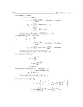


Applied-thermodynamics-onkar-singh-new.pdf
- 5. Copyright © 2009, 2006, 2003, NewAge International (P) Ltd., Publishers Published by New Age International (P) Ltd., Publishers All rights reserved. No part of this ebook may be reproduced in any form, by photostat, microfilm, xerography, or any other means, or incorporated into any information retrieval system, electronic or mechanical, without the written permission of the publisher. All inquiries should be emailed to rights@newagepublishers.com PUBLISHING FOR ONE WORLD NEWAGE INTERNATIONAL(P) LIMITED, PUBLISHERS 4835/24,Ansari Road, Daryaganj, New Delhi - 110002 Visitusatwww.newagepublishers.com ISBN (13) : 978-81-224-2916-9
- 6. Preface to the Third Edition I feel extremely encouraged at the good response to this textbook. Looking upon the feed back received from its readers third edition of the book is being presented here. In this edition number of solved and unsolved problems have been added in some of the chapters and a few new topics have also been added. I wish to express my sincere thanks to Professors and students for their valuable suggestions and recommending the book to their students and friends. I strongly feel that the book would prove to be further useful to students. I would be obliged for the errors, omissions and suggestions brought to my notice for improvement of the book in its next edition. Onkar Singh
- 8. Preface to the First Edition During teaching of the course of engineering thermodynamics and applied thermodynamics I have felt that the students at the undergraduate level of engineering and technology face difficulty in understanding the concepts of engineering thermodynamics and their applications in the course of applied thermodynamics. Also, the students face great difficulty in referring to the number of text- books for different topics. The present book is an effort in the direction of presenting the concepts of engineering thermodynamics and their applications in clear, concise and systematic manner at one place. Presentation is made in very simple and easily understandable language and well supported with wide ranging illustrations and numerical problems. The subject matter in this book covers the syllabus of the basic and advanced course on engineering thermodynamics/thermal engineering being taught in different institutions and universi- ties across the country. There are total 18 chapters in this book. The initial seven chapters cover the basic course on engineering thermodynamics and remaining chapters cover the advanced course in thermal engineering. These deal with “Fundamental concepts and definitions”, “Zeroth law and thermodynamics”, “First law of thermodynamics”, “Second law of thermodynamics”, “Entropy”, “Availability and general thermodynamic relations”, “Thermodynamic properties of pure substances”, “Fuels and combustion”, “Boilers and boiler calculations”, “Vapour power cycles”, “Gas power cycles”, “Steam engines”, “Nozzles”, “Steam turbines, Steam condenser”, “Reciprocating and rota- tory compressors”, “Introduction to internal combustion engines” and “Introduction to refrigeration and air conditioning”. Each chapter has been provided with sufficient number of typical numerical problems of solved and unsolved type. The book is written in SI system of units and the various tables such as steam tables, refrigeration tables, Mollier chart, psychrometry chart etc. are also provided at the end of the book for quick reference. I hope that the students and teachers referring to this book will find it useful. I am highly indebted to my family members for their continuous encouragement and coopera- tion during the preparation of manuscript. I would like to place on record my gratitude and apologies to my wife Parvin and kids Sneha and Prateek who patiently endured certain neglect and hardships due to my preoccupation with the preparation of this manuscript. I am thankful to AICTE, New Delhi for the financial support provided to me in the Young Teacher Career Award. I am also thankful to Mr. L.N. Mishra and other staff members of New Age International for their cooperation throughout the preparation of the textbook. At the end I thank to all those who supported directly or indirectly in the preparation of this book. I shall be extremely grateful to all the readers of text book for their constructive criticism, indicating any errors and omissions etc. for improving its quality and form. Onkar Singh
- 10. C O N T E N T S Preface to the third edition (v) Preface to the first edition (vii) Chapter 1 Fundamental Concepts and Definitions 1 1.1 Introduction and definition of thermodynamics 1 1.2 Dimensions and units 1 1.3 Concept of continuum 3 1.4 Systems, surroundings and universe 4 1.5 Properties and state 5 1.6 Thermodynamic path, process and cycle 5 1.7 Thermodynamic equilibrium 6 1.8 Reversibility and irreversibility 7 1.9 Quasi-static process 7 1.10 Some thermodynamic properties 8 1.11 Energy and its forms 11 1.12 Heat and work 13 1.13 Gas laws 14 1.14 Ideal gas 14 1.15 Dalton’s law, Amagat’s law and property of mixture of gases 15 1.16 Real gas 17 1.17 Vander Waals and other equations of state for real gas 20 Examples 22 Exercises 38 Chapter 2 Zeroth Law of Thermodynamics 40 2.1 Introduction 40 2.2 Principle of temperature measurement and Zeroth law of thermodynamics 40 2.3 Temperature scales 42 2.4 Temperature measurement 43 Examples 46 Exercises 49 Chapter 3 First Law of Thermodynamics 50 3.1 Introduction 50 3.2 Thermodynamic processes and calculation of work 50 3.3 Non-flow work and flow work 57 3.4 First law of thermodynamics 59 3.5 Internal energy and enthalpy 62 3.6 Specific heats and their relation with internal energy and enthalpy 63
- 11. 3.7 First law of thermodynamics applied to open systems 64 3.8 Steady flow systems and their analysis 65 3.9 First law applied to engineering systems 68 3.10 Unsteady flow systems and their analysis 73 3.11 Limitations of first law of thermodynamics 75 Examples 76 Exercises 94 Chapter 4 Second Law of Thermodynamics 97 4.1 Introduction 97 4.2 Heat reservoir 97 4.3 Heat engine 97 4.4 Heat pump and refrigerator 99 4.5 Statements for IInd law of thermodynamics 100 4.6 Equivalence of Kelvin-Planck and Clausius statements of IInd law of thermodynamics 101 4.7 Reversible and irreversible processes 103 4.8 Carnot cycle and Carnot engine 105 4.9 Carnot theorem and its corollaries 108 4.10 Thermodynamic temperature scale 109 Examples 113 Exercises 128 Chapter 5 Entropy 131 5.1 Introduction 131 5.2 Clausius inequality 131 5.3 Entropy – A property of system 134 5.4 Principle of entropy increase 138 5.5 Entropy change during different thermodynamic processes 140 5.6 Entropy and its relevance 144 5.7 Thermodynamic property relationship 144 5.8 Third law of thermodynamics 146 Examples 146 Exercises 161 Chapter 6 Thermodynamic Properties of Pure Substance 164 6.1 Introduction 164 6.2 Properties and important definitions 164 6.3 Phase transformation process 166 6.4 Graphical representation of pressure, volume and temperature 167 6.5 Thermodynamic relations involving entropy 170 6.6 Properties of steam 172 6.7 Steam tables and mollier diagram 175 6.8 Dryness fraction measurement 177 Examples 181 Exercises 199 (x)
- 12. Chapter 7 Availability and General Thermodynamic Relations 202 7.1 Introduction 202 7.2 Availability or exergy 203 7.3 Availability associated with heat and work 207 7.4 Effectiveness or second law efficiency 210 7.5 Second law analysis of steady flow systems 211 7.6 General thermodynamic relations 213 Examples 230 Exercises 248 Chapter 8 Vapour Power Cycles 250 8.1 Introduction 250 8.2 Performance parameters 250 8.3 Carnot vapour power cycle 251 8.4 Rankine cycle 253 8.5 Desired thermodynamic properties of working fluid 255 8.6 Parametric analysis for performance improvement in Rankine cycle 256 8.7 Reheat cycle 258 8.8 Regenerative cycle 260 8.9 Binary vapour cycle 268 8.10 Combined Cycle 270 8.11 Combined Heat and Power 272 8.12 Different steam turbine arrangements 273 Examples 273 Exercises 327 Chapter 9 Gas Power Cycles 330 9.1 Introduction 330 9.2 Air-standard cycles 330 9.3 Brayton cycle 340 9.4 Regenerative gas turbine cycle 345 9.5 Reheat gas turbine cycle 347 9.6 Gas turbine cycle with intercooling 351 9.7 Gas turbine cycle with reheat and regeneration 353 9.8 Gas turbine cycle with reheat and intercooling 354 9.9 Gas turbine cycle with regeneration, reheat and intercooling 355 9.10 Gas turbine irreversibilites and losses 355 9.11 Compressor and turbine efficiencies 358 9.12 Ericsson cycle 362 9.13 Stirling cycle 364 Examples 365 Exercises 396 Chapter 10 Fuel and Combustion 399 10.1 Introduction 399 10.2 Types of fuels 401 10.3 Calorific value of fuel 402 (xi)
- 13. 10.4 Bomb calorimeter 402 10.5 Gas calorimeter 404 10.6 Combustion of fuel 404 10.7 Combustion analysis 407 10.8 Determination of air requirement 409 10.9 Flue gas analysis 411 10.10 Fuel cells 413 Examples 413 Exercises 434 Chapter 11 Boilers and Boiler Calculations 436 11.1 Introduction 436 11.2 Types of boilers 437 11.3 Requirements of a good boiler 438 11.4 Fire tube and water tube boilers 438 11.5 Simple vertical boiler 442 11.6 Cochran boiler 443 11.7 Lancashire boiler 444 11.8 Cornish boiler 446 11.9 Locomotive boilers 446 11.10 Nestler boilers 448 11.11 Babcock and Wilcox boiler 448 11.12 Stirling boiler 449 11.13 High pressure boiler 450 11.14 Benson boiler 451 11.15 Loeffler boiler 452 11.16 Veloxboiler 452 11.17 La Mont boiler 453 11.18 Fluidized bed boiler 454 11.19 Waste heat boiler 456 11.20 Boiler mountings and accessories 459 11.21 Boiler draught 467 11.22 Natural draught 467 11.23 Artificial draught 474 11.24 Equivalent evaporation 477 11.25 Boiler efficiency 478 11.26 Heat balance on boiler 478 11.27 Boilertrial 481 Examples 481 Exercises 502 Chapter 12 Steam Engine 506 12.1 Introduction 506 12.2 Classification of steam engines 506 12.3 Working of steam engine 508 12.4 Thermodynamic cycle 515 12.5 Indicator diagram 518 (xii)
- 14. 12.6 Saturation curve and missing quantity 519 12.7 Heat balance and other performance parameters 521 12.8 Governing of simple steam engines 525 12.9 Compound steam engine 527 12.10 Methods of compounding 527 12.11 Indicator diagram for compound steam engine 530 12.12 Calculations for compound steam engines 531 12.13 Governing of compound steam engine 533 12.14 Uniflow engine 535 Examples 536 Exercises 561 Chapter 13 Nozzles 564 13.1 Introduction 564 13.2 One dimensional steady flow in nozzles 565 13.3 Choked flow 576 13.4 Off design operation of nozzle 577 13.5 Effect of friction on nozzle 580 13.6 Supersaturation phenomenon in steam nozzles 582 13.7 Steam injector 584 Examples 584 Exercises 608 Chapter 14 Steam Turbines 611 14.1 Introduction 611 14.2 Working of steam turbine 612 14.3 Classification of steam turbines 614 14.4 Impulse turbine 619 14.5 Velocity diagram and calculations for impulse turbines 623 14.6 Impulse turbine blade height 632 14.7 Calculations for compounded impulse turbine 634 14.8 Reaction turbines 637 14.9 Losses in steam turbines 644 14.10 Reheat factor 646 14.11 Steam turbine control 649 14.12 Governing of steam turbines 650 14.13 Difference between throttle governing and nozzle control governing 654 14.14 Difference between impulse and reaction turbines 654 Examples 655 Exercises 680 Chapter 15 Steam Condensor 684 15.1 Introduction 684 15.2 Classification of Condenser 685 15.3 Air Leakage 691 15.4 Condenser Performance Measurement 692 15.5 Cooling Tower 693 Examples 695 Exercises 704 (xiii)
- 15. Chapter 16 Reciprocating and Rotary Compressor 706 16.1 Introduction 706 16.2 Reciprocating compressors 708 16.3 Thermodynamic analysis 709 16.4 Actual indicator diagram 715 16.5 Multistage compression 716 16.6 Control of reciprocating compressors 722 16.7 Reciprocating air motor 722 16.8 Rotary compressors 723 16.9 Centrifugal compressors 728 16.10 Axial flow compressors 732 16.11 Surging and choking 733 16.12 Stalling 735 16.13 Centrifugal compressor characteristics 736 16.14 Axial flow compressor characteristics 739 16.15 Comparative study of compressors 740 Examples 742 Exercises 767 Chapter 17 Introduction to Internal Combustion Engines 770 17.1 Introduction 770 17.2 Classification of IC engines 771 17.3 IC Engine terminology 772 17.4 4-Stroke SI Engine 773 17.5 2-Stroke SI Engine 776 17.6 4-Stroke CI Engine 776 17.7 2-Stroke CI Engine 777 17.8 Thermodynamic cycles in IC engines 778 17.9 Indicator diagram and power measurement 780 17.10 Combustion in SI engine 783 17.11 Combustion in CI engines 785 17.12 IC engine fuels 786 17.13 Morse test 787 17.14 Comparative study of IC engines 788 Examples 790 Exercises 802 Chapter 18 Introduction to Refrigeration and Air Conditioning 805 18.1 Introduction 805 18.2 Performance parameters 807 18.3 Unit of refrigeration 808 18.4 Carnot refrigeration cycles 808 18.5 Air refrigeration cycles 809 18.6 Vapour compression cycles 813 18.7 Multistage vapour compression cycle 819 18.8 Absorption refrigeration cycle 820 (xiv)
- 16. 18.9 Modified absorption refrigeration cycle 822 18.10 Heat pump systems 823 18.11 Refrigerants 824 18.12 Desired properties of refrigerants 827 18.13 Psychrometry 827 18.14 Air conditioning systems 835 18.15 Comparison of different refrigeration methods 837 Examples 838 Exercises 855 Chapter 19 Jet Propulsion and Rocket Engines 858 19.1 Introduction 858 19.2 Principle of jet propulsion 858 19.3 Classification of jet propulsion engines 860 19.4 Performance of jet propulsion engines 861 19.5 Turbojet engine 863 19.6 Turbofan engine 867 19.7 Turboprop engine 868 19.8 Turbojet engine with afterburner 868 19.9 Ramjet engine 869 19.10 Pulse jet engine 870 19.11 Principle of rocket propulsion 871 19.12 Rocket engine 872 19.13 Solid propellant rocket engines 872 19.14 Liquid propellant rocket engines 873 Examples 873 Exercises 891 Multiple Answer Type Questions 892 Appendix 917 Table 1 : Ideal gas specific heats of various common gases at 300 K 917 Table 2 : Saturated steam (temperature) table 917 Table 3 : Saturated steam (pressure) table 919 Table 4 : Superheated steam table 921 Table 5 : Compressed liquid water table 927 Table 6 : Saturated ice-steam (temperature) table 928 Table 7 : Critical point data for some substances 929 Table 8 : Saturated ammonia table 930 Table 9 : Superheated ammonia table 931 Table 10 : Saturated Freon – 12 table 933 Table 11 : Superheated Freon – 12 table 934 Table 12 : Enthalpies of Formation, Gibbs Function of Formation, and Absolute Entropy at 25°C and 1 atm Pressure 937 Chart 1 : Psychrometric chart 938 Chart 2 : Mollier diagram 939 Index 941 (xv)
- 18. 1 Fundamental Concepts and Definitions 1.1 INTRODUCTION AND DEFINITION OF THERMODYNAMICS Thermodynamics is a branch of science which deals with energy. Engineering thermodynamics is modified name of this science when applied to design and analysis of various energy conversion systems. Thermodynamics has basically a few fundamental laws and principles applied to a wide range of problems. Thermodynamics is core to engineering and allows understanding of the mechanism of energy conversion. It is really very difficult to identify any area where there is no interaction in terms of energy and matter. It is a science having its relevance in every walk of life. Thermodynamics can be classified as ‘Classical thermodynamics’ and ‘Statistical thermodynamics’. Here in engineering systems analysis the classical thermodynamics is employed. “Thermodynamics is the branch of physical science that deals with the various phenomena of energy and related properties of matter, especially of the laws of transformations of heat into other forms of energy and vice-versa.” Internal combustion engines employed in automobiles are a good example of the energy conversion equipments where fuel is being burnt inside the piston cylinder arrangement and chemical energy liberated by the fuel is used for getting the shaft work from crankshaft. Thermodynamics lets one know the answer for the questions as, what shall be the amount of work available from engine?, what shall be the efficiency of engine?, etc. For analysing any system there are basically two approaches available in engineering thermodynamics. Approach of thermodynamic analysis means how the analyser considers the system. Macroscopic approach is the one in which complete system as a whole is considered and studied without caring for what is there constituting the system at microscopic level. Contrary to this the microscopic approach is one having fragmented the system under consideration upto microscopic level and analysing the different constituent subsystems/microsystems. In this approach study is made at the microscopic level. For studying the system the microlevel studies are put together to see the influences on overall system. Thus, the statistical techniques are used for integrating the studies made at microscopic level. This is how the studies are taken up in statistical thermodynamics. In general it can be said that, Macroscopic approach analysis = ∑ (Microscopic approach analysis). 1.2 DIMENSIONS AND UNITS “Dimension” refers to certain fundamental physical concepts that are involved in the process of nature and are more or less directly evident to our physical senses, thus dimension is used for characterizing
- 19. 2 _________________________________________________________ Applied Thermodynamics any physical quantity. Dimensions can be broadly classified as “primary dimensions” and “secondary or derived dimensions”. “Basic dimensions such as mass ‘M’, length ‘L’, time ‘t’ and temperature ‘T’ are called primary dimensions, while quantities which are described using primary dimensions are called secondary dimensions such as for energy, velocity, force, volume, etc”. “Units” are the magnitudes assigned to the dimensions. Units assigned to “primary dimensions” are called “basic units” whereas units assigned to “secondary dimensions” are called “derived units”. Various systems of units have prevailed in the past such as FPS (Foot-Pound-Second), CGS (Centimetre- Gram-Second), MKS (Metre-Kilogram-Second) etc. but at present SI system (System-International) of units has been accepted world wide. Here in the present text also SI system of units has been used. Following table gives the basic and derived units in SI system of units. Table 1.1 SI system of units Quantity Unit Symbol Basic Units Length (L) Metre m Mass (M) Kilogram kg Time (t) Second s Temperature (T) Kelvin K Plane angle Radian rad Solid angle Steradian sr Luminous intensity Candela cd Molecular substance Mole mol. Electric Current Ampere A Derived Units Force (F) Newton N {kg.m/s2} Energy (E) Joule J {N.m = kg. m2/s2} Power Watt W {J/s = kg. m2/s3} Pressure Pascal Pa {N/m2 = kg/(ms2)} Equivalence amongst the various systems of unit for basic units is shown in table 1.2. Table 1. 2 Various systems of units Unit - (Symbol) Quantity SI MKS CGS FPS Length Metre (m) Metre (m) Centimetre (cm) Foot (ft) Mass Kilogram (kg) Kilogram (kg) Gram (gm) Pound (lb) Time Second (s) Second (s) Second (s) Second (s) Temperature Kelvin (K) Centigrade (ºC) Centigrade (ºC) Fahrenheit (ºF) The various prefixes used with SI units are given as under :
- 20. Fundamental Concepts and Definitions ____________________________________________ 3 Prefix Factor Symbol Prefix Factor Symbol deca 10 da deci 10–1 d hecto 102 h centi 10–2 c kilo 103 k milli 10–3 m mega 106 M micro 10–6 µ giga 109 G nano 10–9 n tera 1012 T pico 10–12 p peta 1015 P femto 10–15 f exa 1018 E atto 10–18 a The conversion table for one unit into the other is given in table 1.3. Table 1.3 Unit conversion table 1 ft = 0.3048 m 1 ft2 = 0.09290 m2 1 in = 0.0254 m 1 in2 = 6.45 cm2 1 lb = 453.6 gm 1 lb = 0.4536 kg 1 lbf = 4.45 N 1 kgf = 9.81 N 1 lbf/in2 = 6.989 kN/m2 = 0.0689 bar = 703 kgf/m2 1 bar = 105 N/m2 = 14.5038 1bf/in2 = 0.9869 atm = 1.0197 kgf/cm2 1 ft. lbf = 1.356 Joules 1 Btu = 778.16 ft. lbf = 1.055 kJ 1Btu/lb = 2.326 kJ/kg 1 ft3/lb = 0.0624 m3/kg, 1 Cal = 4.18 J 1.3 CONCEPT OF CONTINUUM In Macroscopic approach of thermodynamics the substance is considered to be continuous whereas every matter actually comprises of myriads of molecules with intermolecular spacing amongst them. For analyzing a substance in aggregate it shall be desired to use laws of motion for individual molecules and study at molecular level be put together statistically to get the influence upon aggregate. In statistical thermodynamics this microscopic approach is followed, although it is often too cumbersome for practical calculations. In engineering thermodynamics where focus lies upon the gross behaviour of the system and substance in it, the statistical approach is to be kept aside and classical thermodynamics approach be followed. In classical thermodynamics, for analysis the atomic structure of substance is considered to be continuous. For facilitating the analysis this concept of continuum is used in which the substance is treated free from any kind of discontinuity. As this is an assumed state of continuum in substance so the order of analysis or scale of analysis becomes very important. Thus, in case the scale of analysis is large enough and the discontinuities are of the order of intermolecular spacing or mean free path then due to relative order of discontinuity being negligible it may be treated continuous. In the situations when scale of analysis is too small such that even the intermolecular spacing or mean free path are not negligible i.e. the mean free path is of comparable size with smallest significant dimension in analysis then it can not be considered continuous and the microscopic approach for analysis should be followed. For example, whenever one deals with highly rarefied gases such as in rocket flight at very high altitudes or electron tubes, the concept of continuum of classical thermodynamics
- 21. 4 _________________________________________________________ Applied Thermodynamics should be dropped and statistical thermodynamics using microscopic approach should be followed. Thus, in general it can be said that the assumption of continuum is well suited for macroscopic approach where discontinuity at molecular level can be easily ignored as the scale of analysis is quite large. The concept of continuum is thus a convenient fiction which remains valid for most of engineering problems where only macroscopic or phenomenological informations are desired. For example, let us see density at a point as a property of continuum. Let us take some mass of fluid ∆m in some volume ∆V enveloping a point ‘P’ in the continuous fluid. Average mass density of fluid within volume ∆V shall be the ratio (∆m/∆V). Now let us shrink the volume ∆V enveloping the point to volume ∆V′. It could be seen that upon reducing the volume, ∆V′ may be so small as to contain relatively few molecules which may also keep on moving in and out of the considered very small volume, thus average density keeps on fluctuating with time. For such a situation the definite value of density can not be given. Therefore, we may consider some limiting volume ∆Vlimit such that the fluid around the point may be treated continuous and the average density at the point may be given by the ratio limit m V ∆ ∆ . Thus, it shows how the concept of continuum although fictitious is used for defining density at a point as given below, Average density at the point = limit lim V V ∆ →∆ m V ∆ ∆ 1.4 SYSTEMS, SURROUNDINGS AND UNIVERSE In thermodynamics the ‘system’ is defined as the quantity of matter or region in space upon which the attention is concentrated for the sake of analysis. These systems are also referred to as thermodynamic systems. For the study these systems are to be clearly defined using a real or hypothetical boundary. Every thing outside this real/hypothetical boundary is termed as the ‘surroundings’. Thus, the surroundings may be defined as every thing surrounding the system. System and surroundings when put together result in universe. Universe = System + Surroundings The system is also some times defined as the control system and the boundary defined for separating it from surroundings is called control boundary, the volume enclosed within the boundary is control volume and the space enclosed within the boundary is called control space. Based on the energy and mass interactions of the systems with surroundings/other systems across the boundary the system can be further classified as the open, close, and isolated system. The ‘open system’ is one in which the energy and mass interactions take place at the system boundary, for example automobile engine etc. ‘Closed system’ is the system having only energy interactions at its boundary, for example, boiling water in a closed pan etc. The mass interactions in such system are absent. ‘Isolated system’ refers to the system which neither has mass interaction nor energy interaction across system boundary, for example Thermos Flask etc. Thus, the isolated system does not interact with the surroundings/ systems in any way.
- 22. Fundamental Concepts and Definitions ____________________________________________ 5 Fig. 1.1 (a) Open system (b) Closed system (c) Isolated system 1.5 PROPERTIES AND STATE For defining any system certain parameters are needed. ‘Properties’ are those observable characteristics of the system which can be used for defining it. Thermodynamic properties are observable characteristics of the thermodynamic system. Pressure, temperature, volume, viscosity, modulus of elasticity etc. are the examples of property. These properties are some times observable directly and some times indirectly. Properties can be further classified as the ‘intensive property’ and ‘extensive property’. The intensive properties are those properties which have same value for any part of the system or the properties that are independent of the mass of system are called intensive properties, e.g. pressure, temperature etc. Extensive properties on the other hand are those which depend upon the mass of system and do not maintain the same value for any path of the system. e.g. mass, volume, energy, enthalpy etc. These extensive properties when estimated on the unit mass basis result in intensive property which is also known as specific property, e.g. specific heat, specific volume, specific enthalpy etc. ‘State’ of a system indicates the specific condition of the system. To know the characteristics of the system quantitatively refers to knowing the state of system. Thus, when the properties of system are quantitatively defined then it refers to the ‘state’. For completely specifying the state of a system number of properties may be required which depends upon the complexity of the system. Thermodynamic state in the same way refers to the quantitative definition of the thermodynamic properties of a thermodynamic system e.g. for defining a gas inside the cylinder one may have to define the state using pressure and temperature as 12 bar, 298 K. When the thermodynamic properties defining a state undergo a change in their values it is said to be the ‘change of state’. 1.6 THERMODYNAMIC PATH, PROCESS AND CYCLE Thermodynamic system undergoes changes due to the energy and mass interactions. Thermodynamic state of the system changes due to these interactions. The mode in which the change of state of a system takes place is termed as the process such as constant pressure process, constant volume process etc. Let us take gas contained in a cylinder and being heated up. The heating of gas in the cylinder shall result in change in state of gas as its pressure, temperature etc. shall increase. However, the mode in
- 23. 6 _________________________________________________________ Applied Thermodynamics which this change of state in gas takes place during heating shall be constant volume mode and hence the process shall be called constant volume heating process. The path refers to the series of state changes through which the system passes during a process. Thus, path refers to the locii of various intermediate states passed through by a system during a process. Cycle refers to a typical sequence of processes in such a fashion that the initial and final states are identical. Thus, a cycle is the one in which the processes occur one after the other so as to finally bring the system at the same state. Thermodynamic path in a cycle is in closed loop form. After the occurrence of a cyclic process system shall show no sign of the processes having occurred. Mathematically, it can be said that the cyclic integral of any property in a cycle is zero, i.e., dp ∫ Ñ = 0, where p is any thermodynamic property. Thermodynamic processes, path and cycle are shown on p-v diagram in Fig. 1.2 Fig. 1.2 Thermodynamic process, path and cycle. 1.7 THERMODYNAMIC EQUILIBRIUM Equilibrium of a system refers to the situation in which it’s “state” does not undergo any change in itself with passage of time without the aid of any external agent. Equilibrium state of a system can be examined by observing whether the change in state of the system occurs or not. If no change in state of system occurs then the system can be said in equilibrium. Thermodynamic equilibrium is a situation in which thermodynamic system does not undergo any change in its state. Let us consider a steel glass full of hot milk kept in open atmosphere. It is quite obvious that the heat from milk shall be continuously transferred to atmosphere till the temperature of milk, glass and atmosphere are not alike. During the transfer of heat from milk the temperature of milk could be seen to decrease continually. Temperature attains some final value and does not change any more. This is the equilibrium state at which the properties stop showing any change in themselves. Generally, thermodynamic equilibrium of a system may be ensured by ensuring the mechanical, thermal, chemical and electrical equilibriums of the system. ‘Mechanical equilibrium’ of the system can be well understood from the principles of applied mechanics which say that the net force and moment shall be zero in case of such equilibrium. Thus, in the state of mechanical equilibrium the system does not have any tendency to change mechanical state as it is the state at which the applied forces and developed stresses are fully balanced. ‘Thermal equilibrium’ is that equilibrium which can be stated to be achieved if there is absence of any heat interactions. Thus, if the temperature states of the system do not change then thermal equilibrium is said to be attained. Equality of temperature of the two systems interacting with each other shall ensure thermal equilibrium. ‘Chemical equilibrium’ is the one which can be realized if the chemical potential of the systems interacting are same. The equality of forward rate of chemical reaction and backward rate of chemical reaction can be taken as criterion for ensuring the chemical equilibrium. Similar to this, in case the electrical potential of the systems interacting are same, the ‘electrical equilibrium’ is said be attained.
- 24. Fundamental Concepts and Definitions ____________________________________________ 7 Thus, a system can be said to be in thermodynamic equilibrium if it is in mechanical, thermal, chemical and electrical equilibrium. 1.8 REVERSIBILITY AND IRREVERSIBILITY Thermodynamic processes may have the change of state occuring in two ways. One is the change of state occuring so that if the system is to restore its original state, it can be had by reversing the factors responsible for occurrence of the process. Other change of state may occur such that the above restoration of original state is not possible. Thermodynamic system that is capable of restoring its original state by reversing the factors responsible for occurrence of the process is called reversible system and the thermodynamic process involved is called reversible process. Thus, upon reversal of a process there shall be no trace of the process being ocurred, i.e. state changes during the forward direction of occurrence of a process are exactly similar to the states passed through by the system during the reversed direction of the process. It is quite obvious that the such reversibility can be realised only if the system maintains its thermodynamic equilibrium throughout the occurrence of process. Fig. 1.3 Reversible and Irreversible processes The irreversibility is the characteristics of the system which forbids system from retracing the same path upon reversal of the factors causing the state change. Thus, irreversible systems are those which do not maintain equilibrium during the occurrence of a process. Various factors responsible for the nonattainment of equilibrium are generally the reasons responsible for irreversibility. Presence of friction, dissipative effects etc. have been identified as a few of the prominent reasons for irreversibility. The reversible and irreversible processes are shown on p-v diagram in Fig. 1.3 by ‘1–2 and 2–1’ and ‘3–4 and 4–3’ respectively. 1.9 QUASI-STATIC PROCESS Thermodynamic equilibrium of a system is very difficult to be realised during the occurrence of a thermodynamic process. It may be understood that this kind of equilibrium is rather practically impossible. In case such equilibrium could not be attained then the thermodynamic analysis cannot be done, as the exact analysis of a system not in equilibrium is impossible. ‘Quasi-static’ consideration is one of the ways to consider the real system as if it is behaving in thermodynamic equilibrium and thus permitting the thermodynamic study. Actually, system does not attain thermodynamic equilibrium only certain assumptions make it akin to a system in equilibrium, for the sake of study and analysis. Quasi-static literally refers to “almost static” and the infinite slowness of the occurrence of a process is considered as the basic premise for attaining near equilibrium in the system. Here it is considered that the change in state of a system occurs at infinitely slow pace, thus consuming very large time for completion of the process. During the dead slow rate of state change the magnitude of change in a state
- 25. 8 _________________________________________________________ Applied Thermodynamics shall also be infinitely small. This infinitely small change in state when repeatedly undertaken one after the other consecutively, results in overall state change. Quasi-static process is considered to remain in thermodynamic equilibrium just because of infinitesimal state changes taking place during the occurrence of the process. Quasi static process can be understood from the following example. Let us consider the heating of gas in a container with certain mass ‘W’ kept on the top of lid (lid is such that it does not permit leakage across its interface with vessel wall) of the vessel as shown in Fig. 1.4. After certain amount of heat being added to the gas it is found that the lid gets raised up. Thermodynamic state change is shown in figure. The “change in state” is significant. During the change of state since the states could not be considered to be in equilibrium, hence for unsteady state of system, thermodynamic analysis could not be extended. Let us now assume that the total mass comprises of infinitesimal small masses of ‘w’ such that all ‘w’ masses put together become equal to W. Now let us start heat addition to vessel and as soon as the lifting of lid is observed put first fraction mass ‘w’ over the lid so as to counter the lifting and estimate the state change. During this process it is found that the state change is negligible. Let us further add heat to the vessel and again put the second fraction mass ‘w’ as soon as the lift is felt so as to counter it. Again the state change is seen to be negligible. Continue with the above process and at the end it shall be seen that all fraction masses ‘w’ have been put over the lid, thus Fig. 1.4 Quasi static process amounting to mass ‘W’ kept over the lid of vessel and the state change occurred is exactly similar to the one which occurred when the mass kept over the lid was ‘W’. In this way the equilibrium nature of system can be maintained and the thermodynamic analysis can be carried out. p-v representation for the series of infinitesimal state changes occuring between states 1 and 2 is shown in Fig. 1.4. 1.10 SOME THERMODYNAMIC PROPERTIES Pressure, temperature, density, volume etc. are some of the thermodynamic properties frequently used. Pressure is defined as the force per unit area. Mathematically, it can be given by the ratio of force applied on a area (say F) divided by the area (say A) as ; p = F/A, (N/m2). In general during analysis one comes across the following four types of pressure, (i) Atmospheric pressure (ii) Absolute pressure (iii) Gauge pressure (iv) Vacuum pressure Atmospheric pressure is defined as the pressure exerted by the atmosphere. It is said to be equal to 760 mm of mercury column at 0ºC for mercury density of 0.0135951 kg/cm3, gravitational acceleration of 9.80665 m/s2 and has magnitude of 1.013 bar (= 1.013 × 10⁵ N/m2). The instrument used for
- 26. Fundamental Concepts and Definitions ____________________________________________ 9 measuring this pressure is called barometer. Italian scientist Torricelli was first to construct the barometer to measure the pressure. In his honour the pressure exerted by one millimeter column of mercury under atmospheric conditions is known as ‘Torr’ (1 atm = 760 Torr). Absolute pressure of gas refers to the actual pressure of the gas. Let us consider a U-tube manometer as shown in Fig. 1.5. It shows the manometer with its one limb connected to bulb containing the gas while other limb is open to atmosphere. Fig. 1.5a describes a special case in which the pressure of the gas is more than the atmospheric pressure and it is the reason for the rise in level of mercury in the open limb. The difference in the pressure of fluid and atmosphere which is measurable by the rise of mercury column (= h.d.g. where h is the rise in mercury column, d is the density of mercury, g is the gravitational acceleration) is known as the Gauge pressure. Mathematically, it can be shown that, Absolute pressure = Atmospheric pressure + Gauge pressure Figure 1.5b shows another typical case in which the pressure of gas is less than the atmospheric pressure and that is why the mercury column is depressed in the open limb. The amount by which the pressure of gas is less than the atmospheric pressure is called Vacuum pressure. Thus, the vacuum pressure is the negative gauge pressure. Mathematically it can be shown by, Absolute pressure = Atmospheric pressure – Vacuum pressure Fig. 1.5 U-tube manometer The bar chart shown in Fig. 1.6 further clarifies the interrelationship amongst the different pressures. Fig. 1.6 Different pressures
- 27. 10 _________________________________________________________ Applied Thermodynamics Pressure could also be measured by a Bourdan tube. Bourdan tube has a flattened cross section (oval) closed at one end. Other end of tube connects to the region whose pressure is to be measured. Gas whose pressure is being measured acts on inside of tube surface, thus causing it to change its section from oval section to circular section. Pressure exerted by gas works against tube stresses and air pressure. This change in cross-section from elliptical to circular causes straightening of tube and thus deflecting free end of tube through some distance ‘d’ as shown in figure 1.7. This deflection in free end of tube measures the pressure difference between gas pressure and atmospheric pressure. Generally this free end of tube is connected to an indicating hand sweeping over a graduated dial showing the gauge pressure directly. Temperature is another thermodynamic property which is normally used in Kelvin scale in engineering thermodynamic analysis. It is dealt in detail in subsequent chapter. Density which refers to the mass per unit volume is the ratio of mass and volume occupied. Its units are kg/m3. Density = (Mass/Volume) Fig. 1.7 Bourdan tube for pressure measurement The specific volume is the volume per unit mass of the substance. It is defined by ratio of the volume occupied and the mass of substance. Its units are m3/kg. Specific volume = (Volume/Mass) Density or specific volume conform to the definitive specification of a thermodynamic property and are capable of getting associated with other properties such as temperature, pressure and internal
- 28. Fundamental Concepts and Definitions ____________________________________________ 11 energy. Also, the volume occupied by a material is a measure of distance between molecules and thus indicates their molecular energy. Weight is actually the force due to gravity acting on any substance. Thus, it is the product of mass and gravitational acceleration. Its units are Newtons. Weight = (mass × gravitational acceleration) Specific weight of a substance is the ratio of weight of substance and volume of substance. Specific weight = (Weight/Volume) = (density × gravitational acceleration) Specific gravity is defined as the ratio of the density of any substance and standard density of some reference substance. For solids and liquids the water density at some specified temperature say 0ºC or 4ºC is taken as standard density. 1.11 ENERGY AND ITS FORMS “Energy is usually defined as the ability to do mechanical work”. It is indeed quite difficult to precisely define the “energy”. We feel energy at every moment and can sense it very oftenly. Another broader definition of energy says that “energy refers to the capacity for producing effects.” Total energy at any moment may be the algebraic summation of the different forms of energy. Conversion of energy from one to other is also possible. In thermodynamics we are primarily interested in studying the change in total energy of a system. Thus, for analysis relative value of energy is considered instead of absolute value. Energy can be classified in the following general categories; (a) Energy in transition: It refers to the energy that is in process of transition between substances or regions because of some driving potential, such as difference or gradient of force, or of temperature, or of electrical potential etc. For example heat, work etc. (b) Energy stored in particular mass: It refers to the potential and kinetic energy associated with masses that are elevated or moving with respect to the earth. Apart from above broad classification the energy can also be categorised into various forms. (i) Macroscopic energy: It refers to the energy possessed by a system considered at macro- scopic level such as kinetic energy, potential energy etc. (ii) Microscopic energy: It refers to the energy defined at molecular level. Summation of energy at molecular level or microscopic energy results in internal energy. Some of the popular forms of energy are described below : Potential energy: This type of energy is based on relative position of bodies in a system, i.e. elevation in a gravitational field. Potential energy for a mass m at elevation z is given as : P.E. = m.g.z Here g is the gravitational acceleration and elevation is measured from some reference point. Kinetic energy: It is based on the relative movement of bodies. For a mass m moving with certain velocity c it could be mathematically expressed as; K.E. = (1/2) m.c2 Internal energy: Internal energy of a system is the energy associated with the molecular structure at molecular level. Let us study fall of a ‘weight’ from certain height on the floor. Upon hitting the floor, ‘weight’ comes to dead stop and its potential energy and kinetic energy both reduce to zero. Question arises, where does the vanishing potential energy and kinetic energy go upon ‘weight’ touching the floor. If we touch the point of contact between ‘weight’ and floor, it is observed that both these points are slightly hotter than before impact. Thus, it is obvious that the energy has changed its form from potential and kinetic to internal energy and causes rise in temperature of ‘weight’ and floor at the points of contact.
- 29. 12 _________________________________________________________ Applied Thermodynamics Internal energy is sum of energy associated with molecules which may have translational, vibrational and rotational motions etc. and respective energies causing these motions. Internal energy may be thus comprising of sensible energy, latent energy, chemical energy, nuclear energy etc. ‘Sensible energy’ refers to the kinetic energy associated with molecules. ‘Latent energy’ refers to the energy associated with phase of a substance. ‘Chemical energy’ refers to the energy associated with molecular bonds. ‘Nuclear energy’ refers to the energy associated with the bonds within nucleus of atom itself. Total energy of a system may be given as summation of different forms of energy at a moment. Mathematically; T.E (Total energy) = K.E + P.E + I.E where K.E = Kinetic energy P.E = Potential energy I.E = Internal energy Some different forms of energy interaction and associated work interactions with block diagram are given in table 1.4. Table 1.4 Some forms of energy and the associated work interactions S. Macroscopic Governing Energy Work Block diagram No. form of energy equation interaction interaction 1. Kinetic energy F = m · dV dt ∆E = 1 2 m· = – F · dx m F x (translation) ( ) 2 2 2 1 V V − 2. Kinetic energy T = J · d dt ω ∆E = 1 2 J· = – T · dθ J T θ (rotational) ( ) 2 2 2 1 ω ω − 3. Spring stored F = kx ∆E = 1 2 k· = – F · dx k F F x F = 0 energy (translational) ( ) 2 2 2 1 x x − 4. Spring stored T = K · θ ∆E = 1 2 K· = – T · dθ K T = 0 T T θ energy (rotational) ( ) 2 2 2 1 θ θ − 5. Gravitational F = mg ∆E = mg· = – F · dz m F z g energy (Z2 – Z1) 6. Electrical energy u = q c ∆E = 1 2 2 q c = – u · dq q u c (capacitance) = 1 2 cu2 7. Electrical energy φ = L · i ∆E = 1 2 Li2 = – i · dφ u L i (inductance) = 1 2 2 L φ
- 30. Fundamental Concepts and Definitions ____________________________________________ 13 1.12. HEAT AND WORK When two systems at different temperatures are brought into contact there are observable changes in some of their properties and changes continue till the two don’t attain the same temperature if contact is prolonged. Thus, there is some kind of energy interaction at the boundary which causes change in temperatures. This form of energy interaction is called heat. Thus ‘heat’ may be termed as the energy interaction at the system boundary which occurs due to temperature difference only. Heat is observable in transit at the interface i.e. boundary, it can not be contained in a system. In general the heat transfer to the system is assigned with positive (+) sign while the heat transfer from the system is assigned with negative (–) sign. Its units are Calories. In thermodynamics the work can be defined as follows: “Work shall be done by the system if the total effect outside the system is equivalent to the raising of weight and this work shall be positive work”. In above definition the work has been defined as positive work and says that there need not be actual raising of weight but the effect of the system behaviour must be reducible to the raising of a weight and nothing else. Its units are N. m or Joule. Heat and work are two transient forms of energy. Let us look at a piston cylinder mechanism (closed system), where high pressure air is filled inside the cylinder fitted with a piston exerting force against some resistance. As the piston moves a distance say ‘l’, the work would be done. It can be reduced to the raising of weight by replacing this resisting system by a frictionless pulley and lever such that a weight W is raised, Fig. 1.8. For example, if an electrical battery and resistance is considered as a system, then this system shall do work when electric current flows in an external resistance as this resistance could be replaced by an ideal frictionless motor driving a frictionless pulley and raising a weight. Here, also in reference to work it is obvious that the work is the entity which is available at the boundary of system, thus work can not be stored rather it is energy interaction in transit at the boundary. From the thermodynamic definition of work the sign convention established as positive work shall be the one which is done by the system while the negative work shall be the one that is done upon the system. Fig. 1.8 Thermodynamic work
- 31. 14 _________________________________________________________ Applied Thermodynamics 1.13 GAS LAWS Thermodynamic analysis relies largely upon the gas laws, which are known as Boyle’s law (1662) and Charle’s law (1787). Boyle’s law says that if temperature of a gas is held constant then its molar volume is inversely proportional to the pressure. Mathematically it can be related as p v = constant. Here p is the pressure and v is the molar volume of gas, i.e. volume per mole. Charle’s law says that for the pressure of gas held constant the volume of gas is directly proportional to the temperature of gas. Mathematically it can be given as v /T = constant, where T is the temperature of the gas. It also says that if the molar volume of gas is held constant, the pressure of gas is directly proportional to temperature, i.e. p/T = constant. Figure 1.9 shows the graphical representation. Fig 1.9 Graphical representations of gas laws at constant temperature and at constant pressure Boyle’s and Charle’s law when combined together result in, p v /T = constant or p v = R T, where R is the universal gas constant. 1.14 IDEAL GAS Engineering thermodynamics deals with different systems having gaseous working fluids. Some gases behave as ideal gas and some as non-ideal gas. Based on the experimental methods various equations of state of gases have been developed. For perfect gas the ideal gas equation shows that pv = R T, where R is the universal gas constant and can be related as R = R /M, here R is the characteristic gas constant and M is the molar mass or molecular weight of the substance, v is volume per mole. Universal gas constant has value given as 8.31441 kJ/k mol.K. or pV= m RT, where m is mass of the substance, V is the volume of substance, i.e. V = n · v m = n · M, where ‘n’ is no. of moles. Gas constant is also related to specific heats at constant pressure and volume as follows, R = cp – cv Upon plotting the variables P, V, T for an ideal gas on three mutually perpendicular axes, the three dimensional entity generated is called P-V-T surface and can be used for studying the thermodynamic properties of ideal gas. Figure 1.10 shows the typical P-V-T surface for an ideal gas.
- 32. Fundamental Concepts and Definitions ____________________________________________ 15 Fig. 1.10 P-V-T surface for ideal gas For certain gases the molecular weight and gas constant are given in table 1.5. Table 1.5 Gas Molecular weight, kg/kmol Gas constant, kJ/kg.K Air 28.97 0.287 Carbon dioxide 44.01 0.189 Hydrogen 2.016 4.124 Helium 4.004 2.077 Nitrogen 28.01 0.297 Oxygen 32.00 0.260 Steam 18.02 0.461 1.15 DALTON’S LAW, AMAGAT’S LAW AND PROPERTY OF MIXTURE OF GASES Dalton’s law of partial pressures states that the “total pressure of a mixture of gases is equal to the sum of partial pressures of constituent gases.” Partial pressure of each constituent can be defined as the pressure exerted by the gas if it alone occupied the volume at the same temperature. Thus, for any mixture of gases having ‘j’ gases in it, the mathematical statement of Dalton’s law says, p = p1 + p2 + p3 + ..... + pj if V = V1 = V2 = V3 = ..... = Vj and T = T1 = T2 = T3 = ..... Tj Dalton’s law can be applied to both mixture of real gases and ideal gases. (a) 1 1 , , m p V T + 2 2 , , m p V T → , , m p V T (b) 1 1 , , m V p T + 2 2 , , m V p T → , , m V p T constituent gases Mixture Fig. 1.11 (a) Dalton’s law of partial pressures, (b) Amagat’s law Let us take mixture of any three, perfect gases, say, 1, 2, 3 in a container having volume ‘V’ and temperature T.
- 33. 16 _________________________________________________________ Applied Thermodynamics Equation of state for these gases shall be, p1V = m1R1T ; p2 V = m2 · R2 · T, p3V = m3 · R3 · T The partial pressures of three gases shall be, p1 = 1 1 m R T V , p2 = 2 2 · · m R T V , p3 = 3 3 · · m R T V From Dalton’s law; p = p1 + p2 + p3 = (m1R1 + m2R2 + m3R3) · T V or, it can be given in general form as, pV = T · 1 · j i i i m R = ∑ where i refers to constituent gases Amagat’s law of additive volumes states that volume of a gas mixture is equal to the sum of volumes each gas would occupy at the mixture pressure and temperature. V = V1 + V2 + V3 ........... + Vj p = p1 = p2 = p3 ........ pj T = T1 = T2 = T3 = ........ Tj Mass balance upon mixture yields m = m1 + m2 + m3 or m = 1 j i i m = ∑ From above the gas constant for the mixture can be given as; R = 1 1 2 2 3 3 1 2 3 ( ) m R m R m R m m m + + + + or, in general form, R = 1 1 · j i i i j i i m R m = = ∑ ∑ Mole fraction xi of a constituent gas can be defined as the ratio of number of moles of that constituent to the total number of moles of all constituents. Thus mole fractions of three gases, if number of moles of three gases are n1, n2 and n3; x1 = 1 1 2 3 n n n n + + x2 = 2 1 2 3 n n n n + + x3 = 3 1 2 3 n n n n + +
- 34. Fundamental Concepts and Definitions ____________________________________________ 17 or, in general xi = i i n n ∑ Total no. of moles, n = n1 + n2 + n3 or, n = 1 j i i n = ∑ Sum of mole fractions of all constituent equals to 1, i x ∑ = i n n ∑ = 1 Number of moles of any constituent gas, ni = n · xi For Mi being the molecular weight of a constituent gas, the mass mi of that constituent shall be mi = ni · Mi or, mi = n · xi · Mi and the total mass m, shall be m = i m ∑ = n. i x ∑ · Mi Molecular weight of mixture shall be: M = m n = i x ∑ · Mi 1.16 REAL GAS When a gas is found to disobey the perfect gas law, i.e. the equation of state for ideal gas, then it is called ‘real gas’. Real gas behaviour can also be shown by a perfect gas at the changed thermodynamic states such as high pressure etc. Deviation of real gas from ideal gas necessitates the suitable equation of state which can be used for interrelating the thermodynamic properties P, V, and T. From the kinetic theory of gases it is obvious that the ideal gas equation of state suits the gas behaviour when intermolecular attraction and volume occupied by the molecules themselves is negligibly small in reference to gas volume. At high pressures intermolecular forces and volume of molecules both increase and so the gas behaviour deviates from ideal gas to real gas. A number of mathematical equations of state suggested by Van der-Waals, Berthelot, Dieterici, Redlich-Kwong, Beattie-Bridgeman and Martin-Hou etc. are available for analysing the real gas behaviour. Dalton’s law and Amagat’s law can also be used for real gases with reasonable accuracy in conjunction with modified equations of state. As the ideal gas equation does not conform to the real gas behaviour in certain ranges of pressures and temperatures, so the perfect gas equation should be modified using compressibility factor for the gas at given pressure and temperature. Such modified form of equations shall be; P v = Z · R · T Here Z is the compressibility factor, a function of pressure and temperature. Thus, compressibility factor is like a correction factor introduced in ideal equation of state for suiting the real gas behaviour. Compressibility factor is an indication of deviation of a gas from ideal gas behaviour and can be mathematically given as;
- 35. 18 _________________________________________________________ Applied Thermodynamics Z = ƒ(P, T) or Z = actual ideal v v Here, ideal v = RT P i.e. Z = 1 for ideal gases while Z can be greater than or less than unity. Individual graphical representations are available for getting the compressibility factor as shown in Fig 1.12. Compressibility factor charts are available for different substances. Compressibility factors for various substances can also be shown on a generalized compressibility chart using reduced properties. Reduced properties are non-dimensional properties given as ratio of existing property to critical property of substance. Such as reduced pressure is ratio of pressure of gas to critical pressure of gas. Similarly, reduced temperature can be given by ratio of temperature of gas to critical temperature of gas. Reduced pressure, pR = c p p Reduced temperature, TR = c T T (a) Oxygen (b) Carbon dioxide Fig. 1.12 Compressibility factors, Z
- 36. Fundamental Concepts and Definitions ____________________________________________ 19 where Pc and Tc denote critical pressure and critical temperature respectively. These reduced pressure and reduced temperature are used for getting the generalized compressibility chart of the form, Z = ƒ (pR,TR) where Z for all gases is approximately same. This similar behaviour of compressibility correction factor for different gases in respect to reduced pressures and temperatures is called "principle of corresponding states." Fig. 1.13 shows a generalized compressibility chart. In generalized compressibility chart a set of curves is fitted through a set of experimentally determined Z values plotted against reduced Fig. 1.13 (a) Generalized compressibility chart, pR ≤ 1.0 Fig. 1.13 (b) Generalized compressibility chart, pR ≤ 10.0
- 37. 20 _________________________________________________________ Applied Thermodynamics Fig. 1.13 (c) Generalized compressibility chart, 10 ≤ pR ≤ 40 pressure and reduced temperatures for several gases. On the generalized compressibility chart it could be seen that at “very small pressures the gases behave as an ideal gas irrespective of its temperature” and also at “very high temperatures the gases behave as ideal gas irrespective of its pressure”. 1.17 VANDER’ WAALS AND OTHER EQUATIONS OF STATE FOR REAL GAS Vander’ Waals suggested the equation of state for real gas in 1873. The equation has been obtained applying the laws of mechanics at molecular level and introducing certain constants in the equation of state for ideal gas. This equation agrees with real gas behaviour in large range of gas pressures and temperatures. Vander’ Waals equation of state for real gas is as follows, ( ) 2 a p v b RT v + − = where ‘a’ is the constant to take care of the mutual attraction amongst the molecules and thus 2 a v accounts for cohesion forces. Table 1.6 Vander’ Waals constant Gas Constant a, N.m4/(kg. mol)2 Constant b, m3/kg.mol Helium 34176.2 × 102 2.28 × 10⁻² Hydrogen 251.05 × 10² 2.62 × 10⁻² Oxygen 1392.5 × 102 3.14 × 10⁻² Air 1355.22 × 102 3.62 × 10⁻² Carbon dioxide 3628.50 × 102 3.14 × 10⁻²
- 38. Fundamental Concepts and Definitions ____________________________________________ 21 Constant ‘b’ accounts for the volumes of molecules which are neglected in perfect gas equation, thus it denotes “co-volume”, Mathematically, ( ) ( ) 2 2 27 , · / 8 64 c c c c R T a b R T p p = = Here, pc, Tc are critical point pressures and temperatures having values as given in appendix. Thus these constants ‘a’ & ‘b’ are determined from behaviour of substance at the critical point. In general it is not possible to have a single equation of state which conforms to the real gas behaviour at all pressures and temperatures. A few more equations of state for real gas as suggested by various researchers are as follows. Redlich-Kwong equation of state for real gas, ( ) ( ) · · RT a p v b v v b T = − − + where a = 0.4278 2 2.5 · c c R T p and b = 0.08664 · c c R T p Berthelot equation of state for real gas, p = 2 ( ) · RT a v b T v − − , where a = 2 3 27· · 64 · c c R T p and b = · 8 c c R T p Here a and b refer to the constants as suggested in respective equations. Beattie-Bridgeman equation of state given in 1928, for real gas has five constants determined experimentally. It is, ( ) ( ) 2 3 2 · 1 ( ) · R T C A p v B v v T v = − + − where, 0 1 a A A v = − and 0 1 b B B v = − Constants used in Beattie – Bridgeman equation are given in Table 1.7 when p is in k pa, v is in m3/k mol, T is in K, and R = 8.314 k pa m3/k mol.K. Table 1.7. Beattie -Bridgeman constants Gas A0 a B0 b c Helium 2.1886 0.05984 0.01400 0.0 40 Hydrogen 20.0117 –0.00506 0.02096 –0.04359 504 Oxygen 151.0857 0.02562 0.04624 0.004208 4.80 ×10⁴ Air 131.8441 0.01931 0.04611 –0.001101 4.34 × 10⁴ Carbon dioxide 507.2836 0.07132 0.10476 0.07235 6.60 × 10⁵
- 39. 22 _________________________________________________________ Applied Thermodynamics Virial equations of state propose a form of equation which can be suitably modified and used for real gases. These equations of state are in the form, pv RT = A0 + A1 . p + A2 . p2 + A3 . p3 + ..... or pv RT = B0 + 1 B v + 2 2 B v + 3 3 B v +....... Where A0, A1, A2, A3, .........and B0, B1, B2, B3....... are called the "virial coefficients" and depend upon temperature alone. Virial equations of state can be suitably modified based on experimental P, v, T data for the real gas analysis. Virial constants can be calculated if the suitable model for describing the forces of interaction between the molecules of gas under consideration is known. EXAMPLES 1. Find out the pressure difference shown by the manometer deflection of 30 cm of Mercury. Take local acceleration of gravity as 9.78 m/s2 and density of mercury at room temperature as 13,550 kg/m3. Solution: From the basic principles of fluid statics, Pressure difference = ρ·gh = 13550 × 30 × 10–2 × 9.78 = 39755.70 Pa Ans. 2. An evacuated cylindrical vessel of 30 cm diameter is closed with a circular lid. Estimate the effort required for lifting the lid, if the atmospheric pressure is 76 cm of mercury column (Take g = 9.78 m/s2) Solution: Effort required for lifting the lid shall be equal to the force acting upon the lid. Thus, effort required = Pressure × Area = (76 × 10–2 × 13550 × 9.78) × (3.14 × (30 × 10–2)2/4) = 7115.48 N Ans. 3. Calculate the actual pressure of air in the tank if the pressure of compressed air measured by manometer is 30 cm of mercury and atmospheric pressure is 101 kPa. (Take g = 9.78 m/s2) Solution: Pressure measured by manometer on the tank is gauge pressure, which shall be = ρ.g.h = (13550 × 9.78 × 30 × 10–2) = 39755.70 Pa = 39.76 kPa Actual pressure of air = Gauge pressure + atmospheric pressure = 39.76 + 101 = 140.76 kPa Ans. 4. Determine gauge pressure at a depth of 1 m in a tank filled with oil of specific gravity 0.8. Take density of water as 1000 kg/m3 and g = 9.81 m/s2.
- 40. Fundamental Concepts and Definitions ____________________________________________ 23 Solution: Density of oil = Specific gravity × Density of water ρoil = 0.8 × 1000 ρoil = 800 kg/m3 Gauge pressure = (ρoil × g × h) = 800 × 9.81 × 1 or = 7848 N/m2 Gauge pressure = 7.848 kPa. Ans. 5. Calculate the gas pressure using a mercury manometer with one limb open to atmosphere as shown in Fig. 1.14. Barometer reading is 76 cm and density of mercury is 13.6 × 10³ kg/m3. Take g = 9.81 m/s2. Solution: Figure shows that the difference of height in mercury columns is 40 cm. In reference to level AB the pressure exerted by gas, pgas can be written as sum of atmospheric pressure and pressure due to mercury column at AB pgas = (ρmercury × 9.81 × 40 × 10–2) + Atmospheric pressure = (13.6 × 103 × 9.81 × 40 × 10–2) + (13.6 × 103 × 9.81 × 76 × 10–2) = 154762.56 N/m2 or Pgas = 154.76 kPa Ans. Fig. 1.14 6. 1 kg of water falls from an altitude of 1000 m above ground level. What will be change in the temperature of water at the foot of fall, if there are no losses during the fall. Take specific heat of water as 1 kcal/kg·K Solution: Initially when water is at 1000 m, it shall have potential energy in it. This potential energy shall get transformed upon its fall and change the temperature of water. By law of energy conservation Potential energy = Heat required for heating water = 1 9.81 1000 4.18 × × = 1 × 1 × 103 × ∆T or ∆T = 2.35ºC Change in temperature of water = 2.35ºC Ans.
- 41. 24 _________________________________________________________ Applied Thermodynamics 7. A spring balance is used for measurement of weight. At standard gravitational acceleration it gives weight of an object as 100 N. Determine the spring balance reading for the same object when measured at a location having gravitational acceleration as 8.5 m/s2. Solution: At standard gravitational acceleration, mass of object = 100 9.81 = 10.194 kg Spring balance reading = Gravitational force in mass = 10.194 × 8.5 = 86.649 N = 86.65 N Ans. 8. An incompressible gas in the cylinder of 15 cm diameter is used to support a piston, as shown. Manometer indicates a difference of 12 cm of Hg column for the gas in cylinder. Estimate the mass of piston that can be supported by the gas. Take density of mercury as 13.6 × 10³ kg/m3. Solution: Piston shall be supported by the gas inside, therefore, let mass of piston be ‘m’ kg. Weight of piston = Upward thrust by gas m.g = p × π × 2 4 d m × 9.81 = (12 × 10–2 × 13.6 × 103 × 9.81) × ð 4 × (15 × 10–2)2 m = 28.84 kg Mass of piston = 28.84 kg. Ans. 9. Determine pressure of steam flowing through a steam pipe when the U-tube manometer connected to it indicates as shown in figure 1.16. During pressure measurement some steam gets condensed in manometer tube and occupies a column of height 2 cm (AB) while mercury gets raised by 10 cm (CD) in open limb. Consider barometer reading as 76 cm of Hg, density of mercury and water as 13.6 × 10³ kg/m3 and 1000 kg/m3 respectively. Solution: Let us make pressure balance at plane BC. psteam + pwater, AB = patm + pHg , CD psteam = patm + pHg, CD – pwater, AB patm = (13.6 × 103 × 76 × 10–2 × 9.81) patm = 101396.16 N/m2 pwater, AB = (1000 × 2 × 10–2 × 9.81) pwater, AB = 196.2 N/m2 Fig. 1.15 Fig. 1.16
- 42. Fundamental Concepts and Definitions ____________________________________________ 25 pHg, CD = (13.6 × 103 × 10 × 10–2 × 9.81) pHg, CD = 13341.6 N/m2 Substituting for getting steam pressure, psteam = 101396.16 + 13341.6 – 196.2 psteam = 114541.56 N/m2 or psteam = 114.54 kPa Ans. 10. A vessel has two compartments ‘A’ and ‘B’ as shown with pressure gauges mounted on each compartment. Pressure gauges of A and B read 400 kPa and 150 kPa respectively. Determine the absolute pressures existing in each compartment if the local barometer reads 720 mm Hg. Solution: Atmospheric pressure from barometer = (9810) × (13.6) × (0.720) = 96060 Pa = 96.06 kPa Absolute pressure in compartment A, Pabs, A = Pgauge, A + Patm = 400 + 96.06 = 496.06 kPa Absolute pressure in compartment B, Pabs, B = Pgauge, B + Patm = 150 + 96.06 = 246.06 kPa Absolute pressure in compartments A & B = 496.06 kPa & 246.06 kPa Ans. 11. Determine the air pressure in a tank having multifluid manometer connected to it, with the tube open to atmosphere as shown in figure. Tank is at an altitude where atmospheric pressure is 90 kPa. Take densities of water, oil and mercury as 1000 kg/m3, 850 kg/m3 and 13600 kg/m3 respectively. Fig. 1.18 Fig. 1.17
- 43. 26 _________________________________________________________ Applied Thermodynamics Solution: It is obvious that the lengths of different fluids in U-tube are due to the air pressure and the pressure of air in tank can be obtained by equalizing pressures at some reference line. Strating from point (1) the pressure can be given as under for equilibrium, p1 + ρwater · g · h1 + ρoil · g · h2= patm + ρmercury · g · h3 Given : ρwater = 1000 kg/m3, ρoil = 850 kg/m3, ρmercury = 13600 kg/m3 h1 = 0.15 m, h2 = 0.25 m, h3 = 0.40 m, patm = 90 kPa Substituting we get p1 = 139.81 kPa Air pressure = 139.81 kPa Ans. 12. Estimate the kinetic energy associated with space object revolving around earth with a relative velocity of 750 m/s and subjected to gravitational force of 4000 N. Gravitational acceleration may be taken as 8 m/s2. Solution: Mass of object = Gravitational force Gravitational acceleration = 4000 8 = 500 kg Kinetic energy = 1 2 × 500 × (750)2 = 140625000 J Kinetic energy = 1.4 × 10⁸ J Ans. 13. Determine the molecular weight of a gas if its specific heats at constant pressure and volume are cp = 2.286 kJ/kg K and cv = 1.768 kJ/kg K. Solution: Gas constant shall be, R = cp – cv = 0.518 kJ/kg.K Molecular weight of gas = R R = Universal gas constant Characteristic gas constant = 8.3143 0.518 = 16.05 kg/k mol Ans. 14. A perfect gas at pressure of 750 kPa and 600 K is expanded to 2 bar pressure. Determine final temperature of gas if initial and final volume of gas are 0.2 m3 and 0.5 m3 respectively.
- 44. Fundamental Concepts and Definitions ____________________________________________ 27 Solution: Initial states = 750 × 103 Pa, 600 K, 0.2 m3 Final states = 2 bar or 2 × 10⁵ Pa, 0.5 m3. Using perfect gas equation, 1 1 1 p V T = 2 2 2 p V T 3 750 10 0.2 600 × × = 5 2 2 10 0.5 T × × T2 = 400 K Final temperature = 400 K or 127º C Ans. 15. A vessel of 5 m3 capacity contains air at 100 kPa and temperature of 300K. Some air is removed from vessel so as to reduce pressure and temperature to 50 kPa and 7ºC respectively. Find the amount of of air removed and volume of this mass of air at initial states of air. Take R = 287 J/kg.K for air. Solution: Initial states : 100 × 103 Pa, 300 K, 5 m3 Final states : 50 × 103 Pa, 280 K, 5 m3 Let initial and final mass of air be m1 and m2. From perfect gas equation of air, m1 = 1 1 1 p V RT ; m2 = 2 2 2 p V RT m1 = 3 100 10 5 287 300 × × × ; m2 = 3 50 10 5 287 280 × × × Mass of removed, (m1 – m2) = 3 100 10 5 287 300 × × × – 3 50 10 5 287 280 × × × m1 – m2 = 2.696 kg Volume of this mass of air at initial states i.e 100 kPa and 300 K; V = 1 2 1 1 ( ) . m m RT p − = 3 2.696 287 300 100 10 × × × Volume = 2.32 m3 Mass of air removed = 2.696 kg Volume of air at initial states = 2.32 m3 Ans. 16. A cylindrical vessel of 1 m diameter and 4 m length has hydrogen gas at pressure of 100 kPa and 27ºC. Determine the amount of heat to be supplied so as to increase gas pressure to 125 kPa. For hydrogen take Cp = 14.307 kJ/kg.K, Cv = 10.183 kJ/kg K.
- 45. 28 _________________________________________________________ Applied Thermodynamics Solution: Assuming hydrogen to be perfect gas let initial and final states be denoted by subscript 1 and 2. 1 1 1 p V T = 2 2 2 p V T , Here V2 = V1 T2 = 2 2 1 1 1 · p V T p V = 2 1 1 p T p = 3 3 125 10 300 100 10 × × × T2 = 375 K As it is constant volume heating so, heat supplied, Q = m · Cv (T2 – T1) From perfect gas characteristics, R = Cp – Cv R = 4.124 kJ/kg · K Mass of hydrogen, m = 1 1 1 p V RT = 3 2 3 100 10 (0.5) 4 4.124 10 300 × × × × × × π m = 0.254 kg Heat added, Q = 0.254 × 10.183 × (375 – 300) Heat to be supplied = 193.99 kJ Ans. 17. Two cylindrical vessels of 2 m3 each are inter connected through a pipe with valve in-between. Initially valve is closed and one vessel has 20 kg air while 4 kg of air is there in second vessel. Assuming the system to be at 27ºC temperature initially and perfectly insulated, determine final pressure in vessels after the valve is opened to attain equilibrium. Solution: When the valve is opened then the two vessels shall be connected through pipe and transfer of air shall take place in order to attain equilibrium state. After attainment of equilibrium total mass of air shall be 24 kg. Final total volume = 2 × 2 = 4 m3 Using perfect gas equation. pV = mRT p = mRT V For air, R = 287 J/kg K Substituting values, p = 24 287 300 4 × × = 516600 N/m2 Final pressure = 516.6 kPa Ans. 18. Determine the pressure of 5 kg carbon dixoide contained in a vessel of 2 m3 capacity at 27º C, considering it as (i) perfect gas (ii) real gas.
- 46. Fundamental Concepts and Definitions ____________________________________________ 29 Solution: Given : Volume, V = 2 m3, Universal gas constt. = 8.314 kJ/kg . K Temperature, T = 27ºC = (273 + 27) K T = 300 K Mass, m = 5 kg Let pressure exerted be ‘p’. (i) Considering it as perfect gas, pV = CO2 mR T CO2 R = 2 Universal gas constt. Molecular weight of CO CO2 R = 3 8.314 10 44.01 × CO2 R = 188.9 J/kg · K Substituting in perfect gas equation, p = 5 188.9 300 2 × × = 141675 N/m2 Pressure = 1.417 × 10⁵ N/m2 Ans. (ii) Considering it as real gas let us use Vander-Waals equation; ( ) 2 a p v b v + − = RT where ‘ v ’ is molar specific volume and constants ‘a’ and ‘b’ can be seen from Table 1.6. R = 8.314 × 10³ Molar specific volume, v = 2 44.01 5 × v =17.604 m3/kg · mol Vander-Waals Constant, a = 3628.5 × 102 N . m4/(kg · mol)2 b = 3.14 × 10⁻² m3/kg · mol Substituting values in Vander Waals equation, 2 2 3628.5 10 (17.604) p × + (17.604 – 3.14 × 10⁻²) = (8.314 × 103 × 300) p + 1170.86 = 141936.879 p = 140766.019 N/m2 Pressure = 1.408 × 10⁵ N/m2 For CO2 as perfect gas = 1.417 × 10⁵ N/m2 For CO2 as real gas = 1.408 × 10⁵ N/m2 Ans. (using Vander-Waals equation)
- 47. 30 _________________________________________________________ Applied Thermodynamics 19. Determine the specific volume of steam at 17672 kPa and 712 K considering it as (a) perfect gas, (b) considering compressibility effects. Take critical pressure = 22.09 MPa, critical temperature =647.3 K, Rsteam = 0.4615 kJ/kg·K. Solution: (a) Considering steam as perfect gas, Sp. volume = steam · R T p = 0.4615 712 17672 × Specific volume = 0.0186 m3/kg Ans. (b) Considering compressibility effects, the specific volume can be given by product of compressibility factor ‘Z’ and “specific volume when perfect gas”. Reduced pressure = Critical pressure p = 3 17672 22.09×10 Reduced pressure = 0.8 Reduced temperature = Critical temperature T = 712 647.3 Reduced temperature = 1.1 From generalized compressibility chart compressibility factor ‘Z’ can be seen for reduced pressure and reduced temperatures of 0.8 and 1.1. We get, Z = 0.785 Actual specific volume = 0.785 × 0.0186 = 0.0146 m3/kg. Ans. 20. A spherical balloon of 5 m diameter is filled with Hydrogen at 27ºC and atmospheric pressure of 1.013 bar. It is supposed to lift some load if the surrounding air is at 17ºC. Estimate the maximum load that can be lifted. Solution: Balloon filled with H2 shall be capable of lifting some load due to buoyant forces. Volume of balloon = 3 4 5 . . 3 2 π = 65.45 m3 Mass of H2 in balloon can be estimated considering it as perfect gas. Gas constant for H2 = 3 8.314 10 2 × = 4.157 × 10³ J/kg · K
- 48. Fundamental Concepts and Definitions ____________________________________________ 31 Mass of H2 in balloon = balloon balloon 2 2 · · H H P V R T = 5 3 1.013 10 65.45 4.157 10 300 × × × × 2 H m = 5.316 kg Volume of air displaced = Volume of balloon = 65.45 m3 Mass of air displaced = 5 air 1.013 10 65.45 (17 273) R × × × + Rair = 0.287 kJ/kg . K mair = 5 3 1.013 10 65.45 0.287 10 290 × × × × mair = 79.66 kg Load lifting capacity due to buoyant force = mair – 2 H m = 79.66 – 5.316 = 74.344 kg Ans. 21. A pump draws air from large air vessel of 20 m3 at the rate of 0.25 m3/min. If air is initially at atmospheric pressure and temperature inside receiver remains constant then determine time required to reduce the receiver pressure to 1 4 th of its original value. Solution: Let volume of receiver be V, m3 and volume sucking rate of pump be v m3/min, then theoretically problem can be modelled using perfect gas equation. Here p is pressure in receiver and T is temperature in vessel. pV = mRT Here pressure ‘p’ and temperature ‘T’ shall change with respect to time t. Differentiating perfect gas equation with respect to time. V · dp dt = RT dm dt Here dm dt is mass extraction rate from receiver in kg/min. This mass rate can be given using perfect gas equation when volume flow rate (m3/min) is given as v. So. dm dt = pv RT − (–ve as mass gets reduced with time) Substituting, V· dp dt = – RT· pv RT
- 49. 32 _________________________________________________________ Applied Thermodynamics V· dp dt = – pv 0 t dt ∫ = – 0 t V dp v p ∫ t = V v − ln 2 1 p p Here final pressure, p2 = 1 4 p , V = 20 m2 , v = 0.25 m3/min So time, t = V v ln 1 4 time = 20 0.25 ln (4) = 110.9 minutes = 110.9 minutes Ans. 22. In 5 kg mixture of gases at 1.013 bar and 300 K the various constituent gases are as follows, 80% N2, 18% O2, 2% CO2. Determine the specific heat at constant pressure, gas constant for the constituents and mixture and also molar mass of mixture taking γ = 1.4 for N2 and O2 and γ = 1.3 for CO2. Universal gas constant = 8314 J/kg · K Solution: Gas constants for constituent gases shall be, 2 N R = 2 8314 mol. wt.of N = 8314 28 = 296.9 J/kg · K 2 O R = 2 8314 mol. wt.of O = 8314 32 = 259.8 J/kg · K 2 CO R = 2 8314 mol. wt.of CO = 8314 44 = 188.9 J/kg . K Gas constant for mixture, Rmixture = 2 2 2 2 2 2 . . . N O CO N O CO m m m R R R M M M + + = (0.80 × 296.9) + (0.18 × 259.8) + (0.02 × 188.9) Rmixture = 288.06 J/kg . K Specific heat at constant pressure for constituent gases. , 2 p N C = 2 1.4 . 1 0.4 N R γ γ = − × 296.9 = 1.039 kJ/kg . K
- 50. Fundamental Concepts and Definitions ____________________________________________ 33 , 2 p O C = 2 1.4 . 1 0.4 O R γ γ = − × 259.8 = 0.909 kJ/kg . K , 2 p CO C = 2 1.3 . 1 0.3 CO R γ γ = − × 188.9 = 0.819 kJ/kg . K , mixture p C = 2 2 2 , , , 2 2 2 . . . N O CO P N P O P CO m m m C C C M M M + + , mixture p C = (0.80 × 1.039) + (0.18 × 0.909) + (0.02 × 0.819) = 1.0276 kJ/kg . K Molar mass of mixture = ∑xi . Mi = Total mass of mixture Total no.of moles xi = i i n n ∑ , here Mi = mol. wt. of ith constituent. No. of moles of constituent gases, 2 N n = 2 2 Mol. wt. N m N = 0.8 5 28 × = 0.143 2 O n = 2 2 Mol. wt. O m O = 0.18 5 32 × = 0.028 2 CO n = 2 2 Mol. wt. CO m CO = 0.02 5 44 × = 0.0023 Total mole numbers in mixture = 2 N n + 2 O n + 2 CO n = (0.143 + 0.028 + 0.0023) ∑ni = 0.1733 Mole fractions of constituent gases, 2 N x = 2 0.143 0.1733 N i n n = ∑ = 0.825 2 O x = 2 0.028 0.1733 O i n n = ∑ = 0.162 2 CO x = 2 0.0023 0.1733 CO i n n = ∑ = 0.0133 Molecular wt. of mixture = Molar mass of mixture = ∑xi . Mi = (0.825 × 28) + (0.162 × 32) + (0.0133 × 44) = 28.87 kg/kmol Ans.
- 51. 34 _________________________________________________________ Applied Thermodynamics 23. A gas mixture comprises of 18% O2, 75% N2 and 7% CO2 by volume at 0.5 MPa and 107ºC. For 5 kg mass of mixture carry out gravimetric analysis and determine the partial pressure of gases in mixture. Solution: Mole fraction of constituents ⇒ xi = i i n V n V = where ‘ni’ and ‘Vi’ are no. of moles and volume fraction of constituent while ‘n’ and V are total no. of moles and total volume of mixture. 2 O x = 0.18 1 = 0.18 2 N x = 0.75 1 = 0.75 2 CO x = 0.07 1 = 0.07 Molecular weight of mixture = Molar mass = (0.18 × 32) + (0.75 ×28) + (0.07 × 44) = 29.84 Gravimetric analysis refers to the mass fraction analysis. Mass fraction of constituents = i m m = ( / ) Mol. wt.of constituent Mol. wt. of mixture i V V × Mole fraction of O2 = 0.18 32 29.84 × = 0.193 Mole fraction of N2 = 0.75 28 29.84 × = 0.704 Ans. Mole fraction of CO2 = 0.07 44 29.84 × = 0.104 Partial pressures of constituents = Volume fraction × Pressure of mixture Partial pressure of O2 = 0.18 × 0.5 = 0.09 MPa Partial pressure of N2 = 0.75 × 0.5 = 0.375 MPa Ans. Partial pressure of CO2 = 0.07 × 0.5 = 0.35 MPa 24. A steel insulated tank of 6 m3 volume is equally divided into two chambers using a partition. The two portions of tank contain N2 gas at 800 kPa and 480 K and CO2 gas at 400 kPa and 390 K. Determine the equilibrium temperature and pressure of mixture after removing the partition. Use γ = 1.4 for N2, γ = 1.3 for CO2. Solution: Since tank is insulated so adiabatic mixing can be considered. Let us consider N2 and CO2 to behave as perfect gas. No. of moles of N2
- 52. Fundamental Concepts and Definitions ____________________________________________ 35 2 N n = 2 2 2 . . N N N p V R T = 3 800 10 3 8314 480 × × × = 0.601 No of moles of CO2 2 CO n = 2 2 2 . . CO CO CO p V R T = 3 400 10 3 8314 390 × × × = 0.370 Total no. of moles of mixture, n = 2 2 N CO n n + = 0.601 + 0.370 = 0.971 Specific heat for N2 at constant volume, , 2 v N C = 2 2 ( 1) N N R − γ = (8314 / 28) (1.4 1) − , 2 v N C = 742.32 J/kg . K Specific heat for CO2 at constant volume, , 2 v CO C = 2 2 ( 1) CO CO R − γ = (8314 / 44) (1.3 1) − , 2 v CO C = 629.85 J/kg . K Mass of N2 = 2 N n × Mol. wt. of N2 = 0.601 × 28 = 16.828 kg Mass of CO2 = CO2 n × Mol. wt. of CO2 = 0.370 × 44 = 16.28 kg. Let us consider the equilibrium temperature of mixture after adiabatic mixing at T. Applying energy conservation principle : N2 m . , N2 v C . N2 ( ) T T − + CO2 m . , CO2 v C . CO2 ( ) T T − = 0 {16.828 × 742.32 (T – 480)} + {16.28 × 629.85 (T – 390)} = 0 22745.7 . T = 9995088.881 Equilibrium temperature, T = 439.4 K Ans. Equilibrium pressure of mixture, Tmixture = 439.4 K, Vmixture = 6 m3 pmixture = mixture mixture . . n R T V = 0.971 8314 439.4 6 × × Equilibrium pressure = 591.205 kPa Ans. 25. 2 kg of Hydrogen and 3 kg of Helium are mixed together in an insulated container at atmospheric pressure and 100 K temperature. Determine the specific heat of final mixture if specific heat at constant pressure is 11.23 kJ/kg. K and 5.193 kJ/kg . K for H2 and He respectively. Solution: Two gases are non reacting, therefore, specific heat of final mixture can be obtained by following
- 53. 36 _________________________________________________________ Applied Thermodynamics for adiabatic mixing. Cp, mixture = , , 2 2 2 . . ( ) p H H p He He H He c m c m m m + + Substituting values, = (2 11.23) (3 5.193) (3 2) × + × + Cp, mixture = 7.608 kJ/kg . K Ans. 26. A mixture of 18 kg hydrogen, 10 kg nitrogen and 2 kg of carbon dioxide is put into a vessel at atmospheric conditions. Determine the capacity of vessel and the pressure in vessel if it is heated upto twice of initial temperature. Take ambient temperature as 27ºC. Solution: Gas constant for mixture can be obtained as; Rmixture = 2 2 2 2 2 2 2 2 2 ( . . . ) ( ) H H N N CO CO H N CO m R m R m R m m m + + + + 2 H R = 8.314 2 kJ/kg . K 2 N R = 8.314 28 kJ/kg . K 2 CO R = 8.314 44 kJ/kg . K 2 H R = 4.15 kJ/kg . K 2 N R = 0.297 kJ/kg . K 2 CO R = 0.189 kJ/kg . K Rmixture = (18 4.15 10 0.297 2 0.189) 30 × + × + × Rmixture = 2.606 kJ/kg . K Considering mixture to be perfect gas; Capacity of vessel Vmixture = mixture mixture . . m R T p Here, p = 101.325 kPa Vmixture = 30 2.606 300.15 101.325 × × Capacity of vessel = 231.58 m3 Ans. For constant volume heating, final pressure shall be,
- 54. Fundamental Concepts and Definitions ____________________________________________ 37 pfinal = pinitial × final initial T T pfinal = 101.325 × 2 = 202.65 kPa Ans. 27. Determine the ratio of exit to inlet diameter of a duct having heating element in the mid of duct. Atmospheric air enters the duct at 27ºC and gets heated up to 500 K before leaving the duct. The kinetic and potential energy changes during passage of air through duct are negligible. Solution: Said air heating process is the case of constant pressure process. Let inlet state be ‘1’ and exit state ‘2’. Therefore, by Charle’s law volume and temperature can be related as; 1 1 V T = 2 2 V T 2 1 V V = 2 1 T T or 2 2 2 1 Velocity at 2 4 Velocity at 1 4 d d π π × × × × = 2 1 T T Since ∆K.E = 0 , so 2 2 2 2 1 1 d T T d = or 2 1 d d = 2 1 T T Exit to inlet diameter ratio = 500 300.15 = 1.29 = 1.29 Ans. 28. A vessel of 2 m3 volume contains hydrogen at atmospheric pressure and 27ºC temperature. An evacuating pump is connected to vessel and the evacuation process is continued till its pressure becomes 70 cm of Hg vacuum. Estimate the mass of hydrogen pumped out. Also determine the final pressure in vessel if cooling is carried up to 10ºC. Take atmospheric pressure as 76 cm of Hg and universal gas constant as 8.314 kJ/kg. K Solution: For hydrogen, gas constant, R = 8.314 2 R = 4.157 kJ/kg . K Say initial and final states are given by ‘1’ and ‘2’. Mass of hydrogen pumped out shall be difference of initial and final mass inside vessel. Final pressure of hydrogen = Atm. pr. – Vacuum pr.
- 55. 38 _________________________________________________________ Applied Thermodynamics = 76 – 70 = 6 cm of Hg. Therefore, pressure difference = 76 – 6 = 70 cm of Hg. = 70 76 × 101.325 kPa = 93.33 kPa Mass pumped out = 1 1 2 2 1 2 p V p V RT RT − ; here V1 = V2 = V and T1 = T2 = T. = 1 2 ( ) V p p RT − = 3 3 2 93.33 10 4.157 300.15 10 × × × × = 0.15 kg. Ans. During cooling upto 10ºC, the process may be considered as constant volume process. Say the state before and after cooling are denoted by suffix 2 and 3. Therefore, p3 = 3 2 2 . T p T = 283.15 6 101.325 300.15 76 × × Final pressure after cooling = 7.546 kPa. Ans. -:-4+15- 1.1 Define thermodynamics and discuss different approaches to study of thermodynamics. 1.2 Write short notes on the following: Thermodynamic properties, state, path, process, closed system, isolated system, open system, extensive and intensive properties. 1.3 What is meant by quasi-static process? Also discuss its physical significance. 1.4 Describe thermodynamic equilibrium of a system. 1.5 State thermodynamic definition of work. Also differentiate between heat and work. 1.6 What is energy? What are different forms of it? 1.7 Explain the concept of continuum. 1.8 Define perfect gas. 1.9 Differentiate between characteristic gas constant and universal gas constant. 1.10 State the Dalton's law of partial pressures and assumptions for it. 1.11 What is meant by real gas? Why ideal equation of state cannot be used for it? 1.12 Write equations of state for real gas. 1.13 Define conpressibility factor.
- 56. Fundamental Concepts and Definitions ____________________________________________ 39 1.14 Write Boyle’s law and Charle's law. 1.15 Determine the absolute pressure of gas in a tank if the pressure gauge mounted on tank reads 120 kPa pressure. [221.3 kPa] 1.16 What shall be the volume of a fluid having its specific gravity as 0.0006 and mass as 10 kg? [16.67 m3 ] 1.17 Determine the pressure of compressed air in an air vessel, if the manometer mounted on it shows a pressure of 3 m of mercury. Assume density of mercury to be 13.6 × 10³ kg/m3 and atmospheric pressure as 101 kPa. [501.25 kPa] 1.18 Calculate the kinetic energy of a satellite revolving around the earth with a speed of 1 km/s. Assume acceleration due to gravity as 9.91 m/s2 and gravitational force of 5 kN. [254.8 MJ] 1.19 If the gauge pressure of oil in a tube is 6.275 kPa and oil’s specific gravity is 0.8, then determine depth of oil inside tube. [80 cm] 1.20 Determine the work required for displacing a block by 50 m and a force of 5 kN. [250 kJ] 1.21 Determine the barometer reading in millimetres of Hg if the vacuum measured on a condenser is 74.5 cm of Hg and absolute pressure is 2.262 kPa. [760mm] 1.22 Determine the absolute pressures for the following; (i) Gauge pressure of 1.4 MPa (ii) Vacuum pressure of 94.7 kPa Take barometric pressure as 77.2 cm of Hg and density of mercury as 13.6 × 10³ kg/m3. [1.5 MPa, 8.3 kPa] 1.23 Determine the pressure acting upon surface of a vessel at 200 m deep from surface of sea. Take barometric pressure as 101 kPa and specific gravity of sea water as 1.025. [2.11 MPa] 1.24 A vacuum gauge gives pressure in a vessel as 0.1 bar, vacuum. Find absolute pressure within vessel in bars. Take atmospheric pressure as 76 cm of mercury column, g = 9.8 m/s2 , density of mercury = 13.6 g/cm3. [0.91 bar] 1.25 Determine the work done upon a spring having spring constant of 50 kN/m. Spring is stretched to 0.1 m from its unstretched length of 0.05 m. [0.0625 kJ] 1.26 Determine the mass of oxygen contained in a tank of 0.042 m3 at 298 K and 1.5 × 10⁷ Pa considering it as perfect gas. Also determine the mass using compressibility charts. [8.25, 8.84] 1.27 What will be specific volume of water vapour at 1 MPa and 523 K, if it behaves as ideal gas? Also determine the same considering generalized compressibility chart. [0.241 m3/kg, 0.234 m3/kg] 1.28 Calculate the pressure of CO2 gas at 27ºC and 0.004 m3/kg treating it as ideal gas. Also determine the pressure using Van der Waals equation of state. [14.17 MPa, 6.9 MPa] 1.29 Determine molecular weight and gas constant for a mixture of gases having 65% N2, 35% CO2 by mole. [33.6 kg/k mol. 0.247 kJ/kg . K] 1.30 Considering air as a mixture of 78% N2, 22% O2 by volume determine gas constant, molecular weight, Cp and Cv for air at 25ºC. [0.2879 kJ/kg . K, 28.88 kg/K mol, 1.0106 kJ/kg . K, 0.722 kJ/kg . K] 1.31 What minimum volume of tank shall be required to store 8 kmol and 4 kmol of O2 and CO2 respectively at 0.2 MPa, 27ºC ? [149.7 m3] 1.32 Two tanks A and B containing O2 and CO2 have volumes of 2 m3 and 4 m3 respectively. Tank A is at 0.6 MPa, 37ºC and tank B is at 0.1 MPa and 17ºC. Two tanks are connected through some pipe so as to allow for adiabatic mixing of two gases. Determine final pressure and temperature of mixture. [0.266 MPa, 30.6ºC] 1.33 Determine the molecular weight and gas constant for some gas having CP = 1.968 kJ/kg . K, Cv = 1.507 kJ/kg . K. [18.04 kg/kmol, 0.461 kJ/kg . K]
- 57. 40 _________________________________________________________ Applied Thermodynamics 2 Zeroth Law of Thermodynamics 2.1 INTRODUCTION Thermodynamics is the branch of science which deals with the energy interactions. In order to find whether energy interactions are taking place or not some measurable mathematical parameters are needed. These parameters are called thermodynamic properties. Out of number of thermodynamic properties discussed earlier the ‘temperature’ is one property. One is well familiar with the qualitative statement of the state of a system such as cold, hot, too cold, too hot etc. based on the day to day experience. The degree of hotness or coldness is relative to the state of observer. For example, let us take an iron bar. Obviously the bar shall have intial temperature equal to the room temperature. Now let us heat this metal bar. Observations at the molecular level show that upon heating the molecular activity inside the bar gets increased. This may be attributed to the more agitated state of molecules as energy is given to them in the form of heating of the bar. From the physiological sensations it can be felt that this has resulted in increase in the degree of hotness of the bar. This qualitative indication of the relative hotness can be exactly defined by using thermodynamic property known as temperature. If this hot bar is brought in contact with another bar at room temperature one can feel that after some time the two bars which were initially at high and low temperatures attain the same temperature which is lying between the two temperatures. It is indicative of the fact that there has been exchange of some entity between two bars resulting in the attainment of final equilibrium temperature. This state of attainment of common equilibrium temperature is also termed as the state of thermal equilibrium. Thus, the temperature becomes a potential indicator of the energy interactions in the systems. A look at the history shows that for quantitative estimation of temperature a German instrument maker Mr. Gabriel Daniel Fahrenheit (1686-1736) came up with idea of instrument like thermometer and developed mercury in glass thermometer. Here he observed that height of mercury column used to change as the bulb of thermometer was brought in the environments having different degrees of hotness. In the year 1742, a Swedish astronomer Mr. Anders Celsius described a scale for temperature measurement. This scale later on became very popular and is known as Centigrade Scale. For caliberation of these measuring instruments some reference states of different substances were used initially and the relative state of temperature of the substance could be quantified. Later on with the passage of time things were standardised and internationally acceptable temperature scales and instruments were developed. 2.2 PRINCIPLE OF TEMPERATURE MEASUREMENT AND ZEROTH LAW OF THERMODYNAMICS After the identification of ‘Temperature’ as a thermodynamic property for quantification of the energy interactions the big question was its estimation. Based on the relative degree of coldness/hotness concept it was concluded that the absolute value of temperature is difficult to be described. Hence it was mooted
- 58. Zeroth Law of Thermodynamics ___________________________________________________ 41 to make temperature estimations in reference to certain widely acceptable known thermal states of the substances. Temperature is thus the intensive parameter and requires reference states. These acceptable known thermal states are such as the boiling point of water commonly called steam point, freezing point of water commonly called ice point etc. These easily reproducible and universally acceptable states of the substance are known as reference states and the temperature values assigned to them are called reference temperatures. Since these reference points and reference temperatures maintain their constant value, therefore these are also called fixed points and fixed temperatures respectively. A list of these fixed points is given in Table 2.1. Table 2.1 Some fixed points used for International Practical Temperature Scale Sl. No. Reference State Temperature °C 1. Ice point 0 2. Steam point 100 3. Triple point of water 0.010 4. Triple point of hydrogen –259.34 5. Triple point of oxygen –218.79 6. Oxygen point (normal boiling point) –182.96 7. Silver point (normal freezing point) 961.93 8. Gold point (normal freezing point) 1064.43 9. Zinc point (normal freezing point) 419.58 10. Neon point (normal boiling point) –246.05 11. Sulphur point (normal boiling point) 444.60 The methodology adopted was to first develop a temperature measurement system which could show some change in its characteristics (property) due to heat interactions taking place with it. Such systems are called thermometers, the characteristics of property which shows change in its value is termed thermometric property and the substance which shows change in its thermometric property is called thermometric substance. Science that deals with the temperature and its measurement is called thermometry. For example in case of clinical thermometer the mercury in glass is the thermometric substance and since there is change in length of mercury column due to the heat interactions taking place between the thermometer and the body whose temperature is to be measured, therefore the length is the thermometric property. Thus, the underlying principle of temperature measurement is to bring the thermometer in thermal equilibrium with the body whose temperature is to be measured, i.e. when there is no heat interaction or the state when two (thermometer and body) attain same temperature. In this process it is to be noted that thermometer is already caliberated using some standard reference points by bringing thermometer in thermal equilibrium with reference states of the substance. Zeroth law of thermodynamics states that if the bodies A and B are in thermal equilibrium with a third body C separately then the two bodies A and B shall also be in thermal equilibrium with each other. This is the principle of temperature measurement. Block diagram shown in Fig. 2.1a and 2.1b show the zeroth law of thermodynamics and its application for temperature measurement respectively. Fig. 2.1a Zeroth law of thermodynamics Body A Body B Body C Thermal equilibrium Thermal equilibrium Thermal equilibrium by Zeroth law
- 59. 42 _________________________________________________________ Applied Thermodynamics Body whose temperature is to be measured Reference body and states Thermometers Thermal equilibrium (for temperature measurement) Thermal equilibrium (for caliberation) Fig. 2.1b Application of Zeroth law for temperature measurement 2.3 TEMPERATURE SCALES Number of temperature measuring scales came up from time to time. The text ahead gives a brief idea of the different temperature scales used in thermometry. Different temperature scales have different names based on the names of persons who originated them and have different numerical values assigned to the reference states. (a) Celsius Scale or Centigrade Scale Anders Celsius gave this Celsius or Centigrade scale using ice point of 0°C as the lower fixed point and steam point of 100ºC as upper fixed point for developing the scale. It is denoted by letter C. Ice point refers to the temperature at which freezing of water takes place at standard atmospheric pressure. Steam point refers to the temperature of water at which its vaporization takes place at standard atmospheric pressure. The interval between the two fixed points was equally divided into 100 equal parts and each part represented 1ºC or 1 degree celsius. (b) Fahrenheit Scale Fahrenheit gave another temperature scale known as Fahrenheit scale and has the lower fixed point as 32 F and the upper fixed point as 212 F. The interval between these two is equally divided into 180 part. It is denoted by letter F. Each part represents 1 F. (c) Rankine Scale Rankine scale was developed by William John MacQuorn Rankine, a Scottish engineer. It is denoted by letter R. It is related to Fahrenheit scale as given below. TR = TF + 459.67 (d) Kelvin Scale Kelvin scale proposed by Lord Kelvin is very commonly used in thermodynamic analysis. It also defines the absolute zero temperature. Zero degree Kelvin or absolute zero temperature is taken as –273.15ºC. It is denoted by letter K.
- 60. Zeroth Law of Thermodynamics ___________________________________________________ 43 0.00 273.15 273.16 373.15 K Kelvi n –273.15 0.00 0.01 100.0 ºC Cels ius 0.00 491.67 491.69 671.67 ºR Rank ine –459.67 32.0 32.02 212 ºF Fahre nheit Steam point Triple point of water Ice point Absolute zero Fig. 2.2 Different temperature scales Detailed discussion on Kelvin scale has been done in chapter 4 along with absolute thermodynamic temperature scale. Mathematically, it is related to the different temperature scales as follows, 100 C T = 32 180 F T − = 273.15 100 K T − = 491.67 180 R T − 100 K T = 180 R T 2.4 TEMPERATURE MEASUREMENT For measurement of temperature number of thermometers are available using different thermometric properties of the thermometric substances. Length, volume, pressure, resistance, e.m.f. etc. are the commonly used thermometric properties for thermometers. Different thermometers developed using these thermometric properties are given below. (a) Liquid Thermometer Liquid thermometers are those thermometers that employ liquids as the thermometric substance and the change in volume of liquid with heat interaction is the characteristics used for temperature measurement. Commonly used liquids in such thermometers are Mercury and Alcohol. Fig. 2.3 shows the mercury in glass thermometer. In this the change in volume of the mercury results in the rise or fall in the level of mercury column in the glass tube. Out of the two liquids mercury is preferred over alcohol as it has low specific heat and hence absorbs little heat from body. Mercury is comparatively a good conductor of heat. Mercury can be seen in a fine capillary tube conveniently. Mercury does not wet the wall of the tube. Mercury has a uniform coefficient of expansion over a wide range of temperature and remains liquid over a large range as its freezing and boiling points are –39ºC and 357°C respectively. Capillary of small volume Thick glass wall Thin glass wall Bulb of large volume having mercury Fig. 2.3 Mercury in glass thermometer
- 61. 44 _________________________________________________________ Applied Thermodynamics (b) Gas Thermometers Thermometers using gaseous thermometric substance are called gas thermometers. Gas thermometers are advantageous over the liquid thermometers as the coefficient of expansion of gases is more compared to liquids therefore these are more sensitive. Also thermal capacity of a gas is low compared to liquid so even a small change can also be recorded accurately. Gas thermometers are not suitable for routine work as they are large, cumbersome and can be used only in certain fixed conditions. These are used mainly for calibration and standardization purpose. Main types of gas thermometers are discussed ahead. (i) Constant volume gas thermometer : Fig. 2.4 shows a typical constant volume gas thermometer having a glass bulb ‘B’ connected to glass tube. Other end of glass tube is connected to mercury reservoir through a rubber tube. There is a fixed marking ‘M’ over the glass tube. Difference in levels of mercury in reservoir with reference to mark ‘M’ is seen on the scale. Bulb ‘B’ is generally filled with 1/7th of its volume by mercury so as to compensate for expansion of bulb ‘B’. This is done so as to keep volume of air in bulb upto the fixed mark ‘M’. P h M B Bulb Tubing Fig. 2.4 Constant volume gas thermometer Initially the bulb ‘B’ is kept in melting ice and reservoir level is suitably adjusted so that mercury level is at mark ‘M’. Corresponding to this difference in level of reservoir and mark ‘M’ of hi height, the ice point pressure shall be, Pi = P + (hi · ρ· g) = P0 Bulb is kept at the boiling water (steam point) and again the reservoir is adjusted so as to keep mercury at the fixed mark. For difference in mercury levels between mark ‘M’ and reservoir level being hs the pressure corresponding to steam point shall be Ps = P + (hs · ρ · g) = P100 Now for the bulb ‘B’ kept in the bath whose temperature is to be measured, again the reservoir is to be adjusted so as to keep mercury level at mark ‘M’. At this state if the difference in mercury levels is ht, then the pressure shall be, Pt = P + (ht · ρ · g) For a fixed volume, the pressure variation with respect to temperature can be given as, P = P0 (1 + α · t) Similarly making appropriate substitutions one can give the temperature t as follows, t = ( ) 100 ( ) t i s i h h h h − × − (ii) Constant pressure gas thermometer : These thermometers are based on the principle that, pressure remaining constant the volume of a given mass of gas is directly proportional to its absolute temperature. Fig. 2.5 shows a constant pressure gas thermometer having a silica bulb ‘B’ connected to
- 62. Zeroth Law of Thermodynamics ___________________________________________________ 45 the reservoir ‘R’ containing mercury through a connecting tube ‘A’, compensating bulb ‘C’ having a compensating tube with volume equal to the connecting tube. Manometer tube contains sulphuric acid. Manometer Silica bulb Reservoir A B C R Compensating bulb Fig. 2.5 Constant pressure gas thermometer Initially the reservoir is filled with mercury upto zero marking and the stop cock is closed. The bulbs ‘B’ ‘R’ and ‘C’ are immersed in melting ice. Tubes are sealed when the pressure on the two sides as shown by manometer is the same i.e. the pressure in silica bulb ‘B’ and compensating bulb ‘C’ are same. When the pressure on two sides of the manometer containing sulphuric acid is same the acid level in two limbs shall be same. This way the pressure of gas and air can be maintained same. Now let us assume the silica bulb ‘B’ to have definite number of molecules of air. Also, the compensating bulb and compensating tube contain the same number of molecules of air. If the silica bulb is immersed in the environment whose temperature is to be measured and compensating bulb being kept in melting ice. Both connecting tube and compensating tubes are at the room temperature and the air in silica bulb attains temperature equal to the temperature to be measured. (c) Electrical resistance thermometer Electrical resistance thermometer first developed by Siemen in 1871, also known as ‘Platinum Resistance Thermometer’ works on the principle of change in resistance of the thermometric substance (platinum) with temperature. Thus resistance is the thermometric property used in these thermometers. It consists of a pure platinum wire wound in a double spiral on a mica plate. Two ends of the platinum wire are connected to the copper leads (for low temperatures) or platinum leads (for high temperatures). Principle of Wheatstone bridge is employed in these thermometers, as shown in Fig. 2.6. It has a set of compensating leads having exactly similar resistance as leads used. Platinum wire and the compensating leads are enclosed in a sealed glazed porcelain tube having binding terminals at the top. The resistance of wire can be mathematically related as Rt = R0 · (1 + a · t + b · t2) where a and b are the constants having their values depending upon the nature of material used. Fig. 2.6 Electrical resistance thermometer, (principle of wheatstone bridge) Galvano meter Resistance (platinum)
- 63. 46 _________________________________________________________ Applied Thermodynamics Fig. 2.8 Thermoelectric thermometer using a potentiometer Fig. 2.7 Thermoelectric thermometer using a galvanometer Using fixed points of ice point and steam point the temperature can be mathematically obtained by substituting the different parameters in the following, t = ( ) 100 ( ) t i s i R R R R − × − , where Ri & Rs are resistance values for ice and steam points (d) Thermoelectric Thermometer Thermo electric thermometer works on the principle of Seebeck effect. Seebeck effect says that a current flows or e.m.f. is produced in a circuit of two dissimilar metals having one junction as hot while other as cold junction. Current produced in this way is called thermo electric current while the e.m.f. produced is called thermo e.m.f. Measurement of temperature is being done by knowing the e.m.f. produced which is the thermometric property here. In such type of thermometer a sensitive galvanometer is connected with thermocouple as shown in Fig. 2.7. One junction is kept at ice point and other in oil bath having any temperature. Upon heating the oil bath it is seen that the thermal e.m.f. is produced by Seebeck effect. Temperature of the oil bath is measured by some calibrated thermometer of any other type. Further the temperature of oil bath is changed to known temperatures and for different temperatures the e.m.f. is noted and a graph is plotted between the temperature of bath and e.m.f. Now for using this thermocouple the cold junction shall still be maintained at the ice point while the hot junction may be kept in contact with the bath whose temperature is to be measured. To get the temperature depending upon the e.m.f. available the caliberated graph is used and corresponding temperature noted from there. In these thermometers the potentiometers may also be used as shown in Fig. 2.8. Here also the one junction is maintained at ice point while the other junction is put at the temperature to be measured. The potentiometer wire is directly calibrated to measure temperature. Here the length of the potentiometer wire at which the balance point is obtained is used for getting temperature. EXAMPLES 1. Determine the human body temperature in degree celsius (°C) if the temperature in Fahrenheit is 98.6°F. Cu Fe Cu Galvanometer Ice Oil bath Battery Galvanometer Rh Standard cell Ice cold Hot
- 64. Zeroth Law of Thermodynamics ___________________________________________________ 47 Solution: Degree Celsius and Fahrenheit are related as below, T (°C) = º( ) 32 1.8 − T F Substituting values. T (°C) = 98.6 32 1.8 − = 37°C Temperature in degree celsius shall be 37°C. Ans. 2. A temperature scale is being developed using the following relation. t = a · ln(p) + 2 b where ‘p’ is thermometric property and ‘a’ and ‘b’ are constants. Determine celsius temperature corresponding to thermometric property of 6.5, if ice point and steam point give thermometric property value of 3 and 8. Solution: For Ice point; t = 0°C and p = 3 For Steam point; t = 100°C and p = 8 Using thermometric relation, 0 = a ln(3) + 2 b 100 = a ln(8) + 2 b Solving the above two equations, we get a = 101.95 b = 224 Thus, t = 101.95. ln(p) + 224 2 t = 101.95 ln(p) + 112 For p = 6.5, t = 302.83°C Ans. 3. In a thermoelectric thermometer for t°C temperature, the emf is given as; E = 0.003 · t – 5 × 10⁻⁷ · t2 + 0.5 × 10⁻³, volts Thermometer is having reference junction at ice point and is calibrated at ice point and steam points. What temperature shall be shown by the thermometer for a substance at 30°C? Solution: At ice point; t = 0°C, E0 = 0.5 × 10⁻³, volts At steam point, t = 100°C, E100 = 0.0265, volts When t = 30°C E30 = 9.14 × 10⁻³ volts Thus temperature shown by this thermometer; t = 30 0 100 0 E E E E − − × (T100 – T0)
- 65. 48 _________________________________________________________ Applied Thermodynamics = 3 3 3 9.14 10 0.5 10 0.0265 0.5 10 − − − × − × − × × 100 = 33.23°C Ans. 4. Estimate the % variation in temperature reading from a thermocouple having its test junction in gas and other reference junction at ice point. The temperature of gas using gas thermometer is found 50°C. Thermocouple is caliberated with emf varying linearly between ice point and steam point. When thermo- couple’s test junction is kept in gas at t°C and reference junction at ice point, the e.m.f. produced in millivolts is, e = 0.18 · t – 5.2 × 10⁻⁴ × t2, millivolts. Solution: As ice point and steam points are two reference points, so at ice point having t = 0°C, e.m.f. = 0 at steam point having t = 100°C, e.m.f. = 12.8 mV at gas temperature of 50°C, e.m.f. = 7.7 mV Since e.m.f. variation is linear so, temperature at e.m.f. of 7.7 mV; = (100 0) 7.7 (12.8 0) − × − = 60.16°C Temperature of gas using thermocouple = 60.16°C % variation in temperature reading with respect to gas thermometer reading of 50°C. = 60.16 50 50 − × 100 = 20.32% Ans. 5. In an unknown temperature scale freezing point of water is 0°X and boiling point of water is 1000°X. Obtain a conversion relation between degrees X and degree celsius. Also determine the absolute zero in degree X. Solution: Let the conversion relation be X = aC + b where C is temperature in degree celsius, a & b are constants and X is temperature in °X. At freezing point, temperature = 0°C, 0°X or, 0 = a . 0 + b ⇒ b = 0 At boiling point, temperature = 100°C, 1000°X 1000 = a · 100 + b ⇒ a = 10 Conversion relation = 10 .C X Ans. Absolute zero temperature in °C = – 273.15°C Absolute zero temperature in °X = – 2731.5°X – 2731.5°X Ans.
- 66. Zeroth Law of Thermodynamics ___________________________________________________ 49 -:-4+15- 2.1 State Zeroth law of thermodynamics. 2.2 Explain, how the Zeroth law of thermodynamics can be used for temperature measurement. 2.3 Write short notes on the following: Thermometry, thermometric substance, thermometric property, Constant volume gas thermometer. 2.4 Sketch and explain the working of constant pressure thermometer. 2.5 Write equivalence amongst different temperature scales. Also write brief note on each of them. 2.6 Obtain triple point of water in Fahrenheit, Rankine and Kelvin scale. 2.7 Heating of a body causes its temperature to change by 30°F. Find out the increase in temperature in °R and °C. 2.8 Temperature of an object changes by 10°C. What is the change in temperature in °R, °F. (–18°R, –18F) 2.9 Prove that the difference between the two temperatures in Celsius scale is same as that in Kelvin scale. 2.10 On some temperature scale 0°C is equivalent to 100°B and 100°C is equivalent to 300°B. Determine the temperature in °C corresponding to 200°B. (50°C) 2.11 During temperature measurement of a body it is seen that the same numerical reading is obtained in Celsius and Fahrenheit scales. What is the temperature in degree Rankine? (419.67°R) 2.12 Write a generic computer program for conversion of temperature in °C, K, °F and °R into one another.
- 67. 50 _________________________________________________________ Applied Thermodynamics 3 First Law of Thermodynamics 3.1 INTRODUCTION Let us take water in a container and heat it from the bottom. What will happen? Container and the water inside shall start getting heated up. This heating is being sensed by either touching it or by measuring its initial and final temperatures. What has caused it to happen so? Let us take bicycle wheel and paddle it very fast, Chained wheel starts rotating very fast. Now let us apply the brake. The wheel gets stopped. What has made it to stop? Also, if we touch the brake shoe and observe its temperature it shall show that the brake shoe has got heated up. Why has it happened so? Answer for the above question lies in the energy interactions. The heating up of the container and water has been caused by the heat being added through the burner flame. Heat available in the flame is being transferred to the container resulting into temperature rise of the container and water. The fast rotation of the bicycle wheel by paddling has been due to work done in the form of paddling and causing wheel to rotate. Subsequent application of the brake has brought wheel to rest as the driving potential with the wheel is gradually dissipated due to the friction between the brake shoe and wheel. Thus the energy of wheel gets transferred to brake shoe bringing it to rest and heating up of the brake shoe (observed by the rise in temperature of brake shoe). Thus, it is obvious that there is some entity which is responsible for the above phenomenon. This entity is called the energy which is available in different forms, some times causing the wheel rotation, heating up of water etc. Similar to the cases discussed above one may look at other real life systems and understand phenomenon occurring in them. It can be concluded that it is the energy interaction in some form which is responsible for occurrence of such phenomenon. These energy interactions only permit the transformation of energy from one form to other while making the creation and destruction of energy impossible. Hence, it is true that “energy can neither be produced nor destroyed, it can only change it’s form”. The prevailing law of “energy conservation” also states the same thing. Here in this chapter we shall look into the first law of thermodynamics, heat, work and its definition, flow and non-flow work, their estimation, steady and unsteady flow processes, their analysis and limitations of the first law of thermodynamics. 3.2 THERMODYNAMIC PROCESSES AND CALCULATION OF WORK Thermodynamic processes can be precisely categorized as cyclic process and non-cyclic process. The cyclic process is the one in which the initial and final states are identical i.e. system returns to its initial states after occurrence of process. The non cyclic process is the one in which the initial and final states are different i.e. the occurrence of process is accompanied by the state change. Thermodynamic work and its explanation has already been given in Article 1.12.
- 68. First Law of Thermodynamics _____________________________________________________ 51 Let us consider a system consisting of a tank filled with water and fitted with a stirrer at room temperature, Fig. 3.1. Work can be transferred to the system by the stirrer and the temperature of water shall rise. When stirring stops, the system shall cool down till it reaches to the room temperature. Thus, the process is cyclic as the initial and final states are identical. Let us now take a cylinder having piston and gas filled inside. If the gas is made to expand due to heating, the piston shall undergo displacement and say the piston displacement is dx. If the force exerted by gas on face of piston is F and the cross section area of piston is A, then the displacement work done may be given by : dW = F · dx For the gas pressure being p, the force may be given by F = p · A. Substituting for F, dW = p · A · dx Tank Stirrer Temperature rises upon stirring, temperature restores its original value when stirring is stopped. Fig. 3.1 Cyclic process or, dW = p · dV, where dV is the elemental change in volume or the volumetric displacement. If the total displacement of piston is given by L then the total work can be had by integrating the above dW with respect to x for displacement L, or with respect to volume for volume change. W = ∫ p·dV = ∫ p · A·dx Now, let us examine whether the work estimated above is in conformity to thermodynamic definition of work or not. If the piston displacement is transferred to a suitable link then the weight can be raised, thus it satisfies thermodynamic definition of work. What about the nature of process? cyclic or non cyclic. It is obvious that the initial and final states are not identical therefore, it is a non-cyclic process. Thus, the work W as defined above refers to thermodynamic work for a non-cyclic process. Thermodynamic processes can be further classified based on the thermodynamic constraints under which they occur. Different types of thermodynamic processes are as detailed below. (i) Constant pressure process or isobaric process: It refers to the thermodynamic process in which there is no change in pressure during the process. Such type of processes are also known as isobaric processes. To understand let us take a cylindrical vessel having gas in it. It has a piston above it. Piston is free to reciprocate in the cylinder. Under normal situation piston shall be subjected to atmospheric pressure. Now, let heat be added to cylinder from bottom of cylinder. Due to heat addition, presuming energy transfer taking place reversibly and system always remaining in equilibrium, the gas shall try to expand. Expansion of gas results in raising up of the piston and it attains a new state say 2. Process is shown on p-V diagram in Fig. 3.2.
- 69. 52 _________________________________________________________ Applied Thermodynamics V1 p = p r Gas Cylinder Piston Volume V2 1 2 Isobaric process Pressure Heating Fig. 3.2 Isobaric process The work involved in the raising of piston shall be given by, W1–2 = 2 1 V V ∫ P·dV = P · (V2 – V1) Mathematically from the first law of thermodynamics, it can be given that, dQ = dU + dW 2 1 ∫ dQ = 2 1 ∫ dU + 2 1 ∫ dW Q1–2 = m cv (T2 – T1) + P(V2 – V1) = m cv (T2 – T1) + mR(T2 – T1) Substituting for cv , i.e. cv = ( 1) R γ − Q1–2 = mR (T2 – T1) 1 1 ( 1) + − γ (ii) Constant volume process or isochoric process: When a fluid undergoes a thermodynamic process in a fixed enclosed space such that the process occurs at constant volume, then the process is called constant volume process or isochoric process. Let us consider heating of a gas in fixed enclosure at constant volume. On p–V diagram this process is represented by a vertical line as shown in Fig. 3.3. Area under the process line is zero which indicates that there is rise in pressure but there is no work done as there is no change in volume. Work involved shall be, W1–2 = 2 1 . V V V V P dV = = ∫ = 0 From first law of thermodynamics, Fig. 3.3 Isochoric process V p1 Volume 1 2 Pressu re p2
- 70. First Law of Thermodynamics _____________________________________________________ 53 dQ = dU + dW 2 1 ∫ dQ = 2 1 ∫ dU + 2 1 ∫ dW = 2 1 ∫ dU + 0 or Q1–2 = U2 – U1 = mcv (T2 – T1) Thus, it indicates that the effect of heat addition in constant volume process is to increase the temperature and consequently the internal energy of system. (iii) Constant temperature process or isothermal process: Thermodynamic process in which the temperature remains constant is called constant temperature or isothermal process. In this case the gas or vapour may be heated at constant temperature and there shall be no change in internal energy. The work done will be equal to the amount of heat supplied, as shown ahead. For a perfect gas during isothermal process; p1V1 = p2V2 = Constant, or, P = 1 1 PV V so work involved, W1–2 = 2 1 V V ∫ P · dV W1–2 = 2 1 V V ∫ 1 1 p V V dV = P1V1 ln 2 1 V V W1–2 = P1V1 ln r where r = ratio of final and initial volumes. By first law of thermodynamics 2 1 ∫ dQ = 2 1 ∫ dW + 2 1 ∫ dU Q1–2 = W1–2 + (U2 – U1) = W1–2 + 0 as U2 – U1 = mcv (T2 – T1), and T1 = T2 (iv) Adiabatic process: An adiabatic process is the thermodynamic process in which there is no heat interaction during the process, i.e. during the process, Q = 0. In these processes the work interaction is there at the expense of internal energy. If we talk of adiabatic expansion then it shall mean that work is done at the cost of its own internal energy. The adiabatic process follows the law PVγ = constant where γ is called adiabatic index and is given by the ratio of two specific heats. Thus, it is obvious that adiabatic expansion shall be accompanied by the fall in temperature while temperature will rise during adiabatic compression. The adiabatic expansion process is shown on Fig. 3.5. Work done during expansion shall be, W1–2 = 2 1 V V ∫ P · dV, where PVγ = constant, therefore solving after substitution. Work shall be, W1–2 = 1 1 2 2 ( 1) PV P V γ − − Fig. 3.4 Isothermal process V1 p1 Volume 1 2 Pressur e p2 V2 T = T 1 2
- 71. 54 _________________________________________________________ Applied Thermodynamics From first law of thermodynamics 2 1 ∫ dQ = 2 1 ∫ dU + 2 1 ∫ dW Q1–2 = (U2 – U1) + 1 1 2 2 ( 1) p V p V γ − − 0 = mcv (T2 – T1) + 1 1 2 2 ( 1) p V p V γ − − ⇒ W1–2 = mcv (T1 – T2) (v) Polytropic process: Polytropic process is the most commonly used process in practice. In this, the thermodynamic process is said to be governed by the law PVn = constant where n is the index which can vary from – ∞ to + ∞. Figure 3.6 shows some typical cases in which the value of n is varied and the type of process indicated for different values of n. Thus the various thermodynamics processes discussed above are special cases of polytropic process. Work interaction in case of polytropic process can be given as, W1–2 = 2 1 V V ∫ p · dV whereP1V1 n = P2V2 n = constant Solving the above, we get W1–2 = 1 1 2 2 ( 1) p V p V n − − From first law of thermodynamics, 2 1 ∫ dQ = 2 1 ∫ dU + 2 1 ∫ dW or Q1–2 = (U2 – U1) + 1 1 2 2 1 pV p V n − − or Q1–2 = mcv (T2 – T1) + 1 2 ( ) ( 1) mR T T n − − also cv = 1 R γ − or R = cv (γ – 1) Q1–2 = mcv {(T2 – T1) + ( 1) ( 1) n γ − − · (T1 – T2)} Thus heat transfer during a polytropic process for a perfect gas; Q1–2 = mcv (T2 – T1) × 1 n n γ − − or also, substituting for cv Q1–2 = 1 n γ γ − − × W Fig. 3.5 Adiabatic expansion Fig. 3.6 Polytropic process V1 p1 Volume 1 2 Pressur e p2 V2 PV = constant γ dV V P n = 0 n = 1 n = 2 n = ∞ n = 0, isobaric process n = 1, isothermal process n = 2, polytropic process n = , isochoric process ∞
- 72. First Law of Thermodynamics _____________________________________________________ 55 (vi) Hyperbolic process: Hyperbolic process is the one in which product of pressure and volume remains constant during the process. The curve for such an expansion process is a rectangular hyperbola and hence this is known as hyperbolic expansion. For a perfect gas PV T = Constant, if T is also constant then it means that for a perfect gas the hyperbolic process shall also be isothermal process. Figure 3.7 shows hyperbolic expansion process between 1 and 2. Work done during process shall be W1–2 = 2 1 ∫ p · dV and p1V1 = p2V2 = constant W1–2 = 2 1 1 1 V V p V V ∫ dV = p1V1 ln 2 1 V V or, W1–2 = p1V1 ln r, where r = 2 1 V V , ratio of final and initial volumes from first law of thermodynamics, 2 1 ∫ dQ = 2 1 ∫ dU + 2 1 ∫ dW = (U2 – U1) + p1V1 ln 2 1 V V V1 p1 Volume 1 2 Pressur e p2 V2 PV = constant dV Fig. 3.7 Hyperbolic expansion (vii) Free Expansion: Free expansion, as the name implies refers to the unrestrained expansion of a gas. Let as take an insulated tank having two compartments separated by a partition, say A and B. Let us assume that compartment A is filled with gas while B is having vacuum. If now the partition is removed and gas allowed to occupy the whole volume of tank, then the gas expands to fill the complete volume space. New pressure of gas will be lesser as compared to initial pressure of gas occupying the compartment A. A close look at the expansion process shows that the expansion due to removal of partition is unresisted expansion due to gas expanding in vacuum. This is also known as free expansion. The reverse of free expansion is impossible and so it is an irreversible process. Fig. 3.8 Free expansion A Gas B Vacuum Partition of removable type Insulated tank
- 73. 56 _________________________________________________________ Applied Thermodynamics During free expansion no work shall be done by the gas or on the gas due to no boundary displacement in the system. Wfree expansion = 0 Also in the above there shall be no heat interaction as tank is insulated. From first law of thermodynamics, ∆Q = ∆U + ∆W O = ∆U + O or, UA + B = UA, i.e. initial and final internal energies are same, which means for a perfect gas initial and final temperatures of gas are same. Table 3.1 Thermodynamic processes Sl. Process Governing Heat Displacement No. equations interaction work or non flow work during state change from 1 to 2 W = 2 1 . p dV ∫ 1. Isobaric p = constant W = p(V2 – V1) process 2 2 1 1 T T = v v q = cp × (T2 – T1) index n = 0 2. Isochoric V = constant W = 0 process 1 1 2 2 T p T p = q = cv × (T2 – T1) index, n = ∞ 3. Isothermal T = constant W = P1V1 ln 2 1 V V process p1V1 = p2V2 q = p1V1 × ln 2 1 V V index, n = 1 4. Adiabatic 1 2 1 2 p V p V γ γ = q = 0 W = 1 1 2 2 1 p V p V γ − − process 1 2 1 1 2 T V T V γ − = 1 2 2 1 1 T p T p γ γ − = index, n = γ
- 74. First Law of Thermodynamics _____________________________________________________ 57 5. Polytropic 1 1 2 2 n n p V p V = q = cv 1 – n n − γ W = 1 1 2 2 1 p V p V n − − process 1 1 2 2 1 n T V T V − = × (T2 – T1) 1 2 2 1 1 n n T p T p − = or, Cn = cv 1 n n γ − − q = 1 n γ γ − − where Cn is × work specific heat for polytropic process. 6. Hyperbolic pV = constant q = cv (T2 – T1) W = RT1 ln 2 1 V V process but not + RT1 ln 2 1 V V necessarily T = constant 7. Free Unresisted q = 0 W = 0 expansion in expansion adiabatic conditions 3.3 NON-FLOW WORK AND FLOW WORK Work interaction taking place in a system can be classified as flow work or non-flow work based on the nature of process. Two basic types of processes are (i) Flow process (ii) Non flow process 3.3.1 Flow Process Flow process is the one in which fluid enters the system and leaves it after work interaction, which means that such processes occur in the systems having open boundary permitting mass interaction across the system boundary. Figure 3.9 shows the flow process occurring in a system. Flow processes can be further classified into steady flow and non-steady flow processes. Examples of engineering systems having steady flow processes are flow through nozzles, turbines, compressors etc. and the examples of nonsteady flow processes are the filling or emptying of any vessel. Flow process shown indicates various energy and mass interactions taking place across the system boundary.
- 75. 58 _________________________________________________________ Applied Thermodynamics Control volume Control system boundary Flow out Wort Flow in Heat addition Fig. 3.9 Flow process As the mass interaction takes place here so for every mass fraction crossing the boundary, work is done upon or by the system. Thus, a portion of work is always required to push the fluid mass into or out of the system. This amount of work is called flow work, or, “work required for causing flow of fluid to or from the system is called flow work”. Here in the control volume shown say, some mass of fluid element is to be pushed into the control volume. Fluid mass can be injected into the control volume with certain force, say F. The force required for pushing (F) owing to the pressure P of fluid element may be quantified as; F = P.A, where A is cross-section area of the passage. For injecting entire mass of fluid, the force F must act through a distance L. Thus, work done in injecting the fluid element across the boundary will be, W = F·L = P·A·L, (kJ) or w = P·v, (kJ/kg) This work is the flow work. Thus, flow work per unit mass can be given as the product of pressure and specific volume. It is also referred to as flow energy or convected energy or transport energy. 3.3.2 Non-Flow Processes Non-flow process is the one in which there is no mass interaction across the system boundaries during the occurrence of the process. Figure 3.11 shows block diagram of a piston-cylinder arrangement in which a constant mass of fluid inside the cylinder is shown to undergo compression. Thus, during compression the type of process shall be non-flow process and the work interaction shall be non-flow work. Say, the force exerted by piston is F, and cross-section area of piston being A, the elemental work done in compressing along the length dL shall be dW = F · dL If pressure of fluid is P then F = P · A. so dW = P · A · dL The total work done in piston displacement, from 1 to 2 shall be, Fig. 3.10 Flow work Control volume Virtual piston P L
- 76. First Law of Thermodynamics _____________________________________________________ 59 2 1 ∫ dW = 2 1 ∫ P · A · dL 2 1 ∫ dW = 2 1 ∫ P · dV or W1–2 = 2 1 ∫ P · dV Thus, this is called the non-flow work or displacement work. 3.4 FIRST LAW OF THERMODYNAMICS Benjamin Thompson (Count Runsford) 1753-1814 discovered the equivalence of work and heat in the course of manufacturing canon (1797) by boring solid metal submerged in the water. He was intrigued by the water boiling because of mechanical work of boring, as no heat had been added to the water. In his words, “is it possible that such a quantity of heat as would have caused five pounds of ice cold water to boil could have been furnished by so inconsiderable a quantity of metallic dust merely in consequence of a change in its capacity for heat?” Other experiments later discovered more evidence until some fifty years after the above experiment. Let as take a bicycle, tyre pump and use it for inflating the bicycle tyre. It is observed that the pump becomes hotter during use. This phenomenon of heating of pump is obviously not from heat transfer but because of the work done. Although the heating of pump could also be realized by heat transfer. It indicates that some effects can be caused equivalently by heat or work and that there exist some relationship between heat and work. James Prescott Joule (1818-1889) an English scientist and one time student assistant to John Dalton (1766-1844) with assistance from Lord Kelvin showed conclusively that mechanical work and heat are equivalent. For example, let us take a closed system which permits work interaction and heat interaction both, as in case of stirring in a container, fig. 3.12. As a result of stirring it is seen that the temperature of water gets raised up. This rise in temperature can be accounted by quantifying the amount of heat supplied for raising this temperature. Thus, it is obvious that for any closed system undergoing a cycle ∫ Ñ W = J · ∫ Ñ Q, where J is Joule’s constant. i.e., the net heat interaction is proportional to the work interaction. Also the constant is known as “Joule’s mechanical equivalent of heat”. Joule’s constant is described as; W Q = J = 4.18 Joules Calories Thus, J is a numerical conversion factor which could be unity if the heat is also given in joules. For any cyclic process in the closed system the relationship between heat and work shall be, (if the consistent units are used) ∫ Ñ δq = ∫ Ñ δW. Fig. 3.11 Non-flow process Fig. 3.12 Closed system L dL F 1 2 Water Stirrer Insulated tank
- 77. 60 _________________________________________________________ Applied Thermodynamics Thus first law of thermodynamics states that “in a closed system undergoing a cyclic process, the net work done is proportional to the net heat taken from the surroundings” or “for any cycle of a closed system the net heat transfer equals the net work”. First law of thermodynamics can’t be proved but it is supported by a large number of experiments and no exceptions have been observed. It is therefore termed as the law of nature. Mathematical expression for the first law of thermodynamics can be rearranged and it shall be, ∫ Ñ (δq – δW) = 0 which shows that the quantity (δq – δW) is a thermodynamic property. For non-cyclic process: Let us now take up a system undergoing a non-cyclic process where transfer of heat and work take place and there is some change in the state of system i.e. initial and final states are different. Figure 3.13 shows the non-cyclic process occurring between states 1 and 2. The change in state is accomplished by the energy interactions. If we assume the system to have the heat interaction ∆Q and work interaction ∆W, then from the basic principles it can be said that : Energy lost = Energy gained as the energy can neither be created nor destroyed. Therefore, between states 1–2 one can write energy balance as, Q1–2 – W1–2 = U1–2 where Q1–2, W1–2 and U1–2 are the heat, work and stored energy values. This stored energy is called as internal energy for a system having negligible electrical, magnetic, solid distortion and surface tension effects. General expression based on above can be given as follows : ∆Q – ∆W = ∆U or 2 1 ∫ dQ – 2 1 ∫ dW = 2 1 ∫ dU or, for elemental interactions; dQ – dW = dU dQ = dU + dW Thus, the first law of thermodynamics for non-cyclic processes can be given by ∫ dQ = ∫ dU + ∫ dW Above equations make it obvious that the internal energy change in the closed system during any non-cyclic process is obtained by subtracting the net amount of work done by the system from the net amount of heat added to the system i.e. ∆U = Q – W. Actually, there is no absolute value of internal energy of any system. Therefore its value may be taken to be zero for any particular state of the system and absolute value in reference to arbitarily assumed state may be easily defined. Mathematically, it can be shown that the internal energy is a thermodynamic property, as explained ahead. Let us consider the non- cyclic process following paths A, B and C in the directions as shown in Fig. 3.14. As the processes A & B and A & C constitute a thermodynamic cycle starting and finishing at state 1, the first law of thermodynamics for cyclic process can be employed, Fig. 3.13 Non cyclic process Fig. 3.14 Two different thermodynamic cycles. p V 1 2 p V 1 2 A B C
- 78. First Law of Thermodynamics _____________________________________________________ 61 ∫ Ñ (δQ – δW) = 0 For the cycle following path 1–A–2–B–1, the first law of thermodynamics says, ∫ Ñ (δQ – δW) = 0 1–A–2–B–1 or 2 1, A ∫ (δQ – δW) + 1 2, B ∫ (δQ – δW) = 0 which can be rewritten as, 2 1, A ∫ (δQ – δW) = – 1 2, B ∫ (δQ – δW) or 2 1, A ∫ (δQ – δW) = 2 1, B ∫ (δQ – δW) (i) Also, for the cycle following path 1–A–2–C–1, the first law of thermodynamics can be applied as, ∫ Ñ (δQ – δW) = 0 1–A–2–C–1 or 2 1, A ∫ (δQ – δW) + 1 2, C ∫ (δQ – δW) = 0 or 2 1, A ∫ (δQ – δW) = – 1 2, C ∫ (δQ – δW) or 2 1, A ∫ (δQ – δW) = 2 1, C ∫ (δQ – δW) (ii) From equations (i) & (ii) it is obvious that 2 1, A ∫ (δQ – δW) = 2 1, B ∫ (δQ – δW) = 2 1, C ∫ (δQ – δW) which shows that (δQ – δW) is some property as it is independent of the path being followed. Also, it can be rewritten as, 2 1, A ∫ δU = 2 1, B ∫ δU = 2 1, C ∫ δU or ∆U1–2, A = ∆U1–2, B = ∆U1–2, C which means the change in internal energy is independent of the path followed and therefore internal energy is a thermodynamic property.
- 79. 62 _________________________________________________________ Applied Thermodynamics 3.5 INTERNAL ENERGY AND ENTHALPY Let us take a mass at certain elevation in earth’s gravitational field and make it move with certain velocity. Energy considerations say that the mass shall have the potential energy (P.E = mgz) and kinetic energy (K.E = (1/2) . mC2) stored in it. Similarly, several other forms of energy such as due to magnetic, electrical, solid distortion and surface tension effects can be estimated as the contributory components of stored energy. Difference of heat and work interactions yield the stored energy as given below; E = Q – W. If the energy at macroscopic level as discussed above could be separated from the total stored energy E, then the amount of energy left shall be called internal energy. Mathematically, Internal energy, U = (Stored energy) – (Kinetic energy) – (Potential energy) – (Magnetic energy) – (Electrical energy) – (Surface tension energy) – (Solid distortion energy). Therefore, stored energy is summation of internal energy, potential energy, kinetic energy, magnetic, electrical, surface tension, solid distortion etc. types of energy. For the situation when magnetic, electric, surface tension, solid distortion effects are negligible, the stored energy shall be; E = U + KE + PE or, E = U + 2 2 mC + mgz or, on unit mass basis; 2 = + + 2 C e u gz and the change in stored energy relative to some reference state shall be given as, ∆E = ∆U + ∆KE + ∆PE. Enthalpy (H) of a substance at any point is quantification of energy content in it, which could be given by summation of internal energy and flow energy. Enthalpy is very useful thermodynamic property for the analysis of engineering systems. Mathematically, it is given as, = + H U PV On unit mass basis, the specific enthalpy could be given as, = + h u pv A look at expression of enthalpy shows that as we can’t have absolute value of internal energy, the absolute value of enthalpy can not be obtained. Therefore only change in enthalpy of substance is considered. For certain frequently used substances such as steam, the enthalpy values of steam are available in tabulated form in Steam Tables at different thermodynamic states. From the definition of enthalpy; h = u + pv or dh = du + p · dv + v · dp. For a constant pressure process, dp = 0. dh = du + pdv or, dh = dqp = constt (From first law of thermodynamics)
- 80. First Law of Thermodynamics _____________________________________________________ 63 3.6 SPECIFIC HEATS AND THEIR RELATION WITH INTERNAL ENERGY AND ENTHALPY Specific heats of the substance refer to the amount of heat interaction required for causing unit change in temperature of the unit mass of substance. This unit change in temperature may be realized under constant volume and constant pressure conditions separately. Therefore, the above heat value obtained with heat interaction occurring under constant volume conditions is called specific heat at constant volume, denoted as cv. Whereas the above heat value obtained with heat interaction occurring under constant pressure conditions is called specific heat at constant pressure, denoted as cp. Mathematically, the heat interaction causing ∆T temperature change in m mass of substance can be given as, For isochoric conditions; Qv = m · cv · ∆T and for isobaric conditions Qp = m · cp · ∆T or cv = · v Q m T ∆ or, cp = · p Q m T ∆ For getting the specific heat values, substituting m = 1, ∆T = 1, c Q = v v and p p c Q = The specific heat at constant volume can also be given as the partial derivative of internal energy with respect to temperature at constant volume. Thus cv = u T ∂ ∂ v or, cv = du dT v Also from first law of thermodynamics, on unit mass basis dq = du + pdv at constant volume, dv = 0 dq = du or dq = cv · dT = du dq c dT = v , for v = constant Specific heat at constant pressure can be given as the partial derivative of enthalpy with respect to temperature at constant pressure. Mathematically: cp = p h T ∂ ∂ or cp = p dh dT
- 81. 64 _________________________________________________________ Applied Thermodynamics From definition of enthalpy, at unit mass basis. h = u + pv or dh = du + pdv + vdp at constant pressure, dp = 0 dh = du + pdv substituting from first law of thermodynamics dq = du + pdv dh = dq or dq = cp · dT = dh p dq c dT = , for p = constant Let us try to establish relationship between cp and cv. From enthalpy definition, at unit mass basis h = u + pv or h = u + RT {for ideal gas} Taking partial derivative, dh = du + RdT Also we know for an ideal gas, cp dh = cp · dT; du = cv · dT Substituting dh and du cp · dT = cv · dT + R · dT or cp = cv + R or p c c R − = v Difference of specific heats at constant pressure and volume is equal to the gas constant for an ideal gas. Also the ratio of specific heats at constant pressure and volume could be given as γ, p c cv = γ Combining above two relations of cp and cv we get, cp = . ( –1) R γ γ and cv = ( –1) R γ 3.7 FIRST LAW OF THERMODYNAMICS APPLIED TO OPEN SYSTEMS Let us consider an open system as shown in Fig. 3.15 having inlet at section 1–1 and outlet at section 2–2. The cross-section area, pressure, specific volume, mass flow rate, energy at section 1–1 and 2–2 are Section 1–1 = A1, p1, v1, m1, e1 Section 2–2 = A2, p2, v2, m2, e2 Fig. 3.15 Control boundary Outlet Inlet Open system W Q 2 2 1 1
- 82. First Law of Thermodynamics _____________________________________________________ 65 Open system is also having heat and work interactions Q, W as shown in figure above. Applying the energy balance at the two sections, it can be given as, Energy added to the system + Stored energy of the fluid at inlet = Stored energy of the fluid at outlet Quantifying the various energies; Energy of fluid at inlet shall comprise of stored energy and flow energy as given here. = m1(e1 + p1v1) Similarly, energy of fluid at outlet shall comprise of stored energy and flow energy, = Stored energy + Flow energy = m2 (e2 + p2v2) The energy added to the system shall be the net energy interaction due to heat and work interactions. = Q – W Writing energy balance, mathematically; Q – W + m1 (e1 + p1v1) = m2 (e2 + p2v2) or Q + m1(e1 + p1v1) = W + m2(e2 + p2v2) If the mass flow rates at inlet and exit are same, then Q + m(e1 + p1v1) = W + m(e2 + p2v2) On unit mass basis q + e1 + p1v1 = w + e2 + p2v2 Thus, Heat + (Stored energy + Flow energy)1 = Work + (Stored energy + Flow energy)2 Stored energy at inlet and outlet can be mathematically given as, e1 = u1 + 2 1 2 C + gz1 and e2 = u2 + 2 2 2 C + gz2 where C1 and C2 are velocities at inlet and exit, u1 and u2 are internal energy at inlet and outlet, z1 and z2 are elevations of inlet and exit. 3.8 STEADY FLOW SYSTEMS AND THEIR ANALYSIS Steady flow refers to the flow in which its properties at any point remain constant with respect to time. Steady system is the system whose properties are independent of time, i.e. any property at a point in system shall not change with time. Let us take an open system having steady flow. Figure 3.16 shows steady flow system having inlet at section 1–1, outlet at section 2–2, heat addition Q and work done by the system W. Fig. 3.16 Steady flow system Control boundary Out In System W Q 2 2 1 1 Z1 Z2 Datum p C A v 2 2 2 2 , , , p C A v 1 1 1 1 , , ,
- 83. 66 _________________________________________________________ Applied Thermodynamics At section 1–1 At section 2–2 Pressure, (N/m2) p1 p2 Sp volume, (m3/kg) v1 v2 Velocity, (m/s) C1 C2 Elevation, (m) z1 z2 Cross-section area, (m2) A1 A2 Mass flow rate, (kg/s) m1 m2 Internal energy, (J/kg) u1 u2 As described in earlier article the energy balance when applied to open system results in Q + m1(e1 + p1v1) = W + m2(e2 + p2v2) Substituting for e1 and e2 Q + m1 2 1 1 1 1 1 2 C u gz p + + + v = W + m2 2 2 2 2 2 2 2 C u gz p + + + v and from definition of enthalpy, h1 = u1 + p1v1 h2 = u2 + p2v2 therefore, 2 2 1 2 1 1 1 2 2 2 2 2 C C Q m h gz W m h gz + + + = + + + Above equation is known as steady flow energy equation (S.F.E.E.). If the mass flow rates at inlet and exit are same, i.e. m1 = m2 = m then, Q + m 2 1 1 1 2 C h gz + + = W + m 2 2 2 2 2 C h gz + + or, on unit mass basis the S.F.E.E. shall be; 2 2 1 2 1 1 2 2 2 2 C C q h gz w h gz + + + = + + + where q = Q m , w = W m The steady flow energy equation can be used as a tool for carrying out thermodynamic analysis of engineering system with suitable modifications. Special Case : Such as for any system of perfectly insulated type, Q = 0 The steady flow energy equation gets modified to; h1 + 2 1 2 C + gz1 = w + h2 + 2 2 2 C + gz2
- 84. First Law of Thermodynamics _____________________________________________________ 67 Application of Continuity equation results in, m1 = m2 or, 1 1 1 A C v = 2 2 2 A C v For any system having more than one inlets, outlets and energy interactions the example is shown below. Salient properties at different sections are tabulated as under Section Section Section Section 1–1 2–2 3–3 4–4 Pressure, (N/m2) p1 p2 p3 p4 Sp. volume, (m3/kg) v1 v2 v3 v4 Mass flow rate, (kg/s) m1 m2 m3 m4 Internal energy, (J/kg) u1 u2 u3 u4 Velocity, (m/s) C1 C2 C3 C4 Elevation, (m) z1 z2 z3 z4 Cross-section area, (m2) A1 A2 A3 A4 Net heat added, Q = Q1 – Q2 + Q3 Net work done, W = W1 + W2 Applying steady flow energy equation on the system as shown in Fig 3.17; Q + m1 2 1 1 1 1 1 2 C u gz p + + + v + m3 2 3 3 3 3 3 2 C u gz p + + + v = W + m2 2 2 2 2 2 2 2 C u gz p + + + v + m4 2 4 4 4 4 4 2 C u gz p + + + v Substituting enthalpy values, h1, h2, h3, h4 and for Q and W; 2 2 1 3 1 2 3 1 1 1 3 3 3 2 2 2 4 1 2 2 2 2 4 4 4 2 2 ( ) 2 2 C C Q Q Q m h gz m h gz C C W W m h gz m h gz − + + + + + + + = + + + + + + + Case 1 If the inlet and exit velocities are negligible, then KE1 = KE2 = KE3 = KE4 = 0 Fig. 3.17 Example of steady flow system In Steady flow system Out 2 2 1 1 4 4 3 3 Q1 Q2 Q3 W2 W1 In Out Datum
- 85. 68 _________________________________________________________ Applied Thermodynamics and S.F.E.E. is modified to Q1 – Q2 + Q3 + m1(h1 + gz1) + m3(h3 + gz3) = W1 + W2 + m2(h2 + gz2) + m4(h4 + gz4) Case 2 If there is no change in elevation and mass flow rates at all inlets and outlets are same, then, m1 = m2 = m3 = m4 = m Q1 – Q2 + Q3 + m . h1 + m h3 = W1 + W2 + m h2 + m h4 or, on unit mass basis q1 – q2 + q3 + h1 + h3 = w1 + w2 + h2 + h4 3.9 FIRST LAW APPLIED TO ENGINEERING SYSTEMS Here the first law of thermodynamics applied to different engineering systems is discussed. It is as- sumed in general that the processes are of steady flow type and so the steady flow energy equation can be directly used with modifications in it. (a) Turbine: It is the device in which the high temperature and high pressure fluid is expanded to low temperature and pressure resulting in generation of positive work at turbine shaft. Thus, turbine is a work producing device. Turbines using gas as working fluid are called gas turbine where as turbines using steam are called steam turbines. Expansion in turbine is assumed to be of adiabatic type so that the maximum amount of work is produced. Assuming change in kinetic energy, potential energy to be negligible, the steady flow energy equation can be modified and written between 1 and 2 as, O + mh1 = WT + mh2 WT = m(h1 – h2) i.e., Q = 0 and total energy interaction is available in the form of work Turbine work = m(h1 – h2) = m cp(T1 – T2) Here m is mass flow rate and T1, T2 are temperatures at inlet and outlet. 1 2 Fluid out Fluid in Q = 0 WT Fig. 3.18 Turbine (b) Compressor: Compressor is a work absorbing device used for increasing the pressure of a fluid. Pressure of a fluid is increased by doing work upon it, which is accompanied by increase in temperature depending on the gas properties.
- 86. First Law of Thermodynamics _____________________________________________________ 69 1 2 High pressure Fluid out WC Low pressure fluid in Fig. 3.19 Compressor For compression of a gas adiabatic process is used as in this there is no heat loss and so minimum work requirement. Let us assume change in kinetic energy and potential energy to be negligible between 1 & 2 and also flow to be of steady type. Applying steady flow energy equation in modified form: Q = 0 ∆KE = 0 ∆PE = 0 Wc = (–ve) work for compression mh1 = – Wc + mh2 or Wc = m(h2 – h1) Adiabatic compression work = m(h2 – h1) = mcp (T2 – T1) Here T1, T2 are temperatures at inlet and outlet and m is mass flow rate. (c) Pump: A pump is used for pumping liquid or suction of liquid. In case of pump the following assumptions can be made for using S.F.E.E. (i) Heat transfer is zero, Q = 0 (ii) Change in internal energy is zero, ∆U = 0 Therefore m 2 1 1 1 1 2 C p gz + + v = m 2 2 2 2 2 2 C p gz + + v – Wpump or, Wpump = m{(p2v2 – p1v1) + 2 2 2 1 2 C C − + g(z2 – z1)} 2 Out 1 In Wpump Fig. 3.20 Pump
- 87. 70 _________________________________________________________ Applied Thermodynamics (d) Boiler: Boiler is the engineering device used for steam generation at constant pressure. Heat is supplied externally to the boiler for steam generation depending upon state of steam desired. Boiler may be assumed similar to a closed vessel having no work interaction, no change in kinetic energy, no change in potential energy. i.e. W = 0, ∆KE = 0, ∆PE = 0. Applying steady flow energy equation Qboiler + m(h1) = m(h2) or Qboiler = m(h2 – h1) = m cp (T2 – T1) 1 Water in Steam out Q 2 boiler Fig. 3.21 Boiler (e) Condenser: Condenser is the device used for condensing vapour into liquid at constant pressure. It is a type of heat exchanger in which another cool fluid is used for condensing the vapours into liquid. Heat exchange between the hot fluid and cold fluid takes place indirectly as cold fluid passes through the tubes and hot vapours are outside tubes in the shell. Steam in Condensate out Fluid out Cold fluid in 1 2 Fig. 3.22 Condenser Steady flow energy equation can be applied with the following assumptions : (i) No work interaction, W = 0 (ii) No change in kinetic energy, ∆KE = 0 (iii) No change in potential energy, ∆PE = 0 Heat lost by steam, Q = m (h1 – h2) ( f ) Nozzle: Nozzle is the engineering device in which expansion of fluid takes place and pressure drops simultaneously. Thus in nozzle the velocity of fluid increases from inlet to exit. In case of subsonic flow the nozzle has converging cross-section area in the duct where as in supersonic flow the nozzle has diverging cross-section area in the duct. Let us take a converging cross-section area duct as shown in Fig. 3.23. Flow through the nozzle may be analysed with following assumptions: (i) No heat interaction, i.e. Q = 0, during passage through duct. (ii) No work interaction, i.e. W = 0, during passage through duct.
- 88. First Law of Thermodynamics _____________________________________________________ 71 (iii) No change in elevation from 1 to 2, i.e. ∆PE = 0. Applying S.F.E.E on nozzle, h1 + 2 1 2 C = h2 + 2 2 2 C or, 2 2 2 1 2 C C − = h1 – h2 C2 = 2 1 1 2 2( ) C h h + − or, C2 = 2 1 1 2 2 ( ) p C c T T + − In case, the velocity at inlet to nozzle is very small, then C1 may be neglected and velocity at nozzle exit shall be: C2 = 1 2 2 ( ) p c T T − 1 1 2 Fluid out Fluid in Nozzle C h 1 1 , C h 2 2 , Fig. 3.23 Nozzle (g) Throttling: Throttling refers to passage of a fluid through some restricted opening under isenthalpic conditions. Thus in the figure shown below the fluid passes through a restriction from section 1 to 2 and undergoes drop in its pressure and increase in volume, but during this passage enthalpy remains con- stant, such that h1 = h2. Based on above throttling process the device called “throttle valve” has been developed in which pressure drop is realized without involving any work and heat interaction, change in kinetic energy and potential energy. Temperature may drop or increase during the throttling process and shall depend upon the Joule-Thomson coefficient, a property based on characteristic of substance. Joule-Thomson coefficient µ = =constt. h T p ∂ ∂ and if µ = 0, Temperature remains constant µ > 0, Temperature decreases. µ < 0 Temperature increases. 1 2 Restricted opening Fig. 3.24 Throttling process
- 89. 72 _________________________________________________________ Applied Thermodynamics (h) Combustion chamber: Combustion chambers are commonly used in gas turbine installations, in which fuel is injected at high pressure into a chamber having high pressure, high temperature air in it and ignited for heat release at constant pressure. Mass balance yields: m2 = m1 + mf where m1, m2, mf are mass flow rates at 1, 2, and f shown in figure. S.F.E.E. may be applied with assumptions of ∆KE = 0, ∆PE = 0, W = 0 Here, Q = mf × Calorific value of fuel or Q = mf × CV Q + m1 h1 + mf hf = m2 h2 substituting for Q mf CV + m1 h1 + mf hf = m2h2 Air in Combustion products, out Fuel m1 m2 mf 1 2 f Fig. 3.25 Combustion chamber (i) Adiabatic mixing: Adiabatic mixing refers to mixing of two or more streams of same or different fluids under adiabatic conditions. Let us consider two streams of same fluid with mass flow rates m1 and m2 to get mixed together adiabatically. Assumptions for applying S.F.E.E shall be; (i) No heat interaction, Q = 0 (ii) No work interaction, W = 0 (iii) No change in kinetic energy, ∆KE = 0 (iv) No change in potential energy, ∆PE = 0. Thus, m1 · h1 + m2 · h2 = m3 · h3. or m1 · cp · T1 + m2 · cp · T2 = m3 · cp · T3 or 1 1 2 2 3 3 m T m T T m + = By mass balance, m1 + m2 = m3 Fig. 3.26 Adiabatic mixing 3 2 3 3 m h 3 3 , m h 2 2 , m h 1 1 , 2 1 1
- 90. First Law of Thermodynamics _____________________________________________________ 73 3.10 UNSTEADY FLOW SYSTEMS AND THEIR ANALYSIS In earlier discussions, for a steady flow system, it has been assumed that the properties do not change with time. However, there exist a number of systems such as filling up of a bottle or emptying of a vessel etc. in which properties change continuously as the process proceeds. Such systems can not be analysed with the steady state assumptions. Unsteady flow processes are also known as transient flow processes or variable flow processes. Let us take example of filling up of the bottle. The bottle is filled up gradually, therefore it is case of an unsteady system. By conservation of mass, the unsteady process over a period of time ‘dt’ can be expressed as following in generic form. (Mass entering the control volume in time dt) – (Mass leaving the control volume in time dt) = Net change in mass in control volume in time dt. If the mass flow rate at inlet and exit are given as mi, me then i e dm dm dt dt − = c dm dt v and also, ∑ mi – ∑ me = (mfinal – minitial)cv By the conservation of energy principle applied on control volume for time ‘t’, energy balance yields; Net energy interaction across the boundary in time dt + Energy entering into control volume in time dt – Energy leaving out of control volume in time dt = Change in energy in control volume in time dt Mathematically, it can be given as: (Q – W) + ∑ Ei – ∑ Ee = ∆Ecv where Ei = 2 0 ( ) . 2 t i i i i C m h gz dt + + ∫ Ee = 2 0 ( ) . 2 t e e e e C m h gz dt + + ∫ Thus, the above mass balance and energy balance can be used for analysing the unsteady flow systems with suitable assumptions. It may be assumed that the control volume state is uniform and fluid properties are uniform and steady at inlet and exit. Simplified form of energy balance written above can be given as; Q – W + ∑ 2 ( ) 2 i i i i C m h gz + + – ∑ 2 ( ) 2 e e e e C m h gz + + = (mfinal . ufinal – minitial . uinitial)cv If the changes in kinetic energy and potential energy are negligible, then energy balance gets modified as; Q – W + ∑ mi · hi – ∑ me · he = (mfinal · ufinal – minitial · uinitial)cv Fig. 3.27 Filling of the bottle
- 91. 74 _________________________________________________________ Applied Thermodynamics Case 1: Let us now use the energy and mass balance to the unsteady flow process of filling up a bottle as shown in Figure 3.27. Bottle is initially empty and connected to a pipe line through valve for being filled. Let us denote initial state of system by subscript 1 and final state by 2. Initially as bottle is empty, so m1 = 0 From mass balance ∑ mi – ∑ me = (m2 – 0)cv Here there is no exit from the bottle so me = 0 hence, ∑ mi = m2 or, mi = m2 Mass entered into bottle = Final mass inside the bottle Applying the energy balance assuming change in kinetic and potential energy to be negligible, treating bottle filling process to be occurring in insulated environment, and no work interaction, we get Q ≈ 0, W ≈ 0, ∆KE ≈ 0, ∆PE ≈ 0, Initial internal energy in bottle = 0 Mass leaving = 0 0 = – ∑ mi · hi + (m2·u2)cv or mi · hi = m2u2 also hi = u2 as mi = m2 Enthalpy of fluid entering bottle = Final internal energy of fluid in bottle. If fluid is ideal gas, then cp·Ti = cv ·T2 or T2 = γ ·Ti where p c cv = γ Case 2: Let us now take a case of emptying of bottle. Arrangement is shown in Fig. 3.28. Initially bottle has mass m1 and finally as a result of emptying, say mass left is m2 after some time. Applying mass balance, (as mass entering is zero), or, 0 – ∑ me = (m2 – m1)cv or ∑ me = (m1 – m2)cv or me = (m1 – m2)cv Total mass leaving the bottle = (Mass reduced in bottle) Applying energy balance, with the assumptions given below; (i) No heat interaction i.e. Q = 0 (ii) No work interaction i.e. W = 0 (iii) No change in kinetic energy i.e. ∆KE = 0 (iv) No change in potential energy i.e. ∆PE = 0 – ∑ me · he = (m2 u2 – m1u1)cv or, (– me · he) = (m2u2 – m1u1)cv Substituting for ‘me’ we get (m2 – m1)cv · he = (m2u2 – m1u1)cv Fig. 3.28 Emptying of bottle
- 92. First Law of Thermodynamics _____________________________________________________ 75 In case of complete emptying, m2 = 0 and so, 1 e h u = 3.11 LIMITATIONS OF FIRST LAW OF THERMODYNAMICS First law of thermodynamics based on law of energy conservation has proved to be a powerful tool for thermodynamic analysis. But over the period of time when it was applied to some real systems, it was observed that theoretically first law stands valid for the processes which are not realizable practically. It was then thought that there exist certain flaws in first law of thermodynamics and it should be used with certain limitations. Say for example let us take a bicycle wheel and paddle it to rotate. Now apply brake to it. As a result of braking wheel comes to rest upon coming in contact with brake shoe. Stopping of wheel is accompanied by heating of brake shoe. Examining the situation from Ist law of thermodynamics point of view it is quite satisfying that rotational energy in wheel has been transformed into heat energy with shoe, thus causing rise in its temperature: Now, if we wish to introduce the same quantity of heat into brake shoe and wish to restore wheel motion then it is not possible simply, whereas theoretically first law permits the conversion from heat to work (rotation of wheel in this case) as well. Therefore, it is obvious that Ist law of thermodynamics has certain limitations as given below: (i) First law of thermodynamics does not differentiate between heat and work and assures full convertibility of one into other whereas full conversion of work into heat is possible but the vice-versa is not possible. (ii) First law of thermodynamics does not explain the direction of a process. Such as theoreti- cally it shall permit even heat transfer from low temperature body to high temperature body which is not practically feasible. Spontaneity of the process is not taken care of by the first law of thermodynamics. Perpetual motion machine of the first kind (PMM-I) is a hypothetical device conceived, based on violation of First law of thermodynamics. Let us think of a system which can create energy as shown below. PMM-I Q = 0 ( ) a W 0 ≠ PMM-I W = 0 ( ) b Q 0 ≠ Fig. 3.29 PMM-I, based on violation of Ist law of thermodynamics Here a device which is continuously producing work without any other form of energy supplied to it has been shown in (a), which is not feasible. Similarly a device which is continuously emitting heat without any other form of energy supplied to it has been shown in (b), which is again not feasible. Above two imaginary machines are called Perpetual Motion Machines of 1st kind.
- 93. 76 _________________________________________________________ Applied Thermodynamics Fig. 3.31 EXAMPLES 1. Figure shows a system comprising of gas in cylinder at pressure of 689 kPa. Paddle wheel Gas Cylinder Piston Fig. 3.30 Fluid expands from a volume of 0.04 m3 to 0.045 m3 while pressure remains constant. Paddle wheel in the system does a work of 4.88 kJ on the system. Determine (a) work done by system on the piston (b) the net amount of work done on or by the system. Solution: (a) It is a closed system. If the pressure on face of piston is uniform, then the work done on piston can be obtained as, W = p 2 1 ∫ dV = 689 × 103 (0.045 – 0.04) Work done on piston, W = 3445 J or 3.445 kJ Work done on piston = 3.445 kJ Ans. (b) Paddle work done on the system = – 4.88 kJ Net work of system⇒ Wnet = Wpiston + Wpaddle = 3445 – 4880 Wnet = –1435 J Work done on system = 1435 J or 1.435 kJ. Work done on system = 1.435 kJ Ans. 2. A gas at 65 kPa, 200°C is heated in a closed, rigid vessel till it reaches to 400°C. Determine the amount of heat required for 0.5 kg of this gas if internal energy at 200°C and 400°C are 26.6 kJ/kg and 37.8 kJ/kg respectively. Solution: Given m = 0.5 kg u1 = 26.6 kJ/kg u2 = 37.8 kJ/kg As the vessel is rigid therefore work done shall be zero. W = 0 From first law of thermodynamics; Q = U2 – U1 + W = m(u2 – u1) + 0 Q = 0.5 (37.8 – 26.6) Q = 5.6 kJ Heat required = 5.6 kJ Ans. Gas in closed rigid vessel W = 0 Q = ?
- 94. First Law of Thermodynamics _____________________________________________________ 77 3. Carbon dioxide passing through a heat exchanger at a rate of 50 kg/hr is to be cooled down from 800°C to 50°C. Determine the rate of heat removal assuming flow of gas to be of steady and constant pressure type. Take cp = 1.08 kJ/kg K. Solution: 1 2 T1 = 800 ºC T2 = 50 ºC Fig. 3.32 Given, m = 50 kg/hr Writing down the steady flow energy equation. q + h1 + 2 1 2 C + gz1 = h2 + 2 2 2 C + gz2 + w Here let us assume changes in kinetic and potential energy to be negligible. During flow the work interaction shall also be zero. Hence q = h2 – h1 or Q = m (h2 – h1) = m · cp · (T2 – T1) = 50 × 1.08 × (750) = 40500 kJ/hr Heat should be removed at the rate of 40500 kJ/hr Ans. 4. A completely evacuated cylinder of 0.78 m3 volume is filled by opening its valve to atmosphere and air rushing into it. Determine the work done by the air and by surroundings on system. Solution : Total work done by the air at atmospheric pressure of 101.325 kPa, W = cylinder air . . p dv p dv + ∫ ∫ = 0 + p.∆v, it is –ve work as air boundary shall contract Work done by air = – 101.325 × 0.78 = – 79.03 kJ Ans. Work done by surroundings on system = + 79.03 kJ 5. A system comprising of a gas of 5 kg mass undergoes expansion process from 1 MPa and 0.5 m3 to 0.5 MPa. Expansion process is governed by, p.v1.3 = constant. The internal energy of gas is given by, u = 1.8 pv + 85, kJ/kg. Here ‘u’ is specific internal energy, ‘p’ is pressure in kPa, ‘v’ is specific volume in m3/kg. Determine heat and work interaction and change in internal energy. Solution: Given mass of gas, m = 5 kg, pv1.3 = constant Assuming expansion to be quasi-static, the work may be given as, W = m∫ p.dv = 2 2 1 1 (1 ) p V p V n − − From internal energy relation, change in specific internal energy, ∆u = u2 – u1 = 1.8 (p2v2 – p1v1), kJ/kg
- 95. 78 _________________________________________________________ Applied Thermodynamics Total change, ∆U = 1.8 × m × (p2v2 – p1v1), kJ ∆U = 1.8 × (p2V2 – p1V1) Between states 1 and 2, p1V1 1.3 = p2V2 1.3 or p1V1 1.3 = p2V2 1.3 ⇒ V2 = (0.5) . 1/1.3 1 0.5 V2 = 0.852 m3 Total change in internal energy, ∆U = –133.2 kJ Work, W = 3 (0.5 0.852 1 0.5) 10 (1 1.3) × − × × − W = 246.67 kJ From first law, ∆Q = ∆U + W = –133.2 + 246.7 ∆Q = 113.5 kJ Heat interaction = 113.5 kJ Work interaction = 246.7 kJ Ans. Change in internal energy = –133.2 kJ 6. A gas contained in a cylinder is compressed from 1 MPa and 0.05 m3 to 2 MPa. Compression is governed by pV1.4 = constant. Internal energy of gas is given by; U = 7.5 pV – 425, kJ. where p is pressure in kPa and V is volume in m3. Determine heat, work and change in internal energy assuming compression process to be quasi- static. Also find out work interaction, if the 180 kJ of heat is transferred to system between same states. Also explain, why is it different from above. Solution: Final state, volume V2 = 1/1.4 1 2 p p · V1 = 1/1.4 1 2 · 0.05 V2 = 0.03 m3 Change in internal energy, ∆U = U2 – U1 = (7.5 p2V2 – 7.5 p1V1) = 7.5 × 10³ (2 × 0.03 – 1 × 0.05) ∆U = 75 kJ For quasi-static process,
- 96. First Law of Thermodynamics _____________________________________________________ 79 Work, W = 2 1 · p dV ∫ = 2 2 1 1 1 p V p V n − − = 3 (2 0.03 1 0.05) 10 (1 1.4) × − × × − W = 25 kJ, (–ve) From first law of thermodynamics, Heat interaction ∆Q = ∆U + W = 75 + (–25) = 50 kJ Heat = 50 kJ Work = 25 kJ (–ve) Ans. Internal energy change = 75 kJ If 180 kJ heat transfer takes place, then from Ist law, ∆Q = ∆U + W Since end states remain same, therefore ∆U, i.e. change in internal energy remains unaltered. 180 = 75 + W or W = 105 kJ This work is different from previous work because the process is not quasi-static in this case. Ans. 7. Determine the heat transfer and its direction for a system in which a perfect gas having molecular weight of 16 is compressed from 101.3 kPa, 20°C to a pressure of 600 kPa following the law pV1.3 = constant. Take specific heat at constant pressure of gas as 1.7 kJ/kg.K. Solution: Characteristic gas constant, R = Universal gas constant Molecular weight = 3 8.3143×10 16 , J/kg.K = 519.64, J/kg.K or = 0.51964, kJ/kg.K R = 0.520, kJ/kg.K Cv = Cp – R = 1.7 – 0.520 Cv = 1.18, kJ/kg.K or γ = 1.7 1.18 p v C C = = 1.44 For polytropic process, V2 = 1/1.3 1 2 p p ·V1
- 97. 80 _________________________________________________________ Applied Thermodynamics or T2 = T1 1.3 1 1.3 2 1 p p − T2 = 293 · 0.231 600 101.3 T2 = 441.9 K Work, W = 1 2 ( ) (1.3 1) R T T − − W = 258.1 kJ/kg For polytropic process Heat, Q = 1 n γ γ − − · W = 1.44 1.3 1.44 1 − − × 258.1 = 82.12, kJ/kg (+ve) Ans. 8. In a nozzle air at 627°C and twice atmospheric pressure enters with negligible velocity and leaves at a temperature of 27°C. Determine velocity of air at exit, assuming no heat loss and nozzle being horizontal. Take CP = 1.005 kJ/kg.K for air. Solution: Applying steady flow energy equation with inlet and exit states as 1, 2 with no heat and work interaction and no change in potential energy. h1 + 2 1 2 C = h2 + 2 2 2 C Given that, C1 ≈ 0, negligible inlet velocity C2 = 1 2 2( ) h h − Exit velocity, C2 = 1 2 2· ·( ) p C T T − Given, T1 = 900 K, T2 = 300 K or C2 = 3 2 1.005 10 (900 300) × × − C2 = 1098.2 m/s Exit velocity = 1098.2 m/s. Ans. 9. An air compressor requires shaft work of 200 kJ/kg of air and the compression of air causes increase in enthalpy of air by 100 kJ/kg of air. Cooling water required for cooling the compressor picks up heat of 90 kJ/kg of air. Determine the heat transferred from compressor to atmosphere. Solution: Work interaction, W = – 200 kJ/kg of air Increase in enthalpy of air = 100 kJ/kg of air Total heat interaction, Q = Heat transferred to water + Heat transferred to atmosphere. Writing steady flow energy equation on compressor, for unit mass of air entering at 1 and leaving at 2. h1 + 2 1 2 C + gZ1 + Q = h2 + 2 2 2 C + gZ2 + W
- 99. 82 _________________________________________________________ Applied Thermodynamics Solution: Let mass of steam to be supplied per kg of water lifted be ‘m’ kg. Applying law of energy conservation upon steam injector, for unit mass of water lifted. Energy with steam entering + Energy with water entering = Energy with mixture leaving + Heat loss to surroundings. 2 2 (50) (720 10 4.18) 2 m + × × + 1 × [(24.6 × 103 × 4.18) + (9.81 × 2)] K.E. Enthalpy Enthalpy P.E = (1 + m) 2 3 (25) (100 10 4.18) 2 × × + + [m × 12 × 103 × 4.18] Enthalpy K.E Heat loss m [3010850] + [102847.62] = (1 + m) . (418312.5) + m[50160] Upon solving, m = 0.124 kg steam/kg of water Steam supply rate = 0.124 kg/s per kg of water. Ans. 12. An inelastic flexible balloon is inflated from initial empty state to a volume of 0.4 m3 with H2 available from hydrogen cylinder. For atmospheric pressure of 1.0313 bar determine the amount of work done by balloon upon atmosphere and work done by atmosphere. Solution: Balloon after being inflated Balloon initially empty Fig. 3.34 Here let us assume that the pressure is always equal to atmospheric pressure as balloon is flexible, inelastic and unstressed and no work is done for stretching balloon during its filling. Figure 3.34 shows the boundary of system before and after filling balloon by firm line and dotted line respectively. Displacement work, W = cylinder . p dV ∫ + balloon . p dV ∫ . p dV ∫ = 0 as cylinder shall be rigid. = 0 + p · ∆V = 0 + 1.013 × 105 × 0.4 = 40.52 kJ Work done by system upon atmosphere = 40.52 kJ Work done by atmosphere = – 40.52 kJ Ans. 13. In a steam power plant 5 kW of heat is supplied in boiler and turbine produces 25% of heat added while 75% of heat added is rejected in condenser. Feed water pump consumes 0.2% of this heat added
- 100. First Law of Thermodynamics _____________________________________________________ 83 for pumping condensate to boiler. Determine the capacity of generator which could be used with this plant. Solution: Given, Qadd = 5000 J/s so, WT = 0.25 × 5000 = 1250 J/s Qrejected = 0.75 × 5000 = 3750 J/s Wp = (–) 0.002 × 5000 = 10 J/s Capacity of generator = WT – WP = 1250 – 10 = 1240 J/s or 1240 W = 1.24 kW Ans. Qadd Boiler Turbine Wp (–ve) Generator Condenser Qrejected WT (+ve) Feed pump Fig. 3.35 14. In a gas turbine installation air is heated inside heat exchanger upto 750°C from ambient tempera- ture of 27°C. Hot air then enters into gas turbine with the velocity of 50 m/s and leaves at 600°C. Air leaving turbine enters a nozzle at 60 m/s velocity and leaves nozzle at temperature of 500°C. For unit mass flow rate of air determine the following assuming adiabatic expansion in turbine and nozzle, (a) heat transfer to air in heat exchanger (b) power output from turbine (c) velocity at exit of nozzle. Take cp for air as 1.005 kJ/kg°K. Solution: In heat exchanger upon applying S.F.E.E. with assumptions of no change in kinetic energy, no work interaction, no change in potential energy, for unit mass flow rate of air, h1 + Q1–2 = h2 Q1–2 = h2 – h1 Q1–2 = Cp · (T2 – T1) Heat transfer to air in heat exchanger Q1–2 = 726.62 kJ Ans. 2 1 27 °C 750 °C Heat exchanger Air Fig. 3.36
- 101. 84 _________________________________________________________ Applied Thermodynamics In gas turbine let us use S.F.E.E., assuming no change in potential energy, for unit mass flow rate of air h2 + 2 2 2 C = h3 + 2 3 2 C + WT WT = (h2 – h3) + 2 2 2 3 2 C C − = Cp(T2 – T3) + 2 2 2 3 2 C C − = 1.005 (750 – 600) + 2 2 50 60 2 − × 10–3 Power output from turbine = 150.2 kJ/s Ans. 50 m/s 750 °C 600 °C, 60 m/s 3 2 Gas turbine WT Fig. 3.37 Applying S.F.E.E. upon nozzle assuming no change in potential energy, no work and heat interac- tions, for unit mass flow rate, h3 + 2 3 2 C = h4 + 2 4 2 C 2 4 2 C = (h3 – h4) + 2 3 2 C = Cp(T3 – T4) + 2 3 2 C = 1.005 (600 – 500) + 2 60 2 × 10⁻³ 2 4 2 C = 102.3 C4 = 14.3 m/s Velocity at exit of nozzle = 14.3 m/s Ans. Fig. 3.38 500 °C 4 3 600 °C 60 m/s Nozzle
- 102. First Law of Thermodynamics _____________________________________________________ 85 15. One mol of air at 0.5 MPa and 400 K, initially undergoes following processes, sequentially (a) heating at constant pressure till the volume gets doubled. (b) expansion at constant temperature till the volume is six times of initial volume. Determine the work done by air. Solution: For constant pressure heating, say state changes from 1 to 2 Wa = 2 1 1 p dV ∫ Wa = p1 (V2 – V1) It is given that V2 = 2V1 so Wa = p1 V1 Wa = RT1 For subsequent expansion at constant temperature say state changes from 2 to 3. Also given that 3 1 V V = 6, so 3 2 V V = 3 Work, Wb = 3 2 pdV ∫ = 3 2 RT dV V ∫ = RT2 ln 3 2 V V Wb = RT2 ln (3) Temperature at 2 can be given by perfect gas considerations as, 2 1 T T = 2 1 V V or T2 = 2 T1 Total work done by air, W = Wa + Wb = RT1 + RT2 ln (3) = RT1 + 2RT1 ln (3) = RT1 (1 + 2 ln 3) = 8.314 × 400 (1 + 2 ln 3) Work done = 10632.69 kJ Ans. 16. Determine the work done by gas for the arrangement shown in Fig. 3.39. Here spring exerts a force upon piston which is proportional to its deformation from equilibrium position. Spring gets deflected due to heating of gas till its volume becomes thrice of original volume. Initial states are 0.5 MPa and 0.5 m3 while final gas pressure becomes 1 MPa. Atmospheric pressure may be taken as 1.013 × 10⁵ Pa. Solution: Let stiffness of spring be k and it undergoes a deflection by ‘x’ along x-axis. Force balance at any equilibrium position of piston shall be, p. A = patm · A + kx, here x shall be linear displacement of piston due to expansion of gas. Let volume of gas change from V0 to some value V. Then, x = 0 V V A − , V0 is volume of gas when spring is at its natural length.
- 103. 86 _________________________________________________________ Applied Thermodynamics p · A = patm · A + k 0 V V A − or (p – patm) = 0 2 ( ) k V V A − Work done by gas between initial and final states, W = . f i p dV ∫ W = patm (Vf – Vi) + 2 0 2 . 2 f i k V V V A − = patm (Vf – Vi) + 2 2 0 0 2 . 2 f i f i V V k V V V V A − − + = (Vf – Vi) patm + 2 2 0 0 2 2 2 . 2 f i f i V V V V V V k A − − + = (Vf – Vi) patm + 0 0 2 (( ) ( ))( ) 2 f i f i k V V V V V V A − + − − = (Vf – Vi) atm 0 0 2 (( ) ( )) 2 f i k P V V V V A − + − from above force balance, (pf – patm) = 0 2 ( ) f k V V A − (pi – patm) = 0 2 ( ) i k V V A − or W = (Vf – Vi) atm atm atm 2 2 f i p p p p p − − + + = (Vf – Vi) 2 i f p p + , substituting pressure and volume values, Vf = 3Vi W = 0.75 × 10⁶ J Ans. x Atm. pr. y x Fig. 3.39
- 104. First Law of Thermodynamics _____________________________________________________ 87 17. A closed insulated container has frictionless and smooth moving insulated partition as shown in Fig. 3.40 such that it equally divides total 1 m3 of volume, when both the gases are at initial pressure of 0.5 MPa and ambient temperature of 27°C. Subsequently the nitrogen is heated using electrical heating element such that volume of N2 becomes 3/4 of total volume of container. Determine, (i) final pressure of hydrogen, (ii) Work done by partition, (iii) Workdone by N2 and H2 (iv) Heat added to N2 by electric heater. Take 2 , p N C = 1.039 kJ/kg. K, 2 , p H C = 14.307 kJ/kg . K, 2 N R = 0.2968 kJ/kg . K, 2 H R = 4.1240 kJ/kg . K Solution: With the heating of N2 it will get expanded while H2 gets compressed simultaneously. Compression of H2 in insulated chamber may be considered of adiabatic type. Adiabatic Index of compression for H2 can be obtained as, 2 , p H C = 2 2 2 1 H H H R − γ γ 14.307 = 4.124 2 2 1 H H − γ γ H2 γ = 1.405 Adiabatic Index of expansion for N2, 2 , p N C = 2 N R 2 2 1 N N − γ γ 1.039 = 0.2968 2 2 1 N N − γ γ 2 N γ = 1.399 (i) For hydrogen, 1 2 1 2 p V p V γ γ = Here γ = 2 H γ = 1.405, V1 = 0.5 m3 p1 = 0.5 × 10⁶ Pa, V2 = 0.25 m3 Final pressure of H2 = 0.5 × 10⁶ 1.405 0.5 0.25 = 1.324 MPa Ans. (ii) Since partition remains in equilibrium throughout hence no work is done by partition. It is a case similar to free expansion. Partition work = 0. Ans. (iii) Work done upon H2, 2 H W = 2 1 1 2 2 ( 1) H PV p V − − γ Fig. 3.40 Electric heating element Insulated Frictionless moving partition H2 N2
- 105. 88 _________________________________________________________ Applied Thermodynamics Here p1 = 0.5 × 10⁶ Pa, p2 = 1.324 × 10⁶ Pa, V1 = 0.5 m3, V2 = 0.25 m3. Work done by hydrogen, 2 H W = 6 ( )0.081 10 0.405 − × = (–) 2 × 10⁵ J Ans. Work done by N2 = Work done upon H2 Work done by nitrogen = + 2 × 10⁵ J Ans. (iv) Heat added to N2 can be obtained using first law of thermodynamics as 2 N Q = 2 N U ∆ + 2 N W ⇒ 2 N Q = mcv(T2 – T1) + 2 N W Final temperature of N2 can be obtained considering it as perfect gas. Therefore, T2 = 2 2 1 1 1 p V T p V p2 = Final pressure of N2 which will be equal to that of H2 as the partition is free and frictionless. p2 = 1.324 × 10⁶ Pa. T2 = Final temperature of N2 = 6 6 1.324 10 0.75 300 0.5 10 0.5 × × × × × = 1191.6 K mass of N2, m = 1 1 1 p V RT = 6 3 0.5 10 0.5 0.2968 10 300 × × × × = 2.8 kg. Specific heat at constant volume, Cv = Cp – R ⇒ 2 , N Cv = 0.7422 kJ/kg . K. Heat added to N2, N2 Q = {2.8 × (1191.6 – 300) × 0.7422 × 103} + 2 × 105 = 2052.9 kJ Ans. 18. A cylinder of 2 m3 has air at 0.5 MPa and temperature of 375°K. Air is released in atmosphere through a valve on cylinder so as to run a frictionless turbine. Find the amount of work available from turbine assuming no heat loss and complete kinetic energy being used for running turbine. Take Cp, air = 1.003 kJ/kg . K, Cv, air = 0.716 kJ/kg . K, Rair = 0.287 kJ/kg . K. Solution: Let initial states and final states of air inside cylinder be given by m1, p1, V1, T1, and m2, p2, V2, T2 respectively. It is a case of emptying of cylinder. Initial mass of air, m1 = 1 1 air 1 . p V P T = 9.29 kg. For adiabatic expansion during release of air through valve from 0.5 MPa to atmospheric pressure. T2 = 1 2 1 1 p T p γ γ − = 375 1.4 1 5 1.4 6 1.013 10 0.5 10 − × ×
- 106. First Law of Thermodynamics _____________________________________________________ 89 T2 = 237.65 K Final mass of air left in tank, m2 = 2 2 2 p V RT m2 = 5 3 1.013 10 2 (0.287 10 237.65) × × × × = 2.97 kg Writing down energy equation for unsteady flow system (m1 – m2) 2 2 2 C h + = m1u1 – m2u2 (m1 – m2) 2 2 C = (m1 u1 – m2u2) – (m1 – m2)h2 Kinetic energy available for running turbine = (m1 Cv T1 – m2 Cv T2) – (m1 – m2) · Cp · T2 = (9.29 × 0.716 × 103 × 375) – (2.97 × 0.716 × 103 × 237.65) – {(9.29 – 2.97) × 1.003 × 103 × 237.65} = 482.54 × 10³ J Amount of work available = 482.54 kJ Ans. 19. A rigid and insulated tank of 1 m3 volume is divided by partition into two equal volume chambers having air at 0.5 MPa, 27°C and 1 MPa, 500 K. Determine final pressure and temperature if the partition is removed. Solution: Using perfect gas equation for the two chambers having initial states as 1 and 2 and final state as 3. p1 = 0.5 × 10⁶ Pa, V1 = 0.5 m3, T1 = 300 K n1 = 1 1 1 p V RT = 6 0.5 10 0.5 8314 300 × × × n1 = 0.1002 and n2 = 2 2 2 p V RT where p2 = 1 × 10⁶ Pa, V2 = 0.5 m3, T2 = 500 K = 6 1 10 0.5 8314 500 × × × n2 = 0.1203 For tank being insulated and rigid we can assume, ∆U = 0, W = 0, Q = 0, so writing ∆U, ∆U = n1 Cv(T3 – T1) + n2 Cv(T3 – T2) = 0 or T3 = 409.11 K Using perfect gas equation for final mixture, p3 = 1 2 3 1 2 ( ) ( ) n n RT V V + + = 0.75 MPa Final pressure and temperature = 0.75 MPa, 409.11 K Ans.
- 107. 90 _________________________________________________________ Applied Thermodynamics 20. An evacuated bottle of 0.5 m3 volume is slowly filled from atmospheric air at 1.0135 bars until the pressure inside the bottle also becomes 1.0135 bar. Due to heat transfer, the temperature of air inside the bottle after filling is equal to the atmospheric air temperature. Determine the amount of heat transfer. [U.P.S.C., 1994] Solution: Final system boundary after filling Evacuated bottle Initial system boundary Valve Initial system boundary P = 1.0135 bar atm Fig. 3.41 Displacement work; W = 1.0135 × 105 × (0 – 0.5) W = – 0.50675 × 10⁵ Nm Heat transfer, Q = 0.50675 × 10⁵ Nm Heat transfer = 0.50675 × 10⁵ Nm Ans. 21. A compressed air bottle of 0.3 m3 volume contains air at 35 bar, 40°C. This air is used to drive a turbogenerator sypplying power to a device which consumes 5 W. Calculate the time for which the device can be operated if the actual output of the turbogenerator is 60% of the maximum theoretical output. The ambient pressure to which the tank pressure has fallen is 1 bar. For air, p C Cv = 1.4. [U.P.S.C. 1993] Solution: Here turbogenerator is fed with compressed air from a compressed air bottle. Pressure inside bottle gradually decreases from 35 bar to 1 bar. Expansion from 35 bar to 1 bar occurs isentropically. Thus, for the initial and final states of pressure, volume, temperature and mass inside bottle being given as P1, V1, T1 & m1 and P2, V2, T2 & m2 respectively. It is transient flow process similar to emptying of the bottle. 1 2 1 P T γ γ − = 2 1 T T , Given: P1 = 35 bar, T1 = 40°C or 313 K V1 = 0.3 m3; V2 = 0.3 m3 P2 = 1 bar.
- 108. First Law of Thermodynamics _____________________________________________________ 91 T2 = T1 1 2 1 P T γ γ − T2 = 113.22 K By perfect gas law, initial mass in bottle, m1 = 1 1 1 PV RT = 2 35 10 0.3 0.287 313 × × × m1 = 11.68 kg Final mass in bottle, m2 = 2 2 2 PV RT = 2 1 10 0.3 0.287 113.22 × × × m2 = 0.923 kg Energy available for running turbo generator or work; W + (m1 – m2) h2 = m1 u1 – m2 u2 W = (m1u1 – m2u2) – (m1 – m2) h2 = (m1 cv T1 – m2 cv T2) – (m1 – m2) · cp · T2 Taking cv = 0.718 kJ/kg . K and cP = 1.005 kJ/kg · K W = {(11.68 × 0.718 × 313) – (0.923 × 0.718 × 113.22)} – {(11.68 – 0.923) × 1.005 × 113.22} W = 1325.86 kJ This is the maximum work that can be had from the emptying of compressed air bottle between given pressure limits. Turbogenerator’s actual output = 5 kJ/s Input to turbogenerator = 5 0.6 = 8.33 kJ/s. Time duration for which turbogenerator can be run; ∆t = 1325.86 8.33 ∆t = 159.17 sec. Duration ≈ 160 seconds Ans. 22. 3 kg of air at 1.5 bar pressure and 77°C temperature at state 1 is compressed polytropically to state 2 at pressure 7.5 bar, index of compression being 1.2. It is then cooled at constant temperature to its original state 1. Find the net work done and heat transferred. [U.P.S.C. 1992] Solution: Different states as described in the problem are denoted as 1, 2 and 3 and shown on p-V diagram. Process 1-2 is polytropic process with index 1.2 So, 2 1 T T = 1 2 1 n n P P − or, T2 = T1 1 2 1 n n P P −
- 109. 92 _________________________________________________________ Applied Thermodynamics 7.5 bar 1.5 bar PV = Constant PV = Constant 1.2 P = Constant 3 2 1 P V Fig. 3.42 = 350 . 1.2 1 1.2 7.5 1.5 − T2 = 457.68 K At state 1, P1V1 = mRT1 5 3 1.5 10 10 × · V1 = 3 × 0.287 × 350 or, V1 = 2.009 ≈ 2.01 m3 For process 1-2, 1.2 2 V = 1.2 1 1 2 PV P , V2 = 1 1.2 5 1.2 5 1.5 (2.01) 10 7.5 10 × × × or, V2 = 0.526 m3 Process 2-3 is constant pressure process, so 2 2 2 P V T = 3 3 3 PV T gets modified as, ⇒ V3 = 2 3 2 · V T T Here process 3-1 is isothermal process, so T1 = T3 or, V3 = 0.526 350 457.68 × or, V3 = 0.402 m3 During process 1-2 the compression work; W1–2 = 1 2 . .( ) 1 m R T T n − − = 3 0.287(457.68 350) (1 1.2) × − − W1–2 = – 463.56 kJ
- 110. First Law of Thermodynamics _____________________________________________________ 93 Work during process 2-3, W2–3 = P2 (V3 – V2) = 7.5 × 10⁵ (0.402 – 0.526) = – 93 kJ Work during process 3-1, W3–1 = P3V3 ln 1 3 V V = 7.5 × 105 × 0.402 × ln 2.01 0.402 W3–1 = 485.25 kJ Net work, Wnet = W1–2 + W2–3 + W3–1 = – 463.56 – 93 + 485.25 Network = – 71.31 kJ Ans. –ve work shows work done upon the system. Since it is the cycle, so Wnet = Qnet φ dW = φ dQ = – 71.31 kJ Heat transferred from system = 71.31 kJ Ans. 23. A compressed air bottle of volume 0.15 m3 contains air at 40 bar and 27°C. It is used to drive a turbine which exhausts to atmosphere at 1 bar. If the pressure in the bottle is allowed to fall to 2 bar, determine the amount of work that could be delivered by the turbine. [U.P.S.C. 1998] Solution: cp = 1.005 kJ/kg . K, cv = 0.718 kJ/kg K, γ = 1.4 Initial mass of air in bottle ⇒ m1 = 2 1 1 1 40 10 0.15 0.287 300 p V RT × × = × m1 = 6.97 kg Final mass of air in bottle ⇒ m2 = 2 2 2 p V RT 2 1 T T = 1 2 1 P P γ γ − , m2 = 2 2 10 0.15 0.287 127.36 × × × = 1.4 1 1.4 2 40 − , m2 = 0.821 kg. T2 = 127.36 K Energy available for running of turbine due to emptying of bottle, = (m1 cv T1 – m2 cv T2) – (m1 – m2) · cp · T2 = {(6.97 × 0.718 × 300) – (0.821 × 0.718 × 127.36)} – {(6.97 – 0.821) × 1.005 × 127.35} = 639.27 kJ. Work available from turbine = 639.27 kJ Ans.
- 111. 94 _________________________________________________________ Applied Thermodynamics -:-4+15- 3.1 Define the first law of thermodynamics. Also give supporting mathematical expression for it. 3.2 How the first law of thermodynamics is applied to a closed system undergoing a non-cyclic process? 3.3 Show that internal energy is a property. 3.4 Explain the following : (a) Free expansion (b) Polytropic process (c) Hyperbolic process Also obtain expressions for work in each case. 3.5 Show that for a polytropic process. Q = 1 n γ γ − − W where Q and W are heat and work interactions and n is polytropic index. 3.6 Derive the steady flow energy equation. 3.7 Explain a unsteady flow process. 3.8 Show that for a given quantity of air supplied with a definite amount of heat at constant volume, the rise in pressure shall be directly proportional to initial absolute pressure and inversely proportional to initial absolute temperature. 3.9 How much work is done when 0.566 m3 of air initially at a pressure of 1.0335 bar and temperature of 7°C undergoes an increase in pressure upto 4.13 bar in a closed vessel? [0] 3.10 An ideal gas and a steel block are initially having same volumes at same temperature and pressure. Pressure on both is increased isothermally to five times of its initial value. Show with the help of P–V diagram, whether the quantities of work shall be same in two processes or different. If different then which one is greater. Assume processes to be quasi-static. 3.11 An inventor has developed an engine getting 1055 MJ from fuel and rejecting 26.375 MJ in exhaust and delivering 25 kWh of mechanical work. Is this engine possible? [No] 3.12 For an ideal gas the pressure is increased isothermally to ‘n’ times its initial value. How high would the gas be raised if the same amount of work were done in lifting it? Assume process to be quasi-static. 3.13 A system’s state changes from a to b as shown on P–V diagram a c b d P V Fig. 3.43 Along path ‘acb’ 84.4 kJ of heat flows into the system and system does 31.65 kJ of work. Determine heat flow into the system along path ‘adb’ if work done is 10.55 kJ. When system returns from ‘b’ to ‘a’ following the curved path then work done on system is 21.1 kJ. How much heat is absorbed or rejected? If internal energy at ‘a’ and ‘d’ are 0 and 42.2 kJ, find the heat absorbed in processes ‘ad’ and ‘db’. [63.3 kJ, – 73.85 kJ, 52.75 kJ, 10.55 kJ] 3.14 A tank contains 2.26 m3 of air at a pressure of 24.12 bar. If air is cooled until its pressure and temperature becomes 13.78 bar and 21.1°C respectively. Determine the decrease of internal energy. [– 5857.36 kJ]
- 112. First Law of Thermodynamics _____________________________________________________ 95 3.15 Water in a rigid, insulating tank is set in rotation and left. Water comes to rest after some time due to viscous forces. Considering the tank and water to constitute the system answer the following. (i) Is any work done during the process of water coming to rest? (ii) Is there a flow of heat? (iii) Is there any change in internal energy (U)? (iv) Is there any change in total energy (E)? [No, No, Yes, No] 3.16 Fuel-air mixture in a rigid insulated tank is burnt by a spark inside causing increase in both temperature and pressure. Considering the heat energy added by spark to be negligible, answer the following : (i) Is there a flow of heat into the system? (ii) Is there any work done by the system? (iii) Is there any change in internal energy (U) of system? (iv) Is there any change in total energy (E) of system? [No, No, No, No] 3.17 Calculate the work if in a closed system the pressure changes as per relation p = 300 . V + 1000 and volume changes from 6 to 4 m3. Here pressure ‘p’ is in Pa and volume ‘V’ is in m3. [– 5000J] 3.18 Hydrogen from cylinder is used for inflating a balloon to a volume of 35m3 slowly. Determine the work done by hydrogen if the atmospheric pressure is 101.325 kPa. [3.55 MJ] 3.19 Show that the work done by an ideal gas is mRT1, if gas is heated from initial temperature T1 to twice of initial temperature at constant volume and subsequently cooled isobarically to initial state. 3.20 Derive expression for work done by the gas in following system. Piston-cylinder device shown has a gas initially at pressure and volume given by P1, V1. Initially the spring does not exert any force on piston. Upon heating the gas, its volume gets doubled and pressure becomes P2. Fig. 3.44 Piston-cylinder arrangement 3.21 An air compressor with pressure ratio of 5, compresses air to 1 4 th of the initial volume. For inlet temperature to be 27°C determine temperature at exit and increase in internal energy per kg of air. [101.83°C, 53.7 kJ/kg] 3.22 In a compressor the air enters at 27°C and 1 atm and leaves at 227°C and 1 MPa. Determine the work done per unit mass of air assuming velocities at entry and exit to be negligible. Also determine the additional work required, if velocities are 10 m/s and 50 m/s at inlet and exit respectively. [200.9 kJ/kg, 202.1 kJ/kg] 3.23 Turbojet engine flies with velocity of 270 m/s at the altitude where ambient temperature is –15°C. Gas temperature at nozzle exit is 873 K and fuel air ratio is 0.019. Corresponding enthalpy values for air and gas at inlet and exit are 260 kJ/kg and 912 kJ/kg respectively. Combustion efficiency is 95% and calorific value of fuel is 44.5 MJ/kg. For the heat losses from engine amounting to 21 kJ/kg of air determine the velocity of gas jet at exit. [613.27 m/s] 3.24 Oxygen at 3MPa and 300°C flowing through a pipe line is tapped out to fill an empty insulated rigid tank. Filling continues till the pressure equilibrium is not attained. What shall be the temperature of the oxygen inside the tank? If γ = 1.39. [662.5°C] 3.25 Determine work done by fluid in the thermodynamic cycle comprising of following processes : (a) Unit mass of fluid at 20 atm and 0.04 m3 is expanded by the law PV1.5 = constant, till volume gets doubled. (b) Fluid is cooled isobarically to its original volume. (c) Heat is added to fluid till its pressure reaches to its original pressure, isochorically. [18.8 kJ]
- 113. 96 _________________________________________________________ Applied Thermodynamics 3.26 An air vessel has capacity of 10 m3 and has air at 10 atm and 27°C. Some leakage in the vessel causes air pressure to drop sharply to 5 atm till leak is repaired. Assuming process to be of reversible adiabatic type determine the mass of air leaked. [45.95 kg] 3.27 Atmospheric air leaks into a cylinder having vacuum. Determine the final temperature in cylinder when inside pressure equals to atmospheric pressure, assuming no heat transferred to or from air in cylinder. [144.3°C] 3.28 Determine the power available from a steam turbine with following details; Steam flow rate = 1 kg/s Velocity at inlet and exit = 100 m/s and 150 m/s Enthalpy at inlet and exit = 2900 kJ/kg, 1600 kJ/kg Change in potential energy may be assumed negligible. [1293.75 kW] 3.29 Determine the heat transfer in emptying of a rigid tank of 1m3 volume containing air at 3 bar and 27°C initially. Air is allowed to escape slowly by opening a valve until the pressure in tank drops to 1 bar pressure. Consider escape of air in tank to follow polytropic process with index n = 1.2 [76.86 kJ] 3.30 A pump is used for pumping water from lake at height of 100 m consuming power of 60 kW. Inlet pipe and exit pipe diameters are 150 mm and 180 mm respectively. The atmospheric temperature is 293 K. Determine the temperature of water at exit of pipe. Take specific heat of water as 4.18 kJ/kg.K [293.05K] 3.31 Air at 8 bar, 100°C flows in a duct of 15 cm diameter at rate of 150 kg/min. It is then throttled by a valve upto 4 bar pressure. Determine the velocity of air after throttling and also show that enthalpy remains constant before and after throttling. [37.8 m/s] 3.32 Determine the power required by a compressor designed to compress atmospheric air (at 1 bar, 20°C) to 10 bar pressure. Air enters compressor through inlet area of 90cm2 with velocity of 50 m/s and leaves with velocity of 120 m/s from exit area of 5 cm2. Consider heat losses to environment to be 10% of power input to compressor. [50.4 kW]
- 114. 4 Second Law of Thermodynamics 4.1 INTRODUCTION Earlier discussions in article 3.11 throw some light on the limitations of first law of thermodynamics. A few situations have been explained where first law of thermodynamics fails to mathematically explain non-occurrence of certain processes, direction of process etc. Therefore, need was felt to have some more law of thermodynamics to handle such complex situations. Second law came up as embodiment of real happenings while retaining the basic nature of first law of thermodynamics. Feasibility of process, direction of process and grades of energy such as low and high are the potential answers provided by IInd law. Second law of thermodynamics is capable of indicating the maximum possible efficiencies of heat engines, coefficient of performance of heat pumps and refrigerators, defining a temperature scale independent of physical properties etc. 4.2 HEAT RESERVOIR Heat reservoir is the system having very large heat capacity i.e. it is a body capable of absorbing or rejecting finite amount of energy without any appreciable change in its’ temperature. Thus in general it may be considered as a system in which any amount of energy may be dumped or extracted out and there shall be no change in its temperature. Such as atmosphere to which large amount of heat can be rejected without measurable change in its temperature. Large river, sea etc. can also be considered as reservoir, as dumping of heat to it shall not cause appreciable change in temperature. Heat reservoirs can be of two types depending upon nature of heat interaction i.e. heat rejection or heat absorption from it. Heat reservoir which rejects heat from it is called source. While the heat reservoir which absorbs heat is called sink. Some times these heat reservoirs may also be called Thermal Energy Reservoirs (TER). 4.3 HEAT ENGINE Heat engine is a device used for converting heat into work as it has been seen from nature that conversion from work to heat may take place easily but the vice-versa is not simple to be realized. Heat and work have been categorized as two forms of energy of low grade and high grade type. Conversion of high grade of energy to low grade of energy may be complete (100%), and can occur directly whereas complete conversion of low grade of energy into high grade of energy is not possible. For converting low grade of energy (heat) into high grade of energy (work) some device called heat engine is required. Thus, heat engine may be precisely defined as “a device operating in cycle between high temperature source and low temperature sink and producing work”. Heat engine receives heat from source, transforms
- 115. 98 _________________________________________________________ Applied Thermodynamics some portion of heat into work and rejects balance heat to sink. All the processes occurring in heat engine constitute cycle. HE Q1 Q2 W Q (= – 1 Q2) T2, Sink T1, Source Fig. 4.1 Heat engine Block diagram representation of a heat engine is shown above. A practical arrangement used in gas turbine plant is also shown for understanding the physical singnificance of heat engine. Tlow Thigh Qadd Heat exchanger 1, Source C T G : Compressor : Turbine : Generator 1 2 3 4 Heat exchanger 2, Sink Qrejected G WC WT T C Fig. 4.2 Closed cycle gas turbine power plant Gas turbine installation shows that heat is added to working fluid from 1–2 in a ‘heat exchanger 1’ and may be treated as heat supply by source. Working fluid is expanded in turbine from 2–3 and produces positive work. After expansion fluid goes to the ‘heat exchanger 2’ where it rejects heat from it like heat rejection in sink. Fluid at state 4 is sent to compressor for being compressed to state 1. Work required for compression is quite small as compared to positive work available in turbine and is supplied by turbine itself. Therefore, heat engine model for it shall be as follows, HE Q = Q add 1 Q Q rejected 2 = ( – W W T C) = W Sink Source Tlow Thigh Fig. 4.3 Heat engine representation for gas turbine plant Efficiency of heat engine can be given by the ratio of net work and heat supplied. heat engine η = Net work Heat supplied = 1 W Q
- 116. Second Law of Thermodynamics ___________________________________________________ 99 For gas turbine plant shown W = WT – WC and Q1 = Qadd Also since it is operating in cycle, so; WT – WC = Qadd – Qrejected therefore, efficiency of heat engine can be given as; heat engine η = add T C W W Q − = add rejected add Q Q Q − heat engine η = rejected add 1 Q Q − 4.4 HEAT PUMP AND REFRIGERATOR Heat pump refers to a device used for extracting heat from a low temperature surroundings and sending it to high temperature body, while operating in a cycle. In other words heat pump maintains a body or system at temperature higher than temperature of surroundings, while operating in cycle. Block diagram representation for a heat pump is given below: HP Q1 Q2 W HP : Heat pump Low temp. surroundings T2 Body, T1 T1 > T2 Fig. 4.4 Heat pump As heat pump transfers heat from low temperature to high temperature, which is non spontaneous process, so external work is required for realizing such heat transfer. Heat pump shown picks up heat Q2 at temperature T2 and rejects heat Q1for maintaining high temperature body at temperature T1. For causing this heat transfer heat pump is supplied with work W as shown. As heat pump is not a work producing machine and also its objective is to maintain a body at higher temperature, so its performance can’t be defined using efficiency as in case of heat engine. Performance of heat pump is quantified through a parameter called coefficient of performance (C.O.P). Coefficient of performance is defined by the ratio of desired effect and net work done for getting the desired effect. Desired effect C.O.P. = Net work done For heat pump : Net work = W Desired effect = heat transferred Q1 to high temperature body at temperature, T1.
- 117. 100 _________________________________________________________ Applied Thermodynamics (COP)HP = 1 Q W also W = Q1 – Q2 so 1 HP 1 2 (COP) = Q Q Q − Refrigerator is a device similar to heat pump but with reverse objective. It maintains a body at temperature lower than that of surroundings while operating in a cycle. Block diagram representation of refrigerator is shown in Fig 4.5. Refrigerator also performs a non spontaneous process of extracting heat from low temperature body for maintaining it cool, therefore external work W is to be done for realizing it. Block diagram shows how refrigerator extracts heat Q2 for maintaining body at low temperature T2 at the expense of work W and rejects heat to high temperature surroundings. R Q1 Q2 W R : Refrigerator High temp. surroundings T1 Body, T2 T < T 2 1 Fig. 4.5 Refrigerator Performance of refrigerator is also quantified by coefficient of performance, which could be defined as: (COP)refrigerator = Desired effect Net work = 2 Q W Here W = Q1 – Q2 or (COP)refrigerator = 2 1 2 Q Q Q − COP values of heat pump and refrigerator can be interrelated as: (COP)HP = (COP)refrigerator + 1 4.5 STATEMENTS FOR IIND LAW OF THERMODYNAMICS Rudolph Julius Emmanuel Clausius, a German physicist presented a first general statement of second law of thermodynamics in 1850 after studying the work of Sadi Carnot. It was termed as Clausius statement of second law. Lord Kelvin and Max Planck also came up with another statement of second law which was termed as Kelvin-Planck statement for second law of thermodynamics. Thus, there are two statements of second law of thermodynamics, (although they are equivalent as explained ahead). Clausius statement of second law of thermodynamics: “It is impossible to have a device that while operating in a cycle produces no effect other than transfer of heat from a body at low temperature to a body at higher temperature.” Above statement clearly indicates that if a non spontaneous process such as transferring heat from low temperature body to high temperature body is to be realized then some other effects such as
- 118. Second Law of Thermodynamics ___________________________________________________ 101 external work requirement is bound to be there. As already seen in case of refrigerator the external work is required for extracting heat from low temperature body and rejecting it to high temperature body. Kelvin-Planck statement of second law of thermodynamics: “It is impossible for a device operating in a cycle to produce net work while exchanging heat with bodies at single fixed temperature”. It says that in order to get net work from a device operating in cycle (i.e. heat engine) it must have heat interaction at two different temperatures or with body/reservoirs at different temperatures (i.e. source and sink). Thus, above two statements are referring to feasible operation of heat pump/refrigerator and heat engine respectively. Devices based on violation of IInd law of thermodynamics are called Perpetual motion machines of 2nd kind (PMM-II). Fig 4.6 shows such PMM-II. HP Q Q 1 2 = Q2 W = 0 High temp. body T1 Low temp. reservoir T2 HE Q1 Q2 = 0 W Q = 1 Source, T1 Sink, T2 ( ) a ( ) b Fig. 4.6 Perpetual Motion Machine of IInd kind PMM-II shown in Fig. 4.6a, refers to a heat engine which produces work while interacting with only one reservoir. PMM-II shown in Fig. 4.6b, refers to the heat pump which transfers heat from low temperature to high temperature body without spending work. 4.6 EQUIVALENCE OF KELVIN-PLANCK AND CLAUSIUS STATEMENTS OF IIND LAW OF THERMODYNAMICS Kelvin-Planck and Clausius statements of IInd law of thermodynamics are actually two different interpretations of the same basic fact. Here the equivalence of two statements has been shown. For establishing equivalence following statements may be proved. (a) System based on violation of Kelvin-Planck statement leads to violation of Clausius statement. (b) System based on violation of Clausius statement leads to violation of Kelvin-Planck statement. The exaplanation for equivalence based on above two is explained ahead. (a) Let us assume a heat engine producing net work while exchanging heat with only one reservoir at temperature T1, thus based on violation of Kelvin Planck statement. Let us also have a perfect heat pump operating between two reservoirs at temperatures T1 and T2. Work requirement of heat pump may be met from the work available from heat engine. Layout shown ahead explains the proposed arrangement. HE Q1 T > T 1 2 HP Q3 Q2 W Source, T1 Sink, T2 W Fig. 4.7 System based on violation of Kelvin Planck statement
- 119. 102 _________________________________________________________ Applied Thermodynamics If heat pump takes input work from output of heat engine then, Q3 = Q2 + W and W = Q1 or Q3 = Q1 + Q2 Combination of heat engine and heat pump shall thus result in an equivalent system working as heat pump transferring heat from low temperature T2 to high temperature T1 without expense of any external work. This heat pump is based on violation of Clausius statement and therefore not possible. Hence, it shows that violation of Kelvin Planck statement leads to violation of Clausius statement. Q3 Q2 Source, T1 Sink, T2 HP due to HE and HP together Fig. 4.8 Equivalent system (b) Let us assume a heat pump which operating in cycle transfers heat from low temperature reservoir to high temperature reservoir without expense of any work, thus based on violation of Clausius statement. HE Q2 W = Q – Q 3 4 Source, T1 Sink, T2 T > T 1 2 Q = Q 3 1 HP Q2 Q Q 1 2 = W = 0 Fig. 4.9 System based on violation of Clausius statement Heat pump transfers heat Q1 to high temperature reservoir while extracting heat Q2 from low temperature reservoir. Mathematically, as no work is done on pump, so Q2 = Q1 Let us also have a heat engine between same temperature limits of T1 and T2 and produce net work W. Heat engine receives heat Q3 from source which may be taken equal to Q1. Let us now devise for heat rejected from heat pump be given directly to heat engine. In such a situation the combination of heat pump and heat engine results in equivalent heat engine which produces work ‘W’ while exchanging heat with only one reservoir at temperature T2. Arrangement is shown by dotted lines. This type of equivalent system is producing work as a result of only one heat interaction and thus violation of Kelvin Planck statement.
- 120. Second Law of Thermodynamics ___________________________________________________ 103 Thus, it shows that violation of Clausius statement also causes violation of Kelvin Planck statement. Hence from (a) and (b) proved above it is obvious that the Clausius and Kelvin-Planck statements are equivalent. Conceptually the two statements explain the basic fact that, (i) net work can’t be produced without having heat interactions taking place at two different temperatures. (ii) non spontaneous process such as heat flow from low temperature body to high temperature body is not possible without spending work. 4.7 REVERSIBLE AND IRREVERSIBLE PROCESSES Reversible processes as described in chapter 1 refer to “the thermodynamic processes occurring in the manner that states passed through are always in thermodynamic equilibrium and no dissipative effects are present.” Any reversible process occurring between states 1–2 upon reversal, while occurring from 2–1 shall not leave any mark of process ever occurred as states traced back are exactly similar to those in forward direction. Reversible processes are thus very difficult to be realized and also called ideal processes. All thermodynamic processes are attempted to reach close to the reversible process in order to give best performance. Thermodynamic process which does not fulfil conditions of a reversible process are termed irreversible processes. Irreversibilities are the reasons causing process to be irreversible. Generally, the irreversibilities can be termed as internal irreversibility and external irreversibility. Internal irreversibility is there because of internal factors whereas external irreversibility is caused by external factors at the system-surrounding interface. Generic types of irreversibilities are due to; (i) Friction, (ii) Electrical resistance, (iii) Inelastic solid deformations, (iv) Free expansion (v) Heat transfer through a finite temperature difference, (vi) Non equilibrium during the process, etc. (i) Friction: Friction is invariably present in real systems. It causes irreversibility in the process as work done does not show equivalent rise in kinetic or potential energy of the system. Fraction of energy wasted due to frictional effects leads to deviation from reversible states. (ii) Electrical resistance: Electrical resistance in the system also leads to presence of dissipation effects and thus irreversibilities. Due to electric resistance dissipation of electrical work into internal energy or heat takes place. The reverse transformation from heat or internal energy to electrical work is not possible, therefore leads to irreversibility. (iii) Inelastic solid deformation: Deformation of solids, when of inelastic type is also irreversible and thus causes irreversibility in the process. If deformation occurs within elastic limits then it does not lead to irreversibility as it is of reversible type. (iv) Free expansion: Free expansion as discussed earlier in chapter 3, refers to the expansion of unresisted type such as expansion in vacuum. During this unresisted expansion the work interaction is zero and without expense of any work it is not possible to restore initial states. Thus, free expansion is irreversible. (v) Heat transfer through a finite temperature difference: Heat transfer occurs only when there exist temperature difference between bodies undergoing heat transfer. During heat transfer if heat addition is carried out in finite number of steps then after every step the new
- 121. 104 _________________________________________________________ Applied Thermodynamics state shall be a non-equilibrium state. In order to have equilibrium states in between, the heat transfer process may be carried out in infinite number of steps. Thus, infinitesimal heat transfer every time causes infinitesimal temperature variation. These infinitesimal state changes shall require infinite time and process shall be of quasi-static type, therefore reversible. Heat transfer through a finite temperature difference which practically occurs is accompanied by irreversible state changes and thus makes processes irreversible. (vi) Non equilibrium during the process: Irreversibilities are introduced due to lack of thermodynamic equilibrium during the process. Non equilibrium may be due to mechanical inequilibrium, chemical inequilibrium, thermal inequilibrium, electrical inequilibrium etc. and irreversibilityarecalledmechanicalirreversibility,chemicalirreversibility,thermalirreversibility, electrical irreversibility respectively. Factors discussed above are also causing non equilibrium during the process and therefore make process irreversible. Comparative study of reversible and irreversible processes shows the following major differences. Difference between reversible and irreversible processes Reversible process Irreversible process (i) Reversible process can not be realized (i) All practical processes occurring are in practice irreversible processes (ii) The process can be carried out in the (ii) Process, when carried out in reverse direction reverse direction following the same follows the path different from that in path as followed in forward direction forward direction. (iii) A reversible process leaves no trace of (iii) The evidences of process having occurred occurrence of process upon the system are evident even after reversal of irreversible and surroundings after its' reversal. process. (iv) Such processes can occur in either (iv) Occurrence of irreversible processes in directions without violating second law either direction is not possible, as in one of thermodynamics. direction it shall be accompanied with the violation of second law of thermodynamics. (v) A system undergoing reversible processes (v) System having irreversible processes do not has maximum efficiency. So the system have maximum efficiency as it is accompanied with reversible processes are considered by the wastage of energy. as reference systems or bench marks. (vi) Reversible process occurs at infinitesimal (vi) Irreversible processes occur at finite rate. rate i.e. quasi-static process. (vii) System remains throughout in (vii) System does not remain in thermodynamic thermodynamic equilibrium during equilibrium during occurrence of irreversible occurrence of such process. processes. (viii) Examples; (viii) Examples; Frictionless motion, controlled expansion Viscous fluid flow, inelastic deformation and and compression, Elastic deformations, hysteresis effect, Free expansion, Electric Electric circuit with no resistance, circuit with resistance, Mixing of dissimilar Electrolysis, Polarization and gases, Throttling process etc. magnetisation process etc.
- 122. Second Law of Thermodynamics ___________________________________________________ 105 4.8 CARNOT CYCLE AND CARNOT ENGINE Nicholas Leonard Sadi Carnot, an engineer in French army originated use of cycle (Carnot) in thermodynamic analysis in 1824 and these concepts provided basics upon which second law of thermodynamics was stated by Clausius and others. Carnot cycle is a reversible thermodynamic cycle comprising of four reversible processes. Thermodynamic processes constituting Carnot cycle are; (i) Reversible isothermal heat addition process, (1–2, Qadd) (ii) Reversible adiabatic expansion process (2–3, Wexpn +ve) (iii) Reversible isothermal heat release process (3–4, Qrejected) (iv) Reversible adiabatic compression process (4–1, Wcompr –ve) Carnot cycle is shown on P–V diagram between states 1, 2, 3 4, and 1. A reciprocating piston- cylinder assembly is also shown below P–V diagram. Process 1 –2 is isothermal heat addition process of reversible type in which heat is transferred to system isothermally. In the piston cylinder arrangement heat Qadd can be transferred to gas from a constant temperature source T1 through a cylinder head of conductor type. First law of thermodynamics applied on 1–2 yields; Qadd = U2 – U1 + W1–2 Reversible adiabatics Reversible isothermals Qadd Wcompr. Wexpn Qrejected 1 2 3 4 System Piston Insulated cylinder Cylinder head of conducting type Cylinder head of insulated type V P Fig. 4.10 Carnot cycle
- 123. 106 _________________________________________________________ Applied Thermodynamics Qadd Heat exchanger 1 C T : Compressor : Turbine 1 2 3 4 Heat exchanger 2 Qrejected WCompr Wexpn T C T1 T3 Fig. 4.11 Gas turbine plant: Carnot heat engine For the perfect gas as working fluid in isothermal process no change in internal energy occurs, therfore U2 = U1 and Qadd = W1–2 Process 2–3 is reversible adiabatic expansion process which may be had inside cylinder with cylinder head being replaced by insulating type cylinder head so that complete arrangement is insulated and adiabatic expansion carried out. During adiabatic expansion say work Wexpn is available, Q2–3 = 0 From first law of thermodynamics; 0 = (U3 – U2) + Wexpn or Wexpn = (U2 – U3) Process 3–4 is reversible isothermal heat rejection for which cylinder head of insulating type may be replaced by conducting type as in 1–2 and heat (Qrejected) be extracted out isothermally. From first law of thermodynamics applied on process 3–4, –Qrejected = (U4 – U3) + (–W3–4) for perfect gas internal energy shall remain constant during isothermal process. Thus, U3 = U4 –Qrejected = –W3–4 or Qrejected = W3–4 Process 4–1 is the reversible adiabatic compression process with work requirement for compression. In the piston cylinder arrangement cylinder head of conducting type as used in 3–4 is replaced by insulating type, so that the whole arrangement becomes insulated and adiabatic compression may be realized, From first law applied on process 4–1 For adiabatic process; Q4–1 = 0 ⇒ 0 = (U1 – U4) + (–Wcompr) or compr 1 4 ( ) W U U = − Efficiency of reversible heat engine can be given as; rev, HE η = Net work Heat supplied Here, Net work = Wexpn – Wcompr
- 124. Second Law of Thermodynamics ___________________________________________________ 107 and heat is supplied only during process 1–2, therefore heat supplied = Qadd Substituting in the expression for efficiency. rev, HE η = expn compr add W W Q − Also for a cycle cycle W ∑ = cycle Q ∑ so Wnet = Qadd – Qrejected Hence rev, HE η = rejected add 1 Q Q − As the heat addition takes place at high temperature, while heat rejection takes place at low temperature, so writing these heat interactions as Qhigh, Qlow we get, low rev, high 1 HE Q Q η = − low Carnot high 1 Q Q η = − Piston-cylinder arrangement shown and discussed for realizing Carnot cycle is not practically feasible as; (i) Frequent change of cylinder head i.e. of insulating type and diathermic type for adiabatic and isothermal processes is very difficult. (ii) Isothermal heat addition and isothermal-heat rejection are practically very difficult to be realized (iii) Reversible adiabatic expansion and compression are not possible. (iv) Even if near reversible isothermal heat addition and rejection is to be achieved then time duration for heat interaction should be very large i.e. infinitesimal heat interaction occurring at dead slow speed. Near reversible adiabatic processes can be achieved by making them to occur fast. In a piston-cylinder reciprocating engine arrangement such speed fluctuation in a single cycle is not possible. Carnot heat engine arrangement is also shown with turbine, compressor and heat exchangers for adiabatic and isothermal processes. Fluid is compressed in compressor adiabatically, heated in heat exchanger at temperature T1, expanded in turbine adiabatically, cooled in heat exchanger at temperature T3 and sent to compressor for compression. Here also following practical difficulties are confronted; (i) Reversible isothermal heat addition and rejection are not possible. (ii) Reversible adiabatic expansion and compression are not possible. Carnot cycle can also operate reversibly as all processes constituting it are of reversible type. Reversed Carnot cycle is shown below;
- 125. 108 _________________________________________________________ Applied Thermodynamics Qadd Wcompr. Wexpn Qrejected 1 2 3 4 V P T1 = constant T3 = constant Fig. 4.12 Reversed Carnot cycle Heat engine cycle in reversed form as shown above is used as ideal cycle for refrigeration and called “Carnot refrigeration cycle”. 4.9 CARNOT THEOREM AND ITS COROLLARIES Carnot theorem states that “any engine cannot have efficiency more than that of reversible engine operating between same temperature limits.” Different corollaries of Carnot theorem are, (i) Efficiency of all reversible engines operating between same temperature limits is same. (ii) Efficiency of a reversible engine does not depend on the working fluid in the cycle. Using Clausius and Kelvin Planck statements, the Carnot theorem can be proved easily. Let us take two heat engines HEI and HEII operating between same temperature limits T1, T2 of source and sink as shown in Fig. 4.13a. HEII Q1, II HEI Q1, I Q2, I W I Source, T1 Sink, T2 W II Q2, II ( ) a HEII Q1, II HEI Q1, I Q2, I W I Source, T1 Sink, T2 W II Q2, II (W W II I – ) ( ) b HEII Q2, II Source, T1 Sink, T2 Q = Q 1, II 1, I HEI Q2, I Q1, I W I W II (W W II I – ) ( ) c Fig. 4.13 Proof of Carnots theorem Arrangement shown has heat engine, HE1 getting Q1,I from source, rejecting Q2, I and producing work WI. Heat engine, HEII receives Q1,II, rejects Q2,II and produces work WII. WI = Q1, I – Q2, I WII = Q1, II – Q2, II Efficiency of engines HEI, HEII I HE η = I 1,I W Q
- 126. Second Law of Thermodynamics ___________________________________________________ 109 II HE η = II 1,II W Q Now let us assume that engine HE1 is reversible engine while HEII is any engine. As per Carnot’s theorem efficiency of HEI (reversible engine) is always more than that of HEII. Let us start with violation of above statement, i.e., efficiency of HEII is more than that of HEI I HE η < II HE η or I 1,I W Q < II 1,II W Q Let us take the heat addition to each engine to be same i.e. Q1, I = Q1, II Hence WI < WII Also we have assumed that engine HE1 is of reversible type, so let us operate it in reversed manner, as shown in Figure 4.13b. Let us also assume that the work requirement of reversed heat engine, HE1 be fed by work output WII of the heat engine HEII. Since WII is more than W1, a net work (WII – WI) shall also be available as output work after driving HE1. Also since Q1, I and Q1, II are assumed to be same, the heat rejected by reversed HE1 may be supplied to heat engine, HEII as shown in figure 4.13c by dotted lines. Thus, it results into an equivalent heat engine which produces net work (WII – WI) while heat interaction takes place with only one reservoir at temperature, T2. This is a violation of Kelvin Planck statement, so the assumption made in beginning that efficiency of reversible engine is less than that of other engine, is not correct. Hence, it is established that out of all heat engines operating within same temperature limits, the reversible engine has highest efficiency. Similarly for showing the correctness of corollaries of Carnot theorem the heat engines and their combinations be considered like above and proved using Kelvin-Planck and Clausius statements. 4.10 THERMODYNAMIC TEMPERATURE SCALE After the Carnot's theorem and its corollary were stated and verified, it was thought to have a thermodynamic temperature scale, independent of thermometric substance and principles of thermometry. Such a temperature scale can be developed with the help of reversible heat engine concept and is called thermodynamic temperature scale. Defining thermodynamic temperature scale refers to the assigning of numerical values to different temperatures using reversible heat engines. From the previous discussions on heat engines it is obvious that the efficiency of a reversible heat engine depends on the temperatures of reservoir with which heat interaction takes place. Mathematically, it can be easily given by any unknown function ‘ƒ’; ηrev, HE = ƒ (Thigh, Tlow) where Thigh and Tlow are the two temperatures of high temperature source and low temperature sink. or ηrev, HE = 1 – low high Q Q = ƒ (Thigh, Tlow) Unknown function ‘ƒ’ may be substituted by another unknown function, say φ
- 127. 110 _________________________________________________________ Applied Thermodynamics (a) HE1 Q1 Q2 W1 Sink, T3 Source, Thigh HE2 W2 Q3 T2, Hypothetical reservoir Temperature (b) HE Qhigh W Qlow Sink, Tlow Source, T1 Fig. 4.14 Reversible heat engine and its combinations high low Q Q = φ (Thigh, Tlow) Thus, some functional relationship as defined by ‘φ’ is established between heat interactions and temperatures. Let us now have more than one reversible heat engines operating in series as shown in Figure 4.14b, between source and sink having T1 and T3 temperatures. In between an imaginary reservoir at temperature T2 may be considered. From the above for two reversible heat engines; 1 2 Q Q = φ (T1, T2) and 2 3 Q Q = φ (T2, T3) Combination of two heat engines may be given as shown here, Source, T1 HE Q1 W Q3 Sink, T3 Fig. 4.15 Equivalent heat engine for two reversible heat engines operating in series. 1 3 Q Q = 1 2 2 3 / / Q Q Q Q or 1 3 Q Q = φ (T1, T3)
- 128. Second Law of Thermodynamics ___________________________________________________ 111 1 3 Q Q = 1 2 2 3 . Q Q Q Q or φ (T1, T3) = φ (T1, T2) . φ (T2, T3) Above functional relation is possible only if it is given by another function ψ as follows. φ (T1, T2) = 1 2 ( ) ( ) T T ψ ψ φ (T2, T3) = 2 3 ( ) ( ) T T ψ ψ φ (T1, T3) = 1 3 ( ) ( ) T T ψ ψ Thus, 1 2 Q Q = 1 2 ( ) ( ) T T ψ ψ 2 3 Q Q = 2 3 ( ) ( ) T T ψ ψ 1 3 Q Q = 1 3 ( ) ( ) T T ψ ψ Lord Kelvin based upon his observations proposed that the function ψ (T) can be arbitrarily chosen based on Kelvin scale or absolute thermodynamic temperature scale as; ψ (T) = Temperature T in Kelvin Scale Therefore, 1 2 Q Q = 1 2 ( ) ( ) T T ψ ψ = 1 2 T T 2 3 Q Q = 2 3 ( ) ( ) T T ψ ψ = 2 3 T T 1 3 Q Q = 1 3 ( ) ( ) T T ψ ψ = 1 3 T T where T1, T2, T3 are temperatures in absolute thermodynamic scale. Here heat absorbed and heat rejected is directly proportional to temperatures of reservoirs supplying and accepting heats to heat engine. For a Carnot heat engine or reversible heat engine operating between reservoirs at temperature T and triple point of water, Tt; t Q Q = t T T = 273.16 T or 273.16. t Q T Q =
- 129. 112 _________________________________________________________ Applied Thermodynamics Here for a known Q and Qt values the temperature T can be defined. Thus, heat interaction acts as thermometric property in thermodynamic temperature scale, which is independent of thermometric substance. It may be noted that negative temperatures cannot exist on thermodynamic temperature scale. Let us now have a large number of reversible heat engines (Carnot engines) operating in series as shown in Figure 4.16. Source, T1 HE1 Q1 W1 Q2 Tn + 1 Sink HE2 Q3 W2 HE3 W3 Q4 HE4 W4 Q5 HE5 W5 Q6 HEn Wn Qn Qn + 1 All temperature are in Kelvin Fig. 4.16 Series of reversible heat engines From thermodynamic temperature scale for different engines, 1 2 Q Q = 1 2 T T 2 3 Q Q = 2 3 T T 3 4 Q Q = 3 4 T T For nth engine
- 130. Second Law of Thermodynamics ___________________________________________________ 113 n n+1 Q Q = n n+1 T T Here work output from each engine shall continuously diminish the heat supplied to subsequent heat engine. Let us assume work outputs from ‘n’ engines to be same; i.e. W1 = W2 = W3 = W4 = ... = Wn or (Q1 – Q2) = (Q2 – Q3) = (Q3 – Q4) = ... = (Qn – Qn + 1) or (T1 – T2) = (T2 – T3) = (T3 – T4) = ... = (Tn – Tn + 1) It is obvious that for a large number of heat engines the heat rejected by nth engine shall be negligible i.e for very large value of n, Qn + 1→ 0 or for Lim n → ∞, Lim Qn + 1 → 0 Thus, from thermodynamic temperature scale when heat rejection approaches zero, the temperature of heat rejection also tends to zero as a limiting case. But in such a situation when heat rejection is zero, the heat engine takes form of a perpetual motion machine of 2nd kind, where work is produced with only heat supplied to it. Thus, it leads to violation of Kelvin-Planck statement. Hence it is not possible. Also it can be said that “it is impossible to attain absolute zero temperature in finite number of operations.” There exists absolute zero temperature on thermodynamic temperature scale, but cannot be attained without violation of second law of thermodynamics. This fact is popularly explained by third law of thermodynamics. Carnot cycle efficiency can now be precisely defined as function of source and sink temperatures. ηcarnot = 1 – low high Q Q ηcarnot = 1 – low high T T Thus, it is seen that Carnot cycle efficiency depends only upon lower and higher temperatures. Carnot cycle efficiency is high for small values of sink temperature (Tlow) and larger values of source temperature (Thigh). Therefore for maximum efficiency, Carnot cycle must operate between maximum possible source and minimum possible sink temperatures. EXAMPLES 1. Using IInd law of thermodynamics show that the following are irreversible (i) Free expansion. (ii) Heat transfer through finite temperature difference. Solution: (i) Let us consider a perfectly insulated tank having two compartments divided by thin wall. Compartment I has gas while II has vacuum. When wall is punctured then gas in I expands till pressure in I and II gets equalised. Let us assume that free expansion is reversible i.e. the gas in II returns into I and original states are restored. When gas is allowed to expand, say it produces work W from a device D due to expansion. This work W is available due to change in internal energy of gas. Internal energy of gas can be restored by adding equivalent heat Q to it from a source as shown. This whole arrangement if consolidated can be
- 131. 114 _________________________________________________________ Applied Thermodynamics treated as a device which is producing work while exchanging heat with single body. Thus, it is violation of IInd law of thermodynamics, therefore the assumption that free expansion is reversible is incorrect. Free expansion is irreversible. Gas I Vacuum II I II Source Q W D Fig. 4.17 Free expansion (ii) For showing that the heat transfer through finite temperature difference is irreversible, let us start with the fact that such heat transfer is reversible. Let us take a heat source (T1) and sink (T2) and assume that a heat Q1–2 flows from T1 to T2. Let us have a heat engine operating between T1 and T2 as shown and producing work W. Let us reverse heat transfer process from T2 to T1 i.e. Q2–1, as assumed. Let us assume Q2 = Q2–1. This assumption paves the way for eliminating sink. Let us now remove sink and directly supply Q2 as Q2–1 (= Q2). This results in formation of a heat engine which produces work while exchanging heat with single reservoir, the violation of IInd law of thermodynamics. (Kelvin Planck statement). Source, T1 HE Q1 W Q2 Sink, T2 T > T2 1 Q1–2 Source, T1 HE Q1 W Q2 Sink, T2 Q2–1 Fig. 4.18 Heat transfer through a finite temperature difference Hence, assumption that heat transfer through finite temperature is reversible, stands incorrect. Therefore, heat transfer through finite temperature difference is irreversible. 2. Determine the heat to be supplied to a Carnot engine operating between 400ºC and 15ºC and producing 200 kJ of work. Solution : To find out Q1 = ? In Carnot engine from thermodynamic temperature scale; 1 2 Q Q = 1 2 T T and work W = Q1 – Q2 Fig. 4.19 T1 400°C HE Q1 200 kJ Q2 15 °C T2
- 132. Second Law of Thermodynamics ___________________________________________________ 115 Thus 1 2 Q Q = 673 288 (1) and Q1 – Q2 = 200 kJ (2) From equations 1 and 2, upon solving Q1 = 349.6 kJ and Q2 = 149.6 kJ Heat to be supplied = 349.6 kJ Ans. 3. A refrigerator operates on reversed Carnot cycle. Determine the power required to drive refrigerator between temperatures of 42ºC and 4ºC if heat at the rate of 2 kJ/s is extracted from the low temperature region. Solution: T K 1 (273 + 42) R Q1 W Q2 (273 + 4) K T2 Fig. 4.20 To find out, W= ? Given : T1 = 315 K, T2 = 277 K and Q2 = 2 kJ/s From thermodynamic temperature scale; 1 2 Q Q = 1 2 T T or 1 2 Q = 315 277 or Q1 = 2.274 kJ/s Power/Work input required = Q1 – Q2 = 2.274 – 2 Power required = 0.274 kJ/s Power required for driving refrigerator = 0.274 kW Ans. 4. A reversible heat engine operates between two reservoirs at 827ºC and 27ºC. Engine drives a Carnot refrigerator maintaining –13ºC and rejecting heat to reservoir at 27ºC. Heat input to the engine is 2000 kJ and the net work available is 300 kJ. How much heat is transferred to refrigerant and total heat rejected to reservoir at 27ºC? Solution: Block diagram based on the arrangement stated;
- 133. 116 _________________________________________________________ Applied Thermodynamics T1, 827 °C HE Q1 W W E R Q2 27 °C –13 °C R Q3 Q4 T2 Low temperature reservoir 300 kJ 2000 kJ T3 Fig. 4.21 We can write, for heat engine, 1 2 Q Q = 1 2 T T 1 2 Q Q = 1100 300 Substituting Q1 = 2000 kJ, we get Q2 = 545.45 kJ Also WE = Q1 – Q2 = 1454.55 kJ For refrigerator, 3 4 Q Q = 260 300 (1) Also, WR = Q4 – Q3 (2) and WE – WR = 300 or WR = 1154.55 kJ Equations (1) & (2) result in, Q4 – Q3 = 1154.55 (3) From equations (1) & (3), Q3 = 7504.58 kJ Q4 = 8659.13 kJ Total heat transferred to low temperature reservoir = Q2 + Q4 = 9204.68 kJ Heat transferred to refrigerant = 7504.58 kJ Total heat transferred to low temperature reservoir = 9204.68 kJ Ans. 5. In a winter season when outside temperature is –1ºC, the inside of house is to be maintained at 25ºC. Estimate the minimum power required to run the heat pump of maintaining the temperature. Assume heating load as 125 MJ/h. Solution: COPHP = 1 Q W = 1 1 2 Q Q Q − = 2 1 1 1 Q Q − Also we know
- 134. Second Law of Thermodynamics ___________________________________________________ 117 1 2 Q Q = 298.15 272.15 Thus COPHP = 11.47 Also COPHP = 1 Q W , Substituting Q1 therefore W= 10.89 MJ/h or, W= 3.02 kW Minimum power required = 3.02 kW Ans. 6. A cold storage plant of 40 tonnes of refrigeration capacity runs with its performance just 1 4 th of its Carnot COP. Inside temperature is –15ºC and atmospheric temperature is 35ºC. Determine the power required to run the plant. [Take : One ton of refrigeration as 3.52 kW] Solution: Cold storage plant can be considered as a refrigerator operating between given temperatures limits. Capacity of plant = Heat to be extracted = 140.8 kW Carnot COP of plant = ( ) 308 258.15 1 1 − = 5.18 Actual COP = 5.18 4 = 1.295 Also actual COP = 2 Q W , hence W = 108.73 kW. Power required = 108.73 kW Ans. 7. What would be maximum efficiency of engine that can be had between the temperatures of 1150ºC and 27ºC ? Solution: Highest efficiency is that of Carnot engine, so let us find the Carnot cycle efficiency for given temperature limits. η = 1 – 273 27 273 1150 + + η = 0.7891 or 78.91% Ans. 8. A domestic refrigerator maintains temperature of – 8ºC when the atmospheric air temperature is 27ºC. Assuming the leakage of 7.5 kJ/min from outside to refrigerator determine power required to run this refrigerator. Consider refrigerator as Carnot refrigerator. Solution: Here heat to be removed continuously from refrigerated space shall be 7.5 kJ/min or 0.125 kJ/s. For refrigerator, C.O.P. shall be, Fig. 4.22 Fig. 4.23 25ºC HP Q1 = 125 MJ/ h W Q2 –1ºC 35°C R Q1 W Q2 = 140.8 kW –15°C
- 135. 118 _________________________________________________________ Applied Thermodynamics 0.125 W = 265 (300 265) − or W = 0.0165 kJ/s. Power required = 0.0165 kW Ans. 9. Three reversible engines of Carnot type are operating in series as shown between the limiting temperatures of 1100 K and 300 K. Determine the intermediate temperatures if the work output from engines is in proportion of 3 : 2 : 1. Solution: Here, W1 : W2 : W3 = 3 : 2 : 1 Efficiency of engine, HE1, 1 1 W Q = 2 1 1100 T − ⇒ Q1 = 1 2 1100. (1100 ) W T − for HE2 engine, 2 2 W Q = 3 2 1 T T − for HE3 engine, 3 3 W Q = 3 300 1 T − From energy balance on engine, HE1 Q1 = W1 + Q2 ⇒ Q2 = Q1 – W1 Above gives, 1 Q = 1 1 2 1100 (1100 ) W W T − − = 2 1 2 1100 T W T − Substituting Q2 in efficiency of HE2 2 2 1 2 1100 W T W T − = 3 2 1 T T − or 2 1 W W = 2 3 2 2 2 1100 T T T T T − − = 2 3 2 1100 T T T − − or 2 3 2 2 3 1100 T T T − = − or 2200 – 2T2 = 3T2 – 3T3 2 3 5 3 2200 T T − = Fig. 4.23 27°C R Q W 7.5 kJ/min – 8°C 7.5 kJ/min
- 136. Second Law of Thermodynamics ___________________________________________________ 119 Energy balance on engine HE2 gives, Q2 = W2 + Q3 Substituting in efficiency of HE2, 2 2 3 ( ) W W Q + = 2 3 2 T T T − or W2. T2 = (W2 + Q3) (T2 – T3) or Q3 = 2 3 2 3 ( ) W T T T − Substituting Q3 in efficiency of HE3, 3 2 3 2 3 W W T T T − = 3 3 300 T T − 3 2 W W = 3 3 2 3 3 300 T T T T T − − 1 2 = 3 2 3 300 T T T − − 3T3 – T2 = 600 Solving, equations of T2 and T3, T3 = 433.33 K T2 = 700 K Intermediate temperatures: 700 K and 433.33 K Ans. 10. A Carnot engine getting heat at 800 K is used to drive a Carnot refrigerator maintaining 280 K temperature. Both engine and refrigerator reject heat at some temperature, T, when heat given to engine is equal to heat absorbed by refrigerator. Determine efficiency of engine and C.O.P. of refrigerator. Solution: Efficiency of engine, 1 W Q = 800 800 T − For refrigerator, COP 3 Q W = 280 ( 280) T − It is given that Q1 = Q3 = Q so, from engine W Q = 800 800 T − From refrigerator, Q W = 280 280 T − Fig. 4.25 1100 K HE1 Q1 W1 Q2 300 K HE2 Q3 W2 HE3 W3 Q4 T2 T3
- 137. 120 _________________________________________________________ Applied Thermodynamics 800 K HE Q1 W Q2 T, K R Q3 Q4 280 K Fig. 4.26 From above two Q W may be equated, 280 280 T − = 800 800 T − Temperature, T = 414.8 K Efficiency of engine = 800 414.8 800 − = 0.4815 Ans. C.O.P. of refrigerator = 280 414.8 280 − = 2.077 Ans. 11. 0.5 kg of air executes a Carnot power cycle having a thermal efficiency of 50%. The heat transfer to the air during isothermal expansion is 40 kJ. At the beginning of the isothermal expansion the pressure is 7 bar and the volume is 0.12 m3. Determine the maximum and minimum temperatures for the cycle in Kelvin, the volume at the end of isothermal expansion in m3, and the work and heat transfer for each of the four processes in kJ. For air cP = 1.008 kJ/kg . K, cv= 0.721 kJ/kg. K. [U.P.S.C. 1993] Solution: Given : ηcarnot = 0.5, m = 0.5 kg P2 = 7 bar, V2 = 0.12 m3 Let thermodynamic properties be denoted with respect to salient states; Carnot efficiency ηCarnot = 1 – 1 2 T T 1 2 4 3 40 kJ T S Fig. 4.27
- 138. Second Law of Thermodynamics ___________________________________________________ 121 or, 1 2 T T = 0.5 or, T2 = 2T1 Corresponding to state 2, P2 V2 = mRT2 7 × 105 × 0.12 = 0.5 × 287 × T2 T2 = 585.36 K Heat transferred during process 2-3 (isothermal expansion), Q23 = 40 kJ Q23 = W23 = P2V2 ln 3 2 V V 40 = mRT2 ln × 3 2 V V = 0.5 × 0.287 × 585.36 ln 3 0.12 V V3 = 0.1932 m3 Temperature at state 1, T1 = 2 2 T T1 = 292.68 K During process 1–2, 2 1 T T = 1 2 1 P P γ γ − γ = p c cυ = 1.008 0.721 , γ = 1.398 Thus, P1 = 0.613 bar P1 V1 = mRT1 0.613 × 10⁵ × V1 = 0.5 × 287 × 292.68 V1 = 6.85 × 10⁻⁴ m3 Heat transferred during process 4 – 1 (isothermal compression) shall be equal to the heat transferred during process 2 – 3 (isothermal expansion). For isentropic process, dQ = 0 dW = dU During process 1 – 2, isentropic process, W12 = –mcv (T2 – T1) Q12 = 0, W12 = –0.5 × 0.721 (585.36 – 292.68) W12 = – 105.51 kJ, (–ve work) During process 3 – 4, isentropic process, W34 = –mcv (T4 – T3) Q34 = 0, W34 = + 0.5 × 0.721 × (585.36 – 292.68) W34 = + 105.51 kJ (+ve work) Ans. Process Heat transfer Work interaction 1 – 2 0 – 105.51, kJ 2 – 3 40 kJ 40 kJ 3 – 4 0 + 105.51, kJ 4 – 1 – 40 kJ – 40 kJ
- 139. 122 _________________________________________________________ Applied Thermodynamics Maximum temperature of cycle = 585.36 kJ Minimum temperature of cycle = 292.68 kJ Volume at the end of isothermal expansion = 0.1932 m3 12. A reversible engine as shown in figure during a cycle of operation draws 5 mJ from the 400 K reservoir and does 840 kJ of work. Find the amount and direction of heat interaction with other reservoirs. [U.P.S.C. 1999] HE Q2 Q3 200 K 300 K 400 K Q1 = 5 mJ W = 840 kJ Fig. 4.28 Solution: Let us assume that heat engine rejects Q2 and Q3 heat to reservoir at 300 K and 200 K respectively. Let us assume that there are two heat engines operating between 400 K and 300 K temperature reservoirs and between 400 K and 200 K temperature reservoirs. Let each heat engine receive 1 Q′ and 1 Q′′ from reservoir at 400 K as shown below: 400 K HE' Q'1 W = 840 kJ Q2 HE' Q3 300 K 300 K Q" Q' Q" Q = 5 1 1 1 1 , + = MJ Fig. 4.29 Assumed arrangement Thus, Q′1 + Q′′1 = Q1 = 5 × 10³ kJ also, 1 2 Q Q ′ = 400 300 , or, Q′1 = 4 3 Q2 and 1 3 Q Q ′′ = 400 200 or, Q′′1= 2Q3 Substituting Q′1 and Q′′1 4 3 Q2 + 2Q3 = 5000 Also from total work output, Q′1 + Q′′1 – Q2 – Q3 = W 5000 – Q2 – Q3 = 840 Q2 + Q3 = 4160 Q3 = 4160 – Q2
- 140. Second Law of Thermodynamics ___________________________________________________ 123 Substituting Q3, 4 3 Q2 + 2(4160 – Q2) = 5000 4 3 Q2 – 2 Q2 = 5000 – 8320 2 2 3 Q − = – 3320 Q2 = 4980 kJ and Q3 = – 820 kJ Negative sign with Q3 shows that the assumed direction of heat Q3 is not correct and actually Q3 heat will flow from reservoir to engine. Actual sign of heat transfers and magnitudes are as under: HE Q2 = 4980 kJ Q3 = 820 kJ 200 K 300 K 400 K Q1 = 5 mJ W = 840 kJ Fig 4.30 Q2 = 4980 kJ, from heat engine Q3 = 820 kJ, to heat engine Ans. 13. A heat pump working on a reversed Carnot cycle takes in energy from a reservoir maintained at 3ºC and delivers it to another reservoir where temperature is 77ºC. The heat pump drives power for it's operation from a reversible engine operating within the higher and lower temperature limits of 1077ºC and 77ºC. For 100 kJ/s of energy supplied to the reservoir at 77ºC, estimate the energy taken from the reservoir at 1077ºC. [U.P.S.C. 1994] Solution: Arrangement for heat pump and heat engine operating together is shown here. Engine and pump both reject heat to the reservoir at 77ºC (350 K). For heat engine. ηE = 1 – 350 1350 = 1 W Q 0.7407 = 1 2 1 Q Q Q − 0.7407 = 1 – 2 1 Q Q Q2 = 0.2593 Q1 For heat pump COPHP = 4 4 3 Q Q Q − Fig. 4.31 77 °C or 350 K HP Q4 Q3 HE Q1 3°C or 276 K 1077 °C or 1350 K Q2 W
- 141. 124 _________________________________________________________ Applied Thermodynamics COPHP = 350 350 276 − = 4 4 3 Q Q Q − ⇒ Q4 = 1.27Q3 Work output from engine = Work input to pump Q1 – Q2 = Q4 – Q3 ⇒ Q1 – 0.2593 Q1 = Q4 – 4 1.27 Q Also it is given that Q2 + Q4 = 100 Substituting Q2 and Q4 as function of Q1 in following expression, Q2 + Q4 = 100 0.2593 Q1 + 1 0.287 Q = 100 Q1 = 26.71 kJ Energy taken by engine from reservoir at 1077ºC = 26.71 kJ Ans. 14. A reversible engine is used for only driving a reversible refrigerator. Engine is supplied 2000 kJ/s heat from a source at 1500 K and rejects some energy to a low temperature sink. Refrigerator is desired to maintain the temperature of 15ºC while rejecting heat to the same low temperature sink. Determine the temperature of sink if total 3000 kJ/s heat is received by the sink. Solution: Let temperature of sink be Tsink K. Given: Qsink, HE + Qsink, R = 3000 kJ/s Since complete work output from engine is used to run refrigerator so, 2000 – Qsink, HE = Qsink, R – QR QR = 3000 – 2000 = 1000 kJ/s Also for engine, 2000 1500 = sink, HE sink Q T ⇒ Qsink, HE = 4 3 Tsink, For refrigerator, 288 R Q = sink,R sink Q T ⇒ Qsink, R = sink 1000 288 T Substituting Qsink, HE and Qsink, R values. 4 3 Tsink + sink 1000 288 T = 3000 ⇒ Tsink = 624.28 K Temperature of sink = 351.28ºC Ans. 15. A reversible heat engine runs between 500ºC and 200ºC temperature reservoirs. This heat engine is used to drive an auxiliary and a reversible heat pump which runs between reservoir at 200ºC and the body at 450ºC. The auxiliary consumes one third of the engine output and remaining is consumed for driving heat pump. Determine the heat rejected to the body at 450ºC as fraction of heat supplied by reservoir at 500ºC. Fig. 4.32 HE Qsink, HE R Qsink, R Source 1500 K 15 °C or 288 K QR W 2000 kJ/s Tsink
- 142. Second Law of Thermodynamics ___________________________________________________ 125 Solution: Let the output of heat engine be W. So 3 W is consumed for driving auxiliary and remaining 2 3 W is consumed for driving heat pump for heat engine, η = 1 W Q = 473 1 773 − 1 W Q = 0.3881 COP of heat pump = 723 723 473 − = 3 2 /3 Q W ⇒ 2.892 = 3 3 2 Q W Substituting W, 3 1 Q Q = 0.7482 Ratio of heat rejected to body at 450ºC to the heat supplied by the reservoir = 0.7482 Ans. HE Q2 HP Q'2 T1 773 K = T3 = 723 K Q3 Auxiliary T2 = 200º C or 473 K Q1 2W 3 W 3 Fig. 4.33 16. A reversible heat engine operates between a hot reservoir at T1 and a radiating surface at T2. Heat radiated from the surface is proportional to the surface area and temperature of surface raised to power 4. Determine the condition for minimum surface area for a given work output. Solution: Heat rejected = Heat radiated from surface at T2 = K . A . 4 2 T , where A is surface area and K is proportionality constant. 2 Q W = 2 1 2 T T T − Fig. 4.34 T1 HE Q1 W = ( – ) Q Q 1 2 Q2 T2
- 143. 126 _________________________________________________________ Applied Thermodynamics 4 2 . . K A T W = 2 1 2 T T T − ⇒ A = 3 2 1 2 ( ) . W T T T K − In order to have minimum surface area the denominator in above expression of A should be maximum i.e. 3 2 T (T1 – T2) should be maximum. Differentiating with respect to T2. 2 d dT {( 3 2 T (T1 – T2))} = 0 3T1. 2 2 T – 4 3 2 T = 0 ⇒ 2 1 T T = 3 4 ⇒ T2 = T1 . 3 4 Taking second differential 2 2 2 d dT { 3 2 T . (T1 – T2)} = 6T1 . T2 – 12 2 2 T Upon substitution it is –ive so 2 1 3 4 T T = is the condition for { 3 2 T (T1 – T2)} to be maximum and so the minimum surface area 2 1 3 4 T T = Ans. 17. A cold body is to be maintained at low temperature T2 when the temperature of surrounding is T3. A source is available at high temperature T1. Obtain the expression for minimum theoretical ratio of heat supplied from source to heat absorbed from cold body. Solution: Let us consider a refrigerator for maintaining cold body and also a reversible heat engine for driving refrigerator to operate together, Fig 4.35. To obtain; 1 3 Q Q For heat engine, 1 W Q = 1 3 1 T T T − For refrigerator, 3 Q W = 2 3 2 T T T − Combining the above two: 1 3 Q Q = 1 3 2 2 1 3 ( ) ( ) T T T T T T × − × − Ratio of heat supplied from source to heat absorbed from cold body = 1 3 2 2 1 3 .( ) .( ) T T T T T T − − Ans.
- 144. Second Law of Thermodynamics ___________________________________________________ 127 HE Q2 R Q4 T1 Source T2 Q3 T3 , Sink Q1 W Fig. 4.35 18. A heat pump is run by a reversible heat engine operating between reservoirs at 800°C and 50°C. The heat pump working on Carnot cycle picks up 15 kW heat from reservoir at 10°C and delivers it to a reservoir at 50°C. The reversible engine also runs a machine that needs 25 kW. Determine the heat received from highest temperature reservoir and heat rejected to reservoir at 50°C. Solution: Schematic arrangement for the problem is given in figure. For heat engine, ηHE = 1 323 1 1173 = − HE W Q ⇒ 1 HE W Q = 0.7246 For heat pump, WHP = Q4 – Q3 = Q4 – 15 COP = 4 4 4 3 4 3 T Q T T Q Q = − − ⇒ 323 (323 283) − = 4 4 15 − Q Q ⇒ Q4 = 17.12 kW ⇒ WHP = 17.12 – 15 = 2.12 kW Since, WHE = WHP + 25 ⇒ WHE = 27.12 kW ηHE = 1 0.7246 = HE W Q ⇒ Q1 = 37.427 kW ⇒ Q2 = Q1 – WHE 800°C or 1173K 10°C or 283K HE HP Q1 WHE WHP 25 kW Q2 Q = 15 kW 3 Q4 50°C or 323 K Fig. 4.36
- 145. 128 _________________________________________________________ Applied Thermodynamics = 37.427 – 27.12 Q2 = 10.307 kW Hence heat rejected to reservoir at 50°C = Q2 + Q4 ⇒ = 10.307 + 17.12 = 27.427 kW Ans. Heat received from highest temperature reservoir = 37.427kW Ans. 19. Two insulated tanks are connected through a pipe with closed valve in between. Initially one tank having volume of 1.8m3 has argon gas at 12 bar, 40°C and other tank having volume of 3.6m3 is completely empty. Subsequently valve is opened and the argon pressure gets equalized in two tanks. Determine, (a) the final pressure & temperature (b) the change of enthalpy and (c) the work done considering argon as perfect gas and gas constant as 0.208 kJ/kg. K Solution: Total volume, V = V1 + V2 = 5.4 m3 By perfect gas law, p1V1 = mRT1 12 × 102 × 1.8 = m × 0.208 × 313 ⇒ m = 33.18 kg By gas law for initial and final state, p1V1 = pfinal×Vfinal 12 × 102 × 1.8 = pfinal × 5.4 Final pressure ⇒ pfinal = 400 kPa or 4 bar Ans. Here since it is insulated system and it has no heat transfer so, there will be no change in internal energy, hence there will be no change in temperature. Also by Ist law of thermodynamics, since there is no heat transfer due to system being insulated and no work due to frictionless expansion; Final temperature = 313K. dq = du + dw ⇒ du = 0 i.e. Tinitial = Tfinal Change in enthalpy = 0 Ans. Work done = 0 Ans. -:-4+15- 4.1 State the Kelvin Planck and Clausius statements of 2nd law of thermodynamics. 4.2 Show the equivalence of two statements of 2nd law of thermodynamics. 4.3 Write short notes on the following: Heat reservoir, Heat engine, Heat pump and refrigerator. 4.4 Explain the reversible and irreversible processes. 4.5 Describe Carnot cycle and obtain expression for its efficiency as applied to a heat engine. Argon 1.8 m3 (1) Valve Empty initially 3.6 m3 (2) Fig. 4.37
- 146. Second Law of Thermodynamics ___________________________________________________ 129 4.6 Why Carnot cycle is a theoretical cycle? Explain. 4.7 Show that coefficient of performance of heat pump and refrigerator can be related as; COPRef = COPHP – 1 4.8 State Carnot theorem. Also prove it. 4.9 Show that the efficiencies of all reversible heat engines operating between same temperature limits are same. 4.10 Show that efficiency af an irreversible engine is always less than the efficiency of reversible engine operating between same temperature limits. 4.11 Assume an engine to operate on Carnot cycle with complete reversibility except that 10% of work is required to overcome friction. For the efficiency of reversible cycle being 30%, what shall be the efficiency of assumed engine. For same magnitude of energy required to overcome friction, if machine operated as heat pump, then what shall be ratio between refrigerating effect and work required. [27%, 2.12] 4.12 A Carnot engine operating between certain temperature limits has an efficiency of 30%. Determine the ratio of refrigerating effect and work required for operating the cycle as a heat pump between the same temperature limits. [2.33] 4.13 An inventor claims to have developed an engine that takes in 1055 mJ at a temperature of 400K and rejects 42.2 MJ at a temperature of 200 K while delivering 15kWh of mechanical work. Check whether engine is feasible or not. [Engine satisfies Ist law but violates 2nd law] 4.14 Determine which of the following is the most effective way to increase Carnot engine efficiency (i) To increase T2 while keeping T1 fixed. (ii) To decrease T1 while keeping T2 fixed. [If T1 is decreased] 4.15 A refrigerator has COP one half as great as that of a Carnot refrigerator operating between reservoirs at temperatures of 200 K and 400 K, and absorbs 633 KJ from low temperature reservoir. How much heat is rejected to the high temperature reservoir? [1899 kJ] 4.16 Derive a relationship between COP of a Carnot refrigerator and the efficiency of same refrigerator when operated as an engine. Is a Carnot engine having very high efficiency suited as refrigerator? 4.17 Calculate COP of Carnot refrigerator and Carnot heat pump, if the efficiency of the Carnot engine between same temperature limits is 0.17. [5, 6] 4.18 For the reversible heat engines operating in series, as shown in figure 4.36. Show the following, if work output is twice that of second. 3T2 = T1 + 2T3 HE1 Q1 W1 Q2 HE2 Q3 W2 T2 T3 T1 Fig. 4.36 4.19 A domestic refrigerator is intended to freeze water at 0ºC while water is available at 20ºC. COP of refrigerator is 2.5 and power input to run it is 0.4 kW. Determine capacity of refrigerator if it takes 14 minutes to freeze. Take specific heat of water as 4.2 kJ/kg. ºC. [10 kg]
- 147. 130 _________________________________________________________ Applied Thermodynamics 4.20 A cold storage plant of 49.64 hp power rating removes 7.4 MJ/min and discharges heat to atmospheric air at 30ºC. Determine the temperature maintained inside the cold storage. [–40ºC] 4.21 A house is to be maintained at 21ºC from inside during winter season and at 26ºC during summer. Heat leakage through the walls, windows and roof is about 3 × 10³ kJ/hr per degree temperature difference between the interior of house and environment temperature. A reversible heat pump is proposed for realizing the desired heating/cooling. What minimum power shall be required to run the heat pump in reversed cycle if outside temperature during summer is 36ºC? Also find the lowest environment temperature during winter for which the inside of house can be maintained at 21ºC. [0.279 kW, 11ºC] 4.22 Estimate the minimum power requirement of a heat pump for maintaining a commercial premises at 22ºC when environment temperature is –5ºC. The heat load on pump is 1 × 10⁷ kJ/day. 4.23 A reversible engine having 50% thermal efficiency operates between a reservoir at 1527ºC and a reservoir at some temperature T. Determine temperature T in K. 4.24 A reversible heat engine cycle gives output of 10 kW when 10 kJ of heat per cycle is supplied from a source at 1227ºC. Heat is rejected to cooling water at 27ºC. Estimate the minimum theoretical number of cycles required per minute. [75] 4.25 Some heat engine A and a reversible heat engine B operate between same two heat reservoirs. Engine A has thermal efficiency equal to two-third of that of reversible engine B. Using second law of thermodynamics show that engine A shall be irreversible engine. 4.26 Show that the COP of a refrigeration cycle operating between two reservoirs shall be, COPref = max 1 1 η − , if ηmax refers to thermal efficiency of a reversible engine operating between same temperature limits. 4.27 A heat pump is used for maintaining a building at 20ºC. Heat loss through roofs and walls is at the rate of 6 × 10⁴ kJ/h. An electric motor of 1 kW rating is used for driving heat pump. On some day when environment temperature is 0ºC, would it be possible for pump to maintain building at desired temperature? [No] 4.28 Three heat engines working on carnot cycle produce work output in proportion of 5 : 4 : 3 when operating in series between two reservoirs at 727°C and 27°C. Determine the temperature of intermediate reservoirs. [435.34°C,202°C] 4.29 Determine the power required for running a heat pump which has to maintain temperature of 20°C when atmospheric temperature is –10°C. The heat losses through the walls of room are 650 W per unit temperature difference of inside room and atmosphere. [2 kW] 4.30 A heat pump is run between reservoirs with temperatures of 7°C and 77°C. Heat pump is run by a reversible heat engine which takes heat from reservoir at 1097°C and rejects heat to reservoir at 77°C. Determine the heat supplied by reservoir at 1097°C if the total heat supplied to reservoir at 77°C is 100 kW. [25.14 kW] 4.31 A refrigerator is used to maintain temperature of 243K when ambient temperature is 303K. A heat engine working between high temperature reservoir of 200°C and ambient temperature is used to run this refrigerator. Considering all processes to be reversible, determine the ratio of heat transferred from high temperature reservoir to heat transferred from refrigerated space. [0.69]
- 148. 5 Entropy 5.1 INTRODUCTION Till now the detailed explanation of Zeroth law, first law and second law of thermodynamics have been made. Also we have seen that the first law of thermodynamics defined a very useful property called internal energy. For overcoming the limitations of first law, the second law of thermodynamics had been stated. Now we need some mathematical parameter for being used as decision maker in respect of feasibility of process, irreversibility, nature of process etc. Here in this chapter a mathematical function called ‘entropy’ has been explained. ‘Entropy’ is the outcome of second law and is a thermodynamic property. Entropy is defined in the form of calculus operation, hence no exact physical description of it can be given. However, it has immense significance in thermodynamic process analysis. 5.2 CLAUSIUS INEQUALITY Let us take any reversible process 1–2 as shown on P–V diagram. Let us also have a reversible adiabatic process 1–1′ followed by reversible isothermal process 1′–2′ and a reversible adiabatic process 2' – 2, as approximation to the original process 1 – 2 such that area under 1 – 2 equals to that under 1–1′–2′ –2. By first law of thermodynamics for process shown by 1–2. p V Reversible adiabatic Reversible isothermal 2′ 2 1 1′ Fig. 5.1 Reversible adiabatic, isothermal and reversible process Q1–2 = (U2 – U1) + W1–2 First law on 1–1′–2′–2 processes; (Heat and work are path functions and internal energy is point function) Q1–1′–2′–2 = (U2 – U1) + W1–1′–2′–2 As already assumed that W1–2 = W1–1′–2′–2 so Q1–1′–2′–2 = Q1–2
- 149. 132 _________________________________________________________ Applied Thermodynamics In the path 1 – 1′ –2′ –2 during adiabatic processes 1 – 1′ & 2 –2′ there is no heat interaction so the total heat interaction in 1 –2 is getting occurred during isothermal process 1′ – 2′ only. Hence, it is always possible to replace any reversible process by a series of reversible adiabatic, reversible isothermal and reversible adiabatic processes between the same end states provided the heat interaction and work involved remains same. If the number of reversible adiabatic and reversible isothermal processes is quite large then the series of such processes shall reach close to the original reversible process. Let us undertake this kind of substitution for the processes in a reversible cycle 1 2 3 4 Q1–2 Q3– 4 Magnified view p V Reversible adiabatic Reversible isothermal 1 5 6 2 Reversible cycle 8 7 4 3 b a Fig. 5.2 A reversible cycle replaced by reversible adiabatics and reversible isotherms Figure 5.2 shows replacement of original processes in cycle a – b – a by adiabatic and isothermals. This shall result in a number of Carnot cycles appearing together in place of original cycle. Two Carnot cycles thus formed are shown by 1 –2 – 4 –3 and 5 – 6 – 8 – 7. Magnified view of first Carnot cycle is also shown separately where heat supplied at high temperature is Q1 –2 and heat rejected at low temperature is Q3 –4. From thermodynamic temperature scale; For Carnot cycle 1 – 2 – 4 – 3, 1 2 3 4 Q Q − − = 1 2 3 4 T T − − or 1 2 1 2 Q T − − = 3 4 3 4 Q T − − For Carnot cycle 5 – 6 – 8 – 7, 5 6 5 6 Q T − − = 7 8 7 8 Q T − − Now taking sign conventions for heat added and rejected; 1 2 1 2 Q T − − + 3 4 3 4 Q T − − = 0 and 5 6 5 6 Q T − − + 7 8 7 8 Q T − − = 0
- 150. Entropy _______________________________________________________________________ 133 Hence, if there are ‘n’ number of Carnot cycles replacing the original reversible cycle, then 3 4 1 2 1 2 3 4 Q Q T T − − − − + + 5 6 7 8 5–6 7 8 Q Q T T − − − + + ... = 0 or, it can be given as summation of the ratio of heat interaction (Q) to the temperature (T) at which it occurs, being equal to zero. Q T ∑ = 0 If number of Carnot cycles is very large, then the zig-zag path formed due to replacing adiabatics and isotherms shall reach very close to original cycle. In such situation the cyclic integral of Q T may be given in place of above. or rev 0 = ∫ Ñ dQ T Here it indicates that dQ T is some thermodynamic property. Above expression developed for a reversible heat engine cycle also remains valid for internally reversible engines. In case of internally reversible engines T shall be temperature of working fluid at the time of heat interaction. int, rev dQ T ∫ Ñ = 0 Let us now try to find out what happens to dQ T ∫ Ñ when we have an irreversible engine cycle. Let there be a reversible and irreversible heat engine operating between same temperature limits, such that heat added to them is same. From Carnot’s theorem for both reversible and irreversible heat engine cycles, ηrev > ηirrev or rejected add rev 1 Q Q − > rejected add irrev 1 Q Q − or rejected add irrev Q Q > rejected add rev Q Q For same heat added, i.e. Qadd, rev = Qadd, irrev = Qadd Qrejected, irrev > Qrejected, rev or rejected, irrev rejected, rev Q Q > 1 For absolute thermodynamic temperature scale, add rejected rev Q Q = add rejected T T , upon substitution we get,
- 151. 134 _________________________________________________________ Applied Thermodynamics rejected,irrev add Q Q > rejected add T T or rejected, irrev rejected Q T > add add Q T Upon substituting sign convention, we get add add Q T + rejected, irrev rejected Q T < 0 or add, irrev add Q T + rejected, irrev rejected Q T < 0 If it is given in the form of cyclic integral. or irrev 0 dQ T < ∫ Ñ Now combining for reversible and irreversible paths it can be given as; dQ T ∫ Ñ ≤ 0 This is called Clausius inequality. here, dQ T ∫ Ñ = 0 for reversible cycle dQ T ∫ Ñ < 0, for irreversible cycle dQ T ∫ Ñ > 0, for impossible cycle 5.3 ENTROPY–A PROPERTY OF SYSTEM From Clausius inequality mathematically it is shown that for a reversible cycle. rev dQ T ∫ Ñ = 0 Let us take a reversible cycle comprising of two processes A and B as shown and apply Clausius inequality. path b a A dQ T ∫ + path a b B dQ T ∫ = 0
- 152. Entropy _______________________________________________________________________ 135 path b a A dQ T ∫ = – path a b B dQ T ∫ or path b a A dQ T ∫ = path a b A dQ T ∫ p V a b B A Rev. cycle Fig. 5.3 Reversible cycle Hence, it shows that dQ T is some property and does not depend upon path followed. This thermodynamic property is called “entropy”. Entropy is generally denoted by ‘S’ or ‘φ’. Thus, the energy interactions in the form of heat are accompanied by entropy changes. Writing it as function of entropy change. path b a A dQ T ∫ = path b a A dQ T ∫ = Sb – Sa or rev dQ T ∫ = dS ∫ Since entropy is point function and depends only upon end states therefore entropy change for any process following reversible or irreversible path shall be same. (Sb – Sa)rev, path = (Sb – Sa)irrev, path rev rev, path irrev,path b a dQ S S T = ∆ = ∆ ∫ Entropy is an extensive property and has units J/K. Specific entropy may be given on unit mass basis; s = S m (J/kg K) Entropy, as obvious from definition is defined for change in entropy value, therefore absolute value of entropy cannot be defined. Entropy is always given as change, i.e. relative values can be expressed. Let us now have two thermodynamic cycles a – b – a following paths (a – R – b, b – R – a) and (a – R – b, b – I – a).
- 153. 136 _________________________________________________________ Applied Thermodynamics p V a b Here : denotes reversible path : denotes irreversible path R I R R I Fig. 5.4 Reversible and irreversible cycle We have from Clausius inequality. For reversible cycle a – R – b – R – a rev dQ T ∫ Ñ = 0 , b a R dQ T ∫ + , a b R dQ T ∫ = 0 For irreversible cycle a – R – b – I – a dQ T ∫ Ñ < 0 or , b a R dQ T ∫ + , a b I dQ T ∫ < 0 or , b a R dQ T ∫ < – , a b I dQ T ∫ Also from definition of entropy. rev dQ T ∫ = dS ∫ so from above , b a R dQ T ∫ = b a dS ∫ or rev dQ T = dS For reversible cycle.
- 154. Entropy _______________________________________________________________________ 137 a, b R dQ T ∫ = – b, a R dQ T ∫ Substituting it in expression for irreversible cycle. – b, a R dQ T ∫ < – , a b I dQ T ∫ also from definition of entropy. – a b dS ∫ < – a b, I dQ T ∫ or a b, I dQ T ∫ < a b dS ∫ or, in general it can be given as, irrev dQ T < dS Combining the above two we get inequality as following, dQ dS T ≥ where dS = dQ T for reversible process dS > dQ T for irreversible process Mathematical formulation for entropy (dQrev = T · dS) can be used for getting property diagrams between “temperature and entropy” (T – S), “enthalpy and entropy” (h – S). T S 1 dA Tds dq = = ds 2 Fig. 5.5 T-S diagram Area under process curve on T–S diagram gives heat transferred, for internally reversible process dQint, rev = T · dS 2 int, rev 1 · Q T dS = ∫
- 155. 138 _________________________________________________________ Applied Thermodynamics 5.4 PRINCIPLE OF ENTROPY INCREASE By second law, entropy principle has been obtained as, dQ dS T ≥ For an isolated system: dQ = 0, therefore dSisolated ≥ 0 for a reversible process dSisolated = 0 i.e. Sisolated = constant for an irreversible process dSisolated > 0 which means the entropy of an isolated system always increases, if it has irreversible processes, In general form isolated 0 dS ≥ It may be concluded here that the entropy of an isolated system always increases or remains constant in case of irreversible and reversible processes respectively. This is known as “Principle of entropy increase” of “entropy principle”. Universe which comprises of system and surroundings may also be treated as isolated system and from entropy principle; dSUniverse ≥ 0 Which means that entropy of universe either increases continuously or remains constant depending upon whether processes occurring in it are of “irreversible” or “reversible” type respectively. Since, Universe = System + Surrounding. therefore dSsystem + dSsurrounding ≥ 0 or ∆Ssystem + ∆Ssurrounding ≥ 0 Since most of the processes occurring generally are of irreversible type in universe, so it can be said that in general entropy of universe keeps on increasing and shall be maximum after attaining the state of equilibrium, which is very difficult to attain. In the above expression, system and surroundings are treated as two parts of universe (an isolated system). So the total entropy change during a process can be given by sum of “entropy change in system” and “entropy change in surroundings”. This total entropy change is also called “entropy generation” or “entropy production”. Entropy generation will be zero in a reversible process. Therefore ∆Stotal = Sgen = ∆Ssystem + ∆Ssurrounding For closed systems In case of closed systems there is no mass interaction but heat and work interactions are there. Entropy change is related to heat interactions occurring in system and surroundings. Total entropy change. or Entropy generated ∆Stotal = Sgen = ∆Ssystem + ∆Ssurrounding For system changing it's state from 1 to 2 i.e. initial and final state. ∆Ssystem = S2 – S1
- 156. Entropy _______________________________________________________________________ 139 For surroundings, entropy change depends upon heat interactions. ∆Ssurrounding = surrounding surrounding Q T Surrounding State change of system from 1 to 2 System Tsurrounding Qsurrounding Fig. 5.6 Closed system or – ∆Stotal = Sgen = (S2 – S1) + surrounding surrounding Q T or S2 – S1 = m(s2 – s1) where m is mass in system and s1 and s2 are specific entropy values at initial and final state, then surrounding gen 2 1 surrounding ( ) Q S m s s T = − + For open systems In case of open systems the mass interactions also take place along with energy interactions. Here mass flow into and out of system shall also cause some entropy change, so a control volume as shown in figure is to be considered. Entropy entering and leaving at section i – i and o – o are considered. Mass flow carries both energy and entropy into or out of control volume. Entropy transfer with mass flow is called “entropy transport”. It is absent in closed systems. i i o o Surrounding Control volume Inlet Outlet Qsurrounding Fig. 5.7 Open system If control volume undergoes state change from 1 to 2, then entropy change in control volume shall be (S2 – S1) while entropy entering and leaving out may be given as Si and So respectively. By principle of entropy increase, total entropy change shall be, ∆Stotal = Sgen = (S2 – S1) + (So – Si) + surrounding surrounding Q T Entropy entering and leaving out may be given as sum of entropy of all mass flows into and out of system in case of uniform flow process.
- 157. 140 _________________________________________________________ Applied Thermodynamics Therefore Si = ∑ mi . si So = ∑ mo . so where mi and mo are mass flows into and out of system, and si and so are specific entropy associated with mass entering and leaving. Substituting, ( ) total gen 2 1 surrounding surrounding ( ) . . o o i i S S S S Q m s m s T ∆ = = − + − + ∑ ∑ In case of steady flow process since properties do not change with respect to time during any process, therefore within control volume there shall be no change in entropy. i.e. S1 = S2 Total entropy change or entropy generation for this case shall be; ∆Stotal = Sgen = (So – Si) + surrounding surrounding Q T ( ) surrounding total gen surrounding . . o o i i Q S S m s m s T ∆ = = ∑ − ∑ + In all the cases discussed above ∆Stotal ≥ 0 or Sgen ≥ 0. Entropy generated can be taken as criterion to indicate feasibility of process as follows; * If Sgen or ∆Stotal = 0 then process is reversible. * If Sgen or ∆Stotal > 0 then process is irreversible. * If Sgen or ∆Stotal < 0 then process is impossible. One thing is very important about entropy generated that Sgen is not a thermodynamic property and it’s value depends on the path followed whereas entropy change of system (S2 – S1) is a point function and so thermodynamic property. It is because of the fact that entropy change is cumulative effect of entropy transfer/change in system and surroundings. 5.5 ENTROPY CHANGE DURING DIFFERENT THERMODYNAMIC PROCESSES Isothermal process Let us find out entropy change for isothermal heat addition process. As isothermal process can be considered internally reversible, therefore entropy change shall be; ∆Sa – b = b a dQ T ∫ or ∆Sa – b = 1 T b a dQ ∫ or a b a b Q S T − − ∆ = where Qa – b is total heat interaction during state change a – b at temperature T.
- 158. Entropy _______________________________________________________________________ 141 Isentropic process It is the process during which change in entropy is zero and entropy remains constant during process. T s a b Isentropic process Fig. 5.8 Isentropic process It indicates that when ∆Sa – b = 0. then Qa – b = 0 which means there is no heat interaction during such process and this is adiabatic process. Hence, it can be said that "a reversible isentropic process shall be adiabatic, where as if isentropic process is adiabatic then it may or may not be reversible’’. Thus, adiabatic process may or may not be reversible. It means in reversible adiabatic process all states shall be in equilibrium and no dissipative effects are present along with no heat interaction whereas in adiabatic process there is no heat interaction but process may be irreversible. Finally, it can be concluded that an adiabatic process may or may not be isentropic whereas a reversible adiabatic process is always isentropic. An adiabatic process of non isentropic type is shown below where irreversibility prevails, say due to internal friction. T s a b d d' b' c Fig. 5.9 Isentropic and non-isentropic processes Here a – b is reversible adiabatic expansion of isentropic type. Non-isentropic or adiabatic expansion is shown by a – b'. Isentropic expansion efficiency may be defined as ratio of actual work to ideal work available during expansion. ηisen, expn = Actual work in expansion Ideal work in expansion ' isen,expn a b a b h h h h η − = −
- 159. 142 _________________________________________________________ Applied Thermodynamics Similarly, isentropic and non-isentropic compression process are shown as c – d and c – d' respectively. Isentropic compression efficiency can be defined on same lines as, ηisen, compr = Ideal work in expansion Actual work in expansion isen, compr ' d c d c h h h h η − = − For ideal gases Combination of first and second law yields; Tds = du + pdv also we know du = cv · dT and for perfect gas p = RT v substituting for du and R T · ds = cv · dT + RT v · dv or ds = cv · dT T + Rdv v or s2 – s1 = 2 2 1 1 · dT Rd c T + ∫ ∫ v v v If cv is function of temperature then, 2 2 2 1 1 1 ( ) · · ln dT s s c T R T − = + ∫ v v v If specific heat is constant then, 2 2 2 1 1 1 ln · ln T s s c R T − = + v v v Also combination of Ist and IInd law yields following using; h = u + pv, or dh = du + pdv + vdp T · ds = dh – v dp substituting dh = cp · dT, and v = RT p T · ds = cp · dT – v · dp or ds = cp · dT Rdp T p − entropy change s2 – s1 = 2 2 1 1 p c dT Rdp T p − ∫ ∫
- 160. Entropy _______________________________________________________________________ 143 If specific heat is function of temperature then 2 2 2 1 1 1 ( ) ln p c T dT p s s R T p − = − ∫ If specific heat is constant, then 2 2 2 1 1 1 ln ln p T p s s c R T p − = − Above expressions given in enclosed box may be suitably used for getting the change in entropy. Polytropic Process Entropy change in a polytropic process having governing equation as pvn = constant, can be obtained as below, For polytropic process between 1 and 2, 1 1 2 2 n n p p = v v or 1 2 p p = 2 1 n v v Also, from gas laws, 1 1 1 p T v = 2 2 2 p T v 1 2 p p = 2 1 1 2 T T × v v Above two pressure ratios give, 2 1 v v = 1 –1 1 2 n T T Substituting 2 1 v v in the entropy change relation derived earlier. s2 – s1 = 2 2 1 1 ln ln T c R T + v v v = 1 –1 2 1 1 2 ln ln n T T c R T T + v s2 – s1 = 2 1 1 2 ln . ln 1 T R T c T n T + − v For perfect gas R = cp – cv R = γ . cv – cv
- 161. 144 _________________________________________________________ Applied Thermodynamics R = cv (γ –1) Substituting R in entropy change s2 – s1 = cv ln 2 1 1 2 ( 1) ln ( 1) T c T T n T γ − + − v = cv ln 2 1 1 1 1 T T n γ − − − s2 – s1 = cv ln 2 1 1 T n T n − γ − Entropy change in polytropic process. 2 2 1 1 · ln 1 T n s s c T n − γ − = − v 5.6 ENTROPY AND ITS RELEVANCE Entropy has been introduced as a property based on the concept of IInd law of thermodynamics and derived from the thermodynamics involved in heat engines. A large number of definitions are available for entropy. To understand entropy let us take some gas in a closed vessel and heat it. Upon heating of gas the motion of gas molecules inside the vessel gets increased. State of molecular motion inside vessel depends upon the quantum of heat supplied. If we measure new kinetic energy of gas molecules, it is found to be larger than that initially. Also, the rate of intermolecular collision and randomness in molecular motion gets increased. In nutshell it could be said that heating has caused increase in energy level of gas molecules and thus resulting in increased disorderness inside the vessel. Higher is the energy with molecules, higher shall be the degree of disorderness. Entropy is closely defined using the degree of disorderness. It is said that greater is the molecular disorderness in the system greater shall be entropy. Mathematically, it can be supported by greater entropy value due to large heat supplied (dQ/T). Thus “entropy can be defined as a parameter for quantifying the degree of molecular disorderness in the system”. “Entropy is a measure of driving potential available for occurrence of a process”. Entropy is also an indicator of the direction of occurrence of any thermodynamic process. Mathematically, it has been seen from second law of thermodynamics that entropy of an isolated system always increases. Therefore, a process shall always occur in such a direction in which either entropy does not change or increases. In general almost all real processes are of irreversible type so entropy tends to increase. As entropy cannot be defined absolutely so the change in entropy should always have a positive or zero value. 5.7 THERMODYNAMIC PROPERTY RELATIONSHIP Different thermodynamic properties such as P, V, T, U, H, S etc. can be related to one another using the combination of mathematical forms of first law, second law of thermodynamics and definitions of properties. Here specific values of properties are related. For a non-flow process in closed system. or dq = du + dw dq = du + p · dv
- 162. Entropy _______________________________________________________________________ 145 Also, for a reversible process from definition of entropy, by second law we can write dq = Tds Combining above two, · Tds du p d = + v From definition of enthalpy, specific enthalpy h = u + pv or dh = du + p·dv + v·dp substituting from above · dh T ds dp = + v Above relations may be used for getting the variation of one property with the other, such as for constant pressure process, dh = T·ds or =constt. p dh ds = T which means slope of constant pressure line on enthalpy – entropy diagram (h – s) is given by temperature. Also from above two relations · · · T ds c dT p d = + v v {as du = cv · dT} Substituting for dh and rearranging, dh = T·ds + v · dp {as dh = cp · dT} or · p Tds c dT dp = − v For a constant pressure process above yields =constt. p dT ds = p T c It gives the slope of constant pressure line on T – s diagram. Similarly, for a constant volume process, =const. dT ds v = T cv It gives the slope of constant volume line on T – s diagram. It can be concluded from the above mathematical explanations for slope that slope of constant volume line is more than the slope of constant pressure line as cp > cv. T s Constant volume lines Constant pressure lines Fig. 5.10 T-s diagram showing isobaric and isochoric process.
- 163. 146 _________________________________________________________ Applied Thermodynamics 5.8 THIRD LAW OF THERMODYNAMICS ‘Third law of thermodynamics’, an independent principle uncovered by ‘Nernst’ and formulated by ‘Planck’, states that the “Entropy of a pure substance approaches zero at absolute zero temperature.” This fact can also be corroborated by the definition of entropy which says it is a measure of molecular disorderness. At absolute zero temperature substance molecules get frozen and do not have any activity, therefore it may be assigned zero entropy value at crystalline state. Although the attainment of absolute zero temperature is impossible practically, however theoretically it can be used for defining absolute entropy value with respect to zero entropy at absolute zero temperature. Second law of thermodynamics also shows that absolute zero temperature can’t be achieved, as proved earlier in article 4.10. Third law of thermodynamics is of high theoretical significance for the sake of absolute property definitions and has found great utility in thermodynamics. EXAMPLES 1. Calculate the change in entropy of air, if it is throttled from 5 bar, 27ºC to 2 bar adiabatically. Solution: Here p1 = 5 bar, T1 = 300 K. p2 = 2 bar, cp air = 1.004 kJ/kg.K R = 0.287 kJ/kg.K Entropy change may be given as; s2 – s1 = 2 2 1 1 ln ln p T p c R T p − for throttling process h1 = h2 i.e. cpT1 = cpT2 or T1 = T2 Hence, Change in entropy = 1.004 ln (1) – 0.287 ln 2 5 = 0.263 kJ/kg.K Change in entropy = 0.263 kJ/kg.K Ans. 2. Find the change in entropy of steam generated at 400ºC from 5 kg of water at 27ºC and atmospheric pressure. Take specific heat of water to be 4.2 kJ/kg.K, heat of vaporization at 100ºC as 2260 kJ/kg and specific heat for steam given by; cp = R (3.5 + 1.2T + 0.14T2), J/kg.K Solution: Total entropy change = Entropy change during water temperature rise (∆S1). + Entropy change during water to steam change (∆S2) + Entropy change during steam temperature rise (∆S3) ∆S1 = 1 1 Q T where Q1 = m cp · ∆T Heat added for increasing water temperature from 27ºC to 100ºC. = 5 × 4.2 × (100 – 27) = 1533 kJ
- 164. Entropy _______________________________________________________________________ 147 therefore, ∆S1 = 1533 300 = 5.11 kJ/K Entropy change during phase transformation; ∆S2 = 2 2 Q T Here Q2 = Heat of vaporization = 5 × 2260 = 11300 kJ Entropy change, ∆S2= 11300 373.15 = 30.28 kJ/K. Entropy change during steam temperature rise; ∆S3 = 673.15 373.15 dQ T ∫ Here dQ = mcp · dT; for steam R = 8.314 18 = 0.462 kJ/kg.K Therefore, cp for steam = 0.462 (3.5 + 1.2 · T + 0.14T2) × 10–3 = (1.617 + 0.5544 T + 0.065 T2) × 10–3 or ∆S3 = 673.15 373.15 ∫ 5 × 10–3 × 1.617 0.5544 0.065T T + + dT = 51843.49 × 10–3 kJ/K ∆S3 = 51.84 kJ/K Total entropy change = 5.11 + 30.28 + 51.84 = 87.23 kJ/K Ans. 3. Oxygen is compressed reversibly and isothermally from 125 kPa and 27ºC to a final pressure of 375 kPa. Determine change in entropy of gas? Solution: Gas constant for oxygen: R = 8.314 32 = 0.259 kJ/kg.K For reversible process the change in entropy may be given as; ∆s = cp ln 2 1 T T – R ln 2 1 p p Substituting values of initial & final states ∆s = – R ln 375 125 = –0.285 kJ/kg.K Entropy change = – 0.285 kJ/kg. K Ans. 4. Determine the change in entropy of universe if a copper block of 1 kg at 150ºC is placed in a sea water at 25ºC. Take heat capacity of copper as 0.393 kJ/kg K.
- 165. 148 _________________________________________________________ Applied Thermodynamics Solution: Entropy change in universe ∆Suniverse = ∆Sblock + ∆Swater where ∆Sblock = mC. ln 2 1 T T Here hot block is put into sea water, so block shall cool down upto sea water at 25ºC as sea may be treated as sink. Therefore, T1 = 150ºC or 423.15 K and T2 = 25ºC or 298.15 K ∆Sblock = 1 × 0.393 × ln 298.15 423.15 = – 0.1376 kJ/K Heat lost by block = Heat gained by water = – 1 × 0.393 × (423.15 – 298.15) = – 49.125 kJ Therefore, ∆Swater = 49.125 298.15 = 0.165 kJ/k Thus, ∆Suniverse = – 0.1376 + 0.165 = 0.0274 kJ/k or 27.4 J/K Entropy change of universe = 27.4 J/K Ans. 5. Determine change in entropy of universe if a copper block of 1 kg at 27ºC is dropped from a height of 200 m in the sea water at 27ºC. (Heat capacity for copper= 0.393 kJ/kg.K) Solution: ∆Suniverse = ∆Sblock + ∆Ssea water Since block and sea water both are at the same temperature so, ∆Suniverse = ∆Ssea water Conservation of energy equation yields; Q – W = ∆U + ∆PE + ∆KE Since in this case, W = 0, ∆KE = 0, ∆U = 0 Q = ∆PE Change in potential energy = ∆PE = mgh = 1 × 9.81 × 200 = 1962 J Q = 1962 J ∆Suniverse = ∆Ssea water = 1962 300 = 6.54 J/kg K Entropy change of universe = 6.54 J/kg.K Ans. 6. Determine entropy change of universe, if two copper blocks of 1 kg & 0.5 kg at 150ºC and 0ºC are joined together. Specific heats for copper at 150ºC and 0ºC are 0.393 kJ/kg K and 0.381 kJ/kg K respectively. Solution: Here, ∆Suniverse = ∆Sblock 1 + ∆Sblock 2 Two blocks at different temperatures shall first attain equilibrium temperature. Let equilibrium temperature be Tƒ.
- 166. Entropy _______________________________________________________________________ 149 Then from energy conservation. 1 × 0.393 × (423.15 – Tƒ) = 0.5 × 0.381 × (Tƒ – 273.15) Tƒ = 374.19 K Hence, entropy change in block 1, due to temperature changing from 423.15 K to 374.19 K. ∆S1 = 1 × 0.393 × ln 374.19 423.15 = – 0.0483 kJ/K Entropy change in block 2 ∆S2 = 0.5 × 0.381 × ln 374.19 273.15 = 0.0599 kJ/K Entropy change of universe = 0.0599 – 0.0483 = 0.0116 kJ/K Entropy change of universe = 0.0116 kJ/K Ans. 7. A cool body at temperature T1 is brought in contact with high temperature reservoir at temperature T2. Body comes in equilibrium with reservoir at constant pressure. Considering heat capacity of body as C, show that entropy change of universe can be given as; 1 2 1 2 2 ln T T T C T T − − Solution: Since body is brought in contact with reservoir at temperature T2, the body shall come in equilibrium when it attains temperature equal to that of reservoir, but there shall be no change in temperature of the reservoir. Entropy change of universe ∆Suniverse = ∆Sbody+ ∆Sreservoir ∆Sbody = C ln 2 1 T T ∆Sreservoir = 2 1 2 ( ) C T T T − − as, heat gained by body = Heat lost by reservoir = C (T2 – T1) Thus, ∆Suniverse = C ln 2 2 1 1 2 ( ) T C T T T T − − or, rearranging the terms, ∆Suniverse = 1 2 2 ( ) C T T T − – C ln 1 2 T T Hence proved. 8. Determine the rate of power loss due to irreversibility in a heat engine operating between temperatures of 1800 K and 300 K. Engine delivers 2 MW of power when heat is added at the rate of 5 MW.
- 167. 150 _________________________________________________________ Applied Thermodynamics Solution: For irreversible operation of engine Rate of entropy generation = 1 2 1 2 Q Q T T + = 2 2 5 1800 Q T − + Also, W = Q1 – Q2 = 5 × 10⁶ – Q2 given W = 2 MW = 2 × 10⁶ W so Q2 = 3 × 10⁶ W Therefore, entropy generated = 6 5 3 10 1800 300 − + × ∆Sgen = 7222.22 W/K Work lost = T2 × ∆Sgen = 300 × 7222.22 = 2.16 × 10⁶ W or = 2.16 MW. Work lost = 2.16 MW Ans. 9. A system at 500 K and a heat reservoir at 300 K are available for designing a work producing device. Estimate the maximum work that can be produced by the device if heat capacity of system is given as; C = 0.05 T 2 + 0.10T + 0.085, J/K Solution: System and reservoir can be treated as source and sink. Device thought of can be a Carnot engine operating between these two limits. Maximum heat available from system shall be the heat rejected till it’s temperature drops from 500 K to 300 K. Q1 HE Q2 W System T1 Reservoir T2 = 500 K = 300 K Fig. 5.12 Therefore, Maximum heat Q1 = 2 1 · T T C dT ∫ Fig. 5.11 Q1 HE Q2 W T2 T1 300 K 1800 K
- 168. Entropy _______________________________________________________________________ 151 Q1 = 300 500 ∫ (0.05 T 2 + 0.10T + 0.085) dT Q1 = 1641.35 × 103 J Entropy change of system, ∆Ssystem = 300 500 ∫ C dT T = – 4020.043 J/K ∆Sreservoir = 2 2 Q T = 1 2 Q W T − = 3 1641.35 10 300 W × − Also, we know from entropy principle ∆Suniverse ≥ 0 and ∆Suniverse = ∆Ssystem + ∆Sreservoir Thus, upon substituting (∆Ssystem + ∆Sreservoir) ≥ 0 3 1641.35 10 4020.043 300 W × − − + ≥ 0 or 1451.123 – 300 W ≥ 0 1451.123 ≥ 300 W W ≤ 435337.10 or W ≤ 435.34 kJ Hence Maximum work = 435.34 kJ For the given arrangement, device can produce maximum 435.34 kJ of work. Ans. 10. Determine the change in enthalpy and entropy if air undergoes reversible adiabatic expansion from 3MPa, 0.05 m3 to 0.3 m3. Solution: For reversible adiabatic process, governing equation for expansion, PV1.4 = Constt. Also, for such process entropy change = 0. Initial state : 3MPa, 0.05 m3 Final state : 0.3 m3 Using 2 1 p p = 1.4 1 2 V V or V = 1 1.4 1.4 1 1 p V p we get p2 = 0.244 MPa
- 169. 152 _________________________________________________________ Applied Thermodynamics From first law, second law and definition of enthalpy; dH = T·dS + Vdp or, for adiabatic process of reversible type, dS = 0. dH = V·dp 2 1 dH ∫ = 2 1 · V dp ∫ Substituting V, and actual states H2 – H1 = 1 244 1.4 1.4 3000 3000 0.05 dp p × ∫ or ∆H = 268.8 kJ Enthalpy change = 268.8 kJ. Entropy change = 0 Ans. 11. During a free expansion 2 kg air expands from 1 m3 to 10m3 volume in an insulated vessel. Determine entropy change of (a) the air (b) the surroundings (c) the universe. Solution: During free expansion temperature remains same and it is an irreversible process. For getting change in entropy let us approximate this expansion process as a reversible isothermal expansion. (a) Change in entropy of air ∆Sair = m.R ln 2 1 V V = 2 × 287 ln 10 1 ∆Sair = 1321.68 J/K = 1321.68 J/K Ans. (b) During free expansion on heat is gained or lost to surroundings so, ∆Ssurroundings = 0 Entropy change of surroundings, = 0 Ans. (c) Entropy change of universe ∆Suniverse = ∆Sair + ∆Ssurroundings = 1321.68 J/K = 1321.68 J/K Ans. 12. Determine the change in entropy of 0.5 kg of air compressed polytropically from 1.013 × 10⁵ a P to 0.8 MPa and 800 K following index 1.2. Take Cv = 0.71 kJ/kg . K. Solution: Let initial and final states be denoted by 1 and 2. For polytropic process pressure and temperature can be related as, 1 2 1 n n p p − = 2 1 T T
- 170. Entropy _______________________________________________________________________ 153 or T2 = 800 × 1.2 1 6 1.2 5 0.8 10 1.013 10 − × × Temperature after compression = 1128.94 K Substituting in entropy change expression for polytropic process, (s2 – s1) = Cv 2 1 .ln 1 n T n T − − γ = 0.71 × 10³ 1.2 1.4 1128.94 ln 1.2 1 800 − − = –244.54, kJ/kg . K Total entropy change = m (s2 – s1) = 0.5 × 244.54 ∆S = 122.27 J/K Ans. 13. A heat engine is working between the starting temperature limits of T1 and T2 of two bodies. Working fluid flows at rate ‘m’ kg/s and has specific heat at constant pressure as Cp. Determine the maximum obtainable work from engine. Solution: In earlier discussions we have seen that in order to have highest output from engine, it should operate in reversible cycle and satisfy following relation, dQ T ∫ Ñ = 0 Let us assume that the two bodies shall attain final temperature of Tƒ and engine shall then get stopped. so, ƒ ƒ 1 2 T T p p T T dT dT mC mC T T + ∫ ∫ = 0 or ƒ ƒ 1 2 ln ln p T T mC T T + = 0 or mCp · ln 2 ƒ 1 2 · T T T = 0 Here, mCp ≠ 0, so, ln 2 ƒ 1 2 · T T T = 0 or Tƒ = 1 2 · T T Maximum work = Qsupplied – Qrejected = mCp(T1 – Tƒ) – mCp(Tƒ – T2) = mCp{T1 – 2Tƒ + T2}
- 171. 154 _________________________________________________________ Applied Thermodynamics = mCp{T1 – 2 · 1 2 · T T + T2} Maximum work = mCp { } 2 1 2 – T T Ans. 14. A heat engine operates between source at 600 K and sink at 300 K. Heat supplied by source is 500 kcal/s. Evaluate feasibility of engine and nature of cycle for the following conditions. (i) Heat rejected being 200 kcal/s, (ii) Heat rejected being 400 kcal/s (iii) Heat rejected being 250 kcal/s. Solution: Clausius inequality can be used for cyclic process as given below; consider ‘1’ for source and ‘2’ for sink. dQ T ∫ Ñ = 1 2 1 2 Q Q T T − (i) For Q2 = 200 kcal/s dQ T ∫ Ñ = 500 200 600 300 − = 0.1667 As dQ T ∫ Ñ > 0, therefore under these conditions engine is not possible. Ans. (ii) For Q2 = 400 kcal/s dQ T ∫ Ñ = 500 400 600 300 − = – 0.5 Here dQ T ∫ Ñ < 0, so engine is feasible and cycle is irreversible Ans. (iii) For Q2 = 250 kcal/s dQ T ∫ Ñ = 500 250 600 300 − = 0 Here, dQ T ∫ Ñ = 0, so engine is feasible and cycle is reversible. Ans. 15. Along a horizontal and insulated duct the pressure and temperatures measured at two points are 0.5 MPa, 400 K and 0.3 MPa, 350 K. For air flowing through duct determine the direction of flow. Solution: Let the two points be given as states 1 and 2, so, p1 = 0.5 MPa, T1 = 400 K p2 = 0.3 MPa, T2 = 350 K Let us assume flow to be from 1 to 2 So entropy change ∆s1–2 = s1 – s2 = Cp ln 1 2 T T – R ln 1 2 p p For air, R = 0.287 kJ/kg . K Cp = 1.004 kJ/kg . K Hence s1 – s2 = 1.004 ln 400 350 – 0.287 ln 0.5 0.3
- 172. Entropy _______________________________________________________________________ 155 = – 0.01254 kJ/kg . K or s1 – s2 = 0.01254 kJ/kg .K It means s2 > s1 hence the assumption that flow is from 1 to 2 is correct as from second law of thermodynamics the entropy increases in a process i.e. s2 ≥ s1. Hence flow occurs from 1 to 2 i.e. from 0.5 MPa, 400 K to 0.3 MPa & 350 K Ans. 16. An ideal gas is heated from temperature T1 to T2 by keeping its volume constant. The gas is expanded back to it's initial temperature according to the law pv n = constant. If the entropy change in the two processes are equal, find the value of ‘n’ in terms of adiabatic index γ. [U.P.S.C. 1997] Solution: During constant volume process change in entropy ∆S12 = mcv . ln 2 1 T T Change in entropy during polytropic process, ∆S23 = mcv 1 n n γ − − ln 2 1 T T Since the entropy change is same, so ∆S12 = ∆S23 mcv ln 2 1 T T = mcv 1 n n γ − − ln 2 1 T T or 1 2 n γ + = Ans. 17. A closed system executed a reversible cycle 1–2–3–4–5–6–1 consisting of six processes. During processes 1–2 and 3–4 the system receives 1000 kJ and 800 kJ of heat, respectively at constant temperatures of 500 K and 400 K, respectively. Processes 2–3 and 4–5 are adiabatic expansions in which the steam temperature is reduced from 500 K to 400 K and from 400 K to 300 K respectively. During process 5–6 the system rejects heat at a temperature of 300 K. Process 6–1 is an adiabatic compression process. Determine the work done by the system during the cycle and thermal efficiency of the cycle. [U.P.S.C. 1995] Solution: T S 500 K 400 K 300 K Q56 1 2 3 4 5 6 Q34 = 800 kJ Q12 = 1000 kJ Fig. 5.13 Heat added = Q12 + Q14 Total heat added = 1800 kJ
- 173. 156 _________________________________________________________ Applied Thermodynamics For heat addition process 1–2, Q12 = T1 · (S2 – S1) 1000 = 500 · (S2 – S1) or, S2 – S1 = 2 For heat addition process 3–4, Q34 = T3 · (S4 – S3) 800 = 400 · (S4 – S3) or, S4 – S3 = 2 Heat rejected in process 5–6 Q56 = T5 · (S5 – S6) = T5 · {(S2 – S1) + (S4 – S3)} Q56 = 300 · {2 + 2} = 1200 kJ Net work done = Net heat = (Q12 + Q34) – Q56 Wnet = 1800 – 1200 Wnet = 600 kJ Thermal efficiency of cycle = net Heat added W = 600 1800 = 0.3333 or 33.33% Work done = 600 kJ Thermal efficiency = 33.33% Ans. 18. A reversible heat engine has heat interaction from three reservoirs at 600 K, 700 K and 800 K. The engine rejects 10 kJ/s to the sink at 320 K after doing 20 kW of work. The heat supplied by reservoir at 800 K is 70% of the heat supplied by reservoir at 700 K then determine the exact amount of heat interaction with each high temperature reservoir. Q " 1 HE Q2 = 10 kW W = 20 kW 600 K 700 K 800 K Q1 Q ''' 1 Q ' = 0.7Q " 1 1 320 K Fig. 5.14 Solution: Let heat supplied by reservoir at 800 K, 700 K and 600 K be Q'1, Q"1, Q'''1. Here, Q1 – Q2 = W ⇒ Q1 = 30 kJ/s Also given that, Q'1 = 0.7 Q''1 Q'''1 = Q1 – (0.7 Q"1 + Q"1)
- 174. Entropy _______________________________________________________________________ 157 Q'''1 = Q1 – 1.7 Q''1 For reversible engine ⇒ 1 1 1 2 800 700 600 320 ' " " ' Q Q Q Q + + − = 0 ⇒ 1 1 1 1 0.7 ( 1.7 ) 10 800 700 600 320 ' " " Q Q Q Q − + + − = 0 ⇒ Q"1 = 88.48 kJ/s Q'1 = 61.94 kJ/s Q'''1 = – 120.42 kJ/s Heat supplied by reservoir at 800 K = 61.94 kJ/s Heat supplied by reservoir at 700 K = 88.48 kJ/s Heat supplied to reservoir at 600 K = 120.42 kJ/s Ans. 19. A rigid insulated tank is divided into two chambers of equal volume of 0.04 m3 by a frictionless, massless thin piston, initially held at position with a locking pin. One chamber is filled with air at 10 bar & 25°C and other chamber is completely evacuated, Subsequently pin is removed and air comes into equilibrium. Determine whether the process is reversible or irreversible. Consider, R = 0.287 kJ/ kg.K and cv = 0.71 kJ/kg.K. Solution: Let us assume process to be adiabatic and so the heat interaction would not be there. Also in view of this expansion being frictionless expansion there would be no work done, i.e., W = 0, Q = 0. Let initial and final states be indicated by subscripts 1 and 2. Using first law of thermodynamics; dQ = dW + dU ⇒ 0 = 0 + mcv(T2 – T1) ⇒ T1 = T2 = 298 K Volume changes are, V2 = 2V1 = 0.08 m3 Using gas laws, p1V1 = p2V2 ⇒ p2 = 0.5p1 = 5 bar Initial Mass of air, m1 = 2 1 1 1 1 10 10 0.04 0.4677 kg 0.287 298 p V m RT × × ⇒ = = × Change of entropy, (S2 – S1) = 2 2 1 1 v V T mRln mc ln V T + (S2 – S1) = 0.4677 {0.287 × ln2 + 0.71 ln1) = 0.09304 kJ/K From reversibility/irreversibility considerations the entropy change should be compared with 2 1 ∫ rev dQ T .
- 175. 158 _________________________________________________________ Applied Thermodynamics In this case; 2 1 ∫ rev dQ T = 0, while entropy change = 0.09304 kJ/K. Here (S2 – S1) > 2 1 ∫ rev dQ T , which means the process is irreversible. Ans. 20. Two tanks A and B are connected through a pipe with valve in between. Initially valve is closed and tanks A and B contain 0.6 kg of air at 90°C, 1 bar and 1 kg of air at 45°C, 2 bar respectively. Subsequently valve is opened and air is allowed to mix until equilibrium. Considering the complete system to be insulated determine the final temperature, final pressure and entropy change. Solution: In this case due to perfectly insulated system, Q = 0, Also W = 0 Let the final state be given by subscript f ′ and initial states of tank be given by subscripts ‘A’ and ‘B’. pA = 1 bar, TA = 363 K, mA = 0.6 kg; TB = 318K, mB = 1kg, pB = 2 bar ∆Q = ∆W + ∆U 0 = 0 + {(mA + mB) + Cv.Tf – (mA.CvTA) – (mB.Cv.TB)} Tf = ( . . . . ) (0.6 363 1 318) ( ). (0.6 1) A v A B v B A B v m C T m C T m m C + × + × = + + Tf = 334.88 K, Final temperature = 334.88 K Ans. Using gas law for combined system after attainment of equilibrium, pf = ( ). ( ) A B f A B m m RT V +V + VA = A A A m RT p ; B B B B m RT V p = VA = 0.625 m3; VB = 0.456 m3 ⇒ pf = (1 0.6) 0.287 334.88 142.25 kPa (0.625 0.456) + × × = + Final pressure = 142.25 kPa Ans. Entropy change; ∆S = {((mA + mB).sf) – (mA.sA + mBsB)} ∆S = {mA(sf – sA) + mB (sf.– sB)} = ln ln ln ln f f f f A p B p A A B B T p T p m C R m C R T p T p − + − Considering Cp = 1.005 kJ/kg.K
- 176. Entropy _______________________________________________________________________ 159 ∆S = 334.88 142.25 0.6 1.005ln 0.287ln 363 100 334.88 142.25 1 1.005ln 0.287ln 318 200 − + − ∆S = { – 0.1093 + 014977} = 0.04047 kJ/K Entropy produced = 0.04047 kJ/K Ans. 21. Three tanks of equal volume of 4m3 each are connected to each other through tubes of negligible volume and valves in between. Tank A contains air at 6 bar, 90°C, tank B has air at 3 bar, 200oC and tank C contains nitrogen at 12 bar, 50oC. Considering adiabatic mixing determine (i) the entropy change when valve between tank A and B is opened until equilibrium, (ii) the entropy change when valves between tank C; tank A and tank B are opened until equilibrium. Consider RAir = 0.287 kJ/kg.K, gAir = 1.4, RNitrogen = 0.297 kJ/kg. K and gNitrogen = 1.4. Solution: Let states in tanks A, B & C be denoted by subscripts A, B & C respectively. (i)When tank A and B are connected; Cv,Air = Air 0.718kJ/kg.K ( 1) Air R r = − After adiabatic mixing let the states be denoted by subscript ‘D’. Internal energy before mixing = Internal energy after mixing , . . . . Air Air A v A B v B m C T m C T + = ( ) , . . Air A B V D m m C T + ⇒ TD = ( . . ) ( ) A A B B A B m T m T m m + + Using gas laws, mA = 2 . 6 10 4 23.04kg 0.287 363 A A Air A p V R T × × = = × mB = 2 . 3 10 4 7.29kg 0.287 573 B B Air B p V R T × × = = × Final temperature ⇒ TD = (23.04 363) (7.29 573) (23.04 7.29) × + × + = 413.47 K Final pressure, pD= . .( ) ( ) Air D D Air D A B D A B R T m R T m m V V V + = + pD = 0.287 413.47 (23.04 7.29) (4 4) × × + + = 449.89 kPa pD = 4.4989 bar
- 177. 160 _________________________________________________________ Applied Thermodynamics Entropy change, ∆∆S = (SD – SA) + (SD – SB) ∆S = , ( . ln . ln ) D D A p Air A Air A A T p m C m R T p − + , ( . ln . ln ) D D B p Air B Air B B T p m C m R T p − ∆S = 413.47 23.04 1.005ln 363 × − 449.89 23.04 0.287ln 600 × + 413.47 7.29 1.005ln 573 × – 449.89 7.29 0.287ln 300 × = {3.014 + 1.904 + (– 2.391) – 0.848} Entropy chnage, ∆S = 1.679 kJ/K Ans. (ii) After the three tanks A, B, and C are interconnected then the equilibrium will be attained amongst three. Equilibrium between A & B will result in state D as estimated in part (i) above. Thus it may be considered as the mixing of state D and nitrogen in tank C. Let the final state attained be ‘F’. After adiabatic mixing the final gas properties (as a result of mixing of air, state D and nitrogen, state C) may be estimated as under mc = 2 . 12 10 4 . 0.297 323 c c Nitrogen c p V R T × × = × mc = 50.04 kg ; mD = mA + mB = 30.33 kg Cv, Nitrogen = 0.297 –1 (1.4 1) Nitrogen Nitrogen R = γ − = 0.7425 kJ/kgK Cp,Nitrogen = γNitrogen .Cv, Nitrogen = 1.4 × 0.7425 = 1.0395 kJ/kg.K mF = (mD + mc) = (23.04 + 7.29 + 50.04) = 80.37 kg Cv,F = {(mD.Cv, Air + mc.Cv, Nitrogen)/(mD + mC)} = 0.733 kJ/kg.K RF = . . ( ) D Air c Nitrogen D C m R m R m m + +
- 178. Entropy _______________________________________________________________________ 161 = (30.33 0.287 50.04 0.297 80.37 × + × RF = 0.293 kJ/kg.K By first law of thermodynamics, ∆Q = ∆W + ∆U; here ∆Q = 0, ∆W = 0 Internal energy before mixing = Internal energy after mixing mD.Cv,Air.TD + mc.Cv,Nitrogen.Tc = ( ) . F D C v F m m C T + ⇒ (30.33 × 0.718 × 413.47) + (50.04 × 0.7425 × 323) = 80.37 × 0.733 × TF ⇒ TF = 356.55 K; Final temperature after mixing = 356.55 K Final pressure after mixing; pF = . . (80.37 0.293 356.55) (4 4 4) F F F F m R T V × × = + + pF = 699.68 kPa; Final pressure. Entropy change after mixing, ∆S = (SF – SD) + (SF – SC) ∆S = , ln ln F F D p Air Air D D T p m C R T p − + , ln ln F F C p Nitrogen Nitrogen C C T p m C R T p − = 356.55 699.68 30.33 1.005ln 0.287ln 413.47 449.89 − 356.55 699.68 50.04 1.0395ln 0.297ln 323 1200 + − = – 8.359 + 13.158 ∆S = 4.799 kJ/kg.K Ans. -:-4+15- 5.1 Discuss the significance of Clausius inequality. 5.2 Define the ‘entropy’. Also explain how it is a measure of irreversibility? 5.3 Explain the difference between isentropic process and adiabatic process. 5.4 How does the second law of thermodynamics overcome limitations of first law of thermodynamics? 5.5 Show that entropy of universe is increasing. 5.6 Is the adiabatic mixing of fluids irreversible ? If yes, explain. 5.7 Why does entropy generally increase ? Explain. 5.8 Explain the entropy principle and apply it to a closed system. 5.9 How the feasibility of any process can be ensured? 5.10 Give the third law of thermodynamics. 5.11 Explain why the slope of constant volume line is more than the slope of constant pressure line on T–S diagram. 5.12 Explain, whether the arrangement shown below for a reversible engine is feasible. If no then why? Give the correct arrangement.
- 179. 162 _________________________________________________________ Applied Thermodynamics HE 840 kJ 20 K 400 K 300 K 5 mJ 0.82 mJ 4.98 mJ Fig. 5.15 5.13 Using second law of thermodynamics check the following and also indicate nature of cycle. (i) Heat engine receiving 1000 kJ of heat from a reservoir at 500 K and rejecting 700 kJ heat to a sink at 27ºC. (ii) Heat engine receiving 1000 kJ of heat from a reservoir at 500 K and rejecting 600 kJ of heat to a sink at 27ºC. (i) Possible, irreversible cycle (ii) Possible, reversible cycle 5.14 Determine the change in entropy of air during it's heating in a perfectly insulated rigid tank having 5 kg of air at 2 atm. Air is heated from 40ºC to 80ºC temperature. 5.15 Calculate change in entropy of air during the process in which a heat engine rejects 1500 kJ of heat to atmosphere at 27ºC during its operation. [5 kJ/K] 5.16 Determine the final temperature and total entropy change during a process in which metal piece of 5 kg at 200ºC falls into an insulated tank containing 125 kg of water at 20ºC. Specific heat of metal = 0.9 kJ/kg.K, Specific heat of water = 4.184 kJ/kg.K. [21.53ºC, 0.592 kJ/K] 5.17 Show that for air undergoing isentropic expansion process; ds = p d dp c c p + v v v 5.18 Determine the change in entropy of air, if it is heated in a rigid tank from 27ºC to 150ºC at low pressure. [246.8 J/kg.K] 5.19 An electrical resistance of 100 ohm is maintained at constant temperature of 27ºC by a continuously flowing cooling water. What is the change in entropy of the resistor in a time interval of one minute ? [0] 5.20 A water tank of steel is kept exposed to sun. Tank has capacity of 10 m3 and is full of water. Mass of steel tank is 50 kg and during bright sun temperature of water is 35ºC and by the evening water cools down to 30ºC. Estimate the entropy change during this process. Take specific heat for steel as 0.45 kJ/ kg.K and water as 4.18 kJ/kg.K. [5.63 kJ/K] 5.21 Heat engine operating on Carnot cycle has a isothermal heat addition process in which 1 MJ heat is supplied from a source at 427ºC. Determine change in entropy of (i) working fluid, (ii) source, (iii) total entropy change in process. [1.43 kJ/K, – 1.43 kJ/K, 0] 5.22 A system operating in thermodynamic cycle receives Q1 heat at T1 temperature and rejects Q2 at temperature T2. Assuming no other heat transfer show that the net work developed per cycle is given as, 1 2 cycle 1 2 gen 1 1 1 · Q T W Q T S T T = + − −
- 180. Entropy _______________________________________________________________________ 163 where Sgen is amount of entropy produced per cycle due to irreversibilities in the system. 5.23 A rigid tank contains 5 kg of ammonia at 0.2 MPa and 298 K. Ammonia is then cooled until its pressure drops to 80 kPa. Determine the difference in entropy of ammonia between initial and final state. [–14.8 kJ/K] 5.24 Determine the change in entropy in each of the processes of a thermodynamic cycle having following processes; (i) Constant pressure cooling from 1 to 2, P1 = 0.5 MPa, V1 = 0.01 m3 (ii) Isothermal heating from 2 to 3, P3 = 0.1 MPa, T3 = 25ºC, V3 = 0.01 m3 (iii) Constant volume heating from 3 to 1. Take Cp = 1 kJ/kg . K for perfect gas as fluid. [–0.0188 kJ/kg . K, 0.00654 kJ/kg . K, 0.0134 kJ/kg . K] 5.25 Conceptualize some toys that may approach close to perpetual motion machines. Discuss them in detail. 5.26 Heat is added to air at 600 kPa, 110°C to raise its temperature to 650°C isochorically. This 0.4 kg air is subsequently expanded polytropically up to initial temperature following index of 1.32 and finally compressed isothermally up to original volume. Determine the change in entropy in each process and pressure at the end of each process. Also show processes on p-V and T-s diagram, Assume Cv = 0.718 kJ/kg.K, R = 0.287 kJ/kg.K [0.2526 kJ/K, 0.0628 kJ/K, 0.3155 kJ/K 1445 kPa, 38.45 kPa] 5.27 Air expands reversibly in a piston-cylinder arrangement isothermally at temperature of 260°C while its volume becomes twice of original. Subsequently heat is rejected isobarically till volume is similar to original. Considering mass of air as 1 kg and process to be reversible determine net heat interaction and total change in entropy. Also show processes on T-s diagram. [– 161.8 kJ/kg, – 0.497 kJ/kg.K] 5.28 Ethane gas at 690 kPa, 260°C is expanded isentropically up to pressure of 105 kPa, 380K. Considering initial volume of ethane as 0.06 m3 determine the work done if it behaves like perfect gas. Also determine the change in entropy and heat transfer if the same ethane at 105 kPa, 380K is compressed up to 690 kPa following p.V. 1.4 = constant. [0.8608 kJ/K, 43.57 kJ] 5.29 Determine the net change in entropy and net flow of heat from or to the air which is initially at 105 kPa, 15°C. This 0.02 m3 air is heated isochorically till pressure becomes 420 kPa and then cooled isobarically back up to original temperature. [– 0.011kJ/K, – 6.3 kJ] 5.30 Air initially at 103 kPa, 15°C is heated through reversible isobaric process till it attains temperature of 300°C and is subsequently cooled following reversible isochoric process up to 15°C temperature. Determine the net heat interaction and net entropy change. [101.9 kJ, 0.246 kJ/K] 5.31 Calculate the entropy change when 0.05 kg of carbon dioxide is compressed from 1 bar, 15°C to 830 kPa pressure and 0.004m3 volume. Take Cp = 0.88 kJ/kg.K. This final state may be attained following isobaric and isothermal process. [0.0113 kJ/K] 5.32 Two insulated tanks containing 1 kg air at 200 kPa, 50°C and 0.5 kg air at 100 kPa, 80°C are connected through pipe with valve. Valve is opened to allow mixing till the equilibrium. Calculate the amount of entropy produced. [0.03175 kJ/K]
- 181. 164 _________________________________________________________ Applied Thermodynamics 6 Thermodynamic Properties of Pure Substance 6.1 INTRODUCTION Engineering systems have an inherent requirement of some substance to act as working fluid i.e. transport agent for energy and mass interactions. Number of working fluids are available and are being used in different systems suiting to the system requirements. Steam is also one of such working fluids used exhaustively because of its favourable properties. In thermal power plants steam is being extensively used. Water has capability to retain its chemical composition in all of its’ phases i.e. steam and ice, and also it is almost freely available as gift of nature. Pure substance refers to the “substance with chemical homogeneity and constant chemical composition.” H2O is a pure substance as it meets both the above requirements. Any substance, which undergoes a chemical reaction, cannot be pure substance. 6.2 PROPERTIES AND IMPORTANT DEFINITIONS Pure substance as defined earlier is used for operating various systems, such as steam is used for power generation in steam power plants. Hence, for thermodynamic analysis thermodynamic properties are required. Pressure and temperature are the properties that can be varied independently over wide range in a particular phase. Therefore, the behaviour of properties of pure substance have to be studied and mathematical formulations be made for their estimation. Various dependent properties discussed ahead shall be enthalpy, internal energy, specific volume, entropy etc. Some of terms used in discussion ahead are given as under. (a) Sensible heating: It refers to the heating of substance in single phase. It causes rise in temperature of substance. In case of cooling in above conditions it shall be called sensible cooling. (b) Latent heating: It is the heating of substance for causing its phase change without any change in it’s temperature. If heat is extracted for causing phase change without any change in its temperature it will be called latent cooling. (c) Normal boiling point: It is the temperature at which vapour pressure equals to atmospheric pressure and at this temperature phase change from liquid to gas begins. (d) Melting point: It is the temperature at which phase change from solid to liquid takes place upon supplying latent heat. (e) Saturation states: Saturation state of a substance refers to the state at which its phase transformation takes place without any change in pressure and temperature. These can be saturated solid state, saturated liquid state and saturated vapour state. For example saturated
- 182. Thermodynamic Properties of Pure Substance ________________________________________ 165 vapour state refers to the state of water at which its phase changes to steam without varying pressure and temperature. (f) Saturation pressure: It is the pressure at which substance changes its phase for any given temperature. Such as at any given temperature water shall get converted into steam at a definite pressure only, this pressure is called saturation pressure corresponding to given temperature. For water at 100°C the saturation pressure is 1 atm pressure. (g) Saturation temperature: It refers to the temperature at which substance changes its phase for any given pressure. For water at 1 atm pressure the saturation temperature is 100°C. (h) Triple point: Triple point of a substance refers to the state at which substance can coexist in solid, liquid and gaseous phase in equilibrium. For water it is 0.01°C i.e. at this temperature ice, water and steam can coexist in equilibrium. Table 6.1 given below gives triple point data for number of substances. Table 6.1 Triple point and critical point Triple point Critical point Substance Pressure, Temperature, Pressure, Temperature, kPa °C MPa °C Water 0.611 0.01 22.12 374.15 Helium 5.1 – 271 0.23 – 268 Hydrogen 7.0 – 259 1.3 – 213 Oxygen 0.15 – 219 5.0 – 119 Nitrogen 12.5 – 210 3.4 – 147 Ammonia 6.1 – 78 11.3 132 Carbondioxide 517 – 57 7.39 31 Mercury 1.65 × 10⁻⁷ – 39 18.2 899 (i) Critical states: “Critical state refers to that state of substance at which liquid and vapour coexist in equilibrium.” In case of water at 22.12 MPa, and 374.15°C the water and vapour coexist in equilibrium, thus it is the highest pressure and temperature at which distinguishable water and vapour exist together. Data for critical state of many substances is given in the table 6.1. Specific volume at critical point for water is 0.00317 m3/kg. (j) Dryness fraction: It is the mass fraction of vapour in a mixture of liquid and vapour at any point in liquid-vapour mixture region. It is generally denoted by ‘x’. It is also called quality of steam. (k) Compressed liquid or subcooled liquid: Liquid at temperature less than saturation temperature corresponding to a given pressure is called compressed liquid or subcooled liquid. Degree of subcooling is given by the temperature difference between liquid temperature and saturation temperature of liquid at given pressure. Degree of subcooling = Saturation temperature at given pressure – Temperature of liquid. (l) Superheated steam: Steam having temperature more than the saturation temperature corresponding to given pressure is called superheated steam. Amount of superheating is quantified by degree of superheating. Degree of superheating is given by difference between temperature of steam and saturation temperature at given pressure. Degree of superheating = Temperature of steam – Saturation temperature at given pressure.
- 183. 166 _________________________________________________________ Applied Thermodynamics 6.3 PHASE TRANSFORMATION PROCESS Let us study phase transformation from ice to steam by taking ice at –20°C in an open vessel i.e. at atmospheric pressure, and heat it from bottom. Salient states passed through the phase change are as given under. Melting point of ice is 0°C and boiling point of water is 100°C for water at 1 atmospheric pressure. 1 atm ( ) a Ice at –20 °C c2 d2 a2 b2 c1 d1 a1 b1 c d a b c3 d3 a3 b3 e2 f2 p2 e1 f1 p1 e f 1 atm e3 f3 p3 p V ( ) Volume change with pressure b Fig. 6.1 Phase transformation process Say initial state is given by ‘a’ at –20°C and 1 atmospheric pressure. (i) Upon heating the ice its temperature increases from –20°C to 0°C while being in solid phase. Temperature increase is accompanied by increase in volume and new state ‘b’ is attained. This heating is sensible heating as heating causes increase in temperature in same phase. (ii) After ice reaches to 0°C, the melting point, it is ready for phase transformation into water. Further heat addition to it causes melting and now water at 0°C is available. This heating is called latent heating and heat added is called latent heat. New state attained is ‘c’ and volume gets reduced due to typical characteristic of water. As defined earlier state ‘b’ is called saturation solid state as phase can change here without any change in pressure and temperature. State ‘c’ is called saturated liquid state with respect to solidification. (iii) Further heating of water at 0°C shall cause increase in its temperature upto 100°C. This heat addition is accompanied by increase in volume and state changes from ‘c’ to ‘d’ as shown on p- V diagram. Here typical behaviour of water from 0 to 4°C is neglected. This heating is sensible heating in liquid phase. State ‘d’ is called saturated liquid state with respect to vaporization. Thus, there are two saturated liquid states ‘c’ and ‘d’ depending upon direction of transformation. (iv) Water at 100°C and 1 atmosphere is ready for getting vaporized with supply of latent heat of vaporization. Upon adding heat to it the phase transformation begins and complete liquid gradually gets transformed into steam at state ‘e’. This phase change is accompanied by large increase in volume. Heating in this zone is called latent heating. State ‘e’ is called saturated vapour state or saturated steam state. (v) Steam at 100°C upon heating becomes hotter and its temperature rises. Say, the heating causes temperature rise upto 200°C. This increase in temperature is also accompanied by increase in volume up to state ‘f’ as shown on p-V diagram. This heating is sensible heating in gaseous phase. Similar phase transformations can be realized at different pressures and such salient states be identified and marked. Joining all saturated solid states at different pressures results in a locii, which is called “saturated solid line.” Similarly, joining all saturated liquid states with respect to solidification and saturated liquid states with respect to vaporization results in two ‘saturated liquid lines’. Locii of all saturated vapour states at different pressure generates ‘saturated vapour line’. The lines thus obtained are shown in Fig. 6.2 detailing p-V diagram for water. Point at which “saturated liquid line” with respect
- 184. Thermodynamic Properties of Pure Substance ________________________________________ 167 Sat solid line Critical Point ( ) CP SV Liquid + Vapour Solid + Vapour Vapour Sat liquid lines Isotherms V P SL S CL L Triple point line Sat vapour line V LV Fig. 6.2 P-V diagram for water to vaporization meets with “saturated vapour line” is called “Critical point”. Critical point is also some- times referred to as “Critical state”. Sat liquid lines Critical Point ( ) CP Liquid + Vapour, LV Solid + Vapour, SV Sat Solid line Isotherms V P SL S L Triple point line Sat vapour line V Fig. 6.3 P-V diagram for Carbon dioxide On P-V diagram region marked S shows the solid region, mark SL shows solid-liquid mixture region, mark LV shows liquid-vapour mixture region, mark CL shows compressed liquid region. Triple point line is also shown and it indicates coexistence of solid, liquid and gas in equilibrium. Region marked SV and lying below triple point line is sublimation region where solid gets transformed directly into vapour upon supply of latent heat of sublimation. P-V diagram for substance which has different characteristics of contraction upon freezing is also shown here, Fig. 6.3. Carbon dioxide is such substance. Difference in p-V diagrams for two different substances (water and CO2) may be understood from here. 6.4 GRAPHICAL REPRESENTATION OF PRESSURE, VOLUME AND TEMPERATURE Graphical representations based on variation of thermodynamic properties can be obtained from the study of actual phase transformation process. In earlier discussion the variation of pressure and volume
- 185. 168 _________________________________________________________ Applied Thermodynamics during phase transformation from ice to steam has been shown and explained. On these lines the standard graphical representations in terms of p-V, T-V, p-T and p-V-T for water can be obtained. p-V diagram as obtained has already been discussed in article 6.2. (i) T-V diagram: It gives variation of temperature with volume. Let us look at different steps involved in phase transformation and how are the temperature variations. a – b: Temperature rises from –20°C to 0°C with volume increase, (ice) b – c: Temperature remains constant at 0°C due to phase change and volume decreases, (ice to water) V T 200 °C 100 °C a b c d e f 0 °C –20°C Fig. 6.4 Temperature-Volume variation at 1 atm pressure c – d: Temperature increases from 0°C to 100°C and volume increases, (water). d – e: Temperature remains constant at 100°C, phase changes from liquid to vapour and volume increases, (water to steam). e – f: Temperature increases from 100°C to 200°C and volume increases, (steam). Similar to above, the T-V variations at different pressures can be obtained and identical states i.e. saturation states be joined to get respective saturation lines as shown in Fig. 6.5 ahead. V Saturated liquid line Liquid-vapour region LV Saturated vapour line Vapour region P = constant 1 P = c o n s t a n t 2 Critical point Compressed liquid region T L V Fig. 6.5 T-V diagram for water (ii) P-T diagram: It is the property diagram having pressure on Y-axis and temperature on X-axis. This can also be obtained by identifying and marking salient states during phase transformation and subsequently generating locii of identical states at different pressures. For the phase change discussed in article 6.3, pressure and temperature variation shall be as described ahead. This phase change occurs at constant pressure of 1 atm.
- 186. Thermodynamic Properties of Pure Substance ________________________________________ 169 a – b: Temperature rises from –20°C to 0°C, phase is solid. b – c: Temperature does not rise, phase changes from ice to water (solid to liquid) c – d: Temperature rises from 0°C to 100°C, phase is liquid d – e: Temperature does not rise, phase changes from liquid to gas (water to steam) e – f: Temperature rises from 100°C to 200°C, phase is gas (steam). a2 b ,c 2 2 a1 b c 1 1 , a b, c d e 2 2 , p2 d e 1 1 , p1 d, e 1 atm p T f2 f1 f – 20 °C Fig. 6.6 P-T variation for phase transformation at constant pressures p S L CP Triple point Vaporisation curve Fusion curve 0.01 °C T V Fig. 6.7 P-T diagram for water (iii) P-V-T surface: This is the three dimensional variation describing three thermodynamic properties P, V and T. As we know that for defining a state at least two properties are needed, therefore on P-V-T surface also, by knowing any two the third can be seen and continuous variation of these properties is available. Here pressure, volume and temperature are taken on mutually perpendicular axis and surface obtained is depicted below with all salient points. P-V-T surface shall be different for different substances depending on their characteristics. Here P-V-T surface for two substances having opposite characteristics are given in Fig. 6.8. P T V SV LV Vap Solid Critical point Liquid Triple point line (A) P-V-T surface for water (which expands upon freezing.)
- 187. 170 _________________________________________________________ Applied Thermodynamics P T V SV LV Vap Solid Critical point Liquid Triple point line Gas (B) P-V-T surface for Carbon dioxide (which contracts upon freezing.) Fig. 6.8 P-V-T surface for water and CO2 6.5 THERMODYNAMIC RELATIONS INVOLVING ENTROPY Entropy change during phase transformation process can be studied with temperature at any given pressure, based on discussions in article 6.3. Entropy changes for every state change are estimated and plotted on T-S diagram for 1 atm. pressure and ‘m’ mass of ice. a – b: Temperature changes from –20°C to 0°C. Phase is solid Entropy change ∆Sa – b = Sb – Sa = Tb a b Ta dQ T − ∫ Here dQa – b = m · cp, ice · dT and Ta = 253 K, Tb = 273 K. or ∆Sa – b = ,ice. Tb p Ta m c dT T ∫ b – c: Temperature does not change. It is constant at 0°C. Entropy change, ∆Sb – c = Sc – Sb = b c b Q T − ∆ Here, ∆Qb – c = Latent heat of fusion/melting of ice at 1 atm Tb = 273 K c – d: Temperature rises from 0°C to 100°C. Phase is liquid. Entropy change, ∆Sc – d = Sd – Sc = Td c d Tc dQ T − ∫
- 188. Thermodynamic Properties of Pure Substance ________________________________________ 171 Here dQc – d = m · cp,water · dT and Tc = 273 K, Td = 373 K. or, ∆Sc – d = ,water Td p Tc m c dT T ∫ d – e: Temperature does not change. It is constant at 100°C. Entropy change, ∆Sd – e = Se – Sd = d e d Q T − ∆ Here, ∆Qd – e = latent heat of vaporization at 1 atm. and Td = 373 K. e – f: Temperature rises from 100°C to 200°C. Phase is gas (steam) Entropy change, ∆Se – f = Sf – Se = Tf e f Te dQ T − ∫ Here, dQe – f = m · cp,steam · dT and Te = 373 K, Tf = 473 K or, ∆Se – f = ,steam . Tf p Te m c dT T ∫ Above entropy change when plotted on T–S axis result as below. 0 C –20 C ° ° Sa–b Sb–c s Sc–d Sd–e Se–f a b c d e f 200 C ° 100 °C 1 atm pressure T Fig. 6.9 Temperature-entropy variation for phase change at 1 atm. On the similar lines, (as discussed above) the T–S variation may be obtained for water at other pressures. In the T–S diagram different important zones and lines are earmarked. Out of whole T–S diagram, generally the portion detailing liquid, liquid-vapour zone, vapour zone are of major interest due to steam undergoing processes and subsequently condensed and evaporated. Both T–S diagrams are shown here.
- 189. 172 _________________________________________________________ Applied Thermodynamics SV LV P2 = C P P 2 1 > P1 = C Triple point line S SL L Critical state s T V Sfg Saturated liquid line P = C o n s t P increasing LV P= Const Critical point P = 2 2 1 . 2 b a r Sf Sg V T L tc = 374.15 °C Saturated vapour line Fig. 6.10 T–s diagram for water Fig. 6.11 T–s diagram showing liquid and vapour regions 6.6 PROPERTIES OF STEAM For thermodynamic analysis the following thermodynamic properties of steam are frequently used. “Saturation temperature (T), saturation pressure (P), specific volume (ν), enthalpy (h), entropy (s), internal energy (u)” Let us look at T–S diagram below. p3 d3 c3 c2 d2 p2 c1 d1 p1 a1 b1 b2 b3 a2 a3 xk k1 j1 xj xe e1 k2 j2 k3 j3 e3 CP Constant dryness fraction lines Subcooled region T1 T2 T3 Super heated region Saturated vapour line Saturated liquid line L V say, = 0.10 = 0.80 = 0.90 x x x k j e T s e2 Fig. 6.12 T–s diagram Thermodynamic properties and nomenclature used is indicated inside bracket along with property. Discussion is based on unit mass of steam/mixture. T–S diagram for 2-phases i.e. liquid and vapour has saturated liquid line and saturated vapour line meeting at critical point. Three constant pressure lines corresponding to pressure P1, P2 and P3 are shown. Let us take a constant pressure line for pressure p1 which has states a1, b1, k1, j1, e1, c1, d1 shown upon it. Region on the left of saturated liquid line is liquid region. Region enclosed between saturated liquid line and saturated vapour line is liquid-vapour mixture
- 190. Thermodynamic Properties of Pure Substance ________________________________________ 173 region or also called wet region. Region on the right of saturated vapour line is vapour region. All the states lying on saturated liquid line are liquid (water) states shown as b1, b2, b3 at different pressures. States a1, a2 and a3 are the states lying in subcooled region. Compressed liquid or subcooled liquid exists at a1, a2 and a3 at pressures p1, p2 and p3. Degree of sub cooling at a1 = Saturation temperature for pressure p1 – Temperature at a1 = (T1 – Ta1) where T1, T2, T3 are saturation temperatures at pressures p1, p2 and p3. At constant pressure p1 when we move towards right of state b1 then the phase transformation of water into steam (vapour) just begins. This conversion from liquid to vapour takes place gradually till whole liquid gets converted to vapour. Phase transformation into vapour gets completed at c1, c2, c3 at pressures p1, p2 and p3 respectively. States c1, c2, c3 are called saturated vapour states and substance is completely in vapour phase at these points. Beyond state c1, at pressure p1 it is vapour phase and sensible heating shall cause increase in temperature. State d1 is the state of steam called superheated steam. Superheated steam exists at d1, d2, and d3 at pressures p1, p2 and p3. Degree of superheat at d1 = Td1 – T1 Similarly, degree of superheat at d2 = Td2 – T2, degree of superheat at d3 = Td3 – T3. As pressure is increased upto critical pressure then constant pressure line is seen to become tangential to critical point (CP) at which water instantaneously flashes into vapour. In the wet region states k1, j1 and e1 are shown at pressure p1. At state b1 mixture is 100% liquid At state k1 mixture has larger liquid fraction, say 90% liquid fraction and 10% vapour fraction. At state j1 mixture has say 20% liquid fraction and 80% vapour fraction. At state e1 mixture has say 10% liquid fraction and 90% vapour fraction. At state c1 mixture is 100% vapour. Similarly, from explanation given above the states b2, k2, j2, e2, c2 and b3, k3, j3, e3 and c3 can be understood at pressures p2 and p3 respectively. At any pressure for identifying the state in wet region, fraction of liquid and vapour must be known, for identifying state in subcooled region, degree of subcooling is desired and for identifying state in superheated region, degree of superheating is to be known. For wet region a parameter called dryness fraction is used. Dryness fraction as defined earlier can be given as, x: Dryness fraction; x = Mass of vapour Mass of liquid + Mass of vapour Dryness fraction values can be defined as follows; Dryness fraction at state b1 = 0 Dryness fraction at state k1 = 0.10 0.10 (m) as assumed = (0.9 + 0.1)m Dryness fraction at state j1 = 0.80 Dryness fraction at state e1 = 0.90 Dryness fraction at state c1 = 1.00 Thus, saturated liquid line and saturated vapour line are locii of all states having 0 and 1 dryness fraction values.
- 191. 174 _________________________________________________________ Applied Thermodynamics At critical point dryness fraction is either 0 or 1. For different pressures the locii of constant dryness fraction points may be obtained and it yields constant dryness fraction lines corresponding to xk(0.10), xj(0.80), xe(0.90), as shown by dotted lines. Let us use subscript ‘f ’ for liquid states and ‘g’ for vapour states. Therefore, enthalpy corresponding to saturated liquid state = hf, Enthalpy corresponding to saturated vapour state = hg. Similarly, entropy may be given as sf and sg. Specific volume may be given as vf and vg. Internal energy may be given as uf and ug. At any pressure for some dryness fraction x, the total volume of mixture shall comprise of volume occupied by liquid and vapour both. Total volume, V = Vf + Vg. Similarly, Total mass, m = mf + mg, i.e. mass of liquid and mass of vapour put together substituting for volume, m·v = mf · vf + mg.vg. where m is total mass and v is specific volume of mixture v = 1– g m m · vf + g m m vg or v = 1 – g m m · vf + g m m · vg or v = 1– g m m · vf + g m m · vg From definition, x = g f g m m m + = g m m or, v = (1 – x) · vf + x · vg or, v = vf + x · (vg – vf) or, v = vf + x · vfg. here vfg indicates change in specific volume from liquid to vapour Similarly, enthalpy, entropy and internal energy may be defined for such states in wet region. i.e. h = hf + x (hg – hf) or h = hf + x · hfg here hfg is difference in enthalpy between saturated liquid and vapour states. Actually hfg is energy or heat required for vaporization or heat to be extracted for condensation i.e. latent heat. Similarly, s = sf + x · sfg where sfg = sg – sf u = uf + x · ufg where ufg = ug – uf .
- 192. Thermodynamic Properties of Pure Substance ________________________________________ 175 6.7 STEAM TABLES AND MOLLIER DIAGRAM Steam being pure substance has its unique and constant properties at different pressures and temperatures. Therefore, thermodynamic properties can be estimated once and tabulated for future use. Steam table is a tabular presentation of properties such as specific enthalpy, entropy, internal energy and specific volume at different saturation pressures and temperatures. Steam table may be on pressure basis or on temperature basis. The table on pressure basis has continuous variation of pressure and corresponding to it : saturation temperature (Tsat), enthalpy of saturated liquid (hf), enthalpy of saturated vapour (hg), entropy of saturated liquid (sf), entropy of saturated vapour (sg), specific volume of saturated liquid (vf), specific volume of saturated vapour (vg), internal energy of saturated liquid (uf), internal energy of saturated vapour (ug) are given on unit mass basis, i.e. as shown in table 6.2. Similar to above the temperature based table which gives continuous variation of temperature and corresponding to it saturation pressure and other properties as hf , hg, hfg, sf , sg, sfg, vf , vg, uf , ug and ufg are given. Similarly, steam properties for superheated steam are also estimated and tabulated at some discrete pressures for varying degree of superheat. Super heated steam table are available for getting enthalpy, entropy, specific volume and internal energy separately. Example of superheated steam table for enthalpy is given here: Table 6.2 Pressure based steam table Pressure Sat. Enthalpy Entropy Specific volume Internal energy Temp. Tsat hf hg hfg sf sg sfg vf vg uf ug ufg °C kJ/kg kJ/kg kJ/kg kJ/kg°K kJ/kg°K kJ/kg°K m3/kg m3/kg kJ/kg kJ/kg kJ/kg Table 6.3 Temperature based steam table Tempe- Sat. Enthalpy Entropy Specific volume Internal energy rature Pressure °C kPa hf hg hfg sf sg sfg vf vg uf ug ufg kJ/kg kJ/kg kJ/kg kJ/kg°K kJ/kg°K kJ/kg°K m3/kg m3/kg kJ/kg kJ/kg kJ/kg Table 6.4 Superheated steam table for enthalpy Pressure Sat. Enthalpy values for varying degree of superheat temp. (kJ/kg) °C kPa (Tsat) T1 T2 T3 T4 T5 T6 T7 Here T1, T2, T3, T4, T5, T6, T7 ... are more than Tsat and have increasing value of degree of superheat. Steam tables as discussed above are available in appendix in this text book. Mollier diagram is the enthalpy-entropy (h–s) diagram for steam. This diagram is obtained on the basis of following equation depending upon the phase transformation as discussed earlier. Tds = dh – vdp. (First and second law combined) For constant pressure p dh ds = T
- 193. 176 _________________________________________________________ Applied Thermodynamics Enthalpy entropy diagram as obtained for all phases of water is as given in Figure 6.13 here. Generally, liquid and vapour region is only of interest in engineering systems, so mostly used portion of h–s diagram is taken out and shown in Fig. 6.14. It is popularly known as mollier diagram or mollier chart. Saturated liquid line Triple point line Saturated vapour line Critical point LV S SL L V h s SV Fig. 6.13 Enthalpy-entropy diagram for all phases h s sfg sg st LV Critical point Sat liq. line P =221.2 bar cr C : Constant Constant temperature lines Saturated vapour line T = c V T = c hg ht (p = ) c/T = c p = c p = c h fg L Fig. 6.14 h–s diagram (Mollier diagram) Different significant lines such as saturated liquid line, saturated vapour line, isobaric lines, isothermal lines, constant specific volume lines, constant dryness fraction lines are shown upon Mollier diagram. Nature of variation of different lines can be explained from the real behaviour of substance and mathematical expression based on combination of first and second law. Such as, why isobaric lines diverge from one another? This is due to the increase in saturation temperature with increase in pressure. Slope of isobar is equal to saturation temperature as shown in the beginning, therefore it also increases with increasing pressure.
- 194. Thermodynamic Properties of Pure Substance ________________________________________ 177 Why isothermal lines are not visible in wet region? It is because constant temperature lines and constant pressure lines coincide upon in wet region. For every pressure there shall be definite saturation temperature which remains constant in wet region. Mollier chart is also given in appendix, at the end of this book. 6.8 DRYNESS FRACTION MEASUREMENT Dryness fraction is the basic parameter required for knowing the state of substance in liquid-vapour mixture region (wet region). For any pressure the dryness fraction varies from 0 to 1 in the wet region i.e. from saturated liquid to saturated vapour. Dryness fraction being ratio of mass of vapour and total mass of substance can be conveniently estimated if these two mass values are known. It may also be termed as ‘quality’ of steam or ‘dryness factor’. Dryness fraction = Mass of vapour Total mass i.e.(mass of vapour + mass of liquid) Here we shall be looking into standard methods available for dryness fraction measurement. These are; (i) Throttling calorimeter (ii) Separating calorimeter (iii) Separating and throttling calorimeter (iv) Electrical calorimeter. h s 1 CP Const. pressure p1 2 p2 Saturated vapour line Constant dryness fraction lines Fig. 6.15 Throttling process on h–s diagram (i) Throttling calorimeter: In this the throttling action is utilised for getting dryness fraction. If a mixture is throttled, then upon throttling its enthalpy remains constant before and after throttling. Let us look upon states of substance on h–s diagram, before and after throttling. Wet mixture being at state ‘1’ initially, attains a new state ‘2’ upon being throttled upto pressure p2. This state at the end of throttling lies in the superheated region such that, h1 = h2 Say, dryness fraction at state 1 is x, then enthalpy at this point can be given as h1 = hf at p 1 + x × hfg at p 1
- 195. 178 _________________________________________________________ Applied Thermodynamics In the above expression at 1 f p h and at 1 fg p h can be seen from steam table if pressure of wet steam is known. Also the enthalpy at state 2 (end of throttling) can be seen from superheated steam table if pressure and temperature at ‘2’ are known. Substituting in, h1 = h2 hf at p 1 + x × hfg at p 1 = h2 Here h2, hf at p 1 , hfg at p 1 are all known as explained above. Therefore, x = 2 at 1 at 1 f p fg p h h h − Now the arrangements are to be made for, (a) measurement of pressure of wet steam in the begining, (b) throttling of wet mixture such that state at the end of throttling lies in superheated region, (c) measurement of pressure, temperature of throttled steam. Arrangement used in throttling calorimeter is as shown in Fig. 6.16. Sampling bulb Pressure measurement before throttling Exhaust to condenser Pressure of steam after throttling Throttle valve Temperature measurement after throttling T2 P1 T2 Steam main Fig. 6.16 Throttling calorimeter (ii) Separating calorimeter: In this type of calorimeter the known mass of wet mixture is collected through a sampling bulb and sent to a separating chamber. Separating chamber has the series of obstacles, and zig-zag path inside it so that when mixture passes through them the liquid particles get separated due to sudden change in direction of flow and gravity action. Liquid thus separated out is collected in a collection tank and is measured. Thus by knowing the two mass values dryness fraction can be estimated as; Dryness fraction = {(Total mass) – (Mass of liquid)} Total mass Layout of separating calorimeter is given in Fig. 6.17.
- 196. Thermodynamic Properties of Pure Substance ________________________________________ 179 Steam main Valve Sampling bulb Wet mixture Valve Liquid Perfectly insulated Vapour out Separating chamber Collection tank Fig. 6.17 Separating calorimeter (iii) Separating and throttling calorimeter: Some times when the wet mixture is extremely wet then upon throttling state of steam is unable to become superheated. In such situations mixture is first passed through separating calorimeter to reduce liquid fraction in it and subsequently this less wet mixture is passed through throttling calorimeter. In such calorimeters the arrangement is as shown below. Here excessively wet steam is first sent to separating calorimeter where its wetness is reduced by separating out some liquid fraction, say mass mf1 . Less wet steam is sent to throttling calorimeter and its dryness fraction estimated as x2. Then at the end this throttled steam (of superheated type) is made to pass through condenser. Mass of condensate is measured from that collected in condensate tank, say m2. Thus m2 is total mass of steam sent from separating calorimeter to throttling calorimeter. As mass of liquid collected in collection tank of separating calorimeter is mf1 then total mass of wet steam under examination is (mf1 + m2). Dryness fraction at section 1–1 shall be; x1 = (Mass of vapour at1–1) Total mass Separating calorimeter 2 2 1' 1' Steam main Sampling bulb 1 1 out Cold water in Pr. gauge Thermometer Condenser Collection tank Condensate tank Valve Throttle valve Valve Throttling calorimeter Fig. 6.18 Separating and throttling calorimeter
- 197. 180 _________________________________________________________ Applied Thermodynamics Mass of vapour at 1–1 shall be similar to mass of vapour entering at 2–2. Mass of vapour at 2–2 = x2 × m2 Hence, dryness fraction at 1–1, x1 = 2 2 1 2 · f x m m m + Separating and throttling processes occurring are also shown on h–s diagram in Fig. 6.19. h s 1 2 p2 p1 x2 x1 1' Fig. 6.19 Separating and throttling together on h–s diagram (iv) Electrical Calorimeter: In electrical calorimeter too the principle employed is similar to that of throttling calorimeter. Here also wet mixture is brought to the superheated state by heating and not by throttling. For known amount of heat added and the final enthalpy for superheated steam being known, one can find out the initial enthalpy. For mass m of mixture, heat Qadd added by heater, and the enthalpies before and after heating being h1, h2, steady flow energy equation may be written as; mh1 + Qadd = mh2. 2 2 Steam main Sampling bulb 1 1 Temperature measurement Insulation Valve Pressure measurement Electrical heater Qadd Exhaust steam collection (m.kg) Fig. 6.20 Electrical calorimeter Here, for electrical heater Qadd = V.I, where V and I are voltage and current. h2 is known, as mixture is brought to superheated state and pressure and temperature measured, locate enthalpy from superheated steam table, also h1 = hf at p1 + x . hfg at p1, here hf at p1 & hfg at p1 can be seen from steam table. Now h1 being known, for known m, h2, Qadd, dryness fraction ‘x’ can be easily obtained.
- 198. Thermodynamic Properties of Pure Substance ________________________________________ 181 EXAMPLES 1. Derive the expressions for the following : (a) Work of evaporation or external work of evaporation (b) True latent heat (c) Internal energy of steam (d) Entropy of water (e) Entropy of evaporation (f) Entropy of wet steam (g) Entropy of superheated steam Solution: (a) Work of evaporation: This is the work done due to evaporation of water to steam as phase transformation from water to steam is accompanied by increase in volume. Work of evaporation can be estimated as; = p (vg – vf), for unit mass For very low pressures of steam generation, where vf <<< vg. Work of evaporation = p·vg Work of evaporation for wet steam with dryness fraction ‘x’ = p ·x ·vg. (b) True latent heat: Latent heat causing the phase transformation from water to steam is accompanied with change in volume as well. Therefore, latent heat shall have two components i.e. (i) true latent heat causing phase change and (ii) work of evaporation due to volume increase. Mathematically, for unit mass, True latent heat = hfg – p(vg – vf). (c) Internal energy of steam: For a given mass of steam the total heat energy with steam can be said to comprise of (i) Sensible heat (ii) True latent heat (iii) Work of evaporation Out of above three the third component gets consumed in doing work. The internal energy of steam shall consist of first two components. For the enthalpy ‘h’ of steam, (for unit mass) Internal energy, u = h – p(vg – vf) neglecting vf for low pressures, u = h – p·vg. for wet steam u = h – p·xvg for super heated steam, h = hg + cp superheat (Tsuperheat – Tsat) Hence u = {hg + cp superheat · (Tsuperheat – Tsat)} – pvsuperheat (d) Entropy of water: Entropy change of water as discussed in article 6.5 can be given as : 2 1 ds ∫ = 2 water 1 T p T dT c T ∫ for constant specific heat of water (s2 – s1) = cp water ln 2 1 T T
- 199. 182 _________________________________________________________ Applied Thermodynamics Absolute entropy may be given in reference to absolute zero temperature s = cp water · ln 273.15 T (e) Entropy of evaporation: During evaporation heat absorbed is equal to latent heat of evaporation. Therefore, for unit mass sevaporation = sat fg h T During incomplete evaporation (for wet steam) sevaporation = sat · fg x h T (f) Entropy of wet steam: Entropy of wet steam = Entropy of water + Entropy of evaporation For unit mass, swet = cp water ln 2 1 2 · fg h T x T T + (g) Entropy of super heated steam: Entropy change during constant pressure heating for superheating unit mass of the steam. = cp steam ln sup sat T T Total entropy of super heated steam, starting with water at temperature T1. ssuperheat = cp water ln sat 1 T T + sat fg h T + cp steam · ln super heat sat T T . 2. Throttling calorimeter has steam entering to it at 10 MPa and coming out of it at 0.05 MPa and 100°C. Determine dryness fraction of steam. Solution: During throttling, h1 = h2 At state 2, enthalpy can be seen for superheated steam at 0.05 MPa and 100°C. Thus, h2 = 2682.5 kJ/kg At state 1, before throttling hf at10MPa = 1407.56 kJ/kg hfg at10MPa = 1317.1 kJ/kg h1 = hf at10MPa + x1 hfg at10MPa = h2 2682.5 = 1407.56 + (x1 · 1317.1) x1 = 0.968
- 200. Thermodynamic Properties of Pure Substance ________________________________________ 183 h s 1 2 10 MPa 0.05 MPa Fig. 6.21 Dryness fraction is 0.968. Ans. 3. Determine internal energy of steam if its enthalpy, pressure and specific volumes are 2848 kJ/kg, 12 MPa and 0.017 m3/kg. Solution: Internal energy, u = h – pv = (2848 – 12 × 103 × 0.017) kJ/kg = 2644 kJ/kg Internal energy = 2644 kJ/kg Ans. 4. Determine entropy of 5 kg of steam at 2 MPa and 300°C. Take specific heat of super heated steam as 2.1 kJ/kg.K. Solution: Steam state 2 MPa and 300°C lies in superheated region as saturation temperature at 2 MPa is 212.42°C and hfg = 1890.7 kJ/kg. Entropy of unit mass of superheated steam with reference to absolute zero. = cp water In sat 273.15 T + ,2MPa sat fg h T + cp superheat ln super heat sat T T Substituting values = 4.18 ln 485.57 273.15 + 1890.7 485.57 + 573.15 2.1ln 485.57 = 6.646 kJ/kg.K. Entropy of 5 kg of steam = 33.23 kJ/K Entropy of steam = 33.23 kJ/K Ans. 5. Water in a pond boils at 110°C at certain depth in water. At what temperature the water shall boil if we intend to boil it at 50 cm depth from above mentioned level. Solution: Boiling point = 110°C, pressure at which it boils = 143.27 kPa (from steam table, sat. pressure for 110°C) At further depth of 50 cm the pressure = 143.27 – ((103 × 9.81 × 0.50) × 10–3) = 138.365 kPa.
- 201. 184 _________________________________________________________ Applied Thermodynamics Boiling point at this depth = Tsat, 138.365 From steam table this temperature = 108.866 = 108.87°C Boilingpoint = 108.87°C Ans. 6. Water-vapour mixture at 100°C is contained in a rigid vessel of 0.5 m3 capacity. Water is now heated till it reaches critical state. What was the mass and volume of water initially? Solution: In a rigid vessel it can be treated as constant volume process. v1 = v2 Since final state is given to be critical state, then specific volume at critical point, v2 = 0.003155 m3/kg At 100°C saturation temperature, from steam table vf = 0.001044 m3/kg, vg = 1.6729 m3/kg Thus for initial quality being x1 v1 = vf 100°C + x1 · vfg100°C or 0.003155 = 0.001044 + x1 × 1.671856 x1 = 0.0012627 Mass of water initially = Total mass · (1 – x1) Total mass of fluid = 2 V v = 0.5 0.003155 = 158.48 kg Mass of water = 158.48 kg Volume of water = 158.48 × 0.001044 = 0.1652 m3 Mass of water = 158.48 kg, Ans. Volume of water = 0.1652 m3 7. Determine slope of an isobar at 2 MPa and 500°C on mollier diagram. Solution: On mollier diagram (h – s diagram) the slope of isobaric line may be given as = const p dh ds = Slope of isobar From Ist and IInd law combined; Tds = dh – vdp for constant pressure = const p dh ds = T Here temperature T = 773.15 K hence slope = = const p dh ds = 773.15 Slope . = 773 15 Ans.
- 202. Thermodynamic Properties of Pure Substance ________________________________________ 185 8. Determine enthalpy, specific volume, entropy for mixture of 10% quality at 0.15 MPa. Solution: Given, x = 0.10 At 0.15 MPa, from steam table; hf = 467.11 kJ/kg, hg = 2693.6 kJ/kg vf = 0.001053 m3/kg, vg = 1.1593 m3/kg sf = 1.4336 kJ/kg.K, sg = 7.2233 kJ/kg.K Enthalpy at x = 0.10 h = hf + x.hfg = 467.11 + {0.10 × (2693.6 – 467.11)} h = 689.759 kJ/kg Specific volume, v = vf + x.vfg = 0.001053 + {0.10 × (1.1593 – 0.001053)} v = 0.116877 m3/kg Entropy, s = sf + x.sfg = 1.4336 + {0.10 × (7.2233 – 1.4336)} s = 2.01257 kJ/kg.K h = 689.759 kJ/kg v = 0.116877 m3/kg s = 2.01257 kJ/kg.K Ans. 9. In a piston-cylinder arrangement the steam at 1.0 MPa, 80% dryness fraction, and 0.05 m3 volume is heated to increase its volume to 0.2 m3. Determine the heat added. Solution: Given; Initial states, 1: P1 = 1.0 MPa, V1 = 0.05 m3, x1 = 0.80 Final state, 2: V2 = 0.2 m3, P2 = 1 MPa Work done during constant pressure process, W = P1(V2 – V1) W = 1000 (0.2 – 0.05) W= 150 kJ Mass of steam = 1 1 V v From steam table at P1; vf = 0.001127 m3/kg vg = 0.19444 m3/kg uf = 761.68 kJ/kg ufg = 1822 kJ/kg so v1 = vf + x1 vfg v1 = 0.15578 m3/kg Hence, mass of steam = 0.05 0.15578 = 0.32097 kg Specific volume at final state = 2 mass of steam V v2 = 0.62311 m3/kg
- 203. 186 _________________________________________________________ Applied Thermodynamics Corresponding to this specific volume the final state is to be located for getting the internal energy at final state at 1 MPa v2 > vg1 MPa hence state lies in superheated region, from the steam table by interpolation we get temperature as; State lies between temperature of 1000°C and 1100°C so exact temperature at final state = 1000 + 100 (0.62311– 0.5871) (0.6335 – 0.5871) × = 1077.61°C Thus internal energy at final state, 1 MPa, 1077.61°C; u2 = 4209.6 kJ/kg Internal energy at initial state, u1 = uf + x1.ufg = 761.68 + 0.8 × 1822 u1 = 2219.28 kJ/kg From first law of thermodynamics; Q – W = ∆U Q = (U2 – U1) + W = m(u2 – u1) + W = 0.32097 (4209.6 – 2219.28) + 150 Q = 788.83 kJ Heat added = 788.83 kJ Ans. 10. Steam at 800 kPa and 200°C in a rigid vessel is to be condensed by cooling. Determine pressure and temperature corresponding to condensation. Solution: Here steam is kept in rigid vessel, therefore its’ specific volume shall remain constant. Specific volume at initial state, 800 kPa, 200°C, v1, It is superheated steam as Tsat = 170.43°C at 800 kPa. From superheated steam table; v1 = 0.2404 m3/kg. At the begining of condensation, specific volume = 0.2404 m3/kg. v2 = 0.2404 m3/kg This v2 shall be specific volume corresponding to saturated vapour state for condensation. Thus v2 = vg = 0.2404 m3/kg Looking into steam table vg = 0.2404 m3/kg shall lie between temperatures 175°C (vg = 0.2168 m3/kg) and 170°C (vg = 0.2428 m3/kg) and pressures 892 kPa (175°C) and 791.7 kPa (170°C). By interpolation, temperature at begining of condensation T2 = 175 – (175 –170) (0.2404 – 0.2168) (0.2428 – 0.2168) × T2 = 170.46°C Similarly, pressure, p2 = 892 – (892 – 791.7) (0.2404 – 0.2168) (0.2428 – 0.2168) × p2 = 800.96 kPa Pressure and temperature at condensation = 800.96 kPa and 170.46°C Ans.
- 204. Thermodynamic Properties of Pure Substance ________________________________________ 187 11. Feed water pump is used for pumping water from 30°C to a pressure of 200 kPa. Determine change in enthalpy assuming water to be incompressible and pumping to be isentropic process. Solution: From Ist and IInd law; Tds = dh – vdp for isentropic process, ds = 0 hence dh = vdp i.e. (h2 – h1) = v1 (p2 – p1) Corresponding to initial state of saturated liquid at 30°C; from steam table; p1 = 4.25 kPa, vf = v1 = 0.001004 m3/kg Therefore (h2 – h1) = 0.001004 (200 – 4.25) (h2 – h1) = 0.197 kJ/kg Enthalpy change = 0.197 kJ/kg Ans. s p1 T 1 2 200 kPa 30 °C Fig. 6.22 12. A rigid vessel contains liquid-vapour mixture in the ratio of 3:2 by volume. Determine quality of water vapour mixture and total mass of fluid in vessel if the volume of vessel is 2 m3 and initial temperature is 150°C. Solution: From steam table at 150°C, vf = 0.001091 m3/kg, vg = 0.3928 m3/kg Volume occupied by water = 1.2 m3 Volume of steam = 0.8 m3 Mass of water ⇒ mf = 1.2 0.001091 = 1099.91 kg Mass of steam ⇒ mg = 0.8 0.3928 = 2.04 kg Total mass in tank = mf + mg = 1103.99 kg Quality or Dryness fraction, x = 2.04 1103.99 = 0.001848 Mass = 1103.99 kg, Quality = 0.001848 Ans.
- 205. 188 _________________________________________________________ Applied Thermodynamics 13. Steam turbine expands steam reversibly and adiabatically from 4 MPa, 300°C to 50°C at turbine exit. Determine the work output per kg of steam. Solution: From SFEE on steam turbine; W = (h1 – h2) Initially at 4 MPa, 300°C the steam is super heated so enthalpy from superheated steam table or Mollier diagram. h1 = 2886.2 kJ/kg, s1 = 6.2285 kJ/kg.K Reversible adiabatic expansion process has entropy remaining constant. On Mollier diagram the state 2 can be simply located at intersection of constant temperature line for 50°C and isentropic expansion line. Else from steam tables at 50°C saturation temperature; hf = 209.33 kJ/kg, sf = 0.7038 kJ/kg.K hfg = 2382.7 kJ/kg, sfg = 7.3725 kJ/kg.K Here s1 = s2, let dryness fraction at 2 be x2, 6.2285 = 0.7038 + x2 × 7.3725 x2 = 0.7494 Hence enthalpy at state 2, h2 = hf + x2.hfg = 209.33 + 0.7494 × 2382.7 h2 = 1994.93 kJ/kg Steam turbine work = (2886.2 – 1994.93) = 891.27 kJ/kg Turbine output = 891.27 kJ/kg Ans. s p1 T 1 2 4 MPa, 300 °C 50 °C Fig. 6.23 14. In a closed vessel the 100 kg of steam at 100 kPa, 0.5 dry is to be brought to a pressure of 1000 kPa inside vessel. Determine the mass of dry saturated steam admitted at 2000 kPa for raising pressure. Also determine the final quality. Solution: It is a constant volume process. Volume of vessel V = (Mass of vapour) × (Specific volume of vapour) Initial specific volume, v1 v1 = vf, 100kPa + x1.vfg, 100kPa at 100 kPa from steam table; hf, 100 kPa = 417.46 kJ/kg
- 206. Thermodynamic Properties of Pure Substance ________________________________________ 189 uf, 100 kPa = 417.36 kJ/kg vf, 100 kPa = 0.001043 m3/kg hfg, 100 kPa = 2258 kJ/kg, ufg, 100 kPa = 2088.7 kJ/kg, vg, 100 kPa = 1.6940 m3/kg given x1 = 0.5, v1 = 0.8475 m3/kg S T 1 2 Fig. 6.24 Enthalpy at 1, h1 = 417.46 + 0.5 × 2258 = 1546.46 kJ/kg Thus, volume of vessel = (100 × 0.5) × (0.8475) V = 42.375 m3 Internal energy in the beginning = U1 = m1 × u1 = 100 (417.36 + 0.5 × 2088.7) U1 = 146171 kJ Let the mass of dry steam added be ‘m’, Final specific volume inside vessel, v2 v2 = vf, 1000 kPa + x2.vfg, 1000 kPa At 2000 kPa, from steam table, vg, 2000 kPa = 0.09963 m3/kg ug, 2000 kPa = 2600.3 kJ/kg hg, 2000 kPa = 2799.5 kJ/kg Total mass inside vessel = Mass of steam at 2000 kPa + Mass of mixture at 100 kPa 2 V v = 2000 kPa g V v + 1 V v 2 42.375 v = 42.375 42.375 0.09963 0.8475 + v2 = 0.089149 substituting v2 = vf, 1000 kPa + x2.vfg, 1000 kPa At 1000 kPa from steam table, hf, 1000 kPa = 762.81 kJ/kg, hfg, 1000 kPa = 2015.3 kJ/kg vf, 1000 kPa = 0.001127 m3/kg vg, 1000 kPa = 0.19444 m3/kg it gives x2 = 0.455 For adiabatic mixing
- 207. 190 _________________________________________________________ Applied Thermodynamics (100 + m) · h2 = 100 × h1 + m × hg, 2000 kPa (100 + m) · (762.81 + 0.455 × 2015.3) = {100 × (1546.46)} + {m × 2799.5} It gives upon solving; (100 + m) (1679.77) = 154646 + (2799.5)m m = 11.91 kg Mass of dry steam at 2000 kPa to be added = 11.91 kg Quality of final mixture = 0.455 Ans. 15. In a condenser the following observations were made, Recorded condenser vacuum = 71.5 cm of Mercury Barometer reading = 76.8 cm of Mercury Temperature of condensation = 35°C Temperature of hot well = 27.6°C Mass of condensate per hour = 1930 kg Mass of cooling water per hour = 62000 kg Inlet temperature = 8.51°C Outlet temperature 26.24°C Determine the state of steam entering condenser. Steam Condensate Hot well Cooling water Fig. 6.25 Solution: From Dalton’s law of partial pressure the total pressure inside condenser will be sum of partial pressures of vapour and liquid inside. Condenser pressure = 76.8 71.5 101.325 (73.55) − × kPa = 7.30 kPa Partial pressure of steam corresponding to 35°C from steam table; = 5.628 kPa Enthalpy corresponding to 35°C from steam table, hf = 146.68 kJ/kg hfg = 2418.6 kJ/kg Let quality of steam entering be ‘x’. From energy balance; mw(26.24 – 8.51) × 4.18 = 1930 (146.68 + x × 2418.6 – 4.18 × 27.6)
- 208. Thermodynamic Properties of Pure Substance ________________________________________ 191 or 62000 (17.73 × 4.18) = 1930 (31.31 + x × 2418.6) which gives x = 0.97 Dryness fraction of steam entering = 0.97 Ans. 16. In a vertical vessel of circular cross section having diameter of 20 cm water is filled upto a depth of 2 cm at a temperature of 150°C. A tight fitting frictionless piston is kept over the water surface and a force of 10 kN is externally applied upon the piston. If 600 kJ of heat is supplied to water determine the dryness fraction of resulting steam and change in internal energy. Also find the work done. Solution: Heating of water in vessel as described above is a constant pressure heating. Pressure at which process occurs = Force area + atmospheric pressure = 2 10 101.3 (0.2) 4 π + kPa = 419.61 kPa Volume of water contained = 4 π × (0.2)2 × (0.02) Volume = 6.28 × 10⁻⁴ m3 Mass of water = 6.28 × 10–4 × 103 = 0.628 kg S T 1 2 Constant pressure Fig. 6.26 Heat supplied shall cause sensible heating and latent heating. Hence, Enthalpy change = Heat supplied 600 = {(hf at 419.6 kPa + x.hfg at 419.6 kPa) – (4.18 × 150)} × 0.628 600 = {(612.1 + x.2128.7) – 627} × 0.628 Dryness fraction x = 0.456 Dryness fraction of steam produced = 0.456 Ans. Internal energy of water, initially U1 = mh1 – p1V1 = (0.628 × 4.18 × 150) – (419.61 × 6.28 × 10–4) U1 = 393.5 kJ
- 209. 192 _________________________________________________________ Applied Thermodynamics Finally, internal energy of wet steam U2 = mh2 – p2V2 Here V2 = m·x·vg at 419.61 kPa = 0.456 × 0.4435 × 0.628 = 0.127 m3 Hence U2 = (0.628 × 1582.8) – (419.61 × 0.127) U2 = 940.71 kJ Change in internal energy = U2 – U1. Change in internal energy = 547.21 kJ Ans. Work done = P · (V2 – V1) = 419.61 × (0.127 – 6.28 × 10⁻⁴) Work done = 53.03 kJ Work done = 53.03 kJ Ans. 17. In a separating and throttling calorimeter the total quantity of steam passed was 40 kg and 2.2 kg of water was collected from separator. Steam pressure before throttling was 1.47 MPa and temperature and pressure after throttling are 120°C and 107.88 kPa. Determine the dryness fraction of steam before entering to calorimeter. Specific heat of superheated steam may be considered as 2.09 kJ/kg.K. Separating calorimeter Throttling calorimeter 1.47 MPa 40 kg 2.2 kg 107.88 kPa 120 °C 2 3 Fig. 6.27 Solution: Consider throttling calorimeter alone, Degree of superheat = 120 – 101.8 = 18.2°C Enthalpy of superheated steam = (2673.95 + (18.2 × 2.09)) = 2711.988 kJ/kg Enthalpy before throttling = Enthalpy after throttling 840.513 + x2.1951.02 = 2711.988 or x2 = 0.9592 For separating calorimeter alone, dryness fraction, x1 = 40 2.2 40 − x1 = 0.945 Overall dryness fraction = (x1.x2) = (0.945 × 0.9592) = 0.9064 Dryness fraction : 0.9064 Ans. 18. A rigid vessel is divided into two parts A and B by means of frictionless, perfectly conducting piston. Initially, part A contains 0.4 m3 of air (ideal gas) at 10 bar pressure and part B contains 0.4 m3 of wet steam at 10 bar. Heat is now added to both parts until all the water in part B is evaporated. At this condition the pressure in part B is 15 bar. Determine the initial quality of steam in part B and the total amount of heat added to both parts. [U.P.S.C. 1995]
- 210. Thermodynamic Properties of Pure Substance ________________________________________ 193 Solution: Here heat addition to part B shall cause evaporation of water and subsequently the rise in pressure. Final, part B has dry steam at 15 bar. In order to have equilibrium the part A shall also have pressure of 15 bar. Thus, heat added Q = V(P2 – P1) = 0.4(15 – 10) × 102 Q = 200 kJ Final enthalpy of dry steam at 15 bar, h2 = hg at 15 bar h2 = 2792.2 kJ/kg Let initial dryness fraction be x1. Initial enthalpy, h1 = hf at 10bar + x1·hfg at 10 bar h1 = 762.83 + x1·2015.3 Heat balance yields, h1 + Q = h2 (762.83 + x1·2015.3) + 200 = 2792.2 x1 = 0.907 Heat added = 200 kJ Initial quality = 0.907 Ans. 19. A piston-cylinder contains 3 kg of wet steam at 1.4 bar. The initial volume is 2.25 m3. The steam is heated until its’ temperature reaches 400°C. The piston is free to move up or down unless it reaches the stops at the top. When the piston is up against the stops the cylinder volume is 4.65 m3. Determine the amounts of work and heat transfer to or from steam. [U.P.S.C. 1994] Solution: From steam table, specific volume of steam at 1.4 bar = 1.2455 m3/kg = vg at 1.4 bar Specific volume of wet steam in cylinder, v1 = 2.25 3 = 0.75 m3/kg Dryness fraction of initial steam, x1 = 0.75 1.2455 = 0.602 Initial enthalpy of wet steam, h1 = hf at 1.4 bar + x1 · hfg at 1.4 bar = 457.99 + (0.602 × 2232.3) ⇒ h1 = 1801.83 kJ/kg At 400°C specific volume of steam, v2 = 4.65 3 = 1.55 m3/kg For specific volume of 1.55 m3/kg at 400°C the pressure can be seen from the steam table. From superheated steam tables the specific volume of 1.55 m3/kg lies between the pressure of 0.10 MPa (specific volume 3.103 m3/kg at 400°C) and 0.20 MPa (specific volume 1.5493 m3/kg at 400°C). Actual pressure can be obtained by interpolation; P2 = 0.10 + 0.20 0.10 (1.5493 3.103) − − × (1.55 – 3.103) P2 = 0.199 MPa ≈ 0.20 MPa Saturation pressure at 0.20 MPa = 120.23°C
- 211. 194 _________________________________________________________ Applied Thermodynamics Finally the degree of superheat = 400 – 120.23 = 279.77°C Final enthalpy of steam at 0.20 MPa and 400°C, h2= 3276.6 kJ/kg Heat added during process = m (h2 – h1) = 3 × (3276.6 – 1801.83) ∆Q = 4424.31 kJ Internal energy of initial wet steam, u1 = uf at 1.4 bar + x1.ufg at 1.4 bar u1 = 457.84 + (0.607 × 2059.34) u1 = 1707.86 kJ/kg Internal energy of final state, u2 = uat 0.2 MPa, 400°C u2 = 2966.7 kJ/kg Change in internal energy ⇒ ∆U = m(u2 – u1) = 3 × (2966.7 – 1707.86) ∆U = 3776.52 kJ From first law of thermodynamics, Work done ∆W = ∆Q – ∆U = 4424.31 – 3776.52 Work done, ∆W = 647.79 kJ Heat transfer = 4424.31 kJ Work transfer = 647.79 kJ Ans. 20. An insulated vessel is divided into two compartments connected by a valve. Initially, one compart- ment contains steam at 10 bar, 500°C, and the other is evacuated. The valve is opened and the steam is allowed to fill the entire volume, achieving a final pressure of 1 bar. Determine the final temperature, in °C, the percentage of the vessel volume initially occupied by steam and the amount of entropy produced, in kJ/kg. K. [U.P.S.C. 1993] Solution: Here throttling process is occurring therefore enthalpy before and after expansion remains same. Let initial and final states be given by 1 and 2. Initial enthalpy, from steam table. h1 at 10 bar and 500°C = 3478.5 kJ/kg s1 at 10 bar and 500°C = 7.7622 kJ/kg.K v1 at 10 bar and 500°C = 0.3541 m3/kg Finally pressure becomes 1 bar so the final enthalpy at this pressure (of 1 bar) is also 3478.5 kJ/kg which lies between superheat temperature of 400°C and 500°C at 1 bar. Let temperature be T2, hat 1 bar, 400°C = 3278.2 kJ/kg hat 1 bar, 500°C = 3488.1 kJ/kg h2 = 3478.5 = hat 1 bar, 400°C + at 1 bar,500ºC at 1bar,400ºC ( ) (500 400) h h − − (T2 – 400)
- 212. Thermodynamic Properties of Pure Substance ________________________________________ 195 3478.5 = 3278.2 + 3488.1 3278.2 100 − (T2 – 400) T2 = 495.43°C, Final temperature = 495.43°C Ans. Entropy for final state, s2 = sat 1 bar, 400°C + at 1bar,500ºC at 1 bar,400ºC ( ) (500 400) s s − − (495.43 – 400) s2 = 8.5435 + 8.8342 8.5435 100 − × (95.43) s2 = 8.8209 kJ/kg. K Change in entropy, ∆s = 8.8209 – 7.7622 = 1.0587 kJ/kg . K Change in entropy = 1.0587 kJ/kg K Ans. Final specific volume, v2 = vat 1 bar, 400°C + at 1bar,500ºC at 1 bar,400ºC ( ) (500 400) v v − − × (95.43) = 3.103 + 3.565 3.103 100 − × 95.43 v2 = 3.544 m3/kg Percentage volume occupied by steam = 0.3541 3.544 × 100 = 9.99% Percentage of vessel volume initially occupied by steam = 9.99% Ans. 21. Determine the maximum work per kg of steam entering the turbine and the irreversibility in a steam turbine receiving steam at 2.5 MPa, 350°C and rejecting steam at 20 kPa, 0.92 dry. Dur- ing the expansion the one-quarter of initial steam is bled at 30 kPa, 200°C. Consider the heat loss during expansion as 10kJ/s and atmospheric temperature as 30°C. Solution: For the states shown on turbine in the figure, the steam table can be used to get following values: At 2.5 MPa, 350°C, h1 = 3126.3 kJ/kg, s1 = 6.8403 kJ/kg.K 2.5 MPa, 350°C, 1kg/s 1 2 3 0.75kg/s 20 kPa. 0.92 dry 30 kPa, 200°C 0.25kg/s Steam Turbine Fig. 6.28
- 213. 196 _________________________________________________________ Applied Thermodynamics At 30 MPa, 200°C, h2 = 2878.6 kJ/kg. s2 = 8.5309 kJ/kg.K At 20 kPa, 0.92 dry, hf = 251.40kJ/kg, hg = 2609.7kJ/kg sf = 0.8320 kJ/kg.K, sfg = 7.0766 kJ/kg.K ⇒ h3 = 251.40 + 0.92 × (2609.7 – 251.40) h3 = 2421.04 kJ/kg s3 = 0.8320 + (0.92 × 7.0766) s3 = 7.3425 kJ/kg.K At atmospheric temperature, hf at 30°C = h0 = 125.79 kJ/kgs; sfat 30°C = s0 = 0.4369kJ/kg.K Availability of steam entering turbine, A1 = (h1 – h0) – T0(s1 – s0) = (3126.3 – 125.79) – 303(6.8403 – 0.4369) = 1060.28 kJ/kg Availability of steam leaving turbine at state 2 & 3, A2 = (h2 – h0) – T0(s2 – s0) = (2878.6 – 125.79) – 303(8.5309 – 0.4369) A2 = 300.328 kJ/kg A3 = (h3 – h0) – T0(s3 – s0) = (2421.04 – 125.79) – 303(7.3425 – 0.4369) A3 = 202.85 kJ/kg Maximum work per kg of steam entering turbine for Wmax = 1 × A1 – m2A2 – m3A3 Wmax = A1 – (0.25)A2 – 0.75A3 = 1060.28 – (0.25 × 300.328) – (0.75 × 202.85) Wmax = 833.06 kJ/kg Ans. Irreversibility, I = T0 (m2 × s2 + m3 × s3 – m1s1) – Q. = 303 (0.25 × 8.5309 + 0.75 × 7.3425 – 6.8403) – (– 10) Irreversibility, I = 252.19 kJ/s Ans. 22. Determine the change in availability due to throttling of steam from 6 MPa and 400°C to 5 MPa when surroundings are at 100 kPa and 20°C. The changes in KE and PE may be considered negligible. Solution: From steam tables Initially at 6 MPa, 400°C, h1 = 3177.2 kJ/kg s1 = 6.5408 kJ/kg.K
- 214. Thermodynamic Properties of Pure Substance ________________________________________ 197 After throttling at 5 Mpa, h2 = h1; in view of throttling process. Hence at 5 MPa and h2 = 3177.2 kJ/kg Superheated Steam table gives, at 5 MPa, hat 350°C = 3068.4 kJ/kg at 5 MPa, hat 400°C = 3195.7 kJ/kg Hence by interpolation at 5 MPa, enthalpy of 3177.2 kJ/kg will be at T2 = 350 + (400 350) (3177.2 3068.4) (3195.7 3068.4) − × − − T2 = 392.7°C After throttling steam will be at 5 MPa, 392.7°C. By interpolation Entropy, s2 = 6.6172 kJ/kg.K 1 6MPa 5MPa 2 h s Fig. 6.29 At dead state of 20°C, hf at 20°C = h0 = 83.96 kJ/kg sf at 20°C = s0 = 0.2966 kJ/kg Hence availability at state 1, A1 = (h1 – h0) – T0 (s1 – s0) 2 1 1 0 1 ( ) ( ) 2 C g z z + + − ⇒ A1 = (3177.2 – 83.96) – 293(6.5408 – 0.2966) + 0 + 0 A1 = 1263.68 kJ/kg Availability of steam after throttling, A2 = (h2 – h0) – T0 (s2 – s0) 2 2 2 0 1 ( ) ( ) 2 C g z z + + −
- 215. 198 _________________________________________________________ Applied Thermodynamics A2 = (3177.2 – 83.96) – 293 (6.6172 – 0.2966) A2 = 1241.30 kJ/kg Change in availability = A2 – A1 = (1241.30 – 1263.68) = – 22.5 kJ/kg = 22.5 kJ/kg, decrease. Ans. 23. A parallel flow heat exchanger has hot water flowing at 95°C for heating cold water at 15°C to 45°C. Hot water flows at the rate of 800 gm/sec and the temperature of this hot water stream should not be less than 50°C at exit. Estimate the second law efficiency and rate of exergy destruction considering dead state temperature of 25°C. Solution: Let hot stream and cold stream be shown to enter at section 1–1 and leave at 2 – 2 Given; TH1 = 95°C, TH2 = 50°C, mH = 800 gm/s TC1 = 15°C, TC2 = 45°C mH = 0.8kg/s 1 2 Hot, TH1 1 2 Cold, TC1 Heat exchanger - Parallel flow T Length along heat exchanger , TH2 mH , T mC T T T Fig. 6.30 For parallel flow heat exchanger as shown in figure; mH × Cp,H.(TH1 – TH2 ) = mc × Cp,c.(TC2 – TC1 ) ⇒ 0.8 × (95 – 50) = mc (45 – 15) ⇒ mc = 1.2 kg/s Second law efficiency = (Rate exergy increase in cold stream) (Rate of exergy input to heat exchanger through hot stream) The exergy entering (input) through hot water stream, AH1 = mH{(hH1 – h0) – T0(sH1 – s0)}
- 216. Thermodynamic Properties of Pure Substance ________________________________________ 199 Using steam tables At 25°C h0 = 104.89 kJ/kg, s0 = 0.3674 kJ/kg.K saturated liquid yields. At 95°C, hH1 = hf at 95°C = 397.96 kJ/kg (for hot stream) sH1 = sf at 95°C = 1.2500 kJ/kg.K At 50°C , hH2 = hf at 50°C = 209.33 kJ/kg.K (for hot stream) sH2 = sf at 50°C = 0.7038 kJ/kg.K At 45°C, hc2 = hf at 45°C = 188.45 kJ/kg.K (for cold stream) sc2 = sf at 45°C = 0.6387 kJ/kg.K At 15°C, hc1 = hf at 15°C = 62.99 kJ/kg.K (for cold stream) sc1 = sf at 15°C = 0.2245 kJ/kg.K Rate of exergy input through hot water stream, AH1 = 0.8 × {(397.96 – 104.89) – 298(1.25 – 0.3674)} AH1 = 24.04 kJ/s Rate of exergy increase in cold stream; ∆Ac = mc{(hc2 – hc1 ) – T0(sc2 – sc1 )} ∆Ac = 1.2{(188.45 – 62.99) – 298(0.6387 – 0.2245)} ∆Ac = 2.43 kJ/s Second law efficiency = 1 A 2.43 0.1011 A 24.04 c H ∆ = = or 10.11% Ans. Rate of exergy loss in hot stream, ∆AH = mH{(hH1 – hH2 ) – T0(sH1 – sH2 )} ∆AH = 0.8{(397.96 – 209.33) – 298(1.25 – 0.7038)} ∆AH = 20.69 kJ/s Hence exergy destruction = ∆AH – ∆AC = 20.69 – 2.43 = 18.26 kJ/s Ans. -:-4+15- 6.1 Discuss generation of steam from ice at –5°C at 1 atm with the help of T–S and P–V diagrams. 6.2 What is meant by mollier diagram? Explain. 6.3 Write short notes on the following; Sensible heating, Latent heating, Critical point, Triple point 6.4 Discuss different zones on T–V diagram for steam.
- 217. 200 _________________________________________________________ Applied Thermodynamics 6.5 Derive the expression for enthalpy change during steam generation from feed water to superheated steam. 6.6 Discuss the throttling calorimeter for dryness fraction measurement. 6.7 Give a neat sketch of “separating and throttling calorimeter” for dryness fraction measurement. 6.8 Sketch the throttling and superheating processes on h–s and T–S diagrams. 6.9 Determine the final condition of steam if it is passed through a reducing valve which lowers the pressure from 2 MPa to 1 MPa. Assume initial state of steam to be 15% wet. [0.87] 6.10 Determine the final condition of steam, workdone, heat transferred and change in entropy if 0.5 kg of steam at 1 MPa and 0.8 dry is heated at constant pressure until its volume gets doubled. [408.6°C, 77.5 kJ, 453.5 kJ, 0.895 kJ/K] 6.11 Determine the state of substance if 3346 kJ of heat is added to wet steam in a closed rigid vessel of 3m3 volume containing 5 kg of wet steam at a pressure of 200 kPa till its pressure become 304 kPa. [Dry] 6.12 Complete the following table from steam table. Pressure Temperature Enthalpy Quality Specific volume Entropy (MPa) (°C) (kJ/kg) (x) (m3/kg) (kJ/kg.K) (a) 1 – – – – 6.5865 (b) – 250.4 – 0 – – (c) 10 – – 0.8 – – (d) 20 700 – – – – (e) 15 800 – – – – (a) 179.9°C, 762.8 kJ/kg, 1, 0.1944 m3/kg. (b) 4 MPa, 1087.31 kJ/kg, 1.252 m3/kg, 2.7964 kJ/kg.K (c) 311.06°C, 2461.33 kJ/kg, 0.01442 m3/kg, 5.1632 kJ/kg.K (d) 3809 kJ/kg, 1, 0.02113 m3/kg, 6.7993 kJ/kg. (e) 4092.4 kJ/kg, 1, 0.0321 m3 /kg, 7.204 kJ/kg.K. 6.13 Determine the pressure in a rigid vessel and volume of rigid vessel if it contains 500 kg of water at 65°C. [25 kPa, 0.51 m3] 6.14 Estimate the change in volume of water and the total heat required for its’ vaporization in a boiler producing saturated steam at 75 kPa. One kg feed water is supplied to boiler as saturated water. [2.22 m3 , 2.28 MJ] 6.15 Determine enthalpy, entropy and specific volume for following cases (i) Steam at 4 MPa and 80% wet. (ii) Steam at 10 MPa and 550°C. (iii) Steam at 8 MPa and 295°C. Also estimate the above properties using Mollier diagram and quantify the percentage variation [1430.13 kJ/kg, 3.45 kJ/kg.K, 0.011 m3/kg] [3500.9 kJ/kg, 6.76 kJ/kg.K, 0.036 m3 /kg] [2758 kJ/kg, 5.74 kJ/kg.K, 0.024 m3/kg] 6.16 Determine the temperature of steam at 20 MPa if its specific volume is 0.0155m3/kg. [520°C] 6.17 Steam undergoes reversible adiabatic expansion in steam turbine from 500 kPa, 300°C to 50 kPa. Determine the work output per kg of steam turbine and quality of steam leaving steam turbine. [357.64 kJ/kg, 0.98] 6.18 Steam flowing through two pipelines at 0.5 MPa are mixed together so as to result in a mixture flowing at 2.2 kg/s and mass flow ratio of two is 0.8. One stream has quality of 0.8. Determine the temperature of second stream so as to result in the final mixture having dryness fraction of 0.994. [300°C approx.] 6.19 A steam turbine operates with isentropic efficiency of 90%. Turbine handles 6 kg/s of steam at 0.980 MPa and 200°C and leaves at 0.294 MPa. Determine the power developed in hp and change of entropy from inlet to exit. [1660 hp, 0.050 kJ/kg.K]
- 218. Thermodynamic Properties of Pure Substance ________________________________________ 201 6.20 A boiler is fed with water velocity of 2m/s, 1.96 MPa, 100°C. Steam is produced at 400°C temperature and comes out with velocity of 50 m/s. Determine the rate at which heat should be supplied per kg of steam for above operation of boiler. [2824.8 kJ/kg] 6.21 A steam nozzle is supplied steam at 1 MPa, 200°C and 100 m/s. Expansion upto 0.3 MPa occurs in the nozzle. Assuming isentropic efficiency of nozzle to be 0.9 determine final steam velocity. 6.22 Combined separating and throttling calorimeter is used to determine quality of steam. Following observations are made; Steam inlet pressure = 1.4 MPa Pressure after throttling = 0.1 MPa Temperature after throttling = 120°C Water collected in separator = 0.45 kg Steam condensed after throttling = 6.75 kg Take specific heat of superheated steam = 2.1 kJ/kg.K Also find the limiting quality of steam to be measured by above throttling calorimeter alone assuming that separating calorimeter is not there. [0.90, 0.94] 6.23 Steam at 400kPa, dryness fraction of 0.963 is isentropically compressed till it becomes dry saturated. This one kg steam is then heated isobarically till the initial volume is attained and subsequently steam is restored to initial state following isochoric cooling. Determine the net work and net heat interac- tions. Also show processes on T-s diagram. [29.93 kJ/kg, 29.93 kJ/kg] 6.24 Wet steam at 1 MPa, 0.125m3 volume and enthalpy of 1814 kJ is throttled up to 0.7 bar pressure. Determine the final state of steam, initial mass and dryness fraction considering cp = 2.1 kJ/kg.K [101.57°C, 0.675kg, 0.953] 6.25 Steam initially at 5 bar, 0.6 dry is isochorically heated till its pressure becomes 10 bar. This 15 kg steam is expanded up to 3 bar following pv1.3 = constant. Subsequently steam is cooled at constant pressure till its dryness fraction becomes half of that existed after second process. Determine the heat, work and entropy change in three processes. [I process: 13.38 MJ, 0, 30,285 kJ/K. II process: – 1.25MJ, 2.73 MJ, – 2.99kJ/K III process: – 15.22 MJ, – 1.28 MJ, 37.4 kJ/K] 6.26 Determine the heat transfer and change in entropy in each process when steam at 20 bar, 250°C expands till it reaches 4 bar following pv1.35 = constant and subsequently heated at constant volume till its pressure becomes 8 bar. [– 319.36 kJ/kg, & – 0.725 kJ/kg.K 764.95kJ/kg & 1.65 kJ/kg.K] 6.27 A closed vessel of 0.6 m3 initially has steam at 15 bar, 250°C. Steam is blown off till pressure drops up to 4 bar. Subsequently vessel is cooled at constant pressure till it becomes 3 bar. Considering the expansion of gas to be isentropic during blow-off determine heat transferred during cooling process. [– 620.38 kJ] 6.28 Determine the heat transferred when steam is taken out isobarically from a boiler tank till boiler is left with 80% water only. Volume of boiler tank is 10m3 and initially it has equal volumes of steam and water at 10 bar. [1.75 × 10⁶ kJ] 6.29 Determine the temperature of steam at 1.5 MPa having mass of 50 gm and stored in vessel with volume of 0.0076 m3 . Vessel is cooled until pressure in vessel becomes 1.1 MPa. Determine the temperature at which steam will be just dry saturated during cooling process. Also determine the final dryness fraction and total heat rejected. [250°C, 191.6°C, 0.85, 18.63 kJ] 6.30 Calculate the dryness fraction of steam after throttling when it is throttled from 1.4 MPa to 1 MPa & 423K. Also determine the final condition of steam if this pressure drop takes place in closed vessel of 0.56 m3 volume and heat is lost by conduction and radiation. [0.98, 0.298]
- 219. 202 _________________________________________________________ Applied Thermodynamics 7 Availability and General Thermodynamic Relations 7.1 INTRODUCTION In the present civilization the use of energy resources has increased tremendously. Fast depleting fossil fuel reserves have inevitably gathered the attention of one and all to think and devise for optimum energy utilization. In order to optimally use energy, the efforts are required for identification and elimination of the sources of inefficiency during it’s use, which obviously requires in depth study and analysis. A look into the laws of thermodynamics shows that the first law of thermodynamics bases upon the series of experiments done by James Joules, demonstrating the bidirectional numerical equivalence of converting work into heat while second law of thermodynamics exhibits a unidirectional equivalence between work and heat, i.e. for a given amount of heat the equivalent amount of work cannot be obtained whereas vice-a-versa may be there. Thus, the concept of quality of energy came into existence and work is considered as high grade of energy and heat as low grade of energy. Other forms of high grade energy are electrical energy, wind energy, tidal energy etc. and low grade energy may be heat from nuclear reactions, heat from combustion of fuel etc. Engineers have been using the first law of thermodynamics stating the energy conservation, therefore it could be concluded that energy can not be destroyed and exists with matters in all forms everywhere. It is now quite convincing to understand that the scarcity of energy resources and energy crisis is a paradox. Still in real life we find scarcity of energy, as in practice one is interested in the ability to feed, drive machines and occurrence of energy processes etc. Such discussions gave birth to the concept of ‘available energy’ and ‘unavailable energy’ or a concept of ‘maximum work’. This concept became very important in phenomenological thermodynamics, as it referred to the possibilities of performing work in real conditions. G. Gouy and A. Stodola pioneered in the studies pertaining to effect of ambient temperature upon the obtainable work and law of the loss of maximum work. The law of the loss of maximum work says that the work obtained is always less than the maximum obtainable work due to the irreversibility in thermal processes. Available energy concept came out of these propositions. Quality of energy, its convertibility into other forms and capability to perform work etc. are quantitatively defined using availability analysis. New term ‘exergy’ was introduced by Z. Rant in 1956 so as to differentiate it from energy. ‘Exergy’ analysis or ‘availability’ analysis has capability to identify and quantify the causes of thermodynamic imperfections in thermodynamic processes and thus indicate about the possibilities of improving the processes. It is preferred over energy analysis as energy analysis can not detect majority of thermodynamic imperfections. Such as the irreversible heat transfer, throttling and adiabatic combustion etc. do not have any energy loss but make the quality of energy inferior. Energy entering with fuel, electricity, flowing streams of matter and so on can be
- 220. Availability and General Thermodynamic Relations __________________________________ 203 accounted for in products and by products. Energy cannot be destroyed. The idea that something can be destroyed is useful but should not be applied to ‘energy’, however it could be applied to another variable ‘exergy’. Moreover, it is exergy and not energy that properly gauges the quality (utility), say one kJ of electricity generated by a power plant versus one kJ in plant cooling water stream. Electricity obviously has greater quality and the greater economic value. These phenomenon can be evaluated by second law analysis easily. Exergy analysis could be integrated with principles of engineering economics to determine the potential for cost effective improvement of existing systems. Exergy and costing principles can also be used at initial design stage to develop systems that are ‘optimized in annualized cost’, ‘sparing in use of fossil fuels’ and ‘environmentally friendly’. Let us see a electricity generating power cycle as shown. 25 units, electricity 100 units 75 units, surroundings (a) Energy basis 25 units, electricity 100 units 7–5 units, surroundings 68-70 units (b) Exergy basis Fig. 7.1 Energy and exergy basis Here Fig. 7.1(a) represents energy basis indicating that out of 100 energy units entering with fuel, 25 energy units are obtained as electricity and the remaining 75 units are discharged to surroundings. On exergy basis it may also be considered that 100 units of exergy enter with fuel are 25 units of exergy exit along with the electricity. For remaining 75 units it is seen that 68-70 units of exergy are destroyed within the plant due to irreversibilities and only 5-7 units are discharged to surroundings. Here it is worth noting from exergy basis that out of 75 units of energy considered to be discharged to surroundings in energy basis actually only 5-7 units are discharged to surroundings and the majority 68-70 units are lost due to irreversibilities. The loss of energy due to irreversibilities can be minimized by minimizing or eliminating the causes of irreversibility. Exergy analysis thus shows that significant performance improvement can come only by identifying and correcting the sources of inefficiency within system as the discharge is a minor area of concern. 7.2 AVAILABILITY OR EXERGY From earlier discussions, it is obvious that energy can be conveniently categorised as low grade energy and high grade energy. Also, the second law of thermodynamics prohibits the complete conversion of low grade energy into high grade energy. The portion of low grade energy that can be converted is called ‘available energy’ or ‘exergy’ or ‘availability’ and the portion of energy not available for conversion is called ‘unavailable energy’ or ‘anergy’. Mathematically; Anergy = Energy – Exergy.
- 221. 204 _________________________________________________________ Applied Thermodynamics “Exergy can be quantified as the amount of work obtainable by bringing some matter to the state of thermodynamic equilibrium with common components of natural surroundings through reversible processes, thus involving interaction only with above mentioned components of nature.” As per Moran and Sciubba (1994), the “exergy refers to the maximum theoretical work that can be extracted from a combined system comprising of ‘system’ and ‘environment’ as the system passes from a given state to equilibrium with the environment—that is, system changes its’ state to the dead state at which combined system possesses energy but no exergy.” Rickert defined “exergy as the shaft work or electrical energy necessary to produce a material in its specified state from materials common in the environment in a reversible way, heat being exchanged only with environment.” Exergy is an extensive property whose value is fixed by the state of system once the environment has been specified. Exergy can also be represented on an intensive basis i.e. per unit mass or per mole basis. For all states of the system exergy shall be numerically greater than or equal to zero. Exergy ≥ 0 Exergy as defined above is a measure of departure of the state of a system from that of environment. For state at emperature T and environment at temperature T0 the difference (T ~ T0) shall decide the value of exergy i.e. greater the difference, the greater shall be exergy value. This exergy can be of basically two types i.e. chemical exergy and thermomechanical exergy. Thermomechanical exergy can be further classified as physical, kinetic and potential exergy. Physical exergy is the work obtainable by taking the substance by reversible physical processes from its initial states pressure ‘p’ and temperature ‘T’ to the state determined by the temperature and pressure of environment. Kinetic exergy is equal to the kinetic energy, when the velocity is considered relative to the surface of the earth. Potential exergy is equal to the potential energy when it is evaluated with respect to the average level of the surface of the earth in the locality of the process under consideration. Chemical exergy refers to the work that can be obtained by taking a substance state at environmental pressure and temperature to the state of thermodynamic equilibrium with environment and bring system to restricted dead state. Thermomechanical exergy refers to the maximum theoretical work obtainable as system passes from some given state to the restricted dead state. Thermal exergy is defined as the sum of ‘physical exergy’ and ‘chemical exergy’. Rant defined, “exergy as that part of energy which could be fully converted into any other kind of energy”. Exergy is function of state parameters of matter under consideration and of the state parameters of common components of environment as exergy results from the possibility of interaction between matter under consideration and common components of environment. ‘Environment’ here refers to the region or part of surroundings whose intensive properties do not change significantly with the occurrence of processes under consideration, while ‘surroundings’ comprise of everything that is not included in system. Environment is considered to be large and homogeneous in terms of pressure and temperature. Environment is regarded free of irreversibilities. All significant irreversibilities are present in the system and its’ immediate surroundings. Irreversibilities present within system are called ‘internal irreversibilities’ while ‘external irreversibilities’ are those present in its’ immediate surroundings. ‘Dead state’ refers to the state at which system and the environment are at mechanical, thermal and chemical equilibrium. Thus neither there can be any spontaneous change within the system or within the environment, nor any spontaneous interaction between the two. Dead state being a limiting state is also called ‘restricted dead state’. At dead state the system is at same temperature and pressure as that of its’ surroundings and shall have no kinetic energy or potential energy relative to surroundings. A system
- 222. Availability and General Thermodynamic Relations __________________________________ 205 shall thus have zero exergy (availability) at dead state and yield maximum possible work only when it follows a reversible process from its’ state to the state of its’ surroundings (dead state). Exergy or availability thus quantifies the maximum theoretical work available without violation of any laws of thermodynamics. An engine operating with heat reservoir at T1 and supplying Q1 amount of heat and the environment temperature being T0 shall give maximum amount of work when it operates between T1 and T0 Maximum efficiency, ηmax = 1 – 0 1 T T = ηrev Maximum work = Q1 . ηmax = Availability Let us consider a ‘combined system’ and find work done. Combined system comprises of control system and environment. Contents of control system do not mix with environment or have any reaction with environment. Maximum work is available when control system changes its state from initial state to dead state. Control system Environment at & T p 0 0 Wc Control surface of combined system W Q Fig. 7.2 Combined system Let the control system have heat and work interaction Q and W with environment. Let us have only work interactions, Wc across the control surface of combined system. Let us use following nomenclature, A = availability or exergy Subscript: E = energy, KE = kinetic energy, c = combined system PE = potential energy e = environment p = pressure s = control system Q = heat 0 = dead state S = entropy i = initial state T = temperature U = internal energy W = work Here for combined system ∆Vc = 0, where Vc = Vs + Ve, although Vs of system or Ve of environment may change but total volume of combined system shall remain constant. Total work interaction of combined system can be given by total energy change of combined system. Wc = – ∆Ec Energy change of combined system = Energy change in control system + Energy change in environment ∆Ec = ∆Es + ∆Ee
- 223. 206 _________________________________________________________ Applied Thermodynamics Energy change in control system, ∆Es = Energy of system at dead state i.e., final state – Energy of system at initial state Energy of system at dead state, as energy E = U + KE + PE Es, at dead state = U0, as KE = PE = 0 Energy of system at initial state, Es,initially = Es,i ∆Es = U0 – Es,i Energy change in environment, shall be due to heat interaction and the work associated with its’ volume change (pdv work). For example expansion inside a piston cylinder arrangement shall have piston also displacing the volume of environment (pdV work is boundary work). Change in extensive properties, internal energy, entropy, volume of environment can be given by first law of thermodynamics. ∆Ee = ∆Ue = T0 ∆Se – p0.∆Ve Hence, work interaction of combined system, Wc = – {(U0 – Es,i) + (T0 ∆Se – p0∆Ve)} Also, we have seen that for combined system ∆Vc = 0 ∆Vs + ∆Ve = 0 or, ∆Vs = – ∆Ve Here, ∆Vs = change in volume of system = (Final volume of system at dead state – Initial volume) ∆Vs = V0 – Vs,i Substituting in Wc, Wc = {(Es,i – U0) + p0(Vs,i – V0) – T0 ∆Se} Total entropy change of combined system shall be due to irreversibilities within the combined system; ∆Sc = ∆Ss + ∆Se ∆Sc = (S0 – Ss,i) + ∆Se or, ∆Se = (– S0 + Ss,i) + ∆Sc Substituting ∆Se in work, Wc, Wc = {(Es,i – U0) + p0(Vs,i – V0) – T0 ((– S0 + Ss,i) + ∆Sc)} For the combined system total entropy change shall be either zero for reversible process or more than zero for irreversible process; Mathematically, ∆ Sc ≥ 0 Hence, Wc ≤ {(Es,i – U0) + p0(Vs,i – V0) – T0(Ss,i – S0)} For reversible processes there will be no entropy generation, i.e. ∆Sc = 0 and work shall be maximum only when the combined system is internally reversible from all respects. Thus, Wc, max = {(Es,i – U0) + p0(Vs,i – V0) – T0(Ss,i – S0)} In general terms for any initial state of system, which is having all reversible processes. Wc, max = {(E – U0) + p0(V – V0) – T0(S – S0)} Availability or exergy, A = Wc, max = {(E – U0) + p0(V – V0) – T0(S – S0)} Availability or exergy cannot be less than zero as the maximum work interaction can not be less than zero.
- 224. Availability and General Thermodynamic Relations __________________________________ 207 Also it can be given as, Wc = A – T0 . ∆Sc Above expression shows that some work done by combined system gets lost i.e. the irreversibilities causing entropy production keep work below its’ maximum value. Availability or exergy is not conserved like energy. Exergy gets destroyed by irreversibilities when the control system changes to dead state and no work is done by combined system as in case of spontaneous change. Availability destruction is proportional to entropy generation due to irreversibilities in processes. Irreversibility can be given as the product of dead state temperature and entropy generation due to irreversible process. I = T0 . ∆Sc and Wc = A – I and I = A – Wc Above discussion indicates that the maximum work shall be obtained when a process takes place in reversible manner. But in fact almost all the processes in real life occur in irreversible manner, so some portion of energy is always unavailable. As irreversible processes are continuously increasing therefore unavailable energy is also gradually increasing. This phenomenon is also called principle of degradation of energy or law of degradation of energy. Availability, A = {(E – U0) – T0(S – S0) + p0(V – V0)}, kJ Availability per unit mass, ω = {(e – u0) – T0(s – s0) + p0(v – v0)}, kJ/kg Availability or exergy is thus a measure of departure of state of system from that of environment. Thus, it is an attribute of system and environment together. However, once the environment is specified, a numerical value can be assigned to availability in terms of property values for system only. Hence, exergy can be regarded as property of the system. 7.3 AVAILABILITY ASSOCIATED WITH HEAT AND WORK Let us consider a reversible heat engine having heat transfer from environment to control system and vice-a-versa. Reversible H.E. Environment, T0 Control system T (– d ) Q dQ0 d (– d ) – d W = Q Q0 T > T (– d ) > 0 (d > 0 0 0 Q Q ) ( ) b Reversible H.E. Environment, T0 Control system T (– d ) Q0 d (– d ) – d W = Q Q 0 (d ) Q (– d ) > 0 d > 0 T < T Q Q 0 0 ( ) a Fig. 7.3 Let us consider a reversible heat engine transferring heat δQ to the control system at temperature T from environment at temperature T0. From second law of thermodynamics,
- 225. 208 _________________________________________________________ Applied Thermodynamics Q T δ = 0 0 Q T −δ work, δW = 0 1 T T − .δQ Let us now consider a reversible heat engine transferring heat δQ from control system to environment at T0. From second law of thermodynamics, 0 0 Q T δ = Q T −δ so work, δW = 0 1 T T − (– δQ) = 0 1 T T − .δQ Availability associated with heat transfer : Let us consider a control system at dead state interacting with other system and there is heat interaction Q in control system. Let the final state of control system be given by ‘f ’. Due to heat interaction Q the control system may get heated up or cooled so that the final state is different from that of environment. Control system’s temperature may increase from T0 to Tf or decrease from Tf to T0 but in every case availability shall increase. Availability of control system at final state gives maximum work that will be available from the combined system (control system + environment) as control system returns to dead state. Work available from a reversible heat engine when control system gets heated or cooled by environment, Wmax = 0 0 1 f T T − ∫ δQ Availability associated with heat transfer = 0 0 1 f T T − ∫ δQ 0 1 Q T A Q T = − δ ∫ If there is irreversibility present within control system due to internal irreversibilities, then availability change from initial to final state can be given as 0 1 Q T A Q I T = − δ − ∫ Since, here control system’s initial state was dead state having zero availability so the change in availability 0 1 Q T A Q I T ∆ = − δ − ∫
- 226. Availability and General Thermodynamic Relations __________________________________ 209 Availability associated with work : Let us consider a control system initially at dead state. Control system has adiabatic compression occurring in it due to work interaction with some other system. – W work is done on control system and it attains some final state, ‘f ’. Availability in this case shall be the maximum work available from the combined system of control system and environment as control system returns to the dead state. If the work W is done by the control system as it returns from final state ‘f ’ to dead state and the change in volume Vf to V0 takes place by displacing the environment (pdV work), then availability associated with work, Aw = ∆Aw = [W – p0(Vf – V0)] In case no boundary work is there, then Vf = V0 Aw = W = ∆Aw Here it is also the availability change as system is returning to dead state. In case there is availability loss due to internal irreversibilities then change in availability, Aw = [W – p0(Vf – V0)] – I = ∆Aw Similarly, availability associated with kinetic energy and potential energy can be given as, 2 1 2 KE A mV = ; availability with K.E. and PE A mgz = ; availability with P.E. Generalized availability equation : A general availability equation for a control system having heat and work interactions with other systems can be obtained using earlier formulations. Let us consider a control system interacting with other systems and also having irreversibilities causing availability destruction in it. For elemental change during a process the energy balance can be given as, dE = δQ – δW. Total entropy change, dS = Q T δ + δSirrev where T is temperature on control surface having δQ heat transfer and δSirrev is entropy generated due to irreversibilities Energy equation can be rewritten as, dE + p0dV = δQ – δW + p0dV Entropy equation can be rewritten as, T0 dS = 0 · Q T T δ + T0.δSirrev Combining modified forms of energy and entropy equations by subtracting one from other, dE + p0dV – T0·dS = δQ – δW + p0dV – 0 · Q T T δ – T0·δSirrev dE + p0dV – T0·dS = 0 1 T T − ·δQ – (δW – p0 . dV) – T0·δSirrev
- 227. 210 _________________________________________________________ Applied Thermodynamics We have already seen in earlier article that the change in availability can be given as, dA = dE + p0.dV – T0.dS Hence, dA = 0 0 0 irrev 1 . ( . ) . T Q W p dV T S T − − − − δ δ δ Here, T0·δSirrev = I For any process in control system between states 1 and 2, availability change can be given as, ∆A 1 –2 = 2 0 1 Availabilityassociated with heat transfer 1 T dQ T − ∫ 14 4 244 3 – 1 2 0 1 2 Availability associated with work interaction ( ) W p V − − − ∆ 144 4 244 4 3 – { Irreversibility I Generally, for any control mass in control system the availability change can be given as, 2 0 1 2 0 1 1 · ( ) T A dQ W p V I T − ∆ = − − − ∆ − ∫ Above availability change can also be given on per unit time basis. 7.4 EFFECTIVENESS OR SECOND LAW EFFICIENCY Performance of engineering systems are generally measured using efficiency as defined by first law of thermodynamics. Efficiency as defined by first law uses energy for its’ quantification. Second law efficiency or effectiveness or exergetic efficiency is an analogous parameter defined using availability. Energy balance for a system with steady state yields, Energy in = Energy output + Energy loss Availability equation shall yield, Availabilityin = (Availability output + Availability loss + Availability destruction due to irreversibility) Mathematically, (by first law), Efficiency η = Energy out in product (= Output) Energy in η = Energy input – Energy loss Energy input Energy loss 1 Energy input η = − (by second law), Effectiveness, ε = Availability output Availability in ε = 1 – Availability loss + Availability destruction due to irreversibility Availability in Effectiveness can also be given as the ratio of thermal efficiency to the maximum possible thermal efficiency (reversible processes) under same conditions.
- 228. Availability and General Thermodynamic Relations __________________________________ 211 ε = th th,rev η η For work producing systems, effectiveness = Useful work Reversible work or maximum work For work absorbing systems, effectiveness = Reversible work or maximum work Useful work For refrigerators and heat pumps, effectiveness = rev. COP COP In general terms, Second law efficiency or effectiveness = Availability used Availability supplied 7.5 SECOND LAW ANALYSIS OF STEADY FLOW SYSTEMS Let us consider a steady flow system as shown, 1 1 m c , , 1 1 1 1 h z , , 2 2 m c , , 2 2 2 2 h z , , W Q Surroundings Fig. 7.4 Steady flow system Section 1–1 and 2–2 refer to inlet and exit respectively. Steady flow system interacts with surroundings at P0 and T0. Steady flow energy equation can be given as, Q + m1 2 1 1 1 2 c h gz + + = W + m2 2 2 2 2 2 c h gz + + Entropy generated, Sgen = m2s2 – m1s1 + surr 0 Q T Heat transfer from control system, (–) = Heat gained by surrounding (+); – Q = Qsurr, from above two equations, substitution for Q yields, –T0 Sgen + m1 2 1 1 1 1 0 2 c h gz s T + + − = W + m2 2 2 2 2 2 0 2 c h gz s T + + −
- 229. 212 _________________________________________________________ Applied Thermodynamics or, W = m1 2 1 1 1 0 1 2 c h gz T s + + − – m2 2 2 2 2 0 2 2 c h gz T s + + − – T0 · Sgen W can be quantified as above. This W shall be actual work available from system. Here entropy generation due to irreversibilities in processes reduce W and so for fully reversible processes Sgen = 0 and we get maximum available work; Wmax = m1 2 1 1 1 0 1 2 c h gz T s + + − – m2 2 2 2 2 0 2 2 c h gz T s + + − In general terms, actual work available in this kind of systems where boundary work (p.dV) is absent can be given as under, W = ∑mi ( 2 0· 2 i i i i c h gz T s + + − ) – ∑me 2 0· 2 e e e e c h gz T s + + − – T0 · Sgen where subscript ‘i’ and ‘e’ refer to inlet and exit in system. For no irreversibilities present or for reversible processes, 2 2 max 0 0 · · 2 2 i e i i i i e e e e c c W m h gz T s m h gz T s = ∑ + + − − ∑ + + − Expression 1 Change in availability, ∆A = ∑mi 2 0 0 0 ( ) ( ) 2 i i i i c h h gz T s s − + + − − – ∑me · 2 0 0 0 ( ) ( ) 2 e e e e c h h gz T s s − + + − − on unit mass basis, ∆ω = {T0 · ∆s – ∆h – ∆K.E. – ∆P.E.} kJ/kg where ∆K.E. and ∆P.E. refer to kinetic energy and potential energy changes in system. It indicates that the change in availability can be given by the difference of fluid stream availability at inlet and exit. “Fluid stream availability” can be defined in respect to dead state as, c0 = 0, z0 = 0 ψ = (h – h0) + 2 2 c + gz – T0(s – s0) kJ/kg ψ = 0 0 0 0 0 ( ) ( ) ( ) u u p v v T s s − + − − − + 2 2 c + gz, kJ/kg. Here underlined terms are called physical exergy, c2/2 is kinetic exergy and gz is potential exergy ∆A = Wmax = ∑mi ψi – ∑me . ψe Changeofavailabilitycanbeobtainedusingstreamavailabilityasdescribedabove.“Streamavailability” is quantification of availability at a point.
- 230. Availability and General Thermodynamic Relations __________________________________ 213 Irreversibility rate in steady flow process can be given as, I = T0.Sgen, (kW) Exergy (Availability) and energy can be compared based upon their characteristics as given below. Exergy (availability) Energy 1. Exergy does not follow the law of 1. Energy follows the law of conservation. conservation. 2. It is function of states of the matter under 2. It is function of the state of matter under consideration and the ‘environment’. consideration. 3. It is estimated with respect to the state 3. It may be calculated based upon the assumed of reference imposed by environment. state of reference. 4. Exergy always depends upon pressure. 4. In case of ideal gas energy does not depend upon pressure. 5. Exergy increases with temperature drop at 5. Energy increases with rise of temperature. low temperatures. For constant pressure processes exergy attains minimum value at the temperature of environment. 6. Exergy has positive value for ideal vacuum. 6. Energy is zero for an ideal vacuum. 7.6 GENERAL THERMODYNAMIC RELATIONS Objective of this section is to develop mathematical relations for estimation of various thermodynamic properties such as u, h, s etc. for a compressible system. Thermodynamic properties such as pressure, volume and temperature (P, V, T) etc. can be directly measured experimentally while some other properties can not be measured directly and require thermodynamic relations for their determination. These thermodynamic relations are the basis for getting useful thermodynamic properties. Important mathematical relations : To define state of a simple compressible system of known mass and composition one requires minimum two independent intensive properties. Thus, all intensive properties can be determined through functions of the two independent intensive properties such as, p = p(T, v), u = u(T, v), h = h(T, v)... Above are functions of two independent variables and can be given in general as, z = z(x, y), where x, y are independent variables. Exact differential : In earlier discussions we have seen that the differential of any property should be exact. Therefore, let us review calculus briefly. Exact differential of any function z shall be as given below for z being continuous function of x and y. dz = y x z z dx dy x y ∂ ∂ + ∂ ∂ or, dz = M · dx + N · dy where, M = y z x ∂ ∂ , N = x z y ∂ ∂ i.e. M is partial derivative of z with respect to x when variable y is held constant and N is partial derivative of z with respect to y when variable x is held constant. Here, since M and N have continuous first partial derivative therefore, order of differentiation is immaterial for properties and second partial derivative can be given as,
- 231. 214 _________________________________________________________ Applied Thermodynamics y x z y x ∂ ∂ ∂ ∂ = x y z x y ∂ ∂ ∂ ∂ or, x M y ∂ ∂ = y N x ∂ ∂ Thus, the test of exactness for any property shall be, y x M N y x ∂ ∂ = ∂ ∂ Reciprocity relation and cyclic relation : Let us consider three variables x, y, z such that any two of these are independent variables. Thus, we can write x = x(y, z); y = y(x, z) In differential form, dx = z x y ∂ ∂ · dy + y x z ∂ ∂ · dz; dy = z y x ∂ ∂ dx + x y z ∂ ∂ dz Combining above two relations we get 1 z z x y y x ∂ ∂ − ∂ ∂ dx = x y z x y x y z z ∂ ∂ ∂ + ∂ ∂ ∂ dz As x and z are independent variables so let us keep z constant and vary x, i.e. dz = 0 and dx ≠ 0 which yields reciprocity relation as, 1 z z x y y x ∂ ∂ − ∂ ∂ = 0 or, 1 z z x y y x ∂ ∂ = ∂ ∂ or, 1 z z x y y x ∂ = ∂ ∂ ∂ Reciprocity relation Similarly, let us keep x constant and vary z i.e. dx = 0, dz ≠ 0 which shall be possible only when; x y z x y x y z z ∂ ∂ ∂ + ∂ ∂ ∂ = 0 or 1 x y z x y z y z x ∂ ∂ ∂ = − ∂ ∂ ∂ Cyclic relation
- 232. Availability and General Thermodynamic Relations __________________________________ 215 7.6.1 Gibbs and Helmholtz Functions For a simple compressible system of fixed chemical composition thermodynamic properties can be given from combination of first law and second law of thermodynamics as, du = T · ds – pdv dh = T · ds + vdp Gibbs function (g) and Helmholtz function (f) are properties defined as below. Gibbs function, · g h T s = − , on unit mass basis i.e. specific Gibb’s function also, · G H T S = − Helmholtz function, ƒ = – u T · s , on unit mass basis i.e. specific Helmholtz function also, = F U – T · S In differential form Gibbs function can be given as below for an infinitesimal reversible process dg = dh – T · ds – s · dT dg vdp sdT = − for a reversible isothermal process, 2 1 dg ∫ = 2 1 vdp ∫ or, also dG Vdp SdT = − for reversible isothermal process; 2 1 dG ∫ = 2 1 Vdp ∫ For a “reversible isobaric and isothermal process”, dp = 0, dT = 0 dG = 0 i.e. G = constant ‘Gibbs function’ is also termed as ‘Gibbs free energy’. For a reversible isobaric and isothermal process Gibbs free energy remains constant or Gibbs function of the process remains constant. Such reversible thermodynamic processes may occur in the processes involving change of phase, such as sublimation, fusion, vaporization etc., in which Gibbs free energy remains constant. ‘Helmholtz function’ is also called ‘Helmholtz free energy’. For any infinitesimal reversible process Helmholtz function can be given in differential form as, dƒ = du – T · ds – sdT or, df pdv sdT = − − or, dF pdV SdT = − − For a reversible isothermal process dƒ = – pdv or, 2 1 df ∫ = – 2 1 · p dv ∫ or, 2 1 dF ∫ = – 2 1 pdV ∫ For a reversible isothermal and isochoric process, dT = 0, dV = 0 df = 0 or, dF = 0
- 233. 216 _________________________________________________________ Applied Thermodynamics or, Constant F = Above concludes that the Helmholtz free energy remains constant during a reversible isothermal and isochoric process. Such processes may occur during chemical reactions occurring isothermally and isochorically. 7.6.2 Maxwell Relations Differential equations of thermodynamic properties, u, h, f and g can be given as function of p, T, v, s as below: du = T · ds – pdv dh = T · ds + vdp df = – pdv – s · dT dg = vdp – s · dT Above equations can be used for defining the functions u, h, f, g based upon analogy with, dz = M · dx + N · dy, for z = z(x, y) and x M y ∂ ∂ = y N x ∂ ∂ . From above four equations for properties to be exact differentials, we can write functions; u = u(s, v) h = h(s, p) f = f(v, T) g = g(p, T) For differential of function ‘u’ to be exact; s T v ∂ ∂ = – v p s ∂ ∂ For differential of function ‘h’ to be exact; s T p ∂ ∂ = p v s ∂ ∂ For differential of function ‘f’ to be exact; v p T ∂ ∂ = T s v ∂ ∂ For differential of function ‘g’ to be exact; p v T ∂ ∂ = – T s p ∂ ∂ Above four conditions for exact differentials of thermodynamic properties result into “Maxwell relations”. Thus, “Maxwell relations” are : s T v ∂ ∂ = – v p s ∂ ∂ s T p ∂ ∂ = p v s ∂ ∂ v p T ∂ ∂ = T s v ∂ ∂
- 234. Availability and General Thermodynamic Relations __________________________________ 217 p v T ∂ ∂ = – T s p ∂ ∂ Maxwell relations have large significance as these relations help in estimating the changes in entropy, internal energy and enthalpy by knowing p, v and T. Some applications of these equations are discussed in subsequent articles. 7.6.3 Clapeyron Equation Let us look upon phase change at fixed temperature and pressure and estimate changes in specific entropy, internal energy and enthalpy during phase change. Let us start with one of Maxwell relations; v T p s T v ∂ ∂ = ∂ ∂ From earlier discussions on pure substances we have seen that during phase transformation at some temperature the pressure is saturation pressure. Thus pressure is also independent of specific volume and can be determined by temperature alone. Hence, psat = f (Tsat) or v p T ∂ ∂ = sat dp dT Here sat dp dT is the slope of saturation curve on pressure-temperature (p – T) diagram at some point determined by fixed constant temperature during phase transformation and is independent of specific volume. Substituting in the Maxwell relation. T s v ∂ ∂ = sat dp dT Liquid Pressure Vapour Temperature Slope = dp dT Sat P T Solid Fig. 7.5 Pressure-temperature diagram for pure substance Thus, during vaporization i.e. phase transformation from liquid to vapour state, above relation can be given as, dry vapour sat.liquid ds ∫ = dry vapour sat.liquid sat dp dT ∫ · dv
- 235. 218 _________________________________________________________ Applied Thermodynamics Using notations for dry vapour and saturated liquid it can be given as, (sg – sf) = sat dp dT · (vg – vf) or, sat dp dT = g f g f s s v v − − sat fg fg s dp dT v = From differential form of specific enthalpy, dh = T·ds + v·dp for phase change occurring at constant pressure and temperature, dh = T·ds for saturated liquid to dry vapour transformation, (hg – hf) = T·(sg – sf) hfg = T·sfg Substituting fg h T in place of entropy sfg in sat dp dT sat · fg fg h dp dT T v = Clapeyron equation Above equation is called Clapeyron equation. It can be used for determination of change in enthalpy during phase change i.e. hfg from the p, v and T values which can be easily measured. Thus, Clapeyron equation can also be used for “sublimation process” or “ melting occurring at constant temperature and pressure” just by knowing slope of saturation curve on p-T diagram, temperature and change in specific volume. Hence, for initial state ‘1’ getting transformed into final state ‘2’ due to phase transformation at constant pressure and temperature, general form of Clapeyron equation: sat dp dT = 12 12 · h T v At low pressure during liquid-vapour transformation it is seen that specific volume of saturated liquid state is very small as compared to dry vapour state, i.e. vf <<< vg. Also at low pressure the substance in vapour phase may be treated as perfect gas. Therefore, Clapeyron equation can be modified in the light of two approximations of “vf being negligible compared to vg at low pressures” and “ideal gas equation of state during vapour phase at low pressure, g RT v p = ”. Clapeyron equation thus becomes, Clausius-Clapeyron equation as given here, sat dp dT = ( ) ( · ) g f g h h T v −
- 236. Availability and General Thermodynamic Relations __________________________________ 219 or, sat dp dT = ·( / ) g f h h T RT p − or, sat dp dT = 2 · fg h p RT or, 2 sat sat · fg dp dT h p RT = Clausius-Clapeyron equation Integrating between two states 1 and 2 2 1 1 2 sat sat 1 1 ln fg h p p R T T = − Clausius-Clapeyron equation is thus a modified form of Clapeyron equation based upon certain approximations and is valid for low pressure phase transformations of liquid-vapour or solid-vapour type. 7.6.4 General Relations for Change in Entropy, Enthalpy, Internal Energy and Specific Heats Let us now derive expressions for changes in entropy, enthalpy, internal energy and specific heats as a function of thermodynamic properties, p, v and T. For defining a state any two of the properties amongst the p, v, and T may be regarded as independent properties. Let us take (T, p) and (T, v) as two sets of independent properties for defining other dependent properties. Temperature and Pressure (T, p) as Independent Properties : By considering T and p as independent properties, dependent property say entropy can be given as, s = s(T, p) Writing differential form of entropy function, ds = p s T ∂ ∂ · dT + T s p ∂ ∂ · dp From Maxwell relations the partial derivative T s p ∂ ∂ can be substituted by – p v T ∂ ∂ as, · · p p s v ds dT dp T T ∂ ∂ = − ∂ ∂ Similarly, specific enthalpy can be given as function of T and p; h = h(T, p) Writing differential form; dh = p h T ∂ ∂ dT + T h p ∂ ∂ · dp We have already seen that specific heat at constant pressure can be given as function of specific enthalpy and temperature at constant pressure. Cp = P h T ∂ ∂
- 237. 220 _________________________________________________________ Applied Thermodynamics Substituting Cp in dh, · · p T h dh C dT dp p ∂ = + ∂ From definition of enthalpy, first and second law combined, dh = T · ds + vdp Substituting dh and ds from above, Cp · dT + T h p ∂ ∂ · dp = T · p s T ∂ ∂ dT – T p v T ∂ ∂ · dp + v· dp or, · p p p T h v s T v dp T C dT p T T ∂ ∂ ∂ + − = − ∂ ∂ ∂ Here T and p are considered to be independent variables so let us keep pressure constant and vary temperature i.e. dp = 0, dT ≠ 0. It yields in modified form of above underlined equation as, · p p s T C T ∂ − ∂ dT = 0 or, CP = T· p s T ∂ ∂ or, p s T ∂ ∂ = p C T Substituting p s T ∂ ∂ in ds expression we get, · p p C dT v ds dp T T ∂ = − ∂ Similarly, temperature can be kept constant and pressure varied independently as, dT = 0, dp ≠ 0 Above underlined equation gets modified as, p T h v T v p T ∂ ∂ + − ∂ ∂ dp = 0 or, p T h v v T p T ∂ ∂ = − ∂ ∂ Substituting T h p ∂ ∂ in expression for dh we get or, p p v dh C dT v T dp T ∂ = + − ∂
- 238. Availability and General Thermodynamic Relations __________________________________ 221 h2 – h1 = 2 2 1 1 T p p T p p v C dT v T dp T ∂ + − ∂ ∫ ∫ Temperature and Specific Volume (T, v) as independent property: Considering T and v as independent properties the dependent properties can be given as, u = u(T, v) Writing differential form of specific internal energy. · v T u u du dT dv T v ∂ ∂ = + ∂ ∂ From definition of specific heat at constant volume, Cv = v u T ∂ ∂ or, · v T u du C dT dv v ∂ = + ∂ Writing specific entropy as function of T and v, s = s(T, v) v T s s ds dT dv T v ∂ ∂ = + ∂ ∂ From Maxwell relations, T s v ∂ ∂ = v p T ∂ ∂ ; substituting in above we get ds = v s T ∂ ∂ dT + v p T ∂ ∂ dv From I and II law combined, du = T · ds – pdv Substituting du and ds in above equation, Cv dT + T u v ∂ ∂ dv = T v s T ∂ ∂ dT + T · v p T ∂ ∂ dv – pdv Rearranging terms, · v T v v u p s T p dv T C dT v T T ∂ ∂ ∂ − + = − ∂ ∂ ∂ As T and v are considered independent variables therefore let us keep T as constant and v as variable, i.e. dT = 0, dv ≠ 0. It yields, T v u p T p v T ∂ ∂ − + ∂ ∂ dv = 0 or, T v u p T p v T ∂ ∂ = − ∂ ∂
- 239. 222 _________________________________________________________ Applied Thermodynamics Similarly, let us keep v constant and T as variable i.e dv = 0 dT ≠ 0. It yields, v v s T C T ∂ − ∂ dT = 0 or, v v s T C T ∂ − ∂ = 0 or, · v v s C T T ∂ = ∂ or, v v s C T T ∂ = ∂ Let us now substitute T u v ∂ ∂ in the differential function du which yields, · · v v p du C dT T p dv T ∂ = + − ∂ For any state change from 1 to 2 we can get change in internal energy, as 2 2 1 1 2 1 · T v v T v v p u u C dT T p dv T ∂ − = + − ∂ ∫ ∫ Also, let us substitute v s T ∂ ∂ in the expression of entropy change ‘ds’. It results in, v v C dT p ds dv T T ∂ = + ∂ Thus, number of expressions are available for getting the change in h, u and s, which are summarized as under. p p v dh C dT v T dp T ∂ = + − ∂ v v p du C dT T p dv T ∂ = + − ∂ · · p p C dT v ds dp T T ∂ = − ∂ · v v C dT p ds dv T T ∂ = + ∂
- 240. Availability and General Thermodynamic Relations __________________________________ 223 From above two expressions of entropy change, the difference between Cp and Cv values can be obtained as, (Cp – Cv)dT = T · v p T ∂ ∂ dv + T p v T ∂ ∂ dp Let us write from equation of state, the function p = p(T, v) Differential, dp = v p T ∂ ∂ dT + T p v ∂ ∂ dv Substituting dp in above equation of (Cp – Cv) dT we get, (Cp – Cv) dT = T v p T ∂ ∂ dv + T p v T ∂ ∂ · v p T ∂ ∂ dT + T p v T ∂ ∂ T p v ∂ ∂ dv or, ( ) p v p v v p C C T T T ∂ ∂ − − ∂ ∂ dT = v p T p v p T T T T v ∂ ∂ ∂ + ∂ ∂ ∂ dv Since T and v are independent so let us keep T as constant and v as variable i.e dT = 0 dv ≠ 0. v p T p v p T T T T v ∂ ∂ ∂ + ∂ ∂ ∂ dv = 0 or, v p T ∂ ∂ = – p T v p T v ∂ ∂ ∂ ∂ Similarly keeping v as constant and T variable i.e., dv = 0, dT ≠ 0 ( ) p v p v v p C C T T T ∂ ∂ − − ∂ ∂ dT = 0 or, ( ) p v p v v p C C T T T ∂ ∂ − = ∂ ∂ Substituting for v p T ∂ ∂ from above in (Cp – Cv) we get, 2 ( ) · p v p T v p C C T T v ∂ ∂ − = − ∂ ∂ In single phase region the specific volume can also be given as function of T & p and the differential of function v shall be, v = v (T, p)
- 241. 224 _________________________________________________________ Applied Thermodynamics or, dv = p v T ∂ ∂ dT + T v p ∂ ∂ dp The above differential form of specific volume indicates that it depends upon partial derivatives of specific volume with respect to temperature and pressure. Partial derivatives of v with respect to temperature can be related to “volume expansivity” or “coefficient of volume expansion” as below, 1 Volume expansivity, p v v T ∂ = ∂ β Partial derivative of specific volume with respect to pressure can be related to “isothermal compressibility”, α as below. 1 Isothermal compressibility, T v v p α − ∂ = ∂ Inverse of isothermal compressibility is called “isothermal bulk modulus”, BT = – v T p v ∂ ∂ Thus, volume expansivity gives the change in volume that occurs when temperature changes while pressure remains constant. Isothermal compressibility gives change in volume when pressure changes while temperature remains constant. These volume expansivity and isothermal compressibility are thermodynamic properties. Similarly, the change in specific volume with change in pressure isentropically is also called “isentropic compressibility” or “adiabatic compressibility”, Mathematically αs = 1 s v v p − ∂ ∂ . Reciprocal of isentropic compressibility is called “isentropic bulk modulus,” Bs = – v s p v ∂ ∂ Substituting β and α in (Cp – Cv) expression; Cp – Cv = – T(β2 · v2) 1 · v α − or, 2 · · p v v T C C − = β α Mayer relation Above difference in specific heat expression is called “Mayer relation” and helps in getting significant conclusion such as, l The difference between specific heats is zero at absolute zero temperature i.e. specific heats at constant pressure and constant volume shall be same at absolute zero temperature (T = 0 K). l Specific heat at constant pressure shall be generally more than specific heat at constant volume i.e., Cp ≥ Cv. It may be attributed to the fact that ‘α’ the isothermal compressibility shall always be
- 242. Availability and General Thermodynamic Relations __________________________________ 225 +ve and volume expansivity ‘β ’ being squared in (Cp – Cv) expression shall also be +ve. Therefore (Cp – Cv), shall be either zero or positive value depending upon magnitudes of v, T, β and α. l For incompressible substances having dv = 0, the difference (Cp – Cv) shall be nearly zero. Hence, specific heats at constant pressure and at constant volume are identical. Let us obtain expression for ratio of specific heats. Earlier we have obtained Cp and Cv as below, Cp = T · p s T ∂ ∂ or, p C T = p s T ∂ ∂ and Cv = T · v s T ∂ ∂ or v C T = v s T ∂ ∂ By cyclic relation we can write for p, T and s properties; p s T ∂ ∂ · s T p ∂ ∂ · T p s ∂ ∂ = – 1 or, p s T ∂ ∂ = 1 · T s T p p s − ∂ ∂ ∂ ∂ Similarly for s, T and v properties we can write using cyclic relation; . . v s T s T v T v s ∂ ∂ ∂ ∂ ∂ ∂ = –1 or, v s T ∂ ∂ = 1 . s T T v v s − ∂ ∂ ∂ ∂ Substituting in the relation for (Cp/T) and v C T . p C T = 1 · T s T p p s − ∂ ∂ ∂ ∂ and v C T = 1 · s T T v v s − ∂ ∂ ∂ ∂ Taking ratio of two specific heats, p v C C = · · s T T s T v v s T p p s ∂ ∂ ∂ ∂ ∂ ∂ ∂ ∂
- 243. 226 _________________________________________________________ Applied Thermodynamics or, p v C C = s T v ∂ ∂ · T v s ∂ ∂ · s p T ∂ ∂ · T s p ∂ ∂ p v C C = · · · T s s T v s p T s p T v ∂ ∂ ∂ ∂ ∂ ∂ ∂ ∂ By chain rule of calculus we can write, T v p ∂ ∂ = T v s ∂ ∂ · T s p ∂ ∂ and s p v ∂ ∂ = s p T ∂ ∂ · s T v ∂ ∂ Upon substitution in specific heat ratio we get, p v C C = · s T v p p v ∂ ∂ ∂ ∂ or, = 1 1 · 1 T s v v p v v p − ∂ ∂ − ∂ ∂ p v C C = s α α = Isothermal compressibility Isentropic compressibility Thus, ratio of specific heats at constant pressure and constant volume can be given by the ratio of isothermal compressibility and isentropic compressibility. 7.6.5 Joule-Thomson Coefficient Joule-Thomson coefficient is defined as the rate of change of temperature with pressure during an isenthalpic process or throttling process. Mathematically, Joule-Thomson coefficient (µ) can be given as, µ = h T p ∂ ∂ It is defined in terms of thermodynamic properties and is itself a property. Joule-Thomson coefficient gives slope of constant enthalpy lines on temperature—pressure diagram. Thus, it is a parameter for characterizing the throttling process. Slope of isenthalpic line may be positive, zero or negative, i.e. µ > 0, µ = 0 and µ < 0 respectively. Mathematically evaluating the consequence of µ we see, – for µ > 0, temperature decreases during the process. – for µ = 0, temperature remains constant during the process. – for µ < 0, temperature increases during the process. Joule-Thomson expansion can be shown as in Fig. 7.6. Here gas or liquid is passed through porous plug for causing isenthalpic process. Valve put near exit is used for regulating pressure after constant enthalpy process i.e. p2.
- 244. Availability and General Thermodynamic Relations __________________________________ 227 = slope, µ Porous plug Inlet p T 1, 1 Valve p T 2, 2 Exit T p 1 1 , µ < 0 Heating region Cooling region h = Constant lines Inversion line Inversion states or points ∂T ∂p p T µ<0 Fig. 7.6 Joule-Thomson expansion If pressure p2 is varied then the temperature variation occurs in the isenthalpic manner as shown in T-p diagram. This graphical representation of isenthalpic curve gives the Joule-Thomson coefficient by its slope at any point. Slope may be positive, negative or zero at different points on the curve. The points at which slope has zero value or Joule-Thomson coefficient is zero are called “inversion points” or “inversion states”. Temperature at these inversion states is called “inversion temperature”. Locii of these inversion states is called “inversion line”. Thus, inversion line as shown divides T-p diagram into two distinct region i.e. one on the left of line and other on the right of line. For the states lying on left of the inversion line temperature shall decrease during throttling process while for the states on right of inversion line throttling shall cause heating of fluid being throttled. Temperature at the intersection of inversion line with zero pressure line is called “maximum inversion temperature”. 7.6.6 Chemical Potential In case of multicomponent systems such as non-reacting gas mixtures the partial molal properties are used for describing the behaviour of mixtures and solutions. Partial molal properties are intensive properties of the mixture and can be defined as, Xi = , , k i T p n X n ∂ ∂ where X is extensive property for multi component system in single phase. X = X(T, p, n) i.e. function of temperature, pressure and no. of moles of each component nk refers to the all n values with varing k values and are kept constant except for ni. In multicomponent systems the partial molal Gibbs function for different constituents are called “chemical potential” for particular constituent. Chemical potential, µ can be defined for ith component as, µi = , , k i T p n G n ∂ ∂ where G, ni, nk , T and P have usual meanings. Chemical potential being a partial molal property is intensive property. Also, it can be given as, G = 1 ( · ) j i i i n µ = ∑ Thus, for non reacting gas mixture the expression for internal energy, enthalpy, Helmholtz function can be given using G defined as above,
- 245. 228 _________________________________________________________ Applied Thermodynamics Internal energy, U = TS – pV + 1 j i i i n µ = ∑ Enthalpy, H = TS + 1 · j i i i n µ = ∑ Helmholtz function, F = – pV + 1 · j i i i n µ = ∑ Writing differential of G considering it as function of (T, p, n1, n2, ... nj) G = G(T, p, n1, n2, n3 ...nj) dG = , T n G p ∂ ∂ dp + , p n G T ∂ ∂ dT + , , 1 k j i T p n i G n = ∂ ∂ ∑ dni From definition of Gibbs function dG = Vdp – SdT, for T = constant, V = , T n G p ∂ ∂ for pressure as constant, – S = , p n G T ∂ ∂ Therefore, 1 – ( · ) j i i i dG Vdp SdT µ dn = = + ∑ Also from G = 1 ( · ) j i i i n µ = ∑ we can write differential as, 1 1 ( · ) ( · ) j j i i i i i i dG n dµ µ dn = = = + ∑ ∑ From two differential of function G we get, 1 ( · ) j i i i Vdp SdT n dµ = − = ∑ Above equation is also called Gibbs-Duhem equation. 7.6.7 Fugacity From earlier discussions for a single component system one can write, G = n · µ
- 246. Availability and General Thermodynamic Relations __________________________________ 229 or, µ = G n ⇒ Chemical potential for pure substance = Gibbs function per mole. or g = G n = µ For Gibbs function written on unit mole basis, For constant temperature v = T µ p ∂ ∂ If single component system is perfect gas then, v = RT p or, T µ p ∂ ∂ = RT p or ln constant T µ RT p = + Here chemical potential may have any value depending upon the value of pressure. Above mathematical formulation is valid only for perfect gas behaviour being exhibited by the system. For a real gas above mathematical equation may be valid if pressure is replaced by some other property called ‘fugacity’. Fugacity was first used by Lewis. Fugacity denoted by ‘.’ can be substituted for pressure in above equation, µ = RT ln . + Constant For constant pressure using v = T p ∂µ ∂ and above equation, we get ln T RT p ∂ ∂ . = v Thus, for a limiting case when ideal gas behaviour is approached the fugacity of a pure component shall equal the pressure in limit of zero pressure. 0 lim p p → . = 1 For an ideal gas . = p For real gas, equation of state can be given using compressibility factor as, pv = ZRT or, v = ZRT p Substituting the fugacity function, ZRT p = RT ln T p ∂ ∂ .
- 247. 230 _________________________________________________________ Applied Thermodynamics ln T p ∂ ∂ . = Z p or, ln ln T p ∂ ∂ . = Z. Here as p → 0 the Z → 1 Also we have seen µT = R T ln . + constant or, (dµ)T = R T d (ln .)T or, dgT = R Td (ln .)T Integrating between very low pressure p* and high pressure p. * T g g dg ∫ = * RT ∫ . . d(ln .)T or g = g* + RT ln . .* Here for very low pressure, . * = p* or, g = g* + RT ln p . * When low pressure is 1 atm then the ratio . .* is called “activity”. EXAMPLES 1. Steam at 1.6 MPa, 300ºC enters a flow device with negligible velocity and leaves at 0.1 MPa, 150ºC with a velocity of 150 m/s. During the flow heat interaction occurs only with the surroundings at 15ºC and steam mass flow rate is 2.5 kg/s. Estimate the maximum possible output from the device. Solution: Let us neglect the potential energy change during the flow. 2 p T 2 2 = 0.1 MPa = 150°C 1 Surroundings at 15°C p T 1 1 = 1.6 MPa = 300°C Flow device Fig. 7.7
- 248. Availability and General Thermodynamic Relations __________________________________ 231 Applying S.F.E.E., neglecting inlet velocity and change in potential energy, Wmax = (h1 – T0 s1) – 2 2 2 2 0 2 C h T s + − Wmax = (h1 – h2) – T0(s1 – s2) – 2 2 2 C From steam tables, h1 = hat 1.6 MPa, 300ºC = 3034.8 kJ/kg s1 = sat 1.6 MPa, 300ºC = 6.8844 kJ/kg · K h2 = hat 0.1 MPa, 150ºC = 2776.4 kJ/kg s2 = sat 0.1 MPa, 150ºC = 7.6134 kJ/kg · K Given; T0 = 288 K Wmax = (3034.8 – 2776.4) – 288(6.8844 – 7.6134) – 2 (150) 2 × 10–3 = 457.1 kJ/kg Maximum possible work = 2.5 × 457.1 kJ/s = 1142.75 kW Maximum possible work = 1142.75 kW Ans. 2. Two tanks A and B contain 1 kg of air at 1 bar, 50ºC and 3 bar, 50ºC when atmosphere is at 1 bar, 15ºC. Identify the tank in which stored energy is more. Also find the availability of air in each tank. Solution: In these tanks the air stored is at same temperature of 50ºC. Therefore, for air behaving as perfect gas the internal energy of air in tanks shall be same as it depends upon temperature alone. But the availability shall be different. Both the tanks have same internal energy Ans. Availability of air in tank A = {E – U0} + p0(V – V0) – T0(S – S0) = m {(e – u0) + p0(v – v0) – T0(s – s0)} = m 0 0 0 0 0 0 0 ( ) ln ln v p RT RT T p c T T p T c R p p T p − + − − − A = m 0 0 0 0 0 0 0 ( ) ln ln v p P T p c T T R T T T c T R p T p − + − − + For tank A, m = 1 kg, cv = 0.717 kJ/kg · K, T = 323 K, R = 0.287 kJ/kg · K, T0 = 288 K, p0 = 1 bar, cp = 1.004 kJ/kg · K AvailabilityA = 1 {0.717 (323 – 288) + 0.287 (1 × 323 – 288) – (288 × 1.004) ln 323 288 + 288 × 0.287 ln 1} = 1.98 kJ
- 249. 232 _________________________________________________________ Applied Thermodynamics For tank B, T = 323 K, p = 3 bar AvailabilityB = 1{ 1 0.717 (323 288) 0.287 323 288 3 − + × − – 323 3 288 1.004 ln 288 0.287 ln 288 1 × + × = 30.98 kJ Availability of air in tank B is more than that of tank A. Availability of air in tank A = 1.98 kJ Ans. Availability of air in tank B = 30.98 kJ 3. 15 kg/s steam enters a perfectly insulated steam turbine at 10 bar, 300ºC and leaves at 0.05 bar, 0.95 dry with velocity of 160 m/s. Considering atmospheric pressure to be 1 bar, 15ºC. Determine (a) power output, (b) the maximum power for given end states, (c) the maximum power that could be obtained from exhaust steam. Turbine rejects heat to a pond having water at 15ºC. Solution: From steam tables, Enthalpy at inlet to turbine, h1 = 3051.2 kJ/kg s1 = 7.1229 kJ/kg · K 0.05 bar, 0.95 1 bar, 15°C 15 kg/s 10 bar, 300°C 1 2 W Fig. 7.8 Enthalpy at exit of turbine, h2 = hat 0.05 bar, 0.95 dry s2 = sf at 0.05 bar + (0.95 × sfg at 0.05 bar) s2 = 0.4764 + (0.95 × 7.9187) s2 = 7.999 kJ/kg · K Similarly, h2 = hf at 0.05 bar + (0.95 × hfg at 0.05 bar) = 137.82 + (0.95 × 2423.7) h2 = 2440.34 kJ/kg Neglecting the change in potential energy and velocity at inlet to turbine, the steady flow energy equation may be written as to give work output. w = (h1 – h2) – 2 2 2 V
- 250. Availability and General Thermodynamic Relations __________________________________ 233 w = (3051.2 – 2440.34) – 2 3 (160) 10 2 − × w = 598.06 kJ/kg Power output = m.w = 15 × 598.06 = 8970.9 kW Power output = 8970.9 kW Ans. Maximum work for given end states, wmax = (h1 – T0 · s1) – 2 2 2 0 2 · 2 V h T s + − wmax = (3051.2 – 288 × 7.1229) – 2 3 (160) 10 2440.34 288 7.999 2 − × + − × wmax = 850.38 kJ/kg Wmax = m·wmax = 15 × 850.38 = 12755.7 kW Maximum power output = 12755.7 kw Ans. Maximum power that could be obtained from exhaust steam shall depend upon availability with exhaust steam and the dead state. Stream availability of exhaust steam, Aexhaust = 2 2 2 2 0 2 V h T s + − – (h0 – T0 s0) = (h2 – h0) + 2 2 2 V – T0 (s2 – s0) Approximately the enthalpy of water at dead state of 1 bar, 15ºC can be approximated to saturated liquid at 15ºC. h0 = hf at 15ºC = 62.99 kJ/kg s0 = sf at 15ºC = 0.2245 kJ/kg · K Maximum work available from exhaust steam = (2440.34 – 62.99) + 2 3 (160) 10 2 − × – 288 (7.999 – 0.2245) Aexhaust = 151.1 kJ/kg Maximum power that could be obtained from exhaust steam = m × Aexhaust = 15 × 151.1 = 2266.5 kW Maximum power from exhaust steam = 2266.5 kW Ans.
- 251. 234 _________________________________________________________ Applied Thermodynamics 4. 5 kg of steam, initially at elevation of 10 m and velocity of 25 m/s undergoes some process such that finally it is at elevation of 2m and velocity of 10 m/s. Determine the availability corresponding to the initial and final states. Also estimate the change in availability assuming environment temperature and pressure at 25ºC and 100 kPa respectively. Thermodynamic properties u, v, s are as under. Dead state of water u0 = 104.86 kJ/kg v0 = 1.0029 × 10⁻³ m3/kg s0 = 0.3673 kJ/kg · K Initial state u1 = 2550 kJ/kg v1 = 0.5089 m3/kg s1 = 6.93 kJ/kg · K Final state u2 = 83.94 kJ/kg v2 = 1.0018 × 10⁻³ m3/kg s2 = 0.2966 kJ/kg · K Solution: Availability at any state can be given by, A = m 2 0 0 0 0 0 ( ) ( ) ( ) 2 V u u P v v T s s gz − + − − − + + Availability at initial state, A1 = 5 3 3 3 (2550 104.86) 10 100 10 (0.5089 1.0029 10 ) − − × + × − × 2 3 (25) 298(6.93 – 0.3673) 10 (9.81 10) 2 − × + + × A1 = 2704.84 kJ. = 2704.84 kJ Availability at initial state Ans. Availability at final state A2 = 5 3 3 3 (83.93 104.86) 10 100 10 (1.0018 10 1.0029 − − × + × × − 2 3 3 (10) 10 ) 298(0.2966 0.3673) 10 (9.81 2) 2 − × − − × + + × A2 = 1.09 kJ Availability at final state = 1.09 kJ Ans. Change in availability: A2 – A1 = 1.09 – 2704.84 = – 2703.75 kJ Hence availability decreases by 2703.75 kJ Ans.
- 252. Availability and General Thermodynamic Relations __________________________________ 235 5. For a steady flow process as shown below, prove that irreversibility, I = T0 Sgen’ where T0 and P0 are temperature and pressure at dead state. 2 1 m m Q T 1 1 at temperature Fig. 7.9 Solution: Let us assume changes in kinetic and potential energy to be negligible. Let us use subscript 1 for inlet and 2 for outlet. From first law of thermodynamics; Q1 + m1h1 = m2h2, here m1 = m2 = m or Q1 = m(h2 –h1) From second law of thermodynamics, Sgen + 1 1 Q T + ms1 = ms2; m(s2 – s1) = 1 1 Q T + Sgen From availability considerations in control volume, 0 1 1 T T − Q1 + ma1 = m·a2 + I or, 0 1 1 T T − Q1 + m{(h1 – h0) – T0(s1 –s0)} = m{(h2 – h0) – T0(s2 – s0)} + I or, Upon substituting from above equations, m(s2 – s1) = 1 1 Q T + 0 I T or it can be given that 0 I T = Sgen or, 0 gen · I T S = Hence proved. 6. Exhaust gases leave an internal combustion engine at 800ºC and 1 atmosphere, after having done 1050 kJ of work per kg of gas in engine. (cp of gas = 1.1 kJ/kg · K). The temperature of surrounding is 30ºC (i) How much available energy per kg of gas is lost by throwing away the exhaust gases? (ii) What is the ratio of the lost available exhaust gas energy to engine work? Solution: Loss of available energy = Irreversibility = T0 · ∆Sc Here, T0 = 303 K = Temperature of surroundings ∆Sc = ∆Ss + ∆Se
- 253. 236 _________________________________________________________ Applied Thermodynamics Change in entropy of system = 1050 (273 800) + = 0.9786 kJ/kg · K Change in entropy of surroundings = ·(800 30) (273 30) p c − − + = 1.1 770 303 − × = – 2.7954 kJ/kg · K Loss of available energy = 303 (– 2.7954 + 0.9786) = – 550.49 kJ/kg Loss of available energy = 550.49 kJ/kg Ratio of lost available exhaust gas energy to engine work = 550.49 1050 = 0.524 1 Ans. 7. 10 kg of water undergoes transformation from initial saturated vapour at 150ºC, velocity of 25 m/s and elevation of 10 m to saturated liquid at 20ºC, velocity of 10 m/s and elevation of 3 m. Determine the availability for initial state, final state and change of availability considering environment to be at 0.1 MPa and 25ºC and g = 9.8 m/s2. Solution: Let us consider velocities and elevations to be given in reference to environment. Availability is given by A = m (u – u0) + P0(v – v0) – T0(s – s0) + 2 2 C + gz Dead state of water, u0 = 104.88 kJ/kg v0 = 1.003 × 10⁻³ m3/kg s0 = 0.3674 kJ/kg · K For initial state of saturated vapour at 150ºC. u1 = 2559.5 kJ/kg, v1 = 0.3928 m3/kg, s1 = 6.8379 kJ/kg · K For final state of saturated liquid at 20ºC, u2 = 83.95 kJ/kg, v2 = 0.001002 m3/kg, s2 = 0.2966 kJ/kg · K Substituting in the expression for availability Initial state availability, A1 = 10 × [(2559.5 – 104.88) + (0.1 × 103 × (0.3928 – 0.001003) – (298.15 × (6.8379 – 0.3674)) + 2 3 (25) 10 2 − × + (9.81 × 10 × 10–3)] A1 = 5650.28 kJ Final state availability A2 = 10[(83.95 – 104.88 + (0.1 × 103 × (0.001002 – 0.001003)) – (298.15 × (0.2966 – 0.3674)) + 2 3 (10) 10 2 − × + (9.81 × 3 × 10–3)
- 254. Availability and General Thermodynamic Relations __________________________________ 237 A2 = 2.5835 kJ ; 2.58 kJ Change in availability, ∆A = A2 – A1 = 2.58 – 5650.28 = – 5647.70 kJ Initialavailability = 5650.28 kJ Finalavailability = 2.58 kJ Change in availability = Decrease by 5647.70 kJ Ans. 8. A steam turbine has steam flowing at steady rate of 5 kg/s entering at 5 MPa and 500ºC and leaving at 0.2 MPa and 140ºC. During flow through turbine a heat loss of 600 kJ/s occurs to the environment at 1 atm and 25ºC. Determine (i) the availability of steam at inlet to turbine, (ii) the turbine output (iii) the maximum possible turbine output, and (iv) the irreversibility Neglect the changes in kinetic energy and potential energy during flow. Solution: Let inlet and exit states of turbine be denoted as 1 and 2. At inlet to turbine, p1 = 5 MPa, T1 = 500ºC, h1 = 3433.8 kJ/kg, s1 = 6.9759 kJ/kg · K At exit from turbine. p2 = 0.2 MPa, T2 = 140ºC, h2 = 2748 kJ/kg, s2 = 7.228 kJ/kg · K At dead state, p0 = 101.3 kPa, T0 = 25ºC, h0 = 104.96 kJ/kg, s0 = 0.3673 kJ/kg · K Availability of steam at inlet, A1 = m[(h1 – h0) – T0 (s1 – s0)] A1 = 5 [(3433.8 – 104.96) – 298.15 (6.9759 – 0.3673)] A1 = 6792.43 kJ Availability of steam at inlet = 6792.43 kJ Ans. Applying first law of thermodynamics Q + mh1 = mh2 + W. W = m(h1 – h2) – Q = 5(3433.8 – 2748) – 600 W = 2829 kJ/s Turbine output = 2829 kW Ans. Maximum possible turbine output will be available when irreversibility is zero. Wrev = Wmax = A1 – A2 = m [(h1 – h2) – T0(s1 – s2)] = 5[(3433.8 – 2748) – 298.15 (6.9759 – 7.228)] Wmax = 3053.18 kJ/s Maximum output = 3053.18 kW Ans.
- 255. 238 _________________________________________________________ Applied Thermodynamics Irreversibility can be estimated by the difference between the maximum output and turbine output. I = Wmax – W = 224.18 kJ/s Irreversibility = 224.18 kW Ans. 9. Show that the sublimation line and vaporization lines have different slopes at triple point on the phase diagram of water. Solution: It is desired to show that slope of sublimation line shown by 0–1 is different than vaporization line 1 – 2. Fusion line Triple point Vaporization line P T Sublimation line 0 2 1 Fig 7.10 To show the slope let us find dp dT values at triple point 1. Here i, f, g subscripts refer to ice, water and steam states, By Clapeyron equation. 0 1 1 2 dp dp dT dT − − − = ig fg ig fg s s v v − For triple point state sig = sif + sfg and vig = vif + vfg Substituting in above slope difference expression 0 1 1 2 dp dp dT dT − − − = if fg fg if fg fg s s s v v v + − + = · · ( ) · if fg fg fg fg if fg fg if fg fg s v s v s v s v v v v + − − + = · · ( ) · if fg fg if if fg fg s v s v v v v − + It is seen that vif <<< vfg but the order of sif being less than sfg is not very small as compared to vif <<< vfg. Neglecting smaller terms by order of magnitude 0 1 1 2 dp dp dT dT − − − = sif vfg
- 256. Availability and General Thermodynamic Relations __________________________________ 239 Here, sif and vfg both are positive quantities so the ratio sif v fg is also positive and hence difference of slopes between sublimation line and vaporization line is positive. Thus, it shows that slope of sublimation line and vaporization line are different. 10. Obtain the expression for change in internal energy of gas obeying the Vander Waals equation of state. Solution: Van der Waals equation of state can be given as under, 2 a p v + (v – b) = RT ⇒ p = 2 RT a v b v − − ⇒ RT v b − = p + 2 a v Differentiating this equation of state, partially w.r.t. T at constant volume, v p T ∂ ∂ = R v b − General expression for change in internal energy can be given as under, du = Cv dT + v p T p T ∂ − ∂ dv Substituting in the expression for change in internal energy du = Cv · dT + · ( ) R T p v b − − dv Substituting for RT v b − is expression of du, du = Cv · dT + 2 a p p v + − dv du = Cv · dT + 2 a v dv The change in internal energy between states 1 and 2, 2 1 du ∫ = u2 – u1 = 2 1 v C ∫ dT – a 2 1 1 1 v v − ∫ 2 2 1 1 2 1 1 1 – = . – – v u u C dT a v v Ans. 11. 500 kJ of heat is removed from a constant temperature heat reservoir maintained at 835 K. Heat is received by a system at constant temperature of 720 K. Temperature of the surroundings, the lowest available temperature is 280 K. Determine the net loss of available energy as a result of this irreversible heat transfer. [U.P.S.C. 1992]
- 257. 240 _________________________________________________________ Applied Thermodynamics Solution: Here, T0 = 280 K, i.e surrounding temperature. Availability for heat reservoir = T0 · ∆Sreservoir = 280 × 500 835 = 167.67 kJ/kg · K Availability for system = T0 · ∆Ssystem = 280 × 500 720 = 194.44 kJ/kg · K Net loss of available energy = (167.67 – 194.44) = – 26.77 kJ/kg · K Loss of available energy = 26.77 kJ/kg · K Ans. 12. Steam flows through an adiabatic steady flow turbine. The enthalpy at entrance is 4142 kJ/kg and at exit 2585 kJ/kg. The values of flow availability of steam at entrance and exit are 1787 kJ/kg and 140 kJ/kg respectively, dead state temperature T0 is 300 K, determine per kg of steam, the actual work, the maximum possible work for the given change of state of steam and the change in entropy of steam. Neglect changes in kinetic and potential energy. [U.P.S.C. 1993] Solution: Here dead state is given as 300 K and the maximum possible work for given change of state of steam can be estimated by the difference of flow availability as given under: Wmax = 1787 – 140 = 1647 kJ/kg Actual work from turbine, Wactual = 4142 – 2585 Actual work = 1557 kJ/kg Actual work = 1557 kJ/kg Maximum possible work = 1647 kJ/kg Ans. 13. What shall be second law efficiency of a heat engine having efficiency of 0.25 and working between reservoirs of 500ºC and 20ºC? Solution: Reversible engine efficiency, ηrev = 1 – min max T T = 1 – 293 773 = 0.6209 Second law efficiency = rev η η = 0.25 0.6209 = 0.4026 or 40.26% = 40.26% Ans. 14. An adiabatic cylinder of volume 10 m3 is divided into two compartments A and B each of volume 6 m3 and 4 m3 respectively, by a thin sliding partition. Initially the compartment A is filled with air at 6 bar and 600 K, while there is a vacuum in the compartment B. Air expands and fills both the compartments.Calculate the loss in available energy. Assume atmosphere is at 1 bar and 300 K. [U.P.S.C. 1997]
- 258. Availability and General Thermodynamic Relations __________________________________ 241 Solution: A m 6 bar, 600 K 6 3 B m 4 3 Fig 7.11 Here T0 = 300 K, P0 = 1 bar VA = 6 m3, VB = 4 m3 P1 = 6 bar, T1 = 600 K Initially, V1 = VA = 6m3, and finally, V2 = VA + VB = 10m3 Expansion occurs in adiabatic conditions. Temperature after expansion can be obtained by considering adiabatic expansion. 2 1 T T = 1 1 2 V V γ− T2 = 600 (1.4 1) 6 10 − = 489.12 K Mass of air, m = 1 1 1 PV RT = 5 6 10 6 287 600 × × × = 20.91 kg Change in entropy of control system, (S2 – S1) = mcv ln 2 1 T T + mR ln 2 1 V V ∆SS = (S2 – S1) = 20.91 489.12 10 0.718 ln 0.287 ln 600 6 × + = –2.01 × 10⁻³ kJ/K Here, there is no change in entropy of environment, ∆Se = 0 Total entropy change of combined system = ∆Sc = ∆Ss + ∆Se = – 2.01 × 10⁻³ kJ/K Loss of available energy = Irreversibility = T0 · ∆Sc = 300 × (–2.01 × 10⁻³) = – 0.603 kJ Loss of available energy = 0.603 kJ Ans. 15. Prove that ideal gas equation satisfies the cyclic relation. Solution: Ideal gas equation, Pv = RT Let us consider two variable (v, T) to be independent and P as dependent variable.
- 259. 242 _________________________________________________________ Applied Thermodynamics P = P(v, T) = RT v By cyclic relation, · · 1 T p v P v T v T P ∂ ∂ ∂ = − ∂ ∂ ∂ Let us find the three partial derivatives separately and then substitute. T P v ∂ ∂ = 2 , , v p RT v R T v p p P R v − ∂ ∂ = = ∂ ∂ Substituting 2 · · RT R v P R v − = RT Pv − = – 1 Hence proved. 16. A heat engine is working between 700º C and 30ºC. The temperature of surroundings is 17ºC. Engine receives heat at the rate of 2×10⁴ kJ/min and the measured output of engine is 0.13 MW. Determine the availability, rate of irreversibility and second law efficiency of engine. Solution: Availability or reversible work, Wrev = ηrev · Q1 = 303 1 573 − × 2 × 104 = 1.38 × 10⁴ kJ/min Rate of irreversibility, I = Wrev – Wuseful = 4 3 1.38 10 0.13 10 60 × − × = 100 kJ/s Second law efficiency = useful rev W W = 3 4 0.13 10 1.38 10 60 × × = 0.5652 or 56.52% Availability = 1.38 × 10⁴ kJ/min, Rate of irreversibility = 100 kW, Second law efficiency = 56.52% Ans. 17. A rigid tank contains air at 1.5 bar and 60ºC. The pressure of air is raised to 2.5 bar by transfer of heat from a constant temperature reservoir at 400ºC. The temperature of surroundings is 27ºC. Determine per kg of air, the loss of available energy due to heat transfer. [U.P.S.C. 1998] Solution: Loss of available energy = Irreversibility = T0 · ∆Sc T0 = 300 K, ∆Sc = ∆Ss + ∆Se Change in entropy of system = ∆Ss
- 260. Availability and General Thermodynamic Relations __________________________________ 243 Change in entropy of environment/surroundings = ∆Se Here heat addition process causing rise in pressure from 1.5 bar to 2.5 bar occurs isochorically. Let initial and final states be given by subscript 1 and 2. 1 2 1 2 P P T T = , T1 = 333 K, T2 = ?, P1 = 1.5 bar, P2 = 2.5 bar T2 = 2.5 333 1.5 × = 555 K Heat addition to air in tank, Q = m · cp · ∆T = 1× 1.005 × (555 – 333) Q = 223.11 kJ/kg ∆Ss = 1 Q T = 223.11 333 = 0.67 kJ/kg · K ∆Se = reservoir Q T − = 223.11 673 − = – 0.332 kJ/kg · K ∆Sc = 0.67 – 0.332 ∆Sc = 0.338 kJ/kg · K Loss of available energy = 300 × (0.338) = 101.4 kJ/kg Loss of available energy = 101.4 kJ/kg Ans. 18. Using the Maxwell relation derive the following T · ds equation, T · ds = Cp · dT – T· p v T ∂ ∂ dp [U.P.S.C. 1998] Solution: Let s = s(T, p) ds = p s T ∂ ∂ · dT + T s p ∂ ∂ · dp or, T·ds = T· p s T ∂ ∂ ·dT + T· T s p ∂ ∂ · dp Using Maxwell’s relation, T s p ∂ ∂ = – p v T ∂ ∂ and T· p s T ∂ ∂ = Cp Substitution yields, · · · · p p v T ds C dT T p T ∂ = − ∂ ∂ Hence proved
- 261. 244 _________________________________________________________ Applied Thermodynamics 19. Determine the enthapy of vaporization of water at 200ºC using Clapeyron equation. Compare it with tabulated value. Solution: Clapeyron equation says, hfg = T · vfg · sat dp dT From steam tables vfg = (vg – vf)at 200ºC = (0.12736 – 0.001157) = 0.126203 m3/kg Let us approximate, sat, 200ºC dp dT = sat, 200ºC p T ∆ ∆ = sat at 205ºC sat at195ºC (205 195) P P − − = (1.7230 1.3978) 10 − = 0.03252 MPa/ºC Substituting in Clapeyron equation, hfg = (273 + 200) × 0.126203 × 0.03252 ×103 = 1941.25 kJ/kg Calculated enthalpy of vaporization = 1941.25 kJ/kg. Enthalpy of vaporization from steam table = 1940.7 kJ/kg. Ans. 20. Determine hfg of R –12 refrigerant at – 10ºC using both Clapeyron equation and the Clapeyron- Clausius equation. Give the deviation in %. Take Psat at – 5ºC = 260.96 kPa Psat at – 15ºC = 182.60 kPa. vg at – 10ºC = 0.07665 m3/kg vf at – 10ºC = 0.00070 m3/kg R = 0.06876 kJ/kg · K hfg at – 10ºC = 156.3 kJ/kg from tables. Solution: By Clapeyron equation hfg = T · vfg sat dP dT = T · (vg – vf) P T ∆ ∆ = (– 5 + 273) × (0.07665 – 0.0007) × sat at 5º sat at 15º ( 5 ( 15)) C C P P − − − − − − = 268 × 0.07595 × (260.96 182.60) 10 − hfg = 159.49 kJ/kg
- 262. Availability and General Thermodynamic Relations __________________________________ 245 By Clapeyron-Clausius equation, ln 2 1 sat P P = fg h R 1 2 sat 1 1 T T − ln sat at 5º sat at 15º C C P P − − = fg h R sat at 15º sat at 5º 1 1 C C T T − − − ln 260.96 182.60 = 0.06876 fg h × 1 1 – ( 15 273) ( 5 273) − + − + ⇒ hfg = 169.76 kJ/kg % deviation from Clapeyron equation = 169.76 159.49 159.49 − × 100 = 6.44% hfg by Clapeyron equation = 159.49 kJ/kg hfg by Clapeyron-Clausius equation = 169.76 kJ/kg % deviation in hfg value by Clapeyron-Clausius equation compared to the value from Clapeyron equation = 6.44% Ans. 21. Determine the volume expansivity and isothermal compressibility of steam at 300 kPa and 300ºC. Solution: Volume expansivity = 1 P v v T ¶ é ù ê ú ¶ ë û Isothermal compressibility = 1 T v v P - ¶ é ù ê ú ¶ ë û Let us write v T ¶ ¶ = v T D D and v P ¶ ¶ = v P D D . The differences may be taken for small pressure and temperature changes. Volume expansivity, = 300 kpa 1 v v T ¶ é ù ê ú ¶ ë û = 350º 250º at 300 kpa, 300ºC 300 kpa 1 (350 250) C C v v v − − = 300 kpa 1 0.9534 0.7964 0.8753 100 - é ù ê ú ë û Volume expansivity = 1.7937 × 10⁻³ K–1 Ans.
- 263. 246 _________________________________________________________ Applied Thermodynamics = 350kpa 250kpa at 300kpa, 300ºC 300 C 1 (350 250) v v v ° − − − = –1 0.76505 1.09575 0.8753 100 - é ù ê ú ë û = 3.778 × 10⁻³ KPa–1 Isothermal compressibility = 3.778 × 10⁻³ kPa–1 Ans. 22. An evacuated tank of 0.5 m3 is filled by atmospheric air at 1 bar till the pressure inside tank becomes equal to atmospheric temperature. Considering filling of tank to occur adiabatically determine final temperature inside the tank and also the irreversibility and change in entropy. Take atmospheric temperature as 25ºC. Solution: Filling of the tank is a transient flow (unsteady flow) process. For the transient filling process, consid- ering subscripts ‘i’ and ‘f’ for initial and final states, hi = uf cp Ti = cv Tf Tf = p v c c Ti Tf = 1.005 0.718 × 298.15 Inside final temperature, Tf = 417.33 · K Ans. Change in entropy ∆Sgen = (Sf – Si) + ∆Ssurr = cp ln f i T T + 0 = 1.005 × ln 417.33 298.15 Change in entropy ∆Sgen = 0.3379 kJ/kg · K Ans. Irreversibility, I = T0 · ∆Sgen = 298.15 × 0.3379 Irreversibility, I = 100. 74 kJ/kg Ans. 23. A closed vessel stores 75 kg of hot water at 400ºC. A heat engine transfers heat from the hot water to environment which is maintained at 27ºC. This operation of heat engine changes temperature of hot water from 400ºC to 27ºC over a finite time. Determine the maximum possible work output from engine. Take specific heat of water as 4.18 kJ/kg· K.
- 264. Availability and General Thermodynamic Relations __________________________________ 247 Solution: Here the combined closed system consists of hot water and heat engine. Here there is no thermal reservoir in the system under consideration. For the maximum work output, irreversibility = 0 Therefore, d dt (E – T0 S) = Wmax or Wmax = (E – T0 S)1 – (E – T0 S)2 Here E1 = U1 = m cp T1, E2 = U2 = m cp T2 T1 = 400 + 273 = 673 K, T2 = 27 + 273 = 300 K = T0 Therefore, Wmax = mcp (T1 – T2) – T0(S1 – S2) = mcp (T1 – T2) – T0 · m·cp 1 2 T T ln = 75 × 4.18 × 673 (673 300) 300 300 − − × ln = 40946.6 kJ Maximum work = 40946.6 kJ Ans. 24. In a steam turbine the steam enters at 50 bar, 600ºC and 150 m/s and leaves as saturated vapour at 0.1 bar, 50 m/s. During expansion, work of 1000 kJ/kg is delivered. Determine the inlet stream availability, exit stream availability and the irreversibility. Take dead state temperature as 25ºC. Solution: h1 = hat 50 bar, 600ºC = 3666.5 kJ/kg, s1 = sat 50 bar, 600ºC = 7.2589 kJ/kg · K h2 = hg at 0.1 bar = 2584.7 kJ/kg, s2 = sg at 0.1 bar = 8.1502 kJ/kg · K Inlet stream availability = 2 1 1 2 c h æ ö + ç ÷ è ø – T0s1 = 2 3 (150) 10 3666.5 2 - æ ö ´ + ç ÷ è ø – (298 × 7.2589) = 1514.59 kJ/kg Input stream availability is equal to the input absolute availability. Exit stream availability = 2 2 2 2 c h æ ö + ç ÷ è ø – T0 s2 = 2 3 (50) 10 2584.7 2 − × + – (298 × 8.1502) = 157.19 kJ/kg
- 265. 248 _________________________________________________________ Applied Thermodynamics Exit stream availability is equal to the exit absolute availability. Wrev = 1514.59 – 157.19 = 1357.4 kJ/kg Irreversibility = Wrev – W = 1357.4 – 1000 = 357.4 kJ/kg This irreversibility is in fact the availability loss. Inlet stream availability = 1514.59 kJ/kg Exit stream availability = 157.19 kJ/kg Irreversibility = 357.4 kJ/kg Ans. -:-4+15- 7.1 Define ‘available energy’ and ‘unavailable energy’. 7.2 What do you understand by second law efficiency? How does it differ from first law efficiency? 7.3 What is meant by a dead state? Discuss its’ importance. 7.4 Define availability. Obtain an expression for availability of closed system. 7.5 Differentiate between useful work and maximum useful work in reference to the availability. 7.6 What do you understand by Gibbs function? How does it differ from the availability function? 7.7 Describe the Helmholtz function. 7.8 What are Maxwell relations? Discuss their significance? 7.9 Describe Clapeyron equation. 7.10 What do you understand by Joule-Thomson coefficient? Explain. 7.11 Describe chemical potential. 7.12 Write short notes on the following: (i) Clapeyron-Clausius equation, (ii) Volume expansivity (iii) Fugacity, (iv) Second law analysis of engineering systems. 7.13 Determine the loss of availability when 1 kg air at 260ºC is reversibly and isothermally expanded from 0.145 m3 initial volume to 0.58 m3 final volume. [70.56 kJ/kg] 7.14 Determine the entropy generation and decrease in available energy when a heat source of 727ºC transfers heat to a body at 127ºC at the rate of 8.35 MJ/min. Consider the temperature of sink as 27ºC. [12.54 kJ/K · min, 3762 kJ] 7.15 Determine the available energy of furnace having the gases getting cooled from 987ºC to 207ºC at constant temperature while the temperature of surroundings is 22ºC. [–518.1 kJ/kg] 7.16 Determine the available amount of energy removed and the entropy increase of universe when 5 kg air at 1.38 bar, 500 K is cooled down to 300 K isobarically. The temperature of surroundings may be taken as 4ºC. [–268.7 kJ. 3.316 kJ/K] 7.17 Determine the entropy change, unavailable energy and available energy for the process in which 2 kg air is heated isobarically so as to cause increase in its temperature from 21ºC to 315ºC. Take T0 = 10ºC. [1.393 kJ/K, 394.2 kJ, 196.6 kJ] 7.18 Steam enters in a steam turbine at 60 bar, 500ºC and leaves at 0.1 bar, 0.89 dry with a flow rate of 3.2652 × 10⁴ kg/hr. Determine the loss of available energy. [1286.2 kJ/s] 7.19 Determine the available portion of heat removed from 2.5 kg air being cooled from 2.1 bar, 205ºC to 5ºC at constant volume. The heat is rejected to surroundings at – 4ºC. [– 97.2 kJ]
- 266. Availability and General Thermodynamic Relations __________________________________ 249 7.20 Prove that heat is an inexact differential. {Q (T, s)}. 7.21 Derive an expression for change in entropy of a gas obeying Vander Waals equation of state. 7.22 Determine the coefficient of thermal expansion and coefficient of isothermal compressibility for a gas obeying Vander Waals equation of state. 7.23 Determine the second law efficiency of a heat engine operating between 700ºC and 30ºC. The heat engine has efficiency of 0.40. [55.74%] 7.24 Determine the amount of heat that can be converted to the useful work if total heat at 1000 kJ is available at 500ºC. The temperature of environment is 17ºC. [624.84 kJ] 7.25 Determine the change in availability of air contained in an insulated vessel of 20 × 103 cm3. The initial state of air is 1 bar. 40ºC. The air is heated so as to arrive at temperature of 150ºC. The temperature of surrounding environment may be considered as 20ºC. [0.027 kJ] 7.26 Determine the enthalpy of vaporization of water at 50ºC using the Clapeyron equation. [2396.44 kJ/kg] 7.27 Determine the % variation in the enthalpy of vaporization of steam at 500 kPa using Clapeyron equation as compared to value in steam table. [0.201%] 7.28 Air enters a compressor at 40ºC, 500 kPa for being compressed upto 2000 kPa. Consider the compression to be at constant temperature without internal irreversibilities. Air flows into compressor at 6 kg/min. Neglecting the changes in kinetic energy and potential energy determine the availability transfers accompanying heat and work and irreversibility. Take T0 = 25ºC, P0 = 1 bar. The control volume may be taken as under, (i) Control volume comprises of compressor alone (ii) Control volume comprises of compressor and its immediate surroundings so that heat transfer occurs at T0. [(i) – 0.597 kJ/s, –12.46 kJ/s, 0.597 kJ/s (ii) 0 kJ/s, –12.46 kJ/s, 0.597 kJ/s] 7.29 Steam expands in a cylinder from 22 bar, 450ºC to 4.5 bar, 250ºC. The environment may be considered to be at 1 bar, 25ºC. Determine (i) the availability of steam at inlet, exit and change in availability. (ii) the irreversibilities in the expansion process. [196 kJ, 132 kJ, –64 kJ, 5.5 kJ] 7.30 In a steam power cycle steam enters at 60 bar, 500ºC into turbine and leaves at 0.04 bar. The isentropic efficiency of turbine is 85% and that of pump is 70%. Considering the environment to have T0 = 25ºC, P0 =1 bar, determine the second law efficiency of constituent components i.e. boiler, turbine, condenser and pump. [67.6%, 99%, 84.4%, 65%]
- 267. 250 ________________________________________________________ Applied Thermodynamics 8 Vapour Power Cycles 8.1 INTRODUCTION Thermodynamic cycles can be primarily classified based on their utility such as for power generation, refrigeration etc. Based on this thermodynamic cycles can be categorized as; (i) Power cycles, (ii) Refrigeration and heat pump cycles. (i) Power cycles: Thermodynamic cycles which are used in devices producing power are called power cycles. Power production can be had by using working fluid either in vapour form or in gaseous form. When vapour is the working fluid then they are called vapour power cycles, whereas in case of working fluid being gas these are called gas power cycles. Thus, power cycles shall be of two types, (a) Vapour power cycle, (b) Gas power cycle. Vapour power cycles can be further classified as, 1. Carnot vapour power cycle 2. Rankine cycle 3. Reheat cycle 4. Regenerative cycle. Gas power cycles can be classified as, 1. Carnot gas power cycle 2. Otto cycle 3. Diesel cycle 4. Dual cycle 5. Stirling cycle 6. Ericsson cycle 7. Brayton cycle Here in the present text Carnot, Rankine, reheat and regenerative cycles are discussed. (ii) Refrigeration and heat pump cycles: Thermodynamic cycles used for refrigeration and heat pump are under this category. Similar to power cycles, here also these cycles can be classified as “air cycles” and “vapour cycles” based on type of working fluid used. 8.2 PERFORMANCE PARAMETERS Some of commonly used performance parameters in cycle analysis are described here. Thermal efficiency: Thermal efficiency is the parameter which gauges the extent to which the energy input to the device is converted to net work output from it.
- 268. Vapour Power Cycles ___________________________________________________________ 251 Thermal efficiency = Net work in cycle Heat added in cycle Heat rate: Heat rate refers to the amount of energy added by heat transfer to cycle to produce unit net work output. Usually energy added may be in kcal, unit of net work output in kW h and unit of heat rate may be in kcal/kW h. It is inverse of thermal efficiency. Back work ratio: Back work ratio is defined as the ratio of pump work input (–ve work) to the work produced (+ve work) by turbine. Back work ratio = pump turbine W W Generally, back work ratio is less than one and as a designer one may be interested in developing a cycle which has smallest possible back-work ratio. Small back-work ratio indicates smaller pump work (–ve work) and larger turbine work (+ve work). Work ratio: It refers to the ratio of net work to the positive work. Mathematically, work ratio = net turbine W W Specific steam consumption: It indicates the steam requirement per unit power output. It is generally given in kg/kW. h and has numerical value lying from 3 to 5 kg/kW. h Specific steam consumption = net 3600 W , kg/kW.h 8.3 CARNOT VAPOUR POWER CYCLE Carnot cycle has already been defined earlier as an ideal cycle having highest thermodynamic efficiency. Let us use Carnot cycle for getting positive work with steam as working fluid. Arrangement proposed for using Carnot vapour power cycle is as follows. 1 – 2 = Reversible isothermal heat addition in the boiler 2 – 3 = Reversible adiabatic expansion in steam turbine 3 – 4 = Reversible isothermal heat rejection in the condenser 4 – 1 = Reversible adiabatic compression or pumping in feed water pump 1 2 3 4 s T Feed pump Steam turbine (Steam) B 1 2 3 4 Condenser Water Water ST Boiler Fig 8.1 Carnot vapour power cycle Fig 8.2 Arrangement for Carnot cycle Assuming steady flow processes in the cycle and neglecting changes in kinetic and potential energies, thermodynamic analysis may be carried out.
- 269. 252 ________________________________________________________ Applied Thermodynamics Thermal efficiency = Net work Heat added Net work = Turbine work – Compression/Pumping work For unit mass flow. W = (h2 – h3) – (h1 – h4) Heat added, Qadd = (h2 – h1) ηCarnot = 2 3 1 4 2 1 ( ) ( ) ( ) h h h h h h − − − − = 1 – 3 4 2 1 h h h h − − Here heat rejected, Qrejected = (h3 – h4) or ηCarnot = 1 – rejected add Q Q Also, heat added and rejected may be given as function of temperature and entropy as follows: Qadd = T1 × (s2 – s1) Qrejected = T3 × (s3 – s4) Also, s1 = s4 and s2 = s3 Therefore, substituting values: ηCarnot = 1 – 3 1 T T or ηCarnot = 1 – minimum maximum T T Let us critically evaluate the processes in Carnot cycle and see why it is not practically possible. 1–2: Reversible Isothermal Heat Addition Isothermal heat addition can be easily realised in boiler within wet region as isothermal and isobaric lines coincide in wet region. But the superheating of steam can’t be undertaken in case of Carnot cycle as beyond saturated steam point isothermal heat addition can’t be had inside boiler. This fact may also be understood from T–S diagram as beyond 2 the constant pressure line and constant temperature lines start diverging. It may be noted that boiler is a device which generates steam at constant pressure. 2–3: Reversible Adiabatic Expansion Saturated steam generated in boiler at state ‘2’ is sent for adiabatic expansion in steam turbine upto state 3. During this expansion process positive work is produced by steam turbine and a portion of this work available is used for driving the pump. 3–4: Reversible Isothermal Heat Rejection Heat release process is carried out from state 3 to 4 in the condenser. Condenser is a device in which constant pressure heat rejection can be realized. Since expanded steam from steam turbine is available in wet region at state 3. Therefore, constant temperature heat rejection can be had as constant temperature and constant pressure lines coincide in wet region. Heat rejection process is to be limited at state 4 which should be vertically below state 1. Practically it is very difficult to have such kind of control.
- 270. Vapour Power Cycles ___________________________________________________________ 253 4–1: Reversible Adiabatic Compression (Pumping) Carnot cycle has reversible adiabatic compression process occurring between 4 and 1, which could be considered for pumping of water into boiler. In fact it is very difficult for a pump to handle wet mixture which undergoes simultaneous change in its phase as its pressure increases. Above discussion indicates that Carnot vapour power cycle is merely theoretical cycle and cannot be used for a practical working arrangement. Also the maximum efficiency of Carnot cycle is limited by maximum and minimum temperatures in the cycle. Highest temperature attainable depends upon metallurgical limits of boiler material. 8.4 RANKINE CYCLE Rankine cycle is a thermodynamic cycle derived from Carnot vapour power cycle for overcoming its limitations. In earlier discussion it has been explained that Carnot cycle cannot be used in practice due to certain limitations. Rankine cycle has the following thermodynamic processes. 1 – 2 = Isobaric heat addition (in boiler) 2 – 3 = Adiabatic expansion (in turbine) 3 – 4 = Isobaric heat release (in condenser) 4 – 1 = Adiabatic pumping (in pump) T – S, h – S and P – V representations are as shown below. 1 2 3 4 s T 1 2 3 4 s h 1 2 3 4 V P p1 p2 Fig. 8.3 T–s, h–S and P–V representations of Rankine cycle Practical arrangement in a simple steam power plant working on Rankine cycle is shown ahead. Thus in Rankine cycle, isothermal heat addition and heat rejection processes have been replaced by isobaric processes. Realization of ‘isobaric heat addition’ and ‘heat rejection’ in ‘boiler’ and ‘condenser’ respectively is in conformity with nature of operation of these devices. Isobaric heat addition can be had in boiler from subcooled liquid to superheated steam without any limitations. Feed pump Steam turbine (Steam) B 1 2 3 4 Condenser Water Water ST Boiler Fig. 8.4 Simple steam power plant layout
- 271. 254 ________________________________________________________ Applied Thermodynamics Let us understand the arrangement. 1 – 2: High pressure water supplied by feed pump is heated and transformed into steam with or without superheat as per requirement. This high pressure and temperature steam is sent for expansion in steam turbine. Heat added in boiler, for unit mass of steam. Qadd = (h2 – h1) 2 – 3: Steam available from boiler is sent to steam turbine, where it's adiabatic expansion takes place and positive work is available. Expanded steam is generally found to lie in wet region. Expansion of steam is carried out to the extent of wet steam having dryness fraction above 85% so as to avoid condensation of steam on turbine blades and subsequently the droplet formation which may hit hard on blade with large force. Turbine work, for unit mass, Wturbine = (h2 – h3). 3 – 4: Heat rejection process occurs in condenser at constant pressure causing expanded steam to get condensed into saturated liquid at state 4. Heat rejected in condenser for unit mass, Qrejected = (h3 – h4) 4 – 1: Condensate available as saturated liquid at state 4 is sent to feed pump for being pumped back to boiler at state 1. For unit mass, Pump work Wpump = h1 – h4. Here pumping process is assumed to be adiabatic for the sake of analysis whereas it is not exactly adiabatic in the pump. From first and second law combined together; dh = T · ds + v · dp. Here in this adiabatic pumping process. ds = 0 Therefore dh = v · dp. or (h1 – h4) = v4 (p1 – p4) or (h1 – h4) = v4 (p1 – p3). {as p3 = p4} Wpump = v4(p1 – p3) Rankine cycle efficiency can be mathematically given by the ratio of net work to heat added. ηRankine = turbine pump add W W Q − ηRankine = 2 3 1 4 2 1 ( ) ( ) ( ) h h h h h h − − − − In the above expression, the enthalpy values may be substituted from steam table, mollier charts and by analysis for getting efficiency value. Rankine cycle efficiency may be improved in the following ways: (a) By reducing heat addition in boiler, which could be realized by preheating water entering into it. (b) By increasing steam turbine expansion work, i.e. by increasing expansion ratio within limiting dryness fraction considerations. (c) By reducing feed pump work. (d) By using heat rejected in condenser for feed water heating. etc. Irreversibilities and losses in Rankine cycle: In actual Rankine cycle there exist various irreversibilities and losses in its’ constituent components and processes in them. In Rankine cycle the major irreversibility is encountered during the expansion through turbine. Irreversibilities in turbine significantly reduce the
- 272. Vapour Power Cycles ___________________________________________________________ 255 expansion work. Heat loss from turbine to surroundings, friction inside turbine and leakage losses contribute to irreversibilities. Due to this irreversible expansion there occurs an increase in entropy as compared to no entropy change during reversible adiabatic expansion process. This deviation of expansion from ideal to actual process can be accounted for by isentropic turbine efficiency. Ideal expansion in steam turbine is shown by 2–3 on T–S representation. Actual expansion process is shown by 2–3'. 11 ' 2 33' 4 S T Fig. 8.5 Rankine cycle showing non-ideal expansion and pumping process Isentropic turbine efficiency, ηisen, t = t,actual t,ideal W W = 2 3' 2 3 W W − − ; Actually, W2–3′ < W2–3 or, ηisen, t = 2 3' 2 3 h h h h − − Another important location for irreversibilities is the pump. During pumping some additional work is required to overcome frictional effects. Ideally pumping is assumed to take place with no heat transfer during pumping whereas actually it may not be so. Thus the pumping process as shown by ideal process 4–1 gets’ modified to 4–1' which is accompanied by increase in entropy across the pump. Isentropic efficiency of pump is a parameter to account for non-idealities of pump operation. Isentropic efficiency of pump is defined by; ηisen, p = p,ideal p,actual W W = 4 1 4 1' W W − − ; Actually, W4–1 < W4–1′ or, ηisen, p = 1 4 1 4 ' h h h h − − Thus, it indicates that actually pump work required shall be more than ideal pump work requirement. Apart from the turbine and pump irreversibilities explained above there may be other sources of inefficiency too. These turbine and pump irreversibilities accounted for by isentropic efficiency of turbine and pump are called external irreversibility. Sources of internal irreversibilities are heat transfer from system to surroundings, frictional pressure loss in rest of components etc. There also occurs the steam pressure drop due to friction between pipe surface and working fluid. 8.5 DESIRED THERMODYNAMIC PROPERTIES OF WORKING FLUID Working fluid being used in vapour power cycles must have following desirable properties. Generally water is used as working fluid in vapour power cycles as it is easily available in abundance and satisfies most of requirements. Other working fluids may be mercury, sulphur dioxide and hydrocarbons etc. (i) Working fluid should be cheap and easily available.
- 273. 256 ________________________________________________________ Applied Thermodynamics (ii) Working fluid should be non-toxic, non-corrosive and chemically stable. (iii) Fluid must have higher saturation temperature at moderate pressures as it shall yield high efficiency because most of heat will be added at high temperature. Thus, mean temperature of heat addition shall be high even at moderate pressure. (iv) Working fluid should have smaller specific heat so that sensible heat supplied is negligible and Rankine cycle approaches to Carnot cycle. In case of fluid having small specific heat hatched portion shown in Fig. 8.6 will be absent or minimum. (v) Saturated vapour line should be steep enough so that state after expansion has high dryness fraction. (vi) Working fluid density should be high so that the size of plant becomes smaller. (vii) Working fluid should have its' critical temperature within metallurgical limits. (viii) It should show significant decrease in volume upon condensation. (ix) Working fluid should have its' freezing point much below atmospheric pressure so that there is no chance of freezing in condenser. 8.6 PARAMETRIC ANALYSIS FOR PERFORMANCE IMPROVEMENT IN RANKINE CYCLE Let us carry out study of the influence of thermodynamic variables upon Rankine cycle performance. (i) Pressure of steam at inlet to turbine: Steam pressure at inlet to turbine may be varied for same temperature of steam at inlet. Two different pressures of steam at inlet to turbine, also called throttle pressure are shown in Fig. 8.7. Comparative study shows that for back pressure and steam inlet temperatures being same the increase in steam inlet pressure from p'1 to p1 is accompanied by the reduction in net heat added as shown by hatched area A2'3'37 and increase in net heat added by the amount shown by area A1'1271' . Generally two areas A2'3'37 and A1'1271' are nearly same which means that the increment in net heat added due to increasing throttle pressure from p1' to p1 is accompanied by decrease in net heat addition and the net heat added remains same as at lower throttle pressure p1'. But increase in throttle pressure to p1 also causes reduction in the heat rejected. At pressure p1' heat rejected is given by area A43'6'54 while at pressure p1 heat rejected is given by area A43654 A43654 < A43'6'54 (Heat rejected)cycle 1234 < (Heat rejected)cycle 1'2'3'4 Cycle efficiency is given by ηcycle = 1– Heat rejected Heat added Fig. 8.6 Carnot cycle and Rankine cycle emphasizing for small specific heat of fluid Fig. 8.7 Rankine cycle showing two different throttle pressures 1 1 ' 2 44' S T 3 1'234' = Carnot cycle 1234 = Rankine cycle T s 1 1' 4 5 6 6' 3 3' 7 2 2' P1 P1' P3
- 274. Vapour Power Cycles ___________________________________________________________ 257 Hence, it is obvious that increasing steam pressure at inlet to steam turbine is accompanied by increase in cycle thermal efficiency. But this increase in pressure increases wetness of steam as shown by states 3 and 3′ i.e. x3 < x3, where x is dryness fraction. This increase in wetness of expanding steam decreases the adiabatic efficiency of turbine and also increases the chances of erosion of steam turbine blades. Therefore, as there are two contrary consequences of increasing throttle pressure so a compromise is to be had. Normally, to avoid erosion of turbine blades the minimum dryness fraction at turbine exhaust should not go below 0.88. (ii) Temperature of steam at inlet to turbine: Increasing temperature of steam at inlet to turbine may also be called as superheating of steam at inlet to turbine. The two Rankine cycles having different degree of superheating are shown in Fig. 8.8. For two different temperatures of steam at inlet to turbine i.e. T2 and T2' while T2 < T2' the comparison of two cycles 12341 and 12'3'41 shows the effect of increasing temperature at inlet to turbine. Rankine cycle represented on T–S diagram show that increasing temperature from T2 to T2' causes increase in net work by amount as shown by area A22'3'32. This increase in steam temperature is also accompanied by increased heat addition as shown by area A22'6'62. It is seen that this ratio of increase in net work to increase in heat addition is more than similar ratio for rest of cycle so the net effect is to improve the cycle thermal efficiency. It may also be stated that this increase in steam temperature from T s 1 4 5 6 6' 3 3' 2 2' P1 P3 T T 2' 2 Fig. 8.8 Effect of increasing temperature at inlet to turbine T2 to T2' i.e. increase in degree of superheat increases mean temperature of heat addition, which increases thermal efficiency. With increased steam temperature the state of steam after expansion becomes more dry i.e. increase in temperature from 2 to 2' makes steam more dry after expansion i.e. from 3 to 3' having dryness fraction x3' > x3. This hotter steam supply to turbine is also advantageous from the specific work point of view. The work done per unit mass gets increased by superheating steam at inlet to turbine. Therefore, one is always interested in realizing highest possible temperature of steam, provided it is within metallurgical temperature limits. Highest practical steam temperature at turbine inlet presently is 650ºC. (iii) Pressure at the end of expansion: Let us see the influence of pressure at the end of expansion from steam turbine. This pressure may also be called exhaust pressure or back pressure or condenser pressure. Rankine cycle with two different exhaust pressures is shown in Fig. 8.9, while the maximum pressure and temperature remains same.
- 275. 258 ________________________________________________________ Applied Thermodynamics With the lowering of back pressure from p3 to p3' Rankine cycles get modified from 12341 to 1'23'4'1'. This reduction in back pressure causes increment in net work as shown by area A1'1433'4'51' and also the heat addition increases by the amount shown by area A1'166'1'. It is seen that the two areas are such that the thermal efficiency of cycle increases by lowering back pressure as increase in heat addition is more than increase in heat rejection. This lowering back pressure is accompanied by increase in wetness of steam from 3 to 3' i.e. dryness fraction x3 > x3'. Practically there exists limitation of dryness fraction after expansion to avoid erosion of turbine blades so lowering exhaust pressure is limited by it, inspite of showing improvement in thermal efficiency. T S 4 5 6 6' 3 3' P1 P3 P3' 2 1' 1 4' Fig. 8.9 Effect of varying exhaust pressure (iv) Temperature of feed water at inlet to boiler: Temperature of feed water at inlet to boiler may be increased by employing some means such as feed water heating. This increase in feed water temperature reduces the heat requirement in boiler for getting desired state at inlet to steam turbine. Thus, with the reduced heat addition the thermal efficiency gets increased. Different approaches practically used for improving the Rankine cycle performance have resulted into modified forms of Rankine cycle also called as Reheat cycle, Regenerative cycle etc. 8.7 REHEAT CYCLE Schematic of reheat cycle is as shown in Fig. 8.10. Reheat cycle is based on the simple fact of realizing high efficiency with higher boiler pressure and yet avoid low quality of steam at turbine exhaust. Here steam generated in boiler is supplied to high pressure steam turbine at state 2 and is expanded upto state 3. This steam is sent to boiler for being reheated so that its temperature gets increased, normally this temperature after reheating may be equal to temperature at inlet of high pressure steam turbine. Steam after reheating is supplied to subsequent turbine at state 4, say to low pressure steam turbine. Steam is now expanded upto the exhaust pressure say state ‘5’. Expanded steam is subsequently sent to condenser and condensate at state ‘6’ is pumped back to the boiler employing feed pump at state ‘1’. Thus, it is possible to take advantage of high steam pressure at inlet to steam turbine as the problem of steam becoming excessively wet with increasing steam pressure could be regulated by reheating during the expansion. Expansion occurs in two stages one begining at high pressure and other occurring at low pressure with reheating in between. The principal advantage of reheat is to increase the quality of steam at turbine exhaust.
- 276. Vapour Power Cycles ___________________________________________________________ 259 Feed pump 1 2 3 6 Condenser Boiler 5 4 HPST : High pressure steam turbine LPST : Low pressure steam turbine HPST LPST Fig 8.10 Reheat cycle T S 1 4 5 6 3 2 Fig 8.11 T–S representation for reheat cycle Secondary advantage of reheating is marginal improvement in thermal efficiency when steam pressure is above 100 bar. At low steam pressure reheating does not show gain in cycle thermal efficiency and even the efficiency may be less than that of Rankine cycle due to mean temperature of heat addition being lower. Generally, with modern high pressure boilers and supercritical boilers reheating is essentially employed. Reheating is disadvantageous from economy of plant perspective as the cost of plant increases due to arrangement for reheating and increased condensation requirements due to increased dryness fraction of steam after expansion. Thermodynamic analysis of reheat cycle as shown on T–S diagram may be carried out for estimation of different parameters as below, Total turbine work output = WHPST + WLPST Net work, Wnet = (Total turbine work output) – (Pump work) Wnet = WHPST + WLPST – Wp where different works for ms mass of steam are, HP steam turbine, WHPST = ms · (h2 –h3)
- 277. 260 ________________________________________________________ Applied Thermodynamics LP steam turbine, WLPST = ms · (h4 –h5) Feed Pump, Wp = (h1 –h6) · ms Wnet = {(h2 – h3) + (h4 – h5) – (h1 – h6)} · ms Heat supplied for ms mass of steam; Qadd = (h2 – h1) · ms + ms · (h4 – h3) Cycle thermal efficiency, ηReheat = net add W Q 2 3 4 5 1 6 Reheat 2 1 4 3 {( ) ( ) ( )} {( ) ( )} h h h h h h h h h h η − + − − − = − + − Specific work output, reheat 2 3 4 5 1 6 {( ) ( ) ( )} W h h h h h h = − + − − − Generally not more than two stages of reheat are practically employed. Theoretically, the improvement in efficiency due to second reheat is about half of that which results from single reheat. Also more number of reheat stages shall result into superheated steam at turbine exhaust. Thus, mean temperature of heat rejection gets raised and efficiency drops. 8.8 REGENERATIVE CYCLE Regenerative cycle is a modified form of Rankine cycle in which it is devised to increase mean temperature of heat addition so that cycle gets close to Carnot cycle in which all heat addition occurs at highest possible temperature. In regenerative cycle the feed water is heated up so as to reduce the heat addition in boiler and heat addition occur at hotter feed water temperature. Theoretically regenerative cycle arrangement is as shown in Fig. 8.12. 6 7 8 9 4' 4 3' 3 5 1 2 p3 p1 1 2 3 4 5 Condenser Feed pump ST : Steam Turbine B : Boiler ST B T s Fig 8.12 Schematic for theoretical regenerative cycle and T-s representation.
- 278. Vapour Power Cycles ___________________________________________________________ 261 Theoretical arrangement shows that the steam enters the turbine at state 2 (temperature T2) and expands to (temperature T3) state 3. Condensate at state 5 enters the turbine casing which has annular space around turbine. Feed water enters turbine casing at state 5 and gets infinitesimally heated upto state 1 while flowing opposite to that of expanding steam. This hot feed water enters into boiler where steam generation occurs at desired state, say 2. Feed water heating in steam turbine casing is assumed to occur reversibly as the heating of feed water occurs by expanding steam with infinitesimal temperature difference and is called “regenerative heating”. This cycle is called regenerative cycle due to regenerative heating employed in it. Regenerative heating refers to the arrangement in which working fluid at one state is used for heating itself and no external heat source is used for this purpose. Here feed water picks up heat from steam expanding in steam turbine, thus the expansion process in steam turbine shall get modified from 2-3' ideally to 2-3. Heat picked up by feed water for getting heated up from state 5 to 1 is shown by hatched area A17651 on T-S diagram. Under ideal conditions for cent per cent heat exchange effectiveness the two areas i.e. A29832 indicating heat extraction from steam turbine and A17651 indicating heat recovered by feed water shall be same. Thus, T-S representation of regenerative cycle indicates that the cycle efficiency shall be more than that of Rankine cycle due to higher average temperature of heat addition. But there exists serious limitation regarding realization of the arrangement described above. Limitations are due to impossibility of having a steam turbine which shall work as both expander for getting work output and heat exchanger for feed water heating. Also with the heat extraction from steam turbine the state of expanded steam at exhaust pressure shall be extremely wet, hence not desired. Due to these limitations the regenerative cycle is realized employing the concept of bleeding out steam from turbine and using it for feed water heating in feed water heaters. Feed Water Heaters: The feed water heater refers to the device in which heat exchange occurs between two fluids i.e. steam and feed water either in direct contact or indirect contact. Direct contact feed water heater is the one in which bled steam and feed water come in direct contact. These are also called open feed water heater. Open feed water heater or, direct contact feed water heater Feed water a b Bled steam c Closed feed water heater or, Indirect contact feed water heater or, surface type feed water heater Feed water a b Bled steam c d Mixture of feed water & Bled steam Fig. 8.13 Feed water heaters In open feed water heater two fluids i.e., bled steam and feed water are at same pressure and adiabatic mixing is assumed to take place. Normally, it is considered that the mixture leaves open feed water heater as saturated liquid. Energy balance upon it shall be as follows, ma · ha + mb · hb = (ma + mb) · hc where subscripts a,b and c are for feed water, bled steam and mixture of the two as shown in Figure 8.13. Indirect contact feed water heater as shown in Figure 8.13 is the one in which two fluid streams i.e. bled steam and feed water do not come in direct contact, but the heat exchange between two streams
- 279. 262 ________________________________________________________ Applied Thermodynamics occurs indirectly through metal interface. These are also called closed feed water heaters. In these feed water heaters since two fluids do not contact each other so they may be at different pressures. In these the arrangement comprises of steel, copper or brass tubes of solid drawn type placed in a shell. The heat transfer takes place through tube surface. Feed water flows inside the tube and is heated by extracted steam from outside. Steam enters in the shell and comes in contact with the tubes and then condenses over tubes. Steam condenses and trickles down and is collected in shell. Figure 8.14 gives schematic of surface type feed water heater. Performance of feed water heater is quantified using a parameter called “terminal temperature difference”. Terminal temperature difference (T.T.D.) refers to the difference of temperature between temperature of feed water outlet and saturation temperature of steam entering the heater. Terminal temperature difference = (Feed water outlet temperature – Saturation temperature of steam entering heater) T.T.D. has its value lying around 5–8ºC. T.T.D. shall be zero in desuperheater type heaters where superheated steam is used for feed water heating upto saturation temperature of steam. In feed water heaters where steam pressure is quite high, the condensate from heater is expanded in an expander called ‘flash tank’ or ‘drain expander’ or ‘drain cooler’. In this flash tank some portion of condensate gets converted into steam which is further used for heating feed water. Steam inlet Condensate out Air vent A A Feed water outlet Feed water inlet Inside of feed water heater A A Fig. 8.14 Surface type feed heater Direct contact heaters or open type heaters are more efficient than indirect contact type due to direct contact between two fluids. Feed water can achieve saturation temperature corresponding to the pressure of heating steam. In this case the terminal temperature difference is zero. During heating the non-condensable gases dissolved in water get released and are thrown out through vent passage. Deaerator is a type of open feed water heater. Schematic is shown in subsequent article on deaerator. Deaerator: Deaerator is a type of open type feed water heater employed for the removal of dissolved oxygen and carbon dioxide from the feed water. The dissolved oxygen when not removed gets disintegrated into nascent oxygen at high temperature and pressure and forms iron oxide upon coming in contact with metal. This iron oxide formed causes pitting on the metal surface. At high temperature and pressure, dissolved CO2 combines with metal and forms carbolic acid which causes mild pitting on
- 280. Vapour Power Cycles ___________________________________________________________ 263 metal surfaces. Therefore, it becomes necessary to remove dissolved gases from the feed water. Although feed water treatment plant is there but still the impurities may creep in along with the make up water added to compensate for loss of water from system due to leakages at valve, pipe flanges, steam valve spindles and boiler blow down etc. Normally added water is 3-5% of total boiler feed. Deaeration of water is based on the principle of decreasing partial pressure of gas for removal of dissolved gases. Henery's law and Dalton's law of partial pressure may be considered in this reference for understanding the phenomenon. Henery's law states that, “the mass of gas dissolved in a definite mass of liquid at a given temperature is directly proportional to partial pressure of gas in contact with liquid”. It is good for the gases having no chemical reaction with water. Decrease in partial pressure of gas in water is achieved by increasing the vapour pressure by heating the water. Here feed water is heated by low pressure steam for heating it upto its saturation temperature. Feed water entering deaerator is broken into small particles so as to increase contact area for better heat exchange with high temperature steam. Constructional detail of deaerator is shown in Fig. 8.15 which has basically deaerator head and storage tank. Water enters deaerator head from top on to a distributor plate. The water trickles down from upper most tray to the bottom trays through tiny holes in these trays. Steam enters storage tank from one end and enters deaerator head after passing through water collected in tank. Steam gradually heats feed water flowing downward with its’ portion getting condensed and remaining steam flowing along with liberated gases out of deaerator head. Steam and gas mixture vented out from the top of deaerator head may be used for preheating make up water or feed water entering deaerator, if economical. The deaerated water is collected in storage tank below the deaerator head. A bubbler line is also provided in deaerator tank for fast heating of deaerator system during start up of unit. Bubbler line is a perforated pipe laid at bottom of storage tank through which steam for heating the water is supplied. Steam Air vent Condensate sprayers Condensate inlet Condensate Bled steam Storage tank Deaerated condensate Fig. 8.15 Deaerator Feed heater arrangements: In regenerative cycle, feed water heaters of different types are employed. There are some generic arrangements frequently used in these cycles. The arrangements are discussed below with two bleed points from where m1 and m2 masses of steam are bled out at pressures p1 and p2 and expansion occurs upto pressure p3. Total steam flowing is taken as 1 kg. (i) Surface type heaters method: This employs surface type feed water heaters and the arrangement for them is as shown in Fig. 8.16. Here two surface heaters are used for showing the arrangement. Condensate of the bled steam is drained out using drain pump and sent in the main line at high pressure. This arrangement is also called as drain pump method.
- 281. 264 ________________________________________________________ Applied Thermodynamics Drain pump Drain pump Condensate extraction pump > > p p p 1 2 3 (1 – ) m – m 1 2 m2 m1 m p 1 1 , m p 2 2 , (1 – ), m – m p 1 2 3 Bled steam Bled steam Expanded steam Boiler feed pump 1 kg (1– ) m1 Fig. 8.16 Arrangement in drain pump method or surface type feed water heaters method (ii) Open type heater method: In this arrangement the open type feed water heaters are employed as shown. Here due to contact of two fluids, there occurs mixing of bled steam with water and is taken out using pump for being sent to next open feed water heater. (iii) Surface type heaters with hot well: This arrangement employs a hot well with surface type heaters. Bled steam condensate leaving surface type heaters is sent to hot well from where it is picked up by pump and flown through heaters for getting heated up. Arrangement is shown in Fig. 8.18. m p 1 1 , Bled steam Boiler feed pump 1 kg Bled steam m p 2 2 , m1 (1 – ), m – m p 1 2 3 Expanded steam Pump Condensate extraction pump (C.E.P.) (1– ) m1 Fig. 8.17 Arrangement with open feed water heaters m1 m p 1 1 , m p 2 2 , Bled steam Bled steam 1 kg (1 – ), m – m 1 2 3 p Expanded steam (1 – ) m – m 1 2 m2 Feed pump Hot well C.E.P. Fig 8.18 Arrangement with surface type feed water heaters and hotwell
- 282. Vapour Power Cycles ___________________________________________________________ 265 (iv) Cascade method: This arrangement is shown in Fig. 8.19. Here bled steam condensate is throttled and cascaded into low pressure surface heaters. Bled steam condensate from last heater is sent to hotwell from where it is picked up and pumped through surface type heaters. For lowering the pressure of condensate before mixing the traps may also be used. A trap allows the liquid to be throttled to a lower pressure and also traps the vapour. m1 m p 1 1 , m p 2 2 , Bled steam Bled steam 1 kg (1 – ) m – m 1 2 (m m 1 2 + ) Feed pump C.E.P. (Trap) Throttle valve (Trap) Throttle valve Fig. 8.19 Cascade method Thermodynamics of regenerative cycle: Schematic of regenerative cycle with single feed water heater of open type is shown in Fig. 8.20. Arrangement shows that steam is bled out from turbine at state 6 and fed into feed heater. Feed pump 2 7 Open feed water heater Boiler 5 1 kg 1 kg 4 Condensate extraction pump 3, (1 – ), kg m m, kg, 6 Turbine Condenser 1 Fig. 8.20 Schematic for regenerative cycle with one open feed water heater
- 283. 266 ________________________________________________________ Applied Thermodynamics Feed water leaving at state 7 as shown on T-S diagram is being pumped upto boiler pressure through feed pump. T-S diagram indicates that the amount of heat picked up by feed water is shown by hatched area A1751'. In case of absence of bleeding and feed heater the feed water will enter into boiler at state 1' as compared to state 1 when regenerative heating is employed. Thus, advantage of hotter feed water to boiler can be realized by bleeding expanding steam from turbine. Regeneration can be seen in the feed water heating as the bled steam gets mixed with feed water at state 5 thus resulting into hot feed water. 1 kg m, kg (1 – ), kg m 4 3 5 7 6 2 1 1' T s Fig. 8.21 T-s representation for regenerative cycle with one open feed water heater As described earlier the bleeding offers advantage in terms of increased cycle efficiency due to increased mean temperature of heat addition. Hotter feed water also offers advantage in terms of reduced thermal stresses in boiler due to reduced temperature difference and less tendency of condensation of sulphur dioxide. Bleeding of steam causes reduced mass flow in condenser thereby reducing size of condenser. Bleeding is also disadvantageous because the work done per unit mass of steam gets reduced, thus increasing cost of the plant. Boiler capacity is to be increased for a given output. Here it can be concluded that if the number of feed heaters be increased then their could be substantial increase in feed water temperature, thus offering a cycle having high mean temperature of heat addition, close to Carnot cycle. But it shall be accompanied by reduced work output and increased cost of the plant. Generally, the number of feed water heaters employed lies between 3 to 8 with average temperature rise in each heater being 10–15ºC. For example, if there are six heaters then first two may be surface type or indirect contact type followed by open type or direct contact feed water heater which shall also act as deaerator followed by three surface type feed water heaters. For the regenerative cycle considered, with unit mass of steam leaving boiler and ‘m’ kg of steam bled out for feed water heating: Steam turbine work = (h2 – h6) + (1 – m) · (h6 – h3) Pump work = (1 – m) · (h5 – h4) + 1 · (h1 – h7) Net work = {(h2 – h6) + (1 – m) · (h6 – h3)} – {(1 – m) · (h5 – h4) + (h1 – h7)} Heat added = 1 · (h2 – h1) Hence, regenerative cycle efficiency= Net work Heat added
- 284. Vapour Power Cycles ___________________________________________________________ 267 ηregenerative = 2 6 6 3 5 4 1 7 2 1 {( ) (1 )( )} {(1 )( ) ( )} ( ) h h m h h m h h h h h h − + − − − − − + − − Example: Regenerative cycle with two surface type heaters, (Fig. 8.22) Let us carry out thermodynamic analysis for 1 kg of steam generated in boiler at pressure p1 and masses of bled steam be m6 and m7 at pressure p6 and p7. Steam turbine work = {1 · (h2 – h6) + (1 – m6) · (h6 – h7) + (1 – m6 – m7) · (h7 – h3)} Total pumping work = {(1 – m6 – m7) · (h5 – h4) + m7 · (h10 – h9) + m6 · (h14 – h8)} Bled steam leaving surface heaters 1 and 2 are at state 8 and 9 which are saturated liquid states at respective pressure, i.e., h8 = at ’ 6 f p h h9 = at 7 f p h Heat added in boiler = 1 · (h2 – h1) Applying heat balance on two surface heaters we get, On surface heater 1, m6 · h6 + (1– m6) · h12 = m6 · h8 + (1 – m6) · h13 On surface heater 2, m7 · h7 + (1– m6 – m7) · h5 = m7 · h9 + (1 – m6 – m7) · h11 At the point of mixing of output from surface heater and bled condensate the heat balance yields. 1 · h1 = (1 – m6) · h13 + m6 · h14 h1 = (1 – m6) · h13 + m6 · h14 and (1 – m6 – m7) · h11 + m7 · h10 = (1 – m6) · h12 Upon the pumps 1, 2 and 3; On pump 1, v4(p1 – p3) = h5 – h4 and h5 = v4 (p1 – p3) + h4 Boiler Condenser Pump 3 Pump 2 Pump 1 SH = Surface heater 13 14 8 10 SH1 12 11 SH2 9 5 4 6 7 3 2 1 Fig. 8.22 (a) Schematic of regenerative cycle with two surface type heaters
- 285. 268 _________________________________________________________ Applied Thermodynamics m6 (1 – ) m – m 6 7 4 3 5 7 6 2 1 T s 13 9 8 p3 p7 p6 p1 m1 (b) T-s diagram Fig. 8.22 Schematic and T-S representation for regenerative cycle with two surface type heaters On pump 2, v9(p1 – p7) = h10 – h9 h10 = v9 (p1 – p7) + h9 On pump 3, v8(p1 – p6) = h14 – h8 h14 = v8 (p1 – p6) + h8 Above different enthalpy expressions can be used for getting enthalpy values at salient points of interest in order to get the net work and cycle efficiency of this arrangement. 8.9 BINARY VAPOUR CYCLE Generally, water is used as working fluid in vapour power cycle as it is found to be better than any other fluid if looked from the point of view of desirable characteristics of working fluid. Water is poor in respect to the following desired characteristics of working fluid. Fluid should have critical temperature well above the highest temperature set by metallurgical limits of construction material. Fluid should have a saturation pressure at the maximum cycle temperature that poses no strength problems and a saturation pressure at the minimum cycle temperature that posses no difficulty of leakage from atmosphere. In respect to above properties water is found to exhibit poor characteristics as; Water has critical temperature of 374ºC which is about 300 ºC less than the temperature limits set by metallurgical prop- erties. The saturation pressure of water is quite high even at moderate temperatures so it does not have desirable properties at higher temperatures. Therefore in high temperature region a substance which has low saturation pressure should be used and the fluid should have its’ critical temperature well above metallurgical limits of about 600ºC. Therefore, it can be concluded that no single working fluid satisfies all the desirable requirements of working fluid, different working fluids may have different attractive features in them, but not all. So let us think of striking a combination of any two working fluids which are well suited together such as mercury and water. In such cases two vapour cycles operating on two different working fluids are put together and the arrangement is called binary vapour cycle. Mercury has comparatively small saturation pressures at high temperature values but due to exces- sively low pressure values and large specific volume values at low temperatures it cannot be used alone
- 286. Vapour Power Cycles ___________________________________________________________ 269 as working fluid. Mercury also does not wet the surface in contact so there is inefficient heat transfer although 0.002% of solution of magnesium and potassium is added to give it wetting property of steel. Steam is used with mercury for overcoming some limitations of mercury. Thus in combination of mercury-steam, the mercury is used for high pressures while steam is used for low pressure region. Layout for mercury-steam binary vapour cycle is shown on Fig. 8.23 along with it’s depiction on T-S diagram. Here, mercury vapour are generated in mercury boiler and sent for expansion in mercury turbine and expanded fluid leaves turbine and enters into condenser. From condenser the mercury condensate is pumped back into the mercury boiler. In mercury condenser the water is used for extracting heat from mercury so as to condense it. The amount of heat liberated during condensation of mercury is too large to evaporate the water entering mercury condenser. Thus, mercury condenser also acts as steam boiler. For superheating of steam an auxilliary boiler may be employed or superheating may be realized in the mercury boiler itself. MT : Mercury turbine ST : Steam turbine M ercury boiler M ercury cycle M ercury condenser P um p P um p Steam cycle Steam C ondenser Steam 1 2 3 4 d e b a M T S T c Mercury-steam binary vapour cycle M ercury cycle : 1 2341 Steam cycle : abcdea a b c d 3 4 2 1 s T e Thermodynamic cycle for mercury-steam binary vapour cycle Fig. 8.23 Schematic of binary vapour cycle
- 287. 270 _________________________________________________________ Applied Thermodynamics Net work from cycle shall be, Wnet = WMT + WST – ∑Wpump Work from mercury turbine, WMT = mMT · (h1 – h2) Work from steam turbine, WST = mST · (ha – hb) Pump work = mMT · (h4 – h3) + mST · (hd – hc) Heat added to the cycle, Qadd = mMT · (h1 – h4) + mST · (ha – he) Binary Cycle efficiency, binary = net add W Q = MT 1 2 ST MT 4 3 ST MT 1 4 ST { ( ) ( ) ( ) ( )} { ( ) ( )} a b d c a e m h h m h h m h h m h h m h h m h h − + − − − − − − + − 8.10 COMBINED CYCLE Combined cycle refers to the combination of two cycles operating in synergy. The thermody- namic cycles operating together in the form of combined cycles have capability to operate in isolation too for producing work output. These different cycles have to operate on different fluids. Among different combined cycles the gas/steam combination is popular. The gas/steam combined cycles have combination of Brayton cycle and Rankine cycle. Exhaust gases from gas turbine in Brayton cycle are sent to heat recovery steam generator (HRSG) or waste heat recovery boiler (WHRB) for generation of steam to be expanded in steam turbine in Rankine cycle. High temperature cycle in combined cycle is called topping cycle and low temperature cycle is called bottoming cycle. Thus, in combined cycle the heat rejected by higher temperature cycle is recovered, in lower temperature cycle such as in heat recovery steam generator for generation of steam which subsequently runs steam turbine and augments the work output. In different combined cycles the topping cycles could be Otto cycle, Brayton cycle and Rankine cycle while Rankine cycle is generally used as bottoming cycle. Fig. 8.24 shows the layout of a typical gas/steam combined cycle. Combined cycle could have various arrangements depending upon the alterations in topping cycle and bottoming cycle arrange- ments. In the shown layout there is simple gas turbine cycle, compression of air occurs between states 1 and 2. Subsequently heat addition and expansion occurs in combustion chamber and gas turbine through processes 2-3 and 3-4 respectively. Exhaust gases from gas turbine enter into heat recovery steam generator (HRSG) at state 4 and leave at state 5. Steam generated at state 6 from HRSG is sent to steam turbine for expansion and thus steam turbine work output augments work output of gas turbine. Expanded steam enters condenser at state 7 and condensate is sent back to HRSG at state 12 after passing it through deaerator. For ma, mf and ms being flow rates of air, fuel and steam respectively thermodynamic analysis is carried out as under.
- 288. Vapour Power Cycles ___________________________________________________________ 271 C GT ST CC 11 BFP Deaerator 9 CEP 8 Condenser 7 10 m s ' ms 12 6 ms HRSG Drum 5 Stack gases (m + m ) a f GT Exhaust (m + m ) a f 4 mf fuel 3 2 1 ma Atm. Air. (a) Layout of gas/steam combined cycle Approach temperature Pinch point temp. difference T S 8 7 7' 11 9 10 6 12 5 2 2' 4 4' 3 (b) T-s diagram representation for combined cycle. Fig. 8.24 (a) Layout of gas/steam combined cycle (b) T-S diagram representation for combined cycle BFP : Boiler feed pump C : Compressor CC : Combustionchamber CEP : Condensate extraction pump GT : Gas Turbine HRSG: Heat recovery steam generator ST : Steamturbine ma : Mass flow rate of air, kg/s mf : Mass flow rate of fuel, kg/s ms : Mass flow rate of steam, kg/s m′s : Mass flow rate of bled steam, kg/s
- 289. 272 _________________________________________________________ Applied Thermodynamics Thus the work requirement in compressor, Wc = ma (h2 – h1) Heat addition in combustion chamber, for fuel having calorific value CV Qadd = mf × CV Energy balance upon combustion chamber yields, ma × h2 + mf × CV = (ma + mf) h3 Work available from gas turbine WGT = (ma + mf) (h3 – h4) Net work from topping cycle, Wtopping = WGT – Wc Work available from steam turbine, for bled steam mass flow rate for deaeration being ms. WST = {ms(h6 – h7) + (ms – m′s) (h7 – h10)} Pump works WCEP = (ms – ms′) (h9 – h8) WBFP = ms.(h12 – h11) Net work available from bottoming cycle Wbottoming = WST – WCEP – WBFP Hence total work output from combined cycle Wcombined = Wtopping + Wbottoming Thermal efficiency of combined cycle, ηcombined = combined add W Q Thermal efficiency of topping cycle (gas turbine cycle), ηtopping = topping add W Q We can see that work output of gas turbine cycle is less than combined cycle work output, while the heat addition remains same. Thus, thermal efficiency of combined cycle is more than gas turbine cycle (topping cycle), As, Wcombined > Wtopping ⇒ ηcombined > ηtopping 8.11 COMBINED HEAT AND POWER Combined heat and power refers to the arrangement in which cycle produces work (power) along with heat utilization for process heating. There exist number of engineering applications where both power and process heat are simultaneously required. Such arrangement is also called cogeneration. Cogeneration may be defined as the arrangement of producing more than one useful form of energy. Food processing
- 290. Vapour Power Cycles ___________________________________________________________ 273 industry and chemical industry are the industries where steam is required for different processes and cogeneration is an attractive option for getting electricity alongwith process steam. Schematic of a cogeneration plant is shown in Fig. 8.25. Pump Boiler Process Heating Pump Pressure reducing valve Qadd Turbine Condenser 1 5 6 2 8 7 3 9 WT 4 Fig. 8.25 Schematic for cogeneration Cogeneration arrangement is popularly used in cold countries for district heating where, in this arrangement the power plant supplies electricity along with steam for process needs, such as space heating and domestic water heating. Thermodynamic analysis of the cogeneration arrangement shows; Heat added in boiler Qadd = m1 (h1 – h9) Heat used in process heating Qprocess = {m5 (h5 – h7) + m6 (h6 –h7)} Turbine work: WT = {(m1 – m5) · (h1 –h6) + (m1 – m5 – m6) · (h6 – h2)} Pump work: WP = {(m5 + m6) · (h8 –h7) + (m1 – m5 – m6) · (h4 – h3)} When there is no process heating then; m5 = 0 and m6 = 0 8.12 DIFFERENT STEAM TURBINE ARRANGEMENT In certain applications simple steam turbines are unable to meet specific requirements. Back pressure turbine, pass out or extraction turbine and mixed pressure turbines are such special purpose turbines whose details are given ahead. (a) Back pressure turbine: Back pressure turbine is the one in which steam is not expanded upto lowest pressure in steam turbine, instead steam leaves the turbine at higher pressure which is appropri- ate for the process steam/heating requirement. Thus, in back pressure turbine expansion is limited to high back pressure and steam leaving turbine goes for process heating. Generally, steam leaving turbine at high back pressure will be superheated. Since steam is to be used for process heating so the rate of heat transfer should be high. Superheated steam is not suitable for heating because of small rate of heat transfer therefore superheated steam should be desuperheated and brought to saturated steam state as saturated steam has high rate of heat transfer and also the control of temperature is convenient. Thus, back pressure turbine has the provision of desuperheating as shown in Fig. 8.26. The steam leaving tubine enters into desuperheater where it is transformed into saturated steam. Saturated steam is subsequently sent for process heating where it gets condensed and condensate is sent back to the boiler through pump. A by pass valve is also provided so that if there is no power requirement then whole steam may be sent for process heating through desuperheater by closing turbine valve and opening by pass valve.
- 291. 274 _________________________________________________________ Applied Thermodynamics (b) Pass out or extraction turbine: Pass out turbine refers to the steam turbine having provision for extraction of steam during expansion. Such provision is required because in combined heat and power requirement the steam available from back pressure turbine may be more than required one or the power produced may be less than the required value. Pass out turbine has arrangement for continuous extrac- tion of a part of steam at the desired pressure for process heating and left out steam goes into low pressure section of turbine through a pressure control valve. In the low pressure section of turbine, a control mechanism is provided so that the speed of turbine and pressure of steam extracted remains constant irrespective of the variations in power produced and process heating. 6 5 4 2 Turbine 3 1 Boiler Pump 8 7 By-pass valve Turbine valve Water Desuperheater Process Heating Fig. 8.26 Back pressure turbine Steam in Extracted steam Steam exhaust Pressure control valve Fig. 8.27 Pass out turbine The pass out turbines have to operate under widely varying load so its efficiency is quite poor. For facilitating the operation of pass out turbine from no extraction to full steam extraction conditions, nozzle control geverning or throttle control governing are used. (c) Mixed pressure turbine: These are the turbines which have capability of admitting steam at more than one pressures and subjecting multiple pressure steam streams to expand. Generally, mixed pressure turbines utilize high pressure steam from a boiler and also low pressure steam from exhaust of a non- condensing engine or some auxiliary of the plant.
- 292. Vapour Power Cycles ___________________________________________________________ 275 Fig. 8.29 Steam out Low pressure steam in High pressure steam in Mixed Pressure Turbine Fig 8.28 Mixed pressure turbine Mixed pressure turbines are preferred when steam at single pressure is not available in desired quantity for producing required power. These mixed pressure turbines actually have more than one turbines in one cylinder. EXAMPLES 1. A Carnot cycle works on steam between the pressure limits of 7 MPa and 7 kPa. Determine thermal efficiency, turbine work and compression work per kg of steam. Solution: T-s representation for the Carnot cycle operating between pressure of 7 MPa and 7 kPa is shown in Fig. 8.29 Enthalpy at state 2, h2 = hg at 7 MPa h = 2772.1 kJ/kg Entropy at state 2, s2 = sg at 7 MPa s2 = 5.8133 kJ/kg · K Enthalpy and entropy at state 3, h3 = hƒ at 7 MPa = 1267 kJ/kg s3 = sƒ at 7 MPa = 3.1211 kJ/kg ·K For process 2 –1, s1 = s2· Let dryness fraction at state 1 be x1. s1 = s2 = sƒ at 7 kPa + x1 · sƒg at 7 kPa 5.8133 = 0.5564 + x1 · 7.7237 x1 = 0.6806 Enthalpy of state 1, h1 = hƒ at 7 kPa + x1· hƒg at 7 kPa = 162.60 + (0.6806 × 2409.54) h1 = 1802.53 kJ/kg Let dryness fraction at state 4 be x4, For process 4–3, s4 = s3 = sƒ at 7 kPa + x4· sƒg at 7 kPa 3.1211 = 0.5564 + x4· 7.7237 T s 1 4 3 2 7 MPa 7 kPa
- 293. 276 _________________________________________________________ Applied Thermodynamics x4 = 0.3321 Enthalpy at state 4, h4 = hƒ at 7 kPa + x4· hƒg at 7 kPa = 162.60 + (0.3321 × 2409.54) h4 = 962.81 kJ/kg Thermal efficiency = Net work Heat added Expansion work per kg = h2 – h1 = (2772.1 – 1802.53) = 969.57 kJ/kg Compression work per kg = h3 – h4 = (1267 – 962.81) = 304.19 kJ/kg (+ve) Heat added per kg = h2 – h3 = (2772.1 – 1267) = 1505.1 kJ/kg (–ve) Net work per kg = (h2 – h1) – (h3 – h4) = 969.57 – 304.19 = 665.38 kJ/kg Thermal efficiency = 665.38 1505.1 = 0.4421 or 44.21% Thermal efficiency = 44.21% Turbine work = 969.57 kJ/kg (+ve) Compression work = 304.19 kJ/kg (–ve) Ans. 2. A steam power plant uses steam as working fluid and operates at a boiler pressure of 5 MPa, dry saturated and a condenser pressure of 5 kPa. Determine the cycle efficiency for (a) Carnot cycle (b) Rankine cycle. Also show the T-s representation for both the cycles. Solution: From steam tables: At 5 MPa hƒ, 5MPa = 1154.23 kJ/kg, sƒ, 5 MPa = 2.92 kJ/kg · K hg, 5MPa = 2794.3 kJ/kg, sg, 5 MPa = 5.97 kJ/kg · K At 5 kPa hƒ, 5kPa = 137.82 kJ/kg, sƒ, 5kPa = 0.4764 kJ/kg · K hg, 5kPa = 2561.5 kJ/kg, sg, 5kPa = 8.3951 kJ/kg · K vƒ, 5kPa = 0.001005 m3/kg As process 2-3 is isentropic, so s2 = s3 and s3 = sƒ, 5kPa + x3 · sƒg, 5kPa = s2 = sg, 5MPa x3 = 0.694 Hence enthalpy at 3, h3 = hƒ, 5kPa + x3· hƒg, 5kPa h3 = 1819.85 kJ/kg Enthalpy at 2, h2 = hg, 5MPa = 2794.3 kJ/kg Fig. 8.30 Carnot cycle : 1–2–3–4–1 Rankine cycle : 1–2–3–5–6–1 T S 1 4 3 2 5 MPa 5 kPa 6 5
- 294. Vapour Power Cycles ___________________________________________________________ 277 Process 1-4 is isentropic, so s1 = s4 s1 = 2.92 = 0.4764 + x4· (8.3951 – 0.4764) x4 = 0.308 Enthalpy at 4, h4 = 137.82 + (0.308 × (2561.5 – 137.82)) h4 = 884.3 kJ/kg Enthapy at 1, h1 = hƒ at 5 MPa h1 = 1154.23 kJ/kg Carnot cycle (1-2-3-4-1) efficiency: ηcarnot = Net work Heat added = 2 3 1 4 2 1 ( ) ( ) ( ) h h h h h h − − − − = {(2794.3 1819.85) (1154.23 884.3)} (2794.3 1154.23) − − − − ηcarnot = 0.4295 or ηcarnot = 42.95% Ans. In Rankine cycle, 1-2-3-5-6-1 Pump work, h6 – h5 = vƒ, 5(p6 – p5) = 0.001005 (5000 – 5) h6 – h5 = 5.02 h5 = hƒ at 5kPa = 137.82 kJ/kg Hence h6 = 137.82 + 5.02 = 142.84 kJ/kg h6 = 142.84 kJ/kg Net work in Rankine cycle = (h2 – h3) – (h6 – h5) = 974.45 – 5.02 = 969.43 kJ/kg Heat added = h2 – h6 = 2794.3 – 142.84 = 2651.46 kJ/kg Rankine cycle efficiency = 969.43 2651.46 ηRankine = 0.3656 or ηRankine = 36.56% Ans.
- 295. 278 _________________________________________________________ Applied Thermodynamics 3. A steam turbine plant operates on Rankine cycle with steam entering turbine at 40 bar, 350ºC and leaving at 0.05 bar. Steam leaving turbine condenses to saturated liquid inside condenser. Feed pump pumps saturated liquid into boiler. Determine the net work per kg of steam and the cycle efficiency assuming all processes to be ideal. Also show cycle on T-s diagram. Also determine pump work per kg of steam considering linear variation of specific volume. Solution: From steam table h2 = hat 40 bar, 350ºC = 3092.5 kJ/kg s2 = sat 40 bar, 350ºC = 6.5821 kJ/kg ·K h4 = hƒ at 0.05 bar = 137.82 kJ/kg s4 = sƒ at 0.05 bar = 0.4764 kJ/kg v4 = vƒ at 0.05 bar = 0.001005 m3/kg T s 1 4 3 2 40 bar 0.05 bar 350°C Fig. 8.31 Let dryness fraction at state 3 be x3, For ideal process, 2-3, s2 = s3 s2 = s3 = 6.5821 = sƒ at 0.05 bar + x3 · sfg at 0.05 bar 6.5821 = 0.4764 + x3 · 7.9187 x3 = 0.7711 h3 = hƒ at 0.05 bar + x3 · hƒg at 0.05 bar = 137.82 + (0.7711 × 2423.7) h3 = 2006.74 kJ/kg For pumping process h1 – h4 = v4 · ∆p = v4 × (p1 – p4) h1 = h4 + v4 × (p1 – p4) = 137.82 + (0.001005 × (40 – 0.05) × 102) h1 = 141.84 kJ/kg Pump work per kg of steam = (h1 – h4) = 4.02 kJ/kg Net work per kg of steam = (Expansion work – Pump work) per kg of steam = (h2 – h3) – (h1 – h4)
- 296. Vapour Power Cycles ___________________________________________________________ 279 = 1081.74 kJ/kg Cycle efficiency = Net work Heat added = 2 1 1081.74 ( ) h h − = 1081.74 (3092.5 141.84) − = 0.3667 or 36.67% Net work per kg of steam = 1081.74 kJ/kg Cycle efficiency = 36.67% Pump work per kg of steam = 4.02 kJ/kg Ans. 4. A steam power plant running on Rankine cycle has steam entering HP turbine at 20 MPa, 500ºC and leaving LP turbine at 90% dryness. Considering condenser pressure of 0.005 MPa and reheating occurring upto the temperature of 500ºC determine, (a) the pressure at wich steam leaves HP turbine (b) the thermal efficiency Solution: Let us assume that the condensate leaves condenser as saturated liquid and the expansion in turbine and pumping processes are isentropic. From steam tables, h2 = hat 20 MPa, 500ºC = 3238.2 kJ/kg s2 = 6.1401 kJ/kg · K h5 = hat 0.005 MPa, 0.90 dry h5 = hƒ at 0.005 MPa, + 0.9 × hƒg at 0.005 MPa = 137.82 + (0.9 × 2423.7) h5 = 2319.15 kJ/kg s5 = sƒ at 0.005 MPa, + 0.9 × sƒg at 0.005 MPa = 0.4764 + (0.9 × 7.9187) s5 = 7.6032 kJ/kg · K h6 = hƒ at 0.005 MPa = 137.82 kJ/kg It is given that temperature at state 4 is 500ºC and due to isentropic process s4 = s5 = 7.6032 kJ/kg ·K. The state 4 can be conveniently located on Mollier chart by the intersection of 500ºC constant temperature line and entropy value of 7.6032 kJ/kg · K and the pressure and enthalpy obtained. But these shall be approximate. Fig. 8.32 T s 1 4 3 2 5 6 0.005 MPa 20 MPa
- 297. 280 _________________________________________________________ Applied Thermodynamics The state 4 can also be located by interpolation using steam table. The entropy value of 7.6032 kJ kg · K lies between the superheated steam states given under, p = 1.20 MPa, sat 1.20 MPa and 500ºC = 7.6759 kJ/kg · K p = 1.40 MPa, sat 1.40 MPa and 500ºC = 7.6027 kJ/kg · K By interpolation state 4 lies at pressure = 1.20 + (1.40 1.20) (7.6027 7.6759) − − (7.6032 – 7.6759) = 1.399 MPa ≈ 1.40 MPa Thus, steam leaves HP turbine at 1.4 MPa Enthalpy at state 4, h4 = 3474.1 kJ/kg For process 2-3, s2 = s3 = 6.1401 kJ/kg · K. The state 3 thus lies in wet region as s3 < sg at 1.40 MPa. Let dryness fraction at state 3 be x3. s3 = sƒ at 1.4 MPa + x3 · sfg at 1.4 MPa 6.1401 = 2.2842 + x3 · 4.1850 x3 = 0.9214 h3 = hƒ at 1.4 MPa + x3 · hƒg at 1.4 MPa = 830.3 + (0.9214 × 1959.7) = 2635.97 kJ/kg Enthalpy at 1, h1 = h6 + v6(p1 – p6) = hƒ at 0.005 MPa + vƒ at 0.005 MPa (20 – 0.005) × 103 = 137.82 + (0.001005 × 19.995 × 103) h1 = 157.91 kJ/kg Net work per kg of steam = (h2 –h3) + (h4 – h5) – (h1 – h6) = 1737.09 kJ/kg Heat added per kg of steam = (h2 – h1) = 3080.29 kJ/kg Thermal efficiency = Net work Heat added = 1737.09 3080.29 = 0.5639 or 56.39% Pressure of steam leaving HP turbine = 1.40 MPa Ans. Thermal efficiency = 56.39% 5. In a steam turbine installation running on ideal Rankine cycle steam leaves the boiler at 10 MPa and 700ºC and leaves turbine at 0.005 MPa. For the 50 MW output of the plant and cooling water entering and leaving condenser at 15ºC and 30ºC respectively determine (a) the mass flow rate of steam in kg/s (b) the mass flow rate of condenser cooling water in kg/s
- 298. Vapour Power Cycles ___________________________________________________________ 281 (c) the thermal efficiency of cycle (d) the ratio of heat supplied and rejected (in boiler and condenser respectively). Neglet K.E. and P.E. changes. Solution: From steam table At inlet to turbine, h2 = hat 10 MPa, 700ºC h2 = 3870.5 kJ/kg s2 = 7.1687 kJ/kg · K For process 2-3, s2= s3 and s3 < sƒ at 0.005 MPa so state 3 lies in wet region. Let dryness fraction at state 3 be x3. s3 = 7.1687 = sƒ at 0.005 MPa + x3 · sƒg at 0.005 MPa 7.1687 = 0.4764 + (x3 × 7.9187) x3 = 0.845 h3 = hƒ at 0.005 MPa + x3 · hfg at 0.005 MPa = 137.82 + (0.845 × 2423.7) h3 = 2185.85 kJ/kg h4 = hƒ at 0.005 MPa = 137.82 kJ/kg For pumping process, (h1 – h4) = v4 × (p1 – p4) T S 1 4 3 2 0.005 MPa 10 MPa Fig. 8.33 v4 = vƒ at 0.005 MPa = 0.001005 m3/kg h1 = 137.82 + (0.001005 × (10 – 0.005)) × 102 h1 = 138.82 kJ/kg Net output per kg of steam, wnet = (h2 – h3) – (h1 – h4) = (3870.5 – 2185.85) – (138.82 – 137.82) wnet = 1683.65 kJ/kg Mass flow rate of steam, ms = 3 50 10 1683.65 × = 29.69 kg/s
- 299. 282 _________________________________________________________ Applied Thermodynamics 15 °C, water 30 °C, water 4, = 137.82 kJ/kg h4 3, = 2185.85 kJ/kg h3 Fig. 8.34 By heat balance on condenser, for mass flow rate of water being mw kg/s. (h3 – h4) × ms = mw · Cp, w (Tw, out – Tw, in) 29.69 × (2185.85 – 137.82) = mw × 4.18 (15) mw = 969.79 kg/s The heat added per kg of steam qadd = (h2 – h1) = 3731.68 kJ/kg Thermal efficiency = net add w q = 1683.65 3731.68 = 0.4512 or 45.12% Ratio of heat supplied and rejected = 2 1 3 4 ( ) ( ) h h h h − − = 1.822 Mass of flow rate of steam = 29.69 kg/s Mass flow rate of condenser cooling water = 969.79 kg/s Thermal efficiency = 45.12% Ratio of heat supplied and rejected = 1.822 Ans. 6. A regenerative Rankine cycle has steam entering turbine at 200 bar, 650ºC and leaving at 0.05 bar. Considering feed water heaters to be of open type determine thermal efficiency for the following conditions; (a) there is no feed water heater (b) there is only one feed water heater working at 8 bar (c) there are two feed water heaters working at 40 bar and 4 bar respectively. Also give layout and T-s representation for each of the case described above. Solution: Case (a) When there is no feed water heater Thermal efficiency of cycle = 2 3 1 4 2 1 ( ) ( ) ( ) h h h h h h − − − − From steam tables,
- 300. Vapour Power Cycles ___________________________________________________________ 283 h2 = hat 200 bar, 650ºC = 3675.3 kJ/kg s2 = sat 200 bar, 650ºC = 6.6582 kJ/kg · K h4 = hƒ at 0.05 bar = 137.82 kJ/kg v4 = vƒ at 0.05 bar = 0.001005 m3/kg. hƒ at 0.05 bar = 137.82 kJ/kg, hƒg at 0.05 bar = 2423.7 kJ/kg sƒ at 0.05 bar = 0.4764 kJ/kg · K, sƒg at 0.05 bar = 7.9187 kJ/kg · K For process 2 – 3, s2= s3. Let dryness fraction at 3 be x3. s3 = 6.6582 = sƒ at 0.05 bar + x3 · sƒg at 0.05 bar 6.6582 = 0.4764 + x3 · 7.9187 x3 = 0.781 h3 = hƒ at 0.05 bar + x3 · hfg at 0.05 bar = 2030.73 kJ/kg For pumping process 4-1, h1 – h4 = v4 · ∆p h1 – 137.82 = 0.001005 × (200 – 0.05) × 102 h1 = 157.92 kJ/kg Thermal efficiency of cycle = (3675.3 2030.73) (157.92 137.82) (3675.3 157.92) − − − − Boiler 2 1 ST 3 0.05 bar Condenser Feed pump 4 200 bar, 650 °C s T 1 4 3 2 0.05 bar 200 bar Fig. 8.35 Layout and T-s diagram, (Q 6.a) = 0.4618 or 46.18% Case (b) When there is only one feed water heater working at 8 bar Here, let mass of steam bled for feed heating be m kg For process 2-6, s2 = s6 = 6.6582 kJ/kg · K Let dryness fraction at state 6 be x6 s6 = sf at 8 bar + x6 · sfg at 8 bar
- 301. 284 _________________________________________________________ Applied Thermodynamics Boiler 2, 1 kg 1 ST 3 Condenser 200 bar, 650 °C 8 bar FP 7 (1 – ) kg m OFWH m kg 4 5 6 CEP 200 bar 2 8 bar 0.05 bar 1 3 4 5 6 7 m kg (1 – ) kg m S T CEP = Condensate Extraction Pump FP = Feed Pump ST = Steam Turbine OFWH = Open Feed Water Heater Fig. 8.36 Layout and T-s diagram, (Q 6,b) From steam tables, hƒ at 8 bar = 721.11 kJ/kg vƒ at 8 bar = 0.001115 m3/kg, hƒg at 8 bar = 2048 kJ/kg sƒ at 8 bar = 2.0462 kJ/kg · K, sƒg at bar = 4.6166 kJ/kg · K Substituting entropy values, x6 = 0.999 h6 = hƒ at 8 bar + x6 · hƒg at 8 bar = 721.11 + (0.999 × 2048) = 2767.06 kJ/kg Assuming the state of fluid leaving open feed water heater to be saturated liquid at 8 bar. h7 = hƒ at 8 bar= 721.11 kJ/kg. For process 4-5, h5 = h4 + v4 × (8 – 0.05) × 102 = 137.82 + (0.001005 × 7.95 × 102) = 138.62 kJ/kg Applying energy balance at open feed water heater, m × h6 + (1 – m) × h5 = 1× h7 (m × 2767.06) + ((1 – m) × 138.62) = 721.11 m = 0.2216 kg For process 7-1, h1 = h7 + v7 (200 – 8) × 102; here h7 = hƒ at 8 bar, 7 v = f v at 8 bar h1 = h7 + at 8bar f v (200 – 8) × 102 = 721.11 + (0.001115 × 192 × 102) h1 = 742.518 kJ/kg Thermal efficiency of cycle = 2 6 6 3 5 4 1 7 2 1 ( ) (1 )·( ) {(1 )( ) ( )} ( ) h h m h h m h h h h h h − + − − − − − + − − = (3675.3 2767.06) (1 0.2216) (2767.06 2030.73) {(1 0.2216) (138.62 137.82) (742.518 721.11)} (3675.3 742.518) − + − × − − − × − + − −
- 302. Vapour Power Cycles ___________________________________________________________ 285 Thermal efficiency of cycle = 0.4976 or 49.76% Case (c) When there are two feed water heaters working at 40 bar and 4 bar Here, let us assume the mass of steam at 40 bar, 4 bar to be m1 kg, and m2 kg respectively. For process 2–10–9–3, s2 = s10 = s9 = s3 = 6.6582 kJ/kg ·K At state 10. s10 > sg at 40 bar (6.0701 kJ/kg · K) so state 10 lies in superheated region at 40 bar pressure. From steam table by interpolation, T10 = 370.36ºC so, h10 = 3141.81 kJ/kg Let dryness fraction at state 9 be x9 so, s9 = 6.6582 = sf at 4 bar + x9 · sfg at 4 bar 6.6582 = 1.7766 + x9 × 5.1193 x9 = 0.9536 h9 = hf at 4 bar + x9 × hfg at 4 bar = 604.74 + 0.9536 × 2133.8 h9 = 2639.53 kJ/kg Assuming the state of fluid leaving open feed water heater to be saturated liquid at respective pressures i.e. h11 = hf at 4 bar = 604.74 kJ/kg, v11 = 0.001084 m3/kg = vf at 4 bar h13 = hf at 40 bar = 1087.31 kJ/kg, v13 = 0.001252 m3/kg = vf at 40 bar For process 4–8, i.e. in CEP. h8 = h4 + v4 × (4 – 0.05) × 102 = 137.82 + (0.001005 × 3.95 × 102) h8 = 138.22 kJ/kg For process 11-12, i.e. in FP2, h12 = h11 + v11(40–4) × 102 = 604.74 + (0.001084 × 36 × 102) h12 = 608.64 kJ/kg Boiler 2, 1 kg 1' ST 3 Condenser 200 bar, 650 °C 40 bar 13 4 9 CEP OFWH 1 OFWH 2 10 4 bar m2 (1 – – ) m m 1 2 m1 12 11 FP2 FP1 8 (1 – ) m1
- 303. 286 _________________________________________________________ Applied Thermodynamics S T 1¢ 4 3 2 0.05 bar 200 bar 4 bar 40 bar 10 8 11 12 13 9 m2 m1 (1– – ) m m 1 2 Fig. 8.37 Layout and T-s diagram. (Q6.c) For process 13-1' i.e. in FP1, h'1= h13 + v13(200 – 40) × 102 = 1087.31 + (0.001252 × 160 × 102) h'1 = 1107.34 kJ/kg (m1 × 3141.81) + (1 – m1) × 608.64 = 1087.31 m1 = 0.189 kg Applying energy balance an open feed water heater 1 (OFWH1) (m1 × h10) + (1 – m1) × h12 = 1 × h13 (m1 × 3141.81) + (1 – m1) × 608.64 = 1087.31 m1 = 0.189 kg Applying energy balance an open feed water heater 2 (OFWH2) m2 × h9 + (1 – m1 – m2) h8 = (1 – m1) × h11 (m2 × 2639.53) + (1 – 0.189 – m2) × 138.22 = (1– 0.189) × 604.74, m2 = 0.151 kg Thermal efficiency of cycle, η = 2 10 1 10 9 1 2 9 3 CEP FP FP 1 2 2 1 {( ) (1 )( ) (1 )( )} { } ( ) ' h h m h h m m h h W W W h h − + − − + − − − − + + − WCEP = (1– m1 – m2) (h8 – h4) = 0.264 kJ/kg steam from boiler FP1 W = (h1' – h13) = 20.03 kJ/kg of steam from boiler FP2 W = (1 – m1) (h12 – h11) = 3.16 kJ/kg of steam from boiler WCEP + FP1 W + FP2 W = 23.454 kJ/kg of steam from boiler η = { } (3675.3 3141.81) (1 0.189)(3141.81 2639.53) (1 0.189 0.151)(2639.53 2030.73) {23.454} (3675.3 1107.34) − + − − + − − − − − = 0.5137 or 51.37% Cycle thermal efficiency ηa = 46.18% ηb = 49.76% ηc = 51.37% Ans. Hence it is obvious that efficiency increases with increase in number of feed heaters.
- 304. Vapour Power Cycles ___________________________________________________________ 287 7. A reheat cycle has steam generated at 50 bar, 500ºC for being sent to high pressure turbine and expanded upto 5 bar before supplied to low pressure turbine. Steam enters at 5 bar, 400ºC into low pressure turbine after being reheated in boiler. Steam finally enters condenser at 0.05 bar and subsequently feed water is sent to boiler. Determine cycle efficiency, specific steam consumption and work ratio. Solution: From steam table, h2 = hat 50 bar, 500ºC = 3433.8 kJ/kg s2 = sat 50 bar, 500ºC = 6.9759 kJ/kg ·K s3 = s2 = 6.9759 kJ/kg · K Since s3 > sg at 5 bar SO state 3 lies in superheated region at 5 bar, By interpolation from steam tables, T3 = 183.14ºC at 5 bar, h3 = 2818.03 kJ/kg h4 = h at 5 bar, 400ºC = 3271.9 kJ/kg s4 = s at 5 bar, 400ºC = 7.7938 kJ/kg · K s T 3 2 4 5 6 1 0.05 bar 5 bar 50 bar Fig. 8.38 For expansion process 4-5, s4 = s5 = 7.7938 kJ/kg · K Let dryness fraction at state 5 be x5. s5 = sf at 0.05 bar + x5 × sfg at 0.05 bar 7.7938 = 0.4764 + x5 × 7.9187 x5 = 0.924 h5 = hf at 0.05 bar + x5 × hfg at 0.05 bar h5 = 137.82 + 0.924 × 2423.7 = 2377.32 kJ/kg h6 = hf at 0.05 bar = 137.82 kJ/kg h6 = vf at 0.05 bar = 0.001005 m3/kg For process 6-1 in feed pump, h1 = h6 + v6 × (50 – 0.05) × 102 h1 = 137.82 + 0.001005 × (49.95 × 102) h1 = 142.84 kJ/kg
- 305. 288 _________________________________________________________ Applied Thermodynamics Cycle efficiency = net add W Q WT = (h2 – h3) + (h4 – h5) = (3433.8 – 2818.03) + (3271.9 – 2377.32) = 1510.35 kJ/kg Wpump = (h1 – h6) = 142.84 – 137.82 = 5.02 kJ/kg Wnet = WT – Wpump = 1505.33 kJ/kg Qadd = (h2 – h1) = 3433.8 – 142.84 = 3290.96 kJ/kg Cycle efficiency = 1505.33 3290.96 = 0.4574 or 45.74% We know, 1 hp = 0.7457 kW Specific steam consumption = 0.7457 3600 1505.33 × = 1.78 kg/hp · hr Work ratio = Net work Positive work = net T W W = 1505.33 1510.35 = 0.9967 Cycle efficiency = 45.74%, Specific steam consumption = 1.78 kg/hp. hr. Work ratio = 0.9967. Ans. 8. In a steam power plant the high pressure turbine is fed with steam at 60 bar, 450ºC and enters low pressure turbine at 3 bar with a portion of steam bled out for feed heating at this intermediate pressure. Steam finally leaves low pressure turbine at 0.05 bar for inlet to condenser. Closed feed heater raises the condensate temperature to 115ºC. Bled steam leaving closed feed heater is passed through trap to mix with condensate leaving condenser. Consider actual alternator output to be 30 MW, boiler efficiency as 90% and alternator efficiency of 98%. Determine, (a) the mass of steam bled for feed heating, (b) the capacity of boiler in kg/hr. (c) the overall thermal efficiency of plant Also give layout and T-s diagram. Solution: From steam tables, At state 2, h2 = 3301.8 kJ/kg, s2 = 6.7193 kJ/kg · K h5 = hf at 0.05 bar = 137.82 kJ/kg, v5 = vf at 0.05 bar = 0.001005 m3/kg Let mass of steam bled for feed heating be m kg/kg of steam generated in boiler. Let us also assume that condensate leaves closed feed water heater as saturated liquid i.e. h8 = hf at 3 bar h8 = 561.47 kJ/kg For process 2–3–4, s2 = s3 = s4 = 6.7193 kJ/kg · K Let dryness fraction at state 3 and state 4 be x3 and x4 respectively. s3 = 6.7193 = sf at 3 bar + x3 · sfg at 3 bar
- 306. Vapour Power Cycles ___________________________________________________________ 289 = 1.6718 + x3 × 5.3201 x3 = 0.949 s4 = 6.7193 = sf at 0.05 bar + x4 · sfg at 0.05 bar = 0.4764 + x4 × 7.9187 x4 = 0.788 Boiler 2 1 HPT 4 0.05 bar Condenser LPT 3 bar 3 8 9 6 FP 60 bar, 450 °C 7 5 s T 3 2 4 5 6 1 0.05 bar 3 bar 60 bar 9 8 7 1 kg m kg (1 – ) kg m Fig. 8.39 Layout and T-s diagram Thus, h3 = hf at 3 bar + x3 · hfg at 3 bar = 561.47 + (0.949 × 2163.8) = 2614.92 kJ/kg h4 = hf at 0.05 bar + x4 · hfg at 0.05 bar = 137.82 + (0.788 × 2423.7) = 2047.6 kJ/kg Assuming process across trap to be of throttling type so, h8 = h9 = 561.47 kJ/kg. Assuming v5 = v6, Pumping work (h7 – h6) = v5 · (60 – 0.05) × 102 (h7 – h6) = 6.02 kJ/kg For mixing process between condenser and feed pump, (1 – m) · h5 + m · h9 = 1 · h6 (1 – m) × 137.82 + m × 561.47 = h6 h6 = 137.82 + m × 423.65 Therefore, h7 = h6 + 6.02 = 143.84 + m × 423.65 Applying energy balance at closed feed water heater; m × h3 + (1 – m)h7 = m · h8 + (4.18 × 115) (m × 2614.92) + (1 – m) (143.84 + m × 423.65) = m × 561.47 + 480.7, m = 0.144 kg Steam bled for feed heating = 0.144 kg/kg steam generated. Ans. The net power output Wnet = (h2 – h3) + (1 – m) (h3 – h4) – (1– m) × (h7 – h6) = 1167.28 kJ/kg steam generated Mass of steam required to be generated = 3 net 30×10 0.98 W ×
- 307. 290 _________________________________________________________ Applied Thermodynamics = 3 30×10 0.98 1167.28 × = 26.23 kg/s = 94428 kg/hr Capacity of boiler required = 94428 kg/hr Ans. Overall thermal efficiency = net add W Q Qadd = 2 1 ( ) 0.90 h h − = (3301.8 4.18 115) 0.90 − × = 3134.56 kJ/kg Overall thermal efficiency = 1167.28 3134.56 = 0.3724 or 37.24% Overall thermal efficiency = 37.24% Ans. 9. A steam power plant has expansion occurring stages in three stages with steam entering first stage at 30 bar, 400°C and leaving first stage at 6 bar for being sent to second stage with some steam being bled out for feed heating in closed feed water heater. Steam leaves second stage at 1 bar and enters third stage with some more steam being bled out for feed heating in closed feed water heater. Steam finally leaves third stage at 0.075 bar after complete expansion and enters condenser. Condensate temperature is 38ºC at inlet to second heater, temperature of feed water after first heater and second heater is 150ºC and 95ºC respectively. Bled steam is condensed to saturated liquid with no undercooling in each of feed heater. Drain from first heater is passed through steam trap into second feed heater and combined drain from second heater is pumped by drain pump into feed line after second heater. Considering efficiency ratio of turbine as 0.8 and turbine output of 15 MW determine the capacity of drain pump. Neglect drain pump work. Solution: Boiler 2 1 HPT Condenser IPT 6 bar 3 8 9 6 LPT 1bar 6' 10 7 12 11 13 5 (1 – – ) m m 1 2 m2 m1 30 bar, 400 °C 4 FP CEP CFWH-1 CFWH-2 T 5 5' 7 12 6' 4 4' 3' 3 6 bar 1 bar 0.075 bar 6 9 10 8 13 11 2 30 bar s Fig. 8.40 Layout and T-s diagram
- 308. Vapour Power Cycles ___________________________________________________________ 291 At inlet to first turbine stage, h2 = 3230.9 kJ/kg, s2 = 6.9212 kJ/kg ·K For ideal expansion process s2 = s3 By interpolation, T3 = 190.97ºC from superheated steam tables at 6 bar h3 = 2829.63 kJ/kg actual state at exit of first stage h'3 = h2 – 0.8 × (h2 – h3) h'3 = 2909.88 kJ/kg Actual state 3' shall be at 232.78ºC, 6 bar, so s'3 = 7.1075 kJ/kg · K For second stage s'3 = s4; By interpolation, s4 = 7.1075 = sf at 1 bar + x4 · sfg at 1 bar 7.1075 = 1.3026 + x4 · 6.0568 x4 = 0.958 h4 = hf at 1 bar + x4 · hfg at 1 bar = 417.46 + (0.958 × 2258) h4 = 2580.62 kJ/kg Actual enthalpy at exit from second stage, h4' = h3' – 0.8 (h3' – h4) h4' = 2646.47 kJ/kg Actual dryness fraction, x4' ⇒ h4' = hf at 1 bar + x4' · hfg at 1 bar x4' = 0.987, Actual entropy, s4' = 7.2806 kJ/kg · K For third stage, s4' = s5 = 7.2806 = sf at 0.075 bar + x5 · sfg at 0.075 bar x5 = 0.8735 h5 = 2270.43 kJ/kg Actual enthalpy at exit from third stage, h5' = h4' – 0.8(h4' – h5) h5' = 2345.64 kJ/kg Let mass of steam bled out be m1 and m2 kg at 6 bar, 1 bar respectively. By heat balance on first closed feed water heater, (see schematic arrangement) h11 = hf at 6 bar = 670.56 kJ/kg m1 × h3' + h10 = m1 · h11 + 4.18 × 150 (m1 × 2829.63) + h10 = (m1 · 670.56) + 627 h10 + (2159.07) m1 = 627 By heat balance on second closed feed water heater, (see schematic arrangement) h7 = hf at 1 bar = 417.46 kJ/kg m2 · h4´ + (1–m1 – m2) × 4.18 × 38 = (m1 + m2) · h7 + 4.18 × 95 × (1 – m1–m2) (m2 · 2646.47) + (1– m1 – m2) × 158.84 = ((m1 + m2) · 417.46) + (397.1 × (1 – m1 – m2)) m2 × 2467.27 – m1 × 179.2 – 238.26 = 0
- 309. 292 _________________________________________________________ Applied Thermodynamics 13 150 °C 10, 1 kg m h 1 11 , m h 1 3 , ' m h 2 4 , ' 9 6 95 °C ( + ), m m h 1 2 7 7 8 (1 – – ) m m 1 2 1 kg, 10 9,(1 – – ) m m 1 2 ( + ) m m 1 2 Heat balance at point of mixing. h10 = (m1 + m2) · h8 + (1 – m1 – m2) × 4.18 × 95 Neglecting pump work, h7 = h8 h10 = m2 × 417.46 + (1 – m1 – m2) × 397.1 8 1 kg, 10 9(1 – – ) m m 1 2 ( + ) m m 1 2 Substituting h10 and solving we get, m1 = 0.1293 kg m2 = 0.1059 kg/kg of steam generated. Turbine output per kg of steam generated, wT = (h2 – h3') + (1 – m1) (h3' – h4') + (1 – m1 – m2) · (h4' – h5') wT = 780.446 kJ/kg of steam generated. Rate of steam generation required = 3 15 10 780.446 × = 19.22 kg/s or = 69192 kg/hr Capacity of drain pump i.e. FP shown in layout = (m1 + m2) × 69192 = 16273.96 kg/hr Capacity of drain pump = 16273.96 kg/hr Ans. 10. A steam power plant has steam entering at 70 bar, 450ºC into HP turbine. Steam is extracted at 30 bar and reheated upto 400ºC before being expanded in LP turbine upto 0.075 bar. Some portion of steam is bled out during expansion in LP turbine so as to yield saturated liquid at 140ºC at the exit of open feed water heater. Considering HP and LP turbine efficiencies of 80% and 85% determine the cycle efficiency. Also give layout and T-s diagram. Solution: At inlet to HP turbine, h2= 3287.1 kJ/kg, s2 = 6.6327 kJ/kg.K
- 310. Vapour Power Cycles ___________________________________________________________ 293 Boiler 2 1 HPT Condenser IPT 9 OFWH CEP FP 8 7 6 5 4 3 T 6' 6 S 9 8 7 5' 5 0.075 bar 1 3 3' 2 4 30 bar 70 bar 450 °C 400 °C 328.98 °C CEP = Condensate extraction pump FP = Feed pump OFWH = Open feed water heater Fig. 8.41 Layout and T-S diagram By interpolation state 3 i.e. for insentropic expansion between 2 – 3 lies at 328.98ºC at 30 bar. h3 = 3049.48 kJ/kg. Actual enthalpy at 3', h3' = h2 – 0.80 (h2 – h3) h3' = 3097 kJ/kg Enthalpy at inlet to LP turbine, h4 = 3230.9 kJ/kg, s4 = 6.9212 kJ · K For ideal expansion from 4-6, s4 = s6 . Let dryness fraction at state 6 be x6. s6 = 6.9212 = sƒ at 0.075 bar + x6 · sƒg at 0.075 bar x6 = 0.827 h6 = hƒ at 0.075 bar + x6 · hƒg at 0.075 bar = 2158.55 kJ/kg For actual expansion process in LP turbine. h6' = h4 – 0.85 (h4 – h6) h6' = 2319.4 kJ/kg
- 311. 294 _________________________________________________________ Applied Thermodynamics Ideally, enthalpy at bleed point can be obtained by locating state 5 using s5 = s4. The pressure at bleed point shall be saturation pressure corresponding to the 140ºC i.e. from steam table p5 = 3.61 bar. Let dryness fraction at state 5 be x5. s5 = 6.9212 = sƒ at 140ºC + x5 · sfg at 140ºC ⇒ x5 = 0.99 h5 = hƒ at 140ºC + x5 · hƒg at 140ºC ⇒ h5 = 2712.38 kJ/kg Actual exthalpy h5' = h4 – 0.85 (h4 – h5) = 2790.16 kJ/kg Enthalpy at exit of open feed water heater, h9 = hƒ at 30 bar = 1008.42 kJ/kg Specific volume at inlet of CEP, v7 = 0.001008 m3/kg, Enthalpy at inlet of CEP, h7 = 168.79 kJ/kg For pumping process 7-8 h8 = h7 + v7 (3.61 – 0.075) × 102 h8 = 169.15 kJ/kg Applying energy balance at open feed water heater. Let mass of bled steam be m kg per kg of steam generated. m × h5' + (1 – m) · h8 = h9 (m × 2790.16) + ((1 – m) · 169.15) = 1008.42 m = 0.32 kg/kg of steam generated For process on feed pump, 9 – 1, v9 = vƒ at 140ºC = 0.00108 h1 = h9 + v9 × (70 – 3.61) × 102 h1 = 1015.59 kJ/kg Net work per kg of steam generated, Wnet = (h2 – h3') + (h4 – h5') + (1 – m) · (h5' – h6') – {(1 – m) (h8 – h7) + (h1 – h9)} = 181.1 + 440.74 + 320.117 – {0.2448 + 7.17} Wnet = 934.54 kJ/kg steam generated Heat added per kg of steam generated, qadd = (h2 –h1) + (h4 – h3') qadd = 2262.51 + 133.9 = 2396.41 kJ/kg of steam generated Thermal efficiency, η = net add W q = 934.54 2396.41 η = 0.3899 or 38.99% Thermal efficiency = 38.99% Ans. 11. A steam power plant works on regenerative cycle with steam entering first turbine stage at 150 bar, 500ºC and getting expanded in three subsequent stages upto the condenser pressure of 0.05 bar. Some steam is bled out between first and second stage for feed heating in closed feed water heater at 10 bar with the saturated liquid condensate being pumped ahead into the boiler feed water line. Feed water leaves closed feed water heater at 150 bar, 150ºC. Steam is also taken out between second and third stages at 1.5 bar for being fed into an open feed water heater working at that pressure. Saturated liquid at 1.5 bar leaves open feed water heater for being sent to closed feed water heater. Considering mass flow rate of 300 kg/s into the first stage of turbine determine cycle thermal efficiency and net power developed in kW. Also give lay out and T-s representation. OFWH 9 8 5 m h ' , 5 1 kg, h9 (1 – ), m h8
- 312. Vapour Power Cycles ___________________________________________________________ 295 Solution: Enthalpy of steam entering ST1, h2 = 3308.6 kJ/kg, s2 = 6.3443 kJ/kg · K For isentropic expansion 2-3-4-5, s2 = s3 = s4 = s5 Let dryness fraction of states 3, 4 and 5 be x3, x4 and x5 s3 = 6.3443 = sƒ at 10 bar + x3 · sƒg at 10 bar ⇒ x3 = 0.945 h3 = 2667.26 kJ/kg s4 = 6.3443 = sƒ at 1.5 bar + x4 · sƒg at 1.5 bar ⇒ x4 = 0.848 ⇒ h4 = 2355.18 kJ/kg s5 = 6.3443 = sƒ at 0.05 bar + x5 · sƒg at 0.05 bar ⇒ x5 = 0.739 · h5 = 1928.93 kJ/kg h6 = hf at 0.05 bar = 137.82 kJ/kg v6 = 0.001005 m3/kg = vf at 0.05 bar h7 = h6 + v6 (1.5 – 0.05) × 102 = 137.96 kJ/kg Boiler 2 1 ST1 ST2 ST3 CFWH OFWH FP2 FP1 CEP Condenser 12 10 9 7 6 8 3 4 5 11 CEP = Condensate extraction pump FP = Feed pump CFWH = Closed feed water heater OFWH = Open feed water heater 150 bar 10 bar 1.5 bar 0.05 bar 3 4 5 6 7 8 10 12 9 11 1 S T 2 Fig. 8.42 Layout and T-s diagram
- 313. 296 _________________________________________________________ Applied Thermodynamics h8 = hƒ at 1.5 bar = 467.11 kJ/kg, v8 = 0.001053 m3/kg = vƒ at 1.5 bar h9 = h8 + v8(150 – 1.5) × 102 = 482.75 kJ/kg h10 = hƒ at 150 bar = 1610.5 kJ/kg v10 = 0.001658 m3/kg = vƒ at 150 bar h12 = h10 + v10 (150 – 10) × 102 = 1633.71 kJ/kg Let mass of steam bled out at 10 bar, 1.5 bar be m1 and m2 per kg of steam generated. Heat balance on closed feed water heater yields, m1 · h3 + (1 – m1) h9 = m1 · h10 + (1 – m1) × 4.18 × 150 (m1 × 2667.26) + (1 – m1) × 482.75 = (m1 × 1610.5) + (627 · (1 – m1)) m1 = 0.12 kg/kg of steam generated. Heat balance on open feed water can be given as under m2 · h4 + (1 – m1 – m2) · h7 = (1 – m1) · h8 (m2 × 2355.18) + (1 – m1 – m2) × 137.96 = (1 – m1) × 467.11 (m2 × 2355.18) + (1 – 0.12 – m2) × 137.96 = (1 – 0.12) × 467.11 m2 = 0.13 kg/kg of steam 7 m h 2 4 , (1 – – ), m m h 1 2 7 4 8 (1 – ), m h 1 8 For mass flow rate of 300 kg/s ⇒ m1 = 36 kg/s, m2 = 39 kg/s For mixing after closed feed water heater, h1 = (4.18 × 150) · (1 – m1) + m1 × h12 = 747.81 kJ/kg Net work output per kg of steam generated = ST1 w + ST2 w + ST3 w – {wCEP + wFP + FP2 w } wnet = (h2 – h3) + (1 – m1) (h3 – h4) + (1 – m1 – m2) (h4 – h5) – {(1 – m1 – m2) · (h7 – h6) + (1 – m1) · (h9 – h8) + (m1 · (h12 – h10))} wnet = 641.34 + 274.63 + 319.69 = {0.105 + 13.76 + 2.7852} wnet = 1219.00 kJ/kg of steam generated. Heat added per kg of steam generated. qadd = (h2 – h1) = 2560.79 kJ/kg Cycle thermal efficiency, η = net add w q = 0.4760 or 47.6% Net power developed in kW = 1219 × 300 = 365700 kW Cycle thermal efficiency = 47.6% Net power developed = 365700 kW Ans. 150 °C, 11 9 m h 1 3 , (1 – ) m1 (1 – ), m h 1 9 3 10 m h 1 10 ,
- 314. Vapour Power Cycles ___________________________________________________________ 297 12. A steam power plant has expansion of steam leaving boiler at 100 bar, 500ºC occurring in three stages i.e. HPT, IPT and LPT (high pressure, intermediate pressure and low pressure turbine) upto condenser pressure of 0.075 bar. At exit of HPT some steam is extracted for feed heating in closed feed water heater at 20 bar and remaining is sent to IPT for subsequent expansion upto 4 bar. Some more quantity of steam is extracted at 4 bar for feed heating in open feed water heater and remaining steam is allowed to expand in low pressure turbine upto condenser pressure. Feed water leaves closed feed water heater at 100 bar and 200ºC. The condensate leaving as saturated liquid at 20 bar is trapped into open feed water heater. The state of liquid leaving open feed water heater may be considered saturated liquid at 4 bar. For a net power output of 100 MW determine thermal efficiency and steam generation rate in boiler. (a) Modify the above arrangement by introducing reheating of steam entering IPT at 20 bar upto 400ºC. Obtain thermal efficiency of modified cycle and compare it with non-reheat type arrangement. Solution: At inlet to HPT, h2 = 3373.7 kJ/kg, s2 = 6.5966 kJ/kg · K For isentropic expansion between 2-3-4-5, s2 = s3 = s4 = s5 State 3 lies in superheated region as s3 > sg at 20 bar. By interpolation from superheated steam table, T3 = 261.6ºC. Enthalpy at 3. h3 = 2930.57 kJ/kg. Since s4 < sg at 4 bar so states 4 and 5 lie in wet region. Let dryness fraction at state 4 and 5 be x4 and x5. s4 = 6.5966 = sƒ at 4 bar + x4 · sƒg at 4 bar x4 = 0.941 h4 = hƒ at 4 bar + x4 · hƒg at 4 bar = 2612.65 kJ/kg for state 5, s5 = 6.5966 = sƒ at 0.075 bar + x5 · sfg at 0.075 bar x5 = 0.784 Boiler 2 1 HPT IPT LPT CFWH OFWH FP CEP Condenser 10 9 7 6 8 3 4 bar 5 100 bar, 200°C 100 bar, 500°C Trap 0.075 bar 11 20 bar 4
- 315. 298 _________________________________________________________ Applied Thermodynamics 3 9 1 10 8 11 7 6 4 4' 5' 5 0.075 bar 4 bar 3' 2 100 bar Non reheat cycle : 1-2-3-4-5-6-7-8-9-10-11-1 Reheat cycle : 1-2-3-3'-4'-5'-6'-7-8-9-10-11-1 S T 20 bar Fig. 8.43 Layout and T-s diagram h5 = hƒ at 0.075 bar + x5 · hfg at 0.075 bar = 2055.09 kJ/kg Let mass of steam bled at 20 bar, 4 bar be m1 and m2 per kg of steam generated respectively. h10 = hƒ at 20 bar = 908.79 kJ/kg, h8 = hƒ at 4 bar = 604.74 kJ/kg At trap h10 = h11 = 908.79 kJ/kg At condensate extraction pump, (CEP), h7 – h6 = v6 (4 – 0.075) × 102 v6 = vƒ at 0.075 bar = 0.001008 m3/kg h6 = hƒ at 0.075 bar = 168.79 kJ/kg ⇒ h7 = 169.18 kJ/kg At feed pump, (FP), h9 – h8 = v8 (20 – 4) × 102 h8 = hƒ at 4 bar = 604.74 kJ/kg v8 = vƒ at 4 bar = 0.001084 m3/kg h9 = 604.74 + (0.001084 × 16 × 102) = 606.47 kJ/kg Let us apply heat balance at closed feed water heater, m1 · h3 + h9 = m1 · h10 + 4.18 × 200 (m1 × 2930.57) + 606.47= (m1 × 908.79) + 836 m1 = 0.114 kg 200 °C, 9 m1 1 1 kg 3 10 m1
- 316. Vapour Power Cycles ___________________________________________________________ 299 Applying heat balance at open feed water, m1 h11 + m2 · h4 + (1 – m1 – m2) · h7 = h8 (m1 · 908.79) + (m2 × 2612.65) + ((1 – m1 – m2) · 169.18) = 604.74, m2 = 0.144 kg 11 7 m h 2 4 , m h 1 11 , (1 – – ), m m h 1 2 7 4 8 1kg h8 Net work per kg steam generated, wnet = (h2 – h3) + (1 – m1) · (h3 – h4) + (1 – m1 – m2) (h4 – h5) – {(1 – m1 – m2) · (h7 – h6) + (h9 – h8)} = 443.13 + 281.67 + 413.7 – {0.288 + 1.73} wnet = 1136.48 kJ/kg Heat added per kg steam generated, qadd = (h2 – h1) = (3373.7 – 4.18 × 200) = 2537.7 kJ/kg Thermal efficiency = net add w q = 0.4478 or 44.78% Steam generation rate = 3 net 100 10 w × = 87.99 kg/s Thermal efficiency = 44.78% Steam generation rate = 87.99 kg/s Ans. (a) For the reheating introduced at 20 bar up to 400ºC: The modified cycle representation is shown on T-s diagram by 1-2-3-3'-4'-5'-6-7-8-9-10-11 Boiler 2 1 HPT IPT LPT CEP 7 6 3 4' 5' 100 bar, 500°C 8 FP 10 Trap OFWH 11 9 CFWH 3' 20 bar, 400°C Fig. 8.44 Reheat cycle
- 317. 300 _________________________________________________________ Applied Thermodynamics At state 2, h2 = 3373.7 kJ/kg, s2 = 6.5966 kJ/kg · K At state 3, h3 = 2930.57 kJ/kg At state 3', h3' = 3247.6 kJ/kg s3' = 7.1271 kJ/kg · K At state 4' and 5' s3' = s4' = s5' = 7.1271 kJ/kg · K From steam tables by interpolation state 4' is seen to be at 190.96ºC at 4 bar h4' = 2841.02 kJ/kg Let dryness fraction at state 5' be x5'. s5' = 7.1271 = sƒ at 0.075 bar + x5' · sƒg at 0.075 bar ⇒ x5' = 0.853 h5' = hƒ at 0.075 bar + x5' · hƒg at 0.075 bar h5' = 2221.11 kJ/kg Let mass of bled steam at 20 bar and 4 bar be m1' , m2' per kg of steam generated. Applying heat balance at closed feed water heater. m1' · h3 + h9 = m1' · h10 + 4.18 × 200 ⇒ m1' = 0.114 kg 9 1 3 10 11 7 4′ 8 Applying heat balance at open feed water heater m1' · h11 + m2' · h4' + (1 – m1' – m2') · h7 = h8 (0.114 × 908.79) + (m2' · 2841.02) + (1 – 0.114 – m2') · 169.18 = 604.74 m2' = 0.131 kg Net work per kg steam generated wnet = (h2 – h3) + (1 – m1') · (h3' – h4') + (1 – m1' – m2') (h4' – h5') – {(1 – m1' – m2') · (h7 – h6) + (h9 – h8)} wnet = 443.13 + 360.22 + 468.03 – {0.293 + 1.73} wnet = 1269.36 kJ/kg Heat added per kg steam generated, qadd = (h2 – h1) + (1 – m1') (h3' – h3) = 2537.7 + 280.88 qadd = 2818.58 kJ/kg
- 318. Vapour Power Cycles ___________________________________________________________ 301 Thermal efficiency η = add net w q = 0.4503 or 45.03% % Increase in thermal efficiency due to reheating = 0.4503 0.4478 0.4478 − × 100 = 0.56% Thermal efficiency of reheat cycle = 45.03% % Increase in efficiency due to reheating = 0.56% Ans. 13. In a binary vapour cycle working on mercury and steam, the mercury vapour is generated dry saturated at 8.45 bar and expanded upto 0.07 bar in mercury turbine. The condenser or mercury cycle is used for generating steam at 40 bar, 0.98 dry. The steam is superheated separately upto 450ºC and then supplied into steam turbine for being expanded upto 0.075 bar. Two closed feed water heaters are used by bleeding out steam at 8 bar and 1 bar so as to provide feed water leaving at 150ºC and 90ºC respectively. Condensate leaves feed water heater as saturated liquid at respective pressures and is mixed with the hot feed water leaving the respective feed heater. The turbine running on mercury has capability of converting 85% of available heat into work. The enthalpies of mercury may be taken as, enthalpy of dry saturated vapour at 8.45 bar = 349 kJ/kg enthalpy after isentropic expansion to 0.07 bar = 234.5 kJ/kg enthalpy of saturated liquid at 0.07 bar = 35 kJ/kg Assume feed water to enter at 150ºC into mercury condenser. Neglect pump work for getting efficiency. Determine the steam generation rate per kg of mercury and efficiency of cycle. Solution: For mercury cycle, Insentropic heat drop = 349 – 234.5 = 114.5 kJ/kg Hg Actual heat drop = 0.85 × 114.5 = 97.325 kJ/kg Hg Heat rejected in condenser = [349 – 97.325 – 35] = 216.675 kJ/kg Heat added in boiler = 349 – 35 = 314 kJ/kg For steam cycle, Enthalpy of steam generated = hat 40 bar, 0.98 dry = 2767.13 kJ/kg Enthalpy of steam at inlet to steam turbine h2 = h at 40 bar, 450ºC = 3330.3 kJ/kg Entropy of steam at inlet to steam turbine, s2 = 6.9363 kJ/kg · K Therefore, heat added in condenser of mercury cycle = hat 40 bar, 0.98 dry – hfeed at 40 bar = 2767.13 – 4.18 × 150 = 2140.13 kJ/kg Therefore, mercury required per kg of steam = 2140.13 Heat rejected in condenser = 2140.13 216.675 = 9.88 kg per kg of steam For isentropic expansion, s2 = s3 = s4 = s5 = 6.9363 kJ/kg · K State 3 lies in superheated region, by interpolation the state can be given by, temperature 227.07ºC at 8 bar, h3 = 2899.23 kJ/kg
- 319. 302 _________________________________________________________ Applied Thermodynamics 12 15 m1 13 7 9 10 6 14 11 CFWH2 CFWH1 m2 FP1 FP2 Regenerative arrangement 8.45 bar a 0.07 bar b b′ 14 1 11 10 13 9 8 7 6 5 4 3 2 steam 40 bar 8 bar 1 bar 0.075 bar m1 m2 T S 12 Fig. 8.45 T-s diagram showing expansion and bleeding State 4 lies in wet region, say with dryness fraction x4, s4 = 6.9363 = sƒ at 1 bar + x4 × sƒg at 1 bar ⇒ x4 = 0.93 h4 = hƒ at 1 bar + x4 · hfg at 1 bar = 2517.4 kJ/kg Let state 5 lie in wet region with dryness fraction x5, s5 = 6.9363 = sƒ at 0.075 bar + x5 · sfg at 0.075 bar x5 = 0.828 h5 = 2160.958 kJ/kg Let mass of steam bled at 8 bar and 1 bar be m1 and m2 per kg of steam generated. h7 = h6 + v6(1 – 0.075) × 102 = hƒ at 0.075 bar + vƒ at 0.075 bar (1 – 0.075) × 102 = 168.79 + 0.001008 × (1 – 0.075) × 102 h7 = 168.88 kJ/kg h9 = hƒ at 1 bar = 417.46 kJ/kg h13 = hƒ at 8 bar = 721.11 kJ/kg Applying heat balance on CFWH1, T1 = 150ºC and also T15 = 150ºC m1 × h3 + (1 – m1) × h12 = m1 × h13 + (4.18 × 150) × (1 – m1) (m1 × 2899.23) + (1– m1) × h12 = (m1 × 721.11) + 627 · (1 – m1) Applying heat balance on CFWH2, T11 = 90ºC m2 × h4 + (1 – m1 – m2) × h7 = m2 × h9 + (1 – m1 – m2) × 4.18 × 90 (m2 × 2517.4) + (1 – m1 – m2) × 168.88 = (m2 × 417.46) + 376.2 (1 – m1 – m2) Heat balance at mixing between CFWH1 and CFWH2, (1 – m1 – m2) × 4.18 × 90 + m2 × h10 = (1 – m1) × h12 376.2 (1 – m1 – m2) + m2 × h10 = (1 – m1) × h12 For pumping process 9–10, h10 = h9 + v9(8 –1) × 102
- 320. Vapour Power Cycles ___________________________________________________________ 303 h10 = hƒ at bar + vƒ at 1 bar (7 × 10²) h10 = 417.46 + 0.001043 × 700 = 418.19 kJ/kg Solving above equations, we get m1 = 0.102 kg per kg steam generated m2 = 0.073 kg per kg steam generated. Pump work in process 13–14, h14 – h13 = v13 × (40 – 8) × 102 = 0.001252 × 32 × 102 h14 – h13 = 4.006 kJ/kg Total heat supplied = (9.88 × 314) + (3330.3 – 2767.13) = 3665.49 kJ/kg of steam Net work per kg of steam, wnet = wmercury + wsteam = {9.88 × 97.325} + {(h2 – h3) + (1 – m1) · (h3 – h4) + (1 – m1 – m2) · (h4 – h5) – (1 – m1 – m2) (h4 – h6) – m2 (h10 – h9) – m1 (h14 – h13)} = {961.571} + {431.07 + 342.88 + 294.06 – 0.074 – 0.053 – 0.408} wnet = 2029.046 kJ/kg Thermal efficiency of binary vapour cycle = 2029.046 3665.49 = 0.5536 or 55.36% Thermal efficiency = 55.36% Ans. 14. A steam power plant has mixed pressure turbine of output 2500 hp with high pressure steam entering at 20 bar, 300ºC and low pressure steam entering at 2 bar and dry saturated. The steam leaves turbine at 0.075 bar and efficiency ratio of both HP and LP stages are 0.8. The Willan’s line for both are straight line and steam consumption at no load is 10% of full load. Determine the HP steam required for producing 1000 hp if low pressure steam is available at the rate of 1.5 kg/s. Solution: This is a mixed pressure turbine so the output of turbine shall be sum of the contributions by HP and LP steam streams. For HP: At Inlet of HP steam, ⇒ h1 = 3023.5 kJ/kg, s1 = 6.7664 kJ/kg · K Ideally, s2 = s1 = 6.7664 s2 = 6.7664 = sƒ at 0.075 bar + x3 × sƒg at 0.075 bar ⇒ x3 = 0.806 h3HP = hƒ at 0.075 bar + x3 · hfg at 0.075 bar = 2108.03 kJ/kg Actual enthalpy drop in HP = (h1 – h3HP) × 0.8 = 732.38 kJ/kg For LP: At inlet of LP steam h2 = 2706.7 kJ/kg, s2 = 7.1271 kJ/kg · K Enthalpy at exit, h3LP = 2222.34 kJ/kg Actual enthalpy drop in LP = (h1 – h3LP) × 0.8 = 387.49 kJ/kg Mixed ST 3 1 2 20 bar, 300°C 2 bar, dry saturated 0.075 bar
- 321. 304 _________________________________________________________ Applied Thermodynamics HP steam consumption at full load = 2500 0.7457 732.38 × = 2.54 kg/s HP steam consumption at no load = 0.1 × 2.54 = 0.254 kg/s LP steam consumption at full load = 2500 0.7457 387.49 × = 4.81 kg/s LP steam consumption at no load = 0.1 × 4.81 = 0.481 kg/s The problem can be solved geometrically by drawing Willan’s line as per scale on graph paper and finding out the HP stream requirement for getting 1000 hp if LP steam is available at 1.5 kg/s. or, Analytically the equation for Willan’s line can be obtained for above full load and no load conditions for HP and LP separately. Willan's line for HP: y = mx + C, here y = steam consumption, kg/s x = load, hp yHP = mHP · x + CHP 2.54 = mHP · 2500 + CHP 0.254 = mHP · 0 + CHP ⇒ CHP = 0.254 and mHP = 9.144 × 10⁻⁴ ⇒ yHP = 9.144 × 10⁻⁴ · xHP + 0.254 Willan's line for LP: yLP = mLP · xLP + CLP 4.81 = mLP · 2500 + CLP 0.481 = mLP · CLP ⇒ CLP = 0.481, mLP = 1.732 × 10⁻³ yLP = 1.732 × 10⁻³ · xLP + 0.481 Total output (load) from mixed turbine, x = xHP + xLP For load of 1000 hp to be met by mixed turbine, let us find out the load shared by LP for steam flow rate of 1.5 kg/s 1.5 = 1.732 × 10⁻³ · xLP + 0.481 xLP = 588.34 hp Since by 1.5 kg/s of LP steam only 588.34 hp output contribution is made so remaining (1000 – 588.34 = 411.66 hp), 411.66 hp should be contributed by HP steam. By Willan’s line for HP turbine, yHP = (9.144 × 10–4 × 411.66) + 0.254 = 0.63 kg/s So, HP steam requirement = 0.63 kg/s HP steam required = 0.63 kg/s Ans. 15. A steam power plant installation has steam leaving boiler at 40 bar, 300ºC and expanding in HP turbine upto 2 bar. Half of steam leaving HP turbine is sent for process heating and remaining enters a separator where all the moisture is removed. Dry steam from separator is sent to low pressure LP turbine at 2 bar and gets expanded upto 0.075 bar. The drain (moisture) of separator gets mixed with condensate from process heater and combined flow enters the hot well at 90ºC. Trap is provided at exit of both process heater and separator. Condensate extraction pump extracts condensate from condenser and sends it to hot well at 40ºC. Neglecting pump work and radiation losses etc. determine temperature of water leaving hotwell and heat transferred per kg in process heater. Also find out thermal efficiency of installation and give layout. Fig. 8.46 Tentative representation of Willan’s line x LP HP load, hp kg/s 0 y
- 322. Vapour Power Cycles ___________________________________________________________ 305 Solution: Let us carry out analysis for 1 kg of steam generated in boiler. Enthalpy at inlet to HPT, h2 = 2960.7 kJ/kg, s2 = 6.3615 kJ/kg · K State at 3 i.e. exit from HPT can be identified by s2 = s3 = 6.3615 kJ/kg · K Let dryness fraction be x3, s3 = 6.3615 = sƒ at 2 bar + x3 · sƒg at 2 bar ⇒ x3 = 0.863 h3 = 2404.94 kJ/kg If one kg of steam is generated in boiler then at exit of HPT, 0.5 kg goes into process heater and 0.5 kg goes into separator Boiler 2 1 40 bar, 300°C 10 Trap 12 HPT IPT FP CEP 11 8 6 7 5 3 4 9 Process heater Separator Hotwell 13 Condenser 2 bar Fig. 8.47 Layout Mass of moisture retained in separator = (1 – 0.863) × 0.5 = 0.0685 kg Therefore, mass of steam entering LPT = 0.5 – 0.0685 = 0.4315 kg Total mass of water entering hot well at 8 (i.e. from process heater and drain from separator) = 0.5685 kg Let us assume the temperature of water leaving hotwell be TºC. Applying heat balance for mixing; (0.5685 × 4.18 × 90) + (0.4315 × 4.18 × 40) = (1 × 4.18 × T), T = 68.425ºC Temperature of water leaving hotwell = 68.425ºC Ans. Applying heat balanced on trap 0.5 × h7 + 0.0685 × hƒ at 2 bar = (0.5685 × 4.18 × 90) h7 = 358.59 kJ/kg Therefore, heat transferred in process heater = 0.5 × (h3 – h7)
- 323. 306 _________________________________________________________ Applied Thermodynamics = 1023.175 kJ/kg steam generated Heat transferred per kg steam generated = 1023.175 kJ/kg steam generated Ans. For state 10 at exit of LPT, s10 = s3 = s2 = 6.3615 kJ/kg · K Let dryness fraction be x10 s10 = 6.3615 = sƒ at 0.075 bar + x10 · sƒg at 0.075 bar ⇒ x10 = 0.754 ⇒ h10 = hf at 0.075 bar + x10 · hfg at 0.075 bar h10 = 1982.91 Net work output, neglecting pump work per kg of steam generated, wnet = (h2 – h3) × 1 + 0.4315 × (h3 – h10) = 555.76 + 182.11 wnet = 737.87 kJ/kg steam generated Heat added in boiler per kg steam generated, qadd = (h2 – h1) = (2960.7 – 4.18 × 68.425) qadd = 2674.68 kJ/kg Thermal efficiency = net add w q = 0.2758 or 27.58% Thermal efficiency = 27.58% Ans. 16. In a steam power plant operating on Rankine cycle, the steam enters the turbine at 70 bar and 550ºC with a velocity of 30 m/s. It discharges to the condenser at 0.20 bar with a velocity 90 m/s. If the steam flow rate is 35 kg/s, find the thermal efficiency and net power produced. [U.P.S.C. 1992] Solution: From steam tables, h1 = 3530.9 kJ/kg, s1 = 6.9486 kJ/kg · K Assuming isentropic expansion in nozzle, s1 = s2 = 6.9486 kJ/kg · K Boiler 4 1 Steam Turbine 0.20 bar 2 Condenser Condensate extraction and feed pump 3 (a) 70 bar, 550°C, 35 kg/s s T 3 2 4 1 0.02 bar 70 bar 550° (b) Fig. 8.48 Schematic and representation on T-s diagram
- 324. Vapour Power Cycles ___________________________________________________________ 307 Let dryness fraction at state 2 be x2 then; s2 = sƒ at 0.2 bar + x2 × sƒg at 0.2 bar 6.9486 = 0.8320 + x2 · (7.0766) Dryness fraction at state 2, x2 = 0.864 Hence, h2 = hf at 0.2 bar + x2· hfg at 0.2 bar = 251.40 + (0.864 × 2358.3) h2 = 2288.97 kJ/kg Considering pump work to be of isentropic type, ∆h34 = v3 × ∆p34 From steam stable, v3 = vƒ at 0.2 bar = 0.001017 m3 /kg or ∆h34 = 0.001017 × 5 3 (70 0.20) 10 10 − × Pump work, WP = ∆h34 = 7.099 kJ/kg Turbine work, WT = ∆h12 = (h1 – h2) = (3530.9 – 2288.97) WT = 1241.93 kJ/kg Net work = WT – WP = 1241.93 – 7.099 Wnet = 1234.831 kJ/kg Power produced = mass flow rate × Wnet = 35 × 1234.831 = 43219.085 kJ/s Net Power = 43.22 MW Ans. Heat supplied in boiler = (h1 – h4), kJ/kg Enthalpy at state 4, h4 = h3 + ∆h34 = hƒ at 0.2 bar + ∆h34 = 251.40 + 7.099 h4 = 258.49 kJ/kg Total Heat supplied to boiler = 35 × (3530.9 – 258.49) = 114534.35 kJ/s Thermal efficiency = Net work Heat supplied = 0.3773 Thermal efficiency = 37.73% Ans. 17. The following data refers to a steam turbine power plant employing one stage of regenerative feed heating: State of steam entering HP stage : 10 MPa, 600ºC State of steam entering LP stage: 2 MPa, 400ºC Condenser pressure: 10 KPa
- 325. 308 _________________________________________________________ Applied Thermodynamics The correct amount of steam is bled for feed heating at exit from the HP stage. Calculate the mass of steam bled per kg of steam passing through the HP stage and the amount of heat supplied in the boiler per second for an output of 10 MW. Neglect pump work, [U.P.S.C. 1993] Solution: Boiler 1 HPT LPT Condenser 2 7 6 5 4 3 Feed pump CEP S T 4 2 7 1 10 kPa 10 MPa 3 6 5 2 MPa Fig. 8.49 Possible arrangement and T-s representation From steam tables: h1 = 3625.3 kJ/kg, s1 = 6.9029 kJ/kg · K Due to isentropic expansion, s1 = s2 = s3 = 6.9029 kJ/kg · K At state 2, i.e. at pressure of 2 MPa and entropy 6.9029 kJ/kg · K. By interpolating state for s2 between 2 MPa, 300ºC and 2 MPa, 350ºC from steam tables, h2 = 3105.08 kJ/kg For state 3, i.e. at pressure of 0.01 MPa entropy, s3 lies in wet region as s3 < sg at 0.01 MPa. Let dryness fraction be x3 at this state s3 = sƒ at 0.01 MPa + x3 · sƒg at 0.01 MPa 6.9029 = 0.6493 + x3 × 7.5009 x3 = 0.834 Enthalpy at state 3, h3 = hf at 0.01 MPa + x3 · hƒg at 0.01 MPa = 191.83 + (0.834 × 2392.8) h3 = 2187.43 kJ/kg Let the mass of steam bled be mb per kg of steam from exit of HP for regenerative feed heating. Considering state at exit from feed heater being saturated liquid the enthalpy at exit of feed heater will be, hƒ at 2 MPa. h6 = hƒ at 2 MPa = 908.79 kJ/kg For adiabatic mixing in feed heater, for one kg of steam leaving boiler, the heat balance yields, (1 – mb) · h5 + mb · h2 = h6 While neglecting pump work, h5 = h4 = hƒ at 0.01 MPa = 191.83 kJ/kg Substituting in heat balance on the feed heater, (1 – mb) · 191.83 + mb · 3105.08 = 908.79
- 326. Vapour Power Cycles ___________________________________________________________ 309 mb = 0.246 kg per kg of steam entering HP turbine Steam bled per kg of steam passing through HP stage = 0.246 kg Ans. Let mass of steam leaving boiler be m kg/s. Output = 10 × 103 = m(h1 – h2) + m(1 – mb) (h2 – h3) 10 × 103 = m{(3625.3 – 3105.08) + (1 – 0.246) (3105.08 – 2187.43)} m = 8.25 kg/s Neglecting pump work, h7 = h6 = 908.79 kJ/kg Heat supplied to boiler, Q7–1 = m(h1 – h7) Q7–1 = 8.25 (3625.3 – 908.79) = 22411.208 kJ/s Heat added = 22411.21 kJ/s Ans. 18. Steam enters the first stage of a turbine at 100 bar, 500ºC and expands isentropically to 10 bar. It is then reheated to 500ºC and expanded in the second stage to the condenser pressure of 0.1 bar. Steam is bled from the first stage at 20 bar and fed to a closed feed water heater. Feed water leaves the closed heater at 100 bar, 200ºC (enthalpy = 856.8 kJ/kg), while the condensate is supplied to the open heater into which steam is bled at 4 bar pressure. Saturated liquid at 4 bar exits from the open heater and enters the closed heater. The net output of the turbine is 50 MW. Assuming the turbine and pump processes to be isentropic, determine the mass of steam bled at each feed water heater per kg of steam entering the first stage, the mass of steam entering the first stage per second, and the thermal efficiency. [U.P.S.C. 1995] Solution: From steam table, at inlet to first stage of turbine, h1 = hat 100 bar, 500ºC = 3373.7 kJ/kg s1 = sat 100 bar, 500ºC = 6.5966 kJ/kg · K Boiler 1 kg HPT Condenser 5 4' 4 1 kg LPT FP 1 kg 9 10 7 OFWH 11 CFWH 7' 8 6 3 2 1 (1 – ) m6 (1 – – ) m m 6 8 CEP m6 m8 m6 S T 3 2 4 100 bar 0.1 bar 500 °C 20 bar 10 bar 4 bar 4' 11 10 5 9 7 8 6 1 7' Fig. 8.50 Arrangement and T-s representation
- 327. 310 _________________________________________________________ Applied Thermodynamics Due to isentropic expansion, s1 = s6 = s2 and s3 = s8 = s4 State at 6 i.e. bleed state from HP turbine, Temperature by interpolation from steam table = 261.6ºC At inlet to second stage of turbine, h6 = 2930.572 kJ/kg h3 = hat 10 bar, 500ºC = 3478.5 kJ/kg s3 = sat 10 bar, 500ºC = 7.7622 kJ/kg · K At exit from first stage of turbine i.e. at 10 bar and entropy of 6.5966 kJ/kg · K Temperature by interpolation from steam table at 10 bar and entropy of 6.5966 kJ/kg · K T2 = 181.8ºC h2 = 2782.8 kJ/kg State at 8, i.e. bleed state from second stage of expansion, i.e. at 4 bar and entropy of 7.7622 kJ/kg · K Temperature by interpolation from steam table, T8 = 358.98ºC ; 359ºC h8 = 3188.7 kJ/kg State at 4 i.e. at condenser pressure of 0.1 bar and entropy of 7.7622 kJ/kg. K the state lies in wet region. So let the dryness fraction be x4. s4 = sƒ at 0.1 bar + x4 · sƒg at 0.1 bar 7.7622 = 0.6493 + x4 · 7.5009 x4 = 0.95 h4 = hƒ at 0.1 bar + x4 · hƒg at 0.1 bar = 191.83 + (0.95 × 2392.8) h4 = 2464.99 kJ/kg Given, h11 = 856.8 kJ/kg, h9 = hƒ at 4 bar h9 = 604.74 kJ/kg Considering pump work, the net output can be given as, Wnet = WHPT + WLPT – (WCEP + WFP) where WHPT = {(h1 – h6) + (1 – m6) (h6 – h2)} per kg of steam from boiler. WLPT = {(1 – m6) + (h3 – h8) (1 – m6 – m8) (h8 – h4)} per kg of steam from boiler. For closed feed water heater, energy balance yields; m6 · h6 + h10 = m6 · h7 + h11 Assuming condensate leaving closed feed water heater to be saturated liquid, h7 = hƒ at 20 bar = 908.79 kJ/kg Due to throttline, h7 = h7' = 908.79 kJ/kg For open feed water heater, energy balance yields, m6 · h7' + m8 · h8 + (1 – m6 – m8) · h5 = h9 For condensate extraction pump, h5 – h4' = v4'· ∆p h5 – hƒ at 0.1 bar = vƒ at 0.1 bar · (4 – 0.1) × 102 h5 – 191.83 = (0.001010) × (3.9 × 102) h5 = 192.224 kJ/kg For feed pump, h10 – h9 = v9 · ∆p h10 – 604.74 = vƒ at 4 bar × (100 – 4) × 102 h10 – 604.74 = 0.001084 × 96 × 102 h10 = 615.15 kJ/kg
- 328. Vapour Power Cycles ___________________________________________________________ 311 Substituting in energy balance upon closed feed water heater, m6 × 2701.2 + 615.15 = m6 × 908.79 + 856.8 m6 = 0.135 kg per kg of steam from boiler. Substituting in energy balance upon feed water heater, m6 · h7' + m8 · h8 + (1 · m6 – m8) · h5 = h9 (0.135 × 908.79) + (m8 × 3188.7) + (1 – 0.135 – m8) × 192.224 = 604.74 m8 = 0.105 kg per kg of steam from boiler Let mass of steam entering first stage of turbine be m kg, then WHPT = m {(h1 – h6) + (1 – m6) (h6 – h2)} = m {(3373.7 – 2930.572) + (1 – 0.135)} (2930.572 – 2782.8) WHPT = m{570.95}, kJ Also, WLPT = {(1– m6) (h3 – h8) + (1 – m6 – m8) · (h8 – h4)}, per kg of steam from boiler WLPT = {(1 – 0.135) (3478.5 – 3188.7) + (1 – 0.135 – 0.105) · (3188.7 – 2464.99)} WLPT = m {800.69} kJ Pump works (negative work) WCEP = m · (1 – m6 – m8) (h5 – h4') = m · (1 – 0.135 – 0.105) · (192.224 – 191.83) WCEP = {0.299 m} WFP = m {h10 – h9} = m {615.45 – 604.74} WFP = {10.71 m} Net output Wnet = WHPT + WLPT – WCEP – WFP 50 × 103 = {570.95 m + 800.69 m – 0.299 m – 10.71 m} m = 36.75 kg/s Heat supplied in boiler, Qadd = m(h1 – h11) = 36.75 (3373.7 – 856.8) = 92496.075 kJ/s Thermal efficiency = net add W Q = 3 50 10 92496.075 × = 0.54056 or 54.06% Mass of steam bled at 20 bar = 0.135 kg per kg of steam entering first stage Mass of steam bled at 4 bar = 0.105 kg per kg of steam entering first stage Mass of steam entering first stage = 36.75 kg/s Thermal efficiency = 54.06% Ans.
- 329. 312 _________________________________________________________ Applied Thermodynamics 19. A steam power plant installation has reheating and regenerative feed water heating employing a surface type feed heater and other contact type feed heater on high pressure side and low pressure side respectively. Steam enters HP turbine at 100 bar, 803 K and leaves high pressure turbine at 25 bar from where some steam is bled for feed heating in high pressure surface type heater and remaining is reheated up to 823 K and then expanded in low pressure turbine up to 0.05 bar pressure. The contact type feed heater is supplied with steam bled at 6 bar from LP steam turbine. There occurs throttling pressure loss of 3 bar in reheater. Surface type feed heater sends the drain to contact type feed heater from where the total feed is sent to surface type feed heater employing a boiler feed water pump as saturated water at pressure of 100 bar. Determine the amounts of steam bled off, overall thermal efficiency and specific steam consumption in kg/kwh. Considering tubring efficiency pump efficiency, generator efficiency, and mechanical efficiency as 0.85, 0.90 & 0.95 respectively and plant output as 120 MW. Consider discharges of drains at saturated liquid state at respective pressures in feed heaters. Also show how the processes on T-s and h-s diagrams along with line sketch of arrangement. Solution: From steam table, At 100 bar, 803 K the state of inlet steam h1 = 3450.02 kJ/kg, s1 = 6.6923 kJ/kgK At inlet to LP steam turbine at 22 bar, 823K h3 = 3576.99 kJ/kg, s3 = 7.52411 kJ/kg.K For exit from HP turbine, s1 = s2 Using Mollier diagram h2 = 3010, kJ/kg.K. LP Turbine HP Turbine Boiler 100 bar, 803 K 1 2 3 22 bar, 823 K 12 Condenser 8 25 bar 7 is similar to 2 Surface type feed heater B.F.P. 10 6 Contact type feed heater C.E.P . 5 9 6 bar 4, 0.05bar 120 MW 11 BFP : Boiler feed pump CEP : Condensate extraction pump
- 330. Vapour Power Cycles ___________________________________________________________ 313 S T 1kg 100 bar 25 bar 2'7' 22 bar 3 6 bar 2 7 9' 9 0.05 bar 4' 4 (1 – m – m ) 1 2 m kg 2 m kg 1 5 6 6' 10 8 11 11' 12 S h 100 bar 25 bar 6 bar 0.05 bar 4' 4 (1 – m – m ) 1 2 m2 m1 2, 7 2'7' 3 1 1 9 Fig. 8.51 Let us consider 1 kg of steam generated in boiler and bled fractions be m1 & m2. Considering turbine efficiency, ηturb = 1 2 1 2 h h h h ′ − − 0.85 = 2 3450.02 (3450.02 3010) h ′ − − ⇒ h2′ = 3076.003 kJ/kg From Mollier diagram, considering isentropic expansion in LP turbine h9 = 3175 kJ/kg h4 = 2300kJ/kg Considering turbine efficiency, 0.85 = 3 9 3 9 h h h h ′ − − 0.85 = 9 (3576.99 ) (3576.99 3175) h ′ − − ⇒ h9′ = 3235.29 kJ/kg Also 0.85 = 3 4 4 3 4 (3576.99 ) (3576.99 2300) h h h h h ′ ′ − − = − − ⇒ h4′ = 2491.5 kJ/kg From steam table h5 = hf at 0.05 bar = 137.82 kJ/kg, vs = vf at 0.05 bar = 0.001005 m3/kg
- 331. 314 _________________________________________________________ Applied Thermodynamics h8 = hf at 25 bar = 962.11 kJ/kg, h12 = hf at 100 bar = 1407.56 kJ/kg, Energy balance at surface type feed heater yields; m1 × h7 + h11′ = h12 + m1h8 ⇒ m1 = 11 12 8 7 ( ) ( ) ′ − − h h h h In this arrangement, h2 = h7 ⇒ m1 = 11 12 8 2 ( ) ( ) ′ − ′ − h h h h Energy balance at contact type heater yields m1 × h8 + m2 × h9 + (1 – m1 – m2)h6′ = 1 × h10 for process 5–6 in condensate extraction pump, h6 – h5 = v5. ∆p = v5 × (p6 – p5) h6 – 137.82 = 0.001005 × (6 – 0.05) × 102 ⇒ h6 = 138.42 kJ/kg Considering pump efficiency ηpump = 6 5 6 5 ( ) ( ) h h h h − ′ − 0.90 = 6 (138.42 137.82) ( 137.82) h − ′ − h6′ = 138.49 kJ/kg From steam tables, h10 = hf at 6 bar = 670.56 kJ/kg v10 = vf at 6 bar = 0.001101 m3/kg h8 = hf at 25 bar = 962.11 kJ/kg Substituting in heat balance of contact type feed heater, (m1 × 962.11) + (m2 × 3175) + ((1 – m1 – m2) × 138.49) = 670.56 (m1 × 823.62) + (m2 × 3036.51) = 532.07 For process 10-11 in boiler feed pump; (h11 – h10) = v10.∆p = 0.001101 × (100 – 6) × 102 h11 = 670.56 + (0.001101 × 94 × 102) h11 = 680.91 Considering pump efficiency, 0.90 = 11 10 11 10 h h h h − ′ − h11′ = 682.06 kJ/kg
- 332. Vapour Power Cycles ___________________________________________________________ 315 Substituting values, m1 = (682.06 1407.56) (962.11 3076.003) − − = 0.343 kg/kg of inlet steam to HP turbine Also substitution yields; (0.343 × 823.62) + (m2 × 3036.51) = 532.07 m2 = 0.082 kg/kg of inlet steam to HP turbine Work from HP turbine, WHP = (h1 – h2′) WHP = (3450.02 – 3076.003) = 374.017 KJ/kg Work from LP turbine, WLP = (1 – m1) (h3 – h9′) + (1 – m1 – m2) (h9′–h4′) WLP = (1 – 0.343)(3576.99 – 3235.29) + (1 – 0.343 – 0.082) × (3235.29 – 2491.5) WLP = 652.18 kJ/kg Pump work = WCEP + WBFP = (1 – m1 – m2) (h6′ – h5) + ( h11′– h10) Wpump = (1 – 0.343 – 0.082) (138.49 – 137.82) + (682.06 – 670.56) = 0.38525 + 11.5 = 11.885 kJ/kg Net work, Wnet = WHP + WLP – Wpump = 374.017 + 652.18 – 11.885 = 1014.312 kJ/kg Specific steam consumption = 3600 net gen mech W × η ×η = 3600 (1014.312 0.95 0.95) × × Specific steam consumption = 3.93 kg/kw.h Ans. Overall thermal efficiency = 1 12 1 3 2 ( ) (1 )( ) net mech gen W h h m h h × η × η ′ − + − − = 1014.312 0.95 0.95 (345.02 1407.56) (1 0.343)(3576.99 3076.003) × × − + − − Overall thermal efficiency, ηoverall = 0.3656 or 36.56% Ans. Mass of steam required = specific steam consumption × 120 × 103 = 471600 kg/hr Mass of steam bled from HP turbine = 0.343 × 471600 = 161758.8 kg/hr Ans. Mass of steam held from LP turbine = 0.082 × 471600 = 38671.2 kg/hr Ans.
- 333. 316 _________________________________________________________ Applied Thermodynamics 20. In an installation where the heating of 14000 kW and electrical power both are required, a back pressure turbine is employed. Back pressure turbine has initial steam state of 20 bar, 350°C and exhaust steam leaves at 1.5 bar. The efficiency ratio of turbine is 0.75 and in this installation the condensate drain from heater is fed back to boiler at condensing temperature. Determine the power available to generator. Solution: The states of steam at inlet and exit of back pressure turbine are shown here. From steam tables: s h 1.5 bar 2 1 2' 350°C 20 bar Fig. 8.52 At 20 bar, 350°C h1 = 3137.0 kJ/kg, s1 = 6.9563 kJ/kg.K s1 = s2 = 6.9563 kJ/kg.K, let dryness fraction be x2 at '2' s2 = 6.9563 kJ/kg.K = sf at 1.5 bar + x2 sfg at 1.5 bar ⇒ 6.9563 = 1.4336 + x2 × 7.2233 ⇒ x2 = 0.765, Enthalpy at '2', h2 = hf at 1.5 bar + x2.hfg at 1.5 bar h2 = 467.11 + (0.765 × 2226.5) h2 = 2170.38 kJ/kg.K For given efficiency ratio of turbine; 0.75 = 1 2 1 2 ( ) ( ) − ′ − h h h h h2′ = 2412.04 kJ/kg.K. Enthalpy of condensed steam = hf at 1.5 bar = 467.11 kJ/kg.K In this back pressure turbine the steam at state h2′ will be available for heaitng till it becomes condensed steam with enthalpy hf at 1.5 bar Thus mass of steam required for heating action. = at 1.5 bar 2 (Heating to be done) ( ) − ′ f h h
- 334. Vapour Power Cycles ___________________________________________________________ 317 = 14000 (2412.04 467.11) − = 7.198 kg/s Hence power available to generator = mass flow rate of steam × (h1 – h2′) = 7.198 × (3137 – 2412.04) = 5218.26 kW 21. In a back pressure turbine installation the steam is supplied at pressure of 20 bar, 350°C and the exhaust steam from turbine at pressure of 2 bar is used for process heating. Condensate from heater is returned to boiler at 120°C. Considering turbine isentropic efficiency of 0.8, boiler efficiency of 80% and heat required for heating being 9000 kW determine the power generated and boiler heat requirement. Solution: From steam table, s h 2 1 2' 350°C 20 bar 2 bar Fig. 8.53 h1 = 3137 kJ/kg s1 = 6.9563 kJ/kg.K. At 2 bar pressure, let dryness fractions fraction be x2. s2 = s1 = 6.9563 = sf at 2 bar + x2.sfg at 2 bar 6.9563 = 1.5301 + (x2 × 5.597) ⇒ x2 = 0.969 hence, h2 = hf at 2 bar + x2.hfg at 2 bar = 504.70 + (0.969 × 2201.9) h2 = 2638.34 kJ/kg Considering turbine insentripic efficiency 0.8 = 1 2 1 2 h h h h ′ − − = 2 3137 (3137 2638.34) h ′ − − ⇒ h2′ = 2738.07 kJ/kg
- 335. 318 _________________________________________________________ Applied Thermodynamics Let us consider the condensate going to boiler to be saturated liquid at 120°C. Let the mass flow rate of steam be ms kg/s. Thus, heat supplied for process heating = 9000 kW 9000 = ms (h2′ – hf at 120°C) 9000 = ms(2738.07 – 503.71) ⇒ ms = 4.03 kg/s Thus, power developed = ms × (h1 – h2′) = 4.03(3137 – 2738.07) Power develped = 1607.68 kW Total heat consumption in in boiler = (h1 – hf at 120°C) × ms = (3137 – 503.71) × 4.03 = 10612.16 kW Actual heat consumption in boiler = 10612.16 0.8 = 13265.2 kJ/s 22. A pass out turbine is fed with steam at 20 bar, 250°C. The pass out steam pressure is 5 bar and the exhaust pressure is 0.075 bar. In this installation the total power required is 4500 kW and heat load is 15000 kW. The efficiency of HP and LP turbine stages is 0.8 in each stage. Considering the reduction in total steam consumption to result in steam consumption rate of 10 kg/s, determine the new power output if the heat load remains same. Also assume the nozzle control governing and throttle governing at the inlets of HP turbine and LP turbine respectively. Solution: For first part of expanssion in HP stage. From steam table h1 = 3137 kJ/kg s1 = 6.9563 kJ/kg.K. It indicates that state of steam after expansion in HP stage lies in superheated region. From superheated steam table, degree of superheat may be estimated. At 5 bar, sg at 5 bar, 151.86°C = 6.8213 kJ/kg.K sat 5 bar, 200°C = 7.0592 kJ/kg.K T2 = (200 151.86) (6.9563 6.8213) 151.86 (7.0592 6.8213) − × − + − T2 = 179.18°C Fig. 8.54 s h 2' 5 bar 20 bar 0.075 bar P3'' 1 2' 2 3'' 4' 3' 3 4
- 336. Vapour Power Cycles ___________________________________________________________ 319 hg at 5 bar, 151.86°C = 2748.7 kJ/kg, hat 5 bar, 200°C = 2855.4 kJ/kg, h2 = (2885.4 2748.7) 2748.7 (179.18 151.86) (200 151.86) − + × − − h2 = 2813.41 kJ/kg. Considering turbine efficiency, 0.8 = 1 2 1 2 ( ) ( ) h h h h ′ − − 0.8 = 2 (3137 ) (3137 2813.41) h ′ − − h2′ = 2878.13 kJ/kg Heat available for process heating = h2′ – hf at 5 bar = 2878.13 – 640.23 = 2237.9 kJ/kg Let mass flow rate of steam be ms, HP to HP turbine and ms,heat for process heating after HP. Thus, mass flow rate of steam required for process heating of 15000 kW ms, heat = 15000 2237.9 = 6.70 kg/s. The h-s diagram shows two different arrangements. One arrangement shown by (1 – 2′ – 3′) indicates the case of no extraction in turbine. While (1 – 2′ – 3′′ – 4′) shows the case of passout turbine. For the first case Using turbine efficiency, 0.8 = 1 2 1 2 ( ) ( ) T T T T ′ − − ⇒ T2′ = T1 – 0.8 (T1 – T2) = 350 – 0.8(350 – 179.18) T2′ = 213.34°C ⇒ s2′ = (7.0592 6.8213) 6.8213 (213.34 151.86) (200 151.86) − + × − − s2′ = 7.125 kJ.kg.K s3 = s2′ = 7.125 kJ/kg.K Let dryness fraction at 3 be x3 s3 = sf at 0.075 bar + x3 × sfg at 0.075 bar 7.125 = 0.5754 + (x3 × 7.675) ⇒ x3 = 0.853
- 337. 320 _________________________________________________________ Applied Thermodynamics ⇒ h3 = hf at 0.075 bar + x3.hfg at 0.075 bar = 168.79 + (0.853 × 2406) h3 = 2221.11 kJ/kg Using LP turbine stage efficiency, 0.8 = 2 3 2 3 ( ) ( ) h h h h ′ ′ ′ − − 0.8 = 3 (2878.13 ) (2878.13 2221.11) h ′ − − h3′ = 2352.5 kJ/kg Power produced by HP stage, = ms,HP × (h1 – h2′) = ms,HP (3137 – 2878.13) P,HP = 258.87 ms,HP Power produced by LP stage, = (ms,HP – ms,heat) (h2′ – h3′) = (ms,HP – 6.7) (2878.13 – 2352.51) P,LP = (ms,HP – 6.7)525.62 Total power produced = PHP + PLP = 258.87 ms,HP + 525.62 (ms,HP – 6.7) 4500 = (784.49 ms,HP – 3521.65) ms,HP = 10.23 kg/s For the IInd case when steam consumption changes Since total steam consumption is reduced to 10 kg/s, i.e., ms,HP = 10kg/s, but heat load remains save, so steam required for process heating would not change and ms,heat remains as 6.7 kg/s. Thus ms,HP, new = 10 kg/s & ms, heat, new = 6.7 kg/s. Also it is given in problem that the nozzle control governing employed at entrance of HP turbine stage therefore pressure at inlet to turbine remains same as 20 bar. Hence power produced by HP turbine = 10 × (h1 – h2′) = 10 × (3137 – 2878.13) = Power, HP, new = 2588.7 kW Also the problem says that LP steam turbine stage is having throttle control governing, so by symmetry of triangles on pressure – steam consumption graph. 3 3 p M ′′ ′′ = 2 2 p M ′ ′ Here, M3′′ = (ms,HP,new – ms,heat, new) = 10 – 6.7 = 3.3 kg/s.
- 338. Vapour Power Cycles ___________________________________________________________ 321 M2′ = (ms,HP – ms,heat) = 10.23 – 6.7 = 3.53 kg/s. p3′′ = 5 3.3 3.53 × = 4.67 bar Also, in view of throttling, h2′ = h3′′ = 2878.13 kJ/kg. From steam table this state of steam at 4.67 bar pressure and enthalpy of 2878.13 kJ/kg can be located as it lies in super heated state by interpolation. Also it can be directly seen from mollier diagram, which would however yield approximate value. After locating this state on mollier diagram considering iseentropic expansion the state 4 can be located and enthalpy value be known. At 4.67 bar, 2878.13 kJ/kg let temperature be T3′′ By interpolation, At 4.67 bar, 200°C,h = 2857.08 kJ/kg s = 7.096kJ/kg.K At 4.67 bar, 250°C, h = 2961.86 kJ/kg, s = 7.30654 T3′′ = (250 200) (2878.13 2857.08) (2961.86 2857.08) − × − − T3′′ = 210.04°C ⇒ s3′′ = (7.30654 7.096) (210.04 200) 7.096 (250 200) − × − + − s3′′ = 7.138 kJ/kg.K. For isentropic expansion in LP turbine stage, s3′′ = s4 At 0.075 bar and entropy value of 7.138 kJ/kg.K the state of steam lies in wet region, hence let us consider dryness fraction at state 4 as x4. s4 = 7.138 = sf at 0.075 bar + x4 .sfg at 0.075 bar 7.138 = 0.5764 + (x4 . 7.6750) ⇒ x4 = 0.855 Enthalpy at state 4 h4 = hf at 0.075 bar + x4.hfg at 0.075 bar h4 = 168.79 + (0.855 × 2406) = 2225.92 kJ/kg Considering isentropic efficiency of LP turbine, 0.8 = 3 4 3 4 h h h h ′′ ′ ′′ − − ⇒ 0.8 = 4 2878.13 2878.13 2225.92 h ′ − − ⇒ h4′ = 2356.36 kJ/kg
- 339. 322 _________________________________________________________ Applied Thermodynamics Power produced by LP turbine = M3′′ × (h3′′ – h4′) = 3.3 × (2878.13 – 2356.36) PowerLP, new = 1721.84 kW. Total power produced = Power, new = 2588.7 + 1721.84 = 4310.54 kw 23. Determine the steam consumption rate and the heat available for process heating from the pass out turbine installation having steam entering HP turbine stage at 20 bar, 350°C and the steam pressure before first stage nozzles is 17.5 bar. Steam is available for process heating at 5 bar pressure, the pressure before LP turbine's first stage nozzles is 4 bar and the exhaust pressure is 0.075 bar. Con- densed steam temperature after process heating is 90°C. Electric power developed is 8 mW, alternator efficiency is 97.5%, turbine's mechanical losses are 50 kW, HP & LP turbine efficiency are 80% each and condenser discharge is 8 kg/s. Solution: All the salient states are tentatively shown on h-s diagram. Steam table can be used to get various enthalpy values at salient states. Also mollier diagram can be used for quick but approximate analysis. h1 = h20bar, 350°C = 3137 kJ/kg. s1 = 6.9563 kJ/kg.K h1′ = h1 = 3137 kJ/kg. s h 17.5 bar 20 bar 0.075 bar 1 2' 2 5 bar 4 bar 1' 3 4' 4 Fig. 8.55 Let us assume total steam consumption rate be m1 kg/s and mh be the mass flowrate of steam for process heating and m3 kg/s be steam flow rate to LP stage for expansion. Let us find out remaining enthalpy and other properties through mollier diagram. entropy s1′ = s2 = 7 kJ/kg.K. h2 = 2830 kJ/kg. Considering HP stage efficiency, 0.8 = 1 2 2 1 − ′ ′ − ′ h h h h
- 340. Vapour Power Cycles ___________________________________________________________ 323 0.8 = 2 (3137 ) (3137 2830) − ′ − h ⇒ h2′ = 2891.4 kJ/kg h3 = h2′ = 2891.4 kJ/kg From mollier diagram, s3 = s4 = 7.1 kJ/kg.K h4 = 2210 kJ/kg Considering LP stage efficiency, 0.8 = 3 4 3 4 ( ) ( ) − ′ − h h h h 0.8 = 4 (2891.4 ) (2891.4 2210) − ′ − h ⇒ h4′ = 2346.28 kJ/kg Consider discharge of 8 kg/s to be the steam flow rate through LP turbine, i.e., m3 = 8 kg/s. The power made available to alternator can be estimated by considering electric power developed. Power available to alternator = 8 0.975 = 8.2051 MW Total power produced = 8.2051 × 10³ + 50 = 8255.1 kW Power produced by LP turbine = m3 × (h3 – h4′) = 5451.2 kW. Power produced by HP turbine = 8255.1 – 5451.2 = 2803.9 kW Mass flow rate through HP turbine ⇒ m1 = 1 2 2803.9 ( ) − ′ ′ h h m1 = 2803.9 (3137 2891.4) − Total steam consumption rate. m1 = 11.42 kg/s Heat available for process heating = mh × (h2 – hf at 90°C) = (m1 – m3) (2830 – 376.92) = (11.42 – 8) (2830 – 376.92) = 8389.53 kW 24. A mixed pressure turbine has high pressure steam entering at 12 bar, 300°C, low pressure steam entering at 2 bar, dry and saturated and exhausts steam at 0.075 bar Turbine delivers 720 kW and mechanical efficiency is 90%. The efficiency of HP and LP turbine stages is 80% each. Determine the steam consumption rate in kg/kW.h at inlet of both HP and LP modes. Fig. 8.56 Schematic for pass out turbine LP For Process heating Mh 3 2,2' HP M1 M3 1 1' 4,4'
- 341. 324 _________________________________________________________ Applied Thermodynamics Solution: The expansion processes are shown on h-s diagram. from steam table, for HP steam, h1 = hat 12 bar,300°C = 3045.8 kJ/kg s1 = 7.0317 kJ/kg.K., s4 = s1 s4 = sf at 0.075 bar + x4.sfg at 0.075 bar 7.0317 = 0.5764 + x4.7.6750 ⇒ x4 = 0.841 h4 = hf at 0.075 bar + x4. hfg at 0.075 bar = 168.79 + (0.841 × 2406) h4 = 2192.24 kJ/kg Considering efficiency, 0.8 = 1 4 1 4 h h h h ′ − − ⇒ h4′ = 2362.95 kJ/kg From steam turbine, for LP steam, h2 = hg at 2 bar = 2706.7 kJ/kg s2 = sg at 2 bar = 7.1271 kJ/kg.K Let dryness fraction at 3 be x3. s3 = s2 = sf at 0.075 bar + x3. sfg at 0.075 bar = 7.1271 = 0.5764 + (x3 × 7.6750) x3 = 0.854 h3 = hf at 0.075 bar + x3.hg at 0.075 bar = 168.79 + (0.854 × 2406) h3 = 2223.51 kJ/kg Considering LP efficiency, 0.8 = 2 3 2 3 ( ) ( ) h h h h ′ − − 0.8 = 3 (2706.7 ) (2706.7 2223.51) h ′ − − h3′ = 2320.15 kJ/kg For given turbine output of 720 kW and mechanical efficiency of 90% the power developed in turbine = 720 0.9 = 800 kW Let the steam consumption rate (in kg/s) of HP and LP steam be mHP & mLP and power produced Fig. 8.57 s h 300°C 12 bar 0.075 bar 1 2 2 bar 3 4' 4 3'
- 342. Vapour Power Cycles ___________________________________________________________ 325 (in kW) be PHP and PLP. PHP = mHP × (h1 – h4′) HP steam consumption, kg/kWh = 1 4 3600 ( ) HP HP m P h h ′ = − = 5.27 kg/kWh LP steam consumption, kg/kWh = 2 3 3600 ( ) LP LP m P h h ′ = − = 9.31 kg/kWh. 25. Determine the power output from a mixed pressure turbine fed with 2 kg/s of HP steam at 16 bar, 300°C and 1.5 kg/s of LP steam at 2 bar dry saturated. The expansion efficiency is 90% for both and the exhaust pressure is 0.075 bar. Consider that low pressure steam is admitted through a throttle value and there is no throttling of high pressure steam. This mixed pressure turbine develops 3 MW power full output when dry and saturated steam at 2 bar is supplied and leaves at 0.075 bar. Neglect the throttling losses. Solution: Let us assume that pressure after mixing of high pressure and low pressure streams is p2 bar. s h 16 bar 0.075 bar 2' 2 P2 3 300°C 3' 2 bar 5' 5 4 Fig. 8.58 mHP = 2kg/s, mLP = 1.5 kg/s From steam tables; h1 = hat 15 bar, 300°C = 3034.8kJ/kg s1 = sat 10 bar, 300°C = 6.8844 kJ/kg.K = s3 Using expansion efficiency; 0.9 = 1 3 1 3 h h h h ′ − − Let dryness fraction at state 3 be x3 so. s3 = 6.8844 = sfat 2bar + x3. sfg at 2bar 6.8844 = 1.5301 + (x3 × 5.597)
- 343. 326 _________________________________________________________ Applied Thermodynamics x3 = 0.9566 h3 = hf at 2 bar + x3. hfg at 2 bar = 504.7 + (0.9566 × 2201.9) h3 = 2611.04 kJ/kg h3′ = h1 – (0.9 × (h1 – h3)) = 2653.42 kJ/kg In this case it is given that this turbine develops 3 MW when LP steam is supplied at 2 bar, dry saturated and expanded upto 0.075 bar. Let mass flow rate of steam in this case be ms kg/s. In this case the enthalpy, hin = hg at 2 bar = 2706.7 kJ/kg = h2 = h2 sin = sg at 2 bar = 7.1271 kJ/kg.K. Let dryness fraction at exit state be xout. sout = sin = sf at 0.075 bar + xout sfg at 0.075 bar 7.1271 = 0.5764 + xout. 7.6750. xout = 0.8535 hout = hf at 0.075 bar + xout.hfg at 0.075 bar = 168.79 + (0.8535 × 2406) hout = 2222.31 kJ/kg Considering expansion efficiency 0.9 = in out out in out (2706.7 h ) (2706.7 2222.31) ′ ′ − − = − − h h h h hout′ = 2270.75 kJ/kg ms ×(hin – hout′) = 3 × 10³ ms = 3000 (2706.7 2270.75) − = 6.88 kg/s. s h 0.075 bar in out 2 bar out' Fig. 8.59
- 344. Vapour Power Cycles ___________________________________________________________ 327 Mixed pressure turbine is being fed with HP steam too along with LP steam. This is normally done when power available cannot be met by LP steam. During this mixed pressure operation it is quite possible that pressure of steam at exit of HP turbine may not be same as LP steam pressure of 2 bar and let us assume that the steam pressure at exit from HP steam be p2. In this case LP steam has to be throttled up to pressure p2 while maintaining speed constant. Thus, for throttle governing considerations. 2 ( ) HP LP p m m + = 2 2 10 s m × p2 = 2 2 10 (2 1.5) 6.88 × × + = 1.017 × 10² kPa For state after mixing; h4 = 3 2 ( ) ( ) ( ) HP LP HP LP m h m h m m ′ ′ × + × × = 2676.25 kJ/kg Power output from mixed pressure turbine Power = mHP(h1 – h3′) + (mHP + mLP)(h4 – h5′) For pressure of 1.017 bar and enthalpy of 2676.25 kJ/kg the iseutropic expansion upto 0.075 bar can be seen. h5 = 2290 kJ/kg Considering expansion efficiency, 0.9 = 4 5 4 5 h h h h ′ − − h5′ = 2328.63 kJ/kg Power = 2(3034.8 – 2653.42) + (2 + 1.5)(2676.25 – 2328.63) = 1979.43 kW. -:-4+15- 8.1 Explain Carnot vapour power cycle and its relevance. 8.2 Give limitations of Carnot vapour power cycle and explain how Rankine cycle helps in overcoming them. 8.3 Discuss the limitations of maximum and minimum temperatures in a steam power cycle. 8.4 What should be the desired properties of a working fluid in a Rankine cycle? 8.5 Compare the efficiency and specific steam consumption of ideal Carnot cycle with Rankine cycle for given pressure limits. 8.6 Discuss the effect of pressure of steam at inlet to turbine, temperature at inlet to turbine and pressure at exit from turbine upon Rankine cycle performance. 8.7 Describe reheat cycle and compare it with simple Rankine cycle. 8.8 What do you understand by ideal regenerative cycle? Why is it not possible in practice? Also give actual regenerative cycle.
- 345. 328 _________________________________________________________ Applied Thermodynamics 8.9 Compare performance of regenerative cycle with simple Rankine cycle. 8.10 What do you understand by binary vapour power cycles? 8.11 Discuss advantages of binary vapour cycles over single vapour cycle. 8.12 What is mixed pressure turbine? 8.13 Describe pass out turbines and back pressure turbines. 8.14 Discuss briefly the factors limiting thermal efficiency of a steam power plant. 8.15 Describe combined heat and power cycles. 8.16 A steam engine working on Rankine cycle operates between 1.96 MPa, 250ºC and 13.7 kPa. If engine consumes steam at the rate of 0.086 kg per second, determine Rankine cycle efficiency, neglecting pump work. Also, find Rankine cycle efficiency considering pump work. [58.8%] 8.17 In a steam power plant working on boiler pressure of 80 bar and condenser pressure of 0.075 bar determine cycle efficiency considering it to work on Carnot cycle. [44.9%] 8.18 A reheat cycle operates between 80 bar and 0.075 bar. Temperature of steam entering turbine is 600ºC and first stage of expansion is carried out till the steam becomes dry saturated. Subsequently steam is reheated upto the initial temperature at inlet. Neglecting pump work determine efficiency and specific steam consumption in kg/hp·hr. [42.5%, 141 kg/hp-hr] 8.19 A steam turbine installation of 60 MW capacity has steam entering turbine at 7 MPa, 500ºC with steam bleeding at 2 MPa and 0.2 MPa for feed heating. Remaining steam at 2 MPa is reheated upto 480ºC. Steam finally leaves turbine at 36 mm Hg (absolute). Give layout, mass fraction of steam bled out per kg of steam generated, cycle efficiency and mass flow rate of steam entering turbine. [0.159, 0.457, 46.58 kg/s] 8.20 In a steam turbine steam enters at 1.4 MPa, 320ºC and exhausts at 175 kPa. Determine the steam flow rate considering turbine internal efficiency of 70% and load requirement of 800 kW. [2.6 kg/s] 8.21 During trial of turbine in steam power plant the steam is found to enter turbine at 2.1 MPa, 260ºC with flow rate of 226 kg/s. Mechanical efficiency is 95% and turbine output is 100 MW. The exhaust pressure is 140 kPa and condensate temperature is 70ºC. Unfortunately the old boiler fails and is to be replaced by another boiler generating steam at 4.9 MPa, 320ºC. This unit may drive an additional turbine with an internal efficiency of 90% which exhausts at 2.1 MPa. A part of exhaust is reheated to above trial conditions, including flow rate and remainder heats feed water to 205ºC. Determine (a) total plant output, (b) new total steam flow rate, kg/s, (c) old turbine internal efficiency, (d) the overall thermal efficiency. [14.9 MW, 293 kg/s, 94.3%, 22.9%] 8.22 A steam turbine has steam entering at 40 bar, 450ºC and leaving at 0.06 bar. Turbine develops 4000 hp at 3000 rpm with expansion occurring in two stages and reheating in between at 2 bar and both stages give equal output. The stages have efficiency ratio of 0.8. Determine thermal efficiency of cycle. [32.2%] 8.23 A regenerative cycle has steam supplied at 28 bar, 300ºC in first stage. A steam fraction is bled out at 3 bar for feed heating. The feed heater drains are pumped into feed line downstream of heater at the same temperature as the bled steam. The steam expansion may be considered isentropic throughout. Condenser works at 0.15 bar. Determine mass of steam bled per kg of steam generated and thermal efficiency. Also give layout and T-s diagram. [0.143 kg/kg steam generated, 31.2%] 8.24 A steam power plant has steam generated at 140 bar, 400ºC and throttled to 70 bar before supplied to turbine. Steam expands isentropically to the pressure of 15 bar and at this pressure some quantity of steam is bled out for feed heating which leaves as condensate at 40ºC. Remaining steam is reheated at constant pressure by mixing it with the throttled steam taken from boiler in such amount that the resultant mixture has temperature of 250ºC. This mixture then expands isentropically upto condenser
- 346. Vapour Power Cycles ___________________________________________________________ 329 pressure of 0.075 bar. Determine horse power developed by turbine for steam generation rate of 50 ton/hr. Also give layout and T-s diagram. [14400 hp] 8.25 Steam is required for process heating at 3 bar, dry saturated along with power output of 1 MW. A back pressure turbine with 70% internal efficiency is used for this purpose. For the steam supplied at the rate of 2.78 kg/s determine the pressure and temperature of steam to be generated from boiler. [37.3 bar, 344ºC] 8.26 A steam turbine has steam being generated at 30 bar, 400ºC for being expanded upto 0.04 bar with bleeding of some steam at 3 bar for feed heating in closed feed water heater. Feed water leaves feed heater at 130ºC and the condensate leaving feed heater as saturated liquid is sent to drain cooler where it gets cooled to 27ºC and finally discharged in hotwell. Condensate from condenser is also discharged in hotwell from where feed water is picked by a pump and passed through drain cooler and subsequently closed feed water heater. Assuming no losses and negligible pump work determine the thermal efficiency of cycle and mass of steam bled out per kg of steam generated. Draw layout and T- s diagram. [38.82%, 0.167 kg/kg steam] 8.27 In a steam turbine plant steam enters turbine at 20 bar, 250ºC and leaves at 0.05 bar. During expansion some amount of steam is bled out at 5 bar, 1.5 bar and 0.3 bar for feed heating in closed feed water heaters. Condensate leaves each feed heater as saturated liquid and is passed through traps into next feed heater at lower pressure. Combined drain at 0.3 bar is cooled in drain cooler upto condenser temperature and then put into hot well which also collects condensate coming from condenser, Determine, (a) the masses of steam bled per kg of steam generated (b) the thermal efficiency of cycle (c) the net work output per kg of steam generated (d) the layout and T-s diagram. Neglect pump work. [0.088 kg, 0.0828 kg, 0.046 kg, 35.63%, 807 kJ/kg ] 8.28 A binary vapour power cycle works on mercury and steam such that dry saturated mercury vapour at 4.5 bar is supplied to mercury turbine and leaves at 0.04 bar. Steam is generated as dry saturated at 15 bar and supplied to steam turbine for being expanded upto condenser pressure of 0.04 bar. Determine thermal efficiency of cycle. For mercury take, hƒ at 4.5 bar = 62.93 kJ/kg, hg at 4.5 bar = 355.98 kJ/kg, vf at 0.04 bar = 0.0000765 m3 /kg hƒ at 0.04 bar = 29.98 kJ/kg, hg at 0.04 bar = 329.85 kJ/kg sg at 4.5 bar = 0.5397 kJ/kg · K, sg at 0.04 bar = 0.6925 kJ/kg · K, sƒ at 0.04 bar = 0.0808 kJ/kg · K
- 347. 330 _________________________________________________________ Applied Thermodynamics 9 Gas Power Cycles 9.1 INTRODUCTION In the preceding chapter brief description is made for thermodynamic cycles comprising of both power and refrigeration cycles. In the present chapter the thermodynamic cycles operating on gas as working fluid and producing power are studied. Gas power cycles are commonly used for power production as in gas turbine plants, internal combustion engines and other applications. Here performance prediction based on thermodynamic analysis is presented for ideal cycles of different types used for gas turbine installations and internal combustion engines. 9.2 AIR-STANDARD CYCLE Air standard cycle refers to thermodynamic cycle being studied with certain assumptions, so as to use the principles of thermodynamics conveniently. It is the most simplified form of thermodynamic cycle under consideration. General assumptions made for a cycle to be air-standard cycle are as follows: (i) Air is the working fluid and behaves as a perfect gas. (ii) Working fluid does not get changed in its mass and composition. (iii) Thermodynamic processes constituting cycle are reversible. (iv) There is no heat loss from system to surrounding and vice-versa. (v) During heat addition process, heat is assumed to be supplied from a high temperature source. (vi) During heat rejection process, heat is assumed to be rejected to a low temperature sink. (vii) Specific heats of working fluid do not change throughout the cycle. After incorporating above assumptions in thermodynamic cycle analysis, the analysis done is called air standard cycle analysis. Results obtained from such analysis disagree quite largely from the actual performances due to over simplification, but to begin with, such analysis is necessary. Gradually the assumptions made may be removed and analysis becomes realistic. Air standard or ideal efficiency can be given as follows: = Ideal work donei.e.(heat supplied – heat rejected) Heat supplied air η = heat rejected 1 heat supplied − Mean effective pressure (m.e.p.) is the parameter which indicates the average pressure throughout the cycle. Mathematically, it is given as follows: m.e.p. = work done per cycle stroke volume
- 348. Gas Power Cycles ______________________________________________________________ 331 Graphically it is given by mean height of P – V diagram. Air standard cycle analysis for Carnot gas power cycle has already been discussed in chapter 4. Otto Cycle : This is a modified form of Carnot cycle in order to make it a realistic cycle. Otto cycle has two constant volume and two adiabatic processes as shown below. p V 4 1 2 3 4 1 2 3 Qadd Wcompr. Wexpn. Qreject S T Fig 9.1 p-V and T-S representations of Otto cycle Thermodynamic processes constituting Otto cycle are 1 – 2 = Adiabatic compression process, (–ve work, Wcompr) 2 – 3 = Constant volume heat addition process (+ve heat, Qadd) 3 – 4 = Adiabatic expansion process, (+ve work, Wexpan) 4 – 1 = Constant volume heat rejection process (–ve heat, Qreject) In order to have an engine based on Otto cycle let us find out the relevance of above processes. Spark ignition type internal combustion engines are based on this cycle. Process 1 – 2, adiabatic compression process can be realized by piston moving from volume V1 to V2 and therefore compressing air. Process 2 – 3, heat addition process can be undertaken in constant volume manner with piston at volume V2 and heat added to woking fluid. Heat addition is practically realized by combustion of fuel and air. As a result of heat addition the compressed air attains state 3 and it is allowed to expand from 3–4 adiabatically. After expansion air is brought back to original state 1 by extracting heat from it at volume V1. Internal combustion engine based on Otto cycle is explained ahead. Let us find air-standard thermal efficiency of Otto cycle. Compression ratio for the cycle shown can be given by the ratio of volumes of air before and after compression. It is generally denoted by r. For unit mass of air and properties at states given with subscript 1, 2, 3, 4, we can write, r = 1 4 2 3 V V V V = Heat added during 2–3, constant volume process qadd = cv × (T3 – T2) Heat rejected during 4–1, constant volume process qrejected = cv × (T4 – T1) Air standard efficiency of Otto cycle ηotto = Net work Heat added For a cycle,
- 349. 332 _________________________________________________________ Applied Thermodynamics Net work = Heat added – Heat rejected = cv {(T3 – T2) – (T4 – T1)} Substituting in the expression for efficiency; ηotto = 3 2 4 1 3 2 {( ) ( )} ( ) c T T T T c T T − − − − v v or ηotto = 1– 4 1 3 2 ( ) ( ) T T T T − − For perfect gas, by gas laws, 2 1 T T = 1 1 2 V V γ − = r γ – 1 and 3 4 T T = 1 4 3 V V γ − = r γ – 1 from above 2 1 T T = 3 4 T T ⇒ 2 3 T T = 1 4 T T or 1 – 2 3 T T = 1 – 1 4 T T or 3 2 4 1 T T T T − − = 3 4 T T = r γ – 1 Substituting in the expression for ηotto ηotto =1 – 1 1 rγ − Air standard efficiency of Otto cycle thus depends upon compression ratio (r) alone. For r = 1, ηotto = 0 As compression ratio increases, the Otto cycle efficiency increases as shown in Fig. 9.2. 100 80 60 40 20 0 4 8 12 16 20 24 28 η % Compression ratio γ = 1.20 γ = 1.67 (Theoretical monotomic gas) γ = 1.40 (Air standard) Fig. 9.2 Otto cycle efficiency vs. compression ratio
- 350. Gas Power Cycles ______________________________________________________________ 333 Mean effective pressure for Otto cycle can be estimated by knowing the area of diagram (work) and length of diagram (volume). Mean effective pressure (m.e.p.) = Net Work (W) Volume change ( V) ∆ Net work can be obtained from the area enclosed by cycle on P–V diagram. Thus, Net work = Area of diagram = 3 3 4 4 2 2 1 1 ( 1) ( 1) p V p V p V p V γ γ − − − − − or = 3 3 2 2 4 4 1 1 4 4 1 1 1 1 1 ( 1) p V p V p V p V p V p V γ − − − − If V2 = V3 1, i.e. unity clearance volume, Then V1 = r and V4 = r Therefore, Net work = 3 2 4 1 4 1 1 1 · 1 ( 1) · · p p p r p r p r p r γ − − − − Also, for adiabatic expansion and compression process; 2 1 p p = 3 4 p p = (r)γ Substituting in expression for Net work, Net work = 1 ( 1) γ − {p4 · r · (rγ – 1 –1) – p1 · r (rγ – 1 – 1)} or = ( 1) r γ − (rγ – 1 –1) · (p4 – p1) Writing expression for m.e.p. as ratio of area of diagram and length of diagram (V1 – V2). (m.e.p.)Otto = 1 4 1 1 2 ( 1)·( ) ( )·( 1) r r p p V V γ γ − − − − − or = 1 4 1 ( 1)·( ) ( 1) ( 1) r r p p r γ− − − − γ − Let us write ratio 4 1 p p = α, Therefore (m.e.p.)Otto = 1 1 ( 1)· ·( 1) ( 1)·( 1) r r p r γ− − α − − γ −
- 351. 334 _________________________________________________________ Applied Thermodynamics Otto cycle has limitations such as isochoric heat addition and rejection is difficult in piston cylinder arrangement. Also, adiabatic compression and expansions are difficult to be realized in practice. Diesel cycle : Diesel cycle is modified form of Otto cycle. Here heat addition process is replaced from constant volume type to constant pressure type. In a piston cylinder arrangement heat addition with piston at one position allows very little time for heat supply in Otto cycle. By having heat addition at constant pressure the sufficient time is available for heat supply in Diesel cycle. Compression ignition engines work based on Diesel cycles. Thermodynamic processes constituting Diesel cycle are as given below. 1 – 2 = Adiabatic compression, (–ve work, Wcompr) 2 – 3 = Heat addition at constant pressure (+ve heat, Qadd) 3 – 4 = Adiabatic expansion, (+ve work, Wexpn) 4 – 1 = Heat rejection at constant volume (–ve heat, Qrejected) p V 4 1 2 3 4 1 2 3 Qadd Wcompr. Wexpn. Qrejected S T Constant volume line Constant pressure line Fig 9.3 p –V and T–S representation for Diesel cycle P – V and T – S representations for the cycle are shown in Fig. 9.3. Thermodynamic analysis of the cycle for unit mass of air shows; Heat added = cp (T3 – T2) Heat rejected = cv (T4 – T1) Let us assume; Compression ratio, r = 1 2 V V Cut off ratio, ρ = 3 2 V V Expansion ratio = 4 3 V V Air standard efficiency for Diesel cycle may be given as, ηdiesel = heat added – heat rejected heat added = 3 2 4 1 3 2 ( ) ( ) ( ) p p c T T c T T c T T − − − − v
- 352. Gas Power Cycles ______________________________________________________________ 335 ηdiesel = 1 – 1 γ 4 1 3 2 ( ) ( ) T T T T − − Using perfect gas equation and governing equation for thermodynamic process 1 –2; 1 1 1 p V T = 2 2 2 p V T and 1 1 p Vγ = 2 2 p Vγ Combining above two, we get 2 1 T T = 1 1 2 V V γ − 2 1 T T = (r)γ – 1 ⇒ T2 = T1 · rγ – 1 also as 3 2 V V = 3 2 T T or 3 2 T T = ρ or T3 = T2 · ρ or T3 = T1 · rγ–1 · ρ Also for adiabatic process 3 – 4 combining the following: 3 3 3 p V T = 4 4 4 p V T · and 3 4 3 4 p V p V γ γ = We get, 3 4 T T = 1 4 3 V V γ − or 3 4 T T = 1 4 2 2 3 V V V V γ − × = 1 1 2 2 3 V V V V γ − × 3 4 T T = 1 r γ ρ − T4 = T1 · ρ · rγ–1 × 1 1 r γ γ ρ − − T4 = T1 · ργ
- 354. Gas Power Cycles ______________________________________________________________ 337 or (m.e.p.)Diesel = 1 1· ( 1) ·( 1) ( 1)( 1) p r r r γ γ γ γ ρ ρ γ − − − − − − Dual cycle : It is also called ‘mixed cycle’ or ‘limited pressure cycle.’ Dual cycle came up as a result of certain merits and demerits associated with Otto cycle and Diesel cycle due to heat addition occurring at constant volume and constant pressure respectively. Dual cycle is the combination of Otto cycle and Diesel cycle in which heat addition takes place partly at constant volume and partly at constant pressure. Thermodynamic processes involved in Dual cycle are given as under. 1 – 2 = Adiabatic compression (–ve work, Wcompr) 2 – 3 = Heat addition at constant volume (+ve heat, Qadd, v) 3 – 4 = Heat addition at constant pressure (+ve heat, Qadd, ρ) 4 – 5 = Adiabatic expansion (+ve work, Wexpn) 5 – 1 = Heat rejection at constant volume (–ve heat, Qrejected) 4 1 2 3 S T 5 p V 5 1 3 4 Qadd,p Wcompr. Wexpn. Qrejected Qadd,v 2 Fig 9.5 P–V and T–S representations of dual cycle Let us assume the following for thermodynamic analysis: Clearance volume = Unity Compression ratio, r = 1 2 V V Cut-off ratio, ρ = 4 3 V V Pressure ratio during heat addition, α = 3 2 p p For unit mass of air as working fluid throughout the cycle. Total Heat added = Heat added at constant volume (2 –3) + Heat added at constant pressure (3 – 4) Qadd = cv (T3 – T2) + cp (T4 – T3) Heat rejected, Qrejected = cv (T5 – T1) Air standard efficiency for Dual cycle can be given as;
- 355. 338 _________________________________________________________ Applied Thermodynamics ηdual = Heat added – Heat rejected Heat added = 3 2 4 3 5 1 3 2 4 3 ( ) ( ) ( ) ( ) ( ) p p c T T c T T c T T c T T c T T − + − − − − + − v v v = 1 – 5 1 3 2 4 3 ( ) ( ) ( ) p c T T c T T c T T − − + − v v or = 1 – 5 1 3 2 4 3 ( ) ( ) ( ) T T T T T T γ − − + − From gas laws applied to process 2–3, 3 3 p T = 2 2 p T or T2 = T3 × 2 3 p p T2 = 3 T α For process 3–4, 4 4 V T = 3 3 V T or T4 = T3 × 4 3 V V T4 = ρ · T3 For adiabatic process 4–5 4 5 T T = 1 5 4 V V γ − or T5 = 4 1 5 4 T V V γ − T5 = 1 4 1 · T r γ γ ρ − − Substituting T4 or T5 = 3 1 · T r − γ γ ρ
- 356. Gas Power Cycles ______________________________________________________________ 339 For adiabatic process 1–2 2 1 T T = 1 1 2 V V γ − or T1 = 2 1 T rγ − Substituting for T2 T1 = 3 1 · T rγ α − Substituting for T1, T2, T4, T5 in expression for efficiency. ηdual = 1 · 1 1 ( 1) · ( 1) r −1 − − − + − γ γ α ρ α α γ ρ For unity cut off ratio i.e. absence of 3 – 4 process, cycle becomes equal to Otto cycle. i.e. for ρ = 1, ηdual = 1 – 1 1 rγ − = ηotto For the pressure ratio α being unity, cycle gets modified to Diesel cycle. i.e. for α = 1, ηdual = 1 – 1 1 · γ γ − r 1 ( 1) − − γ ρ ρ = ηdiesel Mean effective pressure of dual cycle can be obtained as follows: Net work = Area enclosed in P – V diagram = p3 (V4 – V3) + 4 4 5 5 2 2 1 1 1 1 p V p V p V p V γ γ − − − − − or = p3(ρ – 1) + 3 5 2 1 · · ( 1) p p r p p r ρ γ − − + − Making suitable substitutions for p1, p2 and p5, it gets modified as Net work = 1 3 · ( 1) ( 1) ·( · 1) ( 1) p r γ γ α γ ρ α α ρ α γ − − + − − − − Substituting for mean effective pressure (m.e.p.)dual = Area of diagram Length of diagram = 1 ( 1) r − × 1 3 · ( 1) ( 1) ·( · 1) ( 1) p r γ γ α γ ρ α α ρ α γ − − + − − − − Substituting p3 as function of p1 or (m.e.p.)dual = 1 1· · ( 1) ( 1) ·( · 1) ( 1)( 1) p r r r γ γ γ α γ ρ α α ρ γ − − + − − − − −
- 357. 340 _________________________________________________________ Applied Thermodynamics 9.3 BRAYTON CYCLE Brayton cycle, popularly used for gas turbine power plants comprises of adiabatic compression process, constant pressure heat addition, adiabatic expansion process and constant pressure heat release process. A schematic diagram for air-standard Brayton cycle is shown in Fig. 9.6. Simple gas turbine power plant working on Brayton cycle is also shown here. p V 4 1 2 3 5 6 4 1 2 3 S T 7 8 Fig. 9.6 Brayton cycle on P–V and T–S diagram C.C 4 1 3 2 C WC WT F 4 1 3 2 C WC WT HE1 HE2 Qadd Qrejected G G C : Compressor F : Fuel CC : Combustion chamber G : Generator HC : Heat exchanger (a) Open type (b) Closed type Fig. 9.7 Simple gas turbine plant Thermodynamic cycle shows following processes: 1-2 : Adiabatic compression, involving (–ve) work, WC in compressor. 2-3 : Constant pressure heat addition, involving heat Qadd in combustion chamber or heat exchanger. 3-4 : Adiabatic expansion, involving (+ve) work, WT in turbine. 4-1 : Constant pressure heat rejection, involving heat, Qrejected in atmosphere or heat exchanger. In the gas turbine plant layout shown process 1–2 (adiabatic compression) is seen to occur in compressor, heat addition process 2–3 occurs in combustion chamber having open type arrangement and in heat exchanger in closed type arrangement. Process 3–4 of adiabatic expansion occurs in turbine. In open type arrangement exhaust from turbine is discharged to atmosphere while in closed type, heat rejection occurs in heat exchanger. In gas turbine plant of open type, air entering compressor gets compressed and subsequently brought up to elevated temperature in combustion chamber where fuel is added to high pressure air and combustion occurs. High pressure and high temperature combustion products are sent for expansion in turbine where its’ expansion yields positive work. Expanded combustion
- 358. Gas Power Cycles ______________________________________________________________ 341 products are subsequently discharged to atmosphere. Negative work required for compression is drawn from the positive work available from turbine and residual positive work is available as shaft work for driving generator. In gas turbine plant of closed type the working fluid is recycled and performs different processes without getting contaminated. Working fluid is compressed in compressor and subsequently heated up in heat exchanger through indirect heating. High pressure and high temperature working fluid is sent for getting positive work from turbine and the expanded working fluid leaving turbine is passed through heat exchanger where heat is picked up from working fluid. Thus, the arrangement shows that even costly working fluids can also be used in closed type as it remains uncontaminated and is being recycled. Air standard analysis of Brayton cycle gives work for compression and expansion as; WC = m1 · (h2 – h1) WT = m3 · (h3 – h4) for air standard analysis, m1 = m3, where as in actual cycle m3 = m1 + mf , in open type gas turbine m3 = m1, in closed type gas turbine For the fuel having calorific value CV the heat added in air standard cycle; Qadd = m1(h3 – h2), whereas Qadd = mf × CV for actual cycle. Net work = WT – WC Wnet = {m3 (h3 – h4) – m1(h2 – h1)} Air standard cycle efficiency = net add W Q = 1 3 4 2 1 1 3 2 {( ) ( )} ( ) m h h h h m h h − − − − ηBrayton = 4 1 3 2 ( ) 1 ( ) h h h h − − − ηBrayton = 4 1 3 2 ( ) 1 ( ) T T T T − − − as, (h4 – h1) = cp (T4 – T1) and (h3 – h2) = cp (T3 – T2) For processes 1–2 and 3–4, which are of isentropic type, 2 1 T T = ( 1) 2 1 p p γ γ − and 3 4 T T = ( 1) 2 1 p p γ γ − Let the pressure ratio be, 2 1 p p = r, 2 1 T T = ( 1) ( ) r γ γ − and 3 4 T T = ( 1) ( ) r γ γ − so, 2 1 T T = 3 4 T T
- 359. 342 _________________________________________________________ Applied Thermodynamics 4 1 T T = 3 2 T T 4 1 1 T T T − = 3 2 2 T T T − 4 1 3 2 ( ) ( ) T T T T − − = 1 2 T T = 1 1 2 p p γ γ − Making substitution for 4 1 3 2 ( ) ( ) T T T T − − in cycle efficiency: ηBrayton = 1 2 1 T T − = 1 – 1 1 2 p p γ γ − = 1 – 1 1 r γ γ − Air standard Brayton cycle efficiency: Brayton 1 1 1 r γ γ η − = − Thus, it is obvious from the expression of efficiency that it depends only on pressure ratio (r) and nature of gas (γ). For pressure ratio of unity, efficiency shall be zero. For a particular gas the cycle efficiency increases with increasing pressure ratio. Here the variation of efficiency with pressure ratio is shown for air (γ = 1.4) and monoatomic gas as argon (γ = 1.66). 100 80 60 40 20 0 0 2 4 6 8 10 12 14 16 γ = 1.66 γ = 1.4 Pressure ratio, r Efficiency, η% Fig. 9.8 Efficiency vs. pressure ratio in simple cycle Specific work output for the plant can be given as below: w = {(h3 –h4) – (h2 –h1)}, as m1 = 1 w = cp {(T3 – T4) – (T2 –T1)} or, 1 p w c T = 3 4 2 1 1 1 1 T T T T T T − − −
- 360. Gas Power Cycles ______________________________________________________________ 343 = 3 4 1 2 1 3 1 1 · 1 1 · T T T T T T T T − − − In the cycle, states 3 and 1 refer to the states having highest temperature and pressure and lowest temperature and pressure states. T3 is also referred as turbine inlet temperature while T1 is ambient temperature in case of open type arrangement. Let the ratio 3 1 T T be given by some constant ‘t’ i.e. 3 1 T T = t. Therefore, upon making substitutions, 1 p w c T = 4 2 3 1 · 1 1 T T t T T − − − as, 4 3 T T = 1 1 r γ γ − and 2 1 T T = 1 r γ γ − 1 1 1 1 · 1 1 p w t r c T r − − = − − − γ γ γ γ Here 1 p w c T is a non-dimensional form of specific work output. In general for a given arrangement T1 being ambient temperature remains fixed (mostly atmospheric temperature). So specific work output may be said to depend upon ‘t’ (temperature ratio) and pressure ratio ‘r’. Specific work output shall be zero for unity pressure ratio value i.e. for r = 1, 1 p w c T = 0. For certain value of temperature ratio specific work output shall increase with increasing pressure ratio value. Graphical pattern showing variation of specific work output with pressure ratio is shown below for certain values of ‘t’. 1.6 1.4 1.2 1.0 0.8 0.6 0.4 0.2 00 2 4 6 8 10 12 14 Pressure ratio, r Specific work output W/c T p 1 t = 5 4 3 2 Fig. 9.9 Specific work output vs. pressure ratio for simple cycle
- 361. 344 _________________________________________________________ Applied Thermodynamics The temperature ratio ‘t’ is generally used as design parameter. Higher is the ‘t’ value higher shall be specific work output. Maximum value of ‘t’ depends upon the maximum temperature which the highly stressed parts of turbine can withstand for the required working life (also called metallurgical limit). In the modern gas turbine value of ‘t’ ranges from 3.5 to 6. Further higher values of turbine inlet temperature and thus ‘t’ value can be realized with improved gas turbine blade cooling. Specific work output vs. pressure ratio variation shows that there exist some optimum pressure ratio value at which specific work output is maximum at given ‘t’ value. Let us differentiate expression for specific work output with respect to 1 r γ γ − . Let 1 r γ γ − = a, t = constant w = cp T1 1 1 1 · 1 1 t r r γ γ γ γ − − − − − w = cp T1 1 · 1 ( 1) t a a − − − dw da = cp T1 2 1 · 1 t a − Equating dw da = 0, so 2 t a –1 = 0 t = a2 a = t , or / 2( 1) r t − = γ γ Thus, 1 r γ γ − = or, t r r t γ γ γ γ −1 −1 ⋅ = Substituting for r γ γ −1 and t; 3 2 1 4 T T T T × = 3 1 T T or, 2 4 T T = Thus, the specific work output is seen to be maximum for a given ‘t’ value when the pressure ratio is such that temperature at compressor outlet and turbine outlet are equal. For all values of pressure ratio ‘r’ lying between 1 and tγ/2(γ–1) temperature T4 is greater than T2. In order to reduce heat transfer from external source for improving efficiency a heat exchanger can be incorporated. This concept of using heat exchanger gives birth to modified form of simple gas turbine cycle with heat exchange. This modified form of cycle is also called regenerative gas turbine cycle. Simple gas turbine cycles with modifications of reheat and intercooling are also used for improved performance.
- 362. Gas Power Cycles ______________________________________________________________ 345 9.4 REGENERATIVE GAS TURBINE CYCLE In earlier discussions it is seen that for the maximization of specific work output the gas turbine exhaust temperature should be equal to compressor exhaust temperature. The turbine exhaust temperature is normally much above the ambient temperature. Thus, their exist potential for tapping the heat energy getting lost to surroundings with exhaust gases. Here it is devised to use this potential by means of a heat exchanger called regenerator, which shall preheat the air leaving compressor before entering the combustion chamber, thereby reducing the amount of fuel to be burnt inside combustion chamber (combustor). Regenerative air standard gas turbine cycle shown ahead in Fig. 9.10 has a regenerator (counter flow heat exchanger) through which the hot turbine exhaust gas and comparatively cooler air coming from compressor flow in opposite directions. Under ideal conditions, no frictional pressure drop occurs in either fluid stream while turbine exhaust gas gets cooled from 4 to 4' while compressed air is heated from 2 to 2'. Assuming regenerator effectiveness as 100% the temperature rise from 2–2' and drop from 4 to 4' is shown on T-S diagram. CC 1 3 2 C Fuel 2' 4 Regenerator T G 4' Heat exchange 1 2 4 4' 2' 3 T S Fig. 9.10 Regenerative air standard gas turbine cycle. Regenerator effectiveness, ε = 2' 2 4 2 h h h h − − , where ‘h’ refers to specific enthalpy values. Thus, thermodynamically the amount of heat now added shall be Qadd, regen = m(h3 – h2') where as without regenerator the heat added; Qadd = m(h3 – h2) Here it is obvious that, Qadd, regen < Qadd. This shows an obvious improvement in cycle thermal efficiency as every thing else remains same. Net work produced per unit mass flow is not altered by the use of regenerator. Air standard cycle thermal efficiency, ηregen = 3 4 2 1 3 2 ( ) ( ) ( ) ′ − − − − h h h h h h ηregen = 3 4 2 1 3 2 ·( ) ( ) ( ) p p p c T T c T T c T T ′ − − − − Thus, regenerative gas turbine cycle efficiency approaches to Carnot cycle efficiency at r = 1 which is because in this limiting situation the Carnot cycle requirement of total heat addition and rejection at maximum and minimum cycle temperature is satisfied. Variation of efficiency with cycle pressure ratio for regenerative cycle is shown in Fig. 9.11 for fixed ‘t’ values.
- 363. 346 _________________________________________________________ Applied Thermodynamics Cycle efficiency is seen to decrease with increasing pressure ratio till pressure ratio becomes equal to r = 1 2 t γ γ − . In earlier discussions it has been shown that at this pressure ratio value the specific work output becomes maximum. Same specific work output variation is true for this case too. For further higher values of pressure ratio the heat exchanger shall cool the air leaving compressor and lower the cycle efficiency than simple cycle efficiency. This is because of which the constant ‘t’ lines are not extended beyond the point where they meet efficiency curve for simple cycle. 100 80 60 40 20 0 0 2 4 6 8 10 12 14 16 t = 5 Pressure ratio, r Efficiency, η% 4 3 2 Fig. 9.11 Efficiency vs. pressure ratio for regenerative gas turbine cycle. Thus, it can be concluded that for getting improvement in efficiency by incorporating regenerator the pressure ratio ‘r’ appreciably less than the optimum one for maximum specific work output should be used. Also maximum turbine inlet temperature should be used. For ideal heat exchange in regenerator with 100% effectiveness, Upon substitution it yields T2' = T4 ηregen = 3 4 2 1 3 4 ( ) ( ) ( ) T T T T T T − − − − ηregen = 1 – 2 1 3 4 ( ) ( ) T T T T − − From thermodynamic processes 2 1 T T = 3 4 T T = 1 r γ γ − or, 2 1 3 4 T T T T − − = 1 4 T T or, 2 1 3 4 T T T T − − = 3 1 3 4 T T T T ×
- 364. Gas Power Cycles ______________________________________________________________ 347 Also we know 3 1 T T = t; or, 2 1 3 4 T T T T − − = 1 r t γ γ − Substituting in expression for efficiency, ηregen = 1 – 1 r t γ γ − Thus, the expression for regenerative cycle efficiency shows that efficiency of regenerative gas turbine cycle depends upon maximum temperature (T3) in cycle and efficiency increases with increasing ‘t’ value or turbine inlet temperature (T3) at constant cycle pressure ratio. Also the efficiency decreases with increasing pressure ratio for fixed ‘t’ value, contrary to the behaviour of efficiency shown in case of simple gas turbine cycle where efficiency increases with increasing pressure ratio. At r = 1, ηregen = 1 – 1 t = 1 – 1 3 T T = 1 – min max T T i.e. ηregen = ηCarnot at r = 1 9.5 REHEAT GAS TURBINE CYCLE Reheat gas turbine cycle arrangement is shown in Fig. 9.12. In order to maximize the work available from the simple gas turbine cycle one of the option is to increase enthalpy of fluid entering gas turbine and extend its expansion upto the lowest possible enthalpy value. C : Compressor HPT : High pressure turbine CC : Combustion chamber LPT : Low pressure turbine G : Generator RCC : Reheat combustion chamber f : Fuel C HPT CC LPT RCC 1 2 3 4 5 6 G Reheating 1 2 4 4' 3 T S 5 6 f f Fig. 9.12 Reheat gas turbine cycle
- 365. 348 ________________________________________________________ Applied Thermodynamics This can also be said in terms of pressure and temperature values i.e. inject fluid at high pressure and temperature into gas turbine and expand upto lowest possible pressure value. Upper limit at inlet to turbine is limited by metallurgical limits while lower pressure is limited to near atmospheric pressure in case of open cycle. For further increasing the net work output the positive work may be increased by using multistage expansion with reheating in between. In multistage expansion the expansion is divided into parts and after part expansion working fluid may be reheated for getting larger positive work in left out expansion. For reheating another combustion chamber may be used. Here in the arrangement shown ambient air enters compressor and compressed air at high pressure leaves at 2. Compressed air is injected into combustion chamber for increasing its temperature upto desired turbine inlet temperature at state 3. High pressure and high temperature fluid enters high pressure turbine (HPT) for first phase of expansion and expanded gases leaving at 4 are sent to reheat combustion chamber (reheater) for being further heated. Thus, reheating is a kind of energising the working fluid. Assuming perfect reheating (in which temperature after reheat is same as temperature attained in first combustion chamber), the fluid leaves at state 5 and enters low pressure turbine (LPT) for remaining expansion upto desired pressure value. Generally, temperature after reheating at state 5 is less than temperature at state 3. In the absence of reheating the expansion process within similar pressure limits goes upto state 4'. Thus, reheating offers an obvious advantage of work output increase since constant pressure lines on T-S diagram diverge slightly with increasing entropy, the total work of the two stage turbine is greater than that of single expansion from state 3 to state 4'. i.e., (T3 – T4) + (T5 –T6) > (T3 – T4′). Here it may be noted that the heat addition also increases because of additional heat supplied for reheating. Therefore, despite the increase in net work due to reheating the cycle thermal efficiency would not necessarily increase. Let us now carry out air standard cycle analysis. Net work output in reheat cycle, Wnet, reheat = WHPT + WLPT – WC WHPT = m(h3 – h4), WLPT = m(h5 – h6), WC = m(h2 – h1) Wnet, reheat = m{(h3 – h4) + (h5 – h6) – (h2 – h1)} Wnet, reheat = m cp {(T3 – T4) + (T5 – T6) – (T2 – T1)} assuming T3 = T5 i.e. perfect reheating Wnet, reheat = m cp {(2T3 – T4) – T6 – (T2 – T1)} Wnet, reheat = m cp T1 3 6 4 2 1 1 1 1 2 1 T T T T T T T T − − − − Here 3 1 T T = t; pressure ratio, r = 1 2 1 T T γ γ − Let pressure ratio for HP turbine be r1 and for LP turbine be r2 then; r = r1 × r2 r1 = 1 3 4 T T γ γ − , r2 = 1 5 6 T T γ γ − = 1 r r ; or, 5 6 T T = 1 1 r r γ γ − = 3 6 T T
- 366. Gas Power Cycles ______________________________________________________________ 349 net, reheat 1 p W mc T = 1 3 6 3 4 3 1 3 1 2 · 1 T T T T t r T T T T γ γ − − − × − − Let net, reheat 1 p W mc T = w then w = 1 1 1 1 1 2 1 ( ) − − − − − × − − r t t t r r r γ γ γ γ γ γ 1 dw dr = 1/ 2 1 1 1 1 1 1 1 0 0 t t r r r γ γ γ γ γ γ γ γ γ − − − − − × − × − Equating 1 dw dr to zero, 2 1/ 1 1 r γ γ − = 1 1/ 1 1 · r r γ γ γ − ⇒ 1 r γ γ − = 1 2 1 r γ γ − or, r1 = r = r2 Thus, expansion pressure ratio for high pressure turbine and low pressure turbine should be same for maximum work output from the cycle. With such optimum division the expression for work output and efficiency can be given as, w = 1 1 1 2 2 2 1 ( ) ( ) t t t r r r − − − − − − − γ γ γ γ γ γ Let, 1 r − γ γ = c then, net, reheat 1 p W mc T = 2 2 ( 1) t t c c − − − net, reheat 1 2 2 1 p W t t c mc T c = − − + Efficiency for reheat cycle ηreheat = net, reheat 3 2 5 4 ( ) ( ) W m h h m h h − + −
- 367. 350 ________________________________________________________ Applied Thermodynamics = net, reheat 3 2 5 4 {( ) ( )} p W mc T T T T − + − ηreheat = net, reheat 3 5 2 4 1 1 1 1 1 p W T T T T mc T T T T T − + − Let us simplify denominator first, = m cp T1 3 5 2 4 1 1 1 1 T T T T T T T T − + − We know T5 = T3 and 3 1 T T = t = m cp T1 2 4 1 1 T T t t T T − + − Also 2 1 T T = 1 1 2 3 4 , T r r T − − = γ γ γ γ Substituting, = m cp T1 1 4 3 3 1 T T t r t T T − − + − × γ γ = m cp T1 1 1 2 2 t t r r γ γ γ γ − − − − Thus, Denominator = m cp T1 2 t t c c − − Substituting in expression for efficiency for optimum division of pressure ratio; ηreheat = net, reheat 1 2 p W t mc T t c c − − reheat 2 2 1 2 t t c c t t c c η − − + = − −
- 369. 352 ________________________________________________________ Applied Thermodynamics reducing compression work. It is based on the fact that for a fixed compression ratio higher is the inlet temperature higher shall be compression work requirement and vice-a-versa. Schematic for intercooled gas turbine cycle is given in Fig. 9.15. Thermodynamic processes involved in multistage intercooled compression are shown in Figs. 9.16, 9.17. First stage compression occurs in low pressure compressor (LPC) and compressed air leaving LPC at ‘2’ is sent to intercooler where temperature of compressed air is lowered down to state 3 at constant pressure. In case of perfect intercooling the temperatures at 3 and 1 are same. Intercooler is a kind of heat exchanger where heat is picked up from high temperature compressed air. The amount of compression work saved due to intercooling is obvious from p-V diagram and shown by area 2342'. Area 2342' gives the amount of work saved due to intercooling between compression. HPC LPC CC 1 2 3 4 5 G fuel T Q 6 Intercooler CC : Combustion chamber LPC : Low pressure compressor HPC : High pressure compressor T : Turbine G : Generator Fig. 9.15 Gas turbine cycle with intercooling p V 1 3 2 4 4 2 ' ' 1 – 4 = Isothermal process 1 – 2 = Adiabatic compression 3 – 4 = Adiabatic compression ' T S 1 2' 3 6 2 4 5 Fig. 9.16 Intercooled compression Fig. 9.17 T-S diagram for gas turbine cycle with intercooling Some large compressors have several stages of compression with intercooling between stages. Use of multistage compression with intercooling in a gas turbine power plant increases the net work produced because of reduction in compressor work. Intercooled compression results in reduced temperature at the end of final compression. T-S diagram for gas turbine cycle with intercooling shows that in the absence of intercooling within same pressure limits the state at the end of compression would be 2' while with perfect intercooling this state is at 4 i.e., T2' > T4. The reduced temperature at compressor
- 373. 356 ________________________________________________________ Applied Thermodynamics T s p c = p c = 2 1 3 4 T s p c = p c = 2 1 3 4 2s 4s ( ) a ( ) b Fig. 9.22 Effect of irreversibilities and losses in gas turbine cycle. Isentropic efficiency of turbine and compressor can be mathematically given as below: Isentropic efficiency of turbine, ηisen, t = 3 4 3 4s h h h h − − i.e. ηisen, t = Actual expansion work Ideal expansion work Isentropic efficiency of compressor, ηisen, c = 2 1 2 1 s h h h h − − i.e. ηisen, c = Ideal compressor work Actual compressor work Other factors causing the real cycle to be different from ideal cycle are as given below: (i) Fluid velocities in turbomachines are very high and there exists substantial change in kinetic energy between inlet and outlet of each component. In the analysis carried out earlier the changes in kinetic energy have been neglected whereas for exact analysis it cannot be. (ii) In case of regenerator the compressed air cannot be heated to the temperature of gas leaving turbine as the terminal temperature difference shall always exist. (iii) Compression process shall involve work more than theoretically estimated value in order to overcome bearing and windage friction losses. Different factors described above can be accounted for by stagnation properties, compressor and turbine isentropic efficiency and polytropic efficiency. Stagnation properties: Stagnation properties are properties corresponding to stagnation states. Stagnation state of a fluid refers to the state at which fluid is adiabatically brought to the state of rest without work transfer. By using stagnation properties for themodynamic analysis the effect of kinetic energy variation is taken care and analysis becomes realistic. Let us write down the steady flow energy equation considering no heat and work interactions between states 1 and state 0. Let state ‘2’ be the stagnation state. Generally stagnation states are denoted by using subscript ‘0’. At stagnation state velocity of fluid shall be zero. h1 + 2 1 2 c = h0 + 0, or, h0 = h1 + 2 1 2 c
- 374. Gas Power Cycles ______________________________________________________________ 357 or, 2 0 2 c h h = + When the fluid is perfect gas, then 2 0 2 p p c c T c T = + 2 0 2 p c T T c = + where T0 = stagnation temperature or total temperature T = static temperature, c = velocity 2 2 p c c = dynamic temperature When a gas stream is slowed down and the temperature rises then there is simultaneous rise in pressure. The stagnation pressure p0 is defined similar to T0 with certain modification that the gas is brought to rest isentropically Stagnation pressure can be mathematically given as, 0 p p = /( 1) 0 T T γ γ − Let us use stagnation properties for an isentropic compression process between states 1 and 2. Stagnation pressure ratio, 02 01 p p = 02 1 2 2 01 1 p p p p p p × × = /( 1) 02 1 2 2 01 1 T T T T T T γ γ − × × 1 02 02 01 01 p T p T − = γ γ Thus, it shows p0 and T0 can be used similar to static values. Stagnation pressures and temperatures can be used with static values to determine combined thermodynamic and mechanical state of stream. Representation of compression process on T-S diagram using static and stagnation properties gives better conceptual information. Fig. 9.23 Compression process representation using static and stagnation states T S p2 p01 p02 p1 2 01 2' 02' 02 C 2 2 1 (2 ) Cp C 2 1 (2 ) Cp
- 375. 358 ________________________________________________________ Applied Thermodynamics 9.11 COMPRESSOR AND TURBINE EFFICIENCY Isentropic efficiency of compressor and turbine as defined earlier can also be given in terms of stagnation properties. Isentropic compressor efficiency, ηisen, c = ideal actual W W = 0' 0 h h ∆ ∆ In terms of temperature values, assuming mean specific heat value over a range of temperature, the efficiency can be given as, ηisen, c = 02' 01 02 01 T T T T − − Isentropic turbine efficiency, ηisen, t = actual ideal W W ηisen, t = 03 04 03 04' T T T T − − T s p3 p04 p03 p4 04' 3 03 4' 04 4 Fig. 9.24 Expansion process representation using static and stagnation states Polytropic efficiency: In case of multistage compression and expansion the isentropic efficiency of complete machine as defined earlier may vary with pressure ratio. Actually it is found that compressor isentropic efficiency decreases with pressure ratio while turbine isentropic efficiency increases with pressure ratio, therefore use of fixed typical values of these efficiencies is not proper. Let us consider an axial flow compressor comprising of number of stages having equal stage efficiency for all constituent stages as ηs. Let isentropic temperature rise in a stage be ∆Ts' while actual temperature rise is ∆Ts. Let isentropic temperature rise in whole compressor be ∆T' while actual temperature rise be ∆T. For a stage, ηs = ' s s T T ∆ ∆
- 376. Gas Power Cycles ______________________________________________________________ 359 3 4 4' T S Multi stage expansion 1 2 2' T S Multi stage compression Fig. 9.25 Isentropic efficiency of compression, ηisen, c = ' T T ∆ ∆ From stage efficiency expression, ∑ ∆Ts = ' s s T η ∆ ∑ or ∑ ∆Ts = ' s s T η ∑ ∆ It is obvious that, ∑ ∆Ts = ∆T for multistage compressor so, ∆T = ' s s T η ∑ ∆ Substituting from compressor isentropic efficiency in stage efficiency expression isen, c ' T η ∆ = ' s s T η ∑ ∆ or isen, c ' ' s s T T η η ∆ = ∑ ∆ From the nature of constant pressure lines on T-S diagram it could be concluded that constant pressure lines are of diverging type. Therefore, ∆T' < ∑ ∆Ts ' Hence, isen, c s η η < With the increasing pressure ratio this difference between ∑ ∆Ts ' and ∆T' goes on increasing and so with increasing pressure ratio the ηisen, c goes on reducing despite constant stage efficiency. This
- 377. 360 ________________________________________________________ Applied Thermodynamics phenomenon may be attributed to the fact that the increase in temperature due to friction in a stage results in more work requirement on next stage. This effect is also termed as the ‘preheat’ effect. For multistage expansion in turbine: Let expansion in turbine be of multistage tpye with each stage having equal stage efficiency of ηs and stage isentropic temperature drop as ∆T' s and actual stage temperature drop as ∆Ts. Let overall temperature drop in turbine be ∆T' for isentropic expansion and ∆T for actual expansion while turbine isentropic efficiency is ηisen, t. Stage efficiency of turbine, ηs = ' s s T T ∆ ∆ Cumulatively ∑ ∆Ts′ = s s T η ∑∆ It is obvious from Fig. 9.25 showing multistage expansion that, ∑ ∆Ts = ∆T So, ∑ ∆Ts′ = s T η ∆ or, ηs = s T T ∆ ′ ∑∆ Turbine isentropic efficiency, ηisen, t. = ' T T ∆ ∆ Combining two expressions for turbine isentropic efficiency and stage efficiency, it yields, ηisen, t = ηs · s T T ′ ∑∆ ∆ ′ It may also be seen that due to diverging nature of constant pressure lines on T-S diagram, ∆T′ < ∑ ∆Ts′ . Therefore, isen, t s η η > With increasing pressure ratio this difference between ∆T′ and ∑ ∆Ts' goes on increasing and thus with increasing pressure ratio ηisen, t goes on increasing despite constant stage efficiency. This may be attributed to the fact that frictional reheating in one stage is partially recovered as work in next stage. Graphical pattern showing behaviour of ηisen, c and ηisen, t is shown in Fig. 9.26. 95 90 85 80 75 Pressure ratio r Isentropic efficiency % Turbine Compressor Fig. 9.26 Isentropic efficiency of compressor and turbine with pressure ratio
- 378. Gas Power Cycles ______________________________________________________________ 361 Thus, it is seen that isentropic efficiency of turbine and compressor are not suitable parameters to account for non-idealities in turbines and compressors. Hence the polytropic efficiency, also called small-stage efficiency is used for turbines and compressors. “Polytropic efficiency is defined as the isentropic efficiency of an elemental stage in the compression or expansion process such that it remains constant throughout the whole process.” Polytropic efficiency for compressor and turbine may be denoted as ηpoly, c and ηpoly, t. In an elemental stage let the isentropic temperature rise be dT' while actual temperature rise is dT. For compressor, ηpoly, c = ´ dT dT Isentropic compression processes shall follow; 1/ T pγ γ − = constant Taking log of both sides, log T = 1 γ γ − log p + log (constant) Differentiating partially, ´ dT T = 1 γ γ − dp p Substituting dT' from polytropic efficiency expression, ηpoly, c dT T = 1 γ γ − dp p Integrating between states 1 and 2; ηpoly, c ln 2 1 T T = ln 1 2 1 p p γ − γ ηpoly, c = 1 2 1 2 1 ln ln p p T T γ − γ or 2 1 T T = 1 · poly,c 2 1 p p γ γ η − Let us write poly, c 1 · γ γ η − = 1 n n − then, 2 1 T T = ( 1) 2 1 n n p p − Hence ‘n’ is new index of non isentropic compression process and may be called polytropic index. Thus, polytropic efficiency of compressor yields modified index of compression to account for non- isentropic compression.
- 379. 362 ________________________________________________________ Applied Thermodynamics 1 n n − = poly, c 1 · γ γ η − Similarly for polytropic efficiency of expansion in turbine. In elemental stage of turbine the isentropic temperature rise dT´ and actual temperature rise dT occurs. ηpoly, t = ´ dT dT Expansion in elemental stage is governed by 1 T p γ γ − = Constant Taking log and differentiating partially, dT T ′ = 1 γ γ − dp p Substituting from polytropic efficiency of turbine, poly,t · dT T η = 1 γ γ − dp p dT T = poly, t ( 1) · γ η γ − · dp p Integrating between states 3 and 4 3 4 T T = ·( 1) poly,t 3 4 p p η γ γ − Here also the polytropic index for non-isentropic expansion process may be given as, 3 4 T T = ( 1) 3 4 n n p p − poly,t ·( 1) 1 n n η γ γ − − = Thus, the polytropic efficiency may be assumed constant over a range of pressure ratio as it takes care of variation of isentropic efficiency with pressure ratio. 9.12 ERICSSON CYCLE From earlier discussions, we have seen that the thermal efficiency of gas turbine power plant may be increased by regeneration, reheat and intercooling. But there exists limit to the number of stages practically. If a large number of multistages of compression with intercooling and large number of multistages of expansion with reheating and regeneration are employed then the cycle is called Ericsson cycle. Ericsson
- 380. Gas Power Cycles ______________________________________________________________ 363 cycle is shown below in Fig. 9.27. Here 1-2 is isothermal compression while 2-3 is constant pressure heat addition process. 3-4 is isothermal expansion and 4-1 is constant pressure heat rejection process. 3-4 is isothermal expansion and 4-1 is constant pressure heat rejection process.Heat addition and heat rejection processes may be considered to occur in heat exchanger having 100% effectiveness. Tmax S Tmin Tmax Tmin 1 2 3 4 1 2 3 4 p c = p c = p c = p c = T T S Fig. 9.27 Ericsson cycle The Ericsson engine involves; (i) a turbine through which gas expands isothermally doing work and absorbing heat from an energy reservoir at Tmax. (process 3-4). (ii) a compressor that compresses gas isothermally while heat is rejected from the gas at Tmin (process 1-2) to the energy reservoir at Tmin. (iii) a counter flow heat exchanger which is used as regenerator and the gas coming from compressor is heated in process 2-3 while the gas leaving turbine is cooled in process 4-1. In this type of regenerator the desired heat exchange is possible only when an infinitesimal temperature difference exists between two gas streams at any section and regenerator should operate reversibly. Although such regenerator is not practically possible. Thus, all processes in Ericsson cycle are reversible processes and cycle approaches to Carnot cycle. Regenerator (Heat exchanger) Energy reservoir at Tmax Energy reservoir at Tmin 2 C T 1 4 3 C T WT Wc Fig. 9.28 Schematic arrangement for Ericsson cycle Heat added, Qadd = RTmax · ln 4 3 V V = RTmax · 3 4 p p
- 381. 364 _________________________________________________________ Applied Thermodynamics Heat rejected, Qrejected = – RTmin · ln 2 1 V V = RTmin · ln 2 1 p p Here, p2 = p3 & p1 = p4, so 3 4 p p = 2 1 p p Also, Wnet = Qadd – Qrejected Ericsson cycle efficiency, ηEricsson = add rejected add Q Q Q − Substitution yields, ηEricsson = max min max T T T − ηEricsson = 1 – min max T T = ηCarnot 9.13 STIRLING CYCLE Stirling cycle consists of four reversible processes as given below: (i) Isothermal compression from state 1 to 2 at temperature Tmin. (ii) Constant volume heat addition from state 2 to 3. (iii) Isothermal expansion from state 3 to 4 at temperature Tmax. (iv) Constant volume heat rejection from state 4 to 1. Here also similar to Ericsson cycle a regenerator with 100% effectiveness is employed. Regenerator facilitates for the heat rejected during process 4–1 to be used as heat input in process 2-3. Efficiency of Stirling cycle is similar to that of Carnot cycle. P V Tmax Tmin T = c T = c 3 2 1 4 T s Tmax Tmin V = c V = c 3 2 1 4 Fig. 9.29 Stirling cycle For a regenerator having 100% effectiveness the heat added in process 2-3 and heat rejected in process 4-1 will be same. If we consider regenerator as part of system then heat interactions with surroundings shall be taking place at temperatures Tmin and Tmax only. Heat added in cycle will be during process 3–4 at temperature Tmax and heat rejected in cycle will be during process 1-2 at temperature Tmin.
- 382. Gas Power Cycles ______________________________________________________________ 365 Heat added, Qadd = RTmax · ln 4 3 V V Heat rejected, Qrejected = RTmin · ln 1 2 V V Here, V4 = V1 and V3 = V2 so, 4 1 3 2 V V V V = = r Stirling cycle thermal efficiency, ηstirling = net add W Q = add rejected add – Q Q Q = 1 – 1 min 2 4 max 3 ·ln ·ln V RT V V RT V ηstirling = 1 – min max T T = ηCarnot In case of regenerator operating with effectiveness less than 100% the heat added and rejected in processes 2-3 and 4-1 will not be same and some heat would be lost. Let us consider regenerator effectiveness as ‘∈’. Heat added, Qadd = RTmax · ln 4 3 V V + (1 – ∈) · Cv ( ) max min T T − Heat rejected, Qrejected = RTmin · ln 1 2 V V + (1 – ∈) · Cv ( ) max min T T − Modified value of Stirling cycle efficiency, η′ stirling = max min max max min ( )·ln ·ln (1 ) ( ) R T T r R T r C T T − + − ∈ − v EXAMPLES 1. A four stroke SI engine has the compression ratio of 6 and swept volume of 0.15 m3. Pressure and temperature at the beginning of compression are 98 kPa and 60ºC. Determine the pressure, volume and temperatures at all salient points if heat supplied to it is 150 kJ/kg. Also find out entropy change, work done, efficiency and mean effective pressure of cycle assuming cp = 1 kJ/kg · K, cv = 0.71 kJ/kg · K. Also plot the cycle on T-S diagram.
- 383. 366 _________________________________________________________ Applied Thermodynamics 4 1 2 3 S T p V 4 1 2 3 Swept volume Fig. 9.30 Solution: SI engines operate on Otto cycle. Consider working fluid to be perfect gas. Here γ = p v c c = 1.4 cp – cv = R = 0.29 kJ/kg · K. Given: P1 = 98 kPa T1 = 60 + 273.15 = 333.15 K Q2-3 = 150 kJ/kg Compression ratio, r = 1 2 V V = 2 2 0.15 V V + = 6 Therefore, V2 = 0.03 m3 Total cylinder volume = 0.18 m3 = V1 From perfect gas law, PV = mRT m = 1 1 1 PV RT = 0.183 kg. From state 1 to 2 by PVγ = constant 1 1 PVγ = 2 2 PVγ or P2 = P1 × 1 2 V V γ = 1204.03 kPa Also 1 1 1 PV T = 2 2 2 PV T yields, T2 = 682.18 K From heat addition process 2 – 3 Q2-3 = mcv (T3 – T2) 150 = 0.183 × 0.71 (T3 – 682.18) T3 = 1836.65 K Also from
- 384. Gas Power Cycles ______________________________________________________________ 367 3 3 3 PV T = 2 2 2 PV T , P3 = 3241.64 kPa For adiabatic expansion 3-4, 3 3 PVγ = 4 4 P Vγ and V4 = V1 Hence P4 = 3 3 1 · P V V γ γ = 263.85 kPa and from 3 3 3 PV T = 4 4 4 PV T ; T4 = 896.95 K Entropy change from 2-3 and 4-1 are same, and can be given as, S3 – S2 = S4 – S1 = mcv ln 4 1 T T = 0.183 × 0.71 × ln 896.95 333.15 Entropy change ∆S3-2 = ∆S4-1 = 0.1287 kJ/K. Heat rejected, Q4-1 = mcv × (T4 –T1) = 0.183 × 0.71 (896.95 –333.15) Q4–1 = 73.25 kJ Net Work = (Q2-3) – (Q4-1) = 150 – 73.25 Net Work = 76.75 kJ Efficiency = Net work Heat added = 76.75 150 = 0.5117 or 51.17% η = Mean effective pressure = Work Volume change = 76.75 0.15 = 511.67 kPa m.e.p. = 511.67 kPa Ans. 2. In a Diesel engine during the compression process, pressure is seen to be 138 kPa at 1 8 th of stroke and 1.38 MPa at 7 8 th of stroke. The cut-off occurs at 1 15 th of stroke. Calculate air standard efficiency and compression ratio assuming indicated thermal efficiency to be half of ideal efficiency, mechanical efficiency as 0.8, calorific value of fuel = 41800 kJ/kg and γ = 1.4. Also find fuel consumption bhp/hr. Solution: As given VA = V2 + 7 8 (V1 – V2) VB = V2 + 1 8 (V1 – V2)
- 385. 368 _________________________________________________________ Applied Thermodynamics p V 4 1 2 3 A B 1.38 MPa 138 kPa Fig. 9.31 and also pA · A Vγ = pB · B Vγ or A B V V = 1/ B A P P γ = 1/1.4 1380 138 A B V V = 5.18 Also substituting for VA & VB 2 1 2 2 1 2 7 ( ) 8 1 ( ) 8 V V V V V V + − + − = 5.18 It gives r = 19.37 1 2 V V = 19.37, Compression ratio = 19.37 As given; Cut off occurs at 1 2 15 V V − volume or V3 = 1 2 15 V V − + V2 Cut off ratio, ρ = 3 2 V V = 2.22
- 386. Gas Power Cycles ______________________________________________________________ 369 Air standard efficiency for Diesel cycle = 1 – 1 1 · rγ γ − 1 1 γ ρ ρ − − = 0.6325 ηair standard = 63.25% Overall efficiency = air standard efficiency × 0.5 × 0.8 = 0.6325 × 0.5 × 0.8 = 0.253 or 25.3% Fuel consumption, bhp/hr = 2 75 60 60 0.253 41800 10 × × × × = 0.255 kg Compression ratio = 19.37 Air standard efficiency = 63.25% Fuel consumption, bhp/hr = 0.255 kg Ans. 3. In an IC engine using air as working fluid, total 1700 kJ/kg of heat is added during combustion and maximum pressure in cylinder does not exceed 5 MPa. Compare the efficiency of following two cycles used by engine: (a) cycle in which combustion takes place isochorically. (b) cycle in which half of heat is added at constant volume and half at constant pressure. Temperature and pressure at the beginning of compression are 100ºC and 103 kPa. Compression and expansion processes are adiabatic. Specific heat at constant pressure and volume are 1.003 kJ/kg · K and 0.71 kJ/kg · K. Solution: 1-2-3-4 = cycle (a) 1-2´-3´-4´-5 = cycle (b) Here p v c c = γ = 1.4 and R = 0.293 kJ/kg · K Let us consider 1 kg of air for perfect gas, PV = mRT or V1 = 1 1 mRT p = 1 0.293 373.15 103 × × V1 = 1.06 m3 at state 3, p3V3 = mRT3 or T3 = 3 5000 1 0.293 V × × = 17064.8 V2 for cycle (a) and also for cycle (b) T′3 =17064.8 V′2 Fig. 9.32 p V 4 1 2 3 5 2' 3' 4'
- 387. 370 _________________________________________________________ Applied Thermodynamics (a) For Otto cycle Q23 = cv(T3 –T2); given Q23 = 1700 kJ/kg 1700 = 0.71(T3 –T2) or T3 –T2 = 2328.77, or T2 = T3 – 2328.77 From gas law 2 2 2 p V T = 3 3 3 p V T 2 2 3 · ( 2328.77) p V T − = 2 3 5000 V T × , {as V2 = V3} or 2 3 ( 2328.77) p T − = 3 5000 T Substituting T3 as function of V2 2 2 (17064.8 2328.77) p V − = 2 5000 (17064.8 ) V or p2 = 2 2 5000(17064.8 2328.77) (17064.8 ) V V − Also 1 1 p Vγ = 2 2 p Vγ or 103 × (1.06)1.4 = 2 2 5000(17064.8 2328.77) (17064.8 ) V V − · ( 1.4 2 V ) upon solving it yields 381.4V2 = 17064.8 2.4 2 V – 2328.77 1.4 2 V V2 = 44.7 2.4 2 V – 6.1 1.4 2 V 44.7 1.4 2 V – 6.1 0.4 2 V – 1 = 0 or 1.4 2 V – 0.136 0.4 2 V – 0.022 = 0 By hit and trial it yields V2 = 0.18 m3 Thus, compression ratio r = 1 2 V V = 1.06 0.18 = 5.89 Otto cycle efficiency, ηotto = 1– 1 1 rγ − = 0.5083 or ηotto = 50.83% (b) For mixed or dual cycle Given: cp (T4' – T3') = cv (T3' – T2') = 1700 2 = 850
- 388. Gas Power Cycles ______________________________________________________________ 371 or T3' – T2' = 1197.2 or T2' = T3' – 1197.2 Also 2 2 2 ' ' ' P V T = 3 3 3 ' ' ' P V T ⇒ ( ) 2' 2' 3' 1197.2 P V T − = 2' 3' 5000·V T or 2' 3' ( 1197.2) P T − = 3' 5000 T Also we had seen earlier that T3′ = 17064.8 V2′ 2 2 (17064.8 1197.2) P V ′ ′ − = 2 5000 (17064.8 ) V ′ or P2′ = 2 2 5000(17064.8 1197.2) (17064.8 ) V V ′ ′ − For adiabatic process 1-2' 1 1 PVγ = 2 2 P Vγ ′ ′ or 103 × (1.06)1.4 = (V2′)1.4 · 2 350.78 5000 ′ − V 111.75 V2′ = 5000 2.4 2' V – 350.78 1.4 2' V 1 = 44.74 1.4 2' V – 3.14 0.4 2' V or 1.4 2' V – 0.07 0.4 2' V – 0.022 = 0 By hit and trial V2' = 0.122 m3 Therefore upon substituting V2' P2' = 2124.75 kPa T3' = 2082 K T2' = 884.8 K From constant pressure heat addition cp (T4' – T3') = 850 1.003 (T4' – 2082) = 850 T4' = 2929.5 K Also 4 4 4 ' ' ' P V T = 3 3 3 ' ' ' P V T {here p3' = p4' and V2' = V3'} or V4' = 0.122 2929.5 2082 × V4' = 0.172 m3
- 389. 372 _________________________________________________________ Applied Thermodynamics Using adiabatic formulations 1 5 4 V V γ − ′ = 4 5 ' T T {here V5 = V1} or T5 = 2929.5 × 0.4 0.172 1.06 T5 = 1415.4 K Heat rejected in process 5 – 1, Q5–1 = cv (T5 –T1) = 0.71 (1415.4 – 373.15) Q5–1 = 739.99 kJ Efficiency of mixed cycle = 1700 739.99 1700 − = 0.5647 or 56.47% ηOtto cycle = 50.83%; ηmixed cycle = 56.47% Ans. 4. In an air standard Brayton cycle the minimum and maximum temperature are 300 K and 1200 K, respectively. The pressure ratio is that which maximizes the net work developed by the cycle per unit mass of air flow. Calculate the compressor and turbine work, each in kJ/kg air, and thermal efficiency of the cycle. [U.P.S.C. 1994] Solution: Maximum temperature, T3 = 1200 K Minimum temperature, T1 = 300 K Optimum pressure ratio for maximum work output, rp = 2( 1) max min T T γ γ − rp = 2( 1) 3 1 T T γ γ − rp = 11.3 2 1 p p = rp = 11.3, For process 1–2, 2 1 T T = 1 2 1 − P T γ γ T2 = 300 · ( ) 1.4 1 1.4 11.3 − T2 = 600.21 K For process 3–4, 3 4 T T = 1 3 4 P P γ γ − = 1 2 1 P P γ γ − , ⇒ T4 = 599.79 K
- 390. Gas Power Cycles ______________________________________________________________ 373 Heat supplied, Q23 = cp (T3 – T2) = 602.79 kJ/kg T S P = P 2 3 3 2 1 4 P = P 1 4 Fig. 9.33 Compressor work, WC = cp ·(T2 – T1) = 1.005 × (600.21 – 300) = 301.71 kJ/kg Turbine work WT = cp · (T3 – T4) = 1.005 (1200 – 599.79) = 603.21 kJ/kg Thermal efficiency = Net work Heat supplied = 23 T c W W Q − = 603.21– 301.71 602.79 = 0.5002 Compressor work = 301.71 kJ/kg, Turbine work = 603.21 kJ/kg, Thermal efficiency = 50.02% Ans. 5. A gas turbine unit receives air at 1 bar, 300 K and compresses it adiabatically to 6.2 bar. The compressor efficiency is 88%. The fuel has a heating value of 44186 kJ/kg and the fuel-air ratio is 0.017 kg fuel/kg of air. The turbine internal efficiency is 90%. Calculate the work of turbine and compressor per kg of air compressed and thermal efficiency. For products of combustion cp = 1.147 kJ/ kg K, γ = 1.33. [U.P.S.C. 1992] Solution: Gas turbine cycle is shown by 1–2–3–4 on T-S diagram, Given: P1 = 1 bar, P2 = P3 = 6.2 bar, F/A ratio = 0.017 T1 = 300 K, ηcompr. = 88%, ηturb = 90% Heating value of fuel = 44186 kJ/kg For process 1–2 being isentropic, 2 1 T T = 1 2 1 P P γ γ − T2 = 505.26 K Considering compressor efficiency, ηcompr = 2 1 2 1 ' T T T T − − , 0.88 = 2 (505.26 300) ( 300) ' T − − Actual temperature after compression, T' 2 = 533.25 K During process 2–3 due to combustion of unit mass of air compressed the energy balance shall be as under, Heat added = mf × Heating value Fig. 9.34 T S 6.2 bar 3 2 1 4 1 bar 2' 4' 300 K
- 391. 374 _________________________________________________________ Applied Thermodynamics = ((ma + mf) · cp, comb · T3) – (ma · cp, air · T2′) or f a m m × 44186 = , comb 3 1 · · f p a m c T m + – (cp, air × 533.25) Here, f a m m = 0.017, cp, comb = 1.147 kJ/kg · K, cp, air = 1.005 kJ/kg · K Upon substitution (0.017 × 44186) = ((1 + 0.017) × 1.147 × T3) – (1.005 × 533.25) T3 = 1103.37 K For expansion 3–4 being 4 3 T T = 1 4 3 n n P P − T4 = 1103.37 × 0.33 1.33 1 6.2 T4 = 701.64 K Actual temperature at turbine inlet considering internal efficiency of turbine, ηturb = 3 4 3 4 ' T T T T − − ; 0.90 = 4 (1103.37 ) (1103.37 701.64) ' T − − T4′ = 741.81 K Compressor work, per kg of air compressed = cp, air · (T2′ – T1) WC = 1.005 × (533.25 – 300) WC = 234.42 kJ/kg or air Compressor work = 234.42 kJ/kg of air Ans. Turbine work, per kg of air compressed = cp, comb · (T3 – T4′) = 1.147 × (1103.37 – 741.81) Turbine work = 414.71 kJ/kg of air Ans. WT = 414.71, kJ/kg of air Net work = WT – WC = (414.71 – 234.42) Wnet = 180.29, kJ/kg of air Heat supplied = 0.017 × 44186 = 751.162 kJ/kg of air. Thermal efficiency = net Heat supplied W = 180.29 751.162 = 24% Thermal efficiency = 24% Ans. 6. In a Brayton cycle gas turbine power plant the minimum and maximum temperature of the cycle are 300 K and 1200 K. The compression is carried out in two stages of equal pressure ratio with intercooling
- 393. 376 _________________________________________________________ Applied Thermodynamics Compressor work, WC = WC1 + WC2 = cp (T2′ – T1) + cp(T4′ – T3) = cp (T2′ – T1) + cp(T4′ – T1) Using Isentropic efficiency of compressor, ηisen, c = 2 1 2 1 ' T T T T − − = 4 3 3 4 T T T T ′ − − = 4 1 1 4' T T T T − − Thus, WC = cp · 2 1 isen, c ( ) T T η − + cp 4 1 isen, c ( ) T T η − = ( 1) ( 1) 2 2 1 1 1 1 isen, c · · p p p c r T T r T T γ γ γ γ η − − − + − WC = ( 1) 2 1 isen, c 2 · 1 p p c T r γ γ η − − Turbine work, WT = cp · (T5 – T6′) Using isentropic efficiency of turbine, ηisen, T = 5 6 5 6 T T T T ′ − − WT = cp · (T5 – T6) ηisen, T = cp · T5 · ηisen, T 1 1 1 p r γ γ − − Net work Wnet = WT – TC = cp · T5 · ηisen, T · 1 1 1 p r γ γ − − – 1 2 1 isen, c 2 · 1 p p c T r γ γ η − − Differentiating new work with respect to rp. net p d W d r = cp · T5 · ηisen, T · 1 γ γ − · 1 2 p r γ γ − – 1 isen, c 2 · 1 · 2 p c T γ η γ − · 1 2 p r γ γ − − Putting, net p d W d r = 0 cp · T5 · ηisen, T 1 2 p r γ γ − = ( 1 ) 1 2 isen, c · · p p c T r γ γ η − −
- 394. Gas Power Cycles ______________________________________________________________ 377 3(1 ) 2 p r γ γ − = 1 5 isen,c isen, T · T T η η ⇒ rp = 2 3(1 ) 1 5 isen, c isen, T . · T T γ γ η η − rp, opt = 2 3(1 ) 1 5 isen, c isen, T · T T γ γ η η − Substituting known values, rp, opt = 2 1.4 3(1 1.4) 300 1200 0.85 0.90 × − × × = 13.6 Overall optimum pressure ratio = 13.6 Ans. 7. An air compressor has eight stages of equal pressure 1.35. The flow rate through the compressor and its’ overall efficiency are 50 kg/s and 82% respectively. If the air enters the compressor at a pressure of 1 bar and temperature of 313 K, determine; (i) State of air at the exit of compressor (ii) Polytropic or small stage efficiency (iii) Efficiency of each stage (iv) Power required to drive the compressor assuming overall efficiency as 90%. [U.P.S.C. 1992] Solution: (i) Theoretically state of air at exit can be determined by the given stage pressure ratio of 1.35. Let pressure at inlet to first stage be P1 and subsequent intermediate pressure be P2, P3, P4, P5, P6, P7, P8, and exit pressure being P9. Therefore, 2 1 P P = 3 5 6 7 8 9 4 2 3 4 5 6 7 8 P P P P P P P P P P P P P P = = = = = = = 1.35 or 9 1 P P = (1.35)8 = 11.03 Theoretically, the temperature at exit of compressor can be predicted considering isentropic compression of air (γ = 1.4) 9 1 T T = 1 9 1 P P γ γ − = ( ) 0.4 1.4 11.03 T9 = 621.9 K Considering overall efficiency of compression 82% the actual temperature at compressor exit can be obtained 9 1 9, actual 1 T T T T − − = 0.82
- 395. 378 _________________________________________________________ Applied Thermodynamics T9, actual = 689.71 K Let the actual index of compression be ‘n’, then 9,actual 1 T T = 1 9 1 n n P P − 689.71 313 = ( ) 1 11.03 n n − n = 1.49 State of air at exit of compressor, Pressure = 11.03 bar Temperature = 689.71 K Ans. (ii) Let polytropic efficiency be ηpolytropic for compressor, then; 1 n n − = polytropic 1 1 γ γ η − × (1.49 1) 1.49 − = 1.4 1 1.4 − × polytropic 1 η ηpolytropic = 0.8688 or 86.88% Polytropic efficiency= 86.88% Ans. (iii) Stage efficiency can be estimated for any stage. Say first stage. Ideal state at exit of compressor stage ⇒ 2 1 T T = 1 2 1 P P γ γ − T2 = 341.05 K Actual temperature at exit of first stage can be estimated using polytropic index 1.49. 2, actual 1 T T = 1 2 1 n n P P − T2, actual = 345.47 K Stage efficiency for first stage, ηs, 1 = 2 1 2,actual 1 ( ) ( ) − − T T T T = (341.05 313) (345.47 313) − − = 0.8638 or 86.38% Actual temperature at exit of second stage, 3, actual 2, actual T T = 1 3 2 n n P P −
- 396. Gas Power Cycles ______________________________________________________________ 379 T3, actual = 381.30 K Ideal temperature at exit of second stage 3 2, actual T T = 1 3 2 P P γ γ − T3 = 376.43 K Stage efficiency for second stage, ηs,2 = 3 2, actual 3, actual 2, actual T T T T − − = 376.43 345.47 381.3 345.47 − − ηs,2 = 0.8641 or 86.41% Actual temperature at exit of third stage, 4, actual 3, actual T T = 1 4 3 n n P P − T4, actual = 420.85 K Ideal temperature at exit of third stage, 4 3, actual T T = 1 4 3 P P γ γ − , T4 = 415.47 K Stage efficiency for third stage, ηs, 3 = 4 3, actual 4, actual 3, actual T T T T − − = (415.47 381.3) (420.85 381.3) − − = 0.86396 or 86.40% Stage efficiency = 86.4% Ans. (iv) From steady flow energy equation, WC = 9 1 dw ∫ = 9 1 , dh ∫ and dh = du + pdv + vdp dh = dq + vdp for dq = 0 in adiabatic process dh = vdp WC = 9 1 ∫ vdp Here for polytropic compression Pv1.49 = constant i.e. n = 1.49 WC = 1 9 1 1 1 1 n n n P mRT n T − − −
- 397. 380 _________________________________________________________ Applied Thermodynamics = 1.49 0.49 × 50 × 0.287 × 313 1.49 1 1.49 11.03 1 1.0 − − WC = 16419.87 kJ/s Due to overall efficiency being 90% the actual compressor work = 0.90 c W WC, actual = 18244.30 kJ/s Power required to drive compressor = 18244.30 kJ/s Ans. 8. A thermodynamic cycle has following processes occurring sequentially; l Adiabatic compression from 1 to 2 l Constant volume heat addition from 2 to 3 (explosion) l Adiabatic expansion from 3 to 4 l Isothermal heat rejection from 4 to 1 Obtain expression for air standard cycle efficiency considering compression ratio of ‘r’ and expansion ratio of ‘e’. Solution: Let us analyze for 1 kg of air, Given, 1 2 V V = r, 4 3 V V = e; V2 = V3, T1 = T4 1 4 V V = r e , For process 4–1, P1V1 = P4V4 = RT1 Heat added = cv(T3 –T2) Heat rejected in isothermal process, 4–1 = P4V4 ln 4 1 V V Net work = Heat added – Heat rejected Wnet = cv(T3 – T2) – P4V4 ln e r Efficiency, η = Net work Heat added = 3 2 4 4 3 2 ( ) ln ( ) v v e c T T P V r c T T − − − η = 1 – 1 3 2 ln ( ) v e RT r c T T − As, cv = ( 1) R γ − , substituting in expression for efficiency, Fig. 9.36 P V 3 2 1 4
- 398. Gas Power Cycles ______________________________________________________________ 381 η =1 – 1 3 2 ( 1)· ln ( ) e T r T T γ − − η =1 – 3 2 1 1 ( 1) ln e r T T T T γ − − = 1 – 3 2 4 4 ( 1) ln e r T T T T γ − − For process 3–4, 3 4 T T = 1 4 3 V V γ − = eγ–1 For process 1–2, 2 1 T T = 1 1 2 V V γ − ⇒ 2 4 T T = 1 1 2 V V γ − = rγ–1 Substituting in expression of η 1 1 ( 1) ln 1 ( ) e r e r γ γ γ η − − − = − − Ans. 9. In a gas turbine installation air is supplied at 1 bar, 27ºC into compressor having compression ratio of 8. The air leaving combustion chamber is heated upto 1100 K and expanded upto 1 bar. A heat exchanger having effectiveness of 0.8 is fitted at exit of turbine for heating the air before its inlet into combustion chamber. Assuming polytropic efficiency of the compressor and turbine as 0.85 and 0.90 determine cycle efficiency, work ratio and specific work output of plant. Take cp = 1.0032 kJ/kg ·K for air. Solution: γ = 1.4, ηpoly, c = 0.85, ηpoly, T = 0.90 Using polytropic efficiency the index of compression and expansion can be obtained as under, Let compression index be nc 1 c c n n − = poly, c 1 · γ γ η − ηc = 1.506 Let expansion index be nT. 1 T T n n − = poly,T· ( 1) η γ γ − ⇒ nT = 1.346 For process 1–2 Fig. 9.37 T-S representation T 4 4' 1 2' 2 5 6 3 8 bar 1 bar S
- 399. 382 _________________________________________________________ Applied Thermodynamics 2 1 T T = 1 2 1 nc nc P P − 2 300 T = ( ) 1.506 1 1.506 8 − T2 = 603.32 K T3 = 1100 K 4 3 T T = 1 4 3 nT nT P P − 4 1100 T = 1.346 1 1.346 1 8 − T4 = 644.53 K Using heat exchanger effectiveness, ε = 0.8 = 5 2 4 2 T T T T − − 0.8 = 5 603.32 (644.53 603.32) T − − T5 = 636.28 K Heat added in combustion chambers, qadd = cp (T3 – T5) qadd = 1.0032 (1100 – 636.28) qadd = 465.204 kJ/kg Compressor work WC = cp (T2 – T1) = 1.0032 (603.32 – 300) = 304.29 kJ/kg Turbine work, WT = cp (T3 – T4) = 1.0032 (1100 – 644.53) = 456.93 kJ/kg Cycle efficiency = add T C W W q − = 456.93 304.29 465.204 − = 0.3281 or 32.81% Work ratio, T C T W W W − = 0.334 Specific work output = WT – WC = 152.64 kJ/kg Cycle efficiency = 32.81%, Work ratio = 0.334, Ans. Specific work output = 152.64 kJ/kg 10. A gas turbine plant has air being supplied at 1 bar, 27ºC to compressor for getting compressed upto 5 bar with isentropic efficiency of 85%. Compressed air is heated upto 1000 K in combustion chamber where also occurs a pressure drop of 0.2 bar. Subsequently expansion occurs to 1 bar in turbine. Determine isentropic efficiency of turbine, if thermal efficiency of plant is 20%. HE = Heat exchanger C = Compressor CC = Combustion chamber T = Turbine Fig. 9.38 Layout of regenerative cycle 3 5 2 CC 4
- 400. Gas Power Cycles ______________________________________________________________ 383 Neglect the air property variation throughout cycle. Take γ = 1.4 Solution: T1 = 300 K, P1 = 1 bar, P2 = 5 bar, ηc = 0.85, T3 = 1000 K For process 1–2' 2 1 T T ′ = 1 2 1 P P γ γ − ′ ⇒ T2′ = 300 ( ) (1.4 1) 1.4 5 − T2′ = 475.15 K ηc = 0.85 = 2 1 2 1 T T T T ′ − − T2 = 506.06 K For process 3–4' 4 3 ' T T = 1 4 3 P P γ γ − = 1.4 1 1.4 1 4.8 − T4′ = 1000 × 1.4 1 1.4 1 4.8 − T4′ = 638.79 K Compressor work per kg WC = cp (T2 – T1) = 1.0032 × (506.06 – 300) = 206.72 kJ/kg Turbine work per kg, WT = cp(T3 – T4) = 1.0032 × (1000 – T4), kJ/kg Net output, Wnet = WT – WC = {206.72 – (1.0032 (1000 – T4))}, kJ/kg Heat added, qadd = cp (T3 – T2) = 1.0032 (1000 – 506.06) = 495.52 kJ/kg Thermal efficiency, η = net add W q ⇒ 0.20 = 4 206.71 (1.0032 (1000 )) 495.52 T − × − T4 = 892.73 K Therefore, isentropic efficiency of turbine, ηT = 3 4 3 4' T T T T − − = (1000 892.73) (1000 638.79) − − ηT = 0.2969 or 29.69% Turbine isentropic efficiency = 29.69% Ans. 11. A gas turbine plant has air supplied at 1 bar, 27ºC for being compressed through pressure ratio of 10. Compression of air is achieved in two stages with perfect intercooling in between at optimum pressure. The maximum temperature in cycle is 1000 K and compressed air at this temperature is sent for expansion in two stages of gas turbine. First stage expansion occurs upto 3 bar and is subsequently reheated upto 995 K before being sent to second stage. Fuel used for heating in combustion chamber has calorific value of 42,000 kJ/kg. Considering cp = 1.0032 kJ/kg. K throughout cycle determine, net output, thermal efficiency and air fuel ratio when air flows into compressor at 30 kg/s. Take isentropic efficiency of compression and expansion to be 85% and 90% respectively. Fig. 9.39 T-S representation T S 4 4.8 bar 4' 2 2' 1 bar 5 b a r 1 3
- 402. Gas Power Cycles ______________________________________________________________ 385 ⇒ T6 = 738.04 K T7 = 995 K For expansion in 7–8', 8 7 ' T T = 1 8 7 P P γ γ − ⇒ T8' = 995 1.4 1 1.4 1 3 − = 726.95 K Considering expansion efficiency, 0.90 = 7 8 7 8 T T T T ′ − − ⇒ T8 = 753.75 K Expansion work output per kg air = cp (T5 –T6) + cp (T7 – T8) WT = 1.0032 {(1000 – 738.04) + (995 – 753.75)} WT = 514.85 kJ/kg Heat added per kg air = cp(T5 – T4) + cp(T7 – T6) qadd = 1.0032 {(1000 – 437.36) + (995 – 738.04)} qadd = 822.22 kJ/kg Fuel required per kg of air, mf = 822.22 42000 = 0.01958 Air-fuel ratio = 1 0.01958 = 51.07 Net output = WT – WC = 239.26 kJ/kg Output for air flowing at 30 kg/s, = 239.26 × 30 = 7177.8 kW Thermal efficiency = add T C W W q − = 239.26 822.22 = 0.2909 or 29.09% Thermal efficiency = 29.09%, Net output = 7177.8 kW, A/F ratio = 51.07 Ans. 12. A regenerative-reheat cycle has air entering at 1 bar, 300 K into compressor having intercooling in between the two stages of compression. Air leaving first stage of compression is cooled upto 290 K at 4 bar pressure in intercooler and subsequently compressed upto 8 bar. Compressed air leaving second stage compressor is passed through a regenerator having effectiveness of 0.80. Subsequent combustion chamber yields 1300 K at inlet to turbine having expansion upto 4 bar and then reheated upto 1300 K before being expanded upto 1 bar. Exhaust from turbine is passed through regenerator before discharged out of cycle. For the fuel having heating value of 42000 kJ/kg determine fuel-air ratio in each combustion chamber, total turbine work and thermal efficiency. Consider compression and expansion to be isentropic and air as working fluid throughout the cycle. Solution: T1 = 300 K, P1 = 1 bar, P2 = P3 = 4 bar, T3 = 290 K, T6 = 1300 K, P6 = P4 = 8 bar, T8 = 1300 K, P8 = 4 bar
- 404. Gas Power Cycles ______________________________________________________________ 387 WT = 660.85 kJ/kg Heat added per kg air, qadd = cp (T6 – T5) + cp (T8 – T7) qadd = 765.45 kJ/kg Total fuel required per kg of air = 765.45 42000 = 0.0182 Net work Wnet = WT – WC = 450.88 kJ/kg Cycle thermal efficiency, η = net add W q = 450.88 765.45 = 0.5890 or 58.9% Fuel required per kg air in combustion chamber 1, = 6 5 ( ) 42000 − p c T T = 0.0126 Fuel required per kg air in combustion chamber 2, = 8 7 ( ) 42000 − p c T T = 0.0056 Fuel-air ratio in two combustion chambers = 0.0126, 0.0056 Total turbine work = 660.85 kJ/kg Cycle thermal efficiency = 58.9% Ans. 13. A Stirling engine operates between temperature limits of 700 K and 300 K with compression ratio of 3. During heat addition process total 30 kJ/s heat is added. The regenerator efficiency is 90% and the pressure at beginning of compression is 1 bar. The number of cycles per minute is 100. Considering specific heat at constant volume as 0.72 kJ/kg·K, determine the brake output. Take R = 29.27 kJ/kg · K. Also determine stroke volume. Solution: Work done per kg of air = R(T2 – T1). ln r = 29.27 (700 – 300) In 3 W = 12862.55 kJ/kg Heat added per kg of air = RT2 ln r + (1 – ε) cv · (T2 – T1) = (29.27 × 700 × ln 3) + {(1 – 0.9) × 0.72 × (700 – 300)} q = 22538.27 kJ/kg For 30 kJ/s heat supplied, the mass of air/s = 30 22538.27 = 1.33 × 10⁻³ kg/s Mass of air per cycle = 3 1.33 10 100 − × = 1.33 × 10⁻⁵ kg/cycle Brake output = 12862.55 × 1.33 × 10–3 = 17.11 kW
- 405. 388 _________________________________________________________ Applied Thermodynamics C : Compressor CC : Combustion chamber T : Turbine RH : Reheater 1 2 3 4 300 K 700 K T S Fig. 9.42 Stirling cycle Stroke volume, V = mRT P = ( ) 5 2 1.33 10 29.27 300 1 10 − × × × × = 0.00116 m3 Brake output = 17.11 kW Stroke volume = 0.00116 m3 Ans. 14. A gas turbine installation operates with fixed maximum and minimum temperatures T3 and T1 respectively. Show that the optimum specific work output shall be obtained at same overall pressure ratio for each of following arrangement. Also give expression for this pressure ratio for air as working fluid throughout. (i) there is single stage compression followed by two stages of expansion in turbine. The expansion ratio in two stages is equal and reheating is done upto the maximum temperature at inlet of second stage of expansion. (ii) there occurs compression in two stages of equal compression ratio with intercooling upto the minimum cycle temperature at inlet to second stage of compression followed by single stage expansion in turbine. Take isentropic efficiency of compressor and turbine stages as ηc and ηT respectively. Solution: Let the overall pressure ratio be r. For arrangement (i) 1 3 5 CC RH 6 T S 4 1 6 3 2 5 6' 4' 2' T1 T3 Fig. 9.43 Layout and T-S diagram for (i) arrangement
- 406. Gas Power Cycles ______________________________________________________________ 389 In compressor, 2 1 ' T T = 1 2 1 P P γ γ − = 1 r γ γ − T2′ = T1 · 1 r γ γ − ηc = 2 1 2 1 ' T T T T − − ⇒ T2 = T1 1 1 1 c r γ γ η − − + Let expansion ratio in turbine stages be rT = r For first stage expansion 4 3 ' T T = 1 4 3 P P γ γ − T4′ = T3 1 1 T r γ γ − Isentropic efficiency of turbine, ηT = 3 4 3 4' T T T T − − ⇒ T4 = T3 – ηT (T3 – T4') ⇒ T4 = T3 1 1 1 1 T T r γ γ η − − − For second stage expansion, T5 = T3 5 6' T T = 1 5 6 P P γ γ − , T6′ = T3 · 1 1 T r γ γ − Isentropic efficiency, ηT = 5 6 5 6' T T T T − − T6 = T5 – ηT (T5 – T6′) T6 = T5 1 1 1 1 T T r γ γ η − − − = T3 1 1 1 1 T T r γ γ η − − − Net work per kg of air
- 408. Gas Power Cycles ______________________________________________________________ 391 For first stage compressor, 2 1 T T ′ = 1 2 1 P P γ γ − , T2′ = T1 · ( ) 1 c r γ γ − Isentropic compression efficiency, ηc = 2 1 2 1 ' T T T T − − , ⇒ T2 = T1 1 1 1 c c r γ γ η − − + For second stage compressor, Ta = T1 b' a T T = 1 b a P P γ γ − , Tb′ = T1 ( ) 1 c r γ γ − Isentropic efficiency of compression, ηc = b' a b a T T T T − − ⇒ Tb = T1 1 1 1 c c r γ γ η − − + For expansion in turbine, 3 4' T T = 1 3 4 P P γ γ − ⇒ T4' = 3 1 ( ) T r γ γ − Isentropic expansion efficiency, ηT = 3 4 3 4' T T T T − − ⇒ T4 = T3 1 1 1 1 T r γ γ η − − − Net work per kg of air, Wnet = {cp (T2 – T1) + cp(Tb – Ta)} –{cp(T3 – T4)} = cp 1 1 1 1 1 1 1 1 1 1 c c c c r r T T T T γ γ γ γ η η − − − − + − + + − – cp 3 3 1 1 1 1 T T T r γ γ η − − − − Differentiating Wnet with respect to ‘r’ and equating it to zero. net dW dr = 0, yields, 3( 1) 2 ( ) r γ γ − = 3 1 · · T c T T η η ⇒ 2 3 -1 3 1 · · = T c T r T γ γ η η Ans. Hence it is proved that the optimum pressure ratio remains same for both arrangements as shown here.
- 409. 392 _________________________________________________________ Applied Thermodynamics 15. In a gas/steam combined cycle power plant exhaust from gas turbine leaves finally through HRSG at 420 K and generates steam in heat recovery steam generator (HRSG) at 6 MPa and 400ºC. Ambient air at 1 bar, 17ºC enters the compressor operating at pressure ratio of 10. Turbine inlet temperature of gas turbine is 1400 K. The steam turbine operates with condenser pressure of 15 kPa. Consider air as working fluid throughout gas turbine cycle and combined cycle output to be 37.3 MW. Determine the overall efficiency, mass flow rate of steam per kg of air. Take cp, air = 1.0032 kJ/kg · K Solution: 1 3 CC 1 bar, 17°C Gas turbine cycle Steam turbine cycle condenser a S c T d b 15 kPa a Steam turbine cycle 1 2 4 3 Gas turbine cycle Fig. 9.45 Layout and combined T-S diagram (approximate representation) C : Compressor CC : Combustion chamber T : Turbine FP : Feed pump ST : Steam turbine
- 410. Gas Power Cycles ______________________________________________________________ 393 In gas turbine cycle, 2 1 T T = 1 2 1 P P γ γ − ⇒ T2 = 290 × ( ) 1.4 1 1.4 10 − = 559.9 K T3 = 1400 K, 4 3 T T = 1 4 3 P P γ γ − ⇒ T4 = 1400 1.4 1 1.4 1 10 − = 725.13 K Compressor work per kg, WC = cp(T2 – T1) = 1.0032 × (559.9 – 290) = 270.76 kJ/kg Turbine work per kg, WT = cp(T3 – T4) = 677.03 kJ/kg Heat added in combustion chamber per kg, qadd = cp(T3 – T2) = 842.79 kJ/kg Net gas turbine output, Wnet, GT = WT – WC = 406.27 kJ/kg air Heat recovered in HRSG for steam generation per kg of air qHRSG = cp(T4 – T5) = 306.11 kJ/kg At inlet to steam turbine, ha = 3177.2 kJ/kg, sa = 6.5408 kJ/kg · K For expansion in steam turbine, sa = sb Let dryness fraction at state b be x. sb = 6.5408 = sf at 15 kPa + x · sfg at 15 kPa x = 0.7976 hb = hf at 15 kPa + x · hfg at 15 kPa = 2118.72 kJ/kg At exit of condenser, hc = hf at 15 kPa = 225.94 kJ/kg, vc = 0.001014 m3/kg At exit of feed pump, hd ⇒ hd – hc = vc · (6 × 10³ – 15) × 102 hd = 606.88 kJ/kg Heat added per kg of steam = ha – hd = 2570.32 kJ/kg Mass of steam generated per kg of air = HRSG ( ) a d q h h − = 0.119 kg steam per kg air. Net steam turbine cycle output, Wnet, ST = (ha – hb) – (hd – hc) Wnet, ST = 677.54 kJ/kg Steam cycle output per kg of air = Wnet, ST × 0.119 = 80.63 kJ/kg air Total combined cycle output = (Wnet, GT + Wnet, ST) = 486.9 kJ/kg air Combined cycle efficiency, ηcc = net,GT net,ST add ( ) W W q + = 0.5777 or 57.77% In the absence of steam cycle, Gas turbine cycle efficiency, ηGT = net,GT add W q ηGT = 0.4821 or 48.21%
- 411. 394 _________________________________________________________ Applied Thermodynamics Thus, efficiency is seen to increase in combined cycle upto 57.77% as compared to gas turbine offering 48.21% efficiency. Overall efficiency = 57.77% Steam per kg of air = 0.119 kg steam/kg air Ans. 16. In an I.C. engine operating on the dual cycle (limited pressure cycle), the temperature of the working fluid (air) at the beginning of compression is 27ºC. The ratio of the maximum and minimum pressures of the cycle is 70 and the compression ratio is 15. The amount of heat added at constant volume and at constant pressure are equal. Compute the air standard thermal efficiency of the cycle. State three main reasons why the actual thermal efficiency is different from the theoretical value. [U.P.S.C. 1993] Solution: T1 = 27ºC = 300 K 4 1 P P = 3 1 P P = 70 Compression ratio, 1 2 V V = 15 = 1 3 V V Heat added at constant volume = Heat added at constant pressure Q23 = Q34 m · cv(T3 – T2) = m · cp·(T4 – T3) (T3 – T2) = γ ·(T4 – T3) For process 1–2; 2 1 T T = 1 2 1 P P γ γ − 2 1 T T = 1 1 2 V V γ − 2 300 T = (15)0.4 T2 = 886.25 and 2 1 P P = 1 2 V V γ = (15)1.4 P2 = P1 · (15)1.4 P2 = 44.3 P1 For process 2–3 2 3 P P = 2 3 T T Fig. 9.46 V P 1 5 4 3 2
- 412. Gas Power Cycles ______________________________________________________________ 395 1 1 44.3 70 P P = 3 886.25 T or, T3 = 1400.39 Using equal heat additions for processes 2–3 and 3–4, (T3 – T2) = γ (T4 – T3) (1400.39 – 886.25) = 1.4(T4 – 1400.39) T4 = 1767.63 For process 3–4, 3 4 V V = 3 4 T T 3 1 V V × 1 4 V V = 3 4 T T 1 15 × 1 4 V V = 1400.39 1767.63 1 4 V V = 11.88 5 4 V V = 11.88 For process 4–5, 4 5 P P = 5 4 V V γ or, 4 5 T T = 1 5 4 V V γ − 4 5 P P = (11.88)1.4 or, 4 5 T T = (11.88)0.4 T5 = 0.4 1767.63 (11.88) = 656.85 Air standard thermal efficiency = 1 – Heat rejected Heat added = 1 – 5 1 4 3 3 2 ( ) ( ) ( ) v p v m c T T m c T T m c T T − − + − = 1 – 5 1 4 3 3 2 ( ) ·( ) ( ) T T T T T T γ − − + − = 1 – (656.85 300) 1.4 (1767.63 1400.39) (1400.39 886.25) − × − + −
- 413. 396 _________________________________________________________ Applied Thermodynamics Air standard thermal efficiency = 0.6529 Air standard thermal efficiency = 65.29% Ans. Actual thermal efficiency may be different from theoretical efficiency due to following reasons; (a) Air standard cycle analysis considers air as the working fluid while in actual cycle it is not air throughout the cycle. Actual working fluid which are combustion products do not behave as perfect gas. (b) Heat addition does not occur isochorically in actual process. Also combustion is accompanied by inefficiency such as incomplete combustion, dissociation of combustion products, etc. (c) Specific heat variation occurs in actual processes where as in air standard cycle analysis specific heat variation is neglected. Also during adiabatic process theoretically no heat loss occurs while actually these processes are accompanied by heat losses. -:-4+15- 9.1 What do you mean by air standard cycles? Discuss its’ significance. 9.2 Derive the expression for Carnot cycle efficiency. 9.3 Discuss limitations of Carnot cycle and explain Otto cycle, Diesel cycle and Dual cycle in light of these limitations. 9.4 Derive expression for efficiency of Otto cycle, Dual cycle and Diesel cycle. 9.5 What is meant by mean effective pressure? Discuss its’ relevance. 9.6 Obtain expressions for mean effective pressure of Otto cycle, Diesel cycle and Dual cycle. 9.7 Discuss gas turbine cycles. Obtain efficiency of Brayton cycle. 9.8 What are possible modifications in gas turbine cycle? Explain. 9.9 Explain different irreversibilities and losses in gas turbine cycle. 9.10 Define polytropic efficiency and its significance mathematically for compressors. 9.11 Obtain optimum pressure ratio condition for minimum compressor work requirement in two stage perfect intercooled compression. 9.12 Compare the influence of reheating, regeneration and intercooling on performance of gas turbine cycle. 9.13 Discuss Ericsson cycle and obtain its efficiency. 9.14 Obtain efficiency of Stirling cycle. 9.15 Write short notes on compressor and turbine efficiencies. 9.16 An Otto cycle operates between maximum and minimum pressures of 600 kPa and 100 kPa. The minimum and maximum temperatures in the cycle are 27ºC and 1600 K. Determine thermal efficiency of cycle and also show it on T-s and P-V diagram. [48%] 9.17 In an air standard Carnot cycle operating between temperatures of 57ºC and 1327ºC, determine the heat added if cycle efficiency is 79.4% and the minimum pressure of cycle is 100 kPa. [300 kJ/kg] 9.18 Determine air standard efficiency for a diesel engine having L/D ratio of 1.6 and bore as 25 cm. Take the clearance volume and pressure at end of suction as 1.2 litres and 1 atm. respectively. Also obtain mean effective pressure. Volume after combustion is 1.8 times clearance volume. [63.5, 6 bar] 9.19 An engine operates on Dual cycle with a compression ratio of 15. At the end of suction the air is available at 1 atm and 27ºC. Total heat added is 430 kJ/kg. Heat supply is in ratio of (0.536:1) for heat supply at constant volume and constant pressure. Determine cycle efficiency and mean effective pressure. [65%, 0.342 MPa] 9.20 A regenerative cycle has heat exchanger effectiveness of 75% and pressure ratio of 4 with compression occurring in two stages of equal pressure ratio with intercooling back to initial temperature of 15ºC. Maximum temperature in cycle is 650º C and expansion occurs with efficiency of 0.88. Compression process has isentropic efficiency of 0.85 in each stage. Considering air as working fluid throughout the cycle determine efficiency of cycle. [34.6%]
- 414. Gas Power Cycles ______________________________________________________________ 397 9.21 A gas turbine installation has intercooling, regeneration and reheating with air entering compressor at 100 kPa, 290 K and compressed to 0.41 MPa. Subsequently it is cooled until temperature drops to 13ºC in intercooler and finally compressed to 0.75 MPa. Regenerator effectiveness is 0.70 and turbine inlet temperature (TIT) is 1350 K and expands to 0.41 MPa where it is reheated upto 1350 K. The exhaust pressure is 0.1 MPa. Determine overall efficiency considering expansion and compression processes to be of isentropic type. Take air as working fluid throughout. [54.3%] 9.22 In an actual gas turbine the compressor requires 300 kJ/kg of work to quadruple the inlet pressure. For inlet air temperature of 100ºC determine, the compressor exit air temperature and compressor efficiency. [671.6 K, 60.6%] 9.23 In a gas turbine installation the exhaust from gas turbine is sent for process heating at 200 kPa. Turbine produces power just sufficient to drive the compressor. Turbine inlet temperature is 815ºC and air is supplied to compressor at 1 bar, 17ºC. Determine compressor pressure ratio for air as working fluid throughout. [3] 9.24 A Brayton cycle producing 75 kW is designed for maximum work. The compressor inlet conditions are 100 kPa and 27ºC. Compression ratio is 5.5. For air standard Brayton cycle determine the turbine inlet temperature, cycle efficiency and air flow rate. [794 K, 38.6%, 0.631 kg/s] 9.25 A gas turbine cycle has reheating and heat exchanger employed. The air is supplied at 1 bar, 15ºC into compressor where it is compressed upto 4 bar with isentropic efficiency of 82%. Turbine inlet temperature is 700ºC and expansion occurs in two stages with equal pressure ratio upto 1 bar. The reheating between two stages occurs upto 700ºC. Isentropic efficiency of expansion is 85%. Exhaust from low pressure turbine is passed into a heat exchanger having 0.75 effectiveness. Heat exchanger heats the discharge from compressor before being supplied to combustion chamber. Considering air as woking fluid throughout determine cycle efficiency. [32.1%] 9.26 In a gas turbine plant air is supplied at 1 bar, 290 K to compressor having isentropic efficiency of 0.84 and pressure ratio of 5. The air flow rate to compressor is 111600 kg/hr. Compressed air is passed through a heat exchanger and it leaves exchanger at 360ºC, from where it is supplied to combustion chamber. Fuel having calorific value of 41800 kJ/kg is supplied at the rate of 890 kg/hr in combustion chamber. The combustion products expand from 4.7 bar to 1.95 bar, 410ºC in turbine. Take cp air = 1.0032 kJ/kg K, γair = 1.4, cp comb, products = 1.1286 kJ/kg K, γcomb, products = 1.34. Determine hp developed. [3000 hp] 9.27 Show that the necessary condition for positive work output from an open cycle gas turbine can be given by, ηc × ηT × Tmax > Tmin . 1 r γ γ − The simple gas turbine cycle has compressor with isentropic efficiency of ηc and pressure ratio of ‘r’. Turbine has isentropic efficiency of ηT and expansion ratio similar to that of compressor. The maximum and minimum temperature are Tmax and Tmin and air is working fluid throughout with γ as ratio of specific heat. 9.28 In a gas turbine installation based on Brayton cycle the highest and lowest temperatures are TH and TL respectively. The pressure ratio and heat input from high temperature reservoir vary such that temperature TH and TL remain constant. Show that the expression for net maximum work output is, Wmax = 2 . 1 H P L L T C T T − . 9.29 A gas turbine installation has double stage compressor and double stage turbine having pressure ratio across each stage as 8:1 in both compressor and turbine. Pressure at inlet to compressor is 1 bar and temperature entering each compressor is 293K and temperature
- 415. 398 _________________________________________________________ Applied Thermodynamics entering each turbine is 1373K. Considering ideal regenerator in cycle determine cycle thermal efficiency and turbine work output. [0.613, 1.235 MJ/kg] 9.30 An ideal Stirling cycle running on hydrogen works between temperature of 723°C and 23°C while highest and lowest pressure are 30 bar and 5 bar respectively. Considering it to be closed cycle determine the heat transfer to regenerator per cycle, net work per cycle and cycle efficiency. [3.67 MJ, 0.85 MJ, 70%] 9.31 An ideal Eriscsson cycle is running on helium. Helium is at 1.5 bar, 500°C at the start of compression process and expansion process occurs at a pressure of 35 bar. Temperature of low temperature reservoir is 298 K. Determine the thermal efficiency and net work of cycle. [61.5%, 31.075MJ] 9.32 Determine thermal efficiency of cycle, backwork ratio and net power produced from a gas turbine installation having compressor admitting air at 1 bar, 300K & 5 m3 /s volume flow rate. Air is compressed in two stages up to 12 bar with intercooling to 300K between stages at a pressure of 350 kPa. Turbine inlet temperature is 1127 °C and expanssion occurs in two stages with reheat to 1340K between stages at a pressure of 3.5 bar. Compressor and turbine stage efficiencies are 87% and 85% respectively. Also find the % gain in efficiency if a regenerator with effectiveness of 80% is employed in plant. Show the process on T-S diagram. [29.8%, 0.441, 2.17 MW, 59.66%] 9.33 A gas turbine runs at pressure ratio of 7 and maximum temperature of 1000K. Air enters compressor at temperature of 288 K. The isentropic efficiency of turbine and compressor are 90% & 85% respectively. Find the percentage reduction in efficiency compared to ideal Brayton cycle. Also find net work output and back work ratio of gas turbine. Show the processes on T-S diagram. [32.85%, 132.5 kJ/kg, 0.656]
- 416. 10 Fuels and Combustion 10.1 INTRODUCTION Every real life system requires energy input for its’ performance. Energy input may be in the form of heat. Now question arises from where shall we get heat? Traditionally heat for energy input can be had from the heat released by fuel during combustion process. Fuels have been provided by nature and the combustion process provides a fluid medium at elevated temperature. During combustion the energy is released by oxidation of fuel elements such as carbon C, hydrogen H2 and sulphur S, i.e. high tempera- ture chemical reaction of these elements with oxygen O2 (generally from air) releases energy to produce high temperature gases. These high temperature gases act as heat source. In this chapter the detailed study of fuels and their combustion is being made. Air fuel ratio: It refers to the ratio of amount of air in combustion reaction with the amount of fuel. Mathematically, it can be given by the ratio of mass of air and mass of fuel. AF = Mass of air Mass of fuel Molecular wt. of air no. of moles of air Molecular wt. of fuel no. of moles of fuel = ´ ´ F H I K Fuel-air ratio is inverse of Air-fuel ratio. Theoretical air-fuel ratio can be estimated from stoichio- metric combustion analysis for just complete combustion. Equivalence ratio: It is the ratio of actual fuel-air ratio to the theoretical fuel-air ratio for complete combustion. Fuel-air mixture will be called lean mixture when equivalence ratio is less than unity while for equivalence ratio value being greater than unity the mixture will be rich mixture. Theoretical air: Theoretical amount of air refers to the minimum amount of air that is required for providing sufficient oxygen for complete combustion of fuel. Complete combustion means complete reaction of oxygen present in air with C, H2, S etc. resulting into carbon dioxide, water, sulphur dioxide, nitrogen with air as combustion products. At the end of complete reaction there will be no free oxygen in the products. This theoretical air is also called “stoichiometric air”. Excess air: Any air supplied in excess of “theoretical air” is called excess air. Generally excess air is 25 to 100% to ensure better and complete combustion. Flash point and Fire point: Flash point refers to that temperature at which vapour is given off from liquid fuel at a sufficient rate to form an inflammable mixture but not at a sufficient rate to support continuous combustion. Fire point refers to that temperature at which vaporization of liquid fuel is sufficient enough to provide for continuous combustion. These temperatures depend not only on the fuel characteristics but also on the rate of heating, air movement over fuel surface and means of ignition. These temperatures are specified in reference to certain standard conditions. Although flash point and fire point temperatures are defined in relation with ignition but these temperatures are not measure of ignitability of fuel but of the initial volatility of fuel.
- 417. 400 _________________________________________________________ Applied Thermodynamics Adiabatic flame temperature: Adiabatic flame temperature refers to the temperature that could be attained by the products of combustion when the combustion reaction is carried out in limit of adiabatic operation of combustion chamber. Limit of adiabatic operation of combustion chamber means that in the absence of work, kinetic and potential energies the energy released during combustion shall be carried by the combustion products with minimum or no heat transfer to surroundings. This is the maximum temperature which can be attained in a combustion chamber and is very useful parameter for designers. Actual temperature shall be less than adiabatic flame temperature due to heat transfer to surroundings, incomplete combustion and dissociation etc. Wet and dry analysis of combustion: Combustion analysis when carried out considering water vapour into account is called “wet analysis” while the analysis made on the assumption that vapour is removed after condensing it, is called “dry analysis”. Volumetric and gravimetric analysis: Combustion analysis when carried out based upon percent- age by volume of constituent reactants and products is called volumetric analysis. Combustion analysis carried out based upon percentage by mass of reactants and products is called gravimetric analysis. Pour point: It refers to the lowest temperature at which liquid fuel flows under specified condi- tions. Cloud point: When some petroleum fuels are cooled, the oil assumes cloudy appearance. This is due to paraffin wax or other solid substances separating from solution. The temperature at which cloudy appearance is first evident is called cloud point. Composition of air: Atmospheric air is considered to be comprising of nitrogen, oxygen and other inert gases. For combustion calculations the air is considered to be comprising of nitrogen and oxygen in following proportions. Molecular weight of air is taken as 29. Composition of air by mass = Oxygen (23.3%) + Nitrogen (76.7%) Composition of air by volume = Oxygen (21%) + Nitrogen (79%) Enthalpy of combustion: Enthalpy of combustion of fuel is defined as the difference between the enthalpy of the products and enthalpy of reactants when complete combustion occurs at given tempera- ture and pressure. It may be given as higher heating value or lower heating value. Higher heating value (HHV) of fuel is the enthalpy of combustion when all the water (H2O) formed during combustion is in liquid phase. Lower heating value (LHV) of fuel refers to the enthalpy of combustion when all the water (H2O) formed during combustion is in vapour form. The lower heating value will be less than higher heating value by the amount of heat required for evaporation of water. HHV = LHV + (Heat required for evaporation of water) It is also called calorific value of fuel and is defined as the number of heat units liberated when unit mass of fuel is burnt completely in a calorimeter under given conditions. Enthalpy of formation: Enthalpy of formation of a compound is the energy released or absorbed when compound is formed from its elements at standard reference state. Thus enthalpy of formation shall equal heat transfer in a reaction during which compound is formed from its’ elements at standard reference state. Enthalpy of formation will have positive (+ ve) value if formation is by an endothermic reaction and negative (– ve) value if formation is by an exothermic reaction. Standard reference state: It refers to thermodynamic state at which the enthalpy datum can be set for study of reacting systems. At standard reference state, zero value is assigned arbitrarily to the enthalpy of stable elements. Generally, standard reference state is taken as 25°C and 1 atm, i.e. Tref = 25°C = 298.15 K, pref = 1 atm Dissociation: It refers to the combustion products getting dissociated and thus absorbing some of energy. Such as, the case of carbon dioxide getting formed during combustion and subsequently getting dissociated can be explained as below, Combustion: C + O2 ® CO2 + Heat
- 418. Fuels and Combustion __________________________________________________________ 401 Dissociation: Heat + CO2 ® C + O2 Thus generally, dissociation has inherent requirement of high temperature and heat. 10.2 TYPES OF FUELS ‘Fuel’ refers to a combustible substance capable of releasing heat during its combustion. In general fuels have carbon, hydrogen and sulphur as the major combustible chemical elements. Sulphur is found to be relatively less contributor to the total heat released during combustion. Fuels may be classified as solid, liquid and gaseous fuel depending upon their state. Solid fuel: Coal is the most common solid fuel. Coal is a dark brown/black sedimentary rock derived primarily from the unoxidized remains of carbon-bearing plant tissues. It can be further classified into different types based upon the composition. Composition can be estimated using either “proximate analysis” or by “ultimate analysis”. Proximate analysis is the one in which the individual constituent element such as C, H2, S, N2 etc. are not determined rather only fraction of moisture, volatile matter, ash, carbon etc. are determined. Thus proximate analysis is not exact and gives only some idea about the fuel composition. Proximate analysis of coal gives, various constituents in following range, Moisture 3–30%, Volatile matter 3–50%, Ash 2–30% and Fixed carbon 16–92%. In “ultimate analysis” the individual elements such as C, H2, N2, S and ash etc. present in the fuel are determined on mass basis. Thus, it gives relative amounts of chemical elements constituting fuel. In general the percentage by mass of different elements in coal lies in the following range: Carbon : 50 to 95% Hydrogen : 2 to 50% Oxygen : 2 to 40% Nitrogen : 0.5 to 3% Sulphur : 0.5 to 7% Ash : 2 to 30% Different types of coal available are listed in the table hereunder. These are typical values for particular types of coal samples and may change for different types of coal. Table 10.1 Different types of coal Sl. Type % by mass Ultimate analysis, % by mass Lower No. Moisture Volatile C H2 O2 N2+ S2 Ash calorific matter in value, dry coal kcal/kg 1. Peat 20 65 43.70 6.42 44.36 1.52 4.00 3200 2. Lignite 15 50 56.52 5.72 31.89 1.62 4.25 2450 3. Bituminous coal 2 25 74.00 5.98 13.01 2.26 4.75 7300 4. Anthracite coal 1 4 90.27 3.30 2.32 1.44 2.97 7950 Liquid fuels: Fuels in liquid form are called liquid fuels. Liquid fuels are generally obtained from petroleum and its by-products. These liquid fuels are complex mixture of different hydrocarbons, and obtained by refining the crude petroleum oil. Commonly used liquid fuels are petrol, kerosene diesel, aviation fuel, light fuel oil, heavy fuel oil etc. Various liquid fuels of hydrocarbon family lie in Paraffin (CnH2n + 2 – chain structure), Olefins (CnH2n – chain structure), Napthalene (CnH2n – ring structure), Benzene (CnH2n – 6 – ring structure),
- 419. 402 _________________________________________________________ Applied Thermodynamics Nepthalene (CnH2n – 12 – ring structure) category. Percentage by volume composition of some of liquid fuels is given below. Table 10.2 Composition of liquid fuels Sl.No. Fuel % by volume Carbon Hydrogen Sulphur 1. Petrol 85.5 14.4 0.1 2. Kerosene 86.3 13.6 0.1 3. Diesel 86.3 12.8 0.9 4. Benzole 91.7 8.0 0.3 5. Light fuel oil 86.2 12.4 1.4 6. Heavy fuel oil 86.1 11.8 2.1 Liquid fuels offer following advantages over solid fuel. (i) Better mixing of fuel and air is possible with liquid fuel. (ii) Liquid fuels have no problem of ash formation. (iii) Storage and handling of liquid fuels is easy compared to solid fuels. (iv) Processing such as refining of liquid fuels is more convenient. Gaseous fuels: These are the fuels in gaseous phase. Gaseous fuels are also generally hydrocarbon fuels derived from petroleum reserves available in nature. Most common gaseous fuel is natural gas. Gaseous fuels may also be produced artificially from burning solid fuel (coal) and water. Some of gaseous fuels produced artificially are coal gas, producer gas etc. Volumetric analysis of gaseous fuels is presented in Table 10.3. Gaseous fuels offer all advantages as there in liquid fuels except ease of storage. Table 10.3 Composition of gaseous fuels Sl.No. Fuel % by volume H2 O2 N2 CO CH4 C2H4 C2H6 C4H8 CO2 1. Natural gas — — 3 1 93 — 3 — — 2. Coal gas 53.6 0.4 6 9 25 — — 3 3 3. Producer gas 12 — 52 29 2.6 0.4 — — 4 10.3 CALORIFIC VALUE OF FUEL During combustion, the chemical energy of fuel gets transformed into molecular kinetic or molecular potential energy of products. This energy associated with combustion also called calorific value of fuel is very important to be known for thermodynamic design and calculations of combustion systems. “Bomb calorimeter” is one of the ways to get the heating value of solid and liquid fuels when burnt at constant volume. Different types of bomb calorimeters as given by At water, Davis, Emerson, Mahler, Parr, Peters and Williams are available. Bomb calorimeter as given by Emerson is discussed here. For getting the heating value of gaseous fuel the gas calorimeter is also discussed here. 10.4 BOMB CALORIMETER Emerson’s bomb calorimeter is shown in Fig. 10.1 here. Its major components are bomb, bucket, stirrer, crucible or fuel pan, jacket, thermometer etc. A known quantity of fuel under investigation is kept in the crucible. Crucible has a electric coil with d.c. supply in it. Bomb is charged with oxygen under
- 420. Fuels and Combustion __________________________________________________________ 403 pressure. Bomb is surrounded by a bucket containing water to absorb the heat released as fuel burns. Bomb also has an outer jacket with dead air space surrounding the bucket to minimise heat loss to surroundings. When electricity is flown into coil the fuel gets ignited. Bomb is actually a strong shell capable of withstanding about 100 atmosphere pressure. Inner bomb wall surface is lined with enamel and external wall surface is plated so as to prevent corrosion due to high temperature combustion products. Different operations while using it for calorific value measurement are as given ahead. First weigh the empty calorimeter bucket and fill it with a definite quantity of water at temperature about 2–3°C less than jacket water temperature. Charge bomb with oxygen at high pressure without disturb- ing the fuel kept in crucible. Ensure that there are no leaks in bomb and after ensuring it as leak proof place it in bomb jacket. Install thermometer and stirrer. Start stirrer for 3 to 4 minutes for temperature uniformity in bucket. Take temperature readings at definite interval, say after every five minutes. Fig. 10.1 Bomb calorimeter Active the coil so as to fire fuel. Record temperature every 30 seconds until maximum tempera- ture is reached and after attaining maximum temperature read temperature after every 5 minutes. These temperatures are required to account for the heat exchange with jacket water. Later on remove bomb from calorimeter, release the gases and dismantle the bomb. Collect and weigh the iron fuse wire which remains. For getting accurate result the bomb should be washed with distilled water and washings titrated to obtain the amount of nitric acid and sulphuric acid formed. Corrections are made for small amount of heat transfer which occurs. For making the calculations a curve of temperature is plotted with time. Determine the rate of temperature rise before firing. Also, determine the rate of temperature drop after the maximum temperature is reached. Cooling correction may be added to the measured temperature rise. Heat balance may be applied as,
- 421. 404 _________________________________________________________ Applied Thermodynamics Heat released by fuel during combustion + Heat released by combustion of fuse wire = Heat absorbed by water and calorimeter For getting heat absorbed by calorimeter the water equivalent of calorimeter is used which can be determined by burning a fuel of known calorific value. Generally benzoic acid and napthalene having calorific value of 6325 kcal/kg and 9688 kcal/kg are being used for finding water equivalent of calorimeter. Mathematically, mfuel ´ CVfuel + mfw ´ CVfw = (mw + mc) × R CVfuel = ( ) CV fuel + ⋅ − ⋅ m m R m w c fw fw m where mfuel and mfw are mass of fuel and mass of fuse wire, mw and mc are mass of water in calorimeter and water equivalent of calorimeter, R is correct temperature rise, CVfuel is higher calorific value of fuel, CVfw is calorific value of fuse wire. Calorific value of fuel estimated is higher calorific value as the water formed during combustion is condensed. 10.5 GAS CALORIMETER Schematic of gas calorimeter is shown in Fig.10.2 It is used for estimating the heating value of gaseous fuels. It has burner with arrangement to regulate and measure flow rate and pressure of gaseous fuel. Combustion products pass through tubes which are surrounded by flowing water. Here the volume flow rate of gas flowing through calorimeter is measured. Water conditions are adjusted so as to cool the products of combustion to ambient air temperature. Rate of water flow through the calorimeter is measured and its’ temperature rise is determined. If the heat exchange between the calorimeter and its’ surroundings is neglected then the heat received by water shall be equal to the heating value of fuel. For precise estimation of heating value of gaseous fuels the procedure as specified by ASTM is to be followed. 10.6 COMBUSTION OF FUEL Combustion of fuel refers to the chemical reaction that occurs between fuel and air to form combustion products with energy release i.e. oxidation of combustible fuel results into energy and products of combustion. In other words, during chemical reaction the bonds within fuel molecules get broken and atoms and electrons rearrange themselves to yield products. During complete combustion carbon present in fuel transforms into carbon dioxide, hydrogen into water, sulphur into sulphur dioxide and nitrogen into nitrogen oxides. Thus it is obvious that the total mass before combustion and after combustion remains constant although the elements exist in form of different chemical compounds in reactants and prod- ucts. Generic form of combustion equations shall be as follows; (i) C + O2 ® CO2 On mass basis, (12) + (32) ® (44) 1 kg (C) + 8 3 kg(O2) ® 11 3 kg(CO2) 1 mol (C) + 1 mol (O2) ® 1 mol (CO2)
- 422. Fuels and Combustion __________________________________________________________ 405 Fig. 10.2 Gas calorimeter (ii) 2C + O2 ® 2CO On mass basis, (24) + (32) ® (56) 1 kg (C) + 4 3 kg (O2) ® 7 3 kg (CO) On mole basis, 2 mol (C) + 1 mol (O2) ® 2 mol (CO) (iii) 2CO + O2 ® 2CO2 On mass basis, 56 + 32 ® 88 1 kg (CO) + 4 7 kg (O2) ® 11 7 kg (CO2) On mole basis, 2 mol (CO) + 1 mol (O2) ® 2 mol (CO2) (iv) 2H2 + O2 ® 2H2O On mass basis, 4 + 32 ® 36 1 kg (H2) + 8 kg (O2) ® 9 kg (H2O) On mole basis, 2 mol (H2) + 1 mol (O2) ® 2 mol (H2O) (v) S + O2 ® SO2 On mass basis, 32 + 32 ® 64
- 423. 406 _________________________________________________________ Applied Thermodynamics 1 kg (S) + 1 kg (O2) ® 2 kg (SO2) On mole basis, 1 mol (S) + 1 mol (O2) ® 1 mol (SO2) (vi) CH4 + 2O2 ® CO2 + 2H2O On mass basis, 16 + 64 ® 44 + 36 1 kg (CH4) + 4 kg (O2) ® 11 4 kg (CO2) + 9 4 kg (H2O) On mole basis, 1 mol (CH4) + 2 mol (O2) ® 1 mol (CO2) + 2 mol (H2O) (vii) 2C2H6 + 7O2 ® 4CO2 + 6H2O On mass basis, 60 + 224 ® 176 + 108 1 kg (C2H6) + 56 15 kg (O2) ® 44 15 kg (CO2) + 27 15 kg (H2O) On mole basis, 2 mol (C2H6) + 7 mol (O2) ® 4 mol (CO2) + 6 mol (H2O) (viii) In general, for any hydrocarbon’s complete combustion, a × C8H18 + b × O2 ® d × CO2 + e × H2O Equating C, H and O on both sides of above equation, a ´ 8 = d or, d = 8a a ´ 18 = e ´ 2 or, e = 9a b ´ 2 = (d ´ 2) + e or, 2b = 2d + e, or 2b = 16a + 9a Above yield, b = 12.5a, d = 8a, e = 9a In order to avoid fraction let us round it off by multiplying by 2, 2a C8H18 + 25a × O2 ® 16a × CO2 + 18a × H2O Combustion equation shall now be, 2C8H18 + 25O2 ® 16CO2 + 18H2O On mass basis, 228 + 800 ® 704 + 324 1 kg (C8H18) + 200 57 kg (O2) ® 176 57 kg (CO2) + 81 57 kg (H2O) On mole basis, 2 mol (C8H18) + 25 mol (O2) ® 16 mol (CO2) + 18 mol (H2O) Theoretically, the calorific value of fuel can be determined based upon the fuel constituents and the heat evolved upon their oxidation. Heat evolved during oxidation of some of the fuel constituents are as under, Table 10.4 Fuel constituent Higher calorific Lower calorific Products of value, kcal/kg value, kcal/kg oxidation C 8100 — CO2 C 2420 — CO CO 2430 — CO2 H2 34400 29000 H2O S 2200 — SO2
- 424. Fuels and Combustion __________________________________________________________ 407 In any fuel containing carbon (C), hydrogen (H2), oxygen (O) and sulphur (S) the higher calorific value of fuel can be estimated using respective calorific values for constituents. In the fuel oxygen is not present in free form but is associated with hydrogen. H2 + O ® H2O (2) (16) (18) On mass basis, 1 kg (H2) + 8 kg (O) ® 9 kg (H2O) 1 8 kg (H2) + 1 kg (O) ® 9 8 kg (H2O) Above chemical equation indicates that with every unit mass of oxygen, 1 8 of oxygen mass shall be the mass of hydrogen associated with it. Thus, the free hydrogen available for oxidation (combustion) shall be only H O - 8 e j where H refers to hydrogen mass and O refers to oxygen mass. The higher calorific value of fuel can thus be given as under using the mass fractions of constitu- ent elements known. If percentage mass fractions of fuel constituents are given by C, H, O and S then. H.C.V. of fuel = 1 100 [8100·C + 34,400 H O - 8 e j + 2220·S] kcal/kg Lower calorific value of fuel can be given by, L.C.V. of fuel = (H.C.V. of fuel) – (Heat carried by water vapour formed per kg of fuel burnt) The amount of latent heat carried depends upon the pressure at which evaporation takes place and quantity of water vapour formed. Generally, the evaporation is considered to take place at saturation temperature of 15°C and the latent heat of water vapour at this saturation temperature is 588.76 kcal/kg. During combustion of fuel the water shall be formed due to hydrogen present in fuel, therefore mass of water vapour can be given by the mass fraction of hydrogen. Thus, L.C.V. of fuel = H.C.V. of fuel H ( ) - ´ ´ FH IK 9 588 76 100 . { }, kcal/kg 10.7 COMBUSTION ANALYSIS From earlier discussions it is seen how the combustion of a fuel can be written in the form of chemical reactions for the oxidation of different elements constituting fuel. Based on chemical reactions the mass of oxygen required per kg of element can be estimated. From these the oxygen requirement per kg of fuel constituents and subsequently mass of air required for the estimated oxygen requirement can be known. Let us see how air required for complete burning of a fuel having 85.5% carbon, 12.3% hydrogen and 2.2% ash is calculated; Mass of oxygen required for constituents; 1 kg of carbon shall require 8 3 kg of oxygen 1 kg of hydrogen shall require 8 kg of oxygen Ash shall not undergo oxidation.
- 425. 408 _________________________________________________________ Applied Thermodynamics Table 10.5 Air requirement for fuel (on mass basis) Mass of constituents Oxygen required Oxygen required Mass of air required, per kg of fuel per kg of per kg of fuel (theoretical, for air (A) constituent (B) (C) = (A) ´ (B) having 23% oxygen, 77% nitrogen) D = S C 100 23 ( ) ´ C = 0.855 8/3 2.28 H2 = 0.123 8 0.984 = 3 264 100 23 . ´ = 14.19 Ash = 0.022 — — S(C) = 3.264 Above calculations show that for the given fuel composition 14.19 kg of minimum air shall be theoretically required for complete combustion of one kg of fuel. Combustion analysis can be carried out either on mass basis or volume basis. Similar kind of analysis can be made on volume basis. Let us take heptane (C7H16) as the fuel and consider its’ complete combustion. Table 10.6 Air required for fuel (on volume basis) Consti- Propor- Propor- Per- O2 O2 required Air required tuent tional tional centage required per 100 m3 for 100 m3 mass, A volume, volume, per m3 of element, of fuel B = A mol wt. . C = B B S = SE 21 ´ 100 C 12 ´ 7 = 84 7 46.67 1 46.67 = 73 335 21 . ´ 100 H2 2 ´ 8 = 16 8 53.33 0.5 26.665 = 349.21 SB = 15 SE = 73.335 Hence volume of air required is 349.21 m3 for 100 m3 of fuel. Volumetric analysis of combustion can be transformed into gravimetric analysis and vice versa. Such conversion is required because the volumetric analysis is available experimentally. Let us take an exhaust gas sample containing CO, CO2, N2 and O2. Let their volume fractions be X1, X2, X3 and X4 respectively. of D ´ 100 E = D ´ C element (theoretical for air having 21% O2 and 79% N2), F
- 426. Fuels and Combustion __________________________________________________________ 409 Table 10.7 Conversion from volume based analysis to mass based analysis Constituent Volume of Molecular Proportional Mass of constituent Constituent weight, M masses, per kg of per m3 , V X = M.V dry exhaust gases, m = M V X . S CO X1 28 28.X1 28 1 × F H I K X X S CO2 X2 44 44.X2 44 2 × F H I K X X S N2 X3 28 28.X3 28 3 × F H I K X X S O2 X4 32 32.X4 32 4 × F H I K X X S Total of proportional masses SX = 28X1 + 44X2 + 28X3 + 32X4 10.8 DETERMINATION OF AIR REQUIREMENT (a) From combustion equations of fuel constituents (percentage basis) such as C, H, O and S as described earlier the total oxygen required per kg of fuel for complete combustion can be given as; = 1 100 8 3 8 C H O 8 S + - + e j As air is taken to have 23% of oxygen by mass, therefore total air requirement per kg of fuel shall be; = 1 100 8 3 8 100 23 C H O 8 S + - FH IK + L NM O QP´ Minimum air required per kg of fuel for complete combustion = 1 23 8 3 8 C H O 8 S + - + e j (b) Air requirement per kg of fuel can also be determined if the volumetric analysis of dry flue gases and mass fraction of carbon per kg of fuel is known. Let us take the dry flue gases having mass fractions as defined earlier as, 1 kg of flue gas has 28 1 X X S F H I K kg of CO and 44 2 X X S F H I K kg of CO2. Now the total mass of carbon present in CO and CO2 present in 1 kg of flue gas can be estimated and equated with mass of carbon present per kg of fuel. Mass of carbon per kg of flue gas = Mass of carbon in CO per kg flue gas + Mass of carbon in CO2 per kg flue gas Mass of carbon in CO per kg flue gas = 28 12 28 12 1 1 X X X X S S F H I K ´ = F H I K
- 427. 410 _________________________________________________________ Applied Thermodynamics Mass of carbon in CO2 per kg flue gas = 44 12 44 12 2 2 X X X X S S F H I K ´ = F H I K Total carbon per kg of flue gas = 12 12 1 2 X X X X S S + R S T U V W = 12 SX (X1 + X2)kg per kg of flue gas. Now if we look at the fact that from where carbon is coming in flue gases then it is obvious that carbon is available only in fuel. Let us assume that carbon present in fuel completely goes into flue gases. Let us also assume that fuel does not contain nitrogen so what ever nitrogen is there in flue gas it will be because of nitrogen present in air. Let the mass of flue gases formed per kg of fuel after combustion be ‘mg’. The mass of carbon in per kg fuel say C can be equated to total mass of carbon calculated above. Mass fraction of carbon in fuel = Total mass of carbon in mg mass of flue gases. C = 12 1 2 SX X X + R S T U V W a f ´ mg Mass of flue gases, mg = C× + R S T U V W SX X X 12 1 2 a f Mass of air supplied per kg of fuel can be known from the nitrogen fraction present in flue gases as only source of nitrogen is air. 0.77 kg of N2 is available in 1 kg of air. From flue gas analysis 28 3 X X S F H I K is the mass of nitrogen available in per kg of flue gas so total mass of nitrogen present in flue gases (mg) due to combustion of unit mass of fuel shall be g X m X 3 28 ⋅ Σ . From air composition 0.77 kg N2 is present per kg of air so the mass of air supplied per kg of flue gas formed, = 28 1 0 77 3 X X S F H I K ´ . , kg air per kg of flue gas Mass of air supplied per kg of fuel = 28 0 77 3 X X mg S F HG I KJ ´ . Substituting for mg, = ( ) C X X 1 X X X 3 1 2 · 28 0.77 12 Σ × × Σ + Mass of air supplied per kg of fuel = 28 9 24 3 1 2 X X X × + C . a f where X1, X2, X3 are volume fractions of CO, CO2 and N2 present in unit volume of flue gas and C is mass fraction of carbon present in unit mass of fuel. For complete combustion of fuel there shall be no CO and only CO2 shall contain carbon i.e. X1 = 0. (c) Generally for ensuring complete combustion of fuel, excess air is supplied. In case of com- bustion if there is incomplete combustion of carbon resulting into formation of carbon monoxide, then
- 428. Fuels and Combustion __________________________________________________________ 411 additional oxygen shall be required for converting carbon monoxide (CO) into carbon dioxide (CO2). From earlier discussions let us consider unit mass of flue gas containing 28 1 X X S F H I K kg of CO and 32 4 X X S F H I K kg of O2. The oxygen present in fuel remains in association with hydrogen. For combustion of CO into CO2 the mass of oxygen required is 4 7 kg per kg of CO. Thus oxygen required for CO present in 1 kg flue gas = 28 4 7 1 X X S F H I K ´ = 16 1 X X S F H I K kg of oxygen Therefore, excess oxygen available per kg of flue gas formed, = 32 16 4 1 X X X X S S F H I K - F H I K = 16 SX (2X4 – X1) Excess oxygen supplied per kg of fuel burnt = 16 2 4 1 SX X X mg - R S T U V W a f = 16 2 12 4 1 1 2 S S X X X C X X X - + R S T U V W a f a f = 4 3 2 4 1 1 2 X X X X - × + a f a f C Hence excess air supplied per kg of fuel = 4 2 3 1 0 23 4 1 1 2 C X X X X - + ´ a f a f . Excess air supplied per kg of fuel burnt = 4 2 0 69 4 1 1 2 C X X X X × - + a f a f . 10.9 FLUE GAS ANALYSIS Flue gas analysis refers to the determination of composition of exhaust gases. Flue gas analysis can be done theoretically and experimentally. Here experimental method of flue gas analysis is described. Vari- ous devices available for measuring the composition of products of combustion (flue gas) are Orsat Analyzer, Gas chromatograph. Infrared analyzer and Flame ionisation detector etc. Data from these devices can be used to determine the mole fraction of flue gases. Generally this analysis is done on dry basis which may also be termed as “dry product analysis” and it refers to describing mole fractions for all gaseous products except water vapour.
- 429. 412 _________________________________________________________ Applied Thermodynamics Orsat analyzer: It is also called as Orsat apparatus and is used for carrying out volumetric analysis of dry products of combustion. Schematic of apparatus is shown in Fig.10.3 It has three flasks contain- ing different chemicals for absorption of CO2, O2 and CO respectively and a graduated eudiometer tube connected to an aspirator bottle filled with water. Fig. 10.3 Orsat analyzer Flask I is filled with NaOH or KOH solution (about one part of KOH and 2 parts of water by mass). This 33% KOH solution shall be capable of absorbing about fifteen to twenty times its own volume of CO2. Flask II is filled with alkaline solution of pyrogallic acid and above KOH solution. Here 5 gm of pyrogallic acid powder is dissolved in 100 cc of KOH solution as in Flask I. It is capable of absorbing twice its own volume of O2. Flask III is filled with a solution of cuprous chloride which can absorb CO equal to its’ volume. Cuprous chloride solution is obtained by mixing 5 mg of copper oxide in 100 cc of commercial HCl till it becomes colourless. Each flask has a valve over it and C1, C2, C3 valves are put over flasks I, II and III. All the air or any other residual gas is removed from eudiometer by lifting the aspirator bottle and opening main value. The flue gas for analysis is taken by opening the main valve (three way valve) while valves C1, C2 and C3 are closed. 100 cc of flue gas may be taken into eudiometer tube by lowering aspirator bottle until the level is zero and subsequently forced into flasks for absorbing different constituents. Aspirator bottle is lifted so as to inject flue gas into flask I with only valve C1 in open state where CO2 present shall be absorbed. Aspirator bottle is again lowered and reading of eudiometer tube taken. Difference in readings of eudiometer tube initially and after CO2 absorption shall give percentage of CO2 by volume. Similar steps may be repeated for getting O2 and CO percent- age by volume for which respective flask valve shall be opened and gas passed into flask. Thus Orsat analyzer directly gives percentage by volume of constituents. In case of other constituents to be esti- mated the additional flasks with suitable chemical may be used. The remaining volume in eudiometer after absorption of all constituents except N2 shall give percentage volume of N2 in flue gas. As in combustion of hydrocarbon fuel the H2O is present in flue gases but in orsat analysis dry flue gases are taken which means H2O will be condensed and separated out. Therefore the percentage
- 430. Fuels and Combustion __________________________________________________________ 413 by volume of constituents estimated shall be on higher side as in actual product H2O is there but in dry flue gas it is absent. Orsat analyzer does not give exact analysis. 10.10 FUEL CELLS Fuel cell refers to a device having fuel and oxidizer in it which undergoes controlled chemical reaction to produce combustion products and provide electric current directly. In fuel cells the fuel and oxidizer react in stages on two separate electrodes i.e. anode (+ ive electrode) and cathode (– ive electrode). Two electrodes are separated by electrolyte in between. The chemical reaction is carried out to produce electric power without moving parts or the use of intermediate heat transfers as in power cycles. Thus fuel cell does not work on any cycle. Fuel cells based on hydrogen-oxygen fuel cells have been used to provide power to the spacecrafts. Fuel cells based on natural gas are also under process of develop- ment. Fuel cells are also being developed to power automobiles. Let us look at hydrogen-oxygen fuel cell in detail. Figure 10.4 shows the schematic of hydrogen-oxygen fuel cell. Here H2 supplied diffuses through the porous anode and reacts on anode surface with OH–ions resulting into H2O and free electrons, the reaction for it is given in figure. Fig. 10.4 Hydrogen-Oxygen fuel cell Free electrons liberated enter the circuit while water goes into electrolyte. Oxygen supplied com- bines with water in electrolyte and electrons coming from electric circuit to produce OH– ions and H2O as per chemical reaction given in figure. OH– ions are transported through the electrolyte. Overall fuel cell has chemical reaction as H2 + 1 2 O2 ® H2O Thus in hydrogen-oxygen fuel cell electricity and water are produced. EXAMPLES 1. Coal having following composition by mass is burnt with theoretically correct amount of air. 86% C, 6% H, 5% O, 2% N, 1% S Determine the air-fuel ratio.
- 431. 414 _________________________________________________________ Applied Thermodynamics Solution: Combustion equation for the coal (100 kg of coal) can be given as under; 86 12 C 6 1 H 5 16 O 2 14 N 1 32 S × + × + × + × + × FH IK + n(O2 + 3.76 N2) ® a × CO2 + b × SO2 + d × N2 + e × H2O From above equation C, H, O, S, N can be equated on both the sides as under, C; 7.16 = a H; 6 = 2e O; (0.3125 + 2n) = 2a + 2b + e N; (0.1429 + 3.76 ´ 2n) = 2d S; 0.03125 = b Solving we get a = 7.16 b = 0.03125 d = 32.163 e = 3 n = 8.535 Amount of air required shall be [8.535 ´ (4.76)] kg mol per 100 kg of coal. Air-fuel ratio = 8 4 76 28 100 .535 . .97 ´ ´ = 11.77 kg air per kg of fuel Air-fuel ratio = 11.77 Ans. 2. One kg C8H18 fuel is supplied to an engine with 13 kg of air. Determine the percentage by volume of CO2 in dry exhaust gas considering exhaust gas to consist of CO2, CO and N2. Solution: Combustion equation in mol. basis for one kg of fuel supplied shall be as under. 1 114 (C8H18) + n(0.21 O2 + 0.79 N2) “ ® a × CO2 + b × CO + d × N2 + e × H2O Equating the coefficients on both sides, C; 8 114 = 0.0702 = a + b O2; 0.21 n = a + b e 2 2 + H; 18 114 = 0.1579 = 2e N2; 0.79 n = d. Also it is given that 13 kg of air per kg of fuel is supplied, therefore n = 13 28.97 = 0.4487 Solving above following are available, a = 0.0393 b = 0.0309
- 432. Fuels and Combustion __________________________________________________________ 415 d = 0.3545 e = 0.07895 n = 0.4487 Constituents of dry exhaust gas shall be CO2, CO and N2 as indicated, Therefore dry exhaust gas = (a + b + d) = (0.0393 + 0.0309 + 0.3545) = 0.4247 Percentage by volume of CO2 in dry exhaust gas = a a b d + + ( ) ´ 100 = 0 0393 100 0 4247 . . ´ = 9.25% % by volume of CO2 = 9.25% Ans. 3. In a boiler the coal having 88% C, 3.8% H2, 2.2% O2 and remaining ash is burnt in the furnace. It is found that CO2 going with flue gases constitute to be 12% and temperature of flue gases is 260°C. The flue gas sample is analyzed using Orsat apparatus at room temperature. Determine the percentage of CO2 that would be there for complete combustion of fuel. Solution: Actual percentage of CO2 in flue gases = 12% Constituent Combustion product Molecular weight Volume fraction mass per kg (x) (y) z = (x)/(y) of fuel CO2 H2O CO2 H2O CO2 H2O C = 0.88 0 88 44 12 . ´ FH IK 44 0.0733 H2 = 0.038 0 038 18 2 . ´ FH IK 18 0.019 Exhaust gases shall comprise of CO2, H2O, O2 and N2 Actual percentage of CO2 = CO 100 CO H O O N 2 2 2 2 2 ´ + + + a f 12 = 0.0733 100 0.0733 0.019 O N 2 2 ´ + + + a f a f (O2 + N2) = 0.5185 Orsat apparatus analyzes only dry flue gas so the percentage of CO2 can be obtained as, % CO2 = CO 100 CO O N 2 2 2 2 ´ + + a f = 0 0733 100 0 0733 0 . . .5185 ´ + ( ) = 12.38% % CO2 = 12.38% Ans.
- 433. 416 _________________________________________________________ Applied Thermodynamics 4. Determine the percentage analysis of combustion products by mass and by volume when gravimetric analysis of a hydrocarbon fuel indicates 86% C and 14% H2. Excess air supplied is 50% for combustion. Consider air to have 23.2% of oxygen by mass and remaining as nitrogen, molecular weights of carbon, oxygen, nitrogen and hydrogen are 12, 16, 14 and 1 respectively. Also estimate the change in internal energy of per kg of products when cooled from 2100°C to 900°C when the internal energies of combustion products are as under, T°C Internal energy, kJ/kg CO2 H2O N2 O2 2100 2040 3929 1823 1693 900 677 1354 694 635 Solution: Theoretical mass of oxygen required per kg of fuel depending upon its’ constituents C + O2 ® CO2 12 kg + 32 kg ® 44 kg or, 1 kg + 8 3 kg ® 11 3 kg or, 0.86 kg + 2.29 kg ® 3.15 kg For hydrogen, 2H2 + O2 ® 2H2O 4 kg + 32 kg ® 36 kg 1 kg + 8 kg ® 9 kg 0.14 kg + 1.12 kg ® 1.26 kg Hence, minimum mass of oxygen required kg per kg of fuel = 0 86 8 3 0 14 8 . . ´ + ´ FH IK = 3.41 kg As it is given that 50% excess air is supplied so the excess oxygen = 3.41 ´ 0.5 = 1.705 kg Total oxygen supplied = 3.41 + 1.705 = 5.115 kg Constituents of exhaust gases per kg of fuel, CO2 = 11 3 ´ 0.86 = 3.15 kg H2O = 9 ´ 0.14 = 1.26 kg N2 = 5 115 76.8 23 . .2 ´ FH IK = 16.932 kg Excess O2 = 1.705 kg For one kg of fuel the composition of combustion products is as under, Exaust gas Gravimetric Molecular Proportional Volumetric constituents analysis % weight, y volume, analysis %, (x) g = x x ´ ( ) ( ) 100 S z = g y v = z z ´ ( ) ( ) 100 S CO2 = 3.15 kg 13.67 44 0.311 8.963 H2O = 1.26 kg 5.47 18 0.304 8.761 N2 = 16.932 kg 73.47 28 2.624 75.619 O2 = 1.705 kg 7.39 32 0.231 6.657 Total = 23.047 100% 3.47 100%
- 434. Fuels and Combustion __________________________________________________________ 417 Change in internal energy for given temperature variation shall be estimated as under, on gravimetric basis Mass fraction Change in Change in of constituents of internal energy per kg internal energy exhaust gases (g) of constituents, (b) kJ/kg (c) = (g ´ b), kJ CO2 = 0.1367 2040 – 677 = 1363 186.32 H2O = 0.0547 3929 – 1354 = 2575 140.85 N2 = 0.7347 1823 – 694 = 1129 829.48 O2 = 0.0739 1693 – 635 = 1058 78.19 Total change in internal energy = 1234.84 kJ/kg of exhaust gases Change in internal energy = 1234.84 kJ/kg of exhaust gases Ans. 5. Determine the percentage excess air supplied to boiler for burning the coal having following composition on mass basis, C: 0.82 H2: 0.05 O2: 0.08 N2: 0.03 S: 0.005 moisture: 0.015 Volumetric analysis of dry flue gases shows the following composition, CO2 = 10% CO = 1% N2 = 82% O2 = 7% Solution: For constituent components combustion reactions are as under. Out of given constituents only C, H2, and S shall require oxygen for burning reaction. C + O2 ® CO2 12 kg + 32 kg ® 44 kg 1 kg + 8 3 kg ® 11 3 kg 2H2 + O2 ® 2H2O 4 kg + 32 kg ® 36 kg 1 kg + 8 kg ® 9 kg S + O2 ® SO2 32 kg + 32 kg ® 64 kg 1 kg + 1 kg ® 2 kg Net mass of oxygen required per kg of coal = {(0.82 ´ 8 3 ) + (0.05 ´ 8) + (0.005 ´ 1) – (0.08)} = 2.512 kg
- 435. 418 _________________________________________________________ Applied Thermodynamics Mass of air required per kg of coal, considering oxygen to be 23% in the air by mass, = 100 23 ´ 2.512 = 10.92 kg air per kg of coal Volume of Molecular Proportional Mass per kg of Mass of carbon per constituent per wt. mass of flue gas kg of dry flue gas mol. of dry (b) constituents d = c c S( ) flue gas % (a) c = (a ´ b) CO2 = 10 44 440 0.147 0 147 12 44 . ´ = 0.04009 CO = 1 28 28 0.0094 0 0094 12 28 . ´ = 0.00403 N2 = 82 28 2296 0.768 —————————— O2 = 7 32 224 0.075 Total carbon per kg of dry flue gas = 0.04412 S(c) = 2988 Carbon is given to be 0.82 kg in per unit mass of coal and the mass of carbon per unit mass of dry flue gas is 0.04412 kg so the mass of dry flue gases per kg of coal shall be = Carbon mass perkg of dry fluegases Carbon mass perkg of coal = 0.82 0.04412 = 18.59 kg Therefore, the mass of CO per kg of coal = 18.59 ´ 0.0094 = 0.1747 kg The mass of excess O2 per kg of coal (i.e. unutilized O2) = 18.59 ´ 0.075 = 1.394 kg The CO produced in combustion products per kg of coal shall further require O2 for its’ complete burning to CO2. 2CO + O2 ® 2CO2 56 kg + 32 kg ® 88 kg 1 kg + 4 7 kg ® 11 7 kg The mass of O2 required for complete burning of 0.1747 kg CO per kg of coal shall be = 0.1747 ´ 4 7 = 0.998 kg. Out of excess O2 coming out with dry flue gases 0.0998 kg of O2 shall be utilized for complete burning of CO. Thus, the net excess O2 per kg of coal = 1.394 – 0.0998 = 1.2942 kg O2 Hence, excess air required for 1.2942 kg O2 = 1.2942 ´ 100 23 = 5.627 kg air
- 436. Fuels and Combustion __________________________________________________________ 419 % excess air = 5 627 10 . .92 ´ 100 = 51.53% % excess air = 51.53% Ans. 6. C2H6 burns completely with air when the air-fuel ratio is 18 on mass basis. Determine the percent excess or percent deficiency of air as appropriate and the dew point temperature of combustion products when cooled at 1 atm. Solution: Given air-fuel ratio on mass basis is first transformed into the air-fuel ratio on molar basis. A/F ratio on molar basis = No.of molesof air No.of molesof fuel = Massof air Mol.wt.of air Massof fuel Mol.wt.of fuel F HG I KJ F HG I KJ = Massof air Mol.wt.of fuel Massof fuel Mol.wt.of air × = (A/F ratio on mass basis) ´ Mol.wt.of C H Mol.wt.of air 2 6 = 18 ´ 30 29 A/F ratio on molar basis = 18.62 Chemical reaction for complete combustion may be given as, C2H6 + n(O2 + 3.76 N2) ® aCO2 + bN2 + dO2 + eH2O Also, for complete combustion there will be 18.62 4.76 FH IK moles of air for each mole of fuel, So, n = 3.912 Equating coefficient C: 2 = a Solving we get, a = 2 H: 6 = 2e b = 14.71 O: 2n = 2a + 2d + e d = 0.412 N: (3.76 ´ 2n) = 2b e = 3 Complete combustion reaction may be given as, C2H6 + 3.912 (O2 + 3.76 N2) ® 2CO2 + 14.71N2 + 0.412O2 + 3H2O or, C2H6 + 3.5(O2 + 3.76 N2) ® 2CO2 + 13.16 N2 + 3H2O Hence air-fuel ratio (theoretical) on mol. basis (A/F) = 3.5 ´ 4 76 1 . = 16.66 Since theoretical air-fuel ratio is less than actual so it means excess air is supplied. Percentage of excess air = A F A F A F actual theoretical theoretical ( ) - ( ) ( ) ´ 100 = 18 62 16.66 16.66 . - FH IK ´ 100
- 437. 420 _________________________________________________________ Applied Thermodynamics = 11.76% Percentage of excess air = 11.76% Ans. Total amount of mixture = (a + b + d + e) = (2 + 14.71 + 0.412 + 3) = 20.122 kg/mol. of fuel Partial pressure of water vapour P = e a b d e + + + F HG I KJ ´ 1.013 = 0.151 bar From steam table saturation temperature corresponding to 0.151 bar is seen to be 54°C. Dew point temperature = 54°C Ans. 7. Obtain the volumetric composition of combustion products obtained after combustion of C7H16 (heptane) being burnt with 50% excess air. Also obtain the average molecular weight and specific volume of combustion products at S.T.P. Consider the volume per kg mol. at S.T.P. to be 22.4 m3 and air to have 21% O2 and 79% N2 by volume. Solution: Here excess air supplied shall result in unutilized O2 with combustion products. *Excess O2 supplied = 0.5 ´ 73.33 = 36.665 m3 Total O2 supplied = 73.33 + 36.665 = 109.995m3 **Total N2 supplied = (109.995) ´ 79 21 = 413.79m3 Total volume of combustion products = {46.67 + 53.33 + 36.665 + 413.79} = 550.455 m3 Average molecular weight of combustion products can be estimated by summation of mass of constituents per mol. of combustion products. Constituents Fraction of Molecular Mass of constituents Average molecular of combustion constituents weight per mol. weight of products per unit (c) of combustion combustion products (d = b × c) products c = S(d) b = a a S( ) CO2(= 46.67) 46.67 550 455 . = 0.0848 44 3.7312 H2O(= 53.33) 53 33 550 455 . . = 0.0969 18 1.7442 28.65 O2(= 36.665) 36.665 550 455 . = 0.0666 32 2.1312 N2(= 413.79) 413 79 550 455 . . = 0.7517 28 21.0476
- 438. Fuels and Combustion __________________________________________________________ 421 Constituents Proportional Proportional % Volume O2 required O2 required for % Combustion product of C7H16 mass volume per m3 of fuel 100 m3 of fuel per100 m3 of fuel (a) (b) = a mol wt . (c) = b b ´ ( ) 100 S (d) (e) = c ´ d CO2 H2O O2 N2 C 12 ´ 7 = 84 7 46.67 1 46.67 46.67 (mol. wt. (C + O2 ® CO2) = 12) (1 mol 1 mol ® 1 mol.) H2 2 ´ 8 = 16 8 53.33 0.5 26.66 53.33 (mol. wt. (2H2 + O2 ® 2H2O) = 2) 2 mol 1 mol 2 mol S(b) = 15 73.33 46.67 53.33 36.66* 5 413.79
- 439. 422 _________________________________________________________ Applied Thermodynamics Specific volume = 22.4 28.65 = 0.7818 m3/kg Average mol. wt. = 28.65 Ans. Specific volume = 0.7818 m3/kg Mass of fuel having 0.864 kg of carbon = 0.864 Massof carbon per kgof fuel e j = 0 864 0 847 . . = 1.02kg It shows that one mol of dry flue gases shall require burning of 1.02 kg of fuel and 29.89 kg of air. So the air-fuel ratio = 29 89 1 02 . . = 29.3 % Excess air = 29 3 15 100 15 . - ( ) ´ = 95.33% Air fuel ratio = 29.3 Ans. % excess air = 95.33% Here the calculations above have been based on balancing the carbon present. These can also be done based on oxygen-hydrogen balance as under; Alternate approach (Not very accurate) Mass of oxygen present in one mol of dry flue gas = Mass of oxygen in CO2 + Mass of O2 appearing with dry flue gas = 3 168 32 44 . ´ FH IK + (0.108 ´ 32) = 5.76 kg Mass of oxygen present with nitrogen in air = 22 23 76.8 .96 .2 ´ FH IK = 6.94 kg Here, the mass of oxygen supplied in air (6.94 kg) is more than oxygen present in dry flue gases (5.76 kg) which indicates that some oxygen gets consumed in formation of water. Orsat analysis analyzes dry flue gas. Mass of oxygen forming water (H2O) = 6.94 – 5.76 = 1.18 kg 2H2 + O2 ® 2H2O 4 kg + 32 kg ® 36 kg 1 kg + 8 kg ® 9 kg Mass of hydrogen in fuel = 118 8 . FH IK = 0.1475 kg Mass of fuel = 0 1475 0 153 . . = 0.964 kg Thus one mol of dry flue gases are generated when 0.964 kg of fuel is burnt with 29.89 kg of air. 8. During Orsat analysis of the combustion products of an engine running on diesel (C12H26) the CO2 and O2 are found to be 7.2% and 10.8% respectively and rest is N2 by volume. Determine the air- fuel ratio and percentage excess air considering air to have O2 and N2 in proportion of 23.2% and 76.8% respectively by mass.
- 440. Fuels and Combustion __________________________________________________________ 423 Solution: There are two approaches for getting the air-fuel ratio and subsequently excess air. One is by carbon-balancing and other by balancing of oxygen-hydrogen. Minimum air required for complete combustion of 1 kg of fuel can be obtained considering the composition of fuel i.e. C12H26. Mass of Oxygen required Oxygen required Minimum air constituent per kg per kg of fuel required per kg of fuel, of constituents per kg of fuel for C12H26 complete combustion (a) (b) (c) = a ´ b C = 12 12 12 12 26 1 ´ ´ + ´ ( ) 8 3 8 3 ´ 0.847 = 2.259 100 23.2 ´ 3.483 = 0.847 H2 = 26 1 12 12 26 1 ´ ´ + ´ ( ) 8 8 ´ 0.153 = 1.224 = 15 kg = 0.153 Total = 3.483 Dry flue gases contain 7.2% of CO2, 10.8% O2 and 82% N2 by volume. This volumetric compo- sition is to be converted to gravimetric (mass basis) i.e. mol fractions may be estimated as mol is unit of volume. Mass of constituent in one mol of dry flue gases = Volume fraction ´ Mol. wt. of constituent Mass of CO2 in one mol of dry flue gases = 0.072 ´ 44 = 3.168 kg Mass of N2 in one mol of dry flue gases = 0.82 ´ 28 = 22.96 kg Corresponding to N2 the mass of air per mol of dry flue gases can be obtained as, = 22 100 76.8 .96 ´ = 29.89 kg Carbon present in one mol of dry flue gases = 3168 12 44 . ´ FH IK = 0.864 kg Therefore, from the carbon present in one mol of dry flue gases the amount of fuel containing this much of carbon can be calculated. So, air fuel ratio = 29 89 0 . .964 = 31.0 % excess air = 31 15 15 100 - ( ) ´ = 106.67% Air-fuel ratio and % excess air calculated differ from those estimated using balancing of carbon. Generally, carbon balancing is used for getting accurate results. 9. Fuel having 88% C and 12% H2 is burnt using 98% of air compared to theoretical air require- ment for combustion. Determine the following considering that H2 is completely burnt and carbon burns to CO and CO2 leaving no free carbon. (a) % analysis of dry flue gases by volume (b) % heat loss due to incomplete combustion. Consider gross calorific values in kJ/kg as, C to CO2 = 34694 kJ/kg, C to CO = 10324 kJ/kg, H2 = 143792 kJ/kg
- 441. 424 _________________________________________________________ Applied Thermodynamics Solution: Mass of constituent Oxygen required Oxygen Minimum air required per kg of fuel per kg required per kg per kg of of constituent of fuel fuel for complete combustion (a) (b) c = (a ´ b) 100 23.2 ´ S(c) C = 0.88 8 3 2.35 3.30 100 23.2 × = 14.27 kg H2 = 0.12 8 0.95 Total 3.30 Actual air supplied for burning = 0.98 ´ 14.27 = 13.98 kg Less amount of air supplied = 14.27 – 13.98 = 0.29 kg. Due to this amount of air complete carbon could not get burnt into CO2 and CO is there. Let us write burning of carbon to yield CO and CO2 C + O2 ® CO2 2C + O2 ® 2CO 12 kg + 32 kg ® 44 kg 24 kg + 32 kg ® 56 kg 1 kg + 2.67 kg ® 3.67 kg 1kg + 1.33 kg ® 2.33 kg Thus the amount of air saved by burning C to CO instead of CO2, per kg of carbon = (2.67 – 1.33) ´ 100 23.2 = 5.78 kg Thus the amount of carbon burnt to CO per kg of fuel shall be = 0 0 88 5 78 .29 . . ´ = 0.044 kg Out of 0.88 kg C per kg of fuel only 0.044 kg C gives CO while remaining (0.88 – 0.044 = 0.836) 0.836 kg C shall yield CO2. Volumetric analysis of combustion products is present as under. Constituents of Mass of Proportional Percentage volume dry flue gas constituent Volume (c) = b b S( ) ´ 100 per kg of fuel in mol (a) (b) = a Mol wt . FH IK CO2 0.836 ´ 44 12 = 3.06 3 06 44 . = 0.069 15.11% CO 0.044 ´ 28 12 = 0.103 0 103 28 . = 0.0037 0.81% N2 0.768 ´ 13.98 = 10.74 10 74 28 . = 0.384 84.08% S(b) = 0.4567 100%
- 442. Fuels and Combustion __________________________________________________________ 425 Volumetric analysis of dry flue gas = 15.11% CO2, 0.81% CO, 84.08 % N2 Ans. Calorific value of fuel in actual case due to incomplete burning of carbon. = (0.836 ´ 34694) + (0.044 ´ 10324) = 29458.44 kJ Theoretical calorific value of fuel with complete burning of carbon = (0.88 ´ 34694) = 30530.7 kJ Theoretical calorific value of fuel ={(0.88 ´ 34694) + (0.12 ´ 143792)} = 47785.76 kJ Percentage heat loss due to incomplete combustion = 30530 72 29458 44 47785 76 . . . - ( ) ´ 100 = 2.24% % Heat loss = 2.24% Ans. 10. During production of gas the air and steam are passed through an incandescent coal bed. The coal is seen to have 95% of carbon and remaining as incombustible. The gas produced has hydrogen, nitrogen and carbon monoxide. Determine, the steam required per kg of coal and total air required per kg of coal when the heat of formation for steam is 147972 kJ/kg of hydrogen and for carbon monoxide it is 10324 kJ/kg of carbon. Also obtain volumetric analysis of gas. Take temperature of water as 20°C at 1 atm pressure. Take air to have 23.2% O2 and 76.8% N2 by mass. Solution: Combustion equation can be written, separately for reaction with air and with steam as both are passed through. Reaction with air 2C + O2 ® 2CO 24 kg + 32 kg ® 56 kg 1 kg of C + 4 3 kg of O2 ® 7 3 kg of CO + 10324 kJ ...(i) Reaction with steam C + H2O ® CO + H2 12 kg + 18 kg ® 28 kg + 2 kg 1 kg C + 3 2 kg H2O ® 7 3 kg CO + 1 6 kg H2 + {10324 – 1 6 ´ 147972 – 3 2 100 20 4 18 2253 - ( ) ´ + ( )} + . Sensible heat Latent heat ! 1 kg C + 3 2 kg H2O ® 7 3 kg CO + 1 6 kg H2 – 182191 kJ ...(ii)
- 443. 426 _________________________________________________________ Applied Thermodynamics Two equations for burning with air and reaction with steam can be balanced in terms of heat released provided equation (ii) is multiplied by 10324 182191 FH IK throughout, so equation (ii) gets modified into, 0.057 kg C + 0.085 kg H2O (steam) ® 0.1322 kg CO + 0.0094 kg H2 – 10324 kJ ...(iii) Thus, total carbon used from reaction (i) and (iii) with no heat release can be given as, = (1 + 0.057) kg C = 1.057 kg carbon. Steam required per kg of coal = 0 085 0 1 057 . .95 . ´ = 0.0764 kg Total air required per kg of coal = 4 3 0 1 057 100 23 ´ FH IK ´ .95 . .2 = 5.16 kg Steam required per kg of coal = 0.0764 kg Air required per kg of coal = 5.16 kg Ans. Total carbon monoxide = (2.333 + 0.132) = 2.465 kg Total hydrogen = 0.0094 kg Total nitrogen = 4 3 76.8 23 ´ .2 = 4.414 kg Volumetric analysis Constituents Mol. wt. Proportional % volume of gas volume in mol. (a) (b) (c) = a b (d) = c c S( ) ´ 100 CO = 2.465 kg 28 0.088 35.16%, CO H2 = 0.0094 kg 2 0.0047 1.88%, H2 N2 = 4.414 kg 28 0.1576 62.96%, N2 S(c) = 0.2503 100% % by volume = 35.16% CO, 1.88% H2, 62.96% N2 Ans. 11. Determine the higher and lower calorific values of coal for which following observations are made in bomb calorimeter. Mass of coal sample = 1 gm Mass of water in bomb calorimeter = 2.5 kg Initial temperature of water = 20°C Maximum recorded temperature of water = 22.6°C Water equivalent of apparatus = 750 gm Cooling correction = + 0.018°C Consider coal to have 5% H2 in it. Solution: Using the cooling correction the corrected rise in temperature of water can be obtained as, = (22.6 – 20) + 0.018 = 2.618°C
- 444. Fuels and Combustion __________________________________________________________ 427 Heat supplied to calorimeter and water = (2500 + 750) ´ 2.618 = 8508.5 Cal/gm Higher calorific value of coal = 8508.5 Cal/gm In order to get lower calorific value the heat carried by the steam formation is to be excluded from higher calorific value. 2H2 + O2 ® 2H2O 1 kg H2 + 8 kg O2 ® 9 kg H2O (Mass of steam formed per kg of coal) = 0.05 ´ 9 = 0.45 gm steam per gm of coal. From steam table hfg at 20°C = 586 kcal/kg Lower heating value of coal = 8508.5 – 3 3 586 10 0.45 10 × × = 8244.8 cal/gm Higher heating value = 8508.5 kcal/kg Lower heating value = 8244.8 kcal/kg Ans. 12. Composition of a fuel by volume is as follows: H2 – 52% CH4 – 20% CO – 16% CO2 – 3% O2 – 2% N2 – 7% Higher calorific value of fuel constituents H2, CO and CH4 may be taken as 28424 kJ/m3, 27463 kJ/m3, 87780 kJ/m3 at 1 bar and 0°C respectively. The latent heat of one kg of water for transformation to steam at 1 bar, 0°C may be taken as 2445 kJ. Air may be considered to have 21% O2 by volume. Determine (a) the volume of air required for complete combustion of 1 m3 of fuel. (b) the volumetric analysis of dry flue gases considering 20% excess air. (c) the lower calorific value of fuel. Solution: Combustion reactions for constituents are, 2H2 + O2 ® 2H2O, 1 mol 0.5 mol 1 mol CH4 + 2O2 ® 2H2O + CO2, 1 mol 2 mol 2 mol 1 mol 2CO + O2 ® 2CO2, 1 mol 0.5 mol 1 mol Minimum air required = 0.72 ´ 100 21 = 3.43 m3 Volume of air required for complete combustion = 3.43 m3 Ans.
- 445. 428 _________________________________________________________ Applied Thermodynamics Volumetric analysis Constituents O2 required per O2 required Combustion products per m3 of fuel per m3 of fuel m3 of constituents per m3 of fuel CO2 H2O O2 N2 (a) of fuel (b) (c) = a ´ b H2 = 0.52 0.5 0.26 — 0.52 — — CH4 = 0.20 2 0.40 0.20 0.40 — — CO = 0.16 0.5 0.08 0.16 — — — CO2 = 0.03 — — 0.03 — — — O2 = 0.02 — (– 0.02) — — 0.144 — N2 = 0.07 — — — — — 3.322 ΣCO2 = 0.39 ΣH2O = 0.92 ΣO2 = 0.144 ΣN2 = 3.322 Total combustion product per m3 of fuel = 4.776 m3 Total dry flue gases per m3 of fuel = 3.856 m3 Excess air supplied is 20% so total volume of air supplied = Minimum air required + excess air supplied.
- 446. Fuels and Combustion __________________________________________________________ 429 Excess air supplied = 0.2 ´ 3.43 = 0.686 m3 Total air supplied = 3.43 + 0.686 = 4.116 m3 air per m3 of fuel **Oxygen present in excess air = 0.72 ´ 0.2 = 0.144 m3, This will be with combustion products Nitrogen present in total air = 4 116 79 21 . ´ = 3.252 m3 **Since 0.07 m3 N2 per m3 of fuel is already present in fuel so total nitrogen available in combus- tion products = 3.252 + 0.07 = 3.322 m3 per m3 of fuel. % by volume of CO2 = 0 0 16 0 03 100 3 856 .20 . . . + + ( ) ´ = 10.12% % by volume of O2 = 0 144 100 3 856 . . ´ = 3.73% % by volume of N2 = 3 322 100 3 856 . . ´ = 86.15% Volumetric composition of dry flue gases = 10.12% CO2, 3.73% O2, 86.15% N2 Ans. Higher calorific value may be obtained from the values given for constituents H2, CH4 and CO. = {(0.52 ´ 28424) + (0.20 ´ 27463) + (0.16 ´ 87780)} = 34317.88 kJ/m3 Steam produced during combustion of 1 m3 of fuel. msteam = 0 22 4 .92 . = 0.0411 kg Lower calorific value = Higher calorific value – (msteam ´ latent heat) = {34317.88 – (0.0411 ´ 2445)} = 34217.39 kJ/m3 Lower calorific value = 34217.39 kJ/m3 Ans. 13. Determine the volume of air supplied for complete combustion of one m3 of fuel gas. If 40% excess air is supplied then find the percentage contraction in volume after the products of combustion have been cooled. The composition of fuel gas by volume is, H2 = 20%, CH4 = 3%, CO = 22%, CO2 = 8%, N2 = 47%.Consider air to have 21% O2 and 79% N2 by volume. Solution: Combustion reactions for constituents are 2H2 + O2 ® 2H2O 1 mol 0.5 mol 1 mol CH4 + 2O2 ® 2H2O + CO2 1 mol 2 mol 2 mol 1 mol 2CO + O2 ® 2CO2 1 mol 0.5 mol 1 mol
- 447. 430 _________________________________________________________ Applied Thermodynamics Volumetric analysis (without excess air) Constituents per O2 required O2 required Combustion products per m3 m3 per m3 per m3 of fuel of fuel gas of fuel of fuel constituents (a) (b) (c) = a ´ b CO2 H2O O2 N2 H2 = 0.20 0.5 0.1 — 0.2 — — CH4 = 0.03 2 0.06 0.03 0.06 — — CO = 0.22 0.5 0.11 0.22 — — — CO2 = 0.08 — — 0.08 — — N2 = 0.47 — — — — — 0.47 SO2 = 0.27 SCO2 = 0.33 SH2O = 0.26 — SN2 = 0.47 Minimum volume of air required = 0 100 21 .27 ´ = 1.286 m3 air per m3 of fuel. Minimum air required =1.286 m3/m3 of fuel Ans. With excess air there shall be additional amount of O2 and N2 present in combustion products. With 40% excess air the dry flue gas shall comprise of following: (i) CO2 = 0.33 m3 per m3 of fuel. (ii) N2 = 0.47 + nitrogen from total air (minimum air + excess air) = 0.47 + 1 1 4 79 100 .286 . ´ ´ FH IK = 1.89 m3 per m3 of fuel (iii) O2 = oxygen from excess air = 1 0 4 21 100 .286 . ´ ´ FH IK = 0.108 m3 per m3 of fuel Total volume of dry flue gas formed = (0.33 + 1.89 + 0.108) m3 per m3 of fuel = 2.328 m3 per m3 of fuel. Volume before combustion = Volume of fuel gas + Volume of air supplied = (1 + 1.286 ´ 1.5)m3 = 2.929 m3 % Contraction in volume = 2 2 328 2 100 .929 . .929 - FH IK ´ = 20.52% % contraction in volume = 20.52% Ans. 14. A hydrocarbon fuel when burned with air gave the following Orsat analysis, CO2: 11.94%, O2: 2.26%, CO: 0.41%, N2: 83.39% Determine, (i) the air-fuel ratio on mass basis (ii) the percent of carbon and hydrogen in the fuel on mass basis, and (iii) percentage of theoretical air supplied. Assume air to have 21% oxygen.
- 448. Fuels and Combustion __________________________________________________________ 431 Solution: Orsat analysis gives, CO2 = 11.94%, O2 = 2.26%, CO = 0.41%, N2 = 83.39% H2O = 100 – (11.94 + 2.26 + 0.41 + 83.39) H2O = 2% Let hydrogen fuel be ‘CaHb’. CaHb + d×O2 + 79 21 × FH IK d N2 ® e×CO + f×CO2 + 2 b H2O + g×O2 + h × N2 On mass basis, ® 28e + 44f + 9b + 32g + 28h Mass of constituents of exhaust gas, CO2 = 44f, CO = 28e, H2O = 9b, O2 = 32g, N2 = 28h Exhaust gas mass = (28e + 44f + 9b + 32g + 28h) As per analysis, 44f = 0.1194 (28e + 44f + 9b + 32g + 28h) 28e = 0.0041 (28e + 44f + 9b + 32g + 28h) 9b = 0.02 (28e + 44f + 9b + 32g + 28h) 32g = 0.0226 (28e + 44f + 9b + 32g + 28h) 28b = 0.8339 (28e + 44f + 9b + 32g + 28h) Also, 12 × a = 12e + 12f, or, a = e + f 79 21 × d × 28 = 28h h = 3.76d Solving above we get a = 19.53e b = 15.18e d = 54.09e f = 18.53e g = 4.82e h = 203.37e Air-fuel ratio = 32 79 21 28 12 ´ + ´ ´ FH IK ´ + ( ) d d a b = 29.77 Air-fuel ratio = 29.77 Ans. Carbon fraction = 12 12 a a b + ( ) = 0.9392 Hydrogen fraction = b a b 12 + ( ) = 0.0608 % Carbon = 93.92% Ans.
- 449. 432 _________________________________________________________ Applied Thermodynamics % Hydrogen = 6.08% Percentage theoretical air supplied = 32 79 21 28 100 32 79 21 28 12 d d d d a b + ´ ´ FH IK ´ + ´ + + FH IK = 96.75 % Theoretical air supplied = 96.75% Ans. 15. Obtain the stoichiometric reaction equation for CH4 being burnt with (i) 100% theoretical air (ii) 200% excess air (iii) 20% less than theoretical air requirement Consider air to have 21% oxygen and 79% nitrogen by mass. Solution: Let number of air molecules required for one molecule of CH4 be ‘n’. Combustion equation for CH4, CH4 + n O N 2 2 79 21 + × FH IK® a × CO2 + b × N2 + d × H2O From above equation the C, H2 and O2 can be equated as under; C, 1 = a, or a = 1 O2, n = a + d 2 , or 2n = 2a + d H2, 2 = d, or d = 2 N2, n ´ 79 21 = b, or b = 3.76 n It gives n = 2, a = 1 b = 7.52, d = 2 Stoichiometric combustion equation shall be, For 100% theoretical air CH4 + 2(O2 + 3.76 N2) ® CO2 + 7.52N2 + 2H2O Ans. When 200% of excess air is added then total air supplied will be 300% i.e. (200% excess + 100% theoretical). Due to this excess O2 shall be there in combustion products. Thus modified form of combustion equation shall be, CH4 + 3 ´ 2 (O2 + 3.76 N2) ® a × CO2 + b × N2 + d × H2O + e × O2 Equating C, H2, O2 and N2 we get C; a = 1 O2; a + d 2 + e = 6 H2; d = 2 N2; b = 6 ´ 3.76
- 450. Fuels and Combustion __________________________________________________________ 433 It yields, a = 1 b = 22.56 d = 2 e = 4 Now the combustion equation with 200% excess air shall be; With 200% excess air; Ans. CH4 + 6(O2 + 3.76N2) ® CO2 + 22.56N2 + 2H2O + 4O2 When there is 20% less air then actual air supplied will be 20% less than 100% theoretical air. Due to less than theoretical air supplied there will be incomplete combustion and CO will be present with combustion products. CH4 + 0.8 ´ 2 (O2 + 3.76N2) ® aCO2 + bCO + dN2 + eH2O Equating C, H2, O2 and N2 we get C; a + b = 1 O2; a + b e 2 2 + = 1.6 H2; e = 2 N2; d = 1.2 ´ 3.76 = 4.512 It yields, a = 0.2 b = 0.8 d = 4.512 e = 2 Hence for 20% less air the combustion equation shall be as under For 20% less air. CH4 + 1.6 (O2 + 3.76N2) ® 0.2CO2 + 0.8CO + 4.512N2 + 2H2O Ans. 16. Determine the adiabatic flame temperature for the combustion of carbon monoxide (CO) with 150 percent theoretical amount of oxygen to form CO2. The reactants enter the steady flow reactor at 25°C, 1 atm and the products are CO2 and excess O2. Enthalpy of O2, CO and CO2 are 0 kJ/kg mole, – 110418 kJ/kg and – 393,137 kJ/kg mole respectively. The constant pressure specific heats of CO2 and O2 at 1 atm, may be assumed to be 56.43 and 36.5 kJ/kg mole K, respectively.[U.P.S.C. 1993] Solution: Combustion equation of carbon monoxide yields, 2CO + 3 2 O2 ® 2CO2 + 1 2 O2 Since the process is adiabatic so the total enthalpy of reactants and products shall remain same, Enthalpy of reactants = 2 (– 110,418) + 1 2 (0) = – 220,836 kJ/kg × mole
- 451. 434 _________________________________________________________ Applied Thermodynamics Enthalpy of products for adiabatic flame temperature to be T°K. = [2 (– 393,137) + (56.43 × (T – 298)) + ( 1 2 × 36.5 × (T – 298))] Enthalpy of reactants = Enthalpy of products – 220,836 = [2 × (– 393,137) + (56.43 × (T – 298)) + ( 1 2 × 36.5 × (T – 298))} T = 7869.48 K . Adiabatic flame temperature = 7869.48 K Ans -:-4+15- 10.1 What do you understand by fuel? 10.2 Describe different types of fuel. 10.3 What do you mean by endothermic and exothermic reactions? Explain. 10.4 Describe proximate analysis and ultimate analysis and their relevance. 10.5 What is meant by stoichiometric air-fuel ratio? 10.6 Describe calorific values of fuel and its’ measurement. 10.7 What is excess air? 10.8 Explain working of Orsat analyzer for flue gas analysis. 10.9 Describe fuel cells. 10.10 Define adiabatic flame temperature. 10.11 A coal sample has 90% carbon, 3.3% hydrogen, 3% oxygen, 0.8% nitrogen. 0.9% sulphur and 2% ash. For 50% excess air supply determine percentage composition of dry flue gases by volume and minimum oxygen required. [13% CO2, 7.1.% O2, 80% N2, minimum oxygen = 2.64 kg] 10.12 A coal sample has 85% carbon, 6% hydrogen, 6% oxygen and 3% ash by mass. What will be the minimum quantity of air required per kg of coal? Take air to have 23% O2 and 77% N2 by mass. [11.70 kg] 10.13 For a hydrocarbon fuel having 84.8% carbon, 15.2% hydrogen by mass determine the stoichiometric air-fuel ratio. Also obtain the volumetric composition of combustion products with 15% excess air being supplied. [15.11, 12.51% CO2, 2.89% O2, 84.60% N2] 10.14 For a coal fuel sample having 86% carbon, 4% hydrogen, 4.5% oxygen and 5.5% ash by mass determine minimum air required per kg of coal. Also find volumetric composition of combustion products when the actual air supplied for combustion is 1.5 times the minimum air required for complete combustion. [11.16 kg air/kg of fuel, 12.52% CO2, 80.47% N2, 7.01% O2] 10.15 During the combustion of coal having 22% carbon, 3.5% hydrogen, 6.5% oxygen and remaining ash by mass, the dry flue gas has volumetric composition of 8% CO2, 1.5% CO, 80.5% N2 and 10% O2. Calculate the minimum air required per kg of coal and % excess air. Consider air to have 23% and 77% of oxygen and nitrogen respectively by mass. [3.48 kg air, 43.3% excess air] 10.16 A liquid fuel has 86% C and 14% H2 by mass. During combustion actual air supplied is 10% less than the theoretically required for complete combustion. Obtain the volumetric composition of dry flue gases considering that all hydrogen gets burnt and carbon gets burnt to form carbon monoxide and carbon dioxide with no free carbon left. [11.39% CO2, 4.78% CO, 83.82% N2]
- 452. Fuels and Combustion __________________________________________________________ 435 10.17 A producer gas sample has 2% CH4, 2% O2, 14% H2, 22% CO, 5% CO2 and 55% N2 by volume. Determine the minimum air requirement per m3 of gas and the volumetric analysis of combustion products for 40% excess air supply. Take air to have 21% oxygen by volume. [0.952 m3 air, 14.7% CO2, 81.25% N2, 4.05% O2] 10.18 Determine air fuel ratio and percentage excess air for a liquid fuel sample whose ultimate analysis shows 85% carbon and 15% hydrogen. It produces dry exhaust gases having 11.5% CO2, 1.2% CO, 0.9% O2, 86% N2 by volume after combustion. [15.07, 12.47% excess air] 10.19 C10 H22 is burnt with air fuel ratio of 13 by mass. Combustion is such that complete of hydrogen burns into water and there is no free oxygen and no free carbon. Also the carbon dioxide and carbon monoxide are present in combustion products. Determine volumetric analysis of combustion products. [7.68% CO2, 6.25% CO, 15.32% H2O, 70.75% N2] 10.20 A hydrocarbon fuel has 86% carbon and 14% hydrogen. The heat evolved by 1 kg carbon burning to CO2 is 33800 kJ and 1 kg hydrogen burning is 142000 kJ. For 25% of excess air supply determine the mass of air required and higher calorific value. [18.52 kg air, 48948 kJ/kg fuel] 10.21 Determine air fuel ratio for combustion of C3H8 (Propane) with 200 percent theoretical air supplied. [31.62] 10.22 Transform the volumetric analysis as given into gravimetric analysis. 15% CO, 2.2% CO, 1.6% O2, 81.2% N2. [21.6% CO2, 2.2% CO, 1.7% O2, 74.5% N2] 10.23 A coal sample has 66% C, 5.9% H2, 1% S, 19.9% O2, 1.5% N2, 5.6% ash by mass and calorific value of 29000 kJ/kg. When this coal is burnt with 30% excess air the temperature of flue gases leaving is 300°C and ambient temperature is 17°C. Considering combustion to be complete and partial pressure of moisture to be 0.07 bar in flue gases and energy accompanied being 3075 kJ/kg of steam, determine, (i) the air-fuel ratio by mass. (ii) the volumetric analysis of combustion products. (iii) the heat carried away by flue gases as percentage of heat released by coal. [11.55, 19.37% O2, 4.25% H2O, 0.16% SO2, 4.91% O2, 71.31% N2, 17.36%] 10.24 Determine the higher and lower calorific values of gas at atmospheric pressure and 15°C using the following observations from a gas calorimeter for any fixed time. Atmospheric pressure = 76 cm Hg Gas burnt = 0.015 m3 Cooling water collected = 11 kg Condensate collected = 0.01 kg Cooling water temperature rise = 6°C Gas pressure above atmosphere = 4.2 cm of water Gas temperature = 17°C Latent heat of steam at atmospheric pressure = 2440 kJ/kg Density of mercury = 13600 kg/m3 . [Higher calorific value = 18470 kJ/m3 , Lower calorific value = 18445.6 kJ/m3 ] 10.25 Determine the net and gross calorific values per kg of mixture at constant pressure for stoichiometric mixture of air and C6H6 (benzene) vapour at 25°C. Enthalpy of combustion for C6H6 at 25°C is – 3169500 kJ/kmol and the water is present in vapour phase in the combustion products. [2861 kJ/kg, 2981 kJ/kg]
- 453. 436 _________________________________________________________ Applied Thermodynamics 11 Boilers and Boiler Calculations 11.1 INTRODUCTION Steam is extensively used for various applications such as power production, industrial processes, work interaction, heating etc. With the increasing use of steam in different engineering systems the steam generation technology has also undergone various developments starting from 100 B.C. when Hero of Alexandria invented a combined reaction turbine and boiler. Boiler, also called steam generator is the engineering device which generates steam at constant pressure. It is a closed vessel, generally made of steel in which vaporization of water takes place. Heat required for vaporization may be provided by the combustion of fuel in furnace, electricity, nuclear reactor, hot exhaust gases, solar radiations etc. Earlier boilers were closed vessels made from sheets of wrought iron which were lapped, riveted and formed into shapes of simple sphere type or complex sections such as the one shown in Fig. 11.1. It is the ‘Wagon boiler’ of Watt developed in 1788. Fig. 11.1 Wagon boiler of Watt, (1788) According to A.S.M.E. (American Society of Mechanical Engineers, U.S.A.) code a boiler is defined as a combination of apparatus for producing, furnishing or recovering heat together with the apparatus for transferring the heat so made available to water which could be heated and vaporised to steam form.
- 454. Boilers and Boiler Calculations ___________________________________________________ 437 Boiler technology got revolutionized during second world war, when the need arose for the boilers to supply steam to field installations. Field requirements were critical as the boiler installation and commissioning should take place in minimum time. Therefore the ‘Package boilers’ which were com- plete with all auxiliaries as one unit came up and gradually transformed into modern boiler having lot of accessories and mountings. Thus in a boiler other than heat supplying unit, shell and tubes, a number of other devices are used for its control, safe and efficient operation. Devices which are mounted on boiler for its control and safe operation are called “mountings” while devices which are mounted on boiler for improving its performance are called “accessories”. Thus boiler mountings are necessary while boiler accessories are optional. 11.2 TYPES OF BOILERS Boilers are of many types. Depending upon their features they can be classified as given under: (a) Based upon the orientation/axis of the shell: According to the axis of shell boiler can be classified as vertical boiler and horizontal boiler. (i) Vertical boiler has its shell vertical. (ii) Horizontal boiler has its shell horizontal. (iii) Inclined boiler has its shell inclined. (b) Based upon utility of boiler: Boilers can be classified as (i) Stationery boiler, such boilers are stationery and are extensively used in power plants, industrial processes, heating etc. (ii) Portable boiler, such boilers are portable and are of small size. These can be of the following types, Locomotive boiler, which are exclusively used in locomotives. Marine boiler, which are used for marine applications. (c) Based on type of firing employed: According to the nature of heat addition process boilers can be classified as, (i) Externally fired boilers, in which heat addition is done externally i.e. furnace is outside the boiler unit. Such as Lanchashire boiler, Locomotive boiler etc. (ii) Internally fired boilers, in which heat addition is done internally i.e. furnace is within the boiler unit. Such as Cochran boiler, Bobcock Wilcox boiler etc. (d) Based upon the tube content: Based on the fluid inside the tubes, boilers can be, (i) Fire tube boilers, such boilers have the hot gases inside the tube and water is outside surrounding them. Examples for these boilers are, Cornish boiler, Cochran boiler, Lancashire boiler, Locomotive boiler etc. (ii) Water tube boilers, such boilers have water flowing inside the tubes and hot gases surround them. Examples for such boilers are Babcock-Wilcox boiler, Stirling boiler, La-Mont boiler, Benson boiler etc. (e) Based on type of fuel used: According to the type of fuel used the boilers can be, (i) Solid fuel fired boilers, such as coal fired boilers etc. (ii) Liquid fuel fired boilers, such as oil fired boilers etc. (iii) Gas fired boilers, such as natural gas fired boilers etc. (f) Based on circulation: According to the flow of water and steam within the boiler circuit the boilers may be of following types, (i) Natural circulation boilers, in which the circulation of water/steam is caused by the density difference which is due to the temperature variation.
- 455. 438 _________________________________________________________ Applied Thermodynamics (ii) Forced circulation boilers, in which the circulation of water/steam is caused by a pump i.e. externally assisted circulation. (g) Based on extent of firing: According to the extent of firing the boilers may be, (i) Fired boilers, in which heat is provided by fuel firing. (ii) Unfired boilers, in which heat is provided by some other source except fuel firing such as hot flue gases etc. (iii) Supplementary fired boilers, in which a portion of heat is provided by fuel firing and remaining by some other source. 11.3 REQUIREMENTS OF A GOOD BOILER Different requirements of a good boiler are given below. In general boiler is supposed to generate large quantity of steam at desired pressure and temperature quickly and efficiently. (a) It should be capable of generating steam at desired rate at desired pressure and temperature with minimum fuel consumption and cost. (b) It should have sufficient steam and water storage capacity to meet fluctuation in demand and to prevent fluctuation in steam pressure or water level. (c) Boiler should have a constant and thorough circulation of water. (d) It should be equipped with all necessary mountings. (e) Boiler should have capability to get started quickly from cold. (f) Its construction should be simple and have good workmanship for the ease of inspection and repairs i.e. easily accessible parts. (g) Boiler should have its heating surface nearly at right angle to the current of hot gases for good heat transfer. (h) There should be minimum frictional power loss during flow of hot gases and water/steam i.e. pressure drop throughout the system should be minimum. (i) Tubes should be so designed so as to have minimum soot deposition and good strength against wear. Boiler should have a mud drum to receive all impurities. (j) Boiler should have strength to withstand excessive thermal stresses. (k) Boiler should occupy less floor area and space. Boilers may be selected for a particular applications considering above general requirements and constraints, if any. For deciding the boiler for any application, generally following criterion are made; (i) Steam pressure requirement (ii) Steam temperature requirement (iii) Steam generation rate (iv) Initial cost and constraints (v) Running and maintenance costs (vi) Availability of fuel and water (vii) Inspection and maintenance requirements. 11.4 FIRE TUBE AND WATER TUBE BOILERS Fire tube boilers are those boilers in which hot gases (combustion products) flow inside the tubes and water surrounds them. Water extracts heat for its phase transformation from the hot gases flowing inside the tubes, thus heat is indirectly transferred from hot gas to water through a metal interface. Such boilers came up in eighteenth century and were extensively used for steam generation in variety of applications. With the passage of time and coming up of another types of boilers the fire tube
- 456. Boilers and Boiler Calculations ___________________________________________________ 439 Fig. 11.2 Fire tube boiler Fig. 11.3 Water tube boiler
- 457. 440 _________________________________________________________ Applied Thermodynamics boilers have lost their charm to some extent due to limitations in terms of steam pressure. Fire tube boilers are used for applications having small steam requirement. Different types of fire tube boilers have been discussed ahead. Water tube boilers are those boilers in which water flows inside the tubes and hot gases surround them. This type of boilers came up as a solution to the problem of explosion faced in fire tube boilers when the pressure and steam generation capacity were increased. In such boilers the shell behaved as heated pressure vessel subjected to internal pressure which set up tensile stresses (hoop stress) in walls. Mathematically, this stress can be given as, Hoop stress = P D t ´ 2 where P is internal working pressure, D is diameter of shell and t is thickness of shell wall. Above expression shows that if ‘P’ (pressure) increases then either ‘D’ (diameter) should be decreased or ‘t’ (thickness) be increased to keep stress within acceptable limits. While increasing thickness the mass of boiler and cost of manufacturing both increase therefore the reduction of ‘D’ (diameter) is an attractive option. This became the basis for water tube boilers in which small diameter of tube facilitated quite high pressure steam generation. Such boilers came up in late eighteenth and nineteenth century. George Babcock and Stephen Wilcox gave straight-tube boiler of water tube boiler type in 1867 which was subsequently modified and developed as present ‘Babcock and Wilcox boiler’. Water tube boilers may be further classified based on type of tubes employed. These can be Straight water tube boilers and Bent water tube boilers. Straight water tube boilers are those in which tubes carrying water are straight from one end to the other end. At the two ends headers are provided. In general water comes down from drum into down header and after passing through tubes get heated and evaporated to steam which is carried back to drum through upcomer header or riser. Circulation of water is caused by the density difference as density of feed water is more than density of hot water/wet/ dry steam due to lower temperature of feed water. Fig. 11.4 Relative position of boiler sections Bent water tube boilers are those in which bent tubes are employed for carrying water. Bent water tubes are advantageous over straight water tubes in many respects. Bent tubes offer better access into boiler and ease of inspection and maintenance. Also tube arrangement can be modified so as to maximize heating surface and exposure of tubes to hot gases. Circulation is better in case of bent tube boilers as compared to straight tube, since the orientation of tubes in case of former is generally at inclination from vertical while for later it is horizontal. Stirling
- 458. Boilers and Boiler Calculations ___________________________________________________ 441 boiler is one such boiler. In water tube boilers the heat distribution generally occurs amongst economiser tubes, evaporator tubes, superheater tubes. Hottest gases are designed to come in contact with super- heater tubes. The evaporator tubes are in between superheater and economizer tubes. Relative position of three sections shall be as shown here. A comparative study between fire tube and water tube boiler is presented below to understand relative merits of one over the other. Advantages of fire tube boilers (a) Fire tube boilers are more flexible and can meet sudden steam demand without much pressure fluctuations. It is because of the large volume of water contained by these boilers and heat energy stored in hot water. It may be noted that energy stored in a definite volume of water at given pressure and temperature shall be more than that stored in same volume of steam at same thermodynamic states. (b) Fire tube boilers are less sensitive to the failure of feed water supply as they have large capacity of water stored. Such feed water supply failure is very damaging in water tube boilers due to small storage capacity. (c) Fire tube boilers are rigid and simple in construction, therefore have great reliability and less initial cost. Number of parts in fire tube boilers is less than those in water tube boilers so maintenance cost is also small. Since thickness of boiler shell is large enough so the problems of pitting and erosion are less. Also the large drum of boiler provides ample water space and desired conditions for dry steam generation. Advantages of water tube boilers (a) Steam generation rate is large in water tube boilers as compared to fire tube boilers due to small quantity of water contained, large heating surface, better circulation of water etc. Water tube boilers are made in bigger sizes with very high limit to maximum output due to smaller drum, circulation etc. (b) Maximum pressure of steam generation is quite high in water tube boilers (125 bar and above) compared to fire tube boilers (up to 20 bar) due to fluid flowing through tubes of small diameter and diameter of drum being relatively small. (c) In case of explosion the steam generation may not stop in water tube boilers as the place of explosion in tubes can be plugged easily. While in fire tube boilers the explosion is very dangerous due to large quantity of water flashing into steam. (d) Water tube boilers are easy to fabricate and transport due to the small size of drum. The shell of fire tube boiler shall be nearly twice or thrice of the shell of water tube boiler for same power. (e) Water tube boilers are generally externally fired and various parts of boiler are more readily accessible for cleaning, inspection and maintenance, compared to fire tube boilers. Characteristics of fire tube and water tube boilers are tabulated as under Table 11.1 Characteristics Fire tube boiler Water tube boiler (a) Steam Pressure It is limited to 20–30 bar. In It is virtually unlimited case of waste heat boilers, within metallurgical and it can be more. design limits. (b) Unit output Limited to about 20 MW. It is virtually unlimited within design limits. (c) Fuel All commercial fuels and tre- Any fuel can be used. ated waste can be used. Also the furnace size is large.
- 459. 442 _________________________________________________________ Applied Thermodynamics Characteristics Fire tube boiler Water tube boiler (d) Erection It is packaged ready for work It is to be shop assembled site. or erected at site. (e) Efficiency Normally 80–85%, gross calo- Normally 85–90%, rific value, but can be further gross calorific but can be increased using accessories. further increased using accessories. (f) Application Generally for heat supply. Generally for power and heat supply together. (g) Inspection Frequent inspection requirement. Inspection requirement is requirement. It is more than in water tube less than in fire tube boiler. boilers. Composite boilers: These are the boilers developed as combination of fire tube and water tube boilers so as to derive advantages of both designs. In these boilers there is no restriction in pressure and output capabilities. Such boilers are usually transported to site in sections/modules and assembled at site. Generic arrangement in composite boiler is shown in Fig. 11.5. Fig. 11.5 Composite boiler 11.5 SIMPLE VERTICAL BOILER Simple vertical boiler shown in Fig. 11.6 has a vertical boiler shell of cylindrical shape. It has fire box of cylindrical type inside the shell. Vertical passage of tubular type called uptake is provided over fire box for exhaust of flue gases. Cross tubes are provided for improving water circulation and increasing heating surface. At the bottom of fire box a fire grate is provided for burning fuel. Total heating surface area is about 7–10 times grate area. Man hole and hand holes are provided in the shell for access to inside of shell. Hot gases raising from fire grate go upwardly and heat the water contained in shell and tubes. Steam generated in shell can be tapped through a steam stop valve placed on the crown of shell. Such boilers have steam generation capacity up to 1000 kg per hour and maximum steam pressure up to 10 bar. Size of the boiler ranges from 0.6 m diameter to 2 m diameter and height from 1.2 m to 4 m high. Boiler efficiency is nearly 50%.
- 460. Boilers and Boiler Calculations ___________________________________________________ 443 Fig. 11.6 Simple vertical boiler 11.6 COCHRAN BOILER This is a fire tube boiler of vertical type and came up as a modification over the simple vertical boiler in order to maximize heating surface. Total heating surface area is 10–25 times the grate area. It has cylindrical shell with hemispherical crown. Hemispherical geometry offers maximum volume space for given mass of material and is also very good for strength and maximization of radiant heat absorption. Figure. 11.7 shows the schematic of Cochran boiler with various mountings upon it. Fire box is also of hemispherical form. Flue gases flow from fire box to refractory material lined combustion chamber through a flue pipe. Incomplete combustion if any can get completed in combustion chamber and hot gases subsequently enter into tubes. After coming out of fire tubes hot gases enter into smoke box having chimney upon it. As the fire box is separately located so any type of fuel such as wood, paddy husk, oil fuel etc. can be easily burnt. These boilers are capable of generating steam up to pressure of 20 bar and steam generating capacity from 20 kg/hr to 3000 kg/hr. Boilers have dimensions ranging from 1 m diameter and 2 m height to 3 m diameter and 6 m height. Efficiency of such boilers ranges between 70 and 75%.
- 461. 444 _________________________________________________________ Applied Thermodynamics Fig. 11.7 Cochran boiler 11.7 LANCASHIRE BOILER It is a horizontal fire tube boiler. General arrangement in the boiler is shown in Fig. 11.8. Boiler is mounted on a brickwork setting with front end of shell sloping about 1 : 250 for emptying the shell. It has a circular shell connected to end plates supported by gusset plates. Two fire tubes run throughout the length of the boiler. Fire tubes are of diameter less than half the diameter of shell and diameter of fire tubes is reduced as shown to have access to lower side of boiler. Fire bridge is provided to prevent fuel from falling over the end of furnace. Fire bridge also helps in producing a better mixture of air and gases for perfect combustion by partly enveloping the combus- tion space. Hot gases start from grate area, enter into fire tubes and come out at back of boiler from where these gases flow towards the front of boiler through bottom flue. Upon reaching the front these hot gases flow through the side flues and enter the main outlet. Outlet passage may also be used commonly by more than one boilers. About 85% of actual heat transferred is transferred through surface of fire tubes while 15% is transferred through bottom and side flues.
- 462. Boilers and Boiler Calculations ___________________________________________________ 445 Plan, elevation and side views of Lancashire boiler shown in figure explain the furnace, different firetubes, bottom flues, side flues etc. Dampers are provided at the end of side flues for regulating the pressure difference (draught) for exit of burnt gases. Other mountings and accessories are shown in the elevation of Lancashire boiler. Fig. 11.8 Lancashire boiler Working pressure in these boilers are in the range of 0.7 MPa to 2 MPa and efficiency of the boiler is about 65%–70%. Size of these boiler depends upon size of shell which may be 2 m to 3 m in diameter and 6m to 10m in length.
- 463. 446 _________________________________________________________ Applied Thermodynamics 11.8 CORNISH BOILER This is a horizontal fire tube boiler having single flue gas tube. General arrangement is very similar to Lancashire boiler. Water surrounds the flue gas tube in the shell. Hot flue gases after passing through the tube are divided into two portions at the end of boiler and pass through side flue passages to reach upto the front of boiler and then enter into bottom flue gas passage for escaping out through chimney after traversing the entire length of bottom passage. Hot gases thus traverse complete length of passage from end to end of boiler thrice i.e. through main flue gas tube, side flues and bottom flues. Heat transfer is more from side flues than bottom flue due to sedimentation in bottom. These boilers are generally capable of producing steam up to the rate of 1350 kg/hr and maximum steam pressure up to 12 bar. Shell is generally of length 4 to 7 m and diameter 1.2 to 1.8 m. Fig. 11.9 Cornish boiler 11.9 LOCOMOTIVE BOILERS These boilers were invented for getting steam to run a steam engine used in locomotives. These are fire tube type of boilers. It has basically three parts i.e. smoke box, shell and fire box. Figure 11.10 shows a general arrangement in locomotive boiler. Inside fire box the fuel (coal) is burnt over the grate. For feeding fuel the fire hole is used. Hot gases produced in fire box are diverted by fire brick arch and enter into the fire tubes surrounded with water. Steam produced gets collected in a steam drum fitted on top of the shell. Arrangement for super heating is there in these boilers. As shown the wet steam goes through inlet headers of superheater and after passing through tubes, it returns to the outlet header of superheater and is taken out for steam engine. A very large door is provided at the end of smoke box so as to facilitate cleaning and maintenance of complete boiler. As it is a moving boiler, therefore, its chimney is completely eliminated. For expelling the burnt gases (draught) the exhaust steam coming out from steam engine is being used. Thus it is an artificial draught used in these boilers for expelling burnt gases.
- 465. 448 _________________________________________________________ Applied Thermodynamics 11.10 NESTLER BOILERS This is fire tube type of fired horizontal axis boiler. Figure 11.11 shows the schematic arrangement in Nestler boiler. The boiler shell comprising of two thick mild steel plates with large number of fire tubes fitted between two plates is shown here. A bigger diameter furnace tube extending from burner end to other end is used for carrying hot flue gases from one smoke box to the other smoke box. At the rear end smoke box chimney is provided for rejection of exhaust gases. Fig. 11.11 Nestler boiler Hot gases pass through furnace tube and enter into rear end smoke box and pass through fire tubes to front end smoke box for final discharge through chimney. Water surrounding tubes get trans- formed into steam and gets collected in steam space. Here furnace oil, a dark coloured highly viscous oil is used for firing in furnace. Oil is first heated up to 80°C by electric heater before being supplied to burner for injection into furnace tube. Blower is employed for atomization of furnace oil into furnace. Such boilers are capable of generating steam upto pressure of 10–11 bar. 11.11 BABCOCK AND WILCOX BOILER It is a water tube boiler suitable for meeting demand of increased pressure and large evaporation capacity or large sized boiler units. Figure 11.12 shows the Babcock and Wilcox boiler. It has three main parts: (i) Steam and water drum (ii) Water tubes (iii) Furnace. Steam and water drum is a long drum fabricated using small shells riveted together. End cover plates can be opened as and when required. Mountings are mounted on drum as shown. Drum is followed by water tubes which are arranged below drum and connected to one another and drum through headers. Header in which water flows from drum to tubes is called down take header while headers in which flow is from tubes to drum is called uptake header. Soot deposition takes place in mud box which is connected to downtake header. “Blow off cock” for blowing out the sediments settled in mud box is shown in figure. Superheater tubes are also shown in the arrangement, which are U-shape tubes placed horizontally between drum and water tubes. Super- heating of steam is realized in superheater tubes.
- 466. Boilers and Boiler Calculations ___________________________________________________ 449 Fig. 11.12 Babcock and Wilcox boiler Below the superheater and water tubes is the furnace, at the front of which fuel feed hopper is attached. Mechanical stoker is arranged below the hopper for feeding fuel. Bridge wall and baffles made of fire resistant bricks are constructed so as to facilitate hot gases moving upward from the grate area, then downwards and again upwards before escaping to the chimney. A smoke box is put at the back of furnace through which smoke goes out via chimney, put at top of smoke box. A damper is used for regulating pressure difference (draught) causing expulsion of hot gases. The complete boiler unit with all mountings and accessories is suspended by steel slings from girders resting on steel columns. It is done so as to permit free expansion and contraction of boiler parts with temperature. 11.12 STIRLING BOILER This is a water tube boiler in which bent tubes are connected to three or four drums together. These bent tubes are inclined as shown in Fig. 11.13. Bent tubes are advantageous in respect to flexibility in maxi- mizing heating surface and no requirement of headers. For deflecting the hot gases the baffles are provided. Here three steam drums and one mud drum is shown. Feed water enters the first steam drum located near the exit passage and pass through tubes to mud drum and subsequently gets raised through tubes into other steam drum. Thus the water is circulated so as to pick maximum heat from hot gases. Steam generated is collected in upper portion of steam drums from where it can be extracted out. Hot gases coming from furnace area travel across the boiler and go out of exit passage after transferring heat contained by them. Such boilers are capable of generating steam upto maximum pressure of 60 bar and steam gen- eration rate up to 50,000 kg/hr.
- 467. 450 _________________________________________________________ Applied Thermodynamics Fig. 11.13 Stirling boiler 11.13 HIGH PRESSURE BOILER High pressure boilers generally operate in supercritical range. Need of such boilers is felt because high pressure and temperature of steam generated in boiler improves plant efficiency. These boilers have Fig. 11.14 High pressure boiler with natural circulation
- 468. Boilers and Boiler Calculations ___________________________________________________ 451 forced circulation of water/steam in the boiler. This forced circulation is maintained by employing suitable pump. The steam drum is of very small size and in some cases it may be even absent too. This is because of using forced circulation. In case of natural circulation drum size has to be large. Sche- matic of high pressure boiler is shown in figure 11.14. In fact the high pressure boilers have been possible because of availability of high temperature resistant materials. Here direct heating of water tubes is done by the excessively hot gases present in fire box. The fire box has large volume as other- wise exposed water tubes shall melt. Heat is picked by number of parallel tubes containing water. These parallel tubes appear as if it is a wall due to close spacing of tubes. Water circulation circuit is shown in line diagram. High pressure boilers may have natural circulation in case the steam pressure desired lies between 100 and 170 bar and size is not constraint. High pressure boilers have capability of generating larger quantity of steam per unit of furnace volume. High pressure boilers are disadvantageous from safety point of view and therefore, stringent reliability requirements of mountings is there. 11.14 BENSON BOILER It is a water tube boiler capable of generating steam at supercritical pressure. Figure 11.15. shows the schematic of Benson boiler. Mark benson, 1992 conceived the idea of generating steam at supercritical pressure in which water flashes into vapour without any latent heat requirement. Above critical point the water transforms into steam in the absence of boiling and without any change in volume i.e. same density. Contrary to the bubble formation on tube surface impairing heat transfer in the normal pressure boilers, the supercritical steam generation does not have bubble formation and pulsations etc. due to it. Steam generation also occurs very quickly in these boilers. As the pressure and temperatures have to be more than critical point, so material of construction should be strong enough to withstand thermal stresses. Feed pump has to be of large capacity as pressure inside is quite high, which also lowers the plant efficiency due to large negative work requirement. Benson boilers generally have steam generation pressure more than critical pressure and steaming rate of about 130–135 tons/hr. Thermal efficiency of these boilers is of the order of 90%. Fig. 11.15 Benson boiler
- 469. 452 _________________________________________________________ Applied Thermodynamics 11.15 LOEFFLER BOILER This a forced circulation type boiler having both direct and indirect type of heat exchange between superheated steam/water and hot gases/steam respectively. Schematic arrangement of a Loeffler boiler is shown in Fig. 11.16. Here the hot combustion gases emerging out of furnace are firstly used for superheating of steam and secondly for reheating/economiser sections. Steam generation is realized through the superheated steam being injected into evaporator drum. Saturated steam thus generated in evaporator drum as a result of mixing of superheated steam and water is picked up by steam circulation pump. This pump forces saturated steam at high pressure through superheater tubes where the hottest flue gases from furnace superheat steam coming from evaporator. Flue gases subsequently pass through reheater/economiser sections as shown. Superheated steam coming out of superheater section is partly taken out through steam main and remaining is injected into evaporator drum. Generally superheated steam is divided in proportion of 1 : 2 for steam main and evaporator drum respectively. Feed water to the boiler is pumped by feed pump through the economiser section to evaporator drum. Generally steam generated is at pressure of about 120 bar and temperature of 500°C. Fig. 11.16 Schematic arrangement in Loeffler Boiler Loeffler boiler is advantageous in many respects such as there is no possibility of soot deposition in evaporator section. Also by the use of higher pressure steam the heat transfer rate gets improved. This boiler is much compact as compared to other natural circulation boilers. 11.16 VELOX BOILER Velox boiler is a fire tube boiler having forced circulation. Boiler has gas turbine, compressor, generator, feed pump, circulation pump etc. as its integral components. Thus Velox boiler unit is a compact steam generating plant. Figure 11.17 shows the line diagram of Velox boiler unit. Boiler unit has a compressor supplying high pressure air at about 3 bar into the oil burner so as to produce combustion products at high pressure and thus have hot flue gases flowing through fire tubes at very high velocity of the order of supersonic velocity. Flue gases flowing at supersonic velocity
- 470. Boilers and Boiler Calculations ___________________________________________________ 453 Fig. 11.17 Velox boiler unit facilitate very high rate of heat interaction between two fluids, generally of the order of 2 ´ 107 kcal/m3 of combustion volume. Combustion space is lined with concentric vertical tubes having hot flue gases passing through the inner tube and water surrounding it in outer tube. Hot flue gases pass through superheater section and subsequently enter into gas turbine for its expansion. Gas turbine drives the compressor used for producing compressed air. Expanded gases coming out of gas turbine at about 100–125 m/sec enter into economiser where feed water picks up heat from gas turbine exhaust. Hot feed water coming out of economiser is sent into steam/water drum from where water is circulated through vertical concentric tubes using a circulating pump. During the water flow in combustion vol- ume space it partially gets transformed into steam and the mixture is injected tangentially into drum. Tangential discharge of mixture forms a circulatory flow (vortex) causing steam release due to centrifu- gal action, thus separation of water/steam. Steam is subsequently passed through superheater section while water is again circulated using circulation pump. Steam passes through steam headers after superheating. Surplus energy, if any in gas turbine is used by alternator attached to it which supplements the electricity requirement in various auxiliary devices. Velox boilers are very flexible and capable of quick starting. Overall efficiency of the boiler unit is about 55–60%. Boiler is capable of handling maximum of 100 tons/hr water which is limited by the limitation of maximum power requirement in compressor. 11.17 LA MONT BOILER This is a water tube boiler having forced circulation. Schematic showing the arrangement inside boiler is given in Fig. 11.18. Boiler has vertical shell having three distinct zones having water tubes in them, namely evaporator section, superheater section and economiser section.
- 471. 454 _________________________________________________________ Applied Thermodynamics Fig. 11.18 La Mont boiler Feed water is fed from feed pump to pass through economiser tubes. Hot water from econo- miser goes into drum from where hot feed water is picked up by a circulating pump. Centrifugal pump may be steam driven or of electric driven type. Pump increases pressure and water circulates through evaporation section so as to get converted into steam and enters back to drum. Steam available in drum enters into superheater tubes and after getting superheated steam leaves through steam main. 11.18 FLUIDIZED BED BOILER Fluidized bed combustion is the recent development and large number of boilers are coming up with this arrangement. Schematic of fluidized bed combustion is shown in Fig. 11.19 for explaining the principle of fluidized combustion. Here a bed of inert, refractory sand type material is forced to get fluidized by the air passing through it. Air used for fluidization is heated before being sent into the bed. Auxiliary fuel which is generally gas gets burnt above or within the bed so as to cause bed tempera- ture to go up to about 650°C. When suitable temperature level is attained then coal is fed on it or into it for being burnt. The burning of auxiliary fuel is stopped at the moment when burning of coal becomes self sustainable.
- 472. Boilers and Boiler Calculations ___________________________________________________ 455 Fig. 11.19 Horizontal fire tube boiler with fluidized bed The supply of coal and air are governed by the demand on the boiler. Maximum bed temperature generally reaches up to 950°C as this temperature control avoids clinker formation and emission of undesirable salts. For maintaining temperature of bed the arrangement is made for cooling of bed by water tubes and also by supplying excess air for cooling. Sometimes the low temperature flue gases leaving boiler are recirculated for bed cooling. Fluidized bed combustion offers advantage of using any kind of fuel i.e. solid, liquid or gaseous fuel. Also in this type of combustion the use of dolomite or lime stone as bed material helps in retaining sulphur in fuel. The clinker formation and emission of undesired substances is also avoided as the combustion can be controlled up to 950°C. Due to large quantity of both combustible and incombustible material present on the bed there occurs the problems of erosion in bed tubes and surroundings and also large burden on bed etc. Fluidized bed combustion is used in both fire tube and water tube boilers but the water tube boiler offers advantage of greater flexibility in design of furnace shape and allowing for greater freeboard in which entrained particles can drop back into bed. Air velocity is generally limited to 2.5 m/s as beyond this the possibility of incomplete combustion increases. Fluidized bed boilers may have different types of fluidized beds such as, (i) Shallow beds, which have bed depth up to about 30 cm. Due to such small depth the tubes for cooling can’t be used in bed and excess air or recirculated flue gases are used for cooling.
- 474. Boilers and Boiler Calculations ___________________________________________________ 457 Fig. 11.21 Line diagram for single pressure HRSG 01 02 03 04 05 06 07 08 09 10 11 12 13 Fig. 11.22 Multi pressure HRSG Heat recovery steam generators may generate steam at single pressure or at multiple pressures. The schematic for single pressure and multi pressure steam generation are shown in Figs. 11.21, 11.22. Circulation system in such boilers may be natural circulation or forced circulation. Natural circulation HRSG typically consist of vertical tubes and horizontal flow arrangement. Circulation is maintained by the density difference between cold water in downcomer and hot steam-water mixture in evaporator tubes. Forced circulation HRSG are characterized by horizontal tubes with vertical gas flow and use of pumps to circulate steam-water mixture inside the tubes. Due to vertical arrangement of forced circu- lation HRSG’s, the plan area required is less. Therefore, where available floor space is limited, vertical waste heat boilers are suitable. Different aspects like performance, start up time and field erection requirements are generally same for both forced and natural circulation boilers but the operation and maintenance costs are higher for forced circulation HRSG due to presence of circulation pump. Gener- ally horizontal natural circulation HRSG’s are preferred choice, not withstanding their disadvantage in respect of space requirements. However, in applications where space constraints exist, vertical HRSG’s with natural circulation have been recently developed. HRSG’s generating steam at multipressure are attractive as they extract heat effectively and efficiently. Each pressure level of steam generation requires an economiser, an evaporator and a super-
- 475. 458 _________________________________________________________ Applied Thermodynamics heater as shown. The positioning of these various heat exchangers in the gas stream is critical as general design philosophy is to exchange heat from gas to fluid at the highest temperature difference available. This is best accomplished by making gas and steam/water temperature gradient nearly parallel to each other. In single pressure HRSG the superheater, evaporator and economiser are placed in descending order along the gas path while in multi pressure HRSG this general order is maintained but various sections may be interchanged so that a nearly parallel temperature gradient may be achieved. Figure. 11.23 details temperature variation along the length of HRSG. Fig. 11.23 Temperature variation in HRSG HRSG has three basic parameters of pinch point, approach temperature and allowable gas side pressure drop through heat recovery system which effect the effectiveness of heat exchange. Pinch
- 476. Boilers and Boiler Calculations ___________________________________________________ 459 point is the difference between the gas temperature leaving the evaporator section of system and the saturation temperature corresponding to the steam pressure in that section. Approach temperature is the difference between the saturation temperature of fluid and inlet temperature of fluid. In general it is seen that lowering the pinch point shows an increase in total heat recovered in system. However, lowering pinch point shall require more heat exchange surface and result in increase in cost and gas side draught losses. Unit investment cost is higher at low pinch point. Thus optimum design is obtained based upon it. Generally pinch point of 8–10°C is used in view of above aspects. Lowering the approach temperature can result in more steam production at that pressure level but high approach temperature offers high level of stability. Higher approach temperatures in economiser section will eliminate the probability of steam formation in economiser at lower loads or during start up. The allowable gas side pressure drop through HRSG influences the design and cost of unit. Very low pressure drop results in large heat exchange surface and low gas velocities. Very small gas velocity produces higher uncertainty of design with consequence of unstable performances. Generally allowable pressure drop is 250 mm to 300 mm of H2O. Stack gas temperature (temperature of exhaust gases leaving HRSG) selection depends upon the need to effectively recover the heat and also prevent corrosion etc. in stack. The HRSG may also be of supplementary fired type when heat input by exhaust gases is insuffi- cient for steam generation of desired quantity and quality. In supplementary fired HRSG burners are also put in HRSG for increasing its steam generation capacity. 11.20 BOILER MOUNTINGS AND ACCESSORIES Boiler mountings and accessories have been defined earlier and shown on the different boilers. Different mountings are (i) Water level indicator (ii) Safety valves (iii) High steam and low water safety valves (iv) Fusible plug (v) Pressure gauge (vi) Stop valve (vii) Feed check valve (viii) Blow off cock (ix) Manhole and mud box Various boiler accessories are: (i) Superheater (ii) Economiser (iii) Air preheater (iv) Feed pump Water level indicator: It is used for knowing the level of water in boiler as water level inside boiler should not go below a certain limit. General arrange- ment is shown in Fig. 11.24 with the different parts in it. It has two tubes one is front glass tube while other is metal tube. Water level is seen through glass tube which is made strong enough to withstand high steam pressure and temperature. Two control cocks Fig. 11.24 Water level indicator
- 477. 460 _________________________________________________________ Applied Thermodynamics are provided for regulating steam and water passage from boiler to glass tube. For blow off purpose a blowing cock is also provided as shown. In case of breakage of glass tube the possibility of accident is prevented by providing two balls. As glass tube breaks the rush of water and steam carries the two balls with it and closes the openings for glass tube, thus water and steam flowing out can be prevented. Number of other types of water level indicators are also available. Safety valve: Its function is to prevent the steam pressure from exceeding a limiting maximum pressure value. Safety valve should operate automatically by releasing excess steam and bring pressure down within safe limits. These are of different types such as ‘dead weight safety valve’, ‘lever safety valve’ ‘spring loaded safety valve’ etc. Figure 11.25 gives the general description of ‘dead weight safety valve’. Fig. 11.25 Dead weight safety valve It has a large vertical pipe on the top of which a valve seat is fixed. Valve rests upon this valve seat. A weight carrier is hung on the top of valve upon which cast iron rings enclosed in cast iron cover are placed in weight carrier as dead weight. When the pressure of steam exceeds the total weight of valve, it is lifted and falls back as steam pressure gets reduced. High steam and low water safety valve: This is a combined form of safety valve and low water level indicator. Figure. 11.26 shows the high steam and low water safety valve. It prevents from exces- sive pressure as it has a simple lever safety valve loaded by two weights as shown. Low water safety arrangement is activated through float put in boiler shell and prevents from overheating due to low water. It has two distinct valves as shown in Fig. 11.26. When the pressure inside goes beyond limiting value then high steam valve gets lifted up and excess pressure of steam is released. When the water level goes below critical level then low water valve gets raised up as it is fulcrumed and is linked to float on one end and balance weight on other end. With raising of low water valve the hemispherical valve shifts up from valve seat and steam escapes out with hissing sound. This hissing sound is loud enough to warn
- 478. Boilers and Boiler Calculations ___________________________________________________ 461 attendant about the low water level in boiler. When the water level is correct then high steam valve simply acts as the dead weight safety valve. A drain pipe is also provided so that the steam getting condensed can be drained out. Condensation of steam is possible due to throttle of steam during its release from valves. Fig. 11.26 High steam and low water safety valve Fusible plug: It is a safety device used for preventing the level of water from going down below a critical point and thus avoid overheating. Fusible plug is mounted at crown plate of combustion chamber. Fig. 11.27 Fusible plug Fusible plug has gun metal body and a copper plug put with fusible metal at interface of copper plug and gun metal body. As water level goes down the heat available from furnace could not be completely utilized for steam formation and so the overheating may cause melting of fusible metal. Fusible metal is a low melting point metal. Thus upon melting of lining the copper plug falls down and
- 479. 462 _________________________________________________________ Applied Thermodynamics water falls from this opening onto furnace and thus quenches fire. Pressure gauge: It is mounted at front top. Generally Bourdon type pressure gauge are being used for pressure measurement. Pressure is continuously monitored so as to avoid occurrence of over shooting of boiler pressure. Although safety devices to protect boiler against pressure rising beyond a limit are provided but pressure gauges are also used for monitoring pressure. Stop valve: It regulates the flow of steam from the boiler as shown in Fig 11.28. This is generally mounted on highest part of boiler shell and performs function of regulating the flow of steam from boiler. Stop valve generally has main body of cast steel, valve, valve seat and nut etc. are of brass. Stop valve can be easily operated by rotating the hand wheel which causes lifting or lowering of spindle, thus causing opening or closing of valve. Fig. 11.28 Stop valve Feed check valve: It is a non return valve at the end of delivery pipe from feed water pump and is placed on boiler shell slightly below normal water level. Figure 11.29 shows the arrangement in a feed check valve. It has a check valve whose opening and closing are regulated by the position of spindle. By Fig. 11.29 Feed check valve hand wheel rotation the position of spindle can be altered suitably. Feed check valve permits unidirec-
- 480. Boilers and Boiler Calculations ___________________________________________________ 463 tional flow of water from feed pump to be boiler shell. Under normal running the pressure of feed water coming from pump is more than pressure inside the boiler and so the feed water continues to enter the shell. While during the non working of feed pump the pressure in boiler shell is more and so the check valve gets closed. Blow off cock: It is used for periodical cleaning by discharging the water and sediments from bottom of boiler. Figure 11.29 shows the blow off cock. Blow off cock is fitted to the bottom of boiler shell. Blow off cock has a plug of conical type put into the mating casing. Plug position is altered for opening and closing the flow. Plug has rectangular opening which when comes in line with inlet and outlet passage then blow off cock is open and when opening is not in line then cock is closed. Plug is rotated by spindle. Fig. 11.30 Blow off cock Blow off cock also helps in regulating the salt concentration as frequent draining helps in throw- ing out the salt deposited over period of time. Opening blow off cock removes deposited sediments in boiler. Manhole and mud box: Manhole provides opening for cleaning, inspection and maintenance purpose. Mud box is a collection chamber (as shown in Babcock and Wilcox boiler) for collecting the mud. Superheater: Its purpose is to super heat steam and is a type of heat exchanger in which steam flows inside tubes and hot gases surround it. Figure 11.31 shows the smooth tube hairpin type super- heater (Sudgen’s superheater) and convective and radiant superheater.
- 481. 464 _________________________________________________________ Applied Thermodynamics Fig. 11.31 Superheater In hair pin superheater the steam generated is passed through isolating valve to U-shaped steel tubes. Superheated steam leaves superheater through tube connected to steam stop valve. Hot gases from fire tube are diverted over superheater tubes by damper as shown. These hot gases upon passing over steel tubes leave boiler through bottom flue. The convective and radiant superheater as shown has two set of tubes picking up heat through convection and radiation. Economizer: It is also a heat recovery device in which feed water is heated from heat available with exhaust gases. Thus hot feed water available from economizer lowers the fuel requirement in Fig. 11.32 Economizer
- 482. Boilers and Boiler Calculations ___________________________________________________ 465 combustion. It is also a type of heat exchanger having exhaust gas and feed water as two fluids. General arrangement in economizer is shown in Fig. 11.32. Economizer also helps in removal of dissolved gases by preheating of water and thus minimizes tendency of corrosion and pitting. Hotter feed water also reduces thermal strain in boiler parts. Economizer is located in the boiler structure so as to expose the economizer surface to hot gases. Its location varies with the boiler designs. Typical economizer called Green’s economizer as shown in Fig. 11.32 has vertical pipes of cast iron fitted with two headers at bottom and top respectively. Feed water passes through bottom header, economizer tubes and top header to boiler. Thus economizer is simply a heat exchanger where heat is transferred from hot flue gases to water inside the tubes through metal interface. Top header is also provided with a safety valve so as to avoid explosion due to excessive pressure of water developing inside economizer tubes. Bottom header is also provided with a blow off valve so as to throw out the sediments deposited in feed water. Economizer is also provided with scrapers fitted to clean pipes from the deposition of soot carried by the flue gases. Continuous scrap- ping is always desired so as to maximize heat transfer rate. Economizer also has a by pass provided so that flue gases can be diverted when economizer is out of full or part operation due to failure or cleaning purpose or feed water temperature control. Air preheater: It is used for recovering the heat going along with exhaust gases by the air before being sent to furnace. Heat is recovered by passing exhaust gases through an air to air heat exchanger as shown in Fig. 11.33. Air preheaters are generally placed after economizer and before chimney. Air when preheated before supply to furnace/combustion chamber helps in achieving ‘faster rate of combustion’, ‘possibility of burning inferior quality coal/fuel’ and ‘increased rate of evaporation from boiler’ etc. Air preheaters are of tubular type, plate type and regenerative type. This classification of air preheaters bases upon the kind of arrangement used for heat exchange between two fluids. Generally, tubular type air preheater are generally used in small boilers. Tubular air preheater has hot flue gases passing inside tubes and air blown over these tubes. Fig. 11.33 Tubular air preheater In case of plate type air preheater there are number of plates having air and flue gases flowing through alternative spacings. In regenerative type air preheater there is a wire mesh rotor which is alternatively heated and cooled by the hot flue gases and air to be used for combustion. Feed pump: Feed pump is used for sending water into boiler at the pressure at which steam generation takes place. It is generally of three types i.e. centrifugal pump, reciprocating pump and injectors. A reciprocating type feed pump is shown in Fig. 11.34. In boilers the pumps raise feed water pressure to the value more than the highest operating pressure of boiler. Pumps also have capability to deliver feed water in excess to the maximum evaporation rate of boiler. This excess capacity of feed pump is generally 15–20% of maximum continuous rating and is required to meet one or more of following situations. (i) Sometimes excessive steam demand may occur.
- 483. 466 _________________________________________________________ Applied Thermodynamics (ii) Since boilers are to be blown out frequently to remove depositions and salts, therefore excess capacity is required. (iii) Malfunctioning of boiler may cause carrying away of water with steam, thereby causing water shortage in boiler. (iv) Over a period of time pump capacity decreases and so excess pump capacity is desired. Fig. 11.34 Reciprocating type pump, Duplex feed pump Now a days multistage centrifugal type pumps are used, which have favourable pressure/volume characteristics. Steam trap: Steam traps perform function of catching steam getting condensed in the form of condensate (water) due to partial condensation of steam in pipes, steam jackets etc. Figure 11.35 shows a bucket type steam trap. Water available due to partial condensation enters steam trap at inlet A. Steam Fig. 11.35 Bucket type steam trap trap casing already has water in it and bucket keeps on floating. As the water level in steam trap casing rises to the extent that water overflows from the bucket, due to excess weight of water in bucket the bucket sinks down and discharge valve opens causing water to leave through outlet passage B. After sufficient water is drained out the weight of water in bucket reduces and the bucket starts floating again. This rise of bucket closes the discharge valve again.
- 484. Boilers and Boiler Calculations ___________________________________________________ 467 11.21 BOILER DRAUGHT Draught refers to the pressure difference created for the flow of gases inside the boiler. Boiler unit has a requirement of the expulsion of combustion products and supply of fresh air inside furnace for continuous combustion. The obnoxious gases formed during combustion should be discharged at such an height as will render the gases unobjectionable. A chimney or stack is generally used for carrying these combustion products from inside of boiler to outside, i.e. draught is created by use of chimney. Draught may be created naturally or artificially by using some external device. Draught can be classified as below: · In this the pressure difference is created naturally without using any positive displacement device. · Artificial draught is created using some external assistance causing forced displacement of gases. It can be created either by using mechanical devices or steam. Artificial draught can be of induced type, forced type or combination of two types. Thus the draught in boiler may be said to be required for, ‘providing and maintaining the supply of sufficient air for combustion’, ‘expulsion of combustion products from furnace region’ and ‘dis- charge of burnt gases to atmosphere’. The amount of draught required shall depend upon, ‘type of boiler’, ‘rate of fuel burning’, ‘rate at which combustion products are produced’ and ‘the air require- ment rate’. As the pressure difference is very small so draught is measured in ‘mm’ of water. Math- ematically, pressure due to 1 mm of water column is equivalent to 1 kgf/m2. 11.22 NATURAL DRAUGHT It is produced employing chimney. The natural draught is produced by a chimney due to the fact that the hot gases inside the chimney are lighter than the outside cold air i.e. density difference of hot gases inside chimney and cold atmospheric air. Thus in a boiler unit the combustion products (hot) rise from fuel bed through chimney, and are replaced by fresh air (cold) entering the grate. It means that amount of draught produced by a chimney depends upon flue-gas temperature. Intensity of draught produced by chimney also depends upon height of chimney. Draught produced by a taller chimney is large as the difference in weight between the column of air inside and that of air outside increases with height. Generally draught is less than 12 kgf/m2 in chimneys.
- 485. 468 _________________________________________________________ Applied Thermodynamics In stricter terms the word ‘chimney’ is used for brick or concrete structure and ‘stack’ is used for metallic one. Chimneys are generally made of steel, brick or reinforced concrete. Steel chimneys or stacks are most desirable for smaller boiler units due to small initial cost, ease of construction and erection. On account of small space requirement as compared to other stacks, self sustaining steel stacks are used in some large power plants. Steel stacks have problem of rust and corrosion, so painting requirements are quite stringent. Brick chimneys are required where permanent chimney with longer life is required. Such chimneys have inherent disadvantages of leakages etc. across the construction, there- fore careful construction is required. Leakage of air across chimney wall effects intensity of draught. Brick chimneys are constructed of round, octagonal, or square section. Generally brick chimney has two walls with air space between them and inner wall having fire brick lining. Concrete chimneys are used due to the absence of joints, light weight and space economy as compared with brick chimneys. Also the reinforced concrete chimney is less expensive compared to brick chimney along with minimum chances of leakage across walls. Calculations: As it is obvious from earlier discussion that the vertical duct called chimney creates natural draught so estimation of height of chimney is very important. Figure 11.36 shows the schematic of chimney in a boiler unit. During no working of boiler the pressure inside boiler is atmospheric pressure. Pressure at outlet of chimney will be less than atmospheric pressure due to altitude difference. Fig. 11.36 Schematic of chimney During boiler operation the chimney shall be filled with hot gases and the pressure at bottom of chimney (pb) shall be summation of ‘pressure at chimney outlet’, (p0) and ‘pressure due to hot gas column of height H’. Pressure at bottom of chimney = Pressure at outlet + Pressure due to hot gas column pb = p0 + rg × g × H where rg is density of hot gases. However, the pressure at grate level remains unchanged. Pressure difference between the grate level pressure and bottom of chimney causes flow of gases. This pressure difference is also called static draught. Let us consider the combustion of fuel in furnace. Combustion products are released as a result of this combustion process. Fuel may be considered to be comprising of hydrocarbons. Fuel + Air ® Combustion products + Heating value In the hydrocarbon fuel major constituents are carbon, hydrogen, nitrogen etc. As a result of complete combustion carbon gets transformed into carbon dioxide and hydrogen yields steam. The combustion products have major fraction of carbon dioxide and steam, but the volume of steam is negligible compared to volume of combustion product. The volume of combustion products can be taken equal to volume of air supplied, measured at same temperature and pressure.
- 486. Boilers and Boiler Calculations ___________________________________________________ 469 Let us assume various properties as, Ta = Atmospheric temperature, K Tg = Average temperature of hot gases inside chimney, K T0 = Absolute zero temperature, 273.15 K ra = Density of air at absolute temperature, 1.293 kg/m3 rg = Density of hot gases inside chimney, kg/m3 Dp = Pressure difference, draught in Pa Dp¢ = Pressure difference, draught in kgf/m2 hg = Equivalent height of hot gas column to produce draught, Dp in ‘metres’. hw = Equivalent height of water column in ‘mm’ to produce draught, Dp m = Mass of air supplied per kg of fuel C = Hot gas velocity in chimney, m/s Mg = Discharge rate through chimney, kg/s Total mass of combustion products (hot gases) for one kg of fuel = (m + 1), kg Using the assumption regarding combustion products, Volume of hot gases at temperature, Tg = Volume of air supplied at temperature, Tg = Massof air Densityof airatTg = m T T a g r × F HG I KJ 0 = m T T g a × × r 0 Pressure of hot gases in chimney at grate level = Density of hot gases ´ height of chimney ´ gravitational acceleration = Mass of hot gases Volume of hot gases at Tg F HG I KJ ´ H ´ g = m m T T g a + ( ) × × F HG I KJ R S | | T | | U V | | W | | 1 r 0 ´ H ´ g = m m T T H g a g + FH IK × R S T U V W × 1 0 r Pressure due to cool air (outside) column of height H at grate level = Density of air at Ta ´ Height ´ g = ra a T T × F H I K 0 ´ H ´ g
- 487. 470 _________________________________________________________ Applied Thermodynamics = ra a T H g T × × × 0 Natural Draught produced = Difference of pressures due to cool air column and hot gas column of height ‘H’. Dp = r r a a a g T H g T m T H g m T × × × R S T U V W- + ( )× × × × × R S T U V W 0 0 1 Dp = ra × T0 × H × g 1 1 1 T m m T a g - + FH IK× R S T U V W , Pa Or Draught in kgf/m2, Dp¢ = ra×T0×H 1 1 1 T m m T a g - + FH IK× R S T U V W , kgf/m2 Substituting values for T0, ra and rounding off values we get, Dp¢ = 353 × H 1 1 1 T m m T a g - + FH IK× R S T U V W , kgf/m2 Height of hot gas column equivalent to draught produced, hg = 3 , kgf m Densityof hotgases,kg m at 2 ∆ ′ g p T = r r a a g a g T H T m m T T T m m × × × - + FH IK× R S T U V W × × + FH IK R S T U V W 0 0 1 1 1 1 hg = H × m m T T g a + F H I K× - R S T U V W 1 1 , metres As the 1 mm of water column exerts a pressure of 1 kgf/m2 so the draught in terms of water column can be given by, hw = ra × T0 × H 1 1 1 T m m T a g - + FH IK× R S T U V W , mm of water. Thus natural draught can be mathematically given by Dp, Dp¢, hg and hw. Actually in boilers this draught requirement is different from that theoretically estimated due to the draught losses. The magnitude of these losses varies from boiler to boiler due to different arrange- ments within them. Some of generic losses shall be because of: · frictional losses due to resistance offered by passage surface roughness, different equipments as grate, superheater, air preheater, economiser etc. through which gas passes.
- 488. Boilers and Boiler Calculations ___________________________________________________ 471 · pressure losses in bends, baffles, supports etc. · kinetic energy required with gases for moving at certain velocity throughout. Therefore while designing the chimney due considerations should be made for overcoming above losses. These losses constitute about 20% of the static draught produced. Hot gas velocity in chimney: Assuming chimney to be frictionless the hot gas velocity in chimney could be given using the equivalent hot gas column height; C = 2g hg × , m/s For the chimney having friction losses, the hot gas velocity shall be lesser. If the equivalent pressure loss due to friction in hot gas column is given by hf then the velocity of hot gases, C = 2g h h g f × - c h , m/s = 2 1 g h h h g f g × - F HG I KJ Substituting values for ‘g’ C = 4.43 h h h g f g 1 - F HG I KJ or C = K hg × where K is a constant and its value is available for different types of chimneys as given below. It depends upon the friction loss fraction. K = 0.825 for brick chimney, and K = 1.1 for steel chimney Diameter of chimney: Diameter of chimney could be estimated from the mass flow rate of hot gases through chimney and its velocity. Chimney cross-sectional area, A = Discharge rate Velocity of hot gases Density of hot gas ´ Diameter of chimney = 4 g g M C × π ⋅ρ Discharge through chimney: Mass flow rate of hot gases through chimney could be obtained as, Mg = Cross-sectional area ´ Velocity of hot gas ´ Density Mg = A ´ C ´ rg Mg = A ´ rg ´ K hg × For hot gas pressure pg , the density of gas rg can be given using perfect gas approximation, rg = p R T g g . Here R is gas constant
- 489. 472 _________________________________________________________ Applied Thermodynamics so Mg = A p K h R T g g g × × × Discharge through chimney can be mathematically maximized for certain conditions. A look at expression of discharge given earlier shows that for a particular chimney. Mg µ h T g g c h´ F HG I KJ R S T U V W 1 or Mg = Constant × H T m m T T g g a 2 1 2 1 1 × + F HG I KJ× - R S T U V W L NM O QP Differentiating discharge with respect to hot gas temperature and equating it to zero for optimum condition, d M dT g g = 0 we get, T T g a = 2 1 m m + ( ) or Tg = 2 1 m m + ( ) × Ta Upon substituting Tg value in d M d T g g 2 2 = 0 we see that it is condition for maxima of Mg. Thus discharge through chimney is maximum for the hot gas temperature given by Tg = 2 1 m m + FH IK × Ta This hot gas temperature shall be slightly more than twice of ambient temperature for maximum discharge rate through chimney. For the condition of maximum discharge, draught can be obtained as, Dpfor max. discharge = ra × T0 × H × g 1 2Ta R S T U V W Dpfor max. discharge = ra a T H g T × × × 0 2 In terms of water column, hw, for max. discharge = ra a T H T × × 0 2 mm of water column.
- 490. Boilers and Boiler Calculations ___________________________________________________ 473 Maximum discharge could be obtained upon substituting optimum temperature, Tg Mg, max = K A p m H R T m g a × × × × × + ( ) 2 1 For a smooth and frictionless chimney, Mg, max = 2 2 1 g A p m H R T m g a × × × × × + ( ) , kg/s Above expression for maximum discharge rate can also be used for getting the height of chimney for a given gas flow rate. Efficiency of chimney: It has been explained in natural draught that the pressure difference is created due to density difference caused by temperature difference. Hence it is obvious that the flue gases should leave at quite high temperature for creating required density difference. Thus the flue gases leave with sufficient heat energy, which could be used in boiler if some other mechanism is employed for exhaust of flue gases such as artificial draught. Therefore, efficient chimney should have such a design so that flue gases leave at lowest possible temperature. Efficiency of chimney is quantification of the cost of natural draught in terms of energy, i.e. the large amount of usable energy going along waste hot gases. Normally this efficiency of chimney is less than 1 percent. Chimney efficiency is defined as the ratio of “energy with unit mass of gas in natural draught” and “the extra heat carried by same mass of gas due to high temperature in natural draught as compared to that in artificial draught”. Chimney efficiency = Energy with unit massof gasin naturaldraught Extra heat carried away in naturaldraught compared toartificaldraught by unit massof gas Let us assume that the temperature of flue gases in artificial draught is Tg,a which will be less than Tg in natural draught. Let the specific heat of hot flue gases be Cp,g, J/kg × K. So, energy with unit mass of hot flue gas in nature draught = 1 ´ hg ´ g, joule = 9.81 ´ H m m T T g a + F HG I KJ× - R S T U V W 1 1 Extra heat carried by unit mass of hot gas in natural draught compared to artificial draught = Cp, g ´ 1 ´ (Tg – Tg, a) = Cp, g ´ 1 ´ (Tg – Tg, a), joule hchimney = 9 81 1 1 . , , ´ + F H I K× - R S T U V W - H m m T T C T T g a p g g g a b g Expression for efficiency of chimney shows that it is directly proportional to the height of chim- ney, but the efficiency is found to be very small even for very tall chimney. It is seen that about more than 20% of total heat released gets lost along with hot flue gases in case of natural draught. Therefore the artificial draught becomes more economical in the situation where cost of harnessing the extra heat carried with flue gases is less than the cost of energy lost in natural draught.
- 491. 474 _________________________________________________________ Applied Thermodynamics 11.23 ARTIFICIAL DRAUGHT Artificial draught refers to the externally created draught employing some equipments for it. Its require- ment is felt, when the natural draught becomes insufficient for exhaust of flue gases. In general it is seen that for draught requirements being more than 40 mm of water, the natural draught does not work and becomes highly uneconomical. In the modern large power plants this draught produced by chimney is insufficient and requires some artificial method. Also the size of boiler units in use today forbid the use zof natural draught as the flue gas handling capacity is limited. In case of natural draught the fuel rate upto (20 kg/hr per m2 of grate area could be handled while with artificial draught it goes up to 300 kg/hr per m2 of grate area. Apart from these limitations the economy of using artificial draught over natural draught beyond a limit also make it attractive. For same steam generation the fuel consumption gets reduced by up to 15% with use of artificial draught in a boiler. Artificial draught may be produced either by mechanical means such as fans, blowers etc. or by using steam jet for producing draught. Thus artificial draught can be classified as, (i) Mechanical draught (ii) Steam jet draught. Artificial draught systems do not require tall chimney/stack, but small stack is always required for discharge of flue gases to certain height in atmosphere for minimizing pollution. 11.23.1 Mechanical Draught Mechanical draught produced using fans, blowers etc. could be of forced type, induced type or the combination of the two. Line diagram showing the arrangements is shown in Fig. 11.37. (i) Forced draught: It is the arrangement in which high pressure air is delivered to the furnace so as to force flue gases out through stack. Air under pressure may be fed to stokers or grate for which a fan/blower is put at the bottom of furnace. As due to pressurised air the pressure inside furnace becomes more than atmospheric pressure so it should be properly sealed, otherwise gas may leak through the cracks in setting into the boiler unit. Also the flames from furnace may flare out upon opening the fire door, so it should be equipped with dampers to shut off air supply when furnace doors are opened. It is obvious from here that the fan in case of forced draught shall handle fresh atmospheric air. (ii) Induced draught: Induced draught is the one in which the suction created on furnace side draws flue gases and throws them out through small chimney/stack. Fan is located at base of chimney in induced draught so as to reduce pressure at fuel bed below atmospheric pressure. The fan in induced draught shall handle hot flue gases. Power required to drive the fan/blower in case of induced draught is less than that in case of forced draught fan. Mathematically it can be given as below. For volume of fluid handled being V (m3/s) at pressure of p, the power required shall be, = p V × hmech In case of induced draught fan, as hot flue gases are to be handled, so, total mass handled by fan for mf kg of fuel burnt per unit time = mf + m × mf = mf (1 + m), kg/s From earlier article, density of hot flue gases = ra g m T m T × + ( )× × 1 0
- 492. Boilers and Boiler Calculations ___________________________________________________ 475 Therefore, volume handled by fan = Mass Density = m m m T m T f g a 1 1 0 + ( )× × × + ( )× r Vinduced = m m T T f g a × × × r 0 Power required = p V × induced mech h Induced draught fan power requirement = p m m T T f g a × × × × × r h 0 mech In case of forced draught the fan handles air at atmospheric temperature so, total mass of air handled = mf × m, kg/s Volume of air at absolute zero temperature = m m f a × r Volume of air at atmospheric temperature = m m T T f a a × × × r 0 m3/s Power required in forced draught fan = p m m T T f a a × × × × × r h 0 mech Forced draught fan power requirement = p m m T T f a a × × × × × r h 0 mech Comparing the two power requirements, Power required in induceddraught Power required inforceddraught = T T g a = More than 1 As Tg Ta so the power requirement in induced draught is more than that of forced draught. Fig. 11.37 Mechanical draught (iii) Balanced draught: Sometimes it is seen that forced draught or induced draught alone is not suitable for boiler unit due to their own inherent limitations. In these situations a combination of forced draught and induced draught is being used. Such combined arrangement for
- 493. 476 _________________________________________________________ Applied Thermodynamics draught is called balanced draught. Here both forced draught fan/blower and induced draught fan/blower are employed. Forced draught fan ensures complete supply of air for proper combustion after overcoming all resistances while induced draught fan takes care of post combustion resistances, thus ensuring complete removal of flue gases. Pressure variation in balanced draught shows the pressure values through out boiler unit. Fig. 11.38 Pressure variation in balanced draught (iv) Comparison of forced and induced draught: A comparison of forced and induced draught system shows that, · Power requirement is more in case of induced draught fan blower as compared to forced draught because of hot flue gases being handled by induced draught fan and atmospheric air being handled by forced draught fan. Induced draught fan size may be upto twice of the fan size in forced draught. Material of induced draught fan should be capable of handling hot gases laden with solid particles (ash). · As the induced draught fan/blower withstands high temperature, so the fan cooling requirements are very stringent as compared to forced draught. · Leakage of atmospheric air into furnace due to sub atmospheric pressure inside the induced draught system causes dilution of flue gases. In case of forced draught, the pressure inside is more than atmospheric pressure so chances of leakage of furnace gases out to atmosphere are there. This may cause blow out upon opening of furnace doors in case of forced draught. · Combustion rate is better in case of forced draught system due to better air dispersion across the grate, as compared to induced draught system. · Maintenance is easy in forced draught fan as compared to induced draught due to their locations. (v) Advantages of mechanical draught: Mechanical draught has various advantages in comparison with natural draught. Such as, · Better fuel economy due to complete utilization of heat in boiler, i.e. flue gases could be cooled to lowest possible temperature before exhaust. · Better combustion rate as compared to natural draught system, because of better distribution and mixing of air and fuel. · Combustion and evaporation rates can be easily regulated in case of mechanical draught by varying operating states of fan/blower.
- 494. Boilers and Boiler Calculations ___________________________________________________ 477 · Inferior quality fuel may also be used in mechanical draught. · Height of chimney/stack used in mechanical draught is much smaller as compared to natural draught. · Boiler plant efficiency gets improved with mechanical draught. · Efficiency of mechanical draught is much more than that of natural draught. · Fuel burning per unit grate area per unit time is up to 300 kg/m2 ·hr in mechanical draught as compared to upto 100 kg/m2 ·hr in natural draught. · Mass of flue gases handled is more in mechanical draught as compared to natural draught. 11.23.2 Steam Jet Draught Artificial draught may also be produced by steam jets. Draught produced using steam jets may also be of induced type or forced type. In case of forced steam jet draught, the steam jet is located so as to force air and steam up through the bed, i.e. steam-jet is placed before the grate. In case of induced draught the steam jet is placed near stack with direction to smoke box so as to induce air across the grate and throw it out from stack. Steam jet draught is simple, cheap and requires minimum attention. With forced draught, the use of steam jet also prevents the formation of clinkers, thus permitting for low grade fuels in furnace. Schematic for steam jet draught is shown in Fig. 11.39. Steam jet draught is disadvantageous because of the fact that steam is not available initially when boiler unit just starts. Steam for draught is taken from boiler unit itself. Initially high pressure steam may be supplied externally. Steam jet draught is used in locomotive boilers. Various merits of steam jet draught are listed below, Fig. 11.39 Schematic for steam jet draught. · For operation of steam jet draught steam is required, which is available without much investment. · Low grade fuels can also be used in furnace with steam jet draught. · Steam jet draught is simple, economical, requires least attention and minimum space. · Use of steam and its mixing with ash/burnt residuals prevent formation of clinkers. 11.24 EQUIVALENT EVAPORATION From earlier discussions it is seen that there exists a large variety of the boilers in terms of their arrangement, efficiency, steam generation rate, steam condition, type of fuel used, firing method and draught etc. For comparing one boiler with other any of the above parameters can not be considered as they are interdependent. Therefore, for comparing the capacity of boilers working at different pressures, temperatures, different final steam conditions etc. a parameter called “equivalent evaporation” can be
- 495. 478 _________________________________________________________ Applied Thermodynamics used. Equivalent evaporation actually indicates the amount of heat added in the boiler for steam generation. Equivalent evaporation refers to the quantity of dry saturated steam generated per unit time from feed water at 100°C to steam at 100°C at the saturation pressure corresponding to 100°C. Sometimes it is also called equivalent evaporation from and at 100°C. Thus, mathematically it could be given as, Equivalent evaporation = ( ) ( ) Mass of steam generated per hour Heat supplied to generate steam in boiler Heat supplied for steam generation at 100 C from water at 100 C i.e. Latent heat × ° ° Heat supplied for generating steam at 100°C from water at 100°C at respective saturation pressure is 538.9 or 539 kcal/kg. For a boiler generating steam at ‘m’ kg/hr at some pressure ‘p’ and temperature ‘T’, the heat supplied for steam generation = m ´ (h – hw), where h is enthalpy of final steam generated and hw is enthalpy of feed water. Enthalpy of final steam shall be; h =hf + hfg = hg, for final steam being dry saturated steam hf, hfg and hg are used for their usual meanings. h = hf + x × hfg, for wet steam as final steam. h = hg + cp, sup. steam × (Tsup – Tsat), for superheated final steam. Equivalent evaporation, (kg/kg of fuel) = m h hw - R S T U V W a f 538.9 Equivalent evaporation is thus a parameter which could be used for comparing the capacities of different boilers. 11.25 BOILER EFFICIENCY Boiler efficiency quantifies, how effectively the heat is being used in boiler. Thus it could be given by the ratio of heat actually used for steam generation and total heat available due to combustion of fuel in boiler. Boiler efficiency = Heat usedinsteamgeneration Totalheat availableduetofuel burning = ( ) C.V. w f m h h m − × here mf is the mass of fuel burnt per hour, C.V. is calorific value of fuel used (kcal/kg), m is mass of steam generated per hour and enthalpies h and hw are that of final steam and feed water, kcal/kg. Generally high heating value of fuel is used as calorific value of fuel. 11.26 HEAT BALANCE ON BOILER Heat balance on boiler refers to the accounting for total heat released inside boiler and its distribution. Total heat available inside boiler is due to burning of fuel and can be quantified by the product of mass of fuel and heating value of fuel. Heat distribution can be given comprising of the following, based on unit mass of fuel burnt.
- 496. Boilers and Boiler Calculations ___________________________________________________ 479 (a) Heat used for generation of steam: Heat taken for generation of steam per kg of fuel burnt shall be; Qsteam = msteam × (h – hw) Here msteam is mass of steam generated per kg of fuel burnt, h is enthalpy of final steam produced and hw is enthalpy of feed water. Qsteam = Equivalent evaporation ´ 539, kcal/kg of fuel burnt (b) Heat lost due to incomplete combustion: Combustion is said to be complete when the carbon and hydrogen present in fuel get burnt into carbon dioxide and water vapour respectively. If the carbon burns into carbon monoxide instead of carbon dioxide then combustion is said to be incomplete. This incomplete combustion can be easily made complete by supplying excess air and devising for its fast mixing with fuel inside combustion chamber. Heat loss due to incomplete combustion can be quantified by knowing the additional heat that would be available with complete combustion. Heat loss due to incomplete combustion = Heat released when carbon burns into CO2 – Heat released when carbon burns into CO. During complete combustion of carbon into CO2, 3.38 ´ 104 kJ of heat is released while with incomplete combustion of carbon into CO, 1.012 ´ 104 kJ of heat is released by burning one kg, of carbon. Hence heat loss due to incomplete combustion of one kg of carbon shall be = (3.38 ´ 104 – 1.012 ´ 104 ), kJ = 2.368 ´ 104 kJ per kg of carbon In order to get the estimate of total heat loss, it is first required to get the mass of carbon burnt to CO instead of CO2. For which the mass fraction of CO present in flue gas mixture comprising of CO and CO2 is required. Fraction of CO in flue gases = f f f CO CO CO2 + where fCO and fCO2 are percentage by volume of CO and CO2 present in flue gases. Mass of carbon burnt into CO instead of CO2 = f f f CO CO CO + F HG I KJ 2 ´ fc where fC is fraction of carbon present in per kg of fuel. Qincomplete = Heat loss due to incomplete combustion = f f f CO CO CO + F HG I KJ 2 ´ fc ´ 2.368 ´ 104 , kJ/kg of fuel (c) Heat loss to dry flue gases: A large portion of heat getting lost goes along with flue gases. Flue gases leaving boiler comprises of dry flue gases and steam. Heat loss with dry flue gases can be given by, Qdry flue = mdfg ´ Cpg ´ (Tg – Ta) where mdfg is mass of dry flue gas per kg of fuel, Cpg is specific heat of dry flue gas and Tg and Ta are temperature of flue gas and air entering combustion chamber. (d) Heat loss to steam in flue gases: Steam is produced due to burning of hydrogen present in fuel into water vapour. Heat lost with steam in flue gases shall be Qsteam in flue = ms ´ (hs1 – hf1)
- 497. 480 _________________________________________________________ Applied Thermodynamics where ms is mass of steam produced per kg of fuel, hs1 and hf1 are “enthalpy values of steam at gas temperature Tg and partial pressure of vapour in flue gas” and “enthalpy of water at mean boiler temperature” respectively. (e) Heat lost in unburnt fuel: Some portion of heat may get lost in unburnt fuel, which could be given by the product of mass of unburnt fuel per kg of fuel and its calorific value, as Qunburnt = mubf ´ CV where mubf is mass of unburnt fuel per kg of fuel and CV is calorific value of fuel. (f) Heat loss due to moisture in fuel: Moisture present in fuel shall also cause the loss of heat. This moisture shall get evaporated and superheated as fuel is burnt. For evaporation and superheating of moisture latent and sensible heat requirement shall be met from heat available in boiler due to burning of fuel. Mathematically, for unit mass of fuel burnt, it can be given as, Qmoisture = mmoist ´ (hs2 – hf2) where mmoist is mass of moisture per kg of fuel burnt, hs2 is enthalpy of final steam produced and hf2 is enthalpy of water at boiler furnace temperature. (g) Heat loss due to convection, radiation and other unaccountable losses: In a boiler heat also gets lost due to convection, radiation from the boiler’s surface exposed to atmosphere. The heat loss may also be there due to unconsumed hydrogen and hydrocarbon etc. Exact quantification of these losses is not possible, therefore these can be estimated by the difference of total heat available and cumulative heat loss described from (a) to (f). Heat loss due to convection, radiation and other unaccounted losses = Heat released by per kg fuel burnt – S Heat loss components described from (a) to (f). Qunaccounted = (mf ´ CV) – (Qsteam + Qincomplete + Qdry flue + Qsteam in flue + Qunburnt + Qmoisture) Heat balance sheet can be drawn after the above different components are quantified. It gives a quick account of heat released and its distribution for unit mass of fuel burnt or unit time. Heat balanced sheet shall be as given below. Table 11.2 Heat balance sheet on per minute basis (unit time basis) Total Heat Supplied Heat distribution percentage, % (kcal) percentage (kcal) Q = mf ´ CV 100% (a) Heat used for generation Q Q stream ´ 100 Qsteam = msteam × (h – hw) (b) Heat lost due to incomplete Q Q incomplete ´ 100 combustion, Qincomplete = f f f co co co + F HG I KJ 2 ´ fc ´ 2.368 ´ 104 ´ 4.18 (c) Heat lost due to dry flue gas, Q Q dryflue ´100 Qdry flue = mdfg × Cpg × (Tg – Ta) (d) heat loss of steam in flue gas, Q Q steamin flue ´ 100 (contd.)
- 498. Boilers and Boiler Calculations ___________________________________________________ 481 Total Heat Supplied Heat distribution (kcal) percentage kcal percentage, % Qsteam in flue = ms × (hs1 – hf1) (e) Heat lost in unburnt fuels Q Q unbrunt ´ 100 Qunburnt = mubf × CV (f) Heat loss due to moisture in fuel Q Q moisture ´ 100 Qmoisture = mmoist × (hs2 – hf2) (g) Heat loss due to convection, radiation and other unaccounted Q Q unaccounted ´100 losses,Qunaccounted = Q – Qsteam – Qincomplete – Qdry flue– Qsteam in flue – Qunburnt – Qmoisture 11.27 BOILER TRIAL Boiler trial refers to running the boiler under test conditions for its performance estimation. It gives the steam generation capacity of boiler, thermal efficiency of plant and heat balance sheet of the boiler. Under trial the boiler is run for quite long durations so as to attain steady state. Generally the boilers are run for 4 to 6 hours duration for the boilers of oil fired type and coal fired types. Duration of boiler run for attaining steady state changes from boiler to boiler. Observations are taken after the boiler attains steady state for a duration ranging from 10–15 minutes. Measurements are made for fuel supply, com- bustion analysis, steam generation rate and its quality/state, flue gas and their analysis, temperature and pressure at salient locations and all other measurements as required for heat balance sheet preparation. EXAMPLES 1. A boiler has chimney of 30 m height to produce natural draught of 12 mm of water column. Ambient air temperature is 27°C and boiler furnace requires 20 kg of air per kg of fuel for complete combustion. Determine minimum temperature of burnt gases leaving chimney. Solution: Given: m = 20 kg air per kg of fuel, H = 30 m, Ta = 273 + 27 = 300 K Draught in terms of water column, hw = ra × T0 × H × 1 1 1 T m m T a g - + FH IK× R S T U V W , mm of water Substituting ra, T0 and rounding off hw = 353 H 1 1 1 T m m T a g - + FH IK× R S T U V W , mm of water 12 = 353 ´ 30 1 300 20 1 20 1 - + FH IK× R S T U V W Tg Tg = 432.86 K Temperature of burnt gases = 432.86 K Ans.
- 499. 482 _________________________________________________________ Applied Thermodynamics 2. Determine the height of chimney required in a boiler having natural draught equivalent to 20 mm of water. The flue gases are at temperature of 300°C, atmospheric air temperature is 27°C and 18 kg air per kg of fuel is required in boiler. Solution: Given: m = 18 kg air per kg of fuel, hw = 20 mm, Ta = 300K, Tg = 573 K Draught in terms of water column, hw = 353 H 1 1 1 T m m T a g - + FH IK× R S T U V W mm of water 20 = 353 H 1 300 18 1 18 1 573 - + FH IK× { } H = 37.99 m Height of chimney = 37.99 m Ans. 3. A boiler house has natural draught chimney of 20 m height. Flue gases are at temperature of 380°C and ambient temperature is 27°C. Determine the draught in mm of water column for maximum discharge through chimney and also the air supplied per kg of fuel. Solution: Given: Height of chimney, H = 20 m, Tg = 653 K, Ta = 300 K For maximum discharge condition, T T g a = 2 1 m m + FH IK 2 1 1 + FH IK m = 653 300 m = 11.32 kg air per kg of fuel Air supplied = 11.32 kg/kg of fuel Ans. Draught in mm of water column hw = 353 ´ 20 1 300 11 32 1 11 32 1 653 - + FH IK× L NM O QP . . hw = 11.77 mm of water Draught = 11.77 mm of water Ans. 4. A boiler may have waste gases leaving the installation when artificial draught is used at 150°C. The natural draught chimney is of 60 m height. The hot gases within chimney are at temperature of 300°C and air requirement is 19 kg per kg of fuel burnt. The atmospheric air is at 17°C temperature and mean specific heat of hot gases is 1.0032 kJ/kg × K. The calorific value of fuel burnt is 32604 kJ/kg. Determine (i) the draught produced in mm of water (ii) the efficiency of chimney (iii) the extra heat carried away by flue gases per kg of fuel.
- 500. Boilers and Boiler Calculations ___________________________________________________ 483 Solution: Given: Tg = 300 + 273 = 573 K, Ta = 17 + 273 = 290 K, Tg, a = 150 + 273, H = 60 m, m = 19 kg air per kg of fuel, Tg, a = 423 K Draught in mm of water column hw = 353 × H × 1 1 1 T m m T a g - + FH IK× L NM O QP = 353 ´ 60 ´ 1 290 19 1 19 1 573 - + FH IK× L NM O QP = 34.13 mm Draught = 34.13 mm of water column Ans. Chimney efficiency = 9 81 1 1 . , ´ ´ + F HG I KJ× - R S T U V W × - H m m T T c T T g a pg g g a b g = 9 81 60 19 19 1 573 290 1 1 0032 573 423 103 . . ´ ´ + F H I K× - R S T U V W ´ - ( ) ´ = 3.431´ 10–3 or0.3431% Chimney efficiency = 0.3431% Ans. Extra heat carried by flue gases per kg of fuel = (19 + 1) Cp, g ´ (Tg – Tg, a) = 20 ´ 1.0032 ´ (573 – 423) = 3009.6 kJ per kg of fuel Extra heat carried away by flue gases per kg of fuel burnt = 3009.6 kJ Ans. 5. Determine the temperature of hot flue gases, natural draught produced and efficiency of chimney for maximum discharge through chimney having height of 80 m. Boiler furnace is supplied with 20 kg air per kg of fuel. The minimum temperature of hot gases with artificial draught is 110°C. Temperature of surroundings is 27°C and specific heat of flue gases is 1.0032 kJ/kg K. Solution: Given: Ta = 27 + 273 = 300 K, Tg, a = 110 + 273 = 383 K, m = 20, H = 80m, cp, g = 1.0032 kJ/kg × K For maximum discharge through chimney, T T g a = 2 1 m m + FH IK Tg = 300 ´ 2 ´ 20 1 20 + FH IK = 630 K Natural draught produced in mm of water column,
- 501. 484 _________________________________________________________ Applied Thermodynamics hw = 353 × H × 1 1 1 T m m T a g - + FH IK× R S T U V W = 353 ´ 80 ´ 1 300 20 1 20 1 630 - + FH IK× { } hw = 47.07 mm of water Efficiency of chimney = 9 81 1 1 . , , ´ ´ + F H I K ´ - R S T U V W ´ - H m m T T c T T g a p g g g a c h = 9 81 80 20 21 630 300 1 1 0032 630 383 103 . . ´ ´ FH IK ´ - ´ - ( ) ´ { } = 3.167 ´ 10–3 or 0.3167% Hot gas temperature in chimney = 630 K Natural draught = 47.07 mm of water Chimney efficiency = 0.3167% Ans. 6. In a boiler installation coal is burnt at the rate of 2.5 ´ 103 kg/hr and hot gases are generated at the rate of 20 kg per kg of coal burnt. Hot gases are at the temperature of 327°C and ambient air temperature is 27°C. Different pressure losses in furnace grate, flues, bends and chimney are measured to be 7 mm, 6 mm, 3 mm, and 2 mm of water respectively. Hot gases leaving chimney have velocity equivalent to 1.2 mm of water column. Considering the actual natural draught to be 90% of theoretical draught determine the height and diameter of chimney. Solution: Given: Tg = 327 + 273 = 600 K, Ta = 27 + 273 = 300 K, m + 1 = 20, m = 19 kg air/kg fuel Pressure head required to overcome different losses and velocity head shall be sum of all losses, given h = 7 + 6 + 3 + 2 = 18 mm of water. Theoretically the draught of 18 mm of water is to be produced but as mentioned, the actual draught will be more than theoretical draught produced. Actual natural draught, hw = 18 0.9 = 20 mm of water. Let height of chimney be H, hw =353 × H 1 1 1 T m m T a g - + FH IK× R S T U V W 20 = 353 ´ H 1 300 20 19 1 600 - FH IK ´ { } ∴ H = 35.88 m Height of chimney = 35.88 m Ans. Density of hot gases, rg = ra g T T m m × + FH IK 0 1
- 502. Boilers and Boiler Calculations ___________________________________________________ 485 = 353 1 T m m g + FH IK rg = 353 600 19 1 19 ´ + FH IK = 0.619 kg/m3 Velocity of hot gases, C = 2 g hg × Height of hot gases column, hg = H m m T T g a + F HG I KJ× - R S T U V W 1 1 = 35.88 ´ 19 20 600 300 1 FH IK ´ FH IK - { } hg = 32.29 m Mass flow rate of hot gases, Mg = 2 10 20 3600 3 .5 ´ ´ = 13.89 kg/s Velocity, C = 2ghg = 2 9 81 32 ´ ´ . .29 = 25.17 m/s Mg = p 4 D2 ´ C ´ rg D = 4 ´ ´ ´ M c g p r Diameter of chimney, D = 4 13 89 2517 0 619 ´ ´ ´ . . . p D = 1.06 m Diameter of chimney = 1.06 m Ans. 7. Determine the capacity of motor required for running induced draught fan and forced draught fan required for maintaining draught of 50 mm of water column. Consider hot gases to leave boiler at 300°C, coal being burnt per hour at the rate of 2000 kg/hr, air supplied at the rate of 19 kg/kg of coal, ambient air temperature of 27°C and mechanical efficiency as 90%. Solution: Power required in FD fan = P m M T T × × × × 1 0 r hmech Power required in 1D fan = P m M T T × × × × r h 0 mech Given, T1 = 300 K, T0 = 273 K, T = 573 K, m = 19 kg/kg coal, M = 2000 kg/hr = 0.556 kg/s, r = 1.293 kg/m3, hwater = 50 mm or 50 kgf/m2, hmech = 0.90 P = 50 kgf/m2 or P = 490.5 N/m2
- 503. 486 _________________________________________________________ Applied Thermodynamics Substituting in expression for power outputs, For FD fan, power = 490 5 19 0 300 1 273 0 × ´ ´ ´ ´ ´ .556 .293 .90 = 4893.11 W = 4.89 kW For 1D fan, power = 490 5 19 0 573 1 273 0 × ´ ´ ´ ´ ´ .556 .293 .90 = 9345.84 W = 9.35 kW Power for FD fan = 4.89 kW Power for 1D fan = 9.35 kW Ans. 8. A boiler installation is seen to have operating parameters as given under when natural draught system, forced draught system and induced draught systems are used. Considering specific heat of hot gases as 1.0032 kJ/kg × K determine, (i) the ratio of power required for induced and forced draught system. (ii) the ratio of heat carried away with flue gases in artificial draught and natural draught. Artificial draught Natural draught Forced Induced Hot gas temperature, °C 327 27 177 Temperature of surroundings, °C 27 27 27 Mass of air required per kg of fuel 25 20 20 Solution: Brakepower for induceddraught Brake power for forceddraught = T T g a = 177 273 27 273 + ( ) + ( ) = 1.5 Heat carried by hot flue gases in artificial draught for unit mass of fuel burnt Qg, ad = (20 + 1) ´ 1.0032 ´ (177 – 27) = 3160.08 kJ per kg of fuel burnt Heat carried by hot flue gases in natural draught for unit mass of fuel burnt Qg, ad = (25 + 1) ´ 1.0032 ´ (327 – 27) = 7824.96 kJ per kg of fuel burnt Thus it shows that significantly large amount of heat is lost in natural draught as compared to artificial draught. Ratio of heat carried away in artificial and natural draught = 3160 08 7824 . .96 = 0.404 Ratio of power required = 1.5 Ratio of heat carried away = 0.404 Ans. 9. Determine the actual evaporation per kg of coal and the equivalent evaporation if during boiler trial of one hour duration following observations are made: Feed water supply temperature: 27°C Mean steam generation pressure: 10 bar,
- 504. Boilers and Boiler Calculations ___________________________________________________ 487 Dryness fraction of steam generated: 0.95 Feed water supplied: 2500 kg/hr Coal burnt: 275 kg/hr Mass of water in boiler after trial = 300 kg less than that at commencenent of trial. Solution: From steam table at 10 bar, hf = 762.81 kJ/kg, hg = 2778.1 kJ/kg hfg = 2015.29 kJ/kg Enthalpy of steam steam generated, h = hf + x × hfg = 762.81 + 0.95 ´ 2015.29 h = 2677.34 kJ/kg Mass of water evaporator per hour = 2500 + 300 = 2800 kg/hr Water evaporated per kg of coal = 2800 275 = 10.18 kg per kg of coal. Actual evaporation = 10.18 kg per kg of coal Ans. Equivalent evaporation = 10 18 2677 34 2257 . . ´ = 12.08 kg per kg of coal Equivalent evaporation = 12.08 kg per kg of coal Ans. 10. A boiler is being tested for 24 hours and during this trial steam at average pressure of 10 bar, dry saturated is produced from 15 ton of water consuming 1.5 ton of coal. Composition of coal has 3% moisture and 4% ash. Feed water is added at 35°C. Determine, (i) the boiler efficiency, (ii) the equivalent evaporation per kg of dry coal, and (iii) the equivalent evaporation per kg of combustible present in coal. Solution: Enthalpy of steam generated = hg at 10 bar = 2778.1 kJ/kg Heat supplied per kg of water for steam generation = 2778.1 – 4.18 ´ 35 = 2631.8 kJ/kg Steam generated per kg of coal = 15 10 1 10 3 3 ´ ´ .5 = 10 kg Boiler efficiency = 10 26318 30 1 103 ´ ´ . . = 0.8744 or 87.44% Boiler efficiency = 87.44% Ans. Equivalent evaporation per kg of dry coal = 10 2631 8 2257 1 0 03 ´ ´ - ( ) . . = 12.02 kg Equivalent evaporation per kg of combustible present in coal = 12 02 0 0 . .97 .93 ´
- 505. 488 _________________________________________________________ Applied Thermodynamics = 12.53 kg Equivalent evaporation per kg of dry coal = 12.02 kg Equivalent evaporation per kg of combustible = 12.53 kg Ans. 11. During the boiler trial for 24 hours following observations were made. Steam generation: 16 bar, dry saturated. Coal consumed: 10,000 kg Rate of steam generation: 2500 kg/hr Feed water temperature: 27°C Total heating surface area: 3000 m2 Total grate area: 4m2 Calorific value of coal: 28000 kJ/kg Determine: (i) the mass of coal burnt per m2 of grate per hour (ii) the equivalent evaporation from and at 100°C per kg of coal (iii) the equivalent evaporation from and at 100°C per m2 of total heating surface per hour (iv) the boiler efficiency Solution: Coal burnt per hour = 10 000 24 , = 416.67 kg/hr Coal burnt per m2 of grate per hour = 416.67 4 = 104.17 kg/m2 grate surface per hr Equivalent evaporation from and at 100°C per kg of coal can be obtained by the ratio of heat added to steam per kg of coal burnt and latent heat from and at 100°C = Heataddedtosteam per kgof coal burnt Latent heat fromandat100 C ° Rate of steam generated per kg of coal = 2500 416.67 = 5.99 » 6 kg steam/kg coal Heat added to steam per kg of coal = 6 [hg at 16 bar – 4.18 ´ 27} = 6{2794 – 112.86} = 16086.84 kJ Latent, heat from and at 100°C = 2257 kJ/kg Equivalent evaporation from and at 100°C per kg of coal = 16086.84 2257 = 7.13 kg Equivalent evaporation from and at 100°C per m2 of total surface per hour = 7 13 416.67 3000 . ´ = 0.99 kg Boiler efficiency = 7.13 2257 28000 × = 0.5747 or 57.47%
- 506. Boilers and Boiler Calculations ___________________________________________________ 489 Mass of coal burnt per m2 of grate per hour = 104.17 kg Equivalent evaporation from and at 100°C per kg of coal = 7.13 kg Equivalent evaporation from and at 100°C per m2 of total heating surface per hour = 0.99 kg Boiler efficiency = 57.47% Ans. 12. Steam is generated in a boiler at 30 bar 300°C at the rate of 11 kg/s with feed water entering economiser at 100°C. During one hour test 5000 kg fuel is used in boiler. Calorific value of fuel is 35000 kJ/kg. For the feed water being supplied to boiler to be at 27°C determine; (i) the equivalent evaporation per kg of fuel (ii) the boiler efficiency (iii) the percentage of fuel energy utilised in economiser Solution: Mass of steam generated per kg of fuel = 7.92 kg/kg fuel = ´ FH IK 11 3600 5000 Heat added to per kg steam per kg of fuel = (Enthalpy of steam at 30 bar, 300°C – Enthalpy of feed water) = (2993.5 – (4.18 ´ 27)) = 2880.64 kJ Equivalent evaporation per kg of fuel = 7 2880 64 2257 .92 . ´ = 10.11 kg Boiler efficiency = 10 11 2257 35000 . ´ = 0.6519 or 65.19% Heat utilised in economiser per kg of fuel = 7.92 ´ 4.18 ´ (100 – 27) = 2416.71 kJ Percentage of energy utilised in economiser = 2416.71 35000 = 0.069, or 6.9% Equivalent evaporation per kg of fuel = 10.11 kg Boiler efficiency = 65.19% Percentage of energy utilised in economiser = 6.9% Ans. 13. A boiler is capable of generating 8 kg steam per kg of fuel at 400°C. Feed water is supplied at pressure of 30 bar, 40°C and leaves economiser at 150°C for entering to evaporator. Steam leaves evaporator with dryness fraction of 0.98 and enters the superheater. Fuel used has calorific value of 29000 kJ/kg. Considering no pressure loss inside the boiler determine boiler efficiency and fraction of heat given to steam in each section of boiler. Solution: From steam table; hf at 30 bar = 1008.42 kJ/kg, hg at 30 bar = 2804.2 kJ/kg Enthalpy of final steam generated = hat 30 bar, 400°C = 3230.9 kJ/kg Heat supplied per kg of fuel = 1 ´ 29000 kJ/kg = 29000 kJ/kg Heat to be added for per kg steam generation = hat 30 bar, 400°C – hwater at 40°C = 3230.9 – 4.18(40)
- 507. 490 _________________________________________________________ Applied Thermodynamics = 3063.7 kJ/kg Boiler efficiency = 8 3063 7 29000 ´ . = 0.8452 » 84.52% Heat added in economiser per kg of steam generated = 4.18 ´ (150 – 40) = 459.8 kJ/kg % Fraction of heat in economiser = 459 8 3063 7 . . ´ 100 = 15.01% Heat added in evaporator per kg of steam generated = (hf at 30 bar + 0.98 ´ hfg at 30 bar) – (4.18 ´ 150) = 1008.42 + (0.98 ´ 1795.78) – 627 = 2141.28 kJ/kg % Fraction of heat in evaporator = 2141 3063 7 .28 . ´ 100 = 69.89% Heat added in super heater per kg of steam generated, by difference = (3063.7 – 459.8 – 2141.28) = 462.62 kJ/kg % Fraction of heat in superheater = 462 62 3063 7 . . ´ 100 = 15.1% Boiler efficiency = 84.52% % fraction of heat in economiser, evaporator and superheater = 15.01%, 69.89% and 15.1% Ans. 14. During a boiler trial the volumetric analysis of flue gases (combustion products) going across the economiser section are 8.4% CO2, 11.3% O2 and 80.3% N2 and 8% CO2, 11.4% O2 and 80.6% N2 respectively at inlet and exit of economiser section of boiler. Feed water enters economiser at 20°C and leaves at 125°C at the rate of 3 kg/s. Temperature of flue gases at inlet and exit of economiser are 425°C and 300°C respectively. Coal is supplied to boiler at the rate of 18 kg/min and the coal used has 80% of carbon by mass in it. Considering atmospheric air to be at 15°C and specific heat of flue gases as 1.05 kJ/kg × °C determine, (i) the heat released by flue gases in economiser section, (ii) the amount of air leaked into economiser, (iii) the heat gained by feed water in economiser. Solution: Given: 0.8 kg of C in 1 kg of coal. Table 11.3 gives the mass of dry flue gas at inlet and exit of economiser as 23.65 kg and 24.78 kg respectively. Thus, there is increase in mass of dry flue gases from inlet to exit. This increase in flue gases may be attributed to the leakage of air. Therefore, air leakage in economiser per kg of coal = 24.78 – 23.65 = 1.13 kg air per kg coal Heat rejected by flue gases during its’ passage through economiser shall be given by the differ- ence of heat entering with flue gas and air leakage and heat leaving with flue gases at exit of economiser.
- 508. Boilers and Boiler Calculations ___________________________________________________ 491 Table 9.3 Volumetric and gravimetric analysis of flue gas in economiser Constituents Mol. Wt. Volume per m3 , (b) Proportional mass C per kg of flue gases, (c = a ´ b) d = c c S F HG I KJ ´ 12 44 (a) At inlet At exit At inlet At exit At inlet At exit CO2 44 0.084 0.08 3.696 3.52 0.03383 0.03228 O2 32 0.113 0.114 3.616 3.648 Dry flue gas per kg Dry flue gas per kg of of coal = 0 8 0 03383 . . coal = 0 8 0 03228 . . = 23.65 kg = 24.78 kg N2 28 0.803 0.806 22.484 22.568 Total 1.00 1.00 29.796 29.736
- 509. 492 _________________________________________________________ Applied Thermodynamics It may be assumed that the specific heat of leakage and flue gases are same. Heat entering economiser with flue gases and leakage = (23.65 ´ 1.05 ´ 425) + (1.13 ´ 1.05 ´ 15) = 10571.61 kJ Heat leaving economiser with flue gases = (24.78 ´ 1.05 ´ 300) = 7805.7 kJ Thus, heat lost in economiser per kg of coal = 10571.61 – 7805.7 = 2765.91 kJ Heat picked by feed water in economiser per kg of coal = mw ´ Cp,w ´ DT = 3 60 18 ´ FH IK´ 4.18 ´ (125 – 20) = 3971 kJ per kg of coal Heat released by flue gases = 2765.91 kJ per kg of coal Air leakage = 1.13 kg air per kg of coal Heat gained by feed water = 3971 kJ per kg of coal Ans. 15. Draw up a heat balance sheet for the boiler in kJ per kg of dry coal and also determine the boiler efficiency and effectiveness of air heater for the following data obtained during boiler trial. The boiler has economiser and air preheater as two accessories in it. Atmospheric air temperature: 15°C Steam generation: 40 bar, 400°C Steam generated per kg of coal = 8 kg Feed water temperature at inlet to economiser = 27°C Feed water temperature at exit of economiser = 137°C Moisture in coal burnt = 1.5% Flue gas temperature entering air heater =300°C Flue gas temperature leaving air heater and entering chimney = 150°C Temperature of air entering boiler furnace = 120°C Dry coal composition by mass = 84% C, 4% H2, 7% O2 and remainder ash Dry flue gas composition by volume = 12.5% CO2, 7.5% O2, 80% N2 Datum temperature = 15°C Calorific value of coal = 32600 kJ/kg For air and dry flue gas, cp =1.0032 kJ/kg × K Partial pressure of vapour in flue gas = 0.075 bar Specific pressure of vapour = 2.0064 kJ/kg × K Determine the boiler efficiency and the efficiency of heat exchange in air heater. Also prepare heat balance sheet in kJ per kg of dry coal.
- 510. Boilers and Boiler Calculations ___________________________________________________ 493 Solution: Here the schematic of economiser, boiler and air heater are as shown below: Fig. 11.40 Let us now determine the mass of dry flue gas per kg of dry coal for which the mass of carbon per kg of dry flue gas can be obtained by the following analysis. Composition by Molecular Mass of Mass per kg Mass of carbon volume of dry weight constituents of dry flue gas, per kg of flue gas (a) b = a a S dry flue gas CO2 = 0.125 44 0.125 ´ 44 = 5.5 0.1815 O2 = 0.075 32 0.075 ´ 32 = 2.4 0.0792 01815 12 44 . ´ = 0.0495 N2 = 0.80 28 0.80 ´ 28 = 22.4 0.7393 Sa = 30.3 The dry coal is given to have C as 0.84 kg per kg of coal. Therefore, the mass of dry flue gas per kg of coal = carbon present per kgof coal carbon present per kgof dryfluegas = 0.84 0.0495 = 16.97 kg dry flue gas per kg of coal For the given coal composition the H2O produced during combustion = 0.04 ´ 9 = 0.36 Given coal has 0.05 kg ash per kg of coal. Amount of air supplied for combustion of one kg of dry coal = 16.97 – (1 – ash content – H2O formed) = 16.97 – (1 – 0.05 – 0.36) = 16.38 kg Moisture per kg of dry coal = Moistureincoal burnt per kgof coal Massof drycoal per kgof coal fired = 0.015 1 - ( ) 0 015 . = 0.0152 kg
- 511. 494 _________________________________________________________ Applied Thermodynamics Hence, the total moisture per kg of dry coal = 0.36 + 0.0152 = 0.3752 kg Steam generated per kg of dry coal = 8 1 0 015 - ( ) . = 8.12 kg steam From steam tables Enthalpy of steam generated = hat 40 bar, 400°C = 3213.6 kJ/kg At partial pressure of vapour i.e. 0.075 bar, saturation temperature is 40.29°C and hg at 0.075 bar = 1168.79 kJ/kg For the given datum temperature of 15°C the heat available with steam, dry flue gas, moisture in flue gas, feed water etc. can be estimated as under. Heat available with steam = 8.12 (3213.6 – (4.18 ´ 15)) = 25585.31 kJ Heat carried by dry flue gases = (16.97 ´ 1.0032 ´ (150 – 15) = 2298.28 kJ Heat carried by moisture in flue gas = 0.3752 ´ {(168.79 – (4.18 ´ 15)) + 2.0064 ´ (150 – 40.29)} = 122.39 kJ Heat available with feed water = 8.12 ´ (27 – 15) ´ 4.18 = 407.29 kJ Heat available with one kg of coal = 32600 kJ/kg The heat balance sheet may be prepared for datum state of 15°C as under per kg of dry coal. Heat Supplied/kg of coal Heat Utilized/kg of coal Quantity, kJ% Quantity, kJ% (a) Heat utilized by steam 25585.31 77.51% Heat available 32600 98.77% (b) Heat carried by dry 2298.28 6.96% with coal flue gas Heat available 407.29 1.23% (c) Heat carried by moisture with feed in flue gas 122.39 0.37 water (d) Heat loss due to radiation etc. 5001.31 15.16 Total 33007.29 100% 33007.29 100% Boiler efficiency can be obtained as under, Heat utilized by steam per kg of coal = 8.12 (3213.6 – (4.18 ´ 27)) = 25178.01 kJ Heat supplied by fuel = 32600 kJ/kg coal Boiler efficiency = 25178 01 32600 . = 77.23% For getting the efficiency of heat exchange in air heater the accounting may be made for total heat available and heat utilized. Heat utilized by air = 16.38 ´ 1.0032 ´ (120 – 15) = 1725.4 kJ/kg coal Heat available in air heater = Heat available with dry flue gas + Heat supplied by the moisture. = {16.97 ´ 1.0032 ´ (300 – 137)} + {0.3752 ´ 2.0064 ´ (300 – 137)} = 2897.67 kJ/kg coal
- 512. Boilers and Boiler Calculations ___________________________________________________ 495 Efficiency of heat exchange in air heater = 1725 4 2897 67 . . = 59.54% Boiler efficiency = 86.75% Efficiency of heat exchange in air heater = 59.54% Ans. 16. In a boiler the coal utilized has composition by mass as 85% C, 5% H2, 6% ash and remaining oxygen. The combustion results in flue gases at 200°C temperature and composition by volume of dry flue gas as 11% CO2, 1% CO, 8% O2 and 80% N2. The temperature of air is 20°C and the pressure of flue gas is 1.5 bar. Consider the specific heat of dry flue gas as 1.0032 kJ/kg, specific heat of super- heated steam 2.05 kJ/kg.K, air to have 23% O2 by mass and calorific value of 1 kg CO getting burnt to CO2 as 10,000 kJ/kg. Determine, (a) total air supplied per kg of coal, (b) heat carried away by moist flue gas per kg of coal, and (c) the partial pressure of steam in hot flue gas. Solution: Here for getting the mass of air supplied per kg of coal the combustion analysis may be carried out as under. Composition Molecular Mass of Mass per kg Mass of by weight constituents of dry flue carbon per kg of volume of dry (a) gas dry flue gas flue (b) = a a S CO2 = 0.11 44 0.11 ´ 44 = 4.84 0.1611 0.1611 ´ 12 44 = 0.0439 CO = 0.01 28 0.01 ´ 28 = 0.28 0.0093 0.0093 ´ 12 28 = 0.0039 O2 = 0.08 32 0.08 ´ 32 = 2.56 0.0085 ——————————— N2 = 0.80 28 0.80 ´ 28 = 22.4 0.7457 Total mass of carbon = 0.0478 Total = 1.00 Sa = 30.04 Sb = 0.9246 Mass of dry flue gas per kg of coal = Massof carbon per kgof coal givenas0.85 Massof carbon per kgof dryfluegas ( ) = 0.85 0.0478 = 17.78 kg/kg of coal H2O generated during combustion = 0.05 ´ 9 = 0.45 kg/kg of coal Mass of air supplied per kg of coal = 17.78 – (1 – ash – H2O) = 17.78 – (1 – 0.06 – 0.45) = 17.29 kg/kg of coal Total air supplied per kg of coal = 17.29 kg Ans.
- 513. 496 _________________________________________________________ Applied Thermodynamics For the pressure of flue gas being 1.5 bar the partial pressure of steam can be given as 2 No.of H O mol in flue gas Totalno.of mol in flue gas ´ Total pressure = 0.45 18 17.78 30.04 FH IK + FH IK 0 45 18 . ´ 1.05 = 0.04 bar The enthalpy of this steam from steam table, hg at 0.04bar = 2554.4 kJ/kg, Tsat = 28.96°C Therefore, heat in vapour = 0.45 {(2554.4 – 4.18 ´ 20) + 2.05 ´ (200 – 28.96)} = 1269.64 kJ/kg of coal Heat in dry flue gas = 1.0032 ´ (17.78 ´ (200 – 20)) = 3210.64 kJ/kg of coal Heat in CO = 0 30 04 .28 . ´ 17.78 ´ 10000 = 1657.26 kJ/kg of coal Total heat carried by most flue gas = 1269.64 + 3210.64 + 1657.26 = 6137.54 kJ/kg of coal Partial pressure of steam = 0.04 bar Heat carried by moist flue gas per kg of coal = 6137.54 kJ Ans. 17. A boiler unit generates steam at 20 bar, 300°C from feed water supplied to boiler at 50°C. Coal used in boiler has calorific value of 30,000 kJ/kg and is used at rate of 600 kg/hr for steam generation rate of 5000 kg/hr. Determine the overall efficiency of boiler and the equivalent evaporation of boiler unit at 100°C in kg/hr. Determine the saving of coal in kg/hr if an economiser fitted to boiler to raise feed water temperature up to 75°C increases the overall efficiency of boiler unit by 5% for all other things remaining same. Solution: Steam generation per unit coal burnt per hour = 5000 600 msteam = 8.33kg steam/kg of coal At 20 bar, 300°C, the enthalpy of final steam, hfinal = 3023.5 kJ/kg Enthalpy of feed water , hwater = 209.33 kJ/kg Overall efficiency of boiler = 8.33(3023.5 209.33) 30000 − = 0.7814 = 78.14% Equivalent evaporation of boiler unit
- 514. Boilers and Boiler Calculations ___________________________________________________ 497 = steam final water ( ) 2257 m h h − = 8.33(3023.5 209.33) 2257 − = 10.386 kg steam per kg of coal Equivalent evaporation of boiler unit at 100°C in kg/hr = (10.386 × 600) kg/hr = 6231.6 kg/hr After fitting economiser the enthalpy of feed water, hwater = 313.93 kJ/kg Modified overall efficiency of boiler unit = 78.14 + 5 = 83.14% Let the coal consumption be mcoal kg per hour. Modified overall efficiency of boiler unit = 0.8314 = coal (3023.5 313.93) 5000 30,000 m − × × mcoal = 543.17 kg/hr Saving of coal = 600 – 543.17 = 56.83 kg/hr Ans. 18. A boiler generates 5000 kg/hr steam at 20 bar, 0.98 dry from feed water supplied to it at 60°C. Boiler sums on coal supplied at the rate of 600 kg/hr and air supplied at the rate of 16 kg per kg coal. The calorific value of coal is 30000 kJ/kg and boiler room temperature is 20°C. Considering 86% of heat being lost with flue gases. Determine temperature of flue gases leaving boiler. Take specific heat of flue gases as 1.005 kJ/kg·K. Solution: Mass of steam generated per kg of coal = 5000 600 = 8.33 kg steam per kg coal Enthalpy of final steam produced at 20 bar, 0.98 dry hfinal = hf at 20 bar + 0.98 × hfg at 20 bar = 908.79 + (0.98 × 1890.7) = 2761.67 kJ/kg Enthalpy of feed water, hwater = hf at 60° C = 251.13 kJ/kg Heat utilized for steam generation = 8.33(2761.67 – 251.13) = 20912.8 kJ per kg of coal For the given coal, the heat lost per kg of coal = 30,000 – 20912.8 = 9087.2 kJ per kg coal
- 515. 498 _________________________________________________________ Applied Thermodynamics Heat lost with flue gases = 0.86 × 9087.2 = 7814.9 kJ per kg coal Let the temperature of flue gases leaving boiler be Tgas. Heat lost with flue gases = 7814.9 = (mflue + mair) × cp gas (Tgas – 293) 7814.19 = (16 + 1) × 1.005 × (Tgas – 293) Tgas = 750.37 K = 477.37°C Ans. 19. In a boiler unit forced draught fan delivers ambient air at 20°C with velocity of 20 m/s. The draught lost through grate is 30 mm of water column. Determine the power required to drive the fan if fan's mechanical efficiency is 80% and coal is burnt at the rate of 1000 kg per hour and air is supplied at the rate of 16 kg per kg of coal. Ambient pressure and density of air may be taken as 1.01325 bar and 1.29 kg/m3. Solution: Total draught loss = Pressure equivalent to velocity head + Draught loss through grate. Pressure equivalent to velocity head = 2 2 1 1 1.29 (20) 2 2 V ρ = × × = 258 N/m2 Since 1 mm of water column is equal to 9.81 N/m2; so pressure equivalent to velocity head = 258 9.81 = 26.29 mm of water Hence total draught loss = 26.29 + 30 = 56.29 mm of water column Pressure required, p = 56.29 × 9.81, N/m2 = 552.21 N/m2 Forced draught fan power requirement = · · · · · f a a a o mech p m m T T ρ η = 552.21 1000 16 293 1.29 273 0.80 3600 × × × × × × , W F.D. fan, power = 2552.39 W or 2.55 kW Ans. 20. A boiler unit has 45 m high chimney through which flue gases at 630K flow. Air requirement is 15 kg air per kg of fuel burnt and ambient temperature is 300 K. Determine the draught produced in mm of water column, equivalent draught in metre of hot gas column and temperature of chimney gases for maximum discharge in a given time and the draught produced. Also find the efficiency of chimney if the minimum temperature of artificial draught is 150°C and mean specific heat of flue gas is 1.005 kJ/kg.K. If net calorific value of fuel is 30,000 kJ/kg then determine the percentage of extra heat spent in natural draught. Solution: Given Tg = 630K, Ta = 300K, Tg, a = 150 + 273 = 423K, H = 45m, m = 15 kg air/kg fuel Draught in mm of water column = hw = 1 1 1 353 . a g m H T m T + − hw = 1 15 1 1 353 45 . 300 15 630 + × −
- 516. Boilers and Boiler Calculations ___________________________________________________ 499 hw = 26.06 mm of water column Ans. Draught in metres of hot gas column = hg = . 1 1 g a T m H m T − + hg = 15 630 45 . 1 15 1 300 − + hg = 43.59 metres of hot gas column Ans. Temperature of chimney gases for maximum discharge, Tg,max = 1 ·2· a m T m + ⇒ Tg,max = 15 1 300 2 640K 15 + × × = . Ans. Draught produced for condition of maximum discharge. hw = 1 1 1 353 . a g m H T m T + − = 1 15 1 1 353 45 300 15 630 + × − × = 26.05 mm = 26.05 mm of water column Ans. Efficiency of chimney = , , 9.81 1 1 ( ) g a p g g g a T m H m T c T T × × − + − = 3 15 630 9.81 45 1 15 1 300 1.005 (630 423) 10 × × × − + × − × = 2.0556 × 10⁻³ Efficiency of chimney = 0.2056% Ans. Extra heat carried away by the flue gases per kg of fuel = (15 + 1) × cp.g × (Tg – Tg,a) = (15 + 1) × 1.005 × (630 – 423) = 3328.56 kJ
- 517. 500 _________________________________________________________ Applied Thermodynamics % Heat spent in natural draught = 3328.56 100 30000 × percentage extra heat carried in natural draught = 11.09% Ans. 21. In a boiler installation dry flue gases are formed at the mean temperature of 630 K when outside air temperature is 300 K. Air is consumed at the rate of 15 kg air per kg of coal and coal is required at the rate of 1600 kg per hour. Actual draught may be taken as 60% of theoretical draught. Determine height of chimney, if the various draught losses are 14 mm of water column. Solution: Theoretical draught = 14 0.6 = 23.33 mm of water column We know hw = 1 1 1 353 a g m H T m T + × − ⇒ 23.33 = 1 15 1 1 353 300 15 630 H + − ⇒ H = 40.29 m Height of chimney = 40.29 m Ans. 22. A boiler unit has forced draught fan maintaining draught of 100 mm of water column while discharging 30 m3/s through outlet section of 1.8m2 area. Ambient temperature is 300 K and assume mass of 1 m3 of air at NTP as 1.293 kg to find out power of motor of forced draught fan if fan efficiency is 85%. Determine the power consumption if FD fan is substituted by ID fan of similar efficiency considering flue gas temperature of 150°C. Solution: Considering the discharge rate, the velocity of air through outlet = . 30 16.67m/s 1.8 f a m m = = ρ Pressure created due to the gases flowing at 16.67 m/s = 2 2 1 1 1.293 (16.67) 2 2 V ρ = × × = 179.66 N/m2 or 18.31 mm of water Total draught = Static draught + Draught due to discharge = (100 + 18.31)mm of water = 118.31 mm of water column Power of motor of forced draught fan = f a a o mech P m m T T ⋅ ⋅ ρ ⋅η
- 518. Boilers and Boiler Calculations ___________________________________________________ 501 = 3 118.31 9.81 300 30 0.85 273 10 × × × × × = 45.01 kW Power consumption of induced draught (ID) fan = PowerFD × , g a a T T = 423 45.01 63.46 300 × = kW Ans. 23. In a boiler installation feed water enters at 30°C and leaves economiser section at 110°C for being fed into boiler. Steam generated in boiler at 20 bar, 0.98 dry and fed to super heater where its' temperature is raised up to 300°C. For the coal with calorific value of 30,500 kJ/kg and steam generation rate of 10kg/kg of coal burnt determine the energy received per kg of water and steam in economiser, boiler and superheater section as fraction of energy supplied by coal. Take Cp,feed water = 4.18 kJ/kg·K, Cp,superheated steam = 2.093 kJ/kg·K. Solution: Fig. 11.41 From steam table, h4 = 3023.5 kJ/kg hf at 20 bar = 908.79 kJ/kg hfg at 20 bar = 1890.7 kJ/kg h3 = 908.79 + (0.98 × 1890.7) = 2761.7 kJ/kg For feed water, h1 = hf at 30°C = 125.79 kJ/kg Total heat supplied = (h4 – h1) = (3023.5 – 125.79) = 2897.71 kJ/kg Heat consumed in economiser = Cp, feed water × (110 – 30) = 4.18 × (110 – 30) = 334.4 kJ/kg steam = 334.4 × 8 = 2678.4 kJ/kg coal Heat consumed in boiler = h3 – h2 = 2761.7 – (Cp feed water × 110) = 2301.9 kJ/kg steam = 2301.9 × 8 = 18415.2 kJ/kg coal Heat consumed in super heater = h4 – h3 = 3023.5 – 2761.7 = 261.8 kJ/kg steam = 261.8 × 8 = 2094.4 kJ/kg coal Heat provided by burning of coal = 30,500 kJ/kg coal Fraction of energy consumed in economiser = 2678.4 30,500 = 0.0878 or 8.78% Ans.
- 519. 502 _________________________________________________________ Applied Thermodynamics Fraction of energy consumed in boiler = 18415.2 30500 = 0.6038 or 60.38% Ans. Fracton of energy consumed in superheater = 2094.4 30500 = 0.0687 or 6.87% -:-4+15- 11.1 Define boiler. 11.2 Classify the boilers and briefly describe each type of them. 11.3 Enlist the requirements of a good boiler. 11.4 Differentiate between fire tube and water tube boilers. 11.5 Describe briefly a vertical boiler. Also give its’ neat sketch. 11.6 Sketch and completely label a Lancashire boiler. Also explain its’ working. 11.7 Sketch and describe working of Locomotive boilers. 11.8 What do you understand by high pressure boilers? 11.9 Explain working of Bacock and Wilcox boiler. 11.10 Sketch and describe a Stirling boiler. 11.11 Sketch and describe working of Loeffler boiler. 11.12 Differentiate between mountings and accessories. 11.13 Classify mountings into safety fittings and control fittings. 11.14 Describe superheater, economiser and air preheater with neat sketches. Also indicate suitable location of these on a boiler with line diagram. 11.15 Write short notes on, water level indicator, safety valves, fusible plug, feed check valve, pressure gauge, stop valve and blow off cock. 11.16 Define boiler draught and also classify it. 11.17 Describe functions of chimney in a boiler. 11.18 Obtain the expression for the natural draught in terms of height of water column. Also state the assumption made. 11.19 Derive the condition for maximum discharge through a chimney in natural draught. 11.20 Compare natural draught with artificial draught. 11.21 Describe briefly different types of mechanical draught. 11.22 Compare the power requirements for forced draught and induced draught. 11.23 Define equivalent evaporation and also give its significance. 11.24 Describe balanced draught. 11.25 What is meant by boiler trial? Explain. 11.26 Determine the height of chimney required to produce draught equivalent to 16.7 mm of water column for the flue gases at 300°C and ambient temperature of 20°C. Take the air requirement to be 20 kg/kg of fuel. [30 m] 11.27 Calculate the draught produced in mm of water by chimney of 35 m height, flue gas temperature of 643 K, boiler house temperature of 307 K and air supplied at 18.8 kg per kg of coal. [20 mm] 11.28 Show that the height of chimney required for producing a draight equivalent to 15 mm of water can not be less than 30 m, if the flue gas temperature is 250°C, ambient temperature is 20°C and minimum 18 kg air per kg of fuel is required.
- 520. Boilers and Boiler Calculations ___________________________________________________ 503 11.29 In a boiler installation the height of chimney is 38 m and the hot gas temperature is 570 K and ambient air temperature is 300 K. Considering the diameter of chimney to be 2m, air/fuel ratio being 19 determine the mass flow rate of flue gases flowing out. [3012 kg/min] 11.30 Determine the percentage of excess air supplied in a boiler where coal having 80% C, 6% moisture, 14% ash by mass is burnt inside. Hot gas temperature is 570 K and ambient air temperature is 300 K. The height of chimney is 30 m to produce draught equivalent to 1.5 cm of water column. [20.1%] 11.31 For the maximum discharge condition through a chimney having height of 15 m determine the draught in mm of water when ambient air temperature is 15°C. [9.2 mm] 11.32 Determine the efficiency of chimney which operates with hot gas temperature of 370°C in natural draught and if it is operated with artificial draught the hot gas temperature drops down to 150°C. The height of chimney is 45 m, air/fuel ratio is 24 and ambient temperature is 35°C, Take Cp for hot gases as 1.004 kJ/kg × K. [0.2%] 11.33 In a boiler chimney the different pressure losses are measured to be as under, Pressure loss on grate and boiler flues = 6 mm of water in each. Pressure loss in bends and chimney duct = 2 mm of water in each. Pressure head causing flow of hot gases = 1.2 mm of water. Determine the height and diameter of chimney if air/coal ratio is 14, average coal consumption is 2000 kg/hr, hot gas temperature is 300°C, ambient air temperature is 310 K and actual draught is 0.8 times theoretical draught. [44.8 m, 1.6 m] 11.34 Determine the power required for a forced draught and induced draught fan in a boiler having coal consumption of 25 kg/min and air/fuel ratio of 19 by mass. The ambient air temperature and hot gas temperature at exit are 30°C and 140°C respectively. Draught required is equivalent to 32.2 mm of water and mechanical efficiency of motor/fan is merely 70%. [4.16 hp, 5.97 hp] 11.35 Determine the capacity of motor required for running forced draught fan to maintain draught of 50 mm of water when the hot flue gas temperature and boiler house temperature are 175°C and 30°C respectively. The boiler has coal requirement of 25.4 kg/hr and the flue gases are produced at the rate of 19 kg per kg of coal burnt. Considering mechanical efficiency of 78% compare the power requirement of forced draught and induced draught arrangement. [50.5 hp, FD requires 33% less power than 1D] 11.36 A boiler has equivalent evaporation of 1300 kg/hr from and at 100°C. The fuel consumption per hour is 159.5 kg/hr and the boiler efficiency is 72%. Determine actual equivalent evaporation if feed is supplied at 110°C to generate steam at 100 kg/m2 per hour and 15 bar, 200°C. Also find calorific value of coal burnt and the grate area. [1255 kg/hr, 25498 kJ/kg, 12.6 m2 ] 11.37 Determine equivalent evaporation per kg of coal and efficiency of boiler when it consumes coal at the rate of 52 kg/hr and steam is generated at 7 bar, 0.907 dry, 541.7 kg/hr from feed water supplied at 40°C. [11.075 kg per kg of coal, 83.3%] 11.38 During a boiler trial for 24 hour the following is observed; Steam generated = 160000 kg Mean steam pressure = 12 bar State of steam generated = 0.85 Feed water temperature = 30°C Coal burnt = 16000 kg
- 521. 504 _________________________________________________________ Applied Thermodynamics C.V. of coal = 33400 kJ/kg Determine equivalent evaporation from and at 100°C and efficiency of boiler. [10.45 kg/kg of coal, 70.65%] 11.39 A boiler has air supplied at 20°C and flue gas temperature of 220°C. The coal burnt has composition by mass of 85% C, 3.9% H, 1.4% O and remaining ash. Volumetric composition of dry flue gas is 12.7% CO2, 1.4% CO, 4.1.% O2, 81.8% N2. The dew point temperature of wet flue gases is 50°C. Calorific value of coal may be taken as 10157.4 kJ/kg. Take Cp of dry flue gas as 1.0032 kJ/kg × K, Cp of superheated steam as 1.5048 kJ/kg × K. Determine the heat carried away by dry flue gas, heat carried by moisture from combustion and heat loss due to incomplete combustion of carbon for per kg of coal burnt. [3080.7 kJ/kg, 969.8 kJ/kg, 2027.3 kJ/kg] 11.40 Draw heat balance sheet for a boiler whose 24 hour trial yields following; Ambient temperature = 35°C Coal burnt = 19200 kg, Ash collected = 1440 kg, Combustion in ash = 54 kg, Steam generated = 198000 kg, Moisture in coal = 2.16%, Steam temperature = 198.9°C, Feed water temperature = 150°C, Flue gas temperature = 315°C, Coal composition by mass = 83.39% C, 4.56% H2, 5.05% O2, 0.64% S, 1.03% N2, 5.33% ash Flue gas analysis by volume = 12.8% CO2, 6.4% O2, 0.2% CO, 80.6% N2 The partial pressure of steam = 0.07 bar, Specific heat of steam = 2.0064 kJ/kg × K [Heat supplied in steam generation = 66.62% Heat carried by dry flue gas = 13.38%, Heat carried by moisture = 3.76%, Heat carried by ash = 0.28%, Unaccounted heat = 15.96%] 11.41 Steam is generated at 100000 kg/hr from a boiler at 100 bar, 500°C with feed water supplied at 160°C. The fuel burnt in boiler has calorific value of 21000 kJ/kg and boiler efficiency is 88%. Determine rate of fuel burnt per hour and percentage of total heat absorbed in economiser, evaporator and superheater. [14592 kg/hr, 27.09%, 48.84%, 24.07%] 11.42 Compare the steam generation capacities of two boilers A and B for which operating parameters are, Steam generation pressure = 14 bar, feed water temperature = 27°C, Specific heat of feed water = 41.8 kJ/kg × K, Specific heat of steam = 2.1 kJ/kg × K, For boiler A: State of steam = 0.9 dry Boiler efficiency = 73% Calorific value of coal = 34000 kJ/kg For boiler B: State of steam = 240°C Boiler efficiency = 79.5% Calorific value of coal = 46000 kJ/kg [For boiler A 10 kg/kg of coal burnt, for boiler B 14 kg/kg of coal burnt]
- 522. Boilers and Boiler Calculations ___________________________________________________ 505 11.43 A boiler generates steam at 15 bar, 0.95 dry from feed water entering at 65°C, 2040 kg/hr. Dry coal burnt is 232 kg/hr and mean boiler house temperature is 25.3°C and flue gas temperature is 440°C. Consider partial pressure of steam as 0.07 bar. Composition of dry coal by mass: 83% C, 6% H2, 5% O2, 6% ash. Composition of dry flue gas by volume: 10.50% CO2, 1.3% CO, 7.67% O2, 80.53% N2 Higher calorific value of dry coal = 34276 kJ/kg Specific heat of dry flue gas = 0.9948 kJ/kg × K Determine (a) total mass of flue gases per kg of coal, (b) percentage of excess air supplied, (c) heat balance sheet per kg of dry coal [17.58 kg/kg of coal, excess air = 49.51%, Heat taken by steam = 62.02%,Heat taken by dry flue gas = 21.1%, Heat by moisture = 5.32%, Unaccounted = 11.56%]
- 523. 506 ________________________________________________________ Applied Thermodynamics 12 Steam Engine 12.1 INTRODUCTION Steam engine is a device which is especially designed to transform energy, originally dormant or poten- tial, into active and usefully available kinetic energy. Origin of reciprocating steam engine dates back to BC 200. Steam engine is an exceedingly ingenious, but unfortunately, still very imperfect device for transforming heat obtained by chemical combination of combustible substance with air into mechanical energy. In steam engine the mechanical effect is seen due to the expansion of steam which is generated in boiler and supplied to steam engine. Steam engines have been successfully used in the mill, driving locomotive or steam boat, pumps, fans, blowers, small electricity generators, road rollers etc. A steam engine plant shall have boiler, condenser, feed pump along with steam engine. Steam generated in boiler is sent to steam engine where it is expanded upto certain pressure. Steam leaving engine are fed to condenser where steam gets converted into condensate (water) which is sent back to boiler through feed pump. Figure 12.1 shows the schematic of simple steam engine plant. Fig. 12.1 Schematic for simple steam engine plant Here in this chapter the philosophy of steam engine, its construction and working, compound steam engine etc. are described in detail. 12.2 CLASSIFICATION OF STEAM ENGINES Steam engines can be classified in the following ways. Selection of particular steam engine depends upon the requirements and constraints of an application and features of the engine (i) Based on axis of engine: Steam engine can be classified as horizontal or vertical steam engine based upon the orientation of cylinder axis. Engine having vertical axis cylinder is called vertical steam engine and engine having horizontal axis cylinder is called horizontal steam engine.
- 524. Steam Engine _________________________________________________________________ 507 (ii) Based on speed of engine: Speed of steam engine can be considered for classifying steam engine as below: (a) High speed engine—having speed of 250 rpm and above. (b) Medium speed engine having speed lying between 100 to 250 rpm. (c) Slow speed engine having speed less than 100 rpm. (iii) Based on type of steam action: Depending upon whether the steam acts on both sides of piston or only on one side of piston the engine can be classified as double acting steam engine or single acting steam engine. In case of single acting engine out of two piston strokes i.e. forward stroke and backward stroke, only one stroke is used for work output. While in double acting engine both the forward and backward strokes of piston are used for work output alternatively i.e. expansion of steam occurs from both sides of piston alternatively. Theoretically, it may be said that power developed from double acting engine will be nearly double of power developed from single acting steam engine. Power output from double acting engine is not exactly twice of output from single acting engine because only one side complete piston face is available for action on other side piston face area available for action is less due to presence of connecting rod, pin etc. (iv) Based on expansive or non expansive type of working: Steam engines can be of non expansive type in which steam is injected throughout the piston stroke i.e. piston movement is caused due to high pressure steam forcing piston from one end to other end throughout and not due to expansion of steam. Such type of steam engines are called non-expansive steam engine. P-V diagram showing expansive and non expansive engine is given in Fig. 12.2. Expansive type steam engine has steam injection for only a part of piston stroke and the expansion occurs in remaining part of stroke. The cut off ratio in case of non expansive engine is unity while for expansive engine it is less than unity. Expansive engines offer greater efficiency as compared to non expansive engine but the work out put per stroke from expansive engine is less as compared to non expansive engine. Expansive engines are used where efficiency is important or engine operation is required on intermittent basis. For large power requirements such as in case of boiler feed pumps, hoist engines etc. the non-expansive engines are required. Fig. 12.2 Expansive and non-expansive engine on P-V diagram (v) Based on type of exhaust from engine: Exhaust from steam engine may either go to atmosphere or to condenser. In certain applications where expansion in steam engine is
- 525. 508 ________________________________________________________ Applied Thermodynamics extended up to sub atmospheric pressure then the exhaust steam from engine is sent to condenser. Such type of engine whose exhaust goes to condenser are termed as ‘Condensing engine’. The steam engines whose exhaust steam is delivered to atmosphere is called ‘non-condensing engine’. Steam engine of condensing type generally deliver steam at 0.05 bar inside condenser. Steam transforms into condensate in condenser and condensate is sent again to boiler through feed pump. Due to lower back pressure in condensing engine the work output from such engine is more. Non condensing engine delivers steam at pressure more than atmospheric pressure or near atmospheric pressure and this steam can not be re-used for the engine cycle. (vi) Based on number of stages: Depending upon the number of stages of expansion in steam engine, it may be termed as single stage, two stage, three stage, four stage engine etc. (vii) Based on number of cylinders: Steam engine may have steam expanding in single cylinder and engine is called “simple steam engine”. Steam engine may have the expansion of steam occuring in more than one cylinder such as expansion occurring in high pressure cylinder and low pressure cylinder etc. Such steam engine having expansion in more than one cylinders sequentially are termed as “Compound steam engine”. Compound steam engine having three cylinders may have one cylinder called as high pressure cylinder, second cylinder as intermediate pressure cylinder and third cylinder as low pressure cylinder. (viii) Based on type of governing: Steam engine may have different types of governing as throttle governing and cut-off governing. Engine may be called as throttle governed engine or cut- off governed engine. (ix) Based on type of application: Steam engine may be of following types depending upon applications as; (a) Stationary engine (b) Marine engine (c) Locomotive engine 12.3 WORKING OF STEAM ENGINE Schematic of simple steam engine is shown in Fig. 12.3 along with important components labelled upon it. Fig.12.3 Schematic of simple steam engine
- 526. Steam Engine _________________________________________________________________ 509 Simple steam engine shown is a horizontal double acting steam engine having cylinder fitted with cylinder cover on left side of cylinder. Cylinder cover has stuffing box and gland through which the piston rod reciprocates. One end of piston rod which is inside cylinder has piston attached to it. Piston has piston rings upon it for preventing leakage across the piston. Other end of piston rod which is outside cylinder has cross head attached to it. Cross head slides in guide ways so as to have linear motion in line with engine axis. Cross head is connected to the small end of connecting rod by the gudgeon pin. Big end of connecting rod is mounted over crank pin of the crank. Reciprocating motion of piston rod is transformed into rotary motion of crankshaft by cross head, connecting rod and crank. Cross head transmits the motion of piston rod to connecting rod. Cross head guide ways bear the reaction force. Crank is integral part of crank shaft mounted on bearings. Crankshaft has fly wheel mounted on one end and pulley mounted on other end. Crankshaft also has an eccentric with eccentric rod mounted on it. Eccentric performs function of converting rotary motion of crankshaft into reciprocating motion of valve rod. Other end of eccentric rod transmits motion to valve rod which passes through stuffing box fitted in steam chest. Valve rod controls the movement of D-slide valve inside the seam chest. D- slide valve opens and closes the exhaust and inlet passages from steamchest to engine cylinder. Steam chest has two openings one for inlet of live steam and other for exit of dead or expanded steam. Live steam refers to the steam having sufficient enthalpy with it for doing work in steam engine. Dead steam refers to the steam having insufficient enthalpy with it and does not have capability to produce work. High pressure and high temperature steam (live steam) enters from main inlet passage into steam chest. D-slide valve occupies such a position that passage (port 1) from the steam chest to engine cylinder gets opened. High pressure steam enters cylinder and forces piston towards other dead centre. Linear motion of piston is transformed into rotation of crankshaft through crosshead, connecting rod, gudgeon pin and crank. When piston reaches other dead centre then the corresponding displacement of valve rod causes shifting of D-slide valve such that other passage (port 2) from steam chest to cylinder gets opened and passage 1 comes in communication with the exhaust passage. Thus the live steam enters from steam chest to cylinder through passage 1 and dead steam leaves from cylinder to exhaust passage through passage 2. Steam forces piston from inner dead centre to outer dead centre and from other side of piston dead steam leaves from exhaust passage simultaneously. Since it is double acting steam engine so both strokes produce shaft work due to steam being injected on both sides of piston alternatively. If it is a single acting steam engine then steam injection takes place on one side of piston only for producing power and return stroke occurs due to inertia of flywheel. Flywheel mounted on crankshaft overcomes the fluctuations in speed, if any due to its high inertia. Pulley mounted on shaft is used for transmitting power. Apart from the components shown in figure the engine has throttle valve, governor mechanism, oil pump, relief valves etc. for its proper functioning. Different major components of steam engine are described as below. (i) Piston and Piston rod: Piston is a cylindrical part made of cast iron, cast steel or forged steel depending upon application. Piston has rectangular grooves upon it to prevent leakage across the piston-cylinder interface. Piston is fitted on the piston rod by nut. Generally piston rod is tapered for its’ portion inside piston and has threaded portion at end with provision of tightening nut upon it as shown in Fig. 12.4.
- 527. 510 ________________________________________________________ Applied Thermodynamics (ii) Piston rings: Piston rings are fitted over piston in circumferential grooves. Piston rings are generally two or three in number so as to prevent leakage. Rings are split and in case of single ring leakage may occur across the point of split of ring. Hence more than one rings are put upon piston with staggered split ends so that leakage may not occur across these openings. Rings have sufficient elasticity in them so as to exert continuous force on cylinder wall for preventing leakage. Rings may be of cast iron and are turned slightly more than bore of cylinder and split at some point. Fig. 12.4 Piston with piston rod Fig. 12.5 Piston rings (iii) Connecting rod: Connecting rod as shown in Fig. 12.6 has big end and small end fitted upon crank pin and cross head respectively. It generally has I-section or circular section and is made of steel by forging. Connecting rod has relative motion occurring at big end and small end so there is requirement of lubrication at these locations. There is suitable passage inside connecting rod for carrying lubricant under pressure to the respective locations. Lubricant generally passes from main bearing section to the crankshaft and subsequently to crank pin. Crank pin has holes over it from where lubricant oozes out and lubricates the mating parts of big end and pin. Crank pin also forces lubricant through connecting rod to the gudgeon pin on the cross head. Connecting rod has a through hole from big end to small end for this purpose.
- 528. Steam Engine _________________________________________________________________ 511 Fig. 12.6 Connecting rod Fig. 12.7 Crank pin, crank and crank shaft
- 529. 512 ________________________________________________________ Applied Thermodynamics (iv) Crank and Crank shaft: Figure 12.7 shows the crank pin, crank and crank shaft as integral part. Reciprocating motion of cross head is transmitted to crank pin through connecting rod and can be transformed into rotary motion of crank shaft due to typical geometry. Connecting rod has its big end mounted on crank pin and the size of stroke depends upon the distance between the shaft and crank pin. Distance between the crank pin axis and axis of crankshaft is called radius of crank. Stroke of piston is double of the radius of crank as one complete rotation of crank shaft shall occur due to displacement of piston between two dead centres. Different types of crank arrangements used in steam engines are of overhung crank and disc crank as shown in Fig. 12.7. The overhung crank has crank pin mounted on crank as a cantilever supported element. Crank pin is shrunk fit on the crank i.e. heating for expanding the hole and subsequent cooling for shrunk fit. Disc crank has a cast iron disc in place of crank, upon which the crank pin is mounted. In case of crank shaft of heavier engines having bearing support on both ends their are two discs having pin in between. (v) Stuffing box: Stuffing box is a kind of packing box through which the reciprocating shaft/ rod passes and leakage across the reciprocating member is prevented. Stuffing box and different parts of it are shown in Fig. 12.8. Body of stuffing box is integral casting with cylinder cover and has gland to be tightened upon it with packing in between. Subsequently the packing is compressed by tightening gland by nuts and studs. Fig. 12.8 Stuffing box Leakage is prevented due to tightening of gland causing packing to be under pressure. Generally greased hempen rope, or asbestos or rubber ropes are used as packing material. Pressure exerted by packing can be changed by degree of tightening of studs and nuts. Metal packings, are also sometimes used in case of high pressure steam engines. Stuffing box are placed at the location where piston rod passes through cylinder head and where the valve rod passes through the steam chest. (vi) Crosshead and guideways: Piston rod is connected to connecting rod through cross head in between. Piston rod always does linear motion while connecting rod has continuously varying positions depending upon the position of crankshaft. Thus inspite of oblique position of connecting rod at any instant the piston rod has to be always in line with cylinder axis. Cross head and guides are the intermediate members which permit this transfer of motion from piston rod to connecting rod.
- 530. Steam Engine _________________________________________________________________ 513 Since directions of forces acting in linearly moving piston rod and oblique moving connecting rod are different so they result into a third resultant force which is countered by guides. During both forward stroke and backward stroke these resultant forces are of different types thereby requiring guides on both sides of cross head. Fig. 12.9 Crosshead and guides (vii) Eccentric: Eccentric performs the function of transforming only rotary motion of crankshaft into reciprocating motion of valve rod. Operating principle of eccentric is quite similar to that of crank as both transform one type of motion into other. Important difference between the eccentric and crank is that eccentric can not convert reciprocating motion into rotary motion as done by crank. Figure 12.10 shows the eccentric which has three basic parts called eccentric sheave, eccentric strap and eccentric rod. There is relative motion between the sheave and strap. Arrangement of lubrication is also provided at the interface of sheave and strap. Sheave is fixed on the shaft using a key. Sheave may be of solid (single piece) type or of split type. Split sheaves are preferred when eccentric is to be used between two cranks and single piece eccentric can not be slided on the shaft. Sheaves are made out of cast iron and steel. After placing sheave upon shaft the eccentric strap is tightened through bolts and nuts. Distance between centre of sheave to centre of crankshaft is called “radius of eccentric” and the total linear displacement of valve is called “throw of eccentric”. Throw of eccentric is equal to twice the radius of eccentric. Fig. 12.10 Eccentric
- 531. 514 ________________________________________________________ Applied Thermodynamics (viii) Slide valve: Slide valve is provided in steam chest for quantitative regulation of supply of live steam into cylinder and exhaust of dead steam from cylinder. Slide valve is operated by the valve rod connected to eccentric rod and eccentric. Slide valves are of two types namely D-slide valve and Piston valve. Figure 12.11 shows the D-slide valve having shape of alphabet-D. Valve has its’ two ends resting upon the steam chest having three openings comprising of two between cylinder and chest and one between chest and exhaust port. Amongst three ports two outer ports are called steam ports at head end and crank end respectively. Third port in middle is called exhaust port. In one position of D-slide valve as shown in figure both passages connecting steam chest with cylinder are closed due to overlap of valve over passages. Distance by which valve overlaps the ports in its middle position is called ‘lap’. Every valve while resting on port shall have overlaps on both sides and are called as ‘steam lap’ or ‘outside lap’ on one side and on other side it is called ‘exhaust lap’ or ‘inside lap’. When valve moves towards cylinder head then the port 2 is open for live steam to enter into cylinder from crank end. Also port 1 and port 2 are enclosed in D-slide valve and dead steam coming out from cylinder port 1 leaves out through exhaust port 3. When valve moves from cylinder head end to crank end then the port 1 is open for live steam to enter into cylinder while dead steam shall leave cylinder from port 2 to port 3. The cut off of steam occurs till the valve keeps ports in open state, allowing entry of live steam (high pressure and high temperature steam). The size of lap decides the point of cut off. In case of no lap the admission of steam and cut off shall occur at the dead centres. Also the exhaust of steam shall occur at dead centres. Due to non linear motion of connecting rod and eccentric rod the steam lap and exhaust laps are not equal. Ports are made open somewhat earlier than the stipulated position of piston so as to reduce throttling losses. Thus valve opens the port even when piston is at dead centre. This distance by which valve covers the steam port when piston is at dead centre is called ‘lead’. Similarly the ‘angle of advance’ can be obtained for lead. Amount of valve opening/closing can be modified by the valve gear mechanism and thus allowing for variable expansion in cylinder. Fig. 12.11 D-slide valve
- 532. Steam Engine _________________________________________________________________ 515 D-slide valve has simple construction and ease of repair and maintenance. But these valves have significant amount of frictional losses and excessive wear of valve seat. There occurs large amount of throttling due to gradual opening/closing of ports. Also there are large condensation losses as the ports 1 and 3 are alternatively used by live steam (high pressure and temperature steam) and dead steam (low pressure and temperature steam) thereby causing alternate heating and cooling of steam chest ports. These valves are not suited for super- heated steam as due to valve and seat being of flat type can not be properly lubricated and so high temperature steam may cause excessive thermal stresses and distortion of valve/valve seat. Piston valve: Piston valve has piston-cylinder kind of arrangement for regulating the opening/ closing of different ports. These piston valves have lesser frictional resistance compared to D-slide valve as D-slide valves are highly pressed down against valve seat in steam chest and have larger frictional losses. Schematic of piston valve for double acting steam engine is shown in Fig. 12.12. Fig. 12.12 Piston valve Here similar to D-slide valve having D-shape, a piston valve with neck in between performs the similar function. Two pistons (P1 and P2) on same valve rod cover and uncover the ports 1 and 3 for the purpose of injecting high pressure steam and rejecting low pressure steam alternately. Working principle is similar to that of D-slide valve. For example when piston is near the cylinder head end then it shall uncover port 2 for live steam to enter into cylinder. Expanded steam or low pressure steam on other side of piston shall find its way out to exhaust through port 1 and 3. Similarly during piston valve’s position near crank end the port 1 acts as inlet port and port 2 acts as exhaust port. These piston valves also suffer from disadvantages of throttling of steam due to slow opening/closing of ports. Also the points of admission of steam, cut-off and exhaust etc. are not independently adjustable. 12.4 THERMODYNAMIC CYCLE Steam engine works on the modified Rankine cycle. P-V representation of cycle is shown in Fig. 12.13 for steam engine with and without clearance volume. Let us take steam engine without clearance in which live steam enters the cylinder at state 1 and steam injection continues up to state 2. Point 2 is showing the state at cut-off. Subsequently steam is expanded up to state 3 theoretically and stroke gets completed. The expansion process is of hyperbolic type. Hyperbolic expansion process is one having the P-V = constant. In actual practice this expansion is not continued upto 3 due to the fact that positive work available from engine in later part of stroke is
- 533. 516 ________________________________________________________ Applied Thermodynamics much less than negative work required for maintaining piston movement. Hence expansion process is terminated even before this piston reaches the extreme position (dead centre). Fig. 12.13 Modified Rankine cycle on P-V diagram for steam engines Here expansion process is shown to be terminated at state 5 and exhaust port is opened at this point, thereby causing sudden drop of pressure as shown in 5-6. Exhaust of dead steam occurs from 6 to 4. It is obvious from P-V diagram that the terminating expansion process before piston reaching dead centre shortens the expansion stroke length although actual work output from engine does not get affected. This modified form of cycle is called as ‘modified Rankine cycle’. In case of steam engine with clearance volume the modified Rankine cycle is as shown by 1¢2564¢1¢ while for engine without clearance volume it is given by 125641. Practically steam engine always has clearance volume but for the ease of mathematical analysis it may be considered to be without clearance volume. Therefore such cycle without clearance is also termed as hypothetical cycle. T-S representation of the modified Rankine cycle is shown in Fig. 12.14. Fig. 12.14 T-S representation of modified Rankine cycle From p-V diagram the work output from steam engine can be mathematically given by knowing the area enclosed by cycle. Theoretical work in case of hypothetical cycle, i.e. without clearance. W = Area enclosed by 125641 on P-V diagram W = Area 1290 + Area 25689 – Area 4680 W = p1(V2 – V1) + p1 V2 log V V 5 2 F HG I KJ – p3 (V5 – V1)
- 534. Steam Engine _________________________________________________________________ 517 Here expansion ratio, r = V V 5 2 and V1 = 0 as zero clearance is there. W = (p1 × V2) + (p1 × V2 ln r) – p3 × V5 Work output neglecting clearance volume; Wwithout CV = p1 V2 (1 + ln r) – p3 V5 For steam engine cycle considering clearance volume cycle work shall be, W = Area 1¢2564¢1¢ on p-V diagram W = Area 1290 + Area 2589 – Area 4680 – Area 11¢4¢4 W = (p1 V2) + p1 V2 ln V V 5 2 F HG I KJ – (p3 × V6) – (p1 – p3) V1¢ W = (p1 V2) + p1 V2 ln r – (p3 V6) – (p1 – p3) V1¢ As V5 = V6 Wwith CV = (p1 V2) (1 + ln r) – (p3 V5) – (p1 – p3) V1¢ Let us denote pressure p3 as back pressure pb and clearance volume as VC then expressions for cycle work without and with clearance volume are as follows; Wwithout CV = p1 V2 (1 + ln r) – (pb × rV2) Wwith CV = p1 V2 (1 + ln r) – (pb × rV2) – (p1 – pb) VC Mean effective pressure for the hypothetical cycle can be obtained using the work obtained earlier. Mean effective pressure = Cyclework Strokevolume In case of without clearance volume mepwithout CV = W V withoutCV 5 F HG I KJ or, mepwithout CV = p V r p r V r V b 1 2 2 2 1 + ( ) - × × × ln a f k p mepwithout CV = p r r 1 1 + ( ) ln – pb In case of cycle with clearance volume, mepwith CV = with CV Stroke volume W = p V r p r V p p V V V b b c C 1 2 2 1 5 1 + ( ) - × × - - × - ln a f a f a f mepwith CV = p V r p rV p p V rV V b b c c 1 2 2 1 2 1 + ( ) - × - - × - ln a f a f a f a f
- 535. 518 ________________________________________________________ Applied Thermodynamics 12.5 INDICATOR DIAGRAM Indicator diagrams for steam engine are shown in Fig. 12.15. Hypothetical indicator diagram shown by cycle abcde and the actual indicator diagram for an engine are given here. Hypothetical indicator dia- gram is obtained considering all processes in cycle to be ideal and assuming no heat loss and pressure drop etc. Fig. 12.15 Hypothetical and actual indicator diagram Hypothetical indicator diagram shows the indicator diagram having steam admission beginning at a and continuing up to b. Expansion occurs between b and c in hyperbolic manner. At c there occurs sudden pressure drop due to opening of exhaust valve up to d. Piston travels from d to e and steam injection begins at a and thus cycle gets completed. In this hypothetical diagram all processes are considered to occur as per their theoretical assumptions. While actual diagram is based upon the actual occurrence of all processes. This is a reason why actual diagram shown by a¢b¢c¢d¢e¢ differs from hypothetical indicator diagram. In hypothetical diagram it is assumed that there occurs no pressure drop, valves open and close instantaneously, expansion occurs following hyperbolic process and admis- sion of steam and its exhaust occur at end of strokes etc. The actual indicator diagram differs from hypothetical indicator diagram because of the following factors. (i) Practically there shall be pressure drop due to friction, throttling and wire drawing etc. Friction, throttling and wire drawing occur in valves and ports connecting steam chest and cylinder thereby causing pressure drop. (ii) Inlet and exit valves (ports 1, 2 and 3) can never be opened or closed instantaneously, which means that there shall always be some time required for completely opening or closing the valves. Therefore, in order to ensure entry of maximum amount of high pressure and temperature (live steam) steam it is desired to advance the opening of inlet valve and suitably modify the operation of valves for remaining processes. Thus it may be said that actually the inlet, cut off and release occur gradually. (iii) Expansion in steam engine does not occur hyperbolically in actual process due to varying heat interactions. This causes shift in expansion line from bc in hypothetical engine to the actual expansion line as shown in actual indicator diagram (b¢c¢). It may be understood that due to condensation of steam the expansion follows some other law. (iv) Exhaust of steam begins at c¢ in order to overcome limitation of gradual opening of exhaust valve. Also the sudden pressure drop is not possible. Actual pressure drop occurs during c¢d¢ in non-instantaneous manner upto back pressure value.
- 536. Steam Engine _________________________________________________________________ 519 (v) In actual cycle the exhaust pressure will always be above the back pressure in order to overcome the friction and throttling losses during exhaust. (vi) In actual indicator diagram exit of steam is stopped at e¢, thereby causing trapping of some steam which gets subsequently compressed in cylinder till piston moves towards inner dead centre and inlet port is opened. This residual steam getting compressed offers cushioning effect. This compression of residual steam is represented on actual indicator diagram by e¢a¢. (vii) Actual engine shall always have clearance volume contrary to hypothetical diagram based on no clearance volume assumption. Clearance volume is required, because, the piston can not be allowed to collide with cylinder head. Clearance volume offers cushioning effect due to steam occupying it and ‘clearance volume also allows for accumulation of condensate (water) with excessive pressure rise which may otherwise cause damage to cylinder head’. Thus it is seen that the actual indicator diagram is modified form of hypothetical indicator dia- gram due to practical limitations. The amount by which actual indicator diagram differs from hypotheti- cal indicator diagram is quantified by parameter called ‘diagram factor’. Diagram factor is the ratio of area enclosed in actual indicator diagram to the area enclosed in hypothetical indicator diagram. Diagram factor has value less than unity. Designer shall always intend to have engine having diagram factor close to unity. Diagram factor = Areaenclosed inactual indicator diagram Areaenclosedin hypothetical indicatordiagram . 12.6 SATURATION CURVE AND MISSING QUANTITY In a steam engine it could be seen that the same passage acts as the passage for inlet of live steam (high pressure and high temperature steam) and exit of dead steam (low pressure and low temperature steam). During the steam admission stroke passage walls, valve face/port and cylinder walls become hotter and in exhaust stroke these surfaces become cooler due to low temperature steam passing through passages. Subsequently when high temperature steam again enters the engine cylinder then the hot steam comes in contact with cool surfaces which lead to condensation of a portion of fresh steam entering. Condensation is visible till the temperature of contact surfaces equals the hot steam temperature. Later on during exhaust stroke when cooler steam exits through valve then cold steam comes in contact with hot surfaces (surfaces are hot due to hot steam admission). Due to cold steam contact with hot surfaces reevaporation of condensed steam occurs. This reevaporation of steam slightly increases work and reduces wetness of steam. During admission of steam the condensation causes loss of steam without doing work. Condensation during intake generally causes increase in steam consumption by up to 40%. Condensation of steam can be prevented to some extent by one or more of the following ways. (a) Superheated steam may be supplied to engine thereby offering great margin upto the condensation state. It will allow for only reduction in degree of superheat due to contact with low temperature surfaces and thus condensation is prevented. (b) Condensation can also be controlled by providing steam jacket around cylinder wall so as to maintain engine’s contact surfaces at high temperatures thereby, preventing condensation. (c) Valve timings can be modified so as to result in greater degree of compression prior to admission of steam. This increased compression yields increased temperature of residual steam therefore, causing increased temperature of engine surfaces. Thus during the
- 537. 520 ________________________________________________________ Applied Thermodynamics subsequent admission of steam condensation of admitting steam shall be limited due to less temperature difference. (d) Condensation can be reduced by increasing the speed of engine for definite output because for particular power output higher speed shall reduce size of engine, thereby reducing the contact surface area. Hence with smaller contact surface area the condensation gets reduced. If the multiple expansion is employed in place of single stage expansion then also condensation gets reduced as the temperature range in every expansion stage gets lowered. Smaller temperature range in any expansion causes lower temperature variations and so reduced condensation. Thus it is seen that condensation and reevaporation are processes which shall always be there whether in large quantity or small quantity in an actual engine. Because of this condensation the actual volume occupied by steam will be less than hypothetical (theoretical) volume. This difference between the actual volume of steam and theoretical volume of steam at any point is known as ‘missing quantity’. If we assume all steam states during expansion to be dry and saturated and obtain the expansion curve throughout the stroke, then such curve is called saturation curve. Figure 12.16 shows the saturation curve and missing quantity of steam. Fig. 12.16 Saturation curve Here b¢c¢ shows the actual expansion curve and bc is the expansion curve considering all states of steam during expansion to be dry and saturated. At any point during expansion the amount of steam condensed can be accounted by missing quantity. At some pressure, line ghi shows the volume occu- pied by steam in actual engine as Vgh and theoretical volume occupied being Vgi. Length ‘gh’ and ‘gi’ indicate these volumes. Using these volume values dryness fraction neglecting leakage and other losses can be given by, xh = gh gi . Similarly dryness fraction at ‘k’, xk = jk j l . During return stroke there shall occur reevaporation of expanded steam leaving cylinder and this reduces the missing quantity of steam in this stroke. This missing quantity of steam causes the loss of work as evident from p-V diagram. Loss of work can be quantified by the area between saturation curve (bc) and actual expansion curve (b¢c¢). Missing quantity can be quantified as, At point ‘h’ the volume of missing quantity = ‘hi’ ´ S FV where SFV is scaling factor for volume axis of indicator diagram. Similarly at other pressure, the volume of missing quantity of steam at point ‘k’ = ‘kl’ ´ S FV
- 538. Steam Engine _________________________________________________________________ 521 12.7 HEAT BALANCE AND OTHER PERFORMANCE PARAMETERS Heat balance for steam engine is the accounting of the total heat supplied to engine. Heat balance sheet is documentation of heat supplied to engine and the different items in which this heat supplied gets consumed. For preparing heat balance sheet the engine is run for known time at constant load and constant steam supply rate and observations taken for different parameters. Table 12.1 Heat balance sheet for steam engine Heat supplied Heat utilization 1. Heat added in steam, Q1, 100% (a) Heat equivalent to bhp, Qa (b) Heat lost in condensate, Qb (c) Heat lost in cooling water, Qc (d) Unaccounted heat lost in radiation, friction etc. Qd = Q1 – (Qa + Qb + Qc) Fig. 12.17 Schematic for trial of steam engine 1. Heat supplied with steam; Q1 = ms × hs1 , where ms is mass flow rate of steam in kg/min and hs1 is enthalpy of steam at inlet to engine. (a) Heat equivalent to B.H.P.: Brake power of engine is the power available at crank shaft of engine. Brake power of engine is always less than indicated power by the amount of power lost in overcoming friction in moving parts. Brake power of engine is generally measured employing dynamometers which are of many types. Power output of steam engines was determined originally by use of brake, hence the power output of steam engines was termed as brake power. This term ‘brake power’ has persisted since then and is now used for all kind of engines. A mechanical friction dynamometer of ‘Rope brake’ type is shown in Fig. 12.18. Schematic of rope brake dynamometer has a rope wound around the flywheel of steam engine as shown. Rope is hung from a spring balance suspended from rigid support. On the other end of rope a known weight ‘W’ is suspended. Rope wound round engine flywheel absorbs energy from flywheel. Friction between rope and flywheel can be increased by increasing the weight suspended. For the different parameters having values as denoted in Fig. 12.18 the torque acting on flywheel can be given by T = Net force or frictional force ´ Radius. where, Net force = (W – S) ´ g newton
- 539. 522 ________________________________________________________ Applied Thermodynamics Fig. 12.18 Schematic of rope brake dynamometer Radius = D d + FH IK 2 , m Hence, torque T = (W – S)g × D d + FH IK 2 , N × m. Power absorbed or brake power = T ´ 2pN Brake horse power = ( ) ( ) 2 4500 2 W S D d N − + ⋅ π , H.P. Brake power in kW, BP = ( ) ( ) ( ) 2 1000 60 2 W S g D d N − ⋅ + ⋅ π × , kW Heat equivalent of Brake power may be obtained by converting it from kW to kcal/min, i.e. Qa = BP ´ 60 4 18 . , kcal/min (b) Heat lost in condensate, Qb = ms × hs3 (c) Heat lost in cooling water, Qc = mw cp,w (Tw, out – Tw, in), where mw is mass flow rate of cooling water in kg/min.
- 540. Steam Engine _________________________________________________________________ 523 (d) Unaccounted heat lost, Qd = Q1 – Qa – Qb – Qc Other Performance Parameters: Other performance parameters of steam engine comprise of different efficiencies, steam consumption etc. For getting different efficiencies of engine the estimation of indicated power becomes necessary. (i) Calculation of indicated power: Indicated power of steam engine refers to the power developed inside the engine. It is called indicated power because it is obtained using a mechanism called indicator diagram arrangement. Mechanism is explained along with internal combustion engines. Indicator diagram has the actual pressure and volume variation plotted on p-V diagram. For a single acting steam engine, the indicated power can be given by, IP1 = p L A N mep1 1 4500 × × × F HG I KJ, H.P. where pmep1 = Mean effective pressure, i.e. A L C d d ´ F HG I KJ, here Ad and Ld are area and length of diagram and C is indicator spring constant in N/cm2 ´ cm travel. A1 = Piston surface area, i.e. p Dp 2 4 F HG I KJ for bore diameter being Dp L = Stroke length N = Speed of rotation in r.p.m. For a double acting engine, the indicated power shall be sum of the indicated power developed on cylinder head side and crank end side both. Power developed on cylinder head side, IP1 = p L A N mep1 1 4500 × × × F HG I KJ, H.P. Similarly, Power developed on crank end side, IP2 = p L A N mep2 2 4500 × × × F HG I KJ, H.P. Total indicated power, IP = IP1 + IP2 where pmep2 = Mean effective pressure on crank end side of piston. A2 = Piston surface area on crank end side i.e. (A1 – Area of piston rod) = A1 – p dR 2 4 , where dR is diameter of piston rod A2 = p 4 (D2 p – d2 R ) If piston rod area is neglected then A1 = A2 and also pmep1 = pmep2 Thus in such case IP1 = IP2 and total indicated power, IP = 2 × IP1 Here this indicated power is expressed in horse power so may be called ‘indicated horse power’.
- 541. 524 ________________________________________________________ Applied Thermodynamics (ii) Mechanical efficiency: Mechanical efficiency of engine is given by the ratio of brake power to indicated power. Thus it quantifies that how effectively power developed inside cylinder can be transferred to crank shaft. Brake power i.e. power available at crank shaft is less than that developed inside cylinder due to frictional losses etc. Mechanical efficiency, hmech = Brakepower Indicatedpower or, hmech = Brakehorsepower Indicatedhorsepower Also, it can be said that brake power is less than indicated power by an amount of friction power, thus Indicated power = Brake power + Friction power Brake power = Indicated power – Friction power So, hmech = Indicated power – Friction power Indicated power (iii) Thermal efficiency: Thermal efficiency is the ratio of work done to the energy supplied to the steam engine cylinder. Thermal efficiency may also be defined as the ratio of work done on brake power basis to the energy supplied to steam engine cylinder. When work done per minute is taken on IHP basis then it is called ‘indicated thermal efficiency’ and when work done per minute is taken on BHP basis then it is called brake thermal efficiency.’ Thus for steam flow rate of ms, kg/min, enthalpy of steam entering being hs1 and enthalpy of condensate leaving to hotwell being hs3 the thermal efficiency may be given as, Energy supplied to engine = ms (hs1 – hs3) kcal/min Work done per minute on IHP basis = IHP 4500 J × , kcal/min Work done per minute on BHP basis = BHP 4500 J × , kcal/min Hence, Indicated thermal efficiency, hith = IHP ´ ´ - 4500 1 3 J m h h s s s a f Brake thermal efficiency, hbth = BHP ´ ´ - 4500 1 3 J m h h s s s a f or, Mechanical efficiency = Brakethermalefficiency Indicatedthermalefficiency (iv) Specific steam consumption: Specific steam consumption refers to steam consumption per hour per unit power. When this is defined in respect to indicated horse power then it is called specific steam consumption on IHP basis and when it is defined in respect to brake horse power then it is called specific steam consumption on BHP basis. Specific steam consumption on IHP basis = ms ´ 60 IHP , kg per hour per IHP Specific steam consumption on BHP basis = 60 BHP s m × , kg per hour per BHP
- 542. Steam Engine _________________________________________________________________ 525 (v) Overall efficiency: This is given by the ratio of brake work (shaft work) available to the energy supplied to the boiler. Say, for mf being mass of fuel burnt in kg/min and calorific value of fuel, being CV, kcal/kg. The total energy input to boiler, Qinput = mf ´ CV, kcal. Overall efficiency, hoverall = BHP input ´ ´ 4500 J Q = BHP ´ ´ ´ 4500 J m CV f (vi) Rankine efficiency: This efficiency is given by the ratio of Rankine work available from engine to the energy supplied to steam engine. Rankine efficiency, hRankine = h h h h s s s s 1 2 1 3 - - a f a f Nomenclature is similar to that used in heat balance. Ratio of thermal efficiency to Rankine efficiency is given as the relative efficiency. Relative efficiency, hRelative = Thermal efficiency Rankine efficiency . 12.8 GOVERNING OF SIMPLE STEAM ENGINES In a steam engine operating at varying loads it is desired to have some regulating mechanism so that constant speed is available at engine shaft even when the loads are varying. When load on engine is increased then the speed may get decreased and in order to have constant speed running of engine the steam supply rate should be increased. Similarly, when load on engine is decreased then the speed may get increased and in order to have constant speed of engine the steam supply rate should be decreased. This arrangement by which steam engine output is altered so as to meet fluctuating load while maintain- ing constant speed at engine shaft is called governing of steam engine. Generally, there are two basic principles of governing as described ahead. Governing of steam engine can be either ‘throttle governing’ or ‘cut-off governing’. Fig. 12.19 Effect of throttle governing shown on p-V diagram (i) Throttle governing: Throttle governing employs throttling of steam at inlet to steam engine thereby varying the output from engine. In throttle governing the cut-off point in engine is kept constant and only pressure of steam entering steam engine is altered. Throttling of steam at inlet is shown on p-V diagram in Fig. 12.19. In throttle governing the throttle action causes wastage of steam energy as
- 543. 526 ________________________________________________________ Applied Thermodynamics the available heat drop gets reduced due to it. Thermal efficiency of steam engine gets reduced due to throttling of steam at inlet to steam engine. p-V diagram shows that at full load cycle is abcde. At reduced loads the throttling causes reduction in steam engine inlet pressure resulting in cycles given by a¢b¢c¢de, a¢¢b¢¢c¢¢de, a¢¢¢b¢¢¢c¢¢¢de. Due to throttle action the work output gets reduced as evident from modified cycles shown on p-V diagram. Pressure ‘pa’ at full load is throttled to pa¢, pa¢¢, pa¢¢¢ etc. depending upon load on engine. In throttle governing of steam engines the steam consumption is directly proportional to indicated power. There- fore, graphical pattern between steam consumption and indicated power is a straight line as shown in Fig. 12.20. Straight line variation between steam consumption and indicated power is called ‘Willan’s law’ and straight line is called Willan’s line. Willan’s law is given by, m = (S ´ ip) + C. Here ‘S’ is slope of Willan’s line, ‘C’ is steam consumption at zero indicated power and ‘ip’ is indicated power at any point. Fig. 12.20 Steam consumption vs. indicated power, Willan’s law (ii) Cut-off governing: In cut-off governing the regulation is made by varying the point of cut-off. Cut-off point is modified and thus the steam engine output is altered due to alteration in period of admission of steam. Principle behind cut-off governing is to change the quantity of steam admitted by changing the cut-off point depending on the load on engine. For full load the cut-off point is located such that the maximum amount of steam is admitted. Here the inlet pressure and back pressure do not change due to governing. Figure 12.21 shows the cut-off governing on p-V diagram. Fig. 12.21 Effect of cut off governing shown on p-V diagram
- 544. Steam Engine _________________________________________________________________ 527 P-V diagram shows that at full load the cycle abcde gives the maximum output which varies upon change in cut-off point to b¢, b¢¢, b¢¢¢ etc. When cut off points are changed then it results in modified outputs from engine as given by area enclosed in ab¢c¢de, ab¢¢c¢¢de, ab¢¢¢c¢¢¢de etc. Cutoff governing employs special kind of valve which has provision for changing the cut-off point. This may be realized by employing Mayer’s expansion valve or suitable linkages for getting the changed cut off points. Cut-off governing is successfully used in steam engine based locomotive where torque available at crank shaft should match with load in the train. Cut-off governing is efficient and economical as compared to throttle governing due to optimal steam utilization. 12.9 COMPOUND STEAM ENGINE Performance of steam engine can be increased by increasing the pressure and temperature of steam entering the steam engine and lowering the back pressure. Since the lowering of back pressure is limited by the atmospheric pressure in case of non condensing engine and by the condenser pressure in case of condensing engines. Therefore, increasing pressure and temperature of steam at inlet to steam engine can be used for improving efficiency of steam engine. But the high pressure at inlet and low back pressure result into number of practical difficulties such as; the size of cylinder has to be of large volume and should have heavy structure in order to bear with large pressure difference, large volume after expansion and higher mechanical stresses, tendency of condensation loss and leakage loss gets increased, large temperature difference causes excessive thermal stresses, heavy structure poses the difficulty in balancing etc. In order to overcome these difficulties instead of realizing expansion in single steam engine more than one steam engine cylinders are employed for achieving total expansion from high inlet pressure to low back pressure. Thus for any given expansion ratio (i.e. ratio of high pressure to low pressure) total expansion occurs in more than one engine cylinders successively. The arrangement in which expansion occurs in two or more engine cylinders successively is called compound steam engine. Compounding is thus the phenomenon of realizing expansion in more than one steam engine cylinders in succession. In case of two cylinder engines first cylinder is called high pressure cylinder (HP cylinder) and second cylinder is called low pressure cylinder (LP cylinder). In case of three cylinders the engine cylinders shall be called as high pressure (HP), intermediate pressure (IP) and low pressure (LP) cylin- ders. 12.10 METHODS OF COMPOUNDING Compounding of steam engines can be done by combining more than one cylinders of steam engines such that expansion of steam occurs successively in these cylinders. There are basically two approaches of compounding, namely ‘Tandem type’ and ‘Cross type’. Cross type compounding can be of ‘Woolf type’ and ‘Receiver type’. Thus compound steam engines can be classified as below based on method of compounding. (i) Tandem compound engines (ii) Woolf compound engines (iii) Receiver compound engines U V W Cross type compounding. Arrangement in each type of compounding is described ahead. (i) Tandem compound engines: Tandem type compounding of steam engines has the in line cylinders having pistons mounted on the same piston rod which is further having crosshead and con- necting rod providing power output at crankshaft. Figure 12.22 shows schematic of tandem compound
- 545. 528 ________________________________________________________ Applied Thermodynamics steam engine having two in line cylinders. Steam at high pressure first enters the HP cylinder and after getting partially expanded enters the LP cylinders. Two pistons of HP and LP cylinders are mounted such that the two cylinders produce power output without any phase difference. Maximum output and minimum output from both cylinders is available at same crank angle position and output is of additive type i.e. maximum torque from compound engine. Fig. 12.22 Tandem compound engine Thus there exists very large variation of torque during a cycle and for compensating this large variation heavy flywheel and large balancing weights are required. (ii) Woolf compound engine: It is a cross type compounding having two cylinders having pistons at 180° phase difference i.e. at some position one cylinder may have piston at inner dead centre and other cylinder has piston at outer dead centre. The cylinders are arranged parallel to one another and steam leaving HP cylinder enters into LP cylinder directly thereby expansion remains continuous throughout the stroke. Since the power output from two cylinders is available with phase difference of 180° so the torque variation is very large similar to that in case of tandem compounding. Therefore, in woolf compound engine also large flywheel is required. Fig. 12.23 Woolf compound engine.
- 546. Steam Engine _________________________________________________________________ 529 (iii) Receiver compound engine: Receiver compound engine is also a cross compound engine having two cylinders with out of phase pistons and receiver in between. In this the cranks for two cylinders are at 90° as shown in Fig. 12.24. Here steam leaving HP cylinder passes into receiver and subsequently at correct time steam enters LP cylinder. Receiver is required because the two cylinders have out of phase pistons and exhaust from HP does not go directly into LP cylinder, so some kind of storage is a necessity. The maximum torque and minimum torques are not at the same time so the torque variation is not too much in this compounding. Hence the size of flywheel required is smaller in this arrangement. Also balancing requirement is not too much in case of receiver compounding. Since steam is stored in reservoir so there are chances of pressure drop and heat loss taking place in receiver. These losses reduce efficiency of receiver compound engine and so require some jacketing/ steam heating of receiver to prevent heat loss. Advantages of compounding: Compounding of steam engine offers number of advantages over the simple steam engine as given below: Fig. 12.24 Receiver compound engine (a) Thermal stresses and phenomenon of condensation and reevaporation is reduced due to lesser temperature variation in different steam engine cylinders. (b) Loss of work due to condensation of steam is reduced as the condensation and reevaporation is utilised in cylinders subsequent to first cylinder. Loss due to condensation is only there with last cylinder. (c) Due to reduced pressure difference the chances of leakage are reduced. (d) Due to expansion occurring in parts in different cylinders the reheating can be employed, if desired to control condensation of steam.
- 547. 530 ________________________________________________________ Applied Thermodynamics (e) In compound steam engine the HP cylinder is fed with high pressure steam so the sturdy structure requirement is there only for HP cylinder. LP cylinders need not be of very sturdy type due to low pressure steam entering it although volume of LP cylinder has to be large. Due to lighter reciprocating parts the vibrations are also minimized. (f) Compound steam engine is capable of getting started at any crank position due to phase difference between different cylinders. (g) Compound steam engines are better balanced and more uniform torque is available, thus requiring light flywheel. (h) Due to multi cylinder engine the reliability of compound steam engine is better as in the event of failure of even one cylinder the reduced power will be available from other cylinder. (i) Compound steam engines are cheaper than simple steam engine for same power output and efficiency. (j) Steam economy is increased by 10 to 25% at rated load for non-condensing engine and by 15 to 40% for condensing engine. Disadvantages of compound steam engine: Disadvantages with compounding are as under: (a) Compound steam engine requires more maintenance and attention due to complexity. (b) Lubrication requirements are excessive because of increased wear and tear in engine parts. (c) Heat losses are more due to large surface area of compound engines. (d) Compound steam engines are bulky and require large space. 12.11 INDICATOR DIAGRAM FOR COMPOUND STEAM ENGINE Combined indicator diagram for the compound steam engine having HP and LP cylinder can be obtained similar to that in simple steam engine. Figure 12.25 shows the actual indicator diagram for compound steam engine. For getting the actual indicator diagram the indicator diagram arrangement is used sepa- rately and subsequently the diagrams for two cylinders are combined together. Actually the indicator diagrams obtained from respective cylinders shall be on separate p-V scales with different spring constants, different masses of cushion steam etc. Combined indicator diagrams are obtained after getting the average indicator diagrams for HP and LP cylinders (both sides in case of double acting) being reduced to common pressure and volume scales. These individual indicator dia- grams are plotted with definite clearance volumes in respective cylinders. Saturation curves shall be different for HP and LP cylinders because of different masses of cushion steam in clearance volume, pressure drop during transfer of steam from HP to LP and condensation etc. Hypothetical diagram shown has been drawn with common saturation curve as it has been drawn assuming zero clearance volume, no pressure loss and no condensation etc. In hypothetical indicator diagrams for HP and LP when combined show loss of work due to unresisted expansion at interface of HP and LP cylinders, as shown by hatched area on p-V diagram Fig. 12.25 (a). Hypothetical indicator diagram drawn on com- mon scale is generally used for all calculations. Combined indicator diagram shown has HP cylinder having steam entering at p1, getting expanded up to p2 and exhausted at p3 for entering into LP cylinder, getting expanded upto p4 and finally exhausted at pressure p5 from LP cylinder. Hypothetical cycle for HP cylinder is shown by ‘abhog’ and for LP cylinder is given by ‘gcdef ’.
- 548. Steam Engine _________________________________________________________________ 531 Fig. 12.25 Indicator diagram for compound steam engine 12.12 CALCULATIONS FOR COMPOUND STEAM ENGINES Compound steam engine cylinders may be designed based upon the assumption of ‘equal initial piston loads on all pistons’ or ‘equal power developed in each cylinder for getting uniform torque’ or ‘equal temperature drop in every cylinder for optimal use of steam. The hypothetical work output (indicator work) for HP and LP cylinders can be given as below; Hypothetical indicator work from HP cylinder = [p1 Vb (1 + ln rHP) – p3 × Vh] Actual indicator work from HP cylinder = [p1 Vb × (1 + ln rHP) – p3 × Vh] × dfHP where rHP and dfHP are expansion ratio and diagram factor for HP cylinder. So, rHP = V V h b Hypothetical indicator work from LP cylinder = [p3 Vc (1 + ln rLP) – p5 × Vd]
- 549. 532 ________________________________________________________ Applied Thermodynamics Actual indicator work from LP cylinder = [p3 Vc (1 + ln rLP) – p5 × Vd] × dfLP where rLP and dfLP are expansion ratio and diagram factor for LP cylinder. Here rLP = V V d c . Total actual indicator work from compound steam engine = [p1 Vb ( 1 + ln rHP) – p3 × Vh] × dfHP + [p3 Vc (1 + ln rLP) – p5 × Vd] × dfLP Expansion ratio and diagram factors for two cylinders may be same or different. Loss of work due to unresisted expansion can be quantified by the difference between total hypothetical output and actual output from compound engine Loss of work = Area of total hypothetical diagram – (Area of hypothetical HP diagram + Area of hypothetical LP diagram) = Aabdef – (Aabhog + Agcdef) Mean effective pressures of both cylinders may be given separately or with reference to common cylinder. Mean effective pressure of HP cylinder = Area of indicator diagram for HP cylinder Stroke volume for HP cylinder i.e. length of diagram for HP mepHP = W V HP HP D Similarly, Mean effective pressure of LP cylinder = Area of indicator diagram for LP cylinder Stroke volume for LP cylinder i.e. length of diagram for LP mepLP = W V LP LP D Mean effective pressures can be mathematically given as below, mepHP = p r r 1 1 + ln HP HP a f – p3 mepLP = p r r 3 1 + ln LP LP a f – p5 In case of multi cylinder engines as in case of compound steam engines mean effective pressures when defined separately offer difficulty in comparing them. Therefore, mean effective pressure is defined in reference to LP cylinder, which means it is assumed that the stroke volume of LP cylinder is used for all cylinders and the mean effective pressure values can be directly used for comparing work output from respective cylinders. In case of compound engine having HP and LP cylinders the mean effective pressure of HP cylinder referred to LP cylinder can be given as below.
- 550. Steam Engine _________________________________________________________________ 533 Mean effective pressure of HP referred to LP cylinder, mepHP ref LP = mepHP Stroke volume of HP cylinder Stroke volume of LP cylinder ´ or, mepHP ref LP = mep V V HP HP LP ´ D D Mathematical conditions for different basis of compounding steam engine cylinders can be given as below. (a) For equal initial piston loads on all pistons the loads on both HP and LP cylinder pistons can be equated. Mathematically, Load on HP piston = Load on LP piston (p1 – p3) × AHP = (p3 – p5) ALP where AHP and ALP are cross section areas of HP and LP piston respectively (b) For equal power developed in each cylinder the power developed in HP and LP cylinders can be given as, Power developed in HP cylinder = Power developed in LP cylinder Work output in HP cylinder = Work output in LP cylinder mepHP ´ DVHP = mepLP ´ DVLP or mepLP = mep V V HP HP LP ´ D D mepLP = mepHP ref. LP In case of actual indicator diagram of compound steam engine, (Mean effective pressure of combined diagram) ´ df combined = (mepHP ref. LP ´ dfHP) + (mepLP ´ dfLP) or Mean effective pressure of combined diagram = mep df mep df df HPref LP HP LP LP combined ´ + ´ c h a f where ‘df ’ refers to diagram factor. 12.13 GOVERNING OF COMPOUND STEAM ENGINE Governing of compound steam engines is done based on the principles similar to that of simple steam engine i.e. throttle governing and cut-off governing. Throttle governing is based on qualitative regulation while cut-off governing is based on quantitative regulation of steam. (i) Throttle governing: Throttle governing of compound steam engine is done by throttling steam before being admitted to HP cylinder, thereby yielding reduced output from both HP and LP cylinders. In fact throttling reduces the heat potential of steam due to its throttling at constant heat, thereby lowering capacity of producing work by throttled steam. Figure 12.26 shows throttle governing being used in compound steam engine. Reduction in steam inlet pressure at inlet of HP cylinder without varying cut-
- 551. 534 ________________________________________________________ Applied Thermodynamics off point alters the discharge pressure from HP and subsequently steam with reduced enthalpy enters LP cylinder. Thus total output from engine is reduced because of less output available from both HP and LP cylinders. Throttle governing involves wastage of steam. Fig. 12.26 Throttle governing of compound steam engine (ii) Cut-off governing: In cut-off governing the point of cut-off of steam admission is modified in HP cylinder thereby modifying quantity of steam admitted. Here in cut-off governing the work produc- ing capacity is not modified instead its quantity available for doing work in engine is modified. Figure 12.27 shows the cut-off governing. Mayer’s expansion valve is generally used for altering the cut-off point in HP cylinder. This expansion valve is operated independently depending upon load on engine. Work output from both HP and LP cylinders is modified due to change in cut-off point. How- ever, change in LP cylinder work is much more than change in HP cylinder work due to varying cut off point. This offers unbalance in work done by HP and LP cylinders. Fig. 12.27 Cut-off governing of compound steam engine
- 552. Steam Engine _________________________________________________________________ 535 Therefore, in order to have balance in the work outputs from HP and LP cylinders i.e. maintaining the right proportion of works from two cylinders for getting balance, the cut off point is changed in both HP and LP cylinders. Variation of cut off point in LP and HP both is done not to change total work output but to change the proportion of work from two. Thus in some cases where unbalance in work is not problem the cut-off governing is employed for only HP cylinder while when unbalance is serious problem then cut-off governing is employed for both HP and LP cylinders. 12.14 UNIFLOW ENGINE Uniflow engines are also called as straight flow engines. Uniflow engines have flow of steam through inlet and exit ports and passages in one direction only. Generally in a steam engine same port/passage is for inlet of steam and exit of steam from cylinder thereby causing severe problem of condensation and reevaporation. In uniflow engine steam enters at the ends of cylinder and leaves out as exhaust from centre. Thus the hot steam does not come in contact with low temperature parts and cold steam does not come in contact with hot parts of engine, similar to compound steam engine. Uniflow engines offer higher diagram factor in the absence of condensation and receiver loss. Uniflow engines of horizontal type are available in sizes up to 1200 hp while vertical type uniflow engines are available in sizes up to 7000 hp. Figure 12.28 shows the schematic of uniflow engine in its two sectional views. It has mechani- cally operated valves at two ends of cylinder for admitting steam and exhaust port is located at centre of cylinder. Let us consider piston to be on inner dead centre and inlet valve gets opened. Thus live steam (high pressure and temperature steam) enters cylinder causing piston displacement towards crank end. Piston movement is caused by pushing of piston by steam till cut-off point and subsequent expansion of steam till exhaust port gets uncovered. Piston subsequently reaches to the outer dead centre when inlet valve at this end gets opened thereby causing inlet of live steam. Thus again piston moves towards inner dead centre partly due to push of live steam and partly due to its expansion. Again in this stroke exhaust shall occur as the exhaust ports get uncovered. Hence it is seen that there is straight flow of steam, eliminating problem of condensation. Here exhaust stroke is very small compared to stroke length in cylinder. Again piston reaches inner dead centre with cushion steam in clearance volume. This cushion steam gets compressed in clearance volume before inlet of live steam. Thus temperature of cushion steam gets increased before it comes in contact with live steam and condensation is regulated. Fig. 12.28 Sectional view of uniflow engine.
- 553. 536 ________________________________________________________ Applied Thermodynamics Live steam again enters cylinder upon opening of inlet valve causing piston to move toward outer dead centre and thus engine operates. Uniflow engine offers advantages of ‘reduced condensation of steam’, ‘less specific steam con- sumption and so higher thermal efficiency’, ‘simple and ease of design and fabrication’ and ‘reduced friction loss due to elimination of D-slide or other complex valves’ etc. Disadvantages of the engine are, ‘large size flywheel requirement to smoothen torque fluctuations compared to compound engine’, ‘poor mechanical balancing of engine’, ‘robustness of cylinder’ and ‘reduced output because of early com- pression of steam’ etc. EXAMPLES 1. A steam engine operates with steam being supplied at 0.2 MPa, 250°C and expanding upto 0.3 bar. Steam is finally released out at 0.05 bar. Determine the modified Rankine cycle efficiency and compare it with the efficiency of Carnot cycle operating between given limits of pressure. Neglect pump work. Solution: Here states 1, 2, and 3 refer to cut-off point, state at the end of expansion and after release from engine. Fig. 12.29 p-V and T-s representation for modified Rankine cycle At inlet to engine, from steam tables, h1 = 2971 kJ/kg s1 = 7.7086 kJ/kg×K Let dryness fraction at 2 be x2. s1 = s2; s2 = 7.7086 = sf at 0.3 bar + x2 × sfg at 0.3 bar Þ x2 = 0.99 v2 = vf at 0.3 bar + x2 × vfg at 0.3 bar = 5.1767 m3/kg h2 = 2601.97 kJ/kg Work output from engine cycle per kg of steam = (h1 – h2) + v2(p2 – p3) = (2971 – 2601.97) + 5.1767 (0.3 – 0.05) ´ 102
- 554. Steam Engine _________________________________________________________________ 537 = 511.95 kJ/kg Heat input per kg of steam = h1 – hf at 0.05 bar = 2971 – 137.82 = 2833.18 kJ/kg Efficiency of modified Rankine cycle = 511 283318 .95 . = 0.1807 = 18.07 % In order to find out Carnot cycle efficiency let us find out saturation temperature corresponding to 0.2 MPa and 0.05 bar. Tmax = Tsat at 0.2 MPa = 120.23°C or 393.23 K Tmin = Tsat at 0.05 bar = 32.88°C or 305.88 K Carnot cycle efficiency = 1 – T T min max = 0.2221 or 22.21% Modified Rankine cycle efficiency = 18.07%, Carnot efficiency = 22.21% Ans. 2. A steam engine has steam being supplied at 10 bar, 100°C into a cylinder of 30 cm diameter and stroke to bore ratio of 2. Steam is expanded upto 0.75 bar and then released into condenser at 0.25 bar. Determine (i) the modified Rankine efficiency and (ii) the modified stroke length considering that the same steam is expanded from inlet state to the condenser pressure. Neglect pump work. Solution: States 1, 2 and 3 refer to point of cut off, end of expansion and release. At 10 bar, 100°C h1 = 2676.2 kJ/kg From steam table, s1 = 7.3614 kJ/kg × K Fig. 12.30
- 555. 538 ________________________________________________________ Applied Thermodynamics At state 2, s1 = s2 s2 = 7.3614 = sf at 0.75 bar + x2 × sfg at 0.75 bar Þ x2 = 0.9848 v2 = vf at 0.75 bar + x2 × vfg at 0.75 bar v2 = 2.1833 m3/kg h2 = hf at 0.75 bar + x2 × hfg at 0.75 bar h2 = 2628.35 kJ/kg h4 = hf at 0.25 bar = 271.93 kJ/kg Work output from steam engine per kg of steam, wnet = (h1 – h2) + v2(0.75 – 0.25) ´ 102 = 157.015 kJ/kg Heat added, qadd = (h1 – h4) = 2676.2 – 271.93 = 2404.27 kJ/kg Efficiency of modified Rankine cycle h = w q net add = 0.0653 or 6.53% Let us now consider the expansion to occur up to condenser pressure i.e. state 6 s1 = s2 = s6 = 7.3614 kJ/kg × K s6 = 7.3614 = sf at 0.25 bar + x6 × sfg at 0.25 bar Þ x6 = 0.9323 h6 = hf at 0.25 bar + x6 × hfg at 0.25 bar = 2459.38 kJ/kg v6 = vf at 0.25 bar + x6 × vfg at 0.25 bar = 5.784 m3/kg Given volume of cylinder, V = p 4 × d2 × L = p 4 ´ (0.3)2 ´ 0.6 = 0.0424 In a stroke the mass of steam at 2, m = V v2 = 0.0194 kg Let the modified stroke length be L¢ m. Volume requirement at 6, V¢ = m × v6 = 0.0194 ´ 5.784 V¢ = 0.1122 m3 or V¢ = p 4 d2 L¢ = 0.1122 Þ L¢ = 1.5873 m or 158.73 cm Modified Rankine cycle efficiency = 6.53% New stroke length = 158.73 cm Ans. 3. A double acting steam engine has bore of 30 cm and stroke to bore ratio of 2 with cut-off occurring at 40% of stroke. Steam enters the engine cylinder at 7.5 bar and exhausts at 0.1 bar. Engine runs at 180 rpm. Neglecting clearance volume and considering diagram factor of 0.6 determine the indicated horse power. Solution: Cut off occurs at 40% of stroke, so 0.4 = V V 1 2
- 556. Steam Engine _________________________________________________________________ 539 Fig. 12.31 Indicator diagram (hypothetical) Expansion ratio, r = V V 2 1 = 1 0 4 . = 2.5 Hypothetical mean effective pressure mep = p r 1 (1 + ln r) – p3 = 7 2 .5 .5 FH IK (1 + ln 2.5) – 0.1 mep = 5.65 bar Actual mean effective pressure = mep ´ diagram factor = 5.65 ´ 0.6 = 3.39 bar Indicated power = 3 39 0 6 0 09 2 180 10 4 60 2 . . . ´ ´ ´ ´ ´ ´ ´ p , (1 hp = 0.7457 kW) = 86.26 kW or 115.67 hp Indicated power = 115.67 hp Ans. 4. In a single acting steam engine, steam is admitted at 15 bar, 200°C and exhausts at 0.75 bar with cut-off occurring at 25% of stroke. Engine produces 150 hp at 240 rpm. The mechanical efficiency of engine is 85%, diagram factor is 0.7, brake thermal efficiency is 20% and stroke to bore ratio is 1.5. Determine the specific steam consumption and cylinder dimensions. Neglect the cross-section area of piston rod and clearance volume. Solution: Neglecting clearance volume, Expansion ratio = 1 0.25 = 4
- 557. 540 ________________________________________________________ Applied Thermodynamics P1 = 15 bar, P3 = 0.75 bar, mephypothetical = P r 1 (1 + ln r) – P3 = 15 1 4 4 + ( ) ln – 0.75 mephypothetical = 8.19 bar Fig. 12.32 Actual mean effective pressure = 8.19 ´ 0.7 = 5.733 bar Indicated horse power = Brake horse power/hmech = 176.47 hp Let diameter of cylinder be ‘d’, Stroke = (1.5 d), {1 hp = 0.7457 kW} Indicated horse power = mep L A N ´ ´ ´ ´ 60 0 7457 . 176.47 = 5 733 10 1 240 4 60 0 7457 2 2 . .5 . ´ ´ ´ ´ ´ ´ ´ d d p Þ d = 0.3652 m L = 1.5 ´ 0.3652 = 0.5478 m Ans. Bore = 36.52 cm Stroke = 54.78 cm Heat added per kg of steam = h15 bar, 200°C – hf at 0.75 bar qadd = 2803.3 – 384.39 = 2418.91 kJ/kg Let specific steam consumption be m kg/hp. hr So Brake thermal efficiency = 1hpbrakeoutput add m q ´ 0.2 = 1 0 7457 3600 2418 ´ ´ ´ . .91 m Þ m = 5.55 kg/hp. hr Specific steam consumption = 5.55 kg/hp. hr Ans.
- 558. Steam Engine _________________________________________________________________ 541 5. A single cylinder steam engine has steam consumption of 18 kg/min and yields indicated power of 100 kW while running at 240 rpm. Engine cylinder has bore of 30 cm and stroke of 40 cm. Steam is admitted at 10 bar, 200°C and exhausted at 0.75 bar with cut-off occurring at 25% of stroke. Determine the diagram factor and indicated thermal efficiency. Neglect clearance volume. Solution: p1 = 10 bar, p3 = 0.75 bar Enthalpy at inlet to cylinder, At 10 bar, 200°C, h1 = 2875.3 kJ/kg At 0.75 bar, hf = 384.39 kJ/kg Heat added per kg of steam, qadd = h1 – hf at 0.75 bar qadd = 2490.91 kJ/kg Expansion ratio, r = 1 0.25 = 4 Hypothetical mep = p r 1 (1 + ln r) – p3 = 5.215 bar Fig. 12.33 Theoretically, Indicated power output = mep L A N ´ ´ ´ 60 = 5 0 40 0 3 240 10 60 2 2 .215 . . ´ ´ ´ ´ ´ ( ) p = 235.92 kW or 316.37 hp. Diagram factor = Actualindicated power Theoreticalindicated power = 100 235.92 = 0.4238 Indicated thermal efficiency = Indicatedwork Heatadded Here, steam supplied is 18 kg/min or 0.3 kg/s.
- 559. 542 ________________________________________________________ Applied Thermodynamics Indicated thermal efficiency = 235.92 m q ´ add = 235 0 3 2490 .92 . .91 ´ = 0.3157 or 31.57% Diagram factor = 0.4238 Ans. Indicated thermal efficiency = 31.57% 6. A steam engine has steam being supplied at 10 bar, 0.9 dry and exhausted at 1 bar. Cut-off occurs at 60% of stroke. Determine (i) the fraction of work obtained by expansion working of engine. (ii) the efficiency of cycle (iii) the % increase in work and efficiency when engine works as non-expansive engine. Neglect clearance volume and assume expansion to be hyperbolic. Solution: Let us analyze for 1 kg of steam. At inlet to engine cylinder, h1 = hf at 10 bar + 0.9 ´ hfg at 10 bar h1 = 2576.58 kJ/kg, v1 = vf at 10 bar + 0.9 ´ vfg at 10 bar v1 = 0.1751 m3/kg At 1 bar, hf = 417.46 kJ/kg Heat added per kg of steam, qadd = h1 – hf at 1 bar qadd = 2159.12 kJ/kg Fig. 12.34 For given cut-off volume, v1 = 0.6 ´ v2 or v2 = 0.2918 m3/kg, Expansion ratio, r = 1 0 6 . = 5 3
- 560. Steam Engine _________________________________________________________________ 543 Non expansive work in cycle 1-2-3-4-5 can be given by area 1-3¢-4-5. Non expansive work per kg of steam wne = v1 ´ (10 – 1) ´ 102 = 157.59 kJ/kg Expansive work in cycle 1-2-3-4-5 can be given by area 1-2-3-3¢. Expansive work per kg of steam. we = [p1 v1 ln r – p3(v2 – v1)] we = [10 ´ 102 ´ 0.1751 ´ ln 5 3 FH IK – 1 ´ 102 (0.2918 – 0.1751) we = 77.77 kJ/kg Total work per kg of steam = wne + we = 235.36 kJ/kg Fraction of work obtained by expansive working = + e ne e w w w = 77 77 235 36 . . = 0.3304 or 33.04% Thermal efficiency of cycle = 235 36 . qadd = 235 36 2159 12 . . = 0.1090 or 10.90% Fraction of expansive work = 33.04% of total output Ans. Thermal efficiency = 10.90% For cycle having complete non expansive work: Such modified cycle is shown by 1¢-3-4-5. This refers to the situation when cut-off shall become unity. Therefore, the mass of steam admitted shall be increased as compared to previous case in which 1 kg steam is admitted up to 60% cut-off point. Steam admitted per cycle when cut off is at 60% = 1 kg Steam admitted per cycle when cut off becomes unity = 1 0 6 . = 1.66 kg Total work per cycle = Area 1¢-3-4-5 = (p1 – p3) × v1 ´ 1.66 = 261.59 kJ % increase in work = 261 235 36 235 36 .59 . . - FH IK ´ 100 = 11.14% Modified thermal efficiency = 261 1 66 2159 12 .59 . . ´ = 0.0729 or 7.29% There is reduction in thermal efficiency. % decrease in efficiency = 10 7 10 .9 .29 .9 - FH IK ´ 100 = 33.12% Ans. % increase in work = 11.14% % decrease in efficiency = 33.12% 7. A non condensing double acting steam engine produces 60 bhp when steam at 12 bar pressure is admitted and exhausted at 1 bar. Engine runs at 240 rpm and piston speed of 2 m/s. The piston rod has diameter of 4 cm. Cut off occurs at 60% of stroke. Clearance volume is 5% of stroke volume. Consid- ering diagram factor as 0.8 and mechanical efficiency of 90% determine the bore of the cylinder.
- 561. 544 ________________________________________________________ Applied Thermodynamics Solution: p1 = 12 bar, p3 = 1 bar V1 = 0.6 (V2 – V5) V5 = 0.05 (V2 – V5) Þ V5 = 0 05 1 05 . . V2 Expansion ratio, r = V V 2 1 Substituting V1 and V2 from above as, V2 = 1 05 0 05 . . V5 = 21 V5 V1 = 0 6 0 05 5 . . V = 12 V5 r = 1.75 Hypothetical mean effective pressure mep = PV r P V P P V V V 1 1 3 2 1 3 5 2 5 1 + ( ) - - - - ln a f a f = ( ) ( ) ( ) ( ) 5 5 5 5 5 12 12 1 ln 1.75 1 21 12 1 21 V V V V V × + − × − − × − mep = 9.63 bar Fig. 12.35 Actual mean effective pressure mepactual = Hypothetical mean effective pressure ´ diagram factor = 9.63 ´ 0.8 = 7.704 bar » 7.70 bar Indicated power = mepactual ´ Effective area ´ Piston speed 60 0 7457 0 ´ . .9 = 7.70 ´ 102 ´ A ´ 2 Þ A = 0.03228 m2
- 562. Steam Engine _________________________________________________________________ 545 Let diameter of piston be D meter. Since it is double acting engine so this area A calculated shall include area on both sides of piston. A = 2 × Apiston + Apiston rod A = 2 4 2 × FH IK p D + 4 10 4 2 2 ´ ´ - b g e j p 0.03228 = 2 4 2 ´ ´ p D e j + p 4 4 10 2 2 ´ ´ - b g e j Þ D = 0.1405 m or 14.05 m Bore = 14.05 cm Ans. 8. A double acting steam engine has cylinder diameter of 20 cm and stroke of 30 cm. Clearance volume is 2 ´ 103 cm3. Engine uses 0.05 kg steam per stroke effectively i.e. after correction for leakage. Compression starts at 80% of stroke with pressure of 1 bar and steam is dry at the point of starting of compression. Cut-off point is at 10% of stroke and release occurs at 90% of stroke. The pressures at cut off point and point of release are 15 bar and 3 bar. Determine total mass of steam present during expansion and dryness at cut-off and release. Consider the expansion to follow PVn = constant and find heat leaking through cylinder walls per kg of steam during expansion. Solution: Fig. 12.36 p-V diagram Clearance volume, V6 = V5 = 2 ´ 103 cm3 = 2 ´ 10–3 m3 Stroke volume, V3 – V6 = p 4 ´ (0.2)2 ´ 0.3= 9.42 ´ 10–3 m3 Total volume = V3 = 2 ´ 10–3 + 9.42 ´ 10–3 = 11.42 ´ 10–3 m3
- 563. 546 ________________________________________________________ Applied Thermodynamics At the point of beginning of compression, i.e. ‘4’ V4 = V3 – 0.8 ´ (V3 – V6) = 3.884 ´ 10–3 m3 At the start of compression, v4 = vg at 1 bar, dry saturated = 1.6940 m3/kg Therefore, mass of steam at state 4, i.e. cushion steam = V v 4 4 = 2.293 ´ 10–3 kg Total mass of steam during expansion = Cushion steam + Steam used per stroke = 2.293 ´ 103 + 0.05 = 0.052293 kg Volume at cut-off point, V1 = V6 + 0.1 (V3 – V6) V1 = 2.942 ´ 10–3 m3 Dryness fraction at cut-off point, x1 = gat15bar Volume m v ⋅ = 2 49 10 0 052293 0 13177 3 . . . ´ ´ ( ) - x1 = 0.4269 Volume at point of release, V2 = V6 + 0.9 (V3 – V6) = 0.010478 m3 Dryness fraction at point of release, x2 = Volume g at3bar ,V m v 2 × = 0 010478 0 052293 0 6058 . . . ´ ( ) x2 = 0.3307 Let us find out index of expansion n for process 1–2. P1 Vn 1 = P2 V n 2 15 ´ (2.942 ´ 10–3)n = 3 ´ (0.010478)n n = 1.267 Work done in a stroke = PV P V n 1 1 2 2 1 - - F HG I KJ = 102 ´ 15 2 10 3 0 010478 1 1 3 ´ ´ - ´ - F HG I KJ - .942 . .267 = 4.755 kJ Work done per kg of steam = 4 755 . Steamavailableperstroke = 4 755 . 0.052293 = 90.93 kJ/kg Change in internal energy during expansion = u1 – u2 u1 = uf at 15 bar + x1 × ufg at 15 bar = 1590.79 kJ/kg
- 564. Steam Engine _________________________________________________________________ 547 u2 = uf at 3 bar + x2 × ufg at 3 bar u2 = 1216.73 kJ/kg Applying first law of thermodynamics, Dq = Du + Dw = (u2 – u1) – Dw = (1216.73 – 1590.79) – 90.93 = – 464.99 kJ/kg Total mass of steam during expansion = 0.052293 kg Ans. Dryness fraction at cut off and release = 0.4269, 0.3307 Heat leakage = 464.99 kJ/kg steam 9. Determine dryness fraction and missing quantity of steam in kg/hr at point of cut-off and point of release for the following data available from steam engine; Point of cut off: 30% of stroke At any point on compression curve: pressure = 4 bar, indicated volume = 0.15m3 At any point on expansion curve immediately after cut off: pressure = 12 bar Pressure at release: 5 bar Indicated volume at release: 0.5 m3 Bore and stroke: 60 cm and 120 cm Clearance volume: 10% of stroke volume Mass of steam admitted = 1.5 kg/stroke. Number of working strokes = 180 per minute. Also determine the percentage re-evaporation during expansion. Solution: Fig. 12.37 p-V diagram
- 565. 548 ________________________________________________________ Applied Thermodynamics Let us approximate a point immediately after cut-off to be cut-off point. Vs = Stroke volume = p 4 ´ (0.6)2 ´ 1.2 = 0.339 m3 Clearance volume, V5 = 0.1 ´ Vs = 0.0339 m3 Total volume of cylinder, V3 = V5 + Vs = 0.3729 m3 V1 = Volume at cut-off point V1 = V5 + 0.3 ´ Vs V1 = 0.1356 m3 Pressure at cut-off point = 12 bar Volume at release,V2 = 0.5 m3 At the point on compression curve, point 4 The steam present in cylinder at state 4 shall act as cushion steam. Mass of cushion steam = 0 15 . vgat4bar = 0 15 0 4625 . . = 0.3243 kg Total mass of steam during expansion = Cushion steam + Mass of steam admitted = 0.3243 + 1.5 = 1.8243 kg At cut-off point Dryness fraction at cut-off point, x1 = V m v 1 × gat12bar = 0 1356 18243 0 16333 . . . ´ = 0.455 Missing quantity per hour = (1.8243 – 1.8243 ´ 0.455) ´ 180 ´ 60 = 10737.83 kg At point of release Dryness fraction at point of release, x2 = V m v 2 × gat5bar = 0 18243 0 3749 .5 . . ´ x2 = 0.731 Missing quantity per hour = (1.8243 – 1.8243 ´ 0.731) ´ 180 ´ 60 = 5299.96 kg Percentage re-evaporation during expansion = Missingquantityat cut off Missingquantityat release Missingquantityat cut-off − Percentage re-evaporation = 10737 83 5299 10737 83 . .96 . - = 0.5064 or 50.64%
- 566. Steam Engine _________________________________________________________________ 549 Dryness fraction at cut-off = 0.455 Ans. Dryness fraction at release = 0.731 Missing quantity at cut-off = 10737.83 kg/hr Missing quantity at release = 5299.96 kg/hr Percentage re-evaporation = 50.64% 10. A double acting compound steam engine has two cylinders. Steam is supplied at 1.5 MPa and 0.9 dry. Each cylinder has equal initial piston loads and the exhaust from engine occurs at 40 kPa into condenser. Diagram factor referred to low pressure cylinder is 0.8 and length of stroke of both cylinders is 38 cm. Bore of cylinders of HP and LP cylinders are 20 cm and 30 cm. Expansion occur completely in HP cylinder and engine runs at 240 rpm. Neglecting clearance volume determine. (i) intermediate pressure, (ii) indicated power output and (iii) steam consumption in kg/hr. Solution: On P-V diagram, HP engine: 1267, LP engine: 23456 For equal initial piston load, (P1 – P2) × AHP = (P2 – P4) × ALP (1.5 ´ 103 – P2) ´ p 4 0 2 ´ FH IK ( ) .2 = (P2 – 40) ´ p 4 0 3 2 ´ FH IK ( ) . Solving, we get P2 = 192 kPa Ans. Intermediate pressure = 192 kPa Fig. 12.38 P-V diagram For expansion process 1-2-3, for hyperbolic expansion, P1 V1 = P2 V2 Þ V1 = P V P 2 2 1 Due to no clearance,
- 567. 550 ________________________________________________________ Applied Thermodynamics V2 = p 4 ´ (0.2)2 ´ 0.38 m3 Þ V1 = 192 4 0 0 38 1 10 2 3 ´ ´ ´ ´ ( ) p .2 . .5 = 1.53 ´ 10–3 m3 Cut-off volume in HP cylinder = 1.53 ´ 10–3 m3 Volume of LP cylinder = p 4 ´ (0.3)2 ´ 0.38 = 0.0268 m3 Expansion ratio throughout the engine = Volume of LP cylinder Cut-off volumein HP cylinder = 0.0268 1.53 ´ - 10 3 = 17.52 Mean effective pressure for compound engine referred to LP cylinder mep = P r 1 (1 + ln r) – P4 = 1 10 17 3 .5 .52 ´ (1 + ln 17.52) – 40 mep = 290.76 kPa Actual mep = Hypothetical mep ´ diagram factor referred to LP = 290.76 ´ 0.8 = 232.608 kPa Indicated power = mepactual ´ L ´ A ´ N = 232.608 ´ 0.38 ´ p 4 ´ (0.3)2 ´ 240 60 ´ 2 = 49.98 kW Volume of steam admitted per hour = V1 ´ 240 ´ 2 ´ 60 = 1.53 ´ 10–3 ´ 240 ´ 2 ´ 60 = 44.064 m3 Specific volume of steam being admitted, v1 = vf at1.5 MPa + 0.9 ´ vfg at 1.5 MPa v1 = 0.1187 m3/kg Steam consumption, kg/hr = 44 064 0 1187 . . = 371.22 kg/hr Indicated power = 49.98 kW, Steam consumption = 371.22 kg/hr Ans. 11. A double acting compound steam engine has two cylinders. Steam is admitted at 1.4 MPa and is exhausted at 25 kPa. Engine runs at 240 rpm. Low pressure cylinder has bore of 60 cm and stroke of 60 cm. Diagram factor referred to LP cylinder is 0.8 while expansion is hyperbolic throughout. Expansion is complete in high pressure cylinder and the clearance volume may be
- 568. Steam Engine _________________________________________________________________ 551 neglected. Total expansion ratio is 8 throughout the engine. Considering equal work to be pro- duced by each cylinder determine, (i) the indicated power output (ii) the diameter of high pressure cylinder considering same stroke length for both cylinders. (iii) the intermediate pressure. Solution: Overall expansion ratio, r = 8 Hypothetical mep referred to LP cylinder = P r 1 (1 + ln r) – P4 = 1 4 10 8 3 . ´ (1 + ln 8) – 25 = 513.9 kPa Fig. 12.39 P-V diagram Actual mep = Hypothetical mep ´ d.f. referred to LP mepactual = 513.9 ´ 0.8 = 411.12 kPa Indicated power output = mepactual ´ L ´ A ´ N = 411.12 ´ 0.6 ´ p 4 (0.6)2 ´ 240 60 ´ 2 = 557.96 kW Total area of diagram = mepactual ´ Volume of LP cylinder Since each HP and LP perform equal work so work done in HP cylinder = Totalareaof diagram 2 = 411 12 0 6 0 6 4 2 2 × ´ ´ ´ ´ ( ) p . . = 34.87 kJ
- 569. 552 ________________________________________________________ Applied Thermodynamics HP cylinder work = P1 V1 ln V V 2 1 F H I K = 34.87 kJ Also from expansion ratio, V V 3 1 = 8 Þ V1 = V3 8 = p 4 0 6 0 6 8 2 ´ ´ ( ) . . V1 = 0.0212 m3 Substituting P1 = 1.4 ´ 103 kPa and V1 = 0.0212 m3, we get (1.4 ´ 103 ´ 0.0212) ln V2 0 0212 . FH IK = 34.87 V2 = 0.0686 m3 Thus, the volume of HP cylinder shall be 0.0686 m3. Let diameter of HP cylinder be ‘d’ so. 0.0686 = p 4 ´ (d2) ´ 0.6 d = 0.3815 m or 38.15 cm From hyperbolic process consideration on process 1–2. P1 V1 = P2 V2 (1.4 ´ 103 ´ 0.0212) = P2 ´ 0.0686 Þ P2 = 432.65 kPa Indicated power = 557.96 kW Diameter of HP cylinder = 38.15 cm Intermediate pressure = 432.65 kPa Ans. 12. A double acting compound steam engine has HP and LP cylinders to produce output of 250 kW. Steam is admitted at 1.5 MPa and exhausted at 25 kPa. Overall expansion ratio referred to LP cylinder is 12. Diameter of LP cylinder is 40 cm and stroke length in both cylinders is 60 cm each. Diagram factor is 0.75. Expansion ratio in H.P. cylinder is 2.5. Neglecting clearance vol- ume and considering expansion to be hyperbolic, determine the speed of engine in rpm and diam- eter of HP cylinder. Solution: Hypothetical mep referred to LP cylinder, mephypothetical = 1 10 12 3 .5 ´ (1 + ln 12) – 25 mephypothetical = 410.61 kPa Actual mep = 410.61 ´ 0.75 mepactual = 307.96 kPa Power output = 250 = mepactual ´ L ´ A ´ N ´ 2 250 = 307.96 ´ 0.6 ´ p 4 ´ (0.4)2 ´ N 60 ´ 2 Þ N = 323 rpm
- 570. Steam Engine _________________________________________________________________ 553 Speed of engine = 323 rpm Ans. Fig. 12.40 P-V diagram Volume of low-pressure cylinder = p 4 ´ (0.4)2 ´ 0.6 = 0.0754 m3 = V3 = V4 Cut-off volume in HP cylinder = 0 0754 12 . = 6.28 ´ 10–3 m3 Total volume in HP cylinder = 6.28 ´ 10–3 ´ 2.5 = 0.0157 m3 Let diameter of HP cylinder be ‘d’ meter, then p 4 ´ d2 ´ 0.60 = 0.0157 d = 0.1825 m or 18.25 cm Diameter of HP cylinder = 18.25 cm Ans. 13. A triple expansion steam engine has HP, IP and LP cylinder diameters of 25 cm, 40 cm and 85 cm with actual mean effective pressures of 0.5 MPa, 0.3 MPa and 0.1 MPa. Steam is supplied at 1.5 MPa and the exhaust finally occurs at 25 kPa. The cut-off in HP cylinder occurs at 60% of the stroke. Considering all the cylinders to have some stroke length determine, (i) the actual and hypothetical mep referred to LP cylinder, (ii) the overall diagram factor (iii) the contribution of each cylinder in overall output. Neglect clearance volume. Solution: In HP cylinder, mep of HP referred to LP = 0.5 ´ 103 ´ A A HP LP = 0.5 ´ 103 ´ p p 4 0 4 0 85 2 2 ´ ´ ( ) ( ) .25 . = 43.25 kPa
- 571. 554 ________________________________________________________ Applied Thermodynamics In IP cylinder, mep of IP referred to LP = 0.3 ´ 103 ´ A A IP LP = 0.3 ´ 103 ´ p p 4 0 40 4 0 85 2 2 ´ ´ ( ) ( ) . . = 66.44 kPa For complete engine the overall mep referred to LP cylinder = 43.25 + 66.44 + 0.1 ´ 103 = 209.69 kPa Volume of LP cylinder = p 4 ´ (0.85)2 ´ L = 0.567 L Volume of HP cylinder = p 4 ´ (0.25)2 ´ L = 0.049 L Cut-off volume of HP cylinder = 0.6 ´ Volume of HP cylinder = 0.0294 L For zero clearance volume, Overall expansion ratio = Volumeof LPcylinder Cut off volumeof HPcylinder = 0.567 L 0.0294 L r = 19.28 Hypothetical m.e.p overall = 1.5 ´ 10 19 3 .28 (1 + ln 19.28) – 25 = 283.02 kPa Overall diagram factor = Actual m.e.p. Hypothetical m.e.p. = 209 69 283 02 . . = 0.741 Percentage of total indicated power developed in HP, IP and LP cylinder. Since stroke length for each cylinder is same so the ratio of indicated power output of each cylinder to total output shall be the ratio of m.e.p of specific cylinder referred to LP cylinder and overall mep referred to LP cylinder % of HP cylinder output = 43 209 69 .25 . ´ 100 = 20.63% % of IP cylinder output = 66.44 209 69 . ´ 100 = 31.68% % of LP cylinder output = 0 1 10 209 69 3 . . ´ ´ 100 = 47.69% Actual mep referred to LP = 209.69 kPa Hypothetical mep referred to LP = 283.02 kPa Overall diagram factor = 0.741 % of HP, IP and LP cylinder outputs = 20.63%, 31.68%, 47.69% Ans.
- 572. Steam Engine _________________________________________________________________ 555 14. A double acting compound steam engine has steam supplied at 7 bar and exhausted at 0.25 bar. HP cylinder: diameter = 25 cm cut-off point = 30% stroke clearance volume = 10% of swept volume LP cylinder: diameter = 50 cm cut-off point = 45% stroke clearance volume = 5% of swept volume Fig. 12.41 Diagram factors of HP and LP cylinder are 0.8 and 0.7 respectively. Considering hyperbolic expansion and neglecting cushioning effect estimate mep in each cylinder and total hp developed for engine running at 100 rpm. Take account of clearance volumes. Solution: Let the common stroke of cylinders be ‘L’ m. Assuming the expansion curve to be continu- ous the P-V diagram is shown here. Volume of HP cylinder = p 4 ´ (0.25)2 ´ L = 0.04908 L m3 Clearance volume = 0.1 ´ 0.04908 L = 0.004908 L m3 = V9 Total volume of HP = 0.04908 L + 0.004908 L = 0.053988 L m3 = V2 Volume at cut-off in HP cylinder = (0.004908 × L) + (0.3 ´ 0.04908 × L) = 0.019632 L m3 = V1 For LP cylinder Volume of LP cylinder = p 4 ´ (0.5)2 × L = 0.1963 L m3 Clearance volume of LP cylinder = 0.05 ´ 0.1963 L = 9.815 ´ 10–3 L m3 = V7
- 573. 556 ________________________________________________________ Applied Thermodynamics Total volume of LP cylinder = (0.1963 L + 9.815 ´ 10–3 L) = 0.206115 L m3 = V5 Volume at cut-off of LP cylinder = 9.815 ´ 10–3 L + (0.45 ´ 0.1963 L) = 0.09815 L m3 = V3 Expansion ratio for HP cylinder, rHP = 0 053988 0 019632 . . L L = 2.75 Expansion ratio for LP cylinder, rLP = 0 0 09815 .206115 . L L = 2.1 P1 V1 = P2 V2 = P3 V3 = P4 V4 Þ P1 V1 = P3 V3 or, (7 ´ 102 ´ 0.019632 L) = (P3 ´ 0.09815 L) Þ p3 = 140.01 kPa Actual m.e.p. for HP cylinder = 0.8 P V r P V P P V 1 1 3 2 1 3 9 1 + - × - - ´ ln HP Strokevolumeof HP a f a f c h = 0.8 7 10 0 019632 1 2 75 140 01 0 053988 7 10 140 01 0 004908 0 04908 2 2 ´ ´ + ( ) - ´ ( ) - ´ - ´ L NM O QP × . ln . . . . . . b g b g L L = 282.59 kPa Actual mep of LP cylinder = 0.7 ´ P V r P P V 3 3 3 5 7 1 + - - ´ ln LP Strokevolumeof LP a f a f = 0.7 140 01 0 09815 1 2 1 25 0 140 01 25 9 815 10 3 . . ln . .206115 . . ´ + ( ) ( ) - ´ ( ) - - ( ) ´ ´ L NM O QP - L L 0.1963 L = 62.96 kPa Actual mep of HP referred to LP cylinder = 282 0 04908 0 1963 .59 . . ´ L L = 70.65 kPa Total mep = 62.96 + 70.65 = 133.61 kPa Total output = Total mep ´ L ´ A ´ N = 133 61 4 0 100 60 2 . .5 ´ ´ ´ ´ ( ) L p = 43.72 L kW
- 574. Steam Engine _________________________________________________________________ 557 mep of HP referred to LP = 70.65 kPa mep of LP = 62.96 kPa Total output = 43.72 L kW where L is stroke length Ans. 15. During the trial of a single-cylinder double acting steam engine following is observed. Duration of trial = 15 min, Bore = 25 cm, Stroke = 30 cm, Brake diameter = 1.5 m, Net brake load = 300 N, Speed = 240 rpm, Steam pressure = 10 bar, Dryness fraction = 0.9, Cover end mean effective pressure = 0.9 bar, Crank end mean effective pressure = 0.9 bar, Steam utilized = 15 kg. Condensate temperature = 45°C. Amount of water circulating = 450 kg/hr. Rise in cooling water temperature = from 20°C to 30°C. Determine, (i) steam used per ihp. hr, (ii) mechanical efficiency, (iii) brake thermal efficiency, (iv) heat balance sheet on one hour basis. Solution: From given data; Average value of mean effective pressure = 1 2 (mepcover end + mep crank end) mep = 0.9 bar Steam consumption per hour = 15 15 ´ 60 = 60 kg/hr Indicated horse power = mep L A N ´ ´ ´ ´ ´ 2 0 7457 60 . ,{as 1 HP = 0.7457kW} = 0 10 0 30 4 0 240 2 60 0 7457 2 2 .9 . .25 . ´ ´ ´ ´ ´ ´ ( ) p = 14.22 hp or 10.604 kJ/s or 38174.4 kJ/hr Therefore, steam used per ihp. hr = 60 14.22 = 4.22 kg/ihp. hr Steam used per ihp. hr = 4.22 kg/ihp. hr Ans. Brake power can be obtained using the dynamometer data given i.e. brake load, brake drum diameter etc. Brake horse power = 3 2 60 0.7457 10 N T π ⋅ × × = 2 240 300 0 75 60 0 7457 103 ´ ´ ´ ´ ´ ´ p . . Brake horse power = 7.58 hp or 5.65 kJ/s or 20340 kJ/hr Mechanical efficiency = Brakehorsepower Indicated horse power = 0.5331 or 53.31% Heat available with steam/hr = 60 [hat 10 bar, 0.9 dry – hat 45°C] = 60 [(762.81 + 0.9 ´ 2015.3) – (4.18 ´ 45)] = 143308.8 kJ/hr
- 575. 558 ________________________________________________________ Applied Thermodynamics Brake thermal efficiency = Heat equivalent of bhp Heatavailablewithsteam / sec = 7.58 ´ ´ 0 7457 3600 143308 8 . . = 0.14199 or 14.19% Heat carried away by circulating water in condenser = 450 ´ 4.18 ´ [30 – 20] = 18810 kJ/hr Heat balance sheet on one hour basis Input kJ % Output kJ % Heat available 143308.8 100% bhp 20340 14.19 with steam/hr fhp(= ihp - bhp) 17834.4 12.44 Heat carried away by circulating water 18810 13.13 Unaccounted losses 86324.4 60.24 (by difference) Total 143308.8 100% Total 143308.8 100% 16. During trial of steam engine following observation are made; Bore:38 cm, Stroke 50 cm, Piston rod diameter: 5 cm, Speed:150 rpm, Steam consumption: 36 kg/min, Brake load = 7kN at 2 m brake diameter. Area of indicator diagram at cover end: 28 cm2 Area of indicator diagram at crank end: 26cm2 Length of indicated diagram: 7 cm Spring scale: 15 kPa/mm Determine brake power, indicated power, mechanical efficiency, brake specific steam consumption and indicated specific steam consumption. Solution: M.E.P.crank = 2600 15 70 × = 557.14 kPa M.E.P.cover = 2800 15 70 × = 600 kPa Indicated power at crank end, IPcrank = MEPcrank × L × Acrank × N At crank end piston area will be reduced due to piston rod, IPcrank = 557.14 × 50 × 10–2 × 2 2 150 {(0.38) (0.05) } 4 60 π − × IPcrank = 77.62 kW Indicated power at cover end, IPcover = MEPcover × L × Acover × N IPcover = 600 × 50 × 10–2 × 2 150 (0.38) 4 60 π × ×
- 576. Steam Engine _________________________________________________________________ 559 IPcover = 85.06 kW Indicated power = IPcrank + IPcover = 162.68 kW Ans. Brake power, BP = 2πNT = 150 2 7 1 60 × π× × × = 109.96 kW Ans. Mechanical efficiency, ηmech = BP 109.96 IP 162.68 = = 0.6759 = 67.59% Indicated specific steam consumption, ISFC = Steam consumption IP = 36 60 162.68 × Indicated specific steam consumption = 13.28 kg/kWh Ans. Brake specific steam consumption, BSFC = Steam consumption BP Brake specific steam consumption = 36 60 109.96 × = 19.64 kg/kwh 17. During trial of single cylinder, double acting steam engine of condensing type following observations were made; Bore: 24 cm, Stroke: 34 cm; Engine speed: 150 rpm, Piston rod diameter: 5cm, Brake load: 120kg. Spring balance reading: 100N. Brake wheel drum diameter: 100cm; Steam inlet state: 15 bar, 0.98 dry, Mean effective pressure at cover end: 1.8 bar Mean effective pressure at crank end: 1.6 bar Cooling water flow through condenser: 42 kg/min Rise in temperature of cooling water: 20°C Condensate discharged from condensor: 4 kg/min Temperature of condensate: 50°C Determine brake power, indicated power, mechanical efficiency, brake thermal efficiency, indicated steam consumption and energy balance sheet on minute basis. Solution: Brake power = 2πN(Brake load – Spring balance reading) × Drum radius Brake power = 2 2 150(120 9.81 100) (100/ 2) 10 1000 60 − π× × − × × × = 8.46 kW Indicated power, cover end = MEPcover × L × Acover × N = 2 4 150 1.8 10 0.34 (0.24) 4 60 π × × × × ×
- 577. 560 ________________________________________________________ Applied Thermodynamics = 6.92 kW Indicated power, crank end = MEPcrank × L × Acrank × N = 2 2 2 150 1.6 10 0.34 {(0.24) (0.05) } 4 60 π × × × × − × = 5.89 kW Total indicated power = 6.92 + 5.89 = 12.81 kW Mechanical efficiency = Brake power Indicated power = 8.46 12.81 = 0.6604 or 66.04% Enthalpy of steam at inlet, hs,in = hf at 15 bar + 0.98 . hfg at 15 bar = 844.89 + (0.98 × 1947.3) hs,in = 2753.24 kJ/kg Enthalpy of condensate, hcond = hf at 50°C = 209.33 kJ/kg Energy supplied by steam = hs,in – hcond = 2753.24 – 209.33 = 2543.91 kJ/kg Steam consumption rate = 4 kg/min = 240 kg/hr Brake thermal efficiency = , 3600 ( ) BP × − steam s in cond m h h = 3600 8.46 240 2543.91 × × = 0.0498 or 4.98% Ans. Indicated steam consumption = 240 12.81 steam m IP = = 18.74 kg/kWh Ans. Energy balance sheet on per minute basis. Energy supplied per minute, Qin = 4(hs,in – hcond) = 4 × 2543.91 = 10175.64 kJ/min Energy consumed by brake or available at shaft Q1 = 8.46 × 60 = 507.6 kJ/min Energy consumed by cooling water in condenser, Q2 = mwater × Cp,water × ∆T = 42 × 4.18 × 20 = 3511.2 kJ/min Energy going alongwith condensate, Q3 = msteam × Cp × ∆T = 4 × 4.18 × 50 = 836 kJ/min
- 578. Steam Engine _________________________________________________________________ 561 Engery loss to surroundings, Q4 = Qin – (Q1 + Q2 + Q3) = 10175.64 – (507.6 + 3511.2 + 836) = 5320.84 kJ/min Energy Balance sheet on per minute basis Energy in, kJ/min Energy out, kJ/min Energy supplied = 10175.64 Energy available at shaft = 507.6 Energy consumed by cooling water = 3511.2 Energy lost with condensate = 836 Energy loss to surroundings = 5320.84 Total: 10175.64, kJ/min Total: 10175.64 kJ/min -:-4+15- 12.1 Classify steam engines. 12.2 Give a neat sketch of simple steam engine and explain its working. 12.3 Describe with sketches any five different parts of steam engines. 12.4 Why is it necessary to provide guides for a cross-head? 12.5 Describe the function of crank. 12.6 What is the eccentric? Explain its utility? 12.7 Describe the working of D-slide valve. 12.8 Describe hypothetical and actual indicator diagrams for a simple steam engine. 12.9 What are factors responsible for actual indicator diagram differing from hypothetical diagram? 12.10 Describe significance of diagram factor. 12.11 What do you understand by missing quantity of steam? 12.12 Why the cylinder of steam engine is generally steam jacketed? 12.13 What do you understand by compound steam engines? 12.14 Describe various types of compounding in steam engines and their relative merits and demerits. 12.15 Show the hypothetical and actual P-V diagram for compound steam engine having HP and LP cylinders. 12.16 Discuss the relevance of mep referred to LP cylinder in compound steam engines. 12.17 Discuss different methods of governing of steam engines. 12.18 Explain Willan’s line. 12.19 What do you understand by unresisted expansion in reference to compound steam engines? 12.20 Discuss different types of governing of compound steam engines with p-V diagrams. 12.21 A single cylinder double acting steam engine is supplied with steam at 5 bar and steam is exhausted at 0.34 bar. Cut-off occurs at one-third of stroke. The swept volume of cylinder is 0.05 m3 and diagram factor is 0.85. The engine delivers brake power of 37.5 kW at the speed of 120 rpm. Determine the mechanical efficiency of engine. [85%] 12.22 In a steam engine the steam is supplied at 20 bar, 340°C and is expanded adiabatically up to 1.5 bar after which there occurs instantaneous pressure drop at constant volume up to 0.07 bar. Determine the work done per kg of steam supplied and the modified Rankine cycle efficiency. [694.72 kJ, 23.5%] 12.23 Determine the indicated power output from a double acting single cylinder steam engine having stroke of 30 cm and stroke to bore ratio of 1.3. The steam is admitted at 67.45 bar and the back
- 579. 562 ________________________________________________________ Applied Thermodynamics pressure is 1.3 bar with expansion ratio of 2.5. The engine runs at 210 rpm and the diagram factor is 0.8. [27 kW] 12.24 A single cylinder double acting steam engine has steam being admitted at 10 bar, 0.96 dry and exhausted at 0.5 bar. The expansion occurs up to 1.64 bar. Power output from engine is 60 hp at 210 rpm. The cylinder stroke volume is 0.021 m3 . Determine the diagram factor. [0.75] 12.25 A single cylinder double acting steam engine has bore of 25 cm and stroke to bore ratio of 1.2. What shall be the indicated power output from engine if steam is admitted at 10.35 bar and discharged at 0.34 bar. The diagram factor is 0.81 and cut off occurs at 50% of stroke. [94.27 hp] 12.26 In a double acting steam engine the steam is supplied at 6.5 bar and 0.85 dry and exhausted at 0.28 bar. The engine runs with speed of 150 rpm. The diameter of piston is 500 mm and piston rod has diameter of 64 mm. The expansion ratio at the front end and back end of piston are 10 and 8 respectively. Stroke length is 600 mm. Steam is being supplied at 6.8 kg per ihp. hr. Steam leaving engine is condensed and the feed water at 35°C is sent back. Determine thermal efficiency and total indicated horse power of engine. [19%, 159.6 hp] 12.27 A steam engine has throttle governing such that it develops 37.5 kW with steam consumption of 1000 kg/hr. The steam consumption at no load is 125 kg/hr. Determine the steam consumption for the indicated power developed being 25.8 kW. [750 kg/hr] 12.28 Determine the missing quantity of steam at cut-off, release and percentage reevaporation for the double acting steam engine having following details. Steam pressure at cut-off = 6 bar, the cut-off point is at distance of 38 cm from zero. Steam pressure at release = 3 bar, the point of release is at distance of 8.3 cm from zero. Steam pressure at beginning of compression = 1.05 bar, the point of start of compression is at distance of 1.3 cm from zero. Clearance length = 0.86 cm Speed of engine = 150 rpm Steam consumption = 270 kg/hr Steam is supplied dry saturated. Mean stroke volume = 7300 cm3 [0.005 kg, 0.003 kg, 32.4%] 12.29 In a two cylinder double acting compound steam engine the stroke in each cylinder is 50 cm and the indicated power output is 220 kW at speed of 270 rpm. Steam is supplied at 12 bar and exhausted at 0.28 bar. The total expansion ratio through the engine is 10 and the two cylinders develop equal power. Neglecting clearance volume and assuming expansion to be complete in HP cylinder and hyperbolic throughout determine the diameters of HP and LP cylinder. [37.3 cm, 47.5 cm] 12.30 A double acting compound steam engine has HP and LP cylinder with steam being admitted at 17.25 bar and exhausted at 0.415 bar. Two cylinders have common stroke length with LP cylinder having bore of 45 cm and stroke of 40 cm and HP cylinder bore is 28.5 cm. Engine runs at 270 rpm and the total expansion ratio is 9. The diagram factor of engine referred to LP cylinder is 0.78. Considering hyperbolic expansion, zero clearance and each cylinder having equal initial piston loads determine the intermediate pressure and indicated power of engine. [5.23 bar, 364.75 hp] 12.31 A double acting compound steam engine has stroke length of 40 cm for both HP and LP cylinders. The bore of HP and LP cylinders are 30 cm and 60 cm respectively. The steam is supplied at pressure of 13.8 bar and the back pressure is 0.28 bar. The cut-off in HP cylinder occurs at 1 3 rd of stroke. The engine develops brake power of 125 kW while running at 160 rpm. Considering mechanical efficiency of 0.78 determine the actual and hypothetical mean effective pressures, overall diagram factor. [2.66 bar, 3.73 bar, 0.7]
- 580. Steam Engine _________________________________________________________________ 563 12.32 Determine the overall diagram factor and the actual mean effective pressure of a triple expansion engine having following details: Steam admission pressure = 13.8 bar, Back pressure = 0.28 bar, Cut-off in HP = 60% of stroke HP IP LP Bore (cm) 30 45 75 Indicator Diagram area (mm2 ) 1805 1875 2000 Indicator diagram length (mm) 104 105 103 Indicator constant (kg/mm2 /m) 40 16 5.35 [0.76, 3.18 bar] 12.33 A compound steam engine has following details; No. of cylinders = 2, HP and LP. HP cylinder piston area = 480 cm2 front and 450 cm2 back end. LP cylinder piston area = 1920 cm2 front and 1890 cm2 back end. Mean effective pressure of HP = 2.8 bar front and 2.67 back end. Mean effective pressure of LP = 0.77 bar front and 0.84 back end. Stroke length = 92 cm for both HP and LP. Steam admission = 10.5 bar, dry saturated. Temperature of hot well = 48°C Speed of engine = 198 rpm Steam consumption = 1225 kg per hour Condenser circulating water requirement = 23400 kg/hr Circulating water temperature rise = From 11°C to 36°C Draw up a heat balance for engine on per minute basis and also determine thermal efficiency. [Thermal efficiency = 17.7%]
- 581. 564 ________________________________________________________ Applied Thermodynamics 13 Nozzles 13.1 INTRODUCTION A nozzle is a flow passage of varying cross sectional area in which the velocity of fluid increases and pressure drops in the direction of flow. Thus in nozzle the fluid enters the variable cross section area duct with small velocity and high pressure and leaves it with high velocity and small pressure. During flow through nozzle the enthalpy drops and heat drop in expansion is spent in increasing the velocity of fluid. Similar to nozzle a duct with variable cross-section area will be called diffuser if the fluid gets decelerated, causing a rise in pressure along the direction of flow. Nozzles are generally used in turbines, jet engines, rockets, injectors, ejectors etc. Fig. 13.1 General arrangement in nozzle and diffuser Here in this chapter the one-dimensional analysis of nozzle has been considered. Different types of nozzles, thermodynamic analysis and different phenomenon in nozzles are discussed ahead. Momentum transfer across the control volume may be accounted for as, [Time rate of momentum transfer across the control volume] = m¢C Newton’s law states that resultant force F acting on the control volume equals the difference between the rates of momentum leaving and entering the control volume accompanying mass flow. Momentum equation says; F = m¢2 C2 – m¢1 C1 Since at steady state, m¢2 = m¢1 i.e. continuity equation being satisfied F = m¢ (C2 – C1) The resultant force F includes forces due to pressure acting at inlet and exit, forces acting on the portion of the boundary through which there is no mass flow, and force due to gravity.
- 582. Nozzles _______________________________________________________________________ 565 13.2 ONE DIMENSIONAL STEADY FLOW IN NOZZLES Here one dimensional steady flow analysis in nozzle is carried out assuming the change in cross- sectional area and axis to be gradual and thermodynamic properties being uniform across planes normal to axis of duct. In general real flow through nozzle is not truly one-dimensional but this assumption offers fairly correct analysis. Flow through nozzle occurs at comparatively high velocities in many engineering applications and so exhibits changes in fluid density. Therefore, it is necessary to first look at the compressible flow preliminaries. Compressible flow preliminaries: Let as consider compressible flow and obtain momentum equa- tion for one dimensional steady flow. Fig. 13.2 The one dimensional steady flow through a duct is shown above. For control volume shown the principle of conservation of mass, energy and Newton’s law of motion may be applied. By Newton’s law of motion, F = m × a where F is the resultant force acting on system of mass ‘m’ and acceleration ‘a’. Pressure waves and Sound waves: Let us consider a cylindrical duct having piston on one end for generating the pressure wave. Figure 13.3 shows the arrangement for producing a pressure wave moving to right with velocity ‘a’. Sound wave is also a small pressure disturbance that propagates through a gas, liquid or solid with velocity ‘a’ that depends on the properties of medium. Fig. 13.3 Propagation of pressure wave (sound wave) Figure 13.3 shows how the generation of pressure wave causes displacement of fluid thereby causing rise in pressure, density and temperature by Dp, Dr and DT in respect to the region on the right of wave (undisturbed region). In the undisturbed region say pressure, density, temperature and fluid velocity be p, r, T and C = 0 respectively. Due to piston movement fluid velocity increases by DC and other properties also change by elemental values as shown. For analysing there are two approaches available as shown in Figs. 13.3 (a) and (b). One approach considers observer to be stationary and gas moving and second approach considers observer to be moving along with wave i.e. relative velocity of observer with respect to wave is zero.
- 583. 566 ________________________________________________________ Applied Thermodynamics Respective values of fluid velocity, wave propagation velocity, pressure, density and temperature are labelled on figure. For an observer at rest relative to wave (observer moving with wave) it seems as if the fluid is moving towards the stationary wave from right with velocity a, pressure p, density r and temperature T and moves away on left with velocity ‘a – DC’, pressure ‘p + Dp’, density ‘r + Dr’ and temperature ‘T + DT’. From conservation of mass, applying continuity equation upon control volume we get m¢1 = m¢2 = m¢ r×A×a = (r + Dr)×A(a – DC) where A is constant cross section area of duct. r×A×a = (r×A×a) – (r×A×DC) + (Dr×A×a) – (Dr×A×DC) Upon neglecting higher order terms and rearranging we get, (a×Dr) – (r×DC) = 0 or, DC = a × D r r Applying momentum equation to the control volume; (p×A) – ((p + Dp)×A) = (m¢ (a – DC)) – (m¢×a) – Dp × A = m¢×(– DC) for mass flow rate m¢ we can write, m¢ = r×A×a so, Dp×A = r×A×a×DC or, DC = D p a r × Equating two values obtained for ‘DC’ we get a × D r r = D p a r × a = D D p r Thus, velocity of wave propagation comes out as the square root of the ratio of change in pressure and change in density. In case of sound waves the magnitude of changes in pressure, density and temperature are infinitesimal and so these may also be called as infinitesimal pressure wave. It is also seen that thermo- dynamic process occurring across an infinitesimal pressure wave may be considered nearly isentropic. Therefore the velocity of sound can be given as square root of derivative of pressure with respect to density across the wave under isentropic conditions. a = s constt. p = ∂ ∂ρ in terms of specific volume values; dr = 2 dv v − so, a = 2 s constt = ∂ − ∂ p v v
- 584. Nozzles _______________________________________________________________________ 567 Let us consider fluid to be a perfect gas following isentropic process given by pvk = constt. Taking log of both sides and then partially differentiating we get, ¶ ¶ F HG I KJ p v s = - × k p v Substituting in expression for sound velocity a = k pv For ideal gas, a = k RT . In case of air, a = g RT Using the velocity of sound and fluid velocity a non dimensional parameter called Mach number can be defined. Mach number is given by the ratio of velocity of fluid (object) to the velocity of sound. It is generally denoted by M. M = C a Based upon Mach no. value flow can be classified as given below. For M 1 flow is called subsonic flow. M = 1 flow is called sonic flow. M 1 flow is called supersonic flow. Nozzle flow analysis: Let us consider one dimensional steady flow in nozzles. Let us take a varying cross-section area duct such that velocity increases and pressure decreases from inlet to exit. Fig. 13.4 From conservation of mass, upon applying continuity equation, it can be given that, r×A×C = constant Taking log of both the sides, ln r + ln A + ln C = ln constant Differentiating partially we get, d d A A d C C r r + + = 0 Let us now apply steady flow energy equation assuming no change in potential energy, no heat interaction and no work interaction during the flow across control volume. S.F.E.E. yields, dq = dh + dw + d(KE) + d(PE) Applying assumptions,
- 585. 568 ________________________________________________________ Applied Thermodynamics dh + d(KE) = 0 It can be rewritten for section 1 and 2 as, KE = R S T U V W C2 2 or h1 + C1 2 2 = h2 + C2 2 2 ho1 = ho2 Stagnation enthalpy at section 1 = Stagnation enthalpy at section 2. From differential form, dh + d C2 2 F H I K = 0 dh + 2 2 C dC = 0 or, dh = – CdC From first and second law combined we know, dh = Tds + vdp Using the adiabatic flow considerations, ds = 0, so dh = vdp = d p r Above shows that with increase or decrease in pressure along the direction of flow the specific enthalpy also change in same way. From thermodynamic property relations pressure can be given as function of density and entropy i.e. p = p(r, s). or, dp = ¶ ¶ F HG I KJ p s r × dr + ¶ ¶ F HG I KJ p s r × ds For isentropic flow considerations dp = ¶ ¶ F HG I KJ p s r × dr We know from sound velocity a = ¶ ¶ F HG I KJ p s r so, dp = a2×dr Combining two expressions for dh we get – C × dC = d p r . This shows that as pressure increases in direction of flow then velocity must decrease. Substituting from dp as obtained above, it yields, – C × dC = a d 2 × r r
- 586. Nozzles _______________________________________________________________________ 569 or, -FH IK dC C = a C d 2 2 r r F H I K Þ dr r F H I K = - C a dC C 2 2 e j Substituting above in the equation available from continuity equation, d d A A dC C r r + + = 0 or, dA A = dC d C ρ − − ρ = - + F H I K dC C C a dC C 2 2 or d A A = dC C C a 2 2 1 F H I K - R S T U V W As Mach no. M = C a so, d A A = dC C {M 2 – 1} Using above relation the effect of area variation upon the flow can be seen in subsonic, sonic and super sonic flow regimes. Case 1 For subsonic flow i.e. M 1 Nozzle: For positive velocity gradient i.e. velocity increases along the direction of flow as in case of nozzle is ve dC C + , it yields d A A as – ve. Negative area gradient means cross section area decreases along the direction of flow. Fig. 13.5 Diffuser: For negative velocity gradient i.e., is ve dC C − the velocity decreases along the direc- tion of flow as in case of diffuser, it yields d A A as + ve. Positive area gradient means duct has diverging cross section area along the direction of flow.
- 587. 570 ________________________________________________________ Applied Thermodynamics Case 2 For supersonic flow i.e. M 1 Nozzle: For positive velocity gradient i.e. dC C being + ve, it yields d A A as + ve. It means that in supersonic flow the nozzle duct shall have diverging cross-sectional area along the direction of flow. Fig. 13.6 Diffuser: For negative velocity gradient i.e. dC C being – ve it yields d A A as – ve. It means in supersonic flow the diffuser duct shall have converging cross-sectional area along the direction of flow. From above discussion it can be concluded that (i) Nozzle must be of convergent duct type in subsonic flow region and such nozzles are called subsonic nozzles or convergent nozzles. (ii) Nozzle must be of divergent duct type in supersonic flow region and such nozzles are called supersonic nozzles or divergent nozzles. (iii) For acceleration of fluid flow from subsonic to supersonic velocity the nozzle must be first of converging type till flow becomes sonic and subsequently nozzle should be of diverging type in supersonic flow. The portion of duct at which flow becomes sonic (M = 1) and dA is zero i.e. duct is constant cross-section area duct, is called throat. Thus in this type of flow from subsonic to supersonic the duct is of converging type followed by throat and a diverging duct. Such nozzles are also called convergent-divergent nozzles. Throat gives the minimum cross-section area in convergent-divergent nozzles. Let us consider the expansion through a nozzle between sections 1 and 2. In nozzle the velocity of fluid is so high that there is no time available for heat exchange with the surroundings and the expansion may be considered adiabatic. Also the change in potential energy may be negligible if the elevation does not change from inlet to exit. Work done during flow is absent. Application of steady flow energy equation yields, h1 + C1 2 2 = h2 + C2 2 2 Velocity at exit from nozzle: C2 = 2 1 2 1 2 h h C - + a f , m/s For negligible velocity of fluid at inlet to nozzle, C1 » 0 C2 = 2 1 2 h h - a f, m/s, where h1 and h2 are enthalpy in J/kg at sections 1 and 2 respectively.
- 588. Nozzles _______________________________________________________________________ 571 Expansion of fluid on p-v diagram is shown below. Fig. 13.7 P-V diagram for flow through nozzle Expansion of gases on T-s diagram is as shown in Fig. 13.8. Fig. 13.8 T-s diagram for flow through nozzle Expansion of steam on T-s and h-s diagram for superheated steam and wet steam is shown by 1–2 and 3–4 respectively under ideal conditions. Fig. 13.9 T-s and h-s representation for steam flow through nozzle In above representations the isentropic heat drop shown by 1–2 and 3–4 is also called ‘Rankine heat drop’. Mass flow through a nozzle can be obtained from continuity equation between sections 1 and 2. m¢ = A C v 1 1 1 = A C v 2 2 2 Mass flow per unit area; m A ¢ 2 = C v 2 2 From different from of S.F.E.E. dq = dh + dw + d(K.E.) + d(P.E.) or, dh + d(K.E.) = 0
- 589. 572 ________________________________________________________ Applied Thermodynamics du + pdv + vdp + d(K.E.) = 0 also as dq = du + pdv = 0, so d(K.E.) = – vdp or C C 2 2 1 2 2 - = - zvd p p p 1 2 For the expansion through a nozzle being governed by process pvn = constt., C2 2 – C1 2 = 2 1 n n - F HG I KJ p1 v1 1 2 2 1 1 - F HG I KJ p v p v or, Velocity at exit from nozzle C2 = 2 1 1 1 1 2 2 1 1 1 2 n n p v p v p v C - - F H I K + e j For negligible inlet velocity, say C1 » 0 Velocity at exit from nozzle C2 = 2 1 1 1 1 2 2 1 1 n n p v p v p v - FH IK - F HG I KJ If the working fluid is perfect gas then n = g and for air g = 1.4. However, if working fluid is steam a good approximation for n can be obtained from some polytropic considerations. For steam being dry saturated initially and process of expansion occurring in wet region the index n can be approximated as 1.135. For steam being initially superheated and expanded in superheated region the index n can be approximated as 1.3. Looking at mathematical expression for exit velocity it could be concluded that maximum exit velocity is possible only when fluid is expanded upto zero pressure. The maximum velocity is, Cmax = 2 1 1 1 n n p v - F HG I KJ Mass flow rate, m¢ = A C v 2 2 2 Mass flow rate per unit area, m A ¢ 2 = 2 2 1 1 1 1 2 2 1 1 p v n p v n p v v − − From expansion’s governing equation, p1 v1 n = p2 v2 n or, v2 = p p v n 1 2 1 1 F HG I KJ × /
- 590. Nozzles _______________________________________________________________________ 573 or, m A ¢ 2 = 2 1 1 1 1 2 2 1 1 1 2 1 1 n n p v p v p v p p v n - F HG I KJ - F HG I KJ F HG I KJ × / or, m A ¢ 2 = 2 1 1 1 2 1 2 2 1 1 1 2 n n p v p p p p n n n - F H I K F H I K - F H I K R S | T | U V | W | L N MM O Q PP + ( ) F H I K / / This expression for mass flow rate through nozzle depends upon inlet and exit pressures, initial specific volume and index of expansion. It has been seen earlier that the mass flow per unit area is maximum at throat and nozzle should be designed for maximum discharge per unit area. Thus there will be some value of throat pressure (p2) which offers maximum discharge per unit area. Mathematically this pressure value can be obtained by differentiating expression for mass flow per unit area and equat- ing it to zero. This pressure at throat for maximum discharge per unit area is also called ‘critical pressure’ and pressure ratio with inlet pressure is called ‘critical pressure ratio’. Let pressure ratio p p 2 1 = r, then mass flow per unit area can be re-written as; m A ¢ 2 = 2 1 1 1 2 1 1 2 n n p v r r n n n - F H I K - F HG I KJ R S T U V W + ( ) / / d m A dr ¢ F H I K 2 = d dr n n p v r r n n n 2 1 1 1 2 1 1 2 - F H I K - F HG I KJ R S T U V W + ( ) / / Here p1, v1 are inlet conditions and remain constant. Also n being index of expansion remains constant so differentiating and putting equal to zero. 2 1 2 1 n r n n r n n n × - + FH IK - ( ) / = 0 or, 2 2 n r n n × - ( ) = n n r n + FH IK 1 1/ r n n 1 - = n + FH IK 1 2 or, Critical pressure ratio, r = ( ) 1 2 1 n n n − + Let critical pressure at throat be given by pc or pt then, 1 c p p = ( ) 1 2 1 n n n − + Þ 1 t p p = ( ) 1 2 1 n n n − +
- 591. 574 ________________________________________________________ Applied Thermodynamics Here subscript ‘c’ and ‘t’ refer to critical and throat respectively. While designing a nozzle the critical pressure ratio at throat is equal to the one obtained above. Critical pressure ratio value depends only upon expansion index and so shall have constant value. Value of adiabatic expansion index and critical pressure ratio are tabulated ahead; Table 13.1: Adiabatic expansion index and critical pressure ratio for selected fluids Fluid Adiabatic expansion index, n Critical pressure ratio p p c 1 = 2 1 1 n n n + F H I K - ( ) Wet steam 1.135 (n = 1.035 + 0.1x, where x is dryness fraction of wet steam) 0.577 Superheated 1.3 0.545 steam Air 1.4 0.528 The maximum discharge per unit area can be obtained by substituting critical pressure ratio in expression for mass flow per unit area at throat section. m At ¢ = 2 1 2 1 2 1 1 1 2 1 1 1 n n p v n n n n n - F H I K× + F H I K - + F H I K R S | T | U V | W | L N MM O Q PP - ( ) + ( ) - ( ) m At ¢ = 2 1 2 1 2 1 1 1 1 1 1 1 1 1 2 n n p v n n n n n n - F H I K × + F H I K × + F H I K - R S | T | U V | W | L N MM O Q PP + ( ) - ( ) - ( ) - ( ) / = 2 1 2 1 1 2 1 1 1 1 1 1 2 n n p v n n n n - F H I K × + F H I K × + - L N MM O Q PP + ( ) - ( ) { } / m At ¢ = n p v n n n × + F H I K L N MM O Q PP + ( ) - ( ) 1 1 1 1 1 2 2 1 / Maximum discharge per unit area = n p v n n n × + F H I K + ( ) - ( ) 1 1 1 1 2 1 For this maximum discharge per unit area at throat the velocity at throat can be obtained for critical pressure ratio. This velocity may also be termed as ‘critical velocity’. C2 = ( ) 1 1 2 2 2 1 n p v p v n − − At throat Ct = 1 1 2 1 1 t t t t p v n p v n p v − −
- 592. Nozzles _______________________________________________________________________ 575 Ct = 2 1 1 1 1 n n p v p p t t t n n - F H I K× F H I K - R S | T | U V | W | - ( ) Substituting critical pressure ratio p p t 1 F HG I KJ Ct = 2 1 1 2 1 n n p v n t t - F HG I KJ× + FH IK - { } Ct = n p v t t Hence, critical velocity = n p v t t × × For perfect gas; Ct = n RTt × For n = g, Ct = g RTt = a = Velocity of sound. Thus it can be concluded that for maximum discharge per unit area at throat the fluid velocity (critical velocity) equals to the sonic velocity. At the throat section mach no. M = 1 for critical pressure ratio. For perfect gas: All the above equations obtained for the flow through nozzle can also be obtained for perfect gas by substituting n = g and pv = RT Velocity at exit from nozzles C2 = 2 1 1 1 2 2 g g - F HG I KJ× - p v p v a f or, C2 = 2 1 1 2 g g - F HG I KJ - R T T a f or, C2 = 2 1 2 c T T p - a f as cp = g g R - 1 or, C2 = 2 1 2 h h - a f Critical velocity at throat, Ct = g RTt Mass flow rate per unit area, m A ¢ 2 = 2 1 1 1 2 1 2 2 1 1 1 2 g g g g g - F H I K× F H I K - F H I K R S | T | U V | W | L N MM O Q PP + ( ) p v p p p p / / Maximum discharge per unit area at throat for critical conditions, m At ¢ = g g g g × + F H I K + ( ) - ( ) p v 1 1 1 1 2 1
- 593. 576 ________________________________________________________ Applied Thermodynamics Critical pressure ratio, p p c 1 = 2 1 1 g g g + F H I K - ( ) 13.3 CHOKED FLOW Let us consider a converging nozzle as shown in Fig. 13.10 with arrangement for varying back pres- sure. A valve is provided at exit of nozzle for regulating the back pressure at section 2-2. Let us denote back pressure by pb. Expansion occurs in nozzle from pressure p1 to pb. Initially when back pressure pb is equal to p1 there shall be no flow through the nozzle but as back pressure pb is reduced the mass flow through nozzle increases. With the reduction in back pressure a situation comes when pressure ratio equals to critical pressure ratio (back pressure attains critical pressure value) then mass flow through nozzle is found maximum. Further reduction in back pressure beyond critical pressure value does not affect the mass flow i.e. mass flow rate does not increase beyond its’ limiting value at critical pressure ratio. Thus under these situations flow is said to be choked flow or critical flow. Fig. 13.10 Flow through a convergent nozzle A nozzle operating with maximum mass flow rate condition is called choked fl