SlideShare a Scribd company logo
Quantitative Analysis for BusinessLecture 12 – Final Exam ReviewOctober 4th, 2010http://www.slideshare.net/saark/ibm401-lecture-12
Final examNo. of questions: 3Duration: 3 hoursGrade: 50% of final gradeTopics:Everything
Linear regressionIdentifying independent and dependent variableThe sample correlation coefficient for two variablesLinear regression model form
Linear regressionThe assumptions of linear regression model are the following:A linear relations exists between the dependent variable and the independent variable.The independent variable is not random.The expected value of the error term is  0.The variance of the error term is the same for all observationsThe error term is uncorrelated across observations.The error term is normally distributed.
Linear regressionIn the regression model Yi = bo + b1Xi + Ei, if we know the estimated parameters, bo and b1, for any value of the independent variable, X, then the predicted value of the dependent variable Y is Y = b0 + b1XIn simple linear regression, the F-test tests the same null hypothesis as testing the statistical significance of b1 (or the t-test)H0: b1 = 0H1: b1 ≠ 0If F > Fc, then reject H0^^
Multiple regressionMultiple regression modelIntercept – the value of the dependent variable when the independent variables are all equal to zeroEach slope coefficient – the estimated change in the dependent variable for a one-unit change in the independent variable, holding the other independent variables contantY = 0 + 1X1 + 2X2 + … + kXk + 
Hypothesis testing of regression coefficientst-statistic – used to test the significance of the individual coefficient in a multiple regressiont-statistic has n-k-1 degrees of freedomEstimated regression coefficient – hypothesized valueCoefficient standard error of bj
F-statisticF-test assesses how well the set of independent variables, as a group, explains the variation of the dependent variableF-statistic is used to test whether at least one of the independent variables explains a significant portion of the variation of the dependent variable
Coefficient of determination (R2)Multiple coefficient of determination, R2, can be used to test the overall effectiveness of the entire set of independent variables in explaining the dependent variable.
Adjusted R2Unfortunately, R2 by itself may not be a reliable measure of the multiple regression modelR2 almost always increases as variables are added to the modelWe need to take new variables into accountWheren = number of observationsk = number of independent variablesRa2 = adjusted R2
Adjusted R2Whenever there is more than 1 independent variableRa2 is less than or equal to R2So adding new variables to the model will increase R2 but may increase or decrease the Ra2Ra2  maybe less than 0 if R2 is low enough
Time-Series ModelsTime-series models attempt to predict the future based on the pastCommon time-series models areMoving averageExponential smoothingTrend projectionsDecompositionRegression analysis is used in trend projections and one type of decomposition model
Decomposition of a Time-SeriesA time series typically has four componentsTrend (T) is the gradual upward or downward movement of the data over timeSeasonality (S) is a pattern of demand fluctuations above or below trend line that repeats at regular intervalsCycles (C) are patterns in annual data that occur every several yearsRandom variations (R) are “blips” in the data caused by chance and unusual situations
Mathematicallywherewi	= weight for the ith observationWeighted Moving AveragesWeighted moving averages use weights to put more emphasis on recent periods
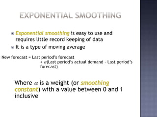
Often used when a trend or other pattern is emergingExponential SmoothingExponential smoothing is easy to use and requires little record keeping of dataIt is a type of moving averageNew forecast = Last period’s forecast	+ (Last period’s actual demand - Last period’s forecast)Where  is a weight (or smoothing constant) with a value between 0 and 1 inclusive
Exponential SmoothingMathematicallywhereFt+1	= new forecast (for time period t + 1)Ft	= previous forecast (for time period t)	= smoothing constant (0 ≤  ≤ 1)Yt	= pervious period’s actual demandThe idea is simple – the new estimate is the old estimate plus some fraction of the error in the last periodExponential Smoothing with Trend AdjustmentLike all averaging techniques, exponential smoothing does not respond to trendsA more complex model can be used that adjusts for trendsThe basic approach is to develop an exponential smoothing forecast then adjust it for the trendForecast including trend (FITt) =	New forecast (Ft)	+ Trend correction (Tt)
Exponential Smoothing with Trend AdjustmentThe equation for the trend correction uses a new smoothing constant Tt is computed bywhereTt+1 =	smoothed trend for period t + 1Tt =	smoothed trend for preceding period =	trend smooth constant that we selectFt+1 =	simple exponential smoothed forecast for period t + 1Ft =	forecast for pervious period
Seasonal Variations with TrendWhen both trend and seasonal components are present, the forecasting task is more complexSeasonal indices should be computed using a centered moving average (CMA) approachThere are four steps in computing CMAsCompute the CMA for each observation (where possible)Compute the seasonal ratio = Observation/CMA for that observationAverage seasonal ratios to get seasonal indicesIf seasonal indices do not add to the number of seasons, multiply each index by (Number of seasons)/(Sum of indices)
IBM401 Lecture 12

More Related Content

PPTX
Trend and Seasonal Components
PPTX
Trend and seasonal components/Abshor Marantika/Cindy Aprilia Anggaresta
PPTX
Forcasting methods
PPTX
Time series, forecasting, and index numbers
PDF
Box jenkins method of forecasting
PPTX
Time series analysis
PPT
CFA II Quantitative Analysis
PPTX
Time series
Trend and Seasonal Components
Trend and seasonal components/Abshor Marantika/Cindy Aprilia Anggaresta
Forcasting methods
Time series, forecasting, and index numbers
Box jenkins method of forecasting
Time series analysis
CFA II Quantitative Analysis
Time series

What's hot (20)

PPTX
Time Series Analysis - 2 | Time Series in R | ARIMA Model Forecasting | Data ...
PPT
Chapter 16
PPT
Time Series Analysis Ravi
PDF
Quantitative Methods - Level II - CFA Program
PPTX
Time Series - Auto Regressive Models
PPT
Adj Exp Smoothing
PDF
prediction of_inventory_management
 
PDF
Confirmatory Factor Analysis
PPTX
Classical control 2(3)
PPTX
Exponential Weighting Moving Average.
PDF
Goodness of fit statistics poisson regression
PPTX
Poisson regression models for count data
PPTX
Chem unit 1 presentation
PPTX
Lesson 2 stationary_time_series
PPTX
Time series
PPTX
Week 4 forecasting - time series - smoothing and decomposition - m.awaluddin.t
PDF
Data Science - Part X - Time Series Forecasting
PPTX
Time Series Analysis - 1 | Time Series in R | Time Series Forecasting | Data ...
PPT
POMDP Seminar Backup3
PDF
Business forecasting decomposition & exponential smoothing - bhawani nandan...
Time Series Analysis - 2 | Time Series in R | ARIMA Model Forecasting | Data ...
Chapter 16
Time Series Analysis Ravi
Quantitative Methods - Level II - CFA Program
Time Series - Auto Regressive Models
Adj Exp Smoothing
prediction of_inventory_management
 
Confirmatory Factor Analysis
Classical control 2(3)
Exponential Weighting Moving Average.
Goodness of fit statistics poisson regression
Poisson regression models for count data
Chem unit 1 presentation
Lesson 2 stationary_time_series
Time series
Week 4 forecasting - time series - smoothing and decomposition - m.awaluddin.t
Data Science - Part X - Time Series Forecasting
Time Series Analysis - 1 | Time Series in R | Time Series Forecasting | Data ...
POMDP Seminar Backup3
Business forecasting decomposition & exponential smoothing - bhawani nandan...
Ad

Viewers also liked (16)

PPT
Tbs910 regression models
PPTX
IBE303 Lecture 8
PPTX
Dummy variable’
PPT
Dummy variables xd
DOCX
Regression with Time Series Data
PDF
Durbin watson tables
PPTX
IBM401 Lecture 10
PPTX
IBE303 Lecture 12
PPTX
IBE303 Lecture 10
PPTX
IBE303 Lecture 7
PPTX
Dummy Variable Regression Analysis
PDF
Ibe303 grade
PPTX
Dummy variables
PPT
14 dummy
DOCX
Dummy variable
PPT
Dummy Variable Regression
Tbs910 regression models
IBE303 Lecture 8
Dummy variable’
Dummy variables xd
Regression with Time Series Data
Durbin watson tables
IBM401 Lecture 10
IBE303 Lecture 12
IBE303 Lecture 10
IBE303 Lecture 7
Dummy Variable Regression Analysis
Ibe303 grade
Dummy variables
14 dummy
Dummy variable
Dummy Variable Regression
Ad

Similar to IBM401 Lecture 12 (20)

DOCX
ForecastingBUS255 GoalsBy the end of this chapter, y.docx
PDF
Applied statistics lecture_6
PPT
Multiple Regression.ppt
PPT
Regression analysis ppt
PPTX
Linear Regression and Logistic Regression in ML
PDF
PDF
regression-130929093340-phpapp02 (1).pdf
PDF
Linear regression model in econometrics undergraduate
PPTX
IBM401 Lecture 5
PPT
PPTX
Regression_JAMOVI.pptx- Statistical data analysis
PPTX
Regression
PDF
Group 5 - Regression Analysis.pdf
PPT
Forecasting
PPTX
Regression & correlation
PDF
Regression Analysis-Machine Learning -Different Types
PPT
A presentation for Multiple linear regression.ppt
PPTX
Regression analysis complete notes along with exampls
PPTX
Time Series Decomposition
PPTX
Stat 1163 -correlation and regression
ForecastingBUS255 GoalsBy the end of this chapter, y.docx
Applied statistics lecture_6
Multiple Regression.ppt
Regression analysis ppt
Linear Regression and Logistic Regression in ML
regression-130929093340-phpapp02 (1).pdf
Linear regression model in econometrics undergraduate
IBM401 Lecture 5
Regression_JAMOVI.pptx- Statistical data analysis
Regression
Group 5 - Regression Analysis.pdf
Forecasting
Regression & correlation
Regression Analysis-Machine Learning -Different Types
A presentation for Multiple linear regression.ppt
Regression analysis complete notes along with exampls
Time Series Decomposition
Stat 1163 -correlation and regression

More from saark (19)

PDF
Ibm401 grade
PPTX
IBM401 Lecture 11
PPTX
IBE303 Lecture 11
PPTX
IBE303 Lecture 9
PPTX
IBM401 Lecture 9
PPTX
IBM401 Lecture 8
PPTX
IBM401 Lecture 7
PPTX
IBE303 - Lecture 6
PPTX
IBM401 - Lecture 6
PPTX
IBM401 Midterm key
PPTX
IBE303 Midterm key
PPTX
IBE303 Lecture 5
PPTX
IBE303 International Economic Lecture 4
PPTX
IBM401 Assignment
PPTX
Business Quantitative Lecture 3
PPTX
IBE303 Assignment
PPTX
International Economic Lecture 3
PPTX
International Economic Lecture 2
PPTX
Business Quantitative - Lecture 2
Ibm401 grade
IBM401 Lecture 11
IBE303 Lecture 11
IBE303 Lecture 9
IBM401 Lecture 9
IBM401 Lecture 8
IBM401 Lecture 7
IBE303 - Lecture 6
IBM401 - Lecture 6
IBM401 Midterm key
IBE303 Midterm key
IBE303 Lecture 5
IBE303 International Economic Lecture 4
IBM401 Assignment
Business Quantitative Lecture 3
IBE303 Assignment
International Economic Lecture 3
International Economic Lecture 2
Business Quantitative - Lecture 2

IBM401 Lecture 12

  • 1. Quantitative Analysis for BusinessLecture 12 – Final Exam ReviewOctober 4th, 2010http://www.slideshare.net/saark/ibm401-lecture-12
  • 2. Final examNo. of questions: 3Duration: 3 hoursGrade: 50% of final gradeTopics:Everything
  • 3. Linear regressionIdentifying independent and dependent variableThe sample correlation coefficient for two variablesLinear regression model form
  • 4. Linear regressionThe assumptions of linear regression model are the following:A linear relations exists between the dependent variable and the independent variable.The independent variable is not random.The expected value of the error term is 0.The variance of the error term is the same for all observationsThe error term is uncorrelated across observations.The error term is normally distributed.
  • 5. Linear regressionIn the regression model Yi = bo + b1Xi + Ei, if we know the estimated parameters, bo and b1, for any value of the independent variable, X, then the predicted value of the dependent variable Y is Y = b0 + b1XIn simple linear regression, the F-test tests the same null hypothesis as testing the statistical significance of b1 (or the t-test)H0: b1 = 0H1: b1 ≠ 0If F > Fc, then reject H0^^
  • 6. Multiple regressionMultiple regression modelIntercept – the value of the dependent variable when the independent variables are all equal to zeroEach slope coefficient – the estimated change in the dependent variable for a one-unit change in the independent variable, holding the other independent variables contantY = 0 + 1X1 + 2X2 + … + kXk + 
  • 7. Hypothesis testing of regression coefficientst-statistic – used to test the significance of the individual coefficient in a multiple regressiont-statistic has n-k-1 degrees of freedomEstimated regression coefficient – hypothesized valueCoefficient standard error of bj
  • 8. F-statisticF-test assesses how well the set of independent variables, as a group, explains the variation of the dependent variableF-statistic is used to test whether at least one of the independent variables explains a significant portion of the variation of the dependent variable
  • 9. Coefficient of determination (R2)Multiple coefficient of determination, R2, can be used to test the overall effectiveness of the entire set of independent variables in explaining the dependent variable.
  • 10. Adjusted R2Unfortunately, R2 by itself may not be a reliable measure of the multiple regression modelR2 almost always increases as variables are added to the modelWe need to take new variables into accountWheren = number of observationsk = number of independent variablesRa2 = adjusted R2
  • 11. Adjusted R2Whenever there is more than 1 independent variableRa2 is less than or equal to R2So adding new variables to the model will increase R2 but may increase or decrease the Ra2Ra2 maybe less than 0 if R2 is low enough
  • 12. Time-Series ModelsTime-series models attempt to predict the future based on the pastCommon time-series models areMoving averageExponential smoothingTrend projectionsDecompositionRegression analysis is used in trend projections and one type of decomposition model
  • 13. Decomposition of a Time-SeriesA time series typically has four componentsTrend (T) is the gradual upward or downward movement of the data over timeSeasonality (S) is a pattern of demand fluctuations above or below trend line that repeats at regular intervalsCycles (C) are patterns in annual data that occur every several yearsRandom variations (R) are “blips” in the data caused by chance and unusual situations
  • 14. Mathematicallywherewi = weight for the ith observationWeighted Moving AveragesWeighted moving averages use weights to put more emphasis on recent periods
  • 15. Often used when a trend or other pattern is emergingExponential SmoothingExponential smoothing is easy to use and requires little record keeping of dataIt is a type of moving averageNew forecast = Last period’s forecast + (Last period’s actual demand - Last period’s forecast)Where  is a weight (or smoothing constant) with a value between 0 and 1 inclusive
  • 16. Exponential SmoothingMathematicallywhereFt+1 = new forecast (for time period t + 1)Ft = previous forecast (for time period t) = smoothing constant (0 ≤  ≤ 1)Yt = pervious period’s actual demandThe idea is simple – the new estimate is the old estimate plus some fraction of the error in the last periodExponential Smoothing with Trend AdjustmentLike all averaging techniques, exponential smoothing does not respond to trendsA more complex model can be used that adjusts for trendsThe basic approach is to develop an exponential smoothing forecast then adjust it for the trendForecast including trend (FITt) = New forecast (Ft) + Trend correction (Tt)
  • 17. Exponential Smoothing with Trend AdjustmentThe equation for the trend correction uses a new smoothing constant Tt is computed bywhereTt+1 = smoothed trend for period t + 1Tt = smoothed trend for preceding period = trend smooth constant that we selectFt+1 = simple exponential smoothed forecast for period t + 1Ft = forecast for pervious period
  • 18. Seasonal Variations with TrendWhen both trend and seasonal components are present, the forecasting task is more complexSeasonal indices should be computed using a centered moving average (CMA) approachThere are four steps in computing CMAsCompute the CMA for each observation (where possible)Compute the seasonal ratio = Observation/CMA for that observationAverage seasonal ratios to get seasonal indicesIf seasonal indices do not add to the number of seasons, multiply each index by (Number of seasons)/(Sum of indices)