SlideShare a Scribd company logo
2
Most read
4
Most read
5
Most read
What is dummy variable?
Qualitative variable usually indicates the presence and absence of quality or an
attribute such as male and female, black and white, democrat and republican. If the
qualitative variables takes only two values 0 and 1 (absence or presence) then the
variable is called dummy variable. Example: suppose a qualitative variable sex
indicates the presence or absence of attribute such as male or female.
“1” may indicate that a person is a male and “0” may indicate that a person is
female. Variables that assume that “0” and “1” values are called dummy variables.

Alternative name of dummy variable
-indicator variable
-binary variable
-qualitative variable
-categorical variable
-dichotomous variable

Explain dummy variables in term of model or ANOVA model.
Dummy variables can be used in regression model just as easily as qualitative
variables. As a matter of fact that a linear regression model may contain
explanatory variables that are exclusively dummy or qualitative in nature. Such
model are called analysis of variance model or ANOVA model.
Let us consider the following modelYi=α+βDi+µi …………. (i)
where Yi= annual salary of a college professor
1 𝑖𝑓 𝑚𝑎𝑙𝑒 𝑝𝑟𝑜𝑓𝑒𝑠𝑠𝑜𝑟
𝐷𝑖 = {
0 𝑖𝑓 𝑓𝑒𝑚𝑎𝑙𝑒 𝑝𝑟𝑜𝑓𝑒𝑠𝑠𝑜𝑟
Di is called dummy variable
µi ~ NID (0, σ²)
we get from equation (i)
Mean salary of female professor,
E(Yi│Di=o)= α
Mean salary of male professor,
E(Yi│Di=1)= α+β

Interpretation:
Here the intercept term α gives the mean salary of female college
professor. The slope coefficient β tells by how much the mean salary of male
professor differs from the mean salary of his female counter part.
α+β reflecting the mean salary of college professor.

Write down the advantages of dummy variables.
1. Dummy variables are data classifying device that is they divide a sample into
various subgroups based on qualitative or attributes.
2. If a model has several qualitative variables with several classes introduction of
dummy variables can consume a large number of d.f.
3. Since the dummy variable are non-stochastic they create no special problems
in the application of OLS.

What is a dummy variable trap? How will you avoid dummy variable
trap?
Let us consider a modelYi= α1+ α2D2i+ α3D3i+βXi+µi ………………… (i)
Here Yi are the annual salary of a college professor.
Xi is the years of teaching experience of college professor
D2i = {

1 𝑖𝑓 𝑚𝑎𝑙𝑒 𝑝𝑟𝑜𝑓𝑒𝑠𝑠𝑜𝑟
0 𝑖𝑓 𝑓𝑒𝑚𝑎𝑙𝑒 𝑝𝑟𝑜𝑓𝑒𝑠𝑠𝑜𝑟

D3i = {

1 𝑖𝑓 𝑓𝑒𝑚𝑎𝑙𝑒 𝑝𝑟𝑜𝑓𝑒𝑠𝑠𝑜𝑟
0 𝑖𝑓 𝑚𝑎𝑙𝑒 𝑝𝑟𝑜𝑓𝑒𝑠𝑠𝑜𝑟

The model (i) cannot be estimated because of perfect collinearity between D2 and
D3. To see this we have a sample of 3 male professors and 2 female professors.
The design matrix is-
Male
Male
Female
Male
Female

Y1
Y2
Y3
Y4
Y5

α1
1
1
1
1
1

D2
1
1
0
1
0

D3
0
0
1
0
1

X
X1
X2
X3
X4
X5

The first column denote the common intercept term α1. We see that,
D2 =1-D3 and D3 =1-D2.
That means, D2 and D3 are perfectly collinear. Thus avoiding the perfect
collinearity the general rule is if a qualitative variable has m categories then it has
only (m-1) dummy variables. If this rule is not followed we shall fall into dummy
variable trap.
To avoid the dummy variable trap we can write the above model asYi= α2D2i+ α3D3i+βXi+µi
In this mode we have drop the intercept term αi. If we drop the intercept term αi we
will not fall into perfect multicollinearity/the dummy variable trap because we
have no longer the perfect collinearity.

Comparing two regression lines in terms dummy variable approach
Let us consider, pool all n1 and n2 observations together and estimating the
following regressionYi= α1+ α2Di+ β1Xi+ β2DiXi +µi …………………….(i)
Where, Yi and Xi are savings and income and
Di = {

1 𝑓𝑜𝑟 𝑜𝑏𝑠𝑒𝑟𝑣𝑎𝑡𝑖𝑜𝑛 𝑖𝑛 𝑡ℎ𝑒 1𝑠𝑡
0 𝑓𝑜𝑟 𝑜𝑏𝑠𝑒𝑟𝑣𝑎𝑡𝑖𝑜𝑛 𝑖𝑛 𝑡ℎ𝑒 𝑛𝑒𝑥𝑡

To see the implication of model (i) and assuming that, E(µi)=0 we obtain
E (Yi│Di=0; Xi) = αi+β1Xi ………….. (ii)
E (Yi│Di=1; Xi) = (α1+ α2) + (β1+ β2)Xi……………… (iii)
Let,

α1 = γ1
β1 = γ 2
α1+ α2= λ1
β1+ β2= λ2

So the equation of (ii) and (iii) is,
E (Yi│Di=0; Xi) = γ1+ γ2Xi…………….. (iv)
E (Yi│Di=1; Xi) = λ1+ λ2Xi……………... (v)
Therefore estimating equation (i) is equivalent to estimating the two individuals,
Re-construction period and post-reconstruction period. Where in equation (i) α1 is
the differential intercept term and α2 is the differential slope coefficient.

Find out the aggregate saving income relationship has changed between
the two periods.
Let us consider two linear regression model are, Re-construction period
Yi= λ1+ λ2Xi+ µ1i………………….(i)
i=1,2,…,ni
Post-construction period,
Yi= γ1+ γ2Xi+ µ2i………………….(i)
i=1,2,…,n2i
where, Yi= savings
X= income
µ1i and µ2i are the disturbance term in the two regression model.
Now regression model (i) and (ii) present the following four possibility
1) If λ1= γ1 and λ2= γ2 that means, the two regression model are identical then
it is called coincident regression.
Y

λ2= γ2

λ1= γ1
X
Income
(a) Coincident

2) If λ1≠γ1 and λ2= γ2 that means the two regression differ only in their
locations that means intercept then it is called parallel regression.

Y
λ2= γ2

λ2= γ2
γ1
λ1
X
(b) Coincident
3) If λ1=γ1 and λ2≠ γ2 that means the two regression have same intercept
different slopes. Then it is called concurrent regression

Y
γ2
λ2

λ1= γ1
X
(c) concurrent

4) If λ1≠γ1 and λ2≠ γ2 then the two regression equation are completely
different that means the regression is called dissimilar regression.
Y
γ2

λ2
λ1
γ1
X
(d) dissimilar

Question: Suppose the college professor salary regression model defined asYi= α1+ α2D2i+ α3D3i + α4(D2iD3i)+BXi +µi
Where Yi=annual salary of a college professor
Xi= years of experience
D2=

1 if male professor
0 if female professor

D3= 1 if the professor is white or 0 otherwise
Explain the terms (i) α2 (ii) α4 (iii) D2iD3i
(v) What about the effect of female and non-white professor
(vi) Find,
E(Yi│D2=1, D3=1,Xi=10) and interpret it.
Solution:
1. α2 is the differential effect of being male professor
2. α4 is the differential effect of male-white professor
3. D2iD3i be the interaction between two qualitative variables D2 and D3. It
means non-white have lower mean salary i. e they are male or female. A
female non-white may earn lower salary than a male non-white. So
interaction may be expressed such kind of assumption which may be
untrainable
4. The effect of female and non-white professor are the followingE(Yi│D2i=0, D3i=0)= α1+βXi
5. So it can be concluded that the mean salary depends on only the slope
coefficient and the coefficient of years of experience.
6.
E(Yi│D2=1, D3=1,Xi=10)
So the mean salary of male and white professor is which is the mean salary of
male and white professor when years of experience are 10 years.

More Related Content

PPTX
Dummy variables
PPTX
Heteroscedasticity
PDF
Heteroscedasticity
PPTX
Heteroscedasticity
PPTX
Arrows Impossibility Theorem.pptx
PPTX
Multicollinearity PPT
PPTX
General equilibrium : Neo-classical analysis
PPTX
Autocorrelation
Dummy variables
Heteroscedasticity
Heteroscedasticity
Heteroscedasticity
Arrows Impossibility Theorem.pptx
Multicollinearity PPT
General equilibrium : Neo-classical analysis
Autocorrelation

What's hot (20)

PPTX
General equilibrium ppt
PPTX
General equilibrium theory
PPT
Econometrics ch3
PPTX
Permanent income hypothesis
PPTX
Multicolinearity
PDF
Autocorrelation (1)
PDF
The Kaldor Hicks Compensation Principle
PPTX
Slutsky theorem
PPTX
INDIRECT UTILITY FUNCTION AND ROY’S IDENTITIY by Maryam Lone
DOCX
DUMMY VARIABLE REGRESSION MODEL
PPSX
Pareto optimality 2
PPSX
Bain’s limit pricing model
PPSX
Welfare economics
PPTX
New keynesian economics
PPT
Autocorrelation- Remedial Measures
PPTX
Heteroscedasticity | Eonomics
PPTX
Permanent and Life Cycle Income Hypothesis
PPTX
Williamson's Managerial Discretion Model (4).pptx
PPTX
Friedmans theory of demand
PDF
Dummyvariable1
General equilibrium ppt
General equilibrium theory
Econometrics ch3
Permanent income hypothesis
Multicolinearity
Autocorrelation (1)
The Kaldor Hicks Compensation Principle
Slutsky theorem
INDIRECT UTILITY FUNCTION AND ROY’S IDENTITIY by Maryam Lone
DUMMY VARIABLE REGRESSION MODEL
Pareto optimality 2
Bain’s limit pricing model
Welfare economics
New keynesian economics
Autocorrelation- Remedial Measures
Heteroscedasticity | Eonomics
Permanent and Life Cycle Income Hypothesis
Williamson's Managerial Discretion Model (4).pptx
Friedmans theory of demand
Dummyvariable1
Ad

Viewers also liked (9)

PPT
14 dummy
PDF
Bias and confounding
PPTX
Confounder and effect modification
PPTX
Research Methodology
PPTX
Antenatal care
PPT
Logistic Regression in Case-Control Study
PPT
Variables
PPT
Variables
PPT
SAMPLING AND SAMPLING ERRORS
14 dummy
Bias and confounding
Confounder and effect modification
Research Methodology
Antenatal care
Logistic Regression in Case-Control Study
Variables
Variables
SAMPLING AND SAMPLING ERRORS
Ad

Similar to Dummy variable (20)

PPT
Lecture7-DummyVariables.ppt
PDF
Module 3 Course Slides Lesson 1 McGill University
PDF
3 handouts section3-11
PDF
Program on Quasi-Monte Carlo and High-Dimensional Sampling Methods for Applie...
PPT
B.tech admissions in delhi
PPT
Statistics lesson 2
PDF
Chapter5.pdf.pdf
PPT
Econometrics_ch11.ppt
PPT
Econometrics ch11
PPTX
HOMOGENEOUS DIFFERENTIAL LINEAR EQUATION.pptx
PDF
Regression on gaussian symbols
PDF
01. Differentiation-Theory & solved example Module-3.pdf
PDF
functionalform2up.pdf
PPT
Top Schools in delhi NCR
PDF
A Case Study of Teaching the Concept of Differential in Mathematics Teacher T...
DOCX
Mc0079 computer based optimization methods--phpapp02
PDF
DOCX
General Mathematics
PPT
TWO-VARIABLE REGRESSION ANALYSIS SOME BASIC IDEAS.ppt
Lecture7-DummyVariables.ppt
Module 3 Course Slides Lesson 1 McGill University
3 handouts section3-11
Program on Quasi-Monte Carlo and High-Dimensional Sampling Methods for Applie...
B.tech admissions in delhi
Statistics lesson 2
Chapter5.pdf.pdf
Econometrics_ch11.ppt
Econometrics ch11
HOMOGENEOUS DIFFERENTIAL LINEAR EQUATION.pptx
Regression on gaussian symbols
01. Differentiation-Theory & solved example Module-3.pdf
functionalform2up.pdf
Top Schools in delhi NCR
A Case Study of Teaching the Concept of Differential in Mathematics Teacher T...
Mc0079 computer based optimization methods--phpapp02
General Mathematics
TWO-VARIABLE REGRESSION ANALYSIS SOME BASIC IDEAS.ppt

Recently uploaded (20)

PDF
Roadmap Map-digital Banking feature MB,IB,AB
PDF
Katrina Stoneking: Shaking Up the Alcohol Beverage Industry
DOCX
Business Management - unit 1 and 2
PDF
Reconciliation AND MEMORANDUM RECONCILATION
PDF
Elevate Cleaning Efficiency Using Tallfly Hair Remover Roller Factory Expertise
DOCX
unit 2 cost accounting- Tender and Quotation & Reconciliation Statement
PDF
Power and position in leadershipDOC-20250808-WA0011..pdf
PPT
Chapter four Project-Preparation material
PDF
MSPs in 10 Words - Created by US MSP Network
PPTX
Amazon (Business Studies) management studies
PDF
Nidhal Samdaie CV - International Business Consultant
PDF
A Brief Introduction About Julia Allison
PDF
How to Get Funding for Your Trucking Business
PPTX
Dragon_Fruit_Cultivation_in Nepal ppt.pptx
DOCX
unit 1 COST ACCOUNTING AND COST SHEET
PDF
Stem Cell Market Report | Trends, Growth & Forecast 2025-2034
PDF
Unit 1 Cost Accounting - Cost sheet
PPTX
5 Stages of group development guide.pptx
PDF
Outsourced Audit & Assurance in USA Why Globus Finanza is Your Trusted Choice
PPTX
job Avenue by vinith.pptxvnbvnvnvbnvbnbmnbmbh
Roadmap Map-digital Banking feature MB,IB,AB
Katrina Stoneking: Shaking Up the Alcohol Beverage Industry
Business Management - unit 1 and 2
Reconciliation AND MEMORANDUM RECONCILATION
Elevate Cleaning Efficiency Using Tallfly Hair Remover Roller Factory Expertise
unit 2 cost accounting- Tender and Quotation & Reconciliation Statement
Power and position in leadershipDOC-20250808-WA0011..pdf
Chapter four Project-Preparation material
MSPs in 10 Words - Created by US MSP Network
Amazon (Business Studies) management studies
Nidhal Samdaie CV - International Business Consultant
A Brief Introduction About Julia Allison
How to Get Funding for Your Trucking Business
Dragon_Fruit_Cultivation_in Nepal ppt.pptx
unit 1 COST ACCOUNTING AND COST SHEET
Stem Cell Market Report | Trends, Growth & Forecast 2025-2034
Unit 1 Cost Accounting - Cost sheet
5 Stages of group development guide.pptx
Outsourced Audit & Assurance in USA Why Globus Finanza is Your Trusted Choice
job Avenue by vinith.pptxvnbvnvnvbnvbnbmnbmbh

Dummy variable

  • 1. What is dummy variable? Qualitative variable usually indicates the presence and absence of quality or an attribute such as male and female, black and white, democrat and republican. If the qualitative variables takes only two values 0 and 1 (absence or presence) then the variable is called dummy variable. Example: suppose a qualitative variable sex indicates the presence or absence of attribute such as male or female. “1” may indicate that a person is a male and “0” may indicate that a person is female. Variables that assume that “0” and “1” values are called dummy variables. Alternative name of dummy variable -indicator variable -binary variable -qualitative variable -categorical variable -dichotomous variable Explain dummy variables in term of model or ANOVA model. Dummy variables can be used in regression model just as easily as qualitative variables. As a matter of fact that a linear regression model may contain explanatory variables that are exclusively dummy or qualitative in nature. Such model are called analysis of variance model or ANOVA model. Let us consider the following modelYi=α+βDi+µi …………. (i) where Yi= annual salary of a college professor 1 𝑖𝑓 𝑚𝑎𝑙𝑒 𝑝𝑟𝑜𝑓𝑒𝑠𝑠𝑜𝑟 𝐷𝑖 = { 0 𝑖𝑓 𝑓𝑒𝑚𝑎𝑙𝑒 𝑝𝑟𝑜𝑓𝑒𝑠𝑠𝑜𝑟
  • 2. Di is called dummy variable µi ~ NID (0, σ²) we get from equation (i) Mean salary of female professor, E(Yi│Di=o)= α Mean salary of male professor, E(Yi│Di=1)= α+β Interpretation: Here the intercept term α gives the mean salary of female college professor. The slope coefficient β tells by how much the mean salary of male professor differs from the mean salary of his female counter part. α+β reflecting the mean salary of college professor. Write down the advantages of dummy variables. 1. Dummy variables are data classifying device that is they divide a sample into various subgroups based on qualitative or attributes. 2. If a model has several qualitative variables with several classes introduction of dummy variables can consume a large number of d.f. 3. Since the dummy variable are non-stochastic they create no special problems in the application of OLS. What is a dummy variable trap? How will you avoid dummy variable trap? Let us consider a modelYi= α1+ α2D2i+ α3D3i+βXi+µi ………………… (i) Here Yi are the annual salary of a college professor. Xi is the years of teaching experience of college professor D2i = { 1 𝑖𝑓 𝑚𝑎𝑙𝑒 𝑝𝑟𝑜𝑓𝑒𝑠𝑠𝑜𝑟 0 𝑖𝑓 𝑓𝑒𝑚𝑎𝑙𝑒 𝑝𝑟𝑜𝑓𝑒𝑠𝑠𝑜𝑟 D3i = { 1 𝑖𝑓 𝑓𝑒𝑚𝑎𝑙𝑒 𝑝𝑟𝑜𝑓𝑒𝑠𝑠𝑜𝑟 0 𝑖𝑓 𝑚𝑎𝑙𝑒 𝑝𝑟𝑜𝑓𝑒𝑠𝑠𝑜𝑟 The model (i) cannot be estimated because of perfect collinearity between D2 and D3. To see this we have a sample of 3 male professors and 2 female professors. The design matrix is-
  • 3. Male Male Female Male Female Y1 Y2 Y3 Y4 Y5 α1 1 1 1 1 1 D2 1 1 0 1 0 D3 0 0 1 0 1 X X1 X2 X3 X4 X5 The first column denote the common intercept term α1. We see that, D2 =1-D3 and D3 =1-D2. That means, D2 and D3 are perfectly collinear. Thus avoiding the perfect collinearity the general rule is if a qualitative variable has m categories then it has only (m-1) dummy variables. If this rule is not followed we shall fall into dummy variable trap. To avoid the dummy variable trap we can write the above model asYi= α2D2i+ α3D3i+βXi+µi In this mode we have drop the intercept term αi. If we drop the intercept term αi we will not fall into perfect multicollinearity/the dummy variable trap because we have no longer the perfect collinearity. Comparing two regression lines in terms dummy variable approach Let us consider, pool all n1 and n2 observations together and estimating the following regressionYi= α1+ α2Di+ β1Xi+ β2DiXi +µi …………………….(i) Where, Yi and Xi are savings and income and Di = { 1 𝑓𝑜𝑟 𝑜𝑏𝑠𝑒𝑟𝑣𝑎𝑡𝑖𝑜𝑛 𝑖𝑛 𝑡ℎ𝑒 1𝑠𝑡 0 𝑓𝑜𝑟 𝑜𝑏𝑠𝑒𝑟𝑣𝑎𝑡𝑖𝑜𝑛 𝑖𝑛 𝑡ℎ𝑒 𝑛𝑒𝑥𝑡 To see the implication of model (i) and assuming that, E(µi)=0 we obtain E (Yi│Di=0; Xi) = αi+β1Xi ………….. (ii) E (Yi│Di=1; Xi) = (α1+ α2) + (β1+ β2)Xi……………… (iii)
  • 4. Let, α1 = γ1 β1 = γ 2 α1+ α2= λ1 β1+ β2= λ2 So the equation of (ii) and (iii) is, E (Yi│Di=0; Xi) = γ1+ γ2Xi…………….. (iv) E (Yi│Di=1; Xi) = λ1+ λ2Xi……………... (v) Therefore estimating equation (i) is equivalent to estimating the two individuals, Re-construction period and post-reconstruction period. Where in equation (i) α1 is the differential intercept term and α2 is the differential slope coefficient. Find out the aggregate saving income relationship has changed between the two periods. Let us consider two linear regression model are, Re-construction period Yi= λ1+ λ2Xi+ µ1i………………….(i) i=1,2,…,ni Post-construction period, Yi= γ1+ γ2Xi+ µ2i………………….(i) i=1,2,…,n2i where, Yi= savings X= income µ1i and µ2i are the disturbance term in the two regression model. Now regression model (i) and (ii) present the following four possibility 1) If λ1= γ1 and λ2= γ2 that means, the two regression model are identical then it is called coincident regression. Y λ2= γ2 λ1= γ1 X Income
  • 5. (a) Coincident 2) If λ1≠γ1 and λ2= γ2 that means the two regression differ only in their locations that means intercept then it is called parallel regression. Y λ2= γ2 λ2= γ2 γ1 λ1 X (b) Coincident 3) If λ1=γ1 and λ2≠ γ2 that means the two regression have same intercept different slopes. Then it is called concurrent regression Y γ2 λ2 λ1= γ1
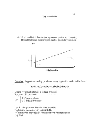
  • 6. X (c) concurrent 4) If λ1≠γ1 and λ2≠ γ2 then the two regression equation are completely different that means the regression is called dissimilar regression. Y γ2 λ2 λ1 γ1 X (d) dissimilar Question: Suppose the college professor salary regression model defined asYi= α1+ α2D2i+ α3D3i + α4(D2iD3i)+BXi +µi Where Yi=annual salary of a college professor Xi= years of experience D2= 1 if male professor 0 if female professor D3= 1 if the professor is white or 0 otherwise Explain the terms (i) α2 (ii) α4 (iii) D2iD3i (v) What about the effect of female and non-white professor (vi) Find,
  • 7. E(Yi│D2=1, D3=1,Xi=10) and interpret it. Solution: 1. α2 is the differential effect of being male professor 2. α4 is the differential effect of male-white professor 3. D2iD3i be the interaction between two qualitative variables D2 and D3. It means non-white have lower mean salary i. e they are male or female. A female non-white may earn lower salary than a male non-white. So interaction may be expressed such kind of assumption which may be untrainable 4. The effect of female and non-white professor are the followingE(Yi│D2i=0, D3i=0)= α1+βXi 5. So it can be concluded that the mean salary depends on only the slope coefficient and the coefficient of years of experience. 6. E(Yi│D2=1, D3=1,Xi=10) So the mean salary of male and white professor is which is the mean salary of male and white professor when years of experience are 10 years.