Aspen utilities user guide v7 2
10 likes4,258 views

This document is the user guide for Aspen Utilities version 7.2 software. It introduces the Aspen Utilities Planner interface and describes how to create and simulate an Aspen Utilities model. It also provides details on using the software's data editors to manage profiles, tariffs, demands and perform optimization configuration. The guide explains how to implement the software for online optimization and interface it with Microsoft Excel.


![Entering Tariff Cost Equations
In many cases, the cost for a particular utility can be broken down to several
contributing cost components. For example, electricity cost typically consists
of a fixed standing charge, taxes, a unit price, delivery cost, etc. The fixed
and variable cost for each tier can be calculated by combining these individual
cost components.
In order to do this, you need to input the individual cost components and the
equations that use the cost components, for each tier.
Adding Utility Cost Components
1 Click Costing on the main command bar in the combined editor and the
cost component form is displayed:
2 Enter the name, description, and value for each cost component in the
grid.
Note: The names of the cost components cannot be duplicated. In
addition, the names cannot contain square brackets ([ and ]).
Editing Utility Cost Components
Edit or change data by typing in the cell.
40 2 Data Editors](https://image.slidesharecdn.com/aspenutilitiesuserguidev72-141104075704-conversion-gate01/85/Aspen-utilities-user-guide-v7-2-46-320.jpg)


![Demand Forecasting Equation Editor Layout
The Equation Editor contains two fields:
Equation Editor
Equations Viewer
Equation Editor
The Equation Editor field is for you to edit demand forecasting equations. The
table at the top contains all of the equations that have been defined. When
you click on an equation in the grid, the equation definition is displayed in the
below text box.
The equations with the Demand check box selected at the top table means
they are the equations for utility demand.
In the example above the HP Steam Use equation contains two variables:
[cvY1] and [cvY2]. Variables are contained with square brackets [ ].
Variables can be defined as values (e.g., 5, Mode1, True), or other
equations. Variables that represent equations are displayed in the table at the
top and all other variables are displayed by clicking Variables….
Equations Viewer
You can view the equations defined in this field and evaluate them. Select the
variable you want to see from drop-down list and the equation it represents is
displayed in the text box at the bottom. In this field, you can only check the
equations but cannot edit. In the example above, [cvY1] is selected in the
drop-down list and the equation it represents seen at the bottom. You can
evaluate the equation by clicking Evaluate next to the equation.
Using the DFE Equation Editor
An example will show how to use the DFE Equation Editor. The example will
create the HP Steam Use equation, starting with nothing.
The HP Steam use is given by:
If the season is winter:
HP Steam Use = 6 + 0.2*X1 + 2*X1^2
Where X1 is the propylene production rate. And if X1 is less than or equal
to zero, it returns 0.
If season is not winter, HP Steam Use = 90 tonnes/hr
If the Acetic acid mode is Lean:
HP Steam Use = 0
1 Click on Edit next to the unit of measure for HP Steam Use.
The Equation Editor window appears:
52 2 Data Editors](https://image.slidesharecdn.com/aspenutilitiesuserguidev72-141104075704-conversion-gate01/85/Aspen-utilities-user-guide-v7-2-58-320.jpg)

![The basic equation is given by: 6 + 0.2*X1 + 2*X1^2 where X1 is the
propylene production rate. Because we want this to be evaluated only
when the season is winter we can put an IF statement around the
equation:
IF("[SEASON]"="(SEASON.Winter)",6+0.2*[X1]+2*[X1]^2,0)
Note: In this example, SEASON is case sensitive, The value in the
equation should use the same case as what is displayed in the Variables
table (click Variables… to open). If you use SEASON.WINTER in the
equation, the equation will not work properly.
Also, we want to return 0 if X1 is less than or equal to zero. We can create
a nested IF statement to do this:
IF("[SEASON]"="(SEASON.Winter)",IF([X1]>0,6+0.2*[X1]+2*[X1]^2,
0))
And if season is not winter, the value of HP Steam Use is 90 tonnes/hr. So
the final equation should be:
IF(“[SEASON]”=”(SEASON.Winter)”,IF([X1]>0,6=0.2*[X1]+2*[X1]^2,
0),90)
Begin by typing to the first left square bracket [. When you type the left
bracket, a list is displayed with all of the variables known to DFE:
54 2 Data Editors](https://image.slidesharecdn.com/aspenutilitiesuserguidev72-141104075704-conversion-gate01/85/Aspen-utilities-user-guide-v7-2-60-320.jpg)

![Notes:
1. Notice that the right bracket is automatically inserted for you.
2. Notice that the [SEASON] is enclosed in double-quotes “” because it
contains text.
5 Continue editing:
56 2 Data Editors](https://image.slidesharecdn.com/aspenutilitiesuserguidev72-141104075704-conversion-gate01/85/Aspen-utilities-user-guide-v7-2-62-320.jpg)


![Note: Newly created equation variables like cvY1 will be displayed
automatically in the drop-down variable list after entering left square
bracket [.
10 Finally, click Evaluate for HP Steam Use to check the equation entered.
11 Click OK to save your data and close the Equation Editor
Tips for Creating Equations
Here are some tips for creating equations:
Variable substitution and equation evaluation is faster if you enter the
coefficient values directly in the equation, rather than using variables. For
example:
3.1 + 10.22*[X2]
will evaluate faster than
Var_A + Var_B*[X2]
62 2 Data Editors](https://image.slidesharecdn.com/aspenutilitiesuserguidev72-141104075704-conversion-gate01/85/Aspen-utilities-user-guide-v7-2-68-320.jpg)


![ Variable names may not contain square brackets [ and ] since these are
used by DFE to enclose variable names.
Variable values can be changed for any variable but only values for user
variables are saved when you click OK. This allows you to temporarily
change production rates, modes, etc., while evaluating an equation.
Once created, a variable name and description cannot be edited. You must
delete the variable and recreate it.
Demand Forecasting Variable Location
The DFE variables are located in the following tables in the Demand database,
DemandData.mdb:
Variable Type Demand Database Table
Production rates DemandForecastingInput
Mode variables tblModes
Equation variables tblEquationDefinition
User variables tblUserVariables
Using the Variable Filter
You can shorten the list of variables displayed in the drop-down variable list
by clicking Variable Filter…:
2 Data Editors 67](https://image.slidesharecdn.com/aspenutilitiesuserguidev72-141104075704-conversion-gate01/85/Aspen-utilities-user-guide-v7-2-73-320.jpg)


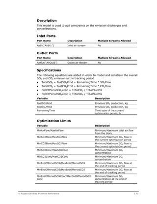
![The kInterstange can be used to linearly capture the effect of extraction flow
to nominal power after properly specify the Interstage.
The kInterstage for induction Interstage type is used as:
nominalPower = LooUpTable(Steam Flow) – (kInterStage *
ExtractionFlow)
The kInterstage for induction InterStage type is used as:
nominalPower = LookUpTable(Steam Flow) + (kInterStage *
InductionFlow)
The kInterStage for “Both” Interstage type is used as:
nominalPower = LookUpTable(Steam Flow) + [kInterstage *
(InductionFlow – ExtractionFlow)]
For example, when the Interstage is specified as “Extraction”, the kInterstage
is used to correct the nominal power got from the steam flow by substracting
the product of extraction flow and kInterstage.
If Linear Efficiency method is selected, you must specify the slope and
intercept for the power calculation from steam flow for each stage.
If LookUpTable is selected, you must enter the efficiency curve in the
PerformanceData form. A minimum of two points (nSections) must be
specified. The data is entered as flow against power generated in the turbine.
140 6 Aspen Utilities Planner Reference](https://image.slidesharecdn.com/aspenutilitiesuserguidev72-141104075704-conversion-gate01/85/Aspen-utilities-user-guide-v7-2-146-320.jpg)


![Configuring Calculations
Refer to the CalcVars section if you need to reference earlier versions of the
Demand database.
tblEquationDefinition
This table specifies the equations used for calculating the utility demands
from production parameters and modes of operation.
The table consists of the following fields:
Field Description
recID An ID created automatically by Microsoft Access.
EqnID The equation ID referenced by DemandVarEquationID in the
DemandCalcsEquations table
EqnDescription A description of the utility demand being calculated by the
equation. The description is displayed in Equation Editor.
EqnString Description of each equation.
In our example, if the production rate is zero, the utility demands should be
zero also. Therefore we need to put a conditional (IF statement) around the
equation.
The completed table might be:
recID EqnID EqnDescription EqnString
1 cvY1 Reboiler Steam IF("[SEASON]"="(SEASON.WINTER)",
IF([X1]>0,6+0.2*[X1]+2*[X1]^2,0),90)
2 cvY10 CT2 Turbines Y10 IF("[EO]"="(EO.MEDIUM)",5,0)
3 cvY11 CT2 Turbines Y11 IF("[EO]"="(EO.LOW)",0,0)
4 cvY12 CT2 Turbines Y1 IF("[SEASON]"="(SEASON.FALL)",1,0)
5 cvY13 CT2 Turbines Y13 IF("[SEASON]"="(SEASON.SUMMER)",3,0
)
6 cvY14 CT2 Turbines Y14 IF("[SEASON]"="(SEASON.WINTER)",4,0)
7
cvY2 Stripping Steam IF("[ACETIC]"="(ACETIC.LEAN)",0,0)
8 cvY3 Turbine PT5 0
9 cvY4 CT1 Turbines 15
10 cvY5 CT2 Turbines Y5 0.5*[X1]^1.5 + 37.71
11 cvY6 CT2 Turbines Y6 IF("[ACETIC]"="(ACETIC.RICH)",1000,0)
12 cvY7 CT2 Turbines Y7 IF("[SEASON]"="(SEASON.SPRING)",2,0)
13 cvY8 CT2 Turbines Y8 IF("[EO]"="(EO.HIGH)",10,0)
14 cvY9 CT2 Turbines Y9 IF("[ACETIC]"="(ACETIC.LEAN)",0.5,0)
15 HPUSE.St
eamIn1
Total
HPUSE.SteamIn1
+[cvY1] +[cvY2]
16 LPGEN.St
eamOut1
Total
LPGEN.SteamOut
1
+[cvY4] +[cvY3]
192 Appendix 1 – Configuring the Demand Forecasting Editor](https://image.slidesharecdn.com/aspenutilitiesuserguidev72-141104075704-conversion-gate01/85/Aspen-utilities-user-guide-v7-2-198-320.jpg)


Aspen utilities user guide v7 2
- 1. Aspen Utilities V7.2 User Guide
- 2. Version V7.2 July 2010 Copyright (c) 1981 – 2010 by Aspen Technology, Inc. All rights reserved. Aspen Utilities™, Aspen Online®, Aspen InfoPlus.21®, Aspen Utilities Planner, Aspen Utilities On-Line Optimizer (Utilities Optimizer), Aspen Utilities Operations, Aspen SLM, Aspen Engineering Suite, the aspen leaf logo, and Plantelligence & Enterprise Optimization Solutions are trademarks or registered trademarks of Aspen Technology, Inc., Burlington, MA. All other brand and product names are trademarks or registered trademarks of their respective companies. This document is intended as a guide to using AspenTech's software. This documentation contains AspenTech proprietary and confidential information and may not be disclosed, used, or copied without the prior consent of AspenTech or as set forth in the applicable license agreement. Users are solely responsible for the proper use of the software and the application of the results obtained. Although AspenTech has tested the software and reviewed the documentation, the sole warranty for the software may be found in the applicable license agreement between AspenTech and the user. ASPENTECH MAKES NO WARRANTY OR REPRESENTATION, EITHER EXPRESSED OR IMPLIED, WITH RESPECT TO THIS DOCUMENTATION, ITS QUALITY, PERFORMANCE, MERCHANTABILITY, OR FITNESS FOR A PARTICULAR PURPOSE. Aspen Technology, Inc. 200 Wheeler Road Burlington, MA 01803-5501 USA Phone: + (781) 221-6400 Toll Free: +(1) (888) 996-7001 URL: http://www.aspentech.com
- 3. Contents Introducing Aspen Utilities .....................................................................................1 What You Need To Use This Guide......................................................................1 Section Descriptions ...............................................................................2 About This Document .......................................................................................2 Related Documentation.....................................................................................2 Technical Support ............................................................................................3 1 Aspen Utilities Planner User Interface .................................................................5 Starting Aspen Utilities Planner ..........................................................................5 Aspen Utilities Planner Main Window...................................................................5 Flowsheet Window..................................................................................6 Explorer Window....................................................................................6 Message Window....................................................................................6 Optimization Menu .................................................................................6 Initializing Physical Properties ............................................................................6 Creating and Simulating an Aspen Utilities Model .................................................8 Aspen Utilities Model Library....................................................................8 Adding Data to the Blocks .......................................................................8 Running in Simulation Mode ....................................................................8 2 Data Editors .......................................................................................................11 Profiles Editor ................................................................................................ 12 Accessing the Profiles Data Editor........................................................... 14 Editing Demand Profile.......................................................................... 15 Editing Availability Profile ...................................................................... 17 Updating Profiles.................................................................................. 18 Filtering Profile Data ............................................................................. 21 Viewing Profiles.................................................................................... 22 Printing Profiles.................................................................................... 24 Saving and Transferring Profile Data....................................................... 25 Selecting a Case .................................................................................. 26 Editing a Case...................................................................................... 27 Copying a Case .................................................................................... 28 Exporting a Case.................................................................................. 29 Changing the Location of the Databases.................................................. 31 Tariff Editor ................................................................................................... 32 Accessing the Tariff Editor ..................................................................... 33 Adding Contract ................................................................................... 35 Editing a Contract ................................................................................ 36 Deleting a Contract .............................................................................. 37 Adding Tiers ........................................................................................ 38 Editing a Tier ....................................................................................... 39 Contents iii
- 4. Entering Tariff Cost Equations................................................................ 40 Deleting a Tier ..................................................................................... 46 Saving and Transferring Tariff Data ........................................................ 47 Printing Contracts and Tiers................................................................... 48 Demand Forecasting Editor.............................................................................. 48 Accessing the Demand Forecasting Editor................................................ 49 Calculating Utility Demands ................................................................... 50 Saving Utility Demands......................................................................... 51 Modifying Demand Equations................................................................. 51 Using the DFE Equation Editor ............................................................... 52 Tips for Creating Equations.................................................................... 62 Adding an Equation .............................................................................. 64 Deleting an Equation ............................................................................ 65 Displaying Equation Variables ................................................................ 66 Using the Variable Filter ........................................................................ 67 Modifying Independent Variables in Equations.......................................... 68 Calculating Utility Demands for Multiple Periods ....................................... 69 3 Optimization Configuration ................................................................................71 Enforcing Hot Standby Requirements................................................................ 71 Configuring Startup/Shutdown Constraints ........................................................ 73 Configuring Load Shedding.............................................................................. 75 Obtaining Marginal Utility Cost ......................................................................... 77 Identifying Optimization Errors ........................................................................ 80 Presolve Error Checking ........................................................................ 81 Error Tracking...................................................................................... 82 Setting up Options for Optimization.................................................................. 85 Multiple Period Run Mode ...................................................................... 85 Settings for Mixed Integer Linear Solver............................................................ 86 Cut Strategy........................................................................................ 86 Cut off Value (Max. Expected Cost) ........................................................ 87 Optimum Gap from Optimality (%)......................................................... 87 Presolve Strategy................................................................................. 87 4 Aspen Utilities On-line Implementation..............................................................89 Calculating Utility Demand Targets ................................................................... 89 Specifying Demands for On-line Optimization .................................................... 91 5 Microsoft Excel Interface....................................................................................93 Installing the Aspen Utilities Planner Add-In ...................................................... 93 Aspen Utilities Excel Menu Items ............................................................ 94 Open Aspen Utilities File........................................................................ 95 Running a Simulation from Excel ...................................................................... 95 Creating a Simulation Links worksheet.................................................... 96 Configuring Blocks and Variables for Input to Aspen Utilities Planner .......... 97 Configuring Blocks and Variables for Retrieval from Aspen Utilities Planner.. 98 Mapping Variable Values to the Excel Flowsheet ..................................... 100 Running Data Reconciliation from Excel........................................................... 101 Accessing Reconciliation Worksheet ...................................................... 102 Configuring Blocks and Variables for Reconciliation................................. 103 Running Optimization from Excel.................................................................... 104 iv Contents
- 5. Performing User Specific Tasks before Optimization................................ 105 Producing Optimization Results and Tariff Information from Aspen Utilities 106 Obtaining Results from Multi-Period Optimization ................................... 109 6 Aspen Utilities Planner Reference ....................................................................111 Model Library............................................................................................... 111 List of Models .................................................................................... 112 General Model Structure ..................................................................... 113 Standard Variable Names in Models...................................................... 114 Ports and Streams.............................................................................. 115 Specifying Capacity Limits ................................................................... 115 Feeds ............................................................................................... 116 Demands .......................................................................................... 120 Headers ............................................................................................ 124 Steam Models .................................................................................... 127 Pumps .............................................................................................. 132 Turbines............................................................................................ 137 Heat Exchangers ................................................................................ 142 Multipliers ......................................................................................... 151 Fuel Models ....................................................................................... 154 Emissions.......................................................................................... 169 Templates ......................................................................................... 177 Flowsheet Development ................................................................................ 179 Dealing with Snapshots....................................................................... 179 Variable Specification – Fixed and Free ................................................. 179 Appendix 1 – Configuring the Demand Forecasting Editor...................................181 Before you Start .......................................................................................... 183 Units of Measure .......................................................................................... 185 Configuring General Information .................................................................... 185 EquationTypes ................................................................................... 185 Operators.......................................................................................... 186 Config............................................................................................... 186 PeriodSet .......................................................................................... 186 Period............................................................................................... 186 GeneralInput ..................................................................................... 187 Configuring Production Parameters................................................................. 187 DemandForecasting Input ................................................................... 187 XinVal............................................................................................... 189 Configuring Modes........................................................................................ 190 TblModes .......................................................................................... 190 TblModeValues................................................................................... 191 PeriodModes ...................................................................................... 191 Configuring Calculations................................................................................ 192 tblEquationDefinition .......................................................................... 192 CalcVars ........................................................................................... 193 Configuring Demand Calculations ................................................................... 195 DemandCalcsEquations ....................................................................... 195 DemandCalcs..................................................................................... 195 Contents v
- 7. Introducing Aspen Utilities In this document Aspen Utilities is used as a generic term to refer to both Aspen Utilities On-Line Optimizer (Utilities Optimizer), formerly known as Aspen Utilities Operations, and Aspen Utilities Planner. Aspen Utilities V7.2 is an equation-oriented tool for the simulation and optimization of Utility Systems (Fuel, Steam and Power), specially designed to address all the business processes related to the operation and management of utility systems. It can be used to address all the key issues in the purchase, supply and usage of fuel, steam and power within environmental constraints, and provides a single tool to optimize energy business processes and substantially improve financial performance. Aspen Utilities is based on Aspen Custom Modeler. The software is supplied with a library of unit operations associated with utility systems. You can also write your own unit operation models and add these to the library. Aspen Utilities uses a Mixed Integer Linear Programming (MILP) solver for optimization. What You Need To Use This Guide To use this guide, you need Aspen Utilities Planner™ installed on PC or PC file server running Windows 2000 or Windows XP. For information on how to do this, read the Installation Guide supplied with the product, or contact your system administrator. Introducing Aspen Utilities 1
- 8. Section Descriptions This guide contains the following sections: Introduction a brief overview of the guide and a list of related documentation. Section 1 Aspen Utilities Planner User Interface an overview of the application software and how to create an Aspen Utilities model. Section 2 Data Editors – Detailed information on inputting data into Aspen Utilities – utility demands, equipment availability, tariff information, and utility demand forecasting. Section 3 Optimization Configuration – how to achieve certain optimization objectives such as hot standby requirements, startup/shutdown constraints, load shedding, and others. Also how to diagnose optimization problems. Section 4 Aspen Utilities On-line Implementation – an overview of using Aspen Utilities Planner with Aspen Online to get data from the plant data historian and run calculations. Section 5 Microsoft Excel Interface how to run Aspen Utilities and view results from Microsoft Excel and the necessary prerequisites. Section 6 Aspen Utilities Reference detailed information covering the models used in Aspen Utilities and some ideas on flowsheet development. Appendix 1 Configuring the Demand Forecasting Editor detailed information about the demand forecasting application; a subset of tables within the demand database. These need to be configured following a certain convention. Glossary an explanation of terms used throughout this guide. About This Document This guide is suitable for Aspen Utilities Planner V7.2 users of all levels of experience, from new user to power-user. For details of basic workflow, refer to the associated Getting Started guide or the Getting Started topics in the on-line help. Related Documentation In addition to this document and the on-line Help system supplied with Aspen Utilities, the following documents are provided in PDF format to help users install, learn and use Aspen Utilities. Title Content Aspen Engineering What’s New and Aspen Information about new features and 2 Introducing Aspen Utilities
- 9. Engineering Known Issues known issues and workarounds. Aspen Engineering Installation Guide and SLM Installation and Reference Guide Full installation requirements and procedures required to install, verify license and run Aspen Utilities. Aspen Utilities Getting Started Guide Tutorials designed to train first-time users in the main functionality and features of Aspen Utilities. Technical Support AspenTech customers with a valid license and software maintenance agreement can register to access the online AspenTech Support Center at: http://support.aspentech.com This Web support site allows you to: Access current product documentation Search for tech tips, solutions and frequently asked questions (FAQs) Search for and download application examples Search for and download service packs and product updates Submit and track technical issues Send suggestions Report product defects Review lists of known deficiencies and defects Registered users can also subscribe to our Technical Support e-Bulletins. These e-Bulletins are used to alert users to important technical support information such as: Technical advisories Product updates and releases Customer support is also available by phone, fax, and email. The most up-to-date contact information is available at the AspenTech Support Center at http://support.aspentech.com. Introducing Aspen Utilities 3
- 10. 4 Introducing Aspen Utilities
- 11. 1 Aspen Utilities Planner User Interface Starting Aspen Utilities Planner To start Aspen Utilities Planner: 1 Click Start, and then select All Programs. 2 Point to AspenTech | Process Modeling V7.2, | Aspen Utilities Planner, and then click Aspen Utilities Planner to launch the application with a new flowsheet file already loaded. 3 To open an existing simulation, click File | Open. 4 In the Open dialog box, use the Look in list box to locate the directory where the file is stored, select the file you want to open, and click Open. Aspen Utilities Planner Main Window When you start Aspen Utilities Planner, the main window appears: 1 Aspen Utilities Planner User Interface 5
- 12. Optimization Menu All Items Pane Contents Pane Flowsheet Window Message Window Flowsheet Window The flowsheet window is where you build the flowsheet. Explorer Window The Explorer Window contains the All Items pane and the Contents pane. Message Window The message window displays all messages from Simulation to Optimization. Optimization Menu These menu items are used to edit/set the input for optimization – to launch the Profiles and Tariff Editors, to make optimization settings, and to start an optimization run. Initializing Physical Properties When starting a new Aspen Utilities model you must initialize the physical properties: 6 1 Aspen Utilities Planner User Interface
- 13. 1 Click on Component Lists in the Explorer pane. 2 Double-click on Default in the Contents pane. Please Confirm This Operation dialog box is generated. Click Yes. 3 Physical Properties Configuration dialog box appears, allowing you to set the physical properties. o Use Aspen property system – allows you to configure using embedded Aspen properties. Click Use Properties definition file. Click Browse and use the Look In list box to locate the directory where the file AspenUtilities.appdf is stored. This is stored in the Examples subdirectory of the Aspen Utilities installation. Note: The default location of AspenUtilities.appdf is: installation driveProgram FilesAspenTechAspen Utilities Planner V7.2Examples. The other two options: Import Aspen Properties file and Edit using Aspen Properties are used to change the water physical property methods or to add components for some custom reason. o Use custom properties – allows you to use custom physical properties. You can build a component set. o Don’t use properties – allows properties not to be used. 4 Click OK when you have located the file. 5 If you select AspenUtilites.appdf, a Build Component List form is loaded. This has a single component, H2O in the left hand pane. Use the arrows in the center of the form to move the component to the right hand pane. Click OK. 1 Aspen Utilities Planner User Interface 7
- 14. Creating and Simulating an Aspen Utilities Model Aspen Utilities Model Library All unit operation and stream models are located in the Utilities Library. This can be accessed from the All Items pane in the Explorer window. To select a model or stream: 1 In the tree view in the All Items pane, expand the Utilities subfolder under the Libraries folder, you can select all utilities models and streams from Stream Type subfolder and Utility_Models subfolder. 2 Drag the model or stream onto the flowsheet window. 3 All of the functionality of Aspen Custom Modeler is available within Aspen Utilities Planner. You can rename blocks and streams, and resize, rotate, and flip blocks. Click on the block and right click to allow access to all of these functions. Adding Data to the Blocks Data input for the various blocks is done with forms. Double-clicking on a block loads a Summary form which contains most of the variables you want to access. Other forms can be accessed by choosing the block, right clicking, then choosing Forms in the context menu. All blocks have the following forms: AllVariables – contains all of the variables within the block. Summary – contains a selection of variables that you may want to specify or view. Optimization_Limits – allows you to specify hard constraints for the item of equipment, for example, minimum steam generation capacity or maximum power generation, etc. Blocks may have additional forms, for example to add efficiency curves to the block. Running in Simulation Mode When the flowsheet is built, it can be run in Simulation Mode provided the model is square (i.e., the number of equations defined in the model is equal to the number of Free variables). 8 1 Aspen Utilities Planner User Interface
- 15. ……. A simulation can be started by clicking Simulation Run on the tool bar or from the Run menu. 1 Aspen Utilities Planner User Interface 9
- 16. 10 1 Aspen Utilities Planner User Interface
- 17. 2 Data Editors There are three basic types of information input into Aspen Utilities: utility demands, equipment availabilities, and utility tariffs. Utility demands are the amount of each utility (e.g., HP Steam, LP Steam, etc.) that must be supplied by the utility system. Equipment availabilities define the availability of utility system equipment – whether the equipment is available, its minimum and maximum, etc. These demands and availabilities can be entered for one time period or multiple time periods. In Aspen Utilities, demands and availabilities are entered in the Profiles Editor; the utility tariffs are entered in the Tariff Editor. Both editors are available within the same form. Apart from the above two editors, Aspen Utilities also has a tool for calculating utility demands from plant production rates and operating conditions, called Demand Forecasting. Results from Demand Forecasting can be transferred to the demand profile in the Profiles Form. The Demand Forecasting Editor, also known as DFE, is now available within the same form as the Tariff and Profiles editors. All data is stored in Microsoft Access databases by default, but other databases – Oracle and SQL Server – are supported. Profile data is stored in ProfileData.mdb, Tariff data is stored in TariffData.mdb, and Demand forecasting data is stored in DemandData.mdb. Apart from these three databases, there is a fourth database used by Aspen Utilities – Interface.mdb – which is an internal database used by optimization to collect and hold data from the other databases and store results from an optimization run. The following diagram highlights the overall relationships between various data editors and corresponding databases. 2 Data Editors 11
- 18. Profiles Editor The Profiles Editor is used to enter data for utility demands and equipment availability. Profile data is grouped in cases. Each case contains an equipment availability profile, a utility demand profile, and a period set. A period set contains any number of time periods, each with its own start and end time. The Profiles Editor form is shown here for a case named Case1. 12 2 Data Editors
- 19. The Demand Profile for Case1 is displayed with all areas, all equipments, and all periods: The demand profile shown above relates to the example.auf flowsheet in the Aspen Utilities Examples folder. In general, the demand profile shows the demand for utilities external to the utility system flowsheet, from the process units. The example above shows steam demand from the process units as HP Steam Use. Demands are usually linked to feed or demand blocks in the flowsheet. The availability profile shows availability and constraints on equipment modeled in the Aspen Utilities flowsheet. Data for demands and availabilities are entered in the form of a range – Min and Max. If the value is fixed, enter the same value for the minimum and maximum. Before the Profiles Editor can be used it is necessary to configure the profiles database with data from the Aspen Utilities model that has been developed. Refer to the Updating Profiles section later in this chapter. In general, the steps in using the editor are: 1 Open the Profiles Editor. 2 Make the changes required to the demand and availability profiles. Use Update to add or delete profiles according to the flowsheet changes. Note: The Update button is only available when the editor is launched from within Aspen Utilities. It’s not available in the standalone Editor launched from the Start menu. 3 Click Save to save the data. The running status bar shows the progress. It displays “Profile data saved successfully” when the save is completed. 2 Data Editors 13
- 20. 4 Click Commit to send the data to the optimizer. (Specifically, to the Interface database.) 5 When prompted by a period dialog, select the periods that should have data sent to the optimizer. 6 Click Apply. 7 Click to close the editor. Accessing the Profiles Data Editor You can access the Profiles Editor from the Optimization menu within Aspen Utilities by clicking on Editors… then clicking Profile on the Aspen Utilities Planner Data Editors menu bar. 14 2 Data Editors
- 21. The following editor appears: Editing Demand Profile Before editing demand profiles, you need to have the equipment names and related port names set up in the profile database tables. Please refer to the Updating Profiles section for details. In this section, we assume all the database tables are set up and you are only interested in editing the existing profiles. 2 Data Editors 15
- 22. When the editor starts, it displays the Demand profiles. You can change between Demand and Availability profiles by selecting the appropriate radio button as shown below: You can type in the minimum and maximum values for the selected demand profiles as well as its unit of measure. The fields for the demand profile are: Legend – this is a description of the data. Start Time – this is the starting time and date for the period to which the data relates. End Time – this is the ending time and date for the period to which the data relates. You cannot alter Legend, Start Time, and End Time with the editor. The time is setup in the demand database. However, you could change them directly in the profile database if necessary. Min – the minimum value in the range. Max – the maximum value in the range. Unit – the unit of measure for data entry and display. The default unit of measure is defined within the profiles database but for any editing session this can be changed by double clicking on the unit and selecting a new unit. Area – the field used to group the processes in the plant. Area is particularly useful for a multiplant case, where process units are often located in different geographical locations (north, south, etc.). Refer to the Updating Profiles section for how to set areas. 16 2 Data Editors
- 23. Editing Availability Profile You display and edit the equipment availability profile by selecting the View Availability Profile radio icon. The availability profile shown below relates to the example.auf flowsheet in the Aspen Utilities Examples directory. The Availability profile allows you to define equipment availability (on or off) and set equipment constraints. Usually equipment design constraints are set within the definition of the block in Aspen Utilities. However, these constraints can be further refined within the availability profile. For example, a boiler may be designed to generate a maximum 200 t/h of steam and have a 25% turndown. Therefore, within the definition of the block in Aspen Utilities the optimization limits can be set as follows: MinStmFlow = 50 ton/hr. MaxStmFlow = 200 ton/hr. However, if for some reason the maximum generation of steam from the boiler is limited to 150 ton/hr, this can be set as the maximum value. When optimization is invoked, the more constraining of the limits set in the availability profile or the optimization limits are taken. Note: The availability profile has more than one type of data for the same piece of equipment - availability and range (Minimum and Maximum). The availability profile has the following data: Legend – a description of the data. You cannot change this value within the editor. Start Time – the starting time and date for the period to which the data relates. You cannot change this value within the editor. End Time – the ending time and date for the period to which the data relates. You cannot change this value within the editor. Min Value – the minimum value of the range. If the data item is related to equipment availability then this box is disabled. Max Value – the maximum value of the range. If the data item is related to equipment availability then the box has a drop down list allowing you to select the following options: o Not Available – the item of equipment is not available for use; for example, it is down for maintenance. In this case the optimizer cannot switch on the unit even if it is economic to do so. 2 Data Editors 17
- 24. o Available – the item of equipment is available for use. The optimizer can switch it on or off depending upon the economics. o Must be on – the item of equipment must be used even if it is not economic to do so. If equipment must be on and it is not economic to do so, the item of equipment is usually operated at the minimum setting. Unit – the unit of measure for data entry and display. The default unit of measure is defined within the profiles database but for any editing session this can be changed by double clicking on the unit and selecting a new unit. Area – The field used to group the processes in the plant. Area is particularly useful for a multiplant case, where process units are often located in different geographical locations (north, south, etc.). Refer to the Updating Profiles section for how to set areas. If equipment availability is set as Available, the minimum value for all settings for that piece of equipment should be set to 0 within the availability profile. This allows the equipment usage to go to zero (not used) during the optimization. Updating Profiles Before using the Editor to edit the demand and availability profiles, the underlying Profiles database must be set up properly. The database must contain the equipment and port name associated with the profile, its display unit of measure, etc. As the flowsheet is developed, new process blocks might be added to the flowsheet while others might be deleted. It is necessary to keep the profile database updated with the changing flowsheet. The Update feature in the Profiles Editor facilitates this and is available when the editor is launched from within Aspen Utilities. Note: The Update button is not available in the standalone Editor launched from the Start Menu. 18 2 Data Editors
- 25. When you click Update on the Editor Menu bar, you are first asked to select the profile that you wish to update: Select the appropriate choice and click OK. Here we select Demand profile as an example. 2 Data Editors 19
- 26. Select Ports for Demand Profile window appears: To add a profile, select the equipment and port in the left-most two panes and then click Add. The newly added profile will be displayed in the Selected Ports list in the form Equipment*Port. To remove an existing profile, select it in the Selected Ports list and click Remove. When you close the form the selected profile is removed from the grid. Note: You need to click Save on the Editor Command bar to save your changes in the Profiles database. The following list contains brief descriptions of fields shown in the Update window: Blocks – contains all blocks in the current flowsheet. Ports – contains all possible profile variables associated with the selected block. Selected Ports – current selected profile variables and those in the profile database. Add/Remove – Add/Remove port to/from the Selected Port column. Configure – the Configure new ports window appears when you click Configure after new ports are added. In this window, you can select the display unit of measurement and categorize the selected ports into predefined areas. After clicking OK, the newly added/removed profile on the grid appears/disappears. 20 2 Data Editors
- 27. This window will only appear for newly added profiles and will close upon completion of last new profile configuration. Filtering Profile Data For a large flowsheet, there could be many demand and availability profiles, in multiple periods. In such cases it may be difficult to locate specific profiles. The profile filtering feature addresses this issue. You can filter the profile data by area, equipment, or period. By Area Click on the area filter displays a drop-down list with all defined areas listed. Select an item to view data relating to a specific area or to all areas. By Equipment Click on the equipment filter displays a drop-down list with all items of equipment listed. Select an item to view data relating to a single piece of equipment or to all equipments. By Period Click on the period filter displays a drop-down list with all periods listed. Select an item to view data relating to a single period or to all periods. Note: The equipment filter and the period filter can be used together. 2 Data Editors 21
- 28. Viewing Profiles In addition to the equipment view of profile data, you can click on View in the main command bar in the editor and switch to period view. Equipment View 22 2 Data Editors
- 29. Period View 2 Data Editors 23
- 30. Printing Profiles Demand and equipment availability profiles can be viewed and printed in HTML format. The Print preview window appears when you click Print on the Editor Menu bar. This is the HTML view format of the selected profile. Click Print on the Print preview window, the report will be sent to the printer. Meanwhile, a Save As dialog box appears which allows you to save the report. 24 2 Data Editors
- 31. Saving and Transferring Profile Data After changing demand and equipment profiles, save the changes to the Profiles database by clicking Save on the Command bar. In order for optimization to use the modified profile data, you also need to transfer the profile data to the Interface database. This is done by clicking Commit on the Command bar. Commit also saves the profile data to the Profiles database: 2 Data Editors 25
- 32. Selecting a Case Each Profiles database can contain many cases, which may represent different operating scenarios for the utility plant. When the Profiles editor is first launched, the profile data in the default case is displayed, as shown below: You can display, edit, and transfer profile data in other cases by selecting a different case in the drop-down list. 26 2 Data Editors
- 33. Editing a Case Each case contains a set of demand profiles and a set of availability profiles. The Demand and Availability profiles that comprise a case can be changed with the Edit Case dialog box shown below. This case editing capability, along with other case management features, allows you to easily carry out What-if analyses when multiple operating scenarios exist in the utility plant. The following dialog box is displayed when you click Edit on the Editor Menu bar: Demand profile – all demand profiles are listed in the drop-down list and the current demand profile is highlighted. Availability profile – all availability profiles are listed in the drop-down list and the current availability profile is highlighted. Select Period Set – all period sets are listed in the drop-down list and the current period set is highlighted. 2 Data Editors 27
- 34. Copying a Case Copy case is used to copy an entire case to a new case. This is also an easy way to generate a new case. Clicking Copy in the Editor Menu bar displays the following dialog box: Case Frame Name – the name for the new case. Description – the new case description. Profile Frame Copy Profile (check box) - Indicates that the current demand and availability profiles, listed here, should be copied to the new case. ID - The demand and availability profile ids for the new case. Name - The demand and availability profile names for the new case. Description - The demand and availability profile descriptions in the new case. Period Set Frame Copy Period Set (check box) - Indicates that the current period set, listed here, should be copied to the new case. ID - Period set ID for the new case. Description - Period set description for the new case. 28 2 Data Editors Case Frame Profile frame Period set frame
- 35. Exporting a Case Export case is used to Import/Export the case from/to an external source (database or data source file). The Select database to import/export case window appears when you click Export on the Editor Menu bar: Select the correct location in Look in drop down list to find the external data source file you want to import/export. 2 Data Editors 29
- 36. After a source has been selected, the Import/Export Case window displays: All cases in the current profile database are listed in the left column. All the cases in the external database are listed in the right column. From here, you can decide which case or which profile in the case to export or import. 30 2 Data Editors
- 37. Changing the Location of the Databases You can change the location of the Aspen Utilities databases by clicking Configure on the Editor Menu bar: Browse to each of the Profile, Tariff, Demand and Interface databases and click OK. The Set for all users checkbox is used to set the same database location for all users. When this is unchecked, only Registry values in HKEY_CURRENT_USER are set. When this is checked, Registry values in both HKEY_CURRENT_USER and HKEY_LOCAL_MACHINE are set. 2 Data Editors 31
- 38. Tariff Editor Optimization in Aspen Utilities is all about cost saving on utilities, i.e., minimizing the total utility cost during the plant operation. The input cost data to Aspen Utilities is the price of each purchased or sold utility. The Tariff editor is used to enter this information. This Tariff data is stored in an Access database (TariffData.mdb). As in Profiles data, you must transfer the data to the optimizer before an optimization run takes place. The tariff structure defined in Aspen Utilities contains two components, the Contract and the Tier. In the tariff editor, you define a Contract in Contract Definition Table for each utility purchased or sold. For each contract, you create one or more tiers to define the actual utility price. In many cases, utility tariffs vary non-continually with usage or usage rate. To handle these types of contracts, multiple tiers are used to define various price structures in a utility contract. In general, follow below steps to use the Tariff Editor: 1 Open the Tariff editor from the Optimization menu. 2 Make the necessary changes to the contracts and tiers. 3 Click Save to save the data in the Tariffs Database. 4 Click Commit to save the data in the Tariff database and to send the data to the optimizer. 5 Click Exit to close the editor. 32 2 Data Editors
- 39. Accessing the Tariff Editor The Tariff Editor is accessed from the Optimization menu in Aspen Utilities Planner by clicking Editors…, then clicking Tariff on the Aspen Utilities Planner Data Editors Menu bar. 2 Data Editors 33
- 40. The following window appears after clicking Tariff: All contracts are listed in the upper-half of the table, and the tiers of the selected contract are listed in the lower half of the table. You can add and delete contracts and tiers by using Add and Delete on the Command bar. 34 2 Data Editors
- 41. Adding Contract When new purchased or sold utilities are introduced into the flowsheet, you will need to add a new contract. To add a new contract, right click the mouse somewhere in the top table and select Add contract. Alternatively, you can click the arrow on Add and select Contract in the drop-down menu: To edit an existing contract, double-click on a selected field to enter edit mode. To delete an existing contract, click on the relevant contract in the contract definition table, then either right click the mouse and select Delete Contract, or click the arrow on Delete and select Contract in the drop-down menu. For each new contract, you need to provide a unique Contract ID. You must also specify the Block and Port that the utility represents in the flowsheet. Click on the drop-down list in the Block and Port fields to select blocks and ports. The following data is required for defining a contract: Contract ID – you must supply a unique name for the contract. Block – the name of the block (usually a feed or demand block) in Aspen Utilities flowsheet which uses or provides the utility in the contract. The 2 Data Editors 35
- 42. previous example shows a Block name of FuelFeed, which is a unit operation in the example file, example.auf. Port – a drop-down list from which you select the port in the block that provides or uses the utility in the contract. The previous example shows a Port name of FuelOut1, which is a port name in unit operation FuelFeed in the example file, example.auf. Buy/Sell – this allows you to specify whether the utility is bought or sold. In the previous example the utility is bought. Utility Type – a drop-down list from which you select one of three utility types: Fuel, Electricity, or Steam. In the previous example the utility type is Fuel. Use Forecast – allows you to specify if a forecast is to be used. This is very important if there are (for example) annual limits associated with the contract. If ‘Yes’ is selected, additional data is required. Used to Date - this input is only enabled if a Forecast is used. You must enter the amount of utility used from the start of the contract period to the current date. Forecast - this input is only enabled if a Forecast is used. You must enter a forecast of the amount of utility used between the end of the run period and the end of the contract period. Do Peak – a peak contract is defined as a contract in which the cost is linked to the peak usage. Select Yes to define a peak contract, No otherwise. Peak Price – enter here the peak cost in the contract, in units of monetary unit/usage. Valid when Do Peak is Yes. Peak Value – specify the peak usage value. For Usage type contracts (Rate/Usage field), this is the maximum amount of the utility used so far. Disabled – a contract can be temporarily disabled so that it will not be used in the optimization. Rate/Usage – you can select how the contract is controlled, on an hourly basis or on a total usage basis. If the contract is controlled on a total usage basis, then it is advisable to use a forecast. Unit – you can select the unit of measure for data entry and display. Editing a Contract Edit mode is entered when you double-click in any grid cell. 36 2 Data Editors
- 43. Deleting a Contract To delete a contract, select a contract in the contract definition table and click Delete | Contract on the Command bar: Alternatively, select a contract in the Contract Definition table, right click the mouse in any cell, and select Delete Contract. 2 Data Editors 37
- 44. Adding Tiers You can add, edit, or delete tiers associated with a particular contract the same way as for contracts. To see the tiers associated with a particular contract, click on a Contract ID in the top Contract Definition table. To add a tier for a contract, click Add on the Editor Menu bar, and then select Tier from the drop-down menu (or right-click the mouse and click Add tier) a new row is generated in the Tier Definition table. Alternatively, select a contract, right click the mouse in any cell of the tier in the Tier Definition table, and select Add Tier. The following data is required to complete a tier definition: Tier ID – a unique identifier supplied by you. Variable Cost – the cost of utility per unit of use. The base unit is the same unit of measure defined for the related contract. In this case we would need to add the cost per GJ of fuel. Fixed Cost – the fixed cost portion of the contract, if any. Enter 0 if there is no fixed cost (you cannot leave this field blank). Min Rate – the minimum amount of the utility that can be used in an hour. This field is used only if the contract is controlled by Rate. If the contract is controlled by usage, enter 0 (you cannot leave this field blank). If the field is disabled, any entry here is not being used in optimization. Max Rate – the maximum amount of the utility that can be used in an hour. This field is used only if the contract is controlled by Rate. If the 38 2 Data Editors
- 45. contract is controlled by usage, enter 0 (you cannot leave this field blank). If the field is disabled, any entry here is not being used in optimization. Min Usage – the minimum amount that can be used within this tier. This field is active if the contract is controlled by Usage. If the contract is controlled by rate, enter 0 (you cannot leave this field blank). If the field is disabled, any entry here is not being used in optimization. Max Usage – the maximum amount that can be used within this tier. This field is used only if the contract is controlled by Usage. If the contract is controlled by rate, enter 0 (you cannot leave this field blank). If the field is disabled, any entry here is not being used in optimization. Priority – the priority order of the tiers considered in optimization. We recommended you use integer numbers starting from 1. The lower the number the higher the priority. For example, the optimizer is set to maximize the use of a tier with priority 1 before using a tier with priority 2. When two tiers have same priorities the optimizer is allowed to use any of the two or both. Time dependent – if the variable cost of a tier varies with time, select Yes, if not select No. When Yes is selected, Variable Cost by Period table appears below the Tier Definition table. Enter the variable cost for each period. Editing a Tier Edit mode is entered when you double-click in any grid cell. 2 Data Editors 39
- 46. Entering Tariff Cost Equations In many cases, the cost for a particular utility can be broken down to several contributing cost components. For example, electricity cost typically consists of a fixed standing charge, taxes, a unit price, delivery cost, etc. The fixed and variable cost for each tier can be calculated by combining these individual cost components. In order to do this, you need to input the individual cost components and the equations that use the cost components, for each tier. Adding Utility Cost Components 1 Click Costing on the main command bar in the combined editor and the cost component form is displayed: 2 Enter the name, description, and value for each cost component in the grid. Note: The names of the cost components cannot be duplicated. In addition, the names cannot contain square brackets ([ and ]). Editing Utility Cost Components Edit or change data by typing in the cell. 40 2 Data Editors
- 47. Deleting Utility Cost Component Delete a component by selecting the record and pressing the Delete key. A confirmation dialog is displayed to verify the change. Note: Deleting a cost component that is referenced in an equation will cause errors during the equation evaluation. Therefore be careful when deleting cost components and be sure to remove any references in the Cost Equations. Saving Utility Cost Components Click OK to save changes and close the form. Click Cancel to discard changes and close the form. 2 Data Editors 41
- 48. Accessing the Tier Cost Equation Form Cost equations can be entered for each tier when the individual cost components have been added. Cost equations can be entered for the fixed cost, the variable cost, or both. The cost equation input form can be displayed in two ways: Click Equation on the main command bar. Right click the mouse in the fixed or variable cost cell in the tier table and select Cost Equations… from the context menu. 42 2 Data Editors
- 49. Adding a Tier Cost Equation There is a slight difference depending on how the Cost Equation form is launched. When Equation is clicked the entire table is displayed with no specific record highlighted. When the Cost Equations… menu item is selected from a tier cell, the record for this tier is highlighted in the table. If no cost equation exists, one is automatically added, as shown below. In this screenshot, the Cost Equation form is launched from Contract Natural Gas, tier Tier1 and the Variable Cost cell. A new record is added automatically and you only need to enter the Equation and the optional Notes. When the equation form is launched by clicking Equation, you need to manually enter the Contract, Tier, and Type by selecting from the drop-down lists. Entering a Tier Cost Equation When a record is selected in the Cost Equation table, the equation string is displayed in the Cost Equation = textbox beneath the table. Edit the equation in the textbox. To display a list of cost components, type an open square bracket ([) and a dropdown list is displayed containing all cost component names defined in Tariff cost components form. Scroll to the desired cost component and select it by pressing the Space bar or by double-clicking on it in the list. 2 Data Editors 43
- 50. Note: The equation cannot be more than 65535 characters. If this becomes a limitation, Aspen Utilities recommend using shorter cost component names to reduce the length of the equation string. You can provide a meaningful description for the cost component in the Notes field; this description is shown when the cost component is selected. You can use any functions or mathematical operators that are recognized by Microsoft Excel since Excel is used to evaluate the equation. When you click on the Value cell the equation is evaluated and the result will be displayed. The following screenshots illustrate how to select cost components, their descriptions, and building an equation: Typing a left square bracket [ displays a list of all defined cost components. The text entered in the Notes field is displayed in the tool-tip window. 44 2 Data Editors
- 51. Pressing the Space bar or double-clicking on the name in the list substitutes the name into the equation and closes the bracket. Editing a Tier Cost Equation Edit or change equation by typing in the text box. 2 Data Editors 45
- 52. Deleting a Tier Cost Equation Delete a cost equation by selecting the record and pressing the Delete key. A confirmation dialog is displayed to verify the change. Saving a Tier Cost Equation After editing the cost equation in the text box, you can close the Tariff Cost Equations dialog box directly and the new edited cost equation will be saved automatically. This also means there is no cancel that discards changes. Deleting a Tier To delete an existing tier, select the desired contract in the top table, then select the desired tier in the Tier Definition table, and click Delete | Tier from the Command bar. Alternatively, select the tier, right click the mouse in any cell, and select Delete Tier from the context menu. 46 2 Data Editors
- 53. Saving and Transferring Tariff Data After you add, edit, or delete contracts and tiers, you can save the changes in the Tariff database by clicking Save on the Command bar. In order for optimization to use the modified tariff data, you need to transfer the tariff data to the Interface database. This is done by clicking Commit on the Command bar. Commit also saves the tariff data to the Tariff database: 2 Data Editors 47
- 54. Printing Contracts and Tiers Like the Profiles editor, the Tariff editor also allows you to view and print the contracts and tiers in HTML format. The following window is displayed by clicking Print on the Menu bar: When you select and click OK, the corresponding report print preview is displayed. Click Print on the Print preview window, the report will be sent to the printer and at the same time a Save As dialog box will be loaded which allows you to save the report. Demand Forecasting Editor The Demand Forecasting Editor is used in conjunction with two Access databases to calculate utility demands from plant production rates. The equations relating utility demand to production rate are stored in an Access database, DemandData.mdb. The calculated utility demands are stored in a second access database, ProfileData.mdb. The DemandData.mdb file for a specific application must be pre-configured before the Demand Forecasting Editor can access it. Refer to Appendix 1 – Configuring the Demand Forecasting Editor for information how to do this. The discussion here assumes the Demand database has been configured. In general, follow below steps when using the Demand Forecasting Editor. 1 Click Optimization | Editors… from the Aspen Utilities menu to open the Demand Forecasting Editor or launch the standalone editor from the Start menu. Click on DFE in the command bar. 2 Make the changes required to the demand and availability profiles. 3 Click Calc in the Command bar to calculate the utility demands. The running status bar shows the progress. 4 Click Save to save the data. This saves the utility demands to the Profiles database (ProfileData.mdb) and updates the production parameter information in the Demand database (DemandData.mdb). 5 Click to close the editor. 6 At any time you can click on (in the lower right-hand corner) to view a log file detailing the status of the Demand Forecasting Data and Calculations. 48 2 Data Editors
- 55. Accessing the Demand Forecasting Editor The Demand Forecasting Editor can be accessed by clicking DFE in the Aspen Utilities Editor, launched from Start | All Programs | AspenTech | Process Modeling V7.2 | Aspen Utilities Planner | Editors. The following editor appears: 2 Data Editors 49
- 56. Calculating Utility Demands 1 Enter the following data to calculating utility demands: o Number of Periods – the number of periods to calculate. o Start time – the starting time for the first period. o Start date – the starting date for the first period. o Period Length – the length of each period in hours. o Modes – select the mode of operation for the period for each process unit that has multiple modes of operation, using the drop-down list. o Inputs – the value of each production parameter for each period (e.g., production flow rate). 2 Click Calc to calculate the utility demands. The calculated utility demands can be seen in the lower pane of the window: 50 2 Data Editors
- 57. Saving Utility Demands Click Save to save the calculated utility demands to the Profiles database (ProfileData.mdb) and to update the production parameter information to the Demand database (DemandData.mdb). Modifying Demand Equations Go to the bottom pane and use the scroll bars to search for the utility demand you want to change. Click Edit next to the Unit column to see the equation editor. The equation editor for the utility HP Steam Use is shown here: 2 Data Editors 51
- 58. Demand Forecasting Equation Editor Layout The Equation Editor contains two fields: Equation Editor Equations Viewer Equation Editor The Equation Editor field is for you to edit demand forecasting equations. The table at the top contains all of the equations that have been defined. When you click on an equation in the grid, the equation definition is displayed in the below text box. The equations with the Demand check box selected at the top table means they are the equations for utility demand. In the example above the HP Steam Use equation contains two variables: [cvY1] and [cvY2]. Variables are contained with square brackets [ ]. Variables can be defined as values (e.g., 5, Mode1, True), or other equations. Variables that represent equations are displayed in the table at the top and all other variables are displayed by clicking Variables…. Equations Viewer You can view the equations defined in this field and evaluate them. Select the variable you want to see from drop-down list and the equation it represents is displayed in the text box at the bottom. In this field, you can only check the equations but cannot edit. In the example above, [cvY1] is selected in the drop-down list and the equation it represents seen at the bottom. You can evaluate the equation by clicking Evaluate next to the equation. Using the DFE Equation Editor An example will show how to use the DFE Equation Editor. The example will create the HP Steam Use equation, starting with nothing. The HP Steam use is given by: If the season is winter: HP Steam Use = 6 + 0.2*X1 + 2*X1^2 Where X1 is the propylene production rate. And if X1 is less than or equal to zero, it returns 0. If season is not winter, HP Steam Use = 90 tonnes/hr If the Acetic acid mode is Lean: HP Steam Use = 0 1 Click on Edit next to the unit of measure for HP Steam Use. The Equation Editor window appears: 52 2 Data Editors
- 59. Notice that there is no equation defined for HP Steam Use. The first step is to create the equation. 2 Click Add Equation… and fill information requested in Add Equation dialog box: If you need to set this equation as a utility demand, then select the Set this equation to be a utility demand check box. 3 Click OK and you return to the Equation editor ready to create the equation for cvY1: 2 Data Editors 53
- 60. The basic equation is given by: 6 + 0.2*X1 + 2*X1^2 where X1 is the propylene production rate. Because we want this to be evaluated only when the season is winter we can put an IF statement around the equation: IF("[SEASON]"="(SEASON.Winter)",6+0.2*[X1]+2*[X1]^2,0) Note: In this example, SEASON is case sensitive, The value in the equation should use the same case as what is displayed in the Variables table (click Variables… to open). If you use SEASON.WINTER in the equation, the equation will not work properly. Also, we want to return 0 if X1 is less than or equal to zero. We can create a nested IF statement to do this: IF("[SEASON]"="(SEASON.Winter)",IF([X1]>0,6+0.2*[X1]+2*[X1]^2, 0)) And if season is not winter, the value of HP Steam Use is 90 tonnes/hr. So the final equation should be: IF(“[SEASON]”=”(SEASON.Winter)”,IF([X1]>0,6=0.2*[X1]+2*[X1]^2, 0),90) Begin by typing to the first left square bracket [. When you type the left bracket, a list is displayed with all of the variables known to DFE: 54 2 Data Editors
- 61. 4 Scroll down to SEASON and double-click. The Equation description is shown as a small tool-tip window when a variable is clicked: 2 Data Editors 55
- 62. Notes: 1. Notice that the right bracket is automatically inserted for you. 2. Notice that the [SEASON] is enclosed in double-quotes “” because it contains text. 5 Continue editing: 56 2 Data Editors
- 63. Note: The parentheses ( ) around the value of the text variable: (SEASON.Winter) When values are substituted for variables, DFE places parentheses around the variable contents. For text values the brackets signifying variable names are inside the double quotes, resulting in the parentheses being inside the double quotes after substitution. Therefore, you must add parentheses around all text values being compared. 6 Click Variables… to see the variables defined for DFE. Refer to the section Displaying Equation Variables for more information. Finally, complete the equation: 2 Data Editors 57
- 64. Here, X1 is the propylene production rate. The variable values substituted into the equation are those seen by clicking Variables…. Refer to Displaying Equation Variables for more information. 7 Click Evaluate to evaluate the equation: 58 2 Data Editors
- 65. If there is an error, a red exclamation point is displayed. Holding the mouse pointer over the exclamation point shows the error in a tool-tip window. 2 Data Editors 59
- 66. Note: Not all errors are caught this way. Some equation errors are not caught until Microsoft Excel is evaluating the equation. In these cases you will see a large negative number being displayed. 8 You can edit other equations for HP Steam Use in a similar fashion. 60 2 Data Editors
- 67. 9 Finally, the HP Steam Use is created in the middle text box. 2 Data Editors 61
- 68. Note: Newly created equation variables like cvY1 will be displayed automatically in the drop-down variable list after entering left square bracket [. 10 Finally, click Evaluate for HP Steam Use to check the equation entered. 11 Click OK to save your data and close the Equation Editor Tips for Creating Equations Here are some tips for creating equations: Variable substitution and equation evaluation is faster if you enter the coefficient values directly in the equation, rather than using variables. For example: 3.1 + 10.22*[X2] will evaluate faster than Var_A + Var_B*[X2] 62 2 Data Editors
- 69. This will be more noticeable as the number of equations and variables get larger. The maximum length of an equation string is 65535 characters, including all spaces, brackets, and variable names. If you have a longer equation, create multiple equation variables, an equation can be made up entirely of equation variables and that equation can be referenced by a single variable in another equation. That way, extremely long equation strings can be created; there is no limit. 2 Data Editors 63
- 70. Adding an Equation To add an equation, first create the equation variable by clicking Add Equation… and the Add Equation dialog box appears: Enter the Equation ID and Equation description. The Equation ID becomes the equation variable name seen in the equation drop-down list in the Equations Viewer field and drop-down variable list. 64 2 Data Editors
- 71. Click OK to return to the equation editor. The new equation is selected and can be entered in the text box in Equation Editor field: Note: When adding an arbitrary equation, you must to uncheck the Set this equation to be a utility demand checkbox. When checked, the system assumes you are creating an equation that is linked to a utility. Deleting an Equation Delete an equation by selecting an equation and clicking Delete Equation…. You will be asked to confirm the deletion. 2 Data Editors 65
- 72. Displaying Equation Variables You can view the variables that have been defined by clicking Variables…: This table contains variables that come from the Demand and Profiles databases as well as user-defined variables. User-defined variables include production rate variable, mode variable and user variable. To create a user defined variable, click Add…. The Add Variable dialog box appears: Notes: 66 2 Data Editors
- 73. Variable names may not contain square brackets [ and ] since these are used by DFE to enclose variable names. Variable values can be changed for any variable but only values for user variables are saved when you click OK. This allows you to temporarily change production rates, modes, etc., while evaluating an equation. Once created, a variable name and description cannot be edited. You must delete the variable and recreate it. Demand Forecasting Variable Location The DFE variables are located in the following tables in the Demand database, DemandData.mdb: Variable Type Demand Database Table Production rates DemandForecastingInput Mode variables tblModes Equation variables tblEquationDefinition User variables tblUserVariables Using the Variable Filter You can shorten the list of variables displayed in the drop-down variable list by clicking Variable Filter…: 2 Data Editors 67
- 74. Check the variables that you want to display in the drop-down variable list when a left bracket [ is typed in the equation editor. Modifying Independent Variables in Equations With the exception of user variables, the values of independent variables can only be changed within the Microsoft Access database editor. The default Demand database, DemandData.mdb, is located in Installation Drive:Documents and SettingsAll UsersApplication DataAspenTechAspen Utilities Planner V7.2Example Databases. Refer to the Changing the location of the databases section earlier in this chapter for how to change the location. Click Variables… to display all variables. Find the variable description of interest and get the Variable name. Open the appropriate table in the Demand database (refer to Demand Forecasting Variable Location section), find the variable name, and change its value. 68 2 Data Editors
- 75. Calculating Utility Demands for Multiple Periods If you set the number of periods to be higher than 1, the Demand Forecasting editor shows an additional column of data for each additional period. The example below shows a 5-period forecast: The editor displays the additional columns using default values as inputs for period length, mode values, and production rates. You can edit these inputs either manually or by copying and pasting data from Microsoft Excel. 2 Data Editors 69
- 76. 70 2 Data Editors
- 77. 3 Optimization Configuration This chapter describes how to set your input data to achieve specific types of optimizations. Topics covered are: enforcing hot standby requirements, configuring startup/shutdown constraints, configuring load shedding, and obtaining marginal utility costs. This chapter also describes how to identify optimization errors and gives tips on how to fix them. Advanced optimizer settings are also discussed here. Enforcing Hot Standby Requirements To enforce hot standby requirements, it is necessary to indicate which of the steam generators are to be included within the calculation of hot standby capacity. This setting is accessed from the Optimization_Settings form for the block. Right click on the boiler block, for example, and select Forms | Optimization_Settings from the context menu: 3 Optimization Configuration 71
- 78. If the block is to be included in the calculation of hot standby capacity, set DoSteamReserve to True. The default setting is False. To enable the hot standby calculations within the optimization: 1 Select Edit Optimization Settings from the Optimization menu in Aspen Utilities Planner. 2 Check the Enable hot standby calculations check box. 3 The hot standby requirement is also set in this dialog box. This value must be specified in tonnes/hr. 72 3 Optimization Configuration
- 79. 4 Run the optimization as usual either from the Microsoft Excel Interface or from Aspen Utilities Planner. 5 If the hot standby constraint cannot be met, the optimization will still complete but with a lower hot standby capacity. Configuring Startup/Shutdown Constraints It is possible to set start-up and shut-down times and costs within Aspen Utilities. When carrying out a multi-period optimization, these values are taken into account to determine the economic profile for utility generation and/or purchase over the entire optimization timeframe. Start-up and shut-down times and costs can be provided for most blocks by accessing the Optimization_Settings form. To enable startup and shutdown calculations, set the DoStartStop variable to True. The default for all blocks is False. You must then specify: StartUpTime – the time taken to start the unit from cold to actually producing utility. StartUpCost – the hourly cost of starting up the unit. ShutDownTime – the time taken to shut the unit down. It is assumed that utility is not generated from the start of the shutdown period to the end of it. ShutdownCost – the hourly cost of shutting down the unit. 3 Optimization Configuration 73
- 80. To enable the startup/shutdown calculations within the optimization: 1 Select Edit Optimization Settings from the Optimization menu in Aspen Utilities Planner. 2 Check the Enable start/stop calculations check box. 3 Run the optimization as usual. If an item of equipment is set as available within the optimization input, the cost for changing the state of that item of equipment (starting it up if it is currently off or shutting it down if is currently on) is calculated. 74 3 Optimization Configuration
- 81. Configuring Load Shedding Aspen Utilities Planner can be used to determine the optimum load shedding scheme. In order to configure Aspen Utilities Planner for load shedding optimization, you need to specify which blocks are to be included in the optimization and their load shedding cost. Follow the steps below to configure the Aspen Utilities model for load shedding: 1 Specify which blocks should be included in the loadshedding calculation. This is done by setting the AllowLoadShedding parameter to True in the AllVariables table. Right click on the block and select Forms | AllVariables. Repeat this step until all blocks have been specified. 2 To account for lost production and other related costs, you can enter the cost of load shedding in LoadShedCost, further down in the AllVariables table. 3 You must also provide the availability and demand profiles to be used in the load shedding calculation. Do this by filling in the OptInputMods table in the Interface database (Interface.mdb). An example is shown below. The example also shows multiple profiles – two time periods to be considered in the optimization. 3 Optimization Configuration 75
- 82. 4 As a last step of configuration, you create a loadshedding problem by creating and invoking a script in Aspen Utilities Planner. Do the following to create a new script: a Click Add Script at the Flowsheet Level in the Aspen Utilities Planner Explorer and Enter a name, e.g. SteamLoadShedding. b Click OK and a text editor is displayed. Enter the text shown in the screen below. Here, n should be replaced with the number of periods that are being considered in the load shedding calculation. 76 3 Optimization Configuration
- 83. c You can run the script by double-clicking on it in the Contents Pane. You can also run the script programmatically. For example, you can create a Visual Basic script function in Excel with the following contents: Public Sub cmdCreateShed_Click() On Error GoTo ErrHandle Set AUapp = Application.Run("GetAMApp") … … AUapp.Simulation.Flowsheet.Invoke "SteamLoadShedding" Exit Sub ErrHandle: MsgBox Err.Description End Sub 5 Run optimization. When the optimization is complete you can check the solution as usual in Aspen Utilities Planner or create a Visual Basic function to extract the results from Aspen Utilities Planner to Excel in a user-preferred format. Obtaining Marginal Utility Cost To obtain the marginal cost of utility headers (e.g. steam header, fuel header, etc.) at the optimal solution you should follow below steps: 1 Display the Optimization Setting dialog by selecting Optimization | Edit Optimization Settings… from the Aspen Utilities Planner menu. 2 Select the check box Calculate marginal utility costs. 3 Optimization Configuration 77
- 84. You must indicate which headers are to be included in the marginal cost calculation. 3 Display the summary table for the desired header by double-clicking on it. Select True for the IncludeMarginalCost parameter. Repeat this step until all desired headers are specified: 78 3 Optimization Configuration
- 85. 4 Run the optimization. When the optimization completes the marginal cost of header is reported in the variable MarginalCost in the summary table of the header model. 3 Optimization Configuration 79
- 86. Identifying Optimization Errors The Aspen Utilities optimization model is linear and uses a mature integer linear programming technique do the optimization. In the majority of the cases the model will run without problems. However, data input errors can cause optimization failure – namely infeasibilities. Aspen Utilities Planner contains two error diagnostic mechanisms to help detect optimization errors: presolve checking and error tracking. You can access optimization error diagnostics from the Optimization menu in Aspen Utilities Planner: Click Optimization Error Diagnostics… to display the following window: Run Presolve Error Check – executes presolve error checking. Execute Error Tracking Run – performs error tracking. 80 3 Optimization Configuration
- 87. View LP Model – brings up a list file, (a Dash compilation file for the model). View Log file – the optimization iteration log, which could contain infeasibility information if the optimization failure is caused by infeasibility. This file is displayed at the end of running Presolve Error Check. Presolve Error Checking Presolve error checking uses the built-in solver presolve checking function to identify possible infeasibility errors (for example, a minimum bound is greater than a maximum bound on a variable). Below is an example of a typical user input error and presolve checking report: This error report indicates that the particular LP problem is infeasible due to the equation FPort(1, Boiler, BFW), which points to port BFW in block Boiler in the flowsheet. The infeasibility is that in this case, the lower bound of the BFW port in the boiler is 75.8 tonnes/hr but the upper bound of connected stream flow is 30 tonners/hr only. So the Lower Bound is greater than the Upper Bound. Therefore, you can correct the incorrect data and then begin your calculation. 3 Optimization Configuration 81
- 88. Error Tracking Apart from the above obvious type of infeasibility, there could be other infeasibility due to the failure of closing the mass balance on a process block. This is more difficult to detect and usually cannot be picked up by the solver built-in presolve mechanism. In Aspen Utilities Planner, error tracking is carried out by introducing a balance variable on each mass balance equation which is minimized in the objective function. When the optimization completes, the problematic balance equations and corresponding blocks containing the balance equations will be listed in the simulation message window. This should give an indication of where to search for faulty limit specifications. In general, this type of error is much more difficult to detect than the first type. It requires careful engineering analysis and familiarity with the flowsheet even after identifying the error by using Error tracking. The following forms show an example of input error and using the error-tracking mechanism to detect it: 82 3 Optimization Configuration
- 89. Note: LP Process Steam Generation is 1000 tonnes/hr (much higher than the maximum boiler steam generation (200 tonnes/hr)). Although the input is correct in mathematical terms (minimum<=maximum) and the presolve mechanism does not detect any error, it causes an infeasible solution when the optimization runs. An Error Tracking run with the input data has the following output: 3 Optimization Configuration 83
- 90. Note: The solution contains objective function values that are very big numbers. This usually indicates the balance variables are non-zero in some process balance equations. In the simulation message window, the error messages indicate that the balance equation in block HPHDR is not balanced (this becomes balanced only with non-zero relaxation variables). By inspecting the profiles data, we find that the LP Steam Generation (LPGEN) is too large and hence causes the infeasible solution. 84 3 Optimization Configuration
- 91. Setting up Options for Optimization Multiple Period Run Mode When running a multi-period optimization in Aspen Utilities Planner, you can use one of two modes: Simultaneous or MultiRun. The MultiPeriodRunMode parameter in the Globals Table is set to the desired mode: Simultaneous mode means that the entire optimization model covering all periods is solved simultaneously. This approach can be slow and poses numerical difficulties when dealing with a large optimization model. However, under some circumstances (e.g., equipment Startup/Shutdown, when time-dependent utility contracts need to be taken into account, etc.), this mode must be used to satisfy optimization constraints. MultiRun, as indicated by its name, makes optimization runs as many times as there are periods defined in the model. Convergence is relatively fast and robust with this mode. You should use this mode when there is no requirement to connect one period optimization to another period optimization. 3 Optimization Configuration 85
- 92. Settings for Mixed Integer Linear Solver Please refer to the following Optimization Settings dialog box for settings discussed in this section: Cut Strategy Cut strategy is a setting that controls the number of cuts generated in each branch and bound solution. The following table summarizes the available cut strategy. You should refer to general Branch and Bound methods for mixer integer linear programming to understand more about Cuts: 86 3 Optimization Configuration
- 93. Values for Cut Strategy Description -1 Automatic selection of the cut strategy. 0 No cuts. 1 Conservative cut strategy. 2 Moderate cut strategy. 3 Aggressive cut strategy. Cut off Value (Max. Expected Cost) If you know you are interested only in values of the objective function which are better than some value, you can specify this value in Cut off value (Max. expected cost). This allows the Optimizer to ignore solving any nodes which may yield worse objective values, saving solution time. It is set automatically after an LP Optimizer command, unless it was previously input here. Note: Since cost minimization is the objective in an Aspen Utilities optimization, the cut off value can also described as the maximum expected utility cost. Optimum Gap from Optimality (%) This determines whether or not the global search will terminate. Essentially, the global search will stop if: | MIPOBJVAL - BESTBOUND | <= GAP (%) * BESTBOUND where MIPOBJVAL is the value of the best solution's objective function and BESTBOUND is the current best solution bound. For example, if you enter a 5 (%) here, the global search will stop when a MIP solution has been found and the Optimizer can guarantee it is within 5% of the optimal solution. Presolve Strategy The Optimizer provides a number of algorithms for simplifying a problem prior to the optimization process. This elaborate collection of procedures, known as presolve, can often greatly improve the Optimizer's performance by modifying the problem matrix, making it easier to solve. The presolve algorithms identify and remove redundant rows and columns, reducing the size of the matrix. In most cases this is a helpful tool in reducing solution times. However, presolve is included as an option and can be disabled by entering 0 for Presolve Strategy. Here, we have other three options: 1, 2 and 3. 1 means conservative, 2 moderate and 3 aggressive. The default value is 2 (moderate). 3 Optimization Configuration 87
- 94. 88 3 Optimization Configuration
- 95. 4 Aspen Utilities On-line Implementation Linking with InfoPlus.21 via Aspen Online, Aspen Utilities can be configured as an on-line implementation. In online mode, Aspen Utilities takes data automatically from the real-time data historian at certain time intervals and updates the demand profiles automatically. One of the main differences between offline implementation and online implementation is that Aspen Utilities must run unattended. Therefore Aspen Utilities must be configured to run without user intervention. Calculating Utility Demand Targets The Demand Forecasting Editor (DFE) is normally used interactively to calculate the utility demands. Since this is not possible in online mode you must configure it to run in an automatic manner as described in the steps below: 1 Setup the demand forecasting database, DemandData.mdb. Refer to Appendix 1 – Configuring the Demand Forecasting Editor for the detailed information on how to configure the demand forecasting database. 2 Open the On_Line form. This form is available for all demand blocks and for the GeneralModel block. Right click the mouse on one of these block types and select Forms | On_Line. 4 Aspen Utilities On-line Implementation 89
- 96. In this form you need to give the number of inputs (nInputs), its corresponding ID and input values (array OptInputVar), the number of process operating modes (nModes), its corresponding ID (array ModeID) and mode value (array ModeValue). The On_line form is illustrated in the following example. In this example, two blocks, FCC and CRU, contribute to the total LP consumption (LPUSE). The LP consumption correlation for FCC has one independent variable (FCC_Throughtput) and the correlation for CRU has two independent variables (CRU_Throughput and CRU_ARO); therefore, the total number of inputs (nInputs) is 3. Each process has a different operating mode and thus nModes is 2. The values for ModeID are given as FCC_Mode and CRU_Mode, respectively (arbitrary, but descriptive). There are two operating modes for each process and thus nModeValue is 2 respectively. You also need to specify the number of target variables, in this case the number of LP consumption for nTargets and name of the contribution from each process (FCC_LPUSE and CRU_LPUSE) for TargetVariableID. The calculation result will be displayed and stored in array TargetValue for each processes. 90 4 Aspen Utilities On-line Implementation
- 97. Note: All these names (IDs) must be the same as those defined in the database. Specifying Demands for On-line Optimization Utility import and export can be varied in an Aspen Utilities on-line optimization. For instance, natural gas import from the supplier could be minimized while power export could be maximized. This might not be the case for other utility supplies and demands. For example, steam export from production processes cannot be changed due to fixed production throughput or operating conditions, and steam demand from production is also fixed due to fixed process throughput. To handle these situations properly, you must specify which utility feeds/demand blocks have fixed utility flow at its current value in the optimization. Specify fixed utility flow by setting the OptInputFlag 4 Aspen Utilities On-line Implementation 91
- 98. parameter to True in the On_Line form for the various types of Feed and Demand blocks and the GeneralModel block. 92 4 Aspen Utilities On-line Implementation
- 99. 5 Microsoft Excel Interface You can run Aspen Utilities Planner and view the results from within Microsoft Excel. This allows you to develop a graphical representation of your flowsheet and to retrieve and report Aspen Utilities Planner results within Excel. This chapter describes how to use the Aspen Utilities Planner – Microsoft Excel interface. Installing the Aspen Utilities Planner Add-In The first step is to install the Aspen Utilities Planner Excel Add-In. Execute the following steps to install the Add-In: 1 Start Microsoft Excel. 2 Select Tools | Add-ins. 3 Use Browse to find the Aspen Utilities Planner Add-In, named utilities240.xla. This file is located in the bin subdirectory of the Aspen Utilities installation (default location is installation drive:Program FilesAspenTechAspen Utilities Planner V7.2bin). 4 Select utilities240.xla and click OK. If you previously had installed this Add-In you are asked if you want to replace the existing reference, click Yes. 5 When the Add-In installed a new menu item - named Aspen Utilities – is added to the Excel menu bar. 5 Microsoft Excel Interface 93
- 100. Aspen Utilities Excel Menu Items When the Aspen Utilities Planner Add-In is installed, the Aspen Utilities menu item will be present on the main excel menu bar. Open Aspen Utilities File – used to browse to and select an Aspen Utilities Planner file (an .auf file). Show Aspen Utilities – make Aspen Utilities Planner visible. By default, Aspen Utilities Planner is not visible when an Aspen Utilities Planner file is opened. Hide Aspen Utilities – allows you to hide Aspen Utilities Planner. Close Aspen Utilities – close the Aspen Utilities file and shutdown Aspen Utilities Planner. Simulate Flowsheet – run a flowsheet simulation. This option is the same as the run simulation in Aspen Utilities Planner with two important additions: 1. before the simulation runs, values are sent from the spreadsheet to Aspen Utilities Planner, and 2. when the run has finished the latest values are retrieved from Aspen Utilities Planner. Run Reconciliation – runs data Reconciliation. Optimize Flowsheet – runs an optimization. As with Simulate Flowsheet, values are sent from the spreadsheet to Aspen Utilities Planner before the optimization and values are retrieved from Aspen Utilities Planner when the optimization is complete. Simulation Menu o Load Simulation Links – loads the Simulation Links command bar and generates the Simulation Links worksheet if it not present. 94 5 Microsoft Excel Interface
- 101. o Send Values – this option retrieves the values of variables on the Simulation Links worksheet and sends them to Aspen Utilities Planner o Get Latest Values – this option retrieves the latest values from Aspen Utilities Planner for the variables selected on the Simulation Links worksheet. Reconciliation Menu o Load Reconciliation – loads the reconciliation bar and generates the Reconciliation worksheet if it not present. o Get Latest Values – this option retrieves the latest values from Aspen Utilities Planner for the variables selected on the Simulation Links worksheet. Optimization Menu o Get Optimization Results – when an optimization run is completed, the results shown in the Simulation Links sheet are for the first period only. To view the results from other periods, select this menu item and input the period number of interest. The flowsheet re-simulates and the results are displayed for that period. o Editors… – displays the Profiles and Tariff Data editors. Refresh Data – updates the data shown in the spreadsheet. At the bottom of the Aspen Utilities menu item is a list of the most recently opened Aspen Utilities files. This recent file list is discarded when the Add-In is uninstalled. Open Aspen Utilities File An Aspen Utilities file must be opened before any Aspen Utilities menu items become available and before the Simulation Links worksheet can be configured. 1 Select Open Aspen Utilities File from the Aspen Utilities menu item. 2 Use Browse to search for the file you want to open. 3 Click OK. The status bar in Excel shows the full path name of the file being opened. When the file is open the status area message changes to Ready. If required, you can make Aspen Utilities Planner visible by selecting Show Aspen Utilities from the Aspen Utilities menu. Running a Simulation from Excel This section describes how to setup Excel to send and retrieve values from Aspen Utilities Planner. 5 Microsoft Excel Interface 95
- 102. Creating a Simulation Links worksheet Simulation Links is used, as the name implies, to create links between Excel and your Aspen Utilities Planner flowsheet (the .auf file). You can add a simulation links worksheet by selecting the menu item Aspen Utilities | Simulation | Load Simulation Links. Note: If a Simulation Links worksheet already exists a new one will not be added. A blank Simulation Links worksheet is shown below: There are two sections in the Simulation Links sheet: the left-hand side is used for sending values to Aspen Utilities Planner and the right-hand side is used to retrieve values from Aspen Utilities Planner. Note: A Simulation Links command bar is added to the Excel menu area. All information is saved with the spreadsheet. If you change the Aspen Utilities Planner file in certain ways (e.g., renaming a block, removing a block, changing the model by removing a variables, etc.), some links may become invalid and these cells are highlighted yellow the next time the spreadsheet is open. A yellow highlight indicates the block or variable in the simulation link does not exist in the currently opened Aspen Utilities flowsheet. 96 5 Microsoft Excel Interface
- 103. Configuring Blocks and Variables for Input to Aspen Utilities Planner To configure blocks and variables to send to Aspen Utilities Planner follow below steps: 1 Click on the left-hand side dropdown list to display all block names in the flowsheet as shown below: 2 Select the block of interest and the name will be added to the first empty row on the Send Values side. 3 Click Load Variables (see above figure). 4 Click on the Variable Name drop-down list to display all the variables associated with the selected block. Select a variable and its name is inserted next to the block name in the worksheet. An example of the variable name list is shown below. 5 Microsoft Excel Interface 97
- 104. 5 Enter the desired value in the Value cell. 6 Continue the above steps until all your input variables are selected. When the data on the spreadsheet reaches the last couple of rows near the bottom of the worksheet a line is automatically added. 7 By default, the value you enter must be in the current unit of measure defined in Aspen Utilities Planner. You can enter a different unit of measure in the Unit column (e.g., GJ/hr for energy flow, ton/hr for mass flow, etc.). The value will be converted to the new unit when it is sent to Aspen Utilities Planner. If you select the menu item Aspen Utilities | Simulation | Send Values, the values are converted and sent without executing simulation. This is done automatically when you simulate or optimize the flowsheet. Take care when entering a different unit of measure, that the string you enter is known to Aspen Utilities Planner. Configuring Blocks and Variables for Retrieval from Aspen Utilities Planner Configuring blocks and variables to retrieve from Aspen Utilities Planner is very similar to the procedure outlined in the previous section. Blocks and variables to be retrieved from Aspen Utilities Planner are configured on the right-hand side of the spreadsheet. Follow below steps: 1 Click on the third drop-down list from left to display all block names in the flowsheet: 2 Select the block of interest and the name will be added to the first empty row on the Retrieve Values side. 3 Click Load Variables (see above figure). 98 5 Microsoft Excel Interface
- 105. 4 Click on the Variable Name drop-down list to display all the variables associated with the selected block. Select a variable and its name is inserted next to the block name in the worksheet. An example of the variable name list is shown below: 5 By default, the displayed value is in the current unit of measure defined in Aspen Utilities Planner. You can enter a different unit of measure in the Unit column (e.g., GJ/hr for energy flow, ton/hr for mass flow, etc.). The value will be converted to the new unit when it is retrieved from Aspen Utilities Planner. If you select the menu item Aspen Utilities | Simulation | Get Latest Values, the values are retrieved and converted immediately. This is done automatically when you simulate or optimize the flowsheet. Take care when entering a different unit of measure, that the string you enter is known to Aspen Utilities Planner. 5 Microsoft Excel Interface 99
- 106. Mapping Variable Values to the Excel Flowsheet There are many advantages when using Microsoft Excel to run Aspen Utilities Planner. One advantage is that it allows you to decompose complex flowsheets into sub-flowsheets and draw them on separate worksheets. You can then map variables from the Simulation Links worksheet to the cells in the sub-flowsheet drawing in an intuitive way. A simple boiler model is used here to illustrate this: 1 Starting with a new blank worksheet, draw a boiler and associated streams using the drawing tools provided with Excel. It might look like: 2 Place the mouse cursor in the cell that you want to map to a Simulation link and type = in the cell (cell E17 in the example above). 3 Switch to Simulation Links worksheet and click on the Value column for the variable to map. Press the Enter key and Excel links the cells in the two worksheets. Note: The value column you should choose for the variable to map is the value column in Retrieve latest values from Aspen Utilities form on the right side. 4 Repeat these steps until all Simulation links have been mapped to your flowsheet drawing. 100 5 Microsoft Excel Interface
- 107. By doing this, cell values in your flowsheet drawing will change when the variable values change in the Simulation Links sheet – that is, when Get Latest Values is selected or a flowsheet simulation or optimization is performed. Note: The unit of measure is not always shown after mapping. The units fields in the table are used to display/send values in units of measure that are different than the flowsheet. If the Units field is blank, values are sent to or retrieved from the flowsheet with no unit conversion. If the Units field has a string (UOM), the value is sent to or retrieved from the flowsheet along with the UOM. Aspen Modeler attempts to convert the value. Running Data Reconciliation from Excel Many factors can affect the quality of data collected from the plant. Some places in the plant may not have meters installed and others may have meters that are malfunctioning. These data uncertainties cause the mass and energy balances in the plant model to become unbalanced. In order to reconcile the values calculated by the flowsheet models with those collected from the plant, a data reconciliation tool is provided in Aspen Utilities. Before using this tool in Aspen Utilities, you are encouraged to read the related sections in the Aspen Custom Modeler User Guide. From the Aspen Utilities Planner menu select Help | Aspen Custom Modeler Topics. Refer to the online help on Estimation in this guide. 5 Microsoft Excel Interface 101
- 108. With the Aspen Utilities Planner Excel Interface, you can set up and run the data reconciliation problem. Accessing Reconciliation Worksheet You set up the reconciliation problem in a Reconciliation worksheet. If your existing Excel file does not contains a Reconciliation worksheet, you can create one by selecting the menu item Aspen Utilities | Reconciliation | Load Reconciliation: A new worksheet named Reconciliation will be added to your workbook: The Reconciliation worksheet has a Reconciliation command bar that is used to set up the reconciliation problem. This is described in the next section. 102 5 Microsoft Excel Interface
- 109. Configuring Blocks and Variables for Reconciliation To reconcile the flowsheet model, you must specify which data are measured, the quality of the data, and which model variables need to be reconciled. Follow below steps to set up the information in the Reconciliation worksheet: 1 Click on the Model Names drop-down list to display all block names in the flowsheet. Select the block in which the data measurement is located. 2 Click Load Variables. 3 Click on the Variable Name drop-down list to display all variables for the selected block. Select the variable name that represents the measured data. 4 The block and variable names along with its data will appear in the worksheet as shown below: Repeat the above steps until all desired variables are configured. The columns in the Reconciliation worksheet are: o Value - shows the current value in the flowsheet and will show the reconciled value after the reconciliation run is executed. o Units - indicates the unit of measurement used for the selected variable in the flowsheet and can be changed. Take care when entering a different unit of measure, that the string you enter is known to Aspen Utilities Planner. o Estimate - is where you enter the meter reading or the estimated number. o Variance/Relative/Confidence - indicates the type of weighting methods used in the reconciliation. The weighting method can be 5 Microsoft Excel Interface 103
- 110. changed by selecting from the Weighting Method list on the Reconciliation command bar. o Add - indicates whether the selected variable in the reconciliation worksheet is added into the model and reconciled. Y means to include the variable and N means to exclude the variable. o Spec - indicates the current specification of the selected variable: Fixed or Free. Note: The reconciliation problem must include at least one fixed variable. o Lower Bound and Upper Bound - indicate the range that variables are allowed to vary during the reconciliation run. o Absolute Error - indicates the absolute difference between the estimated value and the calculated model value. o % Error - indicates the percentage difference between the estimated value and the calculated model value. Once the reconciliation sheet is configured, you can reconcile the flowsheet by selecting the menu item Aspen Utilities | Run Reconciliation. Here are a few tips that may help you set up the reconciliation problem: 1 If an associated variable that is connected to a reconciled variable is fixed then include the associated variable with a small weight. For example, if fuel molar flow is measured and the fuel mass flow is fixed in the simulation, include both fuel mass flow and molar flow in the estimation. The weight of fuel mass flow should be small. 2 Interrelated variables cannot be reconciled independently. For example, a mass balance equation would have the form: A + B + C = D. If A, B and C are reconciled in the above equation and D has a status of fixed in the simulation then include D with a small weight in estimation. 3 Do not constrain free variables and place sensible bounds on reconciled variables (fixed variables). 4 Make sure the steady state simulation runs OK before using data reconciliation. Running Optimization from Excel The Aspen Utilities Planner Excel interface also allows you to optimize your flowsheet. As is the case in optimizing from within the Aspen Utilities Planner product, you should configure the utility demands and equipment availability profiles as well as tariff data using the Profile and Tariff Editors. These can be accessed by selecting the menu item Aspen Utilities | Optimization | Editors…. In addition, the Excel interface has two built-in functions that are automatically called before and after the optimization: BeforeOptimise and FlowsheetUpdate. These are present to allow any user-specific tasks before and after flowsheet optimization. 104 5 Microsoft Excel Interface
- 111. Performing User Specific Tasks before Optimization You may want to conduct some specific tasks before doing an optimization, such as running simulation, reconciling the flowsheet, etc. The BeforeOptimise function can be used to do these tasks. Follow below steps to execute BeforeOptimise function: 1 In Excel, select Tools | Macros | Visual Basic Editor to display the Excel Visual Basic Editor. 2 Double-click on the Simulation Links sheet in the tree view and add the function BeforeOptimise in the source code window as shown below: You can put the tasks you want to run before optimization inside this BeforeOptimise function. These tasks may, of course, call Excel functions, other functions you create, or Aspen Utilities functions. 5 Microsoft Excel Interface 105
- 112. Producing Optimization Results and Tariff Information from Aspen Utilities One of the most common tasks is to retrieve optimization results from Aspen Utilities Planner back to Excel. Follow these steps to configure a worksheet to retrieve Aspen Utilities Planner results. 1 Click Tools | Macros | Visual Basic Editor to display the Excel Visual Basic Editor. 2 Double-click on the Simulation Links sheet in the tree view and add function FlowsheetUpdate in the source code window as shown below. Here, functions MPUpdate and CostsUpdate are two built-in functions in the Aspen Utilities Planner Excel Add-In that transfer the results and costing information from Aspen Utilities Planner to Excel worksheet: 3 Add a worksheet in your workbook and name it MP Results. Configure the worksheet so it has the column header names, highlighting, etc., as shown below. An even easier way to add the worksheet is by running an optimization (select Aspen Utilities | Optimize Flowsheet). When the optimization completes, the function MPUpdate called in FlowsheetUpdate will automatically create and configure the MP Results worksheet. 106 5 Microsoft Excel Interface
- 113. 4 Enter the Block ID and Port ID and corresponding legend. Refer to the Configuring Blocks and Variables for Retrieval from Aspen Utilities section earlier in this chapter for how to determine valid Block and Port IDs. 5 Enter the desired unit of measure you want the value displayed in (the Units column) and give the conversion factor that converts the value from the current unit in Aspen Utilities Planner to this unit (the Conversion Factor column): Value2 CF Value1 Where: Value2 = number in the desired unit Value1 = number in the current unit in Aspen Utilities Planner For example, if current unit for mass flow in Aspen Utilities Planner is ton/hr and you want to show the number in Mlb/hr, the conversion factor is 2.21 (Mlb/hr = 2.21 ∙ton/hr). 5 Microsoft Excel Interface 107
- 114. 6 Run optimization and the results will be populated into the worksheet as shown here: 108 5 Microsoft Excel Interface
- 115. In addition to the MPResults worksheet, a new worksheet named Costs is added to the workbook as a result of calling Application.Run(“CostsUpdate”) In the function FlowsheetUpdate.This worksheet lists all the utilities tariff information as shown below. Of course, the FlowsheetUpdate function is not limited to calling these two built-in functions. You can add any tasks you want to run after optimization inside this function. These tasks could call Excel functions, other functions you create, or Aspen Utilities functions. Obtaining Results from Multi-Period Optimization After a multi-period optimization has run, the Aspen Utilities Planner Excel interface retrieves and displays the results for period 1. To obtain the results for other periods, select Aspen Utilities | Optimization | Get Optimization Results from the Aspen Utilities menu. A form is displayed which allows you to enter the period number to retrieve. The simulation is rerun and results are displayed for that optimization period. 5 Microsoft Excel Interface 109
- 116. 110 5 Microsoft Excel Interface
- 117. 6 Aspen Utilities Planner Reference Model Library An Aspen Utilities flowsheet consists of a number of Models. Models are joined together by Streams. Streams are connected to the Models by Ports. In the majority of cases the specification takes place in the models. Each model has two areas for specifying the equipment. Most of the specifications for the simulation mode are made in the Summary table (loaded by double-clicking on the model). It may also be necessary to provide constraints for equipment used in the optimization mode. These constraints should be viewed as the physical limits of a piece of equipment. For example, a boiler has a maximum steam generation capacity. It also has a minimum turndown which can be translated into a minimum steam flow if the boiler is in use. Each model has various limits that can be applied to it in the optimization mode. These limits are accessed in the Optimization_Limits table. All models have these optimization limits specified with a default value. You can replace the default values as required. During optimization if the model is ‘on’ (in operation) the constraints set in the Optimization_Limits table are always obeyed. If a block is ‘off’ during the optimization, any minimum constraints are ignored. The only blocks that cannot be switched off during optimization are Feed and Demand blocks. It is possible to put optimization limits on streams, however, it is advised not to do this unless the constraint is associated with the pipe work rather than equipment. 6 Aspen Utilities Planner Reference 111
- 118. List of Models The following table lists the Aspen Utilities Planner models and their categories: Model Name Model Category Air_Mix Headers AirMultiplier Multipliers AS_HeatEx Heat_Exchangers Boiler Fuel_Models Chiller Heat_Exchangers Combustor Fuel_Models Condenser Heat_Exchangers Deaerator Steam_Models DemandAir Demands DemandFuel Demands DemandPower Demands DemandSteam Demands Desuperheater Steam_Models DFBoiler Fuel_Models DriveList Pumps Dual_Fuel_Demand Demands FeedAir Feeds FeedFuel Feeds FeedPower Feeds FeedSteam Feeds Fuel_Vap Heat_Exchangers FuelHeader Headers FuelMultiplier Multipliers GasTurbine Fuel_Models GeneralModel Templates Heater Heat_Exchangers Heater_1 Heat_Exchangers HRSG Fuel_Models MultiStageTurbine Steam_Turbines PowerHeader Headers PowerMultiplier Multipliers Pump Pumps PumpList Pumps SteamEjector Steam_Models SteamHeader Headers SteamMultiplier Multipliers Stm_Flash Steam_Models Stm_Mix Steam_Models 112 6 Aspen Utilities Planner Reference
- 119. Stm_Turb Steam_Turbines Stm_Valve Steam_Models WW_HeatEx Heat_Exchangers AirAirExchanger Heat_Exchangers FuelMixer Fuel_Models FuelSwitch1toN Fuel_Models Burner Emissions_Model EmissionsChemney Emissions_Model EmissionsNode Emissions_Model EmissionsSwitch Emissions_Model NOXEstimator Emissions_Model General Model Structure All models have one or more inlet ports and one or more outlet ports. In most models you can connect multiple streams to one port. In some models only one stream can be connected to either the inlet or outlet port and where this is the case it is stated in the model description. The model has the following general structure: Model Specific Calculations Mixer Mixer Splitter Splitter Inlet Port (Type 1) Inlet Port (Type 2) Outlet Port (Type 1) Outlet Port (Type 2) 6 Aspen Utilities Planner Reference 113
- 120. Where a port is of a single stream type, the associated splitter or mixer is not required. Variable Naming Convention The variable naming convention used within a model is as follows: Portname(“PortnameN”).Variable Name Where: N = number of the port if there are a number of ports of the same type. For the vast majority of cases N is 1. Where there are multiple streams connecting to a port the variable naming convention is: Portname(“PortnameN”).Connection(“X”).Variable Name Where: X = name of the stream. Standard Variable Names in Models Variable Description F Flow. This is mass flow for all streams except fuel streams where it is heat flow. h Enthalpy. P Pressure. T Temperature. vf Steam vapor fraction. StartUpCost Cost of starting up equipment. ShutDownCost Cost of shutting down equipment. StartUpTime Time to start up equipment. ShutDownTime Time to shut down equipment. DoOnOff Allow optimizer to switch the unit on/off. DoStartStop Startup/Shutdown constraints to be used. DoSteamReserve Include steam reserve in optimization. CI Carbon Index. F_mass Fuel Mass Flow. F_mol Fuel Molar Flow. MW Molecular Weight. OD Stoichiometric Oxygen Demand. SI Sulfur Index. CO2 Carbon Dioxide concentration. SOx Oxides of Sulfur concentration. O2 Oxygen concentration. Pout Outlet Pressure (Global model parameter). Tout Outlet Temperature (Global model parameter). DelP Pressure drop. 114 6 Aspen Utilities Planner Reference
- 121. Duty Heat Duty. Power Power. Ports and Streams Four port types have been defined: Steam Port (also used for water). Fuel Port. Power Port. Air Port. Four stream types have been defined: Steam Stream which is used for steam and water streams. Fuel Stream. Air Stream used for air and for flue gas. Power Stream. Streams can only connect ports of the same type. Therefore a steam stream can only connect two steam ports. When a stream is dragged onto the flowsheet only the appropriate ports are highlighted for connection. It is not possible to connect to the incorrect port type. Specifying Capacity Limits Two types of equipment constraints can be specified in Aspen Utilities Planner; namely equipment design constraints and temporary equipment constraints. In the optimization, if both constraints are specified for a particular equipment, then the lower bounds would be determined by the minimum values whichever is larger, while the upper bound is determined by the maximum values whichever is smaller. Equipment Design Constraints Equipment design constraints should be specified in the Aspen Utilities file using the Optimization_Limits table associated with each block as shown in the table below. Care should be taken not to over constrain the problem as this may results in infeasible solutions. 6 Aspen Utilities Planner Reference 115
- 122. Temporary Equipment Constraints Temporary equipment constraints should be specified in the Availability Profile for the piece of equipment. Feeds Feed blocks are used to represent/define the supply of utilities from outside the boundary of the utility system model. There are four utility supply blocks corresponding to the four stream types. Only one stream can be connected to each feed block. It is possible to set minimum and maximum flow limits on all feed blocks. It is not possible to switch off feed blocks during optimization. FeedSteam FeedSteam 116 6 Aspen Utilities Planner Reference
- 123. Description The FeedSteam model is used to model the external supply of steam or water to the utility system. This may be purchased steam from an external supplier, steam generated in a process unit or the supply of make-up water. Inlet Ports There are no inlet ports. Outlet Ports Port Name Description Multiple Streams Allowed SteamOut(“SteamOut1”) Outlet Stream No Specifications Variable Description Tout Temperature of the steam/water supply. Pout Pressure of the steam/water supply. SteamOut(“SteamOut1”).F Flowrate of the steam/water supply. Note: The flowrate: SteamOut(“SteamOut1”).F, of the steam feed is a fixed variable (value must be specified), but may be switched to become a free variable to satisfy degree of freedom requirements. FeedFuel FeedFuel Description The FeedFuel model is used to model the external supply of fuel to the utility system. This steam may be purchased fuel from an external supplier or fuel generated in a process unit. Inlet Ports There are no inlet ports. 6 Aspen Utilities Planner Reference 117
- 124. Outlet Ports Port Name Description Multiple Streams Allowed FuelOut(“FuelOut1”) Outlet Stream No Specifications Variable Description CVout Calorific value of the fuel. MWout Molecular Weight of the fuel. OD Oxygen demand of the fuel. FuelOut(‘FuelOut1”).F The heat flow of the fuel. CI Optional. Carbon Index. SI Optional. Sulfur Index. Notes: The oxygen demand of a fuel is the mass ratio oxygen to fuel under stoichiometric conditions. The enthalpy flow of the fuel feed: FuelOut(“FuelOut1).F, is a fixed variable by default, but may be switched to become a free variable to satisfy degree of freedom requirements. If emissions (CO2 and SOX) are to be calculated within the model then the Carbon Index (CI) and the Sulphur Index (SI) must be specified. Both of these indices are the mass ratio of the emission to fuel. FeedPower FeedPower Description The FeedPower model is used to model the external supply of power to the utility system. This steam may be purchased power from an external supplier or power generated in a process unit. Inlet Ports There are no inlet ports. 118 6 Aspen Utilities Planner Reference
- 125. Outlet Ports Port Name Description Multiple Streams Allowed PowerOut(“PowerOut1”) Outlet Stream No Specifications Variable Description PowerOut(“PowerOut1”).Power Power Supply. Note: The power flow: PowerOut(“PowerOut1”).Power, is specified as fixed by default, but may be switched to become a free variable to satisfy degree of freedom requirements. FeedAir FeedAir Description The FeedAir model is used to model the external supply of air to the utility system. Inlet Ports There are no inlet ports. Outlet Ports Port Name Description Multiple Streams Allowed AirOut(“AirOut1”) Outlet Stream No Specifications Variable Description AirOut(“AirOut1”).F Mass flowrate. Tout Temperature of the air. O2 Oxygen content by mass. 6 Aspen Utilities Planner Reference 119
- 126. Note: The mass flow of the air: AirOut(“AirOut1”).F, is a fixed variable by default, but may be switched to become a free variable to satisfy degree of freedom requirements. Demands Demand blocks are used to represent/define the demand of utilities from outside the boundary of the utility system model. There are four utility demand blocks corresponding to the four stream types. Only one stream can be connected to the demand blocks It is possible to set minimum and maximum flow limits on all demand blocks. It is not possible to switch demand blocks off during optimization. DemandSteam DemandSteam Description The DemandSteam model is used to model demand for steam or water external to the utility system. Inlet Ports Port Name Description Multiple Streams Allowed SteamIn(“SteamIn1”) Inlet Stream No Outlet Ports There are no outlet ports. Specifications Variable Description SteamIn(“SteamIn1”).F Steam/Water mass flowrate. Notes: The mass flow of steam, SteamIn(“SteamIn1”).F, is a fixed variable by default, but may be switched to become a free variable to satisfy degree of freedom requirements. The temperature, pressure, vapor fraction and enthalpy of the steam are inherited from the outlet of the upstream block. These variables should never be fixed. 120 6 Aspen Utilities Planner Reference
- 127. DemandFuel DemandFuel Description The DemandFuel model is used to model demand for fuel external to the utility system. Inlet Ports Port Name Description Multiple Streams Allowed FuelIn(“FuelIn1”) Inlet Stream No Outlet Ports There are no outlet ports. Specifications Variable Description FuelIn(“FuelIn1”).F Fuel Heat Flow. Notes: The enthalpy flow of the fuel: FuelIn(“FuelIn1”).F, is a fixed variable by default, but may be switched to become a free variable to satisfy degree of freedom requirements. The calorific value, molecular weight, oxygen demand, carbon index and sulphur index are inherited from the outlet of the upstream block. These variables should never be fixed. DemandPower DemandPower Description The DemandPower model is used to model demand for power external to the utility system. 6 Aspen Utilities Planner Reference 121
- 128. Inlet Ports Port Name Description Multiple Streams Allowed PowerIn(“PowerIn1”) Inlet Stream No Outlet Ports There are no outlet ports. Specifications Variable Description PowerIn(“PowerIn1”).Power Power Demand. Note: The power demand: PowerIn(“PowerIn1”).Power, is a fixed variable by default, but may be switched to become a free variable to satisfy degree of freedom requirements. DemandAir DemandAir Description The DemandAir model is used to model demand for air external to the utility system. Inlet Ports Port Name Description Multiple Streams Allowed AirIn(“AirIn1”) Inlet Stream No Outlet Ports There are no outlet ports. Specifications Variable Description AirIn(“AirIn1”).F Air mass flowrate. 122 6 Aspen Utilities Planner Reference
- 129. Notes: The mass flow of the air: AirIn(“AirIn1”).F, is a fixed variable by default, but may be switched to become a free variable to satisfy degree of freedom requirements. The enthalpy, oxygen, CO2 and SOX content of the air are inherited from the upstream block. These variables should never be fixed. Dual_Fuel_Demand Dual_Fuel_Demand Description This block is used to represent a demand for fuel, but where one of two fuels or a mix of the two fuels can satisfy the demand. Inlet Ports Port Name Description Multiple Streams Allowed FuelIn(“FuelIn1”) Inlet Stream 1 No FuelIn(“FuelIn2”) Inlet Stream 2 No Outlet Ports There are no outlet ports. Specifications Variable Description FuelIn(“FuelIn1”).F Heat Flow of Fuel 1. FuelIn(“FuelIn2”).F Heat Flow of Fuel 2. Optimization Limits Variable Description MinFuelDuty_1/MaxFuelDuty_1 Minimum/maximum Fuel1 Duty. MinFuelDuty_2/MaxFuelDuty_2 Minimum/maximum Fuel2 Duty. Ratio_min/Ratio_max Minimum/Maximum ratio of Fuel1 to Fuel2 duty. Note: The calorific value, molecular weight, oxygen demand, carbon index and sulphur index for each fuel are inherited from the outlet of the upstream blocks. These variables should never be fixed. 6 Aspen Utilities Planner Reference 123
- 130. Headers There are four headers corresponding to the four stream types. SteamHeader Steamheader Description The steam header block is used to represent the site steam header systems. It can also be used to split a steam/water stream. The model allows multiple feeds and products. Inlet Ports Port Name Description Multiple Streams Allowed SteamIn(“SteamIn1”) Inlet Streams Yes Outlet Ports Port Name Description Multiple Streams Allowed SteamOut(“SteamOut1”) Outlet Streams Yes Blowsteam(“BlowSteam1”) Vent Flow No WaterOut(“Blowdown”) Blowdown Flow No Specifications Variable Description Tout Nominal Header Temperature. Pout Nominal Header Pressure. BlowSteam(“BlowSteam1”).F Vent Steam Flow (Default value is 0). BDRatio Blowdown Ratio (Default value is 0). Optimization Limits Variable Description MinFlow/MaxFlow Minimum and maximum flow of steam/water in the header. MinBDFlow/MaxBDFlow Minimum and maximum blowdown flow. MinVentFlow/MaxVentFlow Minimum and maximum vent flow. 124 6 Aspen Utilities Planner Reference
- 131. Note: The heat loss and pressure drop in the header are calculated. The enthalpy and vapor fraction of outlet are calculated from the temperature and pressure specification. FuelHeader Fuelheader Description The fuel header block is used to represent the site fuel distribution system. The model allows multiple feeds and consumers. The property (MW, OD, CV, CI, SI) of the fuel within the header is based on an average of the feeds. These properties are transferred to the outlet streams. Inlet Ports Port Name Description Multiple Streams Allowed FuelIn(“FuelIn1”) Inlet Streams Yes Outlet Ports Port Name Description Multiple Streams Allowed FuelOut(“FuelOut1”) Outlet Streams Yes Specifications No specifications required. Optimization Limits Variable Description MinFuelDuty/MaxFuel Duty Minimum and maximum total fuel (heating duty) in the header. PowerHeader PowerHeader 6 Aspen Utilities Planner Reference 125
- 132. Description The power header block is used to represent the site power distribution system. The model allows multiple feeds and consumers. Inlet Ports Port Name Description Multiple Streams Allowed PowerIn(“PowerIn1”) Inlet Streams Yes Outlet Ports Port Name Description Multiple Streams Allowed PowerOut(“PowerOut1”) Outlet Streams Yes Specifications No specifications required. Optimization Limits Variable Description MinPower/MaxPower Minimum and maximum total power in the header. Air_Mix Air_Mix Description The Air_Mix model is used to mix air flows. Inlet Ports Port Name Description Multiple Streams Allowed AirIn(“AirIn1”) Inlet Streams Yes Outlet Ports Port Name Description Multiple Streams Allowed AirOut(“AirOut1”) Outlet Streams No Specifications No specifications required. 126 6 Aspen Utilities Planner Reference
- 133. Optimization Limits Variable Description MinFlow/MaxFlow Minimum and maximum total air flow in the mixer. Steam Models Deaerator Description The deaerator is used for deaeration of water for steam generation. The deaerator model allows multiple water feeds and a single steam feed. A single boiler feed water stream is produced. You can also connect a vent stream. The model calculates the amount of steam required to heat the feed water to the saturated conditions at the deaerator operating pressure. Ensure that the water and steam feeds are connected to the correct ports. Inlet Ports Port Name Description Multiple Streams Allowed SteamIn(“SteamIn1”) Deaeration Steam No WaterIn(“WaterIn1”) Water Feed Yes Outlet Ports Port Name Description Multiple Streams Allowed WaterOut(“WaterOut1”) Water Outlet No Blowsteam(“BlowSteam1”) Vent Flow No Specifications Variable Description Pdeaer Deaerator operating pressure. VR Vent Ratio. 6 Aspen Utilities Planner Reference 127
- 134. Optimization Limits Variable Description MinBFWout/MaxBFWou t Minimum/maximum boiler feed water flow out of the deaerator. MinDFWin/MaxDFWin Minimum/maximum water flow to the deaerator. MinSteam/MaxSteam Minimum/maximum steam flow to the deaerator. MinVent/MaxVent Minimum/maximum vent flow. Note: The vent ratio is specified as follows: VR = Vent Steam/(Steam Feed- Vent Steam) Stm_Valve Stm_valve Description This model is used to reduce the pressure of a steam/water stream. Inlet Ports Port Name Description Multiple Streams Allowed SteamIn(“SteamIn1”) Inlet Stream No Outlet Ports Port Name Description Multiple Streams Allowed SteamOut(“SteamOut1”) Outlet Stream No Specifications Variable Description Psout Outlet Pressure. Optimization Limits Variable Description MinFlow/MaxFlow Minimum/maximum flow through the valve. 128 6 Aspen Utilities Planner Reference
- 135. Desuperheater Description This is used to model letdown stations where the steam is desuperheated. The amount of water required to desuperheat the steam is calculated. Ensure that the water and steam feeds are connected to the correct ports. Inlet Ports Port Name Description Multiple Streams Allowed SteamIn(“SteamIn1”) Inlet Steam No WaterIn(“WaterIn1”) Desuperheating Water No Outlet Ports Port Name Description Multiple Streams Allowed SteamOut(“SteamOut1”) Outlet Stream No Specifications Variable Description Psout Outlet Pressure. Tsout Outlet Temperature. Optimization Limits Variable Description MinSteam/MaxSteam Minimum/maximum steam flow. MinWater/MaxWater Minimum/maximum water flow. 6 Aspen Utilities Planner Reference 129
- 136. Stm_Flash Description This is used to model flash drums. The model allows multiple steam streams at the inlet. The block allows two outlet streams, a water stream, and a steam stream, both at saturated conditions. Ensure that the water and steam products are connected to the correct ports. Inlet Ports Port Name Description Multiple Streams Allowed SteamIn(“SteamIn1”) Inlet Steams Yes Outlet Ports Port Name Description Multiple Streams Allowed SteamOut(“SteamOut1”) Flash Steam No WaterOut(“WaterOut1”) Flash Condensate No Specifications Variable Description Pflash Flash drum operating pressure. Optimization Limits Variable Description MinFeedFlow/MaxFeedFlow Minimum/maximum total feed flow. MinVapFlow/MaxVapFlow Minimum/maximum flash steam flow. MinLiqFlow/MaxLiqFlow Minimum/maximum flash condensate flow. 130 6 Aspen Utilities Planner Reference
- 137. Stm_Mix Description This model is used to mix steam/water streams. The condition of the outlet stream is calculated from an energy and mass balance of the feeds. Inlet Ports Port Name Description Multiple Streams Allowed SteamIn(“SteamIn1”) Inlet Steams Yes Outlet Ports Port Name Description Multiple Streams Allowed SteamOut(“SteamOut1”) Flash Steam No Specifications No specifications required. Optimization Limits Variable Description MinFlow/MaxFlow Minimum/maximum total flow. SteamEjector Description This model acts as a steam thermocompressor. The outlet steam pressure and entrainment ratio need to be specified, and the model calculates the inlet HP and LP steam required. 6 Aspen Utilities Planner Reference 131
- 138. Inlet Ports Port Name Description Multiple Streams Allowed SteamIn(“HPSteamIn”) Inlet Steam No SteamIn(“LPSteamIn”) Inlet Steam No Outlet Ports Port Name Description Multiple Streams Allowed SteamOut(“IPSteamOut”) Outlet Steam No Specifications Variable Description EntrainmentRatio Ratio of LP to HP inlet steam. Optimization Limits Variable Description MinHPInletSteam/MaxHPInletSteam Minimum/maximum HP steam flow. MinLPInletSteam/MaxLPInletSteam Minimum/maximum LP steam flow. MinOutletSteam/MaxOutletSteam Minimum/maximum outlet steam flow. Pumps Pump Description The pump model is used to increase the pressure of a water stream. The model allows multiple water feeds and one outlet. One or more power feeds can also be added to the model. The pump efficiency can be specified as a fixed value or as an efficiency curve. The default efficiency method is Constant and in this case, you must specify the efficiency (ConstEff). 132 6 Aspen Utilities Planner Reference
- 139. Inlet Ports Port Name Description Multiple Streams Allowed SteamIn(“SteamIn1”) Inlet Streams Yes PowerIn(“PowerIn1”) Inlet Power Yes Outlet Ports Port Name Description Multiple Streams Allowed SteamOut(“SteamOut1”) Outlet Stream No Specifications Variable Description Pout Outlet Pressure. EffMethod Efficiency Method (default Constant). ConstEff Fixed Efficiency (used if efficiency method is Constant). NEffPoints Number of points on the efficiency curve (used is efficiency method LookUpTable). If LookUpTable is selected, you must enter the efficiency curve in the EffTable form. A minimum of two points (NeffPoints) must be specified. The data is entered as efficiency against volumetric flow through the pump. 6 Aspen Utilities Planner Reference 133
- 140. Optimization Limits Variable Description PowerMin/PowerMax Minimum/maximum power to the pump. FlowMin/FlowMax Minimum/maximum mass flow through the pump. Note: If an efficiency curve is entered for the pump the minimum and maximum mass flow limits are determined by the range of the efficiency curve. Drive List Description The drive list model is used to represent a number of motor/turbine drives that can be used for a particular pump or group of pumps that have the same service, e.g., cooling tower pumps. The model has both a single steam feed and steam product, which are connected to each turbine drive in the list. This means all drives included in the drive list have to be between the same steam levels. The model also has a single power feed and power product. The power product stream is connected to a single power demand (a pump or power demand block). Inlet Ports Port Name Description Multiple Streams Allowed SteamIn(“SteamIn1”) Inlet Streams No PowerIn(“PowerIn1”) Inlet Power No 134 6 Aspen Utilities Planner Reference
- 141. Outlet Ports Port Name Description Multiple Streams Allowed SteamOut(“SteamOut1”) Outlet Stream No PowerOut(“PowerOut1”) Outlet Power No Specifications Variable Description NoDrives Number of drives being represented 1-n. DriveName(n) The name of each drive (Optional). DriveOption(n) The type of drive either motor or turbine. Psout The outlet pressure of the steam from the turbine drives (Psout). Shaftwork(n) The shaftwork of the drives. SteamFlow_A(n) Constant for specifying efficiency of each turbine – base unit ton/hr. SteamFlow_B(n) Constant for specifying efficiency of each turbine – base unit ton/hr/MW. Efficiency(n) Efficiency of each motor. Optimization Limits Variable Description MinWork(n)/MaxWork(n) Minimum/maximum shaftwork produced by a specific drive. MinShaftwork/MaxShaftwork Minimum/maximum shaftwork produced by the block. MinFlow/MaxFlow Minimum/maximum steam flow to the block. MinPower/MaxPower Minimum/maximum power flow to the block. Notes: The shaftwork should be supplied for n-1 drives. In simulation mode the shaftwork for the remaining drive is calculated along with the steam demand of the turbine drives and the power demand for the motor drives. For each of the turbine drives a set of constants must be supplied to represent the efficiency of the turbine. The constants can be entered on the SteamFlow_Constants table. The efficiency of the turbines are represented as follows: Steam Demand = SteamFlow_A + SteamFlow_B*Shaftwork In optimization mode the economic mix of drivers is calculated. 6 Aspen Utilities Planner Reference 135
- 142. Pump List Description The pump list model represents one or more process pumps which have the option of either a turbine or motor driver. The model allows only one steam inlet and one steam outlet stream so pumps should be grouped together by turbine drivers operating between the same steam levels. The model also allows a single power feed. The model does not have a power out port therefore it is not possible to connect this model to another model on the Aspen Utilities flowsheet as in the case of the drive list. Instead the power demand is specified directly in the block for each pair of drives. For optimization, this power demand can be set in the profiles data editor. Inlet Ports Port Name Description Multiple Streams Allowed SteamIn(“SteamIn1”) Inlet Streams No PowerIn(“PowerIn1”) Inlet Power No Outlet Ports Port Name Description Multiple Streams Allowed SteamOut(“SteamOut1”) Outlet Stream No Specifications Variable Description NoPumps Number of pumps being represented 1-n. PumpName(n) The name of each pump (Optional). PumpOption(n) The default drive used for the pump. Psout The outlet pressure of the steam from the turbine drives. PowerRequired(n) The power required for each pump. SteamFlow_A(n) Constant for specifying efficiency of each turbine – base unit ton/hr. SteamFlow_B(n) Constant for specifying efficiency of each turbine – base unit ton/hr/MW. Efficiency(n) Efficiency of each motor. 136 6 Aspen Utilities Planner Reference
- 143. Optimization Limits Variable Description MinFlow/MaxFlow Minimum/maximum steam flow to the block. MinPower/MaxPower Minimum/maximum power flow to the block. Notes: For each of the turbine drives a set of constants must be supplied to represent the efficiency of the turbine. The constants can be entered on the SteamFlow_Constants table. The efficiency of the turbines are represented as follows: Steam Demand = SteamFlow_A + SteamFlow_B*PowerRequired In optimization mode the economic mix of drivers is calculated. Turbines Stm_Turbine Description This is used to model a single stage turbine. The isentropic efficiency can be specified as a fixed value or as an efficiency curve. The default efficiency method is Constant and you must specify the efficiency (ConstEff). Inlet Ports Port Name Description Multiple Streams Allowed SteamIn(“SteamIn1”) Inlet Streams No Outlet Ports Port Name Description Multiple Streams Allowed SteamOut(“SteamOut1”) Outlet Stream No PowerOut(“PowerOut1”) Outlet Power No 6 Aspen Utilities Planner Reference 137
- 144. Specifications Variable Description Pout Outlet Pressure. SteamOut(“SteamOut1”).F Flow of steam through the turbine. EffMethod Efficiency Method (default Constant). ConstEff Fixed Efficiency (used if efficiency method is Constant). NEffPoints Number of points on the efficiency curve (used if efficiency method LookUpTable). If LookUpTable is selected then you must enter the efficiency curve in the EffTable form. A minimum of two points (NeffPoints) must be specified. The data is entered as flow against power generated in the turbine. Optimization Limits Variable Description PowerMin/PowerMax Minimum/maximum power from the turbine. FlowMin/FlowMax Minimum/maximum mass flow of steam through the turbine. If an efficiency curve is entered for the turbine the minimum and maximum mass flow limits are determined by the range of the efficiency curve. Note: The conditions (temperature and pressure) of the steam feed is supplied by an upstream block. You can change the mass flow of steam specification to a power specification by fixing variable PowerOut(“PowerOut1”).Power or linking it to a power demand on another block. 138 6 Aspen Utilities Planner Reference
- 145. MultiStageTurbine Description This is used to model a multiple stage turbine. There are three ways to specify the performance of multistage turbine: constant isentropic efficiency, linear relation between power and mass flow and lookup table. The default efficiency method is Constant and in this case, you must specify the efficiency (ConstEff). Inlet Ports Port Name Description Multiple Streams Allowed SteamIn(n) Inlet Streams Yes Outlet Ports Port Name Description Multiple Streams Allowed SteamOut(n) Outlet Stream Yes PowerOut(“PowerOut1”) Outlet Power No Specifications Variable Description nStages Number of Stages. SPout(n) Outlet Pressure for stages. SteamIn(n). Inlet flow of steam through the turbine (includes flow to any induction stages). SteamOut(n-1) Outlet flow of all Extraction stages. EffMethod Efficiency Method (default Constant). ConstEff Fixed Efficiency (used if efficiency method is Constant). STout(n-1) Outlet stage temperature (To be specified if efficiency method is LookUpTable). NeffPoints Number of points on the efficiency curve (used if efficiency method LookUpTable). You should specify the type of stages in the stage data form. A multistage turbine with n stages has n-1 interstages. 6 Aspen Utilities Planner Reference 139
- 146. The kInterstange can be used to linearly capture the effect of extraction flow to nominal power after properly specify the Interstage. The kInterstage for induction Interstage type is used as: nominalPower = LooUpTable(Steam Flow) – (kInterStage * ExtractionFlow) The kInterstage for induction InterStage type is used as: nominalPower = LookUpTable(Steam Flow) + (kInterStage * InductionFlow) The kInterStage for “Both” Interstage type is used as: nominalPower = LookUpTable(Steam Flow) + [kInterstage * (InductionFlow – ExtractionFlow)] For example, when the Interstage is specified as “Extraction”, the kInterstage is used to correct the nominal power got from the steam flow by substracting the product of extraction flow and kInterstage. If Linear Efficiency method is selected, you must specify the slope and intercept for the power calculation from steam flow for each stage. If LookUpTable is selected, you must enter the efficiency curve in the PerformanceData form. A minimum of two points (nSections) must be specified. The data is entered as flow against power generated in the turbine. 140 6 Aspen Utilities Planner Reference
- 147. Optimization Limits Variable Description MinInlet/MaxInlet Minimum/Maximum inlet flow to the turbine. MinimumInduction(n-1) Minimum induction flow into the stage. MaximumInduction(n-1) Maximum induction flow into the stage. MinimumExtraction(n-1) Minimum extraction flow from the stage. MaximumExtraction(n-1) Maximum extraction flow from the stage. MinPassout/MaxPassout Minimum/maximum passout flow from the last stage. PowerMin/PowerMax Minimum/maximum power from the turbine. sMinFlow(n)/sMaxFlow(n) Minimum/maximum steam flow through turbine stage. ExtrLimitConstant(n-1) Constant term in extraction flow constraint equation. ExtrLimitPowerTerm(n-1) Power term in extraction flow constraint equation. ExtrLimitInletSteamTerm(n-1) Inlet steam term in extraction flow constraint equation. ExtrLimitPassoutTerm(n-1) Passout steam term in extraction flow constraint equation. IndLimitConstant(n-1) Constant term in induction flow constraint equation. IndLimitPowerTerm(n-1) Power term in induction flow constraint equation. IndLimitInletSteamTerm(n-1) Inlet steam term in induction flow constraint equation. IndLimitPassoutTerm(n-1) Passout steam term in induction flow constraint equation. If LookUpTable method is selected for the turbine, the minimum and maximum mass flow limits are determined by the range of the efficiency curve. 6 Aspen Utilities Planner Reference 141
- 148. Notes: The conditions (temperature and pressure) of the steam feed are supplied by an upstream block. You can change the mass flow of steam specification to a power specification by fixing variable PowerOut(“PowerOut1”).Power or linking it to a power demand on another block. Heat Exchangers AS_HeatEx Description This model is used to model either a steam generator using flue gas or as an air/steam heat exchanger. You must specify the type of exchanger to be modeled using HXMode. The options are either HX to model the air/steam heat exchanger or StmGen to model the steam generator. Inlet Ports Port Name Description Multiple Streams Allowed WaterIn(“WaterIn1”) Inlet Steam/Water Yes AirIn(“AirIn1”) Inlet Air/Fluegas No Outlet Ports Port Name Description Multiple Streams Allowed SteamOut(“SteamOut1”) Outlet Stream No AirOut(“AirOut1”) Outlet Air/Fluegas No 142 6 Aspen Utilities Planner Reference
- 149. Specifications Variable Description HXMode Heat exchanger type to be modeled. Tsout Temperature of the water leaving the exchanger. Required only for HX mode. DelPs Steam side pressure drop. Optimization Limits Variable Description MinStmFlow/MaxStmFlow Minimum/maximum steam flow. MinAirFlow/MaxAirFlow Minimum/maximum air flow. Qmin/Qmax Minimum/maximum duty. Tcinmin/Tcinmax Minimum/maximum temperature of the cold stream entering the block. Tcoutmin/Tcoutmax Minimum/maximum temperature of the cold stream leaving the block. Thinmin/Thinmax Minimum/maximum temperature of the hot stream entering the block. Thoutmin/Thoutmax Minimum/maximum steam flow. Notes: In StmGen mode, the duty of the steam generator is calculated assuming the steam outlet conditions are saturated vapor. The temperature and enthalpy of outlet air stream is calculated by heat balance. It is assumed that the flow and conditions of both the air and water streams are specified in upstream blocks, if not you must also specify these. In HX mode, you can set the Tsout specification to free and fix either the duty on the exchanger (Duty) or the temperature of the air leaving the exchanger (Taout). Chiller Description The air chiller model represents an air cooler using refrigeration. The refrigeration system is not modeled and the refrigeration system utility 6 Aspen Utilities Planner Reference 143
- 150. requirements are calculated using factors that relate the chiller duty to the steam and power requirements. The temperature of the outlet air stream is specified. A heat balance is not carried out on the block. Inlet Ports Port Name Description Multiple Streams Allowed SteamIn(“SteamIn1”) Inlet Steam/Water No PowerIn(“PowerIn1”) Inlet Power No AirIn(“AirIn1”) Inlet Air No Outlet Ports Port Name Description Multiple Streams Allowed WaterOut(“WaterOut1”) Steam Condensate No AirOut(“AirOut1”) Outlet Air No Specifications Variable Description DelP Pressure drop on the steam side. Tsout The temperature of the steam/water leaving the refrigeration system. Taout The temperature of the air leaving the chiller. StmFact The steam factor, which is defined as the mass flow of steam required per unit of cooling duty. The default units are therefore ton/GJ. PowFac The power factor, which is defined as the power demand per unit of cooling duty. The default units are therefore MW∙hr/GJ. Optimization Limits Variable Description MinStmFlow/MaxStmFlow Minimum/maximum steam flow. MinAirFlow/MaxAirFlow Minimum/maximum air flow. Qmin/Qmax Minimum/maximum duty. PowerMin/PowerMax Minimum/maximum power. Condenser 144 6 Aspen Utilities Planner Reference
- 151. Description This model is used to condense steam. The product stream is saturated water at the outlet pressure of the condenser. Inlet Ports Port Name Description Multiple Streams Allowed SteamIn(“SteamIn1”) Inlet Steam/Water No FuelIn(“FuelIn1”) Inlet Fuel No Outlet Ports Port Name Description Multiple Streams Allowed WaterOut(“WaterOut1”) Steam Condensate No FuelOut(“FuelOut1”) Fuel No Specifications Variable Description DelP Pressure drop on the steam side. Optimization Limits Variable Description MinStmFlow/MaxStmFlow Minimum/maximum steam flow. Qmin/Qmax Minimum/maximum duty. FuelVap Description This model is used to calculate the amount of steam that is required to vaporize a liquid fuel stream. It is not a rigorous heat balance, as the properties of the fuel are not modeled. Instead, you must specify a mass ratio of steam to fuel required to heat and vaporize the fuel steam. 6 Aspen Utilities Planner Reference 145
- 152. Inlet Ports Port Name Description Multiple Streams Allowed SteamIn(“SteamIn1”) Inlet Steam/Water No Outlet Ports Port Name Description Multiple Streams Allowed WaterOut(“WaterOut1” Steam Condensate No ) Specifications Variable Description DelP Pressure drop on the steam side. Optimization Limits Variable Description MinStmFlow/MaxStmFlow Minimum/maximum steam flow. Qmin/Qmax Minimum/maximum duty. MinHFuel/MaxHFuel Minimum/maximum fuel heat duty. Heater Description This model is used to heat water or steam. It is represented as a single sided heat exchanger with a single steam feed in and a single steam feed out. The duty of the heater must be fixed and the data is supplied via the profiles database. Inlet Ports Port Name Description Multiple Streams Allowed SteamIn(“SteamIn1”) Inlet Steam/Water No 146 6 Aspen Utilities Planner Reference
- 153. Outlet Ports Port Name Description Multiple Streams Allowed SteamOut(“SteamOut1”) Outlet Steam/Water No Specifications Variable Description DelP Pressure drop on the steam side. Duty Heat exchanger duty. Optimization Limits Variable Description MinStmFlow/MaxStmFlow Minimum/maximum steam flow. Heater_1 Description This model is used to heat water or steam. It is represented as a single sided heat exchanger with multiple steam feeds in and a single steam feed out. The outlet temperature of the heater must be fixed. Inlet Ports Port Name Description Multiple Streams Allowed SteamIn(“SteamIn1”) Inlet Steam/Water No Outlet Ports Port Name Description Multiple Streams Allowed SteamOut(“SteamOut1”) Outlet Steam/Water No Specifications Variable Description DelP Pressure drop on the steam side. Tsout Outlet steam/water temperature. 6 Aspen Utilities Planner Reference 147
- 154. Optimization Limits Variable Description MinStmFlow/MaxStmFlow Minimum/maximum steam flow. Qmin/Qmax Minimum/maximum duty. WW_HeatEx WW_HeatEx The model is used to exchange heat between two water/steam streams. The model allows multiple water/steam feeds and single product streams. You must ensure you have connected the feed and product streams to the correct ports (hot or cold side). Inlet Ports Port Name Description Multiple Streams Allowed WaterIn(“ColdWaterIn”) Inlet cold water Yes WaterIn(“HotWaterIn”) Inlet hot water Yes Outlet Ports Port Name Description Multiple Streams Allowed WaterOut(“ColdWaterOut”) Outlet cold water No WaterOut(“HotWaterIn”) Outlet cold water No Specifications Variable Description DelPhw Pressure drop on the hot water side. DelPcw Pressure drop on the cold water side. Thwout Hot water side outlet temperature. Optimization Limits Variable Description Tcwinmin/Tcwinmax Minimum/maximum temperature of the cold water entering the block. Tcwoutmin/Tcwoutmax Minimum/maximum temperature of the cold water leaving the block. Thwinmin/Thwinmax Minimum/maximum temperature of the hot water entering the block. 148 6 Aspen Utilities Planner Reference
- 155. Thwoutmin/Thwoutmax Minimum/maximum temperature of the hot water leaving the block. MinCWFlow/MaxCWFlow Minimum/maximum hot water flow to the block. MinHWFlow/MaxHWFlow Minimum/maximum cold water flow to the block. Qmin/Qmax Minimum/maximum duty of the block. Notes: The default specification on this block is fixed hot outlet temperature. A deviation from the default specifications requires changes to be made to the type of flash being used by the model. Use of default flash type and any other specification than default causes the model to not converge or give erroneous results. Some other common specifications and the changes that are required are listed below. The changes can be made in the Flash_Type form. Default - Fixed Hot Outlet Temperature o Cold_Outlet.FlashMode SetPH o Hot_Outlet.FlashMode SetPT Fixed Cold Outlet Temperature o Cold_Outlet.FlashMode SetPT o Hot_Outlet.FlashMode SetPH Condensing Steam o Cold_Outlet.FlashMode SetPH o Hot_Outlet.FlashMode SetPV Fixed Duty o Cold_Outlet.FlashMode SetPH o Hot_Outlet.FlashMode SetPH Duty should be a positive number during specification. 6 Aspen Utilities Planner Reference 149
- 156. AirAirExchanger Description The model is used to exchange heat between two air streams. The model allows a single air feed in and single outlet stream. You must ensure you have connected the feed and product streams to the correct ports (hot or cold side). Inlet Ports Port Name Description Multiple Streams Allowed AirIn(“ColdIn”) Inlet cold air port No AirIn(“HotIn”) Inlet hot air port No Outlet Ports Port Name Description Multiple Streams Allowed AirOut(“ColdOut”) Outlet cold air port No AirOut(“HotIn”) Outlet hot air port No Specifications Variable Description Duty Heat Duty. Optimization Limits Variable Description MinColdAirFlow/MaxC oldAirFlow Minimum/Maximum cold air flow. MinHotAirFlow/MaxHo tAirFlow Minimum/Maximum hot air flow. TColdAirInMin/TColdAi rInMax Minimum/Maximum cold air inlet temperature. THotAirInMin/THotAirI nMax Minimum/Maximum hot air inlet temperature. TColdAirOutMin/TCold AirOutMax Minimum/Maximum cold air outlet temperature. THotAirOutMin/THotAi rOutMax Minimum/Maximum hot air outlet temperature. 150 6 Aspen Utilities Planner Reference
- 157. Qmin/Qmax Minimum/Maximum heat duty (only used when duty is specified as fixed variable) Multipliers There are four Multipliers corresponding to the four stream types. SteamMultiplier Description The steam multiplier block provides a quick and simple mechanism for augmenting or decreasing the flowrate of steam in a stream by a fixed factor. The model supports multiple feed streams but only a single outlet stream. Inlet Ports Port Name Description Multiple Streams Allowed SteamIn(“SteamIn1”) Inlet Streams Yes Outlet Ports Port Name Description Multiple Streams Allowed SteamOut(“SteamOut1”) Outlet Stream No Specifications Variable Description Multiplier Multiplication factor applied to outlet. Optimization Limits Variable Description MinFlow Minimum inlet steam flow. MaxFlow Maximum outlet steam flow. Note: There is no heat loss and pressure drop in the block, and all the properties of the outlet stream are calculated from the mixed inlet stream. 6 Aspen Utilities Planner Reference 151
- 158. FuelMultiplier Description The fuel multiplier block provides a quick and simple mechanism for augmenting or decreasing the flowrate of fuel in a stream by a fixed factor. The model supports multiple feed streams but only a single outlet stream. Inlet Ports Port Name Description Multiple Streams Allowed FuelIn(“FuelIn1”) Inlet Streams Yes Outlet Ports Port Name Description Multiple Streams Allowed FuelOut(“FuelOut1”) Outlet Stream No Specifications Variable Description Multiplier Multiplication factor applied to outlet. Optimization Limits Variable Description MinFuelDuty Minimum inlet fuel flow. MaxFuelDuty Maximum outlet fuel flow. Note: All the properties of the outlet stream are calculated from the mixed inlet stream.set to those of the inlet stream. PowerMultiplier 152 6 Aspen Utilities Planner Reference
- 159. Description The power multiplier block provides a quick and simple mechanism for augmenting or decreasing the flowrate of power in a stream by a fixed factor. The model supports multiple feed streams but only a single outlet stream. Inlet Ports Port Name Description Multiple Streams Allowed PowerIn(“PowerIn1”) Inlet Streams Yes Outlet Ports Port Name Description Multiple Streams Allowed PowerOut(“PowerOut1”) Outlet Stream No Specifications Variable Description Multiplier Multiplication factor applied to outlet. Optimization Limits Variable Description MinPower Minimum inlet power flow. MaxPower Maximum outlet power flow. AirMultiplier Description The air multiplier block provides a quick and simple mechanism for augmenting or decreasing the flowrate of air in a stream by a fixed factor. The model supports multiple feed streams but only a single outlet stream. Inlet Ports Port Name Description Multiple Streams Allowed AirIn(“AirIn1”) Inlet Streams Yes Outlet Ports Port Name Description Multiple Streams Allowed 6 Aspen Utilities Planner Reference 153
- 160. AirOut(“AirOut1”) Outlet Stream No Specifications Variable Description Multiplier Multiplication factor applied to outlet. Optimization Limits Variable Description MinFlow Minimum inlet air flow. MaxFlow Maximum outlet air flow. Note: There is no heat loss and pressure drop in the block, and all the properties of the outlet stream are calculated from the mixed inlet stream. Fuel Models Boiler Description This is a simplified boiler model. A rigorous heat and material balance is calculated. It is possible to calculate the boiler fan power requirement within the model and in this case, you can also connect a power feed to the model. The efficiency can be specified as a fixed value or as an efficiency curve. The default efficiency method is Constant and in this case you must specify the efficiency (ConstEff). 154 6 Aspen Utilities Planner Reference
- 161. Inlet Ports Port Name Description Multiple Streams Allowed WaterIn(“BFW”) Inlet BFW Yes AirIn(“AirIn1”) Inlet Air No FuelIn(“Fuel”) Inlet Fuel No Outlet Ports Port Name Description Multiple Streams Allowed SteamOut(“VHPSteam”) Steam Production No WaterOut(“Blowdown”) Blowdown No AirOut(“Fluegases”) Fuelgas No Specifications Variable Description SteamOut(“VHPSteam”).F Steam generation rate. EffMethod Efficiency method. The default is Constant. The options are Constant or LookUpTable. BDRate Blowdown rate. O2out Oxygen content of the fluegas. Pdrop_Gen Pressure drop in the steam drum and economizer. Pdrop_SH Pressure drop in the superheater. Tboiler Temperature of the outlet steam. FanCoeffB Coefficients for calculating the boiler fan power requirement. This is optional. FanCoeffC Coefficients for calculating the boiler fan power requirement. This is optional. If LookUpTable is selected as the efficiency method, you must enter the efficiency curve in the EffTable form. A minimum of two points (NeffPoints) must be specified. The curve is in the form efficiency against steam flow. Optimization Limits Variable Description MinAirFlow/MaxAirFlow Minimum/maximum air flow. MinFuelDuty/MaxFuelDuty Minimum/maximum fuel flow (enthalpy). MinStmFlow/MaxStmFlow Minimum/maximum steam flow. If an efficiency curve is used then the optimization limits for the minimum/maximum steam flow are defined as the range of the efficiency curve. Note: There is a state parameter defined in the model called OperationalStatus with possible values of InService and Shutdown. 6 Aspen Utilities Planner Reference 155
- 162. This parameter is updated during the flowsheet update after optimization completes. If the optimization decides the boiler equipment is off and hence the flows through this equipment are zero, the parameter will be assigned as Shutdown. As a result, the related equipment design equations are excluded from the model and related variables are changed to Fixed to keep the model Square. This process during the flowsheet update can only work when the default variable specifications do not change except the SteamOut(“VHPSteam”).F. DF_Boiler Description This model is an extension of the boiler model as it allows two fuel feeds. Inlet Ports Port Name Description Multiple Streams Allowed WaterIn(“BFW”) Inlet BFW Yes AirIn(“AirIn1”) Inlet Air No FuelIn(“Fuel1”) Inlet Fuel No FuelIn(“Fuel2”) Inlet Fuel No Outlet Ports Port Name Description Multiple Streams Allowed SteamOut(“VHPSteam”) Steam Production No WaterOut(“Blowdown”) Blowdown No AirOut(“Fluegases”) Fuelgas No 156 6 Aspen Utilities Planner Reference
- 163. Specifications Variable Description SteamOut(“VHPSteam”).F Steam generation rate. FuelIn(“FuelIn1”).F Heat flow of the first fuel. This can be interchanged with the flow of the second fuel. EffMethod Efficiency method. The default is Constant. The options are Constant or LookUpTable. BDRate Blowdown rate. O2out Oxygen content of the fluegas. Pdrop_Gen Pressure drop in the steam drum and economizer. Pdrop_SH Pressure drop in the superheater. Tboiler Temperature of the outlet steam. FanCoeffB Coefficients for calculating the boiler fan power requirement. This is optional. FanCoeffC Coefficients for calculating the boiler fan power requirement. This is optional. If LookUpTable is selected as the efficiency method, then you must enter the efficiency curve in the EffTable form. A minimum of two points (NeffPoints) must be specified. The curve is in the form efficiency against steam flow. Optimization Limits Variable Description MinAirFlow/MaxAirFlow Minimum/maximum air flow. MinFuelDuty/MaxFuelDuty Minimum/maximum fuel flow (enthalpy). MinStmFlow/MaxStmFlow Minimum/maximum steam flow. If an efficiency curve is used then the optimization limits for the minimum/maximum steam flow are defined as the range of the efficiency curve. Note: As two types of fuel can be used in the dual fuel boiler, one of them must be specified as Fixed and another must be Free. In order to have flowsheet updated successfully after the optimization, parameter BalancingFuel must be specified as the correct fuel stream that are free to change. Otherwise the flowsheet update will make flowsheet non-square. Combustor 6 Aspen Utilities Planner Reference 157
- 164. Description This model is used to combust fuel in an air stream and so raises the temperature of the air stream. Inlet Ports Port Name Description Multiple Streams Allowed AirIn(“AirIn1”) Inlet Air No FuelIn(“FuelIn1”) Inlet Fuel No Outlet Ports Port Name Description Multiple Streams Allowed AirOut(“AirOut1”) Outlet Air No Specifications Variable Description FuelIn(“FuelIn1”).F Heat flow of the fuel used in the combustor. Optimization Limits Variable Description MinAirFlow/MaxAirFlow Minimum/maximum air flow. MinFuelDuty/MaxFuelDuty Minimum/maximum fuel flow (enthalpy). O2min Minimum O2 in the exhaust. Gas Turbine Description This is a simplified gas turbine model using performance curves. The model uses lookup tables relating the heat consumption, exhaust flow, and exhaust temperature to power production. Heat losses are a result of the model calculations. 158 6 Aspen Utilities Planner Reference
- 165. Inlet Ports Port Name Description Multiple Streams Allowed AirIn(“AirIn1”) Inlet Air No FuelIn(“FuelIn1”) Inlet Fuel No SteamIn(“SteamIn1”) Inlet Steam No Outlet Ports Port Name Description Multiple Streams Allowed AirOut(“AirOut1”) Outlet Air No PowerOut(“PowerOut1”) Generated Power No Specifications Variable Description Npoints The number of points that are available on the performance curves. This can be entered on the FlowTable or HeatTable forms. Pow_Vals(n) The power values against which the performance curves are entered. Theses are entered on the Pow_Vals form. HeatVals(n) The fuel demand at the various loads on the HeatTable. FlowVals(n) The exhaust flow at the various loads on the FlowTable. TempVals(n) The temperature of the exhaust gas on the TempTable. PowerOut(“PowerOut1”).Power The power generated by the gas turbine. ApplyTemperatureCorrection Binary variable used to choose to apply temperature correction. K1Power Temperature correction factor for power production (to be specified if temperature correction is to be used). K2Power Temperature correction factor for power production (to be specified if temperature correction is to be used). K1HeatCons Temperature correction factor for fuel consumption (to be specified if temperature correction is to be used). K2HeatCons Temperature correction factor for fuel consumption (to be specified if temperature correction is to be used). K1Exhaust Temperature correction factor for Exhaust flow (to be specified if temperature correction is to be used). K2Exhaust Temperature correction factor for Exhaust flow (to be specified if temperature correction is to be used). 6 Aspen Utilities Planner Reference 159
- 166. Variable Description K1ExhaustTemp Temperature correction factor for Exhaust temperature (to be specified if temperature correction is to be used). K2ExhaustTemp Temperature correction factor for Exhaust temperature (to be specified if temperature correction is to be used). Tref Reference temperature to be used in temperature correction factors. ApplyHumidityCorrection Binary variable used to choose to apply humidity correction. K1Humidity Humidity correction factor for power production (to be specified if humidity correction is to be used). K2Humidity Humidity correction factor for power production (to be specified if humidity correction is to be used). AugmentationFactor Power produced per unit of steam injection. SteamInjectionPercent Steam flow as percentage of inlet air. Optimization Limits All limits for the optimization are determined from the performance curves. Gas Turbine Model Input Forms The gas turbine model requires relatively complicated input compared to other process models in Aspen Utilities Planner model library and a custom input form has been created to ease this task. Access to Model Input Forms. The gas turbine model input form is displayed by right clicking on the gas turbine model on the flowsheet and then choosing Form | PerformanceCorrectionInput from the context menu. 160 6 Aspen Utilities Planner Reference
- 167. The input parameters are self-explanatory and consistent with the terms used in the Specifications table earlier in the previous section. Specify Humidity and temperature factors To specify humidity and temperature correction factors, change the value of ApplyTemperatureCorrection and ApplyHumidityCorrection into True. New items will appear automatically, and you can input values as required. 6 Aspen Utilities Planner Reference 161
- 168. The humidity correction coefficients are at the bottom of the form. The humidity correction is calculated from these according to: HumidityCorrection = Humidity*k1 + k2 Input Performance Curves You can enter three performance curves for the gas turbine: Exhaust flow vs. Power. Exhaust temperature vs. Power. Heat consumption vs. Power. To specify gas turbine performance curves, right click on the gas turbine and choose from the Form menu item in the context menu. Flow Curve To open the flow curve, right click on the gas turbine and choose Form | FlowCurve. FlowCurve Profile Plot appears. 162 6 Aspen Utilities Planner Reference
- 169. Double click on any part of the diagram (the curve, coordinate, etc.) You can change the text font, line color, point mark, etc. as you like. If you want to edit the value of each point or enter additional points, right click on the gas turbine and choose Form | FlowTable to open the FlowTable table. You can edit the value of existing points by changing the Value column. Change the NPoints to add new points or delete existing points. After entering the value, the new point will be shown in FlowCurve. 6 Aspen Utilities Planner Reference 163
- 170. Heat Curve To open the heat curve, right click on the gas turbine and choose Form | HearCurve. HeatCurve Profile Plot appears. Double click on any part of the diagram (the curve, coordinate, etc.) You can change the text font, line color, point mark, etc. as you like. If you want to edit the value of each point or enter additional points, right click on the gas turbine and choose Form | HeatTable to open the HeatTable table. 164 6 Aspen Utilities Planner Reference
- 171. You can edit the value of existing points by changing the Value column. Change the NPoints to add new points or delete existing points. After entering the value, the new point will be shown in HeatCurve. Temp Curve To open the temp curve, right click on the gas turbine and choose Form | TempCurve. TempCurve Profile Plot appears. Double click on any part of the diagram (the curve, coordinate, etc.) You can change the text font, line color, point mark, etc. as you like. If you want to edit the value of each point or enter additional points, right click the mouse on the gas turbine and choose Form | TempTable to open the TempTable table. 6 Aspen Utilities Planner Reference 165
- 172. You can edit the value of existing points by changing the Value column. Change the NPoints to add new points or delete existing points. After entering the value, the new point will be shown in TempCurve. HRSG Description This is a simplified model of a heat recovery steam generator. A rigorous heat and material balance is calculated. The inlets to the model are a steam stream for the boiler feed water, air stream and fuel stream for supplementary firing. The outlets of the model are two steam streams, one for boiler blowdown and one for steam, and an air stream for flue gas. The efficiency is specified as the maximum efficiency in the HRSG. 166 6 Aspen Utilities Planner Reference
- 173. Inlet Ports Port Name Description Multiple Streams Allowed WaterIn(“BFW”) Inlet BFW Yes AirIn(“AirIn1”) Inlet Air No FuelIn(“Fuel”) Inlet Fuel No Outlet Ports Port Name Description Multiple Streams Allowed SteamOut(“VHPSteam”) Steam Production No WaterOut(“Blowdown”) Blowdown No AirOut(“Fluegases”) Fuelgas No Specifications Variable Description SteamOut(“VHPSteam”).F Steam generation rate. FuelIn(“Fuel”).F Heat flow of the first fuel. This can be interchanged with the flow of the second fuel. BDRate Blowdown rate. O2out Oxygen content of the fluegas. Pdrop_Gen Pressure drop in the steam drum and economizer. Pdrop_SH Pressure drop in the superheater. Tboiler Temperature of the outlet steam. Tref The reference temperature against which efficiency is defined, i.e. stack temperature at which the efficiency of the boiler would be 100%. MaxEff Maximum efficiency. Optimization Limits Variable Description MinAirFlow/MaxAirFlow Minimum/maximum air flow. MinFuelDuty/MaxFuelDuty Minimum/maximum fuel flow (enthalpy). MinStmFlow/MaxStmFlow Minimum/maximum steam flow. Note: There is a state parameter defined in the model called OperationalStatus with possible values of InService and Shutdown. This parameter is updated during the flowsheet update after optimization completes. If the optimization decides the HRSG equipment is off and hence the flows through this equipment are zero, the parameter will be assigned as Shutdown. As a result, the related equipment design equations are excluded from the model and related variables are changed to Fixed to keep the model Square. 6 Aspen Utilities Planner Reference 167
- 174. This process during the flowsheet update can only work when the default variable specifications do not change except the SteamOut(“VHPSteam”).F. FuelMixer Description This model is used to mix fuel streams. Inlet Ports Port Name Description Multiple Streams Allowed FuelIn(“FuelIn1”) Inlet fuel stream Yes Outlet Ports Port Name Description Multiple Streams Allowed FuelOut(“FuelOut1”) Outlet fuel stream no Specifications No specifications need to be defined in this model. Optimization Limits Variable Description MinFuelDuty Minimum inlet fuel flow MaxFuelDuty Maximum inlet fuel flow FuelSwitch1toN 168 6 Aspen Utilities Planner Reference
- 175. Description This model is used to route a fuel stream to an outlet port. Inlet Ports Port Name Description Multiple Streams Allowed FuelIn(“FuelIn1”) Inlet fuel port No Outlet Ports Port Name Description Multiple Streams Allowed FuelOut(“FuelOutX”) Outlet fuel ports. X represents the number of the outlet port. No Specifications Variable Description nFuelOut Number of outlet fuel streams Optimization Limits Variable Description MinimumFuelInletFlow/MaximumFuelInletFlow Minimum/Maximum flow on the inlet fuel. MinimumFlow(“FuelOutX”)/MaximumFlow(“Fuel OutX”) Minimum/Maximum flow on the outlet fuel port X. nMinOutlets/nMaxOutlets Minimum/Maximum number of active outlet ports. Emissions Burner Description The Burner model is used to do the following tasks: Using multiple fuels, create emission flows based on “standard” flue-gas generation (m3/tonne fuel fired). 6 Aspen Utilities Planner Reference 169
- 176. Note: The theoretical flue-gas flow is calculated based on factors. Different factors are available for gas fuels and liquid fuels. These factors have to be converted in the same units of measure used for the AirFlowFactors in the burner models. Model an individual burner, a group of burners, or a duel fuel burner, and then build the necessary constraints. Calculate the flue-gas flow and composition. A butner block does not carry out the thermal calculation. The fuel out of the burner block should be connected to the fuel block where it is consumed. Inlet Ports Port Name Description Multiple Streams Allowed SteamIn(“SteamIn1”) Inlet steam No FuelIn(“FuelInX”) Inlet fuel – X represents the number of inlet fuel ports specified by variable nFuelIn. Yes Outlet Ports Port Name Description Multiple Streams Allowed FuelOut(“FuelOutX”) Outlet fuel ports. X represents the number of the outlet port. No AirOut(“AirOut1”) Outlet air No 170 6 Aspen Utilities Planner Reference
- 177. Specifications Variable Description nBurners Define the number of burners that exist nBurnerGroups Define the number of groups in which these burners are placed nBurnerFuels Specify the number of burners in which each fuel is used BurnerFuel Specify the actual burners in which the fuel is used BurnersInGroup Specify the burners that form part of each burner group AtomisationSteamFactor(“FuelInletX”) Atomidation steam required per kg fuel. X represents the number of the inlet fuel FuelInletToOutlet(“FuelOutletX”) Mapping inlet fuel to outlet fuel port. X represents the number of outlet fuel. AirOut(“AirOut1”).T Outlet flue gas temperature AirDensity Flue gas density AirFlowFactor(“FuelInX”) Theoretical mass flow (tonner/hr) of flue gas generation per GJ of fuel. X represents the number of inlet fuels AirOut(“AirOut1).O2 Oxygen mass concentration of flue gas stream. Optimization Limits Variable Description nMinBurners/nMaxBurners Minimum/Maximum limits on the total number of burners that can be active at a time nMinGroupBurners/nMaxGroupBurners Minimum/Maximum limits on the total number of burners that can be active in the given burner group at a time BurnersInGroup Specify the burners that form part of each burner group 6 Aspen Utilities Planner Reference 171
- 178. EmissionsChimney Description This model is used to combine multiple air/emission streams into a single stream. Inlet Ports Port Name Description Multiple Streams Allowed AirIn(“AirIn1”) Inlet air streams Yes Outlet Ports Port Name Description Multiple Streams Allowed AirOut(“AirOut1”) Outlet air streams. No Specifications No specifications need to be defined in the model. Optimization Limits Variable Description MinFlow Minimum total air flow in the mixer MaxFlow Maximum total air flow in the mixer EmissionsNode 172 6 Aspen Utilities Planner Reference
- 179. Description This model is used to add constraints on the emission discharges and concentrations. Inlet Ports Port Name Description Multiple Streams Allowed AirIn(“AirIn1”) Inlet air stream No Outlet Ports Port Name Description Multiple Streams Allowed AirOut(“AirOut1”) Outlet air stream No Specifications The following equations are added in order to model and constrain the overall SOX and CO2 emission in the tracking period: TotalSOX = PastSOXProd + RemainingTime * SOXFlow TotalCO2 = PastCO2Prod + RemainingTime * CO2Flow EndOfPeriodCO2conc = TotalCO2 / TotalFlueVol EndOfPeriodSOXconc = TotalSOX / TotalFlueVol Variable Description PastSOXProd Previous SOX production, kg PastCO2Prod Previous CO2 production, kg RemainingTime Time span of the current optimization period, hr Optimization Limits Variable Description MinAirFlow/MaxAirFlow Minimum/Maximum total air flow from the block MinSOXFlow/MaxSOXFlow Minimum/Maximum SOX flow in the current optimization period MinCO2Flow/MaxCO2Flow Minimum/Maximum CO2 flow in the current optimization period MinSOXConc/MaxSOXConc Minimum/Maximum SOX concentration MinCO2Conc/MaxCO2Conc Minimum/Maximum CO2 concentration MinEndOfPeriodSOX/MaxEndOfPeriodSOX Minimum/Maximum SOX flow at the end of tracking period MinEndOfPeriodCO2/MaxEndOfPeriodCO2 Minimum/Maximum CO2 flow at the end of tracking period MinEndOfPeriodSOXConc/MaxEndOfPeriodSOX Conc Minimum/Maximum SOX concentration at the end of tracking period 6 Aspen Utilities Planner Reference 173
- 180. Variable Description MinEndOfPeriodCO2Conc/MaxEndOfPeriodCO2 Conc Minimum/Maximum CO2 concentration at the end of tacking period MinTotalFlueGas/MaxTotalFlueGas Minimum/Maximum volumetric flow of flue gas EmissionsSwitch Description This model is used to route an emission stream to an outlet subject to the SOX and CO2 flow and concentration limits specified for the ports. Inlet Ports Port Name Description Multiple Streams Allowed AirIn(“AirIn1”) Inlet air No Outlet Ports Port Name Description Multiple Streams Allowed AirOut(“AirOutX”) Outlet air, X represents the number of outlet air ports No Specifications Variable Description nAirOut Specify the number of outlet air ports Optimization Limits Variable Description MinInletAirFlow/MaxInletAirFlow Minimum/Maximum inlet air flow MinAirFlowOut(“AirOutX”)/MaxAirFlowOut(“Air OutX”) Minimum/Maximum outlet air flow on the outlet port X MinSOXInletFlow/MaxSOXInletFlow Minimum/Maximum inlet SOX flow MinSOXInletConc/MaxSOXInletConc Minimum/Maximum inlet SOX concentration MinCO2InletFlow/MaxCO2InletFlow Minimum/Maximum inlet CO2 flow 174 6 Aspen Utilities Planner Reference
- 181. Variable Description MinCO2Conc/MaxCO2Conc Minimum/Maximum inlet CO2 concentration MinSOXOutConc(‘AirOutX”)/MaxSOXOutConc(“ AirOutX”) Minimum/Maximum outlet SOX concentration on outlet air port X MinCO2OutConc(“AirOutX”)/MaxCO2OutConc(“ AirOutX”) Minimum/Maximum outlet CO2 concentration on outlet air port X NOXEstimator Description NOXEstimator is used as a general block to model NOX generation processes such as Boiler, HRSG, Gas Turbine, etc. The model is typically used to handle nonlinear NOX generation curve by piecewise linearization. Inlet Ports Port Name Description Multiple Streams Allowed AirIn(“AirIn1”) Air inlet port Yes SteamIn(“SteamIn1”) Steam inlet port Yes FuelIn(“FuelIn1”) Fuel inlet port Yes PowerIn(“PowerIn1”) Power inlet port Yes WaterIn(“WaterIn1”) Water inlet port Yes Outlet Ports Port Name Description Multiple Streams Allowed AirOut(“AirOut1”) Air outlet port No SteamOut(“SteamOut1”) Steam outlet port No FuelOut(“FuelOut1”) Fuel outlet port No PowerOut(“PowerOut1”) Power outlet port No WaterOut(“WaterOut1”) Water outlet port No 6 Aspen Utilities Planner Reference 175
- 182. Specifications Variable Description nAirIn Number of air inlet ports nSteamIn Number of steam inlet ports nPowerIn Number of power inlet ports nFuelIn Number of fuel inlet ports nWaterIn Number of water inlet ports nAirOut Number of air outlet ports nSteamOut Number of steam outlet ports nPowerOut Number of power outlet ports nFuelOut Number of fuel outlet ports nWaterOut Number of water outlet ports nPoints Number of points in the NOX generation NOXCorrVars Boolean indicator of additional correction variables on the NOX generation nNOXCorrVars Number of correction variables NOXCorrectionVariables(*) The port name related to the correction variables NOXGenCorr_A(*) Parameter A in the correction for the corresponding correction variable NOXGenCorr_B(*) Parameter B in the correction for the corresponding correction variable Notes: The above parameters for specifying the number of inlet and outlet ports have a maximum limit of 1 and minimum limit of 0. This indicates these parameters behave more like Boolean indicators of whether the block has the particular type of ports (1 = Yes, 0 = No). In the Emissions table, you must specify nPoints and then enter the NOX generation curve in terms of Fuel consumption vs. NOX generation. If the NOX generation curve also involves other variables, they can be included by specifying the correction variables. For example, if the NOX generation curve can be expressed as an nonlinear function of fuel NOXCorrectionVariables(1) should be SteamOut1. NOX = f (Fuel) + A*Steam + B This block is typically inserted in front of a fuel consumption block such as Boiler, GT, HRSG, etc. The inlet fuel is first fed to the NOX Estimator and then passes through to the fuel consumption block. In the NOXEstimator block, at least an inlet fuel port and an outlet air port must be specified. Other ports can be added depending on the correction terms. NOXGen, NOXGen_Fuel and NOXGen_TotalCorr are the variables that store the results of NOX generated in the progress. 176 6 Aspen Utilities Planner Reference
- 183. Optimization Limits There are no optimization limits for this model. Templates General Model Description This is a general model, which has all the types of ports at the inlet and at the outlet. You can specify the number of ports for each type in the Summary form. Inlet Ports Port Name Description Multiple Streams Allowed SteamIn(“SteamInn”) Steams Port 1 to n Yes AirIn(“AirInn”) Air Ports 1 to n Yes FuelIn(“FuelInn”) Fuel Ports 1 to n Yes PowerIn(“PowerInn”) Power Ports 1 to n Yes WaterIn(“WaterInn”) Water Ports 1 to n Yes 6 Aspen Utilities Planner Reference 177
- 184. Outlet Ports Port Name Description Multiple Streams Allowed SteamOut(“SteamOutn”) Steams Port 1 to n No AirOut(“AirOutn”) Air Ports 1 to n No FuelOut(“FuelOutn”) Fuel Ports 1 to n No PowerOut(“PowerOutn”) Power Ports 1 to n No WaterOut(“WaterOutn”) Water Ports 1 to n No Specifications Variable Description SteamOut(“SteamOutn”).F Steam Mass Flow SteamOut(“SteamOutn”).T Steam Temperature SteamOut(“SteamOutn”).P Steam Pressure FuelOut(“FuelOutn”).F Fuel Heat Flow FuelOut(“FuelOutn”).OD Fuel Oxygen Demand FuelOut(“FuelOutn”).CV Fuel Calorific Value FuelOut(“FuelOutn”).MW Fuel Molecular Weight WaterOut(“WaterOutn”).F Water Mass Flow WaterOut(“WaterOutn”).T Water Temperature WaterOut(“WaterOutn”).P Water Pressure AirOut(“AirOutn”).F Air Mass Flow AirOut(“AirOutn”).O2 Air O2 Content AirOut(“AirOutn”).SOx Air SOx Content AirOut(“AirOutn”).T Air Temperature AirOut(“AirOutn”).CO2 Air CO2 Content PowerOut(“PowerOutn”).Power Power Flow SteamIn(“SteamInn”).F Steam Mass Flow FuelIn(“FuelInn”).F Fuel Heat Flow WaterIn(“WaterInn”).F Water Mass Flow AirIn(“AirInn”).F Air Mass Flow PowerIn(“PowerInn”).Power Power Flow In all cases n refers to the port number. Optimization Limits There are no optimization limits for this model. 178 6 Aspen Utilities Planner Reference
- 185. Flowsheet Development Dealing with Snapshots A Snapshot is a binary data file that stores all the variable values in the simulation. The snapshot files are generated by Aspen Utilities Planner/Aspen Custom Modeler according to the snapshot settings in Tools | Settings. Please refer to the Aspen Custom Modeler User Guide to learn more about snapshots (search for Snapshot). Variable Specification – Fixed and Free Since Aspen Utilities Planner is derived from Aspen Custom Modeler, all utilities models are written in the Equation Oriented (EO) form. All variables declared in models have three specifications by default: Fixed, Free, and Initial. The Initial specification is used by dynamic simulation and ignored in Aspen Utilities Planner. When a variable is specified as Fixed, it is an input value, and the value will not be changed during the simulation. If a variable is declared as Free, it is an output variable, and its value will be determined by the equation calculations. The value is updated when the simulation or optimization is complete. All equations are solved simultaneously in the static-state EO model by an algebraic algorithm (e.g., Newton-Raphason method). In order to solve the model, the flowsheet must be square, i.e., the number of equations defined in the model must be equal to the number of Free variables. To learn more about variable specification, please refer to the Aspen Custom Modeler User Guide. 6 Aspen Utilities Planner Reference 179
- 186. 180 6 Aspen Utilities Planner Reference
- 187. Appendix 1 – Configuring the Demand Forecasting Editor The demand forecasting application uses a subset of tables within the demand database which need to be configured following a certain convention. The structure and relationships between these tables is shown in the diagram below: Structure of the Demand Forecasting Module The demand forecasting application calculates a number of utility demands (known as DemandCalcs or DemandVars within the database) from general equations that contain production parameters and operation modes. These DemandCalcs are linked to appropriate block ports within the Aspen Utilities Flowsheet via a mapping in the Profiles Database. Appendix 1 – Configuring the Demand Forecasting Editor 181
- 188. In earlier versions the equations were of the form: y = f(x) where: y = the utility demand x = production parameter and five equation functions were supported: Fixed (y = A) Linear (y = Bx+A) Quadratic (y = Cx2+Bx+A) Power (y=DxE) Exponential (y=GeFx) You selected the equation type and entered the equation coefficients. The new equations are much more general and flexible. Because DFE uses Microsoft Excel to evaluate the equations, the equations can contain any operation that can be used in Excel. This version of the Demand Forecasting is configured slightly differently than 11.1 to support the use of multiple cases within the profiles editor. It will however read databases configured for the 11.1 editor. To distinguish between various configurations of Demand Database there is a version field in the VersionInfo table of the Demand Database. The possible values are: 1.0.0.1 – Describes an 11.1 database without any support for modes. 2.0.0.1 – Describes an 11.1 database with support for modes. 2.0.0.2 – Describes a database configured to be compatible with multiple Cases. The following steps are required to configure the Demand Forecasting module. 1 Configuring the demand profile and period set ID the data is saved to. This is achieved by configuring the data within the following tables: o PeriodSet o Period o GeneralInput o Config 2 Configuring the data about the production parameters. This is achieved by configuring the following tables: o DemandForecastingInput o XinVal 182 Appendix 1 – Configuring the Demand Forecasting Editor
- 189. 3 Configuring the various modes of operation for each unit – if applicable. This is achieved by configuring the following tables: o TblModeValues o TblModes o PeriodModes 4 Configuring the individual equations that make up the CalcVars. This is achieved by configuring the CalcVars table. 5 Configuring the link between CalcVars and the variables within the Aspen Utilities Model. This is achieved by configuring the DemandCalcs table. Before you Start The easiest way of configuring the demand forecasting application is to configure each table in turn in the order shown above. Before starting to configure the demand database the demand profiles within the profiles database should already have been configured using the Profile data editor. We will use the example file that comes with the Aspen Utilities Planner Installation (example.auf) to show how to configure Demand Forecasting. Note: This example does not refer to the example databases in the Aspen Utilities installation. Example Aspen Utilities Flowsheet Demands need to be calculated for five demand blocks: SteamFeed Appendix 1 – Configuring the Demand Forecasting Editor 183
- 190. HPUSE LPGEN LPUSE PWRUSE There are three process units on the site (Acetic Acid, VAM and EtAc) each of which takes a different mix of utilities. The individual utility demands for each of the process units need to be calculated, summed and linked to the correct demand block. The table below shows which unit uses/generates which utility and the equation that links the utility demand to the production parameter. All of the production rates are in ton/hr. Unit Process Equation HP Generation Acetic Acid Process Mode 1: (ton/hr) 0.4* Acetic Acid production rate + 2 Mode 2: 2.3 * Acetic Acid production rate VAM Process 1.2* HP Use VAM production rate + 1 (ton/hr) EtAc Process 0.03* (EtAc production rate)2 +0.4* EtAc production rate LP Generation (ton/hr) EtAc Process 1.7* EtAc production rate + 3.8 Acetic Acid Process Mode 1: 1.02* Acetic Acid production rate Mode 2: 23 LP Use (ton/hr) VAM Process 3e(VAM production rate*0.06) Acetic Acid Process 9.5 VAM Process 3.2 Power Use (MWh) EtAc Process 0.27* EtAc production rate Demand Forecasting Correlations The equation coefficients should be such that the y value is calculated in the Aspen Utilities Planner base units of measurement. Units of measurement for the x parameter can be chosen. When the demand forecasting application is also used for performance monitoring, the equations should be set up so that the x parameter is in the same units of measure as any corresponding IMS tag which measures that parameter. 184 Appendix 1 – Configuring the Demand Forecasting Editor
- 191. The Profiles database should already have been generated and the Demand Variable Map is shown below: ID DemandProfileId EquipmentPropId IP21SourceTag HPUSE.D1 D1 HPUSE.SteamIn1 LPGEN.D1 D1 LPGEN.SteamOut11 LPUSE.D1 D1 LPUSE.SteamIn1 PWRUSE.D1 D1 PWRUSE.PowerIn1 SteamFeed.D1 D1 SteamFeed.SteamOut 1 Configured tblDemandVarMap Units of Measure All utility demands should be calculated in the Aspen Utilities Planner base units of measure. These are: For steam/water flows ton/hr. For power flows MW. For fuel flows GJ/hr. For air flows, ton/hr. The units of measure for each of the production parameters needs to be consistent within Demand forecasting, for example all correlations which use VAM production rate need to have the VAM production rate in the same units of measure. However, the units of measure for production parameters can be mixed, e.g., VAM production rate can be entered in ton/hr and EtAc production rate can be entered in kg/hr. If Demand forecasting is used on-line for utility target calculations, the unit of measure for each of the production parameters should be the same as the unit of measure for that parameter within the IMS. Configuring General Information EquationTypes This table lists all of the equation types that are used within Demand forecasting. Important: Do not edit this table. Appendix 1 – Configuring the Demand Forecasting Editor 185
- 192. Operators This table lists the operators used within the demand forecasting module. Important: Do not edit this table. Config This table is used to set the number of decimal places that are used to display the results of the calculation. PeriodSet There are three fields for each record: Field Description PeriodSetID This is the ID of the period set that the data is saved to. The period set ID must be the same as the period set ID used to define the default case within the profiles database. This is usually P1. NoOfPeriods This is the number of periods within the profile. When setting up the database this can be entered as 1 and then can be increased when the data base configuration is complete and the editor can be used. StartTime This is the starting time for the first period. Again any date/time can be entered here as it can be altered using the editor. The format for the data/time is dd/mm/yyyy hh:mm:ss. PeriodSetID NoOfPeriods StartTime P1 1 07/05/2002 00:00:01 Completed PeriodSet Table Note: If your database has a version number of 2.0.0.2, the PeriodSetID field is not used to determine the periodset written to in the profiles database, instead the PeriodSetID as defined by the Case (from tblCases in the Profiles Database) is used. Period There are four fields in the Period table: Field Description PeriodID A unique ID for the period, used when specifying the values of the production parameters. When periods are added to the demand forecasting database, the PeriodIDs are generated automatically and are of the form Period1, Period2 etc. It is therefore recommended but not necessary to use Period1 as the ID for the first period. PeriodNo This is the order number of the period, i.e., period 1 has the PeriodNo 1, period 2 has the PeriodNo 2 and so on. 186 Appendix 1 – Configuring the Demand Forecasting Editor
- 193. Field Description PeriodLength This is the length of the period in hours. Any number can be entered here as it can be changed within the editor. PeriodSetID This is the period set that has been set in the PeriodSet Table. PeriodID PeriodNo PeriodLength PeriodSetID Period1 1 1 P1 Completed Period Table GeneralInput There are three fields in the GeneralInput table: Field Description DemandProfileID The ID of the demand profile the data is saved to. In the first instance you cannot change the profile the data is saved as because the profiles editor does not support multiple profiles. The ID selected must be the same ID and the default demand profile ID used in the profiles database. This is usually D1. PeriodSetID This is the ID of the period set the period data is saved to. As with the demand profile ID, you cannot change this information and the selected ID must be the same as the default period set ID used in the profiles database. This is usually P1. DefaultCase This field is not used. For our example the completed table looks like this: DemandProfileID PeriodSetID DefaultCase D1 PS1 1 Completed GeneralInput Table Note: If your database has a version number of 2.0.0.2 then the DemandProfileID field and PeriodSetID field are not used. These values are taken from the Current case (and are defined in tblCases of the Profiles Database). Configuring Production Parameters DemandForecasting Input This table is used to list all of the production parameters used in demand forecasting equations: Appendix 1 – Configuring the Demand Forecasting Editor 187
- 194. Field Description ID A short ID for the production parameter used internally within the database. It should be descriptive enough for you to configure the database but not too long. For example, one of our production parameters is VAM production so the ID could be VAMProd. Legend The legend for the production parameter. This legend is displayed within the editor and therefore should provide sufficient information to the reader. It is also useful to include the unit of measure for the production parameter. For our example, the legend could be VAM Production Rate, ton/hr TagID This field is not used. DefaultXVal The default value for the production parameter used if the number of periods used for demand generation is increased. These data can be altered using the editor. In our example, we have the following production parameters: Acetic Acid Production Rate VAM Production Rate EtAc Production Rate All of these production rates are in ton/hr. For our example, the completed table is as follows: ID Legend TagID DefaultXVal AAProd Acetic Acid Production Rate, ton/hr 25 VAMProd VAM Production Rate, ton/hr 31 EtAcProd EtAc Production Rate, ton/hr 27 Completed DemandForecastingInput Table 188 Appendix 1 – Configuring the Demand Forecasting Editor
- 195. XinVal This table is used to specify the value of the production parameters. Some data needs to be entered into the table initially but this data can then be edited using the editor: Field Description ID A unique ID consisting of a concatenation of the DemandForecastingID and the Period Number. This must be typed into the database initially but is automatically generated when further periods are added to the demand forecast. DFID The DemandForecastingID for the production parameter and is selected from a drop-down box DemandProfileID The demand profile ID associated with the values. This is selected from the drop-down box PeriodID The period that the production parameter is being set for. This is always likely to be period 1 as it is unlikely the database would initially be set up for more than one period. X This is the value for the particular production parameter for the particular period. ID DFID DemandProfileID PeriodID X AAProd.1 AAProd D1 Period1 23 EtAcProd.1 EtAcProd D1 Period1 28 VAMProd.1 VAMProd D1 Period1 30 Completed XinVal Table Appendix 1 – Configuring the Demand Forecasting Editor 189
- 196. Configuring Modes TblModes This table is used to provide information on which plants have modes. The table consists of the following fields: Field Description Mode_ID This ID is used to link the mode to the Plant. Legend The legend viewed through the demand forecasting editor. Description This field provides a more detailed description. This is not viewed through the editor. DefaultValue The default mode used if additional periods are added to the profile. This is used to initialize the program and the value can be changed. Mode_ID Legend Description DefaultValue ACETIC Acetic Acid Plant Mode Correlation adjuster for Acetic values ACETIC.LEAN EO EO Mode Correlation Adjuster for EO values EO.MEDIUM SEASON Season Seasonal adjuster for correlations SEASON.WINTER Completed tblModes Table 190 Appendix 1 – Configuring the Demand Forecasting Editor
- 197. TblModeValues This table is used to list all of the available modes for each of the process units. The table consists of the following fields: Field Description ID A unique ID for each mode the plant can operate it. The convention is to concatenate the Mode_ID with the mode ordinal value. Mode_ID The Mode_ID as described in the previous table. ValueString Description of the mode. OrdinalValue An integer value for the mode. This must be unique within a Mode_ID. ID Mode_ID ValueString OrdinalValue ACETIC.LEAN ACETIC Lean 1 ACETIC.RICH ACETIC Rich 2 EO.HIGH EO High 1 EO.LOW EO Low 3 EO.MEDIUM EO Medium 2 SEASON.FALL SEASON Fall 4 SEASON.SPRING SEASON Spring 2 SEASON.SUMMER SEASON Summer 3 SEASON.WINTER SEASON Winter 1 Completed tblModeValues Table PeriodModes This table is used to store the mode setting for each period in the profile. The table consists of the following fields: Field Description PeriodMode_ID A concatenation of PeriodID and Mode_ID to make a unique identifier. Period_ID The ID of the period in question. Mode_ID The Mode_ID as described in the previous table. ModeValueID ID (from tblModeValues) of the mode to be used in that period. PeriodMode_ID Period_ID Mode_ID ModeValueID Period1.ACETIC Period1 ACETIC ACETIC.LEAN Period1.SEASON Period1 SEASON SEASON.FALL Completed PeriodModes Table Appendix 1 – Configuring the Demand Forecasting Editor 191
- 198. Configuring Calculations Refer to the CalcVars section if you need to reference earlier versions of the Demand database. tblEquationDefinition This table specifies the equations used for calculating the utility demands from production parameters and modes of operation. The table consists of the following fields: Field Description recID An ID created automatically by Microsoft Access. EqnID The equation ID referenced by DemandVarEquationID in the DemandCalcsEquations table EqnDescription A description of the utility demand being calculated by the equation. The description is displayed in Equation Editor. EqnString Description of each equation. In our example, if the production rate is zero, the utility demands should be zero also. Therefore we need to put a conditional (IF statement) around the equation. The completed table might be: recID EqnID EqnDescription EqnString 1 cvY1 Reboiler Steam IF("[SEASON]"="(SEASON.WINTER)", IF([X1]>0,6+0.2*[X1]+2*[X1]^2,0),90) 2 cvY10 CT2 Turbines Y10 IF("[EO]"="(EO.MEDIUM)",5,0) 3 cvY11 CT2 Turbines Y11 IF("[EO]"="(EO.LOW)",0,0) 4 cvY12 CT2 Turbines Y1 IF("[SEASON]"="(SEASON.FALL)",1,0) 5 cvY13 CT2 Turbines Y13 IF("[SEASON]"="(SEASON.SUMMER)",3,0 ) 6 cvY14 CT2 Turbines Y14 IF("[SEASON]"="(SEASON.WINTER)",4,0) 7 cvY2 Stripping Steam IF("[ACETIC]"="(ACETIC.LEAN)",0,0) 8 cvY3 Turbine PT5 0 9 cvY4 CT1 Turbines 15 10 cvY5 CT2 Turbines Y5 0.5*[X1]^1.5 + 37.71 11 cvY6 CT2 Turbines Y6 IF("[ACETIC]"="(ACETIC.RICH)",1000,0) 12 cvY7 CT2 Turbines Y7 IF("[SEASON]"="(SEASON.SPRING)",2,0) 13 cvY8 CT2 Turbines Y8 IF("[EO]"="(EO.HIGH)",10,0) 14 cvY9 CT2 Turbines Y9 IF("[ACETIC]"="(ACETIC.LEAN)",0.5,0) 15 HPUSE.St eamIn1 Total HPUSE.SteamIn1 +[cvY1] +[cvY2] 16 LPGEN.St eamOut1 Total LPGEN.SteamOut 1 +[cvY4] +[cvY3] 192 Appendix 1 – Configuring the Demand Forecasting Editor
- 199. CalcVars This CalcVars section, while obsolete, is included in case you need to reference earlier versions of the Demand database. Refer to the tblEquationDefinition section for a description of the current database. This table specifies the equations used for calculating the utility demands from the production parameters. The table consists of the following fields: Field Description DemandForecastingInputID The ID of the production parameter used to calculate the utility demand. This ID is selected from a drop-down box. YvalID This field is not used. CalcVarID A short but descriptive ID for the utility demand that is being calculated. This ID must be unique. In our example, we calculate the HP use on the EtAc plant. Therefore the CalcVarID could be EtAcHPUse. Legend A longer description of the utility demand being calculated. This is the description displayed. Therefore for our example, the legend may be EtAc HP Steam Use, ton/hr. EquType The type of equation used to calculate the utility demand. This is selected from a drop-down list. TagID This field is not used. CoeffA - CoeffG These are the coefficient for the demand generation equation. Use the convention shown in section A1. IsZeroNotZero A flag used to ignore any fixed consumptions if the production rate is zero, i.e., if an equation is of the form 2 * production rate +3, if the production rate is zero the equation still yields a demand of 3. If the utility demand of the unit is zero when the unit is shut down then this field should be ticked off. Mode The particular mode for which this calculation is applicable. This is the ID from tblModeValues. If there are no modes then the value NONE.ALL should be entered. ModeID This is the mode_ID from tblModes. In our example, if the production rate is zero, the utility demands should be zero as well. Therefore, the IsZeroNotZero flag must be set if there are any fixed consumptions. Also the power usage correlations on Acetic Acid and VAM are not a function of production rate but they need to be linked to production rate to enable the flag to work. Appendix 1 – Configuring the Demand Forecasting Editor 193
- 200. For the example, the completed table is shown in the following table: Completed CalcVars Table 194 Appendix 1 – Configuring the Demand Forecasting Editor
- 201. Configuring Demand Calculations Refer to the DemandCalcs section if you need to reference earlier versions of the Demand database. DemandCalcsEquations This table is used to relate a Demand variable to the equation that calculates the demand. The DemandVarID along with tblDemandVarMap in the Profiles database link the total utility demand to a variable in the Aspen Utilities flowsheet. The table consists of the following fields: Field Description DemandVarID This field maps a demand to an Equipment Property in the Profiles database to one equation in tblEquationDefinition. The name of this field is a legacy from 11.1. This field should contain the EquipmentPropId defined for the Demand in question from the tblDemandVarMap table in the profiles database DemandVarEquationID The ID of the equation that calculates the demand for DemandVarID For our example the completed table looks like this: DemandVarID DemandVarEquationID HPUSE.SteamIn1 HPUSE.SteamIn1 LPGEN.SteamOut1 LPGEN.SteamOut1 PWRUSE.PowerIn1 PWRUSE.PowerIn1 SteamFeed.SteamOut1 SteamFeed.SteamOut1 Configured DemandCalcsEquations Table DemandCalcs This DemandCalcs section, while obsolete, is included in case you need to reference earlier versions of the Demand database. Refer to the DemandCalcsEquations section for a description of the current database. This table is used to add all of the individual CalcVars together and link them to a DemandVarID, which through the profiles database, links the total utility demand to a variable in the Aspen Utilities flowsheet. The table consists of the following fields: Field Description DemandVarID This field maps a demand to an Equipment Property in the Profiles database to one or more calculations the results of which are combined to produce the overall demand. The name of this field is Appendix 1 – Configuring the Demand Forecasting Editor 195
- 202. Field Description a legacy from 11.1. This field should contain the EquipmentPropId defined for the Demand in question from the tblDemandVarMap table in the profiles database. CalcVarID The calculated utility demand that is part of that particular overall utility demand. This is selected from a drop-down box. Operator An operator which shows the relationship of that particular utility demand (CalcVar) to the overall demand (i.e., is added to the overall demand or taken away). In our example, we have a single block representing HP Use and the DemandVarID defined for this in the Profiles database is HPUSE.D1. Therefore, we enter the EquipmentPropId value for that record in the Profiles database which is HPUSE.SteamIn1 However, two plants take HP steam: VAM and EtAc. The two demands must be added together to give the total HP Demand. Therefore, in the table we must add a record with the DemandVarID of HPUSE.SteamIn1, select the CalcVar associated with HP Steam demand in VAM (VAMHPUse) and then select the operator +, since this demand is being added to the overall demand. A second record is then added to the table, again with the DemandVarID of HPUSE.SteamIn1 but this time select the CalcVar associated with HP Steam use in EtAc (EtAcHPUse). Again, the operator to use is +. Where there are specific calculations for modes all of the calculations should be included (as shown for SteamFeed.SteamOut1) below. The executable determines which equations should be ‘switched on’ depending upon the particulate mode selected by the user. For our example the completed table looks like this: DemandVarID CalcVarID Operator SteamFeed.D1 AAHPGenMode1 + SteamFeed.D1 AAHPGenMode2 + LPUSE.D1 AALPUseMode1 + LPUSE.D1 AALPUseMode2 + PWRUSE.D1 AAPower + HPUSE.D1 EtAcHPUse + LPGEN.D1 EtAcLPGen + PWRUSE.D1 EtAcPower + HPUSE.D1 VAMHPUse + LPUSE.D1 VAMLPUse + PWRUSE.D1 VAMPower + Configured DemandCalcs Table 196 Appendix 1 – Configuring the Demand Forecasting Editor
- 203. Index A Adding data to the blocks 8 Aspen Utilities menu bar in Microsoft Excel 94 Aspen Utilities models creating 8 selecting 8 Aspen Utilities windows 5 AspenTech support 3 AspenTech Support Center 3 Availability profile 17 C customer support 3 D Demand air 122 blocks 120 dual fuel 123 fuel 121 min. and max. flow limits 120 power 121 steam 120 Demand profile 13 documentation 2 E e-bulletins 3 Emissions models Burner 169 EmissionsChemney 172 EmissionsNode 173 EmissionsSwitch 174 NOXEstimator 175 Equipment constraints 111 Equipment filter 21 F Feed blocks 116 Filter types equipment 21 Fuel models boiler 154 combustor 158 df_boiler 156 FuelMixer 168 FuelSwitch1toN 169 gas turbine 158 HRSG 166 H Headers air mix 126 fuel 125 power 126 steam 124, 151, 152, 153 Heat exchangers airairexchanger 150 as_heatex 142 chiller 143 condenser 145 fuelvap 145 heater 146 heater_1 147 ww_heatex 148 help desk 3 Hot standby requirements 71 I Initializing physical properties 6 Index 197
- 204. Installing the Microsoft Excel add-in 93 M Microsoft Excel add-in 93 Aspen Utilities menu bar 94 simulation links worksheet 96 Model limits 111 lists 112 standard variable names 114 structure 113 Multi-period optimization 109 P Port types 115 Profile types availability 17 demand 13 Profiles data editor accessing 14, 33 availability profile data 17 availabilty profile 17 demand profile 13 overview 12 using 13, 48 Pumps drive list 134 pump 132 pump list 136 S Section contents 2 Simulation mode 8 Starting a simulation 9 Starting Aspen Utilities 5 Startup/shutdown constraints 73 Steam models deaerator 127 desuperheater 129 sim_valve 128 stm_flash 130 stm_mix 131 Stream types 115 support, technical 3 T Tariff data editor contract definition table 34 data required 35 editing the add contract dialog 36, 39 overview 32 using 32 technical support 3 Templates 177 Turbines stm_turbine 137, 139 U Utility supply blocks 116 V Viewing results from Microsoft Excel 93 W web site, technical support 3 198 Index