SlideShare a Scribd company logo
PID CONTROLLER
19-Apr-17
1
Eng. Mahmoud Hussein
RTECS
The Classical Three-Term Controller
PID Controller3
RTECS
Rationale (Physical Sense)
4
 How to determine the control action?
 based on the error (the difference between the set-point and the
actual output value)
 PID = Proportional + Integral + Derivative
 Proportional mode
 reacts to the present error
 Integral mode
 reacts to the past history of the error signal
 Derivative mode
 reacts to the expected future of the error signal (rate)
RTECS
Block Diagram
5
Gc(s)
Controller
  n
sensor
noise

w load disturbance

Gprocess(s)
u
control
y
output
r
reference
input, or
set-point
e
 sensed
error
GActuator(s)
Actuator Process
W(s)
Gp (s)
1GcGp (s)
N(s) 
GcGp (s)
1GcGp (s)
R(s) 
GcGp (s)
1GcGp (s)
Y (s)
RTECS
Block Diagram
6
 PID = Proportional + Integral + Derivative
 Also known as: Three-term controller
Kp
Ki ()dt
Kd
d()
dt
+
P
I
D
e(t) u(t)
Kp
Ki
s
Kd s
+
P
I
D
E(s) U(s)
RTECS
PID Time Domain Representation
7







dtT
 K
dt
d
t
i
p
dp i
de(t) 
e(t)dt T
1
e(t) 
de(t)t
u(t)  K e(t)  K e(t)dt  K
0
0
p
d
d
i
p
i
K
K
K
K
T where T  ,
proportional gain integral gain
derivative gain
derivative time constantintegral time constant
RTECS
S-Domain Representation
8
KTs
s
s
Tis
p
Kd
d
i
Kp
id
i
p
dpc
p
1
E(s)
TT s2
T s 1
 Kp
i d i
where T  , T 
K






1 T s K
 K s
 Ki
G (s) 
U (s)
 K




 Kd sE(s)
 Ki
U(s)  K
RTECS
Open loop Response
Mass Spring Damper Problem9
RTECS
Mass Spring Damper Problem
10
 Consider the simple mass, spring, and damper system
d
ms2
 ds k
1
F(s)
G(s) 
X (s)

mx dx kx  f
ms2
X (s)  dsX (s)  kX(s)  F(s)
RTECS
Mass Spring Damper Problem
11
1
s2
10s 20
G(s) 
1
F(s) ms2
 ds k
G(s) 
X (s)

 m = 1
 d = 10
;% kg
;% N s/m
 k = 20 ;% N/m
 F = 1 ;% N
 step(P)
0 0.5 1 2 2.5 3
 s = tf('s'); 0.005
 P = 1/(s^2 + 10*s + 20); 0
0.015
0.01
0.02
0.025
0.03
0.035
0.04
0.045
0.05
Step Response
1.5
Time (seconds)
Amplitude
RTECS
Step Response
Amplitude
0.5 1 1.5
Time (seconds)
2 2.5 3
0
0
0.025
0.02
0.015
0.01
0.005
0.03
0.035
0.045
0.05
System: P
Settling time (seconds): 1.59
System: P
0.04 Rise time (seconds): 0.884
Mass Spring Damper Problem
Open-Loop Step Response - Matlab
12
 DC gain = 1/20
 Output = 0.05
 Steady state error = 0.95
 Rise time = 0.884 s
 Settling time = 1.59 s
RTECS
Mass Spring Damper Problem
Open-Loop Step Response - Simulink13
RTECS
P-Term14
RTECS
Rationale (Physical Sense)
15
 Intuitively one can deduce that the
amount of correction applied to the
system should be directly proportional
to the error.
 As the gain increases (Kp), the applied
correction to the Process becomes
more aggressive
RTECS
Advantages
16
 Immediate corrective action
 Simple to implement
RTECS
Disadvantages
17
 It leaves a steady state error in
some cases (when the error is zero
action is zero  steady state
error reproduced)
 High values of proportional gain
reduces the stability of the system
RTECS
Steady State Error
18
Gc(s)
Controller
  n
sensor
noise

w load disturbance

Gp(s)
Plant
u
control
y
output
r
reference
input, or
set-point
e
 sensed
error
W(s)
Gp (s)GcGp (s)GcGp (s)
1GcGp (s)
N(s) 
1GcGp (s)
R(s) 
1GcGp (s)
Y(s) 
RTECS
Steady State Error
19
R(s)
G G (s)
K
Kdc
Kdc
Kp
dc
p
p
1s
1 K
1sR(s) c p
1GcGp (s)
Y (s)
1s
and for a firstorder systemG (s) 
For a proportional controller Gc (s)  Kp
RTECS
Steady State Error
20
This can happenonly if Kp Kdc isinfinite
Kp Kdc
 Required to be1
s 1Kp Kdc
 lim sG(s)
1

In case R(s) is a unit step,using the final value theorem
y()  limsG(s)R(s)
s0
s0
RTECS
Mass Spring Damper Problem
Proportional Controller - Simulink21
RTECS
Mass Spring Damper Problem
Proportional Controller22
 Closed loop transfer function with a proportional controller
p
p
CL
K
G (s) 
s2
10s 20 K 
RTECS
Proportional Gain Design
23
0.2 0.4 0.6 0.8 1 1.2 1.4 1.6 1.8 2
0
0
0.1
0.2
0.3
0.4
0.5
0.6
0.7
0.8
0.9
1
open
0.001
0.01
0.1
1
10
50
100
0.5 1 1.5
-2
0
-1
0
1
2
3
4
5
6
open
0.001
0.01
0.1
1
10
50
100
RTECS
Proportional Gain Design
24
 Increasing the controller gain
 less sluggish process response
 steady state error reduced
 Too large controller gain
 undesirable degree of oscillation or even
 unstable response
 An intermediate value
 best control result
RTECS
I-Term25
RTECS
Rationale (Physical Sense)
26
 Unlike proportional control, which looks
at the present error, integral control
looks at past errors
 it looks at the history of the error signal.
 if there is a continuous error even if it is
a small error, add more control action
 since the integration of the error signal
grows as the signal persists to exist.
 control action will continue correcting the
error until it vanishes
RTECS
Advantages
27
 Main advantage is steady state
error elimination
RTECS
Disadvantages
28
 More oscillatory response & overshoot
 For a very slow system the error signal will accumulate fast and a
large integrator action will be introduced
 this can cause serious overshoots
 the system response becomes more oscillatory
RTECS
Integral Gain Design
29
0.2 0.4 0.6 0.8 1 1.2 1.4 1.6 1.8 2
0
0
0.2
0.4
0.6
0.8
1
1.2
1.4
1.6
open
0.001
0.01
0.1
1
10
50
100
0.2 0.4 0.6 0.8 1 1.2 1.4 1.6 1.8 2
-2
0
-1.5
-1
-0.5
0
0.5
1
1.5
2
2.5
3
open
0.001
0.01
0.1
1
10
50
100
RTECS
PID Time Domain Representation
30







dtT
 K
dt
d
t
i
p
dp i
de(t) 
e(t)dt T
1
e(t) 
de(t)t
u(t)  K e(t)  K e(t)dt  K
0
0
p
d
d
i
p
i
K
K
K
K
T where T  ,
proportional gain integral gain
derivative gain
derivative time constantintegral time constant
RTECS
Integral Time Constant
31
 Integral time constant represents the time needed for
the Integral control to have an effect equal to the
proportional control
 Increasing the integral time
 more conservative (sluggish) process response
 Average value of
error over a wider
time slot
i
p
i
K
K
T 
RTECS
Integral Time Constant
32
 For slow systems with large system time constants  use large integral
time constant and vice versa
 Too large integral time
 Too long time to reach to the set point after load upset or set-point change
occurs.
 Steady state error
 Theoretically, offset will be eliminated for all values of integral time constant
 Decreasing the integral time constant
 response becomes more oscillatory
 further increase  system instability and wind up problems if saturation
occurs
RTECS
Disadvantages
33
 Integral windup
 refers to the situation where the integral action continues to integrate
(ramp) indefinitely
 This usually occurs when the controller's output can no longer affect
the controlled variable, which in turn can be caused by controller
saturation
RTECS
Mass Spring Damper Problem
Proportional-Integral Controller34
 Closed loop transfer function with a proportional-integral
controller
ip sK
Kps  Ki
s 10s  20 K
GCL (s)  3 2
RTECS
Mass Spring Damper Problem
Proportional-Integral Controller - Simulink
RTECS 2015 4/19/2017
35
RTECS
D-Term36
RTECS
Rationale (Physical Sense)
37
 Expected future of the error signal
 While the proportional control reacts only to
the present error and the integral control
reacts to the past history of the error signal
the derivative control reacts to the
expected future of the error signal.
 Tendency of the error signal
 it uses the present and past errors to
forecast/ anticipate the future behaviour of
the error signal and reacts according to the
tendency of the error signal with the
appropriate action
RTECS
Rationale (Physical Sense)
38
 Avoiding overshoot
 if the error is decreasing too fast that means that the current control
action is very high so it needs to be decreased substantially to avoid
overshoots in the system.
 Braking system
 derivative action is against other actions like the proportional or the
integral actions, so the derivative action acts as a braking system
for the response.
RTECS
Derivative Gain Design
39
0 0.02 0.04 0.06 0.08 0.1 0.12 0.14 0.16 0.18 0.2
-20
0
20
40
60
80
100
0 0.02 0.04 0.06 0.08 0.1 0.12 0.14 0.16 0.18 0.2
0
0.1
0.2
0.3
0.4
0.5
0.6
0.7
open
0.001
0.01
0.1
1
10
50
100
0.8
0.9
1
open
0.001
0.01
0.1
1
10
50
100
RTECS
Advantages
40
 Reduces system oscillations
 Main advantage: reduces system
oscillations by braking the response
(braking here will not slow the system,
it will increase the rise time … On the
other hand reducing oscillations will
reduce the settling time)
RTECS
Advantages
41
 Quick response for abrupt changes
 enhance the robustness of the PID controller by considering abrupt
change of the error.
e(t)
dpresent (t) future ( t   )
d de(t) / dt
d
e(t)
p
d
d
c p d
K
K
where T 
E(s)
G (s) 
U (s)
 K T s
RTECS
Disadvantages
42
 Amplifies high frequency noise
 Noise signal : n(t) = a sin(ωt)
 After derivative part: d/dt( a sin(ωt) )= a ω cos(ω t)
 The derivative action amplifies noise
RTECS
Derivative Filter
43
 Derivative part is not a proper transfer function in addition
it amplifies noise signal
 Derivative filter approximation acts as a derivative for low-
frequency signals and as a constant gain for the high
frequency signals.
RTECS
PID Time Domain Representation
44







dtT
 K
dt
d
t
i
p
dp i
de(t) 
e(t)dt T
1
e(t) 
de(t)t
u(t)  K e(t)  K e(t)dt  K
0
0
p
d
d
i
p
i
K
K
K
K
T where T  ,
proportional gain integral gain
derivative gain
derivative time constantintegral time constant
RTECS
Derivative Time Constant Design
45
 Increasing the derivative time
 improved response by reducing
 the maximum deviation,
 Settling time and
 the degree of oscillation.
 Too large derivative time
 measurement noise tends to be amplified and the response may be
oscillatory.
 Intermediate value of derivative time is desirable.
RTECS
Derivative Time Constant
46
 Effect of increasing derivative gain
 as the derivative gain increases  system becomes more
susceptible to noises  further increase  extreme behaviour
RTECS
Mass Spring Damper Problem
Proportional-Derivative Controller47
 Closed loop transfer function with a proportional-derivative
controller
2
pd
pd
10 K s  K  20s     
K s K
GCL (s) 
RTECS
Mass Spring Damper Problem
Proportional-Derivative Controller - Simulink
RTECS 2015 4/19/2017
48
RTECS
Mass Spring Damper Problem
Proportional-Integral-Derivative Controller
49
 Closed loop transfer function with a proportional-integral-
derivative controller
  ipd
id p
CL
 20 s  K
G (s) 
 s2
 Ks3
 10  K
K s2
 K s K
RTECS
Mass Spring Damper Problem
Proportional-Integral-Derivative Controller
50
RTECS
PID Controller Effects51
RTECS
Closed-loop Response
52
Rise time Maximum
overshoot
Settling time Steady-state
error
P Decrease Increase Small change Decrease
I Decrease Increase Increase Eliminate
D Small change Decrease Decrease No Change
RTECS
Controller Effects
53
 Proportional controller (P)
 reduces error responses to disturbances,
 speeds up the process response
 but still allows a steady-state error.
 Integral controller (I)
 When the controller includes a term proportional to the integral of the
error (I), then the steady state error to a constant input is eliminated,
although typically at the cost of deterioration in the dynamic
response.
 Derivative controller (D)
 typically makes the system better damped and more stable.
RTECS
General Tips for Designing a PID Controller
54
 Obtain an open-loop response and determine what needs to be
improved
 Add a proportional control to improve the rise time
 Add an integral control to eliminate the steady-state error
 Add a derivative control to improve the overshoot
 Adjust each of Kp, Ki, and Kd until you obtain a desired overall
response
RTECS
General Tips for Designing a PID Controller
55
RTECS
How to Represent PID Controller in Matlab56
RTECS
Defining a PID Controller Using Transfer
57
Function Command
 Kp = 1;
 Ki = 1;
 Kd = 1;
 s = tf('s');
 C = Kp + Ki/s + Kd*s
RTECS
MATLAB's PID Controller
 Kp = 1;
 Ki = 1;
 Kd = 1;
 PID_O = pid(Kp,Ki,Kd)
 PID_Tf = tf(PID_O)
Mass Spring Damper Problem
Proportional Controller - Matlab58
 s = tf('s');
 P = 1/(s^2 + 10*s + 20);
 Kp = 300;
 C = Kp + Ki/s + Kd*s
 T = feedback(C*P,1)
 t = 0:0.01:2;
 step(T,t)
Step Response
Amplitude
0.2 0.4 0.6 0.8 1 1.2 1.4 1.6 1.8
Time (seconds)
2
0
0
0.2
0.4
0.6
0.8
1
1.2
1.4
System: T
Peak amplitude: 1.31
Overshoot (%): 40
At time (seconds): 0.18
System: T
Settling time (seconds): 0.772
System: T
Final value: 0.938
System: T
Rise time (seconds): 0.0728
RTECS
Mass Spring Damper Problem
Proportional-Integral Controller - Matlab59
 Kp = 30;
 Ki = 70;
 C = pid(Kp, Ki)
 T = feedback(C*P,1)
 t = 0:0.01:2;
 step(T,t)
Step Response
Amplitude
0.2 0.4 0.6 0.8 1 1.2 1.4 1.6 1.8
Time (seconds)
2
0
0
0.4
0.2
0.6
0.8
1
1.2
1.4
System: T
Settling time (seconds): 0.618
System: T
Peak amplitude: 1.01
Overshoot (%): 1.26
At time (seconds): 0.81
System: T
Rise time (seconds): 0.408
RTECS
Mass Spring Damper Problem
Proportional-Derivative Controller - Matlab60
 Kp = 300;
 Kd = 10;
 C = pid(Kp,0,Kd)
 T = feedback(C*P,1)
 t = 0:0.01:2;
 step(T,t)
Step Response
Amplitude
0.2 0.4 0.6 0.8 1 1.2 1.4 1.6 1.8
Time (seconds)
2
0
0
0.4
0.2
0.6
0.8
1
1.2
1.4
System: T
Peak amplitude: 1.08
Overshoot (%): 15.3
At time (seconds): 0.17
System: T
Rise time (seconds): 0.0779
System: T
Settling time (seconds): 0.29
RTECS
Mass Spring Damper Problem
Proportional-Integral-Derivative Controller61
 Kp = 350;
 Ki = 300;
 Kd = 50;
 C = pid(Kp,Ki,Kd)
 T = feedback(C*P,1);
 t = 0:0.01:2;
 step(T,t)
Step Response
Amplitude 0.2 0.4 0.6 0.8 1 1.2 1.4 1.6 1.8
Time (seconds)
2
0
0
0.1
0.2
0.3
0.7
0.6
0.5
0.4
0.8
0.9
1
System: T
Final value: 1
System: T
Settling time (seconds): 0.831
System: T
Rise time (seconds): 0.0549
RTECS
Variations of PID Controller62
RTECS
Variations of PID Controller
63
 P
 P+D (Lead) Compensation
 P+I (Lag) Compensation
 Is generally adequate when plant/process dynamics are essentially
of 1st-order
 P+I+D (Lead-Lag) Compensation
 Is generally ok if dominant plant dynamics are of 2nd-order
RTECS
PI Controller: The Need
64
 In a feedback control system, sensor’s noise is propagated via
the controller to the control signal, causing variations in the
control signal.
 The derivative term of the controller amplifies these variations.
 These variations can be reduced in several ways:
 Using a measurement low-pass filter
 Setting the derivative gain to zero, i.e. using PI in stead of PID
RTECS
PI Controller: Transfer Function
65
Ts
s
i
p
i
Kp
i
p
pc
E(s)
Tis1
 K
 whereT 
T s 
i
K
1 


 K 1
 Ki
G (s) 
U (s)
K
proportional gain
integral gain
RTECS
Design Guidelines
66
 Liquid level
 Integrating process
 Use P or PI controller with high gain
 D-mode is not suitable since level signal is usually noisy due to the
splashing and turbulence of the liquid entering the tank
 Flow control
 Use PI controller with intermediate gain
 No D-mode because of high frequency noise
 Fast response, no time delay
RTECS
Design Guidelines
67
 Temperature
 Various characteristics with time delay.
 Use PID or PI controller
 (D-mode can accelerate the response)
RTECS
PID script
68
RTECS
for i=1:length(kgain)
if control_type ==1;
C=kp(i)+ki/s+kd*s;
elseif control_type ==2;
C=kp+ki(i)/s+kd*s;
elseif control_type ==3;
C=kp+ki/s+kd(i)*s; end
GF=feedback(C*g,1);
if input_type==0;
[ytc,ttc]=impulse(GF,t);
elseif input_type==1;
[ytc,ttc]=step(GF,t); end
plot(ttc,ytc,c_gain{i})
end
legend('close',num2str(kgain(1)),
num2str(kgain(2)),num2str(kgain(3)),...
num2str(kgain(4)),num2str(kgain(5)))
clc,clear all, close all
t_F=10; input_type=1; control_type=3;
t=0:.001:t_F;
s=tf('s'); g=1/(s^2+10*s+20);
G_close=feedback(1*g,1);
if input_type==0; [yt,tt]=impulse(G_close,t);
elseif input_type==1; [yt,tt]=step(G_close,t); end
plot(tt,yt,'-k','linewidth',2),hold on, grid on
kgain=[1 5 10 15 20];
c_gain={'--b','--r','--g','--m','--k'};
if control_type ==1;
kp=kgain;ki=0;kd=0;
elseif control_type ==2;
kp=0;ki=kgain;kd=0;
elseif control_type ==3;
kp=300;ki=0;kd=kgain;end
Home Work: Cruise Control
69
RTECS
RTECS

More Related Content

PPTX
Time Response Analysis
PDF
Ch5 transient and steady state response analyses(control)
PPTX
Lecture 14 15-time_domain_analysis_of_2nd_order_systems
PDF
TIME RESPONSE ANALYSIS
PDF
Ch2 mathematical modeling of control system
PPTX
Tuning of pid controller
PPT
STate Space Analysis
PDF
6. steady state error
Time Response Analysis
Ch5 transient and steady state response analyses(control)
Lecture 14 15-time_domain_analysis_of_2nd_order_systems
TIME RESPONSE ANALYSIS
Ch2 mathematical modeling of control system
Tuning of pid controller
STate Space Analysis
6. steady state error

What's hot (20)

PPTX
Lecture 2 transfer-function
PDF
Dcs lec03 - z-analysis of discrete time control systems
PPTX
state space representation,State Space Model Controllability and Observabilit...
PPT
P1111223206
PDF
Modern Control - Lec 02 - Mathematical Modeling of Systems
PDF
Lecture 13 ME 176 6 Steady State Error Re
PPTX
PID Control
PDF
BEC- 26 control systems_unit-II
PPTX
PID Control Basics
PDF
Modern Control - Lec 03 - Feedback Control Systems Performance and Characteri...
PPTX
PID Controller and its design
PDF
Class 37 inferential control, gain scheduling
PPT
Transfer function and mathematical modeling
PPTX
State space analysis.pptx
PPTX
Time response of discrete systems 4th lecture
PPTX
Discrete state space model 9th &10th lecture
PPTX
Lecture 8-9 block-diagram_representation_of_control_systems
PPTX
modeling of system electrical, Basic Elements Modeling-R,L,C Solved Examples ...
PPTX
Control system basics, block diagram and signal flow graph
PPTX
Chapter 4 time domain analysis
Lecture 2 transfer-function
Dcs lec03 - z-analysis of discrete time control systems
state space representation,State Space Model Controllability and Observabilit...
P1111223206
Modern Control - Lec 02 - Mathematical Modeling of Systems
Lecture 13 ME 176 6 Steady State Error Re
PID Control
BEC- 26 control systems_unit-II
PID Control Basics
Modern Control - Lec 03 - Feedback Control Systems Performance and Characteri...
PID Controller and its design
Class 37 inferential control, gain scheduling
Transfer function and mathematical modeling
State space analysis.pptx
Time response of discrete systems 4th lecture
Discrete state space model 9th &10th lecture
Lecture 8-9 block-diagram_representation_of_control_systems
modeling of system electrical, Basic Elements Modeling-R,L,C Solved Examples ...
Control system basics, block diagram and signal flow graph
Chapter 4 time domain analysis
Ad

Similar to 08 pid.controller (20)

PPTX
Proportional integral and derivative PID controller
PPT
Mechatroincs universitty for students .ppt
PPT
Buck boost converter of pid design controller
PPTX
Lecture 10 PID and its Tuning (9) (1).pptx
PPTX
06 control.systems
PPTX
pc-lec4.pptx pid controller presentation
PPT
PID-Control_automation_Engineering_chapter6.ppt
PPTX
Introduction to control system 2
PPTX
05 tuning.pid.controllers
PPTX
Week 14 pid may 24 2016 pe 3032
PDF
L1811_PID_experiment.pdf
PDF
L1811_PID.pdf
PPTX
Chapter_6.pptx_Control_systems
PPT
14446351.ppt
PDF
Basics On Process Control and PID's.pdf
PDF
Introduction to control system
PDF
Ece4510 notes07
PDF
Control engineering module wise notes ppt
PPTX
EE-324-Feedback-and-Control-System-Introduction-2024.pptx
Proportional integral and derivative PID controller
Mechatroincs universitty for students .ppt
Buck boost converter of pid design controller
Lecture 10 PID and its Tuning (9) (1).pptx
06 control.systems
pc-lec4.pptx pid controller presentation
PID-Control_automation_Engineering_chapter6.ppt
Introduction to control system 2
05 tuning.pid.controllers
Week 14 pid may 24 2016 pe 3032
L1811_PID_experiment.pdf
L1811_PID.pdf
Chapter_6.pptx_Control_systems
14446351.ppt
Basics On Process Control and PID's.pdf
Introduction to control system
Ece4510 notes07
Control engineering module wise notes ppt
EE-324-Feedback-and-Control-System-Introduction-2024.pptx
Ad

More from Mahmoud Hussein (20)

PPTX
07 modelling.electric.motors
PPTX
Dc dc converter
PPTX
02 physical.system.modelling mechanical.systems.
PPTX
03 dynamic.system.
PPTX
Lecture 02 laplace transformation
PPTX
PPTX
Model based design-Hardware in loop-software in loop
PPTX
Ac drive basics
PPTX
Velocity kinematics
PPT
MPI Communication
PPT
PPT
Analogue Module
PPT
Function Block & Organization Block
PPT
Data Block
PPT
Declaration Table
PPT
Math operation
PPTX
Industrial communication
PPTX
Computer vision
PPTX
Neural network
PPTX
Fuzzy logic
07 modelling.electric.motors
Dc dc converter
02 physical.system.modelling mechanical.systems.
03 dynamic.system.
Lecture 02 laplace transformation
Model based design-Hardware in loop-software in loop
Ac drive basics
Velocity kinematics
MPI Communication
Analogue Module
Function Block & Organization Block
Data Block
Declaration Table
Math operation
Industrial communication
Computer vision
Neural network
Fuzzy logic

Recently uploaded (20)

PDF
BMEC211 - INTRODUCTION TO MECHATRONICS-1.pdf
PPTX
additive manufacturing of ss316l using mig welding
PPT
Project quality management in manufacturing
PPTX
Sustainable Sites - Green Building Construction
PPTX
KTU 2019 -S7-MCN 401 MODULE 2-VINAY.pptx
PDF
Enhancing Cyber Defense Against Zero-Day Attacks using Ensemble Neural Networks
PPTX
Lecture Notes Electrical Wiring System Components
PPTX
UNIT 4 Total Quality Management .pptx
PPTX
CYBER-CRIMES AND SECURITY A guide to understanding
PPTX
Infosys Presentation by1.Riyan Bagwan 2.Samadhan Naiknavare 3.Gaurav Shinde 4...
PPTX
OOP with Java - Java Introduction (Basics)
PDF
July 2025 - Top 10 Read Articles in International Journal of Software Enginee...
PPTX
Foundation to blockchain - A guide to Blockchain Tech
PPTX
web development for engineering and engineering
PDF
R24 SURVEYING LAB MANUAL for civil enggi
PDF
Evaluating the Democratization of the Turkish Armed Forces from a Normative P...
PPTX
Internet of Things (IOT) - A guide to understanding
PPTX
Engineering Ethics, Safety and Environment [Autosaved] (1).pptx
PDF
Operating System & Kernel Study Guide-1 - converted.pdf
PPTX
IOT PPTs Week 10 Lecture Material.pptx of NPTEL Smart Cities contd
BMEC211 - INTRODUCTION TO MECHATRONICS-1.pdf
additive manufacturing of ss316l using mig welding
Project quality management in manufacturing
Sustainable Sites - Green Building Construction
KTU 2019 -S7-MCN 401 MODULE 2-VINAY.pptx
Enhancing Cyber Defense Against Zero-Day Attacks using Ensemble Neural Networks
Lecture Notes Electrical Wiring System Components
UNIT 4 Total Quality Management .pptx
CYBER-CRIMES AND SECURITY A guide to understanding
Infosys Presentation by1.Riyan Bagwan 2.Samadhan Naiknavare 3.Gaurav Shinde 4...
OOP with Java - Java Introduction (Basics)
July 2025 - Top 10 Read Articles in International Journal of Software Enginee...
Foundation to blockchain - A guide to Blockchain Tech
web development for engineering and engineering
R24 SURVEYING LAB MANUAL for civil enggi
Evaluating the Democratization of the Turkish Armed Forces from a Normative P...
Internet of Things (IOT) - A guide to understanding
Engineering Ethics, Safety and Environment [Autosaved] (1).pptx
Operating System & Kernel Study Guide-1 - converted.pdf
IOT PPTs Week 10 Lecture Material.pptx of NPTEL Smart Cities contd

08 pid.controller

  • 2. The Classical Three-Term Controller PID Controller3 RTECS
  • 3. Rationale (Physical Sense) 4  How to determine the control action?  based on the error (the difference between the set-point and the actual output value)  PID = Proportional + Integral + Derivative  Proportional mode  reacts to the present error  Integral mode  reacts to the past history of the error signal  Derivative mode  reacts to the expected future of the error signal (rate) RTECS
  • 4. Block Diagram 5 Gc(s) Controller   n sensor noise  w load disturbance  Gprocess(s) u control y output r reference input, or set-point e  sensed error GActuator(s) Actuator Process W(s) Gp (s) 1GcGp (s) N(s)  GcGp (s) 1GcGp (s) R(s)  GcGp (s) 1GcGp (s) Y (s) RTECS
  • 5. Block Diagram 6  PID = Proportional + Integral + Derivative  Also known as: Three-term controller Kp Ki ()dt Kd d() dt + P I D e(t) u(t) Kp Ki s Kd s + P I D E(s) U(s) RTECS
  • 6. PID Time Domain Representation 7        dtT  K dt d t i p dp i de(t)  e(t)dt T 1 e(t)  de(t)t u(t)  K e(t)  K e(t)dt  K 0 0 p d d i p i K K K K T where T  , proportional gain integral gain derivative gain derivative time constantintegral time constant RTECS
  • 7. S-Domain Representation 8 KTs s s Tis p Kd d i Kp id i p dpc p 1 E(s) TT s2 T s 1  Kp i d i where T  , T  K       1 T s K  K s  Ki G (s)  U (s)  K      Kd sE(s)  Ki U(s)  K RTECS
  • 8. Open loop Response Mass Spring Damper Problem9 RTECS
  • 9. Mass Spring Damper Problem 10  Consider the simple mass, spring, and damper system d ms2  ds k 1 F(s) G(s)  X (s)  mx dx kx  f ms2 X (s)  dsX (s)  kX(s)  F(s) RTECS
  • 10. Mass Spring Damper Problem 11 1 s2 10s 20 G(s)  1 F(s) ms2  ds k G(s)  X (s)   m = 1  d = 10 ;% kg ;% N s/m  k = 20 ;% N/m  F = 1 ;% N  step(P) 0 0.5 1 2 2.5 3  s = tf('s'); 0.005  P = 1/(s^2 + 10*s + 20); 0 0.015 0.01 0.02 0.025 0.03 0.035 0.04 0.045 0.05 Step Response 1.5 Time (seconds) Amplitude RTECS
  • 11. Step Response Amplitude 0.5 1 1.5 Time (seconds) 2 2.5 3 0 0 0.025 0.02 0.015 0.01 0.005 0.03 0.035 0.045 0.05 System: P Settling time (seconds): 1.59 System: P 0.04 Rise time (seconds): 0.884 Mass Spring Damper Problem Open-Loop Step Response - Matlab 12  DC gain = 1/20  Output = 0.05  Steady state error = 0.95  Rise time = 0.884 s  Settling time = 1.59 s RTECS
  • 12. Mass Spring Damper Problem Open-Loop Step Response - Simulink13 RTECS
  • 14. Rationale (Physical Sense) 15  Intuitively one can deduce that the amount of correction applied to the system should be directly proportional to the error.  As the gain increases (Kp), the applied correction to the Process becomes more aggressive RTECS
  • 15. Advantages 16  Immediate corrective action  Simple to implement RTECS
  • 16. Disadvantages 17  It leaves a steady state error in some cases (when the error is zero action is zero  steady state error reproduced)  High values of proportional gain reduces the stability of the system RTECS
  • 17. Steady State Error 18 Gc(s) Controller   n sensor noise  w load disturbance  Gp(s) Plant u control y output r reference input, or set-point e  sensed error W(s) Gp (s)GcGp (s)GcGp (s) 1GcGp (s) N(s)  1GcGp (s) R(s)  1GcGp (s) Y(s)  RTECS
  • 18. Steady State Error 19 R(s) G G (s) K Kdc Kdc Kp dc p p 1s 1 K 1sR(s) c p 1GcGp (s) Y (s) 1s and for a firstorder systemG (s)  For a proportional controller Gc (s)  Kp RTECS
  • 19. Steady State Error 20 This can happenonly if Kp Kdc isinfinite Kp Kdc  Required to be1 s 1Kp Kdc  lim sG(s) 1  In case R(s) is a unit step,using the final value theorem y()  limsG(s)R(s) s0 s0 RTECS
  • 20. Mass Spring Damper Problem Proportional Controller - Simulink21 RTECS
  • 21. Mass Spring Damper Problem Proportional Controller22  Closed loop transfer function with a proportional controller p p CL K G (s)  s2 10s 20 K  RTECS
  • 22. Proportional Gain Design 23 0.2 0.4 0.6 0.8 1 1.2 1.4 1.6 1.8 2 0 0 0.1 0.2 0.3 0.4 0.5 0.6 0.7 0.8 0.9 1 open 0.001 0.01 0.1 1 10 50 100 0.5 1 1.5 -2 0 -1 0 1 2 3 4 5 6 open 0.001 0.01 0.1 1 10 50 100 RTECS
  • 23. Proportional Gain Design 24  Increasing the controller gain  less sluggish process response  steady state error reduced  Too large controller gain  undesirable degree of oscillation or even  unstable response  An intermediate value  best control result RTECS
  • 25. Rationale (Physical Sense) 26  Unlike proportional control, which looks at the present error, integral control looks at past errors  it looks at the history of the error signal.  if there is a continuous error even if it is a small error, add more control action  since the integration of the error signal grows as the signal persists to exist.  control action will continue correcting the error until it vanishes RTECS
  • 26. Advantages 27  Main advantage is steady state error elimination RTECS
  • 27. Disadvantages 28  More oscillatory response & overshoot  For a very slow system the error signal will accumulate fast and a large integrator action will be introduced  this can cause serious overshoots  the system response becomes more oscillatory RTECS
  • 28. Integral Gain Design 29 0.2 0.4 0.6 0.8 1 1.2 1.4 1.6 1.8 2 0 0 0.2 0.4 0.6 0.8 1 1.2 1.4 1.6 open 0.001 0.01 0.1 1 10 50 100 0.2 0.4 0.6 0.8 1 1.2 1.4 1.6 1.8 2 -2 0 -1.5 -1 -0.5 0 0.5 1 1.5 2 2.5 3 open 0.001 0.01 0.1 1 10 50 100 RTECS
  • 29. PID Time Domain Representation 30        dtT  K dt d t i p dp i de(t)  e(t)dt T 1 e(t)  de(t)t u(t)  K e(t)  K e(t)dt  K 0 0 p d d i p i K K K K T where T  , proportional gain integral gain derivative gain derivative time constantintegral time constant RTECS
  • 30. Integral Time Constant 31  Integral time constant represents the time needed for the Integral control to have an effect equal to the proportional control  Increasing the integral time  more conservative (sluggish) process response  Average value of error over a wider time slot i p i K K T  RTECS
  • 31. Integral Time Constant 32  For slow systems with large system time constants  use large integral time constant and vice versa  Too large integral time  Too long time to reach to the set point after load upset or set-point change occurs.  Steady state error  Theoretically, offset will be eliminated for all values of integral time constant  Decreasing the integral time constant  response becomes more oscillatory  further increase  system instability and wind up problems if saturation occurs RTECS
  • 32. Disadvantages 33  Integral windup  refers to the situation where the integral action continues to integrate (ramp) indefinitely  This usually occurs when the controller's output can no longer affect the controlled variable, which in turn can be caused by controller saturation RTECS
  • 33. Mass Spring Damper Problem Proportional-Integral Controller34  Closed loop transfer function with a proportional-integral controller ip sK Kps  Ki s 10s  20 K GCL (s)  3 2 RTECS
  • 34. Mass Spring Damper Problem Proportional-Integral Controller - Simulink RTECS 2015 4/19/2017 35 RTECS
  • 36. Rationale (Physical Sense) 37  Expected future of the error signal  While the proportional control reacts only to the present error and the integral control reacts to the past history of the error signal the derivative control reacts to the expected future of the error signal.  Tendency of the error signal  it uses the present and past errors to forecast/ anticipate the future behaviour of the error signal and reacts according to the tendency of the error signal with the appropriate action RTECS
  • 37. Rationale (Physical Sense) 38  Avoiding overshoot  if the error is decreasing too fast that means that the current control action is very high so it needs to be decreased substantially to avoid overshoots in the system.  Braking system  derivative action is against other actions like the proportional or the integral actions, so the derivative action acts as a braking system for the response. RTECS
  • 38. Derivative Gain Design 39 0 0.02 0.04 0.06 0.08 0.1 0.12 0.14 0.16 0.18 0.2 -20 0 20 40 60 80 100 0 0.02 0.04 0.06 0.08 0.1 0.12 0.14 0.16 0.18 0.2 0 0.1 0.2 0.3 0.4 0.5 0.6 0.7 open 0.001 0.01 0.1 1 10 50 100 0.8 0.9 1 open 0.001 0.01 0.1 1 10 50 100 RTECS
  • 39. Advantages 40  Reduces system oscillations  Main advantage: reduces system oscillations by braking the response (braking here will not slow the system, it will increase the rise time … On the other hand reducing oscillations will reduce the settling time) RTECS
  • 40. Advantages 41  Quick response for abrupt changes  enhance the robustness of the PID controller by considering abrupt change of the error. e(t) dpresent (t) future ( t   ) d de(t) / dt d e(t) p d d c p d K K where T  E(s) G (s)  U (s)  K T s RTECS
  • 41. Disadvantages 42  Amplifies high frequency noise  Noise signal : n(t) = a sin(ωt)  After derivative part: d/dt( a sin(ωt) )= a ω cos(ω t)  The derivative action amplifies noise RTECS
  • 42. Derivative Filter 43  Derivative part is not a proper transfer function in addition it amplifies noise signal  Derivative filter approximation acts as a derivative for low- frequency signals and as a constant gain for the high frequency signals. RTECS
  • 43. PID Time Domain Representation 44        dtT  K dt d t i p dp i de(t)  e(t)dt T 1 e(t)  de(t)t u(t)  K e(t)  K e(t)dt  K 0 0 p d d i p i K K K K T where T  , proportional gain integral gain derivative gain derivative time constantintegral time constant RTECS
  • 44. Derivative Time Constant Design 45  Increasing the derivative time  improved response by reducing  the maximum deviation,  Settling time and  the degree of oscillation.  Too large derivative time  measurement noise tends to be amplified and the response may be oscillatory.  Intermediate value of derivative time is desirable. RTECS
  • 45. Derivative Time Constant 46  Effect of increasing derivative gain  as the derivative gain increases  system becomes more susceptible to noises  further increase  extreme behaviour RTECS
  • 46. Mass Spring Damper Problem Proportional-Derivative Controller47  Closed loop transfer function with a proportional-derivative controller 2 pd pd 10 K s  K  20s      K s K GCL (s)  RTECS
  • 47. Mass Spring Damper Problem Proportional-Derivative Controller - Simulink RTECS 2015 4/19/2017 48 RTECS
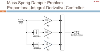
  • 48. Mass Spring Damper Problem Proportional-Integral-Derivative Controller 49  Closed loop transfer function with a proportional-integral- derivative controller   ipd id p CL  20 s  K G (s)   s2  Ks3  10  K K s2  K s K RTECS
  • 49. Mass Spring Damper Problem Proportional-Integral-Derivative Controller 50 RTECS
  • 51. Closed-loop Response 52 Rise time Maximum overshoot Settling time Steady-state error P Decrease Increase Small change Decrease I Decrease Increase Increase Eliminate D Small change Decrease Decrease No Change RTECS
  • 52. Controller Effects 53  Proportional controller (P)  reduces error responses to disturbances,  speeds up the process response  but still allows a steady-state error.  Integral controller (I)  When the controller includes a term proportional to the integral of the error (I), then the steady state error to a constant input is eliminated, although typically at the cost of deterioration in the dynamic response.  Derivative controller (D)  typically makes the system better damped and more stable. RTECS
  • 53. General Tips for Designing a PID Controller 54  Obtain an open-loop response and determine what needs to be improved  Add a proportional control to improve the rise time  Add an integral control to eliminate the steady-state error  Add a derivative control to improve the overshoot  Adjust each of Kp, Ki, and Kd until you obtain a desired overall response RTECS
  • 54. General Tips for Designing a PID Controller 55 RTECS
  • 55. How to Represent PID Controller in Matlab56 RTECS
  • 56. Defining a PID Controller Using Transfer 57 Function Command  Kp = 1;  Ki = 1;  Kd = 1;  s = tf('s');  C = Kp + Ki/s + Kd*s RTECS MATLAB's PID Controller  Kp = 1;  Ki = 1;  Kd = 1;  PID_O = pid(Kp,Ki,Kd)  PID_Tf = tf(PID_O)
  • 57. Mass Spring Damper Problem Proportional Controller - Matlab58  s = tf('s');  P = 1/(s^2 + 10*s + 20);  Kp = 300;  C = Kp + Ki/s + Kd*s  T = feedback(C*P,1)  t = 0:0.01:2;  step(T,t) Step Response Amplitude 0.2 0.4 0.6 0.8 1 1.2 1.4 1.6 1.8 Time (seconds) 2 0 0 0.2 0.4 0.6 0.8 1 1.2 1.4 System: T Peak amplitude: 1.31 Overshoot (%): 40 At time (seconds): 0.18 System: T Settling time (seconds): 0.772 System: T Final value: 0.938 System: T Rise time (seconds): 0.0728 RTECS
  • 58. Mass Spring Damper Problem Proportional-Integral Controller - Matlab59  Kp = 30;  Ki = 70;  C = pid(Kp, Ki)  T = feedback(C*P,1)  t = 0:0.01:2;  step(T,t) Step Response Amplitude 0.2 0.4 0.6 0.8 1 1.2 1.4 1.6 1.8 Time (seconds) 2 0 0 0.4 0.2 0.6 0.8 1 1.2 1.4 System: T Settling time (seconds): 0.618 System: T Peak amplitude: 1.01 Overshoot (%): 1.26 At time (seconds): 0.81 System: T Rise time (seconds): 0.408 RTECS
  • 59. Mass Spring Damper Problem Proportional-Derivative Controller - Matlab60  Kp = 300;  Kd = 10;  C = pid(Kp,0,Kd)  T = feedback(C*P,1)  t = 0:0.01:2;  step(T,t) Step Response Amplitude 0.2 0.4 0.6 0.8 1 1.2 1.4 1.6 1.8 Time (seconds) 2 0 0 0.4 0.2 0.6 0.8 1 1.2 1.4 System: T Peak amplitude: 1.08 Overshoot (%): 15.3 At time (seconds): 0.17 System: T Rise time (seconds): 0.0779 System: T Settling time (seconds): 0.29 RTECS
  • 60. Mass Spring Damper Problem Proportional-Integral-Derivative Controller61  Kp = 350;  Ki = 300;  Kd = 50;  C = pid(Kp,Ki,Kd)  T = feedback(C*P,1);  t = 0:0.01:2;  step(T,t) Step Response Amplitude 0.2 0.4 0.6 0.8 1 1.2 1.4 1.6 1.8 Time (seconds) 2 0 0 0.1 0.2 0.3 0.7 0.6 0.5 0.4 0.8 0.9 1 System: T Final value: 1 System: T Settling time (seconds): 0.831 System: T Rise time (seconds): 0.0549 RTECS
  • 61. Variations of PID Controller62 RTECS
  • 62. Variations of PID Controller 63  P  P+D (Lead) Compensation  P+I (Lag) Compensation  Is generally adequate when plant/process dynamics are essentially of 1st-order  P+I+D (Lead-Lag) Compensation  Is generally ok if dominant plant dynamics are of 2nd-order RTECS
  • 63. PI Controller: The Need 64  In a feedback control system, sensor’s noise is propagated via the controller to the control signal, causing variations in the control signal.  The derivative term of the controller amplifies these variations.  These variations can be reduced in several ways:  Using a measurement low-pass filter  Setting the derivative gain to zero, i.e. using PI in stead of PID RTECS
  • 64. PI Controller: Transfer Function 65 Ts s i p i Kp i p pc E(s) Tis1  K  whereT  T s  i K 1     K 1  Ki G (s)  U (s) K proportional gain integral gain RTECS
  • 65. Design Guidelines 66  Liquid level  Integrating process  Use P or PI controller with high gain  D-mode is not suitable since level signal is usually noisy due to the splashing and turbulence of the liquid entering the tank  Flow control  Use PI controller with intermediate gain  No D-mode because of high frequency noise  Fast response, no time delay RTECS
  • 66. Design Guidelines 67  Temperature  Various characteristics with time delay.  Use PID or PI controller  (D-mode can accelerate the response) RTECS
  • 67. PID script 68 RTECS for i=1:length(kgain) if control_type ==1; C=kp(i)+ki/s+kd*s; elseif control_type ==2; C=kp+ki(i)/s+kd*s; elseif control_type ==3; C=kp+ki/s+kd(i)*s; end GF=feedback(C*g,1); if input_type==0; [ytc,ttc]=impulse(GF,t); elseif input_type==1; [ytc,ttc]=step(GF,t); end plot(ttc,ytc,c_gain{i}) end legend('close',num2str(kgain(1)), num2str(kgain(2)),num2str(kgain(3)),... num2str(kgain(4)),num2str(kgain(5))) clc,clear all, close all t_F=10; input_type=1; control_type=3; t=0:.001:t_F; s=tf('s'); g=1/(s^2+10*s+20); G_close=feedback(1*g,1); if input_type==0; [yt,tt]=impulse(G_close,t); elseif input_type==1; [yt,tt]=step(G_close,t); end plot(tt,yt,'-k','linewidth',2),hold on, grid on kgain=[1 5 10 15 20]; c_gain={'--b','--r','--g','--m','--k'}; if control_type ==1; kp=kgain;ki=0;kd=0; elseif control_type ==2; kp=0;ki=kgain;kd=0; elseif control_type ==3; kp=300;ki=0;kd=kgain;end
  • 68. Home Work: Cruise Control 69 RTECS
  • 69. RTECS