SlideShare a Scribd company logo
A cell-based variational inequality formulation of the
dynamic user optimal assignment problem
Hong K. Lo *, W.Y. Szeto
Department of Civil Engineering, Hong Kong University of Science and Technology, Clear Water Bay,
Kowloon, Hong Kong, People’s Republic of China
Received 12 May 2000; received in revised form 28 December 2000; accepted 28 February 2001
Abstract
This paper developed a cell-based dynamic traffic assignment formulation that follows the ideal dynamic
user optimal (DUO) principle through a variational inequality approach. To improve the accuracy of
dynamic traffic modeling, this formulation encapsulates a network version of the Cell Transmission Model
(CTM). Moreover, this formulation satisfies the first-in-first-out (FIFO) conditions through the CTM. For
solutions, we employed an alternating direction method developed for co-coercive variational inequality
problems. We set up two scenarios to evaluate the properties of this formulation, in the areas of traffic
dynamics and the ideal DUO principle. The results showed that the formulation was capable of capturing
dynamic phenomena, such as shockwaves, queue formation and dissipation. Moreover, the results dem-
onstrated that this cell-based formulation produced solutions that precisely followed the ideal DUO
principle.  2002 Elsevier Science Ltd. All rights reserved.
Keywords: Dynamic traffic assignment; Variational inequality
1. Introduction
Dynamic traffic assignment (DTA) models recently have attracted a lot of research interest
in the areas of transportation, operations research and computer science. Their develop-
ments basically follow two approaches: simulation and mathematical formulation. The first ap-
proach emphasizes microscopic traffic flow characteristics. Strict adherence to traffic assignment
Transportation Research Part B 36 (2002) 421–443
www.elsevier.com/locate/trb
*
Corresponding author. Tel.: +852-2358-8742; fax: +852-2358-1534.
E-mail address: cehklo@ust.hk (H.K. Lo).
0191-2615/02/$ - see front matter  2002 Elsevier Science Ltd. All rights reserved.
PII: S0191-2615(01)00011-X
principles, such as Wardrop’s, is secondary. These models simulate the probable results of a
certain traffic management strategy but do not prescribe what the strategy ought to be. Fur-
thermore, they lack well-defined solution properties. One cannot be sure whether the solution has
achieved the required optimality.
DTA models can also be developed through an analytical approach (examples, Ran and Boyce,
1996; Ran et al., 1996; Lo et al., 1996a; Lo, 1999b; Jayakrishnan et al., 1995; Janson, 1991; Friesz
et al., 1993; Smith, 1993; Wie et al., 1990). This approach has well-defined properties, in terms of
optimality conditions, adherence to a dynamic version of Wardrop’s principle (1952), and the
first-in-first-out (FIFO) conditions. Depending on how the objective functions are defined, these
models may be used for prescriptive or descriptive purposes. The main difficulty with the ana-
lytical approach is adding realistic traffic dynamics to already complicated formulations. For this
reason, most DTA models use macroscopic link travel time functions (e.g., variations of the
Bureau of Public Roads or BPR function) to approximate traffic dynamics. This lack of accurate
traffic dynamics is a potential shortcoming. Daganzo (1995b) pointed to the potential problem of
link travel time functions under dynamic loads. Our studies (Lo et al., 1996b,c) confirmed that
capturing accurate traffic dynamics is an important component of developing DTA models.
Traffic assignment formulations generally rely on four approaches: (i) mathematical pro-
gramming (MP) (example, Sheffi, 1985); (ii) variational inequality (VI) (examples, Dafermos,
Notation
rs OD pair, rs 2 RS
Prs
set of routes connecting OD pair rs
p route between an OD pair, p 2 Prs
Td set of demand periods when traffic is loaded to the network, Td  T
t index for departure time, t 2 Td
f rs
p ðtÞ route flow on p between OD pair rs departing at time t
fðtÞ vector of ðf rs
p ðtÞ 8p 2 Prs
; 8rs 2 RSÞ with dimension n1 ¼
P
rs jPrs
j
f vector of ðfðtÞ 8tÞ with dimension n2 ¼ n1  N
grs
p ðtÞ actual route travel time on route p between OD pair rs for flows departing at time t
nðtÞ vector of ðgrs
p ðtÞ 8p 2 Prs
; 8rs 2 RSÞ with dimension n1
n vector of ðnðtÞ 8tÞ with dimension n2
prs
ðtÞ shortest travel time between OD pair rs for flows departing at time t
uðtÞ vector of ðprs
ðtÞ 8rs 2 RSÞ with dimension n3 ¼ jRSj
u vector of ðuðtÞ 8tÞ with dimension n4 ¼ n3  N
qrs
ðtÞ demand between OD pair rs, considered as fixed in this study
qðtÞ vector of ðqrs
ðtÞ 8rs 2 RSÞ with dimension n3
q vector of ðqðtÞ 8tÞ with dimension n4
AðtÞ OD-route incidence matrix; dimensions jRSj jPrs
j where its element ðrs; kÞ ¼ 1 if the
kth route departing at time t is an element of Prs
; 0 otherwise
A Diagonal matrix with AðtÞ as its diagonal; dimensions n4 n2
422 H.K. Lo, W.Y. Szeto / Transportation Research Part B 36 (2002) 421–443
1980; Nagurney, 1993; extensions to dynamic traffic: Ran and Boyce, 1996; Friesz et al., 1993);
(iii) non-linear complementarity problem (NCP) (Aashtiani, 1979); and (iv) fixed-point problem
(FPP) (Asmuth, 1978). Lin and Lo (2000) discussed a potential problem of extending the MP
approach for dynamic traffic assignment. Two summaries of these approaches were annotated by
Patriksson (1994) and Florian and Hearn (1995). They showed the linkages and equivalence
conditions among these approaches.
This study develops a cell-based DTA model through a variational inequality approach. The
formulation has well-defined solution properties by following a dynamic extension of Wardrop’s
Principle, referred to as dynamic user optimal (DUO) (Ran and Boyce, 1996) and satisfies the
FIFO conditions. To capture realistic traffic dynamics, we encapsulate the Cell Transmission
Model (CTM) (Daganzo, 1994, 1995a) in this formulation. CTM provides a convergent nu-
merical approximation to the Lighthill and Whitham (1955) and Richards (1956) (LWR) model
and covers the full range of the fundamental diagram. It can well capture traffic dynamics such as
shockwaves, queue formation, queue dissipation and dynamic traffic interactions across multiple
links.
Encapsulating a macroscopic simulation model in a traffic assignment framework is not new.
Merchant and Nemhauser (1978) used a macroscopic simulation model in their system optimal
assignment formulation. Recently, Wong et al. (2001) combined a path-based static traffic as-
signment formulation by Lo and Chen (2000) with the TRANSYT traffic model. In that study,
route travel time was determined by summing the delay and cruise time on each link. In this
present formulation, we use the time variant cumulative occupancy counts at the origins and
destinations determined from CTM to determine the en route travel time for each departing traffic
packet. The details are described in Section 3.
This formulation sets out to explicitly model the physical effect of queuing. It is, therefore,
important to be able to track the routes of the spillback queues, which may extend over multiple
links. To this end, route flows provide important information to model traffic at diverges and
merges and to track the end of queues. For these reasons, we develop this DUO formulation
based on the route-flow variables. The possible routes between each origin–destination (OD) pair
could be either predefined or generated through a column generation procedure in the solution
algorithm. In practice, the predefined routes could be based on travelers’ preferences or interview
results. The formulation will then equilibrate traffic flows according to the DUO principle. That
is, all the used routes between the same OD pair will have equal travel time; while the unused ones
will have equal or higher travel times.
To solve this VI formulation, we employ an alternating direction method proposed by Han
and Lo (2001) for co-coercive VI problems. This method requires that route travel time is a
co-coercive mapping of route flow and the solution set is non-empty. To illustrate the solu-
tion quality of this formulation, we apply it to two scenarios, demonstrating three aspects; (i)
traffic dynamics, (ii) traffic interactions across multiple links; and (iii) adherence to the DUO
principle. The results are promising with regard to each of these aspects, as discussed in Sec-
tion 4. The rest of paper is organized as follows. Section 2 describes the cell-based DUO
formulation. Section 3 depicts the dynamic traffic model adopted in this formulation. The so-
lution method based on the alternating direction approach is described in Section 4. Sec-
tion 5 contains the numerical studies, and finally, some concluding remarks are provided in
Section 6.
H.K. Lo, W.Y. Szeto / Transportation Research Part B 36 (2002) 421–443 423
2. Variational inequality formulation of the dynamic user optimal route choice problem
We consider a general transportation network with multiple OD flows. The traffic network is
represented by a set of cells J and directed links. Road segments are represented by a series of cells
that have physical length, while links are there merely to delineate connectivity between cells. As
such, links have no physical length and cannot hold traffic. Traffic begins at an origin cell (denoted
as r) and terminates at a destination cell (denoted as s). The study horizon ½0; T is discretized into
N intervals of length d such that T ¼ N  d. We use two types of time indices to track traffic. The
first type, denoted by t ¼ 1; . . . ; N, marks the departure time of traffic leaving an origin, which is
used to ensure the dynamic user optimal conditions, as discussed below. The actual departure time
of a particular traffic is thus t  d. The second time index, denoted by x ¼ 1; . . . ; N, tracks the
movements over time of traffic that is already in the network. We further assume that the study
horizon is long enough to allow all traffic to clear the network.
This paper focuses on the conditions of ideal DUO, stated as: for each OD pair at each instant
of time, the actual travel times experienced by travelers departing at the same time are equal and
minimal (Ran and Boyce, 1996). Possible scenarios where this could happen include: (i) in
commuting traffic where the patterns were reproduced every day and hence, commuters could
modify their route choices until they could improve no further after many days of experience; (ii)
in the future when the technologies of traffic detection and prediction will become accurate.
The ideal DUO conditions imply that a route p between OD pair r–s will not be used for flows
departing at time t if its actual travel time is longer than the shortest travel time between r–s.
Conversely, any used route p departing at time t must have its travel time equal to the shortest
travel time between r–s. Mathematically, it can be expressed as:
f rs
p ðtÞ grs
p ðtÞ
h
prs
ðtÞ
i
¼ 0 8rs 2 RS; 8p 2 Prs
; 8t 2 Td; ð1Þ
grs
p ðtÞ prs
ðtÞ P 0 8rs 2 RS; 8p 2 Prs
; 8t 2 Td: ð2Þ
We emphasize that the index t above refers to the departure time of the flows. The DUO problem
is to find f such that (1) and (2) and the following demand and non-negativity constraints are
satisfied.
X
p2Prs
f rs
p ðtÞ ¼ qrs
ðtÞ 8rs 2 RS; 8t 2 Td; ð3Þ
f P 0; u P 0: ð4Þ
The DUO problem (1)–(4) can be expressed as a finite dimensional variational inequality problem
(VIP), VIðn; XÞ: find a vector f such that
ðf f ÞT
 n P 0 8f 2 X; ð5Þ
where
X ¼ ff jAf ¼ q; f 2 Rn2
þ g: ð6Þ
The superscript ‘‘ ’’ refers to a solution of f that fulfills the DUO conditions and Rn2
þ the non-
negative orthant of dimension n2. It should be reminded that the actual route travel time n is a
function of route flows f, i.e., n ¼ nðfÞ.
424 H.K. Lo, W.Y. Szeto / Transportation Research Part B 36 (2002) 421–443
The equivalence between the DUO problem (1)–(4) and VIðn; XÞ (5)–(6) is established in Ran
and Boyce (1996) and not repeated here. The existence of solution of VIðn; XÞ requires that: (i) n is
a continuous function of f and (ii) X is a non-empty compact convex set (Theorem 1.4 in
Nagurney, 1993). For this time-discretized problem, care must be exercised to ensure the conti-
nuity of n with respect to f. This consideration will be further elaborated in Section 3. The second
requirement is satisfied for the linear demand constraints depicted in X.
The uniqueness of solution further requires that n is strongly monotone. This requirement is
generally not fulfilled for traffic assignment problems, making multiple route-flow solutions un-
avoidable. This aspect is well known in route-flow formulations of static traffic assignment
problems (see for example, Aashtiani, 1979) and exhibits itself in a similar fashion in this DUO
problem.
Most of the above development follows from ideas of previous studies (examples, Ran and
Boyce, 1996; Lo et al., 1996a; Friesz et al., 1993). The key difference we propose in this study is in
how traffic dynamics and actual route travel times are modeled. Previous VI formulations, gen-
erally considered traffic dynamics as additional side constraints in X. This approach makes direct
VI solution methods based on projections on X rather difficult. To rectify this problem, they
generally transformed the VI formulation to an equivalent mathematical program through a
relaxation technique and solved the resultant mathematical program repeatedly instead. There are
a number of issues associated with this approach that requires attention. First, representing traffic
dynamics as side constraints explicitly is cumbersome and makes solution difficult, especially, if
more complicated (but realistic) traffic models are attempted (see Lo, 1999b). Second, compu-
tationally, this may not be efficient, as the entire ‘‘relaxed’’ mathematical program (which is te-
dious to solve by itself) is solved hundreds of times for solutions. Third, there is no guarantee that
the route travel time function is differentiable with respect to route flows especially if stop-and-go
queued traffic is considered; deeming techniques based on sub-gradient solution methods neces-
sary, which could introduce further computational inefficiency.
To overcome the above difficulties, in this study, rather than considering traffic dynamics as
constraints, we model it as a mapping of f directly, which then allows us to determine n as a
function of f. In Section 3, we discuss in some detail how this is achieved.
3. Dynamic traffic flow modeling
A key to this model development is the determination of the actual travel times n from the
route flows f. Many dynamic link travel time functions or even traffic simulation models could be
used for this purpose. This VIP imposes no particular restrictions on the use of traffic models as
long as they maintain n as a continuous function of f.
To capture traffic dynamics, this formulation encapsulates the CTM (Daganzo, 1994, 1995a) as
the underlying dynamic traffic model. For this purpose, CTM seems to strike an appropriate
balance between capturing sufficient details for modeling queue dynamics and leaving out mi-
croscopic features that would slow down computation. The following subsection describes the
basic principles of CTM. Note that we distinguish the difference between two time indices: t
defined earlier refers to the traffic’s departure time; whereas x to be used in the following is to
keep track of the departed traffic along its course in the network.
H.K. Lo, W.Y. Szeto / Transportation Research Part B 36 (2002) 421–443 425
3.1. Cell Transmission Model (CTM): basic principles
The LWR model can be stated by the following two conditions:
oy
ox
þ
ok
ox
¼ 0 and y ¼ Y ðk; xÞ; ð7Þ
where y is the traffic flow, k the density, x and x, respectively, the space and time variables, and Y
is a function relating y and k. The first partial differential equation states the traffic flow con-
servation. The relation Y defines the fundamental diagram. Given a set of well-posed initial
conditions, one can determine y and k at any ðx; xÞ by solving (7). In other words, one knows the
traffic flow and density at any location x and any time instance x in the modeling horizon. This
model is sometimes referred to as the hydrodynamic or kinematic wave model of traffic flow.
Lighthill and Whitham (1955) and Newell (1991) developed two different solution approaches to
this model. Daganzo (1994, 1995a) simplified the solution scheme by adopting the following re-
lationship between traffic flow, y, and density, k:
y ¼ minfVk; Q; W ðkjam kÞg; ð8Þ
where kjam; Q; V ; W denote, respectively, jam density, inflow capacity (or maximum allowable
inflow), free-flow speed and the speed of the backward shock wave (or the backward propagation
speed of disturbances in congested traffic), then the LWR equations for a single highway link are
approximated by a set of difference equations. Essentially, (8) approximates the fundamental
diagram by a piece-wise linear model as shown in Fig. 1.
By discretizing the road into homogeneous sections (or cells) and time into intervals such that
the cell length is equal to the distance traveled by free-flowing traffic in one time interval, then the
LWR results are approximated by this set of recursive equations (Daganzo, 1994, 1995a):
njðx þ 1Þ ¼ njðxÞ þ yjðxÞ yjþ1ðxÞ; ð9Þ
yjðxÞ ¼ minfnj 1ðxÞ; QjðxÞ; ðW =V Þ NjðxÞ

njðxÞ

g; ð10Þ
where the subscript j refers to cell j, and j þ 1ðj 1Þ represents the cell downstream (upstream) of
j. The variables njðxÞ; yjðxÞ; NjðxÞ denote the number of vehicles, the actual inflow, and the
maximum number of vehicles (or holding capacity) that can be held in cell j at time x, respec-
tively. The variables QjðxÞ; V ; W follow the earlier definitions. It is important to differentiate
Flow y
Qmax
V W
Density
Fig. 1. The fundamental diagram used in CTM.
426 H.K. Lo, W.Y. Szeto / Transportation Research Part B 36 (2002) 421–443
between QjðxÞ and yjðxÞ: the former is the inflow capacity while the latter is the actual inflow.
Because (9) and (10) provide a numerical approximation to the LWR equations, all the traffic
phenomena demonstrated in the LWR model are replicated in CTM. The key is to determine
yjðxÞ from the minimization (10). Once this is accomplished, njðxÞ can be determined recursively
from the linear equations (9). Eqs. (9) and (10) provide the basic principle of modeling traffic flow
on a series of straight cells.
To apply this principle to a general network with multiple OD pairs, three extensions are re-
quired: (a) modeling merge and diverge junctions; (b) differentiating the OD specific traffic; (c)
maintaining the FIFO property. To maintain the intended routes of traffic and the FIFO prop-
erty, traffic in each cell is disaggregated by route ðpÞ and waiting time at the cell ðsÞ. The route
variable is used to direct traffic along its route. By tracking s, the FIFO property at the cell level is
maintained by ensuring that earlier arrivals (with a larger s) will leave sooner. The detailed
mathematical operations to ensuring these conditions were addressed in Daganzo (1995a) and Lo
(1999b). The description of which is lengthy; in the interest of space, we do not repeat the analysis
here but illustrate it with an example through the origin cell.
For the construction of an origin cell, we create a cell just upstream of an origin cell with an
infinite capacity to store the traffic that intends to enter the network. Let us call this cell r 1. To
load traffic into the network according to the departing demand f rs
p ðtÞ, we set the inflow into this
cell at the time instance x ¼ t such that:
yr 1;pðxÞ ¼ f rs
p ðtÞ;
nr 1;pðx þ 1Þ ¼ nr 1;pðxÞ þ yr 1;pðxÞ yr;pðxÞ:
ð11Þ
The subscripts r, p extend the definitions of inflow and occupancy for each cell under these con-
ditions: cell location – r, route – p. Note that yr;p is the outflow of r 1 but inflow to the origin cell r,
which is subject to the congestion and flow restriction effects at r similar to the expression in (10).
Once the traffic is loaded to the network, the basic principles of (9) and (10) and the conditions for
merge and diverge (not shown here) hold to ensure proper dynamics of traffic propagation.
In brevity, given a set of time-sequenced inflow f rs
p ðtÞ as in (11), based on the traffic propagation
conditions (i.e., such as the recursive equations (9) and (10)), one can obtain a set of unique
occupancy counts nj;pðxÞ for traffic in cell j on route p at any time instance x. Such information on
cell occupancy is used to determine the actual route travel times for the entire modeling horizon.
In addition to modeling network traffic, CTM can be easily modified to handle signalized
networks as well as the occurrence of incident or link blockage. Traffic signals and incidents can
be modeled by modifying the values of the flow capacity QjðxÞ of the affected cells. Specifically,
for the case of signals, the inflow capacity of the signalized cells can be altered according to
whether the time is in a green or red phase:
QjðxÞ ¼ sf for x 2 green phase and j 2 a signalized cell;
QjðxÞ ¼ 0 for x 2 red phase and j 2 a signalized cell;
where sf is the saturation flow rate. One could model both fixed and dynamic timing plans with
CTM, as demonstrated in Lo (1999a, 2001). The treatment of incident modeling is similar.
To summarize, this section described a way to model the propagation of traffic flow in the
network. By tracking the flow’s departure time, route and waiting time at each cell along the
H.K. Lo, W.Y. Szeto / Transportation Research Part B 36 (2002) 421–443 427
route, one can determine the occupancy of each packet of traffic on route p in each cell and at each
time instance throughout the modeling horizon.
3.2. Determination of actual route travel time
Knowing the occupancy of each package of traffic on route p in origin cell r and destination cell s
at each time instance, the actual en route travel time grs
p ðtÞ of flow f rs
p ðtÞ can be determined through
the use of cumulative counts. Let kr
pðtÞ be the cumulative traffic departing from cell r on route p at
time t and ks
pðxÞ be the cumulative traffic arriving at cell s on route p at time x, defined by:
kr
pðtÞ ¼
X
t0 6 t
nr;pðt0
Þ; ð12Þ
ks
pðxÞ ¼
X
x0 6 x
ns;pðx0
Þ: ð13Þ
Fig. 2 shows that the cumulative count curves kr
pðtÞ and ks
pðxÞ on route p between OD pair rs. The
actual en route travel time of traffic departing at t (i.e., f rs
p ðtÞ) is the horizontal distance between
the two cumulative curves as shown in Fig. 2. If time is discretized, subject to the en route
conditions, there is no guarantee that the entire packet f rs
p ðtÞ will arrive at the destination s in the
same discretized time tick x. As shown in Fig. 2, the front part of the packet has an actual travel
time of g whereas the latter parts have longer actual travel times. The extent of this difference in en
route travel times of the same departing packet depends on the size of the discretized time. Ac-
curacy can be introduced with finer departure time intervals at the expense of requiring more cells,
more time intervals, and eventually higher computational efforts.
In this study, we adopt the following averaging scheme so that the entire departing traffic f rs
p ðtÞ
has one uniquely determined average en route travel time grs
p ðtÞ. Mathematically, this scheme can
be stated as:
grs
p ðtÞ ¼
Rkr
pðtÞ
kr
pðt 1Þ ks 1
p ðtÞ kr 1
p ðtÞ
h i
dt
kr
pðtÞ kr
pðt 1Þ
; ð14Þ
Fig. 2. The cumulative vehicle counts in origin cell r and destination cell s.
428 H.K. Lo, W.Y. Szeto / Transportation Research Part B 36 (2002) 421–443
where
f rs
p ðtÞ ¼ kr
pðtÞ kr
pðt 1Þ: ð15Þ
The numerator on the right-hand side of (14) is the area of the shaded region in Fig. 2 or the total
en route travel time of the entire packet f rs
p ðtÞ. The denominator is the packet departing at time t
as defined in (15).
The above averaging scheme is well defined for used routes with positive departure flows. For
an unused route with f rs
p ðtÞ ¼ 0, we define its actual route travel time to be equal to that of
f rs
p ðtÞ ¼ r; r ! 0þ
. For an infinitely small r, the whole packet shall arrive at the same discretized
tick. According to (14), grs
p ðtÞ ¼ ðg  rÞ=r ¼ g or x t. Summarizing, we have this definition:
Definition 1. The actual en route travel time of an unused route is defined to be that of an infi-
nitely small traffic traveling on the route.
Let us consider the following case: assuming that a particular departure f rs
p ðtÞ arrives at the
destination in m sub-packets with arrival times at the destination to be t þ 1, t þ 2;    ; t þ m,
respectively. Let the amount of traffic in each sub-packet to be ak, k ¼ 1; . . . ; m, where
ak P 0 and
X
m
k¼1
ak ¼ f rs
p ðtÞ: ð16Þ
Obviously, ak is a function of f. More congested situations will render a later arrival of the first
packet, making the earlier ak ¼ 0. We have the following assumption:
Assumption 1. A small change in the departure flow pattern will incur a small change in the arrival
pattern. Specifically, this assumption can be stated as:
8e  0; 9d such that jf0
fj 6 e ) ja0
k akj 6 de for all k;
where f; f0
2 Rn2
þ , ak, a0
k P 0, d and e are infinitely small. ak and a0
k correspond to the arrival pat-
terns of f and f0
, respectively.
Proposition 1. Under Assumption 1, the actual route travel time n is a continuous function of f.
Proof. To prove that n is a continuous function of f, we prove that each component of n (i.e.,
grs
p ðtÞ) is. Given that f 2 Rn2
þ , we show that (14) is a continuous function of f.
For an arbitrary flow vector f, through the traffic model (CTM in this case), one can obtain a
set of uniquely determined cumulative arrival curve for each route p departed at t. Putting the
general expression (16) into (14), one has:
grs
p ðtÞ ¼
a1ðt þ 1 tÞ þ a2ðt þ 2 tÞ þ    þ amðt þ m tÞ
a1 þ a2 þ    þ am
¼
a1 þ 2a2 þ    þ mam
f rs
p ðtÞ
;
which is a continuous function under Assumption 1 for positive f rs
p ðtÞ and ak 2 Rþ [ f0g. This
completes the proof for the used routes with f rs
p ðtÞ  0. For the unused routes with f rs
p ðtÞ ¼ 0,
H.K. Lo, W.Y. Szeto / Transportation Research Part B 36 (2002) 421–443 429
according to Definition 1, their actual travel times are equivalent to those of f rs
p ðtÞ ¼ r, where r is
a positive small constant. Thus, this proof also works for the actual travel times of unused routes.
Without loss of generality, the above proof works for each component of n and therefore for n.
This completes the proof. 
One thing to note is that even though n defined in (14) is a continuous function of f, it is not
continuously differentiable with respect to f. If one were to hold the arrival pattern in Fig. 2
constant while varying f rs
p ðtÞ, one would observe that grs
p ðtÞ is non-differentiable at the kinks of
f rs
p ðtÞ ¼ a; a þ b or a þ b þ c or at each separation of arrivals of the sub-packets, as shown in
Fig. 3. This non-smooth property renders solution methods based on derivatives of n with respect
to f rather difficult. This is why solution methods based on projections are more suitable for this
problem.
3.3. First-in-first-out (FIFO) conditions
FIFO plays an importance role in DUO problems. Three types of FIFO conditions are ad-
dressed in the literature, namely, cell, route, and OD. The cell (route) FIFO condition is satisfied if
every user who enters the cell (route) earlier will leave sooner. Likewise, the OD FIFO condition is
satisfied if every user who departs from the origin cell earlier will arrive at its destination sooner.
Mathematically, they can be written as:
Definition 2. (Cell FIFO) The cell FIFO condition is satisfied if and only if
x0
j  x00
j ) x0
j þ hjðx0
Þ  x00
j þ hjðx00
j Þ 8j 2 J; 8x0
j; x00
j 2 -;
where - is the set containing integer from 1 to N, J is the set of cells, hjðxjÞ is the travel time in cell
j for flows entering at xj.
Similarly,
Definition 3. (Route FIFO) The route FIFO condition is satisfied if and only if
t0
 t00
) t0
þ grs
p ðt0
Þ  t00
þ grs
p ðt00
Þ 8p 2 Prs
; 8rs 2 RS; 8t0
; t00
2 Td:
Fig. 3. The actual travel time function while fixing the arrival pattern.
430 H.K. Lo, W.Y. Szeto / Transportation Research Part B 36 (2002) 421–443
Definition 4. (OD FIFO) The OD FIFO condition is satisfied if and only if
t0
 t00
) t0
þ prs
ðt0
Þ  t00
þ prs
ðt00
Þ 8rs 2 RS; 8t0
; t00
2 Td:
In our formulation, the CTM ensures the cell FIFO condition in its entirety through carefully
tracking the waiting time of each packet at the cell (see Daganzo, 1995a). Given the cell FIFO
condition, route FIFO can be proven through repeatedly applying the principle of cell FIFO
along a particular route.
Proposition 2. The Cell FIFO condition implies the Route FIFO condition.
Proof. We consider a traffic packet traveling along route p consisting of j ¼ 1; . . . ; k cells. Let xj 2
- be its entry time into cell j; x1 2 Td its entry time into the first cell; and xkþ1 the time the packet
leaves the route. The entry time into the next cell j þ 1 is: xjþ1 ¼ xj þ hjðxjÞ. Using the Cell FIFO
definition, x0
j  x00
j ) x0
jþ1  x00
jþ1; j ¼ 1; 2; . . . ; k 1. Applying this relationship recursively,
one obtains: x0
1  x00
1 ) x0
kþ1  x00
kþ1. Since xkþ1 ¼ x1 þ gpðx1Þ, it becomes: x0
1  x00
1 ) x0
1 þ
gpðx0
1Þ  x00
1 þ gpðx00
1Þ. In other words, for traffic packets that entered the first cell on p earlier,
they will leave it sooner. This completes the proof. 
Finally, Route FIFO together with the DUO conditions implies the OD FIFO condition
(Theorem 2.1 in Wu et al., 1998). Therefore, in this DUO formulation, by guaranteeing the cell
FIFO condition, which is achieved by the CTM, it satisfies both route and OD FIFO. One thing
to note is that the scheme adopted for determining the actual route travel time averages out the
travel times of the faster and slower sub-packets within the same departing packet. Hence, the OD
FIFO property is only approximate. Obviously, these FIFO properties are subject to the accuracy
of the time discretization adopted. Finer departing time steps and smaller cell sizes will improve
these FIFO properties as desired.
Summarizing, given a route flow vector f, we determine the cumulative counts in each cell by
route and time according to the CTM. Based on these cumulative counts, we determine the actual
route travel for each departing flow according to the averaging scheme (14). As the CTM de-
termines a unique set of cumulative counts from f and the averaging scheme determines a unique
set of route travel times n from the cumulative count curves, through these two processes, one
establishes a one-to-one mapping from f to n. This mapping is continuous and ensures the
properties of cell, route, and OD FIFO.
4. A solution method based on alternating direction
The non-smooth nature of the route travel time function renders solution methods based on
derivative information rather difficult. Therefore, we develop a solution method aimed at solving
the VIP (5) and (6) with projection methods. We begin by attaching a Lagrangian multiplier
u 2 Rn4 to the linear demand constraint Af ¼ q to obtain the following equivalent VIP: find
x 2 W such that:
ðx x ÞT
Fðx Þ P 0; x 2 W; ð17Þ
H.K. Lo, W.Y. Szeto / Transportation Research Part B 36 (2002) 421–443 431
where
x ¼
f
u

; FðxÞ ¼
nðfÞ AT
u
Af q

; W 2 Rn2
þ Rn4
: ð18Þ
The motivation for this modification is to construct a set W that has an easier projection than
on the original set X in (6). For this type of problem, Gabay and Mercier (1976) and Gabay (1983)
proposed the following alternating direction method:
• Given ðfk
; uk
Þ 2 Rn2
þ Rn4 at the kth iteration, find fk
2 Rn2
þ such that:
ðf0
fkþ1
ÞT
nðfkþ1
Þ AT
uk
bkþ1ðAfkþ1
qÞ P 0 8f0
2 Rn2
þ : ð19Þ
• Then update u via:
ukþ1
¼ uk
bkþ1ðAfkþ1
qÞ; ð20Þ
where bkþ1  0 is a given penalty parameter (or a sequence of parameters) for the linear constraint
Af ¼ q.
With known uk
, bkþ1, the bracket fg on the left-hand side of (19) is a function of fkþ1
. Thus, (19) is
a reduced VIP sub-problem involving only f. Alternating direction method is attractive for large-
scale problems if the sub-problems can be solved efficiently. Nevertheless, solving the sub-problem
(19) exactly could be computationally intensive by itself. Moreover, there is little justification to
solve it exactly at each iteration, especially when u is far away from u .
To overcome this shortcoming of Gabay’s approach, recently, He and Zhou (2000) proposed a
modified alternating direction method for the case of nðfÞ ¼ Mf þ b, where M is a symmetric
positive semi-definite matrix and b is a given vector. He and Zhou’s method is attractive for its
simplicity since each iteration requires only one projection to the simple convex set and a function
evaluation. However, for this DUO problem, the underlying mapping nðfÞ is neither symmetric
nor linear. Recently, Zhu and Marcotte (1996) considered the case of co-coercive mappings and
proved that many iterative schemes based on the auxiliary problem framework (Cohen, 1988) and
the projection method proposed by Bertsekas and Gafni (1987) converge to a solution of
VIðn; XÞ. Motivated by these studies, in Han and Lo (2001), we recently developed a modified
alternating direction method by extending He and Zhou (2000) solution method for non-linear
mappings. The solution method has been proven to be convergent for co-coercive mappings
of nðfÞ.
Definition 5. Let U be a non-empty close convex subset of Rn
, an operator F : U ! Rn
is said to be
co-coercive if there exists a positive constant l such that ðu vÞT
½F ðuÞ F ðvÞ P lkF ðuÞ
F ðvÞk2
8u; v 2 U.
According to Zhu and Marcotte (1996), co-coercive mappings are monotone but may not
necessarily be strongly monotone. Conversely, strongly monotone and Lipschitz continuous
mappings are co-coercive. Thus, co-coercive mappings are an intermediate concept between
simple and strongly monotone mappings.
In Han and Lo (2001), we proved the convergence for this new alternating direction based
on: (i) the underlying mapping n(f) is co-coercive on Rn2
þ and (ii) the solution set of VIðn; XÞ is
non-empty. In the following, we restate this algorithm based on the approach of alternating
432 H.K. Lo, W.Y. Szeto / Transportation Research Part B 36 (2002) 421–443
direction. First, we denote the set K being the same as Rn2
þ and the residual error function for the
problem under consideration as:
eðx; bÞ ¼ eðf; u; bÞ ¼
f PK f b½nðfÞ AT
u
bðAf qÞ

;
where b is a (set of) given penalty parameter(s) and PKfg the projection on K. It can be verified
readily that if eðx; bÞ ¼ 0, the VIP expressed in (17) and (18) is solved. Furthermore, we define
rðx; bÞ as:
rðx; bÞ ¼
f PKff b½nðfÞ AT
ðu bðAf qÞÞ g
bðAf qÞ

: ð21Þ
Likewise, it can be verified that solving the VIP (17) and (18) is equivalent to finding a zero point
of rðx; bÞ.
The detailed algorithmic steps are the following:
Step 0. Given an initial arbitrary point x ¼ ðf0
; u0
ÞT
2 K Rn4 and positive constants
b  4l; e  0, set k ¼ 0
Step 1. Compute 
x
xk
¼ ð
f
fk
; 
u
uk
ÞT
2 K Rn4 by:

f
fk
¼ PKffk
b½nðfk
Þ AT
ðuk
bðAfk
qÞÞ g

u
uk
¼ uk
bðA
f
fk
qÞ
Step 2. Compute xkþ1
¼ ðfk
; uk
ÞT
2 K Rn4
xkþ1
¼ xk
tkckðxk

x
xk
Þ,
where tk ¼ dk 1 b
4l
 
; dk 2 ð0; 2Þ such that tk 2 ð0; 1Þ and
ck ¼ krðxk
; bÞk2
=krðxk
; bk2
H with
H ¼
I þ bAT
A 0
0 I

and krðxk
; bÞk2
H ¼ rT
ðxk
; bÞHrðxk
; bÞ
Step 3. If krðxkþ1
; bÞk  e, stop;
Else set k ¼ k þ 1 and go to Step 1
Each iteration requires the determination of the actual route travel time vector nðfk
Þ from route
flows of the last iteration. For this purpose, the CTM and the averaging scheme (14) for the entire
modeling horizon are executed once per iteration. Furthermore, the algorithm requires merely
projections on the non-negative orthant (Step 1) without the need for any matrix inversion. Thus,
the computational load per iteration is mild. We are able to solve relatively large networks with
this code in reasonable time, as discussed in Section 5.
5. Numerical studies
To illustrate this cell-based DUO formulation, we set up two test scenarios. The first scenario
is set up to illustrate the dynamic traffic phenomena captured by this formulation. To clearly
show the traffic dynamics without being smeared by other factors, this scenario does not pro-
vide for route choice considerations for each OD pair. In the second scenario, we demonstrate
H.K. Lo, W.Y. Szeto / Transportation Research Part B 36 (2002) 421–443 433
that the solution follows the ideal DUO conditions precisely in a reasonably sized network (by
standards of previous DUO studies).
5.1. Scenario 1. Diverge network with an incident
Fig. 4 shows a diverge network with one origin and two destinations. Links 1 and 2 form Route
1 (R1) and Links 1 and 3 form Route 2 (R2). Two traffic streams, going to D1 and D2, are
generated for some period of time. During this time, an incident occurs at the midway on Link 2,
which completely blocks the link. It is expected that a queue would form and propagate backward
passing the junction. This scenario examines the capability of this formulation in capturing how
queues are formed and dissipated at the junction area and how traffic on the unblocked Link 3
would be affected.
The modeling horizon is set at 1000 s. Traffic demands from O to D1 and to D2, respectively,
are at 10 vehicles per time interval (or 3600 vehicles per hour) and five vehicles per time interval
(or 1800 vehicles per hour). Each of these demands lasts for 350 s from the start of the modeling
horizon. The incident on Link 2 starts at 160 s from the start of the modeling horizon and lasts for
130 s. Each route is 1.25 miles (or 15 cells). The detailed input parameters include:
• Jam density: 200 vehicles/mile (or 125 vehicles/km)
• Free-flow and backward shock-wave speed: 30 miles/h (or 48 km/h)
• Flow capacity: 1800 vehicles/h/lane (or 10 vehicles/time interval/lane)
• Number of lanes: 2
• The length of each time interval d: 10 s
Figs. 5(a) and (b) show the occupancy plots over time and space for Scenario 1. The intensities
of the shades correspond to the occupancy levels, as shown in the legend on the right side of the
Fig. 4. A diverge network with an incident.
434 H.K. Lo, W.Y. Szeto / Transportation Research Part B 36 (2002) 421–443
plot. As is customary, traffic propagates in the direction of vertical axis, whereas the horizontal
axis is for time. One can see how the incident on Link 2 affects the traffic on Link 3. Queue
formation, queue dissipation and shock waves are also evidenced in Figs. 5(a) and (b). In Fig.
5(a), after the incident occurred on Link 2 at t ¼ 160, a queue is formed that spills backward
towards the junction. When the end of queue spills beyond the junction, it affects the traffic
Fig. 5. The occupancy plots for Scenario 1: (a) the occupancy plot along Route 1 (R1); (b) the occupancy plot along
Route 2 (R2).
H.K. Lo, W.Y. Szeto / Transportation Research Part B 36 (2002) 421–443 435
destined for D2 also. From Fig. 5(b), despite that Link 3 is empty, traffic for D2 cannot leave the
junction until after t ¼ 320, when the queue on Link 2 has started to dissipate. Note that the
destination cell is modeled as a traffic sink that has an infinite capacity; all the traffic that enters
this cell is considered to have left the network.
To summarize, this formulation is capable of capturing traffic interactions across multiple links,
including such details as the queue formation and dissipation at the junction area.
Fig. 6. Nguyen and Dupius’s 13-node network.
Fig. 7. Cell representation of Nguyen and Dupius’s 13-node network.
436 H.K. Lo, W.Y. Szeto / Transportation Research Part B 36 (2002) 421–443
Table 3
The number of iterations for different precisions
 0.1 0.01 0.001 0.0001
No. of iterations 89 296 323 422
Table 1
Traffic demand and routes for Nguyen and Dupius’s network
OD # Demand per time interval Route no. Node sequence
1, 2 5 1 1-12-8-2
2 1-5-6-7-8-2
3 1-5-6-7-11-2
4 1-5-6-10-11-2
5 1-5-9-10-11-2
6 1-12-6-7-8-2
7 1-12-6-7-11-2
8 1-12-6-10-11-2
1, 3 10 9 1-5-9-13-3
10 1-5-6-7-11-3
11 1-5-6-10-11-3
12 1-5-9-10-11-3
13 1-12-6-7-11-3
14 1-12-6-10-11-3
4, 2 7.5 15 4-9-10-11-2
16 4-5-6-7-8-2
17 4-5-6-11-2
18 4-5-6-10-11-2
19 4-5-9-10-11-2
4, 3 7.5 20 4-9-13-3
21 4-9-10-11-3
22 4-5-9-13-3
23 4-5-6-7-11-3
24 4-5-6-10-11-3
25 4-5-9-10-11-3
Table 2
Signal positions and their fixed time plans
Signal position
(in cell #)
Cycle time
(in time intervals)
Green time
(in time intervals)
Time when first green
appear (in time intervals)
21 12 4 4
39 10 5 0
41 12 5 0
50 11 5 0
54 15 4 5
H.K. Lo, W.Y. Szeto / Transportation Research Part B 36 (2002) 421–443 437
Fig. 8. The convergence plot for the second scenario.
Table 4
(a) Traffic flows for OD pair (1, 2); (b) Route travel times for OD pair (1, 2)
Departure time
(interval)
Route no.
1 2 3 4 5 6 7 8
1 5 – – – – – – –
2 5 – – – – – – –
3 5 – – – – – – –
4 5 – – – – – – –
5 5 – – – – – – –
6 5 – – – – – – –
7 5 – – – – – – –
8 5 – – – – – – –
9 5 – – – – – – –
10 5 – – – – – – –
1 2 3 4 5 6 7 8
1 11 18.78 19.13 19.13 21.68 17 18 18
2 11 23 19.66 18.63 21.81 17.78 18.13 18.13
3 11 23.99 25 24.73 30 22 17.79 18.24
4 11 23 24 24 29 30.92 29 29
5 11 23 24 24 28 30 28 28
6 11 22.44 23.44 23.44 27 29 27 27
7 11 22 23 23 26 28 26 26
8 11 25.88 22.81 22.81 25 27 25 25
9 13 26 22.13 22.13 24 26 24 24
10 12.86 25 22.91 22.91 23.11 25 23 23
438 H.K. Lo, W.Y. Szeto / Transportation Research Part B 36 (2002) 421–443
5.2. Scenario 2. Nguyen and Dupius (1984) network with signals
Ultimately, the formulation aims at solving the ideal DUO problem. This scenario is con-
structed to evaluate whether solutions of this formulation follow the ideal DUO principle. This
network used in this scenario is similar to the Nguyen and Dupius (1984) network, as shown in
Fig. 6. It has 13 nodes, 19 links and 4 OD pairs. The cell representation of this network is shown
in Fig. 7, consisting of 60 cells. The input parameters are the same as the first scenario, except that
all routes have three lanes. Demands are loaded to each OD pair during the first 10 time intervals.
The demand per time interval for each OD pair is shown in Table 1, as are the 25 routes in this
network. Signal positions and their fixed timing plans are shown in Table 2. Traffic streams en-
tering an unsignalized merge junction have equal priority. For the alternating direction algorithm,
we set the parameters to be: tk ¼ 1, b ¼ 0:5 and the convergence criterion: e ¼ 10 4
.
Table 3 illustrates the iterations required for different convergence criteria. The algorithm
stopped after 422 iterations for a rather tight convergence criterion of 10 4
. On a Pentium III PC,
these 422 iterations took a modest runtime of 257 s. The convergence plot of this alternating
direction algorithm is provided in Fig. 8. It shows a sharp decrease of the residual error in the
early iterations. However, the residual error does not decrease monotonically. It is possibly due to
violations of the assumption that route travel time function is co-coercive. The nature of the route
travel time function deserves further investigation, especially on its monotone properties. This has
Table 5
(a) Traffic flows for OD pair (1, 3); (b) Route travel times for OD pair (1, 3)
Departure time (interval) Route no.
9 10 11 12 13 14
1 – – – – 5 5
2 – – – – 10 –
3 – – – – 10 –
4 – 5 5 – – –
5 – 5 5 – – –
6 – 5 5 – – –
7 – 5.05 4.94 – – –
8 – 5.08 4.92 – – –
9 10 – – – – –
10 10 – – – – –
9 10 11 12 13 14
1 20.87 19.19 19.86 22.32 18 18
2 21.22 22.41 23.58 24.24 18.14 18.25
3 30 25 25 30 18.97 21
4 29 24 24 29 29 29
5 28 24.12 24.12 28 28 28
6 27 24.37 24.37 27 27 27
7 26 24.25 24.25 26 26 26
8 25 24.28 24.28 25 25 25
9 24 25 25 24.28 24.33 24.14
10 23.71 24 24 24 24 24
H.K. Lo, W.Y. Szeto / Transportation Research Part B 36 (2002) 421–443 439
important implications on developing efficient solution algorithms. We leave this to a future
study.
Tables 4–7 show the traffic flows and their corresponding route travel times (correct to two
decimal places) on all routes and for all departure times. One can verify that the used route/s
always has/have the minimum route travel time (bolded in the Tables) whereas the unused ones
have equal or higher route travel times. Note that these results have already considered the delay
and queuing effects of the signal. To summarize, this scenario shows that the formulation can
equilibrate traffic according to the ideal DUO conditions.
A more detailed examination of the results shows that despite the constant demand pattern for
each of the OD pairs, the routes used change over time. See Tables 5(a), 6(a) and 7(a). The only
exception is OD pair (1, 2), in which Route No. 1 is located with a marked advantage over the
alternatives (see its route travel time in Table 4(b)). These results give evidence that route
switching over time is fairly common to achieve the ideal DUO conditions.
6. Concluding remarks
This paper developed a cell-based dynamic traffic assignment formulation that follows the ideal
DUO principle. Traffic dynamics is modeled according to the CTM. This formulation automat-
Table 6
(a) Traffic flows for OD pair (4, 2); (b) Route travel times for OD pair (4, 2)
Departure time (interval) Route no.
15 16 17 18 19
1 – 7.5 – – –
2 7.5 – – – –
3 7.5 – – – –
4 7.5 – – – –
5 7.5 – – – –
6 7.5 – – – –
7 7.5 – – – –
8 – 7.5 – – –
9 – 7.5 – – –
10 – – 3.78 3.72 –
15 16 17 18 19
1 20 18.86 19 19.2 21
2 19 23 20.11 21.35 20.85
3 18.86 22 19.42 21 20.58
4 18.72 21 20.32 20.49 19.93
5 18.1 20 20 20 22.17
6 18 19 20 20 27
7 17.2 18 19.11 19.11 26
8 25 18 19 19 25
9 25 18.33 19.33 19.34 24
10 23 25 20 20 23
440 H.K. Lo, W.Y. Szeto / Transportation Research Part B 36 (2002) 421–443
ically satisfies the FIFO conditions as a result of encapsulating CTM. We set up two scenarios to
evaluate the properties of this formulation, in the areas of traffic dynamics, traffic interactions
across multiple links, and the ideal DUO principle. This formulation produced outputs that are in
agreement with what the results ought to be. Namely, the formulation is able to capture dynamic
traffic phenomena, such as shockwaves, queue formation and dissipation. Moreover, it is capable
of capturing dynamic traffic interactions across multiple links. Both of these characteristics
are inherent from the underlying traffic model adopted. The results from solving Nguyen and
Dupius’s network demonstrated that this cell-based formulation follows the ideal DUO principle
precisely.
To solve this VI formulation, we employed an alternating direction method proposed by Han
and Lo (2001) for co-coercive VI problems. This method requires that route travel time is a co-
coercive mapping of route flow and the solution set is non-empty. While sufficient to solve this
formulation, the residual error does not drop in a monotonic manner with the iterations, sug-
gesting that the route travel time function may not be co-coercive. The nature of the route travel
time function considered in this formulation deserves further investigation, especially on its
monotone properties. This has important implications on developing efficient solution algorithms.
We leave this to a future study.
Table 7
(a) Traffic flows for OD pair (4, 3); (b) Route travel times for OD pair (4, 3)
Departure time (interval) Route no.
20 21 22 23 24 25
1 7.5 – – – – –
2 7.5 – – – – –
3 7.5 – – – – –
4 7.5 – – – – –
5 7.5 – – – – –
6 7.5 – – – – –
7 7.5 – – – – –
8 7.5 – – – – –
9 7.5 – – – – –
10 – – – 3.75 3.75 –
20 21 22 23 24 25
1 11 20 20.38 19.16 19.16 21.63
2 19 20.09 21.38 19.83 19.99 21.57
3 18.6 21.07 21 21.36 21.78 21.83
4 18.15 20 20.71 21.21 24.72 21.71
5 18 19 20 21 21 21
6 17.52 19 22.92 20 20 22.41
7 17 18.51 26 19 19 26
8 16.52 18 25 19.14 19.14 25
9 16 22.74 24 19.3 19.3 24
10 23 23 23 20 20 23
H.K. Lo, W.Y. Szeto / Transportation Research Part B 36 (2002) 421–443 441
Acknowledgements
This research was sponsored by the Hong Kong University of Science and Technology’s Re-
search Grant DAG96/97.EG32. We are grateful to three anonymous referees for constructive
comments.
References
Aashtiani, H., 1979. The multi-modal traffic assignment problem. Ph.D. Thesis. Operations Research Center, MIT,
Cambridge, MA.
Asmuth, R., 1978. Traffic network equilibria. Ph.D. Thesis. Department of Operations Research, Stanford University,
Stanford, CA.
Bertsekas, D.P., Gafni, E.M., 1987. Projection method for variational inequalities with applications to the traffic
assignment problem. Mathematical Programming Study 17, 139–159.
Cohen, G., 1988. Auxiliary problem principle extended to variational inequalities. Journal of Optimization Theory and
Applications 59, 325–333.
Dafermos, S., 1980. Traffic equilibrium and variational inequalities. Transportation Science 14, 42–54.
Daganzo, C.F., 1994. The cell transmission model: a simple dynamic representation of highway traffic. Transportation
Research B 28 (4), 269–287.
Daganzo, C.F., 1995a. The cell transmission model part II: network traffic. Transportation Research B 29 (2), 79–93.
Daganzo, C.F., 1995b. Properties of link travel time functions under dynamic loads. Transportation Research B 29 (2),
93–98.
Florian, M., Hearn, D. 1995. Network equilibrium models and algorithms. In: Ball, M.O., et al. (Eds.), Handbooks in
Operations Research and Management Science, vol. 8. Network Routing. Elsevier Science, The Netherlands.
Friesz, T., Bernstein, D., Smith, T., Tobin, R., Wie, B., 1993. A variational inequality formulation of the dynamic
network user equilibrium problem. Operations Research 41, 179–191.
Gabay, D., 1983. Applications of the method of multipliers to variational inequalities. In: Fortin, M., Glowinski, R.
(Eds.), Augmented Lagrangian Methods: Applications to the Numerical Solution of Boundary-Value Problems.
North-Holland, Amsterdam, The Netherlands, pp. 299–331.
Gabay, D., Mercier, B., 1976. A dual algorithm for the solution of nonlinear variational problems via finite element
approximations. Computer and Mathematics with Applications 2, 17–40.
Han, D., Lo, H., 2001. A new alternating direction method for a class of nonlinear variational inequality problems.
Journal of Optimization Theory and Applications, accepted.
He, B.S., Zhou, J., 2000. A modified alternating direction method for convex minimization problems. Applied
Mathematics Letters 13, 123–130.
Janson, B., 1991. Dynamic traffic assignment with arrival time costs. Transportation Research B 25, 143–161.
Jayakrishnan, R., Tsai, W.K., Chen, J., Chen, A., 1995. A dynamic traffic assignment model with traffic flow
relationship. Transportation Research C 3, 51–82.
Lighthill, M.J., Whitham, J.B., 1955. On kinematic waves. I. Flow movement in long rivers. II. A theory of traffic flow
on long crowded road. Proceedings of Royal Society A 229, 281–345.
Lin, W., Lo, H., 2000. Are the objectives and solutions of the dynamic user-equilibrium models always consistent?
Transportation Research A 34, 137–144.
Lo, H., Ran, B., Hongola, B., 1996a. A multi-class dynamic traffic assignment model: formulation and computational
experiences. Transportation Research Record 1537, 74–82.
Lo, H., Lin, W., Liao, L., Chang, E., Tsao, J., 1996b. A comparison of dynamic traffic models: part I framework.
Technical report, UCB-ITS-PRR-96-22. Institute of Transportation Studies, University of California, Berkeley.
Lo, H., Lin, W., Liao, L., Chang, E., Tsao, J., 1996c. A comparison of dynamic traffic models: part II results. Technical
report, UCB-ITS-PWP-97-15. Institute of Transportation Studies, University of California, Berkeley.
Lo, H., 1999a. A novel traffic control formulation. Transportation Research A 33, 433–448.
442 H.K. Lo, W.Y. Szeto / Transportation Research Part B 36 (2002) 421–443
Lo, H., 1999b. A dynamic traffic assignment formulation that encapsulates the cell transmission model. In: Ceder, A.,
(Ed.), Transportation and Traffic Theory, pp. 327–350.
Lo, H., 2001. A cell-based traffic control formulation: strategies and benefits of dynamic plans. Transportation Science,
in press.
Lo, H., Chen, A., 2000. Reformulating the traffic equilibrium problem via a smooth gap function. Mathematical and
Computer Modelling 31, 179–195.
Merchant, D.K., Nemhauser, G.L., 1978. A model and an algorithm for the dynamic traffic assignment problem.
Transportation Science 12, 183–199.
Nagurney, A., 1993. Network Economics: A Variational Inequality Approach. Kluwer Academic Publishers, Norwell,
MA, USA.
Newell, G.F., 1991. A simplified theory of kinematic waves. Research report, UCB-ITS-RR-91-12. University of
California, Berkeley.
Nguyen, S., Dupius, C., 1984. An efficient method for computing traffic equilibria in networks with asymmetric
transportation costs. Transportation Science 18, 185–202.
Patriksson, M., 1994. The Traffic Assignment Problem: Models and Methods. VSP, The Netherlands.
Ran, B., Boyce, D., 1996. Modeling Dynamic Transportation Networks. An Intelligent Transportation System
Oriented Approach, second revised ed. Springer, Heidelberg.
Ran, B, Lo, H., Boyce, D., 1996. A formulation and solution algorithm for a multi-class dynamic traffic assignment
problem. In: Lesort (Ed.), Transportation and Traffic Theory, pp. 195–216.
Richards, P.I., 1956. Shockwaves on the highway. Operations Research 4, 42–51.
Sheffi, Y., 1985. Urban Transportation Networks: Equilibrium Analysis with Mathematical Programming Methods.
Prentice-Hall, Englewood Cliffs, NJ.
Smith, M.J., 1993. A new dynamic traffic and the existence and calculation of dynamic user equilibria on congestion
capacity-constrained road networks. Transportation Research B 27, 49–63.
Wardrop, J., 1952. Some theoretical aspects of road traffic research. In: Proceedings of the Institute of Civil Engineers,
Part II, pp. 325–378.
Wie, B., Friesz, T., Tobin, R., 1990. Dynamic user optimal traffic assignment on congestion multidestination networks.
Transportation Research B 24, 431–442.
Wong, S.C., Yang, C., Lo, H., 2001. A path-based traffic assignment algorithm using TRANSYT traffic model.
Transportation Research B 35, 163–181.
Wu, J.H., Florian, M., Xu, Y.W., Rubio-Ardanaz, J.M., 1998. A projection algorithm for the dynamic network
equilibrium problem. In: Traffic and Transportation Studies. Proceedings of ICTTS 98, pp. 379–390.
Zhu, D.L., Marcotte, P., 1996. Co-coercivity and its role in the convergence of iterative schemes for solving variational
inequalities. SIAM Journal of Optimization 6, 714–726.
H.K. Lo, W.Y. Szeto / Transportation Research Part B 36 (2002) 421–443 443

More Related Content

PDF
Analytical Dynamic Traffic Assignment Models
DOCX
Pergamon Transpn. Res.-B. Vol. 28B, No. 4, pp. 269-287, 19.docx
PDF
A Model For The Dynamic System Optimum Traffic Assignment Problem
PDF
A Gradient Projection Algorithm For Side-Constrained Traffic Assignment
PDF
Applying Projection-Based Methods To The Asymmetric Traffic Assignment Problem
PDF
A Computational Study Of Traffic Assignment Algorithms
PDF
A Computational Study Of Traffic Assignment Algorithms
PDF
A Unified Framework For Traffic Assignment Deriving Static And Quasi-Dynamic...
Analytical Dynamic Traffic Assignment Models
Pergamon Transpn. Res.-B. Vol. 28B, No. 4, pp. 269-287, 19.docx
A Model For The Dynamic System Optimum Traffic Assignment Problem
A Gradient Projection Algorithm For Side-Constrained Traffic Assignment
Applying Projection-Based Methods To The Asymmetric Traffic Assignment Problem
A Computational Study Of Traffic Assignment Algorithms
A Unified Framework For Traffic Assignment Deriving Static And Quasi-Dynamic...

Similar to A Cell-Based Variational Inequality Formulation Of The Dynamic User Optimal Assignment Problem (20)

PPTX
Traffic assignment
PDF
A Dual Scheme For Traffic Assignment Problems
PDF
Urban Traffic Estimation & Optimization: An Overview
PDF
Ant Colony Optimisation Approaches For The Transportation Assignment Problem
PPTX
ESCC 2016, July 10-16, Athens, Greece
PPTX
A Macroscopic Dynamic model integrated into Dynamic Traffic Assignment: advan...
PDF
A partial linearization method for the traffic assignment problem.pdf
PPTX
Dr. Mohamad Kamal - a link-node nonlinear complementarity model for a multicl...
PPTX
Lecture 01 intro.pptx
PDF
Intelligent Traffic Management System using Shortest Path
PDF
A Strategic Model For Dynamic Traffic Assignment
PDF
A Frequency Based Transit Assignment Model That Considers Online Information ...
PPTX
Prediction of traveller information and route choice
PPTX
Unit 3.pptx for civil engineering second year
PDF
Traffic Dynamics in Virtual Routing Multi Topology System
PPTX
Dynamic demand
PDF
Solving real world delivery problem using improved max-min ant system with lo...
PPT
Transportation problem
PDF
Optimizing IP Networks for Uncertain Demands Using Outbound Traffic Constraints
PPTX
Static traffic assignment with Queues (STAQ) without routeset enumeration
Traffic assignment
A Dual Scheme For Traffic Assignment Problems
Urban Traffic Estimation & Optimization: An Overview
Ant Colony Optimisation Approaches For The Transportation Assignment Problem
ESCC 2016, July 10-16, Athens, Greece
A Macroscopic Dynamic model integrated into Dynamic Traffic Assignment: advan...
A partial linearization method for the traffic assignment problem.pdf
Dr. Mohamad Kamal - a link-node nonlinear complementarity model for a multicl...
Lecture 01 intro.pptx
Intelligent Traffic Management System using Shortest Path
A Strategic Model For Dynamic Traffic Assignment
A Frequency Based Transit Assignment Model That Considers Online Information ...
Prediction of traveller information and route choice
Unit 3.pptx for civil engineering second year
Traffic Dynamics in Virtual Routing Multi Topology System
Dynamic demand
Solving real world delivery problem using improved max-min ant system with lo...
Transportation problem
Optimizing IP Networks for Uncertain Demands Using Outbound Traffic Constraints
Static traffic assignment with Queues (STAQ) without routeset enumeration
Ad

More from Joe Osborn (20)

PDF
Research Paper Template Outline For A Short Resear
PDF
Narrative Essay Graphic Organizer BrainPOP Edu
PDF
Fantastic College Admissions Essay Help
PDF
College Essay Career Goals Career Goals Essay Exa
PDF
Professional Paper Writing
PDF
Consumer Reports Buying Guide 2022 Mustang
PDF
College Athletes Should Get Paid Argument Essay. Should College
PDF
Edit My College Essay. College Essay Editing And Proofreading Service
PDF
Academic Writing CELC E-Resources
PDF
Patriotic Computer Paper - TCR5894 Teacher Create
PDF
Quality Writing Paper. Paper Help For Studen
PDF
Scholarship Application Essay Format. Write A Tel
PDF
An Effective Topic Sentence Will Reflect Which Of The Following
PDF
General Agreement Contract Template Word 2003 Mas
PDF
21 Hilarious Tumblr Posts To Read When
PDF
Film Analysis Paper. How To Write A Film Analysis Essa
PDF
White Writing On Black Background Cotton F
PDF
A Feminist Critical Discourse Analysis Of Qaisra Shahraz S The Holy Woman In ...
PDF
A Glance To Teachers Work With Resources Case Of Olcay
PDF
3G RBS Overview Field Support Operations Contents
Research Paper Template Outline For A Short Resear
Narrative Essay Graphic Organizer BrainPOP Edu
Fantastic College Admissions Essay Help
College Essay Career Goals Career Goals Essay Exa
Professional Paper Writing
Consumer Reports Buying Guide 2022 Mustang
College Athletes Should Get Paid Argument Essay. Should College
Edit My College Essay. College Essay Editing And Proofreading Service
Academic Writing CELC E-Resources
Patriotic Computer Paper - TCR5894 Teacher Create
Quality Writing Paper. Paper Help For Studen
Scholarship Application Essay Format. Write A Tel
An Effective Topic Sentence Will Reflect Which Of The Following
General Agreement Contract Template Word 2003 Mas
21 Hilarious Tumblr Posts To Read When
Film Analysis Paper. How To Write A Film Analysis Essa
White Writing On Black Background Cotton F
A Feminist Critical Discourse Analysis Of Qaisra Shahraz S The Holy Woman In ...
A Glance To Teachers Work With Resources Case Of Olcay
3G RBS Overview Field Support Operations Contents
Ad

Recently uploaded (20)

PDF
STATICS OF THE RIGID BODIES Hibbelers.pdf
PPTX
Lesson notes of climatology university.
PPTX
Pharmacology of Heart Failure /Pharmacotherapy of CHF
PDF
Classroom Observation Tools for Teachers
PDF
TR - Agricultural Crops Production NC III.pdf
PDF
Computing-Curriculum for Schools in Ghana
PPTX
Cell Structure & Organelles in detailed.
PDF
RMMM.pdf make it easy to upload and study
PPTX
master seminar digital applications in india
PPTX
human mycosis Human fungal infections are called human mycosis..pptx
PPTX
Renaissance Architecture: A Journey from Faith to Humanism
PDF
Pre independence Education in Inndia.pdf
PDF
VCE English Exam - Section C Student Revision Booklet
PDF
Physiotherapy_for_Respiratory_and_Cardiac_Problems WEBBER.pdf
PDF
102 student loan defaulters named and shamed – Is someone you know on the list?
PDF
01-Introduction-to-Information-Management.pdf
PDF
Insiders guide to clinical Medicine.pdf
PDF
Complications of Minimal Access Surgery at WLH
PPTX
Institutional Correction lecture only . . .
PPTX
PPH.pptx obstetrics and gynecology in nursing
STATICS OF THE RIGID BODIES Hibbelers.pdf
Lesson notes of climatology university.
Pharmacology of Heart Failure /Pharmacotherapy of CHF
Classroom Observation Tools for Teachers
TR - Agricultural Crops Production NC III.pdf
Computing-Curriculum for Schools in Ghana
Cell Structure & Organelles in detailed.
RMMM.pdf make it easy to upload and study
master seminar digital applications in india
human mycosis Human fungal infections are called human mycosis..pptx
Renaissance Architecture: A Journey from Faith to Humanism
Pre independence Education in Inndia.pdf
VCE English Exam - Section C Student Revision Booklet
Physiotherapy_for_Respiratory_and_Cardiac_Problems WEBBER.pdf
102 student loan defaulters named and shamed – Is someone you know on the list?
01-Introduction-to-Information-Management.pdf
Insiders guide to clinical Medicine.pdf
Complications of Minimal Access Surgery at WLH
Institutional Correction lecture only . . .
PPH.pptx obstetrics and gynecology in nursing

A Cell-Based Variational Inequality Formulation Of The Dynamic User Optimal Assignment Problem

  • 1. A cell-based variational inequality formulation of the dynamic user optimal assignment problem Hong K. Lo *, W.Y. Szeto Department of Civil Engineering, Hong Kong University of Science and Technology, Clear Water Bay, Kowloon, Hong Kong, People’s Republic of China Received 12 May 2000; received in revised form 28 December 2000; accepted 28 February 2001 Abstract This paper developed a cell-based dynamic traffic assignment formulation that follows the ideal dynamic user optimal (DUO) principle through a variational inequality approach. To improve the accuracy of dynamic traffic modeling, this formulation encapsulates a network version of the Cell Transmission Model (CTM). Moreover, this formulation satisfies the first-in-first-out (FIFO) conditions through the CTM. For solutions, we employed an alternating direction method developed for co-coercive variational inequality problems. We set up two scenarios to evaluate the properties of this formulation, in the areas of traffic dynamics and the ideal DUO principle. The results showed that the formulation was capable of capturing dynamic phenomena, such as shockwaves, queue formation and dissipation. Moreover, the results dem- onstrated that this cell-based formulation produced solutions that precisely followed the ideal DUO principle. 2002 Elsevier Science Ltd. All rights reserved. Keywords: Dynamic traffic assignment; Variational inequality 1. Introduction Dynamic traffic assignment (DTA) models recently have attracted a lot of research interest in the areas of transportation, operations research and computer science. Their develop- ments basically follow two approaches: simulation and mathematical formulation. The first ap- proach emphasizes microscopic traffic flow characteristics. Strict adherence to traffic assignment Transportation Research Part B 36 (2002) 421–443 www.elsevier.com/locate/trb * Corresponding author. Tel.: +852-2358-8742; fax: +852-2358-1534. E-mail address: cehklo@ust.hk (H.K. Lo). 0191-2615/02/$ - see front matter 2002 Elsevier Science Ltd. All rights reserved. PII: S0191-2615(01)00011-X
  • 2. principles, such as Wardrop’s, is secondary. These models simulate the probable results of a certain traffic management strategy but do not prescribe what the strategy ought to be. Fur- thermore, they lack well-defined solution properties. One cannot be sure whether the solution has achieved the required optimality. DTA models can also be developed through an analytical approach (examples, Ran and Boyce, 1996; Ran et al., 1996; Lo et al., 1996a; Lo, 1999b; Jayakrishnan et al., 1995; Janson, 1991; Friesz et al., 1993; Smith, 1993; Wie et al., 1990). This approach has well-defined properties, in terms of optimality conditions, adherence to a dynamic version of Wardrop’s principle (1952), and the first-in-first-out (FIFO) conditions. Depending on how the objective functions are defined, these models may be used for prescriptive or descriptive purposes. The main difficulty with the ana- lytical approach is adding realistic traffic dynamics to already complicated formulations. For this reason, most DTA models use macroscopic link travel time functions (e.g., variations of the Bureau of Public Roads or BPR function) to approximate traffic dynamics. This lack of accurate traffic dynamics is a potential shortcoming. Daganzo (1995b) pointed to the potential problem of link travel time functions under dynamic loads. Our studies (Lo et al., 1996b,c) confirmed that capturing accurate traffic dynamics is an important component of developing DTA models. Traffic assignment formulations generally rely on four approaches: (i) mathematical pro- gramming (MP) (example, Sheffi, 1985); (ii) variational inequality (VI) (examples, Dafermos, Notation rs OD pair, rs 2 RS Prs set of routes connecting OD pair rs p route between an OD pair, p 2 Prs Td set of demand periods when traffic is loaded to the network, Td T t index for departure time, t 2 Td f rs p ðtÞ route flow on p between OD pair rs departing at time t fðtÞ vector of ðf rs p ðtÞ 8p 2 Prs ; 8rs 2 RSÞ with dimension n1 ¼ P rs jPrs j f vector of ðfðtÞ 8tÞ with dimension n2 ¼ n1 N grs p ðtÞ actual route travel time on route p between OD pair rs for flows departing at time t nðtÞ vector of ðgrs p ðtÞ 8p 2 Prs ; 8rs 2 RSÞ with dimension n1 n vector of ðnðtÞ 8tÞ with dimension n2 prs ðtÞ shortest travel time between OD pair rs for flows departing at time t uðtÞ vector of ðprs ðtÞ 8rs 2 RSÞ with dimension n3 ¼ jRSj u vector of ðuðtÞ 8tÞ with dimension n4 ¼ n3 N qrs ðtÞ demand between OD pair rs, considered as fixed in this study qðtÞ vector of ðqrs ðtÞ 8rs 2 RSÞ with dimension n3 q vector of ðqðtÞ 8tÞ with dimension n4 AðtÞ OD-route incidence matrix; dimensions jRSj jPrs j where its element ðrs; kÞ ¼ 1 if the kth route departing at time t is an element of Prs ; 0 otherwise A Diagonal matrix with AðtÞ as its diagonal; dimensions n4 n2 422 H.K. Lo, W.Y. Szeto / Transportation Research Part B 36 (2002) 421–443
  • 3. 1980; Nagurney, 1993; extensions to dynamic traffic: Ran and Boyce, 1996; Friesz et al., 1993); (iii) non-linear complementarity problem (NCP) (Aashtiani, 1979); and (iv) fixed-point problem (FPP) (Asmuth, 1978). Lin and Lo (2000) discussed a potential problem of extending the MP approach for dynamic traffic assignment. Two summaries of these approaches were annotated by Patriksson (1994) and Florian and Hearn (1995). They showed the linkages and equivalence conditions among these approaches. This study develops a cell-based DTA model through a variational inequality approach. The formulation has well-defined solution properties by following a dynamic extension of Wardrop’s Principle, referred to as dynamic user optimal (DUO) (Ran and Boyce, 1996) and satisfies the FIFO conditions. To capture realistic traffic dynamics, we encapsulate the Cell Transmission Model (CTM) (Daganzo, 1994, 1995a) in this formulation. CTM provides a convergent nu- merical approximation to the Lighthill and Whitham (1955) and Richards (1956) (LWR) model and covers the full range of the fundamental diagram. It can well capture traffic dynamics such as shockwaves, queue formation, queue dissipation and dynamic traffic interactions across multiple links. Encapsulating a macroscopic simulation model in a traffic assignment framework is not new. Merchant and Nemhauser (1978) used a macroscopic simulation model in their system optimal assignment formulation. Recently, Wong et al. (2001) combined a path-based static traffic as- signment formulation by Lo and Chen (2000) with the TRANSYT traffic model. In that study, route travel time was determined by summing the delay and cruise time on each link. In this present formulation, we use the time variant cumulative occupancy counts at the origins and destinations determined from CTM to determine the en route travel time for each departing traffic packet. The details are described in Section 3. This formulation sets out to explicitly model the physical effect of queuing. It is, therefore, important to be able to track the routes of the spillback queues, which may extend over multiple links. To this end, route flows provide important information to model traffic at diverges and merges and to track the end of queues. For these reasons, we develop this DUO formulation based on the route-flow variables. The possible routes between each origin–destination (OD) pair could be either predefined or generated through a column generation procedure in the solution algorithm. In practice, the predefined routes could be based on travelers’ preferences or interview results. The formulation will then equilibrate traffic flows according to the DUO principle. That is, all the used routes between the same OD pair will have equal travel time; while the unused ones will have equal or higher travel times. To solve this VI formulation, we employ an alternating direction method proposed by Han and Lo (2001) for co-coercive VI problems. This method requires that route travel time is a co-coercive mapping of route flow and the solution set is non-empty. To illustrate the solu- tion quality of this formulation, we apply it to two scenarios, demonstrating three aspects; (i) traffic dynamics, (ii) traffic interactions across multiple links; and (iii) adherence to the DUO principle. The results are promising with regard to each of these aspects, as discussed in Sec- tion 4. The rest of paper is organized as follows. Section 2 describes the cell-based DUO formulation. Section 3 depicts the dynamic traffic model adopted in this formulation. The so- lution method based on the alternating direction approach is described in Section 4. Sec- tion 5 contains the numerical studies, and finally, some concluding remarks are provided in Section 6. H.K. Lo, W.Y. Szeto / Transportation Research Part B 36 (2002) 421–443 423
  • 4. 2. Variational inequality formulation of the dynamic user optimal route choice problem We consider a general transportation network with multiple OD flows. The traffic network is represented by a set of cells J and directed links. Road segments are represented by a series of cells that have physical length, while links are there merely to delineate connectivity between cells. As such, links have no physical length and cannot hold traffic. Traffic begins at an origin cell (denoted as r) and terminates at a destination cell (denoted as s). The study horizon ½0; T is discretized into N intervals of length d such that T ¼ N d. We use two types of time indices to track traffic. The first type, denoted by t ¼ 1; . . . ; N, marks the departure time of traffic leaving an origin, which is used to ensure the dynamic user optimal conditions, as discussed below. The actual departure time of a particular traffic is thus t d. The second time index, denoted by x ¼ 1; . . . ; N, tracks the movements over time of traffic that is already in the network. We further assume that the study horizon is long enough to allow all traffic to clear the network. This paper focuses on the conditions of ideal DUO, stated as: for each OD pair at each instant of time, the actual travel times experienced by travelers departing at the same time are equal and minimal (Ran and Boyce, 1996). Possible scenarios where this could happen include: (i) in commuting traffic where the patterns were reproduced every day and hence, commuters could modify their route choices until they could improve no further after many days of experience; (ii) in the future when the technologies of traffic detection and prediction will become accurate. The ideal DUO conditions imply that a route p between OD pair r–s will not be used for flows departing at time t if its actual travel time is longer than the shortest travel time between r–s. Conversely, any used route p departing at time t must have its travel time equal to the shortest travel time between r–s. Mathematically, it can be expressed as: f rs p ðtÞ grs p ðtÞ h prs ðtÞ i ¼ 0 8rs 2 RS; 8p 2 Prs ; 8t 2 Td; ð1Þ grs p ðtÞ prs ðtÞ P 0 8rs 2 RS; 8p 2 Prs ; 8t 2 Td: ð2Þ We emphasize that the index t above refers to the departure time of the flows. The DUO problem is to find f such that (1) and (2) and the following demand and non-negativity constraints are satisfied. X p2Prs f rs p ðtÞ ¼ qrs ðtÞ 8rs 2 RS; 8t 2 Td; ð3Þ f P 0; u P 0: ð4Þ The DUO problem (1)–(4) can be expressed as a finite dimensional variational inequality problem (VIP), VIðn; XÞ: find a vector f such that ðf f ÞT n P 0 8f 2 X; ð5Þ where X ¼ ff jAf ¼ q; f 2 Rn2 þ g: ð6Þ The superscript ‘‘ ’’ refers to a solution of f that fulfills the DUO conditions and Rn2 þ the non- negative orthant of dimension n2. It should be reminded that the actual route travel time n is a function of route flows f, i.e., n ¼ nðfÞ. 424 H.K. Lo, W.Y. Szeto / Transportation Research Part B 36 (2002) 421–443
  • 5. The equivalence between the DUO problem (1)–(4) and VIðn; XÞ (5)–(6) is established in Ran and Boyce (1996) and not repeated here. The existence of solution of VIðn; XÞ requires that: (i) n is a continuous function of f and (ii) X is a non-empty compact convex set (Theorem 1.4 in Nagurney, 1993). For this time-discretized problem, care must be exercised to ensure the conti- nuity of n with respect to f. This consideration will be further elaborated in Section 3. The second requirement is satisfied for the linear demand constraints depicted in X. The uniqueness of solution further requires that n is strongly monotone. This requirement is generally not fulfilled for traffic assignment problems, making multiple route-flow solutions un- avoidable. This aspect is well known in route-flow formulations of static traffic assignment problems (see for example, Aashtiani, 1979) and exhibits itself in a similar fashion in this DUO problem. Most of the above development follows from ideas of previous studies (examples, Ran and Boyce, 1996; Lo et al., 1996a; Friesz et al., 1993). The key difference we propose in this study is in how traffic dynamics and actual route travel times are modeled. Previous VI formulations, gen- erally considered traffic dynamics as additional side constraints in X. This approach makes direct VI solution methods based on projections on X rather difficult. To rectify this problem, they generally transformed the VI formulation to an equivalent mathematical program through a relaxation technique and solved the resultant mathematical program repeatedly instead. There are a number of issues associated with this approach that requires attention. First, representing traffic dynamics as side constraints explicitly is cumbersome and makes solution difficult, especially, if more complicated (but realistic) traffic models are attempted (see Lo, 1999b). Second, compu- tationally, this may not be efficient, as the entire ‘‘relaxed’’ mathematical program (which is te- dious to solve by itself) is solved hundreds of times for solutions. Third, there is no guarantee that the route travel time function is differentiable with respect to route flows especially if stop-and-go queued traffic is considered; deeming techniques based on sub-gradient solution methods neces- sary, which could introduce further computational inefficiency. To overcome the above difficulties, in this study, rather than considering traffic dynamics as constraints, we model it as a mapping of f directly, which then allows us to determine n as a function of f. In Section 3, we discuss in some detail how this is achieved. 3. Dynamic traffic flow modeling A key to this model development is the determination of the actual travel times n from the route flows f. Many dynamic link travel time functions or even traffic simulation models could be used for this purpose. This VIP imposes no particular restrictions on the use of traffic models as long as they maintain n as a continuous function of f. To capture traffic dynamics, this formulation encapsulates the CTM (Daganzo, 1994, 1995a) as the underlying dynamic traffic model. For this purpose, CTM seems to strike an appropriate balance between capturing sufficient details for modeling queue dynamics and leaving out mi- croscopic features that would slow down computation. The following subsection describes the basic principles of CTM. Note that we distinguish the difference between two time indices: t defined earlier refers to the traffic’s departure time; whereas x to be used in the following is to keep track of the departed traffic along its course in the network. H.K. Lo, W.Y. Szeto / Transportation Research Part B 36 (2002) 421–443 425
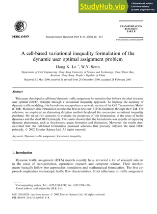
  • 6. 3.1. Cell Transmission Model (CTM): basic principles The LWR model can be stated by the following two conditions: oy ox þ ok ox ¼ 0 and y ¼ Y ðk; xÞ; ð7Þ where y is the traffic flow, k the density, x and x, respectively, the space and time variables, and Y is a function relating y and k. The first partial differential equation states the traffic flow con- servation. The relation Y defines the fundamental diagram. Given a set of well-posed initial conditions, one can determine y and k at any ðx; xÞ by solving (7). In other words, one knows the traffic flow and density at any location x and any time instance x in the modeling horizon. This model is sometimes referred to as the hydrodynamic or kinematic wave model of traffic flow. Lighthill and Whitham (1955) and Newell (1991) developed two different solution approaches to this model. Daganzo (1994, 1995a) simplified the solution scheme by adopting the following re- lationship between traffic flow, y, and density, k: y ¼ minfVk; Q; W ðkjam kÞg; ð8Þ where kjam; Q; V ; W denote, respectively, jam density, inflow capacity (or maximum allowable inflow), free-flow speed and the speed of the backward shock wave (or the backward propagation speed of disturbances in congested traffic), then the LWR equations for a single highway link are approximated by a set of difference equations. Essentially, (8) approximates the fundamental diagram by a piece-wise linear model as shown in Fig. 1. By discretizing the road into homogeneous sections (or cells) and time into intervals such that the cell length is equal to the distance traveled by free-flowing traffic in one time interval, then the LWR results are approximated by this set of recursive equations (Daganzo, 1994, 1995a): njðx þ 1Þ ¼ njðxÞ þ yjðxÞ yjþ1ðxÞ; ð9Þ yjðxÞ ¼ minfnj 1ðxÞ; QjðxÞ; ðW =V Þ NjðxÞ njðxÞ g; ð10Þ where the subscript j refers to cell j, and j þ 1ðj 1Þ represents the cell downstream (upstream) of j. The variables njðxÞ; yjðxÞ; NjðxÞ denote the number of vehicles, the actual inflow, and the maximum number of vehicles (or holding capacity) that can be held in cell j at time x, respec- tively. The variables QjðxÞ; V ; W follow the earlier definitions. It is important to differentiate Flow y Qmax V W Density Fig. 1. The fundamental diagram used in CTM. 426 H.K. Lo, W.Y. Szeto / Transportation Research Part B 36 (2002) 421–443
  • 7. between QjðxÞ and yjðxÞ: the former is the inflow capacity while the latter is the actual inflow. Because (9) and (10) provide a numerical approximation to the LWR equations, all the traffic phenomena demonstrated in the LWR model are replicated in CTM. The key is to determine yjðxÞ from the minimization (10). Once this is accomplished, njðxÞ can be determined recursively from the linear equations (9). Eqs. (9) and (10) provide the basic principle of modeling traffic flow on a series of straight cells. To apply this principle to a general network with multiple OD pairs, three extensions are re- quired: (a) modeling merge and diverge junctions; (b) differentiating the OD specific traffic; (c) maintaining the FIFO property. To maintain the intended routes of traffic and the FIFO prop- erty, traffic in each cell is disaggregated by route ðpÞ and waiting time at the cell ðsÞ. The route variable is used to direct traffic along its route. By tracking s, the FIFO property at the cell level is maintained by ensuring that earlier arrivals (with a larger s) will leave sooner. The detailed mathematical operations to ensuring these conditions were addressed in Daganzo (1995a) and Lo (1999b). The description of which is lengthy; in the interest of space, we do not repeat the analysis here but illustrate it with an example through the origin cell. For the construction of an origin cell, we create a cell just upstream of an origin cell with an infinite capacity to store the traffic that intends to enter the network. Let us call this cell r 1. To load traffic into the network according to the departing demand f rs p ðtÞ, we set the inflow into this cell at the time instance x ¼ t such that: yr 1;pðxÞ ¼ f rs p ðtÞ; nr 1;pðx þ 1Þ ¼ nr 1;pðxÞ þ yr 1;pðxÞ yr;pðxÞ: ð11Þ The subscripts r, p extend the definitions of inflow and occupancy for each cell under these con- ditions: cell location – r, route – p. Note that yr;p is the outflow of r 1 but inflow to the origin cell r, which is subject to the congestion and flow restriction effects at r similar to the expression in (10). Once the traffic is loaded to the network, the basic principles of (9) and (10) and the conditions for merge and diverge (not shown here) hold to ensure proper dynamics of traffic propagation. In brevity, given a set of time-sequenced inflow f rs p ðtÞ as in (11), based on the traffic propagation conditions (i.e., such as the recursive equations (9) and (10)), one can obtain a set of unique occupancy counts nj;pðxÞ for traffic in cell j on route p at any time instance x. Such information on cell occupancy is used to determine the actual route travel times for the entire modeling horizon. In addition to modeling network traffic, CTM can be easily modified to handle signalized networks as well as the occurrence of incident or link blockage. Traffic signals and incidents can be modeled by modifying the values of the flow capacity QjðxÞ of the affected cells. Specifically, for the case of signals, the inflow capacity of the signalized cells can be altered according to whether the time is in a green or red phase: QjðxÞ ¼ sf for x 2 green phase and j 2 a signalized cell; QjðxÞ ¼ 0 for x 2 red phase and j 2 a signalized cell; where sf is the saturation flow rate. One could model both fixed and dynamic timing plans with CTM, as demonstrated in Lo (1999a, 2001). The treatment of incident modeling is similar. To summarize, this section described a way to model the propagation of traffic flow in the network. By tracking the flow’s departure time, route and waiting time at each cell along the H.K. Lo, W.Y. Szeto / Transportation Research Part B 36 (2002) 421–443 427
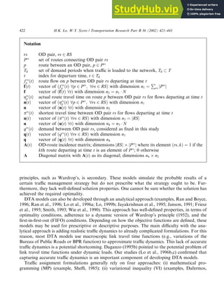
  • 8. route, one can determine the occupancy of each packet of traffic on route p in each cell and at each time instance throughout the modeling horizon. 3.2. Determination of actual route travel time Knowing the occupancy of each package of traffic on route p in origin cell r and destination cell s at each time instance, the actual en route travel time grs p ðtÞ of flow f rs p ðtÞ can be determined through the use of cumulative counts. Let kr pðtÞ be the cumulative traffic departing from cell r on route p at time t and ks pðxÞ be the cumulative traffic arriving at cell s on route p at time x, defined by: kr pðtÞ ¼ X t0 6 t nr;pðt0 Þ; ð12Þ ks pðxÞ ¼ X x0 6 x ns;pðx0 Þ: ð13Þ Fig. 2 shows that the cumulative count curves kr pðtÞ and ks pðxÞ on route p between OD pair rs. The actual en route travel time of traffic departing at t (i.e., f rs p ðtÞ) is the horizontal distance between the two cumulative curves as shown in Fig. 2. If time is discretized, subject to the en route conditions, there is no guarantee that the entire packet f rs p ðtÞ will arrive at the destination s in the same discretized time tick x. As shown in Fig. 2, the front part of the packet has an actual travel time of g whereas the latter parts have longer actual travel times. The extent of this difference in en route travel times of the same departing packet depends on the size of the discretized time. Ac- curacy can be introduced with finer departure time intervals at the expense of requiring more cells, more time intervals, and eventually higher computational efforts. In this study, we adopt the following averaging scheme so that the entire departing traffic f rs p ðtÞ has one uniquely determined average en route travel time grs p ðtÞ. Mathematically, this scheme can be stated as: grs p ðtÞ ¼ Rkr pðtÞ kr pðt 1Þ ks 1 p ðtÞ kr 1 p ðtÞ h i dt kr pðtÞ kr pðt 1Þ ; ð14Þ Fig. 2. The cumulative vehicle counts in origin cell r and destination cell s. 428 H.K. Lo, W.Y. Szeto / Transportation Research Part B 36 (2002) 421–443
  • 9. where f rs p ðtÞ ¼ kr pðtÞ kr pðt 1Þ: ð15Þ The numerator on the right-hand side of (14) is the area of the shaded region in Fig. 2 or the total en route travel time of the entire packet f rs p ðtÞ. The denominator is the packet departing at time t as defined in (15). The above averaging scheme is well defined for used routes with positive departure flows. For an unused route with f rs p ðtÞ ¼ 0, we define its actual route travel time to be equal to that of f rs p ðtÞ ¼ r; r ! 0þ . For an infinitely small r, the whole packet shall arrive at the same discretized tick. According to (14), grs p ðtÞ ¼ ðg rÞ=r ¼ g or x t. Summarizing, we have this definition: Definition 1. The actual en route travel time of an unused route is defined to be that of an infi- nitely small traffic traveling on the route. Let us consider the following case: assuming that a particular departure f rs p ðtÞ arrives at the destination in m sub-packets with arrival times at the destination to be t þ 1, t þ 2; ; t þ m, respectively. Let the amount of traffic in each sub-packet to be ak, k ¼ 1; . . . ; m, where ak P 0 and X m k¼1 ak ¼ f rs p ðtÞ: ð16Þ Obviously, ak is a function of f. More congested situations will render a later arrival of the first packet, making the earlier ak ¼ 0. We have the following assumption: Assumption 1. A small change in the departure flow pattern will incur a small change in the arrival pattern. Specifically, this assumption can be stated as: 8e 0; 9d such that jf0 fj 6 e ) ja0 k akj 6 de for all k; where f; f0 2 Rn2 þ , ak, a0 k P 0, d and e are infinitely small. ak and a0 k correspond to the arrival pat- terns of f and f0 , respectively. Proposition 1. Under Assumption 1, the actual route travel time n is a continuous function of f. Proof. To prove that n is a continuous function of f, we prove that each component of n (i.e., grs p ðtÞ) is. Given that f 2 Rn2 þ , we show that (14) is a continuous function of f. For an arbitrary flow vector f, through the traffic model (CTM in this case), one can obtain a set of uniquely determined cumulative arrival curve for each route p departed at t. Putting the general expression (16) into (14), one has: grs p ðtÞ ¼ a1ðt þ 1 tÞ þ a2ðt þ 2 tÞ þ þ amðt þ m tÞ a1 þ a2 þ þ am ¼ a1 þ 2a2 þ þ mam f rs p ðtÞ ; which is a continuous function under Assumption 1 for positive f rs p ðtÞ and ak 2 Rþ [ f0g. This completes the proof for the used routes with f rs p ðtÞ 0. For the unused routes with f rs p ðtÞ ¼ 0, H.K. Lo, W.Y. Szeto / Transportation Research Part B 36 (2002) 421–443 429
  • 10. according to Definition 1, their actual travel times are equivalent to those of f rs p ðtÞ ¼ r, where r is a positive small constant. Thus, this proof also works for the actual travel times of unused routes. Without loss of generality, the above proof works for each component of n and therefore for n. This completes the proof. One thing to note is that even though n defined in (14) is a continuous function of f, it is not continuously differentiable with respect to f. If one were to hold the arrival pattern in Fig. 2 constant while varying f rs p ðtÞ, one would observe that grs p ðtÞ is non-differentiable at the kinks of f rs p ðtÞ ¼ a; a þ b or a þ b þ c or at each separation of arrivals of the sub-packets, as shown in Fig. 3. This non-smooth property renders solution methods based on derivatives of n with respect to f rather difficult. This is why solution methods based on projections are more suitable for this problem. 3.3. First-in-first-out (FIFO) conditions FIFO plays an importance role in DUO problems. Three types of FIFO conditions are ad- dressed in the literature, namely, cell, route, and OD. The cell (route) FIFO condition is satisfied if every user who enters the cell (route) earlier will leave sooner. Likewise, the OD FIFO condition is satisfied if every user who departs from the origin cell earlier will arrive at its destination sooner. Mathematically, they can be written as: Definition 2. (Cell FIFO) The cell FIFO condition is satisfied if and only if x0 j x00 j ) x0 j þ hjðx0 Þ x00 j þ hjðx00 j Þ 8j 2 J; 8x0 j; x00 j 2 -; where - is the set containing integer from 1 to N, J is the set of cells, hjðxjÞ is the travel time in cell j for flows entering at xj. Similarly, Definition 3. (Route FIFO) The route FIFO condition is satisfied if and only if t0 t00 ) t0 þ grs p ðt0 Þ t00 þ grs p ðt00 Þ 8p 2 Prs ; 8rs 2 RS; 8t0 ; t00 2 Td: Fig. 3. The actual travel time function while fixing the arrival pattern. 430 H.K. Lo, W.Y. Szeto / Transportation Research Part B 36 (2002) 421–443
  • 11. Definition 4. (OD FIFO) The OD FIFO condition is satisfied if and only if t0 t00 ) t0 þ prs ðt0 Þ t00 þ prs ðt00 Þ 8rs 2 RS; 8t0 ; t00 2 Td: In our formulation, the CTM ensures the cell FIFO condition in its entirety through carefully tracking the waiting time of each packet at the cell (see Daganzo, 1995a). Given the cell FIFO condition, route FIFO can be proven through repeatedly applying the principle of cell FIFO along a particular route. Proposition 2. The Cell FIFO condition implies the Route FIFO condition. Proof. We consider a traffic packet traveling along route p consisting of j ¼ 1; . . . ; k cells. Let xj 2 - be its entry time into cell j; x1 2 Td its entry time into the first cell; and xkþ1 the time the packet leaves the route. The entry time into the next cell j þ 1 is: xjþ1 ¼ xj þ hjðxjÞ. Using the Cell FIFO definition, x0 j x00 j ) x0 jþ1 x00 jþ1; j ¼ 1; 2; . . . ; k 1. Applying this relationship recursively, one obtains: x0 1 x00 1 ) x0 kþ1 x00 kþ1. Since xkþ1 ¼ x1 þ gpðx1Þ, it becomes: x0 1 x00 1 ) x0 1 þ gpðx0 1Þ x00 1 þ gpðx00 1Þ. In other words, for traffic packets that entered the first cell on p earlier, they will leave it sooner. This completes the proof. Finally, Route FIFO together with the DUO conditions implies the OD FIFO condition (Theorem 2.1 in Wu et al., 1998). Therefore, in this DUO formulation, by guaranteeing the cell FIFO condition, which is achieved by the CTM, it satisfies both route and OD FIFO. One thing to note is that the scheme adopted for determining the actual route travel time averages out the travel times of the faster and slower sub-packets within the same departing packet. Hence, the OD FIFO property is only approximate. Obviously, these FIFO properties are subject to the accuracy of the time discretization adopted. Finer departing time steps and smaller cell sizes will improve these FIFO properties as desired. Summarizing, given a route flow vector f, we determine the cumulative counts in each cell by route and time according to the CTM. Based on these cumulative counts, we determine the actual route travel for each departing flow according to the averaging scheme (14). As the CTM de- termines a unique set of cumulative counts from f and the averaging scheme determines a unique set of route travel times n from the cumulative count curves, through these two processes, one establishes a one-to-one mapping from f to n. This mapping is continuous and ensures the properties of cell, route, and OD FIFO. 4. A solution method based on alternating direction The non-smooth nature of the route travel time function renders solution methods based on derivative information rather difficult. Therefore, we develop a solution method aimed at solving the VIP (5) and (6) with projection methods. We begin by attaching a Lagrangian multiplier u 2 Rn4 to the linear demand constraint Af ¼ q to obtain the following equivalent VIP: find x 2 W such that: ðx x ÞT Fðx Þ P 0; x 2 W; ð17Þ H.K. Lo, W.Y. Szeto / Transportation Research Part B 36 (2002) 421–443 431
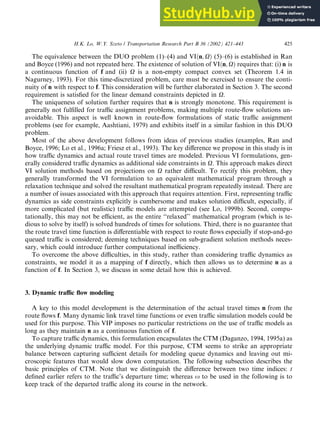
  • 12. where x ¼ f u ; FðxÞ ¼ nðfÞ AT u Af q ; W 2 Rn2 þ Rn4 : ð18Þ The motivation for this modification is to construct a set W that has an easier projection than on the original set X in (6). For this type of problem, Gabay and Mercier (1976) and Gabay (1983) proposed the following alternating direction method: • Given ðfk ; uk Þ 2 Rn2 þ Rn4 at the kth iteration, find fk 2 Rn2 þ such that: ðf0 fkþ1 ÞT nðfkþ1 Þ AT uk bkþ1ðAfkþ1 qÞ P 0 8f0 2 Rn2 þ : ð19Þ • Then update u via: ukþ1 ¼ uk bkþ1ðAfkþ1 qÞ; ð20Þ where bkþ1 0 is a given penalty parameter (or a sequence of parameters) for the linear constraint Af ¼ q. With known uk , bkþ1, the bracket fg on the left-hand side of (19) is a function of fkþ1 . Thus, (19) is a reduced VIP sub-problem involving only f. Alternating direction method is attractive for large- scale problems if the sub-problems can be solved efficiently. Nevertheless, solving the sub-problem (19) exactly could be computationally intensive by itself. Moreover, there is little justification to solve it exactly at each iteration, especially when u is far away from u . To overcome this shortcoming of Gabay’s approach, recently, He and Zhou (2000) proposed a modified alternating direction method for the case of nðfÞ ¼ Mf þ b, where M is a symmetric positive semi-definite matrix and b is a given vector. He and Zhou’s method is attractive for its simplicity since each iteration requires only one projection to the simple convex set and a function evaluation. However, for this DUO problem, the underlying mapping nðfÞ is neither symmetric nor linear. Recently, Zhu and Marcotte (1996) considered the case of co-coercive mappings and proved that many iterative schemes based on the auxiliary problem framework (Cohen, 1988) and the projection method proposed by Bertsekas and Gafni (1987) converge to a solution of VIðn; XÞ. Motivated by these studies, in Han and Lo (2001), we recently developed a modified alternating direction method by extending He and Zhou (2000) solution method for non-linear mappings. The solution method has been proven to be convergent for co-coercive mappings of nðfÞ. Definition 5. Let U be a non-empty close convex subset of Rn , an operator F : U ! Rn is said to be co-coercive if there exists a positive constant l such that ðu vÞT ½F ðuÞ F ðvÞ P lkF ðuÞ F ðvÞk2 8u; v 2 U. According to Zhu and Marcotte (1996), co-coercive mappings are monotone but may not necessarily be strongly monotone. Conversely, strongly monotone and Lipschitz continuous mappings are co-coercive. Thus, co-coercive mappings are an intermediate concept between simple and strongly monotone mappings. In Han and Lo (2001), we proved the convergence for this new alternating direction based on: (i) the underlying mapping n(f) is co-coercive on Rn2 þ and (ii) the solution set of VIðn; XÞ is non-empty. In the following, we restate this algorithm based on the approach of alternating 432 H.K. Lo, W.Y. Szeto / Transportation Research Part B 36 (2002) 421–443
  • 13. direction. First, we denote the set K being the same as Rn2 þ and the residual error function for the problem under consideration as: eðx; bÞ ¼ eðf; u; bÞ ¼ f PK f b½nðfÞ AT u bðAf qÞ ; where b is a (set of) given penalty parameter(s) and PKfg the projection on K. It can be verified readily that if eðx; bÞ ¼ 0, the VIP expressed in (17) and (18) is solved. Furthermore, we define rðx; bÞ as: rðx; bÞ ¼ f PKff b½nðfÞ AT ðu bðAf qÞÞ g bðAf qÞ : ð21Þ Likewise, it can be verified that solving the VIP (17) and (18) is equivalent to finding a zero point of rðx; bÞ. The detailed algorithmic steps are the following: Step 0. Given an initial arbitrary point x ¼ ðf0 ; u0 ÞT 2 K Rn4 and positive constants b 4l; e 0, set k ¼ 0 Step 1. Compute x xk ¼ ð f fk ; u uk ÞT 2 K Rn4 by: f fk ¼ PKffk b½nðfk Þ AT ðuk bðAfk qÞÞ g u uk ¼ uk bðA f fk qÞ Step 2. Compute xkþ1 ¼ ðfk ; uk ÞT 2 K Rn4 xkþ1 ¼ xk tkckðxk x xk Þ, where tk ¼ dk 1 b 4l ; dk 2 ð0; 2Þ such that tk 2 ð0; 1Þ and ck ¼ krðxk ; bÞk2 =krðxk ; bk2 H with H ¼ I þ bAT A 0 0 I and krðxk ; bÞk2 H ¼ rT ðxk ; bÞHrðxk ; bÞ Step 3. If krðxkþ1 ; bÞk e, stop; Else set k ¼ k þ 1 and go to Step 1 Each iteration requires the determination of the actual route travel time vector nðfk Þ from route flows of the last iteration. For this purpose, the CTM and the averaging scheme (14) for the entire modeling horizon are executed once per iteration. Furthermore, the algorithm requires merely projections on the non-negative orthant (Step 1) without the need for any matrix inversion. Thus, the computational load per iteration is mild. We are able to solve relatively large networks with this code in reasonable time, as discussed in Section 5. 5. Numerical studies To illustrate this cell-based DUO formulation, we set up two test scenarios. The first scenario is set up to illustrate the dynamic traffic phenomena captured by this formulation. To clearly show the traffic dynamics without being smeared by other factors, this scenario does not pro- vide for route choice considerations for each OD pair. In the second scenario, we demonstrate H.K. Lo, W.Y. Szeto / Transportation Research Part B 36 (2002) 421–443 433
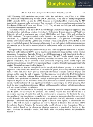
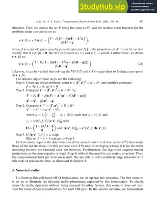
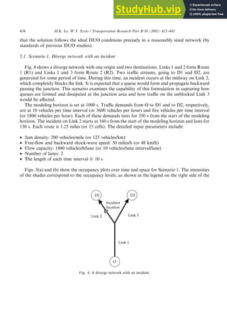
  • 14. that the solution follows the ideal DUO conditions precisely in a reasonably sized network (by standards of previous DUO studies). 5.1. Scenario 1. Diverge network with an incident Fig. 4 shows a diverge network with one origin and two destinations. Links 1 and 2 form Route 1 (R1) and Links 1 and 3 form Route 2 (R2). Two traffic streams, going to D1 and D2, are generated for some period of time. During this time, an incident occurs at the midway on Link 2, which completely blocks the link. It is expected that a queue would form and propagate backward passing the junction. This scenario examines the capability of this formulation in capturing how queues are formed and dissipated at the junction area and how traffic on the unblocked Link 3 would be affected. The modeling horizon is set at 1000 s. Traffic demands from O to D1 and to D2, respectively, are at 10 vehicles per time interval (or 3600 vehicles per hour) and five vehicles per time interval (or 1800 vehicles per hour). Each of these demands lasts for 350 s from the start of the modeling horizon. The incident on Link 2 starts at 160 s from the start of the modeling horizon and lasts for 130 s. Each route is 1.25 miles (or 15 cells). The detailed input parameters include: • Jam density: 200 vehicles/mile (or 125 vehicles/km) • Free-flow and backward shock-wave speed: 30 miles/h (or 48 km/h) • Flow capacity: 1800 vehicles/h/lane (or 10 vehicles/time interval/lane) • Number of lanes: 2 • The length of each time interval d: 10 s Figs. 5(a) and (b) show the occupancy plots over time and space for Scenario 1. The intensities of the shades correspond to the occupancy levels, as shown in the legend on the right side of the Fig. 4. A diverge network with an incident. 434 H.K. Lo, W.Y. Szeto / Transportation Research Part B 36 (2002) 421–443
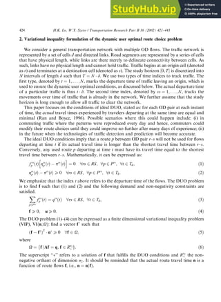
  • 15. plot. As is customary, traffic propagates in the direction of vertical axis, whereas the horizontal axis is for time. One can see how the incident on Link 2 affects the traffic on Link 3. Queue formation, queue dissipation and shock waves are also evidenced in Figs. 5(a) and (b). In Fig. 5(a), after the incident occurred on Link 2 at t ¼ 160, a queue is formed that spills backward towards the junction. When the end of queue spills beyond the junction, it affects the traffic Fig. 5. The occupancy plots for Scenario 1: (a) the occupancy plot along Route 1 (R1); (b) the occupancy plot along Route 2 (R2). H.K. Lo, W.Y. Szeto / Transportation Research Part B 36 (2002) 421–443 435
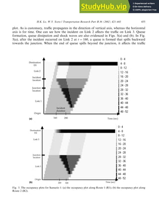
  • 16. destined for D2 also. From Fig. 5(b), despite that Link 3 is empty, traffic for D2 cannot leave the junction until after t ¼ 320, when the queue on Link 2 has started to dissipate. Note that the destination cell is modeled as a traffic sink that has an infinite capacity; all the traffic that enters this cell is considered to have left the network. To summarize, this formulation is capable of capturing traffic interactions across multiple links, including such details as the queue formation and dissipation at the junction area. Fig. 6. Nguyen and Dupius’s 13-node network. Fig. 7. Cell representation of Nguyen and Dupius’s 13-node network. 436 H.K. Lo, W.Y. Szeto / Transportation Research Part B 36 (2002) 421–443
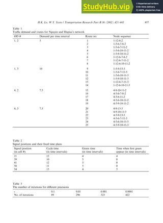
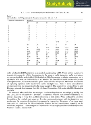
  • 17. Table 3 The number of iterations for different precisions 0.1 0.01 0.001 0.0001 No. of iterations 89 296 323 422 Table 1 Traffic demand and routes for Nguyen and Dupius’s network OD # Demand per time interval Route no. Node sequence 1, 2 5 1 1-12-8-2 2 1-5-6-7-8-2 3 1-5-6-7-11-2 4 1-5-6-10-11-2 5 1-5-9-10-11-2 6 1-12-6-7-8-2 7 1-12-6-7-11-2 8 1-12-6-10-11-2 1, 3 10 9 1-5-9-13-3 10 1-5-6-7-11-3 11 1-5-6-10-11-3 12 1-5-9-10-11-3 13 1-12-6-7-11-3 14 1-12-6-10-11-3 4, 2 7.5 15 4-9-10-11-2 16 4-5-6-7-8-2 17 4-5-6-11-2 18 4-5-6-10-11-2 19 4-5-9-10-11-2 4, 3 7.5 20 4-9-13-3 21 4-9-10-11-3 22 4-5-9-13-3 23 4-5-6-7-11-3 24 4-5-6-10-11-3 25 4-5-9-10-11-3 Table 2 Signal positions and their fixed time plans Signal position (in cell #) Cycle time (in time intervals) Green time (in time intervals) Time when first green appear (in time intervals) 21 12 4 4 39 10 5 0 41 12 5 0 50 11 5 0 54 15 4 5 H.K. Lo, W.Y. Szeto / Transportation Research Part B 36 (2002) 421–443 437
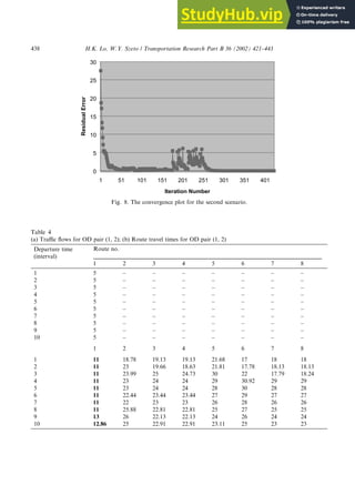
  • 18. Fig. 8. The convergence plot for the second scenario. Table 4 (a) Traffic flows for OD pair (1, 2); (b) Route travel times for OD pair (1, 2) Departure time (interval) Route no. 1 2 3 4 5 6 7 8 1 5 – – – – – – – 2 5 – – – – – – – 3 5 – – – – – – – 4 5 – – – – – – – 5 5 – – – – – – – 6 5 – – – – – – – 7 5 – – – – – – – 8 5 – – – – – – – 9 5 – – – – – – – 10 5 – – – – – – – 1 2 3 4 5 6 7 8 1 11 18.78 19.13 19.13 21.68 17 18 18 2 11 23 19.66 18.63 21.81 17.78 18.13 18.13 3 11 23.99 25 24.73 30 22 17.79 18.24 4 11 23 24 24 29 30.92 29 29 5 11 23 24 24 28 30 28 28 6 11 22.44 23.44 23.44 27 29 27 27 7 11 22 23 23 26 28 26 26 8 11 25.88 22.81 22.81 25 27 25 25 9 13 26 22.13 22.13 24 26 24 24 10 12.86 25 22.91 22.91 23.11 25 23 23 438 H.K. Lo, W.Y. Szeto / Transportation Research Part B 36 (2002) 421–443
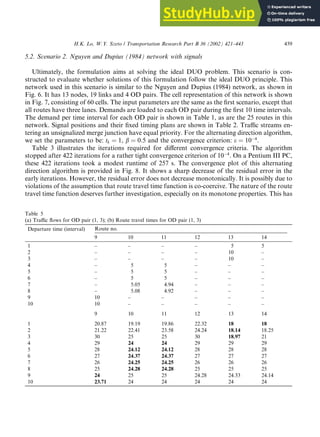
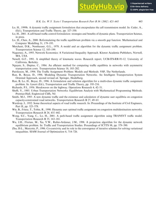
  • 19. 5.2. Scenario 2. Nguyen and Dupius (1984) network with signals Ultimately, the formulation aims at solving the ideal DUO problem. This scenario is con- structed to evaluate whether solutions of this formulation follow the ideal DUO principle. This network used in this scenario is similar to the Nguyen and Dupius (1984) network, as shown in Fig. 6. It has 13 nodes, 19 links and 4 OD pairs. The cell representation of this network is shown in Fig. 7, consisting of 60 cells. The input parameters are the same as the first scenario, except that all routes have three lanes. Demands are loaded to each OD pair during the first 10 time intervals. The demand per time interval for each OD pair is shown in Table 1, as are the 25 routes in this network. Signal positions and their fixed timing plans are shown in Table 2. Traffic streams en- tering an unsignalized merge junction have equal priority. For the alternating direction algorithm, we set the parameters to be: tk ¼ 1, b ¼ 0:5 and the convergence criterion: e ¼ 10 4 . Table 3 illustrates the iterations required for different convergence criteria. The algorithm stopped after 422 iterations for a rather tight convergence criterion of 10 4 . On a Pentium III PC, these 422 iterations took a modest runtime of 257 s. The convergence plot of this alternating direction algorithm is provided in Fig. 8. It shows a sharp decrease of the residual error in the early iterations. However, the residual error does not decrease monotonically. It is possibly due to violations of the assumption that route travel time function is co-coercive. The nature of the route travel time function deserves further investigation, especially on its monotone properties. This has Table 5 (a) Traffic flows for OD pair (1, 3); (b) Route travel times for OD pair (1, 3) Departure time (interval) Route no. 9 10 11 12 13 14 1 – – – – 5 5 2 – – – – 10 – 3 – – – – 10 – 4 – 5 5 – – – 5 – 5 5 – – – 6 – 5 5 – – – 7 – 5.05 4.94 – – – 8 – 5.08 4.92 – – – 9 10 – – – – – 10 10 – – – – – 9 10 11 12 13 14 1 20.87 19.19 19.86 22.32 18 18 2 21.22 22.41 23.58 24.24 18.14 18.25 3 30 25 25 30 18.97 21 4 29 24 24 29 29 29 5 28 24.12 24.12 28 28 28 6 27 24.37 24.37 27 27 27 7 26 24.25 24.25 26 26 26 8 25 24.28 24.28 25 25 25 9 24 25 25 24.28 24.33 24.14 10 23.71 24 24 24 24 24 H.K. Lo, W.Y. Szeto / Transportation Research Part B 36 (2002) 421–443 439
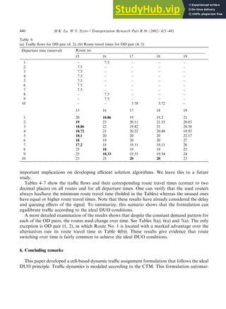
  • 20. important implications on developing efficient solution algorithms. We leave this to a future study. Tables 4–7 show the traffic flows and their corresponding route travel times (correct to two decimal places) on all routes and for all departure times. One can verify that the used route/s always has/have the minimum route travel time (bolded in the Tables) whereas the unused ones have equal or higher route travel times. Note that these results have already considered the delay and queuing effects of the signal. To summarize, this scenario shows that the formulation can equilibrate traffic according to the ideal DUO conditions. A more detailed examination of the results shows that despite the constant demand pattern for each of the OD pairs, the routes used change over time. See Tables 5(a), 6(a) and 7(a). The only exception is OD pair (1, 2), in which Route No. 1 is located with a marked advantage over the alternatives (see its route travel time in Table 4(b)). These results give evidence that route switching over time is fairly common to achieve the ideal DUO conditions. 6. Concluding remarks This paper developed a cell-based dynamic traffic assignment formulation that follows the ideal DUO principle. Traffic dynamics is modeled according to the CTM. This formulation automat- Table 6 (a) Traffic flows for OD pair (4, 2); (b) Route travel times for OD pair (4, 2) Departure time (interval) Route no. 15 16 17 18 19 1 – 7.5 – – – 2 7.5 – – – – 3 7.5 – – – – 4 7.5 – – – – 5 7.5 – – – – 6 7.5 – – – – 7 7.5 – – – – 8 – 7.5 – – – 9 – 7.5 – – – 10 – – 3.78 3.72 – 15 16 17 18 19 1 20 18.86 19 19.2 21 2 19 23 20.11 21.35 20.85 3 18.86 22 19.42 21 20.58 4 18.72 21 20.32 20.49 19.93 5 18.1 20 20 20 22.17 6 18 19 20 20 27 7 17.2 18 19.11 19.11 26 8 25 18 19 19 25 9 25 18.33 19.33 19.34 24 10 23 25 20 20 23 440 H.K. Lo, W.Y. Szeto / Transportation Research Part B 36 (2002) 421–443
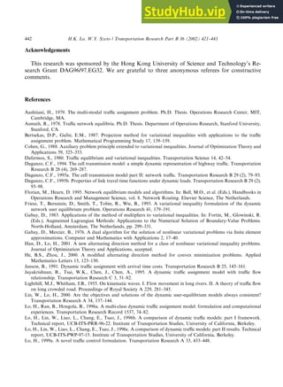
  • 21. ically satisfies the FIFO conditions as a result of encapsulating CTM. We set up two scenarios to evaluate the properties of this formulation, in the areas of traffic dynamics, traffic interactions across multiple links, and the ideal DUO principle. This formulation produced outputs that are in agreement with what the results ought to be. Namely, the formulation is able to capture dynamic traffic phenomena, such as shockwaves, queue formation and dissipation. Moreover, it is capable of capturing dynamic traffic interactions across multiple links. Both of these characteristics are inherent from the underlying traffic model adopted. The results from solving Nguyen and Dupius’s network demonstrated that this cell-based formulation follows the ideal DUO principle precisely. To solve this VI formulation, we employed an alternating direction method proposed by Han and Lo (2001) for co-coercive VI problems. This method requires that route travel time is a co- coercive mapping of route flow and the solution set is non-empty. While sufficient to solve this formulation, the residual error does not drop in a monotonic manner with the iterations, sug- gesting that the route travel time function may not be co-coercive. The nature of the route travel time function considered in this formulation deserves further investigation, especially on its monotone properties. This has important implications on developing efficient solution algorithms. We leave this to a future study. Table 7 (a) Traffic flows for OD pair (4, 3); (b) Route travel times for OD pair (4, 3) Departure time (interval) Route no. 20 21 22 23 24 25 1 7.5 – – – – – 2 7.5 – – – – – 3 7.5 – – – – – 4 7.5 – – – – – 5 7.5 – – – – – 6 7.5 – – – – – 7 7.5 – – – – – 8 7.5 – – – – – 9 7.5 – – – – – 10 – – – 3.75 3.75 – 20 21 22 23 24 25 1 11 20 20.38 19.16 19.16 21.63 2 19 20.09 21.38 19.83 19.99 21.57 3 18.6 21.07 21 21.36 21.78 21.83 4 18.15 20 20.71 21.21 24.72 21.71 5 18 19 20 21 21 21 6 17.52 19 22.92 20 20 22.41 7 17 18.51 26 19 19 26 8 16.52 18 25 19.14 19.14 25 9 16 22.74 24 19.3 19.3 24 10 23 23 23 20 20 23 H.K. Lo, W.Y. Szeto / Transportation Research Part B 36 (2002) 421–443 441
  • 22. Acknowledgements This research was sponsored by the Hong Kong University of Science and Technology’s Re- search Grant DAG96/97.EG32. We are grateful to three anonymous referees for constructive comments. References Aashtiani, H., 1979. The multi-modal traffic assignment problem. Ph.D. Thesis. Operations Research Center, MIT, Cambridge, MA. Asmuth, R., 1978. Traffic network equilibria. Ph.D. Thesis. Department of Operations Research, Stanford University, Stanford, CA. Bertsekas, D.P., Gafni, E.M., 1987. Projection method for variational inequalities with applications to the traffic assignment problem. Mathematical Programming Study 17, 139–159. Cohen, G., 1988. Auxiliary problem principle extended to variational inequalities. Journal of Optimization Theory and Applications 59, 325–333. Dafermos, S., 1980. Traffic equilibrium and variational inequalities. Transportation Science 14, 42–54. Daganzo, C.F., 1994. The cell transmission model: a simple dynamic representation of highway traffic. Transportation Research B 28 (4), 269–287. Daganzo, C.F., 1995a. The cell transmission model part II: network traffic. Transportation Research B 29 (2), 79–93. Daganzo, C.F., 1995b. Properties of link travel time functions under dynamic loads. Transportation Research B 29 (2), 93–98. Florian, M., Hearn, D. 1995. Network equilibrium models and algorithms. In: Ball, M.O., et al. (Eds.), Handbooks in Operations Research and Management Science, vol. 8. Network Routing. Elsevier Science, The Netherlands. Friesz, T., Bernstein, D., Smith, T., Tobin, R., Wie, B., 1993. A variational inequality formulation of the dynamic network user equilibrium problem. Operations Research 41, 179–191. Gabay, D., 1983. Applications of the method of multipliers to variational inequalities. In: Fortin, M., Glowinski, R. (Eds.), Augmented Lagrangian Methods: Applications to the Numerical Solution of Boundary-Value Problems. North-Holland, Amsterdam, The Netherlands, pp. 299–331. Gabay, D., Mercier, B., 1976. A dual algorithm for the solution of nonlinear variational problems via finite element approximations. Computer and Mathematics with Applications 2, 17–40. Han, D., Lo, H., 2001. A new alternating direction method for a class of nonlinear variational inequality problems. Journal of Optimization Theory and Applications, accepted. He, B.S., Zhou, J., 2000. A modified alternating direction method for convex minimization problems. Applied Mathematics Letters 13, 123–130. Janson, B., 1991. Dynamic traffic assignment with arrival time costs. Transportation Research B 25, 143–161. Jayakrishnan, R., Tsai, W.K., Chen, J., Chen, A., 1995. A dynamic traffic assignment model with traffic flow relationship. Transportation Research C 3, 51–82. Lighthill, M.J., Whitham, J.B., 1955. On kinematic waves. I. Flow movement in long rivers. II. A theory of traffic flow on long crowded road. Proceedings of Royal Society A 229, 281–345. Lin, W., Lo, H., 2000. Are the objectives and solutions of the dynamic user-equilibrium models always consistent? Transportation Research A 34, 137–144. Lo, H., Ran, B., Hongola, B., 1996a. A multi-class dynamic traffic assignment model: formulation and computational experiences. Transportation Research Record 1537, 74–82. Lo, H., Lin, W., Liao, L., Chang, E., Tsao, J., 1996b. A comparison of dynamic traffic models: part I framework. Technical report, UCB-ITS-PRR-96-22. Institute of Transportation Studies, University of California, Berkeley. Lo, H., Lin, W., Liao, L., Chang, E., Tsao, J., 1996c. A comparison of dynamic traffic models: part II results. Technical report, UCB-ITS-PWP-97-15. Institute of Transportation Studies, University of California, Berkeley. Lo, H., 1999a. A novel traffic control formulation. Transportation Research A 33, 433–448. 442 H.K. Lo, W.Y. Szeto / Transportation Research Part B 36 (2002) 421–443
  • 23. Lo, H., 1999b. A dynamic traffic assignment formulation that encapsulates the cell transmission model. In: Ceder, A., (Ed.), Transportation and Traffic Theory, pp. 327–350. Lo, H., 2001. A cell-based traffic control formulation: strategies and benefits of dynamic plans. Transportation Science, in press. Lo, H., Chen, A., 2000. Reformulating the traffic equilibrium problem via a smooth gap function. Mathematical and Computer Modelling 31, 179–195. Merchant, D.K., Nemhauser, G.L., 1978. A model and an algorithm for the dynamic traffic assignment problem. Transportation Science 12, 183–199. Nagurney, A., 1993. Network Economics: A Variational Inequality Approach. Kluwer Academic Publishers, Norwell, MA, USA. Newell, G.F., 1991. A simplified theory of kinematic waves. Research report, UCB-ITS-RR-91-12. University of California, Berkeley. Nguyen, S., Dupius, C., 1984. An efficient method for computing traffic equilibria in networks with asymmetric transportation costs. Transportation Science 18, 185–202. Patriksson, M., 1994. The Traffic Assignment Problem: Models and Methods. VSP, The Netherlands. Ran, B., Boyce, D., 1996. Modeling Dynamic Transportation Networks. An Intelligent Transportation System Oriented Approach, second revised ed. Springer, Heidelberg. Ran, B, Lo, H., Boyce, D., 1996. A formulation and solution algorithm for a multi-class dynamic traffic assignment problem. In: Lesort (Ed.), Transportation and Traffic Theory, pp. 195–216. Richards, P.I., 1956. Shockwaves on the highway. Operations Research 4, 42–51. Sheffi, Y., 1985. Urban Transportation Networks: Equilibrium Analysis with Mathematical Programming Methods. Prentice-Hall, Englewood Cliffs, NJ. Smith, M.J., 1993. A new dynamic traffic and the existence and calculation of dynamic user equilibria on congestion capacity-constrained road networks. Transportation Research B 27, 49–63. Wardrop, J., 1952. Some theoretical aspects of road traffic research. In: Proceedings of the Institute of Civil Engineers, Part II, pp. 325–378. Wie, B., Friesz, T., Tobin, R., 1990. Dynamic user optimal traffic assignment on congestion multidestination networks. Transportation Research B 24, 431–442. Wong, S.C., Yang, C., Lo, H., 2001. A path-based traffic assignment algorithm using TRANSYT traffic model. Transportation Research B 35, 163–181. Wu, J.H., Florian, M., Xu, Y.W., Rubio-Ardanaz, J.M., 1998. A projection algorithm for the dynamic network equilibrium problem. In: Traffic and Transportation Studies. Proceedings of ICTTS 98, pp. 379–390. Zhu, D.L., Marcotte, P., 1996. Co-coercivity and its role in the convergence of iterative schemes for solving variational inequalities. SIAM Journal of Optimization 6, 714–726. H.K. Lo, W.Y. Szeto / Transportation Research Part B 36 (2002) 421–443 443