


![top layer L layer l evidence layer
RLDA vs. other
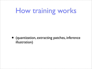
igure 3: RLDA conditional probabilities for a two-layer model, which is then generalized to an L-layer model
hierarchies
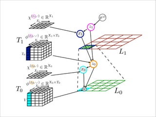
: Comparison of the top performing RLDA with 128 components at L0 and 1024 components at layer L1 t
hical approaches. “bottom” is used to denote the L0 features of the RLDA model, “top” for L1 features, while
stacked features from L0 and L1 layers.
Approach Caltech-101
Model Layer(s) used 15 30
RLDA (1024t/128b) bottom 56.6 ± 0.8% 62.7 ± 0.5%
Our Model RLDA (1024t/128b) top 66.7 ± 0.9% 72.6 ± 1.2%
RLDA (1024t/128b) both 67.4 ± 0.5 73.7 ± 0.8%
Sparse-HMAX [21] top 51.0% 56.0%
CNN [15] bottom – 57.6 ± 0.4%
CNN [15] top – 66.3 ± 1.5%
Hierarchical CNN + Transfer [2] top 58.1% 67.2%
Models CDBN [17] bottom 53.2 ± 1.2% 60.5 ± 1.1%
CDBN [17] both 57.7 ± 1.5% 65.4 ± 0.4%
Hierarchy-of-parts [8] both 60.5% 66.5%
Ommer and Buhmann [23] top – 61.3 ± 0.9%
-101 evaluations. A spatial pyramid with 3 layers of components, demonstrating the lack of discrimina
re grids of 1, 2, and 4 cells each was always con- the baseline LDA-SIFT model: for 1024 topics the](https://image.slidesharecdn.com/aprobabilisticmodelforrecursivefactorizedimagefeaturesppt-110428055538-phpapp02/85/A-probabilistic-model-for-recursive-factorized-image-features-ppt-35-320.jpg)


A probabilistic model for recursive factorized image features ppt
- 1. A probabilistic model for recursive factorized image features. Sergey Karayev Mario Fritz Sanja Fidler Trevor Darrell
- 2. Outline • Motivation: ✴Distributed coding of local image features ✴Hierarchical models ✴Bayesian inference • Our model: Recursive LDA • Evaluation
- 3. Local Features • Gradient energy histograms by orientation and grid position in local patches. • Coded and used in bag-of-words or spatial model classifiers.
- 4. Feature Coding • Traditionally vector quantized as visual words. Local codes vs. Dense codes • But coding as mixture of components, such as in sparse coding, is empirically better. se codes (ascii) (Yang Sparse, distributed codes et al. 2009) Local codes (grandmother cells) ... ... ombinatorial + Decent combinatorial - Low combinatorial ty (2N) capacity (~NK) capacity (N) t to read out + Still easy to read out + Easy to read out picture from Bruno Olshausen
- 5. Another motivation: additive image formation Fritz et al. An Additive Latent Feature Model for Transparent Object Recognition. NIPS (2009).
- 6. Outline • Motivation: ✴Distributed coding of local image features ✴Hierarchical models ✴Bayesian inference • Our model: Recursive LDA • Evaluation
- 7. Hierarchies • Biological evidence for increasing spatial support and complexity of visual pathway. • Local features not robust to ambiguities. Higher layers can help resolve. • Efficient parametrization possible due to sharing of lower-layer components.
- 8. Past Work • HMAX models (Riesenhuber and Poggio 1999, Mutch and Lowe 2008) • Convolutional networks (Ranzato et al. 2007, Ahmed et al. 2009) • Deep Belief Nets (Hinton 2007, Lee et al. 2009) • Hyperfeatures (Agarwal and Triggs 2008) • Fragment-based hierarchies (Ullman 2007) • Stochastic grammars (Zhu and Mumford 2006) • Compositional object representations (Fidler and Leonardis 2007, Zhu et al. 2008)
- 9. articles HMAX was an extension of from simple cells4, near (‘S’ units in the View-tuned cells plate matching, solid ling units6, perform- The nonlinear MAX Complex composite cells (C2) m of the cell’s inputs the model’s proper- near summation of These two types of Composite feature cells (S2) and invariance to ed to different posi- oling over afferents Complex cells (C1) Simple cells (S1) overlap in space weighted sum of the ‘complex’ MAX e stimulus size, size invariance! sing a simplified mechanism, how- variation, even as stimulus Poggio. Hierarchical models of object recognition in cortex. Nature Riesenhuber and mix up signals caused by different stimuli. However, if the affer- ponse would be determined Neuroscience (1999). ents are specific enough to respond only to one pattern, as one
- 10. Convolutional Deep Belief Convolutional Deep Belief Networks for Scalable Unsupervised Learning of Hierarchical Representations (NW NV − NH + 1); the filter weights are shared across all the hidden units within the group. In addi- (# ,# !200#13()*'+, Nets -, tion, each hidden group has a bias bk and all visible units share a single bias c. -+ . $#%' +# !-'.'/.#01()*'+, We define the energy function E(v, h) as: 1 P (v, h) = exp(−E(v, h)) # Stacked layers, each consisting of Z K NH NW feature extraction, E(v, h) = − hk Wrs vi+r−1,j+s−1 ij k k=1 i,j=1 r,s=1 -) - ! )**!#$#%'()*'+, transformation, and K pooling. NH NV Figure 1. Convolutional RBM with probabilistic max- − bk hk ij −c vij . (1) pooling. For simplicity, only group k of the detection layer k=1 i,j=1 i,j=1 and the pooing layer are shown. The basic CRBM corre- sponds to a simplified structure with only visible layer and Using the operators defined previously, detection (hidden) layer. See text for details. K K E(v, h) = − ˜ h • (W ∗ v) − k k vij . To simplify the notation, we consider a model with a bk hk i,j −c k=1 k=1 i,j i,j visible layer V , a detection layer H, and a pooling layer P , as shown in Figure 1. The detection and pooling As with standard RBMs (Section 2.1), we can perform layers both have K groups of units, and each group block Gibbs sampling using the following conditional of the pooling layer has NP × NP binary units. For distributions: each k ∈ {1, ..., K}, the pooling layer P k shrinks the Lee et al. Convolutional deep belief networks for scalable unsupervised learning of H k by a factor representation of the detection layer hierarchical …. ˜ P (hk = 1|v) = theW k ∗ v)ij + bk ) International Conference on Machine where C is(2009) in- Proceedings of σ(( Annual ij 26th of C along each dimension, Learning a small k k teger such as 2 or 3. I.e., the detection layer H k is
- 11. Hyperfeatures Int J Comput Vis (2008) 78: 15–27 17 Fig. 1 Constructing a hyperfeature stack. The ‘level 0’ (base fea- more generally capturing local statistics using posterior membership ture) pyramid is constructed by calculating a local image descriptor probabilities of mixture components or similar latent models. Softer Agarwal and Triggs. Multilevel Image Coding with Hyperfeatures. International Journal of vector for each patch in a multiscale pyramid of overlapping image spatial windowing is also possible. The process simply repeats itself at patches. These vectors are vector quantized according to the level 0 Computer Vision (2008). codebook, and local histograms of codebook memberships are accu- higher levels. The level l to l + 1 coding is also used to generate the level l output vectors—global histograms over the whole level-l pyra-
- 12. Compositional Representations !#$% '( )*+ %,-+./%$,/-+. -0 /1 2*%+3 4*%/. 5.4*/*2 !672/8 *2.- 9-323 78 /1 4*%/. . -9//3 3$ /- 2*,: -0 .4*,;( !# $% L2 = L3 5/1 %./ 186 -0 *22 499 4*%/. *% .1-+;= '() $% L4 4*%/. 0-% 0*,.= ,*%.= *+3 9$#.= *$) $% L5 4*%/. 0-% 0*,.= ,*%. 5-7/*+3 -+ 3 300%+/ .,*2.;= *+3 9$#.( Fidler and Leonardis. Towards Scalable Representations of Object Categories: Learning a Hierarchy of Parts. CVPR (2007)
- 13. Outline • Motivation: ✴Distributed coding of local image features ✴Hierarchical models ✴Bayesian inference • Our model: Recursive LDA • Evaluation
- 14. Bayesian inference Kersten.qxd 12/17/2003 9:17 AM Page 2 C-2 KERSTEN ! MAMASSIAN ! YUILLE • The human visual cortex deals with inherently ambiguous data. • Annu. Rev. Psychol. 2004.55:271-304. Downloaded from arjournals.annualreviews.org Role of priors and by University of California - Berkeley on 08/26/09. For personal use only. inference (Lee and Mumford 2003). See legend on next page Kersten et al. Object perception as Bayesian inference. Annual Reviews (2004)
- 15. • But most hierarchical approaches do both learning and inference only from the bottom-up.
- 16. L1 T1 representation activations lea rn inference ing L1 patch L0 T0 activations representation inference lea rn i ng w L0 patch
- 17. L1 T1 activations lea rn ing Joint Inference L1 patch L0 T0 activations lea rn ing Joint representation w L0 patch
- 18. What we would like • Distributed coding of local features in a hierarchical model that would allow full inference.
- 19. Outline • Motivation: ✴Distributed coding of local image features ✴Hierarchical models ✴Bayesian inference • Our model: Recursive LDA • Evaluation
- 20. Our model: rLDA • Based on Latent Dirichlet Allocation L1 T1 activations (LDA). lea rn ing • Multiple layers, with Joint Inference L1 patch increasing spatial support. L0 T0 activations lea • rn ing Learns Joint representation representation w L0 patch jointly across layers.
- 21. Latent Dirichlet Allocation LDA Griffiths α θ • Bayesian multinomial β mixture model originally z formulated for text analysis. φ w Nd T D Blei et al. Latent Dirichlet allocation. Journal of Machine Learning Research (2003)
- 22. Latent Dirichlet Allocation LDA Griffiths Corpus-wide, the multinomial distributions of words (topics) are sampled: • φ ∼ Dir(β) α θ For each document, d ∈ 1, . . . , D, mixing propor- tions θ(d) are sampled according to: • θ(d) ∼ Dir(α) β z And Nd words w are sampled according to: • z ∼ M ult(θ(d) ): sample topic given the document-topic mixing proportions φ w Nd (z) T D • w ∼ M ult(φ : sample word given the topic and the topic-word multinomials
- 23. LDA in vision • Past work has applied LDA to visual words, with topics being distributions over them. 0.3 highway 0.1 highway 0.25 0.2 0.05 0.15 0.1 0 0.05 0 0 5 10 15 20 25 30 35 40 0 20 40 60 80 100 120 140 160 0.1 tall building inside of city 0.3 inside 0.25 of city 0.2 0.05 0.15 0.1 0 0.05 0 0 5 10 15 20 25 30 35 40 0 20 40 60 80 100 120 140 160 0.1 0.3 tall 0.25 buildings 0.2 0.05 0.15 0.1 0 0.05 0 0 5 10 15 20 25 30 35 40 0 20 40 60 80 100 120 140 160 street 0.1 street 0.3 0.25 0.2 0.05 0.15 0.1 0.05 0 Fei-Fei and Perona. A Bayesian 80Hierarchical Model for Learning Natural Scene Categories. CVPR (2005) 0 0 5 0 20 10 40 60 15 20100 120 25 140 160 30 35 40 urb 0.1 0.3 suburb
- 24. LDA-SIFT Distinctive Image Features from Scale-Invariant Keypoints 101 Figure 7. A keypoint descriptor is created by first computing the gradient magnitude and orientation at each image sample point in a region around the keypoint location, as shown on the left. These are weighted by a Gaussian window, indicated by the overlaid circle. These samples are then accumulated into orientation histograms summarizing the contents over 4x4 subregions, as shown on the right, with the length of each arrow corresponding to the sum of the gradient magnitudes near that direction within the region. This figure shows a 2 × 2 descriptor array computed from an 8 × 8 set of samples, whereas the experiments in this paper use 4 × 4 descriptors computed from a 16 × 16 sample array. token 6.1. Descriptor Representation Figure 7 illustrates the computation of the keypoint de- histogram on the right, thereby achieving the objective of allowing for larger local positional shifts. It is important to avoid all boundary affects in which count scriptor. First the image gradient magnitudes and ori- entations are sampled around the keypoint location, using the scale of the keypoint to select the level of the descriptor abruptly changes as a sample shifts smoothly from being within one histogram to another or from one orientation to another. Therefore, trilin- Gaussian blur for the image. In order to achieve ori- ear interpolation is used to distribute the value of each entation invariance, the coordinates of the descriptor gradient sample into adjacent histogram bins. In other and the gradient orientations are rotated relative to words, each entry into a bin is multiplied by a weight of the keypoint orientation. For efficiency, the gradients 1 − d for each dimension, where d is the distance of the are precomputed for all levels of the pyramid as de- sample from the central value of the bin as measured scribed in Section 5. These are illustrated with small in units of the histogram bin spacing. arrows at each sample location on the left side of The descriptor is formed from a vector containing Fig. 7. A Gaussian weighting function with σ equal to one half the width of the descriptor window is used to as- words the values of all the orientation histogram entries, cor- responding to the lengths of the arrows on the right side of Fig. 7. The figure shows a 2 × 2 array of orienta- sign a weight to the magnitude of each sample point. tion histograms, whereas our experiments below show
- 25. How training works • (quantization, extracting patches, inference illustration)
- 26. Topics SIFT average image (subset of 1024 topics)
- 27. Stacking two layers of LDA L1 T1 representation activations lea rn inference ing L1 patch L0 T0 activations representation inference lea rn ing w L0 patch
- 28. In contrast to previous approaches to latent factor mod- approach. eling, we formulate a layered approach that derives progres- sively higher-level spatial distributions based on the under- 3.1. Generative Process Recursive LDA lying latent activations of the lower layer. For clarity, we will first derive this model for two layers (L0 and L1 ) as shown in Figure 2a, but will show how it Given symmetric Dirichlet priors α, β0 , β1 and a fixed choice of the number of mixture components T0 and T1 for layer L1 and L0 respectively, we define the following gener- generalizes to an arbitrary number of layers. For illustra- ative process which is also illustrated in Figure 2b. Mixture tion purposes, the reader may visualize a particular instance distributions are sampled globally according to: of our model that observes SIFT descriptors (such as the L0 patch in Figure 2a) as discrete spatial distributions on the • φ1 ∼ Dir(β1 ) and φ0 ∼ Dir(β0 ): sample L1 and L0 α θ L0 -layer. In this particular case, L0 layer models the dis- multinomial parameters tribution of words from a vocabulary of size V = 8 over a • χ1 ← φ1 and χ0 ← φ0 : compute spatial distributions spatial grid X0 of size 4 × 4. The vocabulary represents the from mixture distributions 8 gradient orientations used by the SIFT descriptor, which z1 we interpret as words. The frequency of these words is then For each document, d ∈ {1, . . . , D} top level mixing pro- the histogram energy in the corresponding bin of the SIFT χ x1 portions θ(d) are sampled according to: descriptor. The mixture model of T0 components is parameterized • θ(d) ∼ Dir(α) : sample top level mixing proportions by multinomial parameters φ0 ∈ RT0 ×X0 ×V zin our partic- ; β1 example φ0 ∈ ular φ1 RT0 ×(4×4)×8 . The L1 aggregates the 0 For each document d, N (d) words w are sampled according to: mixing proportionsT obtained at layer L0 over a spatial grid 1 X1 to an L1 patch. In contrast to the L0 layer, L1 mod- • z1 ∼ Mult(θ(d) ) : sample L1 mixture distribution els a spatial distribution over L0 components. The mixture (z ,·) • x1 ∼ Mult(χ1 1 ) : sample spatial position on L1 model of T1 components at layer L1 is parameterized by χ x0 given z1 multinomial parameters φ1 ∈ R T1 ×X1 ×T0 . (z ,x ,·) • z0 ∼ Mult(φ1 1 1 ) : sample L0 mixture distribution The spatial grid is considered to be deterministic at each given z1 and x1 from L1 layer and position variables for each word x are observed. w • x0 ∼ Mult(χ0 (z0,·) ) : sample spatial position on L0 β0 φ0 However, the distribution of words / topics over the grid is given z0 not uniform and may0 T N (d) vary across different components. We (z ,x ,·) • w ∼ Mult(φ0 0 0 ) : sample word given z0 and x0 D thus have to introduce a spatial (multinomial) distribution χ at each layer which is computed from the mixture distribu- According to the proposed generative process, the joint dis- tion φ. This is needed to define a full generative model. tribution of the model parameters given the hyperparame-
- 29. χ(z1 ,·) ∈ RX1 θ(d) X1 z1 (z1 ,·,·) X1 ×T0 x1 φ ∈R T1 X1 T0 L1 (z0 ,·) X0 z0 χ ∈R x0 X0 φ(z0 ,·,·) ∈ RX0 ×T0 X 0 T0 w L0 V
- 30. Inference scheme • Gibbs sampling: sequential updates of random variables with all others held constant. • Linear topic response for initialization.
- 31. Outline • Motivation: ✴Distributed coding of local image features ✴Hierarchical models ✴Value of Bayesian inference • Our model: Recursive LDA • Evaluation
- 32. Evaluation • 16px SIFT, extracted densely every 6px; max value normalized to 100 tokens • Three conditions: ✴Single-layer LDA ✴Feed-forward two-layer LDA (FLDA) ✴Recursive two-layer LDA (RLDA)
- 33. CVPR 2011 Submission #1888. CONFIDENTIAL REVIEW COPY. DO NOT DISTRIBUTE. RLDA FLDA LDA Results for different implementations of our model with 128 components at L0 and 128 componen Approach Caltech-101 Model Basis size Layer(s) used 15 30 LDA 128 “bottom” 52.3 ± 0.5% 58.7 ± 1.1% RLDA 128t/128b bottom 55.2 ± 0.3% 62.6 ± 0.9% LDA 128 “top” 53.7 ± 0.4% 60.5 ± 1.0% 128-dim FLDA 128t/128b top 55.4 ± 0.5% 61.3 ± 1.3% models RLDA 128t/128b top 59.3 ± 0.3% 66.0 ± 1.2% FLDA 128t/128b both 57.8 ± 0.8% 64.2 ± 1.0% RLDA 128t/128b both 61.9 ± 0.3% 68.3 ± 0.7% • additional layer increases performance 70 • full inference increases performance 65 % correct 60 55
- 34. RLDA FLDA LDA 70 70 65 65 Average % correct Average % correct 60 60 55 55 50 RLDA,top,128t/128b 50 RDLA,both,128t/128b 45 FLDA,top,128t/128b RLDA,top,128t/128b 40 LDA,top,128b 45 FLDA,both,128t/128b LDA,bottom,128b FLDA,top,128t/128b 35 40 5 10 15 20 25 30 5 10 15 20 25 30 Number of training examples Number of training examples • additional layer increases performance • full inference increases performance • using both layers increases performance
- 35. top layer L layer l evidence layer RLDA vs. other igure 3: RLDA conditional probabilities for a two-layer model, which is then generalized to an L-layer model hierarchies : Comparison of the top performing RLDA with 128 components at L0 and 1024 components at layer L1 t hical approaches. “bottom” is used to denote the L0 features of the RLDA model, “top” for L1 features, while stacked features from L0 and L1 layers. Approach Caltech-101 Model Layer(s) used 15 30 RLDA (1024t/128b) bottom 56.6 ± 0.8% 62.7 ± 0.5% Our Model RLDA (1024t/128b) top 66.7 ± 0.9% 72.6 ± 1.2% RLDA (1024t/128b) both 67.4 ± 0.5 73.7 ± 0.8% Sparse-HMAX [21] top 51.0% 56.0% CNN [15] bottom – 57.6 ± 0.4% CNN [15] top – 66.3 ± 1.5% Hierarchical CNN + Transfer [2] top 58.1% 67.2% Models CDBN [17] bottom 53.2 ± 1.2% 60.5 ± 1.1% CDBN [17] both 57.7 ± 1.5% 65.4 ± 0.4% Hierarchy-of-parts [8] both 60.5% 66.5% Ommer and Buhmann [23] top – 61.3 ± 0.9% -101 evaluations. A spatial pyramid with 3 layers of components, demonstrating the lack of discrimina re grids of 1, 2, and 4 cells each was always con- the baseline LDA-SIFT model: for 1024 topics the
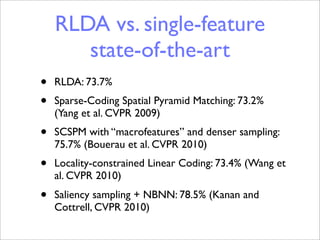
- 36. RLDA vs. single-feature state-of-the-art • RLDA: 73.7% • Sparse-Coding Spatial Pyramid Matching: 73.2% (Yang et al. CVPR 2009) • SCSPM with “macrofeatures” and denser sampling: 75.7% (Bouerau et al. CVPR 2010) • Locality-constrained Linear Coding: 73.4% (Wang et al. CVPR 2010) • Saliency sampling + NBNN: 78.5% (Kanan and Cottrell, CVPR 2010)
- 37. Bottom and top layers FLDA 128t/128b RLDA 128t/128b Top Bottom
- 38. Conclusions • Presented Bayesian hierarchical approach to modeling sparsely coded visual features of increasing complexity and spatial support. • Showed value of full inference.
- 39. Future directions • Extend hierarchy to object level. • Direct discriminative component • Non-parametrics • Sparse Coding + LDA