A Solution Manual And Notes For Kalman Filtering Theory And Practice Using MATLAB
0 likes105 views

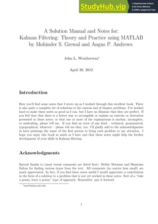
This document contains notes and solutions for a book on Kalman filtering. It includes notes on chapters explaining linear dynamic systems and derivations of fundamental solutions and state transition matrices for differential equations like dy/dt=0 and d2y/dt2=0. The author provides complete solutions to problems at the end of chapters and welcomes feedback to improve the notes.


![Problem Solutions
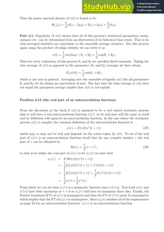
Problem 2.2 (the companion matrix for dny
dtn = 0)
We begin by defining the following functions xi(t)
x1(t) = y(t)
x2(t) = ẋ1(t) = ẏ(t)
x3(t) = ẋ2(t) = ¨
x1(t) = ÿ(t)
.
.
.
xn(t) = ẋn−1(t) = · · · =
dn−1
y(t)
dtn−1
,
as the components of a state vector x. Then the companion form for this system is given by
d
dt
x(t) =
d
dt
x1(t)
x2(t)
.
.
.
xn−1(t)
xn(t)
=
x2(t)
x3(t)
.
.
.
xn(t)
dny(t)
dtn
=
0 1 0 0 · · · 0
0 0 1 0 · · · 0
0 0 0 1 · · · 0
... 1
0 . . . 0 0
x1(t)
x2(t)
.
.
.
xn−1(t)
xn(t)
= Fx(t)
With F the companion matrix given by
F =
0 1 0 0 · · · 0
0 0 1 0 · · · 0
0 0 0 1 · · · 0
... 1
0 . . . 0 0
.
Which is of dimensions of n × n.
Problem 2.3 (the companion matrix for dy
dt
= 0 and d2y
dt2 = 0)
If n = 1 the above specifies to the differential equation dy
dt
= 0 and the companion matrix F
is the zero matrix i.e. F = [0]. When n = 2 we are solving the differential equation given
by d2y
dt2 = 0, and a companion matrix F given by
F =
0 1
0 0
.
Problem 2.4 (the fundamental solution matrix for dy
dt
= 0 and d2y
dt2 = 0)
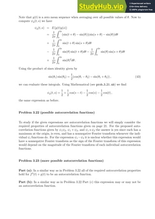
The fundamental solution matrix Φ(t) satisfies
dΦ
dt
= F(t)Φ(t) ,](https://image.slidesharecdn.com/asolutionmanualandnotesforkalmanfilteringtheoryandpracticeusingmatlab-230805193035-a97ddfb0/85/A-Solution-Manual-And-Notes-For-Kalman-Filtering-Theory-And-Practice-Using-MATLAB-4-320.jpg)
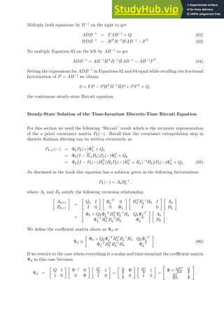
![with an initial condition Φ(0) = I. When n = 1, we have F = [0], so dΦ
dt
= 0 giving that
Φ(t) is a constant, say C. To have the initial condition hold Φ(0) = 1, we must have C = 1,
so that
Φ(t) = 1 . (2)
When n = 2, we have F =
0 1
0 0
, so that the equation satisfied by Φ is
dΦ
dt
=
0 1
0 0
Φ(t) .
If we denote the matrix Φ(t) into its components Φij(t) we have that
0 1
0 0
Φ(t) =
0 1
0 0
Φ11 Φ12
Φ21 Φ22
=
Φ21 Φ22
0 0
,
so the differential equations for the components of Φij satisfy
dΦ11
dt
dΦ12
dt
dΦ21
dt
dΦ22
dt
=
Φ21 Φ22
0 0
.
Solving the scalar differential equations above for Φ21 and Φ22 using the known initial con-
ditions for them we have Φ21 = 0 and Φ22 = 1. With these results the differential equations
for Φ11 and Φ12 become
dΦ11
dt
= 0 and
dΦ12
dt
= 1 ,
so that
Φ11 = 1 and Φ21(t) = t .
Thus the fundamental solution matrix Φ(t) in the case when n = 2 is
Φ(t) =
1 t
0 1
. (3)
Problem 2.5 (the state transition matrix for dy
dt
= 0 and d2y
dt2 = 0)
Given the fundamental solution matrix Φ(t) for a linear system dx
dt
= F(t)x the state transi-
tion matrix Φ(τ, t) is given by Φ(τ)Φ(t)−1
. When n = 1 since Φ(t) = 1 the state transition
matrix in this case is Φ(τ, t) = 1 also. When n = 2 since Φ(t) =
1 t
0 1
we have
Φ(t)−1
=
1 −t
0 1
,
so that
Φ(τ)Φ(t)−1
=
1 τ
0 1
1 −t
0 1
=
1 −t + τ
0 1
.](https://image.slidesharecdn.com/asolutionmanualandnotesforkalmanfilteringtheoryandpracticeusingmatlab-230805193035-a97ddfb0/85/A-Solution-Manual-And-Notes-For-Kalman-Filtering-Theory-And-Practice-Using-MATLAB-5-320.jpg)


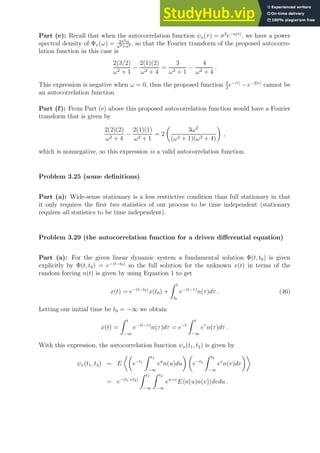
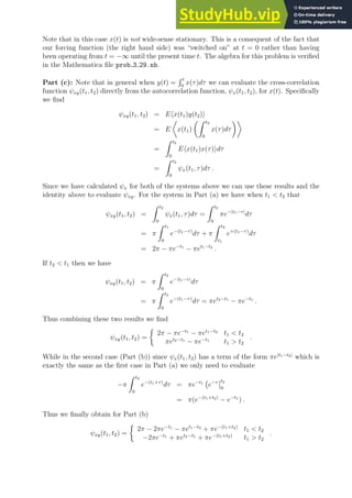
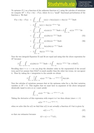
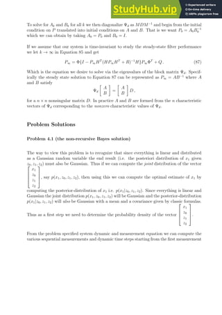
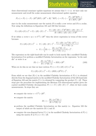
![Part (d): To predict x(t+α) using x(t) using an estimate x̂(t+α) = ax(t) we will minimize
the mean-square prediction error Eh[x̂(t + α) − x(t + α)]2
i as a function of a. For the given
linear form for x̂(t + α) the expression we will minimize for a is given by
F(a) ≡ Eh[ax(t) − x(t + α)]2
i
Eha2
x2
(t) − 2ax(t)x(t + α) + x2
(t + α)i
= a2
ψx(t, t) − 2aψx(t, t + α) + ψx(t + α, t + α) .
Since we are considering the functional form for ψx(t1, t2) derived for in Part (a) above we
know that ψx(t1, t2) = πe−|t1−t2|
so
ψx(t, t) = π = ψx(t + α, t + α) and ψx(t, t + α) = πe−|α|
= πe−α
,
since α 0. Thus the function F(a) then becomes
F(a) = πa2
− 2πae−α
+ π .
To find the minimum of this expression we take the derivative of F with respect to a, set
the resulting expression equal to zero and solve for a. We find
F′
(a) = 2πa − 2πe−α
= 0 so a = e−α
.
Thus to optimally predict x(t + α) given x(t) on should use the prediction x̂(t + α) given by
x̂(t + α) = e−α
x(t) . (48)
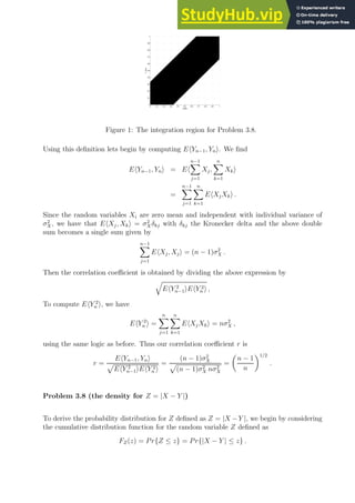
Problem 3.30 (a random initial condition)
Part (a): This equation is similar to Problem 3.29 Part (b) but now x(t0) = x0 is non-zero
and random rather than deterministic. For this given linear system we have a solution still
given by Equation 46
x(t) = e−t
x0 + e−t
Z t
0
eτ
n(τ)dτ = e−t
x0 + I(t) ,
where we have defined the function I(t) ≡ e−t
R t
0
eτ
n(τ)dτ. To compute the autocorrelation
function ψx(t1, t2) we use its definition to find
ψx(t1, t2) = Ehx(t1)x(t2)i
= Eh(e−t1
x0 + I(t1))(e−t2
x0 + I(t2))i
= e−(t1+t2)
Ehx2
0i + e−t1
Ehx0I(t2)i + e−t2
EhI(t1)x0i + EhI(t1)I(t2)i
= σ2
e−(t1+t2)
+ EhI(t1)I(t2)i ,
since the middle two terms are zero and we are told that x0 is zero mean with a variance σ2
.
The expression EhI(t1)I(t2)i was computed in Problem 3.29 b. Thus we find
ψx(t1, t2) = σ2
e−(t1+t2)
+ π(e−|t1−t2|
− e−(t1+t2)
) .](https://image.slidesharecdn.com/asolutionmanualandnotesforkalmanfilteringtheoryandpracticeusingmatlab-230805193035-a97ddfb0/85/A-Solution-Manual-And-Notes-For-Kalman-Filtering-Theory-And-Practice-Using-MATLAB-36-320.jpg)


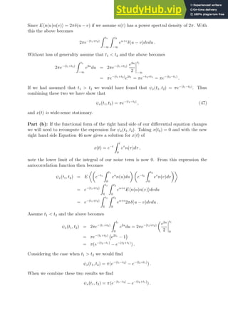
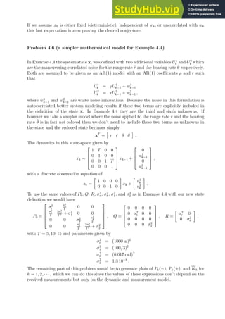
![which for this discrete linear system is given by
Pk =
0 1/2
−1/2 2
Pk−1
0 −1/2
1/2 2
+
1
1
1
1 1
Define Pk =
p11(k) p12(k)
p12(k) p22(k)
and we obtain the set of matrix equations given by
p11(k + 1) p12(k + 1)
p12(k + 1) p22(k + 1)
=
1
4
p22(k) −1
4
p12(k) + p22(k)
−1
4
p12(k) + p22(k) 1
4
p11(k) − 2p12(k) + 4p22(k)
+
1 1
1 1
,
As a linear system for the unknown functions p11(k), p12(k), and p22(k) we can write it as
p11(k + 1)
p12(k + 1)
p22(k + 1)
=
0 0 1/4
0 −1/4 1
1/4 −2 4
p11(k)
p12(k)
p22(k)
+
1
1
1
This is a linear vector difference equation and can be solved by methods discussed in [1].
Using Rather than carry out these calculations by hand in the Mathematica file prob 3 33.nb
their solution is obtained symbolically.
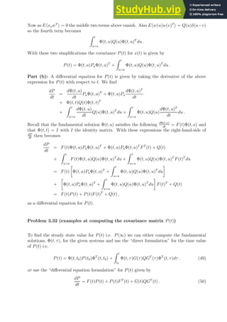
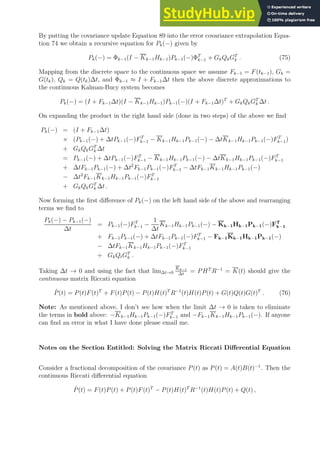
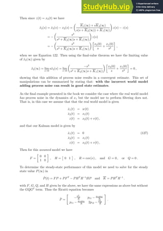
Problem 3.34 (the steady-state covariance matrix for the harmonic oscillator)
Example 3.4 is a linear dynamic system given by
ẋ1(t)
ẋ2(t)
=
0 1
−ω2
n −2ζωn
x1(t)
x2(t)
+
a
b − 2aζωn
w(t) .
Then the equation for the covariance of these state x(t) or P(t) is given by
dP
dt
= F(t)P(t) + P(t)F(t)T
+ G(t)Q(t)G(t)T
=
0 1
−ω2
n −2ζωn
p11(t) p12(t)
p12(t) p22(t)
+
p11(t) p12(t)
p12(t) p22(t)
0 −ω2
n
1 −2ζωn
+
a
b − 2aζωn
a b − 2aζωn
.
Since we are only looking for the steady-state value of P i.e. P(∞) let t → ∞ in the above
to get a linear system for the limiting values p11(∞), p12(∞), and p22(∞). The remaining
portions of this exercise are worked just like Example 3.9 from the book.
Problem 3.35 (a negative solution to the steady-state Ricatti equation)
Consider the scalar case suggested where F = Q = G = 1 and we find that the continuous-
time steady state algebraic equation becomes
0 = 1P(+∞) + P(+∞) + 1 ⇒ P(∞) = −
1
2
,
which is a negative solution in contradiction to the definition of P(∞).](https://image.slidesharecdn.com/asolutionmanualandnotesforkalmanfilteringtheoryandpracticeusingmatlab-230805193035-a97ddfb0/85/A-Solution-Manual-And-Notes-For-Kalman-Filtering-Theory-And-Practice-Using-MATLAB-41-320.jpg)
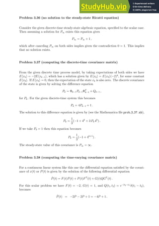
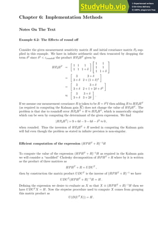
![as we were to show.
Part (b): To find the mean-square error we want to evaluate F(a) at the a(·) we calculated
above. We find
F(a) = Eh[e−cα
x(t) − x(t + α)]2
i
= Ehe−2cα
x2
(t) − 2e−cα
x(t)x(t + α) + x2
(t + α)i
= e−2cα
− 2e−cα
e−cα
+ 1
= 1 − e−2cα
.](https://image.slidesharecdn.com/asolutionmanualandnotesforkalmanfilteringtheoryandpracticeusingmatlab-230805193035-a97ddfb0/85/A-Solution-Manual-And-Notes-For-Kalman-Filtering-Theory-And-Practice-Using-MATLAB-45-320.jpg)
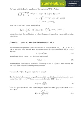
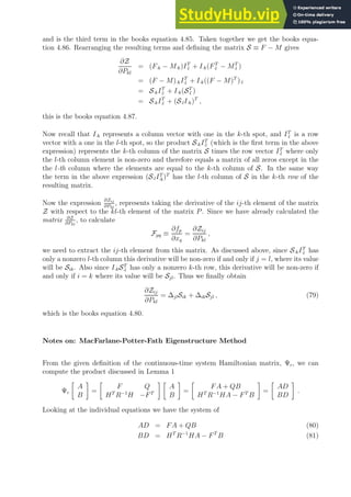
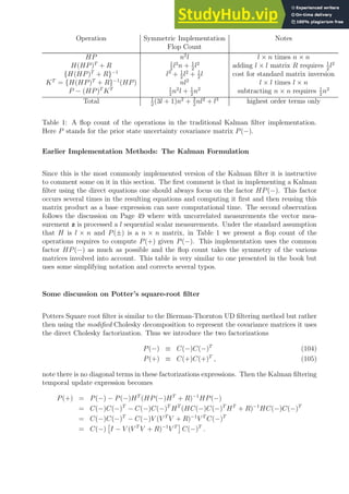
![Chapter 4: Linear Optimal Filters and Predictors
Notes On The Text
Estimators in Linear Form
For this chapter we will consider an estimator of the unknown state x at the k-th time step
to be denoted x̂k(+), given the k-th measurement zk, and our previous estimate of x before
the measurement (denoted x̂k(−)) of the following linear form
x̂k(+) = K1
kx̂k(−) + Kkzk , (59)
for some as yet undetermined coefficients K1
k and Kk. The requiring the orthogonality
condition that this estimate must satisfy is then that
Eh[xk − x̂k(+)]zT
i i = 0 for i = 1, 2, · · · , k − 1 . (60)
Note that this orthogonality condition is stated for the posterior (after measurement) esti-
mate x̂k(+) but for a recursive filter we expect it to hold for the a-priori (before measure-
ment) estimate x̂k(−) also. These orthogonality conditions can be simplified to determine
conditions on the unknown coefficients K1
k and Kk. From our chosen form for x̂k(+) from
Equation 59 the orthogonality conditions imply
Eh[xk − K1
kx̂k(−) − Kkzk]zT
i i = 0 .
Since our measurement zk in terms of the true state xk is given by
zk = Hkxk + vk , (61)
the above expression becomes
Eh[xk − K1
kx̂k(−) − KkHkxk − Kkvk]zT
i i = 0 .
Recognizing that the measurement noise vk is assumed uncorrelated with the measurement
zi we EhvkzT
k i = 0 so this term drops from the orthogonality conditions and we obtain
Eh[xk − K1
k x̂k(−) − KkHkxk]zT
i i = 0 .
From this expression we now adding and subtracting K1
kxk to obtain
Eh[xk − KkHkxk − K1
kxk − K1
Kx̂k(−) + K1
k xk]zT
i i = 0 ,
so that by grouping the last two terms we find
Eh[xk − KkHkxk − K1
k xk − K1
K (x̂k(−) − xk)]zT
i i = 0 .
This last term Eh(x̂k(−) − xk)zT
i i = 0 due to the orthogonality condition satisfied by the
previous estimate x̂k(−). Factoring out xk and applying the expectation to each individual
term this becomes
(I − KkHk − K1
k )EhxkzT
i i = 0 . (62)](https://image.slidesharecdn.com/asolutionmanualandnotesforkalmanfilteringtheoryandpracticeusingmatlab-230805193035-a97ddfb0/85/A-Solution-Manual-And-Notes-For-Kalman-Filtering-Theory-And-Practice-Using-MATLAB-46-320.jpg)
 − zk)T
i = 0 .
using the expression we found for K1
k in Equation 63 and the measurement Equation 61 this
becomes
Eh[xk − x̂k(−) − KkHkx̂k(−) − KkHkxk − Kkvk](Hkx̂k(−) − Hkxk − vk)T
i = 0 .
Group some terms to introduce the definition of x̃k(−)
x̃k = xk − x̂k(−) , (66)
we have
Eh[−x̃k(−) + KkHkx̃k(−) − Kkvk](Hkx̃k(−) − vk)T
i = 0 .
If we define the value of Pk(−) to be the prior covariance Pk(−) ≡ Ehx̃k(−)x̃k(−)T
i the
above becomes six product terms
0 = −Ehx̃k(−)x̃k(−)T
iHT
k + Ehx̃k(−)vT
k i
+ KkHkEhx̃k(−)x̃k(−)T
iHT
k − KkHkEhx̃k(−)vT
k i
− KkEhvkx̃k(−)T
iHT
k + KkEhvkvT
k i .
Since Ehx̃k(−)vT
k i = 0 several terms cancel and we obtain
−Pk(−)HT
k + KkHkPk(−)HT
k + KkRk = 0 . (67)
Which is a linear equation for the unknown Kk. Solving it we find the gain or the multiplier
of the measurement given by solving the above for Kk or
Kk = Pk(−)HT
k (HkPk(−)HT
k + Rk)−1
. (68)
Using the expressions just derived for K1
k and Kk, we would like to derive an expression for
the posterior covariance error. The posterior covariance error is defined in a similar manner
to the a-priori error Pk(−) namely
Pk(+) = Ehx̃k(+)x̃k(+)i , (69)](https://image.slidesharecdn.com/asolutionmanualandnotesforkalmanfilteringtheoryandpracticeusingmatlab-230805193035-a97ddfb0/85/A-Solution-Manual-And-Notes-For-Kalman-Filtering-Theory-And-Practice-Using-MATLAB-47-320.jpg)
![Then with the value of K1
k given by K1
k = I − KkHk we have our posterior state estimate
x̂k(+) using Equation 59 in terms of our prior estimate x̂k(−) and our measurement zk of
x̂k(+) = (I − KkHk)x̂k(−) + Kkzk
= x̂k(−) + Kk(zk − Hkx̂k(−)) .
Subtracting the true state xk from this and writing the measurement in terms of the state
as zk = Hkxk + vk we have
x̂k(+) − xk = x̂k(−) − xk + KkHkxk + Kkvk − KkHkx̂k(−)
= x̃k(−) − KkHk(x̂k(−) − xk) + Kkvk
= x̃k(−) − KkHkx̃k(−) + Kkvk .
Thus the update of x̃k(+) from x̃k(−) is given by
x̃k(+) = (I − KkHk)x̃k(−) + Kkvk . (70)
Using this expression we can derive Pk(+) in terms of Pk(−) as
Pk(+) = Ehx̃k(+)x̃T
k i
= Eh[I − KkHk)x̃k(−) + Kkvk][x̃T
k (−)(I − KkHk)T
+ vT
k K
T
k ]i .
By expanding the terms on the right hand side and remembering that Ehvkx̃T
k (−)i = 0 gives
Pk(+) = (I − KkHk)Pk(−)(I − KkHk)T
+ KkRkK
T
k (71)
or the so called Joseph form of the covariance update equation.
Alternative forms for the state covariance update equation can also be obtained. Expanding
the product on the right-hand-side of Equation 71 gives
Pk(+) = Pk(−) − Pk(−)(KkHk)T
− KkHkPk(−) + KkHkPk(−)(KkHk)T
+ KkRkK
T
k .
Grouping the first and third term and the last two terms together in the expression in the
right-hand-side we find
Pk(+) = (I − KkHk)Pk(−) − Pk(−)HT
k K
T
k + Kk(HkPk(−)HT
k + Rk)K
T
k .
Recognizing that since the expression HkPk(−)HT
k + Rk appears in the definition of the
Kalman gain Equation 68 the product Kk(HkPk(−)HT
k + Rk) is really equal to
Kk(HkPk(−)HT
k + Rk) = Pk(−)HT
k ,
and we find Pk(+) takes the form
Pk(+) = (I − KkHk)Pk(−) − Pk(−)HT
k K
T
k + Pk(−)HT
k K
T
k
= (I − KkHk)Pk(−) . (72)
This later form is most often used in computation.
Given the estimate of the error covariance at the previous time step or Pk−1(+) by using the
discrete state-update equation
xk = Φk−1xk−1 + wk−1 , (73)
the prior error covariance at the next time step k is given by the simple form
Pk(−) = Φk−1Pk−1(+)ΦT
k−1 + Qk−1 . (74)](https://image.slidesharecdn.com/asolutionmanualandnotesforkalmanfilteringtheoryandpracticeusingmatlab-230805193035-a97ddfb0/85/A-Solution-Manual-And-Notes-For-Kalman-Filtering-Theory-And-Practice-Using-MATLAB-48-320.jpg)
![Notes on Treating Uncorrelated Measurement Vectors as Scalar Measurements
In this subsection of the book a very useful algorithm for dealing with uncorrelated mea-
surement vectors is presented. The main idea is to treat the totality of vector measurement
z as a sequence of scalar measurements zk for k = 1, 2, · · · , l. This can have several benefits.
In addition to the two reasons stated in the text: reduced computational time and improved
numerical accuracy, in practice this algorithm can be especially useful in situations where
the individual measurements are known with different uncertainties where some maybe more
informative and useful in predicting an estimate of the total state x̂k(+) than others. In an
ideal case one would like to use the information from all of the measurements but time may
require estimates of x̂k(+) quicker than the computation with all measurements could be
done. If the measurements could be sorted based on some sort of priority (like uncertainty)
then an approximation of x̂k(+) could be obtained by applying on the most informative mea-
surements zk first and stopping before processing all of the measurements. This algorithm
is also a very interesting way of thinking about how the Kalman filter is in general pro-
cessing vector measurements. There is slight typo in the book’s presented algorithm which
we now fix. The algorithm is to begin with our initial estimate of the state and covariance
P
[0]
k = Pk(−) and x̂
[0]
k = x̂k(−) and then to iteratively apply the following equations
K
[i]
k =
1
H
[i]
k P
[i−1]
k HT
[i] + R
[i]
k
(H
[i]
k P
[i−1]
k )T
P
[i]
k = P
[i−1]
k − K
[i]
k H
[i]
k P
[i−1]
k
x̂
[i]
k = x̂
[i−1]
k + K
[i]
k [{zk}i − H
[i]
k x̂
[i−1]
k ] ,
for i = 1, 2, · · · , l. As shown above, a simplification over the normal Kalman update equa-
tions that comes from using this procedure is that now the expression H
[i]
k P
[i−1]
k HT
[i] + R
[i]
k
is a scalar and inverting it is simply division. Once we have processed the l-th scalar mea-
surement {zk}l, using this procedure the final state and uncertainty estimates are given
by
Pk(+) = P
[l]
k and x̂k(+) = x̂
[l]
k .
On Page 80 of these notes we derive the computational requirements for the normal Kalman
formulation (where the measurements z are treated as a vector) and the above “scalar”
procedure. In addition, we should note that theoretically the order in which we process each
scalar measurement should not matter. In practice, however, it seems that it does matter
and different ordering can give different state estimates. Ordering the measurements from
most informative (the measurement with the smallest uncertainty is first) to least informative
seems to be a good choice. This corresponds to a greedy like algorithm in that if we have
to stop processing measurements at some point we would have processed the measurements
with the largest amount of information.
Notes on the Section Entitled: The Kalman-Bucy filter
Warning: I was not able to get the algebra in this section to agree with the results
presented in the book. If anyone sees an error in my reasoning or a method by which I
should do these calculations differently please email me.](https://image.slidesharecdn.com/asolutionmanualandnotesforkalmanfilteringtheoryandpracticeusingmatlab-230805193035-a97ddfb0/85/A-Solution-Manual-And-Notes-For-Kalman-Filtering-Theory-And-Practice-Using-MATLAB-49-320.jpg)
![Consider the expression in the upper right hand “corner” of the above expression or
Q
q
F2 + H2Q
R
+ F
,
by multiplying top and bottom of this fraction by
q
F 2+ H2Q
R
−F
q
F 2+ H2Q
R
−F
we get
Q
q
F2 + H2Q
R
− F
F2 + H2Q
R
− F2
=
R
H2
r
F2 +
H2Q
R
− F
!
,
and the terms in the brackets [·] cancel each from the numerator and denominator to give
the expression
lim
t→∞
P(t) =
R
H2
F +
r
F2 +
H2Q
R
!
, (77)
which is the books equation 4.72.
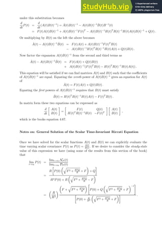
Notes on: The Steady-State Riccati equation using the Newton-Raphson Method
In the notation of this section, the identity that
∂P
∂Pkl
= I·kIT
·l , (78)
can be reasoned as correct by recognizing that IT
l̇
represents the row vector with a one in
the l-th spot and I·k represents a column vector with a one in the k-th spot, so the product
of I·kIT
·l represents a matrix of zeros with a single non-zero element (a 1) in the kl-th spot.
This is the equivalent effect of taking the derivative of P with respect to its kl-th element
or the expression ∂P
∂Pkl
.
From the given definition of Z, the product rule, and Equation 78 we have
∂Z
∂Pkl
=
∂
∂Pkl
(FP + PFT
− PHT
R−1
HP + Q)
= F
∂P
∂Pkl
+
∂P
∂Pkl
FT
−
∂P
∂Pkl
HT
R−1
HP − PHT
R−1
H
∂P
∂Pkl
= FI·kIT
·l + I·kIT
·l FT
− I·kIT
·l HT
R−1
HP − PHT
R−1
HI·kIT
·l
= F·kIT
·l + I·kFT
·l − I·kIT
·l (PHT
R−1
H)T
− (PHT
R−1
H)I·kIT
·l .
In deriving the last line we have used the fact IT
·l FT
= (FI·l)T
= FT
·l . Note that the last
term above is
−(PHT
R−1
H)I·kIT
·l = −MI·kIT
·l = −M·kIT
·l ,
where we have introduced the matrix M ≡ PHT
R−1
H, since MI·k selects the kth column
from the matrix M. This is the fourth term in the books equation 4.85. The product in the
second to last term is given by
−I·kIT
·l HT
R−1
HP = −I·k(PHT
R−1
HI·l)T
= −I·kMT
·l ,](https://image.slidesharecdn.com/asolutionmanualandnotesforkalmanfilteringtheoryandpracticeusingmatlab-230805193035-a97ddfb0/85/A-Solution-Manual-And-Notes-For-Kalman-Filtering-Theory-And-Practice-Using-MATLAB-52-320.jpg)

![Given X, a multivariate Gaussian random variable of dimension n with vector mean µ and
covariance matrix Σ. If we partition X, µ, and Σ into two parts of sizes q and n − q as
X =
X1
X2
, µ =
µ1
µ2
, and Σ =
Σ11 Σ12
ΣT
12 Σ22
.
Then the conditional distribution of the first q random variables in X given the second
n − q of the random variables (say X2 = a) is another multivariate normal with mean µ̄ and
covariance Σ̄ given by
µ̄ = µ1 + Σ12Σ−1
22 (a − µ2) (88)
Σ̄ = Σ11 − Σ12Σ−1
22 . (89)
For this problem we have that Σ11 = c2
x1
, Σ12 = bT
, and Σ22 = Ĉ, so that we compute the
matrix product Σ12Σ−1
22 of
Σ12Σ−1
22 =
1
145
16 72 18
.
Thus if we are given the values of z0, z1, and z2 for the components of X2 from the above
theorem the value of E[x1|z0, z1, z2] is given by µ̄ which in this case since µ1 = 0 and µ2 = 0
becomes
E[x1|z0, z1, z2] =
1
145
16 72 18
z0
z1
z2
=
1
145
(16z0 + 72z1 + 18z2) .
The simple numerics for this problem are worked in the MATLAB script prob 4 1.m.
Problem 4.2 (solving Problem 4.1 using the discrete Kalman filter)
Part (a): For this problem we have Φk−1 = 1
2
, Hk = 1, Rk = 1, and Qk = 1, then the
discrete Kalman equations become
x̂k(−) = Φk−1x̂k−1(+) =
1
2
x̂k−1(+)
Pk(−) = Φk−1Pk−1(+)ΦT
k−1 + Qk−1 =
1
4
Pk−1(+) + 1
Kk = Pk(−)HT
k (HkPk(−)HT
k + Rk)−1
=
Pk(−)
Pk(−) + 1
x̂k(+) = x̂k(−) + Kk(zk − Hkx̂k(−)) = x̂k(−) + Kk(zk − x̂k(−)) (90)
Pk(+) = (I − KkHk)Pk(−) = (1 − Kk)Pk(−) . (91)
Part (b): If the measurement z2 was not received we can skip the equations used to update
the state and covariance after each measurement. Thus Equations 90 and 91 would instead
become (since z2 is not available)
x̂2(+) = x̂2(−)
P2(+) = P2(−) ,](https://image.slidesharecdn.com/asolutionmanualandnotesforkalmanfilteringtheoryandpracticeusingmatlab-230805193035-a97ddfb0/85/A-Solution-Manual-And-Notes-For-Kalman-Filtering-Theory-And-Practice-Using-MATLAB-57-320.jpg)


![would iterate
x̂k(−) = x̂k−1(+)
Pk(−) = Pk−1(+)
Kk = Pk(−)HT
k (HkPk(−)HT
k + Rk)−1
= Pk(−)[Pk(−) + R]−1
x̂k(+) = x̂k(−) + Kk(zk − x̂k(−))
Pk(+) = (I − KkHk)Pk(−) = (1 − Kk)Pk(−) .
Combining these we get the following iterative equations for Kk, x̂k(+), and Pk(+)
Kk = Pk−1(+)[Pk−1(+) + R]−1
x̂k(+) = x̂k−1(+) + Kk(zk − x̂k−1(+))
Pk(+) = (1 − Kk)Pk−1(+) .
Part (b): If R = 0 we have no measurement noise and the given measurement should give
all needed information about the state. The Kalman update above would predict
K1 = P0(P−1
0 ) = I ,
so that
x̂1(+) = x0 + I(z1 − x0) = z1 ,
thus the first measurement gives the entire estimate of the state and would be exact (since
there is no measurement noise).
Part (c): If R = ∞ we have infinite measurement noise and the measurement of z1 should
give almost no information on the state x1. When R = ∞ we find the Kalman gain given
by K1 = 0 so that
x̂1(+) = x0 ,
i.e. the measurement does not change our initial estimate of what x is.
Problem 4.10 (calculating K(t))
Part (a): The mean squared estimation error, P(t), satisfies Equation 121 which for this
system since F(t) = −1, H(t) = 1, the measurement noise covariance R(t) = 20 and the
dynamic noise covariance matrix Q(t) = 30 becomes (with G(t) = 1)
dP(t)
dt
= −P(t) − P(t) −
P(t)2
20
+ 30 = −2P(t) −
P(t)2
20
+ 30 ,
which we can solve. For this problem since it is a scalar-time invariance problem the solu-
tion to this differential equation can be obtained as in the book by performing a fractional
decomposition. Once we have the solution for P(t) we can calculate K(t) from
K(t) = P(t)Ht
R−1
=
1
20
P(t) .](https://image.slidesharecdn.com/asolutionmanualandnotesforkalmanfilteringtheoryandpracticeusingmatlab-230805193035-a97ddfb0/85/A-Solution-Manual-And-Notes-For-Kalman-Filtering-Theory-And-Practice-Using-MATLAB-62-320.jpg)


![Chapter 5: Nonlinear Applications
Notes On The Text
Notes on Table 5.3: The Discrete Linearized Filter Equations
Since I didn’t see this equation derived in the book, in this section of these notes we derive
the “predicted perturbation from the measurement” equation which is given in Table 5.3 in
the book. The normal discrete Kalman state estimate observational update when we Taylor
expand about xnom
k can be written as
x̂k(+) = x̂k(−) + Kk(zk − h(x̂k(−)))
= x̂k(−) + Kk(zk − h(xnom
k + c
δxk(−)))
≈ x̂k(−) + Kk(zk − h(xnom
k ) − H
[1]
k
c
δxk(−)) .
But the perturbation definition c
δxk(+) = x̂k(+) − xnom
k , means that x̂k(+) = xnom
k + c
δxk(+)
and we have
xnom
k + c
δxk(+) = xnom
k + c
δxk(−) + Kk(zk − h(xnom
k ) − H
[1]
k
c
δxk(−)) ,
or canceling the value of xnom
k from both sides we have
c
δxk(+) = c
δxk(−) + Kk(zk − h(xnom
k ) − H
[1]
k
c
δxk(−)) , (93)
which is the predicted perturbation update equation presented in the book.
Notes on Example 5.1: Linearized Kalman and Extended Kalman Filter Equa-
tions
In this section of these notes we provide more explanation and derivations on Example 5.1
from the book which computes the linearized and the extended Kalman filtering equations
for a simple discrete scalar non-linear problem. We first derive the linearized Kalman filter
equations and then the extended Kalman filtering equations.
For xnom
k = 2 the linearized Kalman filtering have their state x̂k(+) determined from the
perturbation c
δxk(+) by
x̂k(+) = x̂nom
k + c
δxk(+) = 2 + c
δxk(+) .
Linear prediction of the state perturbation becomes
c
δxk(−) = Φ
[1]
k−1
c
δxk−1(+) = 4c
δxk−1(+) ,
since
Φ
[1]
k−1 =
dxk−1
2
dxk−1 xk−1=xnom
k−1
= 2xk−1|xk−1=2 = 4 .](https://image.slidesharecdn.com/asolutionmanualandnotesforkalmanfilteringtheoryandpracticeusingmatlab-230805193035-a97ddfb0/85/A-Solution-Manual-And-Notes-For-Kalman-Filtering-Theory-And-Practice-Using-MATLAB-65-320.jpg)
![The a priori covariance equation is given by
Pk(−) = Φ
[1]
k Pk−1(+)Φ
[1]T
k + Qk
= 16Pk−1(+) + 1 .
Since Kk in the linearized Kalman filter is given by Pk(−)H
[1]T
k [H
[1]
k Pk(−)H
[1]T
k + Rk]−1
, we
need to evaluate H
[1]
k . For this system we find
H
[1]
k =
dxk
3
dxk xk=xnom
k
= 3xk
2
xk=2
= 12 .
With this then
Kk =
12Pk(−)
144Pk(−) + 2
,
and we can compute the predicted perturbation conditional on the measurement
c
δxk(+) = c
δxk(−) + Kk(zk − hk(xnom
k ) − H
[1]
k
c
δxk(−)) .
Note that hk(xnom
k ) = 23
= 8 and we have
c
δxk(+) = c
δxk(−) + Kk(zk − 8 − 12c
δxk(−)) .
Finally, the a posteriori covariance matrix is given by
Pk(+) = (1 − KkH
[1]
k )Pk(−)
= (1 − 12Kk)Pk(−) .
The extended Kalman filter equations can be derived from the steps presented in Table 5.4
in the book. For the system given here we first evaluate the needed linear approximations
of fk−1(·) and hk(·)
Φ
[1]
k−1 =
∂fk−1
∂x x=x̂k−1(−)
= 2x̂k−1(−)
H
[1]
k =
∂hk
∂x x=x̂k(−)
= 3x̂k(−)2
.
Using these approximations, given values for x̂0(+) and P0(+) for k = 1, 2, · · · the discrete
extended Kalman filter equations become
x̂k(−) = fk−1(x̂k−1(+)) = x̂k−1(+)2
Pk(−) = Φ
[1]
k−1Pk−1(+)ΦT
k−1 + Qk−1 = 4x̂k−1(−)2
Pk−1(+) + 1
ẑk = hk(x̂k(−)) = x̂k(−)3
Kk = Pk(−)(3x̂k(−)2
)(9x̂k(−)4
Pk(−) + 2)−1
=
3x̂k(−)2
Pk(−)
9x̂k(−)4
Pk(−) + 2
x̂k(+) = x̂k(−) + Kk(zk − ẑk)
Pk(+) = (1 − Kk(3x̂k(−)2
))Pk(−) = (1 − 3Kkx̂k(−)2
)Pk(−) .](https://image.slidesharecdn.com/asolutionmanualandnotesforkalmanfilteringtheoryandpracticeusingmatlab-230805193035-a97ddfb0/85/A-Solution-Manual-And-Notes-For-Kalman-Filtering-Theory-And-Practice-Using-MATLAB-66-320.jpg)
![Since we have an explicit formula for the state propagation dynamics we can simplify the
state update equation to get
x̂k(+) = x̂k−1(+)2
+ Kk(zk − x̂k(−)3
)
= x̂k−1(+)2
+ Kk(zk − x̂k−1(+)6
) .
These equations agree with the ones given in the book.
Notes on Quadratic Modeling Error
For these notes we assume that h(·) in our measurement equation z = h(x) has the specific
quadratic form given by
h(x) = H1x + xT
H2x + v .
Then with error x̃ defined as x̃ ≡ x̂ − x so that the state x in terms of our estimate x̂ is
given by x = x̂ − x̃ we can compute the expected measurement ẑ with the following steps
ẑ = Ehh(x)i
= EhH1x + xT
H2xi
= EhH1(x̂ − x̃) + (x̂ − x̃)T
H2(x̂ − x̃)i
= H1x̂ − H1Ehx̃i + Ehx̂T
H2x̂i − Ehx̃T
H2x̂i − Ehx̂T
H2x̃i + Ehx̃T
H2x̃i .
Now if we assume that the error x̃ is zero mean so that Ehx̃i = 0 and x̂ is deterministic the
above simplifies to
ẑ = H1x̂ + x̂T
H2x̂ + Ehx̃T
H2x̃i .
Since x̃T
H2x̃ is a scalar it equals its own trace and by the trace product permutation theorem
we have
Ehx̃T
H2x̃i = Ehtrace[x̃T
H2x̃]i = Ehtrace[H2x̃x̃T
]i
= trace[H2Ehx̃x̃T
i] .
To simplify this recognize that Ehx̃x̃T
i is the covariance of the state error and should equal
P(−) thus
ẑ = H1x̂ + x̂T
H2x̂ + trace[H2P(−)]
= h(x̂) + trace[H2P(−)] ,
the expression presented in the book.
Notes on Example 5.2: Using the Quadratic Error Correction
For a measurement equation given by z = sy + b + v for a state consisting of the unknowns
s, b, and y we compute the matrix, H2 in its quadratic form representation as
H2 =
1
2
∂2z
∂s2
∂2z
∂s∂b
∂2z
∂s∂y
∂2z
∂s∂b
∂2z
∂b2
∂2z
∂b∂y
∂2z
∂s∂y
∂2z
∂b∂y
∂2z
∂y2
=
1
2
0 0 1
0 0 0
1 0 0
,](https://image.slidesharecdn.com/asolutionmanualandnotesforkalmanfilteringtheoryandpracticeusingmatlab-230805193035-a97ddfb0/85/A-Solution-Manual-And-Notes-For-Kalman-Filtering-Theory-And-Practice-Using-MATLAB-67-320.jpg)
![therefore the expected measurement h(ẑ) can be corrected at each Kalman step by adding
the term
trace
0 0 1/2
0 0 0
1/2 0 0
P(−)
.
Problem Solutions
Problem 5.1 (deriving the linearized and the extended Kalman estimator)
For this problem our non-linear dynamical equation is given by
xk = −0.1xk−1 + cos(xk−1) + wk−1 , (94)
and our non-linear measurement equation is given by
zk = x2
k + vk . (95)
We will derive the equation for the linearized perturbed trajectory and the equation for
the predicted perturbation given the measurement first and then list the full set of dis-
crete Kalman filter equations that would be iterated in an implementation. If our nominal
trajectory xnom
k = 1, then the linearized Kalman estimator equations becomes
c
δxk(−) ≈
∂fk−1
∂x x=xnom
k−1
c
δxk−1(+) + wk−1
= (−0.1 − sin(xnom
k−1))c
δxk−1(+) + wk−1
= (−0.1 − sin(1))c
δxk−1(+) + wk−1 ,
with an predicted a priori covariance matrix given by
Pk(−) = Φ
[1]
k−1Pk−1(+)Φ
[1] T
k−1 + Qk−1
= (0.1 + sin(1))2
Pk−1(+) + 1 .
The linear measurement prediction equation becomes
c
δxk(+) = c
δxk(−) + Kk[zk − hk(xnom
k ) − H
[1]
k
c
δxk(−)]
= c
δxk(−) + Kk[zk − (12
) −
∂hk
∂x xnom
k
!
c
δxk(−)]
= c
δxk(−) + Kk[zk − 1 − 2c
δxk(−)] .
where the Kalman gain Kk is given by
Kk = Pk(−)(2)
4Pk(−) +
1
2
−1
.](https://image.slidesharecdn.com/asolutionmanualandnotesforkalmanfilteringtheoryandpracticeusingmatlab-230805193035-a97ddfb0/85/A-Solution-Manual-And-Notes-For-Kalman-Filtering-Theory-And-Practice-Using-MATLAB-68-320.jpg)

![Problem 5.2 (continuous linearized and extended Kalman filters)
To compute the continuous linearized Kalman estimator equations we recall that when the
dynamics and measurement equations are given by
ẋ(t) = f(x(t), t) + G(t)w(t)
z(t) = h(x(t), t) + v(t) ,
that introducing the variables
δx(t) = x(t) − xnom
(t)
δz(t) = z(t) − h(xnom
(t), t) ,
representing perturbations from a nominal trajectory the linearized differential equations for
δx and δz are given by
˙
δx(t) =
∂f(x(t), t)
∂x(t) x(t)=xnom(t)
!
δx(t) + G(t)w(t)
= F[1]
δx(t) + G(t)w(t) (96)
δz(t) =
∂h(x(t), t)
∂x(t) x(t)=xnom(t)
!
δx(t) + v(t)
= H[1]
δx(t) + v(t) . (97)
Using these two equations for the system governed by δx(t) and δz(t) we can compute
an estimate for δx(t), denoted δx̂(t), using the continuous Kalman filter equations from
Chapter 4 by solving (these are taken from the summary section from Chapter 4 but specified
to the system above)
d
dt
δx̂(t) = F[1]
δx̂(t) + K(t)[δz(t) − H[1]
δx̂(t)]
K(t) = P(t)H[1]T
(t)R−1
(t)
d
dt
P(t) = F[1]
P(t) + P(t)F[1]T
− K(t)R(t)K
T
(t) + G(t)Q(t)G(t)T
.
For this specific problem formulation we have the linearized matrices F[1]
and H[1]
given by
F[1]
=
∂
∂x(t)
(−0.5x2
(t))
x(t)=xnom(t)
= −xnom
(t) = −1
H[1]
=
∂
∂x(t)
(x3
(t))
x(t)=xnom(t)
= 3 x(t)2
x(t)=xnom = 3 .
Using R(t) = 1/2, Q(t) = 1, G(t) = 1 we thus obtain the Kalman-Bucy equations of
d
dt
δx̂(t) = −δx̂(t) + K(t)[z(t) − h(xnom
(t), t) − 3δx̂(t)]
= −δx̂(t) + K(t)[z(t) − 1 − 3δx̂(t)]
K(t) = 6P(t)
d
dt
P(t) = −P(t) − P(t) −
1
2
K(t)2
+ 1 ,](https://image.slidesharecdn.com/asolutionmanualandnotesforkalmanfilteringtheoryandpracticeusingmatlab-230805193035-a97ddfb0/85/A-Solution-Manual-And-Notes-For-Kalman-Filtering-Theory-And-Practice-Using-MATLAB-70-320.jpg)
![which would be solved for δx̂(t) and P(t) as measurements z(t) come in.
For the extended Kalman filter we only change the dynamic equation in the above. Thus we
are requested to solve the following Kalman-Bucy system (these are taken from Table 5.5 in
this chapter)
d
dt
x̂(t) = f(x̂(t), t) + K(t)[z(t) − h(x̂(t), t)]
K(t) = P(t)H[1]T
(t)R−1
(t)
d
dt
P(t) = F[1]
P(t) + P(t)F[1]T
− K(t)R(t)K
T
(t) + G(t)Q(t)G(t)T
.
Where now
F[1]
=
∂
∂x(t)
(f(x(t), t))
x(t)=x̂(t)
= −x̂
H[1]
=
∂
∂x(t)
(h(x(t), t))
x(t)=x̂(t)
= 3x̂2
(t) .
Again with R(t) = 1/2, Q(t) = 1, G(t) = 1 we obtain the Kalman-Bucy equations of
d
dt
x̂(t) = −
1
2
x̂(t)2
+ K(t)[z(t) − x̂(t)3
]
K(t) = 6P(t)x̂2
(t)
d
dt
P(t) = −x̂(t)P(t) − P(t)x̂(t) −
K(t)
2
2
+ 1 .
Problem 5.4 (deriving the linearized and the extended Kalman estimator)
For this problem we derive the linearized Kalman filter for the state propagation equation
xk = f(xk−1, k − 1) + Gwk−1 , (98)
and measurement equation
zk = h(xk, k) + vk . (99)
We need the definitions
Φ
[1]
k−1 ≡
∂fk−1
∂x x=xnom
k−1
= f′
(xnom
k−1, k − 1)
H
[1]
k ≡
∂hk
∂x x=xnom
k
= h′
(xnom
k , k) .
Then the linearized Kalman filter algorithm is given by the following steps:
• Pick/specify x̂0(+) and P0(+).](https://image.slidesharecdn.com/asolutionmanualandnotesforkalmanfilteringtheoryandpracticeusingmatlab-230805193035-a97ddfb0/85/A-Solution-Manual-And-Notes-For-Kalman-Filtering-Theory-And-Practice-Using-MATLAB-71-320.jpg)
![• Compute c
δx0(+) = x̂0(+) − xnom
0 , using these values.
• Set k = 1 and begin iterating:
• State/Covariance propagation from k − 1 to k
c
δxk(−) = f′
(xnom
k−1, k − 1)c
δxk−1(+)
Pk(−) = f′
(xnom
k−1, k − 1)2
Pk−1(+) + GQk−1GT
.
• The measurement update:
Kk = Pk(−)H
[1]
k (H
[1]
k Pk(−)H
[1]T
k + Rk)−1
= h′
(xnom
k , k)Pk(−)(h′
(xnom
k , k)
2
Pk(−) + Rk)−1
c
δxk(+) = c
δxk(−) + Kk(zk − h(xnom
k , k) − h′
(xnom
k , k)c
δxk(−))
Pk(+) = (1 − h′
(xnom
k , k)Kk)Pk(−) .
Next we compute the extended Kalman filter (EKF) for this system
• Pick/specify x̂0(+) and P0(+).
• Set k = 1 and begin iterating
• State propagation from k − 1 to k
xk(−) = f(x̂k−1(+), k − 1)
Pk(−) = f′
(x̂k−1(+), k − 1)
2
Pk−1(+) + GQk−1GT
.
• The measurement update:
Kk = h′
(x̂k(−), k)Pk(−)(h′
(x̂k(−), k)
2
Pk(−) + Rk)−1
x̂k(+) = x̂k(−) + Kk(zk − h(x̂k(−), k))
Pk(+) = (1 − h′
(x̂k(−), k)Kk)Pk(−) .
Problem 5.5 (parameter estimation via a non-linear filtering)
We can use non-linear Kalman filtering to derive an estimate the value for the parameter a in
the plant model in the same way the book estimated the driving parameter ζ in example 5.3.
To do this we consider introducing an additional state x2(t) = a, which since a is a constant
has a very simple dynamic equation ẋ2(t) = 0. Then the total linear system when we take
x1(t) ≡ x(t) then becomes
d
dt
x1(t)
x2(t)
=
x2(t)x1(t)
0
+
w(t)
0
,](https://image.slidesharecdn.com/asolutionmanualandnotesforkalmanfilteringtheoryandpracticeusingmatlab-230805193035-a97ddfb0/85/A-Solution-Manual-And-Notes-For-Kalman-Filtering-Theory-And-Practice-Using-MATLAB-72-320.jpg)
![which is non-linear due to the product x1(t)x2(t). The measurement equation is
z(t) = x1(t) + v(t) =
1 0
x1(t)
x2(t)
+ v(t) .
To derive an estimator for a we will use the extended Kalman filter (EKF) equations to
derive estimates of x1(t) and x2(t) and then the limiting value of the estimate of x2(t) will
be the value of a we seek. In extended Kalman filtering we need
F[1]
=
∂
∂x(t)
(f(x(t), t))
x(t)=x̂(t)
=
x̂2(t) x̂1(t)
0 0
H[1]
=
∂
∂x(t)
(h(x(t), t))
x(t)=x̂(t)
=
∂h1
∂x1
∂h1
∂x2
=
1 0
.
Then the EKF estimate x̂(t) is obtained by recognizing that for this problem R(t) = 2,
G(t) = I, and Q =
1 0
0 0
and solving the following coupled dynamical system (see
table 5.5 from the book)
d
dt
x̂1(t)
x̂2(t)
=
x̂1(t)x̂2(t)
0
+ K(t)(z(t) − x̂1(t))
K(t) =
1
2
P(t)
1
0
d
dt
P(t) =
x̂2(t) x̂1(t)
0 0
P(t) + P(t)
x̂2(t) 0
x̂1(t) 0
+
1 0
0 0
− 2K(t)K(t)T
,
here P(t) is a two by two matrix with three unique elements (recall P12(t) = P21(t) since
P(t) is a symmetric matrix).
Problem 5.9 (the linearized Kalman filter for a space vehicle)
To apply the Kalman filtering framework we need to first write the second order differential
equation as a first order system. If we try the state-space representation given by
x(t) =
x1(t)
x2(t)
x3(t)
x4(t)
=
r
ṙ
θ
θ̇
,
then our dynamical system would then become
ẋ(t) =
ṙ
r̈
θ̇
θ̈
=
x2
rθ̇2
− k
r2 + wr(t)
x4
−2ṙ
r
θ̇ − wθ(t)
r
=
x2
x1x2
4 − k
x2
1
x4
−2x2x4
x1
+
0
wr(t)
0
wθ(t)
x1
.](https://image.slidesharecdn.com/asolutionmanualandnotesforkalmanfilteringtheoryandpracticeusingmatlab-230805193035-a97ddfb0/85/A-Solution-Manual-And-Notes-For-Kalman-Filtering-Theory-And-Practice-Using-MATLAB-73-320.jpg)
![This system will not work since it has values of the state x, namely x1 in the noise term.
Thus instead consider the state definition given by
x(t) =
x1(t)
x2(t)
x3(t)
x4(t)
=
r
ṙ
θ
rθ̇
,
where only the definition of x4 has changed from earlier. Then we have a dynamical system
for this state given by
x(t)
dt
=
ṙ
r̈
θ̇
d(rθ̇)
dt
=
x2
rθ̇2
− k
r2 + wr
x4
r
ṙθ̇ + rθ̈
=
x2
x2
4
x1
− k
x2
1
+ wr
x4
x1
ṙθ̇ − 2ṙθ̇ + wθ
=
x2
x2
4
x1
− k
x2
1
x4
x1
−x2x4
x1
+
0
wr
0
wθ
.
We can apply extended Kalman filtering (EKF) to this system. Our observation equation
(in terms of the components of the state x(t) is given by z(t) =
sin−1
( Re
x1(t)
)
α0 − x3(t)
. To linearize
this system about rnom = R0 and θnom = ω0t we have ṙnom = 0 and θ̇nom = ω0 so
xnom
(t) =
R0
0
ω0t
R0ω0
.
Thus to perform extended Kalman filtering we need F[1]
given by
F[1]
=
∂f(x(t), t)
∂x(t) x(t)=xnom(t)
=
0 1 0 0
−x4
2
x1
2 + 2k
x1
3 0 0 2x4
x1
− x4
x1
2 0 0 1
x1
x2x4
x1
2 −x4
x1
0 −x2
x1
x(t)=xnom(t)
=
0 1 0 0
−ω2
0 + + 2k
R3
0
0 0 2ω0
−ω0
R0
0 0 1
R0
0 −ω0 0 0
,
and H[1]
given by
H[1]
=
∂h(x(t), t)
∂x(t) x(t)=xnom(t)
=
1
√
1−(Re/x1)2
−Re
x2
1
0 0 0
0 0 −1 0
#
x(t)=xnom(t)
=
− Re
R0
2
1
√
1−(Re/R0)2
0 0 0
0 0 −1 0
#
.](https://image.slidesharecdn.com/asolutionmanualandnotesforkalmanfilteringtheoryandpracticeusingmatlab-230805193035-a97ddfb0/85/A-Solution-Manual-And-Notes-For-Kalman-Filtering-Theory-And-Practice-Using-MATLAB-74-320.jpg)

![Now define X[1] as X[1] ≡ D(UT
X), and we begin by solving UX[1] = H, for X[1]. This
is relatively easy to do since U is upper triangular. Next defining X[2] as X[2] ≡ UT
X the
equation for X[2] is given by DX[2] = X[1], we we can easily solve for X[2], since D is diagonal.
Finally, recalling how X[2] was defined, as UT
X = X[2], since we have just computed X[2] we
solve this equation for the desired matrix X.
Householder reflections along a single coordinate axis
In this subsection we duplicate some of the algebraic steps derived in the book that show
the process of triangulation using Householder reflections. Here x is a row vector and v a
column vector given by v = xT
+ αeT
k so that
vT
v = |x|2
+ 2αxk + α2
,
and the inner product xv is
xv = x(xT
+ αeT
k ) = |x|2
+ αxk .
so the Householder transformation T(v) is then given by
T(v) = I −
2
vT v
vvT
= I −
2
(|x|2 + 2αxk + α2)
vvT
.
Using this we can compute the Householder reflection of x or xT(v) as
xT(v) = x −
2xv
(|x|2 + 2αxk + α2)
vT
= x −
2(|x|2
+ αxk)
(|x|2 + 2αxk + α2)
(x + αek)
=
α2
− |x|2
|x|2 + 2αxk + α2
x −
2α(|x|2
+ αxk)
|x|2 + 2αxk + α2
ek .
In triangularization, our goal is to map x (under T(v)) so that the product xT(v) is a multiple
of ek. Thus if we let α = ∓|x|, then we see that the coefficient in front of x above vanishes
and xT(v) becomes a multiple of ek as
xT(v) = ±
2|x|(|x|2
∓ |x|xk)
|x|2 ∓ 2|x|xk + |x|2
ek = ±|x|ek .
This specific result is used to zero all but one of the elements in a given row of a matrix M.
For example, if in block matrix form our matrix M has the form M =
Z
x
, so that x is
the bottom row and Z represents the rows above x when we pick α = −|x| and form the
vector v = xT
+ αek (and the corresponding Householder transformation matrix T(v)) we
find that the product MT(v) is given by
MT(v) =
ZT(v)
xT(v)
=
ZT(v)
0 0 0 · · · 0 |x|
,
showing that the application of T(v) has been able to achieve the first step at upper trian-
gularizing the matrix M.](https://image.slidesharecdn.com/asolutionmanualandnotesforkalmanfilteringtheoryandpracticeusingmatlab-230805193035-a97ddfb0/85/A-Solution-Manual-And-Notes-For-Kalman-Filtering-Theory-And-Practice-Using-MATLAB-77-320.jpg)


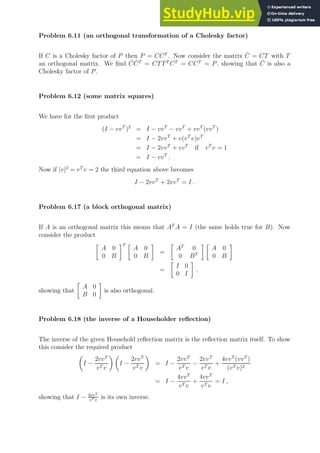
![Problem 6.19 (the number of Householder transformations to triangulate)
Assume that n q the first Householder transformation will zero all elements in Aij for Ank
where 1 ≤ k ≤ q−1. The second Householder transformation will zero all elements of An−1,k
for 1 ≤ k ≤ q − 2. We can continue this n − q + 1 times. Thus we require q − 1 Householder
transformations to triangulate a n × q matrix. This does not change if n = q.
Now assume n q. We will require n Householder transformations when n q. If n = q
the last Householder transformation is not required. Thus we require n − 1 in this case.
Problem 6.20 (the nonlinear equation solved by C(t))
Warning: There is a step below this is not correct or at least it doesn’t seem to be correct
for 2x2 matrices. I was not sure how to fix this. If anyone has any ideas please email me.
Consider the differential equation for the continuous covariance matrix P(t) given by
Ṗ(t) = F(t)P(t) + P(t)FT
(t) + G(t)Q(t)G(t)T
, (112)
We want to prove that if C(t) is the differentiable Cholesky factor of P(t) i.e. P(t) =
C(t)C(t)T
then C(t) are solutions to the following nonlinear equation
Ċ(t) = F(t)C(t) +
1
2
[G(t)Q(t)GT
(t) + A(t)]C−T
(t) ,
where A(t) is a skew-symmetric matrix. Since C(t) is a differentiable Cholesky factor of P(t)
then P(t) = C(t)C(t)T
and the derivative of P(t) by the product rule is given by
Ṗ(t) = Ċ(t)C(t)T
+ C(t)Ċ(t)T
.
When this expression is put into Equation 112 we have
Ċ(t)C(t)T
+ C(t)Ċ(t)T
= F(t)C(t)C(t)T
+ C(t)C(t)T
FT
+ GQGT
.
Warning: This next step does not seem to be correct.
If I could show that Ċ(t)C(t)T
+ C(t)Ċ(t)T
= 2Ċ(t)C(t)T
then I would have
2Ċ(t)C(t)T
= F(t)C(t)C(t)T
+ C(t)C(t)T
FT
+ GQGT
,
Thus when we solve for Ċ(t) we find
Ċ(t) =
1
2
F(t)C(t) +
1
2
C(t)C(t)T
F(t)T
C(t)−T
+
1
2
G(t)Q(t)G(t)T
C(t)−T
= F(t)C(t) +
1
2
G(t)Q(t)G(t)T
− F(t)C(t)C(t)T
+ C(t)C(t)T
F(t)T
C(t)−T
.
From this expression if we define the matrix A(t) as A(t) ≡ −F(t)C(t)C(t)T
+C(t)C(t)T
F(t)T
we note that
A(t)T
= −C(t)C(t)T
F(t)T
+ F(t)C(t)C(t)T
= −A(t) ,
so A(t) is skew symmetric and we have the desired nonlinear differential equation for C(t).](https://image.slidesharecdn.com/asolutionmanualandnotesforkalmanfilteringtheoryandpracticeusingmatlab-230805193035-a97ddfb0/85/A-Solution-Manual-And-Notes-For-Kalman-Filtering-Theory-And-Practice-Using-MATLAB-85-320.jpg)

![Problem 6.24 (Swerling’s informational form)
Consider the suggested product we find
P(+)P(+)−1
= P(−) − P(−)HT
[HP(−)HT
+ R]−1
HP(−)
P(−)−1
+ HT
R−1
H
= I + P(−)HT
R−1
H − P(−)HT
[HP(−)HT
+ R]−1
H
− P(−)HT
[HP(−)HT
+ R]−1
HP(−)HT
R−1
H
= I
+ P(−)HT
R−1
H − [HP(−)HT
+ R]−1
H − [HP(−)HT
+ R]−1
HP(−)HT
R−1
H
= I + P(−)HT
[HP(−)HT
+ R]−1
[HP(−)HT
+ R]R−1
H − H − HP(−)HT
R−1
H
= I ,
as we were to show.
Problem 6.25 (Cholesky factors of Y = P−1
)
If P = CCT
then defining Y −1
as Y −1
= P = CCT
we have that
Y = (CCT
)−1
= C−T
C−1
= (C−T
)(C−T
)T
,
showing that the Cholesky factor of Y = P−1
is given by C−T
.](https://image.slidesharecdn.com/asolutionmanualandnotesforkalmanfilteringtheoryandpracticeusingmatlab-230805193035-a97ddfb0/85/A-Solution-Manual-And-Notes-For-Kalman-Filtering-Theory-And-Practice-Using-MATLAB-87-320.jpg)

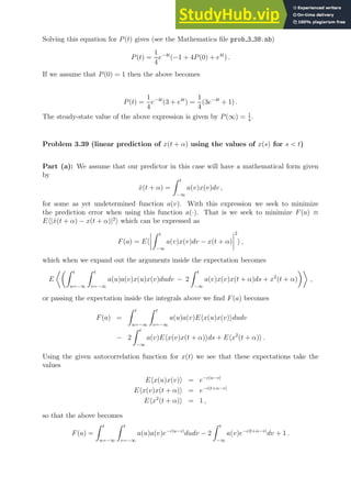
![If we look for the steady-state solution we have P(∞) =
√
RQ. The steady-state Kalman
gain in this case is given by
K(∞) = P(∞)HT
R−1
=
√
RQ
R
=
r
Q
R
.
which is a constant and never decays to zero. This is a good property in that it means
that the filter will never become so over confident that it will not update its belief with new
measurements. For the modified state equations (where we have added process noise) we
can explicitly compute the error between our state estimate x̂2(t) and the “truth” x2(t). To
do this recall that we will be filtering and computing x̂2(t) using
˙
x̂2(t) = Fx̂2 + K(t)(z(t) − Hx̂2(t)) .
When we consider the long time limit we can take K(t) → K(∞) and with F = 0, H = 1
we find our estimate of the state is the solution to
˙
x̂2 + K(∞)x̂2 = K(∞)z(t) .
We can solve this equation using Laplace transforms where we get (since L( ˙
x̂2) = sx̂2)
[s + K(∞)]x̂2(s) = K(∞)z(s) ,
so that our steady-state filtered solution x̂2(s) looks like
x̂2(s) =
K(∞)
s + K(∞)
z(s) .
We are now in a position to see how well our estimate of the state x̂2 compares with the
actual true value given by Equation 118. We will do this by considering the error in the
state i.e. x̃(t) = x̂2(t) − x2(t), specifically the Laplace transform of this error or x̃(s) =
x̂2(s) − x2(s). Now under the best case possible, where there is no measurement noise v = 0,
our measurement z(t) in these models (Equations 117, 119, and 120) is exactly x2(t) which
we wish to estimate. In this case since we know the functional form of the true solution x2(t)
via. Equation 118, we know then the Laplace transform of z(t)
z(s) = x2(s) = L{x2(0) + x1(0)t} =
x2(0)
s
+
x1(0)
s2
. (122)
With this we get
x̃2(s) = x̂2(s) − x2(s) =
K(s)
s + K(s)
− 1
x2(s)
= −
s
s + K(∞)
x2(s) .
Using the final value theorem we have that
x̃2(∞) = x̂2(∞) − x2(∞) = lim
s→0
s [x̂2(s) − x2(s)]
= lim
s→0
s
−
s
s + K(s)
x2(s)
.](https://image.slidesharecdn.com/asolutionmanualandnotesforkalmanfilteringtheoryandpracticeusingmatlab-230805193035-a97ddfb0/85/A-Solution-Manual-And-Notes-For-Kalman-Filtering-Theory-And-Practice-Using-MATLAB-89-320.jpg)
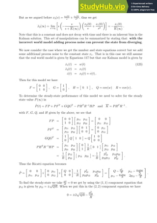
![Which means that p2
22 = ±2R
√
QR. We must take the positive sign as p22 must be a positive
real number. To take the positive number we have p12 =
√
QR. Thus p2
22 = 2Q1/2
R3/2
or
p22 =
√
2(R3
Q)1/4
.
When we put this value into the (1, 2) component equation we get
p11 =
p12p22
R
=
√
2
(QR)1/2
R
(R3
Q)1/4
=
√
2(Q3
R)1/4
.
Thus the steady-state Kalman gain K(∞) then becomes
K(∞) = P(∞)HT
R−1
=
1
R
p11(∞) p12(∞)
p12(∞) p22(∞)
0
1
=
1
R
p12(∞)
p22(∞)
=
Q
R
1/2
√
2 Q
R
1/4
#
. (124)
To determine how the steady-state Kalman estimate x̂(t) will compare to the truth x given
via x1(t) = x1(0) and Equation 118 for x2(t). We start with the dynamical system we solve
to get the estimate x̂ given by
˙
x̂ = Fx̂ + K(z − Hx̂) .
Taking the long time limit where t → ∞ of this we have
˙
x̂(t) = Fx̂(t) + K(∞)z(t) − K(∞)Hx̂(t) = (F − K(∞)H)x̂(t) + K(∞)z(t) .
Taking the Laplace transform of the above we get
sx̂(s) − x̂(0) = (F − K(∞)H)x̂(s) + K(∞)z(s) ,
or
[sI − F − K(∞)H]x̂(s) = x̂(0) + K(∞)z(s) .
Dropping the term x̂(0) as t → ∞ and it influence will be negligible we get
x̂(s) = [sI − F − K(∞)]−1
K(∞)z(s) . (125)
From the definitions of the matrices above we have that
sI − F + K(∞)H =
s K1(∞)
−1 s + K2(∞)
,
and the inverse is given by
[sI − F + K(∞)H]−1
=
1
s(s + K2(∞)) + K1(∞)
s + K2(∞) −K1(∞)
1 s
.
Since we know that z(s) is given by Equation 122 we can use this expression to evaluate the
vector x̂(s) via Equation 125. We could compute both x̂1(s) and x̂2(s) but since we only
want to compare performance of x̂2(s) we only calculate that component. We find
x̂2(s) =
K1(∞) + sK2(∞)
s(s + K2(∞)) + K1(∞)
z(s) . (126)](https://image.slidesharecdn.com/asolutionmanualandnotesforkalmanfilteringtheoryandpracticeusingmatlab-230805193035-a97ddfb0/85/A-Solution-Manual-And-Notes-For-Kalman-Filtering-Theory-And-Practice-Using-MATLAB-91-320.jpg)

![References
[1] W. G. Kelley and A. C. Peterson. Difference Equations. An Introduction with Applica-
tions. Academic Press, New York, 1991.](https://image.slidesharecdn.com/asolutionmanualandnotesforkalmanfilteringtheoryandpracticeusingmatlab-230805193035-a97ddfb0/85/A-Solution-Manual-And-Notes-For-Kalman-Filtering-Theory-And-Practice-Using-MATLAB-94-320.jpg)
A Solution Manual And Notes For Kalman Filtering Theory And Practice Using MATLAB
- 1. A Solution Manual and Notes for: Kalman Filtering: Theory and Practice using MATLAB by Mohinder S. Grewal and Angus P. Andrews. John L. Weatherwax∗ April 30, 2012 Introduction Here you’ll find some notes that I wrote up as I worked through this excellent book. There is also quite a complete set of solutions to the various end of chapter problems. I’ve worked hard to make these notes as good as I can, but I have no illusions that they are perfect. If you feel that that there is a better way to accomplish or explain an exercise or derivation presented in these notes; or that one or more of the explanations is unclear, incomplete, or misleading, please tell me. If you find an error of any kind – technical, grammatical, typographical, whatever – please tell me that, too. I’ll gladly add to the acknowledgments in later printings the name of the first person to bring each problem to my attention. I hope you enjoy this book as much as I have and that these notes might help the further development of your skills in Kalman filtering. Acknowledgments Special thanks to (most recent comments are listed first): Bobby Motwani and Shantanu Sultan for finding various typos from the text. All comments (no matter how small) are much appreciated. In fact, if you find these notes useful I would appreciate a contribution in the form of a solution to a problem that is not yet worked in these notes. Sort of a “take a penny, leave a penny” type of approach. Remember: pay it forward. ∗ wax@alum.mit.edu 1
- 2. Chapter 2: Linear Dynamic Systems Notes On The Text Notes on Example 2.5 We are told that the fundamental solution Φ(t) to the differential equation dny dt = 0 when written in companion form as the matrix dx dt = Fx or in components d dt x1 x2 x3 . . . xn−2 xn−1 xn = 0 1 0 0 0 1 0 0 0 ... ... ... ... ... 0 1 0 0 0 1 0 0 0 x1 x2 x3 . . . xn−2 xn−1 xn , is Φ(t) = 1 t 1 2 t2 1 3! t3 · · · 1 (n−1)! tn−1 0 1 t 1 2 t2 · · · 1 (n−2)! tn−2 0 0 1 t · · · 1 (n−3)! tn−3 0 0 0 1 · · · 1 (n−4)! tn−4 . . . . . . 0 0 0 0 · · · 1 . Note here the only nonzero values in the matrix F are the ones on its first superdiagonal. We can verify this by showing that the given Φ(t) satisfies the differential equation and has the correct initial conditions, that is Φ(t) dt = FΦ(t) and Φ(0) = I. That Φ(t) has the correct initial conditions Φ(0) = I is easy to see. For the t derivative of Φ(t) we find Φ′ (t) = 0 1 t 1 2! t2 · · · 1 (n−2)! tn−2 0 0 1 t · · · 1 (n−3)! tn−3 0 0 0 1 · · · 1 (n−4)! tn−4 0 0 0 0 · · · 1 (n−5)! tn−5 . . . . . . 0 0 0 0 · · · 0 . From the above expressions for Φ(t) and F by considering the given product FΦ(t) we see that it is equal to Φ′ (t) derived above as we wanted to show. As a simple modification of the above example consider what the fundamental solution would be if we were given the
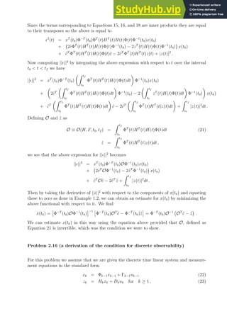
- 3. following companion form for a vector of unknowns x d dt x̂1 x̂2 x̂3 . . . x̂n−2 x̂n−1 x̂n = 0 0 0 1 0 0 0 1 0 ... ... ... ... ... 0 0 0 1 0 0 0 1 0 x̂1 x̂2 x̂3 . . . x̂n−2 x̂n−1 x̂n = F̂ x̂1 x̂2 x̂3 . . . x̂n−2 x̂n−1 x̂n . Note in this example the only nonzero values in F̂ are the ones on its first subdiagonal. To determine Φ(t) we note that since this coefficient matrix F̂ in this case is the transpose of the first system considered above F̂ = FT the system we are asking to solve is d dt x̂ = FT x̂. Thus the fundamental solution to this new problem is Φ̂(t) = eF T t = (eF t )T = Φ(t)T , and that this later matrix looks like Φ̂(t) = 1 0 0 0 · · · 0 t 1 0 0 · · · 0 1 2 t2 t 1 0 · · · 0 1 3! t3 1 2 t2 t 1 · · · 0 . . . . . . . . . . . . ... . . . 1 (n−1)! tn−1 1 (n−2)! tn−2 1 (n−3)! tn−3 1 (n−4)! tn−4 · · · 1 . Verification of the Solution to the Continuous Linear System We are told that a solution to the continuous linear system with a time dependent companion matrix F(t) is given by x(t) = Φ(t)Φ(t0)−1 x(t0) + Φ(t) Z t t0 Φ−1 (τ)C(τ)u(τ)dτ . (1) To verify this take the derivative of x(t) with respect to time. We find x′ (t) = Φ′ (t)Φ−1 (t0) + Φ′ (t) Z t t0 Φ−1 (τ)C(τ)u(τ)dτ + Φ(t)Φ−1 (t)C(t)u(t) = Φ′ (t)Φ−1 (t)x(t) + C(t)u(t) = F(t)Φ(t)Φ−1 (t)x(t) + C(t)u(t) = F(t)x(t) + C(t)u(t) . showing that the expression given in Equation 1 is indeed a solution. Note that in the above we have used the fact that for a fundamental solution Φ(t) we have Φ′ (t) = F(t)Φ(t).
- 4. Problem Solutions Problem 2.2 (the companion matrix for dny dtn = 0) We begin by defining the following functions xi(t) x1(t) = y(t) x2(t) = ẋ1(t) = ẏ(t) x3(t) = ẋ2(t) = ¨ x1(t) = ÿ(t) . . . xn(t) = ẋn−1(t) = · · · = dn−1 y(t) dtn−1 , as the components of a state vector x. Then the companion form for this system is given by d dt x(t) = d dt x1(t) x2(t) . . . xn−1(t) xn(t) = x2(t) x3(t) . . . xn(t) dny(t) dtn = 0 1 0 0 · · · 0 0 0 1 0 · · · 0 0 0 0 1 · · · 0 ... 1 0 . . . 0 0 x1(t) x2(t) . . . xn−1(t) xn(t) = Fx(t) With F the companion matrix given by F = 0 1 0 0 · · · 0 0 0 1 0 · · · 0 0 0 0 1 · · · 0 ... 1 0 . . . 0 0 . Which is of dimensions of n × n. Problem 2.3 (the companion matrix for dy dt = 0 and d2y dt2 = 0) If n = 1 the above specifies to the differential equation dy dt = 0 and the companion matrix F is the zero matrix i.e. F = [0]. When n = 2 we are solving the differential equation given by d2y dt2 = 0, and a companion matrix F given by F = 0 1 0 0 . Problem 2.4 (the fundamental solution matrix for dy dt = 0 and d2y dt2 = 0) The fundamental solution matrix Φ(t) satisfies dΦ dt = F(t)Φ(t) ,
- 5. with an initial condition Φ(0) = I. When n = 1, we have F = [0], so dΦ dt = 0 giving that Φ(t) is a constant, say C. To have the initial condition hold Φ(0) = 1, we must have C = 1, so that Φ(t) = 1 . (2) When n = 2, we have F = 0 1 0 0 , so that the equation satisfied by Φ is dΦ dt = 0 1 0 0 Φ(t) . If we denote the matrix Φ(t) into its components Φij(t) we have that 0 1 0 0 Φ(t) = 0 1 0 0 Φ11 Φ12 Φ21 Φ22 = Φ21 Φ22 0 0 , so the differential equations for the components of Φij satisfy dΦ11 dt dΦ12 dt dΦ21 dt dΦ22 dt = Φ21 Φ22 0 0 . Solving the scalar differential equations above for Φ21 and Φ22 using the known initial con- ditions for them we have Φ21 = 0 and Φ22 = 1. With these results the differential equations for Φ11 and Φ12 become dΦ11 dt = 0 and dΦ12 dt = 1 , so that Φ11 = 1 and Φ21(t) = t . Thus the fundamental solution matrix Φ(t) in the case when n = 2 is Φ(t) = 1 t 0 1 . (3) Problem 2.5 (the state transition matrix for dy dt = 0 and d2y dt2 = 0) Given the fundamental solution matrix Φ(t) for a linear system dx dt = F(t)x the state transi- tion matrix Φ(τ, t) is given by Φ(τ)Φ(t)−1 . When n = 1 since Φ(t) = 1 the state transition matrix in this case is Φ(τ, t) = 1 also. When n = 2 since Φ(t) = 1 t 0 1 we have Φ(t)−1 = 1 −t 0 1 , so that Φ(τ)Φ(t)−1 = 1 τ 0 1 1 −t 0 1 = 1 −t + τ 0 1 .
- 6. Problem 2.6 (an example in computing the fundamental solution) We are asked to find the fundamental solution Φ(t) for the system d dt x1(t) x2(t) = 0 0 −1 −2 x1(t) x2(t) + 1 1 . To find the fundamental solution for the given system we first consider the homogeneous system d dt x1(t) x2(t) = 0 0 −1 −2 x1(t) x2(t) . To solve this system we need to find the eigenvalues of 0 0 −1 −2 . We solve for λ in the following −λ 0 −1 −2 − λ = 0 , or λ2 + 2λ = 0. This equation has roots given by λ = 0 and λ = −2. The eigenvector of this matrix for the eigenvalue λ = 0 is given by solving for the vector with components v1 and v2 that satisfies 0 0 −1 −2 v1 v2 = 0 , so −v1 − 2v2 = 0 so v1 = −2v2. Which can be made true if we take v2 = −1 and v1 = 2, giving the eigenvector of 2 −1 . When λ = −2 we have to find the vector v1 v2 such that 2 0 −1 0 v1 v2 = 0 , is satisfied. If we take v1 = 0 and v2 = 1 we find an eigenvector of v = 0 1 . Thus with these eigensystem the general solution for x(t) is then given by x(t) = c1 2 −1 + c2 0 1 e−2t = 2 0 −1 e−2t c1 c2 , (4) for two constants c1 and c2. The initial condition requires that x(0) be related to c1 and c2 by x(0) = x1(0) x2(0) = 2 0 −1 1 c1 c2 . Solving for c1 and c2 we find c1 c2 = 1/2 0 1/2 1 x1(0) x2(0) . (5) Using Equation 4 and 5 x(t) is given by x(t) = 2 0 −1 e−2t 1/2 0 1/2 1 x1(0) x2(0) = 1 0 1 2 (−1 + e−2t ) e−2t x1(0) x2(0) .
- 7. From this expression we see that our fundamental solution matrix Φ(t) for this problem is given by Φ(t) = 1 0 −1 2 (1 − e−2t ) e−2t . (6) We can verify this result by checking that this matrix has the required properties that Φ(t) should have. One property is Φ(0) = 1 0 0 1 , which can be seen true from the above expression. A second property is that Φ′ (t) = F(t)Φ(t). Taking the derivative of Φ(t) we find Φ′ (t) = 0 0 −1 2 (2e−2t ) −2e−2t = 0 0 −e−2t −2e−2t , while the product F(t)Φ(t) is given by 0 0 −1 −2 1 0 −1 2 (1 − e−2t ) e−2t = 0 0 −e−2t −2e−2t , (7) showing that indeed Φ′ (t) = F(t)Φ(t) as required for Φ(t) to be a fundamental solution. Recall that the full solution for x(t) is given by Equation 1 above. From this we see that we still need to calculate the second term above involving the fundamental solution Φ(t), the input coupling matrix C(t), and the input u(t) given by Φ(t) Z t t0 Φ−1 (τ)C(τ)u(τ)dτ . (8) Now we can compute the inverse of our fundamental solution matrix Φ(t)−1 as Φ(t)−1 = 1 e−2t e−2t 0 1 2 (1 − e−2t ) 1 = 1 0 1 2 (e2t − 1) e2t . Then this term is given by = 1 0 −1 2 (1 − e−2t ) e−2t Z t 0 1 0 1 2 (e2τ − 1) e2τ 1 1 dτ = 1 0 −1 2 (1 − e−2t ) e−2t Z t 0 1 1 2 e2τ − 1 2 + e2τ dτ = 1 0 −1 2 (1 − e−2t ) e−2t t 3 4 (e2t − 1) − t 2 dτ = t −t 2 + 3 4 (1 − e−2t ) . Thus the entire solution for x(t) is given by x(t) = 1 0 −1 2 (1 − e−2t ) e−2t x1(0) x2(0) + t −t 2 + 3 4 (1 − e−2t ) . (9) We can verify that this is indeed a solution by showing that it satisfies the original differential equation. We find x′ (t) given by x′ (t) = 0 0 −e−2t −2e−2t x1(0) x2(0) + 1 −1 2 + 3 2 e−2t = 0 0 −1 −2 1 0 −1 2 (1 − e−2t ) e−2t x1(0) x2(0) + 1 −1 2 + 3 2 e−2t ,
- 8. where we have used the factorization given in Equation 7. Inserting the the needed term to complete an expression for x(t) (as seen in Equation 9) we find x′ (t) = 0 0 −1 −2 1 0 −1 2 (1 − e−2t ) e−2t x1(0) x2(0) + t −t 2 + 3 4 (1 − e−2t ) − 0 0 −1 −2 t −t 2 + 3 4 (1 − e−2t ) + 1 −1 2 + 3 2 e−2t . or x′ (t) = 0 0 −1 −2 x(t) − 0 −3 2 (1 − e−2t ) + 1 −1 2 + 3 2 e−2t = 0 0 −1 −2 x(t) + 1 1 , showing that indeed we do have a solution. Problem 2.7 (solving a dynamic linear system) Studying the homogeneous problem in this case we have d dt x1(t) x2(t) = −1 0 0 −1 x1(t) x2(t) . which has solution by inspection given by x1(t) = x1(0)e−t and x2(t) = x2(0)e−t . Thus as a vector we have x(t) given by x1(t) x2(t) = e−t 0 0 e−t x1(0) x2(0) . Thus the fundamental solution matrix Φ(t) for this problem is seen to be Φ(t) = e−t 1 0 0 1 so that Φ−1 (t) = et 1 0 0 1 . Using Equation 8 we can calculate the inhomogeneous solution as Φ(t) Z t t0 Φ−1 (τ)C(τ)u(τ)dτ = e−t 1 0 0 1 Z t 0 eτ 1 0 0 1 5 1 dτ = e−t (et − 1) 5 1 . Thus the total solution is given by x(t) = e−t 1 0 0 1 x1(0) x2(0) + (1 − e−t ) 5 1 .
- 9. Problem 2.8 (the reverse problem) Warning: I was not really sure how to answer this question. There seem to be multiple possible continuous time systems for a given discrete time system and so multiple solutions are possible. If anyone has an suggestions improvements on this please let me know. From the discussion in Section 2.4 in the book we can study our continuous system at only the discrete times tk by considering x(tk) = Φ(tk, tk−1)x(tk−1) + Z tk tk−1 Φ(tk, σ)C(σ)u(σ)dσ . (10) Thus for the discrete time dynamic system given in this problem we could associate Φ(tk, tk−1) = 0 1 −1 2 , to be the state transition matrix which also happens to be a constant matrix. To complete our specification of the continuous problem we still need to find functions C(·) and u(·) such that they satisfy Z tk tk−1 Φ(tk, σ)C(σ)u(σ)dσ = Z tk tk−1 0 1 −1 2 C(σ)u(σ)dσ = 0 1 . There are many way to satisfy this equation. One simple method is to take C(σ), the input coupling matrix, to be the identity matrix which then requires the input u(σ) satisfy the following 0 1 −1 2 Z tk tk−1 u(σ)dσ = 0 1 . On inverting the matrix on the left-hand-side we obtain Z tk tk−1 u(σ)dσ = 2 −1 1 0 0 1 = −1 0 . If we take u(σ) as a constant say u1 u2 , then this equation will be satisfied if u2 = 0, and u1 = − 1 ∆t with ∆t = tk − tk−1 assuming a constant sampling step size ∆t. Problem 2.9 (conditions for observability and controllability) Since the dynamic system we are given is continuous, with a dynamic coefficient matrix F given by F = 1 1 0 1 , an input coupling matrix C(t) given by C = c1 c2 , and a measure- ment sensitivity matrix H(t) given by H(t) = h1 h2 , all of which are independent of time. The condition for observability is that the matrix M defined as M = HT FT HT (FT )2 HT · · · (FT )n−1 HT , (11)
- 10. has rank n = 2. We find with the specific H and F for this problem that M = h1 h2 1 0 1 1 h1 h2 = h1 h1 h2 h1 + h2 , needs to have rank 2. By reducing M to row reduced echelon form (assuming h1 6= 0) as M ⇒ h1 h1 0 h1 + h2 − h2 ⇒ h1 h1 0 h1 ⇒ 1 1 0 1 . Thus we see that M will have rank 2 and our system will be observable as long as h1 6= 0. To be controllable we need to consider the matrix S given by S = C FC F2 C · · · Fn−1 C , (12) or in this case S = c1 c1 + c2 c2 c2 . This matrix is the same as that in M except for the rows of S are exchanged from that of M. Thus for the condition needed for S to have a rank n = 2 requires c2 6= 0. Problem 2.10 (controllability and observability of a dynamic system) For this continuous time system the dynamic coefficient matrix F(t) is given by F(t) = 1 0 1 0 , the input coupling matrix C(t) is given by C(t) = 1 0 0 −1 , and the measurement sensitivity matrix H(t) is given by H(t) = 0 1 . The observability of this system is determined by the rank of M defined in Equation 11, which in this case is given by M = 0 1 1 1 0 0 0 1 = 0 1 1 0 . Since this matrix M is of rank two, this system is observable. The controllability of this system is determined by the rank of the matrix S defined by Equation 12, which in this case since FC = 1 0 1 0 1 0 0 −1 = 1 0 1 0 becomes S = 1 0 1 0 0 −1 1 0 . Since this matrix has a rank of two this system is controllable. Problem 2.11 (the state transition matrix for a time-varying system) For this problem the dynamic coefficient matrix is given by F(t) = t 1 0 0 1 . In terms of the components of the solution x(t) of we see that each xi(t) satisfies dxi(t) dt = txi(t) for i = 1, 2 .
- 11. Then solving this differential equation we have xi(t) = cie t2 2 for i = 1, 2. As a vector x(t) can be written as x(t) = c1 c2 e t2 2 = e t2 2 0 0 e t2 2 # x1(0) x2(0) . Thus we find Φ(t) = e t2 2 1 0 0 1 , is the fundamental solution and the state transition matrix Φ(τ, t) is given by Φ(τ, t) = Φ(τ)Φ(t)−1 = e− 1 2 (t2−τ2) 1 0 0 1 . Problem 2.12 (an example at finding the state transformation matrix) We desire to find the state transition matrix for a continuous time system with a dynamic coefficient matrix given by F = 0 1 1 0 . We will do this by finding the fundamental solution matrix Φ(t) that satisfies Φ′ (t) = FΦ(t), with an initial condition of Φ(0) = I. We find the eigenvalues of F to be given by −λ 1 1 −λ = 0 ⇒ λ2 − 1 = 0 ⇒ λ = ±1 . The eigenvalue λ1 = −1 has an eigenvector given by 1 −1 , while the eigenvalue λ2 = 1 has an eigenvalue of 1 1 . Thus the general solution to this linear time invariant system is given by x(t) = c1 1 −1 e−t + c2 1 1 et = e−t et −e−t et c1 c2 . To satisfy the required initial conditions x(0) = x1(0) x2(0) , the coefficients c1 and c2 must equal c1 c2 = 1 1 −1 1 −1 x1(0) x2(0) = 1 2 1 −1 1 1 x1(0) x2(0) . Thus the entire solution for x(t) in terms of its two components x1(t) and x2(t) is given by x(t) = 1 2 e−t et −et et 1 −1 1 1 x1(0) x2(0) = 1 2 e−t + et −e−t + et −et + et e−t + et x1(0) x2(0) .
- 12. From which we see that the fundamental solution matrix Φ(t) for this system is given by Φ(t) = 1 2 e−t + et −e−t + et −et + et e−t + et . The state transition matrix Φ(τ, t) = Φ(τ)Φ−1 (t). To get this we first compute Φ−1 . We find Φ−1 (t) = 2 (e−t + et)2 − (e−t − et)2 e−t + et e−t − et e−t − et e−t + et = 2 ((e−t + et) − (e−t − et))((e−t + et) + (e−t − et)) e−t + et e−t − et e−t − et e−t + et = 1 (2et)(e−t) e−t + et e−t − et e−t − et e−t + et = 1 2 e−t + et e−t − et e−t − et e−t + et = Φ(t) . Thus we have Φ(τ, t) given by Φ(τ, t) = 1 4 e−τ + eτ e−τ − eτ e−τ − eτ e−τ + eτ e−t + et e−t − et e−t − et e−t + et . Problem 2.13 (recognizing the companion form for d3y dt3 ) Part (a): Writing this system in the vector form with x = x1(t) x2(t) x3(t) , we have ẋ(t) = 0 1 0 0 0 1 0 0 0 x1(t) x2(t) x3(t) , so we see the system companion matrix, F, is given by F = 0 1 0 0 0 1 0 0 0 . Part (b): For the F given above we recognize it as the companion matrix for the system d3y dt3 = 0, (see the section on Fundamental solutions of Homogeneous equations), and as such has a fundamental solution matrix Φ(t) given as in Example 2.5 of the appropriate dimension. That is Φ(t) = 1 t 1 2 t2 0 1 t 0 0 1 .
- 13. Problem 2.14 (matrix exponentials of antisymmetric matrices are orthogonal) If M is an antisymmetric matrix then MT = −M. Consider the matrix A defined as the matrix exponential of M i.e. A ≡ eM . Then since AT = eMT = e−M , is the inverse of eM (equivalently A) we see that AT = A−1 so A is orthogonal. Problem 2.15 (a derivation of the condition for continuous observability) We wish to derive equation 2.32 which states that the observability of a continuous dynamic system is given by the singularity of the matrix O where O = O(H, F, t0, tf ) = Z tf t0 ΦT (t)HT (t)H(t)Φ(t)dt , in that if O is singular the Storm is not observable and if it is non-singular the system is observable. As in example 1.2 we measure z(t) where z(t) is obtained from x(t) using the measurement sensitivity matrix H(t) as z(t) = H(t)x(t). Using our general solution for x(t) from Equation 1 we have z(t) = H(t)Φ(t)Φ(t0)−1 x(t0) + H(t)Φ(t) Z t t0 Φ−1 (τ)C(τ)u(τ)dτ , (13) observability is whether we can compute x(t0) given its inputs u(τ) and its outputs z(t), over the real interval t0 t tf . Setting up an error criterion to estimate how well we estimate x̂0, assume that we have measured z(t) out instantaneous error will then be ǫ(t)2 = |z(t) − H(t)x(t)|2 = xT (t)HT (t)H(t)x(t) − 2xT (t)HT (t)z(t) + |z(t)|2 . Since we are studying a linear continuous time system, the solution x(t) in terms of the state transition matrix Φ(t, τ), the input coupling matrix C(t), the input u(t), and the initial state x(t0) is given by Equation 1 above. Defining c̃ as the vector c̃ = Z tf t0 Φ−1 (τ)C(τ)u(τ)dτ , we then have x(t) given by x(t) = Φ(t)Φ−1 (t0)x(t0) + Φ(t)c̃, thus the expression for ǫ(t)2 in terms of x(t0) is given by ǫ2 (t) = (xT (t0)Φ−T (t0)ΦT (t) + c̃T ΦT (t))HT (t)H(t)(Φ(t)Φ−1 (t0)x(t0) + Φ(t)c̃) − 2(xT (t0)Φ−T (t0)ΦT (t) + c̃T ΦT (t))HT (t)z(t) + |z(t)|2 = xT (t0)Φ−T (t0)ΦT (t)HT (t)H(t)Φ(t)Φ−1 (t0)x(t0) (14) + xT (t0)Φ−T (t0)ΦT (t)HT (t)H(t)Φ(t)c̃ (15) + c̃T ΦT (t)HT (t)H(t)Φ(t)Φ−1 (t0)x(t0) (16) + c̃T ΦT (t)HT (t)H(t)Φ(t)c̃ (17) − 2xT (t0)Φ−T (t0)ΦT (t)HT (t)z(t) (18) − 2c̃T ΦT (t)HT (t)z(t) (19) + |z(t)|2 . (20)
- 14. Since the terms corresponding to Equations 15, 16, and 18 are inner products they are equal to their transposes so the above is equal to ǫ2 (t) = xT (t0)Φ−T (t0)ΦT (t)HT (t)H(t)Φ(t)Φ−1 (t0)x(t0) + 2c̃ΦT (t)HT (t)H(t)Φ(t)Φ−1 (t0) − 2zT (t)H(t)Φ(t)Φ−1 (t0) x(t0) + c̃T ΦT (t)HT (t)H(t)Φ(t)c̃ − 2c̃T ΦT (t)HT (t)z(t) + |z(t)|2 . Now computing ||ǫ||2 by integrating the above expression with respect to t over the interval t0 t tf we have ||ǫ||2 = xT (t0)Φ−T (t0) Z tf t0 ΦT (t)HT (t)H(t)Φ(t)dt Φ−1 (t0)x(t0) + 2c̃T Z tf t0 ΦT (t)HT (t)H(t)Φ(t)dt Φ−1 (t0) − 2 Z tf t0 zT (t)H(t)Φ(t)dt Φ−1 (t0) x(t0) + c̃T Z tf t0 ΦT (t)HT (t)H(t)Φ(t)dt c̃ − 2c̃T Z tf t0 ΦT (t)HT (t)z(t)dt + Z tf t0 |z(t)|2 dt . Defining O and z̃ as O ≡ O(H, F, t0, tf ) = Z tf t0 ΦT (t)HT (t)H(t)Φ(t)dt (21) z̃ = Z tf t0 ΦT (t)HT (t)z(t)dt , we see that the above expression for ||ǫ||2 becomes ||ǫ||2 = xT (t0)Φ−T (t0)OΦ−1 (t0)x(t0) + 2c̃T OΦ−1 (t0) − 2z̃T Φ−1 (t0) x(t0) + c̃T Oc̃ − 2c̃T z̃ + Z tf t0 |z(t)|2 dt . Then by taking the derivative of ||ǫ||2 with respect to the components of x(t0) and equating these to zero as done in Example 1.2, we can obtain an estimate for x(t0) by minimizing the above functional with respect to it. We find x̂(t0) = Φ−T (t0)OΦ−1 (t0) −1 Φ−T (t0)OT c̃ − Φ−T (t0)z̃ = Φ−T (t0)O−1 OT c̃ − z̃ . We can estimate x(t0) in this way using the equation above provided that O, defined as Equation 21 is invertible, which was the condition we were to show. Problem 2.16 (a derivation of the condition for discrete observability) For this problem we assume that we are given the discrete time linear system and measure- ment equations in the standard form xk = Φk−1xk−1 + Γk−1uk−1 (22) zk = Hkxk + Dkuk for k ≥ 1 , (23)
- 15. and that we wish to estimate the initial state x0 from the received measurements zk for a range of k say 1 ≤ k ≤ kf . To do this we will solve Equation 22 and 23 for xk directly in terms of x0 by induction. To get an idea of what the solution for xk and zk should look like a a function of k we begin by computing xk and zk for a few values of k. To begin with lets take k = 1 in Equation 22 and Equation 23 to find x1 = Φ0x0 + Γ0u0 z1 = H1x1 + D1u1 = H1Φ0x0 + H1Γ0u0 + D1u1 . Where we have substituted x1 into the second equation for z1. Letting k = 2 in Equation 22 and Equation 23 we obtain x2 = Φ1x1 + Γ1u1 = Φ1(Φ0x0 + Γ0u0) + Γ1u1 = Φ1Φ0x0 + Φ1Γ0u0 + Γ1u1 z2 = H2Φ1Φ0x0 + H2Φ1Γ0u0 + H2Γ1u1 . Observing one more value of xk and zk let k = 3 in Equation 22 and Equation 23 to obtain x3 = Φ2Φ1Φ0x0 + Φ2Φ1Γ0u0 + Φ2Γ1u1 + Γ2u2 z3 = H3Φ2Φ1Φ0x0 + H3Φ2Φ1Γ0u0 + H3Φ2Γ1u1 + H3Γ2u2 . From these specific cases we hypothesis that that the general expression for xk in terms of x0 is be given by the following specific expression xk = k−1 Y i=0 Φi ! x0 + k−1 X l=0 k−1−l Y i=0 Φi ! Γlul (24) Lets define some of these matrices. Define Pk−1 as Pk−1 ≡ k−1 Y i=0 Φi = Φk−1Φk−2 · · · Φ1Φ0 , (25) where since Φk are matrices the order of the factors in the product matters. Our expression for xk in terms of x0 becomes xk = Pk−1x0 + k−1 X l=0 Pk−1−lΓlul . From this expression for xk we see that zk is given by (in terms of x0) zk = HkPk−1x0 + Hk k−1 X l=0 Pk−1−lΓlul + Dkuk for k ≥ 1 . (26) We now set up a least squares problem aimed at the estimation of x0. We assume we have kf measurements of zk and form the L2 error functional ǫ(x0) of all received measurements as ǫ2 (x0) = kf X i=1 |HiPi−1x0 + Hi i−1 X l=0 Pi−1−lΓlul + Diui − zi|2
- 16. As in Example 1.1 in the book we can minimize ǫ(x0)2 as a function of x0 by taking the partial derivatives of the above with respect to x0, setting the resulting expressions equal to zero and solving for x0. To do this we simply things by writing ǫ(x0)2 as ǫ2 (x0) = kf X i=1 |HiPi−1x0 − z̃i|2 , where z̃i is defined as z̃i = zi − Hi i−1 X l=0 Pi−1−lΓlul − Diui . (27) With this definition the expression for ǫ2 (x0) can be simplified by expanding the quadratic to get ǫ2 (x0) = kf X i=1 xT 0 PT i−1HT i HiPi−1x0 − 2xT 0 PT i−1HT i z̃i + z̃T i z̃i = xT 0 kf X i=1 PT i−1HT i Pi−1 x0 − 2xT 0 kf X i=1 PT i−1HT i z̃i + kf X i=1 z̃T i z̃i . Taking the derivative of this expression and setting it equal to zero (so that we can solve for x0) our least squares solution is given by solving 2Ox0 − 2 kf X i=1 PT i−1HT i z̃i = 0 , where we have defined the matrix O as O = tf X k=1 PT i−1HT i HiPi−1 = kf X k=1 k−1 Y i=0 Φi #T HT k Hk k−1 Y i=0 Φi # . (28) Where its important to take the products of the matrices Φk as in the order expressed in Equation 25. An estimate of x0 can then be obtain as x̂0 = O−1 kf X i=1 PT i−1HT i z̃i , provided that the inverse of O exists, which is the desired discrete condition for observability.
- 17. Chapter 3: Random Processes and Stochastic Systems Problem Solutions Problem 3.1 (each pile contains one ace) We can solve this problem by thinking about placing the aces individually ignoring the placement of the other cards. Then once the first ace is placed on a pile we have a probability of 3/4 to place the next ace in a untouched pile. Once this second ace is placed we have 2/4 of a probability of placing a new ace in another untouched pile. Finally, after the third ace is placed we have a probability of 1/4 of placing the final ace on the one pile that does not yet have an ace on it. Thus the probability that each pile contains an ace to be 3 4 2 4 1 4 = 3 32 . Problem 3.2 (a combinatorial identity) We can show the requested identity by recalling that n k represents the number of ways to select k object from n where the order of the k selected objects does not matter. Using this representation we will derive an expression for n k as follows. We begin by considering the group of n objects with one object specified as distinguished or “special”. Then the number of ways to select k objects from n can be decomposed into two distinct occurrences. The times when this “special” object is selected in the subset of size k and the times when its not. When it is not selected in the subset of size k we are specifying our k subset elements from the n − 1 remaining elements giving n − 1 k total subsets in this case. When it is selected into the subset of size k we have to select k − 1 other elements from the n − 1 remaining elements, giving n − 1 k − 1 additional subsets in this case. Summing the counts from these two occurrences we have that factorization can be written as the following n k = n − 1 k + n − 1 k − 1 . Problem 3.3 (dividing the deck into four piles of cards) We have 52 13 ways of selecting the first hand of thirteen cards. After this hand is selected we have 52 − 13 13 = 48 13 ways to select the second hand of cards. After these first
- 18. two hands are selected we have 52 − 2 ∗ 13 13 = 26 13 ways to select the third hand after which the fourth hand becomes whatever cards are left. Thus the total number of ways to divide up a deck of 52 cards into four hands is given by the product of each of these expressions or 52 13 48 13 26 13 . Problem 3.4 (exactly three spades in a hand) We have 52 13 ways to draw a random hand of cards. To draw a hand of cards with explicitly three spades, the spades can be drawn in 13 3 ways, and the remaining nine other cards can be drawn in 52 − 13 9 = 39 9 ways. The probability we have the hand requested is then 13 3 39 9 52 13 . Problem 3.5 (south has three spades when north has three spades) Since we are told that North has exactly three spades from the thirteen possible spade cards the players at the West, East, and South locations must have the remaining spade cards. Since they are assumed to be dealt randomly among these three players the probability South has exactly three of them is 10 3 2 3 7 1 3 3 , This is the same as a binomial distribution with probability of success of 1/3 (i.e. a success is when a spade goes to the player South) and 10 trials. In general, the probability South has k spade cards is given by 10 k 1 3 k 2 3 10−k k = 0, 1, · · · , 10 . Problem 3.6 (having 7 hearts) Part (a): The number of ways we can select thirteen random cards from 52 total cards is 52 13 . The number of hands that contain seven hearts can be derived by first selecting the
- 19. seven hearts to be in that hand in 13 7 ways and then selecting the remaining 13 −7 = 6 cards in 52 − 13 6 = 39 6 ways. Thus the probability for this hand of seven hearts is given by 13 7 39 6 52 13 = 0.0088 . Part (b): Let Ei be the event that our hand has i hearts where 0 ≤ i ≤ 13. Then P(E7) is given in Part (a) above. Let F be the event that we observe a one card from our hand and it is a heart card. Then we want to calculate P(E7|F). From Bayes’ rule this is given by P(E7|F) = P(F|E7)P(E7) P(F) . Now P(F|Ei) is the probability one card observed as hearts given that we have i hearts in the hand. So P(F|Ei) = i 13 for 0 ≤ i ≤ 13 and the denominator P(F) can be computed as P(F) = 13 X i=0 P(F|Ei)P(Ei) = 13 X i=0 i 13 13 i 52 − 13 13 − i 52 13 Using this information and Bayes’ rule above we can compute P(E7|F). Performing the above summation that P(F) = 0.25, see the MATLAB script prob 3 6.m. After computing this numerically we recognize that it is the probability we randomly draw a heart card and given that there are 13 cards from 52 this probability P(F) = 13 52 = 0.25. Then computing the desired probability P(E7|F) we find P(E7|F) = 0.0190 . As a sanity check note that P(E7|F) is greater than P(E7) as it should be, since once we have seen a heart in the hand there is a greater chance we will have seven hearts in that hand. Problem 3.7 (the correlation coefficient between sums) The correlation of a vector valued process x(t) has components given by Ehxi(t1), xj(t2)i = Z ∞ −∞ Z ∞ −∞ xi(t1)xj(t2)p(xi(t1)xj(t2))dxi(t1)dxj(t2) .
- 20. 0 0.1 0.2 0.3 0.4 0.5 0.6 0.7 0.8 0.9 1 0 0.1 0.2 0.3 0.4 0.5 0.6 0.7 0.8 0.9 1 X (RV) Y (RV) Figure 1: The integration region for Problem 3.8. Using this definition lets begin by computing EhYn−1, Yni. We find EhYn−1, Yni = Eh n−1 X j=1 Xj, n X k=1 Xki = n−1 X j=1 n X k=1 EhXjXki . Since the random variables Xi are zero mean and independent with individual variance of σ2 X , we have that EhXj, Xki = σ2 X δkj with δkj the Kronecker delta and the above double sum becomes a single sum given by n−1 X j=1 EhXj, Xji = (n − 1)σ2 X . Then the correlation coefficient is obtained by dividing the above expression by q EhY 2 n−1iEhY 2 n i , To compute EhY 2 n i, we have EhY 2 n i = n X j=1 n X k=1 EhXjXki = nσ2 X , using the same logic as before. Thus our correlation coefficient r is r = EhYn−1, Yni p EhY 2 n−1iEhY 2 n i = (n − 1)σ2 X p (n − 1)σ2 X nσ2 X = n − 1 n 1/2 . Problem 3.8 (the density for Z = |X − Y |) To derive the probability distribution for Z defined as Z = |X −Y |, we begin by considering the cumulative distribution function for the random variable Z defined as FZ(z) = Pr{Z ≤ z} = Pr{|X − Y | ≤ z} .
- 21. The region in the X − Y plane where |X − Y | ≤ z is bounded by a strip around the line X = Y given by X − Y = ±z or Y = X ± z , see Figure 1. Thus we can evaluate this probability Pr{|X − Y | ≤ z} as follows FZ(z) = ZZ ΩXY p(x, y)dxdy = ZZ |X−Y |≤z dxdy . This later integral can be evaluated by recognizing that the geometric representation of an integral is equivalent to the area in the X −Y plane. From Figure 1 this is given by the sum of two trapezoids (the one above and the one below the line X = Y ). Thus we can use the formula for the area of a trapezoid to evaluate the above integral. The area of a trapezoid requires knowledge of the lengths of the two trapezoid “bases” and its height. Both of these trapezoids have a larger base of √ 2 units long (the length of the diagonal line X = Y ). For the trapezoid above the line X = Y the other base has a length that can be derived by computing the distance between its two endpoints of (0, z) and (1 − z, 1) or b2 = (0 − (1 − z))2 + (z − 1)2 = 2(z − 1)2 for 0 ≤ z ≤ 1 , where b is this upper base length. Finally, the height of each trapezoid is z. Thus each trapezoid has an area given by A = 1 2 z( √ 2 + p 2(z − 1)2) = z √ 2 (1 + |z − 1|) = z √ 2 (1 + 1 − z) = 1 √ 2 z(2 − z) . Thus we find Pr{Z ≤ z} given by (remembering to double the above expression) FZ(z) = 2 √ 2 z(2 − z) = √ 2(2z − z2 ) . Thus the probability density function for Z is then given by F′ Z(z) or fZ(z) = 2 √ 2(1 − z) . Problem 3.11 (an example autocorrelation functions) Part (a): To be a valid autocorrelation function, ψx(τ) one must have the following prop- erties • it must be even • it must have its maximum at the origin • it must have a non-negative Fourier transform
- 22. For the given proposed autocorrelation function, ψx(τ), we see that it is even, has its maxi- mum at the origin, and has a Fourier transform given by Z ∞ −∞ 1 1 + τ2 e−jωτ dτ = πe−|ω| , (29) which is certainly non-negative. Thus ψx(τ) is a valid autocorrelation function. Part (b): We want to calculate the power spectral density (PSD) of y(t) given that it is related to the stochastic process x(t) by y(t) = (1 + mx(t)) cos(Ωt + λ) . The direct method of computing the power spectral density of y(t) would be to first compute the autocorrelation function of y(t) in terms of the autocorrelation function of x(t) and then from this, compute the PSD of y(t) in terms of the known PSD of x(t). To first evaluate the autocorrelation of y(t) we have ψy(τ) = Ehy(t)y(t + τ)i = Eh(1 + mx(t)) cos(Ωt + λ)(1 + mx(t + τ)) cos(Ω(t + τ) + λ)i = Eh(1 + mx(t))(1 + mx(t + τ))iEhcos(Ωt + λ) cos(Ω(t + τ) + λ)i , since we are told that the random variable λ is independent of x(t). Continuing we can expand the products involving x(t) to find ψy(τ) = 1 + mEhx(t)i + mEhx(t + τ)i + m2 Ehx(t)x(t + τ)i Ehcos(Ωt + λ) cos(Ω(t + τ) + λ)i = (1 + m2 ψx(τ))Ehcos(Ωt + λ) cos(Ω(t + τ) + λ)i , using the fact that Ehx(t)i = 0. Continuing to evaluate ψy(τ) we use the product of cosigns identity cos(θ1) cos(θ2) = 1 2 (cos(θ1 + θ2) + cos(θ1 − θ2)) , (30) to find Ehcos(Ωt + λ) cos(Ω(t + τ) + λ)i = 1 2 Ehcos(2Ωt + Ωτ + 2λ) + cos(Ωτ)i = 1 2 cos(Ωτ) , since the expectation of the first term is zero. Thus we find for ψy(τ) the following ψy(τ) = 1 2 (1 + m2 ψx(τ)) cos(Ωτ) = 1 2 1 + m2 τ2 + 1 cos(Ωτ) . To continue we will now take this expression for ψy(τ) and compute its PSD function. Recalling the product of convolution identity for Fourier transforms of f(τ)g(τ) ⇔ ( ˆ f ⋆ ĝ)(ω) , and the fact that the Fourier Transform (FT) of cos(aτ) given by Z ∞ −∞ cos(aτ)e−jωτ dτ = π(δ(ω − a) + δ(ω + a)) . (31)
- 23. We begin with the Fourier transform of the expression cos(Ωτ) 1+τ2 . We find Z ∞ −∞ cos(Ωτ) 1 + τ2 e−jωτ dτ = π(δ(τ − Ω) + δ(τ + Ω)) ⋆ πe−|τ| = π2 Z ∞ −∞ e−|τ−ω| (δ(τ − Ω) + δ(τ + Ω))dτ = π2 e−|Ω−ω| + e−|Ω+ω| , Thus the total PSD of y(t) is then given by Ψy(τ) = π 2 (δ(ω − Ω) + δ(ω + Ω)) + π2 m2 2 e−|Ω−ω| + e−|Ω+ω| , which shows that the combination of a fixed frequency term and an exponential decaying component. Problem 3.12 (do PSD functions always decay to zero) The answer to the proposed question is no and an example where lim|ω|→∞ Ψx(ω) 6= 0 is if x(t) is the white noise process. This process has an autocorrelation function that is a delta function ψx(τ) = σ2 δ(τ) , (32) which has a Fourier transform Ψx(ω) that is a constant Ψx(ω) = σ2 . (33) This functional form does not have limits that decay to zero as |ω| → ∞. This assumes that the white noise process is mean square continuous. Problem 3.13 (the Dryden turbulence model) The Dryden turbulence model a type of exponentially correlated autocorrelation model under which when ψx(τ) = σ̂2 e−α|τ| has a power spectral density (PSD) given by Ψx(ω) = 2σ̂2 α ω2 + α2 . (34) From the given functional form for the Dryden turbulence PSD given in the text we can write it as Ψ(ω) = 2 σ2 π V L ω2 + V L 2 (35)
- 24. To match this to the exponential decaying model requires α = V L , σ̂2 = σ2 π , and the continuous state space formulation of this problem is given by ẋ(t) = −αx(t) + σ̂ √ 2αw(t) = − V L x(t) + σ √ π r 2 V L w(t) = − V L x(t) + σ r 2V πL w(t) . The different models given in this problem simply specify different constants to use in the above formulation. Problem 3.14 (computing ψx(τ) and Ψx(ω) for a product of cosigns) Part (a): Note that for the given stochastic process x(t) we have Ehx(t)i = 0, due to the randomness of the variables θi for i = 1, 2. To derive the autocorrelation function for x(t) consider Ehx(t)x(t + τ)i as Ehx(t)x(t + τ)i = Ehcos(ω0t + θ1) cos(ω0t + θ2) cos(ω0(t + τ) + θ1) cos(ω0(t + τ) + θ2)i = Ehcos(ω0t + θ1) cos(ω0(t + τ) + θ1)iEhcos(ω0t + θ2) cos(ω0(t + τ) + θ2)i , by the independence of the random variables θ1 and θ2. Recalling the product of cosign identity given in Equation 30 we have that Ehcos(ω0t + θ1) cos(ω0(t + τ) + θ1)i = 1 2 Ehcos(2ω0t + ω0τ + 2θ1)i + 1 2 Ehcos(ω0τ)i = 1 2 cos(ω0τ) . So the autocorrelation function for x(t) (denoted ψx(τ)) then becomes, since we have two products of the above expression for Ehx(t)x(t + τ)i, the following ψx(τ) = 1 4 cos(ω0τ)2 . Since this is a function of only τ, the stochastic process x(t) is wide-sense stationary. Part (b): To calculate Ψx(ω) we again use the product of cosign identity to write ψx(τ) as ψx(τ) = 1 4 1 2 (cos(2ω0τ) + 1) . Then to take the Fourier transform (FT) of ψx(τ) we need the Fourier transform of cos(·) and the Fourier transform of the constant 1. The Fourier transform of cos(·) is given in Equation 31 while the Fourier transform of 1 is given by Z ∞ −∞ 1e−jωτ dτ = 2πδ(ω) . (36)
- 25. Thus the power spectral density of x(t) is found to be Ψx(ω) = π 8 (δ(ω − 2ω0) + δ(ω + 2ω0) + π 4 δ(ω) . Part (c): Ergodicity of x(t) means that all of this process’s statistical parameters, mean, variance etc. can be determined from an observation of its historical time series. That is its time-averaged statistics are equivalent to the ensemble average statistics. For this process again using the product of cosign identity we can write it as x(t) = 1 2 cos(2ω0t + θ1 + θ2) + 1 2 cos(θ1 + θ2) . Then for every realization of this process θ1 and θ2 are specified fixed constants. Taking the time average of x(t) as apposed to the parameter (θ1 and θ2) averages we then obtain Ethx(t)i = 1 2 cos(θ1 + θ2) , which is not zero in general. Averaging over the ensemble of signals x(t) (for all parameters θ1 and θ2) we do obtain an expectation of zero. The fact that the time average of x(t) does not equal the parameter average implies that x(t) is not ergodic. Problem 3.15 (the real part of an autocorrelation function) From the discussion in the book if x(t) is assumed to be a real valued stochastic process then it will have a real autocorrelation function ψ(τ), so its real part will the same as itself and by definition will again be an autocorrelation function. In the case where the stochastic process x(t) is complex the common definition of the autocorrelation function is ψ(τ) = Ehx(t)x∗ (t + τ)i , (37) which may or may not be real and depends on the values taken by x(t). To see if the real part of ψ(τ) is an autocorrelation function recall that for any complex number z the real part of z can be obtained by Re(z) = 1 2 (z + z∗ ) , (38) so that if we define the real part of ψ(τ) to be ψr(τ) we have that ψr(τ) = EhRe(x(t)x∗ (t + τ))i = 1 2 Eh(x(t)x∗ (t + τ) + x∗ (t)x(t + τ))i = 1 2 Eh(x(t)x∗ (t + τ)i + 1 2 Ehx∗ (t)x(t + τ))i = 1 2 ψ(τ) + 1 2 ψ∗ (τ) . From which we can see that ψr(τ) is a symmetric function since ψ(τ) is. Now both ψ(τ) and ψ∗ (τ) have their maximum at τ = 0 so ψr(τ) will have its maximum there also. Finally, the Fourier transform (FT) of ψ(τ) is nonnegative and thus the FT of ψ∗ (τ) must be nonnegative which implies that the FT of ψr(τ) is nonnegative. Since ψr(τ) satisfies all of the requirements on page 21 for an autocorrelation function, ψr(τ) is an autocorrelation function.
- 26. Problem 3.16 (the cross-correlation of a cosign modified signal) We compute the cross-correlation ψxy(τ) directly ψxy(τ) = Ehx(t)y(t + τ)i = Ehx(t)x(t + τ) cos(ωt + ωτ + θ)i = Ehx(t)x(t + τ)iEhcos(ωt + ωτ + θ)i , assuming that x(t) and θ are independent. Now Ehx(t)x(t + τ)i = ψx(τ) by definition. We next compute Ehcos(ωt + ωτ + θ)i = 1 2π Z 2π 0 cos(ωt + ωτ + θ)dθ = 1 2π (sin(ωt + ωτ + θ)|2π 0 = 0 . Thus ψxy(τ) = 0. Problem 3.17 (the autocorrelation function for the integral) We are told the autocorrelation function for x(t) is given by ψx(τ) = e−|τ| and we want to compute the autocorrelation function for y(t) = R t 0 x(u)du. Computing this directly we have Ehy(t)y(t + τ)i = Eh Z t 0 x(u)du Z t+τ 0 x(v)dv i = Z t 0 Z t+τ 0 Ehx(u)x(v)idvdu = Z t 0 Z t+τ 0 e−|u−v| dvdu , Where we have used the fact that we know the autocorrelation function for x(t) that is Ehx(u)x(v)i = e−|u−v| . To perform this double integral in the (u, v) plane to evaluate |u−v| we need to break the domain of integration up into two regions depending on whether v u
- 27. or v u. We find (assuming that τ 0) = Z t u=0 Z u v=0 e−|u−v| dvdu + Z t u=0 Z t+τ v=u e−|u−v| dvdu = Z t u=0 Z u v=0 e−(u−v) dvdu + Z t u=0 Z t+τ v=u e−(v−u) dvdu = Z t u=0 Z u v=0 e−u ev dvdu + Z t u=0 Z t+τ v=u e−v eu dvdu = Z t u=0 e−u (eu − 1)du − Z t u=0 eu e−v t+τ u du = Z t u=0 (1 − e−u )du − Z t u=0 eu e−(t+τ) − e−u du = t + e−t − 1 − e−(t+τ) Z t u=0 eu du + t = 2t + e−t − e−τ + e−(t+τ) − 1 . As this is not a function of only τ the stochastic process y(t) is not wide-sense stationary. The calculation when τ 0 would be similar. Problem 3.18 (the power spectral density of a cosign modified signal) When y(t) = x(t) cos(Ωt + θ) we find its autocorrelation function ψy(τ) given by ψy(τ) = Ehx(t + τ)x(t) cos(Ω(t + τ) + θ) cos(Ωt + θ)i = ψx(τ)Ehcos(Ω(t + τ) + θ) cos(Ωt + θ)i = 1 2 ψx(τ) cos(Ωτ) . Then using this expression, the power spectral density of the signal y(t) where y’s autocor- relation function ψy(τ) is a product like above is the convolution of the Fourier transform of ψx(τ) and that of 1 2 cos(Ωτ). The Fourier transform of ψx(τ) is given in the problem. The Fourier transform of 1 2 cos(Ωτ) is given by Equation 31 or π 2 (δ(ω − Ω) + δ(ω + Ω)) . Thus the power spectral density for y(t) is given by Ψy(ω) = π 2 Z ∞ −∞ Ψx(ξ − ω)(δ(ξ − Ω) + δ(ξ + Ω))dξ = π 2 (Ψx(Ω − ω) + Ψx(−Ω − ω)) = π 2 (Ψx(ω − Ω) + Ψx(ω + Ω)) . The first term in the above expression is Ψx(ω) shifted to the right by Ω, while the second term is Ψx(ω) shifted to the left by Ω. Since we are told that Ω a we have that these two shifts move the the functional form of Ψx(ω) to the point where there is no overlap between the support of the two terms.
- 28. Problem 3.19 (definitions of random processes) Part (a): A stochastic process is wide-sense stationary (WSS) if it has a constant mean for all time i.e. Ehx(t)i = c and its second order statistics are independent of the time origin. That is, its autocorrelation function defined by Ehx(t1)x(t2)t i is a function of the time difference t2 − t1, rather than an arbitrary function of two variables t1 and t2. In equations this is represented as Ehx(t1)x(t2)t i = Q(t2 − t1) , (39) where Q(·) is a arbitrary function. Part (b): A stochastic process x(t) is strict-sense stationary (SSS) if it has all of its pointwise sample statistics independent of the time origin. In terms of the density function of samples of x(t) this becomes p(x1, x2, · · · , xn, t1, t2, · · · , tn) = p(x1, x2, · · · , xn, t1 + ǫ, t2 + ǫ, · · · , tn + ǫ) . Part (c): A linear system is said to realizable if the time domain representation of the impulse response of the system h(t) is zero for t 0. This a representation of the fact that in the time domain representation of the output signal y(t) cannot depend on values of the input signal x(t) occurring after time t. That is if h(t) = 0, when t 0 we see that our system output y(t) is given by y(t) = Z ∞ −∞ h(t − τ)x(τ)dτ = Z t −∞ h(t − τ)x(τ)dτ , and y(t) can be computed only using values of x(τ) “in the past” i.e. when τ t. Part (d): Considering the table of properties required for an autocorrelation function given on page 21 the only one that is not obviously true for the given expression ψ(τ) is that the Fourier transform of ψ(τ) be nonnegative. Using the fact that the Fourier transform of this function (called the triangular function) is given by Z ∞ −∞ tri(aτ)ejωτ dτ = 1 |a| sinc2 ( ω 2πa ) , (40) where the functions tri(·) and sinc(·) are defined by tri(τ) = max(1 − |τ|, 0) = 1 − |τ| |τ| 1 0 otherwise and (41) sinc(τ) = sin(πτ) πτ . (42) This result is derived when a = 1 in Problem 3.20 below. We see that in fact the above Fourier transform is nonnegative and the given functional form for ψ(τ) is an autocorrelation function.
- 29. Problem 3.20 (the power spectral density of the product with a cosign) The autocorrelation function for y(t) is given by ψy(τ) = ψx(τ) 1 2 cos(ω0τ) , see Exercise 3.18 above where this expression is derived. Then the power spectral density, Ψy(ω), is the Fourier transform of the above product, which in tern is the convolution of the Fourier transforms of the individual terms in the product above. Since the Fourier transform of cos(ω0τ) is given by Equation 31 we need to compute the Fourier transform of ψx(τ). Z ∞ −∞ ψx(τ)e−jωτ dτ = Z 0 −1 (1 + τ)e−jωτ dτ + Z 1 0 (1 − τ)e−jωτ dτ = Z 0 −1 e−jωτ dτ + Z 0 −1 τe−jωτ dτ + Z 1 0 e−jωτ dτ − Z 1 0 τe−jωτ dτ = e−jωτ (−jω) 0 −1 + τe−jωτ (−jω) 0 −1 − Z 0 −1 e−jωτ (−jω) dτ + e−jωτ (−jω) 1 0 − τe−jωτ (−jω) 1 0 + Z 1 0 e−jωτ (−jω) dτ = 1 − ejω (−jω) + ejω (−jω) − 1 (−jω)2 e−jωτ 0 −1 + e−jω − 1 (−jω) − e−jω (−jω) + 1 (−jω)2 e−jωτ 1 0 = 2 ω2 − ejω ω2 − e−jω ω2 = 2 1 − cos(ω) ω2 = 4 sin2 (ω/2) ω2 = sin2 (ω/2) (ω/2)2 = sinc2 ω 2π , providing a proof of Equation 40 when a = 1. With these two expressions we can compute the power spectral density of y(t) as the convolution. We find Ψy(ω) = π 2 Z ∞ −∞ Ψx(ξ − ω) (δ(ξ − ω0) + δ(ξ + ω0)) dξ = π 2 (Ψx(ω − ω0) + Ψx(ω + ω0)) = π 2 sinc2 ω − ω0 2π + sinc2 ω + ω0 2π .
- 30. Problem 3.21 (the autocorrelation function for an integral of cos(·)) When x(t) = cos(t + θ) we find ψy(t, s) from its definition the following ψy(t, s) = Ehy(t)y(s)i = Eh Z t 0 x(u)du Z s 0 x(v)dvi = Z t 0 Z s 0 Ehx(u)x(v)idvdu . From the given definition of x(t) (and the product of cosign identity Equation 30) we now see that the expectation in the integrand becomes Ehx(u)x(v)i = Ehcos(u + θ) cos(v + θ)i = 1 2 Ehcos(u − v)i + 1 2 Ehcos(u + v + 2θ)i = 1 2 cos(u − v) + 1 2 1 2π Z 2π 0 cos(u + v + 2θ)dθ = 1 2 cos(u − v) + 1 8π sin(u + v + 2θ)|2π 0 = 1 2 cos(u − v) . Thus we see that ψy(t, s) is given by ψy(t, s) = Z t 0 Z s 0 1 2 cos(u − v)dvdu = 1 2 Z t 0 − sin(u − v)|s v=0 du = − 1 2 Z t 0 (sin(u − s) − sin(u))du = − 1 2 (− cos(u − s) + cos(u)|t 0 = 1 2 cos(t − s) − 1 2 cos(s) − 1 2 cos(t) + 1 2 . As an alternative way to work this problem, in addition to the above method, since we explicitly know the functional form form x(t) we can directly integrate it to obtain the function y(t). We find y(t) = Z t 0 x(u)du = Z t 0 cos(u + θ)du = sin(u + θ)|t 0 = sin(t + θ) − sin(θ) .
- 31. Note that y(t) is a zero mean sequence when averaging over all possible values of θ. Now to compute ψy(t, s) we have ψy(t, s) = Ehy(t)y(s)i = 1 2π Z 2π 0 (sin(t + θ) − sin(θ))(sin(s + θ) − sin(θ))dθ + 1 2π Z 2π 0 sin(t + θ) sin(s + θ)dθ − 1 2π Z 2π 0 sin(θ) sin(t + θ)dθ − 1 2π Z 2π 0 sin(θ) sin(s + θ)dθ + 1 2π Z 2π 0 sin(θ)2 dθ . Using the product of sines identity given by sin(θ1) sin(θ2) = 1 2 (cos(θ1 − θ2) − sin(θ1 + θ2)) , (43) we can evaluate these integrals. Using Mathematical (see prob 3 21.nb) we find ψy(t, s) = 1 2 + 1 2 cos(s − t) − 1 2 cos(s) − 1 2 cos(t) , the same expression as before. Problem 3.22 (possible autocorrelation functions) To study if the given expressions are autocorrelation functions we will simply consider the required properties of autocorrelation functions given on page 21. For the proposed auto- correlation functions given by ψ1ψ2, ψ1 + ψ2, and ψ1 ⋆ ψ2 the answer is yes since each has a maximum at the origin, is even, and has a nonnegative Fourier transform whenever the indi- vidual ψi functions do. For the expression ψ1 −ψ2 it is unclear whether this expression would have a nonnegative Fourier transform as the sign of the Fourier transform of this expression would depend on the magnitude of the Fourier transform of each individual autocorrelation functions. Problem 3.23 (more possible autocorrelation functions) Part (a): In a similar way as in Problem 3.22 all of the required autocorrelation properties hold for f2 (t) + g(t) to be an autocorrelation function. Part (b): In a similar way as in Problem 3.22 Part (c) this expression may or may not be an autocorrelation function.
- 32. −20 −15 −10 −5 0 5 10 15 20 −1 −0.8 −0.6 −0.4 −0.2 0 0.2 0.4 0.6 0.8 1 Figure 2: A plot of the function w(τ) given in Part (d) of Problem 3.23. Part (c): If x(t) is strictly stationary then all of its statistics are invariant of the time origin. As in the expression x2 (t) + 2x(t − 1) each term is strictly stationary then I would guess the entire expression is strictly stationary. Part (d): The function w(τ) is symmetrical and has a positive (or zero Fourier transform) but w(τ) has multiple maximum, see Figure 2 and so it cannot be an autocorrelation function. This figure is plotted using the MATLAB script prob 3 23 d.m. Part (e): Once the random value of α is drawn the functional form for y(t) is simply a multiple of that of x(t) and would also be ergodic. Problem 3.24 (possible autocorrelation functions) Part (a), (b): These are valid autocorrelation functions. Part (c): The given function, Γ(t), is related to the rectangle function defined by rect(τ) = 0 |τ| 1 2 1 2 |τ| = 1 2 1 |τ| 1 2 , (44) as Γ(t) = rect(1 2 t). This rectangle function has a Fourier transform given by Z ∞ −∞ rect(aτ)ejωτ dτ = 1 |a| sinc( ω 2πa ) . (45) this later expression is non-positive and therefore Γ(t) cannot be an autocorrelation function. Part (d): This function is not even and therefore cannot be an autocorrelation function.
- 33. Part (e): Recall that when the autocorrelation function ψx(τ) = σ2 e−α|τ| , we have a power spectral density of Ψx(ω) = 2σ2α ω2+α2 , so that the Fourier transform of the proposed autocorre- lation function in this case is 2(3/2) ω2 + 1 − 2(1)(2) ω2 + 4 = 3 ω2 + 1 − 4 ω2 + 4 . This expression is negative when ω = 0, thus the proposed function 3 2 e−|τ| − e−2|τ| cannot be an autocorrelation function. Part (f): From Part (e) above this proposed autocorrelation function would have a Fourier transform that is given by 2(2)(2) ω2 + 4 − 2(1)(1) ω2 + 1 = 2 3ω2 (ω2 + 1)(ω2 + 4) , which is nonnegative, so this expression is a valid autocorrelation function. Problem 3.25 (some definitions) Part (a): Wide-sense stationary is a less restrictive condition than full stationary in that it only requires the first two statistics of our process to be time independent (stationary requires all statistics to be time independent). Problem 3.29 (the autocorrelation function for a driven differential equation) Part (a): For the given linear dynamic system a fundamental solution Φ(t, t0) is given explicitly by Φ(t, t0) = e−(t−t0) so the full solution for the unknown x(t) in terms of the random forcing n(t) is given by using Equation 1 to get x(t) = e−(t−t0) x(t0) + Z t t0 e−(t−τ) n(τ)dτ . (46) Letting our initial time be t0 = −∞ we obtain x(t) = Z t −∞ e−(t−τ) n(τ)dτ = e−t Z t −∞ eτ n(τ)dτ . With this expression, the autocorrelation function ψx(t1, t2) is given by ψx(t1, t2) = E e−t1 Z t1 −∞ eu n(u)du e−t2 Z t2 −∞ ev n(v)dv = e−(t1+t2) Z t1 −∞ Z t2 −∞ eu+v Ehn(u)n(v)idvdu .
- 34. Since Ehn(u)n(v)i = 2πδ(u − v) if we assume n(t) has a power spectral density of 2π. With this the above becomes 2πe−(t1+t2) Z t1 −∞ Z t2 −∞ eu+v δ(u − v)dvdu . Without loss of generality assume that t1 t2 and the above becomes 2πe−(t1+t2) Z t1 −∞ e2u du = 2πe−(t1+t2) e2u 2 t1 −∞ = πe−(t1+t2) e2t1 = πe−t2+t1 = πe−(t2−t1) . If we had assumed that t1 t2 we would have found that ψx(t1, t2) = πe−(t1−t2) . Thus combining these two we have show that ψx(t1, t2) = πe−|t1−t2| , (47) and x(t) is wide-sense stationary. Part (b): If the functional form of the right hand side of our differential equation changes we will need to recompute the expression for ψx(t1, t2). Taking x(t0) = 0 and with the new right hand side Equation 46 now gives a solution for x(t) of x(t) = e−t Z t 0 eτ n(τ)dτ , note the lower limit of the integral of our noise term is now 0. From this expression the autocorrelation function then becomes ψx(t1, t2) = E e−t1 Z t1 0 eu n(u)du e−t2 Z t2 0 ev n(v)dv = e−(t1+t2) Z t1 0 Z t2 0 eu+v Ehn(u)n(v)idvdu = e−(t1+t2) Z t1 0 Z t2 0 eu+v 2πδ(u − v)dvdu . Assume t1 t2 and the above becomes ψx(t1, t2) = 2πe−(t1+t2) Z t1 0 e2u du = 2πe−(t1+t2) e2u 2 t1 0 = πe−(t1+t2) e2t1 − 1 = π(e−(t2−t1) − e−(t2+t1) ) . Considering the case when t1 t2 we would find ψx(t1, t2) = π(e−(t1−t2) − e−(t2+t1) ) . When we combine these two results we find ψx(t1, t2) = π(e−|t1−t2| − e−(t2+t1) ) .
- 35. Note that in this case x(t) is not wide-sense stationary. This is a consequent of the fact that our forcing function (the right hand side) was “switched on” at t = 0 rather than having been operating from t = −∞ until the present time t. The algebra for this problem is verified in the Mathematica file prob 3 29.nb. Part (c): Note that in general when y(t) = R t 0 x(τ)dτ we can evaluate the cross-correlation function ψxy(t1, t2) directly from the autocorrelation function, ψx(t1, t2), for x(t). Specifically we find ψxy(t1, t2) = Ehx(t1)y(t2)i = E x(t1) Z t2 0 x(τ)dτ = Z t2 0 Ehx(t1)x(τ)idτ = Z t2 0 ψx(t1, τ)dτ . Since we have calculated ψx for both of the systems above we can use these results and the identity above to evaluate ψxy. For the system in Part (a) we have when t1 t2 that ψxy(t1, t2) = Z t2 0 ψx(t1, τ)dτ = Z t2 0 πe−|t1−τ| dτ = π Z t1 0 e−(t1−τ) dτ + π Z t2 t1 e+(t1−τ) dτ = 2π − πe−t1 − πet1−t2 . If t2 t1 then we have ψxy(t1, t2) = π Z t2 0 e−|t1−τ| dτ = π Z t2 0 e−(t1−τ) dτ = πet2−t1 − πe−t1 . Thus combining these two results we find ψxy(t1, t2) = 2π − πe−t1 − πet1−t2 t1 t2 πet2−t1 − πe−t1 t1 t2 . While in the second case (Part (b)) since ψx(t1, t2) has a term of the form πe|t1−t2| which is exactly the same as the first case in Part (a) we only need to evaluate −π Z t2 0 e−(t1+τ) dτ = πe−t1 e−τ t2 0 = π(e−(t1+t2) − e−t1 ) . Thus we finally obtain for Part (b) ψxy(t1, t2) = 2π − 2πe−t1 − πet1−t2 + πe−(t1+t2) t1 t2 −2πe−t1 + πet2−t1 + πe−(t1+t2) t1 t2 .
- 36. Part (d): To predict x(t+α) using x(t) using an estimate x̂(t+α) = ax(t) we will minimize the mean-square prediction error Eh[x̂(t + α) − x(t + α)]2 i as a function of a. For the given linear form for x̂(t + α) the expression we will minimize for a is given by F(a) ≡ Eh[ax(t) − x(t + α)]2 i Eha2 x2 (t) − 2ax(t)x(t + α) + x2 (t + α)i = a2 ψx(t, t) − 2aψx(t, t + α) + ψx(t + α, t + α) . Since we are considering the functional form for ψx(t1, t2) derived for in Part (a) above we know that ψx(t1, t2) = πe−|t1−t2| so ψx(t, t) = π = ψx(t + α, t + α) and ψx(t, t + α) = πe−|α| = πe−α , since α 0. Thus the function F(a) then becomes F(a) = πa2 − 2πae−α + π . To find the minimum of this expression we take the derivative of F with respect to a, set the resulting expression equal to zero and solve for a. We find F′ (a) = 2πa − 2πe−α = 0 so a = e−α . Thus to optimally predict x(t + α) given x(t) on should use the prediction x̂(t + α) given by x̂(t + α) = e−α x(t) . (48) Problem 3.30 (a random initial condition) Part (a): This equation is similar to Problem 3.29 Part (b) but now x(t0) = x0 is non-zero and random rather than deterministic. For this given linear system we have a solution still given by Equation 46 x(t) = e−t x0 + e−t Z t 0 eτ n(τ)dτ = e−t x0 + I(t) , where we have defined the function I(t) ≡ e−t R t 0 eτ n(τ)dτ. To compute the autocorrelation function ψx(t1, t2) we use its definition to find ψx(t1, t2) = Ehx(t1)x(t2)i = Eh(e−t1 x0 + I(t1))(e−t2 x0 + I(t2))i = e−(t1+t2) Ehx2 0i + e−t1 Ehx0I(t2)i + e−t2 EhI(t1)x0i + EhI(t1)I(t2)i = σ2 e−(t1+t2) + EhI(t1)I(t2)i , since the middle two terms are zero and we are told that x0 is zero mean with a variance σ2 . The expression EhI(t1)I(t2)i was computed in Problem 3.29 b. Thus we find ψx(t1, t2) = σ2 e−(t1+t2) + π(e−|t1−t2| − e−(t1+t2) ) .
- 37. Part (b): If we take σ2 = σ2 0 = π then the autocorrelation function becomes ψx(t1, t2) = πe−|t1−t2| , so in this case x(t) is wide-sense stationary (WSS). Part (c): Now x(t) will be wise-sense stationary since if the white noise is turned on at t = −∞ because the initial condition x0 will have no effect on the solution x(t) at current times. This is because the effect of the initial condition at the time t0 from Equation 46 is given by x0e−t+t0 , and if t0 → −∞ the contribution of this term vanishes no matter what the statistical properties of x0 are. Problem 3.31 (the mean and covariance for the given dynamical system) From the given dynamical system ẋ(t) = F(t)x(t) + w(t) with x(a) = xa , The full solution to this equation can be obtained symbolically given the fundamental solu- tion matrix Φ(t, t0) as x(t) = Φ(t, a)x(a) + Z t a Φ(t, τ)w(τ)dτ , then taking the expectation of this expression gives an equation for the mean m(t) m(t) = Ehx(t)i = Φ(t, a)Ehx(a)i + Z t a Φ(t, τ)Ehw(τ)idτ = 0 , since Ehw(τ)i = 0, and Ehx(a)i = Ehxai = 0 as we assume that xa is zero mean. The covariance matrix P(t) for this system is computed as P(t) = Eh(x(t) − m(t))(x(t) − m(t))T i = E * Φ(t, a)xa + Z t a Φ(t, τ)w(τ)dτ Φ(t, a)xa + Z t a Φ(t, τ)w(τ)dτ T + = Φ(t, a)EhxaxT a iΦ(t, a)T + Φ(t, a)E * xa Z t a Φ(t, τ)w(τ)dτ T + + E Z t a Φ(t, τ)w(τ)dτ xT a Φ(t, a)T + E *Z t a Φ(t, τ)w(τ)dτ Z t a Φ(t, τ)w(τ)dτ T + = Φ(t, a)PaΦ(t, a)T + Φ(t, a) Z t a EhxawT (τ)iΦ(t, τ)T dτ + Z t a Φ(t, τ)Ehw(τ)xT a idτ Φ(t, a)T + Z t u=a Z t v=a Φ(t, u)Ehw(u)w(v)T iΦ(t, v)T dvdu .
- 38. Now as EhxawT i = 0 the middle two terms above vanish. Also Ehw(u)w(v)T i = Q(u)δ(u−v) so the fourth term becomes Z t u=a Φ(t, u)Q(u)Φ(t, u)T du . With these two simplifications the covariance P(t) for x(t) is given by P(t) = Φ(t, a)PaΦ(t, a)T + Z t u=a Φ(t, u)Q(u)Φ(t, u)T du . Part (b): A differential equation for P(t) is given by taking the derivative of the above expression for P(t) with respect to t. We find dP dt = dΦ(t, a) dt PaΦ(t, a)T + Φ(t, a)Pa dΦ(t, a)T dt + Φ(t, t)Q(t)Φ(t, t)T + Z t u=a dΦ(t, u) dt Q(u)Φ(t, u)T du + Z t u=a Φ(t, u)Q(u) dΦ(t, u)T dt du . Recall that the fundamental solution Φ(t, a) satisfies the following dΦ(t,a) dt = F(t)Φ(t, a) and that Φ(t, t) = I with I the identity matrix. With these expressions the right-hand-side of dP dt then becomes dP dt = F(t)Φ(t, a)PaΦ(t, a)T + Φ(t, a)PaΦ(t, a)T FT (t) + Q(t) + Z t u=a F(t)Φ(t, u)Q(u)Φ(t, u)T du + Z t u=a Φ(t, u)Q(u)Φ(t, u)T F(t)T du = F(t) Φ(t, a)PaΦ(t, a)T + Z t u=a Φ(t, u)Q(u)Φ(t, u)T du + Φ(t, a)PaΦ(t, a)T + Z t u=a Φ(t, u)Q(u)Φ(t, u)T du F(t)T + Q(t) = F(t)P(t) + P(t)F(t)T + Q(t) , as a differential equation for P(t). Problem 3.32 (examples at computing the covariance matrix P(t)) To find the steady state value for P(t) i.e. P(∞) we can either compute the fundamental solutions, Φ(t, τ), for the given systems and use the “direct formulation” for the time value of P(t) i.e. P(t) = Φ(t, t0)P(t0)ΦT (t, t0) + Z t t0 Φ(t, τ)G(τ)QGT (τ)ΦT (t, τ)dτ . (49) or use the “differential equation formulation” for P(t) given by dP dt = F(t)P(t) + P(t)FT (t) + G(t)QGT (t) . (50)
- 39. Since this later equation involves only the expressions F, G, and Q which we are given directly from the continuous time state definition repeated here for convenience ẋ = F(t)x(t) + G(t)w(t) (51) Ehw(t)i = 0 (52) Ehw(t1)wT (t2)i = Q(t1, t2)δ(t1 − t2) . (53) Part (a): For this specific linear dynamic system we have Equation 50 given by Ṗ(t) = −1 0 −1 0 P(t) + P(t) −1 0 −1 0 T + 1 1 1 1 1 = −1 0 −1 0 P(t) + P(t) −1 −1 0 0 + 1 1 1 1 , In terms of components of the matrix P(t) we would have the following system ṗ11(t) ṗ21(t) ṗ21(t) ṗ22(t) = −p11 −p12 −p11 −p12 + −p11 −p11 −p21 −p21 + 1 1 1 1 . or ṗ11(t) ṗ21(t) ṗ21(t) ṗ22(t) = −2p11 + 1 −p21 − p11 + 1 −p11 − p21 + 1 −2p21 + 1 . Note that we have enforced the symmetry of P(t) by explicitly taking p12 = p21. To solve the (1, 1) component in the matrix above we need to consider the differential equation given by ṗ11(t) = −2p11(t) + 1 with p11(0) = 1 . which has a solution p11(t) = 1 2 (1 + e−2t ) . Using this then p21(t) must satisfy ṗ21(t) = −p21(t) − p11 + 1 = −p21(t) + 1 2 − 1 2 e−2t , with an initial condition of p21(0) = 0. Solving this we find a solution given by p21(t) = 1 2 − e−t + 1 2 e−2t . Finally the function p22(t) must solve ṗ22(t) = −2p21(t) + 1 = 2e−t − e−2t , with the initial condition that p22(0) = 1. Solving this we conclude that p22(t) = 5 2 − 2e−t + 1 2 e−2t .
- 40. The time-dependent matrix P(t) is then given by placing all of these function in a matrix form. All of the functions considered above give P(∞) = p11(∞) p21(∞) p21(∞) p22(∞) = 1 2 1 2 1 2 5 2 . Part (b): For the given linear dynamic system, the differential equations satisfied by the covariance matrix P(t) become (when we recognized that F = −1 0 0 −1 and G = 5 1 ) Ṗ(t) = F(t)P(t) + P(t)F(t)T + G(t)QGT (t) = −p11 −p21 −p21 −p22 + −p11 −p21 −p21 −p22 + 25 5 5 1 = −2p11 + 25 −2p21 + 5 −2p21 + 5 −2p22 + 1 . Solving for the (1, 1) element we have the differential equation given by ṗ11(t) = −2p11(t) + 25 with p11(0) = 1 . This has a solution given by p11(t) = 1 2 e−2t (−23 + 25e2t ) . Solving for the (2, 2) element we have the differential equation ṗ22(t) = −2p22(t) + 1 with p22(0) = 1 . This has a solution given by p22(t) = 1 2 e−2t (1 + e2t ) . Finally, equation for the (1, 2) element (equivalently the (2, 1) element) when solved gives p21(t) = 5 2 e−2t (−1 + e2t ) . All of the functions considered above give P(∞) = p11(∞) p21(∞) p21(∞) p22(∞) = 25 2 0 0 1 2 , for the steady-state covariance matrix. The algebra for solving these differential equation is given in the Mathematica file prob 3 32.nb. Problem 3.33 (an example computing the discrete covariance matrix Pk) The discrete covariance propagation equation is given by Pk = Φk−1Pk−1ΦT k−1 + Gk−1Qk−1GT k−1 , (54)
- 41. which for this discrete linear system is given by Pk = 0 1/2 −1/2 2 Pk−1 0 −1/2 1/2 2 + 1 1 1 1 1 Define Pk = p11(k) p12(k) p12(k) p22(k) and we obtain the set of matrix equations given by p11(k + 1) p12(k + 1) p12(k + 1) p22(k + 1) = 1 4 p22(k) −1 4 p12(k) + p22(k) −1 4 p12(k) + p22(k) 1 4 p11(k) − 2p12(k) + 4p22(k) + 1 1 1 1 , As a linear system for the unknown functions p11(k), p12(k), and p22(k) we can write it as p11(k + 1) p12(k + 1) p22(k + 1) = 0 0 1/4 0 −1/4 1 1/4 −2 4 p11(k) p12(k) p22(k) + 1 1 1 This is a linear vector difference equation and can be solved by methods discussed in [1]. Using Rather than carry out these calculations by hand in the Mathematica file prob 3 33.nb their solution is obtained symbolically. Problem 3.34 (the steady-state covariance matrix for the harmonic oscillator) Example 3.4 is a linear dynamic system given by ẋ1(t) ẋ2(t) = 0 1 −ω2 n −2ζωn x1(t) x2(t) + a b − 2aζωn w(t) . Then the equation for the covariance of these state x(t) or P(t) is given by dP dt = F(t)P(t) + P(t)F(t)T + G(t)Q(t)G(t)T = 0 1 −ω2 n −2ζωn p11(t) p12(t) p12(t) p22(t) + p11(t) p12(t) p12(t) p22(t) 0 −ω2 n 1 −2ζωn + a b − 2aζωn a b − 2aζωn . Since we are only looking for the steady-state value of P i.e. P(∞) let t → ∞ in the above to get a linear system for the limiting values p11(∞), p12(∞), and p22(∞). The remaining portions of this exercise are worked just like Example 3.9 from the book. Problem 3.35 (a negative solution to the steady-state Ricatti equation) Consider the scalar case suggested where F = Q = G = 1 and we find that the continuous- time steady state algebraic equation becomes 0 = 1P(+∞) + P(+∞) + 1 ⇒ P(∞) = − 1 2 , which is a negative solution in contradiction to the definition of P(∞).
- 42. Problem 3.36 (no solution to the steady-state Ricatti equation) Consider the given discrete-time steady-state algebraic equation, specified to the scalar case. Then assuming a solution for P∞ exists this equation gives P∞ = P∞ + 1 , which after canceling P∞ on both sides implies given the contradiction 0 = 1. This implies that no solution exists. Problem 3.37 (computing the discrete-time covariance matrix) From the given discrete time process model, by taking expectations of both sides we have Ehxki = −2Ehxk−1i, which has a solution given by Ehxki = Ehx0i(−2)k , for some constant Ehx0i. If Ehx0i = 0, then the expectation of the state xk is also zero. The discrete covariance of the state is given by solving the difference equation Pk = Φk−1Pk−1ΦT k−1 + Qk−1 , for Pk. For the given discrete-time system this becomes Pk = 4Pk−1 + 1 . The solution to this difference equation is given by (see the Mathematica file prob 3 37.nb), Pk = 1 3 (−1 + 4k + 3 P0 4k ) . If we take P0 = 1 then this equation becomes Pk = 1 3 (−1 + 4k+1 ) . The steady-state value of this covariance is P∞ = ∞. Problem 3.38 (computing the time-varying covariance matrix) For a continuous linear system like this one the differential equation satisfied by the covari- ance of x(t) or P(t) is given by the solution of the following differential equation Ṗ(t) = F(t)P(t) + P(t)FT (t) + G(t)QGT (t) . For this scalar problem we have F(t) = −2, G(t) = 1, and Q(t1, t2) = e−|t2−t1| δ(t1 − t2), becomes Ṗ(t) = −2P − 2P + 1 = −4P + 1 .
- 43. Solving this equation for P(t) gives (see the Mathematica file prob 3 38.nb) P(t) = 1 4 e−4t (−1 + 4P(0) + e4t ) . If we assume that P(0) = 1 then the above becomes P(t) = 1 4 e−4t (3 + e4t ) = 1 4 (3e−4t + 1) . The steady-state value of the above expression is given by P(∞) = 1 4 . Problem 3.39 (linear prediction of x(t + α) using the values of x(s) for s t) Part (a): We assume that our predictor in this case will have a mathematical form given by x̂(t + α) = Z t −∞ a(v)x(v)dv , for some as yet undetermined function a(v). With this expression we seek to minimize the prediction error when using this function a(·). That is we seek to minimize F(a) ≡ Eh|x̂(t + α) − x(t + α)|2 i which can be expressed as F(a) = Eh Z t −∞ a(v)x(v)dv − x(t + α) 2 i , which when we expand out the arguments inside the expectation becomes E Z t u=−∞ Z t v=−∞ a(u)a(v)x(u)x(v)dudv − 2 Z t −∞ a(v)x(v)x(t + α)ds + x2 (t + α) , or passing the expectation inside the integrals above we find F(a) becomes F(a) = Z t u=−∞ Z t v=−∞ a(u)a(v)Ehx(u)x(v)idudv − 2 Z t −∞ a(v)Ehx(v)x(t + α)ids + Ehx2 (t + α)i . Using the given autocorrelation function for x(t) we see that these expectations take the values Ehx(u)x(v)i = e−c|u−v| Ehx(v)x(t + α)i = e−c|t+α−v| Ehx2 (t + α)i = 1 , so that the above becomes F(a) = Z t u=−∞ Z t v=−∞ a(u)a(v)e−c|u−v| dudv − 2 Z t −∞ a(v)e−c|t+α−v| dv + 1 .
- 44. To optimize F(·) as a function of the unknown function a(·) using the calculus of variations we compute δF = F(a + δa) − F(a), where δa is a “small” functional perturbation of the function a. We find F(a + δa) − F(a) = Z t u=−∞ Z t v=−∞ (a(u) + δa(u))(a(v) + δa(v))e−c|u−v| dudv − 2 Z t v=−∞ (a(v) + δa(v))e−c|t+α−v| dv − Z t u=−∞ Z t v=−∞ a(u)a(v)e−c|u−v| dudv + 2 Z t v=−∞ a(v)e−c|t+α−v| dv = Z t u=−∞ Z t v=−∞ a(u)δa(v)e−c|u−v| dudv (55) + Z t u=−∞ Z t v=−∞ a(v)δa(u)e−c|u−v| dudv (56) + Z t u=−∞ Z t v=−∞ δa(u)δa(v)e−c|u−v| dudv − 2 Z t v=−∞ δa(v)e−c|t+α−v| dv . Now the two integrals Equation 55 and 56 are equal and using this the above expression for δF becomes 2 Z t u=−∞ Z t v=−∞ a(u)δa(v)e−c|u−v| dudv − 2 Z t v=−∞ δa(v)e−c|t+α−v| dv + O(δa2 ) . Recalling that t + α v we can drop the absolute value in the exponential of the second term and if we assume that O(δa2 ) is much smaller than the other two terms, we can ignore it. Then by taking the v integration to the outside we obtain 2 Z t v=−∞ Z t u=−∞ a(u)e−c|u−v| du − e−c(t+α−v) δa(v)dv . Now the calculus of variations assumes that at the optimum value for a, the first variation vanishes or δF = 0. This implies that we must have in argument of the above integrand identically equal to zero or a(·) must satisfy Z t u=−∞ a(u)e−c|u−v| du − e−c(t+α−v) = 0 . Taking the derivative of this expression with respect to t we then obtain (since v t) a(t)e−c(t−v) = e−c(t+α−v) . when we solve this for a(t) we find that a(t) is not actually a function of t but is given by a(t) = e−cα , (57) so that our estimator becomes x̂(t + α) = e−cα x(t) , (58)
- 45. as we were to show. Part (b): To find the mean-square error we want to evaluate F(a) at the a(·) we calculated above. We find F(a) = Eh[e−cα x(t) − x(t + α)]2 i = Ehe−2cα x2 (t) − 2e−cα x(t)x(t + α) + x2 (t + α)i = e−2cα − 2e−cα e−cα + 1 = 1 − e−2cα .
- 46. Chapter 4: Linear Optimal Filters and Predictors Notes On The Text Estimators in Linear Form For this chapter we will consider an estimator of the unknown state x at the k-th time step to be denoted x̂k(+), given the k-th measurement zk, and our previous estimate of x before the measurement (denoted x̂k(−)) of the following linear form x̂k(+) = K1 kx̂k(−) + Kkzk , (59) for some as yet undetermined coefficients K1 k and Kk. The requiring the orthogonality condition that this estimate must satisfy is then that Eh[xk − x̂k(+)]zT i i = 0 for i = 1, 2, · · · , k − 1 . (60) Note that this orthogonality condition is stated for the posterior (after measurement) esti- mate x̂k(+) but for a recursive filter we expect it to hold for the a-priori (before measure- ment) estimate x̂k(−) also. These orthogonality conditions can be simplified to determine conditions on the unknown coefficients K1 k and Kk. From our chosen form for x̂k(+) from Equation 59 the orthogonality conditions imply Eh[xk − K1 kx̂k(−) − Kkzk]zT i i = 0 . Since our measurement zk in terms of the true state xk is given by zk = Hkxk + vk , (61) the above expression becomes Eh[xk − K1 kx̂k(−) − KkHkxk − Kkvk]zT i i = 0 . Recognizing that the measurement noise vk is assumed uncorrelated with the measurement zi we EhvkzT k i = 0 so this term drops from the orthogonality conditions and we obtain Eh[xk − K1 k x̂k(−) − KkHkxk]zT i i = 0 . From this expression we now adding and subtracting K1 kxk to obtain Eh[xk − KkHkxk − K1 kxk − K1 Kx̂k(−) + K1 k xk]zT i i = 0 , so that by grouping the last two terms we find Eh[xk − KkHkxk − K1 k xk − K1 K (x̂k(−) − xk)]zT i i = 0 . This last term Eh(x̂k(−) − xk)zT i i = 0 due to the orthogonality condition satisfied by the previous estimate x̂k(−). Factoring out xk and applying the expectation to each individual term this becomes (I − KkHk − K1 k )EhxkzT i i = 0 . (62)
- 47. For this to be true in general the coefficient of EhxkzT i i must vanish, thus we conclude that K1 k = I − KkHk , (63) which is the books equation 4.13. Using the two orthogonality conditions Eh(xk −x̂k(+))zk(−)T i = 0 and Eh(xk −x̂k(+))zT k i = 0 we can subtract these two expressions and introduce the variable z̃k defined as the error in our measurement prediction zk(−) or z̃k = zk(−) − zk , (64) to get Eh(xk − x̂k(+))z̃T k i = 0. Now using the definition of z̃k written in terms of x̂k of z̃k = Hkx̂k(−) − zk , (65) we find the orthogonality Eh(xk − x̂k(+))z̃T k i = 0 condition becomes Eh[xk − K1 kx̂k(−) − Kkzk](Hkx̂k(−) − zk)T i = 0 . using the expression we found for K1 k in Equation 63 and the measurement Equation 61 this becomes Eh[xk − x̂k(−) − KkHkx̂k(−) − KkHkxk − Kkvk](Hkx̂k(−) − Hkxk − vk)T i = 0 . Group some terms to introduce the definition of x̃k(−) x̃k = xk − x̂k(−) , (66) we have Eh[−x̃k(−) + KkHkx̃k(−) − Kkvk](Hkx̃k(−) − vk)T i = 0 . If we define the value of Pk(−) to be the prior covariance Pk(−) ≡ Ehx̃k(−)x̃k(−)T i the above becomes six product terms 0 = −Ehx̃k(−)x̃k(−)T iHT k + Ehx̃k(−)vT k i + KkHkEhx̃k(−)x̃k(−)T iHT k − KkHkEhx̃k(−)vT k i − KkEhvkx̃k(−)T iHT k + KkEhvkvT k i . Since Ehx̃k(−)vT k i = 0 several terms cancel and we obtain −Pk(−)HT k + KkHkPk(−)HT k + KkRk = 0 . (67) Which is a linear equation for the unknown Kk. Solving it we find the gain or the multiplier of the measurement given by solving the above for Kk or Kk = Pk(−)HT k (HkPk(−)HT k + Rk)−1 . (68) Using the expressions just derived for K1 k and Kk, we would like to derive an expression for the posterior covariance error. The posterior covariance error is defined in a similar manner to the a-priori error Pk(−) namely Pk(+) = Ehx̃k(+)x̃k(+)i , (69)
- 48. Then with the value of K1 k given by K1 k = I − KkHk we have our posterior state estimate x̂k(+) using Equation 59 in terms of our prior estimate x̂k(−) and our measurement zk of x̂k(+) = (I − KkHk)x̂k(−) + Kkzk = x̂k(−) + Kk(zk − Hkx̂k(−)) . Subtracting the true state xk from this and writing the measurement in terms of the state as zk = Hkxk + vk we have x̂k(+) − xk = x̂k(−) − xk + KkHkxk + Kkvk − KkHkx̂k(−) = x̃k(−) − KkHk(x̂k(−) − xk) + Kkvk = x̃k(−) − KkHkx̃k(−) + Kkvk . Thus the update of x̃k(+) from x̃k(−) is given by x̃k(+) = (I − KkHk)x̃k(−) + Kkvk . (70) Using this expression we can derive Pk(+) in terms of Pk(−) as Pk(+) = Ehx̃k(+)x̃T k i = Eh[I − KkHk)x̃k(−) + Kkvk][x̃T k (−)(I − KkHk)T + vT k K T k ]i . By expanding the terms on the right hand side and remembering that Ehvkx̃T k (−)i = 0 gives Pk(+) = (I − KkHk)Pk(−)(I − KkHk)T + KkRkK T k (71) or the so called Joseph form of the covariance update equation. Alternative forms for the state covariance update equation can also be obtained. Expanding the product on the right-hand-side of Equation 71 gives Pk(+) = Pk(−) − Pk(−)(KkHk)T − KkHkPk(−) + KkHkPk(−)(KkHk)T + KkRkK T k . Grouping the first and third term and the last two terms together in the expression in the right-hand-side we find Pk(+) = (I − KkHk)Pk(−) − Pk(−)HT k K T k + Kk(HkPk(−)HT k + Rk)K T k . Recognizing that since the expression HkPk(−)HT k + Rk appears in the definition of the Kalman gain Equation 68 the product Kk(HkPk(−)HT k + Rk) is really equal to Kk(HkPk(−)HT k + Rk) = Pk(−)HT k , and we find Pk(+) takes the form Pk(+) = (I − KkHk)Pk(−) − Pk(−)HT k K T k + Pk(−)HT k K T k = (I − KkHk)Pk(−) . (72) This later form is most often used in computation. Given the estimate of the error covariance at the previous time step or Pk−1(+) by using the discrete state-update equation xk = Φk−1xk−1 + wk−1 , (73) the prior error covariance at the next time step k is given by the simple form Pk(−) = Φk−1Pk−1(+)ΦT k−1 + Qk−1 . (74)
- 49. Notes on Treating Uncorrelated Measurement Vectors as Scalar Measurements In this subsection of the book a very useful algorithm for dealing with uncorrelated mea- surement vectors is presented. The main idea is to treat the totality of vector measurement z as a sequence of scalar measurements zk for k = 1, 2, · · · , l. This can have several benefits. In addition to the two reasons stated in the text: reduced computational time and improved numerical accuracy, in practice this algorithm can be especially useful in situations where the individual measurements are known with different uncertainties where some maybe more informative and useful in predicting an estimate of the total state x̂k(+) than others. In an ideal case one would like to use the information from all of the measurements but time may require estimates of x̂k(+) quicker than the computation with all measurements could be done. If the measurements could be sorted based on some sort of priority (like uncertainty) then an approximation of x̂k(+) could be obtained by applying on the most informative mea- surements zk first and stopping before processing all of the measurements. This algorithm is also a very interesting way of thinking about how the Kalman filter is in general pro- cessing vector measurements. There is slight typo in the book’s presented algorithm which we now fix. The algorithm is to begin with our initial estimate of the state and covariance P [0] k = Pk(−) and x̂ [0] k = x̂k(−) and then to iteratively apply the following equations K [i] k = 1 H [i] k P [i−1] k HT [i] + R [i] k (H [i] k P [i−1] k )T P [i] k = P [i−1] k − K [i] k H [i] k P [i−1] k x̂ [i] k = x̂ [i−1] k + K [i] k [{zk}i − H [i] k x̂ [i−1] k ] , for i = 1, 2, · · · , l. As shown above, a simplification over the normal Kalman update equa- tions that comes from using this procedure is that now the expression H [i] k P [i−1] k HT [i] + R [i] k is a scalar and inverting it is simply division. Once we have processed the l-th scalar mea- surement {zk}l, using this procedure the final state and uncertainty estimates are given by Pk(+) = P [l] k and x̂k(+) = x̂ [l] k . On Page 80 of these notes we derive the computational requirements for the normal Kalman formulation (where the measurements z are treated as a vector) and the above “scalar” procedure. In addition, we should note that theoretically the order in which we process each scalar measurement should not matter. In practice, however, it seems that it does matter and different ordering can give different state estimates. Ordering the measurements from most informative (the measurement with the smallest uncertainty is first) to least informative seems to be a good choice. This corresponds to a greedy like algorithm in that if we have to stop processing measurements at some point we would have processed the measurements with the largest amount of information. Notes on the Section Entitled: The Kalman-Bucy filter Warning: I was not able to get the algebra in this section to agree with the results presented in the book. If anyone sees an error in my reasoning or a method by which I should do these calculations differently please email me.
- 50. By putting the covariance update Equation 89 into the error covariance extrapolation Equa- tion 74 we obtain a recursive equation for Pk(−) given by Pk(−) = Φk−1(I − Kk−1Hk−1)Pk−1(−)ΦT k−1 + GkQkGT k . (75) Mapping from the discrete space to the continuous space we assume Fk−1 = F(tk−1), Gk = G(tk), Qk = Q(tk)∆t, and Φk−1 ≈ I + Fk−1∆t then the above discrete approximations to the continuous Kalman-Bucy system becomes Pk(−) = (I + Fk−1∆t)(I − Kk−1Hk−1)Pk−1(−)(I + Fk−1∆t)T + GkQkGT k ∆t . On expanding the product in the right hand side (done in two steps) of the above we find Pk(−) = (I + Fk−1∆t) × (Pk−1(−) + ∆tPk−1(−)FT k−1 − Kk−1Hk−1Pk−1(−) − ∆tKk−1Hk−1Pk−1(−)FT k−1) + GkQkGT k ∆t = Pk−1(−) + ∆tPk−1(−)FT k−1 − Kk−1Hk−1Pk−1(−) − ∆tKk−1Hk−1Pk−1(−)FT k−1 + ∆tFk−1Pk−1(−) + ∆t2 Fk−1Pk−1(−)FT k−1 − ∆tFk−1Kk−1Hk−1Pk−1(−) − ∆t2 Fk−1Kk−1Hk−1Pk−1(−)FT k−1 + GkQkGT k ∆t . Now forming the first difference of Pk(−) on the left hand side of the above and rearranging terms we find to Pk(−) − Pk−1(−) ∆t = Pk−1(−)FT k−1 − 1 ∆t Kk−1Hk−1Pk−1(−) − Kk−1Hk−1Pk−1(−)FT k−1 + Fk−1Pk−1(−) + ∆tFk−1Pk−1(−)FT k−1 − Fk−1Kk−1Hk−1Pk−1(−) − ∆tFk−1Kk−1Hk−1Pk−1(−)FT k−1 + GkQtGT k . Taking ∆t → 0 and using the fact that lim∆t→0 Kk−1 ∆t = PHT R−1 = K(t) should give the continuous matrix Riccati equation Ṗ(t) = P(t)F(t)T + F(t)P(t) − P(t)H(t)T R−1 (t)H(t)P(t) + G(t)Q(t)G(t)T . (76) Note: As mentioned above, I don’t see how when the limit ∆t → 0 is taken to eliminate the terms in bold above: −Kk−1Hk−1Pk−1(−)FT k−1 and −Fk−1Kk−1Hk−1Pk−1(−). If anyone can find an error in what I have done please email me. Notes on the Section Entitled: Solving the Matrix Riccati Differential Equation Consider a fractional decomposition of the covariance P(t) as P(t) = A(t)B(t)−1 . Then the continuous Riccati differential equation Ṗ(t) = F(t)P(t) + P(t)F(t)T − P(t)H(t)T R−1 (t)H(t)P(t) + Q(t) ,
- 51. under this substitution becomes d dt P(t) = d dt (A(t)B(t)−1 ) = Ȧ(t)B(t)−1 − A(t)B(t)−1 Ḃ(t)B−1 (t) = F(t)A(t)B(t)−1 + A(t)B(t)−1 F(t)T − A(t)B(t)−1 H(t)T R(t)−1 H(t)A(t)B(t)−1 + Q(t) . Or multiplying by B(t) on the left the above becomes Ȧ(t) − A(t)B(t)−1 Ḃ(t) = F(t)A(t) + A(t)B(t)−1 F(t)T B(t) − A(t)B(t)−1 H(t)T R(t)−1 H(t)A(t) + Q(t)B(t) . Now factor the expansion A(t)B(t)−1 from the second and third terms as Ȧ(t) − A(t)B(t)−1 Ḃ(t) = F(t)A(t) + Q(t)B(t) + A(t)B(t)−1 (F(t)T B(t) − H(t)T R(t)−1 H(t)A(t)) . This equation will be satisfied if we can find matrices A(t) and B(t) such that the coefficients of A(t)B(t)−1 are equal. Equating the zeroth power of A(t)B(t)−1 gives an equation for A(t) of Ȧ(t) = F(t)A(t) + Q(t)B(t) . Equating the first powers of A(t)B(t)−1 requires that B(t) must satisfy Ḃ(t) = H(t)T R(t)−1 H(t)A(t) − F(t)T B(t) . In matrix form these two equations can be expressed as d dt A(t) B(t) = F(t) Q(t) H(t)T R(t)−1 H(t) −F(t)T A(t) B(t) , which is the books equation 4.67. Notes on: General Solution of the Scalar Time-Invariant Riccati Equation Once we have solved for the scalar functions A(t) and B(t) we can explicitly evaluate the time varying scalar covariance P(t) as P(t) = A(t) B(t) . If we desire to consider the steady-state value of this expression we have (using some of the results from this section of the book) that lim t→∞ P(t) = limt→∞ NP (t) limt→∞ DP (t) = R P(0) q F2 + H2Q R + F + Q H2P(0) + R q F2 + H2Q R − F = R H2 F + q F2 + H2Q R P(0) + Q q F2 + H2Q R + F −1 # P(0) + R H2 q F2 + H2Q R + F .
- 52. Consider the expression in the upper right hand “corner” of the above expression or Q q F2 + H2Q R + F , by multiplying top and bottom of this fraction by q F 2+ H2Q R −F q F 2+ H2Q R −F we get Q q F2 + H2Q R − F F2 + H2Q R − F2 = R H2 r F2 + H2Q R − F ! , and the terms in the brackets [·] cancel each from the numerator and denominator to give the expression lim t→∞ P(t) = R H2 F + r F2 + H2Q R ! , (77) which is the books equation 4.72. Notes on: The Steady-State Riccati equation using the Newton-Raphson Method In the notation of this section, the identity that ∂P ∂Pkl = I·kIT ·l , (78) can be reasoned as correct by recognizing that IT l̇ represents the row vector with a one in the l-th spot and I·k represents a column vector with a one in the k-th spot, so the product of I·kIT ·l represents a matrix of zeros with a single non-zero element (a 1) in the kl-th spot. This is the equivalent effect of taking the derivative of P with respect to its kl-th element or the expression ∂P ∂Pkl . From the given definition of Z, the product rule, and Equation 78 we have ∂Z ∂Pkl = ∂ ∂Pkl (FP + PFT − PHT R−1 HP + Q) = F ∂P ∂Pkl + ∂P ∂Pkl FT − ∂P ∂Pkl HT R−1 HP − PHT R−1 H ∂P ∂Pkl = FI·kIT ·l + I·kIT ·l FT − I·kIT ·l HT R−1 HP − PHT R−1 HI·kIT ·l = F·kIT ·l + I·kFT ·l − I·kIT ·l (PHT R−1 H)T − (PHT R−1 H)I·kIT ·l . In deriving the last line we have used the fact IT ·l FT = (FI·l)T = FT ·l . Note that the last term above is −(PHT R−1 H)I·kIT ·l = −MI·kIT ·l = −M·kIT ·l , where we have introduced the matrix M ≡ PHT R−1 H, since MI·k selects the kth column from the matrix M. This is the fourth term in the books equation 4.85. The product in the second to last term is given by −I·kIT ·l HT R−1 HP = −I·k(PHT R−1 HI·l)T = −I·kMT ·l ,
- 53. and is the third term in the books equation 4.85. Taken together we get the books equa- tion 4.86. Rearranging the resulting terms and defining the matrix S ≡ F − M gives ∂Z ∂Pkl = (F·k − M·k)IT ·l + I·k(FT ·l − MT ·l ) = (F − M)·kIT ·l + I·k((F − M)T )·l = S·kIT ·l + I·k(ST ·l ) = S·kIT ·l + (S·lI·k)T , this is the books equation 4.87. Now recall that I·k represents a column vector with one in the k-th spot, and IT ·l is a row vector with a one in the l-th spot, so the product S·kIT ·l (which is the first term in the above expression) represents the k-th column of the matrix S times the row vector IT ·l where only the l-th column element is non-zero and therefore equals a matrix of all zeros except in the the l-th column where the elements are equal to the k-th column of S. In the same way the term in the above expression (S·lIT ·k)T has the l-th column of S in the k-th row of the resulting matrix. Now the expression ∂Zij ∂Pkl , represents taking the derivative of the ij-th element of the matrix Z with respect to the kl-th element of the matrix P. Since we have already calculated the matrix ∂Z ∂Pkl , to calculate Fpq ≡ ∂fp ∂xq = ∂Zij ∂Pkl , we need to extract the ij-th element from this matrix. As discussed above, since S·kIT ·l has only a nonzero l-th column this derivative will be non-zero if and only if j = l, where its value will be Sik. Also since I·kST ·l has only a nonzero k-th row, this derivative will be non-zero if and only if i = k where its value will be Sjl. Thus we finally obtain ∂Zij ∂Pkl = ∆jlSik + ∆ikSjl , (79) which is the books equation 4.80. Notes on: MacFarlane-Potter-Fath Eigenstructure Method From the given definition of the continuous-time system Hamiltonian matrix, Ψc, we can compute the product discussed in Lemma 1 Ψc A B = F Q HT R−1 H −FT A B = FA + QB HT R−1 HA − FT B = AD BD . Looking at the individual equations we have the system of AD = FA + QB (80) BD = HT R−1 HA − FT B (81)
- 54. Multiply both equations by B−1 on the right to get ADB−1 = FAB−1 + Q (82) BDB−1 = HT R−1 HAB−1 − FT (83) No multiply Equation 83 on the left by AB−1 to get ADB−1 = AB−1 HT R−1 HAB−1 − AB−1 FT . (84) Setting the expressions for ADB−1 in Equations 82 and 84 equal while recalling our fractional factorization of P = AB−1 we obtain 0 = FP − PHT R−1 HP + PFT + Q , the continuous steady-state Riccati equation. Steady-State Solution of the Time-Invariant Discrete-Time Riccati Equation For this section we need the following “Riccati” result which is the recursive representation of the a priori covariance matrix Pk(−). Recall that the covariance extrapolation step in discrete Kalman filtering can be written recursively as Pk+1(−) = ΦkPk(+)ΦT k + Qk = Φk(I − KkHk)Pk(−)ΦT k + Qk = Φk{I − Pk(−)HT k (HkPk(−)HT k + Rk)−1 Hk}Pk(−)ΦT k + Qk . (85) As discussed in the book this equation has a solution given in the following factorization Pk(−) = AkB−1 k , where Ak and Bk satisfy the following recursion relationship Ak+1 Bk+1 = Qk I I 0 Φ−T k 0 0 Φk HT k R−1 k Hk I I 0 Ak Bk = Φk + QkΦ−T k HT k R−1 k Hk QkΦ−T k Φ−T k HT k R−1 k Hk Φ−T k Ak Bk . We define the coefficient matrix above as Ψd or Ψd ≡ Φk + QkΦ−T k HT k R−1 k Hk QkΦ−T k Φ−T k HT k R−1 k Hk Φ−T k . (86) If we restrict to the case where everything is a scalar and time-invariant the coefficient matrix Ψd in this case becomes Ψd = Q 1 1 0 Φ−1 0 0 Φ H2 R 1 1 0 = Q Φ Φ 1 Φ 0 H2 R 1 1 0 = Φ + QH2 ΦR Q Φ H2 ΦR 1 Φ # .
- 55. To solve for Ak and Bk for all k we then diagonalize Ψd as MDM−1 and begin from the initial condition on P translated into initial conditions on A and B. That is we want P0 = A0B−1 0 which we can obtain by taking A0 = P0 and B0 = I. If we assume that our system is time-invariant to study the steady-state filter performance we let k → ∞ in Equation 85 and get P∞ = Φ{I − P∞HT (HP∞HT + R)−1 H}P∞ΦT + Q . (87) Which is the equation we desire to solve via the eigenvalues of the block matrix Ψd. Specif- ically the steady state solution to Equation 87 can be represented as P∞ = AB−1 where A and B satisfy Ψd A B = A B D , for a n × n nonsingular matrix D. In practice A and B are formed from the n characteristic vectors of Ψd corresponding to the nonzero characteristic values of Ψd. Problem Solutions Problem 4.1 (the non-recursive Bayes solution) The way to view this problem is to recognize that since everything is linear and distributed as a Gaussian random variable the end result (i.e. the posteriori distribution of x1 given z0, z1, z2) must also be Gaussian. Thus if we can compute the joint distribution of the vector x1 z0 z1 z2 , say p(x1, z0, z1, z2), then using this we can compute the optimal estimate of x1 by computing the posterior-distribution of x1 i.e. p(x1|z0, z1, z2). Since everything is linear and Gaussian the joint distribution p(x1, z0, z1, z2) will be Gaussian and the posterior-distribution p(x1|z0, z1, z2) will also be Gaussian with a mean and a covariance given by classic formulas. Thus as a first step we need to determine the probability density of the vector x1 z0 z1 z2 . From the problem specified system dynamic and measurement equation we can compute the various sequential measurements and dynamic time steps starting from the first measurement
- 56. z0 until the third measurement z2 as z0 = x0 + v0 x1 = 1 2 x0 + w0 z1 = x1 + v1 = 1 2 x0 + w0 + v1 x2 = 1 2 x1 + w1 = 1 2 1 2 x0 + w0 + w1 = 1 4 x0 + 1 2 w0 + w1 z2 = x2 + v2 = 1 4 x0 + 1 2 w0 + w1 + v2 . In matrix notation these equations are given by x1 z0 z1 z2 = 1 2 0 1 0 0 0 1 1 0 0 0 0 1 2 0 1 1 0 0 1 4 0 1 2 0 1 1 x0 v0 w0 v1 w1 v2 . Note these are written in such a way that the variables on the right-hand-side of the above expression: x0, v0, w0, v1, w1, v1 are independent and drawn from zero mean unit variance nor- mal distributions. Because of this, the vector on the left-hand-side, x1 z0 z1 z2 , has a Gaussian distribution with a expectation given by the zero vector and a covariance given by C ≡ 1 2 0 1 0 0 0 1 1 0 0 0 0 1 2 0 1 1 0 0 1 4 0 1 2 0 1 1 1 2 0 1 0 0 0 1 1 0 0 0 0 1 2 0 1 1 0 0 1 4 0 1 2 0 1 1 T = 1 16 20 8 20 10 8 32 8 4 20 8 36 10 10 4 10 37 , since the variance of the vector of variables x0, v0, w0, v1, w1, v1 is the six-by-six identity matrix. We will partition this covariance matrix in the following way C = c2 x1 bT b Ĉ . Here the upper left corner element c2 x1 is the variance of the random variable x1 that we want to compute the expectation of. Thus we have defined c2 x1 = 5/4 , bT = 1/2 5/4 5/8 , and Ĉ = 2 1/2 1/4 1/2 9/4 5/8 1/4 5/8 37/16 . Given the distribution of the joint we would like to compute the distribution of x1 given the values of z0, z1, and z2. To do this we will use the following theorem.
- 57. Given X, a multivariate Gaussian random variable of dimension n with vector mean µ and covariance matrix Σ. If we partition X, µ, and Σ into two parts of sizes q and n − q as X = X1 X2 , µ = µ1 µ2 , and Σ = Σ11 Σ12 ΣT 12 Σ22 . Then the conditional distribution of the first q random variables in X given the second n − q of the random variables (say X2 = a) is another multivariate normal with mean µ̄ and covariance Σ̄ given by µ̄ = µ1 + Σ12Σ−1 22 (a − µ2) (88) Σ̄ = Σ11 − Σ12Σ−1 22 . (89) For this problem we have that Σ11 = c2 x1 , Σ12 = bT , and Σ22 = Ĉ, so that we compute the matrix product Σ12Σ−1 22 of Σ12Σ−1 22 = 1 145 16 72 18 . Thus if we are given the values of z0, z1, and z2 for the components of X2 from the above theorem the value of E[x1|z0, z1, z2] is given by µ̄ which in this case since µ1 = 0 and µ2 = 0 becomes E[x1|z0, z1, z2] = 1 145 16 72 18 z0 z1 z2 = 1 145 (16z0 + 72z1 + 18z2) . The simple numerics for this problem are worked in the MATLAB script prob 4 1.m. Problem 4.2 (solving Problem 4.1 using the discrete Kalman filter) Part (a): For this problem we have Φk−1 = 1 2 , Hk = 1, Rk = 1, and Qk = 1, then the discrete Kalman equations become x̂k(−) = Φk−1x̂k−1(+) = 1 2 x̂k−1(+) Pk(−) = Φk−1Pk−1(+)ΦT k−1 + Qk−1 = 1 4 Pk−1(+) + 1 Kk = Pk(−)HT k (HkPk(−)HT k + Rk)−1 = Pk(−) Pk(−) + 1 x̂k(+) = x̂k(−) + Kk(zk − Hkx̂k(−)) = x̂k(−) + Kk(zk − x̂k(−)) (90) Pk(+) = (I − KkHk)Pk(−) = (1 − Kk)Pk(−) . (91) Part (b): If the measurement z2 was not received we can skip the equations used to update the state and covariance after each measurement. Thus Equations 90 and 91 would instead become (since z2 is not available) x̂2(+) = x̂2(−) P2(+) = P2(−) ,
- 58. but this modification happens only for this one step. Part (c): Now when we compute x̂3(−) assuming we had the measurement z2 we would have a contribution x̂3(−) = 1 2 x̂2(+) = 1 2 x̂2(−) + K2(z2 − x̂2(−) = 1 2 x̂2(−) + 1 2 K2 (z2 − x̂2(−)) . The measured z2 is not received the corresponding expression above won’t have the term 1 2 K2(z2 − x̂2(−)) which quantifies the loss of information in the estimate x̂3(−). Part (d): The iterative update equations for Pk(+) are obtained as Pk(+) = 1 − Pk(−) Pk(−) + 1 Pk(−) = 1 Pk(−) + 1 Pk(−) = 1 1 4 Pk−1(+) + 2 1 4 Pk−1(+) + 1 . When k → ∞ our steady state covariance Pk(+) = P∞(+) which we could then solve. For P∞(−) we have Pk(−) = 1 4 Pk−1(+) + 1 = 1 4 (1 − Kk−1)Pk−1(−) + 1 = 1 4 1 − Pk−1(−) Pk−1(−) + 1 Pk−1(−) + 1 = 1 4 1 Pk−1(−) + 1 Pk−1(−) + 1 . When k → ∞ our steady state covariance Pk(−) = P∞(−) which we could then solve. Part (e): If every other measurement is missing then we replace Equations 90 and 91 with x̂2k(+) = x̂2k(−) P2k(+) = P2k(−) ,
- 59. so that the total discrete filter becomes x̂k(−) = 1 2 x̂k−1(+) Pk(−) = 1 4 Pk−1(+) + 1 Kk = Pk(−) Pk(−) + 1 x̂k(+) = x̂k(−) + Kk(zk − x̂k(−)) Pk(+) = (1 − Kk)Pk(−) x̂k+1(−) = 1 2 x̂k(+) Pk+1(−) = 1 4 Pk(+) + 1 x̂k+1(+) = x̂k+1(−) Pk+1(+) = Pk+1(−) . Problem 4.3 (filtering a continuous problem using discrete measurements) I was not sure how to do this problem. Please email me if you have suggestions. Problem 4.4 (filtering a continuous problem using integrated measurements) I was not sure how to do this problem. Please email me if you have suggestions. Problem 4.5 (deriving that EhwkzT i i = 0) Consider the expression EhwkzT i i. By using zi = Hixi + vi we can write this expression as EhwkzT i i = Ehwk(Hixi + vi)T i = EhwkxT i iHT i + EhwkvT i i = EhwkxT i iHT i , since wk and vk are uncorrelated. Using the discrete dynamic equation xi = Φi−1xi−1 + wi−1 we can write the above as EhwkzT i i = Ehwk(Φi−1xi−1 + wi−1)T iHT i = EhwkxT i−1iΦT i−1HT i + EhwkwT i−1iHT i = EhwkxT i−1iΦT i−1HT i , since EhwkwT i−1i = 0 when i ≤ k as wk is uncorrelated white noise. Continuing to use dynamic equations to replace xl with an expression in terms of xl−1 we eventually get EhwkzT i i = EhwkxT 0 iΦT 0 ΦT 1 · · · ΦT i−2ΦT i−1HT i .
- 60. If we assume x0 is either fixed (deterministic), independent of wk, or uncorrelated with wk this last expectation is zero proving the desired conjecture. Problem 4.6 (a simpler mathematical model for Example 4.4) In Exercise 4.4 the system state x, was defined with two additional variables U1 k and U2 k which are the maneuvering-correlated noise for the range rate ṙ and the bearing rate θ̇ respectively. Both are assumed to be given as an AR(1) model with an AR(1) coefficients ρ and r such that U1 k = ρU1 k−1 + w1 k−1 U2 k = rU2 k−1 + w2 k−1 , where w1 k−1 and w2 k−1 are white noise innovations. Because the noise in this formulation is autocorrelated better system modeling results if these two terms are explicitly included in the definition of the state x. In Example 4.4 they are the third and sixth unknowns. If however we take a simpler model where the noise applied to the range rate ṙ and the bearing rate θ̇ is in fact not colored then we don’t need to include these two terms as unknowns in the state and the reduced state becomes simply xT = r ṙ θ θ̇ . The dynamics in this state-space given by xk = 1 T 0 0 0 1 0 0 0 0 1 T 0 0 0 1 xk−1 + 0 w1 k−1 0 w2 k−1 , with a discrete observation equation of zk = 1 0 0 0 0 0 1 0 xk + v1 k v2 k . To use the same values of P0, Q, R, σ2 r , σ2 θ , σ2 1, and σ2 2 as in Example 4.4 with our new state definition we would have P0 = σ2 r σ2 r T 0 0 σ2 r T 2σ2 r T2 + σ2 1 0 0 0 0 σ2 θ σ2 θ T 0 0 σ2 θ T 2σ2 θ T2 + σ2 2 , Q = 0 0 0 0 0 σ2 1 0 0 0 0 0 0 0 0 0 σ2 2 , R = σ2 r 0 0 σ2 θ , with T = 5, 10, 15 and parameters given by σ2 r = (1000 m)2 σ2 1 = (100/3)2 σ2 θ = (0.017 rad)2 σ2 2 = 1.3 10−8 . The remaining part of this problem would be to generate plots of Pk(−), Pk(+), and Kk for k = 1, 2, · · ·, which we can do this since the values of these expressions don’t depend on the received measurements but only on the dynamic and measurement model.
- 61. Problem 4.8 (Calculating Pk(−) and Pk(+)) Given the system and measurement equations presented the discrete Kalman equations in this case would have Φk = 1, Hk = 1, Qk = 30, and Rk = 20. Now we can simplify our work by just performing iterations on the equations for just the covariance measurement and propagation updates. To do this we recognize that we are given P0(+) = P0 = 150 and the iterations for k = 1, 2, 3, 4 would be done with Pk(−) = Φk−1Pk−1(+)ΦT k−1 + Qk−1 = Pk−1(+) + 30 Kk = Pk(−)HT k (HkPk(−)HT k + Rk)−1 = Pk(−) Pk(−) + 20 Pk(+) = (I − KkHk)Pk(−) = (1 − Kk)Pk(−) . To compute the required values of Pk(+), Pk(−), and Kk for k = 1, 2, 3, 4 we iterate these equations. See the MATLAB script prob 4 8.m where this is done. To compute P∞(+) we put the equation for Pk(−) into the equation for Pk(+) to derive a recursive expression for Pk(+). We find Pk(+) = (1 − Kk)Pk(−) = 1 − Pk(−) Pk(−) + 20 Pk(−) = 20 Pk(−) + 20 Pk(−) = 20(Pk−1(+) + 30) Pk−1(+) + 50 . Taking the limit where k → ∞ and assuming steady state conditions where Pk(+) = Pk−1(+) ≡ P we can solve P = 20(P + 30) P + 50 , for a positive P to determine the value of P∞(+). Problem 4.9 (a parameter estimation problem) Part (a): We can solve this problem as if there is no dynamic component to the model i.e. assuming a continuous system model of dx dt = 0 which in discrete form is given by xk = xk−1. To have xk truly stationary we have no error in the dynamics i.e. the covariance matrix Qk in the dynamic equation is taken to be zero. Thus the state and error covariance extrapolation equations are given by x̂k(−) = x̂k−1(+) Pk(−) = Pk−1(+) . Since the system and measurement equations presented in this problem have Φk = 1, Hk = 1, Qk = 0, and Rk = R, given x̂0(+) and P0(+) for k = 1, 2, · · · the discrete Kalman filter
- 62. would iterate x̂k(−) = x̂k−1(+) Pk(−) = Pk−1(+) Kk = Pk(−)HT k (HkPk(−)HT k + Rk)−1 = Pk(−)[Pk(−) + R]−1 x̂k(+) = x̂k(−) + Kk(zk − x̂k(−)) Pk(+) = (I − KkHk)Pk(−) = (1 − Kk)Pk(−) . Combining these we get the following iterative equations for Kk, x̂k(+), and Pk(+) Kk = Pk−1(+)[Pk−1(+) + R]−1 x̂k(+) = x̂k−1(+) + Kk(zk − x̂k−1(+)) Pk(+) = (1 − Kk)Pk−1(+) . Part (b): If R = 0 we have no measurement noise and the given measurement should give all needed information about the state. The Kalman update above would predict K1 = P0(P−1 0 ) = I , so that x̂1(+) = x0 + I(z1 − x0) = z1 , thus the first measurement gives the entire estimate of the state and would be exact (since there is no measurement noise). Part (c): If R = ∞ we have infinite measurement noise and the measurement of z1 should give almost no information on the state x1. When R = ∞ we find the Kalman gain given by K1 = 0 so that x̂1(+) = x0 , i.e. the measurement does not change our initial estimate of what x is. Problem 4.10 (calculating K(t)) Part (a): The mean squared estimation error, P(t), satisfies Equation 121 which for this system since F(t) = −1, H(t) = 1, the measurement noise covariance R(t) = 20 and the dynamic noise covariance matrix Q(t) = 30 becomes (with G(t) = 1) dP(t) dt = −P(t) − P(t) − P(t)2 20 + 30 = −2P(t) − P(t)2 20 + 30 , which we can solve. For this problem since it is a scalar-time invariance problem the solu- tion to this differential equation can be obtained as in the book by performing a fractional decomposition. Once we have the solution for P(t) we can calculate K(t) from K(t) = P(t)Ht R−1 = 1 20 P(t) .
- 63. Problem 4.11 (the Riccati equation implies symmetry) In Equation 71 since Pk(−) and Rk are both symmetric covariance matrices, the matrix Pk(+) will be also. In Equation 121, since P(t0) is symmetric since it represents the initial state covariance matrix, the right hand side of this expression is symmetric. Thus Ṗ(t)T = Ṗ(t) and the continuous matrix P(t) must therefor be symmetric for all times. Problem 4.12 (observability of a time-invariant system) The discrete observability matrix M for time-invariant systems is given by M = HT ΦT HT (ΦT )2 HT · · · (ΦT )n−1 HT , (92) and must have rank n for the given system to be observable. Note that this matrix can some- times be more easily constructed (i.e. in Mathematica) by first constructing the transpose of M. We have MT = H HΦ HΦ2 . . . HΦn−1 . Now for Example 4.4 we have the dimension on the state space n = 6, with Φ and H given by Φ = 1 T 0 0 0 0 0 1 1 0 0 0 0 0 ρ 0 0 0 0 0 0 1 T 0 0 0 0 0 1 1 0 0 0 0 0 r and H = 1 0 0 0 0 0 0 0 0 1 0 0 . From these, the observability matrix M is given by M = 1 0 1 0 1 0 1 0 1 0 1 0 0 0 T 0 2T 0 3T 0 4T 0 5T 0 0 0 0 0 T 0 (2 + ρ)T 0 M3,9 0 M3,11 0 0 1 0 1 0 1 0 1 0 1 0 1 0 0 0 T 0 2T 0 3T 0 4T 0 5T 0 0 0 0 0 T 0 (2 + r)T 0 M6,10 0 M6,12 , with components M39 = (3 + 2ρ + ρ2 )T M3,11 = (4 + 3ρ + 2ρ2 + ρ3 )T M6,10 = (3 + 2r + r2 )T M6,12 = (4 + 3r + 2r2 + r3 )T ,
- 64. which can be shown to have rank of six showing that this system is observable. For Prob- lem 4.6 we have the dimension on the state space n = 4, with Φ and H given by Φ = 1 T 0 0 0 1 0 0 0 0 1 T 0 0 0 1 and H = 1 0 0 0 0 0 1 0 . From these components, the observability matrix M is given by M = 1 0 1 0 1 0 1 0 0 0 T 0 2T 0 3T 0 0 1 0 1 0 1 0 1 0 0 0 T 0 2T 0 3T , which can be shown to have rank of six showing that this system is observable. The algebra for these examples was done in the Mathematica file prob 4 12.nb. Problem 4.13 (a time varying measurement noise variance Rk) For the given system we have Φk−1 = 1 1 0 1 , Qk = 1 0 0 1 , Hk = 1 0 , Rk = 2+(−1)k . Then with P0 = 10 0 0 10 to evaluate Pk(+), Pk(−), and Kk we take P0(+) = P0 and for k = 1, 2, · · · iterate the following equations Pk(−) = ΦkPk−1(+)ΦT k + Qk = 1 1 0 1 Pk−1(+) 1 0 1 1 + 1 0 0 1 Kk = Pk(−)HT k (HkPk(−)HT k + Rk)−1 = Pk(−) 1 0 1 0 Pk(−) 1 0 + (2 + (−1)k ) −1 Pk(+) = (I − KkHk)Pk(−) = 1 0 0 1 − Kk 1 0 Pk(−) .
- 65. Chapter 5: Nonlinear Applications Notes On The Text Notes on Table 5.3: The Discrete Linearized Filter Equations Since I didn’t see this equation derived in the book, in this section of these notes we derive the “predicted perturbation from the measurement” equation which is given in Table 5.3 in the book. The normal discrete Kalman state estimate observational update when we Taylor expand about xnom k can be written as x̂k(+) = x̂k(−) + Kk(zk − h(x̂k(−))) = x̂k(−) + Kk(zk − h(xnom k + c δxk(−))) ≈ x̂k(−) + Kk(zk − h(xnom k ) − H [1] k c δxk(−)) . But the perturbation definition c δxk(+) = x̂k(+) − xnom k , means that x̂k(+) = xnom k + c δxk(+) and we have xnom k + c δxk(+) = xnom k + c δxk(−) + Kk(zk − h(xnom k ) − H [1] k c δxk(−)) , or canceling the value of xnom k from both sides we have c δxk(+) = c δxk(−) + Kk(zk − h(xnom k ) − H [1] k c δxk(−)) , (93) which is the predicted perturbation update equation presented in the book. Notes on Example 5.1: Linearized Kalman and Extended Kalman Filter Equa- tions In this section of these notes we provide more explanation and derivations on Example 5.1 from the book which computes the linearized and the extended Kalman filtering equations for a simple discrete scalar non-linear problem. We first derive the linearized Kalman filter equations and then the extended Kalman filtering equations. For xnom k = 2 the linearized Kalman filtering have their state x̂k(+) determined from the perturbation c δxk(+) by x̂k(+) = x̂nom k + c δxk(+) = 2 + c δxk(+) . Linear prediction of the state perturbation becomes c δxk(−) = Φ [1] k−1 c δxk−1(+) = 4c δxk−1(+) , since Φ [1] k−1 = dxk−1 2 dxk−1 xk−1=xnom k−1 = 2xk−1|xk−1=2 = 4 .
- 66. The a priori covariance equation is given by Pk(−) = Φ [1] k Pk−1(+)Φ [1]T k + Qk = 16Pk−1(+) + 1 . Since Kk in the linearized Kalman filter is given by Pk(−)H [1]T k [H [1] k Pk(−)H [1]T k + Rk]−1 , we need to evaluate H [1] k . For this system we find H [1] k = dxk 3 dxk xk=xnom k = 3xk 2 xk=2 = 12 . With this then Kk = 12Pk(−) 144Pk(−) + 2 , and we can compute the predicted perturbation conditional on the measurement c δxk(+) = c δxk(−) + Kk(zk − hk(xnom k ) − H [1] k c δxk(−)) . Note that hk(xnom k ) = 23 = 8 and we have c δxk(+) = c δxk(−) + Kk(zk − 8 − 12c δxk(−)) . Finally, the a posteriori covariance matrix is given by Pk(+) = (1 − KkH [1] k )Pk(−) = (1 − 12Kk)Pk(−) . The extended Kalman filter equations can be derived from the steps presented in Table 5.4 in the book. For the system given here we first evaluate the needed linear approximations of fk−1(·) and hk(·) Φ [1] k−1 = ∂fk−1 ∂x x=x̂k−1(−) = 2x̂k−1(−) H [1] k = ∂hk ∂x x=x̂k(−) = 3x̂k(−)2 . Using these approximations, given values for x̂0(+) and P0(+) for k = 1, 2, · · · the discrete extended Kalman filter equations become x̂k(−) = fk−1(x̂k−1(+)) = x̂k−1(+)2 Pk(−) = Φ [1] k−1Pk−1(+)ΦT k−1 + Qk−1 = 4x̂k−1(−)2 Pk−1(+) + 1 ẑk = hk(x̂k(−)) = x̂k(−)3 Kk = Pk(−)(3x̂k(−)2 )(9x̂k(−)4 Pk(−) + 2)−1 = 3x̂k(−)2 Pk(−) 9x̂k(−)4 Pk(−) + 2 x̂k(+) = x̂k(−) + Kk(zk − ẑk) Pk(+) = (1 − Kk(3x̂k(−)2 ))Pk(−) = (1 − 3Kkx̂k(−)2 )Pk(−) .
- 67. Since we have an explicit formula for the state propagation dynamics we can simplify the state update equation to get x̂k(+) = x̂k−1(+)2 + Kk(zk − x̂k(−)3 ) = x̂k−1(+)2 + Kk(zk − x̂k−1(+)6 ) . These equations agree with the ones given in the book. Notes on Quadratic Modeling Error For these notes we assume that h(·) in our measurement equation z = h(x) has the specific quadratic form given by h(x) = H1x + xT H2x + v . Then with error x̃ defined as x̃ ≡ x̂ − x so that the state x in terms of our estimate x̂ is given by x = x̂ − x̃ we can compute the expected measurement ẑ with the following steps ẑ = Ehh(x)i = EhH1x + xT H2xi = EhH1(x̂ − x̃) + (x̂ − x̃)T H2(x̂ − x̃)i = H1x̂ − H1Ehx̃i + Ehx̂T H2x̂i − Ehx̃T H2x̂i − Ehx̂T H2x̃i + Ehx̃T H2x̃i . Now if we assume that the error x̃ is zero mean so that Ehx̃i = 0 and x̂ is deterministic the above simplifies to ẑ = H1x̂ + x̂T H2x̂ + Ehx̃T H2x̃i . Since x̃T H2x̃ is a scalar it equals its own trace and by the trace product permutation theorem we have Ehx̃T H2x̃i = Ehtrace[x̃T H2x̃]i = Ehtrace[H2x̃x̃T ]i = trace[H2Ehx̃x̃T i] . To simplify this recognize that Ehx̃x̃T i is the covariance of the state error and should equal P(−) thus ẑ = H1x̂ + x̂T H2x̂ + trace[H2P(−)] = h(x̂) + trace[H2P(−)] , the expression presented in the book. Notes on Example 5.2: Using the Quadratic Error Correction For a measurement equation given by z = sy + b + v for a state consisting of the unknowns s, b, and y we compute the matrix, H2 in its quadratic form representation as H2 = 1 2 ∂2z ∂s2 ∂2z ∂s∂b ∂2z ∂s∂y ∂2z ∂s∂b ∂2z ∂b2 ∂2z ∂b∂y ∂2z ∂s∂y ∂2z ∂b∂y ∂2z ∂y2 = 1 2 0 0 1 0 0 0 1 0 0 ,
- 68. therefore the expected measurement h(ẑ) can be corrected at each Kalman step by adding the term trace 0 0 1/2 0 0 0 1/2 0 0 P(−) . Problem Solutions Problem 5.1 (deriving the linearized and the extended Kalman estimator) For this problem our non-linear dynamical equation is given by xk = −0.1xk−1 + cos(xk−1) + wk−1 , (94) and our non-linear measurement equation is given by zk = x2 k + vk . (95) We will derive the equation for the linearized perturbed trajectory and the equation for the predicted perturbation given the measurement first and then list the full set of dis- crete Kalman filter equations that would be iterated in an implementation. If our nominal trajectory xnom k = 1, then the linearized Kalman estimator equations becomes c δxk(−) ≈ ∂fk−1 ∂x x=xnom k−1 c δxk−1(+) + wk−1 = (−0.1 − sin(xnom k−1))c δxk−1(+) + wk−1 = (−0.1 − sin(1))c δxk−1(+) + wk−1 , with an predicted a priori covariance matrix given by Pk(−) = Φ [1] k−1Pk−1(+)Φ [1] T k−1 + Qk−1 = (0.1 + sin(1))2 Pk−1(+) + 1 . The linear measurement prediction equation becomes c δxk(+) = c δxk(−) + Kk[zk − hk(xnom k ) − H [1] k c δxk(−)] = c δxk(−) + Kk[zk − (12 ) − ∂hk ∂x xnom k ! c δxk(−)] = c δxk(−) + Kk[zk − 1 − 2c δxk(−)] . where the Kalman gain Kk is given by Kk = Pk(−)(2) 4Pk(−) + 1 2 −1 .
- 69. and a posteriori covariance matrix, Pk(+), given by Pk(+) = (1 − 2Kk)Pk(−) . With all of these components the iterations needed to perform discrete Kalman filtering algorithm are then given by • Pick/specify x̂0(+) and P0(+) say x̂0(+) = 0 and P0(+) = 1. • Compute c δx0(+) = x̂0(+) − xnom 0 = 0 − 1 = −1. • Set k = 1 and begin iterating • State/Covariance propagation from step k − 1 to step k – c δxk(−) = (−0.1 − sin(1))c δxk−1(+) – Pk(−) = (0.1 + sin(1))2 Pk−1(+) + 1 • The measurement update: Kk = 2Pk(−) 4Pk(−) + 1 2 −1 c δxk(+) = c δxk(−) + Kk(zk − 1 − 2c δxk(−)) Pk(+) = (1 − 2Kk)Pk(−) Now consider the extended Kalman filter (EKF) for this problem. The only thing that changes between this and the linearized formulation above is in the state prediction equation and the innovation update equation. Thus in implementing the extended Kalman filter we have the following algorithm (changes from the previous algorithm are shown in bold) • Pick/specify x̂0(+) and P0(+) say x̂0(+) = 0 and P0(+) = 1. • Set k = 1 and begin iterating • State/Covariance propagation from step k − 1 to step k – x̂k(−) = −0.1x̂k−1(+) + cos(x̂k−1(+)) – Pk(−) = (0.1 + sin(1))2 Pk−1(+) + 1 • The measurement update: – Kk = 2Pk(−) 4Pk(−) + 1 2 −1 – x̂k(+) = x̂k(−) + Kk(zk − x̂k(−)2 ) – Pk(+) = (1 − 2Kk)Pk(−)
- 70. Problem 5.2 (continuous linearized and extended Kalman filters) To compute the continuous linearized Kalman estimator equations we recall that when the dynamics and measurement equations are given by ẋ(t) = f(x(t), t) + G(t)w(t) z(t) = h(x(t), t) + v(t) , that introducing the variables δx(t) = x(t) − xnom (t) δz(t) = z(t) − h(xnom (t), t) , representing perturbations from a nominal trajectory the linearized differential equations for δx and δz are given by ˙ δx(t) = ∂f(x(t), t) ∂x(t) x(t)=xnom(t) ! δx(t) + G(t)w(t) = F[1] δx(t) + G(t)w(t) (96) δz(t) = ∂h(x(t), t) ∂x(t) x(t)=xnom(t) ! δx(t) + v(t) = H[1] δx(t) + v(t) . (97) Using these two equations for the system governed by δx(t) and δz(t) we can compute an estimate for δx(t), denoted δx̂(t), using the continuous Kalman filter equations from Chapter 4 by solving (these are taken from the summary section from Chapter 4 but specified to the system above) d dt δx̂(t) = F[1] δx̂(t) + K(t)[δz(t) − H[1] δx̂(t)] K(t) = P(t)H[1]T (t)R−1 (t) d dt P(t) = F[1] P(t) + P(t)F[1]T − K(t)R(t)K T (t) + G(t)Q(t)G(t)T . For this specific problem formulation we have the linearized matrices F[1] and H[1] given by F[1] = ∂ ∂x(t) (−0.5x2 (t)) x(t)=xnom(t) = −xnom (t) = −1 H[1] = ∂ ∂x(t) (x3 (t)) x(t)=xnom(t) = 3 x(t)2 x(t)=xnom = 3 . Using R(t) = 1/2, Q(t) = 1, G(t) = 1 we thus obtain the Kalman-Bucy equations of d dt δx̂(t) = −δx̂(t) + K(t)[z(t) − h(xnom (t), t) − 3δx̂(t)] = −δx̂(t) + K(t)[z(t) − 1 − 3δx̂(t)] K(t) = 6P(t) d dt P(t) = −P(t) − P(t) − 1 2 K(t)2 + 1 ,
- 71. which would be solved for δx̂(t) and P(t) as measurements z(t) come in. For the extended Kalman filter we only change the dynamic equation in the above. Thus we are requested to solve the following Kalman-Bucy system (these are taken from Table 5.5 in this chapter) d dt x̂(t) = f(x̂(t), t) + K(t)[z(t) − h(x̂(t), t)] K(t) = P(t)H[1]T (t)R−1 (t) d dt P(t) = F[1] P(t) + P(t)F[1]T − K(t)R(t)K T (t) + G(t)Q(t)G(t)T . Where now F[1] = ∂ ∂x(t) (f(x(t), t)) x(t)=x̂(t) = −x̂ H[1] = ∂ ∂x(t) (h(x(t), t)) x(t)=x̂(t) = 3x̂2 (t) . Again with R(t) = 1/2, Q(t) = 1, G(t) = 1 we obtain the Kalman-Bucy equations of d dt x̂(t) = − 1 2 x̂(t)2 + K(t)[z(t) − x̂(t)3 ] K(t) = 6P(t)x̂2 (t) d dt P(t) = −x̂(t)P(t) − P(t)x̂(t) − K(t) 2 2 + 1 . Problem 5.4 (deriving the linearized and the extended Kalman estimator) For this problem we derive the linearized Kalman filter for the state propagation equation xk = f(xk−1, k − 1) + Gwk−1 , (98) and measurement equation zk = h(xk, k) + vk . (99) We need the definitions Φ [1] k−1 ≡ ∂fk−1 ∂x x=xnom k−1 = f′ (xnom k−1, k − 1) H [1] k ≡ ∂hk ∂x x=xnom k = h′ (xnom k , k) . Then the linearized Kalman filter algorithm is given by the following steps: • Pick/specify x̂0(+) and P0(+).
- 72. • Compute c δx0(+) = x̂0(+) − xnom 0 , using these values. • Set k = 1 and begin iterating: • State/Covariance propagation from k − 1 to k c δxk(−) = f′ (xnom k−1, k − 1)c δxk−1(+) Pk(−) = f′ (xnom k−1, k − 1)2 Pk−1(+) + GQk−1GT . • The measurement update: Kk = Pk(−)H [1] k (H [1] k Pk(−)H [1]T k + Rk)−1 = h′ (xnom k , k)Pk(−)(h′ (xnom k , k) 2 Pk(−) + Rk)−1 c δxk(+) = c δxk(−) + Kk(zk − h(xnom k , k) − h′ (xnom k , k)c δxk(−)) Pk(+) = (1 − h′ (xnom k , k)Kk)Pk(−) . Next we compute the extended Kalman filter (EKF) for this system • Pick/specify x̂0(+) and P0(+). • Set k = 1 and begin iterating • State propagation from k − 1 to k xk(−) = f(x̂k−1(+), k − 1) Pk(−) = f′ (x̂k−1(+), k − 1) 2 Pk−1(+) + GQk−1GT . • The measurement update: Kk = h′ (x̂k(−), k)Pk(−)(h′ (x̂k(−), k) 2 Pk(−) + Rk)−1 x̂k(+) = x̂k(−) + Kk(zk − h(x̂k(−), k)) Pk(+) = (1 − h′ (x̂k(−), k)Kk)Pk(−) . Problem 5.5 (parameter estimation via a non-linear filtering) We can use non-linear Kalman filtering to derive an estimate the value for the parameter a in the plant model in the same way the book estimated the driving parameter ζ in example 5.3. To do this we consider introducing an additional state x2(t) = a, which since a is a constant has a very simple dynamic equation ẋ2(t) = 0. Then the total linear system when we take x1(t) ≡ x(t) then becomes d dt x1(t) x2(t) = x2(t)x1(t) 0 + w(t) 0 ,
- 73. which is non-linear due to the product x1(t)x2(t). The measurement equation is z(t) = x1(t) + v(t) = 1 0 x1(t) x2(t) + v(t) . To derive an estimator for a we will use the extended Kalman filter (EKF) equations to derive estimates of x1(t) and x2(t) and then the limiting value of the estimate of x2(t) will be the value of a we seek. In extended Kalman filtering we need F[1] = ∂ ∂x(t) (f(x(t), t)) x(t)=x̂(t) = x̂2(t) x̂1(t) 0 0 H[1] = ∂ ∂x(t) (h(x(t), t)) x(t)=x̂(t) = ∂h1 ∂x1 ∂h1 ∂x2 = 1 0 . Then the EKF estimate x̂(t) is obtained by recognizing that for this problem R(t) = 2, G(t) = I, and Q = 1 0 0 0 and solving the following coupled dynamical system (see table 5.5 from the book) d dt x̂1(t) x̂2(t) = x̂1(t)x̂2(t) 0 + K(t)(z(t) − x̂1(t)) K(t) = 1 2 P(t) 1 0 d dt P(t) = x̂2(t) x̂1(t) 0 0 P(t) + P(t) x̂2(t) 0 x̂1(t) 0 + 1 0 0 0 − 2K(t)K(t)T , here P(t) is a two by two matrix with three unique elements (recall P12(t) = P21(t) since P(t) is a symmetric matrix). Problem 5.9 (the linearized Kalman filter for a space vehicle) To apply the Kalman filtering framework we need to first write the second order differential equation as a first order system. If we try the state-space representation given by x(t) = x1(t) x2(t) x3(t) x4(t) = r ṙ θ θ̇ , then our dynamical system would then become ẋ(t) = ṙ r̈ θ̇ θ̈ = x2 rθ̇2 − k r2 + wr(t) x4 −2ṙ r θ̇ − wθ(t) r = x2 x1x2 4 − k x2 1 x4 −2x2x4 x1 + 0 wr(t) 0 wθ(t) x1 .
- 74. This system will not work since it has values of the state x, namely x1 in the noise term. Thus instead consider the state definition given by x(t) = x1(t) x2(t) x3(t) x4(t) = r ṙ θ rθ̇ , where only the definition of x4 has changed from earlier. Then we have a dynamical system for this state given by x(t) dt = ṙ r̈ θ̇ d(rθ̇) dt = x2 rθ̇2 − k r2 + wr x4 r ṙθ̇ + rθ̈ = x2 x2 4 x1 − k x2 1 + wr x4 x1 ṙθ̇ − 2ṙθ̇ + wθ = x2 x2 4 x1 − k x2 1 x4 x1 −x2x4 x1 + 0 wr 0 wθ . We can apply extended Kalman filtering (EKF) to this system. Our observation equation (in terms of the components of the state x(t) is given by z(t) = sin−1 ( Re x1(t) ) α0 − x3(t) . To linearize this system about rnom = R0 and θnom = ω0t we have ṙnom = 0 and θ̇nom = ω0 so xnom (t) = R0 0 ω0t R0ω0 . Thus to perform extended Kalman filtering we need F[1] given by F[1] = ∂f(x(t), t) ∂x(t) x(t)=xnom(t) = 0 1 0 0 −x4 2 x1 2 + 2k x1 3 0 0 2x4 x1 − x4 x1 2 0 0 1 x1 x2x4 x1 2 −x4 x1 0 −x2 x1 x(t)=xnom(t) = 0 1 0 0 −ω2 0 + + 2k R3 0 0 0 2ω0 −ω0 R0 0 0 1 R0 0 −ω0 0 0 , and H[1] given by H[1] = ∂h(x(t), t) ∂x(t) x(t)=xnom(t) = 1 √ 1−(Re/x1)2 −Re x2 1 0 0 0 0 0 −1 0 # x(t)=xnom(t) = − Re R0 2 1 √ 1−(Re/R0)2 0 0 0 0 0 −1 0 # .
- 75. These two expressions would then be used in Equations 96 and 97.
- 76. Chapter 6: Implementation Methods Notes On The Text Example 6.2: The Effects of round off Consider the given measurement sensitivity matrix H and initial covariance matrix P0 sup- plied in this example. We have in infinite arithmetic and then truncated by dropping the term δ2 since δ2 εroundoff the product HP0HT given by HP0HT = 1 1 1 1 1 1 + δ 1 1 1 1 1 1 + δ = 3 3 + δ 3 + δ 2 + (1 + δ)2 = 3 3 + δ 3 + δ 2 + 1 + 2δ + δ2 ≈ 3 3 + δ 3 + δ 3 + 2δ . If we assume our measurement covariance R is taken to be R = δ2 I then adding R to HP0HT (as required in computing the Kalman gain K) does not change the value of HP0HT . The problem is that due to roundoff error HP0HT + R ≈ HP0HT , which is numerically singular which can be seen by computing the determinant of the given expression. We find |HP0HT | = 9 + 6δ − 9 − 6δ − δ2 ≈ 0 , when rounded. Thus the inversion of HP0HT + R needed in computing the Kalman gain will fail even though the problem as stated in infinite precision is non-singular. Efficient computation of the expression (HPHT + R)−1 H To compute the value of the expression (HPHT + R)−1 H as required in the Kalman gain we will consider a “modified” Cholesky decomposition of HPHT + R where by it is written as the product of three matrices as HPHT + R = UDUT , then by construction the matrix product UDUT is the inverse of (HPHT + R)−1 we have UDUT (HPHT + R)−1 H = H . Defining the expression we desire to evaluate as X so that X ≡ (HPHT + R)−1 H then we have UDUT X = H. Now the stepwise procedure used to compute X comes from grouping this matrix product as U(D(UT X)) = H .
- 77. Now define X[1] as X[1] ≡ D(UT X), and we begin by solving UX[1] = H, for X[1]. This is relatively easy to do since U is upper triangular. Next defining X[2] as X[2] ≡ UT X the equation for X[2] is given by DX[2] = X[1], we we can easily solve for X[2], since D is diagonal. Finally, recalling how X[2] was defined, as UT X = X[2], since we have just computed X[2] we solve this equation for the desired matrix X. Householder reflections along a single coordinate axis In this subsection we duplicate some of the algebraic steps derived in the book that show the process of triangulation using Householder reflections. Here x is a row vector and v a column vector given by v = xT + αeT k so that vT v = |x|2 + 2αxk + α2 , and the inner product xv is xv = x(xT + αeT k ) = |x|2 + αxk . so the Householder transformation T(v) is then given by T(v) = I − 2 vT v vvT = I − 2 (|x|2 + 2αxk + α2) vvT . Using this we can compute the Householder reflection of x or xT(v) as xT(v) = x − 2xv (|x|2 + 2αxk + α2) vT = x − 2(|x|2 + αxk) (|x|2 + 2αxk + α2) (x + αek) = α2 − |x|2 |x|2 + 2αxk + α2 x − 2α(|x|2 + αxk) |x|2 + 2αxk + α2 ek . In triangularization, our goal is to map x (under T(v)) so that the product xT(v) is a multiple of ek. Thus if we let α = ∓|x|, then we see that the coefficient in front of x above vanishes and xT(v) becomes a multiple of ek as xT(v) = ± 2|x|(|x|2 ∓ |x|xk) |x|2 ∓ 2|x|xk + |x|2 ek = ±|x|ek . This specific result is used to zero all but one of the elements in a given row of a matrix M. For example, if in block matrix form our matrix M has the form M = Z x , so that x is the bottom row and Z represents the rows above x when we pick α = −|x| and form the vector v = xT + αek (and the corresponding Householder transformation matrix T(v)) we find that the product MT(v) is given by MT(v) = ZT(v) xT(v) = ZT(v) 0 0 0 · · · 0 |x| , showing that the application of T(v) has been able to achieve the first step at upper trian- gularizing the matrix M.
- 78. Notes on Carlson-Schmidt square-root filtering We begin with the stated matrix identity in that if W is the Cholesky factor of the rank one modification of the identity as WWT = I − vvT R + |v|2 then j X k=m WikWmk = ∆im − vivm R + Pj k=1 v2 k , (100) for all 1 ≤ i ≤ m ≤ j ≤ n. Now if we take m = j in this expression we have WijWjj = ∆ij − vivj R + Pj k=1 v2 k . If we first consider the case where i = j we have W2 jj = 1 − v2 j R + Pj k=1 v2 k = R + Pj k=1 v2 k − v2 j R + Pj k=1 v2 k or Wjj = s R + Pj−1 k=1 v2 k R + Pj k=1 v2 k . When i j then we have WijWjj = 0 − vivj R + Pj k=1 v2 k , so that with the value of Wjj we found above we find Wij = − vivj R + Pj k=1 v2 k ! q R + Pj k=1 v2 k q R + Pj−1 k=1 v2 k = − vivj r R + Pj k=1 v2 k R + Pj−1 k=1 v2 k . when i j. Note that this result is slightly different than what the book has in that the square root is missing the the books result. Since W is upper triangular Wij = 0 when i j. Combining these three cases gives the expression found in equation 6.55 in the book. Some discussion on Bierman’s UD observational update In Bierman’s UD observational covariance update algorithm uses the modified Cholesky decomposition of the a-priori and a-posterori covariance matrices P(−) and P(+) defined as P(−) ≡ U(−)D(−)U(−)T (101) P(+) ≡ U(+)D(+)U(+)T , (102) to derive a numerically stable way to compute P(+) based on the factors U(−) and D(−) and the modified Cholesky factorization of an intermediate matrix (defined below). To derive
- 79. these observational covariance update equations we assume that l = 1 i.e. we have only one measurement and recall the scalar measurement observational update equation P(+) = P(−) − P(−)HT (HP(−)HT + R)−1 HP(−) = P(−) − P(−)HT HP(−) R + HP(−)HT , since in the scalar measurement case the matrix H is really a row vector and R is a scalar. Now using the definitions in Equations 101 and 102 this becomes U(+)D(+)U(+)T = U(−)D(−)U(−)T − U(−)D(−)U(−)T HT HU(−)D(−)U(−)T R + HU(−)D(−)U(−)T HT . If we define a vector v as v ≡ UT (−)HT then the above expression in terms of this vector becomes U(+)D(+)U(+)T = U(−)D(−)U(−)T − U(−)D(−)vvT D(−)UT (−) R + vT D(−)v = U(−) D(−) − D(−)vvT D(−) R + vT D(−)v U(−)T . The expression on the right-hand-side can be made to look exactly like a modified Cholesky factorization if we perform a modified Cholesky factorization on the expression “in the mid- dle” or write it as D(−) − D(−)vvT D(−) R + vT D(−)v = BD(+)BT . (103) When we do this we see that we have written P(+) = U(+)D(+)U(+)T as U(+)D(+)U(+)T = U(−)BD(+)BT U(−)T . From which we see that D(+) in the modified Cholesky factorization of P(+) is obtained directly from the diagonal matrix in the modified Cholesky factorization of the left-hand-side of Equation 103 and the matrix U(+) is obtained by computing the product U(−)B. These steps give the procedure for implementing the Bierman UD observational update given the a-priori modified Cholesky decomposition P(−) = U(−)D(−)U(−)T , when we have scalar measurements. In steps they are • compute the vector v = UT (−)HT . • compute the matrix D(−) − D(−)vvT D(−) R + vT D(−)v • perform the modified Cholesky factorization on this matrix i.e. Equation 103 the output of which are the matrices D(+) and B. • compute the non-diagonal factor U(+) in the modified Cholesky factorization of P(+) using the matrix B as U(+) = U(−)B.
- 80. Operation Symmetric Implementation Notes Flop Count HP n2 l l × n times n × n H(HP)T + R 1 2 l2 n + 1 2 l2 adding l × l matrix R requires 1 2 l2 {H(HP)T + R}−1 l3 + 1 2 l2 + 1 2 l cost for standard matrix inversion KT = {H(HP)T + R}−1 (HP) nl2 l × l times l × n P − (HP)T KT 1 2 n2 l + 1 2 n2 subtracting n × n requires 1 2 n2 Total 1 2 (3l + 1)n2 + 3 2 nl2 + l3 highest order terms only Table 1: A flop count of the operations in the traditional Kalman filter implementation. Here P stands for the prior state uncertainty covariance matrix P(−). Earlier Implementation Methods: The Kalman Formulation Since this is the most commonly implemented version of the Kalman filter it is instructive to comment some on it in this section. The first comment is that in implementing a Kalman filter using the direct equations one should always focus on the factor HP(−). This factor occurs several times in the resulting equations and computing it first and then reusing this matrix product as a base expression can save computational time. The second observation follows the discussion on Page 49 where with uncorrelated measurements the vector mea- surement z is processed a l sequential scalar measurements. Under the standard assumption that H is l × n and P(±) is a n × n matrix, in Table 1 we present a flop count of the operations requires to compute P(+) given P(−). This implementation uses the common factor HP(−) as much as possible and the flop count takes the symmetry of the various matrices involved into account. This table is very similar to one presented in the book but uses some simplifying notation and corrects several typos. Some discussion on Potter’s square-root filter Potters Square root filter is similar to the Bierman-Thornton UD filtering method but rather then using the modified Cholesky decomposition to represent the covariance matrices it uses the direct Cholesky factorization. Thus we introduce the two factorizations P(−) ≡ C(−)C(−)T (104) P(+) ≡ C(+)C(+)T , (105) note there is no diagonal terms in these factorizations expressions. Then the Kalman filtering temporal update expression becomes P(+) = P(−) − P(−)HT (HP(−)HT + R)−1 HP(−) = C(−)C(−)T − C(−)C(−)T HT (HC(−)C(−)T HT + R)−1 HC(−)C(−)T = C(−)C(−)T − C(−)V (V T V + R)−1 V T C(−)T = C(−) I − V (V T V + R)−1 V T C(−)T .
- 81. Where in the above we have introduced the n × l matrix V as V ≡ C(−)T HT . We are able to write P(+) in the required factored form expressed in Equation 105 when l = 1 (we have one measurement) then H is 1 × n so the matrix V = CT (−)HT is actually a n × 1 vector say v and the “matrix in the middle” or In − V (V T V + R)−1 V T = In − vvT vT v + R , is a rank-one update of the n × n identity matrix In. To finish the development of Potters square root filter we have to find the “square root” of this rank one-update. This result is presented in the book section entitled: “symmetric square root of a symmetric elementary matrix”, where we found that the square root of the matrix I − svvT is given by the matrix I − σvvT with σ = 1 + p 1 − s|v|2 |v|2 . (106) In the application we want to use this result for we have s = 1 vT v+R so the radicand in the expression for σ is given by 1 − s|v|2 = 1 − |v|2 vT v + R = R |v|2 + R . and so σ then is σ = 1 + p R/(R + |v|2) |v|2 . Thus we have the factoring In − vvT vT v + R = WWT = (In − σvvT )(In − σvvT )T , (107) from which we can write the Potter factor of P(+) as C(+) = C(−)W = C(−)(In − σvvT ), which is equation 6.122 in the book. Some discussion on the Morf-Kailath combined observational/temporal update In the Morf-Kailath combined observational temporal update we desire to take the Cholesky factorization of P(−) at timestep k and produce the Cholesky factorization of P(−) at the next timestep k + 1. To do this recall that at timestep k we know directly values for Gk, Φk, and Hk. In addition, we can Cholesky factor the measurement covariance, Rk, the model noise covariance, and the a-priori state covariance matrix Pk(−) as Rk ≡ CR(k)CT R(k) Qk ≡ CQ(k)CT Q(k) Pk(−) ≡ CP (k)CT P (k) . From all of this information we compute the block matrix Ak defined as Ak = GkCQ(k) ΦkCP (k) 0 0 HkCP (k) CR(k) .
- 82. Then notice that AkAT k is given by AkAT k = GkCQ(k) ΦkCP (k) 0 0 HkCP (k) CR(k) CT Q(k)GT k 0 CT P (k)ΦT k CT P (k)HT k 0 CT R(k) = GkQkGT k + ΦkPk(−)ΦT k ΦkPk(−)HT k HkPk(−)ΦT k HkPk(−)HT k + Rk . (108) Using Householder transformations or Givens rotations we will next triangulate this block matrix Ak triangulate it in the process define the matrices CP (k+1), Ψk, and CE(k). AkT = Ck = 0 CP (k+1) Ψk 0 0 CE(k) . Here T is the orthogonal matrix that triangulates Ak. At this point the introduced matrices: CP (k+1), Ψk, and CE(k) are simply names. To show that they also provide the desired Cholesky factorization of Pk+1(−) that we seek consider the product CkCT k CkCT k = AkAT k = 0 CP (k+1) Ψk 0 0 CE(k) 0 0 CT P (k+1) 0 ΨT k CT E(k) = CP (k+1)CT P (k+1) + ΨkΨT k ΨkCT E(k) CE(k)ΨT k CE(k)CT E(k) . Equating these matrix elements to the corresponding ones from AkAT k in Equation 108 we have CP (k+1)CT P (k+1) + ΨkΨT k = ΦkPk(−)ΦT k + GkQkGT k (109) ΨkCT E(k) = ΦkPk(−)HT k (110) CE(k)CT E(k) = HkPk(−)HT k + Rk . (111) These are the books equations 6.133-6.138. Now Equation 110 is equivalent to Ψk = ΦkPk(−)HT k C−T E(k) , so that when we use this expression Equation 109 becomes CP (k+1)CT P (k+1) + ΦkPk(−)HT k C−T E(k)C−1 E(k)HkPk(−)ΦT k = ΦkPk(−)ΦT k + GkQkGT k , or solving for CP (k+1)CT P (k+1) CP (k+1)CT P (k+1) = Φk Pk(−) − Pk(−)HT k (CE(k)CT E(k))−1 HkPk(−) ΦT k + GkQkGT k . Now using Equation 111 we have that the above can be written as CP (k+1)CT P (k+1) = Φk Pk(−) − Pk(−)HT k (HkPk(−)HT k + Rk)−1 HkPk(−) ΦT k + GkQkGT k . The right-hand-side of this expression is equivalent to the expression Pk+1(−) showing that CP (k+1) is indeed the Cholesky factor of Pk+1(−) and proving correctness of the Morf-Kailath update procedure.
- 83. Problem Solutions Problem 6.1 (Moler matrices) The Moler matrix M is defined as Mij = i i = j min(i, j) i 6= j , so the three by three Moler matrix is given by M = 1 1 1 1 2 2 1 2 3 . Using MATLAB and the chol command we find the Cholesky decomposition of M given by 1 1 1 0 1 1 0 0 1 , or an upper-triangular matrix of all ones. In fact this makes me wonder if a Moler matrix is defined as the product CCT where C is an upper-triangular matrix of all ones (see the next problem). Problem 6.2 (more Moler matrices) Note one can use the MATLAB command gallery(’moler’,n,1) to generate this definition of a Moler matrix. In the MATLAB script prob 6 2.m we call the gallery command and compute the Cholesky factorization for each resulting matrix. It appears that for the Moler matrices considered here the hypothesis presented in Problem 6.1 that the Cholesky factor of a Moler matrix is an upper triangular matrix of all ones is still supported. Problem 6.8 (the SVD) For C to be a Cholesky factor for P requires P = CCT . Computing this product for the given expression for C = ED1/2 ET we find CCT = ED1/2 ET (ED1/2 ET ) = EDET = P . For C to be a square root of P means that P = C2 . Computing this product for the given expression for C gives ED1/2 ET (ED1/2 ET ) = EDET = P .
- 84. Problem 6.11 (an orthogonal transformation of a Cholesky factor) If C is a Cholesky factor of P then P = CCT . Now consider the matrix Ĉ = CT with T an orthogonal matrix. We find ĈĈT = CTTT CT = CCT = P, showing that Ĉ is also a Cholesky factor of P. Problem 6.12 (some matrix squares) We have for the first product (I − vvT )2 = I − vvT − vvT + vvT (vvT ) = I − 2vvT + v(vT v)vT = I − 2vvT + vvT if vT v = 1 = I − vvT . Now if |v|2 = vT v = 2 the third equation above becomes I − 2vvT + 2vvT = I . Problem 6.17 (a block orthogonal matrix) If A is an orthogonal matrix this means that AT A = I (the same holds true for B). Now consider the product A 0 0 B T A 0 0 B = AT 0 0 BT A 0 0 B = I 0 0 I , showing that A 0 B 0 is also orthogonal. Problem 6.18 (the inverse of a Householder reflection) The inverse of the given Household reflection matrix is the reflection matrix itself. To show this consider the required product I − 2vvT vT v I − 2vvT vT v = I − 2vvT vT v − 2vvT vT v + 4vvT (vvT ) (vT v)2 = I − 4vvT vT v + 4vvT vT v = I , showing that I − 2vvT vT v is its own inverse.
- 85. Problem 6.19 (the number of Householder transformations to triangulate) Assume that n q the first Householder transformation will zero all elements in Aij for Ank where 1 ≤ k ≤ q−1. The second Householder transformation will zero all elements of An−1,k for 1 ≤ k ≤ q − 2. We can continue this n − q + 1 times. Thus we require q − 1 Householder transformations to triangulate a n × q matrix. This does not change if n = q. Now assume n q. We will require n Householder transformations when n q. If n = q the last Householder transformation is not required. Thus we require n − 1 in this case. Problem 6.20 (the nonlinear equation solved by C(t)) Warning: There is a step below this is not correct or at least it doesn’t seem to be correct for 2x2 matrices. I was not sure how to fix this. If anyone has any ideas please email me. Consider the differential equation for the continuous covariance matrix P(t) given by Ṗ(t) = F(t)P(t) + P(t)FT (t) + G(t)Q(t)G(t)T , (112) We want to prove that if C(t) is the differentiable Cholesky factor of P(t) i.e. P(t) = C(t)C(t)T then C(t) are solutions to the following nonlinear equation Ċ(t) = F(t)C(t) + 1 2 [G(t)Q(t)GT (t) + A(t)]C−T (t) , where A(t) is a skew-symmetric matrix. Since C(t) is a differentiable Cholesky factor of P(t) then P(t) = C(t)C(t)T and the derivative of P(t) by the product rule is given by Ṗ(t) = Ċ(t)C(t)T + C(t)Ċ(t)T . When this expression is put into Equation 112 we have Ċ(t)C(t)T + C(t)Ċ(t)T = F(t)C(t)C(t)T + C(t)C(t)T FT + GQGT . Warning: This next step does not seem to be correct. If I could show that Ċ(t)C(t)T + C(t)Ċ(t)T = 2Ċ(t)C(t)T then I would have 2Ċ(t)C(t)T = F(t)C(t)C(t)T + C(t)C(t)T FT + GQGT , Thus when we solve for Ċ(t) we find Ċ(t) = 1 2 F(t)C(t) + 1 2 C(t)C(t)T F(t)T C(t)−T + 1 2 G(t)Q(t)G(t)T C(t)−T = F(t)C(t) + 1 2 G(t)Q(t)G(t)T − F(t)C(t)C(t)T + C(t)C(t)T F(t)T C(t)−T . From this expression if we define the matrix A(t) as A(t) ≡ −F(t)C(t)C(t)T +C(t)C(t)T F(t)T we note that A(t)T = −C(t)C(t)T F(t)T + F(t)C(t)C(t)T = −A(t) , so A(t) is skew symmetric and we have the desired nonlinear differential equation for C(t).
- 86. Problem 6.21 (the condition number of the information matrix) The information matrix Y is defined as Y = P−1 . Since a matrix and its inverse have the same condition number the result follows immediately. Problem 6.22 (the correctness of the observational triangularization in SRIF) The observation update in the square root information filter (SRIF) is given by producing an orthogonal matrix Tobs that performs triangularization on the following block matrix CYk(−) HT k CR−1 k ŝT k (−) zT k CR−1 k # Tobs = CYk(+) 0 ŝT k (+) ε . Following the hint given for this problem we take the product of this expression and its own transpose. We find CYk(+) 0 ŝT k (+) ε CT Yk(+) ŝk(+) 0 εT = CYk(−) HT k CR−1 k ŝT k (−) zT k CR−1 k # CT Yk(−) ŝk(−) CT R−1 k Hk CT R−1 k zk # , (113) since TobsTT obs = I. The right-hand-side of Equation 113 is given by CYk(−)CT Yk(−) + HT k CR−1 k CT R−1 k Hk CYk(−)ŝk(−) + HT k CR−1 k CT R−1 k zk ŝk(−)T CT Yk(−) + zT k CR−1 k CT R−1 k Hk ŝk(−)T ŝk(−) + zT k CR−1 k CT R−1 k zk # which becomes Yk(−) + HT k R−1 k Hk CYk(−)ŝk(−) + HT k R−1 k zk ŝT k (−)CT Yk(−) + zT k R−1 k Hk ŝk(−)T ŝk(−) + zT k R−1 k zk . (114) while the left-hand-side of Equation 113 is given by Yk(+) CYk(+)ŝk(+) ŝT k (+)CT Yk(+) ŝk(+)T ŝk(+) + εεT (115) Equating the (1, 1) component in Equations 114 and 115 gives the covariance portion of the observational update Yk(+) = Yk(−) + HT k R−1 k Hk . Equating the (1, 2) component in Equations 114 and 115 gives CYk(+)ŝk(+) = CYk(−)ŝk(−) + HT k R−1 k zk , or when we recall the definition of the square-root information state ŝk(±) given by ŝk(±) = CT Yk(±)x̂k(±) , (116) we have CYk(+)CT Yk(+)x̂k(+) = CYk(−)CT Yk(−)x̂k(−) + HT k R−1 k zk , or Yk(+)x̂k(+) = Yk(−)x̂k(−) + HT k R−1 k zk , the measurement update equation showing the desired equivalence.
- 87. Problem 6.24 (Swerling’s informational form) Consider the suggested product we find P(+)P(+)−1 = P(−) − P(−)HT [HP(−)HT + R]−1 HP(−) P(−)−1 + HT R−1 H = I + P(−)HT R−1 H − P(−)HT [HP(−)HT + R]−1 H − P(−)HT [HP(−)HT + R]−1 HP(−)HT R−1 H = I + P(−)HT R−1 H − [HP(−)HT + R]−1 H − [HP(−)HT + R]−1 HP(−)HT R−1 H = I + P(−)HT [HP(−)HT + R]−1 [HP(−)HT + R]R−1 H − H − HP(−)HT R−1 H = I , as we were to show. Problem 6.25 (Cholesky factors of Y = P−1 ) If P = CCT then defining Y −1 as Y −1 = P = CCT we have that Y = (CCT )−1 = C−T C−1 = (C−T )(C−T )T , showing that the Cholesky factor of Y = P−1 is given by C−T .
- 88. Chapter 7: Practical Considerations Notes On The Text Example 7.10-11: Adding Process Noise to the Model Consider the true real world model ẋ1(t) = 0 (117) ẋ2(t) = x1 z(t) = x2(t) + v(t) , In this model x1 is a constant say x1(0) and then the second equation is ẋ2 = x1(0) so x2(t) is given by x2(t) = x2(0) + x1(0)t , (118) a linear “ramp”. Assume next that we have modeled this system incorrectly. We first consider processing the measurements z(t) with the incorrect model ẋ2(t) = 0 (119) z(t) = x2(t) + v(t) . Using this model the estimated state x̂2(t) will converge to a constant, say x̂2(0), and thus the filter error in state x̃2(t) = x̂2(t) − x2(t) will be given by x̃2(t) = x̂2(0) − x2(0) + x1(0)t , which will grow without bounds as t → +∞. This set of manipulations can be summarized by stating that: with the incorrect world model the state estimate can diverge. Note that there is no process noise in this system formulation. One “ad hoc” fix one could try would be to add some process noise so that we consider the alternative model ẋ2(t) = w(t) (120) z(t) = x2(t) + v(t) . Note that in this model the equation for x2 is in the same form as Equation 119 but with the addition of a w(t) or a process noise term. This is a scalar system which we can solve explicitly. The time dependent covariance matrix P(t) for this problem can be obtained by solving Equation 121 or Ṗ(t) = P(t)F(t)T + F(t)P(t) − P(t)H(t)T R−1 (t)H(t)P(t) + G(t)Q(t)G(t)T (121) with F = 0, H = 1, G = 1, and R(t) and Q(t) constants to get Ṗ(t) = − P(t)2 R + Q .
- 89. If we look for the steady-state solution we have P(∞) = √ RQ. The steady-state Kalman gain in this case is given by K(∞) = P(∞)HT R−1 = √ RQ R = r Q R . which is a constant and never decays to zero. This is a good property in that it means that the filter will never become so over confident that it will not update its belief with new measurements. For the modified state equations (where we have added process noise) we can explicitly compute the error between our state estimate x̂2(t) and the “truth” x2(t). To do this recall that we will be filtering and computing x̂2(t) using ˙ x̂2(t) = Fx̂2 + K(t)(z(t) − Hx̂2(t)) . When we consider the long time limit we can take K(t) → K(∞) and with F = 0, H = 1 we find our estimate of the state is the solution to ˙ x̂2 + K(∞)x̂2 = K(∞)z(t) . We can solve this equation using Laplace transforms where we get (since L( ˙ x̂2) = sx̂2) [s + K(∞)]x̂2(s) = K(∞)z(s) , so that our steady-state filtered solution x̂2(s) looks like x̂2(s) = K(∞) s + K(∞) z(s) . We are now in a position to see how well our estimate of the state x̂2 compares with the actual true value given by Equation 118. We will do this by considering the error in the state i.e. x̃(t) = x̂2(t) − x2(t), specifically the Laplace transform of this error or x̃(s) = x̂2(s) − x2(s). Now under the best case possible, where there is no measurement noise v = 0, our measurement z(t) in these models (Equations 117, 119, and 120) is exactly x2(t) which we wish to estimate. In this case since we know the functional form of the true solution x2(t) via. Equation 118, we know then the Laplace transform of z(t) z(s) = x2(s) = L{x2(0) + x1(0)t} = x2(0) s + x1(0) s2 . (122) With this we get x̃2(s) = x̂2(s) − x2(s) = K(s) s + K(s) − 1 x2(s) = − s s + K(∞) x2(s) . Using the final value theorem we have that x̃2(∞) = x̂2(∞) − x2(∞) = lim s→0 s [x̂2(s) − x2(s)] = lim s→0 s − s s + K(s) x2(s) .
- 90. But as we argued before x2(s) = x2(0) s + x1(0) s2 , thus we get x̃2(∞) = lim s→∞ s − s s + K(∞) x2(0) s + x1(0) s2 = − x1(0) K(∞) . Note that this is a constant and does not decay with time and there is an inherent bias in the Kalman solution. This set of manipulations can be summarized by stating that: with the incorrect world model adding process noise can prevent the state from diverging. We now consider the case where we get the number and state equations correct but we add some additional process noise to the constant state x1. That is in this case we still assume that the real world model is given by Equations 117 but that our Kalman model is given by ẋ1(t) = w(t) (123) ẋ2(t) = x1(t) z(t) = x2(t) + v(t) , Then for this model we have F = 0 0 1 0 , G = 1 0 , H = 0 1 , Q = cov(w) R = cov(v) . To determine the steady-state performance of this model we need to solve for the steady state value P(∞) in Ṗ(t) = FP + PFT + GQGT − PHT R−1 HP and K = PHT R−1 . with F, G, Q, and H given by the above, we see that FP = 0 0 1 0 p11 p12 p12 p22 = 0 0 p11 p12 PFT = p11 p12 p12 p22 0 1 0 0 = 0 p11 0 p12 GQGT = 1 0 Q 1 0 = Q 1 0 0 0 PHT R−1 HP = p11 p12 p21 p22 0 1 1 R 0 1 p11 p12 p12 p22 = 1 R p12 p22 p12 p22 = 1 R p2 12 p12p22 p22p12 p2 22 . Thus the Ricatti equation becomes Ṗ = 0 0 p11 p12 + 0 p11 0 p12 + Q 0 0 0 − 1 R p2 12 p12p22 p22p12 p2 22 = Q − p2 12 R p11 − p12p22 R p11 − p12p22 R 2p12 − p2 22 R # . To find the steady-state we take dP dt = 0 we get by using the (1, 1) component equation that p12 is given by p12 = ± √ QR. When we put this in the (2, 2) component equation we have 0 = ±2 p QR − p2 22 R .
- 91. Which means that p2 22 = ±2R √ QR. We must take the positive sign as p22 must be a positive real number. To take the positive number we have p12 = √ QR. Thus p2 22 = 2Q1/2 R3/2 or p22 = √ 2(R3 Q)1/4 . When we put this value into the (1, 2) component equation we get p11 = p12p22 R = √ 2 (QR)1/2 R (R3 Q)1/4 = √ 2(Q3 R)1/4 . Thus the steady-state Kalman gain K(∞) then becomes K(∞) = P(∞)HT R−1 = 1 R p11(∞) p12(∞) p12(∞) p22(∞) 0 1 = 1 R p12(∞) p22(∞) = Q R 1/2 √ 2 Q R 1/4 # . (124) To determine how the steady-state Kalman estimate x̂(t) will compare to the truth x given via x1(t) = x1(0) and Equation 118 for x2(t). We start with the dynamical system we solve to get the estimate x̂ given by ˙ x̂ = Fx̂ + K(z − Hx̂) . Taking the long time limit where t → ∞ of this we have ˙ x̂(t) = Fx̂(t) + K(∞)z(t) − K(∞)Hx̂(t) = (F − K(∞)H)x̂(t) + K(∞)z(t) . Taking the Laplace transform of the above we get sx̂(s) − x̂(0) = (F − K(∞)H)x̂(s) + K(∞)z(s) , or [sI − F − K(∞)H]x̂(s) = x̂(0) + K(∞)z(s) . Dropping the term x̂(0) as t → ∞ and it influence will be negligible we get x̂(s) = [sI − F − K(∞)]−1 K(∞)z(s) . (125) From the definitions of the matrices above we have that sI − F + K(∞)H = s K1(∞) −1 s + K2(∞) , and the inverse is given by [sI − F + K(∞)H]−1 = 1 s(s + K2(∞)) + K1(∞) s + K2(∞) −K1(∞) 1 s . Since we know that z(s) is given by Equation 122 we can use this expression to evaluate the vector x̂(s) via Equation 125. We could compute both x̂1(s) and x̂2(s) but since we only want to compare performance of x̂2(s) we only calculate that component. We find x̂2(s) = K1(∞) + sK2(∞) s(s + K2(∞)) + K1(∞) z(s) . (126)
- 92. Then since z(t) = x2(t) we have x̃2(s) = x̂2(s) − x2(s) = K1(∞) + sK2(∞) s(s + K2(∞)) + K1(∞) z(s) − z(s) = − s2 s2 + K2(∞)s + K1(∞) z(s) = − s2 s2 + K2(∞)s + K1(∞) x2(0) s + x1(0) s2 , when we use Equation 122. Then using the final-value theorem we have the limiting value of x̃2(∞) given by x̃2(∞) = lim s→0 sx̃2(s) = lim s→0 −s3 s2 + K2(∞)s + K1(∞) x2(0) s + x1(0) s2 = 0 , showing that this addition of process noise results in a convergent estimate. This set of manipulations can be summarized by stating that: with the incorrect world model adding process noise can result in good state estimates. As the final example presented in the book we consider the case where the real world model has process noise in the dynamics of x1 but the model use to perform filtering does not. That is, in this case we assume that that the real world model is given ẋ1(t) = w(t) ẋ2(t) = x1(t) z(t) = x2(t) + v(t) , and that our Kalman model is given by ẋ1(t) = 0 (127) ẋ2(t) = x1(t) z(t) = x2(t) + v(t) , Then for this assumed model we have F = 0 0 1 0 , H = 0 1 , R = cov(v) , and G = 0 , or Q = 0 . To determine the steady-state performance of this model we need to solve for the steady state value P(∞) in Ṗ(t) = FP + PFT − PHT R−1 HP and K = PHT R−1 . with F, G, Q, and H given by the above, we have the same expressions as above but without the GQGT term. Thus the Ricatti equation becomes Ṗ = − p2 12 R p11 − p12p22 R p11 − p12p22 R 2p12 − p2 22 R # .
- 93. To find the steady-state we take dP dt = 0 we get by using the (1, 1) component equation that p12 is given by p12 = 0. When we put this in the (2, 2) component equation we have that p22 = 0. When we put this value into the (1, 2) component equation we get p11 = 0. Thus the steady-state Kalman gain K(∞) is zero. To determine how the steady-state Kalman estimate x̂(t) will compare to the truth x given via x1(t) = x1(0) and Equation 118 for x2(t). We start with the dynamical system we solve to get the estimate x̂ given by ˙ x̂ = Fx̂ . This has the simple solution given by x̂1(t) = x̂1(0) or a constant x̂2(t) = x̂1(0)t + x̂2(0) or the ”ramp” function . Since the true solution for x1(t) is not a constant this approximate solution is poor.
- 94. References [1] W. G. Kelley and A. C. Peterson. Difference Equations. An Introduction with Applica- tions. Academic Press, New York, 1991.