Antenna basic

3
1
[A m s ]
dI dv
L Q
dt dt
−
= ⋅ ⋅
Basic equation of radiation:
2 2
Time-changing current radiates & accelerated charge radiates. or
Radiation is perpendicular to the acceleration. (
( )
Radiated power ( ) or ( ) .
)
LI Qv∝
⊥
i
i
i ɺ ɺ
時變電流加速電荷都能產生輻射
輻射主要方向加速度
Radio communication link with Tx antenna & Rx antenna.

4
From the ckt point of view:
From the ckt point of view, the antennas appear to the TLs as a resistance Rr(radiation resistance).
Not related to any resistance in the antenna itself but is a resistance coupled from space to the
antenna.

5
Radiation patterns
2
3-D quantities involving the variation of field or power( field ) as a function of the spherical coordinates ( , ).
Under the , the shape offar-field condition field pattern is indepenthe den ot f
θ φ∝i
i
: HPBW(half-power beamwidth), FNBW(first-null
distanc
s b
e.
eamwidth).i 重要參數

6
Radiation patterns
To completely specify the radiation pattern with respect to field intensity & polarization, one needs:
1. ( , ) : the -component of the E field as a function of & [V/m].
2. ( , ) : the -component of the E field as a function of & [V/m].
3. ( , ) & ( , ): phase of these fields as a function
E
E
θ
φ
θ φ
θ φ θ θ φ
θ φ φ θ φ
δ θ φ δ θ φ of & [rad or deg].θ φ
max
max
( , )
Normalized field pattern ( , ) [dimsionless]
( , )
Half-power level occurs at those angles & for which ( , ) 1/ 2 0.707.
( , )
Normalized power pattern ( , )
( , )
n
n
n n
E
E
E
E
S
P
S
θ
θ
θ
θ
θ φ
θ φ
θ φ
θ φ θ φ
θ φ
θ φ
θ φ
= =
= =
= =
i
i
10
[dimsionless]
The dB level is given by dB 10log ( , ).nP θ φ=
P.S. E-plane and H-plane
天線的方向圖一般是一個空間的立體圖, 在分析中為了方便起見, 一般只研究兩個主面內的方向圖, 這兩個主
面是相互垂直的E面和H面.
E面: 是指通過最大輻射方向並平行於電場向量的平面, 通常指yz平面,
H面: 是指通過最大輻射方向並垂直於電場向量的平面, 通常指xy平面,
/ 2.
/ 2.
φ π
θ π
=
=
x y
z

7
Radiation patterns
Normalized 2-D principal plane patterns.
(c)

8
Radiation patterns
Several simple single-valued scalar quantities can provide the radiation pattern characteristics
required for many engineering applications.
• HPBW, FNBW, SLL, F/B, …
• Beam area, beam efficiency.
• Directivity, gain, efficiency.
• Effective aperture, effective height.
• Polarization.

9
Beam area
In polar coordinates, an incremental area dA on the surface of a sphere
2
2
0
2 2 2
( )( sin ) , where solid angle sin
Solid angle subtended by a sphere: Area of sphere 2 sin 4 .
1 sr(steradian) 1 rad (180 / ) deg 3282.81 square degrees.
Solid angle
dA rd r d r d d d d
r rd r
π
θ θ φ θ θ φ
π θ θ π
π
= = Ω Ω =
= =
= = =
∫
i
i
i
i 2
of a sphere 4 sr 4 3282.81 deg 41253 square degrees.π π= = × ≃

10
Beam area
2
0 0
4
Beam area of an antenna: ( , )sin ( , ) [sr]
Solid angle through which all the power radiated by the antenna would stream if ( , )
maintained its max. over
A A n nP d d P d
S
φ π θ π
φ θ
π
θ φ θ θ φ θ φ
θ φ
= =
= =
Ω Ω ≡ = Ω∫ ∫ ∫∫i
i
2
max
and was zero elsewhere.
Total radiated power [W].
Beam area of an antenna can be approximated by [sr].
HPBWs in the two principal planes( and planes).
A HP HP
A
AS r
xz yz
θ φΩ
Ω
= Ω
≅
i
i

11
Beam efficiency
Beam area consists of the main beam area plus the minor-lobe area .
.
Beam efficiency : .
stray factor : , 1.
A M m
A M m
M
M M
A
m
m m M m
A
ε ε
ε ε ε ε
Ω Ω Ω
⇒ Ω = Ω + Ω
Ω
≡
Ω
Ω
≡ ∴ + =
Ω
i
i
i

12
Radiation intensity
2
Radiation intensity : Power radiated from an antenna per unit solid angle (W/sr or W/deg ).
Independent of distance.
In the far-field of the antenna.
Normalized power pattern can also be expressed i
Ui
i
max max
n terms of radiation intensity.
( , ) ( , )
( , ) .
( , ) ( , )
n
S U
P
S U
θ φ θ φ
θ φ
θ φ θ φ
⇒ = =

13
Directivity
where dBi decibels over isotropic( dB ).= 相對於各向同性的數

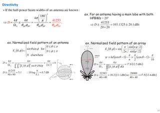
14
Directivity
2
If the half-power beam widths of an antenna are known :
180
41253
4
4 4
.
A HP HP HP H P HP H P
D
π
π π π
θ φ θθ φ φ
 
 
 ⇒ = ≅ = =
Ω
i

15
Directivity & resolution
Antenna能夠分辨出均勻分布於天空的衛星 or 點輻射源的數目N ~ D.

18
Antenna aperture
* 2
2
Consider a receiving rectangular horn antenna immersed in the field of a uniform plane wave:
1
Poynting vector of the plane wave is Re[ ] [W/m ].
2
Physical aperture of the horn is [m
av
p
P S
A
= = ×E Hi
i
2
].
If horn extracts all the power from the wave over its entire physical aperture,
then the total power absorbed from the wave [W].
However, the field response of the horn is NOT uniform
p p
E
P P SA A
Z
= =
across the aperture.
Effective aperture .
Aperture efficiency .
For horn & parabolic reflector antenna, 0.5 0.8.
e p
e
ap
p
ap
A A
A
A
ε
ε
<
=
≤ ≤
i
i

20
cf:
max max
* 2
4
1. [dimensionless] Directivity from pattern
1
where , Poynting vector of the plane wave is Re[ ] [W/m ].
2
4
2. [dimensionless] Directivity from
av r
r av
A
U U
D
U P
P d Ud P S
D
π
π
≡ =
= ⋅ = Ω = = ×
≡
Ω
∫ ∫avP s E H
2
0 0
4
2
beam area.
where ( , )sin ( , ) [sr]
44
3. [dimensionless] Directivity from aperture.
A n n
e
A
P d d P d
A
D
φ π θ π
φ θ
π
θ φ θ θ φ θ φ
ππ
λ
= =
= =
Ω ≡ = Ω
≡ =
Ω
∫ ∫ ∫∫

21
Effective height
for sin wave
1
0.707
2
2
0.637
rms pk pk
av pk pk
V V V
V V V
π
= ≈
= ≈

22
Effective height/aperture
2 22
Relation between the effective height & effective aperture
( / 2)
For an antenna of matched to its load , the power delivered to the load is equal to [W].
4
In terms of the effecti
e
r L
L r
h EV
R R P
R R
= =i
i
2
0
2 20
ve aperture, [W].
[m ].
4
e
e
e e
r
E A
P SA
Z
Z
A h
R
= =
∴ =

25
Polarization
AR = 長軸長軸長軸長軸/短軸短軸短軸短軸

28
H/V polarization vs. E/H plane radiation pattern “don’t confuse”
E-plane and H-plane
天線的方向圖一般是一個空間的立體圖, 在分析中為了方便起見, 一般只研究兩個主面內的方向圖, 這兩個主
面是相互垂直的E面和H面.
E面: 是指通過最大輻射方向並平行於電場向量的平面, 通常指yz平面,
H面: 是指通過最大輻射方向並垂直於電場向量的平面, 通常指xy平面,
/ 2.
/ 2.
φ π
θ π
=
=
horizontal/vertical polarization
E/H plane radiation pattern

29
Dual polarization
由於水平極化傳播的信號在貼近地面時會在大地表面產生極化電流(polarization current), 極化
電流因受大地阻抗影響產生熱能而使電場信號迅速衰減, 而垂直極化方式則不易產生極化電流,
從而避免了能量的大幅衰減, 保證了信號的有效傳播.
因此, 在移動通信系統中, 一般均採用垂直極化的傳播方式.
隨著新技術的發展, 現在大量採用雙極化天線(dual polarization).
就其設計思路而言, 一般分為垂直與水平極化和±45°極化兩種方式, 性能±45°極化比較優, 因此
目前大部分採用的是±45°極化方式.
雙極化天線組合了+45°和-45°兩副極化方向相互正交的天線, 並同時工作在收發雙工模式下, 大
大節省了每個cell的天線數量; 同時由於±45°為正交極化, 有效保證了receive diversity的良好效
果. (其polarization diversity gain約為5dB, 比單極化天線提高約2dB).
Earth

30
2
0
0
0
polarization density:
bound volumetric charge dens
[Q/m ]
ity:
where : electric sus
bound surface charge density:
free volumetric charge density:
ceptibility 1,
b
b
e
e r e
ε χ
ε
ε
χ ε χ
ε
ρ
σ
≡ −
=
=
∇
+
≡
+
⋅
= =
⋅ n
P E
D E
a
P
P
P
free surface charge density:
polarization density changes with time, the time-dependent bound-charge density creates a polarization current density
total current density that enter
f
f
t
ρ
σ
≡ ∇⋅
≡ ⋅
∴
∂
=
∂
n
p
D
D a
P
J
s Maxwell's equations is given by
where is the free-charge current density, and the second term is the magnetization current density
also called the bound current density , a contrib( ut) i
t
∂
= + ∇× +
∂
f
f
P
J J M
J
on from atomic-scale magnetic dipoles when they are present.
H-polarization wave , , ( ), magnetic dipoles( )
, .∴
∵當近地傳播時會產生極化電流外加自由電荷很小地磁很小
總電荷密度大小會是上式產生的熱會使信號迅速衰減
Polarization current detail analysis

31
Poynting vector for EP waves

32
Terminology of antennas Review…

36
The antenna Family
The antennas are grouped into
Loops, dipoles, & slots.
Open-out coaxial, twin-line, & waveguide.
Reflector & aperture types.
End-fire & broadband types.
Patch & grid flat-panel arrays.

37
Loops, dipoles, & slots
Small horizontal loop antenna
• Short vertical magnetic dipole.
• Identical field patterns but …with E and H interchanged.
• Horizontal loop is horizontal polarized, vertical loop is vertical polarized, with the same D = 1.5.
Omnidirectional CP
• Place the short dipole inside the small loop on its axis.
small, short means dimensions
10
λ
≤

38
Loops, dipoles, & slots
Dipole & slot are complementary.
• Identical field patterns but … with E and H interchanged.
• Horizontally polarized.
• Booker’s relation
2
0
0
terminal impedance of the dipole
terminal impedance of slot
intrinsic i
Babinet's princip
mpedance of space 377
Booker's relatiol ne .
4
d
s
d s
Z
Z
Z
Z Z
Z
= =
= Ω
⇒
slot antenna are typically / 2 longλ

40
Open-out coaxial, twin-line, & waveguide

41
Open-out coaxial, twin-line, & waveguide

46
Introduction
In the far field of an antenna:
• Radiated fields are transverse.
• Poynting vector is radial.
Point source
• Only far-field fields.
• Ignore near-field types.
At a sufficient distance, any antenna can be represented by a point source.
• Fictitious volumeless emitter at the center O, where the waves originate.
Far-field measurements
• With antenna fixed
• With observation point fixed, rotating the antenna around the center O more convenient.
Displaced observation circle
• For
• Field patterns
• Phase patterns
• Minimum phase variation around the observation circle for d = 0.
, , , field pattern .R d R b R dλ≫ ≫ ≫ 才能忽略對的影響
Complete description of the far field of a source requires three patterns:
( , ), ( , ), ( , ).
It may suffice to specify only the variation with angle of the Poynting vector magnitude ( ,r
E E
S
θ φθ φ θ φ δ θ φ
θ
i
i ).φ

47
Power patterns
A Tx antenna can be represented by a point source at the origin
• Radiated energy streams out in radial lines.
• Time rate of energy flow per unit area [W/m2].
• Poynting vector has only a radial component.
An isotropic source radiates energy uniformly in all directions.
All antennas have directional properties anisotropic sources
• Absolute power pattern.
• Relative power pattern.
• Normalized power pattern.
ˆ rrS=S

50
Point Source Patterns Summery

51
Examples of power patterns: side lobes affect D so much!!

52
Field patterns
To completely describe the field of a point source, we need to consider the electric (magnetic)
vector fields.

56
Array of Point Sources
Part I
Jay Chang

57
Array of 2 “isotropic” point sources
The pattern of any antenna can be regarded as produced by an array of (isotropic) point sources.
Array of 2 isotropic point sources:
• Same amplitude & phase.
• Same amplitude but opposite phase.
• Same amplitude & in-phase quadrature.
• Same amplitude & any phase difference.
• Unequal amplitude & any phase difference.

58
Same amplitude & phase
Point sources 1 & 2 are separated by & located symmetrically with respect to the origin.
The origin of the coordinates is taken as the reference for phase.
In the direction , the fields from sources
d
φ
/2 /2
0 0
/2,
00
1
1 & 2 are retarded & advanced, respectively by cos ,
2
2
where .
Total field at a distance
( ) cos
in direction
where
cos
2 co2 c s .
2
ex:
os
2
c
r
r
j j
d
d
d
d kd
r
k
E E e
E
d
E
E
E
E eψ ψ
λ β π
φ
π
λ
φ
π φ
φ φ
ψ
ψ
− +
= =
= =
= +
 
⇒ =  
 
=
=
=
cos
os .
2
π φ 
 
 
cos
cos
2
E
π φ 
=  
  0.0
0.2
0.4
0.6
0.8
1.0
0
30
60
90
120
150
180
210
240
270
300
330
0.0
0.2
0.4
0.6
0.8
1.0
• 寫code練習畫

59
Same amplitude & phase
/2 /2
0 0 0
Point sources 1 & 2 are separated by & located symmetrically with respect to the origin.
2
Field from source 2 in direction is advanced by cos , where .
(
r r
j j j j
d
d
d d kd
E E E e E e e eψ ψ ψ ψ
π
φ ψ φ
λ
+ + − +
= = =
⇒ = + = + /2 2/
/2
0)
ex : cos .
2
2 cos
2
j
j
E
E e
e ψ
ψ
ψ
ψ
+
+
=
=

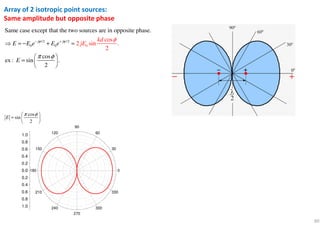
60
Same amplitude but opposite phase
/2 /2
0 0 0
Same case except that the two sources are in opposite phase.
cos
2 si
cos
ex : sin .
n
2
.
2
j j
E E e E
k
jE
E
d
eψ ψ φ
π φ
− +
⇒ = − + =
 
=  
 
cos
sin
2
E
π φ 
=  
 
0.0
0.2
0.4
0.6
0.8
1.0
0
30
60
90
120
150
180
210
240
270
300
330
0.0
0.2
0.4
0.6
0.8
1.0

61
Same amplitude & in-phase quadrature
cos cos
2 4 2 4
0 00
Let sources 1 & 2 be retarded & advanced, respectively, both by / 4.
cos
ex : / 2, cos
cos
2 cos .
4
2 4
2
.
kd kd
j j
E E
kd
e E e
d E
E
φ π φ π
π
π φ
π
π
λ
φ
   
− + + +   
     
+ 
 
⇒ = + =
 
= = + 
 
cos
cos
4 2
E
π π φ 
= + 
 
0.0
0.2
0.4
0.6
0.8
1.0
0
30
60
90
120
150
180
210
240
270
300
330
0.0
0.2
0.4
0.6
0.8
1.0

62
Same amplitude & in-phase quadrature
cos cos
2 4 2 4
0 00
Let sources 1 & 2 be retarded & advanced, respectively, both by / 4.
cos
ex : / 4, cos
cos
2 cos .
4
4 4
2
.
kd kd
j j
E E
kd
e E e
d E
E
φ π φ π
π
π φ
π
π
λ
φ
   
− + + +   
     
+ 
 
⇒ = + =
 
= = + 
 
cos
cos
4 4
E
π π φ 
= + 
 
0.0
0.2
0.4
0.6
0.8
1.0
0
30
60
90
120
150
180
210
240
270
300
330
0.0
0.2
0.4
0.6
0.8
1.0

63
sin
cos
4 4
E
π π φ 
= + 
 
0.0
0.2
0.4
0.6
0.8
1.0
0
30
60
90
120
150
180
210
240
270
300
330
0.0
0.2
0.4
0.6
0.8
1.0
工程師的浪漫工程師的浪漫工程師的浪漫工程師的浪漫…<3

64
Same amplitude & any phase difference

65
Unequal amplitude & any phase difference

66
Nonisotropic point sources & principle of pattern multiplication
Field pattern of an array of similar nonisotropic point sources = Pattern of the individual source ×
Pattern of an array of isotropic point sources with the same locations, relative amplitudes, & phase.
• Applied to arrays of any number of similar sources.
• For field magnitude only.
Phase pattern of an array of similar nonisotropic point sources = Phase pattern of the individual
source + Phase pattern of an array of isotropic sources with the same locations, relative amplitudes,
& phase.
波辦圖乘法原理波辦圖乘法原理波辦圖乘法原理波辦圖乘法原理

67
Nonisotropic point sources & principle of pattern multiplication cos
sin cos
2
E
π φ
φ
 
= ×  
 
0.0
0.2
0.4
0.6
0.8
1.0
0
30
60
90
120
150
180
210
240
270
300
330
0.0
0.2
0.4
0.6
0.8
1.0
cos
cos cos
2
E
π φ
φ
 
= ×  
 
0.0
0.2
0.4
0.6
0.8
1.0
0
30
60
90
120
150
180
210
240
270
300
330
0.0
0.2
0.4
0.6
0.8
1.0

70
Equispaced linear arrays of identical isotropic point sources
2 3 ( 1)
Consider isotropic point sources of equal amplitude & spacing arranged as a linear array.
2
1 ... , where cos cos , .j j j j n
r
n
d
E e e e e dψ ψ ψ ψ π
ψ φ δ φ δ δ
λ
−
⇒ = + + + + + = + = + 是相鄰點源的相位差
/2 /2 /2
/2 /2 /2
1
2
sin
2
sin
2
sin
1 2. If the phase is referred to the center point of the array, .
1 sin
2
j n
j
n jn jn jn
j j j j
n
e e
n
e e
e e
e
e e
E E
ψ ψ ψ ψ
ψ
ψ
ψ ψ ψ
ψ
ψψ
ψ
− −
−
 − −
∴ = = = = 
− − 
Equal amp. with source 1 as phase center(ref. phase) Same but with midpoint array (source 3) as phase center.

71
1
ma
2
x
The phase of the field is constant wherever has a value but changes sign when goes through zero.
For 0 , we have .
Therefore, the mormalized
si
total field i
n
1 2 calls
2
ed
sin
n
j
n
E e
n
E E
E E n
ψ
ψ
ψ
ψ
−
= = =
= → Array factor.
0 .ψ φ=陣列電場的最的任何值出現在使方向大

72

73
Case 1. Broadside array
2 (2 1)
For isotropic sources of the same amplitude & phase cos cos , to make 0 , , where 0,1,2...
2
r
d k
n d k
π π
ψ φ φ ψ φ
λ
+
= = = = =
1 sin( / 2)
, cos 0
sin( / 2)
n
AF
n
ψ
ψ π φ
ψ
= = + °
0.0
0.2
0.4
0.6
0.8
1.0
0
30
60
90
120
150
180
210
240
270
300
330
0.0
0.2
0.4
0.6
0.8
1.0 0 90 180 270 360
0.0
0.2
0.4
0.6
0.8
1.0
φ degree (o)
|AF|
0 90 180 270 360
-450
-360
-270
-180
-90
0
90
180
270
φ degree (o)Totalphaseangle(o)
0δ =
0δ =

74
Case 2. Ordinary end-fire array
To make the field a max. ( 0) in the direction of the array 0
cos
0 cos0 , .
Hence, the phase between sources of an end-fire array is retarded progressively by
the same amount as the
r
r r
d
d d
ψ φ
ψ φ δ
δ δ
= =
= +
⇒ = + ∴ = −
∵
spacing between sources in radians.
1 sin( / 2)
, cos
sin( / 2)
n
AF
n
ψ
ψ π φ π
ψ
= = −
0.0
0.2
0.4
0.6
0.8
1.0
0
30
60
90
120
150
180
210
240
270
300
330
0.0
0.2
0.4
0.6
0.8
1.0 0 90 180 270 360
0.0
0.2
0.4
0.6
0.8
1.0
φ degree (o)
|AF|
0 90 180 270 360
-450
-360
-270
-180
-90
0
90
180
φ degree (o)
Totalphaseangle(o)
rdδ = −

75
Case 2. Ordinary end-fire array
1 sin( / 2)
, cos
sin( / 2) 2 2
n
AF
n
ψ π π
ψ φ
ψ
= = −
0.0
0.2
0.4
0.6
0.8
1.0
0
30
60
90
120
150
180
210
240
270
300
330
0.0
0.2
0.4
0.6
0.8
1.0 0 90 180 270 360
0.0
0.2
0.4
0.6
0.8
1.0
φ degree (o)
|AF|
rdδ = −

76
Case 3. End-fire array with increased D
Larger can be obtained by increasing the phase change between sources
Phase difference of the fields cos (cos 1)
r
r r
D d
n
d d
n
π
δ
π
ψ φ δ φ
 
⇒ = − + 
 
= + = − −∵
,
0 , 180 .
D
d
n
π
ψ φ φ π= =
⇒
增強減小為了
限制在方向不能超過在方向約
後瓣
減小間距就能滿足
0.0
0.2
0.4
0.6
0.8
1.0
0
30
60
90
120
150
180
210
240
270
300
330
0.0
0.2
0.4
0.6
0.8
1.0
0 90 180 270 360
0.0
0.2
0.4
0.6
0.8
1.0
φ degree (o)
|AF|

77
0.0
0.2
0.4
0.6
0.8
1.0
0
30
60
90
120
150
180
210
240
270
300
330
0.0
0.2
0.4
0.6
0.8
1.0 0 90 180 270 360
0.0
0.2
0.4
0.6
0.8
1.0
φ degree (o)
|AF|
Case 3. End-fire array with increased D
sin( / 2)
sin , (cos 1)
2 sin( /
(cos 1) 0.6
2 02) 1
n
AF kd
n n
π ππ
φ
π
φ
ψ
ψ
πψ
 
= = = − − =− − − 
 
0.0
0.2
0.4
0.6
0.8
1.0
0
30
60
90
120
150
180
210
240
270
300
330
0.0
0.2
0.4
0.6
0.8
1.0 0 90 180 270 360
0.0
0.2
0.4
0.6
0.8
1.0
φ degree (o)
|AF|
1 sin( / 2)
, cos 0.5
sin( / 2)
n
AF kd
n
ψ
ψ φ δ π
ψ
= = + = −
HPBW = 38 deg
FNBW = 74 deg
HPBW = 69 deg
FNBW = 109 deg

78
Case 4. Scanning array = phase array
0.0
0.2
0.4
0.6
0.8
1.0
0
30
60
90
120
150
180
210
240
270
300
330
0.0
0.2
0.4
0.6
0.8
1.0 0 90 180 270 360
0.0
0.2
0.4
0.6
0.8
1.0
φ degree (o)
|AF|
1 sin( / 2)
, cos 0
sin( / 2)
n
AF kd
n
ψ
ψ φ δ
ψ
= = + =

79
Null directions
一樣分3種討論
• In a broadside array δ = 0.
• In an ordinary end-fire array δ = -dr .
• For increased-D end-fire arrays.

80
Null directions
In a broadside array δ = 0

81
Null directions
In an ordinary end-fire array δ = -dr

82
Null directions
In an ordinary end-fire array δ = -dr

86
Array of Point Sources
Part II
Jay Chang

87
Linear broadside arrays with nonuniform amplitude distributions
Four types of amplitude distributions: uniform, edge, optimum, binomial

88
Binomial distribution: To reduce the SLL(side-lobe level) of linear in-phase broadside arrays, it is
required that the sources have amplitudes proportional to the coefficients of a binomial series.
No minor lobes BUT with increased beamwidth(HPBW).
Edge distribution: only the end sources of the array are excited.
• Degenerate to two sources (n – 1)d apart.
Edge vs. binomial distributions: Trade-off between HPBW & SLL.
HPBW , D↑ ↓

89
Dolph’s optimum distribution: optimize the relation between beamwidth & SLL.
If the SLL (FNBW) is specified, the FNBW (SLL) is minimized.
• Based on the properties of Tchebyscheff(Chebyshev) polynomials.
Optimum distribution includes all distributions between binomial & edge.
Summary
Amplitude tapers to a small value at the array edges → eliminated minor lobes.
Inverse taper with max. amplitude at the edges & none at the array center → accentuated minor
lobes.
Analogy between this situation & the Fourier analysis of wave shapes.
• Square vs. Gaussian waves
Apply not only to arrays of discrete sources separated by finite distances but also to (large) arrays of
continuous distributions of an infinite number of point sources.

90
Linear broadside arrays with D-T distributions
Far-field pattern of a linear array of isotropic point sources can be expressed as a finite Fourier series
of N terms.
Match the terms of the Fourier polynomial with the terms of like degree of a Tchebyscheff
polynomial.
• D-T distribution for a specified SLL.
3 (2 1)
2 2 2
0 1
Consider a linear array of isotropic point sources of uniform spacing .
Amplitude distribution is symmetric about the array center.
Total field in : ... ( )e
e
k
j j j
n k
n d
E A e Ae A e
ψ ψ ψ
θ
+
− − −
= + + + +
i
i
右半邊
3 (2 1)
2 2 2
0 1
0 1
... ( )
( 1)3 2
2 cos 2 cos ... 2 cos where sin sin .
2 2 2
( 1) (2 1)
Let 2( 1) , 0, 1, 2, 3... .
2 2
The total field thus becomes:
e
k
j j j
k
e
n k r
e
e
A e Ae A e
n d
E A A A d
n k
k n k
ψ ψ ψ
ψψ ψ π
ψ θ θ
λ
+
+ + +
−
= + + + = =
− +
+ = = ⇒ =
左半邊

91
Far-field pattern of a linear array of isotropic point sources can be expressed as a finite Fourier series
of N terms.
Match the terms of the Fourier polynomial with the terms of like degree of a Tchebyscheff
polynomial.
• D-T distribution for a specified SLL.

92

93
1 1Chebyshev recurrence: ( ) 2 ( ) ( )n n nT x xT x T x+ −= −
1 roots 1x′− ≤ ≤
Fig. Tchebysheff polynomials of degree m = 0 through m = 5

94

95
Example of D-T distribution
normalized

96
Example of D-T distribution
0
sin
cos cos to plot field pattern
2 2
x kd
w
x
ψ θ
= = =

97
Example of D-T distribution: Comparison of amplitude distributions
40000
9.2 9.6 dBi
12 360
D ≈ =
⋅
≃
0θ =

98
Continuous arrays
2
c
ω π
β
λ
= =
2
sin sin sinr
a
a a
π
ψ β θ θ θ
λ
′ = = =

99
Continuous arrays
2
sin sin sinr
a
a a
π
ψ β θ θ θ
λ
′ = = =

100
Broadside v.s. end-fire arrays

101
Broadside v.s. end-fire arrays

103
Thank you for your attention

Antenna basic

More Related Content

What's hot (20)

Similar to Antenna basic (20)

More from Pei-Che Chang (20)

Recently uploaded (20)

Antenna basic