Chapter 3 Built-in Data Structures, Functions, and Files .pptx

Built-in Data Structures, Functions
and Files
Chapter 3

Outline
3.1 Data Structures and Sequences
3.2 Function
3.3 Files and the Operating System

3.1 Data Structures and Sequences
 Tuple
• Fixed size in 1-dimension
• Immutable data structure
• We define tuple as
tup = 4, 5, 6
tup
> (4, 5, 6)
• We can define nested tuple using bracket ( )
nested_tup = (4, 5, 6), (7, 8)
nested_tup
> ((4, 5, 6), (7, 8))
3

 Tuple
 All sequential data can change to tuple using the tuple()
tuple([4, 0 , 2])
> (4, 0, 2)
tup = tuple(“string”)
tup
> (‘s’, ‘t’, ‘r’, ‘i’, ‘n’, ‘g’)
 Each element can be accessed by [ ]
tup[0]
> ‘s’
3.1 Data Structures and Sequences (cont.)

 Tuple
 The stored object can be modified
 But once created, it is impossible to change the object stored in
each slot
tup = tuple([“foo”, [1, 2], True])
tup[2] = False
> TypeError: ‘tuple’ object does not support item assignment
tup = tuple([“foo”, [1, 2], True])
tup[1].append(3)
tup
> (‘foo’, [1, 2, 3], True)

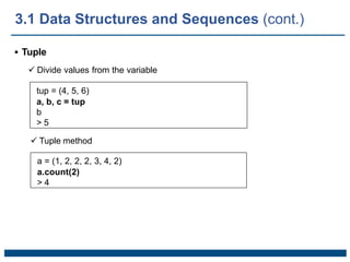
 Tuple
 Divide values from the variable
tup = (4, 5, 6)
a, b, c = tup
b
> 5
 Tuple method
a = (1, 2, 2, 2, 3, 4, 2)
a.count(2)
> 4

 List
 Mutable data structure
 Define list using [ ] or list()
a_list = [2, 3, 7, None]
tup = (‘foo’, ‘bar’, ‘baz’)
b_list = list(tup)
b_list
> [‘foo’, ‘bar’, ‘baz’]
b_list[1] = ‘test’
b_list
> [‘foo’, ‘test’, ‘baz’]

 List
 Add an element
b_list.append(‘dwarf’)
b_list
> [‘foo’, ‘test’, ‘baz’, ‘dwarf’]
b_list.insert(1, ‘red’)
b_list
> [‘foo’, ‘red’, ‘test’, ‘baz’, ‘dwarf’]
 Delete an element
b_list.pop(2)
> ‘test’ b_list
> [‘foo’, ‘red’, ‘baz’, ‘dwarf’]
b_list.remove(‘foo’)
b_list
> [‘red’, ‘baz’, ‘dwarf’]

 List
 Check the element
‘dwarf’ in b_list
> True
‘dwarf’ not in b_list
> False
 Sort
a = [7, 2, 5, 1, 3] b = [‘saw’, ‘small’, ‘He’, ‘foxes’, ‘six’]
a.sort() b.sort(key=len)
a b
> [1, 2, 3, 5, 7] > [‘He’, ‘saw’, ‘six’, ‘small’, ‘foxes’]

 List
 Binary search & sort using the bisect module
 bisect() : returns the location where the list can remain sorted
when values are added
 insort() : add values while keeping the sorted list
import bisect
c = [1, 2, 2, 2, 3, 4, 7]
bisect.bisect(c, 2)
> 4
bisect.bisect(c, 5)
> 6
bisect.insort(c, 6)
c
> [1, 2, 2, 2, 3, 4, 6, 7]

 List
 Slicing : obtain data in the given range from the list
 The value of the start position is included, but the value of the
end position is not
 Number of slicing = stop - start
seq = [7, 2, 3, 7, 5, 6, 0, 1]
seq[1:5]
> [2, 3, 7, 5]
 We can assign data as
seq[3:4] = [6, 3]
seq
> [7, 2, 3, 6, 3, 5, 6, 0, 1]

 List
 Slicing : The start position or end position can be omitted
seq = [7, 2, 3, 6, 3, 5, 6, 0, 1]
seq[:5]
> [7, 2, 3, 6, 3]
seq[3:]
> [6, 3, 5, 6, 0, 1]
 Negative index means the position from the end of the sequential data
seq[-4:]
> [5, 6, 0, 1]
seq[-6:-2]
> [6, 3, 5, 6]

 List
 Duplicate colon : determine step size
seq = [7, 2, 3, 6, 3, 5, 6, 0, 1]
seq[::2]
> [7, 3, 3, 6, 1]
 Negative step size -1 : return in reverse order
seq = [7, 2, 3, 6, 3, 5, 6, 0, 1]
seq[::-1]
> [1, 0, 6, 5, 3, 6, 3, 2, 7]

 Embedding function
 zip: pair different sequential data to form a list of tuples
seq1 = [‘foo’, ‘bar’, ‘baz’]
seq2 = [‘one’, ‘two’, ‘three’]
zipped = zip(seq1, seq2)
list(zipped)
> [(‘foo’, ‘one’), (‘bar’, ‘two’), (‘baz’, ‘three’)]
 reversed: return sequential data in reverse order
list(reversed(range(10))
> [9, 8, 7, 6, 5, 4, 3, 2, 1, 0]

 Dictionary
 Hash-map with key and value
 {key : value}
empty_dict = {}
d1 = {‘a’ : ‘some value’, ‘b’ : [1, 2, 3, 4] d1
> {‘a’: ‘some value’, ‘b’: [1, 2, 3, 4]}
 Use dictionary as a tuple and a list
d1[7] = ‘an integer’ d1
> {‘a’: ‘some value’, ‘b’: [1, 2, 3, 4], 7: ‘an integer’}
d1[‘b’]
> [1, 2, 3, 4]

 Dictionary
 dell & pop to remove key-value
d1[5] = ‘some value’
d1
> {‘a’: ‘some value’, ‘b’: [1, 2, 3, 4], 7: ‘an integer’, 5: ‘some value’}
del d1[5]
d1
> {‘a’: ‘some value’, ‘b’: [1, 2, 3, 4], 7: ‘an integer’}
ret = d1.pop(‘b’)
ret
> [1, 2, 3, 4]
d1
> {‘a’: ‘some value’, 7: ‘an integer’}

 Dictionary
 update(): connect two dictionaries
d1 = {‘a’: ‘some value’, 7: ‘ an integer’}
d1.update({‘b’: ‘foo’, ‘c’: 12})
d1
> {‘a’: ‘some value’, 7: ‘an integer’, ‘b’: ‘foo’, ‘c’: 12}
 make a dictionary with two sequential data
mapping = {}
for key, value in zip(key_list, value_list):
mapping[key] = value

 Dictionary
 General logic
if key in some_dict:
value = some_dict[key]
else:
value = default_value
 the same code using get()
value = some_dict.get(key, default_vale)

 Set
 Unordered data type consisting of only elements
 It is similar to a dictionary, but has no value, only a key
 set() or { }
set([2, 2, 2, 1, 3, 3])
> {1, 2, 3}
{2, 2, 2, 1, 3, 3}
> {1, 2, 3}

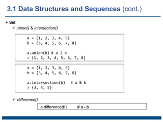
 Set
 union() & intersection()
a = {1, 2, 3, 4, 5}
b = {3, 4, 5, 6, 7, 8}
a.union(b) # a | b
> {1, 2, 3, 4, 5, 6, 7, 8}
a = {1, 2, 3, 4, 5}
b = {3, 4, 5, 6, 7, 8}
a.intersection(b) # a & b
> {3, 4, 5}
 difference()
a.difference(b) # a - b

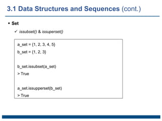
 Set
 issubset() & issuperset()
a_set = {1, 2, 3, 4, 5}
b_set = {1, 2, 3}
b_set.issubset(a_set)
> True
a_set.issupperset(b_set)
> True

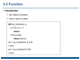
3.2 Function
 Introduction
 def: define a function
 return: return a value
def my_function(x, y,
z=1.5): if z > 1:
return
z*(x+y) else:
return z/(x+y)
ret = my_function(4, 6, 3.5)
> 35.0
ret = my_function(10, 20)
> 45.0

 Scope
def func():
a = [] # local variable
for j in range(5):
a.append(j)
a = [] # global variable
def func():
for j in range(5):
a.append(j)
a = None
def bind_var_func():
global a; # declare global
variable a = []
for j in range(5):
a.append(j)
3.2 Function (cont.)

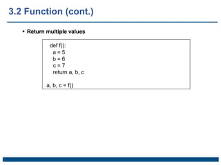
 Return multiple values
def f():
a = 5
b = 6
c = 7
return a, b, c
a, b, c = f()

 Function as object
 Easy to handle object creation in a function
 Ex.) Modify the string list
import re
states = [‘Alabama’, ‘Georgia!’, ‘Georgia’, ‘georgia’,
‘FlOrIda’, ‘southcarolina##’, ‘West virginia?’]
def clean_strings(strings):
result = []
for value in strings:
value = value.strip()
value = re.sub(‘[!#?]’, ‘’, value)
value = value.title()
result.append(value)
return result
clean_strings(states)
> [‘Alabama’,
‘Georgia’,
‘Georgia’,
‘Georgia’,
‘Florida’,
‘South Carolina’,
‘West Virginia’]

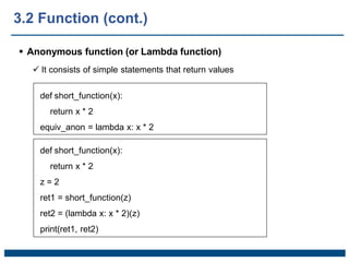
 Anonymous function (or Lambda function)
 It consists of simple statements that return values
def short_function(x):
return x * 2
equiv_anon = lambda x: x * 2
def short_function(x):
return x * 2
z = 2
ret1 = short_function(z)
ret2 = (lambda x: x * 2)(z)
print(ret1, ret2)

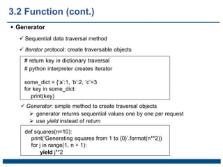
 Generator
 Sequential data traversal method
 Iterator protocol: create traversable objects
# return key in dictionary traversal
# python interpreter creates iterator
some_dict = {‘a’:1, ‘b’:2, ‘c’=3
for key in some_dict:
print(key)
 Generator: simple method to create traversal objects
 generator returns sequential values one by one per request
 use yield instead of return
def squares(n=10):
print(‘Generating squares from 1 to {0}’.format(n**2))
for j in range(1, n + 1):
yield j**2

 Generator
 Simpler generator
gen = (x ** 2 for x in range(10))
l = list(gen)
print(l)
> [1, 4, 9, 16, 25, 36, 47, 64, 81]

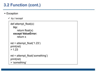
 Exception
 try / except
def attempt_float(x):
try:
return float(x)
except ValueError:
return x
ret = attempt_float(‘1.23’)
print(ret)
> 1.23
ret = attempt_float(‘something’)
print(ret)
> ‘something’

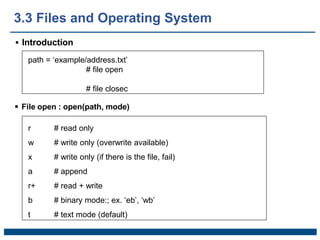
3.3 Files and Operating System
 Introduction
path = ‘example/address.txt’
# file open
# file closec
r # read only
w # write only (overwrite available)
x # write only (if there is the file, fail)
a # append
r+ # read + write
b # binary mode:; ex. ‘eb’, ‘wb’
t # text mode (default)
 File open : open(path, mode)

 Unicode files
 Read a Unicode file
# when data is encoded with utf-8 (Non-ASCII),
with open(path, ‘rb’) as f:
data = f.read(10)
data.decode(‘utf8’)
 Change encoding mode when file open
with open(path, encoding=‘iso-8859-1’) as f:
print(f.read(10))
 Change string to utf-8
str = ‘test string’
encoded = str.encode(‘utf-8’)
3.3 Files and Operating System (cont.)

Chapter 3 Built-in Data Structures, Functions, and Files .pptx

More Related Content

Similar to Chapter 3 Built-in Data Structures, Functions, and Files .pptx (20)

Recently uploaded (20)

Chapter 3 Built-in Data Structures, Functions, and Files .pptx