SlideShare a Scribd company logo
Control System
Bode Plot
Nilesh Bhaskarrao Bahadure
nbahadure@gmail.com
https://www.sites.google.com/site/nileshbbahadure/home
June 30, 2021
Nilesh Bhaskarrao Bahadure (Ph.D.) Control System June 30, 2021 1 / 51
Overview I
1 Frequency Response Specifications
Band Width
Cut off Frequency
2 Bode Plot of Transfer Function
Bode gain of factor K1
Poles at origin
Zeros at origin
First Order Poles
First Order Zeros
Second Order Poles
Second Order Zeros
Summary
3 Steps for solving Bode plots
4 Examples on Bode Plot
Example:01
Example:02
Nilesh Bhaskarrao Bahadure (Ph.D.) Control System June 30, 2021 2 / 51
Overview II
5 Thank You
Nilesh Bhaskarrao Bahadure (Ph.D.) Control System June 30, 2021 3 / 51
Bode Plots
Nilesh Bhaskarrao Bahadure (Ph.D.) Control System June 30, 2021 4 / 51
What is Band Width?
What is Band Width?
Nilesh Bhaskarrao Bahadure (Ph.D.) Control System June 30, 2021 5 / 51
What is Band Width?
What is Band Width?
It is defined as the range of frequencies over which the system will respond
satisfactorily
Figure : Closed loop system
Nilesh Bhaskarrao Bahadure (Ph.D.) Control System June 30, 2021 5 / 51
What is Band Width?
What is Band Width?
It is defined as the range of frequencies over which the system will respond
satisfactorily
Figure : Closed loop system
from Figure 1 the range o to ωb is nothing but band width.
Nilesh Bhaskarrao Bahadure (Ph.D.) Control System June 30, 2021 5 / 51
What Cut-off Frequency (wb)?
Nilesh Bhaskarrao Bahadure (Ph.D.) Control System June 30, 2021 6 / 51
What Cut-off Frequency (wb)?
The frequency at which the magnitude of the closed loop response is 3dB
down from its zero frequency value is called cut-off frequency.
What Cut-off Rate?
Nilesh Bhaskarrao Bahadure (Ph.D.) Control System June 30, 2021 6 / 51
What Cut-off Frequency (wb)?
The frequency at which the magnitude of the closed loop response is 3dB
down from its zero frequency value is called cut-off frequency.
What Cut-off Rate?
The slope of resultant magnitude curve near the cut-off frequency is called
cut-off rate.
What Resonant Peak (Mr)?
It is maximum value of magnitude of closed loop frequency response
What Resonant Frequency (Wr)?
The frequency at which resonant peak occur.
Nilesh Bhaskarrao Bahadure (Ph.D.) Control System June 30, 2021 6 / 51
Gain Cross Over Frequency ωgc
Nilesh Bhaskarrao Bahadure (Ph.D.) Control System June 30, 2021 7 / 51
Gain Cross Over Frequency ωgc
The frequency at which magnitude of G(jω).H(jω) is unity i.e. 1 is called
gain cross over frequency.
|G(jω).H(jω)| = 1 (1)
in dB,
20log10|G(jω).H(jω)| = 20log101 = 0dB (2)
Phase Cross Over Frequency ωpc
The frequency at which phase angle of G(jω).H(jω) is −180o is called
phase cross over frequency ωpc.
Nilesh Bhaskarrao Bahadure (Ph.D.) Control System June 30, 2021 7 / 51
Gain Margin (GM)
Nilesh Bhaskarrao Bahadure (Ph.D.) Control System June 30, 2021 8 / 51
Gain Margin (GM)
It is defined as the magnitude of the reciprocal of the closed loop transfer
function, evaluate at the phase cross over frequency ωpc which is the
frequency at which phase is −180o. That is,
Gain Margin (GM) =
1
|G(jω).H(jω)|
(3)
where,
∠G(jω).H(jω) = −180o
Nilesh Bhaskarrao Bahadure (Ph.D.) Control System June 30, 2021 8 / 51
Figure : Closed loop Gain and Phase Margin
Nilesh Bhaskarrao Bahadure (Ph.D.) Control System June 30, 2021 9 / 51
Phase Margin (PM)
Nilesh Bhaskarrao Bahadure (Ph.D.) Control System June 30, 2021 10 / 51
Phase Margin (PM)
It is defined as 180o plus the phase angle φ of the open loop transfer
function at unity gain i.e.
φPM = 180 + ∠G(jω).H(jω) (4)
Nilesh Bhaskarrao Bahadure (Ph.D.) Control System June 30, 2021 10 / 51
Bode Plot of Transfer Function
Nilesh Bhaskarrao Bahadure (Ph.D.) Control System June 30, 2021 11 / 51
Bode Plot of Transfer Function
The frequency transfer function can be written in a generalized form as
the ratio of polynomials
G(s).H(s) =
N(s)
D(s)
=
a0sm + a1sm−1 + a2sm−2 + ....
b0sn + b1sn−1 + b2sn−2 + ....
(5)
Nilesh Bhaskarrao Bahadure (Ph.D.) Control System June 30, 2021 11 / 51
Bode Plot of Transfer Function
The frequency transfer function can be written in a generalized form as
the ratio of polynomials
G(s).H(s) =
N(s)
D(s)
=
a0sm + a1sm−1 + a2sm−2 + ....
b0sn + b1sn−1 + b2sn−2 + ....
(5)
This must be factorized to obtain a general type,
G(s).H(s) =
N(s)
D(s)
=
K1sg (s + z1)(s + z2)....
sh(s + p1)(s + p2)....
(6)
We convert the above equation in time constant form,
G(s).H(s) =
N(s)
D(s)
=
K1sg (1 + s
z1
)(1 + s
z2
)....
sh(1 + s
p1
)(1 + s
p2
)...
(7)
Nilesh Bhaskarrao Bahadure (Ph.D.) Control System June 30, 2021 11 / 51
Bode Plot of Transfer Function
Nilesh Bhaskarrao Bahadure (Ph.D.) Control System June 30, 2021 12 / 51
Bode Plot of Transfer Function
Note
K1 =
Kz1z2
p1p2
Nilesh Bhaskarrao Bahadure (Ph.D.) Control System June 30, 2021 12 / 51
Bode Plot of Transfer Function
Note
K1 =
Kz1z2
p1p2
we now put s = jω to convert the transfer function to the frequency
domain
G(jω).H(jω) =
K1jωg (1 + jω
z1
)(1 + jω
z2
)....
jωh(1 + jω
p1
)(1 + jω
p2
)...
(8)
Nilesh Bhaskarrao Bahadure (Ph.D.) Control System June 30, 2021 12 / 51
Bode Plot of Transfer Function
Note
K1 =
Kz1z2
p1p2
we now put s = jω to convert the transfer function to the frequency
domain
G(jω).H(jω) =
K1jωg (1 + jω
z1
)(1 + jω
z2
)....
jωh(1 + jω
p1
)(1 + jω
p2
)...
(8)
Here K1 is the gain constant or Bode gain. Equation 8 is the standard
form or Bode form.
The following is a list of possible factors of G(jω).H(jω) from Equation 8
Nilesh Bhaskarrao Bahadure (Ph.D.) Control System June 30, 2021 12 / 51
Bode Plot of Transfer Function...
1 Bode gain K1 or constant factor
Nilesh Bhaskarrao Bahadure (Ph.D.) Control System June 30, 2021 13 / 51
Bode Plot of Transfer Function...
1 Bode gain K1 or constant factor
2 Poles at origin 1
(jω)K of order K
Nilesh Bhaskarrao Bahadure (Ph.D.) Control System June 30, 2021 13 / 51
Bode Plot of Transfer Function...
1 Bode gain K1 or constant factor
2 Poles at origin 1
(jω)K of order K
3 Zeros at origin (jω)g of order g
Nilesh Bhaskarrao Bahadure (Ph.D.) Control System June 30, 2021 13 / 51
Bode Plot of Transfer Function...
1 Bode gain K1 or constant factor
2 Poles at origin 1
(jω)K of order K
3 Zeros at origin (jω)g of order g
4 Finite simple poles at 1
1+ jω
p1
or first order poles.
Nilesh Bhaskarrao Bahadure (Ph.D.) Control System June 30, 2021 13 / 51
Bode Plot of Transfer Function...
1 Bode gain K1 or constant factor
2 Poles at origin 1
(jω)K of order K
3 Zeros at origin (jω)g of order g
4 Finite simple poles at 1
1+ jω
p1
or first order poles.
5 Finite simple zero at (1 + jω
z1
) or first order zeros.
6 Second order poles 1
1+j2ξω−ω2
7 Second order zeros (1 + j2ξω − ω2)
Any transfer function will contain a few of the listed several factors. We
shall now understand how each of these 7 terms can be represented on the
magnitude plot and the phase plot.
Nilesh Bhaskarrao Bahadure (Ph.D.) Control System June 30, 2021 13 / 51
Bode Plot of Standard Factors
Bode gain of factor K1
Magnitude Plot
Nilesh Bhaskarrao Bahadure (Ph.D.) Control System June 30, 2021 14 / 51
Bode Plot of Standard Factors
Bode gain of factor K1
Magnitude Plot
consider G(s).H(s) = K1, replace s = jω to convert it to frequency
domain, therefore G(jω).K(jω) = K1
For the magnitude in dB we use the standard formula
20log10G(jω).H(jω) = 20log10|K1| = MdB
This is a straight line independent of the input frequency. Hence we
represent the gain factor by a straight line on the Y-axis.
Example, Bode magnitude for K1 = 5 will give us a straight line of
20log5 = 13.98dB on the Y-axis.
Nilesh Bhaskarrao Bahadure (Ph.D.) Control System June 30, 2021 14 / 51
Bode Plot of Standard Factors...
Bode gain of factor K1
Phase Plot for Bode gain K1
Nilesh Bhaskarrao Bahadure (Ph.D.) Control System June 30, 2021 15 / 51
Bode Plot of Standard Factors...
Bode gain of factor K1
Phase Plot for Bode gain K1
Since K1 is a constant, it can be written as,
G(jω)H(jω) = K1 + j0
Nilesh Bhaskarrao Bahadure (Ph.D.) Control System June 30, 2021 15 / 51
Bode Plot of Standard Factors...
Bode gain of factor K1
Phase Plot for Bode gain K1
Since K1 is a constant, it can be written as,
G(jω)H(jω) = K1 + j0
For finding phase angle in degree we have the equation
φ = tan−1 Imaginary Part
Real Part
φ = tan−1 0
K1
= 0
i.e. for positive value of K1, the phase is zero
Hence a positive value of K1 has no effect on the phase. The phase angle is equal to
−180o
for all ω for negative value of K1
Both magnitude and phase are shown below figure (3). They have been drawn
separately for better understanding. In practice magnitude and phase have to be drawn
one below the other.
Nilesh Bhaskarrao Bahadure (Ph.D.) Control System June 30, 2021 15 / 51
Bode Plot of Standard Factors...
Figure : Magnitude and Phase plot for gain K1
Nilesh Bhaskarrao Bahadure (Ph.D.) Control System June 30, 2021 16 / 51
Poles at Origin or Integral factor ( 1
jω )K
Poles at Origin or Integral factor ( 1
jω
)K
Magnitude Plot
Nilesh Bhaskarrao Bahadure (Ph.D.) Control System June 30, 2021 17 / 51
Poles at Origin or Integral factor ( 1
jω )K
Poles at Origin or Integral factor ( 1
jω
)K
Magnitude Plot
Consider G(s).H(s) = 1
sK , replace s = jω to convert it to frequency domain, therefore
G(jω).H(jω) = 1
(jω)K = (jω)−K
Since the magnitude is plotted in decibel dB we have
20log10G(jω).H(jω) = 20log10|(jω)|−K
= −20Klog10(ω)dB
This is a straight line passing though the point ω = rad/sec and Y = 0dB
This is because at ω = 1rad/sec, Y = −20Klog10(ω)dB = −20Klog10(0)dB = 0dB
1 If K = 1 straight line passes through (0 dB, ω = 1), at slope −20db/dec
2 If K = 2 straight line passes through (0 dB, ω = 1), at slope −40db/dec and so
on.
Nilesh Bhaskarrao Bahadure (Ph.D.) Control System June 30, 2021 17 / 51
Poles at Origin or Integral factor ( 1
jω
)K
Phase Plot
Nilesh Bhaskarrao Bahadure (Ph.D.) Control System June 30, 2021 18 / 51
Poles at Origin or Integral factor ( 1
jω
)K
Phase Plot
Consider G(s).H(s) = 1
sK , replace s = jω to convert it to frequency domain, therefore
Nilesh Bhaskarrao Bahadure (Ph.D.) Control System June 30, 2021 18 / 51
Poles at Origin or Integral factor ( 1
jω
)K
Phase Plot
Consider G(s).H(s) = 1
sK , replace s = jω to convert it to frequency domain, therefore
G(jω).H(jω) =
1
(jω)K
= (jω)−K
Nilesh Bhaskarrao Bahadure (Ph.D.) Control System June 30, 2021 18 / 51
Poles at Origin or Integral factor ( 1
jω
)K
Phase Plot
Consider G(s).H(s) = 1
sK , replace s = jω to convert it to frequency domain, therefore
G(jω).H(jω) =
1
(jω)K
= (jω)−K
For K = 1, ∠G.H(jω) = ∠ 1
jω
Nilesh Bhaskarrao Bahadure (Ph.D.) Control System June 30, 2021 18 / 51
Poles at Origin or Integral factor ( 1
jω
)K
Phase Plot
Consider G(s).H(s) = 1
sK , replace s = jω to convert it to frequency domain, therefore
G(jω).H(jω) =
1
(jω)K
= (jω)−K
For K = 1, ∠G.H(jω) = ∠ 1
jω
= ∠
1 + j0
0 + jω
=
tan−1 0
1
tan−1 ω
0
=
0
tan−1∞
=
0
90o
= −90o
∠G.H(jω) = ∠
1
(jω)K
=
1
jω
+
1
jω
+ ... +
1
jω
Each term is pole at origin
∠G.H(jω) = ∠
1
(jω)K
=
1 + j0
0 + jω
+
1 + j0
0 + jω
+ ... +
1 + j0
0 + jω
Nilesh Bhaskarrao Bahadure (Ph.D.) Control System June 30, 2021 18 / 51
Poles at Origin or Integral factor ( 1
jω
)K
Phase Plot...
Nilesh Bhaskarrao Bahadure (Ph.D.) Control System June 30, 2021 19 / 51
Poles at Origin or Integral factor ( 1
jω
)K
Phase Plot...
We now find phase φ for each term
φ =
0
90
+
0
90
+
0
90
+ .... +
0
90
φ = −90o
+ (−90o
) + (−90o
) + .... + (−90o
)
Nilesh Bhaskarrao Bahadure (Ph.D.) Control System June 30, 2021 19 / 51
Poles at Origin or Integral factor ( 1
jω
)K
Phase Plot...
We now find phase φ for each term
φ =
0
90
+
0
90
+
0
90
+ .... +
0
90
φ = −90o
+ (−90o
) + (−90o
) + .... + (−90o
)
Hence each pole at origin contributes a phase of −90o
Hence if we have 1 pole at the origin, the phase φ = −90o
if we have 2 pole at the origin, the phase φ = −180o
if we have 3 pole at the origin, the phase φ = −270o
and so on
Nilesh Bhaskarrao Bahadure (Ph.D.) Control System June 30, 2021 19 / 51
Zeros at Origin or Derivative factor (jω)g
Magnitude Plot
Nilesh Bhaskarrao Bahadure (Ph.D.) Control System June 30, 2021 20 / 51
Zeros at Origin or Derivative factor (jω)g
Magnitude Plot
Consider G(s).H(s) = (sg
), replace s = jω to convert it to frequency domain, therefore
G(jω).H(jω) = (jω)g
Since the magnitude is plotted in decibel dB we have
20log10G(jω).H(jω) = 20log10|(jω)|g
= 20glog10(ω)dB
This is a plot of slope of 20gdB/dec
1 For g = 1 straight line passes through (0 dB, ω = 1), at slope +20db/dec
2 For g = 2 straight line passes through (0 dB, ω = 1), at slope +40db/dec and so
on.
Nilesh Bhaskarrao Bahadure (Ph.D.) Control System June 30, 2021 20 / 51
Zeros at Origin or Derivative factor (jω)g
Phase Plot
Nilesh Bhaskarrao Bahadure (Ph.D.) Control System June 30, 2021 21 / 51
Zeros at Origin or Derivative factor (jω)g
Phase Plot
Consider G(s).H(s) = sg
, replace s = jω to convert it to frequency domain, therefore
Nilesh Bhaskarrao Bahadure (Ph.D.) Control System June 30, 2021 21 / 51
Zeros at Origin or Derivative factor (jω)g
Phase Plot
Consider G(s).H(s) = sg
, replace s = jω to convert it to frequency domain, therefore
G(jω).H(jω) = (jω)g
Nilesh Bhaskarrao Bahadure (Ph.D.) Control System June 30, 2021 21 / 51
Zeros at Origin or Derivative factor (jω)g
Phase Plot
Consider G(s).H(s) = sg
, replace s = jω to convert it to frequency domain, therefore
G(jω).H(jω) = (jω)g
For g = 1, ∠G.H(jω) = ∠jω
Nilesh Bhaskarrao Bahadure (Ph.D.) Control System June 30, 2021 21 / 51
Zeros at Origin or Derivative factor (jω)g
Phase Plot
Consider G(s).H(s) = sg
, replace s = jω to convert it to frequency domain, therefore
G(jω).H(jω) = (jω)g
For g = 1, ∠G.H(jω) = ∠jω
= ∠0 + jω = tan−1 ω
0
= 90o
Nilesh Bhaskarrao Bahadure (Ph.D.) Control System June 30, 2021 21 / 51
Zeros at Origin or Derivative factor (jω)g
Phase Plot
Consider G(s).H(s) = sg
, replace s = jω to convert it to frequency domain, therefore
G(jω).H(jω) = (jω)g
For g = 1, ∠G.H(jω) = ∠jω
= ∠0 + jω = tan−1 ω
0
= 90o
∠G.H(jω) = ∠(jω)g
= jω + jω + ... + jω
Each term is zero at origin
∠G.H(jω) = ∠(jω)K
= 0 + jω + 0 + jω + ... + 0 + jω
Nilesh Bhaskarrao Bahadure (Ph.D.) Control System June 30, 2021 21 / 51
Zeros at Origin or Derivative factor (jω)g
Phase Plot...
Nilesh Bhaskarrao Bahadure (Ph.D.) Control System June 30, 2021 22 / 51
Zeros at Origin or Derivative factor (jω)g
Phase Plot...
We now find phase φ for each term
φ = 90o
+ 90o
+ 90o
+ .... + 90o
Nilesh Bhaskarrao Bahadure (Ph.D.) Control System June 30, 2021 22 / 51
Zeros at Origin or Derivative factor (jω)g
Phase Plot...
We now find phase φ for each term
φ = 90o
+ 90o
+ 90o
+ .... + 90o
Hence each zero at origin contributes a phase of 90o
Nilesh Bhaskarrao Bahadure (Ph.D.) Control System June 30, 2021 22 / 51
Zeros at Origin or Derivative factor (jω)g
Phase Plot...
We now find phase φ for each term
φ = 90o
+ 90o
+ 90o
+ .... + 90o
Hence each zero at origin contributes a phase of 90o
Hence if we have 1 zero at the origin, the phase φ = 90o
if we have 2 zero at the origin, the phase φ = 180o
if we have 3 zero at the origin, the phase φ = 270o
and so on
Nilesh Bhaskarrao Bahadure (Ph.D.) Control System June 30, 2021 22 / 51
Zeros at Origin or Derivative factor (jω)g
...
Figure : Magnitude plot
Nilesh Bhaskarrao Bahadure (Ph.D.) Control System June 30, 2021 23 / 51
First Order Poles 1
1+jω
p1
First Order Poles 1
1+jω
p1
Magnitude Plot
Nilesh Bhaskarrao Bahadure (Ph.D.) Control System June 30, 2021 24 / 51
First Order Poles 1
1+jω
p1
First Order Poles 1
1+jω
p1
Magnitude Plot
Consider G(s).H(s) = 1
1+ s
p1
, replace s = jω to convert it to frequency domain, therefore
G(jω).H(jω) = 1
1+ jω
p1
Since the magnitude is plotted in decibel dB we have
20log10G(jω).H(jω) = 20log10|
1
1 + jω
p1
| = 20log10(
1
q
12 + ω2
p2
1
)dB
20log10G(jω).H(jω) = −20log10
s
12 +
ω2
p2
1
dB
Nilesh Bhaskarrao Bahadure (Ph.D.) Control System June 30, 2021 24 / 51
First Order Poles 1
1+jω
p1
Magnitude Plot...
Nilesh Bhaskarrao Bahadure (Ph.D.) Control System June 30, 2021 25 / 51
First Order Poles 1
1+jω
p1
Magnitude Plot...
We consider range of ω
1 The graph has a slope of 0 db for ω
p1
<< 1 i.e. ω < p1
Nilesh Bhaskarrao Bahadure (Ph.D.) Control System June 30, 2021 25 / 51
First Order Poles 1
1+jω
p1
Magnitude Plot...
We consider range of ω
1 The graph has a slope of 0 db for ω
p1
<< 1 i.e. ω < p1
2 The graph has a slope of -20 db for ω
p1
>> 1 i.e. ω > p1
Nilesh Bhaskarrao Bahadure (Ph.D.) Control System June 30, 2021 25 / 51
First Order Poles 1
1+jω
p1
Magnitude Plot...
We consider range of ω
1 The graph has a slope of 0 db for ω
p1
<< 1 i.e. ω < p1
2 The graph has a slope of -20 db for ω
p1
>> 1 i.e. ω > p1
3 The change slope occurs at −ω
p1
= 1 i.e. ω = p1
Nilesh Bhaskarrao Bahadure (Ph.D.) Control System June 30, 2021 25 / 51
Videos on LaTeX, CorelDraw and Many More
Nilesh Bhaskarrao Bahadure (Ph.D.) Control System June 30, 2021 26 / 51
First Order Poles 1
1+jω
p1
Phase Plot
Nilesh Bhaskarrao Bahadure (Ph.D.) Control System June 30, 2021 27 / 51
First Order Poles 1
1+jω
p1
Phase Plot
G(jω).H(jω) =
1
1 + jω
p1
Nilesh Bhaskarrao Bahadure (Ph.D.) Control System June 30, 2021 27 / 51
First Order Poles 1
1+jω
p1
Phase Plot
G(jω).H(jω) =
1
1 + jω
p1
G(jω).H(jω) =
1 + j0
1 + jω
p1
Nilesh Bhaskarrao Bahadure (Ph.D.) Control System June 30, 2021 27 / 51
First Order Poles 1
1+jω
p1
Phase Plot
G(jω).H(jω) =
1
1 + jω
p1
G(jω).H(jω) =
1 + j0
1 + jω
p1
∠GH(jω) =
tan−1
(0
1
)
tan−1( ω
p1
)
Nilesh Bhaskarrao Bahadure (Ph.D.) Control System June 30, 2021 27 / 51
First Order Poles 1
1+jω
p1
Phase Plot
G(jω).H(jω) =
1
1 + jω
p1
G(jω).H(jω) =
1 + j0
1 + jω
p1
∠GH(jω) =
tan−1
(0
1
)
tan−1( ω
p1
)
∠GH(jω) =
0
tan−1( ω
p1
)
Nilesh Bhaskarrao Bahadure (Ph.D.) Control System June 30, 2021 27 / 51
First Order Poles 1
1+jω
p1
Phase Plot
G(jω).H(jω) =
1
1 + jω
p1
G(jω).H(jω) =
1 + j0
1 + jω
p1
∠GH(jω) =
tan−1
(0
1
)
tan−1( ω
p1
)
∠GH(jω) =
0
tan−1( ω
p1
)
∠GH(jω) = −tan−1
(
ω
p1
)
Nilesh Bhaskarrao Bahadure (Ph.D.) Control System June 30, 2021 27 / 51
First Order Poles 1
1+jω
p1
Phase Plot
G(jω).H(jω) =
1
1 + jω
p1
G(jω).H(jω) =
1 + j0
1 + jω
p1
∠GH(jω) =
tan−1
(0
1
)
tan−1( ω
p1
)
∠GH(jω) =
0
tan−1( ω
p1
)
∠GH(jω) = −tan−1
(
ω
p1
)
As ω becomes larger the phase angle value approaches −90o
Nilesh Bhaskarrao Bahadure (Ph.D.) Control System June 30, 2021 27 / 51
First Order Poles 1 + jω
z1
First Order Poles 1 + jω
z1
Magnitude Plot
Nilesh Bhaskarrao Bahadure (Ph.D.) Control System June 30, 2021 28 / 51
First Order Poles 1 + jω
z1
First Order Poles 1 + jω
z1
Magnitude Plot
The analysis has the same treatment as first order poles
1 For all ω ≤ z1 we obtain a straight line of -20 dB/dec
Nilesh Bhaskarrao Bahadure (Ph.D.) Control System June 30, 2021 28 / 51
First Order Poles 1 + jω
z1
First Order Poles 1 + jω
z1
Magnitude Plot
The analysis has the same treatment as first order poles
1 For all ω ≤ z1 we obtain a straight line of -20 dB/dec
2 For all ω > z1 we obtain a straight line of +20 dB/dec
3 The change of slope occurs at ω = z1
Nilesh Bhaskarrao Bahadure (Ph.D.) Control System June 30, 2021 28 / 51
First Order Poles 1 + jω
z1
Phase Plot
Nilesh Bhaskarrao Bahadure (Ph.D.) Control System June 30, 2021 29 / 51
First Order Poles 1 + jω
z1
Phase Plot
G(jω).H(jω) = 1 +
jω
z1
Nilesh Bhaskarrao Bahadure (Ph.D.) Control System June 30, 2021 29 / 51
First Order Poles 1 + jω
z1
Phase Plot
G(jω).H(jω) = 1 +
jω
z1
∠GH(jω) = tan−1
(
ω
z1
)
Nilesh Bhaskarrao Bahadure (Ph.D.) Control System June 30, 2021 29 / 51
First Order Poles 1 + jω
z1
Phase Plot
G(jω).H(jω) = 1 +
jω
z1
∠GH(jω) = tan−1
(
ω
z1
)
To put the phase, we take different values of ω starting from 0.1 rad/sec and compute
the angle.
Nilesh Bhaskarrao Bahadure (Ph.D.) Control System June 30, 2021 29 / 51
First Order Poles 1 + jω
z1
...
Figure : Magnitude plot
Nilesh Bhaskarrao Bahadure (Ph.D.) Control System June 30, 2021 30 / 51
Second Order Poles
Second Order Poles
Magnitude Plot
Nilesh Bhaskarrao Bahadure (Ph.D.) Control System June 30, 2021 31 / 51
Second Order Poles
Second Order Poles
Magnitude Plot
GH(s) =
ω2
n
s2 + 2ξωns + ω2
n
Nilesh Bhaskarrao Bahadure (Ph.D.) Control System June 30, 2021 31 / 51
Second Order Poles
Second Order Poles
Magnitude Plot
GH(s) =
ω2
n
s2 + 2ξωns + ω2
n
Put s = jω
Nilesh Bhaskarrao Bahadure (Ph.D.) Control System June 30, 2021 31 / 51
Second Order Poles
Second Order Poles
Magnitude Plot
GH(s) =
ω2
n
s2 + 2ξωns + ω2
n
Put s = jω
GH(jω) =
ω2
n
(jω)2 + 2ξωn(jω) + ω2
n
Nilesh Bhaskarrao Bahadure (Ph.D.) Control System June 30, 2021 31 / 51
Second Order Poles
Second Order Poles
Magnitude Plot
GH(s) =
ω2
n
s2 + 2ξωns + ω2
n
Put s = jω
GH(jω) =
ω2
n
(jω)2 + 2ξωn(jω) + ω2
n
GH(jω) =
ω2
n
1 − ( ω
ωn
)2 + 2jξ ω
ωn
M = |GH(jω)| =
1
q
(1 − ω
ωn
)2 + (2ξ ω
ωn
)2
Nilesh Bhaskarrao Bahadure (Ph.D.) Control System June 30, 2021 31 / 51
Second Order Poles
Second Order Poles
Magnitude Plot
GH(s) =
ω2
n
s2 + 2ξωns + ω2
n
Put s = jω
GH(jω) =
ω2
n
(jω)2 + 2ξωn(jω) + ω2
n
GH(jω) =
ω2
n
1 − ( ω
ωn
)2 + 2jξ ω
ωn
M = |GH(jω)| =
1
q
(1 − ω
ωn
)2 + (2ξ ω
ωn
)2
As GH(ω) is a second order pole, approximate Bode magnitude plot is shown
1 0 dB line for ω < ωn
2 -40 db/dec line for ω > ωn
Nilesh Bhaskarrao Bahadure (Ph.D.) Control System June 30, 2021 31 / 51
Second Order Poles
Phase Plot
Nilesh Bhaskarrao Bahadure (Ph.D.) Control System June 30, 2021 32 / 51
Second Order Poles
Phase Plot
∠G(jω).H(jω) = φ =
tan−1
(0
1
)
tan−1(
2ξ ω
ωn
1−( ω
ωn
)2 )
φ = −tan−1
"
2ξ ω
ωn
1 − ( ω
ωn
)2
#
Nilesh Bhaskarrao Bahadure (Ph.D.) Control System June 30, 2021 32 / 51
Second Order Zeros
Second Order Zeros
Magnitude Plot
Nilesh Bhaskarrao Bahadure (Ph.D.) Control System June 30, 2021 33 / 51
Second Order Zeros
Second Order Zeros
Magnitude Plot
GH(jω) = 1 − (
ω
ωn
)2
+ 2jξ
ω
ωn
1 0 dB line for ω < ωn
Nilesh Bhaskarrao Bahadure (Ph.D.) Control System June 30, 2021 33 / 51
Second Order Zeros
Second Order Zeros
Magnitude Plot
GH(jω) = 1 − (
ω
ωn
)2
+ 2jξ
ω
ωn
1 0 dB line for ω < ωn
2 +40 db/dec line for ω > ωn
Nilesh Bhaskarrao Bahadure (Ph.D.) Control System June 30, 2021 33 / 51
Second Order Zeros
Phase Plot
φ = tan−1
"
2ξ ω
ωn
1 − ( ω
ωn
)2
#
Nilesh Bhaskarrao Bahadure (Ph.D.) Control System June 30, 2021 34 / 51
Second Order Zeros...
Figure : Magnitude plot
Nilesh Bhaskarrao Bahadure (Ph.D.) Control System June 30, 2021 35 / 51
Summary of Bode Parameters
Type of term G(jω)H(jω) Slope(dB/dec) Magnitude (dB) Phase an-
gle(degrees)
Nilesh Bhaskarrao Bahadure (Ph.D.) Control System June 30, 2021 36 / 51
Summary of Bode Parameters
Type of term G(jω)H(jω) Slope(dB/dec) Magnitude (dB) Phase an-
gle(degrees)
Constant
K 0 20logK 0
Nilesh Bhaskarrao Bahadure (Ph.D.) Control System June 30, 2021 36 / 51
Summary of Bode Parameters
Type of term G(jω)H(jω) Slope(dB/dec) Magnitude (dB) Phase an-
gle(degrees)
Constant
K 0 20logK 0
Zero at origin
jω 20 20log(ω) 90
Nilesh Bhaskarrao Bahadure (Ph.D.) Control System June 30, 2021 36 / 51
Summary of Bode Parameters
Type of term G(jω)H(jω) Slope(dB/dec) Magnitude (dB) Phase an-
gle(degrees)
Constant
K 0 20logK 0
Zero at origin
jω 20 20log(ω) 90
’n’ zeros at origin
(jω)n 20n 20nlog(ω) 90n
Nilesh Bhaskarrao Bahadure (Ph.D.) Control System June 30, 2021 36 / 51
Summary of Bode Parameters
Type of term G(jω)H(jω) Slope(dB/dec) Magnitude (dB) Phase an-
gle(degrees)
Constant
K 0 20logK 0
Zero at origin
jω 20 20log(ω) 90
’n’ zeros at origin
(jω)n 20n 20nlog(ω) 90n
Pole at origin
1
jω
-20 −20log(ω) -90 or 270
’n’ poles at origin
1
(jω)n -20n −20nlog(ω) -90n or 270n
Simple zero
1 + jωr 20 0 for ω < 1
r
0 for ω < 1
r
20logωr for ω > 1
r
90 for ω > 1
r
Simple pole
1
1+jωr
-20 0 for ω < 1
r
0 for ω < 1
r
−20logωr for ω >
1
r
-90 or 270 for ω > 1
r
Second order deriva-
tive term
ω2
n(1 − ω2
ω2
n
+ 2jξω
ωn
) 40 40logωn for ω < ωn 0 for ω < ωn
20log(2ξω2
n) for ω =
ωn
90 for ω = ωn
40logω for ω > ωn 180 for ω > ωn
Second order integral
term
1
ω2
n(1− ω2
ω2
n
+
2jξω
ωn
)
-40 −40logωn for ω <
ωn
0 for ω < ωn
−20log(2ξω2
n) for
ω = ωn
-90 for ω = ωn
−40logω for ω >
ωn
-180 for ω > ωn
Table : Bode Parameters
Nilesh Bhaskarrao Bahadure (Ph.D.) Control System June 30, 2021 36 / 51
Steps for solving Bode plots:
1 Bring the given G(s).H(s) transfer function in to standard time
constant form
Nilesh Bhaskarrao Bahadure (Ph.D.) Control System June 30, 2021 37 / 51
Steps for solving Bode plots:
1 Bring the given G(s).H(s) transfer function in to standard time
constant form
2 Replace all s by jω to get the frequency domain transfer function
Nilesh Bhaskarrao Bahadure (Ph.D.) Control System June 30, 2021 37 / 51
Steps for solving Bode plots:
1 Bring the given G(s).H(s) transfer function in to standard time
constant form
2 Replace all s by jω to get the frequency domain transfer function
3 Prepare a list of standard factor present in the given transfer function
and prepare tables for factors
4 Prepare the table for magnitude plot
5 Choose suitable Y and X scales for magnitude plot. Draw the lines of
corresponding factors from starting point to corner frequency (end
point)
6 Write the phase angle equation corresponding to the phase of each
factor present
7 Prepare the phase angle table & obtain the resultant phase angle by
actual calculation
8 Depending upon largest frequency term present, choose the starting
point of log scale. Plot the points as per phase angle table φ & draw
the smooth curve to obtain the phase angle plot.
Nilesh Bhaskarrao Bahadure (Ph.D.) Control System June 30, 2021 37 / 51
Steps for solving Bode plots:...
Note:
Nilesh Bhaskarrao Bahadure (Ph.D.) Control System June 30, 2021 38 / 51
Steps for solving Bode plots:...
Note:
Consider the starting frequency of the Bode plot as 1
10th of the minimum
corner frequency or 0.1 rad/sec whichever is smaller value and draw the
Bode plot upto 10 times maximum corner frequency.
Nilesh Bhaskarrao Bahadure (Ph.D.) Control System June 30, 2021 38 / 51
Example: 01
Example:
A unity feedback control system has
G(s) =
100
s(s + 0.5)(s + 10)
Draw the Bode plot and determine GM, PM, ωgc, and ωpc
Nilesh Bhaskarrao Bahadure (Ph.D.) Control System June 30, 2021 39 / 51
Solution:
Nilesh Bhaskarrao Bahadure (Ph.D.) Control System June 30, 2021 40 / 51
Solution:
Step 1: Bring equation in standard form:
Nilesh Bhaskarrao Bahadure (Ph.D.) Control System June 30, 2021 40 / 51
Solution:
Step 1: Bring equation in standard form:
G(s).H(s) =
100
0.5 × 10 × s(1 + s
0.5
)(1 + s
10
)
=
20
s(1 + s
0.5
)(1 + s
10
)
Nilesh Bhaskarrao Bahadure (Ph.D.) Control System June 30, 2021 40 / 51
Solution:
Step 1: Bring equation in standard form:
G(s).H(s) =
100
0.5 × 10 × s(1 + s
0.5
)(1 + s
10
)
=
20
s(1 + s
0.5
)(1 + s
10
)
Step 2: Convert to frequency domain by replacing s = jω
Nilesh Bhaskarrao Bahadure (Ph.D.) Control System June 30, 2021 40 / 51
Solution:
Step 1: Bring equation in standard form:
G(s).H(s) =
100
0.5 × 10 × s(1 + s
0.5
)(1 + s
10
)
=
20
s(1 + s
0.5
)(1 + s
10
)
Step 2: Convert to frequency domain by replacing s = jω
G(jω).H(jω) =
20
jω(1 + jω
0.5
)(1 + jω
10
)
Step 3: The following factors are present:
1 Constant K = 20
2 Poles at origin 1
jω
3 First order pole 1
1+ jω
0.5
4 First order pole 1
1+ jω
10
Nilesh Bhaskarrao Bahadure (Ph.D.) Control System June 30, 2021 40 / 51
Solution:
Sr. No. Factors Magnitude Curve Phase Curve
Nilesh Bhaskarrao Bahadure (Ph.D.) Control System June 30, 2021 41 / 51
Solution:
Sr. No. Factors Magnitude Curve Phase Curve
1 K = 20 straight line φ = 0
20log1020 = 26.02dB
Nilesh Bhaskarrao Bahadure (Ph.D.) Control System June 30, 2021 41 / 51
Solution:
Sr. No. Factors Magnitude Curve Phase Curve
1 K = 20 straight line φ = 0
20log1020 = 26.02dB
2 1
jω
slope of -20dB/dec passing though φ = −90
0 dB at ω = 1rad/sec
Nilesh Bhaskarrao Bahadure (Ph.D.) Control System June 30, 2021 41 / 51
Solution:
Sr. No. Factors Magnitude Curve Phase Curve
1 K = 20 straight line φ = 0
20log1020 = 26.02dB
2 1
jω
slope of -20dB/dec passing though φ = −90
0 dB at ω = 1rad/sec
3 1
1+ jω
0.5
Line slopes are φ = −tan−1 ω
0.5
1. 0 dB for ω < 0.5
2. -20 dB for ω ≥ 0.5
4 1
1+ jω
10
Line slopes are φ = −tan−1 ω
10
1. 0 dB for ω < 10
2. -20 dB for ω ≥ 10
Nilesh Bhaskarrao Bahadure (Ph.D.) Control System June 30, 2021 41 / 51
Solution:
Nilesh Bhaskarrao Bahadure (Ph.D.) Control System June 30, 2021 42 / 51
Solution:
Step 4: Magnitude plot table:
Sr. No. Factors Resultant slope S.P. (ω) E.P. (ω)
Nilesh Bhaskarrao Bahadure (Ph.D.) Control System June 30, 2021 42 / 51
Solution:
Step 4: Magnitude plot table:
Sr. No. Factors Resultant slope S.P. (ω) E.P. (ω)
1 K = 20 straight line of 26.02 dB 0.1 ∞
Nilesh Bhaskarrao Bahadure (Ph.D.) Control System June 30, 2021 42 / 51
Solution:
Step 4: Magnitude plot table:
Sr. No. Factors Resultant slope S.P. (ω) E.P. (ω)
1 K = 20 straight line of 26.02 dB 0.1 ∞
2 1
jω
-20 dB/dec 0.1 0.5
Nilesh Bhaskarrao Bahadure (Ph.D.) Control System June 30, 2021 42 / 51
Solution:
Step 4: Magnitude plot table:
Sr. No. Factors Resultant slope S.P. (ω) E.P. (ω)
1 K = 20 straight line of 26.02 dB 0.1 ∞
2 1
jω
-20 dB/dec 0.1 0.5
3 1
1+ jω
0.5
-20 + (-20) = -40 dB/dec 0.5 10
Nilesh Bhaskarrao Bahadure (Ph.D.) Control System June 30, 2021 42 / 51
Solution:
Step 4: Magnitude plot table:
Sr. No. Factors Resultant slope S.P. (ω) E.P. (ω)
1 K = 20 straight line of 26.02 dB 0.1 ∞
2 1
jω
-20 dB/dec 0.1 0.5
3 1
1+ jω
0.5
-20 + (-20) = -40 dB/dec 0.5 10
4 1
1+ jω
10
-40 + (-20) = -60 dB/dec 10 ∞
Nilesh Bhaskarrao Bahadure (Ph.D.) Control System June 30, 2021 42 / 51
Solution:
Nilesh Bhaskarrao Bahadure (Ph.D.) Control System June 30, 2021 43 / 51
Solution:
Step 5: Phase angle:
Nilesh Bhaskarrao Bahadure (Ph.D.) Control System June 30, 2021 43 / 51
Solution:
Step 5: Phase angle: φresultant (ω) = −90o
− tan−1
( ω
0.5
) − tan−1
( ω
10
)
ω 1
jω
−tan−1
( ω
0.5
) −tan−1
( ω
10
) φresultant (ω)
Nilesh Bhaskarrao Bahadure (Ph.D.) Control System June 30, 2021 43 / 51
Solution:
Step 5: Phase angle: φresultant (ω) = −90o
− tan−1
( ω
0.5
) − tan−1
( ω
10
)
ω 1
jω
−tan−1
( ω
0.5
) −tan−1
( ω
10
) φresultant (ω)
0.1 −90o
-11.3 -0.5 -101.8
Nilesh Bhaskarrao Bahadure (Ph.D.) Control System June 30, 2021 43 / 51
Solution:
Step 5: Phase angle: φresultant (ω) = −90o
− tan−1
( ω
0.5
) − tan−1
( ω
10
)
ω 1
jω
−tan−1
( ω
0.5
) −tan−1
( ω
10
) φresultant (ω)
0.1 −90o
-11.3 -0.5 -101.8
0.5 −90o
-45 -2.8 -137.8
Nilesh Bhaskarrao Bahadure (Ph.D.) Control System June 30, 2021 43 / 51
Solution:
Step 5: Phase angle: φresultant (ω) = −90o
− tan−1
( ω
0.5
) − tan−1
( ω
10
)
ω 1
jω
−tan−1
( ω
0.5
) −tan−1
( ω
10
) φresultant (ω)
0.1 −90o
-11.3 -0.5 -101.8
0.5 −90o
-45 -2.8 -137.8
1 −90o
-63.4 -5.7 -159.1
Nilesh Bhaskarrao Bahadure (Ph.D.) Control System June 30, 2021 43 / 51
Solution:
Step 5: Phase angle: φresultant (ω) = −90o
− tan−1
( ω
0.5
) − tan−1
( ω
10
)
ω 1
jω
−tan−1
( ω
0.5
) −tan−1
( ω
10
) φresultant (ω)
0.1 −90o
-11.3 -0.5 -101.8
0.5 −90o
-45 -2.8 -137.8
1 −90o
-63.4 -5.7 -159.1
2 −90o
-75.96 -11.3 -177.2
3 −90o
-80.53 -16.6 -187.13
4 −90o
-82.87 -21.8 -194.67
5 −90o
-84.2 -26.2 -200.7
10 −90o
-87.1 -45 -222.1
100 −90o
-89.7 -84.2 -263.9
500 −90o
-89.94 -88.8 -268.7
1000 −90o
-89.97 -89.4 -289.3
Nilesh Bhaskarrao Bahadure (Ph.D.) Control System June 30, 2021 43 / 51
Nilesh Bhaskarrao Bahadure (Ph.D.) Control System June 30, 2021 44 / 51
Example: 02
Example:
A feedback control system has
G(s)H(s) =
100(s + 3)
s(s + 1)(s + 5)
Draw the Bode plot and comments on stability
Nilesh Bhaskarrao Bahadure (Ph.D.) Control System June 30, 2021 45 / 51
Solution:
Nilesh Bhaskarrao Bahadure (Ph.D.) Control System June 30, 2021 46 / 51
Solution:
Step 1: Bring equation in standard form:
Nilesh Bhaskarrao Bahadure (Ph.D.) Control System June 30, 2021 46 / 51
Solution:
Step 1: Bring equation in standard form:
G(s).H(s) =
100 × 3(1 + s
3
)
5 × s(1 + s)(1 + s
5
)
=
60(1 + s
3
)
s(1 + s)(1 + s
5
)
Nilesh Bhaskarrao Bahadure (Ph.D.) Control System June 30, 2021 46 / 51
Solution:
Step 1: Bring equation in standard form:
G(s).H(s) =
100 × 3(1 + s
3
)
5 × s(1 + s)(1 + s
5
)
=
60(1 + s
3
)
s(1 + s)(1 + s
5
)
Step 2: Convert to frequency domain by replacing s = jω
Nilesh Bhaskarrao Bahadure (Ph.D.) Control System June 30, 2021 46 / 51
Solution:
Step 1: Bring equation in standard form:
G(s).H(s) =
100 × 3(1 + s
3
)
5 × s(1 + s)(1 + s
5
)
=
60(1 + s
3
)
s(1 + s)(1 + s
5
)
Step 2: Convert to frequency domain by replacing s = jω
G(jω).H(jω) =
60(1 + jω
3
)
jω(1 + jω)(1 + jω
5
)
Step 3: The following factors are present:
1 Constant K = 60
2 Poles at origin 1
jω
3 First order pole 1
1+jω
4 First order pole 1
1+ jω
5
5 First order zero 1 + jω
3
Nilesh Bhaskarrao Bahadure (Ph.D.) Control System June 30, 2021 46 / 51
Solution:
Sr. No. Factors Magnitude Curve Phase Curve
Nilesh Bhaskarrao Bahadure (Ph.D.) Control System June 30, 2021 47 / 51
Solution:
Sr. No. Factors Magnitude Curve Phase Curve
1 K = 60 straight line φ = 0
20log1060 = 35.56dB
Nilesh Bhaskarrao Bahadure (Ph.D.) Control System June 30, 2021 47 / 51
Solution:
Sr. No. Factors Magnitude Curve Phase Curve
1 K = 60 straight line φ = 0
20log1060 = 35.56dB
2 1
jω
slope of -20dB/dec passing though φ = −90
0 dB at ω = 1rad/sec
Nilesh Bhaskarrao Bahadure (Ph.D.) Control System June 30, 2021 47 / 51
Solution:
Sr. No. Factors Magnitude Curve Phase Curve
1 K = 60 straight line φ = 0
20log1060 = 35.56dB
2 1
jω
slope of -20dB/dec passing though φ = −90
0 dB at ω = 1rad/sec
3 1
1+jω
Line slopes are φ = −tan−1
(ω)
1. 0 dB for ω < 1
2. -20 dB for ω ≥ 1
4 1
1+ jω
5
Line slopes are φ = −tan−1 ω
5
1. 0 dB for ω < 5
2. -20 dB for ω ≥ 5
5 1 + jω
3
Line slopes are φ = tan−1 ω
3
1. 0 dB for ω < 3
2. +20 dB for ω ≥ 3
Nilesh Bhaskarrao Bahadure (Ph.D.) Control System June 30, 2021 47 / 51
Solution:
Nilesh Bhaskarrao Bahadure (Ph.D.) Control System June 30, 2021 48 / 51
Solution:
Step 4: Magnitude plot table:
Sr. No. Factors Resultant slope S.P. (ω) E.P. (ω)
Nilesh Bhaskarrao Bahadure (Ph.D.) Control System June 30, 2021 48 / 51
Solution:
Step 4: Magnitude plot table:
Sr. No. Factors Resultant slope S.P. (ω) E.P. (ω)
1 K = 60 straight line of 35.56 dB 0.1 ∞
Nilesh Bhaskarrao Bahadure (Ph.D.) Control System June 30, 2021 48 / 51
Solution:
Step 4: Magnitude plot table:
Sr. No. Factors Resultant slope S.P. (ω) E.P. (ω)
1 K = 60 straight line of 35.56 dB 0.1 ∞
2 1
jω
-20 dB/dec 0.1 1
Nilesh Bhaskarrao Bahadure (Ph.D.) Control System June 30, 2021 48 / 51
Solution:
Step 4: Magnitude plot table:
Sr. No. Factors Resultant slope S.P. (ω) E.P. (ω)
1 K = 60 straight line of 35.56 dB 0.1 ∞
2 1
jω
-20 dB/dec 0.1 1
3 1
1+jω
-20 + (-20) = -40 dB/dec 1 3
Nilesh Bhaskarrao Bahadure (Ph.D.) Control System June 30, 2021 48 / 51
Solution:
Step 4: Magnitude plot table:
Sr. No. Factors Resultant slope S.P. (ω) E.P. (ω)
1 K = 60 straight line of 35.56 dB 0.1 ∞
2 1
jω
-20 dB/dec 0.1 1
3 1
1+jω
-20 + (-20) = -40 dB/dec 1 3
4 1 + jω
3
-40 + (+20) = -20 dB/dec 3 5
5 1
1+ jω
3
-20 + (-20) = -40 dB/dec 5 ∞
Nilesh Bhaskarrao Bahadure (Ph.D.) Control System June 30, 2021 48 / 51
Solution:
Nilesh Bhaskarrao Bahadure (Ph.D.) Control System June 30, 2021 49 / 51
Solution:
Step 5: Phase angle:
Nilesh Bhaskarrao Bahadure (Ph.D.) Control System June 30, 2021 49 / 51
Solution:
Step 5: Phase angle: φresultant (ω) = −90o
− tan−1
(ω) − tan−1
(ω
5
) + tan−1
(ω
3
)
ω 1
jω
−tan−1
(ω) −tan−1
(ω
5
) +tan−1
(ω
3
) φresultant (ω)
Nilesh Bhaskarrao Bahadure (Ph.D.) Control System June 30, 2021 49 / 51
Solution:
Step 5: Phase angle: φresultant (ω) = −90o
− tan−1
(ω) − tan−1
(ω
5
) + tan−1
(ω
3
)
ω 1
jω
−tan−1
(ω) −tan−1
(ω
5
) +tan−1
(ω
3
) φresultant (ω)
0.1 −90o
-5.7 -1.1 1.9 -94.9
Nilesh Bhaskarrao Bahadure (Ph.D.) Control System June 30, 2021 49 / 51
Solution:
Step 5: Phase angle: φresultant (ω) = −90o
− tan−1
(ω) − tan−1
(ω
5
) + tan−1
(ω
3
)
ω 1
jω
−tan−1
(ω) −tan−1
(ω
5
) +tan−1
(ω
3
) φresultant (ω)
0.1 −90o
-5.7 -1.1 1.9 -94.9
0.5 −90o
-26.5 -5.7 9.46 -112.9
Nilesh Bhaskarrao Bahadure (Ph.D.) Control System June 30, 2021 49 / 51
Solution:
Step 5: Phase angle: φresultant (ω) = −90o
− tan−1
(ω) − tan−1
(ω
5
) + tan−1
(ω
3
)
ω 1
jω
−tan−1
(ω) −tan−1
(ω
5
) +tan−1
(ω
3
) φresultant (ω)
0.1 −90o
-5.7 -1.1 1.9 -94.9
0.5 −90o
-26.5 -5.7 9.46 -112.9
1 −90o
-45 -11.3 18.4 -127.9
5 −90o
-78.69 -45 59 -154.79
10 −90o
-84.3 -63.4 73.3 -164.4
100 −90o
-89.4 -87.1 88.3 -178.2
500 −90o
-89.8 -89.4 89.6 -179.6
1000 −90o
-89.9 -89.71 89.8 -179.8
Nilesh Bhaskarrao Bahadure (Ph.D.) Control System June 30, 2021 49 / 51
Nilesh Bhaskarrao Bahadure (Ph.D.) Control System June 30, 2021 50 / 51
Thank you
Please send your feedback at nbahadure@gmail.com
Nilesh Bhaskarrao Bahadure (Ph.D.) Control System June 30, 2021 51 / 51
Thank you
Please send your feedback at nbahadure@gmail.com
For download and more information Click Here
Nilesh Bhaskarrao Bahadure (Ph.D.) Control System June 30, 2021 51 / 51

More Related Content

PDF
Compensating Joint Configuration through Null Space Control in Composite Weig...
PDF
Discrete form of the riccati equation
PDF
Manual solucoes ex_extras
PDF
Presentation OCIP2014
PDF
Lec4a policy-gradients-actor-critic
PDF
Message Passing
PDF
Amirim Project - Threshold Functions in Random Simplicial Complexes - Avichai...
Compensating Joint Configuration through Null Space Control in Composite Weig...
Discrete form of the riccati equation
Manual solucoes ex_extras
Presentation OCIP2014
Lec4a policy-gradients-actor-critic
Message Passing
Amirim Project - Threshold Functions in Random Simplicial Complexes - Avichai...

What's hot (17)

PDF
Master's thesis
PDF
Recurrence relation solutions
PDF
Fast and efficient exact synthesis of single qubit unitaries generated by cli...
PDF
Direct split-radix algorithm for fast computation of type-II discrete Hartley...
PPTX
Friedlander et al. Evolution of Bow-Tie Architectures in Biology (2015)
PDF
PR 113: The Perception Distortion Tradeoff
PDF
L(2,1)-labeling
PDF
State equationlecture
DOCX
Lagrangian Relaxation And Danzig Wolfe Scheduling Problem
PDF
On approximate bounds of zeros of polynomials within
PDF
Equivariance
PDF
Timoteo carletti stefano marmi
PDF
Ma2002 1.12 rm
PPT
Great Pyramid of Giza and Golden Section Transform Preview
PDF
A Proof of Twin primes and Golbach's Conjecture
PDF
Solving the energy problem of helium final report
Master's thesis
Recurrence relation solutions
Fast and efficient exact synthesis of single qubit unitaries generated by cli...
Direct split-radix algorithm for fast computation of type-II discrete Hartley...
Friedlander et al. Evolution of Bow-Tie Architectures in Biology (2015)
PR 113: The Perception Distortion Tradeoff
L(2,1)-labeling
State equationlecture
Lagrangian Relaxation And Danzig Wolfe Scheduling Problem
On approximate bounds of zeros of polynomials within
Equivariance
Timoteo carletti stefano marmi
Ma2002 1.12 rm
Great Pyramid of Giza and Golden Section Transform Preview
A Proof of Twin primes and Golbach's Conjecture
Solving the energy problem of helium final report
Ad

Similar to Control system bode plot (20)

PDF
Control system stability root locus
PPT
Control chap10
PPTX
fcs-0202.pptx
PPTX
Lec 4 design via frequency response
PPSX
Project Presentation
PDF
A Mathematical Introduction to Robotic Manipulation 輪講 第三回.pdf
PDF
Presentation OCIP 2015
PDF
Efficient Identification of Improving Moves in a Ball for Pseudo-Boolean Prob...
PDF
Mathematics HL and Further mathematics HL Formula Booklet Zimsec Cambridge Zi...
PDF
Hso201 a solutions to practice problem set 3-2015-16-ii
PDF
Introduction to control systems lecture 3 slides
PDF
Prof A Giaralis, STOCHASTIC DYNAMICS AND MONTE CARLO SIMULATION IN EARTHQUAKE...
PDF
Lecture 2 sapienza 2017
PDF
Modern Control - Lec 05 - Analysis and Design of Control Systems using Freque...
PPT
Direct method for soliton solution
PPTX
Module 2_Decrease and Conquer_2021 Scheme.pptx
PPTX
Ch-5 computational method 2022 Interpolation and curve
PDF
Evaluating definite integrals
PDF
A coefficient inequality for the starlike univalent functions in the unit dis...
PPTX
Kumaraswamy disribution
Control system stability root locus
Control chap10
fcs-0202.pptx
Lec 4 design via frequency response
Project Presentation
A Mathematical Introduction to Robotic Manipulation 輪講 第三回.pdf
Presentation OCIP 2015
Efficient Identification of Improving Moves in a Ball for Pseudo-Boolean Prob...
Mathematics HL and Further mathematics HL Formula Booklet Zimsec Cambridge Zi...
Hso201 a solutions to practice problem set 3-2015-16-ii
Introduction to control systems lecture 3 slides
Prof A Giaralis, STOCHASTIC DYNAMICS AND MONTE CARLO SIMULATION IN EARTHQUAKE...
Lecture 2 sapienza 2017
Modern Control - Lec 05 - Analysis and Design of Control Systems using Freque...
Direct method for soliton solution
Module 2_Decrease and Conquer_2021 Scheme.pptx
Ch-5 computational method 2022 Interpolation and curve
Evaluating definite integrals
A coefficient inequality for the starlike univalent functions in the unit dis...
Kumaraswamy disribution
Ad

More from Nilesh Bhaskarrao Bahadure (20)

PDF
Biomedical Signal Origin and Dynamics
PDF
Introduction to Medical Image Processing
PDF
Timing diagram of microprocessor 8085
PDF
Timers and counters of microcontroller 8051
PDF
Serial communication of microcontroller 8051
PDF
Peripherals of Microprocessor 8085
PDF
Microprocessor 8085 Basics
PDF
Microcontroller 8051 instruction set and assemble directives
PDF
Microcontroller 8051 basics (part I)
PDF
Memory interfacing of microprocessor 8085
PDF
Memory interfacing of microcontroller 8051
PDF
Interrupts of microprocessor 8085
PDF
Interrupts of microcontroller 8051
PDF
Instruction sets of microprocessor 8085
PDF
Embedded Systems
PDF
Basic Electronics Semiconductor Diodes
PDF
Basic Electronics Electrical Transducers
PDF
Basic Electronics BJT
PDF
Applications of Microcontroller 8051
PDF
Question Bank Programmable Logic Controller
Biomedical Signal Origin and Dynamics
Introduction to Medical Image Processing
Timing diagram of microprocessor 8085
Timers and counters of microcontroller 8051
Serial communication of microcontroller 8051
Peripherals of Microprocessor 8085
Microprocessor 8085 Basics
Microcontroller 8051 instruction set and assemble directives
Microcontroller 8051 basics (part I)
Memory interfacing of microprocessor 8085
Memory interfacing of microcontroller 8051
Interrupts of microprocessor 8085
Interrupts of microcontroller 8051
Instruction sets of microprocessor 8085
Embedded Systems
Basic Electronics Semiconductor Diodes
Basic Electronics Electrical Transducers
Basic Electronics BJT
Applications of Microcontroller 8051
Question Bank Programmable Logic Controller

Recently uploaded (20)

PDF
The CXO Playbook 2025 – Future-Ready Strategies for C-Suite Leaders Cerebrai...
PPTX
OOP with Java - Java Introduction (Basics)
PPTX
CYBER-CRIMES AND SECURITY A guide to understanding
PDF
SM_6th-Sem__Cse_Internet-of-Things.pdf IOT
PPTX
CH1 Production IntroductoryConcepts.pptx
PDF
PPT on Performance Review to get promotions
PDF
Automation-in-Manufacturing-Chapter-Introduction.pdf
PPTX
Foundation to blockchain - A guide to Blockchain Tech
PPTX
Current and future trends in Computer Vision.pptx
PDF
Digital Logic Computer Design lecture notes
PPTX
CARTOGRAPHY AND GEOINFORMATION VISUALIZATION chapter1 NPTE (2).pptx
PDF
Mitigating Risks through Effective Management for Enhancing Organizational Pe...
PPTX
bas. eng. economics group 4 presentation 1.pptx
PDF
Embodied AI: Ushering in the Next Era of Intelligent Systems
PPTX
M Tech Sem 1 Civil Engineering Environmental Sciences.pptx
PPTX
Engineering Ethics, Safety and Environment [Autosaved] (1).pptx
PPTX
UNIT 4 Total Quality Management .pptx
PPT
Mechanical Engineering MATERIALS Selection
PPTX
Internet of Things (IOT) - A guide to understanding
PDF
Model Code of Practice - Construction Work - 21102022 .pdf
The CXO Playbook 2025 – Future-Ready Strategies for C-Suite Leaders Cerebrai...
OOP with Java - Java Introduction (Basics)
CYBER-CRIMES AND SECURITY A guide to understanding
SM_6th-Sem__Cse_Internet-of-Things.pdf IOT
CH1 Production IntroductoryConcepts.pptx
PPT on Performance Review to get promotions
Automation-in-Manufacturing-Chapter-Introduction.pdf
Foundation to blockchain - A guide to Blockchain Tech
Current and future trends in Computer Vision.pptx
Digital Logic Computer Design lecture notes
CARTOGRAPHY AND GEOINFORMATION VISUALIZATION chapter1 NPTE (2).pptx
Mitigating Risks through Effective Management for Enhancing Organizational Pe...
bas. eng. economics group 4 presentation 1.pptx
Embodied AI: Ushering in the Next Era of Intelligent Systems
M Tech Sem 1 Civil Engineering Environmental Sciences.pptx
Engineering Ethics, Safety and Environment [Autosaved] (1).pptx
UNIT 4 Total Quality Management .pptx
Mechanical Engineering MATERIALS Selection
Internet of Things (IOT) - A guide to understanding
Model Code of Practice - Construction Work - 21102022 .pdf

Control system bode plot

  • 1. Control System Bode Plot Nilesh Bhaskarrao Bahadure nbahadure@gmail.com https://www.sites.google.com/site/nileshbbahadure/home June 30, 2021 Nilesh Bhaskarrao Bahadure (Ph.D.) Control System June 30, 2021 1 / 51
  • 2. Overview I 1 Frequency Response Specifications Band Width Cut off Frequency 2 Bode Plot of Transfer Function Bode gain of factor K1 Poles at origin Zeros at origin First Order Poles First Order Zeros Second Order Poles Second Order Zeros Summary 3 Steps for solving Bode plots 4 Examples on Bode Plot Example:01 Example:02 Nilesh Bhaskarrao Bahadure (Ph.D.) Control System June 30, 2021 2 / 51
  • 3. Overview II 5 Thank You Nilesh Bhaskarrao Bahadure (Ph.D.) Control System June 30, 2021 3 / 51
  • 4. Bode Plots Nilesh Bhaskarrao Bahadure (Ph.D.) Control System June 30, 2021 4 / 51
  • 5. What is Band Width? What is Band Width? Nilesh Bhaskarrao Bahadure (Ph.D.) Control System June 30, 2021 5 / 51
  • 6. What is Band Width? What is Band Width? It is defined as the range of frequencies over which the system will respond satisfactorily Figure : Closed loop system Nilesh Bhaskarrao Bahadure (Ph.D.) Control System June 30, 2021 5 / 51
  • 7. What is Band Width? What is Band Width? It is defined as the range of frequencies over which the system will respond satisfactorily Figure : Closed loop system from Figure 1 the range o to ωb is nothing but band width. Nilesh Bhaskarrao Bahadure (Ph.D.) Control System June 30, 2021 5 / 51
  • 8. What Cut-off Frequency (wb)? Nilesh Bhaskarrao Bahadure (Ph.D.) Control System June 30, 2021 6 / 51
  • 9. What Cut-off Frequency (wb)? The frequency at which the magnitude of the closed loop response is 3dB down from its zero frequency value is called cut-off frequency. What Cut-off Rate? Nilesh Bhaskarrao Bahadure (Ph.D.) Control System June 30, 2021 6 / 51
  • 10. What Cut-off Frequency (wb)? The frequency at which the magnitude of the closed loop response is 3dB down from its zero frequency value is called cut-off frequency. What Cut-off Rate? The slope of resultant magnitude curve near the cut-off frequency is called cut-off rate. What Resonant Peak (Mr)? Nilesh Bhaskarrao Bahadure (Ph.D.) Control System June 30, 2021 6 / 51
  • 11. What Cut-off Frequency (wb)? The frequency at which the magnitude of the closed loop response is 3dB down from its zero frequency value is called cut-off frequency. What Cut-off Rate? The slope of resultant magnitude curve near the cut-off frequency is called cut-off rate. What Resonant Peak (Mr)? It is maximum value of magnitude of closed loop frequency response What Resonant Frequency (Wr)? Nilesh Bhaskarrao Bahadure (Ph.D.) Control System June 30, 2021 6 / 51
  • 12. What Cut-off Frequency (wb)? The frequency at which the magnitude of the closed loop response is 3dB down from its zero frequency value is called cut-off frequency. What Cut-off Rate? The slope of resultant magnitude curve near the cut-off frequency is called cut-off rate. What Resonant Peak (Mr)? It is maximum value of magnitude of closed loop frequency response What Resonant Frequency (Wr)? The frequency at which resonant peak occur. Nilesh Bhaskarrao Bahadure (Ph.D.) Control System June 30, 2021 6 / 51
  • 13. Gain Cross Over Frequency ωgc Nilesh Bhaskarrao Bahadure (Ph.D.) Control System June 30, 2021 7 / 51
  • 14. Gain Cross Over Frequency ωgc The frequency at which magnitude of G(jω).H(jω) is unity i.e. 1 is called gain cross over frequency. |G(jω).H(jω)| = 1 (1) in dB, 20log10|G(jω).H(jω)| = 20log101 = 0dB (2) Phase Cross Over Frequency ωpc Nilesh Bhaskarrao Bahadure (Ph.D.) Control System June 30, 2021 7 / 51
  • 15. Gain Cross Over Frequency ωgc The frequency at which magnitude of G(jω).H(jω) is unity i.e. 1 is called gain cross over frequency. |G(jω).H(jω)| = 1 (1) in dB, 20log10|G(jω).H(jω)| = 20log101 = 0dB (2) Phase Cross Over Frequency ωpc The frequency at which phase angle of G(jω).H(jω) is −180o is called phase cross over frequency ωpc. Nilesh Bhaskarrao Bahadure (Ph.D.) Control System June 30, 2021 7 / 51
  • 16. Gain Margin (GM) Nilesh Bhaskarrao Bahadure (Ph.D.) Control System June 30, 2021 8 / 51
  • 17. Gain Margin (GM) It is defined as the magnitude of the reciprocal of the closed loop transfer function, evaluate at the phase cross over frequency ωpc which is the frequency at which phase is −180o. That is, Gain Margin (GM) = 1 |G(jω).H(jω)| (3) where, ∠G(jω).H(jω) = −180o Nilesh Bhaskarrao Bahadure (Ph.D.) Control System June 30, 2021 8 / 51
  • 18. Figure : Closed loop Gain and Phase Margin Nilesh Bhaskarrao Bahadure (Ph.D.) Control System June 30, 2021 9 / 51
  • 19. Phase Margin (PM) Nilesh Bhaskarrao Bahadure (Ph.D.) Control System June 30, 2021 10 / 51
  • 20. Phase Margin (PM) It is defined as 180o plus the phase angle φ of the open loop transfer function at unity gain i.e. φPM = 180 + ∠G(jω).H(jω) (4) Nilesh Bhaskarrao Bahadure (Ph.D.) Control System June 30, 2021 10 / 51
  • 21. Bode Plot of Transfer Function Nilesh Bhaskarrao Bahadure (Ph.D.) Control System June 30, 2021 11 / 51
  • 22. Bode Plot of Transfer Function The frequency transfer function can be written in a generalized form as the ratio of polynomials G(s).H(s) = N(s) D(s) = a0sm + a1sm−1 + a2sm−2 + .... b0sn + b1sn−1 + b2sn−2 + .... (5) Nilesh Bhaskarrao Bahadure (Ph.D.) Control System June 30, 2021 11 / 51
  • 23. Bode Plot of Transfer Function The frequency transfer function can be written in a generalized form as the ratio of polynomials G(s).H(s) = N(s) D(s) = a0sm + a1sm−1 + a2sm−2 + .... b0sn + b1sn−1 + b2sn−2 + .... (5) This must be factorized to obtain a general type, G(s).H(s) = N(s) D(s) = K1sg (s + z1)(s + z2).... sh(s + p1)(s + p2).... (6) We convert the above equation in time constant form, G(s).H(s) = N(s) D(s) = K1sg (1 + s z1 )(1 + s z2 ).... sh(1 + s p1 )(1 + s p2 )... (7) Nilesh Bhaskarrao Bahadure (Ph.D.) Control System June 30, 2021 11 / 51
  • 24. Bode Plot of Transfer Function Nilesh Bhaskarrao Bahadure (Ph.D.) Control System June 30, 2021 12 / 51
  • 25. Bode Plot of Transfer Function Note K1 = Kz1z2 p1p2 Nilesh Bhaskarrao Bahadure (Ph.D.) Control System June 30, 2021 12 / 51
  • 26. Bode Plot of Transfer Function Note K1 = Kz1z2 p1p2 we now put s = jω to convert the transfer function to the frequency domain G(jω).H(jω) = K1jωg (1 + jω z1 )(1 + jω z2 ).... jωh(1 + jω p1 )(1 + jω p2 )... (8) Nilesh Bhaskarrao Bahadure (Ph.D.) Control System June 30, 2021 12 / 51
  • 27. Bode Plot of Transfer Function Note K1 = Kz1z2 p1p2 we now put s = jω to convert the transfer function to the frequency domain G(jω).H(jω) = K1jωg (1 + jω z1 )(1 + jω z2 ).... jωh(1 + jω p1 )(1 + jω p2 )... (8) Here K1 is the gain constant or Bode gain. Equation 8 is the standard form or Bode form. Nilesh Bhaskarrao Bahadure (Ph.D.) Control System June 30, 2021 12 / 51
  • 28. Bode Plot of Transfer Function Note K1 = Kz1z2 p1p2 we now put s = jω to convert the transfer function to the frequency domain G(jω).H(jω) = K1jωg (1 + jω z1 )(1 + jω z2 ).... jωh(1 + jω p1 )(1 + jω p2 )... (8) Here K1 is the gain constant or Bode gain. Equation 8 is the standard form or Bode form. The following is a list of possible factors of G(jω).H(jω) from Equation 8 Nilesh Bhaskarrao Bahadure (Ph.D.) Control System June 30, 2021 12 / 51
  • 29. Bode Plot of Transfer Function... 1 Bode gain K1 or constant factor Nilesh Bhaskarrao Bahadure (Ph.D.) Control System June 30, 2021 13 / 51
  • 30. Bode Plot of Transfer Function... 1 Bode gain K1 or constant factor 2 Poles at origin 1 (jω)K of order K Nilesh Bhaskarrao Bahadure (Ph.D.) Control System June 30, 2021 13 / 51
  • 31. Bode Plot of Transfer Function... 1 Bode gain K1 or constant factor 2 Poles at origin 1 (jω)K of order K 3 Zeros at origin (jω)g of order g Nilesh Bhaskarrao Bahadure (Ph.D.) Control System June 30, 2021 13 / 51
  • 32. Bode Plot of Transfer Function... 1 Bode gain K1 or constant factor 2 Poles at origin 1 (jω)K of order K 3 Zeros at origin (jω)g of order g 4 Finite simple poles at 1 1+ jω p1 or first order poles. Nilesh Bhaskarrao Bahadure (Ph.D.) Control System June 30, 2021 13 / 51
  • 33. Bode Plot of Transfer Function... 1 Bode gain K1 or constant factor 2 Poles at origin 1 (jω)K of order K 3 Zeros at origin (jω)g of order g 4 Finite simple poles at 1 1+ jω p1 or first order poles. 5 Finite simple zero at (1 + jω z1 ) or first order zeros. Nilesh Bhaskarrao Bahadure (Ph.D.) Control System June 30, 2021 13 / 51
  • 34. Bode Plot of Transfer Function... 1 Bode gain K1 or constant factor 2 Poles at origin 1 (jω)K of order K 3 Zeros at origin (jω)g of order g 4 Finite simple poles at 1 1+ jω p1 or first order poles. 5 Finite simple zero at (1 + jω z1 ) or first order zeros. 6 Second order poles 1 1+j2ξω−ω2 Nilesh Bhaskarrao Bahadure (Ph.D.) Control System June 30, 2021 13 / 51
  • 35. Bode Plot of Transfer Function... 1 Bode gain K1 or constant factor 2 Poles at origin 1 (jω)K of order K 3 Zeros at origin (jω)g of order g 4 Finite simple poles at 1 1+ jω p1 or first order poles. 5 Finite simple zero at (1 + jω z1 ) or first order zeros. 6 Second order poles 1 1+j2ξω−ω2 7 Second order zeros (1 + j2ξω − ω2) Nilesh Bhaskarrao Bahadure (Ph.D.) Control System June 30, 2021 13 / 51
  • 36. Bode Plot of Transfer Function... 1 Bode gain K1 or constant factor 2 Poles at origin 1 (jω)K of order K 3 Zeros at origin (jω)g of order g 4 Finite simple poles at 1 1+ jω p1 or first order poles. 5 Finite simple zero at (1 + jω z1 ) or first order zeros. 6 Second order poles 1 1+j2ξω−ω2 7 Second order zeros (1 + j2ξω − ω2) Nilesh Bhaskarrao Bahadure (Ph.D.) Control System June 30, 2021 13 / 51
  • 37. Bode Plot of Transfer Function... 1 Bode gain K1 or constant factor 2 Poles at origin 1 (jω)K of order K 3 Zeros at origin (jω)g of order g 4 Finite simple poles at 1 1+ jω p1 or first order poles. 5 Finite simple zero at (1 + jω z1 ) or first order zeros. 6 Second order poles 1 1+j2ξω−ω2 7 Second order zeros (1 + j2ξω − ω2) Any transfer function will contain a few of the listed several factors. We shall now understand how each of these 7 terms can be represented on the magnitude plot and the phase plot. Nilesh Bhaskarrao Bahadure (Ph.D.) Control System June 30, 2021 13 / 51
  • 38. Bode Plot of Standard Factors Bode gain of factor K1 Magnitude Plot Nilesh Bhaskarrao Bahadure (Ph.D.) Control System June 30, 2021 14 / 51
  • 39. Bode Plot of Standard Factors Bode gain of factor K1 Magnitude Plot consider G(s).H(s) = K1, replace s = jω to convert it to frequency domain, therefore G(jω).K(jω) = K1 For the magnitude in dB we use the standard formula 20log10G(jω).H(jω) = 20log10|K1| = MdB Nilesh Bhaskarrao Bahadure (Ph.D.) Control System June 30, 2021 14 / 51
  • 40. Bode Plot of Standard Factors Bode gain of factor K1 Magnitude Plot consider G(s).H(s) = K1, replace s = jω to convert it to frequency domain, therefore G(jω).K(jω) = K1 For the magnitude in dB we use the standard formula 20log10G(jω).H(jω) = 20log10|K1| = MdB This is a straight line independent of the input frequency. Hence we represent the gain factor by a straight line on the Y-axis. Nilesh Bhaskarrao Bahadure (Ph.D.) Control System June 30, 2021 14 / 51
  • 41. Bode Plot of Standard Factors Bode gain of factor K1 Magnitude Plot consider G(s).H(s) = K1, replace s = jω to convert it to frequency domain, therefore G(jω).K(jω) = K1 For the magnitude in dB we use the standard formula 20log10G(jω).H(jω) = 20log10|K1| = MdB This is a straight line independent of the input frequency. Hence we represent the gain factor by a straight line on the Y-axis. Example, Bode magnitude for K1 = 5 will give us a straight line of 20log5 = 13.98dB on the Y-axis. Nilesh Bhaskarrao Bahadure (Ph.D.) Control System June 30, 2021 14 / 51
  • 42. Bode Plot of Standard Factors... Bode gain of factor K1 Phase Plot for Bode gain K1 Nilesh Bhaskarrao Bahadure (Ph.D.) Control System June 30, 2021 15 / 51
  • 43. Bode Plot of Standard Factors... Bode gain of factor K1 Phase Plot for Bode gain K1 Since K1 is a constant, it can be written as, G(jω)H(jω) = K1 + j0 Nilesh Bhaskarrao Bahadure (Ph.D.) Control System June 30, 2021 15 / 51
  • 44. Bode Plot of Standard Factors... Bode gain of factor K1 Phase Plot for Bode gain K1 Since K1 is a constant, it can be written as, G(jω)H(jω) = K1 + j0 For finding phase angle in degree we have the equation φ = tan−1 Imaginary Part Real Part φ = tan−1 0 K1 = 0 i.e. for positive value of K1, the phase is zero Nilesh Bhaskarrao Bahadure (Ph.D.) Control System June 30, 2021 15 / 51
  • 45. Bode Plot of Standard Factors... Bode gain of factor K1 Phase Plot for Bode gain K1 Since K1 is a constant, it can be written as, G(jω)H(jω) = K1 + j0 For finding phase angle in degree we have the equation φ = tan−1 Imaginary Part Real Part φ = tan−1 0 K1 = 0 i.e. for positive value of K1, the phase is zero Hence a positive value of K1 has no effect on the phase. The phase angle is equal to −180o for all ω for negative value of K1 Nilesh Bhaskarrao Bahadure (Ph.D.) Control System June 30, 2021 15 / 51
  • 46. Bode Plot of Standard Factors... Bode gain of factor K1 Phase Plot for Bode gain K1 Since K1 is a constant, it can be written as, G(jω)H(jω) = K1 + j0 For finding phase angle in degree we have the equation φ = tan−1 Imaginary Part Real Part φ = tan−1 0 K1 = 0 i.e. for positive value of K1, the phase is zero Hence a positive value of K1 has no effect on the phase. The phase angle is equal to −180o for all ω for negative value of K1 Both magnitude and phase are shown below figure (3). They have been drawn separately for better understanding. In practice magnitude and phase have to be drawn one below the other. Nilesh Bhaskarrao Bahadure (Ph.D.) Control System June 30, 2021 15 / 51
  • 47. Bode Plot of Standard Factors... Figure : Magnitude and Phase plot for gain K1 Nilesh Bhaskarrao Bahadure (Ph.D.) Control System June 30, 2021 16 / 51
  • 48. Poles at Origin or Integral factor ( 1 jω )K Poles at Origin or Integral factor ( 1 jω )K Magnitude Plot Nilesh Bhaskarrao Bahadure (Ph.D.) Control System June 30, 2021 17 / 51
  • 49. Poles at Origin or Integral factor ( 1 jω )K Poles at Origin or Integral factor ( 1 jω )K Magnitude Plot Consider G(s).H(s) = 1 sK , replace s = jω to convert it to frequency domain, therefore G(jω).H(jω) = 1 (jω)K = (jω)−K Since the magnitude is plotted in decibel dB we have 20log10G(jω).H(jω) = 20log10|(jω)|−K = −20Klog10(ω)dB Nilesh Bhaskarrao Bahadure (Ph.D.) Control System June 30, 2021 17 / 51
  • 50. Poles at Origin or Integral factor ( 1 jω )K Poles at Origin or Integral factor ( 1 jω )K Magnitude Plot Consider G(s).H(s) = 1 sK , replace s = jω to convert it to frequency domain, therefore G(jω).H(jω) = 1 (jω)K = (jω)−K Since the magnitude is plotted in decibel dB we have 20log10G(jω).H(jω) = 20log10|(jω)|−K = −20Klog10(ω)dB This is a straight line passing though the point ω = rad/sec and Y = 0dB Nilesh Bhaskarrao Bahadure (Ph.D.) Control System June 30, 2021 17 / 51
  • 51. Poles at Origin or Integral factor ( 1 jω )K Poles at Origin or Integral factor ( 1 jω )K Magnitude Plot Consider G(s).H(s) = 1 sK , replace s = jω to convert it to frequency domain, therefore G(jω).H(jω) = 1 (jω)K = (jω)−K Since the magnitude is plotted in decibel dB we have 20log10G(jω).H(jω) = 20log10|(jω)|−K = −20Klog10(ω)dB This is a straight line passing though the point ω = rad/sec and Y = 0dB This is because at ω = 1rad/sec, Y = −20Klog10(ω)dB = −20Klog10(0)dB = 0dB 1 If K = 1 straight line passes through (0 dB, ω = 1), at slope −20db/dec Nilesh Bhaskarrao Bahadure (Ph.D.) Control System June 30, 2021 17 / 51
  • 52. Poles at Origin or Integral factor ( 1 jω )K Poles at Origin or Integral factor ( 1 jω )K Magnitude Plot Consider G(s).H(s) = 1 sK , replace s = jω to convert it to frequency domain, therefore G(jω).H(jω) = 1 (jω)K = (jω)−K Since the magnitude is plotted in decibel dB we have 20log10G(jω).H(jω) = 20log10|(jω)|−K = −20Klog10(ω)dB This is a straight line passing though the point ω = rad/sec and Y = 0dB This is because at ω = 1rad/sec, Y = −20Klog10(ω)dB = −20Klog10(0)dB = 0dB 1 If K = 1 straight line passes through (0 dB, ω = 1), at slope −20db/dec 2 If K = 2 straight line passes through (0 dB, ω = 1), at slope −40db/dec and so on. Nilesh Bhaskarrao Bahadure (Ph.D.) Control System June 30, 2021 17 / 51
  • 53. Poles at Origin or Integral factor ( 1 jω )K Phase Plot Nilesh Bhaskarrao Bahadure (Ph.D.) Control System June 30, 2021 18 / 51
  • 54. Poles at Origin or Integral factor ( 1 jω )K Phase Plot Consider G(s).H(s) = 1 sK , replace s = jω to convert it to frequency domain, therefore Nilesh Bhaskarrao Bahadure (Ph.D.) Control System June 30, 2021 18 / 51
  • 55. Poles at Origin or Integral factor ( 1 jω )K Phase Plot Consider G(s).H(s) = 1 sK , replace s = jω to convert it to frequency domain, therefore G(jω).H(jω) = 1 (jω)K = (jω)−K Nilesh Bhaskarrao Bahadure (Ph.D.) Control System June 30, 2021 18 / 51
  • 56. Poles at Origin or Integral factor ( 1 jω )K Phase Plot Consider G(s).H(s) = 1 sK , replace s = jω to convert it to frequency domain, therefore G(jω).H(jω) = 1 (jω)K = (jω)−K For K = 1, ∠G.H(jω) = ∠ 1 jω Nilesh Bhaskarrao Bahadure (Ph.D.) Control System June 30, 2021 18 / 51
  • 57. Poles at Origin or Integral factor ( 1 jω )K Phase Plot Consider G(s).H(s) = 1 sK , replace s = jω to convert it to frequency domain, therefore G(jω).H(jω) = 1 (jω)K = (jω)−K For K = 1, ∠G.H(jω) = ∠ 1 jω = ∠ 1 + j0 0 + jω = tan−1 0 1 tan−1 ω 0 = 0 tan−1∞ = 0 90o = −90o Nilesh Bhaskarrao Bahadure (Ph.D.) Control System June 30, 2021 18 / 51
  • 58. Poles at Origin or Integral factor ( 1 jω )K Phase Plot Consider G(s).H(s) = 1 sK , replace s = jω to convert it to frequency domain, therefore G(jω).H(jω) = 1 (jω)K = (jω)−K For K = 1, ∠G.H(jω) = ∠ 1 jω = ∠ 1 + j0 0 + jω = tan−1 0 1 tan−1 ω 0 = 0 tan−1∞ = 0 90o = −90o ∠G.H(jω) = ∠ 1 (jω)K = 1 jω + 1 jω + ... + 1 jω Nilesh Bhaskarrao Bahadure (Ph.D.) Control System June 30, 2021 18 / 51
  • 59. Poles at Origin or Integral factor ( 1 jω )K Phase Plot Consider G(s).H(s) = 1 sK , replace s = jω to convert it to frequency domain, therefore G(jω).H(jω) = 1 (jω)K = (jω)−K For K = 1, ∠G.H(jω) = ∠ 1 jω = ∠ 1 + j0 0 + jω = tan−1 0 1 tan−1 ω 0 = 0 tan−1∞ = 0 90o = −90o ∠G.H(jω) = ∠ 1 (jω)K = 1 jω + 1 jω + ... + 1 jω Each term is pole at origin Nilesh Bhaskarrao Bahadure (Ph.D.) Control System June 30, 2021 18 / 51
  • 60. Poles at Origin or Integral factor ( 1 jω )K Phase Plot Consider G(s).H(s) = 1 sK , replace s = jω to convert it to frequency domain, therefore G(jω).H(jω) = 1 (jω)K = (jω)−K For K = 1, ∠G.H(jω) = ∠ 1 jω = ∠ 1 + j0 0 + jω = tan−1 0 1 tan−1 ω 0 = 0 tan−1∞ = 0 90o = −90o ∠G.H(jω) = ∠ 1 (jω)K = 1 jω + 1 jω + ... + 1 jω Each term is pole at origin ∠G.H(jω) = ∠ 1 (jω)K = 1 + j0 0 + jω + 1 + j0 0 + jω + ... + 1 + j0 0 + jω Nilesh Bhaskarrao Bahadure (Ph.D.) Control System June 30, 2021 18 / 51
  • 61. Poles at Origin or Integral factor ( 1 jω )K Phase Plot... Nilesh Bhaskarrao Bahadure (Ph.D.) Control System June 30, 2021 19 / 51
  • 62. Poles at Origin or Integral factor ( 1 jω )K Phase Plot... We now find phase φ for each term φ = 0 90 + 0 90 + 0 90 + .... + 0 90 φ = −90o + (−90o ) + (−90o ) + .... + (−90o ) Nilesh Bhaskarrao Bahadure (Ph.D.) Control System June 30, 2021 19 / 51
  • 63. Poles at Origin or Integral factor ( 1 jω )K Phase Plot... We now find phase φ for each term φ = 0 90 + 0 90 + 0 90 + .... + 0 90 φ = −90o + (−90o ) + (−90o ) + .... + (−90o ) Hence each pole at origin contributes a phase of −90o Nilesh Bhaskarrao Bahadure (Ph.D.) Control System June 30, 2021 19 / 51
  • 64. Poles at Origin or Integral factor ( 1 jω )K Phase Plot... We now find phase φ for each term φ = 0 90 + 0 90 + 0 90 + .... + 0 90 φ = −90o + (−90o ) + (−90o ) + .... + (−90o ) Hence each pole at origin contributes a phase of −90o Hence if we have 1 pole at the origin, the phase φ = −90o Nilesh Bhaskarrao Bahadure (Ph.D.) Control System June 30, 2021 19 / 51
  • 65. Poles at Origin or Integral factor ( 1 jω )K Phase Plot... We now find phase φ for each term φ = 0 90 + 0 90 + 0 90 + .... + 0 90 φ = −90o + (−90o ) + (−90o ) + .... + (−90o ) Hence each pole at origin contributes a phase of −90o Hence if we have 1 pole at the origin, the phase φ = −90o if we have 2 pole at the origin, the phase φ = −180o Nilesh Bhaskarrao Bahadure (Ph.D.) Control System June 30, 2021 19 / 51
  • 66. Poles at Origin or Integral factor ( 1 jω )K Phase Plot... We now find phase φ for each term φ = 0 90 + 0 90 + 0 90 + .... + 0 90 φ = −90o + (−90o ) + (−90o ) + .... + (−90o ) Hence each pole at origin contributes a phase of −90o Hence if we have 1 pole at the origin, the phase φ = −90o if we have 2 pole at the origin, the phase φ = −180o if we have 3 pole at the origin, the phase φ = −270o and so on Nilesh Bhaskarrao Bahadure (Ph.D.) Control System June 30, 2021 19 / 51
  • 67. Zeros at Origin or Derivative factor (jω)g Zeros at Origin or Derivative factor (jω)g Magnitude Plot Nilesh Bhaskarrao Bahadure (Ph.D.) Control System June 30, 2021 20 / 51
  • 68. Zeros at Origin or Derivative factor (jω)g Zeros at Origin or Derivative factor (jω)g Magnitude Plot Consider G(s).H(s) = (sg ), replace s = jω to convert it to frequency domain, therefore G(jω).H(jω) = (jω)g Since the magnitude is plotted in decibel dB we have 20log10G(jω).H(jω) = 20log10|(jω)|g = 20glog10(ω)dB Nilesh Bhaskarrao Bahadure (Ph.D.) Control System June 30, 2021 20 / 51
  • 69. Zeros at Origin or Derivative factor (jω)g Zeros at Origin or Derivative factor (jω)g Magnitude Plot Consider G(s).H(s) = (sg ), replace s = jω to convert it to frequency domain, therefore G(jω).H(jω) = (jω)g Since the magnitude is plotted in decibel dB we have 20log10G(jω).H(jω) = 20log10|(jω)|g = 20glog10(ω)dB This is a plot of slope of 20gdB/dec 1 For g = 1 straight line passes through (0 dB, ω = 1), at slope +20db/dec Nilesh Bhaskarrao Bahadure (Ph.D.) Control System June 30, 2021 20 / 51
  • 70. Zeros at Origin or Derivative factor (jω)g Zeros at Origin or Derivative factor (jω)g Magnitude Plot Consider G(s).H(s) = (sg ), replace s = jω to convert it to frequency domain, therefore G(jω).H(jω) = (jω)g Since the magnitude is plotted in decibel dB we have 20log10G(jω).H(jω) = 20log10|(jω)|g = 20glog10(ω)dB This is a plot of slope of 20gdB/dec 1 For g = 1 straight line passes through (0 dB, ω = 1), at slope +20db/dec 2 For g = 2 straight line passes through (0 dB, ω = 1), at slope +40db/dec and so on. Nilesh Bhaskarrao Bahadure (Ph.D.) Control System June 30, 2021 20 / 51
  • 71. Zeros at Origin or Derivative factor (jω)g Phase Plot Nilesh Bhaskarrao Bahadure (Ph.D.) Control System June 30, 2021 21 / 51
  • 72. Zeros at Origin or Derivative factor (jω)g Phase Plot Consider G(s).H(s) = sg , replace s = jω to convert it to frequency domain, therefore Nilesh Bhaskarrao Bahadure (Ph.D.) Control System June 30, 2021 21 / 51
  • 73. Zeros at Origin or Derivative factor (jω)g Phase Plot Consider G(s).H(s) = sg , replace s = jω to convert it to frequency domain, therefore G(jω).H(jω) = (jω)g Nilesh Bhaskarrao Bahadure (Ph.D.) Control System June 30, 2021 21 / 51
  • 74. Zeros at Origin or Derivative factor (jω)g Phase Plot Consider G(s).H(s) = sg , replace s = jω to convert it to frequency domain, therefore G(jω).H(jω) = (jω)g For g = 1, ∠G.H(jω) = ∠jω Nilesh Bhaskarrao Bahadure (Ph.D.) Control System June 30, 2021 21 / 51
  • 75. Zeros at Origin or Derivative factor (jω)g Phase Plot Consider G(s).H(s) = sg , replace s = jω to convert it to frequency domain, therefore G(jω).H(jω) = (jω)g For g = 1, ∠G.H(jω) = ∠jω = ∠0 + jω = tan−1 ω 0 = 90o Nilesh Bhaskarrao Bahadure (Ph.D.) Control System June 30, 2021 21 / 51
  • 76. Zeros at Origin or Derivative factor (jω)g Phase Plot Consider G(s).H(s) = sg , replace s = jω to convert it to frequency domain, therefore G(jω).H(jω) = (jω)g For g = 1, ∠G.H(jω) = ∠jω = ∠0 + jω = tan−1 ω 0 = 90o ∠G.H(jω) = ∠(jω)g = jω + jω + ... + jω Nilesh Bhaskarrao Bahadure (Ph.D.) Control System June 30, 2021 21 / 51
  • 77. Zeros at Origin or Derivative factor (jω)g Phase Plot Consider G(s).H(s) = sg , replace s = jω to convert it to frequency domain, therefore G(jω).H(jω) = (jω)g For g = 1, ∠G.H(jω) = ∠jω = ∠0 + jω = tan−1 ω 0 = 90o ∠G.H(jω) = ∠(jω)g = jω + jω + ... + jω Each term is zero at origin Nilesh Bhaskarrao Bahadure (Ph.D.) Control System June 30, 2021 21 / 51
  • 78. Zeros at Origin or Derivative factor (jω)g Phase Plot Consider G(s).H(s) = sg , replace s = jω to convert it to frequency domain, therefore G(jω).H(jω) = (jω)g For g = 1, ∠G.H(jω) = ∠jω = ∠0 + jω = tan−1 ω 0 = 90o ∠G.H(jω) = ∠(jω)g = jω + jω + ... + jω Each term is zero at origin ∠G.H(jω) = ∠(jω)K = 0 + jω + 0 + jω + ... + 0 + jω Nilesh Bhaskarrao Bahadure (Ph.D.) Control System June 30, 2021 21 / 51
  • 79. Zeros at Origin or Derivative factor (jω)g Phase Plot... Nilesh Bhaskarrao Bahadure (Ph.D.) Control System June 30, 2021 22 / 51
  • 80. Zeros at Origin or Derivative factor (jω)g Phase Plot... We now find phase φ for each term φ = 90o + 90o + 90o + .... + 90o Nilesh Bhaskarrao Bahadure (Ph.D.) Control System June 30, 2021 22 / 51
  • 81. Zeros at Origin or Derivative factor (jω)g Phase Plot... We now find phase φ for each term φ = 90o + 90o + 90o + .... + 90o Hence each zero at origin contributes a phase of 90o Nilesh Bhaskarrao Bahadure (Ph.D.) Control System June 30, 2021 22 / 51
  • 82. Zeros at Origin or Derivative factor (jω)g Phase Plot... We now find phase φ for each term φ = 90o + 90o + 90o + .... + 90o Hence each zero at origin contributes a phase of 90o Hence if we have 1 zero at the origin, the phase φ = 90o Nilesh Bhaskarrao Bahadure (Ph.D.) Control System June 30, 2021 22 / 51
  • 83. Zeros at Origin or Derivative factor (jω)g Phase Plot... We now find phase φ for each term φ = 90o + 90o + 90o + .... + 90o Hence each zero at origin contributes a phase of 90o Hence if we have 1 zero at the origin, the phase φ = 90o if we have 2 zero at the origin, the phase φ = 180o Nilesh Bhaskarrao Bahadure (Ph.D.) Control System June 30, 2021 22 / 51
  • 84. Zeros at Origin or Derivative factor (jω)g Phase Plot... We now find phase φ for each term φ = 90o + 90o + 90o + .... + 90o Hence each zero at origin contributes a phase of 90o Hence if we have 1 zero at the origin, the phase φ = 90o if we have 2 zero at the origin, the phase φ = 180o if we have 3 zero at the origin, the phase φ = 270o and so on Nilesh Bhaskarrao Bahadure (Ph.D.) Control System June 30, 2021 22 / 51
  • 85. Zeros at Origin or Derivative factor (jω)g ... Figure : Magnitude plot Nilesh Bhaskarrao Bahadure (Ph.D.) Control System June 30, 2021 23 / 51
  • 86. First Order Poles 1 1+jω p1 First Order Poles 1 1+jω p1 Magnitude Plot Nilesh Bhaskarrao Bahadure (Ph.D.) Control System June 30, 2021 24 / 51
  • 87. First Order Poles 1 1+jω p1 First Order Poles 1 1+jω p1 Magnitude Plot Consider G(s).H(s) = 1 1+ s p1 , replace s = jω to convert it to frequency domain, therefore G(jω).H(jω) = 1 1+ jω p1 Since the magnitude is plotted in decibel dB we have Nilesh Bhaskarrao Bahadure (Ph.D.) Control System June 30, 2021 24 / 51
  • 88. First Order Poles 1 1+jω p1 First Order Poles 1 1+jω p1 Magnitude Plot Consider G(s).H(s) = 1 1+ s p1 , replace s = jω to convert it to frequency domain, therefore G(jω).H(jω) = 1 1+ jω p1 Since the magnitude is plotted in decibel dB we have 20log10G(jω).H(jω) = 20log10| 1 1 + jω p1 | = 20log10( 1 q 12 + ω2 p2 1 )dB Nilesh Bhaskarrao Bahadure (Ph.D.) Control System June 30, 2021 24 / 51
  • 89. First Order Poles 1 1+jω p1 First Order Poles 1 1+jω p1 Magnitude Plot Consider G(s).H(s) = 1 1+ s p1 , replace s = jω to convert it to frequency domain, therefore G(jω).H(jω) = 1 1+ jω p1 Since the magnitude is plotted in decibel dB we have 20log10G(jω).H(jω) = 20log10| 1 1 + jω p1 | = 20log10( 1 q 12 + ω2 p2 1 )dB 20log10G(jω).H(jω) = −20log10 s 12 + ω2 p2 1 dB Nilesh Bhaskarrao Bahadure (Ph.D.) Control System June 30, 2021 24 / 51
  • 90. First Order Poles 1 1+jω p1 Magnitude Plot... Nilesh Bhaskarrao Bahadure (Ph.D.) Control System June 30, 2021 25 / 51
  • 91. First Order Poles 1 1+jω p1 Magnitude Plot... We consider range of ω 1 The graph has a slope of 0 db for ω p1 << 1 i.e. ω < p1 Nilesh Bhaskarrao Bahadure (Ph.D.) Control System June 30, 2021 25 / 51
  • 92. First Order Poles 1 1+jω p1 Magnitude Plot... We consider range of ω 1 The graph has a slope of 0 db for ω p1 << 1 i.e. ω < p1 2 The graph has a slope of -20 db for ω p1 >> 1 i.e. ω > p1 Nilesh Bhaskarrao Bahadure (Ph.D.) Control System June 30, 2021 25 / 51
  • 93. First Order Poles 1 1+jω p1 Magnitude Plot... We consider range of ω 1 The graph has a slope of 0 db for ω p1 << 1 i.e. ω < p1 2 The graph has a slope of -20 db for ω p1 >> 1 i.e. ω > p1 3 The change slope occurs at −ω p1 = 1 i.e. ω = p1 Nilesh Bhaskarrao Bahadure (Ph.D.) Control System June 30, 2021 25 / 51
  • 94. Videos on LaTeX, CorelDraw and Many More Nilesh Bhaskarrao Bahadure (Ph.D.) Control System June 30, 2021 26 / 51
  • 95. First Order Poles 1 1+jω p1 Phase Plot Nilesh Bhaskarrao Bahadure (Ph.D.) Control System June 30, 2021 27 / 51
  • 96. First Order Poles 1 1+jω p1 Phase Plot G(jω).H(jω) = 1 1 + jω p1 Nilesh Bhaskarrao Bahadure (Ph.D.) Control System June 30, 2021 27 / 51
  • 97. First Order Poles 1 1+jω p1 Phase Plot G(jω).H(jω) = 1 1 + jω p1 G(jω).H(jω) = 1 + j0 1 + jω p1 Nilesh Bhaskarrao Bahadure (Ph.D.) Control System June 30, 2021 27 / 51
  • 98. First Order Poles 1 1+jω p1 Phase Plot G(jω).H(jω) = 1 1 + jω p1 G(jω).H(jω) = 1 + j0 1 + jω p1 ∠GH(jω) = tan−1 (0 1 ) tan−1( ω p1 ) Nilesh Bhaskarrao Bahadure (Ph.D.) Control System June 30, 2021 27 / 51
  • 99. First Order Poles 1 1+jω p1 Phase Plot G(jω).H(jω) = 1 1 + jω p1 G(jω).H(jω) = 1 + j0 1 + jω p1 ∠GH(jω) = tan−1 (0 1 ) tan−1( ω p1 ) ∠GH(jω) = 0 tan−1( ω p1 ) Nilesh Bhaskarrao Bahadure (Ph.D.) Control System June 30, 2021 27 / 51
  • 100. First Order Poles 1 1+jω p1 Phase Plot G(jω).H(jω) = 1 1 + jω p1 G(jω).H(jω) = 1 + j0 1 + jω p1 ∠GH(jω) = tan−1 (0 1 ) tan−1( ω p1 ) ∠GH(jω) = 0 tan−1( ω p1 ) ∠GH(jω) = −tan−1 ( ω p1 ) Nilesh Bhaskarrao Bahadure (Ph.D.) Control System June 30, 2021 27 / 51
  • 101. First Order Poles 1 1+jω p1 Phase Plot G(jω).H(jω) = 1 1 + jω p1 G(jω).H(jω) = 1 + j0 1 + jω p1 ∠GH(jω) = tan−1 (0 1 ) tan−1( ω p1 ) ∠GH(jω) = 0 tan−1( ω p1 ) ∠GH(jω) = −tan−1 ( ω p1 ) As ω becomes larger the phase angle value approaches −90o Nilesh Bhaskarrao Bahadure (Ph.D.) Control System June 30, 2021 27 / 51
  • 102. First Order Poles 1 + jω z1 First Order Poles 1 + jω z1 Magnitude Plot Nilesh Bhaskarrao Bahadure (Ph.D.) Control System June 30, 2021 28 / 51
  • 103. First Order Poles 1 + jω z1 First Order Poles 1 + jω z1 Magnitude Plot The analysis has the same treatment as first order poles 1 For all ω ≤ z1 we obtain a straight line of -20 dB/dec Nilesh Bhaskarrao Bahadure (Ph.D.) Control System June 30, 2021 28 / 51
  • 104. First Order Poles 1 + jω z1 First Order Poles 1 + jω z1 Magnitude Plot The analysis has the same treatment as first order poles 1 For all ω ≤ z1 we obtain a straight line of -20 dB/dec 2 For all ω > z1 we obtain a straight line of +20 dB/dec Nilesh Bhaskarrao Bahadure (Ph.D.) Control System June 30, 2021 28 / 51
  • 105. First Order Poles 1 + jω z1 First Order Poles 1 + jω z1 Magnitude Plot The analysis has the same treatment as first order poles 1 For all ω ≤ z1 we obtain a straight line of -20 dB/dec 2 For all ω > z1 we obtain a straight line of +20 dB/dec 3 The change of slope occurs at ω = z1 Nilesh Bhaskarrao Bahadure (Ph.D.) Control System June 30, 2021 28 / 51
  • 106. First Order Poles 1 + jω z1 Phase Plot Nilesh Bhaskarrao Bahadure (Ph.D.) Control System June 30, 2021 29 / 51
  • 107. First Order Poles 1 + jω z1 Phase Plot G(jω).H(jω) = 1 + jω z1 Nilesh Bhaskarrao Bahadure (Ph.D.) Control System June 30, 2021 29 / 51
  • 108. First Order Poles 1 + jω z1 Phase Plot G(jω).H(jω) = 1 + jω z1 ∠GH(jω) = tan−1 ( ω z1 ) Nilesh Bhaskarrao Bahadure (Ph.D.) Control System June 30, 2021 29 / 51
  • 109. First Order Poles 1 + jω z1 Phase Plot G(jω).H(jω) = 1 + jω z1 ∠GH(jω) = tan−1 ( ω z1 ) To put the phase, we take different values of ω starting from 0.1 rad/sec and compute the angle. Nilesh Bhaskarrao Bahadure (Ph.D.) Control System June 30, 2021 29 / 51
  • 110. First Order Poles 1 + jω z1 ... Figure : Magnitude plot Nilesh Bhaskarrao Bahadure (Ph.D.) Control System June 30, 2021 30 / 51
  • 111. Second Order Poles Second Order Poles Magnitude Plot Nilesh Bhaskarrao Bahadure (Ph.D.) Control System June 30, 2021 31 / 51
  • 112. Second Order Poles Second Order Poles Magnitude Plot GH(s) = ω2 n s2 + 2ξωns + ω2 n Nilesh Bhaskarrao Bahadure (Ph.D.) Control System June 30, 2021 31 / 51
  • 113. Second Order Poles Second Order Poles Magnitude Plot GH(s) = ω2 n s2 + 2ξωns + ω2 n Put s = jω Nilesh Bhaskarrao Bahadure (Ph.D.) Control System June 30, 2021 31 / 51
  • 114. Second Order Poles Second Order Poles Magnitude Plot GH(s) = ω2 n s2 + 2ξωns + ω2 n Put s = jω GH(jω) = ω2 n (jω)2 + 2ξωn(jω) + ω2 n Nilesh Bhaskarrao Bahadure (Ph.D.) Control System June 30, 2021 31 / 51
  • 115. Second Order Poles Second Order Poles Magnitude Plot GH(s) = ω2 n s2 + 2ξωns + ω2 n Put s = jω GH(jω) = ω2 n (jω)2 + 2ξωn(jω) + ω2 n GH(jω) = ω2 n 1 − ( ω ωn )2 + 2jξ ω ωn M = |GH(jω)| = 1 q (1 − ω ωn )2 + (2ξ ω ωn )2 Nilesh Bhaskarrao Bahadure (Ph.D.) Control System June 30, 2021 31 / 51
  • 116. Second Order Poles Second Order Poles Magnitude Plot GH(s) = ω2 n s2 + 2ξωns + ω2 n Put s = jω GH(jω) = ω2 n (jω)2 + 2ξωn(jω) + ω2 n GH(jω) = ω2 n 1 − ( ω ωn )2 + 2jξ ω ωn M = |GH(jω)| = 1 q (1 − ω ωn )2 + (2ξ ω ωn )2 As GH(ω) is a second order pole, approximate Bode magnitude plot is shown 1 0 dB line for ω < ωn Nilesh Bhaskarrao Bahadure (Ph.D.) Control System June 30, 2021 31 / 51
  • 117. Second Order Poles Second Order Poles Magnitude Plot GH(s) = ω2 n s2 + 2ξωns + ω2 n Put s = jω GH(jω) = ω2 n (jω)2 + 2ξωn(jω) + ω2 n GH(jω) = ω2 n 1 − ( ω ωn )2 + 2jξ ω ωn M = |GH(jω)| = 1 q (1 − ω ωn )2 + (2ξ ω ωn )2 As GH(ω) is a second order pole, approximate Bode magnitude plot is shown 1 0 dB line for ω < ωn 2 -40 db/dec line for ω > ωn Nilesh Bhaskarrao Bahadure (Ph.D.) Control System June 30, 2021 31 / 51
  • 118. Second Order Poles Phase Plot Nilesh Bhaskarrao Bahadure (Ph.D.) Control System June 30, 2021 32 / 51
  • 119. Second Order Poles Phase Plot ∠G(jω).H(jω) = φ = tan−1 (0 1 ) tan−1( 2ξ ω ωn 1−( ω ωn )2 ) φ = −tan−1 " 2ξ ω ωn 1 − ( ω ωn )2 # Nilesh Bhaskarrao Bahadure (Ph.D.) Control System June 30, 2021 32 / 51
  • 120. Second Order Zeros Second Order Zeros Magnitude Plot Nilesh Bhaskarrao Bahadure (Ph.D.) Control System June 30, 2021 33 / 51
  • 121. Second Order Zeros Second Order Zeros Magnitude Plot GH(jω) = 1 − ( ω ωn )2 + 2jξ ω ωn 1 0 dB line for ω < ωn Nilesh Bhaskarrao Bahadure (Ph.D.) Control System June 30, 2021 33 / 51
  • 122. Second Order Zeros Second Order Zeros Magnitude Plot GH(jω) = 1 − ( ω ωn )2 + 2jξ ω ωn 1 0 dB line for ω < ωn 2 +40 db/dec line for ω > ωn Nilesh Bhaskarrao Bahadure (Ph.D.) Control System June 30, 2021 33 / 51
  • 123. Second Order Zeros Phase Plot φ = tan−1 " 2ξ ω ωn 1 − ( ω ωn )2 # Nilesh Bhaskarrao Bahadure (Ph.D.) Control System June 30, 2021 34 / 51
  • 124. Second Order Zeros... Figure : Magnitude plot Nilesh Bhaskarrao Bahadure (Ph.D.) Control System June 30, 2021 35 / 51
  • 125. Summary of Bode Parameters Type of term G(jω)H(jω) Slope(dB/dec) Magnitude (dB) Phase an- gle(degrees) Nilesh Bhaskarrao Bahadure (Ph.D.) Control System June 30, 2021 36 / 51
  • 126. Summary of Bode Parameters Type of term G(jω)H(jω) Slope(dB/dec) Magnitude (dB) Phase an- gle(degrees) Constant K 0 20logK 0 Nilesh Bhaskarrao Bahadure (Ph.D.) Control System June 30, 2021 36 / 51
  • 127. Summary of Bode Parameters Type of term G(jω)H(jω) Slope(dB/dec) Magnitude (dB) Phase an- gle(degrees) Constant K 0 20logK 0 Zero at origin jω 20 20log(ω) 90 Nilesh Bhaskarrao Bahadure (Ph.D.) Control System June 30, 2021 36 / 51
  • 128. Summary of Bode Parameters Type of term G(jω)H(jω) Slope(dB/dec) Magnitude (dB) Phase an- gle(degrees) Constant K 0 20logK 0 Zero at origin jω 20 20log(ω) 90 ’n’ zeros at origin (jω)n 20n 20nlog(ω) 90n Nilesh Bhaskarrao Bahadure (Ph.D.) Control System June 30, 2021 36 / 51
  • 129. Summary of Bode Parameters Type of term G(jω)H(jω) Slope(dB/dec) Magnitude (dB) Phase an- gle(degrees) Constant K 0 20logK 0 Zero at origin jω 20 20log(ω) 90 ’n’ zeros at origin (jω)n 20n 20nlog(ω) 90n Pole at origin 1 jω -20 −20log(ω) -90 or 270 Nilesh Bhaskarrao Bahadure (Ph.D.) Control System June 30, 2021 36 / 51
  • 130. Summary of Bode Parameters Type of term G(jω)H(jω) Slope(dB/dec) Magnitude (dB) Phase an- gle(degrees) Constant K 0 20logK 0 Zero at origin jω 20 20log(ω) 90 ’n’ zeros at origin (jω)n 20n 20nlog(ω) 90n Pole at origin 1 jω -20 −20log(ω) -90 or 270 ’n’ poles at origin 1 (jω)n -20n −20nlog(ω) -90n or 270n Nilesh Bhaskarrao Bahadure (Ph.D.) Control System June 30, 2021 36 / 51
  • 131. Summary of Bode Parameters Type of term G(jω)H(jω) Slope(dB/dec) Magnitude (dB) Phase an- gle(degrees) Constant K 0 20logK 0 Zero at origin jω 20 20log(ω) 90 ’n’ zeros at origin (jω)n 20n 20nlog(ω) 90n Pole at origin 1 jω -20 −20log(ω) -90 or 270 ’n’ poles at origin 1 (jω)n -20n −20nlog(ω) -90n or 270n Simple zero 1 + jωr 20 0 for ω < 1 r 0 for ω < 1 r 20logωr for ω > 1 r 90 for ω > 1 r Nilesh Bhaskarrao Bahadure (Ph.D.) Control System June 30, 2021 36 / 51
  • 132. Summary of Bode Parameters Type of term G(jω)H(jω) Slope(dB/dec) Magnitude (dB) Phase an- gle(degrees) Constant K 0 20logK 0 Zero at origin jω 20 20log(ω) 90 ’n’ zeros at origin (jω)n 20n 20nlog(ω) 90n Pole at origin 1 jω -20 −20log(ω) -90 or 270 ’n’ poles at origin 1 (jω)n -20n −20nlog(ω) -90n or 270n Simple zero 1 + jωr 20 0 for ω < 1 r 0 for ω < 1 r 20logωr for ω > 1 r 90 for ω > 1 r Simple pole 1 1+jωr -20 0 for ω < 1 r 0 for ω < 1 r −20logωr for ω > 1 r -90 or 270 for ω > 1 r Nilesh Bhaskarrao Bahadure (Ph.D.) Control System June 30, 2021 36 / 51
  • 133. Summary of Bode Parameters Type of term G(jω)H(jω) Slope(dB/dec) Magnitude (dB) Phase an- gle(degrees) Constant K 0 20logK 0 Zero at origin jω 20 20log(ω) 90 ’n’ zeros at origin (jω)n 20n 20nlog(ω) 90n Pole at origin 1 jω -20 −20log(ω) -90 or 270 ’n’ poles at origin 1 (jω)n -20n −20nlog(ω) -90n or 270n Simple zero 1 + jωr 20 0 for ω < 1 r 0 for ω < 1 r 20logωr for ω > 1 r 90 for ω > 1 r Simple pole 1 1+jωr -20 0 for ω < 1 r 0 for ω < 1 r −20logωr for ω > 1 r -90 or 270 for ω > 1 r Second order deriva- tive term ω2 n(1 − ω2 ω2 n + 2jξω ωn ) 40 40logωn for ω < ωn 0 for ω < ωn 20log(2ξω2 n) for ω = ωn 90 for ω = ωn 40logω for ω > ωn 180 for ω > ωn Nilesh Bhaskarrao Bahadure (Ph.D.) Control System June 30, 2021 36 / 51
  • 134. Summary of Bode Parameters Type of term G(jω)H(jω) Slope(dB/dec) Magnitude (dB) Phase an- gle(degrees) Constant K 0 20logK 0 Zero at origin jω 20 20log(ω) 90 ’n’ zeros at origin (jω)n 20n 20nlog(ω) 90n Pole at origin 1 jω -20 −20log(ω) -90 or 270 ’n’ poles at origin 1 (jω)n -20n −20nlog(ω) -90n or 270n Simple zero 1 + jωr 20 0 for ω < 1 r 0 for ω < 1 r 20logωr for ω > 1 r 90 for ω > 1 r Simple pole 1 1+jωr -20 0 for ω < 1 r 0 for ω < 1 r −20logωr for ω > 1 r -90 or 270 for ω > 1 r Second order deriva- tive term ω2 n(1 − ω2 ω2 n + 2jξω ωn ) 40 40logωn for ω < ωn 0 for ω < ωn 20log(2ξω2 n) for ω = ωn 90 for ω = ωn 40logω for ω > ωn 180 for ω > ωn Second order integral term 1 ω2 n(1− ω2 ω2 n + 2jξω ωn ) -40 −40logωn for ω < ωn 0 for ω < ωn −20log(2ξω2 n) for ω = ωn -90 for ω = ωn −40logω for ω > ωn -180 for ω > ωn Table : Bode Parameters Nilesh Bhaskarrao Bahadure (Ph.D.) Control System June 30, 2021 36 / 51
  • 135. Steps for solving Bode plots: 1 Bring the given G(s).H(s) transfer function in to standard time constant form Nilesh Bhaskarrao Bahadure (Ph.D.) Control System June 30, 2021 37 / 51
  • 136. Steps for solving Bode plots: 1 Bring the given G(s).H(s) transfer function in to standard time constant form 2 Replace all s by jω to get the frequency domain transfer function Nilesh Bhaskarrao Bahadure (Ph.D.) Control System June 30, 2021 37 / 51
  • 137. Steps for solving Bode plots: 1 Bring the given G(s).H(s) transfer function in to standard time constant form 2 Replace all s by jω to get the frequency domain transfer function 3 Prepare a list of standard factor present in the given transfer function and prepare tables for factors Nilesh Bhaskarrao Bahadure (Ph.D.) Control System June 30, 2021 37 / 51
  • 138. Steps for solving Bode plots: 1 Bring the given G(s).H(s) transfer function in to standard time constant form 2 Replace all s by jω to get the frequency domain transfer function 3 Prepare a list of standard factor present in the given transfer function and prepare tables for factors 4 Prepare the table for magnitude plot Nilesh Bhaskarrao Bahadure (Ph.D.) Control System June 30, 2021 37 / 51
  • 139. Steps for solving Bode plots: 1 Bring the given G(s).H(s) transfer function in to standard time constant form 2 Replace all s by jω to get the frequency domain transfer function 3 Prepare a list of standard factor present in the given transfer function and prepare tables for factors 4 Prepare the table for magnitude plot 5 Choose suitable Y and X scales for magnitude plot. Draw the lines of corresponding factors from starting point to corner frequency (end point) Nilesh Bhaskarrao Bahadure (Ph.D.) Control System June 30, 2021 37 / 51
  • 140. Steps for solving Bode plots: 1 Bring the given G(s).H(s) transfer function in to standard time constant form 2 Replace all s by jω to get the frequency domain transfer function 3 Prepare a list of standard factor present in the given transfer function and prepare tables for factors 4 Prepare the table for magnitude plot 5 Choose suitable Y and X scales for magnitude plot. Draw the lines of corresponding factors from starting point to corner frequency (end point) 6 Write the phase angle equation corresponding to the phase of each factor present Nilesh Bhaskarrao Bahadure (Ph.D.) Control System June 30, 2021 37 / 51
  • 141. Steps for solving Bode plots: 1 Bring the given G(s).H(s) transfer function in to standard time constant form 2 Replace all s by jω to get the frequency domain transfer function 3 Prepare a list of standard factor present in the given transfer function and prepare tables for factors 4 Prepare the table for magnitude plot 5 Choose suitable Y and X scales for magnitude plot. Draw the lines of corresponding factors from starting point to corner frequency (end point) 6 Write the phase angle equation corresponding to the phase of each factor present 7 Prepare the phase angle table & obtain the resultant phase angle by actual calculation Nilesh Bhaskarrao Bahadure (Ph.D.) Control System June 30, 2021 37 / 51
  • 142. Steps for solving Bode plots: 1 Bring the given G(s).H(s) transfer function in to standard time constant form 2 Replace all s by jω to get the frequency domain transfer function 3 Prepare a list of standard factor present in the given transfer function and prepare tables for factors 4 Prepare the table for magnitude plot 5 Choose suitable Y and X scales for magnitude plot. Draw the lines of corresponding factors from starting point to corner frequency (end point) 6 Write the phase angle equation corresponding to the phase of each factor present 7 Prepare the phase angle table & obtain the resultant phase angle by actual calculation 8 Depending upon largest frequency term present, choose the starting point of log scale. Plot the points as per phase angle table φ & draw the smooth curve to obtain the phase angle plot. Nilesh Bhaskarrao Bahadure (Ph.D.) Control System June 30, 2021 37 / 51
  • 143. Steps for solving Bode plots:... Note: Nilesh Bhaskarrao Bahadure (Ph.D.) Control System June 30, 2021 38 / 51
  • 144. Steps for solving Bode plots:... Note: Consider the starting frequency of the Bode plot as 1 10th of the minimum corner frequency or 0.1 rad/sec whichever is smaller value and draw the Bode plot upto 10 times maximum corner frequency. Nilesh Bhaskarrao Bahadure (Ph.D.) Control System June 30, 2021 38 / 51
  • 145. Example: 01 Example: A unity feedback control system has G(s) = 100 s(s + 0.5)(s + 10) Draw the Bode plot and determine GM, PM, ωgc, and ωpc Nilesh Bhaskarrao Bahadure (Ph.D.) Control System June 30, 2021 39 / 51
  • 146. Solution: Nilesh Bhaskarrao Bahadure (Ph.D.) Control System June 30, 2021 40 / 51
  • 147. Solution: Step 1: Bring equation in standard form: Nilesh Bhaskarrao Bahadure (Ph.D.) Control System June 30, 2021 40 / 51
  • 148. Solution: Step 1: Bring equation in standard form: G(s).H(s) = 100 0.5 × 10 × s(1 + s 0.5 )(1 + s 10 ) = 20 s(1 + s 0.5 )(1 + s 10 ) Nilesh Bhaskarrao Bahadure (Ph.D.) Control System June 30, 2021 40 / 51
  • 149. Solution: Step 1: Bring equation in standard form: G(s).H(s) = 100 0.5 × 10 × s(1 + s 0.5 )(1 + s 10 ) = 20 s(1 + s 0.5 )(1 + s 10 ) Step 2: Convert to frequency domain by replacing s = jω Nilesh Bhaskarrao Bahadure (Ph.D.) Control System June 30, 2021 40 / 51
  • 150. Solution: Step 1: Bring equation in standard form: G(s).H(s) = 100 0.5 × 10 × s(1 + s 0.5 )(1 + s 10 ) = 20 s(1 + s 0.5 )(1 + s 10 ) Step 2: Convert to frequency domain by replacing s = jω G(jω).H(jω) = 20 jω(1 + jω 0.5 )(1 + jω 10 ) Nilesh Bhaskarrao Bahadure (Ph.D.) Control System June 30, 2021 40 / 51
  • 151. Solution: Step 1: Bring equation in standard form: G(s).H(s) = 100 0.5 × 10 × s(1 + s 0.5 )(1 + s 10 ) = 20 s(1 + s 0.5 )(1 + s 10 ) Step 2: Convert to frequency domain by replacing s = jω G(jω).H(jω) = 20 jω(1 + jω 0.5 )(1 + jω 10 ) Step 3: The following factors are present: 1 Constant K = 20 Nilesh Bhaskarrao Bahadure (Ph.D.) Control System June 30, 2021 40 / 51
  • 152. Solution: Step 1: Bring equation in standard form: G(s).H(s) = 100 0.5 × 10 × s(1 + s 0.5 )(1 + s 10 ) = 20 s(1 + s 0.5 )(1 + s 10 ) Step 2: Convert to frequency domain by replacing s = jω G(jω).H(jω) = 20 jω(1 + jω 0.5 )(1 + jω 10 ) Step 3: The following factors are present: 1 Constant K = 20 2 Poles at origin 1 jω Nilesh Bhaskarrao Bahadure (Ph.D.) Control System June 30, 2021 40 / 51
  • 153. Solution: Step 1: Bring equation in standard form: G(s).H(s) = 100 0.5 × 10 × s(1 + s 0.5 )(1 + s 10 ) = 20 s(1 + s 0.5 )(1 + s 10 ) Step 2: Convert to frequency domain by replacing s = jω G(jω).H(jω) = 20 jω(1 + jω 0.5 )(1 + jω 10 ) Step 3: The following factors are present: 1 Constant K = 20 2 Poles at origin 1 jω 3 First order pole 1 1+ jω 0.5 Nilesh Bhaskarrao Bahadure (Ph.D.) Control System June 30, 2021 40 / 51
  • 154. Solution: Step 1: Bring equation in standard form: G(s).H(s) = 100 0.5 × 10 × s(1 + s 0.5 )(1 + s 10 ) = 20 s(1 + s 0.5 )(1 + s 10 ) Step 2: Convert to frequency domain by replacing s = jω G(jω).H(jω) = 20 jω(1 + jω 0.5 )(1 + jω 10 ) Step 3: The following factors are present: 1 Constant K = 20 2 Poles at origin 1 jω 3 First order pole 1 1+ jω 0.5 4 First order pole 1 1+ jω 10 Nilesh Bhaskarrao Bahadure (Ph.D.) Control System June 30, 2021 40 / 51
  • 155. Solution: Sr. No. Factors Magnitude Curve Phase Curve Nilesh Bhaskarrao Bahadure (Ph.D.) Control System June 30, 2021 41 / 51
  • 156. Solution: Sr. No. Factors Magnitude Curve Phase Curve 1 K = 20 straight line φ = 0 20log1020 = 26.02dB Nilesh Bhaskarrao Bahadure (Ph.D.) Control System June 30, 2021 41 / 51
  • 157. Solution: Sr. No. Factors Magnitude Curve Phase Curve 1 K = 20 straight line φ = 0 20log1020 = 26.02dB 2 1 jω slope of -20dB/dec passing though φ = −90 0 dB at ω = 1rad/sec Nilesh Bhaskarrao Bahadure (Ph.D.) Control System June 30, 2021 41 / 51
  • 158. Solution: Sr. No. Factors Magnitude Curve Phase Curve 1 K = 20 straight line φ = 0 20log1020 = 26.02dB 2 1 jω slope of -20dB/dec passing though φ = −90 0 dB at ω = 1rad/sec 3 1 1+ jω 0.5 Line slopes are φ = −tan−1 ω 0.5 1. 0 dB for ω < 0.5 2. -20 dB for ω ≥ 0.5 Nilesh Bhaskarrao Bahadure (Ph.D.) Control System June 30, 2021 41 / 51
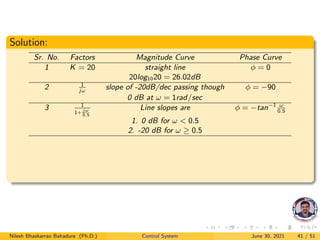
  • 159. Solution: Sr. No. Factors Magnitude Curve Phase Curve 1 K = 20 straight line φ = 0 20log1020 = 26.02dB 2 1 jω slope of -20dB/dec passing though φ = −90 0 dB at ω = 1rad/sec 3 1 1+ jω 0.5 Line slopes are φ = −tan−1 ω 0.5 1. 0 dB for ω < 0.5 2. -20 dB for ω ≥ 0.5 4 1 1+ jω 10 Line slopes are φ = −tan−1 ω 10 1. 0 dB for ω < 10 2. -20 dB for ω ≥ 10 Nilesh Bhaskarrao Bahadure (Ph.D.) Control System June 30, 2021 41 / 51
  • 160. Solution: Nilesh Bhaskarrao Bahadure (Ph.D.) Control System June 30, 2021 42 / 51
  • 161. Solution: Step 4: Magnitude plot table: Sr. No. Factors Resultant slope S.P. (ω) E.P. (ω) Nilesh Bhaskarrao Bahadure (Ph.D.) Control System June 30, 2021 42 / 51
  • 162. Solution: Step 4: Magnitude plot table: Sr. No. Factors Resultant slope S.P. (ω) E.P. (ω) 1 K = 20 straight line of 26.02 dB 0.1 ∞ Nilesh Bhaskarrao Bahadure (Ph.D.) Control System June 30, 2021 42 / 51
  • 163. Solution: Step 4: Magnitude plot table: Sr. No. Factors Resultant slope S.P. (ω) E.P. (ω) 1 K = 20 straight line of 26.02 dB 0.1 ∞ 2 1 jω -20 dB/dec 0.1 0.5 Nilesh Bhaskarrao Bahadure (Ph.D.) Control System June 30, 2021 42 / 51
  • 164. Solution: Step 4: Magnitude plot table: Sr. No. Factors Resultant slope S.P. (ω) E.P. (ω) 1 K = 20 straight line of 26.02 dB 0.1 ∞ 2 1 jω -20 dB/dec 0.1 0.5 3 1 1+ jω 0.5 -20 + (-20) = -40 dB/dec 0.5 10 Nilesh Bhaskarrao Bahadure (Ph.D.) Control System June 30, 2021 42 / 51
  • 165. Solution: Step 4: Magnitude plot table: Sr. No. Factors Resultant slope S.P. (ω) E.P. (ω) 1 K = 20 straight line of 26.02 dB 0.1 ∞ 2 1 jω -20 dB/dec 0.1 0.5 3 1 1+ jω 0.5 -20 + (-20) = -40 dB/dec 0.5 10 4 1 1+ jω 10 -40 + (-20) = -60 dB/dec 10 ∞ Nilesh Bhaskarrao Bahadure (Ph.D.) Control System June 30, 2021 42 / 51
  • 166. Solution: Nilesh Bhaskarrao Bahadure (Ph.D.) Control System June 30, 2021 43 / 51
  • 167. Solution: Step 5: Phase angle: Nilesh Bhaskarrao Bahadure (Ph.D.) Control System June 30, 2021 43 / 51
  • 168. Solution: Step 5: Phase angle: φresultant (ω) = −90o − tan−1 ( ω 0.5 ) − tan−1 ( ω 10 ) ω 1 jω −tan−1 ( ω 0.5 ) −tan−1 ( ω 10 ) φresultant (ω) Nilesh Bhaskarrao Bahadure (Ph.D.) Control System June 30, 2021 43 / 51
  • 169. Solution: Step 5: Phase angle: φresultant (ω) = −90o − tan−1 ( ω 0.5 ) − tan−1 ( ω 10 ) ω 1 jω −tan−1 ( ω 0.5 ) −tan−1 ( ω 10 ) φresultant (ω) 0.1 −90o -11.3 -0.5 -101.8 Nilesh Bhaskarrao Bahadure (Ph.D.) Control System June 30, 2021 43 / 51
  • 170. Solution: Step 5: Phase angle: φresultant (ω) = −90o − tan−1 ( ω 0.5 ) − tan−1 ( ω 10 ) ω 1 jω −tan−1 ( ω 0.5 ) −tan−1 ( ω 10 ) φresultant (ω) 0.1 −90o -11.3 -0.5 -101.8 0.5 −90o -45 -2.8 -137.8 Nilesh Bhaskarrao Bahadure (Ph.D.) Control System June 30, 2021 43 / 51
  • 171. Solution: Step 5: Phase angle: φresultant (ω) = −90o − tan−1 ( ω 0.5 ) − tan−1 ( ω 10 ) ω 1 jω −tan−1 ( ω 0.5 ) −tan−1 ( ω 10 ) φresultant (ω) 0.1 −90o -11.3 -0.5 -101.8 0.5 −90o -45 -2.8 -137.8 1 −90o -63.4 -5.7 -159.1 Nilesh Bhaskarrao Bahadure (Ph.D.) Control System June 30, 2021 43 / 51
  • 172. Solution: Step 5: Phase angle: φresultant (ω) = −90o − tan−1 ( ω 0.5 ) − tan−1 ( ω 10 ) ω 1 jω −tan−1 ( ω 0.5 ) −tan−1 ( ω 10 ) φresultant (ω) 0.1 −90o -11.3 -0.5 -101.8 0.5 −90o -45 -2.8 -137.8 1 −90o -63.4 -5.7 -159.1 2 −90o -75.96 -11.3 -177.2 Nilesh Bhaskarrao Bahadure (Ph.D.) Control System June 30, 2021 43 / 51
  • 173. Solution: Step 5: Phase angle: φresultant (ω) = −90o − tan−1 ( ω 0.5 ) − tan−1 ( ω 10 ) ω 1 jω −tan−1 ( ω 0.5 ) −tan−1 ( ω 10 ) φresultant (ω) 0.1 −90o -11.3 -0.5 -101.8 0.5 −90o -45 -2.8 -137.8 1 −90o -63.4 -5.7 -159.1 2 −90o -75.96 -11.3 -177.2 3 −90o -80.53 -16.6 -187.13 Nilesh Bhaskarrao Bahadure (Ph.D.) Control System June 30, 2021 43 / 51
  • 174. Solution: Step 5: Phase angle: φresultant (ω) = −90o − tan−1 ( ω 0.5 ) − tan−1 ( ω 10 ) ω 1 jω −tan−1 ( ω 0.5 ) −tan−1 ( ω 10 ) φresultant (ω) 0.1 −90o -11.3 -0.5 -101.8 0.5 −90o -45 -2.8 -137.8 1 −90o -63.4 -5.7 -159.1 2 −90o -75.96 -11.3 -177.2 3 −90o -80.53 -16.6 -187.13 4 −90o -82.87 -21.8 -194.67 Nilesh Bhaskarrao Bahadure (Ph.D.) Control System June 30, 2021 43 / 51
  • 175. Solution: Step 5: Phase angle: φresultant (ω) = −90o − tan−1 ( ω 0.5 ) − tan−1 ( ω 10 ) ω 1 jω −tan−1 ( ω 0.5 ) −tan−1 ( ω 10 ) φresultant (ω) 0.1 −90o -11.3 -0.5 -101.8 0.5 −90o -45 -2.8 -137.8 1 −90o -63.4 -5.7 -159.1 2 −90o -75.96 -11.3 -177.2 3 −90o -80.53 -16.6 -187.13 4 −90o -82.87 -21.8 -194.67 5 −90o -84.2 -26.2 -200.7 Nilesh Bhaskarrao Bahadure (Ph.D.) Control System June 30, 2021 43 / 51
  • 176. Solution: Step 5: Phase angle: φresultant (ω) = −90o − tan−1 ( ω 0.5 ) − tan−1 ( ω 10 ) ω 1 jω −tan−1 ( ω 0.5 ) −tan−1 ( ω 10 ) φresultant (ω) 0.1 −90o -11.3 -0.5 -101.8 0.5 −90o -45 -2.8 -137.8 1 −90o -63.4 -5.7 -159.1 2 −90o -75.96 -11.3 -177.2 3 −90o -80.53 -16.6 -187.13 4 −90o -82.87 -21.8 -194.67 5 −90o -84.2 -26.2 -200.7 10 −90o -87.1 -45 -222.1 Nilesh Bhaskarrao Bahadure (Ph.D.) Control System June 30, 2021 43 / 51
  • 177. Solution: Step 5: Phase angle: φresultant (ω) = −90o − tan−1 ( ω 0.5 ) − tan−1 ( ω 10 ) ω 1 jω −tan−1 ( ω 0.5 ) −tan−1 ( ω 10 ) φresultant (ω) 0.1 −90o -11.3 -0.5 -101.8 0.5 −90o -45 -2.8 -137.8 1 −90o -63.4 -5.7 -159.1 2 −90o -75.96 -11.3 -177.2 3 −90o -80.53 -16.6 -187.13 4 −90o -82.87 -21.8 -194.67 5 −90o -84.2 -26.2 -200.7 10 −90o -87.1 -45 -222.1 100 −90o -89.7 -84.2 -263.9 Nilesh Bhaskarrao Bahadure (Ph.D.) Control System June 30, 2021 43 / 51
  • 178. Solution: Step 5: Phase angle: φresultant (ω) = −90o − tan−1 ( ω 0.5 ) − tan−1 ( ω 10 ) ω 1 jω −tan−1 ( ω 0.5 ) −tan−1 ( ω 10 ) φresultant (ω) 0.1 −90o -11.3 -0.5 -101.8 0.5 −90o -45 -2.8 -137.8 1 −90o -63.4 -5.7 -159.1 2 −90o -75.96 -11.3 -177.2 3 −90o -80.53 -16.6 -187.13 4 −90o -82.87 -21.8 -194.67 5 −90o -84.2 -26.2 -200.7 10 −90o -87.1 -45 -222.1 100 −90o -89.7 -84.2 -263.9 500 −90o -89.94 -88.8 -268.7 Nilesh Bhaskarrao Bahadure (Ph.D.) Control System June 30, 2021 43 / 51
  • 179. Solution: Step 5: Phase angle: φresultant (ω) = −90o − tan−1 ( ω 0.5 ) − tan−1 ( ω 10 ) ω 1 jω −tan−1 ( ω 0.5 ) −tan−1 ( ω 10 ) φresultant (ω) 0.1 −90o -11.3 -0.5 -101.8 0.5 −90o -45 -2.8 -137.8 1 −90o -63.4 -5.7 -159.1 2 −90o -75.96 -11.3 -177.2 3 −90o -80.53 -16.6 -187.13 4 −90o -82.87 -21.8 -194.67 5 −90o -84.2 -26.2 -200.7 10 −90o -87.1 -45 -222.1 100 −90o -89.7 -84.2 -263.9 500 −90o -89.94 -88.8 -268.7 1000 −90o -89.97 -89.4 -289.3 Nilesh Bhaskarrao Bahadure (Ph.D.) Control System June 30, 2021 43 / 51
  • 180. Nilesh Bhaskarrao Bahadure (Ph.D.) Control System June 30, 2021 44 / 51
  • 181. Example: 02 Example: A feedback control system has G(s)H(s) = 100(s + 3) s(s + 1)(s + 5) Draw the Bode plot and comments on stability Nilesh Bhaskarrao Bahadure (Ph.D.) Control System June 30, 2021 45 / 51
  • 182. Solution: Nilesh Bhaskarrao Bahadure (Ph.D.) Control System June 30, 2021 46 / 51
  • 183. Solution: Step 1: Bring equation in standard form: Nilesh Bhaskarrao Bahadure (Ph.D.) Control System June 30, 2021 46 / 51
  • 184. Solution: Step 1: Bring equation in standard form: G(s).H(s) = 100 × 3(1 + s 3 ) 5 × s(1 + s)(1 + s 5 ) = 60(1 + s 3 ) s(1 + s)(1 + s 5 ) Nilesh Bhaskarrao Bahadure (Ph.D.) Control System June 30, 2021 46 / 51
  • 185. Solution: Step 1: Bring equation in standard form: G(s).H(s) = 100 × 3(1 + s 3 ) 5 × s(1 + s)(1 + s 5 ) = 60(1 + s 3 ) s(1 + s)(1 + s 5 ) Step 2: Convert to frequency domain by replacing s = jω Nilesh Bhaskarrao Bahadure (Ph.D.) Control System June 30, 2021 46 / 51
  • 186. Solution: Step 1: Bring equation in standard form: G(s).H(s) = 100 × 3(1 + s 3 ) 5 × s(1 + s)(1 + s 5 ) = 60(1 + s 3 ) s(1 + s)(1 + s 5 ) Step 2: Convert to frequency domain by replacing s = jω G(jω).H(jω) = 60(1 + jω 3 ) jω(1 + jω)(1 + jω 5 ) Nilesh Bhaskarrao Bahadure (Ph.D.) Control System June 30, 2021 46 / 51
  • 187. Solution: Step 1: Bring equation in standard form: G(s).H(s) = 100 × 3(1 + s 3 ) 5 × s(1 + s)(1 + s 5 ) = 60(1 + s 3 ) s(1 + s)(1 + s 5 ) Step 2: Convert to frequency domain by replacing s = jω G(jω).H(jω) = 60(1 + jω 3 ) jω(1 + jω)(1 + jω 5 ) Step 3: The following factors are present: 1 Constant K = 60 Nilesh Bhaskarrao Bahadure (Ph.D.) Control System June 30, 2021 46 / 51
  • 188. Solution: Step 1: Bring equation in standard form: G(s).H(s) = 100 × 3(1 + s 3 ) 5 × s(1 + s)(1 + s 5 ) = 60(1 + s 3 ) s(1 + s)(1 + s 5 ) Step 2: Convert to frequency domain by replacing s = jω G(jω).H(jω) = 60(1 + jω 3 ) jω(1 + jω)(1 + jω 5 ) Step 3: The following factors are present: 1 Constant K = 60 2 Poles at origin 1 jω Nilesh Bhaskarrao Bahadure (Ph.D.) Control System June 30, 2021 46 / 51
  • 189. Solution: Step 1: Bring equation in standard form: G(s).H(s) = 100 × 3(1 + s 3 ) 5 × s(1 + s)(1 + s 5 ) = 60(1 + s 3 ) s(1 + s)(1 + s 5 ) Step 2: Convert to frequency domain by replacing s = jω G(jω).H(jω) = 60(1 + jω 3 ) jω(1 + jω)(1 + jω 5 ) Step 3: The following factors are present: 1 Constant K = 60 2 Poles at origin 1 jω 3 First order pole 1 1+jω Nilesh Bhaskarrao Bahadure (Ph.D.) Control System June 30, 2021 46 / 51
  • 190. Solution: Step 1: Bring equation in standard form: G(s).H(s) = 100 × 3(1 + s 3 ) 5 × s(1 + s)(1 + s 5 ) = 60(1 + s 3 ) s(1 + s)(1 + s 5 ) Step 2: Convert to frequency domain by replacing s = jω G(jω).H(jω) = 60(1 + jω 3 ) jω(1 + jω)(1 + jω 5 ) Step 3: The following factors are present: 1 Constant K = 60 2 Poles at origin 1 jω 3 First order pole 1 1+jω 4 First order pole 1 1+ jω 5 Nilesh Bhaskarrao Bahadure (Ph.D.) Control System June 30, 2021 46 / 51
  • 191. Solution: Step 1: Bring equation in standard form: G(s).H(s) = 100 × 3(1 + s 3 ) 5 × s(1 + s)(1 + s 5 ) = 60(1 + s 3 ) s(1 + s)(1 + s 5 ) Step 2: Convert to frequency domain by replacing s = jω G(jω).H(jω) = 60(1 + jω 3 ) jω(1 + jω)(1 + jω 5 ) Step 3: The following factors are present: 1 Constant K = 60 2 Poles at origin 1 jω 3 First order pole 1 1+jω 4 First order pole 1 1+ jω 5 5 First order zero 1 + jω 3 Nilesh Bhaskarrao Bahadure (Ph.D.) Control System June 30, 2021 46 / 51
  • 192. Solution: Sr. No. Factors Magnitude Curve Phase Curve Nilesh Bhaskarrao Bahadure (Ph.D.) Control System June 30, 2021 47 / 51
  • 193. Solution: Sr. No. Factors Magnitude Curve Phase Curve 1 K = 60 straight line φ = 0 20log1060 = 35.56dB Nilesh Bhaskarrao Bahadure (Ph.D.) Control System June 30, 2021 47 / 51
  • 194. Solution: Sr. No. Factors Magnitude Curve Phase Curve 1 K = 60 straight line φ = 0 20log1060 = 35.56dB 2 1 jω slope of -20dB/dec passing though φ = −90 0 dB at ω = 1rad/sec Nilesh Bhaskarrao Bahadure (Ph.D.) Control System June 30, 2021 47 / 51
  • 195. Solution: Sr. No. Factors Magnitude Curve Phase Curve 1 K = 60 straight line φ = 0 20log1060 = 35.56dB 2 1 jω slope of -20dB/dec passing though φ = −90 0 dB at ω = 1rad/sec 3 1 1+jω Line slopes are φ = −tan−1 (ω) 1. 0 dB for ω < 1 2. -20 dB for ω ≥ 1 Nilesh Bhaskarrao Bahadure (Ph.D.) Control System June 30, 2021 47 / 51
  • 196. Solution: Sr. No. Factors Magnitude Curve Phase Curve 1 K = 60 straight line φ = 0 20log1060 = 35.56dB 2 1 jω slope of -20dB/dec passing though φ = −90 0 dB at ω = 1rad/sec 3 1 1+jω Line slopes are φ = −tan−1 (ω) 1. 0 dB for ω < 1 2. -20 dB for ω ≥ 1 4 1 1+ jω 5 Line slopes are φ = −tan−1 ω 5 1. 0 dB for ω < 5 2. -20 dB for ω ≥ 5 Nilesh Bhaskarrao Bahadure (Ph.D.) Control System June 30, 2021 47 / 51
  • 197. Solution: Sr. No. Factors Magnitude Curve Phase Curve 1 K = 60 straight line φ = 0 20log1060 = 35.56dB 2 1 jω slope of -20dB/dec passing though φ = −90 0 dB at ω = 1rad/sec 3 1 1+jω Line slopes are φ = −tan−1 (ω) 1. 0 dB for ω < 1 2. -20 dB for ω ≥ 1 4 1 1+ jω 5 Line slopes are φ = −tan−1 ω 5 1. 0 dB for ω < 5 2. -20 dB for ω ≥ 5 5 1 + jω 3 Line slopes are φ = tan−1 ω 3 1. 0 dB for ω < 3 2. +20 dB for ω ≥ 3 Nilesh Bhaskarrao Bahadure (Ph.D.) Control System June 30, 2021 47 / 51
  • 198. Solution: Nilesh Bhaskarrao Bahadure (Ph.D.) Control System June 30, 2021 48 / 51
  • 199. Solution: Step 4: Magnitude plot table: Sr. No. Factors Resultant slope S.P. (ω) E.P. (ω) Nilesh Bhaskarrao Bahadure (Ph.D.) Control System June 30, 2021 48 / 51
  • 200. Solution: Step 4: Magnitude plot table: Sr. No. Factors Resultant slope S.P. (ω) E.P. (ω) 1 K = 60 straight line of 35.56 dB 0.1 ∞ Nilesh Bhaskarrao Bahadure (Ph.D.) Control System June 30, 2021 48 / 51
  • 201. Solution: Step 4: Magnitude plot table: Sr. No. Factors Resultant slope S.P. (ω) E.P. (ω) 1 K = 60 straight line of 35.56 dB 0.1 ∞ 2 1 jω -20 dB/dec 0.1 1 Nilesh Bhaskarrao Bahadure (Ph.D.) Control System June 30, 2021 48 / 51
  • 202. Solution: Step 4: Magnitude plot table: Sr. No. Factors Resultant slope S.P. (ω) E.P. (ω) 1 K = 60 straight line of 35.56 dB 0.1 ∞ 2 1 jω -20 dB/dec 0.1 1 3 1 1+jω -20 + (-20) = -40 dB/dec 1 3 Nilesh Bhaskarrao Bahadure (Ph.D.) Control System June 30, 2021 48 / 51
  • 203. Solution: Step 4: Magnitude plot table: Sr. No. Factors Resultant slope S.P. (ω) E.P. (ω) 1 K = 60 straight line of 35.56 dB 0.1 ∞ 2 1 jω -20 dB/dec 0.1 1 3 1 1+jω -20 + (-20) = -40 dB/dec 1 3 4 1 + jω 3 -40 + (+20) = -20 dB/dec 3 5 Nilesh Bhaskarrao Bahadure (Ph.D.) Control System June 30, 2021 48 / 51
  • 204. Solution: Step 4: Magnitude plot table: Sr. No. Factors Resultant slope S.P. (ω) E.P. (ω) 1 K = 60 straight line of 35.56 dB 0.1 ∞ 2 1 jω -20 dB/dec 0.1 1 3 1 1+jω -20 + (-20) = -40 dB/dec 1 3 4 1 + jω 3 -40 + (+20) = -20 dB/dec 3 5 5 1 1+ jω 3 -20 + (-20) = -40 dB/dec 5 ∞ Nilesh Bhaskarrao Bahadure (Ph.D.) Control System June 30, 2021 48 / 51
  • 205. Solution: Nilesh Bhaskarrao Bahadure (Ph.D.) Control System June 30, 2021 49 / 51
  • 206. Solution: Step 5: Phase angle: Nilesh Bhaskarrao Bahadure (Ph.D.) Control System June 30, 2021 49 / 51
  • 207. Solution: Step 5: Phase angle: φresultant (ω) = −90o − tan−1 (ω) − tan−1 (ω 5 ) + tan−1 (ω 3 ) ω 1 jω −tan−1 (ω) −tan−1 (ω 5 ) +tan−1 (ω 3 ) φresultant (ω) Nilesh Bhaskarrao Bahadure (Ph.D.) Control System June 30, 2021 49 / 51
  • 208. Solution: Step 5: Phase angle: φresultant (ω) = −90o − tan−1 (ω) − tan−1 (ω 5 ) + tan−1 (ω 3 ) ω 1 jω −tan−1 (ω) −tan−1 (ω 5 ) +tan−1 (ω 3 ) φresultant (ω) 0.1 −90o -5.7 -1.1 1.9 -94.9 Nilesh Bhaskarrao Bahadure (Ph.D.) Control System June 30, 2021 49 / 51
  • 209. Solution: Step 5: Phase angle: φresultant (ω) = −90o − tan−1 (ω) − tan−1 (ω 5 ) + tan−1 (ω 3 ) ω 1 jω −tan−1 (ω) −tan−1 (ω 5 ) +tan−1 (ω 3 ) φresultant (ω) 0.1 −90o -5.7 -1.1 1.9 -94.9 0.5 −90o -26.5 -5.7 9.46 -112.9 Nilesh Bhaskarrao Bahadure (Ph.D.) Control System June 30, 2021 49 / 51
  • 210. Solution: Step 5: Phase angle: φresultant (ω) = −90o − tan−1 (ω) − tan−1 (ω 5 ) + tan−1 (ω 3 ) ω 1 jω −tan−1 (ω) −tan−1 (ω 5 ) +tan−1 (ω 3 ) φresultant (ω) 0.1 −90o -5.7 -1.1 1.9 -94.9 0.5 −90o -26.5 -5.7 9.46 -112.9 1 −90o -45 -11.3 18.4 -127.9 Nilesh Bhaskarrao Bahadure (Ph.D.) Control System June 30, 2021 49 / 51
  • 211. Solution: Step 5: Phase angle: φresultant (ω) = −90o − tan−1 (ω) − tan−1 (ω 5 ) + tan−1 (ω 3 ) ω 1 jω −tan−1 (ω) −tan−1 (ω 5 ) +tan−1 (ω 3 ) φresultant (ω) 0.1 −90o -5.7 -1.1 1.9 -94.9 0.5 −90o -26.5 -5.7 9.46 -112.9 1 −90o -45 -11.3 18.4 -127.9 5 −90o -78.69 -45 59 -154.79 Nilesh Bhaskarrao Bahadure (Ph.D.) Control System June 30, 2021 49 / 51
  • 212. Solution: Step 5: Phase angle: φresultant (ω) = −90o − tan−1 (ω) − tan−1 (ω 5 ) + tan−1 (ω 3 ) ω 1 jω −tan−1 (ω) −tan−1 (ω 5 ) +tan−1 (ω 3 ) φresultant (ω) 0.1 −90o -5.7 -1.1 1.9 -94.9 0.5 −90o -26.5 -5.7 9.46 -112.9 1 −90o -45 -11.3 18.4 -127.9 5 −90o -78.69 -45 59 -154.79 10 −90o -84.3 -63.4 73.3 -164.4 Nilesh Bhaskarrao Bahadure (Ph.D.) Control System June 30, 2021 49 / 51
  • 213. Solution: Step 5: Phase angle: φresultant (ω) = −90o − tan−1 (ω) − tan−1 (ω 5 ) + tan−1 (ω 3 ) ω 1 jω −tan−1 (ω) −tan−1 (ω 5 ) +tan−1 (ω 3 ) φresultant (ω) 0.1 −90o -5.7 -1.1 1.9 -94.9 0.5 −90o -26.5 -5.7 9.46 -112.9 1 −90o -45 -11.3 18.4 -127.9 5 −90o -78.69 -45 59 -154.79 10 −90o -84.3 -63.4 73.3 -164.4 100 −90o -89.4 -87.1 88.3 -178.2 Nilesh Bhaskarrao Bahadure (Ph.D.) Control System June 30, 2021 49 / 51
  • 214. Solution: Step 5: Phase angle: φresultant (ω) = −90o − tan−1 (ω) − tan−1 (ω 5 ) + tan−1 (ω 3 ) ω 1 jω −tan−1 (ω) −tan−1 (ω 5 ) +tan−1 (ω 3 ) φresultant (ω) 0.1 −90o -5.7 -1.1 1.9 -94.9 0.5 −90o -26.5 -5.7 9.46 -112.9 1 −90o -45 -11.3 18.4 -127.9 5 −90o -78.69 -45 59 -154.79 10 −90o -84.3 -63.4 73.3 -164.4 100 −90o -89.4 -87.1 88.3 -178.2 500 −90o -89.8 -89.4 89.6 -179.6 Nilesh Bhaskarrao Bahadure (Ph.D.) Control System June 30, 2021 49 / 51
  • 215. Solution: Step 5: Phase angle: φresultant (ω) = −90o − tan−1 (ω) − tan−1 (ω 5 ) + tan−1 (ω 3 ) ω 1 jω −tan−1 (ω) −tan−1 (ω 5 ) +tan−1 (ω 3 ) φresultant (ω) 0.1 −90o -5.7 -1.1 1.9 -94.9 0.5 −90o -26.5 -5.7 9.46 -112.9 1 −90o -45 -11.3 18.4 -127.9 5 −90o -78.69 -45 59 -154.79 10 −90o -84.3 -63.4 73.3 -164.4 100 −90o -89.4 -87.1 88.3 -178.2 500 −90o -89.8 -89.4 89.6 -179.6 1000 −90o -89.9 -89.71 89.8 -179.8 Nilesh Bhaskarrao Bahadure (Ph.D.) Control System June 30, 2021 49 / 51
  • 216. Nilesh Bhaskarrao Bahadure (Ph.D.) Control System June 30, 2021 50 / 51
  • 217. Thank you Please send your feedback at nbahadure@gmail.com Nilesh Bhaskarrao Bahadure (Ph.D.) Control System June 30, 2021 51 / 51
  • 218. Thank you Please send your feedback at nbahadure@gmail.com For download and more information Click Here Nilesh Bhaskarrao Bahadure (Ph.D.) Control System June 30, 2021 51 / 51