CPSC 340: Machine Learning and Data Mining More Clustering Andreas Lehrmann and Mark Schmidt University of British Columbia, Fall 2022

CPSC 340:
Machine Learning and Data Mining
More Clustering
Andreas Lehrmann and Mark Schmidt
University of British Columbia, Fall 2022
https://www.students.cs.ubc.ca/~cs-340

Last Time: K-Means Clustering
• We want to cluster data:
– Assign examples to groups.
• K-means clustering:
– Define groups by “means”
– Assigns examples to nearest mean.
(And updates means during training.)
• Issues with k-means:
– Fast but sensitive to initialization.
– Choosing ‘k’ is annoying.

Vector Quantization
• K-means originally comes from signal processing.
• Designed for vector quantization:
– Replace examples with the mean of their cluster (“prototype”).
• Example:
– Facebook places: 1 location summarizes many.
– What sizes of clothing should I make?
http://wannabite.com/wp-content/uploads/2014/10/ragu-pasta-sauce-printable-coupon.jpg

Vector Quantization for Basketball Players
• Clustering NBA basketball players based on shot type/percentage:
• The “prototypes” (means) give offensive styles (like “catch and shoot”).
https://fansided.com/2018/08/23/nylon-calculus-shooting-volume-versus-efficiency/

(Bad) Vector Quantization in Practice
• Political parties can be thought as a form of vector quantization:
– Hope is that parties represent what a cluster of voters want.
• With larger ‘k’ more voters have a party that closely reflects them.
• With smaller ‘k’, parties are less accurate reflections of people’s views.
https://globalnews.ca/news/5191123/federal-election-seat-projection-trudeau-liberals-minority/

Shape of K-Means Clusters
• Recall that k-means assigns cluster based on nearest mean.
• This leads to partitions the space :
• Observe that the clusters are convex regions (proof in bonus).

Convex Sets
• A set is convex if line between two points in the set stays in the set.
Convex
Convex
Not Convex

Shape of K-Means Clusters
Animation

K-Means with Non-Convex Clusters
https://corelifesciences.com/human-long-non-coding-rna-expression-microarray-service.html

K-means cannot separate
some non-convex clusters

K-means cannot separate
some non-convex clusters
Though over-clustering can help
(“hierarchical”)

CPSC 340: Machine Learning and Data Mining More Clustering Andreas Lehrmann and Mark Schmidt University of British Columbia, Fall 2022

John Snow and Cholera Epidemic
• John Snow’s 1854 spatial histogram of deaths from cholera:
• Found cluster of cholera deaths around a particular water pump.
– Went against airborne theory, but pump later found to be contaminated.
– “Father” of epidemiology.
https://en.wikipedia.org/wiki/John_Snow

Motivation for Density-Based Clustering
• Density-based clustering:
– Clusters are defined by “dense” regions.
– Examples in non-dense regions don’t get clustered.
• Not trying to “partition” the space.
• Clusters can be non-convex:
– Elephant clusters affected by vegetation,
mountains, rivers, water access, etc.
• It’s a non-parametric clustering method:
– No fixed number of clusters ‘k’.
– Clusters can become more complicated with more data.
http://www.defenders.org/elephant/basic-facts

Other Potential Applications
• Where are high crime regions of a city?
• Where should taxis patrol?
• Where can proteins ‘dock’?
• Where are people tweeting?
• Where does Iguodala make/miss shots?
• Which products are similar to this one?
• Which pictures are in the same place?
https://en.wikipedia.org/wiki/Cluster_analysis
https://www.flickr.com/photos/dbarefoot/420194128/
http://letsgowarriors.com/replacing-jarrett-jack/2013/10/04/
http://www.dbs.informatik.uni-muenchen.de/Forschung/KDD/Clustering/

Density-Based Clustering in Action
Interactive demo

Density-Based Clustering
• Density-based clustering algorithm (DBSCAN) has two hyperparameters:
– Epsilon (ε): distance we use to decide if another point is a “neighbour”.

Density-Based Clustering
• Density-based clustering algorithm (DBSCAN) has two hyperparameters:
– Epsilon (ε): distance we use to decide if another point is a “neighbour”.
– MinNeighbours: number of neighbours needed to say a region is “dense”.
• If you have at least minNeighbours “neighbours”, you are called a “core” point.
• Main idea: merge all neighbouring core points to form clusters.

• Intuitively, density-based clustering algorithm
implements a “chain reaction” throughout the dense areas.
• For each example xi:
– If xi is already assigned to a cluster, do nothing.
– Test whether xi is a ‘core’ point (≥ minNeighbours examples within ‘ε’).
• If xi is not core point, do nothing (this could be an outlier).
• If xi is a core point, make a new cluster and call the “expand cluster” function.
– Which spreads the “reaction” to nearby points.
Density-Based Clustering Pseudo-Code

Density-Based Clustering Pseudo-Code
• “Expand cluster” function:
– Assign to this cluster all xj within distance ‘ε’ of core point xi to this cluster.
– For each new “core” point found, call “expand cluster” (recursively).

Density-Based Clustering Issues
• Some points are not assigned to a cluster.
– Good or bad, depending on the application.
• Ambiguity of “non-core” (boundary) points:
• Sensitive to the choice of ε and minNeighbours.
– Original paper proposed an “elbow” method (see bonus slide).
– Otherwise, not sensitive to initialization (except for boundary points).
• If you get a new example, finding cluster is expensive.
– Need to compute distances to core points (or maybe all training points).
• In high-dimensions, need a lot of points to ‘fill’ the space.

Density-Based Clustering in Bacteria
• Quorum sensing:
– Bacteria continuously release a particular molecule.
– They have sensors for this molecule.
• If sensors become very active:
– It means cell density is high.
– Causes cascade of changes in cells.
(Some cells “stick together” to
form a physical cluster via “biofilm”.)
https://en.wikipedia.org/wiki/Quorum_sensing

Density-Based Clustering in People
• “High density leading a chain reaction” can also happen in people.
– “Social distancing”: try to reduce the number of people within 𝜖.
– “Wearing masks”: try to increase the 𝜖 needed for a chain reaction.

Next Topic: Ensemble Clustering

Ensemble Clustering
• We can consider ensemble methods for clustering.
– “Consensus clustering”
• It’s a good/important idea:
– Bootstrapping is widely-used.
– “Do clusters change if the data was slightly different?”
• But we need to be careful about how we combine models.

Ensemble Clustering
• E.g., run k-means 20 times and then cluster using the mode of each !
𝑦i.
• Normally, averaging across models doing different things is good.
• But this is a bad ensemble method: worse than k-means on its own.

Label Switching Problem
• This doesn’t work because of “label switching” problem:
– The cluster labels $
𝑦i are meaningless.
– We could get same clustering with permuted labels (“exchangeable”):
– All $
𝑦i become equally likely as number of initializations increases.

Addressing Label Switching Problem
• Ensembles can’t depend on label “meaning”:
– Don’t ask “is point xi in red square cluster?”, which is meaningless.
– Ask “is point xi in the same cluster as xj?”, which is meaningful.
– Bonus slides give an example method (“UBClustering”).

Next Topic: Hierarchical Clustering

Differing Densities
• Consider density-based clustering on this data:

Differing Densities
• Increase epsilon and run it again:
• There may be no density-level that gives you 3 clusters.

Differing Densities
• Here is a worse situation:
• Now you need to choose between coarse/fine clusters.
• Instead of fixed clustering, we often want hierarchical clustering.

Hierarchical Clustering
• Hierarchical clustering produces a tree of clusterings.
– Each node in the tree splits the data into 2 or more clusters.
– Much more information than using a fixed clustering.
– Often have individual data points as leaves.
GIF

Application: Phylogenetics
• We sequence genomes of a set of organisms.
• Can we construct the “tree of life”?
• Comments on this application:
– On the right are individuals.
– As you go left, clusters merge.
– Merges are ‘common ancestors’.
• More useful information in the plot:
– Line lengths: chosen here to approximate time.
– Numbers: #clusterings across bootstrap samples.
– ‘Outgroups’ (walrus, panda) are a sanity check.
http://www.nature.com/nature/journal/v438/n7069/fig_tab/nature04338_F10.html

• Interactive demo of model of full tree of life: www.onezoom.org

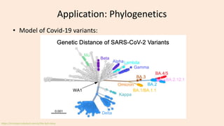
• Model of Covid-19 variants:
https://erictopol.substack.com/p/the-ba5-story

• Comparative method in linguistics studies evolution of languages:
https://en.wikipedia.org/wiki/Comparative_method_(linguistics)

• January 2016: evolution of fairy tales.
– Evidence that “Devil and the Smith”
goes back to bronze age.
– “Beauty and the Beast” published
in 1740, but might be 2500-6000 years old.
http://rsos.royalsocietypublishing.org/content/3/1/150645

• January 2016: evolution of fairy tales.
– Evidence that “Devil and the Smith”
goes back to bronze age.
– “Beauty and the Beast” published
in 1740, but might be 2500-6000 years old.
• September 2016: evolution of myths.
– “Cosmic hunt” story:
• Person hunts animal that becomes constellation.
– Previously known to be at least 15,000 years old.
• May go back to paleololithic period.
http://www.nature.com/nature/journal/v438/n7069/fig_tab/nature04338_F10.html

Application: Fashion?
• Hierarchical clustering of clothing material words in Vogue:
http://dh.library.yale.edu/projects/vogue/fabricspace/

Agglomerative (Bottom-Up) Clustering
• Most common hierarchical method: agglomerative clustering.
1. Starts with each point in its own cluster.
https://en.wikipedia.org/wiki/Hierarchical_clustering

2. Each step merges the two “closest” clusters.

2. Each step merges the two “closest” clusters.
3. Stop with one big cluster that has all points.
Animation

• Reinvented by different fields under different names (“UPGMA”).
• Needs a “distance” between two clusters.
• A standard choice: distance between means of the clusters.
– Not necessarily the best, many choices exist (bonus slide).
• Cost is O(n3d) for basic implementation.
– Each step costs O(n2d), and each step might only cluster 1 new point.

Summary
• Shape of K-means clusters:
– Partitions space into convex sets.
• Density-based clustering:
– “Expand” and “merge” dense regions of points to find clusters.
– Not sensitive to initialization or outliers.
– Useful for finding non-convex connected clusters.
• Ensemble clustering: combines multiple clusterings.
– Can work well but need to account for label switching.
• Hierarchical clustering: more informative than fixed clustering.
• Agglomerative clustering: standard hierarchical clustering method.
– Each point starts as a cluster, sequentially merge clusters.
• Next time:
• Discovering (and then ignoring) a hole in the ozone layer.

Why are k-means clusters convex?
• K-means clusters are formed by the intersection of half-spaces.
Half-space

• K-means clusters are formed by the intersection of half-spaces.
Half-space
Intersection
Half-space

“Closer to red” half-space
“Closer to green” half-space

Blue over green half-space
Green over blue half-space

Magenta over green half-space
Green over magenta half-space

• Half-spaces are convex sets.
• Intersection of convex sets is a convex set.
– Line segment between points in each set are still in each set.
• So intersection of half-spaces is convex.
Half-space
Intersection
Half-space

• Formal proof that “cluster 1” is convex (works for other clusters).

Voronoi Diagrams
• The k-means partition can be visualized as a Voronoi diagram:
• Can be a useful visualization of “nearest available” problems.
– E.g., nearest tube station in London.
http://datagenetics.com/blog/may12017/index.html

Density-Based Clustering Runtime

“Elbow” Method for Density-Based Clustering
• From the original DBSCAN paper:
– Choose some ‘k’ (they suggest 4) and set minNeighbours=k.
– Compute distance of each points to its ‘k’ nearest neighbours.
– Sort the points based on these distances and plot the distances:
– Look for an “elbow” to choose 𝜖.
https://www.aaai.org/Papers/KDD/1996/KDD96-037.pdf

OPTICS
• Related to the DBSCAN “elbow” is “OPTICS”.
– Sort the points so that neighbours are close to each other in the ordering.
– Plot the distance from each point to the next point.
– Clusters should correspond to sequencers with low distance.
https://en.wikipedia.org/wiki/OPTICS_algorithm

UBClustering Algorithm
• Let’s define a new ensemble clustering method: UBClustering.
1. Run k-means with ‘m’ different random initializations.
2. For each example i and j:
– Count the number of times xi and xj are in the same cluster.
– Define p(i,j) = count(xi in same cluster as xj)/m.
3. Put xi and xj in the same cluster if p(i,j) > 0.5.
• Like DBSCAN merge clusters in step 3 if i or j are already assigned.
– You can implement this with a DBSCAN code (just changes “distance”).
– Each xi has an xj in its cluster with p(i,j) > 0.5.
– Some points are not assigned to any cluster.

Distances between Clusters
• Other choices of the distance between two clusters:
– “Single-link”: minimum distance between points in clusters.
– “Average-link”: average distance between points in clusters.
– “Complete-link”: maximum distance between points in clusters.
– Ward’s method: minimize within-cluster variance.
– “Centroid-link”: distance between a representative point in the cluster.
• Useful for distance measures on non-Euclidean spaces (like Jaccard similarity).
• “Centroid” often defined as point in cluster minimizing average distance to other
points.

Cost of Agglomerative Clustering
• One step of agglomerative clustering costs O(n2d):
– We need to do the O(d) distance calculation between up to O(n2) points.
– This is assuming the standard distance functions.
• We do at most O(n) steps:
– Starting with ‘n’ clusters and merging 2 clusters on each step, after O(n) steps
we’ll only have 1 cluster left (though typically it will be much smaller).
• This gives a total cost of O(n3d).
• This can be reduced to O(n2d log n) with a priority queue:
– Store distances in a sorted order, only update the distances that change.
• For single- and complete-linkage, you can get it down to O(n2d).
– “SLINK” and “CLINK” algorithms.

Bonus Slide: Divisive (Top-Down) Clustering
• Start with all examples in one cluster, then start dividing.
• E.g., run k-means on a cluster, then run again on resulting clusters.
– A clustering analogue of decision tree learning.

CPSC 340: Machine Learning and Data Mining More Clustering Andreas Lehrmann and Mark Schmidt University of British Columbia, Fall 2022

More Related Content

Similar to CPSC 340: Machine Learning and Data Mining More Clustering Andreas Lehrmann and Mark Schmidt University of British Columbia, Fall 2022 (20)

Recently uploaded (20)

CPSC 340: Machine Learning and Data Mining More Clustering Andreas Lehrmann and Mark Schmidt University of British Columbia, Fall 2022