


CST413 KTU S7 CSE Machine Learning Clustering K Means Hierarchical Agglomerative clustering Principal Component Analysis Expectation Maximization Module 4.pptx
- 2. Syllabus Clustering - Similarity measures, Hierarchical Agglomerative Clustering, K-means partitional clustering, Expectation maximization (EM) for soft clustering. Dimensionality reduction – Principal ComponentAnalysis.
- 3. Clustering Clustering or cluster analysis is a machine learning technique, which groups the unlabelled dataset. It can be defined as "A way of grouping the data points into different clusters, consisting of similar data points. The objects with the possible similarities remain in a group that has less or no similarities with another group."
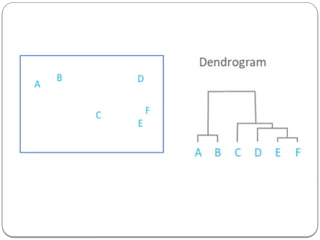
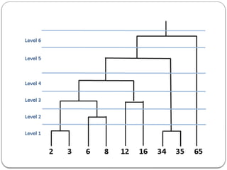
- 6. Hierarchical Clustering Given n points in a d-dimensional space, the goal of hierarchical clustering is to create a sequence of nested partitions, which can be conveniently visualized via a tree or hierarchy of clusters, also called the cluster dendrogram. The clusters in the hierarchy range from the fine-grained to the coarse-grained – the lowest level of the tree (the leaves) consists of each point in its own cluster, whereas the highest level (the root) consists of all points in one cluster. At some intermediate level, we may find meaningful clusters. If the user supplies k, the desired number of clusters, we can choose the level at which there are k clusters.
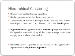
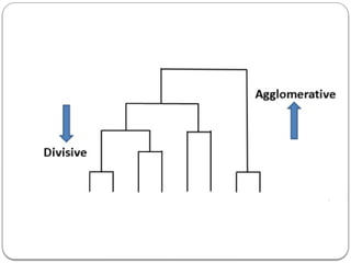
- 7. Hierarchical Clustering Unsupervised machine learning algorithm. Used to group the unlabelled datasets into clusters. The hierarchy of clusters is developed in the form of a tree, and this tree-shaped structure is known as the dendrogram. Agglomerative: Agglomerative is a bottom-up approach, in which the algorithm starts with taking all data points as single clusters and merging them until one cluster is left. Divisive: Divisive algorithm is the reverse of the agglomerative algorithm as it is a top-down approach.
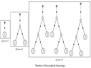
- 12. The number of different nested or hierarchical clusterings corresponds to the number of different binary rooted trees or dendrograms with n leaves with distinct labels. Any tree with t nodes has t −1 edges. Also, any rooted binary tree with m leaves has m−1 internal nodes. Thus, a dendrogram with m leaf nodes has a total of t = m+ m−1 = 2m−1 nodes, and consequently t −1=2m−2 edges. The total number of different dendrograms with n leaves is
- 13. In agglomerative hierarchical clustering, we begin with each of the n points in a separate cluster. Repeatedly merge the two closest clusters until all points are members of the same cluster.
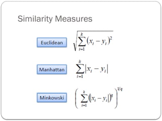
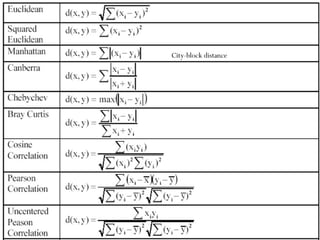
- 14. Distance between Clusters Euclidean distance or L2 – norm Single linkage The name single link comes from the observation that if we choose the minimum distance between points in the two clusters and connect those points, then (typically) only a single link would exist between those clusters because all other pairs of points would be farther away.
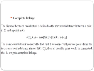
- 17. In Single Linkage, the distance between two clusters is the minimum distance between members of the two clusters In Complete Linkage, the distance between two clusters is the maximum distance between members of the two clusters In Average Linkage, the distance between two clusters is the average of all distances between members of the two clusters In Centroid Linkage, the distance between two clusters is is the distance between their centroids
- 19. Complete link
- 21. Construct the dendrograms using single and complete linkage methods for the given data points.
- 23. k-means Algorithm: 1. Choose k points as cluster centers. 2. Repeat until no change in cluster center calculation A) Compute distance of each point to each of the cluster centres. B) Partition by assigning or reassigning all data objects to their closest cluster center. b) Compute new cluster centers as mean value of the objects in each cluster.
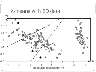
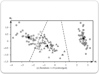
- 26. K-means with 2D data
- 28. Consider 10 points A1(2,5), A2(2,3), A3(4,5), A4(4,2), A5(6,5), A6(8,9), A7(2,1), A8(4,3), A9(1,6) and A10(3,7). Find 3 clusters after 2 epochs considering A1, A4 and A6 as the initial cluster centres. Use Euclidean distance as the distance function.
- 29. Point C1(2,5) C2(4,2) C3(8,9) Label A1(2,5) 0 3.606 7.211 C1 A2(2,3) 2 2.236 8.485 C1 A3(4,5) 2 3 5.657 C1 A4(4,2) 3.606 0 8.062 C2 A5(6,5) 4 3.606 4.472 C2 A6(8,9) 7.211 8.062 0 C3 A7(2,1) 4 2.236 10 C2 A8(4,3) 2.828 1 7.211 C2 A9(1,6) 1.414 5 7.616 C1 A10(3,7) 2.236 5.099 5.385 C1 •Using Euclidean Distance •Iteration 1
- 30. •Iteration 2 Point C1(2.4,5.2) C2(4,2.75) C3(8,9) Label A1(2,5) 0.447 3.010 7.211 C1 A2(2,3) 2.236 2.016 8.485 C2 A3(4,5) 1.612 2.25 5.657 C1 A4(4,2) 3.578 0.75 8.062 C2 A5(6,5) 3.606 3.010 4.472 C2 A6(8,9) 6.768 7.420 0 C3 A7(2,1) 4.219 2.658 10 C2 A8(4,3) 2.720 0.25 7.211 C2 A9(1,6) 1.612 4.423 7.616 C1 A10(3,7 ) 1.897 4.366 5.385 C1
- 31. KERNEL K-MEANS In K-means, the separating boundary between clusters is linear. Kernel K-means allows one to extract nonlinear boundaries between clusters via the use of the kernel trick. In kernel K-means, the main idea is to conceptually map a data point xi in input space to a point ( φ xi ) in some high- dimensional feature space, via an appropriate nonlinear mapping . φ However, the kernel trick allows us to carry out the clustering in feature space purely in terms of the kernel function K(xi,xj ), which can be computed in input space, but corresponds to a dot (or inner) product ( φ xi )T (xj ) in feature space. φ
- 32. EXPECTATION-MAXIMIZATION CLUSTERING The K-means approach is an example of a hard assignment clustering,where each point can belong to only one cluster. We now generalize the approach to consider soft assignment of points to clusters, so that each point has a probability of belonging to each cluster. The primary goal of the EM algorithm is to use the available observed data of the dataset to estimate the missing data of the latent variables and then use that data to update the values of the parameters.
- 35. Expectation step (E - step): It involves the estimation (guess) of all missing values in the dataset so that after completing this step, there should not be any missing value. Maximization step (M - step): This step involves the use of estimated data in the E-step and updating the parameters.
- 38. Given the dataset D, we define the likelihood of as the θ conditional probability of the data D given the model parameters , denoted as P(D| ). θ θ We can use the expectation-maximization (EM) approach for finding the maximum likelihood estimates for the parameters . θ EM is a two-step iterative approach that starts from an initial guess for the parameters . θ
- 40. The re-estimated mean is given as the weighted average of all the points, the re-estimated covariance matrix is given as the weighted covariance over all pairs of dimensions, and the re- estimated prior probability for each cluster is given as the fraction of weights that contribute to that cluster.
- 43. We start by setting the Gaussian parameters to random values. Then we perform the optimization by iterating through the two successive steps until convergence : We assign labels to the observations using the current Gaussian parameters. We update the Gaussian parameters so that the fit is more likely.
- 44. Usage of EM algorithm – It can be used to fill the missing data in a sample. It can be used as the basis of unsupervised learning of clusters. It can be used for the purpose of estimating the parameters of Hidden Markov Model (HMM). It can be used for discovering the values of latent variables. https://www.geeksforgeeks.org/ml-expectation-maximization-algorithm/
- 45. Advantages of EM algorithm – It is always guaranteed that likelihood will increase with each iteration. Disadvantages of EM algorithm – It has slow convergence. It makes convergence to the local optima only. It requires both the probabilities, forward and backward (numerical optimization requires only forward probability).
- 46. Example Consider 2 biased coins. Suppose bias (probability of heads) for 1st coin is‘ _A’ & Θ for 2nd is‘ _B’ where _A & _B lies between 0<x<1. Θ Θ Θ https://medium.com/data-science-in-your-pocket/expectation-maximization-em-algorithm-explained- 288626ce220e
- 47. In this case,we know the trials done by each coin. Therefore, the probability of heads for coin A and coin B could be easily obtained as: _ Θ A = 24/30=0.8 _ Θ B=9/20=0.45
- 48. Suppose, we do not know which coin is responsible for each of the given trials(Hidden).We can still have an estimate of ‘ _A’ &‘ _B’ using the EM algorithm!! Θ Θ The algorithm follows 2 steps iteratively: 1) Expectation 2) Maximization Expect: Estimate the expected value for the hidden variable Maximize: Optimize parameters using Maximum likelihood
- 49. EM Algorithm Steps: Assume some random values for your hidden variables: _A = 0.6 & _B = 0.5 in our example. Θ Θ Tossing a coin m times and the probability of getting a head n times follows Binomial Distribution.
- 50. Look at the first experiment with 5 Heads & 5Tails (1st row, grey block). P(1st coin used for 1st experiment) = (0.6) x(0.4) = 0.00079 ⁵ ⁵ P(2nd coin used for 1st experiment) = 0.5 x0.5 = 0.0009 ⁵ ⁵ On normalizing these 2 probabilities, we get P(1st coin used for 1st experiment)=0.45 P(2nd coin used for 1st experiment)=0.55
- 51. Similarly, for the 2nd experiment, we have 9 Heads & 1Tail. Hence, P(1st coin used for 2nd experiment) = 0.6 x0.4¹=0.004 ⁹ P(2nd coin used for 2nd experiment) = 0.5 x0.5 = 0.0009 ⁹ On Normalizing, the values we get are approximately 0.8 & 0.2 respectively
- 53. Moving to 2nd step: Now, we will be multiplying the Probability of the experiment to belong to the specific coin(calculated above) to the number of Heads &Tails in the experiment i.e 0.45 * 5 Heads, 0.45* 5 Tails= 2.2 Heads, 2.2 Tails for 1st Coin (Bias‘ _A’) Θ Similarly, 0.55 * 5 Heads,0.55* 5Tails = 2.8 Heads,2.8Tails for 2nd coin Repeat for all trials. Calculate the total number of Heads & Tails for respective coins. For 1st coin,we have 21.3 H & 8.6T; For 2nd coin,11.7 H & 8.4T
- 55. Maximization step: Now, what we want to do is to converge to the correct values of‘ _A’ &‘ _B’. Θ Θ On 10 such iterations, we will get _A=0.8 & _B=0.52 Θ Θ
- 58. Principal Component Analysis (PCA) is a technique that seeks a r-dimensional basis that best captures the variance in the data. The direction with the largest projected variance is called the first principal component. The orthogonal direction that captures the second largest projected variance is called the second principal component, and so on. The direction that maximizes the variance is also the one that minimizes the mean squared error.
- 59. Best Line Approximation We will start with r = 1, that is, the one-dimensional subspace or line u that best approximates D in terms of the variance of the projected points. We also assume that the data has been centered so that it has mean = μ 0.
- 60. where Sigma is the covariance matrix for the centered data D.
- 63. Step 1: Get the data Step 2: Subtract the mean from each of the data dimensions. Step 3: Calculate the covariance matrix. Step 4: Calculate the eigenvectors and eigenvalues of the covariance matrix. Step 5: Arrange the eigenvectors in the decreasing order of eigenvalues. Step 6: Choosing components and forming a feature vector FV – Matrix with the eigenvectors corresponding to the k largest eigenvalues as columns. Step 7: Deriving the new data set – Final Data = Row FeatureVector x Row DataAdjust Final Data is the final data set, with data items in columns, and dimensions along rows.
- 65. Thank You