Introduction to ArcGIS
Download as PPTX, PDF26 likes18,295 views

The document provides an introduction to Geographic Information Systems (GIS), focusing on the ArcGIS software version 10.1. It covers the fundamental concepts of GIS, the types of spatial data, and common applications, such as environmental hazard analysis and facility planning. Additionally, it includes instructions for managing files, customizing maps, and sharing GIS data and maps using ArcCatalog.


Introduction to ArcGIS
- 1. Intro to ArcGIS Kate Dougherty, Geosciences & Maps Librarian Tutorial created for version 10.1 in February 2013
- 2. Overview • What is GIS? • Select features by • Common uses attribute • Software • Select features by • Interface & navigation location • Adding layers • Buffer features tool • Customizing & • Layout view displaying layers • Datums & projections • File management • Data sources
- 3. What is GIS? • Geographic Information Systems (GIS) is a computer-based methodology for collecting, managing, analyzing, modeling, and presenting geographic or spatial data. • Allows you to overlay datasets and query them in terms of their spatial relation to each other
- 4. Two Types of Spatial Data • Raster - continuous data – E.G., air photos, scanned maps, elevation layers – Most remote sensing data is raster data • Vector - discrete features – A layer comprised of individual points, lines or polygons (e.g., roads or states) – This presentation focuses on vector data
- 5. Common Uses • Analyzing potential environmental hazards • Emergency services planning and routing • Siting new facilities: – wind farms – power plants – vineyards • Identifying food deserts in urban areas • Much more!
- 6. Esri • Environmental Systems Research Institute • ESRI is now Esri • Industry leader for GIS software • Program is ArcGIS/ArcMap – Now up to version 10.1. – (This presentation done with V. 10)
- 13. Table of contents that The “data frame” that displays the spatial data. shows the doc’s layers.
- 14. Identify Go to full Go to Go to Select feature map previous next features extent extent extent (by hand) Select elements Clear (to move selected or edit) features Add data
- 15. Project: Identify Washington County Parcels Near Perennial Streams
- 16. Add Layers • States (Census Bureau) • Counties (Census Bureau) • Hydrography (Area - National Hydrography Dataset) • Parcels (Washington County – Wash_Co_Data_Month_Year.zip) • Public lands (GeoStor)
- 17. Click to add data
- 20. Coordinate Systems • All your layers may not necessarily use the same coordinate system. – OK to draw and display – Not OK for detailed analysis (need to reproject layers – advanced step) • Data frame will use the coordinate system of the first layer that’s added – (displays feet, meters, or decimal degrees/lat/long of cursor location in bottom-right corner, depending on coordinate system)
- 21. View With All Layers Added
- 22. Zoomed to Washington County
- 23. Rename States Layer State layer renamed
- 24. Open the Attribute Table
- 26. Customizing Layers Select by Attribute Tool
- 35. New Layer is Added to Map
- 37. Arkansas Only Remaining State
- 38. Changing the Display of Layers • Change symbology/colors • Turn individual layers on or off • Change the display order – Layers on map display according to their order in the table of contents – Top layers may hide features in layers under them – Click & drag a layer in the table of contents to change its display order on the map
- 39. Change the Display Order
- 40. Change Symbology of Layers
- 41. Change Color of Streams
- 43. Clip Streams to Washington County Clip Tool
- 44. Access Clip in Geoprocessing Menu
- 45. Clip Tool Dialog Box
- 46. Clip Tool Progress Indicator
- 49. Change Symbology of New Clipped Hydro Layer
- 50. New Clipped File Looks Great!
- 51. Analysis • We will find parcels that: – Contain perennial streams And note their status in the parcel layer’s attribute table.
- 52. Add New Columns to Attribute Table
- 55. Field Types Whole Numbers Decimals • Short Integer • Double (integers from -32,768 (up to 6 decimal places) to 32,767) • Float • Long Integer (unlimited # of decimal (integers from - places) 2,147,483,648 to 2,147,483,647)
- 57. Task: Select Parcels with a Perennial Stream
- 60. View Selected in Attribute Table
- 61. View Selected Records Only
- 66. Task: Select Parcels in a “flood Zone” Within a Distance of Perennial Streams • Use the buffer tool to draw a “buffer zone” around specified features
- 81. Manage Files with ArcCatalog • File manager for files used in ArcMap • Best to manage moving pieces this way, instead of Windows Explorer
- 84. Use ArcCatalog to View Metadata
- 85. Share Maps and Layers with Packages • Package up all the information used to create a layer or map document for easy sharing by email, a shared drive on the LAN, etc. • Right-click a layer in the TOC and select “Create Layer Package”
- 87. Share a Map Package • To package up an entire map document for sharing, use File | Create Map Package
- 89. ArcMap will force you to create some limited metadata before creating a sharable package. Click OK.
- 91. Creating Packages • Save the package as a file and share as you usually would • You must “validate” your package before saving – Detects any errors that would impede sharing
- 93. Validation • Any errors need to be corrected. Click on any error messages to see a help document. • Warnings are warnings only – can go ahead and publish. • If no problems, the share button will become active.
- 94. What Else Can You Do with GIS? • Join stats based on • Analyze viewsheds and geography (i.e., states) shadows to a states GIS layer and view the data spatially • Use web map services – Excel, CSV, text formats for mashups in your own applications • Create/digitize your own data • Much more! • import GPS data
- 95. GIS Software at University of Arkansas • Reference desk machine (version 10.1) • Campus-wide license – administered by the Center for Advanced Spatial Technologies (CAST) • Free software
- 96. Sources of GIS Data • Search for selected base layers (reference maps) from right within the application • GeoStor (Arkansas state portal) • geo.data.gov (federal portal) • National Map (USGS) • TIGER/Census Shapefiles (reference layers – boundaries, roads)
- 97. LibGuide • The Maps, GIS and Remote Sensing LibGuide can point you to: – Information on how to get Esri software through the campus license – Resources for learning GIS – Sources of GIS data (spatial and attribute)
- 103. Good luck! Thank you!
Editor's Notes
- #4: More background information on GIS:bit.ly/T7Du2n
- #5: What is raster data? bit.ly/13o1cxK
- #7: Esri is the maker of the foremost GIS software package. ArcGIS refers to a suite of GIS products from Esri, including the desktop program, ArcMap. However, the desktop program is also sometimes referred to as “ArcGIS”.
- #8: This “Getting Started” dialog box is what the user sees when the program is first opened. It will ask if you want to open a recent map document or start with a saved template. A new user can just click “New Maps” in the left-hand panel, then “blank map” in the right panel.
- #9: It also asks what you want to use as the “Default geodatabase” for the map. The default geodatabase is a file management tool that gives you the option to save all the output from your operations in one place. Click on the folder to browse to the location where you want to save your work.
- #10: Click on the “New File Geodatabase” icon, just as if you were creating a new file folder in this location.
- #11: A new geodatabase is created. Click the name to change it something that makes more sense.
- #12: Highlight the new geodatabase and click “Add”.
- #13: Your new geodatabase is now associated with your new map document. Click OK.
- #14: This is the ArcMap interface. There a table of contents panel on the left that will list all the layers in our map document once they’ve been added. On the right is the “data frame” that will display the data layers.
- #15: An overview of some of the main icons on the Tools toolbar.
- #17: This tutorial uses data downloaded from the sources shown above. (Note: it’s preferable to download data to your default geodatabase, though that’s not the case in this tutorial). The data on your machine can then be loaded into ArcMap. For more on file geodatabases and the data types that can be stored in them, see bit.ly/WXFSdk.
- #18: Click the “add data” button to load your geospatial data into ArcMap.
- #19: ArcMap isn’t like Windows, where you can just browse to any location. First you have to “connect” to the folder you want to use in order for it to appear as a choice in your drop-down list, using the “Connect to Folder” button. Only the folders I’ve connected to will appear in the “Look in” drop-down. The folders needed for this map have already been connected.
- #20: Choose from available files.
- #21: The added file is displayed in the data frame on the right, and is listed in the table of contents (TOC) on the left.
- #22: About coordinate systems: bit.ly/SoWYVB
- #23: This is what the data frame/Arkansas looks like once all layers have been added. Let’s zoom in to Washington County. There are a number of ways to do that. One option is to use the “spyglass with plus sign” icon and draw a box around the area. Or, since the parcels layer covers the desired extent we can right-click on it in the TOC and select “zoom to”…
- #25: Layer names can be edited to be more intuitive. Click on the name in the TOC until you get the typing cursor. Renaming them here in the map document will not change the names of the actual files on your computer – just in the TOC in ArcMap.
- #26: In most cases the spatial data comes withassociated attribute data. Right-click on the states layer and select “Open Attribute Table” to view it.
- #27: Each table will have an FID column (unique feature ID auto-generated by the system) and a shape column (for point, line, or polygon). For example, a parcel is represented by a polygon, a road is a line, and statue would be a point or dot. The rest of the information is supplied by the originator of the dataset.
- #29: We have all the 50 states in our map but are only interested in Arkansas. So we can search for the feature representing Arkansas and export it to create a new layer that has Arkansas only, and then remove the layer with all the states. To do this, use the selection menu, and select “Select by Attributes”…
- #30: In the new dialog box, choose the layer that has the feature(s) you want to select. Then, choose the field in that layer’s table you want to search by. Next, choose the operator you want to use (equals, greater than, etc.), then enter the value you’re looking for in the large text box at the bottom. If you don’t know offhand the value you’re looking for, click the “get unique values” button to see all available values in that field of that table. The search is based on SQL queries and must be entered with quotations marks correctly, so you may want to use the “Get Unique Values” button to choose from presets rather than typing things in.
- #31: Using Select by Attributes: bit.ly/VY5rLj
- #32: If you were going to search for both Arkansas and Louisiana, you’d have to enter the name of the field each time…(e.g., “name” = ‘arkansas’ or “name” = ‘louisiana’)
- #33: The feature with the requested value (i.e., “name” = ‘Arkansas’) is now highlighted, both on the map and in the attribute table.
- #34: Export your selection to a new layer. To do this, right-click on the layer, select “data”, then “export data”.
- #35: Choose to export the selected features only. It will ask about the coordinate system you want to use – it defaults to the same coordinate system that the existing layer (that you’ve selected from) uses, so you don’t need to do anything. (Your other choice is the data frame – remember that the data frame uses the coordinate system of the first layer that’s added to it.) In the “Output feature class” field, browse to the location where you want to save the file and give it a name, as you would normally do in Windows.
- #37: The new layer appears in the data frame (with a new color chosen at random by the system to represent it), as well as in the TOC.
- #38: We are only interested in Arkansas. Now the layer with all U.S. states can be removed. Right-click the layer and select “Remove” to remove the layer from this map.
- #39: The blue U.S. states layer has been removed, leaving only Arkansas.
- #41: Drag the Arkansas layer to bottom so it will be drawn “below” the other layers and won’t obscure them.
- #42: Each layer has its own icon that’s auto-generated by the system. Click on a layer’s icon in the TOC to change it. Change the color of the public lands layer to green.
- #43: Do the same for the streams layer, so that the color is more intuitive.
- #44: This is how our layers now appear, which is a bit more intuitive.
- #45: The clip tool crops a layer based on the spatial extent of another layer in the map document.
- #46: There are different ways to access to access the tools. The most commonly used tools appear in the Geoprocessing menu.
- #47: Choose the input features (layer to crop), clip features (layer with the desired extent upon which to base the crop), and a name/location for the new feature class/layer (it should save to the default geodatabase you created earlier by default). The last field is optional and can be left empty. Click “OK”.
- #48: A progress indicator will appear at the bottom right of the screen. It will show the user that the clip is in progress.
- #49: A blue window will appear in the same location to notify the user once the process is completed.
- #50: The original streams layer for the entire state can now be removed.
- #51: A nicely clipped version of the streams layer remains. A random color will be assigned for it. Change the symbology to something that makes more sense.
- #54: Right-click on the parcel layer in the TOC and choose “Open Attribute Table”. Then, click the drop-down arrow next to the first icon in the new window and choose “Add Field…”.
- #55: Name your field.
- #56: Choose a field type…
- #57: The field type definitions look scary, but just remember that if you will be using whole numbers, use an integer field. Usually all you need is a short integer. If you need to enter decimals, use a non-integer field. Again, your choice will depend on how many characters you’ll need. More on field types: bit.ly/XWtPmH.
- #58: Under some circumstances you can set a default value for the field. In this case we would like to set a default value of 0. However this option is unavailable for the file type of this layer. Another option is to use the field calculator. Right-click on the column header and select the field calculator to give all rows a value of “0” in that column. It could take a good amount of time to process, depending on the number of rows involved – in this case about half an hour. Just leave ArcMap alone and work on something else in the meantime. An image of the field calculator window is included within the next few slides.
- #60: Instead of selecting by attribute, this time create a selection by location (i.e., search for features having a particular spatial characteristic). Return to the selection menu and select “select by location”.
- #61: Select the layer you want to select features from (parcels). Next, choose a “source layer”, or the layer with the spatial/locational aspects you want to cross-reference with the first layer (perennial streams). You have a number of options for operations, and you can play with them to see how they work, and if you get the expected results. One common method is “contains”. There’s also a “completely contains”. We don’t want to do that here, since it wouldn’t necessarily return instances where a stream runs between two parcels and separates them. Intersect is another common method. It will select areas where the two layers intersect. It’s an option for what we want to do, but “crossed by the outline of” works better in this case. Try out different operations until you are familiar with them. More on Select by Location: bit.ly/TPqS3B
- #62: Open the parcel layer’s attribute table to note the selected parcels.
- #63: Click the blue icon at the bottom of the table to switch from an “all rows” view to “selected rows only” view.
- #64: You are now seeing the rows for the selected parcels only.
- #65: Right-click the column header for the streams column, and select “Field Calculator”.
- #66: Simply enter a number one (1) in the large box at the bottom. This tells ArcMap to make the streams field for the selected parcels to equal 1.
- #67: All of our selected parcels now have a value of “1”. In the TOC, you can right-click on the layer and choose selection | switch selection to view all non-selected parcels (those without a perennial stream). You could then use the field calculator to give them a value of zero. Again, depending on how many parcels/features there are, it could take some time for ArcMap to complete the operation.
- #69: Access the buffer tool from the Geoprocessing menu.
- #70: The buffer tool dialog box appears. For “input features”, select the layer with the features to buffer around. For “output feature class”, choose the name and location for the new buffer layer that will be created by this tool. For “linear unit”, enter a number and unit of measurement for the buffer distance. In this case we’ll create a 1 mile buffer around the streams. (Alternatively, if you want to create a variable buffer with different distances for different features within the same layer, you can enter the various distances in a column in the attribute table, and use that column or field as the basis of your buffer using the “Field” option.)
- #71: The new buffer layer is drawn in the data frame and added to the TOC. At this point a real-world user would run another “select by location” operation to select parcels falling within the buffer zones, and then note them in the attribute table using the field calculator to enter a “1” in a new column. As this has already been covered in this presentation, we’ll move on to the final steps - layout view.
- #72: Go to the view menu -> Layout view to switch from data view to layout view. Data view is for working with the data and layers themselves and performing analysis, while layout view is for designing a final map product for output.
- #73: This is what layout view looks like. It will show how the map will be laid out on a page.
- #74: Use the “insert” menu to insert a title, legend, scale bar, etc. First, insert a title.
- #76: Next insert a legend.
- #77: Choose the layers to include in your legend. By default, everything that’s checked in the TOC in data view will be included. Highlight any unwanted layers on the right side and use the arrow to move them to the left side to eliminate them from the legend. If you wish, accept all default options presented and continue through all legend customization screens.
- #78: Next insert a north arrow and scale bar.
- #79: The finished document.
- #80: Next export your map.
- #81: There are several file options. Export to a PDF file.
- #83: Geospatial data files are similar to jigsaw puzzles in that many pieces and supporting files come together to comprise one layer. GIS software is specialized software that’s better able to recognize these file types and how they fit together. Use ArcCatalog (Windows menu | Catalog) to move, delete and rename your geospatial data.
- #86: This is the default ArcGIS metadata.FGDC Metadata and ISO MetadataEditor add-in downloads are available for data creators wanting to use those standards. More about metadata standards for geospatial data: bit.ly/WJO8Nj.
- #88: More about layer packages: bit.ly/TPkglN
- #95: More about map packages: bit.ly/TPkmdc
- #96: About adding a table of statistics: bit.ly/VUnvGIAbout joining tables: bit.ly/VQ9hJm
- #97: More on GIS software: bit.ly/3vaUYY
- #100: The Maps LibGuide links to the most common/most useful data sources. The first option is GeoStor, Arkansas’ state GIS portal, which was originally developed by UA’s CAST and is now run by the Arkansas Geographic Information Office.
- #101: Search for “park*” to get data on Arkansas parks.
- #102: You can get an idea of what a dataset will look like before downloading it by clicking on “view” in the thumbnail column for the layer of interest.
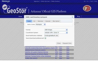
- #103: Data is available by several spatial extents, including county, city, watershed, and statewide. choose Washington County, and the local coordinate system. Enter your email address. You can also save your download preferences so it will remember your email and preferred coordinate system in the future.
- #104: The data request will be entered in a queue, and you’ll be sent an email with a link to the data when it’s ready. Then download and add it to ArcMap to start working with it!