SlideShare a Scribd company logo
Section 2.8
 Linear Approximation and Differentials

                      V63.0121.021, Calculus I

                           New York University


                          October 14, 2010


Announcements

   Quiz 2 in recitation this week on §§1.5, 1.6, 2.1, 2.2
   Midterm on §§1.1–2.5

                                                 .   .   .   .   .   .
Announcements


         Quiz 2 in recitation this
         week on §§1.5, 1.6, 2.1,
         2.2
         Midterm on §§1.1–2.5


                                                                     .   .   .        .      .      .

 V63.0121.021, Calculus I (NYU)   Section 2.8 Linear Approximation               October 14, 2010       2 / 36
Midterm FAQ
Question
What sections are covered on the midterm?


                                                                     .   .   .        .      .      .

 V63.0121.021, Calculus I (NYU)   Section 2.8 Linear Approximation               October 14, 2010       3 / 36
Midterm FAQ
Question
What sections are covered on the midterm?

Answer
The midterm will cover Sections 1.1–2.5 (The Chain Rule).

Question
Is Section 2.6 going to be on the midterm?

Answer
The midterm will cover Sections 1.1–2.5 (The Chain Rule).

Question
Is Section 2.8 going to be on the midterm?...
                                                                     .   .   .        .      .      .

 V63.0121.021, Calculus I (NYU)   Section 2.8 Linear Approximation               October 14, 2010       3 / 36
Midterm FAQ, continued

Question
What format will the exam take?


                                                                     .   .   .        .      .      .

 V63.0121.021, Calculus I (NYU)   Section 2.8 Linear Approximation               October 14, 2010       4 / 36
Midterm FAQ, continued

Question
What format will the exam take?

Answer
There will be both fixed-response (e.g., multiple choice) and
free-response questions.

Question
Will explanations be necessary?

Answer
Yes, on free-response problems we will expect you to explain yourself.
This is why it was required on written homework.
                                                                     .   .   .        .      .      .

 V63.0121.021, Calculus I (NYU)   Section 2.8 Linear Approximation               October 14, 2010       4 / 36
Midterm FAQ, continued


Question
Is (topic X) going to be tested?


                                                                     .   .   .        .      .      .

 V63.0121.021, Calculus I (NYU)   Section 2.8 Linear Approximation               October 14, 2010       5 / 36
Midterm FAQ, continued


Question
Is (topic X) going to be tested?

Answer
Everything covered in class or on homework is fair game for the exam.
No topic that was not covered in class nor on homework will be on the
exam. (This is not the same as saying all exam problems are similar to
class examples or homework problems.)


                                                                     .   .   .        .      .      .

 V63.0121.021, Calculus I (NYU)   Section 2.8 Linear Approximation               October 14, 2010       5 / 36
Midterm FAQ, continued


Question
Will there be a review session?


                                                                     .   .   .        .      .      .

 V63.0121.021, Calculus I (NYU)   Section 2.8 Linear Approximation               October 14, 2010       6 / 36
Midterm FAQ, continued


Question
Will there be a review session?

Answer
We’re working on it.


                                                                     .   .   .        .      .      .

 V63.0121.021, Calculus I (NYU)   Section 2.8 Linear Approximation               October 14, 2010       6 / 36
Midterm FAQ, continued


Question
Will calculators be allowed?


                                                                     .   .   .        .      .      .

 V63.0121.021, Calculus I (NYU)   Section 2.8 Linear Approximation               October 14, 2010       7 / 36
Midterm FAQ, continued


Question
Will calculators be allowed?

Answer
No. The exam is designed for pencil and brain.


                                                                     .   .   .        .      .      .

 V63.0121.021, Calculus I (NYU)   Section 2.8 Linear Approximation               October 14, 2010       7 / 36
Midterm FAQ, continued


Question
How should I study?


                                                                     .   .   .        .      .      .

 V63.0121.021, Calculus I (NYU)   Section 2.8 Linear Approximation               October 14, 2010       8 / 36
Midterm FAQ, continued


Question
How should I study?

Answer

      The exam has problems; study by doing problems. If you get one
      right, think about how you got it right. If you got it wrong or didn’t
      get it at all, reread the textbook and do easier problems to build up
      your understanding.
      Break up the material into chunks. (related) Don’t put it all off until
      the night before.
      Ask questions.


                                                                     .   .   .        .      .      .

 V63.0121.021, Calculus I (NYU)   Section 2.8 Linear Approximation               October 14, 2010       8 / 36
Midterm FAQ, continued


Question
How many questions are there?


                                                                     .   .   .        .      .      .

 V63.0121.021, Calculus I (NYU)   Section 2.8 Linear Approximation               October 14, 2010       9 / 36
Midterm FAQ, continued


Question
How many questions are there?

Answer
Does this question contribute to your understanding of the material?


                                                                     .   .   .        .      .      .

 V63.0121.021, Calculus I (NYU)   Section 2.8 Linear Approximation               October 14, 2010       9 / 36
Midterm FAQ, continued


Question
Will there be a curve on the exam?


                                                                     .   .   .         .       .    .

 V63.0121.021, Calculus I (NYU)   Section 2.8 Linear Approximation               October 14, 2010   10 / 36
Midterm FAQ, continued


Question
Will there be a curve on the exam?

Answer
Does this question contribute to your understanding of the material?


                                                                     .   .   .         .       .    .

 V63.0121.021, Calculus I (NYU)   Section 2.8 Linear Approximation               October 14, 2010   10 / 36
Midterm FAQ, continued


Question
When will you grade my get-to-know-you and photo extra credit?


                                                                     .   .   .         .      .     .

 V63.0121.021, Calculus I (NYU)   Section 2.8 Linear Approximation               October 14, 2010   11 / 36
Midterm FAQ, continued


Question
When will you grade my get-to-know-you and photo extra credit?

Answer
Does this question contribute to your understanding of the material?


                                                                     .   .   .         .      .     .

 V63.0121.021, Calculus I (NYU)   Section 2.8 Linear Approximation               October 14, 2010   11 / 36
Objectives
         Use tangent lines to make
         linear approximations to a
         function.
                Given a function and a
                point in the domain,
                compute the
                linearization of the
                function at that point.
                Use linearization to
                approximate values of
                functions
         Given a function, compute
         the differential of that
         function
         Use the differential
         notation to estimate error
         in linear approximations.                                   .   .   .         .       .    .

 V63.0121.021, Calculus I (NYU)   Section 2.8 Linear Approximation               October 14, 2010   12 / 36
Outline


The linear approximation of a function near a point
  Examples
  Questions


Differentials
    Using differentials to estimate error


Advanced Examples


                                                                     .   .   .         .       .    .

 V63.0121.021, Calculus I (NYU)   Section 2.8 Linear Approximation               October 14, 2010   13 / 36
The Big Idea

Question
Let f be differentiable at a. What linear function best approximates f
near a?


                                                                     .   .   .         .       .    .

 V63.0121.021, Calculus I (NYU)   Section 2.8 Linear Approximation               October 14, 2010   14 / 36
The Big Idea

Question
Let f be differentiable at a. What linear function best approximates f
near a?

Answer
The tangent line, of course!

Question
What is the equation for the line tangent to y = f(x) at (a, f(a))?

Answer

                                  L(x) = f(a) + f′ (a)(x − a)

                                                                        .   .   .         .       .    .

 V63.0121.021, Calculus I (NYU)      Section 2.8 Linear Approximation               October 14, 2010   14 / 36
The tangent line is a linear approximation


                                                        y
                                                        .


     L(x) = f(a) + f′ (a)(x − a)

is a decent approximation to f                  L
                                                . (x)                              .
near a.                                          f
                                                 .(x)                              .

                                                 f
                                                 .(a)                .
                                                                         .
                                                                         x−a


                                                         .                                           x
                                                                                                     .
                                                                     a
                                                                     .         x
                                                                               .

                                                                         .     .       .         .       .    .

 V63.0121.021, Calculus I (NYU)   Section 2.8 Linear Approximation                         October 14, 2010   15 / 36
The tangent line is a linear approximation


                                                        y
                                                        .


     L(x) = f(a) + f′ (a)(x − a)

is a decent approximation to f                  L
                                                . (x)                              .
near a.                                          f
                                                 .(x)                              .
How decent? The closer x is to
a, the better the approxmation                   f
                                                 .(a)                .
                                                                         .
                                                                         x−a
L(x) is to f(x)

                                                         .                                           x
                                                                                                     .
                                                                     a
                                                                     .         x
                                                                               .

                                                                         .     .       .         .       .    .

 V63.0121.021, Calculus I (NYU)   Section 2.8 Linear Approximation                         October 14, 2010   15 / 36
Example
.
Example
Estimate sin(61◦ ) = sin(61π/180) by using a linear approximation
(i) about a = 0     (ii) about a = 60◦ = π/3.


.

                                                                        .   .   .         .       .    .

    V63.0121.021, Calculus I (NYU)   Section 2.8 Linear Approximation               October 14, 2010   16 / 36
Example
.
Example
Estimate sin(61◦ ) = sin(61π/180) by using a linear approximation
(i) about a = 0     (ii) about a = 60◦ = π/3.


Solution (i)

        If f(x) = sin x, then f(0) = 0
        and f′ (0) = 1.
        So the linear approximation
        near 0 is L(x) = 0 + 1 · x = x.
        Thus
             (      )
                61π       61π
         sin           ≈       ≈ 1.06465
                180       180

.

                                                                        .   .   .         .       .    .

    V63.0121.021, Calculus I (NYU)   Section 2.8 Linear Approximation               October 14, 2010   16 / 36
Example
.
Example
Estimate sin(61◦ ) = sin(61π/180) by using a linear approximation
(i) about a = 0     (ii) about a = 60◦ = π/3.


Solution (i)                                            Solution (ii)
                                                                            (π)
                                                               We have f            =             and
        If f(x) = sin x, then f(0) = 0                           ( )            3
        and f′ (0) = 1.                                        f′ π = .
                                                                  3
        So the linear approximation
        near 0 is L(x) = 0 + 1 · x = x.
        Thus
             (      )
                61π       61π
         sin           ≈       ≈ 1.06465
                180       180

.

                                                                        .   .       .         .         .   .

    V63.0121.021, Calculus I (NYU)   Section 2.8 Linear Approximation                   October 14, 2010    16 / 36
Example
.
Example
Estimate sin(61◦ ) = sin(61π/180) by using a linear approximation
(i) about a = 0     (ii) about a = 60◦ = π/3.


Solution (i)                                            Solution (ii)
                                                                            (π)           √
                                                                                           3
                                                               We have f            =              and
        If f(x) = sin x, then f(0) = 0                           ( )            3         2
        and f′ (0) = 1.                                        f′ π = .
                                                                  3
        So the linear approximation
        near 0 is L(x) = 0 + 1 · x = x.
        Thus
             (      )
                61π       61π
         sin           ≈       ≈ 1.06465
                180       180

.

                                                                        .   .       .          .         .   .

    V63.0121.021, Calculus I (NYU)   Section 2.8 Linear Approximation                   October 14, 2010     16 / 36
Example
.
Example
Estimate sin(61◦ ) = sin(61π/180) by using a linear approximation
(i) about a = 0     (ii) about a = 60◦ = π/3.


Solution (i)                                            Solution (ii)
                                                                            (π)           √
                                                                                           3
                                                               We have f            =              and
        If f(x) = sin x, then f(0) = 0                           ( )            3         2
        and f′ (0) = 1.                                        f′ π = 1 .
                                                                  3   2
        So the linear approximation
                                                               So L(x) =
        near 0 is L(x) = 0 + 1 · x = x.
        Thus
             (      )
                61π       61π
         sin           ≈       ≈ 1.06465
                180       180

.

                                                                        .   .       .          .         .   .

    V63.0121.021, Calculus I (NYU)   Section 2.8 Linear Approximation                   October 14, 2010     16 / 36
Example
.
Example
Estimate sin(61◦ ) = sin(61π/180) by using a linear approximation
(i) about a = 0     (ii) about a = 60◦ = π/3.


Solution (i)                                            Solution (ii)
                                                                            (π)           √
                                                                                           3
                                                               We have f            =              and
        If f(x) = sin x, then f(0) = 0                           ( )            3         2
        and f′ (0) = 1.                                        f′ π = 1 .
                                                                  3   2         √
        So the linear approximation                                               3 1(    π)
                                                               So L(x) =           +   x−
        near 0 is L(x) = 0 + 1 · x = x.                                          2   2    3
        Thus
             (      )
                61π       61π
         sin           ≈       ≈ 1.06465
                180       180

.

                                                                        .   .       .          .         .   .

    V63.0121.021, Calculus I (NYU)   Section 2.8 Linear Approximation                   October 14, 2010     16 / 36
Example
.
Example
Estimate sin(61◦ ) = sin(61π/180) by using a linear approximation
(i) about a = 0     (ii) about a = 60◦ = π/3.


Solution (i)                                            Solution (ii)
                                                                                  (π)           √
                                                                                                 3
                                                               We have f                  =              and
        If f(x) = sin x, then f(0) = 0                           ( )                  3         2
        and f′ (0) = 1.                                        f′ π = 1 .
                                                                  3   2               √
        So the linear approximation                                                     3 1(    π)
                                                               So L(x) =                 +   x−
        near 0 is L(x) = 0 + 1 · x = x.                                                2   2    3
        Thus                                                   Thus
             (      )                                                         (           )
                61π       61π                                                     61π
         sin           ≈       ≈ 1.06465                                sin                   ≈
                180       180                                                     180


.

                                                                         .        .       .          .         .   .

    V63.0121.021, Calculus I (NYU)   Section 2.8 Linear Approximation                         October 14, 2010     16 / 36
Example
.
Example
Estimate sin(61◦ ) = sin(61π/180) by using a linear approximation
(i) about a = 0     (ii) about a = 60◦ = π/3.


Solution (i)                                            Solution (ii)
                                                                                  (π)           √
                                                                                                 3
                                                               We have f                  =              and
        If f(x) = sin x, then f(0) = 0                           ( )                  3         2
        and f′ (0) = 1.                                        f′ π = 1 .
                                                                  3   2               √
        So the linear approximation                                                     3 1(    π)
                                                               So L(x) =                 +   x−
        near 0 is L(x) = 0 + 1 · x = x.                                                2   2    3
        Thus                                                   Thus
             (      )                                                         (           )
                61π       61π                                                     61π
         sin           ≈       ≈ 1.06465                                sin                   ≈ 0.87475
                180       180                                                     180


Calculator check: sin(61◦ ) ≈
.

                                                                         .        .       .          .         .   .

    V63.0121.021, Calculus I (NYU)   Section 2.8 Linear Approximation                         October 14, 2010     16 / 36
Example
.
Example
Estimate sin(61◦ ) = sin(61π/180) by using a linear approximation
(i) about a = 0     (ii) about a = 60◦ = π/3.


Solution (i)                                            Solution (ii)
                                                                                  (π)           √
                                                                                                 3
                                                               We have f                  =              and
        If f(x) = sin x, then f(0) = 0                           ( )                  3         2
        and f′ (0) = 1.                                        f′ π = 1 .
                                                                  3   2               √
        So the linear approximation                                                     3 1(    π)
                                                               So L(x) =                 +   x−
        near 0 is L(x) = 0 + 1 · x = x.                                                2   2    3
        Thus                                                   Thus
             (      )                                                         (           )
                61π       61π                                                     61π
         sin           ≈       ≈ 1.06465                                sin                   ≈ 0.87475
                180       180                                                     180


Calculator check: sin(61◦ ) ≈ 0.87462.
.

                                                                         .        .       .          .         .   .

    V63.0121.021, Calculus I (NYU)   Section 2.8 Linear Approximation                         October 14, 2010     16 / 36
Illustration

       y
       .


                                                               y
                                                               . = sin x


        .                                                                    x
                                                                             .
                                           . 1◦
                                           6
                                                                     .   .       .         .       .    .

 V63.0121.021, Calculus I (NYU)   Section 2.8 Linear Approximation                   October 14, 2010   17 / 36
Illustration

       y
       .
                                                            y
                                                            . = L1 (x) = x


                                                               y
                                                               . = sin x


        .                                                                    x
                                                                             .
            0
            .                              . 1◦
                                           6
                                                                     .   .       .         .       .    .

 V63.0121.021, Calculus I (NYU)   Section 2.8 Linear Approximation                   October 14, 2010   17 / 36
Illustration

       y
       .
                                                              y
                                                              . = L1 (x) = x


                         b
                         . ig difference!                        y
                                                                 . = sin x


        .                                                                      x
                                                                               .
            0
            .                                . 1◦
                                             6
                                                                       .   .       .         .       .    .

 V63.0121.021, Calculus I (NYU)     Section 2.8 Linear Approximation                   October 14, 2010   17 / 36
Illustration

       y
       .
                                                            y
                                                            . = L1 (x) = x


                                                                             √                      (            )
                                                            y
                                                            . = L2 (x) =     2
                                                                              3
                                                                                        +       1
                                                                                                2       x−   π
                                                                                                             3
                                                              y
                                                              . = sin x
                                         .


        .                                .                                   x
                                                                             .
            0
            .                     .
                                  π/3        . 1◦
                                             6
                                                                     .   .       .          .           .        .

 V63.0121.021, Calculus I (NYU)   Section 2.8 Linear Approximation                   October 14, 2010            17 / 36
Illustration

       y
       .
                                                            y
                                                            . = L1 (x) = x


                                                                             √                      (            )
                                                         y
                                                         . = L2 (x) =        2
                                                                              3
                                                                                        +       1
                                                                                                2       x−   π
                                                                                                             3
                                                           y
                                                           . = sin x
                                         . . ery little difference!
                                           v


        .                                .                                   x
                                                                             .
            0
            .                     .
                                  π/3        . 1◦
                                             6
                                                                     .   .       .          .           .        .

 V63.0121.021, Calculus I (NYU)   Section 2.8 Linear Approximation                   October 14, 2010            17 / 36
Another Example

Example
              √
Estimate       10 using the fact that 10 = 9 + 1.


                                                                     .   .   .         .       .    .

 V63.0121.021, Calculus I (NYU)   Section 2.8 Linear Approximation               October 14, 2010   18 / 36
Another Example

Example
              √
Estimate       10 using the fact that 10 = 9 + 1.

Solution
                                                                             √
The key step is to use a linear approximation to f(x) =
                    √                                                         x near a = 9
to estimate f(10) = 10.

                      f(10) ≈ L(10) = f(9) + f′ (9)(10 − 9)
                                            1          19
                                    =3+          (1) =    ≈ 3.167
                                           2·3          6


                                                                     .   .   .         .       .    .

 V63.0121.021, Calculus I (NYU)   Section 2.8 Linear Approximation               October 14, 2010   18 / 36
Another Example

Example
              √
Estimate       10 using the fact that 10 = 9 + 1.

Solution
                                                                             √
The key step is to use a linear approximation to f(x) =
                    √                                                         x near a = 9
to estimate f(10) = 10.

           f(10) ≈ L(10) = f(9) + f′ (9)(10 − 9)
                                 1          19
                         =3+          (1) =    ≈ 3.167
                                2·3          6
       ( )2
        19
Check:       =
        6

                                                                     .   .   .         .       .    .

 V63.0121.021, Calculus I (NYU)   Section 2.8 Linear Approximation               October 14, 2010   18 / 36
Another Example

Example
              √
Estimate       10 using the fact that 10 = 9 + 1.

Solution
                                                                             √
The key step is to use a linear approximation to f(x) =
                    √                                                         x near a = 9
to estimate f(10) = 10.

           f(10) ≈ L(10) = f(9) + f′ (9)(10 − 9)
                                 1          19
                         =3+          (1) =    ≈ 3.167
                                2·3          6
       ( )2
        19      361
Check:       =      .
        6       36

                                                                     .   .   .         .       .    .

 V63.0121.021, Calculus I (NYU)   Section 2.8 Linear Approximation               October 14, 2010   18 / 36
Dividing without dividing?
Example
A student has an irrational fear of long division and needs to estimate
577 ÷ 408. He writes
                      577            1             1  1
                          = 1 + 169     = 1 + 169 × ×    .
                      408           408            4 102
                                   1
Help the student estimate             .
                                  102


                                                                     .   .   .         .       .    .

 V63.0121.021, Calculus I (NYU)   Section 2.8 Linear Approximation               October 14, 2010   19 / 36
Dividing without dividing?
Example
A student has an irrational fear of long division and needs to estimate
577 ÷ 408. He writes
                      577            1             1  1
                          = 1 + 169     = 1 + 169 × ×    .
                      408           408            4 102
                                   1
Help the student estimate             .
                                  102

Solution
                1
Let f(x) =        . We know f(100) and we want to estimate f(102).
                x
                                                        1   1
          f(102) ≈ f(100) + f′ (100)(2) =                 −     (2) = 0.0098
                                                       100 1002
                                          577
                                  =⇒          ≈ 1.41405
                                          408                        .   .   .         .       .    .

 V63.0121.021, Calculus I (NYU)   Section 2.8 Linear Approximation               October 14, 2010   19 / 36
Questions

Example
Suppose we are traveling in a car and at noon our speed is 50 mi/hr.
How far will we have traveled by 2:00pm? by 3:00pm? By midnight?


                                                                     .   .   .         .       .    .

 V63.0121.021, Calculus I (NYU)   Section 2.8 Linear Approximation               October 14, 2010   20 / 36
Answers


Example
Suppose we are traveling in a car and at noon our speed is 50 mi/hr.
How far will we have traveled by 2:00pm? by 3:00pm? By midnight?


                                                                     .   .   .         .       .    .

 V63.0121.021, Calculus I (NYU)   Section 2.8 Linear Approximation               October 14, 2010   21 / 36
Answers


Example
Suppose we are traveling in a car and at noon our speed is 50 mi/hr.
How far will we have traveled by 2:00pm? by 3:00pm? By midnight?

Answer

      100 mi
      150 mi
      600 mi (?) (Is it reasonable to assume 12 hours at the same
      speed?)


                                                                     .   .   .         .       .    .

 V63.0121.021, Calculus I (NYU)   Section 2.8 Linear Approximation               October 14, 2010   21 / 36
Questions

Example
Suppose we are traveling in a car and at noon our speed is 50 mi/hr.
How far will we have traveled by 2:00pm? by 3:00pm? By midnight?

Example
Suppose our factory makes MP3 players and the marginal cost is
currently $50/lot. How much will it cost to make 2 more lots? 3 more
lots? 12 more lots?


                                                                     .   .   .         .       .    .

 V63.0121.021, Calculus I (NYU)   Section 2.8 Linear Approximation               October 14, 2010   22 / 36
Answers


Example
Suppose our factory makes MP3 players and the marginal cost is
currently $50/lot. How much will it cost to make 2 more lots? 3 more
lots? 12 more lots?

Answer

      $100
      $150
      $600 (?)


                                                                     .   .   .         .       .    .

 V63.0121.021, Calculus I (NYU)   Section 2.8 Linear Approximation               October 14, 2010   23 / 36
Questions

Example
Suppose we are traveling in a car and at noon our speed is 50 mi/hr.
How far will we have traveled by 2:00pm? by 3:00pm? By midnight?

Example
Suppose our factory makes MP3 players and the marginal cost is
currently $50/lot. How much will it cost to make 2 more lots? 3 more
lots? 12 more lots?

Example
Suppose a line goes through the point (x0 , y0 ) and has slope m. If the
point is moved horizontally by dx, while staying on the line, what is the
corresponding vertical movement?

                                                                     .   .   .         .       .    .

 V63.0121.021, Calculus I (NYU)   Section 2.8 Linear Approximation               October 14, 2010   24 / 36
Answers


Example
Suppose a line goes through the point (x0 , y0 ) and has slope m. If the
point is moved horizontally by dx, while staying on the line, what is the
corresponding vertical movement?


                                                                     .   .   .         .       .    .

 V63.0121.021, Calculus I (NYU)   Section 2.8 Linear Approximation               October 14, 2010   25 / 36
Answers


Example
Suppose a line goes through the point (x0 , y0 ) and has slope m. If the
point is moved horizontally by dx, while staying on the line, what is the
corresponding vertical movement?

Answer
The slope of the line is
                                     rise
                                          m=
                                     run
We are given a “run” of dx, so the corresponding “rise” is m dx.


                                                                     .   .   .         .       .    .

 V63.0121.021, Calculus I (NYU)   Section 2.8 Linear Approximation               October 14, 2010   25 / 36
Outline


The linear approximation of a function near a point
  Examples
  Questions


Differentials
    Using differentials to estimate error


Advanced Examples


                                                                     .   .   .         .       .    .

 V63.0121.021, Calculus I (NYU)   Section 2.8 Linear Approximation               October 14, 2010   26 / 36
Differentials are another way to express derivatives
The fact that the the tangent
line is an approximation means
that
                                                             y
                                                             .
    f(x + ∆x) − f(x) ≈ f′ (x) ∆x
               ∆y                     dy

Rename ∆x = dx, so we can
write this as                                                                        .
                                                                                              .
                                                                                              dy
                                                                                         .
                                                                                         ∆y
                                  ′
          ∆y ≈ dy = f (x)dx.                                              .
                                                                           .
                                                                           dx = ∆x

Note this looks a lot like the
Leibniz-Newton identity
                                                              .                                             x
                                                                                                            .
                  dy                                                      x x
                                                                          . . + ∆x
                     = f′ (x)
                  dx
                                                                           .     .            .         .       .    .

 V63.0121.021, Calculus I (NYU)        Section 2.8 Linear Approximation                           October 14, 2010   27 / 36
Using differentials to estimate error


                                                         y
                                                         .
Estimating error with
differentials
If y = f(x), x0 and ∆x is known,
and an estimate of ∆y is
desired:                                                                        .
                                                                                             .
      Approximate: ∆y ≈ dy
                                                                                             dy
                                                                                    .
                                                                                    ∆y

      Differentiate: dy = f′ (x) dx                                  .
                                                                      .
                                                                      dx = ∆x
      Evaluate at x = x0 and
      dx = ∆x.
                                                          .                                            x
                                                                                                       .
                                                                     x x
                                                                     . . + ∆x

                                                                     .      .            .         .       .    .

 V63.0121.021, Calculus I (NYU)   Section 2.8 Linear Approximation                           October 14, 2010   28 / 36
Example
A sheet of plywood measures 8 ft × 4 ft. Suppose our plywood-cutting
machine will cut a rectangle whose width is exactly half its length, but
the length is prone to errors. If the length is off by 1 in, how bad can the
area of the sheet be off by?


                                                                     .   .   .         .       .    .

 V63.0121.021, Calculus I (NYU)   Section 2.8 Linear Approximation               October 14, 2010   29 / 36
Example
A sheet of plywood measures 8 ft × 4 ft. Suppose our plywood-cutting
machine will cut a rectangle whose width is exactly half its length, but
the length is prone to errors. If the length is off by 1 in, how bad can the
area of the sheet be off by?

Solution
                     1 2
Write A(ℓ) =           ℓ . We want to know ∆A when ℓ = 8 ft and ∆ℓ = 1 in.
                     2


                                                                     .   .   .         .       .    .

 V63.0121.021, Calculus I (NYU)   Section 2.8 Linear Approximation               October 14, 2010   29 / 36
Example
A sheet of plywood measures 8 ft × 4 ft. Suppose our plywood-cutting
machine will cut a rectangle whose width is exactly half its length, but
the length is prone to errors. If the length is off by 1 in, how bad can the
area of the sheet be off by?

Solution
             1 2
Write A(ℓ) =   ℓ . We want to know ∆A when ℓ = 8 ft and ∆ℓ = 1 in.
             2      ( )
                      97     9409         9409
  (I) A(ℓ + ∆ℓ) = A       =       So ∆A =       − 32 ≈ 0.6701.
                      12      288          288


                                                                     .   .   .         .       .    .

 V63.0121.021, Calculus I (NYU)   Section 2.8 Linear Approximation               October 14, 2010   29 / 36
Example
A sheet of plywood measures 8 ft × 4 ft. Suppose our plywood-cutting
machine will cut a rectangle whose width is exactly half its length, but
the length is prone to errors. If the length is off by 1 in, how bad can the
area of the sheet be off by?

Solution
              1 2
Write A(ℓ) =    ℓ . We want to know ∆A when ℓ = 8 ft and ∆ℓ = 1 in.
              2      ( )
                       97      9409            9409
  (I) A(ℓ + ∆ℓ) = A         =       So ∆A =         − 32 ≈ 0.6701.
                       12      288             288
      dA
 (II)     = ℓ, so dA = ℓ dℓ, which should be a good estimate for ∆ℓ.
      dℓ
      When ℓ = 8 and dℓ = 12 , we have dA = 12 = 2 ≈ 0.667. So we
                             1                  8
                                                    3
      get estimates close to the hundredth of a square foot.

                                                                     .   .   .         .       .    .

 V63.0121.021, Calculus I (NYU)   Section 2.8 Linear Approximation               October 14, 2010   29 / 36
Why?


Why use linear approximations dy when the actual difference ∆y is
known?
      Linear approximation is quick and reliable. Finding ∆y exactly
      depends on the function.
      These examples are overly simple. See the “Advanced Examples”
      later.
      In real life, sometimes only f(a) and f′ (a) are known, and not the
      general f(x).


                                                                     .   .   .         .       .    .

 V63.0121.021, Calculus I (NYU)   Section 2.8 Linear Approximation               October 14, 2010   30 / 36
Outline


The linear approximation of a function near a point
  Examples
  Questions


Differentials
    Using differentials to estimate error


Advanced Examples


                                                                     .   .   .         .       .    .

 V63.0121.021, Calculus I (NYU)   Section 2.8 Linear Approximation               October 14, 2010   31 / 36
Gravitation
Pencils down!

Example

       Drop a 1 kg ball off the roof of the Silver Center (50m high). We
       usually say that a falling object feels a force F = −mg from gravity.


                                                                      .   .   .         .       .    .

  V63.0121.021, Calculus I (NYU)   Section 2.8 Linear Approximation               October 14, 2010   32 / 36
Gravitation
Pencils down!

Example

       Drop a 1 kg ball off the roof of the Silver Center (50m high). We
       usually say that a falling object feels a force F = −mg from gravity.
       In fact, the force felt is
                                                         GMm
                                         F(r) = −            ,
                                                          r2
       where M is the mass of the earth and r is the distance from the
       center of the earth to the object. G is a constant.
                                              GMm
       At r = re the force really is F(re ) =      = −mg.
                                               r2
                                                e
       What is the maximum error in replacing the actual force felt at the
       top of the building F(re + ∆r) by the force felt at ground level
       F(re )? The relative error? The percentage error?              .   .   .         .       .    .

  V63.0121.021, Calculus I (NYU)   Section 2.8 Linear Approximation               October 14, 2010   32 / 36
Gravitation Solution
Solution
We wonder if ∆F = F(re + ∆r) − F(re ) is small.
      Using a linear approximation,

                                              dF           GMm
                                  ∆F ≈ dF =         dr = 2 3 dr
                                              dr re         re
                                              (      )
                                                GMm dr           ∆r
                                            =     2
                                                           = 2mg
                                                 re     re       re

                          ∆F        ∆r
      The relative error is   ≈ −2
                           F        re
      re = 6378.1 km. If ∆r = 50 m,
            ∆F      ∆r         50
               ≈ −2    = −2         = −1.56 × 10−5 = −0.00156%
             F      re      6378100
                                                                         .   .   .         .       .    .

 V63.0121.021, Calculus I (NYU)       Section 2.8 Linear Approximation               October 14, 2010   33 / 36
Systematic linear approximation

      √                    √
       2 is irrational, but 9/4 is rational and 9/4 is close to 2.


                                                                     .   .   .         .       .    .

 V63.0121.021, Calculus I (NYU)   Section 2.8 Linear Approximation               October 14, 2010   34 / 36
Systematic linear approximation

      √                    √
       2 is irrational, but 9/4 is rational and 9/4 is close to 2. So
                       √   √           √                         1                    17
                        2 = 9/4 − 1/4 ≈ 9/4 +                            (−1/4) =
                                                             2(3/2)                   12


                                                                     .     .   .         .       .    .

 V63.0121.021, Calculus I (NYU)   Section 2.8 Linear Approximation                 October 14, 2010   34 / 36
Systematic linear approximation

      √                    √
       2 is irrational, but 9/4 is rational and 9/4 is close to 2. So
                       √   √           √                         1                    17
                        2 = 9/4 − 1/4 ≈ 9/4 +                            (−1/4) =
                                                             2(3/2)                   12


      This is a better approximation since (17/12)2 = 289/144


                                                                     .     .   .         .       .    .

 V63.0121.021, Calculus I (NYU)   Section 2.8 Linear Approximation                 October 14, 2010   34 / 36
Systematic linear approximation

      √                    √
       2 is irrational, but 9/4 is rational and 9/4 is close to 2. So
                       √   √           √                             1                    17
                        2 = 9/4 − 1/4 ≈ 9/4 +                                (−1/4) =
                                                                 2(3/2)                   12


      This is a better approximation since (17/12)2 = 289/144
      Do it again!
          √   √                 √                                     1
           2 = 289/144 − 1/144 ≈ 289/144 +                                  (−1/144) = 577/408
                                                                   2(17/12)
               (         )2
                   577            332, 929             1
      Now                     =            which is          away from 2.
                   408            166, 464          166, 464

                                                                         .     .   .         .       .    .

 V63.0121.021, Calculus I (NYU)       Section 2.8 Linear Approximation                 October 14, 2010   34 / 36
Illustration of the previous example


                                  .


                                                                         .   .   .         .       .    .

 V63.0121.021, Calculus I (NYU)       Section 2.8 Linear Approximation               October 14, 2010   35 / 36
Illustration of the previous example


                                  .


                                                                         .   .   .         .       .    .

 V63.0121.021, Calculus I (NYU)       Section 2.8 Linear Approximation               October 14, 2010   35 / 36
Illustration of the previous example


                                  .
                                                        2
                                                        .


                                                                         .   .   .         .       .    .

 V63.0121.021, Calculus I (NYU)       Section 2.8 Linear Approximation               October 14, 2010   35 / 36
Illustration of the previous example


                                                             .


                                  .
                                                        2
                                                        .


                                                                         .   .   .         .       .    .

 V63.0121.021, Calculus I (NYU)       Section 2.8 Linear Approximation               October 14, 2010   35 / 36
Illustration of the previous example


                                             . 2, 17 )
                                             ( 12
                                                         . .


                                  .
                                                         2
                                                         .


                                                                         .   .   .         .       .    .

 V63.0121.021, Calculus I (NYU)       Section 2.8 Linear Approximation               October 14, 2010   35 / 36
Illustration of the previous example


                                                                 .
                                  . 2, 17/12)
                                  (
                                                  .                  . 4, 3)
                                                                     (9 2


                                                                      .        .   .         .       .    .

 V63.0121.021, Calculus I (NYU)   Section 2.8 Linear Approximation                     October 14, 2010   35 / 36
Illustration of the previous example


                                                                 .
                                  . 2, 17/12)
                                  (
                                                  .. (              . 9, 3)
                                                                    (
                                                                    )4 2
                                                         289 17
                                                    .    144 , 12


                                                                      .       .   .         .       .    .

 V63.0121.021, Calculus I (NYU)   Section 2.8 Linear Approximation                    October 14, 2010   35 / 36
Illustration of the previous example


                                                           .
                                  . 2, 17/12)
                                  (
                                              .. (           . 9, 3)
                                                             (
                                   ( 577 )                  )4 2
                                   . 2, 408        289 17
                                                 . 144 , 12


                                                                     .   .   .         .       .    .

 V63.0121.021, Calculus I (NYU)   Section 2.8 Linear Approximation               October 14, 2010   35 / 36
Summary


     Linear approximation: If f is differentiable at a, the best linear
     approximation to f near a is given by

                                 Lf,a (x) = f(a) + f′ (a)(x − a)

     Differentials: If f is differentiable at x, a good approximation to
     ∆y = f(x + ∆x) − f(x) is

                                                  dy        dy
                                 ∆y ≈ dy =           · dx =    · ∆x
                                                  dx        dx
     Don’t buy plywood from me.


                                                                      .   .   .         .       .    .

V63.0121.021, Calculus I (NYU)     Section 2.8 Linear Approximation               October 14, 2010   36 / 36

More Related Content

PPTX
Article II Philippine Constitution
PDF
Lesson 12: Linear Approximation and Differentials (Section 21 handout)
PDF
Lesson 12: Linear Approximation (Section 41 handout)
PDF
Lesson 12: Linear Approximations and Differentials (handout)
PDF
Lesson 12: Linear Approximation
PDF
Lesson 12: Linear Approximation
PDF
Lesson 12: Linear Approximation and Differentials (Section 41 slides)
Article II Philippine Constitution
Lesson 12: Linear Approximation and Differentials (Section 21 handout)
Lesson 12: Linear Approximation (Section 41 handout)
Lesson 12: Linear Approximations and Differentials (handout)
Lesson 12: Linear Approximation
Lesson 12: Linear Approximation and Differentials (Section 41 slides)

Similar to Lesson 12: Linear Approximation and Differentials (Section 21 slides) (20)

PDF
Lesson 12: Linear Approximation and Differentials (Section 41 slides)
PDF
Lesson 15: Linear Approximation and Differentials
PDF
Lesson 4: Calculating Limits (Section 21 slides)
PDF
Lesson 4: Calculating Limits (Section 21 slides)
PDF
Lesson 4: Calculating Limits (handout)
PDF
Lesson 12: Linear Approximations and Differentials (slides)
PDF
Lesson 12: Linear Approximations and Differentials (slides)
PDF
Lesson 6: Limits Involving ∞ (Section 21 handout)
PDF
Lesson 5: Continuity (handout)
PDF
Lesson 5: Continuity (Section 21 handout)
PDF
Lesson 6: Limits Involving Infinity (Section 41 handout)
PDF
Lesson 1: Functions
PDF
Lesson 1: Functions
PDF
Lesson 5: Continuity (handout)
PDF
Lesson 23: The Definite Integral (handout)
PDF
Lesson 12: Linear Approximation
PDF
Lesson 12: Linear Approximation
PDF
Lesson 6: Limits Involving ∞ (Section 41 slides)
PDF
Lesson 6: Limits Involving ∞ (Section 41 slides)
PDF
Lesson 6: Limits Involving ∞ (Section 21 slides)
Lesson 12: Linear Approximation and Differentials (Section 41 slides)
Lesson 15: Linear Approximation and Differentials
Lesson 4: Calculating Limits (Section 21 slides)
Lesson 4: Calculating Limits (handout)
Lesson 12: Linear Approximations and Differentials (slides)
Lesson 6: Limits Involving ∞ (Section 21 handout)
Lesson 5: Continuity (handout)
Lesson 5: Continuity (Section 21 handout)
Lesson 6: Limits Involving Infinity (Section 41 handout)
Lesson 1: Functions
Lesson 1: Functions
Lesson 5: Continuity (handout)
Lesson 23: The Definite Integral (handout)
Lesson 12: Linear Approximation
Lesson 6: Limits Involving ∞ (Section 41 slides)
Lesson 6: Limits Involving ∞ (Section 21 slides)
Ad

More from Mel Anthony Pepito (20)

PDF
Lesson 16: Inverse Trigonometric Functions
PDF
Lesson 11: Implicit Differentiation
PDF
Lesson 13: Related Rates Problems
PDF
Lesson 14: Derivatives of Logarithmic and Exponential Functions
PDF
Lesson 15: Exponential Growth and Decay
PDF
Lesson 17: Indeterminate Forms and L'Hôpital's Rule
PDF
Lesson 21: Curve Sketching
PDF
Lesson18 -maximum_and_minimum_values_slides
PDF
Lesson 19: The Mean Value Theorem
PDF
Lesson 25: The Definite Integral
PDF
Lesson22 -optimization_problems_slides
PDF
Lesson 24: Area and Distances
PDF
Lesson 23: Antiderivatives
PDF
Lesson 26: Evaluating Definite Integrals
PDF
Lesson 27: The Fundamental Theorem of Calculus
PDF
Introduction
PDF
Lesson 28: Integration by Subsitution
PDF
Introduction
PDF
Lesson 3: Limits (Section 21 slides)
PDF
Lesson 3: Limits
Lesson 16: Inverse Trigonometric Functions
Lesson 11: Implicit Differentiation
Lesson 13: Related Rates Problems
Lesson 14: Derivatives of Logarithmic and Exponential Functions
Lesson 15: Exponential Growth and Decay
Lesson 17: Indeterminate Forms and L'Hôpital's Rule
Lesson 21: Curve Sketching
Lesson18 -maximum_and_minimum_values_slides
Lesson 19: The Mean Value Theorem
Lesson 25: The Definite Integral
Lesson22 -optimization_problems_slides
Lesson 24: Area and Distances
Lesson 23: Antiderivatives
Lesson 26: Evaluating Definite Integrals
Lesson 27: The Fundamental Theorem of Calculus
Introduction
Lesson 28: Integration by Subsitution
Introduction
Lesson 3: Limits (Section 21 slides)
Lesson 3: Limits
Ad

Recently uploaded (20)

PDF
Dropbox Q2 2025 Financial Results & Investor Presentation
PPTX
20250228 LYD VKU AI Blended-Learning.pptx
PDF
Building Integrated photovoltaic BIPV_UPV.pdf
PDF
Electronic commerce courselecture one. Pdf
PPT
“AI and Expert System Decision Support & Business Intelligence Systems”
PPTX
Understanding_Digital_Forensics_Presentation.pptx
PDF
Machine learning based COVID-19 study performance prediction
PPTX
sap open course for s4hana steps from ECC to s4
PDF
Encapsulation_ Review paper, used for researhc scholars
PDF
cuic standard and advanced reporting.pdf
PDF
Encapsulation theory and applications.pdf
PPTX
Cloud computing and distributed systems.
PDF
Diabetes mellitus diagnosis method based random forest with bat algorithm
PDF
Empathic Computing: Creating Shared Understanding
PDF
How UI/UX Design Impacts User Retention in Mobile Apps.pdf
PDF
Unlocking AI with Model Context Protocol (MCP)
PDF
Build a system with the filesystem maintained by OSTree @ COSCUP 2025
PDF
Spectral efficient network and resource selection model in 5G networks
PPTX
KOM of Painting work and Equipment Insulation REV00 update 25-dec.pptx
PDF
Review of recent advances in non-invasive hemoglobin estimation
Dropbox Q2 2025 Financial Results & Investor Presentation
20250228 LYD VKU AI Blended-Learning.pptx
Building Integrated photovoltaic BIPV_UPV.pdf
Electronic commerce courselecture one. Pdf
“AI and Expert System Decision Support & Business Intelligence Systems”
Understanding_Digital_Forensics_Presentation.pptx
Machine learning based COVID-19 study performance prediction
sap open course for s4hana steps from ECC to s4
Encapsulation_ Review paper, used for researhc scholars
cuic standard and advanced reporting.pdf
Encapsulation theory and applications.pdf
Cloud computing and distributed systems.
Diabetes mellitus diagnosis method based random forest with bat algorithm
Empathic Computing: Creating Shared Understanding
How UI/UX Design Impacts User Retention in Mobile Apps.pdf
Unlocking AI with Model Context Protocol (MCP)
Build a system with the filesystem maintained by OSTree @ COSCUP 2025
Spectral efficient network and resource selection model in 5G networks
KOM of Painting work and Equipment Insulation REV00 update 25-dec.pptx
Review of recent advances in non-invasive hemoglobin estimation

Lesson 12: Linear Approximation and Differentials (Section 21 slides)

  • 1. Section 2.8 Linear Approximation and Differentials V63.0121.021, Calculus I New York University October 14, 2010 Announcements Quiz 2 in recitation this week on §§1.5, 1.6, 2.1, 2.2 Midterm on §§1.1–2.5 . . . . . .
  • 2. Announcements Quiz 2 in recitation this week on §§1.5, 1.6, 2.1, 2.2 Midterm on §§1.1–2.5 . . . . . . V63.0121.021, Calculus I (NYU) Section 2.8 Linear Approximation October 14, 2010 2 / 36
  • 3. Midterm FAQ Question What sections are covered on the midterm? . . . . . . V63.0121.021, Calculus I (NYU) Section 2.8 Linear Approximation October 14, 2010 3 / 36
  • 4. Midterm FAQ Question What sections are covered on the midterm? Answer The midterm will cover Sections 1.1–2.5 (The Chain Rule). . . . . . . V63.0121.021, Calculus I (NYU) Section 2.8 Linear Approximation October 14, 2010 3 / 36
  • 5. Midterm FAQ Question What sections are covered on the midterm? Answer The midterm will cover Sections 1.1–2.5 (The Chain Rule). Question Is Section 2.6 going to be on the midterm? . . . . . . V63.0121.021, Calculus I (NYU) Section 2.8 Linear Approximation October 14, 2010 3 / 36
  • 6. Midterm FAQ Question What sections are covered on the midterm? Answer The midterm will cover Sections 1.1–2.5 (The Chain Rule). Question Is Section 2.6 going to be on the midterm? Answer The midterm will cover Sections 1.1–2.5 (The Chain Rule). . . . . . . V63.0121.021, Calculus I (NYU) Section 2.8 Linear Approximation October 14, 2010 3 / 36
  • 7. Midterm FAQ Question What sections are covered on the midterm? Answer The midterm will cover Sections 1.1–2.5 (The Chain Rule). Question Is Section 2.6 going to be on the midterm? Answer The midterm will cover Sections 1.1–2.5 (The Chain Rule). Question Is Section 2.8 going to be on the midterm?... . . . . . . V63.0121.021, Calculus I (NYU) Section 2.8 Linear Approximation October 14, 2010 3 / 36
  • 8. Midterm FAQ, continued Question What format will the exam take? . . . . . . V63.0121.021, Calculus I (NYU) Section 2.8 Linear Approximation October 14, 2010 4 / 36
  • 9. Midterm FAQ, continued Question What format will the exam take? Answer There will be both fixed-response (e.g., multiple choice) and free-response questions. . . . . . . V63.0121.021, Calculus I (NYU) Section 2.8 Linear Approximation October 14, 2010 4 / 36
  • 10. Midterm FAQ, continued Question What format will the exam take? Answer There will be both fixed-response (e.g., multiple choice) and free-response questions. Question Will explanations be necessary? . . . . . . V63.0121.021, Calculus I (NYU) Section 2.8 Linear Approximation October 14, 2010 4 / 36
  • 11. Midterm FAQ, continued Question What format will the exam take? Answer There will be both fixed-response (e.g., multiple choice) and free-response questions. Question Will explanations be necessary? Answer Yes, on free-response problems we will expect you to explain yourself. This is why it was required on written homework. . . . . . . V63.0121.021, Calculus I (NYU) Section 2.8 Linear Approximation October 14, 2010 4 / 36
  • 12. Midterm FAQ, continued Question Is (topic X) going to be tested? . . . . . . V63.0121.021, Calculus I (NYU) Section 2.8 Linear Approximation October 14, 2010 5 / 36
  • 13. Midterm FAQ, continued Question Is (topic X) going to be tested? Answer Everything covered in class or on homework is fair game for the exam. No topic that was not covered in class nor on homework will be on the exam. (This is not the same as saying all exam problems are similar to class examples or homework problems.) . . . . . . V63.0121.021, Calculus I (NYU) Section 2.8 Linear Approximation October 14, 2010 5 / 36
  • 14. Midterm FAQ, continued Question Will there be a review session? . . . . . . V63.0121.021, Calculus I (NYU) Section 2.8 Linear Approximation October 14, 2010 6 / 36
  • 15. Midterm FAQ, continued Question Will there be a review session? Answer We’re working on it. . . . . . . V63.0121.021, Calculus I (NYU) Section 2.8 Linear Approximation October 14, 2010 6 / 36
  • 16. Midterm FAQ, continued Question Will calculators be allowed? . . . . . . V63.0121.021, Calculus I (NYU) Section 2.8 Linear Approximation October 14, 2010 7 / 36
  • 17. Midterm FAQ, continued Question Will calculators be allowed? Answer No. The exam is designed for pencil and brain. . . . . . . V63.0121.021, Calculus I (NYU) Section 2.8 Linear Approximation October 14, 2010 7 / 36
  • 18. Midterm FAQ, continued Question How should I study? . . . . . . V63.0121.021, Calculus I (NYU) Section 2.8 Linear Approximation October 14, 2010 8 / 36
  • 19. Midterm FAQ, continued Question How should I study? Answer The exam has problems; study by doing problems. If you get one right, think about how you got it right. If you got it wrong or didn’t get it at all, reread the textbook and do easier problems to build up your understanding. Break up the material into chunks. (related) Don’t put it all off until the night before. Ask questions. . . . . . . V63.0121.021, Calculus I (NYU) Section 2.8 Linear Approximation October 14, 2010 8 / 36
  • 20. Midterm FAQ, continued Question How many questions are there? . . . . . . V63.0121.021, Calculus I (NYU) Section 2.8 Linear Approximation October 14, 2010 9 / 36
  • 21. Midterm FAQ, continued Question How many questions are there? Answer Does this question contribute to your understanding of the material? . . . . . . V63.0121.021, Calculus I (NYU) Section 2.8 Linear Approximation October 14, 2010 9 / 36
  • 22. Midterm FAQ, continued Question Will there be a curve on the exam? . . . . . . V63.0121.021, Calculus I (NYU) Section 2.8 Linear Approximation October 14, 2010 10 / 36
  • 23. Midterm FAQ, continued Question Will there be a curve on the exam? Answer Does this question contribute to your understanding of the material? . . . . . . V63.0121.021, Calculus I (NYU) Section 2.8 Linear Approximation October 14, 2010 10 / 36
  • 24. Midterm FAQ, continued Question When will you grade my get-to-know-you and photo extra credit? . . . . . . V63.0121.021, Calculus I (NYU) Section 2.8 Linear Approximation October 14, 2010 11 / 36
  • 25. Midterm FAQ, continued Question When will you grade my get-to-know-you and photo extra credit? Answer Does this question contribute to your understanding of the material? . . . . . . V63.0121.021, Calculus I (NYU) Section 2.8 Linear Approximation October 14, 2010 11 / 36
  • 26. Objectives Use tangent lines to make linear approximations to a function. Given a function and a point in the domain, compute the linearization of the function at that point. Use linearization to approximate values of functions Given a function, compute the differential of that function Use the differential notation to estimate error in linear approximations. . . . . . . V63.0121.021, Calculus I (NYU) Section 2.8 Linear Approximation October 14, 2010 12 / 36
  • 27. Outline The linear approximation of a function near a point Examples Questions Differentials Using differentials to estimate error Advanced Examples . . . . . . V63.0121.021, Calculus I (NYU) Section 2.8 Linear Approximation October 14, 2010 13 / 36
  • 28. The Big Idea Question Let f be differentiable at a. What linear function best approximates f near a? . . . . . . V63.0121.021, Calculus I (NYU) Section 2.8 Linear Approximation October 14, 2010 14 / 36
  • 29. The Big Idea Question Let f be differentiable at a. What linear function best approximates f near a? Answer The tangent line, of course! . . . . . . V63.0121.021, Calculus I (NYU) Section 2.8 Linear Approximation October 14, 2010 14 / 36
  • 30. The Big Idea Question Let f be differentiable at a. What linear function best approximates f near a? Answer The tangent line, of course! Question What is the equation for the line tangent to y = f(x) at (a, f(a))? . . . . . . V63.0121.021, Calculus I (NYU) Section 2.8 Linear Approximation October 14, 2010 14 / 36
  • 31. The Big Idea Question Let f be differentiable at a. What linear function best approximates f near a? Answer The tangent line, of course! Question What is the equation for the line tangent to y = f(x) at (a, f(a))? Answer L(x) = f(a) + f′ (a)(x − a) . . . . . . V63.0121.021, Calculus I (NYU) Section 2.8 Linear Approximation October 14, 2010 14 / 36
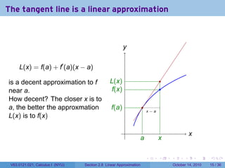
  • 32. The tangent line is a linear approximation y . L(x) = f(a) + f′ (a)(x − a) is a decent approximation to f L . (x) . near a. f .(x) . f .(a) . . x−a . x . a . x . . . . . . . V63.0121.021, Calculus I (NYU) Section 2.8 Linear Approximation October 14, 2010 15 / 36
  • 33. The tangent line is a linear approximation y . L(x) = f(a) + f′ (a)(x − a) is a decent approximation to f L . (x) . near a. f .(x) . How decent? The closer x is to a, the better the approxmation f .(a) . . x−a L(x) is to f(x) . x . a . x . . . . . . . V63.0121.021, Calculus I (NYU) Section 2.8 Linear Approximation October 14, 2010 15 / 36
  • 34. Example . Example Estimate sin(61◦ ) = sin(61π/180) by using a linear approximation (i) about a = 0 (ii) about a = 60◦ = π/3. . . . . . . . V63.0121.021, Calculus I (NYU) Section 2.8 Linear Approximation October 14, 2010 16 / 36
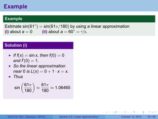
  • 35. Example . Example Estimate sin(61◦ ) = sin(61π/180) by using a linear approximation (i) about a = 0 (ii) about a = 60◦ = π/3. Solution (i) If f(x) = sin x, then f(0) = 0 and f′ (0) = 1. So the linear approximation near 0 is L(x) = 0 + 1 · x = x. Thus ( ) 61π 61π sin ≈ ≈ 1.06465 180 180 . . . . . . . V63.0121.021, Calculus I (NYU) Section 2.8 Linear Approximation October 14, 2010 16 / 36
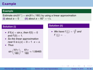
  • 36. Example . Example Estimate sin(61◦ ) = sin(61π/180) by using a linear approximation (i) about a = 0 (ii) about a = 60◦ = π/3. Solution (i) Solution (ii) (π) We have f = and If f(x) = sin x, then f(0) = 0 ( ) 3 and f′ (0) = 1. f′ π = . 3 So the linear approximation near 0 is L(x) = 0 + 1 · x = x. Thus ( ) 61π 61π sin ≈ ≈ 1.06465 180 180 . . . . . . . V63.0121.021, Calculus I (NYU) Section 2.8 Linear Approximation October 14, 2010 16 / 36
  • 37. Example . Example Estimate sin(61◦ ) = sin(61π/180) by using a linear approximation (i) about a = 0 (ii) about a = 60◦ = π/3. Solution (i) Solution (ii) (π) √ 3 We have f = and If f(x) = sin x, then f(0) = 0 ( ) 3 2 and f′ (0) = 1. f′ π = . 3 So the linear approximation near 0 is L(x) = 0 + 1 · x = x. Thus ( ) 61π 61π sin ≈ ≈ 1.06465 180 180 . . . . . . . V63.0121.021, Calculus I (NYU) Section 2.8 Linear Approximation October 14, 2010 16 / 36
  • 38. Example . Example Estimate sin(61◦ ) = sin(61π/180) by using a linear approximation (i) about a = 0 (ii) about a = 60◦ = π/3. Solution (i) Solution (ii) (π) √ 3 We have f = and If f(x) = sin x, then f(0) = 0 ( ) 3 2 and f′ (0) = 1. f′ π = 1 . 3 2 So the linear approximation near 0 is L(x) = 0 + 1 · x = x. Thus ( ) 61π 61π sin ≈ ≈ 1.06465 180 180 . . . . . . . V63.0121.021, Calculus I (NYU) Section 2.8 Linear Approximation October 14, 2010 16 / 36
  • 39. Example . Example Estimate sin(61◦ ) = sin(61π/180) by using a linear approximation (i) about a = 0 (ii) about a = 60◦ = π/3. Solution (i) Solution (ii) (π) √ 3 We have f = and If f(x) = sin x, then f(0) = 0 ( ) 3 2 and f′ (0) = 1. f′ π = 1 . 3 2 So the linear approximation So L(x) = near 0 is L(x) = 0 + 1 · x = x. Thus ( ) 61π 61π sin ≈ ≈ 1.06465 180 180 . . . . . . . V63.0121.021, Calculus I (NYU) Section 2.8 Linear Approximation October 14, 2010 16 / 36
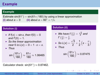
  • 40. Example . Example Estimate sin(61◦ ) = sin(61π/180) by using a linear approximation (i) about a = 0 (ii) about a = 60◦ = π/3. Solution (i) Solution (ii) (π) √ 3 We have f = and If f(x) = sin x, then f(0) = 0 ( ) 3 2 and f′ (0) = 1. f′ π = 1 . 3 2 √ So the linear approximation 3 1( π) So L(x) = + x− near 0 is L(x) = 0 + 1 · x = x. 2 2 3 Thus ( ) 61π 61π sin ≈ ≈ 1.06465 180 180 . . . . . . . V63.0121.021, Calculus I (NYU) Section 2.8 Linear Approximation October 14, 2010 16 / 36
  • 41. Example . Example Estimate sin(61◦ ) = sin(61π/180) by using a linear approximation (i) about a = 0 (ii) about a = 60◦ = π/3. Solution (i) Solution (ii) (π) √ 3 We have f = and If f(x) = sin x, then f(0) = 0 ( ) 3 2 and f′ (0) = 1. f′ π = 1 . 3 2 √ So the linear approximation 3 1( π) So L(x) = + x− near 0 is L(x) = 0 + 1 · x = x. 2 2 3 Thus Thus ( ) ( ) 61π 61π 61π sin ≈ ≈ 1.06465 sin ≈ 180 180 180 . . . . . . . V63.0121.021, Calculus I (NYU) Section 2.8 Linear Approximation October 14, 2010 16 / 36
  • 42. Example . Example Estimate sin(61◦ ) = sin(61π/180) by using a linear approximation (i) about a = 0 (ii) about a = 60◦ = π/3. Solution (i) Solution (ii) (π) √ 3 We have f = and If f(x) = sin x, then f(0) = 0 ( ) 3 2 and f′ (0) = 1. f′ π = 1 . 3 2 √ So the linear approximation 3 1( π) So L(x) = + x− near 0 is L(x) = 0 + 1 · x = x. 2 2 3 Thus Thus ( ) ( ) 61π 61π 61π sin ≈ ≈ 1.06465 sin ≈ 0.87475 180 180 180 . . . . . . . V63.0121.021, Calculus I (NYU) Section 2.8 Linear Approximation October 14, 2010 16 / 36
  • 43. Example . Example Estimate sin(61◦ ) = sin(61π/180) by using a linear approximation (i) about a = 0 (ii) about a = 60◦ = π/3. Solution (i) Solution (ii) (π) √ 3 We have f = and If f(x) = sin x, then f(0) = 0 ( ) 3 2 and f′ (0) = 1. f′ π = 1 . 3 2 √ So the linear approximation 3 1( π) So L(x) = + x− near 0 is L(x) = 0 + 1 · x = x. 2 2 3 Thus Thus ( ) ( ) 61π 61π 61π sin ≈ ≈ 1.06465 sin ≈ 0.87475 180 180 180 Calculator check: sin(61◦ ) ≈ . . . . . . . V63.0121.021, Calculus I (NYU) Section 2.8 Linear Approximation October 14, 2010 16 / 36
  • 44. Example . Example Estimate sin(61◦ ) = sin(61π/180) by using a linear approximation (i) about a = 0 (ii) about a = 60◦ = π/3. Solution (i) Solution (ii) (π) √ 3 We have f = and If f(x) = sin x, then f(0) = 0 ( ) 3 2 and f′ (0) = 1. f′ π = 1 . 3 2 √ So the linear approximation 3 1( π) So L(x) = + x− near 0 is L(x) = 0 + 1 · x = x. 2 2 3 Thus Thus ( ) ( ) 61π 61π 61π sin ≈ ≈ 1.06465 sin ≈ 0.87475 180 180 180 Calculator check: sin(61◦ ) ≈ 0.87462. . . . . . . . V63.0121.021, Calculus I (NYU) Section 2.8 Linear Approximation October 14, 2010 16 / 36
  • 45. Illustration y . y . = sin x . x . . 1◦ 6 . . . . . . V63.0121.021, Calculus I (NYU) Section 2.8 Linear Approximation October 14, 2010 17 / 36
  • 46. Illustration y . y . = L1 (x) = x y . = sin x . x . 0 . . 1◦ 6 . . . . . . V63.0121.021, Calculus I (NYU) Section 2.8 Linear Approximation October 14, 2010 17 / 36
  • 47. Illustration y . y . = L1 (x) = x b . ig difference! y . = sin x . x . 0 . . 1◦ 6 . . . . . . V63.0121.021, Calculus I (NYU) Section 2.8 Linear Approximation October 14, 2010 17 / 36
  • 48. Illustration y . y . = L1 (x) = x √ ( ) y . = L2 (x) = 2 3 + 1 2 x− π 3 y . = sin x . . . x . 0 . . π/3 . 1◦ 6 . . . . . . V63.0121.021, Calculus I (NYU) Section 2.8 Linear Approximation October 14, 2010 17 / 36
  • 49. Illustration y . y . = L1 (x) = x √ ( ) y . = L2 (x) = 2 3 + 1 2 x− π 3 y . = sin x . . ery little difference! v . . x . 0 . . π/3 . 1◦ 6 . . . . . . V63.0121.021, Calculus I (NYU) Section 2.8 Linear Approximation October 14, 2010 17 / 36
  • 50. Another Example Example √ Estimate 10 using the fact that 10 = 9 + 1. . . . . . . V63.0121.021, Calculus I (NYU) Section 2.8 Linear Approximation October 14, 2010 18 / 36
  • 51. Another Example Example √ Estimate 10 using the fact that 10 = 9 + 1. Solution √ The key step is to use a linear approximation to f(x) = √ x near a = 9 to estimate f(10) = 10. . . . . . . V63.0121.021, Calculus I (NYU) Section 2.8 Linear Approximation October 14, 2010 18 / 36
  • 52. Another Example Example √ Estimate 10 using the fact that 10 = 9 + 1. Solution √ The key step is to use a linear approximation to f(x) = √ x near a = 9 to estimate f(10) = 10. f(10) ≈ L(10) = f(9) + f′ (9)(10 − 9) 1 19 =3+ (1) = ≈ 3.167 2·3 6 . . . . . . V63.0121.021, Calculus I (NYU) Section 2.8 Linear Approximation October 14, 2010 18 / 36
  • 53. Another Example Example √ Estimate 10 using the fact that 10 = 9 + 1. Solution √ The key step is to use a linear approximation to f(x) = √ x near a = 9 to estimate f(10) = 10. f(10) ≈ L(10) = f(9) + f′ (9)(10 − 9) 1 19 =3+ (1) = ≈ 3.167 2·3 6 ( )2 19 Check: = 6 . . . . . . V63.0121.021, Calculus I (NYU) Section 2.8 Linear Approximation October 14, 2010 18 / 36
  • 54. Another Example Example √ Estimate 10 using the fact that 10 = 9 + 1. Solution √ The key step is to use a linear approximation to f(x) = √ x near a = 9 to estimate f(10) = 10. f(10) ≈ L(10) = f(9) + f′ (9)(10 − 9) 1 19 =3+ (1) = ≈ 3.167 2·3 6 ( )2 19 361 Check: = . 6 36 . . . . . . V63.0121.021, Calculus I (NYU) Section 2.8 Linear Approximation October 14, 2010 18 / 36
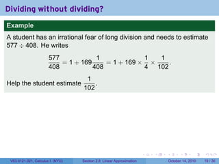
  • 55. Dividing without dividing? Example A student has an irrational fear of long division and needs to estimate 577 ÷ 408. He writes 577 1 1 1 = 1 + 169 = 1 + 169 × × . 408 408 4 102 1 Help the student estimate . 102 . . . . . . V63.0121.021, Calculus I (NYU) Section 2.8 Linear Approximation October 14, 2010 19 / 36
  • 56. Dividing without dividing? Example A student has an irrational fear of long division and needs to estimate 577 ÷ 408. He writes 577 1 1 1 = 1 + 169 = 1 + 169 × × . 408 408 4 102 1 Help the student estimate . 102 Solution 1 Let f(x) = . We know f(100) and we want to estimate f(102). x 1 1 f(102) ≈ f(100) + f′ (100)(2) = − (2) = 0.0098 100 1002 577 =⇒ ≈ 1.41405 408 . . . . . . V63.0121.021, Calculus I (NYU) Section 2.8 Linear Approximation October 14, 2010 19 / 36
  • 57. Questions Example Suppose we are traveling in a car and at noon our speed is 50 mi/hr. How far will we have traveled by 2:00pm? by 3:00pm? By midnight? . . . . . . V63.0121.021, Calculus I (NYU) Section 2.8 Linear Approximation October 14, 2010 20 / 36
  • 58. Answers Example Suppose we are traveling in a car and at noon our speed is 50 mi/hr. How far will we have traveled by 2:00pm? by 3:00pm? By midnight? . . . . . . V63.0121.021, Calculus I (NYU) Section 2.8 Linear Approximation October 14, 2010 21 / 36
  • 59. Answers Example Suppose we are traveling in a car and at noon our speed is 50 mi/hr. How far will we have traveled by 2:00pm? by 3:00pm? By midnight? Answer 100 mi 150 mi 600 mi (?) (Is it reasonable to assume 12 hours at the same speed?) . . . . . . V63.0121.021, Calculus I (NYU) Section 2.8 Linear Approximation October 14, 2010 21 / 36
  • 60. Questions Example Suppose we are traveling in a car and at noon our speed is 50 mi/hr. How far will we have traveled by 2:00pm? by 3:00pm? By midnight? Example Suppose our factory makes MP3 players and the marginal cost is currently $50/lot. How much will it cost to make 2 more lots? 3 more lots? 12 more lots? . . . . . . V63.0121.021, Calculus I (NYU) Section 2.8 Linear Approximation October 14, 2010 22 / 36
  • 61. Answers Example Suppose our factory makes MP3 players and the marginal cost is currently $50/lot. How much will it cost to make 2 more lots? 3 more lots? 12 more lots? Answer $100 $150 $600 (?) . . . . . . V63.0121.021, Calculus I (NYU) Section 2.8 Linear Approximation October 14, 2010 23 / 36
  • 62. Questions Example Suppose we are traveling in a car and at noon our speed is 50 mi/hr. How far will we have traveled by 2:00pm? by 3:00pm? By midnight? Example Suppose our factory makes MP3 players and the marginal cost is currently $50/lot. How much will it cost to make 2 more lots? 3 more lots? 12 more lots? Example Suppose a line goes through the point (x0 , y0 ) and has slope m. If the point is moved horizontally by dx, while staying on the line, what is the corresponding vertical movement? . . . . . . V63.0121.021, Calculus I (NYU) Section 2.8 Linear Approximation October 14, 2010 24 / 36
  • 63. Answers Example Suppose a line goes through the point (x0 , y0 ) and has slope m. If the point is moved horizontally by dx, while staying on the line, what is the corresponding vertical movement? . . . . . . V63.0121.021, Calculus I (NYU) Section 2.8 Linear Approximation October 14, 2010 25 / 36
  • 64. Answers Example Suppose a line goes through the point (x0 , y0 ) and has slope m. If the point is moved horizontally by dx, while staying on the line, what is the corresponding vertical movement? Answer The slope of the line is rise m= run We are given a “run” of dx, so the corresponding “rise” is m dx. . . . . . . V63.0121.021, Calculus I (NYU) Section 2.8 Linear Approximation October 14, 2010 25 / 36
  • 65. Outline The linear approximation of a function near a point Examples Questions Differentials Using differentials to estimate error Advanced Examples . . . . . . V63.0121.021, Calculus I (NYU) Section 2.8 Linear Approximation October 14, 2010 26 / 36
  • 66. Differentials are another way to express derivatives The fact that the the tangent line is an approximation means that y . f(x + ∆x) − f(x) ≈ f′ (x) ∆x ∆y dy Rename ∆x = dx, so we can write this as . . dy . ∆y ′ ∆y ≈ dy = f (x)dx. . . dx = ∆x Note this looks a lot like the Leibniz-Newton identity . x . dy x x . . + ∆x = f′ (x) dx . . . . . . V63.0121.021, Calculus I (NYU) Section 2.8 Linear Approximation October 14, 2010 27 / 36
  • 67. Using differentials to estimate error y . Estimating error with differentials If y = f(x), x0 and ∆x is known, and an estimate of ∆y is desired: . . Approximate: ∆y ≈ dy dy . ∆y Differentiate: dy = f′ (x) dx . . dx = ∆x Evaluate at x = x0 and dx = ∆x. . x . x x . . + ∆x . . . . . . V63.0121.021, Calculus I (NYU) Section 2.8 Linear Approximation October 14, 2010 28 / 36
  • 68. Example A sheet of plywood measures 8 ft × 4 ft. Suppose our plywood-cutting machine will cut a rectangle whose width is exactly half its length, but the length is prone to errors. If the length is off by 1 in, how bad can the area of the sheet be off by? . . . . . . V63.0121.021, Calculus I (NYU) Section 2.8 Linear Approximation October 14, 2010 29 / 36
  • 69. Example A sheet of plywood measures 8 ft × 4 ft. Suppose our plywood-cutting machine will cut a rectangle whose width is exactly half its length, but the length is prone to errors. If the length is off by 1 in, how bad can the area of the sheet be off by? Solution 1 2 Write A(ℓ) = ℓ . We want to know ∆A when ℓ = 8 ft and ∆ℓ = 1 in. 2 . . . . . . V63.0121.021, Calculus I (NYU) Section 2.8 Linear Approximation October 14, 2010 29 / 36
  • 70. Example A sheet of plywood measures 8 ft × 4 ft. Suppose our plywood-cutting machine will cut a rectangle whose width is exactly half its length, but the length is prone to errors. If the length is off by 1 in, how bad can the area of the sheet be off by? Solution 1 2 Write A(ℓ) = ℓ . We want to know ∆A when ℓ = 8 ft and ∆ℓ = 1 in. 2 ( ) 97 9409 9409 (I) A(ℓ + ∆ℓ) = A = So ∆A = − 32 ≈ 0.6701. 12 288 288 . . . . . . V63.0121.021, Calculus I (NYU) Section 2.8 Linear Approximation October 14, 2010 29 / 36
  • 71. Example A sheet of plywood measures 8 ft × 4 ft. Suppose our plywood-cutting machine will cut a rectangle whose width is exactly half its length, but the length is prone to errors. If the length is off by 1 in, how bad can the area of the sheet be off by? Solution 1 2 Write A(ℓ) = ℓ . We want to know ∆A when ℓ = 8 ft and ∆ℓ = 1 in. 2 ( ) 97 9409 9409 (I) A(ℓ + ∆ℓ) = A = So ∆A = − 32 ≈ 0.6701. 12 288 288 dA (II) = ℓ, so dA = ℓ dℓ, which should be a good estimate for ∆ℓ. dℓ When ℓ = 8 and dℓ = 12 , we have dA = 12 = 2 ≈ 0.667. So we 1 8 3 get estimates close to the hundredth of a square foot. . . . . . . V63.0121.021, Calculus I (NYU) Section 2.8 Linear Approximation October 14, 2010 29 / 36
  • 72. Why? Why use linear approximations dy when the actual difference ∆y is known? Linear approximation is quick and reliable. Finding ∆y exactly depends on the function. These examples are overly simple. See the “Advanced Examples” later. In real life, sometimes only f(a) and f′ (a) are known, and not the general f(x). . . . . . . V63.0121.021, Calculus I (NYU) Section 2.8 Linear Approximation October 14, 2010 30 / 36
  • 73. Outline The linear approximation of a function near a point Examples Questions Differentials Using differentials to estimate error Advanced Examples . . . . . . V63.0121.021, Calculus I (NYU) Section 2.8 Linear Approximation October 14, 2010 31 / 36
  • 74. Gravitation Pencils down! Example Drop a 1 kg ball off the roof of the Silver Center (50m high). We usually say that a falling object feels a force F = −mg from gravity. . . . . . . V63.0121.021, Calculus I (NYU) Section 2.8 Linear Approximation October 14, 2010 32 / 36
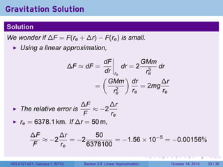
  • 75. Gravitation Pencils down! Example Drop a 1 kg ball off the roof of the Silver Center (50m high). We usually say that a falling object feels a force F = −mg from gravity. In fact, the force felt is GMm F(r) = − , r2 where M is the mass of the earth and r is the distance from the center of the earth to the object. G is a constant. GMm At r = re the force really is F(re ) = = −mg. r2 e What is the maximum error in replacing the actual force felt at the top of the building F(re + ∆r) by the force felt at ground level F(re )? The relative error? The percentage error? . . . . . . V63.0121.021, Calculus I (NYU) Section 2.8 Linear Approximation October 14, 2010 32 / 36
  • 76. Gravitation Solution Solution We wonder if ∆F = F(re + ∆r) − F(re ) is small. Using a linear approximation, dF GMm ∆F ≈ dF = dr = 2 3 dr dr re re ( ) GMm dr ∆r = 2 = 2mg re re re ∆F ∆r The relative error is ≈ −2 F re re = 6378.1 km. If ∆r = 50 m, ∆F ∆r 50 ≈ −2 = −2 = −1.56 × 10−5 = −0.00156% F re 6378100 . . . . . . V63.0121.021, Calculus I (NYU) Section 2.8 Linear Approximation October 14, 2010 33 / 36
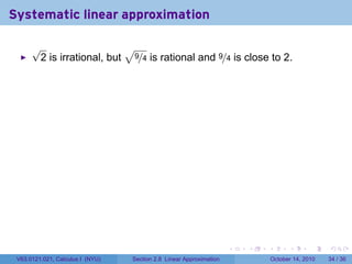
  • 77. Systematic linear approximation √ √ 2 is irrational, but 9/4 is rational and 9/4 is close to 2. . . . . . . V63.0121.021, Calculus I (NYU) Section 2.8 Linear Approximation October 14, 2010 34 / 36
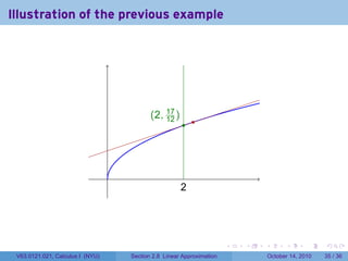
  • 78. Systematic linear approximation √ √ 2 is irrational, but 9/4 is rational and 9/4 is close to 2. So √ √ √ 1 17 2 = 9/4 − 1/4 ≈ 9/4 + (−1/4) = 2(3/2) 12 . . . . . . V63.0121.021, Calculus I (NYU) Section 2.8 Linear Approximation October 14, 2010 34 / 36
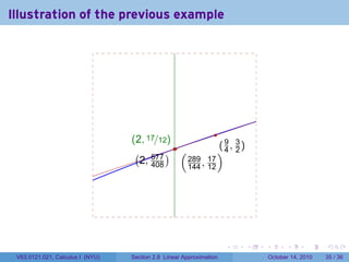
  • 79. Systematic linear approximation √ √ 2 is irrational, but 9/4 is rational and 9/4 is close to 2. So √ √ √ 1 17 2 = 9/4 − 1/4 ≈ 9/4 + (−1/4) = 2(3/2) 12 This is a better approximation since (17/12)2 = 289/144 . . . . . . V63.0121.021, Calculus I (NYU) Section 2.8 Linear Approximation October 14, 2010 34 / 36
  • 80. Systematic linear approximation √ √ 2 is irrational, but 9/4 is rational and 9/4 is close to 2. So √ √ √ 1 17 2 = 9/4 − 1/4 ≈ 9/4 + (−1/4) = 2(3/2) 12 This is a better approximation since (17/12)2 = 289/144 Do it again! √ √ √ 1 2 = 289/144 − 1/144 ≈ 289/144 + (−1/144) = 577/408 2(17/12) ( )2 577 332, 929 1 Now = which is away from 2. 408 166, 464 166, 464 . . . . . . V63.0121.021, Calculus I (NYU) Section 2.8 Linear Approximation October 14, 2010 34 / 36
  • 81. Illustration of the previous example . . . . . . . V63.0121.021, Calculus I (NYU) Section 2.8 Linear Approximation October 14, 2010 35 / 36
  • 82. Illustration of the previous example . . . . . . . V63.0121.021, Calculus I (NYU) Section 2.8 Linear Approximation October 14, 2010 35 / 36
  • 83. Illustration of the previous example . 2 . . . . . . . V63.0121.021, Calculus I (NYU) Section 2.8 Linear Approximation October 14, 2010 35 / 36
  • 84. Illustration of the previous example . . 2 . . . . . . . V63.0121.021, Calculus I (NYU) Section 2.8 Linear Approximation October 14, 2010 35 / 36
  • 85. Illustration of the previous example . . 2 . . . . . . . V63.0121.021, Calculus I (NYU) Section 2.8 Linear Approximation October 14, 2010 35 / 36
  • 86. Illustration of the previous example . 2, 17 ) ( 12 . . . 2 . . . . . . . V63.0121.021, Calculus I (NYU) Section 2.8 Linear Approximation October 14, 2010 35 / 36
  • 87. Illustration of the previous example . 2, 17 ) ( 12 . . . 2 . . . . . . . V63.0121.021, Calculus I (NYU) Section 2.8 Linear Approximation October 14, 2010 35 / 36
  • 88. Illustration of the previous example . . 2, 17/12) ( . . 4, 3) (9 2 . . . . . . V63.0121.021, Calculus I (NYU) Section 2.8 Linear Approximation October 14, 2010 35 / 36
  • 89. Illustration of the previous example . . 2, 17/12) ( .. ( . 9, 3) ( )4 2 289 17 . 144 , 12 . . . . . . V63.0121.021, Calculus I (NYU) Section 2.8 Linear Approximation October 14, 2010 35 / 36
  • 90. Illustration of the previous example . . 2, 17/12) ( .. ( . 9, 3) ( ( 577 ) )4 2 . 2, 408 289 17 . 144 , 12 . . . . . . V63.0121.021, Calculus I (NYU) Section 2.8 Linear Approximation October 14, 2010 35 / 36
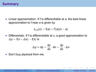
  • 91. Summary Linear approximation: If f is differentiable at a, the best linear approximation to f near a is given by Lf,a (x) = f(a) + f′ (a)(x − a) Differentials: If f is differentiable at x, a good approximation to ∆y = f(x + ∆x) − f(x) is dy dy ∆y ≈ dy = · dx = · ∆x dx dx Don’t buy plywood from me. . . . . . . V63.0121.021, Calculus I (NYU) Section 2.8 Linear Approximation October 14, 2010 36 / 36