Modern Compiler Design 2e.pdf
0 likes194 views

This document provides a preface for the second edition of the book "Modern Compiler Design". It summarizes changes made for the new edition, including rearranging content, adding new material, and updating existing material. It also acknowledges contributions from reviewers and outlines how the book could be used for compiler design courses.


![2 1 Introduction
the baron pulled himself from a swamp by his hair plait, rather than by his boot-
straps [14].
Program
Compiler
txt
txt
X
Compiler
exe
exe
Y
=
=
Executable compiler
code
Compiler source text
Input in
code for target
Executable program
language
in implementation
in source language
Program source text
some input format
machine
Output in
some output format
Fig. 1.1: Compiling and running a compiler
Compilation does not differ fundamentally from file conversion but it does differ
in degree. The main aspect of conversion is that the input has a property called
semantics—its “meaning”—which must be preserved by the process. The structure
of the input and its semantics can be simple, as, for example in a file conversion
program which converts EBCDIC to ASCII; they can be moderate, as in an WAV
to MP3 converter, which has to preserve the acoustic impression, its semantics;
or they can be considerable, as in a compiler, which has to faithfully express the
semantics of the input program in an often extremely different output format. In the
final analysis, a compiler is just a giant file conversion program.
The compiler can work its magic because of two factors:
• the input is in a language and consequently has a structure, which is described in
the language reference manual;
• the semantics of the input is described in terms of and is attached to that same
structure.
These factors enable the compiler to “understand” the program and to collect its
semantics in a semantic representation. The same two factors exist with respect
to the target language. This allows the compiler to rephrase the collected semantics
in terms of the target language. How all this is done in detail is the subject of this
book.](https://image.slidesharecdn.com/moderncompilerdesign2e-220513113004-0b36a6ff/85/Modern-Compiler-Design-2e-pdf-22-320.jpg)


![8 1 Introduction
1.1.1.3 Use of program-generating tools
Once one has the proper formalism in which to describe what a program should
do, one can generate a program from it, using a program generator. Examples are
lexical analyzers generated from regular descriptions of the input, parsers generated
from grammars (syntax descriptions), and code generators generated from machine
descriptions. All these are generally more reliable and easier to debug than their
handwritten counterparts; they are often more efficient too.
Generating programs rather than writing them by hand has several advantages:
• The input to a program generator is of a much higher level of abstraction than the
handwritten program would be. The programmer needs to specify less, and the
tools take responsibility for much error-prone housekeeping. This increases the
chances that the program will be correct. For example, it would be cumbersome
to write parse tables by hand.
• The use of program-generating tools allows increased flexibility and modifiabil-
ity. For example, if during the design phase of a language a small change in the
syntax is considered, a handwritten parser would be a major stumbling block
to any such change. With a generated parser, one would just change the syntax
description and generate a new parser.
• Pre-canned or tailored code can be added to the generated program, enhancing
its power at hardly any cost. For example, input error handling is usually a dif-
ficult affair in handwritten parsers; a generated parser can include tailored error
correction code with no effort on the part of the programmer.
• A formal description can sometimes be used to generate more than one type of
program. For example, once we have written a grammar for a language with the
purpose of generating a parser from it, we may use it to generate a syntax-directed
editor, a special-purpose program text editor that guides and supports the user in
editing programs in that language.
In summary, generated programs may be slightly more or slightly less efficient than
handwritten ones, but generating them is so much more efficient than writing them
by hand that whenever the possibility exists, generating a program is almost always
to be preferred.
The technique of creating compilers by program-generating tools was pioneered
by Brooker et al. in 1963 [51], and its importance has continually risen since. Pro-
grams that generate parts of a compiler are sometimes called compiler compilers,
although this is clearly a misnomer. Yet, the term lingers on.
1.1.2 Compiler construction has a wide applicability
Compiler construction techniques can be and are applied outside compiler construc-
tion in its strictest sense. Alternatively, more programming can be considered com-
piler construction than one would traditionally assume. Examples are reading struc-](https://image.slidesharecdn.com/moderncompilerdesign2e-220513113004-0b36a6ff/85/Modern-Compiler-Design-2e-pdf-28-320.jpg)


![30 1 Introduction
an attempt to obtain information from a module whose loop has terminated fails.
A well-known implementation of the coroutine mechanism is the UNIX pipe, in
which the two separate stacks reside in different processes and therefore in differ-
ent address spaces; threads are another. (Implementation of coroutines in imperative
languages is discussed in Section 11.3.8).
Although the coroutine mechanism was proposed by Conway [68] early in the
history of compiler construction, the main stream programming languages used in
compiler construction do not have this feature. In the absence of coroutines we have
to choose one of our modules as the main loop in a narrow compiler and implement
the other loops through trickery.
If we choose the bb → c filter as the main loop, it obtains the next character
from the aa → b filter by calling the subroutine ObtainedFromPreviousModule.
This means that we have to rewrite that filter as subroutine. This requires major
surgery as shown by Figure 1.25, which contains our filter as a loop-less subroutine
to be used before the main loop.
InputExhausted ← False;
CharacterStored ← False;
StoredCharacter ← Undefined; −− can never be an ’a’
function FilteredCharacter returning (a Boolean, a character):
if InputExhausted: return (False, NoCharacter);
else if CharacterStored:
−− It cannot be an ’a’:
CharacterStored ← False;
return (True, StoredCharacter);
else −− not InputExhausted and not CharacterStored:
if ObtainedFromPreviousModule (Ch):
if Ch = ’a’:
−− See if there is another ’a’:
if ObtainedFromPreviousModule (Ch1):
if Ch1 = ’a’:
−− We have ’aa’:
return (True, ’b’);
else −− Ch1 = ’a’:
StoredCharacter ← Ch1;
CharacterStored ← True;
return (True, ’a’);
else −− There were no more characters:
InputExhausted ← True;
return (True, ’a’);
else −− Ch = ’a’:
return (True, Ch);
else −− There were no more characters:
InputExhausted ← True;
return (False, NoCharacter);
Fig. 1.25: The filter aa → b as a pre-main subroutine module](https://image.slidesharecdn.com/moderncompilerdesign2e-220513113004-0b36a6ff/85/Modern-Compiler-Design-2e-pdf-50-320.jpg)


![1.7 A short history of compiler construction 33
is written in a reasonably good style in a modern high-level language, good porta-
bility can be expected. Retargeting is achieved by replacing the entire back-end; the
retargetability is thus inversely related to the effort to create a new back-end.
In this context it is important to note that creating a new back-end does not nec-
essarily mean writing one from scratch. Some of the code in a back-end is of course
machine-dependent, but much of it is not. If structured properly, some parts can be
reused from other back-ends and other parts can perhaps be generated from formal-
ized machine-descriptions. This approach can reduce creating a back-end from a
major enterprise to a reasonable effort. With the proper tools, creating a back-end
for a new machine may cost between one and four programmer-months for an expe-
rienced compiler writer. Machine descriptions range in size between a few hundred
lines and many thousands of lines.
This concludes our introductory part on actually constructing a compiler. In the
remainder of this chapter we consider three further issues: the history of compiler
construction, formal grammars, and closure algorithms.
1.7 A short history of compiler construction
Three periods can be distinguished in the history of compiler construction: 1945–
1960, 1960–1975, and 1975–present. Of course, the years are approximate.
1.7.1 1945–1960: code generation
During this period programming languages developed relatively slowly and ma-
chines were idiosyncratic. The primary problem was how to generate code for a
given machine. The problem was exacerbated by the fact that assembly program-
ming was held in high esteem, and high(er)-level languages and compilers were
looked at with a mixture of suspicion and awe: using a compiler was often called
“automatic programming”. Proponents of high-level languages feared, not without
reason, that the idea of high-level programming would never catch on if compilers
produced code that was less efficient than what assembly programmers produced
by hand. The first FORTRAN compiler, written by Sheridan et al. in 1959 [260],
optimized heavily and was far ahead of its time in that respect.
1.7.2 1960–1975: parsing
The 1960s and 1970s saw a proliferation of new programming languages, and lan-
guage designers began to believe that having a compiler for a new language quickly](https://image.slidesharecdn.com/moderncompilerdesign2e-220513113004-0b36a6ff/85/Modern-Compiler-Design-2e-pdf-53-320.jpg)


![1.9 Closure algorithms 45
SomethingWasChanged ← True;
while SomethingWasChanged:
SomethingWasChanged ← False;
for each Node1 in Graph:
for each Node2 in descendants of Node1:
for each Node3 in descendants of Node2:
if there is no arrow from Node1 to Node3:
Add an arrow from Node1 to Node3;
SomethingWasChanged ← True;
Fig. 1.33: Outline of a bottom-up algorithm for transitive closure
A sweep consists of finding the nodes of the graph one by one, and for each node
adding an arrow from it to all its descendants’ descendants, as far as these are known
at the moment. It is important to recognize the restriction “as far as the arrows are
known at the moment” since this is what forces us to repeat the sweep until we find
a sweep in which no more arrows are added. We are then sure that the descendants
we know are all the descendants there are.
The algorithm seems quite inefficient. If the graph contains n nodes, the body of
the outermost for-loop is repeated n times; each node can have at most n descen-
dants, so the body of the second for-loop can be repeated n times, and the same
applies to the third for-loop. Together this is O(n3) in the worst case. Each run of
the while-loop adds at least one arc (except the last run), and since there are at most
n2 arcs to be added, it could in principle be repeated n2 times in the worst case. So
the total time complexity would seem to be O(n5), which is much too high to be
used in a compiler.
There are, however, two effects that save the iterative bottom-up closure algo-
rithm. The first is that the above worst cases cannot materialize all at the same time.
For example, if all nodes have all other nodes for descendants, all arcs are already
present and the algorithm finishes in one round. There is a well-known algorithm by
Warshall [292] which does transitive closure in O(n3) time and O(n2) space, with
very low multiplication constants for both time and space. Unfortunately it has the
disadvantage that it always uses this O(n3) time and O(n2) space, and O(n3) time is
still rather stiff in a compiler.
The second effect is that the graphs to which the closure algorithm is applied are
usually sparse, which means that almost all nodes have only a few outgoing arcs.
Also, long chains of arcs are usually rare. This changes the picture of the complexity
of the algorithm completely. Let us say for example that the average fan-out of a
routine is f, which means that a routine calls on average f other routines; and that
the average calling depth is d, which means that on the average after d calls within
calls we reach either a routine that does not call other routines or we get involved in
recursion. Under these assumptions, the while-loop will be repeated on the average
d times, since after d turns all required arcs will have been added. The outermost
for-loop will still be repeated n times, but the second and third loops will be repeated](https://image.slidesharecdn.com/moderncompilerdesign2e-220513113004-0b36a6ff/85/Modern-Compiler-Design-2e-pdf-65-320.jpg)
![46 1 Introduction
f times during the first turn of the while-loop, f2 times during the second turn, f3
times during the third turn, and so on, until the last turn, which takes fd times. So
on average the if-statement will be executed
n × (f2 + f4 + f6 +...f2d) = f2(d+1)−f2
f2−1
× n
times. Although the constant factor can be considerable —for f = 4 and d = 4 it
is almost 70 000— the main point is that the time complexity is now linear in the
number of nodes, which suggests that the algorithm may be practical after all. This is
borne out by experience, and by many measurements [270]. For non-sparse graphs,
however, the time complexity of the bottom-up transitive closure algorithm is still
O(n3).
In summary, although transitive closure has non-linear complexity in the general
case, for sparse graphs the bottom-up algorithm is almost linear.
1.10 The code forms used in this book
Three kinds of code are presented in this book: sample input to the compiler, sample
implementations of parts of the compiler, and outline code. We have seen an exam-
ple of compiler input in the 3, (5+8), and (2*((3*4)+9)) on page 13. Such
text is presented in a constant-width computer font; the same font is used for
the occasional textual output of a program.
Examples of compiler parts can be found in the many figures in Section 1.2 on
the demo compiler. They are presented in a sans serif font.
In addition to being explained in words and by examples, the outline of an algo-
rithm is sometimes sketched in an outline code; we have already seen an example
in Figure 1.33. Outline code is shown in the same font as the main text of this book;
segments of outline code in the running text are distinguished by presenting them in
italic.
The outline code is an informal, reasonably high-level language. It has the ad-
vantage that it allows ignoring much of the problematic details that beset many
real-world programming languages, including memory allocation and deallocation,
type conversion, and declaration before use. We have chosen not to use an existing
programming language, for several reasons:
• We emphasize the ideas behind the algorithms rather than their specific imple-
mentation, since we believe the ideas will serve for a longer period and will allow
the compiler designer to make modifications more readily than a specific imple-
mentation would. This is not a cookbook for compiler construction, and supply-
ing specific code might suggest that compilers can be constructed by copying
code fragments from books.
• We do not want to be drawn into a C versus C++ versus Java versus other lan-
guages discussion. We emphasize ideas and principles, and we find each of these
languages pretty unsuitable for high-level idea expression.](https://image.slidesharecdn.com/moderncompilerdesign2e-220513113004-0b36a6ff/85/Modern-Compiler-Design-2e-pdf-66-320.jpg)


![1.11 Conclusion 49
new information can be obtained at any node. The algorithms differ in what in-
formation is collected and how.
Further reading
The most famous compiler construction book ever is doubtlessly Compilers: Prin-
ciples, Techniques and Tools, better known as “The Red Dragon Book” by Aho,
Sethi and Ullman [4]; a second edition, by Aho, Lam, Sethi and Ullman [6], has ap-
peared, and extends the Red Dragon book with many optimizations. There are few
books that also treat compilers for programs in other paradigms than the imperative
one. For a code-oriented treatment we mention Appel [18] and for a more formal
treatment the four volumes by Wilhelm, Seidl and Hack [113, 300–302]. Srikant
and Shankar’s Compiler Design Handbook [264] provides insight in a gamut of
advanced compiler design subjects, while the theoretical, formal basis of compiler
design is presented by Meduna [189].
New developments in compiler construction are reported in journals, for ex-
ample ACM Transactions on Programming Languages and Systems, Software—
Practice and Experience, ACM SIGPLAN Notices, Computer Languages, and
the more theoretical Acta Informatica; in the proceedings of conferences, for
example ACM SIGPLAN Conference on Programming Language Design and
Implementation—PLDI, Conference on Object-Oriented Programming Systems,
Languages and Applications—OOPSLA, and IEEE International Conference on
Computer Languages—ICCL; and in some editions of “Lecture Notes in Computer
Science”, more in particular the Compiler Construction International Conference
and Implementation of Functional Languages.
Interpreters are the second-class citizens of the compiler construction world: ev-
erybody employs them, but hardly any author pays serious attention to them. There
are a few exceptions, though. Griswold and Griswold [111] is the only textbook ded-
icated solely to interpreter construction, and a good one at that. Pagan [209] shows
how thin the line between interpreters and compilers is.
The standard work on grammars and formal languages is still Hopcroft and Ull-
man [124]. A relatively easy introduction to the subject is provided by Linz [180]; a
modern book with more scope and more mathematical rigor is by Sudkamp [269].
The most readable book on the subject is probably that by Révész [234].
Much has been written about transitive closure algorithms. Some interesting
papers are by Feijs and van Ommering [99], Nuutila [206], Schnorr [254], Pur-
dom Jr. [226], and Warshall [292]. Schnorr presents a sophisticated but still rea-
sonably simple version of the iterative bottom-up algorithm shown in Section 1.9.3
and proves that its expected time requirement is linear in the sum of the number
of nodes and the final number of edges. Warshall’s algorithm is very famous and is
treated in any text book on algorithms, for example Sedgewick [257] or Baase and
Van Gelder [23].
The future of compiler research is discussed by Hall et al. [115] and Bates [33].](https://image.slidesharecdn.com/moderncompilerdesign2e-220513113004-0b36a6ff/85/Modern-Compiler-Design-2e-pdf-69-320.jpg)

![1.11 Conclusion 51
1.12. For those who already know what a finite-state automaton (FSA) is: rewrite
the pre-main and post-main versions of the aa → b filter using an FSA. You will
notice that now the code is simpler: an FSA is a more efficient but less structured
device for the storage of state than a set of global variables.
1.13. (785) What is an “extended subset” of a language? Why is the term usually
used in a pejorative sense?
1.14. (www) The grammar for expression in Section 1.2.1 has:
expression → expression ’+’ term | expression ’−’ term | term
If we replaced this by
expression → expression ’+’ expression | expression ’−’ expression | term
the grammar would still produce the same language, but the replacement is not
correct. What is wrong?
1.15. (www) Rewrite the EBNF rule
parameter_list → (’IN’ | ’OUT’)? identifier (’,’ identifier)*
from Section 1.8.3 to BNF.
1.16. (www) Given the grammar:
S → A | B | C
A → B | ε
B → x | C y
C → B C S
in which S is the start symbol.
(a) Name the non-terminals that are left-recursive, right-recursive, nullable, or use-
less, if any.
(b) What language does the grammar produce?
(c) Is the grammar ambiguous?
1.17. (www) Why could one want two or more terminal symbols with the same
representation? Give an example.
1.18. (www) Why would it be considered bad design to have a terminal symbol
with an empty representation?
1.19. (785) Refer to Section 1.8.5.1 on the definition of a grammar, condition (1).
Why do we have to be able to tell terminals and non-terminals apart?
1.20. (785) Argue that there is only one “smallest set of information items” that
fulfills the requirements of a closure specification.
1.21. History of compiler construction: Study Conway’s 1963 paper [68] on the
coroutine-based modularization of compilers, and write a summary of it.](https://image.slidesharecdn.com/moderncompilerdesign2e-220513113004-0b36a6ff/85/Modern-Compiler-Design-2e-pdf-71-320.jpg)


![2 Program Text to Tokens — Lexical Analysis 57
2. the semantics of identifier (in two different cases), expression, and factor are
trivial (just passing on the value) and need not be recorded.
This means that nodes for constant_definition can be implemented in the compiler
as records with two fields:
struct constant_definition {
Identifier *CD_idf;
Expression *CD_expr;
}
(in addition to some standard fields recording in which file and at what line the
constant definition was found).
Another example of a useful difference between parse tree and AST is the combi-
nation of the node types for if-then-else and if-then into one node type if-then-else.
An if-then node is represented by an if-then-else node, in which the else part has
been supplemented as an empty statement, as shown in Figure 2.2.
if_statement
condition
IF THEN statement
if_statement
condition statement statement
(b)
(a)
Fig. 2.2: Syntax tree (a) and abstract syntax tree (b) of an if-then statement
Noonan [205] gives a set of heuristic rules for deriving a good AST structure
from a grammar. For an even more compact internal representation of the program
than ASTs see Waddle [290].
The context handling module gathers information about the nodes and combines
it with that of other nodes. This information serves to perform contextual checking
and to assist in code generation. The abstract syntax tree adorned with these bits of
information is called the annotated abstract syntax tree. Actually the abstract syntax
tree passes through many stages of “annotatedness” during compilation. The degree
of annotatedness starts out at almost zero, straight from parsing, and continues to
grow even through code generation, in which, for example, actual memory addresses
may be attached as annotations to nodes.
At the end of the context handling phase our AST might have the form](https://image.slidesharecdn.com/moderncompilerdesign2e-220513113004-0b36a6ff/85/Modern-Compiler-Design-2e-pdf-75-320.jpg)


![62 2 Program Text to Tokens — Lexical Analysis
Basic pattern Matching string
x The character x
. Any character, usually except a newline
[xyz.. . ] Any of the characters x, y, z, ...
Repetition operators:
R? An R or nothing (= optionally an R)
R∗ Zero or more occurrences of R
R+ One or more occurrences of R
Composition operators:
R1 R2 An R1 followed by an R2
R1|R2 Either an R1 or an R2
Grouping:
(R) R itself
Fig. 2.4: Components of regular expressions
The most basic regular expression is a pattern that matches just one character, and
the simplest of these is the one that specifies that character explicitly; an example is
the pattern a which matches the character a. There are two more basic patterns, one
for matching a set of characters and one for matching all characters (usually with
the exception of the end-of-line character, if it exists). These three basic patterns
appear at the top of Figure 2.4. In this figure, x, y, z, ... stand for any character and
R, R1, R2, ... stand for any regular expression.
A basic pattern can optionally be followed by a repetition operator; examples
are b? for an optional b; b* for a possibly empty sequence of bs; and b+ for a non-
empty sequence of bs.
There are two composition operators. One is the invisible operator, which in-
dicates concatenation; it occurs for example between the a and the b in ab*. The
second is the | operator which separates alternatives; for example, ab*|cd? matches
anything that is matched by ab* or alternatively by cd?.
The repetition operators have the highest precedence (bind most tightly); next
comes the concatenation operator; and the alternatives operator | has the lowest
precedence. Parentheses can be used for grouping. For example, the regular ex-
pression ab*|cd? is equivalent to (a(b*))|(c(d?)).
A more extensive set of operators might for example include a repetition oper-
ator of the form Rm − n, which stands for m to n repetitions of R, but such forms
have limited usefulness and complicate the implementation of the lexical analyzer
considerably.](https://image.slidesharecdn.com/moderncompilerdesign2e-220513113004-0b36a6ff/85/Modern-Compiler-Design-2e-pdf-80-320.jpg)
![2.3 Regular expressions and regular descriptions 63
2.3.1 Regular expressions and BNF/EBNF
A comparison with the right-hand sides of production rules in CF grammars sug-
gests itself. We see that only the basic patterns are characteristic of regular expres-
sions. Regular expressions share with the BNF notation the invisible concatenation
operator and the alternatives operator, and with EBNF the repetition operators and
parentheses.
2.3.2 Escape characters in regular expressions
The superscript operators *, +, and ? do not occur in widely available character set
and on keyboards, so for computer input the characters *, +, ? are often used. This
has the unfortunate consequence that these characters cannot be used to match them-
selves as actual characters. The same applies to the characters |, [, ], (, and ), which
are used directly by the regular expression syntax. There is usually some trickery
involving escape characters to force these characters to stand for themselves rather
than being taken as operators or separators One example of such an escape char-
acter is the backslash, , which is used as a prefix: * denotes the asterisk, the
backslash character itself, etc. Another is the quote, , which is used to surround the
escaped part: * denotes the asterisk, +? denotes a plus followed by a question
mark, denotes the quote character itself, etc. As we can see, additional trickery
is needed to represent the escape character itself.
It might have been more esthetically satisfying if the escape characters had been
used to endow the normal characters *, +, ?, etc., with a special meaning rather than
vice versa, but this is not the path that history has taken and the present situation
presents no serious problems.
2.3.3 Regular descriptions
Regular expressions can easily become complicated and hard to understand; a more
convenient alternative is the so-called regular description. A regular description is
like a context-free grammar in EBNF, with the restriction that no non-terminal can
be used before it has been fully defined.
As a result of this restriction, we can substitute the right-hand side of the first rule
(which obviously cannot contain non-terminals) in the second and further rules,
adding pairs of parentheses where needed to obey the precedences of the repeti-
tion operators. Now the right-hand side of the second rule will no longer contain
non-terminals and can be substituted in the third and further rules, and so on; this
technique, which is also used elsewhere, is called forward substitution, for obvi-
ous reasons. The last rule combines all the information of the previous rules and its
right-hand side corresponds to the desired regular expression.](https://image.slidesharecdn.com/moderncompilerdesign2e-220513113004-0b36a6ff/85/Modern-Compiler-Design-2e-pdf-81-320.jpg)
![64 2 Program Text to Tokens — Lexical Analysis
The regular description for the identifier defined at the beginning of this section
is:
letter → [a−zA−Z]
digit → [0−9]
underscore → ’_’
letter_or_digit → letter | digit
underscored_tail → underscore letter_or_digit+
identifier → letter letter_or_digit* underscored_tail*
It is relatively easy to see that this implements the restrictions about the use of the
underscore: no two consecutive underscores and no trailing underscore.
The substitution process described above combines this into
identifier → [a−zA−Z] ([a−zA−Z] | [0−9])* (_ ([a−zA−Z] | [0−9])+)*
which, after some simplification, reduces to:
identifier → [a−zA−Z][a−zA−Z0−9]*(_[a−zA−Z0−9]+)*
The right-hand side is the regular expression for identifier. This is a clear case of
conciseness versus readability.
2.4 Lexical analysis
Each token class of the source language is specified by a regular expression or reg-
ular description. Some tokens have a fixed shape and correspond to a simple regular
expression; examples are :, :=, and =/=. Keywords also fall in this class, but are usu-
ally handled by a later lexical identification phase; this phase is discussed in Section
2.10. Other tokens can occur in many shapes and correspond to more complicated
regular expressions; examples are identifiers and numbers. Strings and comments
also fall in this class, but again they often require special treatment. The combina-
tion of token class name and regular expression is called a token description. An
example is
assignment_symbol → :=
The basic task of a lexical analyzer is, given a set S of token descriptions and a
position P in the input stream, to determine which of the regular expressions in S
will match a segment of the input starting at P and what that segment is.
If there is more than one such segment, the lexical analyzer must have a disam-
biguating rule; normally the longest segment is the one we want. This is reasonable:
if S contains the regular expressions =, =/, and =/=, and the input is =/=, we want
the full =/= matched. This rule is known as the maximal-munch rule.
If the longest segment is matched by more than one regular expression in S, again
tie-breaking is needed and we must assign priorities to the token descriptions in S.
Since S is a set, this is somewhat awkward, and it is usual to rely on the textual
order in which the token descriptions are supplied: the token that has been defined
textually first in the token description file wins. To use this facility, the compiler](https://image.slidesharecdn.com/moderncompilerdesign2e-220513113004-0b36a6ff/85/Modern-Compiler-Design-2e-pdf-82-320.jpg)
![2.5 Creating a lexical analyzer by hand 65
writer has to specify the more specific token descriptions before the less specific
ones: if any letter sequence is an identifier except xyzzy, then the following will do
the job:
magic_symbol → xyzzy
identifier → [a−z]+
Roadmap
2.4 Lexical analysis 64
2.5 Creating a lexical analyzer by hand 65
2.6 Creating a lexical analyzer automatically 73
2.7 Transition table compression 89
2.8 Error handling in lexical analyzers 95
2.9 A traditional lexical analyzer generator—lex 96
2.5 Creating a lexical analyzer by hand
Lexical analyzers can be written by hand or generated automatically, in both cases
based on the specification of the tokens through regular expressions; the required
techniques are treated in this and the following section, respectively. Generated lex-
ical analyzers in particular require large tables and it is profitable to consider meth-
ods to compress these tables (Section 2.7). Next, we discuss input error handling in
lexical analyzers. An example of the use of a traditional lexical analyzer generator
concludes the sections on the creation of lexical analyzers.
It is relatively easy to write a lexical analyzer by hand. Probably the best way is to
start it with a case statement over the first character of the input. The first characters
of the different tokens are often different, and such a case statement will split the
analysis problem into many smaller problems, each of which can be solved with
a few lines of ad hoc code. Such lexical analyzers can be quite efficient, but still
require a lot of work, and may be difficult to modify.
Figures 2.5 through 2.12 contain the elements of a simple but non-trivial lex-
ical analyzer that recognizes five classes of tokens: identifiers as defined above,
integers, one-character tokens, and the token classes ERRONEOUS and EoF. As
one-character tokens we accept the operators +, −, *, and /, and the separators ;,
,(comma), (, ), {, and }, as an indication of what might be used in an actual pro-
gramming language. We skip layout characters and comment; comment starts with
a sharp character # and ends either at another # or at end of line. Single charac-
ters in the input not covered by any of the above are recognized as tokens of class
ERRONEOUS. An alternative action would be to discard such characters with a
warning or error message, but since it is likely that they represent some typing error
for an actual token, it is probably better to pass them on to the parser to show that](https://image.slidesharecdn.com/moderncompilerdesign2e-220513113004-0b36a6ff/85/Modern-Compiler-Design-2e-pdf-83-320.jpg)

![2.5 Creating a lexical analyzer by hand 67
#include input.h /* for get_input() */
#include lex.h
/* PRIVATE */
static char *input;
static int dot; /* dot position in input */
static int input_char; /* character at dot position */
#define next_char() (input_char = input[++dot])
/* PUBLIC */
Token_Type Token;
void start_lex (void) {
input = get_input ();
dot = 0; input_char = input[dot ];
}
Fig. 2.6: Data and start-up of the handwritten lexical analyzer
void get_next_token(void) {
int start_dot;
skip_layout_and_comment();
/* now we are at the start of a token or at end−of−file, so: */
note_token_position();
/* split on first character of the token */
start_dot = dot;
if (is_end_of_input(input_char)) {
Token.class = EoF; Token.repr = EoF; return;
}
if ( is_letter (input_char)) { recognize_identifier ();}
else
if ( is_digit (input_char)) {recognize_integer();}
else
if (is_operator(input_char) || is_separator(input_char)) {
Token.class = input_char; next_char();
}
else {Token.class = ERRONEOUS; next_char();}
Token.repr = input_to_zstring(start_dot, dot−start_dot);
}
Fig. 2.7: Main reading routine of the handwritten lexical analyzer](https://image.slidesharecdn.com/moderncompilerdesign2e-220513113004-0b36a6ff/85/Modern-Compiler-Design-2e-pdf-85-320.jpg)
![68 2 Program Text to Tokens — Lexical Analysis
void skip_layout_and_comment(void) {
while (is_layout(input_char)) {next_char();}
while (is_comment_starter(input_char)) {
next_char();
while (!is_comment_stopper(input_char)) {
if (is_end_of_input(input_char)) return;
next_char();
}
next_char();
while (is_layout(input_char)) {next_char();}
}
}
Fig. 2.8: Skipping layout and comment in the handwritten lexical analyzer
void recognize_identifier (void) {
Token.class = IDENTIFIER; next_char();
while ( is_letter_or_digit (input_char)) {next_char();}
while (is_underscore(input_char) is_letter_or_digit (input[dot+1])) {
next_char();
while ( is_letter_or_digit (input_char)) {next_char();}
}
}
Fig. 2.9: Recognizing an identifier in the handwritten lexical analyzer
past the end of the form they recognize. In addition, recognize_identifier() and
recognize_integer() set the attribute Token.class.
void recognize_integer(void) {
Token.class = INTEGER; next_char();
while ( is_digit (input_char)) {next_char();}
}
Fig. 2.10: Recognizing an integer in the handwritten lexical analyzer
The routine get_next_token() and its subroutines frequently test the present in-
put character to see whether it belongs to a certain class; examples are calls of
is_letter(input_char) and is_digit(input_char). The routines used for this are defined
as macros and are shown in Figure 2.11.
As an example of its use, Figure 2.12 shows a simple main program that calls
get_next_token() repeatedly in a loop and prints the information found in Token.
The loop terminates when a token with class EoF has been encountered and pro-
cessed. Given the input #*# 8; ##abc__dd_8;zz_#/ it prints the results
shown in Figure 2.13.](https://image.slidesharecdn.com/moderncompilerdesign2e-220513113004-0b36a6ff/85/Modern-Compiler-Design-2e-pdf-86-320.jpg)

![70 2 Program Text to Tokens — Lexical Analysis
2.5.1 Optimization by precomputation
We see that often questions of the type is_letter(ch) are asked. These questions have
the property that their input parameters are from a finite set and their result depends
on the parameters only. This means that for given input parameters the answer will
be the same every time. If the finite set defined by the parameters is small enough,
we can compute all the answers in advance, store them in an array and replace the
routine and macro calls by simple array indexing. This technique is called precom-
putation and the gains in speed achieved with it can be considerable. Often a special
tool (program) is used which performs the precomputation and creates a new pro-
gram containing the array and the replacements for the routine calls. Precomputation
is closely linked to the use of program generation tools.
Precomputation can be applied not only in handwritten lexical analyzers but ev-
erywhere the conditions for its use are fulfilled. We will see several other examples
in this book. It is especially appropriate here, in one of the places in a compiler
where speed matters: roughly estimated, a program line contains perhaps 30 to 50
characters, and each of them has to be classified by the lexical analyzer.
Precomputation for character classification is almost trivial; most programmers
do not even think of it as precomputation. Yet it exhibits some properties that are
representative of the more serious applications of precomputation used elsewhere in
compilers. One characteristic is that naive precomputation yields very large tables,
which can then be compressed either by exploiting their structure or by more general
means. We will see examples of both.
2.5.1.1 Naive precomputation
The input parameter to each of the macros of Figure 2.11 is an 8-bit character,
which can have at most 256 values, and the outcome of the macro is one bit. This
suggests representing the table of answers as an array A of 256 1-bit elements, in
which element A[ch] contains the result for parameter ch. However, few languages
offer 1-bit arrays, and if they do, accessing the elements on a byte-oriented machine
is slow. So we decide to sacrifice 7 × 256 bits and allocate an array of 256 bytes
for the answers. Figure 2.14 shows the relevant part of a naive table implementation
of is_operator(), assuming that the ASCII character set is used. The answers are
collected in the table is_operator_bit[]; the first 42 positions contain zeroes, then
we get some ones in the proper ASCII positions and 208 more zeroes fill up the
array to the full 256 positions. We could have relied on the C compiler to fill out the
rest of the array, but it is neater to have them there explicitly, in case the language
designer decides that (position 126) or ≥ (position 242 in some character codes) is
an operator too. Similar arrays exist for the other 11 character classifying macros.
Another small complication arises from the fact that the ANSI C standard leaves
it undefined whether the range of a char is 0 to 255 (unsigned char) or −128 to 127
(signed char). Since we want to use the input characters as indexes into arrays, we
have to make sure the range is 0 to 255. Forcibly extracting the rightmost 8 bits by](https://image.slidesharecdn.com/moderncompilerdesign2e-220513113004-0b36a6ff/85/Modern-Compiler-Design-2e-pdf-88-320.jpg)
![2.5 Creating a lexical analyzer by hand 71
#define is_operator(ch) (is_operator_bit [(ch)0377])
static const char is_operator_bit[256] = {
0, /* position 0 */
0, 0, ... /* another 41 zeroes */
1, /* ’*’, position 42 */
1, /* ’+’ */
0,
1, /* ’−’ */
0,
1, /* ’/’, position 47 */
0, 0, ... /* 208 more zeroes */
};
Fig. 2.14: A naive table implementation of is_operator()
ANDing with the octal number 0377—which reads 11111111 in binary—solves the
problem, at the expense of one more operation, as shown in Figure 2.14.
This technique is usually called table lookup, which is somewhat misleading
since the term seems to suggest a process of looking through a table that may cost
an amount of time linear in the size of the table. But since the table lookup is imple-
mented by array indexing, its cost is constant, like that of the latter.
In C, the ctype package provides similar functions for the most usual subsets of
the characters, but one cannot expect it to provide tests for sets like { ’+’ ’−’ ’*’ ’/’ }.
One will have to create one’s own, to match the requirements of the source language.
There are 12 character classifying macros in Figure 2.11, each occupying 256
bytes, totaling 3072 bytes. Now 3 kilobytes is not a problem in a compiler, but in
other compiler construction applications naive tables are closer to 3 megabytes, 3
gigabytes or even 3 terabytes [90], and table compression is usually essential. We
will show that even in this simple case we can easily compress the tables by more
than a factor of ten.
2.5.1.2 Compressing the tables
We notice that the leftmost 7 bits of each byte in the arrays are always zero, and the
idea suggests itself to use these bits to store outcomes of some of the other functions.
The proper bit for a function can then be extracted by ANDing with a mask in which
one bit is set to 1 at the proper bit position. Since there are 12 functions, we need 12
bit positions, or, rounded upwards, 2 bytes for each parameter value. This reduces
the memory requirements to 512 bytes, a gain of a factor of 6, at the expense of one
bitwise AND instruction.
If we go through the macros in Figure 2.14, however, we also notice that three
macros test for one character only: is_end_of_input(), is_comment_starter(), and
is_underscore(). Replacing the simple comparison performed by these macros by a
table lookup would not bring in any gain, so these three macros are better left un-](https://image.slidesharecdn.com/moderncompilerdesign2e-220513113004-0b36a6ff/85/Modern-Compiler-Design-2e-pdf-89-320.jpg)
![72 2 Program Text to Tokens — Lexical Analysis
changed. This means they do not need a bit position in the table entries. Two macros
define their classes as combinations of existing character classes: is_letter() and
is_letter_or_digit(). These can be implemented by combining the masks for these
existing classes, so we do not need separate bits for them either. In total we need
only 7 bits per entry, which fits comfortably in one byte. A representative part of
the implementation is shown in Figure 2.15. The memory requirements are now a
single array of 256 bytes, charbits[].
#define UC_LETTER_MASK (11) /* a 1 bit , shifted left 1 pos. */
#define LC_LETTER_MASK (12) /* a 1 bit , shifted left 2 pos. */
#define OPERATOR_MASK (15)
#define LETTER_MASK (UC_LETTER_MASK | LC_LETTER_MASK)
#define bits_of(ch) (charbits [(ch)0377])
#define is_end_of_input(ch) ((ch) == ’0’ )
#define is_uc_letter(ch) ( bits_of (ch) UC_LETTER_MASK)
#define is_lc_letter (ch) ( bits_of (ch) LC_LETTER_MASK)
#define is_letter (ch) ( bits_of (ch) LETTER_MASK)
#define is_operator(ch) ( bits_of (ch) OPERATOR_MASK)
static const char charbits[256] = {
0000, /* position 0 */
...
0040, /* ’*’, position 42 */
0040, /* ’+’ */
...
0000, /* position 64 */
0002, /* ’A’ */
0002, /* ’B’ */
0000, /* position 96 */
0004, /* ’a’ */
0004, /* ’b’ */
...
0000 /* position 255 */
};
Fig. 2.15: Efficient classification of characters (excerpt)
This technique exploits the particular structure of the arrays and their use; in
Section 2.7 we will see a general compression technique. They both reduce the
memory requirements enormously at the expense of a small loss in speed.](https://image.slidesharecdn.com/moderncompilerdesign2e-220513113004-0b36a6ff/85/Modern-Compiler-Design-2e-pdf-90-320.jpg)


![76 2 Program Text to Tokens — Lexical Analysis
expression: R→•α. We will now turn to the rules for computing a new item from
a previous one and an input character. Since the old item is conceptually stored on
the left of the input character and the new item on the right (as shown in Figure
2.18), the computation is usually called “moving the item over a character”. Note
that the regular expression in the item does not change in this process, only the dot
in it moves.
2.6.1.1 Character moves
For shift items, the rules for moving the dot are simple. If the dot is in front of a
character c and if the input has c at the next position, the item is transported to the
other side and the dot is moved accordingly:
α β
T c α c β
T
c c
And if the character after the dot and the character in the input are not equal,
the item is not transported over the character at all: the hypothesis it contained is
rejected. The character set pattern [abc...] is treated similarly, except that it can
match any one of the characters in the pattern.
If the dot in an item is in front of the basic pattern ., the item is always moved
over the next character and the dot is moved accordingly, since the pattern . matches
any character.
Since these rules involve moving items over characters, they are called character
moves. Note that for example in the item T→•a*, the dot is not in front of a basic
pattern. It seems to be in front of the a, but that is an illusion: the a is enclosed in
the scope of the repetition operator * and the item is actually T→•(a*).
2.6.1.2 ε-moves
A non-basic item cannot be moved directly over a character since there is no char-
acter set to test the input character against. The item must first be processed (“de-
veloped”) until only basic items remain. The rules for this processing require us to
indicate very precisely where the dot is located, and it becomes necessary to put
parentheses around each part of the regular expression that is controlled by an oper-
ator.
An item in which the dot is in front of an operator-controlled pattern has to be
replaced by one or more other items that express the meaning of the operator. The
rules for this replacement are easy to determine. Suppose the dot is in front of an
expression R followed by a star:
(1) : T→α•(R)∗β](https://image.slidesharecdn.com/moderncompilerdesign2e-220513113004-0b36a6ff/85/Modern-Compiler-Design-2e-pdf-94-320.jpg)
![2.6 Creating a lexical analyzer automatically 77
The star means that R may occur zero or more times in the input. So the item actually
represents two items, one in which R is not present in the input, and one in which
there is at least one R. The first has the form
(2) : T→α(R)∗•β
and the second one:
(3) : T→α(•R)∗β
Note that the parentheses are essential to express the difference between item (1)
and item (3). Note also that the regular expression itself is not changed, only the
position of the dot in it is.
When the dot in item (3) has finally moved to the end of R, there are again two
possibilities: either this was the last occurrence of R or there is another one coming;
therefore, the item
(4) : T→α(R•)∗β
must be replaced by two items, (2) and (3).
When the dot has been moved to another place, it may of course end up in front
of another non-basic pattern, in which case the process has to be repeated until there
are only basic items left.
Figure 2.19 shows the rules for the operators from Figure 2.4. In analogy to
the character moves which move items over characters, these rules can be viewed
as moving items over the empty string. Since the empty string is represented as ε
(epsilon), they are called ε-moves.
2.6.1.3 A sample run
To demonstrate the technique, we need a simpler example than the identifier
used above. We assume that there are two token classes, integral_number and
fixed_point_number. They are described by the regular expressions shown in Fig-
ure 2.20. If regular descriptions are provided as input to the lexical analyzer, these
must first be converted to regular expressions. Note that the decimal point has been
put between apostrophes, to prevent its interpretation as the basic pattern for “any
character”. The second definition says that fixed-point numbers need not start with
a digit, but that at least one digit must follow the decimal point.
We now try to recognize the input 3.1; using the regular expression
fixed_point_number → ([0−9])* ’.’ ([0−9])+
We then observe the following chain of events. The initial item set is
fixed_point_number → • ([0−9])* ’.’ ([0−9])+
Since this is a non-basic pattern, it has to be developed using ε moves; this yields
two items:](https://image.slidesharecdn.com/moderncompilerdesign2e-220513113004-0b36a6ff/85/Modern-Compiler-Design-2e-pdf-95-320.jpg)
![78 2 Program Text to Tokens — Lexical Analysis
T→α•(R)∗β ⇒ T→α(R)∗•β
T→α(•R)∗β
T→α(R•)∗β ⇒ T→α(R)∗•β
T→α(•R)∗β
T→α•(R)+β ⇒ T→α(•R)+β
T→α(R•)+β ⇒ T→α(R)+•β
T→α(•R)+β
T→α•(R)?β ⇒ T→α(R)?•β
T→α(•R)?β
T→α(R•)?β ⇒ T→α(R)?•β
T→α•(R1|R2|...)β ⇒ T→α(•R1|R2|...)β
T→α(R1|•R2|...)β
...
T→α(R1•|R2|...)β ⇒ T→α(R1|R2|...)•β
T→α(R1|R2•|...)β ⇒ T→α(R1|R2|...)•β
... ... ...
Fig. 2.19: ε-move rules for the regular operators
integral_number → [0−9]+
fixed_point_number → [0−9]*’.’[0−9]+
Fig. 2.20: A simple set of regular expressions
fixed_point_number → (• [0−9])* ’.’ ([0−9])+
fixed_point_number → ([0−9])* • ’.’ ([0−9])+
The first item can be moved over the 3, resulting in
fixed_point_number → ([0−9] •)* ’.’ ([0−9])+
but the second item is discarded. The new item develops into
fixed_point_number → (• [0−9])* ’.’ ([0−9])+
fixed_point_number → ([0−9])* • ’.’ ([0−9])+
Moving this set over the character ’.’ leaves only one item:
fixed_point_number → ([0−9])* ’.’ • ([0−9])+
which develops into
fixed_point_number → ([0−9])* ’.’ (• [0−9])+
This item can be moved over the 1, which results in
fixed_point_number → ([0−9])* ’.’ ([0−9] •)+
This in turn develops into](https://image.slidesharecdn.com/moderncompilerdesign2e-220513113004-0b36a6ff/85/Modern-Compiler-Design-2e-pdf-96-320.jpg)
![2.6 Creating a lexical analyzer automatically 79
We note that the last item is a reduce item, so we have recognized a token; the
token class is fixed_point_number. We record the token class and the end point, and
continue the algorithm, to look for a longer matching sequence. We find, however,
that neither of the items can be moved over the semicolon that follows the 3.1 in
the input, so the process stops.
When a token is recognized, its class and its end point are recorded, and when a
longer token is recognized later, this record is updated. Then, when the item set is
exhausted and the process stops, this record is used to isolate and return the token
found, and the input position is moved to the first character after the recognized
token. So we return a token with token class fixed_point_number and representation
3.1, and the input position is moved to point at the semicolon.
2.6.2 Concurrent search
The above algorithm searches for one token class only, but it is trivial to modify it
to search for all the token classes in the language simultaneously: just put all initial
items for them in the initial item set. The input 3.1; will now be processed as
follows. The initial item set
integral_number → • ([0−9])+
fixed_point_number → • ([0−9])* ’.’ ([0−9])+
develops into
integral_number → (• [0−9])+
fixed_point_number → (• [0−9])* ’.’ ([0−9])+
fixed_point_number → ([0−9])* • ’.’ ([0−9])+
Processing the 3 results in
integral_number → ([0−9] •)+
fixed_point_number → ([0−9] •)* ’.’ ([0−9])+
which develops into
integral_number → (• [0−9])+
integral_number → ([0−9])+ • ← recognized
fixed_point_number → (• [0−9])* ’.’ ([0−9])+
fixed_point_number → ([0−9])* • ’.’ ([0−9])+
Processing the . results in
fixed_point_number → ([0−9])* ’.’ • ([0−9])+
which develops into
fixed_point_number → ([0−9])* ’.’ (• [0−9])+
Processing the 1 results in
fixed_point_number → ([0−9])* ’.’ (• [0−9])+
fixed_point_number → ([0−9])* ’.’ ([0−9])+ • ← recognized](https://image.slidesharecdn.com/moderncompilerdesign2e-220513113004-0b36a6ff/85/Modern-Compiler-Design-2e-pdf-97-320.jpg)
![80 2 Program Text to Tokens — Lexical Analysis
fixed_point_number → ([0−9])* ’.’ ([0−9] •)+
which develops into
Processing the semicolon results in the empty set, and the process stops. Note that
no integral_number items survive after the decimal point has been processed.
The need to record the latest recognized token is illustrated by the input 1.g,
which may for example occur legally in FORTRAN, where .ge. is a possible form
of the greater-than-or-equal operator. The scenario is then as follows. The initial
item set
integral_number → • ([0−9])+
fixed_point_number → • ([0−9])* ’.’ ([0−9])+
develops into
integral_number → (• [0−9])+
fixed_point_number → (• [0−9])* ’.’ ([0−9])+
fixed_point_number → ([0−9])* • ’.’ ([0−9])+
Processing the 1 results in
integral_number → ([0−9] •)+
fixed_point_number → ([0−9] •)* ’.’ ([0−9])+
which develops into
integral_number → (• [0−9])+
integral_number → ([0−9])+ • ← recognized
fixed_point_number → (• [0−9])* ’.’ ([0−9])+
fixed_point_number → ([0−9])* • ’.’ ([0−9])+
Processing the . results in
fixed_point_number → ([0−9])* ’.’ • ([0−9])+
which develops into
fixed_point_number → ([0−9])* ’.’ (• [0−9])+
Processing the letter g results in the empty set, and the process stops. In this run, two
characters have already been processed after the most recent token was recognized.
So the read pointer has to be reset to the position of the point character, which turned
out not to be a decimal point after all.
In principle the lexical analyzer must be able to reset the input over an arbitrarily
long distance, but in practice it only has to back up over a few characters. Note that
this backtracking is much easier if the entire input is in a single array in memory.
We now have a lexical analysis algorithm that processes each character once,
except for those that the analyzer backed up over. An outline of the algorithm is
given in Figure 2.21. The function GetNextToken() uses three functions that derive
from the token descriptions of the language:
• InitialItemSet() (Figure 2.22), which supplies the initial item set;
fixed_point_number → ([0−9])* ’.’ (• [0−9])+
fixed_point_number → ([0−9])* ’.’ ([0−9])+ • ← recognized](https://image.slidesharecdn.com/moderncompilerdesign2e-220513113004-0b36a6ff/85/Modern-Compiler-Design-2e-pdf-98-320.jpg)
![2.6 Creating a lexical analyzer automatically 81
import InputChar [1..]; −− as from the previous module
ReadIndex ← 1; −− the read index into InputChar [ ]
procedure GetNextToken:
StartOfToken ← ReadIndex;
EndOfLastToken ← Uninitialized;
ClassOfLastToken ← Uninitialized;
ItemSet ← InitialItemSet ();
while ItemSet = /
0:
Ch ← InputChar [ReadIndex];
ItemSet ← NextItemSet (ItemSet, Ch);
Class ← ClassOfTokenRecognizedIn (ItemSet);
if Class = NoClass:
ClassOfLastToken ← Class;
EndOfLastToken ← ReadIndex;
ReadIndex ← ReadIndex + 1;
Token.class ← ClassOfLastToken;
Token.repr ← InputChar [StartOfToken .. EndOfLastToken];
ReadIndex ← EndOfLastToken + 1;
Fig. 2.21: Outline of a linear-time lexical analyzer
function InitialItemSet returning an item set:
NewItemSet ← /
0;
−− Initial contents—obtain from the language specification:
for each token description T→R in the language specification:
Insert item T→•R into NewItemSet;
return ε-closure (NewItemSet);
Fig. 2.22: The function InitialItemSet for a lexical analyzer
function NextItemSet (ItemSet, Ch) returning an item set:
NewItemSet ← /
0;
−− Initial contents—obtain from character moves:
for each item T→α•Bβ in ItemSet:
if B is a basic pattern and B matches Ch:
Insert item T→αB•β into NewItemSet;
return ε-closure (NewItemSet);
Fig. 2.23: The function NextItemSet() for a lexical analyzer](https://image.slidesharecdn.com/moderncompilerdesign2e-220513113004-0b36a6ff/85/Modern-Compiler-Design-2e-pdf-99-320.jpg)
![82 2 Program Text to Tokens — Lexical Analysis
function ε-closure (ItemSet) returning an item set:
ClosureSet ← the closure set produced by the
closure algorithm of Figure 2.25, passing the ItemSet to it;
−− Filter out the interesting items:
NewItemSet ← /
0;
for each item I in ClosureSet:
if I is a basic item:
Insert I into NewItemSet;
return NewItemSet;
Fig. 2.24: The function ε-closure() for a lexical analyzer
Data definitions:
ClosureSet, a set of dotted items.
Initializations:
Put each item in ItemSet in ClosureSet.
Inference rules:
If an item in ClosureSet matches the left-hand side of one of the ε moves in Figure
2.19, the corresponding right-hand side must be present in ClosureSet.
Fig. 2.25: Closure algorithm for dotted items
• NextItemSet(ItemSet, Ch) (Figure 2.23), which yields the item set resulting from
moving ItemSet over Ch;
• ClassOfTokenRecognizedIn(ItemSet), which checks to see if any item in ItemSet
is a reduce item, and if so, returns its token class. If there are several such items,
it applies the appropriate tie-breaking rules. If there is none, it returns the value
NoClass.
The functions InitialItemSet() and NextItemSet() are similar in structure. Both start
by determining which items are to be part of the new item set for external rea-
sons. InitialItemSet() does this by deriving them from the language specification,
NextItemSet() by moving the previous items over the character Ch. Next, both func-
tions determine which other items must be present due to the rules from Figure 2.19,
by calling the function ε-closure (). This function, which is shown in Figure 2.24,
starts by applying a closure algorithm from Figure 2.25 to the ItemSet being pro-
cessed. The inference rule of the closure algorithm adds items reachable from other
items by ε-moves, until all such items have been found. For example, from the input
item set
integral_number → • ([0−9])+
fixed_point_number → • ([0−9])* ’.’ ([0−9])+
it produces the item set
integral_number → (• [0−9])+
fixed_point_number → (• [0−9])* ’.’ ([0−9])+
fixed_point_number → ([0−9])* • ’.’ ([0−9])+](https://image.slidesharecdn.com/moderncompilerdesign2e-220513113004-0b36a6ff/85/Modern-Compiler-Design-2e-pdf-100-320.jpg)

![84 2 Program Text to Tokens — Lexical Analysis
ton, or FSA. Since there are only a finite number of states, it is customary to number
them, starting from S0 for the initial state.
The question remains how to determine the set of reachable item sets. The answer
is very simple: by just constructing them, starting from the initial item set; that
item set is certainly reachable. For each character Ch in the character set we then
compute the item set NextItemSet(ItemSet, Ch). This process yields a number of new
reachable item sets (and perhaps some old ones we have already met). We repeat the
process for each of the new item sets, until no new item sets are generated anymore.
Since the set of item sets is finite, this will eventually happen. This procedure is
called the subset algorithm; it finds the reachable subsets of the set of all possible
items, plus the transitions between them. It is depicted as a closure algorithm in
Figure 2.26.
Data definitions:
1. States, a set of states, where a “state” is a set of items.
2. Transitions, a set of state transitions, where a “state transition” is a triple (start
state, character, end state).
Initializations:
1. Set States to contain a single state, InitialItemSet().
2. Set Transitions to the empty set.
Inference rules:
If States contains a state S, States must contain the state E and Transitions must
contain the state transition (S, Ch, E) for each character Ch in the input character
set, where E = NextItemSet(S, Ch).
Fig. 2.26: The subset algorithm for lexical analyzers
For the two token descriptions above, we find the initial state InitialItemSet():
integral_number → (• [0−9])+
fixed_point_number → (• [0−9])* ’.’ ([0−9])+
fixed_point_number → ([0−9])* • ’.’ ([0−9])+
We call this state S0. For this example we consider only three character classes: dig-
its, the decimal points and others—semicolons, parentheses, etc. We first compute
NextItemSet(S0, digit), which yields
integral_number → (• [0−9])+
integral_number → ([0−9])+ • ← recognized
fixed_point_number → (• [0−9])* ’.’ ([0−9])+
fixed_point_number → ([0−9])* • ’.’ ([0−9])+
and which we call state S1; the corresponding transition is (S0, digit, S1). Next we
compute NextItemSet(S0, ’.’), which yields state S2:
fixed_point_number → ([0−9])* ’.’ (• [0−9])+
with the transition (S0, ’.’, S2). The third possibility, NextItemSet(S0, other) yields
the empty set, which we call Sω; this supplies transition (S0, other, Sω).](https://image.slidesharecdn.com/moderncompilerdesign2e-220513113004-0b36a6ff/85/Modern-Compiler-Design-2e-pdf-102-320.jpg)
![2.6 Creating a lexical analyzer automatically 85
We have thus introduced three new sets, S1, S2, and Sω, and we now have to apply
the inference rule to each of them. NextItemSet(S1, digit) yields
integral_number → (• [0−9])+
integral_number → ([0−9])+ • ← recognized
fixed_point_number → (• [0−9])* ’.’ ([0−9])+
fixed_point_number → ([0−9])* • ’.’ ([0−9])+
which we recognize as the state S1 we have already met. NextItemSet(S1, ’.’) yields
fixed_point_number → ([0−9])* ’.’ (• [0−9])+
which is our familiar state S2. NextItemSet(S1, other) yields the empty set Sω, as
does every move over the character class other.
We now turn to state S2. NextItemSet(S2, digit) yields
which is new and which we call S3. And NextItemSet(S2, ’.’) yields Sω.
It is easy to see that state S3 allows a non-empty transition only on the digits, and
then yields state S3 again. No new states are generated, and our closure algorithm
terminates after having generated five sets, out of a possible 64 (see Exercise 2.19).
The resulting transition table NextState[State, Ch] is given in Figure 2.27; note
that we speak of NextState now rather than NextItemSet since the item sets are
gone. The empty set Sω is shown as a dash. As is usual, the states index the rows
and the characters the columns. This figure also shows the token recognition table
ClassOfTokenRecognizedIn[State], which indicates which token is recognized in a
given state, if any. It can be computed easily by examining the items in each state;
it also applies tie-breaking rules if more than one token is recognized in a state.
NextState [ ] ClassOfTokenRecognizedIn[ ]
State Ch
digit point other
S0 S1 S2 − −
S1 S1 S2 − integral_number
S2 S3 − − −
S3 S3 − − fixed_point_number
Fig. 2.27: Transition table and recognition table for the regular expressions from Figure
2.20
It is customary to depict the states with their contents and their transitions in a
transition diagram, as shown in Figure 2.28. Each bubble represents a state and
shows the item set it contains. Transitions are shown as arrows labeled with the
character that causes the transition. Recognized regular expressions are marked with
an exclamation mark. To fit the items into the bubbles, some abbreviations have been
used: D for [0−9], I for integral_number, and F for fixed_point_number.
fixed_point_number → ([0−9])* ’.’ (• [0−9])+
fixed_point_number → ([0−9])* ’.’ ([0−9])+ • ← recognized](https://image.slidesharecdn.com/moderncompilerdesign2e-220513113004-0b36a6ff/85/Modern-Compiler-Design-2e-pdf-103-320.jpg)
![86 2 Program Text to Tokens — Lexical Analysis
S2
S0
S1
S3
F−(D)*.’.’(D)+
’.’
D
F−(D)*’.’(.D)+
F−(.D)*’.’(D)+
I−(.D)+
F−(D)*.’.’(D)+
F−(.D)*’.’(D)+
I−(D)+ .
I−(.D)+
D
!
F−(D)*’.’(.D)+
F−(D)*’.’(D)+.
D
D
’.’
!
Fig. 2.28: Transition diagram of the states and transitions for Figure 2.20
2.6.4 The final lexical analyzer
Precomputing the item sets results in a lexical analyzer whose speed is indepen-
dent of the number of regular expressions to be recognized. The code it uses is
almost identical to that of the linear-time lexical analyzer of Figure 2.21. The
only difference is that in the final lexical analyzer InitialItemSet is a constant and
NextItemSet[ ] and ClassOfTokenRecognizedIn[ ] are constant arrays. For reference,
the code for the routine GetNextToken() is shown in Figure 2.29.
procedure GetNextToken:
StartOfToken ← ReadIndex;
EndOfLastToken ← Uninitialized;
ClassOfLastToken ← Uninitialized;
ItemSet ← InitialItemSet;
while ItemSet = /
0:
Ch ← InputChar [ReadIndex];
ItemSet ← NextItemSet [ItemSet, Ch];
Class ← ClassOfTokenRecognizedIn [ItemSet];
if Class = NoClass:
ClassOfLastToken ← Class;
EndOfLastToken ← ReadIndex;
ReadIndex ← ReadIndex + 1;
Token.class ← ClassOfLastToken;
Token.repr ← InputChar [StartOfToken .. EndOfLastToken];
ReadIndex ← EndOfLastToken + 1;
Fig. 2.29: Outline of an efficient linear-time routine GetNextToken()](https://image.slidesharecdn.com/moderncompilerdesign2e-220513113004-0b36a6ff/85/Modern-Compiler-Design-2e-pdf-104-320.jpg)


![2.7 Transition table compression 89
single_a → ’a’
a_string_plus_b → ’a’*’b’
and suppose the input is a sequence of n as, with no b anywhere. Then the input
must be divided into n tokens single_a, but before recognizing each single_a, the
lexical analyzer must hunt down the entire input to convince itself that there is no b.
When it finds out so, it yields the token single_a and resets the ReadIndex back to
EndOfLastToken + 1, which is actually StartOfToken + 1 in this case. So recogniz-
ing the first single_a touches n characters, the second hunt touches n−1 characters,
the third n−2 characters, etc., resulting in quadratic behavior of the lexical analyzer.
Fortunately, as in the previous section, such cases do not occur in programming
languages. If the lexical analyzer has to scan right to the end of the text to find out
what token it should recognize, then so will the human reader, and a programming
language designed with two tokens as defined above would definitely have a less
than average chance of survival. Also, Reps [233] describes a more complicated
lexical analyzer that will divide the input stream into tokens in linear time.
2.7 Transition table compression
Transition tables are not arbitrary matrices; they exhibit a lot of structure. For one
thing, when a token is being recognized, only very few characters will at any point
continue that token; so most transitions lead to the empty set, and most entries in the
table are empty. Such low-density transition tables are called sparse. Densities (fill
ratios) of 5% or less are not unusual. For another, the states resulting from a move
over a character Ch all contain exclusively items that indicate that a Ch has just been
recognized, and there are not too many of these. So columns tend to contain only
a few different values which, in addition, do not normally occur in other columns.
The idea suggests itself to exploit this redundancy to compress the transition table.
Now with a few hundred states, perhaps a hundred different characters, and say
two or four bytes per entry, the average uncompressed lexical analysis transition
table occupies perhaps a hundred kilobytes. On modern computers this is bearable,
but parsing and code generation tables may be ten or a hundred times larger, and
compressing them is still essential, so we will explain the techniques here.
The first idea that may occur to the reader is to apply compression algorithms
of the Huffman or Lempel–Ziv variety to the transition table, in the same way
they are used in well-known file compression programs. No doubt they would do
an excellent job on the table, but they miss the point: the compressed table must
still allow cheap access to NextState[State, Ch], and digging up that value from a
Lempel–Ziv compressed table would be most uncomfortable!
There is a rich collection of algorithms for compressing tables while leaving the
accessibility intact, but none is optimal and each strikes a different compromise.
As a result, it is an attractive field for the inventive mind. Most of the algorithms
exist in several variants, and almost every one of them can be improved with some](https://image.slidesharecdn.com/moderncompilerdesign2e-220513113004-0b36a6ff/85/Modern-Compiler-Design-2e-pdf-107-320.jpg)
![90 2 Program Text to Tokens — Lexical Analysis
ingenuity. We will show here the simplest versions of the two most commonly used
algorithms, row displacement and graph coloring.
All algorithms exploit the fact that a large percentage of the entries are empty
by putting non-empty entries in those locations. How they do this differs from al-
gorithm to algorithm. A problem is, however, that the so-called empty locations are
not really empty but contain the number of the empty set Sω. So we end up with
locations containing both a non-empty state and Sω (no location contains more than
one non-empty state). When we access such a location we must be able to find out
which of the two is our answer. Two solutions exist: mark the entries with enough
information so we can know which is our answer, or make sure we never access the
empty entries.
The implementation of the first solution depends on the details of the algorithm
and will be covered below. The second solution is implemented by having a bit map
with a single bit for each table entry, telling whether the entry is the empty set.
Before accessing the compressed table we check the bit, and if we find the entry is
empty we have got our answer; if not, we access the table after all, but now we know
that what we find there is our answer. The bit map takes 1/16 or 1/32 of the size of
the original uncompressed table, depending on the entry size; this is not good for
our compression ratio. Also, extracting the correct bit from the bit map requires code
that slows down the access. The advantage is that the subsequent table compression
and its access are simplified. And surprisingly, having a bit map often requires less
space than marking the entries.
2.7.1 Table compression by row displacement
Row displacement cuts the transition matrix into horizontal strips: each row be-
comes a strip. For the moment we assume we use a bit map EmptyState[ ] to weed
out all access to empty states, so we can consider the empty entries to be really
empty. Now the strips are packed in a one-dimensional array Entry[ ] of minimal
length according to the rule that two entries can share the same location if either
one of them is empty or both are the same. We also keep an array Displacement[ ]
indexed by row number (state) to record the position at which we have packed the
corresponding row in Entry[ ].
Figure 2.31 shows the transition matrix from Figure 2.27 in reduced form; the
first column contains the row (state) numbers, and is not part of the matrix. Slicing
it yields four strips, (1, −, 2), (1, −, 2), (3, −, −) and (3, −, −), which can be fitted at
displacements 0, 0, 1, 1 in an array of length 3, as shown in Figure 2.32. Ways of
finding these displacements will be discussed in the next subsection.
The resulting data structures, including the bit map, are shown in Figure 2.33.
We do not need to allocate room for the fourth, empty element in Figure 2.32, since
it will never be accessed. The code for retrieving the value of NextState[State, Ch]
is given in Figure 2.34.](https://image.slidesharecdn.com/moderncompilerdesign2e-220513113004-0b36a6ff/85/Modern-Compiler-Design-2e-pdf-108-320.jpg)
![2.7 Transition table compression 91
state digit=1 other=2 point=3
0 1 − 2
1 1 − 2
2 3 − −
3 3 − −
Fig. 2.31: The transition matrix from Figure 2.27 in reduced form
0 1 − 2
1 1 − 2
2 3 − −
3 3 − −
1 3 2 −
Fig. 2.32: Fitting the strips into one array
EmptyState [0..3][1..3] =
((0, 1, 0), (0, 1, 0), (0, 1, 1), (0, 1, 1));
Displacement [0..3] = (0, 0, 1, 1);
Entry [1..3] = (1, 3, 2);
Fig. 2.33: The transition matrix from Figure 2.27 in compressed form
if EmptyState [State][Ch]:
NewState ← NoState;
else −− entry in Entry [ ] is valid:
NewState ← Entry [Displacement [State] + Ch];
Fig. 2.34: Code for NewState ← NextState[State, Ch]
Assuming two-byte entries, the uncompressed table occupied 12 × 2 = 24
bytes. In the compressed table, the bit map occupies 12 bits = 2 bytes, the array
Displacement[ ] 4 × 2 = 8 bytes, and Entry[ ] 3 × 2 = 6 bytes, totaling 16 bytes. In
this example the gain is less than spectacular, but on larger tables, especially on very
large tables, the algorithm performs much better and compression ratios of 90–95%
can be expected. This reduces a table of a hundred kilobytes to ten kilobytes or less.
Replacing the bit map with markings in the entries turns out to be a bad idea
in our example, but we will show the technique anyway, since it performs much
better on large tables and is often used in practice. The idea of marking is to extend
an entry with index [State, Ch] with a field containing either the State or the Ch,
and to check this field when we retrieve the entry. Marking with the state is easy to
understand: the only entries marked with a state S in the compressed array are those
that originate from the strip with the values for S, so if we find that the entry we
retrieved is indeed marked with S we know it is from the correct state.
The same reasoning cannot be applied to marking with the character, since the
character does not identify the strip. However, when we index the position found
from Displacement[State] by a character C and we find there an entry marked C, we
know that it originates from a strip starting at Displacement[State]. And if we make](https://image.slidesharecdn.com/moderncompilerdesign2e-220513113004-0b36a6ff/85/Modern-Compiler-Design-2e-pdf-109-320.jpg)
![92 2 Program Text to Tokens — Lexical Analysis
sure that no two strips have the same displacement, this identifies the strip. So we
can also mark with the character, provided no two strips get the same displacement.
Since the state requires two bytes of storage and the character only one, we will
choose marking by character (see Exercise 2.21 for the other choice). The strips now
become ((1, 1), −, (2, 3)), ((1, 1), −, (2, 3)), ((3, 1), −, −) and ((3, 1), −, −), which
can be fitted as shown in Figure 2.35. We see that we are severely hindered by the
requirement that no two strips should get the same displacement. The complete data
structures are shown in Figure 2.36. Since the sizes of the markings and the entries
differ, we implement them in different arrays. The corresponding code is given in
Figure 2.37. The array Displacement[ ] still occupies 4 × 2 = 8 bytes, Mark[ ] oc-
cupies 8×1 = 8 bytes, and Entry[ ] 6×2 = 12 bytes, totaling 28 bytes. We see that
our gain has turned into a loss.
0 (1, 1) − (2, 3)
1 (1, 1) − (2, 3)
2 (3, 1) − −
3 (3, 1) − −
(1, 1) (1, 1) (2, 3) (2, 3) (3, 1) (3, 1) − −
Fig. 2.35: Fitting the strips with entries marked by character
Displacement [0..3] = (0, 1, 4, 5);
Mark [1..8] = (1, 1, 3, 3, 1, 1, 0, 0);
Entry [1..6] = (1, 1, 2, 2, 3, 3);
Fig. 2.36: The transition matrix compressed with marking by character
if Mark [Displacement [State] + Ch] = Ch:
NewState ← NoState;
else −− entry in Entry [ ] is valid:
NewState ← Entry [Displacement [State] + Ch];
Fig. 2.37: Code for NewState ← NextState[State, Ch] for marking by character
As mentioned before, even the best compression algorithms do not work well
on small-size data; there is just not enough redundancy there. Try compressing a
10-byte file with any of the well-known file compression programs!
2.7.1.1 Finding the best displacements
Finding those displacements that result in the shortest entry array is an NP-complete
problem; see below for a short introduction to what “NP-complete” means. So we](https://image.slidesharecdn.com/moderncompilerdesign2e-220513113004-0b36a6ff/85/Modern-Compiler-Design-2e-pdf-110-320.jpg)
![2.7 Transition table compression 93
have to resort to heuristics to find sub-optimal solutions. One good heuristic is to
sort the strips according to density, with the most dense (the one with the most
non-empty entries) first. We now take an extensible array (see Section 10.1.3.2) of
entries, in which we store the strips by first-fit. This means that we take the strips
in decreasing order as sorted, and store each in the first position from the left in
which it will fit without conflict. A conflict arises if both the array and the strip have
non-empty entries at a certain position and these entries are different.
1 0 0 0 0 1 0 1
1 1
0
0 0 1 0 1 1 1 1 1 0 1 0 0 1 1 0 0 1 0 1 1 0 0 1 0 0 0 1
0
Fig. 2.38: A damaged comb finding room for its teeth
It is helpful to picture the non-empty entries as the remaining teeth on a damaged
comb and the first-fit algorithm as finding the first place where we can stick in the
comb with all its teeth going into holes left by the other combs; see Figure 2.38. This
is why the row-displacement algorithm is sometimes called the comb algorithm.
The heuristic works because it does the difficult cases (the densely filled strips)
first. The sparse and very sparse strips come later and can find room in the holes left
by their big brothers. This philosophy underlies many fitting heuristics: fit the large
objects first and put the small objects in the holes left over; this applies equally to
packing vacation gear in a trunk and to strips in an array.
A more advanced table compression algorithm using row displacement is given
by Driesen and Hölzle [89].
2.7.2 Table compression by graph coloring
There is another, less intuitive, technique to compress transition tables, which works
better for large tables when used in combination with a bit map to check for empty
entries. In this approach, we select a subset S from the total set of strips, such that we
can combine all strips in S without displacement and without conflict: they can just
be positioned all at the same location. This means that the non-empty positions in
each strip in S avoid the non-empty positions in all the other strips or have identical
values in those positions. It turns out that if the original table is large enough we can
find many such subsets that result in packings in which no empty entries remain.
The non-empty entries in the strips just fill all the space, and the packing is optimal.](https://image.slidesharecdn.com/moderncompilerdesign2e-220513113004-0b36a6ff/85/Modern-Compiler-Design-2e-pdf-111-320.jpg)
![94 2 Program Text to Tokens — Lexical Analysis
NP-complete problems
As a rule, solving a problem is more difficult than verifying a solution, once it has been
given. For example, sorting an array of n elements costs at least O(n ln n) operations, but
verifying that an array is sorted can be done with n−1 operations.
There is a large class of problems which nobody knows how to solve in less than ex-
ponential time, but for which verifying a given solution can be done in less than exponen-
tial time (in so-called polynomial time). Remarkably, all these problems are equivalent in
the sense that each can be converted to any of the others without introducing exponential
time dependency. Why this is so, again nobody knows. These problems are called the NP-
complete problems, for “Nondeterministic-Polynomial”. An example is “Give me a set of
displacements that results in a packing of k entries or less” (Prob(k)).
In practice we are more interested in the optimization problem “Give me a set of dis-
placements that results the smallest packing” (Opt) than in Prob(k). Formally, this problem
is not NP-complete, since when we are given the answer, we cannot check in polynomial
time that it is optimal. But Opt is at least as difficult as Prob(k), since once we have solved
Opt we can immediately solve Prob(k) for all values of k. On the other hand we can use
Prob(k) to solve Opt in ln n steps by using binary search, so Opt is not more difficult than
Prob(k), within a polynomial factor. We conclude that Prob(k) and Opt are equally difficult
within a polynomial factor, so by extension we can call Opt NP-complete too.
It is unlikely that an algorithm will be found that can solve NP-complete problems in
less than exponential time, but fortunately this need not worry us too much, since for almost
all of these problems good heuristic algorithms have been found, which yield answers that
are good enough to work with. The first-fit decreasing heuristic for row displacement is an
example.
A good introduction to NP-complete can be found in Baase and Van Gelder [23, Chapter
13]; the standard book on NP-complete problems is by Garey and Johnson [104].
The sets are determined by first constructing and then coloring a so-called in-
terference graph, a graph in which each strip is a node and in which there is an
edge between each pair of strips that cannot coexist in a subset because of con-
flicts. Figure 2.39(a) shows a fictitious but reasonably realistic transition table, and
its interference graph is given in Figure 2.40.
w x y z wx y z w x y z
0 1 2 − − 0 1 2 − −
1 3 − 4 − 1 3 − 4 −
2 1 − − 6 2 1 − − 6
3 − 2 − − 3 − 2 − −
4 − − − 5 4 − − − 5
5 1 − 4 − 5 1 − 4 −
6 − 7 − − 6 − 7 − −
7 − − − − 7 − − − −
1 2 4 6 3 7 4 5
(a) (b)
Fig. 2.39: A transition table (a) and its compressed form packed by graph coloring (b)](https://image.slidesharecdn.com/moderncompilerdesign2e-220513113004-0b36a6ff/85/Modern-Compiler-Design-2e-pdf-112-320.jpg)

![96 2 Program Text to Tokens — Lexical Analysis
If one wants to be more charitable towards the compiler user, one can add spe-
cial regular expressions that match erroneous tokens that are likely to occur in the
input. An example is a regular expression for a fixed-point number along the above
lines that has no digits after the point; this is explicitly forbidden by the regular ex-
pressions in Figure 2.20, but it is the kind of error people make. If the grammar of
the language does not allow an integral_number to be followed by a point in any
position, we can adopt the specification
integral_number → [0−9]+
fixed_point_number → [0−9]*’.’[0−9]+
bad_fixed_point_number → [0−9]*’.’
This specification will produce the token bad_fixed_point_number on such erro-
neous input. The lexical identification layer can then give a warning or error mes-
sage, append a character 0 to the end of Token.repr to turn it into a correct represen-
tation, and change Token.class to fixed_point_number.
Correcting the representation by appending a 0 is important, since it allows rou-
tines further on in the compiler to blindly accept token representations knowing that
they are correct. This avoids inefficient checks in semantic routines or alternatively
obscure crashes on incorrect compiler input.
It is in general imperative that phases that check incoming data for certain prop-
erties do not pass on any data that does not conform to those properties, even if
that means patching the data and even if that patching is algorithmically inconve-
nient. The only alternative is to give up further processing altogether. Experience
has shown that if the phases of a compiler do not adhere strictly to this rule, avoid-
ing compiler crashes on incorrect programs is very difficult. Following this rule does
not prevent all compiler crashes, but at least implies that for each incorrect program
that causes a compiler crash, there is also a correct program that causes the same
compiler crash.
The user-friendliness of a compiler shows mainly in the quality of its error re-
porting. As we indicated above, the user should at least be presented with a clear
error message including the perceived cause of the error, the name of the input file,
and the position in it. Giving a really good error cause description is often hard or
impossible, due to the limited insight compilers have into incorrect programs. Pin-
pointing the error is aided by recording the file name and line number with every
token and every node in the AST, as we did in Figure 2.5. More fancy reporting
mechanisms, including showing parts of the syntax tree, may not have the benefi-
cial effect the compiler writer may expect from them, but it may be useful to provide
some visual display mechanism, for example opening a text editor at the point of the
error.
2.9 A traditional lexical analyzer generator—lex
The best-known interface for a lexical analyzer generator is that of the UNIX pro-
gram lex. In addition to the UNIX implementation, there are several freely available
V413HAV](https://image.slidesharecdn.com/moderncompilerdesign2e-220513113004-0b36a6ff/85/Modern-Compiler-Design-2e-pdf-114-320.jpg)
![2.9 A traditional lexical analyzer generator—lex 97
implementations that are for all practical purposes compatible with UNIX lex, for
example GNU’s flex. Although there are small differences between them, we will
treat them here as identical. Some of these implementations use highly optimized
versions of the algorithm explained above and are very efficient.
%{
#include lex.h
Token_Type Token;
int line_number = 1;
%}
whitespace [ t ]
letter [a−zA−Z]
digit [0−9]
underscore _
letter_or_digit ({ letter }|{ digit })
underscored_tail ({underscore}{ letter_or_digit }+)
identifier ({ letter }{ letter_or_digit }*{underscored_tail}*)
operator [−+*/]
separator [;,(){}]
%%
{ digit }+ {return INTEGER;}
{ identifier } {return IDENTIFIER;}
{operator }|{ separator} {return yytext [0];}
#[^#n]*#? { /* ignore comment */}
{whitespace} { /* ignore whitespace */}
n {line_number++;}
. {return ERRONEOUS;}
%%
void start_lex (void) {}
void get_next_token(void) {
Token.class = yylex ();
if (Token.class == 0) {
Token.class = EoF; Token.repr = EoF; return;
}
Token.pos.line_number = line_number;
Token.repr = strdup(yytext );
}
int yywrap(void) {return 1;}
Fig. 2.41: Lex input for the token set used in Section 2.5](https://image.slidesharecdn.com/moderncompilerdesign2e-220513113004-0b36a6ff/85/Modern-Compiler-Design-2e-pdf-115-320.jpg)
![98 2 Program Text to Tokens — Lexical Analysis
Figure 2.41 shows a lexical analyzer description in lex format for the same token
set as used in Section 2.5. Lex input consists of three sections: one for regular defini-
tions, one for pairs of regular expressions and code segments, and one for auxiliary
C code. The program lex generates from it a file in C, which contains the declara-
tion of a single routine, int yylex(void). The semantics of this routine is somewhat
surprising, since it contains a built-in loop. When called, it starts isolating tokens
from the input file according to the regular expressions in the second section, and
for each token found it executes the C code associated with it. This code can find
the representation of the token in the array char yytext[]. When the code executes a
return statement with some value, the routine yylex() returns with that value; other-
wise, yylex() proceeds to isolate the next token. This set-up is convenient for both
retrieving and skipping tokens.
The three sections in the lexical analyzer description are separated by lines that
contain the characters %% only. The first section contains regular definitions which
correspond to those in Figure 2.20; only a little editing was required to conform
to the lex format. The most prominent difference is the presence of braces ({. . . })
around the names of regular expressions when they are applied rather than defined.
The section also includes the file lex.h to introduce definitions for the token classes;
the presence of the C code is signaled to lex by the markers %{ and %}.
The second section contains the regular expressions for the token classes to
be recognized together with their associated C code; again the regular expression
names are enclosed in braces. We see that the code segments for integer, identifier,
operator/separator, and unrecognized character stop the loop inside yylex() by re-
turning with the token class as the return value. For the operator/separator class this
is the first (and only) character in yytext[]. Comment and layout are skipped auto-
matically by associating empty C code with them. The regular expression for the
comment means: a # followed by anything except (ˆ) the character # and end of line
(n), occurring zero or more times (*), and if that stops at a #, include the # as well.
To keep the interface clean, the only calls to yylex() occur in the third section.
This section is written to fit in with the driver for the handwritten lexical analyzer
from Figure 2.12. The routine start_lex() is empty since lex generated analyzers do
not need to be started. The routine get_next_token() starts by calling yylex(). This
call will skip layout and comments until it has recognized a real token, the class
value of which is then returned. It also detects end of input, since yylex() returns
the value 0 in that case. Finally, since the representation of the token in the array
yytext[] will be overwritten by that of the next token, it is secured in Token.repr. The
function yywrap() arranges the proper end-of-file handling; further details can be
found in any lex manual, for example that by Levine, Mason and Brown [174].
The handwritten lexical analyzer of Section 2.5 recorded the position in the input
file of the token delivered by tracking that position inside the routine next_char().
Unfortunately, we cannot do this in a reliable way in lex, for two reasons. First,
some variants of lex read ahead arbitrary amounts of input before producing the first
token; and second, some use the UNIX input routine fread() rather than getc() to
obtain input. In both cases, the relation between the characters read and the token
recognized is lost. We solve half the problem by explicitly counting lines in the](https://image.slidesharecdn.com/moderncompilerdesign2e-220513113004-0b36a6ff/85/Modern-Compiler-Design-2e-pdf-116-320.jpg)


![2.11 Symbol tables 101
of the compiler than the lexical analyzer itself has, the process is best delegated to
a separate module, the symbol table module. In practical terms this means that the
routine GetNextToken(), which is our version of the routine get_next_token() de-
scribed extensively above, is renamed to something like GetNextSimpleToken(), and
that the real GetNextToken() takes on the structure shown in Figure 2.42. The pro-
cedure SwitchToMacro() does the fancy footwork needed to redirect further input to
the macro body; see Section 2.12.1 for details.
function GetNextToken () returning a token:
SimpleToken ← GetNextSimpleToken ();
if SimpleToken.class = Identifier:
SimpleToken ← IdentifyInSymbolTable (SimpleToken);
−− See if this has reset SimpleToken.class:
if SimpleToken.class = Macro:
SwitchToMacro (SimpleToken);
return GetNextToken ();
else −− SimpleToken.class = Macro:
−− Identifier or TypeIdentifier or Keyword:
return SimpleToken;
else −− SimpleToken.class = Identifier:
return SimpleToken;
Fig. 2.42: A GetNextToken() that does lexical identification
Effectively this introduces a separate phase between the lexical analyzer proper
and the parser, the lexical identification phase, as shown in Figure 2.43. Lexical
identification is also called screening [81]. Once we have this mechanism in place,
it can also render services in the implementation of generic declarations; this as-
pect is covered in Section 2.12.3. We will first consider implementation techniques
for symbol tables, and then see how to do macro processing and file inclusion; the
section on lexical analysis closes by examining the use of macro processing in im-
plementing generic declarations.
Program
reading
module
Lexical
analyzer
module
Lexical
identification
Fig. 2.43: Pipeline from input to lexical identification
2.11 Symbol tables
In its basic form a symbol table (or name list) is a mapping from an identifier
onto an associated record which contains collected information about the identifier.](https://image.slidesharecdn.com/moderncompilerdesign2e-220513113004-0b36a6ff/85/Modern-Compiler-Design-2e-pdf-119-320.jpg)
![102 2 Program Text to Tokens — Lexical Analysis
The name “symbol table” derives from the fact that identifiers were once called
“symbols”, and that the mapping is often implemented using a hash table.
The primary interface of a symbol table module consists of one single function:
function Identify (IdfName)
returning a pointer to IdfInfo;
When called with an arbitrary string IdfName it returns a pointer to a record of
type IdfInfo; when it is later called with that same string, it returns the same pointer,
regardless of how often this is done and how many other calls of Identify() intervene.
The compiler writer chooses the record type IdfInfo so that all pertinent information
that will ever need to be collected for an identifier can be stored in it.
It is important that the function Identify() return a pointer to the record rather
than a copy of the record, since we want to be able to update the record to collect
information in it. In this respect Identify() acts just like an array of records in C. If
C allowed arrays to be indexed by strings, we could declare an array
struct Identifier_info Sym_table[];
and use Sym_table[Identifier_name] instead of Identify(IdfName).
When used in a symbol table module for a C compiler, IdfInfo could, for example,
contain pointers to the following pieces of information:
• the actual string (for error messages; see below)
• a macro definition (see Section 2.12)
• a keyword definition
• a list of type, variable and function definitions (see Section 11.1.1)
• a list of struct and union name definitions (see Section 11.1.1)
• a list of struct and union field selector definitions (see Section 11.1.1)
In practice, many of these pointers would be null for most of the identifiers.
This approach splits the problem of building a symbol table module into two
problems: how to obtain the mapping from identifier string to information record,
and how to design and maintain the information attached to the identifier string.
For the first problem several data structures suggest themselves; examples are hash
tables and various forms of trees. These are described in any book about data struc-
tures, for example Sedgewick [257] or Baase and Van Gelder [23]. The second prob-
lem is actually a set of problems, since many pieces of information about identifiers
have to be collected and maintained, for a variety of reasons and often stemming
from different parts of the compiler. We will treat these where they occur.
2.12 Macro processing and file inclusion
A macro definition defines an identifier as being a macro and having a certain string
as a value; when the identifier occurs in the program text, its string value is to be
substituted in its place. A macro definition can specify formal parameters, which
have to be substituted by the actual parameters. An example in C is](https://image.slidesharecdn.com/moderncompilerdesign2e-220513113004-0b36a6ff/85/Modern-Compiler-Design-2e-pdf-120-320.jpg)
![2.12 Macro processing and file inclusion 103
#define is_capital (ch) ( ’A’ = (ch) (ch) = ’Z’)
which states that is_capital(ch) must be substituted by (’A’ = (ch) (ch) = ’Z’)
with the proper substitution for ch. The parentheses around the expression and the
parameters serve to avoid precedence conflicts with operators outside the expression
or inside the parameters. A call (also called application) of this macro
is_capital ( txt [ i ])
which supplies the actual parameter txt[i], is to be replaced by
( ’A’ = ( txt [ i ]) (txt [ i ]) = ’Z’)
The string value of the macro is kept in the macro field of the record associated
with the identifier. We assume here that there is only one level of macro definition,
in that each macro definition of an identifier I overwrites a previous definition of
I, regardless of scopes. If macro definitions are governed by scope in the source
language, the macro field will have to point to a stack (linked list) of definitions.
Many macro processors, including that of C, define a third substitution mecha-
nism in addition to macro substitution and parameter substitution: file inclusion. A
file inclusion directive contains a file name, and possibly formal parameters; the cor-
responding file is retrieved from the file system and its contents are substituted for
the file inclusion directive, possibly after parameter substitution. In C, file inclusions
can nest to arbitrary depth.
Another text manipulation feature, related to the ones mentioned above, is con-
ditional compilation. Actually, conditional text inclusion would be a better name,
but the feature is traditionally called conditional compilation. The text inclusion is
controlled by some form of if-statement recognizable to the macro processor and
the condition in it must be such that the macro processor can evaluate it. It may,
for example, test if a certain macro has been defined or compare two constants. If
the condition evaluates to true, the text up to the following macro processor ELSE
or END IF is included; nesting macro processor IF statements should be honored as
they are met in this process. And if the condition evaluates to false, the text up to
the following macro ELSE or END IF is skipped, but if an ELSE is present, the text
between it and the matching END IF is included instead. An example from C is
# ifdef UNIX
char *file_name_separator = ’/’ ;
#else
# ifdef MSDOS
char *file_name_separator = ’ ’ ;
#endif
#endif
Here the #ifdef UNIX tests if the macro UNIX has been defined. If so, the line
char *file_name_separator = ’/’; is processed as program text, otherwise a test for
the presence of a macro MSDOS is done. If both tests fail, no program code re-
sults from the above example. The conditional compilation in C is line-oriented;
only complete lines can be included or skipped and each syntax fragment involved](https://image.slidesharecdn.com/moderncompilerdesign2e-220513113004-0b36a6ff/85/Modern-Compiler-Design-2e-pdf-121-320.jpg)


![106 2 Program Text to Tokens — Lexical Analysis
The second concerns the substitution itself. It requires the formal parameters to
be replaced by the actual parameters, which can in principle be done by using the
normal macro-substitution mechanism. In doing so, one has to take into account,
however, that the scope of the formal parameter is just the macro itself, unlike the
scopes of real macros, which are global. So, when we try to implement the macro
call
is_capital ( txt [ i ])
by simply defining its formal parameter and substituting its body:
#define ch txt [ i ]
( ’A’ = (ch) (ch) = ’Z’)
we may find that we have just redefined an existing macro ch. Also, the call
is_capital(ch + 1) would produce
#define ch ch + 1
( ’A’ = (ch) (ch) = ’Z’)
with disastrous results.
One simple way to implement this is to generate a new name for each actual (not
formal!) parameter. So the macro call
is_capital ( txt [ i ])
may be implemented as
#define arg_00393 txt [ i ]
( ’A’ = (arg_00393) (arg_00393) = ’Z’)
assuming that txt[i] happens to be the 393rd actual parameter in this run of the macro
processor. Normal processing then turns this into
( ’A’ = ( txt [ i ]) (txt [ i ]) = ’Z’)
which is correct. A more efficient implementation that causes less clutter in the
symbol table keeps a set of “local” macros with each buffer in the input buffer
stack. These local macros apply to that buffer only; their values are set from the
actual parameters.
Figure 2.45 shows the situation in which the above macro call occurs in an in-
cluded file mac.h; the lexical analyzer has just read the [ in the first substitution of
the parameter.
Depending on the language definition, it may or may not be an error for a macro
to be recursive or for a file to include itself; if the macro system also features condi-
tional text inclusion, such recursion may be meaningful. A check for recursion can
be made simply by stepping down the input buffer stack and comparing identifiers.](https://image.slidesharecdn.com/moderncompilerdesign2e-220513113004-0b36a6ff/85/Modern-Compiler-Design-2e-pdf-124-320.jpg)
![2.12 Macro processing and file inclusion 107
readptr
readptr
readptr
readptr
file
endptr
file
macro
parameter
endptr
endptr
mac.h
input.c
is_capital
ch
development of
parameter list
t x t [ i ]
( ’ A ’ = ( c h ) ( c h ) = ’ Z ’ )
. . . . i s _ c a p i t a l ( t x t [ i ] ) . . . . .
. . . . # i n c l u d e m a c . h . . . .
ch = txt[i]
endptr
Fig. 2.45: An input buffer stack of include files, macro calls, and macro parameters
2.12.2 Conditional text inclusion
The actual logic of conditional text inclusion is usually simple to implement; the
difficult question is where it fits in the character to token pipeline of Figure 2.44,
or the input buffer stack of Figure 2.45. The answer varies considerably with the
details of the mechanism.
Conditional text inclusion as described in the language manual is controlled by
certain items in the text and acts on certain items in the text. The C preprocessor
is controlled by tokens that are matched by the regular expression n#[nt ]*[a−z]+
(which describes tokens like #ifdef starting right after a newline). These tokens must
be recognized by the tokenizing process, to prevent them from being recognized
inside other tokens, for example inside comments. Also, the C preprocessor works
on entire lines. The PL/I preprocessor is controlled by tokens of the form %[A−Z]*
and works on tokens recognized in the usual way by the lexical analyzer.
The main point is that the place in the input pipeline where the control originates
may differ from the place where the control is exerted, as was also the case in macro
substitution. To make the interaction possible, interfaces must be present in both
places.
So, in the C preprocessor, a layer must be inserted between the input module
and the lexical analyzer. This layer must act on input lines, and must be able to
perform functions like “skip lines up to and including a preprocessor #else line”. It
is controlled from the lexical identification module, as shown in Figure 2.46.](https://image.slidesharecdn.com/moderncompilerdesign2e-220513113004-0b36a6ff/85/Modern-Compiler-Design-2e-pdf-125-320.jpg)

![2.13 Conclusion 109
detail from macro substitution. In our example we have to replace the text
INSTANTIATED List_link(Integer) by the fields themselves, but List_link(Integer) by
the name Integer_list_link.
The obvious disadvantage is that code is duplicated, which costs compilation
time and run-time space. With nested generics, the cost can be exponential in the
number of generic units. This can be a problem, especially if libraries use generics
liberally.
For another way to handle generics that does not result in code duplication, see
Section 11.5.3.2.
2.13 Conclusion
We have seen that lexical analyzers can conveniently be generated from the regular
expressions that describe the tokens in the source language. Such generated lexical
analyzers record their progress in sets of “items”, regular expressions in which a dot
separates the part already matched from the part still to be matched. It turned out that
the results of all manipulations of these item sets can be precomputed during lexical
analyzer generation, leading to finite-state automata or FSAs. Their implementation
results in very efficient lexical analyzers, both in space, provided the transition tables
are compressed, and in time.
Traditionally, lexical analysis and lexical analyzers are explained and imple-
mented directly from the FSA or transition diagrams of the regular expressions
[278], without introducing dotted items [93]. Dotted items, however, unify lexical
and syntactic analysis and play an important role in tree-rewriting code generation,
so we have based our explanation of lexical analysis on them.
We have seen that the output of a lexical analyzer is a sequence of tokens, (to-
ken class, token representation) pairs. The identifiers in this sequence often need
some identification and further processing for the benefit of macro processing and
subsequent syntax analysis. This processing is conveniently done in a lexical iden-
tification phase. We will now proceed to consider syntax analysis, also known as
parsing.
Summary
• Lexical analysis turns a stream of characters into a stream of tokens; syntax anal-
ysis turns a stream of tokens into a parse tree, or, more probably, an abstract
syntax tree. Together they undo the linearization the program suffered in being
written out sequentially.
• An abstract syntax tree is a version of the syntax tree in which only the semanti-
cally important nodes are retained. What is “semantically important” is up to the
compiler writer.](https://image.slidesharecdn.com/moderncompilerdesign2e-220513113004-0b36a6ff/85/Modern-Compiler-Design-2e-pdf-127-320.jpg)


![112 2 Program Text to Tokens — Lexical Analysis
2.4. Somebody in a compiler construction project suggests solving the newline
problem by systematically replacing all newlines by spaces, since they mean the
same anyway. Why is this almost certainly wrong?
2.5. (786) Some programming languages, for example Algol 68, feature a token
class similar to strings—the format. It is largely similar to the formats used in C
printf() calls. For example, $3d$ described the formatting of an integer value in
3 digits. Additionally, numbers in formats may be dynamic expressions: integers
formatted under $n(2*a)d$ will have 2*a digits. Design a lexical analyzer that will
handle this. Hint 1: the dynamic expressions can, of course, contain function calls
that have formats as parameters, recursively. Hint 2: this is not trivial.
2.6. (www) Give a regular expression for all sequences of 0s and 1s that (a) contain
exactly 2 1s. (b) contain no consecutive 1s. (c) contain an even number of 1s.
2.7. Why would the dot pattern (.) usually exclude the newline (Figure 2.4)?
2.8. (786) What does the regular expression a?* mean? And a**? Are these expres-
sions erroneous? Are they ambiguous?
2.9. (from Stuart Broad) The following is a highly simplified grammar for URLs,
assuming proper definitions for letter and digit.
URL → label | URL ’.’ label
label → letter ’(’ letgit_hyphen_string? letgit ’)’?
letgit_hyphen_string →
letgit_hyphen | letgit_hyphen letgit_hyphen_string
letgit_hyphen → letgit | ’−’
letgit → letter | digit
(a) Turn this grammar into a regular description. (b) Turn this regular description
into a regular expression.
2.10. (www) Rewrite the skip_layout_and_comment routine of Figure 2.8 to allow
for nested comments.
2.11. The comment skipping scheme of Figure 2.8 suffices for single-character
comment-delimiters. However, multi-character comment-delimiters require some
more attention. Write a skip_layout_and_comment routine for C, where comments
are delimited by “/*” and “*/”, and don’t nest.
2.12. (786) Section 2.5.1.2 leaves us with a single array of 256 bytes, charbits[ ].
Since programs contain only ASCII characters in the range 32 through 126, plus
newline and perhaps tab, somebody proposes to gain another factor of 2 and reduce
the array to a length of 128. What is your reaction?
2.13. (www) Explain why is there a for each statement in Figure 2.16 rather than
just:
if the input matches T1 → R1 over Length:
...](https://image.slidesharecdn.com/moderncompilerdesign2e-220513113004-0b36a6ff/85/Modern-Compiler-Design-2e-pdf-130-320.jpg)

![114 2 Program Text to Tokens — Lexical Analysis
state principal i + ( ) $ E T
0 7 1
3 7 4
7 5 7 8 6 shift
If, upon retrieval, an empty entry is obtained from a row that has a principal, the
actual answer can be obtained from that principal. Fill in the details to turn this idea
into an algorithm.
2.23. Compress the SLR(1) table of Figure 3.46 in two ways: using row displace-
ment with marking by state, and using column displacement with marking by state.
2.24. (www) Use lex, flex, or a similar lexical analyzer generator to generate a filter
that removes comment from C program files. One problem is that the comment
starter /* may occur inside strings. Another is that comments may be arbitrarily
long and most generated lexical analyzers store a token even if it is subsequently
discarded, so removing comments requires arbitrarily large buffers, which are not
supplied by all generated lexical analyzers. Hint: use the start condition feature of
lex or flex to consume the comment line by line.
2.25. (786) An adviser to a compiler construction project insists that the program-
matically correct way to do macro processing is in a separate phase between reading
the program and lexical analysis. Show this person the errors of his or her ways.
2.26. In Section 2.12.1.1, we need a back-call because the process of recognizing the
identifier mac overruns the end of the identifier by one character. The handwritten
lexical analyzer in Section 2.5 also overruns the end of an identifier. Why do we not
need a back-call there?
2.27. (www) Give a code segment (in some ad hoc notation) that uses N generic
items and that will cause a piece of code to be generated 2N−1 times under generics
by macro expansion.
2.28. (www) History of lexical analysis: Study Rabin and Scott’s 1959 paper Fi-
nite Automata and their Decision Problems [228], and write a summary of it, with
special attention to the “subset construction algorithm”.](https://image.slidesharecdn.com/moderncompilerdesign2e-220513113004-0b36a6ff/85/Modern-Compiler-Design-2e-pdf-132-320.jpg)


![3.2 Error detection and error recovery 121
The position at which the error is detected may be unrelated to the position of the
actual error the user made. In the C fragment
x = a(p+q( − b(r−s);
the error is most probably the opening parenthesis after the q, which should have
been a closing parenthesis, but almost all parsers will report two missing closing
parentheses before the semicolon. It will be clear that it is next to impossible to spot
this error at the right moment, since the segment x = a(p+q(−b(r−s) is correct with q
a function and − a monadic minus. Some advanced error handling methods consider
the entire program when producing error messages, but after 30 years these are still
experimental, and are hardly ever found in compilers. The best one can expect from
the efficient methods in use today is that they do not derail the parser any further.
Sections 3.4.5 and 3.5.10 discuss such methods.
It has been suggested that with today’s fast interactive systems, there is no point
in continuing program processing after the first error has been detected, since the
user can easily correct the error and then recompile in less time than it would take to
read the next error message. But users like to have some idea of how many syntax
errors there are left in their program; recompiling several times, each time expecting
it to be the last time, is demoralizing. We therefore like to continue the parsing and
give as many error messages as there are syntax errors. This means that we have to
do error recovery.
There are two strategies for error recovery. One, called error correction modifies
the input token stream and/or the parser’s internal state so that parsing can continue;
we will discuss below the question of whether the resulting parse tree will still be
consistent. There is an almost infinite number of techniques to do this; some are
simple to implement, others complicated, but all of them have a significant chance
of derailing the parser and producing an avalanche of spurious error messages. The
other, called non-correcting error recovery, does not modify the input stream, but
rather discards all parser information and continues parsing the rest of the program
with a grammar for “rest of program” [235]. If the parse succeeds, there were no
more errors; if it fails it has certainly found another error. It may miss errors, though.
It does not produce a parse tree for syntactically incorrect programs.
The grammar for “rest of program” for a language L is called the suffix grammar
of L, since it generates all suffixes (tail ends) of all programs in L. Although the
suffix grammar of a language L can be derived easily from the original grammar
of L, suffix grammars can generally not be handled by any of the deterministic
parsing techniques. They need stronger but slower parsing methods, which requires
the presence of two parsers in the compiler. Non-correcting error recovery yields
very reliable error detection and recovery, but is relatively difficult to implement. It
is not often found in parser generators.
It is important that the parser never allows an inconsistent parse tree to be con-
structed, when given syntactically incorrect input. All error recovery should be ei-
ther error-correcting and always produce parse trees that conform to the syntax, or
be non-correcting and produce no parse trees for incorrect input.](https://image.slidesharecdn.com/moderncompilerdesign2e-220513113004-0b36a6ff/85/Modern-Compiler-Design-2e-pdf-139-320.jpg)


![3.3 Creating a top-down parser manually 125
term → IDENTIFIER | indexed_element | parenthesized_expression
indexed_element → IDENTIFIER ’[’ expression ’]’
and create a recursive descent parser for the new grammar. We then find
that the routine for indexed_element will never be tried: when the sequence
IDENTIFIER ’[’ occurs in the input, the first alternative of term will succeed, con-
sume the identifier, and leave the indigestible part ’[’expression’]’ in the input.
2. A similar but slightly different phenomenon occurs in the grammar of Figure 3.7,
which produces ab and aab. A recursive recognizer for it contains the routines
shown in Figure 3.8. This recognizer will not recognize ab, since A() will con-
sume the a and require(token(’a’)) will fail. And when the order of the alternatives
in A() is inverted, aab will not be recognized.
S → A ’a’ ’b’
A → ’a’ | ε
Fig. 3.7: A simple grammar with a FIRST/FOLLOW conflict
int S(void) {
return A() require(token(’a’ )) require(token(’b’ ));
}
int A(void) {
return token(’a’) || 1;
}
Fig. 3.8: A faulty recursive recognizer for grammar of Figure 3.7
3. Suppose we want to replace the + for addition by a − for subtraction. Then the
right associativity expressed in the grammar from Figure 3.4 is no longer accept-
able. This means that the rule for expression will now have to read:
expression → expression ’−’ term | . . .
If we construct the recursive descent routine for this, we get
int expression(void) {
return expression() require(token(’−’))
require(term()) || ...;
}
but a call to this routine is guaranteed to loop. Recursive descent parsers can-
not handle left-recursive grammars, which is a serious disadvantage, since most
programming language grammars are left-recursive in places.](https://image.slidesharecdn.com/moderncompilerdesign2e-220513113004-0b36a6ff/85/Modern-Compiler-Design-2e-pdf-143-320.jpg)


![134 3 Tokens to Syntax Tree — Syntax Analysis
deterministic parsing method. Also, top-down parsers are more convenient to use
than bottom-up parsers when context handling is involved, as we will see in Sec-
tion 4.2.1. So there may be reason to resort to the second alternative: making the
grammar LL(1). LL(1) parsers enhanced by dynamic conflict resolvers are treated
in Section 3.4.3.3.
3.4.3.1 Making a grammar LL(1)
Making a grammar LL(1) means creating a new grammar which generates the same
language as the original non-LL(1) grammar and which is LL(1). The advantage of
the new grammar is that it can be used for automatic parser generation; the disad-
vantage is that it does not construct exactly the right syntax trees, so some semantic
patching up will have to be done.
There is no hard and fast recipe for making a grammar LL(1); if there were,
the parser generator could apply it and the problem would go away. In this section
we present some tricks and guidelines. Applying them so that the damage to the
resulting syntax tree is minimal requires judgment and ingenuity.
There are three main ways to remove LL(1) conflicts: left-factoring, substitution,
and left-recursion removal.
Left-factoring can be applied when two alternatives start directly with the same
grammar symbol, as in:
term → IDENTIFIER | IDENTIFIER ’[’ expression ’]’ | . . .
Here the common left factor IDENTIFIER is factored out, in the same way as for
example the x can be factored out in x*y+x*z, leaving x*(y+z). The resulting
grammar fragment is now LL(1), unless of course term itself can be followed by a [
elsewhere in the grammar:
term → IDENTIFIER after_identifier | . . .
after_identifier → ’[’ expression ’]’ | ε
or more concisely with a repetition operator:
term → IDENTIFIER ( ’[’ expression ’]’ )? | . . .
Substitution involves replacing a non-terminal N in a right-hand side α of a pro-
duction rule by the alternatives of N. If N has n alternatives, the right-hand side α
is replicated n times, and in each copy N is replaced by a different alternative. For
example, the result of substituting the rule
A → ’a’ | B c | ε
in
S → ’p’ A q
is:
S → ’p’ a ’q’ | ’p’ B ’c’ q | p q](https://image.slidesharecdn.com/moderncompilerdesign2e-220513113004-0b36a6ff/85/Modern-Compiler-Design-2e-pdf-152-320.jpg)
![3.4 Creating a top-down parser automatically 135
In a sense, substitution is the opposite of factoring. It is used when the conflicting
entities are not directly visible; this occurs in indirect conflicts and FIRST/FOL-
LOW conflicts. The grammar fragment
term → IDENTIFIER | indexed_element | parenthesized_expression
indexed_element → IDENTIFIER ’[’ expression ’]’
exhibits an indirect FIRST/FIRST conflict on the token IDENTIFIER. Substitution
of indexed_element in term turns it into a direct conflict, which can then be handled
by left-factoring.
Something similar occurs in the grammar of Figure 3.7, which has a FIRST/-
FOLLOW conflict. Substitution of A in S yields:
S → ’a’ ’a’ ’b’ | ’a’ ’b’
which can again be made LL(1) by left-factoring.
Left-recursion removal can in principle be performed automatically. The algo-
rithm removes all left-recursion from any grammar, but the problem is that it man-
gles the grammar beyond recognition. Careful application of the manual technique
explained below will also work in most cases, and leave the grammar largely intact.
Three types of left-recursion must be distinguished:
• direct left-recursion, in which an alternative of N starts with N;
• indirect left-recursion, in which an alternative of N starts with A, an alternative
of A starts with B, and so on, until finally an alternative in this chain brings us
back to N;
• hidden left-recursion, in which an alternative of N starts with αN and α can
produce ε.
Indirect and hidden left-recursion (and hidden indirect left-recursion!) can usually
be turned into direct left-recursion by substitution. We will now see how to remove
direct left-recursion.
We assume that only one alternative of the left-recursive rule N starts with N;
if there are more, left-factoring will reduce them to one. Schematically, N has the
form
N → Nα|β
in which α represents whatever comes after the N in the left-recursive alternative
and β represents the other alternatives. This rule produces the set of strings
β
βα
βαα
βααα
βαααα
. . .
which immediately suggests the two non-left-recursive rules
N → βN
N → αN | ε](https://image.slidesharecdn.com/moderncompilerdesign2e-220513113004-0b36a6ff/85/Modern-Compiler-Design-2e-pdf-153-320.jpg)

![3.4 Creating a top-down parser automatically 137
right; the initial application of the rule expression somewhere else in the grammar
will have to supply a pointer to an integer variable.
Now we find that
N = expression(int *e)
α = ’−’ term(int *t) {*e −= *t;}
β = term(int *t) {*e = *t;}
So the semantically corrected non-left-recursive equivalent is
expression(int *e) →
term(int *t) *e = *t; expression_tail_option(int *e)
expression_tail_option(int *e) →
’−’ term(int *t) *e −= *t; expression_tail_option(int *e) |
ε
This makes sense: the C fragment {*e = *t;} now copies the value obtained from
term to a location shared with expression_tail_option; the code {*e −= *t;} does ef-
fectively the same.
If the reader feels that all this is less than elegant patchwork, we agree. Still, the
transformations can be performed almost mechanically and few errors are usually
introduced. A somewhat less objectionable approach is to rig the markers so that
the correct syntax tree is constructed in spite of the transformations, and to leave all
semantic processing to the next phase, which can then proceed as if nothing out of
the ordinary had happened. In Section 3.4.6.2 we show how this can be done in a
traditional top-down parser generator.
3.4.3.3 Automatic conflict resolution
There are two ways in which LL parsers can be strengthened: by increasing the
look-ahead and by allowing dynamic conflict resolvers. Distinguishing alternatives
not by their first token but by their first two tokens is called LL(2). It helps, for ex-
ample, to differentiate between IDENTIFIER ’(’ (routine call), IDENTIFIER ’[’ (array
element), IDENTIFIER ’of’ (field selection), IDENTIFIER ’+’ (expression) and per-
haps others. A disadvantage of LL(2) is that the parser code can get much bigger.
On the other hand, only a few rules need the full power of the two-token look-ahead,
so the problem can often be limited. The ANTLR parser generator [214] computes
the required look-ahead for each rule separately: it is LL(k), for varying k. But no
amount of look-ahead can resolve left-recursion.
Dynamic conflict resolvers are conditions expressed in some programming lan-
guage that are attached to alternatives that would otherwise conflict. When the con-
flict arises during parsing, some of the conditions are evaluated to resolve it. The
details depend on the parser generator.
The parser generator LLgen (which will be discussed in Section 3.4.6) requires
a conflict resolver to be placed on the first of two conflicting alternatives. When
the parser has to decide between the two, the condition is evaluated and if it yields
true, the first alternative is considered to apply. If it yields false, the parser continues
with the second alternative, which, of course, may be the first of another pair of
conflicting alternatives.](https://image.slidesharecdn.com/moderncompilerdesign2e-220513113004-0b36a6ff/85/Modern-Compiler-Design-2e-pdf-155-320.jpg)
![138 3 Tokens to Syntax Tree — Syntax Analysis
An important question is: what information can be accessed by the dynamic
conflict resolvers? After all, this information must be available dynamically dur-
ing parsing, which may be a problem. The simplest information one can offer is no
information. Remarkably, this already helps to solve, for example, the LL(1) conflict
in the conditional statement in some languages. After left-factoring, the conditional
statement in C may have the following form:
conditional_statement → ’if’ ’(’ expression ’)’ statement else_tail_option
else_tail_option → ’else’ statement | ε
statement → . . . | conditional_statement | . . .
in which the rule for else_tail_option has a FIRST/FOLLOW conflict. The reason is
that it has an alternative that produces ε, and both its FIRST set and its FOLLOW
set contain the token ’else’. The conflict materializes for example in the C statement
if (x 0) if (y 0) p = 0; else q = 0;
where the else could derive from the FIRST set of else_tail_option, in which case it
belongs to the second if, or from its FOLLOW set, in which case the if (y 0) p = 0;
ends here and the else belongs to the first if. This is called the dangling-else prob-
lem. (Actually the grammar is ambiguous; see Section 3.5.9.)
Since the manual [150, § 3.2] says that an else must be associating the with the
closest previous else-less if, the LL(1) conflict can be solved by attaching to the first
alternative of else_tail_option a conflict resolver which always returns true:
else_tail_option → %if (1) ’else’ statement | ε
The static conflict resolver %if (1) can be expressed more appropriately as %prefer
in LLgen.
A more informative type of information that can be made available easily is one
or more look-ahead tokens. Even one token can be very useful: supposing the lexical
analyzer maintains a global variable ahead_token, we can write
basic_expression:
%if (ahead_token == ’(’) routine_call |
%if (ahead_token == ’[’) indexed_element |
%if (ahead_token == OF_TOKEN ) field_selection |
identifier
;
in which all four alternatives start with IDENTIFIER. This implements a poor man’s
LL(2) parser.
Narrow parsers—in which the actions attached to a node are performed as soon
as the node becomes available—can consult much more information in conflict re-
solvers than broad compilers can, for example symbol table information. This way,
the parsing process can be influenced by an arbitrarily remote context, and the parser
is no longer context-free. It is not context-sensitive either in the technical sense of
the word: it has become a fully-fledged program, of which determinacy and termi-
nation are no longer guaranteed. Dynamic conflict resolution is one of those features
that, when abused, can lead to big problems, and when used with caution can be a
great help.](https://image.slidesharecdn.com/moderncompilerdesign2e-220513113004-0b36a6ff/85/Modern-Compiler-Design-2e-pdf-156-320.jpg)

![140 3 Tokens to Syntax Tree — Syntax Analysis
A push-down automaton uses and modifies a push-down prediction stack and the
input stream, and consults a transition table PredictionTable[Non_terminal, Token].
Only the top of the stack and the first token in the input stream are consulted by and
affected by the algorithm. The table is two-dimensional and is indexed with non-
terminals in one dimension and tokens in the other; the entry indexed with a non-
terminal N and a token t either contains the alternative of N that must be predicted
when the present input starts with t, or is empty.
prediction stack
input
. . . . .
k
t k+1
t
A 0
A
i−1
A
transition table
A
t
prediction stack
input
i
k
t
A 0
i−1
A
k+1
t
A
Fig. 3.18: Prediction move in an LL(1) push-down automaton
The automaton starts with the start symbol of the grammar as the only element
on the prediction stack, and the token stream as the input. It knows two major and
one minor types of moves; which one is applied depends on the top of the prediction
stack:
• Prediction: The prediction move applies when the top of the prediction stack is
a non-terminal N. N is removed (popped) from the stack, and the transition table
entry PredictionTable[N, t] is looked up. If it contains no alternatives, we have
found a syntax error in the input. If it contains one alternative of N, then this
alternative is pushed onto the prediction stack. The LL(1) property guarantees
that the entry will not contain more than one alternative. See Figure 3.18.](https://image.slidesharecdn.com/moderncompilerdesign2e-220513113004-0b36a6ff/85/Modern-Compiler-Design-2e-pdf-158-320.jpg)
![3.4 Creating a top-down parser automatically 141
prediction stack
input
prediction stack
input
k
t
k
t
A 0
i−1
A
k+1
t
i−1
A A 0
k+1
t
Fig. 3.19: Match move in an LL(1) push-down automaton
• Match: The match move applies when the top of the prediction stack is a termi-
nal. It must be equal to the first token of the present input. If it is not, there is a
syntax error; if it is, both tokens are removed. See Figure 3.19.
• Termination: Parsing terminates when the prediction stack is exhausted. If the
input stream is also exhausted, the input has been parsed successfully; if it is not,
there is a syntax error.
The push-down automaton repeats the above moves until it either finds a syntax
error or terminates successfully. Note that the algorithm as described above does
not construct a syntax tree; it is a recognizer only. If we want a syntax tree, we have
to use the prediction move to construct nodes for the members of the alternative and
connect them to the node that is being expanded. In the match move we have to
attach the attributes of the input token to the syntax tree.
Unlike the code for the recursive descent parser and the recursive predictive
parser, the code for the non-recursive predictive parser is independent of the lan-
guage; all language dependence is concentrated in the PredictionTable[ ]. Outline
code for the LL(1) push-down automaton is given in Figure 3.20, where ⊥ denotes
the empty stack. It assumes that the input tokens reside in an array InputToken[1..];
if the tokens are actually obtained by calling a function like NextInputToken(), care
has to be taken not to read beyond end-of-file. The algorithm terminates success-
fully when the prediction stack is empty; since the prediction stack can only become
empty by matching the EoF token, we know that the input is empty as well. When
the stack is not empty, the prediction on the top of it is examined. It is either a ter-
minal, which then has to match the input token, or it is a non-terminal, which then
has to lead to a prediction, taking the input token into account. If either of these
requirements is not fulfilled, an error message follows; an error recovery algorithm
may then be activated. Such algorithms are described in Section 3.4.5.
It is instructive to see how the automaton arrived at the state of Figure 3.17.
Figure 3.21 shows all the moves.
Whether to use an LL(1) predictive parser or an LL(1) push-down automaton
is mainly decided by the compiler writer’s preference, the general structure of the](https://image.slidesharecdn.com/moderncompilerdesign2e-220513113004-0b36a6ff/85/Modern-Compiler-Design-2e-pdf-159-320.jpg)
![142 3 Tokens to Syntax Tree — Syntax Analysis
import InputToken [1..]; −− from lexical analyzer
InputTokenIndex ← 1;
PredictionStack ← ⊥;
Push (StartSymbol, PredictionStack);
while PredictionStack = ⊥:
Predicted ← Pop (PredictionStack);
if Predicted is a terminal:
−− Try a match move:
if Predicted = InputToken [InputTokenIndex].class:
InputTokenIndex ← InputTokenIndex + 1; −− matched
else:
error Expected token not found: , Predicted;
else −− Predicted is a non-terminal:
−− Try a prediction move, using the input token as look-ahead:
Prediction ← PredictionTable [Predicted, InputToken [InputTokenIndex]];
if Prediction = /
0:
error Token not expected: , InputToken [InputTokenIndex]];
else −− Prediction = /
0:
for each symbol S in Prediction reversed:
Push (S, PredictionStack);
Fig. 3.20: Predictive parsing with an LL(1) push-down automaton
Initial situation:
PredictionStack: input
Input: ’(’ IDENTIFIER ’+’ IDENTIFIER ’)’ ’+’ IDENTIFIER EoF
Prediction moves:
PredictionStack: expression EoF
PredictionStack: term rest_expression EoF
PredictionStack: parenthesized_expression rest_expression EoF
PredictionStack: ’(’ expression ’)’ rest_expression EoF
Input: ’(’ IDENTIFIER ’+’ IDENTIFIER ’)’ ’+’ IDENTIFIER EoF
Match move on ’(’:
PredictionStack: expression ’)’ rest_expression EoF
Input: IDENTIFIER ’+’ IDENTIFIER ’)’ ’+’ IDENTIFIER EoF
Fig. 3.21: The first few parsing moves for (i+i)+i](https://image.slidesharecdn.com/moderncompilerdesign2e-220513113004-0b36a6ff/85/Modern-Compiler-Design-2e-pdf-160-320.jpg)

![144 3 Tokens to Syntax Tree — Syntax Analysis
into the prediction stack, to prevent corrupting the syntax tree. We will now discuss
such a strategy, the acceptable-set method.
3.4.5.1 The acceptable-set method
The acceptable-set method is actually a framework for systematically constructing
a safe error recovery method [267]. It centers on an “acceptable set” of tokens, and
consists of three steps, all of which are performed after the error has been detected.
The three steps are:
• Step 1: construct the acceptable set A from the state of the parser, using some
suitable algorithm C; it is required that A contain the end-of-file token;
• Step 2: discard tokens from the input stream until a token tA from the set A is
found;
• Step 3: resynchronize the parser by advancing it until it arrives in a state in which
it consumes the token tA from the input, using some suitable algorithm R; this
prevents looping.
Algorithm C is a parameter to the method, and in principle it can be determined
freely. The second step is fixed. Algorithm R, which is used in Step 3 to resynchro-
nize the parser, must fit in with algorithm C used to construct the acceptable set. In
practice this means that the algorithms C and R have to be designed together. The
acceptable set is sometimes called the follow set and the technique follow-set error
recovery, but to avoid confusion with the FOLLOW set described in Section 3.4.1
and the FOLLOW-set error recovery described below, we will not use these terms.
A wide range of algorithms presents itself for Step 1, but the two simplest pos-
sibilities, those that yield the singleton {end-of-file} or the set of all tokens, are
unsuitable: all input and no input will be discarded, respectively, and in both cases
it is difficult to see how to advance the parser to accept the token tA. The next pos-
sibility is to take the empty algorithm for R. This means that the state of the parser
must be corrected by Step 2 alone and so equates the acceptable set with the set of
tokens that is correct at the moment the error is detected. Step 2 skips all tokens
until a correct token is found, and parsing can continue immediately. The disadvan-
tage is that this method has the tendency again to throw away important structuring
tokens like procedure or ), after which the situation is beyond redemption. The term
panic-mode for this technique is quite appropriate.
Another option is to have the compiler writer determine the acceptable set by
hand. If, for example, expressions in a language are always followed by ), ;, or ,,
we can store this set in a global variable AcceptableSet whenever we start parsing
an expression. Then, when we detect an error, we skip the input until we find a
token that is in AcceptableSet (Step 2), discard the fragment of the expression we
have already parsed and insert a dummy expression in the parse tree (Step 3) and
continue the parser. This is sometimes called the “acceptable-set method” in a more
narrow sense.](https://image.slidesharecdn.com/moderncompilerdesign2e-220513113004-0b36a6ff/85/Modern-Compiler-Design-2e-pdf-162-320.jpg)
![3.4 Creating a top-down parser automatically 145
Although it is not unusual in recursive descent parsers to have the acceptable sets
chosen by hand, the choice can also be automated: use the FOLLOW sets of the
non-terminals. This approach is called FOLLOW-set error recovery [117,216].
Both methods are relatively easy to implement but have the disadvantage that
there is no guarantee that the parser can indeed consume the input token in Step 3.
For example, if we are parsing a program in the language C and the input contains
a(b + int; c), a syntax error is detected upon seeing the int, which is a keyword, not
an identifier, in C. Since we are at that moment parsing an expression, the FOL-
LOW set does not contain a token int but it does contain a semicolon. So the int is
skipped in Step 2 but the semicolon is not. Then a dummy expression is inserted in
Step 3 to replace b +, This leaves us with a( _dummy_expression_ ; c) in which the
semicolon still cannot be consumed. The reason is that, although in general expres-
sions may indeed be followed by semicolons, which is why the semicolon is in the
FOLLOW set, expressions in parameter lists may not, since a closing parenthesis
must intervene according to C syntax.
Another problem with FOLLOW sets is that they are often quite small; this re-
sults in skipping large chunks of text. So the FOLLOW set is both too large and
not large enough to serve as the acceptable set. Both problems can be remedied to a
large extent by basing the acceptable set on continuations, as explained in the next
section.
3.4.5.2 A fully automatic acceptable-set method based on continuations
The push-down automaton implementation of an LL(1) parser shows clearly what
material we have to work with when we encounter a syntax error: the prediction
stack and the first few tokens of the rest of the input. More in detail, the situation
looks as follows:
PredictionStack: A B C EoF
Input: i . . .
in which we assume for the moment that the prediction starts with a non-terminal,
A. Since there is a syntax error, we know that A has no predicted alternative on the
input token i, but to guarantee a correct parse tree, we have to make sure that the
prediction on the stack comes true. Something similar applies if the prediction starts
with a terminal.
Now suppose for a moment that the error occurred because the end of input
has been reached; this simplifies our problem temporarily by reducing one of the
participants, the rest of the input, to a single token, EoF. In this case we have no
option but to construct the rest of the parse tree out of thin air, by coming up with
predictions for the required non-terminals and by inserting the required terminals.
Such a sequence of terminals that will completely fulfill the predictions on the stack
is called a continuation of that stack [240].
A continuation can be constructed for a given stack by replacing each of the non-
terminals on the stack by a terminal production of it. So there are almost always](https://image.slidesharecdn.com/moderncompilerdesign2e-220513113004-0b36a6ff/85/Modern-Compiler-Design-2e-pdf-163-320.jpg)

![3.4 Creating a top-down parser automatically 147
−− Step 1: construct acceptable set:
AcceptableSet ← AcceptableSetFor (PredictionStack);
−− Step 2: skip unacceptable tokens:
while InputToken [InputTokenIndex] /
∈ AcceptableSet:
report Token skipped: , InputToken [InputTokenIndex];
InputTokenIndex ← InputTokenIndex + 1;
−− Step 3: resynchronize the parser:
Resynchronized ← False;
while not Resynchronized:
Predicted ← Pop (PredictionStack);
if Predicted is a terminal:
−− Try a match move:
if Predicted = InputToken [InputTokenIndex].class:
InputTokenIndex ← InputTokenIndex + 1; −− matched
Resynchronized ← True; −− resynchronized!
else −− Predicted = InputToken:
Insert a token of class Predicted, including representation;
report Token inserted of class , Predicted;
else −− Predicted is a non-terminal:
−− Do a prediction move:
Prediction ← PredictionTable [Predicted, InputToken [InputTokenIndex]];
if Prediction = /
0:
Prediction ← ShortestProductionTable [Predicted];
−− Now Prediction = /
0:
for each symbol S in Prediction reversed:
Push (S, PredictionStack);
Fig. 3.22: Acceptable-set error recovery in a predictive parser
tokens to be inserted. We see that this approach requires the user to supply a rou-
tine that will create the tokens to be inserted, with their representations, but such a
routine is usually easy to write.
3.4.5.3 Finding the alternative with the shortest production
Each alternative of each non-terminal in a grammar defines in itself a language, a
set of strings. We are interested here in the length of the shortest string in each of
these languages. Once we have computed these, we know for each non-terminal
which of its alternatives produces the shortest string; if two alternatives produce
shortest strings of the same length, we simply choose one of them. We then use this
information to fill the array ShortestProductionTable[ ].
The lengths of the shortest productions of all alternatives of all non-terminals
can be computed by the closure algorithm in Figure 3.23. It is based on the fact
that the length of shortest productions of an alternative N→AB... is the sum of the
lengths of the shortest productions of A, B, etc. The initializations 1b and 2b set
the minimum lengths of empty alternatives to 0 and those of terminal symbols to](https://image.slidesharecdn.com/moderncompilerdesign2e-220513113004-0b36a6ff/85/Modern-Compiler-Design-2e-pdf-165-320.jpg)
![148 3 Tokens to Syntax Tree — Syntax Analysis
1. All other lengths are set to ∞, so any actual length found will be smaller. The
first inference rule says that the shortest length of an alternative is the sum of the
shortest lengths of its components; more complicated but fairly obvious rules apply
if the alternative includes repetition operators. The second inference rule says that
the shortest length of a non-terminal is the minimum of the shortest lengths of its
alternatives. Note that we have implemented variables as (name, value) pairs.
Data definitions:
1. A set of pairs of the form (production rule, integer).
2a. A set of pairs of the form (non-terminal, integer).
2b. A set of pairs of the form (terminal, integer).
Initializations:
1a. For each production rule N→A1...An with n 0 there is a pair (N→A1...An, ∞).
1b. For each production rule N→ε there is a pair (N→ε, 0).
2a. For each non-terminal N there is a pair (N, ∞).
2b. For each terminal T there is a pair (T, 1).
Inference rules:
1. For each production rule N→A1...An with n 0, if there are pairs (A1, l1) to (An,
ln) with all li ∞, the pair (N→A1...An, lN) must be replaced by a pair
(N→A1...An, lnew) where lnew = Σn
i=1li provided lnew lN.
2. For each non-terminal N, if there are one or more pairs of the form (N→α, li)
with li ∞, the pair (N, lN) must be replaced by (N, lnew) where lnew is the
minimum of the lis, provided lnew lN.
Fig. 3.23: Closure algorithm for computing lengths of shortest productions
Figure 3.24 shows the table ShortestProductionTable[ ] for the grammar of Fig-
ure 3.4. The recovery steps on parsing (i++i)+i are given in Figure 3.25. The figure
starts at the point at which the error is discovered and continues until the parser is on
the rails again. Upon detecting the error, we determine the acceptable set of the stack
expression ’)’ rest_expression EoF to be { IDENTIFIER ( + ) EoF }. So, we see that
we do not need to skip any tokens, since the + in the input is in the acceptable set: it
is unacceptable to normal parsing but is acceptable to the error recovery. Replacing
expression and term with their shortest productions brings the terminal IDENTIFIER
to the top of the stack. Since it does not match the +, it has to be inserted. It will be
matched instantaneously, which brings the non-terminal rest_expression to the top
of the stack. Since that non-terminal has a normal prediction for the + symbol, the
parser is on the rails again. We see that it has inserted an identifier between the two
pluses.
3.4.6 A traditional top-down parser generator—LLgen
LLgen is the parser generator of the Amsterdam Compiler Kit [271]. It accepts as
input a grammar that is more or less LL(1), interspersed with segments of C code.](https://image.slidesharecdn.com/moderncompilerdesign2e-220513113004-0b36a6ff/85/Modern-Compiler-Design-2e-pdf-166-320.jpg)
![3.4 Creating a top-down parser automatically 149
Non-terminal Alternative Shortest length
input expression EoF 2
expression term rest_expression 1
term IDENTIFIER 1
parenthesized_expression ’(’ expression ’)’ 3
rest_expression ε 0
Fig. 3.24: Shortest production table for the grammar of Figure 3.4
Error detected, since PredictionTable [expression, ’+’] is empty:
PredictionStack: expression ’)’ rest_expression EoF
Input: ’+’ IDENTIFIER ’)’ ’+’ IDENTIFIER EoF
Shortest production for expression:
PredictionStack: term rest_expression ’)’ rest_expression EoF
Input: ’+’ IDENTIFIER ’)’ ’+’ IDENTIFIER EoF
Shortest production for term:
PredictionStack: IDENTIFIER rest_expression ’)’ rest_expression EoF
Input: ’+’ IDENTIFIER ’)’ ’+’ IDENTIFIER EoF
Token IDENTIFIER inserted in the input and matched:
PredictionStack: rest_expression ’)’ rest_expression EoF
Input: ’+’ IDENTIFIER ’)’ ’+’ IDENTIFIER EoF
Normal prediction for rest_expression, resynchronized:
PredictionStack: ’+’ expression ’)’ rest_expression EoF
Input: ’+’ IDENTIFIER ’)’ ’+’ IDENTIFIER EoF
Fig. 3.25: Some steps in parsing (i++i)+i
The non-terminals in the grammar can have parameters, and rules can have local
variables, both again expressed in C. Formally, the segments of C code correspond
to anonymous ε-producing rules and are treated as such, but in practice an LL(1)
grammar reads like a program with a flow of control that always chooses the right
alternative. In this model, the C code is executed when the flow of control passes
through it. In addition, LLgen features dynamic conflict resolvers as explained in
Section 3.4.3, to cover the cases in which the input grammar is not entirely LL(1),
and automatic error correction as explained in Section 3.4.5, which edits any syn-
tactically incorrect program into a syntactically correct one.
The grammar may be distributed over multiple files, thus allowing a certain de-
gree of modularity. Each module file may also contain C code that belongs specif-
ically to that module; examples are definitions of routines that are called in the C
segments in the grammar. LLgen translates each module file into a source file in
C. It also generates source and include files which contain the parsing mechanism,
the error correction mechanism and some auxiliary routines. Compiling these and
linking the object files results in a parser.
Figure 3.26 shows the template from which LLgen generates code for the rule](https://image.slidesharecdn.com/moderncompilerdesign2e-220513113004-0b36a6ff/85/Modern-Compiler-Design-2e-pdf-167-320.jpg)


![168 3 Tokens to Syntax Tree — Syntax Analysis
import InputToken [1..]; −− from the lexical analyzer
InputTokenIndex ← 1;
ReductionStack ← ⊥;
Push (StartState, ReductionStack);
while ReductionStack = {StartState, StartSymbol, EndState}:
State ← TopOf (ReductionStack);
Action ← ActionTable [State];
if Action = shift:
−− Do a shift move:
ShiftedToken ← InputToken [InputTokenIndex];
InputTokenIndex ← InputTokenIndex + 1; −− shifted
Push (ShiftedToken, ReductionStack);
NewState ← GotoTable [State, ShiftedToken.class];
Push (NewState, ReductionStack);
−− can be /
0
else if Action = (reduce, N→α):
−− Do a reduction move:
Pop the symbols of α from ReductionStack;
State ← TopOf (ReductionStack);
−− update State
Push (N, ReductionStack);
NewState ← GotoTable [State, N];
Push (NewState, ReductionStack);
−− cannot be /
0
else −− Action = /
0:
error Error at token , InputToken [InputTokenIndex];
Fig. 3.44: LR(0) parsing with a push-down automaton
items; and some states may contain more than one reduce item. The first situation is
called a shift-reduce conflict, the second a reduce-reduce conflict. In both cases
the ACTION table contains entries with multiple values and the algorithm is no
longer deterministic. If the ACTION table produced from a grammar in the above
way is deterministic (conflict-free), the grammar is called an LR(0) grammar.
Very few grammars are LR(0). For example, no grammar with an ε-rule can be
LR(0). Suppose the grammar contains the production rule A→ε. Then an item A→•
will be predicted by any item of the form P→α•Aβ. The first is a reduce item, the
second has an arrow on A, so we have a shift-reduce conflict. And ε-rules are very
frequent in grammars.
Even modest extensions to our example grammar cause trouble. Suppose we ex-
tend it to allow array elements in expressions, by adding the production rule T→i[E].
When we construct the transition diagram, we meet the item set corresponding to
S5:
T → i•
T → i•[E]
and we have a shift-reduce conflict on our hands: the ACTION table requires both a
shift and a reduce, and the grammar is no longer LR(0).](https://image.slidesharecdn.com/moderncompilerdesign2e-220513113004-0b36a6ff/85/Modern-Compiler-Design-2e-pdf-186-320.jpg)
![3.5 Creating a bottom-up parser automatically 169
Or suppose we want to allow assignments in the input by adding the rules
Z→V:=E$ and V→i, where V stands for variable; we want a separate rule for V,
since its semantics differs from that of T→i. Now we find the item set correspond-
ing to S5 to be
T → i•
V → i•
and we have a reduce-reduce conflict. These are very common cases.
Note that states that do not contain reduce items cannot cause conflicts: reduce
items are required both for shift-reduce and for reduce-reduce conflicts. For more
about the non-existence of shift-shift conflicts see Exercise 3.20.
For a run-of-the-mill programming language grammar, one can expect the LR(0)
automaton to have some thousands of states. With, say, 50 tokens in the language
and 2 or 4 bytes to represent an entry, the ACTION/GOTO table will require some
hundreds of kilobytes. Table compression will reduce this to some tens of kilobytes.
So the good news is that LR(0) tables claim only a moderate amount of memory;
the bad news is that LR(0) tables are almost certainly full of conflicts.
The above examples show that the LR(0) method is just too weak to be useful.
This is caused by the fact that we try to decide from the transition diagram alone
what action to perform, and that we ignore the input: the ACTION table construction
uses a zero-token look-ahead, hence the name LR(0). There are basically three ways
to use a one-token look-ahead, SLR(1), LR(1), and LALR(1). All three methods use
a two-dimensional ACTION table, indexed by the state on the top of the stack and
the first token of the present input. The construction of the states and the table differ,
though.
3.5.4 SLR(1) parsing
The SLR(1) (for Simple LR(1)) [80] parsing method has little practical significance
these days, but we treat it here because we can explain it in a few lines at this
stage and because it provides a good stepping stone to the far more important LR(1)
method. For one thing it allows us to show a two-dimensional ACTION table of
manageable proportions.
The SLR(1) method is based on the consideration that a handle should not be
reduced to a non-terminal N if the look-ahead is a token that cannot follow N: a
reduce item N→α• is applicable only if the look-ahead is in FOLLOW(N). Conse-
quently, SLR(1) has the same transition diagram as LR(0) for a given grammar, the
same GOTO table, but a different ACTION table.
Based on this rule and on the FOLLOW sets
FOLLOW(Z) = { $ }
FOLLOW(E) = { ) + $ }
FOLLOW(T) = { ) + $ }](https://image.slidesharecdn.com/moderncompilerdesign2e-220513113004-0b36a6ff/85/Modern-Compiler-Design-2e-pdf-187-320.jpg)
![170 3 Tokens to Syntax Tree — Syntax Analysis
look-ahead token
state i + ( ) $
0 shift shift
1 shift shift
2 Z→E$
3 shift shift
4 E→E+T E→E+T E→E+T
5 T→i T→i T→i
6 E→T E→T E→T
7 shift shift
8 shift shift
9 T→(E) T→(E) T→(E)
Fig. 3.45: ACTION table for the SLR(1) automaton for the grammar of Figure 3.37
we can construct the SLR(1) ACTION table for the grammar of Figure 3.37. The
result is shown in Figure 3.45, in which a reduction to a non-terminal N is indicated
only for look-ahead tokens in FOLLOW(N).
When we compare the ACTION table in Figure 3.45 to the GOTO table from
Figure 3.42, we see that the columns marked with non-terminals are missing; non-
terminals do not occur in the input and they do not figure in look-aheads. Where the
ACTION table has “shift”, the GOTO table has a state number; where the ACTION
table has a reduction, the GOTO table is empty. It is customary to superimpose the
ACTION and GOTO tables in the implementation. The combined ACTION/GOTO
table has shift entries of the form sN, which mean “shift to state N”; reduce entries
rN, which mean “reduce using rule number N”; and of course empty entries which
mean syntax errors. The ACTION/GOTO table is also called the parse table. It is
shown in Figure 3.46, in which the following numbering of the grammar rules is
used:
1: Z → E $
2: E → T
3: E → E + T
4: T → i
5: T → ( E )
Note that each alternative counts as a separate rule. Also note that there is a lot of
structure in the ACTION/GOTO table, which can be exploited by a compression
algorithm.
It should be emphasized that in spite of their visual similarity the GOTO and
ACTION tables are fundamentally different. The GOTO table is indexed by a state
and one grammar symbol that resides on the stack, whereas the ACTION table is
indexed by a state and a look-ahead token that resides in the input. That they can be
superimposed in the case of a one-token look-ahead is more or less accidental, and
the trick is not available for look-ahead lengths other than 1.
When we now introduce a grammar rule T→i[E], we find that the shift-reduce
conflict has gone away. The reduce item T→i• applies only when the look-ahead is](https://image.slidesharecdn.com/moderncompilerdesign2e-220513113004-0b36a6ff/85/Modern-Compiler-Design-2e-pdf-188-320.jpg)
![3.5 Creating a bottom-up parser automatically 171
stack symbol/look-ahead token
state i + ( ) $ E T
0 s5 s7 s1 s6
1 s3 s2
2 r1
3 s5 s7 s4
4 r3 r3 r3
5 r4 r4 r4
6 r2 r2 r2
7 s5 s7 s8 s6
8 s3 s9
9 r5 r5 r5
Fig. 3.46: ACTION/GOTO table for the SLR(1) automaton for the grammar of Figure 3.37
one of ’)’, ’+’, and ’$’, so the ACTION table can freely specify a shift for ’[’. The
SLR(1) table will now contain the line
state i + ( ) [ ] $
5 T→i T→i shift T→i T→i
Note the reduction on ], since ] is in the new FOLLOW(T). The ACTION table is
deterministic and the grammar is SLR(1).
It will be clear that the SLR(1) automaton has the same number of states as the
LR(0) automaton for the same grammar. Also, the ACTION/GOTO table of the
SLR(1) automaton has the same size as the GOTO table of the LR(0) automaton,
but it has fewer empty entries.
Experience has shown that SLR(1) is a considerable improvement over LR(0),
but is still far inferior to LR(1) or LALR(1). It was a popular method for some years
in the early 1970s, mainly because its parsing tables are the same size as those of
LR(0). It has now been almost completely superseded by LALR(1).
3.5.5 LR(1) parsing
The reason why conflict resolution by FOLLOW set does not work nearly as well
as one might wish is that it replaces the look-ahead of a single item of a rule N in a
given LR state by FOLLOW set of N, which is the union of all the look-aheads of all
alternatives of N in all states. LR(1) item sets are more discriminating: a look-ahead
set is kept with each separate item, to be used to resolve conflicts when a reduce
item has been reached. This greatly increases the strength of the parser, but also the
size of its parse tables.
The LR(1) technique will be demonstrated using the rather artificial grammar
shown in Figure 3.47. The grammar has been chosen because, first, it is not LL(1)
or SLR(1), so these simpler techniques are ruled out, and second, it is both LR(1)
and LALR(1), but the two automata differ.](https://image.slidesharecdn.com/moderncompilerdesign2e-220513113004-0b36a6ff/85/Modern-Compiler-Design-2e-pdf-189-320.jpg)


![3.5 Creating a bottom-up parser automatically 175
import InputToken [1..]; −− from the lexical analyzer
InputTokenIndex ← 1;
ReductionStack ← ⊥;
Push (StartState, ReductionStack);
while ReductionStack = {StartState, StartSymbol, EndState}:
State ← TopOf (ReductionStack);
LookAhead ← InputToken [InputTokenIndex].class;
Action ← ActionTable [State, LookAhead];
if Action = shift:
−− Do a shift move:
ShiftedToken ← InputToken [InputTokenIndex];
InputTokenIndex ← InputTokenIndex + 1; −− shifted
Push (ShiftedToken, ReductionStack);
NewState ← GotoTable [State, ShiftedToken.class];
Push (NewState, ReductionStack);
−− cannot be /
0
else if Action = (reduce, N→α):
−− Do a reduction move:
Pop the symbols of α from ReductionStack;
State ← TopOf (ReductionStack);
−− update State
Push (N, ReductionStack);
NewState ← GotoTable [State, N];
Push (NewState, ReductionStack);
−− cannot be /
0
else −− Action = /
0:
error Error at token , InputToken [InputTokenIndex];
Fig. 3.51: LR(1) parsing with a push-down automaton
a one-token look-ahead in linear time can be parsed using the LR(1) method: LR(1)
is the strongest possible linear left-to-right parsing method. The reason for this is
that it can be shown [155] that the set of LR items implements the best possible
breadth-first search for handles.
It is possible to define an LR(k) parser, with k 1, which does a k-token look-
ahead. This change affects the ACTION table only: rather than being indexed by
a state and a look-ahead token it is indexed by a state and a look-ahead string of
length k. The GOTO table remains unchanged. It is still indexed by a state and one
stack symbol, since the symbol in the GOTO table is not a look-ahead; it already
resides on the stack. LR(k 1) parsers are stronger than LR(1) parsers, but only
marginally so. If a grammar is not LR(1), chances are slim that it is LR(2). Also, it
can be proved that any language that can be expressed by an LR(k 1) grammar
can be expressed by an LR(1) grammar. LR(k 1) parsing has some theoretical
significance but has never become popular.
The increased parsing power of the LR(1) technique does not come entirely free
of charge: LR(1) parsing tables are one or two orders of magnitude larger than
SLR(1) parsing tables. Whereas the average compressed SLR(1) automaton for a
programming language will require some tens of kilobytes of memory, LR(1) ta-
bles may require some megabytes of memory, with perhaps ten times that amount
required during the construction of the table. This may present little problem in](https://image.slidesharecdn.com/moderncompilerdesign2e-220513113004-0b36a6ff/85/Modern-Compiler-Design-2e-pdf-193-320.jpg)
![176 3 Tokens to Syntax Tree — Syntax Analysis
present-day computers, but traditionally compiler writers have been unable or un-
willing to use that much memory just for parsing, and ways to reduce the LR(1)
memory requirements have been sought. This has resulted in the discovery of
LALR(1) parsing. Needless to say, memory requirements for LR(k) ACTION ta-
bles with k 1 are again orders of magnitude larger.
A different implementation of LR(1) that reduces the table sizes somewhat has
been presented by Fortes Gálvez [100].
3.5.6 LALR(1) parsing
When we look carefully at the states in the LR(1) automaton in Figure 3.49, we see
that some of the item sets are very similar to some other sets. More in particular, S3
and S10 are similar in that they are equal if one ignores the look-ahead sets, and so
are S4 and S9, S6 and S11, and S8 and S12. What remains of the item set of an LR(1)
state when one ignores the look-ahead sets is called the core of the LR(1) state. For
example, the core of state S2 in Figure 3.49 is
S → x•b
B → x•
All cores of LR(1) states correspond to LR(0) states. The reason for this is that
the contents of the cores are determined only by the results of shifts allowed from
other states. These shifts are determined by the GOTO table and are not influenced
by the look-aheads. So, given an LR(1) state whose core is an LR(0) state, shifts
from the item set in it will produce new LR(1) states whose cores are again LR(0)
states, regardless of look-aheads. We see that the LR(1) states are split-up versions
of LR(0) states.
Of course this fine split is the source of the power of the LR(1) automaton, but this
power is not needed in each and every state. For example, we could easily combine
states S8 and S12 into one new state S8,12 holding one item A→aAb•{b$}, without
in the least compromising the discriminatory power of the LR(1) automaton. Note
that we combine states with the same cores only, and we do this by adding the look-
ahead sets of the corresponding items they contain.
Next we lead the transitions away from the old states and to the new state. In
our example, the transitions on b in S6 and S11 leading to S8 and S12 respectively,
are moved to lead to S8,12. The states S8 and S12 can then be removed, reducing the
number of states by 1.
Continuing this way, we can reduce the number of states considerably. Due to
the possibility of cycles in the LR(1) transition diagrams, the actual algorithm for
doing so is much more complicated than shown here [211], but since it is not used
in practice, we will not give it in detail.
It would seem that if one goes on combining states in the fashion described above,
one would very soon combine two (or more) states into a new state that would have
a conflict, since after all we are gradually throwing away the look-ahead informa-
tion that we have just built up to avoid such conflicts. It turns out that for the average](https://image.slidesharecdn.com/moderncompilerdesign2e-220513113004-0b36a6ff/85/Modern-Compiler-Design-2e-pdf-194-320.jpg)

![178 3 Tokens to Syntax Tree — Syntax Analysis
memory requirements as LR(0). Its disadvantages, which it shares with the other
bottom-up methods, will become clear in the chapter on context handling, espe-
cially Section 4.2.1. Still, one wonders if the LALR method would ever have been
discovered [165] if computers in the late 1960s had not been so starved of memory.
One reason why the LALR method works so well is that state combination cannot
cause shift-reduce conflicts. Suppose the LALR(1) automaton has a state S with a
shift-reduce conflict on the token t. Then S contains at least two items, a shift item
A→α•tβ{σ} and a reduce item B→γ•{σ1tσ2}. The shift item is present in all the
LR(1) states that have been combined into S, perhaps with different look-aheads.
A reduce item B→γ•{σ3tσ4} with a look-ahead that includes t must be present
in at least one of these LR(1) states, or t would not be in the LALR reduce item
look-ahead set of S. But that implies that this LR(1) state already had a shift-reduce
conflict, so the conflict was not caused by combining.
3.5.7 Making a grammar (LA)LR(1)—or not
Most grammars of programming languages as specified in the manual are not
(LA)LR(1). This may comes as a surprise, since programming languages are sup-
posed to be deterministic, to allow easy reading and writing by programmers; and
the LR grammars are supposed to cover all deterministic languages. Reality is more
complicated. People can easily handle moderate amounts of non-determinism; and
the LR grammars can generate all deterministic languages, but there is no guarantee
that they can do so with a meaningful grammar. So language designers often take
some liberties with the deterministicness of their grammars in order to obtain more
meaningful ones.
A simple example is the declaration of integer and real variables in a language:
declaration → int_decl | real_decl
int_decl → int_var_seq ’int’
real_decl → real_var_seq ’real’
int_var_seq → int_var_seq int_var | int_var
real_var_seq → real_var_seq real_var | real_var
int_var → IDENTIFIER
real_var → IDENTIFIER
This grammar shows clearly that integer declarations declare integer variables, and
real declarations declare real ones; it also allows the compiler to directly enter the
variables into the symbol table with their correct types. But the grammar is not
(LA)LR(k) for any k, since the tokens ’int’ or ’real’, which are needed to decide
whether to reduce an IDENTIFIER to int_var or real_var, can be arbitrarily far ahead
in the input. This does not bother the programmer or reader, who have no trouble
understanding declarations like:
i j k p q r ’ int ’
dist height ’ real ’](https://image.slidesharecdn.com/moderncompilerdesign2e-220513113004-0b36a6ff/85/Modern-Compiler-Design-2e-pdf-196-320.jpg)


![182 3 Tokens to Syntax Tree — Syntax Analysis
We will use the following grammar to demonstrate the technique:
Z → E $
E → T | E M T
M → ’*’ | ε
T → ’i’ | ’n’
It is a variant of the grammar for simple expressions in Figure 3.37, in which ’i’
represents identifiers and ’n’ numbers. It captures the feature that the multiplication
sign in an arithmetic expression may be left out; this allows the programmer to write
expressions in a more algebra-like notation: 2x, x(x+1), etc. It is a feature that one
might well find in legacy code. We will use an LR(0) table, the transition diagram
of which is shown in Figure 3.53. The ACTION table is not deterministic, since the
entry for S4 contains both “shift” and “reduce by M→ε”.
Fig. 3.53: The LR(0) automaton for the GLR demo grammar
The actions of the parser on an input text like 2x are shown in Figure 3.54. This
input is represented by the token string ni. The first three steps reduce the n to a E,
which brings the non-deterministic state S4 to the top of the stack. We duplicate the
stack, obtaining stacks 1.1 and 1.2. First we perform all required reductions; in our
case that amounts to the reduction M→ε on stack 1.1. Now both stacks have states
on top that (also) specify a shift: S5 and S4. After performing a shift on both stacks,
we find that the GOTO table for the combination [S4, i] on stack 1.2 indicates an
error. So we reject stack 1.2 and continue with stack 1.1 only. The rest of the parsing
proceeds as usual.
n n
0
S
S4
Z − ·E$
E − ·T
E − ·E M T
T − ·i
T − ·n
i
E − E M·T
T − ·i
T − ·n
i
T
M − *·
*
$
E M
T
E − T·
S1
T − i·
S
T − n·
S3
S5
E − E M T·
S6
S8
Z − E$·
S7
2
Z − E·$
E − E·M T
M − ·*
M − ·](https://image.slidesharecdn.com/moderncompilerdesign2e-220513113004-0b36a6ff/85/Modern-Compiler-Design-2e-pdf-200-320.jpg)

![184 3 Tokens to Syntax Tree — Syntax Analysis
and parsing proceeds as usual.
To demonstrate the second optimization, a much larger example would be
needed, so a sketch will have to suffice. When there are many forks in the stack
and, consequently there are many tops of stack, it often happens that two or more
top states are the same. These are then combined, causing joins in the stack; this lim-
its the number of possible tops of stack to the number of states in the LR automaton,
and results in stack configurations which resemble shunting-yard tracks:
S
S
S
57
31
199
S
T
R
Q
Q
M
S0 P
This optimization reduces the time complexity of the algorithm to some grammar-
dependent polynomial in the length of the input.
We may have to undo some of these combinations when doing reductions. Sup-
pose we have to do a reduction by T→PQR on state S57 in the above picture. To do
so, we have to undo the sharing of S57 and the state below it, and copy the segment
containing P:
S57
S57
S31
S199
S0
S
T
M
R
R
Q
P
Q
P
We can now do the reduction T→PQR and use the GOTO table to obtain the state
to put on top. Suppose this turns out to be S31; it must then be combined with the
existing S31:
S57
S31
S199
S0
S
M R
Q
T
T
P
We see that a single reduction can change the appearance of a forked stack com-
pletely.
More detailed explanations of GLR parsing and its optimizations can be found
in Grune and Jacobs [112, Sct. 11.1] and Rekers [232].](https://image.slidesharecdn.com/moderncompilerdesign2e-220513113004-0b36a6ff/85/Modern-Compiler-Design-2e-pdf-202-320.jpg)
![3.5 Creating a bottom-up parser automatically 185
GLL parsing It is also possible to construct a generalized LL (GLL) parser, but,
surprisingly, this is much more difficult. The main reason is that in a naive imple-
mentation a left-recursive grammar rule causes an infinite number of stacks to be
copied, but there are also subtler problems, due to ε-rules. A possible advantage of
GLL parsing is the closer relationship of the parser to the grammar than is possible
with LR parsing. This may make debugging the grammar easier, but there is not yet
enough experience with GLL parsing to tell.
Grune and Jacobs [112, Sct. 11.2] explain in detail the problems of GLL parsing,
together with possible solutions. Scott and Johnstone [256] describe a practical way
to construct a GLL parser from templates, much like LLgen does for LL(1) parsing
(Figure 3.26).
3.5.9 Making a grammar unambiguous
Generalized LR solves all our parsing problems; actually, it solves them a little too
well, since for an ambiguous grammar it will easily produce multiple parse trees,
specifying multiple semantics, which is not acceptable in a compiler. There are two
ways to solve this problem. The first is to check the parse trees from the produced set
against further syntactic or perhaps context-dependent conditions, and reject those
that fail. A problem with this approach is that it does not guarantee that only one
tree will remain; another is that the parser can produce exponentially many parse
trees, unless a very specific and complicated data structure is chosen for them. The
second is to make the grammar unambiguous.
There is no algorithm to make a grammar unambiguous, so we have to resort to
heuristics, as with making a grammar LL(1) or LALR(1). Where LL(1) conflicts
could often be eliminated by left-factoring, substitution, and left-recursion removal,
and LALR(1) conflicts could sometimes be removed by combining rules, ambiguity
is not sensitive to any grammar rewriting: removing all but one of the rules that
cause the ambiguity is the only option. To do so these rules must first be brought to
the surface.
Once again we will use the grammar fragment for the conditional statement in
C, which we repeat here in Figure 3.55, and concentrate now on its ambiguity. The
conditional_statement → if_statement | if_else_statement
if_statement → ’if’ ’(’ expression ’)’ statement
if_else_statement → ’if’ ’(’ expression ’)’ statement ’else’ statement
statement → . . . | conditional_statement | . . .
Fig. 3.55: Standard, ambiguous, grammar for the conditional statement
statement
if (x 0) if (y 0) p = 0; else q = 0;](https://image.slidesharecdn.com/moderncompilerdesign2e-220513113004-0b36a6ff/85/Modern-Compiler-Design-2e-pdf-203-320.jpg)


![188 3 Tokens to Syntax Tree — Syntax Analysis
3.5.10 Error handling in LR parsers
When an LR parser finds a syntax error, it has a reduction stack and an input token,
such that the ACTION table entry for the top of the stack st and the input token tx is
empty:
s0A1s1A2...Atst tx
To recover from the error we need to reach a situation in which this is no longer
true. Since two parties are involved, the stack and the input, we can consider mod-
ifying either or both, but just as in Section 3.4.5, modifying the stack endangers
our chances of obtaining a correct syntax tree. Actually, things are even worse in
an LR parser, since removing states and grammar symbols from the reduction stack
implies throwing away parts of the syntax tree that have already been found to be
correct.
There are many proposed techniques to do repairs, almost all of them moderately
successful at best. Some even search the states on the stack and the next few input
tokens combinatorially to find the most promising match [37,188].
3.5.10.1 Recovery without modifying the stack
One would prefer not to modify the stack, but this is difficult. Several techniques
have been proposed.
If the top state st allows a shift or reduction on a token, say tr, one can insert
this tr, and perform the shift or reduction. Unfortunately, this has a good chance of
bringing us back to a situation with the same top state st, and since the rest of the
input has not changed, history will repeat itself.
We have seen that the acceptable-set techniques from Section 3.4.5 avoid mod-
ifying the stack, so they suggest themselves for LR parsers too, but they are less
successful there. A naive approach is to take the set of correct tokens as the accept-
able set. This causes the parser to discard tokens from the input one by one until a
token is found that does have an entry in the ACTION/GOTO table, so parsing can
continue, but this panic-mode error recovery tends to throw away important tokens,
and yields bad results. An approach similar to the one based on continuations, de-
scribed for LL parsers in Section 3.4.5, is possible, but the corresponding algorithm
is much more complicated for LR parsers [240].
All in all, practical error recovery techniques in LR parsers tend to modify the
stack.
3.5.10.2 Recovery with stack modification
The best known method is the one used by the LALR(1) parser generator yacc
[224]. The method requires some non-terminals to be chosen as error-recovering
non-terminals; these are usually the “big names” from the grammar: declaration,](https://image.slidesharecdn.com/moderncompilerdesign2e-220513113004-0b36a6ff/85/Modern-Compiler-Design-2e-pdf-206-320.jpg)
![3.5 Creating a bottom-up parser automatically 189
expression, etc. If a syntax error is detected while constructing a node for an error-
recovering non-terminal, say R, the idea is to give up the entire attempt to construct
that node, construct a dummy node instead that has the proper attributes, and discard
tokens from the input until one is found that indicates the end of the damaged pro-
duction of R in the input. Needless to say, finding the end of the damaged production
is the risky part.
This idea is implemented as follows. The grammar writer adds the alternative
erroneous to the right-hand side of one or more non-terminals, thereby marking
them as non-terminals that are licensed to produce a dummy syntax subtree. During
the construction of the LR states, each state that contains an item of the form
N → α•Rβ
in which R is an error-recovering non-terminal, is marked as “error-recovering”.
When a syntax error occurs, the top of the stack exhibits a state sx and the present
input starts with a token tx, such that ACTION[sx, tx] is empty. See Figure 3.57, in
which we assume that R was defined as
R → G H I | erroneous
and that we have already recognized and reduced the G and H. The pseudo-terminal
erroneous_R represents the dummy node that is allowed as an alternative of R.
sw sx
sv tx
−
N α β
. R
−
R . G H I
−
R . erroneous_R
−
G .....
G H
Fig. 3.57: LR error recovery—detecting the error
sv tx
−
N α β
. R
−
R . G H I
−
R . erroneous_R
−
G .....
Fig. 3.58: LR error recovery—finding an error recovery state](https://image.slidesharecdn.com/moderncompilerdesign2e-220513113004-0b36a6ff/85/Modern-Compiler-Design-2e-pdf-207-320.jpg)
![190 3 Tokens to Syntax Tree — Syntax Analysis
sz tx tz
sv
− . ...
ty
tz
β
−
N α β
R .
β − . ...
...
. . . . . .
R
Fig. 3.59: LR error recovery—repairing the stack
sz
sv
− . ...
ty
tz
β
−
N α β
R .
β − . ...
...
tz
R
Fig. 3.60: LR error recovery—repairing the input
sz
sv tz sa
z
t
β − . ...
...
...
R
Fig. 3.61: LR error recovery—restarting the parser
The error recovery starts by removing elements from the top of the stack one
by one until it finds an error-recovering state. See Figure 3.58, where the algorithm
finds the error-recovering state sv. Note that this action removes correctly parsed
nodes that could have become part of the tree for R. We now construct the dummy
node erroneous_R for R, push R onto the stack and use the GOTO table to determine
the new state on top of the stack. Since the error-recovering state contains the item
N→α•Rβ, we can be certain that the new state is not empty, as shown in Figure
3.59. The new state sz defines a set of acceptable tokens, tokens for which the row
ACTION[sz,...] contains a non-empty entry; these are the tokens that are acceptable](https://image.slidesharecdn.com/moderncompilerdesign2e-220513113004-0b36a6ff/85/Modern-Compiler-Design-2e-pdf-208-320.jpg)
![3.5 Creating a bottom-up parser automatically 191
in sz. We then discard tokens from the input until we find a token tz that is in the
acceptable set and can therefore follow R. This action attempts to remove the rest of
the production of R from the input; see Figure 3.60. Now at least one parsing step
can be taken, since ACTION[sz, tz] is not empty. This prevents looping. The final
situation is depicted in Figure 3.61.
The procedure described here cannot loop, restricts the damage to the syntax tree
to a known place and has a reasonable chance of getting the parser on the rails again.
There is a risk, however, that it will discard an important token and derail the parser
further. Also, the rest of the compiler must be based on the grammar as extended
with the alternatives erroneous in all error-recovering non-terminals. In the above
example that means that all code that processes nodes of type R must allow the
possibility that the node is actually a dummy node erroneous_R.
3.5.11 A traditional bottom-up parser generator—yacc/bison
Probably the most famous parser generator is yacc, which started as a UNIX utility
in the mid-1970s and has since seen more than twenty years of service in many com-
pilation and conversion projects. Yacc is an LALR(1) parser generator. The name
stands for “Yet Another Compiler Compiler”, but it is not a compiler compiler in
that it generates parsers rather than compilers. From the late 1990s on it has grad-
ually been replaced by a yacc look-alike called bison, provided by GNU, which
generates ANSI C rather than C. The yacc code shown in this section has been
tested using bison.
The most striking difference between top-down and bottom-up parsing is that
where top-down parsing determines the correct alternative right at the beginning
and then works its way through it, bottom-up parsing considers collections of alter-
natives simultaneously and only decides at the last possible moment on the correct
alternative. Although this openness of mind increases the strength of the method
considerably, it makes it much more difficult to execute code. In fact code can only
be executed safely at the end of an alternative, when its applicability has been firmly
established. This also rules out the use of parameters since it would be unclear when
(or even whether) to evaluate them and to pass them on.
Yacc’s approach to this is to associate with each member exactly one parameter,
which should be set by that member when it has been recognized. By induction,
this means that when the entire alternative of a non-terminal N has been recog-
nized, all parameters of its members are in place and can be used to construct the
parameter for N. The parameters are named $1, $2, . . . $n, for the n members of an
alternative; the count includes terminal symbols. The parameter associated with the
rule non-terminals itself is $$. The full yacc code for constructing parse trees for
simple expressions is shown in Figure 3.62. The code at the end of the first alterna-
tive of expression allocates a new node and yields its address as the parameter for
expression. Next, it sets the type and the two pointer fields to the parameter of the
first member and the third member, respectively. The second member is the terminal](https://image.slidesharecdn.com/moderncompilerdesign2e-220513113004-0b36a6ff/85/Modern-Compiler-Design-2e-pdf-209-320.jpg)

![3.6 Recovering grammars from legacy code 193
second occurrence of %% ends the grammar and starts auxiliary C code. This code
is very simple and is shown in Figure 3.63.
#include lex.h
int main(void) {
start_lex ();
yyparse(); /* routine generated by yacc */
return 0;
}
int yylex(void) {
get_next_token();
return Token.class;
}
int
yyerror(const char *msg) {
fprintf (stderr , %sn, msg);
return 0;
}
Fig. 3.63: Auxiliary code for the yacc parser for simple expressions
The generated parser produces the same output as the LLgen example on correct
input. The output for the incorrect input i i-i is:
(I)
parse error
3.6 Recovering grammars from legacy code
Grammars are the foundations of compiler design. From the early 1970s on the
grammars were supplied through programming language manuals, but many pro-
grams still in use today are written in languages invented before that era. So when
we want to construct a modern compiler to port such programs to a modern plat-
form the grammar we need may not be available. And the problems do not end with
the early 1970s. Many programs written in modern standard languages are devel-
oped on compilers which actually implement dialects or supersets of those standard
languages. In addition many programs are written in local or ad-hoc languages,
sometimes with poor or non-existing documentation. In 1998 Jones [134] estimated
the number of such languages in use in industry at about 500, plus about 200 pro-
prietary languages. All these programs conform to grammars which may not be
available explicitly. With hardware changes and staff turnover, chances are high that
these programs can no longer be modified and recompiled with reasonable effort,
which makes them legacy code.](https://image.slidesharecdn.com/moderncompilerdesign2e-220513113004-0b36a6ff/85/Modern-Compiler-Design-2e-pdf-211-320.jpg)
![194 3 Tokens to Syntax Tree — Syntax Analysis
The first step in remedying this situation is to recover the correct grammar; this
is the subject of this section. Unavoidably, recovering a grammar from whatever can
be found in the field is more an art than a science. Still, the work can be structured;
Lämmel and Verhoef [166] distinguish five levels of grammar quality, each next
level derived by specific actions from the previous one. We will illustrate their ap-
proach using a fictional report of a grammar recovering project, starting from some
documentation of mixed quality and a large body of code containing millions of
lines of code, and ending with an LALR(1) grammar for that code body.
Most examples in this book are perhaps two or three orders of magnitude smaller
than what one may encounter in the real world. Given the nature of legacy code
recovery it will not surprise the reader that the following example is easily six orders
of magnitude (106 times) smaller than a real project; still it shows many realistic
traits.
The process starts with the construction of a level 0 grammar from whatever
documentation can be found: paper manuals, on-line manuals, old compiler (parser)
code, pretty-printers, test-set generation tools, interviews with (former) program-
mers, etc. For our fictional project this yielded the following information:
bool_expr: (expr AND)+ expr
if_statement: IF cond_expr THEN statement
statement:: assignment | BEGIN statements END | if_statement
assignation: dest := expr
dest − idf | idf [ expr ]
expr: ( expr oper )* expr | dest | idf ( expr )
command == block | conditional | expression
Several features catch the eye: the format of the grammar rules is not uniform; there
are regular-language repetition operators, which are not accepted by many parser
generators; parentheses are used both for the grouping of symbols in the grammar
and as tokens in function calls in the language; and some rules occur multiple times,
with small variations. The first three problems, being linear in the number of rules,
can be dealt with by manual editing. The multiple occurrence problem is at least
quadratic, so with hundreds of rules it can be difficult to sort out; Lämmel and
Zaytsev [167] describe software to assist in the process. We decide that the rules
statement:: assignment | BEGIN statements END | if_statement
command == block | conditional | expression
describe the same grammatical category, and we merge them into
statement: assignment | BEGIN statements END | if_statement | expression
We also find that there is no rule for the start symbol program; inspection of exam-
ples in the manual suggests
program: PROG statements END
This yields a level 1 grammar, the first grammar in standard format:](https://image.slidesharecdn.com/moderncompilerdesign2e-220513113004-0b36a6ff/85/Modern-Compiler-Design-2e-pdf-212-320.jpg)
![3.6 Recovering grammars from legacy code 195
program → PROG statements END
bool_expr → expr AND expr | bool_expr AND expr
if_statement → IF cond_expr THEN statement
statement → assignment | BEGIN statements END | if_statement | expression
assignation → dest ’:=’ expr
dest → idf | idf ’[’ expr ’]’
expr → expr oper expr | dest | idf ’(’ expr ’)’
The level 1 grammar contains a number of unused symbols, called top symbols
because they label the tops of production trees, and a number of undefined symbols,
called bottom symbols. The top symbols are program, bool_expr, statement, and
assignation; the bottom symbols are AND, BEGIN, END, IF, PROG, THEN, assign-
ment, cond_expr, expression, idf, oper, and statements. Only one top symbol can
remain, program. The others must be paired with appropriate bottom symbols. The
names suggest that assignation is the same as assignment, and bool_expr the same
as cond_expr; and since one of the manuals states that “statements are separated by
semicolons”, statement and statements can be paired through the rule
statements → statements ’;’ statement | statement
The bottom symbol expression is probably the same as expr. Inspection of program
examples revealed that the operators ’+’ and ’−’ are in use. The remaining bottom
symbols are suspected to be terminals. This yields our level 2 grammar, the first
grammar in which the only top symbol is the start symbol and the only bottom
symbols are terminals:
program → PROG statements END
bool_expr → expr AND expr | bool_expr AND expr
if_statement → IF cond_expr THEN statement
statement → assignment | BEGIN statements END | if_statement | expression
assignation → dest ’:=’ expr
dest → idf | idf ’[’ expr ’]’
expr → expr oper expr | dest | idf ’(’ expr ’)’
assignment → assignation
cond_expr → bool_expr
expression → expr
statements → statements ’;’ statement | statement
oper → ’+’ | ’−’
terminal symbols: AND, BEGIN, END, IF, PROG, THEN, idf
Note that we did not substitute the pairings; this is because they are tentative, and
are more easily modified and updated if the nonterminals involved have separate
rules.
This grammar is completed by supplying regular expressions for the terminal
symbols. The manual shows that keywords consist of capital letters, between apos-
trophes:
AND → ’AND’
BEGIN → ’BEGIN’
END → ’END’
IF → ’IF’
PROG → ’PROG’
THEN → ’THEN’](https://image.slidesharecdn.com/moderncompilerdesign2e-220513113004-0b36a6ff/85/Modern-Compiler-Design-2e-pdf-213-320.jpg)
![196 3 Tokens to Syntax Tree — Syntax Analysis
The only more complex terminal is idf:
idf → LETTER idf | LETTER
Again we leave them in as rules. Integrating them into the level 2 grammar gives us
a level 3 grammar, the first complete grammar.
This level 3 grammar is then tested and refined against several millions of lines
of code, called the “code body”. It is represented here by
’PROG’ a(i) := start; ’IF’ a[i] ’THEN’ ’BGN’ b := F(i) + i − j; ’END’ ’End’
Since our grammar has no special properties which would allow the use of simpler
parser, we use a generalized LR parser (Section 3.5.8) in this phase, which works
with any grammar. When during normal compilation we find a syntax error, the
program being compiled is in error; when during grammar recovery we find a syntax
error, it is the grammar that needs correction.
Many syntax errors were found, the first one occurring at the first (. Indeed a
function call cannot be the destination of an assignment, so why is it in the code
body? It turns out that an appendix to a manual contains the phase “Due to character
representation problems on some data input equipment the compiler allows square
brackets to be replaced by round ones.” Such were the problems of the 1960s and
70s. So we extend the rule for dest:
dest → idf | idf ’[’ expr ’]’ | idf ’(’ expr ’)’
Next the parsing gets stuck at the ’THEN’. This is more puzzling. Upon inspection
it turns out that bool_expr requires at least one ’AND’, and is not a correct match for
cond_expr. It seems the 1972 language designer thought: “It’s only Boolean if it
contains a Boolean operator”. We follow this reasoning and extend cond_expr with
expr, rather than adapting bool_expr.
The next parsing error occurs at the G of ’BGN’. Inspection of some of the code
body shows that the original compiler allowed some abbreviations of the keywords.
These were not documented, but extracting all keywords from the code body and
sorting and counting them using the Unix commands sort | uniq –c provided a useful
list. In fact, the official way to start a program was apparently with ’PROGRAM’,
rather than with ’PROG’.
The next problem is caused by the right-most semicolon in the code body.
Much of the code body used the semicolon as a terminator rather than as a sepa-
rator, and the original compiler accepted that. The rule for statements was modi-
fied to be equally accommodating, by renaming the original nonterminal to state-
ments_proper and allowing an optional trailing semicolon in the new nonterminal
statements.
A second problem with keywords was signaled at the n of the keyword ’End’.
Apparently keywords are treated as case-insensitive, a feature which is not easily
handled in a CF grammar. So a lexical (flex-based) scan was added, which solves
this keyword problem in an inelegant but relatively simple way:](https://image.slidesharecdn.com/moderncompilerdesign2e-220513113004-0b36a6ff/85/Modern-Compiler-Design-2e-pdf-214-320.jpg)
![3.6 Recovering grammars from legacy code 197
’[Aa][Nn][Dd]’ return AND;
’[Bb][Ee][Gg][Ii][Nn]’ return BEGIN;
’[Bb][Gg][Nn]’ return BEGIN;
’[Ee][Nn][Dd]’ return END;
’[Ii][Ff]’ return IF;
’[Pp][Rr][Oo][Gg][Rr][Aa][Mm]’ return PROGRAM;
’[Pp][Rr][Oo][Gg]’ return PROGRAM;
’[Tt][Hh][Ee][Nn]’ return THEN;
With these modifications in place the entire code body parsed correctly, and we have
obtained our level 4 grammar, which we present in bison format in Figure 3.64.
%glr−parser
%token AND BEGIN END IF PROGRAM THEN
%token LETTER
%%
program: PROGRAM statements END ;
bool_expr: expr AND expr | bool_expr AND expr ;
if_statement: IF cond_expr THEN statement ;
statement: assignment | BEGIN statements END |
if_statement | expression ;
assignation: dest ’ : ’ ’=’ expr ;
dest: idf | idf ’ [ ’ expr ’ ] ’ | idf ’ ( ’ expr ’ ) ’ ;
expr: expr oper expr %merge dummy |
dest %merge dummy| idf ’(’ expr ’)’ %merge dummy;
assignment: assignation ;
cond_expr: bool_expr | expr ;
expression: expr ;
statements: statements_proper | statements_proper ’;’ ;
statements_proper: statements_proper ’;’ statement | statement ;
oper: ’+’ | ’−’ ;
idf : LETTER idf | LETTER ;
%%
Fig. 3.64: The GLR level 4 grammar in bison format
The %glr-parser directive activates bison’s GLR feature. The %merge directives
in the rule for expr tell bison how to merge the semantics of two stacks when an am-
biguity is found in the input; leaving them out causes the ambiguity to be reported as
an error. Since an ambiguity is not an error when recovering a grammar, we supply
the %merge directives, and since at this stage we are not interested in semantics, we
declare the merge operation as dummy.
To reach the next level we need to remove the ambiguities. Forms like F(i) are
produced twice, once directly through expr and once through dest in expr. The am-
biguity can be removed by deleting the alternative idf ’(’ expr ’)’ from expr (or, more
in line with Section 3.5.9: 1. substitute dest in expr to bring the ambiguity to the
surface; 2. delete all but one occurrence of the ambiguity-causing alternative; 3. roll
back the substitution):](https://image.slidesharecdn.com/moderncompilerdesign2e-220513113004-0b36a6ff/85/Modern-Compiler-Design-2e-pdf-215-320.jpg)
![198 3 Tokens to Syntax Tree — Syntax Analysis
expr → expr oper expr %merge dummy| dest
dest → idf | idf ’[’ expr ’]’ | idf ’(’ expr ’)’
Now it is easier to eliminate the second ambiguity, the double parsing of F(i)−i+j as
(F(i)−i)+j or as F(i)−(i+j), where the first parsing is the correct one. The rule
expr → expr oper expr | dest
produces a sequence (dest oper)* dest. The grammar must produce a left-
associative parsing for this, which is achieved by the rule
expr → expr oper dest | dest
Now all %merge directives have been eliminated, which allows us to conclude that
we have obtained a level 5 grammar, an unambiguous grammar for the entire code
body.1 Note that although there are no formal proofs for unambiguity, in grammar
recovery there is an empirical proof: parsing of the entire code body by bison with
a grammar without %merge directives.
The above tests were done with a generalized LR parser, but further development
of the compiler and the code body (which was the purpose of the exercise in the first
place) requires a deterministic, linear-time parser. Fortunately the level 5 grammar
is already LALR(1), as running it through the non-GLR version of bison shows. The
final LALR(1) level 6 grammar in bison format is shown in Figure 3.65.
%token AND BEGIN END IF PROGRAM THEN
%token LETTER
%%
program: PROGRAM statements END ;
statements: statements_proper | statements_proper ’;’ ;
statements_proper: statements_proper ’;’ statement | statement ;
statement: assignment | BEGIN statements END |
if_statement | expression ;
assignment: assignation ;
assignation: dest ’ : ’ ’=’ expr ;
if_statement: IF cond_expr THEN statement ;
cond_expr: bool_expr | expr ;
bool_expr: expr AND expr | bool_expr AND expr ;
expression: expr ;
expr: expr oper dest | dest ;
dest: idf | idf ’ [ ’ expr ’ ] ’ | idf ’ ( ’ expr ’ ) ’ ;
idf : LETTER idf | LETTER ;
oper: ’+’ | ’−’ ;
%%
Fig. 3.65: The LALR(1) level 6 grammar in bison format
In summary, most of the work on the grammar is done manually, often with the
aid of a grammar editing system. All processing of the code body is done using
1 Lämmel and Verhoef [166] use a different, unrelated definition of level 5.](https://image.slidesharecdn.com/moderncompilerdesign2e-220513113004-0b36a6ff/85/Modern-Compiler-Design-2e-pdf-216-320.jpg)
![3.7 Conclusion 199
generalized LR and/or (LA)LR(1) parsers; the code body itself is never modified,
except perhaps for converting it to a modern character code. Experience shows that
a grammar of a real-world language can be recovered in a short time, not exceeding
a small number of weeks (see for example Biswas and Aggarwal [42] or Lämmel
and Verhoef [166]). The recovery levels of the grammar are summarized in the table
in Figure 3.66.
Level Properties
level 0 consists of collected information
level 1 is a grammar in uniform format
level 2 is a complete grammar
level 3 includes a complete lexical description
level 4 parses the entire code body
level 5 is unambiguous
level 6 is deterministic, (LA)LR(1)
Fig. 3.66: The recovery levels of a grammar
3.7 Conclusion
This concludes our discussion of the first stage of the compilation process—textual
analysis: the conversion from characters in a source file to abstract syntax tree. We
have seen that the conversion takes places in two major steps separated by a minor
one. The major steps first assemble the input characters into tokens (lexical anal-
ysis) and then structure the sequence of tokens into a parse tree (syntax analysis).
Between the two major steps, some assorted language-dependent character and to-
ken manipulation may take place, to perform preliminary identifier identification,
macro processing, file inclusion, and conditional assembly (screening). Both major
steps are based on more or less automated pattern matching, using regular expres-
sions and context-free grammars respectively. Important algorithms in both steps
use “items”, which are simple data structures used to record partial pattern matches.
We have also seen that the main unsolved problem in textual analysis is the han-
dling of syntactically incorrect input; only ad-hoc techniques are available. A very
high-level view of the relationships of the techniques is given in Figure 3.67.
Lexical analysis Syntax analysis
Top-down Decision on first character: Decision on first token:
manual method LL(1) method
Bottom-up Decision on reduce items: Decision on reduce items:
finite-state automata LR techniques
Fig. 3.67: A very high-level view of program text analysis techniques
V413HAV](https://image.slidesharecdn.com/moderncompilerdesign2e-220513113004-0b36a6ff/85/Modern-Compiler-Design-2e-pdf-217-320.jpg)

![3.7 Conclusion 201
GOTO table, which can be precomputed in the same way. For LR parsers with a
one-token look-ahead, the ACTION and GOTO tables can be superimposed.
• The LALR(1) item sets and tables are obtained by combining those LR(1) item
sets that differ in look-ahead sets only. This reduces the table sizes to those of
LR(0) parsers, but, remarkably, keeps almost all parsing power.
• An LR item set has a shift-reduce conflict if one item in it orders a shift and
another a reduce, taking look-ahead into account. An LR item set has a reduce-
reduce conflict if two items in it order two different reduces, taking look-ahead
into account.
• LR shift-reduce conflicts can be resolved by always preferring shift over reduce;
LR reduce-reduce conflicts can be resolved by accepting the longest sequence of
tokens for the reduce action. The precedence of operators can also help.
• Generalized LR (GLR) solves the non-determinism left in a non-deterministic
LR parser by making multiple copies of the stack, and applying the required
actions to the individual stacks. Stacks that are found to lead to an error are aban-
doned. The stacks can be combined at their heads and at their tails for efficiency;
reductions may require this combining to be undone partially.
• Ambiguous grammars can sometimes be made unambiguous by developing the
rule that causes the ambiguity until it becomes explicit; then all rules causing the
ambiguity except are removed, and the developing action is rolled back partially.
• Error recovery in an LR parser is difficult, since much of the information it
gathers is of a tentative nature. In one approach, some non-terminals are de-
clared error-recovering by the compiler writer. When an error occurs, states are
removed from the stack until a state is uncovered that allows a shift on an error-
recovering non-terminal R; next, a dummy node R is inserted; finally, input to-
kens are skipped until one is found that is acceptable in the new state. This at-
tempts to remove all traces of the production of R and replaces it with a dummy
R.
• A grammar can be recovered from legacy code in several steps, in which the code
body is the guide and the grammar is adapted to it by manual and semi-automated
means, using generalized LR and (LA)LR(1) parsers.
Further reading
The use of finite-state automata for lexical analysis was first described by Johnson
et al. [130] and the use of LL(1) was first described by Lewis and Stearns [176],
although in both cases the ideas were older. LR(k) parsing was invented by Knuth
[155].
Lexical analysis and parsing are covered to varying degrees in all compiler design
books, but few books are dedicated solely to them. We mention here a practice-
oriented book by Grune and Jacobs [112], and two theoretical books, one by Sippu
and Soisalon-Soininen [262] and the other by Aho and Ullman [5], both in two
volumes. A book by Chapman [57] gives a detailed treatment of LR parsing.](https://image.slidesharecdn.com/moderncompilerdesign2e-220513113004-0b36a6ff/85/Modern-Compiler-Design-2e-pdf-219-320.jpg)

![3.7 Conclusion 203
declaration → decl_specifiers init_declarator? ’;’
decl_specifiers → type_specifier decl_specifiers?
type_specifier → ’int’ | ’long’
init_declarator → declarator initializer?
declarator → IDENTIFIER | declarator ’(’ ’)’ | declarator ’[’ ’]’
initializer →
’=’ expression
| ’=’ ’{’ initializer_list ’}’ | ’=’ ’{’ initializer_list ’,’ ’}’
initializer_list →
expression
| initializer_list ’,’ initializer_list | ’{’ initializer_list ’}’
Fig. 3.68: A simplified grammar for declarations in C
3.10. (a) Construct the transition table of the LL(1) push-down automaton for the
grammar
S → A B C
A → ’a’ A | C
B → ’b’
C → c
(b) Repeat, but with the above definition of B replaced by
B → ’b’ | ε
3.11. Complete the parsing started in Figure 3.21.
3.12. (787) Determine where exactly the prediction stack is located in a predictive
parser.
3.13. (www) Full-LL(1), advanced parsing topic:
(a) The LL(1) method described in this book uses the FOLLOW set of a non-
terminal N to decide when to predict a nullable production of N. As in the SLR(1)
method, the FOLLOW set is too coarse an approximation since it includes any token
that can ever follow N, whereas we are interested in the set of tokens that can follow
N on the actual prediction stack during parsing. Give a simple grammar in which
this makes a difference.
(b) We can easily find the exact token set that can actually follow the top non-
terminal T on the prediction stack [ T, α ]: it is FIRST(α). How can we use this
exact token set to improve our prediction?
(c) We can incorporate the exact follow set of each prediction stack entry into the
LL(1) push-down automaton by expanding the prediction stack entries to (gram-
mar symbol, token set) pairs. In analogy to the LR(1) automaton, these token sets
are called “look-ahead sets”. Design rules for computing the look-ahead sets in the
predictions for the stack element (N, σ) for production rules N→β.
(d) The LL(1) method that uses the look-aheads described here rather than the FOL-
LOW set is called “full-LL(1)”. Show that full-LL(1) provides better error detection
than strong-LL(1), in the sense that it will not incorrectly predict a nullable alterna-
tive. Give an example using the grammar from part (a).](https://image.slidesharecdn.com/moderncompilerdesign2e-220513113004-0b36a6ff/85/Modern-Compiler-Design-2e-pdf-221-320.jpg)

![3.7 Conclusion 205
3.23. (www) Which of the following pairs of items can coexist in an LR item set?
(a) A → P • Q and B → Q P • (b) A → P • Q and B → P Q • (c) A → • x and B → x •
(d) A → P • Q and B → P • Q (e) A → P • Q and A → • Q
3.24. (a) Can
A → P • Q
P → • ’p’
Q → • p
be an item set in an LR automaton?
(b) Repeat for the item set
A → P • P
A → P • Q
P → • ’p’
Q → • p
(c) Show that no look-ahead can make the item set in part (b) conflict-free.
3.25. (788) Refer to Section 3.5.7.1, where precedence information about opera-
tors is used to help resolve shift-reduce conflicts. In addition to having precedences,
operators can be left- or right-associative. For example, the expression a+b+c must
be grouped as (a+b)+c, but a**b**c, in which the ** represents the exponentiation
operator, must be grouped as a**(b**c), a convention arising from the fact that
(a**b)**c would simply be equal to a**(b*c). So, addition is left-associative and
exponentiation is right-associative. Incorporate associativity into the shift-reduce
conflict-resolving rules stated in the text.
3.26. (a) Show that the grammar for type in some programming language, shown in
Figure 3.69, exhibits a reduce-reduce conflict.
type → actual_type | virtual_type
actual_type → actual_basic_type actual_size
virtual_type → virtual_basic_type virtual_size
actual_basic_type → ’int’ | ’char’
actual_size → ’[’ NUMBER ’]’
virtual_basic_type → ’int’ | ’char’ | ’void’
virtual_size → ’[’ ’]’
Fig. 3.69: Sample grammar for type
(b) Make the grammar LALR(1); check your answer using an LALR(1) parser gen-
erator.
(c) Add code that constructs the proper parse tree in spite of the transformation.
3.27. (788) The GLR method described in Section 3.5.8 finds all parse trees for
a given input. This suggests a characterization of the set of grammars GLR cannot
handle. Find this characterization.
3.28. (www) The grammar](https://image.slidesharecdn.com/moderncompilerdesign2e-220513113004-0b36a6ff/85/Modern-Compiler-Design-2e-pdf-223-320.jpg)
![206 3 Tokens to Syntax Tree — Syntax Analysis
expression → expression oper expression %merge decide | term
oper → ’+’ | ’−’ | ’*’ | ’/’ | ’ˆ
’
term → identifier
is a simpler version of the grammar on page 10. It is richer, in that it allows many
more operators, but it is ambiguous. Construct a parser for it using bison and its GLR
facility; more in particular, write the decide(YYSTYPE x0, YYSTYPE x1) routine
(see the bison manual) required by bison’s %merge mechanism, to do the disam-
biguation in such a way that the traditional precedences and associativities of the
operators are obeyed.
3.29. (788) This exercise shows the danger of using a textual description in lieu of
a syntactic description (a grammar). The C manual (Kernighan and Ritchie [150, §
3.2]) states with respect to the dangling else “This [ambiguity] is resolved by asso-
ciating the ’else’ with the closest previous ’else’-less ’if’”. If implemented literally
this fails. Show how.
3.30. (www) Consider a variant of the grammar from Figure 3.47 in which A is
error-recovering:
S → A | ’x’ ’b’
A → ’a’ A ’b’ | B | erroneous
B → x
How will the LR(1) parser for this grammar react to empty input? What will the
resulting parse tree be?
3.31. (788) LR error recovery with stack modification throws away trees that have
already been constructed. What happens to pointers that already point into these
trees from elsewhere?
3.32. (788) Constructing a suffix grammar is easy. For example, the suffix rule for
the non-terminal A → B C D is:
A_suffix → B_suffix C D | C D | C_suffix D | D | D_suffix
Using this technique, construct the suffix grammar for the grammar of Figure
3.36. Try to make the resulting suffix grammar LALR(1) and check this property
using an LALR(1) parser generator. Use the resulting parser to recognize tails of
productions of the grammar of Figure 3.36.
3.33. History of parsing: Study Samelson and Bauer’s 1960 paper [248], which in-
troduces the use of a stack in parsing, and write a summary of it.](https://image.slidesharecdn.com/moderncompilerdesign2e-220513113004-0b36a6ff/85/Modern-Compiler-Design-2e-pdf-224-320.jpg)

![Chapter 4
Grammar-based Context Handling
The lexical analysis and parsing described in Chapters 2 and 3, applied to a pro-
gram text, result in an abstract syntax tree (AST) with a minimal but important
degree of annotation: the Token.class and Token.repr attributes supplied by the lexi-
cal analyzer as the initial attributes of the terminals in the leaf nodes of the AST. For
example, a token representing an integer has the class “integer” and its value derives
from the token representation; a token representing an identifier has the class “iden-
tifier”, but completion of further attributes may have to wait until the identification
mechanism has done its work.
Lexical analysis and parsing together perform the context-free processing of the
source program, which means that they analyze and check features that can be ana-
lyzed and checked either locally or in a nesting fashion. Other features, for example
checking the number of parameters in a call to a routine against the number of pa-
rameters in its declaration, do not fall into this category. They require establishing
and checking long-range relationships, which is the domain of context handling.
Context handling is required for two different purposes: to collect information
for semantic processing and to check context conditions imposed by the language
specification. For example, the Java Language Specification [108, 3rd edition, page
527] specifies that:
Each local variable and every blank final field must have a definitely assigned value when
any access of its value occurs.
This restriction cannot be enforced by just looking at a single part of the AST. The
compiler has to collect information from the entire program to verify this restriction.
In an extremely clean compiler, two different phases would be assigned to this:
first all language-required context checking would be done, then the input program
would be declared contextually correct, and only then would the collection of other
information start. The techniques used are, however, exactly the same, and it would
be artificial to distinguish the two aspects on a technical level. After all, when we
try to find out if a given array parameter A to a routine has more than one dimen-
sion, it makes no difference whether we do so because the language forbids multi-
dimensional array parameters and we have to give an error message if A has more
209
Springer Science+Business Media New York 2012
©
D. Grune et al., Modern Compiler Design, DOI 10.1007/978-1-4614-4699-6_4,](https://image.slidesharecdn.com/moderncompilerdesign2e-220513113004-0b36a6ff/85/Modern-Compiler-Design-2e-pdf-226-320.jpg)


![4.1 Attribute grammars 215
prompted us to return the old symbol table rather than a corrupted one in the case
of a duplicate identifier in the call of UpdatedSymbolTable() above.
There is some disagreement on whether the start symbol and terminal symbols
are different from other symbols with respect to attributes. In the original theory as
published by Knuth [156], the start symbol has no inherited attributes, and terminal
symbols have no attributes at all. The idea was that the AST has a certain semantics,
which would emerge as the synthesized attribute of the start symbol. Since this
semantics is independent of the environment, there is nothing to inherit. Terminal
symbols serve syntactic purposes most of the time and then have no semantics.
Where they do have semantics, as for example digits do, each terminal symbol is
supposed to identify a separate alternative and separate attribute rules are associated
with each of them.
In practice, however, there are good reasons besides orthogonality to allow both
types of attributes to both the start symbol and terminal symbols. The start sym-
bol may need inherited attributes to supply, for example, definitions from standard
libraries, or details about the machine for which to generate code; and terminals
symbols already have synthesized attributes in the form of their representations.
The conversion from representation to synthesized attribute could be controlled by
an inherited attribute, so it is reasonable for terminal symbols to have inherited at-
tributes.
We will now look into means of evaluating the attributes. One problem with
this is the possibility of an infinite loop in the computations. Normally it is the
responsibility of the programmer—in this case the compiler writer—not to write
infinite loops, but when one provides a high-level mechanism, one hopes to be able
to give a bit more support. And this is indeed possible: there is an algorithm for
loop detection in attribute grammars. We will have a look at it in Section 4.1.3.2;
remarkably, it also leads to a more effective way of attribute evaluation. Our main
tool in understanding these algorithms is the “dependency graph”, which we will
discuss in the following section.
4.1.2 Dependency graphs
Each node in a syntax tree corresponds to a production rule N→M1...Mn; it is la-
beled with the symbol N and contains the attributes of N and n pointers to nodes,
labeled with M1 through Mn. It is useful and customary to depict the data flow in a
node for a given production rule by a simple diagram, called a dependency graph.
The inherited attributes of N are represented by named boxes on the left of the label
and synthesized attributes by named boxes on the right. The diagram for an alterna-
tive consists of two levels, the top depicting the left-hand side of the grammar rule
and the bottom the right-hand side. The top level shows one non-terminal with at-
tributes, the bottom level zero or more grammar symbols, also with attributes. Data
flow is indicated by arrows leading from the source attributes to the destination at-
tributes.](https://image.slidesharecdn.com/moderncompilerdesign2e-220513113004-0b36a6ff/85/Modern-Compiler-Design-2e-pdf-232-320.jpg)
![216 4 Grammar-based Context Handling
Figure 4.3 shows the dependency graph for the only production rule for
Constant_definition; note that the dependency graph is based on the abstract syn-
tax tree. The short incoming and outgoing arrows are not part of the dependency
graph but indicate the communication of this node with the surrounding nodes. Ac-
tually, the use of the term “dependency graph” for diagrams like the one in Figure
4.3 is misleading: the arrows show the data flow, not the dependency, since the lat-
ter points in the other direction. If data flows from variable a to variable b, then
b is dependent on a. Also, data dependencies are sometimes given in the form of
pairs; a pair (a, b) means “b depends on a”, but it is often more useful to read it as
“data flows from a to b” or as “a is prerequisite to b”. Unfortunately, “dependency
graph” is the standard term for the graph of the attribute data flow (see, for example,
Aho, Sethi and Ullman [4, page 284]), and in order to avoid heaping confusion on
confusion we will follow this convention. In short, an attribute dependency graph
contains data-flow arrows.
old symbol table new symbol table
Constant_definition
name
efined_identifier symbol table type value
Expression
Fig. 4.3: Dependency graph of the rule for Constant_definition from Figure 4.2
Expression (INH symbolTable, SYN type, SYN value) →
Number
attribute rules:
Expression.type ← Number.type;
Expression.value ← Number.value;
Fig. 4.4: Trivial attribute grammar for Expression
Using the trivial attribute grammar for Expression from Figure 4.4, we can now
construct the complete data-flow graph for the Constant_definition
CONST pi = 3.14159265;
The result is shown in Figure 4.5. Normally, the semantics of an expression depends
on the contents of the symbol table, which is why the symbol table is an inherited
attribute of Expression. The semantics of a number, however, is independent of the
symbol table; this explains the arrow going nowhere in the middle of the diagram in
our example.](https://image.slidesharecdn.com/moderncompilerdesign2e-220513113004-0b36a6ff/85/Modern-Compiler-Design-2e-pdf-233-320.jpg)

![218 4 Grammar-based Context Handling
S
old symbol table= new symbol table=
pi
Identifier
Defined_identifier Expression
Number
3.14159265
name= symbol table= type= value=
value=
type=
name=
pi
type=
real
value=
3.14..
pi
name=
real 3.14..
real 3.14..
pi S
S+(pi,real,3.14..)
Constant_definition
Fig. 4.6: The attributed syntax tree from Figure 4.5 after attribute evaluation
attribute1 := func1(attribute1,1, attribute1,2, ...)
attribute2 := func2(attribute2,1, attribute2,2, ...)
. . .
as in the example above. This makes it very easy for the system to check that the
code fulfills its obligations of setting all synthesized attributes of the left-hand side
and all inherited attributes of all members of the right-hand side. The actual context
handling and semantic processing is delegated to the functions func1(), func2(),
etc., which are written in some language external to the attribute grammar system,
for example C.
More elaborate systems allow actual programming language features to be used
in the rules segment, including if, while, and case statements, local variables called
local attributes, etc. Some systems have their own programming language for this,
which makes checking the obligations relatively easy, but forces the user to learn
yet another language (and the implementer to implement one!). Other systems use
an existing language, for example C, which is easier for user and implementer but
makes it difficult or impossible for the system to see where exactly attributes are set
and used.
The naive and at the same time most general way of implementing attribute eval-
uation is just to implement the data-flow machine. There are many ways to imple-
ment the data-flow machine of attribute grammars, some very ingenious; see, for
example, Katayama [147] and Jourdan [137].](https://image.slidesharecdn.com/moderncompilerdesign2e-220513113004-0b36a6ff/85/Modern-Compiler-Design-2e-pdf-235-320.jpg)
![4.1 Attribute grammars 219
We will stick to being naive and use the following technique: visit all nodes of the
data-flow graph, performing all possible assignments in each node when we visit it,
and repeat this process until all synthesized attributes of the root have been given a
value. An assignment is possible when all attributes needed for the assignment have
already been given a value. It will be clear that this algorithm is wasteful of computer
time, but for educational purposes it has several advantages. First, it shows convinc-
ingly that general attribute evaluation is indeed algorithmically possible; second, it
is relatively easy to implement; and third, it provides a good stepping stone to more
realistic attribute evaluation.
The method is an example of dynamic attribute evaluation, since the order
in which the attributes are evaluated is determined dynamically, at run time of the
compiler; this is opposed to static attribute evaluation, where the evaluation order
is fixed in advance during compiler generation. (The term “static attribute evaluation
order” would actually be more appropriate, since it is the evaluation order that is
static rather than the evaluation.)
Number → Digit_Seq Base_Tag
Digit_Seq → Digit_Seq Digit | Digit
Digit → Digit_Token −− 0 1 2 3 4 5 6 7 8 9
Base_Tag → ’B’ | ’D’
Fig. 4.7: A context-free grammar for octal and decimal numbers
4.1.3.1 A dynamic attribute evaluator
The strength of attribute grammars lies in the fact that they can transport infor-
mation from anywhere in the parse tree to anywhere else, in a controlled way. To
demonstrate the attribute evaluation method, we use a simple attribute grammar that
exploits this possibility. It is shown in Figure 4.8 and calculates the value of integral
numbers, in octal or decimal notation; the context-free version is given in Figure 4.7.
If the number, which consists of a sequence of Digits, is followed by a Base_Tag ’B’
it is to be interpreted as octal; if followed by a ’D’ it is decimal. So 17B has the value
15, 17D has the value 17 and 18B is an error. Each Digit and the Base_Tag are all
considered separate tokens for this example. The point is that the processing of the
Digits depends on a token (B or D) elsewhere, which means that the information of
the Base_Tag must be distributed over all the digits. This models the distribution of
information from any node in the AST to any other node.
The multiplication and addition in the rules section of the first alternative of
Digit_Seq in Figure 4.8 do the real work. The index [1] in Digit_Seq[1] is needed
to distinguish this Digit_Seq from the Digit_Seq in the header. A context check is
done in the attribute rules for Digit to make sure that the digit found lies within the
range of the base indicated. Contextually improper input is detected and corrected by
passing the value of the digit through a testing function CheckedDigitValue, the code](https://image.slidesharecdn.com/moderncompilerdesign2e-220513113004-0b36a6ff/85/Modern-Compiler-Design-2e-pdf-236-320.jpg)
![220 4 Grammar-based Context Handling
Number(SYN value) →
Digit_Seq Base_Tag
attribute rules:
Digit_Seq.base ← Base_Tag.base;
Number.value ← Digit_Seq.value;
Digit_Seq(INH base, SYN value) →
Digit_Seq [1] Digit
attribute rules:
Digit_Seq [1].base ← Digit_Seq.base;
Digit.base ← Digit_Seq.base;
Digit_Seq.value ← Digit_Seq [1].value × Digit_Seq.base + Digit.value;
|
Digit
attribute rules:
Digit.base ← Digit_Seq.base;
Digit_Seq.value ← Digit.value;
Digit(INH base, SYN value) →
Digit_Token
attribute rules:
Digit.value ← CheckedDigitValue (
Value_of (Digit_Token.repr [0]) − Value_of (’0’), base
);
Base_Tag(SYN base) →
’B’
attribute rules:
Base_Tag.base ← 8;
|
’D’
attribute rules:
Base_Tag.base ← 10;
Fig. 4.8: An attribute grammar for octal and decimal numbers
function CheckedDigitValue (TokenValue, Base) returning an integer:
if TokenValue Base: return TokenValue;
else −− TokenValue = Base:
error Token TokenValue cannot be a digit in base Base;
return Base − 1;
Fig. 4.9: The function CheckedDigitValue](https://image.slidesharecdn.com/moderncompilerdesign2e-220513113004-0b36a6ff/85/Modern-Compiler-Design-2e-pdf-237-320.jpg)


![4.1 Attribute grammars 223
procedure EvaluateForDigit_SeqAlternative_1 (
pointer to digit_seqNode Digit_Seq,
pointer to digit_seqAlt_1Node Digit_SeqAlt_1
):
−− Propagate attributes:
PropagateForDigit_SeqAlternative_1 (Digit_Seq, Digit_SeqAlt_1);
−− Traverse subtrees:
EvaluateForDigit_Seq (Digit_SeqAlt_1.digit_Seq);
EvaluateForDigit (Digit_SeqAlt_1.digit);
−− Propagate attributes:
PropagateForDigit_SeqAlternative_1 (Digit_Seq, Digit_SeqAlt_1);
procedure PropagateForDigit_SeqAlternative_1 (
pointer to digit_seqNode Digit_Seq,
pointer to digit_seqAlt_1Node Digit_SeqAlt_1
):
if Digit_SeqAlt_1.digit_Seq.base is not set and Digit_Seq.base is set:
Digit_SeqAlt_1.digit_Seq.base ← Digit_Seq.base;
if Digit_SeqAlt_1.digit.base is not set and Digit_Seq.base is set:
Digit_SeqAlt_1.digit.base ← Digit_Seq.base;
if Digit_Seq.value is not set
and Digit_SeqAlt_1.digit_Seq.value is set
and Digit_Seq.base is set
and Digit_SeqAlt_1.digit.value is set:
Digit_Seq.value ←
Digit_SeqAlt_1.digit_Seq.value × Digit_Seq.base
+ Digit_SeqAlt_1.digit.value;
Fig. 4.14: Data-flow code for the first alternative of Digit_Seq
are working on nodes that represent the first alternative of the grammar rule for
Digit_Seq. The two pointers represent the two levels in dependency graph diagrams
like the one in Figure 4.3.
The routine EvaluateForDigit_SeqAlternative_1 is called by a routine
EvaluateForDigit_Seq when this routine finds that the Digit_Seq node it is called
for derives its first alternative. The code in EvaluateForDigit_SeqAlternative_1 is
straightforward. The first IF statement in PropagateForDigit_SeqAlternative_1 cor-
responds to the assignment
Digit_Seq [1].base ← Digit_Seq.base;
in the rules section of Digit_Seq in Figure 4.8. It shows the same assignment, now
expressed as
Digit_SeqAlt_1.digit_Seq.base ← Digit_Seq.base;
but preceded by a test for appropriateness. The assignment is appropriate only if the
destination value has not yet been set and the source value(s) are available. A more](https://image.slidesharecdn.com/moderncompilerdesign2e-220513113004-0b36a6ff/85/Modern-Compiler-Design-2e-pdf-240-320.jpg)


![228 4 Grammar-based Context Handling
The reason is as follows. At attribute evaluation time, all data flow enters the node
through the inherited attributes of N, may pass through trees produced by P and/or
Q, in any order, and emerge to the node and may end up in synthesized attributes.
Since the IS-SI graphs of P and Q summarize all possible data paths through all
possible trees produced by P and Q, and since the dependency graph of N→PQ
already showed the fixed direct dependencies within that rule, the effects of all data
paths in trees below N→PQ are now known. Next we take the transitive closure
of the dependencies. This has two effects: first, if there is a possible cycle in the
tree below N including the node for N→PQ, it will show up here; and second, it
gives us all data-flow paths that lead from the inherited attributes of N in N→PQ
to synthesized attributes. If we do this for all production rules for N, we obtain the
complete set of IS-dependencies of N.
Likewise, if we had all dependency graphs of all production rules in which N
is a child, and the complete IS-SI graphs of all the other non-terminals in those
production rules, we could in the same manner detect any cycle that runs through a
tree of which N is a child, and obtain all SI-dependencies of N. Together this leads
to the IS-SI graph of N and the detection of all cycles involving N.
Initially, however, we do not have any complete IS-SI graphs. So we start with
empty IS-SI graphs and perform the transitive closure algorithm on each production
rule in turn and repeat this process until no more changes occur to the IS-SI graphs.
The first sweep through the production rules will find all IS- and SI-dependencies
that follow directly from the dependency graphs, and each following sweep will col-
lect more dependencies, until all have been found. Then, if no IS-SI graph exhibits
a cycle, the attribute grammar is non-cyclic and is incapable of producing an AST
with a circular attribute dependency path. We will examine the algorithm more in
detail and then see why it cannot miss any dependencies.
An outline of the algorithm is given in Figure 4.20, where we denote the IS-SI
graph of a symbol S by IS-SI_Graph[S]. It examines each production rule in turn,
takes a copy of its dependency graph, merges in the dependencies already known
through the IS-SI graphs of the non-terminal and its children, and takes the transitive
closure of the dependencies. If a cycle is discovered, an error message is given. Then
the algorithm updates the IS-SI graphs of the non-terminal and its children with any
newly discovered dependencies. If any IS-SI graph changes as a result of this, the
process is repeated, since still more dependencies might be discovered.
Figures 4.19 through 4.23 show the actions of one such step. The dependencies
in Figure 4.19 derive directly from the attribute evaluation rules given for N→PQ in
the attribute grammar. These dependencies are immutable, so we make a working
copy of them in D. The IS-SI graphs of N, P, and Q collected so far are shown in
Figure 4.21. The diagrams contain three IS-dependencies, in N, P, and Q; these may
originate directly from the dependency graphs of rules of these non-terminals, or
they may have been found by previous rounds of the algorithm. The diagrams also
contain one SI-dependency, from N.s1 to N.i2; it must originate from a previous
round of the algorithm, since the dependency graphs of rules for a non-terminal do
not contain assignments to the inherited attributes of that non-terminal. The value
of the synthesized attribute Q.s1 does not depend on any input to Q, so it is either](https://image.slidesharecdn.com/moderncompilerdesign2e-220513113004-0b36a6ff/85/Modern-Compiler-Design-2e-pdf-245-320.jpg)
![4.1 Attribute grammars 229
−− Initialization step:
for each terminal T in AttributeGrammar:
IS-SI_Graph [T] ← T’s dependency graph;
for each non-terminal N in AttributeGrammar:
IS-SI_Graph [N] ← the empty set;
−− Closure step:
SomethingWasChanged ← True;
while SomethingWasChanged:
SomethingWasChanged ← False;
for each production rule P = M0→M1...Mn in AttributeGrammar:
−− Construct the dependency graph copy D:
D ← a copy of the dependency graph of P;
−− Add the dependencies already found for Mi=0...n:
for each M in M0...Mn:
for each dependency d in IS-SI_Graph [M]:
Insert d in D;
−− Use the dependency graph D:
Compute all induced dependencies in D by transitive closure;
if D contains a cycle:
error Cycle found in production, P;
−− Propagate the newly discovered dependencies:
for each M in M0...Mn:
for each d in D such that the attributes in d are attributes of M:
if d /
∈ IS-SI_Graph [M]:
Insert d into IS-SI_Graph [M];
SomethingWasChanged ← True;
Fig. 4.20: Outline of the strong-cyclicity test for an attribute grammar
generated inside Q or derives from a terminal symbol in Q; this is shown as an arrow
starting from nowhere.
The dotted lines in Figure 4.22 show the result of merging the IS-SI graphs of N,
P, and Q into the copy D. Taking the transitive closure adds many more dependen-
cies, but to avoid clutter, we have drawn only those that connect two attributes of
the same non-terminal. There are two of these, one IS-dependency from N.i1 to N.s2
(because of the path N.i1→P.i1→P.s1→Q.i1→Q.s2→N.s2), and one SI-dependency
from Q.s1 to Q.i1 (because of the path Q.s1→N.s1→N.i2→Q.i1). These are added
to the IS-SI graphs of N and Q, respectively, resulting in the IS-SI graphs shown in
Figure 4.23.
We now want to show that the algorithm of Figure 4.20 cannot miss cycles that
might occur; the algorithm may, however, sometimes detect cycles that cannot oc-
cur in actual trees, as we will see below. Suppose the algorithm has declared the
attribute grammar to be cycle-free, and we still find a tree T with a cyclic attribute
dependency path P in it. We shall now show that this leads to a contradiction. We](https://image.slidesharecdn.com/moderncompilerdesign2e-220513113004-0b36a6ff/85/Modern-Compiler-Design-2e-pdf-246-320.jpg)

![4.1 Attribute grammars 231
Next we shift our attention to node G. A1 and A2 cannot be connected in the IS-SI
graph of G, since if they were the dependency would have been copied to the IS-SI
graph of N. So it is obvious that the dependency between A1 and A2 cannot be a
direct dependency in the dependency graph of G. We are forced to conclude that the
path continues and that G too must have at least one parent or child node H, different
from N, through which the circular path leaves G and returns to it, through attributes
that are not connected by a dependency arc in the IS-SI graph of G: if they were all
connected the transitive closure step would have added the dependency between A1
and A2.
The same reasoning applies to H, and so on. This procedure crosses off all nodes
as possible sources of circularity, so the hypothetical circular path P cannot exist,
which leads to our claim that the algorithm of Figure 4.20 cannot miss cycles.
An attribute grammar in which no cycles are detected by the algorithm of Figure
4.20 is called strongly non-cyclic. The algorithm presented here is actually too
pessimistic about cyclicity and may detect cycles where none can materialize. The
reason is that the algorithm assumes that when the data flow from an attribute of
node N passes through N’s child Mk more than once, it can find a different subtree
there on each occasion. This is the result of merging into D in Figure 4.20 the IS-SI
graph of Mk, which represents the data flow through all possible subtrees for Mk.
This assumption is clearly incorrect, and it occasionally allows dependencies to be
detected that cannot occur in an actual tree, leading to false cyclicity messages.
A correct algorithm exists, and uses a set of IS-SI graphs for each non-terminal,
rather than a single IS-SI graph. Each IS-SI graph in the set describes a combination
of dependencies that can actually occur in a tree; the union of the IS-SI graphs in the
set of IS-SI graphs for N yields the single IS-SI graph used for N in the algorithm of
Figure 4.20, much in the same way as the union of the look-ahead sets of the items
for N in an LR(1) parser yields the FOLLOW set of N. In principle, the correct
algorithm is exponential in the maximum number of members in any grammar rule,
but tests [229] have shown that cyclicity testing for practical attribute grammars is
quite feasible. A grammar that shows no cycles under the correct algorithm is called
non-cyclic. Almost all grammars that are non-cyclic are also strongly non-cyclic, so
in practice the simpler, heuristic, algorithm of Figure 4.20 is completely satisfactory.
Still, it is not difficult to construct a non-cyclic but not strongly non-cyclic attribute
grammar, as is shown in Exercise 4.5.
The data-flow technique from Section 4.1.3 enables us to create very general
attribute evaluators easily, and the circularity test shown here allows us to make
sure that they will not loop. It is, however, felt that this full generality is not always
necessary and that there is room for less general but much more efficient attribute
evaluation methods. We will cover three levels of simplification: multi-visit attribute
grammars (Section 4.1.5), L-attributed grammars (Section 4.2.1), and S-attributed
grammars (Section 4.2.2). The latter two are specially important since they do not
need the full syntax tree to be stored, and are therefore suitable for narrow compilers.](https://image.slidesharecdn.com/moderncompilerdesign2e-220513113004-0b36a6ff/85/Modern-Compiler-Design-2e-pdf-248-320.jpg)
![232 4 Grammar-based Context Handling
4.1.4 Attribute allocation
So far we have assumed that the attributes of a node are allocated in that node, like
fields in a record. For simple attributes—integers, pointers to types, etc.—this is
satisfactory, but for large values, for example the environment, this is clearly unde-
sirable. The easiest solution is to implement the routine that updates the environment
such that it delivers a pointer to the new environment. This pointer can then point to
a pair containing the update and the pointer to the old environment; this pair would
be stored in global memory, hidden from the attribute grammar. The implementa-
tion suggested here requires a lookup time linear in the size of the environment, but
better solutions are available.
Another problem is that many attributes are just copies of other attributes on a
higher or lower level in the syntax tree, and that much information is replicated
many times, requiring time for the copying and using up memory. Choosing a good
form for the abstract syntax tree already alleviates the problem considerably. Many
attributes are used in a stack-like fashion only and can be allocated very profitably
on a stack [129]. Also, there is extensive literature on techniques for reducing the
memory requirements further [9,94,98,145].
Simpler attribute allocation mechanisms are possible for the more restricted at-
tribute grammar types discussed below.
4.1.5 Multi-visit attribute grammars
Now that we have seen a solution to the cyclicity problem for attribute grammars,
we turn to their efficiency problems. The dynamic evaluation of attributes exhibits
some serious inefficiencies: values must repeatedly be tested for availability; the
complicated flow of control causes much overhead; and repeated traversals over the
syntax tree may be needed to obtain all desired attribute values.
4.1.5.1 Multi-visits
The above problems can be avoided by having a fixed evaluation sequence, imple-
mented as program code, for each production rule of each non-terminal N; this im-
plements a form of static attribute evaluation. The task of such a code sequence is to
evaluate the attributes of a node P, which represents production rule N→M1M2....
The attribute values needed to do so can be obtained in two ways:
• The code can visit a child C of P to obtain the values of some of C’s synthesized
attributes while supplying some of C’s inherited attribute values to enable C to
compute those synthesized attributes.](https://image.slidesharecdn.com/moderncompilerdesign2e-220513113004-0b36a6ff/85/Modern-Compiler-Design-2e-pdf-249-320.jpg)


![4.1 Attribute grammars 243
procedure Visit_1_to_Digit_SeqAlternative_1 (
pointer to digit_seqNode Digit_Seq,
pointer to digit_seqAlt_1Node Digit_SeqAlt_1
):
−− Visit 1 from the parent: flow of control from the parent enters here.
−− The parent has set the attributes in IN1 of Digit_Seq, the set { base }.
−− Visit some children:
−− Compute the attributes in IN1 of Digit_Seq (), the set { base }:
Digit_SeqAlt_1.digit_Seq.base ← Digit_Seq.base;
−− Visit Digit_Seq for the first time:
Visit_1_to_Digit_Seq (Digit_SeqAlt_1.digit_Seq);
−− Digit_Seq returns with its SN1, the set { value }, evaluated.
−− Compute the attributes in IN1 of Digit (), the set { base }:
Digit_SeqAlt_1.digit.base ← Digit_Seq.base;
−− Visit Digit for the first time:
Visit_1_to_Digit (Digit_SeqAlt_1.digit);
−− Digit returns with its SN1, the set { value }, evaluated.
−− End of the visits to children.
−− Compute the attributes in SN1 of Digit_Seq, the set { value }:
Digit_Seq.value ←
Digit_SeqAlt_1.digit_Seq.value × Digit_Seq.base +
Digit_SeqAlt_1.digit.value;
Fig. 4.30: Visiting code for Digit_SeqAlternative_1 nodes
Of course, numbers of the form [0−9]+[BD] can be and normally are handled by
the lexical analyzer, but that is beside the point. The point is, however, that
• the grammar for Number is representative of those language constructs in which
information from further on in the text must be used,
• the algorithms for ordered attribute evaluation have found out automatically that
no node needs to be visited more than once in this case, provided they are visited
in the right order.
See Exercises 4.6 and 4.7 for situations in which more than one visit is necessary.
The above construction was driven by the contents of the partitioning sets and
the data dependencies of the attribute evaluation rules. This suggests a somewhat
simpler way of constructing the evaluator while avoiding testing the partitionings
for being appropriate:
• Construct the IS-SI graphs while testing for circularities.
• Construct from the IS-SI graphs the partitionings using late evaluation.
• Construct the code for the visiting routines, starting from the obligation to set the
attributes in SNk and working backwards from there, using the data dependencies
and the IN and SN sets of the building blocks supplied by the other visit routines
as our guideline. If we can construct all visit routine bodies without violating the](https://image.slidesharecdn.com/moderncompilerdesign2e-220513113004-0b36a6ff/85/Modern-Compiler-Design-2e-pdf-260-320.jpg)
![244 4 Grammar-based Context Handling
data dependencies, we have proved that the grammar was ordered and have at the
same time obtained the multi-visit attribute evaluation code.
This technique is more in line with the usual compiler construction approach: just
try to generate correct efficient code; if you can you win, no questions asked.
Farrow [97] discusses a more complicated technique that creates attribute evalua-
tors for almost any non-cyclic attribute grammar, ordered or not. Rodriguez-Cerezo
et al. [239] supply templates for the generation of attribute evaluators for arbitrary
non-cyclic attribute grammars.
4.1.6 Summary of the types of attribute grammars
There are a series of restrictions that reduce the most general attribute grammars to
ordered attribute grammars. The important point about these restrictions is that they
increase considerably the algorithmic tractability of the grammars but are almost no
obstacle to the compiler writer who uses the attribute grammar.
The first restriction is that all synthesized attributes of a production and all in-
herited attributes of its children must get values assigned to them in the production.
Without this restriction, the attribute grammar is not even well-formed.
The second is that no tree produced by the grammar may have a cycle in the at-
tribute dependencies. This property is tested by constructing for each non-terminal
N, a summary, the IS-SI graph set, of the data-flow possibilities through all subtrees
deriving from N. The test for this property is exponential in the number of attributes
in a non-terminal and identifies non-cyclic attribute grammars. In spite of its ex-
ponential time requirement the test is feasible for “normal” attribute grammars on
present-day computers.
The third restriction is that the grammar still be non-cyclic even if a single IS-
SI graph is used per non-terminal rather than an IS-SI graph set. The test for this
property is linear in the number of attributes in a non-terminal and identifies strongly
non-cyclic attribute grammars.
The fourth restriction requires that the attributes can be evaluated using the fixed
multi-visit scheme of Figure 4.24. This leads to multi-visit attribute grammars. Such
grammars have a partitioning for the attributes of each non-terminal, as described
above. Testing whether an attribute grammar is multi-visit is exponential in the total
number of attributes in the worst case, and therefore prohibitively expensive (in the
worst case).
The fifth restriction is that the partitioning constructed heuristically using the
late evaluation criterion turn out to be acceptable and not create any new cycles.
This leads to ordered attribute grammars. The test is O(n2) where n is the number
of attributes per non-terminal if implemented naively, and O(n ln n) in theory, but
since n is usually small, this makes little difference.
Each of these restrictions is a real restriction, in that the class it defines is a proper
subclass of the class above it. So there are grammars that are non-cyclic but not
strongly non-cyclic, strongly non-cyclic but not multi-visit, and multi-visit but not](https://image.slidesharecdn.com/moderncompilerdesign2e-220513113004-0b36a6ff/85/Modern-Compiler-Design-2e-pdf-261-320.jpg)


![248 4 Grammar-based Context Handling
{
#include symbol_table.h
}
%lexical get_next_token_class;
%token IDENTIFIER;
%token DIGIT;
%start Main_Program, main;
main {symbol_table sym_tab; int result ;}:
{init_symbol_table(sym_tab);}
declarations(sym_tab)
expression(sym_tab, result)
{ printf ( result = %dn, result );}
;
declarations(symbol_table sym_tab):
declaration(sym_tab) [ ’ , ’ declaration(sym_tab) ]* ’ ; ’
;
declaration(symbol_table sym_tab) {symbol_entry *sym_ent;}:
IDENTIFIER {sym_ent = look_up(sym_tab, Token.repr);}
’=’ DIGIT {sym_ent−value = Token.repr − ’0’;}
;
expression(symbol_table sym_tab; int *e) {int t ;}:
term(sym_tab, t) {*e = t ;}
expression_tail_option(sym_tab, e)
;
expression_tail_option(symbol_table sym_tab; int *e) {int t ;}:
’−’ term(sym_tab, t) {*e −= t;}
expression_tail_option(sym_tab, e)
|
;
term(symbol_table sym_tab; int *t):
IDENTIFIER {* t = look_up(sym_tab, Token.repr)−value;}
;
Fig. 4.32: LLgen code for an L-attributed grammar for simple expressions](https://image.slidesharecdn.com/moderncompilerdesign2e-220513113004-0b36a6ff/85/Modern-Compiler-Design-2e-pdf-265-320.jpg)


![252 4 Grammar-based Context Handling
L-attributed grammars. Unfortunately, the transformation is practically feasible for
small problems only, and serious problems soon arise. For example, attempts to
eliminate the entire symbol table as an inherited attribute (as used in Figure 4.2)
lead to a scheme in which at the end of each visibility range the identifiers used
in it are compared to those declared in it, and any identifiers not accounted for are
passed on upwards to surrounding visibility ranges. Also, much information has
to be carried around to provide relevant error messages. See Exercise 4.12 for a
possibility to automate the process. Note that the code in Figures 4.33 and 4.34
dodges the problem by having the symbol table as a hidden variable, outside the
domain of attribute grammars.
4.3 Extended grammar notations and attribute grammars
Notations like E.attr for an attribute deriving from grammar symbol E break down
if there is more than one E in the grammar rule. A possible solution is to use E[1],
E[2], etc., for the children and E for the non-terminal itself, as we did for Digit_Seq
in Figure 4.8. More serious problems arise when the right-hand side is allowed to
contain regular expressions over the grammar symbols, as in EBNF notation. Given
an attribute grammar rule
Declaration_Sequence(SYN symbol table) →
Declaration*
attribute rules:
...
it is less than clear how the attribute evaluation code could access the symbol tables
produced by the individual Declarations, to combine them into a single symbol table.
Actually, it is not even clear exactly what kind of node must be generated for a rule
with a variable number of children. As a result, most general attribute grammar
systems do not allow EBNF-like notations. If the system has its own attribute rule
language, another option is to extend this language with data access operations to
match the EBNF extensions.
L-attributed and S-attributed grammars have fewer problems here, since one can
just write the pertinent code inside the repeated part. This approach is taken in LLgen
and a possible form of the above rule for Declaration_Sequence in LLgen would be
Declaration_Sequence(struct Symbol_Table *Symbol_Table)
{ struct Symbol_Table st;}:
{Clear_Symbol_Table(Symbol_Table);}
[ Declaration(st)
{Merge_Symbol_Tables(Symbol_Table, st);}
]*
;
given proper declarations of the routines Clear_Symbol_Table() and
Merge_Symbol_Tables(). Note that LLgen uses square brackets [ ] for the](https://image.slidesharecdn.com/moderncompilerdesign2e-220513113004-0b36a6ff/85/Modern-Compiler-Design-2e-pdf-269-320.jpg)


![256 4 Grammar-based Context Handling
Summary—L- and S-attributed grammars
• An L-attributed grammar is an attribute grammar in which no dependency graph
of any of its production rules has a data-flow arrow that points from an attribute
to an attribute to the left of it. L-attributed grammars allow the attributes to be
evaluated in one left-to-right traversal of the syntax tree.
• Many programming language grammars are L-attributed.
• L-attributed ASTs can be processed with only the information on the path from
the present node to the top, plus information collected about the nodes on the left
of this path. This is exactly what a narrow compiler provides.
• L-attributed grammar processing can be incorporated conveniently in top-down
parsing. L-attributed processing during bottom-up parsing requires assorted
trickery, since there is no path to the top in such parsers.
• S-attributed grammars have no inherited attributes at all.
• In an S-attributed grammar, attributes need to be retained only for non-terminal
nodes that have not yet been reduced to other non-terminals. These are exactly
the non-terminals on the stack of a bottom-up parser.
• Everything that can be done in an L-attributed grammar can be done in an S-
attribute grammar: just package any computation you cannot do for lack of an
inherited attribute into a data structure, pass it as a synthesized attribute, and do
it when you can.
Further reading
Synthesized attributes have probably been used since the day grammars were in-
vented, but the usefulness and manageability of inherited attributes was first shown
by Knuth [156,157].
Whereas there are many parser generators, attribute evaluator generators are
much rarer. The first practical one for ordered attribute grammars was constructed
by Kastens et al. [146]. Several more modern ones can be found on the Internet. For
an overview of possible attribute evaluation methods see Alblas [10].
Exercises
4.1. (www) For each of the following items, indicate whether it belongs to a non-
terminal or to a production rule of a non-terminal.
(a) inherited attribute;
(b) synthesized attribute;
(c) attribute evaluation rule;
(d) dependency graph;](https://image.slidesharecdn.com/moderncompilerdesign2e-220513113004-0b36a6ff/85/Modern-Compiler-Design-2e-pdf-273-320.jpg)


![4.4 Conclusion 259
Choose a language T with routines as first-class values. Design a simple language
L for L-attributed grammars in which the evaluation rules are expressed in T. L-
attributed grammars in L will be the input to your software. Design, and possibly
write, a converter from L to a version of L in which there are no more inherited
attributes. These S-attributed grammars are the output of your software, and can be
processed by a T speaking version of Bison or another LALR(1) parser generator,
if one exists. For hints see the Answer section.
4.13. History of attribute grammars: Study Knuth’s 1968 paper [156], which intro-
duces inherited attributes, and summarize its main points.](https://image.slidesharecdn.com/moderncompilerdesign2e-220513113004-0b36a6ff/85/Modern-Compiler-Design-2e-pdf-276-320.jpg)


![5.2 Symbolic interpretation 269
function SymbolicallyInterpretIfStatement (
StackRepresentation, IfNode
) returning a stack representation:
NewStackRepresentation ←
SymbolicallyInterpretCondition (
StackRepresentation, IfNode.condition
);
DiscardTopEntryFrom (NewStackRepresentation);
return MergeStackRepresentations (
SymbolicallyInterpretStatementSequence (
NewStackRepresentation, IfNode.thenPart
),
SymbolicallyInterpretStatementSequence (
NewStackRepresentation, IfNode.elsePart
)
);
Fig. 5.9: Outline of a routine SymbolicallyInterpretIfStatement
It will be clear that many properties can be propagated in this way through the
control-flow graph, and that the information obtained can be very useful both for
doing context checks and for doing optimizations. In fact, this is how some imple-
mentations of the C context checking program lint work.
Symbolic interpretation in one form or another was already used in the 1960s
(for example, Naur [199] used symbolic interpretation to do type checking in AL-
GOL 60) but was not described in the mainstream literature until the mid-1970s
[153]; it was just one of those things one did.
We will now consider the check for uninitialized variables in more detail, using
two variants of symbolic interpretation. The first, simple symbolic interpretation,
works in one scan from routine entrance to routine exit and applies to structured
programs and specific properties only; a program is structured when it consists of
flow-of-control structures with one entry point and one exit point only. The second
variant, full symbolic interpretation, works in the presence of any kind of flow of
control and for a wider range of properties.
The fundamental difference between the two is that simple symbolic interpre-
tation follows the AST closely: for each node it analyzes its children once, in the
order in which they occur in the syntax, and the stack representations are processed
as L-attributes. This restricts the method to structured programs only, and to simple
properties, but allows it to be applied in a narrow compiler. Full symbolic interpre-
tation, on the other hand, follows the threading of the AST as computed in Section
5.1. This obviously requires the entire AST and since the threading of the AST may
and usually will contain cycles, a closure algorithm is needed to compute the full
required information. In short, the difference between full and simple symbolic in-
terpretation is the same as that between general attribute grammars and L-attributed
grammars.](https://image.slidesharecdn.com/moderncompilerdesign2e-220513113004-0b36a6ff/85/Modern-Compiler-Design-2e-pdf-285-320.jpg)


![5.2 Symbolic interpretation 275
Next we note that the simple symbolic interpretation algorithm without jumps
can be run in one scan, simultaneously with the rest of the processing in a narrow
compiler and that the full algorithm with the jumps cannot: the tree for the routine
has to be visited repeatedly. So, checking initialization in the presence of jumps is
fundamentally more difficult than in their absence.
But the most important thing to note is that although full symbolic interpretation
removes almost all the requirements listed in the previous section, it does not solve
all problems. We want the algorithm to terminate, but it is not at all certain it does.
When trying naively to establish the set of values possible for i in Figure 5.11, we
first find the set { 0 }. The statement i++ then turns this into the set { 0, 1 }. Merging
this with the { 0 } at the loop entrance yields { 0, 1 }. The statement i++ now turns
this into the set { 0, 1, 2 }, and so on, and the process never terminates.
The formal requirements to be imposed on the property examined have been
analyzed by Wegbreit [293]; the precise requirements are fairly complicated, but
in practice it is usually not difficult to see if a certain property can be determined.
It is evident that the property “the complete set of possible values” of a variable
cannot be determined at compile time in all cases. A good approximation is “a set
of at most two values, or any value”. The set of two values allows a source language
variable that is used as a Boolean to be recognized in a language that does not feature
Booleans. If we use this property in the analysis of the code in Figure 5.11, we find
successively the property values { 0 }, { 0, 1 }, and “any value” for i. This last
property value does not change any more, and the process terminates.
Symbolic interpretation need not be restricted to intermediate code: Regehr and
Reid [231] show how to apply symbolic interpretation to object code of which the
source code is not available, for a variety of purposes. We quote the following ac-
tions from their paper: analyzing worst-case execution time; showing type safety;
inserting dynamic safety checks; obfuscating the program; optimizing the code; an-
alyzing worst-case stack depth; validating the compiler output; finding viruses; and
decompiling the program.
A sophisticated treatment of generalized constant propagation, both intraproce-
dural and interprocedural, is given by Verbrugge, Co and Hendren [287], with spe-
cial attention to convergence. See Exercise 5.9 for an analysis of constant propaga-
tion by symbolic interpretation and by data-flow equations.
5.2.3 Last-def analysis
Last-def analysis attaches to each use of a variable V pointers to all the places
where the present value of V could have come from; these are the last places where
the value of V has been defined before arriving at this use of V along any path in
the control-flow graph. Hence the term “last def”, short for “last definition”. It is
also called reaching-definitions analysis. The word “definition” is used here rather
than “assignment” because there are other language constructs besides assignments](https://image.slidesharecdn.com/moderncompilerdesign2e-220513113004-0b36a6ff/85/Modern-Compiler-Design-2e-pdf-291-320.jpg)


![5.3 Data-flow equations 279
items say “Variable V is guaranteed to have a value here”, the ∪ operator must be
interpreted as set intersection, since for the value of V to be guaranteed at node N
it must be guaranteed at the exits of all its predecessors. And merging information
items of the type “The value of variable x lies between i and j” requires special
code that has little to do with set unions. Still, it is often possible to choose the
semantics of the information items so that ∪ can be implemented as set union and
as set difference, as shown below. We shall therefore stick to the traditional notation
of Figure 5.14. For a more liberal interpretation see Morel [195], who incorporates
the different meanings of information union and information difference in a single
theory, extends it to global optimization, and applies it to suppress some run-time
checks in Ada.
There is a third data-flow equation in addition to the two shown in Figure 5.14—
although the term “zeroth data-flow equation” would probably be more appropriate.
It defines the IN set of the first node of the routine as the set of information items
established by the parameters of the routine. More in particular, each IN and INOUT
parameter gives rise to an item “Parameter Pi has a value here”. It is convenient to
add control-flow arrows from all return statements in the routine to the end node of
the routine, and to make the OUT sets of the return statements, which are normally
empty, equal to their IN sets. The KILL set of the end node contains any item con-
cerned with variables local to the routine. This way the routine has one entry point
and one exit point, and all information valid at routine exit is collected in the OUT
set of the end node; see Figure 5.15.
first node
return
return
exit node KILL = all local information
IN := all value parameters have values
Fig. 5.15: Data-flow details at routine entry and exit
This streamlining of the external aspects of the data flow of a routine is helpful
in interprocedural data-flow analysis, as we will see below.](https://image.slidesharecdn.com/moderncompilerdesign2e-220513113004-0b36a6ff/85/Modern-Compiler-Design-2e-pdf-295-320.jpg)


![292 5 Manual Context Handling
it can handle complicated cases) and require all attributes to be present in all nodes
(which is why it collects more information). Symbolic interpretation can handle ar-
bitrary flow graphs, but the algorithm begins to approach that of data-flow equations
and loses much of its attraction.
An unusual approach to data-flow analysis, based on a grammatical paradigm
different from that of the attribute grammars, is given by Uhl and Horspool [282],
in which the kinds of information to be gathered by data-flow analysis must be
specified and the processing is automatic.
5.7 Conclusion
This concludes our discussion of context-handling methods. We have seen that they
serve to annotate the AST of the source program with information that can be ob-
tained by combining bits of information from arbitrarily far away in the AST, in
short, from the context. These annotations are required for checking the contextual
correctness of the source program and for the intermediate and low-level code gen-
eration processes that must follow.
The manual context-handling methods are based on abstract symbolic interpre-
tation, and come mainly in three variants: full symbolic interpretation on the stack,
simple symbolic interpretation, and data-flow equations.
Summary
• The two major manual methods for context handling are symbolic interpretation
(simulation on the stack) and data-flow equations. Both need the control-flow
graph rather than the AST.
• The control-flow graph can be obtained by threading the AST; the thread is an
additional pointer in each node that points to the dynamic successor of that node.
Some trickery is needed if a node has more than one dynamic successor.
• The AST can be threaded by a recursive visit which keeps a pointer to the dy-
namically last node. When reaching a new node the thread in the dynamically
last node is updated and the new node becomes the dynamically last node.
• Symbolic interpretation works by simulating the dynamic behavior of the global
data of the program and the local data of each of the routines at compile time.
The possibilities for such a simulation are limited, but still useful information
can be obtained.
• In symbolic interpretation, a symbolic version of the activation record of the
routine to be analyzed is constructed, the stack representation. A similar repre-
sentation of the global data may be used.](https://image.slidesharecdn.com/moderncompilerdesign2e-220513113004-0b36a6ff/85/Modern-Compiler-Design-2e-pdf-308-320.jpg)

![294 5 Manual Context Handling
• Live analysis can be done naturally using backwards data-flow equations.
• Interprocedural data-flow is the data flow between routines, as opposed to that
inside routines.
• Interprocedural data-flow analysis can obtain information about the IN and IN-
OUT parameters of a routine R by collecting their states in all stack representa-
tions at calls to R in all routines. Transitive closure over the complete program
must be done to obtain the full information.
Further reading
Extensive information about many aspects of data-flow analysis can be found in
Muchnick and Jones [198]. Since context handling and analysis is generally done
for the purpose of optimization, most of the algorithms are discussed in literature
about optimization, pointers to which can be found in the “Further reading” section
of Chapter 9, on page 456.
Exercises
5.1. (www) Give the AST after threading of the while statement with syntax
while_statement →
’WHILE’ condition ’DO’ statements ’;’
as shown in Figure 5.5 for the if-statement.
5.2. (www) Give the AST after threading of the repeat statement with syntax
repeat_statement →
’REPEAT’ statements ’UNTIL’ condition ’;’
as shown in Figure 5.5 for the if-statement.
5.3. (790) The global variable LastNode can be eliminated from the threading
mechanism described in Section 5.1 by using the technique from Figure 5.6: pass
one or more successor pointers to each threading routine and let each threading rou-
tine return a pointer to its dynamically first node. Implement threading for the demo
compiler of Section 1.2 using this technique.
5.4. (www) Describe the simple symbolic interpretation of a while statement.
5.5. (www) Describe the simple symbolic interpretation of a repeat-until state-
ment.](https://image.slidesharecdn.com/moderncompilerdesign2e-220513113004-0b36a6ff/85/Modern-Compiler-Design-2e-pdf-310-320.jpg)

![296 5 Manual Context Handling
x = ...; (1)
y := 1; (2)
print(x); (4)
z := x*x − y*y; (3)
y := y+1; (5)
y100 (6)
Fig. 5.26: Example program for a very busy expression
(c) Solve the data-flow equations for the expression x*x. What optimization becomes
possible?
5.14. (791) Show that live analysis cannot be implemented by the forwards-
operating data-flow equations mechanism of Section 5.3.1.
5.15. History of context analysis: Study Naur’s 1965 paper on the checking of
operand types in ALGOL 60 by symbolic interpretation [199], and write a summary
of it.](https://image.slidesharecdn.com/moderncompilerdesign2e-220513113004-0b36a6ff/85/Modern-Compiler-Design-2e-pdf-312-320.jpg)


![6.3 Iterative interpreters 307
while ActiveNode.type = EndOfProgramType:
select ActiveNode.type:
case ...
case IfType:
−− We arrive here after the condition has been evaluated;
−− the Boolean result is on the working stack.
Value ← Pop (WorkingStack);
if Value.boolean.value = True:
ActiveNode ← ActiveNode.trueSuccessor;
else −− Value.boolean.value = False:
if ActiveNode.falseSuccessor = NoNode:
ActiveNode ← ActiveNode.falseSuccessor;
else −− ActiveNode.falseSuccessor = NoNode:
ActiveNode ← ActiveNode.successor;
case ...
Fig. 6.5: Sketch of the main loop of an iterative interpreter, showing the code for an if-
statement
Figure 6.6 shows an iterative interpreter for the demo compiler of Section 1.2.
Its structure is based on Figure 6.5, and consists of one “large” loop controlled by
the active-node pointer. Since there is only one node type in our demo compiler,
Expression, the body of the loop is simple. It is very similar to the code in Figure
1.19, except that the values are retrieved from and delivered onto the stack, using
Pop() and Push(), rather than being yielded and returned by function calls. Note that
the interpreter starts by threading the tree, in the routine Process().
The iterative interpreter usually has much more information about the run-time
events inside a program than a compiled program does, but less than a recursive
interpreter. A recursive interpreter can maintain an arbitrary amount of information
for a variable by storing it in the symbol table, whereas an iterative interpreter only
has a value at a given address. This can be largely remedied by having shadow
memory in the form of arrays, parallel to the memory arrays maintained by the
interpreter. Each byte in the shadow array holds properties of the corresponding byte
in the memory array. Examples of such properties are: “This byte is uninitialized”,
“This byte is a non-first byte of a pointer”, “This byte belongs to a read-only array”,
“This byte is part of the routine call linkage”, etc. The 256 different values provided
by one byte for this are usually enough but not ample, and some clever packing may
be required.
The shadow data can be used for interpret-time checking, for example to detect
the use of uninitialized memory, incorrectly aligned data access, overwriting read-
only and system data, and other mishaps, in languages in which these cannot be
excluded by static context checking. An advantage of the shadow memory is that
it can be disabled easily, when faster processing is desired. An implementation of
shadow memory in an object code interpreter is described by Nethercote and Seward
[200].
Some iterative interpreters also store the AST in a single array; there are several
reasons for doing so, actually none of them of overriding importance. One reason is](https://image.slidesharecdn.com/moderncompilerdesign2e-220513113004-0b36a6ff/85/Modern-Compiler-Design-2e-pdf-322-320.jpg)


![6.4 Conclusion 311
to that of a compiled program.
• Additional information about the run-time data in an iterative interpreter can be
kept in shadow arrays that parallel the data arrays. These shadow arrays can be
of assistance in detecting the use of uninitialized data, the improper use of data,
alignment errors, attempts to overwrite protected or system area data, etc.
• Using an iterative interpreter can be expected to be between 30 and 100 times
slower than running a compiled program, but an interpreter optimized for speed
can reduce the loss to perhaps a factor 10.
Further reading
Books and general discussions on interpreter design are rare, unfortunately. The
most prominent examples are by Griswold and Griswold [111], who describe an
Icon interpreter in detail, and by Klint [154], who describes a variety of interpreter
types. Much valuable information can still be found in the Proceedings of the SIG-
PLAN ’87 Symposium on Interpreters and Interpretive Techniques (1987). With the
advent of Java and rapid prototyping, many papers on interpreters have been written
recently, often in the journal Software, Practice Experience.
Exercises
6.1. (www) This is an exercise in memoization, which is not properly a compiler
Fig. 6.9: Test graph for recursive descent marking
construction subject, but the exercise is still instructive. Given a directed acyclic
graph G and a node N in it, design and implement an algorithm for finding the](https://image.slidesharecdn.com/moderncompilerdesign2e-220513113004-0b36a6ff/85/Modern-Compiler-Design-2e-pdf-326-320.jpg)
![312 6 Interpretation
shortest distance from N to a leaf of G by recursive descent, where a leaf is a node
with no outgoing arcs. Test your implementation on a large graph of the structure
shown in Figure 6.9.
6.2. (www) Extend the iterative interpreter in Figure 6.5 with code for operators.
6.3. (www) Iterative interpreters are much faster than recursive interpreters, but
yield less extensive run-time diagnostics. Explain. Compiled code gives even poorer
error messages. Explain.
6.4. (www) History of interpreters: Study McCarthy’s 1960 paper on LISP [186],
and write a summary with special attention to the interpreter. Or
For those who read German: Study what may very well be the first book on
compiler construction, Rutishauser’s 1952 book [244], and write a summary with
special attention to the described equivalence of interpretation and compilation.](https://image.slidesharecdn.com/moderncompilerdesign2e-220513113004-0b36a6ff/85/Modern-Compiler-Design-2e-pdf-327-320.jpg)


![7.2 Introduction to code generation 317
ment. Occasionally it might be worth it though, for example if it allows code to be
squeezed into smaller memory in an embedded system.
7.2 Introduction to code generation
Compilation produces object code from the intermediate code tree through a pro-
cess called code generation. The basis of code generation is the systematic replace-
ment of nodes and subtrees of the AST by target code segments, in such a way that
the semantics is preserved. This replacement process is called tree rewriting. It
is followed by a linearization phase, which produces a linear sequence of instruc-
tions from the rewritten AST. The linearization is controlled by the data-flow and
flow-of-control requirements of the target code segments, and is called scheduling.
The mental image of the gradual transformation from AST into target code, during
which at each stage the semantics remains unchanged conceptually, is a powerful
aid in designing correct code generators. Tree rewriting is also applied in other file
conversion problems, for example for the conversion of SGML and XML texts to
displayable format [163].
As a demonstration of code generation by tree rewriting, suppose we have con-
structed the AST for the expression
a := (b[4*c + d] * 2) + 9;
in which a, c, and d are integer variables and b is a byte array in memory. The AST
is shown on the left in Figure 7.1.
Suppose, moreover, that the compiler has decided that the variables a, c, and d
are in the registers Ra, Rc, and Rd, and that the array indexing operator [ for byte
arrays has been expanded into an addition and a memory access mem. The AST in
that situation is shown on the right in Figure 7.1.
On the machine side we assume the existence of two machine instructions:
• Load_Elem_Addr A[Ri],c,Rd, which loads the address of the Ri-th element of
the array at A into Rd, where the size of the elements of the array is c bytes;
• Load_Offset_Elem (A+Ro)[Ri],c,Rd, which loads the contents of the Ri-th ele-
ment of the array at A plus offset Ro into Rd, where the other parameters have
the same meanings as above.
These instructions are representative of the Intel x86 instructions leal and movsbl.
We represent these instructions in the form of ASTs as well, as shown in Figure 7.2.
Now we can first replace the bottom right part of the original AST by
Load_Offset_Elem (b+Rd)[Rc],4,Rt, obtained from the second instruction by equat-
ing A with b, Ro with Rd, Ri with Rc, c with 4, and using a temporary register Rt
as the result register:](https://image.slidesharecdn.com/moderncompilerdesign2e-220513113004-0b36a6ff/85/Modern-Compiler-Design-2e-pdf-332-320.jpg)
![318 7 Code Generation
:=
a +
9
*
2
[
+
* d
c
4
b
+
9
*
2
mem
*
4
@b +
+
Rc
Rd
Ra
and Register Allocation
Intermediate Code Generation
Fig. 7.1: Two ASTs for the expression a := (b[4*c + d] * 2) + 9
+
A
Rd
*
c
Ri
R
mem
+
+
A
*
R c
R
i
o
d
Load_Elem_Addr A[R ],c,R Load_Offset_Elem (A+R )[R ],c,Rd
i
o
d
i
Fig. 7.2: Two sample instructions with their ASTs
+
9
*
2
Ra
Rt
Load_Offset_Elem (b+R )[R ],4,R t
c
d](https://image.slidesharecdn.com/moderncompilerdesign2e-220513113004-0b36a6ff/85/Modern-Compiler-Design-2e-pdf-333-320.jpg)
![7.2 Introduction to code generation 319
Next we replace the top part by the instruction Load_Elem_Addr 9[Rt],2,Ra ob-
tained from the first instruction by equating A with 9, Ri with Rt, c with 2, and using
the register Ra which holds the variable a as the result register:
Ra
Load_Offset_Elem (b+R )[R ],4,R
d c t
Load_Elem_Addr 9[R ],2,Ra
t
Note that the fixed address of the (pseudo-)array in the Load_Elem_Addr instruction
is specified explicitly as 9. Scheduling is now trivial and yields the object code
sequence
Load_Offset_Elem (b+Rd)[Rc],4,Rt
Load_Elem_Addr 9[Rt],2,Ra
which is indeed a quite satisfactory translation of the AST of Figure 7.1.
7.2.1 The structure of code generation
This depiction of the code generation process is still very scanty and leaves three
questions unanswered: how did we find the subtrees to be replaced, where did the
register Rt come from, and why were the instructions scheduled the way they were?
These are indeed the three main issues in code generation:
1. Instruction selection: which part of the AST will be rewritten with which tem-
plate, using which substitutions for the instruction parameters?
2. Register allocation: what computational results are kept in registers? Note that it
is not certain that there will be enough registers for all values used and results
obtained.
3. Instruction scheduling: which part of the code is will be executed first and which
later?
One would like code generation to produce the most efficient translation pos-
sible for a given AST according to certain criteria, but the problem is that these
three issues are interrelated. The strongest correlation exists between issues 1 and
2: the instructions selected affect the number and types of the required registers,
and the available registers affect the choices for the selected instructions. As to in-
struction scheduling, any topological ordering of the instructions that is consistent
with the flow-of-control and data dependencies is acceptable as far as correctness is
concerned, but some orderings allow better instruction selection than others.
If one considers these three issues as three dimensions that together span a three-
dimensional search space, it can be shown that to find the optimum translation for
an AST essentially the entire space has to be searched: optimal code generation is](https://image.slidesharecdn.com/moderncompilerdesign2e-220513113004-0b36a6ff/85/Modern-Compiler-Design-2e-pdf-334-320.jpg)
![320 7 Code Generation
NP-complete and requires exhaustive search [53]. With perhaps 5 to 10 selectable
instructions for a given node and perhaps 5 registers to choose from, this soon yields
tens of possibilities for every node in the AST. To find the optimum, each of these
possibilities has to be combined with each of the tens of possibilities for all other
nodes, and each of the resulting combinations has to be evaluated against the criteria
for code optimality, a truly Herculean task.
Therefore one compromises (on efficiency, never on correctness!), by restricting
the problem. There are three traditional ways to restrict the code generation problem:
1. consider only small parts of the AST at a time;
2. assume that the target machine is simpler than it actually is, by disregarding some
of its complicating features;
3. limit the possibilities in the three issues by having conventions for their use.
An example of the first restriction can be found in narrow compilers: they read a
single expression, generate code for it and go on to the next expression. An example
of the second type of restriction is the decision not to use the advanced address-
ing modes available in the target machine. And an example of the third restriction
is the convention to use, say, registers R1, R2, and R3 for parameter transfer and
R4 through R7 for intermediate results in expressions. Each of these restrictions
cuts away a very large slice from the search space, thus making the code genera-
tion process more manageable, but it will be clear that in each case we may lose
opportunities for optimization.
Efficient code generation algorithms exist for many combinations of restrictions,
some of them with refinements of great sophistication. We will discuss a represen-
tative sample in Sections 9.1.2 to 9.1.5.
An extreme application of the first restriction is supercompilation, in which the
size of the code to be translated is so severely limited that exhaustive search becomes
feasible. This technique and its remarkable results are discussed briefly in Section
9.1.6.
7.2.2 The structure of the code generator
When generating code, it is often profitable to preprocess the intermediate code, in
order to do efficiency-increasing AST transformations. Examples are the removal
of +0 and ×1 in arithmetic expressions, and the in-lining of routines. Preprocessing
the intermediate code is treated in Section 7.3.
Likewise it is often profitable to postprocess the generated code to remove some
of the remaining inefficiencies. An example is the removal of the load instruction in
sequences like
Store_Reg R1,p
Load_Mem p,R1
Postprocessing the generated code is treated in Section 7.6.](https://image.slidesharecdn.com/moderncompilerdesign2e-220513113004-0b36a6ff/85/Modern-Compiler-Design-2e-pdf-335-320.jpg)

![322 7 Code Generation
7.3.1 Preprocessing of expressions
The most usual preprocessing optimizations on expressions are constant folding and
arithmetic simplification. Constant folding is the traditional term for compile-time
evaluation of constant expressions. For example, most C compilers will compile the
routine
char lower_case_from_capital(char ch) {
return ch + ( ’a’ − ’A’ );
}
as
char lower_case_from_capital(char ch) {
return ch + 32;
}
since ’a’ has the integer value 97 and ’A’ is 65.
Some compilers will apply commutativity and associativity rules to expressions,
in order to find constant expression. Such compilers will even fold the constants in
char lower_case_from_capital(char ch) {
return ch + ’a’ − ’A’;
}
in spite of the fact that both constants do not share a node in the expression.
Constant folding is one of the simplest and most effective optimizations. Al-
though programmers usually will not write constant expressions directly, constant
expressions may arise from character constants, macro processing, symbolic inter-
pretation, and intermediate code generation. Arithmetic simplification replaces ex-
pensive arithmetic operations by cheaper ones. Figure 7.4 shows a number of pos-
sible transformations; E represents a (sub)expression, V a variable, the left-shift
operator, and ** the exponentiation operator. We assume that multiplying is more ex-
pensive that addition and shifting together but cheaper than exponentiation, which
is true for most machines. Transformations that replace an operation by a simpler
one are called strength reductions; operations that can be removed completely are
called null sequences. Some care has to be taken in strength reductions, to see that
the semantics do not change in the process. For example, the multiply operation
on a machine may work differently with respect to integer overflow than the shift
operation does.
Constant folding and arithmetic simplification are performed easily during con-
struction of the AST of the expression or in any tree visit afterwards. Since they are
basically tree rewritings they can also be implemented using the BURS techniques
from Section 9.1.4; these techniques then allow a constant folding and arithmetic
simplification phase to be generated from specifications. In principle, constant fold-
ing can be viewed as an extreme case of arithmetic simplification.
Detailed algorithms for the reduction of multiplication to addition are supplied
by Cocke and Kennedy [64]; generalized operator strength reduction is discussed in
depth by Paige and Koenig [212].](https://image.slidesharecdn.com/moderncompilerdesign2e-220513113004-0b36a6ff/85/Modern-Compiler-Design-2e-pdf-337-320.jpg)

![324 7 Code Generation
void S {
...
print_square(i++);
...
}
void print_square(int n) {
printf (square = %dn, n*n);
}
Fig. 7.5: C code with a routine to be in-lined
void S {
...
{int n = i++; printf (square = %dn, n*n);}
...
}
void print_square(int n) {
printf (square = %dn, n*n);
}
Fig. 7.6: C code with the routine in-lined
fact that it often opens the door to many new optimizations, especially the more
advanced ones. For example, the call print_square(3) is in-lined to
{ int n = 3; printf (square = %dn, n*n);}
which is transformed by constant propagation into
{ int n = 3; printf (square = %dn, 3*3);}
Constant folding then turns this into
{ int n = 3; printf (square = %dn, 9);}
and code generation for basic blocks finds that the variable n is not needed and
generates something like
SetPar_Const square = %dn,0
SetPar_Const 9,1
Call printf
where SetPar_Const c,i sets the i-th parameter to c.
In-lining does not always live up to the expectations of the implementers; see, for
example, Cooper, Hall and Torczon [69]. The reason is that in-lining can compli-
cate the program text to such an extent that some otherwise effective optimizations
fail; also, information needed for optimization can be lost in the process. Extensive
in-lining can, for example, create very large expressions, which may require more
registers than are available, resulting in a degradation in performance. Also, dupli-
cating the code of a routine may increase the load on the instruction cache. These
are examples of conflicting optimizations.](https://image.slidesharecdn.com/moderncompilerdesign2e-220513113004-0b36a6ff/85/Modern-Compiler-Design-2e-pdf-339-320.jpg)
![7.3 Preprocessing the intermediate code 325
Using proper heuristics in-lining can give speed-ups of between 2 and 30%. See,
for example, Cooper et al. [70] and Zhou et al. [313], who also cater for hard upper
memory size limits, as they occur in embedded systems.
Cloning is similar to in-lining in that a copy of a routine is made, but rather
than using the copy to replace a call, it is used to create a new routine in which
one or more parameters have been replaced by constants. The cloning of a routine
R is useful when static analysis shows that R is often called with the same constant
parameter or parameters. Cloning is also known as specialization.
Suppose for example that the routine
double power_series(int n, double a [], double x) {
double result = 0.0;
int p;
for (p = 0; p n; p++) result += a[p] * (x ** p);
return result ;
}
which computes Σn
p=0 apxp, is called with x set to 1.0. Cloning it for this parameter
yields the new routine
double power_series_x_1(int n, double a []) {
double result = 0.0;
int p;
for (p = 0; p n; p++) result += a[p] * (1.0 ** p);
return result ;
}
and arithmetic simplification reduces this to
double power_series_x_1(int n, double a []) {
double result = 0.0;
int p;
for (p = 0; p n; p++) result += a[p];
return result ;
}
Each call of the form power_series(n, a, 1.0) is then replaced by a call
power_series_x_1(n, a), and a more efficient program results. Note that the trans-
formation is useful even if there is only one such call. Note also that in cloning
the constant parameter can be substituted in macro fashion, since it is constant and
cannot have side effects.
A large proportion of the calls with constant parameters concerns calls to library
routines, and cloning is most effective when the complete program is being opti-
mized, including the library routines.](https://image.slidesharecdn.com/moderncompilerdesign2e-220513113004-0b36a6ff/85/Modern-Compiler-Design-2e-pdf-340-320.jpg)


![328 7 Code Generation
The above algorithm has several flaws. First of all, our metric is faulty: the al-
gorithm minimizes the number of nodes, whereas we want to minimize the code
size. The problem can be mitigated somewhat by estimating the code size of each
node, but with a strong code generator such an estimate is full of uncertainty. There-
fore procedural abstraction is often applied to the generated assembly code, but that
approach has problems of its own; see Section 7.6.2.
Second, the complexity of the algorithm is O(k3), where k is the number of nodes
in the AST (k2 for the pairs, and k for the maximum size of the subtree), which
suggests a problem. Fortunately most tests for the equality of nodes will fail, so the
O(k) component does not usually materialize; but the O(k2) remains.
Third, the algorithm finds duplicate occurrences, not multiple occurrences, and
there could easily be three or more occurrences of T in the AST. This case is sim-
ple to catch: if we find that C also contains the tuple ((N,M1),T) in addition to
((N,M),T), we know that a call RT can also be used to replace the T-shaped subtree
at M1. More worrying is the possibility that if we had made T one or more nodes
smaller, we might have matched many more tree segments and made a much larger
profit. To remedy this we need to keep all tree segments for N and M, rather than just
the largest. C will then contain elements ((N1,M1),T1), ((N1,M1),T2), ..., ((Ni,Mj),Tk),
... The algorithm now considers each Ti in turn, collects all elements in which it oc-
curs and computes the profit. Again the most profitable one is then turned into a
routine.
This algorithm is much better than the basic one, but the problem with it is that
it is exponential in the number of nodes in the AST. Dreweke et al. [88] apply a
graph-mining algorithm to the problem; they obtained 50 to 270% improvement
over a simple algorithm, at the expense of a very considerable compile-time slow-
down. Schaekeler and Shang [253] describe a faster algorithm that gives good re-
sults, based on reverse prefix trees, and discuss several other algorithms.
This concludes our discussion of preprocessing of the intermediate code. We
will now turn to actual code generation, paradoxically starting with a technique for
avoiding it altogether.
7.4 Avoiding code generation altogether
Writing a code generator is a fascinating enterprise, but it is also far from trivial,
and it is good to examine options on making it as simple as possible or even not do
it at all.
Surprisingly, we can avoid code generation entirely and still please our customers
to a certain degree, if we have an interpreter for the source language. The trick is to
incorporate the AST of the source program P and the interpreter into one executable
program file, E. This can be achieved by “freezing” the interpreter just before it
begins its task of interpreting the AST, if the operating system allows doing so, or by
copying and combining code segments and data structures. Calling the executable
E starts the interpreter exactly at the point it was frozen, so the interpreter starts](https://image.slidesharecdn.com/moderncompilerdesign2e-220513113004-0b36a6ff/85/Modern-Compiler-Design-2e-pdf-343-320.jpg)


![332 7 Code Generation
#include stack.h
int main(void) {
Push(7);
Push(1);
Push(5);
{
int e_left = Pop(); int e_right = Pop();
switch (43) {
case ’+’: Push(e_left + e_right ); break;
case ’*’ : Push(e_left * e_right ); break;
}}
{
int e_left = Pop(); int e_right = Pop();
switch (42) {
case ’+’: Push(e_left + e_right ); break;
case ’*’ : Push(e_left * e_right ); break;
}}
printf (%dn, Pop()); /* print the result */
return 0;}
Fig. 7.10: Code for (7*(1+5)) generated by the code generator of Figure 7.9
nothing to do with the threading of the AST. Threaded code for the source program
(7*(1+5)) is shown in Figure 7.11, based on the assumption that we have intro-
duced a routine Expression_D for the case ’D’ in the interpreter, and Expression_P
for the case ’P’, as shown in Figure 7.12. Only those interpreter routines that are
actually used by a particular source program need to be included in the threaded
code.
#include expression.h
#include threaded.i
Fig. 7.11: Possible threaded code for (7*(1+5))
The characteristic advantage of threaded code is that it is small. It is mainly used
in process control and embedded systems, to control hardware with very limited
processing power, for example toy electronics. The language Forth allows one to
write threaded code by hand, but threaded code can also be generated very well
from higher-level languages. Threaded code was first researched by Bell for the
PDP-11 [34] and has since been applied in a variety of contexts [82,202,236].
If the ultimate in code size reduction is desired, the routines can be numbered
and the list of calls can be replaced by an array of routine numbers; if there are no
more than 256 different routines, one byte per call suffices (see Exercise 7.5). Since
each routine has a known number of parameters and since all parameters derive
from fields in the AST and are thus constants known to the code generator, the
parameters can be incorporated into the threaded code. A small interpreter is now](https://image.slidesharecdn.com/moderncompilerdesign2e-220513113004-0b36a6ff/85/Modern-Compiler-Design-2e-pdf-347-320.jpg)


![7.5 Code generation proper 335
case ’P’:
printf ( { nint e_left = Pop(); int e_right = Pop();n);
switch (expr−oper) {
case ’+’: printf (Push(e_left + e_right ); n); break;
case ’*’: printf (Push(e_left * e_right ); n); break;
}
printf ( }n);
break;
Fig. 7.16: Background (run-later) view of partially evaluating code
For a detailed description of how to convert an interpreter into a compiler see
Pagan [209]. Extensive discussions of partial evaluation can be found in the book
by Jones, Gomard and Sestoft [135], which applies partial evaluation to the general
problem of program generation, and the more compiler-construction oriented book
by Pagan [210]. An extensive example of generating an object code segment by
manual partial evaluation can be found in Section 13.5.2.
7.5.2 Simple code generation
In simple code generation, a fixed translation to the target code is chosen for each
possible node type. During code generation, the nodes in the AST are rewritten to
their translations, and the AST is scheduled by following the data flow inside expres-
sions and the flow of control elsewhere. Since the correctness of this composition
of translations depends very much on the interface conventions between each of the
translations, it is important to keep these interface conventions simple; but, as usual,
more complicated interface conventions allow more efficient translations.
Simple code generation requires local decisions only, and is therefore especially
suitable for narrow compilers. With respect to machine types, it is particularly suit-
able for two somewhat similar machine models, the pure stack machine and the pure
register machine.
A pure stack machine uses a stack to store and manipulate values; it has no
registers. It has two types of instructions, those that move or copy values between
the top of the stack and elsewhere, and those that do operations on the top element
or elements of the stack. The stack machine has two important data administration
pointers: the stack pointer SP, which points to the top of the stack, and the base
pointer BP, which points to the beginning of the region on the stack where the local
variables are stored; see Figure 7.17. It may have other data administration pointers,
for example a pointer to the global data area and a stack area limit pointer, but these
play no direct role in simple code generation.
For our explanation we assume a very simple stack machine, one in which all
stack entries are of type integer and which features only the machine instructions
summarized in Figure 7.18. We also ignore the problems with stack overflow here;
on many machines stack overflow is detected by the hardware and results in a syn-](https://image.slidesharecdn.com/moderncompilerdesign2e-220513113004-0b36a6ff/85/Modern-Compiler-Design-2e-pdf-350-320.jpg)
![336 7 Code Generation
stack
BP
SP
direction
of
growth
Fig. 7.17: Data administration in a simple stack machine
chronous interrupt, which allows the operating system to increase the stack size.
Instruction Actions
Push_Const c SP:=SP+1; stack[SP]:=c;
Push_Local i SP:=SP+1; stack[SP]:=stack[BP+i];
Store_Local i stack[BP+i]:=stack[SP]; SP:=SP−1;
Add_Top2 stack[SP−1]:=stack[SP−1]+stack[SP]; SP:=SP−1;
Subtr_Top2 stack[SP−1]:=stack[SP−1]−stack[SP]; SP:=SP−1;
Mult_Top2 stack[SP−1]:=stack[SP−1]×stack[SP]; SP:=SP−1;
Fig. 7.18: Stack machine instructions
Push_Const c pushes the constant c (incorporated in the machine instruction)
onto the top of the stack; this action raises the stack pointer by 1. Push_Local i
pushes a copy of the value of the i-th local variable on the top of the stack; i is
incorporated in the machine instruction, but BP is added to it before it is used as an
index to a stack element; this raises the stack pointer by 1. Store_Local i removes
the top element from the stack and stores its value in the i-th local variable; this
lowers the stack pointer by 1. Add_Top2 removes the top two elements from the
stack, adds their values and pushes the result back onto the stack; this action lowers
the stack pointer by 1. Subtr_Top2 and Mult_Top2 do similar things; note the order
of the operands in Subtr_Top2: the deeper stack entry is the left operand since it was
pushed first.
Suppose p is a local variable; then the code for p:=p+5 is
Push_Local #p −− Push value of #p-th local onto stack.
Push_Const 5 −− Push value 5 onto stack.
Add_Top2 −− Add top two elements.
Store_Local #p −− Pop and store result back in #p-th local.](https://image.slidesharecdn.com/moderncompilerdesign2e-220513113004-0b36a6ff/85/Modern-Compiler-Design-2e-pdf-351-320.jpg)


![344 7 Code Generation
Load_Mem b,R1
Load_Mem b,R2
Mult_Reg R2,R1
Load_Mem a,R2
Load_Mem c,R3
Mult_Reg R3,R2
Load_Const 4,R3
Mult_Reg R3,R2
Subtr_Reg R2,R1
Fig. 7.31: Weighted register machine code for the expression b*b − 4*(a*c)
to generate the code for the child that requires the most registers first. In an obvious
analogy, we will call the number of registers required by a node its weight. Since
the weight of each leaf is known and the weight of a node can be computed from
the weights of its children, the weight of a subtree can be determined simply by a
depth-first prescan, as shown in Figure 7.32.
function WeightOf (Node) returning an integer:
select Node.type:
case ConstantType: return 1;
case VariableType: return 1;
case ...
case AddType:
RequiredLeft ← WeightOf (Node.left);
RequiredRight ← WeightOf (Node.right);
if RequiredLeft RequiredRight: return RequiredLeft;
if RequiredLeft RequiredRight: return RequiredRight;
−− At this point we know RequiredLeft = RequiredRight
return RequiredLeft + 1;
case ...
Fig. 7.32: Register requirements (weight) of a node
If the left tree is heavier, we compile it first. Holding its result costs us one regis-
ter, doing the second tree costs RequiredRight registers, together RequiredRight+1,
but since RequiredLeft RequiredRight, RequiredRight+1 cannot be larger than
RequiredLeft, so RequiredLeft registers suffice. The same applies vice versa to the
right tree if it is heavier. If both are equal in weight, we require one extra regis-
ter. This technique is sometimes called Sethi–Ullman numbering, after its design-
ers [259].
Figure 7.33 shows the AST for b*b − 4*(a*c), with the number of required reg-
isters attached to the nodes. We see that the tree a*c is heavier than the tree 4, and
should be processed first. It is easy to see that this leads to the code shown in Figure
7.31.
The above computations generalize to operations with n operands. An example
of such an operation is a routine call with n parameters, under the not unusual con-](https://image.slidesharecdn.com/moderncompilerdesign2e-220513113004-0b36a6ff/85/Modern-Compiler-Design-2e-pdf-359-320.jpg)
![7.5 Code generation proper 345
−
* *
b 4 *
a c
b 1
2
1
3
1
2
1
2
1
Fig. 7.33: AST for b*b − 4*(a*c) with register weights
vention that all parameters must be passed in registers (for n smaller than some
reasonable number). Based on the argument that each finished operand takes away
one register, registers will be used most economically if the parameter trees are
sorted according to weight, the heaviest first, and processed in that order [17]. If the
sorted order is E1...En, then the compilation of tree 1 requires E1 +0 registers, that
of tree 2 requires E2 +1 registers, and that of tree n requires En +n−1 registers. The
total number of required registers for the node is the maximum of these terms, in a
formula maxn
k=1(Ek + k − 1). For n = 2 this reduces to the IF-statements in Figure
7.32.
Suppose, for example, we have a routine with three parameters, to be delivered
in registers R1, R2, and R3, with actual parameters of weights W1 = 1, W2 = 4, and
W3 = 2. By sorting the weights, we conclude that we must process the parameters
in the order 2, 3, 1. The computation
Parameter number (N) 2 3 1
Sorted weight of parameter N 4 2 1
Registers occupied when starting parameter N 0 1 2
Maximum needed for parameter N 4 3 3
Overall maximum 4
shows that we need 4 registers for the code generation of the parameters. Since we
now require the first expression to deliver its result in register 2, we can no longer
use a simple stack in the code of Figure 7.28, but must rather use a set, as in the
original code of Figure 7.27. The process and its results are shown in Figure 7.34.
uses
R1,R2,R3
and one other reg.
R2 R3 R1
uses uses
R1
and
R1 R3
computation order
second parameter third parameter first parameter
Fig. 7.34: Evaluation order of three parameter trees](https://image.slidesharecdn.com/moderncompilerdesign2e-220513113004-0b36a6ff/85/Modern-Compiler-Design-2e-pdf-360-320.jpg)

![7.5 Code generation proper 347
The method uses the set of available registers and a pool of temporary variables
in memory. The main routine repeatedly finds a subtree that can be compiled using
no more than the available registers, and generates code for it which yields the result
in TargetRegister. If the subtree was the entire tree, the code generation process is
complete. Otherwise, a temporary location is chosen, code for moving the contents
of TargetRegister to that location is emitted, and the subtree is replaced by a refer-
ence to that temporary location. (If replacing the subtree is impossible because the
expression tree is an unalterable part of an AST, we have to make a copy first.) The
process of compiling subtrees continues until the entire tree has been consumed.
The auxiliary function MaximalNonLargeTree(Node) returns the largest subtree
of the given node that can be evaluated using registers only. It first checks if the tree
of its parameter Node can already be compiled with the available registers; if so,
the non-large tree has been found. Otherwise, at least one of the children of Node
must require at least all the available registers. The function then looks for a non-
large tree in the left or the right child; since the register requirements decrease going
down the tree, it will eventually succeed.
Figure 7.36 shows the code generated for our sample tree when compiled with 2
registers. Only one register is spilled, to temporary variable T1.
Load_Mem a,R1
Load_Mem c,R2
Mult_Reg R2,R1
Load_Const 4,R2
Mult_Reg R2,R1
Store_Reg R1,T1
Load_Mem b,R1
Load_Mem b,R2
Mult_Reg R2,R1
Load_Mem T1,R2
Subtr_Reg R2,R1
Fig. 7.36: Code generated for b*b − 4*(a*c) with only 2 registers
A few words may be said about the number of registers that a compiler designer
should reserve for expressions. Experience shows [312] that for handwritten pro-
grams 4 or 5 registers are enough to avoid spilling almost completely. A problem
is, however, that generated programs can and indeed do contain arbitrarily com-
plex expressions, for which 4 or 5 registers will not suffice. Considering that such
generated programs would probably cause spilling even if much larger numbers of
registers were set aside for expressions, reserving 4 or 5 registers still seems a good
policy.
Machines with register-memory operations In addition to the pure register ma-
chine instructions described above, many register machines have instructions for
combining the contents of a register with that of a memory location. An example
is an instruction Add_Mem X,R1 for adding the contents of memory location X to
R1. The above techniques are easily adapted to include these new instructions. For](https://image.slidesharecdn.com/moderncompilerdesign2e-220513113004-0b36a6ff/85/Modern-Compiler-Design-2e-pdf-362-320.jpg)
![348 7 Code Generation
example, a memory location as a right operand now requires zero registers rather
than one; this reduces the weights of the trees. The new tree is shown in Figure 7.37
and the resulting new code in Figure 7.38. We see that the algorithm now produces
code for the subtree 4*a*c first, and that the produced code differs completely from
that in Figure 7.31.
−
* *
b 4 *
a c
b 1 1
2
1
2
1
0
0
1
Fig. 7.37: Register-weighted tree for a memory-register machine
Load_Const 4,R2
Load_Mem a,R1
Mult_Mem c,R1
Mult_Reg R1,R2
Load_Mem b,R1
Mult_Mem b,R1
Subtr_Reg R2,R1
Fig. 7.38: Code for the register-weighted tree for a memory-register machine
Procedure-wide register allocation There are a few simple techniques for allo-
cating registers for the entire routine we are compiling. The simplest is to set aside
a fixed number of registers L for the first L local variables and to use the rest of
the available registers as working registers for the evaluation of expressions. Avail-
able registers are those that are not needed for fixed administrative tasks (stack limit
pointer, heap pointer, activation record base pointer, etc.).
With a little bit of effort we can do better; if we set aside L registers for local
variables, giving them to the first L such variables is not the only option. For ex-
ample, the C language allows local variables to have the storage attribute register,
and priority can be given to these variables when handing out registers. A more so-
phisticated approach is to use usage counts [103]. A usage count is an estimate of
how frequently a variable is used. The idea is that it is best to keep the most fre-
quently used variables in registers. Frequency estimates can be obtained from static
or dynamic profiles. See the sidebar for more on profiling information.
A problem with these and all other procedure-wide register allocation schemes is
that they assign a register to a variable even in those regions of the routine in which
the variable is not used. In Section 9.1.5 we will see a method to solve this problem.](https://image.slidesharecdn.com/moderncompilerdesign2e-220513113004-0b36a6ff/85/Modern-Compiler-Design-2e-pdf-363-320.jpg)
![7.6 Postprocessing the generated code 349
Profiling information
The honest, labor-intensive way of obtaining statistical information about code usage is by
dynamic profiling. Statements are inserted, manually or automatically, into the program,
which produce a record of which parts of the code are executed: the program is instru-
mented. The program is then run on a representative set of input data and the records are
gathered and condensed into the desired statistical usage data.
In practice it is simpler to do static profiling, based on the simple control flow traffic rule
which says that the amount of traffic entering a node equals the amount leaving it; this is the
flow-of-control equivalent of Kirchhoff’s laws of electric circuits [159]. The stream entering
a procedure body is set to, say, 1. At if-statements we guess that 70% of the incoming stream
passes through the then-part and 30% through the else-part; loops are (re)entered 9 out of
10 times; etc. This yields a set of linear equations, which can be solved, resulting in usage
estimates for all the basic blocks. See Exercises 7.9 and 7.10.
Evaluation of simple code generation Quite generally speaking and as a very
rough estimate, simple code generation loses about a factor of three over a reason-
able good optimizing compiler. This badly quantified statement means that it would
be surprising if reasonable optimization effort did not bring a factor of two of im-
provement, and that it would be equally surprising if an improvement factor of six
could be reached without extensive effort. Section 9.1 discuses a number of tech-
niques that yield good optimization with reasonable effort. In a highly optimization
compiler these would be supplemented by many small but often complicated refine-
ments, each yielding a speed-up of a few percent.
We will now continue with the next phase in the compilation process, the post-
processing of the generated code, leaving further optimizations to Chapter 9.
7.6 Postprocessing the generated code
Many of the optimizations possible on the intermediate code can also be performed
on the generated code if so preferred, for example arithmetic simplification, dead
code removal and short-circuiting jumps to jumps. We will discus here two tech-
niques: peephole optimization, which is specific to generated code; and procedural
abstraction, which we saw applied to intermediate code in Section 7.3.4, but which
differs somewhat when applied to generated code.
7.6.1 Peephole optimization
Even moderately sophisticated code generation techniques can produce stupid in-
struction sequences like](https://image.slidesharecdn.com/moderncompilerdesign2e-220513113004-0b36a6ff/85/Modern-Compiler-Design-2e-pdf-364-320.jpg)

![7.6 Postprocessing the generated code 351
The second problem is that we would often like to accept replacements that
patently do not do the same thing as the original. For example, we would like to re-
place the sequence Load_Const 1,Rm; Add_Reg Rm,Rn by Increment Rn, but this
is incorrect since the first instruction sequence leaves Rm set to 1 and the second
does not affect that register. If, however, the code generator is kind enough to indi-
cate that the second use of Rm is its last use, the replacement is correct. This could
be expressed in the replacement pattern
Load_Const 1,Ra; Add_Reg Rb,Rc | Ra = Rb, is_last_use(Rb) ⇒
Increment Rc
Last-use information may be readily obtained when the code is being generated, but
will not be available to a general-purpose peephole optimizer.
The third problem is that code generators usually have a very limited repertoire
of instruction sequences, and a general-purpose peephole optimizer contains many
patterns that will just never match anything that is generated.
Replacement patterns can be created by hand or generated by a program. For
simple postprocessing, a handwritten replacement pattern set suffices. Such a set
can be constructed by somebody with a good knowledge of the machine in ques-
tion, by just reading pages of generated code. Good replacement patterns then easily
suggest themselves. Experience shows [272] that about a hundred patterns are suf-
ficient to take care of almost all correctable inefficiencies left by a relatively simple
code generator. Experience has also shown [73] that searching for clever peephole
optimizations is entertaining but of doubtful use: the most useful optimizations are
generally obvious.
Replacement patterns can also be derived automatically from machine descrip-
tions, in a process similar to code generation by bottom-up tree rewriting. Two,
three, or more instruction trees are combined into one tree, and the best possible
rewrite for it is obtained. If this rewrite has a lower total cost than the original in-
structions, we have found a replacement pattern. The process is described by David-
son and Fraser [71].
This automatic process is especially useful for the more outlandish applications
of peephole optimization. An example is the use of peephole optimization to sub-
sume the entire code generation phase from intermediate code to machine instruc-
tions [295]. In this process, the instructions of the intermediate code and the tar-
get machine instructions together are considered instructions of a single imaginary
machine, with the proviso that any intermediate code instruction is more expensive
than any sequence of machine instructions. A peephole optimizer is then used to op-
timize the intermediate code instructions away. The peephole optimizer is generated
automatically from descriptions of both the intermediate and the machine instruc-
tions. This combines code generation and peephole optimization and works because
any rewrite of any intermediate instructions to machine instructions is already an
improvement. It also shows the interchangeability of some compiler construction
techniques.](https://image.slidesharecdn.com/moderncompilerdesign2e-220513113004-0b36a6ff/85/Modern-Compiler-Design-2e-pdf-366-320.jpg)

![7.6 Postprocessing the generated code 353
summarizes all partly matching patterns at that point. No backing up over previous
instructions is required.
7.6.1.3 Evaluation of peephole optimization
The importance of a peephole optimizer is inversely proportional to the quality of
the code yielded by the code generation phase. A good code generator requires little
peephole optimization, but a naive code generator can benefit greatly from a good
peephole optimizer. Some compiler writers [72, 73] report good quality compilers
from naive code generation followed by aggressive peephole optimization.
7.6.2 Procedural abstraction of assembly code
In Section 7.3.4 we saw that the fundamental problem with applying procedural
abstraction to the intermediate code is that it by definition uses the wrong metric: it
minimizes the number of nodes rather than code size. This suggests applying it to
the generated code, which is what is often done.
The basic algorithm is similar to that in Section 7.3.4, in spite of the fact that the
intermediate code is a tree of nodes and the generated code is a linear list of machine
instructions: for each pair of positions (n, m) in the list, determine the longest non-
overlapping sequence of matching instructions following them. The most profitable
of the longest sequences is then turned into a subroutine, and the process is repeated
until no more candidates are found.
In Section 7.3.4 nodes matched when they were equal and parameters were
found as trees hanging from the matched subtree. In the present algorithm instruc-
tions match when they are equal or differ in a non-register operand only. For ex-
ample, Load_Mem T51,R3 and Load_Mem x,R3 match, but Load_Reg R1,R3 and
Load_Mem R2,R3 do not.
The idea is to turn the sequence into a routine and to compensate for the dif-
ferences by turning the differing operands into parameters. To this end a mapping
is created while comparing the sequences for a pair (n, m), consisting of pairs of
differing operands; for the above example, upon accepting the first match it would
contain (T51,x).
The longer the sequence, the more profitable it is, but the longer the mapping,
the less profitable the sequence is. So a compromise is necessary here; since each
entry in the mapping corresponds to one parameter, one may even decide to stop
constructing the sequence when the size of the mapping exceeds a given limit, say
3 entries.
Figure 7.39 shows an example. On the left we see the original machine code
sequence, in which the sequence X; Load_Mem T51,R3; Y matches the sequence
X; Load_Mem x,R3; Y. On the right we see the reduced program. A routine R47
has been created for the common sequences, and in the reduced program these se-](https://image.slidesharecdn.com/moderncompilerdesign2e-220513113004-0b36a6ff/85/Modern-Compiler-Design-2e-pdf-368-320.jpg)
![354 7 Code Generation
quences have been replaced by instructions for setting the parameter and calling
R47. The code for that routine retrieves the parameter and stores it in R3. The gain
is the size of the common sequence, minus the size of the SetPar, Call, and Return
instructions.
In this example the parameter has been passed by value. This is actually an opti-
mization; if either T51 or x is used in the sequence X, the parameter must be passed
by reference, and more complicated code is needed.
. .
. .
. .
X (does not use T51 or x) SetPar T51,1
Load_Mem T51,R3 Call R47
Y .
. .
. .
. SetPar x,1
X (does not use T51 or x) Call R47
Load_Mem x,R3 ⇒ .
Y .
. .
.
. R47:
X
Load_Par 1,R3
Y
Return
Fig. 7.39: Repeated code sequence transformed into a routine
Although this algorithm uses the correct metric, the other problems with the algo-
rithm as applied to the AST still exist: the complexity is still O(k3), and recognizing
multiple occurrences of a subsequence is complicated. There exist linear-time algo-
rithms for finding a longest common substring (McCreight [187], Ukkonen [283]),
but it is very difficult to integrate these with collecting a mapping. Runeson, Nys-
tröm and Jan Sjödin [243] describe a number of techniques to obtain reasonable
compilation times.
A better optimization is available if the last instruction in the common sequence
is a jump or return instruction, and the mapping is empty. In that case we can just
replace one sequence by a jump to the other, no parameter passing or routine linkage
required. This optimization is called cross-jumping or tail merging. Opportunities
for cross-jumping can be found more easily by starting from two jump instructions
to the same label or two return instructions, and working backwards from them
as long as the instructions match, or until the sequences threaten to overlap. This
process is then repeated until no more sequences are found that can be replaced by
jumps.](https://image.slidesharecdn.com/moderncompilerdesign2e-220513113004-0b36a6ff/85/Modern-Compiler-Design-2e-pdf-369-320.jpg)

![356 7 Code Generation
compilers at this moment. This is where C has earned its name as the platform-
independent assembly language.
Code generation into a higher-level language than assembly language is espe-
cially attractive for compilers for non-imperative languages, and many compilers
for functional, logical, distributed, and special-purpose languages produce C code
in their final step. But the approach can also be useful for imperative and object-
oriented languages: one of the first C++ compilers produced C code and even a
heavily checking and profiling compiler for C itself could generate C code in which
all checking and profiling has been made explicit. In each of these situations the
savings in effort and gains in platform-independence are enormous. On the down
side, using C as the target language produces compiled programs that may be up to
a factor of two slower than those generated directly in assembly or machine code.
Lemkin [173] gives a case study of C as a target language for a compiler for the
functional language SAIL, and Tarditi, Lee and Acharya [274] discuss the use of C
for translating Standard ML.
If, for some reason, the compiler should do its own object file generation, the
same techniques can be applied as those used in an assembler. The construction of
assemblers is discussed in Chapter 8.
7.8 Conclusion
The basic process of code generation is tree rewriting: nodes or sets of nodes are
replaced by nodes or sets of nodes that embody the same semantics but are closer
to the hardware. The end result may be assembler code, but C, C−− (Peyton Jones,
Ramsey, and Reig [221]), LLVM (Lattner, [170]), and perhaps others, are viable
options too.
It is often profitable to preprocess the input AST, in order to do efficiency-
increasing AST transformations, and to postprocess the generated code to remove
some of the inefficiencies left by the code generation process. Code generation and
preprocessing is usually done by tree rewriting, and postprocessing by pattern recog-
nition.
Summary
• Code generation converts the intermediate code into symbolic machine instruc-
tions in a paradigm-independent, language-independent, and largely machine-
independent process. The symbolic machine instructions are then converted to
some suitable low-level code: C code, assembly code, machine code.
• The basis of code generation is the systematic replacement of nodes and subtrees
of the AST by target code segments, in such a way that the semantics is pre-](https://image.slidesharecdn.com/moderncompilerdesign2e-220513113004-0b36a6ff/85/Modern-Compiler-Design-2e-pdf-371-320.jpg)


![7.8 Conclusion 359
• Procedural abstraction can also be applied to generated code. A longest common
subsequence is found in which the instructions are equal or differ in an operand
only. The occurrences of the subsequence are then replaced by routine calls to a
routine derived from the subsequence, and the differing operands are passed as
parameters.
• When two subsequences are identical and end in a jump or return instruction,
one can be replaced by a jump to the other; this is called “cross-jumping”. Such
sequences can be found easily by starting from the end.
• Code generation yields a list of symbolic machine instructions, which is still
several steps away from a executable binary program. In most compilers, these
steps are delegated to the local assembler.
Further reading
The annual ACM SIGPLAN Conferences on Programming Language Design and
Implementation, PLDI is a continuous source of information on code generation
in general. A complete compiler, the retargetable C compiler lcc, is described by
Fraser and Hanson [101]. For further reading on optimized code generation, see the
corresponding section in Chapter 9, on page 456.
Exercises
7.1. On some processors, multiplication is extremely expensive, and it is worthwhile
to replace all multiplications with a constant by a combination of left-shifts, addi-
tions, and/or subtractions. Assume that our register machine of Figure 7.19 has an
additional instruction:
Shift_Left c,Rn Rn:=Rnc;
which shifts the contents of Rn over |c| bits, to the right if c 0, and to the left
otherwise. Write a routine that generates code for this machine to multiply R0 with
a positive value multiplier given as a parameter, without using the Mult_Reg instruc-
tion. The routine should leave the result in R1.
Hint: scoop up sequences of all 1s, then all 0s, in the binary representation of
multiplier, starting from the right.
7.2. (www) What is the result of in-lining the call P(0) to the C routine
void P(int i ) {
if ( i 1) return ; else Q();
}
(a) immediately after the substitution?](https://image.slidesharecdn.com/moderncompilerdesign2e-220513113004-0b36a6ff/85/Modern-Compiler-Design-2e-pdf-374-320.jpg)


![362 7 Code Generation
7.11. For a processor of your choice, find out the exact semantics of the
Add_Const 1,Rn and Increment Rn instructions, find out where they differ and
write a complete replacement pattern in the style shown in Section 7.6.1.1 for
Increment Rc.
7.12. Given a simple, one-register processor, with, among others, an instruction
Add_Constant c, which adds a constant c to the only, implicit, register. Two ob-
vious peephole optimization patterns are
Add_Constant c; Add_Constant d ⇒ Add_Constant c+d
Add_Constant 0 ⇒
Show how the FSA recognizer and replacer described in
Section 7.6.1.2 completely removes the instruction sequence
Add_Constant 1; Add_Constant 2; Add_Constant −3. Show all states of the
recognizer during the transformation.
7.13. History of code generation: Study Anderson’s two-page 1964 paper [12],
which introduces a rudimentary form of bottom-up tree-rewriting for code gener-
ation, and identify and summarize the techniques used. Hint: the summary will be
longer than the paper.](https://image.slidesharecdn.com/moderncompilerdesign2e-220513113004-0b36a6ff/85/Modern-Compiler-Design-2e-pdf-377-320.jpg)


![372 8 Assemblers, Disassemblers, Linkers, and Loaders
8.4 Disassembly
Now that we have managed to put together an executable binary file, the inquisitive
mind immediately asks “Can we also take it apart again?” Yes, we can, up to a point,
but why would we? One reason might be that we have an old but useful program,
a so called “legacy program”, for which we do not have the source code, and we
want to make –hopefully small– changes to it. Less obvious is an extreme postpro-
cessing technique that has become popular recently: disassemble the binary code,
construct an overall dependency graph, possibly apply optimizations and security
tests to it, possibly insert dynamic security checks and measurement code, and then
reassemble it into a binary executable. This technique is called binary rewriting
and its power lies in the fact that the executable binary contains all the pertinent
code so there are no calls to routines that cannot be examined. An example of a
binary rewriting system is Valgrind; see Nethercote and Seward [201]. Examples of
applications are given by De Sutter, De Bus, and De Bosschere [75], who use binary
rewriting to optimize code size; and Debray, Muth, and Watterson [78], who use it
for optimizing power consumption.
There is also great interest in disassembly in both the software security and the
software piracy world, for obvious reasons. We will not go into that aspect here.
We have to distinguish between disassembly and decompilation. Disassembly
starts from the executable binary and yields a program in an assembly language.
Usually the idea is to modify and reassemble this program. Using the best present-
day disassembly techniques one can expect all or almost all routines in a large pro-
gram to be disassembled successfully. Decompilation starts from the executable bi-
nary or assembly code and yields a program in a higher-level language. Usually the
idea is to examine this program to gain an understanding of its functioning; often
recompilation is possible only after spending serious manual effort on the code.
We will see that this distinction is actually too coarse — at least four levels of
recovered code must be distinguished: assembler code; unstructured control-flow
graph; structured control flow graph; and high-level language code.
A large part of an executable binary can be disassembled relatively easily, but
properly disassembling the rest may take considerable effort and be very machine-
specific. We will therefore restrict ourselves to the basics of disassembly and de-
compilation.
8.4.1 Distinguishing between instructions and data
Although most assembly languages have separate instruction (code) and data seg-
ments, the assembled program may very well contain data in the code segment.
Examples are the in-line data for some instructions and null bytes for alignment.
So the first problem in disassembly is to distinguish between instructions and data
in the sequence of bytes the disassembler is presented with. More in particular, we
need to know at precisely which addresses instructions start in order to decode them](https://image.slidesharecdn.com/moderncompilerdesign2e-220513113004-0b36a6ff/85/Modern-Compiler-Design-2e-pdf-387-320.jpg)

![374 8 Assemblers, Disassemblers, Linkers, and Loaders
the location is used for multiple purposes by the program; it could be a union, or
reflect tricky programming. It is also possible that an address is both in AI and in AD.
This means that the program uses instructions as data and/or vice versa; although
performing much more analysis may allow such a program to be disassembled cor-
rectly, it is often more convenient to flag such occurrences for manual inspection; if
there are not too many such problems a competent assembly language programmer
can usually figure out what the intended code is. The same situation arises when a
bit pattern at an address in AI does not correspond to an instruction.
8.4.2 Disassembly with indirection
Almost all programs use indirect addresses, addresses obtained by computation
rather than deriving directly from the instruction, and the above approach does not
identify such addresses. We will first discuss this problem for instruction addresses.
The main sources of indirect instruction addresses are the translations of switches
and computed routine calls. Figure 8.7 shows two possible intermediate code trans-
lations of the switch code of Figure 8.6. Both translations use switch tables; the
code in the middle column is common to both. The column on the left uses a ta-
ble of jump instructions, into which the flow of control is led; the one on the right
uses a table of addresses, which are picked up and applied in an indirect jump.
The instruction GOTO_INDEXED reg,L_jump_table jumps to L_jump_table[reg];
GOTO_INDIRECT reg jumps to mem[reg].
switch (ch) {
case ’ ’ : code to handle space; break;
case ’! ’ : code to handle exclamation mark; break;
.
.
.
case ’~’: code to handle tilde ; break;
}
Fig. 8.6: C switch code for translation
Figure 8.8 shows a possible translation for the computed routine call
(pic.width pic.height ? show_landscape : show_portrait)(pic);
The question is now how we obtain the information that L032, L033, . . . , L127, L0,
L1, L_show_landscape, and L_show_portrait are instruction addresses and should
be in AI. In the general case this problem cannot be solved, but we will show here
two techniques, one for switch tables and one for routine pointers, that will often
produce the desired answers. Both require a form of control flow analysis, but ob-
taining the control flow graph is problematic since at this point the full code is not
yet available.](https://image.slidesharecdn.com/moderncompilerdesign2e-220513113004-0b36a6ff/85/Modern-Compiler-Design-2e-pdf-389-320.jpg)
![8.4 Disassembly 375
/* common code */
reg := ch;
IF reg 32 GOTO L_default;
IF reg 127 GOTO L_default;
reg := reg − 32; /* slide to zero */
/* jump table */ /* address table */
reg := reg + L_address_table;
L_jump_table: L_address_table:
GOTO L032; L032;
GOTO L033; L033;
. .
. .
. .
GOTO L127; L127;
L032: code to handle space; GOTO L_default;
L033: code to handle exclamation mark; GOTO L_default;
.
.
.
L127: code to handle tilde; GOTO L_default;
L_default:
Fig. 8.7: Two possible translations of a C switch statement
reg1 := pic.width − pic.height;
IF reg1 0 GOTO L0;
reg2 := L_show_portrait;
GOTO L1;
L0:reg2 := L_show_landscape;
L1:LOAD_PARAM pic;
CALL_REG reg2;
Fig. 8.8: Possible translation for a computed routine call
The presence of a switch table is signaled by the occurrence of an indexed jump
J on a register, R, and we can be almost certain that it is preceded by code to load
this R. The segment of the program that determines the value of R at the position J
is called the program slice of R at J; one can imagine it as the slice of the program
pie with its point at R in J. Program slices are useful for program understanding,
debugging and optimizing. In the general case they can be determined by setting
up data-flow equations similar to those in Section 5.3 and solving them; see Weiser
[294]. For our purpose we can use a simpler approach.
First we scan backwards through the already disassembled code to find the in-
struction IR that set R. We repeat this process for the registers in IR from which R
is set, and so on, but we stop after a register is loaded from memory or when we
reach the beginning of the routine or the program. We now scan forwards, symbol-
ically interpreting the instructions to create symbolic expressions for the registers.
GOTO_INDEXED reg,L_jump_table; GOTO_INDIRECT reg;](https://image.slidesharecdn.com/moderncompilerdesign2e-220513113004-0b36a6ff/85/Modern-Compiler-Design-2e-pdf-390-320.jpg)
![376 8 Assemblers, Disassemblers, Linkers, and Loaders
Suppose, for example, that the forward scan yields the instruction sequence
Load_Mem SP−12,R1
Load_Const 8,R2
Add_Reg R2,R1
This sequence is first rewritten as
R1 := mem[SP−12];
R2 := 8;
R1 := R1 + R2;
and then turned into
R1 := mem[SP−12] + 8;
by forward substitution.
If all goes well, this leaves us with a short sequence of conditional jumps fol-
lowed by the indexed jump, all with expressions as parameters. Since the function
of this sequence is the same in all cases – testing boundaries, finding the switch
table, and indexing it – there are only very few patterns for it, and a simple pattern
match suffices to find the right one. The constants in the sequence are then matched
to the parameters in the pattern. This supplies the position and size of the switch
table; we can then extract the addresses from the table, and insert them in AI. For
details see Cifuentes and Van Emmerik [61], who found that there are basically only
three patterns. And if all did not go well, the code can be flagged for manual inspec-
tion, or more analysis can be performed, as described in the following paragraphs.
The code in Figure 8.8 loads the addresses of L_show_landscape or
L_show_portrait into a register, which means that they occur as addresses in
Load_Addr instructions. Load_Addr instructions, however, are usually used to load
data addresses, so we need to do symbolic interpretation to find the use of the loaded
value(s). Again the problem is the incomplete control-flow graph, and to complete
it we need just the information we are trying to extract from it. This chicken-and-
egg problem can be handled by introducing an Unknown node in the control-flow
graph, which is the source and the destination of jumps we know nothing about; the
Unknown node is also graphically, but not very accurately, called the “hell node”.
All jumps on registers follow edges leading into the Unknown node; if we are
doing interprocedural control flow analysis outgoing edges from the Unknown node
lead to all code positions after routine jumps. This is the most conservative flow-of-
control assumption. For the incoming edges we assume that all registers are live; for
the outgoing edges we assume that all registers have unknown contents. This is the
most conservative data-flow assumption.
With the introduction of the Unknown node the control-flow graph is techni-
cally complete and we can start our traditional symbolic interpretation algorithm, in
which we try to obtain the value sets for all registers at all positions, as described in
Section 5.2.2. If all goes well, we will then find that some edges which went initially
into the Unknown node actually should be rerouted to normal nodes, and that some
of its outgoing edges actually originate from normal nodes. More in particular, sym-
bolic interpretation of the code in Figure 8.8 shows immediately that reg2 holds the](https://image.slidesharecdn.com/moderncompilerdesign2e-220513113004-0b36a6ff/85/Modern-Compiler-Design-2e-pdf-391-320.jpg)
![8.5 Decompilation 377
address value set { L_show_landscape, L_show_portrait }, and since reg2 is used
in a CALL_REG instruction, these addresses belong in AI.
We can now replace the edge from the CALL_REG instruction by edges leading
to L_show_landscape and L_show_portrait. We then run the symbolic interpretation
algorithm again, to find more edges that can be upgraded. Addresses to data can be
discovered in the same process.
The technique sketched here is described extensively by De Sutter et al. [76].
8.4.3 Disassembly with relocation information
The situation is much better when the relocation information produced by the as-
sembler is still available. As we saw in Section 8.1.3, the relocation bit map tells for
every byte position if it is relocatable and if so whether it pertains to the code seg-
ment or the data segment. So scanning the relocation bit map we can easily find the
addresses in instructions and insert them in AI or AD. The algorithm in Figure 8.5
then does the rest. But even with the relocation information present, most disassem-
blers still construct the control-flow graph, to obtain better information on routine
boundaries and data types.
8.5 Decompilation
Decompilation takes the level-raising process a step further: it attempts to derive
code in a high-level programming language from assembler or binary code. The
main reason for doing this is to obtain a form of a legacy program which can be
understood, modified, and recompiled, possibly for a different platform. Depending
on the exact needs, different levels of decompilation can be distinguished; we will
see that for the higher levels the difference between compilation and decompilation
begin to fade.
We will sketch the decompilation process using the sample program seg-
ment from Figure 8.9, in the following setting. The original program, written in
some source language L, derives from the outline code in 8.9(a). The routines
ReadInt(out n), WriteInt(in n), and IsEven(in n) are built-in system routines and
DoOddInt(in n) is a routine from elsewhere in the program. The program was trans-
lated into binary code, and was much later disassembled into the assembly code
in 8.9(b), using the techniques described above. The routines ReadInt, WriteInt,
IsEven, and DoOddInt were identified by the labels R_088, R_089, R_067, and
R_374, respectively, but that mapping is not yet known at this point. The target
language of the decompilation will be C.
The lowest level of decompilation just replaces each assembly instruction with
the semantically equivalent C code. This yields the code given in Figure 8.10(a); the
registers R1, R2, and R3 are declared as global variables. The machine condition](https://image.slidesharecdn.com/moderncompilerdesign2e-220513113004-0b36a6ff/85/Modern-Compiler-Design-2e-pdf-392-320.jpg)
![378 8 Assemblers, Disassemblers, Linkers, and Loaders
while ReadInt (n):
if n = 0:
if IsEven (n):
WriteInt (n / 2);
else:
DoOddInt (n);
(a)
L_043:
Load_Addr V_722,R3
SetPar_Reg R3,0
Call R_088
Goto_False L_044
Load_Reg V_722,R1
Load_Const 0,R2
Comp_Neq R1,R2
Goto_False L_043
SetPar_Reg R1,0
Call R_067
Goto_False L_045
Load_Reg 2,R2
Div_Reg R2,R1
SetPar_ R1,0
Call R_089
Goto L_043
L_045:
SetPar_ R1,0
Call R_374
Goto L_043
L_044:
(b)
Fig. 8.9: Unknown program (a) and its disassembled translation (b)
register has been modeled as a global variable C, and the assembly code parameter
transfer mechanism has been implemented with an additional register-like global
variable P1. One could call this the “register level”. In spite of its very low-level
appearance the code of Figure 8.10(a) already compiles and runs correctly. If the
sole purpose is recompilation for a different system this level of decompilation may
be enough.
If, however, modifications need to be made, a more palatable version is desirable.
The next level is obtained by a simple form of symbolic interpretation combined
with forward substitution. The code in Figure 8.10(a) can easily be interpreted sym-
bolically by using the goto statements as the arrows in a conceptual flow graph. A
symbolic expression is built up for each register during this process, and the expres-
sion is substituted wherever the register is used. This results in the code of Figure
8.10(b). One could call this the “if-goto level”. The actual process is more com-
plicated: unused register expressions need to be removed, register expressions used
multiple times need to be assigned to variables, etc.; the details are described by
Johnstone and Scott [133].
If the goal of the decompilation is a better understanding of the program, or if
a major revision of it is required, a better readable, structured version is needed,
preferably without any goto statements. Basically, the structuring is achieved by a
form of bottom-up rewriting (BURS) for graphs, in which the control-flow graph of
the if-goto level derived above is rewritten using the control structures of the target
language as patterns.](https://image.slidesharecdn.com/moderncompilerdesign2e-220513113004-0b36a6ff/85/Modern-Compiler-Design-2e-pdf-393-320.jpg)


![8.5 Decompilation 381
int V_017;
while (R_088(V_017)) {
if ((V_017 != 0)) {
if (R_067(V_017)) {
R_089(V_017 / 2);
} else {
R_374(V_017);
}
}
}
L_044:
(a)
int i ;
while (ReadInt(i)) {
if (( i != 0)) {
if (IsEven(i)) {
WriteInt( i / 2);
} else {
R_374(i);
}
}
}
(b)
Fig. 8.13: The decompiled text after restructuring (a) and with some name substitution (b)
Two more rewritings reduce the graph to a single node (except for the label
L_044), which contains the code of Figure 8.13(a). At that point it might be pos-
sible to identify the functions of R_088, R_089, R_067, as ReadInt, WriteInt, and
IsEven, respectively, by manually analysing the code attached to these labels. And
since V_017 seems to be the only variable in the code, it may perhaps be given a
more usual name, i for example. This leads to the code in Figure 8.13(b). If the bi-
nary code still holds the symbol table (name list) we might be able to do better or
even much better.
It will be clear that many issues have been swept under the rug in the above
sketch, some of considerable weight. For one thing, the BURS technique as ex-
plained in Section 9.1.4 is applicable to trees only, and here it is applied to graphs.
The tree technique can be adapted to graphs, but since there are far fewer program
construct patterns than machine instruction patterns, simpler search techniques can
often be used. For another, the rewriting patterns may not suffice to rewrite the
graph. However, the control-flow graphs obtained in decompilation are not arbi-
trary graphs in that they derive from what was at one time a program written by a
person, and neither are the rewriting patterns arbitrary. As a result decompilation
graphs occuring in practice can for the larger part be rewritten easily with most of
the high-level language patterns. If the process gets stuck, there are several possibil-
ities, including rewriting one or more arcs to goto statements; duplicating parts of
the graph; and introducing state variables.
The above rewriting technique is from Lichtblau [179]. It is interesting to see that
almost the same BURS process that converted the control-flow graph to assembly
code in Section 9.1.4 is used here to convert it to high-level language code. This
shows that the control-flow graph is the “real” program, of which the assembly
code and the high-level language code are two possible representations for different
purposes.
Cifuentes [60] gives an explicit algorithm to structure any graph into regions with
one entry point only. These regions are then matched to the control structures of the
target language; if the match fails, a goto is used. Cifuentes and Gough [62] describe](https://image.slidesharecdn.com/moderncompilerdesign2e-220513113004-0b36a6ff/85/Modern-Compiler-Design-2e-pdf-396-320.jpg)
![382 8 Assemblers, Disassemblers, Linkers, and Loaders
the entire decompilation process from MSDOS .exe file to C program in reasonable
detail. Vigna [288] discusses disassembly and semantic analysis of obfuscated bi-
nary code, with an eye to malware detection. The problem of the reconstruction of
data types in the decompiled code is treated by Dolgova and Chernov [86].
Decompilation of Java bytecode is easier than that of native assembler code,
since it contains more information, but also more difficult since the target code
(Java) is more complicated. Several books treat the problem in depth, for example
Nolan [204]. Gomez-Zamalloa et al. [107] exploit the intriguing idea of doing de-
compilation of low-level code by partially evaluating (Section 7.5.1.2) an interpreter
for that code with the code as input. Using this technique they obtain a decompiler
for full sequential Java bytecode into Prolog.
8.6 Conclusion
This concludes our discussion of the last step in compiler construction, the transfor-
mation of the fully annotated AST to an executable binary file.
In an extremely high-level view of compiler construction, one can say that textual
analysis is done by pattern matching, context handling by data-flow machine, and
object code synthesis (code generation) again by pattern matching. Many of the
algorithms used in compilation can conveniently be expressed as closure algorithms,
as can those in disassembly. Decompilation can be viewed as compilation towards
a high-level language.
Summary
• The assembler translates the symbolic instructions generated for a source code
module to a relocatable binary object file. The linker combines some relocatable
binary files and probably some library object files into an executable binary pro-
gram file. The loader loads the contents of the executable binary program file into
memory and starts the execution of the program.
• The code and data segments of a relocatable object file consist of binary code
derived directly from the symbolic instructions. Since some machine instruction
require special alignment, it may be necessary to insert no-ops in the relocatable
object code.
• Relocatable binary object files contain code segments, data segments, relocation
information, and external linkage information.
• The memory addresses in a relocatable binary object file are computed as if the
file were loaded at position 0 in memory. The relocation information lists the
positions of the addresses that have to be updated when the file is loaded in a
different position, as it usually will be.](https://image.slidesharecdn.com/moderncompilerdesign2e-220513113004-0b36a6ff/85/Modern-Compiler-Design-2e-pdf-397-320.jpg)
![8.6 Conclusion 383
• Obtaining the relocation information is in principle a two-scan process. The sec-
ond scan can be avoided by backpatching the relocatable addresses as soon as
their values are determined. The relocation information is usually implemented
as a bit map.
• An external entry point marks a given location in a relocatable binary file as avail-
able from other relocatable binary files. An external entry point in one module
can be accessed by an external reference in a different, or even the same, module.
• The external linkage information is usually implemented as an array of records.
• The linker combines the code segments and the data segments of its input files,
converts relative addresses to absolute addresses using the relocation and external
linkage information, and links in library modules to satisfy left-over external
references.
• Linking results in an executable code file, consisting of one code segment and
one data segment. The relocation bit maps and external symbol tables are gone,
having served their purpose. This finishes the translation process.
• In an extremely high-level view of compiler construction, one can say that textual
analysis is done by pattern matching, context handling by data-flow machine, and
object code synthesis (code generation) again by pattern matching.
• Disassembly converts binary to assembly code; decompilation converts it to high-
level language code.
• Instruction and data addresses, badly distinguishable in binary code, are told
apart by inference and symbolic interpretation. Both can be applied to the in-
complete control-flow graph by introducing an Unknown node.
• Decompilation progresses in four steps: assembly instruction to HLL code; regis-
ter removal through forward substitution; construction of the control-flow graph;
rewriting of the control-flow graph using bottom-up rewriting with patterns cor-
responding to control structures from the HLL; name substitution, as far as pos-
sible.
• The use of bottom-up rewriting both to convert the control-flow into assembly
code and to convert it into high-level language suggest that the control-flow graph
is the “real” program, with assembly code and the high-level language code being
two possible representations.
Further reading
As with interpreters, reading material on assembler design is not abundant; we men-
tion Saloman [246] as one of the few books.
Linkers and loaders have long lived in the undergrowth of compilers and operat-
ing systems; yet they are getting more important with each new programming lan-
guage and more complicated with each new operating system. Levine’s book [175]
was the first book in 20 years to give serious attention to them and the first ever to
be dedicated exclusively to them.](https://image.slidesharecdn.com/moderncompilerdesign2e-220513113004-0b36a6ff/85/Modern-Compiler-Design-2e-pdf-398-320.jpg)
![384 8 Assemblers, Disassemblers, Linkers, and Loaders
Exercises
8.1. Learn to use the local assembler, for example by writing, assembling and run-
ning a program that prints the tables of multiplication from 1 to 10.
8.2. (791) Many processors have program-counter relative addressing modes
and/or instructions. They may, for example, have a jump instruction that adds a
constant to the program counter (PC). What is the advantage of such instructions
and addressing modes?
8.3. (www) Many processors have conditional jump instructions only for condi-
tional jumps with a limited range. For example, the target of the jump may not be
further than 128 bytes away from the current program counter. Sometimes, an as-
sembler for such a processor still allows unlimited conditional jumps. How can such
an unlimited conditional jump be implemented?
8.4. Find and study documentation on the object file format of a compiler system
that you use regularly. In particular, read the sections on the symbol table format
and the relocation information.
8.5. Compile the C-code
void copystring(char *s1, const char *s2) {
while (*s1++ = *s2++) {}
}
and disassemble the result by hand.
8.6. History of assemblers: Study Wheeler’s 1950 paper Programme organization
and initial orders for the EDSAC [297], and write a summary with special attention
to the Initial Program Loading and relocation facilities.](https://image.slidesharecdn.com/moderncompilerdesign2e-220513113004-0b36a6ff/85/Modern-Compiler-Design-2e-pdf-399-320.jpg)

![386 9 Optimization Techniques
9.1 General optimization
As explained in Section 7.2, instruction selection, register allocation, and instruction
scheduling are intertwined, and finding the optimal rewriting of the AST with avail-
able instruction templates is NP-complete [3,53]. We present here some techniques
that address part or parts of the problem. The first, “compilation by symbolic inter-
pretation”, tries to combine the three components of code generation by performing
them simultaneously during one or more symbolic interpretation scans. The sec-
ond, “basic blocks”, is mainly concerned with optimization, instruction selection,
and instruction scheduling in limited parts of the AST. The third, “bottom-up tree
rewriting”, discussed in Section 9.1.4, shows how a very good instruction selector
can be generated automatically for very general instruction sets and cost functions,
under the assumption that enough registers are available. The fourth, “register allo-
cation by graph coloring”, discussed in Section 9.1.5, explains a good and very gen-
eral heuristic for register allocation. And the fifth, “supercompilation”, discussed in
Section 9.1.6, shows how exhaustive search can yield optimal code for small rou-
tines. In an actual compiler some of these techniques would be combined with each
other and/or with ad-hoc approaches.
We treat the algorithms in their basic form; the literature on code generation
contains many, many more algorithms, often of a very advanced nature. Careful
application of the techniques described in these sections will yield a reasonably
optimizing compiler but not more than that. The production of a top-quality code
generator is a subject that could easily fill an entire book. In fact, the book actually
exists and is by Muchnick [197].
9.1.1 Compilation by symbolic interpretation
There are a host of techniques in code generation that derive more or less directly
from the symbolic interpretation technique discussed in Section 5.2. Most of them
are used to improve one of the simple code generation techniques, but it is also
possible to employ compilation by symbolic interpretation as a full code generation
technique. We briefly discuss these techniques here, between the simple and the
more advanced compilation techniques.
As we recall, the idea of symbolic interpretation was to have an approximate
representation of the stack at the entry of each node and to transform it into an
approximate representation at the exit of the node. The stack representation was
approximate in that it usually recorded information items like “x is initialized” rather
than “x has the value 3”, where x is a variable on the stack. The reason for using an
approximation is, of course, that it is often impossible to obtain the exact stack
representation at compile time. After the assignment x:=read_real() we know that x
has been initialized, but we have no way of knowing its value.
Compilation by symbolic interpretation (also known as compilation on the
stack) uses the same technique but does keep the representation exact by generat-](https://image.slidesharecdn.com/moderncompilerdesign2e-220513113004-0b36a6ff/85/Modern-Compiler-Design-2e-pdf-401-320.jpg)


![394 9 Optimization Techniques
and hence is cumbersome. Using the φ function, the semantics of a large block of
code can be represented as a list of assignments.
Before going into techniques of converting the dependency graph into efficient
machine instructions, however, we have to discuss two further issues concerning
basic blocks and dependency graphs. The first is an important optimization, common
subexpression elimination, and the second is the traditional representation of basic
blocks and dependency graphs as triples.
Common subexpression elimination Experience has shown that many basic
blocks contain common subexpressions, subexpressions that occur more than once
in the basic block and evaluate to the same value at each occurrence. Common
subexpressions originate from repeated subexpressions in the source code, for ex-
ample
x = a*a + 2*a*b + b*b;
y = a*a − 2*a*b + b*b;
which contains three common subexpressions. This may come as a surprise to C
or Java programmers, who are used to factor out common subexpressions almost
without thinking:
double sum_sqrs = a*a + b*b;
double cross_prod = 2*a*b;
x = sum_sqrs + cross_prod;
y = sum_sqrs − cross_prod;
but such solutions are less convenient in a language that does not allow variable
declarations in sub-blocks. Also, common subexpressions can be generated by the
intermediate code generation phase for many constructs in many languages, includ-
ing C. For example, the C expression a[i] + b[i], in which a and b are arrays of 4-byte
integers, is translated into
*(a + 4*i) + *(b + 4*i)
which features the common subexpression 4*i.
Identifying and combining common subexpressions for the purpose of computing
them only once is useful, since doing so results in smaller and faster code, but this
only works when the value of the expression is the same at each occurrence. Equal
subexpressions in a basic block are not necessarily common subexpressions. For
example, the source code
x = a*a + 2*a*b + b*b;
a = b = 0;
y = a*a − 2*a*b + b*b;
still contains three pairs of equal subexpressions, but they no longer evaluate to the
same value, due to the intervening assignments, and do not qualify as “common
subexpressions”. The effect of the assignments cannot be seen easily in the AST,
but shows up immediately in the data dependency graph of the basic block, since
the as and bs in the third line have different dependencies from those in the first line.](https://image.slidesharecdn.com/moderncompilerdesign2e-220513113004-0b36a6ff/85/Modern-Compiler-Design-2e-pdf-409-320.jpg)


![9.1 General optimization 405
n
y
+
c
+
b *
=:*
x +
1
*
d
n
+
a 1
Fig. 9.21: Cleaned-up data dependency graph with an assignment under a pointer
Load_Mem a,R1
Add_Const 1,R1
Store_Reg R1,n
Load_Mem n,R1
Mult_Mem n,R1
Add_Mem b,R1
Add_Mem c,R1
Store_Indirect_Mem R1,x
Load_Mem n,R1
Add_Const 1,R1
Mult_Mem d,R1
Store_Reg R1,y
Fig. 9.22: Target code generated for the basic block of Figure 9.19
9.1.3 Almost optimal code generation
The above algorithms for code generation from DAGs resulting from basic blocks
use heuristics, and often yield sub-optimal code. The prospects for feasible opti-
mal code generation for DAGs are not good. To produce really optimal code, the
code generator must choose the right combination of instruction selection, instruc-
tion scheduling, and register allocation; and, as said before, that problem is NP-
complete. NP-complete problems almost certainly require exhaustive search; and
exhaustive search is almost always prohibitively expensive. This has not kept some
researchers from trying anyway. We will briefly describe some of their results.
Keßler and Bednarski [151] apply exhaustive search to basic blocks of tens of
instructions, using dynamic programming to keep reasonable compilation times.
Their algorithm handles instruction selection and instruction scheduling only; reg-
ister allocation is done independently on the finished schedule, and thus may not be
optimal.](https://image.slidesharecdn.com/moderncompilerdesign2e-220513113004-0b36a6ff/85/Modern-Compiler-Design-2e-pdf-420-320.jpg)
![406 9 Optimization Techniques
Wilken, Liu, and Heffernan [303] solve the instruction scheduling problem opti-
mally, for large basic blocks. They first apply a rich set of graph-simplifying trans-
formations; the optimization problem is then converted to an integer programming
problem, which is subsequently solved using advanced integer programming tech-
niques. Each of these three steps is tuned to dependency graphs which derive from
real-world programs. Blocks of up to 1000 instructions can be scheduled in a few
seconds. The technique is especially successful for VLIW architectures, which are
outside the scope of this book.
Neither of these approaches solves the problem completely. In particular register
allocation is pretty intractable, since it often forces one to insert code due to regis-
ter spilling, thus upsetting the scheduling and sometimes the instruction selection.
See Section 9.1.6 for a technique for obtaining really optimal code for very simple
functions.
This concludes our discussion of optimized code generation for basic blocks. We
will now turn to a very efficient method to generate optimal code for expressions.
9.1.4 BURS code generation and dynamic programming
In Section 9.1.2.2 we have shown how bottom-up tree rewriting can convert an AST
for an arithmetic expression into an instruction tree which can then be scheduled.
In our example we used only very simple machine instructions, with the result that
the tree rewriting process was completely deterministic. In practice, however, ma-
chines often have a great variety of instructions, simple ones and complicated ones,
and better code can be generated if all available instructions are utilized. Machines
often have several hundred different machine instructions, often each with ten or
more addressing modes, and it would be very advantageous if code generators for
such machines could be derived from a concise machine description rather than be
written by hand. It turns out that the combination of bottom-up pattern matching
and dynamic programming explained below allows precisely that. The technique is
known as BURS, Bottom-Up Rewriting System.
Figure 9.23 shows a small set of instructions of a varied nature; the set is more
or less representative of modern machines, large enough to show the principles in-
volved and small enough to make the explanation manageable. For each instruction
we show the AST it represents, its semantics in the form of a formula, its cost of
execution measured in arbitrary units, its name, both abbreviated and in full, and a
number which will serve as an identifying label in our pattern matching algorithm.
Since we will be matching partial trees as well, each node in the AST of an instruc-
tion has been given a label: for each instruction, the simple label goes to its top node
and the other nodes are labeled with compound labels, according to some scheme.
For example, the Mult_Scaled_Reg instruction has label #8 and its only subnode is
labeled #8.1. We will call the AST of an instruction a pattern tree, because we will
use these ASTs as patterns in a pattern matching algorithm.](https://image.slidesharecdn.com/moderncompilerdesign2e-220513113004-0b36a6ff/85/Modern-Compiler-Design-2e-pdf-421-320.jpg)


![416 9 Optimization Techniques
occur any more. Only a very small fraction of the theoretically possible label sets
are realized in this process.
The label sets are then replaced by numbers, the states. Rather than storing a label
set at each node of the input tree we store a state; this reduces the space needed in
each node for storing operand label set information to a constant and quite small
amount. The result is a three-dimensional table, indexed by operator, left operand
state, and right operand state; the indexed element contains the state of the possible
matches at the operator.
This reduces the time needed for pattern matching at each node to that of simple
table indexing in a transition table; the simplified code is shown in Figure 9.33. As
with lexical analysis, the table algorithm uses constant and small amounts of time
and space per node. In analogy to the finite-state automaton (FSA) used in lexical
analysis, which goes through the character list and computes new states from old
states and input characters using a table lookup, a program that goes through a tree
and computes new states from old states and operators at the nodes using table
indexing, is called a finite-state tree automaton.
procedure BottomUpPatternMatching (Node):
if Node is an operation:
BottomUpPatternMatching (Node.left);
BottomUpPatternMatching (Node.right);
Node.state ← NextState [Node.operator, Node.left.state, Node.right.state];
else if Node is a constant:
Node.state ← StateForConstant;
else −− Node is a variable:
Node.state ← StateForVariable;
Fig. 9.33: Outline code for efficient bottom-up pattern matching in trees
With, say, a hundred operators and some thousand states, the three-dimensional
table would have some hundred million entries. Fortunately almost all of these are
empty, and the table can be compressed considerably. If the pattern matching algo-
rithm ever retrieves an empty entry, the original set of patterns was insufficient to
rewrite the given input tree.
The above description applies only to pattern trees and input trees that are strictly
binary, but this restriction can easily be circumvented. Unary operators can be ac-
commodated by using the non-existing state 0 as the second operand, and nodes
with more than two children can be split into spines of binary nodes. This simplifies
the algorithms without slowing them down seriously.
9.1.4.3 Instruction selection by dynamic programming
Now that we have an efficient representation for all possible rewrites, as developed
in Section 9.1.4.1, we can turn our attention to the problem of selecting the “best”
one from this set. Our final goal is to get the value of the input expression into a](https://image.slidesharecdn.com/moderncompilerdesign2e-220513113004-0b36a6ff/85/Modern-Compiler-Design-2e-pdf-431-320.jpg)


![9.1 General optimization 419
Section 7.5.2.2, we can do this by a recursive process which for each node generates
code for its heavier operand first, followed by code for the lighter operand, followed
by the instruction itself. The result is shown in Figure 9.35, and costs 13 units.
Load_Mem a,R1 ; 3 units
Load_Const 4,R2 ; 1 unit
Mult_Scaled_Reg 8,R1,R2 ; 5 units
Load_Mem b,R1 ; 3 units
Add_Reg R2,R1 ; 1 unit
Total = 13 units
Fig. 9.35: Code generated by bottom-up pattern matching
The gain over the naive code (cost 17 units) and top-down largest-fit (cost 14
units) is not impressive. The reason lies mainly in the artificially small instruction set
of our example; real machines have much larger instruction sets and consequently
provide much more opportunity for good pattern matching.
The BURS algorithm has advantages over the other rewriting algorithms in that
it provides optimal rewriting of any tree and that it cannot get stuck, provided the
set of instruction allows a rewrite at all.
The technique of finding the “best” path through a graph by scanning it in a
fixed order and keeping a set of “best” sub-solutions at each node is called dynamic
programming. The scanning order has to be such that at each node the set of sub-
solutions can be derived completely from the information at nodes that have already
been visited. When all nodes have been visited, the single best solution is chosen
at some “final” node, and working back from there the single best sub-solutions
at the other nodes are determined. This technique is a very common approach to
all kinds of optimization problems. As already suggested above, it can be seen as a
specific implementation of memoization. For a more extensive treatment of dynamic
programming, see text books on algorithms, for example Sedgewick [257] or Baase
and Van Gelder [23].
Although Figure 9.35 shows indeed the best rewrite of the input tree, given the
instruction set, a hand coder would have combined the last two instructions into:
Add_Mem b,R2 ; 3 units
using the commutativity of the addition operator to save another unit. The BURS
code generator cannot do this since it does not know (yet) about such commutativ-
ities. There are two ways to remedy this: specify for each instruction that involves
a commutative operator two pattern trees to the code generator generator, or mark
commutative operators in the input to the code generator generator and let it add the
patterns. The latter approach is probably preferable, since it is more automatic, and
is less work in the long run. With this refinement, the BURS code generator will
indeed produce the Add_Mem instruction for our input tree and reduce the cost to
12, as shown in Figure 9.36.](https://image.slidesharecdn.com/moderncompilerdesign2e-220513113004-0b36a6ff/85/Modern-Compiler-Design-2e-pdf-434-320.jpg)
![420 9 Optimization Techniques
Load_Mem a,R1 ; 3 units
Load_Const 4,R2 ; 1 unit
Mult_Scaled_Reg 8,R1,R2 ; 5 units
Add_Mem b,R1 ; 3 units
Total = 12 units
Fig. 9.36: Code generated by bottom-up pattern matching, using commutativity
9.1.4.4 Pattern matching and instruction selection combined
As we have seen above, the instruction collection phase consists of two subsequent
scans: first use pattern matching by tree automaton to find all possible instructions at
each node and then use dynamic programming to find the cheapest possible rewrite
for each type of destination. If we have a target machine on which the cost func-
tions of the instructions are constants, we can perform an important optimization
which allows us to determine the cheapest rewrite at a node at code generator gener-
ation time rather than at code generation time. This is achieved by combining both
processes into a single tree automaton. This saves compile space as well as com-
pile time, since it is no longer necessary to record the labels with their costs in the
nodes; their effects have already been played out at code generator generation time
and a single state number suffices at each node. The two processes are combined
by adapting the subset algorithm from Section 9.1.4.2 to generate a transition table
CostConsciousNextState[ ]. This adaptation is far from trivial, as we shall see.
Combining the pattern matching and instruction selection algorithms The first
step in combining the two algorithms is easy: the cost of each label is incorpo-
rated into the state; we use almost the same format for a label as in Section 9.1.4.1:
L→location@cost. This extension of the structure of a label causes two problems:
1. Input trees can be arbitrarily complex and have unbounded costs. If we include
the cost in the label, there will be an unbounded number of labels and conse-
quently an unbounded number of states.
2. Subnodes like #7.1 and #8.1 have no cost attached to them in the original algo-
rithm, but they will need one here.
We shall see below how these problems are solved.
The second step is to create the initial states. Initial states derive from instructions
that have basic operands only, operands that are available without the intervention
of further instructions. The most obvious examples of such operands are constants
and memory locations, but the program counter (instruction counter) and the stack
pointer also come into this category. As we have seen above, each basic operand
is the basis of an initial state. Our example instruction set in Figure 9.23 contains
two basic operands—constants and memory locations—and two instructions that
operate on them—#1 and #2. Constants give rise to state S1 and memory locations
to state S2:](https://image.slidesharecdn.com/moderncompilerdesign2e-220513113004-0b36a6ff/85/Modern-Compiler-Design-2e-pdf-435-320.jpg)
![9.1 General optimization 421
State S1:
→cst@0
#1→reg@1
State S2:
→mem@0
#2→reg@3
We are now in a position to create new states from old states, by precomputing
entries of our transition table. To find such new entries, we systematically consider
all triplets of an operator and two existing states, and scan the instruction set to find
nodes that match the triplet; that is, the operators of the instruction and the triplet
are the same and the two operands can be supplied by the two states.
Creating the cost-conscious next-state table The only states we have initially are
state S1 and state S2. Suppose we start with the triplet {’+’, S1, S1}, in which the
first S1 corresponds to the left operand in the input tree of the instruction to be
matched and the second S1 to the right operand. Note that this triplet corresponds
to a funny subtree: the addition of two constants; normally such a node would have
been removed by constant folding during preprocessing, for which see Section 7.3,
but the subset algorithm will consider all combinations regardless of their realizabil-
ity.
There are three nodes in our instruction set that match the + in the above triplet:
#3, #4, and #7. Node #3 does not match completely, since it requires a memory
location as its second operand, which cannot be supplied by state S1, but node #4
does. The cost of the subtree is composed of 1 for the left operand, 1 for its right
operand, and 1 for the instruction itself: together 3; notation: #4→reg@1+1+1=3.
So this match enters the label #4→reg@3 into the label set. The operand require-
ments of node #7 are not met by state S1, since it requires the right operand to be
#7.1, which is not in state S1; it is disregarded. So the new state S3 contains the
label #4→reg@3 only, and CostConsciousNextState[’+’, S1, S1] = S3.
More interesting things happen when we start calculating the transition table
entry CostConsciousNextState[’+’, S1, S2]. The nodes matching the operator are
again #3, #4, and #7, and again #3 and #4 match in the operands. Each node yields
a label to the new state number S4:
#3→reg@1+0+3=4
#4→reg@1+3+1=5
and we see that we can already at this moment (at code generator generation time)
decide that there is no point in using rewrite by #4 when the operands are state S1
and state S2, since rewriting by #3 will always be cheaper. So state S4 reduces to
{#3→reg@4}.
But when we try to compute CostConsciousNextState[’+’, S1, S4], problem 1
noted above rears its head. Only one pattern tree matches: #4; its cost is 1+4+1=6
and it creates the single-label state S5 {#4→reg@6}. Repeating the process for
CostConsciousNextState[’+’, S1, S5] yields a state S6 {#4→reg@8}, etc. It seems
that we will have to create an infinite number of states of the form {#4→reg@C} for
ever increasing Cs, which ruins our plan of creating a finite-state automaton. Still,](https://image.slidesharecdn.com/moderncompilerdesign2e-220513113004-0b36a6ff/85/Modern-Compiler-Design-2e-pdf-436-320.jpg)
![422 9 Optimization Techniques
we feel that somehow all these states are essentially the same, and that we should
be able to collapse them all; it turns out we can.
When we consider carefully how we are using the cost values, we find only two
usages:
1. in composing the costs of rewrites and then comparing the results to other such
compositions;
2. as initial cost values in initial states.
The general form of the cost of a rewrite by a pattern tree p is
cost of label n in the left state +
cost of label m in the right state +
cost of instruction p
and such a form is compared to the cost of a rewrite by a pattern tree s:
cost of label q in the left state +
cost of label r in the right state +
cost of instruction s
But that means that only the relative costs of the labels in each state count: if the
costs of all labels in a state are increased or reduced by the same amount the result
of the comparison will remain the same. The same applies to the initial states. This
observation allows us to normalize a state by subtracting a constant amount from
all costs in the state. We shall normalize states by subtracting the smallest cost it
contains from each of the costs; this reduces the smallest cost to zero.
Normalization reduces the various states #4→reg@3, #4→reg@6, #4→reg@8,
etc., to a single state #4→reg@0. Now this cost 0 no longer means that it costs 0
units to rewrite by pattern tree #4, but that that possibility has cost 0 compared to
other possibilities (of which there happen to be none). All this means that the top
of the tree will no longer carry an indication of the total cost of the tree, as it did in
Figure 9.34, but we would not base any decision on the absolute value of the total
cost anyway, even if we knew it, so its loss is not serious. It is of course possible
to assess the total cost of a given tree in another scan, or even on the fly, but such
action is not finite-state, and requires programming outside the FSA.
Another interesting state to compute is CostConsciousNextState[’*’, S1, S2].
Matching nodes are #5, #6, #7.1, and #8.1; the labels for #5 and #6 are
#5→reg@1+0+6=7
#6→reg@1+3+4=8
of which only label #5→reg@7 survives. Computing the costs for the labels for
the subnodes #7.1 and #8.1 involves the costs of the nodes themselves, which are
undefined. We decide to localize the entire cost of an instruction in its top node, so
the cost of the subnodes is zero. No cost units will be lost or gained by this decision
since subnodes can in the end only combine with their own top nodes, which then
carry the cost. So the new state is
#5→reg@7
#7.1@0+3+0=3
#8.1@0+3+0=3](https://image.slidesharecdn.com/moderncompilerdesign2e-220513113004-0b36a6ff/85/Modern-Compiler-Design-2e-pdf-437-320.jpg)
![9.1 General optimization 423
which after normalization reduces to
#5→reg@4
#7.1@0
#8.1@0
We continue to combine one operator and two operand states using the above tech-
niques until no more new states are found. For the instruction set of Figure 9.23
this process yields 13 states, the contents of which are shown in Figure 9.37. The
states S1, S2, S3, and S4 in our explanation correspond to S01, S02, S03, and S05,
respectively, in the table.
The state S00 is the empty state. Its presence as the value of an entry
CostConsciousNextState[op, Sx, Sy] means that no rewrite is possible for a node
with operator op and whose operands carry the states Sx and Sy. If the input tree
contains such a node, the code generation process will get stuck, and to avoid that
situation any transition table with entries S00 must be rejected at compiler genera-
tion time.
A second table (Figure 9.38) displays the initial states for the basic locations
supported by the instruction set.
S00 = { }
S01 = {→cst@0, #1→reg@1}
S02 = {→mem@0, #2→reg@3}
S03 = {4→reg@0}
S04 = {6→reg@5, #7.1@0, #8.1@0}
S05 = {3→reg@0}
S06 = {5→reg@4, #7.1@0, #8.1@0}
S07 = {6→reg@0}
S08 = {5→reg@0}
S09 = {7→reg@0}
S10 = {8→reg@1, #7.1@0, #8.1@0}
S11 = {8→reg@0}
S12 = {8→reg@2, #7.1@0, #8.1@0}
S13 = {8→reg@4, #7.1@0, #8.1@0}
Fig. 9.37: States of the BURS automaton for Figure 9.23
cst: S01
mem: S02
Fig. 9.38: Initial states for the basic operands
The transition table CostConsciousNextState[ ] is shown in Figure 9.39; we see
that it does not contain the empty state S00. To print the three-dimensional table
on two-dimensional paper, the tables for the operators + and * are displayed sepa-
rately. Almost all rows in the tables are identical and have already been combined
in the printout, compressing the table vertically. Further possibilities for horizontal](https://image.slidesharecdn.com/moderncompilerdesign2e-220513113004-0b36a6ff/85/Modern-Compiler-Design-2e-pdf-438-320.jpg)
![424 9 Optimization Techniques
compression are clear, even in this small table. This redundancy is characteristic of
BURS transition tables, and, using the proper techniques, such tables can be com-
pressed to an amazing degree [225].
The last table, Figure 9.40, contains the actual rewrite information. It specifies,
based on the state of a node, which instruction can be used to obtain the result of the
expression in a given location. Empty entries mean that no instruction is required,
entries with – mean that no instruction is available and that the result cannot be
obtained in the required location. For example, if a node is labeled with the state
S02 and its result is to be delivered in a register, the node should be rewritten using
instruction #2, and if its result is required in memory, no instruction is needed; it is
not possible to obtain the result as a constant.
+ S01 S02 S03 S04 S05 S06 S07 S08 S09 S10 S11 S12 S13
S01
- S03 S05 S03 S09 S03 S09 S03 S03 S03 S03 S03 S03 S09
S13
* S01 S02 S03 S04 S05 S06 S07 S08 S09 S10 S11 S12 S13
S01 S04 S06 S04 S10 S04 S12 S04 S04 S04 S04 S04 S13 S12
S02
- S07 S08 S07 S11 S07 S11 S07 S07 S07 S07 S07 S11 S11
S13
Fig. 9.39: The transition table CostConsciousNextState[ ]
S01 S02 S03 S04 S05 S06 S07 S08 S09 S10 S11 S12 S13
cst −− −− −− −− −− −− −− −− −− −− −− −−
mem −− −− −− −− −− −− −− −− −− −− −− −−
reg #1 #2 #4 #6 #3 #5 #6 #5 #7 #8 #8 #8 #8
Fig. 9.40: The code generation table
Code generation using the cost-conscious next-state table The process of
generating code from an input tree now proceeds as follows. First all leaves
are labeled with their corresponding initial states: those that contain constants
with S01 and those that contain variables in memory with S02, as specified
in the table in Figure 9.38; see Figure 9.41. Next, the bottom-up scan as-
signs states to the inner nodes of the tree, using the tables in Figure 9.39.
Starting at the bottom-most node which has operator * and working our way
upward, we learn from the table that CostConsciousNextState[’*’, S01, S02]
is S06, CostConsciousNextState[’*’, S01, S06] is S12, and
CostConsciousNextState[’+’, S02, S12] is S03. This completes the assign-
ment of states to all nodes of the tree. In practice, labeling the leaves and the
inner nodes can be combined in one bottom-up scan; after all, the leaves can be
considered operators with zero operands. In the same way, the process can easily
be extended for monadic operators.](https://image.slidesharecdn.com/moderncompilerdesign2e-220513113004-0b36a6ff/85/Modern-Compiler-Design-2e-pdf-439-320.jpg)

![426 9 Optimization Techniques
will show for each register in each instruction whether it is an A-register or a B-
register. This is easily handled by the BURS automaton by introducing labels like
#65→regA, #73→regB, etc. A state (label set) {#65→regA@4, #73→regB@3}
would then mean that the result could be delivered into an A-register at cost 4 by
rewriting with instruction #65 and into a B-register at cost 3 by rewriting with in-
struction #73.
As a different example, suppose we want to use the size of the code as a tie
breaker when two rewrites have the same run-time cost (which happens often). To
do so we use a cost pair rather than a single cost value: (run-time cost, code size).
Now, when comparing costs, we first compare the run-time cost fields and if they
turn out to be equal, we compare the code sizes. If these are equal too, the two
sequences are equivalent as to cost, and we can choose either. If, however, we want
to optimize for code size, we just compare them as ordered integer pairs with the
first and the second element exchanged. The run-time cost will then be used as a tie
breaker when two rewrites require the same amount of code.
When compiling for embedded processors, energy consumption is often a con-
cern. Replacing the time costs as used above by energy costs immediately compiles
and optimizes for energy saving. For more on compiling for low energy consump-
tion see Section 9.3.
An adaptation in a completely different direction again is to include all machine
instructions —flow of control, fast move and copy, conversion, etc.— in the instruc-
tion set and take the complete AST of a routine (or even the entire program) as the
input tree. Instruction selection and scheduling would then be completely automatic.
Such applications of BURS technology are still experimental.
An accessible treatment of the theory behind bottom-up tree rewriting is given
by Hemerik and Katoen [119]; for the full theory see Aho and Johnson [2]. A more
recent publication on the application of dynamic programming to tree rewriting is
by Proebsting [225]. An interesting variation on the BURS algorithm, using a multi-
string search algorithm, is described by Aho, Ganapathi, and Tjiang [1]. A real-
world language for expressing processor architecture information, of the kind shown
in Figure 9.23, is described by Farfeleder et al. [96], who show how BURS patterns,
assemblers, and documentation can be derived from an architecture description.
In this section we have assumed that enough registers are available for any rewrite
we choose. For a way to include register allocation into the BURS automaton, see
Exercise 9.15.
BURS as described here does linear-time optimal instruction selection for trees
only; Koes and Goldstein [160] have extended the algorithm to DAGs, using heuris-
tics. Their algorithm is still linear-time, and produces almost always an optimal
instruction selection. Yang [308] uses GLR parsing (Section 3.5.8) rather than dy-
namic programming to do the pattern matching.
This concludes our discussion of code generation by combining bottom-up pat-
tern matching and dynamic programming; it provides optimal instruction selection
for trees. We will now turn to an often optimal register allocation technique.](https://image.slidesharecdn.com/moderncompilerdesign2e-220513113004-0b36a6ff/85/Modern-Compiler-Design-2e-pdf-441-320.jpg)


![9.1 General optimization 431
is non-deterministic: in choosing which of several nodes of lowest degree to detach
and in choosing a free color from C when k |C| − 1. In principle the choice may
influence the further path of the process and affect the total number of registers
used, but it usually does not. Figure 9.46 was constructed using the assumption
that the alphabetically first among the nodes of lowest degree is chosen at each
disconnection step and that the free color with the lowest number is chosen at each
reconnection step. We see that the algorithm can allocate the six variables in three
registers; two registers will not suffice since the values of a, b and c have to be kept
separately, so this is optimal.
f
d e
f
d
f a
d e
c b
f a
d e c
b
f a
d e c
b
f
d
e a c b
f
d e
a c b
f a
d e
c b
f a
d e c
b
f a
d e c
b
Graph:
a c b e a c b
tack:
1 1 1 1
1 1 1 1
2 2 2 2
2
2 1 2 3
2 1 1
f
d e a c b f d e a c b
f
d e a c b
1
Fig. 9.46: Coloring the interference graph for the variables of Figure 9.42
The above algorithm will find the heuristically minimal number of colors re-
quired for any graph, plus the way to use them, but gives no hint about what to do
when we do not have that many registers.
An easy approach is to let the algorithm run to completion and view the colors
as pseudo-registers (of which there are an infinite number). These pseudo-registers
are then sorted according to the usage counts of the variables they hold, and real
registers are assigned to them in that order, highest usage count first; the remaining
pseudo-registers are allocated in memory locations. If our code had to be compiled
with two registers, we would find that pseudo-register 3 has the lowest usage count,
and consequently b would not get a register and its value would be stored in memory.
In this section we have described only the simplest forms of register allocation
through graph coloring and register spilling. Much more sophisticated algorithms
have been designed, for example, by Briggs et al. [49], who describe an algorithm](https://image.slidesharecdn.com/moderncompilerdesign2e-220513113004-0b36a6ff/85/Modern-Compiler-Design-2e-pdf-446-320.jpg)
![432 9 Optimization Techniques
that is linear in the number of variables to be allocated in registers. Extensive de-
scriptions can be found in the books of Morgan [196] and Muchnick [197].
The idea of using graph coloring in memory allocation problems was first pub-
lished by Yershov [310] in 1971, who applied it to the superposition of global vari-
ables in a machine with very little memory. Its application to register allocation was
pioneered by Chaitin et al. [56].
9.1.6 Supercompilation
The compilation methods of Sections 9.1.2 to 9.1.5 are applied at code generation
time and are concerned with rewriting the AST using appropriate templates. Super-
compilation, on the other hand, is applied at compiler writing time and is concerned
with obtaining better templates. It is still an experimental technique at the moment,
and it is treated here briefly because it is an example of original thinking and because
it yields surprising results.
In Section 7.2 we explained that optimal code generation requires exhaustive
search in the general case, although linear-time optimal code generation techniques
are available for expression trees. One way to make exhaustive search feasible is
to reduce the size of the problem, and this is exactly what supercompilation does:
optimal code sequences for some very simple but useful functions are found off-line,
during compiler construction, by doing exhaustive search.
The idea is to focus on a very simple arithmetic or Boolean function F, for which
optimal code is to be obtained. A suitable set S of machine instructions is then
selected by hand; S is restricted to those instructions that do arithmetic and logical
operations on registers; jumps and memory access are explicitly excluded. Next, all
combinations of two instructions from S are tried to see if they perform the required
function F. If no combination works, all combinations of three instructions are tried,
and so on, until we find a combination that works or run out of patience.
Each prospective solution is tested by writing the N-instruction sequence to
memory on the proper machine and trying the resulting small program with a list
of say 1000 well-chosen test cases. Almost all proposed solutions fail on one of the
first few test cases, so testing is very efficient. If the solution survives these tests,
it is checked manually; in practice the solution is then always found to be correct.
To speed up the process, the search tree can be pruned by recognizing repeating or
zero-result instruction combinations. Optimal code sequences consisting of a few
instructions can be found in a few hours; with some luck, optimal code sequences
consisting of a dozen or so instructions can be found in a few weeks.
A good example is the function sign(n), which yields +1 for n 0, 0 for n = 0,
and −1 for n 0. Figure 9.47 shows the optimal code sequence found by supercom-
pilation on the Intel 80x86; the sequence is surprising, to say the least.
The cwd instruction extends the sign bit of the %ax register, which is assumed to
contain the value of n, into the %dx register. Negw negates its register and sets the
carry flag cf to 0 if the register is 0 and to 1 otherwise. Adcw adds the second register](https://image.slidesharecdn.com/moderncompilerdesign2e-220513113004-0b36a6ff/85/Modern-Compiler-Design-2e-pdf-447-320.jpg)
![9.1 General optimization 433
; n in register %ax
cwd ; convert to double word:
; (%dx,%ax) = (extend_sign(%ax), %ax)
negw %ax ; negate: (%ax,cf) := (−%ax, %ax = 0)
adcw %dx,%dx ; add with carry: %dx := %dx + %dx + cf
; sign(n) in %dx
Fig. 9.47: Optimal code for the function sign(n)
plus the carry flag to the first. The actions for n 0, n = 0, and n 0 are shown in
Figure 9.48; dashes indicate values that do not matter to the code. Note how the
correct answer is obtained for n 0: adcw %dx,%dx sets %dx to %dx+%dx+cf =
−1+−1+1 = −1.
Case n 0 Case n = 0 Case n 0
%dx %ax cf %dx %ax cf %dx %ax cf
initially:
− n − − 0 − − n −
cwd
0 n − 0 0 − −1 n −
negw %ax
0 −n 1 0 0 0 −1 −n 1
adcw %dx,%dx
1 −n 1 0 0 0 −1 −n 1
Fig. 9.48: Actions of the 80x86 code from Figure 9.47
Supercompilation was pioneered by Massalin [185], who found many astounding
and very “clever” code sequences for the 68000 and 80x86 machines. Using more
advanced search techniques, Granlund and Kenner [110] have determined surpris-
ing sequences for the IBM RS/6000, which have found their way into the GNU C
compiler.
9.1.7 Evaluation of code generation techniques
Figure 9.49 summarizes the most important code generation techniques we have
covered. The bottom line is that we can only generate optimal code for all simple
expression trees, and for complicated trees when there are sufficient registers. Also,
it can be proved that code generation for dependency graphs is NP-complete under a
wide range of conditions, so there is little hope that we will find an efficient optimal
algorithm for that problem. On the other hand, quite good heuristic algorithms for
dependency graphs and some of the other code generation problems are available.](https://image.slidesharecdn.com/moderncompilerdesign2e-220513113004-0b36a6ff/85/Modern-Compiler-Design-2e-pdf-448-320.jpg)
![434 9 Optimization Techniques
Problem Technique Quality
Expression trees, using
register-register or
memory-register instruc-
tions
Weighted trees;
Figure 7.28
with sufficient registers: Optimal
with insufficient registers: Optimal
Dependency graphs, using
register-register or
memory-register instruc-
tions
Ladder sequences;
Section 9.1.2.2
Heuristic
Expression trees, using any
instructions with cost func-
tion
Bottom-up tree
rewrit-
ing;
Section 9.1.4
with sufficient registers: Optimal
with insufficient registers: Heuristic
Register allocation when all
interferences are known
Graph coloring;
Section 9.1.5
Heuristic
Fig. 9.49: Comparison of some code generation techniques
9.1.8 Debugging of code optimizers
The description of code generation techniques in this book paints a relatively mod-
erate view of code optimization. Real-world code generators are often much more
aggressive and use tens and sometimes hundreds of techniques and tricks, each of
which can in principle interfere with each of the other optimizations. Also, such
code generators often distinguish large numbers of special cases, requiring compli-
cated and opaque code. Each of these special cases and the tricks involved can be
wrong in very subtle ways, by itself or in combination with any of the other special
cases. This makes it very hard to convince oneself and the user of the correctness of
an optimizing compiler.
However, if we observe that a program runs correctly when compiled without
optimizations and fails when compiled with them, it does not necessarily mean that
the error lies in the optimizer: the program may be wrong in a way that depends on
the details of the compilation. Figure 9.50 shows an incorrect C program, the effect
of which was found to depend on the form of compilation. The error is that the array
index runs from 0 to 19 whereas the array has entries from 0 to 9 only; since C has
no array bound checking, the error itself is not detected in any form of compilation
or execution.
In one non-optimizing compilation, the compiler allocated the variable i in mem-
ory, just after the array A[10]. When during execution i reached the value 10, the
assignment A[10] = 2*10 was performed, which updated i to 20, since it was lo-
cated at the position where A[10] would be if it existed. So, the loop terminated](https://image.slidesharecdn.com/moderncompilerdesign2e-220513113004-0b36a6ff/85/Modern-Compiler-Design-2e-pdf-449-320.jpg)
![9.1 General optimization 435
int i , A[10];
for ( i = 0; i 20; i++) {
A[i ] = 2*i ;
}
Fig. 9.50: Incorrect C program with compilation-dependent effect
after having filled the array as expected. In another, more optimizing compilation,
the variable i was allocated in a register, the loop body was performed 20 times and
information outside A[ ] or i was overwritten.
Also, an uninitialized variable in the program may be allocated by chance in a
zeroed location in one form of compilation and in a used register in another, with
predictably unpredictable results for the running program.
All this leads to a lot of confusion and arguments about the demarcation of re-
sponsibilities between compiler writers and compiler users, and compiler writers
have sometimes gone to great lengths to isolate optimization errors.
When introducing an optimization, it is important to keep the non-optimizing
code present in the code generator and to have a simple flag allowing the optimiza-
tion to be performed or skipped. This allows selective testing of the optimizations
and any of their combinations, and tends to keep the optimizations relatively clean
and independent, as far as possible. It also allows the following drastic technique,
invented by Boyd and Whalley [47].
A counter is kept which counts the number of optimizations applied in the com-
pilation of a program; at the end of the compilation the compiler reports something
like “This compilation involved N optimizations”. Now, if the code generated for
a program P malfunctions, P is first compiled with all optimizations off and run
again. If the error persists, P itself is at fault, otherwise it is likely, though not cer-
tain, that the error is with the optimizations. Now P is compiled again, this time
allowing only the first N/2 optimizations; since each optimization can be applied
or skipped at will, this is easily implemented. If the error still occurs, the fault was
dependent on the first N/2 optimizations, otherwise it depended on the last N −N/2
optimizations. Continued binary search will thus lead us to the precise optimization
that caused the error to appear. Of course, this optimization need not itself be wrong;
its malfunctioning could have been triggered by an error in a previous optimization.
But such are the joys of debugging...
These concerns and techniques are not to be taken lightly: Yang et al. [309] tested
eleven C compilers, both open source and commercial, and found that all of them
could crash, and, worse, could silently produce incorrect code.
This concludes our treatment of general optimization techniques, which tradi-
tionally optimize for speed. In the next sections we will discuss code size reduction,
energy saving, and Just-In-Time compilation.](https://image.slidesharecdn.com/moderncompilerdesign2e-220513113004-0b36a6ff/85/Modern-Compiler-Design-2e-pdf-450-320.jpg)
![436 9 Optimization Techniques
9.2 Code size reduction
Code size is of prime importance to embedded systems. Smaller code size allows
such systems to be equipped with less memory and thus be cheaper, or alternatively
allows them to cram more functionality into the same memory, and thus be more
valuable. Small code size also cuts on transmission times and uses an instruction
cache more efficiently.
9.2.1 General code size reduction techniques
There are many ways to reduce the size of generated code, each with different prop-
erties. The most prominent ones are briefly described below. As with speed, some
methods to reduce code size are outside the compiler writer’s grasp. The program-
mer can, for example, use a programming language that allows leaner code, the
ultimate example of which is assembly code. The advantage of writing in assembly
code is that every byte can be used to the full; the disadvantage is the nature and the
extent of the work, and the limited portability of the result.
9.2.1.1 Traditional optimization techniques
We can use traditional optimization techniques to generate smaller code. Some of
the these techniques can be modified easily so as to optimize for code size rather than
for speed; an example is the BURS tree rewriting technique from Section 9.1.4. The
advantage of this form of size reduction is that it comes at no extra cost at run time:
no decompression or interpreter is needed to run the program. A disadvantage it that
obtaining a worth-while code size reduction requires very aggressive optimization.
Debary et al. [79] show that with great effort size reductions of 16 to 40% can be
achieved, usually with a small speed-up.
9.2.1.2 Useless code removal
Much software today is constructed from components. Since often these compo-
nents are designed for general use, many contain features that are not used in a
given application, and considerable space can be saved by weeding out the use-
less code. A small-scale example would be a monolithic print routine that includes
extensive code for formatting floating point numbers, used in a program handling
integers only; on a much larger scale, some graphic libraries drag in large amounts
of code that is actually used by very few programs. Even the minimum C program
int main(void) {return 0;} is compiled into an executable of more than 68 kB by gcc
on a Pentium. Useless code can be found by looking for unreachable code, for exam-
ple routines that are never called; or by doing symbolic interpretation (Section 5.2),](https://image.slidesharecdn.com/moderncompilerdesign2e-220513113004-0b36a6ff/85/Modern-Compiler-Design-2e-pdf-451-320.jpg)
![9.2 Code size reduction 437
preferably of the entire program. The first is relatively simple; the second requires
an extensive effort on the part of the compiler writer.
9.2.1.3 Tailored intermediate code
We can design a specially tailored intermediate code, and supply the program in
that code, accompanied by an interpreter. An advantage is that we are free in our
design of the intermediate code, so considerable size reductions can be obtained.
A disadvantage is that an interpreter has to be supplied, which takes up memory,
and perhaps must be sent along, which takes transmission time; also, this interpreter
will cause a considerable slow-down in the running program. The ultimate in this
technique is threaded code, discussed in Section 7.5.1.1. Hoogerbrugge et al. [123]
show that threaded code can reach a size reduction of no less than 80%! The slow-
down was a factor of 8, using an interpreter written in assembly language.
9.2.1.4 Code compression
Huffman and/or Lempel-Ziv (gzip) compression techniques can be used after the
code has been generated. This approach has many variants and much research has
been done on it. Its advantage is its relative ease of application; a disadvantage is
that decompression is required before the program can be run, which takes time
and space, and requires code to do the decompression. Code compression achieves
code size reductions of between 20 and 40%, often with a slow-down of the same
percentages. It is discussed more extensively in Section 9.2.2.
9.2.1.5 Tailored hardware instructions
Hardware designers can introduce one or more new instructions, aimed at code size
reduction. Examples are ARM and MIPS machines having a small but slow 16-bits
instruction set and a fast but larger 32-bits set, and the “echo instruction” discussed
in Section 9.2.2.3.
9.2.2 Code compression
Almost all techniques used to compress binary code are adaptations of those used
for—lossless—general file compression. Exceptions to this are systems that disas-
semble the binary code, apply traditional code eliminating optimizations like sym-
bolic interpretation to detect useless code and procedural abstraction, and then re-
assemble the binary executable. One such system is Squeeze++, described by De
Sutter, De Bus and De Bosschere [75].](https://image.slidesharecdn.com/moderncompilerdesign2e-220513113004-0b36a6ff/85/Modern-Compiler-Design-2e-pdf-452-320.jpg)


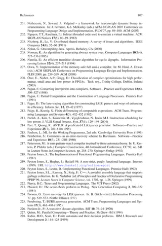


Modern Compiler Design 2e.pdf
- 1. Dick Grune • Kees van Reeuwijk • Henri E. Bal Modern Compiler Design Second Edition Ceriel J.H. Jacobs • Koen Langendoen
- 2. ISBN 978- - - -9 ISBN 978-1-4614-4699- DOI 10.1007/978- - Library of Congress Control Numb Printed on acid-free paper Springer is part of Springer Science+Business Media (www.springer.com) er: This work is subject to copyright. All rights are reserved by the Publisher, whether the whole or part of the material is concerned, specifically the rights of translation, reprinting, reuse of illustrations, recitation, broadcasting, reproduction on microfilms or in any other physical way, and transmission or information storage and retrieval, electronic adaptation, computer software, or by similar or dissimilar methodology now known or hereafter developed. Exempted from this legal reservation are brief excerpts in connection with reviews or scholarly analysis or material supplied specifically for the purpose of being entered and executed on a computer system, for exclusive use by the purchaser of the work. Duplication of this publication or parts thereof is permitted only unde Copyright Law of the Publisher’s location, in its current version, and permission for use must always be obtained from Springer. Permissions for use may be obtained through RightsLink at the Copyright Clearance Center. Violations are liable to prosecution under the respective Copyright Law. The use of general descriptive names, registered names, trademarks, service marks, etc. in thi does not imply, even in the absence of a specific statement, that such names are exemp protective laws and regulations and therefore free for general use. While the advice and information in this book are believed to be tru publication, neither the authors nor the editors nor the publisher can accept any legal responsibility for any errors or omissions that may be made. The publisher makes no warranty, express or implied, with respect to the material contained herein. r the provisions of the s publication t from the relevant e and accurate at the date of Springer New York Heidelberg Dordrecht London 1 4614 6 (eBook) 1 4614-4699-6 4698 © Springer Science+Business Media New York 2012 2012941168 Dick Grune Vrije Universiteit Amsterdam, The Netherlands Vrije Universiteit Amsterdam, The Netherlands Vrije Universiteit Amsterdam, The Netherlands Vrije Universiteit Amsterdam, The Netherlands Kees van Reeuwijk Henri E. Bal Ceriel J.H. Jacobs Koen Langendoen Delft University of Technology Delft, The Netherlands Additional material to this book can be downloaded from http://extras.springer.com.
- 3. Preface Twelve years have passed since the first edition of Modern Compiler Design. For many computer science subjects this would be more than a life time, but since com- piler design is probably the most mature computer science subject, it is different. An adult person develops more slowly and differently than a toddler or a teenager, and so does compiler design. The present book reflects that. Improvements to the book fall into two groups: presentation and content. The ‘look and feel’ of the book has been modernized, but more importantly we have rearranged significant parts of the book to present them in a more structured manner: large chapters have been split and the optimizing code generation techniques have been collected in a separate chapter. Based on reader feedback and experiences in teaching from this book, both by ourselves and others, material has been expanded, clarified, modified, or deleted in a large number of places. We hope that as a result of this the reader feels that the book does a better job of making compiler design and construction accessible. The book adds new material to cover the developments in compiler design and construction over the last twelve years. Overall the standard compiling techniques and paradigms have stood the test of time, but still new and often surprising opti- mization techniques have been invented; existing ones have been improved; and old ones have gained prominence. Examples of the first are: procedural abstraction, in which routines are recognized in the code and replaced by routine calls to reduce size; binary rewriting, in which optimizations are applied to the binary code; and just-in-time compilation, in which parts of the compilation are delayed to improve the perceived speed of the program. An example of the second is a technique which extends optimal code generation through exhaustive search, previously available for tiny blocks only, to moderate-size basic blocks. And an example of the third is tail recursion removal, indispensable for the compilation of functional languages. These developments are mainly described in Chapter 9. Although syntax analysis is the one but oldest branch of compiler construction (lexical analysis being the oldest), even in that area innovation has taken place. Generalized (non-deterministic) LR parsing, developed between 1984 and 1994, is now used in compilers. It is covered in Section 3.5.8. New hardware requirements have necessitated new compiler developments. The main examples are the need for size reduction of the object code, both to fit the code into small embedded systems and to reduce transmission times; and for lower power v
- 4. vi Preface consumption, to extend battery life and to reduce electricity bills. Dynamic memory allocation in embedded systems requires a balance between speed and thrift, and the question is how compiler design can help. These subjects are covered in Sections 9.2, 9.3, and 10.2.8, respectively. With age comes legacy. There is much legacy code around, code which is so old that it can no longer be modified and recompiled with reasonable effort. If the source code is still available but there is no compiler any more, recompilation must start with a grammar of the source code. For fifty years programmers and compiler designers have used grammars to produce and analyze programs; now large legacy programs are used to produce grammars for them. The recovery of the grammar from legacy source code is discussed in Section 3.6. If just the binary executable program is left, it must be disassembled or even decompiled. For fifty years com- piler designers have been called upon to design compilers and assemblers to convert source programs to binary code; now they are called upon to design disassemblers and decompilers, to roll back the assembly and compilation process. The required techniques are treated in Sections 8.4 and 8.5. The bibliography The literature list has been updated, but its usefulness is more limited than before, for two reasons. The first is that by the time it appears in print, the Internet can pro- vide more up-to-date and more to-the-point information, in larger quantities, than a printed text can hope to achieve. It is our contention that anybody who has under- stood a larger part of the ideas explained in this book is able to evaluate Internet information on compiler design. The second is that many of the papers we refer to are available only to those fortunate enough to have login facilities at an institute with sufficient budget to obtain subscriptions to the larger publishers; they are no longer available to just anyone who walks into a university library. Both phenomena point to paradigm shifts with which readers, authors, publishers and librarians will have to cope. The structure of the book This book is conceptually divided into two parts. The first, comprising Chapters 1 through 10, is concerned with techniques for program processing in general; it in- cludes a chapter on memory management, both in the compiler and in the generated code. The second part, Chapters 11 through 14, covers the specific techniques re- quired by the various programming paradigms. The interactions between the parts of the book are outlined in the adjacent table. The leftmost column shows the four phases of compiler construction: analysis, context handling, synthesis, and run-time systems. Chapters in this column cover both the manual and the automatic creation
- 5. Preface vii of the pertinent software but tend to emphasize automatic generation. The other columns show the four paradigms covered in this book; for each paradigm an ex- ample of a subject treated by each of the phases is shown. These chapters tend to contain manual techniques only, all automatic techniques having been delegated to Chapters 2 through 9. in imperative and object- oriented programs (Chapter 11) in functional programs (Chapter 12) in logic programs (Chapter 13) in parallel/ distributed programs (Chapter 14) How to do: analysis (Chapters 2 & 3) −− −− −− −− context handling (Chapters 4 & 5) identifier identification polymorphic type checking static rule matching Linda static analysis synthesis (Chapters 6–9) code for while- statement code for list comprehension structure unification marshaling run-time systems (no chapter) stack reduction machine Warren Abstract Machine replication The scientific mind would like the table to be nice and square, with all boxes filled —in short “orthogonal”— but we see that the top right entries are missing and that there is no chapter for “run-time systems” in the leftmost column. The top right entries would cover such things as the special subjects in the program text analysis of logic languages, but present text analysis techniques are powerful and flexible enough and languages similar enough to handle all language paradigms: there is nothing to be said there, for lack of problems. The chapter missing from the leftmost column would discuss manual and automatic techniques for creating run-time systems. Unfortunately there is little or no theory on this subject: run-time systems are still crafted by hand by programmers on an intuitive basis; there is nothing to be said there, for lack of solutions. Chapter 1 introduces the reader to compiler design by examining a simple tradi- tional modular compiler/interpreter in detail. Several high-level aspects of compiler construction are discussed, followed by a short history of compiler construction and introductions to formal grammars and closure algorithms. Chapters 2 and 3 treat the program text analysis phase of a compiler: the conver- sion of the program text to an abstract syntax tree. Techniques for lexical analysis, lexical identification of tokens, and syntax analysis are discussed. Chapters 4 and 5 cover the second phase of a compiler: context handling. Sev- eral methods of context handling are discussed: automated ones using attribute grammars, manual ones using L-attributed and S-attributed grammars, and semi- automated ones using symbolic interpretation and data-flow analysis.
- 6. viii Preface Chapters 6 through 9 cover the synthesis phase of a compiler, covering both in- terpretation and code generation. The chapters on code generation are mainly con- cerned with machine code generation; the intermediate code required for paradigm- specific constructs is treated in Chapters 11 through 14. Chapter 10 concerns memory management techniques, both for use in the com- piler and in the generated program. Chapters 11 through 14 address the special problems in compiling for the various paradigms – imperative, object-oriented, functional, logic, and parallel/distributed. Compilers for imperative and object-oriented programs are similar enough to be treated together in one chapter, Chapter 11. Appendix B contains hints and answers to a selection of the exercises in the book. Such exercises are marked by a followed the page number on which the answer appears. A larger set of answers can be found on Springer’s Internet page; the corresponding exercises are marked by www. Several subjects in this book are treated in a non-traditional way, and some words of justification may be in order. Lexical analysis is based on the same dotted items that are traditionally reserved for bottom-up syntax analysis, rather than on Thompson’s NFA construction. We see the dotted item as the essential tool in bottom-up pattern matching, unifying lexical analysis, LR syntax analysis, bottom-up code generation and peep-hole op- timization. The traditional lexical algorithms are just low-level implementations of item manipulation. We consider the different treatment of lexical and syntax analy- sis to be a historical artifact. Also, the difference between the lexical and the syntax levels tends to disappear in modern software. Considerable attention is being paid to attribute grammars, in spite of the fact that their impact on compiler design has been limited. Yet they are the only known way of automating context handling, and we hope that the present treatment will help to lower the threshold of their application. Functions as first-class data are covered in much greater depth in this book than is usual in compiler design books. After a good start in Algol 60, functions lost much status as manipulatable data in languages like C, Pascal, and Ada, although Ada 95 rehabilitated them somewhat. The implementation of some modern concepts, for example functional and logic languages, iterators, and continuations, however, requires functions to be manipulated as normal data. The fundamental aspects of the implementation are covered in the chapter on imperative and object-oriented languages; specifics are given in the chapters on the various other paradigms. Additional material, including more answers to exercises, and all diagrams and all code from the book, are available through Springer’s Internet page. Use as a course book The book contains far too much material for a compiler design course of 13 lectures of two hours each, as given at our university, so a selection has to be made. An
- 7. Preface ix introductory, more traditional course can be obtained by including, for example, Chapter 1; Chapter 2 up to 2.7; 2.10; 2.11; Chapter 3 up to 3.4.5; 3.5 up to 3.5.7; Chapter 4 up to 4.1.3; 4.2.1 up to 4.3; Chapter 5 up to 5.2.2; 5.3; Chapter 6; Chapter 7 up to 9.1.1; 9.1.4 up to 9.1.4.4; 7.3; Chapter 10 up to 10.1.2; 10.2 up to 10.2.4; Chapter 11 up to 11.2.3.2; 11.2.4 up to 11.2.10; 11.4 up to 11.4.2.3. A more advanced course would include all of Chapters 1 to 11, possibly exclud- ing Chapter 4. This could be augmented by one of Chapters 12 to 14. An advanced course would skip much of the introductory material and concen- trate on the parts omitted in the introductory course, Chapter 4 and all of Chapters 10 to 14. Acknowledgments We owe many thanks to the following people, who supplied us with help, remarks, wishes, and food for thought for this Second Edition: Ingmar Alting, José Fortes, Bert Huijben, Jonathan Joubert, Sara Kalvala, Frank Lippes, Paul S. Moulson, Pras- ant K. Patra, Carlo Perassi, Marco Rossi, Mooly Sagiv, Gert Jan Schoneveld, Ajay Singh, Evert Wattel, and Freek Zindel. Their input ranged from simple corrections to detailed suggestions to massive criticism. Special thanks go to Stefanie Scherzinger, whose thorough and thoughtful criticism of our outline code format induced us to improve it considerably; any remaining imperfections should be attributed to stub- bornness on the part of the authors. The presentation of the program code snippets in the book profited greatly from Carsten Heinz’s listings package; we thank him for making the package available to the public. We are grateful to Ann Kostant, Melissa Fearon, and Courtney Clark of Springer US, who, through fast and competent work, have cleared many obstacles that stood in the way of publishing this book. We thank them for their effort and pleasant cooperation. We mourn the death of Irina Athanasiu, who did not live long enough to lend her expertise in embedded systems to this book. We thank the Faculteit der Exacte Wetenschappen of the Vrije Universiteit for their support and the use of their equipment. Amsterdam, Dick Grune March 2012 Kees van Reeuwijk Henri E. Bal Ceriel J.H. Jacobs Delft, Koen G. Langendoen
- 8. x Preface Abridged Preface to the First Edition (2000) In the 1980s and 1990s, while the world was witnessing the rise of the PC and the Internet on the front pages of the daily newspapers, compiler design methods developed with less fanfare, developments seen mainly in the technical journals, and –more importantly– in the compilers that are used to process today’s software. These developments were driven partly by the advent of new programming paradigms, partly by a better understanding of code generation techniques, and partly by the introduction of faster machines with large amounts of memory. The field of programming languages has grown to include, besides the tradi- tional imperative paradigm, the object-oriented, functional, logical, and parallel/dis- tributed paradigms, which inspire novel compilation techniques and which often require more extensive run-time systems than do imperative languages. BURS tech- niques (Bottom-Up Rewriting Systems) have evolved into very powerful code gen- eration techniques which cope superbly with the complex machine instruction sets of present-day machines. And the speed and memory size of modern machines allow compilation techniques and programming language features that were unthinkable before. Modern compiler design methods meet these challenges head-on. The audience Our audience are students with enough experience to have at least used a compiler occasionally and to have given some thought to the concept of compilation. When these students leave the university, they will have to be familiar with language pro- cessors for each of the modern paradigms, using modern techniques. Although cur- riculum requirements in many universities may have been lagging behind in this respect, graduates entering the job market cannot afford to ignore these develop- ments. Experience has shown us that a considerable number of techniques traditionally taught in compiler construction are special cases of more fundamental techniques. Often these special techniques work for imperative languages only; the fundamental techniques have a much wider application. An example is the stack as an optimized representation for activation records in strictly last-in-first-out languages. Therefore, this book • focuses on principles and techniques of wide application, carefully distinguish- ing between the essential (= material that has a high chance of being useful to the student) and the incidental (= material that will benefit the student only in exceptional cases); • provides a first level of implementation details and optimizations; • augments the explanations by pointers for further study. The student, after having finished the book, can expect to:
- 9. Preface xi • have obtained a thorough understanding of the concepts of modern compiler de- sign and construction, and some familiarity with their practical application; • be able to start participating in the construction of a language processor for each of the modern paradigms with a minimal training period; • be able to read the literature. The first two provide a firm basis; the third provides potential for growth. Acknowledgments We owe many thanks to the following people, who were willing to spend time and effort on reading drafts of our book and to supply us with many useful and some- times very detailed comments: Mirjam Bakker, Raoul Bhoedjang, Wilfred Dittmer, Thomer M. Gil, Ben N. Hasnai, Bert Huijben, Jaco A. Imthorn, John Romein, Tim Rühl, and the anonymous reviewers. We thank Ronald Veldema for the Pentium code segments. We are grateful to Simon Plumtree, Gaynor Redvers-Mutton, Dawn Booth, and Jane Kerr of John Wiley Sons Ltd, for their help and encouragement in writing this book. Lambert Meertens kindly provided information on an older ABC com- piler, and Ralph Griswold on an Icon compiler. We thank the Faculteit Wiskunde en Informatica (now part of the Faculteit der Exacte Wetenschappen) of the Vrije Universiteit for their support and the use of their equipment. Dick Grune dick@cs.vu.nl, http://www.cs.vu.nl/~dick Henri E. Bal bal@cs.vu.nl, http://www.cs.vu.nl/~bal Ceriel J.H. Jacobs ceriel@cs.vu.nl, http://www.cs.vu.nl/~ceriel Koen G. Langendoen koen@pds.twi.tudelft.nl, http://pds.twi.tudelft.nl/~koen Amsterdam, May 2000
- 11. Contents 1 Introduction . . . . . . . . . . . . . . . . . . . . . . . . . . . . . . . . . . . . . . . . . . . . . . . . . . . 1 1.1 Why study compiler construction? . . . . . . . . . . . . . . . . . . . . . . . . . . . . 5 1.1.1 Compiler construction is very successful . . . . . . . . . . . . . . . . . 6 1.1.2 Compiler construction has a wide applicability . . . . . . . . . . . 8 1.1.3 Compilers contain generally useful algorithms . . . . . . . . . . . . 9 1.2 A simple traditional modular compiler/interpreter. . . . . . . . . . . . . . . . 9 1.2.1 The abstract syntax tree . . . . . . . . . . . . . . . . . . . . . . . . . . . . . . . 9 1.2.2 Structure of the demo compiler. . . . . . . . . . . . . . . . . . . . . . . . . 12 1.2.3 The language for the demo compiler . . . . . . . . . . . . . . . . . . . . 13 1.2.4 Lexical analysis for the demo compiler . . . . . . . . . . . . . . . . . . 14 1.2.5 Syntax analysis for the demo compiler . . . . . . . . . . . . . . . . . . 15 1.2.6 Context handling for the demo compiler . . . . . . . . . . . . . . . . . 20 1.2.7 Code generation for the demo compiler . . . . . . . . . . . . . . . . . . 20 1.2.8 Interpretation for the demo compiler . . . . . . . . . . . . . . . . . . . . 21 1.3 The structure of a more realistic compiler . . . . . . . . . . . . . . . . . . . . . . 22 1.3.1 The structure . . . . . . . . . . . . . . . . . . . . . . . . . . . . . . . . . . . . . . . . 23 1.3.2 Run-time systems . . . . . . . . . . . . . . . . . . . . . . . . . . . . . . . . . . . . 25 1.3.3 Short-cuts . . . . . . . . . . . . . . . . . . . . . . . . . . . . . . . . . . . . . . . . . . 26 1.4 Compiler architectures . . . . . . . . . . . . . . . . . . . . . . . . . . . . . . . . . . . . . . 26 1.4.1 The width of the compiler . . . . . . . . . . . . . . . . . . . . . . . . . . . . . 26 1.4.2 Who’s the boss? . . . . . . . . . . . . . . . . . . . . . . . . . . . . . . . . . . . . . 28 1.5 Properties of a good compiler . . . . . . . . . . . . . . . . . . . . . . . . . . . . . . . . 31 1.6 Portability and retargetability . . . . . . . . . . . . . . . . . . . . . . . . . . . . . . . . . 32 1.7 A short history of compiler construction . . . . . . . . . . . . . . . . . . . . . . . 33 1.7.1 1945–1960: code generation . . . . . . . . . . . . . . . . . . . . . . . . . . . 33 1.7.2 1960–1975: parsing . . . . . . . . . . . . . . . . . . . . . . . . . . . . . . . . . . 33 1.7.3 1975–present: code generation and code optimization; paradigms . . . . . . . . . . . . . . . . . . . . . . . . . . . . . . . . . . . . . . . . . . 34 1.8 Grammars. . . . . . . . . . . . . . . . . . . . . . . . . . . . . . . . . . . . . . . . . . . . . . . . . 34 1.8.1 The form of a grammar . . . . . . . . . . . . . . . . . . . . . . . . . . . . . . . 35 1.8.2 The grammatical production process . . . . . . . . . . . . . . . . . . . . 36 xiii
- 12. xiv Contents 1.8.3 Extended forms of grammars . . . . . . . . . . . . . . . . . . . . . . . . . . 37 1.8.4 Properties of grammars . . . . . . . . . . . . . . . . . . . . . . . . . . . . . . . 38 1.8.5 The grammar formalism . . . . . . . . . . . . . . . . . . . . . . . . . . . . . . 39 1.9 Closure algorithms . . . . . . . . . . . . . . . . . . . . . . . . . . . . . . . . . . . . . . . . . 41 1.9.1 A sample problem . . . . . . . . . . . . . . . . . . . . . . . . . . . . . . . . . . . 41 1.9.2 The components of a closure algorithm . . . . . . . . . . . . . . . . . . 43 1.9.3 An iterative implementation of the closure algorithm . . . . . . 44 1.10 The code forms used in this book . . . . . . . . . . . . . . . . . . . . . . . . . . . . . 46 1.11 Conclusion . . . . . . . . . . . . . . . . . . . . . . . . . . . . . . . . . . . . . . . . . . . . . . . . 47 Part I From Program Text to Abstract Syntax Tree 2 Program Text to Tokens — Lexical Analysis . . . . . . . . . . . . . . . . . . . . . . . 55 2.1 Reading the program text . . . . . . . . . . . . . . . . . . . . . . . . . . . . . . . . . . . . 59 2.1.1 Obtaining and storing the text . . . . . . . . . . . . . . . . . . . . . . . . . . 59 2.1.2 The troublesome newline. . . . . . . . . . . . . . . . . . . . . . . . . . . . . . 60 2.2 Lexical versus syntactic analysis . . . . . . . . . . . . . . . . . . . . . . . . . . . . . . 61 2.3 Regular expressions and regular descriptions . . . . . . . . . . . . . . . . . . . . 61 2.3.1 Regular expressions and BNF/EBNF . . . . . . . . . . . . . . . . . . . . 63 2.3.2 Escape characters in regular expressions . . . . . . . . . . . . . . . . . 63 2.3.3 Regular descriptions . . . . . . . . . . . . . . . . . . . . . . . . . . . . . . . . . . 63 2.4 Lexical analysis . . . . . . . . . . . . . . . . . . . . . . . . . . . . . . . . . . . . . . . . . . . . 64 2.5 Creating a lexical analyzer by hand . . . . . . . . . . . . . . . . . . . . . . . . . . . . 65 2.5.1 Optimization by precomputation . . . . . . . . . . . . . . . . . . . . . . . 70 2.6 Creating a lexical analyzer automatically . . . . . . . . . . . . . . . . . . . . . . . 73 2.6.1 Dotted items . . . . . . . . . . . . . . . . . . . . . . . . . . . . . . . . . . . . . . . . 74 2.6.2 Concurrent search. . . . . . . . . . . . . . . . . . . . . . . . . . . . . . . . . . . . 79 2.6.3 Precomputing the item sets . . . . . . . . . . . . . . . . . . . . . . . . . . . . 83 2.6.4 The final lexical analyzer . . . . . . . . . . . . . . . . . . . . . . . . . . . . . . 86 2.6.5 Complexity of generating a lexical analyzer . . . . . . . . . . . . . . 87 2.6.6 Transitions to Sω . . . . . . . . . . . . . . . . . . . . . . . . . . . . . . . . . . . . . 87 2.6.7 Complexity of using a lexical analyzer . . . . . . . . . . . . . . . . . . 88 2.7 Transition table compression . . . . . . . . . . . . . . . . . . . . . . . . . . . . . . . . . 89 2.7.1 Table compression by row displacement . . . . . . . . . . . . . . . . . 90 2.7.2 Table compression by graph coloring. . . . . . . . . . . . . . . . . . . . 93 2.8 Error handling in lexical analyzers . . . . . . . . . . . . . . . . . . . . . . . . . . . . 95 2.9 A traditional lexical analyzer generator—lex . . . . . . . . . . . . . . . . . . . . 96 2.10 Lexical identification of tokens . . . . . . . . . . . . . . . . . . . . . . . . . . . . . . . 99 2.11 Symbol tables . . . . . . . . . . . . . . . . . . . . . . . . . . . . . . . . . . . . . . . . . . . . . 101 2.12 Macro processing and file inclusion . . . . . . . . . . . . . . . . . . . . . . . . . . . 102 2.12.1 The input buffer stack . . . . . . . . . . . . . . . . . . . . . . . . . . . . . . . . 104 2.12.2 Conditional text inclusion . . . . . . . . . . . . . . . . . . . . . . . . . . . . . 107 2.12.3 Generics by controlled macro processing . . . . . . . . . . . . . . . . 108 2.13 Conclusion . . . . . . . . . . . . . . . . . . . . . . . . . . . . . . . . . . . . . . . . . . . . . . . . 109
- 13. Contents xv 3 Tokens to Syntax Tree — Syntax Analysis . . . . . . . . . . . . . . . . . . . . . . . . . 115 3.1 Two classes of parsing methods . . . . . . . . . . . . . . . . . . . . . . . . . . . . . . . 117 3.1.1 Principles of top-down parsing . . . . . . . . . . . . . . . . . . . . . . . . . 117 3.1.2 Principles of bottom-up parsing . . . . . . . . . . . . . . . . . . . . . . . . 119 3.2 Error detection and error recovery . . . . . . . . . . . . . . . . . . . . . . . . . . . . . 120 3.3 Creating a top-down parser manually . . . . . . . . . . . . . . . . . . . . . . . . . . 122 3.3.1 Recursive descent parsing . . . . . . . . . . . . . . . . . . . . . . . . . . . . . 122 3.3.2 Disadvantages of recursive descent parsing . . . . . . . . . . . . . . . 124 3.4 Creating a top-down parser automatically . . . . . . . . . . . . . . . . . . . . . . 126 3.4.1 LL(1) parsing . . . . . . . . . . . . . . . . . . . . . . . . . . . . . . . . . . . . . . . 126 3.4.2 LL(1) conflicts as an asset . . . . . . . . . . . . . . . . . . . . . . . . . . . . . 132 3.4.3 LL(1) conflicts as a liability . . . . . . . . . . . . . . . . . . . . . . . . . . . 133 3.4.4 The LL(1) push-down automaton . . . . . . . . . . . . . . . . . . . . . . . 139 3.4.5 Error handling in LL parsers . . . . . . . . . . . . . . . . . . . . . . . . . . . 143 3.4.6 A traditional top-down parser generator—LLgen . . . . . . . . . . 148 3.5 Creating a bottom-up parser automatically . . . . . . . . . . . . . . . . . . . . . . 156 3.5.1 LR(0) parsing . . . . . . . . . . . . . . . . . . . . . . . . . . . . . . . . . . . . . . . 159 3.5.2 The LR push-down automaton . . . . . . . . . . . . . . . . . . . . . . . . . 166 3.5.3 LR(0) conflicts . . . . . . . . . . . . . . . . . . . . . . . . . . . . . . . . . . . . . . 167 3.5.4 SLR(1) parsing . . . . . . . . . . . . . . . . . . . . . . . . . . . . . . . . . . . . . . 169 3.5.5 LR(1) parsing . . . . . . . . . . . . . . . . . . . . . . . . . . . . . . . . . . . . . . . 171 3.5.6 LALR(1) parsing . . . . . . . . . . . . . . . . . . . . . . . . . . . . . . . . . . . . 176 3.5.7 Making a grammar (LA)LR(1)—or not . . . . . . . . . . . . . . . . . . 178 3.5.8 Generalized LR parsing . . . . . . . . . . . . . . . . . . . . . . . . . . . . . . . 181 3.5.9 Making a grammar unambiguous . . . . . . . . . . . . . . . . . . . . . . . 185 3.5.10 Error handling in LR parsers . . . . . . . . . . . . . . . . . . . . . . . . . . . 188 3.5.11 A traditional bottom-up parser generator—yacc/bison. . . . . . 191 3.6 Recovering grammars from legacy code . . . . . . . . . . . . . . . . . . . . . . . . 193 3.7 Conclusion . . . . . . . . . . . . . . . . . . . . . . . . . . . . . . . . . . . . . . . . . . . . . . . . 199 Part II Annotating the Abstract Syntax Tree 4 Grammar-based Context Handling. . . . . . . . . . . . . . . . . . . . . . . . . . . . . . . 209 4.1 Attribute grammars . . . . . . . . . . . . . . . . . . . . . . . . . . . . . . . . . . . . . . . . . 210 4.1.1 The attribute evaluator . . . . . . . . . . . . . . . . . . . . . . . . . . . . . . . . 212 4.1.2 Dependency graphs . . . . . . . . . . . . . . . . . . . . . . . . . . . . . . . . . . 215 4.1.3 Attribute evaluation . . . . . . . . . . . . . . . . . . . . . . . . . . . . . . . . . . 217 4.1.4 Attribute allocation. . . . . . . . . . . . . . . . . . . . . . . . . . . . . . . . . . . 232 4.1.5 Multi-visit attribute grammars . . . . . . . . . . . . . . . . . . . . . . . . . 232 4.1.6 Summary of the types of attribute grammars. . . . . . . . . . . . . . 244 4.2 Restricted attribute grammars . . . . . . . . . . . . . . . . . . . . . . . . . . . . . . . . 245 4.2.1 L-attributed grammars . . . . . . . . . . . . . . . . . . . . . . . . . . . . . . . . 245 4.2.2 S-attributed grammars . . . . . . . . . . . . . . . . . . . . . . . . . . . . . . . . 250 4.2.3 Equivalence of L-attributed and S-attributed grammars . . . . . 250 4.3 Extended grammar notations and attribute grammars . . . . . . . . . . . . . 252
- 14. xvi Contents 4.4 Conclusion . . . . . . . . . . . . . . . . . . . . . . . . . . . . . . . . . . . . . . . . . . . . . . . . 253 5 Manual Context Handling . . . . . . . . . . . . . . . . . . . . . . . . . . . . . . . . . . . . . . 261 5.1 Threading the AST . . . . . . . . . . . . . . . . . . . . . . . . . . . . . . . . . . . . . . . . . 262 5.2 Symbolic interpretation . . . . . . . . . . . . . . . . . . . . . . . . . . . . . . . . . . . . . 267 5.2.1 Simple symbolic interpretation . . . . . . . . . . . . . . . . . . . . . . . . . 270 5.2.2 Full symbolic interpretation . . . . . . . . . . . . . . . . . . . . . . . . . . . 273 5.2.3 Last-def analysis . . . . . . . . . . . . . . . . . . . . . . . . . . . . . . . . . . . . . 275 5.3 Data-flow equations . . . . . . . . . . . . . . . . . . . . . . . . . . . . . . . . . . . . . . . . 276 5.3.1 Setting up the data-flow equations . . . . . . . . . . . . . . . . . . . . . . 277 5.3.2 Solving the data-flow equations . . . . . . . . . . . . . . . . . . . . . . . . 280 5.4 Interprocedural data-flow analysis . . . . . . . . . . . . . . . . . . . . . . . . . . . . . 283 5.5 Carrying the information upstream—live analysis . . . . . . . . . . . . . . . 285 5.5.1 Live analysis by symbolic interpretation . . . . . . . . . . . . . . . . . 286 5.5.2 Live analysis by data-flow equations . . . . . . . . . . . . . . . . . . . . 288 5.6 Symbolic interpretation versus data-flow equations . . . . . . . . . . . . . . 291 5.7 Conclusion . . . . . . . . . . . . . . . . . . . . . . . . . . . . . . . . . . . . . . . . . . . . . . . . 292 Part III Processing the Intermediate Code 6 Interpretation . . . . . . . . . . . . . . . . . . . . . . . . . . . . . . . . . . . . . . . . . . . . . . . . . 299 6.1 Interpreters . . . . . . . . . . . . . . . . . . . . . . . . . . . . . . . . . . . . . . . . . . . . . . . . 301 6.2 Recursive interpreters . . . . . . . . . . . . . . . . . . . . . . . . . . . . . . . . . . . . . . . 301 6.3 Iterative interpreters . . . . . . . . . . . . . . . . . . . . . . . . . . . . . . . . . . . . . . . . 305 6.4 Conclusion . . . . . . . . . . . . . . . . . . . . . . . . . . . . . . . . . . . . . . . . . . . . . . . . 310 7 Code Generation . . . . . . . . . . . . . . . . . . . . . . . . . . . . . . . . . . . . . . . . . . . . . . . 313 7.1 Properties of generated code . . . . . . . . . . . . . . . . . . . . . . . . . . . . . . . . . 313 7.1.1 Correctness . . . . . . . . . . . . . . . . . . . . . . . . . . . . . . . . . . . . . . . . . 314 7.1.2 Speed . . . . . . . . . . . . . . . . . . . . . . . . . . . . . . . . . . . . . . . . . . . . . . 314 7.1.3 Size . . . . . . . . . . . . . . . . . . . . . . . . . . . . . . . . . . . . . . . . . . . . . . . 315 7.1.4 Power consumption . . . . . . . . . . . . . . . . . . . . . . . . . . . . . . . . . . 315 7.1.5 About optimizations . . . . . . . . . . . . . . . . . . . . . . . . . . . . . . . . . . 316 7.2 Introduction to code generation . . . . . . . . . . . . . . . . . . . . . . . . . . . . . . . 317 7.2.1 The structure of code generation. . . . . . . . . . . . . . . . . . . . . . . . 319 7.2.2 The structure of the code generator . . . . . . . . . . . . . . . . . . . . . 320 7.3 Preprocessing the intermediate code . . . . . . . . . . . . . . . . . . . . . . . . . . . 321 7.3.1 Preprocessing of expressions . . . . . . . . . . . . . . . . . . . . . . . . . . 322 7.3.2 Preprocessing of if-statements and goto statements . . . . . . . . 323 7.3.3 Preprocessing of routines. . . . . . . . . . . . . . . . . . . . . . . . . . . . . . 323 7.3.4 Procedural abstraction . . . . . . . . . . . . . . . . . . . . . . . . . . . . . . . . 326 7.4 Avoiding code generation altogether . . . . . . . . . . . . . . . . . . . . . . . . . . . 328 7.5 Code generation proper. . . . . . . . . . . . . . . . . . . . . . . . . . . . . . . . . . . . . . 329 7.5.1 Trivial code generation . . . . . . . . . . . . . . . . . . . . . . . . . . . . . . . 330 7.5.2 Simple code generation . . . . . . . . . . . . . . . . . . . . . . . . . . . . . . . 335 7.6 Postprocessing the generated code . . . . . . . . . . . . . . . . . . . . . . . . . . . . 349
- 15. Contents xvii 7.6.1 Peephole optimization . . . . . . . . . . . . . . . . . . . . . . . . . . . . . . . . 349 7.6.2 Procedural abstraction of assembly code . . . . . . . . . . . . . . . . . 353 7.7 Machine code generation . . . . . . . . . . . . . . . . . . . . . . . . . . . . . . . . . . . . 355 7.8 Conclusion . . . . . . . . . . . . . . . . . . . . . . . . . . . . . . . . . . . . . . . . . . . . . . . . 356 8 Assemblers, Disassemblers, Linkers, and Loaders. . . . . . . . . . . . . . . . . . 363 8.1 The tasks of an assembler . . . . . . . . . . . . . . . . . . . . . . . . . . . . . . . . . . . . 363 8.1.1 The running program . . . . . . . . . . . . . . . . . . . . . . . . . . . . . . . . . 363 8.1.2 The executable code file . . . . . . . . . . . . . . . . . . . . . . . . . . . . . . 364 8.1.3 Object files and linkage . . . . . . . . . . . . . . . . . . . . . . . . . . . . . . . 364 8.1.4 Alignment requirements and endianness . . . . . . . . . . . . . . . . . 366 8.2 Assembler design issues . . . . . . . . . . . . . . . . . . . . . . . . . . . . . . . . . . . . . 367 8.2.1 Handling internal addresses. . . . . . . . . . . . . . . . . . . . . . . . . . . . 368 8.2.2 Handling external addresses . . . . . . . . . . . . . . . . . . . . . . . . . . . 370 8.3 Linker design issues . . . . . . . . . . . . . . . . . . . . . . . . . . . . . . . . . . . . . . . . 371 8.4 Disassembly . . . . . . . . . . . . . . . . . . . . . . . . . . . . . . . . . . . . . . . . . . . . . . . 372 8.4.1 Distinguishing between instructions and data . . . . . . . . . . . . . 372 8.4.2 Disassembly with indirection . . . . . . . . . . . . . . . . . . . . . . . . . . 374 8.4.3 Disassembly with relocation information . . . . . . . . . . . . . . . . 377 8.5 Decompilation . . . . . . . . . . . . . . . . . . . . . . . . . . . . . . . . . . . . . . . . . . . . . 377 8.6 Conclusion . . . . . . . . . . . . . . . . . . . . . . . . . . . . . . . . . . . . . . . . . . . . . . . . 382 9 Optimization Techniques. . . . . . . . . . . . . . . . . . . . . . . . . . . . . . . . . . . . . . . . 385 9.1 General optimization. . . . . . . . . . . . . . . . . . . . . . . . . . . . . . . . . . . . . . . . 386 9.1.1 Compilation by symbolic interpretation. . . . . . . . . . . . . . . . . . 386 9.1.2 Code generation for basic blocks . . . . . . . . . . . . . . . . . . . . . . . 388 9.1.3 Almost optimal code generation . . . . . . . . . . . . . . . . . . . . . . . . 405 9.1.4 BURS code generation and dynamic programming . . . . . . . . 406 9.1.5 Register allocation by graph coloring. . . . . . . . . . . . . . . . . . . . 427 9.1.6 Supercompilation . . . . . . . . . . . . . . . . . . . . . . . . . . . . . . . . . . . . 432 9.1.7 Evaluation of code generation techniques . . . . . . . . . . . . . . . . 433 9.1.8 Debugging of code optimizers . . . . . . . . . . . . . . . . . . . . . . . . . 434 9.2 Code size reduction . . . . . . . . . . . . . . . . . . . . . . . . . . . . . . . . . . . . . . . . . 436 9.2.1 General code size reduction techniques . . . . . . . . . . . . . . . . . . 436 9.2.2 Code compression . . . . . . . . . . . . . . . . . . . . . . . . . . . . . . . . . . . 437 9.2.3 Discussion . . . . . . . . . . . . . . . . . . . . . . . . . . . . . . . . . . . . . . . . . . 442 9.3 Power reduction and energy saving . . . . . . . . . . . . . . . . . . . . . . . . . . . . 443 9.3.1 Just compiling for speed . . . . . . . . . . . . . . . . . . . . . . . . . . . . . . 445 9.3.2 Trading speed for power . . . . . . . . . . . . . . . . . . . . . . . . . . . . . . 445 9.3.3 Instruction scheduling and bit switching . . . . . . . . . . . . . . . . . 446 9.3.4 Register relabeling . . . . . . . . . . . . . . . . . . . . . . . . . . . . . . . . . . . 448 9.3.5 Avoiding the dynamic scheduler . . . . . . . . . . . . . . . . . . . . . . . . 449 9.3.6 Domain-specific optimizations . . . . . . . . . . . . . . . . . . . . . . . . . 449 9.3.7 Discussion . . . . . . . . . . . . . . . . . . . . . . . . . . . . . . . . . . . . . . . . . . 450 9.4 Just-In-Time compilation . . . . . . . . . . . . . . . . . . . . . . . . . . . . . . . . . . . . 450
- 16. xviii Contents 9.5 Compilers versus computer architectures . . . . . . . . . . . . . . . . . . . . . . . 451 9.6 Conclusion . . . . . . . . . . . . . . . . . . . . . . . . . . . . . . . . . . . . . . . . . . . . . . . . 452 Part IV Memory Management 10 Explicit and Implicit Memory Management . . . . . . . . . . . . . . . . . . . . . . . 463 10.1 Data allocation with explicit deallocation . . . . . . . . . . . . . . . . . . . . . . . 465 10.1.1 Basic memory allocation . . . . . . . . . . . . . . . . . . . . . . . . . . . . . . 466 10.1.2 Optimizations for basic memory allocation . . . . . . . . . . . . . . . 469 10.1.3 Compiler applications of basic memory allocation . . . . . . . . . 471 10.1.4 Embedded-systems considerations . . . . . . . . . . . . . . . . . . . . . . 475 10.2 Data allocation with implicit deallocation . . . . . . . . . . . . . . . . . . . . . . 476 10.2.1 Basic garbage collection algorithms . . . . . . . . . . . . . . . . . . . . . 476 10.2.2 Preparing the ground . . . . . . . . . . . . . . . . . . . . . . . . . . . . . . . . . 478 10.2.3 Reference counting. . . . . . . . . . . . . . . . . . . . . . . . . . . . . . . . . . . 485 10.2.4 Mark and scan. . . . . . . . . . . . . . . . . . . . . . . . . . . . . . . . . . . . . . . 489 10.2.5 Two-space copying . . . . . . . . . . . . . . . . . . . . . . . . . . . . . . . . . . . 494 10.2.6 Compaction . . . . . . . . . . . . . . . . . . . . . . . . . . . . . . . . . . . . . . . . . 496 10.2.7 Generational garbage collection . . . . . . . . . . . . . . . . . . . . . . . . 498 10.2.8 Implicit deallocation in embedded systems . . . . . . . . . . . . . . . 500 10.3 Conclusion . . . . . . . . . . . . . . . . . . . . . . . . . . . . . . . . . . . . . . . . . . . . . . . . 501 Part V From Abstract Syntax Tree to Intermediate Code 11 Imperative and Object-Oriented Programs . . . . . . . . . . . . . . . . . . . . . . . 511 11.1 Context handling . . . . . . . . . . . . . . . . . . . . . . . . . . . . . . . . . . . . . . . . . . . 513 11.1.1 Identification . . . . . . . . . . . . . . . . . . . . . . . . . . . . . . . . . . . . . . . . 514 11.1.2 Type checking . . . . . . . . . . . . . . . . . . . . . . . . . . . . . . . . . . . . . . . 521 11.1.3 Discussion . . . . . . . . . . . . . . . . . . . . . . . . . . . . . . . . . . . . . . . . . . 532 11.2 Source language data representation and handling . . . . . . . . . . . . . . . 532 11.2.1 Basic types . . . . . . . . . . . . . . . . . . . . . . . . . . . . . . . . . . . . . . . . . 532 11.2.2 Enumeration types . . . . . . . . . . . . . . . . . . . . . . . . . . . . . . . . . . . 533 11.2.3 Pointer types . . . . . . . . . . . . . . . . . . . . . . . . . . . . . . . . . . . . . . . . 533 11.2.4 Record types . . . . . . . . . . . . . . . . . . . . . . . . . . . . . . . . . . . . . . . . 538 11.2.5 Union types . . . . . . . . . . . . . . . . . . . . . . . . . . . . . . . . . . . . . . . . . 539 11.2.6 Array types . . . . . . . . . . . . . . . . . . . . . . . . . . . . . . . . . . . . . . . . . 540 11.2.7 Set types . . . . . . . . . . . . . . . . . . . . . . . . . . . . . . . . . . . . . . . . . . . 543 11.2.8 Routine types . . . . . . . . . . . . . . . . . . . . . . . . . . . . . . . . . . . . . . . 544 11.2.9 Object types . . . . . . . . . . . . . . . . . . . . . . . . . . . . . . . . . . . . . . . . 544 11.2.10Interface types. . . . . . . . . . . . . . . . . . . . . . . . . . . . . . . . . . . . . . . 554 11.3 Routines and their activation . . . . . . . . . . . . . . . . . . . . . . . . . . . . . . . . . 555 11.3.1 Activation records . . . . . . . . . . . . . . . . . . . . . . . . . . . . . . . . . . . 556 11.3.2 The contents of an activation record . . . . . . . . . . . . . . . . . . . . . 557 11.3.3 Routines. . . . . . . . . . . . . . . . . . . . . . . . . . . . . . . . . . . . . . . . . . . . 559 11.3.4 Operations on routines . . . . . . . . . . . . . . . . . . . . . . . . . . . . . . . . 562
- 17. Contents xix 11.3.5 Non-nested routines . . . . . . . . . . . . . . . . . . . . . . . . . . . . . . . . . . 564 11.3.6 Nested routines . . . . . . . . . . . . . . . . . . . . . . . . . . . . . . . . . . . . . . 566 11.3.7 Lambda lifting . . . . . . . . . . . . . . . . . . . . . . . . . . . . . . . . . . . . . . 573 11.3.8 Iterators and coroutines . . . . . . . . . . . . . . . . . . . . . . . . . . . . . . . 576 11.4 Code generation for control flow statements . . . . . . . . . . . . . . . . . . . . 576 11.4.1 Local flow of control . . . . . . . . . . . . . . . . . . . . . . . . . . . . . . . . . 577 11.4.2 Routine invocation . . . . . . . . . . . . . . . . . . . . . . . . . . . . . . . . . . . 587 11.4.3 Run-time error handling . . . . . . . . . . . . . . . . . . . . . . . . . . . . . . 597 11.5 Code generation for modules . . . . . . . . . . . . . . . . . . . . . . . . . . . . . . . . . 601 11.5.1 Name generation. . . . . . . . . . . . . . . . . . . . . . . . . . . . . . . . . . . . . 602 11.5.2 Module initialization . . . . . . . . . . . . . . . . . . . . . . . . . . . . . . . . . 602 11.5.3 Code generation for generics. . . . . . . . . . . . . . . . . . . . . . . . . . . 604 11.6 Conclusion . . . . . . . . . . . . . . . . . . . . . . . . . . . . . . . . . . . . . . . . . . . . . . . . 606 12 Functional Programs . . . . . . . . . . . . . . . . . . . . . . . . . . . . . . . . . . . . . . . . . . . 617 12.1 A short tour of Haskell . . . . . . . . . . . . . . . . . . . . . . . . . . . . . . . . . . . . . . 619 12.1.1 Offside rule . . . . . . . . . . . . . . . . . . . . . . . . . . . . . . . . . . . . . . . . . 619 12.1.2 Lists . . . . . . . . . . . . . . . . . . . . . . . . . . . . . . . . . . . . . . . . . . . . . . . 620 12.1.3 List comprehension . . . . . . . . . . . . . . . . . . . . . . . . . . . . . . . . . . 621 12.1.4 Pattern matching . . . . . . . . . . . . . . . . . . . . . . . . . . . . . . . . . . . . . 622 12.1.5 Polymorphic typing . . . . . . . . . . . . . . . . . . . . . . . . . . . . . . . . . . 623 12.1.6 Referential transparency . . . . . . . . . . . . . . . . . . . . . . . . . . . . . . 624 12.1.7 Higher-order functions . . . . . . . . . . . . . . . . . . . . . . . . . . . . . . . . 625 12.1.8 Lazy evaluation. . . . . . . . . . . . . . . . . . . . . . . . . . . . . . . . . . . . . . 627 12.2 Compiling functional languages . . . . . . . . . . . . . . . . . . . . . . . . . . . . . . 628 12.2.1 The compiler structure . . . . . . . . . . . . . . . . . . . . . . . . . . . . . . . . 628 12.2.2 The functional core . . . . . . . . . . . . . . . . . . . . . . . . . . . . . . . . . . 630 12.3 Polymorphic type checking . . . . . . . . . . . . . . . . . . . . . . . . . . . . . . . . . . 631 12.4 Desugaring . . . . . . . . . . . . . . . . . . . . . . . . . . . . . . . . . . . . . . . . . . . . . . . . 633 12.4.1 The translation of lists . . . . . . . . . . . . . . . . . . . . . . . . . . . . . . . . 634 12.4.2 The translation of pattern matching . . . . . . . . . . . . . . . . . . . . . 634 12.4.3 The translation of list comprehension . . . . . . . . . . . . . . . . . . . 637 12.4.4 The translation of nested functions . . . . . . . . . . . . . . . . . . . . . . 639 12.5 Graph reduction . . . . . . . . . . . . . . . . . . . . . . . . . . . . . . . . . . . . . . . . . . . . 641 12.5.1 Reduction order . . . . . . . . . . . . . . . . . . . . . . . . . . . . . . . . . . . . . 645 12.5.2 The reduction engine . . . . . . . . . . . . . . . . . . . . . . . . . . . . . . . . . 647 12.6 Code generation for functional core programs . . . . . . . . . . . . . . . . . . . 651 12.6.1 Avoiding the construction of some application spines . . . . . . 653 12.7 Optimizing the functional core . . . . . . . . . . . . . . . . . . . . . . . . . . . . . . . 655 12.7.1 Strictness analysis . . . . . . . . . . . . . . . . . . . . . . . . . . . . . . . . . . . 656 12.7.2 Boxing analysis . . . . . . . . . . . . . . . . . . . . . . . . . . . . . . . . . . . . . 662 12.7.3 Tail calls . . . . . . . . . . . . . . . . . . . . . . . . . . . . . . . . . . . . . . . . . . . 663 12.7.4 Accumulator transformation . . . . . . . . . . . . . . . . . . . . . . . . . . . 664 12.7.5 Limitations . . . . . . . . . . . . . . . . . . . . . . . . . . . . . . . . . . . . . . . . . 666 12.8 Advanced graph manipulation . . . . . . . . . . . . . . . . . . . . . . . . . . . . . . . . 667
- 18. xx Contents 12.8.1 Variable-length nodes. . . . . . . . . . . . . . . . . . . . . . . . . . . . . . . . . 667 12.8.2 Pointer tagging . . . . . . . . . . . . . . . . . . . . . . . . . . . . . . . . . . . . . . 667 12.8.3 Aggregate node allocation . . . . . . . . . . . . . . . . . . . . . . . . . . . . . 668 12.8.4 Vector apply nodes . . . . . . . . . . . . . . . . . . . . . . . . . . . . . . . . . . . 668 12.9 Conclusion . . . . . . . . . . . . . . . . . . . . . . . . . . . . . . . . . . . . . . . . . . . . . . . . 669 13 Logic Programs . . . . . . . . . . . . . . . . . . . . . . . . . . . . . . . . . . . . . . . . . . . . . . . . 677 13.1 The logic programming model. . . . . . . . . . . . . . . . . . . . . . . . . . . . . . . . 679 13.1.1 The building blocks . . . . . . . . . . . . . . . . . . . . . . . . . . . . . . . . . . 679 13.1.2 The inference mechanism . . . . . . . . . . . . . . . . . . . . . . . . . . . . . 681 13.2 The general implementation model, interpreted. . . . . . . . . . . . . . . . . . 682 13.2.1 The interpreter instructions . . . . . . . . . . . . . . . . . . . . . . . . . . . . 684 13.2.2 Avoiding redundant goal lists . . . . . . . . . . . . . . . . . . . . . . . . . . 687 13.2.3 Avoiding copying goal list tails. . . . . . . . . . . . . . . . . . . . . . . . . 687 13.3 Unification . . . . . . . . . . . . . . . . . . . . . . . . . . . . . . . . . . . . . . . . . . . . . . . . 688 13.3.1 Unification of structures, lists, and sets . . . . . . . . . . . . . . . . . . 688 13.3.2 The implementation of unification . . . . . . . . . . . . . . . . . . . . . . 691 13.3.3 Unification of two unbound variables . . . . . . . . . . . . . . . . . . . 694 13.4 The general implementation model, compiled . . . . . . . . . . . . . . . . . . . 696 13.4.1 List procedures . . . . . . . . . . . . . . . . . . . . . . . . . . . . . . . . . . . . . . 697 13.4.2 Compiled clause search and unification . . . . . . . . . . . . . . . . . . 699 13.4.3 Optimized clause selection in the WAM . . . . . . . . . . . . . . . . . 704 13.4.4 Implementing the “cut” mechanism . . . . . . . . . . . . . . . . . . . . . 708 13.4.5 Implementing the predicates assert and retract . . . . . . . . . . . 709 13.5 Compiled code for unification . . . . . . . . . . . . . . . . . . . . . . . . . . . . . . . . 715 13.5.1 Unification instructions in the WAM . . . . . . . . . . . . . . . . . . . . 716 13.5.2 Deriving a unification instruction by manual partial evaluation . . . . . . . . . . . . . . . . . . . . . . . . . . . . . . . . . . . . . . . . . . 718 13.5.3 Unification of structures in the WAM . . . . . . . . . . . . . . . . . . . 721 13.5.4 An optimization: read/write mode . . . . . . . . . . . . . . . . . . . . . . 725 13.5.5 Further unification optimizations in the WAM . . . . . . . . . . . . 728 13.6 Conclusion . . . . . . . . . . . . . . . . . . . . . . . . . . . . . . . . . . . . . . . . . . . . . . . . 730 14 Parallel and Distributed Programs . . . . . . . . . . . . . . . . . . . . . . . . . . . . . . . 737 14.1 Parallel programming models . . . . . . . . . . . . . . . . . . . . . . . . . . . . . . . . 740 14.1.1 Shared variables and monitors . . . . . . . . . . . . . . . . . . . . . . . . . 741 14.1.2 Message passing models . . . . . . . . . . . . . . . . . . . . . . . . . . . . . . 742 14.1.3 Object-oriented languages . . . . . . . . . . . . . . . . . . . . . . . . . . . . . 744 14.1.4 The Linda Tuple space . . . . . . . . . . . . . . . . . . . . . . . . . . . . . . . . 745 14.1.5 Data-parallel languages . . . . . . . . . . . . . . . . . . . . . . . . . . . . . . . 747 14.2 Processes and threads . . . . . . . . . . . . . . . . . . . . . . . . . . . . . . . . . . . . . . . 749 14.3 Shared variables . . . . . . . . . . . . . . . . . . . . . . . . . . . . . . . . . . . . . . . . . . . 751 14.3.1 Locks . . . . . . . . . . . . . . . . . . . . . . . . . . . . . . . . . . . . . . . . . . . . . . 751 14.3.2 Monitors . . . . . . . . . . . . . . . . . . . . . . . . . . . . . . . . . . . . . . . . . . . 752 14.4 Message passing . . . . . . . . . . . . . . . . . . . . . . . . . . . . . . . . . . . . . . . . . . . 753
- 19. Contents xxi 14.4.1 Locating the receiver . . . . . . . . . . . . . . . . . . . . . . . . . . . . . . . . . 754 14.4.2 Marshaling . . . . . . . . . . . . . . . . . . . . . . . . . . . . . . . . . . . . . . . . . 754 14.4.3 Type checking of messages . . . . . . . . . . . . . . . . . . . . . . . . . . . . 756 14.4.4 Message selection. . . . . . . . . . . . . . . . . . . . . . . . . . . . . . . . . . . . 756 14.5 Parallel object-oriented languages . . . . . . . . . . . . . . . . . . . . . . . . . . . . . 757 14.5.1 Object location . . . . . . . . . . . . . . . . . . . . . . . . . . . . . . . . . . . . . . 757 14.5.2 Object migration . . . . . . . . . . . . . . . . . . . . . . . . . . . . . . . . . . . . . 759 14.5.3 Object replication . . . . . . . . . . . . . . . . . . . . . . . . . . . . . . . . . . . . 760 14.6 Tuple space . . . . . . . . . . . . . . . . . . . . . . . . . . . . . . . . . . . . . . . . . . . . . . . 761 14.6.1 Avoiding the overhead of associative addressing . . . . . . . . . . 762 14.6.2 Distributed implementations of the tuple space . . . . . . . . . . . 765 14.7 Automatic parallelization . . . . . . . . . . . . . . . . . . . . . . . . . . . . . . . . . . . . 767 14.7.1 Exploiting parallelism automatically . . . . . . . . . . . . . . . . . . . . 768 14.7.2 Data dependencies . . . . . . . . . . . . . . . . . . . . . . . . . . . . . . . . . . . 770 14.7.3 Loop transformations . . . . . . . . . . . . . . . . . . . . . . . . . . . . . . . . . 772 14.7.4 Automatic parallelization for distributed-memory machines . 773 14.8 Conclusion . . . . . . . . . . . . . . . . . . . . . . . . . . . . . . . . . . . . . . . . . . . . . . . . 776 A Machine Instructions . . . . . . . . . . . . . . . . . . . . . . . . . . . . . . . . . . . . . . . . . . . 783 References . . . . . . . . . . . . . . . . . . . . . . . . . . . . . . . . . . . . . . . . . . . . . . . . . . . . . . . . . 799 Index . . . . . . . . . . . . . . . . . . . . . . . . . . . . . . . . . . . . . . . . . . . . . . . . . . . . . . . . . . . . . 813 . . . . . . . . . . . . . . . . . . . . . . . . . 785 B Hints and Solutions to Selected Exercises 4
- 21. Chapter 1 Introduction In its most general form, a compiler is a program that accepts as input a program text in a certain language and produces as output a program text in another language, while preserving the meaning of that text. This process is called translation, as it would be if the texts were in natural languages. Almost all compilers translate from one input language, the source language, to one output language, the target lan- guage, only. One normally expects the source and target language to differ greatly: the source language could be C and the target language might be machine code for the Pentium processor series. The language the compiler itself is written in is the implementation language. The main reason why one wants such a translation is that one has hardware on which one can “run” the translated program, or more precisely: have the hardware perform the actions described by the semantics of the program. After all, hardware is the only real source of computing power. Running a translated program often involves feeding it input data in some format, and will probably result in some output data in some other format. The input data can derive from a variety of sources; examples are files, keystrokes, and network packets. Likewise, the output can go to a variety of places; examples are files, screens, and printers. To obtain the translated program, we run a compiler, which is just another pro- gram whose input is a file with the format of a program source text and whose output is a file with the format of executable code. A subtle point here is that the file con- taining the executable code is (almost) tacitly converted to a runnable program; on some operating systems this requires some action, for example setting the “execute” attribute. To obtain the compiler, we run another compiler whose input consists of com- piler source text and which will produce executable code for it, as it would for any program source text. This process of compiling and running a compiler is depicted in Figure 1.1; that compilers can and do compile compilers sounds more confusing than it is. When the source language is also the implementation language and the source text to be compiled is actually a new version of the compiler itself, the pro- cess is called bootstrapping. The term “bootstrapping” is traditionally attributed to a story of Baron von Münchhausen (1720–1797), although in the original story 1 Springer Science+Business Media New York 2012 © D. Grune et al., Modern Compiler Design, DOI 10.1007/978-1-4614-4699-6_1,
- 22. 2 1 Introduction the baron pulled himself from a swamp by his hair plait, rather than by his boot- straps [14]. Program Compiler txt txt X Compiler exe exe Y = = Executable compiler code Compiler source text Input in code for target Executable program language in implementation in source language Program source text some input format machine Output in some output format Fig. 1.1: Compiling and running a compiler Compilation does not differ fundamentally from file conversion but it does differ in degree. The main aspect of conversion is that the input has a property called semantics—its “meaning”—which must be preserved by the process. The structure of the input and its semantics can be simple, as, for example in a file conversion program which converts EBCDIC to ASCII; they can be moderate, as in an WAV to MP3 converter, which has to preserve the acoustic impression, its semantics; or they can be considerable, as in a compiler, which has to faithfully express the semantics of the input program in an often extremely different output format. In the final analysis, a compiler is just a giant file conversion program. The compiler can work its magic because of two factors: • the input is in a language and consequently has a structure, which is described in the language reference manual; • the semantics of the input is described in terms of and is attached to that same structure. These factors enable the compiler to “understand” the program and to collect its semantics in a semantic representation. The same two factors exist with respect to the target language. This allows the compiler to rephrase the collected semantics in terms of the target language. How all this is done in detail is the subject of this book.
- 23. 1 Introduction 3 Compiler txt Source text Front− end (analysis) Semantic represent− ation (synthesis) end Back− exe Executable code Fig. 1.2: Conceptual structure of a compiler The part of a compiler that performs the analysis of the source language text is called the front-end, and the part that does the target language synthesis is the back-end; see Figure 1.2. If the compiler has a very clean design, the front-end is totally unaware of the target language and the back-end is totally unaware of the source language: the only thing they have in common is knowledge of the semantic representation. There are technical reasons why such a strict separation is inefficient, and in practice even the best-structured compilers compromise. The above description immediately suggests another mode of operation for a compiler: if all required input data are available, the compiler could perform the actions specified by the semantic representation rather than re-express them in a different form. The code-generating back-end is then replaced by an interpreting back-end, and the whole program is called an interpreter. There are several reasons for doing this, some fundamental and some more opportunistic. One fundamental reason is that an interpreter is normally written in a high-level language and will therefore run on most machine types, whereas generated object code will only run on machines of the target type: in other words, portability is increased. Another is that writing an interpreter is much less work than writing a back-end. A third reason for using an interpreter rather than a compiler is that perform- ing the actions straight from the semantic representation allows better error check- ing and reporting. This is not fundamentally so, but is a consequence of the fact that compilers (front-end/back-end combinations) are expected to generate efficient code. As a result, most back-ends throw away any information that is not essential to the program execution in order to gain speed; this includes much information that could have been useful in giving good diagnostics, for example source code and its line numbers. A fourth reason is the increased security that can be achieved by interpreters; this effect has played an important role in Java’s rise to fame. Again, this increased security is not fundamental since there is no reason why compiled code could not do the same checks an interpreter can. Yet it is considerably easier to convince oneself that an interpreter does not play dirty tricks than that there are no booby traps hidden in binary executable code. A fifth reason is the ease with which an interpreter can handle new program code generated by the running program itself. An interpreter can treat the new code exactly as all other code. Compiled code must, however, invoke a compiler (if avail- able), and load and link the newly compiled code to the running program (if pos-
- 24. 4 1 Introduction sible). In fact, if a programming language allows new code to be constructed in a running program, the use of an interpreter is almost unavoidable. Conversely, if the language is typically implemented by an interpreter, the language might as well allow new code to be constructed in a running program. Why is a compiler called a compiler? The original meaning of “to compile” is “to select representative material and add it to a collection”; makers of compilation CDs use the term in its proper meaning. In its early days programming language translation was viewed in the same way: when the input contained for example “a + b”, a prefabricated code fragment “load a in register; add b to register” was selected and added to the output. A compiler compiled a list of code fragments to be added to the translated program. Today’s compilers, especially those for the non-imperative programming paradigms, often perform much more radical transformations on the input program. It should be pointed out that there is no fundamental difference between using a compiler and using an interpreter. In both cases the program text is processed into an intermediate form, which is then interpreted by some interpreting mechanism. In compilation, • the program processing is considerable; • the resulting intermediate form, machine-specific binary executable code, is low- level; • the interpreting mechanism is the hardware CPU; and • program execution is relatively fast. In interpretation, • the program processing is minimal to moderate; • the resulting intermediate form, some system-specific data structure, is high- to medium-level; • the interpreting mechanism is a (software) program; and • program execution is relatively slow. These relationships are summarized graphically in Figure 1.3. Section 7.5.1 shows how a fairly smooth shift from interpreter to compiler can be made. After considering the question of why one should study compiler construction (Section 1.1) we will look at simple but complete demonstration compiler (Section 1.2); survey the structure of a more realistic compiler (Section 1.3); and consider possible compiler architectures (Section 1.4). This is followed by short sections on the properties of a good compiler (1.5), portability and retargetability (1.6), and the history of compiler construction (1.7). Next are two more theoretical subjects: an introduction to context-free grammars (Section 1.8), and a general closure algo- rithm (Section 1.9). A brief explanation of the various code forms used in the book (Section 1.10) concludes this introductory chapter.
- 25. 1.1 Why study compiler construction? 5 code Source code Executable Machine Interpreter code Source Intermediate code processing preprocessing processing preprocessing Compilation Interpretation Fig. 1.3: Comparison of a compiler and an interpreter Occasionally, the structure of the text will be summarized in a “roadmap”, as shown for this chapter. Roadmap 1 Introduction 1 1.1 Why study compiler construction? 5 1.2 A simple traditional modular compiler/interpreter 9 1.3 The structure of a more realistic compiler 22 1.4 Compiler architectures 26 1.5 Properties of a good compiler 31 1.6 Portability and retargetability 32 1.7 A short history of compiler construction 33 1.8 Grammars 34 1.9 Closure algorithms 41 1.10 The code forms used in this book 46 1.1 Why study compiler construction? There are a number of objective reasons why studying compiler construction is a good idea: • compiler construction is a very successful branch of computer science, and one of the earliest to earn that predicate;
- 26. 6 1 Introduction • given its similarity to file conversion, it has wider application than just compilers; • it contains many generally useful algorithms in a realistic setting. We will have a closer look at each of these below. The main subjective reason to study compiler construction is of course plain curiosity: it is fascinating to see how compilers manage to do what they do. 1.1.1 Compiler construction is very successful Compiler construction is a very successful branch of computer science. Some of the reasons for this are the proper structuring of the problem, the judicious use of formalisms, and the use of tools wherever possible. 1.1.1.1 Proper structuring of the problem Compilers analyze their input, construct a semantic representation, and synthesize their output from it. This analysis–synthesis paradigm is very powerful and widely applicable. A program for tallying word lengths in a text could for example consist of a front-end which analyzes the text and constructs internally a table of (length, frequency) pairs, and a back-end which then prints this table. Extending this pro- gram, one could replace the text-analyzing front-end by a module that collects file sizes in a file system; alternatively, or additionally, one could replace the back-end by a module that produces a bar graph rather than a printed table; we use the word “module” here to emphasize the exchangeability of the parts. In total, four pro- grams have already resulted, all centered around the semantic representation and each reusing lots of code from the others. Likewise, without the strict separation of analysis and synthesis phases, program- ming languages and compiler construction would not be where they are today. With- out it, each new language would require a completely new set of compilers for all interesting machines—or die for lack of support. With it, a new front-end for that language suffices, to be combined with the existing back-ends for the current ma- chines: for L languages and M machines, L front-ends and M back-ends are needed, requiring L+M modules, rather than L×M programs. See Figure 1.4. It should be noted immediately, however, that this strict separation is not com- pletely free of charge. If, for example, a front-end knows it is analyzing for a ma- chine with special machine instructions for multi-way jumps, it can probably an- alyze case/switch statements so that they can benefit from these machine instruc- tions. Similarly, if a back-end knows it is generating code for a language which has no nested routine declarations, it can generate simpler code for routine calls. Many professional compilers are integrated compilers for one programming language and one machine architecture, using a semantic representation which derives from the source language and which may already contain elements of the target machine.
- 27. 1.1 Why study compiler construction? 7 L M Language 1 Language 2 Back−ends for Front−ends for Machine Language Machine 2 Machine 1 Semantic represent− ation Fig. 1.4: Creating compilers for L languages and M machines Still, the structuring has played and still plays a large role in the rapid introduction of new languages and new machines. 1.1.1.2 Judicious use of formalisms For some parts of compiler construction excellent standardized formalisms have been developed, which greatly reduce the effort to produce these parts. The best examples are regular expressions and context-free grammars, used in lexical and syntactic analysis. Enough theory about these has been developed from the 1960s onwards to fill an entire course, but the practical aspects can be taught and under- stood without going too deeply into the theory. We will consider these formalisms and their applications in Chapters 2 and 3. Attribute grammars are a formalism that can be used for handling the context, the long-distance relations in a program that link, for example, the use of a variable to its declaration. Since attribute grammars are capable of describing the full semantics of a language, their use can be extended to interpretation or code generation, although other techniques are perhaps more usual. There is much theory about them, but they are less well standardized than regular expressions and context-free grammars. Attribute grammars are covered in Section 4.1. Manual object code generation for a given machine involves a lot of nitty-gritty programming, but the process can be automated, for example by using pattern matching and dynamic programming. Quite a number of formalisms have been de- signed for the description of target code, both at the assembly and the binary level, but none of these has gained wide acceptance to date and each compiler writing system has its own version. Automated code generation is treated in Section 9.1.4.
- 28. 8 1 Introduction 1.1.1.3 Use of program-generating tools Once one has the proper formalism in which to describe what a program should do, one can generate a program from it, using a program generator. Examples are lexical analyzers generated from regular descriptions of the input, parsers generated from grammars (syntax descriptions), and code generators generated from machine descriptions. All these are generally more reliable and easier to debug than their handwritten counterparts; they are often more efficient too. Generating programs rather than writing them by hand has several advantages: • The input to a program generator is of a much higher level of abstraction than the handwritten program would be. The programmer needs to specify less, and the tools take responsibility for much error-prone housekeeping. This increases the chances that the program will be correct. For example, it would be cumbersome to write parse tables by hand. • The use of program-generating tools allows increased flexibility and modifiabil- ity. For example, if during the design phase of a language a small change in the syntax is considered, a handwritten parser would be a major stumbling block to any such change. With a generated parser, one would just change the syntax description and generate a new parser. • Pre-canned or tailored code can be added to the generated program, enhancing its power at hardly any cost. For example, input error handling is usually a dif- ficult affair in handwritten parsers; a generated parser can include tailored error correction code with no effort on the part of the programmer. • A formal description can sometimes be used to generate more than one type of program. For example, once we have written a grammar for a language with the purpose of generating a parser from it, we may use it to generate a syntax-directed editor, a special-purpose program text editor that guides and supports the user in editing programs in that language. In summary, generated programs may be slightly more or slightly less efficient than handwritten ones, but generating them is so much more efficient than writing them by hand that whenever the possibility exists, generating a program is almost always to be preferred. The technique of creating compilers by program-generating tools was pioneered by Brooker et al. in 1963 [51], and its importance has continually risen since. Pro- grams that generate parts of a compiler are sometimes called compiler compilers, although this is clearly a misnomer. Yet, the term lingers on. 1.1.2 Compiler construction has a wide applicability Compiler construction techniques can be and are applied outside compiler construc- tion in its strictest sense. Alternatively, more programming can be considered com- piler construction than one would traditionally assume. Examples are reading struc-
- 29. 1.2 A simple traditional modular compiler/interpreter 9 tured data, rapid introduction of new file formats, and general file conversion prob- lems. Also, many programs use configuration or specification files which require processing that is very similar to compilation, if not just compilation under another name. If input data has a clear structure it is generally possible to write a grammar for it. Using a parser generator, a parser can then be generated automatically. Such techniques can, for example, be applied to rapidly create “read” routines for HTML files, PostScript files, etc. This also facilitates the rapid introduction of new formats. Examples of file conversion systems that have profited considerably from compiler construction techniques are TeX text formatters, which convert TeX text to dvi for- mat, and PostScript interpreters, which convert PostScript text to image rendering instructions for a specific printer. 1.1.3 Compilers contain generally useful algorithms A third reason to study compiler construction lies in the generally useful data struc- tures and algorithms compilers contain. Examples are hashing, precomputed tables, the stack mechanism, garbage collection, dynamic programming, and graph algo- rithms. Although each of these can be studied in isolation, it is educationally more valuable and satisfying to do so in a meaningful context. 1.2 A simple traditional modular compiler/interpreter In this section we will show and discuss a simple demo compiler and interpreter, to introduce the concepts involved and to set the framework for the rest of the book. Turning to Figure 1.2, we see that the heart of a compiler is the semantic represen- tation of the program being compiled. This semantic representation takes the form of a data structure, called the “intermediate code” of the compiler. There are many possibilities for the form of the intermediate code; two usual choices are linked lists of pseudo-instructions and annotated abstract syntax trees. We will concentrate here on the latter, since the semantics is primarily attached to the syntax tree. 1.2.1 The abstract syntax tree The syntax tree of a program text is a data structure which shows precisely how the various segments of the program text are to be viewed in terms of the grammar. The syntax tree can be obtained through a process called “parsing”; in other words,
- 30. 10 1 Introduction parsing1 is the process of structuring a text according to a given grammar. For this reason, syntax trees are also called parse trees; we will use the terms interchange- ably, with a slight preference for “parse tree” when the emphasis is on the actual parsing. Conversely, parsing is also called syntax analysis, but this has the problem that there is no corresponding verb “to syntax-analyze”. The parser can be written by hand if the grammar is very small and simple; for larger and/or more complicated grammars it can be generated by a parser generator. Parser generators are discussed in Chapter 3. The exact form of the parse tree as required by the grammar is often not the most convenient one for further processing, so usually a modified form of it is used, called an abstract syntax tree, or AST. Detailed information about the semantics can be attached to the nodes in this tree through annotations, which are stored in additional data fields in the nodes; hence the term annotated abstract syntax tree. Since unannotated ASTs are of limited use, ASTs are always more or less annotated in practice, and the abbreviation “AST” is used also for annotated ASTs. Examples of annotations are type information (“this assignment node concerns a Boolean array assignment”) and optimization information (“this expression does not contain a function call”). The first kind is related to the semantics as described in the manual, and is used, among other things, for context error checking. The second kind is not related to anything in the manual but may be important for the code generation phase. The annotations in a node are also called the attributes of that node and since a node represents a grammar symbol, one also says that the grammar symbol has the corresponding attributes. It is the task of the context handling module to determine and place the annotations or attributes. Figure 1.5 shows the expression b*b − 4*a*c as a parse tree; the grammar used for expression is similar to those found in the Pascal, Modula-2, or C manuals: expression → expression ’+’ term | expression ’−’ term | term term → term ’*’ factor | term ’/’ factor | factor factor → identifier | constant | ’(’ expression ’)’ Figure 1.6 shows the same expression as an AST and Figure 1.7 shows it as an annotated AST in which possible type and location information has been added. The precise nature of the information is not important at this point. What is important is that we see a shift in emphasis from syntactic structure to semantic contents. Usually the grammar of a programming language is not specified in terms of input characters but of input “tokens”. Examples of input tokens are identifiers (for example length or a5), strings (Hello!, !@#), numbers (0, 123e−5), keywords (begin, real), compound operators (++, :=), separators (;, [), etc. Input tokens may be and sometimes must be separated by white space, which is otherwise ignored. So before feeding the input program text to the parser, it must be divided into tokens. Doing so is the task of the lexical analyzer; the activity itself is sometimes called “to tokenize”, but the literary value of that word is doubtful. 1 In linguistic and educational contexts, the verb “to parse” is also used for the determination of word classes: determining that in “to go by” the word “by” is an adverb and in “by the way” it is a preposition. In computer science the word is used exclusively to refer to syntax analysis.
- 31. 1.2 A simple traditional modular compiler/interpreter 11 expression identifier constant factor identifier factor identifier term factor term factor identifier term term factor expression term ’*’ ’b’ ’b’ ’4’ ’a’ ’c’ ’*’ ’*’ ’−’ Fig. 1.5: The expression b*b − 4*a*c as a parse tree ’b’ ’b’ ’*’ ’−’ ’*’ ’*’ ’c’ ’a’ ’4’ Fig. 1.6: The expression b*b − 4*a*c as an AST
- 32. 12 1 Introduction type: real loc: var b type: real loc: tmp1 type: real loc: tmp1 type: real loc: var b type: real loc: const type: real loc: var a loc: tmp2 type: real type: real loc: var c type: real loc: tmp2 ’b’ ’*’ ’−’ ’b’ ’4’ ’a’ ’c’ ’*’ ’*’ Fig. 1.7: The expression b*b − 4*a*c as an annotated AST 1.2.2 Structure of the demo compiler We see that the front-end in Figure 1.2 must at least contain a lexical analyzer, a syntax analyzer (parser), and a context handler, in that order. This leads us to the structure of the demo compiler/interpreter shown in Figure 1.8. Syntax analysis Lexical analysis Code Context handling generation Interpretation code (AST) Intermediate Fig. 1.8: Structure of the demo compiler/interpreter The back-end allows two intuitively different implementations: a code generator and an interpreter. Both use the AST, the first for generating machine code, the second for performing the implied actions immediately.
- 33. 1.2 A simple traditional modular compiler/interpreter 13 1.2.3 The language for the demo compiler To keep the example small and to avoid the host of detailed problems that marks much of compiler writing, we will base our demonstration compiler on fully paren- thesized expressions with operands of one digit. An arithmetic expression is “fully parenthesized” if each operator plus its operands is enclosed in a set of parenthe- ses and no other parentheses occur. This makes parsing almost trivial, since each open parenthesis signals the start of a lower level in the parse tree and each close parenthesis signals the return to the previous, higher level: a fully parenthesized expression can be seen as a linear notation of a parse tree. expression → digit | ’(’ expression operator expression ’)’ operator → ’+’ | ’*’ digit → ’0’ | ’1’ | ’2’ | ’3’ | ’4’ | ’5’ | ’6’ | ’7’ | ’8’ | ’9’ Fig. 1.9: Grammar for simple fully parenthesized expressions To simplify things even further, we will have only two operators, + and *. On the other hand, we will allow white space, including tabs and newlines, in the input. The grammar in Figure 1.9 produces such forms as 3, (5+8), and (2*((3*4)+9)). Even this almost trivial language allows us to demonstrate the basic principles of both compiler and interpreter construction, with the exception of context handling: the language just has no context to handle. #include parser.h /* for type AST_node */ #include backend.h /* for Process() */ #include error .h /* for Error() */ int main(void) { AST_node *icode; if (!Parse_program(icode)) Error(No top−level expression); Process(icode); return 0; } Fig. 1.10: Driver for the demo compiler Figure 1.10 shows the driver of the compiler/interpreter, in C. It starts by includ- ing the definition of the syntax analyzer, to obtain the definitions of type AST_node and of the routine Parse_program(), which reads the program and constructs the AST. Next it includes the definition of the back-end, to obtain the definition of the routine Process(), for which either a code generator or an interpreter can be linked in. It then calls the front-end and, if it succeeds, the back-end.
- 34. 14 1 Introduction (It should be pointed out that the condensed layout used for the program texts in the following sections is not really favored by any of the authors but is solely intended to keep each program text on a single page. Also, the #include commands for various system routines have been omitted.) 1.2.4 Lexical analysis for the demo compiler The tokens in our language are (, ), +, *, and digit. Intuitively, these are five different tokens, but actually digit consists of ten tokens, for a total of 14. Our intuition is based on the fact that the parser does not care exactly which digit it sees; so as far as the parser is concerned, all digits are one and the same token: they form a token class. On the other hand, the back-end is interested in exactly which digit is present in the input, so we have to preserve the digit after all. We therefore split the information about a token into two parts, the class of the token and its representation. This is reflected in the definition of the type Token_type in Figure 1.11, which has two fields, one for the class of the token and one for its representation. /* Define class constants */ /* Values 0−255 are reserved for ASCII characters */ #define EoF 256 #define DIGIT 257 typedef struct {int class; char repr;} Token_type; extern Token_type Token; extern void get_next_token(void); Fig. 1.11: Header file lex.h for the demo lexical analyzer For token classes that contain only one token which is also an ASCII character (for example +), the class is the ASCII value of the character itself. The class of digits is DIGIT, which is defined in lex.h as 257, and the repr field is set to the representation of the digit. The class of the pseudo-token end-of-file is EoF, which is defined as 256; it is useful to treat the end of the file as a genuine token. These numbers over 255 are chosen to avoid collisions with any ASCII values of single characters. The representation of a token has at least two important uses. First, it is processed in one or more phases after the parser to produce semantic information; examples are a numeric value produced from an integer token, and an identification in some form from an identifier token. Second, it is used in error messages, to display the exact form of the token. In this role the representation is useful for all tokens, not just for those that carry semantic information, since it enables any part of the compiler to produce directly the correct printable version of any token.
- 35. 1.2 A simple traditional modular compiler/interpreter 15 The representation of a token is usually a string, implemented as a pointer, but in our demo compiler all tokens are single characters, so a field of type char suffices. The implementation of the demo lexical analyzer, as shown in Figure 1.12, defines a global variable Token and a procedure get_next_token(). A call to get_next_token() skips possible layout characters (white space) and stores the next single character as a (class, repr) pair in Token. A global variable is appropriate here, since the corresponding input file is also global. In summary, a stream of tokens can be obtained by calling get_next_token() repeatedly. #include lex.h /* for self check */ /* PRIVATE */ static int Is_layout_char(int ch) { switch (ch) { case ’ ’ : case ’ t ’ : case ’n’: return 1; default: return 0; } } /* PUBLIC */ Token_type Token; void get_next_token(void) { int ch; /* get a non−layout character: */ do { ch = getchar(); if (ch 0) { Token.class = EoF; Token.repr = ’#’; return; } } while (Is_layout_char(ch)); /* classify it : */ if ( ’0’ = ch ch = ’9’) {Token.class = DIGIT;} else {Token.class = ch;} Token.repr = ch; } Fig. 1.12: Lexical analyzer for the demo compiler 1.2.5 Syntax analysis for the demo compiler It is the task of syntax analysis to structure the input into an AST. The grammar in Figure 1.9 is so simple that this can be done by two simple Boolean read routines, Parse_operator() for the non-terminal operator and Parse_expression() for the non-
- 36. 16 1 Introduction terminal expression. Both routines are shown in Figure 1.13 and the driver of the parser, which contains the initial call to Parse_expression(), is in Figure 1.14. static int Parse_operator(Operator *oper) { if (Token.class == ’+’) { *oper = ’+’; get_next_token(); return 1; } if (Token.class == ’*’ ) { *oper = ’*’ ; get_next_token(); return 1; } return 0; } static int Parse_expression(Expression **expr_p) { Expression *expr = *expr_p = new_expression(); /* try to parse a digit : */ if (Token.class == DIGIT) { expr−type = ’D’; expr−value = Token.repr − ’0’; get_next_token(); return 1; } /* try to parse a parenthesized expression: */ if (Token.class == ’( ’ ) { expr−type = ’P’; get_next_token(); if (!Parse_expression(expr−left)) { Error(Missing expression); } if (!Parse_operator(expr−oper)) { Error(Missing operator); } if (!Parse_expression(expr−right)) { Error(Missing expression); } if (Token.class != ’ ) ’ ) { Error(Missing ) ); } get_next_token(); return 1; } /* failed on both attempts */ free_expression(expr); return 0; } Fig. 1.13: Parsing routines for the demo compiler Each of the routines tries to read the syntactic construct it is named after, using the following strategy. The routine for the non-terminal N tries to read the alter-
- 37. 1.2 A simple traditional modular compiler/interpreter 17 #include stdlib .h #include lex.h #include error .h /* for Error() */ #include parser.h /* for self check */ /* PRIVATE */ static Expression *new_expression(void) { return (Expression *)malloc(sizeof (Expression)); } static void free_expression(Expression *expr) {free((void *)expr);} static int Parse_operator(Operator *oper_p); static int Parse_expression(Expression **expr_p); /* PUBLIC */ int Parse_program(AST_node **icode_p) { Expression *expr; get_next_token(); /* start the lexical analyzer */ if (Parse_expression(expr)) { if (Token.class != EoF) { Error(Garbage after end of program); } *icode_p = expr; return 1; } return 0; } Fig. 1.14: Parser environment for the demo compiler natives of N in order. For each alternative A it tries to read its first member A1. If A1 is found present, the routine assumes that A is the correct alternative and it then requires the presence of the other members of A. This assumption is not always warranted, which is why this parsing method is quite weak. But for the grammar of Figure 1.9 the assumption holds. If the routine succeeds in reading the syntactic construct in this way, it yields a pointer to the corresponding AST as an output parameter, and returns a 1 for success; the output parameter is implemented as a pointer to the location where the output value must be stored, a usual technique in C. If the routine fails to find the first member of any alternative of N, it does not consume any input, does not set its output parameter, and returns a 0 for failure. And if it gets stuck in the middle it stops with a syntax error message. The C template used for a rule P → A1 A2 . . . An | B1 B2 . . . | . . . is presented in Figure 1.15. More detailed code is required if any of Ai, Bi, . . . , is a terminal symbol; see the examples in Figure 1.13. An error in the input is detected when we require a certain syntactic construct and find it is not there. We then give
- 38. 18 1 Introduction an error message by calling Error() with an appropriate message; this routine does not return and terminates the program, after displaying the message to the user. int P(...) { /* try to parse the alternative A1 A2 ... An */ if (A1(...)) { if (!A2(...)) Error(Missing A2); ... if (!An(...)) Error(Missing An); return 1; } /* try to parse the alternative B1 B2 ... */ if (B1(...)) { if (!B2(...)) Error(Missing B2); ... return 1; } ... /* failed to find any alternative of P */ return 0; } Fig. 1.15: A C template for the grammar rule P → A1A2...An|B1B2...|... This approach to parsing is called “recursive descent parsing”, because a set of routines descend recursively to construct the parse tree. It is a rather weak parsing method and makes for inferior error diagnostics, but is, if applicable at all, very sim- ple to implement. Much stronger parsing methods are discussed in Chapter 3, but recursive descent is sufficient for our present needs. The recursive descent parsing presented here is not to be confused with the much stronger predictive recursive descent parsing, which is discussed amply in Section 3.4.1. The latter is an imple- mentation of LL(1) parsing, and includes having look-ahead sets to base decisions on. Although in theory we should have different node types for the ASTs of different syntactic constructs, it is more convenient to group them in broad classes and have only one node type for each of these classes. This is one of the differences between the parse tree, which follows the grammar faithfully, and the AST, which serves the convenience of the compiler writer. More in particular, in our example all nodes in an expression are of type Expression, and, since we have only expressions, that is the only possibility for the type of AST_node. To differentiate the nodes of type Expression, each such node contains a type attribute, set with a characteristic value: ’D’ for a digit and ’P’ for a parenthesized expression. The type attribute tells us how to interpret the fields in the rest of the node. Such interpretation is needed in the code generator and the interpreter. The header file with the definition of node type Expression is shown in Figure 1.16. The syntax analysis module shown in Figure 1.14 defines a single Boolean rou- tine Parse_program() which tries to read the program as an expression by calling
- 39. 1.2 A simple traditional modular compiler/interpreter 19 typedef int Operator; typedef struct _expression { char type; /* ’D’ or ’P’ */ int value; /* for ’D’ */ struct _expression *left , * right ; /* for ’P’ */ Operator oper; /* for ’P’ */ } Expression; typedef Expression AST_node; /* the top node is an Expression */ extern int Parse_program(AST_node **); Fig. 1.16: Parser header file for the demo compiler Parse_expression() and, if it succeeds, converts the pointer to the expression to a pointer to AST_node, which it subsequently yields as its output parameter. It also checks if the input is indeed finished after the expression. Figure 1.17 shows the AST that results from parsing the expression (2*((3*4)+9)). Depending on the value of the type attribute, a node contains either a value attribute or three attributes left, oper, and right. In the diagram, the non-applicable attributes have been crossed out in each node. ’D’ ’D’ ’D’ ’D’ type oper value ’P’ ’P’ ’P’ * * + 2 3 4 9 left right Fig. 1.17: An AST for the expression (2*((3*4)+9))
- 40. 20 1 Introduction 1.2.6 Context handling for the demo compiler As mentioned before, there is no context to handle in our simple language. We could have introduced the need for some context handling in the form of a context check by allowing the logical values t and f as additional operands (for true and false) and defining + as logical or and * as logical and. The context check would then be that the operands must be either both numeric or both logical. Alternatively, we could have collected optimization information, for example by doing all arithmetic that can be done at compile time. Both would have required code that is very similar to that shown in the code generation and interpretation sections below. (Also, the op- timization proposed above would have made the code generation and interpretation trivial!) 1.2.7 Code generation for the demo compiler The code generator receives the AST (actually a pointer to it) and generates code from it for a simple stack machine. This machine has four instructions, which work on integers: PUSH n pushes the integer n onto the stack ADD replaces the topmost two elements by their sum MULT replaces the topmost two elements by their product PRINT pops the top element and prints its value The module, which is shown in Figure 1.18, defines one routine Process() with one parameter, a pointer to the AST. Its purpose is to emit—to add to the object file— code with the same semantics as the AST. It first generates code for the expression by calling Code_gen_expression() and then emits a PRINT instruction. When run, the code for the expression will leave its value on the top of the stack where PRINT will find it; at the end of the program run the stack will again be empty (provided the machine started with an empty stack). The routine Code_gen_expression() checks the type attribute of its parameter to see if it is a digit node or a parenthesized expression node. In both cases it has to generate code to put the eventual value on the top of the stack. If the input node is a digit node, the routine obtains the value directly from the node and generates code to push it onto the stack: it emits a PUSH instruction. Otherwise the input node is a parenthesized expression node; the routine first has to generate code for the left and right operands recursively, and then emit an ADD or MULT instruction. When run with the expression (2*((3*4)+9)) as input, the compiler that results from combining the above modules produces the following code:
- 41. 1.2 A simple traditional modular compiler/interpreter 21 #include parser.h /* for types AST_node and Expression */ #include backend.h /* for self check */ /* PRIVATE */ static void Code_gen_expression(Expression *expr) { switch (expr−type) { case ’D’: printf (PUSH %dn, expr−value); break; case ’P’: Code_gen_expression(expr−left); Code_gen_expression(expr−right); switch (expr−oper) { case ’+’: printf (ADDn); break; case ’*’ : printf (MULTn); break; } break; } } /* PUBLIC */ void Process(AST_node *icode) { Code_gen_expression(icode); printf(PRINTn); } Fig. 1.18: Code generation back-end for the demo compiler PUSH 2 PUSH 3 PUSH 4 MULT PUSH 9 ADD MULT PRINT 1.2.8 Interpretation for the demo compiler The interpreter (see Figure 1.19) is very similar to the code generator. Both perform a depth-first scan of the AST, but where the code generator emits code to have the actions performed by a machine at a later time, the interpreter performs the actions right away. The extra set of braces ({. . . }) after case ’P’: is needed because we need two local variables and the C language does not allow declarations in the case parts of a switch statement. Note that the code generator code (Figure 1.18) and the interpreter code (Figure 1.19) share the same module definition file (called a “header file” in C), backend.h, shown in Figure 1.20. This is possible because they both implement the same inter- face: a single routine Process(AST_node *). Further on we will see an example of a different type of interpreter (Section 6.3) and two other code generators (Section
- 42. 22 1 Introduction #include parser.h /* for types AST_node and Expression */ #include backend.h /* for self check */ /* PRIVATE */ static int Interpret_expression(Expression *expr) { switch (expr−type) { case ’D’: return expr−value; break; case ’P’: { int e_left = Interpret_expression(expr−left); int e_right = Interpret_expression(expr−right); switch (expr−oper) { case ’+’: return e_left + e_right; case ’*’ : return e_left * e_right; }} break; } } /* PUBLIC */ void Process(AST_node *icode) { printf (%dn, Interpret_expression(icode)); } Fig. 1.19: Interpreter back-end for the demo compiler 7.5.1), each using this same interface. Another module that implements the back- end interface meaningfully might be a module that displays the AST graphically. Each of these can be combined with the lexical and syntax modules, to produce a program processor. extern void Process(AST_node *); Fig. 1.20: Common back-end header for code generator and interpreter 1.3 The structure of a more realistic compiler Figure 1.8 showed that in order to describe the demo compiler we had to decompose the front-end into three modules and that the back-end could stay as a single module. It will be clear that this is not sufficient for a real-world compiler. A more realistic picture is shown in Figure 1.21, in which front-end and back-end each consists of five modules. In addition to these, the compiler will contain modules for symbol table handling and error reporting; these modules will be called upon by almost all other modules.
- 43. 1.3 The structure of a more realistic compiler 23 Lexical Context Syntax Intermediate Program Code Executable Machine Target text input code generation code optimization code generation code output analysis analysis handling generation file file Front−end Back−end IC IC characters tokens AST annotated AST bit patterns IC optimization IC symbolic instructions Intermediate symbolic instructions code Fig. 1.21: Structure of a compiler 1.3.1 The structure A short description of each of the modules follows, together with an indication of where the material is discussed in detail. The program text input module finds the program text file, reads it efficiently, and turns it into a stream of characters, allowing for different kinds of newlines, escape codes, etc. It may also switch to other files, when these are to be included. This function may require cooperation with the operating system on the one hand and with the lexical analyzer on the other. The lexical analysis module isolates tokens in the input stream and determines their class and representation. It can be written by hand or generated from a de- scription of the tokens. Additionally, it may do some limited interpretation on some of the tokens, for example to see if an identifier is a macro identifier or a keyword (reserved word). The syntax analysis module structures the stream of tokens into the correspond- ing abstract syntax tree (AST). Some syntax analyzers consist of two modules. The first one reads the token stream and calls a function from the second module for
- 44. 24 1 Introduction each syntax construct it recognizes; the functions in the second module then con- struct the nodes of the AST and link them. This has the advantage that one can replace the AST generation module to obtain a different AST from the same syntax analyzer, or, alternatively, one can replace the syntax analyzer and obtain the same type of AST from a (slightly) different language. The above modules are the subject of Chapters 2 and 3. The context handling module collects context information from various places in the program, and annotates AST nodes with the results. Examples are: relating type information from declarations to expressions; connecting goto statements to their labels, in imperative languages; deciding which routine calls are local and which are remote, in distributed languages. These annotations are then used for performing context checks or are passed on to subsequent modules, for example to aid in code generation. This module is discussed in Chapters 4 and 5. The intermediate-code generation module translates language-specific constructs in the AST into more general constructs; these general constructs then constitute the intermediate code, sometimes abbreviated IC. Deciding what is a language-specific and what a more general construct is up to the compiler designer, but usually the choice is not very difficult. One criterion for the level of the intermediate code is that it should be reasonably straightforward to generate machine code from it for various machines, as suggested by Figure 1.4. Usually the intermediate code consists almost exclusively of expressions and flow-of-control instructions. Examples of the translations done by the intermediate-code generation module are: replacing a while statement by tests, labels, and jumps in imperative languages; inserting code for determining which method to call for an object in languages with dynamic binding; replacing a Prolog rule by a routine that does the appropriate backtracking search. In each of these cases an alternative translation would be a call to a routine in the run-time system, with the appropriate parameters: the Prolog rule could stay in symbolic form and be interpreted by a run-time routine, a run- time routine could dynamically find the method to be called, and even the while statement could be performed by a run-time routine if the test and the body were converted to anonymous subroutines. Thus, the intermediate-code generation mod- ule is the place where the division of labor between in-line code and the run-time system is decided. This module is treated in Chapters 11 through 14, for the imper- ative, object-oriented, functional, logic, and parallel and distributed programming paradigms, respectively. The intermediate-code optimization module performs preprocessing on the in- termediate code, with the intention of improving the effectiveness of the code gen- eration module. A straightforward example of preprocessing is constant folding, in which operations in expressions with known simple operands are performed. A more sophisticated example is in-lining, in which carefully chosen calls to some routines are replaced by the bodies of those routines, while at the same time substi- tuting the parameters. The code generation module rewrites the AST into a linear list of target machine instructions, in more or less symbolic form. To this end, it selects instructions for
- 45. 1.3 The structure of a more realistic compiler 25 segments of the AST, allocates registers to hold data and arranges the instructions in the proper order. The target-code optimization module considers the list of symbolic machine in- structions and tries to optimize it by replacing sequences of machine instructions by faster or shorter sequences. It uses target-machine-specific properties. The precise boundaries between intermediate-code optimization, code genera- tion, and target-code optimization are floating: if the code generation is particularly good, little target-code optimization may be needed or even possible. Conversely, an optimization like constant folding can be done during code generation or even on the target code. Still, some optimizations fit better in one module than in another, and it is useful to distinguish the above three levels. The machine-code generation module converts the symbolic machine instruc- tions into the corresponding bit patterns. It determines machine addresses of pro- gram code and data and produces tables of constants and relocation tables. The executable-code output module combines the encoded machine instructions, the constant tables, the relocation tables, and the headers, trailers, and other material required by the operating system into an executable code file. It may also apply code compression, usually for embedded or mobile systems. The back-end modules are discussed in Chapters 6 through 9. 1.3.2 Run-time systems There is one important component of a compiler that is traditionally left out of com- piler structure pictures: the run-time system of the compiled programs. Some of the actions required by a running program will be of a general, language-dependent, and/or machine-dependent housekeeping nature; examples are code for allocating arrays, manipulating stack frames, and finding the proper method during method invocation in an object-oriented language. Although it is quite possible to generate code fragments for these actions wherever they are needed, these fragments are usu- ally very repetitive and it is often more convenient to compile them once and store the result in library modules. These library modules together form the run-time system. Some imperative languages need only a minimal run-time system; others, especially the logic and distributed languages, may require run-time systems of con- siderable size, containing code for parameter unification, remote procedure call, task scheduling, etc. The parts of the run-time system needed by a specific program can be linked in by the linker when the complete object program is constructed, or even be linked in dynamically when the compiled program is called; object programs and linkers are explained in Chapter 8. If the back-end is an interpreter, the run-time system must be incorporated in it. It should be pointed out that run-time systems are not only traditionally left out of compiler overview pictures like those in Figure 1.8 and Figure 1.21, they are also sometimes overlooked or underestimated in compiler construction planning. Given
- 46. 26 1 Introduction the fact that they may contain such beauties as printf(), malloc(), and concurrent task management, overlooking them is definitely inadvisable. 1.3.3 Short-cuts It is by no means always necessary to implement all modules of the back-end: • Writing the modules for generating machine code and executable code can be avoided by using the local assembler, which is almost always available. • Writing the entire back-end can often be avoided by generating C code from the intermediate code. This exploits the fact that good C compilers are available on virtually any platform, which is why C is sometimes called, half jokingly, “The Machine-Independent Assembler”. This is the usual approach taken by compilers for the more advanced paradigms, but it can certainly be recommended for first implementations of compilers for any new language. The object code produced by the above “short-cuts” is often of good to excellent quality, but the increased compilation time may be a disadvantage. Most C compilers are quite substantial programs and calling them may well cost noticeable time; their availability may, however, make them worth it. 1.4 Compiler architectures The internal architecture of compilers can differ considerably; unfortunately, ter- minology to describe the different types is lacking or confusing. Two architectural questions dominate the scene. One is concerned with the granularity of the data that is passed between the compiler modules: is it bits and pieces or is it the entire pro- gram? In other words, how wide is the compiler? The second concerns the flow of control between the compiler modules: which of the modules is the boss? 1.4.1 The width of the compiler A compiler consists of a series of modules that transform, refine, and pass on in- formation between them. Information passes mainly from the front to the end, from module Mn to module Mn+1. Each such consecutive pair of modules defines an interface, and although in the end all information has to pass through all these inter- faces, the size of the chunks of information that are passed on makes a considerable difference to the structure of the compiler. Two reasonable choices for the size of the chunks of information are the smallest unit that is meaningful between the two modules; and the entire program. This leads to two types of compilers, neither of
- 47. 1.4 Compiler architectures 27 which seems to have a name; we will call them “narrow” and “broad” compilers, respectively. A narrow compiler reads a small part of the program, typically a few tokens, processes the information obtained, produces a few bytes of object code if appro- priate, discards most of the information about these tokens, and repeats this process until the end of the program text is reached. A broad compiler reads the entire program and applies a series of transforma- tions to it (lexical, syntactic, contextual, optimizing, code generating, etc.), which eventually result in the desired object code. This object code is then generally writ- ten to a file. It will be clear that a broad compiler needs an amount of memory that is propor- tional to the size of the source program, which is the reason why this type has always been rather unpopular. Until the 1980s, a broad compiler was unthinkable, even in academia. A narrow compiler needs much less memory; its memory requirements are still linear in the length of the source program, but the proportionality constant is much lower since it gathers permanent information (for example about global variables) at a much slower rate. From a theoretical, educational, and design point of view, broad compilers are preferable, since they represent a simpler model, more in line with the functional programming paradigm. A broad compiler consists of a series of function calls (Fig- ure 1.22) whereas a narrow compiler consists of a typically imperative loop (Figure 1.23). In practice, “real” compilers are often implemented as narrow compilers. Still, a narrow compiler may compromise and have a broad component: it is quite natural for a C compiler to read each routine in the C program in its entirety, process it, and then discard all but the global information it has obtained. Object code ← Assembly( CodeGeneration( ContextCheck( Parse( Tokenize( SourceCode ) ) ) ) ); Fig. 1.22: Flow-of-control structure of a broad compiler In the future we expect to see more broad compilers and fewer narrow ones. Most of the compilers for the new programming paradigms are already broad, since they often started out as interpreters. Since scarcity of memory will be less of a problem in the future, more and more imperative compilers will be broad. On the other hand, almost all compiler construction tools have been developed for the narrow model
- 48. 28 1 Introduction while not Finished: Read some data D from the source code; Process D and produce the corresponding object code, if any; Fig. 1.23: Flow-of-control structure of a narrow compiler and thus favor it. Also, the narrow model is probably better for the task of writing a simple compiler for a simple language by hand, since it requires much less dynamic memory allocation. Since the “field of vision” of a narrow compiler is, well, narrow, it is possible that it cannot manage all its transformations on the fly. Such compilers then write a partially transformed version of the program to disk and, often using a different program, continue with a second pass; occasionally even more passes are used. Not surprisingly, such a compiler is called a 2-pass (or N-pass) compiler, or a 2-scan (N-scan) compiler. If a distinction between these two terms is made, “2-scan” often indicates that the second pass actually re-reads (re-scans) the original program text, the difference being that it is now armed with information extracted during the first scan. The major transformations performed by a compiler and shown in Figure 1.21 are sometimes called phases, giving rise to the term N-phase compiler, which is of course not the same as an N-pass compiler. Since on a very small machine each phase could very well correspond to one pass, these notions are sometimes confused. With larger machines, better syntax analysis techniques and simpler program- ming language grammars, N-pass compilers with N 1 are going out of fashion. It turns out that not only compilers but also people like to read their programs in one scan. This observation has led to syntactically stronger programming languages, which are correspondingly easier to process. Many algorithms in a compiler use only local information; for these it makes little difference whether the compiler is broad or narrow. Where it does make a difference, we will show the broad method first and then explain the narrow method as an optimization, if appropriate. 1.4.2 Who’s the boss? In a broad compiler, control is not a problem: the modules run in sequence and each module has full control when it runs, both over the processor and over the data. A simple driver can activate the modules in the right order, as already shown in Figure 1.22. In a narrow compiler, things are more complicated. While pieces of data are moving forward from module to module, control has to shuttle forward and backward, to activate the proper module at the proper time. We will now examine the flow of control in narrow compilers in more detail. The modules in a compiler are essentially “filters”, reading chunks of infor- mation, processing them, and writing the result. Such filters are most easily pro-
- 49. 1.4 Compiler architectures 29 grammed as loops which execute function calls to obtain chunks of information from the previous module and routine calls to write chunks of information to the next module. An example of a filter as a main loop is shown in Figure 1.24. while ObtainedFromPreviousModule (Ch): if Ch = ’a’: −− See if there is another ’a’: if ObtainedFromPreviousModule (Ch1): if Ch1 = ’a’: −− We have ’aa’: OutputToNextModule (’b’); else −− Ch1 = ’a’: OutputToNextModule (’a’); OutputToNextModule (Ch1); else −− There were no more characters: OutputToNextModule (’a’); exit; else −− Ch = ’a’: OutputToNextModule (Ch); Fig. 1.24: The filter aa → b as a main loop It describes a simple filter which copies input characters to the output while re- placing the sequence aa by b; the filter is representative of, but of course much simpler than, the kind of transformations performed by an actual compiler module. The reader may nevertheless be surprised at the complexity of the code, which is due to the requirements for the proper termination of the previous, the present, and the next module. The need for proper handling of end of input is, however, very much a fact of life in compiler construction and we cannot afford to sweep its complexities under the rug. The filter obtains its input characters by calling upon its predecessor in the mod- ule sequence; such a call may succeed and yield a character, or it may fail. The transformed characters are passed on to the next module. Except for routine calls to the previous and the next module, control remains inside the while loop all the time, and no global variables are needed. Although main loops are efficient, easy to program and easy to understand, they have one serious flaw which prevents them from being used as the universal pro- gramming model for compiler modules: a main loop does not interface well with another main loop in traditional programming languages. When we want to connect the main loop of Figure 1.24, which converts aa to b, to a similar one which con- verts bb to c, such that the output of the first becomes the input of the second, we need a transfer of control that leaves both environments intact. The traditional function call creates a new environment for the callee and the subsequent return destroys the environment. So it cannot serve to link two main loops. A transfer of control that does possess the desired properties is the coroutine call, which involves having separate stacks for the two loops to preserve both en- vironments. The coroutine mechanism also takes care of the end-of-input handling:
- 50. 30 1 Introduction an attempt to obtain information from a module whose loop has terminated fails. A well-known implementation of the coroutine mechanism is the UNIX pipe, in which the two separate stacks reside in different processes and therefore in differ- ent address spaces; threads are another. (Implementation of coroutines in imperative languages is discussed in Section 11.3.8). Although the coroutine mechanism was proposed by Conway [68] early in the history of compiler construction, the main stream programming languages used in compiler construction do not have this feature. In the absence of coroutines we have to choose one of our modules as the main loop in a narrow compiler and implement the other loops through trickery. If we choose the bb → c filter as the main loop, it obtains the next character from the aa → b filter by calling the subroutine ObtainedFromPreviousModule. This means that we have to rewrite that filter as subroutine. This requires major surgery as shown by Figure 1.25, which contains our filter as a loop-less subroutine to be used before the main loop. InputExhausted ← False; CharacterStored ← False; StoredCharacter ← Undefined; −− can never be an ’a’ function FilteredCharacter returning (a Boolean, a character): if InputExhausted: return (False, NoCharacter); else if CharacterStored: −− It cannot be an ’a’: CharacterStored ← False; return (True, StoredCharacter); else −− not InputExhausted and not CharacterStored: if ObtainedFromPreviousModule (Ch): if Ch = ’a’: −− See if there is another ’a’: if ObtainedFromPreviousModule (Ch1): if Ch1 = ’a’: −− We have ’aa’: return (True, ’b’); else −− Ch1 = ’a’: StoredCharacter ← Ch1; CharacterStored ← True; return (True, ’a’); else −− There were no more characters: InputExhausted ← True; return (True, ’a’); else −− Ch = ’a’: return (True, Ch); else −− There were no more characters: InputExhausted ← True; return (False, NoCharacter); Fig. 1.25: The filter aa → b as a pre-main subroutine module
- 51. 1.5 Properties of a good compiler 31 We see that global variables are needed to record information that must remain available between two successive calls of the function. The variable InputExhausted records whether the previous call of the function returned from the position before the exit in Figure 1.24, and the variable CharacterStored records whether it returned from before outputting Ch1. Some additional code is required for proper end-of- input handling. Note that the code is 29 lines long as opposed to 15 for the main loop. An additional complication is that proper end-of-input handling requires that the filter be flushed by the using module when it has supplied its final chunk of information. If we choose the aa → b filter as the main loop, similar considerations apply to the bb → c module, which must now be rewritten into a post-main loop-less subroutine module. Doing so is given as an exercise (Exercise 1.11). Figure B.1 shows that the transformation is similar to but differs in many details from that in Figure 1.25. Looking at Figure 1.25 above and B.1 in the answers to the exercises, we see that the complication comes from having to save program state that originally resided on the stack. So it will be convenient to choose for the main loop the module that has the most state on the stack. That module will almost always be the parser; the code gen- erator may gather more state, but it is usually stored in a global data structure rather than on the stack. This explains why we almost universally find the parser as the main module in a narrow compiler: in very simple-minded wording, the parser pulls the program text in through the lexical analyzer, and pushes the code out through the code generator. 1.5 Properties of a good compiler The foremost property of a good compiler is of course that it generates correct code. A compiler that occasionally generates incorrect code is useless; a compiler that generates incorrect code once a year may seem useful but is dangerous. It is also important that a compiler conform completely to the language speci- fication. It may be tempting to implement a subset of the language, a superset or even what is sometimes sarcastically called an “extended subset”, and users may even be grateful, but those same users will soon find that programs developed with such a compiler are much less portable than those written using a fully conforming compiler. (For more about the notion of “extended subset”, see Exercise 1.13.) Another property of a good compiler, one that is often overlooked, is that it should be able to handle programs of essentially arbitrary size, as far as available memory permits. It seems very reasonable to say that no sane programmer uses more than 32 parameters in a routine or more than 128 declarations in a block and that one may therefore allocate a fixed amount of space for each in the compiler. One should, however, keep in mind that programmers are not the only ones who write programs. Much software is generated by other programs, and such generated software may easily contain more than 128 declarations in one block—although more than 32 pa-
- 52. 32 1 Introduction rameters to a routine seems excessive, even for a generated program; famous last words ... Especially any assumptions about limits on the number of cases in a case/switch statement are unwarranted: very large case statements are often used in the implementation of automatically generated parsers and code generators. Section 10.1.3.2 shows how the flexible memory allocation needed for handling programs of essentially arbitrary size can be achieved at an almost negligible increase in cost. Compilation speed is an issue but not a major one. Small programs can be ex- pected to compile in under a second on modern machines. Larger programming projects are usually organized in many relatively small subprograms, modules, li- brary routines, etc., together called compilation units. Each of these compilation units can be compiled separately, and recompilation after program modification is usually restricted to the modified compilation units only. Also, compiler writers have traditionally been careful to keep their compilers “linear in the input”, which means that the compilation time is a linear function of the length of the input file. This is even more important when generated programs are being compiled, since these can be of considerable length. There are several possible sources of non-linearity in compilers. First, all linear- time parsing techniques are rather inconvenient, but the worry-free parsing tech- niques can be cubic in the size of the input in the worst case. Second, many code optimizations are potentially exponential in the size of the input, since often the best code can only be found by considering all possible combinations of machine instructions. Third, naive memory management can result in quadratic time con- sumption. Fortunately, good linear-time solutions or heuristics are available for all these problems. Compiler size is almost never an issue anymore, with most computers having gigabytes of primary memory nowadays. Compiler size and speed are, however, of importance when programs call the compiler again at run time, as in just-in-time compilation. The properties of good generated code are discussed in Section 7.1. 1.6 Portability and retargetability A program is considered portable if it takes a limited and reasonable effort to make it run on different machine types. What constitutes “a limited and reasonable effort” is, of course, a matter of opinion, but today many programs can be ported by just editing the makefile to reflect the local situation and recompiling. And often even the task of adapting to the local situation can be automated, for example by using GNU’s autoconf. With compilers, machine dependence not only resides in the program itself, it resides also—perhaps even mainly—in the output. Therefore, with a compiler we have to consider a further form of machine independence: the ease with which it can be made to generate code for another machine. This is called the retargetabil- ity of the compiler, and must be distinguished from its portability. If the compiler
- 53. 1.7 A short history of compiler construction 33 is written in a reasonably good style in a modern high-level language, good porta- bility can be expected. Retargeting is achieved by replacing the entire back-end; the retargetability is thus inversely related to the effort to create a new back-end. In this context it is important to note that creating a new back-end does not nec- essarily mean writing one from scratch. Some of the code in a back-end is of course machine-dependent, but much of it is not. If structured properly, some parts can be reused from other back-ends and other parts can perhaps be generated from formal- ized machine-descriptions. This approach can reduce creating a back-end from a major enterprise to a reasonable effort. With the proper tools, creating a back-end for a new machine may cost between one and four programmer-months for an expe- rienced compiler writer. Machine descriptions range in size between a few hundred lines and many thousands of lines. This concludes our introductory part on actually constructing a compiler. In the remainder of this chapter we consider three further issues: the history of compiler construction, formal grammars, and closure algorithms. 1.7 A short history of compiler construction Three periods can be distinguished in the history of compiler construction: 1945– 1960, 1960–1975, and 1975–present. Of course, the years are approximate. 1.7.1 1945–1960: code generation During this period programming languages developed relatively slowly and ma- chines were idiosyncratic. The primary problem was how to generate code for a given machine. The problem was exacerbated by the fact that assembly program- ming was held in high esteem, and high(er)-level languages and compilers were looked at with a mixture of suspicion and awe: using a compiler was often called “automatic programming”. Proponents of high-level languages feared, not without reason, that the idea of high-level programming would never catch on if compilers produced code that was less efficient than what assembly programmers produced by hand. The first FORTRAN compiler, written by Sheridan et al. in 1959 [260], optimized heavily and was far ahead of its time in that respect. 1.7.2 1960–1975: parsing The 1960s and 1970s saw a proliferation of new programming languages, and lan- guage designers began to believe that having a compiler for a new language quickly
- 54. 34 1 Introduction was more important than having one that generated very efficient code. This shifted the emphasis in compiler construction from back-ends to front-ends. At the same time, studies in formal languages revealed a number of powerful techniques that could be applied profitably in front-end construction, notably in parser generation. 1.7.3 1975–present: code generation and code optimization; paradigms From 1975 to the present, both the number of new languages proposed and the number of different machine types in regular use decreased, which reduced the need for quick-and-simple/quick-and-dirty compilers for new languages and/or ma- chines. The greatest turmoil in language and machine design being over, people began to demand professional compilers that were reliable, efficient, both in use and in generated code, and preferably with pleasant user interfaces. This called for more attention to the quality of the generated code, which was easier now, since with the slower change in machines the expected lifetime of a code generator increased. Also, at the same time new paradigms in programming were developed, with functional, logic, and distributed programming as the most prominent examples. Almost invariably, the run-time requirements of the corresponding languages far exceeded those of the imperative languages: automatic data allocation and dealloca- tion, list comprehensions, unification, remote procedure call, and many others, are features which require much run-time effort that corresponds to hardly any code in the program text. More and more, the emphasis shifts from “how to compile” to “what to compile to”. 1.8 Grammars Grammars, or more precisely context-free grammars, are the essential formalism for describing the structure of programs in a programming language. In principle the grammar of a language describes the syntactic structure only, but since the semantics of a language is defined in terms of the syntax, the grammar is also instrumental in the definition of the semantics. There are other grammar types besides context-free grammars, but we will be mainly concerned with context-free grammars. We will also meet regular gram- mars, which more often go by the name of “regular expressions” and which result from a severe restriction on the context-free grammars; and attribute grammars, which are context-free grammars extended with parameters and code. Other types of grammars play only a marginal role in compiler construction. The term “context- free” is often abbreviated to CF. We will give here a brief summary of the features of CF grammars.
- 55. 1.8 Grammars 35 A “grammar” is a recipe for constructing elements of a set of strings of sym- bols. When applied to programming languages, the symbols are the tokens in the language, the strings of symbols are program texts, and the set of strings of symbols is the programming language. The string BEGIN print ( Hi! ) END consists of 6 symbols (tokens) and could be an element of the set of strings of sym- bols generated by a programming language grammar, or in more normal words, be a program in some programming language. This cut-and-dried view of a program- ming language would be useless but for the fact that the strings are constructed in a structured fashion; and to this structure semantics can be attached. 1.8.1 The form of a grammar A grammar consists of a set of production rules and a start symbol. Each production rule defines a named syntactic construct. A production rule consists of two parts, a left-hand side and a right-hand side, separated by a left-to-right arrow. The left-hand side is the name of the syntactic construct; the right-hand side shows a possible form of the syntactic construct. An example of a production rule is expression → ’(’ expression operator expression ’)’ The right-hand side of a production rule can contain two kinds of symbols, termi- nal symbols and non-terminal symbols. As the word says, a terminal symbol (or terminal for short) is an end point of the production process, and can be part of the strings produced by the grammar. A non-terminal symbol (or non-terminal for short) must occur as the left-hand side (the name) of one or more production rules, and cannot be part of the strings produced by the grammar. Terminals are also called tokens, especially when they are part of an input to be analyzed. Non-terminals and terminals together are called grammar symbols. The grammar symbols in the right- hand side of a rule are collectively called its members; when they occur as nodes in a syntax tree they are more often called its “children”. In discussing grammars, it is customary to use some conventions that allow the class of a symbol to be deduced from its typographical form. • Non-terminals are denoted by capital letters, mostly A, B, C, and N. • Terminals are denoted by lower-case letters near the end of the alphabet, mostly x, y, and z. • Sequences of grammar symbols are denoted by Greek letters near the beginning of the alphabet, mostly α (alpha), β (beta), and γ (gamma). • Lower-case letters near the beginning of the alphabet (a, b, c, etc.) stand for themselves, as terminals. • The empty sequence is denoted by ε (epsilon).
- 56. 36 1 Introduction 1.8.2 The grammatical production process The central data structure in the production process is the sentential form. It is usually described as a string of grammar symbols, and can then be thought of as representing a partially produced program text. For our purposes, however, we want to represent the syntactic structure of the program too. The syntactic structure can be added to the flat interpretation of a sentential form as a tree positioned above the sentential form so that the leaves of the tree are the grammar symbols. This combination is also called a production tree. A string of terminals can be produced from a grammar by applying so-called production steps to a sentential form, as follows. The sentential form is initialized to a copy of the start symbol. Each production step finds a non-terminal N in the leaves of the sentential form, finds a production rule N → α with N as its left- hand side, and replaces the N in the sentential form with a tree having N as the root and the right-hand side of the production rule, α, as the leaf or leaves. When no more non-terminals can be found in the leaves of the sentential form, the production process is finished, and the leaves form a string of terminals in accordance with the grammar. Using the conventions described above, we can write that the production process replaces the sentential form βNγ by βαγ. The steps in the production process leading from the start symbol to a string of terminals are called the derivation of that string. Suppose our grammar consists of the four numbered production rules: 1. expression → ’(’ expression operator expression ’)’ 2. expression → ’1’ 3. operator → ’+’ 4. operator → ’*’ in which the terminal symbols are surrounded by apostrophes and the non-terminals are identifiers, and suppose the start symbol is expression. Then the sequence of sentential forms shown in Figure 1.26 forms the derivation of the string (1*(1+1)). More in particular, it forms a leftmost derivation, a derivation in which it is always the leftmost non-terminal in the sentential form that is rewritten. An indication R@P in the left margin in Figure 1.26 shows that grammar rule R is used to rewrite the non-terminal at position P. The resulting parse tree (in which the derivation order is no longer visible) is shown in Figure 1.27. We see that recursion—the ability of a production rule to refer directly or indi- rectly to itself—is essential to the production process; without recursion, a grammar would produce only a finite set of strings. The production process is kind enough to produce the program text together with the production tree, but then the program text is committed to a linear medium (paper, computer file) and the production tree gets stripped off in the process. Since we need the tree to find out the semantics of the program, we use a special program, called a “parser”, to retrieve it. The systematic construction of parsers is treated in Chapter 3.
- 57. 1.8 Grammars 37 expression 1@1 ’(’ expression operator expression ’)’ 2@2 ’(’ ’1’ operator expression ’)’ 4@3 ’(’ ’1’ ’*’ expression ’)’ 1@4 ’(’ ’1’ ’*’ ’(’ expression operator expression ’)’ ’)’ 2@5 ’(’ ’1’ ’*’ ’(’ ’1’ operator expression ’)’ ’)’ 3@6 ’(’ ’1’ ’*’ ’(’ ’1’ ’+’ expression ’)’ ’)’ 2@7 ’(’ ’1’ ’*’ ’(’ ’1’ ’+’ ’1’ ’)’ ’)’ Fig. 1.26: Leftmost derivation of the string (1*(1+1)) expression ’1’ ’+’ ’1’ ’)’ expression operator expression ’(’ expression ’)’ ’*’ ’1’ expression operator ’(’ Fig. 1.27: Parse tree of the derivation in Figure 1.26 1.8.3 Extended forms of grammars The single grammar rule format non-terminal → zero or more grammar symbols used above is sufficient in principle to specify any grammar, but in practice a richer notation is used. For one thing, it is usual to combine all rules with the same left- hand side into one rule: for example, the rules N → α N → β N → γ are combined into one rule N → α | β | γ in which the original right-hand sides are separated by vertical bars. In this form α, β, and γ are called the alternatives of N. The format described so far is known as BNF, which may be considered an ab- breviation of Backus–Naur Form or of Backus Normal Form. It is very suitable for expressing nesting and recursion, but less convenient for expressing repetition and optionality, although it can of course express repetition through recursion. To remedy this, three additional notations are introduced, each in the form of a postfix operator:
- 58. 38 1 Introduction • R+ indicates the occurrence of one or more Rs, to express repetition; • R? indicates the occurrence of zero or one Rs, to express optionality; and • R∗ indicates the occurrence of zero or more Rs, to express optional repetition. Parentheses may be needed if these postfix operators are to operate on more than one grammar symbol. The grammar notation that allows the above forms is called EBNF, for Extended BNF. An example is the grammar rule parameter_list → (’IN’ | ’OUT’)? identifier (’,’ identifier)* which produces program fragments like a, b IN year, month, day OUT left, right 1.8.4 Properties of grammars There are a number of properties of grammars and its components that are used in discussing grammars. A non-terminal N is left-recursive if, starting with a senten- tial form N, we can produce another sentential form starting with N. An example of direct left-recursion is expression → expression ’+’ factor | factor but we will meet other forms of left-recursion in Section 3.4.3. By extension, a grammar that contains one or more left-recursive rules is itself called left-recursive. Right-recursion also exists, but is less important. A non-terminal N is nullable if, starting with a sentential form N, we can produce an empty sentential form ε. A grammar rule for a nullable non-terminal is called an ε-rule. Note that nullability need not be directly visible from the ε-rule. A non-terminal N is useless if it can never produce a string of terminal symbols: any attempt to do so inevitably leads to a sentential that again contains N. A simple example is expression → ’+’ expression | ’−’ expression but less obvious examples can easily be constructed. Theoretically, useless non- terminals can just be ignored, but in real-world specifications they almost certainly signal a mistake on the part of the user; in the above example, it is likely that a third alternative, perhaps | factor, has been omitted. Grammar-processing software should check for useless non-terminals, and reject the grammar if they are present. A grammar is ambiguous if it can produce two different production trees with the same leaves in the same order. That means that when we lose the production tree due to linearization of the program text we cannot reconstruct it unambiguously; and since the semantics derives from the production tree, we lose the semantics as well. So ambiguous grammars are to be avoided in the specification of programming languages, where attached semantics plays an important role.
- 59. 1.8 Grammars 39 1.8.5 The grammar formalism Thoughts, ideas, definitions, and theorems about grammars are often expressed in a mathematical formalism. Some familiarity with this formalism is indispensable in reading books and articles about compiler construction, which is why we will briefly introduce it here. Much, much more can be found in any book on formal languages, for which see the Further Reading section of this chapter. 1.8.5.1 The definition of a grammar The basic unit in formal grammars is the symbol. The only property of these sym- bols is that we can take two of them and compare them to see if they are the same. In this they are comparable to the values of an enumeration type. Like these, symbols are written as identifiers, or, in mathematical texts, as single letters, possibly with subscripts. Examples of symbols are N, x, procedure_body, assignment_symbol, tk. The next building unit of formal grammars is the production rule. Given two sets of symbols V1 and V2, a production rule is a pair (N,α) such that N ∈ V1,α ∈ V∗ 2 in which X∗ means a sequence of zero or more elements of the set X. This means that a production rule is a pair consisting of an N which is an element of V1 and a sequence α of elements of V2. We call N the left-hand side and α the right-hand side. We do not normally write this as a pair (N,α) but rather as N → α; but technically it is a pair. The V in V1 and V2 stands for vocabulary. Now we have the building units needed to define a grammar. A context-free grammar G is a 4-tuple G = (VN,VT ,S,P) in which VN and VT are sets of symbols, S is a symbol, and P is a set of production rules. The elements of VN are called the non-terminal symbols, those of VT the ter- minal symbols, and S is called the start symbol. In programmer’s terminology this means that a grammar is a record with four fields: the non-terminals, the terminals, the start symbol, and the production rules. The previous paragraph defines only the context-free form of a grammar. To make it a real, acceptable grammar, it has to fulfill three context conditions: (1) VN ∩VT = / 0 in which / 0 denotes the empty set and which means that VN and VT are not allowed to have symbols in common: we must be able to tell terminals and non-terminals apart; (2) S ∈ VN which means that the start symbol must be a non-terminal; and
- 60. 40 1 Introduction (3) P ⊆ {(N,α) | N ∈ VN,α ∈ (VN ∪VT )∗} which means that the left-hand side of each production rule must be a non-terminal and that the right-hand side may consist of both terminals and non-terminals but is not allowed to include any other symbols. 1.8.5.2 Definition of the language generated by a grammar Sequences of symbols are called strings. A string may be derivable from another string in a grammar; more in particular, a string β is directly derivable from a string α, written as α ⇒ β, if and only if there exist strings γ, δ1, δ2, and a non-terminal N ∈ VN, such that α = δ1Nδ2, β = δ1γδ2, (N,γ) ∈ P This means that if we have a string and we replace a non-terminal N in it by its right-hand side γ in a production rule, we get a string that is directly derivable from it. This replacement is called a production step. Of course, “replacement” is an imperative notion whereas the above definition is purely functional. A string β is derivable from a string α, written as α ∗ ⇒ β, if and only if α = β or there exists a string γ such that α ∗ ⇒ γ and γ ⇒ β. This means that a string is derivable from another string if we can reach the second string from the first through zero or more production steps. A sentential form of a grammar G is defined as α | S ∗ ⇒ α which is any string that is derivable from the start symbol S of G. Note that α may be the empty string. A terminal production of a grammar G is defined as a sentential form that does not contain non-terminals: α | S ∗ ⇒ α ∧ α ∈ V∗ T which denotes a string derivable from S which is in V∗ T , the set of all strings that consist of terminal symbols only. Again, α may be the empty string. The language L generated by a grammar G is defined as L (G) = {α | S ∗ ⇒ α ∧α ∈ V∗ T } which is the set of all terminal productions of G. These terminal productions are called sentences in the language L (G). Terminal productions are the main raison d’être of grammars: if G is a grammar for a programming language, then L (G) is the set of all programs in that language that are correct in a context-free sense. This is because terminal symbols have another property in addition to their identity: they have a representation that can be typed, printed, etc. For example the representation of the assignment_symbol could be := or =, that of integer_type_symbol could be int, etc. By replacing all terminal symbols in a sentence by their representations
- 61. 1.9 Closure algorithms 41 and possibly mixing in some blank space and comments, we obtain a program. It is usually considered unsociable to have a terminal symbol that has an empty representation; it is only slightly less objectionable to have two different terminal symbols that share the same representation. Since we are, in this book, more concerned with an intuitive understanding than with formal proofs, we will use this formalism sparingly or not at all. 1.9 Closure algorithms Quite a number of algorithms in compiler construction start off by collecting some basic information items and then apply a set of rules to extend the information and/or draw conclusions from them. These “information-improving” algorithms share a common structure which does not show up well when the algorithms are treated in isolation; this makes them look more different than they really are. We will therefore treat here a simple representative of this class of algorithms, the construction of the calling graph of a program, and refer back to it from the following chapters. 1.9.1 A sample problem The calling graph of a program is a directed graph which has a node for each routine (procedure or function) in the program and an arrow from node A to node B if routine A calls routine B directly or indirectly. Such a graph is useful to find out, for example, which routines are recursive and which routines can be expanded in-line inside other routines. Figure 1.28 shows the sample program in C, for which we will construct the calling graph; the diagram shows the procedure headings and the procedure calls only. void P(void) { ... Q(); ... S(); ... } void Q(void) { ... R(); ... T(); ... } void R(void) { ... P(); } void S(void) { ... } void T(void) { ... } Fig. 1.28: Sample C program used in the construction of a calling graph When the calling graph is first constructed from the program text, it contains only the arrows for the direct calls, the calls to routine B that occur directly in the body of routine A; these are our basic information items. (We do not consider here calls of anonymous routines, routines passed as parameters, etc.; such calls can be handled too, but their problems have nothing to do with the algorithm being discussed here.)
- 62. 42 1 Introduction The initial calling graph of the code in Figure 1.28 is given in Figure 1.29, and derives directly from that code. P Q S R T Fig. 1.29: Initial (direct) calling graph of the code in Figure 1.28 The initial calling graph is, however, of little immediate use since we are mainly interested in which routine calls which other routine directly or indirectly. For ex- ample, recursion may involve call chains from A to B to C back to A. To find these additional information items, we apply the following rule to the graph: If there is an arrow from node A to node B and one from B to C, make sure there is an arrow from A to C. If we consider this rule as an algorithm (which it is not yet), this set-up computes the transitive closure of the relation “calls directly or indirectly”. The transitivity axiom of the relation can be written as: A ⊆ B ∧ B ⊆ C → A ⊆ C in which the operator ⊆ should be read as “calls directly or indirectly”. Now the statements “routine A is recursive” and “A ⊆ A” are equivalent. The resulting calling graph of the code in Figure 1.28 is shown in Figure 1.30. We see that the recursion of the routines P, Q, and R has been brought into the open. P Q S R T Fig. 1.30: Calling graph of the code in Figure 1.28
- 63. 1.9 Closure algorithms 43 1.9.2 The components of a closure algorithm In its general form, a closure algorithm exhibits the following three elements: • Data definitions— definitions and semantics of the information items; these de- rive from the nature of the problem. • Initializations— one or more rules for the initialization of the information items; these convert information from the specific problem into information items. • Inference rules— one or more rules of the form: “If information items I1,I2,... are present then information item J must also be present”. These rules may again refer to specific information from the problem at hand. The rules are called inference rules because they tell us to infer the presence of information item J from the presence of information items I1,I2,.... When all infer- ences have been drawn and all inferred information items have been added, we have obtained the closure of the initial item set. If we have specified our closure algo- rithm correctly, the final set contains the answers we are looking for. For example, if there is an arrow from node A to node A, routine A is recursive, and otherwise it is not. Depending on circumstances, we can also check for special, exceptional, or er- roneous situations. Figure 1.31 shows recursion detection by calling graph analysis written in this format. Data definitions: 1. G, a directed graph with one node for each routine. The information items are arrows in G. 2. An arrow from a node A to a node B means that routine A calls routine B directly or indirectly. Initializations: If the body of a routine A contains a call to routine B, an arrow from A to B must be present. Inference rules: If there is an arrow from node A to node B and one from B to C, an arrow from A to C must be present. Fig. 1.31: Recursion detection as a closure algorithm Two things must be noted about this format. The first is that it does specify which information items must be present but it does not specify which information items must not be present; nothing in the above prevents us from adding arbitrary infor- mation items. To remedy this, we add the requirement that we do not want any information items that are not required by any of the rules: we want the smallest set of information items that fulfills the rules in the closure algorithm. This constellation is called the least fixed point of the closure algorithm. The second is that the closure algorithm as introduced above is not really an algorithm in that it does not specify when and how to apply the inference rules and when to stop; it is rather a declarative, Prolog-like specification of the requirements
- 64. 44 1 Introduction that follow from the problem, and “closure specification” would be a more proper term. Actually, it does not even correspond to an acceptable Prolog program: the Prolog program in Figure 1.32 gets into an infinite loop immediately. calls (A, C) :− calls (A, B), calls (B, C). calls (a, b). calls (b, a). :−? calls(a, a). Fig. 1.32: A Prolog program corresponding to the closure algorithm of Figure 1.31 What we need is an implementation that will not miss any inferred informa- tion items, will not add any unnecessary information items, and will not get into an infinite loop. The most convenient implementation uses an iterative bottom-up algorithm and is treated below. General closure algorithms may have inference rules of the form “If informa- tion items I1,I2,... are present then information item J must also be present”, as ex- plained above. If the inference rules are restricted to the form “If information items (A,B) and (B,C) are present then information item (A,C) must also be present”, the algorithm is called a transitive closure algorithm. On the other hand, it is often useful to extend the possibilities for the inference rules and to allow them also to specify the replacement or removal of information items. The result is no longer a proper closure algorithm, but rather an arbitrary recursive function of the initial set, which may or may not have a fixed point. When operations like replacement and re- moval are allowed, it is quite easy to specify contradictions; an obvious example is “If A is present, A must not be present”. Still, when handled properly such extended closure algorithms allow some information handling to be specified very efficiently. An example is the closure algorithm in Figure 3.23. 1.9.3 An iterative implementation of the closure algorithm The usual way of implementing a closure algorithm is by repeated bottom-up sweep. In this approach, the information items are visited in some systematic fashion to find sets of items that fulfill a condition of an inference rule. When such a set is found, the corresponding inferred item is added, if it was not already there. Adding items may fulfill other conditions again, so we have to repeat the bottom-up sweeps until there are no more changes. The exact order of investigation of items and conditions depends very much on the data structures and the inference rules. There is no generic closure algorithm in which the inference rules can be plugged in to obtain a specific closure algorithm; programmer ingenuity is still required. Figure 1.33 shows code for a bottom-up implementation of the transitive closure algorithm.
- 65. 1.9 Closure algorithms 45 SomethingWasChanged ← True; while SomethingWasChanged: SomethingWasChanged ← False; for each Node1 in Graph: for each Node2 in descendants of Node1: for each Node3 in descendants of Node2: if there is no arrow from Node1 to Node3: Add an arrow from Node1 to Node3; SomethingWasChanged ← True; Fig. 1.33: Outline of a bottom-up algorithm for transitive closure A sweep consists of finding the nodes of the graph one by one, and for each node adding an arrow from it to all its descendants’ descendants, as far as these are known at the moment. It is important to recognize the restriction “as far as the arrows are known at the moment” since this is what forces us to repeat the sweep until we find a sweep in which no more arrows are added. We are then sure that the descendants we know are all the descendants there are. The algorithm seems quite inefficient. If the graph contains n nodes, the body of the outermost for-loop is repeated n times; each node can have at most n descen- dants, so the body of the second for-loop can be repeated n times, and the same applies to the third for-loop. Together this is O(n3) in the worst case. Each run of the while-loop adds at least one arc (except the last run), and since there are at most n2 arcs to be added, it could in principle be repeated n2 times in the worst case. So the total time complexity would seem to be O(n5), which is much too high to be used in a compiler. There are, however, two effects that save the iterative bottom-up closure algo- rithm. The first is that the above worst cases cannot materialize all at the same time. For example, if all nodes have all other nodes for descendants, all arcs are already present and the algorithm finishes in one round. There is a well-known algorithm by Warshall [292] which does transitive closure in O(n3) time and O(n2) space, with very low multiplication constants for both time and space. Unfortunately it has the disadvantage that it always uses this O(n3) time and O(n2) space, and O(n3) time is still rather stiff in a compiler. The second effect is that the graphs to which the closure algorithm is applied are usually sparse, which means that almost all nodes have only a few outgoing arcs. Also, long chains of arcs are usually rare. This changes the picture of the complexity of the algorithm completely. Let us say for example that the average fan-out of a routine is f, which means that a routine calls on average f other routines; and that the average calling depth is d, which means that on the average after d calls within calls we reach either a routine that does not call other routines or we get involved in recursion. Under these assumptions, the while-loop will be repeated on the average d times, since after d turns all required arcs will have been added. The outermost for-loop will still be repeated n times, but the second and third loops will be repeated
- 66. 46 1 Introduction f times during the first turn of the while-loop, f2 times during the second turn, f3 times during the third turn, and so on, until the last turn, which takes fd times. So on average the if-statement will be executed n × (f2 + f4 + f6 +...f2d) = f2(d+1)−f2 f2−1 × n times. Although the constant factor can be considerable —for f = 4 and d = 4 it is almost 70 000— the main point is that the time complexity is now linear in the number of nodes, which suggests that the algorithm may be practical after all. This is borne out by experience, and by many measurements [270]. For non-sparse graphs, however, the time complexity of the bottom-up transitive closure algorithm is still O(n3). In summary, although transitive closure has non-linear complexity in the general case, for sparse graphs the bottom-up algorithm is almost linear. 1.10 The code forms used in this book Three kinds of code are presented in this book: sample input to the compiler, sample implementations of parts of the compiler, and outline code. We have seen an exam- ple of compiler input in the 3, (5+8), and (2*((3*4)+9)) on page 13. Such text is presented in a constant-width computer font; the same font is used for the occasional textual output of a program. Examples of compiler parts can be found in the many figures in Section 1.2 on the demo compiler. They are presented in a sans serif font. In addition to being explained in words and by examples, the outline of an algo- rithm is sometimes sketched in an outline code; we have already seen an example in Figure 1.33. Outline code is shown in the same font as the main text of this book; segments of outline code in the running text are distinguished by presenting them in italic. The outline code is an informal, reasonably high-level language. It has the ad- vantage that it allows ignoring much of the problematic details that beset many real-world programming languages, including memory allocation and deallocation, type conversion, and declaration before use. We have chosen not to use an existing programming language, for several reasons: • We emphasize the ideas behind the algorithms rather than their specific imple- mentation, since we believe the ideas will serve for a longer period and will allow the compiler designer to make modifications more readily than a specific imple- mentation would. This is not a cookbook for compiler construction, and supply- ing specific code might suggest that compilers can be constructed by copying code fragments from books. • We do not want to be drawn into a C versus C++ versus Java versus other lan- guages discussion. We emphasize ideas and principles, and we find each of these languages pretty unsuitable for high-level idea expression.
- 67. 1.11 Conclusion 47 • Real-world code is much less intuitively readable, mainly due to historical syntax and memory allocation problems. The rules of the outline code are not very fixed, but the following notes may help in reading the code. Lines can end in a semicolon (;), which signals a command, or in a colon (:), which signals a control structure heading. The body of a control structure is indented by some white space with respect to its heading. The end of a control structure is evident from a return to a previous indentation level or from the end of the code segment; so there is no explicit end line. The format of identifiers follows that of many modern programming languages. They start with a capital letter, and repeat the capital for each following word: EndOfLine. The same applies to selectors, except that the first letter is lower case: RoadToNowhere.leftFork. A command can, among other things, be an English-language command starting with a verb; an example from Figure 1.33 is Add an arrow from Node1 to Node3; Other possibilities are procedure calls, and the usual control structures: if, while, return, etc. Long lines may be broken for reasons of page width; the continuation line or lines are indented by more white space. Broken lines can be recognized by the fact that they do not end in a colon or semicolon. Comments start at −− and run to the end of the line. 1.11 Conclusion This concludes our introduction to compiler writing. We have seen a toy interpreter and compiler that already show many of the features of a real compiler. A discussion of the general properties of compilers was followed by an introduction to context- free grammars and closure algorithms. Finally, the outline code used in this book was introduced. As in the other chapters, a summary, suggestions for further reading, and exercises follow. Summary • A compiler is a big file conversion program. The input format is called the source language, the output format is called the target language, and the language it is written in is the implementation language. • One wants this file conversion because the result is in some sense more useful, like in any other conversion. Usually the target code can be run efficiently, on hardware.
- 68. 48 1 Introduction • Target code need not be low-level, as in assembly code. Many compilers for high- and very high-level languages generate target code in C or C++. • Target code need not be run on hardware, it can also be interpreted by an inter- preter; in that case the conversion from source to target can be much simpler. • Compilers can compile newer versions of themselves; this is called bootstrap- ping. • Compiling works by first analyzing the source text to construct a semantic repre- sentation, and then synthesizing target code from this semantic representation. This analysis/synthesis paradigm is very powerful, and is also useful outside compiler construction. • The usual form of the semantic representation is the AST, abstract syntax tree, which is the syntax tree of the input, with useful context and semantic annotations at the nodes. • Large parts of compilers are generated automatically, using program generators written in special-purpose programming languages. These “tiny” languages are often based on formalisms; important formalisms are regular and context-free grammars (for program text analysis), attribute grammars (for context handling), and bottom-up tree rewriting systems (for code generation). • The source code input consists of characters. Lexical analysis constructs tokens from the characters. Syntax analysis constructs a syntax tree from the tokens. Context handling checks and annotates the syntax tree. Code generation con- structs target code from the annotated syntax tree. Usually the target code needs the support of a run-time system. • Broad compilers have the entire AST at their disposal all the time; narrow com- pilers make do with the path from the node under consideration upwards to the top of the AST, plus information collected about the branches on the left of that path. • The driving loop of a narrow compiler is usually inside the parser: it pulls tokens out of the lexical analyzer and pushes parse tree nodes to the code generator. • A good compiler generates correct, truthful code, conforms exactly to the source language standard, is able to handle programs of virtually arbitrary size, and contains no quadratic or worse algorithms. • A compiler that can easily be run on different platforms is portable; a compiler that can easily produce target code for different platforms is retargetable. • Target code optimizations are attractive and useful, but dangerous. First make it correct, then make it fast. • Over the years, emphasis in compiler construction has shifted from how to com- pile it to what to compile it into. Most of the how-to problems have been solved by automatic generation from formalisms. • Context-free grammars and parsing allow us to recover the structure of the source program; this structure was lost when its text was linearized in the process of committing it to paper or text file. • Many important algorithms in compiler construction are closure algorithms: in- formation is propagated in a graph to collect more information, until no more
- 69. 1.11 Conclusion 49 new information can be obtained at any node. The algorithms differ in what in- formation is collected and how. Further reading The most famous compiler construction book ever is doubtlessly Compilers: Prin- ciples, Techniques and Tools, better known as “The Red Dragon Book” by Aho, Sethi and Ullman [4]; a second edition, by Aho, Lam, Sethi and Ullman [6], has ap- peared, and extends the Red Dragon book with many optimizations. There are few books that also treat compilers for programs in other paradigms than the imperative one. For a code-oriented treatment we mention Appel [18] and for a more formal treatment the four volumes by Wilhelm, Seidl and Hack [113, 300–302]. Srikant and Shankar’s Compiler Design Handbook [264] provides insight in a gamut of advanced compiler design subjects, while the theoretical, formal basis of compiler design is presented by Meduna [189]. New developments in compiler construction are reported in journals, for ex- ample ACM Transactions on Programming Languages and Systems, Software— Practice and Experience, ACM SIGPLAN Notices, Computer Languages, and the more theoretical Acta Informatica; in the proceedings of conferences, for example ACM SIGPLAN Conference on Programming Language Design and Implementation—PLDI, Conference on Object-Oriented Programming Systems, Languages and Applications—OOPSLA, and IEEE International Conference on Computer Languages—ICCL; and in some editions of “Lecture Notes in Computer Science”, more in particular the Compiler Construction International Conference and Implementation of Functional Languages. Interpreters are the second-class citizens of the compiler construction world: ev- erybody employs them, but hardly any author pays serious attention to them. There are a few exceptions, though. Griswold and Griswold [111] is the only textbook ded- icated solely to interpreter construction, and a good one at that. Pagan [209] shows how thin the line between interpreters and compilers is. The standard work on grammars and formal languages is still Hopcroft and Ull- man [124]. A relatively easy introduction to the subject is provided by Linz [180]; a modern book with more scope and more mathematical rigor is by Sudkamp [269]. The most readable book on the subject is probably that by Révész [234]. Much has been written about transitive closure algorithms. Some interesting papers are by Feijs and van Ommering [99], Nuutila [206], Schnorr [254], Pur- dom Jr. [226], and Warshall [292]. Schnorr presents a sophisticated but still rea- sonably simple version of the iterative bottom-up algorithm shown in Section 1.9.3 and proves that its expected time requirement is linear in the sum of the number of nodes and the final number of edges. Warshall’s algorithm is very famous and is treated in any text book on algorithms, for example Sedgewick [257] or Baase and Van Gelder [23]. The future of compiler research is discussed by Hall et al. [115] and Bates [33].
- 70. 50 1 Introduction Exercises 1.1. (785) Compilers are often written in the language they implement. Identify advantages and disadvantages of this technique. 1.2. (www) Referring to Section 1.1.1.1, give additional examples of why a lan- guage front-end would need information about the target machine and why a back- end would need information about the source language. 1.3. Redo the demo compiler from Section 1.2 in your favorite programming lan- guage. Compare it to the version in this book. 1.4. Given the following incomplete grammar for a very simple segment of English: Sentence → Subject Verb Object Subject → Noun_Phrase Object → Noun_Phrase Noun_Phrase → Noun_Compound | Personal_Name | Personal_Pronoun Noun_Compound → Article? Adjective_Sequence? Noun . . . (a) What is the parse tree for the sentence I see you, in which I and you are terminal productions of Personal_Pronoun and see is a terminal production of Verb? (b) What would be a sensible AST for this parse tree? 1.5. Consider the demo compiler from Section 1.2. One property of a good compiler is that it is able to give good error messages, and good error messages require, at least, knowledge of the name of the input file and the line number in this file where an error occurred. Adapt the lexical analyzer from Section 1.2.4 to record these data in the nodes and use them to improve the quality of the error reporting. 1.6. (www) Implement the constant folding optimization discussed in Section 1.2.6: do all arithmetic at compile time. 1.7. (www) One module that is missing from Figure 1.21 is the error reporting module. Which of the modules shown would use the error reporting module and why? 1.8. Modify the code generator of Figure 1.18 to generate code in a language you are comfortable with –rather than PUSH, ADD, MULT and PRINT instructions– and compile and run that code. 1.9. (785) Where is the context that must be remembered between each cycle of the while loop in Figure 1.23 and the next? 1.10. Is the compiler implemented in Section 1.2 a narrow or a broad compiler? 1.11. (785) Construct the post-main version of the main-loop module in Figure 1.24.
- 71. 1.11 Conclusion 51 1.12. For those who already know what a finite-state automaton (FSA) is: rewrite the pre-main and post-main versions of the aa → b filter using an FSA. You will notice that now the code is simpler: an FSA is a more efficient but less structured device for the storage of state than a set of global variables. 1.13. (785) What is an “extended subset” of a language? Why is the term usually used in a pejorative sense? 1.14. (www) The grammar for expression in Section 1.2.1 has: expression → expression ’+’ term | expression ’−’ term | term If we replaced this by expression → expression ’+’ expression | expression ’−’ expression | term the grammar would still produce the same language, but the replacement is not correct. What is wrong? 1.15. (www) Rewrite the EBNF rule parameter_list → (’IN’ | ’OUT’)? identifier (’,’ identifier)* from Section 1.8.3 to BNF. 1.16. (www) Given the grammar: S → A | B | C A → B | ε B → x | C y C → B C S in which S is the start symbol. (a) Name the non-terminals that are left-recursive, right-recursive, nullable, or use- less, if any. (b) What language does the grammar produce? (c) Is the grammar ambiguous? 1.17. (www) Why could one want two or more terminal symbols with the same representation? Give an example. 1.18. (www) Why would it be considered bad design to have a terminal symbol with an empty representation? 1.19. (785) Refer to Section 1.8.5.1 on the definition of a grammar, condition (1). Why do we have to be able to tell terminals and non-terminals apart? 1.20. (785) Argue that there is only one “smallest set of information items” that fulfills the requirements of a closure specification. 1.21. History of compiler construction: Study Conway’s 1963 paper [68] on the coroutine-based modularization of compilers, and write a summary of it.
- 72. Part I From Program Text to Abstract Syntax Tree
- 73. Chapter 2 Program Text to Tokens — Lexical Analysis The front-end of a compiler starts with a stream of characters which constitute the program text, and is expected to create from it intermediate code that allows context handling and translation into target code. It does this by first recovering the syntactic structure of the program by parsing the program text according to the grammar of the language. Since the meaning of the program is defined in terms of its syntactic structure, possessing this structure allows the front-end to generate the correspond- ing intermediate code. For example, suppose a language has constant definitions of the form CONST pi = 3.14159265; CONST pi_squared = pi * pi; and that the grammar for such constant definitions is: constant_definition → ’CONST’ identifier ’=’ expression ’;’ Here the apostrophes (”) demarcate terminal symbols that appear unmodified in the program, and identifier and expression are non-terminals which refer to grammar rules supplied elsewhere. The semantics of the constant definition could then be: “The occurrence of the constant definition in a block means that the expression in it is evaluated to give a value V and that the identifier in it will represent that value V in the rest of the block.” (The actual wording will depend on the context of the given language.) The syntactic analysis of the program text results in a syntax tree, which contains nodes representing the syntactic structures. Since the desired semantics is defined based on those nodes, it is reasonable to choose some form of the syntax tree as the intermediate code. In practice, the actual syntax tree contains too many dead or uninteresting branches and a cleaned up version of it, the abstract syntax tree or AST, is more efficient. The difference between the two is pragmatic rather than fundamental, and the details depend on the good taste and design skills of the compiler writer. Con- sider the (oversimplified) grammar rule for expression in Figure 2.1. Then the actual syntax tree for 55 Springer Science+Business Media New York 2012 © D. Grune et al., Modern Compiler Design, DOI 10.1007/978-1-4614-4699-6_2,
- 74. 56 2 Program Text to Tokens — Lexical Analysis CONST pi_squared = pi * pi; is constant_definition CONST identifier = expression ; pi_squared product expression * factor factor identifier identifier pi pi as specified by the grammar, and a possible abstract syntax tree could be: constant_definition pi pi_squared expression * pi expression → product | factor product → expression ’*’ factor factor → number | identifier Fig. 2.1: A very simple grammar for expression The simplifications are possible because 1. the tokens ’CONST’, ’=’, and ’;’ serve only to alert the reader and the parser to the presence of the constant definition, and do not have to be retained for further processing;
- 75. 2 Program Text to Tokens — Lexical Analysis 57 2. the semantics of identifier (in two different cases), expression, and factor are trivial (just passing on the value) and need not be recorded. This means that nodes for constant_definition can be implemented in the compiler as records with two fields: struct constant_definition { Identifier *CD_idf; Expression *CD_expr; } (in addition to some standard fields recording in which file and at what line the constant definition was found). Another example of a useful difference between parse tree and AST is the combi- nation of the node types for if-then-else and if-then into one node type if-then-else. An if-then node is represented by an if-then-else node, in which the else part has been supplemented as an empty statement, as shown in Figure 2.2. if_statement condition IF THEN statement if_statement condition statement statement (b) (a) Fig. 2.2: Syntax tree (a) and abstract syntax tree (b) of an if-then statement Noonan [205] gives a set of heuristic rules for deriving a good AST structure from a grammar. For an even more compact internal representation of the program than ASTs see Waddle [290]. The context handling module gathers information about the nodes and combines it with that of other nodes. This information serves to perform contextual checking and to assist in code generation. The abstract syntax tree adorned with these bits of information is called the annotated abstract syntax tree. Actually the abstract syntax tree passes through many stages of “annotatedness” during compilation. The degree of annotatedness starts out at almost zero, straight from parsing, and continues to grow even through code generation, in which, for example, actual memory addresses may be attached as annotations to nodes. At the end of the context handling phase our AST might have the form
- 76. 58 2 Program Text to Tokens — Lexical Analysis constant_definition pi_squared TYPE: real expression TYPE: real * pi pi TYPE: real VAL: 3.14159265 TYPE: real VAL: 3.14159265 and after constant folding—the process of evaluating constant expressions in the compiler rather than at run time—it might be pi_squared TYPE: real constant_definition expression TYPE: real VAL: 9.86960437 Having established the annotated abstract syntax tree as the ultimate goal of the front-end, we can now work our way back through the design. To get an abstract syntax tree we need a parse tree; to get a parse tree we need a parser, which needs a stream of tokens; to get the tokens we need a lexical analyzer, which needs a stream of characters, and to get these characters we need to read them. See Figure 2.3. Input text Lexical analysis Syntax analysis Context handling Annotated AST tokens AST AST chars Fig. 2.3: Pipeline from input to annotated syntax tree Some compiler systems come with a so-called structure editor and a program management system which stores the programs in parsed form. It would seem that such systems can do without much of the machinery described in this chapter, but if they allow unstructured program text to be imported or allow such modifications to the existing text that parts of it have to be reanalyzed from the character level on, they still need the full apparatus. The form of the tokens to be recognized by lexical analyzers is almost always specified by “regular expressions” or “regular descriptions”; these are discussed in Section 2.3. Taking these regular expressions as input, the lexical analyzers them- selves can be written by hand, or, often more conveniently, generated automatically, as explained in Sections 2.5 through 2.9. The applicability of lexical analyzers can be increased considerably by allowing them to do a limited amount of symbol han- dling, as shown in Sections 2.10 through 2.12.
- 77. 2.1 Reading the program text 59 Roadmap 2 Program Text to Tokens — Lexical Analysis 55 2.1 Reading the program text 59 2.2 Lexical versus syntactic analysis 61 2.3 Regular expressions and regular descriptions 61 2.4 Lexical analysis 64 2.5–2.9 Creating lexical analyzers 65–96 2.10–2.12 Symbol handling and its applications 99–102 2.1 Reading the program text The program reading module and the lexical analyzer are the only components of a compiler that get to see the entire program text. As a result, they do a lot of work in spite of their simplicity, and it is not unusual for 30% of the time spent in the front-end to be actually spent in the reading module and lexical analyzer. This is less surprising when we realize that the average line in a program may be some 30 to 50 characters long and may contain perhaps no more than 3 to 5 tokens. It is not uncommon for the number of items to be handled to be reduced by a factor of 10 between the input to the reading module and the input to the parser. We will therefore start by paying some attention to the reading process; we shall also focus on efficiency more in the input module and the lexical analyzer than elsewhere in the compiler. 2.1.1 Obtaining and storing the text Program text consists of characters, but the use of the standard character-reading routines provided by the implementation language is often inadvisable: since these routines are intended for general purposes, it is likely that they are slower than nec- essary, and on some systems they may not even produce an exact copy of the char- acters the file contains. Older compilers featured buffering techniques, to speed up reading of the program file and to conserve memory at the same time. On mod- ern machines the recommended method is to read the entire file with one system call. This is usually the fastest input method and obtaining the required amount of memory should not be a problem: modern machines have many megabytes of mem- ory and even generated program files are seldom that large. Also, most operating systems allow the user to obtain the size of a file, so memory can be allocated com- pletely before reading the file. In addition to speed, there is a second advantage to having the entire file in mem- ory: it makes it easier to manage tokens of variable size. Examples of such tokens are identifiers, strings, numbers, and perhaps comments. Many of these need to be stored for further use by the compiler and allocating space for them is much easier
- 78. 60 2 Program Text to Tokens — Lexical Analysis if their sizes are known in advance. Suppose, for example, that a string is read using a routine that yields characters one by one. In this set-up, the incoming characters have to be stored in some temporary buffer until the end of the string is found; the size of this buffer is not known in advance. Only after the end of the string has been read can the final allocation of space for the string take place; and once we have the final destination we still have to copy the characters there. This may lead to compli- cated allocation techniques, or alternatively the compiler writer is tempted to impose arbitrary limits on the largest allowable string length; it also costs processing time for the copying operation. With the entire file in memory, however, one can just note the position of the first string character, find the end, calculate the size, allocate space, and copy it. Or, if the input file stays in memory throughout the entire compilation, one could represent the string by a pointer to the first character and its length, thus avoiding all allocation and copying. Keeping the entire program text in memory has the ad- ditional advantage that error messages can easily show the precise code around the place of the problem. 2.1.2 The troublesome newline There is some disagreement as to whether “newline” is a character or not, and if it is, what it looks like. Trivial as the question may seem, it can be a continuous source of background bother in writing and using the compiler. Several facts add to the confusion. First, each operating system has its own convention. In UNIX, the newline is a character, with the value of octal 12. In MS-DOS the newline is a combination of two characters, with values octal 15 and 12, in that order; the meaning of the reverse order and that of the characters in isolation is undefined. And in OS-370 the newline is not a character at all: a text file consists of lines called “logical records” and reading it produces a series of data structures, each containing a single line. Second, in those systems that seem to have a newline character, it is actually rather an end-of-line character, in that it does not occur at the beginning of the first line, but does occur at the end of the last line. Again, what happens when the last line is not terminated properly by a “newline character” is undefined. Last but not least, some people have strong opinions on the question, not all of them in agreement with the actual or the desired situation. Probably the sanest attitude to this confusion is to convert the input to a fixed internal format as soon as possible. This keeps the operating-system-dependent part of the compiler to a minimum; some implementation languages already provide library routines that do this. The internal format must allow easy lexical analysis, for normal processing, and easy reproduction of the original program text, for error reporting. A convenient format is a single character array in which the lines are stored consecutively, each terminated by a newline character. But when the text file format of the operating system differs too much from this, such an array may be expensive to construct.
- 79. 2.3 Regular expressions and regular descriptions 61 2.2 Lexical versus syntactic analysis Having both a lexical and a syntax analysis requires one to decide where the border between the two lies. Lexical analysis produces tokens and syntax analysis con- sumes them, but what exactly is a token? Part of the answer comes from the lan- guage definition and part of it is design. A good guideline is “If it can be separated from its left and right neighbors by white space without changing the meaning, it’s a token; otherwise it isn’t.” If white space is allowed between the colon and the equals sign in :=, it is two tokens, and each has to appear as a separate token in the grammar. If they have to stand next to each other, with nothing intervening, it is one token, and only one token occurs in the grammar. This does not mean that tokens cannot include white space: strings can, and they are tokens by the above rule, since adding white space in a string changes its meaning. Note that the quotes that demar- cate the string are not tokens, since they cannot be separated from their neighboring characters by white space without changing the meaning. Comments and white space are not tokens in that the syntax analyzer does not consume them. They are generally discarded by the lexical analyzer, but it is often useful to preserve them, to be able to show some program text surrounding an error. From a pure need-to-know point of view, all the lexical analyzer has to supply in the struct Token are the class and repr fields as shown in Figure 1.11, but in practice it is very much worthwhile to also record the name of the file, line number, and character position in which the token was found (or actually where it started). Such information is invaluable for giving user-friendly error messages, which may surface much later on in the compiler, when the actual program text may be long discarded from memory. 2.3 Regular expressions and regular descriptions The shapes of the tokens of a language may be described informally in the language manual, for example: “An identifier is a sequence of letters, digits, and underscores that starts with a letter; no two consecutive underscores are allowed in it, nor can it have a trailing underscore.” Such a description is quite satisfactory for the user of the language, but for compiler construction purposes the shapes of the tokens are more usefully expressed in what are called “regular expressions”. Regular expressions are well known from their use as search expressions in text editors, where for example the search expression ab* is used to find a text segment that consists of an a followed by zero or more bs. A regular expression is a formula that describes a possibly infinite set of strings. Like a grammar, it can be viewed both as a recipe for generating these strings and as a pattern to match these strings. The above regular expression ab*, for example, generates the infinite set { a ab abb abbb ... }. When we have a string that can be generated by a given regular expression, we say that the regular expression matches the string.
- 80. 62 2 Program Text to Tokens — Lexical Analysis Basic pattern Matching string x The character x . Any character, usually except a newline [xyz.. . ] Any of the characters x, y, z, ... Repetition operators: R? An R or nothing (= optionally an R) R∗ Zero or more occurrences of R R+ One or more occurrences of R Composition operators: R1 R2 An R1 followed by an R2 R1|R2 Either an R1 or an R2 Grouping: (R) R itself Fig. 2.4: Components of regular expressions The most basic regular expression is a pattern that matches just one character, and the simplest of these is the one that specifies that character explicitly; an example is the pattern a which matches the character a. There are two more basic patterns, one for matching a set of characters and one for matching all characters (usually with the exception of the end-of-line character, if it exists). These three basic patterns appear at the top of Figure 2.4. In this figure, x, y, z, ... stand for any character and R, R1, R2, ... stand for any regular expression. A basic pattern can optionally be followed by a repetition operator; examples are b? for an optional b; b* for a possibly empty sequence of bs; and b+ for a non- empty sequence of bs. There are two composition operators. One is the invisible operator, which in- dicates concatenation; it occurs for example between the a and the b in ab*. The second is the | operator which separates alternatives; for example, ab*|cd? matches anything that is matched by ab* or alternatively by cd?. The repetition operators have the highest precedence (bind most tightly); next comes the concatenation operator; and the alternatives operator | has the lowest precedence. Parentheses can be used for grouping. For example, the regular ex- pression ab*|cd? is equivalent to (a(b*))|(c(d?)). A more extensive set of operators might for example include a repetition oper- ator of the form Rm − n, which stands for m to n repetitions of R, but such forms have limited usefulness and complicate the implementation of the lexical analyzer considerably.
- 81. 2.3 Regular expressions and regular descriptions 63 2.3.1 Regular expressions and BNF/EBNF A comparison with the right-hand sides of production rules in CF grammars sug- gests itself. We see that only the basic patterns are characteristic of regular expres- sions. Regular expressions share with the BNF notation the invisible concatenation operator and the alternatives operator, and with EBNF the repetition operators and parentheses. 2.3.2 Escape characters in regular expressions The superscript operators *, +, and ? do not occur in widely available character set and on keyboards, so for computer input the characters *, +, ? are often used. This has the unfortunate consequence that these characters cannot be used to match them- selves as actual characters. The same applies to the characters |, [, ], (, and ), which are used directly by the regular expression syntax. There is usually some trickery involving escape characters to force these characters to stand for themselves rather than being taken as operators or separators One example of such an escape char- acter is the backslash, , which is used as a prefix: * denotes the asterisk, the backslash character itself, etc. Another is the quote, , which is used to surround the escaped part: * denotes the asterisk, +? denotes a plus followed by a question mark, denotes the quote character itself, etc. As we can see, additional trickery is needed to represent the escape character itself. It might have been more esthetically satisfying if the escape characters had been used to endow the normal characters *, +, ?, etc., with a special meaning rather than vice versa, but this is not the path that history has taken and the present situation presents no serious problems. 2.3.3 Regular descriptions Regular expressions can easily become complicated and hard to understand; a more convenient alternative is the so-called regular description. A regular description is like a context-free grammar in EBNF, with the restriction that no non-terminal can be used before it has been fully defined. As a result of this restriction, we can substitute the right-hand side of the first rule (which obviously cannot contain non-terminals) in the second and further rules, adding pairs of parentheses where needed to obey the precedences of the repeti- tion operators. Now the right-hand side of the second rule will no longer contain non-terminals and can be substituted in the third and further rules, and so on; this technique, which is also used elsewhere, is called forward substitution, for obvi- ous reasons. The last rule combines all the information of the previous rules and its right-hand side corresponds to the desired regular expression.
- 82. 64 2 Program Text to Tokens — Lexical Analysis The regular description for the identifier defined at the beginning of this section is: letter → [a−zA−Z] digit → [0−9] underscore → ’_’ letter_or_digit → letter | digit underscored_tail → underscore letter_or_digit+ identifier → letter letter_or_digit* underscored_tail* It is relatively easy to see that this implements the restrictions about the use of the underscore: no two consecutive underscores and no trailing underscore. The substitution process described above combines this into identifier → [a−zA−Z] ([a−zA−Z] | [0−9])* (_ ([a−zA−Z] | [0−9])+)* which, after some simplification, reduces to: identifier → [a−zA−Z][a−zA−Z0−9]*(_[a−zA−Z0−9]+)* The right-hand side is the regular expression for identifier. This is a clear case of conciseness versus readability. 2.4 Lexical analysis Each token class of the source language is specified by a regular expression or reg- ular description. Some tokens have a fixed shape and correspond to a simple regular expression; examples are :, :=, and =/=. Keywords also fall in this class, but are usu- ally handled by a later lexical identification phase; this phase is discussed in Section 2.10. Other tokens can occur in many shapes and correspond to more complicated regular expressions; examples are identifiers and numbers. Strings and comments also fall in this class, but again they often require special treatment. The combina- tion of token class name and regular expression is called a token description. An example is assignment_symbol → := The basic task of a lexical analyzer is, given a set S of token descriptions and a position P in the input stream, to determine which of the regular expressions in S will match a segment of the input starting at P and what that segment is. If there is more than one such segment, the lexical analyzer must have a disam- biguating rule; normally the longest segment is the one we want. This is reasonable: if S contains the regular expressions =, =/, and =/=, and the input is =/=, we want the full =/= matched. This rule is known as the maximal-munch rule. If the longest segment is matched by more than one regular expression in S, again tie-breaking is needed and we must assign priorities to the token descriptions in S. Since S is a set, this is somewhat awkward, and it is usual to rely on the textual order in which the token descriptions are supplied: the token that has been defined textually first in the token description file wins. To use this facility, the compiler
- 83. 2.5 Creating a lexical analyzer by hand 65 writer has to specify the more specific token descriptions before the less specific ones: if any letter sequence is an identifier except xyzzy, then the following will do the job: magic_symbol → xyzzy identifier → [a−z]+ Roadmap 2.4 Lexical analysis 64 2.5 Creating a lexical analyzer by hand 65 2.6 Creating a lexical analyzer automatically 73 2.7 Transition table compression 89 2.8 Error handling in lexical analyzers 95 2.9 A traditional lexical analyzer generator—lex 96 2.5 Creating a lexical analyzer by hand Lexical analyzers can be written by hand or generated automatically, in both cases based on the specification of the tokens through regular expressions; the required techniques are treated in this and the following section, respectively. Generated lex- ical analyzers in particular require large tables and it is profitable to consider meth- ods to compress these tables (Section 2.7). Next, we discuss input error handling in lexical analyzers. An example of the use of a traditional lexical analyzer generator concludes the sections on the creation of lexical analyzers. It is relatively easy to write a lexical analyzer by hand. Probably the best way is to start it with a case statement over the first character of the input. The first characters of the different tokens are often different, and such a case statement will split the analysis problem into many smaller problems, each of which can be solved with a few lines of ad hoc code. Such lexical analyzers can be quite efficient, but still require a lot of work, and may be difficult to modify. Figures 2.5 through 2.12 contain the elements of a simple but non-trivial lex- ical analyzer that recognizes five classes of tokens: identifiers as defined above, integers, one-character tokens, and the token classes ERRONEOUS and EoF. As one-character tokens we accept the operators +, −, *, and /, and the separators ;, ,(comma), (, ), {, and }, as an indication of what might be used in an actual pro- gramming language. We skip layout characters and comment; comment starts with a sharp character # and ends either at another # or at end of line. Single charac- ters in the input not covered by any of the above are recognized as tokens of class ERRONEOUS. An alternative action would be to discard such characters with a warning or error message, but since it is likely that they represent some typing error for an actual token, it is probably better to pass them on to the parser to show that
- 84. 66 2 Program Text to Tokens — Lexical Analysis there was something there. Finally, since most parsers want to see an explicit end- of-file token, the pseudo-character end-of-input yields the real token of class EoF for end-of-file. /* Define class constants; 0−255 reserved for ASCII characters: */ #define EoF 256 #define IDENTIFIER 257 #define INTEGER 258 #define ERRONEOUS 259 typedef struct { char *file_name; int line_number; int char_number; } Position_in_File ; typedef struct { int class; char *repr; Position_in_File pos; } Token_Type; extern Token_Type Token; extern void start_lex(void); extern void get_next_token(void); Fig. 2.5: Header file lex.h of the handwritten lexical analyzer Figure 2.5 shows that the Token_Type has been extended with a field for record- ing the position in the input at which the token starts; it also includes the definitions of the class constants. The lexical analyzer driver, shown in Figure 2.6, consists of declarations of local data to manage the input, a global declaration of Token, and the routines start_lex(), which starts the machine, and get_next_token(), which scans the input to obtain the next token and put its data in Token. After skipping layout and comment, the routine get_next_token() (Figure 2.7) records the position of the token to be identified in the field Token.pos by call- ing note_token_position(); the code for this routine is not shown here. Next, get_next_token() takes a five-way split based on the present input character, a copy of which is stored in input_char. Three cases are treated on the spot; two more complicated cases are referred to routines. Finally, get_next_token() converts the chunk of the input which forms the token into a zero-terminated string by calling input_to_zstring() (not shown) and stores the result as the representation of the to- ken. Creating a representation for the EoF token is slightly different since there is no corresponding chunk of input. Figures 2.8 through 2.10 show the routines for skipping layout and recog- nizing identifiers and integers. Their main task is to move the variable dot just
- 85. 2.5 Creating a lexical analyzer by hand 67 #include input.h /* for get_input() */ #include lex.h /* PRIVATE */ static char *input; static int dot; /* dot position in input */ static int input_char; /* character at dot position */ #define next_char() (input_char = input[++dot]) /* PUBLIC */ Token_Type Token; void start_lex (void) { input = get_input (); dot = 0; input_char = input[dot ]; } Fig. 2.6: Data and start-up of the handwritten lexical analyzer void get_next_token(void) { int start_dot; skip_layout_and_comment(); /* now we are at the start of a token or at end−of−file, so: */ note_token_position(); /* split on first character of the token */ start_dot = dot; if (is_end_of_input(input_char)) { Token.class = EoF; Token.repr = EoF; return; } if ( is_letter (input_char)) { recognize_identifier ();} else if ( is_digit (input_char)) {recognize_integer();} else if (is_operator(input_char) || is_separator(input_char)) { Token.class = input_char; next_char(); } else {Token.class = ERRONEOUS; next_char();} Token.repr = input_to_zstring(start_dot, dot−start_dot); } Fig. 2.7: Main reading routine of the handwritten lexical analyzer
- 86. 68 2 Program Text to Tokens — Lexical Analysis void skip_layout_and_comment(void) { while (is_layout(input_char)) {next_char();} while (is_comment_starter(input_char)) { next_char(); while (!is_comment_stopper(input_char)) { if (is_end_of_input(input_char)) return; next_char(); } next_char(); while (is_layout(input_char)) {next_char();} } } Fig. 2.8: Skipping layout and comment in the handwritten lexical analyzer void recognize_identifier (void) { Token.class = IDENTIFIER; next_char(); while ( is_letter_or_digit (input_char)) {next_char();} while (is_underscore(input_char) is_letter_or_digit (input[dot+1])) { next_char(); while ( is_letter_or_digit (input_char)) {next_char();} } } Fig. 2.9: Recognizing an identifier in the handwritten lexical analyzer past the end of the form they recognize. In addition, recognize_identifier() and recognize_integer() set the attribute Token.class. void recognize_integer(void) { Token.class = INTEGER; next_char(); while ( is_digit (input_char)) {next_char();} } Fig. 2.10: Recognizing an integer in the handwritten lexical analyzer The routine get_next_token() and its subroutines frequently test the present in- put character to see whether it belongs to a certain class; examples are calls of is_letter(input_char) and is_digit(input_char). The routines used for this are defined as macros and are shown in Figure 2.11. As an example of its use, Figure 2.12 shows a simple main program that calls get_next_token() repeatedly in a loop and prints the information found in Token. The loop terminates when a token with class EoF has been encountered and pro- cessed. Given the input #*# 8; ##abc__dd_8;zz_#/ it prints the results shown in Figure 2.13.
- 87. 2.5 Creating a lexical analyzer by hand 69 #define is_end_of_input(ch) ((ch) == ’0’ ) #define is_layout(ch) (!is_end_of_input(ch) (ch) = ’ ’ ) #define is_comment_starter(ch) ((ch) == ’#’) #define is_comment_stopper(ch) ((ch) == ’#’ || (ch) == ’ n’) #define is_uc_letter(ch) ( ’A’ = (ch) (ch) = ’Z’) #define is_lc_letter (ch) ( ’a’ = (ch) (ch) = ’z’) #define is_letter (ch) ( is_uc_letter (ch) || is_lc_letter (ch)) #define is_digit (ch) ( ’0’ = (ch) (ch) = ’9’) #define is_letter_or_digit (ch) ( is_letter (ch) || is_digit (ch)) #define is_underscore(ch) ((ch) == ’_’) #define is_operator(ch) ( strchr (+−*/, (ch)) != 0) #define is_separator(ch) ( strchr ( ;,(){} , (ch)) != 0) Fig. 2.11: Character classification in the handwritten lexical analyzer #include lex.h /* for start_lex (), get_next_token() */ int main(void) { start_lex (); do { get_next_token(); switch (Token.class) { case IDENTIFIER: printf ( Identifier ); break; case INTEGER: printf (Integer ); break; case ERRONEOUS: printf(Erroneous token); break; case EoF: printf (End−of−file pseudo−token); break; default: printf (Operator or separator); break; } printf (: %sn, Token.repr); } while (Token.class != EoF); return 0; } Fig. 2.12: Driver for the handwritten lexical analyzer Integer: 8 Operator or separator: ; Identifier: abc Erroneous token: _ Erroneous token: _ Identifier: dd_8 Operator or separator: ; Identifier: zz Erroneous token: _ End-of-file pseudo-token: EoF Fig. 2.13: Sample results of the hand-written lexical analyzer
- 88. 70 2 Program Text to Tokens — Lexical Analysis 2.5.1 Optimization by precomputation We see that often questions of the type is_letter(ch) are asked. These questions have the property that their input parameters are from a finite set and their result depends on the parameters only. This means that for given input parameters the answer will be the same every time. If the finite set defined by the parameters is small enough, we can compute all the answers in advance, store them in an array and replace the routine and macro calls by simple array indexing. This technique is called precom- putation and the gains in speed achieved with it can be considerable. Often a special tool (program) is used which performs the precomputation and creates a new pro- gram containing the array and the replacements for the routine calls. Precomputation is closely linked to the use of program generation tools. Precomputation can be applied not only in handwritten lexical analyzers but ev- erywhere the conditions for its use are fulfilled. We will see several other examples in this book. It is especially appropriate here, in one of the places in a compiler where speed matters: roughly estimated, a program line contains perhaps 30 to 50 characters, and each of them has to be classified by the lexical analyzer. Precomputation for character classification is almost trivial; most programmers do not even think of it as precomputation. Yet it exhibits some properties that are representative of the more serious applications of precomputation used elsewhere in compilers. One characteristic is that naive precomputation yields very large tables, which can then be compressed either by exploiting their structure or by more general means. We will see examples of both. 2.5.1.1 Naive precomputation The input parameter to each of the macros of Figure 2.11 is an 8-bit character, which can have at most 256 values, and the outcome of the macro is one bit. This suggests representing the table of answers as an array A of 256 1-bit elements, in which element A[ch] contains the result for parameter ch. However, few languages offer 1-bit arrays, and if they do, accessing the elements on a byte-oriented machine is slow. So we decide to sacrifice 7 × 256 bits and allocate an array of 256 bytes for the answers. Figure 2.14 shows the relevant part of a naive table implementation of is_operator(), assuming that the ASCII character set is used. The answers are collected in the table is_operator_bit[]; the first 42 positions contain zeroes, then we get some ones in the proper ASCII positions and 208 more zeroes fill up the array to the full 256 positions. We could have relied on the C compiler to fill out the rest of the array, but it is neater to have them there explicitly, in case the language designer decides that (position 126) or ≥ (position 242 in some character codes) is an operator too. Similar arrays exist for the other 11 character classifying macros. Another small complication arises from the fact that the ANSI C standard leaves it undefined whether the range of a char is 0 to 255 (unsigned char) or −128 to 127 (signed char). Since we want to use the input characters as indexes into arrays, we have to make sure the range is 0 to 255. Forcibly extracting the rightmost 8 bits by
- 89. 2.5 Creating a lexical analyzer by hand 71 #define is_operator(ch) (is_operator_bit [(ch)0377]) static const char is_operator_bit[256] = { 0, /* position 0 */ 0, 0, ... /* another 41 zeroes */ 1, /* ’*’, position 42 */ 1, /* ’+’ */ 0, 1, /* ’−’ */ 0, 1, /* ’/’, position 47 */ 0, 0, ... /* 208 more zeroes */ }; Fig. 2.14: A naive table implementation of is_operator() ANDing with the octal number 0377—which reads 11111111 in binary—solves the problem, at the expense of one more operation, as shown in Figure 2.14. This technique is usually called table lookup, which is somewhat misleading since the term seems to suggest a process of looking through a table that may cost an amount of time linear in the size of the table. But since the table lookup is imple- mented by array indexing, its cost is constant, like that of the latter. In C, the ctype package provides similar functions for the most usual subsets of the characters, but one cannot expect it to provide tests for sets like { ’+’ ’−’ ’*’ ’/’ }. One will have to create one’s own, to match the requirements of the source language. There are 12 character classifying macros in Figure 2.11, each occupying 256 bytes, totaling 3072 bytes. Now 3 kilobytes is not a problem in a compiler, but in other compiler construction applications naive tables are closer to 3 megabytes, 3 gigabytes or even 3 terabytes [90], and table compression is usually essential. We will show that even in this simple case we can easily compress the tables by more than a factor of ten. 2.5.1.2 Compressing the tables We notice that the leftmost 7 bits of each byte in the arrays are always zero, and the idea suggests itself to use these bits to store outcomes of some of the other functions. The proper bit for a function can then be extracted by ANDing with a mask in which one bit is set to 1 at the proper bit position. Since there are 12 functions, we need 12 bit positions, or, rounded upwards, 2 bytes for each parameter value. This reduces the memory requirements to 512 bytes, a gain of a factor of 6, at the expense of one bitwise AND instruction. If we go through the macros in Figure 2.14, however, we also notice that three macros test for one character only: is_end_of_input(), is_comment_starter(), and is_underscore(). Replacing the simple comparison performed by these macros by a table lookup would not bring in any gain, so these three macros are better left un-
- 90. 72 2 Program Text to Tokens — Lexical Analysis changed. This means they do not need a bit position in the table entries. Two macros define their classes as combinations of existing character classes: is_letter() and is_letter_or_digit(). These can be implemented by combining the masks for these existing classes, so we do not need separate bits for them either. In total we need only 7 bits per entry, which fits comfortably in one byte. A representative part of the implementation is shown in Figure 2.15. The memory requirements are now a single array of 256 bytes, charbits[]. #define UC_LETTER_MASK (11) /* a 1 bit , shifted left 1 pos. */ #define LC_LETTER_MASK (12) /* a 1 bit , shifted left 2 pos. */ #define OPERATOR_MASK (15) #define LETTER_MASK (UC_LETTER_MASK | LC_LETTER_MASK) #define bits_of(ch) (charbits [(ch)0377]) #define is_end_of_input(ch) ((ch) == ’0’ ) #define is_uc_letter(ch) ( bits_of (ch) UC_LETTER_MASK) #define is_lc_letter (ch) ( bits_of (ch) LC_LETTER_MASK) #define is_letter (ch) ( bits_of (ch) LETTER_MASK) #define is_operator(ch) ( bits_of (ch) OPERATOR_MASK) static const char charbits[256] = { 0000, /* position 0 */ ... 0040, /* ’*’, position 42 */ 0040, /* ’+’ */ ... 0000, /* position 64 */ 0002, /* ’A’ */ 0002, /* ’B’ */ 0000, /* position 96 */ 0004, /* ’a’ */ 0004, /* ’b’ */ ... 0000 /* position 255 */ }; Fig. 2.15: Efficient classification of characters (excerpt) This technique exploits the particular structure of the arrays and their use; in Section 2.7 we will see a general compression technique. They both reduce the memory requirements enormously at the expense of a small loss in speed.
- 91. 2.6 Creating a lexical analyzer automatically 73 2.6 Creating a lexical analyzer automatically The previous sections discussed techniques for writing a lexical analyzer by hand. An alternative method to obtain a lexical analyzer is to have it generated automati- cally from regular descriptions of the tokens. This approach creates lexical analyzers that are fast and easy to modify. We will consider the pertinent techniques in detail, first because automatically generated lexical analyzers are interesting and important in themselves and second because the techniques involved will be used again in syntax analysis and code generation. Roadmap 2.6 Creating a lexical analyzer automatically 73 2.6.1 Dotted items 74 2.6.2 Concurrent search 79 2.6.3 Precomputing the item sets 83 2.6.4 The final lexical analyzer 86 2.6.5 Complexity of generating a lexical analyzer 87 2.6.6 Transitions to Sω 87 2.6.7 Complexity of using a lexical analyzer 88 A naive way to determine the longest matching token in the input is to try the reg- ular expressions one by one, in textual order; when a regular expression matches the input, we note the token class and the length of the match, replacing shorter matches by longer ones as they are found. This gives us the textually first token among those that have the longest match. An outline of the code for n token descriptions is given in Figure 2.16; it is similar to that for a handwritten lexical analyzer. This process has two disadvantages: it is linearly dependent on the number of token classes, and it requires restarting the search process for each regular expression. We will now develop an algorithm which does not require restarting and the speed of which does not depend on the number of token classes. For this, we first describe a peculiar implementation of the naive search, which still requires restart- ing. Then we show how to perform this search in parallel for all token classes while stepping through the input; the time required will still be proportional to the num- ber of token classes, but restarting is not necessary: each character is viewed only once. Finally we will show that the results of the steps can be precomputed for ev- ery possible input character (but not for unbounded sequences of them!) so that the computations that depended on the number of token classes can be replaced by a table lookup. This eliminates the dependency on the number of token classes and improves the efficiency enormously.
- 92. 74 2 Program Text to Tokens — Lexical Analysis (Token.class, Token.length) ← (0, 0); −− Token is a global variable −− Try to match token description T1 → R1: for each Length such that the input matches T1 → R1 over Length: if Length Token.length: (Token.class, Token.length) ← (T1, Length); −− Try to match token description T2 → R2: for each Length such that the input matches T2 → R2 over Length: if Length Token.length: (Token.class, Token.length) ← (T2, Length); ... for each Length such that the input matches Tn → Rn over Length: if Length Token.length: (Token.class, Token.length) ← (Tn, Length); if Token.length = 0: HandleNonMatchingCharacter(); Fig. 2.16: Outline of a naive generated lexical analyzer 2.6.1 Dotted items Imagine we stop the attempt to match the input to a given token description before it has either succeeded or failed. When we then study it, we see that we are dealing with four components: the part of the input that has already been matched, the part of the regular expression that has matched it, the part of the regular expression that must still find a match, and the rest of the input which will hopefully provide that match. A schematic view is shown in Figure 2.17. regular expression input gap Already matched Still to be matched Fig. 2.17: Components of a token description and components of the input The traditional and very convenient way to use these components is as follows. The two parts of the regular expression are recombined into the original token de- scription, with the gap marked by a dot •. Such a dotted token description has the form
- 93. 2.6 Creating a lexical analyzer automatically 75 T → α•β and is called a dotted item, or an item for short. The dotted item is then viewed as positioned between the matched part of the input and the rest of the input, as shown schematically in Figure 2.18. by α β by input Dotted item T α β Already matched Still to be matched n c c n+1 Fig. 2.18: The relation between a dotted item and the input When attempting to match a given token description, the lexical analyzer con- structs sets of dotted items between each consecutive pair of input characters. The presence of a dotted item T→α•β between two input characters cn and cn+1 means that at this position the part α has already been matched by the characters between the start of the token and cn, and that if part β is matched by a segment of the input starting with cn+1, a token of class T will have been recognized. The dotted item at a given position represents a “hypothesis” about the presence of a token T in the input. An item with the dot in front of a basic pattern is called a shift item, one with the dot at the end a reduce item; together they are called basic items. A non-basic item has the dot in front of a regular subexpression that corresponds to a repetition operator or a parenthesized subexpression. What makes the dotted items extremely useful is that the item between cn and cn+1 can be computed from the one between cn−1 and cn, on the basis of cn. The result of this computation can be zero, one or more than one item— in short, a set of items. So lexical analyzers record sets of items between the input characters. Starting with a known item set at the beginning of the input and repeating the computation for each next character in the input, we obtain successive sets of items to be positioned between the characters of the input. When during this process we construct a reduce item, an item with the dot at the end, the corresponding token has been recognized in the input. This does not mean that the correct token has been found, since a longer token may still be ahead. So the recognition process must continue until all hypotheses have been refuted and there are no more items left in the item set. Then the token most recently recognized is the longest token. If there is more than one longest token, a tie-breaking rule is invoked; as we have seen, the code in Figure 2.16 implements the rule that the first among the longest tokens prevails. This algorithm requires us to have a way of creating the initial item set and to compute a new item set from the previous one and an input character. Creating the initial item set is easy: since nothing has been recognized yet, it consists of the token description of the token we are hunting for, with the dot placed before the regular
- 94. 76 2 Program Text to Tokens — Lexical Analysis expression: R→•α. We will now turn to the rules for computing a new item from a previous one and an input character. Since the old item is conceptually stored on the left of the input character and the new item on the right (as shown in Figure 2.18), the computation is usually called “moving the item over a character”. Note that the regular expression in the item does not change in this process, only the dot in it moves. 2.6.1.1 Character moves For shift items, the rules for moving the dot are simple. If the dot is in front of a character c and if the input has c at the next position, the item is transported to the other side and the dot is moved accordingly: α β T c α c β T c c And if the character after the dot and the character in the input are not equal, the item is not transported over the character at all: the hypothesis it contained is rejected. The character set pattern [abc...] is treated similarly, except that it can match any one of the characters in the pattern. If the dot in an item is in front of the basic pattern ., the item is always moved over the next character and the dot is moved accordingly, since the pattern . matches any character. Since these rules involve moving items over characters, they are called character moves. Note that for example in the item T→•a*, the dot is not in front of a basic pattern. It seems to be in front of the a, but that is an illusion: the a is enclosed in the scope of the repetition operator * and the item is actually T→•(a*). 2.6.1.2 ε-moves A non-basic item cannot be moved directly over a character since there is no char- acter set to test the input character against. The item must first be processed (“de- veloped”) until only basic items remain. The rules for this processing require us to indicate very precisely where the dot is located, and it becomes necessary to put parentheses around each part of the regular expression that is controlled by an oper- ator. An item in which the dot is in front of an operator-controlled pattern has to be replaced by one or more other items that express the meaning of the operator. The rules for this replacement are easy to determine. Suppose the dot is in front of an expression R followed by a star: (1) : T→α•(R)∗β
- 95. 2.6 Creating a lexical analyzer automatically 77 The star means that R may occur zero or more times in the input. So the item actually represents two items, one in which R is not present in the input, and one in which there is at least one R. The first has the form (2) : T→α(R)∗•β and the second one: (3) : T→α(•R)∗β Note that the parentheses are essential to express the difference between item (1) and item (3). Note also that the regular expression itself is not changed, only the position of the dot in it is. When the dot in item (3) has finally moved to the end of R, there are again two possibilities: either this was the last occurrence of R or there is another one coming; therefore, the item (4) : T→α(R•)∗β must be replaced by two items, (2) and (3). When the dot has been moved to another place, it may of course end up in front of another non-basic pattern, in which case the process has to be repeated until there are only basic items left. Figure 2.19 shows the rules for the operators from Figure 2.4. In analogy to the character moves which move items over characters, these rules can be viewed as moving items over the empty string. Since the empty string is represented as ε (epsilon), they are called ε-moves. 2.6.1.3 A sample run To demonstrate the technique, we need a simpler example than the identifier used above. We assume that there are two token classes, integral_number and fixed_point_number. They are described by the regular expressions shown in Fig- ure 2.20. If regular descriptions are provided as input to the lexical analyzer, these must first be converted to regular expressions. Note that the decimal point has been put between apostrophes, to prevent its interpretation as the basic pattern for “any character”. The second definition says that fixed-point numbers need not start with a digit, but that at least one digit must follow the decimal point. We now try to recognize the input 3.1; using the regular expression fixed_point_number → ([0−9])* ’.’ ([0−9])+ We then observe the following chain of events. The initial item set is fixed_point_number → • ([0−9])* ’.’ ([0−9])+ Since this is a non-basic pattern, it has to be developed using ε moves; this yields two items:
- 96. 78 2 Program Text to Tokens — Lexical Analysis T→α•(R)∗β ⇒ T→α(R)∗•β T→α(•R)∗β T→α(R•)∗β ⇒ T→α(R)∗•β T→α(•R)∗β T→α•(R)+β ⇒ T→α(•R)+β T→α(R•)+β ⇒ T→α(R)+•β T→α(•R)+β T→α•(R)?β ⇒ T→α(R)?•β T→α(•R)?β T→α(R•)?β ⇒ T→α(R)?•β T→α•(R1|R2|...)β ⇒ T→α(•R1|R2|...)β T→α(R1|•R2|...)β ... T→α(R1•|R2|...)β ⇒ T→α(R1|R2|...)•β T→α(R1|R2•|...)β ⇒ T→α(R1|R2|...)•β ... ... ... Fig. 2.19: ε-move rules for the regular operators integral_number → [0−9]+ fixed_point_number → [0−9]*’.’[0−9]+ Fig. 2.20: A simple set of regular expressions fixed_point_number → (• [0−9])* ’.’ ([0−9])+ fixed_point_number → ([0−9])* • ’.’ ([0−9])+ The first item can be moved over the 3, resulting in fixed_point_number → ([0−9] •)* ’.’ ([0−9])+ but the second item is discarded. The new item develops into fixed_point_number → (• [0−9])* ’.’ ([0−9])+ fixed_point_number → ([0−9])* • ’.’ ([0−9])+ Moving this set over the character ’.’ leaves only one item: fixed_point_number → ([0−9])* ’.’ • ([0−9])+ which develops into fixed_point_number → ([0−9])* ’.’ (• [0−9])+ This item can be moved over the 1, which results in fixed_point_number → ([0−9])* ’.’ ([0−9] •)+ This in turn develops into
- 97. 2.6 Creating a lexical analyzer automatically 79 We note that the last item is a reduce item, so we have recognized a token; the token class is fixed_point_number. We record the token class and the end point, and continue the algorithm, to look for a longer matching sequence. We find, however, that neither of the items can be moved over the semicolon that follows the 3.1 in the input, so the process stops. When a token is recognized, its class and its end point are recorded, and when a longer token is recognized later, this record is updated. Then, when the item set is exhausted and the process stops, this record is used to isolate and return the token found, and the input position is moved to the first character after the recognized token. So we return a token with token class fixed_point_number and representation 3.1, and the input position is moved to point at the semicolon. 2.6.2 Concurrent search The above algorithm searches for one token class only, but it is trivial to modify it to search for all the token classes in the language simultaneously: just put all initial items for them in the initial item set. The input 3.1; will now be processed as follows. The initial item set integral_number → • ([0−9])+ fixed_point_number → • ([0−9])* ’.’ ([0−9])+ develops into integral_number → (• [0−9])+ fixed_point_number → (• [0−9])* ’.’ ([0−9])+ fixed_point_number → ([0−9])* • ’.’ ([0−9])+ Processing the 3 results in integral_number → ([0−9] •)+ fixed_point_number → ([0−9] •)* ’.’ ([0−9])+ which develops into integral_number → (• [0−9])+ integral_number → ([0−9])+ • ← recognized fixed_point_number → (• [0−9])* ’.’ ([0−9])+ fixed_point_number → ([0−9])* • ’.’ ([0−9])+ Processing the . results in fixed_point_number → ([0−9])* ’.’ • ([0−9])+ which develops into fixed_point_number → ([0−9])* ’.’ (• [0−9])+ Processing the 1 results in fixed_point_number → ([0−9])* ’.’ (• [0−9])+ fixed_point_number → ([0−9])* ’.’ ([0−9])+ • ← recognized
- 98. 80 2 Program Text to Tokens — Lexical Analysis fixed_point_number → ([0−9])* ’.’ ([0−9] •)+ which develops into Processing the semicolon results in the empty set, and the process stops. Note that no integral_number items survive after the decimal point has been processed. The need to record the latest recognized token is illustrated by the input 1.g, which may for example occur legally in FORTRAN, where .ge. is a possible form of the greater-than-or-equal operator. The scenario is then as follows. The initial item set integral_number → • ([0−9])+ fixed_point_number → • ([0−9])* ’.’ ([0−9])+ develops into integral_number → (• [0−9])+ fixed_point_number → (• [0−9])* ’.’ ([0−9])+ fixed_point_number → ([0−9])* • ’.’ ([0−9])+ Processing the 1 results in integral_number → ([0−9] •)+ fixed_point_number → ([0−9] •)* ’.’ ([0−9])+ which develops into integral_number → (• [0−9])+ integral_number → ([0−9])+ • ← recognized fixed_point_number → (• [0−9])* ’.’ ([0−9])+ fixed_point_number → ([0−9])* • ’.’ ([0−9])+ Processing the . results in fixed_point_number → ([0−9])* ’.’ • ([0−9])+ which develops into fixed_point_number → ([0−9])* ’.’ (• [0−9])+ Processing the letter g results in the empty set, and the process stops. In this run, two characters have already been processed after the most recent token was recognized. So the read pointer has to be reset to the position of the point character, which turned out not to be a decimal point after all. In principle the lexical analyzer must be able to reset the input over an arbitrarily long distance, but in practice it only has to back up over a few characters. Note that this backtracking is much easier if the entire input is in a single array in memory. We now have a lexical analysis algorithm that processes each character once, except for those that the analyzer backed up over. An outline of the algorithm is given in Figure 2.21. The function GetNextToken() uses three functions that derive from the token descriptions of the language: • InitialItemSet() (Figure 2.22), which supplies the initial item set; fixed_point_number → ([0−9])* ’.’ (• [0−9])+ fixed_point_number → ([0−9])* ’.’ ([0−9])+ • ← recognized
- 99. 2.6 Creating a lexical analyzer automatically 81 import InputChar [1..]; −− as from the previous module ReadIndex ← 1; −− the read index into InputChar [ ] procedure GetNextToken: StartOfToken ← ReadIndex; EndOfLastToken ← Uninitialized; ClassOfLastToken ← Uninitialized; ItemSet ← InitialItemSet (); while ItemSet = / 0: Ch ← InputChar [ReadIndex]; ItemSet ← NextItemSet (ItemSet, Ch); Class ← ClassOfTokenRecognizedIn (ItemSet); if Class = NoClass: ClassOfLastToken ← Class; EndOfLastToken ← ReadIndex; ReadIndex ← ReadIndex + 1; Token.class ← ClassOfLastToken; Token.repr ← InputChar [StartOfToken .. EndOfLastToken]; ReadIndex ← EndOfLastToken + 1; Fig. 2.21: Outline of a linear-time lexical analyzer function InitialItemSet returning an item set: NewItemSet ← / 0; −− Initial contents—obtain from the language specification: for each token description T→R in the language specification: Insert item T→•R into NewItemSet; return ε-closure (NewItemSet); Fig. 2.22: The function InitialItemSet for a lexical analyzer function NextItemSet (ItemSet, Ch) returning an item set: NewItemSet ← / 0; −− Initial contents—obtain from character moves: for each item T→α•Bβ in ItemSet: if B is a basic pattern and B matches Ch: Insert item T→αB•β into NewItemSet; return ε-closure (NewItemSet); Fig. 2.23: The function NextItemSet() for a lexical analyzer
- 100. 82 2 Program Text to Tokens — Lexical Analysis function ε-closure (ItemSet) returning an item set: ClosureSet ← the closure set produced by the closure algorithm of Figure 2.25, passing the ItemSet to it; −− Filter out the interesting items: NewItemSet ← / 0; for each item I in ClosureSet: if I is a basic item: Insert I into NewItemSet; return NewItemSet; Fig. 2.24: The function ε-closure() for a lexical analyzer Data definitions: ClosureSet, a set of dotted items. Initializations: Put each item in ItemSet in ClosureSet. Inference rules: If an item in ClosureSet matches the left-hand side of one of the ε moves in Figure 2.19, the corresponding right-hand side must be present in ClosureSet. Fig. 2.25: Closure algorithm for dotted items • NextItemSet(ItemSet, Ch) (Figure 2.23), which yields the item set resulting from moving ItemSet over Ch; • ClassOfTokenRecognizedIn(ItemSet), which checks to see if any item in ItemSet is a reduce item, and if so, returns its token class. If there are several such items, it applies the appropriate tie-breaking rules. If there is none, it returns the value NoClass. The functions InitialItemSet() and NextItemSet() are similar in structure. Both start by determining which items are to be part of the new item set for external rea- sons. InitialItemSet() does this by deriving them from the language specification, NextItemSet() by moving the previous items over the character Ch. Next, both func- tions determine which other items must be present due to the rules from Figure 2.19, by calling the function ε-closure (). This function, which is shown in Figure 2.24, starts by applying a closure algorithm from Figure 2.25 to the ItemSet being pro- cessed. The inference rule of the closure algorithm adds items reachable from other items by ε-moves, until all such items have been found. For example, from the input item set integral_number → • ([0−9])+ fixed_point_number → • ([0−9])* ’.’ ([0−9])+ it produces the item set integral_number → (• [0−9])+ fixed_point_number → (• [0−9])* ’.’ ([0−9])+ fixed_point_number → ([0−9])* • ’.’ ([0−9])+
- 101. 2.6 Creating a lexical analyzer automatically 83 We recognize the item sets from the example at the beginning of this section. The function ε-closure () then removes all non-basic items from the result and returns the cleaned-up ε-closure. 2.6.3 Precomputing the item sets We have now constructed a lexical analyzer that will work in linear time, but con- siderable work is still being done for each character. In Section 2.5.1 we saw the beneficial effect of precomputing the values yielded by functions, and the question arises whether we can do the same here. Intuitively, the answer seems to be negative; although characters are a finite domain, we seem to know nothing about the domain of ItemSet. (The value of InitialItemSet() can obviously be precomputed, since it depends on the token descriptions only, but it is called only once for every token, and the gain would be very limited.) We know, however, that the domain is finite: there is a finite number of token descriptions in the language specification, there is a finite number of places where a dot can be put in a regular expression, so there is a finite number of dotted items. Consequently, there is a finite number of sets of items, which means that, at least in principle, we can precompute and tabulate the values of the functions NextItemSet(ItemSet, Ch) and ClassOfTokenRecognizedIn(ItemSet). There is a problem here, however: the domain not only needs to be finite, it has to be reasonably small too. Suppose there are 50 regular expressions (a reasonable number), with 4 places for the dot to go in each. So we have 200 different items, which can be combined into 2200 or about 1.6 × 1060 different sets. This seriously darkens the prospect of tabulating them all. We are, however, concerned only with item sets that can be reached by repeated applications of NextItemSet() to the initial item set: no other sets will occur in the lexical analyzer. Fortunately, most items cannot coexist with most other items in such an item set. The reason is that for two items to coexist in the same item set, their portions before the dots must be able to match the same string, the input recognized until that point. As an example, the items some_token_1 → ’a’ • ’x’ some_token_2 → ’b’ • x cannot coexist in the same item set, since the first item claims that the analyzer has just seen an a and the second claims that it has just seen a b, which is contradictory. Also, the item sets can contain basic items only. Both restrictions limit the number of items so severely, that for the above situation of 50 regular expressions, one can expect perhaps a few hundreds to a few thousands of item sets to be reachable, and experience has shown that tabulation is quite feasible. The item set considered by the lexical analyzer at a given moment is called its state. The function InitialItemSet() provides its initial state, and the function NextItemSet(ItemSet, Ch) describes its state transitions; the function NextItemSet() is called a transition function. The algorithm itself is called a finite-state automa-
- 102. 84 2 Program Text to Tokens — Lexical Analysis ton, or FSA. Since there are only a finite number of states, it is customary to number them, starting from S0 for the initial state. The question remains how to determine the set of reachable item sets. The answer is very simple: by just constructing them, starting from the initial item set; that item set is certainly reachable. For each character Ch in the character set we then compute the item set NextItemSet(ItemSet, Ch). This process yields a number of new reachable item sets (and perhaps some old ones we have already met). We repeat the process for each of the new item sets, until no new item sets are generated anymore. Since the set of item sets is finite, this will eventually happen. This procedure is called the subset algorithm; it finds the reachable subsets of the set of all possible items, plus the transitions between them. It is depicted as a closure algorithm in Figure 2.26. Data definitions: 1. States, a set of states, where a “state” is a set of items. 2. Transitions, a set of state transitions, where a “state transition” is a triple (start state, character, end state). Initializations: 1. Set States to contain a single state, InitialItemSet(). 2. Set Transitions to the empty set. Inference rules: If States contains a state S, States must contain the state E and Transitions must contain the state transition (S, Ch, E) for each character Ch in the input character set, where E = NextItemSet(S, Ch). Fig. 2.26: The subset algorithm for lexical analyzers For the two token descriptions above, we find the initial state InitialItemSet(): integral_number → (• [0−9])+ fixed_point_number → (• [0−9])* ’.’ ([0−9])+ fixed_point_number → ([0−9])* • ’.’ ([0−9])+ We call this state S0. For this example we consider only three character classes: dig- its, the decimal points and others—semicolons, parentheses, etc. We first compute NextItemSet(S0, digit), which yields integral_number → (• [0−9])+ integral_number → ([0−9])+ • ← recognized fixed_point_number → (• [0−9])* ’.’ ([0−9])+ fixed_point_number → ([0−9])* • ’.’ ([0−9])+ and which we call state S1; the corresponding transition is (S0, digit, S1). Next we compute NextItemSet(S0, ’.’), which yields state S2: fixed_point_number → ([0−9])* ’.’ (• [0−9])+ with the transition (S0, ’.’, S2). The third possibility, NextItemSet(S0, other) yields the empty set, which we call Sω; this supplies transition (S0, other, Sω).
- 103. 2.6 Creating a lexical analyzer automatically 85 We have thus introduced three new sets, S1, S2, and Sω, and we now have to apply the inference rule to each of them. NextItemSet(S1, digit) yields integral_number → (• [0−9])+ integral_number → ([0−9])+ • ← recognized fixed_point_number → (• [0−9])* ’.’ ([0−9])+ fixed_point_number → ([0−9])* • ’.’ ([0−9])+ which we recognize as the state S1 we have already met. NextItemSet(S1, ’.’) yields fixed_point_number → ([0−9])* ’.’ (• [0−9])+ which is our familiar state S2. NextItemSet(S1, other) yields the empty set Sω, as does every move over the character class other. We now turn to state S2. NextItemSet(S2, digit) yields which is new and which we call S3. And NextItemSet(S2, ’.’) yields Sω. It is easy to see that state S3 allows a non-empty transition only on the digits, and then yields state S3 again. No new states are generated, and our closure algorithm terminates after having generated five sets, out of a possible 64 (see Exercise 2.19). The resulting transition table NextState[State, Ch] is given in Figure 2.27; note that we speak of NextState now rather than NextItemSet since the item sets are gone. The empty set Sω is shown as a dash. As is usual, the states index the rows and the characters the columns. This figure also shows the token recognition table ClassOfTokenRecognizedIn[State], which indicates which token is recognized in a given state, if any. It can be computed easily by examining the items in each state; it also applies tie-breaking rules if more than one token is recognized in a state. NextState [ ] ClassOfTokenRecognizedIn[ ] State Ch digit point other S0 S1 S2 − − S1 S1 S2 − integral_number S2 S3 − − − S3 S3 − − fixed_point_number Fig. 2.27: Transition table and recognition table for the regular expressions from Figure 2.20 It is customary to depict the states with their contents and their transitions in a transition diagram, as shown in Figure 2.28. Each bubble represents a state and shows the item set it contains. Transitions are shown as arrows labeled with the character that causes the transition. Recognized regular expressions are marked with an exclamation mark. To fit the items into the bubbles, some abbreviations have been used: D for [0−9], I for integral_number, and F for fixed_point_number. fixed_point_number → ([0−9])* ’.’ (• [0−9])+ fixed_point_number → ([0−9])* ’.’ ([0−9])+ • ← recognized
- 104. 86 2 Program Text to Tokens — Lexical Analysis S2 S0 S1 S3 F−(D)*.’.’(D)+ ’.’ D F−(D)*’.’(.D)+ F−(.D)*’.’(D)+ I−(.D)+ F−(D)*.’.’(D)+ F−(.D)*’.’(D)+ I−(D)+ . I−(.D)+ D ! F−(D)*’.’(.D)+ F−(D)*’.’(D)+. D D ’.’ ! Fig. 2.28: Transition diagram of the states and transitions for Figure 2.20 2.6.4 The final lexical analyzer Precomputing the item sets results in a lexical analyzer whose speed is indepen- dent of the number of regular expressions to be recognized. The code it uses is almost identical to that of the linear-time lexical analyzer of Figure 2.21. The only difference is that in the final lexical analyzer InitialItemSet is a constant and NextItemSet[ ] and ClassOfTokenRecognizedIn[ ] are constant arrays. For reference, the code for the routine GetNextToken() is shown in Figure 2.29. procedure GetNextToken: StartOfToken ← ReadIndex; EndOfLastToken ← Uninitialized; ClassOfLastToken ← Uninitialized; ItemSet ← InitialItemSet; while ItemSet = / 0: Ch ← InputChar [ReadIndex]; ItemSet ← NextItemSet [ItemSet, Ch]; Class ← ClassOfTokenRecognizedIn [ItemSet]; if Class = NoClass: ClassOfLastToken ← Class; EndOfLastToken ← ReadIndex; ReadIndex ← ReadIndex + 1; Token.class ← ClassOfLastToken; Token.repr ← InputChar [StartOfToken .. EndOfLastToken]; ReadIndex ← EndOfLastToken + 1; Fig. 2.29: Outline of an efficient linear-time routine GetNextToken()
- 105. 2.6 Creating a lexical analyzer automatically 87 We have now reached our goal of generating a very efficient lexical analyzer that needs only a few instructions for each input character and whose operation is independent of the number of token classes it has to recognize. The code shown in Figure 2.29 is the basic code that is generated by most modern lexical analyzer generators. An example of such a generator is lex, which is discussed briefly in Section 2.9. It is interesting and in some sense satisfying to note that the same technique is used in computer virus scanners. Each computer virus is identified by a specific regular expression, its signature, and using a precomputed transition table allows the virus scanner to hunt for an arbitrary number of different viruses in the same time it would need to hunt for one virus. 2.6.5 Complexity of generating a lexical analyzer The main component in the amount of work done by the lexical analyzer generator is proportional to the number of states of the FSA; if there are NFSA states, NFSA actions have to be performed to find them, and a table of size NFSA× the number of characters has to be compressed. All other tasks—reading and parsing the regular descriptions, writing the driver—are negligible in comparison. In principle it is possible to construct a regular expression that requires a number of states exponential in the length of the regular expression. An example is: a_and_b_6_apart → .*a. . . . . . b which describes the longest token that ends in an a and a b, 6 places apart. To check this condition, the automaton will have to remember the positions of all as in the last 7 positions. There are 27 = 128 different combinations of these positions. Since an FSA can distinguish different situations only by having a different state for each of them, it will have to have at least 128 different states. Increasing the distance between the a and the b by 1 doubles the number of states, which leads to exponential growth. Fortunately, such regular expressions hardly ever occur in practical applications, and five to ten states per regular pattern are usual. As a result, almost all lexical analyzer generation is linear in the number of regular patterns. 2.6.6 Transitions to Sω Our attitude towards transitions to the empty state Sω is ambivalent. On the one hand, transitions to Sω are essential to the functioning of the lexical analyzer. They signal that the game is over and that the time has come to take stock of the results and isolate the token found. Also, proper understanding of some algorithms, theorems, and proofs in finite-state automata requires us to accept them as real transitions. On
- 106. 88 2 Program Text to Tokens — Lexical Analysis the other hand, it is customary and convenient to act, write, and speak as if these transitions do not exist. Traditionally, Sω and transitions leading to it are left out of a transition diagram (see Figure 2.28), the corresponding entries in a transition table are left empty (see Figure 2.27), and we use phrases like “the state S has no transition on the character C” when actually S does have such a transition (of course it does) but it leads to Sω. We will conform to this convention, but in order to show the “real” situation, we show the transition diagram again in Figure 2.30, now with the omitted parts added. S2 S0 S1 S3 S ω F−(D)*.’.’(D)+ ’.’ D F−(D)*’.’(.D)+ F−(.D)*’.’(D)+ I−(.D)+ F−(D)*.’.’(D)+ F−(.D)*’.’(D)+ I−(D)+ . I−(.D)+ D ! F−(D)*’.’(.D)+ F−(D)*’.’(D)+. D D ’.’ ’.’ other other ’.’ ! other other Fig. 2.30: Transition diagram of all states and transitions for Figure 2.20 2.6.7 Complexity of using a lexical analyzer The time required to divide a program text into tokens seems linear in the length of that text, since the automaton constructed above seems to touch each character in the text only once. But in principle this is not true: since the recognition process may overshoot the end of the token while looking for a possible longer token, some characters will be touched more than once. Worse, the entire recognition process can be quadratic in the size of the input. Suppose we want to recognize just two tokens:
- 107. 2.7 Transition table compression 89 single_a → ’a’ a_string_plus_b → ’a’*’b’ and suppose the input is a sequence of n as, with no b anywhere. Then the input must be divided into n tokens single_a, but before recognizing each single_a, the lexical analyzer must hunt down the entire input to convince itself that there is no b. When it finds out so, it yields the token single_a and resets the ReadIndex back to EndOfLastToken + 1, which is actually StartOfToken + 1 in this case. So recogniz- ing the first single_a touches n characters, the second hunt touches n−1 characters, the third n−2 characters, etc., resulting in quadratic behavior of the lexical analyzer. Fortunately, as in the previous section, such cases do not occur in programming languages. If the lexical analyzer has to scan right to the end of the text to find out what token it should recognize, then so will the human reader, and a programming language designed with two tokens as defined above would definitely have a less than average chance of survival. Also, Reps [233] describes a more complicated lexical analyzer that will divide the input stream into tokens in linear time. 2.7 Transition table compression Transition tables are not arbitrary matrices; they exhibit a lot of structure. For one thing, when a token is being recognized, only very few characters will at any point continue that token; so most transitions lead to the empty set, and most entries in the table are empty. Such low-density transition tables are called sparse. Densities (fill ratios) of 5% or less are not unusual. For another, the states resulting from a move over a character Ch all contain exclusively items that indicate that a Ch has just been recognized, and there are not too many of these. So columns tend to contain only a few different values which, in addition, do not normally occur in other columns. The idea suggests itself to exploit this redundancy to compress the transition table. Now with a few hundred states, perhaps a hundred different characters, and say two or four bytes per entry, the average uncompressed lexical analysis transition table occupies perhaps a hundred kilobytes. On modern computers this is bearable, but parsing and code generation tables may be ten or a hundred times larger, and compressing them is still essential, so we will explain the techniques here. The first idea that may occur to the reader is to apply compression algorithms of the Huffman or Lempel–Ziv variety to the transition table, in the same way they are used in well-known file compression programs. No doubt they would do an excellent job on the table, but they miss the point: the compressed table must still allow cheap access to NextState[State, Ch], and digging up that value from a Lempel–Ziv compressed table would be most uncomfortable! There is a rich collection of algorithms for compressing tables while leaving the accessibility intact, but none is optimal and each strikes a different compromise. As a result, it is an attractive field for the inventive mind. Most of the algorithms exist in several variants, and almost every one of them can be improved with some
- 108. 90 2 Program Text to Tokens — Lexical Analysis ingenuity. We will show here the simplest versions of the two most commonly used algorithms, row displacement and graph coloring. All algorithms exploit the fact that a large percentage of the entries are empty by putting non-empty entries in those locations. How they do this differs from al- gorithm to algorithm. A problem is, however, that the so-called empty locations are not really empty but contain the number of the empty set Sω. So we end up with locations containing both a non-empty state and Sω (no location contains more than one non-empty state). When we access such a location we must be able to find out which of the two is our answer. Two solutions exist: mark the entries with enough information so we can know which is our answer, or make sure we never access the empty entries. The implementation of the first solution depends on the details of the algorithm and will be covered below. The second solution is implemented by having a bit map with a single bit for each table entry, telling whether the entry is the empty set. Before accessing the compressed table we check the bit, and if we find the entry is empty we have got our answer; if not, we access the table after all, but now we know that what we find there is our answer. The bit map takes 1/16 or 1/32 of the size of the original uncompressed table, depending on the entry size; this is not good for our compression ratio. Also, extracting the correct bit from the bit map requires code that slows down the access. The advantage is that the subsequent table compression and its access are simplified. And surprisingly, having a bit map often requires less space than marking the entries. 2.7.1 Table compression by row displacement Row displacement cuts the transition matrix into horizontal strips: each row be- comes a strip. For the moment we assume we use a bit map EmptyState[ ] to weed out all access to empty states, so we can consider the empty entries to be really empty. Now the strips are packed in a one-dimensional array Entry[ ] of minimal length according to the rule that two entries can share the same location if either one of them is empty or both are the same. We also keep an array Displacement[ ] indexed by row number (state) to record the position at which we have packed the corresponding row in Entry[ ]. Figure 2.31 shows the transition matrix from Figure 2.27 in reduced form; the first column contains the row (state) numbers, and is not part of the matrix. Slicing it yields four strips, (1, −, 2), (1, −, 2), (3, −, −) and (3, −, −), which can be fitted at displacements 0, 0, 1, 1 in an array of length 3, as shown in Figure 2.32. Ways of finding these displacements will be discussed in the next subsection. The resulting data structures, including the bit map, are shown in Figure 2.33. We do not need to allocate room for the fourth, empty element in Figure 2.32, since it will never be accessed. The code for retrieving the value of NextState[State, Ch] is given in Figure 2.34.
- 109. 2.7 Transition table compression 91 state digit=1 other=2 point=3 0 1 − 2 1 1 − 2 2 3 − − 3 3 − − Fig. 2.31: The transition matrix from Figure 2.27 in reduced form 0 1 − 2 1 1 − 2 2 3 − − 3 3 − − 1 3 2 − Fig. 2.32: Fitting the strips into one array EmptyState [0..3][1..3] = ((0, 1, 0), (0, 1, 0), (0, 1, 1), (0, 1, 1)); Displacement [0..3] = (0, 0, 1, 1); Entry [1..3] = (1, 3, 2); Fig. 2.33: The transition matrix from Figure 2.27 in compressed form if EmptyState [State][Ch]: NewState ← NoState; else −− entry in Entry [ ] is valid: NewState ← Entry [Displacement [State] + Ch]; Fig. 2.34: Code for NewState ← NextState[State, Ch] Assuming two-byte entries, the uncompressed table occupied 12 × 2 = 24 bytes. In the compressed table, the bit map occupies 12 bits = 2 bytes, the array Displacement[ ] 4 × 2 = 8 bytes, and Entry[ ] 3 × 2 = 6 bytes, totaling 16 bytes. In this example the gain is less than spectacular, but on larger tables, especially on very large tables, the algorithm performs much better and compression ratios of 90–95% can be expected. This reduces a table of a hundred kilobytes to ten kilobytes or less. Replacing the bit map with markings in the entries turns out to be a bad idea in our example, but we will show the technique anyway, since it performs much better on large tables and is often used in practice. The idea of marking is to extend an entry with index [State, Ch] with a field containing either the State or the Ch, and to check this field when we retrieve the entry. Marking with the state is easy to understand: the only entries marked with a state S in the compressed array are those that originate from the strip with the values for S, so if we find that the entry we retrieved is indeed marked with S we know it is from the correct state. The same reasoning cannot be applied to marking with the character, since the character does not identify the strip. However, when we index the position found from Displacement[State] by a character C and we find there an entry marked C, we know that it originates from a strip starting at Displacement[State]. And if we make
- 110. 92 2 Program Text to Tokens — Lexical Analysis sure that no two strips have the same displacement, this identifies the strip. So we can also mark with the character, provided no two strips get the same displacement. Since the state requires two bytes of storage and the character only one, we will choose marking by character (see Exercise 2.21 for the other choice). The strips now become ((1, 1), −, (2, 3)), ((1, 1), −, (2, 3)), ((3, 1), −, −) and ((3, 1), −, −), which can be fitted as shown in Figure 2.35. We see that we are severely hindered by the requirement that no two strips should get the same displacement. The complete data structures are shown in Figure 2.36. Since the sizes of the markings and the entries differ, we implement them in different arrays. The corresponding code is given in Figure 2.37. The array Displacement[ ] still occupies 4 × 2 = 8 bytes, Mark[ ] oc- cupies 8×1 = 8 bytes, and Entry[ ] 6×2 = 12 bytes, totaling 28 bytes. We see that our gain has turned into a loss. 0 (1, 1) − (2, 3) 1 (1, 1) − (2, 3) 2 (3, 1) − − 3 (3, 1) − − (1, 1) (1, 1) (2, 3) (2, 3) (3, 1) (3, 1) − − Fig. 2.35: Fitting the strips with entries marked by character Displacement [0..3] = (0, 1, 4, 5); Mark [1..8] = (1, 1, 3, 3, 1, 1, 0, 0); Entry [1..6] = (1, 1, 2, 2, 3, 3); Fig. 2.36: The transition matrix compressed with marking by character if Mark [Displacement [State] + Ch] = Ch: NewState ← NoState; else −− entry in Entry [ ] is valid: NewState ← Entry [Displacement [State] + Ch]; Fig. 2.37: Code for NewState ← NextState[State, Ch] for marking by character As mentioned before, even the best compression algorithms do not work well on small-size data; there is just not enough redundancy there. Try compressing a 10-byte file with any of the well-known file compression programs! 2.7.1.1 Finding the best displacements Finding those displacements that result in the shortest entry array is an NP-complete problem; see below for a short introduction to what “NP-complete” means. So we
- 111. 2.7 Transition table compression 93 have to resort to heuristics to find sub-optimal solutions. One good heuristic is to sort the strips according to density, with the most dense (the one with the most non-empty entries) first. We now take an extensible array (see Section 10.1.3.2) of entries, in which we store the strips by first-fit. This means that we take the strips in decreasing order as sorted, and store each in the first position from the left in which it will fit without conflict. A conflict arises if both the array and the strip have non-empty entries at a certain position and these entries are different. 1 0 0 0 0 1 0 1 1 1 0 0 0 1 0 1 1 1 1 1 0 1 0 0 1 1 0 0 1 0 1 1 0 0 1 0 0 0 1 0 Fig. 2.38: A damaged comb finding room for its teeth It is helpful to picture the non-empty entries as the remaining teeth on a damaged comb and the first-fit algorithm as finding the first place where we can stick in the comb with all its teeth going into holes left by the other combs; see Figure 2.38. This is why the row-displacement algorithm is sometimes called the comb algorithm. The heuristic works because it does the difficult cases (the densely filled strips) first. The sparse and very sparse strips come later and can find room in the holes left by their big brothers. This philosophy underlies many fitting heuristics: fit the large objects first and put the small objects in the holes left over; this applies equally to packing vacation gear in a trunk and to strips in an array. A more advanced table compression algorithm using row displacement is given by Driesen and Hölzle [89]. 2.7.2 Table compression by graph coloring There is another, less intuitive, technique to compress transition tables, which works better for large tables when used in combination with a bit map to check for empty entries. In this approach, we select a subset S from the total set of strips, such that we can combine all strips in S without displacement and without conflict: they can just be positioned all at the same location. This means that the non-empty positions in each strip in S avoid the non-empty positions in all the other strips or have identical values in those positions. It turns out that if the original table is large enough we can find many such subsets that result in packings in which no empty entries remain. The non-empty entries in the strips just fill all the space, and the packing is optimal.
- 112. 94 2 Program Text to Tokens — Lexical Analysis NP-complete problems As a rule, solving a problem is more difficult than verifying a solution, once it has been given. For example, sorting an array of n elements costs at least O(n ln n) operations, but verifying that an array is sorted can be done with n−1 operations. There is a large class of problems which nobody knows how to solve in less than ex- ponential time, but for which verifying a given solution can be done in less than exponen- tial time (in so-called polynomial time). Remarkably, all these problems are equivalent in the sense that each can be converted to any of the others without introducing exponential time dependency. Why this is so, again nobody knows. These problems are called the NP- complete problems, for “Nondeterministic-Polynomial”. An example is “Give me a set of displacements that results in a packing of k entries or less” (Prob(k)). In practice we are more interested in the optimization problem “Give me a set of dis- placements that results the smallest packing” (Opt) than in Prob(k). Formally, this problem is not NP-complete, since when we are given the answer, we cannot check in polynomial time that it is optimal. But Opt is at least as difficult as Prob(k), since once we have solved Opt we can immediately solve Prob(k) for all values of k. On the other hand we can use Prob(k) to solve Opt in ln n steps by using binary search, so Opt is not more difficult than Prob(k), within a polynomial factor. We conclude that Prob(k) and Opt are equally difficult within a polynomial factor, so by extension we can call Opt NP-complete too. It is unlikely that an algorithm will be found that can solve NP-complete problems in less than exponential time, but fortunately this need not worry us too much, since for almost all of these problems good heuristic algorithms have been found, which yield answers that are good enough to work with. The first-fit decreasing heuristic for row displacement is an example. A good introduction to NP-complete can be found in Baase and Van Gelder [23, Chapter 13]; the standard book on NP-complete problems is by Garey and Johnson [104]. The sets are determined by first constructing and then coloring a so-called in- terference graph, a graph in which each strip is a node and in which there is an edge between each pair of strips that cannot coexist in a subset because of con- flicts. Figure 2.39(a) shows a fictitious but reasonably realistic transition table, and its interference graph is given in Figure 2.40. w x y z wx y z w x y z 0 1 2 − − 0 1 2 − − 1 3 − 4 − 1 3 − 4 − 2 1 − − 6 2 1 − − 6 3 − 2 − − 3 − 2 − − 4 − − − 5 4 − − − 5 5 1 − 4 − 5 1 − 4 − 6 − 7 − − 6 − 7 − − 7 − − − − 7 − − − − 1 2 4 6 3 7 4 5 (a) (b) Fig. 2.39: A transition table (a) and its compressed form packed by graph coloring (b)
- 113. 2.8 Error handling in lexical analyzers 95 0 1 6 2 5 3 4 7 Fig. 2.40: Interference graph for the automaton of Figure 2.39(a) This seemingly arbitrary technique hinges on the possibility of coloring a graph (almost) optimally. A graph is colored when colors have been assigned to its nodes, such that no two nodes that are connected by an edge have the same color; usu- ally one wants to color the graph with the minimal number of different colors. The important point is that there are very good heuristic algorithms to almost always find the minimal number of colors; the problem of always finding the exact minimal number of colors is again NP-complete. We will discuss some of these algorithms in Section 9.1.5, where they are used for register allocation. The relation of graph coloring to our subset selection problem is obvious: the strips correspond to nodes, the colors correspond to the subsets, and the edges pre- vent conflicting strips from ending up in the same subset. Without resorting to the more sophisticated heuristics explained in Section 9.1.5, we can easily see that the interference graph in Figure 2.40 can be colored with two colors. It happens to be a tree, and any tree can be colored with two colors, one for the even levels and one for the odd levels. This yields the packing as shown in Figure 2.39(b). The cost is 8×2 = 16 bytes for the entries, plus 32 bits = 4 bytes for the bit map, plus 8×2 = 16 bytes for the mapping from state to strip, totaling 36 bytes, against 32 × 2 = 64 bytes for the uncompressed matrix. 2.8 Error handling in lexical analyzers The only error that can occur in the scheme described in Section 2.6.4 is that no reg- ular expression matches the current input. This is easily remedied by specifying at the very end of the list of regular expressions a regular expression ., which matches any single character, and have it return a token UnknownCharacter. If no further action is taken, this token is then passed to the parser, which will reject it and enter its error recovery. Depending on the quality of the error recovery of the parser this may or may not be a good idea, but it is likely that the resulting error message will not be very infor- mative. Since the lexical analyzer usually includes an identification layer (see Sec- tion 2.10), the same layer can be used to catch and remove the UnknownCharacter token and give a more sensible error message.
- 114. 96 2 Program Text to Tokens — Lexical Analysis If one wants to be more charitable towards the compiler user, one can add spe- cial regular expressions that match erroneous tokens that are likely to occur in the input. An example is a regular expression for a fixed-point number along the above lines that has no digits after the point; this is explicitly forbidden by the regular ex- pressions in Figure 2.20, but it is the kind of error people make. If the grammar of the language does not allow an integral_number to be followed by a point in any position, we can adopt the specification integral_number → [0−9]+ fixed_point_number → [0−9]*’.’[0−9]+ bad_fixed_point_number → [0−9]*’.’ This specification will produce the token bad_fixed_point_number on such erro- neous input. The lexical identification layer can then give a warning or error mes- sage, append a character 0 to the end of Token.repr to turn it into a correct represen- tation, and change Token.class to fixed_point_number. Correcting the representation by appending a 0 is important, since it allows rou- tines further on in the compiler to blindly accept token representations knowing that they are correct. This avoids inefficient checks in semantic routines or alternatively obscure crashes on incorrect compiler input. It is in general imperative that phases that check incoming data for certain prop- erties do not pass on any data that does not conform to those properties, even if that means patching the data and even if that patching is algorithmically inconve- nient. The only alternative is to give up further processing altogether. Experience has shown that if the phases of a compiler do not adhere strictly to this rule, avoid- ing compiler crashes on incorrect programs is very difficult. Following this rule does not prevent all compiler crashes, but at least implies that for each incorrect program that causes a compiler crash, there is also a correct program that causes the same compiler crash. The user-friendliness of a compiler shows mainly in the quality of its error re- porting. As we indicated above, the user should at least be presented with a clear error message including the perceived cause of the error, the name of the input file, and the position in it. Giving a really good error cause description is often hard or impossible, due to the limited insight compilers have into incorrect programs. Pin- pointing the error is aided by recording the file name and line number with every token and every node in the AST, as we did in Figure 2.5. More fancy reporting mechanisms, including showing parts of the syntax tree, may not have the benefi- cial effect the compiler writer may expect from them, but it may be useful to provide some visual display mechanism, for example opening a text editor at the point of the error. 2.9 A traditional lexical analyzer generator—lex The best-known interface for a lexical analyzer generator is that of the UNIX pro- gram lex. In addition to the UNIX implementation, there are several freely available V413HAV
- 115. 2.9 A traditional lexical analyzer generator—lex 97 implementations that are for all practical purposes compatible with UNIX lex, for example GNU’s flex. Although there are small differences between them, we will treat them here as identical. Some of these implementations use highly optimized versions of the algorithm explained above and are very efficient. %{ #include lex.h Token_Type Token; int line_number = 1; %} whitespace [ t ] letter [a−zA−Z] digit [0−9] underscore _ letter_or_digit ({ letter }|{ digit }) underscored_tail ({underscore}{ letter_or_digit }+) identifier ({ letter }{ letter_or_digit }*{underscored_tail}*) operator [−+*/] separator [;,(){}] %% { digit }+ {return INTEGER;} { identifier } {return IDENTIFIER;} {operator }|{ separator} {return yytext [0];} #[^#n]*#? { /* ignore comment */} {whitespace} { /* ignore whitespace */} n {line_number++;} . {return ERRONEOUS;} %% void start_lex (void) {} void get_next_token(void) { Token.class = yylex (); if (Token.class == 0) { Token.class = EoF; Token.repr = EoF; return; } Token.pos.line_number = line_number; Token.repr = strdup(yytext ); } int yywrap(void) {return 1;} Fig. 2.41: Lex input for the token set used in Section 2.5
- 116. 98 2 Program Text to Tokens — Lexical Analysis Figure 2.41 shows a lexical analyzer description in lex format for the same token set as used in Section 2.5. Lex input consists of three sections: one for regular defini- tions, one for pairs of regular expressions and code segments, and one for auxiliary C code. The program lex generates from it a file in C, which contains the declara- tion of a single routine, int yylex(void). The semantics of this routine is somewhat surprising, since it contains a built-in loop. When called, it starts isolating tokens from the input file according to the regular expressions in the second section, and for each token found it executes the C code associated with it. This code can find the representation of the token in the array char yytext[]. When the code executes a return statement with some value, the routine yylex() returns with that value; other- wise, yylex() proceeds to isolate the next token. This set-up is convenient for both retrieving and skipping tokens. The three sections in the lexical analyzer description are separated by lines that contain the characters %% only. The first section contains regular definitions which correspond to those in Figure 2.20; only a little editing was required to conform to the lex format. The most prominent difference is the presence of braces ({. . . }) around the names of regular expressions when they are applied rather than defined. The section also includes the file lex.h to introduce definitions for the token classes; the presence of the C code is signaled to lex by the markers %{ and %}. The second section contains the regular expressions for the token classes to be recognized together with their associated C code; again the regular expression names are enclosed in braces. We see that the code segments for integer, identifier, operator/separator, and unrecognized character stop the loop inside yylex() by re- turning with the token class as the return value. For the operator/separator class this is the first (and only) character in yytext[]. Comment and layout are skipped auto- matically by associating empty C code with them. The regular expression for the comment means: a # followed by anything except (ˆ) the character # and end of line (n), occurring zero or more times (*), and if that stops at a #, include the # as well. To keep the interface clean, the only calls to yylex() occur in the third section. This section is written to fit in with the driver for the handwritten lexical analyzer from Figure 2.12. The routine start_lex() is empty since lex generated analyzers do not need to be started. The routine get_next_token() starts by calling yylex(). This call will skip layout and comments until it has recognized a real token, the class value of which is then returned. It also detects end of input, since yylex() returns the value 0 in that case. Finally, since the representation of the token in the array yytext[] will be overwritten by that of the next token, it is secured in Token.repr. The function yywrap() arranges the proper end-of-file handling; further details can be found in any lex manual, for example that by Levine, Mason and Brown [174]. The handwritten lexical analyzer of Section 2.5 recorded the position in the input file of the token delivered by tracking that position inside the routine next_char(). Unfortunately, we cannot do this in a reliable way in lex, for two reasons. First, some variants of lex read ahead arbitrary amounts of input before producing the first token; and second, some use the UNIX input routine fread() rather than getc() to obtain input. In both cases, the relation between the characters read and the token recognized is lost. We solve half the problem by explicitly counting lines in the
- 117. 2.10 Lexical identification of tokens 99 lex code. To solve the entire problem and record also the character positions inside a line, we need to add code to measure and tally the lengths of all patterns recognized. We have not shown this in our code to avoid clutter. This concludes our discussion of lexical analyzers proper. The basic purpose of the stream of tokens generated by a lexical analyzer in a compiler is to be passed on to a syntax analyzer. For purely practical reasons it is, however, convenient, to introduce additional layers between lexical and syntax analysis. These layers may assist in further identification of tokens (Section 2.10), macro processing and file inclusion (Section 2.12.1), conditional text inclusion (Section 2.12.2), and possibly generics (Section 2.12.3). We will now first turn to these intermediate layers. 2.10 Lexical identification of tokens In a clean design, the only task of a lexical analyzer is isolating the text of the token and identifying its token class. The lexical analyzer then yields a stream of (token class, token representation) pairs. The token representation is carried through the syntax analyzer to the rest of the compiler, where it can be inspected to yield the appropriate semantic information. An example is the conversion of the representa- tion 377#8 (octal 377 in Ada) to the integer value 255. In a broad compiler, a good place for this conversion would be in the initialization phase of the annotation of the syntax tree, where the annotations that derive from the tokens form the basis of further attributes. In a narrow compiler, however, the best place to do computations on the token text is in the lexical analyzer. Such computations include simple conversions, as shown above, but also more elaborate actions, for example identifier identification. Traditionally, almost all compilers were narrow for lack of memory and did consid- erable semantic processing in the lexical analyzer: the integer value 255 stored in two bytes takes less space than the string representation 377#8. With modern ma- chines the memory considerations have for the most part gone away, but language properties can force even a modern lexical analyzer to do some semantic processing. Three such properties concern identifiers that influence subsequent parsing, macro processing, and keywords. In C and C++, typedef and class declarations introduce identifiers that influence the parsing of the subsequent text. In particular, in the scope of the declaration typedef int T; the code fragment (T *) is a cast which converts the subsequent expression to “pointer to T”, and in the scope of the variable declaration int T;
- 118. 100 2 Program Text to Tokens — Lexical Analysis it is an incorrect expression with a missing right operand to the multiplication sign. In C and C++ parsing can only continue when all previous identifiers have been identified sufficiently to decide if they are type identifiers or not. We said “identified sufficiently” since in many languages we cannot do full iden- tifier identification at this stage. Given the Ada declarations type Planet = (Mercury, Venus, Earth, Mars); type Goddess = (Juno, Venus, Minerva, Diana); then in the code fragment for P in Mercury .. Venus loop the identifier Venus denotes a planet, and in for G in Juno .. Venus loop it denotes a goddess. This requires overloading resolution and the algorithm for this belongs in the context handling module rather than in the lexical analyzer. (Identifi- cation and overloading resolution are covered in Section 11.1.1.) A second reason to have at least some identifier identification done by the lexical analyzer is related to macro processing. Many languages, including C, have a macro facility, which allows chunks of program text to be represented in the program by identifiers. Examples of parameterless macros are #define EoF 256 #define DIGIT 257 from the lexical analyzer in Figure 1.11; a macro with parameters occurred in #define is_digit (c) ( ’0’ = (c) (c) = ’9’) The straightforward approach is to do the macro processing as a separate phase between reading the program and lexical analysis, but that means that each and every character in the program will be processed several times; also the intermediate result may be very large. See Exercise 2.25 for additional considerations. Section 2.12 shows that macro processing can be conveniently integrated into the reading module of the lexical analyzer, provided the lexical analyzer checks each identifier to see if it has been defined as a macro. A third reason to do some identifier identification in the lexical analyzer stems from the existence of keywords. Most languages have a special set of tokens that look like identifiers but serve syntactic purposes: the keywords or reserved words. Examples are if, switch, case, etc. from Java and C, and begin, end, task, etc. from Ada. There is again a straightforward approach to deal with the problems that are caused by this, which is specifying each keyword as a separate regular expression to the lexical analyzer, textually before the regular expression for identifier. Doing so increases the size of the transition table considerably, however, which may not be acceptable. These three problems can be solved by doing a limited amount of identifier iden- tification in the lexical analyzer, just enough to serve the needs of the lexical an- alyzer and parser. Since identifier identification has many more links with the rest
- 119. 2.11 Symbol tables 101 of the compiler than the lexical analyzer itself has, the process is best delegated to a separate module, the symbol table module. In practical terms this means that the routine GetNextToken(), which is our version of the routine get_next_token() de- scribed extensively above, is renamed to something like GetNextSimpleToken(), and that the real GetNextToken() takes on the structure shown in Figure 2.42. The pro- cedure SwitchToMacro() does the fancy footwork needed to redirect further input to the macro body; see Section 2.12.1 for details. function GetNextToken () returning a token: SimpleToken ← GetNextSimpleToken (); if SimpleToken.class = Identifier: SimpleToken ← IdentifyInSymbolTable (SimpleToken); −− See if this has reset SimpleToken.class: if SimpleToken.class = Macro: SwitchToMacro (SimpleToken); return GetNextToken (); else −− SimpleToken.class = Macro: −− Identifier or TypeIdentifier or Keyword: return SimpleToken; else −− SimpleToken.class = Identifier: return SimpleToken; Fig. 2.42: A GetNextToken() that does lexical identification Effectively this introduces a separate phase between the lexical analyzer proper and the parser, the lexical identification phase, as shown in Figure 2.43. Lexical identification is also called screening [81]. Once we have this mechanism in place, it can also render services in the implementation of generic declarations; this as- pect is covered in Section 2.12.3. We will first consider implementation techniques for symbol tables, and then see how to do macro processing and file inclusion; the section on lexical analysis closes by examining the use of macro processing in im- plementing generic declarations. Program reading module Lexical analyzer module Lexical identification Fig. 2.43: Pipeline from input to lexical identification 2.11 Symbol tables In its basic form a symbol table (or name list) is a mapping from an identifier onto an associated record which contains collected information about the identifier.
- 120. 102 2 Program Text to Tokens — Lexical Analysis The name “symbol table” derives from the fact that identifiers were once called “symbols”, and that the mapping is often implemented using a hash table. The primary interface of a symbol table module consists of one single function: function Identify (IdfName) returning a pointer to IdfInfo; When called with an arbitrary string IdfName it returns a pointer to a record of type IdfInfo; when it is later called with that same string, it returns the same pointer, regardless of how often this is done and how many other calls of Identify() intervene. The compiler writer chooses the record type IdfInfo so that all pertinent information that will ever need to be collected for an identifier can be stored in it. It is important that the function Identify() return a pointer to the record rather than a copy of the record, since we want to be able to update the record to collect information in it. In this respect Identify() acts just like an array of records in C. If C allowed arrays to be indexed by strings, we could declare an array struct Identifier_info Sym_table[]; and use Sym_table[Identifier_name] instead of Identify(IdfName). When used in a symbol table module for a C compiler, IdfInfo could, for example, contain pointers to the following pieces of information: • the actual string (for error messages; see below) • a macro definition (see Section 2.12) • a keyword definition • a list of type, variable and function definitions (see Section 11.1.1) • a list of struct and union name definitions (see Section 11.1.1) • a list of struct and union field selector definitions (see Section 11.1.1) In practice, many of these pointers would be null for most of the identifiers. This approach splits the problem of building a symbol table module into two problems: how to obtain the mapping from identifier string to information record, and how to design and maintain the information attached to the identifier string. For the first problem several data structures suggest themselves; examples are hash tables and various forms of trees. These are described in any book about data struc- tures, for example Sedgewick [257] or Baase and Van Gelder [23]. The second prob- lem is actually a set of problems, since many pieces of information about identifiers have to be collected and maintained, for a variety of reasons and often stemming from different parts of the compiler. We will treat these where they occur. 2.12 Macro processing and file inclusion A macro definition defines an identifier as being a macro and having a certain string as a value; when the identifier occurs in the program text, its string value is to be substituted in its place. A macro definition can specify formal parameters, which have to be substituted by the actual parameters. An example in C is
- 121. 2.12 Macro processing and file inclusion 103 #define is_capital (ch) ( ’A’ = (ch) (ch) = ’Z’) which states that is_capital(ch) must be substituted by (’A’ = (ch) (ch) = ’Z’) with the proper substitution for ch. The parentheses around the expression and the parameters serve to avoid precedence conflicts with operators outside the expression or inside the parameters. A call (also called application) of this macro is_capital ( txt [ i ]) which supplies the actual parameter txt[i], is to be replaced by ( ’A’ = ( txt [ i ]) (txt [ i ]) = ’Z’) The string value of the macro is kept in the macro field of the record associated with the identifier. We assume here that there is only one level of macro definition, in that each macro definition of an identifier I overwrites a previous definition of I, regardless of scopes. If macro definitions are governed by scope in the source language, the macro field will have to point to a stack (linked list) of definitions. Many macro processors, including that of C, define a third substitution mecha- nism in addition to macro substitution and parameter substitution: file inclusion. A file inclusion directive contains a file name, and possibly formal parameters; the cor- responding file is retrieved from the file system and its contents are substituted for the file inclusion directive, possibly after parameter substitution. In C, file inclusions can nest to arbitrary depth. Another text manipulation feature, related to the ones mentioned above, is con- ditional compilation. Actually, conditional text inclusion would be a better name, but the feature is traditionally called conditional compilation. The text inclusion is controlled by some form of if-statement recognizable to the macro processor and the condition in it must be such that the macro processor can evaluate it. It may, for example, test if a certain macro has been defined or compare two constants. If the condition evaluates to true, the text up to the following macro processor ELSE or END IF is included; nesting macro processor IF statements should be honored as they are met in this process. And if the condition evaluates to false, the text up to the following macro ELSE or END IF is skipped, but if an ELSE is present, the text between it and the matching END IF is included instead. An example from C is # ifdef UNIX char *file_name_separator = ’/’ ; #else # ifdef MSDOS char *file_name_separator = ’ ’ ; #endif #endif Here the #ifdef UNIX tests if the macro UNIX has been defined. If so, the line char *file_name_separator = ’/’; is processed as program text, otherwise a test for the presence of a macro MSDOS is done. If both tests fail, no program code re- sults from the above example. The conditional compilation in C is line-oriented; only complete lines can be included or skipped and each syntax fragment involved
- 122. 104 2 Program Text to Tokens — Lexical Analysis in conditional compilation occupies a line of its own. All conditional compilation markers start with a # character at the beginning of a line, which makes them easy to spot. Some macro processors allow even more elaborate text manipulation. The PL/I preprocessor features for-statements and procedures that will select and produce program text, in addition to if-statements. For example, the PL/I code %DECLARE I FIXED; %DO I := 1 TO 4; A(I) := I * (I − 1); %END; %DEACTIVATE I; in which the % sign marks macro keywords, produces the code A(1) := 1 * (1 − 1); A(2) := 2 * (2 − 1); A(3) := 3 * (3 − 1); A(4) := 4 * (4 − 1); In fact, the PL/I preprocessor acts on segments of the parse tree rather than on se- quences of characters, as the C preprocessor does. Similar techniques are used to generate structured document text, in for example SGML or XML, from templates. 2.12.1 The input buffer stack All the above substitution and inclusion features can be implemented conveniently by a single mechanism: a stack of input buffers. Each stack element consists at least of a read pointer and an end-of-text pointer. If the text has been read in from a file, these pointers point into the corresponding buffer; this is the case for the initial input file and for included files. If the text is already present in memory, the pointers point there; this is the case for macros and parameters. The initial input file is at the bottom of the stack, and subsequent file inclusions, macro calls, and parameter substitutions are stacked on top of it. The actual input for the lexical analyzer is taken from the top input buffer, until it becomes exhausted; we know this has happened when the read pointer becomes equal to the end pointer. Then the input buffer is unstacked and reading continues on what is now the top buffer. 2.12.1.1 Back-calls The input buffer stack is incorporated in the module for reading the input. It is controlled by information obtained in the lexical identification module, which is at least two steps further on in the pipeline. So, unfortunately we need up-calls, or rather back-calls, to signal macro substitution, which is recognized in the lexical identification module, back to the input module. See Figure 2.44. It is easy to see that in a clean modularized system these back-calls cannot be written. We have seen that a lexical analyzer can overshoot the end of the token
- 123. 2.12 Macro processing and file inclusion 105 Program reading module Lexical analyzer module Lexical identification back−calls Fig. 2.44: Pipeline from input to lexical identification, with feedback by some characters, and these characters have already been obtained from the input module when the signal to do macro expansion arrives. This signal in fact requests the input module to insert text before characters it has already delivered. More in particular, if a macro mac has been defined as donald and the input reads mac;, the lexical analyzer requires to see the characters m, a, c, and ; before it can recognize the identifier mac and pass it on. The lexical identification module then identifies mac as a macro and signals to the input module to insert the text donald right after the end of the characters m, a, and c. The input module cannot do this since it has already sent off the semicolon following these characters. Fighting fire with fire, the problem is solved by introducing yet another back- call, one from the lexical analyzer to the input module, signaling that the lexical analyzer has backtracked over the semicolon. This is something the input module can implement, by just resetting a read pointer, since the characters are in a buffer in memory. This is another advantage of maintaining the entire program text in a single buffer. If a more complicated buffering scheme is used, caution must be exercised if the semicolon is the last character in an input buffer: exhausted buffers cannot be released until it is certain that no more backtracking back-calls for their contents will be issued. Depending on the nature of the tokens and the lexical analyzer, this may be difficult to ascertain. All in all, the three modules have to be aware of each other’s problems and inter- nal functions; actually they form one integrated module. Still, the structure shown in Figure 2.44 is helpful in programming the module(s). 2.12.1.2 Parameters of macros Handling the parameters requires some special care, on two counts. The first one is that one has to be careful to determine the extent of an actual parameter before any substitution has been applied to it. Otherwise the sequence #define A a,b #define B(p) p B(A) would cause B(A) to be replaced by B(a,b) which gives B two parameters instead of the required one.
- 124. 106 2 Program Text to Tokens — Lexical Analysis The second concerns the substitution itself. It requires the formal parameters to be replaced by the actual parameters, which can in principle be done by using the normal macro-substitution mechanism. In doing so, one has to take into account, however, that the scope of the formal parameter is just the macro itself, unlike the scopes of real macros, which are global. So, when we try to implement the macro call is_capital ( txt [ i ]) by simply defining its formal parameter and substituting its body: #define ch txt [ i ] ( ’A’ = (ch) (ch) = ’Z’) we may find that we have just redefined an existing macro ch. Also, the call is_capital(ch + 1) would produce #define ch ch + 1 ( ’A’ = (ch) (ch) = ’Z’) with disastrous results. One simple way to implement this is to generate a new name for each actual (not formal!) parameter. So the macro call is_capital ( txt [ i ]) may be implemented as #define arg_00393 txt [ i ] ( ’A’ = (arg_00393) (arg_00393) = ’Z’) assuming that txt[i] happens to be the 393rd actual parameter in this run of the macro processor. Normal processing then turns this into ( ’A’ = ( txt [ i ]) (txt [ i ]) = ’Z’) which is correct. A more efficient implementation that causes less clutter in the symbol table keeps a set of “local” macros with each buffer in the input buffer stack. These local macros apply to that buffer only; their values are set from the actual parameters. Figure 2.45 shows the situation in which the above macro call occurs in an in- cluded file mac.h; the lexical analyzer has just read the [ in the first substitution of the parameter. Depending on the language definition, it may or may not be an error for a macro to be recursive or for a file to include itself; if the macro system also features condi- tional text inclusion, such recursion may be meaningful. A check for recursion can be made simply by stepping down the input buffer stack and comparing identifiers.
- 125. 2.12 Macro processing and file inclusion 107 readptr readptr readptr readptr file endptr file macro parameter endptr endptr mac.h input.c is_capital ch development of parameter list t x t [ i ] ( ’ A ’ = ( c h ) ( c h ) = ’ Z ’ ) . . . . i s _ c a p i t a l ( t x t [ i ] ) . . . . . . . . . # i n c l u d e m a c . h . . . . ch = txt[i] endptr Fig. 2.45: An input buffer stack of include files, macro calls, and macro parameters 2.12.2 Conditional text inclusion The actual logic of conditional text inclusion is usually simple to implement; the difficult question is where it fits in the character to token pipeline of Figure 2.44, or the input buffer stack of Figure 2.45. The answer varies considerably with the details of the mechanism. Conditional text inclusion as described in the language manual is controlled by certain items in the text and acts on certain items in the text. The C preprocessor is controlled by tokens that are matched by the regular expression n#[nt ]*[a−z]+ (which describes tokens like #ifdef starting right after a newline). These tokens must be recognized by the tokenizing process, to prevent them from being recognized inside other tokens, for example inside comments. Also, the C preprocessor works on entire lines. The PL/I preprocessor is controlled by tokens of the form %[A−Z]* and works on tokens recognized in the usual way by the lexical analyzer. The main point is that the place in the input pipeline where the control originates may differ from the place where the control is exerted, as was also the case in macro substitution. To make the interaction possible, interfaces must be present in both places. So, in the C preprocessor, a layer must be inserted between the input module and the lexical analyzer. This layer must act on input lines, and must be able to perform functions like “skip lines up to and including a preprocessor #else line”. It is controlled from the lexical identification module, as shown in Figure 2.46.
- 126. 108 2 Program Text to Tokens — Lexical Analysis Lexical analyzer module Lexical identification Program reading module Line−layer module back−calls Fig. 2.46: Input pipeline, with line layer and feedback A PL/I-like preprocessor is simpler in this respect: it is controlled by tokens sup- plied by the lexical identification layer and works on the same tokens. This means that all tokens from the lexical identification module can be stored and the prepro- cessing actions can be performed on the resulting list of tokens. No back-calls are required, and even the more advanced preprocessing features, which include repeti- tion, can be performed conveniently on the list of tokens. 2.12.3 Generics by controlled macro processing A generic unit X is a template from which an X can be created by instantiation; X can be a type, a routine, a module, an object definition, etc., depending on the language definition. Generally, parameters have to be supplied in an instantiation; these parameters are often of a kind that cannot normally be passed as parameters: types, modules, etc. For example, the code GENERIC TYPE List_link (Type): FIELD Value: Type; FIELD Next: Pointer to List_link (Type); declares a generic type for the links in linked lists of values; the type of the values is given by the generic parameter Type. The generic type declaration can be used in an actual type declaration to produce the desired type. A type for links to be used in linked lists of integers could be instantiated from this generic declaration by code like TYPE Integer_list_link: INSTANTIATED List_link (Integer); which supplies the generic parameter Integer to List_link. This instantiation would then act as if the programmer had written TYPE Integer_list_link: FIELD Value: Integer; FIELD Next: Pointer to Integer_list_link; Generic instantiation looks very much like parameterized text substitution, and treating a generic unit as some kind of parameterized macro is often the simplest way to implement generics. Usually generic substitution differs in
- 127. 2.13 Conclusion 109 detail from macro substitution. In our example we have to replace the text INSTANTIATED List_link(Integer) by the fields themselves, but List_link(Integer) by the name Integer_list_link. The obvious disadvantage is that code is duplicated, which costs compilation time and run-time space. With nested generics, the cost can be exponential in the number of generic units. This can be a problem, especially if libraries use generics liberally. For another way to handle generics that does not result in code duplication, see Section 11.5.3.2. 2.13 Conclusion We have seen that lexical analyzers can conveniently be generated from the regular expressions that describe the tokens in the source language. Such generated lexical analyzers record their progress in sets of “items”, regular expressions in which a dot separates the part already matched from the part still to be matched. It turned out that the results of all manipulations of these item sets can be precomputed during lexical analyzer generation, leading to finite-state automata or FSAs. Their implementation results in very efficient lexical analyzers, both in space, provided the transition tables are compressed, and in time. Traditionally, lexical analysis and lexical analyzers are explained and imple- mented directly from the FSA or transition diagrams of the regular expressions [278], without introducing dotted items [93]. Dotted items, however, unify lexical and syntactic analysis and play an important role in tree-rewriting code generation, so we have based our explanation of lexical analysis on them. We have seen that the output of a lexical analyzer is a sequence of tokens, (to- ken class, token representation) pairs. The identifiers in this sequence often need some identification and further processing for the benefit of macro processing and subsequent syntax analysis. This processing is conveniently done in a lexical iden- tification phase. We will now proceed to consider syntax analysis, also known as parsing. Summary • Lexical analysis turns a stream of characters into a stream of tokens; syntax anal- ysis turns a stream of tokens into a parse tree, or, more probably, an abstract syntax tree. Together they undo the linearization the program suffered in being written out sequentially. • An abstract syntax tree is a version of the syntax tree in which only the semanti- cally important nodes are retained. What is “semantically important” is up to the compiler writer.
- 128. 110 2 Program Text to Tokens — Lexical Analysis • Source program processing starts by reading the entire program into a character buffer. This simplifies memory management, token isolation, file position track- ing, and error reporting. • Standardize newline characters as soon as you see them. • A token consists of a number (its class), and a string (its representation); it should also include position-tracking information. • The form of the tokens in a source language is described by patterns in a special formalism; the patterns are called regular expressions. Complicated regular ex- pressions can be simplified by naming parts of them and reusing the parts; a set of named regular expressions is called a regular description. • A lexical analyzer is a repeating pattern matcher that will cut up the input stream into tokens matching the token patterns of the source language. • Ambiguous patterns are resolved by accepting the longest match (maximal munch). If that fails, the order of the patterns is used to break the tie. • Lexical analyzers can be written by hand or generated automatically, in both cases based on the specification of the tokens through regular expressions. • Handwritten lexical analyzers make a first decision based on the first character of the token, and use ad-hoc code thereafter. • The lexical analyzer is the only part of the compiler that sees each character of the source program; as a result, it performs an order of magnitude more actions that the rest of the compiler phases. • Much computation in a lexical analyzer is done by side-effect-free functions on a finite domain. The results of such computations can be determined statically by precomputation and stored in a table. The computation can then be replaced by table lookup, greatly increasing the efficiency. • The resulting tables require and allow table compression. • Generated lexical analyzers represent their knowledge as a set of items. An item is a named fully parenthesized regular expression with a dot somewhere in it. The part before the dot matches the last part of the input scanned; the part after the dot must match the first part of the rest of the input for the item to succeed. • Scanning one character results in an item being transformed into zero, one, or more new items. This transition is called a shift. The set of items kept by the lex- ical analyzer is transformed into another set of items by a shift over a character. • The item sets are called states and the transformations are called state transitions. • An item with the dot at the end, called a reduce item, signals a possible token found, but the end of a longer token may still be ahead. When the item set be- comes empty, there are no more tokens to be expected, and the most recent reduce item identifies the token to be matched and reduced. • All this item manipulation can be avoided by precomputing the states and their transitions. This is possible since there are a finite number of characters and a finite number of item sets; it becomes feasible when we limit the precomputation to those item sets that can occur in practice: the states. • The states, the transition table, and the transition mechanism together are called a finite-state automaton, FSA.
- 129. 2.13 Conclusion 111 • Generated lexical analyzers based on FSAs are very efficient, and are standard, although handwritten lexical analyzers can come close. • Transition tables consist mainly of empty entries. They can be compressed by cutting them into strips, row-wise or column-wise, and fitting the values in one strip into the holes in other strips, by shifting one with respect to the other; the starting positions of the shifted strips are recorded and used to retrieve entries. Some trick must be applied to resolve the value/hole ambiguity. • In another compression scheme, the strips are grouped into clusters, the members of which do not interfere with each other, using graph coloring techniques. All members of a cluster can then be superimposed. • Often, identifiers recognized by the lexical analysis have to be identified further before being passed to the syntax analyzer. They are looked up in the symbol table. This identification can serve type identifier identification, keyword identi- fication, macro processing, conditional compilation, and file inclusion. • A symbol table is an extensible array of records indexed by strings. The string is the identifier and the corresponding record holds all information about the identifier. • String-indexable arrays can be implemented efficiently using hashing. • Macro substitution, macro parameter expansion, conditional compilation, and file inclusion can be implemented simultaneously using a single stack of input buffers. • Often, generics can be implemented using file inclusion and macro processing. This makes generics a form of token insertion, between the lexical and the syntax analyzer. Exercises 2.1. Section 2.1 advises to read the program text with a single system call. Actu- ally, you usually need three: one to find out the size of the input file, one to allocate space for it, and one to read it. Write a program for your favorite operating system that reads a file into memory, and counts the number of occurrences of the charac- ter sequence abcabc. Try to make it as fast as possible. Note: the sequences may overlap. 2.2. On your favorite system and programming language, time the process of read- ing a large file using the language-supplied character read routine. Compare this time to asking the system for the size of the file, allocating the space, and reading the file using one call of the language-supplied mass read routine. 2.3. Using your favorite system and programming language, create a file of size 256 which contains all 256 different 8-bit characters. Read it character by character, and as a block. What do you get?
- 130. 112 2 Program Text to Tokens — Lexical Analysis 2.4. Somebody in a compiler construction project suggests solving the newline problem by systematically replacing all newlines by spaces, since they mean the same anyway. Why is this almost certainly wrong? 2.5. (786) Some programming languages, for example Algol 68, feature a token class similar to strings—the format. It is largely similar to the formats used in C printf() calls. For example, $3d$ described the formatting of an integer value in 3 digits. Additionally, numbers in formats may be dynamic expressions: integers formatted under $n(2*a)d$ will have 2*a digits. Design a lexical analyzer that will handle this. Hint 1: the dynamic expressions can, of course, contain function calls that have formats as parameters, recursively. Hint 2: this is not trivial. 2.6. (www) Give a regular expression for all sequences of 0s and 1s that (a) contain exactly 2 1s. (b) contain no consecutive 1s. (c) contain an even number of 1s. 2.7. Why would the dot pattern (.) usually exclude the newline (Figure 2.4)? 2.8. (786) What does the regular expression a?* mean? And a**? Are these expres- sions erroneous? Are they ambiguous? 2.9. (from Stuart Broad) The following is a highly simplified grammar for URLs, assuming proper definitions for letter and digit. URL → label | URL ’.’ label label → letter ’(’ letgit_hyphen_string? letgit ’)’? letgit_hyphen_string → letgit_hyphen | letgit_hyphen letgit_hyphen_string letgit_hyphen → letgit | ’−’ letgit → letter | digit (a) Turn this grammar into a regular description. (b) Turn this regular description into a regular expression. 2.10. (www) Rewrite the skip_layout_and_comment routine of Figure 2.8 to allow for nested comments. 2.11. The comment skipping scheme of Figure 2.8 suffices for single-character comment-delimiters. However, multi-character comment-delimiters require some more attention. Write a skip_layout_and_comment routine for C, where comments are delimited by “/*” and “*/”, and don’t nest. 2.12. (786) Section 2.5.1.2 leaves us with a single array of 256 bytes, charbits[ ]. Since programs contain only ASCII characters in the range 32 through 126, plus newline and perhaps tab, somebody proposes to gain another factor of 2 and reduce the array to a length of 128. What is your reaction? 2.13. (www) Explain why is there a for each statement in Figure 2.16 rather than just: if the input matches T1 → R1 over Length: ...
- 131. 2.13 Conclusion 113 2.14. The text distinguishes “shift items” with the dot in front of a basic pattern, “reduce items” with the dot at the end, and “non-basic items” with the dot in front of a regular subexpression. What about items with the dot just before the closing parenthesis of a parenthesized subexpression? 2.15. (www) Suppose you are to extend an existing lexical analyzer generator with a basic pattern ≡, which matches two consecutive occurrences of the same charac- ters, for example aa, ==, or „. How would you implement this (not so) basic pattern? 2.16. (www) Argue the correctness of some of the dot motion rules of Figure 2.19. 2.17. (www) Some systems that use regular expressions, for example SGML, add a third composition operator, , with R1R2 meaning that both R1 and R2 must occur but that they may occur in any order; so R1R2 is equivalent to R1R2|R2R1. Show the ε-move rules for this composition operator in a fashion similar to those in Figure 2.19, starting from the item T→α•(R1R2...Rn)β. T→α•(R1R2...Rn)β ⇒ T→α•R1(R2R3...Rn)β T→α•R2(R1R3...Rn)β . . . T→α•Rn(R1R2...Rn−1)β 2.18. (786) Show that the closure algorithm for dotted items (Figure 2.25) termi- nates. 2.19. (www) In Section 2.6.3, we claim that “our closure algorithm terminates after having generated five sets, out of a possible 64”. Explain the 64. 2.20. The task is to isolate keywords in a file. A keyword is any sequence of letters delineated by apostrophes: ’begin’ is the keyword begin. (a) Construct by hand the FSA to do this. (Beware of non-letters between apostro- phes.) (b) Write regular expressions for the process, and construct the FSA. Compare it to the hand version. 2.21. (www) Pack the transition table of Figure 2.31 using marking by state (rather than by character, as shown in Figure 2.36). 2.22. Tables to be compressed often contain many rows that are similar. Examples are rows 0, 3, and 7 of Figure 3.42: state i + ( ) $ E T 0 5 1 6 shift 3 5 7 4 shift 7 5 7 8 6 shift More empty entries—and thus more compressibility—can be obtained by assign- ing to one of the rows in such a group the role of “principal” and reducing the others to the difference with the principal. Taking row 7 for the principal, we can simplify the table to:
- 132. 114 2 Program Text to Tokens — Lexical Analysis state principal i + ( ) $ E T 0 7 1 3 7 4 7 5 7 8 6 shift If, upon retrieval, an empty entry is obtained from a row that has a principal, the actual answer can be obtained from that principal. Fill in the details to turn this idea into an algorithm. 2.23. Compress the SLR(1) table of Figure 3.46 in two ways: using row displace- ment with marking by state, and using column displacement with marking by state. 2.24. (www) Use lex, flex, or a similar lexical analyzer generator to generate a filter that removes comment from C program files. One problem is that the comment starter /* may occur inside strings. Another is that comments may be arbitrarily long and most generated lexical analyzers store a token even if it is subsequently discarded, so removing comments requires arbitrarily large buffers, which are not supplied by all generated lexical analyzers. Hint: use the start condition feature of lex or flex to consume the comment line by line. 2.25. (786) An adviser to a compiler construction project insists that the program- matically correct way to do macro processing is in a separate phase between reading the program and lexical analysis. Show this person the errors of his or her ways. 2.26. In Section 2.12.1.1, we need a back-call because the process of recognizing the identifier mac overruns the end of the identifier by one character. The handwritten lexical analyzer in Section 2.5 also overruns the end of an identifier. Why do we not need a back-call there? 2.27. (www) Give a code segment (in some ad hoc notation) that uses N generic items and that will cause a piece of code to be generated 2N−1 times under generics by macro expansion. 2.28. (www) History of lexical analysis: Study Rabin and Scott’s 1959 paper Fi- nite Automata and their Decision Problems [228], and write a summary of it, with special attention to the “subset construction algorithm”.
- 133. Chapter 3 Tokens to Syntax Tree — Syntax Analysis There are two ways of doing parsing: top-down and bottom-up. For top-down parsers, one has the choice of writing them by hand or having them generated auto- matically, but bottom-up parsers can only be generated. In all three cases, the syntax structure to be recognized is specified using a context-free grammar; grammars were discussed in Section 1.8. Sections 3.2 and 3.5.10 detail considerations concerning error detection and error recovery in syntax analysis. Roadmap 3 Tokens to Syntax Tree — Syntax Analysis 115 3.1 Two classes of parsing methods 117 3.2 Error detection and error recovery 120 3.3 Creating a top-down parser manually 122 3.4 Creating a top-down parser automatically 126 3.5 Creating a bottom-up parser automatically 156 3.6 Recovering grammars from legacy code 193 Grammars are an essential tool in language specification; they have several im- portant aspects. First, a grammar serves to impose a structure on the linear sequence of tokens which is the program. This structure is all-important since the semantics of the program is specified in terms of the nodes in this structure. The process of finding the structure in the flat stream of tokens is called parsing, and a module that performs this task is a parser. Second, using techniques from the field of formal languages, a parser can be constructed automatically from a grammar. This is a great help in compiler con- struction. Third, grammars are a powerful documentation tool. They help programmers to write syntactically correct programs and provide answers to detailed questions about the syntax. They do the same for compiler writers. There are two well-known and well-researched ways to do parsing, determinis- tic left-to-right top-down (the LL method) and deterministic left-to-right bottom-up 115 Springer Science+Business Media New York 2012 © D. Grune et al., Modern Compiler Design, DOI 10.1007/978-1-4614-4699-6_3,
- 134. 116 3 Tokens to Syntax Tree — Syntax Analysis (the LR and LALR methods), and a third, emerging, technique, generalized LR. Left-to-right means that the program text, or more precisely the sequence of to- kens, is processed from left to right, one token at the time. Intuitively speaking, deterministic means that no searching is involved: each token brings the parser one step closer to the goal of constructing the syntax tree, and it is never necessary to undo one of these steps. The theory of formal languages provides a more rigorous definition. The terms top-down and bottom-up will be explained below. The deterministic parsing methods have the advantage that they require an amount of time that is a linear function of the length of the input: they are linear- time methods. There is also another reason to require determinacy: a grammar for which a deterministic parser can be generated is guaranteed to be non-ambiguous, which is of course a very important property of a programming language grammar. Being non-ambiguous and allowing deterministic parsing are not exactly the same (the second implies the first but not vice versa), but requiring determinacy is techni- cally the best non-ambiguity test we have. Unfortunately, deterministic parsers do not solve all parsing problems: they work for restricted classes of grammars only. A grammar copied “as is” from a language manual has a very small chance of leading to a deterministic method, unless of course the language designer has taken pains to make the grammar match such a method. There are several ways to deal with this problem: • transform the grammar so that it becomes amenable to a deterministic method; • allow the user to “add” sufficient determinism; • use a non-deterministic method. Methods to transform the grammar are explained in Sections 3.4.3. The transformed grammar will assign syntax trees to at least some programs that differ from the original trees. This unavoidably causes some problems in further processing, since the semantics is described in terms of the original syntax trees. So grammar trans- formation methods must also create transformed semantic rules. Methods to add extra-grammatical determinism are described in Section 3.4.3.3 and 3.5.7. They use so-called “conflict resolvers,” which specify decisions the parser cannot take. This can be convenient, but takes away some of the safety inherent in grammars. Dropping the determinism—allowing searching to take place—results in algo- rithms that can handle practically all grammars. These algorithms are not linear-time and their time and space requirements vary. One such algorithm is “generalized LR”, which is reasonably well-behaved when applied to programming language gram- mars. Generalized LR is most often used in (re)compiling legacy code for which no deterministic grammar exists. Generalized LR is treated in Section 3.5.8. We will assume that the grammar of the programming language is non- ambiguous. This implies that to each input program there belongs either one syntax tree, and then the program is syntactically correct, or no syntax tree, and then the program contains one or more syntax errors.
- 135. 3.1 Two classes of parsing methods 117 3.1 Two classes of parsing methods A parsing method constructs the syntax tree for a given sequence of tokens. Con- structing the syntax tree means that a tree of nodes must be created and that these nodes must be labeled with grammar symbols, in such a way that: • leaf nodes are labeled with terminals and inner nodes are labeled with non- terminals; • the top node is labeled with the start symbol of the grammar; • the children of an inner node labeled N correspond to the members of an alterna- tive of N, in the same order as they occur in that alternative; • the terminals labeling the leaf nodes correspond to the sequence of tokens, in the same order as they occur in the input. Left-to-right parsing starts with the first few tokens of the input and a syntax tree, which initially consists of the top node only. The top node is labeled with the start symbol. The parsing methods can be distinguished by the order in which they construct the nodes in the syntax tree: the top-down method constructs them in pre-order, the bottom-up methods in post-order. A short introduction to the terms “pre-order” and “post-order” can be found below. The top-down method starts at the top and con- structs the tree downwards to match the tokens in the input; the bottom-up methods combine the tokens in the input into parts of the tree to finally construct the top node. The two methods do quite different things when they construct a node. We will first explain both methods in outline to show the similarities and then in enough detail to design a parser generator. Note that there are three different notions involved here: visiting a node, which means doing something with the node that is significant to the algorithm in whose service the traversal is performed;traversing a node, which means visiting that node and traversing its subtrees in some order; and traversing a tree, which means travers- ing its top node, which will then recursively traverse the entire tree. “Visiting” be- longs to the algorithm; “traversing” in both meanings belongs to the control mech- anism. This separates two concerns and is the source of the usefulness of the tree traversal concept. In everyday speech these terms are often confused, though. 3.1.1 Principles of top-down parsing A top-down parser begins by constructing the top node of the tree, which it knows to be labeled with the start symbol. It now constructs the nodes in the syntax tree in pre-order, which means that the top of a subtree is constructed before any of its lower nodes are. When the top-down parser constructs a node, the label of the node itself is already known, say N; this is true for the top node and we will see that it is true for all other nodes as well. Using information from the input, the parser then determines the
- 136. 118 3 Tokens to Syntax Tree — Syntax Analysis Pre-order and post-order traversal The terms pre-order visit and post-order visit describe recursive processes traversing trees and visiting the nodes of those tree. Such traversals are performed as part of some algo- rithms, for example to draw a picture of the tree. When a process visits a node in a tree it performs a specific action on it: it can, for example, print information about the node. When a process traverses a node in a tree it does two things: it traverses the subtrees (also known as children) and it visits the node itself; the order in which it performs these actions is crucial and determines the nature of the traversal. A process traverses a tree by traversing its top node. The traversal process starts at the top of the tree in both cases and eventually visits all nodes in the tree; the order in which the nodes are visited differs, though. When traversing a node N in pre-order, the process first visits the node N and then traverses N’s subtrees in left-to-right order. When traversing a node N in post-order, the process first traverses N’s subtrees in left-to-right order and then visits the node N. Other variants (multiple visits, mixing the visits inside the left-to-right traversal, deviating from the left-to-right traversal) are possible but less usual. Although the difference between pre-order and post-order seems small when written down in two sentences, the effect is enormous. For example, the first node visited in pre- order is the top of the tree, in post-order it is its leftmost bottom-most leaf. Figure 3.1 shows the same tree, once with the nodes numbered in pre-order and once in post-order. Pre-order is generally used to distribute information over the tree, post-order to collect information from the tree. 3 4 5 1 2 1 2 3 4 5 (a) Pre−order (b) Post−order Fig. 3.1: A tree with its nodes numbered in pre-order and post-order correct alternative for N; how it can do this is explained in Section 3.4.1. Knowing which alternative applies, it knows the labels of all the children of this node labeled N. The parser then proceeds to construct the first child of N; note that it already knows its label. The process of determining the correct alternative for the leftmost child is repeated on the further levels, until a leftmost child is constructed that is a terminal symbol. The terminal then “matches” the first token t1 in the program. This does not happen by accident: the top-down parser chooses the alternatives of the higher nodes precisely so that this will happen. We now know “why the first token is there,” which syntax tree segment produced the first token.
- 137. 3.1 Two classes of parsing methods 119 The parser then leaves the terminal behind and continues by constructing the next node in pre-order; this could for example be the second child of the parent of the first token. See Figure 3.2, in which the large dot is the node that is being constructed, the smaller dots represent nodes that have already been constructed and the hollow dots indicate nodes whose labels are already known but which have not yet been constructed. Nothing is known about the rest of the parse tree yet, so that part is not shown. In summary, the main task of a top-down parser is to choose the correct alternatives for known non-terminals. Top-down parsing is treated in Sections 3.3 and 3.4. parse tree 3 t t t t 2 9 8 1 t input t t t t 4 5 6 7 2 3 4 5 1 Fig. 3.2: A top-down parser recognizing the first token in the input 3.1.2 Principles of bottom-up parsing The bottom-up parsing method constructs the nodes in the syntax tree in post- order: the top of a subtree is constructed after all of its lower nodes have been con- structed. When a bottom-up parser constructs a node, all its children have already been constructed, and are present and known; the label of the node itself is also known. The parser then creates the node, labels it, and connects it to its children. A bottom-up parser always constructs the node that is the top of the first complete subtree it meets when it proceeds from left to right through the input; a complete subtree is a tree all of whose children have already been constructed. Tokens are considered as subtrees of height 1 and are constructed as they are met. The new subtree must of course be chosen so as to be a subtree of the parse tree, but an
- 138. 120 3 Tokens to Syntax Tree — Syntax Analysis obvious problem is that we do not know the parse tree yet; Section 3.5 explains how to deal with this. The children of the first subtree to be constructed are leaf nodes only, labeled with terminals, and the node’s correct alternative is chosen to match them. Next, the second subtree in the input is found all of whose children have already been constructed; the children of this node can involve non-leaf nodes now, created by earlier constructing of nodes. A node is constructed for it, with label and appropriate alternative. This process is repeated until finally all children of the top node have been constructed, after which the top node itself is constructed and the parsing is complete. Figure 3.3 shows the parser after it has constructed (recognized) its first, sec- ond, and third nodes. The large dot indicates again the node being constructed, the smaller ones those that have already been constructed. The first node spans tokens t3, t4, and t5; the second spans t7 and t8; and the third node spans the first node, token t6, and the second node. Nothing is known yet about the existence of other nodes, but branches have been drawn upward from tokens t1 and t2, since we know that they cannot be part of a smaller subtree than the one spanning tokens t3 through t8; otherwise that subtree would have been the first to be constructed. In summary, the main task of a bottom-up parser is to repeatedly find the first node all of whose children have already been constructed. Bottom-up parsing is treated in Section 3.5. 3 t t t t 2 9 8 1 t input t t t t 4 5 6 7 tree parse 3 1 2 Fig. 3.3: A bottom-up parser constructing its first, second, and third nodes 3.2 Error detection and error recovery An error is detected when the construction of the syntax tree fails; since both top- down and bottom-up parsing methods read the tokens from left to right, this occurs when processing a specific token. Then two questions arise: what error message to give to the user, and whether and how to proceed after the error.
- 139. 3.2 Error detection and error recovery 121 The position at which the error is detected may be unrelated to the position of the actual error the user made. In the C fragment x = a(p+q( − b(r−s); the error is most probably the opening parenthesis after the q, which should have been a closing parenthesis, but almost all parsers will report two missing closing parentheses before the semicolon. It will be clear that it is next to impossible to spot this error at the right moment, since the segment x = a(p+q(−b(r−s) is correct with q a function and − a monadic minus. Some advanced error handling methods consider the entire program when producing error messages, but after 30 years these are still experimental, and are hardly ever found in compilers. The best one can expect from the efficient methods in use today is that they do not derail the parser any further. Sections 3.4.5 and 3.5.10 discuss such methods. It has been suggested that with today’s fast interactive systems, there is no point in continuing program processing after the first error has been detected, since the user can easily correct the error and then recompile in less time than it would take to read the next error message. But users like to have some idea of how many syntax errors there are left in their program; recompiling several times, each time expecting it to be the last time, is demoralizing. We therefore like to continue the parsing and give as many error messages as there are syntax errors. This means that we have to do error recovery. There are two strategies for error recovery. One, called error correction modifies the input token stream and/or the parser’s internal state so that parsing can continue; we will discuss below the question of whether the resulting parse tree will still be consistent. There is an almost infinite number of techniques to do this; some are simple to implement, others complicated, but all of them have a significant chance of derailing the parser and producing an avalanche of spurious error messages. The other, called non-correcting error recovery, does not modify the input stream, but rather discards all parser information and continues parsing the rest of the program with a grammar for “rest of program” [235]. If the parse succeeds, there were no more errors; if it fails it has certainly found another error. It may miss errors, though. It does not produce a parse tree for syntactically incorrect programs. The grammar for “rest of program” for a language L is called the suffix grammar of L, since it generates all suffixes (tail ends) of all programs in L. Although the suffix grammar of a language L can be derived easily from the original grammar of L, suffix grammars can generally not be handled by any of the deterministic parsing techniques. They need stronger but slower parsing methods, which requires the presence of two parsers in the compiler. Non-correcting error recovery yields very reliable error detection and recovery, but is relatively difficult to implement. It is not often found in parser generators. It is important that the parser never allows an inconsistent parse tree to be con- structed, when given syntactically incorrect input. All error recovery should be ei- ther error-correcting and always produce parse trees that conform to the syntax, or be non-correcting and produce no parse trees for incorrect input.
- 140. 122 3 Tokens to Syntax Tree — Syntax Analysis As already explained in Section 2.8 where we were concerned with token repre- sentations, allowing inconsistent data to find their way into later phases in a compiler is asking for trouble, the more so when this data is the parse tree. Any subsequent phase working on an inconsistent parse tree may easily access absent nodes, apply algorithms to the wrong data structures, follow non-existent pointers, and get itself in all kinds of trouble, all of which happens far away from the place where the error occurred. Any error recovery technique should be designed and implemented so that it will under no circumstances produce an inconsistent parse tree; if it cannot avoid doing so for technical reasons, the implementation should stop further processing after the parsing phase. Non-correcting error recovery has to do this anyway, since it does not produce a parse tree at all for an incorrect program. Most parser generators come with a built-in error detection and recovery mech- anism, so the compiler writer has little say in the matter. Knowing how the error handling works may allow the compiler writer to make it behave in a more user- friendly way, however. 3.3 Creating a top-down parser manually Given a non-terminal N and a token t at position p in the input, a top-down parser must decide which alternative of N must be applied so that the subtree headed by the node labeled N will be the correct subtree at position p. We do not know, however, how to tell that a tree is correct, but we do know when a tree is incorrect: when it has a different token than t as its leftmost leaf at position p. This provides us with a reasonable approximation to what a correct tree looks like: a tree that starts with t or is empty. The most obvious way to decide on the right alternative for N is to have a (re- cursive) Boolean function which tests N’s alternatives in succession and which suc- ceeds when it finds an alternative that can produce a possible tree. To make the method deterministic, we decide not to do any backtracking: the first alternative that can produce a possible tree is assumed to be the correct alternative; needless to say, this assumption gets us into trouble occasionally. This approach results in a recur- sive descent parser; recursive descent parsers have for many years been popular with compiler writers and writing one may still be the simplest way to get a simple parser. The technique does have its limitations, though, as we will see. 3.3.1 Recursive descent parsing Figure 3.5 shows a recursive descent parser for the grammar from Figure 3.4; the driver is shown in Figure 3.6. Since it lacks code for the construction of the parse tree, it is actually a recognizer. The grammar describes a very simple-minded kind of arithmetic expression, one in which the + operator is right-associative. It produces
- 141. 3.3 Creating a top-down parser manually 123 token strings like IDENTIFIER + (IDENTIFIER + IDENTIFIER) EoF, where EoF stands for end-of-file. The parser text shows an astonishingly direct rela- tionship to the grammar for which it was written. This similarity is one of the great attractions of recursive descent parsing; the lazy Boolean operators and || in C are especially suitable for expressing it. input → expression EoF expression → term rest_expression term → IDENTIFIER | parenthesized_expression parenthesized_expression → ’(’ expression ’)’ rest_expression → ’+’ expression | ε Fig. 3.4: A simple grammar for demonstrating top-down parsing #include tokennumbers.h /* PARSER */ int input(void) { return expression() require(token(EoF)); } int expression(void) { return term() require(rest_expression()); } int term(void) { return token(IDENTIFIER) || parenthesized_expression(); } int parenthesized_expression(void) { return token(’( ’ ) require(expression()) require(token(’) ’ )); } int rest_expression(void) { return token(’+’) require(expression()) || 1; } int token(int tk) { if (tk != Token.class) return 0; get_next_token(); return 1; } int require(int found) { if (!found) error (); return 1; } Fig. 3.5: A recursive descent recognizer for the grammar of Figure 3.4
- 142. 124 3 Tokens to Syntax Tree — Syntax Analysis #include lex.h /* for start_lex (), get_next_token(), Token */ /* DRIVER */ int main(void) { start_lex (); get_next_token(); require(input ()); return 0; } void error(void) { printf (Error in expressionn); exit (1); } Fig. 3.6: Driver for the recursive descent recognizer Each rule N corresponds to an integer routine that returns 1 (true) if a terminal production of N was found in the present position in the input stream, and then the part of the input stream corresponding to this terminal production of N has been consumed. Otherwise, no such terminal production of N was found, the routine returns 0 (false) and no input was consumed. To this end, the routine tries each of the alternatives of N in turn, to see if one of them is present. To see if an alternative is present, the presence of its first member is tested, recursively. If it is there, the alternative is considered the correct one, and the other members are required to be present. If the first member is not there, no input has been consumed, and the routine is free to test the next alternative. If none of the alternatives succeeds, N is not there, the routine for N returns 0, and no input has been consumed, since no successful call to a routine has been made. If a member is required to be present and it is not found, there is a syntax error, which is reported, and the parser stops. The routines for expression, term, and parenthesized_expression in Figure 3.5 are the direct result of this approach, and so is the routine token(). The rule for rest_expression contains an empty alternative; since this can always be assumed to be present, it can be represented simply by a 1 in the routine for rest_expression. Notice that the precedence and the semantics of the lazy Boolean operators and || give us exactly what we need. 3.3.2 Disadvantages of recursive descent parsing In spite of their initial good looks, recursive descent parsers have a number of draw- backs. First, there is still some searching through the alternatives; the repeated test- ing of the global variable Token.class effectively implements repeated backtracking over one token. Second, the method often fails to produce a correct parser. Third, error handling leaves much to be desired. The second problem in particular is both- ersome, as the following three examples will show. 1. Suppose we want to add an array element as a term:
- 143. 3.3 Creating a top-down parser manually 125 term → IDENTIFIER | indexed_element | parenthesized_expression indexed_element → IDENTIFIER ’[’ expression ’]’ and create a recursive descent parser for the new grammar. We then find that the routine for indexed_element will never be tried: when the sequence IDENTIFIER ’[’ occurs in the input, the first alternative of term will succeed, con- sume the identifier, and leave the indigestible part ’[’expression’]’ in the input. 2. A similar but slightly different phenomenon occurs in the grammar of Figure 3.7, which produces ab and aab. A recursive recognizer for it contains the routines shown in Figure 3.8. This recognizer will not recognize ab, since A() will con- sume the a and require(token(’a’)) will fail. And when the order of the alternatives in A() is inverted, aab will not be recognized. S → A ’a’ ’b’ A → ’a’ | ε Fig. 3.7: A simple grammar with a FIRST/FOLLOW conflict int S(void) { return A() require(token(’a’ )) require(token(’b’ )); } int A(void) { return token(’a’) || 1; } Fig. 3.8: A faulty recursive recognizer for grammar of Figure 3.7 3. Suppose we want to replace the + for addition by a − for subtraction. Then the right associativity expressed in the grammar from Figure 3.4 is no longer accept- able. This means that the rule for expression will now have to read: expression → expression ’−’ term | . . . If we construct the recursive descent routine for this, we get int expression(void) { return expression() require(token(’−’)) require(term()) || ...; } but a call to this routine is guaranteed to loop. Recursive descent parsers can- not handle left-recursive grammars, which is a serious disadvantage, since most programming language grammars are left-recursive in places.
- 144. 126 3 Tokens to Syntax Tree — Syntax Analysis 3.4 Creating a top-down parser automatically The principles of constructing a top-down parser automatically derive from those of writing one by hand, by applying precomputation. Grammars which allow this construction of a top-down parser to be performed are called LL(1) grammars, those that do not exhibit LL(1) conflicts. The LL(1) parsing mechanism represents a push- down automaton, as described in Section 3.4.4. An important aspect of a parser is its error recovery capability; manual and automatic techniques are discussed in Section 3.4.5. An example of the use of a traditional top-down parser generator concludes this section on the creation of top-down parsers. Roadmap 3.4 Creating a top-down parser automatically 126 3.4.1 LL(1) parsing 126 3.4.2 LL(1) conflicts as an asset 132 3.4.3 LL(1) conflicts as a liability 133 3.4.4 The LL(1) push-down automaton 139 3.4.5 Error handling in LL parsers 143 3.4.6 A traditional top-down parser generator—LLgen 148 In previous sections we have obtained considerable gains by using precomputa- tion, and we can do the same here. When we look at the recursive descent parsing process in more detail, we see that each time a routine for N is called with the same token t as first token of the input, the same sequence of routines gets called and the same alternative of N is chosen. So we can precompute for each rule N the alter- native that applies for each token t in the input. Once we have this information, we can use it in the routine for N to decide right away which alternative applies on the basis of the input token. One advantage is that this way we will no longer need to call other routines to find the answer, thus avoiding the search overhead. Another advantage is that, unexpectedly, it also provides a solution of sorts to the problems with the three examples above. 3.4.1 LL(1) parsing When we examine the routines in Figure 3.5 closely, we observe that the final decision on the success or failure of, for example, the routine term() is made by comparing the input token to the first token produced by the alternatives of term(): IDENTIFIER and parenthesized_expression(). So we have to precompute the sets of first tokens produced by all alternatives in the grammar, their so-called FIRST sets. It is easy to see that in order to do so, we will also have to precompute the FIRST sets of all non-terminals; the FIRST sets of the terminals are obvious.
- 145. 3.4 Creating a top-down parser automatically 127 The FIRST set of an alternative α, FIRST(α), contains all terminals α can start with; if α can produce the empty string ε, this ε is included in the set FIRST(α). Finding FIRST(α) is trivial when α starts with a terminal, as it does for example in parenthesized_expression → ’(’ expression ’)’ but when α starts with a non-terminal, say N, we have to find FIRST(N). FIRST(N), however, is the union of the FIRST sets of its alternatives. So we have to determine the FIRST sets of the rules and the alternatives simultaneously in one algorithm. The FIRST sets can be computed by the closure algorithm shown in Figure 3.9. The initializations set the FIRST sets of the terminals to contain the terminals as singletons, and set the FIRST set of the empty alternative to ε; all other FIRST sets start off empty. Notice the difference between the empty set { } and the singleton containing ε: {ε}. The first inference rule says that if α is an alternative of N, N can start with any token α can start with. The second inference rule says that an alternative α can start with any token its first member can start with, except ε. The case that the first member of α is nullable (in which case its FIRST set contains ε) is covered by the third rule. The third rule says that if the first member of α is nullable, α can start with any token the rest of the alternative after the first member (β) can start with. If α contains only one member, the rest of the alternative is the empty alternative and FIRST(α) contains ε, as per initialization 4. Data definitions: 1. Token sets called FIRST sets for all terminals, non-terminals and alternatives of non-terminals in G. 2. A token set called FIRST for each alternative tail in G; an alternative tail is a sequence of zero or more grammar symbols α if Aα is an alternative or alternative tail in G. Initializations: 1. For all terminals T, set FIRST(T) to {T}. 2. For all non-terminals N, set FIRST(N) to {}. 3. For all non-empty alternatives and alternative tails α, set FIRST(α) to {}. 4. Set the FIRST set of all empty alternatives and alternative tails to {ε}. Inference rules: 1. For each rule N→α in G, FIRST(N) must contain all tokens in FIRST(α), including ε if FIRST(α) contains it. 2. For each alternative or alternative tail α of the form Aβ, FIRST(α) must contain all tokens in FIRST(A), excluding ε, should FIRST(A) contain it. 3. For each alternative or alternative tail α of the form Aβ and FIRST(A) contains ε, FIRST(α) must contain all tokens in FIRST(β), including ε if FIRST(β) contains it. Fig. 3.9: Closure algorithm for computing the FIRST sets in a grammar G The closure algorithm terminates since the FIRST sets can only grow in each application of an inference rule, and their largest possible contents is the set of all terminals and ε. In practice it terminates very quickly. The initial and final FIRST sets for our simple grammar are shown in Figures 3.10 and 3.11, respectively.
- 146. 128 3 Tokens to Syntax Tree — Syntax Analysis Rule / alternative (tail) FIRST set input { } expression EoF { } EoF { EoF } expression { } term rest_expression { } rest_expression { } term { } IDENTIFIER { IDENTIFIER } | parenthesized_expression { } parenthesized_expression { } ’(’ expression ’)’ { ’(’ } expression ’)’ { } ’)’ { ’)’ } rest_expression { } ’+’ expression { ’+’ } expression { } | ε { ε } Fig. 3.10: The initial FIRST sets Rule/alternative (tail) FIRST set input { IDENTIFIER ’(’ } expression EoF { IDENTIFIER ’(’ } EoF { EoF } expression { IDENTIFIER ’(’ } term rest_expression { IDENTIFIER ’(’ } rest_expression { ’+’ ε } term { IDENTIFIER ’(’ } IDENTIFIER { IDENTIFIER } | parenthesized_expression { ’(’ } parenthesized_expression { ’(’ } ’(’ expression ’)’ { ’(’ } expression ’)’ { IDENTIFIER ’(’ } ’)’ { ’)’ } rest_expression { ’+’ ε } ’+’ expression { ’+’ } expression { IDENTIFIER ’(’ } | ε { ε } Fig. 3.11: The final FIRST sets
- 147. 3.4 Creating a top-down parser automatically 129 The FIRST sets can now be used in the construction of a predictive parser, as shown in Figure 3.12. It is called a predictive recursive descent parser (or predic- tive parser for short) because it predicts the presence of a given alternative without trying to find out explicitly if it is there. Actually the term “predictive” is somewhat misleading: the parser does not predict, it knows for sure. Its “prediction” can only be wrong when there is a syntax error in the input. We see that the code for each alternative is preceded by a case label based on its FIRST set: all testing is done on tokens only, using switch statements in C. The routine for a grammar rule will now only be called when it is certain that a terminal production of that rule starts at this point in the input (barring syntactically incorrect input), so it will always succeed and is represented by a procedure rather than by a Boolean function. This also applies to the routine token(), which now only has to match the input token or give an error message; the routine require() has disap- peared. 3.4.1.1 LL(1) parsing with nullable alternatives A complication arises with the case label for the empty alternative in rest_expression. Since it does not itself start with any token, how can we decide whether it is the correct alternative? We base our decision on the following consid- eration: when a non-terminal N produces a non-empty string we see a token that N can start with; when N produces an empty string we see a token that can follow N. So we choose the nullable alternative of N when we find ourselves looking at a token that can follow N. This requires us to determine the set of tokens that can immediately follow a given non-terminal N; this set is called the FOLLOW set of N: FOLLOW(N). This FOLLOW(N) can be computed using an algorithm similar to that for FIRST(N); in this case we do not need FOLLOW sets of the separate alternatives, though. The closure algorithm for computing FOLLOW sets is given in Figure 3.13. The algorithm starts by setting the FOLLOW sets of all non-terminals to the empty set, and uses the FIRST sets as obtained before. The first inference rule says that if a non-terminal N is followed by some alternative tail β, N can be followed by any token that β can start with. The second rule is more subtle: if β can produce the empty string, any token that can follow M can also follow N. Figure 3.14 shows the result of this algorithm on the grammar of Figure 3.4. We see that FOLLOW(rest_expression) = { EoF ’)’ }, which supplies the case labels for the nullable alternative in the routine for rest_expression in Figure 3.12. The parser construction procedure described here is called LL(1) parser generation: “LL” because the parser works from Left to right identifying the nodes in what is called Leftmost derivation order, and “(1)” because all choices are based on a one- token look-ahead. A grammar that can be handled by this process is called an LL(1) grammar (but see the remark at the end of this section). The above process describes only the bare bones of LL(1) parser generation: real-world LL(1) parser generators also have to worry about such things as
- 148. 130 3 Tokens to Syntax Tree — Syntax Analysis void input(void) { switch (Token.class) { case IDENTIFIER: case ’(’: expression(); token(EoF); break; default: error (); } } void expression(void) { switch (Token.class) { case IDENTIFIER: case ’(’: term(); rest_expression(); break; default: error (); } } void term(void) { switch (Token.class) { case IDENTIFIER: token(IDENTIFIER); break; case ’( ’ : parenthesized_expression(); break; default: error (); } } void parenthesized_expression(void) { switch (Token.class) { case ’( ’ : token(’( ’ ); expression(); token(’) ’ ); break; default: error (); } } void rest_expression(void) { switch (Token.class) { case ’+’: token(’+’ ); expression(); break; case EoF: case ’)’: break; default: error (); } } void token(int tk) { if (tk != Token.class) error (); get_next_token(); } Fig. 3.12: A predictive parser for the grammar of Figure 3.4
- 149. 3.4 Creating a top-down parser automatically 131 Data definitions: 1. Token sets called FOLLOW sets for all non-terminals in G. 2. Token sets called FIRST sets for all alternatives and alternative tails in G. Initializations: 1. For all non-terminals N, set FOLLOW(N) to {}. 2. Set all FIRST sets to the values determined by the algorithm for FIRST sets. Inference rules: 1. For each rule of the form M→αNβ in G, FOLLOW(N) must contain all tokens in FIRST(β), excluding ε, should FIRST(β) contain it. 2. For each rule of the form M→αNβ in G where FIRST(β) contains ε, FOLLOW(N) must contain all tokens in FOLLOW(M). Fig. 3.13: Closure algorithm for the FOLLOW sets in grammar G Rule FIRST set FOLLOW set input { IDENTIFIER ’(’ } { } expression { IDENTIFIER ’(’ } { EoF ’)’ } term { IDENTIFIER ’(’ } { ’+’ EoF ’)’ } parenthesized_expression { ’(’ } { ’+’ EoF ’)’ } rest_expression { ’+’ ε } { EoF ’)’ } Fig. 3.14: The FIRST and FOLLOW sets for the grammar from Figure 3.4 • repetition operators in the grammar; these allow, for example, expression and rest_expression to be combined into expression → term ( ’+’ term )* and complicate the algorithms for the computation of the FIRST and FOLLOW sets; • detecting and reporting parsing conflicts (see below); • including code for the creation of the syntax tree; • including code and tables for syntax error recovery; • optimizations; for example, the routine parenthesized_expression() in Figure 3.12 is only called when it has already been established that Token.class is (, so the test in the routine itself is superfluous. Actually, technically speaking, the above grammar is strongly LL(1) and the parser generation process discussed yields strong-LL(1) parsers. There exists a more complicated full-LL(1) parser generation process, which is more powerful in the- ory, but it turns out that there are no full-LL(1) grammars that are not also strongly- LL(1), so the difference has no direct practical consequences and everybody calls “strong-LL(1) parsers” “LL(1) parsers”. There is an indirect difference, though: since the full-LL(1) parser generation process collects more information, it allows better error recovery. But even this property is not usually exploited in compilers. Further details are given in Exercise 3.13.
- 150. 132 3 Tokens to Syntax Tree — Syntax Analysis 3.4.2 LL(1) conflicts as an asset We now return to the first of our three problems described at the end of Section 3.3.1: the addition of indexed_element to term. When we generate code for the new grammar, we find that FIRST(indexed_element) is { IDENTIFIER }, and the code for term becomes: void term(void) { switch (Token.class) { case IDENTIFIER: token(IDENTIFIER); break; case IDENTIFIER: indexed_element(); break; case ’ ( ’ : parenthesized_expression(); break; default : error (); } } Two different cases are marked with the same case label, which clearly shows the internal conflict the grammar suffers from: the C code will not even compile. Such a conflict is called an LL(1) conflict, and grammars that are free from them are called “LL(1) grammars”. It is the task of the parser generator to check for such conflicts, report them and refrain from generating a parser if any are found. The grammar in Figure 3.4 is LL(1), but the grammar extended with the rule for indexed_element is not: it contains an LL(1) conflict, more in particular a FIRST/FIRST conflict. For this conflict, the parser generator could for example report: “Alternatives 1 and 2 of term have a FIRST/FIRST conflict on token IDENTIFIER”. For the non-terminals in the grammar of Figure 3.7 we find the following FIRST and FOLLOW sets: Rule FIRST set FOLLOW set S → A ’a’ ’b’ { ’a’ } { } A → ’a’ | ε { ’a’ ε } { ’a’ } This yields the parser shown in Figure 3.15. This parser is not LL(1) due to the conflict in the routine for A. Here the first alternative of A is selected on input a, since a is in FIRST(A), but the second alternative of A is also selected on input a, since a is in FOLLOW(A): we have a FIRST/FOLLOW conflict. Our third example concerned a left-recursive grammar: expression → expression ’−’ term | . . . . This will certainly cause an LL(1) conflict, for the following reason: the FIRST set of expression will contain the FIRST sets of its non-recursive alternatives (indicated here by . . . ), but the recursive alternative starts with expression, so its FIRST set will contain the FIRST sets of all the other alternatives: the left-recursive alternative will have a FIRST/FIRST conflict with all the other alternatives. We see that the LL(1) method predicts the alternative Ak for a non-terminal N when the look-ahead token is in the set FIRST(Ak) if Ak is not nullable, or in
- 151. 3.4 Creating a top-down parser automatically 133 void S(void) { switch (Token.class) { case ’a’: A(); token(’a’ ); token(’b’ ); break; default: error (); } } void A(void) { switch (Token.class) { case ’a’: token(’a’ ); break; case ’a’: break; default: error (); } } Fig. 3.15: A predictive parser for the grammar of Figure 3.7 FIRST(Ak) ∪ FOLLOW(N) if Ak is nullable. This information must allow the al- ternative Ak to be identified uniquely from among the other alternatives of N. This leads to the following three requirements for a grammar to be LL(1): • No FIRST/FIRST conflicts: if FIRST(Ai) and FIRST(Aj) (Ai = Aj) of a non- terminal N have a token t in common, LL(1) cannot distinguish between Ai and Aj on look-ahead t. • No FIRST/FOLLOW conflicts: if FIRST(Ai) of a non-terminal N with a nullable alternative Aj (Ai = Aj) has a token t in common with FOLLOW(N), LL(1) can- not distinguish between Ai and Aj on look-ahead t. • No more than one nullable alternative per non-terminal: if a non-terminal N has two nullable alternatives Ai and Aj (Ai = Aj), LL(1) cannot distinguish between Ai and Aj on all tokens in FOLLOW(N). Rather than creating a parser that does not work for certain look-aheads, as the re- cursive descent method would, LL(1) parser generation detects the LL(1) conflict(s) and generates no parser at all. This is safer than the more cavalier approach of the recursive descent method, but has a new disadvantage: it leaves the compiler writer to deal with LL(1) conflicts. 3.4.3 LL(1) conflicts as a liability When a grammar is not LL(1)—and most are not—there are basically two options: use a stronger parsing method or make the grammar LL(1). Using a stronger pars- ing method is in principle preferable, since it allows us to leave the grammar intact. Two kinds of stronger parsing methods are available: enhanced LL(1) parsers, which are still top-down, and the bottom-up methods LALR(1) and LR(1). The problem with these is that they may not help: the grammar may not be amenable to any
- 152. 134 3 Tokens to Syntax Tree — Syntax Analysis deterministic parsing method. Also, top-down parsers are more convenient to use than bottom-up parsers when context handling is involved, as we will see in Sec- tion 4.2.1. So there may be reason to resort to the second alternative: making the grammar LL(1). LL(1) parsers enhanced by dynamic conflict resolvers are treated in Section 3.4.3.3. 3.4.3.1 Making a grammar LL(1) Making a grammar LL(1) means creating a new grammar which generates the same language as the original non-LL(1) grammar and which is LL(1). The advantage of the new grammar is that it can be used for automatic parser generation; the disad- vantage is that it does not construct exactly the right syntax trees, so some semantic patching up will have to be done. There is no hard and fast recipe for making a grammar LL(1); if there were, the parser generator could apply it and the problem would go away. In this section we present some tricks and guidelines. Applying them so that the damage to the resulting syntax tree is minimal requires judgment and ingenuity. There are three main ways to remove LL(1) conflicts: left-factoring, substitution, and left-recursion removal. Left-factoring can be applied when two alternatives start directly with the same grammar symbol, as in: term → IDENTIFIER | IDENTIFIER ’[’ expression ’]’ | . . . Here the common left factor IDENTIFIER is factored out, in the same way as for example the x can be factored out in x*y+x*z, leaving x*(y+z). The resulting grammar fragment is now LL(1), unless of course term itself can be followed by a [ elsewhere in the grammar: term → IDENTIFIER after_identifier | . . . after_identifier → ’[’ expression ’]’ | ε or more concisely with a repetition operator: term → IDENTIFIER ( ’[’ expression ’]’ )? | . . . Substitution involves replacing a non-terminal N in a right-hand side α of a pro- duction rule by the alternatives of N. If N has n alternatives, the right-hand side α is replicated n times, and in each copy N is replaced by a different alternative. For example, the result of substituting the rule A → ’a’ | B c | ε in S → ’p’ A q is: S → ’p’ a ’q’ | ’p’ B ’c’ q | p q
- 153. 3.4 Creating a top-down parser automatically 135 In a sense, substitution is the opposite of factoring. It is used when the conflicting entities are not directly visible; this occurs in indirect conflicts and FIRST/FOL- LOW conflicts. The grammar fragment term → IDENTIFIER | indexed_element | parenthesized_expression indexed_element → IDENTIFIER ’[’ expression ’]’ exhibits an indirect FIRST/FIRST conflict on the token IDENTIFIER. Substitution of indexed_element in term turns it into a direct conflict, which can then be handled by left-factoring. Something similar occurs in the grammar of Figure 3.7, which has a FIRST/- FOLLOW conflict. Substitution of A in S yields: S → ’a’ ’a’ ’b’ | ’a’ ’b’ which can again be made LL(1) by left-factoring. Left-recursion removal can in principle be performed automatically. The algo- rithm removes all left-recursion from any grammar, but the problem is that it man- gles the grammar beyond recognition. Careful application of the manual technique explained below will also work in most cases, and leave the grammar largely intact. Three types of left-recursion must be distinguished: • direct left-recursion, in which an alternative of N starts with N; • indirect left-recursion, in which an alternative of N starts with A, an alternative of A starts with B, and so on, until finally an alternative in this chain brings us back to N; • hidden left-recursion, in which an alternative of N starts with αN and α can produce ε. Indirect and hidden left-recursion (and hidden indirect left-recursion!) can usually be turned into direct left-recursion by substitution. We will now see how to remove direct left-recursion. We assume that only one alternative of the left-recursive rule N starts with N; if there are more, left-factoring will reduce them to one. Schematically, N has the form N → Nα|β in which α represents whatever comes after the N in the left-recursive alternative and β represents the other alternatives. This rule produces the set of strings β βα βαα βααα βαααα . . . which immediately suggests the two non-left-recursive rules N → βN N → αN | ε
- 154. 136 3 Tokens to Syntax Tree — Syntax Analysis in which N produces the repeating tail of N, the set {αn|n = 0}. It is easy to verify that these two rules generate the same pattern as shown above. This transformation gives us a technique to remove direct left-recursion. When we apply it to the traditional left-recursive definition of an arithmetic expression expression → expression ’−’ term | term we find that N = expression α = ’−’ term β = term So the non-left-recursive equivalent is: expression → term expression_tail_option expression_tail_option → ’−’ term expression_tail_option | ε There is no guarantee that repeated application of the above techniques will result in an LL(1) grammar. A not unusual vicious circle is that removal of FIRST/FIRST conflicts through left-factoring results in nullable alternatives, which cause FIRST/- FOLLOW conflicts. Removing these through substitution causes new FIRST/FIRST conflicts, and so on. But for many grammars LL(1)-ness can be achieved relatively easily. 3.4.3.2 Undoing the semantic effects of grammar transformations While it is often possible to transform our grammar into a new grammar that is acceptable by a parser generator and that generates the same language, the new grammar usually assigns a different structure to strings in the language than our original grammar did. Fortunately, in many cases we are not really interested in the structure but rather in the semantics implied by it. In those cases, it is often possible to move the semantics to so-called marker rules, syntax rules that always produce the empty string and whose only task consists of making sure that the right actions are executed at the right time. The trick is then to carry these marker rules along in the grammar transformations as if they were normal syntax rules. It is convenient to collect all the semantics at the end of an alternative: it is the first place in which we are certain we have all the information. Following this technique, we can express the semantics of our traditional definition of arithmetic expressions as follows in a C-like notation: expression(int *e) → expression(int *e) ’−’ term(int *t) {*e −= *t;} | term(int *t) {*e = *t;} We handle the semantics of the expressions as pointers to integers for our demon- stration. The C fragments {*e −= *t;} and {*e = *t;} are the marker rules; the first subtracts the value obtained from term from that obtained from expression, and the second just copies the value obtained from term to the left-hand side. Note that the pointer to the result is shared between expression on the left and expression on the
- 155. 3.4 Creating a top-down parser automatically 137 right; the initial application of the rule expression somewhere else in the grammar will have to supply a pointer to an integer variable. Now we find that N = expression(int *e) α = ’−’ term(int *t) {*e −= *t;} β = term(int *t) {*e = *t;} So the semantically corrected non-left-recursive equivalent is expression(int *e) → term(int *t) *e = *t; expression_tail_option(int *e) expression_tail_option(int *e) → ’−’ term(int *t) *e −= *t; expression_tail_option(int *e) | ε This makes sense: the C fragment {*e = *t;} now copies the value obtained from term to a location shared with expression_tail_option; the code {*e −= *t;} does ef- fectively the same. If the reader feels that all this is less than elegant patchwork, we agree. Still, the transformations can be performed almost mechanically and few errors are usually introduced. A somewhat less objectionable approach is to rig the markers so that the correct syntax tree is constructed in spite of the transformations, and to leave all semantic processing to the next phase, which can then proceed as if nothing out of the ordinary had happened. In Section 3.4.6.2 we show how this can be done in a traditional top-down parser generator. 3.4.3.3 Automatic conflict resolution There are two ways in which LL parsers can be strengthened: by increasing the look-ahead and by allowing dynamic conflict resolvers. Distinguishing alternatives not by their first token but by their first two tokens is called LL(2). It helps, for ex- ample, to differentiate between IDENTIFIER ’(’ (routine call), IDENTIFIER ’[’ (array element), IDENTIFIER ’of’ (field selection), IDENTIFIER ’+’ (expression) and per- haps others. A disadvantage of LL(2) is that the parser code can get much bigger. On the other hand, only a few rules need the full power of the two-token look-ahead, so the problem can often be limited. The ANTLR parser generator [214] computes the required look-ahead for each rule separately: it is LL(k), for varying k. But no amount of look-ahead can resolve left-recursion. Dynamic conflict resolvers are conditions expressed in some programming lan- guage that are attached to alternatives that would otherwise conflict. When the con- flict arises during parsing, some of the conditions are evaluated to resolve it. The details depend on the parser generator. The parser generator LLgen (which will be discussed in Section 3.4.6) requires a conflict resolver to be placed on the first of two conflicting alternatives. When the parser has to decide between the two, the condition is evaluated and if it yields true, the first alternative is considered to apply. If it yields false, the parser continues with the second alternative, which, of course, may be the first of another pair of conflicting alternatives.
- 156. 138 3 Tokens to Syntax Tree — Syntax Analysis An important question is: what information can be accessed by the dynamic conflict resolvers? After all, this information must be available dynamically dur- ing parsing, which may be a problem. The simplest information one can offer is no information. Remarkably, this already helps to solve, for example, the LL(1) conflict in the conditional statement in some languages. After left-factoring, the conditional statement in C may have the following form: conditional_statement → ’if’ ’(’ expression ’)’ statement else_tail_option else_tail_option → ’else’ statement | ε statement → . . . | conditional_statement | . . . in which the rule for else_tail_option has a FIRST/FOLLOW conflict. The reason is that it has an alternative that produces ε, and both its FIRST set and its FOLLOW set contain the token ’else’. The conflict materializes for example in the C statement if (x 0) if (y 0) p = 0; else q = 0; where the else could derive from the FIRST set of else_tail_option, in which case it belongs to the second if, or from its FOLLOW set, in which case the if (y 0) p = 0; ends here and the else belongs to the first if. This is called the dangling-else prob- lem. (Actually the grammar is ambiguous; see Section 3.5.9.) Since the manual [150, § 3.2] says that an else must be associating the with the closest previous else-less if, the LL(1) conflict can be solved by attaching to the first alternative of else_tail_option a conflict resolver which always returns true: else_tail_option → %if (1) ’else’ statement | ε The static conflict resolver %if (1) can be expressed more appropriately as %prefer in LLgen. A more informative type of information that can be made available easily is one or more look-ahead tokens. Even one token can be very useful: supposing the lexical analyzer maintains a global variable ahead_token, we can write basic_expression: %if (ahead_token == ’(’) routine_call | %if (ahead_token == ’[’) indexed_element | %if (ahead_token == OF_TOKEN ) field_selection | identifier ; in which all four alternatives start with IDENTIFIER. This implements a poor man’s LL(2) parser. Narrow parsers—in which the actions attached to a node are performed as soon as the node becomes available—can consult much more information in conflict re- solvers than broad compilers can, for example symbol table information. This way, the parsing process can be influenced by an arbitrarily remote context, and the parser is no longer context-free. It is not context-sensitive either in the technical sense of the word: it has become a fully-fledged program, of which determinacy and termi- nation are no longer guaranteed. Dynamic conflict resolution is one of those features that, when abused, can lead to big problems, and when used with caution can be a great help.
- 157. 3.4 Creating a top-down parser automatically 139 3.4.4 The LL(1) push-down automaton We have seen that in order to construct an LL(1) parser, we have to compute for each non-terminal N, which of its alternatives to predict for each token t in the input. We can arrange these results in a table; for the LL(1) parser of Figure 3.12, we get the table shown in Figure 3.16. Top of stack/state: Look-ahead token IDENTIFIER + ( ) EoF input expression EoF expression EoF expression term rest_expression term rest_expression term IDENTIFIER parenthesized_ expression parenthesized_ expression ( expression ) rest_expression + expression ε ε Fig. 3.16: Transition table for an LL(1) parser for the grammar of Figure 3.4 This table looks suspiciously like the transition tables we have seen in the table- controlled lexical analyzers. Even the meaning often seems the same: for example, in the state term, upon seeing a ’(’, we go to the state parenthesized_expression. Occasionally, there is a difference, though: in the state expression, upon seeing an IDENTIFIER, we go to a series of states, term and rest_expression. There is no provision for this in the original finite-state automaton, but we can keep very close to its original flavor by going to the state term and pushing the state rest_expression onto a stack for later treatment. If we consider the state term as the top of the stack, we have replaced the single state of the FSA by a stack of states. Such an automaton is called a push-down automaton or PDA. A push-down automaton as derived from LL(1) grammars by the above procedure is deterministic, which means that each entry in the transition table contains only one value: it does not have to try more than one alternative. The stack of states contains both non-terminals and terminals; together they form the prediction to which the present input must conform (or it contains a syntax error). This correspondence is depicted most clearly by showing the prediction stack horizontally above the present input, with the top of the stack at the left. Figure 3.17 shows such an arrangement; in it, the input was (i+i)+i where i is the character representation of the token IDENTIFIER, and the ’(’ has just been processed. It is easy to see how the elements on the prediction stack are going to match the input. PredictionStack: expression ’)’ rest_expression EoF Present input: IDENTIFIER ’+’ IDENTIFIER ’)’ ’+’ IDENTIFIER EoF Fig. 3.17: Prediction stack and present input in a push-down automaton
- 158. 140 3 Tokens to Syntax Tree — Syntax Analysis A push-down automaton uses and modifies a push-down prediction stack and the input stream, and consults a transition table PredictionTable[Non_terminal, Token]. Only the top of the stack and the first token in the input stream are consulted by and affected by the algorithm. The table is two-dimensional and is indexed with non- terminals in one dimension and tokens in the other; the entry indexed with a non- terminal N and a token t either contains the alternative of N that must be predicted when the present input starts with t, or is empty. prediction stack input . . . . . k t k+1 t A 0 A i−1 A transition table A t prediction stack input i k t A 0 i−1 A k+1 t A Fig. 3.18: Prediction move in an LL(1) push-down automaton The automaton starts with the start symbol of the grammar as the only element on the prediction stack, and the token stream as the input. It knows two major and one minor types of moves; which one is applied depends on the top of the prediction stack: • Prediction: The prediction move applies when the top of the prediction stack is a non-terminal N. N is removed (popped) from the stack, and the transition table entry PredictionTable[N, t] is looked up. If it contains no alternatives, we have found a syntax error in the input. If it contains one alternative of N, then this alternative is pushed onto the prediction stack. The LL(1) property guarantees that the entry will not contain more than one alternative. See Figure 3.18.
- 159. 3.4 Creating a top-down parser automatically 141 prediction stack input prediction stack input k t k t A 0 i−1 A k+1 t i−1 A A 0 k+1 t Fig. 3.19: Match move in an LL(1) push-down automaton • Match: The match move applies when the top of the prediction stack is a termi- nal. It must be equal to the first token of the present input. If it is not, there is a syntax error; if it is, both tokens are removed. See Figure 3.19. • Termination: Parsing terminates when the prediction stack is exhausted. If the input stream is also exhausted, the input has been parsed successfully; if it is not, there is a syntax error. The push-down automaton repeats the above moves until it either finds a syntax error or terminates successfully. Note that the algorithm as described above does not construct a syntax tree; it is a recognizer only. If we want a syntax tree, we have to use the prediction move to construct nodes for the members of the alternative and connect them to the node that is being expanded. In the match move we have to attach the attributes of the input token to the syntax tree. Unlike the code for the recursive descent parser and the recursive predictive parser, the code for the non-recursive predictive parser is independent of the lan- guage; all language dependence is concentrated in the PredictionTable[ ]. Outline code for the LL(1) push-down automaton is given in Figure 3.20, where ⊥ denotes the empty stack. It assumes that the input tokens reside in an array InputToken[1..]; if the tokens are actually obtained by calling a function like NextInputToken(), care has to be taken not to read beyond end-of-file. The algorithm terminates success- fully when the prediction stack is empty; since the prediction stack can only become empty by matching the EoF token, we know that the input is empty as well. When the stack is not empty, the prediction on the top of it is examined. It is either a ter- minal, which then has to match the input token, or it is a non-terminal, which then has to lead to a prediction, taking the input token into account. If either of these requirements is not fulfilled, an error message follows; an error recovery algorithm may then be activated. Such algorithms are described in Section 3.4.5. It is instructive to see how the automaton arrived at the state of Figure 3.17. Figure 3.21 shows all the moves. Whether to use an LL(1) predictive parser or an LL(1) push-down automaton is mainly decided by the compiler writer’s preference, the general structure of the
- 160. 142 3 Tokens to Syntax Tree — Syntax Analysis import InputToken [1..]; −− from lexical analyzer InputTokenIndex ← 1; PredictionStack ← ⊥; Push (StartSymbol, PredictionStack); while PredictionStack = ⊥: Predicted ← Pop (PredictionStack); if Predicted is a terminal: −− Try a match move: if Predicted = InputToken [InputTokenIndex].class: InputTokenIndex ← InputTokenIndex + 1; −− matched else: error Expected token not found: , Predicted; else −− Predicted is a non-terminal: −− Try a prediction move, using the input token as look-ahead: Prediction ← PredictionTable [Predicted, InputToken [InputTokenIndex]]; if Prediction = / 0: error Token not expected: , InputToken [InputTokenIndex]]; else −− Prediction = / 0: for each symbol S in Prediction reversed: Push (S, PredictionStack); Fig. 3.20: Predictive parsing with an LL(1) push-down automaton Initial situation: PredictionStack: input Input: ’(’ IDENTIFIER ’+’ IDENTIFIER ’)’ ’+’ IDENTIFIER EoF Prediction moves: PredictionStack: expression EoF PredictionStack: term rest_expression EoF PredictionStack: parenthesized_expression rest_expression EoF PredictionStack: ’(’ expression ’)’ rest_expression EoF Input: ’(’ IDENTIFIER ’+’ IDENTIFIER ’)’ ’+’ IDENTIFIER EoF Match move on ’(’: PredictionStack: expression ’)’ rest_expression EoF Input: IDENTIFIER ’+’ IDENTIFIER ’)’ ’+’ IDENTIFIER EoF Fig. 3.21: The first few parsing moves for (i+i)+i
- 161. 3.4 Creating a top-down parser automatically 143 compiler, and the available software. A predictive parser is more usable in a nar- row compiler since it makes combining semantic actions with parsing much easier. The push-down automaton is more important theoretically and much more is known about it; little of this, however, has found its way into compiler writing. Error han- dling may be easier in a push-down automaton: all available information lies on the stack, and since the stack is actually an array, the information can be inspected and modified directly; in predictive parsers it is hidden in the flow of control. 3.4.5 Error handling in LL parsers We have two major concerns in syntactic error recovery: to avoid infinite loops and to avoid producing corrupt syntax trees. Neither of these dangers is imaginary. Many compiler writers, including the authors, have written ad-hoc error correction methods only to find that they looped on the very first error. The grammar S → ’a’ c | b S provides a simple demonstration of the effect; it generates the language b*ac. Now suppose the actual input is c. The prediction is S, which, being a non-terminal, must be replaced by one of its alternatives, in a prediction move. The first alternative, ac, is rejected since the input does not start with a. The alternative bS fails too, since the input does not start with b either. To the naive mind this suggests a way out: predict bS anyhow, insert a b in front of the input, and give an error message “Token b inserted in line ...”. The inserted b then gets matched to the predicted b, which seems to advance the parsing but in effect brings us back to the original situation. Needless to say, in practice such infinite loops originate from much less obvious interplay of grammar rules. Faced with the impossibility of choosing a prediction, one can also decide to discard the non-terminal. This, however, will cause the parser to produce a corrupt syntax tree. To see why this is so, return to Figure 3.2 and imagine what would happen if we tried to “improve” the situation by deleting one of the nodes indicated by hollow dots. A third possibility is to discard tokens from the input until a matching token is found: if you need a b, skip other tokens until you find a b. Although this is guaranteed not to loop, it has two severe problems. Indiscriminate skipping will often skip important structuring tokens like procedure or ), after which our chances for a successful recovery are reduced to nil. Also, when the required token does not occur in the rest of the input at all, we are left with a non-empty prediction and an empty input, and it is not clear how to proceed from there. A fourth possibility is inserting a non-terminal at the front of the prediction, to force a match, but this would again lead to a corrupt syntax tree. So we need a better strategy, one that guarantees that at least one input token will be consumed to prevent looping and that nothing will be discarded from or inserted
- 162. 144 3 Tokens to Syntax Tree — Syntax Analysis into the prediction stack, to prevent corrupting the syntax tree. We will now discuss such a strategy, the acceptable-set method. 3.4.5.1 The acceptable-set method The acceptable-set method is actually a framework for systematically constructing a safe error recovery method [267]. It centers on an “acceptable set” of tokens, and consists of three steps, all of which are performed after the error has been detected. The three steps are: • Step 1: construct the acceptable set A from the state of the parser, using some suitable algorithm C; it is required that A contain the end-of-file token; • Step 2: discard tokens from the input stream until a token tA from the set A is found; • Step 3: resynchronize the parser by advancing it until it arrives in a state in which it consumes the token tA from the input, using some suitable algorithm R; this prevents looping. Algorithm C is a parameter to the method, and in principle it can be determined freely. The second step is fixed. Algorithm R, which is used in Step 3 to resynchro- nize the parser, must fit in with algorithm C used to construct the acceptable set. In practice this means that the algorithms C and R have to be designed together. The acceptable set is sometimes called the follow set and the technique follow-set error recovery, but to avoid confusion with the FOLLOW set described in Section 3.4.1 and the FOLLOW-set error recovery described below, we will not use these terms. A wide range of algorithms presents itself for Step 1, but the two simplest pos- sibilities, those that yield the singleton {end-of-file} or the set of all tokens, are unsuitable: all input and no input will be discarded, respectively, and in both cases it is difficult to see how to advance the parser to accept the token tA. The next pos- sibility is to take the empty algorithm for R. This means that the state of the parser must be corrected by Step 2 alone and so equates the acceptable set with the set of tokens that is correct at the moment the error is detected. Step 2 skips all tokens until a correct token is found, and parsing can continue immediately. The disadvan- tage is that this method has the tendency again to throw away important structuring tokens like procedure or ), after which the situation is beyond redemption. The term panic-mode for this technique is quite appropriate. Another option is to have the compiler writer determine the acceptable set by hand. If, for example, expressions in a language are always followed by ), ;, or ,, we can store this set in a global variable AcceptableSet whenever we start parsing an expression. Then, when we detect an error, we skip the input until we find a token that is in AcceptableSet (Step 2), discard the fragment of the expression we have already parsed and insert a dummy expression in the parse tree (Step 3) and continue the parser. This is sometimes called the “acceptable-set method” in a more narrow sense.
- 163. 3.4 Creating a top-down parser automatically 145 Although it is not unusual in recursive descent parsers to have the acceptable sets chosen by hand, the choice can also be automated: use the FOLLOW sets of the non-terminals. This approach is called FOLLOW-set error recovery [117,216]. Both methods are relatively easy to implement but have the disadvantage that there is no guarantee that the parser can indeed consume the input token in Step 3. For example, if we are parsing a program in the language C and the input contains a(b + int; c), a syntax error is detected upon seeing the int, which is a keyword, not an identifier, in C. Since we are at that moment parsing an expression, the FOL- LOW set does not contain a token int but it does contain a semicolon. So the int is skipped in Step 2 but the semicolon is not. Then a dummy expression is inserted in Step 3 to replace b +, This leaves us with a( _dummy_expression_ ; c) in which the semicolon still cannot be consumed. The reason is that, although in general expres- sions may indeed be followed by semicolons, which is why the semicolon is in the FOLLOW set, expressions in parameter lists may not, since a closing parenthesis must intervene according to C syntax. Another problem with FOLLOW sets is that they are often quite small; this re- sults in skipping large chunks of text. So the FOLLOW set is both too large and not large enough to serve as the acceptable set. Both problems can be remedied to a large extent by basing the acceptable set on continuations, as explained in the next section. 3.4.5.2 A fully automatic acceptable-set method based on continuations The push-down automaton implementation of an LL(1) parser shows clearly what material we have to work with when we encounter a syntax error: the prediction stack and the first few tokens of the rest of the input. More in detail, the situation looks as follows: PredictionStack: A B C EoF Input: i . . . in which we assume for the moment that the prediction starts with a non-terminal, A. Since there is a syntax error, we know that A has no predicted alternative on the input token i, but to guarantee a correct parse tree, we have to make sure that the prediction on the stack comes true. Something similar applies if the prediction starts with a terminal. Now suppose for a moment that the error occurred because the end of input has been reached; this simplifies our problem temporarily by reducing one of the participants, the rest of the input, to a single token, EoF. In this case we have no option but to construct the rest of the parse tree out of thin air, by coming up with predictions for the required non-terminals and by inserting the required terminals. Such a sequence of terminals that will completely fulfill the predictions on the stack is called a continuation of that stack [240]. A continuation can be constructed for a given stack by replacing each of the non- terminals on the stack by a terminal production of it. So there are almost always
- 164. 146 3 Tokens to Syntax Tree — Syntax Analysis infinitely many continuations of a given stack, and any of them leads to an accept- able set in the way explained below. For convenience and to minimize the number of terminals we have to insert we prefer the shortest continuation: we want the shortest way out. This shortest continuation can be obtained by predicting for each non- terminal on the stack the alternative that produces the shortest string. How we find the alternative that produces the shortest string is explained in the next subsection. We now imagine feeding the chosen continuation to the parser. This will cause a number of parser moves, leading to a sequence of stack configurations, the last of which terminates the parsing process and completes the parse tree. The above situation could, for example, develop as follows: A B C EoF p Q B C EoF (say A → pQ is the shortest alternative of A) Q B C EoF (inserted p is matched) q B C EoF (say Q → q is the shortest alternative of Q) B C EoF (inserted q is matched) . . . EoF (always-present EoF is matched) ε (the parsing process ends) Each of these stack configurations has a FIRST set, which contains the tokens that would be correct if that stack configuration were met. We take the union of all these sets as the acceptable set of the original stack configuration A B C EoF. The acceptable set contains all tokens in the shortest continuation plus the first tokens of all side paths of that continuation. It is important to note that such acceptable sets always include the EoF token; see Exercise 3.16. We now return to our original problem, in which the rest of the input is still present and starts with i. After having determined the acceptable set (Step 1), we do the following: • Step 2: skip unacceptable tokens: Zero or more tokens from the input are dis- carded in order, until we meet a token that is in the acceptable set. Since the token EoF is always acceptable, this step terminates. Note that we may not need to discard any tokens at all: the present input token may be acceptable in one of the other stack configurations. • Step 3: resynchronize the parser: We continue parsing with a modified parser. This modified parser first tries the usual predict or match move. If this succeeds the parser is on the rails again and parsing can continue normally, but if the move fails, the modified parser proceeds as follows. For a non-terminal on the top of the prediction stack, it predicts the shortest alternative, and for a terminal it inserts the predicted token. Step 3 is repeated until a move succeeds and the parser is resynchronized. Since the input token was in the “acceptable set”, it is in the FIRST set of one of the stack configurations constructed by the repeated Steps 3, so resynchronization is guaranteed. The code can be found in Figure 3.22. The parser has now accepted one token, and the parse tree is still correct, pro- vided we produced the proper nodes for the non-terminals to be expanded and the
- 165. 3.4 Creating a top-down parser automatically 147 −− Step 1: construct acceptable set: AcceptableSet ← AcceptableSetFor (PredictionStack); −− Step 2: skip unacceptable tokens: while InputToken [InputTokenIndex] / ∈ AcceptableSet: report Token skipped: , InputToken [InputTokenIndex]; InputTokenIndex ← InputTokenIndex + 1; −− Step 3: resynchronize the parser: Resynchronized ← False; while not Resynchronized: Predicted ← Pop (PredictionStack); if Predicted is a terminal: −− Try a match move: if Predicted = InputToken [InputTokenIndex].class: InputTokenIndex ← InputTokenIndex + 1; −− matched Resynchronized ← True; −− resynchronized! else −− Predicted = InputToken: Insert a token of class Predicted, including representation; report Token inserted of class , Predicted; else −− Predicted is a non-terminal: −− Do a prediction move: Prediction ← PredictionTable [Predicted, InputToken [InputTokenIndex]]; if Prediction = / 0: Prediction ← ShortestProductionTable [Predicted]; −− Now Prediction = / 0: for each symbol S in Prediction reversed: Push (S, PredictionStack); Fig. 3.22: Acceptable-set error recovery in a predictive parser tokens to be inserted. We see that this approach requires the user to supply a rou- tine that will create the tokens to be inserted, with their representations, but such a routine is usually easy to write. 3.4.5.3 Finding the alternative with the shortest production Each alternative of each non-terminal in a grammar defines in itself a language, a set of strings. We are interested here in the length of the shortest string in each of these languages. Once we have computed these, we know for each non-terminal which of its alternatives produces the shortest string; if two alternatives produce shortest strings of the same length, we simply choose one of them. We then use this information to fill the array ShortestProductionTable[ ]. The lengths of the shortest productions of all alternatives of all non-terminals can be computed by the closure algorithm in Figure 3.23. It is based on the fact that the length of shortest productions of an alternative N→AB... is the sum of the lengths of the shortest productions of A, B, etc. The initializations 1b and 2b set the minimum lengths of empty alternatives to 0 and those of terminal symbols to
- 166. 148 3 Tokens to Syntax Tree — Syntax Analysis 1. All other lengths are set to ∞, so any actual length found will be smaller. The first inference rule says that the shortest length of an alternative is the sum of the shortest lengths of its components; more complicated but fairly obvious rules apply if the alternative includes repetition operators. The second inference rule says that the shortest length of a non-terminal is the minimum of the shortest lengths of its alternatives. Note that we have implemented variables as (name, value) pairs. Data definitions: 1. A set of pairs of the form (production rule, integer). 2a. A set of pairs of the form (non-terminal, integer). 2b. A set of pairs of the form (terminal, integer). Initializations: 1a. For each production rule N→A1...An with n 0 there is a pair (N→A1...An, ∞). 1b. For each production rule N→ε there is a pair (N→ε, 0). 2a. For each non-terminal N there is a pair (N, ∞). 2b. For each terminal T there is a pair (T, 1). Inference rules: 1. For each production rule N→A1...An with n 0, if there are pairs (A1, l1) to (An, ln) with all li ∞, the pair (N→A1...An, lN) must be replaced by a pair (N→A1...An, lnew) where lnew = Σn i=1li provided lnew lN. 2. For each non-terminal N, if there are one or more pairs of the form (N→α, li) with li ∞, the pair (N, lN) must be replaced by (N, lnew) where lnew is the minimum of the lis, provided lnew lN. Fig. 3.23: Closure algorithm for computing lengths of shortest productions Figure 3.24 shows the table ShortestProductionTable[ ] for the grammar of Fig- ure 3.4. The recovery steps on parsing (i++i)+i are given in Figure 3.25. The figure starts at the point at which the error is discovered and continues until the parser is on the rails again. Upon detecting the error, we determine the acceptable set of the stack expression ’)’ rest_expression EoF to be { IDENTIFIER ( + ) EoF }. So, we see that we do not need to skip any tokens, since the + in the input is in the acceptable set: it is unacceptable to normal parsing but is acceptable to the error recovery. Replacing expression and term with their shortest productions brings the terminal IDENTIFIER to the top of the stack. Since it does not match the +, it has to be inserted. It will be matched instantaneously, which brings the non-terminal rest_expression to the top of the stack. Since that non-terminal has a normal prediction for the + symbol, the parser is on the rails again. We see that it has inserted an identifier between the two pluses. 3.4.6 A traditional top-down parser generator—LLgen LLgen is the parser generator of the Amsterdam Compiler Kit [271]. It accepts as input a grammar that is more or less LL(1), interspersed with segments of C code.
- 167. 3.4 Creating a top-down parser automatically 149 Non-terminal Alternative Shortest length input expression EoF 2 expression term rest_expression 1 term IDENTIFIER 1 parenthesized_expression ’(’ expression ’)’ 3 rest_expression ε 0 Fig. 3.24: Shortest production table for the grammar of Figure 3.4 Error detected, since PredictionTable [expression, ’+’] is empty: PredictionStack: expression ’)’ rest_expression EoF Input: ’+’ IDENTIFIER ’)’ ’+’ IDENTIFIER EoF Shortest production for expression: PredictionStack: term rest_expression ’)’ rest_expression EoF Input: ’+’ IDENTIFIER ’)’ ’+’ IDENTIFIER EoF Shortest production for term: PredictionStack: IDENTIFIER rest_expression ’)’ rest_expression EoF Input: ’+’ IDENTIFIER ’)’ ’+’ IDENTIFIER EoF Token IDENTIFIER inserted in the input and matched: PredictionStack: rest_expression ’)’ rest_expression EoF Input: ’+’ IDENTIFIER ’)’ ’+’ IDENTIFIER EoF Normal prediction for rest_expression, resynchronized: PredictionStack: ’+’ expression ’)’ rest_expression EoF Input: ’+’ IDENTIFIER ’)’ ’+’ IDENTIFIER EoF Fig. 3.25: Some steps in parsing (i++i)+i The non-terminals in the grammar can have parameters, and rules can have local variables, both again expressed in C. Formally, the segments of C code correspond to anonymous ε-producing rules and are treated as such, but in practice an LL(1) grammar reads like a program with a flow of control that always chooses the right alternative. In this model, the C code is executed when the flow of control passes through it. In addition, LLgen features dynamic conflict resolvers as explained in Section 3.4.3, to cover the cases in which the input grammar is not entirely LL(1), and automatic error correction as explained in Section 3.4.5, which edits any syn- tactically incorrect program into a syntactically correct one. The grammar may be distributed over multiple files, thus allowing a certain de- gree of modularity. Each module file may also contain C code that belongs specif- ically to that module; examples are definitions of routines that are called in the C segments in the grammar. LLgen translates each module file into a source file in C. It also generates source and include files which contain the parsing mechanism, the error correction mechanism and some auxiliary routines. Compiling these and linking the object files results in a parser. Figure 3.26 shows the template from which LLgen generates code for the rule
- 168. 150 3 Tokens to Syntax Tree — Syntax Analysis void P(void) { repeat: switch(dot) { case FIRST(Adn{1} Adn{2} {ldots} Adn{n}): record_push(A2); .... record_push(An); {action_A0} A1(); update_dot(); record_pop(A2); {action_A1} A2(); .... break; case FIRST(Bdn{1} {ldots}): shortest_alternative : record_push (....); {action_B0} B1(); .... break; case FIRST(....): .... break; default: /* error */ if (solvable_by_skipping()) goto repeat; goto shortest_alternative; } } Fig. 3.26: Template used for P:{action_A0}A1{action_A1}A2{action_A2}...|{action_B0}B1.. .|.. .; by LLgen P: {action_A0} A1 {action_A1} A2 {action_A2} .... | {action_B0} B1 .... | .... ; which can be compared to Figure 1.15. The alternatives are identified by their FIRST sets, using a switch statement. The calls to report_....() serve to register the stacking and unstacking of nonterminals for the benefit of the error recovery from Section 3.4.5.2. The registering of the pushing of A1 and its immediately following popping have been optimized away. The default case in the switch statement treats the ab- sence of an expected token. If the error can be handled by skipping, another attempt is made to parse P; otherwise the presence of the shortest production is forced. 3.4.6.1 An example with a transformed grammar For a simple example of the application of LLgen we turn towards the minimal non- left-recursive grammar for expressions that we derived in Section 3.4.3, and which we repeat in Figure 3.27. We have completed the grammar by adding an equally
- 169. 3.4 Creating a top-down parser automatically 151 minimal rule for term, one that allows only identifiers having the value 1. In spite of its minimality, the grammar shows all the features we need for our example. It is convenient in LLgen to use the parameters for passing to a rule a pointer to the location in which the rule must deliver its result, as shown. expression(int *e) → term(int *t) {*e = *t;} expression_tail_option(int *e) expression_tail_option(int *e) → ’−’ term(int *t) {*e −= *t;} expression_tail_option(int *e) | ε term(int *t) → IDENTIFIER {*t = 1;}; Fig. 3.27: Minimal non-left-recursive grammar for expressions We need only a few additions and modifications to turn these two rules into work- ing LLgen input, and the result is shown in Figure 3.28. The first thing we need are local variables to store the intermediate results. They are supplied as C code right after the parameters of the non-terminal: this is the {int t;} in the rules expression and expression_tail_option. We also need to modify the actual parameters to suit C syntax; the C code segments remain unchanged. Now the grammar rules themselves are in correct LLgen form. Next, we need a start rule: main. It has one local variable, result, which receives the result of the expression, and whose value is printed when the expression has been parsed. Reading further upward, we find the LLgen directive %start, which tells the parser generator that main is the start symbol and that we want its rule converted into a C routine called Main_Program(). The directive %token registers IDENTIFIER as a token; otherwise LLgen would assume it to be a non-terminal from its use in the rule for term. Finally, the directive %lexical identifies the C rou- tine int get_next_token_class() as the entry point in the lexical analyzer from where to obtain the stream of tokens, or actually token classes. The code from Figure 3.28 resides in a file parser.g. LLgen converts this file to one called parser.c, which con- tains a recursive descent parser. The code is essentially similar to that in Figure 3.12, complicated slightly by the error recovery code. When compiled, it yields the desired parser. The file parser.g also contains some auxiliary code, shown in Figure 3.29. The extra set of braces identifies the enclosed part as C code. The first item in the code is the mandatory C routine main(); it starts the lexical engine and then the generated parser, using the name specified in the %start directive. The rest of the code is dedicated almost exclusively to error recovery support. LLgen requires the user to supply a routine, LLmessage(int) to assist in the error correction process. The routine LLmessage(int) is called by LLgen when an error has been detected. On the one hand, it allows the user to report the error, on the
- 170. 152 3 Tokens to Syntax Tree — Syntax Analysis %lexical get_next_token_class; %token IDENTIFIER; %start Main_Program, main; main {int result ;}: expression(result) { printf ( result = %dn, result );} ; expression(int *e) {int t ;}: term(t) {*e = t ;} expression_tail_option(e) ; expression_tail_option(int *e) {int t ;}: ’−’ term(t) {*e −= t;} expression_tail_option(e) | ; term(int *t ): IDENTIFIER {* t = 1;} ; Fig. 3.28: LLgen code for a parser for simple expressions other it places an obligation on the user: when a token must be inserted, it is up to the user to construct that token, including its attributes. The int parameter class to LLmessage() falls into one of three categories: • class 0: It is the class of a token to be inserted. The user must arrange the situation as if a token of class class had just been read and the token that was actually read were still in the input. In other words, the token stream has to be pushed back over one token. If the lexical analyzer keeps a record of the input stream, this will require negotiations with the lexical analyzer. • class = 0: The present token, whose class can be found in LLsymb, is skipped by LLgen. If the lexical analyzer keeps a record of the input stream, it must be notified; otherwise no further action is required from the user. • class = −1: The parsing stack is exhausted, but LLgen found there is still input left. LLgen skips the rest of the input. Again, the user may want to inform the lexical analyzer. The code for LLmessage() used in Figure 3.29 is shown in Figure 3.30. Pushing back the input stream is the difficult part, but fortunately only one token needs to be pushed back. We avoid negotiating with the lexical analyzer and imple- ment a one-token buffer Last_Token in the routine get_next_token_class(), which is the usual packaging of the lexical analyzer routine yielding the class of the token. The use of this buffer is controlled by a flag Reissue_Last_Token, which is switched on in the routine insert_token() when the token must be pushed back. When a call
- 171. 3.4 Creating a top-down parser automatically 153 { #include lex.h int main(void) { start_lex (); Main_Program(); return 0; } Token_Type Last_Token; /* error recovery support */ int Reissue_Last_Token = 0; /* idem */ int get_next_token_class(void) { if (Reissue_Last_Token) { Token = Last_Token; Reissue_Last_Token = 0; } else get_next_token(); return Token.class; } void insert_token(int token_class) { Last_Token = Token; Reissue_Last_Token = 1; Token.class = token_class; /* and set the attributes of Token, if any */ } void print_token(int token_class) { switch (token_class) { case IDENTIFIER: printf(IDENTIFIER); break; case EOFILE : printf (EoF); break; default : printf (%c, token_class); break; } } } Fig. 3.29: Auxiliary C code for a parser for simple expressions of get_next_token_class() finds the flag on, it reissues the token and switches the flag off. A sample run with the syntactically correct input i-i-i gives the output result = -1 and a run with the incorrect input i i-i gives the messages Token deleted: IDENTIFIER result = 0 3.4.6.2 Constructing a correct parse tree with a transformed grammar In Section 3.4.3.2 we suggested that it is possible to construct a correct parse tree even with a transformed grammar. Using techniques similar to the ones used above,
- 172. 154 3 Tokens to Syntax Tree — Syntax Analysis void LLmessage(int class) { switch (class) { default: insert_token(class); printf (Missing token ); print_token(class); printf ( inserted in front of token ); print_token(LLsymb); printf(n); break; case 0: printf (Token deleted: ); print_token(LLsymb); printf(n); break; case −1: printf (End of input expected, but found token ); print_token(LLsymb); printf(n); break; } } Fig. 3.30: The routine LLmessage() required by LLgen we will now indicate how to do this. The original grammar for simple expressions with code for constructing parse trees can be found in Figure 3.31; the definitions of the node types of the parse tree are given in Figure 3.32. Each rule creates the node corresponding to its non-terminal, and has one parameter, a pointer to a location in which to store the pointer to that node. This allows the node for a non-terminal N to be allocated by the rule for N, but it also means that there is one level of indirection more here than meets the eye: the node itself inside expression is represented by the C expression (*ep) rather than by just ep. Memory for the node is allocated at the beginning of each alternative using calls of new_expr(); this routine is defined in Figure 3.32. Next the node type is set. The early allocation of the node allows the further members of an alternative to write the pointers to their nodes in it. All this hinges on the facility of C to manipulate addresses of fields inside records as separate entities. expression(struct expr **ep) → {(*ep) = new_expr(); (*ep)−type = ’−’;} expression((*ep)−expr) ’−’ term((*ep)−term) | {(*ep) = new_expr(); (*ep)−type = ’T’;} term((*ep)−term) term(struct term **tp) → {(*tp) = new_term(); (*tp)−type = ’I’;} IDENTIFIER Fig. 3.31: Original grammar with code for constructing a parse tree
- 173. 3.4 Creating a top-down parser automatically 155 struct expr { int type; /* ’−’ or ’T’ */ struct expr *expr; /* for ’−’ */ struct term *term; /* for ’−’ and ’T’ */ }; #define new_expr() ((struct expr *)malloc(sizeof(struct expr))) struct term { int type; /* ’ I ’ only */ }; #define new_term() ((struct term *)malloc(sizeof(struct term))) extern void print_expr(struct expr *e); extern void print_term(struct term *t ); Fig. 3.32: Data structures for the parse tree The grammar in Figure 3.31 has a serious LL(1) problem: it exhibits hidden left-recursion. The left-recursion of the rule expression is hidden by the C code {(*ep) = new_expr(); (*ep)−type = ’−’;}, which is a pseudo-rule producing ε. This hidden left-recursion prevents us from applying the left-recursion removal technique from Section 3.4.3. To turn the hidden left-recursion into visible left-recursion, we move the C code to after expression; this requires storing the result of expression temporarily in an auxiliary variable, e_aux. See Figure 3.33, which shows only the new rule for expression; the one for term remains unchanged. expression(struct expr **ep) → expression(ep) {struct expr *e_aux = (*ep); (*ep) = new_expr(); (*ep)−type = ’−’; (*ep)−expr = e_aux; } ’−’ term((*ep)−term) | {(*ep) = new_expr(); (*ep)−type = ’T’;} term((*ep)−term) Fig. 3.33: Visibly left-recursive grammar with code for constructing a parse tree Now that we have turned the hidden left-recursion into direct left-recursion we can apply the technique from Section 3.4.3. We find that N = expression(struct expr **ep) α = { struct expr *e_aux = (*ep); (*ep) = new_expr(); (*ep)−type = ’−’; (*ep)−expr = e_aux; } ’−’ term((*ep)−term)
- 174. 156 3 Tokens to Syntax Tree — Syntax Analysis β = {(*ep) = new_expr(); (*ep)−type = ’T’;} term((*ep)−term) which results in the code shown in Figure 3.34. Figure 3.35 shows what the new code does. The rule expression_tail_option is called with the address (ep) of a pointer (*ep) to the top node collected thus far as a parameter (a). When another term is found in the input, the pointer to the node is held in the auxiliary variable e_aux (b), a new node is inserted above it (c), and the old node and the new term are connected to the new node, which is accessible through ep as the top of the new tree. This technique constructs proper parse trees in spite of the grammar transformation required for LL(1) parsing. expression(struct expr **ep) → {(*ep) = new_expr(); (*ep)−type = ’T’;} term((*ep)−term) expression_tail_option(ep) expression_tail_option(struct expr **ep) → {struct expr *e_aux = (*ep); (*ep) = new_expr(); (*ep)−type = ’−’; (*ep)−expr = e_aux; } ’−’ term((*ep)−term) expression_tail_option(ep) | ε Fig. 3.34: Adapted LLgen grammar with code for constructing a parse tree A sample run with the input i-i-i yields (((I)-I)-I); here i is just an identifier and I is the printed representation of a token of the class IDENTIFIER. 3.5 Creating a bottom-up parser automatically Unlike top-down parsing, for which only one practical technique is available— LL(1)—there are many bottom-up techniques. We will explain the principles using the fundamentally important but impractical LR(0) technique and consider the prac- tically important LR(1) and LALR(1) techniques in some depth. Not all grammars allow the LR(1) or LALR(1) parser construction technique to result in a parser; those that do not are said to exhibit LR(1) or LALR(1) conflicts, and measures to deal with them are discussed in Section 3.5.7. Techniques to incorporate error handling in LR parsers are treated in Section 3.5.10. An example of the use of a traditional bottom- up parser generator concludes this section on the creation of bottom-up parsers. The main task of a bottom-up parser is to find the leftmost node that has not yet been constructed but all of whose children have been constructed. This sequence of
- 175. 3.5 Creating a bottom-up parser automatically 157 (b) (c) (d) (a) tree ep: *ep: e_aux: type:’−’ expr: term: ep: *ep: tree type:’−’ expr: term: tree ep: *ep: new_expr e_aux: tree ep: *ep: Fig. 3.35: Tree transformation performed by expression_tail_option m
- 176. 158 3 Tokens to Syntax Tree — Syntax Analysis Roadmap 3.5 Creating a bottom-up parser automatically 156 3.5.1 LR(0) parsing 159 3.5.2 The LR push-down automaton 166 3.5.3 LR(0) conflicts 167 3.5.4 SLR(1) parsing 169 3.5.5 LR(1) parsing 171 3.5.6 LALR(1) parsing 176 3.5.7 Making a grammar (LA)LR(1)—or not 178 3.5.8 Generalized LR parsing 181 3.5.10 Error handling in LR parsers 188 3.5.11 A traditional bottom-up parser generator—yacc/bison 191 children is called the handle, because this is where we get hold of the next node to be constructed. Creating a node for a parent N and connecting the children in the handle to that node is called reducing the handle to N. In Figure 3.3, node 1, terminal t6, and node 2 together form the handle, which has just been reduced to node 3 at the moment the picture was taken. To construct that node we have to find the handle and we have to know to which right-hand side of which non-terminal it corresponds: its reduction rule. It will be clear that finding the handle involves searching both the syntax tree as constructed so far and the input. Once we have found the handle and its reduction rule, our troubles are over: we reduce the handle to the non-terminal of the reduction rule, and restart the parser to find the next handle. Although there is effectively only one deterministic top-down parsing algorithm, LL(k), there are several different bottom-up parsing algorithms. All these algorithms differ only in the way they find a handle; the last phase, reduction of the handle to a non-terminal, is the same for each of them. We mention the following bottom-up algorithms here: • precedence parsing: pretty weak, but still used in simple parsers for anything that looks like an arithmetic expression; • BC(k,m): bounded-context with k tokens left context and m tokens right context; reasonably strong, very popular in the 1970s, especially BC(2,1), but now out of fashion; • LR(0): theoretically important but too weak to be useful; • SLR(1): an upgraded version of LR(0), but still fairly weak; • LR(1): like LR(0) but both very powerful and very memory-consuming; and • LALR(1): a slightly watered-down version of LR(1), which is both powerful and usable: the workhorse of present-day bottom-up parsing. We will first concentrate on LR(0), since it shows all the principles in a nutshell. The steps to LR(1) and from there to LALR(1) are then simple. It turns out that finding a handle is not a simple thing to do, and all the above algorithms, with the possible exception of precedence parsing, require so much de-
- 177. 3.5 Creating a bottom-up parser automatically 159 tail that it is humanly impossible to write a bottom-up parser by hand: all bottom-up parser writing is done by parser generator. 3.5.1 LR(0) parsing One of the immediate advantages of bottom-up parsing is that it has no prob- lems with left-recursion. We can therefore improve our grammar of Figure 3.4 so as to generate the proper left-associative syntax tree for the + operator. The result is left-recursive—see Figure 3.36. We have also removed the non-terminal parenthesized_expression by substituting it; the grammar is big enough as it is. input → expression EoF expression → term | expression ’+’ term term → IDENTIFIER | ’(’ expression ’)’ Fig. 3.36: A simple grammar for demonstrating bottom-up parsing LR parsers are best explained using diagrams with item sets in them. To keep these diagrams manageable, it is customary to represent each non-terminal by a capital letter and each terminal by itself or by a single lower-case letter. The end-of- input token is traditionally represented by a dollar sign. This form of the grammar is shown in Figure 3.37; we have abbreviated the input to Z, to avoid confusion with the i, which stands for IDENTIFIER. Z → E $ E → T | E ’+’ T T → ’i’ | ’(’ E ’)’ Fig. 3.37: An abbreviated form of the simple grammar for bottom-up parsing In the beginning of our search for a handle, we have only a vague idea of what the handle can be and we need to keep track of many different hypotheses about it. In lexical analysis, we used dotted items to summarize the state of our search and sets of items to represent sets of hypotheses about the next token. LR parsing uses the same technique: item sets are kept in which each item is a hypothesis about the handle. Where in lexical analysis these item sets are situated between successive characters, here they are between successive grammar symbols. The presence of an LR item N→α•β between two grammar symbols means that we maintain the hypothesis of αβ as a possible handle, that this αβ is to be reduced to N when actually found applicable, and that the part α has already been recognized directly to the left of this point. When the dot reaches the right end of the item, as in N→αβ•, we have identified a handle. The members of the right-hand side αβ have all been
- 178. 160 3 Tokens to Syntax Tree — Syntax Analysis recognized, since the item has been obtained by moving the dot successively over each member of them. These members can now be collected as the children of a new node N. As with lexical analyzers, an item with the dot at the end is called a reduce item; the others are called shift items. The various LR parsing methods differ in the exact form of their LR items, but not in their methods of using them. So there are LR(0) items, SLR(1) items, LR(1) items and LALR(1) items, and the methods of their construction differ, but there is essentially only one LR parsing algorithm. We will now demonstrate how LR items are used to do bottom-up parsing. As- sume the input is i+i$. First we are interested in the initial item set, the set of hypotheses about the handle we have before the first token. Initially, we know only one node of the tree: the top. This gives us the first possibility for the handle: Z→•E$, which means that if we manage to recognize an E followed by end-of-input, we have found a handle which we can reduce to Z, the top of the syntax tree. But since the dot is still at the beginning of the right-hand side, it also means that we have not seen any of these grammar symbols yet. The first we need to see is an E. The dot in front of the non-terminal E suggests that we may be looking for the wrong symbol at the moment and that the actual handle may derive from E. This adds two new items to the initial item set, one for each alternative of E: E→•T and E→•E+T, which de- scribe two other hypotheses about the handle. Now we have a dot in front of another non-terminal T, which suggests that perhaps the handle derives from T. This adds two more items to the initial item set: T→•i and T→•(E). The item E→•E+T suggests also that the handle could derive from E, but we knew that already and that item in- troduces no new hypotheses. So our initial item set, s0, contains five hypotheses about the handle: Z → •E$ E → •T E → •E+T T → •i T → •(E) As with a lexical analyzer, the initial item set is positioned before the first input symbol: s0 + i $ i where we have left open spaces between the symbols for the future item sets. Note that the four additional items in the item set s0 are the result of ε-moves, moves made by the handle-searching automaton without consuming input. As be- fore, the ε-moves are performed because the dot is in front of something that cannot be matched directly. The construction of the complete LR item is also very similar to that of a lexical item set: the initial contents of the item set are brought in from outside and the set is completed by applying an ε-closure algorithm. An ε-closure algorithm for LR item sets is given in Figure 3.38. To be more precise, it is the ε- closure algorithm for LR(0) item sets and s0 is an LR(0) item set. Other ε-closure algorithms will be shown below.
- 179. 3.5 Creating a bottom-up parser automatically 161 Data definitions: S, a set of LR(0) items. Initializations: S is prefilled externally with one or more LR(0) items. Inference rules: For each item of the form P→α•Nβ in S and for each production rule N→γ in G, S must contain the item N→•γ. Fig. 3.38: ε-closure algorithm for LR(0) item sets for a grammar G The ε-closure algorithm expects the initial contents to be brought in from else- where. For the initial item set s0 this consists of the item Z→•S$, where S is the start symbol of the grammar and $ represents the end-of-input. The important part is the inference rule: it predicts new handle hypotheses from the hypothesis that we are looking for a certain non-terminal, and is sometimes called the prediction rule; it corresponds to an ε-move, in that it allows the automaton to move to another state without consuming input. Note that the dotted items plus the prediction rule represent a top-down compo- nent in our bottom-up algorithm. The items in an item set form one or more sets of top-down predictions about the handle, ultimately deriving from the start sym- bol. Since the predictions are kept here as hypotheses in a set rather than being transformed immediately into syntax tree nodes as they are in the LL(1) algorithm, left-recursion does not bother us here. Using the same technique as with the lexical analyzer, we can now compute the contents of the next item set s1, the one between the i and the +. There is only one item in s0 in which the dot can be moved over an i: T→•i. Doing so gives us the initial contents of the new item set s1: { T→i• }. Applying the prediction rule does not add anything, so this is the new item set. Since it has the dot at the end, it is a reduce item and indicates that we have found a handle. More precisely, it identifies i as the handle, to be reduced to T using the rule T→i. When we perform this reduction and construct the corresponding part of the syntax tree, the input looks schematically as follows: s0 + i $ T i Having done one reduction, we restart the algorithm, which of course comes up with the same value for s0, but now we are looking at the non-terminal T rather than at the unreduced i. There is only one item in s0 in which the dot can be moved over a T: E→•T. Doing so gives us the initial contents of a new value for s1: { E→T• }. Again, applying the prediction rule does not add anything, so this is the new item set; it contains one reduce item. After reduction by E→T, the input looks as follows:
- 180. 162 3 Tokens to Syntax Tree — Syntax Analysis T i s0 + i $ E and it is quite satisfying to see the syntax tree grow. Restarting the algorithm, we finally get a really different initial value for s1, the set Z → E•$ E → E•+T We now have: T i + i $ E s0 s1 The next token in the input is a +. There is one item in s1 that has the dot in front of a +: E→E•+T. So the initial contents of s2 are { E→E+•T }. Applying the prediction rule yields two more items, for a total of three for s2: E → E+•T T → •i T → •(E) Going through the same motions as with s0 and again reducing the i to T, we get: T i T i + $ E s0 s1 s2 Now there is one item in s2 in which the dot can be carried over a T: E→E+•T; this yields { E→E+T• }, which identifies a new handle, E + T, which is to be reduced to E. So we finally find a case in which our hypothesis that the handle might be E + T is correct. Remember that this hypothesis already occurs in the construction of s0. Performing the reduction we get:
- 181. 3.5 Creating a bottom-up parser automatically 163 T i E T i s0 s1 E + $ which brings us back to a value of s1 that we have seen already: Z → E•$ E → E•+T Unlike last time, the next token in the input is now the end-of-input token $. Moving the dot over it gives us s2, { Z→E$• }, which contains one item, a reduce item, shows that a handle has been found, and says that E $ must be reduced to Z: T i E T i s0 Z $ E + This final reduction completes the syntax tree and ends the parsing process. Note how the LR parsing process (and any bottom-up parsing technique for that matter) structures the input, which is still there in its entirety. 3.5.1.1 Precomputing the item set The above demonstration of LR parsing shows two major features that need to be discussed further: the computation of the item sets and the use of these sets. We will first turn to the computation of the item sets. The item sets of an LR parser show considerable similarities to those of a lexical analyzer. Their number is finite and not embarrassingly large and we can define routines InitialItemSet() and NextItemSet() with meanings corresponding to those in the lexical analyzer. We can therefore pre- compute the contents of all the reachable item sets and the values of InitialItemSet() and NextItemSet() for all their parameters. Even the bodies of the two routines for LR(0) items, shown in Figures 3.39 and 3.40, are similar to those for the lexical an- alyzer, as we can see when we compare them to the ones in Figures 2.22 and 2.23.
- 182. 164 3 Tokens to Syntax Tree — Syntax Analysis One difference is that LR item sets are moved over grammar symbols, rather than over characters. This is reflected in the first parameter of NextItemSet(), which now is a Symbol. Another is that there is no need to test if S is a basic pattern (com- pare Figure 2.23). This is because we have restricted ourselves here to grammars in BNF notation. So S cannot be a non-basic pattern; if, however, we allow EBNF, the code in Figure 3.40 will have to take the repetition and combination operators into account. function InitialItemSet returning an item set: NewItemSet ← / 0; −− Initial contents—obtain from the start symbol: for each production rule S→α for the start symbol S: Insert item S→•α into NewItemSet; return ε-closure (NewItemSet); Fig. 3.39: The routine InitialItemSet for an LR(0) parser function NextItemSet (ItemSet, Symbol) returning an item set: NewItemSet ← / 0; −− Initial contents—obtain from token moves: for each item N→α•Sβ in ItemSet: if S = Symbol: Insert item N→αS•β into NewItemSet; return ε-closure (NewItemSet); Fig. 3.40: The routine NextItemSet() for an LR(0) parser Calling InitialItemSet() yields S0, and repeated application of NextItemSet() gives us the other reachable item sets, in an LR analog of the lexical subset algorithm explained in Section 2.6.3. The reachable item sets are shown, together with the transitions between them, in the transition diagram in Figure 3.41. The reduce items, the items that indicate that a handle has been found, are marked by a double rim. We recognize the sets S0, S5, S6, S1, S3, S4 and S2 (in that order) from the parsing of i+i; the others will occur in parsing different inputs. The transition table is shown in Figure 3.42. This tabular version of NextItemSet() is traditionally called the GOTO table in LR parsing. The empty entries stand for the empty set of hypotheses; if an empty set is obtained while searching for the handle, there is no hypothesis left, no handle can be found, and there is a syntax error. The empty set is also called the error state. It is quite representative that most of the GOTO table is empty; also the non-empty part shows considerable structure. Such LR tables are excellent candidates for transition table compression.
- 183. 3.5 Creating a bottom-up parser automatically 165 Fig. 3.41: Transition diagram for the LR(0) automaton for the grammar of Figure 3.37 | ← GOTO table → | ACTION table symbol state i + ( ) $ E T 0 5 7 1 6 shift 1 3 2 shift 2 Z→E$ 3 5 7 4 shift 4 E→E+T 5 T→i 6 E→T 7 5 7 8 6 shift 8 3 9 shift 9 T→(E) Fig. 3.42: GOTO and ACTION tables for the LR(0) automaton for the grammar of Figure 3.37 S S8 3 T Z − E·$ E − E·+T E − E+·T T − ·i T − ·(E) Z − E$· T − (E)· E − E+T· T − (E·) E − E·+T + E − T· S6 S7 T − ·(E) T − ·i E − ·E+T E − ·T T − (·E) T − i· T T ( i i ( i 0 S ) $ S9 S2 S5 S4 ( S1 + E E E − ·E+T E − ·T Z − ·E$ T − ·i T − ·(E)
- 184. 166 3 Tokens to Syntax Tree — Syntax Analysis 3.5.2 The LR push-down automaton The use of the item sets differs considerably from that in a lexical analyzer, the reason being that we are dealing with a push-down automaton here rather than with a finite-state automaton. The LR push-down automaton also differs from an LL push- down automaton. Its stack consists of an alternation of states and grammar symbols, starting and ending with a state. The grammar symbols on an LR stack represent the input that has already been reduced. It is convenient to draw LR reduction stacks horizontally with the top to the right: s0 A1 s1 A2 ... At st where An is the n-th grammar symbol on the stack and t designates the top of the stack. Like the LL automaton, the LR automaton has two major moves and a minor move, but they are different: • Shift: The shift move removes the first token from the present input and pushes it onto the stack. A new state is determined using the GOTO table indexed by the old state and the input token, and is pushed onto the stack. If the new state is the error state, a syntax error has been found. • Reduce: The reduce move is parameterized with the production rule N→α to be used in the reduction. The grammar symbols in α with the states following them are removed from the stack; in an LR parser they are guaranteed to be there. N is then pushed onto the stack, and the new state is determined using the GOTO table and pushed on top of it. In an LR parser this is guaranteed not to be the error state. • Termination: The input has been parsed successfully when it has been reduced to the start symbol. If there are tokens left in the input though, there is a syntax error. The state on top of the stack in an LR(0) parser determines which of these moves is applied. The top state indexes the so-called ACTION table, which is comparable to ClassOfTokenRecognizedIn() in the lexical analyzer. Like the latter, it tells us whether we have found something or should go on shifting input tokens, and if we found something it tells us what it is. The ACTION table for our grammar is shown as the rightmost column in Figure 3.42. For states that have outgoing arrows it holds the entry “shift”; for states that contain exactly one reduce item, it holds the corresponding rule. We can now summarize our demonstration of the parsing of i+i in a few lines; see Figure 3.43. The code for the LR(0) parser can be found in Figure 3.44. Comparison to Figure 3.20 shows a clear similarity to the LL push-down automaton, but there are also considerable differences. Whereas the stack of the LL automaton contains grammar symbols only, the stack of the LR automaton consists of an alternating sequence of states and grammar symbols, starting and ending with a state, as shown, for example, in Figure 3.43 and in many other figures. Parsing terminates when the entire input has been reduced to the start symbol of the grammar, and when that start symbol is followed on the stack by the end state; as with the LL(1) automaton this will
- 185. 3.5 Creating a bottom-up parser automatically 167 Stack Input Action S0 i + i $ shift S0 i S5 + i $ reduce by T→i S0 T S6 + i $ reduce by E→T S0 E S1 + i $ shift S0 E S1 + S3 i $ shift S0 E S1 + S3 i S5 $ reduce by T→i S0 E S1 + S3 T S4 $ reduce by E→E+T S0 E S1 $ shift S0 E S1 $ S2 reduce by Z→E$ S0 Z stop Fig. 3.43: LR(0) parsing of the input i+i happen only when the EoF token has also been reduced. Otherwise, the state on top of the stack is looked up in the ACTION table. This results in “shift”, “reduce using rule N→α”, or “erroneous”. If the new state is “erroneous” there was a syntax error; this cannot happen in an LR(0) parser, but the possibility is mentioned here for compatibility with other LR parsers. For “shift”, the next input token is stacked and a new state is stacked on top of it. For “reduce”, the grammar symbols in α are popped off the stack, including the intervening states. The non-terminal N is then pushed onto the stack, and a new state is determined by consulting the GOTO table and stacked on top of it. This new state cannot be “erroneous” in any LR parser (see Exercise 3.19). Above we stated that bottom-up parsing, unlike top-down parsing, has no prob- lems with left-recursion. On the other hand, bottom-up parsing has a slight problem with right-recursive rules, in that the stack may grow proportionally to the size of the input program; maximum stack size is normally proportional to the logarithm of the program size. This is mainly a problem with parsers with a fixed stack size; since parsing time is already linear in the size of the input, adding another linear component does not much degrade parsing speed. Some details of the problem are considered in Exercise 3.22. 3.5.3 LR(0) conflicts The above LR(0) method would appear to be a fail-safe method to create a determin- istic parser for any grammar, but appearances are deceptive in this case: we selected the grammar carefully for the example to work. We can make a transition diagram for any grammar and we can make a GOTO table for any grammar, but we cannot make a deterministic ACTION table for just any grammar. The innocuous-looking sentence about the construction of the ACTION table may have warned the reader; we repeat it here: ‘For states that have outgoing arrows it holds the entry “shift”; for states that contain exactly one reduce item, it holds the corresponding rule.’ This points to two problems: some states may have both outgoing arrows and reduce
- 186. 168 3 Tokens to Syntax Tree — Syntax Analysis import InputToken [1..]; −− from the lexical analyzer InputTokenIndex ← 1; ReductionStack ← ⊥; Push (StartState, ReductionStack); while ReductionStack = {StartState, StartSymbol, EndState}: State ← TopOf (ReductionStack); Action ← ActionTable [State]; if Action = shift: −− Do a shift move: ShiftedToken ← InputToken [InputTokenIndex]; InputTokenIndex ← InputTokenIndex + 1; −− shifted Push (ShiftedToken, ReductionStack); NewState ← GotoTable [State, ShiftedToken.class]; Push (NewState, ReductionStack); −− can be / 0 else if Action = (reduce, N→α): −− Do a reduction move: Pop the symbols of α from ReductionStack; State ← TopOf (ReductionStack); −− update State Push (N, ReductionStack); NewState ← GotoTable [State, N]; Push (NewState, ReductionStack); −− cannot be / 0 else −− Action = / 0: error Error at token , InputToken [InputTokenIndex]; Fig. 3.44: LR(0) parsing with a push-down automaton items; and some states may contain more than one reduce item. The first situation is called a shift-reduce conflict, the second a reduce-reduce conflict. In both cases the ACTION table contains entries with multiple values and the algorithm is no longer deterministic. If the ACTION table produced from a grammar in the above way is deterministic (conflict-free), the grammar is called an LR(0) grammar. Very few grammars are LR(0). For example, no grammar with an ε-rule can be LR(0). Suppose the grammar contains the production rule A→ε. Then an item A→• will be predicted by any item of the form P→α•Aβ. The first is a reduce item, the second has an arrow on A, so we have a shift-reduce conflict. And ε-rules are very frequent in grammars. Even modest extensions to our example grammar cause trouble. Suppose we ex- tend it to allow array elements in expressions, by adding the production rule T→i[E]. When we construct the transition diagram, we meet the item set corresponding to S5: T → i• T → i•[E] and we have a shift-reduce conflict on our hands: the ACTION table requires both a shift and a reduce, and the grammar is no longer LR(0).
- 187. 3.5 Creating a bottom-up parser automatically 169 Or suppose we want to allow assignments in the input by adding the rules Z→V:=E$ and V→i, where V stands for variable; we want a separate rule for V, since its semantics differs from that of T→i. Now we find the item set correspond- ing to S5 to be T → i• V → i• and we have a reduce-reduce conflict. These are very common cases. Note that states that do not contain reduce items cannot cause conflicts: reduce items are required both for shift-reduce and for reduce-reduce conflicts. For more about the non-existence of shift-shift conflicts see Exercise 3.20. For a run-of-the-mill programming language grammar, one can expect the LR(0) automaton to have some thousands of states. With, say, 50 tokens in the language and 2 or 4 bytes to represent an entry, the ACTION/GOTO table will require some hundreds of kilobytes. Table compression will reduce this to some tens of kilobytes. So the good news is that LR(0) tables claim only a moderate amount of memory; the bad news is that LR(0) tables are almost certainly full of conflicts. The above examples show that the LR(0) method is just too weak to be useful. This is caused by the fact that we try to decide from the transition diagram alone what action to perform, and that we ignore the input: the ACTION table construction uses a zero-token look-ahead, hence the name LR(0). There are basically three ways to use a one-token look-ahead, SLR(1), LR(1), and LALR(1). All three methods use a two-dimensional ACTION table, indexed by the state on the top of the stack and the first token of the present input. The construction of the states and the table differ, though. 3.5.4 SLR(1) parsing The SLR(1) (for Simple LR(1)) [80] parsing method has little practical significance these days, but we treat it here because we can explain it in a few lines at this stage and because it provides a good stepping stone to the far more important LR(1) method. For one thing it allows us to show a two-dimensional ACTION table of manageable proportions. The SLR(1) method is based on the consideration that a handle should not be reduced to a non-terminal N if the look-ahead is a token that cannot follow N: a reduce item N→α• is applicable only if the look-ahead is in FOLLOW(N). Conse- quently, SLR(1) has the same transition diagram as LR(0) for a given grammar, the same GOTO table, but a different ACTION table. Based on this rule and on the FOLLOW sets FOLLOW(Z) = { $ } FOLLOW(E) = { ) + $ } FOLLOW(T) = { ) + $ }
- 188. 170 3 Tokens to Syntax Tree — Syntax Analysis look-ahead token state i + ( ) $ 0 shift shift 1 shift shift 2 Z→E$ 3 shift shift 4 E→E+T E→E+T E→E+T 5 T→i T→i T→i 6 E→T E→T E→T 7 shift shift 8 shift shift 9 T→(E) T→(E) T→(E) Fig. 3.45: ACTION table for the SLR(1) automaton for the grammar of Figure 3.37 we can construct the SLR(1) ACTION table for the grammar of Figure 3.37. The result is shown in Figure 3.45, in which a reduction to a non-terminal N is indicated only for look-ahead tokens in FOLLOW(N). When we compare the ACTION table in Figure 3.45 to the GOTO table from Figure 3.42, we see that the columns marked with non-terminals are missing; non- terminals do not occur in the input and they do not figure in look-aheads. Where the ACTION table has “shift”, the GOTO table has a state number; where the ACTION table has a reduction, the GOTO table is empty. It is customary to superimpose the ACTION and GOTO tables in the implementation. The combined ACTION/GOTO table has shift entries of the form sN, which mean “shift to state N”; reduce entries rN, which mean “reduce using rule number N”; and of course empty entries which mean syntax errors. The ACTION/GOTO table is also called the parse table. It is shown in Figure 3.46, in which the following numbering of the grammar rules is used: 1: Z → E $ 2: E → T 3: E → E + T 4: T → i 5: T → ( E ) Note that each alternative counts as a separate rule. Also note that there is a lot of structure in the ACTION/GOTO table, which can be exploited by a compression algorithm. It should be emphasized that in spite of their visual similarity the GOTO and ACTION tables are fundamentally different. The GOTO table is indexed by a state and one grammar symbol that resides on the stack, whereas the ACTION table is indexed by a state and a look-ahead token that resides in the input. That they can be superimposed in the case of a one-token look-ahead is more or less accidental, and the trick is not available for look-ahead lengths other than 1. When we now introduce a grammar rule T→i[E], we find that the shift-reduce conflict has gone away. The reduce item T→i• applies only when the look-ahead is
- 189. 3.5 Creating a bottom-up parser automatically 171 stack symbol/look-ahead token state i + ( ) $ E T 0 s5 s7 s1 s6 1 s3 s2 2 r1 3 s5 s7 s4 4 r3 r3 r3 5 r4 r4 r4 6 r2 r2 r2 7 s5 s7 s8 s6 8 s3 s9 9 r5 r5 r5 Fig. 3.46: ACTION/GOTO table for the SLR(1) automaton for the grammar of Figure 3.37 one of ’)’, ’+’, and ’$’, so the ACTION table can freely specify a shift for ’[’. The SLR(1) table will now contain the line state i + ( ) [ ] $ 5 T→i T→i shift T→i T→i Note the reduction on ], since ] is in the new FOLLOW(T). The ACTION table is deterministic and the grammar is SLR(1). It will be clear that the SLR(1) automaton has the same number of states as the LR(0) automaton for the same grammar. Also, the ACTION/GOTO table of the SLR(1) automaton has the same size as the GOTO table of the LR(0) automaton, but it has fewer empty entries. Experience has shown that SLR(1) is a considerable improvement over LR(0), but is still far inferior to LR(1) or LALR(1). It was a popular method for some years in the early 1970s, mainly because its parsing tables are the same size as those of LR(0). It has now been almost completely superseded by LALR(1). 3.5.5 LR(1) parsing The reason why conflict resolution by FOLLOW set does not work nearly as well as one might wish is that it replaces the look-ahead of a single item of a rule N in a given LR state by FOLLOW set of N, which is the union of all the look-aheads of all alternatives of N in all states. LR(1) item sets are more discriminating: a look-ahead set is kept with each separate item, to be used to resolve conflicts when a reduce item has been reached. This greatly increases the strength of the parser, but also the size of its parse tables. The LR(1) technique will be demonstrated using the rather artificial grammar shown in Figure 3.47. The grammar has been chosen because, first, it is not LL(1) or SLR(1), so these simpler techniques are ruled out, and second, it is both LR(1) and LALR(1), but the two automata differ.
- 190. 172 3 Tokens to Syntax Tree — Syntax Analysis S → A | ’x’ ’b’ A → ’a’ A ’b’ | B B → ’x’ Fig. 3.47: Grammar for demonstrating the LR(1) technique The grammar produces the language { xb, anxbn | n = 0}. This language can of course be parsed by much simpler means, but that is beside the point: if semantics is attached to the rules of the grammar of Figure 3.47, we want a structuring of the input in terms of that grammar and of no other. It is easy to see that the grammar is not LL(1): x is in FIRST(B), so it is in FIRST(A), and S exhibits a FIRST/FIRST conflict on x. ✔ shift−reduce conflict S3 0 S S8 S6 S4 a S7 B−x.{b$} S1 S−A.{$} S5 S2 S−.A{$} S−.xb{$} A−.aAb{b$} A−.B{b$} B−.x{b$} A−a.Ab{b$} A−.aAb{b$} A−.B{b$} B−.x{b$} A a B b A−aAb.{b$} A−aA.b{b$} A−B.{b$} x B A x S−xb.{$} B−x.{b$} S−x.b{$} b Fig. 3.48: The SLR(1) automaton for the grammar of Figure 3.47 The grammar is not SLR(1) either, which we can see from the SLR(1) automaton shown in Figure 3.48. Since the SLR(1) technique bases its decision to reduce using
- 191. 3.5 Creating a bottom-up parser automatically 173 an item N→α• on the FOLLOW set of N, these FOLLOW sets have been added to each item in set braces. We see that state S2 contains both a shift item, on b, and a reduce item, B→x•b{$}. The SLR(1) technique tries to solve this conflict by re- stricting the reduction to those look-aheads that are in FOLLOW(B). Unfortunately, however, b is in FOLLOW(A), so it is also in FOLLOW(B), resulting in an SLR(1) shift-reduce conflict. S4 A−B.{$} S9 A−B.{b} S7 B−x.{b} S3 S10 S12 S11 0 S S1 S−A.{$} S5 S2 S−xb.{$} B−x.{$} S−x.b{$} b S8 S6 S−.A{$} S−.xb{$} A−.aAb{$} A−.B{$} B−.x{$} A−a.Ab{$} A−.aAb{b} A−.B{b} B−.x{b} a A−a.Ab{b} A−.aAb{b} A−.B{b} B−.x{b} A−aA.b{b} A−aAb.{b} A a a B B x A x x B A b A−aA.b{$} A−aAb.{$} b Fig. 3.49: The LR(1) automaton for the grammar of Figure 3.47 The LR(1) technique does not rely on FOLLOW sets, but rather keeps the spe- cific look-ahead with each item. We will write an LR(1) item thus: N→α•β{σ}, in which σ is the set of tokens that can follow this specific item. When the dot has reached the end of the item, as in N→αβ•{σ}, the item is an acceptable reduce item only if the look-ahead at that moment is in σ; otherwise the item is ignored. The rules for determining the look-ahead sets are simple. The look-ahead sets of existing items do not change; only when a new item is created, a new look-ahead set must be determined. There are two situations in which this happens.
- 192. 174 3 Tokens to Syntax Tree — Syntax Analysis • When creating the initial item set: The look-ahead set of the initial items in the initial item set S0 contains only one token, the end-of-file token (denoted by $), since that is the only token that can follow the start symbol of the grammar. • When doing ε-moves: The prediction rule creates new items for the alternatives of N in the presence of items of the form P→α•Nβ{σ}; the look-ahead set of each of these items is FIRST(β{σ}), since that is what can follow this specific item in this specific position. Creating new look-ahead sets requires us to extend our definition of FIRST sets to include such look-ahead sets. The extension is simple: if FIRST(β) does not contain ε, FIRST(β{σ}) is just equal to FIRST(β); if β can produce ε, FIRST(β{σ}) con- tains all the tokens in FIRST(β), excluding ε, plus the tokens in σ. The ε-closure algorithm for LR(1) items is given in Figure 3.50. Data definitions: S, a set of LR(1) items of the form N→α•β{σ}. Initializations: S is prefilled externally with one or more LR(1) items. Inference rules: For each item of the form P→α•Nβ{σ} in S and for each production rule N→γ in G, S must contain the item N→•γ{τ}, where τ = FIRST(β{σ}). Fig. 3.50: ε-closure algorithm for LR(1) item sets for a grammar G Supplying the look-ahead of $ to the start symbol yields the items S→•A{$} and S→•xb{$}, as shown in S0, Figure 3.49. Predicting items for the A in the first item gives us A→•aAb{$} and A→•B{$}, both of which carry $ as a look-ahead, since that is what can follow the A in the first item. The same applies to the last item in S0: B→•x{$}. The first time we see a different look-ahead is in S3, in which the prediction rule for A in the first item yields A→•aAb{b} and A→•B{b}. Both have a look-ahead b, since FIRST(b {$}) = {b}. The rest of the look-ahead sets in Figure 3.49 do not contain any surprises. We are pleased to see that the shift-reduce conflict has gone: state S2 now has a shift on b and a reduce on $. The other states were all right already and have of course not been spoiled by shrinking the look-ahead set. So the grammar of Figure 3.47 is LR(1). The code for the LR(1) automaton is shown in Figure 3.51. The only difference with the LR(0) automaton in Figure 3.44 is that the ActionTable is now indexed by the state and the look-ahead symbol. The pattern of Figure 3.51 can also be used in a straightforward fashion for LR(k) parsers for k 1, by simply indexing the ACTION table with more look-ahead symbols. Of course, the ACTION table must have been constructed accordingly. We see that the LR(1) automaton is more discriminating than the SLR(1) automa- ton. In fact, it is so strong that any language that can be parsed from left to right with
- 193. 3.5 Creating a bottom-up parser automatically 175 import InputToken [1..]; −− from the lexical analyzer InputTokenIndex ← 1; ReductionStack ← ⊥; Push (StartState, ReductionStack); while ReductionStack = {StartState, StartSymbol, EndState}: State ← TopOf (ReductionStack); LookAhead ← InputToken [InputTokenIndex].class; Action ← ActionTable [State, LookAhead]; if Action = shift: −− Do a shift move: ShiftedToken ← InputToken [InputTokenIndex]; InputTokenIndex ← InputTokenIndex + 1; −− shifted Push (ShiftedToken, ReductionStack); NewState ← GotoTable [State, ShiftedToken.class]; Push (NewState, ReductionStack); −− cannot be / 0 else if Action = (reduce, N→α): −− Do a reduction move: Pop the symbols of α from ReductionStack; State ← TopOf (ReductionStack); −− update State Push (N, ReductionStack); NewState ← GotoTable [State, N]; Push (NewState, ReductionStack); −− cannot be / 0 else −− Action = / 0: error Error at token , InputToken [InputTokenIndex]; Fig. 3.51: LR(1) parsing with a push-down automaton a one-token look-ahead in linear time can be parsed using the LR(1) method: LR(1) is the strongest possible linear left-to-right parsing method. The reason for this is that it can be shown [155] that the set of LR items implements the best possible breadth-first search for handles. It is possible to define an LR(k) parser, with k 1, which does a k-token look- ahead. This change affects the ACTION table only: rather than being indexed by a state and a look-ahead token it is indexed by a state and a look-ahead string of length k. The GOTO table remains unchanged. It is still indexed by a state and one stack symbol, since the symbol in the GOTO table is not a look-ahead; it already resides on the stack. LR(k 1) parsers are stronger than LR(1) parsers, but only marginally so. If a grammar is not LR(1), chances are slim that it is LR(2). Also, it can be proved that any language that can be expressed by an LR(k 1) grammar can be expressed by an LR(1) grammar. LR(k 1) parsing has some theoretical significance but has never become popular. The increased parsing power of the LR(1) technique does not come entirely free of charge: LR(1) parsing tables are one or two orders of magnitude larger than SLR(1) parsing tables. Whereas the average compressed SLR(1) automaton for a programming language will require some tens of kilobytes of memory, LR(1) ta- bles may require some megabytes of memory, with perhaps ten times that amount required during the construction of the table. This may present little problem in
- 194. 176 3 Tokens to Syntax Tree — Syntax Analysis present-day computers, but traditionally compiler writers have been unable or un- willing to use that much memory just for parsing, and ways to reduce the LR(1) memory requirements have been sought. This has resulted in the discovery of LALR(1) parsing. Needless to say, memory requirements for LR(k) ACTION ta- bles with k 1 are again orders of magnitude larger. A different implementation of LR(1) that reduces the table sizes somewhat has been presented by Fortes Gálvez [100]. 3.5.6 LALR(1) parsing When we look carefully at the states in the LR(1) automaton in Figure 3.49, we see that some of the item sets are very similar to some other sets. More in particular, S3 and S10 are similar in that they are equal if one ignores the look-ahead sets, and so are S4 and S9, S6 and S11, and S8 and S12. What remains of the item set of an LR(1) state when one ignores the look-ahead sets is called the core of the LR(1) state. For example, the core of state S2 in Figure 3.49 is S → x•b B → x• All cores of LR(1) states correspond to LR(0) states. The reason for this is that the contents of the cores are determined only by the results of shifts allowed from other states. These shifts are determined by the GOTO table and are not influenced by the look-aheads. So, given an LR(1) state whose core is an LR(0) state, shifts from the item set in it will produce new LR(1) states whose cores are again LR(0) states, regardless of look-aheads. We see that the LR(1) states are split-up versions of LR(0) states. Of course this fine split is the source of the power of the LR(1) automaton, but this power is not needed in each and every state. For example, we could easily combine states S8 and S12 into one new state S8,12 holding one item A→aAb•{b$}, without in the least compromising the discriminatory power of the LR(1) automaton. Note that we combine states with the same cores only, and we do this by adding the look- ahead sets of the corresponding items they contain. Next we lead the transitions away from the old states and to the new state. In our example, the transitions on b in S6 and S11 leading to S8 and S12 respectively, are moved to lead to S8,12. The states S8 and S12 can then be removed, reducing the number of states by 1. Continuing this way, we can reduce the number of states considerably. Due to the possibility of cycles in the LR(1) transition diagrams, the actual algorithm for doing so is much more complicated than shown here [211], but since it is not used in practice, we will not give it in detail. It would seem that if one goes on combining states in the fashion described above, one would very soon combine two (or more) states into a new state that would have a conflict, since after all we are gradually throwing away the look-ahead informa- tion that we have just built up to avoid such conflicts. It turns out that for the average
- 195. 3.5 Creating a bottom-up parser automatically 177 S7 B−x.{b} S3,10 0 S S1 S−A.{$} S5 S2 S−xb.{$} B−x.{$} S−x.b{$} b S8,12 S6,11 S4,9 a S−.A{$} S−.xb{$} A−.aAb{$} A−.B{$} B−.x{$} A−a.Ab{b$} A−.aAb{b} A−.B{b} B−.x{b} A a B A x b A−aAb.{b$} A−aA.b{b$} A−B.{b$} B x Fig. 3.52: The LALR(1) automaton for the grammar of Figure 3.47 programming language grammar this is not true. Better still, one can almost always afford to combine all states with identical cores, thus reducing the number of states to that of the SLR(1)—and LR(0)—automaton. The automaton obtained by com- bining all states of an LR(1) automaton that have the same cores is the LALR(1) automaton. The LALR(1) automaton for the grammar of Figure 3.47 is shown in Figure 3.52. We see that our wholesale combining of states has done no damage: the automaton is still conflict-free, and the grammar is LALR(1), as promised. The item B→x•{$} in S2 has retained its look-ahead $, which distinguishes it from the shift on b. The item for B that does have a look-ahead of b (since b is in FOLLOW(B), such an item must exist) sits safely in state S7. The contexts in which these two reductions take place differ so much that the LALR(1) method can keep them apart. It is surprising how well the LALR(1) method works. It is probably the most popular parsing method today, and has been so for at least thirty years. It combines power—it is only marginally weaker than LR(1)—with efficiency—it has the same
- 196. 178 3 Tokens to Syntax Tree — Syntax Analysis memory requirements as LR(0). Its disadvantages, which it shares with the other bottom-up methods, will become clear in the chapter on context handling, espe- cially Section 4.2.1. Still, one wonders if the LALR method would ever have been discovered [165] if computers in the late 1960s had not been so starved of memory. One reason why the LALR method works so well is that state combination cannot cause shift-reduce conflicts. Suppose the LALR(1) automaton has a state S with a shift-reduce conflict on the token t. Then S contains at least two items, a shift item A→α•tβ{σ} and a reduce item B→γ•{σ1tσ2}. The shift item is present in all the LR(1) states that have been combined into S, perhaps with different look-aheads. A reduce item B→γ•{σ3tσ4} with a look-ahead that includes t must be present in at least one of these LR(1) states, or t would not be in the LALR reduce item look-ahead set of S. But that implies that this LR(1) state already had a shift-reduce conflict, so the conflict was not caused by combining. 3.5.7 Making a grammar (LA)LR(1)—or not Most grammars of programming languages as specified in the manual are not (LA)LR(1). This may comes as a surprise, since programming languages are sup- posed to be deterministic, to allow easy reading and writing by programmers; and the LR grammars are supposed to cover all deterministic languages. Reality is more complicated. People can easily handle moderate amounts of non-determinism; and the LR grammars can generate all deterministic languages, but there is no guarantee that they can do so with a meaningful grammar. So language designers often take some liberties with the deterministicness of their grammars in order to obtain more meaningful ones. A simple example is the declaration of integer and real variables in a language: declaration → int_decl | real_decl int_decl → int_var_seq ’int’ real_decl → real_var_seq ’real’ int_var_seq → int_var_seq int_var | int_var real_var_seq → real_var_seq real_var | real_var int_var → IDENTIFIER real_var → IDENTIFIER This grammar shows clearly that integer declarations declare integer variables, and real declarations declare real ones; it also allows the compiler to directly enter the variables into the symbol table with their correct types. But the grammar is not (LA)LR(k) for any k, since the tokens ’int’ or ’real’, which are needed to decide whether to reduce an IDENTIFIER to int_var or real_var, can be arbitrarily far ahead in the input. This does not bother the programmer or reader, who have no trouble understanding declarations like: i j k p q r ’ int ’ dist height ’ real ’
- 197. 3.5 Creating a bottom-up parser automatically 179 but it does bother the LALR(1) parser generator, which finds a reduce-reduce con- flict. As with making a grammar LL(1) (Section 3.4.3.1) there is no general tech- nique to make a grammar deterministic; and since LALR(1) is not sensitive to left- factoring and substitution and does not need left-recursion removal, the techniques used for LL(1) conflicts cannot help us here. Still, sometimes reduce-reduce con- flicts can be resolved by combining some rules, since this allows the LR parser to postpone the reductions. In the above case we can combine int_var → IDENTI- FIER and real_var → IDENTIFIER into var → IDENTIFIER, and propagate the combination upwards, resulting in the grammar declaration → int_decl | real_decl int_decl → int_var_seq ’int’ real_decl → real_var_seq ’real’ int_var_seq → var_seq real_var_seq → var_seq var_seq → var_seq var | var var → IDENTIFIER which is LALR(1). A disadvantage is that we now have to enter the variable names into the symbol table without a type indication and come back later (upon the re- duction of var_seq) to set the type. In view of the difficulty of making a grammar LR, and since it is preferable anyhow to keep the grammar in tact to avoid the need for semantic transformations, almost all LR parser generators include ways to resolve LR conflicts. A problem with dynamic conflict resolvers is that very little useful information is available dynamically in LR parsers, since the actions of a rule are not performed until after the rule has been reduced. So LR parser generators stick to static conflict resolvers only: simple rules to resolve shift-reduce and reduce-reduce conflicts. 3.5.7.1 Resolving shift-reduce conflicts automatically Shift-reduce conflicts are traditionally solved in an LR parser generator by the same maximal-munch rule as is used in lexical analyzers: the longest possible sequence of grammar symbols is taken for reduction. This is very simple to implement: in a shift-reduce conflict do the shift. Note that if there is more than one shift-reduce conflict in the same state, this criterion solves them all. As with the lexical analyzer, this almost always does what one wants. We can see this rule in action in the way LR parser generators handle the dangling else. We again use the grammar fragment for the conditional statement in C if_statement → ’if’ ’(’ expression ’)’ statement if_else_statement → ’if’ ’(’ expression ’)’ statement ’else’ statement conditional_statement → if_statement | if_else_statement statement → . . . | conditional_statement | . . . and consider the statement if (x 0) if (y 0) p = 0; else q = 0;
- 198. 180 3 Tokens to Syntax Tree — Syntax Analysis When during parsing we are between the ) and the if, we are in a state which contains at least the items statement → • conditional_statement { . . . ’else’ . . . } conditional_statement → • if_statement { . . . ’else’ . . . } conditional_statement → • if_else_statement { . . . ’else’ . . . } if_statement → • ’if’ ’(’ expression ’)’ statement { . . . ’else’ . . . } if_else_statement → • ’if’ ’(’ expression ’)’ statement ’else’ statement { . . . ’else’ . . . } Then, continuing our parsing, we arrive in a state S between the ; and the else, in which at least the following two items remain: if_statement → ’if’ ’(’ expression ’)’ statement • { . . . ’else’ . . . } if_else_statement → ’if’ ’(’ expression ’)’ statement • ’else’ statement { . . . ’else’ . . . } We see that this state has a shift-reduce conflict on the token else. If we now resolve the shift-reduce conflict by shifting the else, it will be paired with the latest if without an else, thus conforming to the C manual. Another useful technique for resolving shift-reduce conflicts is the use of prece- dences between tokens. The word “precedence” is used here in the traditional sense, in which, for example, the multiplication sign has a higher precedence than the plus sign; the notion may be extended to other tokens as well in parsers. This method can be applied only if the reduce item in the conflict ends in a token followed by at most one non-terminal, but many do. In that case we have the following situation which has a shift-reduce conflict on t: P→α•tβ{...} (the shift item) Q→γuR•{...t...} (the reduce item) where R is either empty or one non-terminal. Now, if the look-ahead is t, we perform one of the following three actions: 1. if symbol u has a higher precedence than symbol t, we reduce; this yields a node Q containing u and leaves t outside of it to the right; 2. if t has a higher precedence than u, we shift; this continues with the node for P which will contain t when recognized eventually, and leaves u out of it to the left; 3. if both have equal precedence, we also shift (but see Exercise 3.25). This method requires the precedence information to be supplied by the user of the parser generator. It allows considerable control over the resolution of shift-reduce conflicts. Note that the dangling else problem can also be solved by giving the else token the same precedence as the ) token; then we do not have to rely on a built-in preference for shifting in a shift-reduce conflict. 3.5.7.2 Resolving reduce-reduce conflicts automatically A reduce-reduce conflict corresponds to the situation in a lexical analyzer in which the longest token still matches more than one pattern. The most common built- in resolution rule is the same as in lexical analyzers: the textually first grammar rule in the parser generator input wins. This is easy to implement and allows the
- 199. 3.5 Creating a bottom-up parser automatically 181 programmer some influence on the resolution. It is often but by no means always satisfactory. Note, for example, that it does not and even cannot solve the int_var versus real_var reduce-reduce conflict. 3.5.8 Generalized LR parsing Although the chances for a grammar to be (LA)LR(1) are much larger than those of being SLR(1) or LL(1), there are several occasions on which one meets a grammar that is not (LA)LR(1). Many official grammars of programming languages are not (LA)LR(1), but these are often easily handled, as explained in Section 3.5.7. Espe- cially grammars for legacy code can be stubbornly non-deterministic. The reason is sometimes that the language in which the code was written was developed in an era when grammar-based compilers were not yet mainstream, for example early ver- sions of Fortran and COBOL; another reason can be that the code was developed on a compiler which implemented ad-hoc language extensions. For the analysis and (re)compilation of such code a parsing method stronger than LR(1) is very helpful; one such method is generalized LR. 3.5.8.1 The basic GLR algorithm The basic principle of generalized LR (or GLR for short) is very simple: if the ACTION table specifies more than one action, we just copy the parser stack and its partially constructed parse tree as often as needed and apply each specified action to a different copy. We then continue with multiple parsing stacks; if, on a subsequent token, one or more of the stacks require more than one action, we copy these again and proceed as above. If at some stage a stack and token combination result in an empty GOTO table entry, that stack is abandoned. If that results in the removal of the last stack the input was in error at that point. If at the end of the parsing one stack (which then contains the start symbol) remains, the program was unambiguous and the corresponding parse tree can be delivered. If more than one stack remains, the program was ambiguous with respect to the given grammar; all parse trees are available for further analysis, based, for example, on context conditions. With this approach the parser can handle almost all grammars (see Exercise 3.27 for grammars this method cannot handle). This wholesale copying of parse stacks and trees may seem very wasteful and inefficient, but, as we shall see below in Section 3.5.8.2, several optimizations are possible, and a good implementation of GLR is perhaps a factor of 2 or 3 slower than a deterministic parser, for most grammars. What is more, its efficiency is not too dependent on the degree of non-determinism in the LR automaton. This implies that a GLR parser works almost as efficiently with an LR(0) or SLR(1) table as with an LALR(1) table; using an LR(1) table is even detrimental, due to its much larger size. So, most GLR parser generators use one of the simpler table types.
- 200. 182 3 Tokens to Syntax Tree — Syntax Analysis We will use the following grammar to demonstrate the technique: Z → E $ E → T | E M T M → ’*’ | ε T → ’i’ | ’n’ It is a variant of the grammar for simple expressions in Figure 3.37, in which ’i’ represents identifiers and ’n’ numbers. It captures the feature that the multiplication sign in an arithmetic expression may be left out; this allows the programmer to write expressions in a more algebra-like notation: 2x, x(x+1), etc. It is a feature that one might well find in legacy code. We will use an LR(0) table, the transition diagram of which is shown in Figure 3.53. The ACTION table is not deterministic, since the entry for S4 contains both “shift” and “reduce by M→ε”. Fig. 3.53: The LR(0) automaton for the GLR demo grammar The actions of the parser on an input text like 2x are shown in Figure 3.54. This input is represented by the token string ni. The first three steps reduce the n to a E, which brings the non-deterministic state S4 to the top of the stack. We duplicate the stack, obtaining stacks 1.1 and 1.2. First we perform all required reductions; in our case that amounts to the reduction M→ε on stack 1.1. Now both stacks have states on top that (also) specify a shift: S5 and S4. After performing a shift on both stacks, we find that the GOTO table for the combination [S4, i] on stack 1.2 indicates an error. So we reject stack 1.2 and continue with stack 1.1 only. The rest of the parsing proceeds as usual. n n 0 S S4 Z − ·E$ E − ·T E − ·E M T T − ·i T − ·n i E − E M·T T − ·i T − ·n i T M − *· * $ E M T E − T· S1 T − i· S T − n· S3 S5 E − E M T· S6 S8 Z − E$· S7 2 Z − E·$ E − E·M T M − ·* M − ·
- 201. 3.5 Creating a bottom-up parser automatically 183 Stack # Stack contents Rest of input Action 1. S0 n i $ shift 1. S0 n S3 i $ reduce by T→n 1. S0 T S1 i $ reduce by E→T 1. S0 E S4 i $ duplicate 1.1 S0 E S4 i $ reduce by M→ε 1.1. S0 E S4 M S5 i $ shift 1.2. S0 E S4 i $ shift 1.1. S0 E S4 M S5 i S2 $ reduce by T→i 1.2. S0 E S4 i $ error 1.1. S0 E S4 M S5 T S6 $ reduce by E→E M T 1.1. S0 E S4 $ shift 1.1. S0 E S4 $ S7 reduce by Z→E$ 1.1. S0 Z stop Fig. 3.54: GLR parsing of the string ni Note that performing all reductions first leaves all stacks with states on top which specify a shift. This allows us to do the shift for all stacks simultaneously, so the input remains in sync for all stacks. This avoids copying the input as well when the stacks and partial parse trees are copied. In principle the algorithm as described here has exponential complexity; in prac- tice it is efficient enough so the GNU parser generator bison uses it as its GLR al- gorithm. The efficiency can be further improved and the exponential sting removed by the two optimizations discussed in the next section. 3.5.8.2 Optimizations for GLR parsers The first optimization is easily demonstrated in the process of Figure 3.54. We im- plement the stack as a linked list, and when we meet a non-deterministic state on top, we duplicate that state only, obtaining a forked stack: 1 S4 i $ reduce by M→ε 1 S0 ← E S4 i $ shift This saves copying the entire stack, but comes at a price: if we have to do a reduction it may reduce a segment of the stack that includes a fork point. In that case we have to copy enough of the stack so the required segment becomes available. After the reduction on stack 1.1 and the subsequent shift on both we get: 1 S4 ← M ← S5 i $ shift 1 S0 ← E S4 i $ shift 1 S4 ← M ← S5 ← i ← S2 $ reduce by T→i 1 S0 ← E S4 ← i $ error When we now want to discard stack 1.2 we only need to remove the top two ele- ments: 1 S0 ← E ← S4 ← M ← S5 ← i ← S2 $ reduce by T→i
- 202. 184 3 Tokens to Syntax Tree — Syntax Analysis and parsing proceeds as usual. To demonstrate the second optimization, a much larger example would be needed, so a sketch will have to suffice. When there are many forks in the stack and, consequently there are many tops of stack, it often happens that two or more top states are the same. These are then combined, causing joins in the stack; this lim- its the number of possible tops of stack to the number of states in the LR automaton, and results in stack configurations which resemble shunting-yard tracks: S S S 57 31 199 S T R Q Q M S0 P This optimization reduces the time complexity of the algorithm to some grammar- dependent polynomial in the length of the input. We may have to undo some of these combinations when doing reductions. Sup- pose we have to do a reduction by T→PQR on state S57 in the above picture. To do so, we have to undo the sharing of S57 and the state below it, and copy the segment containing P: S57 S57 S31 S199 S0 S T M R R Q P Q P We can now do the reduction T→PQR and use the GOTO table to obtain the state to put on top. Suppose this turns out to be S31; it must then be combined with the existing S31: S57 S31 S199 S0 S M R Q T T P We see that a single reduction can change the appearance of a forked stack com- pletely. More detailed explanations of GLR parsing and its optimizations can be found in Grune and Jacobs [112, Sct. 11.1] and Rekers [232].
- 203. 3.5 Creating a bottom-up parser automatically 185 GLL parsing It is also possible to construct a generalized LL (GLL) parser, but, surprisingly, this is much more difficult. The main reason is that in a naive imple- mentation a left-recursive grammar rule causes an infinite number of stacks to be copied, but there are also subtler problems, due to ε-rules. A possible advantage of GLL parsing is the closer relationship of the parser to the grammar than is possible with LR parsing. This may make debugging the grammar easier, but there is not yet enough experience with GLL parsing to tell. Grune and Jacobs [112, Sct. 11.2] explain in detail the problems of GLL parsing, together with possible solutions. Scott and Johnstone [256] describe a practical way to construct a GLL parser from templates, much like LLgen does for LL(1) parsing (Figure 3.26). 3.5.9 Making a grammar unambiguous Generalized LR solves all our parsing problems; actually, it solves them a little too well, since for an ambiguous grammar it will easily produce multiple parse trees, specifying multiple semantics, which is not acceptable in a compiler. There are two ways to solve this problem. The first is to check the parse trees from the produced set against further syntactic or perhaps context-dependent conditions, and reject those that fail. A problem with this approach is that it does not guarantee that only one tree will remain; another is that the parser can produce exponentially many parse trees, unless a very specific and complicated data structure is chosen for them. The second is to make the grammar unambiguous. There is no algorithm to make a grammar unambiguous, so we have to resort to heuristics, as with making a grammar LL(1) or LALR(1). Where LL(1) conflicts could often be eliminated by left-factoring, substitution, and left-recursion removal, and LALR(1) conflicts could sometimes be removed by combining rules, ambiguity is not sensitive to any grammar rewriting: removing all but one of the rules that cause the ambiguity is the only option. To do so these rules must first be brought to the surface. Once again we will use the grammar fragment for the conditional statement in C, which we repeat here in Figure 3.55, and concentrate now on its ambiguity. The conditional_statement → if_statement | if_else_statement if_statement → ’if’ ’(’ expression ’)’ statement if_else_statement → ’if’ ’(’ expression ’)’ statement ’else’ statement statement → . . . | conditional_statement | . . . Fig. 3.55: Standard, ambiguous, grammar for the conditional statement statement if (x 0) if (y 0) p = 0; else q = 0;
- 204. 186 3 Tokens to Syntax Tree — Syntax Analysis has two parsings: if (x 0) { if (y 0) p = 0; else q = 0; } if (x 0) { if (y 0) p = 0; } else q = 0; and the manual defines the first as the correct one. For ease of manipulation and to save paper we rewrite the grammar to C → ’if’ B S ’else’ S C → ’if’ B S S → C S → R in which we expanded the alternatives into separate rules, and abbreviated condi- tional_statement, statement, and ’(’ expression ’)’ to C, S, and B, respectively, and the rest of statement to R. First we substitute the C, which serves naming purposes only: S → ’if’ B S ’else’ S S → ’if’ B S S → R Since the ambiguity shows itself in the Ss after the Bs, we substitute them with the production rules for S; this yields 2×3 = 6 rules: S → ’if’ B ’if’ B S ’else’ S ’else’ S S → ’if’ B ’if’ B S ’else’ S S → ’if’ B R ’else’ S S → ’if’ B ’if’ B S ’else’ S S → ’if’ B ’if’ B S S → ’if’ B R S → R Now the ambiguity has been brought to the surface, in the form of the second and fourth rule, which are identical. When we follow the derivation we see that the second rule is in error, since its derivation associates the ’else’ with the first ’if’. So we remove this rule. When we now try to undo the substitution of the S, we see that we can do so in the second group of three rules, but not in the first. There we have to isolate a shorter rule, which we shall call T: T → ’if’ B S ’else’ S T → R S → ’if’ B T ’else’ S S → ’if’ B S S → R Unfortunately the grammar is still ambiguous, as the two parsings if (x 0) { if (y 0) { if (z 0) p = 0; else q = 0; } else r = 0; } if (x 0) { if (y 0) { if (z 0) p = 0; } else q = 0; } else r = 0;
- 205. 3.5 Creating a bottom-up parser automatically 187 attest; the second one is incorrect. When we follow the production process for these statements, we see that the ambiguity is caused by T allowing the full S, including S → ’if’ B S, in front of the ’else’. When we correct this, we find another ambiguity: if (x 0) { if (y 0) p = 0; else { if (z 0) q = 0; } } else r = 0; if (x 0) { if (y 0) p = 0; else { if (z 0) q = 0; else r = 0 } }; More analysis reveals that the cause is the fact that T can end in S, which can then produce an else-less conditional statement, which can subsequently associate a fol- lowing ’else’ with the wrong ’if’. Correcting this yields the grammar T → ’if’ B T ’else’ T T → R S → ’if’ B T ’else’ S S → ’if’ B S S → R This grammar is unambiguous; the proof is surprisingly simple: feeding it to an LALR parser generator shows that it is LALR(1), and thus unambiguous. Looking back we see that in T we have constructed a sub-rule of S that cannot be continued by an ’else’, and which can thus be used in other grammar rules in front of an ’else’; in short, it is “else-proof”. With this terminology we can now give the final unambiguous grammar for the conditional statement, shown in Figure 3.56. conditional_statement → ’if’ ’(’ expression ’)’ else_proof_statement ’else’ statement | ’if’ ’(’ expression ’)’ statement statement → . . . | conditional_statement | . . . else_proof_conditional_statement → ’if’ ’(’ expression ’)’ else_proof_statement ’else’ else_proof_statement else_proof_statement → . . . | else_proof_conditional_statement | . . . Fig. 3.56: Unambiguous grammar for the conditional statement To finish the job we need to prove that the grammar of Figure 3.56 produces the same language as that of Figure 3.55, that is, that we have not lost any terminal productions. The original grammar produces a sequence of ’if’s and ’else’s, such that there are never more ’else’s than ’if’s, and we only have to show that (1) the unambiguous grammar produces ’if’s in the same places as the ambiguous one, and (2) it pre- serves the above restriction; its unambiguity then guarantees that the correct parsing results. Both conditions can easily be verified by comparing the grammars.
- 206. 188 3 Tokens to Syntax Tree — Syntax Analysis 3.5.10 Error handling in LR parsers When an LR parser finds a syntax error, it has a reduction stack and an input token, such that the ACTION table entry for the top of the stack st and the input token tx is empty: s0A1s1A2...Atst tx To recover from the error we need to reach a situation in which this is no longer true. Since two parties are involved, the stack and the input, we can consider mod- ifying either or both, but just as in Section 3.4.5, modifying the stack endangers our chances of obtaining a correct syntax tree. Actually, things are even worse in an LR parser, since removing states and grammar symbols from the reduction stack implies throwing away parts of the syntax tree that have already been found to be correct. There are many proposed techniques to do repairs, almost all of them moderately successful at best. Some even search the states on the stack and the next few input tokens combinatorially to find the most promising match [37,188]. 3.5.10.1 Recovery without modifying the stack One would prefer not to modify the stack, but this is difficult. Several techniques have been proposed. If the top state st allows a shift or reduction on a token, say tr, one can insert this tr, and perform the shift or reduction. Unfortunately, this has a good chance of bringing us back to a situation with the same top state st, and since the rest of the input has not changed, history will repeat itself. We have seen that the acceptable-set techniques from Section 3.4.5 avoid mod- ifying the stack, so they suggest themselves for LR parsers too, but they are less successful there. A naive approach is to take the set of correct tokens as the accept- able set. This causes the parser to discard tokens from the input one by one until a token is found that does have an entry in the ACTION/GOTO table, so parsing can continue, but this panic-mode error recovery tends to throw away important tokens, and yields bad results. An approach similar to the one based on continuations, de- scribed for LL parsers in Section 3.4.5, is possible, but the corresponding algorithm is much more complicated for LR parsers [240]. All in all, practical error recovery techniques in LR parsers tend to modify the stack. 3.5.10.2 Recovery with stack modification The best known method is the one used by the LALR(1) parser generator yacc [224]. The method requires some non-terminals to be chosen as error-recovering non-terminals; these are usually the “big names” from the grammar: declaration,
- 207. 3.5 Creating a bottom-up parser automatically 189 expression, etc. If a syntax error is detected while constructing a node for an error- recovering non-terminal, say R, the idea is to give up the entire attempt to construct that node, construct a dummy node instead that has the proper attributes, and discard tokens from the input until one is found that indicates the end of the damaged pro- duction of R in the input. Needless to say, finding the end of the damaged production is the risky part. This idea is implemented as follows. The grammar writer adds the alternative erroneous to the right-hand side of one or more non-terminals, thereby marking them as non-terminals that are licensed to produce a dummy syntax subtree. During the construction of the LR states, each state that contains an item of the form N → α•Rβ in which R is an error-recovering non-terminal, is marked as “error-recovering”. When a syntax error occurs, the top of the stack exhibits a state sx and the present input starts with a token tx, such that ACTION[sx, tx] is empty. See Figure 3.57, in which we assume that R was defined as R → G H I | erroneous and that we have already recognized and reduced the G and H. The pseudo-terminal erroneous_R represents the dummy node that is allowed as an alternative of R. sw sx sv tx − N α β . R − R . G H I − R . erroneous_R − G ..... G H Fig. 3.57: LR error recovery—detecting the error sv tx − N α β . R − R . G H I − R . erroneous_R − G ..... Fig. 3.58: LR error recovery—finding an error recovery state
- 208. 190 3 Tokens to Syntax Tree — Syntax Analysis sz tx tz sv − . ... ty tz β − N α β R . β − . ... ... . . . . . . R Fig. 3.59: LR error recovery—repairing the stack sz sv − . ... ty tz β − N α β R . β − . ... ... tz R Fig. 3.60: LR error recovery—repairing the input sz sv tz sa z t β − . ... ... ... R Fig. 3.61: LR error recovery—restarting the parser The error recovery starts by removing elements from the top of the stack one by one until it finds an error-recovering state. See Figure 3.58, where the algorithm finds the error-recovering state sv. Note that this action removes correctly parsed nodes that could have become part of the tree for R. We now construct the dummy node erroneous_R for R, push R onto the stack and use the GOTO table to determine the new state on top of the stack. Since the error-recovering state contains the item N→α•Rβ, we can be certain that the new state is not empty, as shown in Figure 3.59. The new state sz defines a set of acceptable tokens, tokens for which the row ACTION[sz,...] contains a non-empty entry; these are the tokens that are acceptable
- 209. 3.5 Creating a bottom-up parser automatically 191 in sz. We then discard tokens from the input until we find a token tz that is in the acceptable set and can therefore follow R. This action attempts to remove the rest of the production of R from the input; see Figure 3.60. Now at least one parsing step can be taken, since ACTION[sz, tz] is not empty. This prevents looping. The final situation is depicted in Figure 3.61. The procedure described here cannot loop, restricts the damage to the syntax tree to a known place and has a reasonable chance of getting the parser on the rails again. There is a risk, however, that it will discard an important token and derail the parser further. Also, the rest of the compiler must be based on the grammar as extended with the alternatives erroneous in all error-recovering non-terminals. In the above example that means that all code that processes nodes of type R must allow the possibility that the node is actually a dummy node erroneous_R. 3.5.11 A traditional bottom-up parser generator—yacc/bison Probably the most famous parser generator is yacc, which started as a UNIX utility in the mid-1970s and has since seen more than twenty years of service in many com- pilation and conversion projects. Yacc is an LALR(1) parser generator. The name stands for “Yet Another Compiler Compiler”, but it is not a compiler compiler in that it generates parsers rather than compilers. From the late 1990s on it has grad- ually been replaced by a yacc look-alike called bison, provided by GNU, which generates ANSI C rather than C. The yacc code shown in this section has been tested using bison. The most striking difference between top-down and bottom-up parsing is that where top-down parsing determines the correct alternative right at the beginning and then works its way through it, bottom-up parsing considers collections of alter- natives simultaneously and only decides at the last possible moment on the correct alternative. Although this openness of mind increases the strength of the method considerably, it makes it much more difficult to execute code. In fact code can only be executed safely at the end of an alternative, when its applicability has been firmly established. This also rules out the use of parameters since it would be unclear when (or even whether) to evaluate them and to pass them on. Yacc’s approach to this is to associate with each member exactly one parameter, which should be set by that member when it has been recognized. By induction, this means that when the entire alternative of a non-terminal N has been recog- nized, all parameters of its members are in place and can be used to construct the parameter for N. The parameters are named $1, $2, . . . $n, for the n members of an alternative; the count includes terminal symbols. The parameter associated with the rule non-terminals itself is $$. The full yacc code for constructing parse trees for simple expressions is shown in Figure 3.62. The code at the end of the first alterna- tive of expression allocates a new node and yields its address as the parameter for expression. Next, it sets the type and the two pointer fields to the parameter of the first member and the third member, respectively. The second member is the terminal
- 210. 192 3 Tokens to Syntax Tree — Syntax Analysis symbol ’−’; its parameter is not used. The code segments in the second alternative of expression and in term are similar. %union { struct expr *expr; struct term *term; } %type expr expression; %type term term; %token IDENTIFIER %start main %% main: expression {print_expr($1); printf (n );} ; expression: expression ’−’ term {$$ = new_expr(); $$−type = ’−’; $$−expr = $1; $$−term = $3;} | term {$$ = new_expr(); $$−type = ’T’; $$−term = $1;} ; term: IDENTIFIER {$$ = new_term(); $$−type = ’I’;} ; %% Fig. 3.62: Yacc code for constructing parse trees All this raises questions about the types of the parameters. Since the parameters are implemented as an array that parallels the LALR(1) parsing stack, they all have to be of the same type. This is inconvenient, because the user will want to associate different data structures with different non-terminals. A way out is provided by im- plementing the parameters as unions of the various data structures. Yacc is aware of this and allows the union to be defined by the user, through a %union keyword. Re- ferring to Figure 3.62, we see two structures declared inside the %union, with tags expr and term. The %type statements associate the entry tagged expr in the union with the non-terminal expression and the entry term with the non-terminal term. This allows yacc and bison to generate type-correct C code without using casts. The commands %token IDENTIFIER and %start main are similar to those ex- plained for LLgen. The separator %% marks the start of the grammar proper. The
- 211. 3.6 Recovering grammars from legacy code 193 second occurrence of %% ends the grammar and starts auxiliary C code. This code is very simple and is shown in Figure 3.63. #include lex.h int main(void) { start_lex (); yyparse(); /* routine generated by yacc */ return 0; } int yylex(void) { get_next_token(); return Token.class; } int yyerror(const char *msg) { fprintf (stderr , %sn, msg); return 0; } Fig. 3.63: Auxiliary code for the yacc parser for simple expressions The generated parser produces the same output as the LLgen example on correct input. The output for the incorrect input i i-i is: (I) parse error 3.6 Recovering grammars from legacy code Grammars are the foundations of compiler design. From the early 1970s on the grammars were supplied through programming language manuals, but many pro- grams still in use today are written in languages invented before that era. So when we want to construct a modern compiler to port such programs to a modern plat- form the grammar we need may not be available. And the problems do not end with the early 1970s. Many programs written in modern standard languages are devel- oped on compilers which actually implement dialects or supersets of those standard languages. In addition many programs are written in local or ad-hoc languages, sometimes with poor or non-existing documentation. In 1998 Jones [134] estimated the number of such languages in use in industry at about 500, plus about 200 pro- prietary languages. All these programs conform to grammars which may not be available explicitly. With hardware changes and staff turnover, chances are high that these programs can no longer be modified and recompiled with reasonable effort, which makes them legacy code.
- 212. 194 3 Tokens to Syntax Tree — Syntax Analysis The first step in remedying this situation is to recover the correct grammar; this is the subject of this section. Unavoidably, recovering a grammar from whatever can be found in the field is more an art than a science. Still, the work can be structured; Lämmel and Verhoef [166] distinguish five levels of grammar quality, each next level derived by specific actions from the previous one. We will illustrate their ap- proach using a fictional report of a grammar recovering project, starting from some documentation of mixed quality and a large body of code containing millions of lines of code, and ending with an LALR(1) grammar for that code body. Most examples in this book are perhaps two or three orders of magnitude smaller than what one may encounter in the real world. Given the nature of legacy code recovery it will not surprise the reader that the following example is easily six orders of magnitude (106 times) smaller than a real project; still it shows many realistic traits. The process starts with the construction of a level 0 grammar from whatever documentation can be found: paper manuals, on-line manuals, old compiler (parser) code, pretty-printers, test-set generation tools, interviews with (former) program- mers, etc. For our fictional project this yielded the following information: bool_expr: (expr AND)+ expr if_statement: IF cond_expr THEN statement statement:: assignment | BEGIN statements END | if_statement assignation: dest := expr dest − idf | idf [ expr ] expr: ( expr oper )* expr | dest | idf ( expr ) command == block | conditional | expression Several features catch the eye: the format of the grammar rules is not uniform; there are regular-language repetition operators, which are not accepted by many parser generators; parentheses are used both for the grouping of symbols in the grammar and as tokens in function calls in the language; and some rules occur multiple times, with small variations. The first three problems, being linear in the number of rules, can be dealt with by manual editing. The multiple occurrence problem is at least quadratic, so with hundreds of rules it can be difficult to sort out; Lämmel and Zaytsev [167] describe software to assist in the process. We decide that the rules statement:: assignment | BEGIN statements END | if_statement command == block | conditional | expression describe the same grammatical category, and we merge them into statement: assignment | BEGIN statements END | if_statement | expression We also find that there is no rule for the start symbol program; inspection of exam- ples in the manual suggests program: PROG statements END This yields a level 1 grammar, the first grammar in standard format:
- 213. 3.6 Recovering grammars from legacy code 195 program → PROG statements END bool_expr → expr AND expr | bool_expr AND expr if_statement → IF cond_expr THEN statement statement → assignment | BEGIN statements END | if_statement | expression assignation → dest ’:=’ expr dest → idf | idf ’[’ expr ’]’ expr → expr oper expr | dest | idf ’(’ expr ’)’ The level 1 grammar contains a number of unused symbols, called top symbols because they label the tops of production trees, and a number of undefined symbols, called bottom symbols. The top symbols are program, bool_expr, statement, and assignation; the bottom symbols are AND, BEGIN, END, IF, PROG, THEN, assign- ment, cond_expr, expression, idf, oper, and statements. Only one top symbol can remain, program. The others must be paired with appropriate bottom symbols. The names suggest that assignation is the same as assignment, and bool_expr the same as cond_expr; and since one of the manuals states that “statements are separated by semicolons”, statement and statements can be paired through the rule statements → statements ’;’ statement | statement The bottom symbol expression is probably the same as expr. Inspection of program examples revealed that the operators ’+’ and ’−’ are in use. The remaining bottom symbols are suspected to be terminals. This yields our level 2 grammar, the first grammar in which the only top symbol is the start symbol and the only bottom symbols are terminals: program → PROG statements END bool_expr → expr AND expr | bool_expr AND expr if_statement → IF cond_expr THEN statement statement → assignment | BEGIN statements END | if_statement | expression assignation → dest ’:=’ expr dest → idf | idf ’[’ expr ’]’ expr → expr oper expr | dest | idf ’(’ expr ’)’ assignment → assignation cond_expr → bool_expr expression → expr statements → statements ’;’ statement | statement oper → ’+’ | ’−’ terminal symbols: AND, BEGIN, END, IF, PROG, THEN, idf Note that we did not substitute the pairings; this is because they are tentative, and are more easily modified and updated if the nonterminals involved have separate rules. This grammar is completed by supplying regular expressions for the terminal symbols. The manual shows that keywords consist of capital letters, between apos- trophes: AND → ’AND’ BEGIN → ’BEGIN’ END → ’END’ IF → ’IF’ PROG → ’PROG’ THEN → ’THEN’
- 214. 196 3 Tokens to Syntax Tree — Syntax Analysis The only more complex terminal is idf: idf → LETTER idf | LETTER Again we leave them in as rules. Integrating them into the level 2 grammar gives us a level 3 grammar, the first complete grammar. This level 3 grammar is then tested and refined against several millions of lines of code, called the “code body”. It is represented here by ’PROG’ a(i) := start; ’IF’ a[i] ’THEN’ ’BGN’ b := F(i) + i − j; ’END’ ’End’ Since our grammar has no special properties which would allow the use of simpler parser, we use a generalized LR parser (Section 3.5.8) in this phase, which works with any grammar. When during normal compilation we find a syntax error, the program being compiled is in error; when during grammar recovery we find a syntax error, it is the grammar that needs correction. Many syntax errors were found, the first one occurring at the first (. Indeed a function call cannot be the destination of an assignment, so why is it in the code body? It turns out that an appendix to a manual contains the phase “Due to character representation problems on some data input equipment the compiler allows square brackets to be replaced by round ones.” Such were the problems of the 1960s and 70s. So we extend the rule for dest: dest → idf | idf ’[’ expr ’]’ | idf ’(’ expr ’)’ Next the parsing gets stuck at the ’THEN’. This is more puzzling. Upon inspection it turns out that bool_expr requires at least one ’AND’, and is not a correct match for cond_expr. It seems the 1972 language designer thought: “It’s only Boolean if it contains a Boolean operator”. We follow this reasoning and extend cond_expr with expr, rather than adapting bool_expr. The next parsing error occurs at the G of ’BGN’. Inspection of some of the code body shows that the original compiler allowed some abbreviations of the keywords. These were not documented, but extracting all keywords from the code body and sorting and counting them using the Unix commands sort | uniq –c provided a useful list. In fact, the official way to start a program was apparently with ’PROGRAM’, rather than with ’PROG’. The next problem is caused by the right-most semicolon in the code body. Much of the code body used the semicolon as a terminator rather than as a sepa- rator, and the original compiler accepted that. The rule for statements was modi- fied to be equally accommodating, by renaming the original nonterminal to state- ments_proper and allowing an optional trailing semicolon in the new nonterminal statements. A second problem with keywords was signaled at the n of the keyword ’End’. Apparently keywords are treated as case-insensitive, a feature which is not easily handled in a CF grammar. So a lexical (flex-based) scan was added, which solves this keyword problem in an inelegant but relatively simple way:
- 215. 3.6 Recovering grammars from legacy code 197 ’[Aa][Nn][Dd]’ return AND; ’[Bb][Ee][Gg][Ii][Nn]’ return BEGIN; ’[Bb][Gg][Nn]’ return BEGIN; ’[Ee][Nn][Dd]’ return END; ’[Ii][Ff]’ return IF; ’[Pp][Rr][Oo][Gg][Rr][Aa][Mm]’ return PROGRAM; ’[Pp][Rr][Oo][Gg]’ return PROGRAM; ’[Tt][Hh][Ee][Nn]’ return THEN; With these modifications in place the entire code body parsed correctly, and we have obtained our level 4 grammar, which we present in bison format in Figure 3.64. %glr−parser %token AND BEGIN END IF PROGRAM THEN %token LETTER %% program: PROGRAM statements END ; bool_expr: expr AND expr | bool_expr AND expr ; if_statement: IF cond_expr THEN statement ; statement: assignment | BEGIN statements END | if_statement | expression ; assignation: dest ’ : ’ ’=’ expr ; dest: idf | idf ’ [ ’ expr ’ ] ’ | idf ’ ( ’ expr ’ ) ’ ; expr: expr oper expr %merge dummy | dest %merge dummy| idf ’(’ expr ’)’ %merge dummy; assignment: assignation ; cond_expr: bool_expr | expr ; expression: expr ; statements: statements_proper | statements_proper ’;’ ; statements_proper: statements_proper ’;’ statement | statement ; oper: ’+’ | ’−’ ; idf : LETTER idf | LETTER ; %% Fig. 3.64: The GLR level 4 grammar in bison format The %glr-parser directive activates bison’s GLR feature. The %merge directives in the rule for expr tell bison how to merge the semantics of two stacks when an am- biguity is found in the input; leaving them out causes the ambiguity to be reported as an error. Since an ambiguity is not an error when recovering a grammar, we supply the %merge directives, and since at this stage we are not interested in semantics, we declare the merge operation as dummy. To reach the next level we need to remove the ambiguities. Forms like F(i) are produced twice, once directly through expr and once through dest in expr. The am- biguity can be removed by deleting the alternative idf ’(’ expr ’)’ from expr (or, more in line with Section 3.5.9: 1. substitute dest in expr to bring the ambiguity to the surface; 2. delete all but one occurrence of the ambiguity-causing alternative; 3. roll back the substitution):
- 216. 198 3 Tokens to Syntax Tree — Syntax Analysis expr → expr oper expr %merge dummy| dest dest → idf | idf ’[’ expr ’]’ | idf ’(’ expr ’)’ Now it is easier to eliminate the second ambiguity, the double parsing of F(i)−i+j as (F(i)−i)+j or as F(i)−(i+j), where the first parsing is the correct one. The rule expr → expr oper expr | dest produces a sequence (dest oper)* dest. The grammar must produce a left- associative parsing for this, which is achieved by the rule expr → expr oper dest | dest Now all %merge directives have been eliminated, which allows us to conclude that we have obtained a level 5 grammar, an unambiguous grammar for the entire code body.1 Note that although there are no formal proofs for unambiguity, in grammar recovery there is an empirical proof: parsing of the entire code body by bison with a grammar without %merge directives. The above tests were done with a generalized LR parser, but further development of the compiler and the code body (which was the purpose of the exercise in the first place) requires a deterministic, linear-time parser. Fortunately the level 5 grammar is already LALR(1), as running it through the non-GLR version of bison shows. The final LALR(1) level 6 grammar in bison format is shown in Figure 3.65. %token AND BEGIN END IF PROGRAM THEN %token LETTER %% program: PROGRAM statements END ; statements: statements_proper | statements_proper ’;’ ; statements_proper: statements_proper ’;’ statement | statement ; statement: assignment | BEGIN statements END | if_statement | expression ; assignment: assignation ; assignation: dest ’ : ’ ’=’ expr ; if_statement: IF cond_expr THEN statement ; cond_expr: bool_expr | expr ; bool_expr: expr AND expr | bool_expr AND expr ; expression: expr ; expr: expr oper dest | dest ; dest: idf | idf ’ [ ’ expr ’ ] ’ | idf ’ ( ’ expr ’ ) ’ ; idf : LETTER idf | LETTER ; oper: ’+’ | ’−’ ; %% Fig. 3.65: The LALR(1) level 6 grammar in bison format In summary, most of the work on the grammar is done manually, often with the aid of a grammar editing system. All processing of the code body is done using 1 Lämmel and Verhoef [166] use a different, unrelated definition of level 5.
- 217. 3.7 Conclusion 199 generalized LR and/or (LA)LR(1) parsers; the code body itself is never modified, except perhaps for converting it to a modern character code. Experience shows that a grammar of a real-world language can be recovered in a short time, not exceeding a small number of weeks (see for example Biswas and Aggarwal [42] or Lämmel and Verhoef [166]). The recovery levels of the grammar are summarized in the table in Figure 3.66. Level Properties level 0 consists of collected information level 1 is a grammar in uniform format level 2 is a complete grammar level 3 includes a complete lexical description level 4 parses the entire code body level 5 is unambiguous level 6 is deterministic, (LA)LR(1) Fig. 3.66: The recovery levels of a grammar 3.7 Conclusion This concludes our discussion of the first stage of the compilation process—textual analysis: the conversion from characters in a source file to abstract syntax tree. We have seen that the conversion takes places in two major steps separated by a minor one. The major steps first assemble the input characters into tokens (lexical anal- ysis) and then structure the sequence of tokens into a parse tree (syntax analysis). Between the two major steps, some assorted language-dependent character and to- ken manipulation may take place, to perform preliminary identifier identification, macro processing, file inclusion, and conditional assembly (screening). Both major steps are based on more or less automated pattern matching, using regular expres- sions and context-free grammars respectively. Important algorithms in both steps use “items”, which are simple data structures used to record partial pattern matches. We have also seen that the main unsolved problem in textual analysis is the han- dling of syntactically incorrect input; only ad-hoc techniques are available. A very high-level view of the relationships of the techniques is given in Figure 3.67. Lexical analysis Syntax analysis Top-down Decision on first character: Decision on first token: manual method LL(1) method Bottom-up Decision on reduce items: Decision on reduce items: finite-state automata LR techniques Fig. 3.67: A very high-level view of program text analysis techniques V413HAV
- 218. 200 3 Tokens to Syntax Tree — Syntax Analysis Summary • There are two ways of doing parsing: top-down and bottom-up. Top-down pars- ing tries to mimic the program production process; bottom-up parsing tries to roll back the program production process. • Top-down parsers can be written manually or be generated automatically from a context-free grammar. • A handwritten top-down parser consists of a set of recursive routines, each rou- tine corresponding closely to a rule in the grammar. Such a parser is called a recursive descent parser. This technique works for a restricted set of grammars only; the restrictions are not easily checked by hand. • Generated top-down parsers use precomputation of the decisions that predictive recursive descent parsers take dynamically. Unambiguous transition tables are obtained for LL(1) grammars only. • Construction of the table is based on the FIRST and FOLLOW sets of the non- terminals. FIRST(N) contains all tokens any production of N can start with, and ε if N produces the empty string. FOLLOW(N) contains all tokens that can follow any production of N. • The transition table can be incorporated in a recursive descent parser to yield a predictive parser, in which the parsing stack coincides with the routine calling stack; or be used in an LL(1) push-down automaton, in which the stack is an explicit array. • LL(1) conflicts can be removed by left-factoring, substitution, and left-recursion removal in the grammar, and can be resolved by having dynamic conflict re- solvers in the LL(1) parser generator. • LL(1) parsers can recover from syntax errors by plotting a shortest path out, deleting tokens from the rest of the input until one is found that is acceptable on that path, and then following that path until that token can be accepted. This is called acceptable-set error recovery. • Bottom-up parsers work by repeatedly identifying a handle. The handle is the list of children of the last node that was expanded in producing the program. Once found, the bottom-up parser reduces it to the parent node and repeats the process. • Finding the handle is the problem; there are many approximative techniques. • The LR parsing techniques use item sets of proposed handles. Their behavior with respect to shift (over a token) is similar, their reduction decision criteria differ. • In LR(0) parsing any reduce item (= item with the dot at the end) causes a re- duction. In SLR(1) parsing a reduce item N→α• causes a reduction only if the look-ahead token is in the FOLLOW set of N. In LR(1) parsing a reduce item N→α•{σ} causes a reduction only if the look-ahead token is in σ, a small set of tokens computed especially for that occurrence of the item. • Like the generated lexical analyzer, the LR parser can perform a shift over the next token or a reduce by a given grammar rule. The decision is found by con- sulting the ACTION table, which can be produced by precomputation on the item sets. If a shift is prescribed, the new state can be found by consulting the
- 219. 3.7 Conclusion 201 GOTO table, which can be precomputed in the same way. For LR parsers with a one-token look-ahead, the ACTION and GOTO tables can be superimposed. • The LALR(1) item sets and tables are obtained by combining those LR(1) item sets that differ in look-ahead sets only. This reduces the table sizes to those of LR(0) parsers, but, remarkably, keeps almost all parsing power. • An LR item set has a shift-reduce conflict if one item in it orders a shift and another a reduce, taking look-ahead into account. An LR item set has a reduce- reduce conflict if two items in it order two different reduces, taking look-ahead into account. • LR shift-reduce conflicts can be resolved by always preferring shift over reduce; LR reduce-reduce conflicts can be resolved by accepting the longest sequence of tokens for the reduce action. The precedence of operators can also help. • Generalized LR (GLR) solves the non-determinism left in a non-deterministic LR parser by making multiple copies of the stack, and applying the required actions to the individual stacks. Stacks that are found to lead to an error are aban- doned. The stacks can be combined at their heads and at their tails for efficiency; reductions may require this combining to be undone partially. • Ambiguous grammars can sometimes be made unambiguous by developing the rule that causes the ambiguity until it becomes explicit; then all rules causing the ambiguity except are removed, and the developing action is rolled back partially. • Error recovery in an LR parser is difficult, since much of the information it gathers is of a tentative nature. In one approach, some non-terminals are de- clared error-recovering by the compiler writer. When an error occurs, states are removed from the stack until a state is uncovered that allows a shift on an error- recovering non-terminal R; next, a dummy node R is inserted; finally, input to- kens are skipped until one is found that is acceptable in the new state. This at- tempts to remove all traces of the production of R and replaces it with a dummy R. • A grammar can be recovered from legacy code in several steps, in which the code body is the guide and the grammar is adapted to it by manual and semi-automated means, using generalized LR and (LA)LR(1) parsers. Further reading The use of finite-state automata for lexical analysis was first described by Johnson et al. [130] and the use of LL(1) was first described by Lewis and Stearns [176], although in both cases the ideas were older. LR(k) parsing was invented by Knuth [155]. Lexical analysis and parsing are covered to varying degrees in all compiler design books, but few books are dedicated solely to them. We mention here a practice- oriented book by Grune and Jacobs [112], and two theoretical books, one by Sippu and Soisalon-Soininen [262] and the other by Aho and Ullman [5], both in two volumes. A book by Chapman [57] gives a detailed treatment of LR parsing.
- 220. 202 3 Tokens to Syntax Tree — Syntax Analysis There are a number of good to excellent commercial and public domain lexical analyzer generators and parser generators. Information about them can be found in the postings in the comp.compilers usenet newsgroup, which are much more up to date than any printed text can be. Exercises 3.1. Add parse tree constructing code to the recursive descent recognizer of Figure 3.5. 3.2. (a) Construct a (non-predictive) recursive descent parser for the grammar S → ’(’ S ’)’ | ’)’. Will it parse correctly? (b) Repeat for S → ’(’S’)’ | ε. (c) Repeat for S → ’(’S’)’ | ’)’ | ε. 3.3. (www) Why is the correct associativity of the addition operator + (in the gram- mar of Figure 3.4) less important than that of the subtraction operator −? 3.4. (787) Naive recursive descent parsing of expressions with n levels of prece- dence requires n routines in the generated parser. Devise a technique to combine the n routines into one routine, which gets the precedence as a parameter. Modify this code to replace recursive calls to the same precedence level by repetition, so that only calls to parse expressions of higher precedence remain. 3.5. Add parse tree constructing code to the predictive recognizer in Figure 3.12. 3.6. (www) Naively generated predictive parsers often contain useless code. For example, the entire switch mechanism in the routine parenthesized_expression() in Figure 3.12 is superfluous, and so is the default: error(); case in the routine term(). Design rules to eliminate these inefficiencies. 3.7. Answer the questions of Exercise 3.2 for a predictive recursive descent parser. 3.8. (787) (a) Devise the criteria for a grammar to allow parsing with a non- predictive recursive descent parser. Call such a grammar NPRD. (b) Would you create a predictive or non-predictive recursive descent parser for an NPRD grammar? 3.9. The grammar in Figure 3.68 describes a simplified version of declarations in C. (a) Show how this grammar produces the declaration long int i = {1, 2}; (b) Make this grammar LL(1) under the—unrealistic—assumption that expression is a single token. (c) Retrieve the full grammar of the variable declaration in C from the manual and make it LL(1). (Much more difficult.)
- 221. 3.7 Conclusion 203 declaration → decl_specifiers init_declarator? ’;’ decl_specifiers → type_specifier decl_specifiers? type_specifier → ’int’ | ’long’ init_declarator → declarator initializer? declarator → IDENTIFIER | declarator ’(’ ’)’ | declarator ’[’ ’]’ initializer → ’=’ expression | ’=’ ’{’ initializer_list ’}’ | ’=’ ’{’ initializer_list ’,’ ’}’ initializer_list → expression | initializer_list ’,’ initializer_list | ’{’ initializer_list ’}’ Fig. 3.68: A simplified grammar for declarations in C 3.10. (a) Construct the transition table of the LL(1) push-down automaton for the grammar S → A B C A → ’a’ A | C B → ’b’ C → c (b) Repeat, but with the above definition of B replaced by B → ’b’ | ε 3.11. Complete the parsing started in Figure 3.21. 3.12. (787) Determine where exactly the prediction stack is located in a predictive parser. 3.13. (www) Full-LL(1), advanced parsing topic: (a) The LL(1) method described in this book uses the FOLLOW set of a non- terminal N to decide when to predict a nullable production of N. As in the SLR(1) method, the FOLLOW set is too coarse an approximation since it includes any token that can ever follow N, whereas we are interested in the set of tokens that can follow N on the actual prediction stack during parsing. Give a simple grammar in which this makes a difference. (b) We can easily find the exact token set that can actually follow the top non- terminal T on the prediction stack [ T, α ]: it is FIRST(α). How can we use this exact token set to improve our prediction? (c) We can incorporate the exact follow set of each prediction stack entry into the LL(1) push-down automaton by expanding the prediction stack entries to (gram- mar symbol, token set) pairs. In analogy to the LR(1) automaton, these token sets are called “look-ahead sets”. Design rules for computing the look-ahead sets in the predictions for the stack element (N, σ) for production rules N→β. (d) The LL(1) method that uses the look-aheads described here rather than the FOL- LOW set is called “full-LL(1)”. Show that full-LL(1) provides better error detection than strong-LL(1), in the sense that it will not incorrectly predict a nullable alterna- tive. Give an example using the grammar from part (a).
- 222. 204 3 Tokens to Syntax Tree — Syntax Analysis (e) Show that there is no full-LL(1) grammar that is not also strong-LL(1). Hint: try to construct a grammar that has a FIRST/FOLLOW conflict when using the FOLLOW set, such that the conflict goes away in all situations when using the full- LL(1) look-ahead set. (f) Show that there are full-LL(2) grammars that are not strong-LL(2). Hint: con- sider a non-terminal with two alternatives, one producing the empty string and one producing one token. 3.14. (www) Using the grammar of Figure 3.4 and some tables pro- vided in the text, determine the acceptable set of the LL(1) parsing stack parenthesized_expression rest_expression EoF. 3.15. (787) Consider the automatic computation of the acceptable set based on continuations, as explained in Section 3.4.5. The text suggests that upon finding an error, the parser goes through all the motions it would go through if the input were exhausted. This sounds cumbersome and it is. Devise a simpler method to compute the acceptable set. Hint 1: use precomputation. Hint 2: note that the order in which the symbols sit on the stack is immaterial for the value of the acceptable set. 3.16. (www) Explain why the acceptable set of a prediction stack configuration α will always contain the EoF token. 3.17. Project: Find rules for the conversion described in the Section on constructing correct parse trees with transformed grammars (3.4.6.2) that allow the conversion to be automated, or show that this cannot be done. 3.18. Compute the LR(0) item sets and their transitions for the grammar S → ’(’S’)’ | ’(’. (Note: ’(’, not ’)’ in the second alternative.) 3.19. (787) (a) Show that when the ACTION table in an LR parser calls for a “reduce using rule N→α”, the top of the stack does indeed contain the members of α in the correct order. (b) Show that when the reduce move has been performed by replacing α by N, the new state to be stacked on top of it cannot be “erroneous” in an LR parser. 3.20. (787) Explain why there cannot be shift-shift conflicts in an LR automaton. 3.21. (www) Construct the LR(0), SLR(1), LR(1), and LALR(1) automata for the grammar S → ’x’ S ’x’ | x 3.22. (788) At the end of Section 3.5.2 we note in passing that right-recursion causes linear stack size in bottom-up parsers. Explain why this is so. More in par- ticular, show that when parsing the string xn using the grammar S→xS|x the stack will grow at least to n elements. Also, is there a difference in behavior in this respect between LR(0), SLR(1), LR(1), and LALR(1) parsing?
- 223. 3.7 Conclusion 205 3.23. (www) Which of the following pairs of items can coexist in an LR item set? (a) A → P • Q and B → Q P • (b) A → P • Q and B → P Q • (c) A → • x and B → x • (d) A → P • Q and B → P • Q (e) A → P • Q and A → • Q 3.24. (a) Can A → P • Q P → • ’p’ Q → • p be an item set in an LR automaton? (b) Repeat for the item set A → P • P A → P • Q P → • ’p’ Q → • p (c) Show that no look-ahead can make the item set in part (b) conflict-free. 3.25. (788) Refer to Section 3.5.7.1, where precedence information about opera- tors is used to help resolve shift-reduce conflicts. In addition to having precedences, operators can be left- or right-associative. For example, the expression a+b+c must be grouped as (a+b)+c, but a**b**c, in which the ** represents the exponentiation operator, must be grouped as a**(b**c), a convention arising from the fact that (a**b)**c would simply be equal to a**(b*c). So, addition is left-associative and exponentiation is right-associative. Incorporate associativity into the shift-reduce conflict-resolving rules stated in the text. 3.26. (a) Show that the grammar for type in some programming language, shown in Figure 3.69, exhibits a reduce-reduce conflict. type → actual_type | virtual_type actual_type → actual_basic_type actual_size virtual_type → virtual_basic_type virtual_size actual_basic_type → ’int’ | ’char’ actual_size → ’[’ NUMBER ’]’ virtual_basic_type → ’int’ | ’char’ | ’void’ virtual_size → ’[’ ’]’ Fig. 3.69: Sample grammar for type (b) Make the grammar LALR(1); check your answer using an LALR(1) parser gen- erator. (c) Add code that constructs the proper parse tree in spite of the transformation. 3.27. (788) The GLR method described in Section 3.5.8 finds all parse trees for a given input. This suggests a characterization of the set of grammars GLR cannot handle. Find this characterization. 3.28. (www) The grammar
- 224. 206 3 Tokens to Syntax Tree — Syntax Analysis expression → expression oper expression %merge decide | term oper → ’+’ | ’−’ | ’*’ | ’/’ | ’ˆ ’ term → identifier is a simpler version of the grammar on page 10. It is richer, in that it allows many more operators, but it is ambiguous. Construct a parser for it using bison and its GLR facility; more in particular, write the decide(YYSTYPE x0, YYSTYPE x1) routine (see the bison manual) required by bison’s %merge mechanism, to do the disam- biguation in such a way that the traditional precedences and associativities of the operators are obeyed. 3.29. (788) This exercise shows the danger of using a textual description in lieu of a syntactic description (a grammar). The C manual (Kernighan and Ritchie [150, § 3.2]) states with respect to the dangling else “This [ambiguity] is resolved by asso- ciating the ’else’ with the closest previous ’else’-less ’if’”. If implemented literally this fails. Show how. 3.30. (www) Consider a variant of the grammar from Figure 3.47 in which A is error-recovering: S → A | ’x’ ’b’ A → ’a’ A ’b’ | B | erroneous B → x How will the LR(1) parser for this grammar react to empty input? What will the resulting parse tree be? 3.31. (788) LR error recovery with stack modification throws away trees that have already been constructed. What happens to pointers that already point into these trees from elsewhere? 3.32. (788) Constructing a suffix grammar is easy. For example, the suffix rule for the non-terminal A → B C D is: A_suffix → B_suffix C D | C D | C_suffix D | D | D_suffix Using this technique, construct the suffix grammar for the grammar of Figure 3.36. Try to make the resulting suffix grammar LALR(1) and check this property using an LALR(1) parser generator. Use the resulting parser to recognize tails of productions of the grammar of Figure 3.36. 3.33. History of parsing: Study Samelson and Bauer’s 1960 paper [248], which in- troduces the use of a stack in parsing, and write a summary of it.
- 225. Part II Annotating the Abstract Syntax Tree
- 226. Chapter 4 Grammar-based Context Handling The lexical analysis and parsing described in Chapters 2 and 3, applied to a pro- gram text, result in an abstract syntax tree (AST) with a minimal but important degree of annotation: the Token.class and Token.repr attributes supplied by the lexi- cal analyzer as the initial attributes of the terminals in the leaf nodes of the AST. For example, a token representing an integer has the class “integer” and its value derives from the token representation; a token representing an identifier has the class “iden- tifier”, but completion of further attributes may have to wait until the identification mechanism has done its work. Lexical analysis and parsing together perform the context-free processing of the source program, which means that they analyze and check features that can be ana- lyzed and checked either locally or in a nesting fashion. Other features, for example checking the number of parameters in a call to a routine against the number of pa- rameters in its declaration, do not fall into this category. They require establishing and checking long-range relationships, which is the domain of context handling. Context handling is required for two different purposes: to collect information for semantic processing and to check context conditions imposed by the language specification. For example, the Java Language Specification [108, 3rd edition, page 527] specifies that: Each local variable and every blank final field must have a definitely assigned value when any access of its value occurs. This restriction cannot be enforced by just looking at a single part of the AST. The compiler has to collect information from the entire program to verify this restriction. In an extremely clean compiler, two different phases would be assigned to this: first all language-required context checking would be done, then the input program would be declared contextually correct, and only then would the collection of other information start. The techniques used are, however, exactly the same, and it would be artificial to distinguish the two aspects on a technical level. After all, when we try to find out if a given array parameter A to a routine has more than one dimen- sion, it makes no difference whether we do so because the language forbids multi- dimensional array parameters and we have to give an error message if A has more 209 Springer Science+Business Media New York 2012 © D. Grune et al., Modern Compiler Design, DOI 10.1007/978-1-4614-4699-6_4,
- 227. 210 4 Grammar-based Context Handling than one dimension, or because we can generate simpler code if we find that A has only one dimension. The data needed for these analyses and checks is stored as attributes in the nodes of the AST. Whether they are physically stored there or actually reside elsewhere, for example in a symbol table or even in the local variables of an analyzing routine, is more or less immaterial for the basic concepts, although convenience and effi- ciency considerations may of course dictate one implementation or another. Since our prime focus in this book is on understanding the algorithms involved rather than on their implementation, we will treat the attributes as residing in the corresponding node. The context-handling phase performs its task by computing all attributes and checking all context conditions. As was the case with parsers, one can write the code for the context-handling phase by hand or have it generated from a more high- level specification. The most usual higher-level specification form is the attribute grammar. However, the use of attribute grammars for context handling is much less widespread than that of context-free grammars for syntax handling: context- handling modules are still often written by hand. Two possible reasons why this is so come to mind. The first is that attribute grammars are based on the “data-flow paradigm” of programming, a paradigm in which values can be computed in essen- tially arbitrary order, provided that the input values needed for their computations have already been computed. This paradigm, although not really weird, is somewhat unusual, and may be perceived as an obstacle. A second reason might be that the gap between what can be achieved automatically and what can be achieved manually is smaller with attribute grammars than with context-free grammars, so the gain is less. Still, attribute grammars allow one to stay much closer to the context conditions as stated in a programming language manual than ad-hoc programming does. This is very important in the construction of compilers for many modern programming languages, for example C++, Ada, and Java, since these languages have large and often repetitive sets of context conditions, which have to be checked rigorously. Any reduction in the required manual conversion of the text of these context conditions will simplify the construction of the compiler and increase the reliability of the result; attribute grammars can provide such a reduction. We will first discuss attribute grammars in this chapter, and then some manual methods in Chapter 5. We have chosen this order because the manual methods can often be viewed as simplified forms of attribute grammar methods, even though, historically, they were invented earlier. 4.1 Attribute grammars The computations required by context handling can be specified inside the context- free grammar that is already being used for parsing; this results in an attribute grammar. To express these computations, the context-free grammar is extended with two features, one for data and one for computing:
- 228. 4.1 Attribute grammars 211 Roadmap 4 Grammar-based Context Handling 209 4.1 Attribute grammars 210 4.1.1 The attribute evaluator 212 4.1.2 Dependency graphs 215 4.1.3 Attribute evaluation 217 4.1.4 Attribute allocation 232 4.1.5 Multi-visit attribute grammars 232 4.1.6 Summary of the types of attribute grammars 244 4.2.1 L-attributed grammars 245 4.2.2 S-attributed grammars 250 4.2.3 Equivalence of L-attributed and S-attributed grammars 250 4.3 Extended grammar notations and attribute grammars 252 • For each grammar symbol S, terminal or non-terminal, zero or more attributes are specified, each with a name and a type, like the fields in a record; these are formal attributes, since, like formal parameters, they consist of a name and a type only. Room for the actual attributes is allocated automatically in each node that is created for S in the abstract syntax tree. The attributes are used to hold information about the semantics attached to that specific node. So, all nodes in the AST that correspond to the same grammar symbol S have the same formal attributes, but their values—the actual attributes—may differ. • With each production rule N→M1...Mn, a set of computation rules are associated —the attribute evaluation rules— which express some of the attribute values of the left-hand side N and the members of the right-hand side Mi in terms of other attributes values of these. These evaluation rules also check the context conditions and issue warning and error messages. Note that evaluation rules are associated with production rules rather than with non-terminals. This is reason- able since the evaluation rules are concerned with the attributes of the members Mi, which are production-rule-specific. In addition, the attributes have to fulfill the following requirement: • The attributes of each grammar symbol N are divided into two groups, called synthesized attributes and inherited attributes; the evaluation rules for all pro- duction rules of N can count on the values of the inherited attributes of N to be set by the parent node, and have themselves the obligation to set the synthesized attributes of N. Note that the requirement concerns grammar symbols rather than production rules. This is again reasonable, since in any position in the AST in which an N node produced by one production rule for N occurs, a node produced by any other production rule of N may occur and they should all have the same attribute structure. The requirements apply to all alternatives of all grammar symbols, and more in particular to all Mis in the production rule N→M1...Mn. As a result, the evaluation rules for a production rule N→M1...Mn can count on the values of the synthesized
- 229. 212 4 Grammar-based Context Handling attributes of Mi to be set by Mi, and have the obligation to set the inherited attributes of Mi, for all 1 = i = n. The division of attributes into synthesized and inherited is not a logical necessity (see Exercise 4.2), but it is very useful and is an integral part of all theory about attribute grammars. 4.1.1 The attribute evaluator It is the task of an attribute evaluator to activate the evaluation rules in such an order as to set all attribute values in a given AST, without using a value before it has been computed. The paradigm of the attribute evaluator is that of a data-flow machine: a computation is performed only when all the values it depends on have been determined. Initially, the only attributes that have values belong to terminal symbols; these are synthesized attributes and their values derive directly from the program text. These synthesized attributes then become accessible to the evaluation rules of their parent nodes, where they allow further computations, both for the syn- thesized attributes of the parent and for the inherited attributes of the children of the parent. The attribute evaluator continues to propagate the values until all attributes have obtained their values. This will happen eventually, provided there is no cycle in the computations. The attribute evaluation process within a node is summarized in Figure 4.1. It depicts the four nodes that originate from a production rule A → B C D. The inher- ited and synthesized attributes for each node have been indicated schematically to the left and the right of the symbol name. The arrows symbolize the data flow, as explained in the next paragraph. The picture is a simplification: in addition to the attributes, the node for A will also contain three pointers which connect it to its chil- dren, the nodes for B, C, and D, and possibly a pointer that connects it back to its parent. These pointers have been omitted in Figure 4.1, to avoid clutter. Attribute evaluation rules B C D A A Inherited attributes of Synthesized attributes of A inh. synth. inh. synth. inh. synth. Fig. 4.1: Data flow in a node with attributes
- 230. 4.1 Attribute grammars 213 The evaluation rules for the production rule A → B C D have the obligation to set the values of the attributes at the ends of the outgoing arrows in two directions: upwards to the synthesized attributes of A, and downwards to the inherited attributes of B, C, and D. In turn the evaluation rules can count on the parent of A to supply information downward by setting the inherited attributes of A, and on A’s children B, C, and D to supply information upward by setting their synthesized attributes, as indicated by the incoming arrows. In total this results in data flow from the inherited to the synthesized attributes of A. Since the same rules apply to B, C, and D, they too provide data flow from their inherited to their synthesized attributes, under control of their respective attribute evaluation rules. This data flow is shown as dotted arrows in Figure 4.1. We also observe that the attribute evaluation rules of A can cause data to flow from the syn- thesized attributes of B to its inherited attributes, perhaps even passing through C and/or D. Similarly, A can expect data to flow from its synthesized attributes to its inherited attributes, through its parent. This data flow too is shown as a dotted arrow in the diagram. It seems reasonable to call the inherited attributes input parameters and the syn- thesized attributes output parameters, but some caution is required. Input and output suggest some temporal order, with input coming before output, but it is quite pos- sible for some of the synthesized attributes to be set before some of the inherited ones. Still, the similarity is strong, and we will meet below variants of the general attribute grammars in which the terms “input parameters” and “output parameters” are fully justified. A simple example of a practical attribute grammar rule is shown in Figure 4.2; it describes the declaration of constants in a Pascal-like language. The grammar part is in a fairly representative notation, the rules part is in a format similar to that used in the algorithm outlines in this book. The attribute grammar uses the non-terminals Defined_identifier and Expression, the headings of which are also shown. Constant_definition (INH oldSymbolTable, SYN newSymbolTable) → ’CONST’ Defined_identifier ’=’ Expression ’;’ attribute rules: Expression.symbolTable ← Constant_definition.oldSymbolTable; Constant_definition.newSymbolTable ← UpdatedSymbolTable ( Constant_definition.oldSymbolTable, Defined_identifier.name, CheckedTypeOfConstant_definition (Expression.type), Expression.value ); Defined_identifier (SYN name) → ... Expression (INH symbolTable, SYN type, SYN value) → ... Fig. 4.2: A simple attribute rule for Constant_definition
- 231. 214 4 Grammar-based Context Handling The attribute grammar shows that nodes created for the grammar rule Constant_definition have two attributes, oldSymbolTable and newSymbolTable. The first is an inherited attribute and represents the symbol table before the application of the constant definition, and the second is a synthesized attribute representing the symbol table after the identifier has been entered into it. Next comes the only alternative of the grammar rule for Constant_definition, fol- lowed by a segment containing attribute evaluation rules. The first evaluation rule sets the inherited attribute symbol table of Expression equal to the inherited attribute Constant_definition.oldSymbolTable, so the evaluation rules for Expression can con- sult it to determine the synthesized attributes type and value of Expression. We see that symbol names from the grammar can be used as identifiers in the evaluation rules: the identifier Expression stands for any node created for the rule Expression, and the attributes of that node are accessed as if they were fields in a record—which in fact they are in most implementations. The second evaluation rule creates a new symbol table and assigns it to Constant_definition.newSymbolTable. It does this by calling a function, UpdatedSymbolTable(), which has the declaration function UpdatedSymbolTable ( Symbol table, Name, Type, Value ) returning a symbol table; It takes the Symbol table and adds to it a constant identifier with the given Name, Type, and Value, if that is possible; it then returns the new symbol table. If the con- stant identifier cannot be added to the symbol table because of context conditions— there may be another identifier there already with the same name and the same scope—the routine gives an error message and returns the unmodified symbol table. A number of details require more explanation. First, note that, although the order of the two evaluation rules in Figure 4.2 seems very natural, it is in fact immaterial: the execution order of the evaluation rules is not determined by their textual position but rather by the availability of their operands. Second, the non-terminal Defined_identifier is used rather than just Identifier. The reason is that there is actually a great difference between the two: a defining occurrence of an identifier has only one thing to contribute: its name; an applied occurrence of an identifier, on the other hand, brings in a wealth of information in addition to its name: scope information, type, kind (whether it is a constant, variable, parameter, field selector, etc.), possibly a value, allocation information, etc. Third, we use a function call CheckedTypeOfConstant_definition (Expression.type) instead of just Expression.type. The function allows us to perform a context check on the type of the constant definition. Such a check may be needed in a language that forbids constant definitions of certain classes of types, for example unions. If the check succeeds, the original Expression.type is returned; if it fails, an error message is given and the routine returns a special value, Erroneous_Type. This filtering of values is done to prevent inappropriate attribute values from getting into the system and causing trouble later on in the compiler. Similar considerations
- 232. 4.1 Attribute grammars 215 prompted us to return the old symbol table rather than a corrupted one in the case of a duplicate identifier in the call of UpdatedSymbolTable() above. There is some disagreement on whether the start symbol and terminal symbols are different from other symbols with respect to attributes. In the original theory as published by Knuth [156], the start symbol has no inherited attributes, and terminal symbols have no attributes at all. The idea was that the AST has a certain semantics, which would emerge as the synthesized attribute of the start symbol. Since this semantics is independent of the environment, there is nothing to inherit. Terminal symbols serve syntactic purposes most of the time and then have no semantics. Where they do have semantics, as for example digits do, each terminal symbol is supposed to identify a separate alternative and separate attribute rules are associated with each of them. In practice, however, there are good reasons besides orthogonality to allow both types of attributes to both the start symbol and terminal symbols. The start sym- bol may need inherited attributes to supply, for example, definitions from standard libraries, or details about the machine for which to generate code; and terminals symbols already have synthesized attributes in the form of their representations. The conversion from representation to synthesized attribute could be controlled by an inherited attribute, so it is reasonable for terminal symbols to have inherited at- tributes. We will now look into means of evaluating the attributes. One problem with this is the possibility of an infinite loop in the computations. Normally it is the responsibility of the programmer—in this case the compiler writer—not to write infinite loops, but when one provides a high-level mechanism, one hopes to be able to give a bit more support. And this is indeed possible: there is an algorithm for loop detection in attribute grammars. We will have a look at it in Section 4.1.3.2; remarkably, it also leads to a more effective way of attribute evaluation. Our main tool in understanding these algorithms is the “dependency graph”, which we will discuss in the following section. 4.1.2 Dependency graphs Each node in a syntax tree corresponds to a production rule N→M1...Mn; it is la- beled with the symbol N and contains the attributes of N and n pointers to nodes, labeled with M1 through Mn. It is useful and customary to depict the data flow in a node for a given production rule by a simple diagram, called a dependency graph. The inherited attributes of N are represented by named boxes on the left of the label and synthesized attributes by named boxes on the right. The diagram for an alterna- tive consists of two levels, the top depicting the left-hand side of the grammar rule and the bottom the right-hand side. The top level shows one non-terminal with at- tributes, the bottom level zero or more grammar symbols, also with attributes. Data flow is indicated by arrows leading from the source attributes to the destination at- tributes.
- 233. 216 4 Grammar-based Context Handling Figure 4.3 shows the dependency graph for the only production rule for Constant_definition; note that the dependency graph is based on the abstract syn- tax tree. The short incoming and outgoing arrows are not part of the dependency graph but indicate the communication of this node with the surrounding nodes. Ac- tually, the use of the term “dependency graph” for diagrams like the one in Figure 4.3 is misleading: the arrows show the data flow, not the dependency, since the lat- ter points in the other direction. If data flows from variable a to variable b, then b is dependent on a. Also, data dependencies are sometimes given in the form of pairs; a pair (a, b) means “b depends on a”, but it is often more useful to read it as “data flows from a to b” or as “a is prerequisite to b”. Unfortunately, “dependency graph” is the standard term for the graph of the attribute data flow (see, for example, Aho, Sethi and Ullman [4, page 284]), and in order to avoid heaping confusion on confusion we will follow this convention. In short, an attribute dependency graph contains data-flow arrows. old symbol table new symbol table Constant_definition name efined_identifier symbol table type value Expression Fig. 4.3: Dependency graph of the rule for Constant_definition from Figure 4.2 Expression (INH symbolTable, SYN type, SYN value) → Number attribute rules: Expression.type ← Number.type; Expression.value ← Number.value; Fig. 4.4: Trivial attribute grammar for Expression Using the trivial attribute grammar for Expression from Figure 4.4, we can now construct the complete data-flow graph for the Constant_definition CONST pi = 3.14159265; The result is shown in Figure 4.5. Normally, the semantics of an expression depends on the contents of the symbol table, which is why the symbol table is an inherited attribute of Expression. The semantics of a number, however, is independent of the symbol table; this explains the arrow going nowhere in the middle of the diagram in our example.
- 234. 4.1 Attribute grammars 217 name efined_identifier symbol table type value Expression name Identifier type value Number name= pi pi type= real value= 3.14.. 3.14159265 S old symbol table= Constant_definition new symbol table Fig. 4.5: Sample attributed syntax tree with data flow 4.1.3 Attribute evaluation To make the above approach work, we need a system that will • create the abstract syntax tree, • allocate space for the attributes in each node in the tree, • fill the attributes of the terminals in the tree with values derived from the repre- sentations of the terminals, • execute evaluation rules of the nodes to assign values to attributes until no new values can be assigned, and do this in the right order, so that no attribute value will be used before it is available and that each attribute will get a value once, • detect when it cannot do so. Such a system is called an attribute evaluator. Figure 4.6 shows the attributed syntax tree from Figure 4.5 after attribute evaluation has been performed. We have seen that a grammar rule in an attribute grammar consists of a syntax segment, which, in addition to the BNF items, supplies a declaration for the at- tributes, and a rules segment for each alternative, specified at the end of the latter. See Figure 4.2. The BNF segment is straightforward, but a question arises as to ex- actly what the attribute evaluator user can and has to write in the rules segment. The answer depends very much on the attribute system one uses. Simple systems allow only assignments of the form
- 235. 218 4 Grammar-based Context Handling S old symbol table= new symbol table= pi Identifier Defined_identifier Expression Number 3.14159265 name= symbol table= type= value= value= type= name= pi type= real value= 3.14.. pi name= real 3.14.. real 3.14.. pi S S+(pi,real,3.14..) Constant_definition Fig. 4.6: The attributed syntax tree from Figure 4.5 after attribute evaluation attribute1 := func1(attribute1,1, attribute1,2, ...) attribute2 := func2(attribute2,1, attribute2,2, ...) . . . as in the example above. This makes it very easy for the system to check that the code fulfills its obligations of setting all synthesized attributes of the left-hand side and all inherited attributes of all members of the right-hand side. The actual context handling and semantic processing is delegated to the functions func1(), func2(), etc., which are written in some language external to the attribute grammar system, for example C. More elaborate systems allow actual programming language features to be used in the rules segment, including if, while, and case statements, local variables called local attributes, etc. Some systems have their own programming language for this, which makes checking the obligations relatively easy, but forces the user to learn yet another language (and the implementer to implement one!). Other systems use an existing language, for example C, which is easier for user and implementer but makes it difficult or impossible for the system to see where exactly attributes are set and used. The naive and at the same time most general way of implementing attribute eval- uation is just to implement the data-flow machine. There are many ways to imple- ment the data-flow machine of attribute grammars, some very ingenious; see, for example, Katayama [147] and Jourdan [137].
- 236. 4.1 Attribute grammars 219 We will stick to being naive and use the following technique: visit all nodes of the data-flow graph, performing all possible assignments in each node when we visit it, and repeat this process until all synthesized attributes of the root have been given a value. An assignment is possible when all attributes needed for the assignment have already been given a value. It will be clear that this algorithm is wasteful of computer time, but for educational purposes it has several advantages. First, it shows convinc- ingly that general attribute evaluation is indeed algorithmically possible; second, it is relatively easy to implement; and third, it provides a good stepping stone to more realistic attribute evaluation. The method is an example of dynamic attribute evaluation, since the order in which the attributes are evaluated is determined dynamically, at run time of the compiler; this is opposed to static attribute evaluation, where the evaluation order is fixed in advance during compiler generation. (The term “static attribute evaluation order” would actually be more appropriate, since it is the evaluation order that is static rather than the evaluation.) Number → Digit_Seq Base_Tag Digit_Seq → Digit_Seq Digit | Digit Digit → Digit_Token −− 0 1 2 3 4 5 6 7 8 9 Base_Tag → ’B’ | ’D’ Fig. 4.7: A context-free grammar for octal and decimal numbers 4.1.3.1 A dynamic attribute evaluator The strength of attribute grammars lies in the fact that they can transport infor- mation from anywhere in the parse tree to anywhere else, in a controlled way. To demonstrate the attribute evaluation method, we use a simple attribute grammar that exploits this possibility. It is shown in Figure 4.8 and calculates the value of integral numbers, in octal or decimal notation; the context-free version is given in Figure 4.7. If the number, which consists of a sequence of Digits, is followed by a Base_Tag ’B’ it is to be interpreted as octal; if followed by a ’D’ it is decimal. So 17B has the value 15, 17D has the value 17 and 18B is an error. Each Digit and the Base_Tag are all considered separate tokens for this example. The point is that the processing of the Digits depends on a token (B or D) elsewhere, which means that the information of the Base_Tag must be distributed over all the digits. This models the distribution of information from any node in the AST to any other node. The multiplication and addition in the rules section of the first alternative of Digit_Seq in Figure 4.8 do the real work. The index [1] in Digit_Seq[1] is needed to distinguish this Digit_Seq from the Digit_Seq in the header. A context check is done in the attribute rules for Digit to make sure that the digit found lies within the range of the base indicated. Contextually improper input is detected and corrected by passing the value of the digit through a testing function CheckedDigitValue, the code
- 237. 220 4 Grammar-based Context Handling Number(SYN value) → Digit_Seq Base_Tag attribute rules: Digit_Seq.base ← Base_Tag.base; Number.value ← Digit_Seq.value; Digit_Seq(INH base, SYN value) → Digit_Seq [1] Digit attribute rules: Digit_Seq [1].base ← Digit_Seq.base; Digit.base ← Digit_Seq.base; Digit_Seq.value ← Digit_Seq [1].value × Digit_Seq.base + Digit.value; | Digit attribute rules: Digit.base ← Digit_Seq.base; Digit_Seq.value ← Digit.value; Digit(INH base, SYN value) → Digit_Token attribute rules: Digit.value ← CheckedDigitValue ( Value_of (Digit_Token.repr [0]) − Value_of (’0’), base ); Base_Tag(SYN base) → ’B’ attribute rules: Base_Tag.base ← 8; | ’D’ attribute rules: Base_Tag.base ← 10; Fig. 4.8: An attribute grammar for octal and decimal numbers function CheckedDigitValue (TokenValue, Base) returning an integer: if TokenValue Base: return TokenValue; else −− TokenValue = Base: error Token TokenValue cannot be a digit in base Base; return Base − 1; Fig. 4.9: The function CheckedDigitValue
- 238. 4.1 Attribute grammars 221 of which is shown in Figure 4.9. For example, the input 18B draws the error message Token 8 cannot be a digit in base 8, and the attributes are reset to show the situation that would result from the correct input 17B, thus safeguarding the rest of the compiler against contextually incorrect data. The dependency graphs of Number, Digit_Seq, Digit, and Base_Tag can be found in Figures 4.10 through 4.13. value base Digit_Seq base Base_Tag value Number Fig. 4.10: The dependency graph of Number base value Digit_Seq base value Digit base value Digit_Seq base value Digit_Seq base value Digit Fig. 4.11: The two dependency graphs of Digit_Seq The attribute grammar code as given in Figure 4.8 is very heavy and verbose. In particular, many of the qualifiers (text parts like the Digit_Seq. in Digit_Seq.base) could be inferred from the contexts and many assignments are just copy operations between attributes of the same name in different nodes. Practical attribute grammars have abbreviation techniques for these and other repetitive code structures, and in such a system the rule for Digit_Seq could, for example, look as follows:
- 239. 222 4 Grammar-based Context Handling base value Digit repr Digit_Token Fig. 4.12: The dependency graph of Digit base Base_Tag base Base_Tag ’D’ ’B’ Fig. 4.13: The two dependency graphs of Base_Tag Digit_Seq(INH base, SYN value) → Digit_Seq(base, value) Digit(base, value) attribute rules: value ← Digit_Seq.value × base + Digit.value; | Digit(base, value) This is indeed a considerable simplification over Figure 4.8. The style of Figure 4.8 has the advantage of being explicit, unambiguous, and not influenced towards any particular system, and is preferable when many non-terminals have attributes with identical names. But when no misunderstanding can arise in small examples we will use the above abbreviated notation. To implement the data-flow machine in the way explained above, we have to visit all nodes of the data dependency graph. Visiting all nodes of a graph usually requires some care to avoid infinite loops, but a simple solution is available in this case since the nodes are also linked in the parse tree, which is loop-free. By visiting all nodes in the parse tree we automatically visit all nodes in the data dependency graph, and we can visit all nodes in the parse tree by traversing it recursively. Now our algorithm at each node is very simple: try to perform all the assignments in the rules section for that node, traverse the children, and when returning from them again try to perform all the assignments in the rules section. The pre-visit assignments propagate inherited attribute values downwards; the post-visit assignments harvest the synthesized attributes of the children and propagate them upwards. Outline code for the evaluation of nodes representing the first alternative of Digit_Seq is given in Figure 4.14. The code consists of two routines, one, EvaluateForDigit_SeqAlternative_1, which organizes the assignment attempts and the recursive traversals, and one, PropagateForDigit_SeqAlternative_1, which at- tempts the actual assignments. Both get two parameters: a pointer to the Digit_Seq node itself and a pointer, Digit_SeqAlt_1, to a record containing the pointers to the children of the node. The type of this pointer is digit_seqAlt_1Node, since we
- 240. 4.1 Attribute grammars 223 procedure EvaluateForDigit_SeqAlternative_1 ( pointer to digit_seqNode Digit_Seq, pointer to digit_seqAlt_1Node Digit_SeqAlt_1 ): −− Propagate attributes: PropagateForDigit_SeqAlternative_1 (Digit_Seq, Digit_SeqAlt_1); −− Traverse subtrees: EvaluateForDigit_Seq (Digit_SeqAlt_1.digit_Seq); EvaluateForDigit (Digit_SeqAlt_1.digit); −− Propagate attributes: PropagateForDigit_SeqAlternative_1 (Digit_Seq, Digit_SeqAlt_1); procedure PropagateForDigit_SeqAlternative_1 ( pointer to digit_seqNode Digit_Seq, pointer to digit_seqAlt_1Node Digit_SeqAlt_1 ): if Digit_SeqAlt_1.digit_Seq.base is not set and Digit_Seq.base is set: Digit_SeqAlt_1.digit_Seq.base ← Digit_Seq.base; if Digit_SeqAlt_1.digit.base is not set and Digit_Seq.base is set: Digit_SeqAlt_1.digit.base ← Digit_Seq.base; if Digit_Seq.value is not set and Digit_SeqAlt_1.digit_Seq.value is set and Digit_Seq.base is set and Digit_SeqAlt_1.digit.value is set: Digit_Seq.value ← Digit_SeqAlt_1.digit_Seq.value × Digit_Seq.base + Digit_SeqAlt_1.digit.value; Fig. 4.14: Data-flow code for the first alternative of Digit_Seq are working on nodes that represent the first alternative of the grammar rule for Digit_Seq. The two pointers represent the two levels in dependency graph diagrams like the one in Figure 4.3. The routine EvaluateForDigit_SeqAlternative_1 is called by a routine EvaluateForDigit_Seq when this routine finds that the Digit_Seq node it is called for derives its first alternative. The code in EvaluateForDigit_SeqAlternative_1 is straightforward. The first IF statement in PropagateForDigit_SeqAlternative_1 cor- responds to the assignment Digit_Seq [1].base ← Digit_Seq.base; in the rules section of Digit_Seq in Figure 4.8. It shows the same assignment, now expressed as Digit_SeqAlt_1.digit_Seq.base ← Digit_Seq.base; but preceded by a test for appropriateness. The assignment is appropriate only if the destination value has not yet been set and the source value(s) are available. A more
- 241. 224 4 Grammar-based Context Handling elaborate version of the same principle can be seen in the third IF statement. All this means, of course, that attributes have to be implemented in such a way that one can test if their values have been set. The overall driver, shown in Figure 4.15, calls the routine EvaluateForNumber repeatedly, until the attribute Number.value is set. Each such call will cause a com- plete recursive traversal of the syntax tree, transporting values down and up as avail- able. For a “normal” attribute grammar, this process converges in a few rounds. Ac- tually, for the present example it always stops after two rounds, since the traversals work from left to right and the grammar describes a two-pass process. A call of the resulting program with input 567B prints EvaluateForNumber called EvaluateForNumber called Number.value = 375 The above data-flow implementation, charming as it is, has a number of draw- backs. First, if there is a cycle in the computations, the attribute evaluator will loop. Second, the produced code may not be large, but it does a lot of work; with some restrictions on the attribute grammar, much simpler evaluation techniques become possible. There is much theory about both problems, and we will discuss the essen- tials of them in Sections 4.1.3.2 and 4.1.5. procedure Driver: while Number.value is not set: report EvaluateForNumber called; −− report progress EvaluateForNumber (Number); −− Print one attribute: report Number.value = , Number.value; Fig. 4.15: Driver for the data-flow code There is another, almost equally naive, method of dynamic attribute evaluation, which we want to mention here, since it shows an upper bound for the time required to do dynamic attribute evaluation. In this method, we link all attributes in the parse tree into a linked list, sort this linked list topologically according to the data depen- dencies, and perform the assignments in the sorted order. If there are n attributes and d data dependencies, sorting them topologically costs O(n+d); the subsequent assignments cost O(n). The topological sort will also reveal any (dynamic) cycles. For more about topological sort, see below. 4.1.3.2 Cycle handling To prevent the attribute evaluator from looping, cycles in the evaluation computa- tions must be detected. We must distinguish between static and dynamic cycle de- tection. In dynamic cycle detection, the cycle is detected during the evaluation of the
- 242. 4.1 Attribute grammars 225 Topological sort The difference between normal sorting and topological sorting is that the normal sort works with a comparison operator that yields the values “smaller”, “equal”, and “larger”, whereas the comparison operator of the topological sort can also yield the value “don’t care”: normal sorting uses a total ordering, topological sorting a partial ordering. Element that compare as “don’t care” may occur in any order in the ordered result. The topological sort is especially useful when the comparison represents a dependency of some kind: the ordered result will be such that no element in it is dependent on a later element and each element will be preceded by all its prerequisites. This means that the elements can be produced, computed, assigned, or whatever, in their topological order. Topological sort can be performed recursively in time proportional to O(n+d), where n is the number of elements and d the number of dependencies, as follows. Take an arbitrary element not yet in the ordered result, recursively find all elements it is dependent on, and put these in the ordered result in the proper order. Now we can append the element we started with, since all elements it depends on precede it. Repeat until all elements are in the ordered result. For an outline algorithm see Figure 4.16, where denotes the empty list. It assumes that the set of nodes that a given node is dependent on can be found in a time proportional to the size of that set. function TopologicalSort (a set Set) returning a list: List ← ; while there is a Node in Set but not in List: Append Node and its predecessors to List; return List; procedure Append Node and its predecessors to List: −− First append the predecessors of Node: for each N in the Set of nodes that Node is dependent on: if N / ∈ List: Append N and its predecessors to List; Append Node to List; Fig. 4.16: Outline code for a simple implementation of topological sort attributes in an actual syntax tree; it shows that there is a cycle in a particular tree. Static cycle detection looks at the attribute grammar and from it deduces whether any tree that it produces can ever exhibit a cycle: it covers all trees. In other words: if dynamic cycle detection finds that there is no cycle in a particular tree, then all we know is that that particular tree has no cycle; if static cycle detection finds that there is no cycle in an attribute grammar, then we know that no tree produced by that grammar will ever exhibit a cycle. Clearly static cycle detection is much more valuable than dynamic cycle detection; unsurprisingly, it is also much more difficult. Dynamic cycle detection There is a simple way to dynamically detect a cycle in the above data-flow implementation, but it is inelegant: if the syntax tree has N attributes and more than N rounds are found to be required for obtaining an answer, there must be a cycle. The reasoning is simple: if there is no cycle, each round will compute at least one attribute value, so the process will terminate after at most
- 243. 226 4 Grammar-based Context Handling N rounds; if it does not, there is a cycle. Even though this brute-force approach works, the general problem with dynamic cycle detection remains: in the end we have to give an error message saying something like “Compiler failure due to a data dependency cycle in the attribute grammar”, which is embarrassing. It is far preferable to do static cycle checking; if we reject during compiler construction any attribute grammar that can ever produce a cycle, we will not be caught in the above situation. Static cycle checking As a first step in designing an algorithm to detect the pos- sibility of an attribute dependency cycle in any tree produced by a given attribute grammar, we ask ourselves how such a cycle can exist at all. A cycle cannot orig- inate directly from a dependency graph of a production rule P, for the following reason. The attribute evaluation rules assign values to one set of attributes, the in- herited attributes of the children of P and the synthesized attributes of P, while using another set of attributes, the values of the synthesized attributes of the children of P and the inherited attributes of P. And these two sets are disjoint, have no element in common, so no cycle can exist. For an attribute dependency cycle to exist, the data flow has to leave the node, pass through some part of the tree and return to the node, perhaps repeat this pro- cess several times to different parts of the tree and then return to the attribute it started from. It can leave downward through an inherited attribute of a child, into the tree that hangs from this node and then it must return from that tree through a synthesized attribute of that child, or it can leave towards the parent through one of its synthesized attributes, into the rest of the tree, after which it must return from the parent through one of its inherited attributes. Or it can do both in succession, repeatedly, in any combination. Figure 4.17 shows a long, possibly circular, data-flow path. It starts from an in- herited attribute of node N, descends into the tree below N, passes twice through one of the subtrees at the bottom and once through the other, climbs back to a synthe- sized attribute of N, continues to climb into the rest of the tree, where it first passes through a sibling tree of N at the left and then through one at the right, after which it returns to node N, where it lands at an inherited attribute. If this is the same inher- ited attribute the data flow started from, there is a dependency cycle in this particular tree. The main point is that to form a dependency cycle the data flow has to leave the node, sneak its way through the tree and return to the same attribute. It is this behavior that we want to catch at compiler construction time. Figure 4.17 shows that there are two kinds of dependencies between the attributes of a non-terminal N: from inherited to synthesized and from synthesized to inher- ited. The first is called an IS-dependency and stems from all the subtrees that can be found under N; there are infinitely many of these, so we need a summary of the dependencies they can generate. The second is called an SI-dependency and orig- inates from all the trees of which N can be a node; there are again infinitely many of these. The summary of the dependencies between the attributes of a non-terminal can be collected in an IS-SI graph, an example of which is shown in Figure 4.18. Since IS-dependencies stem from things that happen below nodes for N and SI-
- 244. 4.1 Attribute grammars 227 N Fig. 4.17: A fairly long, possibly circular, data-flow path dependencies from things that happen above nodes for N, it is convenient to draw the dependencies (in data-flow direction!) in those same positions. i 3 i 2 i 1 s 1 s 2 N Fig. 4.18: An example of an IS-SI graph The IS-SI graphs are used as follows to find cycles in the attribute dependencies of a grammar. Suppose we are given the dependency graph for a production rule N→PQ (see Figure 4.19), and the complete IS-SI graphs of the children P and Q in it, then we can obtain the IS-dependencies of N caused by N→PQ by adding the dependencies in the IS-SI graphs of P and Q to the dependency graph of N→PQ and taking the transitive closure of the dependencies. This transitive closure uses the inference rule that if data flows from attribute a to attribute b and from attribute b to attribute c, then data flows from attribute a to attribute c. s 1 s 2 i 2 i 1 N s 1 s 2 i 1 Q s 1 i 1 P Fig. 4.19: The dependency graph for the production rule N→PQ
- 245. 228 4 Grammar-based Context Handling The reason is as follows. At attribute evaluation time, all data flow enters the node through the inherited attributes of N, may pass through trees produced by P and/or Q, in any order, and emerge to the node and may end up in synthesized attributes. Since the IS-SI graphs of P and Q summarize all possible data paths through all possible trees produced by P and Q, and since the dependency graph of N→PQ already showed the fixed direct dependencies within that rule, the effects of all data paths in trees below N→PQ are now known. Next we take the transitive closure of the dependencies. This has two effects: first, if there is a possible cycle in the tree below N including the node for N→PQ, it will show up here; and second, it gives us all data-flow paths that lead from the inherited attributes of N in N→PQ to synthesized attributes. If we do this for all production rules for N, we obtain the complete set of IS-dependencies of N. Likewise, if we had all dependency graphs of all production rules in which N is a child, and the complete IS-SI graphs of all the other non-terminals in those production rules, we could in the same manner detect any cycle that runs through a tree of which N is a child, and obtain all SI-dependencies of N. Together this leads to the IS-SI graph of N and the detection of all cycles involving N. Initially, however, we do not have any complete IS-SI graphs. So we start with empty IS-SI graphs and perform the transitive closure algorithm on each production rule in turn and repeat this process until no more changes occur to the IS-SI graphs. The first sweep through the production rules will find all IS- and SI-dependencies that follow directly from the dependency graphs, and each following sweep will col- lect more dependencies, until all have been found. Then, if no IS-SI graph exhibits a cycle, the attribute grammar is non-cyclic and is incapable of producing an AST with a circular attribute dependency path. We will examine the algorithm more in detail and then see why it cannot miss any dependencies. An outline of the algorithm is given in Figure 4.20, where we denote the IS-SI graph of a symbol S by IS-SI_Graph[S]. It examines each production rule in turn, takes a copy of its dependency graph, merges in the dependencies already known through the IS-SI graphs of the non-terminal and its children, and takes the transitive closure of the dependencies. If a cycle is discovered, an error message is given. Then the algorithm updates the IS-SI graphs of the non-terminal and its children with any newly discovered dependencies. If any IS-SI graph changes as a result of this, the process is repeated, since still more dependencies might be discovered. Figures 4.19 through 4.23 show the actions of one such step. The dependencies in Figure 4.19 derive directly from the attribute evaluation rules given for N→PQ in the attribute grammar. These dependencies are immutable, so we make a working copy of them in D. The IS-SI graphs of N, P, and Q collected so far are shown in Figure 4.21. The diagrams contain three IS-dependencies, in N, P, and Q; these may originate directly from the dependency graphs of rules of these non-terminals, or they may have been found by previous rounds of the algorithm. The diagrams also contain one SI-dependency, from N.s1 to N.i2; it must originate from a previous round of the algorithm, since the dependency graphs of rules for a non-terminal do not contain assignments to the inherited attributes of that non-terminal. The value of the synthesized attribute Q.s1 does not depend on any input to Q, so it is either
- 246. 4.1 Attribute grammars 229 −− Initialization step: for each terminal T in AttributeGrammar: IS-SI_Graph [T] ← T’s dependency graph; for each non-terminal N in AttributeGrammar: IS-SI_Graph [N] ← the empty set; −− Closure step: SomethingWasChanged ← True; while SomethingWasChanged: SomethingWasChanged ← False; for each production rule P = M0→M1...Mn in AttributeGrammar: −− Construct the dependency graph copy D: D ← a copy of the dependency graph of P; −− Add the dependencies already found for Mi=0...n: for each M in M0...Mn: for each dependency d in IS-SI_Graph [M]: Insert d in D; −− Use the dependency graph D: Compute all induced dependencies in D by transitive closure; if D contains a cycle: error Cycle found in production, P; −− Propagate the newly discovered dependencies: for each M in M0...Mn: for each d in D such that the attributes in d are attributes of M: if d / ∈ IS-SI_Graph [M]: Insert d into IS-SI_Graph [M]; SomethingWasChanged ← True; Fig. 4.20: Outline of the strong-cyclicity test for an attribute grammar generated inside Q or derives from a terminal symbol in Q; this is shown as an arrow starting from nowhere. The dotted lines in Figure 4.22 show the result of merging the IS-SI graphs of N, P, and Q into the copy D. Taking the transitive closure adds many more dependen- cies, but to avoid clutter, we have drawn only those that connect two attributes of the same non-terminal. There are two of these, one IS-dependency from N.i1 to N.s2 (because of the path N.i1→P.i1→P.s1→Q.i1→Q.s2→N.s2), and one SI-dependency from Q.s1 to Q.i1 (because of the path Q.s1→N.s1→N.i2→Q.i1). These are added to the IS-SI graphs of N and Q, respectively, resulting in the IS-SI graphs shown in Figure 4.23. We now want to show that the algorithm of Figure 4.20 cannot miss cycles that might occur; the algorithm may, however, sometimes detect cycles that cannot oc- cur in actual trees, as we will see below. Suppose the algorithm has declared the attribute grammar to be cycle-free, and we still find a tree T with a cyclic attribute dependency path P in it. We shall now show that this leads to a contradiction. We
- 247. 230 4 Grammar-based Context Handling s 1 s 2 i 2 i 1 N s 1 s 2 i 1 Q s 1 i 1 P Fig. 4.21: The IS-SI graphs of N, P, and Q collected so far s 1 s 2 i 2 i 1 N s 1 s 2 i 1 Q s 1 i 1 P Fig. 4.22: Transitive closure over the dependencies of N, P, Q and D s 1 s 2 i 2 i 1 N s 1 s 2 i 1 Q s 1 i 1 P Fig. 4.23: The new IS-SI graphs of N, P, and Q first take an arbitrary node N on the path, and consider the parts of the path inside N. If the path does not leave N anywhere, it just follows the dependencies of the dependency graph of N; since the path is circular, the dependency graph of N itself must contain a cycle, which is impossible. So the path has to leave the node some- where. It does so through an attribute of the parent or a child node, and then returns through another attribute of that same node; there may be more than one node with that property. Now for at least one of these nodes, the attributes connected by the path leaving and returning to N are not connected by a dependency arc in the IS-SI graph of N: if all were connected they would form a cycle in the IS-SI graph, which would have been detected. Call the node G, and the attributes A1 and A2.
- 248. 4.1 Attribute grammars 231 Next we shift our attention to node G. A1 and A2 cannot be connected in the IS-SI graph of G, since if they were the dependency would have been copied to the IS-SI graph of N. So it is obvious that the dependency between A1 and A2 cannot be a direct dependency in the dependency graph of G. We are forced to conclude that the path continues and that G too must have at least one parent or child node H, different from N, through which the circular path leaves G and returns to it, through attributes that are not connected by a dependency arc in the IS-SI graph of G: if they were all connected the transitive closure step would have added the dependency between A1 and A2. The same reasoning applies to H, and so on. This procedure crosses off all nodes as possible sources of circularity, so the hypothetical circular path P cannot exist, which leads to our claim that the algorithm of Figure 4.20 cannot miss cycles. An attribute grammar in which no cycles are detected by the algorithm of Figure 4.20 is called strongly non-cyclic. The algorithm presented here is actually too pessimistic about cyclicity and may detect cycles where none can materialize. The reason is that the algorithm assumes that when the data flow from an attribute of node N passes through N’s child Mk more than once, it can find a different subtree there on each occasion. This is the result of merging into D in Figure 4.20 the IS-SI graph of Mk, which represents the data flow through all possible subtrees for Mk. This assumption is clearly incorrect, and it occasionally allows dependencies to be detected that cannot occur in an actual tree, leading to false cyclicity messages. A correct algorithm exists, and uses a set of IS-SI graphs for each non-terminal, rather than a single IS-SI graph. Each IS-SI graph in the set describes a combination of dependencies that can actually occur in a tree; the union of the IS-SI graphs in the set of IS-SI graphs for N yields the single IS-SI graph used for N in the algorithm of Figure 4.20, much in the same way as the union of the look-ahead sets of the items for N in an LR(1) parser yields the FOLLOW set of N. In principle, the correct algorithm is exponential in the maximum number of members in any grammar rule, but tests [229] have shown that cyclicity testing for practical attribute grammars is quite feasible. A grammar that shows no cycles under the correct algorithm is called non-cyclic. Almost all grammars that are non-cyclic are also strongly non-cyclic, so in practice the simpler, heuristic, algorithm of Figure 4.20 is completely satisfactory. Still, it is not difficult to construct a non-cyclic but not strongly non-cyclic attribute grammar, as is shown in Exercise 4.5. The data-flow technique from Section 4.1.3 enables us to create very general attribute evaluators easily, and the circularity test shown here allows us to make sure that they will not loop. It is, however, felt that this full generality is not always necessary and that there is room for less general but much more efficient attribute evaluation methods. We will cover three levels of simplification: multi-visit attribute grammars (Section 4.1.5), L-attributed grammars (Section 4.2.1), and S-attributed grammars (Section 4.2.2). The latter two are specially important since they do not need the full syntax tree to be stored, and are therefore suitable for narrow compilers.
- 249. 232 4 Grammar-based Context Handling 4.1.4 Attribute allocation So far we have assumed that the attributes of a node are allocated in that node, like fields in a record. For simple attributes—integers, pointers to types, etc.—this is satisfactory, but for large values, for example the environment, this is clearly unde- sirable. The easiest solution is to implement the routine that updates the environment such that it delivers a pointer to the new environment. This pointer can then point to a pair containing the update and the pointer to the old environment; this pair would be stored in global memory, hidden from the attribute grammar. The implementa- tion suggested here requires a lookup time linear in the size of the environment, but better solutions are available. Another problem is that many attributes are just copies of other attributes on a higher or lower level in the syntax tree, and that much information is replicated many times, requiring time for the copying and using up memory. Choosing a good form for the abstract syntax tree already alleviates the problem considerably. Many attributes are used in a stack-like fashion only and can be allocated very profitably on a stack [129]. Also, there is extensive literature on techniques for reducing the memory requirements further [9,94,98,145]. Simpler attribute allocation mechanisms are possible for the more restricted at- tribute grammar types discussed below. 4.1.5 Multi-visit attribute grammars Now that we have seen a solution to the cyclicity problem for attribute grammars, we turn to their efficiency problems. The dynamic evaluation of attributes exhibits some serious inefficiencies: values must repeatedly be tested for availability; the complicated flow of control causes much overhead; and repeated traversals over the syntax tree may be needed to obtain all desired attribute values. 4.1.5.1 Multi-visits The above problems can be avoided by having a fixed evaluation sequence, imple- mented as program code, for each production rule of each non-terminal N; this im- plements a form of static attribute evaluation. The task of such a code sequence is to evaluate the attributes of a node P, which represents production rule N→M1M2.... The attribute values needed to do so can be obtained in two ways: • The code can visit a child C of P to obtain the values of some of C’s synthesized attributes while supplying some of C’s inherited attribute values to enable C to compute those synthesized attributes.
- 250. 4.1 Attribute grammars 233 • It can leave for the parent of P to obtain the values of some of P’s own inherited attributes while supplying some of P’s own synthesized attributes to enable the parent to compute those inherited attributes. Since there is no point in computing an attribute before it is needed, the computation of the required attributes can be placed just before the point at which the flow of control leaves the node for the parent or for a child. So there are basically two kinds of visits: Supply a set of inherited attribute values to a child Mi Visit child Mi Harvest a set of synthesized attribute values supplied by Mi and Supply a set of synthesized attribute values to the parent Visit the parent Harvest a set of inherited attribute values supplied by the parent This reduces the possibilities for the visiting code of a production rule N→M1...Mn to the outline shown in Figure 4.24. This scheme is called multi-visit attribute evaluation: the flow of control pays multiple visits to each node, according to a scheme fixed at compiler generation time. It can be implemented as a tree-walker, which executes the code sequentially and moves the flow of control to the children or the parent as indicated; it will need a stack to leave to the correct position in the parent. Alternatively, and more usually, multi-visit attribute evaluation is implemented by recursive descent. Each visit from the parent is then implemented as a separate routine, a visiting routine, which evaluates the appropriate attribute rules and calls the appropriate visit routines of the children. In this implementation, the “leave to parent” at the end of each visit is implemented as a return statement and the leave stack is accommodated in the return stack. Figure 4.25 shows a diagram of the i-th visit to a node for the production rule N→M1M2..., during which the routine for that node visits two of its children, Mk and Ml. The flow of control is indicated by the numbered dotted arrows, the data flow by the solid arrows. In analogy to the notation INi for the set of inherited attributes to be supplied to N on the i-th visit, the notation (IMk)i indicates the set of inherited attributes to be supplied to Mk on the i-th visit. The parent of the node has prepared for the visit by computing the inherited attributes in the set INi, and these are supplied to the node for N (1). Assuming that the first thing the i-th visit to a node of that type has to do is to perform the h-th visit to Mk (2), the routine computes the inherited attributes (IMk)h (3), using the data dependencies from the dependency graph for the production rule N→M1M2.... These are passed to the node of type Mk, and its h-th visiting routine is called (4). This call returns with the synthesized attributes (SMk)h set (5). One of these is combined with an attribute value from INi to produce the inherited attributes (IMl)j (7) for the j-th visit to Ml (6). This visit (8) supplies back the values of the attributes in (SMl)j (9). Finally the synthesized attributes in SNi are computed (10), and the routine returns (11). Note that during the visits to Mk and Ml the flow of
- 251. 234 4 Grammar-based Context Handling −− Visit 1 from the parent: flow of control from parent enters here. −− The parent has set some inherited attributes, the set IN1. −− Visit some children Mk, Ml, . . . : Compute some inherited attributes of Mk, the set (IMk)1; Visit Mk for the first time; −− Mk returns with some of its synthesized attributes evaluated. Compute some inherited attributes of Ml, the set (IMl)1; Visit Ml for the first time; −− Ml returns with some of its synthesized attributes evaluated. ... −− Perhaps visit some more children, including possibly Mk or −− Ml again, while supplying the proper inherited attributes −− and obtaining synthesized attributes in return. −− End of the visits to children. Compute some of N’s synthesized attributes, the set SN1; Leave to the parent; −− End of visit 1 from the parent. −− Visit 2 from the parent: flow of control re-enters here. −− The parent has set some inherited attributes, the set IN2. ... −− Again visit some children while supplying inherited −− attributes and obtaining synthesized attributes in return. Compute some of N’s synthesized attributes, the set SN2; Leave to the parent; −− End of visit 2 from the parent. ... −− Perhaps code for some more visits 3..n from the parent, −− supplying sets IN3 to INn and yielding sets SN3 to SNn. Fig. 4.24: Outline code for multi-visit attribute evaluation control ((4) and (8)) and the data flow (solid arrows) coincide; this is because we cannot see what happens inside these visits. An important observation about the sets IN1..n and SN1..n is in order here. INi is associated with the start of the i-th visit by the parent and SNi with the i-th leave to the parent. The parent of the node for N must of course adhere to this interface, but the parent does not know which production rule for N has produced the child it is about to visit. So the sets IN1..n and SN1..n must be the same for all production rules for N: they are a property of the non-terminal N rather than of each separate production rule for N. Similarly, all visiting routines for production rules in the grammar that contain the non-terminal N in the right-hand side must call the visiting routines of N in the same order 1..n. If N occurs more than once in one production rule, each occurrence
- 252. 4.1 Attribute grammars 235 performs −th visit to h Mk yielding providing performs −th visit to j Ml yielding providing −th visit to i N provides yields 1 2 3 6 8 7 10 11 4 5 9 (IM ) l j (SM ) l j (IM ) k h (SM ) k h (SM ) k h (IM ) k h (SM ) l j (IM ) l j INi SN i IN i SNi N . . . . . . . . . M k M l Fig. 4.25: The i-th visit to a node N, visiting two children, Mk and Ml must get its own visiting sequence, which must consist of routine calls in that same order 1..n. It should also be pointed out that there is no reason why one single visiting rou- tine could not visit a child more than once. The visits can even be consecutive, if dependencies in other production rules require more than one visit in general. To obtain a multi-visit attribute evaluator, we will first show that once we know acceptable IN and SN sets for all non-terminals we can construct a multi-visit at- tribute evaluator, and we will then see how to obtain such sets. 4.1.5.2 Attribute partitionings The above outline of the multiple visits to a node for a production rule N→M1M2... partitions the attributes of N into a list of pairs of sets of attributes: (IN1,SN1),(IN2,SN2),...,(INn,SNn) for what is called an n-visit. Visit i uses the attributes in INi, which were set by the parent, visits some children some number of times in some order, and returns after having set the attributes in SNi. The sets IN1..n must contain all inherited attributes of N, and SN1..n all its synthesized attributes,
- 253. 236 4 Grammar-based Context Handling since each attribute must in the end receive a value some way or another. None of the INi and SNi can be empty, except IN1 and perhaps SNn. We can see this as follows. If an INi were empty, the visit from the parent it is associated with would not supply any new information, and the visit could be combined with the previous visit. The only exception is the first visit from the parent, since that one has no previous visit. If an SNi were empty, the leave to the parent it is associated with would not supply any new information to the parent, and the leave would be useless. An exception might be the last visit to a child, if the only purpose of that visit is an action that does not influence the attributes, for example producing an error message. But actually that is an improper use of attribute grammars, since in theory even error messages should be collected in an attribute and produced as a synthesized attribute of the start symbol. Given an acceptable partitioning (INi,SNi)i=1..n, it is relatively simple to gener- ate the corresponding multi-visit attribute evaluator. We will now consider how this can be done and will at the same time see what the properties of an “acceptable” partitioning are. The evaluator we are about to construct consists of a set of recursive routines. There are n routines for each production rule P N→M1... for non-terminal N, one for each of the n visits, with n determined by N. So if there are p production rules for N, there will be a total of p × n visit routines for N. Assuming that P is the k-th alternative of N, a possible name for the routine for the i-th visit to that alter- native might be Visit_i_to_N_alternative_k(). During this i-th visit, it calls the visit routines of some of the M1... in P. When a routine calls the i-th visit routine of a node N, it knows statically that it is called for a node of type N, but it still has to find out dynamically which alternative of N is represented by this particular node. Only then can the routine for the i-the visit to the k-th alternative of N be called. So the routine Visit_i_to_N() contains calls to the routines Visit_i_to_N_alternative_k() as shown in Figure 4.26, for all required values of k. procedure Visit_i_to_N (Node): −− Node is an N-node select Node.type: case alternative_1: Visit_i_to_N_alternative_1 (Node); ... case alternative_k: Visit_i_to_N_alternative_k (Node); ... Fig. 4.26: Structure of an i-th visit routine for N We will now discuss how we can determine which visit routines to call in which order inside a visiting routine Visit_i_to_N_alternative_k(), based on information gathered during the generation of the routines Visit_h_to_N() for 1 = h i, and knowledge of INi.
- 254. 4.1 Attribute grammars 237 When we are about to generate the routine Visit_i_to_N_alternative_k(), we have already generated the corresponding visit routines for visits i. From these we know the numbers of the last visits generated to any of the children M1... of this alternative of N, so for each Mx we have a next_visit_numberMx , which tells us the number of the next required visit to Mx. We also know what attribute values of N and its children have already been eval- uated as a result of previous visits; we call this set E, for “evaluated”. And last but not least we know INi. We add INi to E, since the attributes in it were evaluated by the parent of N. We now check to see if there is any child Mx whose next required visit routine can be called; we designate the visit number of this routine by j and its value is given by next_visit_numberMx . Whether the routine can be called can be determined as follows. The j-th visit to Mx requires the inherited attributes in (IMx)j to be available. Part of them may be in E, part of them must still be computed using the attribute evaluation rules of P. These rules may require the values of other attributes, and so on. If all these attributes are in E or can be computed from attributes that are in E, the routine Visit_j_to_Mx() can be called. If so, we generate code for the evaluation of the required attributes and for the call to Visit_j_to_Mx(). The routine Visit_j_to_Mx() itself has a form similar to that in Figure 4.26, and has to be generated too. When the code we are now generating is run and the call to the visit routine returns, it will have set the values of the attributes in (SMx)j. We can therefore add these to E, and repeat the process with the enlarged E. When no more code for visits to children can be generated, we are about to end the generation of the routine Visit_i_to_N_alternative_k(), but before doing so we have to generate code to evaluate the attributes in SNi to return them to the parent. But here we meet a problem: we can do so only if those evaluations are allowed by the dependencies in P between the attributes; otherwise the code generation for the multi-visit attribute evaluator gets stuck. And there is no a priori reason why all the previous evaluations would allow the attributes in SNi to be computed at precisely this moment. This leads us to the definition of acceptable partitioning: a partitioning is ac- ceptable if the attribute evaluator generation process based on it can be completed without getting stuck. So we have shown what we claimed above: having an accept- able partitioning allows us to generate a multi-visit attribute evaluator. Unfortunately, this only solves half the problem: it is not at all obvious how to obtain an acceptable partitioning for an attribute grammar. To solve the other half of the problem, we start by observing that the heart of the problem is the interaction between the attribute dependencies and the order imposed by the given partitioning. The partitioning forces the attributes to be evaluated in a particular order, and as such constitutes an additional set of data dependencies. More in particular, all attributes of N in INi must be evaluated before all those in SNi, and all attributes in SNi must be evaluated before all those in INi+1. So, by using the given partitioning, we effectively introduce the corresponding data dependencies.
- 255. 238 4 Grammar-based Context Handling To test the acceptability of the given partitioning, we add the data dependencies from the partitioning to the data dependency graphs of the productions of N, for all non-terminals N, and then run the cycle-testing algorithm of Figure 4.20 again, to see if the overall attribute system is still cycle-free. If the algorithm finds a cycle, the set of partitionings is not acceptable, but if there are no cycles, the corresponding code adheres both to the visit sequence requirements and to the data dependencies in the attribute evaluation rules. And this is the kind of code we are after. Most attribute grammars have at least one acceptable set of partitionings. This is not surprising since a grammar symbol N usually represents some kind of semantic unit, connecting some input concept to some output concept, and it is to be expected that in each production rule for N the information flows roughly in the same way. Now we know what an acceptable partitioning is and how to recognize one; the question is how to get one, since it is fairly clear that a random partitioning will almost certainly cause cycles. Going through all possible partitionings is possible in theory, since all sets are finite and non-empty, but the algorithm would take many times the lifetime of the universe even for a simple grammar; it only shows that the problem is solvable. Fortunately, there is a heuristic that will in the large majority of cases find an acceptable partitioning and that runs in linear time: the construction algorithm for ordered attribute evaluators. This construction is based on late evalu- ation ordering of the attributes in the IS-SI graphs we have already computed above in our test for non-cyclicity. 4.1.5.3 Ordered attribute grammars Since the IS-SI graph of N contains only arrows from inherited to synthesized at- tributes and vice versa, it is already close to a partitioning for N. Any partitioning for N must of course conform to the IS-SI graph, but the IS-SI graph does not gen- erally determine a partitioning completely. For example, the IS-SI graph of Figure 4.18 allows two partitionings: ({I1,I3}, {S1}), ({I2}, {S2}) and ({I1}, {S1}), ({I2,I3}, {S2}). Now the idea behind ordered attribute grammars is that the later an attribute is evaluated, the smaller the chance that its evaluation will cause a cycle. This suggests that the second partitioning is preferable. This late evaluation idea is used as follows to derive a partitioning from an IS-SI graph. We want attributes to be evaluated as late as possible; the attribute evaluated last cannot have any other attribute being dependent on it, so its node in the IS- SI graph cannot have outgoing data-flow arrows. This observation can be used to find the synthesized attributes in SNlast; note that we cannot write SNn since we do not know yet the value of n, the number of visits required. SNlast contains all synthesized attributes in the IS-SI graph on which no other attributes depend; these are exactly those that have no outgoing arrows. Next, we remove the attributes in SNlast from the IS-SI graph. This exposes a layer of inherited attributes that have no outgoing data-flow arrows; these make up INlast, and are removed from the IS-SI graph. This process is repeated for the pair (INlast−1,SNlast−1), and so on, until the IS-SI graph has been consumed completely. Note that this makes all the sets in the
- 256. 4.1 Attribute grammars 239 partitioning non-empty except perhaps for IN1, the last set to be created: it may find the IS-SI graph empty already. We observe that this algorithm indeed produces the partitioning ({I1}, {S1}), ({I2,I3}, {S2}) for the IS-SI graph of Figure 4.18. The above algorithms can be performed without problems for any strongly cycle- free attribute grammar, and will provide us with attribute partitionings for all sym- bols in the grammar. Moreover, the partitioning for each non-terminal N conforms to the IS-SI graph for N since it was derived from it. So, adding the data depen- dencies arising from the partition to the IS-SI graph of N will not cause any direct cycle inside that IS-SI graph to be created. But still the fact remains that dependen- cies are added, and these may cause larger cycles, cycles involving more than one non-terminal to arise. So, before we can start generating code, we have to run our cycle-testing algorithm again. If the test does not find any cycles, the grammar is an ordered attribute grammar and the partitionings can be used to generate attribute evaluation code. This code will • not loop on any parse tree, since the final set of IS-SI graphs was shown to be cycle-free; • never use an attribute whose value has not yet been set, since the moment an attribute is used is determined by the partitionings and the partitionings conform to the IS-SI graphs and so to the dependencies; • evaluate the correct values before each visit to a node and before each return from it, since the code scheme in Figure 4.24 obeys the partitioning. Very many, not to say almost all, attribute grammars that one writes naturally turn out to be ordered, which makes the notion of an ordered attribute grammar a very useful one. We have explained the technique using terms like the k-th visit out of n visits, which somehow suggests that considerable numbers of visits may occur. We found it advantageous to imagine that for a while, while trying to understand the algorithms, since thinking so made it easier to focus on the general case. But in practice visit numbers larger than 3 are rare; most of the nodes need to be visited only once, some may need two visits, a small minority may need three visits, and in most attribute grammars no node needs to be visited four times. Of course it is possible to construct a grammar with a non-terminal X whose nodes require, say, 10 visits, but one should realize that its partition consists of 20 non-overlapping sets, IN1..10 and SN1..10, and that only set IN1 may be empty. So X will have to have at least 9 inherited attributes and 10 synthesized attributes. This is not the kind of non-terminal one normally meets during compiler construction. 4.1.5.4 The ordered attribute grammar for the octal/decimal example We will now apply the ordered attribute grammar technique to our attribute gram- mar of Figure 4.8, to obtain a multi-visit attribute evaluator for that grammar. We will at the same time show how the order of the calls to visit routines inside one Visit_i_to_N_alternative_k() routine is determined.
- 257. 240 4 Grammar-based Context Handling The IS-SI graphs of the non-terminals in the grammar, Number, Digit_Seq, Digit, and Base_Tag, are constructed easily; the results are shown in Figure 4.27. value base Digit_Seq value base Digit base Base_Tag value Number Fig. 4.27: The IS-SI graphs of the non-terminals from grammar 4.8 We find no cycles during their construction and see that there are no SI- dependencies: this reflects the fact that no non-terminal has a synthesized attribute whose value is propagated through the rest of the tree to return to the node it origi- nates from. The next step is to construct the partitionings. Again this is easy to do, since each IS-SI graph contains at most one inherited and one synthesized attribute. The table in Figure 4.28 shows the results. IN1 SN1 Number value Digit_Seq base value Digit base value Base_Tag base Fig. 4.28: Partitionings of the attributes of grammar 4.8 As we have seen above, the j-th visit to a node of type Mx in Figure 4.24 is a building block for setting the attributes in (SMx)j:
- 258. 4.1 Attribute grammars 241 −− Require the attributes needed to compute the −− attributes in (IMx)j to be set; Compute the set (IMx)j; Visit child Mx for the j-th time; −− Child Mx returns with the set (SMx)j evaluated. but it can only be applied in an environment in which the values of the attributes in (IMx)j are available or can be evaluated. With this knowledge we can now construct the code for the first (and only) visit to nodes of the type Number. Number has only one alternative NumberAlternative_1, so the code we are about to generate will be part of a rou- tine Visit_1_to_NumberAlternative_1(). The alternative consists of a Digit_Seq and a Base_Tag. The set E of attributes that have already been evaluated is empty at this point and next_visit_numberDigit_Seq and next_visit_numberBase_Tag are both zero. The building block for visiting Digit_Seq is −− Requires NumberAlt_1.base_Tag.base to be set. −− Compute the attributes in IN1 of Digit_Seq (), the set { base }: NumberAlt_1.digit_Seq.base ← NumberAlt_1.base_Tag.base; −− Visit Digit_Seq for the first time: Visit_1_to_Digit_Seq (NumberAlt_1.digit_Seq); −− Digit_Seq returns with its SN1, the set { value }, evaluated; −− it supplies NumberAlt_1.digit_Seq.value. and the one for Base_Tag is −− Requires nothing. −− Compute the attributes in IN1 of Base_Tag (), the set { }: −− Visit Base_Tag for the first time: Visit_1_to_Base_Tag (NumberAlt_1.base_Tag); −− Base_Tag returns with its SN1, the set { base }, evaluated; −− it supplies NumberAlt_1.base_Tag.base. Their data requirements have been shown as comments in the first line; they derive from the set IN1 of Digit_Seq and Base_Tag, as transformed by the data dependen- cies of the attribute evaluation rules. For example, IN1 of Digit_Seq says that the first visit requires NumberAlt_1.digit_Seq.base to be set. The attribute evaluation rule for this is NumberAlt_1.digit_Seq.base ← NumberAlt_1.base_Tag.base; whose data dependency requires NumberAlt_1.base_Tag.base to be set. But the value of NumberAlt_1.base_Tag.base is not in E at the moment, so the building block for visiting Digit_Seq cannot be generated at this moment. Next we turn to the building block for visiting Base_Tag, also shown above. This building block requires no attribute values to be available, so we can generate code for it. The set SN1 of Base_Tag shows that the building block sets the value of NumberAlt_1.base_Tag.base, so NumberAlt_1.base_Tag.base is added to E. This frees the way for the building block for visiting Digit_Seq, code for which is gen- erated next. The set SN1 of Digit_Seq consists of the attribute value, so we can add NumberAlt_1.digit_Seq.value to E.
- 259. 242 4 Grammar-based Context Handling There are no more visits to generate code for, and we now have to wrap up the routine Visit_1_to_NumberAlternative_1(). The set SN1 of Number contains the attribute value, so code for setting Number.value must be generated. The at- tribute evaluation rule in Figure 4.8 shows that Number.value is just a copy of NumberAlt_1.digit_Seq.value, which is available, since it is in E. So the code can be generated and the attribute grammar turns out to be an ordered attribute grammar, at least as far as Number is concerned. All these considerations result in the code of Figure 4.29. Note that we have effectively been doing a topological sort on the building blocks, using the data de- pendencies to compare building blocks. procedure Visit_1_to_NumberAlternative_1 ( pointer to number node Number, pointer to number alt_1Node NumberAlt_1 ): −− Visit 1 from the parent: flow of control from the parent enters here. −− The parent has set the attributes in IN1 of Number, the set { }. −− Visit some children: −− Compute the attributes in IN1 of Base_Tag (), the set { }: −− Visit Base_Tag for the first time: Visit_1_to_Base_Tag (NumberAlt_1.base_Tag); −− Base_Tag returns with its SN1, the set { base }, evaluated. −− Compute the attributes in IN1 of Digit_Seq (), the set { base }: NumberAlt_1.digit_Seq.base ← NumberAlt_1.base_Tag.base; −− Visit Digit_Seq for the first time: Visit_1_to_Digit_Seq (NumberAlt_1.digit_Seq); −− Digit_Seq returns with its SN1, the set { value }, evaluated. −− End of the visits to children. −− Compute the attributes in SN1 of Number, the set { value }: Number.value ← NumberAlt_1.digit_Seq.value; Fig. 4.29: Visiting code for Number nodes For good measure, and to allow comparison with the corresponding routine for the data-flow machine in Figure 4.14, we give the code for visiting the first alterna- tive of Digit_Seq in Figure 4.30. In this routine, the order in which the two children are visited is immaterial, since the data dependencies are obeyed both in the order (Digit_Seq, Digit) and in the order (Digit, Digit_Seq). Similar conflict-free constructions are possible for Digit and Base_Tag, so the grammar of Figure 4.8 is indeed an ordered attribute grammar, and we have con- structed automatically an attribute evaluator for it. The above code indeed visits each node of the integer number only once.
- 260. 4.1 Attribute grammars 243 procedure Visit_1_to_Digit_SeqAlternative_1 ( pointer to digit_seqNode Digit_Seq, pointer to digit_seqAlt_1Node Digit_SeqAlt_1 ): −− Visit 1 from the parent: flow of control from the parent enters here. −− The parent has set the attributes in IN1 of Digit_Seq, the set { base }. −− Visit some children: −− Compute the attributes in IN1 of Digit_Seq (), the set { base }: Digit_SeqAlt_1.digit_Seq.base ← Digit_Seq.base; −− Visit Digit_Seq for the first time: Visit_1_to_Digit_Seq (Digit_SeqAlt_1.digit_Seq); −− Digit_Seq returns with its SN1, the set { value }, evaluated. −− Compute the attributes in IN1 of Digit (), the set { base }: Digit_SeqAlt_1.digit.base ← Digit_Seq.base; −− Visit Digit for the first time: Visit_1_to_Digit (Digit_SeqAlt_1.digit); −− Digit returns with its SN1, the set { value }, evaluated. −− End of the visits to children. −− Compute the attributes in SN1 of Digit_Seq, the set { value }: Digit_Seq.value ← Digit_SeqAlt_1.digit_Seq.value × Digit_Seq.base + Digit_SeqAlt_1.digit.value; Fig. 4.30: Visiting code for Digit_SeqAlternative_1 nodes Of course, numbers of the form [0−9]+[BD] can be and normally are handled by the lexical analyzer, but that is beside the point. The point is, however, that • the grammar for Number is representative of those language constructs in which information from further on in the text must be used, • the algorithms for ordered attribute evaluation have found out automatically that no node needs to be visited more than once in this case, provided they are visited in the right order. See Exercises 4.6 and 4.7 for situations in which more than one visit is necessary. The above construction was driven by the contents of the partitioning sets and the data dependencies of the attribute evaluation rules. This suggests a somewhat simpler way of constructing the evaluator while avoiding testing the partitionings for being appropriate: • Construct the IS-SI graphs while testing for circularities. • Construct from the IS-SI graphs the partitionings using late evaluation. • Construct the code for the visiting routines, starting from the obligation to set the attributes in SNk and working backwards from there, using the data dependencies and the IN and SN sets of the building blocks supplied by the other visit routines as our guideline. If we can construct all visit routine bodies without violating the
- 261. 244 4 Grammar-based Context Handling data dependencies, we have proved that the grammar was ordered and have at the same time obtained the multi-visit attribute evaluation code. This technique is more in line with the usual compiler construction approach: just try to generate correct efficient code; if you can you win, no questions asked. Farrow [97] discusses a more complicated technique that creates attribute evalua- tors for almost any non-cyclic attribute grammar, ordered or not. Rodriguez-Cerezo et al. [239] supply templates for the generation of attribute evaluators for arbitrary non-cyclic attribute grammars. 4.1.6 Summary of the types of attribute grammars There are a series of restrictions that reduce the most general attribute grammars to ordered attribute grammars. The important point about these restrictions is that they increase considerably the algorithmic tractability of the grammars but are almost no obstacle to the compiler writer who uses the attribute grammar. The first restriction is that all synthesized attributes of a production and all in- herited attributes of its children must get values assigned to them in the production. Without this restriction, the attribute grammar is not even well-formed. The second is that no tree produced by the grammar may have a cycle in the at- tribute dependencies. This property is tested by constructing for each non-terminal N, a summary, the IS-SI graph set, of the data-flow possibilities through all subtrees deriving from N. The test for this property is exponential in the number of attributes in a non-terminal and identifies non-cyclic attribute grammars. In spite of its ex- ponential time requirement the test is feasible for “normal” attribute grammars on present-day computers. The third restriction is that the grammar still be non-cyclic even if a single IS- SI graph is used per non-terminal rather than an IS-SI graph set. The test for this property is linear in the number of attributes in a non-terminal and identifies strongly non-cyclic attribute grammars. The fourth restriction requires that the attributes can be evaluated using the fixed multi-visit scheme of Figure 4.24. This leads to multi-visit attribute grammars. Such grammars have a partitioning for the attributes of each non-terminal, as described above. Testing whether an attribute grammar is multi-visit is exponential in the total number of attributes in the worst case, and therefore prohibitively expensive (in the worst case). The fifth restriction is that the partitioning constructed heuristically using the late evaluation criterion turn out to be acceptable and not create any new cycles. This leads to ordered attribute grammars. The test is O(n2) where n is the number of attributes per non-terminal if implemented naively, and O(n ln n) in theory, but since n is usually small, this makes little difference. Each of these restrictions is a real restriction, in that the class it defines is a proper subclass of the class above it. So there are grammars that are non-cyclic but not strongly non-cyclic, strongly non-cyclic but not multi-visit, and multi-visit but not
- 262. 4.2 Restricted attribute grammars 245 ordered. But these “difference” classes are very small and for all practical purposes the above classes form a single class, “the attribute grammars”. 4.2 Restricted attribute grammars In the following two sections we will discuss two classes of attribute grammars that result from far more serious restrictions: the “L-attributed grammars”, in which an inherited attribute of a child of a non-terminal N may depend only on synthesized attributes of children to the left of it in the production rule for N and on the inherited attributes of N itself; and the “S-attributed grammars”, which cannot have inherited attributes at all. 4.2.1 L-attributed grammars The parsing process constructs the nodes in the syntax tree in left-to-right order: first the parent node and then the children in top-down parsing; and first the chil- dren and then the parent node in bottom-up parsing. It is interesting to consider attribute grammars that can match this behavior: attribute grammars which allow the attributes to be evaluated in one left-to-right traversal of the syntax tree. Such grammars are called L-attributed grammars. An L-attributed grammar is charac- terized by the fact that no dependency graph of any of its production rules has a data-flow arrow that points from a child to that child or to a child to the left of it. Many programming language grammars are L-attributed; this is not surprising, since the left-to-right information flow inherent in them helps programmers in read- ing and understanding the resulting programs. An example is the dependency graph of the rule for Constant_definition in Figure 4.3, in which no information flows from Expression to Defined_identifier. The human reader, like the parser and the attribute evaluator, arrives at a Constant_definition with a symbol table, sees the de- fined identifier and the expression, combines the two in the symbol table, and leaves the Constant_definition behind. An example of an attribute grammar that is not L- attributed is the Number grammar from Figure 4.8: the data-flow arrow for base points to the left, and in principle the reader has to read the entire digit sequence to find the B or D which tells how to interpret the sequence. Only the fact that a human reader can grasp the entire number in one glance saves him or her from this effort; computers are less fortunate. The L-attributed property has an important consequence for the processing of the syntax tree: once work on a node has started, no part of the compiler will need to return to one of the node’s siblings on the left to do processing there. The parser is finished with them, and all their attributes have been computed already. Only the data that the nodes contain in the form of synthesized attributes are still important. Figure 4.31 shows part of a parse tree for an L-attributed grammar.
- 263. 246 4 Grammar-based Context Handling B1 B B2 3 C C C 2 3 4 B 1 A Fig. 4.31: Data flow in part of a parse tree for an L-attributed grammar We assume that the attribute evaluator is working on node C2, which is the sec- ond child of node B3, which is the third child of node A; whether A is the top or the child of another node is immaterial. The upward arrows represent the data flow of the synthesized attributes of the children; they all point to the right or to the syn- thesized attributes of the parent. All inherited attributes are already available when work on a node starts, and can be passed to any child that needs them. They are shown as downward arrows in the diagram. Figure 4.31 shows that when the evaluator is working on node C2, only two sets of attributes play a role: • all attributes of the nodes that lie on the path from the top to the node being processed: C2, B3, and A, • the synthesized attributes of the left siblings of those nodes: C1, B1, B2, and any left siblings of A not shown in the diagram. More in particular, no role is played by the children of the left siblings of C2, B3, and A, since all computations in them have already been performed and the results are summarized in their synthesized attributes. Nor do the right siblings of C2, B3, and A play a role, since their synthesized attributes have no influence yet. The attributes of C2, B3, and A reside in the corresponding nodes; work on these nodes has already started but has not yet finished. The same is not true for the left siblings of C2, B3, and A, since the work on them is finished; all that is left of them are their synthesized attributes. Now, if we could find a place to store the data synthesized by these left siblings, we could discard each node in left-to-right order, after the parser has created it and the attribute evaluator has computed its attributes. That would mean that we do not need to construct the entire syntax tree but can always restrict ourselves to the nodes that lie on the path from the top to the node being processed. Everything to the left of that path has been processed and, except for the synthesized attributes of the left siblings, discarded; everything to the right of it has not been touched yet. A place to store the synthesized attributes of left siblings is easily found: we store them in the parent node. The inherited attributes remain in the nodes they belong to and their values are transported down along the path from the top to the node being processed. This structure is exactly what top-down parsing provides.
- 264. 4.2 Restricted attribute grammars 247 This correspondence allows us to write the attribute processing code between the various members, to be performed when parsing passes through. 4.2.1.1 L-attributed grammars and top-down parsers An example of a system for handling L-attributed grammars is LLgen; LLgen was explained in Section 3.4.6, but the sample code in Figure 3.28 featured synthesized attributes only, representing the values of the expression and its subexpressions. Figure 4.32 includes an inherited attribute as well: a symbol table which contains the representations of some identifiers, together with the integer values associated with these identifiers. This symbol table is produced as a synthesized attribute by the non-terminal declarations in the rule main, which processes one or more identifier declarations. The symbol table is then passed as an inherited attribute down through expression and expression_tail_option, to be used finally in term to look up the value of the identifier found. This results in the synthesized attribute *t, which is then passed on upwards. For example, the input b = 9, c = 5; b-c, passed to the pro- gram produced by LLgen from the grammar in Figure 4.32, yields the output result = 4. Note that synthesized attributes in LLgen are implemented as point- ers passed as inherited attributes, but this is purely an implementation trick of LLgen to accommodate the C language, which does not feature output parameters. The coordination of parsing and attribute evaluation is a great simplification com- pared to multi-visit attribute evaluation, but is of course applicable to a much smaller class of attribute grammars. Many attribute grammars can be doctored to become L- attributed grammars, and it is up to the compiler constructor to decide whether to leave the grammar intact and use an ordered attribute evaluator generator or to mod- ify the grammar to adapt it to a system like LLgen. In earlier days much of compiler design consisted of finding ways to allow the—implicit—attribute grammar to be handled by a handwritten left-to-right evaluator, to avoid handwritten multi-visit processing. The L-attributed technique allows a more technical definition of a narrow com- piler than the one given in Section 1.4.1. A narrow compiler is a compiler, based formally or informally on some form of L-attributed grammar, that does not save substantially more information than that which is present on the path from the top to the node being processed. In most cases, the length of that path is proportional to ln n, where n is the length of the program, whereas the size of the entire AST is proportional to n. This, and the intuitive appeal of L-attributed grammars, explains the popularity of narrow compilers. 4.2.1.2 L-attributed grammars and bottom-up parsers We have seen that the attribute evaluation in L-attributed grammars can be incor- porated conveniently in top-down parsing, but its implementation using bottom-up
- 265. 248 4 Grammar-based Context Handling { #include symbol_table.h } %lexical get_next_token_class; %token IDENTIFIER; %token DIGIT; %start Main_Program, main; main {symbol_table sym_tab; int result ;}: {init_symbol_table(sym_tab);} declarations(sym_tab) expression(sym_tab, result) { printf ( result = %dn, result );} ; declarations(symbol_table sym_tab): declaration(sym_tab) [ ’ , ’ declaration(sym_tab) ]* ’ ; ’ ; declaration(symbol_table sym_tab) {symbol_entry *sym_ent;}: IDENTIFIER {sym_ent = look_up(sym_tab, Token.repr);} ’=’ DIGIT {sym_ent−value = Token.repr − ’0’;} ; expression(symbol_table sym_tab; int *e) {int t ;}: term(sym_tab, t) {*e = t ;} expression_tail_option(sym_tab, e) ; expression_tail_option(symbol_table sym_tab; int *e) {int t ;}: ’−’ term(sym_tab, t) {*e −= t;} expression_tail_option(sym_tab, e) | ; term(symbol_table sym_tab; int *t): IDENTIFIER {* t = look_up(sym_tab, Token.repr)−value;} ; Fig. 4.32: LLgen code for an L-attributed grammar for simple expressions
- 266. 4.2 Restricted attribute grammars 249 parsing is less obvious. In fact, it seems impossible. The problem lies in the inher- ited attributes, which must be passed down from parent nodes to children nodes. The problem is that in bottom-up parsing the parent nodes are identified and created only after all of their children have been processed, so there is just no place from where to pass down any inherited attributes when they are needed. Yet the most fa- mous LALR(1) parser generator yacc and its cousin bison do it anyway, and it is interesting to see how they accomplish this feat. As explained in Section 3.5.2, a bottom-up parser has a stack of shifted termi- nals and reduced non-terminals; we parallel this stack with an attribute stack which contains the attributes of each stack element in that same order. The problem is to fill the inherited attributes, since code has to be executed for it. Code in a bottom-up parser can only be executed at the end of an alternative, when the corresponding item has been fully recognized and is being reduced. But now we want to execute code in the middle: A → B {C.inh_attr := f(B.syn_attr);} C where B.syn_attr is a synthesized attribute of B and C.inh_attr is an inherited at- tribute of C. The trick is to attach the code to an ε-rule introduced for the purpose, say A_action1: A → B A_action1 C A_action1 → ε {C.inh_attr ’:=’ f(B.syn_attr);} Yacc does this automatically and also remembers the context of A_action1, so B.syn_attr1 and C.inh_attr1 can be identified in spite of them having been lifted out of their scopes by the above transformation. Now the code in A_action1 is at the end of an alternative and can be executed when the item A_action1 → ε • is reduced. This works, but the problem is that after this transformation the grammar may no longer be LALR(1): introducing ε-rules is bad for bottom-up parsers. The parser will work only if the item A → B • C is the only one in the set of hypotheses at that point. Only then can the parser be confident that this is the item and that the code can be executed. This also ensures that the parent node is A, so the parser knows already it is going to construct a parent node A. These are severe requirements. Fortunately, there are many grammars with only a small number of inherited attributes, so the method is still useful. There are a number of additional tricks to get cooperation between attribute eval- uation and bottom-up parsing. One is to lay out the attribute stack so that the one and only synthesized attribute of one node is in the same position as the one and only inherited attribute of the next node. This way no code needs to be executed in between and the problem of executing code in the middle of a grammar rule is avoided. See the yacc or bison manual for details and notation.
- 267. 250 4 Grammar-based Context Handling 4.2.2 S-attributed grammars If inherited attributes are a problem, let’s get rid of them. This gives S-attributed grammars, which are characterized by having no inherited attributes at all. It is remarkable how much can still be done within this restriction. In fact, anything that can be done in an L-attributed grammar can be done in an S-attributed grammar, as we will show in Section 4.2.3. Now life is easy for bottom-up parsers. Each child node stacks its synthesized attributes, and the code at the end of an alternative of the parent scoops them all up, processes them, and replaces them by the resulting synthesized attributes of the parent. A typical example of an S-attributed grammar can be found in the yacc code in Figure 3.62. The code at the end of the first alternative of expression: {$$ = new_expr(); $$−type = ’−’; $$−expr = $1; $$−term = $3;} picks up the synthesized attributes of the children, $1 and $3, and combines them into the synthesized attribute of the parent, $$. For historical reasons, yacc grammar rules each have exactly one synthesized attribute; if more than one synthesized at- tribute has to be returned, they have to be combined into a record, which then forms the only attribute. This is comparable to functions allowing only one return value in most programming languages. 4.2.3 Equivalence of L-attributed and S-attributed grammars It is relatively easy to convert an L-attributed grammar into an S-attributed grammar, but, as is usual with grammar transformations, this conversion does not improve its looks. The basic trick is to delay any computation that cannot be done now to a later moment when it can be done. More in particular, any computation that would need inherited attributes is replaced by the creation of a data structure specifying that computation and all its synthesized attributes. This data structure (or a pointer to it) is passed on as a synthesized attribute up to the level where the missing inherited attributes are available, either as constants or as synthesized attributes of nodes at that level. Then we do the computation. The traditional example of this technique is the processing of variable decla- ration in a C-like language; an example of such a declaration is int i, j;. When inherited attributes are available, this processing can be described easily by the L-attributed grammar in Figure 4.33. Here the rule Type_Declarator produces a synthesized attribute type, which is then passed on as an inherited attribute to Declared_Idf_Sequence and Declared_Idf. It is combined in the latter with the rep- resentation provided by Idf, and the combination is added to the symbol table. In the absence of inherited attributes, Declared_Idf can do only one thing: yield repr as a synthesized attribute, as shown in Figure 4.34. The various reprs resulting from the occurrences of Declared_Idf in Declared_Idf_Sequence are collected into a data structure, which is yielded as the synthesized attribute reprList. Finally this list
- 268. 4.2 Restricted attribute grammars 251 Declaration → Type_Declarator(type) Declared_Idf_Sequence(type) ’;’ Declared_Idf_Sequence(INH type) → Declared_Idf(type) | Declared_Idf_Sequence(type) ’,’ Declared_Idf(type) Declared_Idf(INH type) → Idf(repr) attribute rules: AddToSymbolTable (repr, type); Fig. 4.33: Sketch of an L-attributed grammar for Declaration reaches the level on which the type is known and where the delayed computations can be performed. Declaration → Type_Declarator(type) Declared_Idf_Sequence(reprList) ’;’ attribute rules: for each repr in reprList: AddToSymbolTable (repr, type); Declared_Idf_Sequence(SYN reprList) → Declared_Idf(repr) attribute rules: reprList ← ConvertToList (repr); | Declared_Idf_Sequence(oldReprList) ’,’ Declared_Idf(repr) attribute rules: reprList ← AppendToList (oldReprList, repr); ; Declared_Idf(SYN repr) → Idf(repr) ; Fig. 4.34: Sketch of an S-attributed grammar for Declaration It will be clear that this technique can in principle be used to eliminate all inher- ited attributes at the expense of introducing more synthesized attributes and moving more code up the tree. In this way, any L-attributed grammar can be converted into an S-attributed one. Of course, in some cases, some of the attribute code will have to be moved right to the top of the tree, in which case the conversion automatically creates a separate postprocessing phase. This shows that in principle one scan over the input is enough. The transformation from L-attributed to S-attributed grammar seems attractive: it allows stronger, bottom-up, parsing methods to be used for the more convenient
- 269. 252 4 Grammar-based Context Handling L-attributed grammars. Unfortunately, the transformation is practically feasible for small problems only, and serious problems soon arise. For example, attempts to eliminate the entire symbol table as an inherited attribute (as used in Figure 4.2) lead to a scheme in which at the end of each visibility range the identifiers used in it are compared to those declared in it, and any identifiers not accounted for are passed on upwards to surrounding visibility ranges. Also, much information has to be carried around to provide relevant error messages. See Exercise 4.12 for a possibility to automate the process. Note that the code in Figures 4.33 and 4.34 dodges the problem by having the symbol table as a hidden variable, outside the domain of attribute grammars. 4.3 Extended grammar notations and attribute grammars Notations like E.attr for an attribute deriving from grammar symbol E break down if there is more than one E in the grammar rule. A possible solution is to use E[1], E[2], etc., for the children and E for the non-terminal itself, as we did for Digit_Seq in Figure 4.8. More serious problems arise when the right-hand side is allowed to contain regular expressions over the grammar symbols, as in EBNF notation. Given an attribute grammar rule Declaration_Sequence(SYN symbol table) → Declaration* attribute rules: ... it is less than clear how the attribute evaluation code could access the symbol tables produced by the individual Declarations, to combine them into a single symbol table. Actually, it is not even clear exactly what kind of node must be generated for a rule with a variable number of children. As a result, most general attribute grammar systems do not allow EBNF-like notations. If the system has its own attribute rule language, another option is to extend this language with data access operations to match the EBNF extensions. L-attributed and S-attributed grammars have fewer problems here, since one can just write the pertinent code inside the repeated part. This approach is taken in LLgen and a possible form of the above rule for Declaration_Sequence in LLgen would be Declaration_Sequence(struct Symbol_Table *Symbol_Table) { struct Symbol_Table st;}: {Clear_Symbol_Table(Symbol_Table);} [ Declaration(st) {Merge_Symbol_Tables(Symbol_Table, st);} ]* ; given proper declarations of the routines Clear_Symbol_Table() and Merge_Symbol_Tables(). Note that LLgen uses square brackets [ ] for the
- 270. 4.4 Conclusion 253 grouping of grammatical constructs, to avoid confusion with the parentheses () used for passing attributes to rules. 4.4 Conclusion This concludes our discussion of grammar-based context handling. In this approach, the context is stored in attributes, and the grammatical basis allows the processing to be completely automatic (for attribute grammars) or largely automatic (for L- and S-attributed grammars). Figure 4.35 summarizes the possible attribute value flow through the AST for ordered attribute grammars, L-attributed grammars, and S- attributed grammars. Values may flow along branches from anywhere to anywhere in ordered attribute grammars, up one branch and then down the next in L-attributed grammars, and upward only in S-attributed grammars. L−attributed S−attributed Ordered Fig. 4.35: Pictorial comparison of three types of attribute grammars In the next chapter we will now discuss some manual methods, in which the con- text is stored in ad-hoc data structures, not intimately connected with the grammar rules. Of course most of the data structures are still associated with nodes of the AST, since the AST is the only representation of the program that we have. Summary Summary—Attribute grammars • Lexical analysis establishes local relationships between characters, syntax analy- sis establishes nesting relationships between tokens, and context handling estab- lishes long-range relationships between AST nodes.
- 271. 254 4 Grammar-based Context Handling • Conceptually, the data about these long-range relationships is stored in the at- tributes of the nodes; implementation-wise, part of it may be stored in symbol tables and other tables. • All context handling is based on a data-flow machine and all context-handling techniques are ways to implement that data-flow machine. • The starting information for context handling is the AST and the classes and representations of the tokens that are its leaves. • Context handlers can be written by hand or generated automatically from at- tribute grammars. • Each non-terminal and terminal in an attribute grammar has its own specific set of formal attributes. • A formal attribute is a named property. An (actual) attribute is a named property and its value; it is a (name, value) pair. • Each node for a non-terminal and terminal S in an AST has the formal attributes of S; their values may and usually will differ. • With each production rule for S, a set of attribute evaluation rules is associated, which set the synthesized attributes of S and the inherited attributes of S’s chil- dren, while using the inherited attributes of S and the synthesized attributes of S’s children. • The attribute evaluation rules of a production rule P for S determine data depen- dencies between the attributes of S and those of the children of P. These data dependencies can be represented in a dependency graph for P. • The inherited attributes correspond to input parameters and the synthesized at- tributes to output parameters—but they need not be computed in that order. • Given an AST, the attribute rules allow us to compute more and more attributes, starting from the attributes of the tokens, until all attributes have been computed or a loop in the attribute dependencies has been detected. • A naive way of implementing the attribute evaluation process is to visit all nodes repeatedly and execute at each visit the attribute rules that have the property that the attribute values they use are available and the attribute values they set are not yet available. This is dynamic attribute evaluation. • Dynamic attribute evaluation is inefficient and its naive implementation does not terminate if there is a cycle in the attribute dependencies. • Static attribute evaluation determines the attribute evaluation order of any AST at compiler construction time, rather than at compiler run time. It is efficient and detects cycles at compiler generation time, but is more complicated. • Static attribute evaluation order determination is based on IS-SI graphs and late evaluation by topological sort. All these properties of the attribute grammar can be determined at compiler construction time. • The nodes in the IS-SI graph of a non-terminal N are the attributes of N, and the arrows in it represent the summarized data dependencies between them. The arrows are summaries of all data dependencies that can result from any tree in which a node for N occurs. The important point is that this summary can be determined at compiler construction time, long before any AST is actually con- structed.
- 272. 4.4 Conclusion 255 • The IS-SI graph of N depends on the dependency graphs of the production rules in which N occurs and the IS-SI graphs of the other non-terminals in these pro- duction rules. This defines recurrence relations between all IS-SI graphs in the grammar. The recurrence relations are solved by transitive closure to determine all IS-SI graphs. • If there is an evaluation cycle in the attribute grammar, an attribute will depend on itself, and at least one of the IS-SI graphs will exhibit a cycle. This provides cycle detection at compiler construction time; it allows avoiding constructing compilers that will loop on some programs. • A multi-visit attribute evaluator visits a node for non-terminal N one or more times; the number is fixed at compiler construction time. At the start of the i-th visit, some inherited attributes have been freshly set, the set INi; at the end some synthesized attributes have been freshly set, the set SNi. This defines an attribute partitioning {(INi,SNi)}i=1..n} for each non-terminal N, leading to an n-visit. The INi together comprise all inherited attributes of N, the SNi all synthesized attributes. • Given an acceptable partitioning, multi-visit code can be generated for the k-th alternative of non-terminal N, as follows. Given the already evaluated attributes, we try to find a child whose IN set allows the next visit to it. If there is one, we generate code for it. Its SN set now enlarges our set of already evaluated attributes, and we repeat the process. When done, we try to generate evaluation code for SN of this visit to this alternative of N. If the partitioning is acceptable, we can do so without violating data dependencies. • Partitionings can be seen as additional data dependencies, which have to be merged with the original data dependencies. If the result is still cycle-free, the partitioning is acceptable. • Any partitioning of the IS-SI graph of a non-terminal N will allow all routines for N to be generated, and could therefore be part of the required acceptable partitioning. Using a specific one, however, creates additional dependencies for other non-terminals, which may cause cycles in any of their dependency graphs. So we have to choose the partitioning of the IS-SI graph carefully. • In an ordered attribute grammar, late partitioning of all IS-SI graphs yields an acceptable partitioning. • In late partitioning, all synthesized attributes on which no other attributes depend are evaluated last. They are immediately preceded by all inherited attributes on which only attributes depend that will be evaluated later, and so on. • Once we have obtained our late partitioning, the cycle-testing algorithm can test it for us, or we can generate code and see if the process gets stuck. If it does get stuck, the attribute grammar was not an ordered attribute grammar.
- 273. 256 4 Grammar-based Context Handling Summary—L- and S-attributed grammars • An L-attributed grammar is an attribute grammar in which no dependency graph of any of its production rules has a data-flow arrow that points from an attribute to an attribute to the left of it. L-attributed grammars allow the attributes to be evaluated in one left-to-right traversal of the syntax tree. • Many programming language grammars are L-attributed. • L-attributed ASTs can be processed with only the information on the path from the present node to the top, plus information collected about the nodes on the left of this path. This is exactly what a narrow compiler provides. • L-attributed grammar processing can be incorporated conveniently in top-down parsing. L-attributed processing during bottom-up parsing requires assorted trickery, since there is no path to the top in such parsers. • S-attributed grammars have no inherited attributes at all. • In an S-attributed grammar, attributes need to be retained only for non-terminal nodes that have not yet been reduced to other non-terminals. These are exactly the non-terminals on the stack of a bottom-up parser. • Everything that can be done in an L-attributed grammar can be done in an S- attribute grammar: just package any computation you cannot do for lack of an inherited attribute into a data structure, pass it as a synthesized attribute, and do it when you can. Further reading Synthesized attributes have probably been used since the day grammars were in- vented, but the usefulness and manageability of inherited attributes was first shown by Knuth [156,157]. Whereas there are many parser generators, attribute evaluator generators are much rarer. The first practical one for ordered attribute grammars was constructed by Kastens et al. [146]. Several more modern ones can be found on the Internet. For an overview of possible attribute evaluation methods see Alblas [10]. Exercises 4.1. (www) For each of the following items, indicate whether it belongs to a non- terminal or to a production rule of a non-terminal. (a) inherited attribute; (b) synthesized attribute; (c) attribute evaluation rule; (d) dependency graph;
- 274. 4.4 Conclusion 257 (e) IS-SI graph; (f) visiting routine; (g) node in an AST; (h) child pointer in an AST. 4.2. (788) The division into synthesized and inherited attributes is presented as a requirement on attribute grammars in the beginning of this chapter. Explore what happens when this requirement is dropped. 4.3. (www) What happens with the topological sort algorithm of Figure 4.16 when there is a cycle in the dependencies? Modify the algorithm so that it detects cycles. 4.4. (www) Consider the attribute grammar of Figure 4.36. Construct the IS-SI graph of A and show that the grammar contains a cycle. S(SYN s) → A(i1, s1) attribute rules: i1 ← s1; s ← s1; A(INH i1, SYN s1) → A(i2, s2) ’a’ attribute rules: i2 ← i1; s1 ← s2; | B(i2, s2) attribute rules: i2 ← i1; s1 ← s2; B(INH i, SYN s) → ’b’ attribute rules: s ← i; Fig. 4.36: Attribute grammar for Exercise 4.4 4.5. (789) Construct an attribute grammar that is non-cyclic but not strongly non- cyclic, so the algorithm of Figure 4.20 will find a cycle but the cycle cannot materi- alize. Hint: the code for rule S visits its only child A twice; there are two rules for A, each with one production only; neither production causes a cycle when visited twice, but visiting one and then the other causes a—false—cycle. 4.6. (www) Given the attributed non-terminal
- 275. 258 4 Grammar-based Context Handling S(INH i1, i2, SYN s1, s2) → T U attribute rules: T.i ← f1(S.i1, U.s); U.i ← f2(S.i2); S.s1 ← f3(T.s); S.s2 ← f4(U.s); draw its dependency graph. Given the IS-SI graphs for T and U shown in Figure 4.37 and given that the final IS-SI graph for S contains no SI arrows, answer the following questions: i s s i T U Fig. 4.37: IS-SI graphs for T and U (a) Construct the complete IS-SI graph of S. (b) Construct the late evaluation partition for S. (c) How many visits does S require? Construct the contents of the visiting routine or routines. 4.7. (www) Consider the grammar and graphs given in the previous exercise and replace the datum that the IS-SI graph of S contains no SI arrows by the datum that the IS-SI graph contains exactly one SI arrow, from S.s2 to S.i1. Draw the complete IS-SI graph of S and answer the same three questions as above. 4.8. (789) Like all notations that try to describe repetition by using the symbol ..., Figure 4.24 is wrong in some border cases. In fact, k can be equal to l, in which case the line “Visit Ml for the first time;” is wrong since actually Mk is being visited for the second time. How can k be equal to l and why cannot the two visits be combined into one? 4.9. (www) Give an L-attributed grammar for Number, similar to the attribute grammar of Figure 4.8. 4.10. (www) Consider the rule for S in Exercise 4.6. Convert it to being L- attributed, using the technique explained in Section 4.2.3 for converting from L- attributed to S-attributed. 4.11. Implement the effect of the LLgen code from Figure 4.32 in yacc. 4.12. (www) Project: As shown in Section 4.2.3, L-attributed grammars can be converted by hand to S-attributed, thereby allowing stronger parsing methods in narrow compilers. The conversion requires delayed computations of synthesized at- tributes to be returned instead of their values, which is very troublesome. A language in which routines are first-class values would alleviate that problem.
- 276. 4.4 Conclusion 259 Choose a language T with routines as first-class values. Design a simple language L for L-attributed grammars in which the evaluation rules are expressed in T. L- attributed grammars in L will be the input to your software. Design, and possibly write, a converter from L to a version of L in which there are no more inherited attributes. These S-attributed grammars are the output of your software, and can be processed by a T speaking version of Bison or another LALR(1) parser generator, if one exists. For hints see the Answer section. 4.13. History of attribute grammars: Study Knuth’s 1968 paper [156], which intro- duces inherited attributes, and summarize its main points.
- 277. Chapter 5 Manual Context Handling Although attribute grammars allow us to generate context processing programs au- tomatically, their level of automation has not yet reached that of lexical analyzer and parser generators, and much context processing programming is still done at a lower level, by writing code in a traditional language like C or C++. We will give here two non-automatic methods to collect context information from the AST; one is com- pletely manual and the other uses some reusable software. Whether this collected information is then stored in the nodes (as with an attribute grammar), stored in com- piler tables, or consumed immediately is immaterial here: since it is all handy-work, it is up to the compiler writer to decide where to put the information. The two methods are “symbolic interpretation” and “data-flow equations”. Both start from the AST as produced by the syntax analysis, possibly already annotated to a certain extent, but both require more flow-of-control information than the AST holds initially. In particular, we need to know for each node its possible flow-of- control successor or successors. Although it is in principle possible to determine these successors while collecting and checking the context information, it is much more convenient to have the flow-of-control available in each node in the form of successor pointers. These pointers link the nodes in the AST together in an addi- tional data structure, the “control-flow graph”. Roadmap 5 Manual Context Handling 261 5.1 Threading the AST 262 5.2 Symbolic interpretation 267 5.3 Data-flow equations 276 5.4 Interprocedural data-flow analysis 283 5.5 Carrying the information upstream—live analysis 285 5.6 Symbolic interpretation versus data-flow equations 291 261 Springer Science+Business Media New York 2012 © D. Grune et al., Modern Compiler Design, DOI 10.1007/978-1-4614-4699-6_5,
- 278. 262 5 Manual Context Handling 5.1 Threading the AST The control-flow graph can be constructed statically by threading the tree, as fol- lows. A threading routine exists for each node type; the threading routine for a node type T gets a pointer to the node N to be processed as a parameter, determines which production rule of N describes the node, and calls the threading routines of its chil- dren, in a recursive traversal of the AST. The set of routines maintains a global variable LastNodePointer, which points to the last node processed on the control- flow path, the dynamically last node. When a new node N on the control path is met during the recursive traversal, its address is stored in LastNodePointer.successor and LastNodePointer is made to point to N. Using this technique, the threading routine for a binary expression could, for example, have the following form: procedure ThreadBinaryExpression (ExprNodePointer): ThreadExpression (ExprNodePointer.left operand); ThreadExpression (ExprNodePointer.right operand); −− link this node to the dynamically last node: LastNodePointer.successor ← ExprNodePointer; −− make this node the new dynamically last node: LastNodePointer ← ExprNodePointer; This makes the present node the successor of the last node of the right operand and then registers it as the next dynamically last node. Last node pointer X initial situation Last node pointer b b 4 * * * − a c b 4 * * * − c b a X final situation Fig. 5.1: Control flow graph for the expression b*b − 4*a*c Figure 5.1 shows the threading of the AST for the expression b*b − 4*a*c; the pointers that make up the AST are shown as solid lines and the control-flow graph is shown using arrows. Initially LastNodePointer points to some node, say X. Next
- 279. 5.1 Threading the AST 263 the threading process enters the AST at the top − node and recurses downwards to the leftmost b node Nb. Here a pointer to Nb is stored in X.successor and LastNodePointer is made to point to Nb. The process continues depth-first over the entire AST until it ends at the top − node, where LastNodePointer is set to that node. So statically the − node is the first node, but dynamically, at run time, the leftmost b is the first node. Threading code in C for the demo compiler from Section 1.2 is shown in Figure 5.2. The threading code for a node representing a digit is trivial, that for a binary expression node derives directly from the code for ThreadBinaryExpression given above. Since there is no first dynamically last node, a dummy node is used to play that role temporarily. At the end of the threading, the thread is terminated prop- erly; its start is retrieved from the dummy node and stored in the global variable Thread_start, to be used by a subsequent interpreter or code generator. #include parser.h /* for types AST_node and Expression */ #include thread.h /* for self check */ /* PRIVATE */ static AST_node *Last_node; static void Thread_expression(Expression *expr) { switch (expr−type) { case ’D’: Last_node−successor = expr; Last_node = expr; break; case ’P’: Thread_expression(expr−left); Thread_expression(expr−right); Last_node−successor = expr; Last_node = expr; break; } } /* PUBLIC */ AST_node *Thread_start; void Thread_AST(AST_node *icode) { AST_node Dummy_node; Last_node = Dummy_node; Thread_expression(icode); Last_node−successor = (AST_node *)0; Thread_start = Dummy_node.successor; } Fig. 5.2: Threading code for the demo compiler from Section 1.2 There are complications if the flow of control exits in more than one place from the tree below a node. For example, with the if-statement there are two problems. The first is that the node that corresponds to the run-time then/else decision has two successors rather than one, and the second is that when we reach the node
- 280. 264 5 Manual Context Handling dynamically following the entire if-statement, its address must be recorded in the dynamically last nodes of both the then-part and the else-part. So a single variable LastNodePointer is no longer sufficient. The first problem can only be solved by just storing two successor pointers in the if-node; this makes the if-node different from the other nodes, but in any graph that is more complicated than a linked list, some node will have to store more than one pointer. One way to solve the second problem is to replace LastNodePointer by a set of last nodes, each of which will be filled in when the dynamically next node in the control-flow path is found. But it is often more convenient to construct a special join node to merge the diverging flow of control. Such a node is then part of the control-flow graph without being part of the AST; we will see in Section 5.2 that it can play a useful role in context checking. The threading routine for an if-statement could then have the form shown in Figure 5.3. The if-node passed as a parameter has two successor pointers, true successor and false successor. Note that these differ from the then part and else part pointers; the part pointers point to the tops of the corresponding syn- tax subtrees, the successor pointers point to the dynamically first nodes in these subtrees. The code starts by threading the expression which is the condition in the if-statement; next, the if-node itself is linked in as the dynamically next node, LastNodePointer having been set by ThreadExpression to point to the dynamically last node in the expression. To prepare for processing the then- and else-parts, an End_if node is created, to be used to combine the control flows from both branches of the if-statement and to serve as a link to the node that dynamically follows the if-statement. Since the if-node does not have a single successor field, it cannot be used as a last node, so we use a local auxiliary node AuxLastNode to catch the pointers to the dynamically first nodes in the then- and else-parts. The call of ThreadBlock(IfNode.thenPart) will put the pointer to its dynamically first node in AuxLastNode, from where it is picked up and assigned to IfNode.trueSuccessor by the next statement. Finally, the end of the then-part will have the end-if-join node set as its successor. Given the AST from Figure 5.4, the routine will thread it as shown in Figure 5.5. Note that the LastNodePointer pointer has been moved to point to the end-if-join node. Threading the AST can also be expressed by means of an attribute grammar. The successor pointers are then implemented as inherited attributes. Moreover, each node has an additional synthesized attribute that is set by the evaluation rules to the pointer to the first node to be executed in the tree. The threading rules for an if-statement are given in Figure 5.6. In this example we assume that there is a special node type Condition (as suggested by the grammar), the semantics of which is to evaluate the Boolean expression and to direct the flow of control to true successor or false successor, as the case may be. It is often useful to implement the control-flow graph as a doubly-linked graph, a graph in which each link consists of a pointer pair: one from the node to the suc- cessor and one from the successor to the node. This way, each node contains a set
- 281. 5.1 Threading the AST 265 procedure ThreadIfStatement (IfNodePointer): ThreadExpression (IfNodePointer.condition); LastNodePointer.successor ← IfNodePointer; EndIfJoinNode ← GenerateJoinNode (); LastNodePointer ← address of a local node AuxLastNode; ThreadBlock (IfNodePointer.thenPart); IfNodePointer.trueSuccessor ← AuxLastNode.successor; LastNodePointer.successor ← address of EndIfJoinNode; LastNodePointer ← address of AuxLastNode; ThreadBlock (IfNodePointer.elsePart); IfNodePointer.falseSuccessor ← AuxLastNode.successor; LastNodePointer.successor ← address of EndIfJoinNode; LastNodePointer ← address of EndIfJoinNode; Fig. 5.3: Sample threading routine for if-statements Then_part Else_part Condition If_statement X Last node pointer Fig. 5.4: AST of an if-statement before threading of pointers to its dynamic successor(s) and a set of pointers to its dynamic prede- cessor(s). This arrangement gives the algorithms working on the control graph great freedom of movement, which will prove especially useful when processing data- flow equations. The doubly-linked control-flow graph of an if-statement is shown in Figure 5.7. No threading is possible in a narrow compiler, for the simple reason that there is no AST to thread. Correspondingly less context handling can be done than in a broad compiler. Still, since parsing of programs in imperative languages tends to follow the flow of control, some checking can be done. Also, context handling that cannot be avoided, for example strong type checking, is usually based on information collected in the symbol table. Now that we have seen means to construct the complete control-flow graph of a program, we are in a position to discuss two manual methods of context handling:
- 282. 266 5 Manual Context Handling Then_part Else_part Condition If_statement X Last node pointer End_if Fig. 5.5: AST and control-flow graph of an if-statement after threading If_statement(INH successor, SYN first) → ’IF’ Condition ’THEN’ Then_part ’ELSE’ Else_part ’END’ ’IF’ attribute rules: If_statement.first ← Condition.first; Condition.trueSuccessor ← Then_part.first; Condition.falseSuccessor ← Else_part.first; Then_part.successor ← If_statement.successor; Else_part.successor ← If_statement.successor; Fig. 5.6: Threading an if-statement using attribute rules Then_part Else_part Condition If_statement X Last node pointer End_if Fig. 5.7: AST and doubly-linked control-flow graph of an if-statement
- 283. 5.2 Symbolic interpretation 267 symbolic interpretation, which tries to mimic the behavior of the program at run time in order to collect context information, and data-flow equations, which is a semi-automated restricted form of symbolic interpretation. As said before, the purpose of the context handling is twofold: 1. context check- ing, and 2. information gathering for code generation and optimization. Examples of context checks are tests to determine if routines are indeed called with the same number of parameters they are declared with, and if the type of the expression in an if-statement is indeed Boolean. In addition they may include heuristic tests, for example for detecting the use of an uninitialized variable, if that is not disallowed by the language specification, or the occurrence of an infinite loop. Examples of information gathered for code generation and optimization are determining if a + operator works on integer or floating point values, and finding out that a variable is actually a constant, that a given routine is always called with the same second parameter, or that a code segment is unreachable and can never be executed. 5.2 Symbolic interpretation When a program is executed, the control follows one possible path through the control-flow graph. The code executed at the nodes is not the rules code of the attribute grammar, which represents (compile-time) context relations, but code that represents the (run-time) semantics of the node. For example, the attribute evalua- tion code in the if-statement in Figure 5.6 is mainly concerned with updating the AST and with passing around information about the if-statement. At run time, how- ever, the code executed by an if-statement node is the simple jump to the then- or else-part depending on a condition bit computed just before. The run-time behavior of the code at each node is determined by the values of the variables it finds at run time upon entering the code, and the behavior determines these values again upon leaving the code. Much contextual information about vari- ables can be deduced statically by simulating this run-time process at compile time in a technique called symbolic interpretation or simulation on the stack. To do so, we attach a stack representation to each arrow in the control-flow graph. In principle, this compile-time representation of the run-time stack holds an entry for each identifier visible at that point in the program, regardless of whether the corre- sponding entity will indeed be put on the stack at run time. In practice we are mostly interested in variables and constants, so most entries will concern these. The entry summarizes all compile-time information we have about the variable or the con- stant, at the moment that at run time the control is following the arrow in the control graph. Such information could, for example, tell whether it has been initialized or not, or even what its value is. The stack representations at the entry to a node and at its exit are connected by the semantics of that node. Figure 5.8 shows the stack representations in the control flow graph of an if- statement similar to the one in Figure 5.5. We assume that we arrive with a stack containing two variables, x and y, and that the stack representation indicates that x
- 284. 268 5 Manual Context Handling is initialized and y has the value 5; so we can be certain that when the program is run and the flow of control arrives at the if-statement, x will be initialized and y will have the value 5. We also assume that the condition is y 0. The flow of control arrives first at the node for y and leaves it with the value of y put on the stack. Next it comes to the 0, which gets stacked, and then to the operator , which unstacks both operands and replaces them by the value true. Note that all these actions can be performed at compile time thanks to the fact that the value of y is known. Now we arrive at the if-node, which unstacks the condition and uses the value to decide that only the then-part will ever be executed; the else-part can be marked as unreachable and no code will need to be generated for it. Still, we depart for both branches, armed with the same stack representation, and we check them both, since it is usual to give compile-time error messages even for errors that occur in unreachable code. If_statement Condition 0 y Then_part End_if Else_part 5 y 5 y 5 y 5 5 0 5 y 1 5 y 5 y 5 y 5 y x x x x x x x x 5 y x Fig. 5.8: Stack representations in the control-flow graph of an if-statement The outline of a routine SymbolicallyInterpretIfStatement is given in Figure 5.9. It receives two parameters, describing the stack representation and the “if” node. First it symbolically interprets the condition. This yields a new stack representation, which holds the condition on top. The condition is unstacked, and the resulting stack representation is then used to obtain the stack representations at the ends of the then- and the else-parts. Finally the routine merges these stack representations and yields the resulting stack representation. The actual code will contain more details. For example, it will have to check for the presence of the else-part, since the original if-statement may have been if-then only. Also, depending on how the stack representation is implemented it may need to be copied to pass one copy to each branch of the if-statement.
- 285. 5.2 Symbolic interpretation 269 function SymbolicallyInterpretIfStatement ( StackRepresentation, IfNode ) returning a stack representation: NewStackRepresentation ← SymbolicallyInterpretCondition ( StackRepresentation, IfNode.condition ); DiscardTopEntryFrom (NewStackRepresentation); return MergeStackRepresentations ( SymbolicallyInterpretStatementSequence ( NewStackRepresentation, IfNode.thenPart ), SymbolicallyInterpretStatementSequence ( NewStackRepresentation, IfNode.elsePart ) ); Fig. 5.9: Outline of a routine SymbolicallyInterpretIfStatement It will be clear that many properties can be propagated in this way through the control-flow graph, and that the information obtained can be very useful both for doing context checks and for doing optimizations. In fact, this is how some imple- mentations of the C context checking program lint work. Symbolic interpretation in one form or another was already used in the 1960s (for example, Naur [199] used symbolic interpretation to do type checking in AL- GOL 60) but was not described in the mainstream literature until the mid-1970s [153]; it was just one of those things one did. We will now consider the check for uninitialized variables in more detail, using two variants of symbolic interpretation. The first, simple symbolic interpretation, works in one scan from routine entrance to routine exit and applies to structured programs and specific properties only; a program is structured when it consists of flow-of-control structures with one entry point and one exit point only. The second variant, full symbolic interpretation, works in the presence of any kind of flow of control and for a wider range of properties. The fundamental difference between the two is that simple symbolic interpre- tation follows the AST closely: for each node it analyzes its children once, in the order in which they occur in the syntax, and the stack representations are processed as L-attributes. This restricts the method to structured programs only, and to simple properties, but allows it to be applied in a narrow compiler. Full symbolic interpre- tation, on the other hand, follows the threading of the AST as computed in Section 5.1. This obviously requires the entire AST and since the threading of the AST may and usually will contain cycles, a closure algorithm is needed to compute the full required information. In short, the difference between full and simple symbolic in- terpretation is the same as that between general attribute grammars and L-attributed grammars.
- 286. 270 5 Manual Context Handling 5.2.1 Simple symbolic interpretation To check for the use of uninitialized variables using simple symbolic interpreta- tion, we make a compile-time representation of the local stack of a routine (and possibly of its parameter stack) and follow this representation through the entire routine. Such a representation can be implemented conveniently as a linked list of names and properties pairs, a “property list”. The list starts off as empty, or, if there are parameters, as initialized with the parameters with their properties: Initialized for IN and INOUT parameters and Uninitialized for OUT parameters. We also maintain a return list, in which we com- bine the stack representations as found at return statements and routine exit. We then follow the arrows in the control-flow graph, all the while updating our list. The precise actions required at each node type depend of course on the seman- tics of the source language, but are usually fairly obvious. We will therefore indicate them only briefly here. When a declaration is met, the declared name is added to the list, with the appropriate status: Initialized if there was an initialization in the declaration, and Uninitialized otherwise. When the flow of control splits, for example in an if-statement node, a copy is made of the original list; one copy is followed on its route through the then-part, the other through the else-part; and at the end-if node the two lists are merged. Merging is trivial except when a variable obtained a value in one branch but not in the other. In that case the status of the variable is set to MayBeInitialized. The status MayBeInitialized is equal to Uninitialized for most purposes since one cannot rely on the value being present at run time, but a different error mes- sage can be given for its use. Note that the status should actually be called MayBeInitializedAndAlsoMayNotBeInitialized. The same technique applies to case statements. When an assignment is met, the status of the destination variable is set to Initialized, after processing the source expression first, since it may contain the same variable. When the value of a variable is used, usually in an expression, its status is checked, and if it is not Initialized, a message is given: an error message if the status is Uninitialized, since the error is certain to happen when the code is executed and a warning for MayBeInitialized, since the code may actually still be all right. An example of C code with this property is /* y is still uninitialized here */ if (x = 0) {y = 0;} if (x 0) {z = y;} Here the status of y after the first statement is MayBeInitialized. This causes a warn- ing concerning the use of y in the second statement, but the error cannot materialize, since the controlled part of the second statement will only be executed if x 0. In that case the controlled part of the first statement will also have been executed, initializing y.
- 287. 5.2 Symbolic interpretation 271 When we meet a node describing a routine call, we need not do anything at all in principle: we are considering information on the run-time stack only, and the called routine cannot touch our run-time stack. If, however, the routine has IN and/or IN- OUT parameters, these have to be treated as if they were used in an expression, and any INOUT and OUT parameters have to be treated as destinations in an assign- ment. When we meet a for-statement, we pass through the computations of the bounds and the initialization of the controlled variable. We then make a copy of the list, which we call the loop-exit list. This list collects the information in force at the exit of the loop. We pass the original list through the body of the for-statement, and combine the result with the loop-exit list, as shown in Figure 5.10. The combination with the loop-exit list represents the possibility that the loop body was executed zero times. Note that we ignore here the back jump to the beginning of the for- statement—the possibility that the loop body was executed more than once. We will see below why this is allowed. When we find an exit-loop statement inside a loop, we merge the list we have collected at that moment into the loop-exit list. We then continue with the empty list. When we find an exit-loop statement outside any loop, we give an error message. When we find a return statement, we merge the present list into the return list, and continue with the empty list. We do the same when we reach the end of the routine, since a return statement is implied there. When all stack representations have been computed, we check the return list to see if all OUT parameters have obtained a value, and give an error message if they have not. Finally, when we reach the end node of the routine, we check all variable iden- tifiers in the list. If one has the status Uninitialized, it was never initialized, and a warning can be given. The above technique can be refined in many ways. Bounds in for-statements are often constants, either literal or named. If so, their values will often prove that the loop will be performed at least once. In that case the original list should not be merged into the exit list, to avoid inappropriate messages. The same applies to the well-known C idioms for infinite loops: for (;;) ... while (1) ... Once we have a system of symbolic interpretation in place in our compiler, we can easily extend it to fit special requirements of and possibilities offered by the source language. One possibility is to do similar accounting to see if a variable, constant, field selector, etc. is used at all. A second possibility is to replace the status Initialized by the value, the range, or even the set of values the variable may hold, a technique called constant propagation. This information can be used for at least two purposes: to identify variables that are actually used as constants in languages that do not have constant declarations, and to get a tighter grip on the tests in for- and while-loops. Both may improve the code that can be generated. Yet another, more substantial, possibility is to do last-def analysis, as discussed in Section 5.2.3.
- 288. 272 5 Manual Context Handling v F from v F T to from v v E F T to from v ? v E’ F from T to v E F T to from For_statement Body End_for =: v v F T to from E From_expr To_expr expr Fig. 5.10: Stack representations in the control-flow graph of a for-statement When we try to implement constant propagation using the above technique, how- ever, we run into problems. Consider the segment of a C program in Figure 5.11. Applying the above simple symbolic interpretation technique yields that i has the value 0 at the if-statement, so the test i 0 can be evaluated at compile time and yields 0 (false). Consequently, an optimizer might conclude that the body of the if- statement, the call to printf(), can be removed since it will not be executed. This is patently wrong. It is therefore interesting to examine the situations in which, and the kind of properties for which, simple symbolic interpretation as explained above will work. Basically, there are four requirements for simple symbolic interpretation to work; motivation for these requirements will be given below. 1. The program must consist of flow-of-control structures with one entry point and one exit point only.
- 289. 5.2 Symbolic interpretation 273 int i = 0; while (some condition) { if ( i 0) printf (Loop reentered: i = %dn, i ); i++; } Fig. 5.11: Value set analysis in the presence of a loop statement 2. The values of the property must form a lattice, which means that the values can be ordered in a sequence v1..vn such that there is no operation that will transform vj into vi with i j; we will write vi vj for all i j. 3. The result of merging two values must be at least as large as the smaller of the two. 4. An action taken on vi in a given situation must make any action taken on vj in that same situation superfluous, for vi = vj. The first requirement allows each control structure to be treated in isolation, with the property being analyzed well-defined at the entry point of the structure and at its exit. The other three requirements allow us to ignore the jump back to the beginning of looping control structures, as we can see as follows. We call the value of the property at the entrance of the loop body vin and that at the exit is vout. Requirement 2 guarantees that vin = vout. Requirement 3 guarantees that when we merge the vout from the end of the first round through the loop back into vin to obtain a value vnew at the start of a second round, then vnew = vin. If we were now to scan the loop body for the second time, we would undertake actions based on vnew. But it follows from requirement 4 that all these actions are superfluous because of the actions already performed during the first round, since vnew = vin. So there is no point in performing a second scan through the loop body, nor is there a need to consider the jump back to the beginning of the loop construct. The initialization property with values v1 = Uninitialized, v2 = MayBeInitialized, and v3 = Initialized fulfills these requirements, since the initialization status can only progress from left to right over these values and the actions on Uninitialized (error messages) render those on MayBeInitialized superfluous (warning messages), which again supersede those on Initialized (none). If these four requirements are not fulfilled, it is necessary to perform full sym- bolic interpretation, which avoids the above short-cuts. We will now discuss this technique, using the presence of jumps as an example. 5.2.2 Full symbolic interpretation Goto statements cannot be handled by simple symbolic interpretation, since they violate requirement 1 in the previous section. To handle goto statements, we need full symbolic interpretation. Full symbolic interpretation consists of performing the
- 290. 274 5 Manual Context Handling simple symbolic interpretation algorithm repeatedly until no more changes in the values of the properties occur, in closure algorithm fashion. We will now consider the details of our example. We need an additional separate list for each label in the routine; these lists start off empty. We perform the simple symbolic interpretation algorithm as usual, taking into account the special actions needed at jumps and labels. Each time we meet a jump to a label L, we merge our present list into L’s list and continue with the empty list. When we meet the label L itself, we merge in our present list, and continue with the merged list. This assembles in the list for L the merger of the situations at all positions from where L can be reached; this is what we can count on in terms of statuses of variables at label L—but not quite! If we first meet the label L and then a jump to it, the list at L was not complete, since it may be going to be modified by that jump. So when we are at the end of the routine, we have to run the simple symbolic interpretation algorithm again, using the lists we have already assembled for the labels. We have to repeat this, until nothing changes any more. Only then can we be certain that we have found all paths by which a variable can be uninitialized at a given label. Data definitions: Stack representations, with entries for every item we are interested in. Initializations: 1. Empty stack representations are attached to all arrows in the control flow graph residing in the threaded AST. 2. Some stack representations at strategic points are initialized in accordance with properties of the source language; for example, the stack representations of input parameters are initialized to Initialized. Inference rules: For each node type, source language dependent rules allow inferences to be made, adding information to the stack representation on the outgoing arrows based on those on the incoming arrows and the node itself, and vice versa. Fig. 5.12: Full symbolic interpretation as a closure algorithm There are several things to note here. The first is that full symbolic interpreta- tion is a closure algorithm, an outline of which is shown in Figure 5.12; actually it is a family of closure algorithms, the details of which depend on the node types, source language rules, etc. Note that the inference rules allow information to be inferred backwards, from outgoing arrow to incoming arrow; an example is “there is no function call on any path from here to the end of the routine.” Implemented naively, such inference rules lead to considerable inefficiency, and the situation is re-examined in Section 5.5. The second is that in full symbolic interpretation we have to postpone the actions on the initialization status until all information has been obtained, unlike the case of simple symbolic interpretation, where requirement 4 allowed us to act immediately. A separate traversal at the end of the algorithm is needed to perform the actions.
- 291. 5.2 Symbolic interpretation 275 Next we note that the simple symbolic interpretation algorithm without jumps can be run in one scan, simultaneously with the rest of the processing in a narrow compiler and that the full algorithm with the jumps cannot: the tree for the routine has to be visited repeatedly. So, checking initialization in the presence of jumps is fundamentally more difficult than in their absence. But the most important thing to note is that although full symbolic interpretation removes almost all the requirements listed in the previous section, it does not solve all problems. We want the algorithm to terminate, but it is not at all certain it does. When trying naively to establish the set of values possible for i in Figure 5.11, we first find the set { 0 }. The statement i++ then turns this into the set { 0, 1 }. Merging this with the { 0 } at the loop entrance yields { 0, 1 }. The statement i++ now turns this into the set { 0, 1, 2 }, and so on, and the process never terminates. The formal requirements to be imposed on the property examined have been analyzed by Wegbreit [293]; the precise requirements are fairly complicated, but in practice it is usually not difficult to see if a certain property can be determined. It is evident that the property “the complete set of possible values” of a variable cannot be determined at compile time in all cases. A good approximation is “a set of at most two values, or any value”. The set of two values allows a source language variable that is used as a Boolean to be recognized in a language that does not feature Booleans. If we use this property in the analysis of the code in Figure 5.11, we find successively the property values { 0 }, { 0, 1 }, and “any value” for i. This last property value does not change any more, and the process terminates. Symbolic interpretation need not be restricted to intermediate code: Regehr and Reid [231] show how to apply symbolic interpretation to object code of which the source code is not available, for a variety of purposes. We quote the following ac- tions from their paper: analyzing worst-case execution time; showing type safety; inserting dynamic safety checks; obfuscating the program; optimizing the code; an- alyzing worst-case stack depth; validating the compiler output; finding viruses; and decompiling the program. A sophisticated treatment of generalized constant propagation, both intraproce- dural and interprocedural, is given by Verbrugge, Co and Hendren [287], with spe- cial attention to convergence. See Exercise 5.9 for an analysis of constant propaga- tion by symbolic interpretation and by data-flow equations. 5.2.3 Last-def analysis Last-def analysis attaches to each use of a variable V pointers to all the places where the present value of V could have come from; these are the last places where the value of V has been defined before arriving at this use of V along any path in the control-flow graph. Hence the term “last def”, short for “last definition”. It is also called reaching-definitions analysis. The word “definition” is used here rather than “assignment” because there are other language constructs besides assignments
- 292. 276 5 Manual Context Handling that cause the value of a variable to be changed: a variable can be passed as an OUT parameter to a routine, it can occur in a read statement in some languages, its address can have been taken, turned into a pointer and a definition of the value under that or a similar pointer can take place, etc. All these rank as “definitions”. A definition of a variable V in a node n is said to reach a node p where V is used, if there is a path through the control-flow graph on which the value of V is not redefined. This explains the name “reaching definitions analysis”: the definitions reaching each node are determined. Last-def information is useful for code generation, in particular for register allo- cation. The information can be obtained by full symbolic interpretation, as follows. A set of last defs is kept for each variable V in the stack representation. If an assign- ment to V is encountered at a node n, the set is replaced by the singleton {n}; if two stack representations are merged, for example in an end-if node, the union of the sets is formed, and propagated as the new last-def information of V. Similar rules apply for loops and other flow-of-control constructs. Full symbolic interpretation is required since last-def information violates re- quirement 4 above: going through a loop body for the first time, we may not have seen all last-defs yet, since an assignment to a variable V at the end of a loop body may be part of the last-def set in the use of V at the beginning of the loop body, and actions taken on insufficient information do not make later actions superfluous. 5.3 Data-flow equations Data-flow equations are a half-way automation of full symbolic interpretation, in which the stack representation is replaced by a collection of sets, the semantics of a node is described more formally, and the interpretation is replaced by a built-in and fixed propagation mechanism. Two set variables are associated with each node N in the control-flow graph, the input set IN(N) and the output set OUT(N). Together they replace the stack repre- sentations; both start off empty and are computed by the propagation mechanism. For each node N two constant sets GEN(N) and KILL(N) are defined, which de- scribe the semantics of the node. Their contents are derived from the information in the node. The IN and OUT sets contain static information about the run-time situa- tion at the node; examples are “Variable x is equal to 1 here”, “There has not been a remote procedure call in any path from the routine entry to here”, “Definitions for the variable y reach here from nodes N1 and N2”, and “Global variable line_count has been modified since routine entry”. We see that the sets can contain any in- formation that the stack representations in symbolic interpretation can contain, and other pieces of information as well. Since the interpretation mechanism is missing in the data-flow approach, nodes whose semantics modify the stack size are not handled easily in setting up the data- flow equations. Prime examples are the nodes occurring in expressions: a node + will remove two entries from the stack and then push one entry onto it. There is
- 293. 5.3 Data-flow equations 277 no reasonable way to express this in the data-flow equations. The practical solution to this problem is to combine groups of control flow nodes into single data-flow nodes, such that the data-flow nodes have no net stack effect. The most obvious example is the assignment, which consists of a control-flow graph resulting from the source expression, a variable node representing the destination, and the assign- ment node itself. For data-flow equations this entire set of control-flow nodes is considered a single node, with one IN, OUT, GEN, and KILL set. Figure 5.13(a) shows the control-flow graph of the assignment x := y + 3; Figure 5.13(b) shows the assignment as a single node. x := y + 3 := x + 3 y (a) (b) Fig. 5.13: An assignment as a full control-flow graph and as a single node Traditionally, IN and OUT sets are defined only at the beginnings and ends of basic blocks, and data-flow equations are used only to connect the output conditions of basic blocks to the input conditions of other basic blocks. (A basic block is a sequence of assignments with the flow of control entering at the beginning of the first assignment and leaving the end of the last assignment; basic blocks are treated more extensively in Section 9.1.2.) In this approach, a different mechanism is used to combine the information about the assignments inside the basic block, and since that mechanism has to deal with assignments only, it can be simpler than general data- flow equations. Any such mechanism is, however, a simplification of or equivalent to the data-flow equation mechanism, and any combination of information about the assignments can be expressed in IN, OUT, GEN, and KILL sets. We will therefore use the more general approach here and consider the AST node rather than the basic block as the unit of data-flow information specification. 5.3.1 Setting up the data-flow equations When control passes through node N at run time, the state of the program is probably changed. This change corresponds at compile time to the removal of some informa-
- 294. 278 5 Manual Context Handling tion items from the set at N and the addition of some other items. It is convenient to keep these two sets separated. The set KILL(N) contains the items removed by the node N and the set GEN(N) contains the items added by the node. A typical exam- ple of an information item in a GEN set is “Variable x is equal to variable y here” for the assignment node x:=y. The same node has the item “Variable x is equal to any value here” in its KILL set, which is actually a finite representation of an infinite set of items. How such items are used will be shown in the next paragraph. The actual data-flow equations are the same for all nodes and are shown in Figure 5.14. IN(N) = M=dynamic predecessor of N OUT(M) OUT(N) = (IN(N) KILL(N)) ∪ GEN(N) Fig. 5.14: Data-flow equations for a node N The first equation tells us that the information at the entrance to a node N is equal to the union of the information at the exit of all dynamic predecessors of N. This is obviously true, since no information is lost going from the end of a predecessor of a node to that node itself. More colorful names for this union are the meet or join operator. The second equation means that the information at the exit of a node N is in principle equal to that at the entrance, except that all information in the KILL set has been removed from it and all information from the GEN set has been added to it. The order of removing and adding is important: first the information being invalidated must be removed, then the new information must be added. Suppose, for example, we arrive at a node x:=y with the IN set { “Variable x is equal to 0 here” }. The KILL set of the node contains the item “Variable x is equal to any value here”, the GEN set contains “Variable x is equal to y here”. First, all items in the IN set that are also in the KILL set are erased. The item “Variable x is equal to any value here” represents an infinite number of items, including “Variable x is equal to 0 here”, so this item is erased. Next, the items from the GEN set are added; there is only one item there, “Variable x is equal to y here”. So the OUT set is { “Variable x is equal to y here” }. The data-flow equations from Figure 5.14 seem to imply that the sets are just normal sets and that the ∪ symbol and the symbol represent the usual set union and set difference operations, but the above explanation already suggests otherwise. Indeed the ∪ and symbols should be read more properly as information union and information difference operators, and their exact workings depend very much on the kind of information they process. For example, if the information items are of the form “VariableV may be uninitialized here”, the ∪ in the first data-flow equation can be interpreted as a set union, since V can be uninitialized at a given node N if it can be uninitialized at the exit of even one of N’s predecessors. But if the information
- 295. 5.3 Data-flow equations 279 items say “Variable V is guaranteed to have a value here”, the ∪ operator must be interpreted as set intersection, since for the value of V to be guaranteed at node N it must be guaranteed at the exits of all its predecessors. And merging information items of the type “The value of variable x lies between i and j” requires special code that has little to do with set unions. Still, it is often possible to choose the semantics of the information items so that ∪ can be implemented as set union and as set difference, as shown below. We shall therefore stick to the traditional notation of Figure 5.14. For a more liberal interpretation see Morel [195], who incorporates the different meanings of information union and information difference in a single theory, extends it to global optimization, and applies it to suppress some run-time checks in Ada. There is a third data-flow equation in addition to the two shown in Figure 5.14— although the term “zeroth data-flow equation” would probably be more appropriate. It defines the IN set of the first node of the routine as the set of information items established by the parameters of the routine. More in particular, each IN and INOUT parameter gives rise to an item “Parameter Pi has a value here”. It is convenient to add control-flow arrows from all return statements in the routine to the end node of the routine, and to make the OUT sets of the return statements, which are normally empty, equal to their IN sets. The KILL set of the end node contains any item con- cerned with variables local to the routine. This way the routine has one entry point and one exit point, and all information valid at routine exit is collected in the OUT set of the end node; see Figure 5.15. first node return return exit node KILL = all local information IN := all value parameters have values Fig. 5.15: Data-flow details at routine entry and exit This streamlining of the external aspects of the data flow of a routine is helpful in interprocedural data-flow analysis, as we will see below.
- 296. 280 5 Manual Context Handling The combining, sifting, and adding of information items described above may look cumbersome, but techniques exist to create very efficient implementations. In practice, most of the information items are Boolean in nature: “Variable x has been given a value here” is an example. Such items can be stored in one bit each, packed efficiently in machine words, and manipulated using Boolean instructions. This ap- proach leads to an extremely efficient implementation, an example of which we will see below. More complicated items are manipulated using ad-hoc code. If it is, for example, decided that information items of the type “Variable x has a value in the range M to N here” are required, data representations for such items in the sets and for the ranges they refer to must be designed, and data-flow code must be written that knows how to create, merge, and examine such ranges. So, usually the IN, OUT, KILL, and GEN sets contain bit sets that are manipulated by Boolean machine instructions, and, in addition to these, perhaps some ad-hoc items that are manipulated by ad-hoc code. 5.3.2 Solving the data-flow equations The first data-flow equation tells us how to obtain the IN set of all nodes when we know the OUT sets of all nodes, and the second data-flow equation tells us how to obtain the OUT set of a node if we know its IN set (and its GEN and KILL sets, but they are constants). This suggests the almost trivial closure algorithm for establishing the values of all IN and OUT sets shown in Figure 5.16. Data definitions: 1. Constant KILL and GEN sets for each node. 2. Variable IN and OUT sets for each node. Initializations: 1. The IN set of the top node is initialized with information established externally. 2. For all other nodes N, IN(N) and OUT(N) are set to empty. Inference rules: 1. For any node N, IN(N) must contain M=dynamic predecessor of N OUT(M) 2. For any node N, OUT(N) must contain (IN(N) KILL(N)) ∪ GEN(N) Fig. 5.16: Closure algorithm for solving the data-flow equations The closure algorithm can be implemented by traversing the control graph re- peatedly and computing the IN and OUT sets of the nodes visited. Once we have
- 297. 5.3 Data-flow equations 281 performed a complete traversal of the control-flow graph in which no IN or OUT set changed, we have found the solution to the set of equations. We then know the values of the IN sets of all nodes and can use this information for context checking and code generation. Note that the predecessors of a node are easy to find if the control graph is doubly-linked, as described in Section 5.1 and shown in Figure 5.7. Figures 5.17 through Figure 5.19 show data-flow propagation through an if- statement, using bit patterns to represent the information. The meanings of the bits shown in Figure 5.17 have been chosen so that the information union in the data- flow equations can be implemented as a Boolean OR, and the information difference as a set difference; the set difference is in turn implemented as a Boolean AND NOT. The initialization status of a variable is coded in two bits; the first means “may be uninitialized”, the second means “may be initialized”. Figure 5.18 gives examples of their application. For example, if the first bit is on and the second is off, the possibility of being uninitialized is left open but the possibility of being initialized is excluded; so the variable is guaranteed to be unini- tialized. This corresponds to the status Uninitialized in Section 5.2.1. Note that the negation of “may be initialized” is not “may be uninitialized” nor “may not be initialized”—it is “cannot be initialized”; trivalent logic is not easily expressed in natural language. If both bits are on, both possibilities are present; this corresponds to the status MayBeInitialized in Section 5.2.1. Both bits cannot be off at the same time: it cannot be that it is impossible for the variable to be uninitialized and also impossible to be initialized at the same time; or put more simply, there is no fourth possibility in trivalent logic. may be initialized y may be uninitialized y may be initialized x may be uninitialized x Fig. 5.17: Bit patterns for properties of the variables x and y 0 1 1 1 is guaranteed to have a value x y may or may not have a value is guaranteed not to have a value x 0 0 0 1 the combination 00 for is an error y Fig. 5.18: Examples of bit patterns for properties of the variables x and y
- 298. 282 5 Manual Context Handling Figure 5.19 shows how the bits and the information they carry are propagated through both branches of the if-statement if y 0 then x := y else y := 0 end if ; Admittedly it is hard to think of a program in which this statement would occur, since it does not have any reasonable effect, but examples that are both illustrative and reasonable are much larger. We assume that x is uninitialized at the entry to this statement and that y is initialized. So the bit pattern at entry is 1001. Since the decision node does not affect either variable, this pattern is still the same at the exit. When the first data-flow equation is used to construct the IN set of x:=y, it combines the sets from all the predecessors of this node, of which there is only one, the decision node. So the IN set of x:=y is again 1001. Its KILL and GEN sets reflect the fact that the node represents an assignment to x; it also uses y, but that usage does not affect the bits for y. So its KILL set is 1000, which tells us to remove the possibility that x is uninitialized, and does not affect y; and its GEN set is 0100, which tells us to add the possibility that x is initialized. Using the second data-flow equation, they yield the new OUT set of the node, 0101, in which both x and y are guaranteed to be initialized. x := y y := 0 1 0 0 1 0 0 0 1 0 0 1 0 0 1 0 1 0 0 0 1 1 0 0 1 1 0 0 1 0 0 0 1 1 0 0 1 0 1 0 0 0 1 0 1 1 0 0 1 1 1 0 1 1 0 0 1 y 0 KILL KILL end_if GEN GEN Fig. 5.19: Data-flow propagation through an if-statement
- 299. 5.4 Interprocedural data-flow analysis 283 Similar but slightly different things happen in the right branch, since there the assignment is to y. The first data-flow equation for the end-if node requires us to combine the bit patterns at all its predecessors. The final result is the bit pattern 1101, which says that x may or may not be initialized and that y is initialized. The above description assumes that we visit all the nodes by traversing the control-flow graph, much in the same way as we did in symbolic interpretation, but it is important to note that this is in no way necessary and is useful for efficiency only. Since all actions are purely local, we can visit the nodes in any permutation we like, as long as we stick to the rule that we repeat our visits until nothing changes any more. Still, since the data-flow equations transport information in the direction of the control flow, it is convenient to follow the latter. Note that the data-flow algorithm in itself collects information only. It does no checking and gives no error messages or warnings. A subsequent traversal, or more likely several subsequent traversals are needed to utilize the information. One such traversal can check for the use of uninitialized variables. Suppose the if-statement in Figure 5.19 is followed by a node z:=x; the traversal visiting this node will then find the IN set to be the bit pattern 1101, the first two bits of which mean that x may or may not be initialized. Since the node uses the value of x, a message saying something like “Variable x may not have a value in assignment z:=x” can be issued. 5.4 Interprocedural data-flow analysis Interprocedural data flow is the data flow between routines, as opposed to that inside routines. Such data flows in two directions, from the caller to the callee in a routine call, and from callee to caller in a return statement. The resulting information seldom serves context checking and is mostly useful for optimization purposes. Symbolic interpretation can handle both kinds of information. One can collect information about the parameters of all calls to a given routine R by extracting it from the stack representations at the calls. This information can then be used to set the stack representations of the IN and INOUT parameters of R, and carried into the routine by symbolic interpretation of R. A useful piece of information uncovered by combining the stack representations at all calls to R could, for example, be that its second parameter always has the value 0. It is almost certain that this information can be used in the symbolic interpretation of R, to simplify the code generated for R. In fact, R can be instantiated for the case that its second parameter is 0. Now one might wonder why a programmer would endow a routine with a param- eter and then always supply the same value for it, and whether it is reasonable for the compiler writer to spend effort to detect such cases. Actually, there are two good reasons why such a situation might arise. First, the routine may have been written for a more general application and be reused in the present source code in a more re- stricted context. Second, the routine may have served abstraction only and is called only once.
- 300. 284 5 Manual Context Handling About the only information that can be passed backwards from the called rou- tine to the caller by symbolic interpretation is that an INOUT or OUT parameter is always set to a given value, but this is less probable. The same techniques can be applied when processing data-flow equations. Rou- tines usually have a unique entry node, and the set-up shown in Figure 5.15 provides each routine with a unique exit node. Collected information from the IN sets of all calls can be entered as the IN set of the entry node, and the OUT set of the exit node can be returned as the OUT set of the calls. Information about global variables is especially interesting in this case. If, for ex- ample, an information item “No global variable has been read or written” is entered in the IN set of the entry node of a routine R and it survives until its exit node, we seem to have shown that R has no side effects and that its result depends exclusively on its parameters. But our conclusion is only correct if the same analysis is also done for all routines called directly or indirectly by R and the results are fed back to R. If one of the routines does access a global variable, the information item will not show up in its OUT set of the exit node, and if we feed back the results to the caller and repeat this process, eventually it will disappear from the OUT sets of the exit nodes of all routines that directly or indirectly access a global variable. One problem with interprocedural data-flow analysis is that we may not know which routine is being called in a given call. For example, the call may invoke a routine under a pointer, or a virtual function in an object-oriented language; the first type of call is also known as an “indirect routine call”. In both cases, the call can invoke any of a set of routines, rather than one specific routine. We will call this set the “candidate set”; the smaller the candidate set, the better the quality of the data-flow analysis will be. In the case of an indirect call to a routine of type T, it is a safe approach to assume the candidate set to contain the set of all routines of type T, but often we can do better: if we can obtain a list of all routines of type T whose addresses are ever taken by the program, we can restrict the candidate set to these. The candidate set for a call to a virtual function V is the set of all functions that override V. In both cases, symbolic execution may be able to restrict the candidate set even further. A second problem with interprocedural data-flow analysis is that it works best when we have all control-flow graphs of all routines in the entire program at our disposal; only then are we certain that we see all calls to a given routine. Having all control-flow graphs available at the same moment, however, conflicts with separate compilation of modules or packages. After all, the point in separate compilation is that only a small part of the program needs to be available. Also, the control-flow graphs of libraries are usually not available. Both problems can be solved to a cer- tain extent by having the compiler produce files with control-flow graph information in addition to the usual compiler output. Most libraries do not contain calls to user programs, which reduces the problem, but some do: a memory allocation package might, for example, call a user routine ReportInsufficientMemory when it runs ir- reparably out of memory.
- 301. 5.5 Carrying the information upstream—live analysis 285 5.5 Carrying the information upstream—live analysis Both symbolic interpretation and data-flow equations follow information as it flows “forward” through the control-flow graph; they collect information from the pre- ceding nodes and can deposit it at the present node. Mathematically speaking, this statement is nonsense, since there is no concept of “forward” in a graph: one can easily run in circles. Still, control-flow graphs are a special kind of graph in that they have one specific entry node and one specific exit node; this does give them a general notion of direction. There are some items of interest that can be determined best (or only) by follow- ing the control-flow backwards. One prominent example of such information is the liveness of variables. A variable is live at a given node N in the control-flow graph if the value it holds is used on at least one path further through the control-flow graph from N; otherwise it is dead. Note that we are concerned with the use of a particular value of V, rather than with the use of the variable V itself. As a result, a variable can have more than one live range, each starting at an assignment of a value to the variable and ending at a node at which the value is used for the last time. During code generation it is important to know if a variable is live or dead at a given node in the code, since if it is dead, the memory allocated to it can be reused. This is especially important if the variable resides in a register, since from that given node on, the register can be used for other purposes. For another application, sup- pose that the variable contains a pointer and that the compiled program uses garbage collection in its memory management. It is then advantageous to generate code that assigns a null pointer to the variable as soon as it becomes dead, since this may allow the garbage collector to free the memory the original pointer pointed to. The start of the live range of a variable V is marked by a node that contains a definition of V, where “definition” is used in the sense of defining V’s value, as in Section 5.2.3. The end of the live range is marked by a node that contains the last use of the value of V, in the sense that on no path from that node will the value be used again. The problem is that this node is hard to recognize, since there is nothing special about it. We only know that a node contains the last use of the value of V if on all paths from that node we either reach the end of the scope of V or meet the start of another live range. Information about the future use of variable values cannot be obtained in a straightforward way using the above methods of symbolic interpretation or data- flow equations. Fortunately, the methods can be modified so they can solve this and other “backward flow” problems and we will discuss these modifications in the fol- lowing two sections. We demonstrate the techniques using the C code segment from Figure 5.20. The assignments x = . . . and y = . . . define the values of x and y; the print state- ments use the values of the variables shown. Code fragments indicated by . . . do not define any values and are subject to the restrictions shown in the accompanying comments. For an assignment, such a restriction applies to the source (right-hand side).
- 302. 286 5 Manual Context Handling { int x = 5; /* code fragment 0, initializes x */ print (x); /* code fragment 1, uses x */ if (...) { ... /* code fragment 2, does not use x */ print (x); /* code fragment 3, uses x */ ... /* code fragment 4, does not use x */ } else { int y; ... /* code fragment 5, does not use x,y */ print (x+3); /* code fragment 6, uses x, but not y */ ... /* code fragment 7, does not use x,y */ y = ...; /* code fragment 8, does not use x,y */ ... /* code fragment 9, does not use x,y */ print (y); /* code fragment 10, uses y but not x */ ... /* code fragment 11, does not use x,y */ } x = ...; /* code fragment 12, does not use x */ ... /* code fragment 13, does not use x */ print (x*x); /* code fragment 14, uses x */ ... /* code fragment 15, does not use x */ } Fig. 5.20: A segment of C code to demonstrate live analysis 5.5.1 Live analysis by symbolic interpretation Since symbolic interpretation follows the control-flow graph, it has no way of look- ing ahead and finding out if there is another use of the value of a given variable V, and so it has no way to set some isLastUseOfV attribute of the node it is visiting. The general solution to this kind of problem is to collect the addresses of the values we cannot compute and to fill them in when we can. Such lists of addresses are called backpatch lists and the activity of filling in values when the time is ripe is called backpatching. In this case backpatching means that for each variable V we keep in our stack representation a set of pointers to nodes that contain the latest, most recent uses of the value of V; note that when looking backwards from a node we can have more than one most recent use, provided they are along different paths. Now, when we arrive at a node that uses the value of V, we set the attributes isLastUseOfV of the nodes in the backpatch list for V to false and set the same attribute of the present node to true. The rationale is that we assume that each use is the last use, until we are proven wrong by a subsequent use. It is in the nature of backpatching that both the pointer sets and the attributes referred to by the pointers in these sets change as the algorithm progresses. We will therefore supply a few snapshots to demonstrate the algorithm. Part of the control-flow graph for the block from Figure 5.20 with live analysis using backpatch lists for the first few nodes is given in Figure 5.21. It shows an attribute LU_x for “Last Use of x” in node 1; this attribute has been set to true, since
- 303. 5.5 Carrying the information upstream—live analysis 287 the node uses x and we know of no later use yet. The stack representation contains a variable BPLU_x for “Backpatch list for the Last Use of x”. Initially its value is the empty set, but when the symbolic interpretation passes node 1, it is set equal to a singleton containing a pointer to node 1. For the moment we follow the true branch of the if-statement, still carrying the variable BPLU_x in our stack representation. When the symbolic interpretation reaches the node print(x) (node 3) and finds a new use of the variable x, the attribute LU_x of the node under the pointer in BPLU_x (node 1) is set to false and subsequently BPLU_x itself is set equal to the singleton {3}. The new situation is depicted in Figure 5.22. x = ...; (1) ... ...; (2) print(x); (3) ...; (4) LU_x = true BPLU_x = {} BPLU_x = {1} Fig. 5.21: The first few steps in live analysis for Figure 5.20 using backpatch lists Figure 5.23 shows the situation after the symbolic interpretation has also finished the false branch of the if-statement. It has entered the false branch with a second copy of the stack representation, the first one having gone down the true branch. Passing the node print(x+3) (node 6) has caused the LU_x attribute of node 1 to be set to false for the second time. Furthermore, the LU_y attributes of nodes 8 and 10 have been set in a fashion similar to that of nodes 1, 2, and 3, using a backpatch list BPLU_y. The two stack representations merge at the end-if node, which results in BPLU_x now holding a set of two pointers, {3, 6} and in BPLU_y being removed due to leaving the scope of y. If we were now to find another use of x, the LU_x attributes of both nodes 3 and 6 would be cleared. But the next node, node 12, is an assignment to x that does not use x in the source expression. So the stack representation variable BPLU_x gets reset to {12}, and the LU_x attributes of nodes 3 and 6 remain set to true, thus signaling two last uses. The rest of the process is straightforward and is not shown. Live analysis in the presence of jumps can be performed by the same technique as used in Section 5.2.2 for checking the use of uninitialized variables in the presence
- 304. 288 5 Manual Context Handling x = ...; (1) ... ...; (2) print(x); (3) ...; (4) LU_x = false LU_x = true BPLU_x = {3} Fig. 5.22: Live analysis for Figure 5.20, after a few steps of jumps. Suppose there is a label retry at the if-statement, just after code fragment 1, and suppose code fragment 11 ends in goto retry;. The stack representation kept for the label retry will contain an entry BPLU_x, which on the first pass will be set to {1} as in Figure 5.21. When the symbolic execution reaches the goto retry;, the value of BPLU_x at node 11 will be merged into that in the stack representation for retry, thus setting BPLU_x to {1, 6}. A second round through the algorithm will carry this value to nodes 3 and 6, and finding new uses of x at these nodes will cause the algorithm to set the LU_x attributes of nodes 1 and 6 to false. So the algorithm correctly determines that the use of x in node 6 is no longer the last use. 5.5.2 Live analysis by data-flow equations Information about what happens further on in the control-flow graph can only be obtained by following the graph backwards. To this end we need a backwards- operating version of the data-flow equations, as shown in Figure 5.24. Basically, the sets IN and OUT have changed roles and “predecessor” has changed to “successor”. Note that the KILL information still has to be erased first, before the GEN information is merged in. Nodes that assign a value to V have KILL = { “V is live here” } and an empty GEN set, and nodes that use the value of V have an empty KILL set and a GEN set { “V is live here” }. The control-flow graph for the block from Figure 5.20 with live analysis using backward data-flow equations is given in Figure 5.25. We implement the OUT and IN sets as two bits, the first one meaning “x is live here” and the second meaning “y is live here”. To get a uniform representation of the information sets, we maintain a
- 305. 5.5 Carrying the information upstream—live analysis 289 x = ...; (1) ... LU_x = false LU_x = true LU_x = true ...; (5) print(x); (6) ...; (7) y = ...; (8) ...; (9) print(y);(10) ...; (11) ...; (4) ...; (2) LU_y = true LU_y = false print(x); (3) end_if x = ...; (12) BPLU_x = BPLU_x = {3} {6} BPLU_y = {10} BPLU_x = {3, 6} Fig. 5.23: Live analysis for Figure 5.20, merging at the end-if node OUT(N) = M=dynamic successor of N IN(M) IN(N) = (OUT(N) KILL(N)) ∪ GEN(N) Fig. 5.24: Backwards data-flow equations for a node N
- 306. 290 5 Manual Context Handling x = ...; (1) ... ...; (5) print(x); (6) ...; (7) y = ...; (8) ...; (9) print(y);(10) ...; (11) ...; (4) ...; (2) print(x); (3) end_if x = ...; (12) ...; (13) ...; (15) print(x);(14) 00 00 00 00 00 00 00 00 10 10 00 01 00 01 10 10 10 10 10 Fig. 5.25: Live analysis for Figure 5.20 using backward data-flow equations
- 307. 5.6 Symbolic interpretation versus data-flow equations 291 bit for each variable declared in the routine even in nodes where the variable does not exist. We start by setting the bits in the OUT set of the bottom-most node in Figure 5.25 to 00: the first bit is 0 because x certainly is not live at the end of its scope, and the second bit is 0 because y does not exist there. Following the control-flow graph backwards, we find that the first change comes at the node for print(x*x). This node uses x, so its GEN set contains the item “x is live here”, or, in bits, 10. Applying the second data-flow equation shown above, we find that the IN set of this node becomes 10. The next node that effects a change is an assignment to x; this makes its GEN set empty, and its KILL set contains the item “x is live here”. After application of the second data-flow equation, the IN set is 00, as shown in Figure 5.25. Continuing this way, we propagate the bits upwards, splitting them at the end-if node and merging them at the if-node, until we reach the beginning of the block with the bits 00. Several observations are in order here. • The union in the data-flow equations can be implemented as a simple Boolean OR, since if a variable is live along one path from a node it is live at that node. • Normally, when we reach the top node of the scope of a variable, its liveness in the IN set is equal to 0, since a variable should not be live at the very top of its scope; if we find its liveness to be 1, its value may be used before it has been set, and a warning message can be given. • The nodes with the last use of the value of a variable V can be recognized by having a 1 for the liveness of V in the IN set and a 0 in the OUT set. • If we find a node with an assignment to a variable V and the liveness of V is 0 both in the IN set and the OUT set, the assignment can be deleted, since no node is going to use the result. Note that the source expression in the assignment can only be deleted simultaneously if we can prove it has no side effects. • It is important to note that the diagram does not contain the bit combination 11, so there is no node at which both variables are live. This means that they can share the same register or memory location. Indeed, the live range of x in the right branch of the if-statement stops at the statement print(x+3) and does not overlap the live range of y. 5.6 Symbolic interpretation versus data-flow equations It is interesting to compare the merits of symbolic interpretation and data-flow equations. Symbolic interpretation is more intuitive and appealing in simple cases (well-structured flow graphs); data-flow equations can retrieve more information and can handle complicated cases (“bad” flow graphs) better. Symbolic interpreta- tion can handle the flow of information inside expressions more easily than data- flow equations can. Symbolic interpretation fits in nicely with narrow compilers and L-attributed grammars, since only slightly more is needed than what is already available in the nodes from the top to the node where the processing is going on. Data-flow equations require the entire flow graph to be in memory (which is why
- 308. 292 5 Manual Context Handling it can handle complicated cases) and require all attributes to be present in all nodes (which is why it collects more information). Symbolic interpretation can handle ar- bitrary flow graphs, but the algorithm begins to approach that of data-flow equations and loses much of its attraction. An unusual approach to data-flow analysis, based on a grammatical paradigm different from that of the attribute grammars, is given by Uhl and Horspool [282], in which the kinds of information to be gathered by data-flow analysis must be specified and the processing is automatic. 5.7 Conclusion This concludes our discussion of context-handling methods. We have seen that they serve to annotate the AST of the source program with information that can be ob- tained by combining bits of information from arbitrarily far away in the AST, in short, from the context. These annotations are required for checking the contextual correctness of the source program and for the intermediate and low-level code gen- eration processes that must follow. The manual context-handling methods are based on abstract symbolic interpre- tation, and come mainly in three variants: full symbolic interpretation on the stack, simple symbolic interpretation, and data-flow equations. Summary • The two major manual methods for context handling are symbolic interpretation (simulation on the stack) and data-flow equations. Both need the control-flow graph rather than the AST. • The control-flow graph can be obtained by threading the AST; the thread is an additional pointer in each node that points to the dynamic successor of that node. Some trickery is needed if a node has more than one dynamic successor. • The AST can be threaded by a recursive visit which keeps a pointer to the dy- namically last node. When reaching a new node the thread in the dynamically last node is updated and the new node becomes the dynamically last node. • Symbolic interpretation works by simulating the dynamic behavior of the global data of the program and the local data of each of the routines at compile time. The possibilities for such a simulation are limited, but still useful information can be obtained. • In symbolic interpretation, a symbolic version of the activation record of the routine to be analyzed is constructed, the stack representation. A similar repre- sentation of the global data may be used.
- 309. 5.7 Conclusion 293 • Where the run-time global and stack representations contain the actual values of the variables in them, the symbolic representations contain properties of those variables, for example initialization status. • Symbolic interpretation follows the control-flow graph from routine entrance to routine exit and records the changes in the properties of the variables. • Simple symbolic interpretation follows the control-flow graph in one top-to- bottom left-to-right scan; this works for structured programs and a very restricted set of properties only. Full symbolic interpretation keeps following the control- flow graph until the properties in the symbolic representations converge; this works for any control structure and a wider—but still limited—set of properties. • The difference between full and simple symbolic interpretation is the same as that between general attribute grammars and L-attributed grammars. • Last-def analysis attaches to each node N representing a variable V, the set of pointers to the nodes of those assignments that result in setting the value of V at N. Last-def analysis can be done by full symbolic interpretation. • A variable is “live” at a given node if its value is used on at least one path through the control-flow graph starting from that node. • Live analysis requires information to be propagated backwards along the flow of control, from an assignment to a variable to its last preceding use: the variable is dead in the area in between. • Information can be passed backwards during symbolic interpretation by propa- gating forwards a pointer to the node that needs the information and filling in the information when it is found, using that pointer. This is called backpatching. • The other manual context-handling method, data-flow equations, is actually semi-automatic: data-flow equations are set up using handwritten code, the equa- tions are then solved automatically, and the results are interpreted by handwritten code. • In data-flow equations, two sets of properties are attached to each node, its IN set and its OUT set. • The IN set of a node I is determined as the union of the OUT sets of the dynamic predecessors of I—all nodes whose outgoing flow of control leads to I. • The OUT set of a node I is determined by its IN set, transformed by the ac- tions inside the node. These transformations are formalized as the removal of the node’s KILL set from its IN set, followed by the addition of its GEN set. In principle, the KILL and GEN sets are constants of the node under consideration. • If the properties in the IN, OUT, KILL, and GEN sets are implemented as bits, the set union and set difference operations in the data-flow equations can be im- plemented very efficiently as bit array manipulations. • Given the IN set at the entrance to the routine and the KILL and GEN sets of all nodes, all other IN sets and the OUT set can be computed by a simple closure algorithm: the information is propagated until nothing changes any more. • In another variant of data-flow equations, information is propagated backwards. Here the OUT set of a node I is determined as the union of the IN sets of the dynamic successors of I, and the IN set of a node I is determined by its OUT set, transformed by the actions inside the node.
- 310. 294 5 Manual Context Handling • Live analysis can be done naturally using backwards data-flow equations. • Interprocedural data-flow is the data flow between routines, as opposed to that inside routines. • Interprocedural data-flow analysis can obtain information about the IN and IN- OUT parameters of a routine R by collecting their states in all stack representa- tions at calls to R in all routines. Transitive closure over the complete program must be done to obtain the full information. Further reading Extensive information about many aspects of data-flow analysis can be found in Muchnick and Jones [198]. Since context handling and analysis is generally done for the purpose of optimization, most of the algorithms are discussed in literature about optimization, pointers to which can be found in the “Further reading” section of Chapter 9, on page 456. Exercises 5.1. (www) Give the AST after threading of the while statement with syntax while_statement → ’WHILE’ condition ’DO’ statements ’;’ as shown in Figure 5.5 for the if-statement. 5.2. (www) Give the AST after threading of the repeat statement with syntax repeat_statement → ’REPEAT’ statements ’UNTIL’ condition ’;’ as shown in Figure 5.5 for the if-statement. 5.3. (790) The global variable LastNode can be eliminated from the threading mechanism described in Section 5.1 by using the technique from Figure 5.6: pass one or more successor pointers to each threading routine and let each threading rou- tine return a pointer to its dynamically first node. Implement threading for the demo compiler of Section 1.2 using this technique. 5.4. (www) Describe the simple symbolic interpretation of a while statement. 5.5. (www) Describe the simple symbolic interpretation of a repeat-until state- ment.
- 311. 5.7 Conclusion 295 5.6. (790) Some source language constructs require temporary variables to be al- located, for example to keep bounds and counters in for-loops, for temporary results in complicated arithmetic expressions, etc. The temporary variables from code seg- ments that cannot be active simultaneously can overlap: if, for example, the then- part of an if-statement requires one temporary variable and the else-part requires one temporary variable too, we can allocate them in the same location and need only one temporary variable. What variable(s) should be used in the stack representation to determine the max- imum number of temporary variables in a routine by symbolic interpretation? Can the computation be performed by simple symbolic interpretation? 5.7. (790) Section 5.2.2 states that each time we meet a jump to a label L, we merge our present stack representation list into L’s list and continue with the empty list. Somebody argues that this is wrong when we are symbolically interpreting the then-part of an if-statement and the then-part ends in a jump. We would then continue to process the else-part starting with an empty list, which is clearly wrong. Where is the error in this reasoning? 5.8. (www) Can simple symbolic interpretation be done in a time linear in the size of the source program? Can full symbolic interpretation? Can the data-flow equations be solved in linear time? 5.9. (790) Why is full symbolic interpretation required to determine the property “X is constant with value V”? Why is simple symbolic interpretation using a 3-point lattice with v1 = “X is uninitialized”, v2 = “X is constant with value V”, and v3 = “X is variable” not enough? 5.10. (www) Why cannot the data-flow equations be used to determine the prop- erty “X is constant with value V”? 5.11. (www) The text in Section 5.3.1 treats the assignment statement only, but consider the routine call. Given the declaration of the routine in terms of IN and OUT parameters, what KILL and GEN sets should be used for a routine call node? 5.12. (790) What is the status of x in the assignment x := y in Figure 5.19 in the event that y is uninitialized? Is this reasonable? Discuss the pros and cons of the present situation. 5.13. (www) An optimization technique called code hoisting moves expressions to the earliest point beyond which they would always be evaluated. An expression that is always evaluated beyond a given point is called very busy at that point. Once it is known at which points an expression is very busy, the evaluation of that expression can be moved to the earliest of those points. Determining these points is a backwards data-flow problem. (a) Give the general data-flow equations to determine the points at which an expres- sion is very busy. (b) Consider the example in Figure 5.26. Give the KILL and GEN sets for the ex- pression x*x.
- 312. 296 5 Manual Context Handling x = ...; (1) y := 1; (2) print(x); (4) z := x*x − y*y; (3) y := y+1; (5) y100 (6) Fig. 5.26: Example program for a very busy expression (c) Solve the data-flow equations for the expression x*x. What optimization becomes possible? 5.14. (791) Show that live analysis cannot be implemented by the forwards- operating data-flow equations mechanism of Section 5.3.1. 5.15. History of context analysis: Study Naur’s 1965 paper on the checking of operand types in ALGOL 60 by symbolic interpretation [199], and write a summary of it.
- 313. Part III Processing the Intermediate Code
- 314. Chapter 6 Interpretation The previous chapters have provided us with an annotated syntax tree, either ex- plicitly available as a data structure in memory in a broad compiler or implicitly available during parsing in a narrow compiler. This annotated syntax tree still bears very much the traces of the source language and the programming paradigm it be- longs to: higher-level constructs like for-loops, method calls, list comprehensions, logic variables, and parallel select statements are all still directly represented by nodes and subtrees. Yet we have seen that the methods used to obtain the annotated syntax tree are largely language- and paradigm-independent. The next step in processing the AST is its transformation to intermediate code, as suggested in Figure 1.21 and repeated in Figure 6.1. The AST as supplied by the context handling module is full of nodes that reflect the specific semantic concepts of the source language. As explained in Section 1.3, the intermediate code generation serves to reduce the set of these specific node types to a small set of general concepts that can be implemented easily on actual machines. Intermediate code generation finds the language-characteristic nodes and subtrees in the AST and rewrites them into (= replaces them by) subtrees that employ only a small number of features, each of which corresponds rather closely to a set of machine instructions. The resulting tree should probably be called an intermediate code tree, but it is usual to still call it an AST when no confusion can arise. The standard intermediate code tree features are • expressions, including assignments, • routine calls, procedure headings, and return statements, and • conditional and unconditional jumps. In addition there will be administrative features, such as memory allocation for global variables, activation record allocation, and module linkage information. The details are up to the compiler writer or the tool designer. Intermediate code genera- tion usually increases the size of the AST, but it reduces the conceptual complexity: the entire range of high-level concepts of the language is replaced by a few rather low-level concepts. 299 Springer Science+Business Media New York 2012 © D. Grune et al., Modern Compiler Design, DOI 10.1007/978-1-4614-4699-6_6,
- 315. 300 6 Interpretation It will be clear that the specifics of these transformations and the run-time fea- tures they require are for a large part language- and paradigm-dependent —although of course the techniques by which they are applied will often be similar. For this reason the transformation specifics and run-time issues have been deferred to Chap- ters 11 through 14. This leaves us free to continue in this chapter with the largely machine- and paradigm-independent processing of the intermediate code. The situ- ation is summarized in Figure 6.1. Machine generation Run−time system design Language− and paradigm− dependent Largely machine− and paradigm− independent Largely language− and paradigm−independent Interpretation generation code Intermediate code Context handling Syntax analysis Lexical analysis Fig. 6.1: The status of the various modules in compiler construction In processing the intermediate code, the choice is between little preprocessing followed by execution on an interpreter, and much preprocessing, in the form of machine code generation, followed by execution on hardware. We will first discuss two types of interpreters (Chapter 6) and then turn to code generation, the latter at several levels of sophistication (Chapters 7 and 9). In principle the methods in the following chapters expect intermediate code of the above simplified nature as input, but in practice the applicability of the methods is more complicated. For one thing, an interpreter may not require all language features to be removed: it may, for example, be able to interpret a for-loop node directly. Or the designer may decide to integrate intermediate code generation and target code generation, in which case a for-loop subtree will be rewritten directly to target code. Code generation transforms the AST into a list of symbolic target machine in- structions, which is still several steps away from an executable binary file. This gap is bridged by assemblers (Chapter 8, which also covers disassemblers). The code generation techniques from Chapter 7 are restricted to simple code with few optimizations. Further optimizations and optimizations for small code size, power- efficient code, fast turn-around time and platform-independence are covered in Chapter 9.
- 316. 6.2 Recursive interpreters 301 Roadmap 6 Interpretation 299 7 Code Generation 313 8 Assemblers, Disassemblers, Linkers, and Loaders 363 9 Optimization Techniques 385 A sobering thought: whatever the processing method, writing the run-time sys- tem and library routines used by the programs will be a substantial part of the work. Little advice can be given on this; most of it is just coding, and usually there is a lot of it. It is surprising how much semantics programming language designers man- age to stash away in innocent-looking library routines, especially formatting print routines. 6.1 Interpreters The simplest way to have the actions expressed by the source program performed is to process the AST using an “interpreter”. An interpreter is a program that con- siders the nodes of the AST in the correct order and performs the actions prescribed for those nodes by the semantics of the language. Note that unlike compilation, this requires the presence of the input data needed for the program. Note also that an in- terpreter performs essentially the same actions as the CPU of the computer, except that it works on AST nodes rather than on machine instructions: a CPU considers the instructions of the machine program in the correct order and performs the actions prescribed for those instructions by the semantics of the machine. Interpreters come in two varieties: recursive and iterative. A recursive interpreter works directly on the AST and requires less preprocessing than an iterative inter- preter, which works on a linearized version of the AST. 6.2 Recursive interpreters A recursive interpreter has an interpreting routine for each node type in the AST. Such an interpreting routine calls other similar routines, depending on its children; it essentially does what it says in the language definition manual. This architecture is possible because the meaning of a language construct is defined as a function of the meanings of its components. For example, the meaning of an if-statement is defined by the meanings of the condition, the then-part, and the else-part it contains, plus a short paragraph in the manual that ties them together. This structure is reflected faithfully in a recursive interpreter, as can be seen in the routine in Figure 6.4, which first interprets the condition and then, depending on the outcome, interprets the then-
- 317. 302 6 Interpretation part or the else-part; since the then and else-parts can again contain if-statements, the interpreter routine for if-statements will be recursive, as will many other interpreter routines. The interpretation of the entire program starts by calling the interpretation routine for Program with the top node of the AST as a parameter. We have already seen a very simple recursive interpreter in Section 1.2.8; its code was shown in Figure 1.19. An important ingredient in a recursive interpreter is the uniform self-identifying data representation. The interpreter has to manipulate data values defined in the program being interpreted, but the types and sizes of these values are not known at the time the interpreter is written. This makes it necessary to implement these values in the interpreter as variable-size records that specify the type of the run-time value, its size, and the run-time value itself. A pointer to such a record can then serve as “the value” during interpretation. As an example, Figure 6.2 shows a value of type Complex_Number as the pro- grammer sees it; Figure 6.3 shows a possible representation of the same value in a recursive interpreter. The fields that correspond to run-time values are marked with a V in the top left corner; each of them is self-identifying through its type field. The data representation consists of two parts, the value-specific part and the part that is common to all values of the type Complex_Number. The first part provides the actual value of the instance; the second part describes the type of the value, which is the same for all values of type Complex_Number. These data structures will con- tain additional information in an actual interpreter, specifying for example source program file names and line numbers at which the value or the type originated. 4.0 3.0 re: im: Fig. 6.2: A value of type Complex_Number as the programmer sees it The pointer is part of the value and should never be copied separately: if a copy is required, the entire record must be copied, and the pointer to the result is the new value. If the record contains other values, these must also be copied. In a recursive interpreter, which is slow anyway, it is probably worthwhile to stick to this represen- tation even for the most basic values, as for example integers and Booleans. Doing so makes processing and reporting much more easy and uniform. Another important feature is the status indicator; it is used to direct the flow of control. Its primary component is the mode of operation of the interpreter. This is an enumeration value; its normal value is something like NormalMode, indicating sequential flow of control, but other values are available, to indicate jumps, excep- tions, function returns, and possibly other forms of flow of control. Its second com- ponent is a value in the wider sense of the word, to supply more information about the non-sequential flow of control. This may be a value for the mode ReturnMode, an exception name plus possible values for the mode ExceptionMode, and a label for JumpMode. The status indicator should also contain the file name and the line
- 318. 6.2 Recursive interpreters 303 name: type: next: name: type: next: re im V V type: value: 3.0 type: value: 4.0 V value: name: class: field: name: class: type number: RECORD BASIC 3 real 2 values: size: type: Specific to the given value of type complex_number complex_number Common to all values of type complex_number Fig. 6.3: A representation of the value of Figure 6.2 in a recursive interpreter. number of the text in which the status indicator was created, and possibly other debugging information. Each interpreting routine checks the status indicator after each call to another routine, to see how to carry on. If the status indicator is NormalMode, the routine carries on normally. Otherwise, it checks to see if the mode is one that it should handle; if it is, it does so, but if it is not, the routine returns immediately, to let one of the parent routines handle the mode. For example, the interpreting routine for the C return-with-expression statement will evaluate the expression in it and combine it with the mode value ReturnMode into a status indicator, provided the status returned by the evaluation of the expres- sion is NormalMode (Rwe stands for ReturnWithExpression):
- 319. 304 6 Interpretation procedure ExecuteReturnWithExpressionStatement (RweNode): Result ← EvaluateExpression (RweNode.expression); if Status.mode = NormalMode: return; Status.mode ← ReturnMode; Status.value ← Result; There are no special modes that a return statement must handle, so if the expression returns with a special mode (a jump out of an expression, an arithmetic error, etc.) the routine returns immediately, to let one of its ancestors handle the mode. The above code follows the convention to refer to processing that results in a value as “evaluating” and processing which does not result in a value as “executing”. Figure 6.4 shows an outline for a routine for handling if-statements. It requires more complex manipulation of the status indicator. First, the evaluation of the con- dition can terminate abnormally; this causes ExecuteIfStatement to return immedi- ately. Next, the result may be of the wrong type, in which case the routine has to take action: it issues an error message and returns. We assume that the error routine ei- ther terminates the interpretation process with the given error message or composes a new status indicator, for example ErroneousMode, with the proper attributes. If we have, however, a correct Boolean value in our hands, we interpret the then-part or the else-part and leave the status indicator as that code leaves it. If the then- or else-part is absent, we do not have to do anything: the status indicator is already NormalMode. procedure ExecuteIfStatement (IfNode): Result ← EvaluateExpression (IfNode.condition); if Status.mode = NormalMode: return; if Result.type = Boolean: error Condition in if-statement is not of type Boolean; return; if Result.boolean.value = True: −− Check if the then-part is there: if IfNode.thenPart = NoNode: ExecuteStatement (IfNode.thenPart); else −− Result.boolean.value = False: −− Check if the else-part is there: if IfNode.elsePart = NoNode: ExecuteStatement (IfNode.elsePart); Fig. 6.4: Outline of a routine for recursively interpreting an if-statement For the sake of brevity the error message in the code above is kept short, but a real interpreter should give a far more helpful message containing at least the actual type of the condition expression and the location in the source code of the problem. One advantage of an interpreter is that this information is readily available. Variables, named constants, and other named entities are handled by entering them into the symbol table, in the way they are described in the manual. Generally it is useful to attach additional data to the entry. For example, if the manual entry for “declaration of a variable V of type T” states that room should be allocated for
- 320. 6.3 Iterative interpreters 305 it, we allocate the required room on the heap and enter into the symbol table under the name V a record of a type called something like Declarable, which could have the following fields: • a pointer to the name V • the file name and line number of its declaration • an indication of the kind of the declarable (variable, constant, etc.) • a pointer to the type T • a pointer to newly allocated room for the value of V • a bit telling whether or not V has been initialized, if known • one or more scope- and stack-related pointers, depending on the language • perhaps other data, depending on the language The variable V is then accessed by looking up the name V in the symbol table; effectively, the name V is the address of the variable V. If the language specifies so, a stack can be kept by the interpreter, but a symbol ta- ble organization like the one shown in Figure 11.2 allows us to use the symbol table as a stack mechanism. Anonymous values, created for example for the parameters of a routine call in the source language, can also be entered, using generated names. In fact, with some dexterity, the symbol table can be used for all data allocation. A recursive interpreter can be written relatively quickly, and is useful for rapid prototyping; it is not the architecture of choice for a heavy-duty interpreter. A sec- ondary but important advantage is that it can help the language designer to debug the design of the language and its description. Disadvantages are the speed of exe- cution, which may be a factor of 1000 or more lower than what could be achieved with a compiler, and the lack of static context checking: code that is not executed will not be tested. Speed can be improved by doing judicious memoizing: if it is known, for example, from the identification rules of the language that an identifier in a given expression will always be identified with the same type (which is true in almost all languages) then the type of an identifier can be memoized in its node in the syntax tree. If needed, full static context checking can be achieved by doing full attribute evaluation before starting the interpretation; the results can also generally be used to speed up the interpretation. For a short introduction to memoization, see below. 6.3 Iterative interpreters The structure of an iterative interpreter is much closer to that of a CPU than that of a recursive interpreter. It consists of a flat loop over a case statement which contains a code segment for each node type; the code segment for a given node type imple- ments the semantics of that node type, as described in the language definition man- ual. It requires a fully annotated and threaded AST, and maintains an active-node pointer, which points to the node to be interpreted, the active node. The iterative interpreter runs the code segment for the node pointed at by the active-node pointer;
- 321. 306 6 Interpretation Memoization Memoization is a dynamic version of precomputation. Whereas in precomputation we com- pute the results of a function F for all its possible parameters before the function F has ever been called, in memoizing we monitor the actual calls to F, record the parameters and the result, and find the result by table lookup when a call for F with the same parameters comes along again. In both cases we restrict ourselves to pure functions—functions whose results do not depend on external values and that have no side effects. Such functions always yield the same result for a given set of input parameters, and therefore it is safe to use a memoized result instead of evaluating the function again. The usual implementation is such that the function remembers the values of the pa- rameters it has been called with, together with the results it has yielded for them, using a hash table or some other efficient data structure. Upon each call, it checks to see if these parameters have already occurred before, and if so it immediately returns the stored answer. Looking up a value in a dynamically created data structure may not be as fast as array indexing, but the point is that looking up an answer can be done in constant time, whereas the time needed for evaluating a function may be erratic. Memoization is especially valuable in algorithms on graphs in which properties of nodes depending on those of other nodes have to be established, a very frequent case. Such algo- rithms can store the property of a node in the node itself, once it has been established by the algorithm. If the property is needed again, it can be retrieved from the node rather than recomputed. This technique can often turn an algorithm with exponential time complexity into a linear one, as is shown, for example, in Exercise 6.1. at the end, this code sets the active-node pointer to another node, its successor, thus leading the interpreter to that node, the code of which is then run, etc. The active- node pointer is comparable to the instruction pointer in a CPU, except that it is set explicitly rather than incremented implicitly. Figure 6.5 shows the outline of the main loop of an iterative interpreter. It con- tains only one statement, a case statement which selects the proper code segment for the active node, based on its type. One code segment is shown, the one for if- statements. We see that it is simpler than the corresponding recursive code in Figure 6.4: the condition code has already been evaluated since it precedes the if node in the threaded AST; it is not necessary to check the type of the condition code since the full annotation has done full type checking; and calling the interpreter for the proper branch of the if-statement is replaced by setting the active-node pointer cor- rectly. Code segments for the other nodes are usually equally straightforward. The data structures inside an iterative interpreter resemble much more those in- side a compiled program than those inside a recursive interpreter. There will be an array holding the global data of the source program, if the source language allows these. If the source language is stack-oriented, the iterative interpreter will maintain a stack, on which local variables are allocated. Variables and other entities have ad- dresses, which are offsets in these memory arrays. Stacking and scope information, if applicable, is placed on the stack. The symbol table is not used, except perhaps to give better error messages. The stack can be conveniently implemented as an extensible array, as explained in Section 10.1.3.2.
- 322. 6.3 Iterative interpreters 307 while ActiveNode.type = EndOfProgramType: select ActiveNode.type: case ... case IfType: −− We arrive here after the condition has been evaluated; −− the Boolean result is on the working stack. Value ← Pop (WorkingStack); if Value.boolean.value = True: ActiveNode ← ActiveNode.trueSuccessor; else −− Value.boolean.value = False: if ActiveNode.falseSuccessor = NoNode: ActiveNode ← ActiveNode.falseSuccessor; else −− ActiveNode.falseSuccessor = NoNode: ActiveNode ← ActiveNode.successor; case ... Fig. 6.5: Sketch of the main loop of an iterative interpreter, showing the code for an if- statement Figure 6.6 shows an iterative interpreter for the demo compiler of Section 1.2. Its structure is based on Figure 6.5, and consists of one “large” loop controlled by the active-node pointer. Since there is only one node type in our demo compiler, Expression, the body of the loop is simple. It is very similar to the code in Figure 1.19, except that the values are retrieved from and delivered onto the stack, using Pop() and Push(), rather than being yielded and returned by function calls. Note that the interpreter starts by threading the tree, in the routine Process(). The iterative interpreter usually has much more information about the run-time events inside a program than a compiled program does, but less than a recursive interpreter. A recursive interpreter can maintain an arbitrary amount of information for a variable by storing it in the symbol table, whereas an iterative interpreter only has a value at a given address. This can be largely remedied by having shadow memory in the form of arrays, parallel to the memory arrays maintained by the interpreter. Each byte in the shadow array holds properties of the corresponding byte in the memory array. Examples of such properties are: “This byte is uninitialized”, “This byte is a non-first byte of a pointer”, “This byte belongs to a read-only array”, “This byte is part of the routine call linkage”, etc. The 256 different values provided by one byte for this are usually enough but not ample, and some clever packing may be required. The shadow data can be used for interpret-time checking, for example to detect the use of uninitialized memory, incorrectly aligned data access, overwriting read- only and system data, and other mishaps, in languages in which these cannot be excluded by static context checking. An advantage of the shadow memory is that it can be disabled easily, when faster processing is desired. An implementation of shadow memory in an object code interpreter is described by Nethercote and Seward [200]. Some iterative interpreters also store the AST in a single array; there are several reasons for doing so, actually none of them of overriding importance. One reason is
- 323. 308 6 Interpretation #include parser.h /* for types AST_node and Expression */ #include thread.h /* for Thread_AST() and Thread_start */ #include stack.h /* for Push() and Pop() */ #include backend.h /* for self check */ /* PRIVATE */ static AST_node *Active_node_pointer; static void Interpret_iteratively (void) { while (Active_node_pointer != 0) { /* there is only one node type, Expression: */ Expression *expr = Active_node_pointer; switch (expr−type) { case ’D’: Push(expr−value); break; case ’P’: { int e_left = Pop(); int e_right = Pop(); switch (expr−oper) { case ’+’: Push(e_left + e_right ); break; case ’*’ : Push(e_left * e_right ); break; }} break; } Active_node_pointer = Active_node_pointer−successor; } printf (%dn, Pop()); /* print the result */ } /* PUBLIC */ void Process(AST_node *icode) { Thread_AST(icode); Active_node_pointer = Thread_start; Interpret_iteratively (); } Fig. 6.6: An iterative interpreter for the demo compiler of Section 1.2 that storing the AST in a single array makes it easier to write it to a file; this allows the program to be interpreted more than once without recreating the AST from the source text every time. Another is that a more compact representation is possible this way. The construction of the AST usually puts the successor of a node right after that node. If this happens often enough it becomes profitable to omit the successor pointer from the nodes and appoint the node following a node N implicitly as the successor of N. This necessitates explicit jumps whenever a node is not immediately followed by its successor or has more than one successor. The three forms of storing an AST are shown in Figures 6.7 and 6.8. A third reason may be purely historical and conceptual: an iterative interpreter mimics a CPU working on a compiled program and the AST array mimics the compiled program.
- 324. 6.3 Iterative interpreters 309 condition statement 1 statement 2 statement 3 statement 4 IF IF END Fig. 6.7: An AST stored as a graph condition statement 1 statement 2 statement 3 statement 4 condition statement 1 statement 2 statement 3 statement 4 IF_FALSE JUMP IF (a) (b) Fig. 6.8: Storing the AST in an array (a) and as pseudo-instructions (b)
- 325. 310 6 Interpretation 6.4 Conclusion Iterative interpreters are usually somewhat easier to construct than recursive inter- preters; they are much faster but yield less extensive run-time diagnostics. Iterative interpreters are much easier to construct than compilers and in general allow far su- perior run-time diagnostics. Executing a program using an interpreter is, however, much slower than running the compiled version of that program on a real machine. Using an iterative interpreter can be expected to be between 100 and 1000 times slower than running a compiled program, but an interpreter optimized for speed can reduce the loss to perhaps a factor of 30 or even less, compared to a program com- piled with an optimizing compiler. Advantages of interpretation unrelated to speed are increased portability and increased security, although these properties may also be achieved in compiled programs. An iterative interpreter along the above lines is the best means to run programs for which extensive diagnostics are desired or for which no suitable compiler is available. Summary • The annotated AST produced by context handling is converted to intermediate code in a paradigm- and language-specific process. The intermediate code usu- ally consist of expressions, routine administration and calls, and jumps; it may include special-purpose language-specific operations, which can be in-lined or hidden in a library routine. The intermediate code can be processed by interpre- tation or compilation. • An interpreter is a program that considers the nodes of the AST in the correct order and performs the actions prescribed for those nodes by the semantics of the language. An interpreter performs essentially the same actions as the CPU of the computer, except that it works on AST nodes rather than on machine instructions. • Interpreters come in two varieties: recursive and iterative. A recursive interpreter has an interpreting routine for each node type in the AST; it follows the control- flow graph. An iterative interpreter consists of a flat loop over a case statement which contains a code segment for each node type; it keeps an active-node pointer similar to the instruction pointer of a CPU. • The routine in a recursive interpreter for the non-terminal N performs the seman- tics of the non-terminal N. It normally follows the control-flow graph, except when a status indicator indicates otherwise. • Unless the source language specifies the data allocation explicitly, run-time data in a recursive interpreter is usually kept in an extensive symbol table. This allows ample debugging information to be kept. • A recursive interpreter can be written relatively quickly, and is useful for rapid prototyping; it is not the architecture of choice for a heavy-duty interpreter. • The run-time data in an iterative interpreter are kept in arrays that represent the global data area and the activation records of the routines, in a form that is close
- 326. 6.4 Conclusion 311 to that of a compiled program. • Additional information about the run-time data in an iterative interpreter can be kept in shadow arrays that parallel the data arrays. These shadow arrays can be of assistance in detecting the use of uninitialized data, the improper use of data, alignment errors, attempts to overwrite protected or system area data, etc. • Using an iterative interpreter can be expected to be between 30 and 100 times slower than running a compiled program, but an interpreter optimized for speed can reduce the loss to perhaps a factor 10. Further reading Books and general discussions on interpreter design are rare, unfortunately. The most prominent examples are by Griswold and Griswold [111], who describe an Icon interpreter in detail, and by Klint [154], who describes a variety of interpreter types. Much valuable information can still be found in the Proceedings of the SIG- PLAN ’87 Symposium on Interpreters and Interpretive Techniques (1987). With the advent of Java and rapid prototyping, many papers on interpreters have been written recently, often in the journal Software, Practice Experience. Exercises 6.1. (www) This is an exercise in memoization, which is not properly a compiler Fig. 6.9: Test graph for recursive descent marking construction subject, but the exercise is still instructive. Given a directed acyclic graph G and a node N in it, design and implement an algorithm for finding the
- 327. 312 6 Interpretation shortest distance from N to a leaf of G by recursive descent, where a leaf is a node with no outgoing arcs. Test your implementation on a large graph of the structure shown in Figure 6.9. 6.2. (www) Extend the iterative interpreter in Figure 6.5 with code for operators. 6.3. (www) Iterative interpreters are much faster than recursive interpreters, but yield less extensive run-time diagnostics. Explain. Compiled code gives even poorer error messages. Explain. 6.4. (www) History of interpreters: Study McCarthy’s 1960 paper on LISP [186], and write a summary with special attention to the interpreter. Or For those who read German: Study what may very well be the first book on compiler construction, Rutishauser’s 1952 book [244], and write a summary with special attention to the described equivalence of interpretation and compilation.
- 328. Chapter 7 Code Generation We will now turn to the generation of target code from the AST. Although simple code generation is possible, the generation of good code is a field full of snags and snares, and it requires considerable care. We will therefore start with a discussion of the desired properties of generated code. Roadmap 7 Code Generation 313 7.1 Properties of generated code 313 7.2 Introduction to code generation 317 7.3 Preprocessing the intermediate code 321 7.4 Avoiding code generation altogether 328 7.5 Code generation proper 329 7.5.1 Trivial code generation 330 7.5.2 Simple code generation 335 7.6 Postprocessing the generated code 349 9 Optimization Techniques 385 7.1 Properties of generated code The desired properties of generated code are complete correctness, high speed, small size, and low energy consumption, roughly in that order unless the application situ- ation dictates otherwise. Correctness is obtained through the use of proper compila- tion techniques, and high speed, small size, and low energy consumption may to a certain extent be achieved by optimization techniques. 313 Springer Science+Business Media New York 2012 © D. Grune et al., Modern Compiler Design, DOI 10.1007/978-1-4614-4699-6_7,
- 329. 314 7 Code Generation 7.1.1 Correctness Correctness may be the most important property of generated code, it is also its most vulnerable one. The compiler writer’s main weapon against incorrect code is the “small semantics-preserving transformation”: the huge and effectively incom- prehensible transformation from source code to binary object code is decomposed into many small semantics-preserving transformations, each small enough to be un- derstood locally and perhaps even be proven correct. Probably the most impressive example of such a semantics-preserving transfor- mation is the BURS tree rewriting technique from Section 9.1.4, in which subtrees from the AST are replaced by machine instructions representing the same seman- tics, thus gradually reducing the AST to a list of machine instructions. A very simple example of a semantics-preserving transformation is transforming the tree for a+0 to that for a. Unfortunately this picture is too rosy: many useful transformations, especially the optimizing ones, preserve the semantics only under special conditions. Checking that these conditions hold often requires extensive analysis of the AST and it is here that the problems arise. Analyzing the code to determine which transformations can be safely applied is typically the more labor-intensive part of the compiler, and also the more error-prone: it is all too easy to overlook special cases in which some otherwise beneficial and clever transformation would generate incorrect code or the code analyzer would give a wrong answer. Compiler writers have learned the hard way to implement test suites to verify that all these transformations are correct, and stay correct when the compiler is developed further. Next to correctness, important properties of generated code are speed, code size, and energy consumption. The relative importance of these properties depends very much on the situation in which the code is used. 7.1.2 Speed There are several ways for the compiler designer to produce faster code. The most important ones are: • We can design code transformations that yield faster code or, even better, no code at all, and do the analysis needed for their correct application. These are the traditional optimizations, and this chapter and Chapter 9 contain many examples. • We can evaluate part of the program already during compilation. Quite reason- ably, this is called “partial evaluation”. Its simplest form is the evaluation of constant expressions at compile time, but a much more general technique is dis- cussed in Section 7.5.1.2, and a practical example is shown in Section 13.5.2. • We can duplicate code segments in line rather than jump to them. Examples are replacing a function call by the body of the called function (“function in-lining”), described in Section 7.3.3; and unrolling a loop statement by repeating the loop
- 330. 7.1 Properties of generated code 315 body, as described on page 586 in the subsection on optimizations in Section 11.4.1.3. It would seem that the gain is meager, but often the expanded code allows new optimizations. Two of the most powerful speed optimizations are outside the realm of compiler design: using a more efficient algorithm; and writing the program in assembly lan- guage. There is no doubt that very fast code can be obtained in assembly language, but some very heavily optimizing compilers generate code of comparable quality; still, a competent and gifted assembly programmer is probably unbeatable. The dis- advantages are that it requires a lot of very specialized work to write, maintain and update an assembly language program, and that even if one spends all the effort the program runs on a specific processor type only. Straightforward translation from high-level language to machine language usu- ally does not result in very efficient code. Moderately advanced optimization tech- niques will perhaps provide a factor of three speed improvement over very naive code generation; implementing such optimizations may take about the same amount of time as the entire compiler writing project. Gaining another factor of two or even three over this may be possible through extensive and aggressive optimization; one can expect to spend many times the original effort on an optimization phase of this nature. In this chapter we will concentrate on the basic and a few of the moderately advanced optimizing code generation techniques. 7.1.3 Size In an increasing number of applications code size matters. The main examples are code for embedded applications as found in cars, remote controls, smart cards, etc., where available memory size restricts code size; and programs that need to be down- loaded to –usually mobile– equipment, where reduced code size is important to keep transmission times low. Often just adapting the traditional speed optimization techniques to code size fails to produce significant size reductions, so other techniques are needed. These include aggressive suppression of unused code; use of special hardware; threaded code (Section 7.5.1.1); procedural abstraction (Section 7.3.3); and assorted code compression techniques (Section 9.2.2). Size optimizations are discussed in Section 9.2. 7.1.4 Power consumption Electrical power management consists of two components. The first is the saving of energy, to increase operation time in battery-powered equipment, and to reduce the electricity bill of wall-powered computers. The second is limiting peak heat dissipation, in all computers large and small, to protect the processor. The traditional
- 331. 316 7 Code Generation optimizations for performance turn out be to a good first approximation for power optimizations, if only for the simple reason that if a program is faster, it finishes sooner and has less time to spend energy. The actual picture is more complicated; a sketch of it is given in Section 9.3. 7.1.5 About optimizations Optimizations are attractive: much research in compiler construction is concerned with them, and compiler writers regularly see all kinds of opportunities for opti- mizations. It should, however, be kept in mind that implementing optimizations is the last phase in compiler construction: unlike correctness, optimizations are an add-on feature. In programming, it is easier to make a correct program fast than a fast program correct; likewise it is easier to make correct generated object code fast than to make fast generated object code correct. There is another reason besides correctness why we tend to focus on the unop- timized algorithm in this book: some traditional algorithms are actually optimized versions of more basic algorithms. Sometimes the basic algorithm has wider appli- cability than the optimized version and in any case the basic version will provide us with more insight and freedom of design than the already optimized version. An example in point is the stack in implementations of imperative languages. At any moment the stack holds the pertinent data —administration, parameters, and local data— for each active routine, a routine that has been called and has not yet terminated. This set of data is called the “activation record” of this activation of the routine. Traditionally, activation records are found only on the stack, and only the one on the top of the stack represents a running routine; we consider the stack as the primary mechanism of which activation records are just parts. It is, however, profitable to recognize the activation record as the primary item: it arises naturally when a routine is called (“activated”) since it is obvious that its pertinent data has to be stored somewhere. Its allocation on a stack is just an optimization that happens to be possible in many—but not all—imperative and object-oriented languages. From this point of view it is easier to understand the implementation of those languages for which stack allocation is not a good optimization: imperative languages with coroutines or Ada-like tasks, object-oriented languages with active Smalltalk-like objects, functional languages, Icon, etc. Probably the best attitude towards optimization is to first understand and imple- ment the basic structure and algorithm, then see what optimizations the actual situ- ation allows, determine which are worthwhile, and then implement some of them, in cost-benefit order. In situations in which the need for optimization is obvious from the start, as for example in code generators, the basic structure would include a framework for these optimizations. This framework can then be filled in as the project progresses. Another consideration is the compiler time doing the optimizations takes. Slow- ing down every compilation for a rare optimization is usually not a good invest-
- 332. 7.2 Introduction to code generation 317 ment. Occasionally it might be worth it though, for example if it allows code to be squeezed into smaller memory in an embedded system. 7.2 Introduction to code generation Compilation produces object code from the intermediate code tree through a pro- cess called code generation. The basis of code generation is the systematic replace- ment of nodes and subtrees of the AST by target code segments, in such a way that the semantics is preserved. This replacement process is called tree rewriting. It is followed by a linearization phase, which produces a linear sequence of instruc- tions from the rewritten AST. The linearization is controlled by the data-flow and flow-of-control requirements of the target code segments, and is called scheduling. The mental image of the gradual transformation from AST into target code, during which at each stage the semantics remains unchanged conceptually, is a powerful aid in designing correct code generators. Tree rewriting is also applied in other file conversion problems, for example for the conversion of SGML and XML texts to displayable format [163]. As a demonstration of code generation by tree rewriting, suppose we have con- structed the AST for the expression a := (b[4*c + d] * 2) + 9; in which a, c, and d are integer variables and b is a byte array in memory. The AST is shown on the left in Figure 7.1. Suppose, moreover, that the compiler has decided that the variables a, c, and d are in the registers Ra, Rc, and Rd, and that the array indexing operator [ for byte arrays has been expanded into an addition and a memory access mem. The AST in that situation is shown on the right in Figure 7.1. On the machine side we assume the existence of two machine instructions: • Load_Elem_Addr A[Ri],c,Rd, which loads the address of the Ri-th element of the array at A into Rd, where the size of the elements of the array is c bytes; • Load_Offset_Elem (A+Ro)[Ri],c,Rd, which loads the contents of the Ri-th ele- ment of the array at A plus offset Ro into Rd, where the other parameters have the same meanings as above. These instructions are representative of the Intel x86 instructions leal and movsbl. We represent these instructions in the form of ASTs as well, as shown in Figure 7.2. Now we can first replace the bottom right part of the original AST by Load_Offset_Elem (b+Rd)[Rc],4,Rt, obtained from the second instruction by equat- ing A with b, Ro with Rd, Ri with Rc, c with 4, and using a temporary register Rt as the result register:
- 333. 318 7 Code Generation := a + 9 * 2 [ + * d c 4 b + 9 * 2 mem * 4 @b + + Rc Rd Ra and Register Allocation Intermediate Code Generation Fig. 7.1: Two ASTs for the expression a := (b[4*c + d] * 2) + 9 + A Rd * c Ri R mem + + A * R c R i o d Load_Elem_Addr A[R ],c,R Load_Offset_Elem (A+R )[R ],c,Rd i o d i Fig. 7.2: Two sample instructions with their ASTs + 9 * 2 Ra Rt Load_Offset_Elem (b+R )[R ],4,R t c d
- 334. 7.2 Introduction to code generation 319 Next we replace the top part by the instruction Load_Elem_Addr 9[Rt],2,Ra ob- tained from the first instruction by equating A with 9, Ri with Rt, c with 2, and using the register Ra which holds the variable a as the result register: Ra Load_Offset_Elem (b+R )[R ],4,R d c t Load_Elem_Addr 9[R ],2,Ra t Note that the fixed address of the (pseudo-)array in the Load_Elem_Addr instruction is specified explicitly as 9. Scheduling is now trivial and yields the object code sequence Load_Offset_Elem (b+Rd)[Rc],4,Rt Load_Elem_Addr 9[Rt],2,Ra which is indeed a quite satisfactory translation of the AST of Figure 7.1. 7.2.1 The structure of code generation This depiction of the code generation process is still very scanty and leaves three questions unanswered: how did we find the subtrees to be replaced, where did the register Rt come from, and why were the instructions scheduled the way they were? These are indeed the three main issues in code generation: 1. Instruction selection: which part of the AST will be rewritten with which tem- plate, using which substitutions for the instruction parameters? 2. Register allocation: what computational results are kept in registers? Note that it is not certain that there will be enough registers for all values used and results obtained. 3. Instruction scheduling: which part of the code is will be executed first and which later? One would like code generation to produce the most efficient translation pos- sible for a given AST according to certain criteria, but the problem is that these three issues are interrelated. The strongest correlation exists between issues 1 and 2: the instructions selected affect the number and types of the required registers, and the available registers affect the choices for the selected instructions. As to in- struction scheduling, any topological ordering of the instructions that is consistent with the flow-of-control and data dependencies is acceptable as far as correctness is concerned, but some orderings allow better instruction selection than others. If one considers these three issues as three dimensions that together span a three- dimensional search space, it can be shown that to find the optimum translation for an AST essentially the entire space has to be searched: optimal code generation is
- 335. 320 7 Code Generation NP-complete and requires exhaustive search [53]. With perhaps 5 to 10 selectable instructions for a given node and perhaps 5 registers to choose from, this soon yields tens of possibilities for every node in the AST. To find the optimum, each of these possibilities has to be combined with each of the tens of possibilities for all other nodes, and each of the resulting combinations has to be evaluated against the criteria for code optimality, a truly Herculean task. Therefore one compromises (on efficiency, never on correctness!), by restricting the problem. There are three traditional ways to restrict the code generation problem: 1. consider only small parts of the AST at a time; 2. assume that the target machine is simpler than it actually is, by disregarding some of its complicating features; 3. limit the possibilities in the three issues by having conventions for their use. An example of the first restriction can be found in narrow compilers: they read a single expression, generate code for it and go on to the next expression. An example of the second type of restriction is the decision not to use the advanced address- ing modes available in the target machine. And an example of the third restriction is the convention to use, say, registers R1, R2, and R3 for parameter transfer and R4 through R7 for intermediate results in expressions. Each of these restrictions cuts away a very large slice from the search space, thus making the code genera- tion process more manageable, but it will be clear that in each case we may lose opportunities for optimization. Efficient code generation algorithms exist for many combinations of restrictions, some of them with refinements of great sophistication. We will discuss a represen- tative sample in Sections 9.1.2 to 9.1.5. An extreme application of the first restriction is supercompilation, in which the size of the code to be translated is so severely limited that exhaustive search becomes feasible. This technique and its remarkable results are discussed briefly in Section 9.1.6. 7.2.2 The structure of the code generator When generating code, it is often profitable to preprocess the intermediate code, in order to do efficiency-increasing AST transformations. Examples are the removal of +0 and ×1 in arithmetic expressions, and the in-lining of routines. Preprocessing the intermediate code is treated in Section 7.3. Likewise it is often profitable to postprocess the generated code to remove some of the remaining inefficiencies. An example is the removal of the load instruction in sequences like Store_Reg R1,p Load_Mem p,R1 Postprocessing the generated code is treated in Section 7.6.
- 336. 7.3 Preprocessing the intermediate code 321 IC pre− processing Inter− mediate code Code generation proper Machine code generation Executable code output post− processing Target code exe Executable code Fig. 7.3: Overall structure of a code generator In summary: code generation is performed in three phases, as shown in Figure 7.3: • preprocessing, in which AST node patterns are replaced by other (“better”) AST node patterns, • code generation proper, in which AST node patterns are replaced by target code sequences, and • postprocessing, in which target code sequences are replaced by other (“better”) target code sequences, using peephole optimization. Both pre- and postprocessing tend to create new opportunities for themselves to be applied, so in some compilers these processes are performed more than once. 7.3 Preprocessing the intermediate code We have seen that the intermediate code originates from source-language-dependent intermediate code generation, which removes most source-language-specific fea- tures and performs the specific optimizations required by these. For example, loops and case statements have been removed from imperative programs, pattern matching from functional programs, and unification from logic programs, and the optimiza- tions involving them have been done. Basically, only expressions, if-statements, and routines remain. So preprocessing the intermediate code concentrates on these.
- 337. 322 7 Code Generation 7.3.1 Preprocessing of expressions The most usual preprocessing optimizations on expressions are constant folding and arithmetic simplification. Constant folding is the traditional term for compile-time evaluation of constant expressions. For example, most C compilers will compile the routine char lower_case_from_capital(char ch) { return ch + ( ’a’ − ’A’ ); } as char lower_case_from_capital(char ch) { return ch + 32; } since ’a’ has the integer value 97 and ’A’ is 65. Some compilers will apply commutativity and associativity rules to expressions, in order to find constant expression. Such compilers will even fold the constants in char lower_case_from_capital(char ch) { return ch + ’a’ − ’A’; } in spite of the fact that both constants do not share a node in the expression. Constant folding is one of the simplest and most effective optimizations. Al- though programmers usually will not write constant expressions directly, constant expressions may arise from character constants, macro processing, symbolic inter- pretation, and intermediate code generation. Arithmetic simplification replaces ex- pensive arithmetic operations by cheaper ones. Figure 7.4 shows a number of pos- sible transformations; E represents a (sub)expression, V a variable, the left-shift operator, and ** the exponentiation operator. We assume that multiplying is more ex- pensive that addition and shifting together but cheaper than exponentiation, which is true for most machines. Transformations that replace an operation by a simpler one are called strength reductions; operations that can be removed completely are called null sequences. Some care has to be taken in strength reductions, to see that the semantics do not change in the process. For example, the multiply operation on a machine may work differently with respect to integer overflow than the shift operation does. Constant folding and arithmetic simplification are performed easily during con- struction of the AST of the expression or in any tree visit afterwards. Since they are basically tree rewritings they can also be implemented using the BURS techniques from Section 9.1.4; these techniques then allow a constant folding and arithmetic simplification phase to be generated from specifications. In principle, constant fold- ing can be viewed as an extreme case of arithmetic simplification. Detailed algorithms for the reduction of multiplication to addition are supplied by Cocke and Kennedy [64]; generalized operator strength reduction is discussed in depth by Paige and Koenig [212].
- 338. 7.3 Preprocessing the intermediate code 323 operation ⇒ replacement E * 2 ** n ⇒ E n 2 * V ⇒ V + V 3 * V ⇒ (V 1) + V V ** 2 ⇒ V * V E + 0 ⇒ E E * 1 ⇒ E E ** 1 ⇒ E 1 ** E ⇒ 1 Fig. 7.4: Some transformations for arithmetic simplification 7.3.2 Preprocessing of if-statements and goto statements When the condition in an if-then-else statement turns out to be a constant, we can delete the code of the branch that will never be executed. This process is a form of dead code elimination. Another example of dead code elimination is the removal of a routine that is never called. Also, if a goto or return statement is followed by code that has no incoming data flow (for example because it does not carry a label), that code is dead and can be eliminated. 7.3.3 Preprocessing of routines The major preprocessing actions that can be applied to routines are in-lining and cloning. The idea of in-lining is to replace a call to a routine R in the AST of a routine S by the body of R. To this end, a copy is made of the AST of R and this copy is attached to the AST of S in the place of the call. Somewhat surprisingly, routines R and S may be the same, since only one call is replaced by each in-lining step. One might be inclined to also replace the parameters in-line, in macro substitution fashion, but this is usually wrong; it is necessary to implement the parameter transfer in the way it is defined in the source language. So the call node in S is replaced by some nodes which do the parameter transfer properly, a block that results from copying the block inside routine R, and some nodes that handle the return value, if applicable. As an example, the C routine print_square() in Figure 7.5 has been in-lined in Figure 7.6. Note that the naive macro substitution printf(square = %dn, i++*i++) would be incorrect, since it would increase i twice. If static analysis has shown that there are no other calls to print_square(), the code of the routine can be eliminated, but this may not be easy to determine, especially not in the presence of separate compilation. The obvious advantage of in-lining is that it eliminates the routine call mecha- nism, which may be expensive on some machines, but its greatest gain lies in the
- 339. 324 7 Code Generation void S { ... print_square(i++); ... } void print_square(int n) { printf (square = %dn, n*n); } Fig. 7.5: C code with a routine to be in-lined void S { ... {int n = i++; printf (square = %dn, n*n);} ... } void print_square(int n) { printf (square = %dn, n*n); } Fig. 7.6: C code with the routine in-lined fact that it often opens the door to many new optimizations, especially the more advanced ones. For example, the call print_square(3) is in-lined to { int n = 3; printf (square = %dn, n*n);} which is transformed by constant propagation into { int n = 3; printf (square = %dn, 3*3);} Constant folding then turns this into { int n = 3; printf (square = %dn, 9);} and code generation for basic blocks finds that the variable n is not needed and generates something like SetPar_Const square = %dn,0 SetPar_Const 9,1 Call printf where SetPar_Const c,i sets the i-th parameter to c. In-lining does not always live up to the expectations of the implementers; see, for example, Cooper, Hall and Torczon [69]. The reason is that in-lining can compli- cate the program text to such an extent that some otherwise effective optimizations fail; also, information needed for optimization can be lost in the process. Extensive in-lining can, for example, create very large expressions, which may require more registers than are available, resulting in a degradation in performance. Also, dupli- cating the code of a routine may increase the load on the instruction cache. These are examples of conflicting optimizations.
- 340. 7.3 Preprocessing the intermediate code 325 Using proper heuristics in-lining can give speed-ups of between 2 and 30%. See, for example, Cooper et al. [70] and Zhou et al. [313], who also cater for hard upper memory size limits, as they occur in embedded systems. Cloning is similar to in-lining in that a copy of a routine is made, but rather than using the copy to replace a call, it is used to create a new routine in which one or more parameters have been replaced by constants. The cloning of a routine R is useful when static analysis shows that R is often called with the same constant parameter or parameters. Cloning is also known as specialization. Suppose for example that the routine double power_series(int n, double a [], double x) { double result = 0.0; int p; for (p = 0; p n; p++) result += a[p] * (x ** p); return result ; } which computes Σn p=0 apxp, is called with x set to 1.0. Cloning it for this parameter yields the new routine double power_series_x_1(int n, double a []) { double result = 0.0; int p; for (p = 0; p n; p++) result += a[p] * (1.0 ** p); return result ; } and arithmetic simplification reduces this to double power_series_x_1(int n, double a []) { double result = 0.0; int p; for (p = 0; p n; p++) result += a[p]; return result ; } Each call of the form power_series(n, a, 1.0) is then replaced by a call power_series_x_1(n, a), and a more efficient program results. Note that the trans- formation is useful even if there is only one such call. Note also that in cloning the constant parameter can be substituted in macro fashion, since it is constant and cannot have side effects. A large proportion of the calls with constant parameters concerns calls to library routines, and cloning is most effective when the complete program is being opti- mized, including the library routines.
- 341. 326 7 Code Generation 7.3.4 Procedural abstraction In-lining and cloning increase speed, which is almost always a good thing, but also increase code size, which is usually not a problem. In some applications, however, mainly in embedded systems, code size is much more important than speed. In these applications it is desirable to perform the inverse process, one which finds multiple occurrences of tree segments in an AST and replaces them by routine calls. This process is called outlining, or, more usually and to avoid confusion, procedural abstraction; it is much less straightforward than in-lining. There is usually ample opportunity for finding repeating tree segments, partly be- cause programmers often use template-like programming constructions (“program- ming idioms”), and partly because intermediate code generation tends to expand specific language constructs into standard translations. Now it could be argued that perhaps these specific language constructs should not have been expanded in the first place, but actually this expansion can be beneficial, since it allows repeating combi- nations of such translations, perhaps even combined with programming idioms, to be recognized. The following is a relatively simple, relatively effective algorithm for procedural abstraction. Each node in the AST is the top of a subtree, and for each pair of nodes (N, M) the algorithm finds the largest top segment the subtrees of N and M have in common. This largest top segment T is easily found by two simultaneous depth- first scans starting from N and M, which stop and backtrack when they find differing nodes or when one scan encounters the top node of the other scan. The latter con- dition is necessary to prevent identifying overlapping segments. This results in a tuple ((N,M),T) for each pair N and M. Together they form the set of common top segments, C. Note that in the tuple ((N,M),T), N and M indicate the nodes with their positions in the AST, whereas T just indicates the extent of the identified segment. PM M PN N PM M PN N (a) (b) Fig. 7.7: Finding a procedure to abstract Figure 7.7(a) gives a snapshot of the algorithm in action. Pointers PN and PM are used for the depth-first scans from N and M, respectively. The dotted areas have j
- 342. 7.3 Preprocessing the intermediate code 327 already been recognized as part of the subtree T; the areas to the right of the point- ers will be compared next. Figure 7.7(b) shows a situation in which the scans stop because the scan pointer of one node (PM) happens to hit the other node (N). The scans will then backtrack over that node and continue to attempt to find the largest common subtree. When the set of common top segments C is complete, the most profitable ((N,M),T) in it is chosen to be abstracted into a procedure. Several routines are then constructed: one, RT , for T, and one for each subtree N1...Nn, M1...Mn hang- ing from N and M; note that the same number (n) of trees hang from N and M. Nodes N and M are then removed from the AST, including their subtrees, and re- placed by routine calls RT (RN1 ...RNn ) and RT (RM1 ...RMn ), respectively, where RNk is the routine constructed for subtree Nk, and likewise for RMk . This process is then repeated until the required size is obtained or no profitable segment can be found any more. An example of the transformation is shown in Figure 7.8. On the left we see the original AST. On the right we have the reduced main AST, in which the occurrences of T have been replaced by routine calls (a); the routine generated for T with its routine entry code, exit code, and calls to its parameters X andY (b); and the routines generated for the parameters P, Q, R, and S, each with its entry and exit code (c). T Return Y() X() (b) proc T(X,Y) T R S T P Q R S Q P T(P,Q) T(R,S) (a) Rtn P() Rtn Rtn R() Rtn S() Q() (c) Fig. 7.8: Procedural abstraction The algorithm requires us to select the “most profitable” of the common top segments. To make this more explicit, we have to consider where the profit comes from. We gain the number of nodes in T, once, but we lose on the new connections we have to make: the two routine calls RT (RN1 ...RNn ) and RT (RM1 ...RMn ); routine entries and exits for RN1 ...RNn ,RM1 ...RMn ; and the calls to these routines inside RT . Note that the subtrees must be passed to RT as unevaluated routines rather than by value, since we have no idea how or if RT is going to use them, or even if they have values at all.
- 343. 328 7 Code Generation The above algorithm has several flaws. First of all, our metric is faulty: the al- gorithm minimizes the number of nodes, whereas we want to minimize the code size. The problem can be mitigated somewhat by estimating the code size of each node, but with a strong code generator such an estimate is full of uncertainty. There- fore procedural abstraction is often applied to the generated assembly code, but that approach has problems of its own; see Section 7.6.2. Second, the complexity of the algorithm is O(k3), where k is the number of nodes in the AST (k2 for the pairs, and k for the maximum size of the subtree), which suggests a problem. Fortunately most tests for the equality of nodes will fail, so the O(k) component does not usually materialize; but the O(k2) remains. Third, the algorithm finds duplicate occurrences, not multiple occurrences, and there could easily be three or more occurrences of T in the AST. This case is sim- ple to catch: if we find that C also contains the tuple ((N,M1),T) in addition to ((N,M),T), we know that a call RT can also be used to replace the T-shaped subtree at M1. More worrying is the possibility that if we had made T one or more nodes smaller, we might have matched many more tree segments and made a much larger profit. To remedy this we need to keep all tree segments for N and M, rather than just the largest. C will then contain elements ((N1,M1),T1), ((N1,M1),T2), ..., ((Ni,Mj),Tk), ... The algorithm now considers each Ti in turn, collects all elements in which it oc- curs and computes the profit. Again the most profitable one is then turned into a routine. This algorithm is much better than the basic one, but the problem with it is that it is exponential in the number of nodes in the AST. Dreweke et al. [88] apply a graph-mining algorithm to the problem; they obtained 50 to 270% improvement over a simple algorithm, at the expense of a very considerable compile-time slow- down. Schaekeler and Shang [253] describe a faster algorithm that gives good re- sults, based on reverse prefix trees, and discuss several other algorithms. This concludes our discussion of preprocessing of the intermediate code. We will now turn to actual code generation, paradoxically starting with a technique for avoiding it altogether. 7.4 Avoiding code generation altogether Writing a code generator is a fascinating enterprise, but it is also far from trivial, and it is good to examine options on making it as simple as possible or even not do it at all. Surprisingly, we can avoid code generation entirely and still please our customers to a certain degree, if we have an interpreter for the source language. The trick is to incorporate the AST of the source program P and the interpreter into one executable program file, E. This can be achieved by “freezing” the interpreter just before it begins its task of interpreting the AST, if the operating system allows doing so, or by copying and combining code segments and data structures. Calling the executable E starts the interpreter exactly at the point it was frozen, so the interpreter starts
- 344. 7.5 Code generation proper 329 interpreting the AST of P. The result is that the frozen interpreter plus AST acts precisely as a compiled program. This admittedly bizarre scheme allows a compiler to be constructed almost overnight if an interpreter is available, which makes it a good way to do rapid pro- totyping. Also, it makes the change from interpreter to compiler transparent to the user. In the introduction of a new language, it is very important that the users have access to the full standard compiler interface, right from day one. First working with an interpreter and then having to update all the makefiles when the real compiler ar- rives, because of changes in the command line calling convention, generates very little goodwill. Occasionally, faking a compiler is a valid option. We will now turn to actual code generation. This chapter covers only trivial and simple code generation techniques. There exist innumerable optimization tech- niques; some of the more important ones are discussed in Chapter 9. 7.5 Code generation proper As we have seen at the beginning of this chapter, the nodes in an intermediate code tree fall mainly in one of three classes: administration, expressions, and flow-of- control. The administration nodes correspond, for example, to declarations, module structure indications, etc. Normally, little or no code corresponds to them in the object code, although they may contain expressions that have to be evaluated. Also, in some cases module linkage may require code at run time to call the initialization parts of the modules in the right order (see Section 11.5.2). Still, the code needed for administration nodes is minimal and almost always trivial. Flow-of-control nodes describe a variety of features: simple skipping deriving from if-then statements, multi-way choice deriving from case statements, computed gotos, function calls, exception handling, method application, Prolog rule selec- tion, RPC (remote procedure calls), etc. If we are translating to real hardware rather than into a language that will undergo further processing, the corresponding target instructions are usually restricted to variants of the unconditional and conditional jump and the stacking routine call and return. For traditional languages, the seman- tics given by the language manual for each of the flow-of-control features can often be expressed easily in terms of the target machine, perhaps with the exception of non-local gotos—jumps that leave a routine. The more modern paradigms often re- quire forms of flow of control that are more easily implemented in library routines than mapped directly onto the hardware. An example is determining the next Prolog clause the head of which matches a given goal. It is often profitable to expand these library routines in-line by substituting their ASTs in the program AST; this results in a much larger AST without the advanced flow-of-control features. This simpli- fied AST is then subjected to more traditional processing. In any case, the nature of the code required for the flow-of-control nodes depends very much on the paradigm of the source language. We will therefore cover this subject again in each of the chapters on paradigm-specific compilation.
- 345. 330 7 Code Generation Expressions occur in all paradigms. They can occur explicitly in the code in all but the logic languages, but they can also be inserted as the translation of higher- level language constructs, for example array indexing. Many of the nodes for which code is to be generated belong to expressions, and most optimizations are concerned with these. 7.5.1 Trivial code generation There is a strong relationship between iterative interpretation and code generation: an iterative interpreter contains code segments that perform the actions required by the nodes in the AST; a compiler generates code segments that perform the actions required by the nodes in the AST. This observation suggests a naive, trivial way to produce code: for each node in the AST, generate the code segment that the iterative interpreter contains for it. This essentially replaces the active-node pointer by the machine instruction pointer. To make this work, some details have to be seen to. First, the data structure definitions and auxiliary routines of the interpreter must be copied into the generated code; second, care must be taken to sequence the code properly, in accordance with the flow of control in the AST. Both are usually easy to do. Figure 7.9 shows the results of this process applied to the iterative interpreter of Figure 6.6. Each case part now consists of a single print statement which pro- duces the code executed by the interpreter. Note that the #include stack.h directive, which made the stack handling module available to the interpreter in Figure 6.6, is now part of the generated code. A call of the code generator of Figure 7.9 with the source program (7*(1+5)) yields the code shown in Figure 7.10; compiled and run, the code indeed prints the answer 42. The code in Figure 7.10 has been edited slightly for layout. At first sight it may seem pointless to compile C code to C code, and we agree that the code thus obtained is inefficient, but still several points have been made: • Compilation has taken place in a real sense, since arbitrarily more complicated source programs will result in the same “flat” and uncomplicated kind of code. • The code generator was obtained with minimal effort. • It is easy to see that the process can be repeated for much more complicated source languages, for example those representing advanced and experimental paradigms. Also, if code with this structure is fed to a compiler that does aggressive optimiza- tion, often quite bearable object code results. Indeed, the full optimizing version of the GNU C compiler gcc removes all code resulting from the switch statements from Figure 7.10. There are two directions into which this idea has been developed; both attempt to address the “stupidness” of the above code. The first has led to threaded code, a technique for obtaining very small object programs, the second to partial evaluation,
- 346. 7.5 Code generation proper 331 #include parser.h /* for types AST_node and Expression */ #include thread.h /* for Thread_AST() and Thread_start */ #include backend.h /* for self check */ /* PRIVATE */ static AST_node *Active_node_pointer; static void Trivial_code_generation(void) { printf (#include stack.h nint main(void) {n); while (Active_node_pointer != 0) { /* there is only one node type, Expression: */ Expression *expr = Active_node_pointer; switch (expr−type) { case ’D’: printf (Push(%d);n, expr−value); break; case ’P’: printf ( {n int e_left = Pop(); int e_right = Pop();n switch (%d) {n case ’+’: Push(e_left + e_right ); break;n case ’*’: Push(e_left * e_right ); break;n }} n, expr−oper ); break; } Active_node_pointer = Active_node_pointer−successor; } printf ( printf (%%dn, Pop()); /* print the result */ n); printf (return 0;} n); } /* PUBLIC */ void Process(AST_node *icode) { Thread_AST(icode); Active_node_pointer = Thread_start; Trivial_code_generation(); } Fig. 7.9: A trivial code generator for the demo compiler of Section 1.2 a very powerful and general but unfortunately still poorly understood technique that can sometimes achieve spectacular speed-ups. 7.5.1.1 Threaded code The code of Figure 7.10 is very repetitive, since it has been generated from a limited number of code segments, and the idea suggests itself to pack the code segments into routines, possibly with parameters. The resulting code then consists of a library of routines derived directly from the interpreter and a list of routine calls derived from the source program. Such a list of routine calls is called threaded code; the term has
- 347. 332 7 Code Generation #include stack.h int main(void) { Push(7); Push(1); Push(5); { int e_left = Pop(); int e_right = Pop(); switch (43) { case ’+’: Push(e_left + e_right ); break; case ’*’ : Push(e_left * e_right ); break; }} { int e_left = Pop(); int e_right = Pop(); switch (42) { case ’+’: Push(e_left + e_right ); break; case ’*’ : Push(e_left * e_right ); break; }} printf (%dn, Pop()); /* print the result */ return 0;} Fig. 7.10: Code for (7*(1+5)) generated by the code generator of Figure 7.9 nothing to do with the threading of the AST. Threaded code for the source program (7*(1+5)) is shown in Figure 7.11, based on the assumption that we have intro- duced a routine Expression_D for the case ’D’ in the interpreter, and Expression_P for the case ’P’, as shown in Figure 7.12. Only those interpreter routines that are actually used by a particular source program need to be included in the threaded code. #include expression.h #include threaded.i Fig. 7.11: Possible threaded code for (7*(1+5)) The characteristic advantage of threaded code is that it is small. It is mainly used in process control and embedded systems, to control hardware with very limited processing power, for example toy electronics. The language Forth allows one to write threaded code by hand, but threaded code can also be generated very well from higher-level languages. Threaded code was first researched by Bell for the PDP-11 [34] and has since been applied in a variety of contexts [82,202,236]. If the ultimate in code size reduction is desired, the routines can be numbered and the list of calls can be replaced by an array of routine numbers; if there are no more than 256 different routines, one byte per call suffices (see Exercise 7.5). Since each routine has a known number of parameters and since all parameters derive from fields in the AST and are thus constants known to the code generator, the parameters can be incorporated into the threaded code. A small interpreter is now
- 348. 7.5 Code generation proper 333 #include stack.h void Expression_D(int digit) { Push(digit ); } void Expression_P(int oper) { int e_left = Pop(); int e_right = Pop(); switch (oper) { case ’+’: Push(e_left + e_right ); break; case ’*’ : Push(e_left * e_right ); break; } } void Print(void) { printf (%dn, Pop()); } Fig. 7.12: Routines for the threaded code for (7*(1+5)) needed to activate the routines in the order prescribed by the threaded code. By now the distinction between interpretation and code generation has become completely blurred. Actually, the above technique only yields the penultimate in code size reduction. Since the code segments from the interpreter generally use fewer features than the code in the source program, they too can be translated to threaded code, leaving only some ten to twenty primitive routines, which load and store variables, perform arithmetic and Boolean operations, effect jumps, etc. This results in extremely com- pact code. Also note that only the primitive routines need to be present in machine code; all the rest of the program including the interpreter is machine-independent. 7.5.1.2 Partial evaluation When we look at the code in Figure 7.10, we see that the code generator generates a lot of code it could have executed itself; prime examples are the switch statements over constant values. It is usually not very difficult to modify the code generator by hand so that it is more discriminating about what code it performs and what code it generates. Figure 7.13 shows a case ’P’ part in which the switch statement is performed at code generation time. The code resulting for (7*(1+5)) is in Figure 7.14, again slightly edited for layout. The process of performing part of a computation while generating code for the rest of the computation is called partial evaluation. It is a very general and power- ful technique for program simplification and optimization, but its automatic applica- tion to real-world programs is still outside our reach. Many researchers believe that many of the existing optimization techniques are special cases of partial evaluation and that a better knowledge of it would allow us to obtain very powerful optimiz-
- 349. 334 7 Code Generation case ’P’: printf ( { nint e_left = Pop(); int e_right = Pop();n); switch (expr−oper) { case ’+’: printf (Push(e_left + e_right ); n); break; case ’*’ : printf (Push(e_left * e_right ); n); break; } printf ( }n); break; Fig. 7.13: Partial evaluation in a segment of the code generator #include stack.h int main(void) { Push(7); Push(1); Push(5); {int e_left = Pop(); int e_right = Pop(); Push(e_left + e_right );} {int e_left = Pop(); int e_right = Pop(); Push(e_left * e_right );} printf (%dn, Pop()); /* print the result */ return 0;} Fig. 7.14: Code for (7*(1+5)) generated by the code generator of Figure 7.13 ers, thus simplifying compilation, program generation, and even program design. Considerable research is being put into it, most of it concentrated on the functional languages. For a real-world example of the use of partial evaluation for optimized code generation, see Section 13.5. Much closer to home, we note that the compile- time execution of the main loop of the iterative interpreter in Figure 6.6, which leads directly to the code generator of Figure 7.9, is a case of partial evaluation: the loop is performed now, code is generated for all the rest, to be performed later. Partially evaluating code has an Escher-like1 quality about it: it has to be viewed at two levels. Figures 7.15 and 7.16 show the foreground (run-now) and background (run-later) view of Figure 7.13. case ’P’: printf ( { nint e_left = Pop(); int e_right = Pop();n); switch (expr−oper) { case ’+’: printf (Push(e_left + e_right ); n); break; case ’*’ : printf (Push(e_left * e_right ); n); break; } printf ( } n); break; Fig. 7.15: Foreground (run-now) view of partially evaluating code 1 M.C. (Maurits Cornelis) Escher (1898–1972), Dutch artist known for his intriguing and ambigu- ous drawings and paintings.
- 350. 7.5 Code generation proper 335 case ’P’: printf ( { nint e_left = Pop(); int e_right = Pop();n); switch (expr−oper) { case ’+’: printf (Push(e_left + e_right ); n); break; case ’*’: printf (Push(e_left * e_right ); n); break; } printf ( }n); break; Fig. 7.16: Background (run-later) view of partially evaluating code For a detailed description of how to convert an interpreter into a compiler see Pagan [209]. Extensive discussions of partial evaluation can be found in the book by Jones, Gomard and Sestoft [135], which applies partial evaluation to the general problem of program generation, and the more compiler-construction oriented book by Pagan [210]. An extensive example of generating an object code segment by manual partial evaluation can be found in Section 13.5.2. 7.5.2 Simple code generation In simple code generation, a fixed translation to the target code is chosen for each possible node type. During code generation, the nodes in the AST are rewritten to their translations, and the AST is scheduled by following the data flow inside expres- sions and the flow of control elsewhere. Since the correctness of this composition of translations depends very much on the interface conventions between each of the translations, it is important to keep these interface conventions simple; but, as usual, more complicated interface conventions allow more efficient translations. Simple code generation requires local decisions only, and is therefore especially suitable for narrow compilers. With respect to machine types, it is particularly suit- able for two somewhat similar machine models, the pure stack machine and the pure register machine. A pure stack machine uses a stack to store and manipulate values; it has no registers. It has two types of instructions, those that move or copy values between the top of the stack and elsewhere, and those that do operations on the top element or elements of the stack. The stack machine has two important data administration pointers: the stack pointer SP, which points to the top of the stack, and the base pointer BP, which points to the beginning of the region on the stack where the local variables are stored; see Figure 7.17. It may have other data administration pointers, for example a pointer to the global data area and a stack area limit pointer, but these play no direct role in simple code generation. For our explanation we assume a very simple stack machine, one in which all stack entries are of type integer and which features only the machine instructions summarized in Figure 7.18. We also ignore the problems with stack overflow here; on many machines stack overflow is detected by the hardware and results in a syn-
- 351. 336 7 Code Generation stack BP SP direction of growth Fig. 7.17: Data administration in a simple stack machine chronous interrupt, which allows the operating system to increase the stack size. Instruction Actions Push_Const c SP:=SP+1; stack[SP]:=c; Push_Local i SP:=SP+1; stack[SP]:=stack[BP+i]; Store_Local i stack[BP+i]:=stack[SP]; SP:=SP−1; Add_Top2 stack[SP−1]:=stack[SP−1]+stack[SP]; SP:=SP−1; Subtr_Top2 stack[SP−1]:=stack[SP−1]−stack[SP]; SP:=SP−1; Mult_Top2 stack[SP−1]:=stack[SP−1]×stack[SP]; SP:=SP−1; Fig. 7.18: Stack machine instructions Push_Const c pushes the constant c (incorporated in the machine instruction) onto the top of the stack; this action raises the stack pointer by 1. Push_Local i pushes a copy of the value of the i-th local variable on the top of the stack; i is incorporated in the machine instruction, but BP is added to it before it is used as an index to a stack element; this raises the stack pointer by 1. Store_Local i removes the top element from the stack and stores its value in the i-th local variable; this lowers the stack pointer by 1. Add_Top2 removes the top two elements from the stack, adds their values and pushes the result back onto the stack; this action lowers the stack pointer by 1. Subtr_Top2 and Mult_Top2 do similar things; note the order of the operands in Subtr_Top2: the deeper stack entry is the left operand since it was pushed first. Suppose p is a local variable; then the code for p:=p+5 is Push_Local #p −− Push value of #p-th local onto stack. Push_Const 5 −− Push value 5 onto stack. Add_Top2 −− Add top two elements. Store_Local #p −− Pop and store result back in #p-th local.
- 352. 7.5 Code generation proper 337 in which #p is the position number of p among the local variables. Note that the operands of the machine instructions are all compile-time constants: the operand of Push_Local and Store_Local is not the value of p—which is a run-time quantity— but the number of p among the local variables. The stack machine model has been made popular by the DEC PDP-11 and VAX machines. Since all modern machines, with the exception of RISC machines, have stack instructions, this model still has wide applicability. Its main disadvantage is that on a modern machine it is not very efficient. A pure register machine has a memory to store values in, a set of registers to perform operations on, and two sets of instructions. One set contains instructions to copy values between the memory and a register. The instructions in the other set perform operations on the values in two registers and leave the result in one of them. In our simple register machine we assume that all registers store values of type integer; the instructions are summarized in Figure 7.19. Instruction Actions Load_Const c,Rn Rn:=c; Load_Mem x,Rn Rn:=x; Store_Reg Rn,x x:=Rn; Add_Reg Rm,Rn Rn:=Rn+Rm; Subtr_Reg Rm,Rn Rn:=Rn−Rm; Mult_Reg Rm,Rn Rn:=Rn×Rm; Fig. 7.19: Register machine instructions The machine instruction names used here consist of two parts. The first part can be Load_, Add_, Subtr_, or Mult_, all of which imply a register as the target, or Store_, which implies a memory location as the target. The second part specifies the type of the source; it can be Const, Reg, or Mem. For example, an instruction Add_Const 5,R3 would add the constant 5 to the contents of register 3. The above instruction names have been chosen for their explanatory value; they do not derive from any assembly language. Each assembler has its own set of instruction names, most of them very abbreviated. Two more remarks are in order here. The first is that the rightmost operand in the instructions is the destination of the operation, in accordance with most assem- bly languages. Note that this is a property of those assembly languages, not of the machine instructions themselves. In two-register instructions, the destination regis- ter doubles as the first source register of the operation during execution; this is a property of the machine instructions of a pure register machine. The second remark is that the above notation Load_Mem x,Rn with semantics Rn:=x is misleading. We should actually have written Load_Mem x,Rn Rn:=*(x); in which x is the address of x in memory. Just as we have to write Push_Local #b, in which #b is the variable number of b, to push the value of b onto the stack,
- 353. 338 7 Code Generation we should, in principle, write Load_Mem x,R1 to load the value of x into R1. The reason is of course that machine instructions can contain constants only: the load-constant instruction contains the constant value directly, the load-memory and store-memory instructions contain constant addresses that allow them to access the values of the variables. But traditionally assembly languages consider the address indication to be implicit in the load and store instructions, making forms like Load_Mem x,R1 the normal way of loading the value of a variable into a register; its semantics is Rn:=*(x), in which the address operator is provided by the assembler or compiler at compile time and the dereference operator * by the instruction at run time. The code for p:=p+5 on a register-memory machine would be: Load_Mem p,R1 Load_Const 5,R2 Add_Reg R2,R1 Store_Reg R1,p in which p represents the address of the variable p. Since all modern machines have registers, the model is very relevant. Its efficiency is good, but its main problem is that the number of registers is limited. 7.5.2.1 Simple code generation for a stack machine We will now see how we can generate stack machine code for arithmetic expres- sions. As an example we take the expression b*b − 4*(a*c); its AST is shown in Figure 7.20. − * * b b 4 * a c Fig. 7.20: The abstract syntax tree for b*b − 4*(a*c) Next we consider the ASTs that belong to the stack machine instructions from Figure 7.18. Under the interface convention that operands are supplied to and retrieved from the top of the stack, their ASTs are trivial: each machine instruction corresponds exactly to one node in the expression AST; see Figure 7.21. As a result, the rewriting of the tree is also trivial: each node is replaced by its straightforward translation; see Figure 7.22, in which #a, #b, and #c are the variable numbers (stack positions) of a, b, and c.
- 354. 7.5 Code generation proper 339 Mult_Top2: Store_Local i: − i Add_Top2: Push_Local i: := c + * ush_Const c: Subtr_Top2: i Fig. 7.21: The abstract syntax trees for the stack machine instructions Push_Local #b Push_Local #b Mult_Top2 Push_Const 4 Push Local #c Push Local #a Mult_Top2 Mult_Top2 Subtr_Top2 Fig. 7.22: The abstract syntax tree for b*b − 4*(a*c) rewritten The only thing that is left to be done is to order the instructions. The conventions that an operand leaves its result on the top of the stack and that an operation may only be issued when its operand(s) are on the top of the stack immediately suggest a simple evaluation order: depth-first visit. Depth-first visit has the property that it first visits all the children of a node and then immediately afterwards the node itself; since the children have put their results on the stack (as per convention) the parent can now find them there and can use them to produce its own result. In other words, depth-first visit coincides with the data-flow arrows in the AST of an expression. So we arrive at the code generation algorithm shown in Figure 7.23, in which the procedure Emit() produces its parameter(s) in the proper instruction format. Applying this algorithm to the top node in Figure 7.22 yields the code sequence shown in Figure 7.24. The successive stack configurations that occur when this se- quence is executed are shown in Figure 7.25, in which the values appear in their symbolic form. The part of the stack on which expressions are evaluated is called the “working stack”; it is treated more extensively in Section 11.3.1.
- 355. 340 7 Code Generation procedure GenerateCode (Node): select Node.type: case ConstantType: Emit (Push_Const Node.value); case LocalVarType: Emit (Push_Local Node.number); case StoreLocalType: Emit (Store_Local Node.number); case AddType: GenerateCode (Node.left); GenerateCode (Node.right); Emit (Add_Top2); case SubtractType: GenerateCode (Node.left); GenerateCode (Node.right); Emit (Subtr_Top2); case MultiplyType: GenerateCode (Node.left); GenerateCode (Node.right); Emit (Mult_Top2); Fig. 7.23: Depth-first code generation for a stack machine Push_Local #b Push_Local #b Mult_Top2 Push_Const 4 Push_Local #a Push_Local #c Mult_Top2 Mult_Top2 Subtr_Top2 Fig. 7.24: Code sequence for the tree of Figure 7.22 b b b b*b b*b 4 a 4 b*b b*b−4*(a*c) b*b 4 a c (a*c) 4 b*b b*b 4*(a*c) (1) (2) (3) (4) (8) (7) (6) (5) (9) Fig. 7.25: Successive stack configurations for b*b − 4*(a*c)
- 356. 7.5 Code generation proper 341 7.5.2.2 Simple code generation for a register machine Much of what was said about code generation for the stack machine applies to the register machine as well. The ASTs of the machine instructions from Figure 7.19 can be found in Figure 7.26. Add_Reg R ,R : m n Subtr_Reg R ,R : m n Rn Rn Rn x Mult_Reg R ,R : m n Store_Reg R ,x: n R R R + n n m R * R n m R R − m n R x n := Rn c c Load_Mem ,R : n Load_Const ,R : n x Fig. 7.26: The abstract syntax trees for the register machine instructions The main difference with Figure 7.21 is that here the inputs and outputs are men- tioned explicitly, as numbered registers. The interface conventions are that, except for the result of the top instruction, the output register of an instruction must be used immediately as an input register of the parent instruction in the AST, and that, for the moment at least, the two input registers of an instruction must be different. Note that as a result of the convention to name the destination last in assem- bly instructions, the two-operand instructions mention their operands in an order reversed from that which appears in the ASTs: these instructions mention their sec- ond source register first, since the first register is the same as the destination, which is mentioned second. Unfortunately, this may occasionally lead to some confusion. We use depth-first code generation again, but this time we have to contend with registers. A simple way to structure this problem is to decree that in the evaluation of each node in the expression tree, the result of the expression is expected in a given register, the target register, and that a given set of auxiliary registers is available to help get it there. We require the result of the top node to be delivered in R1 and observe that all registers except R1 are available as auxiliary registers. Register allocation is now easy; see Figure 7.27, in which Target is a register number and Aux is a set of register numbers. Less accurately, we will refer to Target as a register and to Aux as a set of registers.
- 357. 342 7 Code Generation procedure GenerateCode (Node, a register Target, a register set Aux): select Node.type: case ConstantType: Emit (Load_Const Node.value ,R Target); case VariableType: Emit (Load_Mem Node.address ,R Target); case ... case AddType: GenerateCode (Node.left, Target, Aux); Target2 ← an arbitrary element of Aux; Aux2 ← Aux Target2; −− the denotes the set difference operation GenerateCode (Node.right, Target2, Aux2); Emit (Add_Reg R Target2 ,R Target); case ... Fig. 7.27: Simple code generation with register allocation The code for the leaves in the expression tree is straightforward: just emit the code, using the target register. The code for an operation node starts with code for the left child, using the same parameters as the parent: all auxiliary registers are still available and the result must arrive in the target register. For the right child the situation is different: one register, Target, is now occupied, holding the result of the left tree. We therefore pick a register from the auxiliary set, Target2, and generate code for the right child with that register for a target and the remaining registers as auxiliaries. Now we have our results in Target and Target2, respectively, and we emit the code for the operation. This leaves the result in Target and frees Target2. So when we leave the routine, all auxiliary registers are free again. Since this situation applies at all nodes, our code generation works. Actually, no set manipulation is necessary in this case, because the set can be implemented as a stack of registers. Rather than picking an arbitrary register, we pick the top of the register stack for Target2, which leaves us the rest of the stack for Aux2. Since the register stack is actually a stack of the numbers 1 to the number of available registers, a single integer suffices to represent it. The combined code generation/register allocation code is shown in Figure 7.28. The code it generates is shown in Figure 7.29. Figure 7.30 shows the contents of the registers during the execution of this code. The similarity with Figure 7.25 is immediate: the registers act as a working stack. Weighted register allocation It is somewhat disappointing to see that 4 registers are required for the expression where 3 would do. (The inefficiency of loading b twice is dealt with in the subsection on common subexpression elimination in Sec- tion 9.1.2.1.) The reason is that one register gets tied up holding the value 4 while the subtree a*c is being computed. If we had treated the right subtree first, 3 registers would have sufficed, as is shown in Figure 7.31. Indeed, one register fewer is available for the second child than for the first child, since that register is in use to hold the result of the first child. So it is advantageous
- 358. 7.5 Code generation proper 343 procedure GenerateCode (Node, a register number Target): select Node.type: case ConstantType: Emit (Load_Const Node.value ,R Target); case VariableType: Emit (Load_Mem Node.address ,R Target); case ... case AddType: GenerateCode (Node.left, Target); GenerateCode (Node.right, Target+1); Emit (Add_Reg R Target+1 ,R Target); case ... Fig. 7.28: Simple code generation with register numbering Load_Mem b,R1 Load_Mem b,R2 Mult_Reg R2,R1 Load_Const 4,R2 Load_Mem a,R3 Load_Mem c,R4 Mult_Reg R4,R3 Mult_Reg R3,R2 Subtr_Reg R2,R1 Fig. 7.29: Register machine code for the expression b*b − 4*(a*c) R1: R2: R4: R3: R1: R2: R4: R3: R1: R2: R3: R4: (1) (2) (3) (4) (8) (7) (6) (5) (9) b b b b*b 4 b*b c (a*c) 4*(a*c) b*b b*b 4 (a*c) c c a 4 b*b a 4 b*b c (a*c) 4*(a*c) b*b−4*(a*c) b Fig. 7.30: Successive register contents for b*b − 4*(a*c)
- 359. 344 7 Code Generation Load_Mem b,R1 Load_Mem b,R2 Mult_Reg R2,R1 Load_Mem a,R2 Load_Mem c,R3 Mult_Reg R3,R2 Load_Const 4,R3 Mult_Reg R3,R2 Subtr_Reg R2,R1 Fig. 7.31: Weighted register machine code for the expression b*b − 4*(a*c) to generate the code for the child that requires the most registers first. In an obvious analogy, we will call the number of registers required by a node its weight. Since the weight of each leaf is known and the weight of a node can be computed from the weights of its children, the weight of a subtree can be determined simply by a depth-first prescan, as shown in Figure 7.32. function WeightOf (Node) returning an integer: select Node.type: case ConstantType: return 1; case VariableType: return 1; case ... case AddType: RequiredLeft ← WeightOf (Node.left); RequiredRight ← WeightOf (Node.right); if RequiredLeft RequiredRight: return RequiredLeft; if RequiredLeft RequiredRight: return RequiredRight; −− At this point we know RequiredLeft = RequiredRight return RequiredLeft + 1; case ... Fig. 7.32: Register requirements (weight) of a node If the left tree is heavier, we compile it first. Holding its result costs us one regis- ter, doing the second tree costs RequiredRight registers, together RequiredRight+1, but since RequiredLeft RequiredRight, RequiredRight+1 cannot be larger than RequiredLeft, so RequiredLeft registers suffice. The same applies vice versa to the right tree if it is heavier. If both are equal in weight, we require one extra regis- ter. This technique is sometimes called Sethi–Ullman numbering, after its design- ers [259]. Figure 7.33 shows the AST for b*b − 4*(a*c), with the number of required reg- isters attached to the nodes. We see that the tree a*c is heavier than the tree 4, and should be processed first. It is easy to see that this leads to the code shown in Figure 7.31. The above computations generalize to operations with n operands. An example of such an operation is a routine call with n parameters, under the not unusual con-
- 360. 7.5 Code generation proper 345 − * * b 4 * a c b 1 2 1 3 1 2 1 2 1 Fig. 7.33: AST for b*b − 4*(a*c) with register weights vention that all parameters must be passed in registers (for n smaller than some reasonable number). Based on the argument that each finished operand takes away one register, registers will be used most economically if the parameter trees are sorted according to weight, the heaviest first, and processed in that order [17]. If the sorted order is E1...En, then the compilation of tree 1 requires E1 +0 registers, that of tree 2 requires E2 +1 registers, and that of tree n requires En +n−1 registers. The total number of required registers for the node is the maximum of these terms, in a formula maxn k=1(Ek + k − 1). For n = 2 this reduces to the IF-statements in Figure 7.32. Suppose, for example, we have a routine with three parameters, to be delivered in registers R1, R2, and R3, with actual parameters of weights W1 = 1, W2 = 4, and W3 = 2. By sorting the weights, we conclude that we must process the parameters in the order 2, 3, 1. The computation Parameter number (N) 2 3 1 Sorted weight of parameter N 4 2 1 Registers occupied when starting parameter N 0 1 2 Maximum needed for parameter N 4 3 3 Overall maximum 4 shows that we need 4 registers for the code generation of the parameters. Since we now require the first expression to deliver its result in register 2, we can no longer use a simple stack in the code of Figure 7.28, but must rather use a set, as in the original code of Figure 7.27. The process and its results are shown in Figure 7.34. uses R1,R2,R3 and one other reg. R2 R3 R1 uses uses R1 and R1 R3 computation order second parameter third parameter first parameter Fig. 7.34: Evaluation order of three parameter trees
- 361. 346 7 Code Generation Spilling registers Even the most casual reader will by now have noticed that we have swept a very important problem under the rug: the expression to be translated may require more registers than are available. If that happens, one or more val- ues from registers have to be stored in memory locations, called temporaries, to be retrieved later. One says that the contents of these registers are spilled, or, less accu- rately but more commonly, that the registers are spilled; and a technique of choosing which register(s) to spill is called a register spilling technique. There is no best register spilling technique (except for exhaustive search), and new techniques and improvements to old techniques are still being developed. The simple method we will describe here is based on the observation that the tree for a very complicated expression has a top region in which the weights are higher than the number of registers we have. From this top region a number of trees dangle, the weights of which are equal to or smaller than the number of registers. We can detach these trees from the original tree and assign their values to temporary variables. This leaves us with a set of temporary variables with expressions for which we can generate code since we have enough registers, plus a substantially reduced original tree, to which we repeat the process. An outline of the code is shown in Figure 7.35. procedure GenerateCodeForLargeTrees (Node, TargetRegister): AuxiliaryRegisterSet ← AvailableRegisterSet TargetRegister; while Node = NoNode: Compute the weights of all nodes of the tree Node; TreeNode ← MaximalNonLargeTree (Node); GenerateCode (TreeNode, TargetRegister, AuxiliaryRegisterSet); if TreeNode = Node: TempLoc ← NextFreeTemporaryLocation(); Emit (Store R TargetRegister ,T TempLoc); Replace TreeNode by a reference to TempLoc; Return any temporary locations in the tree of TreeNode to the pool of free temporary locations; else −− TreeNode = Node: Return any temporary locations in the tree of Node to the pool of free temporary locations; Node ← NoNode; function MaximalNonLargeTree (Node) returning a node: if Node.weight ≤ Size of AvailableRegisterSet: return Node; if Node.left.weight Size of AvailableRegisterSet: return MaximalNonLargeTree (Node.left); else −− Node.right.weight ≥ Size of AvailableRegisterSet: return MaximalNonLargeTree (Node.right); Fig. 7.35: Code generation for large trees
- 362. 7.5 Code generation proper 347 The method uses the set of available registers and a pool of temporary variables in memory. The main routine repeatedly finds a subtree that can be compiled using no more than the available registers, and generates code for it which yields the result in TargetRegister. If the subtree was the entire tree, the code generation process is complete. Otherwise, a temporary location is chosen, code for moving the contents of TargetRegister to that location is emitted, and the subtree is replaced by a refer- ence to that temporary location. (If replacing the subtree is impossible because the expression tree is an unalterable part of an AST, we have to make a copy first.) The process of compiling subtrees continues until the entire tree has been consumed. The auxiliary function MaximalNonLargeTree(Node) returns the largest subtree of the given node that can be evaluated using registers only. It first checks if the tree of its parameter Node can already be compiled with the available registers; if so, the non-large tree has been found. Otherwise, at least one of the children of Node must require at least all the available registers. The function then looks for a non- large tree in the left or the right child; since the register requirements decrease going down the tree, it will eventually succeed. Figure 7.36 shows the code generated for our sample tree when compiled with 2 registers. Only one register is spilled, to temporary variable T1. Load_Mem a,R1 Load_Mem c,R2 Mult_Reg R2,R1 Load_Const 4,R2 Mult_Reg R2,R1 Store_Reg R1,T1 Load_Mem b,R1 Load_Mem b,R2 Mult_Reg R2,R1 Load_Mem T1,R2 Subtr_Reg R2,R1 Fig. 7.36: Code generated for b*b − 4*(a*c) with only 2 registers A few words may be said about the number of registers that a compiler designer should reserve for expressions. Experience shows [312] that for handwritten pro- grams 4 or 5 registers are enough to avoid spilling almost completely. A problem is, however, that generated programs can and indeed do contain arbitrarily com- plex expressions, for which 4 or 5 registers will not suffice. Considering that such generated programs would probably cause spilling even if much larger numbers of registers were set aside for expressions, reserving 4 or 5 registers still seems a good policy. Machines with register-memory operations In addition to the pure register ma- chine instructions described above, many register machines have instructions for combining the contents of a register with that of a memory location. An example is an instruction Add_Mem X,R1 for adding the contents of memory location X to R1. The above techniques are easily adapted to include these new instructions. For
- 363. 348 7 Code Generation example, a memory location as a right operand now requires zero registers rather than one; this reduces the weights of the trees. The new tree is shown in Figure 7.37 and the resulting new code in Figure 7.38. We see that the algorithm now produces code for the subtree 4*a*c first, and that the produced code differs completely from that in Figure 7.31. − * * b 4 * a c b 1 1 2 1 2 1 0 0 1 Fig. 7.37: Register-weighted tree for a memory-register machine Load_Const 4,R2 Load_Mem a,R1 Mult_Mem c,R1 Mult_Reg R1,R2 Load_Mem b,R1 Mult_Mem b,R1 Subtr_Reg R2,R1 Fig. 7.38: Code for the register-weighted tree for a memory-register machine Procedure-wide register allocation There are a few simple techniques for allo- cating registers for the entire routine we are compiling. The simplest is to set aside a fixed number of registers L for the first L local variables and to use the rest of the available registers as working registers for the evaluation of expressions. Avail- able registers are those that are not needed for fixed administrative tasks (stack limit pointer, heap pointer, activation record base pointer, etc.). With a little bit of effort we can do better; if we set aside L registers for local variables, giving them to the first L such variables is not the only option. For ex- ample, the C language allows local variables to have the storage attribute register, and priority can be given to these variables when handing out registers. A more so- phisticated approach is to use usage counts [103]. A usage count is an estimate of how frequently a variable is used. The idea is that it is best to keep the most fre- quently used variables in registers. Frequency estimates can be obtained from static or dynamic profiles. See the sidebar for more on profiling information. A problem with these and all other procedure-wide register allocation schemes is that they assign a register to a variable even in those regions of the routine in which the variable is not used. In Section 9.1.5 we will see a method to solve this problem.
- 364. 7.6 Postprocessing the generated code 349 Profiling information The honest, labor-intensive way of obtaining statistical information about code usage is by dynamic profiling. Statements are inserted, manually or automatically, into the program, which produce a record of which parts of the code are executed: the program is instru- mented. The program is then run on a representative set of input data and the records are gathered and condensed into the desired statistical usage data. In practice it is simpler to do static profiling, based on the simple control flow traffic rule which says that the amount of traffic entering a node equals the amount leaving it; this is the flow-of-control equivalent of Kirchhoff’s laws of electric circuits [159]. The stream entering a procedure body is set to, say, 1. At if-statements we guess that 70% of the incoming stream passes through the then-part and 30% through the else-part; loops are (re)entered 9 out of 10 times; etc. This yields a set of linear equations, which can be solved, resulting in usage estimates for all the basic blocks. See Exercises 7.9 and 7.10. Evaluation of simple code generation Quite generally speaking and as a very rough estimate, simple code generation loses about a factor of three over a reason- able good optimizing compiler. This badly quantified statement means that it would be surprising if reasonable optimization effort did not bring a factor of two of im- provement, and that it would be equally surprising if an improvement factor of six could be reached without extensive effort. Section 9.1 discuses a number of tech- niques that yield good optimization with reasonable effort. In a highly optimization compiler these would be supplemented by many small but often complicated refine- ments, each yielding a speed-up of a few percent. We will now continue with the next phase in the compilation process, the post- processing of the generated code, leaving further optimizations to Chapter 9. 7.6 Postprocessing the generated code Many of the optimizations possible on the intermediate code can also be performed on the generated code if so preferred, for example arithmetic simplification, dead code removal and short-circuiting jumps to jumps. We will discus here two tech- niques: peephole optimization, which is specific to generated code; and procedural abstraction, which we saw applied to intermediate code in Section 7.3.4, but which differs somewhat when applied to generated code. 7.6.1 Peephole optimization Even moderately sophisticated code generation techniques can produce stupid in- struction sequences like
- 365. 350 7 Code Generation Load_Reg R1,R2 Load_Reg R2,R1 or Store_Reg R1,n Load_Mem n,R1 One way of remedying this situation is to do postprocessing in the form of peephole optimization. Peephole optimization replaces sequences of symbolic machine in- structions in its input by more efficient sequences. This raises two questions: what instruction sequences are we going to replace, and by what other instruction se- quences; and how do we find the instructions to be replaced? The two questions can be answered independently. 7.6.1.1 Creating replacement patterns The instruction sequence to be replaced and its replacements can be specified in a replacement pattern. A replacement pattern consists of three components: a pattern instruction list with parameters, the left-hand side; conditions on those parameters; and a replacement instruction list with parameters, the right-hand side. A replace- ment pattern is applicable if the instructions in the pattern list match an instruction sequence in the input, with parameters that fulfill the conditions. Its application con- sists of replacing the matched instructions by the instructions in the replacement list, with the parameters substituted. Usual lengths for patterns lists are one, two, three, or perhaps even more instructions; the replacement list will normally be shorter. An example in some ad-hoc notation is Load_Reg Ra,Rb; Load_Reg Rc,Rd | Ra=Rd, Rb=Rc ⇒ Load_Reg Ra,Rb which says that if we find the first two Load_Reg instructions in the input such that (|) they refer to the same but reversed register pair, we should replace them (⇒) by the third instruction. It is tempting to construct a full set of replacement patterns for a given machine, which can be applied to any sequence of symbolic machine instructions to obtain a more efficient sequence, but there are several problems with this idea. The first is that instruction sequences that do exactly the same as other instruction sequences are rarer than one might think. For example, suppose a machine has an in- teger increment instruction Increment Rn, which increments the contents of register Rn by 1. Before accepting it as a replacement for Add_Const 1,Rn we have to ver- ify that both instructions affect the condition registers of the machine in the same way and react to integer overflow in the same way. If there is any difference, the replacement cannot be accepted in a general-purpose peephole optimizer. If, how- ever, the peephole optimizer is special-purpose and is used after a code generator that is known not to use condition registers and is used for a language that declares the effect of integer overflow undefined, the replacement can be accepted without problems.
- 366. 7.6 Postprocessing the generated code 351 The second problem is that we would often like to accept replacements that patently do not do the same thing as the original. For example, we would like to re- place the sequence Load_Const 1,Rm; Add_Reg Rm,Rn by Increment Rn, but this is incorrect since the first instruction sequence leaves Rm set to 1 and the second does not affect that register. If, however, the code generator is kind enough to indi- cate that the second use of Rm is its last use, the replacement is correct. This could be expressed in the replacement pattern Load_Const 1,Ra; Add_Reg Rb,Rc | Ra = Rb, is_last_use(Rb) ⇒ Increment Rc Last-use information may be readily obtained when the code is being generated, but will not be available to a general-purpose peephole optimizer. The third problem is that code generators usually have a very limited repertoire of instruction sequences, and a general-purpose peephole optimizer contains many patterns that will just never match anything that is generated. Replacement patterns can be created by hand or generated by a program. For simple postprocessing, a handwritten replacement pattern set suffices. Such a set can be constructed by somebody with a good knowledge of the machine in ques- tion, by just reading pages of generated code. Good replacement patterns then easily suggest themselves. Experience shows [272] that about a hundred patterns are suf- ficient to take care of almost all correctable inefficiencies left by a relatively simple code generator. Experience has also shown [73] that searching for clever peephole optimizations is entertaining but of doubtful use: the most useful optimizations are generally obvious. Replacement patterns can also be derived automatically from machine descrip- tions, in a process similar to code generation by bottom-up tree rewriting. Two, three, or more instruction trees are combined into one tree, and the best possible rewrite for it is obtained. If this rewrite has a lower total cost than the original in- structions, we have found a replacement pattern. The process is described by David- son and Fraser [71]. This automatic process is especially useful for the more outlandish applications of peephole optimization. An example is the use of peephole optimization to sub- sume the entire code generation phase from intermediate code to machine instruc- tions [295]. In this process, the instructions of the intermediate code and the tar- get machine instructions together are considered instructions of a single imaginary machine, with the proviso that any intermediate code instruction is more expensive than any sequence of machine instructions. A peephole optimizer is then used to op- timize the intermediate code instructions away. The peephole optimizer is generated automatically from descriptions of both the intermediate and the machine instruc- tions. This combines code generation and peephole optimization and works because any rewrite of any intermediate instructions to machine instructions is already an improvement. It also shows the interchangeability of some compiler construction techniques.
- 367. 352 7 Code Generation 7.6.1.2 Locating and replacing instructions We will now turn to techniques for locating instruction sequences in the target in- struction list that match any of a list of replacement patterns; once found, the se- quence must be replaced by the indicated replacement. A point of consideration is that this replacement may cause a new pattern to appear that starts somewhat earlier in the target instruction list, and the algorithm must be capable of catching this new pattern as well. Some peephole optimizers allow labels and jumps inside replacement patterns: GOTO La; Lb: | La = Lb ⇒ Lb: but most peephole optimizers restrict the left-hand side of a replacement pattern to a sequence of instructions with the property that the flow of control is guaranteed to enter at the first instruction and to leave at the end of the last instruction. These are exactly the requirements for a basic block, and most peephole optimization is done on the code produced for basic blocks. The linearized code from the basic block is scanned to find left-hand sides of patterns. When a left-hand side is found, its applicability is checked using the con- ditions attached to the replacement pattern, and if it applies, the matched instructions are replaced by those in the right-hand side. The process is then repeated to see if more left-hand sides of patterns can be found. The total result of all replacements depends on the order in which left-hand sides are identified, but as usual, finding the least-cost result is an NP-complete problem. A simple heuristic scheduling technique is to find the first place in a left-to-right scan at which a matching left-hand side is found and then replace the longest possible match. The scanner must then back up a few instructions, to allow for the possibility that the replacement together with the preceding instructions match another left- hand side. We have already met a technique that will do multiple pattern matching effi- ciently, choose the longest match, and avoid backing up—using an FSA; and that is what most peephole optimizers do. Since we have already discussed several pattern matching algorithms, we will describe this one only briefly here. The dotted items involved in the matching operation consist of the pattern in- struction lists of the replacement patterns, without the attached parameters; the dot may be positioned between two pattern instructions or at the end. We denote an item by P1...•...Pk, with Pi for the i-th instruction in the pattern, and the input by I1...IN. The set of items kept between the two input instructions In and In+1 contains all dotted items P1...Pk•Pk+1... for which P1...Pk matches In−k+1...In. To move this set over the instruction In+1, we keep only the items for which Pk+1 matches In+1, and we add all new items P1•... for which P1 matches In+1. When we find an item with the dot at the end, we have found a matching pattern and only then are we go- ing to check the condition attached to it. If more than one pattern matches, including conditions, we choose the longest. After having replaced the pattern instructions by the replacement instructions, we can start our scan at the first replacing instruction, since the item set just before it
- 368. 7.6 Postprocessing the generated code 353 summarizes all partly matching patterns at that point. No backing up over previous instructions is required. 7.6.1.3 Evaluation of peephole optimization The importance of a peephole optimizer is inversely proportional to the quality of the code yielded by the code generation phase. A good code generator requires little peephole optimization, but a naive code generator can benefit greatly from a good peephole optimizer. Some compiler writers [72, 73] report good quality compilers from naive code generation followed by aggressive peephole optimization. 7.6.2 Procedural abstraction of assembly code In Section 7.3.4 we saw that the fundamental problem with applying procedural abstraction to the intermediate code is that it by definition uses the wrong metric: it minimizes the number of nodes rather than code size. This suggests applying it to the generated code, which is what is often done. The basic algorithm is similar to that in Section 7.3.4, in spite of the fact that the intermediate code is a tree of nodes and the generated code is a linear list of machine instructions: for each pair of positions (n, m) in the list, determine the longest non- overlapping sequence of matching instructions following them. The most profitable of the longest sequences is then turned into a subroutine, and the process is repeated until no more candidates are found. In Section 7.3.4 nodes matched when they were equal and parameters were found as trees hanging from the matched subtree. In the present algorithm instruc- tions match when they are equal or differ in a non-register operand only. For ex- ample, Load_Mem T51,R3 and Load_Mem x,R3 match, but Load_Reg R1,R3 and Load_Mem R2,R3 do not. The idea is to turn the sequence into a routine and to compensate for the dif- ferences by turning the differing operands into parameters. To this end a mapping is created while comparing the sequences for a pair (n, m), consisting of pairs of differing operands; for the above example, upon accepting the first match it would contain (T51,x). The longer the sequence, the more profitable it is, but the longer the mapping, the less profitable the sequence is. So a compromise is necessary here; since each entry in the mapping corresponds to one parameter, one may even decide to stop constructing the sequence when the size of the mapping exceeds a given limit, say 3 entries. Figure 7.39 shows an example. On the left we see the original machine code sequence, in which the sequence X; Load_Mem T51,R3; Y matches the sequence X; Load_Mem x,R3; Y. On the right we see the reduced program. A routine R47 has been created for the common sequences, and in the reduced program these se-
- 369. 354 7 Code Generation quences have been replaced by instructions for setting the parameter and calling R47. The code for that routine retrieves the parameter and stores it in R3. The gain is the size of the common sequence, minus the size of the SetPar, Call, and Return instructions. In this example the parameter has been passed by value. This is actually an opti- mization; if either T51 or x is used in the sequence X, the parameter must be passed by reference, and more complicated code is needed. . . . . . . X (does not use T51 or x) SetPar T51,1 Load_Mem T51,R3 Call R47 Y . . . . . . SetPar x,1 X (does not use T51 or x) Call R47 Load_Mem x,R3 ⇒ . Y . . . . . R47: X Load_Par 1,R3 Y Return Fig. 7.39: Repeated code sequence transformed into a routine Although this algorithm uses the correct metric, the other problems with the algo- rithm as applied to the AST still exist: the complexity is still O(k3), and recognizing multiple occurrences of a subsequence is complicated. There exist linear-time algo- rithms for finding a longest common substring (McCreight [187], Ukkonen [283]), but it is very difficult to integrate these with collecting a mapping. Runeson, Nys- tröm and Jan Sjödin [243] describe a number of techniques to obtain reasonable compilation times. A better optimization is available if the last instruction in the common sequence is a jump or return instruction, and the mapping is empty. In that case we can just replace one sequence by a jump to the other, no parameter passing or routine linkage required. This optimization is called cross-jumping or tail merging. Opportunities for cross-jumping can be found more easily by starting from two jump instructions to the same label or two return instructions, and working backwards from them as long as the instructions match, or until the sequences threaten to overlap. This process is then repeated until no more sequences are found that can be replaced by jumps.
- 370. 7.7 Machine code generation 355 7.7 Machine code generation The result of the above compilation efforts is that our source program has been trans- formed into a linearized list of target machine instructions in some symbolic format. A usual representation is an array or a linked list of records, each describing a ma- chine instruction in a format that was decided by the compiler writer; this format has nothing to do with the actual bit patterns of the real machine instructions. The purpose of compilation is, however, to obtain an executable object file with seman- tics corresponding to that of the source program. Such an object file contains the bit patterns of the machine instructions described by the output of the code generation process, embedded in binary-encoded information that is partly program-dependent and partly operating-system-dependent. For example, the headers and trailers are OS-dependent, information about calls to library routines are program-dependent, and the format in which this information is specified is again OS-dependent. So the task of target machine code generation is the conversion of the symbolic target code in compiler-internal format into a machine object file. Since instruction selection, register allocation, and instruction scheduling have already been done, this conversion is straightforward in principle. But writing code for it is a lot of work, and since it involves specifying hundreds of bit patterns, error-prone work at that. In short, it should be avoided; fortunately that is easy to do, and highly recommended. Almost all systems feature at least one assembler, a program that accepts lists of symbolic machine code instructions and surrounding information in character code format and generates objects files from them. These human-readable lists of sym- bolic machine instructions are called assembly code; the machine instructions we have seen above were in some imaginary assembly code. So by generating assembly code as the last stage of our code generation process we can avoid writing the target machine code generation part of the compiler and capitalize on the work of the peo- ple who wrote the assembler. In addition to reducing the amount of work involved in the construction of our compiler we also gain a useful interface for checking and debugging the generated code: its output in readable assembly code. It is true that writing the assembly output to file and calling another program to finish the job slows down the compilation process, but the costs are often far outweighed by the software-engineering benefits. Even if no assembler is available, as may be the case for an experimental machine, it is probably worth while to first write the assembler and then use it as the final step in the compilation process. Doing so partitions the work, provides an interface useful in constructing the compiler, and yields an assembler, which is a useful program in its own right and which can also be used for other compilers. If a C or C++ compiler is available on the target platform, it is possible and often attractive to take this idea a step further, by changing to existing software earlier in the compiling process: rather than generating intermediate code from the annotated AST we generate C or C++ code from it, which we then feed to the existing C or C++ compiler. The latter does all optimization and target machine code generation, and usually does it very well. We name C and C++ here, since these are probably the languages with the best, the most optimizing, and the most widely available
- 371. 356 7 Code Generation compilers at this moment. This is where C has earned its name as the platform- independent assembly language. Code generation into a higher-level language than assembly language is espe- cially attractive for compilers for non-imperative languages, and many compilers for functional, logical, distributed, and special-purpose languages produce C code in their final step. But the approach can also be useful for imperative and object- oriented languages: one of the first C++ compilers produced C code and even a heavily checking and profiling compiler for C itself could generate C code in which all checking and profiling has been made explicit. In each of these situations the savings in effort and gains in platform-independence are enormous. On the down side, using C as the target language produces compiled programs that may be up to a factor of two slower than those generated directly in assembly or machine code. Lemkin [173] gives a case study of C as a target language for a compiler for the functional language SAIL, and Tarditi, Lee and Acharya [274] discuss the use of C for translating Standard ML. If, for some reason, the compiler should do its own object file generation, the same techniques can be applied as those used in an assembler. The construction of assemblers is discussed in Chapter 8. 7.8 Conclusion The basic process of code generation is tree rewriting: nodes or sets of nodes are replaced by nodes or sets of nodes that embody the same semantics but are closer to the hardware. The end result may be assembler code, but C, C−− (Peyton Jones, Ramsey, and Reig [221]), LLVM (Lattner, [170]), and perhaps others, are viable options too. It is often profitable to preprocess the input AST, in order to do efficiency- increasing AST transformations, and to postprocess the generated code to remove some of the inefficiencies left by the code generation process. Code generation and preprocessing is usually done by tree rewriting, and postprocessing by pattern recog- nition. Summary • Code generation converts the intermediate code into symbolic machine instruc- tions in a paradigm-independent, language-independent, and largely machine- independent process. The symbolic machine instructions are then converted to some suitable low-level code: C code, assembly code, machine code. • The basis of code generation is the systematic replacement of nodes and subtrees of the AST by target code segments, in such a way that the semantics is pre-
- 372. 7.8 Conclusion 357 served. It is followed by a scheduling phase, which produces a linear sequence of instructions from the rewritten AST. • The replacement process is called tree rewriting. The scheduling is controlled by the data-flow and flow-of-control requirements of the target code segments. • The three main issues in code generation are instruction selection, register allo- cation, and instruction scheduling. • Finding the optimal combination is NP-complete in the general case. There are three ways to simplify the code generation problem: 1. consider only small parts of the AST at a time; 2. simplify the target machine; 3. restrict the interfaces between code segments. • Code generation is performed in three phases: 1. preprocessing, in which some AST node patterns are replaced by other (“better”) AST node patterns, using pro- gram transformations; 2. code generation proper, in which all AST node patterns are replaced by target code sequences, using tree rewriting; 3. postprocessing, in which some target code sequences are replaced by other (“better”) target code sequences, using peephole optimization. • Pre- and postprocessing may be performed repeatedly. • Before converting the intermediate code to target code it may be preprocessed to improve efficiency. Examples of simple preprocessing are constant folding and arithmetic simplification. Care has to be taken that arithmetic overflow condi- tions are translated faithfully by preprocessing, if the source language semantics requires so. • More extensive preprocessing can be done on routines: they can be in-lined or cloned. • In in-lining a call to a routine is replaced by the body of the routine called. This saves the calling and return sequences and opens the way for further optimiza- tions. Care has to be taken to preserve the semantics of the parameter transfer. • In cloning, a copy C of a routine R is made, in which the value of a parameter P is fixed to the value V; all calls to R in which the parameter P has the value V are replaced by calls to the copy C. Often a much better translation can be produced for the copy C than for the original routine R. • Procedural abstraction is the reverse of in-lining in that it replaces multiple oc- currences of tree segments by routine calls to a routine derived from the common tree segment. Such multiple occurrences are found by examining the subtrees of pairs of nodes. The non-matching subtrees of these subtrees are processed as parameters to the derived routine. • The simplest way to obtain code is to generate for each node of the AST the code segment an iterative interpreter would execute for it. If the target code is C or C++, all optimizations can be left to the C or C++ compiler. This process turns an interpreter into a compiler with a minimum of investment. • Rather than repeating a code segment many times, routine calls to a single copy in a library can be generated, reducing the size of the object code considerably. This technique is called threaded code. The object size reduction may be important for embedded systems.
- 373. 358 7 Code Generation • An even larger reduction in object size can be achieved by numbering the library routines and storing the program as a list of these numbers. All target machine dependency is now concentrated in the library routines. • Going in the other direction, the repeated code segments may each be partially evaluated in their contexts, leading to more efficient code. • In simple code generation, a fixed translation to the target code is chosen for each possible node type. These translations are based on mutual interface conventions. • Simple code generation requires local decisions only, and is therefore especially suitable for narrow compilers. • Simple code generation for a register machine rewrites each expression node by a single machine instruction; this takes care of instruction selection. The interface convention is that the output register of one instruction must be used immediately as an input register of the parent instruction. • Code for expressions on a register machine can be generated by a depth-first recursive visit; this takes care of instruction scheduling. The recursive routines carry two additional parameters: the register in which the result must be delivered and the set of free registers; this takes care of register allocation. • Since each operand that is not processed immediately ties up one register, it is advantageous to compile code first for the operand that needs the most registers. This need, called the weight of the node, or its Sethi–Ullman number, can be computed in a depth-first visit. • When an expression needs more registers than available, we need to spill one or more registers to memory. There is no best register spilling technique, except for exhaustive search, which is usually not feasible. So we resort to heuristics. • In one heuristic, we isolate maximal subexpressions that can be compiled with the available registers, compile them and store the results in temporary variables. This reduces the original tree, to which we repeat the process. • The machine registers are divided into four groups by the compiler designer: those needed for administration purposes, those reserved for parameter transfer, those reserved for expression evaluation, and those used to store local variables. Usually, the size of each set is fixed, and some of these sets may be empty. • Often, the set of registers reserved for local variables is smaller than the set of candidates. Heuristics include first come first served, register hints from the pro- grammer, and usage counts obtained by static or dynamic profiling. A more ad- vanced heuristic uses graph coloring. • Some sub-optimal symbolic machine code sequences produced by the code gen- eration process can be removed by peephole optimization, in which fixed param- eterized sequences are replaced by other, better, fixed parameterized sequences. About a hundred replacement patterns are sufficient to take care of almost all correctable inefficiencies left by a relatively simple code generator. • Replaceable sequences in the instruction stream are recognized using an FSA based on the replacement patterns in the peephole optimizer. The FSA recog- nizer identifies the longest possible sequence, as it does in a lexical analyzer. The sequence is then replaced and scanning resumes.
- 374. 7.8 Conclusion 359 • Procedural abstraction can also be applied to generated code. A longest common subsequence is found in which the instructions are equal or differ in an operand only. The occurrences of the subsequence are then replaced by routine calls to a routine derived from the subsequence, and the differing operands are passed as parameters. • When two subsequences are identical and end in a jump or return instruction, one can be replaced by a jump to the other; this is called “cross-jumping”. Such sequences can be found easily by starting from the end. • Code generation yields a list of symbolic machine instructions, which is still several steps away from a executable binary program. In most compilers, these steps are delegated to the local assembler. Further reading The annual ACM SIGPLAN Conferences on Programming Language Design and Implementation, PLDI is a continuous source of information on code generation in general. A complete compiler, the retargetable C compiler lcc, is described by Fraser and Hanson [101]. For further reading on optimized code generation, see the corresponding section in Chapter 9, on page 456. Exercises 7.1. On some processors, multiplication is extremely expensive, and it is worthwhile to replace all multiplications with a constant by a combination of left-shifts, addi- tions, and/or subtractions. Assume that our register machine of Figure 7.19 has an additional instruction: Shift_Left c,Rn Rn:=Rnc; which shifts the contents of Rn over |c| bits, to the right if c 0, and to the left otherwise. Write a routine that generates code for this machine to multiply R0 with a positive value multiplier given as a parameter, without using the Mult_Reg instruc- tion. The routine should leave the result in R1. Hint: scoop up sequences of all 1s, then all 0s, in the binary representation of multiplier, starting from the right. 7.2. (www) What is the result of in-lining the call P(0) to the C routine void P(int i ) { if ( i 1) return ; else Q(); } (a) immediately after the substitution?
- 375. 360 7 Code Generation (b) after constant propagation? (c) after constant folding? (d) after dead code elimination? (e) What other optimization (not covered in the book) would be needed to eliminate the sequence entirely? How could the required information be obtained? 7.3. In addition to the tuple ((N,M),T) the naive algorithm on page 326 also pro- duces the tuples ((M,N),T), ((N,N),T), and ((M,M),T), causing it to do more than twice the work it needs to. Give a simple trick to avoid this inefficiency. 7.4. (791) Explain how a self-extracting archive works (a self-extracting archive is a program that, when executed, extracts the contents of the archive that it repre- sents). 7.5. (791) Section 7.5.1.1 outlines how the threaded code of Figure 7.11 can be reduced by numbering the routines and coding the list of calls as an array of routine numbers. Show such a coding scheme and the corresponding interpreter. 7.6. (www) Generating threaded code as discussed in Section 7.5.1.1 reduces the possibilities for partial evaluation as discussed in Section 7.5.1.2, because the switch is in the Expression_P routine. Find a way to prevent this problem. 7.7. (www) The weight of a tree, as discussed in Section 7.5.2.2, can also be used to reduce the maximum stack height when generating code for the stack machine of Section 7.5.2.1. (a) How? (b) Give the resulting code sequence for the AST of Figure 7.20. 7.8. (www) The subsection on machines with register-memory operations on page 347 explains informally how the weight function must be revised in the presence of instructions for combining the contents of a register with that of a memory location. Give the revised version of the weight function in Figure 7.32. 7.9. (791) The code of the C routine of Figure 7.40 corresponds to the flow graph of Figure 7.41. The weights for static profiling have been marked by the letters a to q. Set up the traffic flow equations for this flow graph, under the following assumptions. At an if-node 70% of the traffic goes to the then-part and 30% goes to the else-part; a loop body is (re)entered 9 out of 10 times; in a switch statement, all cases get the same traffic, except the default case, which gets half. 7.10. (www) Using the same techniques as in Exercise 7.9, draw the flow graph for the nested loop while (...) { A; while (...) { B; } } Set up the traffic equations and solve them.
- 376. 7.8 Conclusion 361 void Routine(void) { if (. . . ) { while (. . . ) { A; } } else { switch (. . . ) { case: . . . : B; break; case: . . . : C; break; } } } Fig. 7.40: Routine code for static profiling A if end if while C B switch end switch a c b d e f g h j i k l m n p o q 1 Fig. 7.41: Flow graph for static profiling of Figure 7.40
- 377. 362 7 Code Generation 7.11. For a processor of your choice, find out the exact semantics of the Add_Const 1,Rn and Increment Rn instructions, find out where they differ and write a complete replacement pattern in the style shown in Section 7.6.1.1 for Increment Rc. 7.12. Given a simple, one-register processor, with, among others, an instruction Add_Constant c, which adds a constant c to the only, implicit, register. Two ob- vious peephole optimization patterns are Add_Constant c; Add_Constant d ⇒ Add_Constant c+d Add_Constant 0 ⇒ Show how the FSA recognizer and replacer described in Section 7.6.1.2 completely removes the instruction sequence Add_Constant 1; Add_Constant 2; Add_Constant −3. Show all states of the recognizer during the transformation. 7.13. History of code generation: Study Anderson’s two-page 1964 paper [12], which introduces a rudimentary form of bottom-up tree-rewriting for code gener- ation, and identify and summarize the techniques used. Hint: the summary will be longer than the paper.
- 378. Chapter 8 Assemblers, Disassemblers, Linkers, and Loaders An assembler, like a compiler, is a converter from source code to target code, so many of the usual compiler construction techniques are applicable in assembler construction; they include lexical analysis, symbol table management, and back- patching. There are differences too, though, resulting from the relative simplicity of the source format and the relative complexity of the target format. 8.1 The tasks of an assembler Assemblers are best understood by realizing that even the output of an assembler is still several steps away from a target program ready to run on a computer. To understand the tasks of an assembler, we will start from an execution-ready program and work our way backwards. 8.1.1 The running program A running program consists of four components: a code segment, a stack segment, a data segment, and a set of registers. The contents of the code segment derive from the source code and are usually immutable; the code segment itself is often extendible to allow dynamic linking. The contents of the stack segment are mutable and start off empty. Those of the data segment are also mutable and are prefilled from the literals and strings from the source program. The contents of the registers usually start off uninitialized or zeroed. The code and the data relate to each other through addresses of locations in the segments. These addresses are stored in the machine instructions and in the prefilled part of the data segment. Most operating systems will set the registers of the hard- ware memory manager unit of the machine in such a way that the address spaces 363 Springer Science+Business Media New York 2012 © D. Grune et al., Modern Compiler Design, DOI 10.1007/978-1-4614-4699-6_8,
- 379. 364 8 Assemblers, Disassemblers, Linkers, and Loaders of the code and data segments start at zero for each running program, regardless of where these segments are located in real memory. 8.1.2 The executable code file A run of a program is initiated by loading the contents of an executable code file into memory, using a loader. The loader is usually an integrated part of the operat- ing system, which makes it next to invisible, and its activation is implicit in calling a program, but we should not forget that it is there. As part of the operating sys- tem, it has special privileges. All initialized parts of the program derive from the executable code file, in which all addresses should be based on segments starting at zero. The loader reads these segments from the executable code file and copies them to suitable memory segments; it then creates a stack segment, and jumps to a predetermined location in the code segment, to start the program. So the executable code file must contain a code segment and a data segment; it may also contain other indications, for example the initial stack size and the execution start address. 8.1.3 Object files and linkage The executable code file derives from combining one or more program object files and probably some library object files, and is constructed by a linker. The linker is a normal user program, without any privileges. All operating systems provide at least one, and most traditional compilers use this standard linker, but an increas- ing number of compiling systems come with their own linker. The reason is that a specialized linker can check that the proper versions of various object modules are used, something the standard linker, usually designed for FORTRAN and COBOL, cannot do. Each object file carries its own code and data segment contents, and it is the task of the linker to combine these into the one code segment and one data segment of the executable code file. The linker does this in the obvious way, by making copies of the segments, concatenating them, and writing them to the executable code file, but there are two complications here. (Needless to say, the object file generator and the linker have to agree on the format of the object files.) The first complication concerns the addresses inside code and data segments. The code and data in the object files relate to each other through addresses, the same way those in the executable code file do, but since the object files were created without knowing how they will be linked into an executable code file, the address space of each code or data segment of each object file starts at zero. This means that all addresses inside the copies of all object files except the first one have to be adjusted to their actual positions when code and data segments from different object files are linked together.
- 380. 8.1 The tasks of an assembler 365 Suppose, for example, that the length of the code segment in the first object file a.o is 1000 bytes. Then the second code segment, deriving from object file b.o, will start at the location with machine address 1000. All its internal addresses were originally computed with 0 as start address, however, so all its internal addresses will now have to be increased by 1000. To do this, the linker must know which positions in the object segments contain addresses, and whether the addresses refer to the code segment or to the data segment. This information is called relocation information. There are basically two formats in which relocation information can be provided in an object file: in the form of bit maps, in which some bits correspond to each position in the object code and data segments at which an address may be located, and in the form of a linked list. Bit maps are more usual for this purpose. Note that code segments and data segments may contain addresses in code segments and data segments, in any combination. The second complication is that code and data segments in object files may con- tain addresses of locations in other program object files or in library object files. A location L in an object file, whose address can be used in other object files, is marked with an external symbol, also called an external name; an external sym- bol looks like an identifier. The location L itself is called an external entry point. Object files can refer to L by using an external reference to the external symbol of L. Object files contain information about the external symbols they refer to and the external symbols for which they provide entry points. This information is stored in an external symbol table. For example, if an object file a.o contains a call to the routine printf at location 500, the file contains the explicit information in the external symbol table that it refers to the external symbol printf at location 500. And if the library object file printf.o has the body of printf starting at location 100, the file contains the explicit information in the external symbol table that it features the external entry point printf at address 100. It is the task of the linker to combine these two pieces of information and to update the address at location 500 in the copy of the code segment of file a.o to the address of location 100 in the copy of printf.o, once the position of this copy with respect to the other copies has been established. The linking process for three code segments is depicted in Figure 8.1; the seg- ments derive from the object files a.o, b.o, and printf.o mentioned above. The length of the code segment of b.o is assumed to be 3000 bytes and that of printf.o 500 bytes. The code segment for b.o contains three internal addresses, which refer to locations 1600, 250, and 400, relative to the beginning of the segment; this is indicated in the diagram by having relocation bit maps along the code and data segments, in which the bits corresponding to locations 1600, 250, and 400 are marked with a C for “Code”. The code segment for a.o contains one external address, of the external symbol printf as described above. The code segment for printf.o contains one exter- nal entry point, the location of printf. The code segments for a.o and printf.o will probably also contain many internal addresses, but these have been ignored here. Segments usually contain a high percentage of internal addresses, much higher than shown in the diagram, and relocation information for internal addresses re- quires only a few bits. This explains why relocation bit maps are more efficient than
- 381. 366 8 Assemblers, Disassemblers, Linkers, and Loaders linked lists for this purpose. The linking process first concatenates the segments. It then updates the internal addresses in the copies of a.o, b.o, and printf.o by adding the positions of those segments to them; it finds the positions of the addresses by scanning the reloca- tion maps, which also indicate if the address refers to the code segment or the data segment. Finally it stores the external address of printf, which computes to 4100 (=1000+3000+100), at location 100, as shown. bit maps C C C relocation 1000 4000 4500 0 250 400 1600 0 1000 0 3000 0 a.o b.o printf.o 100 500 entry point _printf reference to _printf segments original code 4100 2600 1250 1400 0 segment executable code resulting Fig. 8.1: Linking three code segments We see that an object file needs to contain at least four components: the code segment, the data segment, the relocation bit map, and the external symbol table. 8.1.4 Alignment requirements and endianness Although almost every processor nowadays uses addresses that represent (8-bit) bytes, there are often alignment requirements for some or all memory accesses. For example, a 16-bit (2-byte) aligned address points to data whose address is a
- 382. 8.2 Assembler design issues 367 multiple of 2. Modern processors require 16, 32, or even 64-bit aligned addresses. Requirements may differ for different types. For example, a processor might re- quire 32-bit alignment for 32-bit words and instructions, 16-bit alignment for 16-bit words, and no particular alignment for bytes. If such restrictions are violated, the penalty is slower memory access or a processor fault, depending on the processor. So the compiler or assembler may need to do padding to honor these requirements, by inserting unused memory segments for data and no-op instructions for code. Another important issue is the exact order in which data is stored in memory. For the bits in a byte there is nowadays a nearly universal convention, but there are two popular choices for storing multi-byte values. First, values can be stored with the least significant byte first, so that for hexadecimal number 1234 the byte 34 has the lowest address, and the value 12 has the address after that. This storage convention is called little-endian. It is also possible to place the most significant byte first, so that the byte 12 has the lowest address. This storage convention is called big-endian. There are no important reasons to choose one endianness over the other1, but since conversion from one form to another takes some time and forgetting to convert can introduce subtle bugs, most architectures pick one of the two and stick to it. We are now in a position to discuss issues in the construction of assemblers and linkers. We will not go into the construction of loaders, since they hardly require any special techniques and are almost universally supplied with the operating system. 8.2 Assembler design issues An assembler converts from symbolic machine code to binary machine code, and from symbolic data to binary data. In principle the conversion is one to one; for example the 80x86 assembler instruction addl %edx,%ecx which does a 32-bit addition of the contents of the %edx register to the %ecx regis- ter, is converted to the binary data 0000 0001 11 010 001 (binary) = 01 D1 (hexadecimal) The byte 0000 0001 is the operation code of the operation addl, the next two bits 11 mark the instruction as register-to-register, and the trailing two groups of three bits 010 and 001 are the translations of %edx and %ecx. It is more usual to write the binary translation in hexadecimal; as shown above, the instruction is 01D1 in this notation. The binary translations can be looked up in tables built into the assembler. In some assembly languages, there are some minor complications due to the over- loading of instruction names, which have to be resolved by considering the types of the operands. The bytes of the translated instructions are packed closely, with no-op 1 The insignificance of the choice is implied in the naming: it refers to Gulliver’s Travels by Jonathan Swift, which describes a war between people who break eggs from the small or the big end to eat them.
- 383. 368 8 Assemblers, Disassemblers, Linkers, and Loaders instructions inserted if alignment requirements would leave gaps. A no-op instruc- tion is a one-byte machine instruction that does nothing (except perhaps waste a machine cycle). The conversion of symbolic data to binary data involves converting, for example, the two-byte integer 666 to hexadecimal 9A02 (again on an 80x86, which is a little- endian machine), the double-length (8-byte) floating point number 3.1415927 to hex 97D17E5AFB210940, and the two-byte string PC to hex 5043. Note that the string in assembly code is not extended with a null byte; the null-byte terminated string is a C convention, and language-specific conventions have no place in an assembler. So the C string PC must be translated by the code generator to PC0 in symbolic assembly code; the assembler will then translate this to hex 504300. The main problem in constructing an assembler lies in the handling of addresses. Two kinds of addresses are distinguished: internal addresses, referring to locations in the same segment; and external addresses, referring to locations in segments in other object files. 8.2.1 Handling internal addresses References to locations in the same code or data segment take the form of identifiers in the assembly code; an example is shown in Figure 8.2. The fragment starts with material for the data segment (.data), which contains a location of 4 bytes (.long) aligned on a 8-byte boundary, filled with the value 666 and labeled with the identifier var1. Next comes material for the code segment (.code) which contains, among other instructions, a 4-byte addition from the location labeled var1 to register %eax, a jump to label label1, and the definition of the label label1. .data . . . .align 8 var1: .long 666 . . . .code . . . addl var1,%eax . . . jmp label1 . . . label1: . . . . . . Fig. 8.2: Assembly code fragment with internal symbols
- 384. 8.2 Assembler design issues 369 The assembler reads the assembly code and assembles the bytes for the data and the code segments into two different arrays. When the assembler reads the fragment from Figure 8.2, it first meets the .data directive, which directs it to start assembling into the data array. It translates the source material for the data segment to binary, stores the result in the data array, and records the addresses of the locations at which the labels fall. For example, if the label var1 turns out to label location 400 in the data segment, the assembler records the value of the label var1 as the pair (data, 400). Note that in the assembler the value of var1 is 400; to obtain the value of the program variable var1, the identifier var1 must be used in a memory-reading instruction, for example addl var1,%eax. Next, the assembler meets the .code directive, after which it switches to assem- bling into the code array. While translating the code segment, the assembler finds the instruction addl var1,%eax, for which it assembles the proper binary pattern and register indication, plus the value of the data segment label var1, 400. It stores the re- sult in the array in which the code segment is being assembled. In addition, it marks the location of this instruction as “relocatable to the data segment” in the reloca- tion bit map. When the assembler encounters the instruction jmp label1, however, it cannot do something similar, since the value of label1 is not yet known. There are two solutions to this problem: backpatching and two-scans assem- bly. When using backpatching, the assembler keeps a backpatch list for each label whose value is not yet known. The backpatch list for a label L contains the addresses A1...An of the locations in the code and data segments being assembled, into which the value of L must eventually be stored. When an applied occurrence of the label L is encountered and the assembler decides that the value of L must be assembled into a location Ai, the address Ai is inserted in the backpatch list for L and the location at Ai is zeroed. The resulting arrangement is shown in Figure 8.3, which depicts the assembly code, the assembled binary code, and one backpatch list, for the label label1. When finally the defining occurrence of L is found, the address of the posi- tion it labels is determined and assigned to L as its value. Next the backpatch list is processed, and for each entry Ak, the value of L is stored in the location addressed by Ak. In two-scans assembly, the assembler processes its input file twice. The purpose of the first scan is to determine the values of all labels. To this end, the assembler goes through the conversion process described above, but without actually assem- bling any code: the assembler just keeps track of where everything would go. During this process it meets the defining occurrences of all labels. For each label L, the as- sembler can record in its symbol table the value of L, since that value derives from the position that L is found to label. During the second scan, the values of all labels are known and the actual translation can take place without problems. Some additional complications may occur if the assembly language supports fea- tures like macro processing, multiple segments, labels in expressions, etc., but these are mostly of an administrative nature.
- 385. 370 8 Assemblers, Disassemblers, Linkers, and Loaders Assembly code Backpatch list for label1 Assembled binary EA EA 0 0 EA 0 . . . . jmp label1 . . . . . . . . . . . . jmp label1 . . . . label1: . . . . jmp label1 . . . . Fig. 8.3: A backpatch list for labels 8.2.2 Handling external addresses The external symbol and address information of an object file is summarized in its external symbol table, an example of which is shown in Figure 8.4. The table spec- ifies, among other things, that the data segment has an entry point named options at location 50, the code segment has an entry point named main at location 100, the code segment refers to an external entry point printf at location 500, etc. Also there is a reference to an external entry point named file_list at location 4 in the data segment. Note that the meaning of the numbers in the address column is completely different for entry points and references. For entry points, the number is the value of the entry point symbol; for references, the number is the address where the value of the referred entry point must be stored. The external symbol table can be constructed easily while the rest of the trans- lation is being done. The assembler then produces a binary version of it and places it in the proper position in the object file, together with the code and data segments, the relocation bit maps, and possibly further header and trailer material. Additionally the linker can create tables for the debugging of the translated pro- gram, using information supplied by the compiler. In fact, many compilers can gen- erate enough information to allow a debugger to find the exact variables and state- ments that originated from a particular code fragment.
- 386. 8.3 Linker design issues 371 External symbol Type Address options entry point 50 data main entry point 100 code printf reference 500 code atoi reference 600 code printf reference 650 code exit reference 700 code msg_list entry point 300 data Out_Of_Memory entry point 800 code fprintf reference 900 code exit reference 950 code file_list reference 4 data Fig. 8.4: Example of an external symbol table 8.3 Linker design issues The basic operation of a linker is simple: it reads each object file and appends each of the four components to the proper one of four lists. This yields one code segment, one data segment, one relocation bit map, and one external symbol table, each con- sisting of the concatenation of the corresponding components of the object files. In addition the linker retains information about the lengths and positions of the various components. It is now straightforward to do the relocation of the internal addresses and the linking of the external addresses; this resolves all addresses. The linker then writes the code and data segments to a file, the executable code file; optionally it can append the external symbol table and debugging information. This finishes the translation process that we started in the first line of Chapter 2! Real-world linkers are often more complicated than described above, and con- structing one is not a particularly simple task. There are several reasons for this. One is that the actual situation around object modules is much hairier than shown here: many object file formats have features for repeated initialized data, special arithmetic operations on relocatable addresses, conditional external symbol resolu- tion, etc. Another is that linkers often have to wade through large libraries to find the required external entry points, and advanced symbol table techniques are used to speed up the process. A third is that users tend to think that linking, like garbage collection, should not take time, so there is pressure on the linker writer to produce a blindingly fast linker. One obvious source of inefficiency is the processing of the external symbol table. For each entry point in it, the entire table must be scanned to find entries with the same symbol, which can then be processed. This leads to a process that requires a time O(n2) where n is the number of entries in the combined external symbol table. Scanning the symbol table for each symbol can be avoided by sorting it first; this brings all entries concerning the same symbol together, so they can be processed efficiently.
- 387. 372 8 Assemblers, Disassemblers, Linkers, and Loaders 8.4 Disassembly Now that we have managed to put together an executable binary file, the inquisitive mind immediately asks “Can we also take it apart again?” Yes, we can, up to a point, but why would we? One reason might be that we have an old but useful program, a so called “legacy program”, for which we do not have the source code, and we want to make –hopefully small– changes to it. Less obvious is an extreme postpro- cessing technique that has become popular recently: disassemble the binary code, construct an overall dependency graph, possibly apply optimizations and security tests to it, possibly insert dynamic security checks and measurement code, and then reassemble it into a binary executable. This technique is called binary rewriting and its power lies in the fact that the executable binary contains all the pertinent code so there are no calls to routines that cannot be examined. An example of a binary rewriting system is Valgrind; see Nethercote and Seward [201]. Examples of applications are given by De Sutter, De Bus, and De Bosschere [75], who use binary rewriting to optimize code size; and Debray, Muth, and Watterson [78], who use it for optimizing power consumption. There is also great interest in disassembly in both the software security and the software piracy world, for obvious reasons. We will not go into that aspect here. We have to distinguish between disassembly and decompilation. Disassembly starts from the executable binary and yields a program in an assembly language. Usually the idea is to modify and reassemble this program. Using the best present- day disassembly techniques one can expect all or almost all routines in a large pro- gram to be disassembled successfully. Decompilation starts from the executable bi- nary or assembly code and yields a program in a higher-level language. Usually the idea is to examine this program to gain an understanding of its functioning; often recompilation is possible only after spending serious manual effort on the code. We will see that this distinction is actually too coarse — at least four levels of recovered code must be distinguished: assembler code; unstructured control-flow graph; structured control flow graph; and high-level language code. A large part of an executable binary can be disassembled relatively easily, but properly disassembling the rest may take considerable effort and be very machine- specific. We will therefore restrict ourselves to the basics of disassembly and de- compilation. 8.4.1 Distinguishing between instructions and data Although most assembly languages have separate instruction (code) and data seg- ments, the assembled program may very well contain data in the code segment. Examples are the in-line data for some instructions and null bytes for alignment. So the first problem in disassembly is to distinguish between instructions and data in the sequence of bytes the disassembler is presented with. More in particular, we need to know at precisely which addresses instructions start in order to decode them
- 388. 8.4 Disassembly 373 properly; and for the data we would like to know their types, so we can decode their values correctly. The only datum we have initially is the start address (entry point) of the binary program, and we are sure it points to an instruction. We analyse this instruction and from its nature we draw conclusions about other addresses. We continue this process until no new conclusions can be drawn. The basic—closure—algorithm is given in Figure 8.5. Jump instructions include routine call and return, in addition to the conditional and unconditional jump. Note that no inference rule is given for the return instruction. The algorithm is often implemented as a depth-first recursive scan rather than as a breadth-first closure algorithm and is then called “recursive traversal”. The basic algorithm works for programs that do not perform indirect addressing or self-modification. Data definitions: 1. AI, the set of addresses at which an instruction starts; each such address is possibly associated with a label. 2. AD, the set of addresses at which a data item starts; each such address is associated with a label and a type. Initializations: AI is filled with the start address of the binary program. AD is empty. Inference rules: For each address A in AI decode the instruction at A and call it I. 1. If I is not a jump instruction, the address following I must be in AI. 2. If I is an unconditional jump, conditional jump or routine call instruction to the address L, L must be in AI, associated with a label different from all other labels. 3. If I is a conditional jump or routine call instruction, the address following I must be in AI. 4. If I accesses data at address L and uses it as type T, L must be in AD, associated with label different from all other labels and type T. Fig. 8.5: The basic disassembly algorithm Next we use the information in AI and AD to convert the binary sequence to assembly code, starting from the beginning. For each address A we meet that is in AI, we produce symbolic code for the instruction I we find at A, preceded by the label if it has one; if I contains one or more addresses, they will be in AI or AD, and have labels, so the labels can be produced in I. For each address A we meet that is in AD, we produce properly formatted data for the bit pattern we find at A, preceded by its label. If we are lucky and the external symbol table is still available, we can identify at least some of the addresses and replace their labels by the original names, thus improving the readability of the resulting assembly program. Many addresses of locations in the analyzed segments will not be in AI or AD, for the simple reason that they point in the middle of an instruction or data item; others may be absent because they address unreachable code or unused data. Some addresses may occur more than once in AD, with different types. This shows that
- 389. 374 8 Assemblers, Disassemblers, Linkers, and Loaders the location is used for multiple purposes by the program; it could be a union, or reflect tricky programming. It is also possible that an address is both in AI and in AD. This means that the program uses instructions as data and/or vice versa; although performing much more analysis may allow such a program to be disassembled cor- rectly, it is often more convenient to flag such occurrences for manual inspection; if there are not too many such problems a competent assembly language programmer can usually figure out what the intended code is. The same situation arises when a bit pattern at an address in AI does not correspond to an instruction. 8.4.2 Disassembly with indirection Almost all programs use indirect addresses, addresses obtained by computation rather than deriving directly from the instruction, and the above approach does not identify such addresses. We will first discuss this problem for instruction addresses. The main sources of indirect instruction addresses are the translations of switches and computed routine calls. Figure 8.7 shows two possible intermediate code trans- lations of the switch code of Figure 8.6. Both translations use switch tables; the code in the middle column is common to both. The column on the left uses a ta- ble of jump instructions, into which the flow of control is led; the one on the right uses a table of addresses, which are picked up and applied in an indirect jump. The instruction GOTO_INDEXED reg,L_jump_table jumps to L_jump_table[reg]; GOTO_INDIRECT reg jumps to mem[reg]. switch (ch) { case ’ ’ : code to handle space; break; case ’! ’ : code to handle exclamation mark; break; . . . case ’~’: code to handle tilde ; break; } Fig. 8.6: C switch code for translation Figure 8.8 shows a possible translation for the computed routine call (pic.width pic.height ? show_landscape : show_portrait)(pic); The question is now how we obtain the information that L032, L033, . . . , L127, L0, L1, L_show_landscape, and L_show_portrait are instruction addresses and should be in AI. In the general case this problem cannot be solved, but we will show here two techniques, one for switch tables and one for routine pointers, that will often produce the desired answers. Both require a form of control flow analysis, but ob- taining the control flow graph is problematic since at this point the full code is not yet available.
- 390. 8.4 Disassembly 375 /* common code */ reg := ch; IF reg 32 GOTO L_default; IF reg 127 GOTO L_default; reg := reg − 32; /* slide to zero */ /* jump table */ /* address table */ reg := reg + L_address_table; L_jump_table: L_address_table: GOTO L032; L032; GOTO L033; L033; . . . . . . GOTO L127; L127; L032: code to handle space; GOTO L_default; L033: code to handle exclamation mark; GOTO L_default; . . . L127: code to handle tilde; GOTO L_default; L_default: Fig. 8.7: Two possible translations of a C switch statement reg1 := pic.width − pic.height; IF reg1 0 GOTO L0; reg2 := L_show_portrait; GOTO L1; L0:reg2 := L_show_landscape; L1:LOAD_PARAM pic; CALL_REG reg2; Fig. 8.8: Possible translation for a computed routine call The presence of a switch table is signaled by the occurrence of an indexed jump J on a register, R, and we can be almost certain that it is preceded by code to load this R. The segment of the program that determines the value of R at the position J is called the program slice of R at J; one can imagine it as the slice of the program pie with its point at R in J. Program slices are useful for program understanding, debugging and optimizing. In the general case they can be determined by setting up data-flow equations similar to those in Section 5.3 and solving them; see Weiser [294]. For our purpose we can use a simpler approach. First we scan backwards through the already disassembled code to find the in- struction IR that set R. We repeat this process for the registers in IR from which R is set, and so on, but we stop after a register is loaded from memory or when we reach the beginning of the routine or the program. We now scan forwards, symbol- ically interpreting the instructions to create symbolic expressions for the registers. GOTO_INDEXED reg,L_jump_table; GOTO_INDIRECT reg;
- 391. 376 8 Assemblers, Disassemblers, Linkers, and Loaders Suppose, for example, that the forward scan yields the instruction sequence Load_Mem SP−12,R1 Load_Const 8,R2 Add_Reg R2,R1 This sequence is first rewritten as R1 := mem[SP−12]; R2 := 8; R1 := R1 + R2; and then turned into R1 := mem[SP−12] + 8; by forward substitution. If all goes well, this leaves us with a short sequence of conditional jumps fol- lowed by the indexed jump, all with expressions as parameters. Since the function of this sequence is the same in all cases – testing boundaries, finding the switch table, and indexing it – there are only very few patterns for it, and a simple pattern match suffices to find the right one. The constants in the sequence are then matched to the parameters in the pattern. This supplies the position and size of the switch table; we can then extract the addresses from the table, and insert them in AI. For details see Cifuentes and Van Emmerik [61], who found that there are basically only three patterns. And if all did not go well, the code can be flagged for manual inspec- tion, or more analysis can be performed, as described in the following paragraphs. The code in Figure 8.8 loads the addresses of L_show_landscape or L_show_portrait into a register, which means that they occur as addresses in Load_Addr instructions. Load_Addr instructions, however, are usually used to load data addresses, so we need to do symbolic interpretation to find the use of the loaded value(s). Again the problem is the incomplete control-flow graph, and to complete it we need just the information we are trying to extract from it. This chicken-and- egg problem can be handled by introducing an Unknown node in the control-flow graph, which is the source and the destination of jumps we know nothing about; the Unknown node is also graphically, but not very accurately, called the “hell node”. All jumps on registers follow edges leading into the Unknown node; if we are doing interprocedural control flow analysis outgoing edges from the Unknown node lead to all code positions after routine jumps. This is the most conservative flow-of- control assumption. For the incoming edges we assume that all registers are live; for the outgoing edges we assume that all registers have unknown contents. This is the most conservative data-flow assumption. With the introduction of the Unknown node the control-flow graph is techni- cally complete and we can start our traditional symbolic interpretation algorithm, in which we try to obtain the value sets for all registers at all positions, as described in Section 5.2.2. If all goes well, we will then find that some edges which went initially into the Unknown node actually should be rerouted to normal nodes, and that some of its outgoing edges actually originate from normal nodes. More in particular, sym- bolic interpretation of the code in Figure 8.8 shows immediately that reg2 holds the
- 392. 8.5 Decompilation 377 address value set { L_show_landscape, L_show_portrait }, and since reg2 is used in a CALL_REG instruction, these addresses belong in AI. We can now replace the edge from the CALL_REG instruction by edges leading to L_show_landscape and L_show_portrait. We then run the symbolic interpretation algorithm again, to find more edges that can be upgraded. Addresses to data can be discovered in the same process. The technique sketched here is described extensively by De Sutter et al. [76]. 8.4.3 Disassembly with relocation information The situation is much better when the relocation information produced by the as- sembler is still available. As we saw in Section 8.1.3, the relocation bit map tells for every byte position if it is relocatable and if so whether it pertains to the code seg- ment or the data segment. So scanning the relocation bit map we can easily find the addresses in instructions and insert them in AI or AD. The algorithm in Figure 8.5 then does the rest. But even with the relocation information present, most disassem- blers still construct the control-flow graph, to obtain better information on routine boundaries and data types. 8.5 Decompilation Decompilation takes the level-raising process a step further: it attempts to derive code in a high-level programming language from assembler or binary code. The main reason for doing this is to obtain a form of a legacy program which can be understood, modified, and recompiled, possibly for a different platform. Depending on the exact needs, different levels of decompilation can be distinguished; we will see that for the higher levels the difference between compilation and decompilation begin to fade. We will sketch the decompilation process using the sample program seg- ment from Figure 8.9, in the following setting. The original program, written in some source language L, derives from the outline code in 8.9(a). The routines ReadInt(out n), WriteInt(in n), and IsEven(in n) are built-in system routines and DoOddInt(in n) is a routine from elsewhere in the program. The program was trans- lated into binary code, and was much later disassembled into the assembly code in 8.9(b), using the techniques described above. The routines ReadInt, WriteInt, IsEven, and DoOddInt were identified by the labels R_088, R_089, R_067, and R_374, respectively, but that mapping is not yet known at this point. The target language of the decompilation will be C. The lowest level of decompilation just replaces each assembly instruction with the semantically equivalent C code. This yields the code given in Figure 8.10(a); the registers R1, R2, and R3 are declared as global variables. The machine condition
- 393. 378 8 Assemblers, Disassemblers, Linkers, and Loaders while ReadInt (n): if n = 0: if IsEven (n): WriteInt (n / 2); else: DoOddInt (n); (a) L_043: Load_Addr V_722,R3 SetPar_Reg R3,0 Call R_088 Goto_False L_044 Load_Reg V_722,R1 Load_Const 0,R2 Comp_Neq R1,R2 Goto_False L_043 SetPar_Reg R1,0 Call R_067 Goto_False L_045 Load_Reg 2,R2 Div_Reg R2,R1 SetPar_ R1,0 Call R_089 Goto L_043 L_045: SetPar_ R1,0 Call R_374 Goto L_043 L_044: (b) Fig. 8.9: Unknown program (a) and its disassembled translation (b) register has been modeled as a global variable C, and the assembly code parameter transfer mechanism has been implemented with an additional register-like global variable P1. One could call this the “register level”. In spite of its very low-level appearance the code of Figure 8.10(a) already compiles and runs correctly. If the sole purpose is recompilation for a different system this level of decompilation may be enough. If, however, modifications need to be made, a more palatable version is desirable. The next level is obtained by a simple form of symbolic interpretation combined with forward substitution. The code in Figure 8.10(a) can easily be interpreted sym- bolically by using the goto statements as the arrows in a conceptual flow graph. A symbolic expression is built up for each register during this process, and the expres- sion is substituted wherever the register is used. This results in the code of Figure 8.10(b). One could call this the “if-goto level”. The actual process is more com- plicated: unused register expressions need to be removed, register expressions used multiple times need to be assigned to variables, etc.; the details are described by Johnstone and Scott [133]. If the goal of the decompilation is a better understanding of the program, or if a major revision of it is required, a better readable, structured version is needed, preferably without any goto statements. Basically, the structuring is achieved by a form of bottom-up rewriting (BURS) for graphs, in which the control-flow graph of the if-goto level derived above is rewritten using the control structures of the target language as patterns.
- 394. 8.5 Decompilation 379 int V_017; L_043: R3 = V_017; P1 = R3; C = R_088(P1); if (C == 0) goto L_044; R1 = V_017; R2 = 0; C = (R1 != R2); if (C == 0) goto L_043; P1 = R1; C = R_067(P1); if (C == 0) goto L_045; R2 = 2; R1 = R1 / R2; P1 = R1; C = R_089(P1); goto L_043; L_045: P1 = R1; C = R_374(P1); goto L_043; L_044: (a) int V_017; L_043: if (!R_088(V_017)) goto L_044; if (!( V_017 != 0)) goto L_043; if (!R_067(V_017)) goto L_045; R_089(V_017 / 2); goto L_043; L_045: R_374(V_017); goto L_043; L_044: (b) Fig. 8.10: Result of naive decompilation (a) and subsequent forward substitution (b) C C C A A L2 L2 A B L L1 L1 1 while (C) {A} if (C) {A} if (C) {A} else {B} Fig. 8.11: Some decompilation patterns for C
- 395. 380 8 Assemblers, Disassemblers, Linkers, and Loaders R_089(V_017/2) L_043 L_044 R_374(V_017) L_045 R_088(V_017) R_067(V_017) V_017!=0 (a) L_043 if (R_067(V_017)) { R_089(V_017/2); } else { R_374(V_017); } L_044 R_088(V_017) V_017!=0 (b) Fig. 8.12: Two stages in the decompilation process Figure 8.11 shows three sample decompilation patterns for C; a real-world de- compiler would contain additional patterns for switch statements with and without defaults, repeat-until statements, negated condition statements, the lazy and || operators, etc. Figure 8.12(a) shows the flow graph to be rewritten; it derives di- rectly from the code in Figure 8.10(b). The labels from the code have been pre- served to help in pattern matching. We use a BURS process that assigns the lowest cost to the largest pattern. The first identification it will make is with the pattern for if (C) {A} else {B}, using the equalities: C = R_067(V_017) A = R_089(V_017/2) L1 = L_045 B = R_374(V_017) L2 = L_043 The rewriting step then substitutes the parameters thus obtained into the pattern and replaces the original nodes with one node containing the result of that substitution; this yields the control-flow graph in Figure 8.12(b).
- 396. 8.5 Decompilation 381 int V_017; while (R_088(V_017)) { if ((V_017 != 0)) { if (R_067(V_017)) { R_089(V_017 / 2); } else { R_374(V_017); } } } L_044: (a) int i ; while (ReadInt(i)) { if (( i != 0)) { if (IsEven(i)) { WriteInt( i / 2); } else { R_374(i); } } } (b) Fig. 8.13: The decompiled text after restructuring (a) and with some name substitution (b) Two more rewritings reduce the graph to a single node (except for the label L_044), which contains the code of Figure 8.13(a). At that point it might be pos- sible to identify the functions of R_088, R_089, R_067, as ReadInt, WriteInt, and IsEven, respectively, by manually analysing the code attached to these labels. And since V_017 seems to be the only variable in the code, it may perhaps be given a more usual name, i for example. This leads to the code in Figure 8.13(b). If the bi- nary code still holds the symbol table (name list) we might be able to do better or even much better. It will be clear that many issues have been swept under the rug in the above sketch, some of considerable weight. For one thing, the BURS technique as ex- plained in Section 9.1.4 is applicable to trees only, and here it is applied to graphs. The tree technique can be adapted to graphs, but since there are far fewer program construct patterns than machine instruction patterns, simpler search techniques can often be used. For another, the rewriting patterns may not suffice to rewrite the graph. However, the control-flow graphs obtained in decompilation are not arbi- trary graphs in that they derive from what was at one time a program written by a person, and neither are the rewriting patterns arbitrary. As a result decompilation graphs occuring in practice can for the larger part be rewritten easily with most of the high-level language patterns. If the process gets stuck, there are several possibil- ities, including rewriting one or more arcs to goto statements; duplicating parts of the graph; and introducing state variables. The above rewriting technique is from Lichtblau [179]. It is interesting to see that almost the same BURS process that converted the control-flow graph to assembly code in Section 9.1.4 is used here to convert it to high-level language code. This shows that the control-flow graph is the “real” program, of which the assembly code and the high-level language code are two possible representations for different purposes. Cifuentes [60] gives an explicit algorithm to structure any graph into regions with one entry point only. These regions are then matched to the control structures of the target language; if the match fails, a goto is used. Cifuentes and Gough [62] describe
- 397. 382 8 Assemblers, Disassemblers, Linkers, and Loaders the entire decompilation process from MSDOS .exe file to C program in reasonable detail. Vigna [288] discusses disassembly and semantic analysis of obfuscated bi- nary code, with an eye to malware detection. The problem of the reconstruction of data types in the decompiled code is treated by Dolgova and Chernov [86]. Decompilation of Java bytecode is easier than that of native assembler code, since it contains more information, but also more difficult since the target code (Java) is more complicated. Several books treat the problem in depth, for example Nolan [204]. Gomez-Zamalloa et al. [107] exploit the intriguing idea of doing de- compilation of low-level code by partially evaluating (Section 7.5.1.2) an interpreter for that code with the code as input. Using this technique they obtain a decompiler for full sequential Java bytecode into Prolog. 8.6 Conclusion This concludes our discussion of the last step in compiler construction, the transfor- mation of the fully annotated AST to an executable binary file. In an extremely high-level view of compiler construction, one can say that textual analysis is done by pattern matching, context handling by data-flow machine, and object code synthesis (code generation) again by pattern matching. Many of the algorithms used in compilation can conveniently be expressed as closure algorithms, as can those in disassembly. Decompilation can be viewed as compilation towards a high-level language. Summary • The assembler translates the symbolic instructions generated for a source code module to a relocatable binary object file. The linker combines some relocatable binary files and probably some library object files into an executable binary pro- gram file. The loader loads the contents of the executable binary program file into memory and starts the execution of the program. • The code and data segments of a relocatable object file consist of binary code derived directly from the symbolic instructions. Since some machine instruction require special alignment, it may be necessary to insert no-ops in the relocatable object code. • Relocatable binary object files contain code segments, data segments, relocation information, and external linkage information. • The memory addresses in a relocatable binary object file are computed as if the file were loaded at position 0 in memory. The relocation information lists the positions of the addresses that have to be updated when the file is loaded in a different position, as it usually will be.
- 398. 8.6 Conclusion 383 • Obtaining the relocation information is in principle a two-scan process. The sec- ond scan can be avoided by backpatching the relocatable addresses as soon as their values are determined. The relocation information is usually implemented as a bit map. • An external entry point marks a given location in a relocatable binary file as avail- able from other relocatable binary files. An external entry point in one module can be accessed by an external reference in a different, or even the same, module. • The external linkage information is usually implemented as an array of records. • The linker combines the code segments and the data segments of its input files, converts relative addresses to absolute addresses using the relocation and external linkage information, and links in library modules to satisfy left-over external references. • Linking results in an executable code file, consisting of one code segment and one data segment. The relocation bit maps and external symbol tables are gone, having served their purpose. This finishes the translation process. • In an extremely high-level view of compiler construction, one can say that textual analysis is done by pattern matching, context handling by data-flow machine, and object code synthesis (code generation) again by pattern matching. • Disassembly converts binary to assembly code; decompilation converts it to high- level language code. • Instruction and data addresses, badly distinguishable in binary code, are told apart by inference and symbolic interpretation. Both can be applied to the in- complete control-flow graph by introducing an Unknown node. • Decompilation progresses in four steps: assembly instruction to HLL code; regis- ter removal through forward substitution; construction of the control-flow graph; rewriting of the control-flow graph using bottom-up rewriting with patterns cor- responding to control structures from the HLL; name substitution, as far as pos- sible. • The use of bottom-up rewriting both to convert the control-flow into assembly code and to convert it into high-level language suggest that the control-flow graph is the “real” program, with assembly code and the high-level language code being two possible representations. Further reading As with interpreters, reading material on assembler design is not abundant; we men- tion Saloman [246] as one of the few books. Linkers and loaders have long lived in the undergrowth of compilers and operat- ing systems; yet they are getting more important with each new programming lan- guage and more complicated with each new operating system. Levine’s book [175] was the first book in 20 years to give serious attention to them and the first ever to be dedicated exclusively to them.
- 399. 384 8 Assemblers, Disassemblers, Linkers, and Loaders Exercises 8.1. Learn to use the local assembler, for example by writing, assembling and run- ning a program that prints the tables of multiplication from 1 to 10. 8.2. (791) Many processors have program-counter relative addressing modes and/or instructions. They may, for example, have a jump instruction that adds a constant to the program counter (PC). What is the advantage of such instructions and addressing modes? 8.3. (www) Many processors have conditional jump instructions only for condi- tional jumps with a limited range. For example, the target of the jump may not be further than 128 bytes away from the current program counter. Sometimes, an as- sembler for such a processor still allows unlimited conditional jumps. How can such an unlimited conditional jump be implemented? 8.4. Find and study documentation on the object file format of a compiler system that you use regularly. In particular, read the sections on the symbol table format and the relocation information. 8.5. Compile the C-code void copystring(char *s1, const char *s2) { while (*s1++ = *s2++) {} } and disassemble the result by hand. 8.6. History of assemblers: Study Wheeler’s 1950 paper Programme organization and initial orders for the EDSAC [297], and write a summary with special attention to the Initial Program Loading and relocation facilities.
- 400. Chapter 9 Optimization Techniques The code generation techniques described in Chapter 7 are simple, and generate straightforward unoptimized code, which may be sufficient for rapid prototyping or demonstration purposes, but which will not satisfy the modern user. In this chapter we will look at many optimization techniques. Since optimal code generation is in general NP-complete, many of the algorithms used are heuristic, but some, for example BURS, yield provably optimal results in restricted situations. The general optimization algorithms in Section 9.1 aim at the over-all improve- ment of the code, with speed as their main target. Next are two sections discussing optimizations which address specific issues: code size reduction, and energy saving and power reduction. They are followed by a section on just-in-time (JIT) compi- lation; this optimization tries to improve the entire process of running a program, including machine and platform independence, compile time, and run time. The chapter closes with a discussion about the relationship between compilers and com- puter architectures. Roadmap 9 Optimization Techniques 385 9.1 General optimization 386 9.1.1 Compilation by symbolic interpretation 386 9.1.2 Code generation for basic blocks 388 9.1.3 Almost optimal code generation 405 9.1.4 BURS code generation and dynamic programming 406 9.1.5 Register allocation by graph coloring 427 9.1.6 Supercompilation 432 9.2 Code size reduction 436 9.2.1 General code size reduction techniques 436 9.2.2 Code compression 437 9.3 Power reduction and energy saving 443 9.4 Just-In-Time compilation 450 9.5 Compilers versus computer architectures 451 385 Springer Science+Business Media New York 2012 © D. Grune et al., Modern Compiler Design, DOI 10.1007/978-1-4614-4699-6_9,
- 401. 386 9 Optimization Techniques 9.1 General optimization As explained in Section 7.2, instruction selection, register allocation, and instruction scheduling are intertwined, and finding the optimal rewriting of the AST with avail- able instruction templates is NP-complete [3,53]. We present here some techniques that address part or parts of the problem. The first, “compilation by symbolic inter- pretation”, tries to combine the three components of code generation by performing them simultaneously during one or more symbolic interpretation scans. The sec- ond, “basic blocks”, is mainly concerned with optimization, instruction selection, and instruction scheduling in limited parts of the AST. The third, “bottom-up tree rewriting”, discussed in Section 9.1.4, shows how a very good instruction selector can be generated automatically for very general instruction sets and cost functions, under the assumption that enough registers are available. The fourth, “register allo- cation by graph coloring”, discussed in Section 9.1.5, explains a good and very gen- eral heuristic for register allocation. And the fifth, “supercompilation”, discussed in Section 9.1.6, shows how exhaustive search can yield optimal code for small rou- tines. In an actual compiler some of these techniques would be combined with each other and/or with ad-hoc approaches. We treat the algorithms in their basic form; the literature on code generation contains many, many more algorithms, often of a very advanced nature. Careful application of the techniques described in these sections will yield a reasonably optimizing compiler but not more than that. The production of a top-quality code generator is a subject that could easily fill an entire book. In fact, the book actually exists and is by Muchnick [197]. 9.1.1 Compilation by symbolic interpretation There are a host of techniques in code generation that derive more or less directly from the symbolic interpretation technique discussed in Section 5.2. Most of them are used to improve one of the simple code generation techniques, but it is also possible to employ compilation by symbolic interpretation as a full code generation technique. We briefly discuss these techniques here, between the simple and the more advanced compilation techniques. As we recall, the idea of symbolic interpretation was to have an approximate representation of the stack at the entry of each node and to transform it into an approximate representation at the exit of the node. The stack representation was approximate in that it usually recorded information items like “x is initialized” rather than “x has the value 3”, where x is a variable on the stack. The reason for using an approximation is, of course, that it is often impossible to obtain the exact stack representation at compile time. After the assignment x:=read_real() we know that x has been initialized, but we have no way of knowing its value. Compilation by symbolic interpretation (also known as compilation on the stack) uses the same technique but does keep the representation exact by generat-
- 402. 9.1 General optimization 387 ing code for all values that cannot be computed at compile time. To this end the representation is extended to include the stack, the machine registers, and perhaps some memory locations; we will call such a representation a register and variable descriptor or regvar descriptor for short. Now, if the effect of a node can be rep- resented exactly in the regvar descriptor, we do so. This is, for example, the case for assignments with a known constant: the effect of the assignment x:=3 can be recorded exactly in the regvar descriptor as “x = 3”. If, however, we cannot, for some reason, record the effect of a node exactly in the regvar descriptor, we solve the problem by generating code for the node and record its effect in the regvar descriptor. When confronted with an assignment x:=read_real() we are forced to generate code for it. Suppose in our compiler we call a function by using a Call instruction and suppose further that we have decided that a function returns its result in register R1. We then generate the code Call read_real and record in the regvar descriptor “The value of x is in R1”. Together they imple- ment the effect of the node x:=read_real() exactly. In this way, the regvar descriptor gets to contain detailed information about which registers are free, what each of the other registers contains, where the present values of the local and temporary variables can be found, etc. These data can then be used to produce better code for the next node. Consider, for example, the code segment x:=read_real(); y:=x * x. At entry to the second assignment, the regvar descriptor contains “The value of x is in R1”. Suppose register R4 is free. Now the second assignment can be translated simply as Load_Reg R1,R4; Mult_Reg R1,R4, which enters a second item into the regvar descriptor, “The value of y is in R4”. Note that the resulting code Call read_real Load_Reg R1,R4 Mult_Reg R1,R4 does not access the memory locations of x and y at all. If we have sufficient registers, the values of x and y will never have to be stored in memory. This technique com- bines very well with live analysis: when we leave the live range of a variable, we can delete all information about it from the regvar description, which will probably free a register. Note that a register can contain the value of more than one variable: after a:=b:=expression, the register that received the value of the expression contains the present values of both a and b. Likewise the value of a variable can sometimes be found in more than one place: after the generated code Load_Mem x,R3, the value of x can be found both in the location x and in register R3. The regvar descriptor can be implemented as a set of information items as sug- gested above, but it is more usual to base its implementation on the fact that the regvar descriptor has to answer three questions: • where can the value of a variable V be found? • what does register R contain? • which registers are free? It is traditionally implemented as a set of three data structures:
- 403. 388 9 Optimization Techniques • a table of register descriptors, addressed by register numbers, whose n-th entry contains information on what register n contains; • a table of variable descriptors (also known as address descriptors), addressed by variable names, whose entry V contains information indicating where the value of variable V can be found; and • a set of free registers. The advantage is that answers to questions are available directly, the disadvantage is that inserting and removing information may require updating three data struc- tures. When this technique concentrates mainly on the registers, it is called register tracking. 9.1.2 Code generation for basic blocks Goto statements, routine calls, and other breaks in the flow of control are compli- cating factors in code generation. This is certainly so in narrow compilers, in which neither the code from which a jump to the present code may have originated nor the code to which control is transferred is available, so no analysis can be done. But it is also true in a broad compiler: the required code may be available (or in the case of a routine it may not), but information about contents of registers and memory locations will still have to be merged at the join nodes in the flow of control, and, as explained in Section 5.2.1, this merge may have to be performed iteratively. Such join nodes occur in many places even in well-structured programs and in the ab- sence of user-written jumps: the join node of the flow of control from the then-part and the else-part at the end of an if-else statement is an example. The desire to do code generation in more “quiet” parts of the AST has led to the idea of basic blocks. A basic block is a part of the control graph that contains no splits (jumps) or combines (labels). It is usual to consider only maximal basic blocks, basic blocks which cannot be extended by including adjacent nodes without violating the definition of a basic block. A maximal basic block starts at a label or at the beginning of the routine and ends just before a jump or jump-like node or label or the end of the routine. A routine call terminates a basic block, after the parameters have been evaluated and stored in their required locations. Since jumps have been excluded, the control flow inside a basic block cannot contain cycles. In the imperative languages, basic blocks consist exclusively of expressions and assignments, which follow each other sequentially. In practice this is also true for functional and logic languages, since when they are compiled, imperative code is generated for them. The effect of an assignment in a basic block may be local to that block, in which case the resulting value is not used anywhere else and the variable is dead at the end of the basic block, or it may be non-local, in which case the variable is an output variable of the basic block. In general, one needs to do routine-wide live analysis to obtain this information, but sometimes simpler means suffice: the scope rules of C tell us that at the end of the basic block in Figure 9.1, n is dead.
- 404. 9.1 General optimization 389 { int n; n = a + 1; x = b + n*n + c; n = n + 1; y = d * n; } Fig. 9.1: Sample basic block in C If we do not have this information (as is likely in a narrow compiler) we have to assume that all variables are live at basic block end; they are all output variables. Similarly, last-def analysis (as explained in Section 5.2.3) can give us information about the values of input variables to a basic block. Both types of information can allow us to generate better code; of the two, knowledge about the output variables is more important. A basic block is usually required to deliver its results in specific places: variables in specified memory locations and routine parameters in specified registers or places on the stack. We will now look at one way to generate code for a basic block. Our code gener- ation proceeds in two steps. First we convert the AST and the control flow implied in it into a dependency graph; unlike the AST the dependency graph is a DAG, a directed acyclic graph. We then rewrite the dependency graph to code. We use the basic block of Figure 9.1 as an example; its AST is shown in Figure 9.2. It is convenient to draw the AST for an assignment with the source as the left branch and the destination as the right branch; to emphasize the inversion, we write the traditional assignment operator := as =:. + a 1 =: n + 1 =: n n =: y * n ; ; ; =: + + b n n c * x d Fig. 9.2: AST of the sample basic block The C program text in Figure 9.1 shows clearly that n is a local variable and is
- 405. 390 9 Optimization Techniques dead at block exit. We assume that the values of x and y are used elsewhere: x and y are live at block exit; it is immaterial whether we know this because of a preceding live analysis or just assume it because we know nothing about them. 9.1.2.1 From AST to dependency graph Until now, we have threaded ASTs to obtain control-flow graphs, which are then used to make certain that code is generated in the right order. But the restrictions imposed by the control-flow graph are often more severe than necessary: actually only the data dependencies have to be obeyed. For example, the control-flow graph for a + b defines that a must be evaluated before b, whereas the data dependency allows a and b to be evaluated in any order. As a result, it is easier to generate good code from a data dependency graph than from a control-flow graph. Although in both cases any topological ordering consistent with the interface conventions of the templates is acceptable, the control flow graph generally defines the order precisely and leaves no freedom to the topological ordering, whereas the data dependency graph often leaves considerable freedom. One of the most important properties of a basic block is that its AST including its control-flow graph is acyclic and can easily be converted into a data dependency graph, which is advantageous for code generation. There are two main sources of data dependencies in the AST of a basic block: • data flow inside expressions. The resulting data dependencies come in two va- rieties, downward from an assignment operator to the destination, and upward from the operands to all other operators. The generated code must implement this data flow (and of course the operations on these data). • data flow from values assigned to variables to the use of the values of these vari- ables in further nodes. The resulting data dependencies need not be supported by code, since the data flow is effected by having the data stored in a machine location, from where it is retrieved later. The order of the assignments to the vari- ables, as implied by the flow of control, must be obeyed, however. The implied flow of control is simple, since basic blocks by definition contain only sequential flow of control. For a third source of data dependencies, concerning pointers, see Section 9.1.2.3. Three observations are in order here: • The order of the evaluation of operations in expressions is immaterial, as long as the data dependencies inside the expressions are respected. • If the value of a variable V is used more than once in a basic block, the order of these uses is immaterial, as long as each use comes after the assignment it depends on and before the next assignment to V. • The order in which the assignments to variables are executed is immaterial, pro- vided that the data dependencies established above are respected. These considerations give us a simple algorithm to convert the AST of a basic block to a data dependency graph:
- 406. 9.1 General optimization 391 1. Replace the arcs that connect the nodes in the AST of the basic block by data dependency arrows. The arrows between assignment nodes and their destinations in the expressions in the AST point from destination node to assignment node; the other arrows point from the parent nodes downward. As already explained in the second paragraph of Section 4.1.2, the data dependency arrows point against the data flow. 2. Insert a data dependency arrow from each variable V used as an operand to the assignment that set its value, or to the beginning of the basic block if V was an input variable. This dependency reflects the fact that a value stays in a variable until replaced. Note that this introduces operand nodes with data dependencies. 3. Insert a data dependency arrow from each assignment to a variable V to all the previous uses of V, if present. This dependency reflects the fact that an assign- ment to a variable replaces the old value of that variable. 4. Designate the nodes that describe the output values as roots of the graph. From a data dependency point of view, they are the primary interesting results from which all other interesting results derive. 5. Remove the ;-nodes and their arrows. The effects of the flow of control specified by them have been taken over by the data dependencies added in steps 2 and 3. =: + + b n n c * + 1 =: n + =: n =: * n x d y n 1 Fig. 9.3: Data dependency graph for the sample basic block Figure 9.3 shows the resulting data dependency graph. Next, we realize that an assignment in the data dependency graph just passes on the value and can be short-circuited; possible dependencies of the assignment move to its destination. The result of this modification is shown in Figure 9.4. Also, local variables serve no other purpose than to pass on values, and can be short- circuited as well; possible dependencies of the variable move to the operator that uses the variable. The result of this modification is shown in Figure 9.5. Finally, we can eliminate from the graph all nodes not reachable through at least one of the
- 407. 392 9 Optimization Techniques + + b n n c * + a 1 + * n x d y n 1 Fig. 9.4: Data dependency graph after short-circuiting the assignments + + b c * + a 1 + * d 1 x y Fig. 9.5: Data dependency graph after short-circuiting the local variables + c + b * + a 1 + 1 * d x y 3x Fig. 9.6: Cleaned-up data dependency graph for the sample basic block
- 408. 9.1 General optimization 393 roots; this does not affect our sample graph. These simplifications yield the final data dependency graph redrawn in Figure 9.6. Note that the only roots to the graph are the external dependencies for x and y. Note also that if we happened to know that x and y were dead at block exit too, the entire data dependency graph would disappear automatically. Figure 9.6 has the pleasant property that it specifies the semantics of the basic block precisely: all required nodes and data dependencies are present and no node or data dependency is superfluous. { int n, n1; n = a + 1; x = b + n*n + c; n1 = n + 1; y = d * n1; } Fig. 9.7: The basic block of Fig. 9.1 in SSA form Considerable simplification can often be obtained by transforming the basic block to Static Single Assignment (SSA) form. As the name suggests, in an SSA basic block each variable is only assigned to in one place. Any basic block can be transformed to this form by introducing new variables. For example, Figure 9.7 shows the SSA form of the basic block of Figure 9.1. The introduction of the new variables does not change the behavior of the basic block. Since in SSA form a variable is always assigned exactly once, data dependency analysis becomes almost trivial: a variable is never available before it is assigned, and is always available after it has been assigned. If a variable is never used, its assignment can be eliminated. To represent more than a single basic block, for example an if- or while statement, SSA analysis traditionally uses an approximation: if necessary, a φ function is used to represent different possible values. For example: if (n 0) { x = 3; } else { x = 4; } is represented in SSA form as: x = φ(3,4); where the φ function is a “choice” function that simply lists possible values at a particular point in the program. Using a φ function for expression approximation is a reasonable compromise between just saying Unknown, which is unhelpful, and exactly specifying the value, which is only possible with the original program code,
- 409. 394 9 Optimization Techniques and hence is cumbersome. Using the φ function, the semantics of a large block of code can be represented as a list of assignments. Before going into techniques of converting the dependency graph into efficient machine instructions, however, we have to discuss two further issues concerning basic blocks and dependency graphs. The first is an important optimization, common subexpression elimination, and the second is the traditional representation of basic blocks and dependency graphs as triples. Common subexpression elimination Experience has shown that many basic blocks contain common subexpressions, subexpressions that occur more than once in the basic block and evaluate to the same value at each occurrence. Common subexpressions originate from repeated subexpressions in the source code, for ex- ample x = a*a + 2*a*b + b*b; y = a*a − 2*a*b + b*b; which contains three common subexpressions. This may come as a surprise to C or Java programmers, who are used to factor out common subexpressions almost without thinking: double sum_sqrs = a*a + b*b; double cross_prod = 2*a*b; x = sum_sqrs + cross_prod; y = sum_sqrs − cross_prod; but such solutions are less convenient in a language that does not allow variable declarations in sub-blocks. Also, common subexpressions can be generated by the intermediate code generation phase for many constructs in many languages, includ- ing C. For example, the C expression a[i] + b[i], in which a and b are arrays of 4-byte integers, is translated into *(a + 4*i) + *(b + 4*i) which features the common subexpression 4*i. Identifying and combining common subexpressions for the purpose of computing them only once is useful, since doing so results in smaller and faster code, but this only works when the value of the expression is the same at each occurrence. Equal subexpressions in a basic block are not necessarily common subexpressions. For example, the source code x = a*a + 2*a*b + b*b; a = b = 0; y = a*a − 2*a*b + b*b; still contains three pairs of equal subexpressions, but they no longer evaluate to the same value, due to the intervening assignments, and do not qualify as “common subexpressions”. The effect of the assignments cannot be seen easily in the AST, but shows up immediately in the data dependency graph of the basic block, since the as and bs in the third line have different dependencies from those in the first line.
- 410. 9.1 General optimization 395 This means that common subexpressions cannot be detected right away in the AST, but their detection has to wait until the data dependency graph has been constructed. Once we have the data dependency graph, finding the common subexpressions is simple. The rule is that two nodes that have the operands, the operator, and the dependencies in common can be combined into one node. This reduces the number of operands, and thus the number of machine instructions to be generated. Note that we have already met a simple version of this rule: two nodes that have the operand and its dependencies in common can be combined into one node. It was this rule that allowed us to short-circuit the assignments and eliminate the variable n in the transformation from Figure 9.3 to Figure 9.6. Consider the basic block in Figure 9.8, which was derived from the one in Figure 9.1 by replacing n by n*n in the third assignment. { int n; n = a + 1; x = b + n*n + c; /* subexpression n*n ... */ n = n*n + 1; /* ... in common */ y = d * n; } Fig. 9.8: Basic block in C with common subexpression Figure 9.9 shows its data dependency graph at the moment that the common variables with identical dependencies have already been eliminated; it is similar to Figure 9.6, with the additional St node. This graph contains two nodes with identi- cal operators (*), identical operands (the + node), and identical data dependencies, again on the + node. The two nodes can be combined (Figure 9.10), resulting in the elimination of the common subexpression. + c + b * + a 1 + 1 * d * x y 4x Fig. 9.9: Data dependency graph with common subexpression
- 411. 396 9 Optimization Techniques + c + b * + a 1 + * d x y 4x Fig. 9.10: Cleaned-up data dependency graph with common subexpression eliminated Detecting that two or more nodes in a graph are the same is usually implemented by storing some representation of each node in a hash table. If the hash value of a node depends on its operands, its operator, and its dependencies, common nodes will hash to the same value. As is usual with hashing algorithms, an additional check is needed to see if they really fulfill the requirements. As with almost all optimization techniques, the usefulness of common subex- pression elimination depends on the source language and the source program, and it is difficult to give figures, but most compiler writers find it useful enough to include it in their compilers. The triples representation of the data dependency graph Traditionally, data de- pendency graphs are implemented as arrays of triples. A triple is a record with three fields representing an operator with its two operands, and corresponds to an operator node in the data dependency graph. If the operator is monadic, the second operand is left empty. The operands can be constants, variables, and indexes to other triples. These indexes to other triples replace the pointers that connect the nodes in the data dependency graph. Figure 9.11 shows the array of triples corresponding to the data dependency graph of Figure 9.6. position triple 1 a + 1 2 @1 * @1 3 b + @2 4 @3 + c 5 @4 =: x 6 @1 + 1 7 d * @6 8 @7 =: y Fig. 9.11: The data dependency graph of Figure 9.6 as an array of triples
- 412. 9.1 General optimization 397 9.1.2.2 From dependency graph to code Generating instructions from a data dependency graph is very similar to doing so from an AST: the nodes are rewritten by machine instruction templates and the re- sult is linearized by scheduling. The main difference is that the data dependency graph allows much more leeway in the order of the instructions than the AST, since the latter reflects the full sequential specification inherent in imperative languages. So we will try to exploit this greater freedom. In this section we assume a “register- memory machine”, a machine with reg op:= mem instructions in addition to the reg op:= reg instructions of the pure register machine, and we restrict our generated code to such instructions, to reduce the complexity of the code generation. The avail- able machine instructions allow most of the nodes to be rewritten simply by a single appropriate machine instruction, and we can concentrate on instruction scheduling and register allocation. We will turn to the scheduling first, and leave the register allocation to the next subsection. Scheduling of the data dependency graph We have seen in Section 7.2.1 that any scheduling obtained by a topological ordering of the instructions is acceptable as far as correctness is concerned, but that for optimization purposes some orderings are better than others. In the absence of other criteria, two scheduling techniques suggest themselves, corresponding to early evaluation and to late evaluation, respectively. In the early evaluation scheduling, code for a node is issued as soon as the code for all of its operands has been issued. In the late evaluation scheduling, code for a node is issued as late as possible. It turns out that early evaluation scheduling tends to require more registers than late evaluation scheduling. The reason is clear: early evaluation scheduling creates values as soon as possible, which may be long before they are used, and these values have to be kept in registers. We will therefore concentrate on late evaluation scheduling. It is useful to distinguish between the notion of “late” evaluation used here and the more common notion of “lazy” evaluation. The difference is that “lazy evalua- tion” implies that we hope to avoid the action at all, which is clearly advantageous; in “late evaluation” we know beforehand that we will have to perform the action any- way, but we find it advantageous to perform it as late as possible, usually because fewer resources are tied up that way. The same considerations applied in Section 4.1.5.3, where we tried to evaluate the attributes as late as possible. Even within the late evaluation scheduling there is still a lot of freedom, and we will exploit this freedom to adapt the scheduling to the character of our machine in- structions. We observe that register-memory machines allow very efficient “ladder” sequences like Load_Mem a,R1 Add_Mem b,R1 Mult_Mem c,R1 Subtr_Mem d,R1 for the expression (((a+b)*c)−d), and we would like our scheduling algorithm to produce such sequences. To this end we first define an available ladder sequence in a data dependency graph: z
- 413. 398 9 Optimization Techniques 1. Each root node of the graph is an available ladder sequence. 2. If an available ladder sequence S ends in an operation node N whose left operand is an operation node L, then S extended with L is also an available ladder se- quence. 3. If an available ladder sequence S ends in an operation node N whose operator is commutative—meaning that the left and right operand can be interchanged without affecting the result—and whose right operand is an operation node R, then S extended with R is also an available ladder sequence. In other words, available ladder sequences start at root nodes, continue normally along left operands but may continue along the right operand for commutative op- erators, may stop anywhere, and must stop at leaves. Code generated for a given ladder sequence starts at its last node, by loading a leaf variable if the sequence ends before a leaf, or by loading an intermediate value if the sequence ends earlier. Working backwards along the sequence, code is then generated for each of the operation nodes. Finally the resulting value is stored as indicated in the root node. For example, the code generated for the ladder sequence x, +, + in Figure 9.6 would be Load_Mem b,R1 Add_Reg I1,R1 Add_Mem c,R1 Store_Reg R1,x assuming that the anonymous right operand of the + is available in some register I1 (for “Intermediate 1”). The actual rewriting is shown in Figure 9.12. + + b I1 c Load_Mem b,R1 Add_Reg I1,R1 Add_Mem c,R1 Store_Reg R1,x x Fig. 9.12: Rewriting and scheduling a ladder sequence The following simple heuristic scheduling algorithm tries to combine the identi- fication of such ladder sequences with late evaluation. Basically, it repeatedly finds a ladder sequence from among those that could be issued last, issues code for it, and removes it from the graph. As a result, the instructions are identified in reverse order and the last instruction of the entire sequence is the first to be determined. To delay the issues of register allocation, we will use pseudo-registers during the scheduling phase. Pseudo-registers are like normal registers, except that we assume that there are enough of them. We will see in the next subsection how the pseudo-registers can be mapped onto real registers or memory locations. However, the register used
- 414. 9.1 General optimization 399 inside the ladder sequence must be a real register or the whole plan fails, so we do not want to run the risk that it gets assigned to memory during register allocation. Fortunately, since the ladder register is loaded at the beginning of the resulting code sequence and is stored at the end of the code sequence, the live ranges of the regis- ters in the different ladders do not overlap, and the same real register, for example R1, can be used for each of them. The algorithm consists of the following five steps: 1. Find an available ladder sequence S of maximum length that has the property that none of its nodes has more than one incoming data dependency. 2. If any operand of a node N in S is not a leaf but another node M not in S, asso- ciate a new pseudo-register R with M if it does not have one already; use R as the operand in the code generated for N and make M an additional root of the dependency graph. 3. Generate code for the ladder sequence S, using R1 as the ladder register. 4. Remove the ladder sequence S from the data dependency graph. 5. Repeat steps 1 through 4 until the entire data dependency graph has been con- sumed and rewritten to code. In step 1 we want to select a ladder sequence for which we can generate code immediately in a last-to-first sense. The intermediate values in a ladder sequence can only be used by code that will be executed later. Since we generate code from last to first, we cannot generate the code for a ladder sequence S until all code that uses intermediate values from S has already been generated. So any sequence that has incoming data dependencies will have to wait until the code that causes the dependencies has been generated and removed from the dependency graph, together with its dependencies. This explains the “incoming data dependency” part in step 1. It is advantageous to use a ladder sequence that cannot be extended without violating the property in step 1; hence the “maximum length”. Using a sequence that ends earlier is not incorrect, but results in code to be generated that includes useless intermediate values. Step 2 does a simple-minded form of register allocation. The other steps speak for themselves. + c + b * + a 1 + 1 * d x y 3x Fig. 9.13: Cleaned-up data dependency graph for the sample basic block
- 415. 400 9 Optimization Techniques Returning to Figure 9.6, which is repeated here for convenience (Figure 9.13), we see that there are two available ladder sequences without multiple incoming data dependencies: x, +, +, *, in which we have followed the right operand of the second addition; and y, *, +. It makes no difference to the algorithm which one we process first; we will start here with the sequence y, *, +, on the weak grounds that we are generating code last-to-first, and y is the rightmost root of the dependency graph. The left operand of the node + in the sequence y, *, + is not a leaf but another node, the + of a + 1, and we associate the first free pseudo-register X1 with it. We make X1 an additional root of the dependency graph. So we obtain the following code: Load_Reg X1,R1 Add_Const 1,R1 Mult_Mem d,R1 Store_Reg R1,y Figure 9.14 shows the dependency graph after the above ladder sequence has been removed. + c + b * + a 1 x Fig. 9.14: Data dependency graph after removal of the first ladder sequence The next available ladder sequence comprises the nodes x, +, +, *. We cannot include the + node of a + 1 in this sequence, since it has three incoming data de- pendencies rather than one. The operands of the final node * are not leaves, but they do not require a new pseudo-register, since they are already associated with the pseudo-register X1. So the generated code is straightforward: Load_Reg X1,R1 Mult_Reg X1,R1 Add_Mem b,R1 Add_Mem c,R1 Store_Reg R1,x Removal of this second ladder sequence from the dependency graph yields the graph shown in Figure 9.15. The available ladder sequence comprises both nodes: X1 and +; it rewrites to the following code:
- 416. 9.1 General optimization 401 + a 1 X1 Fig. 9.15: Data dependency graph after removal of the second ladder sequence Load_Mem a,R1 Add_Const 1,R1 Load_Reg R1,X1 Removing the above ladder sequence removes all nodes from the dependency graph, and we have completed this stage of the code generation. The result is in Figure 9.16. Load_Mem a,R1 Add_Const 1,R1 Load_Reg R1,X1 Load_Reg X1,R1 Mult_Reg X1,R1 Add_Mem b,R1 Add_Mem c,R1 Store_Reg R1,x Load_Reg X1,R1 Add_Const 1,R1 Mult_Mem d,R1 Store_Reg R1,y Fig. 9.16: Pseudo-register target code generated for the basic block Register allocation for the scheduled code One thing remains to be done: the pseudo-registers have to be mapped onto real registers or, failing that, to memory locations. There are several ways to do so. One simple method, which requires no further analysis, is the following. We map the pseudo-registers onto real registers in the order of appearance, and when we run out of registers, we map the remaining ones onto memory locations. Note that mapping pseudo-registers to memory loca- tions is consistent with their usage in the instructions. For a machine with at least two registers, R1 and R2, the resulting code is shown in Figure 9.17. Note the instruction sequence Load_Reg R1,R2; Load_Reg R2,R1, in which the second instruction effectively does nothing. Such “stupid” instructions are generated often during code generation, usually on the boundary between two segments of the code. There are at least three ways to deal with such instructions: improving the code generation algorithm; doing register tracking, as explained in the last paragraph of Section 9.1.1; and doing peephole optimization, as explained in Section 7.6.1.
- 417. 402 9 Optimization Techniques Load_Mem a,R1 Add_Const 1,R1 Load_Reg R1,R2 Load_Reg R2,R1 Mult_Reg R2,R1 Add_Mem b,R1 Add_Mem c,R1 Store_Reg R1,x Load_Reg R2,R1 Add_Const 1,R1 Mult_Mem d,R1 Store_Reg R1,y Fig. 9.17: Code generated for the program segment of Figure 9.1 A more general and better way to map pseudo-registers onto real ones in- volves doing more analysis. Now that the dependency graph has been linearized by scheduling we can apply live analysis, as described in Section 5.5, to determine the live ranges of the pseudo-registers, and apply the algorithms from Section 9.1.5 to do register allocation. For comparison, the code generated by the full optimizing version of the GNU C compiler gcc is shown in Figure 9.18, converted to the notation used in this chap- ter. We see that is has avoided both Load_Reg R2,R1 instructions, possibly using register tracking. Load_Mem a,R1 Add_Const 1,R1 Load_Reg R1,R2 Mult_Reg R1,R2 Add_Mem b,R2 Add_Mem c,R2 Store_Reg R2,x Add_Const 1,R1 Mult_Mem d,R1 Store_Reg R1,y Fig. 9.18: Code generated by the GNU C compiler, gcc 9.1.2.3 Code optimization in the presence of pointers Pointers cause two different problems for the dependency graph construction in the above sections. First, assignment under a pointer may change the value of a variable
- 418. 9.1 General optimization 403 in a subsequent expression: in a = x * y; *p = 3; b = x * y; x * y is not a common subexpression if p happens to point to x or y. Second, the value retrieved from under a pointer may change after an assignment: in a = *p * q; b = 3; c = *p * q; *p * q is not a common subexpression if p happens to point to b. Static data-flow analysis may help to determine if the interference condition holds, but that does not solve the problem entirely. If we find that the condition holds, or if, in the more usual case, we cannot determine that it does not hold, we have to take the interference into account in the dependency graph construction. If we do this, the subsequent code generation algorithm of Section 9.1.2.2 will auto- matically generate correct code for the basic block. The interference caused by an assignment under a pointer in an expression can be incorporated in the dependency graph by recognizing that it makes any variable used in a subsequent expression dependent on that assignment. These extra data de- pendencies can be added to the dependency graph. Likewise, the result of retrieving a value from under a pointer is dependent on all preceding assignments. Figure 9.19 shows a basic block similar to that in Figure 9.1, except that the second assignment assigns under x rather than to x. The data dependency graph in Figure 9.20 features two additional data dependencies, leading from the variables n and d in the third and fourth expression to the assignment under the pointer. The assignment itself is marked with a *; note that the x is a normal input operand to this assignment operation, and that its data dependency is downward. { int n; n = a + 1; *x = b + n*n + c; n = n + 1; y = d * n; } Fig. 9.19: Sample basic block with an assignment under a pointer Since the n in the third expression has more data dependencies than the ones in expression two, it is not a common subexpression, and cannot be combined with the other two. As a result, the variable n cannot be eliminated, as shown in the cleaned- up dependency graph, Figure 9.21. Where the dependency graph of Figure 9.6 had an available ladder sequence x, +, +, *, this sequence is now not available since
- 419. 404 9 Optimization Techniques =:* + + b n n c * + 1 =: n + =: n =: * n x d y n 1 Fig. 9.20: Data dependency graph with an assignment under a pointer the top operator =:* has an incoming data dependence. The only available sequence is now y, *, +. Producing the corresponding code and removing the sequence also removes the data dependency on the =:* node. This makes the sequence =:*, +, +, * available, which stops before including the node n, since the latter has two incoming data dependencies. The remaining sequence is n, =:, +. The resulting code can be found in Figure 9.22. The code features a pseudo-instruction Instruction Actions Store_Indirect_Mem Rn,x *x:=Rn; which stores the contents of register Rn under the pointer found in memory loca- tion x. It is unlikely that a machine would have such an instruction, but the lad- der sequence algorithm requires the right operand to be a constant or variable. On most machines the instruction would have to be expanded to something like Load_Mem x,Rd; Store_Indirect_Reg Rn,Rd, where Rd holds the address of the destination. We see that the code differs from that in Figure 9.16 in that no pseudo-registers were needed and some register-register instructions have been replaced by more expensive memory-register instructions. In the absence of full data-flow analysis, some simple rules can be used to restrict the set of dependencies that have to be added. For example, if a variable is of the register storage class in C, no pointer to it can be obtained, so no assignment under a pointer can affect it. The same applies to local variables in languages in which no pointers to local variables can be obtained. Also, if the source language has strong typing, one can restrict the added dependencies to variables of the same type as that of the pointer under which the assignment took place, since that type defines the set of variables an assignment can possibly affect.
- 420. 9.1 General optimization 405 n y + c + b * =:* x + 1 * d n + a 1 Fig. 9.21: Cleaned-up data dependency graph with an assignment under a pointer Load_Mem a,R1 Add_Const 1,R1 Store_Reg R1,n Load_Mem n,R1 Mult_Mem n,R1 Add_Mem b,R1 Add_Mem c,R1 Store_Indirect_Mem R1,x Load_Mem n,R1 Add_Const 1,R1 Mult_Mem d,R1 Store_Reg R1,y Fig. 9.22: Target code generated for the basic block of Figure 9.19 9.1.3 Almost optimal code generation The above algorithms for code generation from DAGs resulting from basic blocks use heuristics, and often yield sub-optimal code. The prospects for feasible opti- mal code generation for DAGs are not good. To produce really optimal code, the code generator must choose the right combination of instruction selection, instruc- tion scheduling, and register allocation; and, as said before, that problem is NP- complete. NP-complete problems almost certainly require exhaustive search; and exhaustive search is almost always prohibitively expensive. This has not kept some researchers from trying anyway. We will briefly describe some of their results. Keßler and Bednarski [151] apply exhaustive search to basic blocks of tens of instructions, using dynamic programming to keep reasonable compilation times. Their algorithm handles instruction selection and instruction scheduling only; reg- ister allocation is done independently on the finished schedule, and thus may not be optimal.
- 421. 406 9 Optimization Techniques Wilken, Liu, and Heffernan [303] solve the instruction scheduling problem opti- mally, for large basic blocks. They first apply a rich set of graph-simplifying trans- formations; the optimization problem is then converted to an integer programming problem, which is subsequently solved using advanced integer programming tech- niques. Each of these three steps is tuned to dependency graphs which derive from real-world programs. Blocks of up to 1000 instructions can be scheduled in a few seconds. The technique is especially successful for VLIW architectures, which are outside the scope of this book. Neither of these approaches solves the problem completely. In particular register allocation is pretty intractable, since it often forces one to insert code due to regis- ter spilling, thus upsetting the scheduling and sometimes the instruction selection. See Section 9.1.6 for a technique for obtaining really optimal code for very simple functions. This concludes our discussion of optimized code generation for basic blocks. We will now turn to a very efficient method to generate optimal code for expressions. 9.1.4 BURS code generation and dynamic programming In Section 9.1.2.2 we have shown how bottom-up tree rewriting can convert an AST for an arithmetic expression into an instruction tree which can then be scheduled. In our example we used only very simple machine instructions, with the result that the tree rewriting process was completely deterministic. In practice, however, ma- chines often have a great variety of instructions, simple ones and complicated ones, and better code can be generated if all available instructions are utilized. Machines often have several hundred different machine instructions, often each with ten or more addressing modes, and it would be very advantageous if code generators for such machines could be derived from a concise machine description rather than be written by hand. It turns out that the combination of bottom-up pattern matching and dynamic programming explained below allows precisely that. The technique is known as BURS, Bottom-Up Rewriting System. Figure 9.23 shows a small set of instructions of a varied nature; the set is more or less representative of modern machines, large enough to show the principles in- volved and small enough to make the explanation manageable. For each instruction we show the AST it represents, its semantics in the form of a formula, its cost of execution measured in arbitrary units, its name, both abbreviated and in full, and a number which will serve as an identifying label in our pattern matching algorithm. Since we will be matching partial trees as well, each node in the AST of an instruc- tion has been given a label: for each instruction, the simple label goes to its top node and the other nodes are labeled with compound labels, according to some scheme. For example, the Mult_Scaled_Reg instruction has label #8 and its only subnode is labeled #8.1. We will call the AST of an instruction a pattern tree, because we will use these ASTs as patterns in a pattern matching algorithm.
- 422. 9.1 General optimization 407 Fig. 9.23: Sample instruction patterns for BURS code generation 1 R Rm Rm Rm Mult_Scaled_Reg ,R ,R * #8 multiply scaled register cost = 5 R Add_Scaled_Reg ,R ,R #7 add scaled register cost = 4 R #6 m multiply registers cost = 4 R Mult_Mem ,R #5 multiply from memory cost = 6 R #4 Add_Reg R ,R 1 add registers cost = 1 R Add_Mem ,R #3 add from memory cost = 3 R Load_Mem ,R #2 load from memory cost = 3 R Load_Const ,R #1 load constant cost = 1 R cst + + * * + R R R R R R * * mem mem mem cst cst cst cst cst mem mem mem n n n n n n n n n n n n n n n n n n n n n n Mult_Reg R ,R m m #7.1 #8.1
- 423. 408 9 Optimization Techniques As an aside, the cost figures in Figure 9.23 suggest that on this CPU loading from memory costs 3 units, multiplication costs 4 units, addition is essentially free and is apparently done in parallel with other CPU activities, and if an instruction con- tains two multiplications, their activities overlap a great deal. Such conditions and the corresponding irregularities in the cost structure are fairly common. If the cost structure of the instruction set is such that the cost of each instruction is simply the sum of the costs of its apparent components, there is no gain in choosing combined instructions, and simple code generation is sufficient. But real-world machines are more baroque, for better or for worse. The AST contains three types of operands: mem, which indicates the contents of a memory location; cst, which indicates a constant; and reg, which indicates the contents of a register. Each instruction yields its (single) result in a register, which is used as the reg operand of another instruction, or yields the final result of the expres- sion to be compiled. The instruction set shown here has been restricted to addition and multiplication instructions only; this is sufficient to show the algorithms. The “scaled register” instructions #7 and #8 are somewhat unnatural, and are introduced only for the benefit of the explanation. Note that it is quite simple to describe an instruction using linear text, in spite of the non-linear nature of the AST; this is necessary if we want to specify the machine instructions to an automatic code generator generator. Instruction #7 could, for example, be specified by a line containing four semicolon-separated fields: reg +:= (cst*reg1); Add_Scaled_Reg cst,reg1,reg; 4; Add scaled register The first field contains enough information to construct the AST; the second field specifies the symbolic instruction to be issued; the third field is an expression that, when evaluated, yields the cost of the instruction; and the fourth field is the full name of the instruction, to be used in diagnostics, etc. The third field is an expression, to be evaluated by the code generator each time the instruction is considered, rather than a fixed constant. This allows us to make the cost of an instruction dependent on the context. For example, the Add_Scaled_Reg instruction might be faster if the constant cst in it has one of the values 1, 2, or 4. Its cost expression could then be given as: (cst == 1 || cst == 2 || cst == 4) ? 3 : 4 Another form of context could be a compiler flag that indicates that the code gen- erator should optimize for program size rather than for program speed. The cost expression could then be: OptimizeForSpeed ? 3 : (cst = 0 cst 128) ? 2 : 5 in which the 3 is an indication of the time consumption of the instruction and the 2 and 5 are the instruction sizes for small and non-small values of cst, respectively (these numbers suggest that cst is stored in one byte if it fits in 7 bits and in 4 bytes otherwise, a not unusual arrangement). The expression AST we are going to generate code for is given in Figure 9.24; a and b are memory locations. To distinguish this AST from the ASTs of the in- structions, we will call it the input tree. A rewrite of the input tree in terms of the
- 424. 9.1 General optimization 409 instructions is described by attaching the instruction node labels to the nodes of the input tree. It is easy to see that there are many possible rewrites of our input tree using the pattern trees of Figure 9.23. + b * 4 * 8 a Fig. 9.24: Example input tree for the BURS code generation R R 8 * * R R + a 4 b #2 #1 #1 #2 #6 #6 #4 Fig. 9.25: Naive rewrite of the input tree For example, Figure 9.25 shows a naive rewrite, which employs the pattern trees #1, #2, #4, and #6 only; these correspond to those of a pure register machine. The naive rewrite results in 7 instructions and its cost is 17 units, using the data from Figure 9.23. Its scheduling, as obtained following the weighted register allocation technique from Section 7.5.2.2, is shown in Figure 9.26. Load_Const 8,R1 ; 1 unit Load_Mem a,R2 ; 3 units Mult_Reg R2,R1 ; 4 units Load_Const 4,R2 ; 1 unit Mult_Reg R1,R2 ; 4 units Load_Mem b,R1 ; 3 units Add_Reg R2,R1 ; 1 unit Total = 17 units Fig. 9.26: Code resulting from the naive rewrite
- 425. 410 9 Optimization Techniques Figure 9.27 illustrates another rewrite possibility. This one was obtained by ap- plying a top-down largest-fit algorithm: starting from the top, the largest instruction that would fit the operators in the tree was chosen, and the operands were made to conform to the requirements of that instruction. This forces b to be loaded into a register, etc. This rewrite is better than the naive one: it uses 4 instructions, as shown in Figure 9.28, and its cost is 14 units. On the other hand, the top-down largest-fit al- gorithm might conceivably rewrite the top of the tree in such a way that no rewrites can be found for the bottom parts; in short, it may get stuck. R b * 4 * R a 8 #5 #2 #1 + #7 Fig. 9.27: Top-down largest-fit rewrite of the input tree Load_Const 8,R1 ; 1 unit Mult_Mem a,R1 ; 6 units Load_Mem b,R2 ; 3 units Add_Scaled_Reg 4,R1,R2 ; 4 units Total = 14 units Fig. 9.28: Code resulting from the top-down largest-fit rewrite This discussion identifies two main problems: 1. How do we find all possible rewrites, and how do we represent them? It will be clear that we do not fancy listing them all! 2. How do we find the best/cheapest rewrite among all possibilities, preferably in time linear in the size of the expression to be translated? Problem 1 can be solved by a form of bottom-up pattern matching and problem 2 by a form of dynamic programming. This technique is known as a bottom-up rewriting system, abbreviated BURS. More in particular, the code is generated in three scans over the input tree: 1. an instruction-collecting scan: this scan is bottom-up and identifies possible instructions for each node by pattern matching; 2. an instruction-selecting scan: this scan is top-down and selects at each node one instruction out of the possible instructions collected during the previous scan;
- 426. 9.1 General optimization 411 3. a code-generating scan: this scan is again bottom-up and emits the instructions in the correct order. Each of the scans can be implemented as a recursive visit, the first and the third ones as post-order visits and the second as a pre-order visit. The instruction-collecting scan is the most interesting, and four variants will be developed here. The first variant finds all possible instructions using item sets (Sec- tion 9.1.4.1), the second finds all possible instructions using a tree automaton (Sec- tion 9.1.4.2). The third consists of the first variant followed by a bottom-up scan that identifies the best possible instructions using dynamic programming, (Section 9.1.4.3), and the final one combines the second and the third into a single efficient bottom-up scan (Section 9.1.4.4). 9.1.4.1 Bottom-up pattern matching The algorithm for bottom-up pattern matching is in essence a tree version of the lexical analysis algorithm from Section 2.6.1. In the lexical analysis algorithm, we recorded between each pair of characters a set of items. Each item was a regular expression of a token, in which a position was marked by a dot. This dot separated the part we had already recognized from the part we still hoped to recognize. In our tree matching algorithm, we record at the top of each node in the input tree (in bottom-up order) a set of instruction tree node labels. Each such label indicates one node in one pattern tree of a machine instruction, as described at the beginning of Section 9.1.4. The idea is that when label L of pattern tree I is present in the label set at node N in the input tree, then the tree or subtree below L in the pattern tree I (including the node L) can be used to rewrite node N, with node L matching node N. Moreover, we hope to be able to match the entire tree I to the part of the input tree of which N heads a subtree. Also, if the label designates the top of a pattern tree rather than a subtree, we have recognized a full pattern tree, and thus an instruction. One can say that the pattern tree corresponds to a regular expression and that the label points to the dot in it. An instruction leaves the result of the expression in a certain location, usually a register. This location determines which instructions can accept the result as an operand. For example, if the recognized instruction leaves its result in a register, its top node cannot be the operand of an instruction that requires that operand to be in a memory location. Although the label alone determines completely the type of the location in which the result is delivered, it is convenient to show the result location explicitly with the label, by using the notation L→location. All this is depicted in Figure 9.29, using instruction number #7 as an example. The presence of a label #7→reg in a node means that that node can be the top of instruction number #7, and that that instruction will yield its result in a register. The notation #7→reg can be seen as shorthand for the dotted tree of Figure 9.29(a). When the label designates a subnode, there is no result to be delivered, and we
- 427. 412 9 Optimization Techniques write the compound label thus: #7.1; this notation is shorthand for the dotted tree of Figure 9.29(b). When there is no instruction to rewrite, we omit the instruction: the label →cst means that the node is a constant. 1 R 1 R #7−reg #7.1 result recognized + R R * cst recognized (b) + R R * (a) cst to be recognized result Fig. 9.29: The dotted trees corresponding to #7→reg and to #7.1 In the lexical analysis algorithm, we computed the item set after a character from the item set before that character and the character itself. In the tree matching algo- rithm we compute the label set at a node from the label sets at the children of that node and the operator in the node itself. There are substantial differences between the algorithms too. The most obvious one is, of course, that the first operates on a list of characters, and the second on a tree. Another is that in lexical analysis we recognize the longest possible token start- ing at a given position; we then make that decision final and restart the automaton in its initial state. In tree matching we keep all possibilities in parallel until the bottom- up process reaches the top of the input tree and we leave the decision-making to the next phase. Outline code for this bottom-up pattern recognition algorithm can be found in Figure 9.30 and the corresponding type definitions in Figure 9.31. The results of applying this algorithm to the input tree from Figure 9.24 are shown in Figure 9.32. They have been obtained as follows. The bottom-up algo- rithm starts by visiting the node containing b. The routine LabelSetForVariable() first constructs the label →mem and then scans the set of pattern trees for nodes that could match this node: the operand should be a memory location and the operation should be Load. It finds only one such pattern: the variable can be rewritten to a register using instruction #2. So there are two labels here, →mem and #2→reg. The rewrite possibilities for the node with the constant 4 result in two labels too: →cst for the constant itself and #1→reg for rewriting to register using instruction #1. The label sets for nodes 8 and a are obtained similarly. The lower * node is next and its label set is more interesting. We scan the set of pattern trees again for nodes that could match this node: their top nodes should be * and they should have two operands. We find five such nodes: #5, #6, #7.1, #8, and #8.1. First we see that we can match our node to the top node of pattern tree #5:
- 428. 9.1 General optimization 413 procedure BottomUpPatternMatching (Node): if Node is an operation: BottomUpPatternMatching (Node.left); BottomUpPatternMatching (Node.right); Node.labelSet ← LabelSetFor (Node); else if Node is a constant: Node.labelSet ← LabelSetForConstant (); else −− Node is a variable: Node.labelSet ← LabelSetForVariable (); function LabelSetFor (Node) returning a label set: LabelSet ← / 0; for each Label in MachineLabelSet: for each LeftLabel in Node.left.labelSet: for each RightLabel in Node.right.labelSet: if Label.operator = Node.operator and Label.firstOperand = LeftLabel.result and Label.secondOperand = RightLabel.result: Insert Label into LabelSet; return LabelSet; function LabelSetForConstant () returning a label set: LabelSet ← { (NoOperator, NoLocation, NoLocation, Constant) }; for each Label in the MachineLabelSet: if Label.operator = Load and Label.firstOperand = Constant: Insert Label into LabelSet; return LabelSet; function LabelSetForVariable () returning a label set: LabelSet ← { (NoOperator, NoLocation, NoLocation, Memory) }; for each Label in the MachineLabelSet: if Label.operator = Load and Label.firstOperand = Memory: Insert Label into LabelSet; return LabelSet; Fig. 9.30: Outline code for bottom-up pattern matching in trees type operator: Load, ’+’, ’*’; type location: Constant, Memory, Register, a label; type label: −− a node in a pattern tree field operator: operator; field firstOperand: location; field secondOperand: location; field result: location; Fig. 9.31: Types for bottom-up pattern recognition in trees
- 429. 414 9 Optimization Techniques • its left operand is required to be a register, and indeed the label #1→reg at the node with constant 8 in the input tree shows that a register can be found as its left operand; • its right operand is required to be a memory location, the presence of which in the input tree is confirmed by the label →mem in the node with variable a. This match results in the addition of a label #5→reg to our node. Next we match our node to the top node of instruction #6: the right operand is now required to be a register, and the label #2→reg at the node with variable a shows that one can be made available. Next we recognize the subnode #7.1 of pattern tree #7, since it requires a constant for its left operand, which is confirmed by the label →cst at the 8 node, and a register as its right operand, which is also there; this adds the label #7.1. By the same reasoning we recognize subnode #8.1, but we fail to match node #8 to our node: its left operand is a register, which is available at the 4 node, but its right operand is marked #8.1, and #8.1 is not in the label set of the a node. The next node to be visited by the bottom-up pattern matcher is the higher * node, where the situation is similar to that at the lower * node, and where we immediately recognize the top node of instructions #6 and the subnode #7.1. But here we also recognize the top node of instruction #8: the left operand of this top node is a reg- ister, which is available, and its right operand is #8.1, which is indeed in the label set of the right operand of the lower * node. Since the left operand allows a constant and the right operand allows a register, we also include subnode #8.1. Recognizing the top nodes of instructions #4 and #7 for the top node of the input tree is now easy. −mem #2−reg −cst #1−reg #1−reg −cst −mem #2−reg #4−reg #7−reg #6−reg #7.1 #8−reg #8.1 #5−reg #6−reg #7.1 #8.1 a 8 4 b + * * Fig. 9.32: Label sets resulting from bottom-up pattern matching What we have obtained in the above instruction-collecting scan is an annota- tion of the nodes of the input tree with sets of possible rewriting instructions (Figure 9.32). This annotation can serve as a concise recipe for constructing tree rewrites us- ing a subsequent top-down scan. The top node of the input tree gives us the choice of rewriting it by instruction #4 or by instruction #7. We could, for example, decide
- 430. 9.1 General optimization 415 to rewrite by #7. This forces the b node and the lower * node to be rewritten to reg- isters and the higher * node and the 4 node to remain in place. The label set at the b node supplies only one rewriting to register: by instruction #2, but that at the lower * node allows two possibilities: instruction #5 or instruction #6. Choosing instruc- tion #5 results in the rewrite shown in Figure 9.27; choosing instruction #6 causes an additional rewrite of the a node using instruction #2. We have thus succeeded in obtaining a succinct representation of all possible rewrites of the input tree. Theoretically, it is possible for the pattern set to be insufficient to match a given input tree. This then leads to an empty set of rewrite labels at some node, in which case the matching process will get stuck. In practice, however, this is a non-problem since all real machines have so many “small” instructions that they alone will suf- fice to rewrite any expression tree completely. Note, for example, that the instruc- tions #1, #2, #4, and #6 alone are already capable of rewriting any expression tree consisting of constants, variables, additions, and multiplications. Also, the BURS automaton construction algorithm discussed in Section 9.1.4.4 allows us to detect this situation statically, at compiler construction time. 9.1.4.2 Bottom-up pattern matching, efficiently It is important to note that the algorithm sketched above performs at each node an amount of work that is independent of the size of the input tree. Also, the amount of space used to store the label set is limited by the number of possible labels and is also independent of the size of the input tree. Consequently, the algorithm is linear in the size of the input tree, both in time and in space. On the other hand, both the work done and the space required are proportional to the size of the instruction set, which can be considerable, and we would like to remove this dependency. Techniques from the lexical analysis scene prove again valuable; more in particular we can precompute all possible matches at code gener- ator generation time, essentially using the same techniques as in the generation of lexical analyzers. Since there is only a finite number of nodes in the set of pattern trees (which is supplied by the compiler writer in the form of a machine description), there is only a finite number of label sets. So, given the operator of Node in LabelSetFor (Node) and the two label sets of its operands, we can precompute the resulting label set, in a fashion similar to that of the subset algorithm for lexical analyzers in Section 2.6.3 and Figure 2.26. The initial label sets are supplied by the functions LabelSetForConstant () and LabelSetForVariable (), which yield constant results. (Real-world machines might add sets for the stack pointer serving as an operand, etc.) Using the locations in these label sets as operands, we check all nodes in the pattern trees to see if they could work with zero or more of these operands. If they can, we note the relation and add the resulting label set to our set of label sets. We then repeat the process with our enlarged set of label sets, and continue until the process converges and no changes
- 431. 416 9 Optimization Techniques occur any more. Only a very small fraction of the theoretically possible label sets are realized in this process. The label sets are then replaced by numbers, the states. Rather than storing a label set at each node of the input tree we store a state; this reduces the space needed in each node for storing operand label set information to a constant and quite small amount. The result is a three-dimensional table, indexed by operator, left operand state, and right operand state; the indexed element contains the state of the possible matches at the operator. This reduces the time needed for pattern matching at each node to that of simple table indexing in a transition table; the simplified code is shown in Figure 9.33. As with lexical analysis, the table algorithm uses constant and small amounts of time and space per node. In analogy to the finite-state automaton (FSA) used in lexical analysis, which goes through the character list and computes new states from old states and input characters using a table lookup, a program that goes through a tree and computes new states from old states and operators at the nodes using table indexing, is called a finite-state tree automaton. procedure BottomUpPatternMatching (Node): if Node is an operation: BottomUpPatternMatching (Node.left); BottomUpPatternMatching (Node.right); Node.state ← NextState [Node.operator, Node.left.state, Node.right.state]; else if Node is a constant: Node.state ← StateForConstant; else −− Node is a variable: Node.state ← StateForVariable; Fig. 9.33: Outline code for efficient bottom-up pattern matching in trees With, say, a hundred operators and some thousand states, the three-dimensional table would have some hundred million entries. Fortunately almost all of these are empty, and the table can be compressed considerably. If the pattern matching algo- rithm ever retrieves an empty entry, the original set of patterns was insufficient to rewrite the given input tree. The above description applies only to pattern trees and input trees that are strictly binary, but this restriction can easily be circumvented. Unary operators can be ac- commodated by using the non-existing state 0 as the second operand, and nodes with more than two children can be split into spines of binary nodes. This simplifies the algorithms without slowing them down seriously. 9.1.4.3 Instruction selection by dynamic programming Now that we have an efficient representation for all possible rewrites, as developed in Section 9.1.4.1, we can turn our attention to the problem of selecting the “best” one from this set. Our final goal is to get the value of the input expression into a
- 432. 9.1 General optimization 417 register at minimal cost. A naive approach would be to examine the top node of the input tree to see by which instructions it can be rewritten, and to take each one in turn, construct the rest of the rewrite, calculate its cost, and take the minimum. Con- structing the rest of the rewrite after the first instruction has been chosen involves repeating this process for subnodes recursively. When we are, for example, calcu- lating the cost of rewrite starting with instruction #7, we are among other things interested in the cheapest way to get the value of the expression at the higher * node into a register, to supply the second operand to instruction #7. This naive algorithm effectively forces us to enumerate all possible trees, an ac- tivity we would like to avoid since there can be exponentially many of them. When we follow the steps of the algorithm on larger trees, we see that we often recompute the optimal rewrites of the lower nodes in the tree. We could prevent this by doing memoization on the results obtained for the nodes, but it is easier to just precompute these results in a bottom-up scan, as follows. For each node in our bottom-up scan, we examine the possible rewrites as de- termined by the instruction-collecting scan, and for each rewriting instruction we establish its cost by adding the cost of the instruction to the minimal costs of getting the operands in the places in which the instruction requires them to be. We then record the best rewrite in the node, with its cost, in the form of a label with cost indication. For example, we will write the rewrite label #5→reg with cost 7 units as #5→reg@7. The minimal costs of the operands are known because they were pre- computed by the same algorithm, which visited the corresponding nodes earlier, due to the bottom-up nature of the scan. The only thing still needed to get the process started is knowing the minimal costs of the leaf nodes, but since a leaf node has no operands, its cost is equal to the cost of the instruction, if one is required to load the value, and zero otherwise. As with the original instruction-collecting scan (as shown in Figure 9.32), this bottom-up scan starts at the b node; refer to Figure 9.34. There is only one way to get the value in a register, by using instruction #2, and the cost is 3; leaving it in memory costs 0. The situation at the 4 and 8 nodes is also simple (load to register by instruction #1, cost = 1, or leave as constant), and that at the a node is equal to that at the b node. But the lower * node carries four entries, #5→reg, #6→reg, #7.1, and #8.1, resulting in the following possibilities: • A rewrite with pattern tree #5 (= instruction #5) requires the left operand to be placed in a register, which costs 1 unit; it requires its right operand to be in memory, where it already resides; and it costs 6 units itself: together 7 units. This results in the label #5→reg@7. • A rewrite with pattern tree #6 again requires the left operand to be placed in a register, at cost 1; it requires its right operand to be placed in a register too, which costs 3 units; and it costs 4 units itself: together 8 units. This results in the label #6→reg@8. • The labels #7.1 and #8.1 do not correspond with top nodes of expression trees and cannot get a value into a register, so no cost is attached to them.
- 433. 418 9 Optimization Techniques We see that there are two ways to get the value of the subtree at the lower * node into a register, one costing 7 units and the other 8. We keep only the cheaper possibility, the one with instruction #5, and we record its rewrite pattern and its cost in the node. We do not have to keep the rewrite possibility with instruction #6, since it can never be part of a minimal cost rewrite of the input tree. a 8 4 b + #7.1 #8−reg @9 #7.1 #8.1 #4−reg @13 #5−reg @7 −cst @0 #1−reg @1 −mem @0 #2−reg @3 #1−reg @1 −cst @0 −mem @0 #2−reg @3 ✔ ✔ ✔ ✔ ✔ ✔ * * ✔ Fig. 9.34: Bottom-up pattern matching with costs A similar situation obtains at the higher * node: it can be rewritten by instruction #6 at cost 1 (left operand) + 7 (right operand) + 4 (instruction) = 12, or by instruction #8 at cost 1 (left operand) + 3 (right operand) + 5 (instruction) = 9. The choice is obvious: we keep instruction #8 and reject instruction #6. At the top node we get again two possibilities: instruction #4 at cost 3 (left operand) + 9 (right operand) + 1 (instruction) = 13, or by instruction #7 at cost 3 (left operand) + 7 (right operand) + 4 (instruction) = 14. The choice is again clear: we keep instruction #4 and reject instruction #7. Now we have only one rewrite possibility for each location at each node, and we are certain that it is the cheapest rewrite possible, given the instruction set. Still, some nodes have more than one instruction attached to them, and the next step is to remove this ambiguity in a top-down instruction-selecting scan, similar to the one described in Section 9.1.4.1. First we consider the result location required at the top of the input tree, which will almost always be a register. Based on this information, we choose the rewriting instruction that includes the top node and puts its result in the required location. This decision forces the locations of some lower operand nodes, which in turn decides the rewrite instructions of these nodes, and so on. The top node is rewritten using instruction #4, which requires two register operands. This requirement forces the decision to load b into a register, and se- lects instruction #8 for the higher * node. The latter requires a register, a constant, and a register, which decides the instructions for the 4, 8, and a nodes: 4 and a are to be put into registers, but 8 remains a constant. The labels involved in the actual rewrite have been checked in Figure 9.34. The only thing that is left to do is to schedule the rewritten tree into an instruction sequence: the code-generation scan in our code generation scheme. As explained in
- 434. 9.1 General optimization 419 Section 7.5.2.2, we can do this by a recursive process which for each node generates code for its heavier operand first, followed by code for the lighter operand, followed by the instruction itself. The result is shown in Figure 9.35, and costs 13 units. Load_Mem a,R1 ; 3 units Load_Const 4,R2 ; 1 unit Mult_Scaled_Reg 8,R1,R2 ; 5 units Load_Mem b,R1 ; 3 units Add_Reg R2,R1 ; 1 unit Total = 13 units Fig. 9.35: Code generated by bottom-up pattern matching The gain over the naive code (cost 17 units) and top-down largest-fit (cost 14 units) is not impressive. The reason lies mainly in the artificially small instruction set of our example; real machines have much larger instruction sets and consequently provide much more opportunity for good pattern matching. The BURS algorithm has advantages over the other rewriting algorithms in that it provides optimal rewriting of any tree and that it cannot get stuck, provided the set of instruction allows a rewrite at all. The technique of finding the “best” path through a graph by scanning it in a fixed order and keeping a set of “best” sub-solutions at each node is called dynamic programming. The scanning order has to be such that at each node the set of sub- solutions can be derived completely from the information at nodes that have already been visited. When all nodes have been visited, the single best solution is chosen at some “final” node, and working back from there the single best sub-solutions at the other nodes are determined. This technique is a very common approach to all kinds of optimization problems. As already suggested above, it can be seen as a specific implementation of memoization. For a more extensive treatment of dynamic programming, see text books on algorithms, for example Sedgewick [257] or Baase and Van Gelder [23]. Although Figure 9.35 shows indeed the best rewrite of the input tree, given the instruction set, a hand coder would have combined the last two instructions into: Add_Mem b,R2 ; 3 units using the commutativity of the addition operator to save another unit. The BURS code generator cannot do this since it does not know (yet) about such commutativ- ities. There are two ways to remedy this: specify for each instruction that involves a commutative operator two pattern trees to the code generator generator, or mark commutative operators in the input to the code generator generator and let it add the patterns. The latter approach is probably preferable, since it is more automatic, and is less work in the long run. With this refinement, the BURS code generator will indeed produce the Add_Mem instruction for our input tree and reduce the cost to 12, as shown in Figure 9.36.
- 435. 420 9 Optimization Techniques Load_Mem a,R1 ; 3 units Load_Const 4,R2 ; 1 unit Mult_Scaled_Reg 8,R1,R2 ; 5 units Add_Mem b,R1 ; 3 units Total = 12 units Fig. 9.36: Code generated by bottom-up pattern matching, using commutativity 9.1.4.4 Pattern matching and instruction selection combined As we have seen above, the instruction collection phase consists of two subsequent scans: first use pattern matching by tree automaton to find all possible instructions at each node and then use dynamic programming to find the cheapest possible rewrite for each type of destination. If we have a target machine on which the cost func- tions of the instructions are constants, we can perform an important optimization which allows us to determine the cheapest rewrite at a node at code generator gener- ation time rather than at code generation time. This is achieved by combining both processes into a single tree automaton. This saves compile space as well as com- pile time, since it is no longer necessary to record the labels with their costs in the nodes; their effects have already been played out at code generator generation time and a single state number suffices at each node. The two processes are combined by adapting the subset algorithm from Section 9.1.4.2 to generate a transition table CostConsciousNextState[ ]. This adaptation is far from trivial, as we shall see. Combining the pattern matching and instruction selection algorithms The first step in combining the two algorithms is easy: the cost of each label is incorpo- rated into the state; we use almost the same format for a label as in Section 9.1.4.1: L→location@cost. This extension of the structure of a label causes two problems: 1. Input trees can be arbitrarily complex and have unbounded costs. If we include the cost in the label, there will be an unbounded number of labels and conse- quently an unbounded number of states. 2. Subnodes like #7.1 and #8.1 have no cost attached to them in the original algo- rithm, but they will need one here. We shall see below how these problems are solved. The second step is to create the initial states. Initial states derive from instructions that have basic operands only, operands that are available without the intervention of further instructions. The most obvious examples of such operands are constants and memory locations, but the program counter (instruction counter) and the stack pointer also come into this category. As we have seen above, each basic operand is the basis of an initial state. Our example instruction set in Figure 9.23 contains two basic operands—constants and memory locations—and two instructions that operate on them—#1 and #2. Constants give rise to state S1 and memory locations to state S2:
- 436. 9.1 General optimization 421 State S1: →cst@0 #1→reg@1 State S2: →mem@0 #2→reg@3 We are now in a position to create new states from old states, by precomputing entries of our transition table. To find such new entries, we systematically consider all triplets of an operator and two existing states, and scan the instruction set to find nodes that match the triplet; that is, the operators of the instruction and the triplet are the same and the two operands can be supplied by the two states. Creating the cost-conscious next-state table The only states we have initially are state S1 and state S2. Suppose we start with the triplet {’+’, S1, S1}, in which the first S1 corresponds to the left operand in the input tree of the instruction to be matched and the second S1 to the right operand. Note that this triplet corresponds to a funny subtree: the addition of two constants; normally such a node would have been removed by constant folding during preprocessing, for which see Section 7.3, but the subset algorithm will consider all combinations regardless of their realizabil- ity. There are three nodes in our instruction set that match the + in the above triplet: #3, #4, and #7. Node #3 does not match completely, since it requires a memory location as its second operand, which cannot be supplied by state S1, but node #4 does. The cost of the subtree is composed of 1 for the left operand, 1 for its right operand, and 1 for the instruction itself: together 3; notation: #4→reg@1+1+1=3. So this match enters the label #4→reg@3 into the label set. The operand require- ments of node #7 are not met by state S1, since it requires the right operand to be #7.1, which is not in state S1; it is disregarded. So the new state S3 contains the label #4→reg@3 only, and CostConsciousNextState[’+’, S1, S1] = S3. More interesting things happen when we start calculating the transition table entry CostConsciousNextState[’+’, S1, S2]. The nodes matching the operator are again #3, #4, and #7, and again #3 and #4 match in the operands. Each node yields a label to the new state number S4: #3→reg@1+0+3=4 #4→reg@1+3+1=5 and we see that we can already at this moment (at code generator generation time) decide that there is no point in using rewrite by #4 when the operands are state S1 and state S2, since rewriting by #3 will always be cheaper. So state S4 reduces to {#3→reg@4}. But when we try to compute CostConsciousNextState[’+’, S1, S4], problem 1 noted above rears its head. Only one pattern tree matches: #4; its cost is 1+4+1=6 and it creates the single-label state S5 {#4→reg@6}. Repeating the process for CostConsciousNextState[’+’, S1, S5] yields a state S6 {#4→reg@8}, etc. It seems that we will have to create an infinite number of states of the form {#4→reg@C} for ever increasing Cs, which ruins our plan of creating a finite-state automaton. Still,
- 437. 422 9 Optimization Techniques we feel that somehow all these states are essentially the same, and that we should be able to collapse them all; it turns out we can. When we consider carefully how we are using the cost values, we find only two usages: 1. in composing the costs of rewrites and then comparing the results to other such compositions; 2. as initial cost values in initial states. The general form of the cost of a rewrite by a pattern tree p is cost of label n in the left state + cost of label m in the right state + cost of instruction p and such a form is compared to the cost of a rewrite by a pattern tree s: cost of label q in the left state + cost of label r in the right state + cost of instruction s But that means that only the relative costs of the labels in each state count: if the costs of all labels in a state are increased or reduced by the same amount the result of the comparison will remain the same. The same applies to the initial states. This observation allows us to normalize a state by subtracting a constant amount from all costs in the state. We shall normalize states by subtracting the smallest cost it contains from each of the costs; this reduces the smallest cost to zero. Normalization reduces the various states #4→reg@3, #4→reg@6, #4→reg@8, etc., to a single state #4→reg@0. Now this cost 0 no longer means that it costs 0 units to rewrite by pattern tree #4, but that that possibility has cost 0 compared to other possibilities (of which there happen to be none). All this means that the top of the tree will no longer carry an indication of the total cost of the tree, as it did in Figure 9.34, but we would not base any decision on the absolute value of the total cost anyway, even if we knew it, so its loss is not serious. It is of course possible to assess the total cost of a given tree in another scan, or even on the fly, but such action is not finite-state, and requires programming outside the FSA. Another interesting state to compute is CostConsciousNextState[’*’, S1, S2]. Matching nodes are #5, #6, #7.1, and #8.1; the labels for #5 and #6 are #5→reg@1+0+6=7 #6→reg@1+3+4=8 of which only label #5→reg@7 survives. Computing the costs for the labels for the subnodes #7.1 and #8.1 involves the costs of the nodes themselves, which are undefined. We decide to localize the entire cost of an instruction in its top node, so the cost of the subnodes is zero. No cost units will be lost or gained by this decision since subnodes can in the end only combine with their own top nodes, which then carry the cost. So the new state is #5→reg@7 #7.1@0+3+0=3 #8.1@0+3+0=3
- 438. 9.1 General optimization 423 which after normalization reduces to #5→reg@4 #7.1@0 #8.1@0 We continue to combine one operator and two operand states using the above tech- niques until no more new states are found. For the instruction set of Figure 9.23 this process yields 13 states, the contents of which are shown in Figure 9.37. The states S1, S2, S3, and S4 in our explanation correspond to S01, S02, S03, and S05, respectively, in the table. The state S00 is the empty state. Its presence as the value of an entry CostConsciousNextState[op, Sx, Sy] means that no rewrite is possible for a node with operator op and whose operands carry the states Sx and Sy. If the input tree contains such a node, the code generation process will get stuck, and to avoid that situation any transition table with entries S00 must be rejected at compiler genera- tion time. A second table (Figure 9.38) displays the initial states for the basic locations supported by the instruction set. S00 = { } S01 = {→cst@0, #1→reg@1} S02 = {→mem@0, #2→reg@3} S03 = {4→reg@0} S04 = {6→reg@5, #7.1@0, #8.1@0} S05 = {3→reg@0} S06 = {5→reg@4, #7.1@0, #8.1@0} S07 = {6→reg@0} S08 = {5→reg@0} S09 = {7→reg@0} S10 = {8→reg@1, #7.1@0, #8.1@0} S11 = {8→reg@0} S12 = {8→reg@2, #7.1@0, #8.1@0} S13 = {8→reg@4, #7.1@0, #8.1@0} Fig. 9.37: States of the BURS automaton for Figure 9.23 cst: S01 mem: S02 Fig. 9.38: Initial states for the basic operands The transition table CostConsciousNextState[ ] is shown in Figure 9.39; we see that it does not contain the empty state S00. To print the three-dimensional table on two-dimensional paper, the tables for the operators + and * are displayed sepa- rately. Almost all rows in the tables are identical and have already been combined in the printout, compressing the table vertically. Further possibilities for horizontal
- 439. 424 9 Optimization Techniques compression are clear, even in this small table. This redundancy is characteristic of BURS transition tables, and, using the proper techniques, such tables can be com- pressed to an amazing degree [225]. The last table, Figure 9.40, contains the actual rewrite information. It specifies, based on the state of a node, which instruction can be used to obtain the result of the expression in a given location. Empty entries mean that no instruction is required, entries with – mean that no instruction is available and that the result cannot be obtained in the required location. For example, if a node is labeled with the state S02 and its result is to be delivered in a register, the node should be rewritten using instruction #2, and if its result is required in memory, no instruction is needed; it is not possible to obtain the result as a constant. + S01 S02 S03 S04 S05 S06 S07 S08 S09 S10 S11 S12 S13 S01 - S03 S05 S03 S09 S03 S09 S03 S03 S03 S03 S03 S03 S09 S13 * S01 S02 S03 S04 S05 S06 S07 S08 S09 S10 S11 S12 S13 S01 S04 S06 S04 S10 S04 S12 S04 S04 S04 S04 S04 S13 S12 S02 - S07 S08 S07 S11 S07 S11 S07 S07 S07 S07 S07 S11 S11 S13 Fig. 9.39: The transition table CostConsciousNextState[ ] S01 S02 S03 S04 S05 S06 S07 S08 S09 S10 S11 S12 S13 cst −− −− −− −− −− −− −− −− −− −− −− −− mem −− −− −− −− −− −− −− −− −− −− −− −− reg #1 #2 #4 #6 #3 #5 #6 #5 #7 #8 #8 #8 #8 Fig. 9.40: The code generation table Code generation using the cost-conscious next-state table The process of generating code from an input tree now proceeds as follows. First all leaves are labeled with their corresponding initial states: those that contain constants with S01 and those that contain variables in memory with S02, as specified in the table in Figure 9.38; see Figure 9.41. Next, the bottom-up scan as- signs states to the inner nodes of the tree, using the tables in Figure 9.39. Starting at the bottom-most node which has operator * and working our way upward, we learn from the table that CostConsciousNextState[’*’, S01, S02] is S06, CostConsciousNextState[’*’, S01, S06] is S12, and CostConsciousNextState[’+’, S02, S12] is S03. This completes the assign- ment of states to all nodes of the tree. In practice, labeling the leaves and the inner nodes can be combined in one bottom-up scan; after all, the leaves can be considered operators with zero operands. In the same way, the process can easily be extended for monadic operators.
- 440. 9.1 General optimization 425 Now that all nodes have been labeled with a state, we can perform the top-down scan to select the appropriate instructions. The procedure is the same as in Section 9.1.4.3, except that all decisions have already been taken, and the results are sum- marized in the table in Figure 9.40. The top node is labeled with state S03 and the table tells us that the only possibility is to obtain the result in a register and that we need instruction #4 to do so. So both node b and the first * have to be put in a register. The table indicates instruction #2 for b (state S02) and instruction #8 for the * node (state S12). The rewrite by instruction #8 sets the required locations for the nodes 4, 8, and a: reg, cst, and reg, respectively. This, together with their states S01, S01, and S02, leads to the instructions #1, none and #2, respectively. We see that the resulting code is identical to that of Figure 9.35, as it should be. S03 S02 S12 S01 S06 S01 S02 + * * 8 a 4 b #2 #4 #1 #8 #2 − Fig. 9.41: States and instructions used in BURS code generation Experience shows that one can expect a speed-up (of the code generation process, not of the generated code!) of a factor of ten to hundred from combining the scans of the BURS into one single automaton. It should, however, be pointed out that only the speed of the code generation part is improved by such a factor, not that of the entire compiler. The combined BURS automaton is probably the fastest algorithm for good qual- ity code generation known at the moment; it is certainly one of the most advanced and integrated automatic code generation techniques we have. However, full com- bination of the scans is only possible when all costs are constants. This means, un- fortunately, that the technique is not optimally applicable today, since most modern machines do not have constant instruction costs. 9.1.4.5 Adaptation of the BURS algorithm to different circumstances One of the most pleasant properties of the BURS algorithm is its adaptability to different circumstances. We will give some examples. As presented here, it is only concerned with getting the value of the expression in a register, under the assump- tion that all registers are equal and can be used interchangeably. Suppose, however, that a machine has two kinds of registers, A- and B-registers, which figure differ- ently in the instruction set; suppose, for example, that A-registers can be used as operands in address calculations and B-registers cannot. The machine description
- 441. 426 9 Optimization Techniques will show for each register in each instruction whether it is an A-register or a B- register. This is easily handled by the BURS automaton by introducing labels like #65→regA, #73→regB, etc. A state (label set) {#65→regA@4, #73→regB@3} would then mean that the result could be delivered into an A-register at cost 4 by rewriting with instruction #65 and into a B-register at cost 3 by rewriting with in- struction #73. As a different example, suppose we want to use the size of the code as a tie breaker when two rewrites have the same run-time cost (which happens often). To do so we use a cost pair rather than a single cost value: (run-time cost, code size). Now, when comparing costs, we first compare the run-time cost fields and if they turn out to be equal, we compare the code sizes. If these are equal too, the two sequences are equivalent as to cost, and we can choose either. If, however, we want to optimize for code size, we just compare them as ordered integer pairs with the first and the second element exchanged. The run-time cost will then be used as a tie breaker when two rewrites require the same amount of code. When compiling for embedded processors, energy consumption is often a con- cern. Replacing the time costs as used above by energy costs immediately compiles and optimizes for energy saving. For more on compiling for low energy consump- tion see Section 9.3. An adaptation in a completely different direction again is to include all machine instructions —flow of control, fast move and copy, conversion, etc.— in the instruc- tion set and take the complete AST of a routine (or even the entire program) as the input tree. Instruction selection and scheduling would then be completely automatic. Such applications of BURS technology are still experimental. An accessible treatment of the theory behind bottom-up tree rewriting is given by Hemerik and Katoen [119]; for the full theory see Aho and Johnson [2]. A more recent publication on the application of dynamic programming to tree rewriting is by Proebsting [225]. An interesting variation on the BURS algorithm, using a multi- string search algorithm, is described by Aho, Ganapathi, and Tjiang [1]. A real- world language for expressing processor architecture information, of the kind shown in Figure 9.23, is described by Farfeleder et al. [96], who show how BURS patterns, assemblers, and documentation can be derived from an architecture description. In this section we have assumed that enough registers are available for any rewrite we choose. For a way to include register allocation into the BURS automaton, see Exercise 9.15. BURS as described here does linear-time optimal instruction selection for trees only; Koes and Goldstein [160] have extended the algorithm to DAGs, using heuris- tics. Their algorithm is still linear-time, and produces almost always an optimal instruction selection. Yang [308] uses GLR parsing (Section 3.5.8) rather than dy- namic programming to do the pattern matching. This concludes our discussion of code generation by combining bottom-up pat- tern matching and dynamic programming; it provides optimal instruction selection for trees. We will now turn to an often optimal register allocation technique.
- 442. 9.1 General optimization 427 9.1.5 Register allocation by graph coloring In the subsection on procedure-wide register allocation in Section 7.5.2.2 (page 348) we have seen that naive register allocation for the entire routine ignores the fact that variables only need registers when they are live. On the other hand, when two vari- ables are live at the same position in the routine, they need two different registers. We can therefore say that two variables that are both live at a given position in the program “interfere” with each other when register allocation is concerned. It will turn out that this interference information is important for doing high-quality regis- ter allocation. Without live analysis, we can only conclude that all variables have values at all positions in the program and they all interfere with each other. So for good register allocation live analysis on the variables is essential. We will demonstrate the tech- nique of register allocation by graph coloring, using the program segment of Figure 9.42. a := read(); b := read(); c := read(); a := a + b + c; if (a 10) { d := c + 8; print(c); } else if (a 20) { e := 10; d := e + a; print(e); } else { f := 12; d := f + a; print(f); } print(d); Fig. 9.42: A program segment for live analysis This program segment contains 6 variables, a through f; the read() calls symbol- ize unoptimizable expressions and the print() calls unoptimizable variable use. Its flow graph is shown in Figure 9.43. In addition, the diagram shows the live ranges of the six variables as heavy lines along the code. A small but important detail is that the live range of a variable starts “half-way” through its first assignment, and stops “half-way” through the assign- ment in which it is last used. This is of course because an assignment computes the value of the source expression completely before assigning it to the destination variable. In other words, in y:=x*x the live ranges of x and y do not overlap if this is the end of the live range of x and the start of the live range of y.
- 443. 428 9 Optimization Techniques a := read(); a := a+b+c; c := read(); b := read(); d := c+8; print(c); f := 12; d := f+a; print(f); e := 10; d := e+a; print(e); a 10 a 20 a c b e d d f print(d); d Fig. 9.43: Live ranges of the variables from Figure 9.42 9.1.5.1 The register interference graph The live ranges map of Figure 9.43 shows us exactly which variables are live si- multaneously at any point in the code, and thus which variables interfere with each other. This allows us to construct a register interference graph of the variables, as shown in Figure 9.44. f a d e c b Fig. 9.44: Register interference graph for the variables of Figure 9.42 The nodes of this (non-directed) graph are labeled with the variables, and arcs are drawn between each pair of variables that interfere with each other. Note that this interference graph may consist of a number of unconnected parts; this will happen, for example, in routines in which the entire data flow from one part of the code to another goes through global variables. Since variables that interfere with each other cannot be allocated the same register, any actual register allocation must be subject to the restriction that the variables at the ends of an arc must be allocated different registers. This maps the register allocation problem on the well-known
- 444. 9.1 General optimization 429 graph coloring problem from graph theory: how to color the nodes of a graph with the lowest possible number of colors, such that for each arc the nodes at its ends have different colors. Much work has been done on this problem, both theoretical and practical, and the idea is to cash in on it here. That idea is not without problems, however. The bad news is that the problem is NP-complete: even the best known algorithm needs an amount of time exponential in the size of the graph to find the optimal coloring in the general case. The good news is that there are heuristic algorithms that solve the problem in almost linear time and usually do a good to very good job. We will now discuss one such algorithm. 9.1.5.2 Heuristic graph coloring The basic idea of this heuristic algorithm is to color the nodes one by one and to do the easiest node last. The nodes that are easiest to color are the ones that have the smallest number of connections to other nodes. The number of connections of a node is called its degree, so these are the nodes with the lowest degree. Now if the graph is not empty, there must be a node N of degree k such that k is minimal, meaning that there are no nodes of degree k −1 or lower; note that k can be 0. Call the k nodes to which N is connected M1 to Mk. We leave node N to be colored last, since its color is restricted only by the colors of k nodes, and there is no node to which fewer restrictions apply. Also, not all of the k nodes need to have different colors, so the restriction may even be less severe than it would seem. We disconnect N from the graph while recording the nodes to which it should be reconnected. This leaves us with a smaller graph, which we color recursively using the same process. When we return from the recursion, we first determine the set C of colors that have been used to color the smaller graph. We now reconnect node N to the graph, and try to find a color in C that is different from each of the colors of the nodes M1 to Mk to which N is reconnected. This is always possible when k |C|, where |C| is the number of colors in the set C; and may still be possible if k = |C|. If we find one, we use it to color node N; if we do not, we create a new color and use it to color N. The original graph has now been colored completely. Outline code for this recursive implementation of the heuristic graph col- oring algorithm is given in Figure 9.45. The graph is represented as a pair Graph.nodes, Graph.arcs; the arcs are sets of two nodes each, the end points. This is a convenient high-level implementation of an undirected graph. The algorithm as described above is simple but very inefficient. Figure 9.45 already implements one optimization: the set of colors used in coloring the graph is returned as part of the coloring process; this saves it from being recomputed for each reattachment of a node. Figure 9.46 shows the graph coloring process for the variables of Figure 9.42. The top half shows the graph as it is recursively dismantled while the removed nodes are placed on the recursion stack; the bottom half shows how it is reconstructed by the function returning from the recursion. There are two places where the algorithm
- 445. 430 9 Optimization Techniques function ColorGraph (Graph) returning the colors used: if Graph = / 0: return / 0; −− Find the least connected node: LeastConnectedNode ← NoNode; for each Node in Graph.nodes: Degree ← 0; for each Arc in Graph.arcs: if Node ∈ Arc: Degree ← Degree + 1; if LeastConnectedNode = NoNode or Degree MinimumDegree: LeastConnectedNode ← Node; MinimumDegree ← Degree; −− Remove LeastConnectedNode from Graph: ArcsOfLeastConnectedNode ← / 0; for each Arc in Graph.arcs: if LeastConnectedNode ∈ Arc: Remove Arc from Graph.arcs; Insert Arc in ArcsOfLeastConnectedNode; Remove LeastConnectedNode from Graph.nodes; −− Color the reduced Graph recursively: ColorsUsed ← ColorGraph (Graph); −− Color the LeastConnectedNode: AvailableColors ← ColorsUsed; for each Arc in ArcsOfLeastConnectedNode: for each Node in Arc: if Node = LeastConnectedNode: Remove Node.color from AvailableColors; if AvailableColors = / 0: Color ← a new color; Insert Color in ColorsUsed; Insert Color in AvailableColors; LeastConnectedNode.color ← Arbitrary choice from AvailableColors; −− Reattach the LeastConnectedNode: Insert LeastConnectedNode in Graph.nodes; for each Arc in ArcsOfLeastConnectedNode: Insert Arc in Graph.arcs; return ColorsUsed; Fig. 9.45: Outline of a graph coloring algorithm
- 446. 9.1 General optimization 431 is non-deterministic: in choosing which of several nodes of lowest degree to detach and in choosing a free color from C when k |C| − 1. In principle the choice may influence the further path of the process and affect the total number of registers used, but it usually does not. Figure 9.46 was constructed using the assumption that the alphabetically first among the nodes of lowest degree is chosen at each disconnection step and that the free color with the lowest number is chosen at each reconnection step. We see that the algorithm can allocate the six variables in three registers; two registers will not suffice since the values of a, b and c have to be kept separately, so this is optimal. f d e f d f a d e c b f a d e c b f a d e c b f d e a c b f d e a c b f a d e c b f a d e c b f a d e c b Graph: a c b e a c b tack: 1 1 1 1 1 1 1 1 2 2 2 2 2 2 1 2 3 2 1 1 f d e a c b f d e a c b f d e a c b 1 Fig. 9.46: Coloring the interference graph for the variables of Figure 9.42 The above algorithm will find the heuristically minimal number of colors re- quired for any graph, plus the way to use them, but gives no hint about what to do when we do not have that many registers. An easy approach is to let the algorithm run to completion and view the colors as pseudo-registers (of which there are an infinite number). These pseudo-registers are then sorted according to the usage counts of the variables they hold, and real registers are assigned to them in that order, highest usage count first; the remaining pseudo-registers are allocated in memory locations. If our code had to be compiled with two registers, we would find that pseudo-register 3 has the lowest usage count, and consequently b would not get a register and its value would be stored in memory. In this section we have described only the simplest forms of register allocation through graph coloring and register spilling. Much more sophisticated algorithms have been designed, for example, by Briggs et al. [49], who describe an algorithm
- 447. 432 9 Optimization Techniques that is linear in the number of variables to be allocated in registers. Extensive de- scriptions can be found in the books of Morgan [196] and Muchnick [197]. The idea of using graph coloring in memory allocation problems was first pub- lished by Yershov [310] in 1971, who applied it to the superposition of global vari- ables in a machine with very little memory. Its application to register allocation was pioneered by Chaitin et al. [56]. 9.1.6 Supercompilation The compilation methods of Sections 9.1.2 to 9.1.5 are applied at code generation time and are concerned with rewriting the AST using appropriate templates. Super- compilation, on the other hand, is applied at compiler writing time and is concerned with obtaining better templates. It is still an experimental technique at the moment, and it is treated here briefly because it is an example of original thinking and because it yields surprising results. In Section 7.2 we explained that optimal code generation requires exhaustive search in the general case, although linear-time optimal code generation techniques are available for expression trees. One way to make exhaustive search feasible is to reduce the size of the problem, and this is exactly what supercompilation does: optimal code sequences for some very simple but useful functions are found off-line, during compiler construction, by doing exhaustive search. The idea is to focus on a very simple arithmetic or Boolean function F, for which optimal code is to be obtained. A suitable set S of machine instructions is then selected by hand; S is restricted to those instructions that do arithmetic and logical operations on registers; jumps and memory access are explicitly excluded. Next, all combinations of two instructions from S are tried to see if they perform the required function F. If no combination works, all combinations of three instructions are tried, and so on, until we find a combination that works or run out of patience. Each prospective solution is tested by writing the N-instruction sequence to memory on the proper machine and trying the resulting small program with a list of say 1000 well-chosen test cases. Almost all proposed solutions fail on one of the first few test cases, so testing is very efficient. If the solution survives these tests, it is checked manually; in practice the solution is then always found to be correct. To speed up the process, the search tree can be pruned by recognizing repeating or zero-result instruction combinations. Optimal code sequences consisting of a few instructions can be found in a few hours; with some luck, optimal code sequences consisting of a dozen or so instructions can be found in a few weeks. A good example is the function sign(n), which yields +1 for n 0, 0 for n = 0, and −1 for n 0. Figure 9.47 shows the optimal code sequence found by supercom- pilation on the Intel 80x86; the sequence is surprising, to say the least. The cwd instruction extends the sign bit of the %ax register, which is assumed to contain the value of n, into the %dx register. Negw negates its register and sets the carry flag cf to 0 if the register is 0 and to 1 otherwise. Adcw adds the second register
- 448. 9.1 General optimization 433 ; n in register %ax cwd ; convert to double word: ; (%dx,%ax) = (extend_sign(%ax), %ax) negw %ax ; negate: (%ax,cf) := (−%ax, %ax = 0) adcw %dx,%dx ; add with carry: %dx := %dx + %dx + cf ; sign(n) in %dx Fig. 9.47: Optimal code for the function sign(n) plus the carry flag to the first. The actions for n 0, n = 0, and n 0 are shown in Figure 9.48; dashes indicate values that do not matter to the code. Note how the correct answer is obtained for n 0: adcw %dx,%dx sets %dx to %dx+%dx+cf = −1+−1+1 = −1. Case n 0 Case n = 0 Case n 0 %dx %ax cf %dx %ax cf %dx %ax cf initially: − n − − 0 − − n − cwd 0 n − 0 0 − −1 n − negw %ax 0 −n 1 0 0 0 −1 −n 1 adcw %dx,%dx 1 −n 1 0 0 0 −1 −n 1 Fig. 9.48: Actions of the 80x86 code from Figure 9.47 Supercompilation was pioneered by Massalin [185], who found many astounding and very “clever” code sequences for the 68000 and 80x86 machines. Using more advanced search techniques, Granlund and Kenner [110] have determined surpris- ing sequences for the IBM RS/6000, which have found their way into the GNU C compiler. 9.1.7 Evaluation of code generation techniques Figure 9.49 summarizes the most important code generation techniques we have covered. The bottom line is that we can only generate optimal code for all simple expression trees, and for complicated trees when there are sufficient registers. Also, it can be proved that code generation for dependency graphs is NP-complete under a wide range of conditions, so there is little hope that we will find an efficient optimal algorithm for that problem. On the other hand, quite good heuristic algorithms for dependency graphs and some of the other code generation problems are available.
- 449. 434 9 Optimization Techniques Problem Technique Quality Expression trees, using register-register or memory-register instruc- tions Weighted trees; Figure 7.28 with sufficient registers: Optimal with insufficient registers: Optimal Dependency graphs, using register-register or memory-register instruc- tions Ladder sequences; Section 9.1.2.2 Heuristic Expression trees, using any instructions with cost func- tion Bottom-up tree rewrit- ing; Section 9.1.4 with sufficient registers: Optimal with insufficient registers: Heuristic Register allocation when all interferences are known Graph coloring; Section 9.1.5 Heuristic Fig. 9.49: Comparison of some code generation techniques 9.1.8 Debugging of code optimizers The description of code generation techniques in this book paints a relatively mod- erate view of code optimization. Real-world code generators are often much more aggressive and use tens and sometimes hundreds of techniques and tricks, each of which can in principle interfere with each of the other optimizations. Also, such code generators often distinguish large numbers of special cases, requiring compli- cated and opaque code. Each of these special cases and the tricks involved can be wrong in very subtle ways, by itself or in combination with any of the other special cases. This makes it very hard to convince oneself and the user of the correctness of an optimizing compiler. However, if we observe that a program runs correctly when compiled without optimizations and fails when compiled with them, it does not necessarily mean that the error lies in the optimizer: the program may be wrong in a way that depends on the details of the compilation. Figure 9.50 shows an incorrect C program, the effect of which was found to depend on the form of compilation. The error is that the array index runs from 0 to 19 whereas the array has entries from 0 to 9 only; since C has no array bound checking, the error itself is not detected in any form of compilation or execution. In one non-optimizing compilation, the compiler allocated the variable i in mem- ory, just after the array A[10]. When during execution i reached the value 10, the assignment A[10] = 2*10 was performed, which updated i to 20, since it was lo- cated at the position where A[10] would be if it existed. So, the loop terminated
- 450. 9.1 General optimization 435 int i , A[10]; for ( i = 0; i 20; i++) { A[i ] = 2*i ; } Fig. 9.50: Incorrect C program with compilation-dependent effect after having filled the array as expected. In another, more optimizing compilation, the variable i was allocated in a register, the loop body was performed 20 times and information outside A[ ] or i was overwritten. Also, an uninitialized variable in the program may be allocated by chance in a zeroed location in one form of compilation and in a used register in another, with predictably unpredictable results for the running program. All this leads to a lot of confusion and arguments about the demarcation of re- sponsibilities between compiler writers and compiler users, and compiler writers have sometimes gone to great lengths to isolate optimization errors. When introducing an optimization, it is important to keep the non-optimizing code present in the code generator and to have a simple flag allowing the optimiza- tion to be performed or skipped. This allows selective testing of the optimizations and any of their combinations, and tends to keep the optimizations relatively clean and independent, as far as possible. It also allows the following drastic technique, invented by Boyd and Whalley [47]. A counter is kept which counts the number of optimizations applied in the com- pilation of a program; at the end of the compilation the compiler reports something like “This compilation involved N optimizations”. Now, if the code generated for a program P malfunctions, P is first compiled with all optimizations off and run again. If the error persists, P itself is at fault, otherwise it is likely, though not cer- tain, that the error is with the optimizations. Now P is compiled again, this time allowing only the first N/2 optimizations; since each optimization can be applied or skipped at will, this is easily implemented. If the error still occurs, the fault was dependent on the first N/2 optimizations, otherwise it depended on the last N −N/2 optimizations. Continued binary search will thus lead us to the precise optimization that caused the error to appear. Of course, this optimization need not itself be wrong; its malfunctioning could have been triggered by an error in a previous optimization. But such are the joys of debugging... These concerns and techniques are not to be taken lightly: Yang et al. [309] tested eleven C compilers, both open source and commercial, and found that all of them could crash, and, worse, could silently produce incorrect code. This concludes our treatment of general optimization techniques, which tradi- tionally optimize for speed. In the next sections we will discuss code size reduction, energy saving, and Just-In-Time compilation.
- 451. 436 9 Optimization Techniques 9.2 Code size reduction Code size is of prime importance to embedded systems. Smaller code size allows such systems to be equipped with less memory and thus be cheaper, or alternatively allows them to cram more functionality into the same memory, and thus be more valuable. Small code size also cuts on transmission times and uses an instruction cache more efficiently. 9.2.1 General code size reduction techniques There are many ways to reduce the size of generated code, each with different prop- erties. The most prominent ones are briefly described below. As with speed, some methods to reduce code size are outside the compiler writer’s grasp. The program- mer can, for example, use a programming language that allows leaner code, the ultimate example of which is assembly code. The advantage of writing in assembly code is that every byte can be used to the full; the disadvantage is the nature and the extent of the work, and the limited portability of the result. 9.2.1.1 Traditional optimization techniques We can use traditional optimization techniques to generate smaller code. Some of the these techniques can be modified easily so as to optimize for code size rather than for speed; an example is the BURS tree rewriting technique from Section 9.1.4. The advantage of this form of size reduction is that it comes at no extra cost at run time: no decompression or interpreter is needed to run the program. A disadvantage it that obtaining a worth-while code size reduction requires very aggressive optimization. Debary et al. [79] show that with great effort size reductions of 16 to 40% can be achieved, usually with a small speed-up. 9.2.1.2 Useless code removal Much software today is constructed from components. Since often these compo- nents are designed for general use, many contain features that are not used in a given application, and considerable space can be saved by weeding out the use- less code. A small-scale example would be a monolithic print routine that includes extensive code for formatting floating point numbers, used in a program handling integers only; on a much larger scale, some graphic libraries drag in large amounts of code that is actually used by very few programs. Even the minimum C program int main(void) {return 0;} is compiled into an executable of more than 68 kB by gcc on a Pentium. Useless code can be found by looking for unreachable code, for exam- ple routines that are never called; or by doing symbolic interpretation (Section 5.2),
- 452. 9.2 Code size reduction 437 preferably of the entire program. The first is relatively simple; the second requires an extensive effort on the part of the compiler writer. 9.2.1.3 Tailored intermediate code We can design a specially tailored intermediate code, and supply the program in that code, accompanied by an interpreter. An advantage is that we are free in our design of the intermediate code, so considerable size reductions can be obtained. A disadvantage is that an interpreter has to be supplied, which takes up memory, and perhaps must be sent along, which takes transmission time; also, this interpreter will cause a considerable slow-down in the running program. The ultimate in this technique is threaded code, discussed in Section 7.5.1.1. Hoogerbrugge et al. [123] show that threaded code can reach a size reduction of no less than 80%! The slow- down was a factor of 8, using an interpreter written in assembly language. 9.2.1.4 Code compression Huffman and/or Lempel-Ziv (gzip) compression techniques can be used after the code has been generated. This approach has many variants and much research has been done on it. Its advantage is its relative ease of application; a disadvantage is that decompression is required before the program can be run, which takes time and space, and requires code to do the decompression. Code compression achieves code size reductions of between 20 and 40%, often with a slow-down of the same percentages. It is discussed more extensively in Section 9.2.2. 9.2.1.5 Tailored hardware instructions Hardware designers can introduce one or more new instructions, aimed at code size reduction. Examples are ARM and MIPS machines having a small but slow 16-bits instruction set and a fast but larger 32-bits set, and the “echo instruction” discussed in Section 9.2.2.3. 9.2.2 Code compression Almost all techniques used to compress binary code are adaptations of those used for—lossless—general file compression. Exceptions to this are systems that disas- semble the binary code, apply traditional code eliminating optimizations like sym- bolic interpretation to detect useless code and procedural abstraction, and then re- assemble the binary executable. One such system is Squeeze++, described by De Sutter, De Bus and De Bosschere [75].
- 453. 438 9 Optimization Tech