My2dw

Data Warehousing ©Jiawei Han and Micheline Kamber http://www-sal.cs.uiuc.edu/~hanj/bk2/ Chp 3 modified by Donghui Zhang

Chapter 3: Data Warehousing and OLAP Technology for Data Mining What is a data warehouse? A multi-dimensional data model Data warehouse architecture Data warehouse implementation Further development of data cube technology

What is Data Warehouse? Defined in many different ways, but not rigorously. A decision support database that is maintained separately from the organization’s operational database Support information processing by providing a solid platform of consolidated, historical data for analysis. “ A data warehouse is a subject-oriented , integrated , time-variant , and nonvolatile collection of data in support of management’s decision-making process.”—W. H. Inmon Data warehousing: The process of constructing and using data warehouses

Data Warehouse—Subject-Oriented Organized around major subjects, such as customer, product, sales . Focusing on the modeling and analysis of data for decision makers, not on daily operations or transaction processing. Provide a simple and concise view around particular subject issues by excluding data that are not useful in the decision support process .

Data Warehouse—Integrated Constructed by integrating multiple, heterogeneous data sources relational databases, flat files, on-line transaction records Data cleaning and data integration techniques are applied. Ensure consistency in naming conventions, encoding structures, attribute measures, etc. among different data sources E.g., Hotel price: currency, tax, breakfast covered, etc. When data is moved to the warehouse, it is converted.

Data Warehouse—Time Variant The time horizon for the data warehouse is significantly longer than that of operational systems. Operational database: current value data. Data warehouse data: provide information from a historical perspective (e.g., past 5-10 years) Every key structure in the data warehouse Contains an element of time, explicitly or implicitly But the key of operational data may or may not contain “time element”.

Data Warehouse—Non-Volatile A physically separate store of data transformed from the operational environment. Operational update of data does not occur in the data warehouse environment. Does not require transaction processing, recovery, and concurrency control mechanisms Requires only two operations in data accessing: initial loading of data and access of data .

Data Warehouse vs. Heterogeneous DBMS Traditional heterogeneous DB integration: Build wrappers/mediators on top of heterogeneous databases Query driven approach When a query is posed to a client site, a meta-dictionary is used to translate the query into queries appropriate for individual heterogeneous sites involved, and the results are integrated into a global answer set Complex information filtering, compete for resources Data warehouse: update-driven , high performance Information from heterogeneous sources is integrated in advance and stored in warehouses for direct query and analysis

Data Warehouse vs. Operational DBMS OLTP (on-line transaction processing) Major task of traditional relational DBMS Day-to-day operations: purchasing, inventory, banking, manufacturing, payroll, registration, accounting, etc. OLAP (on-line analytical processing) Major task of data warehouse system Data analysis and decision making

Why Separate Data Warehouse? High performance for both systems DBMS— tuned for OLTP: access methods, indexing, concurrency control, recovery Warehouse—tuned for OLAP: complex OLAP queries, multidimensional view, consolidation. Different functions and different data: missing data : Decision support requires historical data which operational DBs do not typically maintain data consolidation : DS requires consolidation (aggregation, summarization) of data from heterogeneous sources data quality : different sources typically use inconsistent data representations, codes and formats which have to be reconciled

From Tables and Spreadsheets to Data Cubes A data warehouse is based on a multidimensional data model which views data in the form of a data cube A data cube, such as sales , allows data to be modeled and viewed in multiple dimensions Dimension tables, such as item (item_name, brand, type), or time(day, week, month, quarter, year) Fact table contains measures (such as dollars_sold ) and keys to each of the related dimension tables In data warehousing literature, an n-D base cube is called a base cuboid . The top most 0-D cuboid, which holds the highest-level of summarization, is called the apex cuboid . The lattice of cuboids forms a data cube.

Cube: A Lattice of Cuboids all time item location supplier time,item time,location time,supplier item,location item,supplier location,supplier time,item,location time,item,supplier time,location,supplier item,location,supplier time, item, location, supplier 0-D(apex) cuboid 1-D cuboids 2-D cuboids 3-D cuboids 4-D(base) cuboid

Conceptual Modeling of Data Warehouses Modeling data warehouses: dimensions & measures Star schema : A fact table in the middle connected to a set of dimension tables Snowflake schema : A refinement of star schema where some dimensional hierarchy is normalized into a set of smaller dimension tables , forming a shape similar to snowflake Fact constellations : Multiple fact tables share dimension tables , viewed as a collection of stars, therefore called galaxy schema or fact constellation

Example of Star Schema Sales Fact Table time_key item_key branch_key location_key units_sold dollars_sold avg_sales Measures time_key day day_of_the_week month quarter year time location_key street city state_or_province country location item_key item_name brand type supplier_type item branch_key branch_name branch_type branch

Example of Snowflake Schema Sales Fact Table time_key item_key branch_key location_key units_sold dollars_sold avg_sales Measures time_key day day_of_the_week month quarter year time location_key street city_key location item_key item_name brand type supplier_key item branch_key branch_name branch_type branch supplier_key supplier_type supplier city_key city state_or_province country city

Example of Fact Constellation Sales Fact Table time_key item_key branch_key location_key units_sold dollars_sold avg_sales Measures Shipping Fact Table time_key item_key shipper_key from_location to_location dollars_cost units_shipped time_key day day_of_the_week month quarter year time location_key street city province_or_state country location item_key item_name brand type supplier_type item branch_key branch_name branch_type branch shipper_key shipper_name location_key shipper_type shipper

A Data Mining Query Language: DMQL Cube Definition (Fact Table) define cube <cube_name> [<dimension_list>]: <measure_list> Dimension Definition ( Dimension Table ) define dimension <dimension_name> as (<attribute_or_subdimension_list>) Special Case (Shared Dimension Tables) First time as “cube definition” define dimension <dimension_name> as <dimension_name_first_time> in cube <cube_name_first_time>

Defining a Star Schema in DMQL define cube sales_star [time, item, branch, location]: dollars_sold = sum(sales_in_dollars), avg_sales = avg(sales_in_dollars), units_sold = count(*) define dimension time as (time_key, day, day_of_week, month, quarter, year) define dimension item as (item_key, item_name, brand, type, supplier_type) define dimension branch as (branch_key, branch_name, branch_type) define dimension location as (location_key, street, city, province_or_state, country)

Defining a Snowflake Schema in DMQL define cube sales_snowflake [time, item, branch, location]: dollars_sold = sum(sales_in_dollars), avg_sales = avg(sales_in_dollars), units_sold = count(*) define dimension time as (time_key, day, day_of_week, month, quarter, year) define dimension item as (item_key, item_name, brand, type, supplier(supplier_key, supplier_type)) define dimension branch as (branch_key, branch_name, branch_type) define dimension location as (location_key, street, city(city_key, province_or_state, country))

Defining a Fact Constellation in DMQL define cube sales [time, item, branch, location]: dollars_sold = sum(sales_in_dollars), avg_sales = avg(sales_in_dollars), units_sold = count(*) define dimension time as (time_key, day, day_of_week, month, quarter, year) define dimension item as (item_key, item_name, brand, type, supplier_type) define dimension branch as (branch_key, branch_name, branch_type) define dimension location as (location_key, street, city, province_or_state, country) define cube shipping [time, item, shipper, from_location, to_location]: dollar_cost = sum(cost_in_dollars), unit_shipped = count(*) define dimension time as time in cube sales define dimension item as item in cube sales define dimension shipper as (shipper_key, shipper_name, location as location in cube sales, shipper_type) define dimension from_location as location in cube sales define dimension to_location as location in cube sales

Measures: Three Categories distributive : if the result derived by applying the function to n aggregate values is the same as that derived by applying the function on all the data without partitioning. E.g., count(), sum(), min(), max(). algebraic : if it can be computed by an algebraic function with M arguments (where M is a bounded integer), each of which is obtained by applying a distributive aggregate function. E.g., avg(), min_N(), standard_deviation(). holistic : if there is no constant bound on the storage size needed to describe a subaggregate. E.g., median(), mode(), rank().

A Concept Hierarchy: Dimension (location) all Europe North_America Mexico Canada Spain Germany Vancouver M. Wind L. Chan ... ... ... ... ... ... all region office country Toronto Frankfurt city

View of Warehouses and Hierarchies Specification of hierarchies Schema hierarchy day < {month < quarter; week} < year Set_grouping hierarchy {1..10} < inexpensive

Multidimensional Data Sales volume as a function of product, month, and region Product Region Month Dimensions: Product, Location, Time Hierarchical summarization paths Industry Region Year Category Country Quarter Product City Month Week Office Day Pick one node from each dimension hierarchy, you get a data cube!

A data cube all product quarter country product, quarter product,country quarter, country product, quarter, country 0-D(apex) cuboid 1-D cuboids 2-D cuboids 3-D(base) cuboid

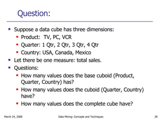
Question: Suppose a data cube has three dimensions: Product: TV, PC, VCR Quarter: 1 Qtr, 2 Qtr, 3 Qtr, 4 Qtr Country: USA, Canada, Mexico Let there be one measure: total sales. Questions: How many values does the base cuboid (Product, Quarter, Country) has? How many values does the cuboid (Quarter, Country) have? How many values does the complete cube have?

A Sample Data Cube Total annual sales of TV in U.S.A. Quarter Product Country All, All, All sum sum TV VCR PC 1Qtr 2Qtr 3Qtr 4Qtr U.S.A Canada Mexico sum

Browsing a Data Cube Visualization OLAP capabilities Interactive manipulation

Typical OLAP Operations Roll up (drill-up): summarize data by climbing up hierarchy or by dimension reduction Drill down (roll down): reverse of roll-up from higher level summary to lower level summary or detailed data, or introducing new dimensions Slice and dice: project and select Pivot (rotate): reorient the cube, visualization, 3D to series of 2D planes.

Design of a Data Warehouse: A Business Analysis Framework Four views regarding the design of a data warehouse Top-down view allows selection of the relevant information necessary for the data warehouse Data source view exposes the information being captured, stored, and managed by operational systems Data warehouse view consists of fact tables and dimension tables Business query view sees the perspectives of data in the warehouse from the view of end-user

Data Warehouse Design Process Top-down, bottom-up approaches or a combination of both Top-down : Starts with overall design and planning (mature) Bottom-up : Starts with experiments and prototypes (rapid) From software engineering point of view Waterfal l: structured and systematic analysis at each step before proceeding to the next Spiral : rapid generation of increasingly functional systems, short turn around time, quick turn around Typical data warehouse design process Choose a business process to model, e.g., orders, invoices, etc. Choose the grain ( atomic level of data ) of the business process Choose the dimensions that will apply to each fact table record Choose the measure that will populate each fact table record

Multi-Tiered Architecture Data Warehouse OLAP Engine Analysis Query Reports Data mining Monitor & Integrator Metadata Data Sources Front-End Tools Serve Data Marts Data Storage OLAP Server Extract Transform Load Refresh Operational DBs other sources

Three Data Warehouse Models Enterprise warehouse collects all of the information about subjects spanning the entire organization Data Mart a subset of corporate-wide data that is of value to a specific groups of users. Its scope is confined to specific, selected groups, such as marketing data mart Independent vs. dependent (directly from warehouse) data mart Virtual warehouse A set of views over operational databases Only some of the possible summary views may be materialized

Data Warehouse Development: A Recommended Approach Define a high-level corporate data model Data Mart Data Mart Distributed Data Marts Multi-Tier Data Warehouse Enterprise Data Warehouse Model refinement Model refinement

OLAP Server Architectures Relational OLAP (ROLAP) Use relational or extended-relational DBMS to store and manage warehouse data and OLAP middle ware to support missing pieces Include optimization of DBMS backend, implementation of aggregation navigation logic, and additional tools and services greater scalability Multidimensional OLAP (MOLAP) Array-based multidimensional storage engine (sparse matrix techniques) fast indexing to pre-computed summarized data Hybrid OLAP (HOLAP) User flexibility, e.g., low level: relational, high-level: array Specialized SQL servers specialized support for SQL queries over star/snowflake schemas

Efficient Data Cube Computation Data cube can be viewed as a lattice of cuboids The bottom-most cuboid is the base cuboid The top-most cuboid (apex) contains only one cell How many cuboids in an n-dimensional cube with L levels? Materialization of data cube Materialize every (cuboid) (full materialization), none (no materialization), or some (partial materialization) Selection of which cuboids to materialize Based on size, sharing, access frequency, etc.

Cube Operation Cube definition and computation in DMQL define cube sales[item, city, year]: sum(sales_in_dollars) compute cube sales Transform it into a SQL-like language (with a new operator cube by , introduced by Gray et al.’96) SELECT item, city, year, SUM (amount) FROM SALES CUBE BY item, city, year Need compute the following Group-Bys ( date, product, customer), (date,product),(date, customer), (product, customer), (date), (product), (customer) () (item) (city) () (year) (city, item) (city, year) (item, year) (city, item, year)

Cube Computation: ROLAP-Based Method Efficient cube computation methods ROLAP-based cubing algorithms (Agarwal et al’96) Array-based cubing algorithm (Zhao et al’97) Bottom-up computation method (Beyer & Ramarkrishnan’99) H-cubing technique (Han, Pei, Dong & Wang:SIGMOD’01) ROLAP-based cubing algorithms Sorting, hashing, and grouping operations are applied to the dimension attributes in order to reorder and cluster related tuples Grouping is performed on some sub-aggregates as a “partial grouping step” Aggregates may be computed from previously computed aggregates, rather than from the base fact table

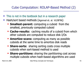
Cube Computation: ROLAP-Based Method (2) This is not in the textbook but in a research paper Hash/sort based methods ( Agarwal et. al. VLDB’96 ) Smallest-parent: computing a cuboid from the smallest, previously computed cuboid Cache-results: caching results of a cuboid from which other cuboids are computed to reduce disk I/Os Amortize-scans: computing as many as possible cuboids at the same time to amortize disk reads Share-sorts: sharing sorting costs cross multiple cuboids when sort-based method is used Share-partitions: sharing the partitioning cost across multiple cuboids when hash-based algorithms are used

Multi-way Array Aggregation for Cube Computation Partition arrays into chunks (a small subcube which fits in memory). Compressed sparse array addressing: (chunk_id, offset) Compute aggregates in “multiway” by visiting cube cells in the order which minimizes the # of times to visit each cell, and reduces memory access and storage cost. What is the best traversing order to do multi-way aggregation? A B 29 30 31 32 1 2 3 4 5 9 13 14 15 16 64 63 62 61 48 47 46 45 a1 a0 c3 c2 c1 c 0 b3 b2 b1 b0 a2 a3 C B 44 28 56 40 24 52 36 20 60

Multi-way Array Aggregation for Cube Computation B A B 29 30 31 32 1 2 3 4 5 9 13 14 15 16 64 63 62 61 48 47 46 45 a1 a0 c3 c2 c1 c 0 b3 b2 b1 b0 a2 a3 C 44 28 56 40 24 52 36 20 60

Multi-way Array Aggregation for Cube Computation A B 29 30 31 32 1 2 3 4 5 9 13 14 15 16 64 63 62 61 48 47 46 45 a1 a0 c3 c2 c1 c 0 b3 b2 b1 b0 a2 a3 C 44 28 56 40 24 52 36 20 60 B Order: A  B  C AB: plane AC: line BC: point

Multi-Way Array Aggregation for Cube Computation (Cont.) Let A: 40 values, B: 400 values, C: 4000 values. One chunk contains 10*100*1000 = 1,000,000 values. A  B  C needs how much memory? AB plane: 40*400=16,000 AC line: 40*(4000/4) = 40,000 BC point: (400/4)*(4000/4) = 100,000 total: 156,000 C  B  A needs how much memory? CB plane: 4000*400=1,600,000 CA line: 4000*(40/4) = 40,000 BA point: (400/4)*(40/4) = 1000 total: 1,641,000 --- 10 times more!

Iceberg Cube Computing only the cuboid cells whose count or other aggregates satisfying the condition: HAVING COUNT(*) >= minsup Motivation Only a small portion of cube cells may be “above the water’’ in a sparse cube Only calculate “interesting” data—data above certain threshold Suppose 100 dimensions, only 1 base cell. How many aggregate (non-base) cells if count >= 1? What about count >= 2?

Example data dimensions: P – 6 product L – 3 location, M – 2 month. Base cuboid: 6*3*2 = 36 cells. Here 30 are empty. Especially when #dimensions is large, should store in a compressed way. SELECT P, L, M, COUNT(*) FROM Sales CUBE BY P, L, M HAVING COUNT(*)>=2 Iceburg cube query asks for non-empty cuboids! E.g. is cuboid (P,L) empty? * m1 l3 p6 * m2 l2 p5 * m1 l2 p4 * m2 l1 p3 * m1 l1 p2 * m1 l1 p1 sale M L P

Naïve approach Given (P, L, M), calculate all cuboids bottom-up. In every cuboid, delete tuples whose count(*)<2. ?? Can we apply count(*)>=2 to (P, L, M) before calculating cuboids? Drawback: calculate the complete iceberg including underwater! all P L M P, L P, M L, M P, L, M 1 m1 l3 p6 1 m2 l2 p5 1 m1 l2 p4 1 m2 l1 p3 1 m1 l1 p2 1 m1 l1 p1 count(*) M L P

Computing iceberg cube using BUC BUC (Beyer & Ramakrishnan, SIGMOD’99) Bottom-up vs. top-down?—depending on how you view it! Apriori property: Aggregate the data, then move to the next level If minsup is not met, stop!

Icerberg: all: ()6 Computing iceberg cube using BUC 1 all 2 P 6 L 8 M 3 P,L 5 P,M 7 L,M 4 P,L,M 1 m1 l3 p6 1 m2 l2 p5 1 m1 l2 p4 1 m2 l1 p3 1 m1 l1 p2 1 m1 l1 p1 count(*) M L P p1: 1 p2: 1 p3: 1 p4: 1 p5: 1 p6: 1

Icerberg: all: ()6 L: (l1)3, (l2)2 L,M: (l1,m1)2 Computing iceberg cube using BUC 1 all 2 P 6 L 8 M 3 P,L 5 P,M 7 L,M 4 P,L,M l1: 3 l2: 2 l3: 1 1 m1 l3 p6 1 m2 l2 p5 1 m1 l2 p4 1 m2 l1 p3 1 m1 l1 p2 1 m1 l1 p1 count(*) M L P m1: 2 m2: 1 m1: 1 m2: 1

Icerberg: all: ()6 L: (l1)3, (l2)2 L,M: (l1,m1)2 M: (m1)4, (m2)2 Computing iceberg cube using BUC 1 all 2 P 6 L 8 M 3 P,L 5 P,M 7 L,M 4 P,L,M m1: 4 m2: 2 1 m1 l3 p6 1 m2 l2 p5 1 m1 l2 p4 1 m2 l1 p3 1 m1 l1 p2 1 m1 l1 p1 count(*) M L P

Range-sum query in a data cube Problem: compute range-sum, e.g. SELECT SUM(C.sales) FROM Customer C WHERE 37<=C.age<=52 and 3<=C.month<=7 Let each dim have n values. query cost = ? O(n 2 ) update (one cell) cost = ? O(1) month age 1 1 1 1 1 1 1 1 59 1 1 1 1 1 1 1 1 58 1 1 1 1 1 1 1 1 52 1 1 1 1 1 1 1 1 40 1 1 1 1 1 1 1 1 37 1 1 1 1 1 1 1 1 33 1 1 1 1 1 1 1 1 25 1 1 1 1 1 1 1 1 20 8 7 6 5 4 3 2 1

Prefix-sum solution Every cell stores the prefix-sum. Can answer a prefix-sum query with cost 1. Update cost? original cube prefix-sum cube O(n 2 )! range-sum query cost? 1 1 1 1 1 1 1 1 8 1 1 1 1 1 1 1 1 7 1 1 1 1 1 1 1 1 6 1 1 1 1 1 1 1 1 5 1 1 1 1 1 1 1 1 4 1 1 1 1 1 1 1 1 3 1 1 1 1 1 1 1 1 2 1 1 1 1 1 1 1 1 1 8 7 6 5 4 3 2 1 64 56 48 40 32 24 16 8 8 56 49 42 35 28 21 14 7 7 48 42 36 30 24 18 12 6 6 40 35 30 25 20 15 10 5 5 32 28 24 20 16 12 8 4 4 24 21 18 15 12 9 6 3 3 16 14 12 10 8 6 4 2 2 8 7 6 5 4 3 2 1 1 8 7 6 5 4 3 2 1

Prefix-sum solution = – – + 42 12 21 6 query cost = O(1) 1 1 1 1 1 1 1 1 8 1 1 1 1 1 1 1 1 7 1 1 1 1 1 1 1 1 6 1 1 1 1 1 1 1 1 5 1 1 1 1 1 1 1 1 4 1 1 1 1 1 1 1 1 3 1 1 1 1 1 1 1 1 2 1 1 1 1 1 1 1 1 1 8 7 6 5 4 3 2 1 1 1 1 1 1 1 1 1 8 1 1 1 1 1 1 1 1 7 1 1 1 1 1 1 1 1 6 1 1 1 1 1 1 1 1 5 1 1 1 1 1 1 1 1 4 1 1 1 1 1 1 1 1 3 1 1 1 1 1 1 1 1 2 1 1 1 1 1 1 1 1 1 8 7 6 5 4 3 2 1 1 1 1 1 1 1 1 1 8 1 1 1 1 1 1 1 1 7 1 1 1 1 1 1 1 1 6 1 1 1 1 1 1 1 1 5 1 1 1 1 1 1 1 1 4 1 1 1 1 1 1 1 1 3 1 1 1 1 1 1 1 1 2 1 1 1 1 1 1 1 1 1 8 7 6 5 4 3 2 1 1 1 1 1 1 1 1 1 8 1 1 1 1 1 1 1 1 7 1 1 1 1 1 1 1 1 6 1 1 1 1 1 1 1 1 5 1 1 1 1 1 1 1 1 4 1 1 1 1 1 1 1 1 3 1 1 1 1 1 1 1 1 2 1 1 1 1 1 1 1 1 1 8 7 6 5 4 3 2 1 1 1 1 1 1 1 1 1 8 1 1 1 1 1 1 1 1 7 1 1 1 1 1 1 1 1 6 1 1 1 1 1 1 1 1 5 1 1 1 1 1 1 1 1 4 1 1 1 1 1 1 1 1 3 1 1 1 1 1 1 1 1 2 1 1 1 1 1 1 1 1 1 8 7 6 5 4 3 2 1

What we have Can we do better? O(n 2 ) O(1) store prefix-sum O(1) O(n 2 ) store original cube update cost query cost O(n) O(log(n)) dynamic data cube (naïve version)

The Dynamic Data Cube [EDBT’00] 1 1 1 1 1 2 3 4 Organize the original cube into a tree structure with fanout = 4. Data is only stored in the leaf node. Each index entry is augmented with… 1..4 5..8 1..4 5..8 1..2 3..4 1..2 3..4 1..2 3..4 5..6 7..8 5..6 7..8 1..2 3..4 5..6 7..8 5..6 7..8

The Dynamic Data Cube [EDBT’00] Each index entry is augmented with an X-border (Y-border), which stores the prefix-sums that: only consider cells in the sub-tree; and cover all rows (columns). 1..4 5..8 1..4 5..8 4 8 12 16 4 8 12 16 1 1 1 1 1 1 1 1 1 1 1 1 1 1 1 1 4 8 12 16 4 8 12 16 1 1 1 1 1 1 1 1 1 1 1 1 1 1 1 1 4 8 12 16 4 8 12 16 1 1 1 1 1 1 1 1 1 1 1 1 1 1 1 1 4 8 12 16 4 8 12 16 1 1 1 1 1 1 1 1 1 1 1 1 1 1 1 1

The Dynamic Data Cube [EDBT’00] A prefix-sum range is broken down into (at most) four pieces. Three calculated by checking the borders at the root. Examine a single sub-tree! 1..4 5..8 1..4 5..8 4 8 12 16 4 8 12 16 1 1 1 1 1 1 1 1 1 1 1 1 1 1 1 1 4 8 12 16 4 8 12 16 1 1 1 1 1 1 1 1 1 1 1 1 1 1 1 1 4 8 12 16 4 8 12 16 1 1 1 1 1 1 1 1 1 1 1 1 1 1 1 1 4 8 12 16 4 8 12 16 1 1 1 1 1 1 1 1 1 1 1 1 1 1 1 1

The Dynamic Data Cube [EDBT’00] A prefix-sum range is broken down into (at most) four pieces. Three calculated by checking the borders at the root. Examine a single sub-tree! 1..4 5..8 1..4 5..8 Query the sub-tree, get 6. 4 8 12 16 4 8 12 16 1 1 1 1 1 1 1 1 1 1 1 1 1 1 1 1 4 8 12 16 4 8 12 16 1 1 1 1 1 1 1 1 1 1 1 1 1 1 1 1 4 8 12 16 4 8 12 16 1 1 1 1 1 1 1 1 1 1 1 1 1 1 1 1 4 8 12 16 4 8 12 16 1 1 1 1 1 1 1 1 1 1 1 1 1 1 1 1

The Dynamic Data Cube [EDBT’00] E.g. 16+12+8+6 = 42. Query cost: O(log(n)) Update cost? O(n) 1..4 5..8 1..4 5..8 4 8 12 16 4 8 12 16 1 1 1 1 1 1 1 1 1 1 1 1 1 1 1 1 4 8 12 16 4 8 12 16 1 1 1 1 1 1 1 1 1 1 1 1 1 1 1 1 4 8 12 16 4 8 12 16 1 1 1 1 1 1 1 1 1 1 1 1 1 1 1 1 4 8 12 16 4 8 12 16 1 1 1 1 1 1 1 1 1 1 1 1 1 1 1 1

The Dynamic Data Cube [EDBT’00] Update cost? At root, (up to) n border cells to modify. One level down, n/2 cells to modify…. 1..4 5..8 1..4 5..8 total: O(n) 4 8 12 16 4 8 12 16 1 1 1 1 1 1 1 1 1 1 1 1 1 1 1 1 4 8 12 16 4 8 12 16 1 1 1 1 1 1 1 1 1 1 1 1 1 1 1 1 4 8 12 16 4 8 12 16 1 1 1 1 1 1 1 1 1 1 1 1 1 1 1 1 4 8 12 16 4 8 12 16 1 1 1 1 1 1 1 1 1 1 1 1 1 1 1 1

What we have Can we do better? Can we do better? O(n 2 ) O(1) store prefix-sum O(1) O(n 2 ) store original cube update cost query cost O(n) O(log(n)) dynamic data cube (naïve version) O(log 2 n) O(log 2 n) dynamic data cube

Key to reducing from O(n) to O(log 2 n) For each update, should update an X-border and a Y-border at each level. How to update an X-border in logarithmic time? More formally, given an array A[1..n] = (4, 8, 12, 16). How to add v to all elements from A[i] to A[n]? Idea: maintain a binary tree. 0 0 0 4 8 12 16 A[1] A[2] A[3] A[4] 0 0 3 4 11 12 16 A[1] A[2] A[3] A[4] add 3 to A[2..4]

Dynamic Data Cube summary A balanced tree with fanout=4. The leaf nodes contains the original data cube. Each index entry stores an X-border and an Y-border. Each border is stored as a binary tree, which supports a 1-dim prefix-sum query and an update in O(log(n)) time. Overall, the DDC supports a range-sum query and an update both in O(log 2 n) time.

Summary Data warehouse A multi-dimensional model of a data warehouse Star schema, snowflake schema, fact constellations A data cube consists of dimensions & measures OLAP operations: drilling, rolling, slicing, dicing and pivoting OLAP servers: ROLAP, MOLAP, HOLAP Efficient computation of data cubes Partial vs. full vs. no materialization Multiway array aggregation Further development of data cube technology Iceberg Cube Dynamic Data Cube

My2dw

More Related Content

What's hot (20)

Viewers also liked (13)

Similar to My2dw (20)

Recently uploaded (20)

My2dw